Simple approach to the relation between laser frequencynoise and laser line shape

Gianni Di Domenico,* Stéphane Schilt, and Pierre ThomannLaboratoire Temps-Fréquence, Université de Neuchâtel, Avenue de Bellevaux 51, CH-2009 Neuchâtel, Switzerland

*Corresponding author: gianni.didomenico@unine.ch

Frequency fluctuations of lasers cause a broadening of their line shapes. Although the relation betweenthe frequency noise spectrum and the laser line shape has been studied extensively, no simple expressionexists to evaluate the laser linewidth for frequency noise spectra that does not follow a power law. Wepresent a simple approach to this relation with an approximate formula for evaluation of the laser line-width that can be applied to arbitrary noise spectral densities.

OCIS codes: 140.3425, 140.3430, 140.3460, 120.0120.

1. Introduction

Lasers with a high spectral purity currently findimportant applications in frequency metrology, high-resolution spectroscopy, coherent optical commu-nications, and atomic physics, to name a few uses.Advances in investigation and narrowing of laserlinewidth have experienced a remarkable evolution,yielding techniques that give us unprecedented con-trol over the optical phase/frequency [1–9]. The spec-tral properties of such lasers can be convenientlydescribed either in terms of their optical line shapeand associated linewidth or in terms of the powerspectral density of their frequency noise. Both ap-proaches are complementary, but the knowledge ofthe frequency noise spectral density provides muchmore information on the laser noise. A measurementof the laser linewidth (obtained by heterodyningwith a reference laser source or by self-homodyne/heterodyne interferometry using a long optical delayline) is often sufficient in many applications (e.g., inhigh-resolution spectroscopy or coherent optical com-munications). Some experiments, though, requiremore complete knowledge of the Fourier distributionof the laser frequency fluctuations. Knowledge of thefrequency noise spectral density enables one to re-trieve the laser line shape and, thus, the linewidth

(while the reverse process, i.e., determining the noisespectral density from the line shape, is not possible),but this operation is most often not straightforward.

The relation between frequency noise spectral den-sity and laser linewidth has already been addressedin many papers dealing with general theoretical con-siderations or with more or less particular cases. Inone of the earliest papers on this topic, Elliott andco-workers [10] derived theoretical formulas linkingthe frequency noise spectral density to the laser lineshape. They also discussed the different line shapesobtained in the case of a rectangular noise spectrumof finite bandwidth in the two extreme conditionswhere the ratio of the frequency deviation to thenoise bandwidth is either large (leading to a Gaus-sian line shape) or small (resulting in a Lorentzianline shape). Their work was supported by experimen-tal results showing the transformation of the laserspectrum from Lorentzian to Gaussian for decreas-ing noise bandwidth. The ideal case of a pure whitefrequency noise spectrum has been extensively re-ported for a long time (see, for example, [11]), asit can be fully solved analytically leading to thewell-known Lorentzian line shape described by theSchawlow–Townes–Henry linewidth [12,13]. How-ever, the real noise spectrum of a laser is much morecomplicated and leads to a nonanalytical line shapethat can be determined only numerically. Lasers are

Published inApplied Optics 49, issue 25, 4801-4807, 2010

which should be used for any reference to this work

1

generally affected by flicker noise at low frequency,and this type of noise has been widely studied inthe literature [14–17]. The major feature of this typeof noise is to produce spectral broadening of the la-ser linewidth compared to the Schawlow–Townes–Henry limit, but an exact expression of the line shapecannot be obtained, and different approximationshave been proposed to describe this situation. For ex-ample, Tourrenc [15] numerically showed the diver-gence of the linewidth with increasing observationtime in the presence of 1=f -type noise, while Mercer[16] gave an analytical approximation for this diver-ging Gaussian linewidth. Stéphan et al. [14] gave adifferent approximation of the 1=f -induced Gaussiancontribution to the line shape, with a linewidth thatdoes not contain any dependency on the observationtime, and Godone et al. [18,19] gave the rf spectra cor-responding to phase noise spectral densities of arbi-trary slopes. Finally, some publications also statedthat the combined contribution of white noiseLorentzian line shape and 1=f -noise Gaussian lineshape resulted in a Voigt profile for the optical lineshape [14,16,20].

In this paper, we present a simple geometricapproach to determine the linewidth of a laser fromits frequency noise spectral density. Our approachmakes use of a simple approximate formula to deter-mine the linewidth corresponding to an arbitrarynoise spectrum. Starting with the ideal case of alow-pass filtered white noise of varying cutoff fre-quency, we show how differently the low- and high-frequency noise components affect the line shapeand how the linewidth changes with respect to thenoise cutoff frequency. Then, we demonstrate inwhich limit conditions the Lorentzian and Gaussianline shapes generally discussed in former publica-tions are retrieved. We introduce our simple approx-imation of the linewidth by showing how the noisespectrum can be geometrically separated in twoareas with a fully different influence on the lineshape. Only one of these spectral areas contributesto the linewidth, the remaining part of the spectruminfluencing only the wings of the line shape. Themain benefit of our work is to make a simple link be-tween the frequency noise spectrum of a laser and itslinewidth, without any assumption on the noise spec-tral distribution. By showing how some spectral com-ponents of the noise determine the linewidth whileothers affect only the wings of the line shape, we pro-vide a simple geometric criterion to determine thosespectral components that contribute to the linewidth.As a result, a simple formula is reported to calculatethe linewidth of a laser for an arbitrary frequencynoise spectrum, i.e., this expression is applicable toany type of frequency noise and is thus not restrictedto the ideal cases of white noise and flicker noiseusually considered.

Before introducing our approach, we give a briefreminder of the important theoretical steps enablingthe linking of the frequency noise spectrum of a laserand its line shape. A detailed theoretical description

can be found in [10,15,16]. Given the frequency noisespectral density Sδνðf Þ (we consider single-sidedspectral densities throughout this article) of the laserlight field EðtÞ ¼ E0 exp½ið2πν0tþ ϕðtÞÞ� (complex re-presentation), one can calculate the autocorrelationfunction ΓEðτÞ ¼ �E�ðtÞEðtþ τÞ as follows:

ΓEðτÞ ¼ E20e

i2πν0τe−2R

∞

0Sδνðf Þsin

2ðπf τÞf2

df; ð1Þ

where δν ¼ ν − ν0 is the laser frequency deviationaround its average value ν0. According to theWiener–Khintchine theorem, the laser line shapeis given by the Fourier transform of the autocorrela-tion function

SEðνÞ ¼ 2Z

∞

−∞

e−i2πντΓEðτÞdτ: ð2Þ

Unfortunately, this general formula most often can-not be analytically integrated, except for the trivialcase of white frequency noise Sδνðf Þ ¼ h0 (with h0given in Hz2=Hz) that leads to the well-knownLorentzian line shape with a full width at half-maximum FWHM ¼ πh0 [10,15,16].

In the following, we will start by studying the caseof a low-pass filtered white frequency noise. This willlead us to establish a simple approximate formula ofthe linewidth of a real laser from its frequency noisespectrum. Finally, we will apply this formula todifferent situations that are of practical interest toexperimentalists and in which frequency noise isimportant.

2. Laser Spectrum in the Case of a Low-Pass FilteredWhite Frequency Noise

As an introduction to the derivation of our approxi-mate expression of the laser linewidth, let us firstconsider a frequency noise spectral density thathas a constant level h0ðHz2=HzÞ below a cutoff fre-quency f c and that drops to zero above this threshold:

Sδνðf Þ ¼�h0 if f ≤ f c0 if f > f c

: ð3Þ

In this simple case, it is possible to evaluate analy-tically the integral in Eq. (1) and obtain the followingexpression for the autocorrelation function:

ΓEðτÞ ¼ E20e

i2πν0τe2h0f cðsin2ðπf cτÞ−πf cτSið2πf cτÞÞ; ð4Þ

where SiðxÞ ¼ Rx0 sinðtÞ=tdt is the sine integral func-

tion. On the other hand, most often, it is not possibleto obtain an analytical expression for the Fouriertransform in Eq. (2), and, therefore, the laser lineshape must be evaluated numerically. An analyticalexpression of the line shape is, however, calculablein the two extreme conditions in which f c → ∞ andf c → 0:

2

• When f c → ∞:

SEðνÞ ¼ E20

h0

ðν − ν0Þ2 þ ðπh0=2Þ2; ð5Þ

and the line shape is Lorentzian with a widthFWHM ¼ πh0 (this corresponds to the white noisepreviously mentioned).

• When f c → 0:

SEðνÞ ¼ E20

�2

πh0f c

�1=2

e−ðν−ν0Þ22h0 f c ; ð6Þ

and the line shape is Gaussian with a widthFWHM ¼ ð8 lnð2Þh0f cÞ1=2 that depends on the cutofffrequency f c.

For a fixed frequency noise level h0, it is interestingto numerically study the evolution of the laser lineshape as a function of the cutoff frequency f c betweenthese two extreme cases. The result is shown in Fig. 1for h0 ¼ 1Hz2=Hz. According to Eqs. (5) and (6), oneobserves that when f c ≪ h0, the line shape is Gaus-sian and the linewidth increases with f c. However,when f c ≫ h0, the line shape becomes Lorentzianand the linewidth stops to increase (it will be shownlater that the noise at high Fourier frequencies con-tributes only to the wings of the line shape). In orderto explore the transition between these two regimes,we numerically calculated the linewidth as a func-tion of the cutoff frequency f c, and the results are pre-sented in Fig. 2. We found that a good approximationvalid for any f c is given by the following expression:

FWHM ¼ h0ð8 lnð2Þf c=h0Þ1=2�1þ

�8 lnð2Þπ2

f ch0

�2�1=4

; ð7Þ

with a relative error smaller than 4% over the entirerange of the cutoff frequency f c, as shown in the lower

graph of Fig. 2. The corner frequency correspondingto the transition between the two regimes is situatedat the intersection of the two asymptotes shown inthe upper graph of Fig. 2 and is given by

f �c ¼π2

8 lnð2Þh0 ≈ 1:78h0: ð8Þ

3. Simple Formula to Estimate the Laser Linewidth

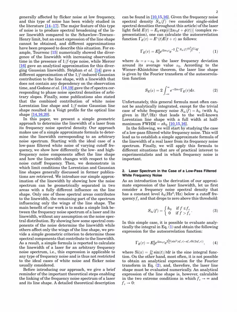
The example of the low-pass filtered white noiseshows that the frequency noise spectrum can be se-parated into two regions that affect the line shape ina radically different way. In the first region, definedby Sδνðf Þ > 8 lnð2Þf =π2, the noise contributes to thecentral part of the line shape, which is Gaussian,and thus to the laser linewidth. In the second region,defined by Sδνðf Þ < 8 lnð2Þf =π2, the noise contributesmainly to the wings of the line shape but does notaffect the linewidth. The striking difference betweenthe noise effects in these two regions can be under-stood in terms of frequency modulation theory. Inthe first region, the noise level is high compared toits Fourier frequency, therefore it produces a slow fre-quency modulation with a high modulation index[21] β > 1. Conversely, in the second region, the noiselevel is small compared to its Fourier frequency, and,accordingly, the modulation index β is small, whichmeans that the modulation is too fast to have a sig-nificant effect on the laser linewidth. In the rest ofthis article, the line separating these two regions will

Fig. 1. (Color online) Numerical calculation of the laser lineshape SEðδνÞ for a fixed frequency noise level h0 ¼ 1Hz2=Hz anddifferent values of the cutoff frequency: a, f c ¼ 0:03Hz; b,f c ¼ 0:3Hz; c, f c ¼ 3Hz; and d, f c ¼ 30Hz. The line shapes are nor-malized to help the comparison of their full width at half-maximum (FWHM). The line shape evolves from a Gaussian whenf c ≪ h0 and to a Lorentzian when f c ≫ h0.

Fig. 2. (Color online) Upper graph: Numerical computation show-ing the evolution of the linewidth (FWHM) with the cutoff fre-quency f c in the case of low-pass filtered white noise. The dotshave been calculated by numerical integration of the exact rela-tions Eqs. (1) and (2). The continuous line is given by our approx-imate formula Eq. (7). Both horizontal and vertical scales havebeen normalized to the noise level h0. The behavior at low and highcutoff frequencies is indicated by the asymptotic response (reddashed lines). Lower graph: Relative error between the exactand approximate values.

3

be called the β-separation line. These observationsare summarized in Fig. 3, where a typical laser fre-quency noise spectral density is represented. A care-ful inspection of Eqs. (1) and (2) shows that the lowfrequency approximation given in Eq. (6) can be ex-tended to arbitrary noise spectra. Indeed, noise com-ponents in the high modulation index area with aspectral density higher than their Fourier frequency(Sδνðf Þ > f ) give rise to Gaussian autocorrelationfunctions, which are multiplied together and thenFourier transformed to give the laser line shape. Asa result, the line shape is a Gaussian function whosevariance is the sum of the contributions of all highmodulation index noise components. Therefore, onecan obtain a good approximation of the laser line-width by the following simple expression:

FWHM ¼ ð8 lnð2ÞAÞ1=2; ð9Þ

where A is the surface of the high modulation indexarea, i.e., the overall surface under the portions ofSδνðf Þ that exceed the β-separation line (see Fig. 3)

A ¼Z

∞

1=To

HðSδνðf Þ − 8 lnð2Þf =π2ÞSδνðf Þdf ; ð10Þ

with HðxÞ being the Heaviside unit step function(HðxÞ ¼ 1 if x ≥ 0 and HðxÞ ¼ 0 if x < 0) and To beingthe measurement time that prevents the observationof low frequencies below 1=To. This low frequencylimit can be set to zero when the area in Eq. (10) doesnot show low frequency divergence. However, this isnot the case in the presence of flicker noise, for whichthe measurement time plays an important role, aswill be shown in the next section.

4. Application 1: Laser Spectrum in the Case ofFlicker Frequency Noise

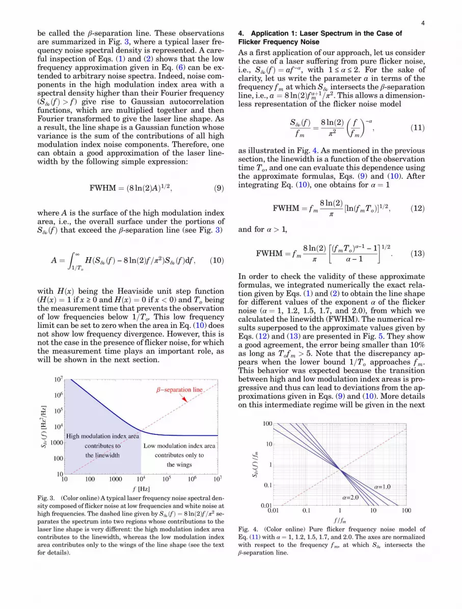
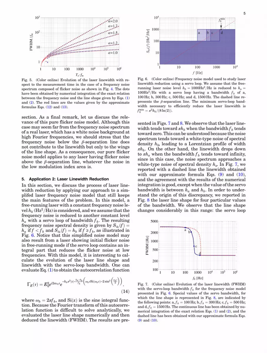
As a first application of our approach, let us considerthe case of a laser suffering from pure flicker noise,i.e., Sδνðf Þ ¼ af −α, with 1 ≤ α ≤ 2. For the sake ofclarity, let us write the parameter a in terms of thefrequency f m at which Sδν intersects the β-separationline, i.e., a ¼ 8 lnð2Þf αþ1

m =π2. This allows a dimension-less representation of the flicker noise model

Sδνðf Þf m

¼ 8 lnð2Þπ2

�ff m

�−α; ð11Þ

as illustrated in Fig. 4. As mentioned in the previoussection, the linewidth is a function of the observationtime To, and one can evaluate this dependence usingthe approximate formulas, Eqs. (9) and (10). Afterintegrating Eq. (10), one obtains for α ¼ 1

FWHM ¼ f m8 lnð2Þ

π ½lnðf mToÞ�1=2; ð12Þ

and for α > 1,

FWHM ¼ f m8 lnð2Þ

π

�ðf mToÞα−1 − 1α − 1

�1=2

: ð13Þ

In order to check the validity of these approximateformulas, we integrated numerically the exact rela-tion given by Eqs. (1) and (2) to obtain the line shapefor different values of the exponent α of the flickernoise (α ¼ 1, 1.2, 1.5, 1.7, and 2.0), from which wecalculated the linewidth (FWHM). The numerical re-sults superposed to the approximate values given byEqs. (12) and (13) are presented in Fig. 5. They showa good agreement, the error being smaller than 10%as long as Tofm > 5. Note that the discrepancy ap-pears when the lower bound 1=To approaches f m.This behavior was expected because the transitionbetween high and low modulation index areas is pro-gressive and thus can lead to deviations from the ap-proximations given in Eqs. (9) and (10). More detailson this intermediate regime will be given in the next

Fig. 3. (Color online) A typical laser frequency noise spectral den-sity composed of flicker noise at low frequencies and white noise athigh frequencies. The dashed line given by Sδνðf Þ ¼ 8 lnð2Þf =π2 se-parates the spectrum into two regions whose contributions to thelaser line shape is very different: the high modulation index areacontributes to the linewidth, whereas the low modulation indexarea contributes only to the wings of the line shape (see the textfor details).

Fig. 4. (Color online) Pure flicker frequency noise model ofEq. (11) with α ¼ 1, 1.2, 1.5, 1.7, and 2.0. The axes are normalizedwith respect to the frequency f m, at which Sδν intersects theβ-separation line.

4

section. As a final remark, let us discuss the rele-vance of this pure flicker noise model. Although thiscase may seem far from the frequency noise spectrumof a real laser, which has a white noise background athigh Fourier frequencies, we should stress that thefrequency noise below the β-separation line doesnot contribute to the linewidth but only to the wingsof the line shape. As a consequence, our pure flickernoise model applies to any laser having flicker noiseabove the β-separation line, whatever the noise inthe low modulation index area is.

5. Application 2: Laser Linewidth Reduction

In this section, we discuss the process of laser line-width reduction by applying our approach to a sim-plifed laser frequency noise model that still keepsthe main features of the problem. In this model, afree-running laser with a constant frequency noise le-vel hb (Hz2=Hz) is considered, andwe assume that thefrequency noise is reduced to another constant levelha with a servo loop of bandwidth f b. The resultingfrequency noise spectral density is given by Sδνðf Þ ¼ha if f < f b and Sδνðf Þ ¼ hb if f ≥ f b, as illustrated inFig. 6. Notice that this simplified noise model mayalso result from a laser showing initial flicker noisein free-running mode if the servo loop contains an in-tegral part that reduces the flicker noise at lowfrequencies. With this model, it is interesting to cal-culate the evolution of the laser line shape andlinewidth with the servo-loop bandwidth. One canevaluateEq. (1) to obtain the autocorrelation function

ΓEðτÞ ¼ E20e

i2πν0τe−hbπ2jτj−ha−hb

f b

�ωbτSiðωbτÞ−2 sin2

�ωbτ2

��;

ð14Þwhere ωb ¼ 2πf b, and SiðxÞ is the sine integral func-tion. Because the Fourier transform of this autocorre-lation function is difficult to solve analytically, weevaluated the laser line shape numerically and thendeduced the linewidth (FWHM). The results are pre-

sented in Figs. 7 and 8.We observe that the laser line-width tends toward πhb when the bandwidth f b tendstoward zero.This canbeunderstoodbecause thenoisespectrum tends toward a white-type noise of spectraldensity hb, leading to a Lorentzian profile of widthπhb. On the other hand, the linewidth drops downto πha when the bandwidth f b tends toward infinity,since in this case, the noise spectrum approaches awhite-type noise of spectral density ha. In Fig. 7, wereported with a dashed line the linewidth obtainedwith our approximate formula Eqs. (9) and (10),and the agreement with the results of the numericalintegration is good, exceptwhen the value of the servobandwidth is between ha and hb. In order to under-stand the origin of this discrepancy, we reported inFig. 8 the laser line shape for four particular valuesof the bandwidth. We observe that the line shapechanges considerably in this range: the servo loop

Fig. 5. (Color online) Evolution of the laser linewidth with re-spect to the measurement time in the case of a frequency noisespectrum composed of flicker noise as shown in Fig. 4. The dotshave been obtained by numerical integration of the exact relationbetween the frequency noise and the line shape given by Eqs. (1)and (2). The red lines are the values given by the approximateformulas Eqs. (12) and (13).

Fig. 6. (Color online) Frequency noise model used to study laserlinewidth reduction using a servo loop. We assume that the free-running laser noise level hb ¼ 1000Hz2=Hz is reduced to ha ¼100Hz2=Hz with a servo loop having a bandwidth f b of a,100Hz; b, 300Hz; c, 500Hz; and d, 1500Hz. The dashed line re-presents the β-separation line. The minimum servo-loop band-width necessary to efficiently reduce the laser linewidth isfminb ¼ π2hb=ð8 lnð2ÞÞ.

Fig. 7. (Color online) Evolution of the laser linewidth (FWHM)with the servo-loop bandwidth f b for the frequency noise modelpresented in Fig. 6. Special values of the servo bandwidth, forwhich the line shape is represented in Fig. 8, are indicated bythe following points: a, f b ¼ 100Hz; b, f b ¼ 300Hz; c, f b ¼ 500Hz;and d, f b ¼ 1500Hz. The continuous line has been obtained by nu-merical integration of the exact relation Eqs. (1) and (2), and thedashed line has been obtained with our approximate formula Eqs.(9) and (10).

5

repels the frequency noise from the center, and, as aconsequence, two sidebands appear outside of the ser-vo bandwidth, i.e., at δν > f b, while the central partstrongly narrows and becomes Lorentzian. Becauseof this radical change of line shape, the different line-widths at half-maximumare not similar in this range,and comparison with the Gaussian linewidth approx-imation Eqs. (9) and (10) loses its significance, whichexplains the observed discrepancy. Nevertheless, ourapproximate formula is able to predict the minimumservo-loop bandwidth necessary to efficiently reducethe laser linewidth, which is given by fmin

b ¼ π2hb=ð8 lnð2ÞÞ. It depends on the free-running laser noiselevel hb and corresponds to the situation in whichthe noise level hb is entirely below the β-separationline for frequencies outside of the servo bandwidth(see Fig. 6). As a consequence, when f b > fmin

b , onlythe low frequency part with noise level ha is abovethe β-separation line and contributes to the laser line-width, which is given by πha. Note that the final laserlinewidth depends on the noise level ha, and thus onthe servo-loop gain at low frequency, but is indepen-dent of the servo bandwidth, provided that f b > fmin

b .

6. Conclusion

The study of a low-pass filteredwhite frequency noisehas led us to the establishment of a new and simpleapproximation of the relation between frequencynoise and laser linewidth, which is valid for arbitrarynoise spectra.Wehave shownhowthe frequencynoisespectrum is separated into twoareas corresponding tohighand lowmodulation indexregimes (i.e.,β > 1andβ < 1) by a simple line that we called the β-separationline. Then, we explainedwhy only those spectral com-ponents for which the frequency noise is higher thanthe β-separation line (thehighmodulation indexarea)contribute to the linewidth. An approximate value ofthe linewidth is simply obtained from the geometricalsurface of the high modulation index area. The appli-cation of this approach to the case of flicker noiseprovides an approximate formula for the linewidth,showing its dependence to the observation time.

Finally, the use of this approach to the reduction ofthe laser linewidth emphasizes some important as-pects of this problem, such as the minimal requiredservo-loop bandwidth and the achievable laser line-width. Moreover, this last example showed that thelimitations of this simplified approach appear onlywhen the laser line shape is too complex to be charac-terized by a mere linewidth.

References

1. M. Zhu and J. L. Hall, “Stabilization of optical phase/frequency of a laser system: application to a commercialdye laser with an external stabilizer,” J. Opt. Soc. Am. B10, 802–816 (1993).

2. B. C. Young, F. C. Cruz, W. M. Itano, and J. C. Bergquist,“Visible lasers with subhertz linewidths,” Phys. Rev. Lett.82, 3799–3802 (1999).

3. L. Conti, M. D. Rosa, and F. Marin, “High-spectral-purity lasersystem for the AURIGA detector optical readout,” J. Opt. Soc.Am. B 20, 462–468 (2003).

4. M. Heurs, V. M. Quetschke, B. Willke, K. Danzmann, andI. Freitag, “Simultaneously suppressing frequency andintensity noise in a Nd:YAG nonplanar ring oscillator bymeans of the current-lock technique,” Opt. Lett. 29, 2148–2150 (2004).

5. J. Alnis, A. Matveev, N. Kolachevsky, T. Udem, and T. W.Hänsch, “Subhertz linewidth diode lasers by stabilization tovibrationally and thermally compensated ultralow-expansionglass Fabry–Pérot cavities,” Phys. Rev. A 77, 053809 (2008).

6. M. Yamanishi, T. Edamura, K. Fujita, N. Akikusa, andH. Kan,“Theory of the intrinsic linewidth of quantum-cascade lasers:Hidden reason for the narrow linewidth and line-broadeningby thermal photons,” IEEE J. Quantum Electron. 44, 12(2008).

7. F. Acernese, M. Alshourbagy, F. Antonucci, S. Aoudia, K. G.Arun, P. Astone, G. Ballardin, F. Barone, L. Barsotti,M. Barsuglia, T. S. Bauer, S. Bigotta, S. Birindelli, M. A.Bizouard, C. Boccara, F. Bondu, L. Bonelli, L. Bosi, S. Braccini,C. Bradaschia, A. Brillet, V. Brisson, H. J. Bulten, D. Buskulic,G. Cagnoli, E. Calloni, and E. Campagna, “Laser with an in-loop relative frequency stability of 1:0 × 10 − 21 on a 100mstime scale for gravitational-wave detection,” Phys. Rev. A79, 053824 (2009).

8. I. Galli, S. Bartalini, P. Cancio, G. Giusfredi, D. Mazzotti, andP. D. Natale, “Ultra-stable, widely tunable and absolutelylinked mid-IR coherent source,” Opt. Express 17, 9582–9587(2009).

9. S. Bartalini, S. Borri, P. Cancio, A. Castrillo, I. Galli, G.Giusfredi, D. Mazzotti, L. Gianfrani, and P. De Natale, “Obser-ving the intrinsic linewidth of a quantum-cascade laser:beyond the Schawlow–Townes limit,” Phys. Rev. Lett. 104,083904 (2010).

10. D. S. Elliott, R. Roy, and S. J. Smith, “Extracavity laser bandshape and bandwidth modification,” Phys. Rev. A 26, 12–18(1982).

11. P. B. Gallion and G. Debarge, “Quantum phase noise and fieldcorrelation in single frequency semiconductor laser systems,”IEEE J. Quantum Electron. 20, 343–350 (1984).

12. A. L. Schawlow and C. H. Townes, “Infrared and opticalmasers,” Phys. Rev. 112, 1940–1949 (1958).

13. C. Henry, “Theory of the linewidth of semiconductor lasers,”IEEE J. Quantum Electron. 18, 259–264 (1982).

14. G. M. Stéphan, T. T. Tam, S. Blin, P. Besnard, and M. Têtu,“Laser line shape and spectral density of frequency noise,”Phys. Rev. A 71, 043809 (2005).

Fig. 8. (Color online) Evolution of the laser line shape with theservo-loop bandwidth for the frequency noise model presentedin Fig. 6. We chose the following values of the servo bandwidth:a, f b ¼ 100Hz; b, f b ¼ 300Hz; c, f b ¼ 500Hz; and d, f b ¼1500Hz, which correspond to the points indicated in Fig. 7.

6

15. J.-P. Tourrenc, “Caractérisation et modélisation du bruit d’am-plitude optique, du bruit de fréquence et de la largeur de raiede VCSELs monomode,” Ph.D. dissertation (Université deMontpellier II, 2005).

16. L.B.Mercer, “1=f frequencynoiseeffectsonself-heterodyneline-widthmeasurements,”J.LightwaveTechnol.9, 485–493(1991).

17. K. Kikuchi, “Effect of llf-type fm noise on semiconductor-laserlinewidth residual in high-power limit,” IEEE J. QuantumElectron. 25, 684–688 (1989).

18. A. Godone and F. Levi, “About the radiofrequency spectrumof a phase noise-modulated carrier,” in Proceedings of the

12th European Frequency and Time Forum (1998), pp.392–396.

19. A. Godone, S. Micalizio, and F. Levi, “Rf spectrum of a carrierwith a random phase modulation of arbitrary slope,” Metrolo-gia 45, 313–324 (2008).

20. S. Viciani, M. Gabrysch, F. Marin, F. M. di Sopra, M. Moser,and K. H. Gulden, “Line shape of a vertical cavity surfaceemitting laser,” Opt. Commun. 206, 89–97 (2002).

21. The modulation index β is defined as the ratio of thefrequency deviationΔf over the modulation frequency f m, i.e.,β ¼ Δf =f m.

7