Automatica 42 (2006) 1637–1650www.elsevier.com/locate/automatica

A speed-sensorless indirect field-oriented control for induction motorsbased on high gain speed estimation�

Marcello Montanaria, Sergei Peresadab, Andrea Tillia,∗aDepartment of Electronics, Computer Science and Systems (DEIS), CASY - Center for Research on Complex Automated Systems “G. Evangelisti”,

Engineering Faculty, University of Bologna, Viale Pepoli 3/2, 40123 Bologna, ItalybDepartment of Electrical Engineering, National Technical University of Ukraine “Kiev Polytechnic Institute”, Prospect Pobedy 37, Kiev 252056, Ukraine

Received 23 June 2005; received in revised form 4 April 2006; accepted 8 May 2006Available online 28 July 2006

Abstract

The authors design a new speed sensorless output feedback control for the full-order model of induction motors with unknown constantload torque, which guarantees local asymptotic tracking of smooth speed and rotor flux modulus reference signals and local asymptotic fieldorientation, on the basis of stator current measurements only. The proposed nonlinear controller exploits the concept of indirect field orientation(no flux estimation is required) in combination with a new high-gain speed estimator based on the torque current tracking error. The estimatesof unknown load torque and time-varying rotor speed converge to the corresponding true values under a persistency of excitation condition witha physically meaningful interpretation, basically equivalent to non-null synchronous frequency. Stability analysis of the overall dynamics hasbeen performed exploiting the singular perturbation method. The proposed control algorithm is a “true” industrial sensorless solution since nosimplifying assumptions (flux and load torque measurements) are required. Simulation and experimental tests show that the proposed controlleris suitable for medium and high performance applications.� 2006 Elsevier Ltd. All rights reserved.

Keywords: Induction motors; Indirect field-oriented control; Lyapunov stability; Speed control

1. Introduction

Vector controlled induction motor (IM) drives are widespread electromechanical conversion systems for high-dynamicperformance applications, where motion control or high pre-cision speed control is needed (Leonhard, 2001). Usually, adigital shaft speed-position sensor is required in these applica-tions. For low dynamic applications such as pumps and fansthe typical solution is the so-called “adjustable-speed” drive.This is a simple low-cost voltage–source inverter fed IM drivewith scalar voltage frequency control. Voltage frequency con-trolled drives typically are speed-sensorless, i.e. without the

� This paper was not presented at any IFAC meeting. This paper wasrecommended for publication in revised form by Associate Editor Yong-YanCao under the direction of the Editor Mituhiko Araki.

∗ Corresponding author. Tel.: +39 051 2093924; fax: +39 051 2093073.E-mail addresses: mmontanari@deis.unibo.it (M. Montanari),

peresada@i.com.ua (S. Peresada), atilli@deis.unibo.it (A. Tilli).

0005-1098/$ - see front matter � 2006 Elsevier Ltd. All rights reserved.doi:10.1016/j.automatica.2006.05.021

speed-position sensor, according to common nomenclature inelectric drive field. An intermediate class of ac drive appli-cations such as elevators and auxiliary machines of rollingmills requires enhanced dynamic performances and wider speedrange as compared with “adjustable-speed” drives, but approx-imatively at the same cost. Typically, for such applications thespeed reference ranges are from 1% to 100% of the IM nom-inal speed (or even more if the field-weakening technique isadopted, Leonhard, 2001) while the load torque could be upto 100–150% of the rated value. Installation of an encoderfor such applications leads to increased cost, reduces reliabil-ity, especially in hostile environments, and increases sensitivityto electromagnetic noise. All leading electrical drive produc-ers have already presented in the market sensorless productseven if a theoretical framework for IM sensorless control is notwell established yet. These reasons stimulated strong researchactivity in the development of sensorless IM drives in bothpractically and theoretically oriented motor control researchgroups.

1638 M. Montanari et al. / Automatica 42 (2006) 1637–1650

There is a large number of investigations related to thisproblem. Extensive overviews of ac sensorless control strate-gies are given in Rajashekara, Kawamura, and Matsuse (1996),Vas (1998), and Holtz (2002). According to these references,contributions are concentrated in three main directions: IM spa-tial saliency methods with fundamental excitation and high-frequency signal injection, extended Kalman filter techniqueand adaptive system approaches.

Interest in medium and potentially high-performance ap-plications of IM pointed main research efforts in the thirddirection. In Kubota and Matsuse (1994) a rotor flux observerand a speed estimator are presented, considering the speed as aconstant parameter of the IM model. Simplified stability proofis used to construct the parameters estimation algorithms.A rotor flux-speed observer, which is adaptive with respectto rotor resistance, presented in Montanari, Peresada, Tilli,and Tonielli (2000), is based on rigorous Lyapunov stabilityanalysis. Simulation and experimental tests demonstrate thefeasibility of the controllers constructed using these flux-speedobservation schemes. The hyperstability approach is utilized inSchauder (1992) under the assumption that the rotor flux vectorcan be detected by integrating the stator current dynamic equa-tion. In order to avoid open loop integration, in Peng and Fukao(1994) the speed-dependent back-EMF vector is computeddifferentiating the stator currents. A modification of that con-trol algorithm is then proposed considering the instantaneousIM reactive power as an output variable. This solution is sta-tor resistance invariant. Both speed estimation algorithms areconstructed considering the rotor speed as a constant parame-ter. VSS technique for speed estimation is exploited in Doki,Sangwongwanick, and Okuma (1992) and Yan, Jin, and Utkin(2000). In Chern, Chang, and Tsai (1998) the speed estimator,which is adaptive with respect to stator and rotor resistance,is developed using integral variable structure approach andneglecting speed dynamics. Important investigations on the ob-servability properties of sensorless controlled induction motorsare reported in Canudas De Wit, Youssef, Barbot, Martin, andMalrait (2000) and Ibarra-Rojas, Moreno, and Espinosa-Perez(2004), where it is shown that the speed and flux state vari-ables are not detectable from current measurements underdc-excitation.

Although an extensive research activity has been carried outduring the last decades, from the theoretical viewpoint theIM sensorless control still represents an open research topicdue to: (1) strong simplifying assumptions on IM speed dyna-mics, e.g. motor speed is considered as a constant parameter;(2) pure integration or derivative of the stator currents areneeded;(3) only few contributions are based on rigorous closed-loop stability analysis. In Feemster, Aquino, Dawson, and Be-hal (2001) a semiglobal exponential speed-flux tracking controlis developed assuming known load torque and rotor flux mea-surements (or obtained using open loop integration of the statorvoltage equations with zero initial conditions). Under the samesimplifying assumptions a globally asymptotically stable (lo-cally exponentially stable) speed-flux tracking control algo-rithm is proposed in Marino, Tomei, and Verrelli (2002b,2004a).A version of this controller, which is adaptive with respect to

rotor resistance variation, is designed in Marino, Tomei, andVerrelli (2002a). Such simplifying assumptions allow to con-sider the rotor speed as an unknown variable but with knowntime derivative. Direct application of adaptive estimation usingLyapunov theory is possible for such structure. In Montanari,Peresada, and Tilli (2003) a local exponential speed tracking-flux regulation control algorithm is designed under standard as-sumption that load torque is unknown but constant. In Marino,Tomei, and Verrelli (2004b) a sensorless controller based on aspeed/flux observer is designed, under assumptions of unknownrotor/stator fluxes but with known and smooth load torque. Itguarantees local exponential rotor flux tracking with explic-itly computable domain of attraction. Under the same hypoth-esis, a speed-flux tracking controller in Montanari, Peresada,and Tilli (2004) guarantees similar features, provided that per-sistency of excitation related to IM observability properties isensured. Nevertheless, all these contributions cannot be con-sidered “true” sensorless solutions since rotor flux informationand/or knowledge of load torque are needed for controller im-plementation.

The aim of this paper is to develop a new true speed-sensorless control for IM speed and flux tracking. For thispurpose a new high-gain speed estimator is designed on thebasis of the torque current regulation error. The controllerdevelopment, which is based on the concept of improvedindirect-field orientation (Peresada & Tonielli, 2000) leads tofeedback interconnected electromechanical (speed) and elec-tromagnetic (flux) subsystems (Peresada, Montanari, Tilli, &Kovbasa, 2002). The fourth order electromechanical dynamics,which is linear if flux regulation errors are zero, is decom-posed into the second order mechanical dynamics and thesecond order torque current regulation and speed estimationsubsystems. Applying time-scale separation concept with thespeed estimation subsystem designed to be much faster thanthe mechanical dynamics, a reduced order model for the con-trolled IM is obtained using singular perturbation technique.The reduced order model is composed of the feedback inter-connected linear asymptotically stable mechanical subsystemand the nonlinear electromagnetic subsystem. Finally, it isshown that local asymptotic speed and rotor flux modulustracking together with asymptotic field orientation are achievedin presence of unknown constant load torque, if persistencyof excitation conditions are satisfied and the speed estimationsubsystem is designed sufficiently faster than the mechanicaldynamics. Stability proof is performed exploiting nonlinearapproach based on Lyapunov-like technique, which representsthe natural framework for nonlinear IM control and leads to abetter understanding of the system properties with respect toother methods, e.g. techniques based on linearization. The pro-posed nonlinear output feedback controller represents a truesensorless solution, since it has the following features: (A) thefull-order IM model is considered; (B) no flux measurementor estimation, based on open-loop integration, is required;(C) it is based only on stator current measurements, with-out any differentiation; (D) load torque is assumed constant,but unknown; (E) by replacing the speed estimation with thespeed measurement, global exponential stability is achieved

M. Montanari et al. / Automatica 42 (2006) 1637–1650 1639

(see Peresada & Tonielli, 2000); (F) control objectives of eachcontrol subsystems are clearly understandable and a regulartuning procedure for the controller gains can be adopted.

Experimental and simulation tests demonstrate that theachievable performances are close to those which are typicallyobtained from standard vector control with speed measure-ments.

The paper is organized as follows. The IM model and con-trol problem statement are given in Section 2. The speed-fluxcontroller and error dynamics are presented and discussed inSection 3. Stability analysis is given in Section 4. Results ofexperimental and simulation tests are reported in Section 5.Conclusions are given in Section 6.

2. Induction motor model and control problem statement

2.1. Induction motor model

The equivalent two-phase model of the symmetrical IM,under assumptions of linear magnetic circuits and balanced op-erating conditions, is presented in an arbitrary rotating refer-ence frame (d–q) (Leonhard, 2001) as

� = �(�d iq − �q id) − TL

J,

id = − �id + �0iq + ���d + ���q + 1

�ud ,

iq = − �iq − �0id + ���q − ���d + 1

�uq ,

�d = − ��d + (�0 − �)�q + �Lmid ,

�q = − ��q − (�0 − �)�d + �Lmiq , (1)

where i= (id , iq)T, �= (�d , �q)T, u = (ud, uq)T denote statorcurrent, rotor flux and stator voltage vectors. Subscripts d andq stand for vector components in the (d–q) reference frame,� is the rotor speed, TL is the load torque and �0, �0 = �0 arethe angular position and speed of the (d–q) reference framewith respect to a fixed stator reference frame (a–b), where thephysical variables are defined. Transformed variables in (1)are given by

xdq = e−J�0 xab

xab = eJ�0 xdqwhere e−J�0 =

[cos �0 sin �0

− sin �0 cos �0

], (2)

where xyz stands for any two-dimensional vector of IM.Positive constants related to the electrical and mechanical

parameters of the IM are defined as � = Ls(1 − L2m/LsLr),

� = Lm/�Lr, � = 32Lm/JLr, � = Rr/Lr, � = Rs/� + �Lm�,

where J is the total rotor inertia, Rs, Rr, Ls, Lr are stator/rotorresistances and inductances, respectively, Lm is the magnetizinginductance. One pole pair is assumed without loss of generality.No mechanical friction is supposed.

General specification for speed-controlled electric drives re-quires to control the two IM outputs, speed and rotor flux mod-ulus, defined as y1 = [�, (�2

d + �2q)1/2]T�(�, |�|)T, using the

two-dimensional stator voltage vector u on the basis of mea-sured variables vector y2 = (id , iq)T.

2.2. Control objectives

Define y∗1 = (�∗, �∗)T, where �∗ and �∗ > 0 are speed and

flux reference trajectories. Speed and flux modulus trackingerrors are �=�−�∗, �= |�| −�∗. Following the concept ofindirect field orientation (IFO) (Peresada & Tonielli, 2000) thed- and q-axis flux tracking errors are defined as �d =�d −�∗,�q=�q . Note that limt→∞�q=0 is the condition of asymptotic

field orientation and that the condition limt→∞(�d , �q) = 0

implies limt→∞� = 0.The speed-flux tracking problem is formulated as follows.

Consider the IM model (1), (2) and assume that:

(A.1) Stator currents are available for measurement.(A.2) Motor parameters are exactly known and constant.(A.3) Load torque TL is unknown, bounded and constant.(A.4) Speed and flux reference trajectories �∗, �∗ are smooth

functions with known and bounded first and second timederivatives; flux reference trajectory is strictly positive,i.e. �∗(t) > 0 ∀t .

Under these assumptions, it is required to design an outputfeedback controller which guarantees local asymptotic speedand rotor flux tracking and asymptotic field orientation, i.e.

limt→∞ � = 0, lim

t→∞ �d = 0, limt→∞ �q = 0 (3)

with all signals bounded.

3. Speed-flux sensorless control algorithm

The general structure and the basic design approach adoptedfor the proposed speed-flux sensorless controller are the fol-lowing. The controller is composed of a feed-forward and afeedback part. The feed-forward part is derived from modelinversion assuming smooth references. The feedback oneis designed exploiting classical cascade structure for innercurrent and outer speed-flux control loops. Lyapunov de-sign is applied following the conceptual line reported inPeresada and Tonielli (2000) and introducing a novel speedestimator. The flux controller is based on the improved in-direct field-oriented control approach, hence no flux esti-mation is required. With suitable gain selection, the torque-current tracking and the speed estimation dynamics are im-posed much faster than the speed-flux control loops, thusachieving two-time scale property. This feature is crucialfor the stability of the overall tracking and estimation errordynamics.

The proposed speed-flux controller and speed estimator aredefined as follows:

flux controller:

i∗d = 1

�Lm(��∗ + �

∗), (4)

1640 M. Montanari et al. / Automatica 42 (2006) 1637–1650

�0 = �0 = � + �Lmiq

�∗ + q

�∗ ,

q = 1

�

[�(1 + �1) + �Lm

iq

�∗]

id , (5)

�1 = 1

�

(Rs

�+ kid1

); (6)

speed controller:

i∗q = 1

��∗ (�∗ + TL − k�e�),

˙T L = − k�ie�; (7)

current controller:

ud = �(�i∗d − �0iq − ���∗ + i∗d − kid1 id ),

uq = �(�i∗q + �0id + ���∗ + i∗q − kiq1 iq ); (8)

speed estimator:

˙� = �∗ − kioiq ; (9)

where � is the speed estimation, TL is the estimation of loadconstant TL/J, e� =�−�∗ is the estimated speed tracking er-ror, id = id − i∗d , iq = iq − i∗q are the current tracking errors withrespect to references generated by flux and speed controllers.Control tuning parameters in (4)–(9) are the speed controllerproportional and integral gains (k�, k�i )

T > 0, the current con-trollers proportional gains kid1, kiq1, the tuning gain �1 and thespeed estimator gain kio > 0. Additional definitions of estima-tion errors for speed and torque are ˜�=�−�, TL =TL/J−TL.It results that e� = − ˜� + �. The correction term q in the fluxcontroller (5) is defined using Lyapunov design as explained inSection 4.2.1.

Applying the proposed solution (4)–(9) to the IM model (1),the resulting dynamics of the error variables (TL, �, e�, iq ,

�d , �q, id )T is

˙T L = k�ie�,˙� = −k�e� − TL + ��∗ iq + �1, (10)

e� = −kioiq ,˙iq = −kiq iq − ��∗(−e� + �) + �2, (11)

˙�d = −��d + �2�q + �Lm id ,˙�q = −��q − �2�d + �∗(−e� + �) − q ,˙id = −kid id + ���d + ���q , (12)

�1(�d , �q, id , iq , TL, e�, t) = �(�d iq − �qid),

�2(�d , �q, �, t) = ���q − ���d , (13)

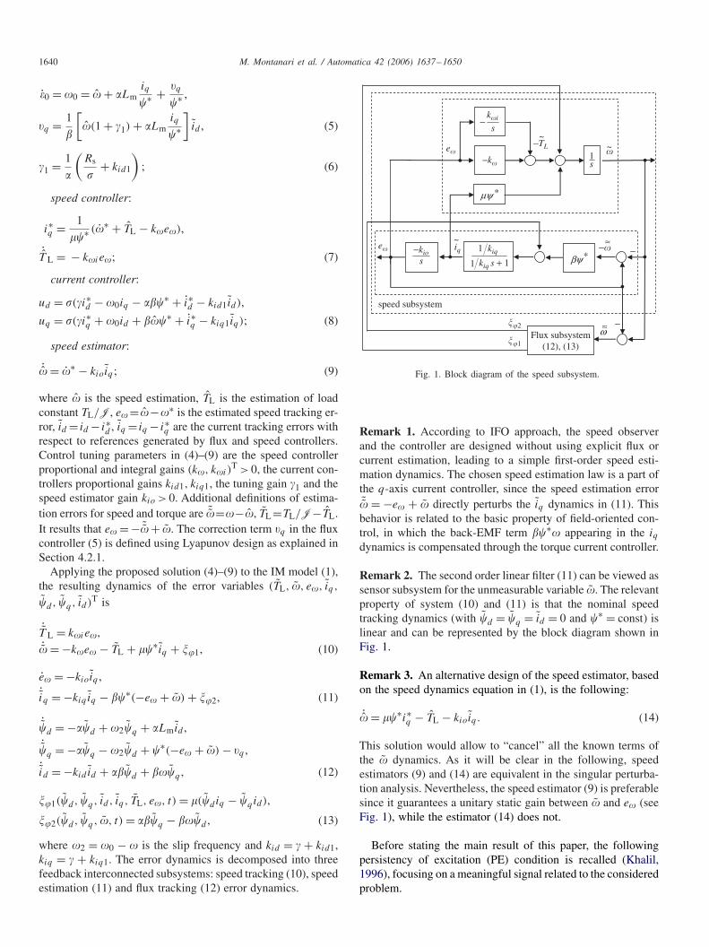
where �2 = �0 − � is the slip frequency and kid = � + kid1,kiq = � + kiq1. The error dynamics is decomposed into threefeedback interconnected subsystems: speed tracking (10), speedestimation (11) and flux tracking (12) error dynamics.

1s−k�

k�i

s−

e�

s−kio

1

1

kiq

kiq s + 1*βψ

−

*µψ

−

�1

�2

speed subsystem

e�

Flux subsystem(12), (13)

ω≈

−TL~

~

iq~

−�≈

�

Fig. 1. Block diagram of the speed subsystem.

Remark 1. According to IFO approach, the speed observerand the controller are designed without using explicit flux orcurrent estimation, leading to a simple first-order speed esti-mation dynamics. The chosen speed estimation law is a part ofthe q-axis current controller, since the speed estimation error˜� = −e� + � directly perturbs the iq dynamics in (11). Thisbehavior is related to the basic property of field-oriented con-trol, in which the back-EMF term ��∗� appearing in the iqdynamics is compensated through the torque current controller.

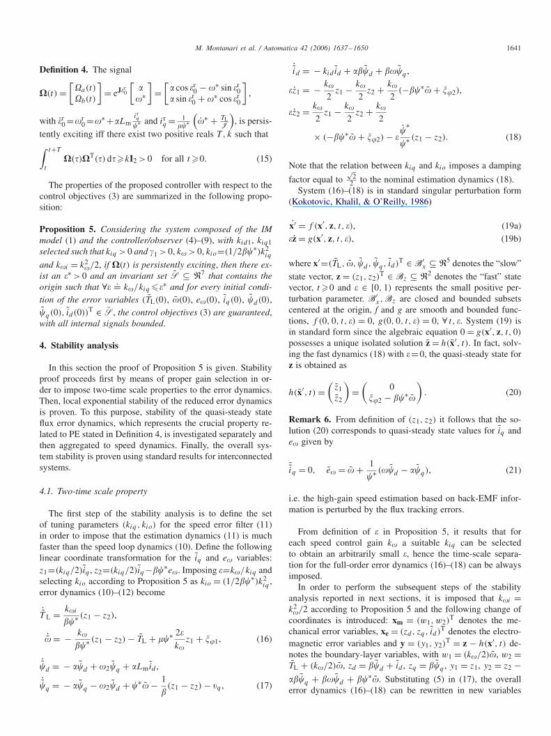
Remark 2. The second order linear filter (11) can be viewed assensor subsystem for the unmeasurable variable �. The relevantproperty of system (10) and (11) is that the nominal speedtracking dynamics (with �d = �q = id = 0 and �∗ = const) islinear and can be represented by the block diagram shown inFig. 1.

Remark 3. An alternative design of the speed estimator, basedon the speed dynamics equation in (1), is the following:

˙� = ��∗i∗q − TL − kioiq . (14)

This solution would allow to “cancel” all the known terms ofthe � dynamics. As it will be clear in the following, speedestimators (9) and (14) are equivalent in the singular perturba-tion analysis. Nevertheless, the speed estimator (9) is preferablesince it guarantees a unitary static gain between � and e� (seeFig. 1), while the estimator (14) does not.

Before stating the main result of this paper, the followingpersistency of excitation (PE) condition is recalled (Khalil,1996), focusing on a meaningful signal related to the consideredproblem.

M. Montanari et al. / Automatica 42 (2006) 1637–1650 1641

Definition 4. The signal

�(t) =[�a(t)

�b(t)

]= eJ�r

0

[��∗

]=

[� cos �r

0 − �∗ sin �r0

� sin �r0 + �∗ cos �r

0

],

with �r0 =�r

0 =�∗ +�Lmirq

�∗ and irq = 1

��∗(�∗ + TL

J

), is persis-

tently exciting iff there exist two positive reals T , k such that∫ t+T

t

�( )�T( ) d �kI2 > 0 for all t �0. (15)

The properties of the proposed controller with respect to thecontrol objectives (3) are summarized in the following propo-sition:

Proposition 5. Considering the system composed of the IMmodel (1) and the controller/observer (4)–(9), with kid1, kiq1selected such that kiq > 0 and �1 > 0, k� > 0, kio=(1/2��∗)k2

iq

and k�i = k2�/2, if �(t) is persistently exciting, then there ex-

ist an �∗ > 0 and an invariant set S ⊆ R7 that contains theorigin such that ∀�

.= k�/kiq ��∗ and for every initial condi-

tion of the error variables (TL(0), �(0), e�(0), iq (0), �d(0),�q(0), id (0))T ∈ S, the control objectives (3) are guaranteed,with all internal signals bounded.

4. Stability analysis

In this section the proof of Proposition 5 is given. Stabilityproof proceeds first by means of proper gain selection in or-der to impose two-time scale properties to the error dynamics.Then, local exponential stability of the reduced error dynamicsis proven. To this purpose, stability of the quasi-steady stateflux error dynamics, which represents the crucial property re-lated to PE stated in Definition 4, is investigated separately andthen aggregated to speed dynamics. Finally, the overall sys-tem stability is proven using standard results for interconnectedsystems.

4.1. Two-time scale property

The first step of the stability analysis is to define the setof tuning parameters (kiq , kio) for the speed error filter (11)in order to impose that the estimation dynamics (11) is muchfaster than the speed loop dynamics (10). Define the followinglinear coordinate transformation for the iq and e� variables:z1=(kiq/2)iq , z2=(kiq/2)iq−��∗e�. Imposing �=k�/kiq andselecting kio according to Proposition 5 as kio = (1/2��∗)k2

iq ,error dynamics (10)–(12) become

˙T L = k�i

��∗ (z1 − z2),

˙� = − k�

��∗ (z1 − z2) − TL + ��∗ 2�

k�z1 + �1, (16)

˙�d = − ��d + �2�q + �Lm id ,

˙�q = − ��q − �2�d + �∗� − 1

�(z1 − z2) − q , (17)

˙id = − kid id + ���d + ���q ,

�z1 = − k�

2z1 − k�

2z2 + k�

2(−��∗� + �2),

�z2 = k�

2z1 − k�

2z2 + k�

2

× (−��∗� + �2) − ��

∗

�∗ (z1 − z2). (18)

Note that the relation between kiq and kio imposes a damping

factor equal to√

22 to the nominal estimation dynamics (18).

System (16)–(18) is in standard singular perturbation form(Kokotovic, Khalil, & O’Reilly, 1986)

x′ = f (x′, z, t, �), (19a)

�z = g(x′, z, t, �), (19b)

where x′=(TL, �, �d , �q, id )T ∈ B′x ⊆ R5 denotes the “slow”

state vector, z = (z1, z2)T ∈ Bz ⊆ R2 denotes the “fast” state

vector, t �0 and � ∈ [0, 1) represents the small positive per-turbation parameter. B′

x,Bz are closed and bounded subsetscentered at the origin, f and g are smooth and bounded func-tions, f (0, 0, t, �) = 0, g(0, 0, t, �) = 0, ∀ t, �. System (19) isin standard form since the algebraic equation 0 = g(x′, z, t, 0)

possesses a unique isolated solution z = h(x′, t). In fact, solv-ing the fast dynamics (18) with �=0, the quasi-steady state forz is obtained as

h(x′, t) =(

z1z2

)=

(0

�2 − ��∗�

). (20)

Remark 6. From definition of (z1, z2) it follows that the so-lution (20) corresponds to quasi-steady state values for iq ande� given by

¯iq = 0, e� = � + 1

�∗ (��d − ��q), (21)

i.e. the high-gain speed estimation based on back-EMF infor-mation is perturbed by the flux tracking errors.

From definition of � in Proposition 5, it results that foreach speed control gain k� a suitable kiq can be selectedto obtain an arbitrarily small �, hence the time-scale separa-tion for the full-order error dynamics (16)–(18) can be alwaysimposed.

In order to perform the subsequent steps of the stabilityanalysis reported in next sections, it is imposed that k�i =k2�/2 according to Proposition 5 and the following change of

coordinates is introduced: xm = (w1, w2)T denotes the me-

chanical error variables, xe = (zd, zq, id )T denotes the electro-magnetic error variables and y = (y1, y2)

T = z − h(x′, t) de-notes the boundary-layer variables, with w1 = (k�/2)�, w2 =TL + (k�/2)�, zd = ��d + id , zq = ��q , y1 = z1, y2 = z2 −���q + ���d + ��∗�. Substituting (5) in (17), the overallerror dynamics (16)–(18) can be rewritten in new variables

1642 M. Montanari et al. / Automatica 42 (2006) 1637–1650

as follows:

[w1w2

]= k�

[− 12 − 1

212 − 1

2

] [w1w2

]

+ k�

[bm1,11(t, xe) − zd−id

2��∗

bm1,21(t, xe) − zd−id2��∗

] [w1w2

]

+ k�

[bm2,1(t, xe)

bm2,2(t, xe)

]

+ k�

⎡⎣ k�(zd−id )

2�2�∗2

(�zq − �∗(zd − id )

)− �zq id

2�

k�(zd−id )

2�2�∗2

(�zq − �∗(zd − id )

)− �zq id

2�

⎤⎦

+ k�

[− k�2��∗

(1 + zd−id

��∗)

(y1 − y2)

− k�2��∗ zd−id

��∗ (y1 − y2)

]

+ �

[�

(�∗ + zd−id

�

)y1

�(�∗ + zd−id

�

)y1

]

= Amxm + Bm1(t, xe)xm + Bm2(t)xe

+ Bm3(t, xe)xe + Bm4(t, xe)y + Bm5(t, xe)y. (22)

⎡⎣ zd

zq˙id

⎤⎦ =

[ 0 �r0 −�1�

−�r0 0 −�1�

∗� �∗ −(� + � + kid1)

] ⎡⎣zd

zq

id

⎤⎦

+[ �x

0zq

be1,2(t, xm, xe)2k�

w1zq

]+

[ �y0zq

be2,2(t, xe, y)

0

]

= Ae(t)xe + Be1(t, xm, xe)xe + Be2(t, xe)y, (23)

�

[y1y2

]= k�

[− 12 − 1

212 − 1

2

] [y1y2

]+ �

[0

by1,2(t, xm, xe, y)

]

= Ayy + �By1(t, xm, xe, y) (24)

with

bm1,11 = − zd − id

��∗ − zd − id

2��∗ − (zd − id )2

�2�∗2 ,

bm1,21 = − zd − id

2��∗ − (zd − id )2

�2�∗2 ,

bm2,1 = k�

2��∗(�zq − �∗(zd − id )

)

+ zd − id

2��∗(

TL

J+ �∗

)− �zq

2�Lm�(��∗ + �

∗),

bm2,2 = zd − id

2��∗(

TL

J+ �∗

)− �zq

2�Lm�(��∗ + �

∗),

be1,2(t, xm, xe) = − �x0zd − �1�

xid

+ i2d

��∗ (�∗ + �x)(1 + �1) + i2

d

��∗�Lm

�∗

× (irq + ixq )

be2,2(t, xe, y) = − �y0zd − y1 + y2

− �1�yid + i2

d

��∗ �y(1 + �1) + i2

d

��∗�Lm

�∗ iyq ,

by1,2 = − �∗

�∗(

y1 − y2 + 2��∗

k�w1 − �2

)

+ d

dt

[−�zq +

(�∗ + 2w1

k�

)(zd − id ) + 2��∗

k�w1

].

Note that in (23) it has been exploited that from definitions(4), (5) it holds �0 id − �q = −�1�id + (q/�∗)id . Signals�0, �, iq have been partitioned into independent time-varyingterms, denoted with superscript “r”, slow state-dependent terms,dependent on (t, xm, xe) and denoted with “x”, and fast state-dependent terms, dependent on (t, xm, xe, y) and denoted with“y”. Expressions of these terms in (22)–(24) are reported inAppendix A.

Remark 7. Design of the correction term q is instrumental tocompensate the flux-dependent perturbing terms in the quasi-steady state value of e� in (21) and to define the expression ofmatrix Ae(t) given in (23). This result is crucial as enlightenedin the Lyapunov analysis reported in Section 4.2.1.

4.2. Stability of the quasi-steady state error dynamics

The quasi-steady state system obtained from (22), (23) with� = 0 and y = (y1, y2)

T = 0 can be compactly expressed as

xm = Amxm + Bm1(t, xe)xm + Bm2(t)xe + Bm3(t, xe)xe, (25)

xe = Ae(t)xe + Be1(t, xm, xe)xe. (26)

It is decomposed into two feedback interconnected subsystems:the mechanical error dynamics (25) and the flux error dynamics(26). In the following, stability analysis of the flux subsystem isreported. Then, stability analysis of the quasi-steady state errordynamics and of the full-order system are carried out.

4.2.1. Flux error subsystemFlux error dynamics (26) has been expressed as a linear time-

varying (LTV) dynamics with the external input Be1xe withbilinear (and higher order) properties. Stability properties ofthe linearization of the quasi-steady state flux error dynamics,given by xe = Ae(t)xe, are studied.

Defining the time-varying coordinate transformation[za

zb

]= eJ�r

0

[zd

zq

]=

[cos �r

0 − sin �r0

sin �r0 cos �r

0

] [zd

zq

],

M. Montanari et al. / Automatica 42 (2006) 1637–1650 1643

the linearization of (26) is the LTV system expressed in thestate variables (id , za, zb)

T as

⎡⎣ ˙

idza

zb

⎤⎦ =

⎡⎢⎣

−(�+�+kid1) �a(t) �b(t)

− 1�

(Rs� +kid1

)�a(t) 0 0

− 1�

(Rs� + kid1

)�b(t) 0 0

⎤⎥⎦

[idza

zb

], (27)

where �a(t), �b(t) and �r0 are introduced in Definition 4 and

�1 is defined in (6). In order to investigate the stability propertiesof (27) the following Lyapunov function is considered

V1 = 1

2

[�

(Rs

�+ kid1

)−1 (z2a + z2

b

)+ i2

d

]. (28)

Its derivative along the trajectories of (27) is equal to

V1 = −(� + � + kid1)i2d . (29)

Hence, from (27)–(29) it follows that (id , za, zb) are boundedfor every t �0. Direct application of Barbalat’s Lemma (Khalil,1996, p. 192) shows that current tracking error id tends asymp-totically to zero for the LTV system (27).

Remark 8. From these preliminary results the asymptotic sta-bility of the quasi-steady state flux error dynamics (26) cannotbe inferred. In the following, it will be shown that exponentialstability of the LTV system (27) and hence local exponentialstability of the flux dynamics (26) hold if some persistency ofexcitation conditions are satisfied.

According to assumptions (A.3) and (A.4), TL is bounded and�∗, �∗ are bounded functions and therefore ‖�(t)‖ and ‖�(t)‖are uniformly bounded. If �(t) is persistently exciting (see(4)), from (28), (29) it follows that system (27) is exponentiallystable (Narendra & Annaswamy, 1989, pp. 72–75).

It is interesting to get insight on the operating conditions ofthe IM where persistency of excitation is satisfied. However, ageneric theoretical analysis cannot be easily performed. A sim-plified but insightful formal analysis is reported in AppendixB. It results that, from a practical point of view, the PE condi-tion (15) is satisfied during all the operating conditions of theIM, apart from dc excitation, i.e. with constant orientation ofthe rotor flux (�0 = 0). This condition corresponds to resultsreported in Canudas De Wit et al. (2000), Ibarra-Rojas et al.(2004) and is related to lack of observability of the speed sen-sorless controlled IM under dc excitation.

4.2.2. Overall error dynamicsLocal stability of the origin of the quasi-steady state error

dynamics (25), (26) will be proved by means of the Lyapunov’smethod.

Assume that the speed and flux error variables of system(25), (26) are inside compact sets centered at the origin, i.e.xe(t) ∈ Be, xm(t) ∈ Bm, ∀t , where Be = {x : ‖x‖ < be}and Bm = {x : ‖x‖ < bm} and assume that the PE condi-tion (15) is satisfied. From the stability analysis of Section4.2.1 for the linearization of the quasi-steady state flux dy-namics and linear/bilinear properties of the interconnection

terms in (22), (23), the slow subsystem (25), (26) has the fol-lowing properties:

(P1) Am is Hurwitz and the Lyapunov equation Am + ATm =

−k�I2 holds;(P2) ‖Bm1(t, xe)xm‖�k�k1‖xe‖‖xm‖ with 0 < k1 < ∞, ∀xe ∈

Be, ∀xm ∈ Bm,∀t ;(P3) ‖Bm2(t)‖�k�k2 with 0 < k2 < ∞, ∀t ;(P4) ‖Bm3(t, xe)xe‖�k�k3‖xe‖2 with 0 < k3 < ∞, ∀xe ∈ Be,

∀t ;(P5) The origin of xe =Ae(t)xe is globally exponentially stable;(P6) ‖Be1(t, xm, xe)xe‖ < k4‖xe‖2+k5‖xe‖‖xm‖, with 0 < (k4,

k5) < ∞, ∀xe ∈ Be, ∀xm ∈ Bm, ∀t ;

where ‖(·)‖ is the Euclidean norm of vector or matrix (·).Properties (P1) and (P5) are related to stability of the isolatedmechanical and flux subsystems, (P3) expresses the presence ofa linear part in the interconnection term Bm2(t)xe, while (P2),(P4), (P6) are relative to bilinear (and higher order) couplingterms. The bounds reported in (P2), (P3), (P4) and (P6) areuniform in t since the time-dependent references and the loadtorque are supposed to be bounded.

Properties of the nonlinear dynamics (25), (26) can be en-lightened first by a preliminary analysis of the linear approx-imation of the quasi-steady state error dynamics. The linearapproximation of (25), (26) is given by

xm = Amxm + Bm2(t)xe,

xe = Ae(t)xe

and is composed of the LTI exponentially stable mechanicaldynamics and the LTV electromagnetic dynamics, which isexponentially stable if the PE condition is satisfied. Mechanicaland electromagnetic linearized dynamics are interconnected inseries structure by means of the bounded matrix Bm2(t). Hence,it follows that the linearized dynamics is globally exponentiallystable if the PE condition is satisfied.

Utilizing results from Khalil (1996, Theorem 3.11) andVidyasagar (1978, Section 5.4), it is shown that the originof the quasi-steady state error dynamics (25), (26) is locallyexponentially stable (see Appendix C).

4.3. Full-order error dynamics

Assuming that state variables of the speed, flux andboundary-layer error dynamics are inside compact sets cen-tered at the origin, i.e. xe(t) ∈ Be, xm(t) ∈ Bm, y(t) ∈ By ,∀t , where Be ={x : ‖x‖ < be}, Bm ={x : ‖x‖ < bm}, By ={x :‖x‖ < by}, and assuming that the PE condition (15) is satisfied,the following properties hold for the full-order error dynamics(22)–(24) in addition to properties P1–P6:

(P7) ‖Bm4(t, xe)‖�k�k6 with 0 < k6 < ∞, ∀xe ∈ Be, ∀t ;(P8) ‖Bm5(t, xe)‖��k7 with 0 < k7 < ∞, ∀xe ∈ Be, ∀t ;(P9) ‖Be2(t, xe)‖�k8 with 0 < k8 < ∞, ∀xe ∈ Be, ∀t ;

(P10) Ay is Hurwitz and the Lyapunov equation Ay + ATy

= − k�I2 holds;

1644 M. Montanari et al. / Automatica 42 (2006) 1637–1650

(P11) ‖By1(t, xm, xe, y)‖�(k9 + k′9/k�)‖xm‖ + k10‖xe‖ +

(k11 +�k′11/k�)‖y‖ with 0 < (k9, k′

9, k10, k11, k′11) < ∞,

∀xm ∈ Bm, ∀xe ∈ Be, ∀y ∈ By , ∀t .

Note that properties P7–P9 and P11 establish the presence oflinear parts in the coupling terms dependent on fast variables y.From properties (P1)–(P11), local uniform asymptotic stabilityof the origin of the full-order error dynamics (22)–(24) turnsout. The stability analysis, which follows the same steps of theproof of Appendix C, and the evaluation of �∗ (see Proposition5) are based on standard methods for singularly perturbed sys-tems with exponentially stable reduced and boundary-layer sub-systems (Khalil, 1996, Chapter 9). Estimate of the domain of at-traction is based on classical Lyapunov-like technique (Khalil,1996, Chapter 4). Stability proof is not reported here for thesake of space. Since xe(t), xm(t), y(t) tend exponentially tozero, provided that initial conditions are inside the domain ofattraction, it follows that asymptotic speed and rotor flux mod-ulus tracking together with field orientation are achieved.

5. Experimental results

The proposed sensorless control algorithm has been experi-mentally tested using a two pole pairs 1.1 kW standard induc-tion motor, with 7.0 Nm rated torque and 1410 rev/ min ratedspeed at 50 Hz. Motor data are the following: rated voltage is220 V, rated current is 2.8 A, excitation current is 1.4 A, statorand rotor resistances are Rs = 10.4 �, Rr = 4.5 �, magnetiza-tion inductance is Lm = 0.434 H, stator and rotor inductancesare Ls = Lr = 0.47 H, total inertia is J = 0.0034 Kg m2.

5.1. Controller tuning

The sensorless controller defined in (4)–(9) generates the er-ror dynamics given by (16)–(18). Parameters tuning is strictlyrelated to the structure of the error dynamics. Control pa-rameters of the flux subsystem (17) are the proportional d-axis current controller gain kid1 and the correction gain �1,linked by relation (6). According to tuning relations in Propo-sition 5 between the speed controller proportional and integralgains k�, k�i and between the proportional gain kiq1 of theq-axis current regulator and the speed estimator gain kio, thesecond order nominal speed error dynamics in (22) and the fast

0 0.5 1 1.50

25

50

75

100

Speed reference and loadtorque profile (∗10)

rad/

s, N

m

time (s)

0 0.5 1 1.50

0.25

0.5

0.75

1Flux reference

Wb

time (s)

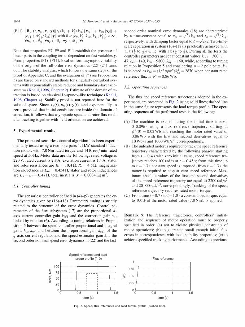
Fig. 2. Speed, flux references and load torque profile (dashed line).

second order nominal error dynamics (18) are characterizedby a time-constant equal to � = √

2/k� and o = √2/kiq ,

respectively, with damping factor equal to �=√2/2. Two-time-

scale separation in system (16)–(18) is practically achieved with o �( 1

4 to 12 ) �, i.e. with ��( 1

4 to 12 ). During all the tests the

controller parameters are set at constant values kid1 =300, �1 =47, k�=140, k�i =9800, kiq1=160, while, according to tuningrelation in Proposition 5 and considering p = 2 pole pairs, kio

is selected as kio = (1/2p��∗)k2iq = 2870 when constant rated

reference flux is �∗ = 0.86 Wb.

5.2. Operating sequences

The flux and speed reference trajectories adopted in the ex-periments are presented in Fig. 2 using solid lines; dashed linein the same figure represents the load torque profile. The oper-ating sequence of the performed tests is the following:

(A) The machine is excited during the initial time interval0–0.096 s using a flux reference trajectory starting at�∗(0) = 0.02 Wb and reaching the motor rated value of0.86 Wb with the first and second derivatives equal to10 Wb/s and 1000 Wb/s2, correspondingly.

(B) The unloaded motor is required to track the speed referencetrajectory characterized by the following phases: startingfrom t = 0.4 s with zero initial value, speed reference tra-jectory reaches 100 rad/s at t = 0.45 s; from this time upto t = 1.3 s constant speed is imposed; from t = 1.3 s themotor is required to stop at zero speed reference. Max-imum absolute values of the first and second derivativesof the speed reference trajectory are equal to 2200 rad/s2

and 20 000 rad/s3, correspondingly. Tracking of the speedreference trajectory requires rated motor torque.

(C) From time t=0.7 s to t=1.0 s a constant load torque, equalto 100% of the motor rated value (7.0 Nm), is applied.

Remark 9. The reference trajectories, controllers’ initial-ization and sequence of motor operation must be properlyspecified in order: (a) not to violate physical constraints ofmotor operations; (b) to guarantee small enough initial fluxerrors in correspondence with local stability properties; (c) toachieve specified tracking performance. According to previous

M. Montanari et al. / Automatica 42 (2006) 1637–1650 1645

0 0.5 1 1.5−15−10

−505

1015

Speed tracking error

rad/

s

0 0.5 1 1.5−15−10

−505

1015

Estimated speed tracking error

rad/

s

0 0.5 1 1.5−6−4−20246

Reference for q−axis current

A

0 0.5 1 1.5−6−4−20246

q−axis current error

A

0 0.5 1 1.5−6−4−20246

Reference for d−axis current

A

0 0.5 1 1.5−6−4−20246

d−axis current error

A

0 0.5 1 1.5−300

−150

0

150

300d−axis voltage (ud)

V

time (s)

0 0.5 1 1.5−300

−150

0

150

300q−axis voltage (uq)

V

time (s)

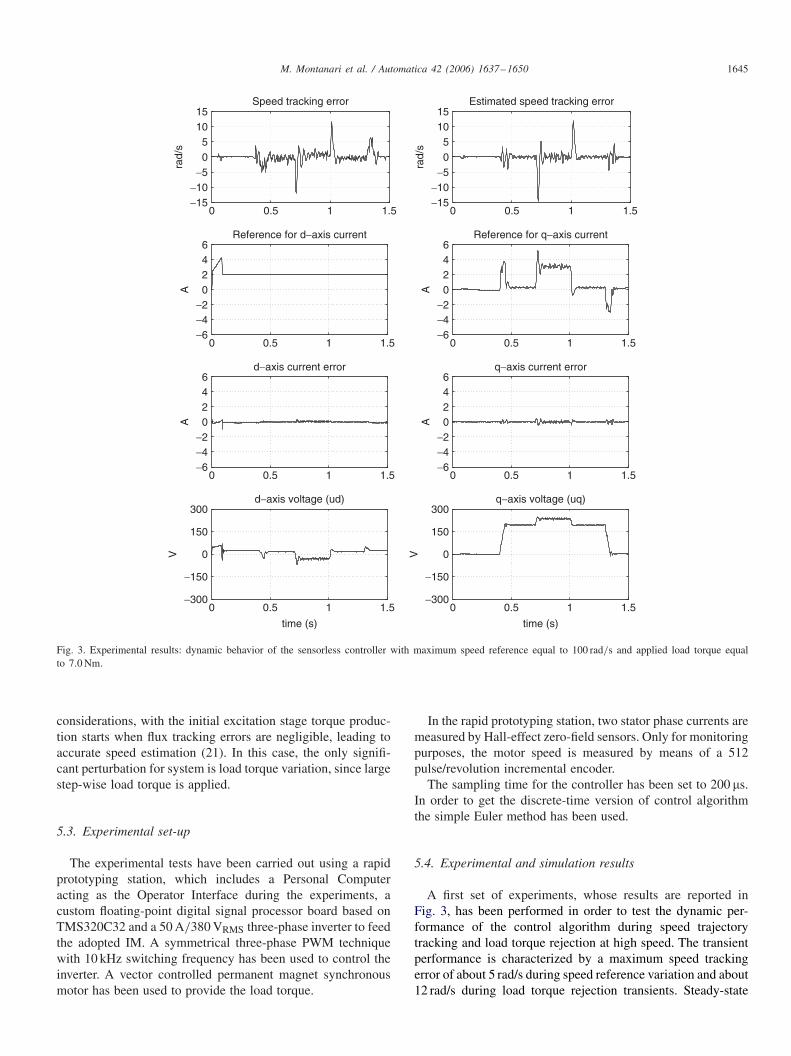
Fig. 3. Experimental results: dynamic behavior of the sensorless controller with maximum speed reference equal to 100 rad/s and applied load torque equalto 7.0 Nm.

considerations, with the initial excitation stage torque produc-tion starts when flux tracking errors are negligible, leading toaccurate speed estimation (21). In this case, the only signifi-cant perturbation for system is load torque variation, since largestep-wise load torque is applied.

5.3. Experimental set-up

The experimental tests have been carried out using a rapidprototyping station, which includes a Personal Computeracting as the Operator Interface during the experiments, acustom floating-point digital signal processor board based onTMS320C32 and a 50 A/380 VRMS three-phase inverter to feedthe adopted IM. A symmetrical three-phase PWM techniquewith 10 kHz switching frequency has been used to control theinverter. A vector controlled permanent magnet synchronousmotor has been used to provide the load torque.

In the rapid prototyping station, two stator phase currents aremeasured by Hall-effect zero-field sensors. Only for monitoringpurposes, the motor speed is measured by means of a 512pulse/revolution incremental encoder.

The sampling time for the controller has been set to 200 �s.In order to get the discrete-time version of control algorithmthe simple Euler method has been used.

5.4. Experimental and simulation results

A first set of experiments, whose results are reported inFig. 3, has been performed in order to test the dynamic per-formance of the control algorithm during speed trajectorytracking and load torque rejection at high speed. The transientperformance is characterized by a maximum speed trackingerror of about 5 rad/s during speed reference variation and about12 rad/s during load torque rejection transients. Steady-state

1646 M. Montanari et al. / Automatica 42 (2006) 1637–1650

0 0.5 1 1.5−15−10

−505

1015

Speed tracking error

rad/

s

0 0.5 1 1.5−15−10

−505

1015

Estimated speed tracking error

rad/

s

0 0.5 1 1.5−6−4−20246

Reference for q−axis current

A

0 0.5 1 1.5−6−4−20246

q−axis current error

A

0 0.5 1 1.5−6−4−20246

Reference for d−axis current

A

0 0.5 1 1.5−6−4−20246

d−axis current error

A

0 0.5 1 1.5−300

−150

0

150

300d−axis voltage (ud)

V

0 0.5 1 1.5−300

−150

0

150

300q−axis voltage (uq)

V

0 0.5 1 1.5−5

−2.5

0

2.5

5x 10−3 d−axis flux error

Wb

time (s)

0 0.5 1 1.5−5

−2.5

0

2.5

5x 10−3 q−axis flux error

Wb

time (s)

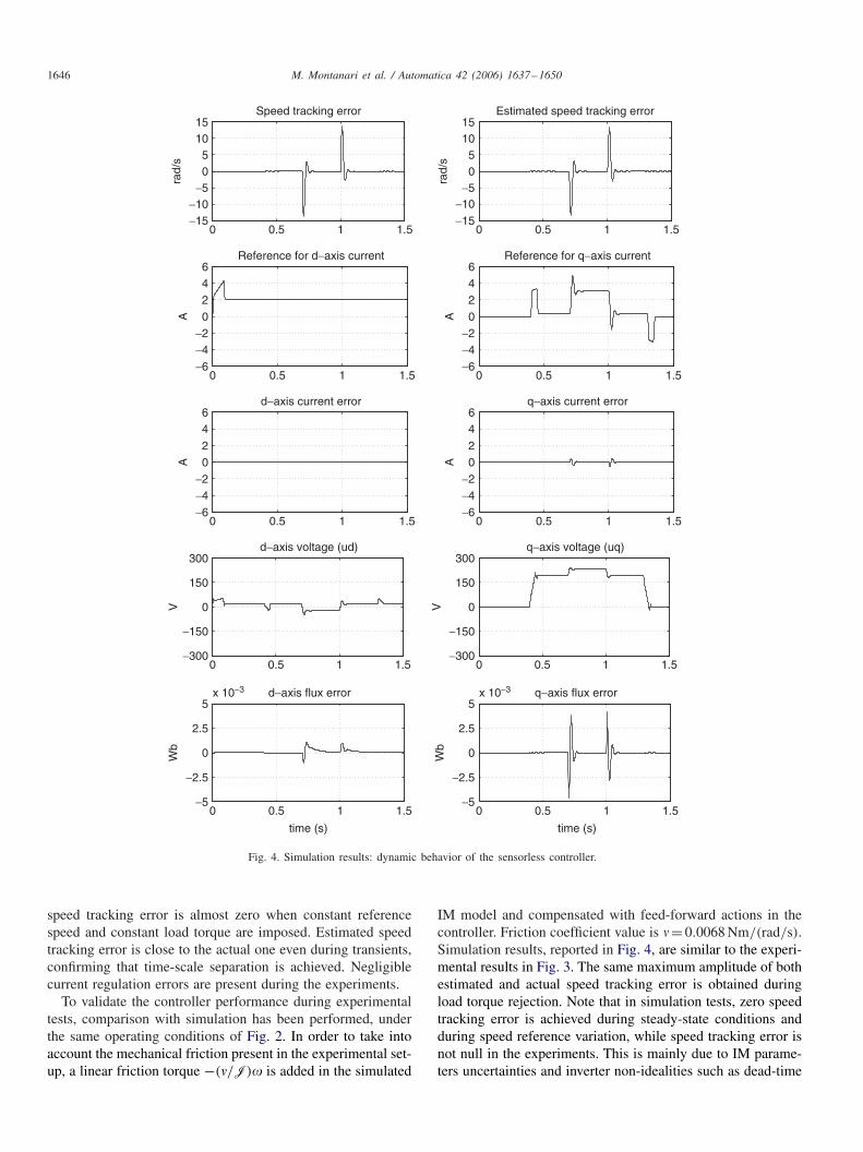
Fig. 4. Simulation results: dynamic behavior of the sensorless controller.

speed tracking error is almost zero when constant referencespeed and constant load torque are imposed. Estimated speedtracking error is close to the actual one even during transients,confirming that time-scale separation is achieved. Negligiblecurrent regulation errors are present during the experiments.

To validate the controller performance during experimentaltests, comparison with simulation has been performed, underthe same operating conditions of Fig. 2. In order to take intoaccount the mechanical friction present in the experimental set-up, a linear friction torque −(�/J)� is added in the simulated

IM model and compensated with feed-forward actions in thecontroller. Friction coefficient value is �= 0.0068 Nm/(rad/s).Simulation results, reported in Fig. 4, are similar to the experi-mental results in Fig. 3. The same maximum amplitude of bothestimated and actual speed tracking error is obtained duringload torque rejection. Note that in simulation tests, zero speedtracking error is achieved during steady-state conditions andduring speed reference variation, while speed tracking error isnot null in the experiments. This is mainly due to IM parame-ters uncertainties and inverter non-idealities such as dead-time

M. Montanari et al. / Automatica 42 (2006) 1637–1650 1647

0.65 0.7 0.75 0.8 0.85−15−10

−505

1015

Quasi−steady state speedestimation error

rad/

s

time (s)

0.65 0.7 0.75 0.8 0.85−15−10

−505

1015

Estimated speed tracking errors

rad/

s

time (s)

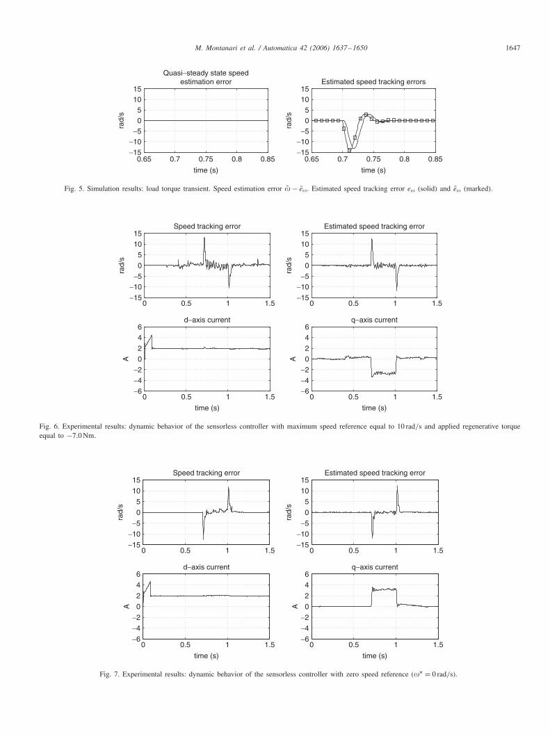
Fig. 5. Simulation results: load torque transient. Speed estimation error � − e�. Estimated speed tracking error e� (solid) and e� (marked).

0 0.5 1 1.5−15

−10−5

0

51015

Speed tracking error

rad/

s

0 0.5 1 1.5−15

−10−50

51015

Estimated speed tracking error

rad/

s

0 0.5 1 1.5−6

−4−2

02

46

q−axis current

A

time (s)

0 0.5 1 1.5−6

−4−2

02

46

d−axis current

A

time (s)

Fig. 6. Experimental results: dynamic behavior of the sensorless controller with maximum speed reference equal to 10 rad/s and applied regenerative torqueequal to −7.0 Nm.

0 0.5 1 1.5−15

−10

−5

0

5

10

15Speed tracking error

rad/

s

0 0.5 1 1.5−15

−10

−5

0

5

10

15Estimated speed tracking error

rad/

s

0 0.5 1 1.5−6

−4

−2

0

2

4

6q−axis current

A

time (s)

0 0.5 1 1.5−6

−4

−2

0

2

4

6d−axis current

A

time (s)

Fig. 7. Experimental results: dynamic behavior of the sensorless controller with zero speed reference (�∗ = 0 rad/s).

1648 M. Montanari et al. / Automatica 42 (2006) 1637–1650

effect and voltage commutations. Stator current and voltageprofiles during experimental and simulation tests are compar-atively shown in Figs. 3 and 4. In Fig. 4 rotor flux errors arealso reported, showing that asymptotic flux amplitude regula-tion and field orientation are achieved.

In Fig. 5 the behavior of �− e�, e� and e� defined in (21) isreported. A zoom of the first load torque transient is considered.From the first picture it can be noted that � − e� is very smallcompared to � and e� in Fig. 4, hence the quasi-steady statebehavior of e� is very similar to � and the contribution relatedto flux errors (see (21)) is almost negligible. In the secondpicture of Fig. 5 the similarity between the actual variable e�and its quasi-steady state version e� is enlightened, confirmingthe established time-scale separation.

A second set of experiments has been performed to test theproposed solution when the PE condition (15) fails or is nearto fail. As it is well-known in the application-oriented litera-ture (Rajashekara et al., 1996) and according to the analysis inSection 4.2.1 and Appendix B, the condition �0 = 0 is criticaland particularly significant in real-world applications.

In Fig. 6 a low-speed, regenerative condition (i.e. with nega-tive output mechanical power) is considered. A speed referenceprofile with shape similar to Fig. 2, maximum speed of 10 rad/sand maximum time derivative of 220 rad/s2 has been imposed;−7.0 Nm regenerative torque is applied following the operatingsequence of Section 5.2. The nominal �0 is very close to zerowith regenerative torque (�0=5.9 rad/s). No significant perfor-mance degradation is present in low-speed regenerative-torquecondition (Fig. 6) with respect to tests at high-speed (Fig. 3).

In Fig. 7 rejection of the rated load torque with zero speedreference is considered according to the operating sequence ofSection 5.2. In this experiment nominal �0 goes from zero to14.1 rad/s and back. Again, the performances are very similarto previous cases; only after the load torque step down a smallresidual speed error can be noted, owing to lack of PE.

Results of experimental tests confirm that the achievabledynamic performances of the speed sensorless controller arecomparable to those obtained with high performance vectorcontrolled induction motor drives with speed measurement,for typical operating conditions including zero speed andregenerative mode.

6. Conclusions

It has been proven that the proposed speed-sensorless con-troller guarantees local asymptotic tracking of smooth speedand flux references along with asymptotic field orientation, withconstant unknown load torque, if the estimation dynamics isimposed to be sufficiently faster than the speed/flux one andif a persistency of excitation condition is satisfied. As far asthe latter is concerned, essentially a non-null synchronous fre-quency is required. This condition is well established in bothmethodological and application-oriented literature; future ef-forts will be devoted to avoid this condition without impairingthe control performances.

Since the stability analysis invokes the converse Lyapunovtheorem and an integral PE condition, the existence of the

small positive real �∗ and the domain of attraction S is proved,without providing their evaluation. A constructive procedurefor controller parameters selection is obtained from the con-troller design. This procedure is conceptually similar to that oneadopted in industrial drives, thanks to cascaded structure of theoverall system dynamics with established time-scale propertiesfor control loops. Moreover, the physically-based structure ofthe controller leads to a straightforward simplification if rotorspeed is measured.

Experiments and simulations in typical operating conditionsdemonstrate high dynamic performance during speed and fluxtracking including load torque rejection, which is of the sameorder as for standard field-oriented solutions with speed mea-surement.

Appendix A. Definitions

� = �∗(t) + �x(t, xm, xe) + �y

(t, xm, xe, y),

�x = 1��∗

[−�zq +

(�∗ + 2

k�w1

)(zd − id ) + 2

k���∗w1

],

�y = 1

��∗ (y1 − y2) ,

iq = irq(t) + ixq (t, xm, xe) + i

yq (t, xm, xe, y),

irq = 1

��∗[�∗ + TL

J

]; i

yq = 2�

k�y1 − k�

��∗1

��∗ (y1 − y2) ,

ixq = 1

��∗ (w1 − w2) + k�

��∗1

��∗

×[�zq −

(�∗ + 2

k�w1

)(zd − id ) − 2

k���∗w1

],

�0 = �r0(t) + �x

0(t, xm, xe) + �y0(t, xm, xe, y),

�r0 = �∗ + �Lm

irq

�∗ ; �x0 = �x + �Lm

ixq

�∗

+ 1

��∗ (1 + �1)(�∗ + �x

)id + 1

��∗�Lm

�∗(irq + ixq

)id ,

�y0 = �y + �Lm

iyq

�∗ + 1

��∗ (1 + �1)�yid + 1

��∗�Lm

�∗ iyq id .

Appendix B. Persistency of excitation

To enlighten when persistency of excitation is guaran-teed for the electromagnetic dynamics, assume for simplic-ity steady-state conditions for the reference speed and forthe reference frame angular speed, i.e. constant steady-stateconditions for �∗, �∗, TL. Supposing �r

0 = const = 0 and�∗ = const, and choosing T = 2�/|�r

0|, the PE condition (15)

becomes∫ t+T

t�( )�( )Td = diag((�2 + �∗2)�/|�r

0|, (�2 +�∗2)�/|�r

0|) > �2�/|�r0|, hence choosing k = �2�/|�r

0|, if�r

0 = 0 the PE condition is satisfied.On the other hand, assuming �r

0 =0 (and �r0 =0 without loss

of generality) during time interval [t, t + T ], with T > 0, andconsidering a generic reference speed �∗(t), the PE condition

M. Montanari et al. / Automatica 42 (2006) 1637–1650 1649

(15) becomes∫ t+T

t

�( )�T( ) d =[∫ t+T

t�2 d

∫ t+T

t��∗( ) d ∫ t+T

t��∗( ) d

∫ t+T

t�∗2( ) d

].

Applying Cauchy–Schwartz–Buniakowsky theorem, it followsthat the PE condition is satisfied if �r

0 =0 and �∗(t) is not con-stant during the time interval [t, t +T ]. Actually this conditionis not meaningful from a practical viewpoint. On the other side,PE is not satisfied with constant �∗ and �0r = 0, i.e. duringregenerative condition with dc excitation.

Appendix C. Stability proof of the origin of the quasi-steadystate system

Recalling property P5 and applying the converse Lya-punov theorem (Khalil, 1996, Theorem 3.12) for exponen-tially stable systems to the linear approximation of theflux error dynamics (26), it follows that there exist posi-tive constants c1, c2, c3, c4 and a function Ve(t, xe) such thatc1‖xe‖2 �Ve(t, xe)�c2‖xe‖2, (�Ve/�xe)Ae(t)xe+�Ve/�t <−c3‖xe‖2, ‖�Ve/�xe‖ < c4‖xe‖. Consider the candidate Lya-punov function V = 1

2 xTmxm + �Ve(t, xe) where � > 0 is

a constant positive gain to be designed. Recalling proper-ties P1–P4, its time derivative along the trajectories of (25),(26) is V � − k�/2‖xm‖2 + k�k1‖xe‖‖xm‖2 − �c3‖xe‖2 +�c4k4‖xe‖3 + k�k2‖xe‖‖xm‖ + (k�k3 + �c4k5)‖xe‖2‖xm‖.Applying Young’s inequalities 2ab�ka2 + b2/k, with a, b ∈R, k ∈ (0, 1) to the last two terms, the following inequa-lities hold: k�k2‖xe‖‖xm‖�k�/4‖xm‖2 + k�k2

2‖xe‖2,(k�k3 + �c4k5)‖xe‖2‖xm‖�k�k3 + �c4k5/2‖xe‖‖xm‖2 +k�k3 + �c4k5/2‖xe‖3. Hence, it follows that V � − [k�/4 −[k�(k1+k3/2)+�c4k5/2]‖xe‖]‖xm‖2−[�c3−k�k2

2−[k�k3/2+�c4(k4 + k5/2)]‖xe‖]‖xe‖2. Choosing � = 2k�k2

2/c3 it holdsV � − k�[ 1

4 − (k1 + k3/2 + c4k5k22/c3)‖xe‖]‖xm‖2 − k�[k2

2 −(k3/2 + 2k2

2c4/c3(k4 + k5/2))‖xe‖]‖xe‖2, ∀ ‖xe‖�be, ∀ ‖xm‖�bm. Imposing that ‖xe(t)‖�Le, ∀ t , where Le=min{be,

18 (k1+

k3/2+c4k5k22/c3)

−1, 12k2

2(k3/2+2k22c4/c3(k4 +k5/2))−1}, the

following inequality holds: V � − k�/8‖xm‖2 − k�k22/2‖xe‖2,

∀‖xe(t)‖ < Le, ∀ ‖xm(t)‖ < bm. Hence, the origin of system(25), (26) is locally exponentially stable.

References

Canudas De Wit, C., Youssef, A., Barbot, J. P., Martin, P. & Malrait, F.(2000). Observability conditions of induction motors at low frequencies.In Proceedings of the 39th IEEE conference on decision and control (Vol.3, pp. 2044–2049). Sydney, Australia.

Chern, T., Chang, J., & Tsai, K. (1998). Integral-variable-structure-control-based adaptive speed estimator and resistance identifier for induction motor.International Journal of Control, 69(1), 31–47.

Doki, S., Sangwongwanick, S. & Okuma, S. (1992). Implementation of speed-sensor-less field oriented vector control using adaptive sliding observer.In Proceedings of the 18th IEEE conference on industrial electronics (pp.453–458). San Diego, CA.

Feemster, M., Aquino, P., Dawson, D. M., & Behal, A. (2001). Sensorlessrotor velocity tracking control for induction motors. IEEE Transactionson Control Systems Technology, 9(4), 645–653.

Holtz, J. (2002). Sensorless control of induction motor drives. Proceedingsof the IEEE, 90(8), 1359–1394.

Ibarra-Rojas, S., Moreno, J., & Espinosa-Perez, G. (2004). Globalobservability analysis of sensorless induction motors. Automatica, 40(6),1079–1085.

Khalil, H. K. (1996). Nonlinear systems. (2nd ed.), Upper Saddle River, NJ:Prentice Hall.

Kokotovic, P. V., Khalil, H. K., & O’Reilly, J. (1986). Singular perturbationmethods in control: Analysis and design. London: Academic Press.

Kubota, H., & Matsuse, K. (1994). Speed sensorless field-oriented control ofinduction motor with rotor resistance adaptation. IEEE Transactions onIndustry Applications, 30(5), 1219–1224.

Leonhard, W. (2001). Control of electrical drives. (3rd ed.), Berlin: Springer.Marino, R., Tomei, P. & Verrelli, C. M. (2002a). Adaptive control of sensorless

induction motors with uncertain rotor resistance. In Proceedings of the41st IEEE conference on decision and control (pp. 148–153). Las Vegas,Nevada.

Marino, R., Tomei, P. & Verrelli, C. M. (2002b). A new global control schemefor sensorless current-fed induction motors. In 15th IFAC triennial worldcongress, Barcelona, Spain.

Marino, R., Tomei, P., & Verrelli, C. M. (2004a). A global tracking controlfor speed-sensorless induction motors. Automatica, 40(6), 1071–1077.

Marino, R., Tomei, P. & Verrelli, C. M. (2004b). Nonlinear tracking control forsensorless induction motors. In Proceedings of the 43rd IEEE conferenceon decision and control. Paradise Island, Bahamas.

Montanari, M., Peresada, S. & Tilli, A. (2003). Sensorless control of inductionmotors with exponential stability property. In Proceedings of the 2003European control conference. Cambridge, UK.

Montanari, M., Peresada, S. & Tilli, A. (2004). Sensorless control of inductionmotor with adaptive speed-flux observer. In Proceedings of the 43rd IEEEconference on decision and control. Paradise Island, Bahamas.

Montanari, M., Peresada, S., Tilli, A. & Tonielli, A. (2000). Speedsensorless control of induction motor based on indirect field-orientation. InProceedings of the 35th IEEE conference on industry application, Rome,Italy.

Narendra, K. S., & Annaswamy, A. M. (1989). Stable adaptive systems.Englewood Cliffs, NJ: Prentice-Hall.

Peng, F., & Fukao, T. (1994). Robust speed identification for speed-sensorlessvector control of induction motors. IEEE Transactions on IndustryApplications, 30(5), 1234–1240.

Peresada, S., Montanari, M., Tilli, A. & Kovbasa, S. (2002). Sensorlessindirect field-oriented control of induction motors, based on high gainspeed estimation. In Proceedings of the 28th IEEE conference on industrialelectronics. Sevilla, Spain.

Peresada, S., & Tonielli, A. (2000). High-performance robust speed-fluxtracking controller for induction motor. International Journal of AdaptiveControl and Signal Processing, 14, 177–200.

Rajashekara, K., Kawamura, A., & Matsuse, K. (1996). Sensorless control ofAC motor drives. New York: IEEE Press.

Schauder, C. (1992). Adaptive speed identification for vector control ofinduction motors without rotational transducers. IEEE Transactions onIndustry Applications, 28(5), 1054–1061.

Vas, P. (1998). Sensorless vector and direct torque control. Oxford: OxfordUniversity Press.

Vidyasagar, M. (1978). Nonlinear systems analysis. Englewood Cliffs, NJ:Prentice-Hall.

Yan, Z., Jin, C. & Utkin, V.I. (2000). Sensorless sliding-mode control ofinduction motors. IEEE Transactions on Industrial Electronics 47 (6).

Marcello Montanari was born in Ravenna, Italy, in1974. He received the Dr. Ing. degree in computerscience engineering and the Ph.D. degree in Auto-matic Control at the University of Bologna, Italy,in 1999 and 2003, respectively. Since 2003, he hasa Post-Doc position within the Department of Elec-tronics, Computer Science and Systems, Universityof Bologna. His current research interests includeapplied nonlinear and adaptive control, in the fieldof electric drives, automotive applications, electro-mechanical and electro-hydraulic systems.

1650 M. Montanari et al. / Automatica 42 (2006) 1637–1650

Sergei M. Peresada was born in 1952, Donetsk,USSR. He received the Diploma of ElectricalEngineer from the Donetsk Polytechnic Insti-tute in 1974 and the Candidate of TechnicalSciences degree (corresponding to Ph.D.) incontrol and automation from the Kiev Poly-technic Institute in 1983. He has been workingat the Department of Electrical Engineeringand Automation of the National Technical Uni-versity of Ukraine “Kiev Polytechnic Institute”

since 1977, where he is currently Professor of Control and Automation. Hehas been Visiting Professor at the University of Illinois (Urbana-Champaign),University of Rome Tor Vergata, DEIS and Institute of Advanced Study Uni-versity of Bologna. He currently serves as Associate Editor of the IEEETransactions on Control Systems Technology.His research interests include nonlinear and adaptive control of electrome-chanical systems based on AC motors, control of power converters. He isauthor of about 150 scientific publications and co-author of the volumes:“Theory and Control of Electrical Drives” and “Control of ElectromechanicalSystems”.

Andrea Tilli was born in Bologna, Italy, onApril 4, 1971. He received the Dr. Ing. degreein electronic engineering from the University ofBologna, Italy, in 1996. On February 29, 2000he received the Ph.D. degree in system scienceand engineering from the same university witha thesis on nonlinear control of standard andspecial asynchronous electric machines.Since 1997, he has been at the Department ofElectronics, Computer Science and Systems

(DEIS) of the University of Bologna. On July 2000, he won a research grantfrom the above department on modeling and control of complex electrome-chanical systems. Starting from October 1, 2001, he is a Research Associateat DEIS.His current research interests include applied nonlinear control techniques,adaptive observers, electric drives, automotive systems, power electronicsequipments, active power filters and DSP-based control architectures.