Scheduling Kernels via Configuration LPDušan KnopDepartment of Theoretical Computer Science, Faculty of Information Technology, Czech TechnicalUniversity in Prague, Czech Republicdusan.knop@fit.cvut.cz

Martin KouteckýComputer Science Institute of Charles University, Charles University, Czech Republickoutecky@iuuk.mff.cuni.cz

AbstractMakespan minimization (on parallel identical or unrelated machines) is arguably the most naturaland studied scheduling problem. A common approach in practical algorithm design is to reducethe size of a given instance by a fast preprocessing step while being able to recover key informationeven after this reduction. This notion is formally studied as kernelization (or simply, kernel) – apolynomial time procedure which yields an equivalent instance whose size is bounded in terms ofsome given parameter. It follows from known results that makespan minimization parameterized bythe longest job processing time pmax has a kernelization yielding a reduced instance whose size isexponential in pmax. Can this be reduced to polynomial in pmax?

We answer this affirmatively not only for makespan minimization, but also for the (morecomplicated) objective of minimizing the weighted sum of completion times, also in the setting ofunrelated machines when the number of machine kinds is a parameter.

Our algorithm first solves the Configuration LP and based on its solution constructs a solution ofan intermediate problem, called huge N -fold integer programming. This solution is further reducedin size by a series of steps, until its encoding length is polynomial in the parameters. Then, weshow that huge N -fold IP is in NP, which implies that there is a polynomial reduction back to ourscheduling problem, yielding a kernel.

Our technique is highly novel in the context of kernelization, and our structural theorem aboutthe Configuration LP is of independent interest. Moreover, we show a polynomial kernel for hugeN -fold IP conditional on whether the so-called separation subproblem can be solved in polynomialtime. Considering that integer programming does not admit polynomial kernels except for quiterestricted cases, our “conditional kernel” provides new insight.

2012 ACM Subject Classification Theory of computation → Fixed parameter tractability; Theoryof computation → Scheduling algorithms; Theory of computation → Integer Programming

Keywords and phrases Scheduling, Kernelization

Acknowledgements Authors wish to thank the Lorentz Center for making it possible to organize theworkshop Scheduling Meets Fixed-Parameter Tractability, which output resulted in this paper. Thecontribution of the Lorentz Center in stimulating suggestions, giving feedback and taking care of allpracticalities, helped us to focus on our research and to organize a meeting of high scientific quality.Furthermore, the authors thank Stefan Kratsch for bringing Proposition 5 to their attention.

arX

iv:2

003.

0218

7v1

[cs

.DS]

4 M

ar 2

020

2 Scheduling Kernels via Configuration LP

1 Introduction

Kernelization, data reduction, or preprocessing: all of these refer to the goal of simplifying andreducing (the size of) the input in order to speed up computation of challenging tasks. Manyheuristic techniques are applied in practice, however, we seek a theoretical understandingin the form of procedure with guaranteed bounds on the sizes of the reduced data. We usethe notion of kernelization from parameterized complexity (cf. [9, 38]), where along with aninput instance I we get a positive integer k expressing the parameter value, which may bethe size of the sought solution or some structural limitation of the input. A kernel is analgorithm running in time poly(|I|) which returns a reduced instance I ′ of the same problemof size bounded in terms of k; we sometimes also refer to I ′ as the kernel.

It is well known [5] that a problem admits a kernel if and only if it has an algorithmrunning in time f(k) poly(|I|) for some computable function f (i.e., if it is fixed-parametertractable, or FPT, parameterized by k). The “catch” is that this kernel may be very large(exponential or worse) in terms of k, while for many problems, kernels of size polynomialin k are known. This raises a fundamental question for any FPT problem: does it have apolynomial kernel? Answering this question typically provides deep insights into a problemand the structure of its solutions.

Parameterized complexity has historically focused primarily on graph problems, butit has been increasingly branching out into other areas. Kernelization, as arguably themost important subfield of parameterized complexity (cf. a recent monograph [15]), followssuit. Scheduling is a fundamental area in combinatorial optimization, with results fromparameterized complexity going back to 1995 [2]. Arguably the most central problem inscheduling is makespan minimization on identical machines, denoted as P ||Cmax, which weshall define soon. It took until the seminal paper of Goemans and Rothvoss [20] to get anFPT algorithm for P ||Cmax parameterized by the number of job types (hence also by thelargest job). Yet, the existence of a polynomial kernel for P ||Cmax remained open, despitebeing raised by Mnich and Wiese [37] and reiterated by van Bevern1. Here, we give anaffirmative answer for this problem:

I Corollary 1. There is a polynomial kernel for P ||Cmax when parameterized by the longestprocessing time pmax.

Let us now introduce and define the scheduling problems P ||Cmax and P ||∑wjCj . There are

n jobs and m identical machines, and the goal is to find a schedule minimizing an objective.For each job j ∈ [n], a processing time pj ∈ N is given and a weight wj are given; in thecase of P ||Cmax the weights play no role and can be assumed to be all zero. A schedule isa mapping which to each job j ∈ [n] assigns some machine i ∈ [m] and a closed interval oflength pj , such that the intervals assigned to each machine do not overlap except for theirendpoints. For each job j ∈ [n], denote by Cj its completion time, which is the time when itfinishes, i.e., the right end point of the interval assigned to j in the schedule. In the makespanminimization (Cmax) problem, the goal is to find a schedule minimizing the time when thelast job finishes Cmax = maxj∈[n] Cj , called the makespan. In the minimization of sum ofweighted completion times (

∑wjCj), the goal is to minimize

∑wjCj . (In the rest of the

paper we formally deal with decision versions of these problems, where the task is to decide

1 The question was asked at the workshop “Scheduling & FPT” at the Lorentz Center, Leiden, in February2019, as a part of the opening talk for the open problem session.

D. Knop and M. Koutecký 3

whether there exists a schedule with objective value at most k. This is a necessary approachwhen speaking of kernels and complexity classes like NP and FPT.)

In fact, our techniques imply results stronger in three ways, where we handle:

(1) the much more complicated∑wjCj objective function involving possibly large job

weights,(2) the unrelated machines setting (denoted R||Cmax and R||

∑wjCj), and

(3) allowing the number of jobs and machines to be very large, known as the high-multiplicitysetting.

For this, we need further notation to allow for different kinds of machines. For each machinei ∈ [m] and job j ∈ [n], a processing time pij ∈ N is given. For a given scheduling instance,say that two jobs j, j′ ∈ [n] are of the same type if pij = pij′ for all i ∈ [m] and wj = wj′ , andsay that two machines i, i′ ∈ [m] are of the same kind if pij = pi

′

j for all jobs j ∈ [n]. Wedenote by τ ∈ N and κ ∈ N the number of job types and machine kinds, respectively, callthis type of encoding the high-multiplicity encoding, and denote the corresponding problemsR|HM |Cmax and R|HM |

∑wjCj .

Our approach is indirect: taking an instance I of scheduling, we produce a small equivalentinstance I ′ of a the so-called huge N-fold integer programming problem with a quadraticobjective function (see more details below). This is known as compression, i.e., a polynomialtime algorithm producing from I a small equivalent instance of a different problem:

I Theorem 2. The problems R|HM |Cmax and R|HM |∑wjCj parameterized by the number

of job types τ , the longest processing time pmax, and the number of machine kinds κ admit apolynomial compression to quadratic huge N -fold IP parameterized by the number of blocktypes τ , the block dimension t, and the largest coefficient ‖E‖∞.

If we can then find a polynomial reduction from quadratic huge N -fold IP to our schedulingproblems, we are finished. For this, it suffices to show NP membership, as we do in Lemma 14.

Configuration LP. Besides giving polynomial kernels for some of the most fundamentalscheduling problems, we wish to highlight the technique behind this result, because it is quiteunlike most techniques used in kernelization and is of independent interest. Our algorithmessentially works by solving the natural Configuration LP of P ||Cmax (and other problems),which can be done in polynomial time when pmax is polynomially bounded, and then usingpowerful structural insights to reduce the scheduling instance based on the ConfigurationLP solution. The Configuration LP is a fundamental tool in combinatorial optimizationwhich goes back to the work of Gilmore and Gomory in 1961 [18]. It is known to providehigh-quality results in practice, in fact, the “modified integer round-up property (MIRUP)”conjecture states that the natural Bin Packing Configuration LP always attains a value whichis at most one larger than the integer optimum [39]. The famous approximation algorithm ofKarmarkar and Karp [28] for Bin Packing is based on rounding the Configuration LP, andmany other results in approximation use the Configuration LP for their respective problemsas the starting point.

In spite of this centrality and vast importance of the Configuration LP, there are onlyfew structural results providing deeper insight. Perhaps the most notable is the work ofGoemans and Rothvoss [20] and later Jansen and Klein [26] who show that there is a certainset of “fundamental configurations” such that in any integer optimum, all but few machines(bins, etc.) will use these fundamental configurations. Our result is based around a theoremwhich shows a similar yet orthogonal result and can be informally stated as follows:

4 Scheduling Kernels via Configuration LP

I Theorem 3. There is an optimum of the Configuration IP where all but few configurationare those discovered by the Configuration LP, and the remaining configurations are not farfrom those discovered by the Configuration LP.

We note that our result, unlike the ones mentioned above [20, 26], also applies to arbitraryseparable convex functions. This has a fundamental reason: the idea behind both previousresults is to shift weight from the inside of a polytope to its vertices without affecting theobjective value, which only works for linear objectives.

Huge N-fold IP. Finally, we highlight that the engine behind our kernels, a conditionalkernel for the so-called quadratic huge N -fold IP, is of independent interest. Integer pro-gramming is a central problem in combinatorial optimization. Its parameterized complexityhas been recently intensely studied [6, 10, 11, 32, 33]. However, it turns out that integerprograms cannot be kernelized in all but the most restricted cases [26, 34, 35]. We give apositive result about a class of block-structured succinctly encoded IPs with a quadraticobjective function, so-called quadratic huge N -fold IPs, which was used to obtain manyinteresting FPT results [3, 4, 17, 29, 31, 32]. However, our result is conditional on havinga polynomial algorithm for the so-called separation subproblem of the Configuration LP ofthe quadratic huge N -fold IP, so there is a price to pay for the generality of this fragmentof IP. The separation subproblem is to optimize a certain objective function (which varies)over the set of configurations. In the cases considered here, we show that this corresponds to(somewhat involved) variations of the knapsack problem with polynomially bounded numbers;in other problems expressible as n-fold IP, the separation subproblem corresponds to a knownhard problem. Informally, our result reads as follows:

I Theorem 4. If the separation subproblem can be solved in polynomial time, then quadratichuge N -fold IP has a polynomial kernel parameterized by the block dimensions, the numberof block types, and the largest coefficient.

One aspect of the algorithm above is reducing the quadratic objective function. The standardapproach, also used in kernelization of weighted problems [1, 7, 13, 19, 21, 42, 43] is to usea theorem of Frank and Tardos [16] which “kernelizes” a linear objective function if thedimension is a parameter. However, we deal with

(1) a quadratic convex (non-linear) function,(2) over a space of large dimension.

We are able to overcome these obstacles by a series of steps which first “linearize” theobjective, then “aggregate” variables of the same type, hence shrinking the dimension, thenreduce the objective using the algorithm of Frank and Tardos, and then we carefully reversethis process (cf. Lemma 23). This result has applications beyond this work: for example, thecurrently fastest strongly FPT algorithm for R||

∑wjCj (i.e., an algorithm whose number of

arithmetic operations does not depend on the weights wj) has dependence of m2 poly log(m)on the number of machines m; applying our new result instead of [11, Corollary 69] reducesthis dependence to m poly log(m).

Other Applications Theorem 4 can be used to obtain kernels for other problems which canbe modeled as huge N -fold IP. First, we may also optimize the `p norms of times when eachmachine finishes, a problem known as R|HM |`p. Our results (Corollary 12) show that alsoin this setting the separation problem can be solved quickly. Second, the P ||Cmax problemis identical to Bin Packing (in their decision form), so our kernel also gives a kernel for

D. Knop and M. Koutecký 5

Bin Packing parameterized by the largest item size. Moreover, also the Bin Packing withCardinality Constraints problem has a huge N -fold IP model [30, Lemma 54] for whichCorollary 12 indicates that the separation subproblem can be solved quickly. Third, Knopet al. [30] give a huge N -fold IP model for the Surfing problem, in which many “surfers”make demands on few different “services” provided by few “servers”, where each surfer mayhave different costs of getting a service from a server; one may think of internet streamingwith different content types, providers, and pricing schemes for different customer types. Theseparation problem there is polynomially solvable for an interesting reason: its constraintmatrix is totally unimodular because it is the incidence matrix of the complete bipartitegraph. Thus, Theorem 4 gives polynomial kernels for all of the problems above with thegiven parameters.

Related Work—Scheduling. Let us finally review related results in the intersection ofparameterized complexity and scheduling. First, up to our knowledge, to study schedulingproblems from the perspective of multivariate complexity were Bodlaender and Fellows [2].Fellows and McCartin [14] study study scheduling on single machine of unit length jobs with(many) different release times and due dates. Single machine scheduling where two agentscompete to schedule their private jobs is investigated by Hermelin et al. [22]. There are fewother result [23, 24, 27, 44] focused on identifying tractable scenarios for various schedulingparadigms (such as flow-shop scheduling or e.g. structural limitations of the job–machineassignment).

2 Preliminaries

We consider zero to be a natural number, i.e., 0 ∈ N. We write vectors in boldface (e.g., x,y)and their entries in normal font (e.g., the i-th entry of a vector x is xi). For positive integersm ≤ n we set [m,n] := m, . . . , n and [n] := [1, n], and we extend this notation for vectors:for l,u ∈ Zn with l ≤ u, [l,u] := x ∈ Zn | l ≤ x ≤ u (where we compare component-wise).For two vectors x,y ∈ Rn, z = maxx,y is defined coordinate-wise, i.e., zi = max xi, yi forall i ∈ [n], and similarly for minx,y.

If A is a matrix, Ai,j denotes the j-th coordinate of the i-th row, Ai,• denotes the i-throw and A•,j denotes the j-th column. We use log := log2, i.e., all our logarithms are base 2.For an integer a ∈ Z, we denote by 〈a〉 := 1 + dlog(|a|+ 1)e the binary encoding length ofa; we extend this notation to vectors, matrices, and tuples of these objects. For example,〈A,b〉 = 〈A〉 + 〈b〉, and 〈A〉 =

∑i,j〈Ai,j〉. For a function f : Zn → Z and two vectors

l,u ∈ Zn, we define f [l,u]max := maxx∈[l,u] |f(x)|; if [l,u] is clear from the context we omit it

and write just fmax.

2.1 Kernel and CompressionLet (Q, κ) be a parameterized problem. We say that (Q, κ) is fized-parameter tractable (orin FPT for short) if there exists an algorithm that given an instance (x, k) decides whether(x, k) ∈ (Q, κ) in f(k) · poly(|x|) time, where f : N→ N is a computable function. A kernelfor (Q, κ) is a polynomial time algorithm (that is, an algorithm that stops in poly(|x|) time)that given an instance (x, k) returns an equivalent instance (x′, k′) (that is, (x′, k′) ∈ (Q, κ)if and only if (x, k) ∈ (Q, κ)) for which both |x′| and k′ are upper-bounded by g(k) for somecomputable function g : N→ N. It is well-known that a parameterized problem is in FPT ifand only if there is a kernel for it. Of course, the smaller the size of the instance returned by

6 Scheduling Kernels via Configuration LP

the kernelization algorithm the better; in particular, we are interested in deciding whether gcan be a polynomial in k and if this is the case, we say there is a polynomial kernel for (Q, κ).A compression is a similar notion to kernel, that is, it is a polynomial time algorithm thatgiven (x, k) returns an instance (y, `) with |y|, ` ≤ g(k), however, this time we allow (y, `) tobe an instance of a different parameterized problem (R, λ) and we require (y, `) ∈ (R, λ) ifand only if (x, k) ∈ (Q, κ). A problem (Q, κ) admits a polynomial compression if the functiong is a polynomial and we say that the problem (Q, κ) admits a polynomial compression intothe problem (R, λ).

I Proposition 5 ([15, Theorem 1.6]). Let (Q, κ), (R, λ) be parameterized problems such thatQ is NP-hard and R is in NP. If (Q, κ) admits a polynomial compression into (R, λ), then itadmits a polynomial kernel.

The above observation is useful when dealing with NP-hard problems. The proof simplyfollows by pipelining the assumed polynomial compression with a polynomial time (Karp)reduction from R to Q.

2.2 Scheduling Notation

Overloading the convention slightly, for each i ∈ [κ] and j ∈ [τ ], denote by pij the processingtime of a job of type j on a machine of kind i, by wj the weight of a job of type j, by nj thenumber of jobs of type j, bymi the number of machines of kind i, and denote n = (n1, . . . , nτ ),m = (m1, . . . ,mκ), p =

(p1

1, . . . , p1τ , p

21, . . . , p

κτ

), w := (w1, . . . , wτ ), pmax := ‖p‖∞, and

wmax := ‖w‖∞. We denote the high multiplicity versions of the previously defined problemsR|HM |Cmax and R|HM |

∑wjCj .

For an instance I ofR||Cmax orR||∑wjCj , we define its size as 〈I〉 :=

∑κi=1∑τj=1〈pij , wj〉,

whereas for an instance I of P |HM |Cmax or P |HM |∑wjCj we define its size as 〈I〉 =

〈n,m,p,w〉. Note that the difference in encoding actually leads to different problems:for example, an instance of R|HM |Cmax with 2k jobs with maximum processing timepmax can be encoded with O(kτκ log pmax) bits while an equivalent instance of R||Cmaxneeds Ω(2k log pmax) bits, which is exponentially more if τ, κ ∈ kO(1). The membershipof high-multiplicity scheduling problems in NP was open for some time, because it is notobvious whether a compactly encoded instance also has an optimal solution with a compactencoding. This question was considered by Eisenbrand and Shmonin, and we shall use theirresult. For a set X ⊆ Zd define the integer cone of X, denoted coneN(X), to be the setconeN(X) :=

∑x∈X λxx | λ ∈ NX

.

I Proposition 6 (Eisenbrand and Shmonin [12, Theorem 2]). Let X ⊆ Zd be a finite setof integer vectors and let b ∈ coneN(X). Then there exists a subset X ⊆ X such thatb ∈ coneN(X) and the following holds for the cardinality of X:

1. if all vectors of X are nonnegative, then |X| ≤ 〈b〉,2. if M = maxx∈X ‖x‖∞, then |X| ≤ 2d(log 4dM).

One can use Proposition 6 to show that the decision versionf ofR|HM |Cmax andR|HM |∑wjCj

have short certificates and thus belong to NP. We will later derive the same result as acorollary of the fact that both of these scheduling problems can be encoded as a certain formof integer programming, which we will show to have short certificates as well.

D. Knop and M. Koutecký 7

2.3 Conformal Order and Graver BasisLet g,h ∈ Zn be two vectors. We say that g is conformal to h (we denote it g v h) if bothgi ·hi ≥ 0 and |gi| ≤ |hi| for all i ∈ [n]. In other words, g v h if they are in the same orthant(the first condition holds) and g is component-wise smaller than h. For a matrix A we defineits Graver basis G(A) to be the set of all v-minimal vectors in Ker(A) \ 0. We defineg∞(A) = max ‖g‖∞ | g ∈ G(A) and g1(A) = max ‖g‖1 | g ∈ G(A).

We say that two functions f, g : Zd → Z are equivalent on a polyhedron P ⊆ Zd iff(x) ≤ f(y) if and only if g(x) ≤ g(y) for all x,y ∈ P . Note that if f and g are equivalenton P , then the set of minimizers of f(x) over P is the same as the set of minimizers of g(x)over P .

I Proposition 7 (Frank and Tardos [16]). Given a rational vector w ∈ Qd and an integer M ,there is a polynomial algorithm which finds a w ∈ Zd such that the linear functions wx andwx are equivalent on [−M,M ]d, and ‖w‖∞ ≤ 2O(d3)MO(d2).

The dual graph GD(A) = (V,E) of a matrix A ∈ Zm×n has V = [m] and i, j ∈ E if rows iand j contain a non-zero at a common coordinate k ∈ [n]. The dual treewidth twD(A) of Ais tw(GD(A)). We do not define treewidth here, but we point out that tw(T ) = 1 for everytree T .

I Proposition 8 (Eisenbrand et al. [11, Theorem 98]). An IP with a constraint matrix A canbe solved in time (‖A‖∞g1(A))O(twD(A)) poly(n,L), where n is the dimension of the IP andL is the length of the input.

I Proposition 9 (Eisenbrand et al. [11, Lemma 25]). For an integer matrix A ∈ Zm×n, wehave g1(A) ≤ (2‖A‖∞m+ 1)m.

Let us use Proposition 6 to show that R|HM |Cmax and R|HM |∑wjCj have short

certificates. Here and later we will use the notion of a configuration: a configuration is avector c ∈ Nτ encoding how many jobs of which type are assigned to some machine.

I Lemma 10. (The decision versions of) R|HM |Cmax and R|HM |∑wjCj belong to NP.

Proof. To show membership in NP, we have to prove the existence of short certificates. Moreprecisely, for a high-multiplicity scheduling instance I with a parameter OPT , we have toshow that if I has an optimum of at most OPT , then there exists a certificate of this fact oflength poly(〈I〉). In both cases (R|HM |Cmax and R|HM |

∑wjCj) the certificate will be a

collection of configurations together with their multiplicities. However, to use Proposition 6 wewill need to introduce a more complicated notion of an extended configuration. R|HM |Cmax.

Let an instance I of R|HM |Cmax together with the value OPT be given. For each machinekind i ∈ [κ], define Xi

Cmax:=

c ∈ Nτ | pic ≤ OPT× 0i−1 × 1 × 0κ−i, and define

the set of its extended configurations of I to be XCmax :=⋃κi=1X

iCmax

. The interpretation isthat in any x ∈ XCmax the first τ coordinates encode a configuration (i.e., an assignment ofjobs to a machine) and the remaining κ coordinates encode the kind of a machine for whichthis configuration can be processed in time at most OPT . Then any decomposition of thevector (n,m) =

∑x∈XCmax

λxx with λ ∈ NXCmax corresponds to a solution of I where thelast job finishes in time at most OPT . Finally, since all vectors in XCmax are nonnegative,Proposition 6 (Part 1) applied to coneN(XCmax) says that if such a decomposition exists (i.e.,if I is a Yes instance), then there exists one with |supp(λ)| ≤ 〈(n,m)〉 ≤ 〈I〉 and we aredone.

8 Scheduling Kernels via Configuration LP

R|HM |∑wjCj . Let I be an instance of R|HM |

∑wjCj together with the value OPT . It

is well known [40] that on a single machine a schedule minimizing∑wjCj is one which

schedules jobs according to their Smith ratios wj/pij non-increasingly. For each machine kindi ∈ [κ], we define f i : Nτ → N to be the value of

∑wjCj for the aforementioned scheduling

of the instance c on a single machine of kind i. Define Xi∑wjCj

:= (c, F ) ∈ Nτ+1 | c ≤

n, f i(c) ≤ F ≤ OPT × 0i−1 × 1 × 0κ−i, and define the set of extended configurationsto be X∑wjCj

:=⋃κi=1X

i∑wjCj

. The difference, as compared with Cmax, is that OPT doesnot define X∑wjCj

(we only use it to ensure finiteness) but we have an additional coordinatewhich expresses (an upper bound on) the contribution of each configuration (machine) tothe objective. Hence, any decomposition of the vector (n, OPT,m) =

∑x∈X∑

wj Cj

λxx

with λ ∈ NX∑

wj Cj corresponds to a solution of I of value at most OPT . Proposition 6says if any decomposition exists (i.e., if I is a Yes instance), then there exists one where|supp(λ)| ≤ 〈(n, OPT,m)〉. Because f is a quadratic function with coefficients bounded bypmax and wmax [29] we have 〈OPT 〉 ≤ 〈I〉2 and hence there exists a certificate of lengthpoly(〈I〉) and R|HM |

∑wjCj is in NP. J

2.4 N-fold Integer ProgrammingThe Integer Programming problem is to solve:

min f(x) : Ax = b, l ≤ x ≤ u, x ∈ Zn, (IP)

where f : Rn → R, A ∈ Zm×n, b ∈ Zm, and l,u ∈ (Z ∪ ±∞)n.A generalized N -fold IP matrix is defined as

E(N) =

E1

1 E21 · · · EN1

E12 0 · · · 0

0 E22 · · · 0

......

. . ....

0 0 · · · EN2

. (1)

Here, r, s, t,N ∈ N, E(N) is an (r + Ns) × Nt-matrix, and Ei1 ∈ Zr×t and Ei2 ∈ Zs×t forall i ∈ [N ], are integer matrices. Problem (IP) with A = E(N) is known as generalizedN -fold integer programming (generalized N -fold IP). “Regular” N -fold IP is the problemwhere Ei1 = Ej1 and Ei2 = Ej2 for all i, j ∈ [N ]. Recent work indicates that the majority oftechniques applicable to “regular” N -fold IP also applies to generalized N -fold IP [11].

The structure of E(N) allows us to divide any Nt-dimensional object, such as the variablesof x, bounds l,u, or the objective f , into N bricks of size t, e.g. x =

(x1, . . . ,xN

). We use

subscripts to index within a brick and superscripts to denote the index of the brick, i.e., xijis the j-th variable of the i-th brick with j ∈ [t] and i ∈ [N ]. We call a brick integral if all ofits coordinates are integral, and fractional otherwise.

Huge N-fold IP. The huge N -fold IP problem is an extension of generalized N -fold IP tothe high-multiplicity scenario, where blocks come in types and are encoded succinctly by typemultiplicities. This means there could be an exponential number of bricks in an instance witha polynomial encoding size. The input to the huge N -fold IP problem with τ types of blocksis defined by matrices Ei1 ∈ Zr×t and Ei2 ∈ Zs×t, i ∈ [τ ], vectors l1, . . . , lτ , u1, . . . ,uτ ∈ Zt,b0 ∈ Zr, b1, . . . ,bτ ∈ Zs, functions f1, . . . , f τ : Rt → R satisfying ∀i ∈ [τ ], ∀x ∈ Zt we

D. Knop and M. Koutecký 9

have f i(x) ∈ Z and given by evaluation oracles, and integers µ1, . . . , µτ ∈ N such that∑τi=1 µ

i = N . We say that a brick is of type i if its lower and upper bounds are li and ui,its right hand side is bi, its objective is f i, and the matrices appearing at the correspondingcoordinates are Ei1 and Ei2. Denote by Ti the indices of bricks of type i, and note |Ti| = µiand |

⋃i∈[τ ] Ti| = N . The task is to solve (IP) with a matrix E(N) which has µi blocks of

type i for each i. Knop et al. [30] have shown a fast algorithm solving huge n-fold IP. Themain idea of their approach is to prove a powerful proximity theorem showing how one candrastically reduce the size of the input instance given that one can solve a correspondingconfiguration LP (which we shall formally define later). We will build on this approach here.When f i are restricted to be separable quadratic (and convex) for all i ∈ [τ ], we call theproblem quadratic huge N -fold IP.

2.5 Configurations LP of Huge N-fold IPHaving modeled our scheduling problems as huge N -fold IP instances, our next goal is tosolve the Configuration LP, which we will now define. Because the results we derive belowapply to any quadratic huge N -fold IP, we state them generally (and not as claims aboutthe specific instances which we shall apply them to).

Let a huge N -fold IP instance with τ types be fixed. Recall that µi denotes the number ofblocks of type i, and let µ =

(µ1, . . . , µτ

). We define for each i ∈ [τ ] the set of configurations

of type i as

Ci =

c ∈ Zt | Ei2c = bi, li ≤ c ≤ ui.

Here we are interested in four instances of convex programming (CP) and convex integerprogramming (IP) related to huge N -fold IP. First, we have the Huge IP

min f(x) : E(N)x = b, l ≤ x ≤ u, x ∈ ZNt . (HugeIP)

Then, there is the Configuration LP of (HugeIP),

min vy =τ∑i=1

∑c∈Ci

f i(c) · y(i, c) (2)

τ∑i=1

Ei1∑c∈Ci

cy(i, c) = b0

∑c∈Ci

y(i, c) = µi ∀i ∈ [τ ]

y ≥ 0 . (3)

Let B be its constraint matrix and d = (b0,µ) be the right hand side and shorten (2)-(3) to

min vy : By = d, y ≥ 0 . (ConfLP)

Finally, by observing that By = d implies y(i, c) ≤ ‖µ‖∞ for all i ∈ [τ ], c ∈ Ci, definingC =

∑i∈[τ ]

∣∣Ci∣∣, leads to the Configuration ILP,

min vy : By = d, 0 ≤ y ≤ (‖µ‖∞, . . . , ‖µ‖∞), y ∈ NC . (ConfILP)

The classical way to solve (ConfLP) is by solving its dual using the ellipsoid methodand then restricting (ConfLP) to the columns corresponding to the rows encountered while

10 Scheduling Kernels via Configuration LP

solving the dual, a technique known as column generation. The Dual LP of (ConfLP) invariables α ∈ Rr, β ∈ Rτ is:

max b0α +τ∑i=1

µiβi

s.t. (αEi1)c− f i(c) ≤ −βi ∀i ∈ [τ ], ∀c ∈ Ci (4)

To verify feasibility of (α,β) for i ∈ [τ ], we need to maximize the left-hand side of (4) overall c ∈ Ci and check if it is at most −βi. This corresponds to solving the following separationproblem: find integer variables c which for a given vector (α,β) solve

min f i(c)− (αEi1)c : Ei2c = bi, li ≤ c ≤ ui, c ∈ Zt . (sep-IP)

Denote by sep(li,ui, f imax, Ei1, E

i2) the time needed to solve (sep-IP).

I Lemma 11 (Knop et al. [30, Lemma 12]). An optimal solution y∗ of (ConfLP) with|supp(y∗)| ≤ r+ τ can be found in (rtτ〈fmax, l,u,b,µ〉)O(1) ·maxi∈[τ ] sep(li,ui, f imax, E

i1, E

i2)

time.

Since (sep-IP) is an IP, it can be solved using Proposition 8 in time g1(Ei2)twD(Ei2) ·

poly(li,ui,bi, ‖Ei1‖∞fmax, t, τ). Hence, together with Lemma 11, we get the followingcorollary:

I Corollary 12. An optimal solution y∗ of (ConfLP) with |supp(y∗)| ≤ r + τ can be foundin time (rtτ〈fmax, l,u,b,µ〉)O(1) ·maxi∈[τ ] g1(Ei2)twD(Ei

2).

We later show how that for our formulations of R|HM |Cmax and R|HM |∑wjCj , indeed

g1(Ei2) is polynomial in τ, pmax, and twD(Ei2) = 1, hence the (ConfLP) optimum can befound in polynomial time.

3 Compressing High Multiplicity Scheduling to Quadratic N-fold IP

In this section we are going to prove Theorem 2. To that end, we use the following assumption(which mainly simplifies notation).I Remark 13. From here on, we assume τ ≥ ‖p‖∞, since both quantities are parameters.

I Theorem 2 (repeated). The problems R|HM |Cmax and R|HM |∑wjCj parameterized by

the number of job types τ , the longest processing time pmax, and the number of machine kindsκ admit a polynomial compression to quadratic huge N -fold IP parameterized by the numberof block types τ , the block dimension t, and the largest coefficient ‖E‖∞.

Recall that in order to use Theorem 2 to provide kernels for selected scheduling problems(which are NP-hard) we want to utilize Proposition 5. Thus, we have to show that the “targetproblem” quadratic huge N -fold IP is in NP.

I Lemma 14. The decision version of quadratic huge N -fold IP belongs to NP.

Proof. We will use Proposition 6 to show that there exists an optimum whose number ofdistinct configurations is polynomial in the input length. Such a solution can then be encodedby giving those configurations together with their multiplicities, and constitutes a polynomialcertificate. Recall that (ConfILP) corresponding to the given instance of huge N -fold is

min vy : By = d, 0 ≤ y ≤ (‖µ‖∞, . . . , ‖µ‖∞), y ∈ NC .

D. Knop and M. Koutecký 11

Let X be the set of columns of the matrix B extended with an additional coordinatewhich is the coefficient of the objective function v corresponding to the given column, thatis, vb for a column b (i.e., the objective value of configuration b). Hence X ⊆ Zr+τ+1

and ‖x‖∞ ≤ ‖l,u, fmax‖∞ =: M for any x ∈ X. Applying Proposition 6, part 2, to X,yields that there exists an optimal solution y of (ConfILP) with supp(y) = X satisfying|X| ≤ 2(r + τ + 1) log(4(r + τ + 1)M), hence polynomial in the input length of the originalinstance. J

I Remark 15. Clearly Lemma 14 holds for any huge N -fold IP whose objective is restrictedby some, not necessarily quadratic, polynomial.

Using Theorem 2. Before we move to the proof of Theorem 2 we first derive two simpleyet interesting corollaries.

I Corollary 16. The problems R||Cmax and R||∑wjCj admit polynomial kernelizations

when parameterized by τ, κ, pmax.

Proof. Let obj ∈ Cmax,∑wjCj. We describe a polynomial compression from R||obj to

quadratic huge N -fold IP which, by Lemma 14, yields the sought kernel, since R||obj isNP-hard and huge N -fold with a quadratic objective is in NP.

We first perform the high-multiplicity encoding of the given instance I of R||obj, thusobtaining an instance IHM of R|HM |obj with the input encoded as (n,m,p,w). Now, wecan apply Theorem 2 and obtain an instance Ihuge N-fold equivalent to IHM with size boundedby a polynomial in κ, τ, pmax. J

Proof of Corollary 1. This is now trivial, since it suffices to observe that P ||Cmax is a specialcase of R||Cmax, where there is only a single machine kind (i.e., κ = 1) and τ ≤ pmax jobtypes. Our claim then follows by Corollary 16 (combined with the fact that P ||Cmax isNP-hard and R||Cmax is in NP). J

3.1 Huge n-fold IP ModelsDenote by nmax the τ -dimensional vector whose all entries are ‖n‖∞. It was shown [29, 30]that R|HM |Cmax is modeled as a feasibility instance of huge n-fold IP as follows. Recallthat we deal with the decision versions and that k is the upper bound on the value of theobjective(s). We set b0 = n, the number of block types is τ = κ, Ei1 := (I 0) ∈ Zτ×(τ+1),Ei2 := (pi 1), li = 0,ui = (n,∞), bi = k, for i ∈ [κ], and the multiplicities of blocks areµ = m. The meaning is that the first type of constraints expressed by the Ei1 matricesensures that every job is scheduled somewhere, and the second type of constraints expressedby the Ei2 matrices ensures that every machine finishes in time Cmax.

In the model of R|HM |∑wjCj , for each machine kind i ∈ [κ], we define i to be

the ordering of jobs by the wj/pij ratio non-increasingly, and let a = (a1, a2, . . . , aτ ) be areordering of pi according to i. We let

Gi :=

a1 0 0 . . . 0a1 a2 0 . . . 0a1 a2 a3 . . . 0...

. . .a1 a2 a3 . . . aτ

, H := −I,

12 Scheduling Kernels via Configuration LP

with I the τ × τ identity, and define F i := (Gi H) in two steps. Denote by Ii a matrixobtained from the τ × τ identity matrix by permuting its columns according to i. Themodel is then b0 = n, the number of block types is again τ = κ, for each i ∈ [κ] we haveEi1 = (Ii 0) ∈ Zτ×2τ , Ei2 = F i, li = 0, ui = (nmax, pmaxτnmax), bi = 0, f i is a separableconvex quadratic function (whose coefficients are related to the wj/pij ratios), and againµ = m. Intuitively, in each brick, the first τ variables represent numbers of jobs of eachtype on a given machine, and the second τ variables represent the amount of processing timespend by jobs of the first j types with respect to the ordering i.

3.2 Solving The Separation Problem Quickly: Cmax

The crucial aspect of complexity of (sep-IP) is its constraint matrix Ei2. For R|HM |Cmax,this is just the vector (pi, 1). Clearly twD((pi, 1)) = 1 since GD((pi, 1)) is a single vertex.By Proposition 9, g1((pi, 1)) ≤ 2‖p‖∞ + 1. Moreover, fmax depends polynomially on‖n,m,p‖∞. Hence, Corollary 12 states that (ConfLP) of the R|HM |Cmax model can besolved in time (rtτ〈fmax, l,u,b,µ〉)O(1) ·maxi g1(Ei2)twD(Ei

2) = poly(pmax, τ, log ‖n,m,p‖∞),which is polynomial in the input.

3.3 Solving The Separation Problem Quickly: ∑wjCj

The situation is substantially more involved in the case of R|HM |∑wjCj : in order to

apply Corollary 12, we need to again bound g1(Ei2) and twD(Ei2), but the matrix Ei2 is moreinvolved now. Let

Gi :=

a1 0 . . . 00 a2 . . . 0...

. . ....

0 0 . . . aτ

, H :=

−1 0 0 . . . 01 −1 0 . . . 00 1 −1 . . . 0...

. . . . . ....

0 0 . . . 1 −1

,

and define F i = (Gi H). Now observe that F i and F i are row-equivalent2. This means thatwe can replace F i with F i without changing the meaning of the constraints and withoutchanging the feasible set. But while twD(Fi) = τ (because it is the clique Kτ ), we have

I Lemma 17. For each i ∈ [κ], twD(F i) = 1.

Proof. Observe that the dual graph of H is a path (on τ vertices). By the definition of thedual graph the Gi part of F i does not add any edges to it. J

Note that application of Proposition 9 yields g1(Ei2) ≤ O(τ τ ). This general upper bound, aswe shall see, is not sufficient for our purposes, since we need g1(Ei2) ≤ poly(τ). However, wecan improve it significantly:

I Lemma 18 (Hill-cutting). We have g∞(F i), g∞(F i) ≤ O(τ4) and g1(F i), g1(F i) ≤ O(τ5)for every i ∈ [κ].

Proof. Let F = F i for some i ∈ [κ]. Let (x, z) ∈ Z2τ be some vector satisfying F · (x, z) = 0.Our goal now is to show that whenever there exists k ∈ [τ ] with |zk − zk−1| > 2τ3 + 1

2 Two matrices A, A′ are row-equivalent if one can be transformed into the other using elementary rowoperations.

D. Knop and M. Koutecký 13

(where we define z0 := 0 for convenience), then we can construct a non-zero integral vector(g,h) ∈ KerZ(F ) satisfying (g,h) v (x, z), which shows that (x, z) 6∈ G(A). If no suchindex k exists, it means that ‖x‖∞ ≤ O(τ3) because zk − zk−1 = akxk holds in F (and F i).Moreover, if |zk − zk−1| ≤ 2τ3 + 1 for all k ∈ [τ ], then |zk| ≤ O(τ4) for every k ∈ [τ ],hence ‖(x, z)‖∞ ≤ O(τ4). Note that, since the dimension of (x, z) is 2τ , this also implies‖(x, z)‖1 ≤ O(τ5). Thus we now focus on the case when ∃k ∈ [τ ] : |zk − zk−1| > 2τ3 + 1.

Let us now assume that (zk−zk−1) is positive and zk ≥ τ3. There are three other possiblescenarios: when (zk − zk−1) is positive but zk < τ3, or when (zk − zk−1) is negative andzk < −τ3 or zk ≥ −τ3. We will later show that all these situations are symmetric to the onewe consider and our arguments carry over easily, hence our assumption is without loss ofgenerality.

B Claim 19. If (zk−zk−1) is positive and zk ≥ τ3, then there exists nonzero (g,h) ∈ KerZ(F )with (g,h) v (x, z).

Proof. We distinguish two cases: either zk, . . . , zτ ≥ τ , or there exists `′ > k such thatz`′ < τ . In the first case, we set gk = 1 and hk = hk+1 = · · · = hτ = ak, and all othercoordinates of (g,h) to zero. It is straightforward to verify that F · (g,h) = 0. Clearly also(g,h) v (x, z) and we are done.

For the second case we assume there exists an index `′ > k such that z`′ < τ . Weclaim that then there exists an ` > k such that x` < −τ . Suppose not: then we have∑`′

q=k+1 aqxq ≥∑`′

q=k+1 τ · (−τ) ≥ −τ2 and hence z`′ = zk +∑`′

q=k+1 aqxq ≥ τ3 − τ2 ≥ τ2,a contradiction (for τ ≥ 2). Let ` be the smallest index larger than k satifying x` < −τ .Note that by the minimality of ` we have zq ≥ τ2 for all q = k, k + 1, . . . , ` − 1. Now letgk := a`, g` := −ak, hk, hk+1, . . . , h`−1 := ak · a`, and all remaining coordinates be zero. Itis easy to check that (g,h) ∈ KerZ(F ), and it remains to show that (g,h) v (x, z). Sinceakxk = zk − zk−1 ≥ τ3 we clearly have xk ≥ τ2 hence gk < xk, and since x` < −τ we alsohave |g`| < |x`|, so g v x. Next, since zk ≥ τ3 and ` is smallest such that x` < −τ , thesequence zk+1, zk+2, . . . , z` decreases by at most τ2 in each step, and there are at most τ − 1steps, hence zq ≥ τ3 − (τ − 1)τ2 = τ2 ≥ ak · a` for all q = k, . . . , `− 1, concluding h v z. C

Let us consider the remaining symmetric cases. If zk − zk−1 is negative and zk < −τ3,then (−x,−z) satisfies the original assumption, leading to some (g′,h′) v (−x,−z), hence(−g′,−h′) v (x, z) and we are done. If zk − zk−1 is negative but zk > −τ3, then we wouldpick the largest index ` smaller than k with x` > τ and continue as before (the symmetryis that now ` is to the left of k rather than to its right; that is, the case distinction fromthe previous paragraph is according to the value of z1). Lastly, if zk − zk−1 is positive butzk < τ3, negating (x, z) gives a reduction to the previous case. J

I Remark 20. We have called Lemma 18 the “Hill-cutting Lemma”. This is based on theintuitive visualization of the proof (a large coordinate corresponds to a hill, and subtractinga Graver element from it cuts the hill down, until no large hills are left). It is also a nameknown in the research of VASSes (vector addition systems with states) where a similar ideaappears in a paper of Valiant and Patterson from 1975 [41].

Together with the observation from the previous section and using our newly obtained boundstogether with Corollary 12, we obtain:

I Corollary 21. Let I = (n,m,p,w) be an instance of R|HM |Cmax or R|HM |∑wjCj.

A (ConfLP) optimum y∗ with |supp(y∗)| ≤ r+τ can be found in time poly(pmax, τ, κ, 〈n,m,p,w〉).

14 Scheduling Kernels via Configuration LP

4 Kernelization of Huge N-fold IP

4.1 Reducing by proximityOur first step in obtaining a kernel for quadratic huge N -fold IP is to solve (ConfLP),as discussed previously (Lemma 11 and Corollary 12). The next step is to obtain anequivalent (quadratic) huge N -fold IP instance whose components will be polynomiallybounded, except for the objective. For that, we derive the following proximity theorem. Welet x = x− bxc be the fractional part of x, and extend this definition coordinate-wise tovectors, i.e., x = (x1, x2, . . . , xn).

I Theorem 3. Let y∗ be an optimum of (ConfLP) with |supp(y∗)| ≤ r + τ and let

P :=((r + τ)26t4 log(t‖E1

2 , . . . , Eτ2 ‖∞)

)(2r)r+1(‖E‖∞s)3rs .

Define y∗−P := max0, byc − P1 (where the max is taken coordinate-wise). and for eachi ∈ [τ ], let ci := 1

‖yi−P‖1

∑c∈Ciy−P (i, c)c and denote C = (i, ci) | i ∈ [τ ]. There exists

an optimal solution ζ = y−P + ζ of (ConfILP) with ‖ζ‖1 ≤ (2τ + r)P and

supp(ζ) ⊆ (i, c) | i ∈ [τ ], c ∈ Ci, ∃(i, c′) ∈ supp(y) ∪ C : ‖c− c′‖∞ ≤ P .

Proof. The proof is by a reinterpretation of a proximity theorem of Knop et al. [30, The-orem 21]. Define a mapping ϕ which assigns to each solution y of (ConfLP) a solution xof the relaxation of (HugeIP) as follows. For each coordinate (i, c) such that y(i, c) > 0,add to x by(i, c)c bricks of type i with configuration c. Then, for each i ∈ [τ ], add∑

c∈Ciy(i, c) = ‖yi‖1 = ‖yi−P ‖1 bricks of type i with value ci, i.e., the remainingbricks take values which are the “average of remaining configurations of type i.”

I Proposition 22 ([30, Theorem 21]). Let y be an optimum of (ConfLP) with |supp(y)| ≤r + τ and x∗ = ϕ(y). Then there exists an optimal solution z∗ of (HugeIP) such that

‖z∗ − x∗‖1 ≤((r + τ)26t4 log(t‖E1

2 , . . . , Eτ2 ‖∞)

)(2r)r+1(‖E‖∞s)3rs = P .

Proposition 22 speaks about the (HugeIP) and its relaxation, and our task now is to interpretthis as a statement about (ConfILP) and (ConfLP). There are two key observations: if z∗and x∗ differ by at most P in `1-norm, then, first, they differ in at most P bricks, and second,they differ in each brick by at most P in `∞-norm. This means that, first, all but at most Pbricks in z∗ take on values c′ with (i, c′) ∈ supp(y), and second, those which have some valuec outside of supp(y) are at `∞-distance at most P from some c′ with (i, c′) ∈ supp(y) ∪ C.So, in a sense, the configurations c for (i, c) ∈ supp(y) ∪ C serve as centers around which thewhole solution ζ is concentrated. Moreover, notice that by the fact that ‖supp(y)‖ ≤ r + τ

and |C| = τ , the number of these centers is at most 2τ + r.The construction of y−P reflects the first observation and, for each (i, c) ∈ supp(y) ∪ C,

corresponds to fixing the value to be c for max0, by(i, c)− P c bricks. Also the bound on‖ζ‖1 follows from the first observation: after we have fixed the value of all but P bricksfor each (i, c) ∈ supp(y) ∪ C, there are at most |supp(y) ∪ C| · P = (2τ + r)P bricks whosevalue is to be decided. The claim about supp(ζ) follows from the second observation: eachof the yet-to-be-assigned bricks has to lie near one of the “centers”. Since there is a 1:1correspondence (up to brick permutation) between the solutions of (HugeIP) and (ConfILP),the theorem follows. J

D. Knop and M. Koutecký 15

Theorem 3 intuitively says, that an optimum y∗ of (ConfLP) tells us around which at most2τ + r “centers” will be an optimum of (ConfILP) concentrated. Based on this, we nowconstruct an equivalent but smaller instance of Huge N -fold.

Let y∗ be an optimum of (ConfLP) as above. thLet τ = τ + |supp(y∗)|; this is thenumber of “centers”. We shall now define an instance of huge N -fold IP with τ typesas follows. For each (i, c′) ∈ supp(y∗) ∪ C, define a type with blocks Ei1, Ei2, with lowerbound bc′c −maxbc′c − P1, li, upper bound bc′c −minbc′c+ (P + 1)1,ui, right handside bi − Ei2bc′c, and objective f i,c′(c) = f i(bc′c + c). (Note that the new objective isseparable quadratic if the old one was.) Let µ(i,c′) = minP, by(i, c′)c if (i, c′) ∈ supp(y∗)and µ(i,c′) = ‖(y∗)i‖1 if (i, c′) ∈ C. Let N = ‖µ‖1. Finally, let

b0 := b0 −By−P −∑

(i,c′)∈supp(y∗)∪C

µ(i,c′)Ei1bc′c .

(In other words, we first define an instance whose bounds are restricted to Ci ∩ [bc′c −P1, dc′e+ P1] for each (i, c′) ∈ supp(y∗) ∪ C. This means that the lower and upper boundsare close to each other but still potentially large Then, we perform the variable transformationc = c− bc′c which “shifts” the origin of our coordinate system to c′ for each brick of type(i, c′), in order to shrink the bounds.)

The resulting instance is

min f(x) : E(N)x = b, l ≤ x ≤ u . (reduced-HugeIP)

The equivalence of the original instance and (reduced-HugeIP) follows immediately from itsdefinition and Theorem 3.

4.2 Objective ReductionIn (reduced-HugeIP), everything except possibly f is bounded by a polynomial of theparameters. The next lemma shows how to replace f with an equivalent but small function.

I Lemma 23 (Quadratic huge N -fold objective reduction). Let a huge N -fold IP instance with aseparable quadratic objective f be given explicitly by its coefficients, and denote D := ‖u−l‖∞.Then, there is a separable quadratic function f which is equivalent to f on x | l ≤ x ≤ u withcoefficients bounded by coeff(f) such that both log f [l,u]

max , log coeff(f) ≤ poly(τ , t, log(ND)).Moreover, f can be computed in polynomial time.

Proof. Our aim is to use Proposition 7. Notice that the statement equivalently applies toany d-dimensional box of largest dimension 2M because the position of the box [−M,M ]drelative to the origin does not matter. There are two obstacles to straightforwardly applyingthis theorem to the assumed huge N -fold IP instance: first, the objective function is nota linear function, and second, the dimension is too large, so we would get an encoding lengthpolynomial in N and not logN . Our approach to these obstacles is to first turn the objectiveinto a linear one in an extended space (“linearization”), then use this linearity to aggregatevariables across bricks of the same type (“aggregation”), then reduce the resulting linearobjective using Proposition 7, and then reverse the take steps, that is, “deaggregate” and“delinearize” the obtained function.

We first deal with the first obstacle. By assumption, for each type i ∈ [τ ], each brickj ∈ Ti, and each coordinate ` ∈ [t], the contribution of the variable xj` to the objective isαj`(x

j`)2 +βj`x

j` +γj` for some αj` , β

j` , γ

j` ∈ Q. Since constant terms make no difference between

solutions, from now on we assume γj` = 0 for all j and `. We define an auxiliary variable

16 Scheduling Kernels via Configuration LP

f(x)x ∈ [l,u]Nt

f(x)x ∈ [l,u]Nt

fmax = Nt(ND2)O((tτ)3)xmax

〈coeff(f)〉 = O((tτ)3) log(ND) + ‖µ‖∞

g(x, z) = (α,β)(z,x)(x, z) ∈ P

2Nt

g(x, z) = (α, β)(z,x)(x, z) ∈ P

2Nt

〈αi〉 = O((tτ)3) log(ND) + ‖µ‖∞〈βi〉 = O((tτ)3) log(ND) + ‖µ‖∞

(A,B)(X,Z)(X,Z) ∈ Q

2tτ

(A, B)(X,Z)(X,Z) ∈ Q

2tτ

linearize

aggregate

reduce

deaggregate

delinearize

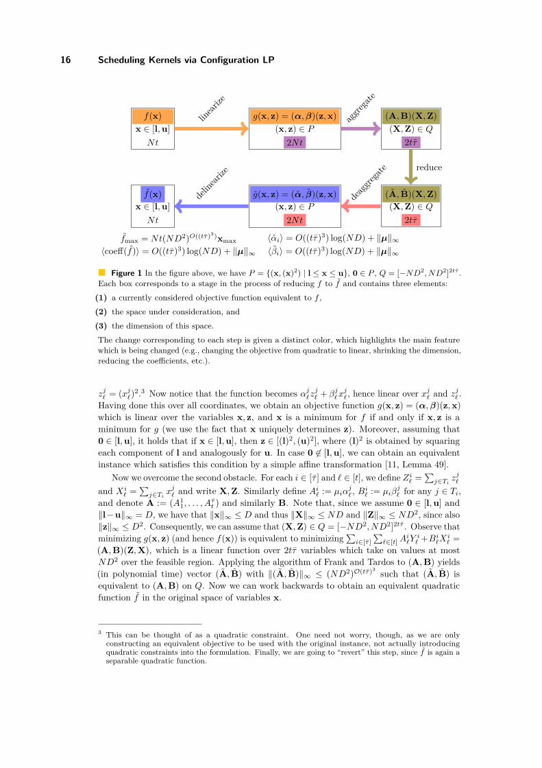
Figure 1 In the figure above, we have P = (x, (x)2) | l ≤ x ≤ u, 0 ∈ P , Q = [−ND2, ND2]2tτ .Each box corresponds to a stage in the process of reducing f to f and contains three elements:

(1) a currently considered objective function equivalent to f ,(2) the space under consideration, and(3) the dimension of this space.The change corresponding to each step is given a distinct color, which highlights the main featurewhich is being changed (e.g., changing the objective from quadratic to linear, shrinking the dimension,reducing the coefficients, etc.).

zj` = (xj`)2.3 Now notice that the function becomes αj`zj` + βj`x

j` , hence linear over xj` and zj` .

Having done this over all coordinates, we obtain an objective function g(x, z) = (α,β)(z,x)which is linear over the variables x, z, and x is a minimum for f if and only if x, z is aminimum for g (we use the fact that x uniquely determines z). Moreover, assuming that0 ∈ [l,u], it holds that if x ∈ [l,u], then z ∈ [(l)2, (u)2], where (l)2 is obtained by squaringeach component of l and analogously for u. In case 0 6∈ [l,u], we can obtain an equivalentinstance which satisfies this condition by a simple affine transformation [11, Lemma 49].

Now we overcome the second obstacle. For each i ∈ [τ ] and ` ∈ [t], we define Zi` =∑j∈Ti

zj`and Xi

` =∑j∈Ti

xj` and write X,Z. Similarly define Ai` := µiαj` , Bi` := µiβ

j` for any j ∈ Ti,

and denote A := (A11, . . . , A

τt ) and similarly B. Note that, since we assume 0 ∈ [l,u] and

‖l−u‖∞ = D, we have that ‖x‖∞ ≤ D and thus ‖X‖∞ ≤ ND and ‖Z‖∞ ≤ ND2, since also‖z‖∞ ≤ D2. Consequently, we can assume that (X,Z) ∈ Q = [−ND2, ND2]2tτ . Observe thatminimizing g(x, z) (and hence f(x)) is equivalent to minimizing

∑i∈[τ ]

∑`∈[t]A

i`Y

i` +Bi`Xi

` =(A,B)(Z,X), which is a linear function over 2tτ variables which take on values at mostND2 over the feasible region. Applying the algorithm of Frank and Tardos to (A,B) yields(in polynomial time) vector (A, B) with ‖(A, B)‖∞ ≤ (ND2)O(tτ)3 such that (A, B) isequivalent to (A,B) on Q. Now we can work backwards to obtain an equivalent quadraticfunction f in the original space of variables x.

3 This can be thought of as a quadratic constraint. One need not worry, though, as we are onlyconstructing an equivalent objective to be used with the original instance, not actually introducingquadratic constraints into the formulation. Finally, we are going to “revert” this step, since f is again aseparable quadratic function.

D. Knop and M. Koutecký 17

B Claim 24. Any function equivalent to f on the variables x on [−1, 2]Nt must have identicalcoefficients across bricks of the same type.

Proof. Let f be any separable quadratic function equivalent to f on [−1, 2]Nt, and αj` , βj`

be such that the contribution of variable xj` of type i is αj`(x

j`)2 + βj`x

j` . In what follows we

fix i ∈ [τ ].We first prove that βj` = βk` for each j, k ∈ Ti and ` ∈ [t]; fix j, k, `. We define a point x

which is 0 everywhere except two coordinates xj` = 1 and xk` = −1. Now, we observe thatf(x) = f(−x). Indeed, since f and f are equivalent on [−1, 1]Nt ⊆ [l,u], it must hold thatf(x) = f(−x). This implies that

f(x) = αj` + βj` + αk` − βk` = αj` − βj` + αk` + βk` = f(−x) .

It follows that 2βj` = 2βk` and we get βj` = βk` .It remains to show that αj` = αk` for each j, k ∈ Ti and ` ∈ [t]; again, fix j, k, `. We define

two points x and x which are 0 everywhere except two coordinates: xj` = 2, xk` = 1 andxj` = 1, xk` = 2. Observe that we have f(x) = f(x) which implies f(x) = f(x). Now, we getthat

f(x) = 4αj` + 2βj` + αk` + βk` = αj` + βj` + 4αk` + 2βk` = f(x) .

Thus, since βj` = βk` , we have that 3αj` = 3αk` and the claim follows. C

We define, for each i ∈ [τ ], j ∈ Ti, and ` ∈ [t], αj` = Ai

µi, βj` = Bi

µi, and define

g(x, z) = (α, β)(x, z). Clearly, g is equivalent to g on P by the equivalence of (A,B)and (A, B) on Q and the claim above. Finally, we define f to be the separable quadraticfunction where the contribution of variable xj` , j ∈ Ti, is α

j`(x

j`)2 + βxj` . By the definition

of the variables zj` , a point x ∈ [l,u] is a minimum for f if and only if (x, z) is a minimumfor g. Now, (x, z) is a minimum for g if and only if it is a minimum for g. Thus, xis a minimum for f , hence f is equivalent with f on [l,u]. Furthermore, we get thatlog f [l,u]

max , log coeff(f) ≤ poly(τ , t, log(ND)). J

The consequence of Lemma 11, Theorem 3, and Lemma 23 is the following:

I Theorem 4. If (sep-IP) is solvable in polynomial time, then quadratic huge N-fold IPadmits a polynomial kernel when parameterized by (τ , t, ‖E‖∞).

5 Conclusions and Research Directions

We designed kernels for scheduling problems based on the (ConfLP), which may be ofpractical interest due to the ubiquity of (ConfLP) (aka column generation) in practice.

On the side of theory, one may wonder why not apply the approach developed here toother scheduling problems, in particular those modeled as quadratic huge N -fold IP in [30],such as R|rj , dj |

∑wjCj . The answer is simple: we are not aware of a way to solve the

separation problem in polynomial time; in fact, we believe this to be a hard problem roughlycorresponding to Unary Vector packing in variable dimension. However, the typical useof Configuration LP is not to obtain an exact optimum (which is often hard), but to obtainan approximation which is good enough. Perhaps a similar approach within our contextmay lead to so-called lossy kernels [36]? However, it is not even clear that an approximateanalogue of Theorem 3 holds, because getting an LP solution whose value is close to optimaldoes not immediately imply getting a solution which is (geometrically) close to some optimum;cf. the discussions on ε-accuracy in [11, Definition 31] and [25, Introduction].

18 REFERENCES

References

1 Matthias Bentert, René van Bevern, Till Fluschnik, André Nichterlein, and Rolf Nie-dermeier. Polynomial-time preprocessing for weighted problems beyond additive goalfunctions. CoRR, abs/1910.00277, 2019. URL: http://arxiv.org/abs/1910.00277,arXiv:1910.00277.

2 Hans L. Bodlaender and Michael R. Fellows. W[2]-hardness of precedence constrainedk-processor scheduling. Operations Research Letters, 18(2):93–97, 1995. doi:10.1016/0167-6377(95)00031-9.

3 Robert Bredereck, Andrzej Kaczmarczyk, Dušan Knop, and Rolf Niedermeier. High-multiplicity fair allocation: Lenstra empowered by n-fold integer programming. In AnnaKarlin, Nicole Immorlica, and Ramesh Johari, editors, Proceedings of the 2019 ACMConference on Economics and Computation, EC 2019, Phoenix, AZ, USA, June 24-28,2019, pages 505–523. ACM, 2019. doi:10.1145/3328526.3329649.

4 Laurent Bulteau, Danny Hermelin, Dušan Knop, Anthony Labarre, and Stéphane Vialette.The clever shopper problem. Theory Comput. Syst., 64(1):17–34, 2020. doi:10.1007/s00224-019-09917-z.

5 Liming Cai, Jianer Chen, Rodney G. Downey, and Michael R. Fellows. Advice classesof parameterized tractability. Annal of Pure Appliled Logic, 84(1):119–138, 1997. doi:10.1016/S0168-0072(95)00020-8.

6 Timothy Chan, Jacob W. Cooper, Martin Koutecký, Daniel Král, and Kristýna Pekárková.A row-invariant parameterized algorithm for integer programming. CoRR, abs/1907.06688,2019. URL: http://arxiv.org/abs/1907.06688, arXiv:1907.06688.

7 Steven Chaplick, Fedor V. Fomin, Petr A. Golovach, Dušan Knop, and Peter Zeman.Kernelization of graph hamiltonicity: Proper h-graphs. In Zachary Friggstad, Jörg-Rüdiger Sack, and Mohammad R. Salavatipour, editors, Algorithms and Data Structures- 16th International Symposium, WADS 2019, Edmonton, AB, Canada, August 5-7,2019, Proceedings, volume 11646 of Lecture Notes in Computer Science, pages 296–310.Springer, 2019. doi:10.1007/978-3-030-24766-9\_22.

8 Ioannis Chatzigiannakis, Christos Kaklamanis, Dániel Marx, and Donald Sannella, editors.45th International Colloquium on Automata, Languages, and Programming, ICALP 2018,July 9-13, 2018, Prague, Czech Republic, volume 107 of LIPIcs. Schloss Dagstuhl -Leibniz-Zentrum für Informatik, 2018.

9 Marek Cygan, Fedor V. Fomin, Lukasz Kowalik, Daniel Lokshtanov, Dániel Marx, MarcinPilipczuk, Michal Pilipczuk, and Saket Saurabh. Parameterized Algorithms. Springer,2015. doi:10.1007/978-3-319-21275-3.

10 Friedrich Eisenbrand, Christoph Hunkenschröder, and Kim-Manuel Klein. Faster al-gorithms for integer programs with block structure. In Chatzigiannakis et al. [8], pages49:1–49:13. doi:10.4230/LIPIcs.ICALP.2018.49.

11 Friedrich Eisenbrand, Christoph Hunkenschröder, Kim-Manuel Klein, Martin Koutecký,Asaf Levin, and Shmuel Onn. An algorithmic theory of integer programming. Technicalreport, 2019. http://arxiv.org/abs/1904.01361.

12 Friedrich Eisenbrand and Gennady Shmonin. Carathéodory bounds for integer cones.Operations Research Letters, 34(5):564–568, 2006.

13 Michael Etscheid, Stefan Kratsch, Matthias Mnich, and Heiko Röglin. Polynomialkernels for weighted problems. Journal of Computer and System Sciences, 84:1–10, 2017.doi:10.1016/j.jcss.2016.06.004.

REFERENCES 19

14 Michael R. Fellows and Catherine McCartin. On the parametric complexity of schedulesto minimize tardy tasks. Theoretical Computer Scicience, 298(2):317–324, 2003. doi:10.1016/S0304-3975(02)00811-3.

15 Fedor V Fomin, Daniel Lokshtanov, Saket Saurabh, and Meirav Zehavi. Kernelization:theory of parameterized preprocessing. Cambridge University Press, 2019.

16 András Frank and Éva Tardos. An application of simultaneous diophantine approximationin combinatorial optimization. Combinatorica, 7(1):49–65, 1987.

17 Tomáš Gavenčiak, Dušan Knop, and Martin Koutecký. Integer programming in paramet-erized complexity: Three miniatures. In Christophe Paul and Michal Pilipczuk, editors,13th International Symposium on Parameterized and Exact Computation, IPEC 2018,August 20-24, 2018, Helsinki, Finland, volume 115 of LIPIcs, pages 21:1–21:16. SchlossDagstuhl - Leibniz-Zentrum für Informatik, 2018. doi:10.4230/LIPIcs.IPEC.2018.21.

18 P. C. Gilmore and R. E. Gomory. A linear programming approach to the cutting-stockproblem. Oper. Res., 9:849–859, 1961.

19 Steffen Goebbels, Frank Gurski, Jochen Rethmann, and Eda Yilmaz. Change-makingproblems revisited: a parameterized point of view. Journal of Combinatorial Optimization,34(4):1218–1236, Nov 2017. doi:10.1007/s10878-017-0143-z.

20 Michel X. Goemans and Thomas Rothvoß. Polynomiality for bin packing with a constantnumber of item types. In Proc. SODA 2014, pages 830–839, 2014.

21 Frank Gurski, Carolin Rehs, and Jochen Rethmann. Knapsack problems: A parameterizedpoint of view. Theoretical Compututer Science, 775:93–108, 2019. doi:10.1016/j.tcs.2018.12.019.

22 Danny Hermelin, Judith-Madeleine Kubitza, Dvir Shabtay, Nimrod Talmon, and Ger-hard J. Woeginger. Scheduling two competing agents when one agent has significantlyfewer jobs. In Thore Husfeldt and Iyad A. Kanj, editors, 10th International Symposiumon Parameterized and Exact Computation, IPEC 2015, September 16-18, 2015, Patras,Greece, volume 43 of LIPIcs, pages 55–65. Schloss Dagstuhl - Leibniz-Zentrum fuerInformatik, 2015. doi:10.4230/LIPIcs.IPEC.2015.55.

23 Danny Hermelin, Michael Pinedo, Dvir Shabtay, and Nimrod Talmon. On the para-meterized tractability of single machine scheduling with rejection. European Journal ofOperational Research, 273(1):67–73, 2019. doi:10.1016/j.ejor.2018.07.038.

24 Danny Hermelin, Dvir Shabtay, and Nimrod Talmon. On the parameterized tractabilityof the just-in-time flow-shop scheduling problem. Journal of Scheduling, 22(6):663–676,2019. doi:10.1007/s10951-019-00617-7.

25 D. S. Hochbaum and J. G. Shantikumar. Convex separable optimization is not muchharder than linear optimization. J. ACM, 37(4):843–862, 1990.

26 Bart M. P. Jansen and Stefan Kratsch. A structural approach to kernels for ilps: Treewidthand total unimodularity. In Nikhil Bansal and Irene Finocchi, editors, Algorithms -ESA 2015 - 23rd Annual European Symposium, Patras, Greece, September 14-16, 2015,Proceedings, volume 9294 of Lecture Notes in Computer Science, pages 779–791. Springer,2015. doi:10.1007/978-3-662-48350-3\_65.

27 Klaus Jansen, Marten Maack, and Roberto Solis-Oba. Structural parameters for schedul-ing with assignment restrictions. In Dimitris Fotakis, Aris Pagourtzis, and Vangelis Th.Paschos, editors, Algorithms and Complexity - 10th International Conference, CIAC2017, Athens, Greece, May 24-26, 2017, Proceedings, volume 10236 of Lecture Notes inComputer Science, pages 357–368, 2017. doi:10.1007/978-3-319-57586-5\_30.

28 Narendra Karmarkar and Richard M. Karp. An efficient approximation scheme for theone-dimensional bin-packing problem. In Proceedings of the 23rd Annual Symposium on

20 REFERENCES

Foundations of Computer Science, FOCS ’82, pages 312–320, Washington, DC, USA,1982. IEEE Computer Society.

29 Dušan Knop and Martin Koutecký. Scheduling meets n-fold integer programming. Journalof Scheduling, 21:493–503, 2018.

30 Dušan Knop, Martin Koutecký, Asaf Levin, Matthias Mnich, and Shmuel Onn. Multitypeinteger monoid optimization and applications. Technical report, 2019. http://arxiv.org/abs/1909.07326.

31 Dušan Knop, Martin Koutecký, and Matthias Mnich. Voting and bribing in single-exponential time. In Heribert Vollmer and Brigitte Vallée, editors, 34th Symposium onTheoretical Aspects of Computer Science, STACS 2017, March 8-11, 2017, Hannover,Germany, volume 66 of LIPIcs, pages 46:1–46:14. Schloss Dagstuhl - Leibniz-Zentrum fürInformatik, 2017. doi:10.4230/LIPIcs.STACS.2017.46.

32 Dušan Knop, Martin Koutecký, and Matthias Mnich. Combinatorial n-fold integerprogramming and applications. Mathematical Programming, Nov 2019. doi:10.1007/s10107-019-01402-2.

33 Martin Koutecký, Asaf Levin, and Shmuel Onn. A parameterized strongly polynomialalgorithm for block structured integer programs. In Chatzigiannakis et al. [8], pages85:1–85:14. doi:10.4230/LIPIcs.ICALP.2018.85.

34 Stefan Kratsch. On polynomial kernels for integer linear programs: Covering, packingand feasibility. In Hans L. Bodlaender and Giuseppe F. Italiano, editors, Algorithms -ESA 2013 - 21st Annual European Symposium, Sophia Antipolis, France, September 2-4,2013. Proceedings, volume 8125 of Lecture Notes in Computer Science, pages 647–658.Springer, 2013. doi:10.1007/978-3-642-40450-4\_55.

35 Stefan Kratsch. On polynomial kernels for sparse integer linear programs. Journal ofComputer and System Sciences, 82(5):758–766, 2016. doi:10.1016/j.jcss.2015.12.002.

36 Daniel Lokshtanov, Fahad Panolan, MS Ramanujan, and Saket Saurabh. Lossy kernel-ization. In Proceedings of the 49th Annual ACM SIGACT Symposium on Theory ofComputing, pages 224–237, 2017.

37 Matthias Mnich and Andreas Wiese. Scheduling and fixed-parameter tractability. Math.Program., 154(1-2):533–562, 2015.

38 Rolf Niedermeier. Invitation to Fixed-Parameter Algorithms. Oxford University Press,2006. doi:10.1093/ACPROF:OSO/9780198566076.001.0001.

39 Guntram Scheithauer and Johannes Terno. The modified integer round-up property ofthe one-dimensional cutting stock problem. European Journal of Operational Research,84(3):562–571, 1995.

40 Wayne E. Smith. Various optimizers for single-stage production. Naval Res. Logist.Quart., 3:59–66, 1956.

41 Leslie G Valiant and Michael S Paterson. Deterministic one-counter automata. Journalof Computer and System Sciences, 10(3):340–350, 1975.

42 René van Bevern, Till Fluschnik, and Oxana Yu. Tsidulko. On (1+\varepsilon)-approximate data reduction for the rural postman problem. In Michael Khachay, YuryKochetov, and Panos M. Pardalos, editors, Mathematical Optimization Theory and Oper-ations Research - 18th International Conference, MOTOR 2019, Ekaterinburg, Russia,July 8-12, 2019, Proceedings, volume 11548 of Lecture Notes in Computer Science, pages279–294. Springer, 2019. doi:10.1007/978-3-030-22629-9\_20.

REFERENCES 21

43 René van Bevern, Till Fluschnik, and Oxana Yu. Tsidulko. Parameterized algorithmsand data reduction for the short secluded s-t-path problem. Networks, 75(1):34–63, 2020.doi:10.1002/net.21904.

44 René van Bevern, Matthias Mnich, Rolf Niedermeier, and Mathias Weller. Intervalscheduling and colorful independent sets. Journal of Scheduling, 18(5):449–469, 2015.doi:10.1007/s10951-014-0398-5.