Scene Reconstruction and Robot Navigation Using Dynamic Fields

Autonomous Robots 8, 71–86 (2000)c© 2000 Kluwer Academic Publishers. Printed in The Netherlands.

Scene Reconstruction and Robot Navigation Using Dynamic Fields

BENEDICT WONG AND MINAS SPETSAKISDepartment of Computer Science, York University, 4700 Keele Street, North York, Ontario, Canada, M3J 1P3

b [email protected]

[email protected]

Abstract. In this paper, we present an approach to autonomous robot navigation in an unknown environment.We design and integrate algorithms to reconstruct the scene, locate obstacles and do short-term field-based pathplanning. The scene reconstruction is done using a region matching flow algorithm to recover image deformationand structure from motion to recover depth. Obstacles are located by comparing the surface normal of the knownfloor with the surface normal of the scene. Our path planning method is based on electric-like fields and uses currentdensities that can guarantee fields without local minima and maxima which can provide solutions without the needof heuristics that plague the more traditional potential fields approaches. We implemented a modular distributedsoftware platform (FBN) to test this approach and we ran several experiments to verify the performance with veryencouraging results.

Keywords: robot autonomous navigation, 2D and 3D scene analysis, structure from motion, field basednavigation

1. Introduction

Autonomous Platforms that can navigate through acluttered environment to a goal have a tremendous po-tential for applications. A typical autonomous platformconsists of a vehicle, a set of sensors, a data communi-cation link and on-board computer. The vehicle can bea wheeled robot, a tracked vehicle, a limbed robot, anaquatic vehicle, an aerial robot etc. The set of sensorsmay include sonar, infrared sensors, bumper switches,laser range finders, video cameras or even a GlobalPositioning System. Both the vehicle and the sensorsare controlled by the on-board computer or other com-puters via the data communication link. The computeranalyses the sensor data and based on the user inputs,guides the autonomous platform to the goal position.Other than performing tasks such as goal selection,most of the navigation is done by computer.

In this paper, we concentrate on the type of navi-gation in which the robot has no predefined informa-tion about the environment except that it contains amostly empty flat floor. Here, the robot’s task will be

to navigate around obstacles on the floor. This kindof navigation is often called short-term navigation orobstacle avoidance. For our experiments we concen-trated on a telerobotics scenario where the user picksthe goals or subgoals from his user interface and therobot navigates to the goal autonomously. Teleroboticsis a valid and realistic application but the main rea-son we chose it is to avoid unnecessary complicationsand keep the focus on the other components of the sys-tem. In case we used high level navigation, FBN wouldsupply obstacle maps, dead reckoning data etc. to thehigh level navigator and in return receive a series oftargets.

There are many other kinds of navigation tasks thatcan be performed by an autonomous robot. A robotcan navigate through the environment using a prede-fined map which represents the available routes or itcan use landmarks to indicate its location and then navi-gate through the open environment without fixed routes(Jenkin et al., 1993). A robot might use only sensorsto navigate though the unknown environment. In somecases, it is necessary to reconstruct the environment, or

72 Wong and Spetsakis

to correct the position of the robot and localize it on apredefined map.

We developed a short term navigation system thatdoes scene reconstruction, obstacle detection and plansa path using current fields. The scene reconstructionuses a flow algorithm that we developed and which isbased on the Lucas and Kanade algorithm (Barron et al.,1994; Lucas, 1984). It incorporates a multi-resolutionscheme to cope with the large displacements and asmoothness factor to stabilize the solution. The accu-racy of the algorithm is enough to distinguish smallobstacles from the floor.

We also introduced the idea of Dynamic (or Cur-rent) Fields to do the navigation to correct some wellknown problems associated with the potential fields.In the dynamic fields approach the robot follows thesame path as the majority of electrons as if the freespace was a conductor and the obstacles were insula-tors. We convert the obstacle map into the RetinotopicConductivity Map (RCM), set the drain of the field tothe target and the source of the field to the positionof the robot. Then we calculate the current flow fromthe source to the drain and based on the current flow,we navigate the robot through the environment. Wealso discovered that many things get simplified if werun these algorithms in image space (retinotopic) ratherthan actual three dimensional space. Among the thingsthat get simpler is that the resolution is better for thingsclose to the robot and worse for things far away (forwhich we do not have to worry now) and the mentalimage of the world has a constant size. In this case therobot does not appear on the image so the source of thecurrent is in the middle of the lowest part of the image.The disadvantage of course is that it is harder to incor-porate past knowledge to the current mental image ofthe world. The target, or at least a subtarget has to beinside the image which is easy in most cases since thefield of view can include the horizon.

One elegant feature of this approach is that the twomost computation intensive components of the system,the flow estimation and the dynamic field generation,are both dominated by very similar differential equa-tions using the same routines and take more or less thesame time to execute. Thus any software or hardwareimprovement in the one can be beneficial to the other.

The idea of local minima-free potential fields whosedynamic lines do not intersect obstacles has been dealtby other papers in the past with very promising resultsfrom simulations (Kim and Khosla, 1991; Feder andSlotine, 1997), where they approximate the solution tothe incompressible fluid flow (mathematically similar

to electric current fields) with the panel method or withtwo dimensional analytic solution augmented by sim-ple heuristics and the robot follows the strongest flowfrom the source (initial position of the robot) to thedrain (target). To do this they need to approximatethe obstacles with either simple geometric objects orpolygons.

Another approach was presented by Singh et al.(1996), where the potential field was complemented bya magnetic-like field to keep the robot away from theobstacles. This has no immediate physical counterpartbut worked fine in simulations.

We have also developed a software platform to facil-itate experimentation. This platform is modular, so thatoriginal components can be interchanged with more ad-vanced ones. It is also portable to survive software orhardware upgrades. Finally, it provides multi-platformsupport to distribute the workload and take advantageof hardware which is installed on different machines.We named it Field Based Navigator (FBN) after its mostimportant component. Using this software platform wedeveloped navigation algorithms and we tested it on aRWI robot with a video camera as the source of sensorinput.

Some of the autonomous platforms using video asmain sensor input are: Vehicle guidance system on ahighway (Chapuis et al., 1995; Dickmanns et al., 1990),off-road navigation with laser range finder and camera(Langer et al., 1994), and planetary rovers (Matthies,1992). All these examples are based on a wheeledrobot platform. Other examples of the autonomous plat-form are: An outdoor tracked robot system (Okui andShinoda, 1996), underwater vehicles (Marco et al.,1996), insect-inspired legged robot system (Ferrell,1995), and NASA’s planetary rovers (Weisbin et al.,1993). Each kind has its own advantages and limita-tions because of the physical properties of the platform,the surrounding environment and the usage.

1.1. System Overview

The FBN system contains a moving platform, a videocamera and a small set of interconnected computersthat run the software. The robot used in this paper isthe RWI B12 mobile robot (Real World Interface, Inc.,1990; 1994). This robot is equipped with sonar sensorsthat we do not use and bump switches which are usedin the default mode that merely stop the robot whenit bumps somewhere. The RWI platform can performtranslation and rotation. The video camera that we useis a simple camera without auto iris or auto focus. It is

Scene Reconstruction and Robot Navigation 73

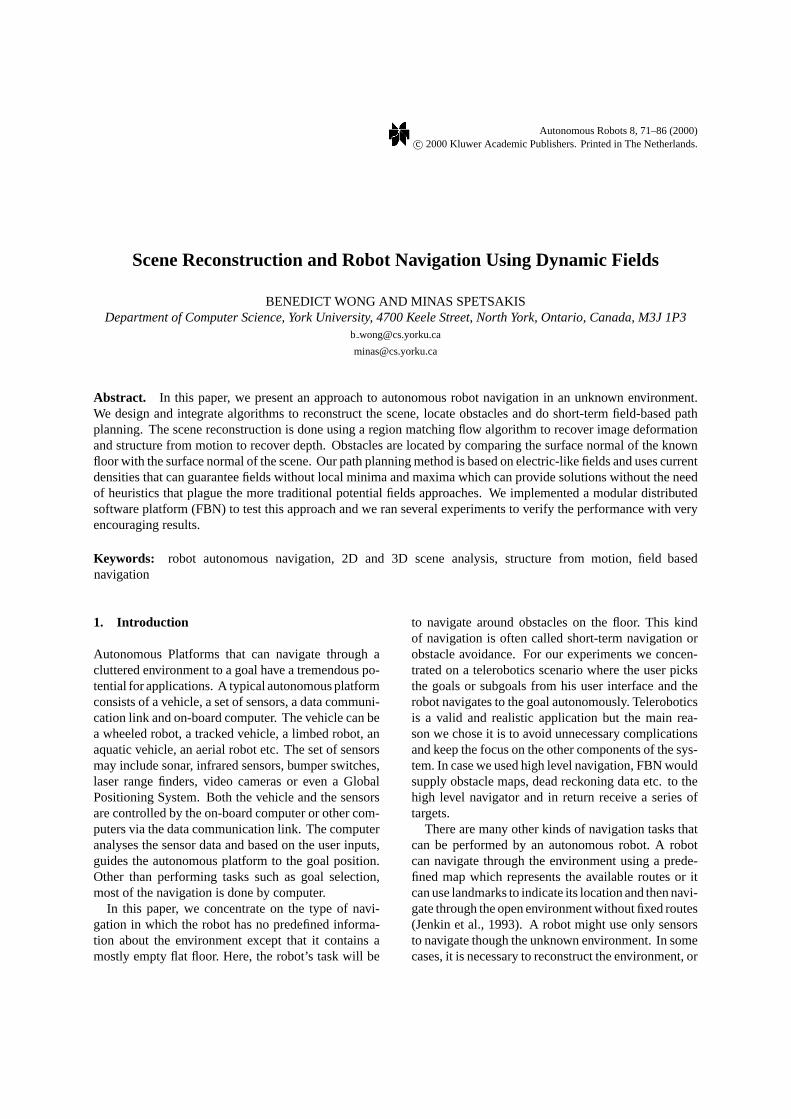
Figure 1. The RWI is a cylindrical robot with 17 cm radius, 46 cm inheight. The mobile base B12 of the RWI robot has three wheels, rigidsuspension, synchronous drive and a forty pound carrying capacity.On top of the mobile base, there are twelve sonars and six bumpswitches. The B12 computer, which is built around the NEC 78310micro controller, controls the mobile base and the bump switches.The sonars are controlled by the G96 Sonar Board which containsa Motorola 68HC11 microprocessor. The control language of theB12 computer and the G96 Sonar Board uses two-letter mnemoniccommands which are sometimes followed by a hexadecimal number.

small enough to fit on the robot (See Fig. 1). Commu-nication between the RWI robot and a host computeris via a pair of serial link cables. The power supply isa rechargeable battery on board the RWI robot.

The camera used in this paper is a WAT-902A cameraby Watec America Corporation. Our experiments areconducted in a room with roughly thirty five squaremeters (35 m2) and it is best viewed with camera lens

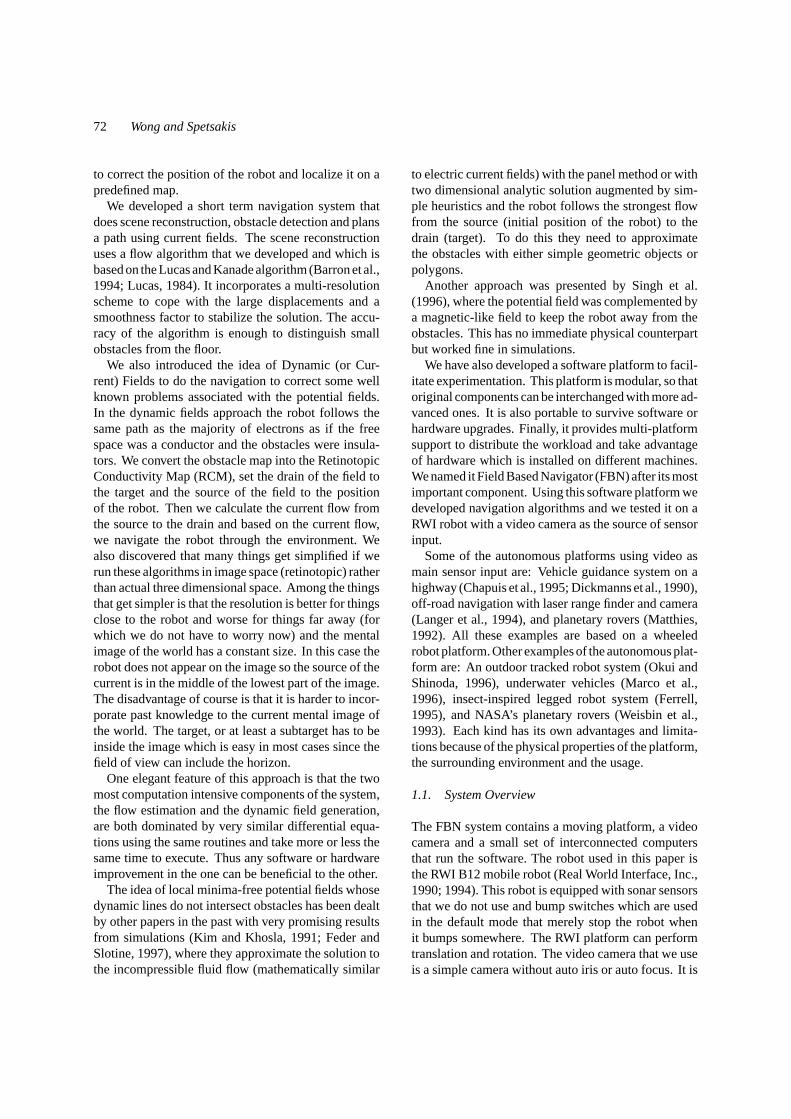
Figure 2. The image processing subsystem is the main process in the system which runs in MediaMath (Spetsakis, 1994). It handles the allcomputations and communications with other subsystem via sockets. The image acquisition system and the user interface program both worktogether. The image acquisition daemon captures images from the camera and sends images to the user interface program for the user to observeand for transmission to the image processing system. The robot command system is a process which controls the RWI robot and communicatesto the image processing system.

that has a short focal length and a wide viewing angle.The platform is tethered with a cable containing thecamera power, the video output and the robot controlcables.

The system that we built is not restricted to a sin-gle operating system or machine. It works on SGImachines and Sparc stations with two different op-erating systems. This distributed system is built fromportable software components running on different ma-chines and operating systems communicating throughmachine independent interfaces.

The distributed system consists of four main subsys-tems: the image processing system, the image acqui-sition system, the robot command system and the userinterface system (Fig. 2).

All programs in this paper are written in the Cprogramming language or the MediaMath (Spetsakis,1994) programming language. The C compiler usedis the ANSI C compiler. The image acquisition sys-tem is based on the IRIS Video Library (VL) on theSGI machines, and the display program uses thext li-brary in X Windows System, Version 11. Most of theprograms can be executed in more than one operatingsystem such as Solaris, SunOs (BSD) and SGI IRIS.The robot daemon is a system dependent program andit is separately implemented in different systems with acommon communication interface. Currently, the im-age acquisition daemon runs only on SGI machines.

In designing the system we strove to achieve robust-ness and simplicity. We avoided heuristics as muchas possible in favor of components with mathemati-cally predictable behavior. Moreover the modularityof the system allows for the incremental developmentof individual components. Among the most interest-ing results that came out of this work is that this can


be done with stereo/structure from motion despite thenoise sensitivity in this kind of computations.

1.2. Overview of the Paper

The structure of the paper is as follows: In Section 2, wedescribe the algorithms in our system. In Section 3, wediscuss the results of our system and the new navigationalgorithm. In Section 4, we present a summary of ourcontribution.

2. Architecture and Algorithms

2.1. Camera Calibration

We used manufacturer’s data and assumed a distor-tionless perspective projection for calibration to keepthings as simple as possible. It turns out that althoughthis incomplete calibration introduced errors that theflat floor was perceived slightly curved by the robot,we did not have any significant problem. The calibra-tion matrix that relates a point on the image coordinatespraw = (k, l , 1)T with the same point in the camera co-ordinate systempi = (xi , yi , 1)T is

pi =

pixelx

f 0 −pixelxf

h2

0pixely

f−pixely

fv2

0 0 1

prawi (1)

where parameterspixelx and pixely are thex and ydimensions of each pixel respectively,f is the effectivefocal length andh andv are the number of pixels inhorizontal and vertical direction respectively.

2.2. Flow Estimation

There are many algorithms for flow estimation but noneof them can claim to solve the problem. A recent pa-per (Barron et al., 1994) evaluated independently manysuch algorithms with rather surprising results. One ofthe simplest, fastest and earliest algorithms by Lucasand Kanade (Lucas, 1984) produced the second mostaccurate results and anything else was either very noisesensitive or computationally very expensive. So we de-veloped an algorithm based on the Lucas and Kanade.The modifications include the initial guess of flow, hier-archical computation (Moravec, 1977; Anandan, 1989;Weber and Malik, 1993) and a smoothness term (Horn,

1986; Horn and Schunck, 1981) to make the solutionmore stable.

The Lucas and Kanade’s region matching algorithmis a weighted least-squares fit of local first-order gra-dient constraints. It assumes a locally constant modelfor the estimated velocity fieldv in small spatial over-lapping neighborhoodsω by minimizing∑

x∈ωW2(x)[∇ I (x, t) · v+ It (x, t)]2 (2)

for every neighborhoodω, whereW(x) is a Gaussianwindow function,I (x, t) is the image intensity andIt

is the partial derivative with respect to time.Horn and Schunck (Horn, 1986; Horn and Schunck,

1981), developed a point matching algorithm whichused a smoothness term

∑(u2

x+u2y+v2

x+v2y)whereu,

v are the two components of the flow andx, y subscriptsdenote differentiation. The smoothness term is an es-sential part of the point matching equation to achievea more stable solution.

Based on Lucas and Kanade’s flow algorithm, we im-plemented a gradient based least-squares region match-ing multi-resolution flow algorithm using Horn andSchunck’s smoothness which leads to a second orderdifferential equation that we solved using the Conju-gate Gradient method.

The initial guess of flow is calculated from the esti-matedZ maps. We estimate theZ map by finding theintersection of the roughly known flat floor and eachimage point vectorpi .

Zguessi = N · Pfloor

N · pi(3)

whereZguessi is thezcomponent of the 3-D object point,

N is the floor normal andPfloor is a point on the floorplane. The initial guess of flow is horizontal and in-versely proportional toZ. The Z map is an image ofZguess

i .

2.3. Depth Recovery

TheZ map is an image data structure which representsthe distance alongZ axis between the camera and thepoints on the scene projected at each pixel. This dis-tance is equivalent toZi . The calculations are based onSpetsakis and Aloimonos (1988), and the equation is

Zi = (T × p′i ) · (p′i × Rpi )

‖p′i × Rpi ‖2 (4)


where the robot moves with rotationR and the trans-lationT andp′i = pi + u(pi ) whereu(pi ) = [u, v]T isthe flow atpi .

2.4. Obstacle Detection

In order for the robot to move around the environment,we need to distinguish obstacles from free space. Weuse theZ map to compute an obstacle map. An obsta-cle map is an image of real values which indicates anobstacle when the pixel value is small and free spacewhen the pixel value is large.

One of the simplest methods to detect obstacles isto compare the estimated floor with calculatedZ mapand the areas with large difference between the two areconsidered as obstacles. However, this method mightbe insensitive to small obstacles and over-sensitive toperceptual distortions of the floor surface that comefrom the imperfect camera calibration or the inaccurateknowledge of robot motion.

The method we used is to compare the roughlyknown floor normal with the image surface normal. Wefirst calculate the actual position vector (or known asdepth map) of the image surface from camera(Zi · pi )

using theZ map, then compute the surface normal fromthe cross product of the derivatives of this position vec-tor with respect tox andy. After we have the imagesurface normal, we calculate the dot product of it andthe roughly known floor normal. A dot product that isvery different from 1 indicates a high probability of anobstacle being present, while a value near 1 indicates ahigh probability of free space. We call this image thebasic obstacle map.

The basic obstacle map indicates only the location ofpossible obstacles; it does not consider the physical sizeof the robot. Since the basic obstacle map is in imagespace, objects at the bottom of the image are scaleddifferently than objects at the top. Using any simpleenlargement method such as convolution between thebasic obstacle map and an enlargement template willresult in improper enhancement due to different scalesin the image. At the top of the image, since each pixelrepresents a large area, the enhancement is too great.At the bottom of the image, the enhancement will beinsufficient due to the small area represented by eachpixel.

The method to solve this problem is to enhance thebasic obstacle map by overlapping it with the warpedversion of itself as if the map was seen from a differ-ent vantage point. Warping is a re-mapping of pixel

positions. Assume that a needle mapU = [u, v]T

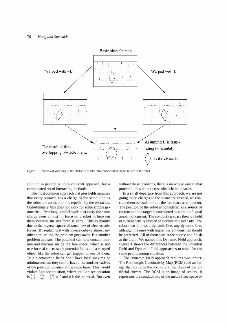
is an image of vectors and we want to warp the im-age I with U. The resulting image will beI ′ whereI ′[x, y] = I [x + u[x, y], y + v[x, y]] and u is theXcomponent ofU andv is theY component ofU. If theneedle mapU represents the motion field of the move-ment on a flat floor, the warped versions of the basicobstacle map will appear to be moving the obstaclesin the basic obstacle map by an amount inversely pro-portional to the actual distance of the obstacle. If weoverlap it with the original, the free space, since it isoverlapping with free space again, will appear to befree space as well, whereas overlapping with an ob-stacle will give an obstacle. In general, this warpingmethod is sensitive to different image depth and with agiven movement on the floor, the far-away points willonly translate a small number of pixels while objectsnear the camera will translate a large number of pixels.Figure 3 shows an example of the warping effect on thebasic obstacle map. We did 9 such warps to cover thefootprint of the robot.

This resulting image is theobstacle map. This mapnot only indicates the obstacles but also enlarges theobstacles so that we take into account the physicaldimensions of the robot, by warping sideways andtowards the camera.

2.5. Path Planning

A very attractive way to do path planning is to use po-tential fields. After all, this is how electrons navigateinside any network of conductors (Hwang and Ahuja,1992; Khatib, 1986; Reid, 1993). Such an approachhas many advantages. The tools needed are very simi-lar to the tools used in optical flow estimation, specif-ically the differential equations. The most importantadvantage is that the solution is almost everywhere acontinuous function of the position and the nature ofthe obstacles.

Most of the approaches to path planning tend to behybrids. The potential fields are used to compute a rep-resentation of the map which is then transformed toa discrete representation and the final solution comesfrom more classical methods, often employing use ofthinning and medial axis transform (Chuang, 1993),Voronoi diagrams (Klein, 1989), and other tools bor-rowed from computational geometry. While the useof fields greatly simplifies the problem, one of thestrengths of the method is lost because the solutionis not a smooth function of the map anymore. And the


Figure 3. Process of widening of the obstacles to take into consideration the finite size of the robot.

solution in general is not a coherent approach, but acomplicated set of interacting methods.

The most common approach that uses fields assumesthat every obstacle has a charge of the same kind asthe robot and so the robot is repelled by the obstacles.Unfortunately, this does not work for some simple ge-ometries. Two long parallel walls that carry the samecharge exert almost no force on a robot in betweenthem because the net force is zero. This is mainlydue to the inverse square distance law of electrostaticforces. By replacing it with inverse cube or almost anyother similar law, the problem goes away. But anotherproblem appears. The potential can now contain min-ima and maxima inside the free space, which is nottrue for real electrostatic potential fields and a chargedobject like the robot can get trapped in one of them.True electrostatic fields don’t have local maxima orminima because they cannot have all second derivativesof the potential positive at the same time. This wouldviolate Laplace equation, where the Laplace equationis ∂2φ

∂x2 + ∂2φ

∂y2 + ∂2φ

∂z2 = 0 andφ is the potential. But even

without these problems, there is no way to ensure thatpotential lines do not cross obstacle boundaries.

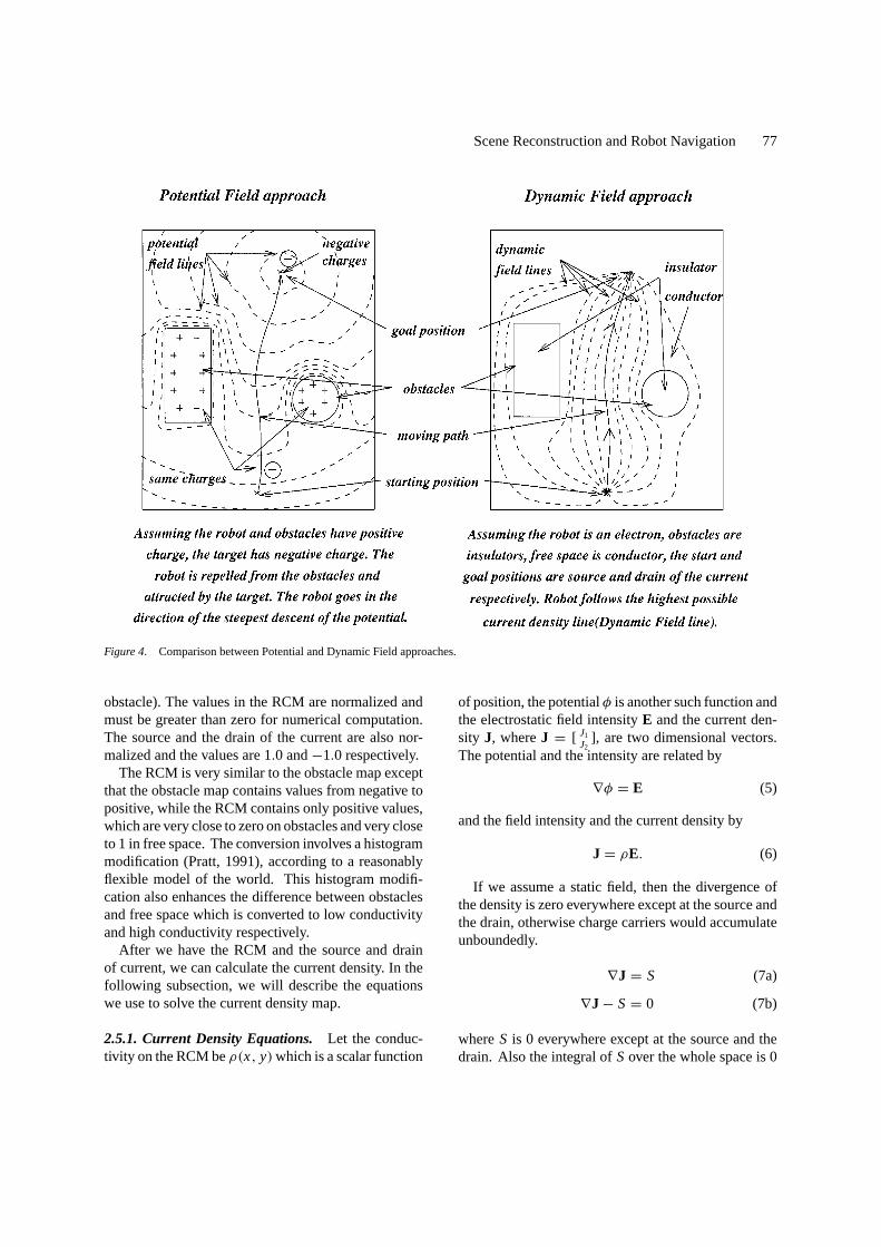
In a small departure from this approach, we are notgoing to use charges on the obstacles. Instead, we con-sider them as insulators and the free space as conductor.The position of the robot is considered as a source ofcurrent and the target is considered as a drain of equalamount of current. The conducting space then is a fieldof current density instead of electrostatic intensity. Therobot then follows a dynamic line, any dynamic line,although the ones with higher current densities shouldbe preferred. All of them start at the source and finishat the drain. We named this Dynamic Field approach.Figure 4 shows the differences between the PotentialField and Dynamic Field approaches to solve for thesame path planning situation.

The Dynamic Field approach requires two inputs:The Retinotopic Conductivity Map (RCM) and an im-age that contains the source and the drain of the ar-tificial current. The RCM is an image of scalars. Itrepresents the conductivity of the media (free space or


Figure 4. Comparison between Potential and Dynamic Field approaches.

obstacle). The values in the RCM are normalized andmust be greater than zero for numerical computation.The source and the drain of the current are also nor-malized and the values are 1.0 and−1.0 respectively.

The RCM is very similar to the obstacle map exceptthat the obstacle map contains values from negative topositive, while the RCM contains only positive values,which are very close to zero on obstacles and very closeto 1 in free space. The conversion involves a histogrammodification (Pratt, 1991), according to a reasonablyflexible model of the world. This histogram modifi-cation also enhances the difference between obstaclesand free space which is converted to low conductivityand high conductivity respectively.

After we have the RCM and the source and drainof current, we can calculate the current density. In thefollowing subsection, we will describe the equationswe use to solve the current density map.

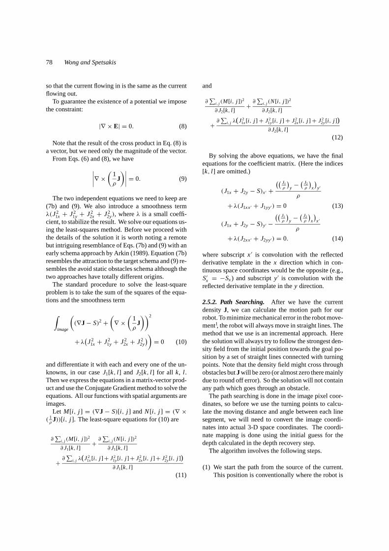
2.5.1. Current Density Equations. Let the conduc-tivity on the RCM beρ(x, y)which is a scalar function

of position, the potentialφ is another such function andthe electrostatic field intensityE and the current den-sity J, whereJ = [ J1

J2], are two dimensional vectors.

The potential and the intensity are related by

∇φ = E (5)

and the field intensity and the current density by

J = ρE. (6)

If we assume a static field, then the divergence ofthe density is zero everywhere except at the source andthe drain, otherwise charge carriers would accumulateunboundedly.

∇J = S (7a)

∇J− S= 0 (7b)

whereS is 0 everywhere except at the source and thedrain. Also the integral ofSover the whole space is 0


so that the current flowing in is the same as the currentflowing out.

To guarantee the existence of a potential we imposethe constraint:

|∇ × E| = 0. (8)

Note that the result of the cross product in Eq. (8) isa vector, but we need only the magnitude of the vector.

From Eqs. (6) and (8), we have∣∣∣∣∇ × ( 1

ρJ)∣∣∣∣ = 0. (9)

The two independent equations we need to keep are(7b) and (9). We also introduce a smoothness termλ(J2

1x + J21y + J2

2x + J22y), whereλ is a small coeffi-

cient, to stabilize the result. We solve our equations us-ing the least-squares method. Before we proceed withthe details of the solution it is worth noting a remotebut intriguing resemblance of Eqs. (7b) and (9) with anearly schema approach by Arkin (1989). Equation (7b)resembles the attraction to the target schema and (9) re-sembles the avoid static obstacles schema although thetwo approaches have totally different origins.

The standard procedure to solve the least-squareproblem is to take the sum of the squares of the equa-tions and the smoothness term

∫image

((∇J− S)2+

(∇ ×

(1

ρJ))2

+ λ(J21x + J2

1y + J22x + J2

2y

)) = 0 (10)

and differentiate it with each and every one of the un-knowns, in our caseJ1[k, l ] and J2[k, l ] for all k, l .Then we express the equations in a matrix-vector prod-uct and use the Conjugate Gradient method to solve theequations. All our functions with spatial arguments areimages.

Let M [i, j ] = (∇J − S)[i, j ] and N[i, j ] = (∇ ×( 1ρJ))[i, j ]. The least-square equations for (10) are

∂∑

i, j (M [i, j ])2

∂ J1[k, l ]+ ∂

∑i, j (N[i, j ])2

∂ J1[k, l ]

+ ∂∑

i, j λ(J21x[i, j ]+ J2

1y[i, j ]+ J22x[i, j ]+ J2

2y[i, j ])∂ J1[k, l ]

(11)

and

∂∑

i, j (M [i, j ])2

∂ J2[k, l ]+ ∂

∑i, j (N[i, j ])2

∂ J2[k, l ]

+ ∂∑

i, j λ(J21x[i, j ] + J2

1y[i, j ] + J22x[i, j ] + J2

2y[i, j ])∂ J2[k, l ]

(12)

By solving the above equations, we have the finalequations for the coefficient matrix. (Here the indices[k, l ] are omitted.)

(J1x + J2y − S)x′ +(( J1

ρ

)y− ( J2

ρ

)x

)y′

ρ

+ λ(J1xx′ + J1yy′) = 0 (13)

(J1x + J2y − S)y′ −(( J1

ρ

)y− ( J2

ρ

)x

)x′

ρ

+ λ(J2xx′ + J2yy′) = 0. (14)

where subscriptx′ is convolution with the reflectedderivative template in thex direction which in con-tinuous space coordinates would be the opposite (e.g.,S′x = −Sx) and subscripty′ is convolution with thereflected derivative template in they direction.

2.5.2. Path Searching. After we have the currentdensityJ, we can calculate the motion path for ourrobot. To minimize mechanical error in the robot move-ment1, the robot will always move in straight lines. Themethod that we use is an incremental approach. Herethe solution will always try to follow the strongest den-sity field from the initial position towards the goal po-sition by a set of straight lines connected with turningpoints. Note that the density field might cross throughobstacles butJ will be zero (or almost zero there mainlydue to round off error). So the solution will not containany path which goes through an obstacle.

The path searching is done in the image pixel coor-dinates, so before we use the turning points to calcu-late the moving distance and angle between each linesegment, we will need to convert the image coordi-nates into actual 3-D space coordinates. The coordi-nate mapping is done using the initial guess for thedepth calculated in the depth recovery step.

The algorithm involves the following steps.

(1) We start the path from the source of the current.This position is conventionally where the robot is


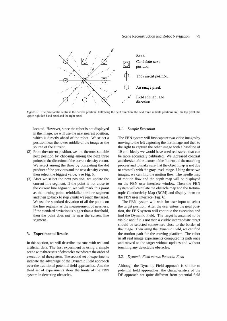
Figure 5. The pixel at the centre is the current position. Following the field direction, the next three suitable positions are: the top pixel, theupper-right left hand pixel and the right pixel.

located. However, since the robot is not displayedin the image, we will use the next nearest position,which is directly ahead of the robot. We select aposition near the lower middle of the image as thesource of the current.

(2) From the current position, we find the most suitablenext position by choosing among the next threepoints in the direction of the current density vector.We select among the three by computing the dotproduct of the previous and the next density vector,then select the biggest value. See Fig. 5.

(3) After we select the next position, we update thecurrent line segment. If the point is not close tothe current line segment, we will mark this pointas the turning point, reinitialize the line segmentand then go back to step 2 until we reach the target.We use the standard deviation of all the points onthe line segment as the measurement of nearness.If the standard deviation is bigger than a threshold,then the point does not lie near the current linesegment.

3. Experimental Results

In this section, we will describe test runs with real andartificial data. The first experiment is using a simplescene with three sets of obstacles to indicate the order ofexecution of the system. The second set of experimentsindicate the advantage of the Dynamic Field approachover the traditional potential field approaches. And thethird set of experiments show the limits of the FBNsystem in detecting obstacles.

3.1. Sample Execution

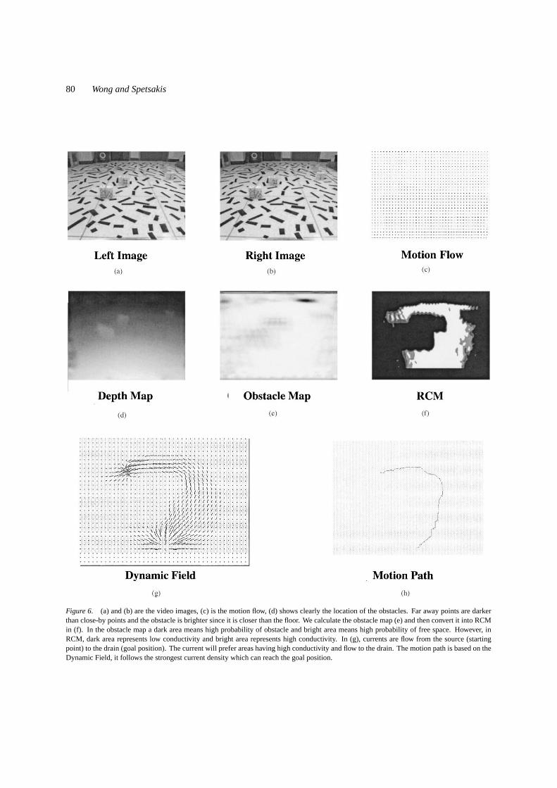
The FBN system will first capture two video images bymoving to the left capturing the first image and then tothe right to capture the other image with a baseline of10 cm. Idealy we would have used real stereo that canbe more accurately calibrated. We increased contrastand the size of the texture of the floor to aid the matchingprocess and to make sure that the object map is not dueto crosstalk with the gray level image. Using these twoimages, we can find the motion flow. The needle mapof motion flow and the depth map will be displayedon the FBN user interface window. Then the FBNsystem will calculate the obstacle map and the Retino-topic Conductivity Map (RCM) and display them onthe FBN user interface (Fig. 6).

The FBN system will wait for user input to selectthe target position. After the user enters the goal posi-tion, the FBN system will continue the execution andfind the Dynamic Field. The target is assumed to bevisible and if it is not then a visible intermediate targetshould be selected somewhere close to the border ofthe image. Then using the Dynamic Field, we can findthe motion path for the moving platform. The robotin all real image experiments computed its path onceand moved to the target without updates and withouttouching any detectable obstacles.

3.2. Dynamic Field versus Potential Field

Although the Dynamic Field approach is similar topotential field approaches, the characteristics of theDF approach are quite different from potential field


Figure 6. (a) and (b) are the video images, (c) is the motion flow, (d) shows clearly the location of the obstacles. Far away points are darkerthan close-by points and the obstacle is brighter since it is closer than the floor. We calculate the obstacle map (e) and then convert it into RCMin (f). In the obstacle map a dark area means high probability of obstacle and bright area means high probability of free space. However, inRCM, dark area represents low conductivity and bright area represents high conductivity. In (g), currents are flow from the source (startingpoint) to the drain (goal position). The current will prefer areas having high conductivity and flow to the drain. The motion path is based on theDynamic Field, it follows the strongest current density which can reach the goal position.


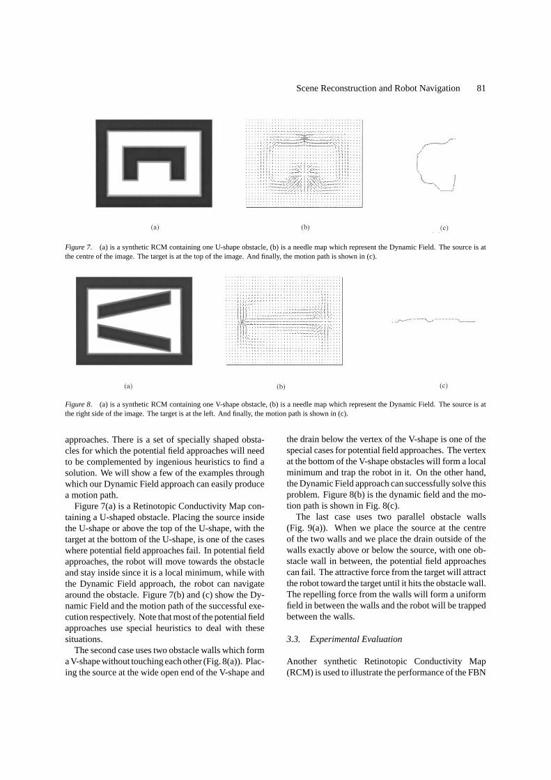
Figure 7. (a) is a synthetic RCM containing one U-shape obstacle, (b) is a needle map which represent the Dynamic Field. The source is atthe centre of the image. The target is at the top of the image. And finally, the motion path is shown in (c).

Figure 8. (a) is a synthetic RCM containing one V-shape obstacle, (b) is a needle map which represent the Dynamic Field. The source is atthe right side of the image. The target is at the left. And finally, the motion path is shown in (c).

approaches. There is a set of specially shaped obsta-cles for which the potential field approaches will needto be complemented by ingenious heuristics to find asolution. We will show a few of the examples throughwhich our Dynamic Field approach can easily producea motion path.

Figure 7(a) is a Retinotopic Conductivity Map con-taining a U-shaped obstacle. Placing the source insidethe U-shape or above the top of the U-shape, with thetarget at the bottom of the U-shape, is one of the caseswhere potential field approaches fail. In potential fieldapproaches, the robot will move towards the obstacleand stay inside since it is a local minimum, while withthe Dynamic Field approach, the robot can navigatearound the obstacle. Figure 7(b) and (c) show the Dy-namic Field and the motion path of the successful exe-cution respectively. Note that most of the potential fieldapproaches use special heuristics to deal with thesesituations.

The second case uses two obstacle walls which forma V-shape without touching each other (Fig. 8(a)). Plac-ing the source at the wide open end of the V-shape and

the drain below the vertex of the V-shape is one of thespecial cases for potential field approaches. The vertexat the bottom of the V-shape obstacles will form a localminimum and trap the robot in it. On the other hand,the Dynamic Field approach can successfully solve thisproblem. Figure 8(b) is the dynamic field and the mo-tion path is shown in Fig. 8(c).

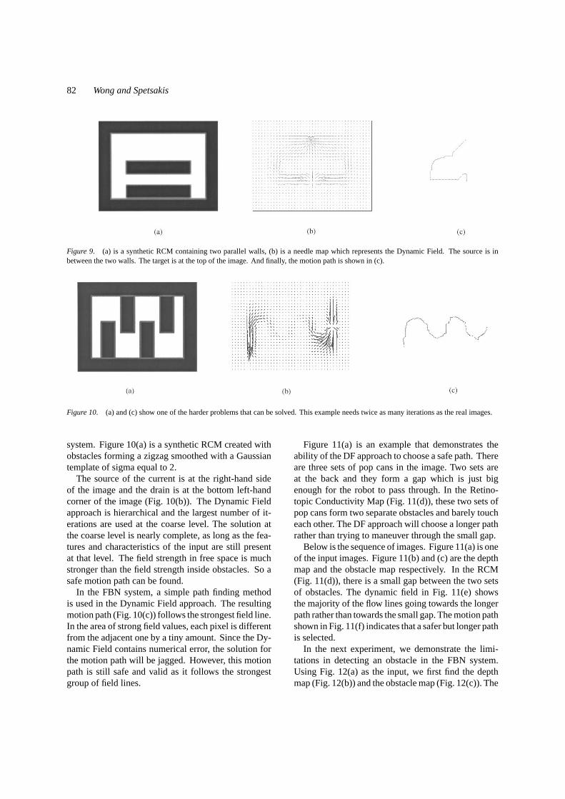
The last case uses two parallel obstacle walls(Fig. 9(a)). When we place the source at the centreof the two walls and we place the drain outside of thewalls exactly above or below the source, with one ob-stacle wall in between, the potential field approachescan fail. The attractive force from the target will attractthe robot toward the target until it hits the obstacle wall.The repelling force from the walls will form a uniformfield in between the walls and the robot will be trappedbetween the walls.

3.3. Experimental Evaluation

Another synthetic Retinotopic Conductivity Map(RCM) is used to illustrate the performance of the FBN


Figure 9. (a) is a synthetic RCM containing two parallel walls, (b) is a needle map which represents the Dynamic Field. The source is inbetween the two walls. The target is at the top of the image. And finally, the motion path is shown in (c).

Figure 10. (a) and (c) show one of the harder problems that can be solved. This example needs twice as many iterations as the real images.

system. Figure 10(a) is a synthetic RCM created withobstacles forming a zigzag smoothed with a Gaussiantemplate of sigma equal to 2.

The source of the current is at the right-hand sideof the image and the drain is at the bottom left-handcorner of the image (Fig. 10(b)). The Dynamic Fieldapproach is hierarchical and the largest number of it-erations are used at the coarse level. The solution atthe coarse level is nearly complete, as long as the fea-tures and characteristics of the input are still presentat that level. The field strength in free space is muchstronger than the field strength inside obstacles. So asafe motion path can be found.

In the FBN system, a simple path finding methodis used in the Dynamic Field approach. The resultingmotion path (Fig. 10(c)) follows the strongest field line.In the area of strong field values, each pixel is differentfrom the adjacent one by a tiny amount. Since the Dy-namic Field contains numerical error, the solution forthe motion path will be jagged. However, this motionpath is still safe and valid as it follows the strongestgroup of field lines.

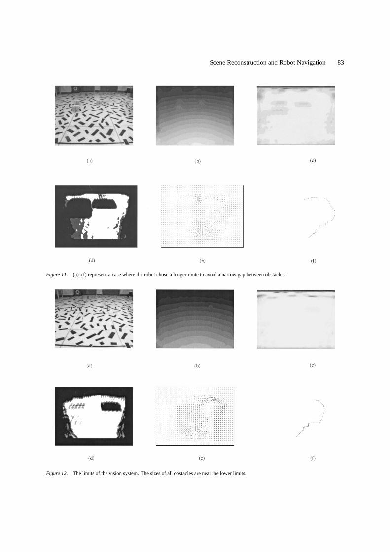
Figure 11(a) is an example that demonstrates theability of the DF approach to choose a safe path. Thereare three sets of pop cans in the image. Two sets areat the back and they form a gap which is just bigenough for the robot to pass through. In the Retino-topic Conductivity Map (Fig. 11(d)), these two sets ofpop cans form two separate obstacles and barely toucheach other. The DF approach will choose a longer pathrather than trying to maneuver through the small gap.

Below is the sequence of images. Figure 11(a) is oneof the input images. Figure 11(b) and (c) are the depthmap and the obstacle map respectively. In the RCM(Fig. 11(d)), there is a small gap between the two setsof obstacles. The dynamic field in Fig. 11(e) showsthe majority of the flow lines going towards the longerpath rather than towards the small gap. The motion pathshown in Fig. 11(f) indicates that a safer but longer pathis selected.

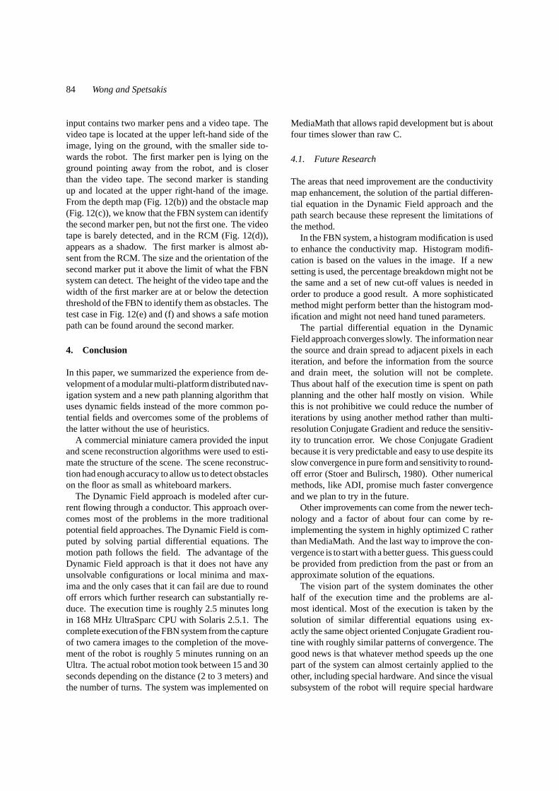
In the next experiment, we demonstrate the limi-tations in detecting an obstacle in the FBN system.Using Fig. 12(a) as the input, we first find the depthmap (Fig. 12(b)) and the obstacle map (Fig. 12(c)). The


Figure 11. (a)–(f) represent a case where the robot chose a longer route to avoid a narrow gap between obstacles.

Figure 12. The limits of the vision system. The sizes of all obstacles are near the lower limits.


input contains two marker pens and a video tape. Thevideo tape is located at the upper left-hand side of theimage, lying on the ground, with the smaller side to-wards the robot. The first marker pen is lying on theground pointing away from the robot, and is closerthan the video tape. The second marker is standingup and located at the upper right-hand of the image.From the depth map (Fig. 12(b)) and the obstacle map(Fig. 12(c)), we know that the FBN system can identifythe second marker pen, but not the first one. The videotape is barely detected, and in the RCM (Fig. 12(d)),appears as a shadow. The first marker is almost ab-sent from the RCM. The size and the orientation of thesecond marker put it above the limit of what the FBNsystem can detect. The height of the video tape and thewidth of the first marker are at or below the detectionthreshold of the FBN to identify them as obstacles. Thetest case in Fig. 12(e) and (f) and shows a safe motionpath can be found around the second marker.

4. Conclusion

In this paper, we summarized the experience from de-velopment of a modular multi-platform distributed nav-igation system and a new path planning algorithm thatuses dynamic fields instead of the more common po-tential fields and overcomes some of the problems ofthe latter without the use of heuristics.

A commercial miniature camera provided the inputand scene reconstruction algorithms were used to esti-mate the structure of the scene. The scene reconstruc-tion had enough accuracy to allow us to detect obstacleson the floor as small as whiteboard markers.

The Dynamic Field approach is modeled after cur-rent flowing through a conductor. This approach over-comes most of the problems in the more traditionalpotential field approaches. The Dynamic Field is com-puted by solving partial differential equations. Themotion path follows the field. The advantage of theDynamic Field approach is that it does not have anyunsolvable configurations or local minima and max-ima and the only cases that it can fail are due to roundoff errors which further research can substantially re-duce. The execution time is roughly 2.5 minutes longin 168 MHz UltraSparc CPU with Solaris 2.5.1. Thecomplete execution of the FBN system from the captureof two camera images to the completion of the move-ment of the robot is roughly 5 minutes running on anUltra. The actual robot motion took between 15 and 30seconds depending on the distance (2 to 3 meters) andthe number of turns. The system was implemented on

MediaMath that allows rapid development but is aboutfour times slower than raw C.

4.1. Future Research

The areas that need improvement are the conductivitymap enhancement, the solution of the partial differen-tial equation in the Dynamic Field approach and thepath search because these represent the limitations ofthe method.

In the FBN system, a histogram modification is usedto enhance the conductivity map. Histogram modifi-cation is based on the values in the image. If a newsetting is used, the percentage breakdown might not bethe same and a set of new cut-off values is needed inorder to produce a good result. A more sophisticatedmethod might perform better than the histogram mod-ification and might not need hand tuned parameters.

The partial differential equation in the DynamicField approach converges slowly. The information nearthe source and drain spread to adjacent pixels in eachiteration, and before the information from the sourceand drain meet, the solution will not be complete.Thus about half of the execution time is spent on pathplanning and the other half mostly on vision. Whilethis is not prohibitive we could reduce the number ofiterations by using another method rather than multi-resolution Conjugate Gradient and reduce the sensitiv-ity to truncation error. We chose Conjugate Gradientbecause it is very predictable and easy to use despite itsslow convergence in pure form and sensitivity to round-off error (Stoer and Bulirsch, 1980). Other numericalmethods, like ADI, promise much faster convergenceand we plan to try in the future.

Other improvements can come from the newer tech-nology and a factor of about four can come by re-implementing the system in highly optimized C ratherthan MediaMath. And the last way to improve the con-vergence is to start with a better guess. This guess couldbe provided from prediction from the past or from anapproximate solution of the equations.

The vision part of the system dominates the otherhalf of the execution time and the problems are al-most identical. Most of the execution is taken by thesolution of similar differential equations using ex-actly the same object oriented Conjugate Gradient rou-tine with roughly similar patterns of convergence. Thegood news is that whatever method speeds up the onepart of the system can almost certainly applied to theother, including special hardware. And since the visualsubsystem of the robot will require special hardware


anyway the additional cost will not be that high if theyshare.

The motion path produced in the FBN system is validand safe, but it fails to create a smooth motion path evenfrom a very smooth field due mainly to the heuristic na-ture of our path searching method. Using a more math-ematical approach of path searching, such as a globalpath searching, we might improve the motion path.

Currently the Dynamic field approach is in two-dimensional space. It could be extended into three-dimensional space by adding new constraints into thepartial differential equation.

Acknowledgment

The support of the NSERC (App. No. OGP0046645)is gratefully acknowledged.

Note

1. The uncertainty of socket delays can interfere with the simulta-neous translation and rotation ability of the robot.

References

Anandan, P. 1989. A computational framework and an algorithm forthe measurement of visual motion.Intl’ J. of Computer Vision,2:283–310.

Arkin, R.C. 1989. Motor schema-based mobile robot navigation.International Journal of Robotics Research, 8(4):92–112.

Barron, J.L., Fleet, D.J., and Beauchemin, S.S. 1994. Performance ofoptical flow techniques.Int’l Journal of Computer Vision, 12:43–77.

Chapuis, R., Potelle, A., Brame, J.L., and Chausse, F. 1995. Real-time vehicle trajectory supervision on the highway.The Interna-tional Journal of Robotics Research, 14:531–542.

Chuang, J.H. 1993. Potential-based modeling of three dimensionalworkspace for obstacle avoidance. InIEEE International Confer-ence on Robotics & Automation, Vol. 3, pp. 19–24.

Dickmanns, E.D., Mysliwetz, B., and Christians, T. 1990. An inte-grated spatio-temporal approach to automatic visual guidance ofautonomous vehicles.IEEE Transaction on System, Man, andCybernetics, 20(6):1273–1990.

Feder, H.J.S. and Slotine, J.-J. 1997. Real-time path planning us-ing harmonic potentials. InDynamic Environments, Proc. IEEEConference on Robotics and Automation, pp. 874–881.

Ferrell, Cynthia. 1995. A comparison of three insect-inspiredlocomotion controllers.Robotics and Autonomous Systems,16:135–159.

Horn, B.K.P. 1986.Robot Vision, McGraw-Hill Book Company:New York.

Horn, B.K.P. and Schunck, B.G. 1981. Determining optical flow.Artificial Intelligence, 17:185–204.

Hwang, Y.K. and Ahuja, N. 1992. A potential field approach topath planning.IEEE Transactions on Robotics and Automation,8(1):23–32.

Real World Interface, Inc. 1990.G96 Sonar Board Guide to Opera-tions Version 1.1, Real World Interface, Inc.: Dublin.

Real World Interface, Inc. 1994.B12 Base Manual Version 2.4, RealWorld Interface, Inc.: Dublin.

Jenkin, M.R.M. et al. 1993. Global navigation for ARK. InProc.IEEE/RSJ, IROS, Yokohama, Japan, pp. 2165–2171.

Khatib, O. 1986. Real-time obstacle avoidance for manipulatorsand mobile robots.International Journal of Robotics Research,5(1):90–98.

Kim, J.O. and Khosla, P. 1991. Real-time obstacle avoidance us-ing harmonic potential function. InProc. IEEE Conference onRobotics and Automation, pp. 790–796.

Klein, R. 1989.Concrete and Abstract Voronoi Diagrams, Springer-Verlag: Berlin.

Langer, D., Rosenblatt, J.K., and Hebert, M. 1994. A behavior-basedsystem for off-road navigation.IEEE Transactions on Roboticsand Automation, 10(6):776–783.

Lucas, B. 1984. Generalized image matching by the method of differ-ences. Ph.D. Dissertation, Dept. of Computer Science, CarnegieMellon University.

Marco, D.B., Healey, A.J., and McGhee, R.B. 1996. Autonomousunderwater vehicles: Hybrid control of mission and motion.Au-tonomous Robots, 3:169–186.

Matthies, Larry. 1992. Stereo vision for planetary rovers: Stochasticmodeling to near real time implementation.International Journalof Computer Vision, 8(1):71–91.

Moravec, H.P. 1977. Towards automatic visual obstacle avoidance.In Proc. 5th IJCAI, IJCAI-77, Cambridge, Massachusetts, p. 584.

Okui, Takao and Shinoda, Yoshiaki. 1996. An outdoor robots sys-tem for autonomous mobile all purpose platform.Robotics andAutonomous Systems, 17:99–106.

Pratt, W.K. 1991.Digital Image Processing, Wiley: New York.Reid, M.B. 1993. Path planning using optically computed potential

fields.IEEE International Conference on Robotics & Automation,Vol. 2, pp. 295–300.

Singh, L., Stephanou, H., and Wen, J. 1996. Real-time motion con-trol with circulatory fields. InProc. IEEE Conference on Roboticsand Automation, pp. 2737–2742.

Spetsakis, M.E. and Aloimonos, J. 1988. Optimal estimation of struc-ture from motion from point correspondences in two frames. InProc. ICCV, Tampa, Florida.

Spetsakis, Minas. 1994. MediaMath: A research environment forvision research. InVision Interface, Banf: Alberta, pp. 118–126.

Stoer, J. and Bulirsch, R. 1980.Introduction to Numerical Analysis,Springer-Verlang.

Weber, J. and Malik, J. 1993. Robust computation of optical flow ina multi-scale differential framework. InICCV, pp. 231–236.

Weisbin, C.R., Montemerlo, M., and Whittaker, W. 1993. Evolvingdirections in NASA’s planetary rover requirements and technol-ogy.Robotics and Autonomous Systems, 11:3–11.

Benedict Wongreceived the B.Sc. and M.Sc. degrees in ComputerScience from York University in Toronto, Ontario. Currently, he isemployed at SystemWare Inc.


Minas E. Spetsakiswas born in 1962 in Greece. He receivedhis undergraduate degree in Electrical Engineering from National

Technical University of Athens in 1985 and his Ph.D. in ComputerScience from University of Maryland in 1989 and joined the de-partment of Computer Science at York the same year. His interestsare in the area of Computer Vision, Robotics and Image ProcessingSoftware.

Documents

Scene Reconstruction and Robot Navigation Using Dynamic Fields