Wireless Indoor Mobile Robot with RFID

Navigation Map and Live Video

A thesis in the partial fulfilment of the requirements for the degree

of

Masters of Engineering

in

Mechatronics

Massey University

Palmerston North

New Zealand

Samuel Garratt

2011

| i

Abstract

A mobile robot was designed in order to move freely within a map built in an indoor

environment. The aim is for the robot to move between passive RFID (Radio Frequency

Identification) tags in an environment that has been previously mapped by the designed

software. Passive RFID tags are inexpensive, the same size and shape as a credit card and are

attached to other objects. They don’t require any power of their own but operate through an

RFID reader that induces a magnetic field in their antenna, which then creates power for the

tag. This makes the tags inexpensive, and easy to setup and maintain.

The robot is a three wheeled vehicle driven by two stepper motors and is controlled

wirelessly through a PC. It has a third omniwheel at the front for maintaining the balance of

the robot. Since the PC communicates continuously with the robot, all the major processing

and data management can be done on the computer making the microcontroller much simpler

and less expensive. Infrared distance sensors are placed around the robot to detect short range

obstacles and a sonar sensor at the front can detect obstacles further away. This data is used

so that the robot can avoid obstacles in its path between tags. An electronic compass is used

to provide absolute orientation of the robot at all times to correct for errors in estimating the

angle. A camera is attached to the front of the robot so that an operator can see the robot and

manually control it if necessary. This could also be used to a video a certain environment

from a robot’s perspective.

The sensors and the RFID tags are all inexpensive, making the mass reproduction of the robot

feasible and implementation practically possible for small firms. The RFID tags can be

quickly attached or detached from an environment leaving no trace of their prior existence. A

map can then be formed on a PC automatically by the robot through its detection of the tags.

ii |

This makes the entire system very flexible and quick to set up, something that is needed in

the present day as changes to buildings and factories become more common.

There are still many improvements needed to improve the stability of the compass’s signal in

the presence of magnetic fields, the stability of the wheels so that slippage is rare, and the

range of the wireless signal and camera.

A flexible, easily configurable moving robot could be used to serve fields such as the medical

field by transporting goods within a hospital, or in factories where goods need to be

transported between locations. Since the system is flexible, and maps can be formed quickly,

the robot can fit in with the changes to an industry’s environment and requirements.

However, since the robot can only move to approximately five metres from the computer

controlling it and the inaccuracy in sensor data, it is not currently ready for industrial use. For

example, the sensors are only placed at 6 orientations around the robot and so do not cover a

full span of the robots area. These sensors also only detect a two dimensional plane around

the robot so could not detect obscure objects that have a part sticking out at height higher

than the sensors. Therefore, further work is needed to be done to make the robot reliable,

safe, and fault-proof before it could be used in industry.

Since the movement of the robot with inexpensive sensors and motors is bound to have

problems in perfectly moving between RFID tags, due to small dead reckoning errors, simple

algorithms are shown in this research that moves the robot around its current location until it

finds a tag. These algorithms involve finding a path between two RFID tags that will make

use of any tags in between them to localise itself and moving in a spiral to search for a tag

when, due to odometry errors, it is not detected where it is expected to be.

The robot built has demonstrated being able to navigate between RFID tags within a small

lab environment. It has proven to be able to avoid obstacles with a size of 30 x 30 cm.

| iii

Acknowledgements

In completing this master degree in mechatronics engineering, I would like to give my

sincere appreciation and thanks to:

My supervisor Dr Liqiong Tang, who encouraged me at times of failure, gave useful advice,

corrected errors, and guided and supported me to the completion of my project.

Christopher Kiesewetter, who made the initial design of the robot base and who was more

than willing to help when asked for information.

Mark Deng, who accompanied me through the entire project, provided useful advice and

encouraged me when progress was slow.

Bruce Collins and Anthony Wade, in the electronics workshop, for their useful advice,

providing of electronics components, and producing of printable circuit boards.

Nick Look, for his help with networks, computer issues, and the rapid prototyping machine.

All the staff in the mechanical workshop for their advice and help in making mechanical

parts.

The staff in the seat administration for their cheerful and friendly support in all the

administrative matters needed in my project.

The Lord Jesus, for His supply enabling me to have the patience and ability to finish this

research.

iv |

Table of Contents

Abstract ................................................................................................................................. i

Acknowledgements.............................................................................................................. iii

List of Figures.................................................................................................................... viii

List of Equations ................................................................................................................. xv

List of Equations ................................................................................................................. xv

List of Tables ..................................................................................................................... xvi

List of Abbreviations......................................................................................................... xvii

Chapter 1: Introduction ......................................................................................................... 1

1.1 Research topic ............................................................................................................. 4

1.2 Scope of research ........................................................................................................ 4

1.3 The organisation of the thesis ...................................................................................... 5

Chapter 2: Literature Review ................................................................................................ 7

2.1 The development history of mobile robots ................................................................... 7

2.2 The need for mobile robots .......................................................................................... 9

2.3 The available methodologies and technologies applied in navigating a mobile robot.. 11

2.3.1 Guide by a map................................................................................................... 11

2.3.2 Odometry ........................................................................................................... 16

2.3.3 Localisation ........................................................................................................ 17

2.3.4 Goal reaching methodology ................................................................................ 23

2.3.5 Sensing technology (safety issues) ...................................................................... 34

| v

2.3.6 Conclusion.......................................................................................................... 35

Chapter 3: Localisation methodology using RFID tags ........................................................ 37

3.1 Low frequency passive RFID tags ............................................................................. 38

3.2 Localisation through RFID tags ................................................................................. 41

3.3 Fixing orientation error through a compass ................................................................ 43

3.4 RFID system setup .................................................................................................... 46

Chapter 4: Component communication................................................................................ 50

4.1 Wireless communication between the host PC and the mobile robot .......................... 50

4.1.1 Role of host PC and mobile robot ....................................................................... 50

4.1.2 Wireless communication using XBee modules.................................................... 52

4.1.3 Receiving data from the sensors.......................................................................... 57

4.2 Communication between the bottom and middle layer microcontrollers..................... 59

4.3 Live image data (Camera).......................................................................................... 63

Chapter 5: Mobile robot software system ............................................................................ 66

5.1 Mobile robot navigation algorithms ........................................................................... 66

5.1.1 Moving from one tag to another.......................................................................... 66

5.1.2 Moving between many tags ................................................................................ 76

5.1.3 Searching for the nearest tag ............................................................................... 81

5.2 Mobile robot navigation simulation ........................................................................... 89

5.2.1 Simulation of the robot’s environment ................................................................ 89

5.2.2 Simulating the robot ........................................................................................... 92

vi |

5.2.3 Testing and evaluating navigation algorithms ..................................................... 95

5.3 Environment map building ........................................................................................ 98

5.3.1 Manual map building .......................................................................................... 99

5.3.2 Auto-map building through detecting RFID tags............................................... 101

Chapter 6: Testing localisation methodology..................................................................... 106

6.1 Indoor mobile service robot design considerations................................................... 106

6.1.1 Constraints of the Robot’s environment ............................................................ 106

6.1.2 Path planning.................................................................................................... 107

6.1.3 Obstacle avoidance ........................................................................................... 108

6.1.4 The usefulness of the designed mobile robot ..................................................... 110

6.2 Mobile robot mechanical system design................................................................... 112

6.2.1 Mechanical system configurations .................................................................... 112

6.2.2 Mobile robot platform design............................................................................ 114

6.3 Control system design ............................................................................................. 120

6.3.1 Motor controller, power supply and testing ....................................................... 120

6.3.2 Sensing implementation.................................................................................... 132

6.4 Mobile service robot prototype system testing ......................................................... 152

6.4.1 Test one – Proving compass.............................................................................. 152

6.4.2 Test two – Avoiding obstacle............................................................................ 155

6.4.3 Test three – Moving through best path .............................................................. 157

Chapter 7: Future improvements ....................................................................................... 159

| vii

Chapter 8: Summary and Conclusions............................................................................... 162

8.1 Summary................................................................................................................. 162

8.2 Conclusions............................................................................................................. 165

References: ....................................................................................................................... 166

Appendix A: Obstacle avoidance decision algorithm......................................................... 173

Appendix B: PC wireless communication procedure ......................................................... 174

Appendix C: C code for reading a serial bit signal manually.............................................. 176

Appendix D: Example map holding RFID tags and obstacles ............................................ 179

Appendix E: Connection of all the sensors to the robot...................................................... 181

Appendix F: Recursive function for finding possible paths among RFID tags.................... 182

Appendix G: Obstacle colours depending on the number of points within a grid ............... 183

Appendix H: AT mega 32 ................................................................................................. 184

Appendix I: GP2D120 Infrared distance sensor................................................................. 186

Appendix J: Compass CMP03........................................................................................... 188

Appendix K: Sonar sensor MB1300 .................................................................................. 189

Appendix L: ID 40 RFID range reader .............................................................................. 191

viii |

List of Figures

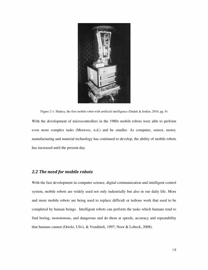
Figure 2-1: Shakey, the first mobile robot with artificial intelligence (Dudek & Jenkin, 2010,

pg. 9) .................................................................................................................................... 9

Figure 2-2: Quad Tree of four levels showing four children under one parent and more

detailed view in each layer (Demmel, 1996, para. 10).......................................................... 14

Figure 2-3: Left - Metric map of a set of rooms (Fabrizi & Saffiotti, 2002, p. 92); Right -

Topological map of the same set of rooms (Fabrizi & Saffiotti, 2002, p. 94) ....................... 15

Figure 2-4: Polarization pattern of light in the sky a mobile robot can use to localise itself

(Lambrinos, et. al, 1999, p. 42)............................................................................................ 18

Figure 2-5: Robot using landmarks for localisation when moving towards a goal

(Kriechbaum, 2006, p. 84)................................................................................................... 20

Figure 2-6: Local tangent graph produced at each step of the Tangent bug algorithm to

determine what step to take next (Kriechbaum, 2006, p. 9).................................................. 25

Figure 2-7: Steps for a robot to avoid an obstacle and find the path to the goal using the

Optim bug algorithm (Kriechbaum, 2006, p. 67) ................................................................. 28

Figure 2-8: Optim bugs avoiding an obstacle, running into another obstacle and the three

tangent lines that will reach the goal (Kriechbaum, 2006, p. 68).......................................... 29

Figure 2-9: Path recalculation using Uncertain Bug (Kriechbaum, 2006, p. 102) ................. 31

Figure 2-10: Avoiding an obstacle through turning to obstacle edge, (Benmounah & Abbassi,

1999, pg 539) ...................................................................................................................... 34

Figure 3-1: Reader generating a magnetic field that powers the antenna to send its data

(FerroxCube International, 2009, para. 3)............................................................................ 39

| ix

Figure 3-2: Detection distance of RFID tag determining the area where the robot could be . 40

Figure 3-3: 125kHz RFID tags that hold a unique ID used to localise a mobile robot........... 41

Figure 3-4: A map showing two paths for a robot that each have RFID tags for the robot to

utilise .................................................................................................................................. 42

Figure 3-5: Disturbance (right) of uniform magnetic field (left) by a magnetic material

(Advanced Safety Devices, 2012, para. 6) ........................................................................... 45

Figure 3-6: Error in orientation causing a difference in position to be created over time ...... 46

Figure 3-7: Graphical representation of the robot's map. Yellow squares are RFID tags,

brown squares are obstacles ................................................................................................ 48

Figure 4-1: Communication between robot and PC using XBee and camera and

communication within the robot itself ................................................................................. 51

Figure 4-2: Modem configuration for the XBee module ...................................................... 53

Figure 4-3: Left – XBee DTE serial board; Right – XBee USB board ................................. 54

Figure 4-4: Left – DTE serial board connected to mobile robot; Right - USB board connected

to PC................................................................................................................................... 55

Figure 4-5: Wireless network composed of a coordinator, routers and end devices, (Digi

International, 2009, pg. 22) ................................................................................................. 56

Figure 4-6: Wireless communication with ‘Terminal’ tab of X-CTU................................... 56

Figure 4-7: AND gates and OR gate used to allow middle layer’s microcontroller to switch

between wireless module and the bottom layer’s microcontroller ........................................ 61

Figure 4-8: Left - Camera used to capture video; Right - Radio receiver that plugs into the PC

........................................................................................................................................... 63

x |

Figure 4-9: Left - Camera with LEDs inserted; Right – Lights shining in a dark room......... 64

Figure 4-10: Image from a recording taken by the robot’s video camera.............................. 65

Figure 5-1: The position where the robot can sense an RIFD tag ........................................ 67

Figure 5-2: Robot moving towards an RFID tag needing to turn to detect the RFID tag....... 69

Figure 5-3: An obstacle detected in a certain spot being considered as covering a large part of

a grid................................................................................................................................... 71

Figure 5-4: Checkboxes that determine which squares ahead of the robot to check for an

obstacle............................................................................................................................... 73

Figure 5-5: Steps for robot to avoid an obstacle by firstly moving to the right, then to the left

and finally by notifying the user so they can avoid it ........................................................... 75

Figure 5-6: Demonstration program showing the message given to the user when the robot

cannot avoid an obstacle and the orange continue auto movement button in the form’s

bottom-right corner ............................................................................................................. 76

Figure 5-7: Showing the space between the start and end RFID tag in the X coordinates

(green rectangle) and with the space between them limited by both the X and Y coordinates

(blue rectangle) ................................................................................................................... 78

Figure 5-8: Showing how using the least maximum distance among the paths results in the

best path for the robot to take (Not drawn to scale).............................................................. 79

Figure 5-9: Program showing the result of the best path method.......................................... 81

Figure 5-10: Showing how the robot can be told to move just before the place where the

RFID tag can be detected .................................................................................................... 83

Figure 5-11: Robot spiral search.......................................................................................... 85

| xi

Figure 5-12: Index locations for robot to search .................................................................. 86

Figure 5-13: Showing the problem with index search in that the robot is unable to move

directly to index 6 due to the obstacle at index location 4 and 5........................................... 88

Figure 5-14: Panel on which movement of the robot is simulated ........................................ 91

Figure 5-15: The dimension height and width dimension textboxes that the user can modify

together with the scale that automatically changes to suit them............................................ 92

Figure 5-16: Dimensions and angles of sensors on the robot. Red circles - infrared distance

sensors; Angles - from north; Green circle – Sonar sensor................................................... 95

Figure 5-17: Status data showing the moving status of the robot.......................................... 96

Figure 5-18: Manual map builder program ........................................................................ 101

Figure 5-19: Showing how the user can set the robot’s starting position ............................ 102

Figure 5-20: The place where the robot first detects the RFID tag versus the best place for the

robot to move to in order to detect it.................................................................................. 103

Figure 5-21: AutoMapBuilderViaDetection program that is used to build maps automatically

while driving the robot ...................................................................................................... 103

Figure 6-1: The simulated beam of the Hokuyo URG laser mounted on a robot, (Collet,

Macdonald, & Gerkey, 2005, pg. 5) .................................................................................. 110

Figure 6-2: Wheel supported by a component in between the two fibreglass layers ........... 115

Figure 6-3: The layout of the bottom layer ........................................................................ 115

Figure 6-4: The layout of the top fibreglass plate............................................................... 116

Figure 6-5: Left – The castor wheel originally used to support the robot; Right – The

omniwheel finally installed ............................................................................................... 117

xii |

Figure 6-6: Gears connecting the motor shaft to wheel axle to increase torque .................. 118

Figure 6-7: Torque versus speed relationship for this research's motor, (RTA PDF Catalogue,

n.d., pg. 15). ...................................................................................................................... 118

Figure 6-8: Circuit diagram for L297 and L298................................................................. 121

Figure 6-9: Heat sink used to dissipate the two motor drivers' excessive heat .................... 122

Figure 6-10: The bottom circuit board showing motor control circuitry on the left side ..... 123

Figure 6-11: Left - Sixteen batteries used to power the robot; Right - Holder for batteries . 124

Figure 6-12: Motor current used versus voltage reference.................................................. 126

Figure 6-13: Speed and distance of robot versus stepper motor increments........................ 128

Figure 6-14: Speed of stepper motors versus number of steps passed................................. 129

Figure 6-15: Infrared distance sensors’ analogue output versus obstacle distance for a grey

and white object ................................................................................................................ 136

Figure 6-16: Voltage of infrared distance sensor versus distance from object .................... 136

Figure 6-17: Object’s distance from infrared sensor versus the 8 bit representation on the

microcontroller.................................................................................................................. 137

Figure 6-18: Relationship of analogue voltage of sonar sensor versus the approximate

distance from it ................................................................................................................. 138

Figure 6-19: Initial robot angle versus compass value........................................................ 139

Figure 6-20: Compass value after fitted to the robot .......................................................... 140

Figure 6-21: Hall effect output from datasheet, (Honeywell, n.d., pg. 2)............................ 141

Figure 6-22: Differential amplifier Op Amp circuit, (Mancini, 2002, pg. 22)..................... 142

Figure 6-23: Schematic of resistor used for Hall Effect sensor........................................... 142

| xiii

Figure 6-24: An illustration of an asynchronous RS232 Byte (ARC Electronics, n.d., section

13) .................................................................................................................................... 144

Figure 6-25: Stop and start timer to pin point the start of recording the bit sequence.......... 145

Figure 6-26: GP2D120 Infrared distance sensor used for detecting obstacles..................... 146

Figure 6-27: Sonar sensor used to detect distances far away .............................................. 148

Figure 6-28: CMP03 compass used to get the angle the robot is facing.............................. 148

Figure 6-29 CMP03 signal in a good environment with no sources of significant magnetic

interference ....................................................................................................................... 149

Figure 6-30: Left - RFID reader used to detect RFID tags (ID Innovations, n.d., pg. 1); Right

- Robot showing RFID reader holder................................................................................. 150

Figure 6-31: Left - RFID laundry tag; Centre: Clamshell RFID card; Right - Flat Sparkfun

RFID card ......................................................................................................................... 150

Figure 6-32: Lab where the robot moving between several tags with compass correction was

tested ................................................................................................................................ 153

Figure 6-33: Approximate path of where robot actually travelled: Green - Path moving

directly to RFID tag; Red - Moving forward and back path; Orange - Spiral search for RFID

......................................................................................................................................... 154

Figure 6-34: Lab showing the obstacle that the robot avoided............................................ 155

Figure 6-35: Approximate path of the robot avoiding an obstacle: Green – Path of robot

moving directly to tag; Blue – path of robot while avoiding the obstacle ........................... 156

Figure 6-36: Lab showing the corner of the best path the robot is travelling between two tags

......................................................................................................................................... 157

xiv |

Figure 6-37: Path of the robot between tag 1 and 4; Green – path of the robot when it is on its

best path algorithm............................................................................................................ 158

| xv

List of Equations

Equation 6-1: Distance robot has travelled depending on how many steps have been given by

the microcontroller............................................................................................................ 129

Equation 6-2: Calculation of the number of steps required to accelerate to constant speed. 130

Equation 6-3: Calculation of constant speed’s value once accelerated ............................... 130

Equation 6-4: Number of steps to move when distance is less than the distance required to

reach constant velocity ...................................................................................................... 131

Equation 6-5: Number of steps to move when distance is greater than that required to reach

constant velocity ............................................................................................................... 131

Equation 6-6: Number of steps required to rotate the robot before its constant velocity is

reached ............................................................................................................................. 131

Equation 6-7: Number of steps to rotate the robot after its constant velocity is reached ..... 132

Equation 6-8: Differential amplifier output based on resistor values, (Mancini, 2002, pg. 22)

......................................................................................................................................... 142

xvi |

List of Tables

Table 2-1: Advantages and disadvantages of map storage methods,

(Robotics/navigation/mapping, n.d., para. 6) ....................................................................... 13

Table 5-1: Showing the tags included in the possible paths from the start RFID tag to the last

one...................................................................................................................................... 78

| xvii

List of Abbreviations

ADC Analogue to Digital Converter

AGV Automated Guided Vehicle

ASCII American Standard Code for Information Interchange

DAC Digital to Analogue converter

DTE Data Terminal Equipment

EIA Electronic Industries Association

GUI Graphical User Interface

IC Integrated Circuit

I2C Inter-Integrated Circuit

MIPS Million Instructions per Second

PAN Personal Area Network

PC Personal computer

PWM Pulse Width Modulation

RFID Radio Frequency Identification

USART Universal Synchronous Asynchronous Receiver Transmitter

SCL Serial clock

SDA Serial data

TTL Transistor-transistor logic

TWI Two-wire Interface

| 1

Chapter 1: Introduction

The purpose of this chapter is to introduce the research presented in this thesis and give an

overview of its content and structure. A description of the research, its value, and the current

status of the system developed, are initially presented. Following are the requirements,

constraints, scope, and objectives of the research. A summary of each chapter that shows the

structure of the thesis is presented at the end.

Radio Frequency Identification (RFID) technology is a field of research that is being

developed by major companies such as Wal-Mart and Tesco and also by the US military. Its

current applications include highway tolling, currency tracking and verification, directed

advertising, pet identification, monitoring animal health (Hoskins, Sobering, Andresen, &

Warren, 2009), locking and indentifying shipping containers, quick identification for voting,

providing ID of intrusion detection devices (Swedberg, 2011), and in a limited way, human

identification (Anderson & Labay, 2006).

As RFID technology is improving and developing, more applications involve the use of RFID

technology to provide solutions for real application problems. This research focuses on the

navigation of a mobile robot using RFID technology. The research approach is to build a

RFID map to estimate the location of a mobile robot and provide guide a mobile robot in an

indoor environment through using a wireless network in which a host computer controls the

mobile robot. The RFID tags used are passive, meaning they do not have any power supply of

their own but rather use a current induced on their antenna (Braaten, Feng, & Nelson, 2006)

from an external RFID reader. With this induced current, their ID information can be

transmitted back to the reader which then uses this ID to determine which tag it is near. The

benefit of such tags over active ones is that they are cheaper and have little maintenance

requirements.

2 |

The mobile robot built for testing the design concept uses distance sensors to detect obstacles

that need avoiding, a compass to correct the estimated orientation of the robot, and a camera

to provide live feedback to a host PC. Through the sensors the robot is able to manoeuvre

between RFID tags in an indoor environment while avoiding obstacles automatically. The

robot is directed by an operator at a host PC. Once the robot receives a command, i.e., which

RFID tag it should go to, the robot will move to the target position without any help from the

operator. However, under certain circumstances, the robot may enter into a situation where it

is not able to automatically reach its destination, as if the path is completed blocked. The

robot then notifies the operator at the host PC, who can then use the camera on the robot to

see the surroundings of the robot and manually guide the robot step by step how to move

around the obstacle and then allow the PC to continue automatically controlling the robot.

Currently, a test robot has successfully navigated in an indoor environment using a RFID

map that contains the information of the RFID tags. The robot is able to avoid simple

obstacles that lie on its path toward its next target position. In the case where the robot did

not detect the RFID tag it was sent to, since, due to dead reckoning errors its position is

slightly off from where it is intended to be, it is able to search around its current area in order

to look for the tag.

A simulation software has been developed and used to successfully evaluate and test the

algorithms and methodologies used in controlling the robot from the host computer through a

local wireless network. By applying the algorithms and rules established in the system, the

software is able to make decisions for the robot and give commands to guide the robot to

move between RFID tags, avoid obstacles and search to detect a nearby RFID tag. The

software traces the robot’s current position with respect to a global reference point on a map

which is built based on the positions of RFID tags. It uses dead reckoning to estimate the

physical location of the robot. This method uses the previously known location of the robot

and the direction and speed it is moving to estimate the robot’s current position. When an

RFID tag is detected, the position of the robot on the computer map is updated to where that

tag is, thus eliminating any cumulative error. The compass is used whenever the robot is not

turning to correct the orientation of the robot. The path to the robot’s destination may have

several RFID tags in between it. By using these tags and the compass, the robot is able to

| 3

reach its destination with much less cumulative error than simply relying on odometry,

meaning that it is more likely to reach its destination.

Two map building methodologies have been implemented in the software, manual map

building and a map created through teaching mode. The manual map building relies on the

manual input of the RFID tag positions in the global reference coordinate system, i.e., the

user needs to have the coordinates of the tag positions in the environment and then put these

into a map builder program. Of course, this is a trivial task. A quicker way is to build the

map through the teaching mode. In this mode, as the robot moves around the environment,

whenever the robot RFID reader detects an RFID tag it will automatically record its location.

Once the robot completes a journey that consists of the entire route within the environment,

the system will build a map based on the locations of the RFID tags.

The system developed by this research demonstrates that a navigation map for a mobile robot

within a global reference coordinate system can be built using a few fixed RFID tags. Once

the map is established, whenever the robot travels within the environment, its position can be

automatically updated based on the RFID locations. Therefore, the system is able to reduce

the cumulated position errors of the mobile robot. Currently, the system utilizes a camera to

allow the operator to manually control the robot in complex environments. With further

improvement, the robot could utilize this camera to automatically manoeuvre in complex

environments.

A robot for testing the concept and algorithms was built using low cost and available

components. It is obvious that for industrial applications, a number of improvements must be

considered. A wireless communication local network that covers a greater distance between

the robot and the PC should be implemented to enable the robot to navigate within a larger

area. The capability in obstacle detection has to be improved in order to identify objects in

different and difficult situations that are likely to exist in an industrial environment. Finally,

to ensure better estimation of the robot’s position, more reliable orientation sensors should be

used to reduce the orientation error.

4 |

1.1 Research topic

The aim of this research is to use RFID technology to develop an automation system that

consists of a mobile robot and a PC-based remote control station. The system is able to

improve the PC’s estimation accuracy of the mobile robot’s position when it moves within

the environment through the implementation of RFID technology. Ideally, the mobile robot

communicates with the control station through wireless communication while the user at a

remote site monitors, directs and controls the robot. The topics of this research include:

1) RFID technologies and their related applications

2) Mobile robot accumulated position errors and methodologies that minimise these errors

3) Mobile robot navigation methodologies

4) Wireless communication systems

5) Real time monitoring and control software development

1.2 Scope of research

The research is required to use RFID technology to improve the position error of a mobile

robot that is monitored, directed, and, if necessary, controlled by a remote PC-based work

station. Based on the literature survey of the research, the technologies available and the

available finance, the scope of this research includes:

1) Developing a methodology that is able to reduce the position error of a mobile robot

while it moves within a given environment through the application of RFID technology.

2) Establishing a wireless communication system between a mobile robot and a PC-based

control station that has the potential to control the mobile robot in real time.

3) Developing a software system that is able to monitor and control a mobile robot on a

remote control station.

| 5

4) Building a testing system that has a PC-based control station and a mobile robot to test

and evaluate the design concept, methodologies and system behaviour. The robot has the

ability to avoid obstacles and reach a given destination while a PC processes all the data

taken from the robot, provides an interface to an operator and tells the robot what to do.

1.3 The organisation of the thesis

The thesis contains twelve chapters. Each chapter has a short introduction to give an

overview of its content. Following is a summary of the chapters. Chapter 1 explains the

topics of this research by stating its requirements, objectives and scope. Chapter 2 provides a

background to the history behind mobile robots, the available approaches and techniques

used in moving a mobile robot around an indoor environment, and the growing need for

mobile robots in general. Chapter 3 discusses the methodology used in this research to

localise a mobile robot as navigates in an indoor environment. Chapter 4 continues by

presenting the way the mobile robot and PC communicate. It firstly mentions the wireless

communication whereby all commands to the robot are sent and from which most of the

sensor data is transmitted back to the PC. Then the methods of communication between the

two microcontrollers on the robot are explained. Finally, the process of displaying live video

from the robot’s camera on the PC is described. Chapter 5 explains the algorithms used in

manoeuvring the robot, the simulation and monitoring of the mobile robot, and how maps

containing the location of RFID tags are built. The first way of creating a map is through the

operator manually building a map through making their own measurements and the second is

to build a map automatically through a teaching model. Chapter 6 describes the environment

in which the mobile robot roams and the capability the robot needs to have in planning a path

between two RFID tags and in avoiding obstacles that may be between them. It further lays

out some of the mechanical designs that can be used for mobile robots and describes the basic

structure of the mobile robot used in this research. With this as a base, the motors and sensors

6 |

used as well as the motor selection, control, powering and testing are then considered and

three tests made on the robot are shown by discussing their testing environment and

demonstrating their outcome. Chapter 7 and 8 conclude with the research’s future

improvements and conclusions.

| 7

Chapter 2: Literature Review

The notion of a robot has existed for thousands of years. Hence, this chapter first reviews the

history of the development of mobile robots. These robots are becoming increasingly useful

in our daily life, in industry, for the military, and for spatial exploration and so a summary of

their various uses is also presented. Following this, available methodologies and technologies

used in navigating a mobile robot are explained to provide an overview of what is currently

used, their benefits, and in particular where further research is required. This overview

includes storing the environment through different types of maps, estimating a robot’s current

position in a map through odometry, using localisation methods to correct odometry errors,

reaching a goal in a map which could be blocked by obstacles, and safety issues necessary

when sensing obstacles. Through this chapter, some areas requiring further research in terms

of indoor mobile robot navigation are established as background to this thesis.

2.1 The development history of mobile robots

The encyclopaedia Britannica defines a robot as: “any automatically operated machine that

replaces human effort, though it may not resemble human beings in appearance or perform

functions in a humanlike manner.” (Moravec, n.d.)

The history of the idea of a robot goes back thousands of years and is seen among many

cultures. For example, King Mu of Zhou was given a human-shaped mechanical figure by an

engineer in China as early as 1023-957BC, a Greek mathematician invented a mechanical

bird propelled by steam in 428-347BC, in 250BC a water-clock was made with moveable

figures on it, an Arab inventor created a robotic boat that had automated musicians (AD

8 |

1136-1206), and Leonardo Da Vinci thought of building a mechanical knight (AD 1495)

(Yates, Vaessen, & Roupret, 2011).

The industrial revolution gave rise to the development of important technological

advancements, such as complex mechanics and electricity. This provided a base for more

useful robots to be created (Yates, et al., 2011). In the 20th century, the first proper robots

were created. The first humanoid robot, Elektro was designed (Noor & Lobeck, 2008) in

1939. The basis for automated vehicle design was established during World War 2 with

Germany developing autonomous aircraft and rockets (Dudek & Jenkin, 2010). Soon after, in

1954, the first industrial mobile robot was created. This was a driverless electric cart that was

used to pull loads around a warehouse (Moravec, n.d.). In the same year, the first industrial

robot arm was designed, something that could be used in many manufacturing environments

(Moravec, n.d.).

Due to the development of computers in the 1960s, scientists were able to implement

artificial intelligence. This enabled more complex mobile robots to be produced (Dudek &

Jenkin, 2010). With this technology, the Stanford Research Institute created Shakey, the first

mobile robot with artificial intelligence as shown in Figure 2-1.

| 9

Figure 2-1: Shakey, the first mobile robot with artificial intelligence (Dudek & Jenkin, 2010, pg. 9)

With the development of microcontrollers in the 1980s mobile robots were able to perform

even more complex tasks (Moravec, n.d.) and be smaller. As computer, sensor, motor,

manufacturing and material technology has continued to develop, the ability of mobile robots

has increased until the present-day.

2.2 The need for mobile robots

With the fast development in computer science, digital communication and intelligent control

system, mobile robots are widely used not only industrially but also in our daily life. More

and more mobile robots are being used to replace difficult or tedious work that used to be

completed by human beings. Intelligent robots can perform the tasks which humans tend to

find boring, monotonous, and dangerous and do them at speeds, accuracy and repeatability

that humans cannot (Oriolo, Ulivi, & Venditteli, 1997; Noor & Lobeck, 2008).

10 |

Mobile robots are becoming more useful as computer intelligence increases. Their sensors are

improving, processing speeds are increasing, and clever methods are being formed to allow

more complex tasks to be done. For example, very recently, improvements in image

processing have allowed a robot to successfully detect and track a person. This detection and

tracking of a person solves one of the most important problems for service robots (Bakar,

Nagarajan, & Saad, 2011) since robots need to follow people in order to serve them wherever

they go. It also helps to open the door for mobile robots to be useful in more areas than

before.

The range of uses for mobile robots include indoor cleaning (vacuuming or sweeping),

mowing lawns, watering the garden, picking fruit, caring for elderly, transporting goods,

making observations on a farm or of a factory’s condition, helping in emergencies, disarming

bombs, fighting fires, and enabling people to control a robot remotely. A typical example is

that a doctor can control a mobile robot to do a surgery from another hospital through a

computer network. There are many new areas that have the potential to use mobile robots.

For example, the University of Magdeburg designed an autonomous robot for use in fighting

fires (Noor & Lobeck, 2008).

Robots designed to understand when a problem may have occurred could be used as

caregivers and emergency aids by providing instant attention when a problem has been

detected with a person or situation (Noor & Lobeck, 2008). With the advancement in

processing speeds and sensor technology, the application of mobile robots will become

common practice in many areas of society.

| 11

2.3 The available methodologies and technologies applied in navigating

a mobile robot

This section discusses the various methodologies and technologies used when navigating a

robot. In order to guide a robot, a map is needed so that a path can be created to get its

destination. Hence, this chapter starts by showing different kind of maps used in guiding a

robot, followed by six different algorithms used for moving a mobile robot to a certain goal

in an environment that could have unforeseen obstacles in its path. These algorithms use the

method of ‘odometry’ to estimate the robot’s current position and ‘localisation’ to reset the

robots accumulated error back to zero. Therefore these methods are explained prior to the six

algorithms so that they can be properly understood. Following this, the importance of a

robot’s safety to others and itself is explained since a mobile robot often encounters

obstacles. With all of this in mind, consideration is then given to areas that need further

research.

2.3.1 Guide by a map

A map is essential for most of the methods used to navigate a robot to a destination.

However, some methods, such as the potential field method presented in section 2.3.2.4, do

not require a map. A robot that travels between two points needs to determine the best path to

travel. This path should both get to its destination as quick as possible and safely avoid

obstacles. A map allows the calculation of this best path as well as the recording of obstacles

that need to be avoided. While a robot is moving to its destination, its estimation about its

position gradually increases and so an error is gradually accumulated. Some use ‘landmarks’,

which are identifiable objects in the environment that a robot can easily detect, to correct

against such errors in the position estimation. A map allows the position of these landmarks

12 |

to be recorded and retrieved when a robot detects them. When a robot detects the landmark, it

looks up the position of the landmark in the map and adjusts its position to the previously

recorded one.

As a robot moves to its destination, it is likely to meet obstacles not recorded in its map.

Therefore, sensors are needed to detect the position of unknown obstacles so that the robot

may safely avoid them. Since distance sensors on a robot are not always perfect, a robot can’t

rely on a single measurement as conclusive evidence of an obstacle’s existence in a certain

position. Therefore the robot should only record an obstacle existing in a certain location in

its map after repeatedly detecting it (Henlich, 1997). However, if the single measurement

would mean immediate obstruction of the robot’s path by an obstacle, the robot should stop

and wait for its sensors to make more measurements before deciding to continue moving or to

avoid an obstacle.

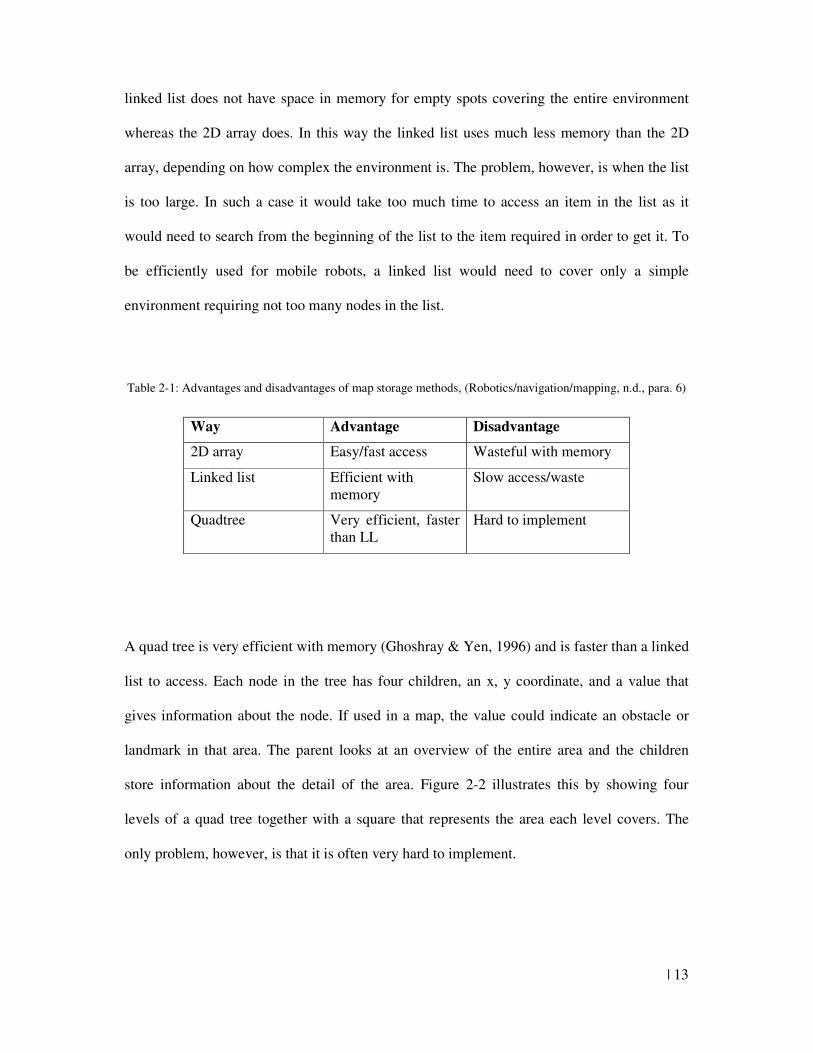
Three different ways for storing items within a map are summarised in Table 2-1. These

items could be obstacle locations, landmarks, or other information that would help a robot

move within an environment. The simplest storage method is a 2D array that simply records

data about every x, y coordinate in a map. To do this, the map needs to be made into a grid so

that each part of the environment can be given coordinates. This is very quick to access but

uses a lot of memory.

Another method, the linked list, uses less memory but takes longer for the computer to

access. When looking through the list, one must always starts from the same node. This node

points to another node which in turn points to another until the end of list is reached. The

| 13

linked list does not have space in memory for empty spots covering the entire environment

whereas the 2D array does. In this way the linked list uses much less memory than the 2D

array, depending on how complex the environment is. The problem, however, is when the list

is too large. In such a case it would take too much time to access an item in the list as it

would need to search from the beginning of the list to the item required in order to get it. To

be efficiently used for mobile robots, a linked list would need to cover only a simple

environment requiring not too many nodes in the list.

Table 2-1: Advantages and disadvantages of map storage methods, (Robotics/navigation/mapping, n.d., para. 6)

Way Advantage Disadvantage

2D array Easy/fast access Wasteful with memory

Linked list Efficient with memory

Slow access/waste

Quadtree Very efficient, faster than LL

Hard to implement

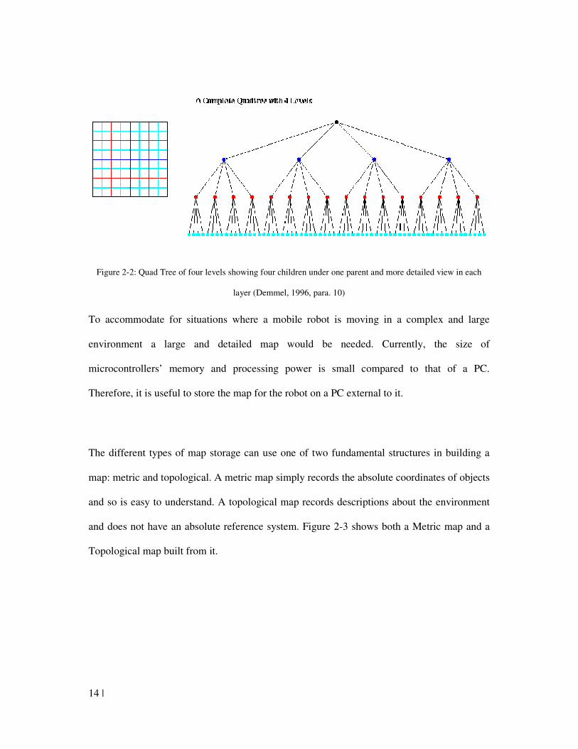
A quad tree is very efficient with memory (Ghoshray & Yen, 1996) and is faster than a linked

list to access. Each node in the tree has four children, an x, y coordinate, and a value that

gives information about the node. If used in a map, the value could indicate an obstacle or

landmark in that area. The parent looks at an overview of the entire area and the children

store information about the detail of the area. Figure 2-2 illustrates this by showing four

levels of a quad tree together with a square that represents the area each level covers. The

only problem, however, is that it is often very hard to implement.

14 |

Figure 2-2: Quad Tree of four levels showing four children under one parent and more detailed view in each

layer (Demmel, 1996, para. 10)

To accommodate for situations where a mobile robot is moving in a complex and large

environment a large and detailed map would be needed. Currently, the size of

microcontrollers’ memory and processing power is small compared to that of a PC.

Therefore, it is useful to store the map for the robot on a PC external to it.

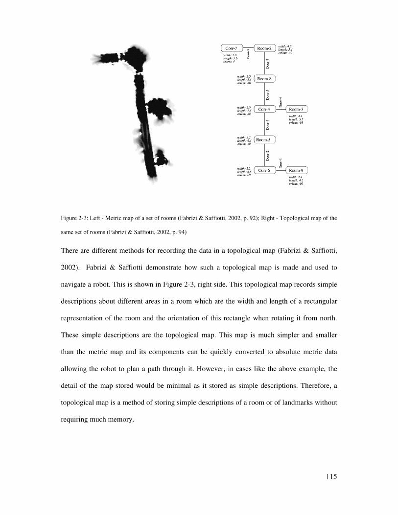
The different types of map storage can use one of two fundamental structures in building a

map: metric and topological. A metric map simply records the absolute coordinates of objects

and so is easy to understand. A topological map records descriptions about the environment

and does not have an absolute reference system. Figure 2-3 shows both a Metric map and a

Topological map built from it.

| 15

Figure 2-3: Left - Metric map of a set of rooms (Fabrizi & Saffiotti, 2002, p. 92); Right - Topological map of the

same set of rooms (Fabrizi & Saffiotti, 2002, p. 94)

There are different methods for recording the data in a topological map (Fabrizi & Saffiotti,

2002). Fabrizi & Saffiotti demonstrate how such a topological map is made and used to

navigate a robot. This is shown in Figure 2-3, right side. This topological map records simple

descriptions about different areas in a room which are the width and length of a rectangular

representation of the room and the orientation of this rectangle when rotating it from north.

These simple descriptions are the topological map. This map is much simpler and smaller

than the metric map and its components can be quickly converted to absolute metric data

allowing the robot to plan a path through it. However, in cases like the above example, the

detail of the map stored would be minimal as it stored as simple descriptions. Therefore, a

topological map is a method of storing simple descriptions of a room or of landmarks without

requiring much memory.

16 |

2.3.2 Odometry

Odometry is a method that uses data that indicates how far a robot has moved to estimate

where it should currently be. For example, if someone counted the number of steps they took

while walking in a straight line they would be able to calculate the approximate distance they

were from the place where they started, based upon the length of a step. In a mobile robot, the

data used for estimating how far the robot has moved comes from either the record of the

commands sent to the moving components (i.e., wheels or legs) or from encoders that provide

feedback of the movement.

The vast majority of mobile robots rely on odometry for their navigation (Henlich, 1997;

Suksakulchai, Thongchai, Wilkes, & Kawamura, 2000). Many different types of encoders can

be used for odometry including: brush encoders, potentiometers, optical encoders, magnetic

encoders, inductive encoders, and capacitive encoders. These encoders usually provide a

good estimate of the distance a wheel has moved. For example, optical encoders have a thin

disc that rotates with the motor wheel. A small light shines through small holes located

around the edge of the disc and a detector on the other side of the disc recognises through the

light every time a hole is detected. Since the distance between holes on the disc is known,

through the number of holes detected, the distance the wheel has turned can be calculated. A

magnetic encoder could simply be magnets placed on the motor shaft that move with the

motor and whose magnetic field is detected by a Hall Effect sensor. Based upon how many

magnets there are on the wheel, the Hall Effect sensor data can then be used to determine

how much the wheel has rotated. However, having the wheel turn does not necessarily

determine the exact distance it has moved.

Odometry is only an estimate of the location of the robot. This estimate becomes worse as the

robot keeps moving since small discrepancies between where the robot should have moved

| 17

and where it did only accumulate over time (Henlich, O. 1997). This position error should be

corrected periodically through some localisation method as discussed in the next section.

These odometry errors could be caused by factors such as (Kriechbaum, 2006; Park & Ji,

2009):

• Low-quality hardware (e.g., such as slight misalignment in the position of the wheels)

• Noise in the encoder’s sensors

• Slippage or sliding of wheels

• An uneven environment surface

Ideally, a robot should be mechanically designed to minimize these errors as much as

possible. For example, the wheels should be an equal distance from the centre and be tightly

held by the motor so they cannot slip. However, small errors will always exist and for

practical use, it cannot be expected that the environment’s floor will always be perfectly

even. Therefore, other methods to correct the robots position should be used whenever

moving a robot a long distance. This correction is discussed in the following section.

2.3.3 Localisation

This section discusses the updating of a robot’s absolute position in relation to a global

reference point in a map. This updating is called ‘localisation’. Localisation is necessary

when the robot needs to travel over a large area (Dudek, Jenkin, Milios, & Wilkes, 1991;

Kim, 2004; Suksakulchai, Thongchai, Wilkes, & Kawamura, 2000), due to the robot’s

estimated position accumulating error over time.

18 |

The method used to locate the robot depends on the type of environment. In large-scale

outdoor environments, a GPS (Global positioning system) that uses time information and

position information from at least four satellites to find the object’s absolute position can be

used. GPS is not applicable to navigating a small indoor mobile robot as the accuracy of GPS

is only within 1-3 meters and the room within which an indoor robot moves will obstruct the

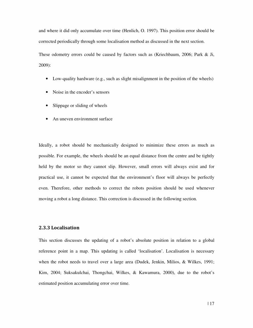
periodic signals used in GPS (Henlich, O. 1997). Another method of locating a robot outside

is shown by Lambrinos, Moller, Labhart, Pfeifer, & Wehner (1999). They illustrate a robot

that uses the polarization pattern of light in the sky (illustrated in Figure 2-4) to localise the

position of a robot. Obviously, the robot needs to be outside to see such patterns so this is not

applicable to navigate a robot indoors either.

Figure 2-4: Polarization pattern of light in the sky a mobile robot can use to localise itself (Lambrinos, et. al,

1999, p. 42)

| 19

Various methods have been invented for localising a robot indoors. These include the use of:

• a camera mounted above the robot that always observes the robot to see where it is

(Gupta, Messom, Demidenko, 2005)

• transmitters placed on the wall or ceiling that bounce off the robot and use the time

their reflection took or the signal strength to estimate the robot’s position (Henlich,

1997)

• the detection of physical landmarks whose location is previously stored in a map

(Henlich, 1997; Kriechbaum, 2006)

• the use of devices that know where they are in a map so that the robot’s position can

be calculated when they are detected (Batalin & Sukhatme, 2004)

The first two methods mentioned above aim at detecting the robot’s location at all times

whereas the last two rely on odometry to estimate the robot’s position and only localise the

robot’s position at particular points around the environment.

The problem with using a camera mounted above the robot is that it should continuously be

able to detect the robot. Many environments have obstacles that would block the camera’s

view of a robot if the camera were placed on the ceiling. Transmitters mounted on a wall may

not require an obstacle free path as their signals often can go through obstacles, yet their

signal is usually obstructed by obstacles that lie between them and the robot.

The detection of recorded landmarks is not troubled by obstacles around the room as the

localisation is done by sensors on the robot itself. These sensors (usually a camera) look for

landmarks and compare their features to landmark features stored in a map. If a match

20 |

between the observation and something in a map is found, the robot’s position can then be set

to the landmarks recorded position in the map and so eliminate any accumulated error in

estimating their position (Henlich, 1997).

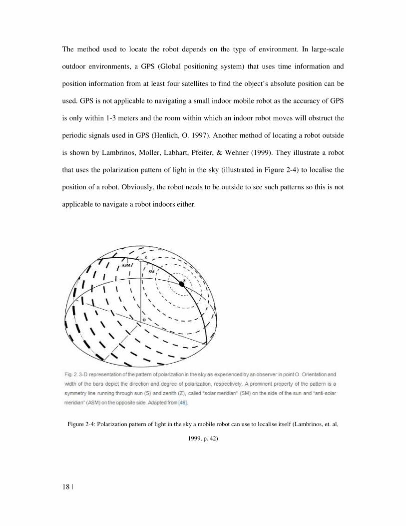
Kriechbaum (2006) showed, with a computer simulation running on Matlab, the usefulness of

landmarks in localising a robot. Figure 2-5 shows this simulation with landmarks placed

between the robot’s starting and ending position. Instead of moving straight to the

destination, the algorithm makes use of landmarks to correct any accumulated error that could

be produced as the robot moves. Therefore the robot plans a path that goes past the obstacles

on its way to the goal and uses them to update the robot’s actual position when it reaches

them.

Figure 2-5: Robot using landmarks for localisation when moving towards a goal (Kriechbaum, 2006, p. 84)

Usually, physical objects already present in the environment are used as landmarks. The

disadvantage of this is that sensors that detect these landmarks can be noisy and there can be

| 21

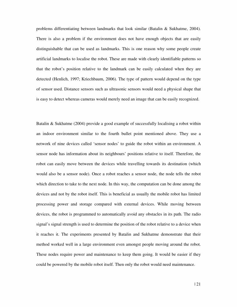
problems differentiating between landmarks that look similar (Batalin & Sukhatme, 2004).

There is also a problem if the environment does not have enough objects that are easily

distinguishable that can be used as landmarks. This is one reason why some people create

artificial landmarks to localise the robot. These are made with clearly identifiable patterns so

that the robot’s position relative to the landmark can be easily calculated when they are

detected (Henlich, 1997; Kriechbaum, 2006). The type of pattern would depend on the type

of sensor used. Distance sensors such as ultrasonic sensors would need a physical shape that

is easy to detect whereas cameras would merely need an image that can be easily recognized.

Batalin & Sukhatme (2004) provide a good example of successfully localising a robot within

an indoor environment similar to the fourth bullet point mentioned above. They use a

network of nine devices called ‘sensor nodes’ to guide the robot within an environment. A

sensor node has information about its neighbours’ positions relative to itself. Therefore, the

robot can easily move between the devices while travelling towards its destination (which

would also be a sensor node). Once a robot reaches a sensor node, the node tells the robot

which direction to take to the next node. In this way, the computation can be done among the

devices and not by the robot itself. This is beneficial as usually the mobile robot has limited

processing power and storage compared with external devices. While moving between

devices, the robot is programmed to automatically avoid any obstacles in its path. The radio

signal’s signal strength is used to determine the position of the robot relative to a device when

it reaches it. The experiments presented by Batalin and Sukhatme demonstrate that their

method worked well in a large environment even amongst people moving around the robot.

These nodes require power and maintenance to keep them going. It would be easier if they

could be powered by the mobile robot itself. Then only the robot would need maintenance.

22 |

RFID technology can be used either to continuously update the position of the robot or to do

so at set points in the environment. Oktem & Aydin (2010) demonstrate the use of three long

range high frequency RFID transmitters placed around a room that continuously detect a

RFID tag on the robot to provide a continuous estimation of the robot’s position. They use

the received signal strength of the RFID tag on the transmitter to estimate the distance from

each transmitter to the robot. By using these three distances together with the coordinates of

the RFID transmitters, the robot’s position is estimated. Their results show that this signal

strength is obstructed by obstacles due to reflections and diffractions (Oktem & Aydin, 2010)

and so has limited accuracy when used in an environment with many large obstacles.

Some indoor navigation algorithms rely purely on localisation through distinguishable

landmarks within a room and do not use any odometry. Such applications have the following

disadvantages:

• Need enough distinguishable features in the environment

• Require accurate sensors to see features well enough so that the robot’s position

relative to them can be determined

• Memory has to be large enough to store a map with enough resolution to store enough

details about landmarks so that the robot can use them to regularly localise itself

(Henlich, 1997).

Despite these disadvantages, such methods would make a robot more robust in environments

where odometry may prove ineffective. Such environments would include places with rough

surfaces, where the robot could go up and down; and slippery surfaces, where the wheels

could easily slip, meaning that the wheel turns but the robot does not move.

| 23

With all this in view, it can be seen that there is a need for more research in localising a

mobile robot in an environment with complex obstacles that obstruct continuous monitoring

techniques. There is also a need for such localisation to be free from maintenance, as active

localising devices would require, in order to make the system more self sustainable. This

research later presents passive RFID tags as a solution to this problem. Passive RFID tags can

be placed at convenient places in a room with complex obstacles and require no power source

of their own as they are powered by the reader that reads them.

2.3.4 Goal reaching methodology

In order for a mobile robot to reach a goal, or final destination, the goal reaching

methodology must be able to avoid obstacles that lie in their path yet still get to their goal in

an efficient amount of time. The goal reaching methodology that can be used depends on:

• the design of the robot (e.g, how many wheels, how are they are driven)

• the complexity of the obstacles (simple rectangles, concave, or having many small

rough edges hard to detect)

• the accuracy and range of the sensors

The number of sensors mounted around the robot, their range of detection, and the frequency

of their measurement will very much influence the algorithm that can be used to avoid

obstacles while the robot travels towards a goal. For example, a robot with only a few

distance sensors at set points around the robot would be unable to safely detect small parts of

a complex obstacle that stick out into the robot’s way of travel.

24 |

These algorithms are primarily methods for avoiding obstacles on the way toward a goal. If

no obstacles are in the robot’s path the robot will simply travel straight towards its goal.

However, the Uncertain bug (Section 2.3.4.3) adds more complexity to this by updating its

position information through the use of landmarks. The potential field method (Section

2.3.4.4) also stands in a category of its own by using forces to detect obstacles and to get to

its goal instead of relying on distance sensors and odometry. The main focus of these

algorithms is for a robot to move to its destination and often this involves various methods of

avoiding or travelling past obstacles.

Kreichbaum (2006) presents three algorithms that a robot can use in order to reach a goal.

These are stated in the next three sections.

2.3.4.1 Tangent bug

Kriechbaum’s first method (2006) is called the ‘Tangent bug’ algorithm. In this algorithm, at

each step on the robot’s path towards its goal, a local tangent graph (LTG) is produced that

consists of nodes and edges as illustrated in Figure 2-6. The dotted circle around the robot

represents the range the robot’s distance sensors can detect. The robot starts at position xR

and is told to move to a position xG. An LTG node is put at the robot’s position and at the

endpoints of detected obstacles. LTG edges are lines that go from the robot’s position to the

LTG nodes created at the detected obstacle’s endpoints. An optional LTG node called Tg,

with a corresponding LTG edge, is formed if:

• The distance from the robot to the goal is greater than the detection range of the robot

• There are no obstacles detected that inhibit a straight line between the robot’s position

and the goal

| 25

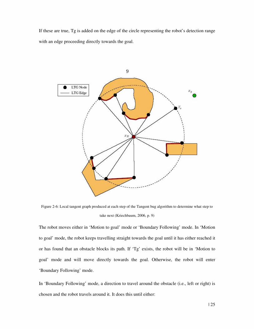
If these are true, Tg is added on the edge of the circle representing the robot’s detection range

with an edge proceeding directly towards the goal.

Figure 2-6: Local tangent graph produced at each step of the Tangent bug algorithm to determine what step to

take next (Kriechbaum, 2006, p. 9)

The robot moves either in ‘Motion to goal’ mode or ‘Boundary Following’ mode. In ‘Motion

to goal’ mode, the robot keeps travelling straight towards the goal until it has either reached it

or has found that an obstacle blocks its path. If ‘Tg’ exists, the robot will be in ‘Motion to

goal’ mode and will move directly towards the goal. Otherwise, the robot will enter

‘Boundary Following’ mode.

In ‘Boundary Following’ mode, a direction to travel around the obstacle (i.e., left or right) is

chosen and the robot travels around it. It does this until either:

26 |

• The goal is reached

• The robot is free from the obstacle and can revert to ‘Motion to goal’ mode

• The robot detects that the goal is unreachable (since the goal or the mobile robot is

completely surrounded by obstacles)

This method assumes that the mobile robot has little or no odometry errors accumulating over

time, so is impractical to use if moving the robot for a long time, since all robots have at least

some amount of error in estimating their position through dead reckoning.

2.3.4.2 Optim bug

The second navigation method presented by Kriechbaum (2006) is ‘Optim bug’. It has a less

uniform path than ‘Tangent bug’ but would more easily extend to three dimensions. It also

automatically builds a map of the environment which can be used when travelling over the

same area in the environment or when moving in the environment at a later date. Like

‘Tangent bug’, this method also unrealistically assumes that the robot used has no odometry

errors accumulating over time.

In this algorithm, the total area that has been scanned, called the ‘visibility set’, is labelled

‘Vtot’. V(k) represents the visibility set at time step k. V(k+1) is the visibility set added by

the robots sensors in the next time step. As shown in the steps below, a time ‘step’ is only

taken when the robot reaches the end of its visibility set. At this point, the mobile robot’s

sensors will be able to detect obstacles from the end of the visibility set and hence increase

the known area, adding V(k+1) to V(k).

Kriechbaum’s steps for the optim bug are:

| 27

1. Compute the shortest path to travel towards the goal based on the area it has mapped

in Vtot.

2. Follow the path to the end of Vtot.

3. Is goal in Vtot?

a. Yes – success since you know exactly how to move to reach the goal. The

robot then simply moves within Vtot until it finishes at Vtot.

b. No - Extend the visibility of Vtot by moving to the edge of Vtot.

4. Add V(k+1) to the Vtot.

5. If there is no path that can reach the goal without passing through obstacles, finish in

failure.

Figure 2-7 shows this algorithm step by step while a robot moves from a position with an

obstacle surrounding it to a position where it sees an obstacle free path towards its goal.

28 |

Figure 2-7: Steps for a robot to avoid an obstacle and find the path to the goal using the Optim bug algorithm

(Kriechbaum, 2006, p. 67)

The direction that the robot takes is always towards its goal unless obstructed by an obstacle.

If no obstacles are seen in a straight path to the goal, then that path is used. Otherwise, the

robot moves to the edge of the known boundary of the obstacle it is currently at. It keeps

doing this, every time extending its visibility set, until it reaches a point where there are no

more obstacles obstructing a straight line between the robot and the goal. Once reaching this

point, the process of trying to move straight towards the goal starts again.

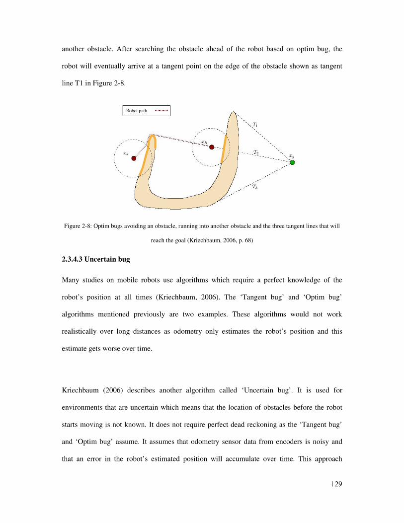
Figure 2-8 shows that a robot using this ‘Optim bug’ trys to find a straight obstacle free path

toward the goal (Tangent line T2 in the figure). After following this path, the robot meets

| 29

another obstacle. After searching the obstacle ahead of the robot based on optim bug, the

robot will eventually arrive at a tangent point on the edge of the obstacle shown as tangent

line T1 in Figure 2-8.

Figure 2-8: Optim bugs avoiding an obstacle, running into another obstacle and the three tangent lines that will

reach the goal (Kriechbaum, 2006, p. 68)

2.3.4.3 Uncertain bug

Many studies on mobile robots use algorithms which require a perfect knowledge of the

robot’s position at all times (Kriechbaum, 2006). The ‘Tangent bug’ and ‘Optim bug’

algorithms mentioned previously are two examples. These algorithms would not work

realistically over long distances as odometry only estimates the robot’s position and this

estimate gets worse over time.

Kriechbaum (2006) describes another algorithm called ‘Uncertain bug’. It is used for

environments that are uncertain which means that the location of obstacles before the robot

starts moving is not known. It does not require perfect dead reckoning as the ‘Tangent bug’

and ‘Optim bug’ assume. It assumes that odometry sensor data from encoders is noisy and

that an error in the robot’s estimated position will accumulate over time. This approach

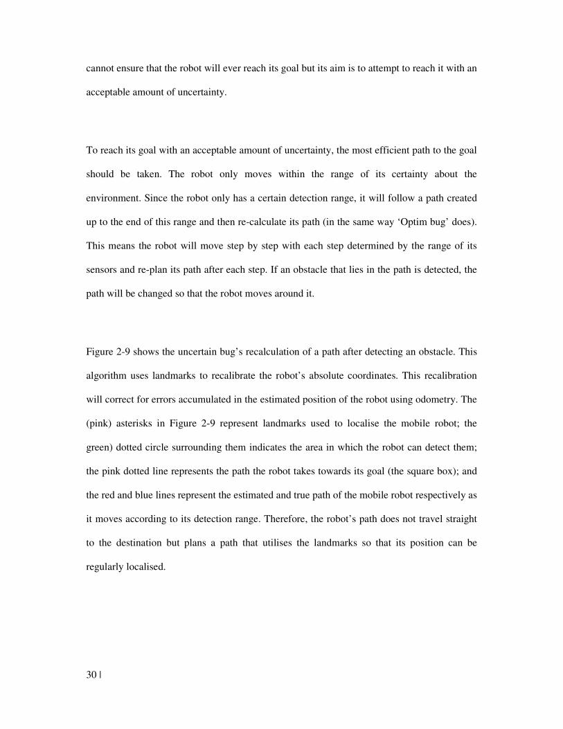
30 |

cannot ensure that the robot will ever reach its goal but its aim is to attempt to reach it with an

acceptable amount of uncertainty.

To reach its goal with an acceptable amount of uncertainty, the most efficient path to the goal

should be taken. The robot only moves within the range of its certainty about the

environment. Since the robot only has a certain detection range, it will follow a path created

up to the end of this range and then re-calculate its path (in the same way ‘Optim bug’ does).

This means the robot will move step by step with each step determined by the range of its

sensors and re-plan its path after each step. If an obstacle that lies in the path is detected, the

path will be changed so that the robot moves around it.

Figure 2-9 shows the uncertain bug’s recalculation of a path after detecting an obstacle. This

algorithm uses landmarks to recalibrate the robot’s absolute coordinates. This recalibration

will correct for errors accumulated in the estimated position of the robot using odometry. The

(pink) asterisks in Figure 2-9 represent landmarks used to localise the mobile robot; the

green) dotted circle surrounding them indicates the area in which the robot can detect them;

the pink dotted line represents the path the robot takes towards its goal (the square box); and

the red and blue lines represent the estimated and true path of the mobile robot respectively as

it moves according to its detection range. Therefore, the robot’s path does not travel straight

to the destination but plans a path that utilises the landmarks so that its position can be

regularly localised.

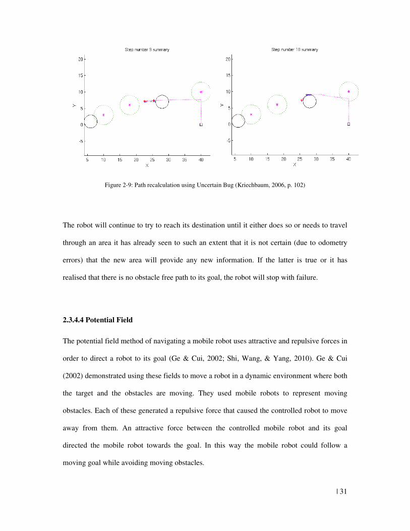
| 31

Figure 2-9: Path recalculation using Uncertain Bug (Kriechbaum, 2006, p. 102)

The robot will continue to try to reach its destination until it either does so or needs to travel

through an area it has already seen to such an extent that it is not certain (due to odometry

errors) that the new area will provide any new information. If the latter is true or it has

realised that there is no obstacle free path to its goal, the robot will stop with failure.

2.3.4.4 Potential Field

The potential field method of navigating a mobile robot uses attractive and repulsive forces in

order to direct a robot to its goal (Ge & Cui, 2002; Shi, Wang, & Yang, 2010). Ge & Cui

(2002) demonstrated using these fields to move a robot in a dynamic environment where both

the target and the obstacles are moving. They used mobile robots to represent moving

obstacles. Each of these generated a repulsive force that caused the controlled robot to move

away from them. An attractive force between the controlled mobile robot and its goal

directed the mobile robot towards the goal. In this way the mobile robot could follow a

moving goal while avoiding moving obstacles.

32 |

This would be impossible for methods such as the Uncertain Bug to use as they assume that

the environment is static. Having such attracting and repelling forces provides much more

flexibility to a system making it easier to manipulate in industry and to work in environments

with moving obstacles. However, in a complex environment it would be difficult to make

every obstacle have some sort of repulsive force. Also, if the environment had large static

obstacles, this method would provide no way to avoid them and such obstacles would

probably interfere with the detection of the attraction and repulsion forces. Other algorithms

using sensors such as distance sensors need to be incorporated with this method to allow it to

avoid large static obstacles.

2.3.4.5 Side step and look

The following algorithm is purely a method for avoiding an obstacle in a simple environment.

For most algorithms the robot will inevitably try to move straight toward a goal (or move past

landmarks on the way to a goal) and then move into an obstacle avoiding mode when one

obstructs its path. This algorithm and the one following assume that this simple method of

moving straight towards the goal is used and provides a simple way to avoid obstacles when

they are detected between the robot and its destination.

Robotics/navigation/collision_avoidance (n.d.) shows a simple algorithm for avoiding an

obstacle. When an obstacle is detected, the robot will move one and a half times its body

length in distance around the side of the obstacle. It will then check if its path is clear and try

to move past it towards the target. If it still detects an obstacle in its path, it will keep moving

one times its body length to the side of the obstacle until it detects a clear path to move.

| 33

This algorithm would be easier for a robot to follow than the boundary following mode of the

‘Tangent bug’ algorithm. The boundary following mode requires sensors to clearly detect

each point along the boundary in order to follow it. This algorithm, however, only moves in

set movements and just needs to detect whether an obstacle is directly ahead of it at any one

time. Hence, it is more practical for robots with simple obstacle detection sensors than the

boundary following mode.

This simple algorithm would work efficiently in very simple environments but not in more

complex ones. For example, in the case of trying to move to a goal when the robot is within a

‘U-shaped’ obstacle, the robot will become stuck, trying to move to the side of the obstacle

when it cannot (Robotics/navigation/collision_avoidance, n.d.).

2.3.4.6 Turn till obstacle is clear

A more efficient method in avoiding an obstacle is to turn the robot until it can’t measure the

obstacle any more so that the width of the obstacle can be estimated. Benmounah & Abbassi

(1999) presented this simple method for avoiding an obstacle using a three wheeled vehicle

that has only one driven wheel at its front. The robot assumes to move from the start to the

goal as can be seen in Figure 2-11. Then the robot determines whether to travel around either

the left or right side of the obstacle. The robot first turns on the spot in the left direction until

it cannot see the obstacle anymore. The angle the robot is at this point from its original

position (β1) is recorded and the same measurement is made on the right side of the robot

(β2). The robot then takes the smallest of β1 and β2 and chooses that direction to travel in. By

using the smallest angle, the distance A2 or A2’ (as shown in Figure 2-10) can be calculated

and the robot can attempt to avoid the obstacle.

34 |

Figure 2-10: Avoiding an obstacle through turning to obstacle edge, (Benmounah & Abbassi, 1999, pg 539)

This method could only move the robot around the robot at steps that would be dependent on

the detection range of the front sensor. If the obstacle’s edge exceeded the detection range of

the front sensor, the robot would need to move to A2 or A2’ and then try to find the edge

again. Also, a mobile robot would be unable to avoid complex obstacles using this algorithm

since it does not take into account situations where another obstacle could be at position A2

where the robot moves to avoid its first obstacle.

2.3.5 Sensing technology (safety issues)

2.3.5.1 Use of various sensors

This research is focused on the methodology of navigating a robot within an indoor

environment using RFID tags. Therefore, the various types of sensors has not been

| 35

researched in depth. Sensors used for the robot to test this concept are explained in section

6.3.2.

2.3.5.2 Safety issues when moving a robot

In all the different methodologies mentioned above, safety must be observed. Issac Asimov

created three laws of robotics in which the first law was that a robot cannot hurt human

beings and the third law that a robot should try and protect itself (Isom, 2005). In order for

this to be practically possible, the size and power of the robot need to be balanced by the

capability and reliability of the sensors on the robot that detect objects external to the robot

itself. Some isolate a robot from the danger of contacting people or harmful objects. Mobile

robots would usually be used in situations where people or obstacles are around. Therefore,

to form a methodology that could be reliably used outside of a testing environment, the safety

of the robot to itself and others must be considered.

2.3.6 Conclusion

From the discussion above, the necessity of a map in most navigation methods has been

explained. Odometry is important in navigating a robot since it provides a method of

estimating the robot’s current position within the environment. Localisation is necessary to

update the mobile robot’s actual position and eliminate the errors that accumulate through

using odometry.

The different goal reaching methodologies mentioned provide insight into the various means

of navigating a mobile robot within an indoor environment. It can be seen that there is a need

for algorithms that do not assume perfect odometry, like Uncertain Bug. These make use of

landmarks to localise the robot at definite points within an environment. Potential field

36 |

algorithms are very useful in simple dynamic environments. A mobile robot can easily follow

a goal that is moving if it produces an attractive force for the robot. Also, moving obstacles

can be avoided if they are fitted with something that produces a force that repels the robot.

These algorithms are not useful, however, within an environment with large static obstacles

unless many repulsive forces are attached to the obstacles. Since environments are complex,

there is also the need for algorithms that avoid obstacles that are of a complex shape, such as

manoeuvring a robot out of a ‘U’ shaped obstacle.

With all this in view, it can be seen that there is a need for more research in algorithms that

navigate within an environment with complex obstacles and not rely on perfect odometry.

Mobile robots also need to be designed so that they are safe both to themselves, other

precious objects and human beings.

| 37

Chapter 3: Localisation methodology using RFID tags

The last chapter mentioned that localising a mobile robot within an indoor environment that

may have static or mobile obstacles is an active area of research. This chapter presents a

method of localising a mobile robot in an indoor environment that has stationary obstacles.

Odometry has been used to continuously estimate the robot’s position. This method

accumulates errors over time. In this research, RFID tags were used and installed on certain

fixed obstacles in order to update the position information of the mobile robot while it moves

within the environment and a compass was used to update the robot’s orientation. These tags

make it possible to localise a mobile robot within an environment where visual observation

from a sensor is not possible. These tags are only required to be detected and a short distance

and therefore have no problem with large obstacles that methodologies relying on attractive

forces would be disrupted by.

In order for the RFID tags to localise the robot, the position of the RFID tags are recorded in

a database based on the IDs of the RFID tags. The system developed by this research uses a

computer to communicate with the mobile robot wirelessly. When the system is set in the

teaching mode, the user can guide the robot through the environment. Whenever the robot

passes by an RFID tag the location and ID of the RFID tag is recorded. With such

information, it is able to build a map that has the RFID location information. Therefore,

whenever the robot moves in the environment, as soon as the robot detects an RFID tag, the

position of the robot can be updated based on the location of the RFID tag detected.

38 |

3.1 Low frequency passive RFID tags

RFID technology is gaining popularity and is being developed by large companies such as

Tesco and Walmart. An RFID system is composed of RFID tags and RFID readers. It also

requires some method of electronically storing a record of the unique IDs stored in the RFID

tags together with information for each ID that can have some use in the RFID system. RFID

applications include any situation where objects need a unique ID that can be detected at a

later date. For example, animals in a farm may be tagged with an RFID tag that holds an ID

unique to them. When an RFID reader detects the tag, a database that contains a list of the

tags and information about the animals that correspond to these IDs can be looked up. This

would allow the one on the farm to know any crucial information stored about the animal

they detected.

An RFID tag is composed of a microchip that stores a unique ID of the tag and an antenna

that transmits its signal. There are different types of tags. The active types have a battery

which they use to power the tag to continuously emit its own RFID. Since they are powered

by their own battery, they have a greater detection distance than passive RFID tags however

are more expensive and would require battery replacement (Persuad, n.d.).

When a battery is undesired, a passive type of tag is used. With passive tags, inductive

coupling occurs in which the RFID tag draws power from the electromagnetic field generated

by the coil in an RFID reader (an external device that reads the tags ID). The field generated

induces a current in the RFID tag’s own antenna (RFID Journal, n.d.). With this current, the

tag sends its unique ID to the RFID reader. Figure 3-1 shows a magnetic field produced by a

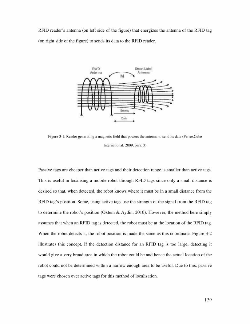
| 39

RFID reader’s antenna (on left side of the figure) that energizes the antenna of the RFID tag

(on right side of the figure) to sends its data to the RFID reader.

Figure 3-1: Reader generating a magnetic field that powers the antenna to send its data (FerroxCube

International, 2009, para. 3)

Passive tags are cheaper than active tags and their detection range is smaller than active tags.

This is useful in localising a mobile robot through RFID tags since only a small distance is

desired so that, when detected, the robot knows where it must be in a small distance from the

RFID tag’s position. Some, using active tags use the strength of the signal from the RFID tag

to determine the robot’s position (Oktem & Aydin, 2010). However, the method here simply

assumes that when an RFID tag is detected, the robot must be at the location of the RFID tag.

When the robot detects it, the robot position is made the same as this coordinate. Figure 3-2

illustrates this concept. If the detection distance for an RFID tag is too large, detecting it

would give a very broad area in which the robot could be and hence the actual location of the

robot could not be determined within a narrow enough area to be useful. Due to this, passive

tags were chosen over active tags for this method of localisation.

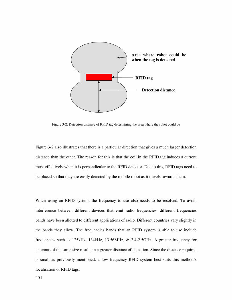
40 |

Figure 3-2: Detection distance of RFID tag determining the area where the robot could be

Figure 3-2 also illustrates that there is a particular direction that gives a much larger detection

distance than the other. The reason for this is that the coil in the RFID tag induces a current

most effectively when it is perpendicular to the RFID detector. Due to this, RFID tags need to

be placed so that they are easily detected by the mobile robot as it travels towards them.

When using an RFID system, the frequency to use also needs to be resolved. To avoid

interference between different devices that emit radio frequencies, different frequencies

bands have been allotted to different applications of radio. Different countries vary slightly in

the bands they allow. The frequencies bands that an RFID system is able to use include

frequencies such as 125kHz, 134kHz, 13.56MHz, & 2.4-2.5GHz. A greater frequency for

antennas of the same size results in a greater distance of detection. Since the distance required

is small as previously mentioned, a low frequency RFID system best suits this method’s

localisation of RFID tags.

Area where robot could be

when the tag is detected

RFID tag

Detection distance

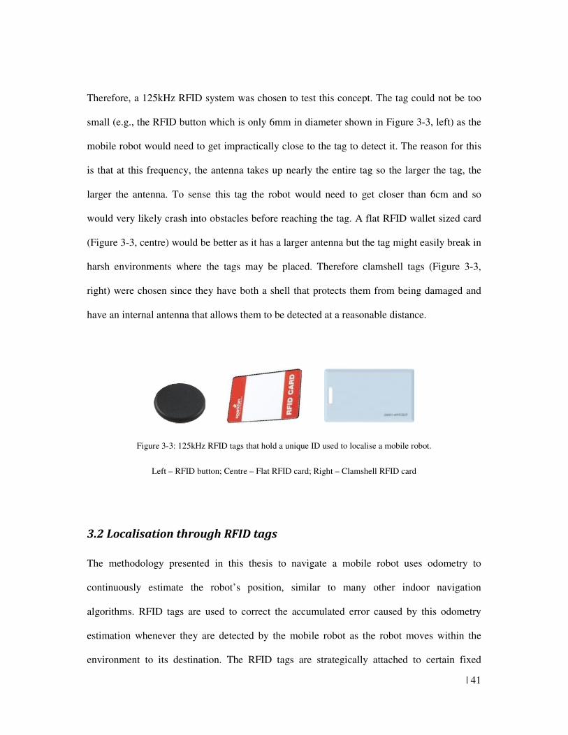
| 41

Therefore, a 125kHz RFID system was chosen to test this concept. The tag could not be too

small (e.g., the RFID button which is only 6mm in diameter shown in Figure 3-3, left) as the

mobile robot would need to get impractically close to the tag to detect it. The reason for this

is that at this frequency, the antenna takes up nearly the entire tag so the larger the tag, the

larger the antenna. To sense this tag the robot would need to get closer than 6cm and so

would very likely crash into obstacles before reaching the tag. A flat RFID wallet sized card

(Figure 3-3, centre) would be better as it has a larger antenna but the tag might easily break in

harsh environments where the tags may be placed. Therefore clamshell tags (Figure 3-3,

right) were chosen since they have both a shell that protects them from being damaged and

have an internal antenna that allows them to be detected at a reasonable distance.

Figure 3-3: 125kHz RFID tags that hold a unique ID used to localise a mobile robot.

Left – RFID button; Centre – Flat RFID card; Right – Clamshell RFID card

3.2 Localisation through RFID tags

The methodology presented in this thesis to navigate a mobile robot uses odometry to

continuously estimate the robot’s position, similar to many other indoor navigation

algorithms. RFID tags are used to correct the accumulated error caused by this odometry

estimation whenever they are detected by the mobile robot as the robot moves within the

environment to its destination. The RFID tags are strategically attached to certain fixed

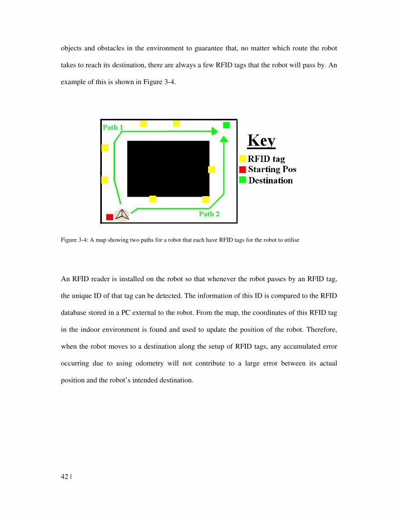
42 |

objects and obstacles in the environment to guarantee that, no matter which route the robot

takes to reach its destination, there are always a few RFID tags that the robot will pass by. An

example of this is shown in Figure 3-4.

Figure 3-4: A map showing two paths for a robot that each have RFID tags for the robot to utilise

An RFID reader is installed on the robot so that whenever the robot passes by an RFID tag,

the unique ID of that tag can be detected. The information of this ID is compared to the RFID

database stored in a PC external to the robot. From the map, the coordinates of this RFID tag

in the indoor environment is found and used to update the position of the robot. Therefore,

when the robot moves to a destination along the setup of RFID tags, any accumulated error

occurring due to using odometry will not contribute to a large error between its actual

position and the robot’s intended destination.

| 43

3.3 Fixing orientation error through a compass

A basic compass simply detects the magnetic field in its environment and assumes that there

are little or no external magnetic fields that prevent the compass from clearly and simply

using the earth’s magnetic field to find its orientation (Caruso, n.d.).

These compasses were designed to point to north so that a human user could use them to

navigate to a particular destination. However, with the invention of robots that rely on

electrical signals, there is the need of an electronic compass that gives an electric signal to a

computer that indicates what direction it is currently facing. The three main types of signals

sent are

• A serial chain of bits (high and low voltages) whose binary value represents an angle.

For example, if a 8 bit signal were used, 1111 1111 could represent 359 degrees, 0000

0001 represent 0 degrees and then all the binary values in between would correspond

to different angles

• A pulse whose length of time depends on the angle (e.g. 1ms = 1 deg, 360ms = 360

deg)

• A voltage whose analogue value represents the angle. For example, if 5V were the

maximum voltage allowed, it would refer to 360 degrees, 2.5V to 180 degrees, 1V to

72 degrees, etc.

The computer would read these signals and then determine the compass’ angle from them. To

produce such a signal, a sensor that generates an electrical signal that varies with the earth’s

magnetic field is needed. Two common electronic sensors (Robert, Christian & Samuel,

2004) that detect this magnetic field are:

44 |

• Magneto-resistive sensors that use materials whose resistance changes depending on

how the angle of the magnetic field lines up with the current of the material (called

anisotropic magnetoresistance). The resistance is greatest when the magnetic field is

parallel to the direction of the magnetic current.

• Fluxgate sensors that use two coils of wire wound around a coil of a material that is

greatly susceptible to magnetic fields. The first wire has an alternating current passing

through it that causes a continuously changing magnetic field to be generated in the

material. This magnetic field will induce a current in the second wire that, under no

external magnetic fields, will exactly match the current in the first wire. However,

under an external magnetic field, the magnetic field in the material will more easily

saturate (that is, reach its maximum magnetization) when aligned to the external field

and less easily saturate when opposing the field. This will cause a time difference

between the first and second wire which is then used to determine the direction of the

external magnetic field.

A robot that uses a compass may have magnetic parts (such as iron) on it that frustrate the

detection of the earth’s magnetic field. These would permanently affect the magnetic field

detected by the compass, preventing it from correctly determining the robot’s angle. Figure 3-

5 shows the disturbance of a uniform magnetic field by a magnetic material. To compensate

for this disturbance, usually the compass is rotated and its magnetic field at different angles is

measured and recorded. With this, equations can be formed that determine the robot’s

orientation when in an environment where ferrous materials disturbance the earth’s magnetic

field.

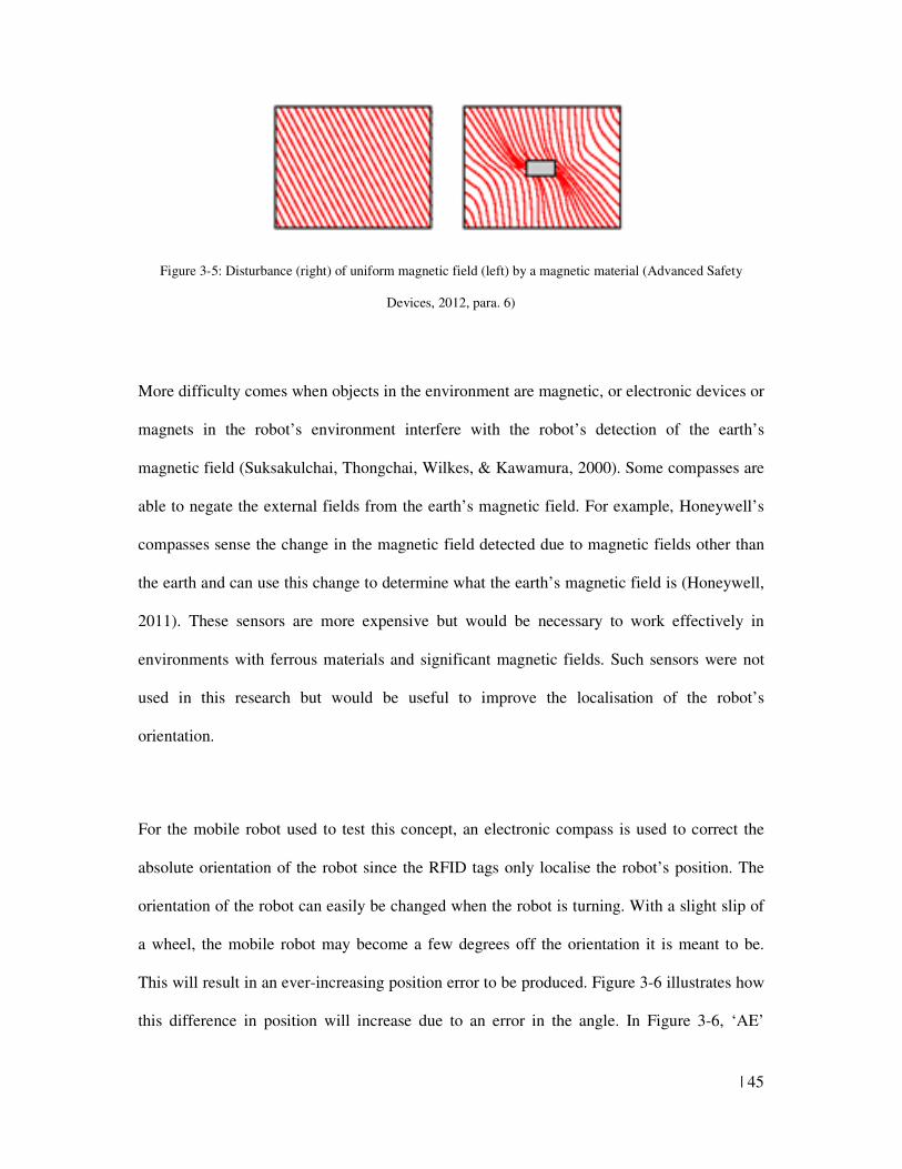
| 45

Figure 3-5: Disturbance (right) of uniform magnetic field (left) by a magnetic material (Advanced Safety

Devices, 2012, para. 6)

More difficulty comes when objects in the environment are magnetic, or electronic devices or

magnets in the robot’s environment interfere with the robot’s detection of the earth’s

magnetic field (Suksakulchai, Thongchai, Wilkes, & Kawamura, 2000). Some compasses are

able to negate the external fields from the earth’s magnetic field. For example, Honeywell’s

compasses sense the change in the magnetic field detected due to magnetic fields other than

the earth and can use this change to determine what the earth’s magnetic field is (Honeywell,

2011). These sensors are more expensive but would be necessary to work effectively in

environments with ferrous materials and significant magnetic fields. Such sensors were not

used in this research but would be useful to improve the localisation of the robot’s

orientation.

For the mobile robot used to test this concept, an electronic compass is used to correct the

absolute orientation of the robot since the RFID tags only localise the robot’s position. The

orientation of the robot can easily be changed when the robot is turning. With a slight slip of

a wheel, the mobile robot may become a few degrees off the orientation it is meant to be.

This will result in an ever-increasing position error to be produced. Figure 3-6 illustrates how

this difference in position will increase due to an error in the angle. In Figure 3-6, ‘AE’

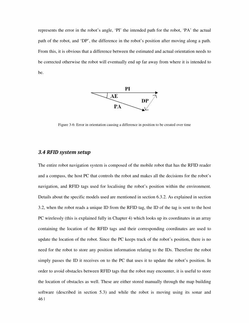
46 |

represents the error in the robot’s angle, ‘PI’ the intended path for the robot, ‘PA’ the actual

path of the robot, and ‘DP’, the difference in the robot’s position after moving along a path.

From this, it is obvious that a difference between the estimated and actual orientation needs to

be corrected otherwise the robot will eventually end up far away from where it is intended to

be.

Figure 3-6: Error in orientation causing a difference in position to be created over time

3.4 RFID system setup

The entire robot navigation system is composed of the mobile robot that has the RFID reader

and a compass, the host PC that controls the robot and makes all the decisions for the robot’s

navigation, and RFID tags used for localising the robot’s position within the environment.

Details about the specific models used are mentioned in section 6.3.2. As explained in section

3.2, when the robot reads a unique ID from the RFID tag, the ID of the tag is sent to the host

PC wirelessly (this is explained fully in Chapter 4) which looks up its coordinates in an array

containing the location of the RFID tags and their corresponding coordinates are used to

update the location of the robot. Since the PC keeps track of the robot’s position, there is no

need for the robot to store any position information relating to the IDs. Therefore the robot

simply passes the ID it receives on to the PC that uses it to update the robot’s position. In

order to avoid obstacles between RFID tags that the robot may encounter, it is useful to store

the location of obstacles as well. These are either stored manually through the map building

software (described in section 5.3) and while the robot is moving using its sonar and

| 47

photodiode distance sensors (explained in section 6.3.2.2.1 and 6.3.2.2.2). The arrays

containing the location of the RFID tags and the location of obstacles in the environment both

constitute the robot map and are used to navigate the robot.

The array containing the location of all the RFID tags can be quickly created by an operator

simply driving the robot through the environment, while running a software that records

where the tag location is. This is called the ‘teaching mode’ as the system is taught the

environment through moving the robot within the environment and recording the RFID tag

locations as the robot detects the RFID tags. The procedure works in the same way as people

learn a place through passing through it and observing what is in it. When the mobile robot

passes an RFID tag and detects it, its unique ID is automatically recorded as well as the

coordinates at which it was detected. Since the software uses odometry to estimate the robot’s

position as it moves through the environment, the operator needs to move the robot step by

step and manually correct the robot’s position whenever they see it slipping or not moving as

it should do. Although the map produced will not be the exact coordinates of the RFID tags,

they will be sufficient to localise the robot when it moves around in the map. The building of

a map of the environment through the teaching mode is further described in section 5.3.

The users of the system may also calculate the location of the RFID tags in the environment

manually and then type the location information into the system. This would take more time

than the teaching method and may not be any more accurate. Therefore, when building a

map, the teaching mode is preferred over the manual method.

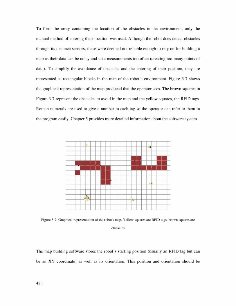
48 |

To form the array containing the location of the obstacles in the environment, only the

manual method of entering their location was used. Although the robot does detect obstacles

through its distance sensors, these were deemed not reliable enough to rely on for building a

map as their data can be noisy and take measurements too often (creating too many points of

data). To simplify the avoidance of obstacles and the entering of their position, they are

represented as rectangular blocks in the map of the robot’s environment. Figure 3-7 shows

the graphical representation of the map produced that the operator sees. The brown squares in

Figure 3-7 represent the obstacles to avoid in the map and the yellow squares, the RFID tags.

Roman numerals are used to give a number to each tag so the operator can refer to them in

the program easily. Chapter 5 provides more detailed information about the software system.

Figure 3-7: Graphical representation of the robot's map. Yellow squares are RFID tags, brown squares are

obstacles

The map building software stores the robot’s starting position (usually an RFID tag but can

be an XY coordinate) as well as its orientation. This position and orientation should be

| 49

known and easy for an operator to put the robot in. For example, the robot’s starting location

may be parallel and at the edge of an object in a room.

The method of localising a mobile robot in an indoor environment has been presented. It uses

odometry to estimate the robot’s position continuously. Since this is only an estimate and

accumulates error as the robot keeps moving, low frequency passive RFID tags placed

strategically around the environment are used to update the robot’s position and a compass is

used to update its orientation. The robot navigates using a map that contains the location of

the RFID tags and obstacles that the robot could encounter.

50 |

Chapter 4: Component communication

The previous chapter presented a methodology used for navigating a mobile robot within an

indoor environment. The map to guide the robot movement can be very large. Processing of

sensor data is complex. Complex algorithms are required to determine what the robot should

do. As a result, an external PC is used as the central processing unit and map storage place for

the mobile robot. This chapter discusses the wireless communication between the PC and the

mobile robot, how the microcontrollers on the robot send commands to and receive data from

one another, and how the robot’s camera sends its video signal to the PC.

4.1 Wireless communication between the host PC and the mobile robot

4.1.1 Role of host PC and mobile robot

The communication standard used for the wireless communication between the PC and the

mobile robot and for the serial communication between the two microcontrollers on the robot

itself is USART (Universal Synchronous Asynchronous Receiver Transmitter). It is a simple

standard for serial communication between two devices. This standard has the benefit of

requiring only two pins on each device, a receive pin and transmit pin. Since there is no clock

pin, the frequency at which they communicate needs to be programmed to be identical before

the devices can communicate. This is realised through the baud rate which is measured in bps

(bits per second). The baud rate used was 9600bps. The communication between all these

devices is illustrated in Figure 4-1.

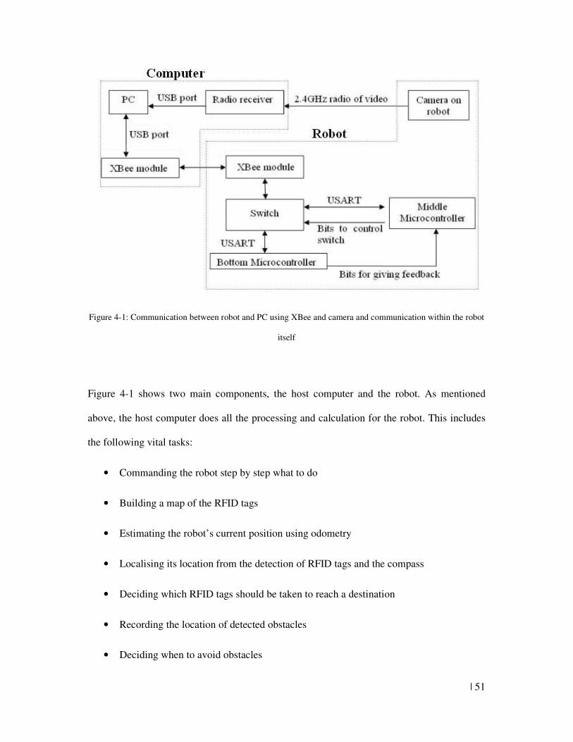
| 51

Figure 4-1: Communication between robot and PC using XBee and camera and communication within the robot

itself

Figure 4-1 shows two main components, the host computer and the robot. As mentioned

above, the host computer does all the processing and calculation for the robot. This includes

the following vital tasks:

• Commanding the robot step by step what to do

• Building a map of the RFID tags

• Estimating the robot’s current position using odometry

• Localising its location from the detection of RFID tags and the compass

• Deciding which RFID tags should be taken to reach a destination

• Recording the location of detected obstacles

• Deciding when to avoid obstacles

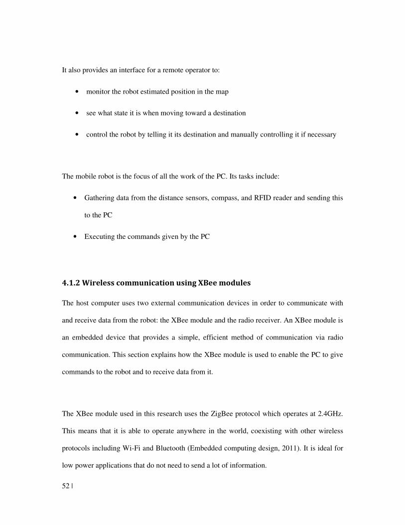
52 |

It also provides an interface for a remote operator to:

• monitor the robot estimated position in the map

• see what state it is when moving toward a destination

• control the robot by telling it its destination and manually controlling it if necessary

The mobile robot is the focus of all the work of the PC. Its tasks include:

• Gathering data from the distance sensors, compass, and RFID reader and sending this

to the PC

• Executing the commands given by the PC

4.1.2 Wireless communication using XBee modules

The host computer uses two external communication devices in order to communicate with

and receive data from the robot: the XBee module and the radio receiver. An XBee module is

an embedded device that provides a simple, efficient method of communication via radio

communication. This section explains how the XBee module is used to enable the PC to give

commands to the robot and to receive data from it.

The XBee module used in this research uses the ZigBee protocol which operates at 2.4GHz.

This means that it is able to operate anywhere in the world, coexisting with other wireless

protocols including Wi-Fi and Bluetooth (Embedded computing design, 2011). It is ideal for

low power applications that do not need to send a lot of information.

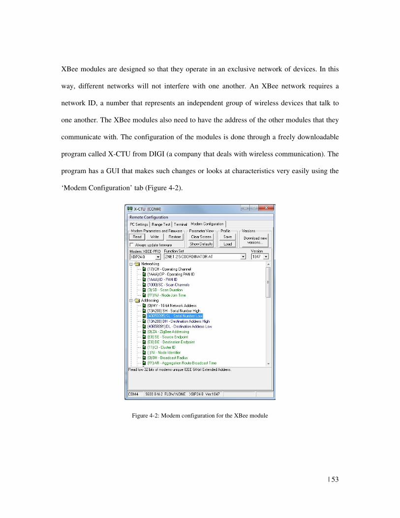
| 53

XBee modules are designed so that they operate in an exclusive network of devices. In this

way, different networks will not interfere with one another. An XBee network requires a

network ID, a number that represents an independent group of wireless devices that talk to

one another. The XBee modules also need to have the address of the other modules that they

communicate with. The configuration of the modules is done through a freely downloadable

program called X-CTU from DIGI (a company that deals with wireless communication). The

program has a GUI that makes such changes or looks at characteristics very easily using the

‘Modem Configuration’ tab (Figure 4-2).

Figure 4-2: Modem configuration for the XBee module

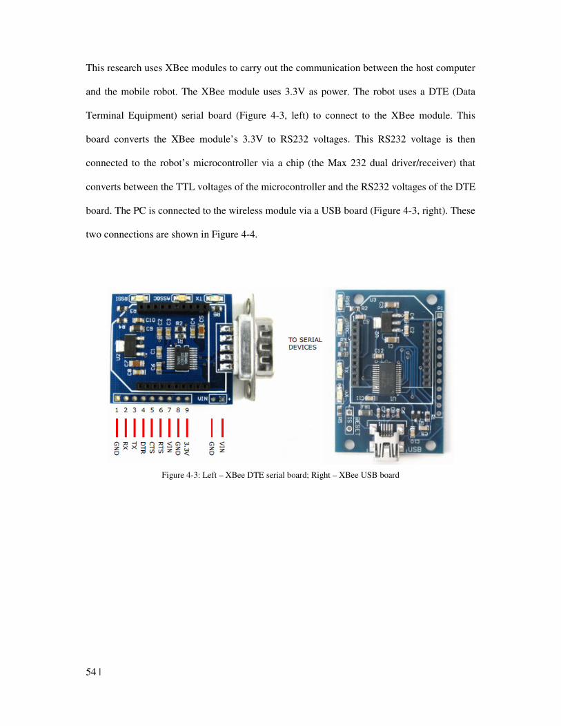
54 |

This research uses XBee modules to carry out the communication between the host computer

and the mobile robot. The XBee module uses 3.3V as power. The robot uses a DTE (Data

Terminal Equipment) serial board (Figure 4-3, left) to connect to the XBee module. This

board converts the XBee module’s 3.3V to RS232 voltages. This RS232 voltage is then

connected to the robot’s microcontroller via a chip (the Max 232 dual driver/receiver) that

converts between the TTL voltages of the microcontroller and the RS232 voltages of the DTE

board. The PC is connected to the wireless module via a USB board (Figure 4-3, right). These

two connections are shown in Figure 4-4.

Figure 4-3: Left – XBee DTE serial board; Right – XBee USB board

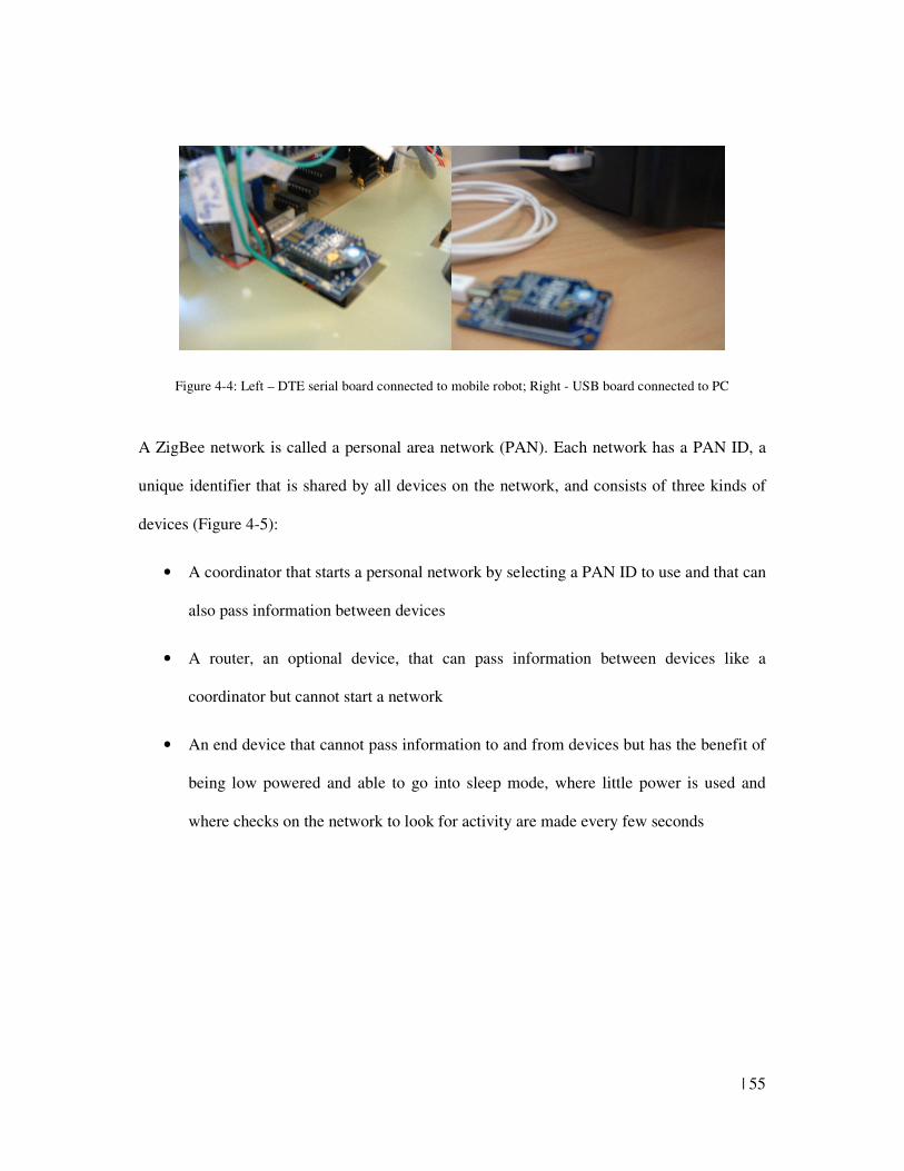
| 55

Figure 4-4: Left – DTE serial board connected to mobile robot; Right - USB board connected to PC

A ZigBee network is called a personal area network (PAN). Each network has a PAN ID, a

unique identifier that is shared by all devices on the network, and consists of three kinds of

devices (Figure 4-5):

• A coordinator that starts a personal network by selecting a PAN ID to use and that can

also pass information between devices

• A router, an optional device, that can pass information between devices like a

coordinator but cannot start a network

• An end device that cannot pass information to and from devices but has the benefit of

being low powered and able to go into sleep mode, where little power is used and

where checks on the network to look for activity are made every few seconds

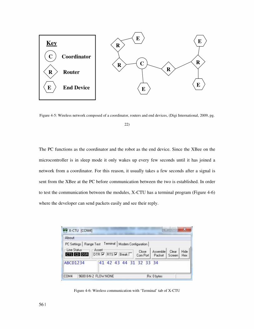
56 |

Figure 4-5: Wireless network composed of a coordinator, routers and end devices, (Digi International, 2009, pg.

22)

The PC functions as the coordinator and the robot as the end device. Since the XBee on the

microcontroller is in sleep mode it only wakes up every few seconds until it has joined a

network from a coordinator. For this reason, it usually takes a few seconds after a signal is

sent from the XBee at the PC before communication between the two is established. In order

to test the communication between the modules, X-CTU has a terminal program (Figure 4-6)

where the developer can send packets easily and see their reply.

Figure 4-6: Wireless communication with ‘Terminal’ tab of X-CTU

C R

R

R

R C

R

Coordinator

Router

End Device

Key

E

E

E

E

E

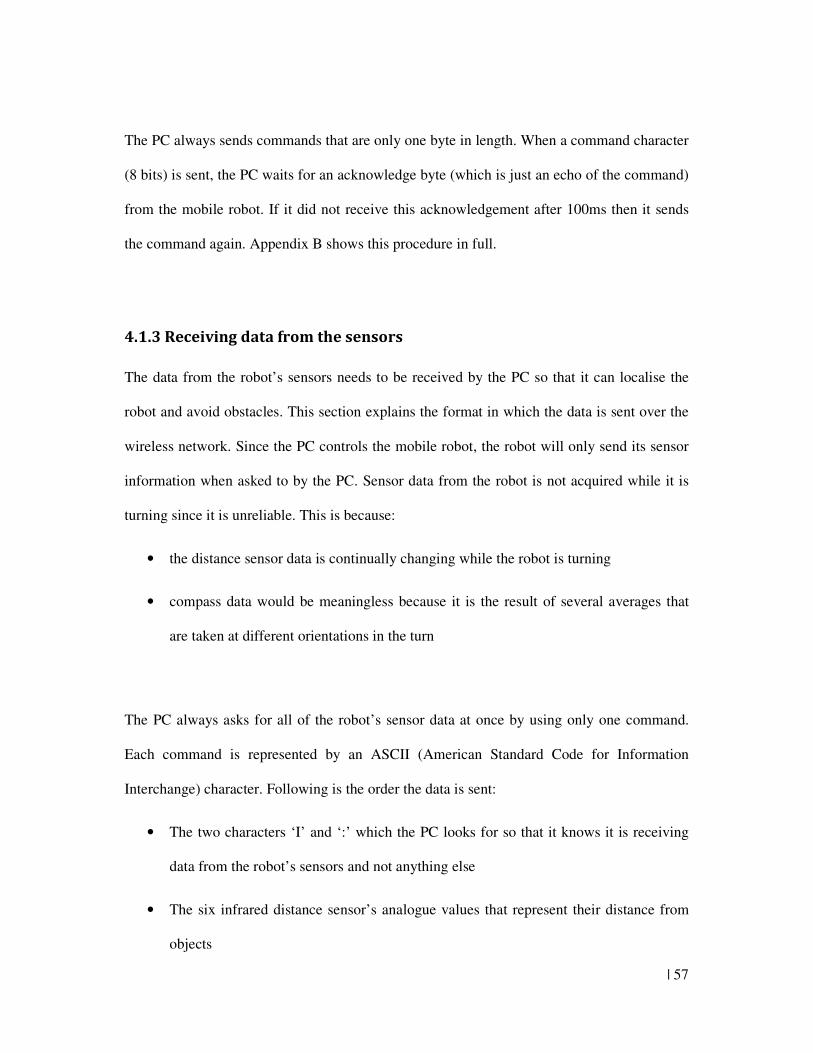
| 57

The PC always sends commands that are only one byte in length. When a command character

(8 bits) is sent, the PC waits for an acknowledge byte (which is just an echo of the command)

from the mobile robot. If it did not receive this acknowledgement after 100ms then it sends

the command again. Appendix B shows this procedure in full.

4.1.3 Receiving data from the sensors

The data from the robot’s sensors needs to be received by the PC so that it can localise the

robot and avoid obstacles. This section explains the format in which the data is sent over the

wireless network. Since the PC controls the mobile robot, the robot will only send its sensor

information when asked to by the PC. Sensor data from the robot is not acquired while it is

turning since it is unreliable. This is because:

• the distance sensor data is continually changing while the robot is turning

• compass data would be meaningless because it is the result of several averages that

are taken at different orientations in the turn

The PC always asks for all of the robot’s sensor data at once by using only one command.

Each command is represented by an ASCII (American Standard Code for Information

Interchange) character. Following is the order the data is sent:

• The two characters ‘I’ and ‘:’ which the PC looks for so that it knows it is receiving

data from the robot’s sensors and not anything else

• The six infrared distance sensor’s analogue values that represent their distance from

objects

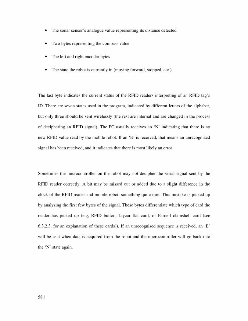
58 |

• The sonar sensor’s analogue value representing its distance detected

• Two bytes representing the compass value

• The left and right encoder bytes

• The state the robot is currently in (moving forward, stopped, etc.)

The last byte indicates the current status of the RFID readers interpreting of an RFID tag’s

ID. There are seven states used in the program, indicated by different letters of the alphabet,

but only three should be sent wirelessly (the rest are internal and are changed in the process

of deciphering an RFID signal). The PC usually receives an ‘N’ indicating that there is no

new RFID value read by the mobile robot. If an ‘E’ is received, that means an unrecognized

signal has been received, and it indicates that there is most likely an error.

Sometimes the microcontroller on the robot may not decipher the serial signal sent by the

RFID reader correctly. A bit may be missed out or added due to a slight difference in the

clock of the RFID reader and mobile robot, something quite rare. This mistake is picked up

by analysing the first few bytes of the signal. These bytes differentiate which type of card the

reader has picked up (e.g, RFID button, Jaycar flat card, or Farnell clamshell card (see

6.3.2.3. for an explanation of these cards)). If an unrecognised sequence is received, an ‘E’

will be sent when data is acquired from the robot and the microcontroller will go back into

the ‘N’ state again.

| 59

When an RFID tag is read successfully, the status will become ‘F’ indicating it has just

finished a reading. Since a new reading is made, the final part of data sent will be:

• The character ‘R’, indicating that a new RFID tag has been detected

• A byte indicating the type of RFID card

• Two bytes that represent the unique RFID of the tag

After sending the unique RFID of a new tag detected, the RFID status in the microcontroller

is set back to the ‘N’ status again. In this way the mobile robot sends all the data needed by

the robot so the PC can determine where obstacles are in relation to the robot and can localise

the robot’s orientation and position through the compass and RFID tag data. The PC asks for

this data regularly whenever the robot is not turning.

4.2 Communication between the bottom and middle layer

microcontrollers

Two ATmega32 microcontrollers are used in the mobile robot used to test the concept of

localisation through passive RFID tags (Figure 4-1). Details about this robot are presented in

section 6.2 and 6.3. A microcontroller placed on the bottom of the robot mainly controls the

robot’s motors while another microcontroller placed above it receives data from the robot’s

sensors and communicates wirelessly with the PC. This section describes how these two

microcontrollers communicate. The microcontrollers used each have four ports. Each port has

eight pins each and each pin can be configured independently as either input or output.

60 |

The middle microcontroller needs to pass on the commands it receives from the PC to the

bottom microcontroller. However, the same USART pins are used on the middle

microcontroller to communicate wirelessly to the PC and to communicate with the bottom

microcontroller. A setup is therefore needed on the middle layer to allow it to switch between

the middle layer’s serial communication to the bottom layer and its communication to the PC.

The position of this switch is illustrated in Figure 4-1.

A two input quad ‘AND’ gate and a two input quad ‘OR’ gate are used to carry out this

switching. A quad chip has four gates embedded into one chip and so reduces the number of

chips needed for an operation. A microcontroller pin is used to turn a particular one of these

gates on, allowing the middle microcontroller to communicate with either the PC or bottom

microcontroller. Figure 4-7 shows the names of the pins on port D, pins 0 - 3, that are used

for the USART communication. D0 is labeled with RXD, meaning it the USART input pin

for the middle layer’s microcontroller. D1 is the microcontroller’s USART output pin and is

labeled TXD. As can be seen, if D2 is high, data will be sent and received to and from the

XBee wireless module. If D3 is high, data will be sent and received from the bottom

microcontroller, which is connected to the middle layer’s 2nd ribbon cable port (with labels

of M2.8 and M2.9). This ribbon cable joins a port of the middle microcontroller to a port of

the bottom one and so is used for communication between them. For this reason, in the code,

D2 and D3 are never made high at the same time as then the middle layer’s microcontroller

would be communicating to both the PC and bottom microcontroller at the same time.

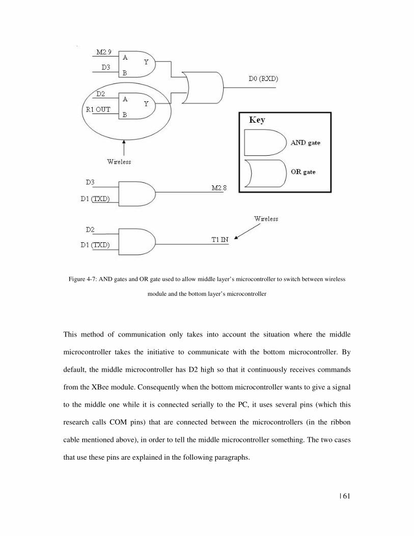
| 61

Figure 4-7: AND gates and OR gate used to allow middle layer’s microcontroller to switch between wireless

module and the bottom layer’s microcontroller

This method of communication only takes into account the situation where the middle

microcontroller takes the initiative to communicate with the bottom microcontroller. By

default, the middle microcontroller has D2 high so that it continuously receives commands

from the XBee module. Consequently when the bottom microcontroller wants to give a signal

to the middle one while it is connected serially to the PC, it uses several pins (which this

research calls COM pins) that are connected between the microcontrollers (in the ribbon

cable mentioned above), in order to tell the middle microcontroller something. The two cases

that use these pins are explained in the following paragraphs.

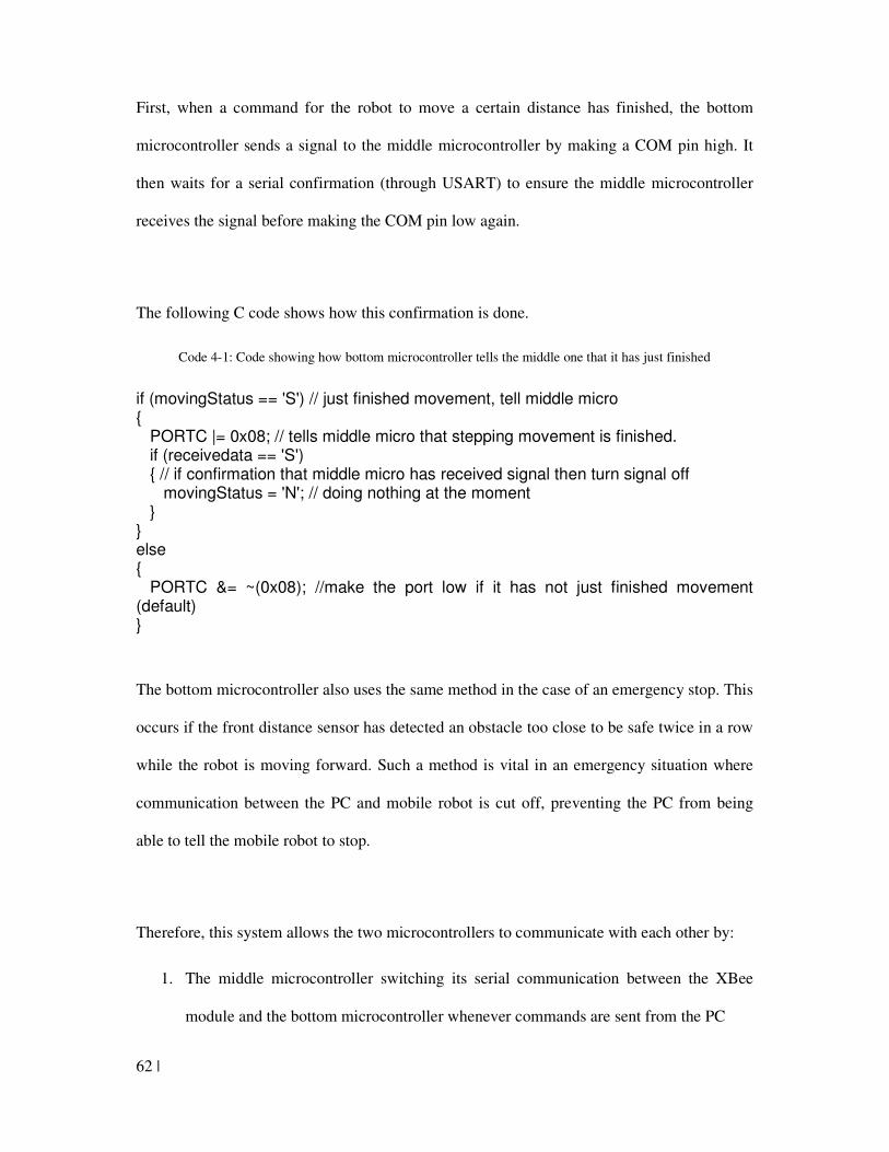
62 |

First, when a command for the robot to move a certain distance has finished, the bottom

microcontroller sends a signal to the middle microcontroller by making a COM pin high. It

then waits for a serial confirmation (through USART) to ensure the middle microcontroller

receives the signal before making the COM pin low again.

The following C code shows how this confirmation is done.

Code 4-1: Code showing how bottom microcontroller tells the middle one that it has just finished

if (movingStatus == 'S') // just finished movement, tell middle micro { PORTC |= 0x08; // tells middle micro that stepping movement is finished. if (receivedata == 'S') { // if confirmation that middle micro has received signal then turn signal off movingStatus = 'N'; // doing nothing at the moment } } else { PORTC &= ~(0x08); //make the port low if it has not just finished movement (default) }

The bottom microcontroller also uses the same method in the case of an emergency stop. This

occurs if the front distance sensor has detected an obstacle too close to be safe twice in a row

while the robot is moving forward. Such a method is vital in an emergency situation where

communication between the PC and mobile robot is cut off, preventing the PC from being

able to tell the mobile robot to stop.

Therefore, this system allows the two microcontrollers to communicate with each other by:

1. The middle microcontroller switching its serial communication between the XBee

module and the bottom microcontroller whenever commands are sent from the PC

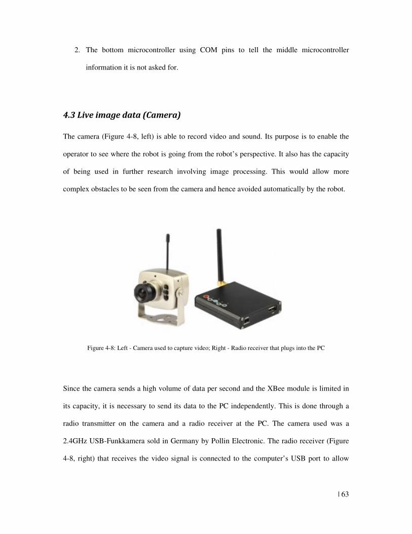
| 63

2. The bottom microcontroller using COM pins to tell the middle microcontroller

information it is not asked for.

4.3 Live image data (Camera)

The camera (Figure 4-8, left) is able to record video and sound. Its purpose is to enable the

operator to see where the robot is going from the robot’s perspective. It also has the capacity

of being used in further research involving image processing. This would allow more

complex obstacles to be seen from the camera and hence avoided automatically by the robot.

Figure 4-8: Left - Camera used to capture video; Right - Radio receiver that plugs into the PC

Since the camera sends a high volume of data per second and the XBee module is limited in

its capacity, it is necessary to send its data to the PC independently. This is done through a

radio transmitter on the camera and a radio receiver at the PC. The camera used was a

2.4GHz USB-Funkkamera sold in Germany by Pollin Electronic. The radio receiver (Figure

4-8, right) that receives the video signal is connected to the computer’s USB port to allow

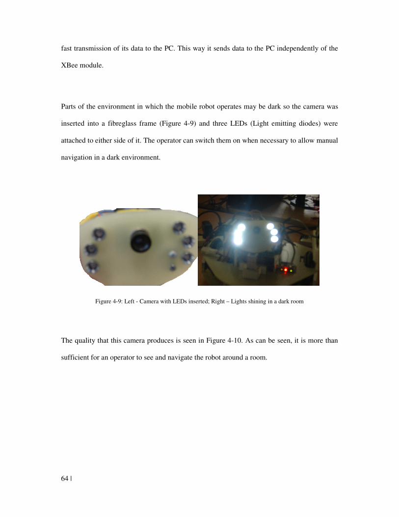
64 |

fast transmission of its data to the PC. This way it sends data to the PC independently of the

XBee module.

Parts of the environment in which the mobile robot operates may be dark so the camera was

inserted into a fibreglass frame (Figure 4-9) and three LEDs (Light emitting diodes) were

attached to either side of it. The operator can switch them on when necessary to allow manual

navigation in a dark environment.

Figure 4-9: Left - Camera with LEDs inserted; Right – Lights shining in a dark room

The quality that this camera produces is seen in Figure 4-10. As can be seen, it is more than

sufficient for an operator to see and navigate the robot around a room.

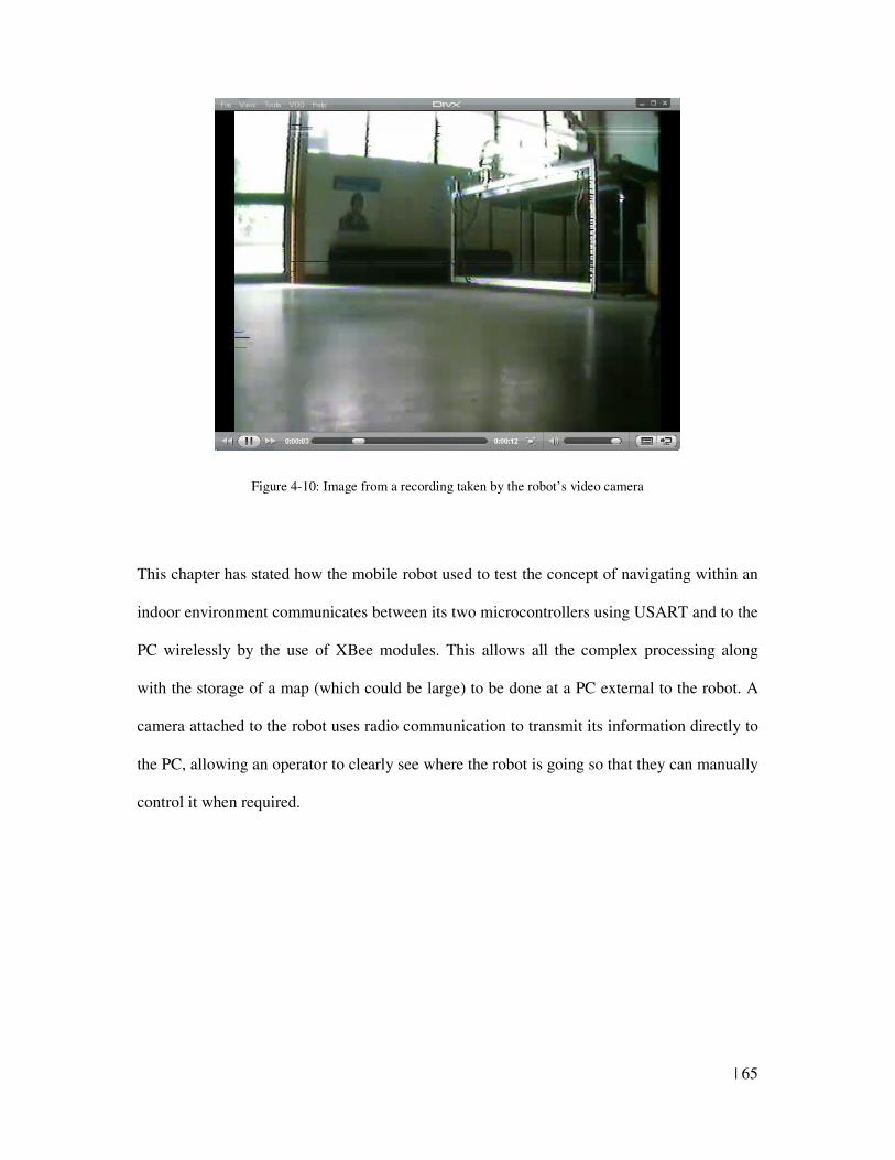
| 65

Figure 4-10: Image from a recording taken by the robot’s video camera

This chapter has stated how the mobile robot used to test the concept of navigating within an

indoor environment communicates between its two microcontrollers using USART and to the

PC wirelessly by the use of XBee modules. This allows all the complex processing along

with the storage of a map (which could be large) to be done at a PC external to the robot. A

camera attached to the robot uses radio communication to transmit its information directly to

the PC, allowing an operator to clearly see where the robot is going so that they can manually

control it when required.

66 |

Chapter 5: Mobile robot software system

With the methodology of localisation using RFID tags and of communicating between the

host PC and the robot presented in the previous chapters, there is the need for algorithms to

control the path that the robot takes and a program to model the robot’s environment so that

its position can be estimated continuously and displayed on the PC. This chapter presents the

methodologies used to model the robot movement in a real time environment and the

software’s functionalities.

5.1 Mobile robot navigation algorithms

To control the movement of the mobile robot in different situations, algorithms have to be

developed and implemented. These include the algorithms for simply moving from one RFID

tag to another and avoiding an obstacle in the robot’s path. As a destination usually lies in

between several tags, the algorithm for moving a robot between several tags is discussed.

Since there are odometry errors that result in the robot being slightly off its intended position,

the robot needs to search for the RFID tag it is sent to. An algorithm to do this searching is

presented.

5.1.1 Moving from one tag to another

5.1.1.1 Moving straight to the next tag

The position of an RFID tag, as recorded in the program, is the best position for the robot to

read the tag. Figure 5-1 shows the position the robot should be in order to sense the tag. This

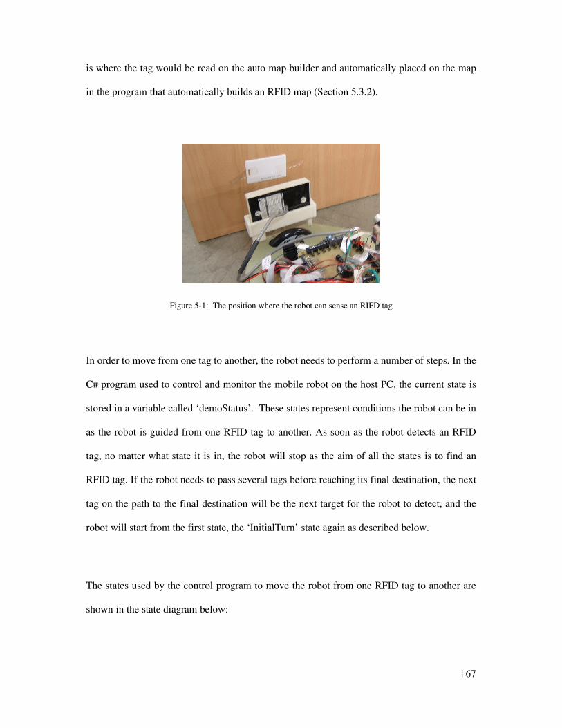
| 67

is where the tag would be read on the auto map builder and automatically placed on the map

in the program that automatically builds an RFID map (Section 5.3.2).

Figure 5-1: The position where the robot can sense an RIFD tag

In order to move from one tag to another, the robot needs to perform a number of steps. In the

C# program used to control and monitor the mobile robot on the host PC, the current state is

stored in a variable called ‘demoStatus’. These states represent conditions the robot can be in

as the robot is guided from one RFID tag to another. As soon as the robot detects an RFID

tag, no matter what state it is in, the robot will stop as the aim of all the states is to find an

RFID tag. If the robot needs to pass several tags before reaching its final destination, the next

tag on the path to the final destination will be the next target for the robot to detect, and the

robot will start from the first state, the ‘InitialTurn’ state again as described below.

The states used by the control program to move the robot from one RFID tag to another are

shown in the state diagram below:

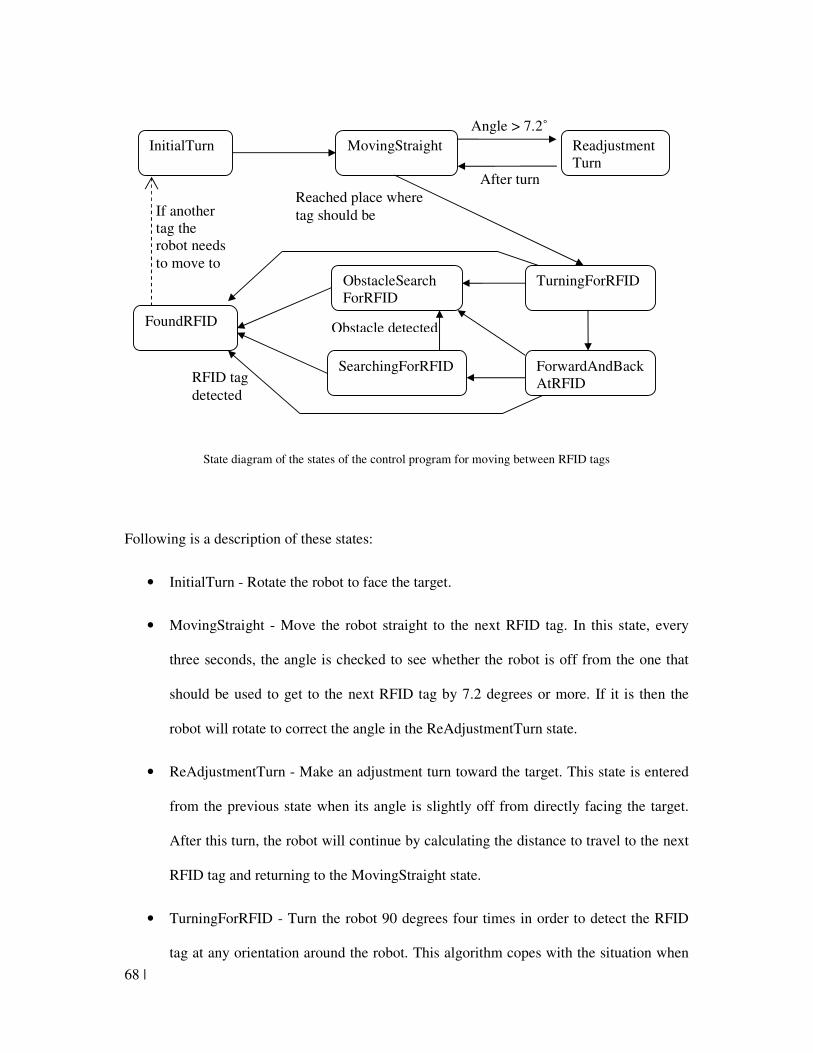
68 |

State diagram of the states of the control program for moving between RFID tags

Following is a description of these states:

• InitialTurn - Rotate the robot to face the target.

• MovingStraight - Move the robot straight to the next RFID tag. In this state, every

three seconds, the angle is checked to see whether the robot is off from the one that

should be used to get to the next RFID tag by 7.2 degrees or more. If it is then the

robot will rotate to correct the angle in the ReAdjustmentTurn state.

• ReAdjustmentTurn - Make an adjustment turn toward the target. This state is entered

from the previous state when its angle is slightly off from directly facing the target.

After this turn, the robot will continue by calculating the distance to travel to the next

RFID tag and returning to the MovingStraight state.

• TurningForRFID - Turn the robot 90 degrees four times in order to detect the RFID

tag at any orientation around the robot. This algorithm copes with the situation when

InitialTurn MovingStraight Readjustment Turn

Angle > 7.2˚

After turn

TurningForRFID

Reached place where

tag should be

ForwardAndBack AtRFID

SearchingForRFID

ObstacleSearch ForRFID

Obstacle detected FoundRFID

RFID tag

detected

If another tag the robot needs to move to

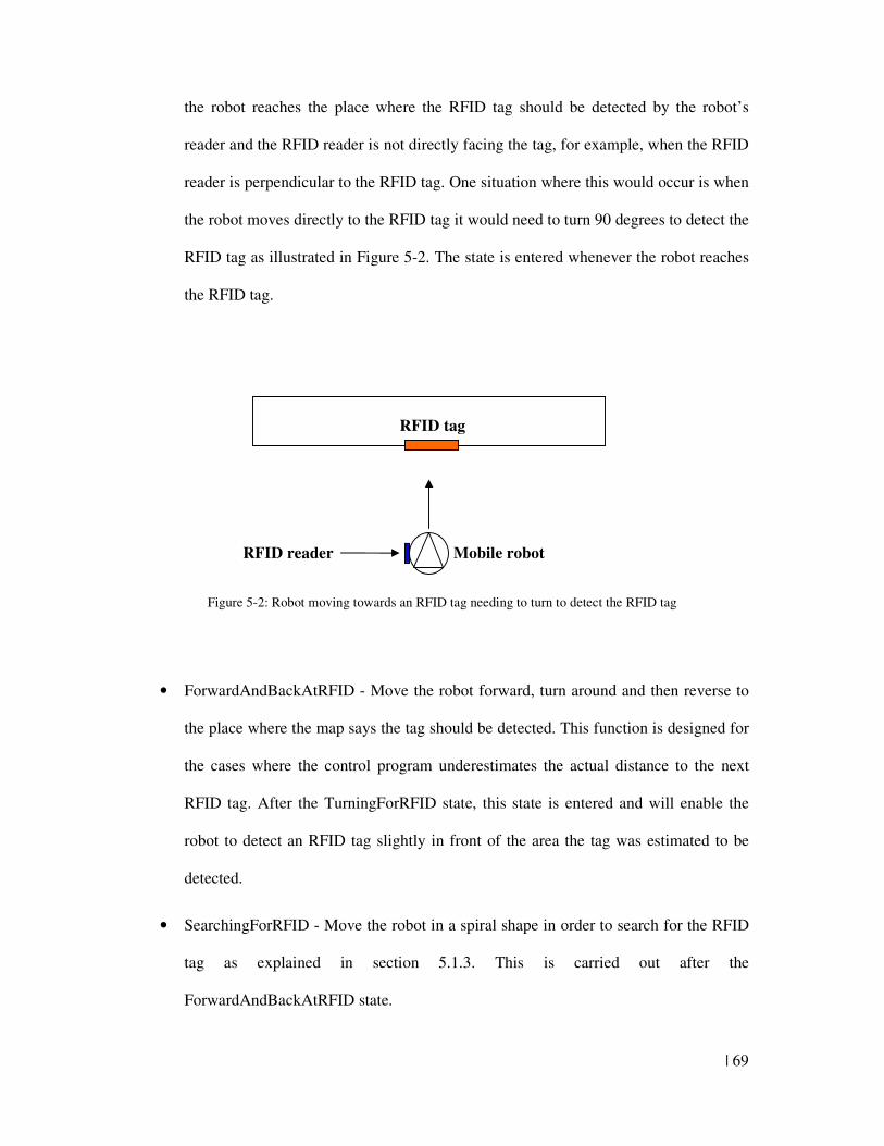
| 69

the robot reaches the place where the RFID tag should be detected by the robot’s

reader and the RFID reader is not directly facing the tag, for example, when the RFID

reader is perpendicular to the RFID tag. One situation where this would occur is when

the robot moves directly to the RFID tag it would need to turn 90 degrees to detect the

RFID tag as illustrated in Figure 5-2. The state is entered whenever the robot reaches

the RFID tag.

Figure 5-2: Robot moving towards an RFID tag needing to turn to detect the RFID tag

• ForwardAndBackAtRFID - Move the robot forward, turn around and then reverse to

the place where the map says the tag should be detected. This function is designed for

the cases where the control program underestimates the actual distance to the next

RFID tag. After the TurningForRFID state, this state is entered and will enable the

robot to detect an RFID tag slightly in front of the area the tag was estimated to be

detected.

• SearchingForRFID - Move the robot in a spiral shape in order to search for the RFID

tag as explained in section 5.1.3. This is carried out after the

ForwardAndBackAtRFID state.

Mobile robot

RFID tag

RFID reader

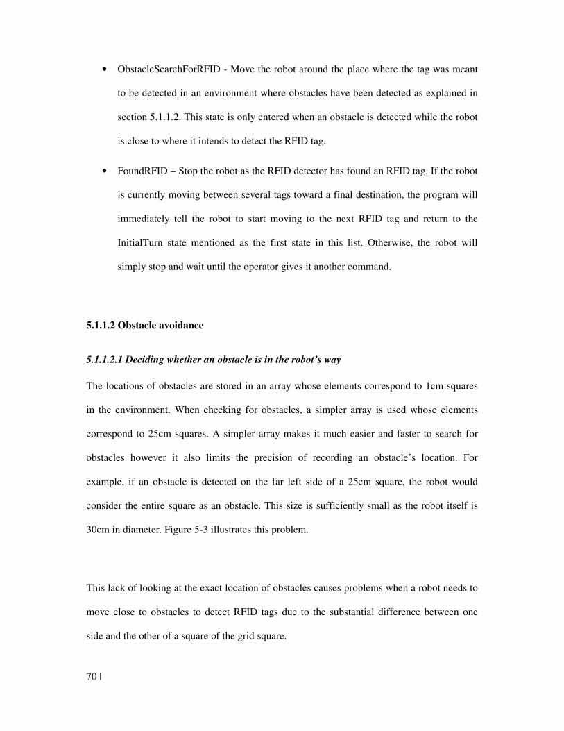
70 |

• ObstacleSearchForRFID - Move the robot around the place where the tag was meant

to be detected in an environment where obstacles have been detected as explained in

section 5.1.1.2. This state is only entered when an obstacle is detected while the robot

is close to where it intends to detect the RFID tag.

• FoundRFID – Stop the robot as the RFID detector has found an RFID tag. If the robot

is currently moving between several tags toward a final destination, the program will

immediately tell the robot to start moving to the next RFID tag and return to the

InitialTurn state mentioned as the first state in this list. Otherwise, the robot will

simply stop and wait until the operator gives it another command.

5.1.1.2 Obstacle avoidance

5.1.1.2.1 Deciding whether an obstacle is in the robot’s way

The locations of obstacles are stored in an array whose elements correspond to 1cm squares

in the environment. When checking for obstacles, a simpler array is used whose elements

correspond to 25cm squares. A simpler array makes it much easier and faster to search for

obstacles however it also limits the precision of recording an obstacle’s location. For

example, if an obstacle is detected on the far left side of a 25cm square, the robot would

consider the entire square as an obstacle. This size is sufficiently small as the robot itself is

30cm in diameter. Figure 5-3 illustrates this problem.

This lack of looking at the exact location of obstacles causes problems when a robot needs to

move close to obstacles to detect RFID tags due to the substantial difference between one

side and the other of a square of the grid square.

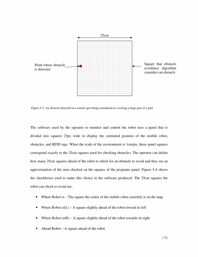
| 71

Figure 5-3: An obstacle detected in a certain spot being considered as covering a large part of a grid

The software used by the operator to monitor and control the robot uses a panel that is

divided into squares 25px wide to display the estimated position of the mobile robot,

obstacles, and RFID tags. When the scale of the environment is 1cm/px, these panel squares

correspond exactly to the 25cm squares used for checking obstacles. The operator can define

how many 25cm squares ahead of the robot to check for an obstacle to avoid and they see an

approximation of the area checked on the squares of the programs panel. Figure 5-4 shows

the checkboxes used to make this choice in the software produced. The 25cm squares the

robot can check to avoid are:

• Where Robot is – The square the center of the mobile robot currently is on the map

• Where Robot is(L) – A square slightly ahead of the robot toward its left

• Where Robot is(R) – A square slightly ahead of the robot towards its right

• Ahead Robot – A square ahead of the robot

25cm

Point where obstacle is detected

Square that obstacle avoidance algorithm considers an obstacle

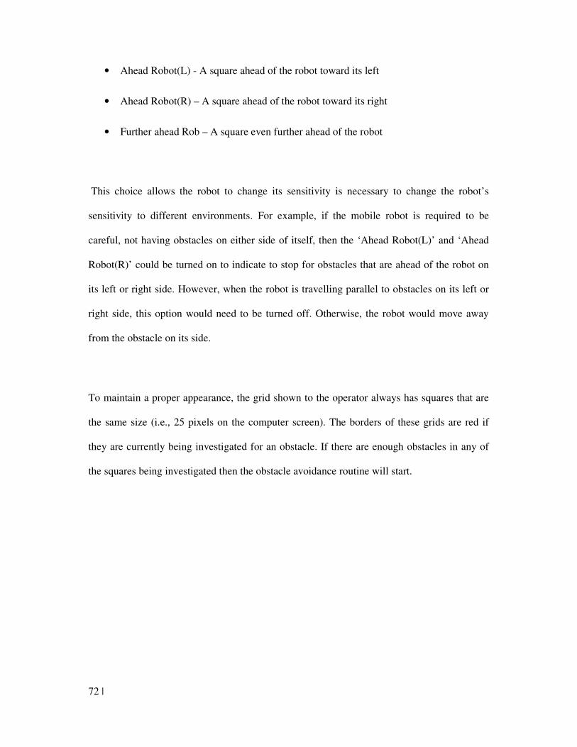
72 |

• Ahead Robot(L) - A square ahead of the robot toward its left

• Ahead Robot(R) – A square ahead of the robot toward its right

• Further ahead Rob – A square even further ahead of the robot

This choice allows the robot to change its sensitivity is necessary to change the robot’s

sensitivity to different environments. For example, if the mobile robot is required to be

careful, not having obstacles on either side of itself, then the ‘Ahead Robot(L)’ and ‘Ahead

Robot(R)’ could be turned on to indicate to stop for obstacles that are ahead of the robot on

its left or right side. However, when the robot is travelling parallel to obstacles on its left or

right side, this option would need to be turned off. Otherwise, the robot would move away

from the obstacle on its side.

To maintain a proper appearance, the grid shown to the operator always has squares that are

the same size (i.e., 25 pixels on the computer screen). The borders of these grids are red if

they are currently being investigated for an obstacle. If there are enough obstacles in any of

the squares being investigated then the obstacle avoidance routine will start.

| 73

Figure 5-4: Checkboxes that determine which squares ahead of the robot to check for an obstacle

Obstacles are considered more hazardous when they have been detected more recently. Since

there is an error in the robot’s estimated position that accumulates over time, the reliability of

previous distance measurements also becomes less and less as time progresses. Therefore,

after a certain period of time, measurements taken previously are counted as having no

significance and so are erased from the map memory.

Since the array that stores the obstacle locations is currently divided into a grid of 1cm wide

squares, as the map gets larger the array produced does so too. Therefore, in large

environments, methods of obstacle storage such as the Quad Tree or Linked List (section

2.3.1) could be used to minimize the size of the map in the computer’s memory.

5.1.1.2.2 Moving automatically around an obstacle’s right and left side

If an obstacle is detected and is in the range of the robot’s avoidance path, it is firstly checked

to see whether an obstacle is truly there. This checking involves waiting for 1.3 seconds and

74 |

then rechecking if the obstacle is still there. A check is done because there can be error in the

distance sensors measurements. If the obstacle is detected again, three steps are made to

avoid the obstacle.

In the first step, the robot will step to the right three times, each time turning to look in the

direction it was originally going in. If the robot still detects the obstacle after three steps, the

robot will try the same thing around the left of the obstacle. Otherwise, if the robot senses the

area is free once moving to the side of the obstacle it will move forward by 32cm and then

recalculate the angle to move back to the robots destination.

If the robot does not find a free path in its searching around the right and left side of the

robot, the program will give a message (see Figure 5-6) to the user that they need to manually

move around the obstacle. These steps in obstacle avoidance are shown briefly in Figure 5-5.

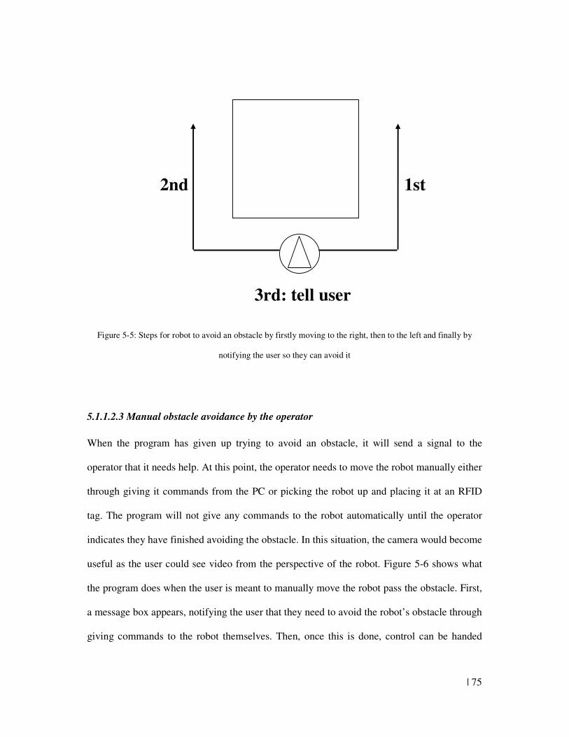
| 75

Figure 5-5: Steps for robot to avoid an obstacle by firstly moving to the right, then to the left and finally by

notifying the user so they can avoid it

5.1.1.2.3 Manual obstacle avoidance by the operator

When the program has given up trying to avoid an obstacle, it will send a signal to the

operator that it needs help. At this point, the operator needs to move the robot manually either

through giving it commands from the PC or picking the robot up and placing it at an RFID

tag. The program will not give any commands to the robot automatically until the operator

indicates they have finished avoiding the obstacle. In this situation, the camera would become

useful as the user could see video from the perspective of the robot. Figure 5-6 shows what

the program does when the user is meant to manually move the robot pass the obstacle. First,

a message box appears, notifying the user that they need to avoid the robot’s obstacle through

giving commands to the robot themselves. Then, once this is done, control can be handed

1st 2nd

3rd: tell user

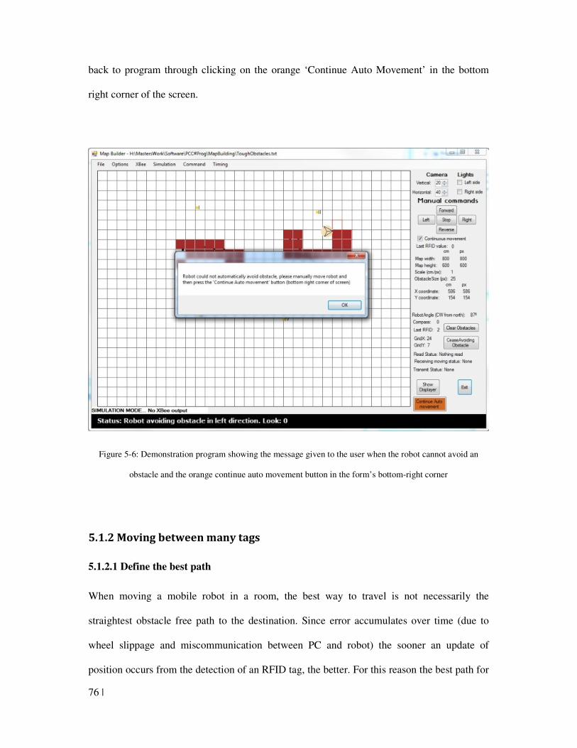
76 |

back to program through clicking on the orange ‘Continue Auto Movement’ in the bottom

right corner of the screen.

Figure 5-6: Demonstration program showing the message given to the user when the robot cannot avoid an

obstacle and the orange continue auto movement button in the form’s bottom-right corner

5.1.2 Moving between many tags

5.1.2.1 Define the best path

When moving a mobile robot in a room, the best way to travel is not necessarily the

straightest obstacle free path to the destination. Since error accumulates over time (due to

wheel slippage and miscommunication between PC and robot) the sooner an update of

position occurs from the detection of an RFID tag, the better. For this reason the best path for

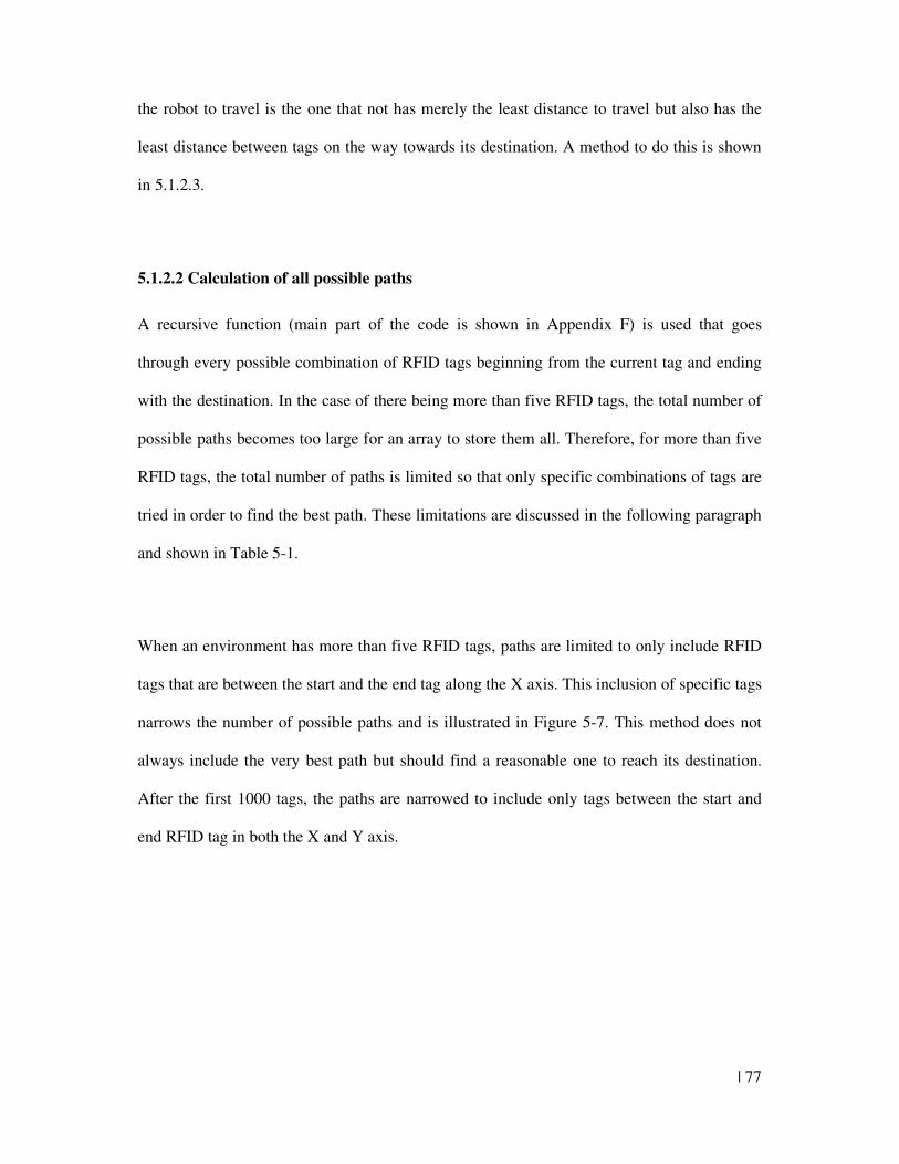
| 77

the robot to travel is the one that not has merely the least distance to travel but also has the

least distance between tags on the way towards its destination. A method to do this is shown

in 5.1.2.3.

5.1.2.2 Calculation of all possible paths

A recursive function (main part of the code is shown in Appendix F) is used that goes

through every possible combination of RFID tags beginning from the current tag and ending

with the destination. In the case of there being more than five RFID tags, the total number of

possible paths becomes too large for an array to store them all. Therefore, for more than five

RFID tags, the total number of paths is limited so that only specific combinations of tags are

tried in order to find the best path. These limitations are discussed in the following paragraph

and shown in Table 5-1.

When an environment has more than five RFID tags, paths are limited to only include RFID

tags that are between the start and the end tag along the X axis. This inclusion of specific tags

narrows the number of possible paths and is illustrated in Figure 5-7. This method does not

always include the very best path but should find a reasonable one to reach its destination.

After the first 1000 tags, the paths are narrowed to include only tags between the start and

end RFID tag in both the X and Y axis.

78 |

Figure 5-7: Showing the space between the start and end RFID tag in the X coordinates (green rectangle) and

with the space between them limited by both the X and Y coordinates (blue rectangle)

Table 5-2: Showing the tags included in the possible paths from the start RFID tag to the last one

Condition Tags to include in possible paths

5 or less tags in the map All tags in the map

More than 5 tags in the map, 1st 1000 paths All tags between start and end in the x axis More than 5 tags in the map, after the 1st 1000 paths

All tags between start and end in the x and y axis

5.1.2.3 Least distance between tags

The ‘Least distance between tags’ algorithm goes through all the paths and finds the 1st, 2nd,

and 3rd maximum distance between any two tags in each path. The purpose of finding the

maximum distance is to find the path with the smallest maximum distances between any two

tags. Since the robot has its position localised whenever a RFID tag is met, the path should

make use of as many RFID tags as possible on the way to its destination to minimize the

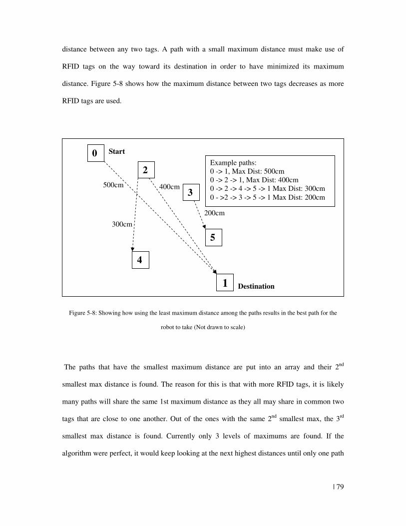
| 79

distance between any two tags. A path with a small maximum distance must make use of

RFID tags on the way toward its destination in order to have minimized its maximum

distance. Figure 5-8 shows how the maximum distance between two tags decreases as more

RFID tags are used.

Figure 5-8: Showing how using the least maximum distance among the paths results in the best path for the

robot to take (Not drawn to scale)

The paths that have the smallest maximum distance are put into an array and their 2nd

smallest max distance is found. The reason for this is that with more RFID tags, it is likely

many paths will share the same 1st maximum distance as they all may share in common two

tags that are close to one another. Out of the ones with the same 2nd smallest max, the 3rd

smallest max distance is found. Currently only 3 levels of maximums are found. If the

algorithm were perfect, it would keep looking at the next highest distances until only one path

0

1

Start

Destination

2

4

5

3

Example paths: 0 -> 1, Max Dist: 500cm 0 -> 2 -> 1, Max Dist: 400cm 0 -> 2 -> 4 -> 5 -> 1 Max Dist: 300cm 0 - >2 -> 3 -> 5 -> 1 Max Dist: 200cm

500cm

200cm

300cm

400cm

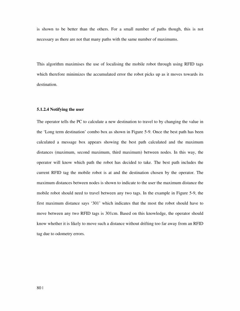
80 |

is shown to be better than the others. For a small number of paths though, this is not

necessary as there are not that many paths with the same number of maximums.

This algorithm maximises the use of localising the mobile robot through using RFID tags

which therefore minimizes the accumulated error the robot picks up as it moves towards its

destination.

5.1.2.4 Notifying the user

The operator tells the PC to calculate a new destination to travel to by changing the value in

the ‘Long term destination’ combo box as shown in Figure 5-9. Once the best path has been

calculated a message box appears showing the best path calculated and the maximum

distances (maximum, second maximum, third maximum) between nodes. In this way, the

operator will know which path the robot has decided to take. The best path includes the

current RFID tag the mobile robot is at and the destination chosen by the operator. The

maximum distances between nodes is shown to indicate to the user the maximum distance the

mobile robot should need to travel between any two tags. In the example in Figure 5-9, the

first maximum distance says ‘301’ which indicates that the most the robot should have to

move between any two RFID tags is 301cm. Based on this knowledge, the operator should

know whether it is likely to move such a distance without drifting too far away from an RFID

tag due to odometry errors.

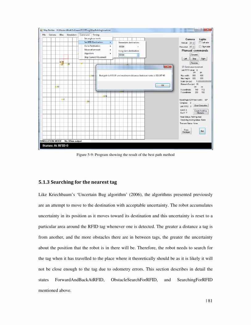
| 81

Figure 5-9: Program showing the result of the best path method

5.1.3 Searching for the nearest tag

Like Kriechbaum’s ‘Uncertain Bug algorithm’ (2006), the algorithms presented previously

are an attempt to move to the destination with acceptable uncertainty. The robot accumulates

uncertainty in its position as it moves toward its destination and this uncertainty is reset to a

particular area around the RFID tag whenever one is detected. The greater a distance a tag is

from another, and the more obstacles there are in between tags, the greater the uncertainty

about the position that the robot is in there will be. Therefore, the robot needs to search for

the tag when it has travelled to the place where it theoretically should be as it is likely it will

not be close enough to the tag due to odometry errors. This section describes in detail the

states ForwardAndBackAtRFID, ObstacleSearchForRFID, and SearchingForRFID

mentioned above.

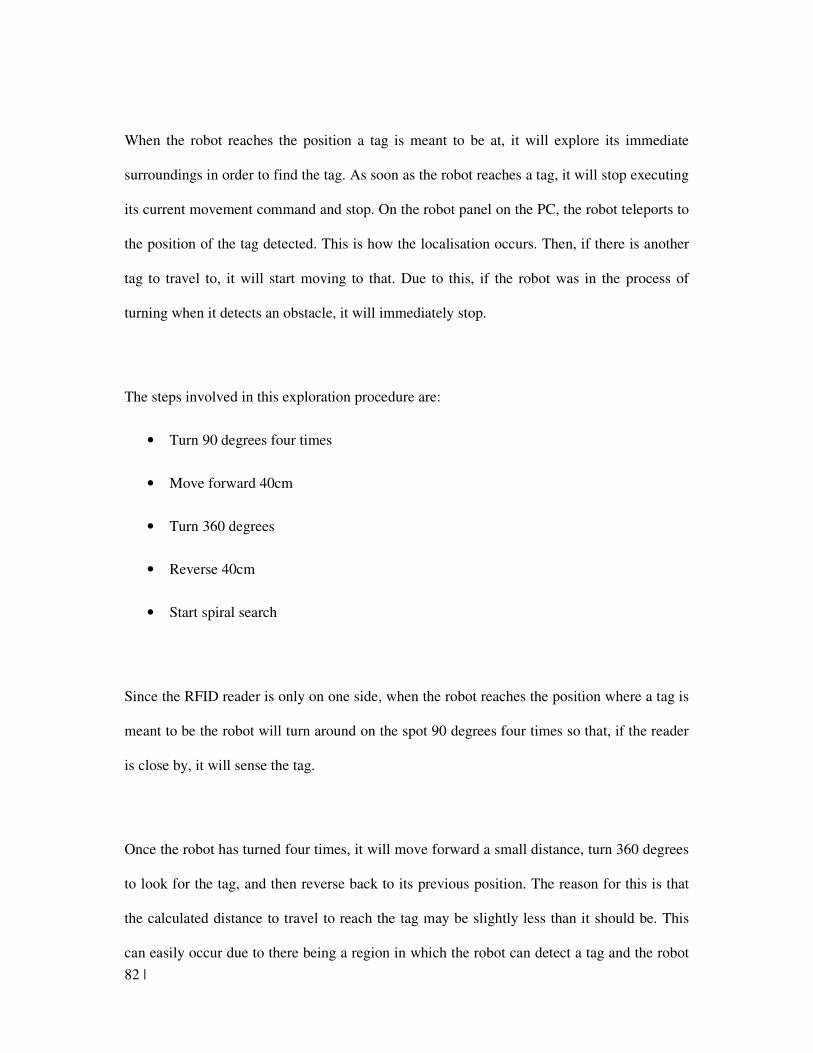
82 |

When the robot reaches the position a tag is meant to be at, it will explore its immediate

surroundings in order to find the tag. As soon as the robot reaches a tag, it will stop executing

its current movement command and stop. On the robot panel on the PC, the robot teleports to

the position of the tag detected. This is how the localisation occurs. Then, if there is another

tag to travel to, it will start moving to that. Due to this, if the robot was in the process of

turning when it detects an obstacle, it will immediately stop.

The steps involved in this exploration procedure are:

• Turn 90 degrees four times

• Move forward 40cm

• Turn 360 degrees

• Reverse 40cm

• Start spiral search

Since the RFID reader is only on one side, when the robot reaches the position where a tag is

meant to be the robot will turn around on the spot 90 degrees four times so that, if the reader

is close by, it will sense the tag.

Once the robot has turned four times, it will move forward a small distance, turn 360 degrees

to look for the tag, and then reverse back to its previous position. The reason for this is that

the calculated distance to travel to reach the tag may be slightly less than it should be. This

can easily occur due to there being a region in which the robot can detect a tag and the robot

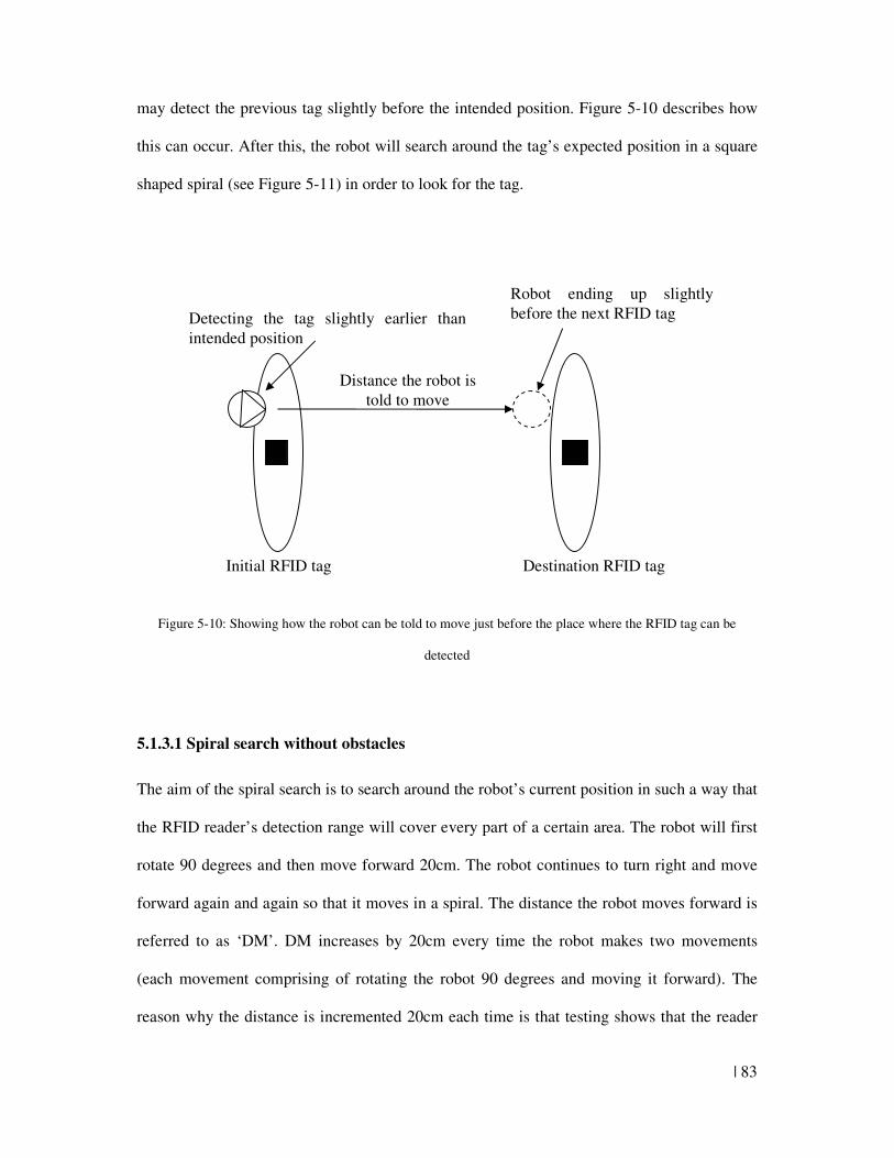
| 83

may detect the previous tag slightly before the intended position. Figure 5-10 describes how

this can occur. After this, the robot will search around the tag’s expected position in a square

shaped spiral (see Figure 5-11) in order to look for the tag.

Figure 5-10: Showing how the robot can be told to move just before the place where the RFID tag can be

detected

5.1.3.1 Spiral search without obstacles

The aim of the spiral search is to search around the robot’s current position in such a way that

the RFID reader’s detection range will cover every part of a certain area. The robot will first

rotate 90 degrees and then move forward 20cm. The robot continues to turn right and move

forward again and again so that it moves in a spiral. The distance the robot moves forward is

referred to as ‘DM’. DM increases by 20cm every time the robot makes two movements

(each movement comprising of rotating the robot 90 degrees and moving it forward). The

reason why the distance is incremented 20cm each time is that testing shows that the reader

Initial RFID tag

Detecting the tag slightly earlier than

intended position

Destination RFID tag

Distance the robot is

told to move

Robot ending up slightly

before the next RFID tag

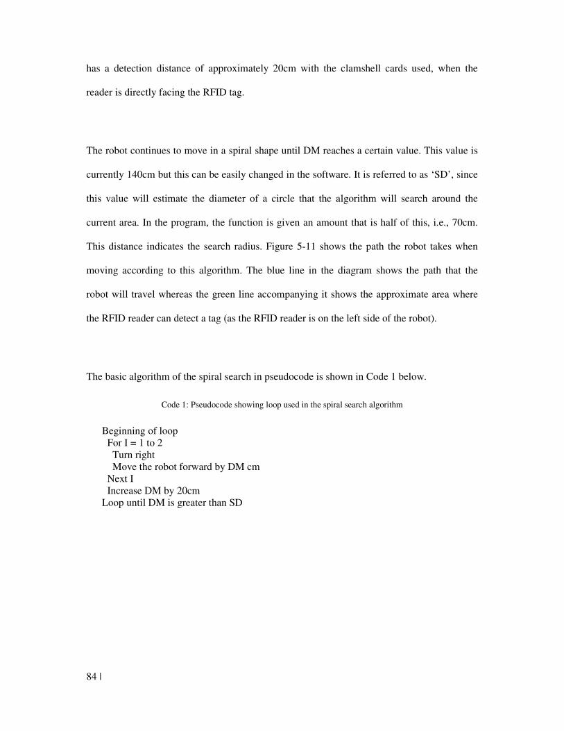
84 |

has a detection distance of approximately 20cm with the clamshell cards used, when the

reader is directly facing the RFID tag.

The robot continues to move in a spiral shape until DM reaches a certain value. This value is

currently 140cm but this can be easily changed in the software. It is referred to as ‘SD’, since

this value will estimate the diameter of a circle that the algorithm will search around the

current area. In the program, the function is given an amount that is half of this, i.e., 70cm.

This distance indicates the search radius. Figure 5-11 shows the path the robot takes when

moving according to this algorithm. The blue line in the diagram shows the path that the

robot will travel whereas the green line accompanying it shows the approximate area where

the RFID reader can detect a tag (as the RFID reader is on the left side of the robot).

The basic algorithm of the spiral search in pseudocode is shown in Code 1 below.

Code 1: Pseudocode showing loop used in the spiral search algorithm

Beginning of loop For I = 1 to 2 Turn right Move the robot forward by DM cm Next I Increase DM by 20cm Loop until DM is greater than SD

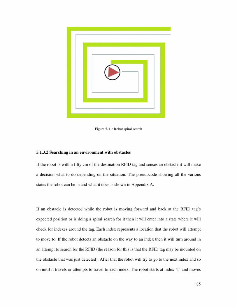
| 85

Figure 5-11: Robot spiral search

5.1.3.2 Searching in an environment with obstacles

If the robot is within fifty cm of the destination RFID tag and senses an obstacle it will make

a decision what to do depending on the situation. The pseudocode showing all the various

states the robot can be in and what it does is shown in Appendix A.

If an obstacle is detected while the robot is moving forward and back at the RFID tag’s

expected position or is doing a spiral search for it then it will enter into a state where it will

check for indexes around the tag. Each index represents a location that the robot will attempt

to move to. If the robot detects an obstacle on the way to an index then it will turn around in

an attempt to search for the RFID (the reason for this is that the RFID tag may be mounted on

the obstacle that was just detected). After that the robot will try to go to the next index and so

on until it travels or attempts to travel to each index. The robot starts at index ‘1’ and moves

86 |

in ascending order until it reaches index 8. The index locations are shown in Figure 5-12. The

figure shows the expected tag’s position in the middle and the locations of the indexes the

robot attempts to move to. The arrows show the position the robot will intend to move at each

position.

Figure 5-12: Index locations for robot to search

The indexes are initially twenty cm away from the tag. After searching through the eight

index locations, the index location is increased by twenty cm further from the expected tag’s

position (as detection distance is 20cm) and the robot moves around the index locations

again, starting from index 1. The robot does this until it has moved the search radius, the

same distance as the spiral algorithm would move to.

An array in the program stores the details about the index positions. This includes their

coordinates and status. The status indicates whether the index has been travelled to or not or

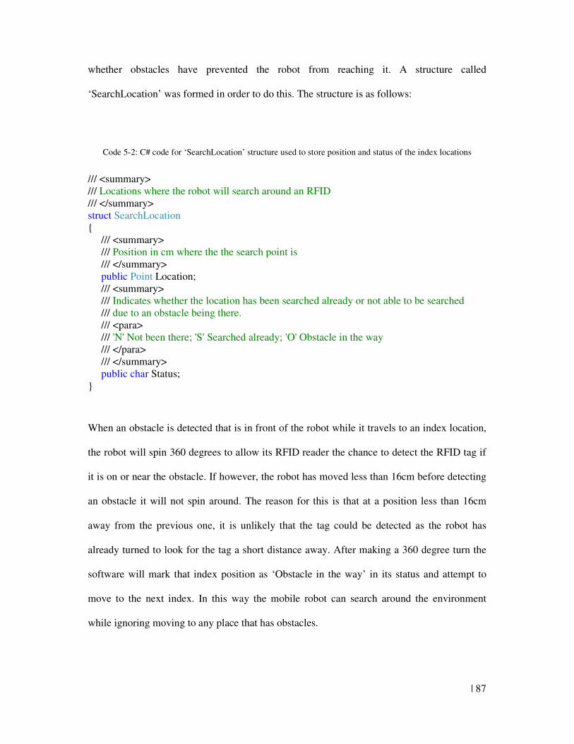
| 87

whether obstacles have prevented the robot from reaching it. A structure called

‘SearchLocation’ was formed in order to do this. The structure is as follows:

Code 5-2: C# code for ‘SearchLocation’ structure used to store position and status of the index locations

/// <summary> /// Locations where the robot will search around an RFID /// </summary> struct SearchLocation { /// <summary> /// Position in cm where the the search point is /// </summary> public Point Location; /// <summary> /// Indicates whether the location has been searched already or not able to be searched /// due to an obstacle being there. /// <para> /// 'N' Not been there; 'S' Searched already; 'O' Obstacle in the way /// </para> /// </summary> public char Status; }

When an obstacle is detected that is in front of the robot while it travels to an index location,

the robot will spin 360 degrees to allow its RFID reader the chance to detect the RFID tag if

it is on or near the obstacle. If however, the robot has moved less than 16cm before detecting

an obstacle it will not spin around. The reason for this is that at a position less than 16cm

away from the previous one, it is unlikely that the tag could be detected as the robot has

already turned to look for the tag a short distance away. After making a 360 degree turn the

software will mark that index position as ‘Obstacle in the way’ in its status and attempt to

move to the next index. In this way the mobile robot can search around the environment

while ignoring moving to any place that has obstacles.

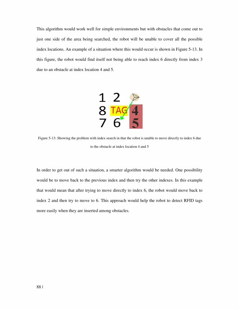
88 |

This algorithm would work well for simple environments but with obstacles that come out to

just one side of the area being searched, the robot will be unable to cover all the possible

index locations. An example of a situation where this would occur is shown in Figure 5-13. In

this figure, the robot would find itself not being able to reach index 6 directly from index 3

due to an obstacle at index location 4 and 5.

Figure 5-13: Showing the problem with index search in that the robot is unable to move directly to index 6 due

to the obstacle at index location 4 and 5

In order to get out of such a situation, a smarter algorithm would be needed. One possibility

would be to move back to the previous index and then try the other indexes. In this example

that would mean that after trying to move directly to index 6, the robot would move back to

index 2 and then try to move to 6. This approach would help the robot to detect RFID tags

more easily when they are inserted among obstacles.

| 89

5.2 Mobile robot navigation simulation

This section discusses the program used to model the mobile robot and its environment. This

simulation program has been used to test and evaluate the various navigation algorithms

made in the previous section, prior to testing them using the actual mobile robot itself, which

is much harder.

Collet, MacDonald, & Gerkey (2005) discuss the development of free robot control and

simulation software. They mention that “The availability of flexible, reliable, and reusable

tools for robot programming is crucial to the research community.” (Collet, et al., 2005, p. 1)

For this specific application, it was easier to construct an independent program since

algorithms specific to moving a mobile robot among RFID tags are required and the control

of the robot is linked to the simulation of its movement. Although this simulation software

was not built using reusable robot tools and does not provide tools that could be used

generically in a library in many kinds of environments, it is hoped that it could provide help

to others working in the same endeavour of simulating a mobile robot using a PC.

5.2.1 Simulation of the robot’s environment

Information about the indoor environment in which the mobile robot moves was displayed to

the operator by a panel on the program’s form. Figure 5-14 shows this panel. The panel is

divided up by many squares that divide the map up so that it is easier to see relatively how far

apart things are from one another. A red border around a square indicates that it is where the

robot is currently searching for obstacles to avoid. Two of these red borders can be see at the

90 |

squares directly in front of the mobile robot in Figure 5-13. The details of how these squares

are searched to find obstacles and how these obstacles are stored are explained in section

5.1.1.2.

When the robot detects an obstacle from its sensors it places a 1px point in the panel to

represent its position. The colour of the point determines how likely it is that it represents an

obstacle that needs avoiding. A list of colours relating to the number of points is shown in

Appendix G. If many points are detected within a 25cm wide grid square, a square will be

shown on the panel proportional to its size. Appendix G mentions the details of when these

are shown. Figure 5-13 shows such squares representing obstacles in the robot’s environment.

These obstacles were set in the map by the manual map builder program explained in section

5.3.

An array is used to store the RFID tags used in the map. They are displayed on the panel as

yellow squares with a Roman numeral beside them. These Roman numerals are not the

complex unique RFIDs of the tags (which are 10 ASCII characters long) but are used simply

for the operator to easily distinguish between tags. The operator uses these numbers when

telling the robot where to move within the environment.

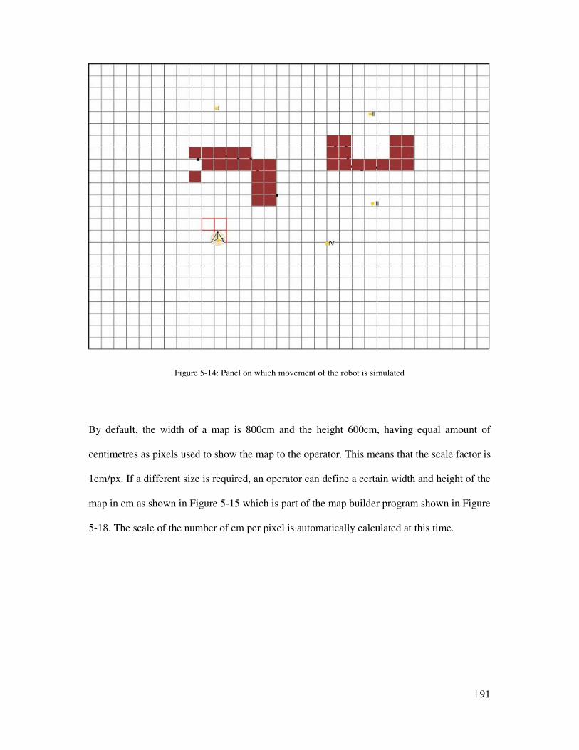
| 91

Figure 5-14: Panel on which movement of the robot is simulated

By default, the width of a map is 800cm and the height 600cm, having equal amount of

centimetres as pixels used to show the map to the operator. This means that the scale factor is

1cm/px. If a different size is required, an operator can define a certain width and height of the

map in cm as shown in Figure 5-15 which is part of the map builder program shown in Figure

5-18. The scale of the number of cm per pixel is automatically calculated at this time.

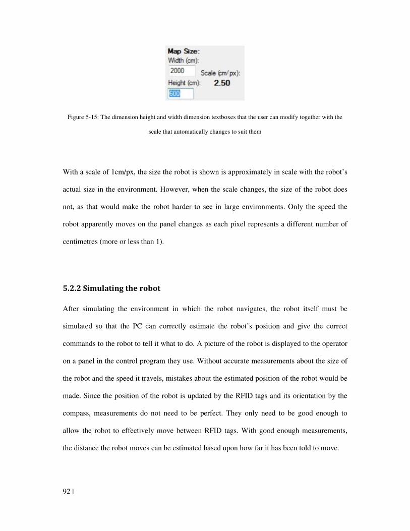
92 |

Figure 5-15: The dimension height and width dimension textboxes that the user can modify together with the

scale that automatically changes to suit them

With a scale of 1cm/px, the size the robot is shown is approximately in scale with the robot’s

actual size in the environment. However, when the scale changes, the size of the robot does

not, as that would make the robot harder to see in large environments. Only the speed the

robot apparently moves on the panel changes as each pixel represents a different number of

centimetres (more or less than 1).

5.2.2 Simulating the robot

After simulating the environment in which the robot navigates, the robot itself must be

simulated so that the PC can correctly estimate the robot’s position and give the correct

commands to the robot to tell it what to do. A picture of the robot is displayed to the operator

on a panel in the control program they use. Without accurate measurements about the size of

the robot and the speed it travels, mistakes about the estimated position of the robot would be

made. Since the position of the robot is updated by the RFID tags and its orientation by the

compass, measurements do not need to be perfect. They only need to be good enough to

allow the robot to effectively move between RFID tags. With good enough measurements,

the distance the robot moves can be estimated based upon how far it has been told to move.

| 93

To estimate this distance the speed of the robot was measured. The speed of the robot moving

in the PC and shown to the operator had to approximate the speed of the mobile robot in the

real world. This is hard to do perfectly due to the time the robot takes to accelerate being hard

to estimate and there being small delays in communication between the robot and the PC.

Therefore, although the user can tell the robot to move continuously without any limit of how

much to move, it is preferred to tell the robot a set distance to move and then wait for it to do

so before giving another command. Therefore, when a command is given to move the robot

to a RFID tag, the commands to the robot are always to move a set distance and then have it

wait for the next command. Also, the program that commands the robot waits for

approximately one second after its simulation has completed a movement command to ensure

that the mobile robot has definitely moved the distance it has been told to before giving it

another command.

For example, suppose the robot needs to turn 90 degrees and then move forward 20cm. The

PC would first tell the robot to move 90 degrees. Then it would simulate it moving 90

degrees by its estimation of the robot’s speed. After the simulation has completed the turn, it

will wait for about 1 second and then tell the robot to move 20cm. After the robot’s

simulation on the PC has moved 20cm, it will again wait a second before giving any further

commands.

In order for the robot to effectively plot where the obstacles that the distances sensors pick up

are the program needs to know:

• The size of the robot

• The position of its sensors

94 |

• The actual distance an object is from the detecting sensors

The robot can be approximated by a circle that has a diameter of 30cm. Six infrared distance

sensors are placed at different angles around the robot and a sonar distance sensor is placed at

its front. The dimensions and angles used to model the robot in the program are shown in

Figure 5-16. The red circles represent the approximate location of the infrared distance

sensors on the robot, the angle is the orientation when moving clockwise from the front of the

robot, and the green circle represents the location of the robot’s sonar sensor.

The location of an obstacle detected by a distance sensor can be plotted by taking into

account the sensors’ position and orientation. The distance for the infrared distance and sonar

sensor from the centre of the robot is approximately 14cm and 19cm respectively. This

distance is added to the distance determined by the sensor itself to determine how far an

obstacle is from the robot’s centre. Then by using the orientation where the sensor is placed,

the coordinate of the obstacle can be recorded in the obstacle map based on the robot’s

coordinate. This calculation stores the location of the obstacle in an array that records the

number of times each square centimetre in the environment has been detected. The way this

data is used has been explained in section 5.2.1.

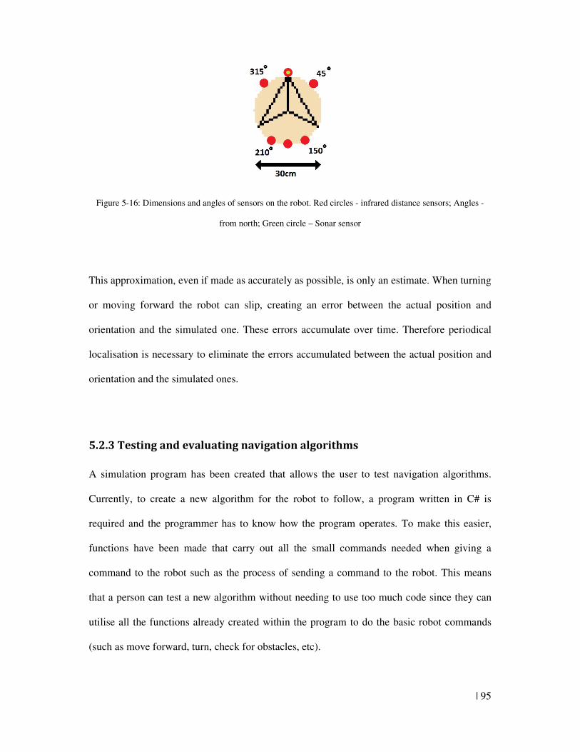
| 95

Figure 5-16: Dimensions and angles of sensors on the robot. Red circles - infrared distance sensors; Angles -

from north; Green circle – Sonar sensor

This approximation, even if made as accurately as possible, is only an estimate. When turning

or moving forward the robot can slip, creating an error between the actual position and

orientation and the simulated one. These errors accumulate over time. Therefore periodical

localisation is necessary to eliminate the errors accumulated between the actual position and

orientation and the simulated ones.

5.2.3 Testing and evaluating navigation algorithms

A simulation program has been created that allows the user to test navigation algorithms.

Currently, to create a new algorithm for the robot to follow, a program written in C# is

required and the programmer has to know how the program operates. To make this easier,

functions have been made that carry out all the small commands needed when giving a

command to the robot such as the process of sending a command to the robot. This means

that a person can test a new algorithm without needing to use too much code since they can

utilise all the functions already created within the program to do the basic robot commands

(such as move forward, turn, check for obstacles, etc).

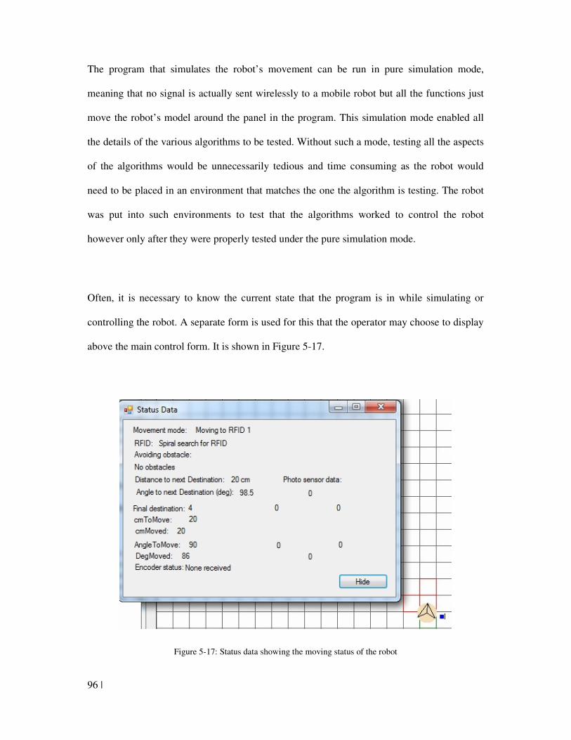
96 |

The program that simulates the robot’s movement can be run in pure simulation mode,

meaning that no signal is actually sent wirelessly to a mobile robot but all the functions just

move the robot’s model around the panel in the program. This simulation mode enabled all

the details of the various algorithms to be tested. Without such a mode, testing all the aspects

of the algorithms would be unnecessarily tedious and time consuming as the robot would

need to be placed in an environment that matches the one the algorithm is testing. The robot

was put into such environments to test that the algorithms worked to control the robot

however only after they were properly tested under the pure simulation mode.

Often, it is necessary to know the current state that the program is in while simulating or

controlling the robot. A separate form is used for this that the operator may choose to display

above the main control form. It is shown in Figure 5-17.

Figure 5-17: Status data showing the moving status of the robot

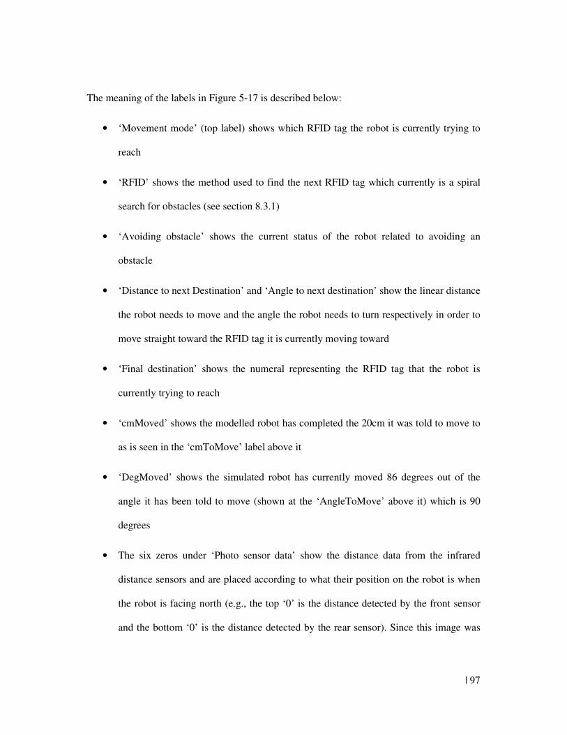
| 97

The meaning of the labels in Figure 5-17 is described below:

• ‘Movement mode’ (top label) shows which RFID tag the robot is currently trying to

reach

• ‘RFID’ shows the method used to find the next RFID tag which currently is a spiral

search for obstacles (see section 8.3.1)

• ‘Avoiding obstacle’ shows the current status of the robot related to avoiding an

obstacle

• ‘Distance to next Destination’ and ‘Angle to next destination’ show the linear distance

the robot needs to move and the angle the robot needs to turn respectively in order to

move straight toward the RFID tag it is currently moving toward

• ‘Final destination’ shows the numeral representing the RFID tag that the robot is

currently trying to reach

• ‘cmMoved’ shows the modelled robot has completed the 20cm it was told to move to

as is seen in the ‘cmToMove’ label above it

• ‘DegMoved’ shows the simulated robot has currently moved 86 degrees out of the

angle it has been told to move (shown at the ‘AngleToMove’ above it) which is 90

degrees

• The six zeros under ‘Photo sensor data’ show the distance data from the infrared

distance sensors and are placed according to what their position on the robot is when

the robot is facing north (e.g., the top ‘0’ is the distance detected by the front sensor

and the bottom ‘0’ is the distance detected by the rear sensor). Since this image was

98 |

taken while the robot is in simulation mode, there are no readings from the distance

sensors and so they all say a distance of ‘0’cm

• ‘Encoder status’ refers to the state the robot should be in as determined by the

encoders on the robot’s wheels. Since the robot is in simulation mode, nothing is

received

By using this data, the operator can understand what stage of movement the robot is in and

therefore determine whether the algorithm created is working as it is intended to.

In summary, a program useful for simulating and controlling a mobile robot has been

developed. This uses a model of the robot itself and its environment and simulates its

movement so that the operator can see an estimated position of the robot on the screen all the

time. The program has been useful for testing all the algorithms the mobile robot uses and

gives clear indication of the state the robot is in as it carries out its commands.

5.3 Environment map building

In this section, the way to build a map of the environment is discussed. A map is simply an

array containing the position of the RFID tags used and obstacles that need avoiding. Two

ways to construct such a map have been developed and are presented in this section. The first

is to build a map by manually entering the coordinates of RFID tags and obstacles by either

clicking on where the relative position is on the map or typing in their co-ordinates in a

textbox. The second way is through the teaching mode, that is by guiding the robot step by

step around the RFID tags while the simulation updates its position as the robot moves and

the software automatically places the coordinates of RFID tags as they are detected.

| 99

The coordinates of the RFID tags do not represent the physical location of the RFID tag, but

rather the optimal position where the robot should move so that it can detect it (as the tags are

placed on objects that are obstacles to the robot). The map is displayed on a panel that is

600px high and 800px wide. The default is to have a scale of 1cm to 1px but this is easily

changed through changing the number of cm for the map’s width and height in the program

made as explained in section 5.2.1.

It is expected that an environment will have the robot start at an RFID tag and from there

move to other tags as RFID tags are this research’s unique method of knowing a certain

location in the map. Therefore, a specific variable called ‘StartPosIndex’ is used to store the

starting RFID tag. However, if the starting position is somewhere other than an RFID tag, the

operator can still manually define a coordinate in the map for the robot to start at and leave

the ‘StartPosIndex’ as ‘-1’ which indicates to the program that the robot is not starting at a

tag. Once a map has been completely configured, it is saved in a text file. Appendix D shows

an example of a map created by the map building software.

5.3.1 Manual map building

A room with RFID tags can be measured manually using a ruler and then built using a

program made in this research called ‘MapBuilder’. This program allows the coordinates of

the environment’s obstacles, the robot’s starting location and of the RFID tags to be entered

(either in cm or px) and then saved into a map that can be later read by a program that

monitors and controls the mobile robot.

100 |

There are two methods for placing objects on the map, a quick method or an accurate one.

The quick and estimated method of placing objects at a position in the environment is done

through hovering the mouse over the map panel and observing its position (cm and px)

shown on the left of it (Figure 5-18, under ‘Mouse Position’). For example, in Figure 5-18,

the cross hairs represent the mouse’s current position and the figure’s left side says its

coordinates are 163 cm in x and 237 cm in y. By clicking on the panel, an object can be

placed there. This is useful for when the exact measurements of an object is unknown. This

method allows an object to be visually placed depending on where it should be in relation to

other objects.

The accurate method of placing an object can be done by manually changing the values of the

set position variable in either pixel or cm textbox under the ‘Set Position’ section of the form

and then clicking on the ‘Place Item’ button. This allows a quick way of entering the position

of objects whose coordinates are known.

Figure 5-18 shows the coordinates with the top-left corner of the panel as the reference point.

This default reference point is easily changed, through an option in the software, to any of the

four corners of the panel to suit the operator’s method of referencing coordinates in a map.

In order for the user to have a visual idea of how big the robot is in relation to the rest of the

map, a circle at the bottom left corner of the form is used to show how big the robot would

actually be on the panel. This size changes when the scale is changed by the operator

specifying a map with different dimensions than the default ones. If the picture of the robot

itself that moved on the map actually got smaller as the map got bigger, it would make it

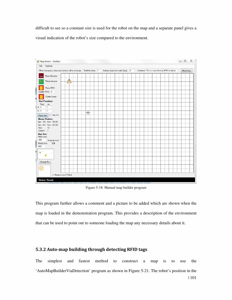
| 101

difficult to see so a constant size is used for the robot on the map and a separate panel gives a

visual indication of the robot’s size compared to the environment.

Figure 5-18: Manual map builder program

This program further allows a comment and a picture to be added which are shown when the

map is loaded in the demonstration program. This provides a description of the environment

that can be used to point out to someone loading the map any necessary details about it.

5.3.2 Auto-map building through detecting RFID tags

The simplest and fastest method to construct a map is to use the

‘AutoMapBuilderViaDetection’ program as shown in Figure 5-21. The robot’s position in the

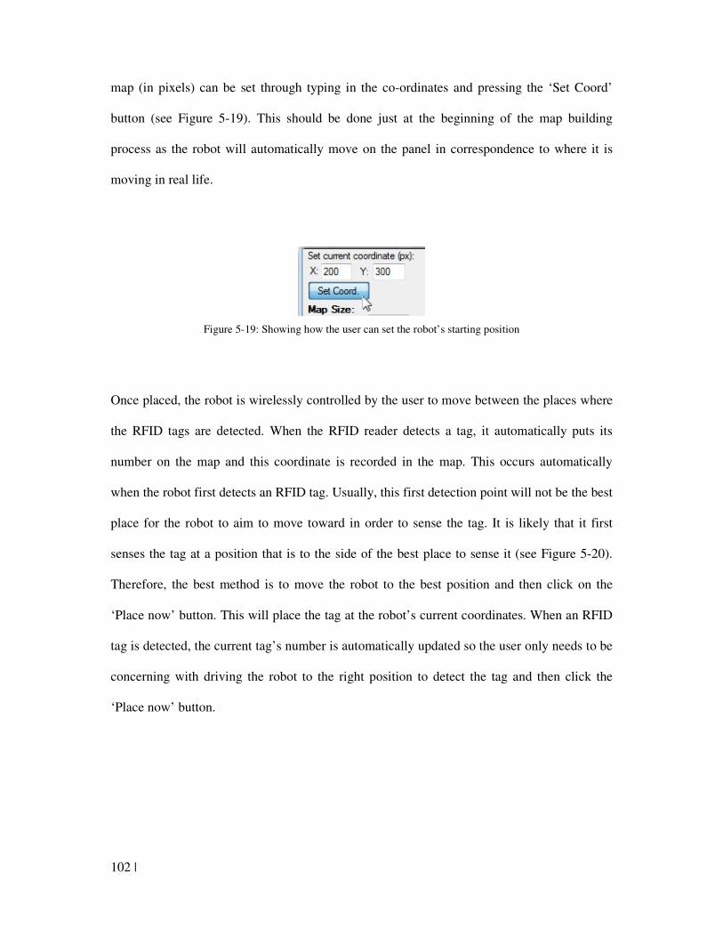
102 |

map (in pixels) can be set through typing in the co-ordinates and pressing the ‘Set Coord’

button (see Figure 5-19). This should be done just at the beginning of the map building

process as the robot will automatically move on the panel in correspondence to where it is

moving in real life.

Figure 5-19: Showing how the user can set the robot’s starting position

Once placed, the robot is wirelessly controlled by the user to move between the places where

the RFID tags are detected. When the RFID reader detects a tag, it automatically puts its

number on the map and this coordinate is recorded in the map. This occurs automatically

when the robot first detects an RFID tag. Usually, this first detection point will not be the best

place for the robot to aim to move toward in order to sense the tag. It is likely that it first

senses the tag at a position that is to the side of the best place to sense it (see Figure 5-20).

Therefore, the best method is to move the robot to the best position and then click on the

‘Place now’ button. This will place the tag at the robot’s current coordinates. When an RFID

tag is detected, the current tag’s number is automatically updated so the user only needs to be

concerning with driving the robot to the right position to detect the tag and then click the

‘Place now’ button.

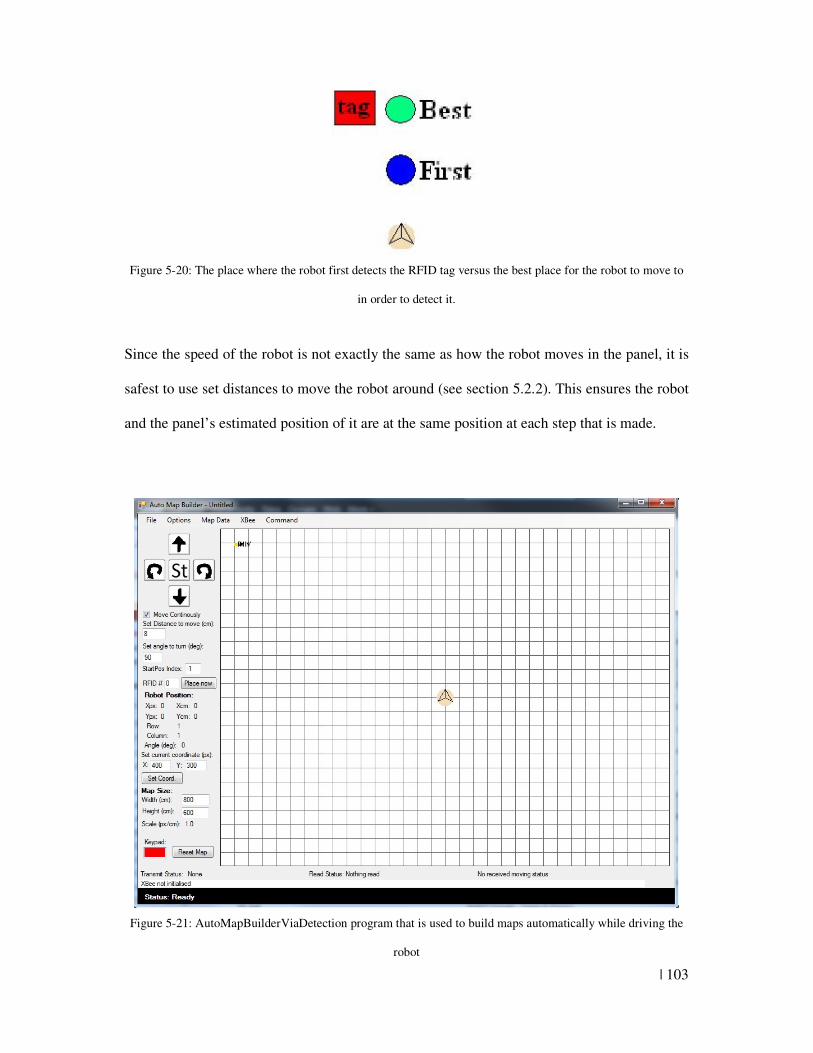
| 103

Figure 5-20: The place where the robot first detects the RFID tag versus the best place for the robot to move to

in order to detect it.

Since the speed of the robot is not exactly the same as how the robot moves in the panel, it is

safest to use set distances to move the robot around (see section 5.2.2). This ensures the robot

and the panel’s estimated position of it are at the same position at each step that is made.

Figure 5-21: AutoMapBuilderViaDetection program that is used to build maps automatically while driving the

robot

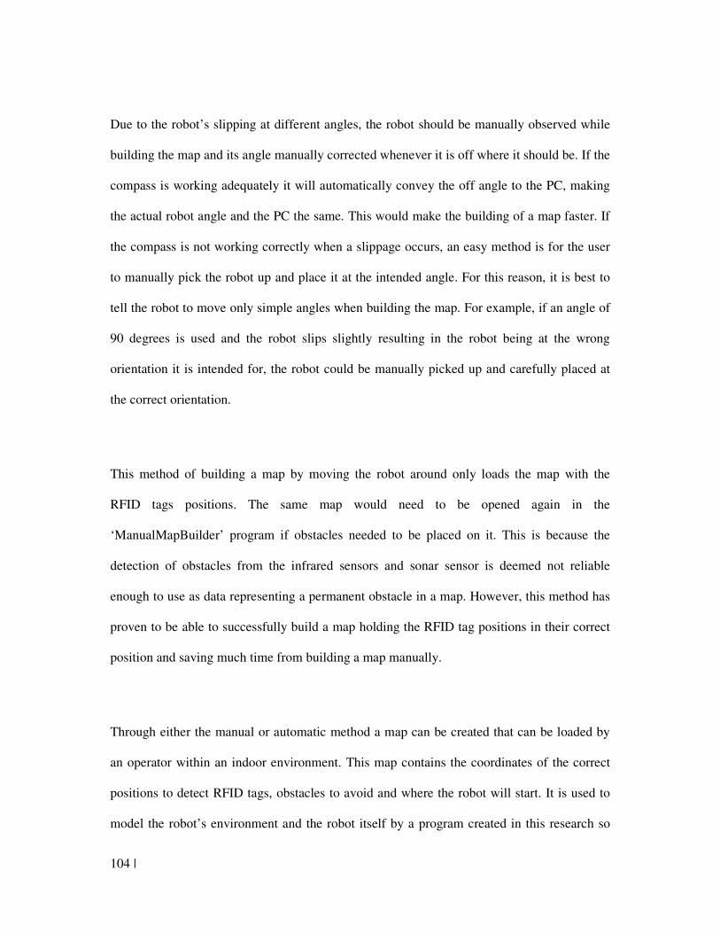
104 |

Due to the robot’s slipping at different angles, the robot should be manually observed while

building the map and its angle manually corrected whenever it is off where it should be. If the

compass is working adequately it will automatically convey the off angle to the PC, making

the actual robot angle and the PC the same. This would make the building of a map faster. If

the compass is not working correctly when a slippage occurs, an easy method is for the user

to manually pick the robot up and place it at the intended angle. For this reason, it is best to

tell the robot to move only simple angles when building the map. For example, if an angle of

90 degrees is used and the robot slips slightly resulting in the robot being at the wrong

orientation it is intended for, the robot could be manually picked up and carefully placed at

the correct orientation.

This method of building a map by moving the robot around only loads the map with the

RFID tags positions. The same map would need to be opened again in the

‘ManualMapBuilder’ program if obstacles needed to be placed on it. This is because the

detection of obstacles from the infrared sensors and sonar sensor is deemed not reliable

enough to use as data representing a permanent obstacle in a map. However, this method has

proven to be able to successfully build a map holding the RFID tag positions in their correct

position and saving much time from building a map manually.

Through either the manual or automatic method a map can be created that can be loaded by

an operator within an indoor environment. This map contains the coordinates of the correct

positions to detect RFID tags, obstacles to avoid and where the robot will start. It is used to

model the robot’s environment and the robot itself by a program created in this research so

| 105

that the robot can navigate within an indoor environment. This navigation is accomplished

through the use of specific algorithms that cater for various situations the robot may

encounter.

106 |

Chapter 6: Testing localisation methodology

This chapter describes the kind of environment in which this methodology is tested and the

constraints for the robot in planning a path between two RFID tags and in avoiding obstacles

in between them. It further lays out some of the mechanical designs that can be used for

mobile robots and describes the basic structure of the mobile robot used in this research. With

this as a base, the motors and sensors used as well as the motor selection, control, powering

and testing are then considered and three tests made on the robot are shown by discussing

their testing environment and demonstrating their outcome.

6.1 Indoor mobile service robot design considerations

This section presents the specific requirements and constraints this research takes into

account for an indoor mobile robot. First, the robot’s environment in which it moves and its

own basic functions are discussed. Then, the constraints defining the particular robot used in

this research are explained, followed by the requirements and characteristics for planning a

path between two locations. Finally, the constraints of obstacle avoidance are discussed and

the purpose of a robot with such constraints is explained.

6.1.1 Constraints of the Robot’s environment

In mobile robot design, the environment that the mobile robot is required to effectively

navigate in has to be first considered. The mobile robot must be in continual communication

with the PC since the PC collects all the data, makes the decisions and guides the robot step

by step as to what to do. Since the robot is being controlled remotely by a PC, the

| 107

environment in which the robot works should be conducive to reliable communication. If the

environment did not allow the robot to be in continual communication with a remote PC, a

different method of mobile robot control would need to be considered.

For this research, a small mobile robot will be designed and built to test the methodologies. In

order to keep the cost low, simple microcontrollers and sensors were used. A simple

inexpensive radio transmitter was used to capture video for the robot. As this transmitter has

a limited communication range, the sustained continuous wireless communication

environment defined for the mobile robot is a round area with a 5-meter radius from the host

PC. As the communication range is fairly small, it is also required that the area be free of any

tall and obtrusive obstacles as these will significantly obstruct the wireless communication

between the controlling PC and the mobile robot.

The floor of the environment should be a flat surface to minimize errors in estimating the

robot’s position using odometry. The obstacles in the environment should be of a reasonable

size and without any thin protruding parts so that they are definitely detected by the robot.

The reason for this is that the robot’s distance sensors that detect obstacles are only placed at

set angles around the robot and do not cover the full span of the area ahead of robot.

6.1.2 Path planning

Path planning means determining the way to travel between two co-ordinates while avoiding

obstacles in between them (Kim, 2004). The current research is constrained in the path

planning algorithms designed. The planning for paths between two points in an environment

should not require detailed data about the obstacles or expect the exact location of the robot

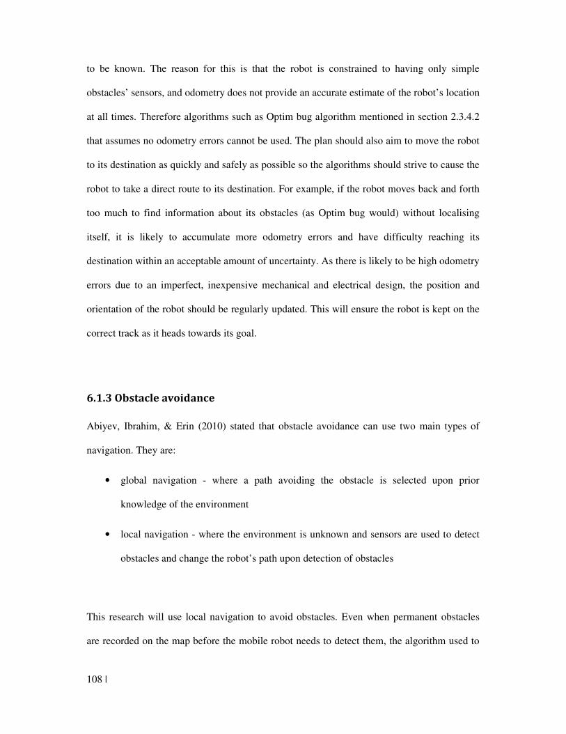
108 |

to be known. The reason for this is that the robot is constrained to having only simple

obstacles’ sensors, and odometry does not provide an accurate estimate of the robot’s location

at all times. Therefore algorithms such as Optim bug algorithm mentioned in section 2.3.4.2

that assumes no odometry errors cannot be used. The plan should also aim to move the robot

to its destination as quickly and safely as possible so the algorithms should strive to cause the

robot to take a direct route to its destination. For example, if the robot moves back and forth

too much to find information about its obstacles (as Optim bug would) without localising

itself, it is likely to accumulate more odometry errors and have difficulty reaching its

destination within an acceptable amount of uncertainty. As there is likely to be high odometry

errors due to an imperfect, inexpensive mechanical and electrical design, the position and

orientation of the robot should be regularly updated. This will ensure the robot is kept on the

correct track as it heads towards its goal.

6.1.3 Obstacle avoidance

Abiyev, Ibrahim, & Erin (2010) stated that obstacle avoidance can use two main types of

navigation. They are:

• global navigation - where a path avoiding the obstacle is selected upon prior

knowledge of the environment

• local navigation - where the environment is unknown and sensors are used to detect

obstacles and change the robot’s path upon detection of obstacles

This research will use local navigation to avoid obstacles. Even when permanent obstacles

are recorded on the map before the mobile robot needs to detect them, the algorithm used to

| 109

move the robot carries out the obstacle avoidance when the robot reaches them instead of

creating a path that will avoid it before reaching them. This is due to the constraint of only

using simple algorithms and also the fact that the system has errors accumulated in its

position estimation so planning a path before reaching an obstacle could incorrectly avoid the

obstacle.

Since this research is merely to test the concept of localising using RFID tags, the memory

size and speed of the microcontrollers does not need to be great, and high accuracy, high

speed sensors such as lasers are unnecessary. For example, the Hokuyo URG-04LX-UG01

from Acroname Robotics (Acroname robotics, 2011) laser costs $1150 US yet can read at a

range of 240 degrees, with 0.36 degree resolution and would provide a lot of data as can be

seen by the red lines on Figure 6-1. However, its cost is too high, and the current

microcontroller used would not be able to process this much data or send it wirelessly to a

computer.

110 |

Figure 6-1: The simulated beam of the Hokuyo URG laser mounted on a robot, (Collet, Macdonald, & Gerkey,

2005, pg. 5)

6.1.4 The usefulness of the designed mobile robot

A robot that is inexpensive, can avoid only simple obstacles, moves in a limited range from

the controller, and uses simple algorithms to get to its destination would not be reliable

enough to be directly useful for industries or households requiring mobile robots in an indoor

environment. However, this research provides a base for further research and development of

more reliable mobile robots that could perform tasks such as making observations (using their

cameras) or transporting goods from one part of a factory to another.

An operator could choose between several mobile robots that could transport goods around a

factory. This would require additional methods of loading inventory from a factory onto the

robot. With improvement made to the reliability of obstacle detection the robot may be able

| 111

to operate in environments with moving obstacles such as an office environment. A doctor in

a hospital could check up on his patients remotely through using such a robot. To do this, the

main thing that would be changed would be the robot’s height so that the robot could show a

doctor’s patients in their bed and the equipment in their room.

112 |

6.2 Mobile robot mechanical system design

This section opens up the various mechanical configurations that can be used to move a robot

around and then talks about the specific mechanical design used in this research.

6.2.1 Mechanical system configurations

There are many configurations for the movement of mobile robots. These include

omniwheels (a group of wheels that co-ordinate to allow movement in any direction without

needing to turn around), two wheeled robots (where balancing would be required to keep the

robot upright), three wheeled robots with either one or two driving wheels, four-wheeled

vehicles, and robots with legs (that can be thinner and that could step up and down steps).

As the number of wheels increases (from two to four), so does the stability (Disabled world,

2009). Three wheeled robots are able to remain upright. They can be designed to be smaller

than a four wheeled robot and can also rotate easily. This makes a three wheeled robot more

flexible to move around than a four wheeled one. An increased mobility means the robot is

more able to avoid obstacles successfully (Shih, Chen, Chou, 2010). Of course, if small

obstacles need to be avoided or a robot needs to travel in spaces with confined space, a

bipedal robot, one with two legs, would be better, as the entire robot itself can be thinner

(Manoonpong, 2009).

The movement of the robot is controlled by motors. In order for the robot to use odometry to

estimate its position, the motor should allow the robot to easily calculate how far the motor

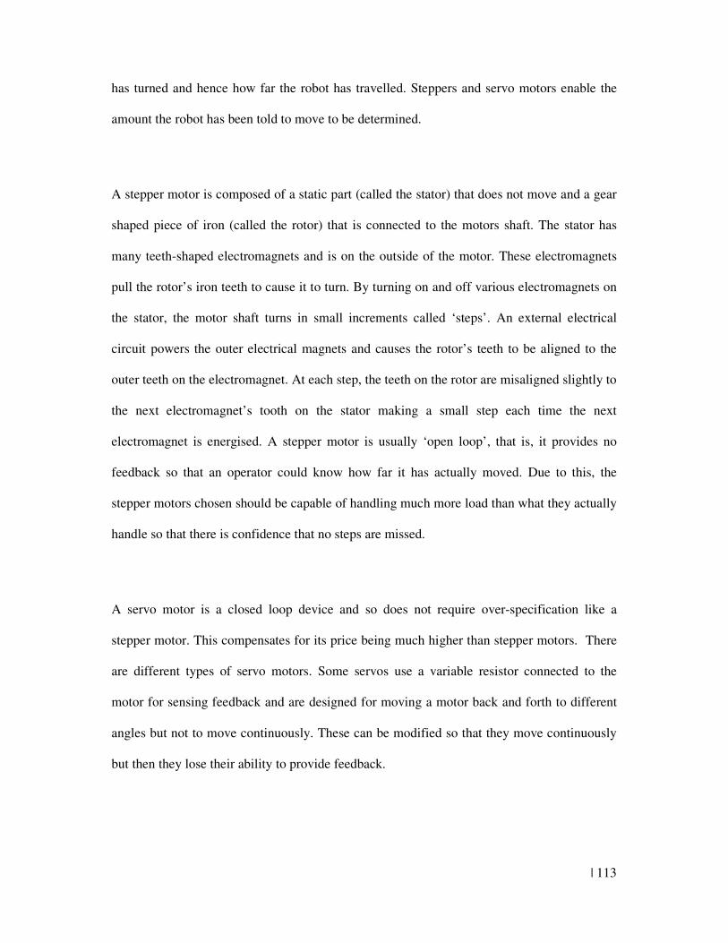
| 113

has turned and hence how far the robot has travelled. Steppers and servo motors enable the

amount the robot has been told to move to be determined.

A stepper motor is composed of a static part (called the stator) that does not move and a gear

shaped piece of iron (called the rotor) that is connected to the motors shaft. The stator has

many teeth-shaped electromagnets and is on the outside of the motor. These electromagnets

pull the rotor’s iron teeth to cause it to turn. By turning on and off various electromagnets on

the stator, the motor shaft turns in small increments called ‘steps’. An external electrical

circuit powers the outer electrical magnets and causes the rotor’s teeth to be aligned to the

outer teeth on the electromagnet. At each step, the teeth on the rotor are misaligned slightly to

the next electromagnet’s tooth on the stator making a small step each time the next

electromagnet is energised. A stepper motor is usually ‘open loop’, that is, it provides no

feedback so that an operator could know how far it has actually moved. Due to this, the

stepper motors chosen should be capable of handling much more load than what they actually

handle so that there is confidence that no steps are missed.

A servo motor is a closed loop device and so does not require over-specification like a

stepper motor. This compensates for its price being much higher than stepper motors. There

are different types of servo motors. Some servos use a variable resistor connected to the

motor for sensing feedback and are designed for moving a motor back and forth to different

angles but not to move continuously. These can be modified so that they move continuously

but then they lose their ability to provide feedback.

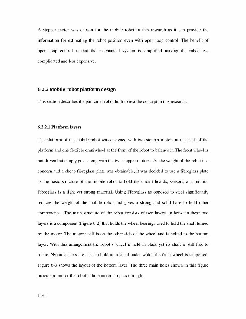
114 |

A stepper motor was chosen for the mobile robot in this research as it can provide the

information for estimating the robot position even with open loop control. The benefit of

open loop control is that the mechanical system is simplified making the robot less

complicated and less expensive.

6.2.2 Mobile robot platform design

This section describes the particular robot built to test the concept in this research.

6.2.2.1 Platform layers

The platform of the mobile robot was designed with two stepper motors at the back of the

platform and one flexible omniwheel at the front of the robot to balance it. The front wheel is

not driven but simply goes along with the two stepper motors. As the weight of the robot is a

concern and a cheap fibreglass plate was obtainable, it was decided to use a fibreglass plate

as the basic structure of the mobile robot to hold the circuit boards, sensors, and motors.

Fibreglass is a light yet strong material. Using Fibreglass as opposed to steel significantly

reduces the weight of the mobile robot and gives a strong and solid base to hold other

components. The main structure of the robot consists of two layers. In between these two

layers is a component (Figure 6-2) that holds the wheel bearings used to hold the shaft turned

by the motor. The motor itself is on the other side of the wheel and is bolted to the bottom

layer. With this arrangement the robot’s wheel is held in place yet its shaft is still free to

rotate. Nylon spacers are used to hold up a stand under which the front wheel is supported.

Figure 6-3 shows the layout of the bottom layer. The three main holes shown in this figure

provide room for the robot’s three motors to pass through.

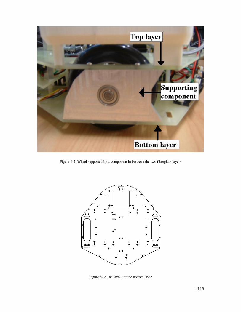
| 115

Figure 6-2: Wheel supported by a component in between the two fibreglass layers

Figure 6-3: The layout of the bottom layer

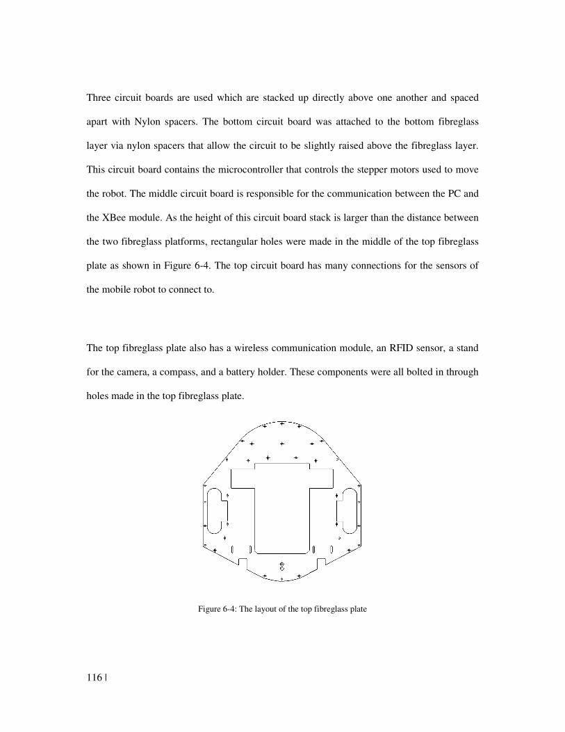
116 |

Three circuit boards are used which are stacked up directly above one another and spaced

apart with Nylon spacers. The bottom circuit board was attached to the bottom fibreglass

layer via nylon spacers that allow the circuit to be slightly raised above the fibreglass layer.

This circuit board contains the microcontroller that controls the stepper motors used to move

the robot. The middle circuit board is responsible for the communication between the PC and

the XBee module. As the height of this circuit board stack is larger than the distance between

the two fibreglass platforms, rectangular holes were made in the middle of the top fibreglass

plate as shown in Figure 6-4. The top circuit board has many connections for the sensors of

the mobile robot to connect to.

The top fibreglass plate also has a wireless communication module, an RFID sensor, a stand

for the camera, a compass, and a battery holder. These components were all bolted in through

holes made in the top fibreglass plate.

Figure 6-4: The layout of the top fibreglass plate

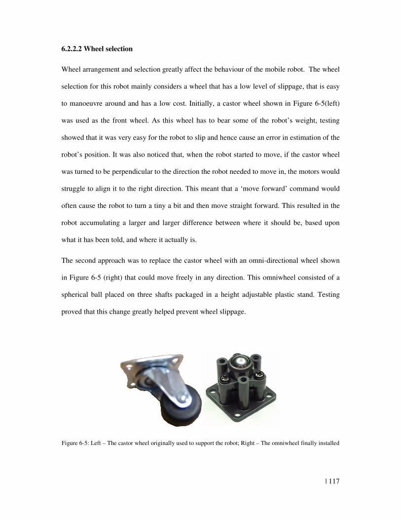
| 117

6.2.2.2 Wheel selection

Wheel arrangement and selection greatly affect the behaviour of the mobile robot. The wheel

selection for this robot mainly considers a wheel that has a low level of slippage, that is easy

to manoeuvre around and has a low cost. Initially, a castor wheel shown in Figure 6-5(left)

was used as the front wheel. As this wheel has to bear some of the robot’s weight, testing

showed that it was very easy for the robot to slip and hence cause an error in estimation of the

robot’s position. It was also noticed that, when the robot started to move, if the castor wheel

was turned to be perpendicular to the direction the robot needed to move in, the motors would

struggle to align it to the right direction. This meant that a ‘move forward’ command would

often cause the robot to turn a tiny a bit and then move straight forward. This resulted in the

robot accumulating a larger and larger difference between where it should be, based upon

what it has been told, and where it actually is.

The second approach was to replace the castor wheel with an omni-directional wheel shown

in Figure 6-5 (right) that could move freely in any direction. This omniwheel consisted of a

spherical ball placed on three shafts packaged in a height adjustable plastic stand. Testing

proved that this change greatly helped prevent wheel slippage.

Figure 6-5: Left – The castor wheel originally used to support the robot; Right – The omniwheel finally installed

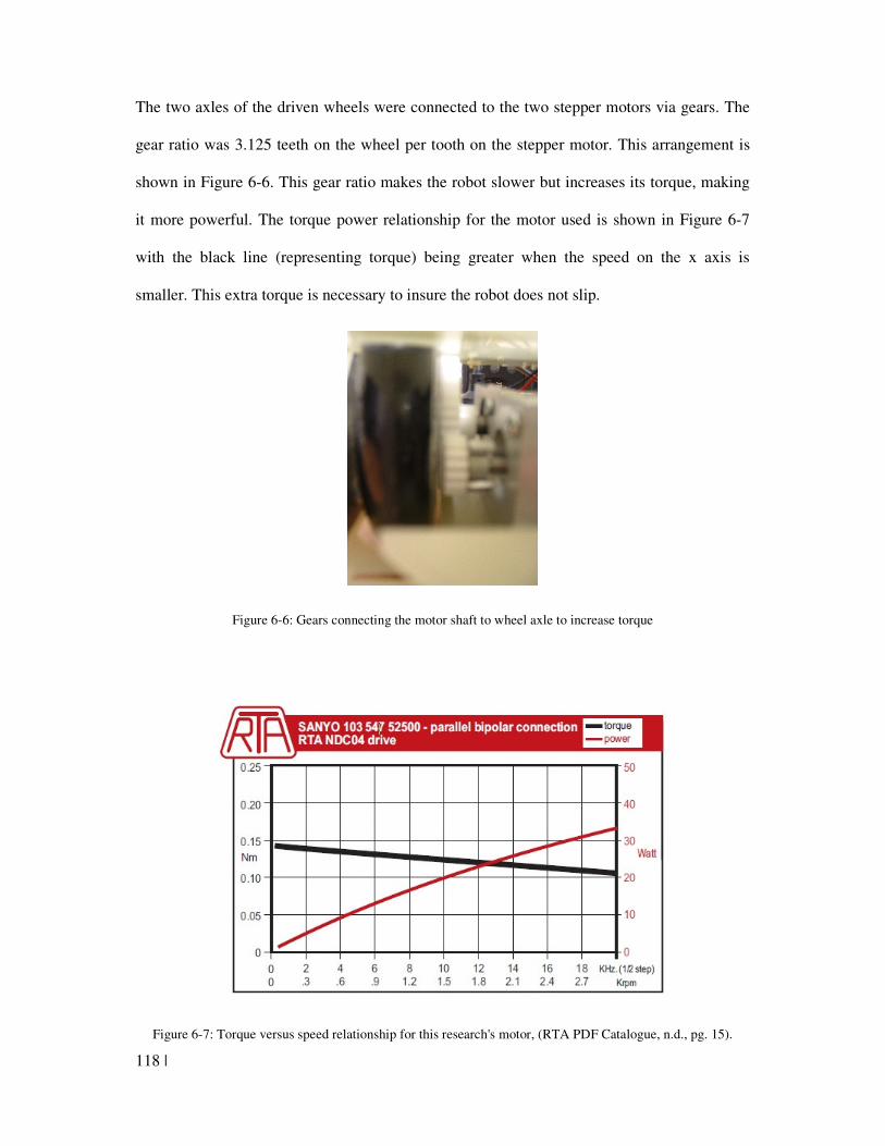
118 |

The two axles of the driven wheels were connected to the two stepper motors via gears. The

gear ratio was 3.125 teeth on the wheel per tooth on the stepper motor. This arrangement is

shown in Figure 6-6. This gear ratio makes the robot slower but increases its torque, making

it more powerful. The torque power relationship for the motor used is shown in Figure 6-7

with the black line (representing torque) being greater when the speed on the x axis is

smaller. This extra torque is necessary to insure the robot does not slip.

Figure 6-6: Gears connecting the motor shaft to wheel axle to increase torque

Figure 6-7: Torque versus speed relationship for this research's motor, (RTA PDF Catalogue, n.d., pg. 15).

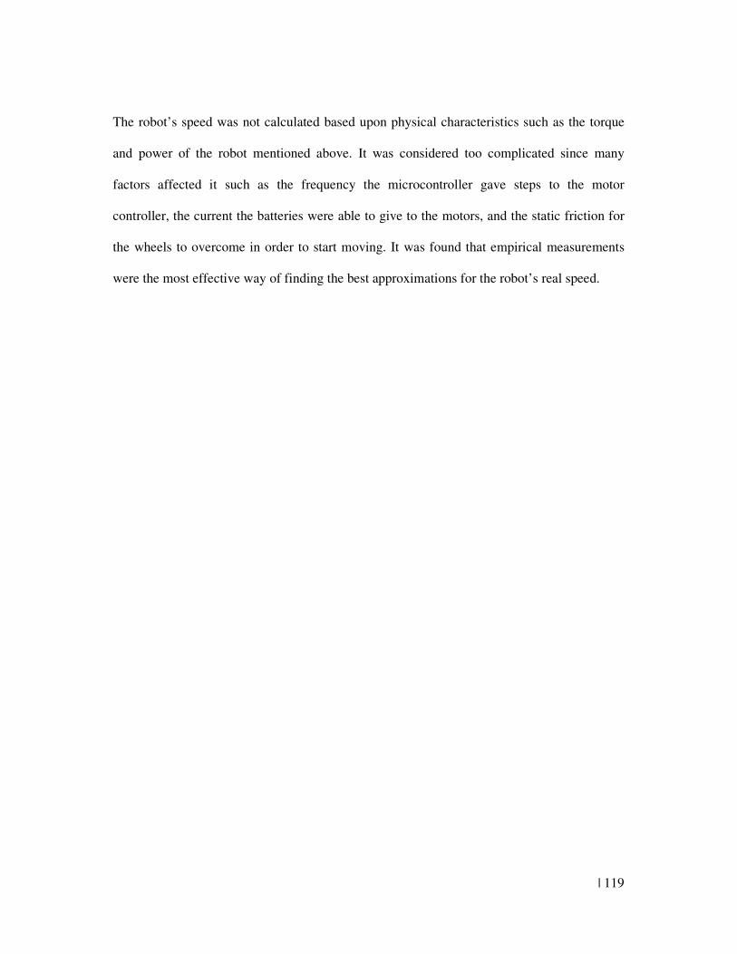
| 119

The robot’s speed was not calculated based upon physical characteristics such as the torque

and power of the robot mentioned above. It was considered too complicated since many

factors affected it such as the frequency the microcontroller gave steps to the motor

controller, the current the batteries were able to give to the motors, and the static friction for

the wheels to overcome in order to start moving. It was found that empirical measurements

were the most effective way of finding the best approximations for the robot’s real speed.

120 |

6.3 Control system design

This section explains the control system for the robot. A robot’s control system should have

input from data about its surroundings and output that controls the robot’s actions. The input

for this robot is the data from all the robot’s sensors and the output is the motors that move

the robot around. Therefore this section explains how the motors and sensors operate and

how they were used.

6.3.1 Motor controller, power supply and testing

6.3.1.1 Motor controller and driver

The motors used for this research were Sanyo Denki stepper motors. Each motor had four

wires and a 1.8 degree step resolution meaning that the motor moves 1.8 degrees each step.

The half step mode is used meaning that the motor will turn in half step increments, i.e., 0.9

degrees per turn of the motor. It does this through turning on two magnets in between each

step, which moves the robot half way between a matching tooth on each electromagnet on the

stator. This not only increases the stepping resolution, but since two electromagnets are

energised at one time during a half-step, it also increases the torque. An increase in torque

will increase the amount of current used but will in turn make the wheel connected to the

motor less susceptible to errors resulting from slipping since it is less likely for a greater

torque to slip.

An L297 stepper motor controller was used to provide the control signal needed to control the

stepper motors. All it needs is the direction to move (clockwise or anticlockwise), mode (full

step or half step), and a falling edge to indicate when another step should be taken. This

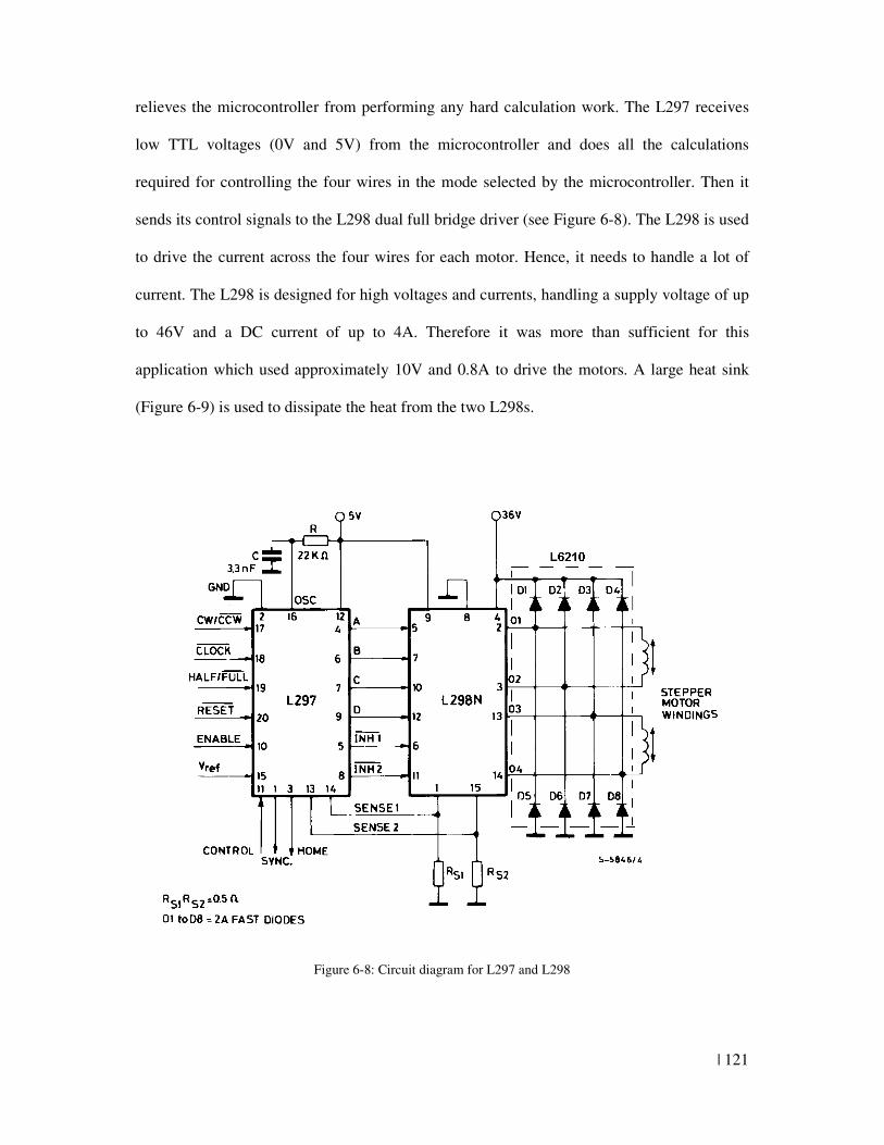
| 121

relieves the microcontroller from performing any hard calculation work. The L297 receives

low TTL voltages (0V and 5V) from the microcontroller and does all the calculations

required for controlling the four wires in the mode selected by the microcontroller. Then it

sends its control signals to the L298 dual full bridge driver (see Figure 6-8). The L298 is used

to drive the current across the four wires for each motor. Hence, it needs to handle a lot of

current. The L298 is designed for high voltages and currents, handling a supply voltage of up

to 46V and a DC current of up to 4A. Therefore it was more than sufficient for this

application which used approximately 10V and 0.8A to drive the motors. A large heat sink

(Figure 6-9) is used to dissipate the heat from the two L298s.

Figure 6-8: Circuit diagram for L297 and L298

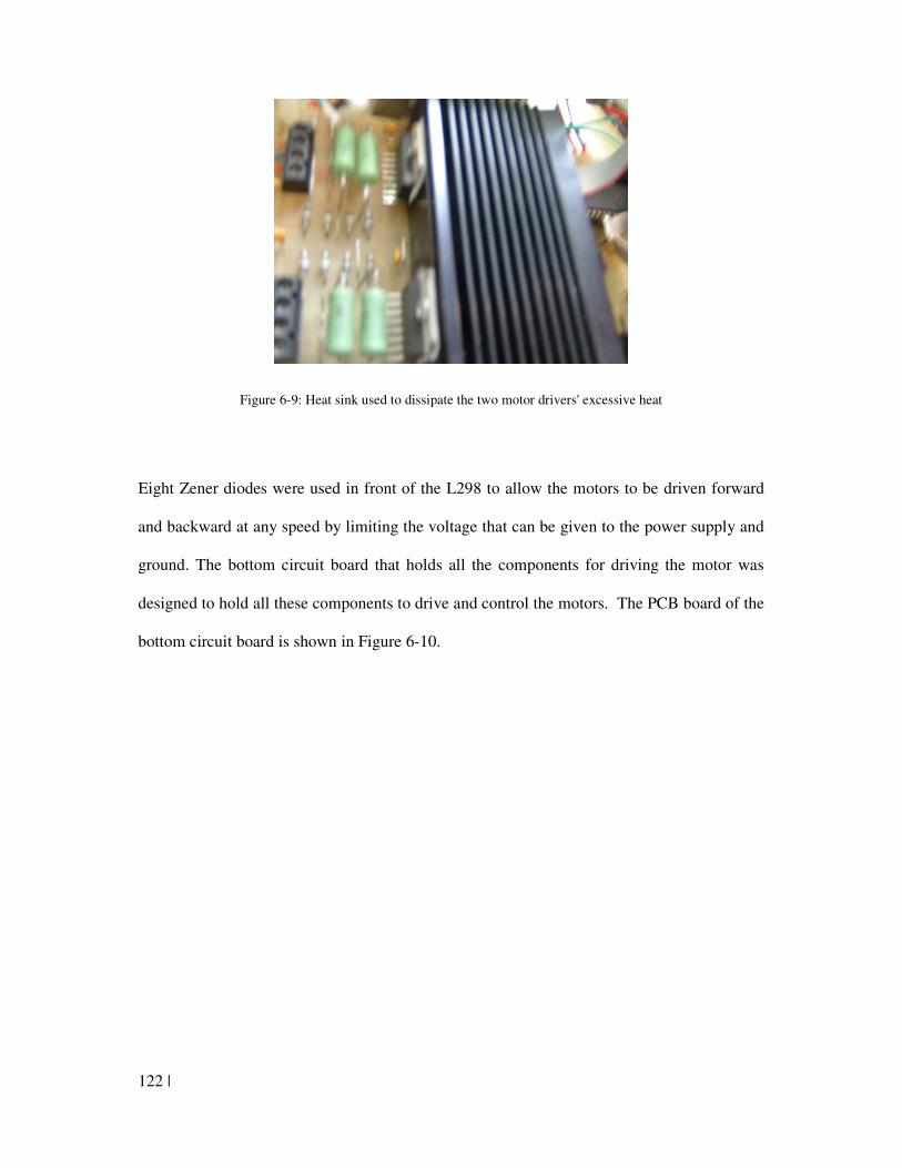
122 |

Figure 6-9: Heat sink used to dissipate the two motor drivers' excessive heat

Eight Zener diodes were used in front of the L298 to allow the motors to be driven forward

and backward at any speed by limiting the voltage that can be given to the power supply and

ground. The bottom circuit board that holds all the components for driving the motor was

designed to hold all these components to drive and control the motors. The PCB board of the

bottom circuit board is shown in Figure 6-10.

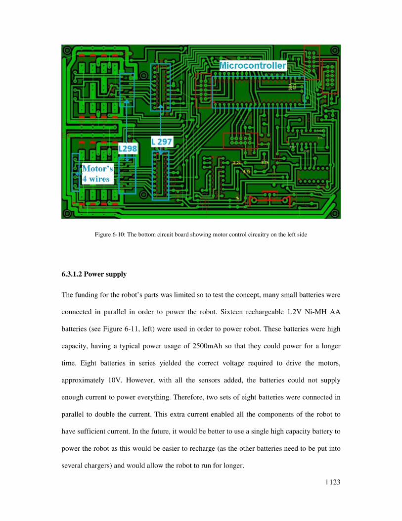
| 123

Figure 6-10: The bottom circuit board showing motor control circuitry on the left side

6.3.1.2 Power supply

The funding for the robot’s parts was limited so to test the concept, many small batteries were

connected in parallel in order to power the robot. Sixteen rechargeable 1.2V Ni-MH AA

batteries (see Figure 6-11, left) were used in order to power robot. These batteries were high

capacity, having a typical power usage of 2500mAh so that they could power for a longer

time. Eight batteries in series yielded the correct voltage required to drive the motors,

approximately 10V. However, with all the sensors added, the batteries could not supply

enough current to power everything. Therefore, two sets of eight batteries were connected in

parallel to double the current. This extra current enabled all the components of the robot to

have sufficient current. In the future, it would be better to use a single high capacity battery to

power the robot as this would be easier to recharge (as the other batteries need to be put into

several chargers) and would allow the robot to run for longer.

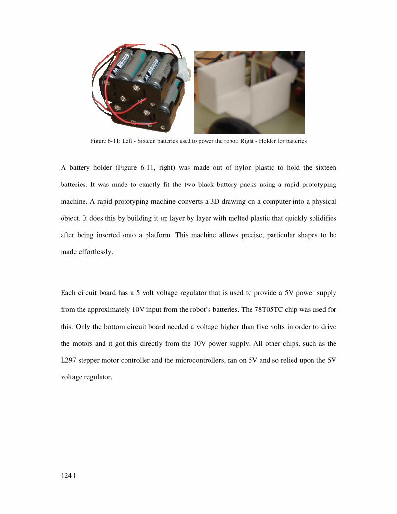
124 |

Figure 6-11: Left - Sixteen batteries used to power the robot; Right - Holder for batteries

A battery holder (Figure 6-11, right) was made out of nylon plastic to hold the sixteen

batteries. It was made to exactly fit the two black battery packs using a rapid prototyping

machine. A rapid prototyping machine converts a 3D drawing on a computer into a physical

object. It does this by building it up layer by layer with melted plastic that quickly solidifies

after being inserted onto a platform. This machine allows precise, particular shapes to be

made effortlessly.

Each circuit board has a 5 volt voltage regulator that is used to provide a 5V power supply

from the approximately 10V input from the robot’s batteries. The 78T05TC chip was used for

this. Only the bottom circuit board needed a voltage higher than five volts in order to drive

the motors and it got this directly from the 10V power supply. All other chips, such as the

L297 stepper motor controller and the microcontrollers, ran on 5V and so relied upon the 5V

voltage regulator.

| 125

6.3.1.3 Motor driver circuit testing

The motor drive circuit was tested by varying the peak current the motor can use and varying

the speed of the motor through changing the frequency of the square wave to the motor

controllers (see section 6.3.1.1). This section briefly describes these tests.

The L297 motor controller has a voltage reference pin whose analogue voltage controls the

maximum current the motor can use. This pin was set through the PCF8591P ADC DAC

converter. This device is necessary since the ATMega32 microcontroller used in this research

has no DAC on it and so can only output digital information. This DAC was given its

analogue voltage via two wire interface (TWI) communication. TWI uses only two pins to

provide serial communication, SCL (Serial clock) and SDA (Serial data). It works on the

basis of having a master that selects a slave and either gives it information or asks for

information from it. The master sets the clock for the slaves to use. This method of I2C

communication makes it very easy to test different voltages by changing only one parameter

in a piece of code instead of changing some electronic physical components as would be

needed if a voltage divider were made with resistors in order to set the voltage.

Figure 6-12 shows the relationship between the serial values given to the DAC through I2C

versus the motor current draw detected by a power supply. As can be seen, the relationship is

linear. Such a relationship makes it easy to change the maximum current the motors can use.

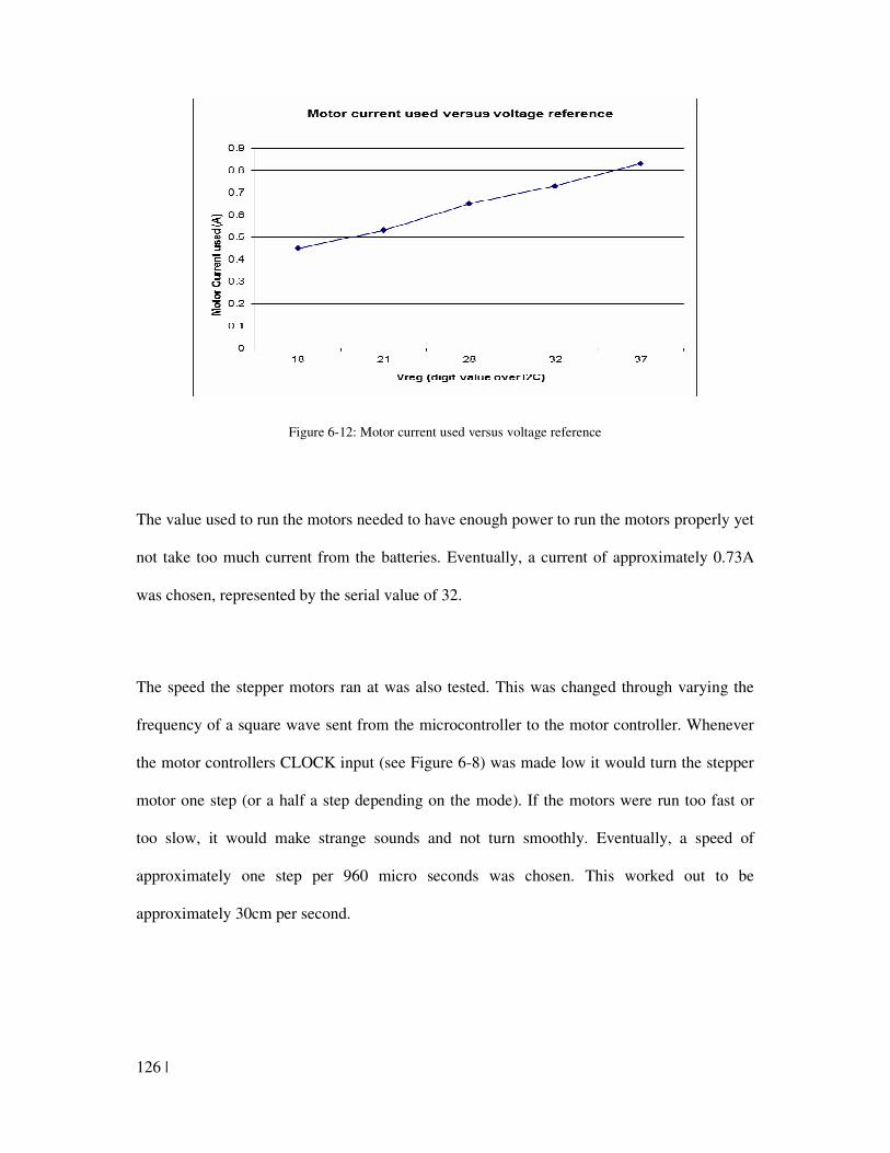
126 |

Figure 6-12: Motor current used versus voltage reference

The value used to run the motors needed to have enough power to run the motors properly yet

not take too much current from the batteries. Eventually, a current of approximately 0.73A

was chosen, represented by the serial value of 32.

The speed the stepper motors ran at was also tested. This was changed through varying the

frequency of a square wave sent from the microcontroller to the motor controller. Whenever

the motor controllers CLOCK input (see Figure 6-8) was made low it would turn the stepper

motor one step (or a half a step depending on the mode). If the motors were run too fast or

too slow, it would make strange sounds and not turn smoothly. Eventually, a speed of

approximately one step per 960 micro seconds was chosen. This worked out to be

approximately 30cm per second.

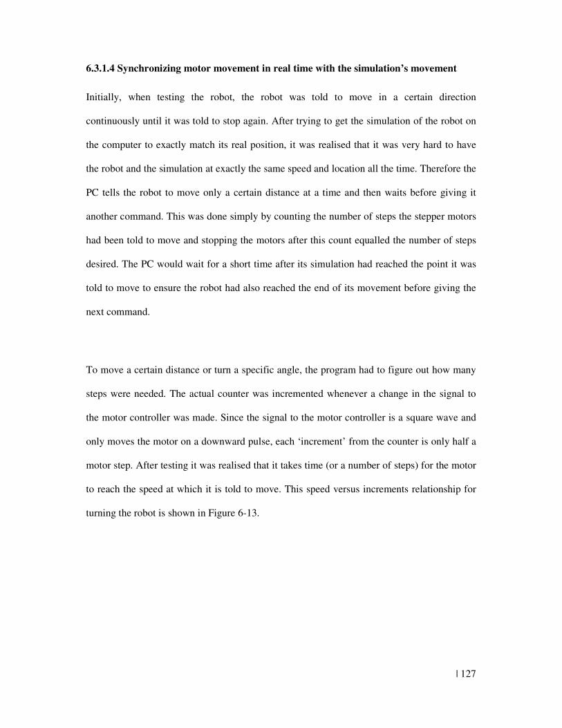
| 127

6.3.1.4 Synchronizing motor movement in real time with the simulation’s movement

Initially, when testing the robot, the robot was told to move in a certain direction

continuously until it was told to stop again. After trying to get the simulation of the robot on

the computer to exactly match its real position, it was realised that it was very hard to have

the robot and the simulation at exactly the same speed and location all the time. Therefore the

PC tells the robot to move only a certain distance at a time and then waits before giving it

another command. This was done simply by counting the number of steps the stepper motors

had been told to move and stopping the motors after this count equalled the number of steps

desired. The PC would wait for a short time after its simulation had reached the point it was

told to move to ensure the robot had also reached the end of its movement before giving the

next command.

To move a certain distance or turn a specific angle, the program had to figure out how many

steps were needed. The actual counter was incremented whenever a change in the signal to

the motor controller was made. Since the signal to the motor controller is a square wave and

only moves the motor on a downward pulse, each ‘increment’ from the counter is only half a

motor step. After testing it was realised that it takes time (or a number of steps) for the motor

to reach the speed at which it is told to move. This speed versus increments relationship for

turning the robot is shown in Figure 6-13.

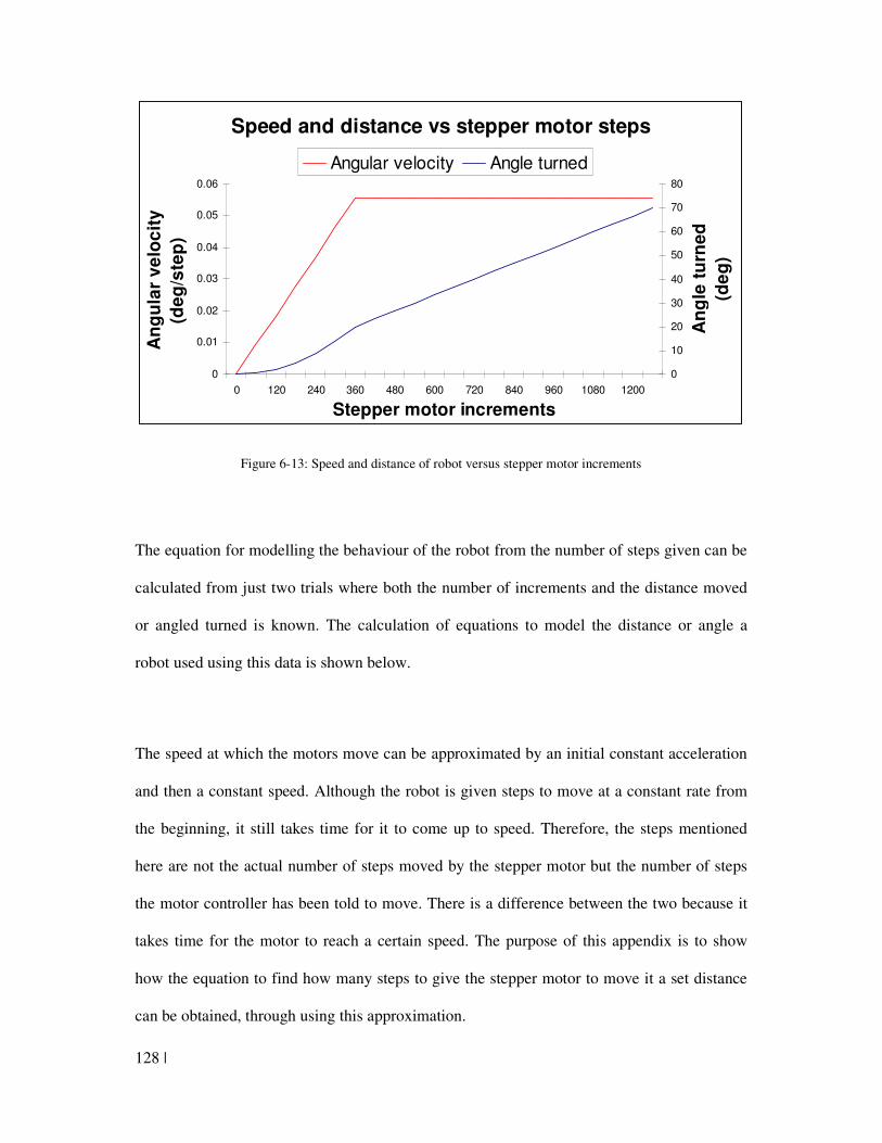
128 |

Speed and distance vs stepper motor steps

0

0.01

0.02

0.03

0.04

0.05

0.06

0 120 240 360 480 600 720 840 960 1080 1200

Stepper motor increments

An

gu

lar

ve

loc

ity

(de

g/s

tep

)

0

10

20

30

40

50

60

70

80

An

gle

tu

rne

d

(de

g)

Angular velocity Angle turned

Figure 6-13: Speed and distance of robot versus stepper motor increments

The equation for modelling the behaviour of the robot from the number of steps given can be

calculated from just two trials where both the number of increments and the distance moved

or angled turned is known. The calculation of equations to model the distance or angle a

robot used using this data is shown below.

The speed at which the motors move can be approximated by an initial constant acceleration

and then a constant speed. Although the robot is given steps to move at a constant rate from

the beginning, it still takes time for it to come up to speed. Therefore, the steps mentioned

here are not the actual number of steps moved by the stepper motor but the number of steps

the motor controller has been told to move. There is a difference between the two because it

takes time for the motor to reach a certain speed. The purpose of this appendix is to show

how the equation to find how many steps to give the stepper motor to move it a set distance

can be obtained, through using this approximation.

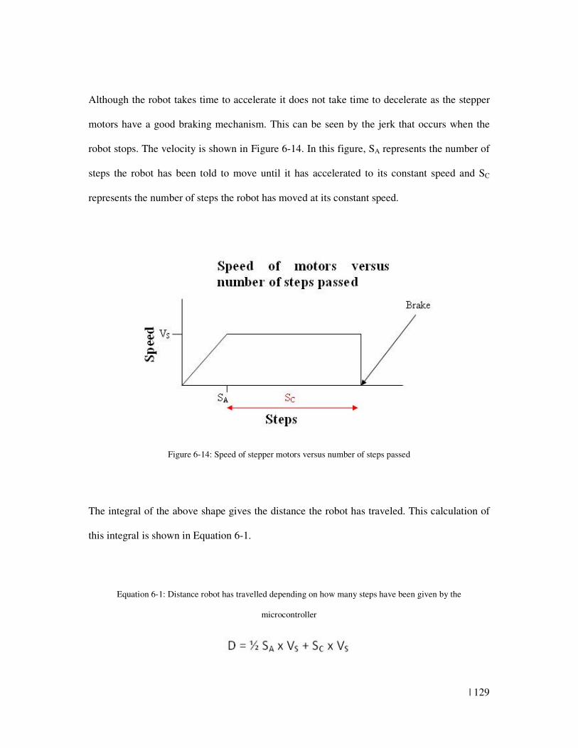
| 129

Although the robot takes time to accelerate it does not take time to decelerate as the stepper

motors have a good braking mechanism. This can be seen by the jerk that occurs when the

robot stops. The velocity is shown in Figure 6-14. In this figure, SA represents the number of

steps the robot has been told to move until it has accelerated to its constant speed and SC

represents the number of steps the robot has moved at its constant speed.

Figure 6-14: Speed of stepper motors versus number of steps passed

The integral of the above shape gives the distance the robot has traveled. This calculation of

this integral is shown in Equation 6-1.

Equation 6-1: Distance robot has travelled depending on how many steps have been given by the

microcontroller

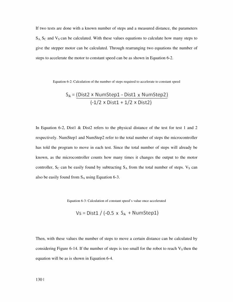
130 |

If two tests are done with a known number of steps and a measured distance, the parameters

SA, SC and VS can be calculated. With these values equations to calculate how many steps to

give the stepper motor can be calculated. Through rearranging two equations the number of

steps to accelerate the motor to constant speed can be as shown in Equation 6-2.

Equation 6-2: Calculation of the number of steps required to accelerate to constant speed

In Equation 6-2, Dist1 & Dist2 refers to the physical distance of the test for test 1 and 2

respectively. NumStep1 and NumStep2 refer to the total number of steps the microcontroller

has told the program to move in each test. Since the total number of steps will already be

known, as the microcontroller counts how many times it changes the output to the motor

controller, SC can be easily found by subtracting SA from the total number of steps. VS can

also be easily found from SA using Equation 6-3.

Equation 6-3: Calculation of constant speed’s value once accelerated

Then, with these values the number of steps to move a certain distance can be calculated by

considering Figure 6-14. If the number of steps is too small for the robot to reach VS then the

equation will be as is shown in Equation 6-4.

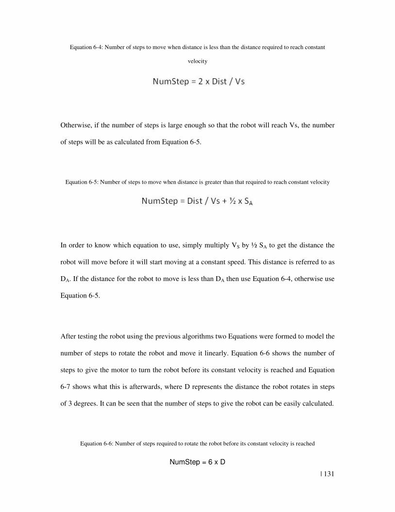
| 131

Equation 6-4: Number of steps to move when distance is less than the distance required to reach constant

velocity

Otherwise, if the number of steps is large enough so that the robot will reach Vs, the number

of steps will be as calculated from Equation 6-5.

Equation 6-5: Number of steps to move when distance is greater than that required to reach constant velocity

In order to know which equation to use, simply multiply VS by ½ SA to get the distance the

robot will move before it will start moving at a constant speed. This distance is referred to as

DA. If the distance for the robot to move is less than DA then use Equation 6-4, otherwise use

Equation 6-5.

After testing the robot using the previous algorithms two Equations were formed to model the

number of steps to rotate the robot and move it linearly. Equation 6-6 shows the number of

steps to give the motor to turn the robot before its constant velocity is reached and Equation

6-7 shows what this is afterwards, where D represents the distance the robot rotates in steps

of 3 degrees. It can be seen that the number of steps to give the robot can be easily calculated.

Equation 6-6: Number of steps required to rotate the robot before its constant velocity is reached

NumStep = 6 x D

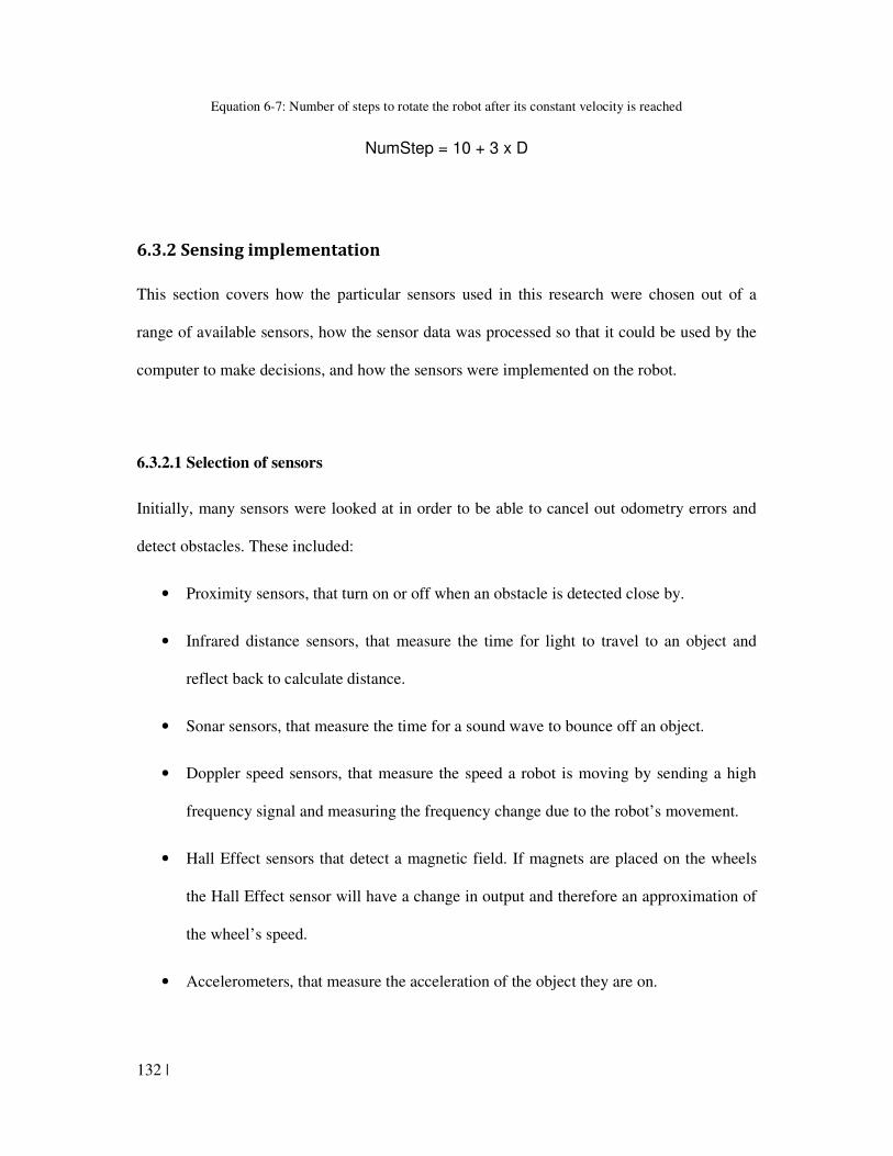
132 |

Equation 6-7: Number of steps to rotate the robot after its constant velocity is reached

NumStep = 10 + 3 x D

6.3.2 Sensing implementation

This section covers how the particular sensors used in this research were chosen out of a

range of available sensors, how the sensor data was processed so that it could be used by the

computer to make decisions, and how the sensors were implemented on the robot.

6.3.2.1 Selection of sensors

Initially, many sensors were looked at in order to be able to cancel out odometry errors and

detect obstacles. These included:

• Proximity sensors, that turn on or off when an obstacle is detected close by.

• Infrared distance sensors, that measure the time for light to travel to an object and

reflect back to calculate distance.

• Sonar sensors, that measure the time for a sound wave to bounce off an object.

• Doppler speed sensors, that measure the speed a robot is moving by sending a high

frequency signal and measuring the frequency change due to the robot’s movement.

• Hall Effect sensors that detect a magnetic field. If magnets are placed on the wheels

the Hall Effect sensor will have a change in output and therefore an approximation of

the wheel’s speed.

• Accelerometers, that measure the acceleration of the object they are on.

| 133

• Gyroscopes, that measure the angular change of an object and therefore the

acceleration.

• Compasses, that use the earth’s magnetic field to output their current orientation.

• RFID (radio frequency identification) tags; both active, that require their own power

source to run, and passive, that have their current induced by the reader. These tags

can store a unique ID and be placed around a map so that a robot detecting them can

localise itself.

Acceleration sensors were deemed unnecessary for this research as acceleration to a fixed

speed takes a very short amount of time, the processing of the microcontroller is limited, and

their reliability for such small distances questionable. Such sensors would be only useful if

they could detect unexpected movements or in the case of slipping, the robot not moving

when it should. It is unlikely that processing would enable such a small difference in

acceleration, from what was intended to what actually happened, to be monitored. In the

same manner, Doppler sensors measuring speed would not be useful in this research as the

speed would mainly be either still or one speed and slippage of wheels would only cause a

minor change that would not be easily noticed.

Proximity sensors are useful for stopping a robot when it is too close to an object and other

methods have failed to stop the robot. These were considered and plan to be implemented on

the robot in the future to increase safety.

134 |

A sonar sensor was installed on the robot. The sonar sensor chosen was the MB1300 from

MaxSonar. Although it is more expensive than some more basic ones, it has automatic

calibration for changes in voltage, temperature, and electrical noise and has no time needed

for calibration when first powered up, as some devices require. These features make it less

prone to error and able to operate immediately upon starting of the robot.

The short range Sharp GP2D120 infrared distance sensor was used to detect obstacles that are

close to the robot. The sensor is able to sense from 4 – 30cm. It has less influence from the

colour of objects it detects as other infrared sensors may. This feature is a necessity for the

mobile robot to be useful in practical applications that have different coloured obstacles. It

also requires no external circuitry making it much easier to use.

The CMPS03 compass used is said to be designed specifically for use in robots as an aid to

navigation. It uses two magnetic field sensors sensitive enough to detect the earth’s magnetic

field to calculate the current angle of the object it is placed on. The PWM (Pulse width

modulated) signal on it was used to obtain the angle.

RFID sensors were also implemented on the robot. A reader to read passive RFID tags with a

frequency of 125kHz (the lowest frequency for RFID tags) was chosen. Having a lower

frequency decreases the detection distance range but this is not a problem as the tags are only

meant to be read when the mobile robot is near them. Passive tags have the benefit of being

inexpensive, simple, and having no need of a power source. The tags are credit card shaped

and can be easily attached or detached to walls or other objects in an indoor environment.

This allows that the indoor environment in which the robot moves to be easily rearranged as

| 135

opposed to using AGVs (Automated guided vehicles) which may require lines to be put on a

floor or wires to be installed underground. This ease of change is important in a changing

working environment where new products are produced more often than before, meaning that

the working environment may need to be rearranged and hence the path of a robot changed to

fit in with it. This method of passive RFID tags allows the creation of new paths for mobile

robots to take to be created quickly.

6.3.2.2 Processing and testing of sensor data

This section describes how the data from the sensors was processed so that the PC could use

the data and make the right decision for the robot.

6.3.2.2.1 Infrared distance sensor

The GP2D120 photodiode sensor (see Appendix I) was used due to its simplicity to use,

availability, and reasonable price as the distance sensor to detect objects around the mobile

robot.

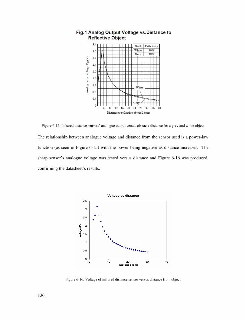
136 |

Figure 6-15: Infrared distance sensors’ analogue output versus obstacle distance for a grey and white object

The relationship between analogue voltage and distance from the sensor used is a power-law

function (as seen in Figure 6-15) with the power being negative as distance increases. The

sharp sensor’s analogue voltage was tested versus distance and Figure 6-16 was produced,

confirming the datasheet’s results.

Figure 6-16: Voltage of infrared distance sensor versus distance from object

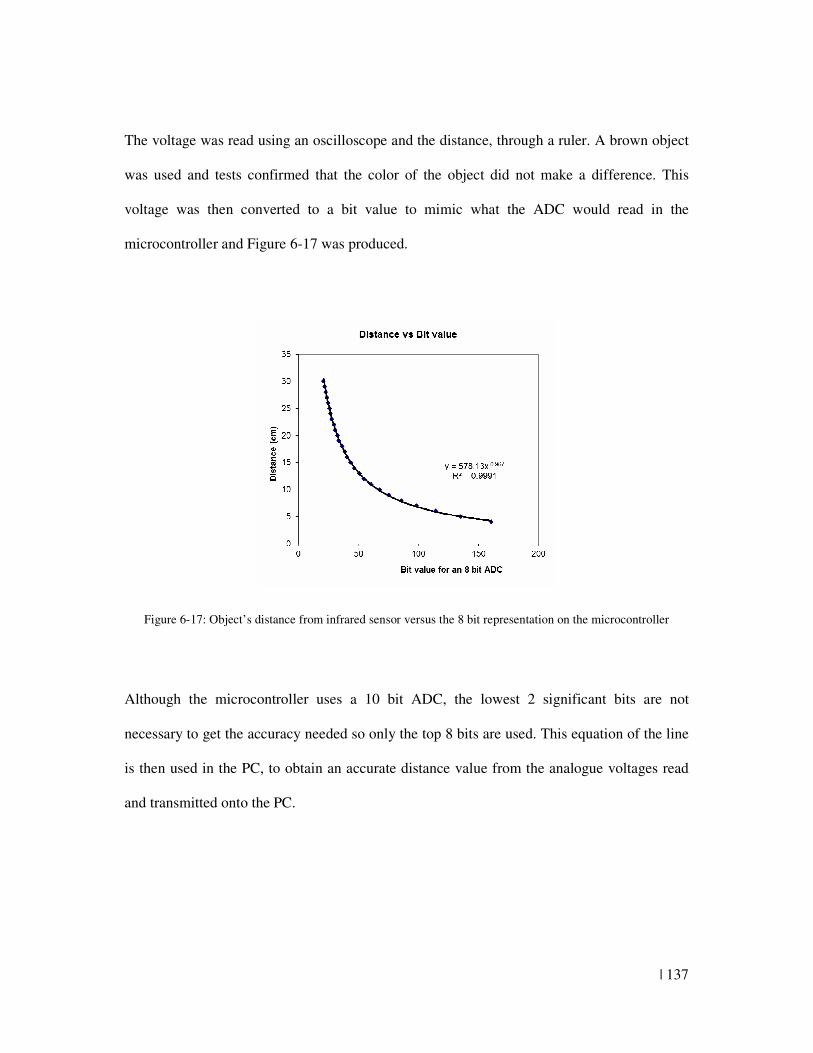
| 137

The voltage was read using an oscilloscope and the distance, through a ruler. A brown object

was used and tests confirmed that the color of the object did not make a difference. This

voltage was then converted to a bit value to mimic what the ADC would read in the

microcontroller and Figure 6-17 was produced.

Figure 6-17: Object’s distance from infrared sensor versus the 8 bit representation on the microcontroller

Although the microcontroller uses a 10 bit ADC, the lowest 2 significant bits are not

necessary to get the accuracy needed so only the top 8 bits are used. This equation of the line

is then used in the PC, to obtain an accurate distance value from the analogue voltages read

and transmitted onto the PC.

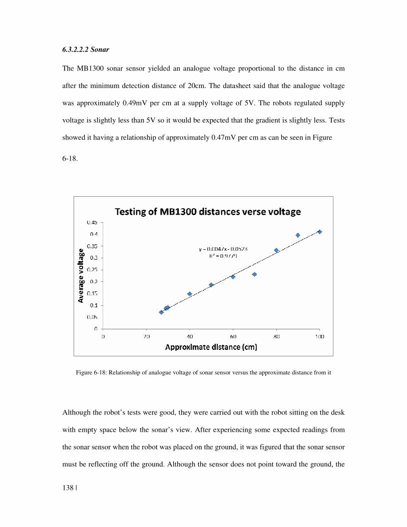
138 |

6.3.2.2.2 Sonar

The MB1300 sonar sensor yielded an analogue voltage proportional to the distance in cm

after the minimum detection distance of 20cm. The datasheet said that the analogue voltage

was approximately 0.49mV per cm at a supply voltage of 5V. The robots regulated supply

voltage is slightly less than 5V so it would be expected that the gradient is slightly less. Tests

showed it having a relationship of approximately 0.47mV per cm as can be seen in Figure

6-18.

Figure 6-18: Relationship of analogue voltage of sonar sensor versus the approximate distance from it

Although the robot’s tests were good, they were carried out with the robot sitting on the desk

with empty space below the sonar’s view. After experiencing some expected readings from

the sonar sensor when the robot was placed on the ground, it was figured that the sonar sensor

must be reflecting off the ground. Although the sensor does not point toward the ground, the

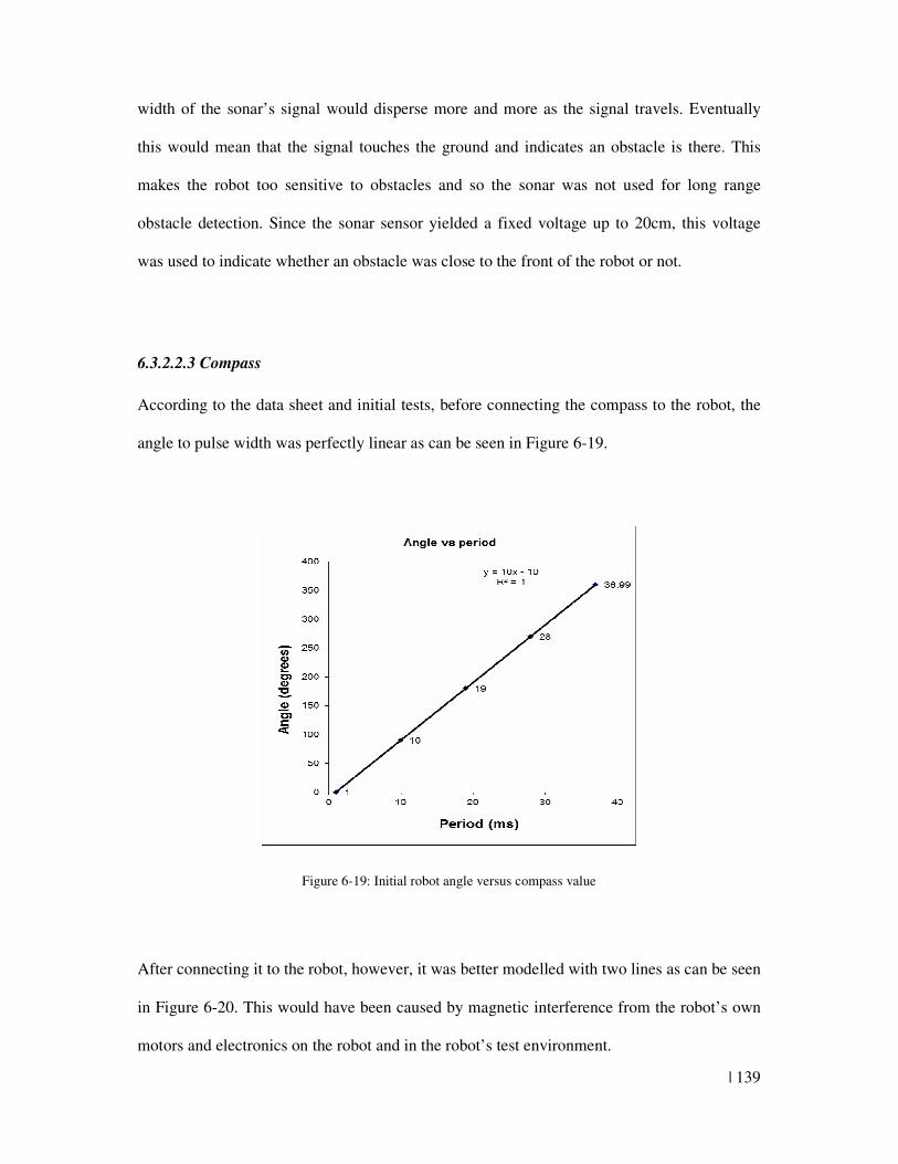
| 139

width of the sonar’s signal would disperse more and more as the signal travels. Eventually

this would mean that the signal touches the ground and indicates an obstacle is there. This

makes the robot too sensitive to obstacles and so the sonar was not used for long range

obstacle detection. Since the sonar sensor yielded a fixed voltage up to 20cm, this voltage

was used to indicate whether an obstacle was close to the front of the robot or not.

6.3.2.2.3 Compass

According to the data sheet and initial tests, before connecting the compass to the robot, the

angle to pulse width was perfectly linear as can be seen in Figure 6-19.

Figure 6-19: Initial robot angle versus compass value

After connecting it to the robot, however, it was better modelled with two lines as can be seen

in Figure 6-20. This would have been caused by magnetic interference from the robot’s own

motors and electronics on the robot and in the robot’s test environment.

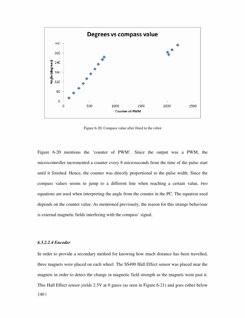
140 |

Figure 6-20: Compass value after fitted to the robot

Figure 6-20 mentions the ‘counter of PWM’. Since the output was a PWM, the

microcontroller incremented a counter every 8 microseconds from the time of the pulse start

until it finished. Hence, the counter was directly proportional to the pulse width. Since the

compass values seems to jump to a different line when reaching a certain value, two

equations are used when interpreting the angle from the counter in the PC. The equation used

depends on the counter value. As mentioned previously, the reason for this strange behaviour

is external magnetic fields interfering with the compass’ signal.

6.3.2.2.4 Encoder

In order to provide a secondary method for knowing how much distance has been travelled,

three magnets were placed on each wheel. The SS490 Hall Effect sensor was placed near the

magnets in order to detect the change in magnetic field strength as the magnets went past it.

This Hall Effect sensor yields 2.5V at 0 gauss (as seen in Figure 6-21) and goes either below

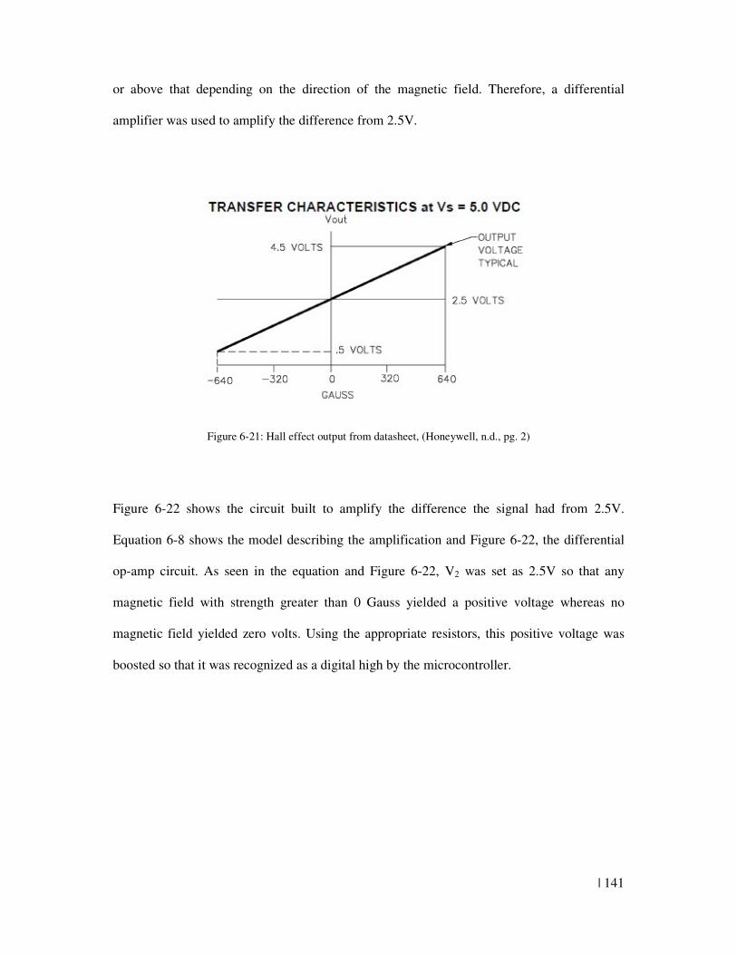
| 141

or above that depending on the direction of the magnetic field. Therefore, a differential

amplifier was used to amplify the difference from 2.5V.

Figure 6-21: Hall effect output from datasheet, (Honeywell, n.d., pg. 2)

Figure 6-22 shows the circuit built to amplify the difference the signal had from 2.5V.

Equation 6-8 shows the model describing the amplification and Figure 6-22, the differential

op-amp circuit. As seen in the equation and Figure 6-22, V2 was set as 2.5V so that any

magnetic field with strength greater than 0 Gauss yielded a positive voltage whereas no

magnetic field yielded zero volts. Using the appropriate resistors, this positive voltage was

boosted so that it was recognized as a digital high by the microcontroller.

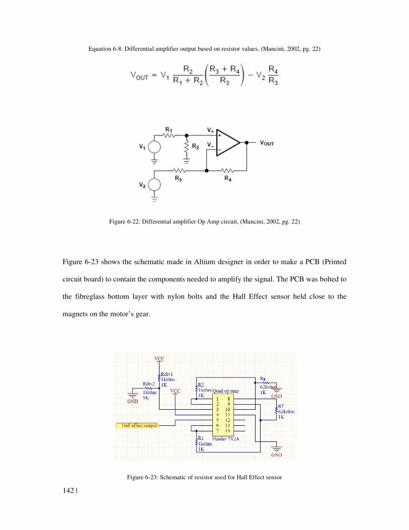
142 |

Equation 6-8: Differential amplifier output based on resistor values, (Mancini, 2002, pg. 22)

Figure 6-22: Differential amplifier Op Amp circuit, (Mancini, 2002, pg. 22)

Figure 6-23 shows the schematic made in Altium designer in order to make a PCB (Printed

circuit board) to contain the components needed to amplify the signal. The PCB was bolted to

the fibreglass bottom layer with nylon bolts and the Hall Effect sensor held close to the

magnets on the motor’s gear.

Figure 6-23: Schematic of resistor used for Hall Effect sensor

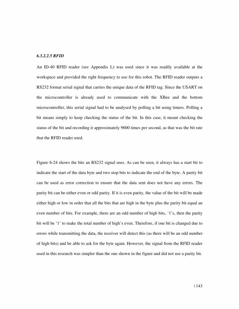
| 143

6.3.2.2.5 RFID

An ID-40 RFID reader (see Appendix L) was used since it was readily available at the

workspace and provided the right frequency to use for this robot. The RFID reader outputs a

RS232 format serial signal that carries the unique data of the RFID tag. Since the USART on

the microcontroller is already used to communicate with the XBee and the bottom

microcontroller, this serial signal had to be analysed by polling a bit using timers. Polling a

bit means simply to keep checking the status of the bit. In this case, it meant checking the

status of the bit and recording it approximately 9600 times per second, as that was the bit rate

that the RFID reader used.

Figure 6-24 shows the bits an RS232 signal uses. As can be seen, it always has a start bit to

indicate the start of the data byte and two stop bits to indicate the end of the byte. A parity bit

can be used as error correction to ensure that the data sent does not have any errors. The

parity bit can be either even or odd parity. If it is even parity, the value of the bit will be made

either high or low in order that all the bits that are high in the byte plus the parity bit equal an

even number of bits. For example, there are an odd number of high bits, ‘1’s, then the parity

bit will be ‘1’ to make the total number of high’s even. Therefore, if one bit is changed due to

errors while transmitting the data, the receiver will detect this (as there will be an odd number

of high bits) and be able to ask for the byte again. However, the signal from the RFID reader

used in this research was simpler than the one shown in the figure and did not use a parity bit.

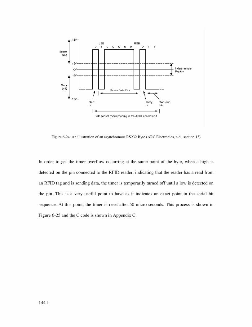
144 |

Figure 6-24: An illustration of an asynchronous RS232 Byte (ARC Electronics, n.d., section 13)

In order to get the timer overflow occurring at the same point of the byte, when a high is

detected on the pin connected to the RFID reader, indicating that the reader has a read from

an RFID tag and is sending data, the timer is temporarily turned off until a low is detected on

the pin. This is a very useful point to have as it indicates an exact point in the serial bit

sequence. At this point, the timer is reset after 50 micro seconds. This process is shown in

Figure 6-25 and the C code is shown in Appendix C.

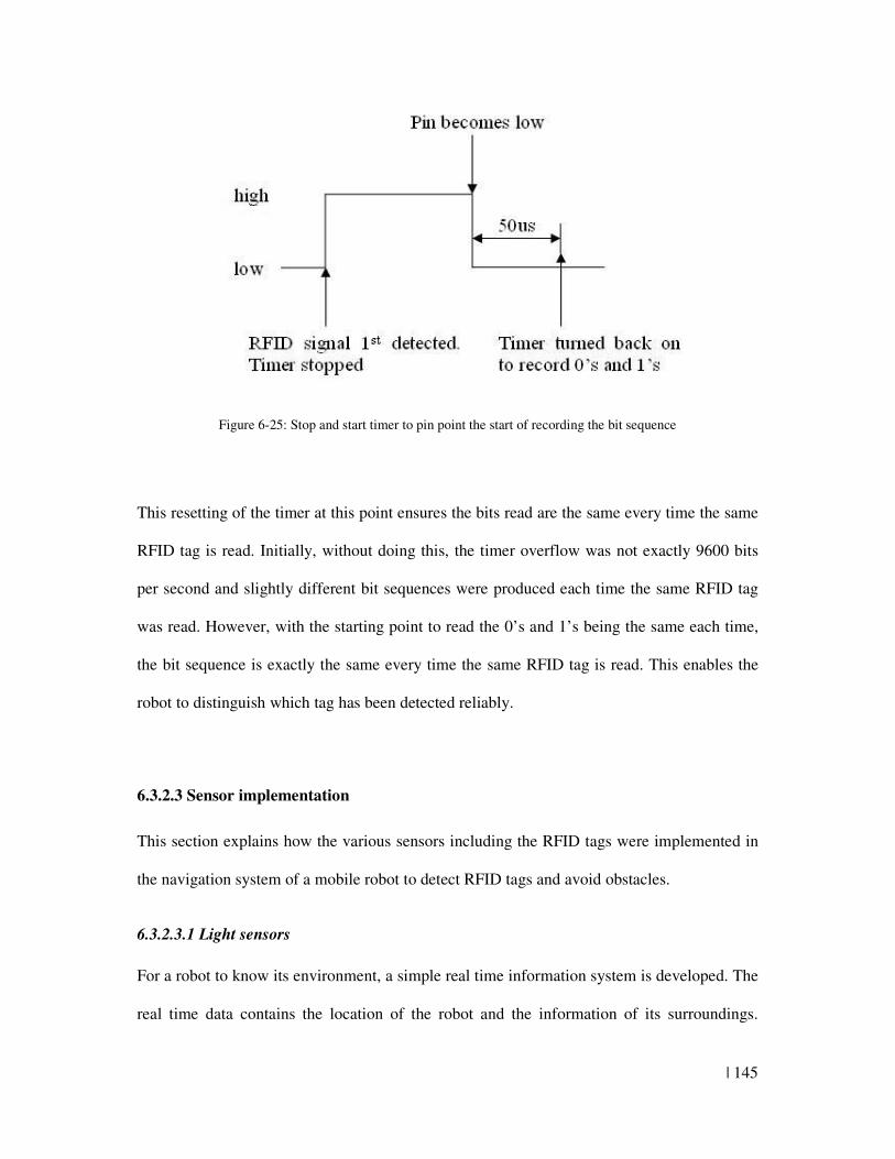
| 145

Figure 6-25: Stop and start timer to pin point the start of recording the bit sequence

This resetting of the timer at this point ensures the bits read are the same every time the same

RFID tag is read. Initially, without doing this, the timer overflow was not exactly 9600 bits

per second and slightly different bit sequences were produced each time the same RFID tag

was read. However, with the starting point to read the 0’s and 1’s being the same each time,

the bit sequence is exactly the same every time the same RFID tag is read. This enables the

robot to distinguish which tag has been detected reliably.

6.3.2.3 Sensor implementation

This section explains how the various sensors including the RFID tags were implemented in

the navigation system of a mobile robot to detect RFID tags and avoid obstacles.

6.3.2.3.1 Light sensors

For a robot to know its environment, a simple real time information system is developed. The

real time data contains the location of the robot and the information of its surroundings.

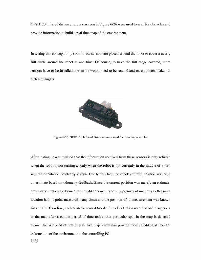
146 |

GP2D120 infrared distance sensors as seen in Figure 6-26 were used to scan for obstacles and

provide information to build a real time map of the environment.

In testing this concept, only six of these sensors are placed around the robot to cover a nearly

full circle around the robot at one time. Of course, to have the full range covered, more

sensors have to be installed or sensors would need to be rotated and measurements taken at

different angles.

Figure 6-26: GP2D120 Infrared distance sensor used for detecting obstacles

After testing, it was realised that the information received from these sensors is only reliable

when the robot is not turning as only when the robot is not currently in the middle of a turn

will the orientation be clearly known. Due to this fact, the robot’s current position was only

an estimate based on odometry feedback. Since the current position was merely an estimate,

the distance data was deemed not reliable enough to build a permanent map unless the same

location had its point measured many times and the position of its measurement was known

for certain. Therefore, each obstacle sensed has its time of detection recorded and disappears

in the map after a certain period of time unless that particular spot in the map is detected

again. This is a kind of real time or live map which can provide more reliable and relevant

information of the environment to the controlling PC.

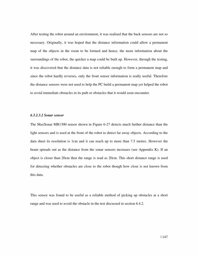
| 147

After testing the robot around an environment, it was realised that the back sensors are not so

necessary. Originally, it was hoped that the distance information could allow a permanent

map of the objects in the room to be formed and hence, the more information about the

surroundings of the robot, the quicker a map could be built up. However, through the testing,

it was discovered that the distance data is not reliable enough to form a permanent map and

since the robot hardly reverses, only the front sensor information is really useful. Therefore

the distance sensors were not used to help the PC build a permanent map yet helped the robot

to avoid immediate obstacles in its path or obstacles that it would soon encounter.

6.3.2.3.2 Sonar sensor

The MaxSonar MB1300 sensor shown in Figure 6-27 detects much further distance than the

light sensors and is used at the front of the robot to detect far away objects. According to the

data sheet its resolution is 1cm and it can reach up to more than 7.5 metres. However the

beam spreads out as the distance from the sonar sensors increases (see Appendix K). If an

object is closer than 20cm then the range is read as 20cm. This short distance range is used

for detecting whether obstacles are close to the robot though how close is not known from

this data.

This sensor was found to be useful as a reliable method of picking up obstacles at a short

range and was used to avoid the obstacle in the test discussed in section 6.4.2.

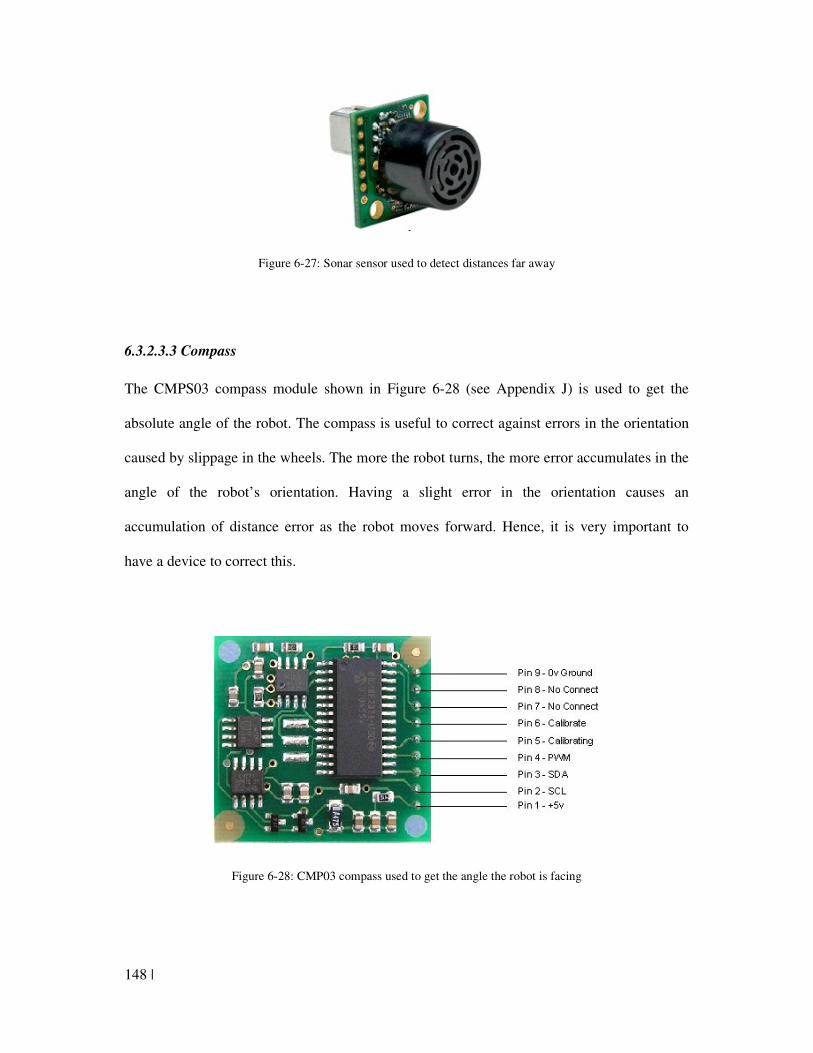
148 |

Figure 6-27: Sonar sensor used to detect distances far away

6.3.2.3.3 Compass

The CMPS03 compass module shown in Figure 6-28 (see Appendix J) is used to get the

absolute angle of the robot. The compass is useful to correct against errors in the orientation

caused by slippage in the wheels. The more the robot turns, the more error accumulates in the

angle of the robot’s orientation. Having a slight error in the orientation causes an

accumulation of distance error as the robot moves forward. Hence, it is very important to

have a device to correct this.

Figure 6-28: CMP03 compass used to get the angle the robot is facing

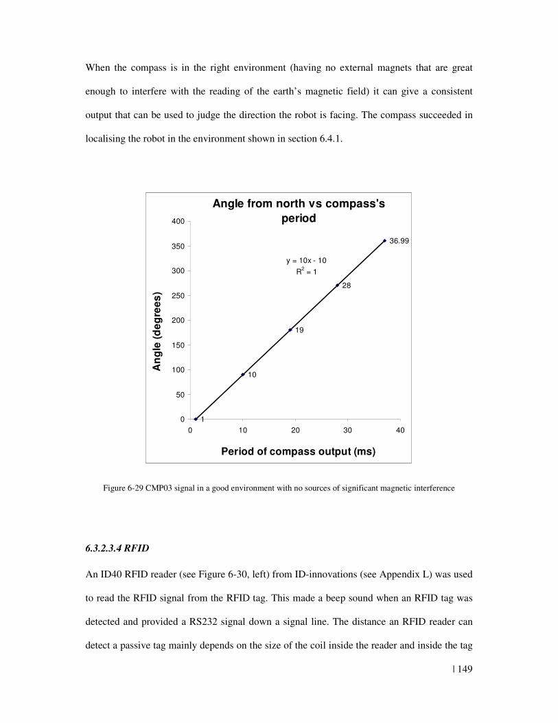
| 149

When the compass is in the right environment (having no external magnets that are great

enough to interfere with the reading of the earth’s magnetic field) it can give a consistent

output that can be used to judge the direction the robot is facing. The compass succeeded in

localising the robot in the environment shown in section 6.4.1.

Angle from north vs compass's

period

1

10

19

28

36.99

y = 10x - 10

R2 = 1

0

50

100

150

200

250

300

350

400

0 10 20 30 40

Period of compass output (ms)

An

gle

(d

eg

ree

s)

Figure 6-29 CMP03 signal in a good environment with no sources of significant magnetic interference

6.3.2.3.4 RFID

An ID40 RFID reader (see Figure 6-30, left) from ID-innovations (see Appendix L) was used

to read the RFID signal from the RFID tag. This made a beep sound when an RFID tag was

detected and provided a RS232 signal down a signal line. The distance an RFID reader can

detect a passive tag mainly depends on the size of the coil inside the reader and inside the tag

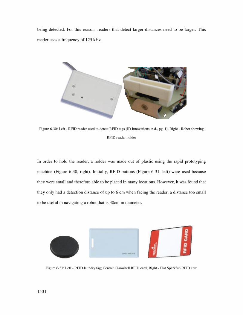
150 |

being detected. For this reason, readers that detect larger distances need to be larger. This

reader uses a frequency of 125 kHz.

Figure 6-30: Left - RFID reader used to detect RFID tags (ID Innovations, n.d., pg. 1); Right - Robot showing

RFID reader holder

In order to hold the reader, a holder was made out of plastic using the rapid prototyping

machine (Figure 6-30, right). Initially, RFID buttons (Figure 6-31, left) were used because

they were small and therefore able to be placed in many locations. However, it was found that

they only had a detection distance of up to 6 cm when facing the reader, a distance too small

to be useful in navigating a robot that is 30cm in diameter.

Figure 6-31: Left - RFID laundry tag; Centre: Clamshell RFID card; Right - Flat Sparkfun RFID card

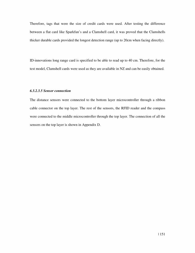
| 151

Therefore, tags that were the size of credit cards were used. After testing the difference

between a flat card like Sparkfun’s and a Clamshell card, it was proved that the Clamshells

thicker durable cards provided the longest detection range (up to 20cm when facing directly).

ID-innovations long range card is specified to be able to read up to 40 cm. Therefore, for the

test model, Clamshell cards were used as they are available in NZ and can be easily obtained.

6.3.2.3.5 Sensor connection

The distance sensors were connected to the bottom layer microcontroller through a ribbon

cable connector on the top layer. The rest of the sensors, the RFID reader and the compass

were connected to the middle microcontroller through the top layer. The connection of all the

sensors on the top layer is shown in Appendix D.

152 |

6.4 Mobile service robot prototype system testing

This section presents three tests that were used to test different functionalities of the robot.

All tests reached their goal successfully although there was a slight error in where their actual

position ended up to be compared to what it should have been. The three tests shows:

•••• The robot’s basic moving from one tag to another using the compass

•••• The robot’s avoiding a simple geometric obstacle that was not previously

recorded in the map

•••• The robot’s moving between several tags in order to reach a destination

6.4.1 Test one – Proving compass

In the first test, the robot was told to move from one tag to another manually at each point,

unlike the third test where the robot is just told the destination and it automatically calculated

the path to travel. The compass worked sufficiently in this environment so was used to

continuously update the robot’s actual orientation whenever the sensor data was read. The

environment used to test the robot is seen in Figure 6-32.

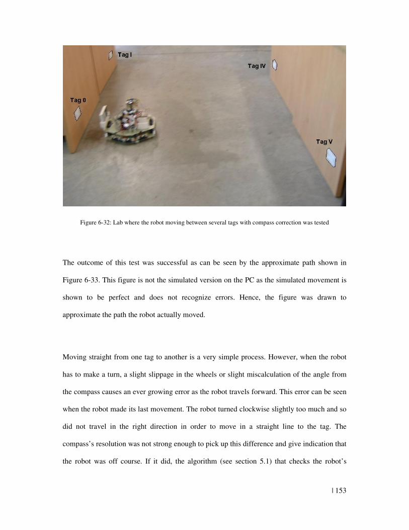
| 153

Figure 6-32: Lab where the robot moving between several tags with compass correction was tested

The outcome of this test was successful as can be seen by the approximate path shown in

Figure 6-33. This figure is not the simulated version on the PC as the simulated movement is

shown to be perfect and does not recognize errors. Hence, the figure was drawn to

approximate the path the robot actually moved.

Moving straight from one tag to another is a very simple process. However, when the robot

has to make a turn, a slight slippage in the wheels or slight miscalculation of the angle from

the compass causes an ever growing error as the robot travels forward. This error can be seen

when the robot made its last movement. The robot turned clockwise slightly too much and so

did not travel in the right direction in order to move in a straight line to the tag. The

compass’s resolution was not strong enough to pick up this difference and give indication that

the robot was off course. If it did, the algorithm (see section 5.1) that checks the robot’s

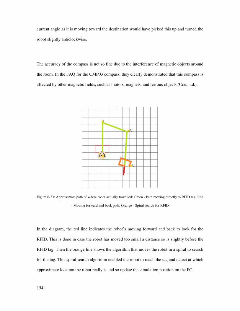
154 |

current angle as it is moving toward the destination would have picked this up and turned the

robot slightly anticlockwise.

The accuracy of the compass is not so fine due to the interference of magnetic objects around

the room. In the FAQ for the CMP03 compass, they clearly demonstrated that this compass is

affected by other magnetic fields, such as motors, magnets, and ferrous objects (Coe, n.d.).

Figure 6-33: Approximate path of where robot actually travelled: Green - Path moving directly to RFID tag; Red

- Moving forward and back path; Orange - Spiral search for RFID

In the diagram, the red line indicates the robot’s moving forward and back to look for the

RFID. This is done in case the robot has moved too small a distance so is slightly before the

RFID tag. Then the orange line shows the algorithm that moves the robot in a spiral to search

for the tag. This spiral search algorithm enabled the robot to reach the tag and detect at which

approximate location the robot really is and so update the simulation position on the PC.

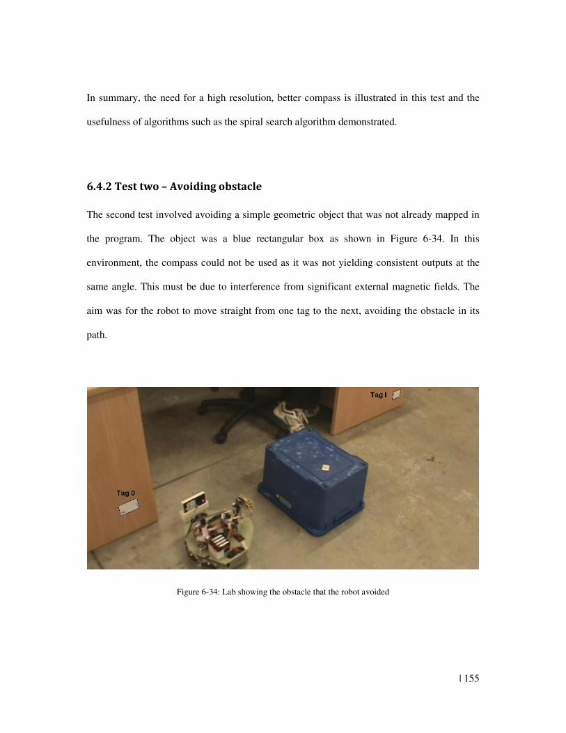
| 155

In summary, the need for a high resolution, better compass is illustrated in this test and the

usefulness of algorithms such as the spiral search algorithm demonstrated.

6.4.2 Test two – Avoiding obstacle

The second test involved avoiding a simple geometric object that was not already mapped in

the program. The object was a blue rectangular box as shown in Figure 6-34. In this

environment, the compass could not be used as it was not yielding consistent outputs at the

same angle. This must be due to interference from significant external magnetic fields. The

aim was for the robot to move straight from one tag to the next, avoiding the obstacle in its

path.

Figure 6-34: Lab showing the obstacle that the robot avoided

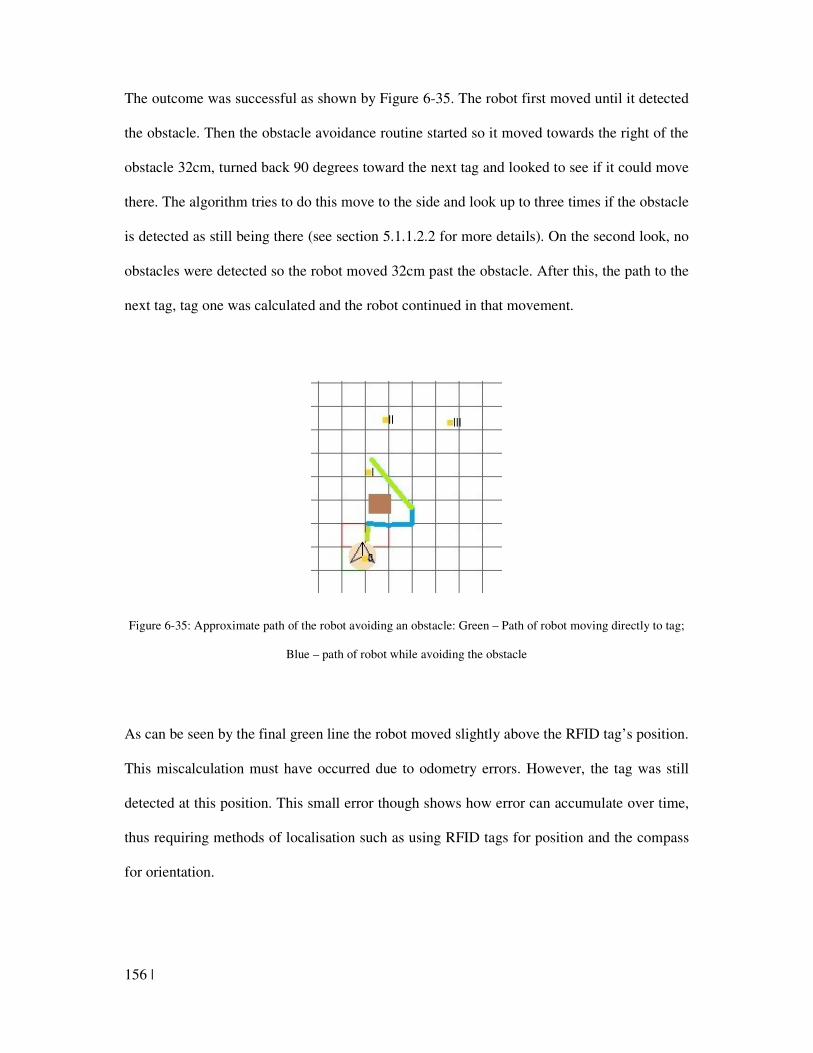
156 |

The outcome was successful as shown by Figure 6-35. The robot first moved until it detected

the obstacle. Then the obstacle avoidance routine started so it moved towards the right of the

obstacle 32cm, turned back 90 degrees toward the next tag and looked to see if it could move

there. The algorithm tries to do this move to the side and look up to three times if the obstacle

is detected as still being there (see section 5.1.1.2.2 for more details). On the second look, no

obstacles were detected so the robot moved 32cm past the obstacle. After this, the path to the

next tag, tag one was calculated and the robot continued in that movement.

Figure 6-35: Approximate path of the robot avoiding an obstacle: Green – Path of robot moving directly to tag;

Blue – path of robot while avoiding the obstacle

As can be seen by the final green line the robot moved slightly above the RFID tag’s position.

This miscalculation must have occurred due to odometry errors. However, the tag was still

detected at this position. This small error though shows how error can accumulate over time,

thus requiring methods of localisation such as using RFID tags for position and the compass

for orientation.

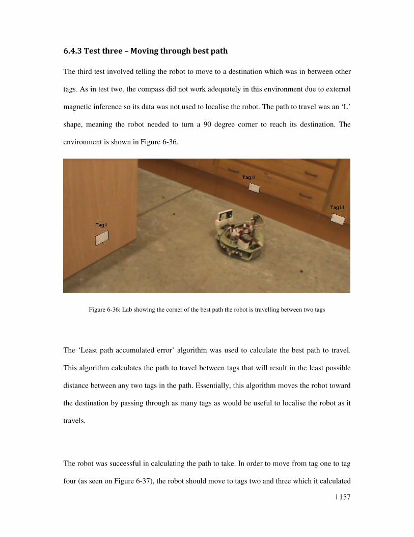
| 157

6.4.3 Test three – Moving through best path

The third test involved telling the robot to move to a destination which was in between other

tags. As in test two, the compass did not work adequately in this environment due to external

magnetic inference so its data was not used to localise the robot. The path to travel was an ‘L’

shape, meaning the robot needed to turn a 90 degree corner to reach its destination. The

environment is shown in Figure 6-36.

Figure 6-36: Lab showing the corner of the best path the robot is travelling between two tags

The ‘Least path accumulated error’ algorithm was used to calculate the best path to travel.

This algorithm calculates the path to travel between tags that will result in the least possible

distance between any two tags in the path. Essentially, this algorithm moves the robot toward

the destination by passing through as many tags as would be useful to localise the robot as it

travels.

The robot was successful in calculating the path to take. In order to move from tag one to tag

four (as seen on Figure 6-37), the robot should move to tags two and three which it calculated

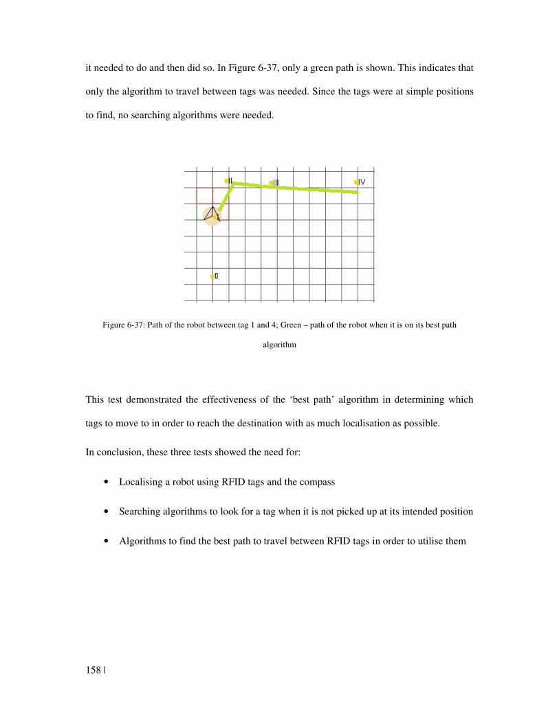
158 |

it needed to do and then did so. In Figure 6-37, only a green path is shown. This indicates that

only the algorithm to travel between tags was needed. Since the tags were at simple positions

to find, no searching algorithms were needed.

Figure 6-37: Path of the robot between tag 1 and 4; Green – path of the robot when it is on its best path

algorithm

This test demonstrated the effectiveness of the ‘best path’ algorithm in determining which

tags to move to in order to reach the destination with as much localisation as possible.

In conclusion, these three tests showed the need for:

• Localising a robot using RFID tags and the compass

• Searching algorithms to look for a tag when it is not picked up at its intended position

• Algorithms to find the best path to travel between RFID tags in order to utilise them

| 159

Chapter 7: Future improvements

The robot built in this research merely tests the concept of navigating a mobile robot in an

indoor environment using passive RFID tags. Hence, in order to produce a robot to be used in

industry many improvements are needed. This chapter mentions the improvements that could

be made to the mobile robot in order to make it more able to detect obstacles, easier to detect

RFID tags, less likely to make odometry errors, and have a faster communication speed.

Some of these improvements would increase the cost and complexity of the robot so they

may not necessarily make the end product better.

To detect more complex obstacles a servo motor holding an infrared distance sensor could be

used. The servo could then be turned to discrete angles and the distance value read at this

angle. By turning back and forth a broader and more detailed range of looking for obstacles

could be made. Also, using just one sensor at the front would prevent the current need to

change between the different analogue pins to read the analogue value from each distance

sensor (see connections on Appendix E). This would make the program for reading the

analogue data simpler, relieving the need for the microcontroller to keep changing which pin

it is taking its measurement from.

Another method of detecting more complex obstacles would be to process the image received

from the robot’s camera. This data is already received through the camera’s radio waves so

all that would be needed is the algorithms to interpret obstacles from the image and

approximate their distance from the robot. If the camera were correctly modified it could also

provide the approximate distance of the objects it sees from the robot’s camera (Xiaoming,

160 |

Tian, Wanchun, 2010). If this could be successfully carried out, the height and shape of

obstacles could be determined. This would require a different method of mapping the

obstacles unless the data was simplified to be a 2D representation.

The detection of the RFID tags that localise the robot could also be improved in a number of

ways. Presently, the robot used in this research only has a RFID reader on its left side. To

make detection of obstacles easier, another reader should be placed on its right side so that

RFID tags to the right of the robot can be detected without needing the robot to turn around.

Also, higher frequencies of RFID could be looked at as they have a greater distance of

detection range. Some have even used high frequencies with long enough ranges so that the

mobile robot can detect three RFID tags at one time and use the power of these signals to

estimate the robots current location (Oktem & Aydin, 2010). Such a method could be

investigated to improve the robot’s localisation.

The robot’s error in odometry could be minimized through using a compass less affected by

external magnetic fields. The current compass used had many problems due to external

magnetic fields as it does not have any protection against them. Due to this it could not be

used to accurately correct the robot’s error in orientation in an environment with significant

magnetic fields. The robot’s odometry error could also be minimised by having a bigger

omniwheel at the front of the robot. Currently, the wheel is 10mm in diameter. This is small

considering the size of the rest of the robot. Having a larger diameter would allow the wheel

to properly touch the ground on uneven surfaces, making the robot less likely to slip in

environments with slight dents or grooves on their surface.

| 161

The speed of the wireless communication greatly affects the amount and frequency of the

data that is sent to the computer about the robot’s surroundings. Increasing the baud rate from

the current value of 9600bps to higher value may help to increase the speed. Other wireless

protocols like Wi-Fi could also be considered as Wi-Fi can communicate information at a

much faster speed than XBee can. Faster communication would allow more data about the

robot’s environment to be obtained at a faster speed, allowing better decisions to be made

about how to control the robot.

The reliability of the robot also needs to be increased to ensure that its movement does not

harm itself or others, and that there is no chance of a serious fault occurring when some

unexpected situation arises. Safety and fault-preventing features would need to be

implemented on this research’s robot before it could be used as a commercial or industrial

product. This may include more emergency stop features like push buttons on the side of the

robot to ensure the robot stops if it touches an obstacle.

162 |

Chapter 8: Summary and Conclusions

8.1 Summary

This research has firstly shown a brief history of the development of mobile robots from the

Chinese development of a mechanical warrior in 1023-957bc to the development of

microcontrollers allowing more complex tasks to be done. The various interoperating

methods in place to help navigate a robot to a certain destination have been discussed. These

were:

• guiding the robot by using a map

• using odometry to estimate the robot’s current position

• using localisation techniques to reset odometry’s accumulated errors

• using an algorithm to determine how the robot travels in order to reach its goal

• using sensors so that the robot can avoid damaging itself or others

Mobile robots are essential for developing the modern world as they are increasing in ability

and have a vast range of applications.

The environment used in this research is defined as:

• small, so that wireless communication can be continuous

• flat so that the robot’s position can be determined most accurately using odometry

• free from obstacles that have thin parts on them hard to detect

| 163

The robot itself is constrained to be one that is inexpensive and simple. This would allow

others to replicate its concept and improve it. Its mechanical system is a three-wheeled robot

with two stepper motors moving the robot and a third to balance it. Using three wheels is

more stable than two and allows the robot to turn around while changing only the orientation,

not the linear position. Stepper motors allow the robot to move set known distances so that

the robot’s position can be estimated using odometry. Fibreglass, a light yet strong material,

has been used as the basic structure that holds the robot’s sensors, circuit boards, and motors.

An omniwheel, composed of a spherical ball resting on three shafts, was used at the front of

the robot to follow the movement of the other two wheels. Using such a ball enabled the

robot to be turned and moved with full freedom, as opposed to the resistance created by a

swivel wheel.

The stepper motors used were powered by two electromagnets, driven by a L298 dual full-

bridge driver that takes in control signals from a L297 stepper motor controller. These two

ICs allowed the motor to be controlled by a simple square wave from the microcontroller. An

external DAC was used to control the peak current of the motors through giving an analogue

value to the L297 motor controller. Infrared and sonar sensors were chosen for the robot and

their data processed to detect obstacles blocking the robot’s path. The compass and the RFID

reader proved to be useful in localising the robot.

An XBee module at the PC and the robot allows transmission of the PC commands to the

robot and the sensors’ data back to the computer. The camera’s radio transmitter enables live

video from the robot to be captured and recorded on the PC.

164 |

Two ways of map building have been presented. The first is for a user to manually measure

RFID tags’ distances from one another, determine their positions on a map, and then put this

position information manually onto the mapping software. The second is to build a map

automatically through controlling a mobile robot, having the program simulate its position in

the environment, and placing RFID tags on the map as it detects them.

Algorithms that use the maps made to navigate the robot made have been presented. These

algorithms enable the robot to avoid obstacles in its path, plan how to move between several

tags in order to more accurately reach a destination, and search around to find a tag when the

robot has arrived at the position it expects it to be. The algorithms made have been tested by

the program made on the computer. This program is able to simulate the robots movement

and uses this simulation to decide how the robot should move. Three tests of these algorithms

in the designed robot have been demonstrated that illustrate the need of an accurate, stable

compass to correct the robot’s orientation, the problem occurring from wheel slippage, and

the benefit of using searching algorithms that make up for inaccuracies in robot movement.

The mobile robot made has shown that the method of localising a robot using passive RFID

tags within an indoor environment works successfully.

| 165

8.2 Conclusions

To conclude, this research has shown:

• A mobile robot can be effectively located through using passive RFID tags around an

indoor environment

• Using passive RFID tags can mean an environment can be quickly created with little

expense

• An RFID map can be built accurately and quickly through automatically detecting the

tags as the robot moves past them

• Intelligent searching algorithms can help a robot overcome position problems caused

by the accumulated error resulting from odometry

• It is not safe to use a low resolution of distance data to build a permanent map due to

the mere estimation of position using odometry

• Back sensors are not useful as their distance measurement is not reliable enough (due

to position error) to be kept in the long term

166 |

References:

Abiyev, R., Ibrahim, D., & Erin, B. (2010) Navigation of mobile robots in the presence of

obstacles. Advances in Engineering Software, 41(10), 1179-1186.

Acroname Robotics. (2011). Hokuyo URG-04LX-UG01 laser. Retrieved December 17, 2011

from: http://www.acroname.com/robotics/parts/R325-URG-04LX-UG01.html.

Advanced Safety Devices. (2012). How Does A Digital Electronic Compass Work? Retrieved

July 30, 2011 from: http://www.safety-devices.com/how_compass_works.htm.

Anderson, A., Labay, V. (2006). Ethical considerations and proposed guidelines for the use

of radio frequency identification: especially concerning its use for promoting public

safety and national security. Science and Engineering Ethics, 12, 265-272.

ARC Electronics. (n.d.) RS232 Tutorial on Data Interface and cables. Retrieved November

1, 2011 from: http://www.arcelect.com/rs232.htm.

Atmel. (2009). 8-bit microcontroller with 32K bytes in-system programmable flash

[Datasheet]. Retrieved December 20, 2012 from:

http://www.wvshare.com/datasheet/ATMEL_PDF/ATmega32.PDF.

Bakar, M., Nagarajan, R., & Saad, A. (2011). Development of a doctor following mobile

robot with mono-vision based marker detection. Applied power electronics colloquium

(IAPEC), 2011 IEEE, 86-91.

Batalin, M, A., & Sukhatme, G. (2004). Mobile Robot Navigation using a Sensor Network. In

IEEE International Conference on Robotics and Automation (pp. 636-642). New

Orleans, LA: (Press).

| 167

Benmounah, A., & Abbassi, H. (1999). Obstacle detection and decision making for intelligent

mobile robot. Lecture notes in control and information sciences, 243, 537-546.

Braaten, B., Feng, Y., Nelson, R. (2006). High-frequency RFID tags: an analytical and

numerical approach for determining the induced currents and scattered fields,

Proceedings of the 2006 IEEE international symposium on electromagnetic

compatibility (n. page #). Portland, Oregon.

Caruso, M. (n.d.). Applications of magnetoresistive sensors in navigation systems. Retrieved

from: http://www51.honeywell.com/aero/common/documents/myaerospacecatalog-

documents/Defense_Brochures-documents/Magnetic__Literature_Technical_Article-

documents/Applications_of_Magnetoresistive_Sensors_in_Navigation_Systems.pdf.

Coe, G. (n.d.). CMPS03 faq. Retrieved July 1, 2012 from: http://www.robot-

electronics.co.uk/htm/cmpsqa.shtml.

Collet, T., Macdonald, B. Gerkey, B. (2005). Player 2.0: toward a practical robot

programming framework, Proceedings of the Australian conference on robotics and

automation, ACRA.

Demmel, J. (1996). CS267: Notes for Lecture 24, Apr 11 1996 Retrieved July 19, 2011 from:

http://www.cs.berkeley.edu/~demmel/cs267/lecture26/lecture26.html.

Digi International. (2009). XBee®/XBee-PRO® ZB RF modules. [Manual] Retrieved July 15,

2011 from: ftp://ftp1.digi.com/support/documentation/90000976_C.pdf.

Disabled world. (2009). 3 wheel 4 wheel and compact mobility scooters. Retrieved December

17, 2011 from: http://www.disabled-

world.com/assistivedevices/mobility/scooters/choices.php.

Dudek, G., & Jenkin, M. (2010). Computational principles of mobile robotics. (2nd. ed.).

Cambridge, United Kingdom: Cambridge University Press.

168 |

Dudek, G., Jenkin, M., Milios, E., & Wilkes, D. (1991) Robotic exploration as graph

construction. IEEE transactions on robotics and automation, 7(6), 859-865.

Embedded computing design. (2011). Smart energy apps making the move to ZigBee: Q&A

with Oyvind Strom, PhD, Senior Director of Wireless Microcontrollers, Atmel

Corporation. Retrieved December 19, 2011 from: http://embedded-

computing.com/smart-microcontrollers-atmel-corporation-2#ixzz1Xs7COh4m.

Fabrizi, E., Saffiotti, A. (2002). Augmenting topology-based maps with geometric

information. Robotics and autonomous systems, 40(2-3), 91-97.

FerroxCube International. (2009). Introducción. Retreived July 27, 2012 from:

http://www.ferroxtag.com/RFID/CP.LFHFUHF.htm.

Ge, S., & Cui, Y. (2002). Dynamic motion planning for mobile robots using potential field

method. Autonomous robots, 13(3), 207-222.

Gerald Coe. (n.d.). CMPS03 faq. Retrieved July 1, 2012 from: http://www.robot-

electronics.co.uk/htm/cmpsqa.shtml.

Gupta, S., Messonm C., Demidenko, S. (2005). Real-time identification and predictive

control of fast mobile robots using global vision sensing. IEEE transactions on

instrumentations and measurement, 54(1), 200-214.

Ghoshray, S., & Yen, K. (1996). A comprehensive robot collision avoidance scheme by two-

dimensional geometric modeling. International conference on robotics and automation,

(2), 1087-1092.

Henlich, O. (1997). Report Mobile Robot Navigation. Retrieved June 20, 2010 from:

http://www.doc.ic.ac.uk/~nd/surprise_97/journal/vol4/jmd/.

| 169

Henlich, O. (1997). Vision-based positioning. Retrieved June 21, 2010 from:

http://www.doc.ic.ac.uk/~nd/surprise_97/journal/vol2/oh/.

Honeywell. (n.d.). Solid state hall effect sensors: High performance miniature radiometric

linear SS490 series [Datasheet]. Retrieved March 23, 2010 from:

http://sensing.honeywell.com/index.php?ci_id=50313.

Honeywell. (2011). Magnetic sensors product catalog. Retrieved November 20, 2011 from

http://www51.honeywell.com/aero/common/documents/myaerospacecatalog-

documents/Missiles-Munitions/Sensors_Product__Catalog.pdf.

Hoskins, S., Sobering, T., Andresen, D., Warren, S. (2009). Near-field wireless magnetic link

for an ingestible cattle health monitoring pull. In Engineering in medicine and biology

society, Proceedings of the annual international conference of the IEEE (pp. 5401-

5404). Manhattan, KS: Department of electrical & computer engineering.

ID Innovations. (n.d.). ID-40 Manual RFID medium range reader. [Manual].

Isom, J. (2005). Megagiant robotics. Retrieved December 16, 2011 from:

http://robotics.megagiant.com/history.html.

Kim, J. (2004). A Framework for Roadmap-Based Navigation and Sector-Based Localization

of Mobile Robots. Texas A&M University, College Station, USA.

Kriechbaum, L. (2006) Tools and algorithms for mobile robot navigation with uncertain

localization. Retrieved from: Caltech thesis. Dissertation (Ph.D.), California Institute of

Technology, USA. http://resolver.caltech.edu/CaltechETD:etd-06012006-150109.

Lambrinos, D., Möller, R., Labhart, T., Pfeifer, R., & Wehner, R. (1999). A mobile robot

employing insect strategies for navigation. Robotics and Automation Systems, 30(1), 39-

64.

170 |

Mancini, R. (2002). Op amps for everyone. Retrieved from:

http://www.ti.com/lit/an/slod006b/slod006b.pdf.

Manoonpong, P., & Worgotter, F. (2009). Efference copies in neural control of dynamic

biped walking. Robotics and Autonomous Systems. 57, 1140-1153.

MaxSonar. (2011). MB1200-MB1300 sonar range finder with high power output, noise

rejection, auto calibration & long-range wide detection zone [Datasheet]. Retrieved from:

http://www.maxbotix.com/documents/MB1200-MB1300_Datasheet.pdf.

Moravec, H. (n.d.) Robot. Encyclopaedia Britannica. Retrieved 16 December 2011 from:

http://www.britannica.com/EBchecked/topic/505818/robot.

Noor, A., & Lobeck, W. (2008). Moving on their own. Mechanical engineering, November

2008 Issue, 27-31.

Oktem, R., & Aydin, E. (2010). An RFID based indoor tracking method for navigating

visually impaired people. Turk J Elec Eng & Comp Sci, 18(2), 185-195.

Oriolo, G., Ulivi, G., Venditteli, M. (1997). A new tool for mobile robot perception and

planning. Journal of robotics systems, 14(3), 179-197.

Park, J., Ji, Y. (2009). Location estimation using passive RFID tags in an indoor

environment. International Journal of Modern Physics Company. 20(4), 619-632.

Persuad, D. (n.d.). Implementation_How-toRFID. Retrieved July 27, 2012 from:

http://rfidjournal.com/whitepapers/download/220.

Racz, R., Schott, C., & Huber, S. (2004). Electronic compass sensor. IEEE. 3, 1446-1449.

Robot Electronics. (2007). CMPS03 documentation. Retrieved February 2, 2011 from:

http://www.robot-electronics.co.uk/htm/cmps3tech.htm.

| 171

Robotics/navigation/collision_avoidance. (n.d.). Retrieved May, 1, 2010 from Wikibooks:

http://en.wikibooks.org/wiki/Robotics/Navigation/Collision_Avoidance.

Robotics/navigation/mapping. (n.d.). Retrieved May 1, 2010 from Wikibooks:

http://en.wikibooks.org/wiki/Robotics/Navigation/Mapping.

RFID Journal. (n.d.). The basics of RFID technology. Retrieved July 27 from:

http://www.rfidjournal.com/article/articleview/1337/1/129/.

RTA PDF Catalogue. (n.d.) The general catalogue of sanyo denki stepping motors. Retrieved

May 10, 2010 from: http://pdf.directindustry.com/pdf/rta/the-general-catalogue-of-

sanyo-denki-stepping-motors-20651-50655.html.

Sharp Corporation. (2006). GP2D120 Optoelectronic Device [Datasheet]. Retrieved from:

http://www.sharpsma.com/webfm_send/1205.

Shih, B., Chen, C., Chou, W. (2010). Obstacle avoidance using a path correction method for

autonomous control of a biped intelligent robot. Journal of Vibration and Control,

17(10), 1567-1573.

Shi, C., Wang, Y., & Yang, J. (2010). A local obstacle avoidance method for mobile robots in

partially known environment. Robotics and autonomous systems, 58(5), 425-434.

Suksakulchai, S., Thongchai, S., Wilkes, D., & Kawamura, K. (2000). Mobile robot

localization using an electronic compass for corridor environment. IEEE, 5, 3354-3359.

Swedberg, C. (2011). Intrusion-detecting sensors protect borders, troops. RFID Journal.

Retrieved 8 December from: http://www.rfidjournal.com/article/articleview/8972.

Swedberg, C. (2011). Canadian Investment Group RFID-Enables Shareholder Elections.

RFID Journal. Retireved 9 December from:

http://www.rfidjournal.com/article/articleview/9030.

172 |

Swedberg, C. (2011). Active e-seals expedite cargo shipments in Taiwan. RFID Journal.

Retrieved 28 October from: http://www.rfidjournal.com/article/view/8907/1.

Xerafy. (2011). Xerafy introduces XS, the world’s smallest RFID tag for surgical instruments

and tool tracing. Retrieved 4 November from: http://www.xerafy.com/news/xerafy-

introduces-xs-worlds-smallest-rfid-tag-surgical-instruments-and-tool-tracking-0.

Xiaoming, L., Tian, Q., Wanchun, C. (2010). Real-time distance measurement using a

modified camera. Symposium conducted at the Sensors applications symposium,

Limerick, Ireland.

Yates, D., Vaessen, C., Roupret, M. (2011). From Leonardo to da vinci: the history of robot-

assisted surgery in urology. BJU international, 108(11), 1708-1713.

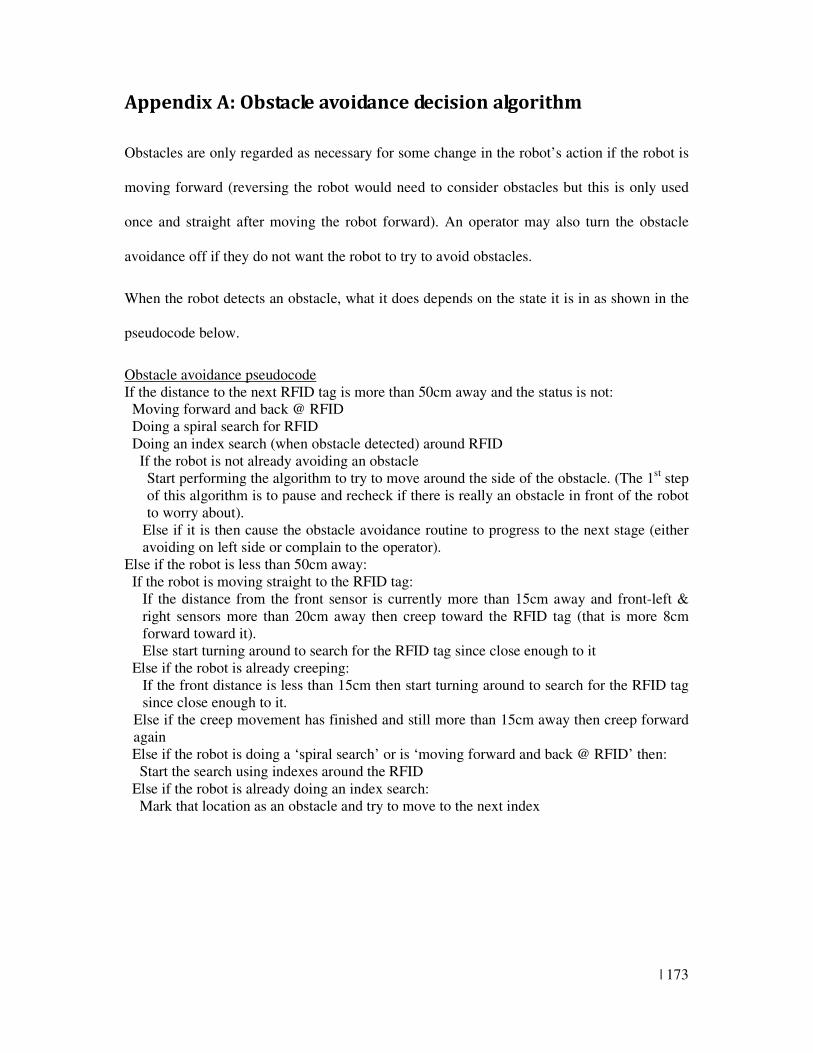
| 173

Appendix A: Obstacle avoidance decision algorithm

Obstacles are only regarded as necessary for some change in the robot’s action if the robot is

moving forward (reversing the robot would need to consider obstacles but this is only used

once and straight after moving the robot forward). An operator may also turn the obstacle

avoidance off if they do not want the robot to try to avoid obstacles.

When the robot detects an obstacle, what it does depends on the state it is in as shown in the

pseudocode below.

Obstacle avoidance pseudocode If the distance to the next RFID tag is more than 50cm away and the status is not: Moving forward and back @ RFID Doing a spiral search for RFID Doing an index search (when obstacle detected) around RFID If the robot is not already avoiding an obstacle

Start performing the algorithm to try to move around the side of the obstacle. (The 1st step of this algorithm is to pause and recheck if there is really an obstacle in front of the robot to worry about).

Else if it is then cause the obstacle avoidance routine to progress to the next stage (either avoiding on left side or complain to the operator).

Else if the robot is less than 50cm away: If the robot is moving straight to the RFID tag:

If the distance from the front sensor is currently more than 15cm away and front-left & right sensors more than 20cm away then creep toward the RFID tag (that is more 8cm forward toward it). Else start turning around to search for the RFID tag since close enough to it

Else if the robot is already creeping: If the front distance is less than 15cm then start turning around to search for the RFID tag since close enough to it.

Else if the creep movement has finished and still more than 15cm away then creep forward again

Else if the robot is doing a ‘spiral search’ or is ‘moving forward and back @ RFID’ then: Start the search using indexes around the RFID Else if the robot is already doing an index search: Mark that location as an obstacle and try to move to the next index

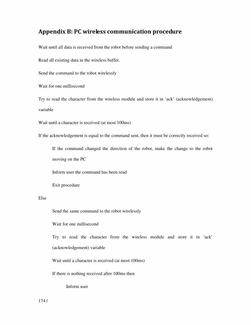
174 |

Appendix B: PC wireless communication procedure

Wait until all data is received from the robot before sending a command

Read all existing data in the wireless buffer.

Send the command to the robot wirelessly

Wait for one millisecond

Try to read the character from the wireless module and store it in ‘ack’ (acknowledgement)

variable

Wait until a character is received (at most 100ms)

If the acknowledgement is equal to the command sent, then it must be correctly received so:

If the command changed the direction of the robot, make the change to the robot

moving on the PC

Inform user the command has been read

Exit procedure

Else

Send the same command to the robot wirelessly

Wait for one millisecond

Try to read the character from the wireless module and store it in ‘ack’

(acknowledgement) variable

Wait until a character is received (at most 100ms)

If there is nothing received after 100ms then

Inform user

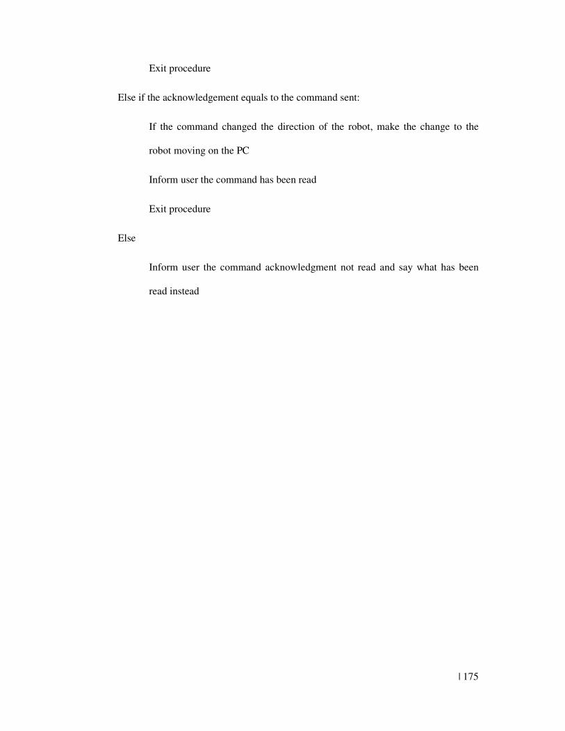
| 175

Exit procedure

Else if the acknowledgement equals to the command sent:

If the command changed the direction of the robot, make the change to the

robot moving on the PC

Inform user the command has been read

Exit procedure

Else

Inform user the command acknowledgment not read and say what has been

read instead

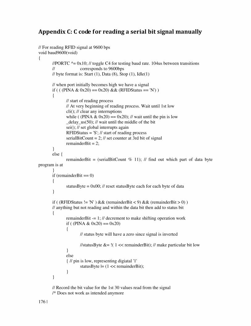
176 |

Appendix C: C code for reading a serial bit signal manually

// For reading RFID signal at 9600 bps void baud9600(void) { //PORTC ^= 0x10; // toggle C4 for testing baud rate. 104us between transitions // corresponds to 9600bps // byte format is: Start (1), Data (8), Stop (1), Idle(1) // when port initially becomes high we have a signal if ( ( (PINA & 0x20) == 0x20) && (RFIDStatus == 'N') ) { // start of reading process // At very beginning of reading process. Wait until 1st low cli(); // clear any interruptions while ( (PINA & 0x20) == 0x20); // wait until the pin is low _delay_us(50); // wait until the middle of the bit sei(); // set global interrupts again RFIDStatus = 'S'; // start of reading process serialBitCount = 2; // set counter at 3rd bit of signal remainderBit = 2; } else { remainderBit = (serialBitCount % 11); // find out which part of data byte program is at } if (remainderBit == 0) { statusByte = 0x00; // reset statusByte each for each byte of data } if ( (RFIDStatus != 'N' ) && (remainderBit < 9) && (remainderBit > 0) ) // anything but not reading and within the data bit then add to status bit { remainderBit -= 1; // decrement to make shifting operation work if ( (PINA & 0x20) == 0x20) { // status byte will have a zero since signal is inverted //statusByte &= !( 1 << remainderBit); // make particular bit low } else { // pin is low, representing digiatal '1' statusByte |= (1 << remainderBit); } } // Record the bit value for the 1st 30 values read from the signal /* Does not work as intended anymore

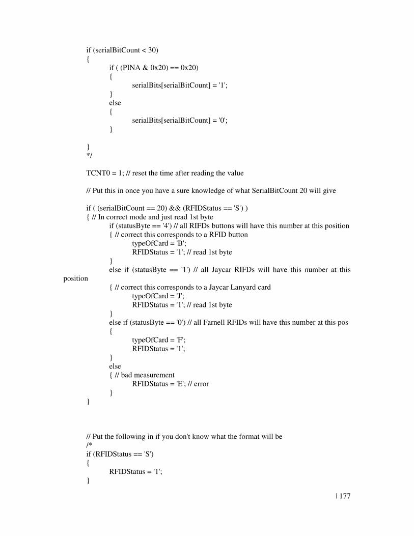
| 177

if (serialBitCount < 30) { if ( (PINA & 0x20) == 0x20) { serialBits[serialBitCount] = '1'; } else { serialBits[serialBitCount] = '0'; } } */ TCNT0 = 1; // reset the time after reading the value // Put this in once you have a sure knowledge of what SerialBitCount 20 will give if ( (serialBitCount == 20) && (RFIDStatus == 'S') ) { // In correct mode and just read 1st byte if (statusByte == '4') // all RIFDs buttons will have this number at this position { // correct this corresponds to a RFID button typeOfCard = 'B'; RFIDStatus = '1'; // read 1st byte } else if (statusByte == '1') // all Jaycar RIFDs will have this number at this position { // correct this corresponds to a Jaycar Lanyard card typeOfCard = 'J'; RFIDStatus = '1'; // read 1st byte } else if (statusByte == '0') // all Farnell RFIDs will have this number at this pos { typeOfCard = 'F'; RFIDStatus = '1'; } else { // bad measurement RFIDStatus = 'E'; // error } } // Put the following in if you don't know what the format will be /* if (RFIDStatus == 'S') { RFIDStatus = '1'; }

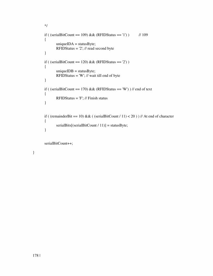
178 |

*/ if ( (serialBitCount == 109) && (RFIDStatus == '1') ) // 109 { uniqueIDA = statusByte; RFIDStatus = '2'; // read second byte } if ( (serialBitCount == 120) && (RFIDStatus == '2') ) { uniqueIDB = statusByte; RFIDStatus = 'W'; // wait till end of byte } if ( (serialBitCount == 170) && (RFIDStatus == 'W') ) // end of text { RFIDStatus = 'F'; // Finish status } if ( (remainderBit == 10) && ( (serialBitCount / 11) < 20 ) ) // At end of character { serialBits[(serialBitCount / 11)] = statusByte; } serialBitCount++; }

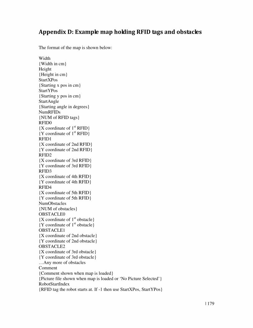
| 179

Appendix D: Example map holding RFID tags and obstacles

The format of the map is shown below: Width {Width in cm} Height {Height in cm} StartXPos {Starting x pos in cm} StartYPos {Starting y pos in cm} StartAngle {Starting angle in degrees} NumRFIDs {NUM of RFID tags} RFID0 {X coordinate of 1st RFID} {Y coordinate of 1st RFID} RFID1 {X coordinate of 2nd RFID} {Y coordinate of 2nd RFID} RFID2 {X coordinate of 3rd RFID} {Y coordinate of 3rd RFID} RFID3 {X coordinate of 4th RFID} {Y coordinate of 4th RFID} RFID4 {X coordinate of 5th RFID} {Y coordinate of 5th RFID} NumObstacles {NUM of obstacles} OBSTACLE0 {X coordinate of 1st obstacle} {Y coordinate of 1st obstacle} OBSTACLE1 {X coordinate of 2nd obstacle} {Y coordinate of 2nd obstacle} OBSTACLE2 {X coordinate of 3rd obstacle} {Y coordinate of 3rd obstacle} …Any more of obstacles Comment {Comment shown when map is loaded} {Picture file shown when map is loaded or ‘No Picture Selected’} RobotStartIndex {RFID tag the robot starts at. If -1 then use StartXPos, StartYPos}

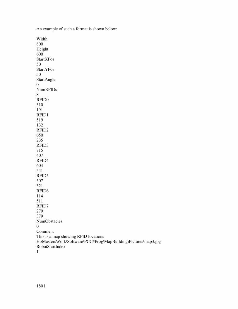
180 |

An example of such a format is shown below: Width 800 Height 600 StartXPos 50 StartYPos 50 StartAngle 0 NumRFIDs 8 RFID0 310 191 RFID1 519 132 RFID2 650 235 RFID3 715 407 RFID4 604 541 RFID5 507 321 RFID6 114 511 RFID7 279 379 NumObstacles 0 Comment This is a map showing RFID locations H:\MastersWork\Software\PCC#Prog\MapBuilding\Pictures\map3.jpg RobotStartIndex 1

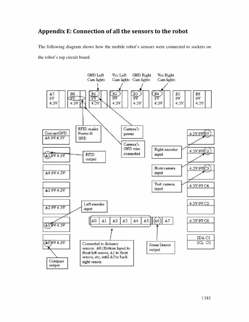
| 181

Appendix E: Connection of all the sensors to the robot

The following diagram shows how the mobile robot’s sensors were connected to sockets on

the robot’s top circuit board.

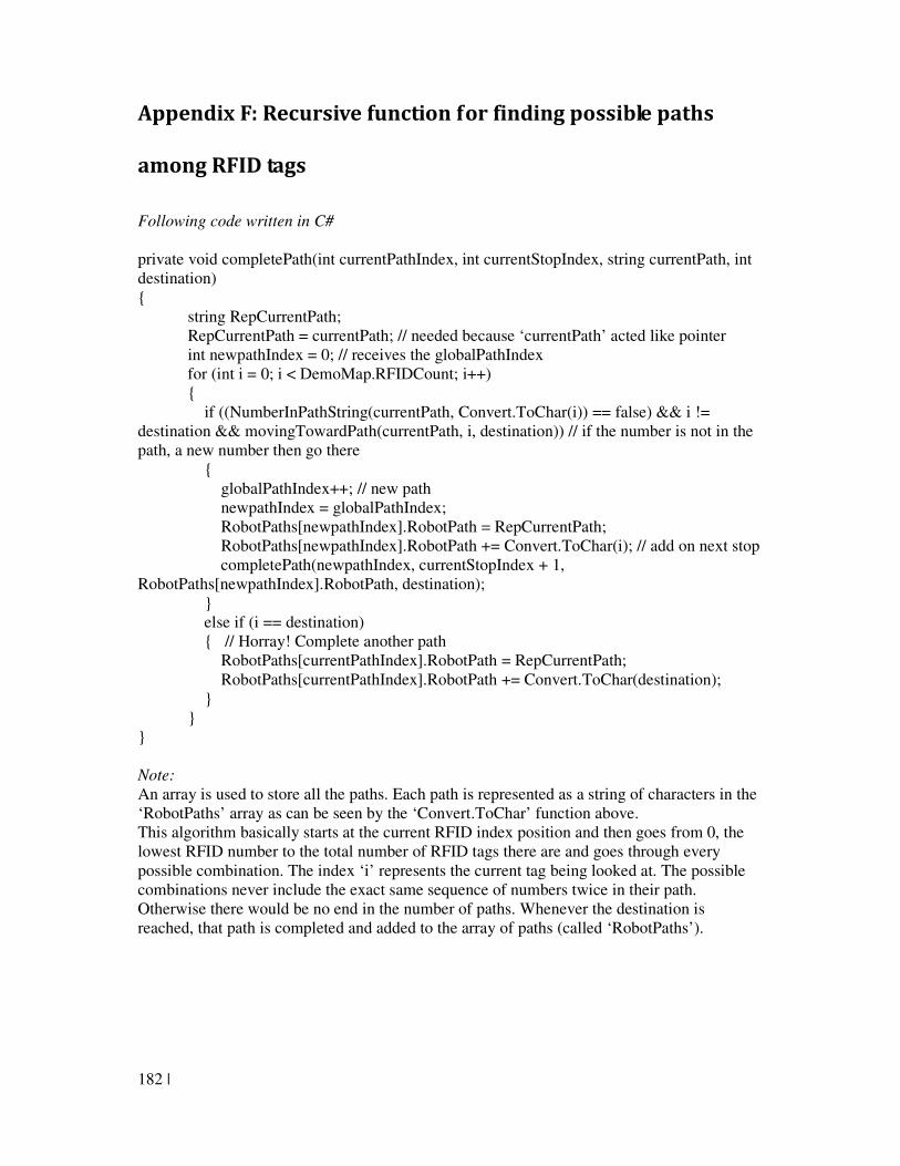
182 |

Appendix F: Recursive function for finding possible paths

among RFID tags

Following code written in C#

private void completePath(int currentPathIndex, int currentStopIndex, string currentPath, int destination) { string RepCurrentPath; RepCurrentPath = currentPath; // needed because ‘currentPath’ acted like pointer int newpathIndex = 0; // receives the globalPathIndex for (int i = 0; i < DemoMap.RFIDCount; i++) { if ((NumberInPathString(currentPath, Convert.ToChar(i)) == false) && i != destination && movingTowardPath(currentPath, i, destination)) // if the number is not in the path, a new number then go there { globalPathIndex++; // new path newpathIndex = globalPathIndex; RobotPaths[newpathIndex].RobotPath = RepCurrentPath; RobotPaths[newpathIndex].RobotPath += Convert.ToChar(i); // add on next stop completePath(newpathIndex, currentStopIndex + 1, RobotPaths[newpathIndex].RobotPath, destination); } else if (i == destination) { // Horray! Complete another path RobotPaths[currentPathIndex].RobotPath = RepCurrentPath; RobotPaths[currentPathIndex].RobotPath += Convert.ToChar(destination); } } } Note:

An array is used to store all the paths. Each path is represented as a string of characters in the ‘RobotPaths’ array as can be seen by the ‘Convert.ToChar’ function above. This algorithm basically starts at the current RFID index position and then goes from 0, the lowest RFID number to the total number of RFID tags there are and goes through every possible combination. The index ‘i’ represents the current tag being looked at. The possible combinations never include the exact same sequence of numbers twice in their path. Otherwise there would be no end in the number of paths. Whenever the destination is reached, that path is completed and added to the array of paths (called ‘RobotPaths’).

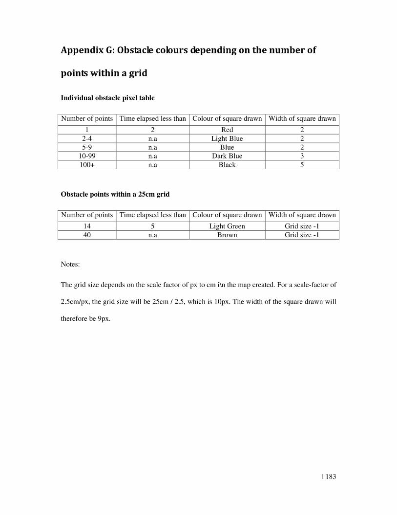
| 183

Appendix G: Obstacle colours depending on the number of

points within a grid

Individual obstacle pixel table

Number of points Time elapsed less than Colour of square drawn Width of square drawn

1 2 Red 2

2-4 n.a Light Blue 2

5-9 n.a Blue 2 10-99 n.a Dark Blue 3

100+ n.a Black 5

Obstacle points within a 25cm grid

Number of points Time elapsed less than Colour of square drawn Width of square drawn

14 5 Light Green Grid size -1

40 n.a Brown Grid size -1

Notes:

The grid size depends on the scale factor of px to cm i\n the map created. For a scale-factor of

2.5cm/px, the grid size will be 25cm / 2.5, which is 10px. The width of the square drawn will

therefore be 9px.

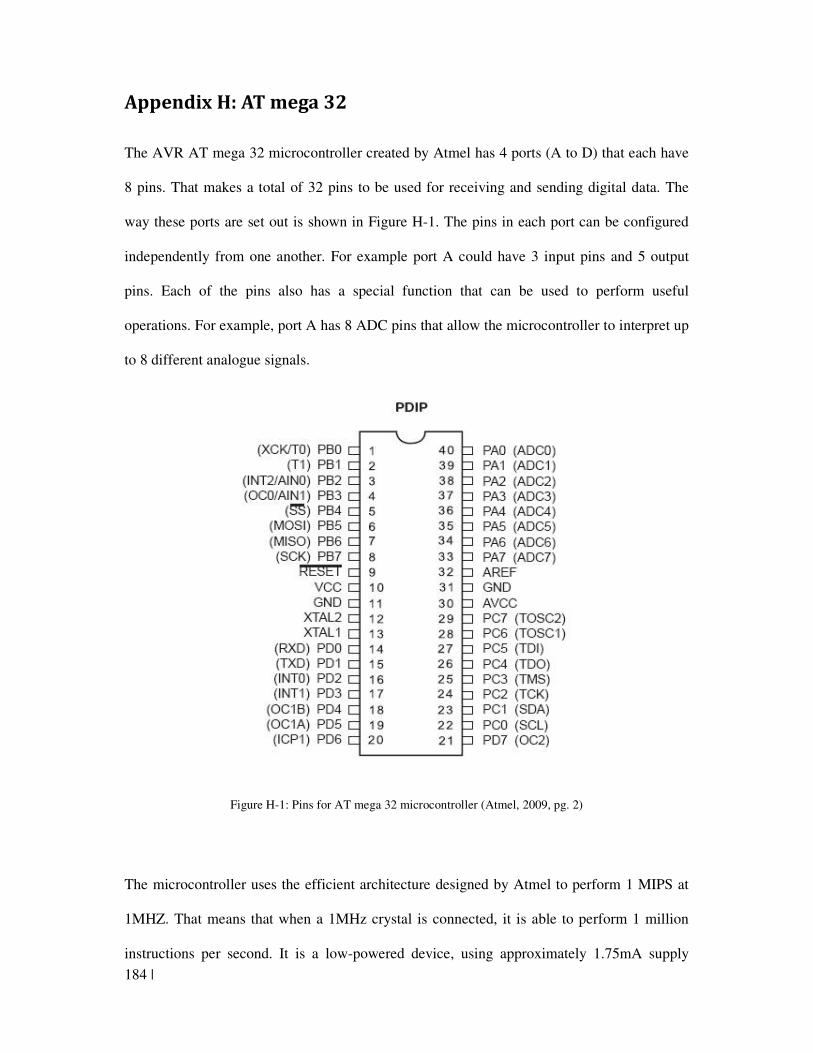
184 |

Appendix H: AT mega 32

The AVR AT mega 32 microcontroller created by Atmel has 4 ports (A to D) that each have

8 pins. That makes a total of 32 pins to be used for receiving and sending digital data. The

way these ports are set out is shown in Figure H-1. The pins in each port can be configured

independently from one another. For example port A could have 3 input pins and 5 output

pins. Each of the pins also has a special function that can be used to perform useful

operations. For example, port A has 8 ADC pins that allow the microcontroller to interpret up

to 8 different analogue signals.

Figure H-1: Pins for AT mega 32 microcontroller (Atmel, 2009, pg. 2)

The microcontroller uses the efficient architecture designed by Atmel to perform 1 MIPS at

1MHZ. That means that when a 1MHz crystal is connected, it is able to perform 1 million

instructions per second. It is a low-powered device, using approximately 1.75mA supply

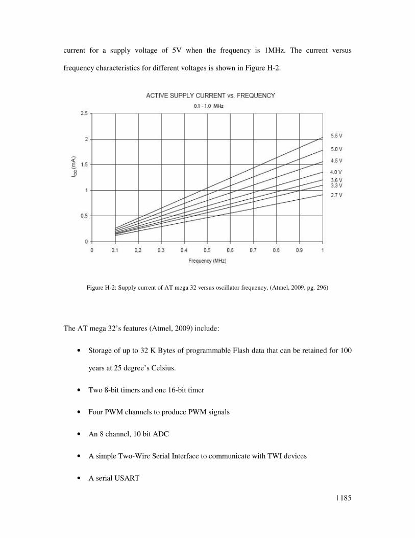
| 185

current for a supply voltage of 5V when the frequency is 1MHz. The current versus

frequency characteristics for different voltages is shown in Figure H-2.

Figure H-2: Supply current of AT mega 32 versus oscillator frequency, (Atmel, 2009, pg. 296)

The AT mega 32’s features (Atmel, 2009) include:

• Storage of up to 32 K Bytes of programmable Flash data that can be retained for 100

years at 25 degree’s Celsius.

• Two 8-bit timers and one 16-bit timer

• Four PWM channels to produce PWM signals

• An 8 channel, 10 bit ADC

• A simple Two-Wire Serial Interface to communicate with TWI devices

• A serial USART

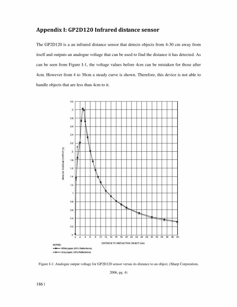
186 |

Appendix I: GP2D120 Infrared distance sensor

The GP2D120 is a an infrared distance sensor that detects objects from 4-30 cm away from

itself and outputs an analogue voltage that can be used to find the distance it has detected. As

can be seen from Figure I-1, the voltage values before 4cm can be mistaken for those after

4cm. However from 4 to 30cm a steady curve is shown. Therefore, this device is not able to

handle objects that are less than 4cm to it.

Figure I-1: Analogue output voltage for GP2D120 sensor versus its distance to an object, (Sharp Corporation,

2006, pg. 4)

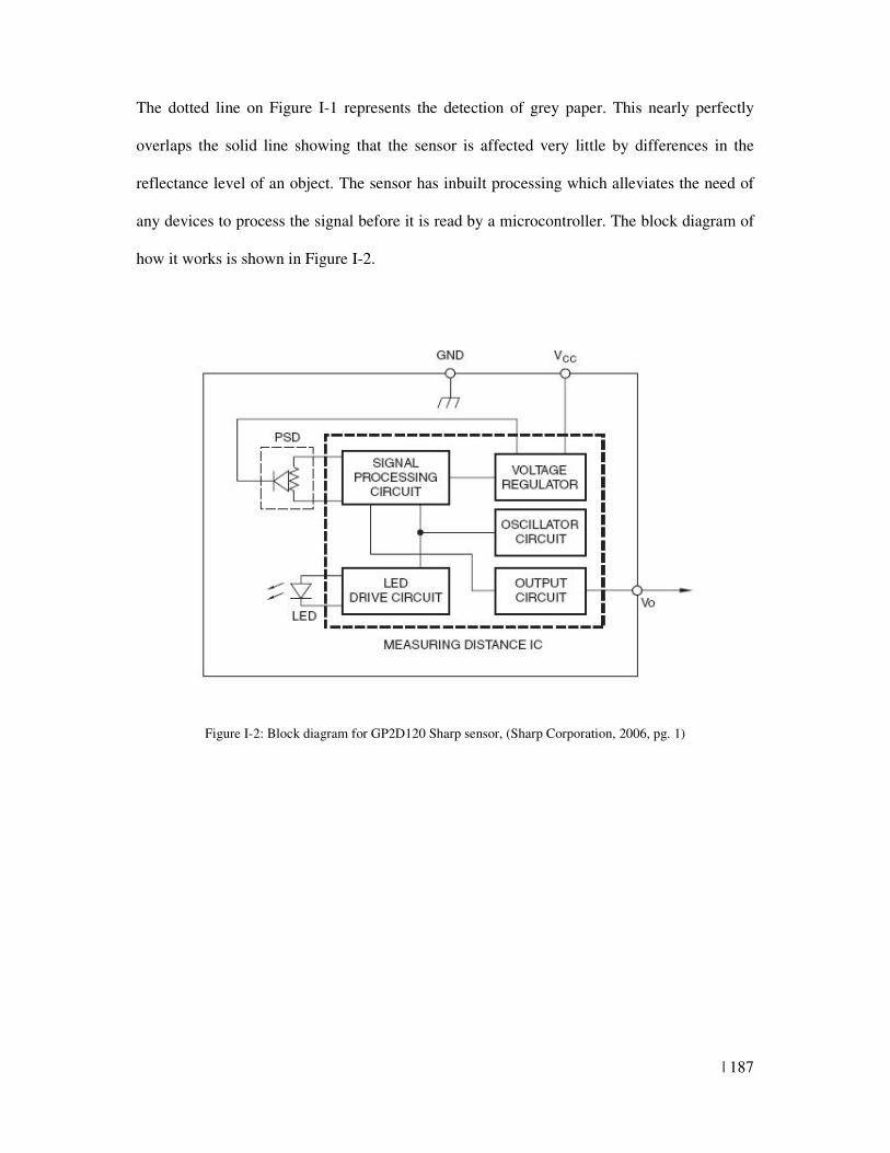
| 187

The dotted line on Figure I-1 represents the detection of grey paper. This nearly perfectly

overlaps the solid line showing that the sensor is affected very little by differences in the

reflectance level of an object. The sensor has inbuilt processing which alleviates the need of

any devices to process the signal before it is read by a microcontroller. The block diagram of

how it works is shown in Figure I-2.

Figure I-2: Block diagram for GP2D120 Sharp sensor, (Sharp Corporation, 2006, pg. 1)

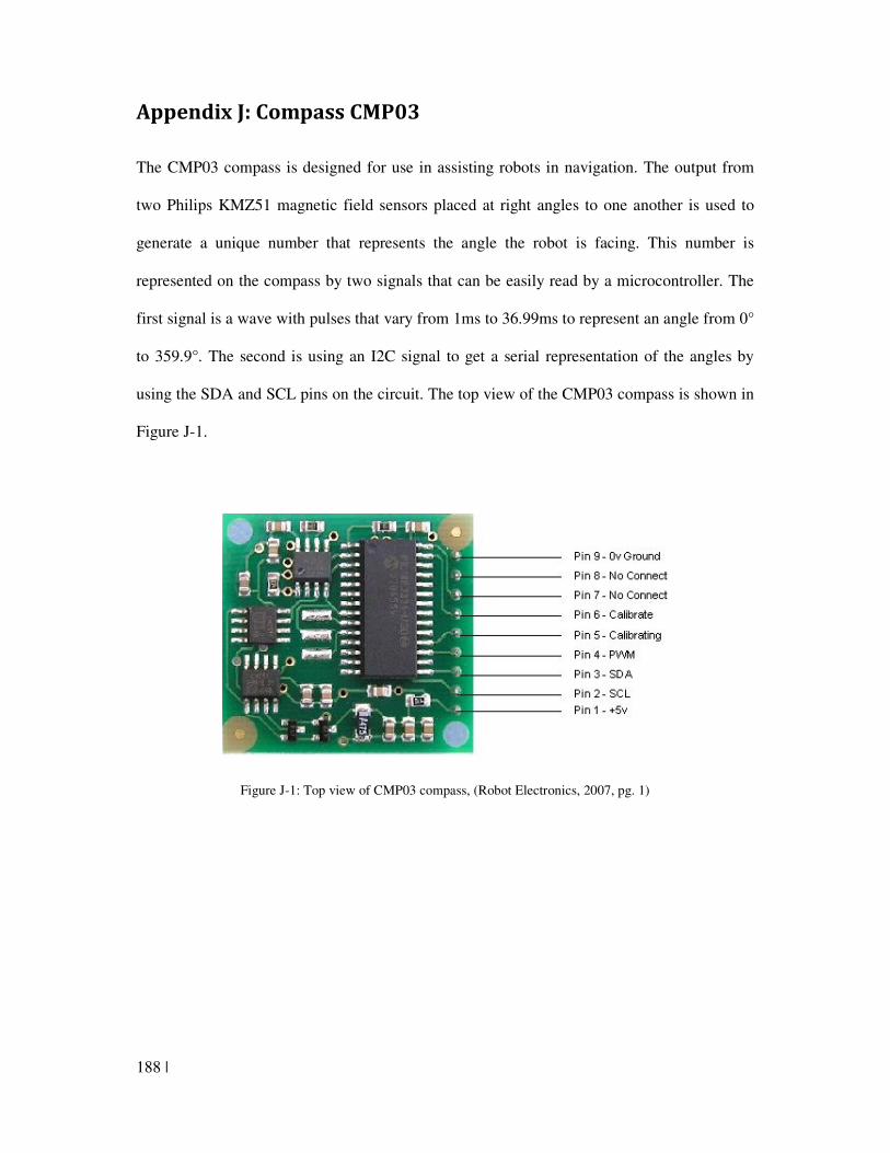
188 |

Appendix J: Compass CMP03

The CMP03 compass is designed for use in assisting robots in navigation. The output from

two Philips KMZ51 magnetic field sensors placed at right angles to one another is used to

generate a unique number that represents the angle the robot is facing. This number is

represented on the compass by two signals that can be easily read by a microcontroller. The

first signal is a wave with pulses that vary from 1ms to 36.99ms to represent an angle from 0°

to 359.9°. The second is using an I2C signal to get a serial representation of the angles by

using the SDA and SCL pins on the circuit. The top view of the CMP03 compass is shown in

Figure J-1.

Figure J-1: Top view of CMP03 compass, (Robot Electronics, 2007, pg. 1)

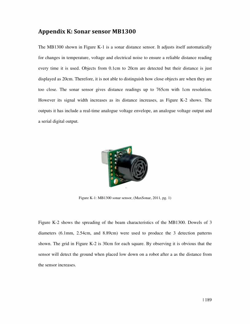
| 189

Appendix K: Sonar sensor MB1300

The MB1300 shown in Figure K-1 is a sonar distance sensor. It adjusts itself automatically

for changes in temperature, voltage and electrical noise to ensure a reliable distance reading

every time it is used. Objects from 0.1cm to 20cm are detected but their distance is just

displayed as 20cm. Therefore, it is not able to distinguish how close objects are when they are

too close. The sonar sensor gives distance readings up to 765cm with 1cm resolution.

However its signal width increases as its distance increases, as Figure K-2 shows. The

outputs it has include a real-time analogue voltage envelope, an analogue voltage output and

a serial digital output.

Figure K-1: MB1300 sonar sensor, (MaxSonar, 2011, pg. 1)

Figure K-2 shows the spreading of the beam characteristics of the MB1300. Dowels of 3

diameters (6.1mm, 2.54cm, and 8.89cm) were used to produce the 3 detection patterns

shown. The grid in Figure K-2 is 30cm for each square. By observing it is obvious that the

sensor will detect the ground when placed low down on a robot after a as the distance from

the sensor increases.

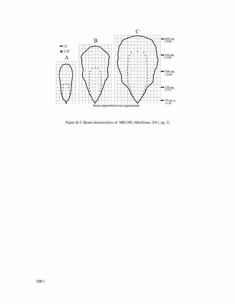
190 |

Figure K-2: Beam characteristics of MB1300, (MaxSonar, 2011, pg. 3)

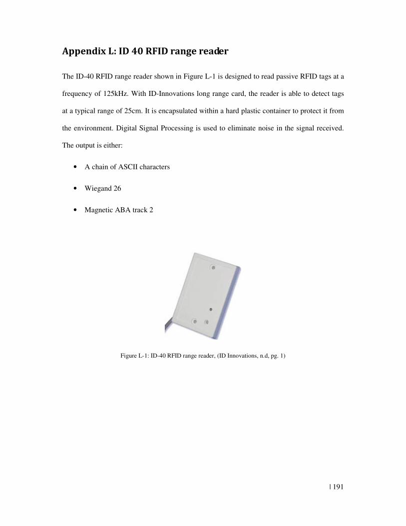
| 191

Appendix L: ID 40 RFID range reader

The ID-40 RFID range reader shown in Figure L-1 is designed to read passive RFID tags at a

frequency of 125kHz. With ID-Innovations long range card, the reader is able to detect tags

at a typical range of 25cm. It is encapsulated within a hard plastic container to protect it from

the environment. Digital Signal Processing is used to eliminate noise in the signal received.

The output is either:

• A chain of ASCII characters

• Wiegand 26

• Magnetic ABA track 2

Figure L-1: ID-40 RFID range reader, (ID Innovations, n.d, pg. 1)