Embed Size (px)
Citation preview
water
Article
Saturated Hydraulic Conductivity Estimation Using ArtificialNeural Networks
Josué Trejo-Alonso 1 , Carlos Fuentes 2,* , Carlos Chávez 1,* , Antonio Quevedo 2 ,Alfonso Gutierrez-Lopez 3 and Brandon González-Correa 4
�����������������
Citation: Trejo-Alonso, J.; Fuentes,
C.; Chávez, C.; Quevedo, A.;
Gutierrez-Lopez, A.;
González-Correa, B. Saturated
Hydraulic Conductivity Estimation
Using Artificial Neural Networks.
Water 2021, 13, 705. https://doi.org/
10.3390/w13050705
Academic Editors: George Kargas,
Petros Kerkides and Paraskevi Londra
Received: 10 February 2021
Accepted: 27 February 2021
Published: 5 March 2021
Publisher’s Note: MDPI stays neutral
with regard to jurisdictional claims in
published maps and institutional affil-
iations.
Copyright: © 2020 by the authors.
Licensee MDPI, Basel, Switzerland.
This article is an open access article
distributed under the terms and
conditions of the Creative Commons
Attribution (CC BY) license (https://
creativecommons.org/licenses/by/
4.0/).
1 Water Research Center, Department of Irrigation and Drainage Engineering, Autonomous University ofQueretaro, Cerro de las Campanas SN, Col. Las Campanas, Queretaro 76010, Mexico; [email protected]
2 Mexican Institute of Water Technology, Paseo Cuauhnáhuac Núm. 8532, Jiutepec 62550, Mexico;[email protected]
3 Water Research Center, Centro de Investigaciones del Agua-Queretaro (CIAQ), International Flood Initiative,Latin-American and the Caribbean Region (IFI-LAC), International Hydrological Programme(IHP-UNESCO), Universidad Autonoma de Queretaro, Queretaro 76010, Mexico; [email protected]
4 Engineering Faculty, Autonomous University of Queretaro, Cerro de las Campanas SN, Col. Las Campanas,Queretaro 70610, Mexico; [email protected]
* Correspondence: [email protected] (C.F.); [email protected] (C.C.);Tel.: +52-442-192-1200 (ext. 6036) (C.C.)
Abstract: In the present work, we construct several artificial neural networks (varying the input data)to calculate the saturated hydraulic conductivity (KS) using a database with 900 measured samplesobtained from the Irrigation District 023, in San Juan del Rio, Queretaro, Mexico. All of them wereconstructed using two hidden layers, a back-propagation algorithm for the learning process, anda logistic function as a nonlinear transfer function. In order to explore different arrays for neuronsinto hidden layers, we performed the bootstrap technique for each neural network and selectedthe one with the least Root Mean Square Error (RMSE) value. We also compared these results withpedotransfer functions and another neural networks from the literature. The results show that ourartificial neural networks obtained from 0.0459 to 0.0413 in the RMSE measurement, and 0.9725to 0.9780 for R2, which are in good agreement with other works. We also found that reducing theamount of the input data offered us better results.
Keywords: modeling water flow; gravity irrigation; infiltration process; artificial intelligence
1. Introduction
Soil water movement is important in several fields, like irrigation, drainage, hydrol-ogy, and agriculture [1]. Among all the measurable quantities in soils, one of the mostimportant is the saturated hydraulic conductivity (KS), defined as the ability to transmitwater throughout the saturated zone [2,3], which is highly correlated with the optimizationof the flow rate applied to the border or furrow in the gravity irrigation [2–6]. Althoughthis property is measured easily in a laboratory, or in the field, it needs to be applied ata small scale, and most of the time, it is required to be used on a large scale [5,6]. This isinconvenient due to the fact that all these tests and measurements are time-consuming,impractical, and not cost-effective [7,8].
In order to solve the inconveniences mentioned above, a great number of studies aboutpedotransfer functions (PTFs) were published [7–10]. These mathematical models allowus to estimate the KS from some soil characteristics, such as texture, field capacity, thepermanent wilting point, bulk density, porosity, and organic matter, among others [7–10].The robustness of the model is linked to the number of physical parameters used tocalculate the saturated hydraulic conductivity; the more parameters, the more accurate theprediction. However, as it was mentioned before, depending on the measurements, thePTFs are difficult to get, due to economic resources and the time it takes to measure all
Water 2021, 13, 705. https://doi.org/10.3390/w13050705 https://www.mdpi.com/journal/water

Water 2021, 13, 705 2 of 15
the variables, which presents as a limitation for this kind of function and the predictivecapacity. Besides, some works have been questioned because the soil in which they wantto apply are different from the soil used for their development, such as [11].
In recent years, another alternative has been explored—Artificial Neural Networks(ANNs), which have become a common tool used as a special class of PTFs, for exam-ple, [12,13]. ANNs are an artificial intelligence that simulate the behavior of the humanbrain, and their structures consist of a number of interconnected elements called neuronswhich are logically arranged in layers, known as input, output, and hidden (see, e.g., [12]and references therein). Each neuron connects to all the neurons in the next layer viaweighted connections. In Figure 1, we show a schematic structure for an ANN.
...
......
I1
I2
I3
In
H1
Hn
O1
On
Inputlayer
Hiddenlayer
Ouputlayer
Figure 1. Schematic representation for an ANN structure. Each circle represents a neuron, where theIj means the neurons in the input layer, and the Oj are the neurons in the output layer. All Hj circlesare the neurons in the hidden layers. The arrows represent the weighted connections.
Until now, there has been no analytical way to obtain the ideal network structure(number of hidden layers and neurons inside them) as a function of the complexity of theproblem. The structure must be selected by performing a trial-and-error process. ANNswith one or two hidden layers and an adequate number of hidden neurons are found tobe sufficient for most problems (e.g., [12,14]). There are also several works studying theideal number of neurons in the hidden layers [15,16], but these methods present generalguidelines for the selection in the number of neurons only.
The ANNs’ name comes not only from of their structure, but because they “learn”.The most common algorithm used in ANNs for the learning process is back-propagation(e.g., [17,18]). Each neuron belonging to a layer receives weighted inputs from the neuronsin the previous layer and processes them to transmit its output to the neurons in the nextlayer, and this is done through links. Each link is assigned a weight that is no more thana numerical estimate of the strength of the connection. This weighted sum of inputs in aneuron are converted into the numerical estimate that we see, according to the nonlineartransfer function (the most commonly used is the sigmoid function). The ANNs thenmodify the weights of neurons in response to errors between the actual output values andthe target output values, using what is known as gradient descent [19,20]. This is thenapplied on the sum of the squares of the errors for all the training patterns, until the meanerror of the sum squared of all the training patterns is minimal or within the tolerancespecified for the problem.
In this work, we use ANNs to obtain the KS in Irrigation District 023 placed inQueretaro Mexico using a sample of 900 plots. The sample, ANN configurations, andvalidation tests are described in Section 2. Finally, in Section 3, we show the results, and acomparison between the several configurations obtained in this work and comparisons ofour results with PTFs and other ANNs in the literature.

Water 2021, 13, 705 3 of 15
2. Materials and Methods2.1. Study Area
The Irrigation District 023 is located in Queretaro, Mexico, at 20◦18′ to 20◦34′ N, 99◦56′ to100◦12′ W with an altitude of 1892 M.A.S.L, and it has an area of 11 048 ha. It includes themunicipalities of San Juan del Rio and Pedro Escobedo (Figure 2). Its predominant climateis semiarid with summer rains, with an annual precipitation avarage of 599 mm and annualaverage temperature of 20 ◦C [21]. The water is conducted through open channels. Themain channels are lined with concrete, but all the lateral channels that carry water to theplots are unlined. The separation of the plots in some cases are by trees, unlined channels,drains, or roads [22].
Figure 2. Location map of the sampling points in Irrigation District 023 San Juan del Río, Querétaro.
2.2. Soil Database
An extensive and detailed database description can be found at [23]. In summary, thedatabase used in this study was developed from samplings in 900 plots at Irrigation District023, San Juan del Rio Queretaro. These samples were sent to the laboratory to obtain thefollowing parameters: soil texture by the Bouyucos hydrometer, bulk density (ρa) by thecylinder method of known volume, moisture content at saturation (θS), field capacity (FC)and permanent wilting point (PWP) by the method of the pressure membrane pot, and thesaturated hydraulic conductivity by the variable head permeameter method. From thesemeasurements, we took seven and considered them through the paper as the input data:percentage of clay, sand and silt, bulk density, permanent wilting point, moisture contentat saturation, and field capacity (Table 1).
2.3. The ANNs’ Setup
As mentioned in Section 1, there is no analytical way to define the ANN structure, butbased on similar several works (e.g., [12,14,16]) we noticed that the ANNs have one or twohidden layers only. With this in mind, we tested several structures for our ANNs with twohidden layers and an additional one with three hidden layers as a test. Details about theANNs’ settings are described below.

Water 2021, 13, 705 4 of 15
Table 1. Statistical properties of data measured in the laboratory.
Variable Min Max Median Mean SD Q1 Q3
Sand (%) 0.07 77.83 28.35 31.14 20.22 13.75 52.00Clay (%) 2.12 59.46 21.74 21.95 12.06 13.44 30.00Silt (%) 0.80 92.00 45.27 46.91 23.48 27.30 59.79
ρa (g/cm3) 1.18 1.70 1.40 1.41 0.11 1.32 1.47PWP (cm3/cm3) 0.07 0.35 0.13 0.15 0.05 0.10 0.17
θS (cm3/cm3) 0.35 0.56 0.47 0.47 0.04 0.45 0.50FC (cm3/cm3) 0.17 0.47 0.29 0.30 0.06 0.25 0.32
KS (cm/h) 0.05 5.15 0.78 1.42 1.42 0.40 1.80
We began with all the input data (seven) and tested several configurations as follows:we start with two neurons in the first layer and two neurons in the second. Then wecontinue to vary the number of neurons in the first layer from two to ten, and leave thesecond layer constant. Next, the number of neurons in the second layer is increased tothree and we vary the number of neurons in the first, again, from two to ten, and so onuntil the number of the second layer varies from two to ten, just like the first one. Thisinput layer has the seven input data mentioned before. Finally, the output layer containsthe KS predicted value.
Then, we changed the number of data in the input layer (decreasing it by one) andrepeated the process as explained before. The choice of which parameter has to be removedis based on the importance plot (details in Section 2.4), except for the last configuration,where we remove θS instead of the percentage of silt, because θS is closely related with theclay percentage. We kept removing input data until we had three measurements only. Foreach configuration, we varied the number of neurons in the hidden layers from two to ten.
The ANN was programmed using the neuralnet package [24] and the caret package [25],both of them provided by the R software [26].
The neuralnet package trains neural networks using backpropagation, resilient back-propagation (RPROP) with [27] or without weight backtracking [28], or the modified glob-ally convergent version (GRPROP) by [29]. The function allows flexible settings throughcustom-choice of error and activation function. The caret package (short for ClassificationAnd REgression Training) is a set of functions that attempts to streamline the process forcreating predictive models. There are many different modeling functions in R. Some havedifferent syntax for model training and/or prediction. The package started off as a way toprovide a uniform interface for the functions themselves, as well as a way to standardizecommon tasks (such as parameter tuning and variable importance). Specifically, we usedthe train function of this package to perform the cross-validation process.
Furthermore, the calculation of generalized weights [30] is implemented. In this work,we use RPROP as an algorithm type to calculate the neural network, the sum of squarederrors as a differentiable function for the calculation of the error and a logistic differentiablefunction for smoothing the result of the cross-product of the covariate or neurons and theweights.
Using the RMSE measurement, we selected the optimal ANN structure in each case,and finally, we kept this last ANN structure as ideal. The Mean Absolute Error (MAE)measurement was calculated as:
MAE =1n
n
∑i=1|yi − xi|, (1)
where yi are the measurement values, xi are the predicted values, and n is the total mea-surement. We also calculate the RMSE as:
RMSE =
√1n
n
∑i=1
(yi − xi)2. (2)
Water 2021, 13, 705 5 of 15
2.4. Cross-Validation
In order to validate our ANN results, we made a cross-validation analysis using thetrain function from the caret package. This function sets up a grid of tuning parametersfor a number of classification and regression routines, fits each model, and calculates aresampling-based performance measure. In this case, we use the parameters optimized toneuralnet, and we generated 25 bootstrap replications for each ANN configuration. Finally,for the prediction of new samples, we used the predict function.
The train function returned several results: the ideal ANN configuration, the bestRMSE, MAE and R2 values for each tested configuration, a RMSE matrix, and an impor-tance plot. This last plot indicates which parameter contributed the most to the KS finalapproximation. Based on this last plot, we decided which input data would be removed onthe next run, with the exception already mentioned above.
3. Results and Discussion
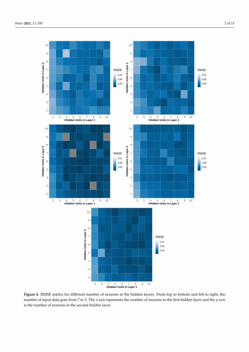
As mentioned in Section 2, we generated several ANNs which contained all thecombinations from two to ten neurons in each hidden layer. In Figure 3 we show the resultsfor these tests. In the x axis we have the number of neurons in the first hidden layer, they axis represents the RMSE value obtained from the 25 bootstrap replications, and eachcolor represents the number of neurons in the second hidden layer. The election of thebest configuration is based on the smallest RMSE value in these plots. Additionally, fromthe top to the bottom and from the left to the right, we show the variation in the inputdata. Another result is shown in Figure 4. This plot is a 10 × 10 matrix where the colorrepresents the RMSE value for each configuration, the rows are the number of neurons inthe second hidden layer, and the columns are the number of neurons in first hidden layer.Remember that each plot differs from the other in the number of input data in the sameway that Figure 3. In general, we can see that a small number of neurons in the first layerpresents higher values of RMSE. Another important result is presented in the Figure 5where we show a density plot representation (varying the input data from top to bottom)for RMSE, MAE, and R2 measurements derived from the bootstrap analysis. From theseplots we have small variations for each measurement which indicate that the results are nothighly dependent on the ANN configurations. Finally, in Figure 6, we show the importanceplots, which are described in the cross-validation section presented previously. These plotshelp us to decide which parameter we must keep or eliminate in each run when we havedifferent numbers of input data.
In order to explore another possibility and to get more confident results, we made atest increasing the number of hidden layers to three. We applied the same process explainedpreviously for this new configuration, and we got an improvement of ∼9% in the RMSEvalues, but with 15 times more computation time. This was the reason for dismissal ofthese configurations.
In Table 2 we present the three best configurations of each run, where we have thenumber of input data, the ANN structure, and the RMSE, MAE, and R2 measurements.
Following the results, we present Figure 7, where we compare the KS measurementswith the KS predicted by the ANNs for all tested configurations. The dotted line is a 1:1relation and the R2 is obtained from the train function. The plotted values were obtainedapplying the best ANN configuration for each run (Figure 7). The histograms in the top-left corner show the residuals (∆KS), which is the difference between the predicted andmeasured values.
Recall that to obtain the ideal neuron configuration, we apply the train package, whichallows us to obtain the RMSE, MAE, and R2 data for each arrangement of neurons in thehidden layers. The only variation was the input data (ranging from 7 to 3). Therefore, itwas possible to obtain five different boxplots for the RMSE, whose only difference wouldbe the aforementioned input data. This is shown in Figure 8, where a trend is observed forthe RMSE to fall, while the number of input data decreases.

Water 2021, 13, 705 6 of 15
0.04
0.05
0.06
0.07
2 4 6 8 10#Hidden Units in Layer 1
RM
SE
(B
oots
trap
)#Hidden Units in Layer 2 2
3 4 5
6 7
8 9
10
0.04
0.05
0.06
0.07
2 4 6 8 10#Hidden Units in Layer 1
RM
SE
(B
oots
trap
)
#Hidden Units in Layer 2 2 3
4 5
6 7
8 9
10
0.04
0.05
0.06
0.07
2 4 6 8 10#Hidden Units in Layer 1
RM
SE
(B
oots
trap
)
#Hidden Units in Layer 2 2 3
4 5
6 7
8 9
10
0.04
0.05
0.06
0.07
2 4 6 8 10#Hidden Units in Layer 1
RM
SE
(B
oots
trap
)#Hidden Units in Layer 2 2
3 4 5
6 7
8 9
10
0.04
0.05
0.06
0.07
2 4 6 8 10#Hidden Units in Layer 1
RM
SE
(B
oots
trap
)
#Hidden Units in Layer 2 2 3
4 5
6 7
8 9
10
Figure 3. ANN test for choosing the ideal number of hidden neurons varying the input data. From top to bottom and left toright the number of input data goes from 7 to 3. The x axis represents the number of neurons in the first hidden layer andthe y axis is the RMSE value. Each color is a different number of neurons in the second hidden layer.
Water 2021, 13, 705 7 of 15
2
3
4
5
6
7
8
9
10
2 3 4 5 6 7 8 9 10#Hidden Units in Layer 1
#Hid
den
Uni
ts in
Lay
er 2
0.05
0.06
0.07
RMSE
2
3
4
5
6
7
8
9
10
2 3 4 5 6 7 8 9 10#Hidden Units in Layer 1
#Hid
den
Uni
ts in
Lay
er 2
0.05
0.06
0.07
RMSE
2
3
4
5
6
7
8
9
10
2 3 4 5 6 7 8 9 10#Hidden Units in Layer 1
#Hid
den
Uni
ts in
Lay
er 2
0.05
0.06
0.07
RMSE
2
3
4
5
6
7
8
9
10
2 3 4 5 6 7 8 9 10#Hidden Units in Layer 1
#Hid
den
Uni
ts in
Lay
er 2
0.05
0.06
0.07
RMSE
2
3
4
5
6
7
8
9
10
2 3 4 5 6 7 8 9 10#Hidden Units in Layer 1
#Hid
den
Uni
ts in
Lay
er 2
0.05
0.06
0.07
RMSE
Figure 4. RMSE matrix for different number of neurons in the hidden layers. From top to bottom and left to right, thenumber of input data goes from 7 to 3. The x axis represents the number of neurons in the first hidden layer and the y axisis the number of neurons in the second hidden layer.

Water 2021, 13, 705 8 of 15
0
50
100
150
200
250
0.03 0.04 0.05 0.06 0.07
Den
sity
RMSE
0
50
100
150
200
0.94 0.96 0.98 1.00
Den
sity
R2
0
200
400
600
0.0100 0.0125 0.0150 0.0175 0.0200 0.0225
Den
sity
MAE
0
50
100
150
200
250
0.03 0.04 0.05 0.06 0.07
Den
sity
RMSE
0
50
100
150
200
0.94 0.96 0.98 1.00
Den
sity
R2
0
200
400
600
0.0100 0.0125 0.0150 0.0175 0.0200 0.0225
Den
sity
MAE
0
50
100
150
200
250
0.03 0.04 0.05 0.06 0.07
Den
sity
RMSE
0
50
100
150
200
0.94 0.96 0.98 1.00
Den
sity
R2
0
200
400
600
0.0100 0.0125 0.0150 0.0175 0.0200 0.0225
Den
sity
MAE
0
50
100
150
200
250
0.03 0.04 0.05 0.06 0.07
Den
sity
RMSE
0
50
100
150
200
0.94 0.96 0.98 1.00
Den
sity
R2
0
200
400
600
0.0100 0.0125 0.0150 0.0175 0.0200 0.0225
Den
sity
MAE
0
50
100
150
200
250
0.03 0.04 0.05 0.06 0.07
Den
sity
RMSE
0
50
100
150
200
0.94 0.96 0.98 1.00
Den
sity
R2
0
200
400
600
0.0100 0.0125 0.0150 0.0175 0.0200 0.0225
Den
sity
MAE
Figure 5. Density plots for (from left to right) RMSE, R2, and MAE resulting from the 25 bootstrap replications. From top tobottom, the number of input data goes from 7 to 3.

Water 2021, 13, 705 9 of 15
FC
PWP
Sand
Silt
Saturation
Density
Clay
0 25 50 75 100Importance
Fea
ture
PWP
Sand
Silt
Saturation
Density
Clay
0 25 50 75 100Importance
Fea
ture
Sand
Silt
Saturation
Density
Clay
0 25 50 75 100Importance
Fea
ture
Silt
Saturation
Density
Clay
0 25 50 75 100Importance
Fea
ture
Silt
Density
Clay
0 25 50 75 100Importance
Fea
ture
Figure 6. Importance plots referring to the weight of each variable in the calculations. From top to bottom and from right toleft, the number of input data goes from 7 to 3.

Water 2021, 13, 705 10 of 15
Table 2. The top three configurations for ANN structure and their statistical measurements. (1) #Input data (2) contains the ANN neurons’ structure (Input-Hidden1-Hidden2-Ouput), where eachnumber represents the quantity of neurons used in each layer, (3) the RMSE measurements, (4) theMAE measurements, and (5) the R2 measurements.
# Input Data ANN Structure RMSE MAE R2
(cm/h) (cm/h)
7-9-3-1 0.0459 0.0159 0.97257 7-7-6-1 0.0460 0.0164 0.9720
7-10-4-1 0.0465 0.0162 0.9715
6-5-7-1 0.0445 0.0171 0.97406 6-6-3-1 0.0455 0.0171 0.9742
6-8-4-1 0.0447 0.0163 0.9739
5-8-3-1 0.0413 0.0152 0.97805 5-4-9-1 0.0417 0.0156 0.9774
5-8-8-1 0.0418 0.0152 0.9777
4-9-10-1 0.0449 0.0152 0.97364 4-8-8-1 0.0450 0.0156 0.9735
4-9-9-1 0.0452 0.0155 0.9734
3-9-6-1 0.0433 0.0155 0.97573 3-8-9-1 0.0434 0.0154 0.9757
3-8-6-1 0.0436 0.0160 0.9755
In Table 3 we show the results obtained from the literature with PTFs or ANNs andcompare them with this work.
Table 3. Comparison between several works for obtaining KS.
Model RMSE R2 Type
This work 0.0413 0.9780 ANNTamari et al. [31] 0.0707 NA ANNBrakensiek et al. [9] 0.1370 0.9953 PTFErzin et al. [12] 0.1700 0.9970 ANNSaxton et al. [32] 0.1895 0.9915 PTFParasuraman et al. [33] 0.1900 NA ANNTrejo-Alonso et al. [23] 0.1983 0.9901 PTFCosby et al. [34] 0.4325 0.9546 PTFAhuja et al. [35] 0.6498 0.8910 PTFSchaap & Leij [36] 0.7130 NA ANNVereecken et al. [37] 0.7143 0.9307 PTFMinasny et al. [38] 0.7330 NA ANNFerrer-Julià et al. [39] 1.3018 0.4083 PTFMerdun et al. [40] 3.5110 0.5240 ANN
The results for RMSE obtained in this work are better in, at least, 35% compared withthe ones presented by [31], and we reported the fifth-best value for R2.

Water 2021, 13, 705 11 of 15
0 1 2 3 4 5
01
23
45
2 Hidden Layers / 7 input data
Measured KS [cm/h]
AN
N K
S [c
m/h
]
−0.5 0.0 0.5 1.0
04
08
012
0
∆KS [cm/h]
N
R2 = 0.9725
0 1 2 3 4 5
01
23
45
2 Hidden Layers / 6 input data
Measured KS [cm/h]
AN
N K
S [c
m/h
]
−1.0 0.0 1.0 2.0
04
08
012
0
∆KS [cm/h]
N
R2 = 0.9740
0 1 2 3 4 5
01
23
45
2 Hidden Layers / 5 input data
Measured KS [cm/h]
AN
N K
S [c
m/h
]
−1.0 −0.5 0.0 0.5
050
100
150
∆KS [cm/h]
N
R2 = 0.9780
0 1 2 3 4 5
01
23
45
2 Hidden Layers / 4 input data
Measured KS [cm/h]
AN
N K
S [c
m/h
]
−1.0 −0.5 0.0 0.5
04
08
012
0
∆KS [cm/h]
N
R2 = 0.9736
0 1 2 3 4 5
01
23
45
2 Hidden Layers / 3 input data
Measured KS [cm/h]
AN
N K
S [c
m/h
]
−1.0 −0.5 0.0 0.5
04
08
012
0
∆KS [cm/h]
N
R2 = 0.9736
Figure 7. Plots for the comparison between KS measurement in the field with the KS value obtained applying the differentANN configurations. The dotted line is a 1:1 desirable relation. The histograms represent the residual distribution (∆KS).

Water 2021, 13, 705 12 of 15
2L7I 2L6I 2L5I 2L4I 2L3I
0.0
45
0.0
500
.055
0.0
60
RMSE for all ANN configurations
RM
SE
Figure 8. Boxplot for each run of the train package. The names means two hidden layers and thenumber of input data used in each run.
Another advantage of ANN is that the initial shape for the function to get the relationbetween the variables or a principal component analysis is not needed. Additionally, aswe can see in Figure 3 and Table 2, the results are independent of the ANN structure.This is supported by the fact that the RMSE values for different configurations are verysimilar (the largest difference is ∼10%), and for R2 values the difference is ∼5%, and wegot ∼11% for MAE. Besides, the Figure 5 presents an almost gaussian distribution for thesethree statistical measurements, which is in agreement with a non-biased result. In thisFigure, we also see that the density distributions are narrower, while the number of inputdata is smaller. This tells us that in contrast with the PTF models, we found a tendencywhich indicates that the less input data we have, the more accurate our prediction of KSis, as well as the Figure 8 shown this tendency too. This result can be explained by thefollowing reasons. Based on the Principal Component Analysis of [23], we noted that theprincipal variables contributing the most to the sample were KS, the percentage of clay,θS, PWP, and FC, which is supported by the importance plots (Figure 6). Additionally, forthe 900 analyzed samples contained in 10 of the 12 existing types of soil (according to theUSDA Textural Soil Classification), they showed that the infiltration rate depended directlyon the percentage of clay and the ρa.
4. Conclusions
In this work, we developed five Artificial Neural Networks in order to calculate thesaturated hydraulic conductivity based on the sample used by [23]. All networks consist ofone input layer, two hidden layers, and one output layer. We tested a network with threehidden layers, but with little better results. We took 75% of the sample for training and25% for validation. We also tested all the possible combinations for the number of neuronsin each hidden layer, taking into account that the number of neurons for each hidden layerwill vary from 2 to 10 neurons. Finally, we selected the best number of neurons in eachlayer based on RMSE measurements obtained from a cross-validation analysis.
The results show that, compared with other works, we get better or similar results forRMSE and R2 measurements and similar configurations for our ANN. Finally, we can saythat if the necessary resources are available to obtain a large number of data in the field,it is necessary to develop a study of PTF as well as ANN to compare the results of eachprocess and be able to choose the best option between both of them. The latter will notonly be based on the RMSE or R2 measurements, but also on the desired application (astatistical ground property study or prediction for irrigation proposes). A more detailed

Water 2021, 13, 705 13 of 15
study to define an exact range of the amount of data needed from a reliable artificial neuralnetwork study should be carried out, but the latter is beyond the objective of this work.Besides, we have to be more careful in the characteristics of the sample where the modelscome out. In our case, we analyzed 10 of the 12 types of soils where the bulk density andthe percentage of clay became more important parameters compared to others. This madeour models more reliable for almost any type of soil.
The coupling of the Saint Venant and Richards equations is the complete mathematicalmodel for modeling gravity irrigation [41]. However, its use requires detailed informationon the physical properties of the soil, as well as a series of field and laboratory experimentsthat can be expensive [42,43]. In this way, the results used in this article, combined withsome rapid field and laboratory tests, can be an excellent alternative to reduce costs andthe time used to obtain that information.
Finally, the application of artificial neural networks have been demonstrated to suc-cessfully solve classification and prediction problems, and this is probably for the nonlinearrelation between the variables. The calculation of the saturated hydraulic conductivityin this work proves that we need only three variables to predict new values, but the soilproperties are crucial for the correct application of these models in contrast with the ANNconfiguration, which has been proved to play a minor role in the final results.
Author Contributions: Conceptualization, C.C. and C.F.; methodology, C.C., J.T.-A. and A.Q.; soft-ware, J.T.-A. and B.G.-C.; validation, B.G.-C., J.T.-A. and A.G.-L.; formal analysis, C.C. and J.T.-A.;investigation, A.G.-L. and J.T.-A.; resources, C.C., C.F. and A.Q.; data curation, C.C. and A.Q.;writing—original draft preparation, J.T.-A.; writing—review and editing, C.C., C.F., A.Q. and A.G.-L.;visualization, J.T.-A. and B.G.-C.; supervision, C.C., C.F. and A.Q.; project administration, C.C.; fund-ing acquisition, C.C. All authors have read and agreed to the published version of the manuscript.
Funding: This research was supported as part of a collaboration between the National Water Com-mission (CONAGUA, according to its Spanish acronym); The Water Users Association of Second Unitof Module Two, Irrigation District No. 023; the Irrigation District 023, San Juan del Río, Querétaro;and the Autonomous University of Querétaro, under the program RIGRAT 2015–2019.
Conflicts of Interest: The authors declare no conflict of interest regarding the publication of thispaper.
References1. Fuentes, S.; Trejo-Alonso, J.; Quevedo, A.; Fuentes, C.; Chávez, C. Modeling Soil Water Redistribution under Gravity Irrigation
with the Richards Equation. Mathematics 2020, 8, 1581. [CrossRef]2. Chávez, C.; Fuentes, C. Design and evaluation of surface irrigation systems applying an analytical formula in the irrigation
district 085, La Begoña, Mexico. Agric. Water Manag. 2019, 221, 279–285. [CrossRef]3. Di, W.; Xue, J.; Bo, X.; Meng, W.; Wu, Y.; Du, T. Simulation of irrigation uniformity and optimization of irrigation technical
parameters based on the SIRMOD model under alternate furrow irrigation. Irrig. Drain 2017, 66, 478–491.4. Gillies, M.H.; Smith, R.J. SISCO: Surface irrigation simulation, calibration and optimization. Irrig. Sci. 2015, 33, 339–355.
[CrossRef]5. Saucedo, H.; Zavala, M.; Fuentes, C. Complete hydrodynamic model for border irrigation. Water Technol. Sci. 2011, 2, 23–38.6. Weibo, N.; Ma, X.; Fei, L. Evaluation of infiltration models and variability of soil infiltration properties at multiple scales. Irrig.
Drain 2017, 66, 589–599.7. Zhang, Y.; Schaap, M.G. Estimation of saturated hydraulic conductivity with pedotransfer functions: A review. J. Hydrol. 2019,
575, 1011–1030. [CrossRef]8. Abdelbaki, A.M. Evaluation of pedotransfer functions for predicting soil bulk density for U.S. soils. Ain Shams Eng. J. 2018, 9,
1611–1619. [CrossRef]9. Brakensiek, D.; Rawls, W.J.; Stephenson, G.R. Modifying SCS Hydrologic Soil Groups and Curve Numbers for Rangeland Soils; Paper
No. PNR-84203; ASAE: St. Joseph, MN, USA, 1984.10. Rasoulzadeh, A. Estimating Hydraulic Conductivity Using Pedotransfer Functions. In Hydraulic Conductivity-Issues, Determination
and Applications; Elango, L., Ed.; InTech: Rijeka, Croatia, 2011; pp. 145–164.11. Moreira, L.; Righetto, A.M.; Medeiros, V.M. Soil hydraulics properties estimation by using pedotransfer functions in a northeastern
semiarid zone catchment, Brazil. International Environmental Modelling and Software Society, 2004, Osnabrueck. Complexityand Integrated Resources Management. In Transactions of the 2nd Biennial Meeting of the International Environmental Modelling and

Water 2021, 13, 705 14 of 15
Software Society, iEMSs 2004; International Environmental Modelling and Software Society: Manno, Switzerland, 2004; Volume 2,pp. 990–995.
12. Erzin, Y.; Gumaste, S.D.; Gupta, A.K.; Singh, D.N. Artificial neural network (ANN) models for determining hydraulic conductivityof compacted fine-grained soils. Can. Geotech. J. 2009, 46, 955–968. [CrossRef]
13. Agyare, W.A.; Park, S.J.; Vlek, P.L.G. Artificial Neural Network Estimation of Saturated Hydraulic Conductivity. VZJAAB 2007, 6,423–431. [CrossRef]
14. Sonmez, H.; Gokceoglu, C.; Nefeslioglu, H.A.; Kayabasi, A. Estimation of rock modulus: For intact rocks with an artificial neuralnetwork and for rock masses with a new empirical equation. Int. J. Rock Mech. Min. Sci. Geomech. Abstr. 2006, 43, 224–235.[CrossRef]
15. Grima, M.A.; Babuska, R. Fuzzy model for the prediction of unconfined compressive strength of rock samples. Int. J. Rock Mech.Min. Sci. Geomech. Abstr. 1999, 36, 339–349. [CrossRef]
16. Haque, M.E.; Sudhakar, K.V. ANN back-propagation prediction model for fracture toughness in microalloy steel. Int. J. Fatigue2002, 24, 1003–1010. [CrossRef]
17. Singh, T.N.; Gupta, A.R.; Sain, R. A comparative analysis of cognitive systems for the prediction of drillability of rocks and wearfactor. Geotech. Geol. Eng. 2006, 24, 299–312. [CrossRef]
18. Erzin, Y.; Rao, B.H.; Singh, D.N. Artificial neural network models for predicting soil thermal resistivity. Int. J. Therm. Sci. 2008, 47,1347–1358. [CrossRef]
19. Rumelhart, D.H.; Hinton, G.E.; Williams, R.J. Learning internal representation by error propagation. In Parallel DistributedProcessing; Rumelhart, D.E., McClelland, J.L., Eds.; MIT Press: Cambridge, MA, USA, 1986; Volume 1, Chapter 8.
20. Goh, A.T.C. Back-propagation neural networks for modelling complex systems. Artif. Intel. Eng. 1995, 9, 143–151. [CrossRef]21. Comisión Nacional del Agua (CONAGUA). Estadísticas del Agua en México; CONAGUA: Coyoacán, México, 2018; p. 306.22. Chávez, C.; Limón-Jiménez, I.; Espinoza-Alcántara, B.; López-Hernández, J.A.; Bárcenas-Ferruzca, E.; Trejo-Alonso, J. Water-Use
Efficiency and Productivity Improvements in Surface Irrigation Systems. Agronomy 2020, 10, 1759. [CrossRef]23. Trejo-Alonso, J.; Quevedo, A.; Fuentes, C.; Chávez, C. Evaluation and Development of Pedotransfer Functions for Predicting
Saturated Hydraulic Conductivity for Mexican Soils. Agronomy 2020, 10, 1516. [CrossRef]24. Fritsch, S.; Guenther, F; Wright, M.N. Neuralnet: Training of Neural Networks. R Package Version 1.44.2. Available online:
https://CRAN.R-project.org/package=neuralnet (accessed on 19 October 2020)25. Kuhn, M. Caret: Classification and Regression Training. R Package Version 6.0-86. 2020. Available online: https://CRAN.R-
project.org/package=caret (accessed on 22 January 2021).26. R Core Team. R: A Language and Environment for Statistical Computing; R Foundation for Statistical Computing: Vienna, Austria,
2020. Available online: https://www.R-project.org/ (accessed on 12 January 2021).27. Riedmiller, M. Rprop—Description and Implementation Details; Technical Report; University of Karlsruhe: Karlsruhe, Germany,
1994.28. Riedmiller, M.; Braun, H. A direct adaptive method for faster backpropagation learning: The RPROP algorithm. In Proceedings
of the IEEE International Conference on Neural Networks (ICNN), San Francisco, CA, USA, 28 March–1 April 1993; pp. 586–591.29. Anastasiadis, A.; Magoulas, G.D.; Vrahatis, M.N. New globally convergent training scheme based on the resilient propagation
algorithm. Neurocomputing 2005, 64, 253–270. [CrossRef]30. Intrator, O.; Intrator, N. Using Neural Nets for Interpretation of Nonlinear Models. In Proceedings of the Statistical Computing
Section; American Statistical Society: San Francisco, CA, USA, 1993; pp. 244–249.31. Tamari, S.; Wösten, J.H.M.; Ruiz-Suárez, J.C. Testing an Artificial Neural Network for Predicting Soil Hydraulic Conductivity. Soil
Sci. Soc. Am. J. 1996, 60, 1732–1741. [CrossRef]32. Saxton, K.; Rawls, W.J.; Romberger, J.S.; Papendick, R.I. Estimating generalized soil water characteristics from texture. Soil Sci.
Soc. Am. J. 1986, 5, 1031–1036. [CrossRef]33. Parasuraman, K.; Elshorbagy, A.; Si, B. Estimating Saturated Hydraulic Conductivity In Spatially Variable Fields Using Neural
Network Ensembles. Soil Sci. Soc. Am. J. 2006, 70, 1851–1859. [CrossRef]34. Cosby, B.; Hornberger, G.; Clapp, R.; Ginn, T. A statistical exploration of the relationship of soil moisture characteristics to the
physical properties of soils. Water Resour. Res. 1984, 20, 682–690 [CrossRef]35. Ahuja, L.R.; Naney, J.W.; Green, R.E.; Nielsen, D.R. Macroporosity to characterize spatial variability of hydraulic conductivity
and effects of land management. Soil Sci. Soc. Am. J. 1984, 48, 699–702. [CrossRef]36. Schaap, M.G.; Leij, F.J. Using neural networks to predict soil water retention and soil hydraulic conductivity. Soil Tillage Res. 1998,
47, 37–42. [CrossRef]37. Vereecken, H.; Schnepf, A.; Hopmans, J.W.; Javaux, M.; Or, D.; Roose, T.; Vanderborght, J.; Young, M.H.; Amelung, W.; Aitkenhead,
M.; et al. Modeling Soil Processes: Review, Key Challenges, and New Perspectives. Vadose Zone J. 2016, 15. [CrossRef]38. Minasny, B.; Hopmans, J.; Harter, T.; Eching, S.; Tuli, A.; Denton, M. Neural Networks Prediction of Soil Hydraulic Functions for
Alluvial Soils Using Multistep Outflow Data. Soil Sci. Soc. Am. J. 2004, 68, 417–429. [CrossRef]39. Ferrer-Julià, M.; Estrela-Monreal, T.; Sánchez-del Corral-Jiménez, A.; García-Meléndez, E. Constructing a saturated hydraulic
conductivity map of spain using pedotransfer functions and spatial prediction. Geoderma 2004, 123, 275–277. [CrossRef]40. Merdun, H.; Cinar, O.; Meral, R.; Apan, M. Comparison of artificial neural network and regression pedotransfer functions for
prediction of soil water retention and saturated hydraulic conductivity. Soil Tillage Res. 2006, 90, 108–116. [CrossRef]

Water 2021, 13, 705 15 of 15
41. Richards, L.A. Capillary conduction of liquids through porous mediums. Physics 1931, 1, 318–333. [CrossRef]42. Saucedo, H.; Fuentes, C.; Zavala, M. The Saint-Venant and Richards equation system in surface irrigation: (2) Numerical coupling
for the advance phase in border irrigation. Ing. Hidraul. Mexico 2005, 20, 109–119.43. Fuentes, C.; Chávez, C. Analytic Representation of the Optimal Flow for Gravity Irrigation. Water 2020, 12, 2710. [CrossRef]


