Revisiting and Computing Reaction Coordinates with Directional Milestoning

Revisiting and Computing Reaction Coordinates with DirectionalMilestoning

Serdal Kirmizialtin and Ron ElberDepartment of Chemistry and Biochemistry Institute for Computational Engineering and SciencesUniversity of Texas at Austin, TX

AbstractThe method of Directional Milestoning is revisited. We start from an exact and more generalexpression and state the conditions and validity of the memory-loss approximation. An algorithmto compute a reaction coordinate from Directional Milestoning data is presented. The reactioncoordinate is calculated as a set of discrete jumps between Milestones that maximizes the fluxbetween two stable states. As an application we consider a conformational transition in solvatedAdenosine. We compare a long molecular dynamic trajectory with Directional Milestoning anddiscuss the differences between the maximum flux path and minimum energy coordinates.

I. IntroductionComputational chemists are charged with predicting thermodynamics and kinetics ofmolecular processes. The charge implies the determination of the stable states of the system,the statistical weights of the states, and the rate of transitions between states. In the presentmanuscript we focus on computational studies of transitions and rates (or kinetics).

Predicting kinetics and mechanisms of molecular processes by computer simulations iscomplex. Indeed, significant advances in computer simulations of kinetics in the condensedphases have been made only recently. In contrast to equilibrium calculations in which thebasic objects we sample and use to compute statistical mechanics averages are structures,studies of kinetics use trajectories as the basic objects. To describe a reaction we considertrajectories that start at the reactant state and end at the product state. Clearly trajectories aremore complex entities than a single configuration, making the sampling and computationalaverages of kinetics more expensive compared to equilibrium calculations.

Trajectory sampling can be done by direct integration. That is, sampling initial conditions(velocities and coordinates) at the reactant state, integrating the equations of motion, andhoping that in a reasonable number of integration steps trajectories will reach the productstate. Trajectories can also be computed by shooting, starting somewhere between reactantsand products and integrating the trajectory backward (to reactants) and forward (to product)in time, like is done in TPS 1. Yet another direction is the sampling of boundary valuetrajectories that are guaranteed to be productive (by construction every computed trajectoryreaches the products from the reactants), Boundary value trajectories are, however,significantly more expensive to compute 2 compared to initial value calculations. Boundaryvalue trajectories can be computed approximately with large time steps 3,4 but in this casetheir statistical weights are not accurate enough to proceed with calculations of ensembleaverages and kinetic.

One of the kinetic observables of significant interest is the mean first passage time <t> (orMFPT). It is the time averaged over an ensemble of trajectories initiated at the reactant statethat are terminated when they reach the product state for the first time. For reactions that

NIH Public AccessAuthor ManuscriptJ Phys Chem A. Author manuscript; available in PMC 2012 June 16.

Published in final edited form as:J Phys Chem A. 2011 June 16; 115(23): 6137–6148. doi:10.1021/jp111093c.

NIH

-PA Author Manuscript

NIH


NIH


obey first order kinetic the inverse of the MFPT is the rate constant. The initial distributionof the trajectories is determined by the preparation of the reactant state and in many cases issimply the canonical distribution restricted to the domain of the reactant.

The need to compute an ensemble of trajectories from reactants to products explains thesignificant difficulties in simulating kinetics on the computers. The time scale of a singleMD trajectory is restricted in routine calculations to the sub-microsecond time scale, farshorter than many processes of interest. For example, channel gating and some foldingevents are in a millisecond time scale. Molecular machines operate and conformationalchanges occur at a time range from microseconds to seconds. While massive parallelizationand special purpose machines can push trajectories to milliseconds5, individual trajectoriesprovide a poor sample for kinetics at that timescale. For numerous molecular processes withtypical time scales of microseconds or longer, straightforward sampling of trajectories is anexceptionally challenging task. Theories and algorithms were therefore developed to addressthe problem and extend the time scales of atomically detailed simulations. Atomicsimulations in biophysics provide the most comprehensive picture of the process underinvestigation.

The oldest theory of molecular reaction kinetic (Transition State Theory6) still provides apowerful and accurate computational tool for a set of reactions in which the reactants andproducts are separated by a large barrier. A large barrier crossing is energetically costly andoccurs rarely. If crossing is assumed to happen only once during the reaction the calculationsof trajectories can be avoided and only equilibrium sampling at the transition state andreactant state remain. Dynamical effects (re-crossing) can be addressed with thetransmission coefficient7. Trajectories are computed from the top of the barrier until they aretrapped either in the reactant or in product states. The probability of making it to the productstates is computed conditioned so the initial configuration is on the transition state and thevelocity points to the product. In the Transition State Theory it is assumed to be one, sinceno-crossings are allowed. The transmission coefficient is a useful computational tool if thebarrier is sufficiently high such that re-crossing events, if they do occur, are diminishedrapidly as a function of time.

Large barriers are exploited also in Transition Path Sampling (TPS)1. It is observed thatwhile very rare, actual transitional trajectories pass over large barriers rapidly and quicklyre-settle in a new or old free energy minimum. This observation is in the spirit of theconvergence condition of the transmission coefficient. The rate is slow (even with rapidtransitional trajectories) because these trajectories are rare. Individually each of thesetrajectories is actually very fast. It is not uncommon to find individual reactive trajectories ofpicoseconds for systems with an overall rate of seconds. The transitional trajectories do notinclude the typically very long waiting time at the minimum until a rare fluctuation pushesthe system over the barrier. It is therefore possible to compute with moderate computerresources the transitional trajectories if a sampling algorithm for these rare trajectories withproper weights is available. Such an algorithm is offered by TPS.

A large number of molecular processes occur however without one clear and dominatingbarrier; for example protein folding8, RNA folding9, conformational transitions10, and ionpermeation through membranes11. In fact, diffusive multi-barrier kinetics is the rule ratherthan the exception in biophysics. In these processes, the individual transitional trajectories(i.e. a trajectory that left the basin of the reactant and did not yet reach the basin of theproduct) are very long and are conducting diffusive motion on a rough energy landscape inmany dimensions. Long individual trajectories (e.g. milliseconds) pose a significantchallenge to theories and algorithms that require the calculations of an ensemble of completetrajectories, or of trajectories that “decide” quickly their final state. Therefore a number of

Kirmizialtin and Elber Page 2

J Phys Chem A. Author manuscript; available in PMC 2012 June 16.

NIH


NIH


NIH


algorithms and theories have emerged in the last ten years to address the problem of multi-barrier diffusive systems and Exceptionally Long Dynamics (ELD). These approachesinclude the PPTIS method 12, the Markov State Model 13-15, and Milestoning16-17.

All current technologies for ELD are using the same concept of breaking the long trajectoryto fragments that are assumed independent. The fragments can be run in trivial parallelism.The split to trajectory fragments and their sampling must be done with care to ensurecorrectness, and is of course approximate. It is the central point of all ELD approaches andis discussed extensively in the context of the Milestoning theory. If done properly the resultsare accurate and a tremendous saving in computational resources can be obtained.Historically, the three major approaches to ELD, which are PPTIS, Milestoning, andMarkov State Model, started from very different viewpoints. PPTIS developed from TPS inwhich the statistics of complete trajectories from reactants to products in TPS is replaced bythe statistics of trajectory fragments along a pre-determined order parameter. The MarkovState Model started from an analysis of long trajectories to identify metastable states andevolved to include additional sampling of trajectories between metastable states.Milestoning the method we focus on in the present article, was initiated as a technique tofind time scales in systems for which the reaction coordinate is known. Recentdevelopments removed the need for a reaction coordinate and introduced the DirectionalMilestoning DiM16. In the present manuscript we extend the theory of DiM to a moregeneral form and consider the limits in which the approximations are satisfied. We furtherillustrate how Directional Milestoning can be used to determine a reaction coordinate.

II. AlgorithmConsider two molecular states A and B. We wish to determine the rate in which A isconverted into B and their relative thermodynamic weight. A phase space (velocity andcoordinate) vector X determines uniquely the state of the molecule. A phase point in A isdenoted by XA and similarly we have XB. A trajectory is somewhere between A and B at timet and is denoted by X(t).

The first step of Directional Milestoning (DiM) is the identification of anchors. Here wefollow the ideas of Markovian Milestoning with Voronoi Tesselation18 though our spacerepresentation is not tessellation. Anchors, Aa, are configurations in the full coordinate spaceof the system (for N atoms A is a vector of length 3N). They are spread over conformationalspace to provide representation of every important portion. An example for the use ofanchors in the present study is given in figure 5 in which the anchors are clustered from along molecular dynamics trajectory. We have used a similar approach in the past20. “Longmolecular dynamics trajectories” means trajectories that are long enough to sample relevantconformations at least once, but not long enough to provide accurate thermodynamics orkinetics. This is similar to the approach taken in the Markov State Model13,14,21,22. Replicaexchange simulation (that provides adequate sampling for thermodynamics but not kinetics)is yet another way to generate candidates for anchors. We derive anchors also from reactionpath calculations23,24. The anchors are important since they mark the initial space in whichwe compute the kinetics. However, optimal determination is not required. The selection ofthe anchors can be re-visited in the calculations that follow.

We define a distance between any pair of phase space points Xi an Xj as the distance inlower dimension using coarse variables.



NIH


NIH


NIH


(1)

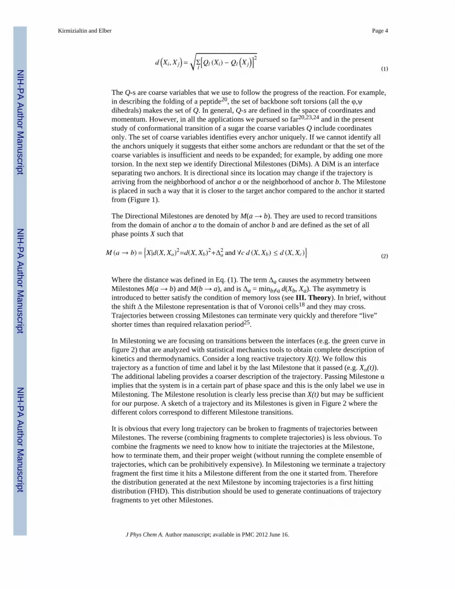
The Q-s are coarse variables that we use to follow the progress of the reaction. For example,in describing the folding of a peptide20, the set of backbone soft torsions (all the φ,ψdihedrals) makes the set of Q. In general, Q-s are defined in the space of coordinates andmomentum. However, in all the applications we pursued so far20,23,24 and in the presentstudy of conformational transition of a sugar the coarse variables Q include coordinatesonly. The set of coarse variables identifies every anchor uniquely. If we cannot identify allthe anchors uniquely it suggests that either some anchors are redundant or that the set of thecoarse variables is insufficient and needs to be expanded; for example, by adding one moretorsion. In the next step we identify Directional Milestones (DiMs). A DiM is an interfaceseparating two anchors. It is directional since its location may change if the trajectory isarriving from the neighborhood of anchor a or the neighborhood of anchor b. The Milestoneis placed in such a way that it is closer to the target anchor compared to the anchor it startedfrom (Figure 1).

The Directional Milestones are denoted by M(a → b). They are used to record transitionsfrom the domain of anchor a to the domain of anchor b and are defined as the set of allphase points X such that

(2)

Where the distance was defined in Eq. (1). The term Δa causes the asymmetry betweenMilestones M(a → b) and M(b → a), and is Δa = minb≠a d(Xb, Xa). The asymmetry isintroduced to better satisfy the condition of memory loss (see III. Theory). In brief, withoutthe shift Δ the Milestone representation is that of Voronoi cells18 and they may cross.Trajectories between crossing Milestones can terminate very quickly and therefore “live”shorter times than required relaxation period25.

In Milestoning we are focusing on transitions between the interfaces (e.g. the green curve infigure 2) that are analyzed with statistical mechanics tools to obtain complete description ofkinetics and thermodynamics. Consider a long reactive trajectory X(t). We follow thistrajectory as a function of time and label it by the last Milestone that it passed (e.g. Xα(t)).The additional labeling provides a coarser description of the trajectory. Passing Milestone αimplies that the system is in a certain part of phase space and this is the only label we use inMilestoning. The Milestone resolution is clearly less precise than X(t) but may be sufficientfor our purpose. A sketch of a trajectory and its Milestones is given in Figure 2 where thedifferent colors correspond to different Milestone transitions.

It is obvious that every long trajectory can be broken to fragments of trajectories betweenMilestones. The reverse (combining fragments to complete trajectories) is less obvious. Tocombine the fragments we need to know how to initiate the trajectories at the Milestone,how to terminate them, and their proper weight (without running the complete ensemble oftrajectories, which can be prohibitively expensive). In Milestoning we terminate a trajectoryfragment the first time it hits a Milestone different from the one it started from. Thereforethe distribution generated at the next Milestone by incoming trajectories is a first hittingdistribution (FHD). This distribution should be used to generate continuations of trajectoryfragments to yet other Milestones.



NIH


NIH


NIH


Algorithmically, the termination step is clear. More complex is the start at the Milestone inwhich we sample initial conditions from a FHD. A FHD is generated by trajectories hittingfor the first time the Milestone we want to start from. Looking backward and forward at thehistory of generating FHDs it seems that in order to generate a FHD we need an ensemble ofcomplete trajectories. Such complete generation of trajectories is possible and is essentiallythe approach taken by the Transition Interface Sampling (TIS)26 and the Forward Flux27

(FF) methods. However, since complete trajectories are computed, these exact proceduresare limited to rapid transitional events. The overall rate can still be slow if reactivetrajectories are rare. TIS and FF are designed to sample such rare trajectories efficiently.However, diffusive barriers and individual long trajectories cannot be computed this way.For diffusive processes there is much to be gained by the additional assumption of fragment-independence, an assumption we exploit in Milestoning. In Milestoning we do not continuea trajectory from a termination point of a previous trajectory. Instead we sample independentphase space points from the FHD. The independently constructed configurations ensureproper sampling to start new trajectory fragments even if only a few fragments reach thecurrent Milestone.

The following procedure is used in DiM to initiate trajectory fragments. We generateconfigurations at a Milestone α by restrained or constrained canonical sampling to theneighborhood of the Milestone25,28. The constrained sampling is made with the help ofharmonic potentials as described in28, or with constraints that are implemented usingLagrange's multipliers23,25. In the past25 we used the distribution generated by constraineddynamics “as is” to approximate the FHD. However, in DiM we offered a correction whichis very much in the spirit of the PPTIS calculations12. Every point sampled in the restrainedcalculations is freely integrated (without the restraint) back in time until it hits a Milestone.If the trajectory hits the Milestone it started from, we eliminate this point from the set sinceit is not a first hitting point. If however, another Milestone is hit then we keep the sampledpoint and use it for integration forward in time.

The integration forward in time is terminated when a new Milestone is hit. The trajectory isnot stopped when re-crossing of the original Milestone is detected (in contrast to theintegration backward in time). See for example the orange trajectory fragment in Figure 2.The orange trajectory starts at the end of the green trajectory. If we integrate it backward intime (follow the green trajectory) we find that the beginning of the orange trajectory isindeed a first hitting point on the desired Milestone. The orange trajectory fragment crossesthe starting Milestone, but this is allowed at this phase, and we continue the integration untilit hits a new Milestone (and terminates).

At the end of a successful calculation of a trajectory fragment in DiM we have the followinginformation: “Touching” of three Milestones and two termination times. We know theMilestone (say α) on which we sample phase space points to start trajectory fragments. Weknow Milestone β that was reached after backward integration in time from α, and Milestoneγ that was reached after forward integration. We also know the times forward and backward.Actually we know more than the list just discussed. We know the complete trajectoryfragments. This is however more than we want to know. Our goal is to construct a coarsegrained model for the system dynamics which is based on lower spatial resolution (usingMilestone crossings) and not the full phase space. We prefer to state that “the system waslast seen in Milestone α” as the spatial descriptor rather than X(t). Finally, in the currentversion of Milestoning we do not use the termination time obtained from backwardintegration nor the identity of the Milestone β. Extensions are in principle possible atadditional computational costs (more statistics are needed to use additional labels). Thebackward integration is used only to verify that the initial phase point is sampled from FHD.We use the trajectory data to estimate the transitional probabilities, Kαβ (t), which are the



NIH


NIH


NIH


probabilities that the system initiated at Milestone α at time 0 will pass Milestone β for thefirst time exactly at time t. If the total number of trajectories initiated at α is nα and if thenumber of trajectories that hit Milestone β at time t is nαβ(t) then we estimate Kαβ(t)≃nαβ(t)/nα . We describe how this information is used to compute overall kinetics andthermodynamics in the next section.

III. TheoryWith a better picture of how trajectories are initiated and computed we now introduce thetheory that uses the fragment statistics to investigate kinetics and thermodynamics. Wedefine the following entities:

p(X̄α,t)-- the probability that at time t the last Milestone that was crossed was α at aninterface point X̄α.

qα (X̄α,t)-- the probability density that a trajectory hit a Milestone coordinate X̄α exactly attime t.

Kαγ(X̄α,t; X̄γ,t′)-- transition probability from a specific phase space point X̄α at time t toanother phase space point X̄γ at time t.

Below we write an expression for the probability distribution generated by Milestoningtrajectories. Note that while the expression resembles Eq. 4 in the original Milestoningpaper17 the expressions are different. The present expression is exact since the explicitcoordinates within the interface are taken into account.

(3)

The notation ᾱ means the set of milestones that are directly accessible (without passinganother milestone) from and to milestone α using trajectory fragments. We also call this set“neighbors to α“. The integration over V̄ is over the hypersurface that makes the Milestone.Verbally the expressions above are simple probability balance. Therefore they are exact andare independent of the specific dynamics that was used to calculate trajectories (can beNewtonian, Langevin, etc.). The first equation states that the probability that the lastmilestone passed is α (pα (X̄α,t)) is the probability that the α milestone was crossed at anearlier time t′ (qα(X̄α,t′)), no other milestone was crossed since then, and we sum over allearlier times. The second equation suggests that milestone α is crossed exactly at time t byone of the two mechanisms: it is exactly at α at the beginning (t=0) or it passes at an earliertime t′ a milestone neighbor to α, and then exactly at time t transitions to α.

The above expressions are exact but also extremely complex to compute. The matrixKαγ(X̄α,t; X̄γ,t′) is of very high dimension. Assume that we use 100 bins to determine theposition of every coordinate x. Assume further that the system under consideration has about10 coarse degrees of freedom. The transition matrix (which is not symmetric) will have~10020(!) elements to compute. Some simplifications are therefore necessary. We firstassume a stationary process. As a result the transition probability depends on the timedifference and not the absolute time. We have



NIH


NIH


NIH


(4)

The second simplification is an approximation and is the core of the theory. We assume thatwhen a trajectory leaves milestone α on its way to terminate on milestone γ it no longer“remembers” the exact phase space point that came from milestone α; i.e., we can write

(5)

The trajectory still remembers the milestone it came from but no longer the exact phasespace point it started in that milestone. This approximation allows for dramaticsimplification and coarse-graining in space as we illustrate below.

When is this approximation valid? A limit in which this approximation is satisfied is whenthe trajectory has been running for a while before terminating on a neighboring Milestone,statistical mechanics takes its course and the precise location of the initial conditions is nolonger important. This limit is clearly correct for a sufficiently long time in which initialconditions are forgotten. However, in practice memory-loss is evident for times muchshorter than this particular limit. Note that the phase space point includes velocity. Inreference 25 we illustrate that if the average termination time between milestones is longerthan the time for velocity de-correlation, then the rate computed for solvated alaninedipeptide is accurate and insensitive to the number of Milestones. We have a reasonablecontrol on this condition. The spatial separation between Milestones determines the de-correlation or memory-loss time and is determined by the number of Milestones we putbetween the cell of reactants and products. It is therefore a good practice to repeat ratecalculations with more than one distribution of Milestones and to verify that the resultsremained unchanged as a function of reasonable separation of Milestones. A clearillustration of the stability of the Milestoning results as a function of the separation size isgiven in reference 25.

Another limit of Milestoning that leads to exact mean first passage time (MFPT) (but nothigher moments of the first passage time) is discussed in 29. If the milestones happened to beiso-committer surfaces (i.e. hypersurfaces for which the probability to reach the productbefore the reactant is a constant), the transition probability does not depend on exact locationin the Milestone (the probability is always the same) and the approximation above becomesexact. In the language of the kernel above we have

(6)

This limit is mathematically elegant and attractive. A concern is that exact determination ofiso-committer surfaces is difficult and in most cases we can only approximate it. It is notclear how good the approximation of a committer surface is compared to the condition ofequation (3). The second concern is that the iso-committer hypersurface is defined for a one-dimensional reaction coordinate and extension to several coarse-grained variables or that theDiM picture we advocate above is not obvious.

Majek and Elber16 formulated yet another condition that provides exact mean first passagetime. Generation of a FHD at a Milestone is obtained from trajectories originating from at



NIH


NIH


NIH


least two different Milestones. If the generated FHD is independent of the initial Milestone,then the overall mean first passage time is exact.

The Milestoning approximation makes it possible to remove the coordinate representationand replace it with the reduced representation of Milestone labels.

The time remains continuous. With the last adjustment and approximation (5) at hand we areready for the next step; we have

(7)

We define the following functions

(8)

Integrating equation (7) over X̄γ and adding yet another integration over X̄α we obtain

(9)

Equation (9) is a central result. These are the Milestoning equations of motion that werewritten ad-hoc in reference 17.

The entities we are interested in at present are pα (∞), which is the equilibrium or thestationary distribution, and the stationary flux qα (∞). We assume that these distributionsexist, in the sense that the probability and the flux become time independent and constants atthe long time limit.

We will need a few mathematical tricks in order to derive the stationary distributions. Belowwe follow the derivation of25,30, however, more details are added to make some of thederivations easier to follow. In particular we give some Laplace transform results in theAppendix.

The Laplace transform of equations (9) are (see Appendix):



NIH


NIH


NIH


(10)

We can formally solve for the vector q̃(u) using the second equation in a matrix form.

(11)

where q and p are row vectors, and K is matrix such that (K̃(u))αβ = K̃αβ (u). Multiplying bythe Laplace variable u and taking the limit to zero we have

(12)

We note that . We used the above formula todefine a new matrix K, which is the probability matrix of transitions between neighboring

Milestones integrated over all times. Because K is a probability we also have . Thevector qstat is an eigenvector of the operator (I-K) with the eigenvalue of zero. In thecalculation of qstat we need only K and not K(t) which is easier. In other words, only thezero moment of the time distribution, K(t), is needed.

The stationary flux is not influenced by the initial conditions, consistent with a statisticalmechanics longtime limit (also for stationary flux).

An example of a transition matrix for three Milestones that leads to a stationary flux isbelow.

(13)

Let the total number of trajectories that we start at interface 1 be n1 and the number oftrajectories that were terminated at interface 2 be n12; a numerical estimate of K12 is n12/n1.The absorbing boundary is the third state. The matrix is set in such a way that a trajectorythat makes it to the absorbing state returns to the initial state which is the first Milestone. Tocreate a stationary flux we must have a cycle in which particles that are lost are returned tothe system. Otherwise loss of probability (and no stationary solution) is unavoidable.

It is important to note that the matrix used to compute the mean first passage time (seebelow) is different. If we do not terminate the trajectory at the absorbing boundary conditionand just return it to the beginning, the trajectory time will be of infinite length in time (!).



NIH


NIH


NIH


For the determination of the mean first passage time we will use a matrix that terminatesevery trajectory that touches the final state.

(14)

Armed with an expression for the stationary flux we are ready to proceed to compute thestationary distribution. We write equation (10) multiplied by the Laplace variable u. Notethat this is not a matrix equation.

(15)

We have to be a little careful when we take the limit of u → 0 in the above expression since

and 1-1 will give us zero. We therefore write

(16)

We are ready to write the stationary distribution of the probability that the last milestonepassed is α. The result below is remarkably simple. It is given by the stationary flux throughthat interface multiplied by the average life-time of trajectories initiated at interface α - ⟨tα⟩

(17)

.

We proceed to consider kinetics. One of the most useful measures of kinetic is the mean firstpassage time and its moments. For simple processes that decay exponentially in time theinverse of the mean first passage time is the rate constant. The overall mean first passagetime is defined as the average time it takes the trajectories to reach for the first time the finalabsorbing state. Formally we write

(18)

Where qf is the probability of entering the final absorbing state. Similar to the calculations ofstationary state, we use Laplace transform to evaluate this entity. Instead of equation (18) wewrite



NIH


NIH


NIH


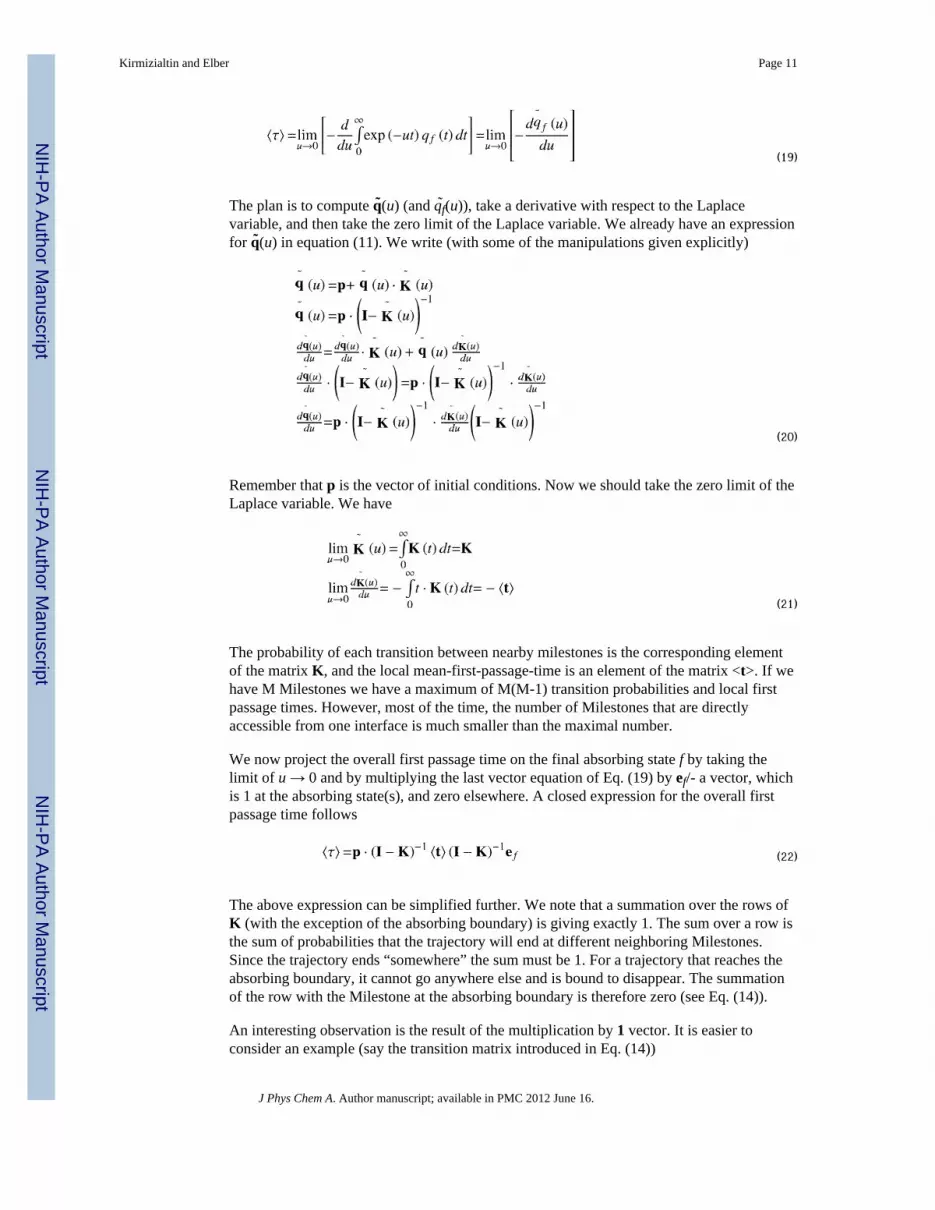
(19)

The plan is to compute q̃(u) (and q̃f(u)), take a derivative with respect to the Laplacevariable, and then take the zero limit of the Laplace variable. We already have an expressionfor q̃(u) in equation (11). We write (with some of the manipulations given explicitly)

(20)

Remember that p is the vector of initial conditions. Now we should take the zero limit of theLaplace variable. We have

(21)

The probability of each transition between nearby milestones is the corresponding elementof the matrix K, and the local mean-first-passage-time is an element of the matrix <t>. If wehave M Milestones we have a maximum of M(M-1) transition probabilities and local firstpassage times. However, most of the time, the number of Milestones that are directlyaccessible from one interface is much smaller than the maximal number.

We now project the overall first passage time on the final absorbing state f by taking thelimit of u → 0 and by multiplying the last vector equation of Eq. (19) by ef/- a vector, whichis 1 at the absorbing state(s), and zero elsewhere. A closed expression for the overall firstpassage time follows

(22)

The above expression can be simplified further. We note that a summation over the rows ofK (with the exception of the absorbing boundary) is giving exactly 1. The sum over a row isthe sum of probabilities that the trajectory will end at different neighboring Milestones.Since the trajectory ends “somewhere” the sum must be 1. For a trajectory that reaches theabsorbing boundary, it cannot go anywhere else and is bound to disappear. The summationof the row with the Milestone at the absorbing boundary is therefore zero (see Eq. (14)).

An interesting observation is the result of the multiplication by 1 vector. It is easier toconsider an example (say the transition matrix introduced in Eq. (14))



NIH


NIH


NIH


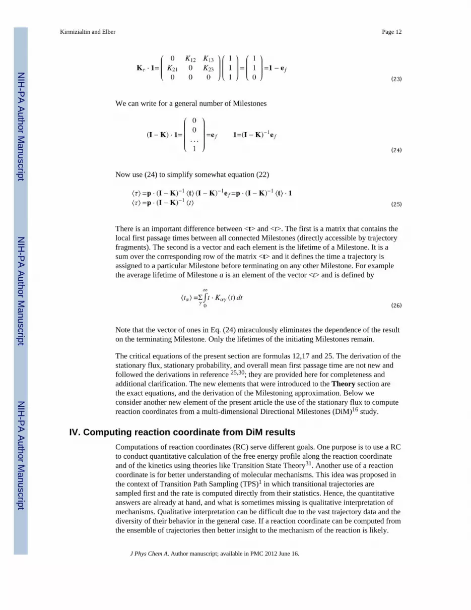
(23)

We can write for a general number of Milestones

(24)

Now use (24) to simplify somewhat equation (22)

(25)

There is an important difference between <t> and <t>. The first is a matrix that contains thelocal first passage times between all connected Milestones (directly accessible by trajectoryfragments). The second is a vector and each element is the lifetime of a Milestone. It is asum over the corresponding row of the matrix <t> and it defines the time a trajectory isassigned to a particular Milestone before terminating on any other Milestone. For examplethe average lifetime of Milestone a is an element of the vector <t> and is defined by

(26)

Note that the vector of ones in Eq. (24) miraculously eliminates the dependence of the resulton the terminating Milestone. Only the lifetimes of the initiating Milestones remain.

The critical equations of the present section are formulas 12,17 and 25. The derivation of thestationary flux, stationary probability, and overall mean first passage time are not new andfollowed the derivations in reference 25,30; they are provided here for completeness andadditional clarification. The new elements that were introduced to the Theory section arethe exact equations, and the derivation of the Milestoning approximation. Below weconsider another new element of the present article the use of the stationary flux to computereaction coordinates from a multi-dimensional Directional Milestones (DiM)16 study.

IV. Computing reaction coordinate from DiM resultsComputations of reaction coordinates (RC) serve different goals. One purpose is to use a RCto conduct quantitative calculation of the free energy profile along the reaction coordinateand of the kinetics using theories like Transition State Theory31. Another use of a reactioncoordinate is for better understanding of molecular mechanisms. This idea was proposed inthe context of Transition Path Sampling (TPS)1 in which transitional trajectories aresampled first and the rate is computed directly from their statistics. Hence, the quantitativeanswers are already at hand, and what is sometimes missing is qualitative interpretation ofmechanisms. Qualitative interpretation can be difficult due to the vast trajectory data and thediversity of their behavior in the general case. If a reaction coordinate can be computed fromthe ensemble of trajectories then better insight to the mechanism of the reaction is likely.



NIH


NIH


NIH


The definition of a reaction coordinate poses a significant challenge. It can be particularlyvague if the goal is of qualitative understanding of mechanisms rather than quantitativecalculation of thermodynamics and kinetics. Iso-committer surfaces1,32,33 were advocated asthe true choice of the reaction coordinate. An iso-committer surface is a set of points withthe same reaction probability (RP). The RP is the probability that trajectories initiated fromthese points will reach the product state before the reactant for the first time. This choice isappealing; however, the determination of the iso-committer surfaces is far from trivial andmust be done approximately and numerically at significant computational cost. Trajectoriesare launched from different positions on the energy landscape and their fate (ending in thereactant or product state) is determined 34,35. In some implementations the iso-committersurface is given a functional form with parameters that are fitted to the trajectory data35,36.

Reaction coordinates have been computed as minimum energy paths for a longtime now.Optimization of functionals 37,40 is a particularly attractive technique to determine RC forlarge molecular systems and has been used extensively. One of the functionals that defines areaction coordinate is based on the notion of flux. Rather than surfaces we seek a lineconnecting the reactants and products such that the flux leading from reactant to productalong this line is a maximum. This is a theoretically appealing idea that is based ondynamics (instead of only the static energy surface). Use of a curvilinear line instead of ahypersurface leads to dramatic simplification of the calculation and in our ability tounderstand the underlying mechanism. The idea was put forward for overdamped systemsby Berkowitz and McCammon 41 and made into a useful algorithm for molecular systems(Maxflux) by Huo and Straub39. The last algorithm was revisited recently by Zhao and co-wrokers 42. The calculations are based on a path integral analysis of overdamped Langevintrajectories with two fixed end points (reactants and products). The flux in an infinitesimaltube around the RC is optimized as a function of the reaction (curvilinear) coordinate.

A disadvantage of the Maxflux functional is that the procedure was limited so far tooverdamped Langevin dynamics. Moreover, the restriction to an infinitesimal volumearound the path makes it harder to estimate fluctuations that are likely to occur if the freeenergy landscape is not an infinitesimally narrow tube. The Maxflux principle should bevalid for analysis of trajectories of arbitrary dynamics. The required operation isstraightforward: collecting trajectories from reactant to products and estimating the reactiveflux of every phase space point and determining a not-so-narrow tube of maximal flux fromreactant to product. We propose to do exactly that in the context of the Milestoningalgorithm.

Interestingly, a Directional Milestoning calculation provides all the fluxes between the cellsor at the interfaces separating the cells (equation 12). The fluxes, qa are a discreterepresentation of the fluxes in the continuous system. A discrete path between the cells thatmaximizes the reactive flux from reactant to product solves the Maxflux problem (seeFigure 5 for an example of such a graph). The advantage of doing it through Milestoning isthat the dynamics in Milestoning are arbitrary and the results are no longer restricted tooverdamped Langevin dynamics. The volumes in phase space that are attached to anchors inMilestoning cannot be made infinitesimal since cell volumes that are too small violate theprinciple of memory loss. However, infinitesimal volumes are not desired since entropiceffects are ignored. We loosely use the term “cell” to denote phase space allocated toanchors. It is a loose term since it is possible for phase space points along trajectoryfragments to have exactly the same coordinates and momenta and originate from differentMilestones.

Consider a graph G with N nodes (which are the cells) and E edges which are Milestonesconnecting the cells. For each edge connecting (say) cells k and l we assign a weight



NIH


NIH


NIH


Wkl=qkl-qlk which is the net forward flux of this edge. We seek in the graph a path thatconnects the reactant and product and that carries maximum flux. The procedure wedescribed below is similar in spirit to an algorithm based on the Master equation43 and on acalculation based on the Transition Path Theory 44 for the analysis of folding trajectories.The Milestoning calculation provides the flux directly, therefore, the current analysis issimple and straightforward.

The following algorithm finds a path of maximum flux on the graph. In case of degeneracy(more than one path with a maximum value for the flux) we pick one of the degeneratereaction coordinates.

Algorithm:

1. Find the link emin with the smallest weight wmin=mini(wi) on the graph Gcurrent (theedge with the smallest flux) and mark it for elimination.

2. Check if after removing emin it is still possible to find a sequence of edges leadingfrom reactants to products. If yes, remove emin from the graph and go to 1. If not,store emin as an edge in the desired path, store the resulting disconnected graphs, Giand Gj, remove emin from the graph, and continue to 3.

3. After the removal of emin in 2 we have at least two disconnected graphs. Pick oneof these graphs (say Gi). If the graph does not have edges, pick another graph fromthe set and repeat the check. If none of the graphs have edges, join all the eminedges discovered so far to create the maximum flux path and stop. If a graph withedges is discovered rename it Gcurrent. Re-assign reactant or product according thenodes of the edge that was removed and go to 1.

The above procedure is guaranteed to provide a maximum flux path in the discrete spacegenerated in the Milestoning calculations. It may not be necessarily the most efficient;however, this is not an expensive calculation compared to the estimates of the transitionkernel by trajectories and is sufficient for the present task.

It is also possible to seek the second (and higher order) best path. One approach is to removeall the edges of the max flux path and to analyze the resulting graph with the same algorithmdescribed above. A disadvantage is that we can have different paths that share parts of theedges. How many edges should be different in the pair of the paths to make them distinct?Chemical intuition suggests a solution that we use: The paths are different if the transitionstates are different. We choose a “transition state” to be the edge along the maximum fluxpath that has the smallest flux. We remove that edge and re-analyze the path for a secondbest pathway. There are two possible outcomes. The first is that a completely new path isobtained. In this case we store the second path, and perhaps continue to search for a thirdpath. The second outcome is that all the remaining edges of the original path are still pickedand a short detour near the old transition state is found. This may suggest that an alternativepath does not exist. We can proceed by removing another edge from the MFP. We removean edge that is carrying the lowest flux among the remaining edges along the path and repeatthe analysis until a new path is found.

V. Example for a Directional Milestoning calculation and determination of areaction coordinate

To illustrate Milestoning on a realistic system of chemical interest we consider aconformational transition in the molecule Adenosine. It is a highly flexible molecule withmultiple reaction coordinates and reactive tubes that further cross each other. This makesreaction coordinate predictions difficult. Adenosine is also an important model system for



NIH


NIH


NIH


conformational transitions in polynucleotides such as DNA and RNA molecules 45.Experiments estimate the relaxation time as nanoseconds 46. This time scale is accessible tostraightforward Molecular Dynamics simulations making the present system a usefulbenchmark in which we compare our approximate result with exact calculation of rate fromMD simulation. The two states of interest (“reactant” and “products”) are shown in Figure 3.A similar system was studied by the Transition Path Sampling method 47.

The overall conformational transitions of the molecule can be described approximately byglycosyl torsion χ (O4`-C1`-N9-C4), which assumes anti or syn conformations at roomtemperature, and the pseudo rotation of the furanose sugar ring denoted here as p′. Thepseudo rotation angle is commonly defined as 48

where the set {νi}i=1,5 are torsions corresponding to C1`-C2`-C3`-C4`, C2`-C3`-C4`-O4`,C3`-C4`-O4`-C1`, C4`-O4`-C1`-C2`,O4`-C1`-C2`-C3` respectively. To have always positiveangles we replaced p′ with p = p′+180° when ν1 = 0° and p = mod(p′+360°) otherwise.Given the definition above, the sugar of adenosine is C3èndo at p ~ 30° and C2èndo at p ~150°.

The molecule was solvated in a periodic box of water as shown in Figure 4.

To obtain an exact comparison to the Milestoning calculations we conducted first 1.1 μsecMD simulation at room temperature, which is sufficient to adequately estimatethermodynamic behavior (free energy surface) and the overall mean first passage time of thetransition between the two states. The free energy surface is constructed for the two degreesof freedom p and χ by binning their sampled values along the trajectory. We choose cells 19and 15 with cluster centers in the two dimensional variables (p,χ): C3a (p,χ=35°, 221°) andC2s (p,χ=154°,30°). The choice of C2s is rather arbitrary as we could also choose cells 6 or18 as they have lower free energy on the contour map. Cell 15 is larger and it has largervolume and entropy. As a result it is sampled more frequently in the long MolecularDynamics run we used for comparison.

The Directional Milestoning approach requires a set of anchors. As argued above this set ofstructures can come from numerous sources: replica exchange simulations 55, configurationsalong a pre-computed minimum energy or free energy path 24 and straightforward and longMolecular Dynamics trajectory (the present study). Interestingly, the present molecule is apoor candidate for Milestoning calculations based on minimum energy or minimum freeenergy pathways since multiple connected channels make such calculations difficult(Kirmizialtin and Elber, unpublished). Especially problematic is the use of the popularhyperplane approximation to determine the minimum energy (or free energy) pathways. Wetherefore use the configurations from the long time MD trajectory, and cluster themaccording to the six torsional angles described above.

The Euclidian distance between the six torsions of the selected atoms defined earlier (Eq.(1)) is used for clustering. We first reduced 275000 structures to 24560 by removingstructures that are different by no more than 2 degrees per torsion. The remaining data isclustered by k-means algorithm56 into N=20 clusters that are used to define the anchors andthe milestones. We conduct the Milestoning calculation in three steps: (1) search, (2) sampleand (3) run to ensure efficiency16. The maximum number of possible interfaces is20×19=380 which is large (reminder: the interfaces are directed and a transition from i->j is



NIH


NIH


NIH


different from a transition from j->i). Rather than exhaustive enumeration of Milestones, andwith an eye to more complex systems with a much larger number of plausible interfaces, wesample the most important milestones. The connectivity between anchors is estimated byfirst launching 500 trajectories of maximum length of 10ps from each anchor until they hitone of the nearby Milestones. We call this step the “search”. Interfaces that are “touched”are recorded and the touching configuration is used to initiate a sampling trajectory at theinterface in a step of “sampling”. The sampling at the interface is performed with umbrellapotential as described in reference 16. Each of the sampling points was tested by computingtrajectories backward in time. Trajectories that return to the original interface during the testare not first hitting points, and are removed from the set as discussed in II Algorithms.

In the final step (called “run”) 400 sampled points were integrated forward in time until theyhit a new interface. The identity of the interface and the termination time are recorded.Interfaces that were not detected in the “search” step can still be discovered in “run” sincetermination is tested for all possible interfaces. Newly discovered Milestones are added tothe set and are “sampled” and “run”. After a few cycles of runs, in which additionalinterfaces are found and are added, the number of interfaces converges to 207. This is a highnumber (more than a half of the total possible), suggesting a very significant connectivitybetween the anchors. All simulations in the “run” step are in the NVT ensemble at 300Kwith a weak Anderson thermostat57. A time step of 0.5 fs is used during the DiMcalculations. The rest of the computational details are the same as in the long MD simulationand described in the caption of Figure 4.

The states C3a and C2s correspond to cell numbers 19 and 15 respectively. We calculatedthe average first passage time in two directions from the long MD trajectory and fromMilestoning.

The error in DiM calculations is estimated by dividing the data into two sets. The results arein reasonable agreement and are within the range of the statistical errors.

In Figure 6 we illustrate that the thermal probability of the individual sites is reasonably wellreproduced in the Milestoning calculation.

The next item of interest is the calculation of the reaction pathway. In Figure 7 we show thecomplete network between the cells.

With the network at hand we followed the algorithm of section IV and derive the maximumflux path (MFP) shown in Figure 5 in red. The MFP is plotted as linear red segmentsbetween the centers of the cells it connects. The MFP is computed in a space of six coarsevariables and not in the two reduced variables that we use to represent the free energylandscape. Hence, what looks like “skipping” some interfaces at the top left of free energysurface is a result of a non-ideal projection of six dimensions into two.

The MFP is different from the Steepest Descent Path (SDP) computed with functionaloptimization as described in reference 37 and is shown in with the black thick line. TheSteepest Descent Path is sometimes called the Intrinsic Reaction Coordinate. The SDPcalculation starts with a linear interpolation between the two end structures. The algorithmfinds a local minimum for the path that is not too far from the initial guess. When we startthe SDP optimization from the MFP the algorithm settles in a path near the MFP (see Figure5). It was probably not detected by the functional optimization since the initial guess of astraight line has a preference to nearby paths. Minimum energy path calculations provide alocal minimum near the initial guess. The MFP graph analysis provides the global optimumover all path space, which is clearly an advantage. Of course in the graph analysis we rely on



NIH


NIH


NIH


a discrete coarse-grained representation from Milestoning and the results will depend on thequality of the DiM sampling.

One can also search for alternative pathways to the MFP that is already found. The secondand third best paths are calculated as outlined in IV and are shown in Figure 8. Note that thesecond best path (in green) is similar to the Steepest Descent Path (SDP) computed withfunctional optimization from straight-line interpolation.

Our free energy calculation and the thermal equilibrium probability shows that C2èndo isslightly more stable than C3èndo while χ has a lower energy at syn.

The reaction coordinates allow for better understanding of the conformational change. Themolecule transitions from syn to anti in multiple pathways as is shown in Figure 8. Themaximum Flux path suggests that the transition starts with a change of the puckering angleand proceeds with the glycosyl angle modification. Transition of the puckering angle fromC2èndo (South) to C3èndo (North) is through the East barrier that is from O1′ endo andC4èxo (see Altona for details of the nomenculature48) and for the glycosyl angle the routeis from 60° → 360° → 204°. The second path follows a route for χ from 60° → 180° →204° after the puckering transition done in a similar way as in the first path. The third bestpath on the other hand starts with glycosyl angle change from 60° → 360° → 204° andfollowed by sugar puckering the same way before. Comparing the flux of the free paths wefocus on the transition states. Path 1 (red line) the transition state is between cell 18 and 11,and the flux is 0.010. Path 2 (green dots) the transition state is between cells 6 and 11 andthe flux is 0.007. Finally, path 3 (black dots) is between cells 10 and 19 and the flux is0.002. The results suggest that while the third path can probably be ignored, the second pathmakes a significant contribution to the overall reactive flux.

Concluding remarksWe describe in detail the theory and application of Directional Milestoning (DiM). It makesit possible to study the kinetic and thermodynamic of complex systems using testable andphysically sensible approximations. We also introduce a novel application of DiM in whicha reaction coordinate, defined as the path of maximum flux, is computed with Milestoning.

AcknowledgmentsThe research was supported by NIH grant GM59796. The help of Peter Majek in setting up the DirectionalMilestoning calculations is gratefully acknowledged. We acknowledge many useful discussions about Milestoningwith Eric vanden Eijnden, Giovanni Ciccotti, and Maddalena Venturoli.

AppendixWe start by defining a Laplace transform

(A.1)

In the limit in which the Laplace variable u is approaching zero the integral is extended toinfinite (or to very large values of t); i.e. most of the contribution will come from largevalues of t. In that limit f(t) is assumed to approach a stationary value (per our assumptionabove for the probability density and flux). In this case we can write



NIH


NIH


NIH


(A.2)

This result is useful since it correlates the Laplace transform with the asymptotic equilibriumdistribution we are after. In short if we know the Laplace transform at the limit u → 0 wealso know the equilibrium distribution. Another properly of Laplace transform that we need(and is quite famous) is that the transform of a convolution is a product of the transforms of

the functions being convoluted. The Laplace transform of an integral is

, which is a two-dimensional integral over t and t′.

Schematically we can draw the integration as

Figure A.1.Laplace transform of an integral up to time t: case AThe vertical lines mean that for a fix value of t, we integrate t′ from 0 to t. This integrationcovers exactly half of the plane (case A). However there is another way of integrating overhalf of the plane, which is more convenient for the problem at hand, and we schematicallydraw as case B

Figure A.2.The same as Figure 3 for case B. See text for more detailsHere the integration is done by fixing the beginning of the integral over t to a particularvalue t′ and then integrating from t′ to infinite. Hence the above integral is translated to

. The integral in the square brackets can be done explicitly to have

. Hence the Laplace transform of an integral is the Laplacetransform of the integrand divided by the Laplace variable. Another “useful-to-know” result



NIH


NIH


NIH


of Laplace transform is that of convolution. Define the convolution .We write

(A.3)

References1. Bolhuis PG, Chandler D, Dellago C, Geissler PL. Annual Review of Physical Chemistry. 2002;

53:291.2. Bai D, Elber R. Journal of Chemical Theory and Computation. 2006; 2:484.3. Elber R, Meller J, Olender R. Journal of Physical Chemistry B. 1999; 103:899.4. Olender R, Elber R. Journal of Chemical Physics. 1996; 105:9299.5. Shaw DE, Maragakis P, Lindorff-Larsen K, Piana S, Dror RO, Eastwood MP, Bank JA, Jumper JM,

Salmon JK, Shan YB, Wriggers W. Science. 2010; 330:341. [PubMed: 20947758]6. Eyring H. Journal of Chemical Physics. 1935; 3:107.7. Chandler D. Journal of Chemical Physics. 1978; 68:2959.8. Cardenas AE, Elber R. Proteins-Structure Function and Genetics. 2003; 51:245.9. Ma HR, Proctor DJ, Kierzek E, Kierzek R, Bevilacqua PC, Gruebele M. Journal of the American

Chemical Society. 2006; 128:1523. [PubMed: 16448122]10. Bourgeois, D.; Vallone, B.; Arcovito, A.; Sciara, G.; Schotte, F.; Anfinrud, PA.; Brunori, M.

Proceedings of the National Academy of Sciences of the United States of America; 2006. p. 492411. Roux B. Annual Review of Biophysics and Biomolecular Structure. 2005; 34:153.12. Moroni D, Bolhuis PG, van Erp TS. Journal of Chemical Physics. 2004; 120:4055. [PubMed:

15268572]13. Sarich M, Noe F, Schutte C. Multiscale Modeling & Simulation. 2010; 8:1154.14. Hinrichs NS, Pande VS. Journal of Chemical Physics. 2007; 12615. Buchete NV, Hummer G. Journal of Physical Chemistry B. 2008; 112:6057.16. Majek P, Elber R. Journal of Chemical Theory and Computation. 2010; 6:1805. [PubMed:

20596240]17. Faradjian AK, Elber R. Journal of Chemical Physics. 2004; 120:10880. [PubMed: 15268118]18. Vanden-Eijnden E, Venturoli M. Journal of Chemical Physics. 2009; 130:13.19. Muller K. Angewandte Chemie-International Edition in English. 1980; 19:1.20. Kuczera K, Jas GS, Elber R. J. Phys. Chem. A. 2009; 113:7461. [PubMed: 19354256]21. Noe F, Horenko I, Schutte C, Smith JC. J Chem Phys. 2007; 126:155102. [PubMed: 17461666]22. Hummer G, Kevrekidis IG. Journal of Chemical Physics. 2003; 118:10762.23. Elber, R.; West, A. Proceedings of the National Academy of Sciences USA; 2010. p. 500124. Elber R. Biophysical Journal. 2007; 92:L85. [PubMed: 17325010]25. West AMA, Elber R, Shalloway D. Journal of Chemical Physics. 2007; 12626. van Erp TS, Moroni D, Bolhuis PG. Journal of Chemical Physics. 2003; 118:7762.



NIH


NIH


NIH


27. Allen RJ, Frenkel D, ten Wolde PR. Journal of Chemical Physics. 2006; 124:17.28. Majek P, Elber R. Journal of Chemical Theory and Computation. 2010 accepted for publication.29. Vanden Eijnden E, Venturoli M, Ciccotti G, Elber R. Journal of Chemical Physics. 2008;

129:174102. [PubMed: 19045328]30. Shalloway D, Faradjian AK. Journal of Chemical Physics. 2006; 12431. Truhlar DG, Garrett BC, Klippenstein SJ. Journal of Physical Chemistry. 1996; 100:12771.32. Maragliano L, Fischer A, Vanden-Eijnden E, Ciccotti G. Journal of Chemical Physics. 2006; 12533. E WN, Vanden-Eijnden E. Annual Review of Physical Chemistry, Vol 61. 2010; 61:391.34. Peters B, Beckham GT, Trout BL. Journal of Chemical Physics. 2007; 12735. Ma A, Dinner AR. Journal of Physical Chemistry B. 2005; 109:6769.36. Peters B, Trout BL. Journal of Chemical Physics. 2006; 12537. Olender R, Elber R. Theochem-Journal of Molecular Structure. 1997; 398:63.38. Jonsson, H.; Mills, G.; Jacobsen, KW. Classical and quantum dynamics in condensed phase

simulations. Berne, BJ.; Ciccotti, G.; Coker, DF., editors. World Scientific; Singapore: 1998. p.385

39. Huo SH, Straub JE. Journal of Chemical Physics. 1997; 107:5000.40. Elber R, Karplus M. Chemical Physics Letters. 1987; 139:375.41. Berkowitz M, Morgan JD, McCammon JA, Northrup SH. Journal of Chemical Physics. 1983;

79:5563.42. Zhao RJ, Shen JF, Skeel RD. Journal of Chemical Theory and Computation. 2010; 6:2411.

[PubMed: 20890401]43. Berezhkovskii A, Hummer G, Szabo A. Journal of Chemical Physics. 2009; 13044. Noe, F.; Schutte, C.; Vanden-Eijnden, E.; Reich, L.; Weikl, TR. Proceedings of the National

Academy of Sciences of the United States of America; 2009. p. 1901145. Rich A. Nature Structural Biology. 2003; 10:247.46. Rhodes LM, Schimmel PR. Biochemistry. 1971; 10:4426. [PubMed: 5316837]47. Radhakrishnan R, Schlick T. Journal of Chemical Physics. 2004; 121:2436. [PubMed: 15260799]48. Altona C, Sundaralingam M. JACS. 1972; 94:8205.49. Jorgensen WL, Chandrasekhar J, Madura JD, Impey RW, Klein ML. Journal of Chemical Physics.

1983; 79:926.50. Weinbach Y, Elber R. Journal of Computational Physics. 2005; 209:193.51. Ryckaert JP, Ciccotti G, Berendsen HJC. Journal of Computational Physics. 1977; 23:327.52. Cornell WD, Cieplak P, Bayly CI, Gould IR, Merz KM, Ferguson DM, Spellmeyer DC, Fox T,

Caldwell JW, Kollman PA. Journal of the American Chemical Society. 1995; 117:5179.53. Pranata J, Wierschke SG, Jorgensen WL. Journal of the American Chemical Society. 1991;

113:2810.54. Elber R, Roitberg A, Simmerling C, Goldstein R, Li HY, Verkhivker G, Keasar C, Zhang J,

Ulitsky A. Computer Physics Communications. 1995; 91:159.55. Sugita Y, Okamoto Y. Chemical Physics Letters. 1999; 314:141.56. Duda, R.; Hart, P.; Stork, D. Pattern Classification. John Wiley and Sons; New York: 2001.57. Juraszek J, Bolhuis PG. Biophysical Journal. 2008; 95:4246. [PubMed: 18676648]



NIH


NIH


NIH


https://www.researchgate.net/publication/259864416_Pattern_Classification?el=1_x_8&enrichId=rgreq-e9e0e470375881182b0f534e812e800a-XXX&enrichSource=Y292ZXJQYWdlOzUxMDU4NjAyO0FTOjk4NzY3NTcxMjU5NDA0QDE0MDA1NTk0MzMwMTg=

Figure 1.A schematic representation of Directional Milestoning. The circles denote anchors, thestraight lines denote interfaces or Milestones, and the curves are trajectory fragments.Consider the red anchor. The Directional Milestones that mark entry to the domain of thered anchor are the green lines. The red trajectory, which starts from the red anchor,illustrates an exit from the red anchor domain. The blue curve denotes a trajectory thatenters from the blue domain to the red domain. Note the asymmetry in the position of theentry and exit Milestones. The green curve illustrates the type of trajectories that we use inMilestoning calculations (a trajectory from an interface or a Milestone to anotherMilestone). The green trajectory starts at an entry to the domain of the green anchor andcontinues until it enters the red domain. It is then terminated and its time and terminatingMilestone are recorded. See text and reference 16 for more details.



NIH


NIH


NIH


Figure 2.A schematic representation of an exact trajectory partitioned to fragments betweenMilestones (or interfaces). Every color denotes a different trajectory fragment. We do notinitiate a new fragment when the trajectory re-crosses the same Milestone it started from(see orange trajectory). For clarity we do not differentiate between incoming and outgoingMilestones in this figure.



NIH


NIH


NIH


Figure 3.Adenosine molecule in C3a (left) and C2s states (right). Labeled atoms are used to definethe coarse variables.



NIH


NIH


NIH


Figure 4.A periodic box of water that was used in the simulation of a conformational transition inadenosine. The molecule is solvated with 420 TIP3P water molecules 49 with a periodiccubic box of 23.8×23.8×23.8Å3. The box size is adjusted to give a pressure of ~1atm at300K. We used a matrix variant50 of the SHAKE algorithm 51 to fix water bond lengths andangles while the solute is not constrained. 8Å cutoff is used for Lennard Jones and 8.5 Å forreal space cutoff of electrostatics. Particle-mesh Ewald summation was used for long rangeelectrostatics. The time step was 2fs. All simulations are performed with AMBER/OPLSAAforce field where bonding terms are taken from Amber99 52 and the nonbonding terms arefrom OPLSAA 53. The parameters are available from MOIL 54

http://clsb.ices.utexas.edu/prebuilt/



NIH


NIH


NIH


http://clsb.ices.utexas.edu/prebuilt/

Figure 5.A contour plot of the two-dimensional free energy profile for adenosine. Each contourcorresponds to one kcal/mol change in free energy with dark blue being the lowest energywhile white is the highest. Black dots are the cluster centers used for the DirectionalMilestoning. The black solid line is a steepest descent path from C3a to C2s computed withthe functional “scalar force”37 while the red line is the Maximum flux reaction coordinatecalculated from Directional Milestoning. The green dashed line is the SDP path if the initialguess for the SDP algorithm is the Maximum Flux Path. The black and red lines clearlyillustrate the existence of multiple channels. Note that six coarse variables were used in theMilestoning calculation and the picture shown is a projection onto two dimensions. Theprojection is not always successful. For example, in the transition from χ≅220 to χ≅360 itseems (incorrectly) that several Milestones are crossed in one transition.



NIH


NIH


NIH


Figure 6.Equilibrium probability of being in a cell of an acnhor calculated from long MD simulation(dashed) is compared with stationary distribution of DiM. In DiM the stationary solution is asum of all the probabilities of crossing a Milestone into a cell and remaining there. Thecontribution of one interface is given by Eq. (17).



NIH


NIH


NIH


Figure 7.A connectivity graph of each cell with its neighbors. Nodes are centers of clusters and edgesrepresent local transition pathways. The arrows indicate the direction of the transition. Fromdetailed balance we expect every transition to be reversal. However, some transitionsbetween nearby milestones are very rare and are not sampled. These transitions do notimpact the overall rate.



NIH


NIH


NIH


Figure 8.Two alternative paths when the graph is blocked at the two lowest bottleneck regions of theMaximum Path (solid red): green dashed when region 18-11 is blocked and black dashedwhen 4-19 is blocked.



NIH


NIH


NIH


NIH


NIH


NIH



Table 1

Mean first passage time computed from exact (and long) Molecular Dynamics Trajectory (MD) and themethod discussed in the present article Directional Milestoning (DiM). The times quoted are in picoseconds.

<τ> DIM MD

19→15 173±79 202±11

15→19 6461±710 5511±377


Documents

Revisiting and Computing Reaction Coordinates with Directional Milestoning