Modeling Data using Directional Distributions

Inderjit S. Dhillon and Suvrit SraDepartment of Computer SciencesThe University of Texas at Austin

Austin, TX 78712{suvrit,inderjit}@cs.utexas.edu

25 January, 2003∗

Technical Report # TR-03-06

Abstract

Traditionally multi-variate normal distributions have been the staple of data modeling inmost domains. For some domains, the model they provide is either inadequate or incorrectbecause of the disregard for the directional components of the data. We present a generativemodel for data that is suitable for modeling directional data (as can arise in text and geneexpression clustering). We use mixtures of von Mises-Fisher distributions to model our datasince the von Mises-Fisher distribution is the natural distribution for directional data. Wederive an Expectation Maximization (EM) algorithm to find the maximum likelihood estimatesfor the parameters of our mixture model, and provide various experimental results to evaluatethe “correctness” of our formulation. In this paper we also provide some of the mathematicalbackground necessary to carry out all the derivations and to gain insight for an implementation.

1 Introduction

Traditional statistical approaches involve multi-variate data drawn from Rp, and little or no signifi-cance is attached to the directional nature of the observed data. For many phenomena or processesit makes more sense to consider the directional components of the data involved, rather than justthe magnitude alone. For example, modeling wind current directions, modeling geomagnetism, andmeasurements derived from clocks and compasses all seem to require a directional model [MJ00]. Amuch wider array of fields and contexts in which directional data arises is enlisted in [MJ00], andthe interested reader is urged to atleast gloss over that information.

A fundamental distribution on the circle called the von Mises distribution was first introducedby von Mises [vM18]. We address the issue of modeling data using the von Mises-Fisher (vMF)distribution [MJ00], which is a generalization (to higher dimensions) of the von Mises distribution.We concentrate on using the vMF distribution as it is a distribution that arises naturally for direc-tional data—akin to the multivariate Normal distribution ([MJ00, pp. 171-172]). Furthermore, ithas been observed that in high dimensional text data, cosine similarity performs much better thana Euclidean distance metric1 [DFG01]. This observation suggests following a directional model forthe text data rather than ascribing significance to a magnitude based (or traditional) model.

∗Revised 7th June, 2003.1Empirically cosine similarity has been observed to outperform Euclidean or Mahalanobis type distance measures

in information retrieval tasks.

1

Another application domain for the vMF model is modeling gene micro-array data (gene ex-pression data). Gene expression data has been found to have unique directional characteristics thatsuggest the use of a directional model for modeling it. Recently Dhillon et. al (see [DMR03])have found that gene expression data yields interesting diametric clusters. Intuitively these clusterscould be thought of as data pointing in opposite directions, hinting at the underlying importance ofdirectional orientation2.

For text data, one byproduct of using a generative model like a mixture of vMF distributions,is the ability to obtain a soft-clustering of the data. The need for soft-clustering comes to theforeground when the text collections to be clustered can have documents with multiple labels. Amore accurate generative model can also serve as an aid for improved classification for text data,especially where more meaningful soft labels are desired3.

Organization of this report

The remainder of this report is organized as follows. Section 2 presents the multi-variate von Mises-Fisher distribution. Section 3 carries out the maximum likelihood estimation of parameters fordata drawn from a single vMF distribution. Section 4 derives and presents the EM algorithm forestimating parameters for data drawn from a mixture of vMFs. In section 5 we show the resultsof experimentation with simulated mixtures of vMF distributions. Section 6 concludes this report.Some useful mathematical details are furnished by Appendices A and B. Appendix A providesmathematical background that is useful in general for understanding the derivations and AppendixB offers a brief primer on directional distributions.

2 The von Mises-Fisher Distribution

A p-dimensional unit random vector x (‖x‖ = 1) is said to have p-variate von Mises-Fisher distri-bution Mp(µ, κ) if its probability density is:

cp(κ)eκµTx, x ∈ Sp−1, (2.1)

where ‖µ‖ = 1, κ ≥ 0, Sp−1 is the p dimensional unit hypersphere (also denoted as Sp in someliterature), and cp(κ) the normalizing constant is given by (see B.2)

cp(κ) =κp/2−1

(2π)p/2Ip/2−1(κ). (2.2)

For more details the interested reader is urged to look at Appendix B.

2.1 Example vMF distribution

In two dimensions (on the circle S0), the probability density assumes the form

g(θ;µ, κ) =1

2πI0(κ)eκ cos(θ−µ), 0 ≤ θ < 2π. (2.3)

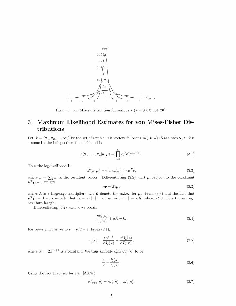
This is called the von Mises distribution. Figure 1 shows a plot of this density with mean at 0radians and for κ ∈ {0, 0.3, 1, 4, 20}.

From the figure we can see that as κ increases the density becomes more and more concentratedabout the mean direction. Thus κ is called the concentration parameter.

2Most clustering algorithms for gene expression data use Pearson correlation, which equals cosine similarity oftransformed vectors, and thus our directional model should fit it well.

3Though given the nature of high-dimensional sparse data and models based on some member of the exponentialfamily of distributions, the ability to obtain useful soft-label remains difficult without explicitly imposing “softness”constraints.

2

-3 -2 -1 1 2 3Theta

0.25

0.5

0.75

1

1.25

1.5

1.75

PDF

Figure 1: von Mises distribution for various κ (κ = 0, 0.3, 1, 4, 20).

3 Maximum Likelihood Estimates for von Mises-Fisher Dis-tributions

Let D = {x1,x2, . . . ,xn} be the set of sample unit vectors following Mp(µ, κ). Since each xi ∈ D isassumed to be independent the likelihood is

p(x1, . . . ,xn|κ,µ) =

n∏

i=1

cp(κ)eκµTxi . (3.1)

Thus the log-likelihood isL (κ,µ) = n ln cp(κ) + κµT r, (3.2)

where r =∑i xi is the resultant vector. Differentiating (3.2) w.r.t µ subject to the constraint

µTµ = 1 we getκr = 2λµ, (3.3)

where λ is a Lagrange multiplier. Let µ denote the m.l.e. for µ. From (3.3) and the fact thatµT µ = 1 we conclude that µ = r/‖r‖. Let us write ‖r‖ = nR, where R denotes the averageresultant length.

Differentiating (3.2) w.r.t κ we obtain

nc′p(κ)

cp(κ)+ nR = 0. (3.4)

For brevity, let us write s = p/2− 1. From (2.1),

c′p(κ) =sκs−1

αIs(κ)− κsI ′s(κ)

αI2s (κ)

, (3.5)

where α = (2π)s+1 is a constant. We thus simplify c′p(κ)/cp(κ) to be

s

κ− I ′s(κ)

Is(κ). (3.6)

Using the fact that (see for e.g., [AS74])

κIs+1(κ) = κI ′s(κ)− sIs(κ), (3.7)

3

we obtain−c′p(κ)

cp(κ)=Is+1(κ)

Is(κ)=

Ip/2(κ)

Ip/2−1(κ)= Ap(κ). (3.8)

Using (3.4) and (3.8) we find that the m.l.e. for κ is given by

κ = A−1p (R). (3.9)

Since Ap(κ) is the ratio of Bessel functions we cannot obtain a closed form functional inverse. Henceto solve for A−1

p (R) we have to resort to numerical or asymptotic methods.For large values of κ the following approximation is well known ([AS74], Chapter 9):

Ip(κ) ≈ 1√2πκ

eκ(

1− 4p2 − 1

8κ

). (3.10)

Using (3.10) we obtain

Ap(κ) ≈(

1− p2 − 1

8κ

)(1− (p− 2)2 − 1

8κ

)−1

. (3.11)

Now using the fact that κ is large, expanding the second term using the binomial theorem andignoring terms that have squares or higher powers of κ in the denominator we are left with

Ap(κ) ≈(

1− p2 − 1

8κ

)(1 +

(p− 2)2 − 1

8κ

). (3.12)

On again ignoring terms containing κ2 in the denominator we finally have

Ap(κ) ≈ 1− p− 1

2κ. (3.13)

Hence for large κ we obtain

κ =12 (p− 1)

1− R . (3.14)

We can write Ip(κ) as (A.8),

Ip(κ) =∑

k≥0

1

Γ(k + p+ 1)k!

(κ2

)2k+p

. (3.15)

For small κ we use only the first two terms of this series, ignoring terms with higher powers of κ toget

Ip(κ) ≈ κp

2p p!+

κ2+p

2p+2 (1 + p)!. (3.16)

Using (3.16) and on simplifying Ap(κ) we obtain

Ap(κ) ≈ κ

p, (3.17)

so that,κ = pR. (3.18)

See [MJ00] for conditions under which the approximations for κ are valid, at least for p = 2, 3.These approximations for κ do not really take into account the dimensionality of the data and

thus for high dimensions (when κ is big by itself but κ/p is not very small or very big) these estimates

4

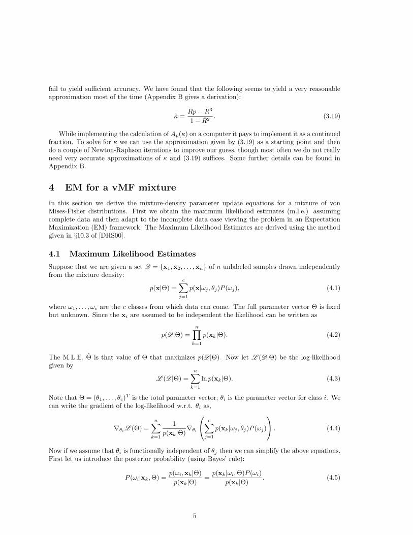
fail to yield sufficient accuracy. We have found that the following seems to yield a very reasonableapproximation most of the time (Appendix B gives a derivation):

κ =Rp− R3

1− R2. (3.19)

While implementing the calculation of Ap(κ) on a computer it pays to implement it as a continuedfraction. To solve for κ we can use the approximation given by (3.19) as a starting point and thendo a couple of Newton-Raphson iterations to improve our guess, though most often we do not reallyneed very accurate approximations of κ and (3.19) suffices. Some further details can be found inAppendix B.

4 EM for a vMF mixture

In this section we derive the mixture-density parameter update equations for a mixture of vonMises-Fisher distributions. First we obtain the maximum likelihood estimates (m.l.e.) assumingcomplete data and then adapt to the incomplete data case viewing the problem in an ExpectationMaximization (EM) framework. The Maximum Likelihood Estimates are derived using the methodgiven in §10.3 of [DHS00].

4.1 Maximum Likelihood Estimates

Suppose that we are given a set D = {x1,x2, . . . ,xn} of n unlabeled samples drawn independentlyfrom the mixture density:

p(x|Θ) =

c∑

j=1

p(x|ωj , θj)P (ωj), (4.1)

where ω1, . . . , ωc are the c classes from which data can come. The full parameter vector Θ is fixedbut unknown. Since the xi are assumed to be independent the likelihood can be written as

p(D |Θ) =

n∏

k=1

p(xk|Θ). (4.2)

The M.L.E. Θ is that value of Θ that maximizes p(D |Θ). Now let L (D |Θ) be the log-likelihoodgiven by

L (D |Θ) =

n∑

k=1

ln p(xk|Θ). (4.3)

Note that Θ = (θ1, . . . , θc)T is the total parameter vector; θi is the parameter vector for class i. We

can write the gradient of the log-likelihood w.r.t. θi as,

∇θiL (Θ) =n∑

k=1

1

p(xk|Θ)∇θi

c∑

j=1

p(xk|ωj , θj)P (ωj)

. (4.4)

Now if we assume that θi is functionally independent of θj then we can simplify the above equations.First let us introduce the posterior probability (using Bayes’ rule):

P (ωi|xk,Θ) =p(ωi,xk|Θ)

p(xk|Θ)=p(xk|ωi,Θ)P (ωi)

p(xk|Θ). (4.5)

5

Using this posterior probability we see that the m.l.e. θi must satisfy:

n∑

k=1

P (ωi|xk,Θ)∇θi ln p(xk|ωi, θi) = 0 i = 1, . . . , c. (4.6)

If the priors are also unknown then maximizing (4.6), subject to the condition

c∑

j=1

P (ωj) = 1, (4.7)

we obtain the following m.l.e. for them:

P (ωi) =1

n

n∑

k=1

P (ωi|xk, Θ). (4.8)

4.1.1 Maximum Likelihood for vMF mixture

The derivation given in the previous section applies to any probability density. Assuming that eachsample xk comes from a von Mises-Fisher distribution, i.e.

p(xk|ωi, θi) = cp(κi)eκiµ

Ti xk , (4.9)

we can solve the above maximum likelihood equations to obtain values of the parameters (κi,µi) fori = 1, . . . , c. We maximize the log-likelihood w.r.t. µi subject to the constraint µTi µi = 1 to obtain:

µi =

∑nk=1 P (ωi|xk, Θ)xk

‖∑nk=1 P (ωi|xk, Θ)xk‖

. (4.10)

Writing −c′p(κi)/cp(κi) = Ap(κi) as usual, we obtain the following m.l.e. equation for κi:

Ap(κi) =

∑nk=1 P (ωi|xk, Θ)µTi xk∑n

k=1 P (ωi|xk, Θ). (4.11)

Hence we obtain κi by calculating A−1p (·) for the above argument (see Section 3).

In all these equations the value of the posterior probability is given by:

P (ωi|xk, Θ) =cp(κi)e

κiµTi xk P (ωi)∑c

j=1 cp(κj)eκjµTj xk P (ωj)

. (4.12)

From these equations it seems that the posterior probability is large when: cp(κi) is large andwhen κiµ

Ti xk is large. We could thus use these in an explicit objective function while iteratively

calculating the m.l.e. for the parameters.

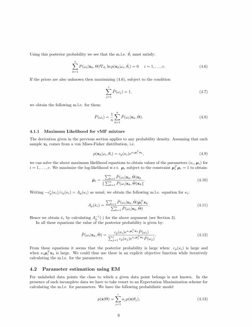
4.2 Parameter estimation using EM

For unlabeled data points the class to which a given data point belongs is not known. In thepresence of such incomplete data we have to take resort to an Expectation Maximization scheme forcalculating the m.l.e. for parameters. We have the following probabilistic model

p(x|Θ) =c∑

j=1

αjp(x|θj), (4.13)

6

where the αj ’s are the so called “mixing” parameters (or class priors) and Θ is the parameter vectorfor the mixture model. The incomplete-data log-likelihood expression for this density from the dataD is given by:

L (D |Θ) = ln

n∏

k=1

p(xk|Θ). (4.14)

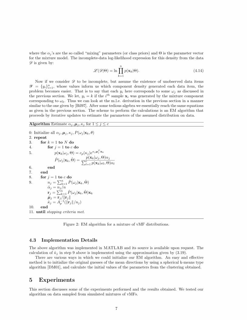
Now if we consider D to be incomplete, but assume the existence of unobserved data itemsY = {yi}ni=1, whose values inform us which component density generated each data item, theproblem becomes easier. That is to say that each yi here corresponds to some ωj as discussed inthe previous section. We let, yi = k if the ith sample xi was generated by the mixture componentcorresponding to ωk. Thus we can look at the m.l.e. derivation in the previous section in a mannersimilar to the one given by [Bil97]. After some tedious algebra we essentially reach the same equationsas given in the previous section. The scheme to perform the calculations is an EM algorithm thatproceeds by iterative updates to estimate the parameters of the assumed distribution on data.

Algorithm Estimate αj ,µj , κj for 1 ≤ j ≤ c

0: Initialize all αj ,µj , κj , P (ωj |xk, θ)2. repeat3. for k = 1 to N do4. for j = 1 to c do

5. p(xk|ωj ,Θ) = cp(κj)eκjµ

Tj xk

P (ωj |xk, Θ) =p(xk|ωj ,Θ)αj∑cl=1 p(xk|ωl,Θ)αl

6. end7. end8. for j = 1 to c do

9. nj =∑nk=1 P (ωj |xk, Θ)

αj = nj/n

rj =∑nk=1 P (ωj |xk, Θ)xk

µj = rj/‖rj‖κj = A−1

p (‖rj‖/nj)10. end11. until stopping criteria met.

Figure 2: EM algorithm for a mixture of vMF distributions.

4.3 Implementation Details

The above algorithm was implemented in MATLAB and its source is available upon request. Thecalculation of κj in step 9 above is implemented using the approximation given by (3.19).

There are various ways in which we could initialize our EM algorithm. An easy and effectivemethod is to initialize the original guesses of the mean directions by using a spherical k-means typealgorithm [DM01], and calculate the initial values of the parameters from the clustering obtained.

5 Experiments

This section discusses some of the experiments performed and the results obtained. We tested ouralgorithm on data sampled from simulated mixtures of vMFs.

7

5.1 Simulation of vMF mixtures

This information is adapted from Chapter 10 of [MJ00]. For κ > 0, the associated vMF distributionhas a mode at the mean direction µ, whereas when κ = 0 the distribution is uniform. The largerthe value of κ, the greater is the clustering around the mean direction.

Since the vMF density depends on x only through µTx, this distribution is rotationally symmetricabout µ. Further in the tangent normal decomposition:

x = tµ+ (1− t2)1/2ζ, (5.1)

t is invariant under rotation about µ while ζ is equivariant (i.e. any such rotation Q takes ζ to Qζ).Thus the conditional distribution ζ|t is uniform on Sp−2. It follows that ζ and t are independentand ζ is uniform on Sp−2. Further (see [MJ00]), we see that the marginal density of t is:

(κ2

) p2−1

Γ(p−12 )Γ( 1

2 )I p−12

(κ)eκt(1− t2)

p−32 , (5.2)

on the interval [−1, 1].

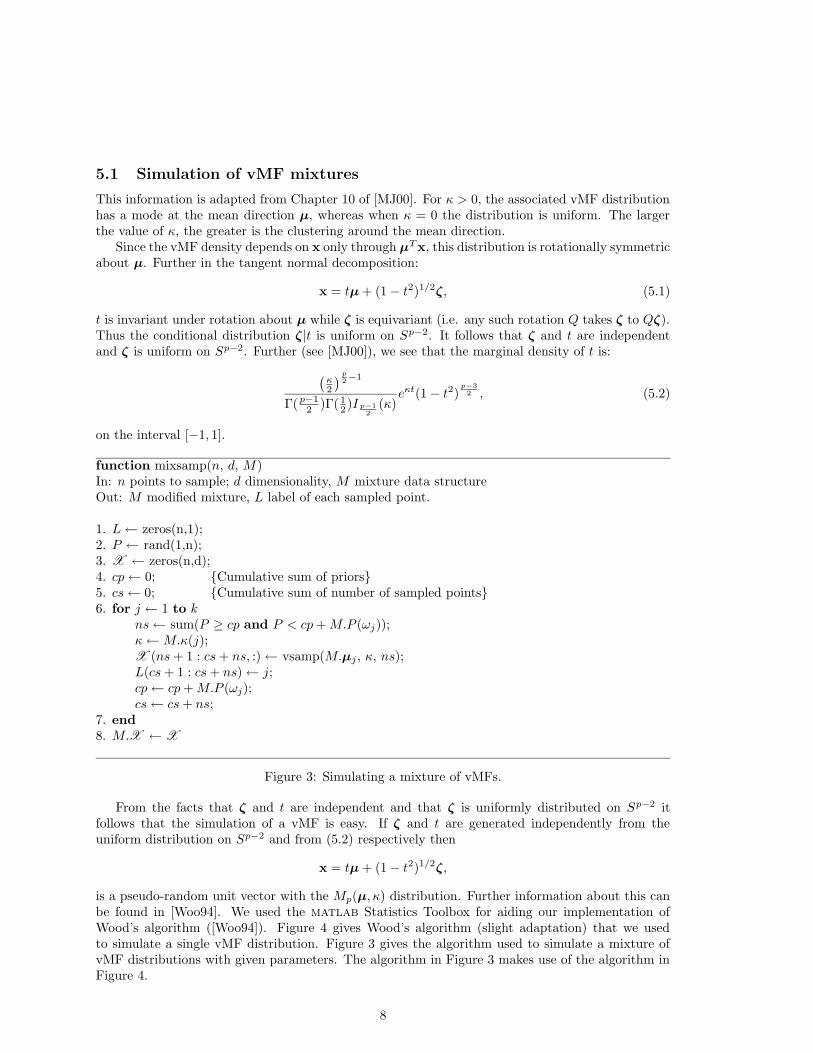
function mixsamp(n, d, M)In: n points to sample; d dimensionality, M mixture data structureOut: M modified mixture, L label of each sampled point.

1. L← zeros(n,1);2. P ← rand(1,n);3. X ← zeros(n,d);4. cp← 0; {Cumulative sum of priors}5. cs← 0; {Cumulative sum of number of sampled points}6. for j ← 1 to k

ns← sum(P ≥ cp and P < cp+M.P (ωj));κ←M.κ(j);X (ns+ 1 : cs+ ns, :)← vsamp(M.µj , κ, ns);L(cs+ 1 : cs+ ns)← j;cp← cp+M.P (ωj);cs← cs+ ns;

7. end8. M.X ←X

Figure 3: Simulating a mixture of vMFs.

From the facts that ζ and t are independent and that ζ is uniformly distributed on Sp−2 itfollows that the simulation of a vMF is easy. If ζ and t are generated independently from theuniform distribution on Sp−2 and from (5.2) respectively then

x = tµ+ (1− t2)1/2ζ,

is a pseudo-random unit vector with the Mp(µ, κ) distribution. Further information about this canbe found in [Woo94]. We used the matlab Statistics Toolbox for aiding our implementation ofWood’s algorithm ([Woo94]). Figure 4 gives Wood’s algorithm (slight adaptation) that we usedto simulate a single vMF distribution. Figure 3 gives the algorithm used to simulate a mixture ofvMF distributions with given parameters. The algorithm in Figure 3 makes use of the algorithm inFigure 4.

8

function vsamp(µ, κ, n){Adapted from [Woo94]}In: µ mean vector for vMF, κ parameter for vMFIn: n, number of points to generateOut: S the Set of n vMF(µ, κ) samples

1. d← dim(µ)

2. t1 ←√

4κ2 + (d− 1)2

3. b← (−2κ+ t1)/(d− 1)4. x0 ← (1− b)/(1 + b)5. S ← zeros(n, d)

6. m← (d− 1)/27. c← κx0 + (d− 1) log(1− x2

0)8. for i← 1 to n

t← −1000u← 1while (t < log(u))

z ← β(m,m) {β(x, y) gives a beta random variable}u← rand {rand gives a uniformly distributed random number.}w ← (1−(1+b)z)

(1−(1−b)z)t← κw + (d− 1) log(1− x0w)

endv← urand(d− 1) {urand(p) gives a p-dim vector from unif. distr. on sphere.}v← v/‖v‖S(i, 1 : d− 1)←

√1− w2vT

S(i, d) = w9. end

{ We now have n samples from vMF([0 0 . . . 1]T , κ) }10. Perform an orthogonal transformation on each sample in S

The transformation has to satisfy Qµ = [0 0 . . . 1]T

11. return S.

Figure 4: Algorithm to simulate a vMF

9

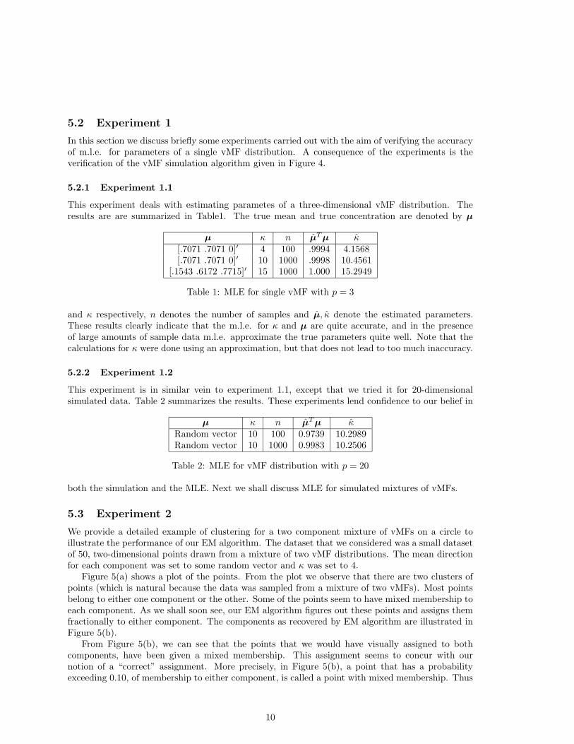
5.2 Experiment 1

In this section we discuss briefly some experiments carried out with the aim of verifying the accuracyof m.l.e. for parameters of a single vMF distribution. A consequence of the experiments is theverification of the vMF simulation algorithm given in Figure 4.

5.2.1 Experiment 1.1

This experiment deals with estimating parametes of a three-dimensional vMF distribution. Theresults are are summarized in Table1. The true mean and true concentration are denoted by µ

µ κ n µTµ κ[.7071 .7071 0]′ 4 100 .9994 4.1568[.7071 .7071 0]′ 10 1000 .9998 10.4561

[.1543 .6172 .7715]′ 15 1000 1.000 15.2949

Table 1: MLE for single vMF with p = 3

and κ respectively, n denotes the number of samples and µ, κ denote the estimated parameters.These results clearly indicate that the m.l.e. for κ and µ are quite accurate, and in the presenceof large amounts of sample data m.l.e. approximate the true parameters quite well. Note that thecalculations for κ were done using an approximation, but that does not lead to too much inaccuracy.

5.2.2 Experiment 1.2

This experiment is in similar vein to experiment 1.1, except that we tried it for 20-dimensionalsimulated data. Table 2 summarizes the results. These experiments lend confidence to our belief in

µ κ n µTµ κRandom vector 10 100 0.9739 10.2989Random vector 10 1000 0.9983 10.2506

Table 2: MLE for vMF distribution with p = 20

both the simulation and the MLE. Next we shall discuss MLE for simulated mixtures of vMFs.

5.3 Experiment 2

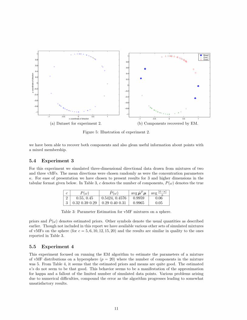
We provide a detailed example of clustering for a two component mixture of vMFs on a circle toillustrate the performance of our EM algorithm. The dataset that we considered was a small datasetof 50, two-dimensional points drawn from a mixture of two vMF distributions. The mean directionfor each component was set to some random vector and κ was set to 4.

Figure 5(a) shows a plot of the points. From the plot we observe that there are two clusters ofpoints (which is natural because the data was sampled from a mixture of two vMFs). Most pointsbelong to either one component or the other. Some of the points seem to have mixed membership toeach component. As we shall soon see, our EM algorithm figures out these points and assigns themfractionally to either component. The components as recovered by EM algorithm are illustrated inFigure 5(b).

From Figure 5(b), we can see that the points that we would have visually assigned to bothcomponents, have been given a mixed membership. This assignment seems to concur with ournotion of a “correct” assignment. More precisely, in Figure 5(b), a point that has a probabilityexceeding 0.10, of membership to either component, is called a point with mixed membership. Thus

10

−1 −0.5 0 0.5 1

−1

−0.8

−0.6

−0.4

−0.2

0

0.2

0.4

0.6

0.8

1

x−coordinate of direction

y−co

ordi

nate

of d

irect

ion

−1 −0.5 0 0.5 1

−1

−0.8

−0.6

−0.4

−0.2

0

0.2

0.4

0.6

0.8

1 MixedClus1Clus2

(a) Dataset for experiment 2. (b) Components recovered by EM.

Figure 5: Illustration of experiment 2.

we have been able to recover both components and also glean useful information about points witha mixed membership.

5.4 Experiment 3

For this experiment we simulated three-dimensional directional data drawn from mixtures of twoand three vMFs. The mean directions were chosen randomly as were the concentration parametersκ. For ease of presentation we have chosen to present results for 3 and higher dimensions in thetabular format given below. In Table 3, c denotes the number of components, P (ω) denotes the true

c P (ω) P (ω) avg µTµ avg |κ−κ|κ

2 0.55, 0.45 0.5424, 0.4576 0.9959 0.063 0.32 0.39 0.29 0.29 0.40 0.31 0.9965 0.05

Table 3: Parameter Estimation for vMF mixtures on a sphere.

priors and P (ω) denotes estimated priors. Other symbols denote the usual quantities as describedearlier. Though not included in this report we have available various other sets of simulated mixturesof vMFs on the sphere (for c = 5, 6, 10, 12, 15, 20) and the results are similar in quality to the onesreported in Table 3.

5.5 Experiment 4

This experiment focused on running the EM algorithm to estimate the parameters of a mixtureof vMF distributions on a hypersphere (p = 20) where the number of components in the mixturewas 5. From Table 4, it seems that the estimated priors and means are quite good. The estimatedκ’s do not seem to be that good. This behavior seems to be a manifestation of the approximationfor kappa and a fallout of the limited number of simulated data points. Various problems arisingdue to numerical difficulties, compound the error as the algorithm progresses leading to somewhatunsatisfactory results.

11

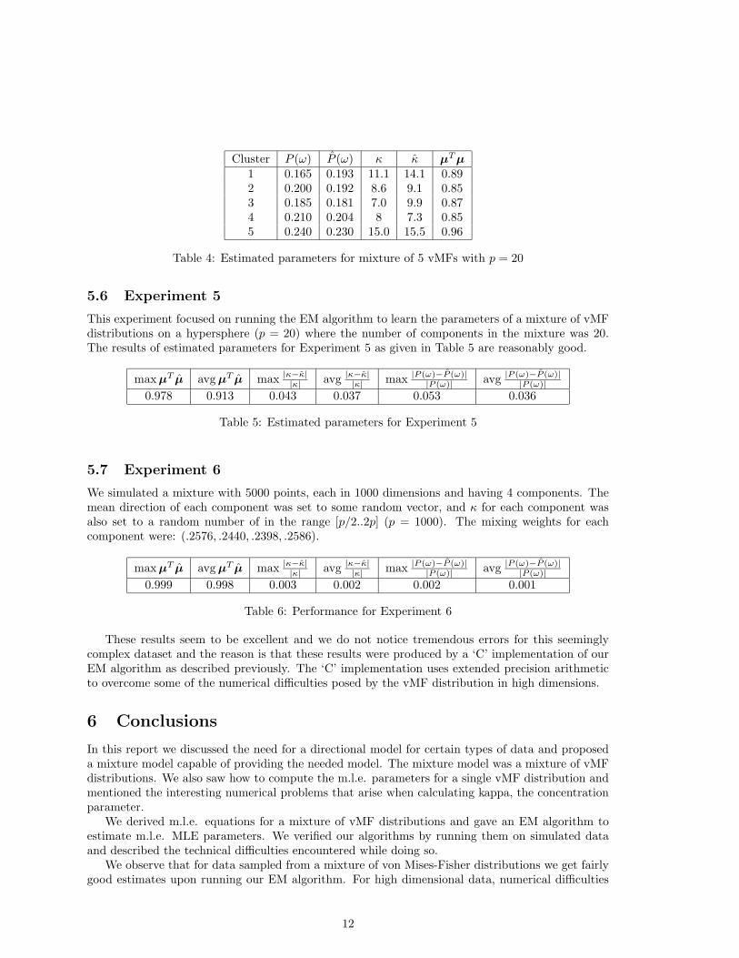
Cluster P (ω) P (ω) κ κ µTµ1 0.165 0.193 11.1 14.1 0.892 0.200 0.192 8.6 9.1 0.853 0.185 0.181 7.0 9.9 0.874 0.210 0.204 8 7.3 0.855 0.240 0.230 15.0 15.5 0.96

Table 4: Estimated parameters for mixture of 5 vMFs with p = 20

5.6 Experiment 5

This experiment focused on running the EM algorithm to learn the parameters of a mixture of vMFdistributions on a hypersphere (p = 20) where the number of components in the mixture was 20.The results of estimated parameters for Experiment 5 as given in Table 5 are reasonably good.

maxµT µ avgµT µ max |κ−κ||κ| avg |κ−κ||κ| max |P (ω)−P (ω)||P (ω)| avg |P (ω)−P (ω)|

|P (ω)|0.978 0.913 0.043 0.037 0.053 0.036

Table 5: Estimated parameters for Experiment 5

5.7 Experiment 6

We simulated a mixture with 5000 points, each in 1000 dimensions and having 4 components. Themean direction of each component was set to some random vector, and κ for each component wasalso set to a random number of in the range [p/2..2p] (p = 1000). The mixing weights for eachcomponent were: (.2576, .2440, .2398, .2586).

maxµT µ avgµT µ max |κ−κ||κ| avg |κ−κ||κ| max |P (ω)−P (ω)||P (ω)| avg |P (ω)−P (ω)|

|P (ω)|0.999 0.998 0.003 0.002 0.002 0.001

Table 6: Performance for Experiment 6

These results seem to be excellent and we do not notice tremendous errors for this seeminglycomplex dataset and the reason is that these results were produced by a ‘C’ implementation of ourEM algorithm as described previously. The ‘C’ implementation uses extended precision arithmeticto overcome some of the numerical difficulties posed by the vMF distribution in high dimensions.

6 Conclusions

In this report we discussed the need for a directional model for certain types of data and proposeda mixture model capable of providing the needed model. The mixture model was a mixture of vMFdistributions. We also saw how to compute the m.l.e. parameters for a single vMF distribution andmentioned the interesting numerical problems that arise when calculating kappa, the concentrationparameter.

We derived m.l.e. equations for a mixture of vMF distributions and gave an EM algorithm toestimate m.l.e. MLE parameters. We verified our algorithms by running them on simulated dataand described the technical difficulties encountered while doing so.

We observe that for data sampled from a mixture of von Mises-Fisher distributions we get fairlygood estimates upon running our EM algorithm. For high dimensional data, numerical difficulties

12

prevent us from getting very accurate results with a limited precision implementation. The extendedprecision implementation was able to get around these difficulties and yield excellent results evenfor high dimensional data.

One of the reasons is numerical difficulty in calculations due to Bessel functions of high order.The second, though more intrinsic difficulty is with the model itself. In very high dimensions weencounter very large values of κ. This leads to clustering decisions being made totally based on κ,something that is not desirable. Kappa captures the concentration, but we would prefer to give morepreference to decisions based on the mean direction. Traditional spherical K-means already doesthat (though it must be noted again that it is a degenerate case of the more general vMF model).Also we note in passing that the “curse of dimensionality” leads to computational difficulties evenin our case.

Further capabilities of the model that we have presented in this report need to be evaluatedby applying to common domains like text clustering and gene expression data clustering. Theinvestigation of such applications is part of our future work.

References

[AS74] M. Abramowitz and I. A. Stegun, editors. Handbook of Mathematical Functions. DoverPubl. Inc., New York, 1974.

[Bil97] J. A. Bilmes. A Gentle Tutorial on the EM Algorithm and its Application to ParameterEstimation for Gaussian Mixture and Hidden Markov Models. Technical Report ICSI-TR-97-021, University of Berkeley, 1997.

[DFG01] I. S. Dhillon, J. Fan, and Y. Guan. Efficient clustering of very large document collec-tions. In V. Kumar R. Grossman, C. Kamath and R. Namburu, editors, Data Mining forScientific and Engineering Applications. Kluwer Academic Publishers, 2001.

[DHS00] R. O. Duda, P. E. Hart, and D. G. Stork. Pattern Classification. John Wiley & Sons,2000.

[DM01] I. S. Dhillon and D. S. Modha. Concept decompositions for large sparse text data usingclustering. Machine Learning, 42(1):143–175, 2001.

[DMR03] I. S. Dhillon, E. M. Marcotte, and U. Roshan. Diametrical clustering for identifyinganti-correlated gene clusters. Bioinformatics, 2003. To appear.

[Hil81] G. W. Hill. Evaluation and inversion of the ratios of modified bessel functions. ACMTransactions on Mathematical Software, 7(2):199–208, June 1981.

[Knu98] D. E. Knuth. The Art of Computer Programming, volume 1: Fundamental Algorithms.Addison-Wesley, 3rd edition, 1998.

[MJ00] K. V. Mardia and P. Jupp. Directional Statistics. John Wiley and Sons Ltd., 2nd edition,2000.

[vM18] R. von Mises. Uber die “Ganzzahligkeit” der Atomgewichte und verwandte Fragen. Phys.Z., 19:490–500, 1918.

[Wat96] G. N. Watson. A treatise on the theory of Bessel functions. Cambridge MathematicalLibrary. Cambridge University Press, 2nd (1944) edition, 1996.

[Woo94] A. T. A. Wood. Simulation of the von-Mises Distribution. Communications of Statistics,Simulation and Computation, 23:157–164, 1994.

13

A Mathematical background

To get a sound understanding of all the derivations performed in this report one needs some back-ground. This Appendix provides the mathematical background required to derive some fundamentalproperties of the von Mises-Fisher distribution and also to supplement the understanding of the m.l.e.calculations for a mixture of vMFs.

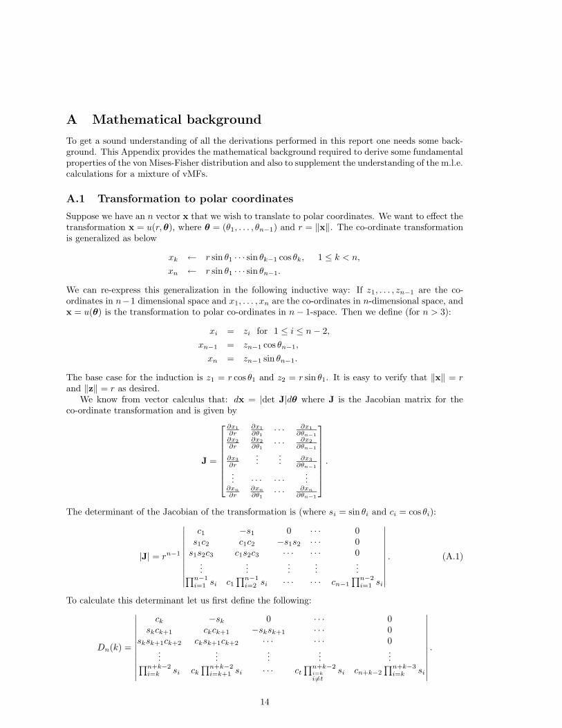
A.1 Transformation to polar coordinates

Suppose we have an n vector x that we wish to translate to polar coordinates. We want to effect thetransformation x = u(r,θ), where θ = (θ1, . . . , θn−1) and r = ‖x‖. The co-ordinate transformationis generalized as below

xk ← r sin θ1 · · · sin θk−1 cos θk, 1 ≤ k < n,

xn ← r sin θ1 · · · sin θn−1.

We can re-express this generalization in the following inductive way: If z1, . . . , zn−1 are the co-ordinates in n−1 dimensional space and x1, . . . , xn are the co-ordinates in n-dimensional space, andx = u(θ) is the transformation to polar co-ordinates in n− 1-space. Then we define (for n > 3):

xi = zi for 1 ≤ i ≤ n− 2,

xn−1 = zn−1 cos θn−1,

xn = zn−1 sin θn−1.

The base case for the induction is z1 = r cos θ1 and z2 = r sin θ1. It is easy to verify that ‖x‖ = rand ‖z‖ = r as desired.

We know from vector calculus that: dx = |det J|dθ where J is the Jacobian matrix for theco-ordinate transformation and is given by

J =

∂x1

∂r∂x1

∂θ1· · · ∂x1

∂θn−1∂x2

∂r∂x2

∂θ1· · · ∂x2

∂θn−1

∂x3

∂r

...... ∂x3

∂θn−1

... · · · · · ·...

∂xn∂r

∂xn∂θ1

· · · ∂xn∂θn−1

.

The determinant of the Jacobian of the transformation is (where si = sin θi and ci = cos θi):

|J| = rn−1

∣∣∣∣∣∣∣∣∣∣∣

c1 −s1 0 · · · 0s1c2 c1c2 −s1s2 · · · 0s1s2c3 c1s2c3 · · · · · · 0

......

......

...∏n−1i=1 si c1

∏n−1i=2 si · · · · · · cn−1

∏n−2i=1 si

∣∣∣∣∣∣∣∣∣∣∣

. (A.1)

To calculate this determinant let us first define the following:

Dn(k) =

∣∣∣∣∣∣∣∣∣∣∣∣

ck −sk 0 · · · 0skck+1 ckck+1 −sksk+1 · · · 0

sksk+1ck+2 cksk+1ck+2 · · · · · · 0...

......

......∏n+k−2

i=k si ck∏n+k−2i=k+1 si · · · ct

∏n+k−2i=k

i6=tsi cn+k−2

∏n+k−3i=k si

∣∣∣∣∣∣∣∣∣∣∣∣

.

14

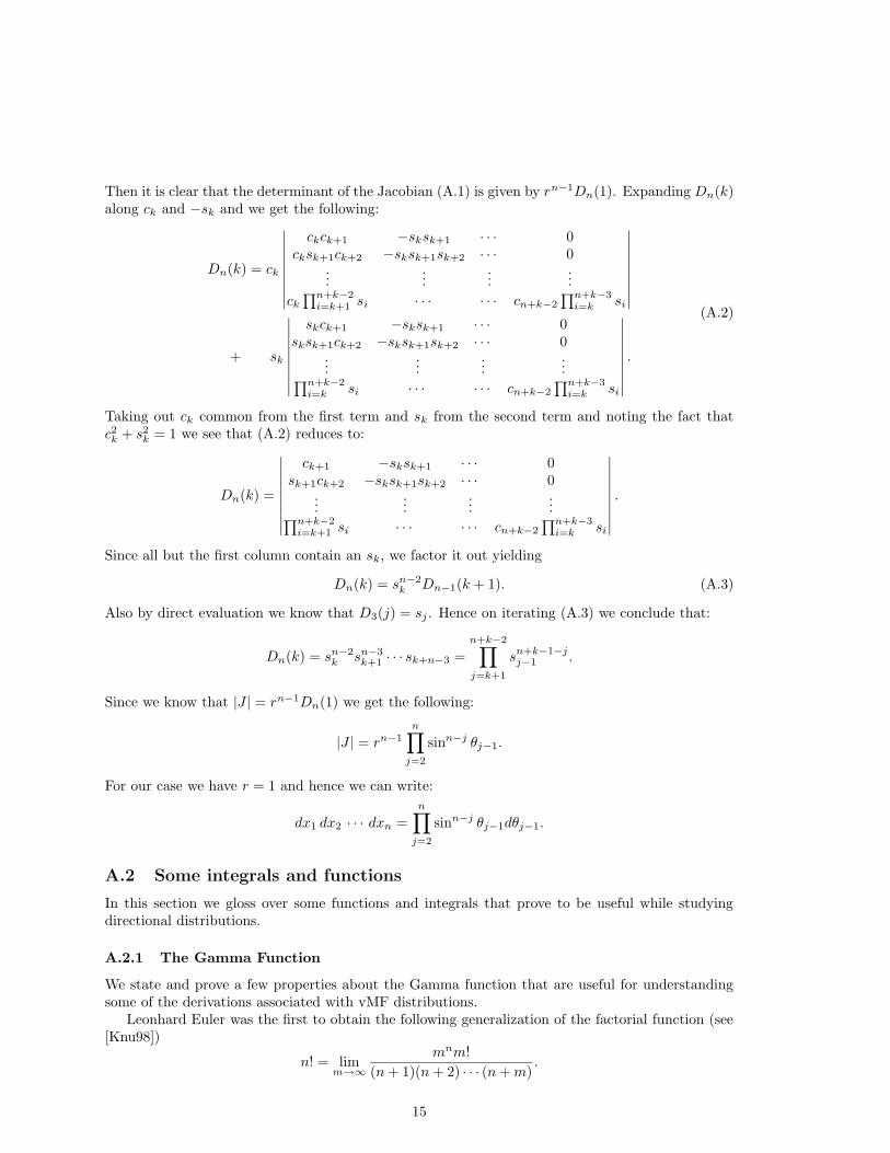
Then it is clear that the determinant of the Jacobian (A.1) is given by rn−1Dn(1). Expanding Dn(k)along ck and −sk and we get the following:

Dn(k) = ck

∣∣∣∣∣∣∣∣∣

ckck+1 −sksk+1 · · · 0cksk+1ck+2 −sksk+1sk+2 · · · 0

......

......

ck∏n+k−2i=k+1 si · · · · · · cn+k−2

∏n+k−3i=k si

∣∣∣∣∣∣∣∣∣

+ sk

∣∣∣∣∣∣∣∣∣

skck+1 −sksk+1 · · · 0sksk+1ck+2 −sksk+1sk+2 · · · 0

......

......∏n+k−2

i=k si · · · · · · cn+k−2

∏n+k−3i=k si

∣∣∣∣∣∣∣∣∣.

(A.2)

Taking out ck common from the first term and sk from the second term and noting the fact thatc2k + s2

k = 1 we see that (A.2) reduces to:

Dn(k) =

∣∣∣∣∣∣∣∣∣

ck+1 −sksk+1 · · · 0sk+1ck+2 −sksk+1sk+2 · · · 0

......

......∏n+k−2

i=k+1 si · · · · · · cn+k−2

∏n+k−3i=k si

∣∣∣∣∣∣∣∣∣.

Since all but the first column contain an sk, we factor it out yielding

Dn(k) = sn−2k Dn−1(k + 1). (A.3)

Also by direct evaluation we know that D3(j) = sj . Hence on iterating (A.3) we conclude that:

Dn(k) = sn−2k sn−3

k+1 · · · sk+n−3 =

n+k−2∏

j=k+1

sn+k−1−jj−1 .

Since we know that |J | = rn−1Dn(1) we get the following:

|J | = rn−1n∏

j=2

sinn−j θj−1.

For our case we have r = 1 and hence we can write:

dx1 dx2 · · · dxn =n∏

j=2

sinn−j θj−1dθj−1.

A.2 Some integrals and functions

In this section we gloss over some functions and integrals that prove to be useful while studyingdirectional distributions.

A.2.1 The Gamma Function

We state and prove a few properties about the Gamma function that are useful for understandingsome of the derivations associated with vMF distributions.

Leonhard Euler was the first to obtain the following generalization of the factorial function (see[Knu98])

n! = limm→∞

mnm!

(n+ 1)(n+ 2) · · · (n+m).

15

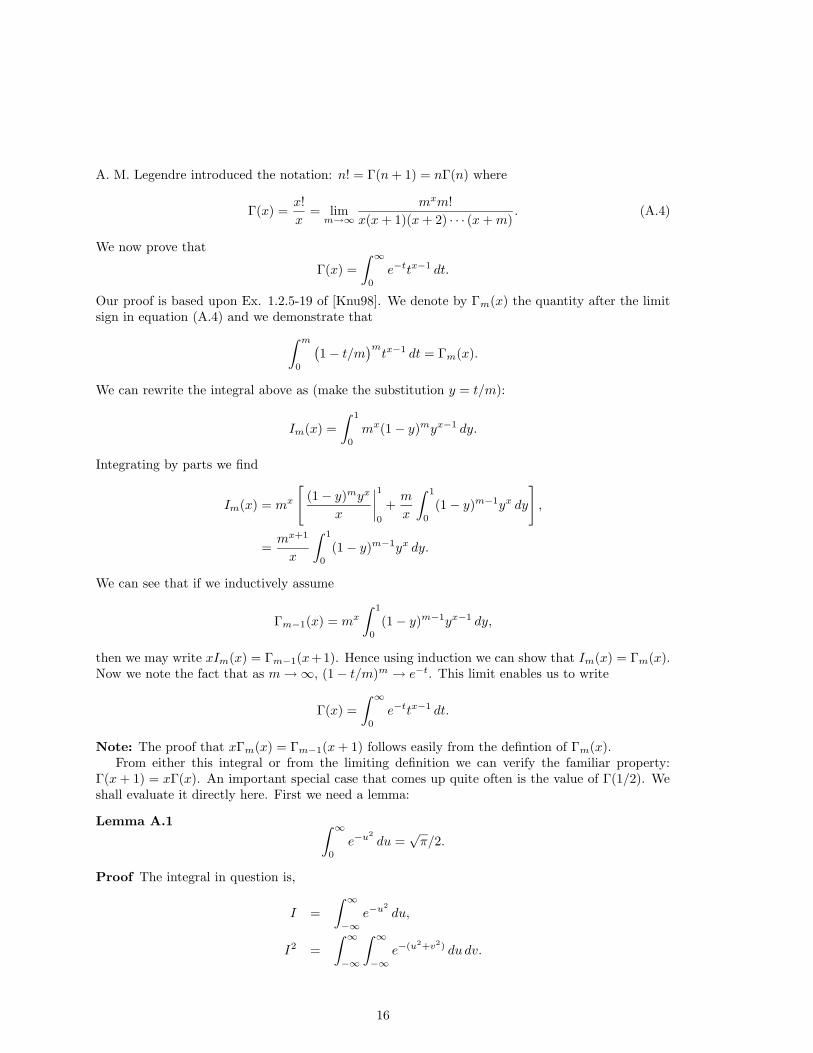
A. M. Legendre introduced the notation: n! = Γ(n+ 1) = nΓ(n) where

Γ(x) =x!

x= limm→∞

mxm!

x(x+ 1)(x+ 2) · · · (x+m). (A.4)

We now prove that

Γ(x) =

∫ ∞

0

e−ttx−1 dt.

Our proof is based upon Ex. 1.2.5-19 of [Knu98]. We denote by Γm(x) the quantity after the limitsign in equation (A.4) and we demonstrate that

∫ m

0

(1− t/m

)mtx−1 dt = Γm(x).

We can rewrite the integral above as (make the substitution y = t/m):

Im(x) =

∫ 1

0

mx(1− y)myx−1 dy.

Integrating by parts we find

Im(x) = mx

[(1− y)myx

x

∣∣∣∣1

0

+m

x

∫ 1

0

(1− y)m−1yx dy

],

=mx+1

x

∫ 1

0

(1− y)m−1yx dy.

We can see that if we inductively assume

Γm−1(x) = mx

∫ 1

0

(1− y)m−1yx−1 dy,

then we may write xIm(x) = Γm−1(x+1). Hence using induction we can show that Im(x) = Γm(x).Now we note the fact that as m→∞, (1− t/m)m → e−t. This limit enables us to write

Γ(x) =

∫ ∞

0

e−ttx−1 dt.

Note: The proof that xΓm(x) = Γm−1(x+ 1) follows easily from the defintion of Γm(x).From either this integral or from the limiting definition we can verify the familiar property:

Γ(x+ 1) = xΓ(x). An important special case that comes up quite often is the value of Γ(1/2). Weshall evaluate it directly here. First we need a lemma:

Lemma A.1 ∫ ∞

0

e−u2

du =√π/2.

Proof The integral in question is,

I =

∫ ∞

−∞e−u

2

du,

I2 =

∫ ∞

−∞

∫ ∞

−∞e−(u2+v2) du dv.

16

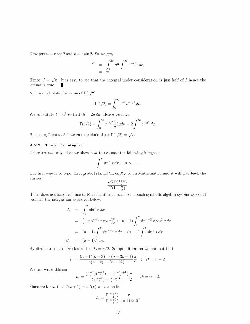
Now put u = r cos θ and v = r sin θ. So we get,

I2 =

∫ 2π

0

dθ

∫ ∞

0

e−r2

r dr,

= π.

Hence, I =√π. It is easy to see that the integral under consideration is just half of I hence the

lemma is true.

Now we calculate the value of Γ(1/2).

Γ(1/2) =

∫ ∞

0

e−tt−1/2 dt.

We substitute t = u2 so that dt = 2u du. Hence we have:

Γ(1/2) =

∫ ∞

0

e−u2 1

u2udu = 2

∫ ∞

0

e−u2

du.

But using Lemma A.1 we can conclude that: Γ(1/2) =√π.

A.2.2 The sinn x integral

There are two ways that we show how to evaluate the following integral:∫ π

0

sinn x dx, n > −1.

The first way is to type: Integrate[Sin[x]^n,{x,0,π}] in Mathematica and it will give back theanswer: √

π Γ( 1+n2 )

Γ(1 + n2 )

.

If one does not have recourse to Mathematica or some other such symbolic algebra system we couldperform the integration as shown below.

In =

∫ π

0

sinn x dx

=[− sinn−1 x cosx

]π0

+ (n− 1)

∫ π

0

sinn−2 x cos2 x dx

= (n− 1)

∫ π

0

sinn−2 x dx− (n− 1)

∫ π

0

sinn x dx

nIn = (n− 1)In−2.

By direct calculation we know that I2 = π/2. So upon iteration we find out that

In =(n− 1)(n− 3) · · · (n− 2k + 1)

n(n− 2) · · · (n− 2k)

π

2; 2k = n− 2.

We can write this as:

In =(n−1

2 )(n−32 ) · · · (n−2k+1

2 )n2 (n−2

2 ) · · · (n−2k2 )

π

2; 2k = n− 2.

Since we know that Γ(x+ 1) = xΓ(x) we can write

In =Γ(n+1

2 )

Γ(n+22 )

π

2× Γ(3/2).

17

Using the fact that Γ(3/2) =√π/2 we conclude that

In =

√π Γ( 1+n

2 )

Γ(1 + n2 )

.

In as given by the above equation is defined only for n > −1.

A.2.3 Useful formulae

The following differential equation gives rise to these modified Bessel functions:

z2w′′(z) + zw′(z)− (z2 + r2)w(z) = 0. (A.5)

This equation has solutions of the form: w(z) = c1Ir(z) + czKr(z) where Kr(z) is the modifiedBessel Function of the second kind.

The following two recurrence relations involving the derivative of the Bessel function are veryuseful in practice.

κI ′p(κ) = pIp(κ) + κIp+1(κ), (A.6)

κI ′p(κ) = κIp−1(κ)− pIp(κ). (A.7)

A standard definition of the modified Bessel function of order p and argument κ is

Ip(κ) =∑

r≥0

1

Γ(p+ r + 1)r!

(κ2

)2r+p

. (A.8)

Yet another definition is

Ip(κ) =2−pκp

Γ(p+ 1/2)Γ(1/2)

∫ π

0

eκ cos θ sin2p θdθ, (A.9)

which is equivalent to

Ip(κ) =1

2π

∫ 2π

0

cos pθeκ cos θdθ. (A.10)

Finally, we can also write the above is a form that might be suitable for numerical integrationprocedures as follows:

Ip(κ) =2−pκp

Γ(p+ 1/2)Γ(1/2)

∫ 1

−1

eκt(1− t2)p−1/2dt. (A.11)

The following ratio is of principal importance to us,

Ap(κ) =Ip/2

Ip/2−1. (A.12)

Another equivalent form can be derived using (A.11),

Ap(κ) =

∫ 1

−1t2eκt(1− t2)(p−3)/2dt

∫ 1

−1eκt(1− t2)(p−3)/2dt

. (A.13)

We can obtain the following asymptotic representation for Ap(κ),

κ

p− κ3

p2 (2 + p)+

2κ5

p3 (2 + p) (4 + p)+

(−12− 5 p) κ7

p4 (2 + p)2

(4 + p) (6 + p)+

2 (24 + 7 p) κ9

p5 (2 + p)2

(4 + p) (6 + p) (8 + p)+O(κ)

10;

(A.14)

18

in fact we can write Ap(κ) as a convergent power series if κ/p < 1.We are also interested in the derivative of Ap(κ). We claim that the derivative of Ap(κ), w.r.t.

κ is given by,

A′p(κ) = 1−Ap(κ)2 − p− 1

κAp(κ). (A.15)

Proof Let s = p/2− 1. Then we have,

A′p(κ) =I ′s+1(κ)

Is(κ)− Is+1(κ)

Is(κ)

I ′s(κ)

Is(κ). (A.16)

Now we make use of (A.7) to obtain

I ′s+1(κ)

Is(κ)= 1− s+ 1

κ

Is+1(κ)

Is(κ), (A.17)

and we use (A.6) to writeI ′s(κ)

Is(κ)=s

κ+Is+1(κ)

Is(κ). (A.18)

We know that Ap(κ) = Is+1(κ)Is(κ) hence we conclude that

A′p(κ) = 1−Ap(κ)2 −(s

κ+s+ 1

κ

)Ap(κ). (A.19)

Putting in p/2− 1 for s we get the desired conclusion.

If we invert the power series representation for Ap(κ) we obtain the following approximation for κ:

p R

(1 +

p R2

2 + p+

p2 (8 + p) R4

(2 + p)2

(4 + p)+

p3 (120 + p (14 + p)) R6

(2 + p)3

(4 + p) (6 + p)+p4 (24 + p) (448 + p (112 + p (6 + p))) R8

(2 + p)4

(4 + p)2

(6 + p) (8 + p)

).

(A.20)

This estimate for κ does not really take into account the dimensionality of the data and thus for highdimensions (when κ is big by itself but κ/p is not very small or very big) it fails to yield accurateapproximations. Note that Ap(κ) is a ratio of Bessel functions that differ in their order by just one,so we can use a well known continued fraction expansion for representing Ap(κ). For notationalsimplicity let us write the continued fraction expansion as:

A2s+2(κ) =Is+1

Is=

12(s+1)κ +

12(s+2)κ +

· · · . (A.21)

The continued fraction on the right is well known [Wat96]. Equation (A.21) and Ap(κ) = R, allowus to write:

1

R≈ 2(s+ 1)

κ+ R.

Thus we can solve for κ to obtain the approximation,

κ ≈ (2s+ 2)R

R− R2. (A.22)

Since we made an approximation above, we incur some error, so we add a correction term (determinedempirically) to the approximation of κ and obtain Equation (A.23),

κ =Rp− R3

1− R2(A.23)

19

The above approximation can be generalized to include higher order terms in R to yield moreaccurate answers.4 For p = 2, 3 highly accurate approximations can be found in [Hil81]. In mostcases this estimate for κ is good enough because as far as inference is concerned a very accurateestimate does not buy us much. (The relative error between the true κ and this estimate has beenfound to be consistently lower than 0.05%)

For solving Ap(κ) − R = 0, we can use (A.15) in any numerical method that may require theevaluation of the derivative of Ap(κ) (such as Newton’s method). In practice however, for very highdimensions (large p), Newton’s iteration does not work that well because of numerical difficulties.In such cases, one could resort to other methods for improving the solution. Note that, again forpractical purposes one does not really need very accurate calculations of κ. It is more of an academicnumerical problem to find a good κ using an efficient and accurate root finder.

B Directional Distributions

The developments in this section are dependent upon the material presented in Appendix A. Thus,the reader who has not read Appendix A is advised to at least glance through it before proceedingwith this appendix. Following the treatment in [MJ00], we will denote the probability element of xon a unit hyper-sphere by dSp−1. The Jacobian of the transformation from (r, θ) to x is given by

dSp−1 = ap(θ) dθ, (B.1)

where we have (see Appendix A),

ap(θ) =

p−1∏

j=2

sinp−j θj−1. (B.2)

B.1 Uniform Distribution

If a direction x is uniformly distributed on Sp−1 (unit hyper-sphere) then its probability element iscp dS

p−1. The p.d.f. of θ is given by: cpap(θ) (See Appendix A for a proof). Now we know that

∫cpap(θ)dθ = 1, (B.3)

hence using (B.2) we can write this as

cp

∫ 2π

0

dθp−1

p−1∏

j=2

∫ π

0

sinp−j θj−1 = 1. (B.4)

Using the fact that (for n > 0, see Appendix A for a proof)

∫ π

0

sinn x dx =

√πΓ(n+1

2 )

Γ(n+22 )

, (B.5)

we can easily solve equation (B.4) to give

cp =Γ(p/2)

2πp/2.

4Note that if one really wants more accurate approximations, it is better to use (A.23) as a starting point and then

perform a couple of Newton-Raphson iterations, because it is easy to evaluate A′p(κ) = 1−Ap(κ)2 − p−1κAp(κ).

20

B.2 The von Mises-Fisher distribution

A unit random vector x is said to have p−variate von Mises-Fisher distribution if its p.e. is:

cp(κ)eκµTx dSp−1, x ∈ Sp−1 ⊆ Rp. (B.6)

Where ‖µ‖ = 1 and κ ≥ 0. We will derive the value of cp the normalizing constant using the factthat: ∫

x∈Sp−1

cp(κ)eκµ′x dx = 1. (B.7)

To evaluate the integral above we make the transformation y = Qx, where y1 = µTx and Q isan orthogonal transformation. x = Q−1y so dx = | ∂∂yQ−1y|dy. But since Q is an orthogonal

transformation we have dx = dy. It is easy to see that the first row of the matrix Q is µT . We nowmake the transformation to polar co-ordinates: y = u(θ). Using Equations (B.1) and (B.2) we canrewrite the integral above as:

∫ 2π

0

dθp−1

∫ π

0

eκ cos θ1 sinp−2 θ1dθ1

p−1∏

j=3

∫ π

0

sinp−j θj−1dθj−1. (B.8)

Using Eq. (B.5) we can rewrite the above integral as:

I = 2π × J1 × πp−3

2Γ(p−2

2 )

Γ(p−12 )

Γ(p−32 )

Γ(p−22 )· · · Γ(1)

Γ( 32 ), (B.9)

where J1 is given by:

J1 =

∫ π

0

eκ cos θ1 sinp−2 θ1dθ1. (B.10)

But we know from (A.9) that:

I p−22

(κ) =(κ

2

) p−22 J1

Γ(p−12 )Γ( 1

2 ). (B.11)

Hence on combining (B.9) and (B.11) and using the fact that Γ( 12 ) =

√π we see that the integral

under question evaluates to:

I =(2π)p/2

κp/2−1Ip/2−1(κ), (B.12)

where Ir(κ) is the modified Bessel Function as given by Eq. (A.9). We see that cp(κ) = I−1 andhence we have:

cp(κ) =κp/2−1

(2π)p/2Ip/2−1(κ). (B.13)

21