w.elsevier.com/locate/rse

Remote Sensing of Environme

Canopy directional emissivity: Comparison between models

Jose A. Sobrino a,*, Juan C. Jimenez-Munoz a, Wout Verhoef b

a Global Change Unit, Department of Thermodynamics, Faculty of Physics, University of Valencia, Burjassot, Spainb National Aerospace Laboratory (NLR), Emmeloord, The Netherlands

Received 22 February 2005; received in revised form 5 September 2005; accepted 10 September 2005

Abstract

Land surface temperature plays an important role in many environmental studies, as for example the estimation of heat fluxes and

evapotranspiration. In order to obtain accurate values of land surface temperature, atmospheric, emissivity and angular effects should be corrected.

This paper focuses on the analysis of the angular variation of canopy emissivity, which is an important variable that has to be known to correct

surface radiances and obtain surface temperatures. Emissivity is also involved in the atmospheric corrections since it appears in the reflected

downwelling atmospheric term. For this purpose, five different methods for simulating directional canopy emissivity have been analyzed and

compared. The five methods are composed of two geometrical models, developed by Sobrino et al. [J. A. Sobrino, V. Caselles, & F. Becker

(1990). Significance of the remotely sensed thermal infrared measurements obtained over a citrus orchard. ISPRS Photogrammetric Engineering

and Remote Sensing 44, 343–354] and Snyder and Wan [W. C. Snyder & Z. Wan, (1998). BRDF models to predict spectral reflectance and

emissivity in the thermal infrared. IEEE Transactions on Geoscience and Remote Sensing 36, 214–225], in which the vegetation is considered as

an opaque medium, and three are based on radiative transfer models, developed by Francois et al. [C. Francois, C. Ottle, & L. Prevot (1997).

Analytical parametrisation of canopy emissivity and directional radiance in the thermal infrared: Application on the retrieval of soil and foliage

temperatures using two directional measurements. International Journal of Remote Sensing 12, 2587–2621], Snyder and Wan [W. C. Snyder & Z.

Wan (1998). BRDF models to predict spectral reflectance and emissivity in the thermal infrared. IEEE Transactions on Geoscience and Remote

Sensing 36, 214–225.] and Verhoef et al. [W. Verhoef, Q. Xiao, L. Jia, & Z. Su (submitted for publication). Extension of SAIL to a 4-component

optical– thermal radiative transfer model simulating thermodynamically heterogenous canopies. IEEE Transactions on Geoscience and Remote

Sensing], in which the vegetation is considered as a turbid medium. Over surfaces with sparse and low vegetation cover, high angular variations of

canopy emissivity are obtained, with differences between at-nadir view and 80- of 0.03. Over fully vegetated surfaces angular effects on

emissivity are negligible when radiative transfer models are applied, so in these situations the angular variations on emissivity are not critical on

the retrieved land surface temperature from remote sensing data. Angular variations on emissivity are lower when the emissivity of the soil and the

emissivity of the vegetation are closer. All the models considered assume Lambertian behaviour for the soil and the leaves. This assumption is also

discussed, showing a different behaviour of directional canopy emissivity when a non-Lambertian soil is considered.

D 2005 Elsevier Inc. All rights reserved.

Keywords: Radiative transfer; Emissivity; Geometrical model; Angular variations

1. Introduction

Land surface temperature (LST) is a key variable for envi-

ronmental studies, as for example the estimation of the fluxes at

the surface/atmosphere interface. Moreover, many other appli-

cations rely on the knowledge of LST (geology, hydrology,

vegetation monitoring, global circulation models—GCMs, etc.).

In order to retrieve accurate LST values from remote

sensing or satellite data, atmospheric and emissivity effects

0034-4257/$ - see front matter D 2005 Elsevier Inc. All rights reserved.

doi:10.1016/j.rse.2005.09.005

* Corresponding author. Tel./fax: +34 96 354 31 15.

E-mail address: sobrino@uv.es (J.A. Sobrino).

must be corrected. Several techniques have been published

since the 1970s for performing this correction. Most of them

applied to thermal data acquired in the atmospheric window

located in the region between 8 and 14 Am. The existence of

different techniques for retrieving LST and emissivity has

triggered the publication of some review papers, which can be

consulted by the reader interested in this topic: Becker and Li

(1995), Dash et al. (2002), Kerr et al. (2004), Sobrino (2000),

Sobrino et al. (2002), among others. Jointly with atmospheric

and emissivity corrections, angular effects must also be

corrected. This last effect is important for satellite sensors

with a large swath angle, like MODIS (Moderate Resolution

nt 99 (2005) 304 – 314

ww

J.A. Sobrino et al. / Remote Sensing of Environment 99 (2005) 304–314 305

Imaging Spectroradiometer) and the NOAA (National Oceanic

and Atmospheric Administration) series (with a swath angle

higher than 50-), or for sensors with off-nadir view observation

angles, like the ATSR (Along Track Scanning Radiometer) or

AATSR (Advanced ATSR), with a forward view of 55-. In fact,the problem of the angular effects on atmospheric parameters is

to a large extent solved, since radiative transfer codes like

MODTRAN (Abreu & Anderson, 1996; Berk et al., 1999)

allow the estimation of these parameters depending on the

observation angle. However, the angular variation of land

surface emissivity (LSE) is not a well-known problem,

especially for bare surfaces like soil or rocks.

The LSE angular dependence has been studied from field

and also laboratory measurements (Cuenca & Sobrino, 2004;

Labed & Stoll, 1991; Rees & James, 1992; Sobrino & Cuenca,

1999; etc.). The results obtained show lower emissivity values

with increasing view angle for bare soil surfaces, whereas for

dense vegetated canopies the angular dependence is minimal,

in agreement with the usual assumption of Lambertian

behaviour for vegetation. Some attempts have been carried

out in order to parameterize in a simple way the angular

variation on LSE, as the one proposed by Prata (1993), in

which directional emissivity is given by ((h)=((0) cos(h/2),where h is the view angle and ((0) the at-nadir emissivity.

However, this expression, despite its easy application, is not

appropriate for all surfaces and does not always provides good

results.

For sea or water surfaces, different models have been

successfully developed for directional emissivity (see for

example Masuda et al., 1988). In recent years different models

have also been developed in order to analyze the angular

variation over vegetation canopies, using among others the soil

and vegetation emissivities as input data and the assumption of

Lambertian behaviour for these components. This study

addresses the simulation of the directional angular variation

of emissivity. LSE is an important variable that has to be

known to correct surface radiances and obtain surface

temperatures. LSE is also involved in the atmospheric

corrections since it appears in the reflected downwelling

atmospheric term. An analysis of how important the knowledge

of LSE in the LST retrieval is can be found in Jimenez-Munoz

and Sobrino (in press). As a general result, an uncertainty on

the LSE of 0.01 leads to an error on the LST of around 0.5 K.

Emissivities are also important per se, so they may be

diagnostic of composition, especially for the silicate minerals.

LSE is thus important for studies of soil development and

erosion and for estimation amounts and changes in sparse

vegetation cover, in addition to bedrock mapping and resource

exploration (Gillespie et al., 1998). The following sections

provide a description of the models used in order to analyze the

angular variation of canopy emissivity, classified as geomet-

rical or radiative transfer models, as well as the results obtained

when these models are applied to mixed surfaces composed by

bare soil and vegetation with different vegetation covers and

different values of soil and vegetation emissivities. Despite that

a detailed comparison between different models can also be

found in Francois (2002), in this paper we include results

obtained with geometrical models as well as a discussion

regarding to the assumption the of Lambertian behaviour for

soils, which is not included in the reference cited.

2. Description of models

Models are interesting tools because they make it possible to

set up relationships between the thermal infrared (TIR)

observations and surface biophysical parameters, as for

example relationships between emissivity and vegetation index

(Olioso, 1995). Models simulate the radiance measured by a

radiometer, provided that the surface, atmosphere and sensor

characteristics are known (Guillevic et al., 2003). In the TIR,

two major types of models can be considered: geometrical

models (GM) and radiative transfer models (RTM). GM

(Jackson et al., 1979; Kimes & Kirchner, 1983; Norman &

Welles, 1983; Sobrino et al., 1990; Sutherland & Bartholic,

1977; etc.) estimate the TIR radiance of a cover with the help

of geometric considerations to describe the canopy structure.

First, they calculate the proportions of projected surface area of

the different surface components, which are directly observed

in a particular view direction. Thus, the TIR radiance at the

sensor is a weighting of these proportions by the TIR radiance

from the respective components. GM represent the vegetation

as an opaque medium and do not simulate radiative transfer

with the cover.

RTM (Francois et al., 1997; Kimes, 1980; Kimes et al.,

1980; Luquet, 2002; Luquet et al., 2001; McGuire et al., 1989;

Olioso, 1995; Olioso et al., 1999; Prevot, 1985; Smith et al.,

1981; etc.) estimate the cover radiance as a function of sensor

viewing direction, temperature distribution, and leaf angle

distribution within the canopy. They simulate the propagation

and the interactions within the cover of TIR radiation emitted

by the cover components or incoming from the atmosphere.

The canopy is represented as a set of plane elements (leaves)

statistically distributed into homogeneous horizontal layers.

The upward and downward radiative contributions of each

layer are based upon the concept of directional gap frequency

through the vegetation. The directional radiance of the cover is

calculated by summing the radiative contributions of all layers.

Iterations are sometimes performed to account for multiple

scattering within the cover.

The aforementioned models do not account for the canopy

three-dimensional (3D) architecture, so they are one-dimen-

sional (1D) models. In this respect and since it has not been

used in this paper, the DART (Discrete Anisotropic Radiative

Transfer) model developed by Guillevic et al. (2003) deserves

special mention, which is a 3D model and simulates the TIR

radiance of vegetation covers with incomplete canopy. More-

over, other models not belonging to geometrical or radiative

transfer models have been developed, like for example models

based on the estimation of the BRDF (Bidirectional Reflec-

tance Distribution Function) (Snyder & Wan, 1998) or hybrid

models (Pinheiro, 2003).

In this paper five models have been considered for

analyzing and comparing the results obtained from them: the

GM for row distributed crops developed by Sobrino et al.

J.A. Sobrino et al. / Remote Sensing of Environment 99 (2005) 304–314306

(1990), the GM based on the estimation of the BRDF (Snyder

& Wan, 1998), the volumetric model (VM) based on the

estimation of the BRDF (Snyder & Wan, 1998), an analytical

parameterization using the gap function based on the model of

Prevot (1985) and described in Francois et al. (1997), and the

extension of SAIL (Scattering by Arbitrarily Inclined Leaves)

to the thermal infrared region and four components, called

4SAIL and developed by Verhoef et al. (submitted for

publication). In order to simplify the notation, these models

will be referred in the paper as SOBGM, S&WGM, S&WVM,

FRARTM and VERRTM, respectively. Previously to the analysis

of the results obtained, we give a brief explanation of each

model in the next sections.

2.1. SOBGM: geometrical model for row distributed crops

(Sobrino et al., 1990)

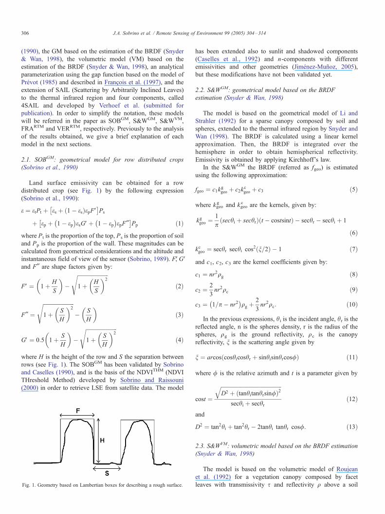
Land surface emissivity can be obtained for a row

distributed crop (see Fig. 1) by the following expression

(Sobrino et al., 1990):

e ¼ etPt þ es þ 1� esð ÞepFV� �

Ps

þ ep þ 1� ep� �

esGVþ 1� ep� �

epF�� �

Pp ð1Þ

where Pt is the proportion of the top, Ps is the proportion of soil

and Pp is the proportion of the wall. These magnitudes can be

calculated from geometrical considerations and the altitude and

instantaneous field of view of the sensor (Sobrino, 1989). FV, GVand F� are shape factors given by:

FV ¼ 1þ H

S

���

ffiffiffiffiffiffiffiffiffiffiffiffiffiffiffiffiffiffiffiffiffiffiffi1þ H

S

�� 2s

ð2Þ

F� ¼

ffiffiffiffiffiffiffiffiffiffiffiffiffiffiffiffiffiffiffiffiffiffiffi1þ S

H

�� 2s

� S

H

��ð3Þ

GV ¼ 0:5 1þ S

H

���

ffiffiffiffiffiffiffiffiffiffiffiffiffiffiffiffiffiffiffiffiffiffiffi1þ S

H

�� 2s

ð4Þ

where H is the height of the row and S the separation between

rows (see Fig. 1). The SOBGM has been validated by Sobrino

and Caselles (1990), and is the basis of the NDVITHM (NDVI

THreshold Method) developed by Sobrino and Raissouni

(2000) in order to retrieve LSE from satellite data. The model

Fig. 1. Geometry based on Lambertian boxes for describing a rough surface.

has been extended also to sunlit and shadowed components

(Caselles et al., 1992) and n-components with different

emissivities and other geometries (Jimenez-Munoz, 2005),

but these modifications have not been validated yet.

2.2. S&WGM: geometrical model based on the BRDF

estimation (Snyder & Wan, 1998)

The model is based on the geometrical model of Li and

Strahler (1992) for a sparse canopy composed by soil and

spheres, extended to the thermal infrared region by Snyder and

Wan (1998). The BRDF is calculated using a linear kernel

approximation. Then, the BRDF is integrated over the

hemisphere in order to obtain hemispherical reflectivity.

Emissivity is obtained by applying Kirchhoff’s law.

In the S&WGM the BRDF (referred as fgeo) is estimated

using the following approximation:

fgeo ¼ c1kggeo þ c2k

cgeo þ c3 ð5Þ

where kgeog and kgeo

c are the kernels, given by:

kggeo ¼1

psechi þ sechrð Þ t � costsintð Þ � sechr � sechi þ 1

ð6Þ

kcgeo ¼ sechr sechi cos2 n=2ð Þ � 1 ð7Þ

and c1, c2, c3 are the kernel coefficients given by:

c1 ¼ nr2qg ð8Þ

c2 ¼2

3nr2qc ð9Þ

c3 ¼ 1=p � nr2� �

qg þ2

3nr2qc: ð10Þ

In the previous expressions, hi is the incident angle, hr is thereflected angle, n is the spheres density, r is the radius of the

spheres, qg is the ground reflectivity, qc is the canopy

reflectivity, n is the scattering angle given by

n ¼ arcos coshicoshr þ sinhisinhrcos/ð Þ ð11Þ

where / is the relative azimuth and t is a parameter given by

cost ¼

ffiffiffiffiffiffiffiffiffiffiffiffiffiffiffiffiffiffiffiffiffiffiffiffiffiffiffiffiffiffiffiffiffiffiffiffiffiffiffiffiffiffiffiffiffiD2 þ tanhitanhrsin/ð Þ2

qsechi þ sechr

ð12Þ

and

D2 ¼ tan2hi þ tan2hr � 2tanhi tanhr cos/: ð13Þ

2.3. S&WVM: volumetric model based on the BRDF estimation

(Snyder & Wan, 1998)

The model is based on the volumetric model of Roujean

et al. (1992) for a vegetation canopy composed by facet

leaves with transmissivity s and reflectivity q above a soil

J.A. Sobrino et al. / Remote Sensing of Environment 99 (2005) 304–314 307

surface with reflectivity q0. Similarly to the previous model,

the BRDF is given by:

fvol ¼ c1kqvol þ c2k

svol þ c3 ð14Þ

the kernels by

kqvol ¼

p � nð Þcosn þ sinncoshi þ coshr

� p2

ð15Þ

ksvol ¼

� ncosn þ sinncoshi þ coshr

ð16Þ

and the coefficients by

c1 ¼2q3p2

1� exp � bFð Þ½ � ð17Þ

c2 ¼2s3p2

1� exp � bFð Þ½ � ð18Þ

c3 ¼q3p

1� exp � bFð Þ½ � þ q0

p1� exp � bFð Þ½ � ð19Þ

0.950

0.955

0.960

0.965

0.970

0.975

0.980

0.985

0.990

0.995

0 10 20 30 40

view

dir

ecti

on

al e

mis

sivi

t y

(a)

0.950

0.955

0.960

0.965

0.970

0.975

0.980

0.985

0.990

0.995

0 10 20 30 40

view

dir

ecti

on

al e

mis

sivi

ty

(b)

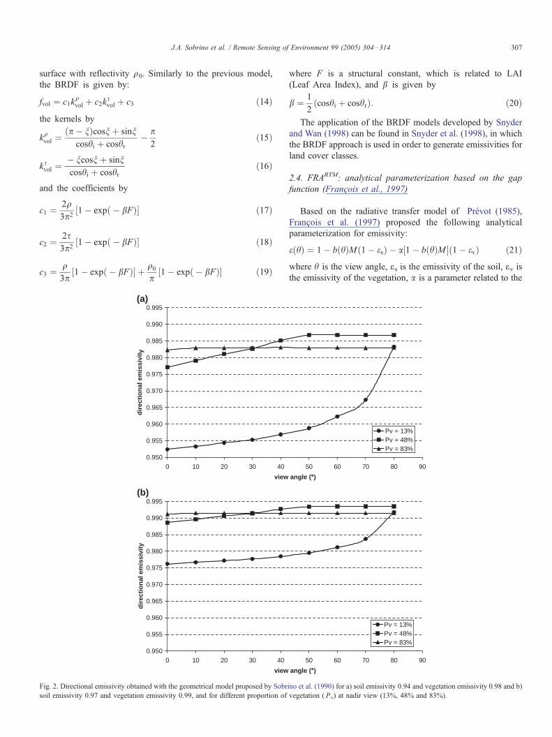
Fig. 2. Directional emissivity obtained with the geometrical model proposed by Sobr

soil emissivity 0.97 and vegetation emissivity 0.99, and for different proportion of

where F is a structural constant, which is related to LAI

(Leaf Area Index), and b is given by

b ¼ 1

2coshi þ coshrÞ:ð ð20Þ

The application of the BRDF models developed by Snyder

and Wan (1998) can be found in Snyder et al. (1998), in which

the BRDF approach is used in order to generate emissivities for

land cover classes.

2.4. FRARTM: analytical parameterization based on the gap

function (Francois et al., 1997)

Based on the radiative transfer model of Prevot (1985),

Francois et al. (1997) proposed the following analytical

parameterization for emissivity:

e hð Þ ¼ 1� b hð ÞM 1� esð Þ � a 1� b hð ÞM½ � 1� evð Þ ð21Þ

where h is the view angle, (s is the emissivity of the soil, (v isthe emissivity of the vegetation, a is a parameter related to the

50 60 70 80 90

angle (°)

Pv = 13%Pv = 48%Pv = 83%

50 60 70 80 90

angle (°)

Pv = 13%Pv = 48%Pv = 83%

ino et al. (1990) for a) soil emissivity 0.94 and vegetation emissivity 0.98 and b)

vegetation ( Pv) at nadir view (13%, 48% and 83%).

0.960

0.965

0.970

0.975

0.980

0.985

0.990

0.995

0 10 20 30 40 50 60 70 80

view angle (°)

dir

ecti

on

al e

mis

sivi

ty

soil = 0.94 vegetation = 0.98

soil = 0.97 vegetation = 0.99

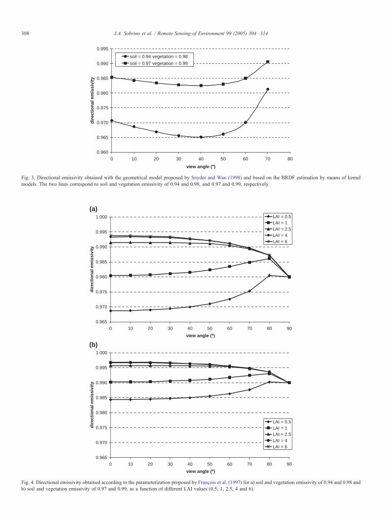
Fig. 3. Directional emissivity obtained with the geometrical model proposed by Snyder and Wan (1998) and based on the BRDF estimation by means of kernel

models. The two lines correspond to soil and vegetation emissivity of 0.94 and 0.98, and 0.97 and 0.99, respectively.

0.965

0.970

0.975

0.980

0.985

0.990

0.995

1.000

0 10 20 30 40 50 60 70 80 90

dir

ecti

on

al e

mis

sivi

ty

LAI = 0.5LAI = 1LAI = 2.5LAI = 4LAI = 6

(a)

0.965

0.970

0.975

0.980

0.985

0.990

0.995

1.000

0 10 20 30 40 50 60 70 80 90

view angle (°)

dir

ecti

on

al e

mis

sivi

ty

LAI = 0.5LAI = 1LAI = 2.5LAI = 4LAI = 6

(b) view angle (°)

Fig. 4. Directional emissivity obtained according to the parameterization proposed by Francois et al. (1997) for a) soil and vegetation emissivity of 0.94 and 0.98 and

b) soil and vegetation emissivity of 0.97 and 0.99, as a function of different LAI values (0.5, 1, 2.5, 4 and 6).

J.A. Sobrino et al. / Remote Sensing of Environment 99 (2005) 304–314308

J.A. Sobrino et al. / Remote Sensing of Environment 99 (2005) 304–314 309

cavity effect which values are given in Francois (2002), b is the

directional gap frequency given for spherical LIDF (Leaf

Inclination Distribution Function) and random dispersion by

b hð Þ ¼ exp � 0:5

coshLAI

��ð22Þ

and M is the hemispheric gap frequency given by

M ¼ 1

p

Z p2

�p2

b hð Þdh: ð23Þ

2.5. VERRTM: 4SAIL radiative transfer model (Verhoef et al.,

submitted for publication)

The 4SAIL model is a modern version of the SAIL

(Scattering by Arbitrarily Inclined Leaves) model, first pub-

lished by Verhoef and Bunnik (1981) in the early eighties in

order to obtain canopy reflectance, and described in detail in

0.965

0.970

0.975

0.980

0.985

0.990

0.995

1.000

0 10 20 30 40

view

dir

ecti

on

al e

mis

sivi

ty

(a)

0.982

0.984

0.986

0.988

0.990

0.992

0.994

0.996

0.998

0 10 20 30 40

dir

ecti

on

al e

mis

sivi

ty

(b)

view

Fig. 5. Directional emissivity obtained from the volumetric BRDF model proposed b

and b) soil and vegetation emissivity of 0.97 and 0.99, as a function of different L

Verhoef (1984, 1985). The SAILmodel is based on a four-stream

approximation of the radiative transfer equation, in which case

one distinguishes two direct fluxes (incident solar flux and

radiance in the viewing direction) and two diffuse fluxes

(upward and downward hemispherical flux). The interactions

of these fluxes with the canopy are described by a system of four

linear differential equations that can be analytically solved.

Incorporation of the hot spot effect in SAIL was accom-

plished in 1989 and resulted in the model called SAILH

(Verhoef, 1998). In SAILH the single scattering contribution

to the bi-directional reflectance was modified according to the

theory of Kuusk (1985), while all other terms remained the same.

The new 4SAIL model differs from its predecessors by im-

provements in numerica robustness and computational efficien-

cy. Moreover, it provides additional facilities to support the

calculation of internal flux profiles and some extra quantities

related to its application in the thermal infrared domain. In this

way, from hemispherical–directional reflectivity values and by

applying Kirchhoff’s law, it is possible to obtain the directional

50 60 70 80 90

angle (°)

LAI = 0.5LAI = 1LAI = 2.5LAI = 4LAI = 6

50 60 70 80 90

LAI = 0.5LAI = 1LAI = 2.5LAI = 4LAI = 6

angle (°)

y Snyder and Wan (1998) for a) soil and vegetation emissivity of 0.94 and 0.98

AI values (0.5, 1, 2.5, 4 and 6).

0.965

0.970

0.975

0.980

0.985

0.990

0.995

1.000

0 10 20 30 40 50 60 70 80 90

view angle (°)

dir

ecti

on

al e

mis

sivi

ty

LAI = 0.5LAI = 1LAI = 2.5LAI = 4LAI = 6

(a)

0.965

0.970

0.975

0.980

0.985

0.990

0.995

1.000

0 10 20 30 40 50 60 70 80 90

dir

ecti

on

al e

mis

sivi

ty

LAI = 0.5LAI = 1LAI = 2.5LAI = 4LAI = 6

(b)

view angle (°)

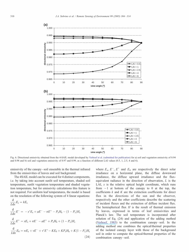
Fig. 6. Directional emissivity obtained from the 4-SAIL model developed by Verhoef et al. (submitted for publication) for a) soil and vegetation emissivity of 0.94

and 0.98 and b) soil and vegetation emissivity of 0.97 and 0.99, as a function of different LAI values (0.5, 1, 2.5, 4 and 6).

J.A. Sobrino et al. / Remote Sensing of Environment 99 (2005) 304–314310

emissivity of the canopy–soil ensemble in the thermal infrared

from the emissivities of leaves and soil background.

The 4SAIL model can be executed for 4 distinct components,

i.e. by taking into account sunlit soil temperature, shaded soil

temperature, sunlit vegetation temperature and shaded vegeta-

tion temperature, but for emissivity calculations this feature is

not required. For uniform leaf temperatures, the model is based

on the resolution of the following system of 4 linear equations:

d

LdxEs ¼ kEs

d

LdxE� ¼ � s VEs þ aE� � rEþ � PsHh � 1� Psð ÞHc

d

LdxEþ ¼ sEs þ rE� � aEþ þ PsHh þ 1� Psð ÞHc

d

LdxE0 ¼ wEs þ vE� þ v VEþ� KE0 þ KPsHh þ K 1� Psð ÞHc

ð24Þ

where Es, E�, E+ and E0 are respectively the direct solar

irradiance on a horizontal plane, the diffuse downward

irradiance, the diffuse upward irradiance and the flux-

equivalent radiance in the direction of observation, L is the

LAI, x is the relative optical height coordinate, which runs

from �1 at bottom of the canopy to 0 at the top, the

coefficients k and K are the extinction coefficients for direct

flux in the directions of the sun and the observer,

respectively and the other coefficients describe the scattering

of incident fluxes and the extinction of diffuse incident flux.

The hemispherical flux H is the result of thermal emission

by leaves, expressed in terms of leaf emissivities and

Planck’s law. The soil temperature is incorporated after

solution of Eq. (24) and application of the adding method

(Verhoef, 1985) to the combination canopy–soil. In the

adding method one combines the optical/thermal properties

of the isolated canopy layer with those of the background

soil in order to compute the optical/thermal properties of the

combination canopy–soil.

J.A. Sobrino et al. / Remote Sensing of Environment 99 (2005) 304–314 311

3. Results

The physics involved in GM, in which vegetation is

considered as an opaque medium, and RTM, in which vegetation

is considered as a turbid medium, is quite different, since the

comparison between GM and RTM is not an easy task and is

difficult to interpret. For this reason, on the one hand a

comparison between SOBGM and S&WGM has been carried

out, whereas in the other hand S&WVM, FRARTM and VERRTM

have been compared.

Fig. 2 shows the results obtained with SOBGM. Values of H

(height of the crop) and S (separation between rows) have been

arbitrarily chosen in order to simulate low (13%), medium

(48%) and high (83%) vegetated cover surfaces. In Fig. 2a

values of (s=0.94 and (v=0.98 have been considered for soil

and vegetation emissivities, respectively, whereas in Fig. 2b

values of (s=0.97 and (v=0.99 have been considered. The

results obtained show low angular variation for high vegetation

-0.0035

-0.0025

-0.0015

-0.0005

0.0005

0.0015

0.0025

0 10 20 30

FR

AR

TM -

S&

WV

M

LAI = 0.5LAI = 1LAI = 2.5LAI = 4LAI = 6

(a)

-0.0035

-0.0025

-0.0015

-0.0005

0.0005

0.0015

0.0025

0 302010

vie

(b)

FR

AR

TM -

VE

RR

TM

vie

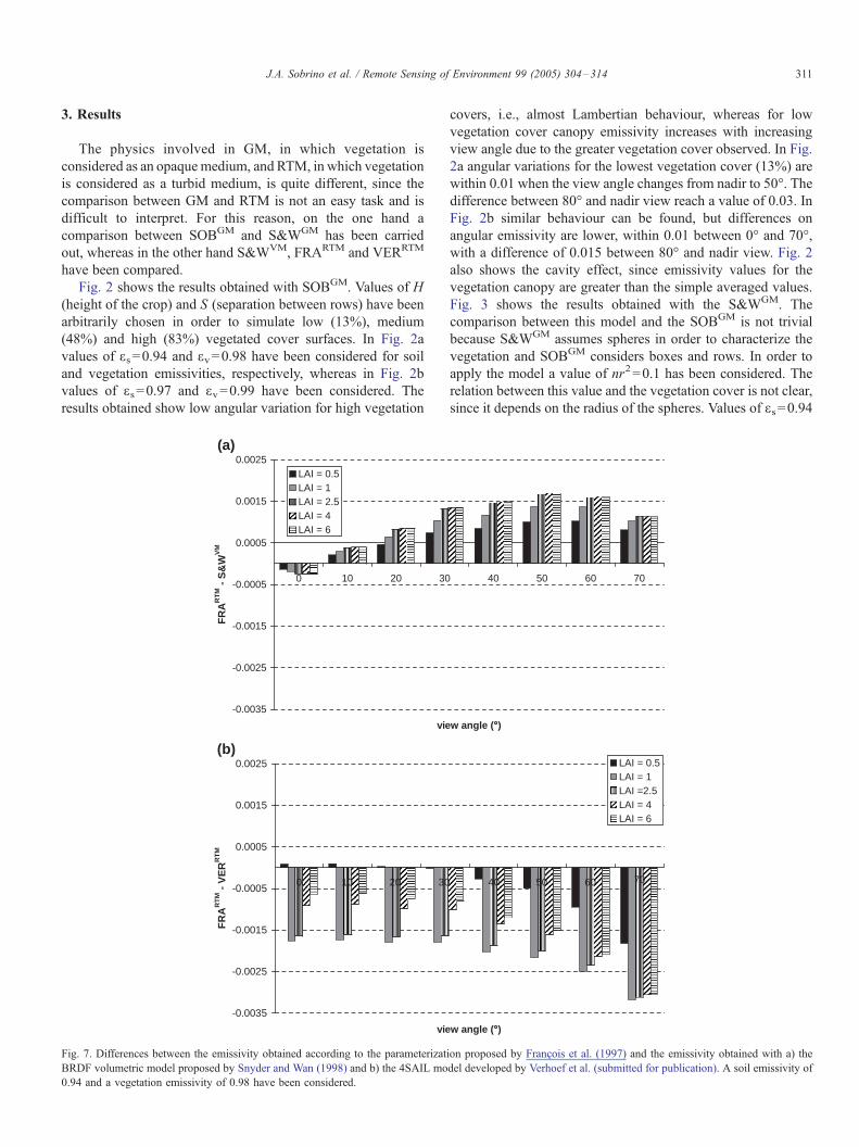
Fig. 7. Differences between the emissivity obtained according to the parameterizati

BRDF volumetric model proposed by Snyder and Wan (1998) and b) the 4SAIL mo

0.94 and a vegetation emissivity of 0.98 have been considered.

covers, i.e., almost Lambertian behaviour, whereas for low

vegetation cover canopy emissivity increases with increasing

view angle due to the greater vegetation cover observed. In Fig.

2a angular variations for the lowest vegetation cover (13%) are

within 0.01 when the view angle changes from nadir to 50-. Thedifference between 80- and nadir view reach a value of 0.03. In

Fig. 2b similar behaviour can be found, but differences on

angular emissivity are lower, within 0.01 between 0- and 70-,with a difference of 0.015 between 80- and nadir view. Fig. 2

also shows the cavity effect, since emissivity values for the

vegetation canopy are greater than the simple averaged values.

Fig. 3 shows the results obtained with the S&WGM. The

comparison between this model and the SOBGM is not trivial

because S&WGM assumes spheres in order to characterize the

vegetation and SOBGM considers boxes and rows. In order to

apply the model a value of nr2=0.1 has been considered. The

relation between this value and the vegetation cover is not clear,

since it depends on the radius of the spheres. Values of (s=0.94

40 50 60 70

40 50 60 70

w angle (°)

LAI = 0.5LAI = 1LAI =2.5LAI = 4LAI = 6

w angle (°)

on proposed by Francois et al. (1997) and the emissivity obtained with a) the

del developed by Verhoef et al. (submitted for publication). A soil emissivity of

J.A. Sobrino et al. / Remote Sensing of Environment 99 (2005) 304–314312

and (v =0.98 or (s = 0.97 and (v = 0.99 have been also

considered. The curves obtained in Fig. 3 have difficult

interpretation because a parabola is obtained, whereas one

expects to obtain a decay curve with increasing angle, as in the

previous case. It should be noted that emissivity retrieval from

BRDF data shows an important problem: the kernel model

diverges at high view angles. Snyder and Wan (1998) point out

that the hemispheric integration can only be done from 0- to

75-. We have observed that the model diverges even before than

75-.In order to obtain the results with the RTM, different

emissivity values, (s=0.94 and (v=0.98 and also (s=0.97 and

(v=0.99, and LAI values, 0.5, 1, 2.5, 4 and 6, have been

considered. Fig. 4 shows the results obtained with the FRARTM.

Two different tendences can be found in this figure. Hence, for

LAI�1 canopy emissivity increases with increasing view angle

due to a similar reason that the one explained in the SOBGM.

However, for LAI>1 a decreasing tendency for canopy

emissivity with increasing view angle is observed. The

proportion of leaves is higher than the proportion of soil for

surfaces with LAI>1, and the at-nadir emissivity is higher than

the vegetation emissivity due to the cavity effect. At 90-, canopyemissivity recovers the vegetation emissivity value, so the cavity

effect seems to disappear at this view angle. The comparison

between Fig. 4a ((s=0.94 and (v=0.98) and Fig. 4b ((s=0.97and (v=0.99) shows that lower angular variations are obtainedwhen (s and (v are closer. Fig. 5 shows the results obtained withthe S&WVM. In order to compare this model with the FRARTM,

the term exp(�bF) involved in Eqs. (17)–(19) has been chosento be equal to the termMb(h) involved in Eq. (21). View angles

up to 70- have not been represented in order to avoid the

divergence problems related to the hemispherical integration of

the BRDF. The results obtained are similar to the ones obtained

with the FRARTM, with differences between both models lower

than 0.0015 in most cases. Fig. 6 shows the results obtained with

the VERRTM. Despite similar behaviour than in the previous

cases is obtained, a significant difference when comparing with

0.970

0.975

0.980

0.985

0 10 20 30

view

dir

ecti

on

al e

mis

sivi

ty

lambertiannon-lambertian

Fig. 8. Comparison between the directional emissivity obtained from the geometrica

soil or considering the angular variations measured in situ by Cuenca and Sobrino (2

0.99 have been considered.

the FRARTM at high view angles can be found. In VERRTM the

cavity effect still remains at 90-. These differences are illustratedin Fig. 7, in which the differences between the S&WVM and the

FRARTM and also between the VERRTM and the FRARTM as a

function of the view angle are represented. The comparison

between the S&WVM and the FRARTM (Fig. 7a) shows dif-

ferences are lower than 0.015 in most cases, whereas the

comparison between the VERRTM and the FRARTM (Fig. 7b)

shows differences higher than 0.015, the maximum difference

found at 90-, higher than 0.025.

Finally, in order to analyze the assumption of Lambertian

behaviour for soil surfaces, the SOBGM has been applied again

assuming the angular variations for soil proposed by Cuenca and

Sobrino (2004) from in situ measurements. The results are

shown in Fig. 8, in which at-nadir values for vegetation cover of

13%, (s=0.97 and (v=0.99 have been considered. The canopy

emissivity considering a Lambertian soil has been also

represented for comparison. Despite the fact that differences

between the Lambertian case and non-Lambertian case are lower

than 0.005, the behaviour is quite different, so errors on

directional canopy emissivity could be significant when

assuming Lambertian behaviour.

4. Conclusions

In this paper two GM (SOBGM, S&WGM) and three RTM

(FRARTM, S&WRTM and VERRTM) have been analyzed and

compared. GM consider a sparse vegetation canopy as an

opaque medium, whereas RTM consider a uniform vegetation

cover as a turbid medium. Models based on the BRDF

estimation show divergence problems for view angles up to

75- or even lower, so the analysis has been mainly focussed on

SOBGM, FRARTM and VERRTM. SOBGM shows an increasing

canopy emissivity with increasing view angle, due to the

greater proportion of vegetation observed at off-nadir view

angles. RTM show different trends depending on the LAI

values. For LAI�1, when the proportion of leaves is lower

40 50 60 70

angle (°)

l model proposed by Sobrino et al. (1990) assuming a Lambertain behaviour for

004). An initial value for soil emissivity of 0.97 and for vegetation emissivity of

J.A. Sobrino et al. / Remote Sensing of Environment 99 (2005) 304–314 313

than the proportion of soil, canopy emissivity grows with

increasing view angle, as in geometrical models, but decreases

for LAI>1, due to the greater proportion of leaves than

proportion of soil and the cavity effect. Differences between

FRARTM and VERRTM have been also found for high view

angles. In particular, for view angles of 90- the cavity effect

disappears in the FRARTM, whereas in the VERRTM it still

remains. An additional comparison between the Prevot (1985)

model, the FRARTM and the VERRTM can be also found in

Francois (2002), from which similar conclusions can be

extracted. Actually land surface emissivity is retrieved with

an accuracy between 0.01 and 0.02 (see for example Gillespie

et al., 1998; Sobrino et al., 2001, 2002), which leads to errors

lower than 1 K for surface temperature. Most of the angular

differences obtained with RTM are lower than these values, so

the impact of angular effects on emissivity are not critical on

the retrieved land surface temperature over fully covered

surfaces, but not over sparse vegetation. The models shown in

the paper are difficult to validate, since angular measurement of

emissivity is not an easy task. Some attempts of validation can

be found in Prevot (1985) and Snyder et al. (1997).

It should be noted that these models assume a Lambertian

behaviour for soil and vegetation surfaces. Under this

assumption, angular variation on emissivity is due to changes

in the observed geometry. Despite the fact that vegetation

surfaces show a near Lambertian behaviour, bare soil surfaces

do not show this behaviour, and the angular variation on

emissivity can not be neglected. However, this angular

dependence is difficult to know, so it depends mainly on the

scattering mechanism, grain size and porosity (Labed & Stoll,

1991). The models analyzed in the paper provide the emissivity

angular variation over vegetation canopies and a better

understanding of the geometrical effects and the role of the

canopy parameters on radiative transfer processes in the

thermal part of the spectrum, but the assumption of Lambertian

behaviour should be revised, at least for the bare soil

component. For this purpose, further research on the angular

variation of emissivity for natural surfaces is needed.

Acknowledgments

We wish to thank to the European Union (EAGLE, project

SST3-CT-2003-502057) and the Ministerio de Ciencia y

Tecnologıa (project REN2001-3105/CLI) for the financial

support. This work has been carried out while Juan C.

Jimenez-Munoz was having a contract ‘‘V segles’’ from the

University of Valencia.

References

Abreu, L. W. & Anderson, G. P. (Eds.) (1996). The MODTRAN 2/3 Report and

LOWTRAN 7 MODEL, Modtran Report, Contract F19628-91-C-0132.

Becker, F., & Li, Z. -L. (1995). Surface temperature and emissivity at various

scales: Definition, measurement and related problems. Remote Sensing

Reviews, 12, 225–253.

Berk, A., Anderson, G. P, Acharya P. K., Chetwynd, J. H., Bernstein, L. S., et al.

(1999). MODTRAN4 User’s Manual, Air Force Research Laboratory,

Hanscom AFB, MA 01731-3010.

Caselles, V., Sobrino, J. A., & Coll, C. (1992). A physical model for

interpreting the land surface temperature obtained by remote sensors

over incomplete canopies. Remote Sensing of Environment, 39(3),

203–211.

Cuenca, J., & Sobrino, J. A. (2004). Experimental measurements for studying

angular and spectral variation of thermal infrared emissivity. Applied

Optics, 43(23), 4598–4602.

Dash, P., Gottsche, F. -M., Olesen, F. -S., & Fischer, H. (2002). Land surface

temperature and emissivity estimation from passive sensor data: Theory and

practice—current trends. International Journal of Remote Sensing, 23(13),

2563–2594.

Francois, C. (2002). The potential of directional radiometric temperatures for

monitoring soil and leaf temperature and soil moisture status. Remote

Sensing of Environment, 80, 122–133.

Francois, C., Ottle, C., & Prevot, L. (1997). Analytical parametrisation of

canopy emissivity and directional radiance in the thermal infrared:

Application on the retrieval of soil and foliage temperatures using two

directional measurements. International Journal of Remote Sensing, 12,

2587–2621.

Gillespie, A., Rokugawa, S., Matsunaga, T., Cothern, J. S., Hook, S., &

Kahle, A. B. (1998). A temperature and emissivity separation algorithm

for advanced spaceborne thermal emission and reflection radiometer

(ASTER) images. IEEE Transactions on Geoscience and Remote Sensing,

36, 1113–1126.

Guillevic, P., Gastellu-Etchegorry, J. P., Demarty, J., & Prevot, L.

(2003). Thermal infrared radiative transfer within three-dimensional

vegetation covers. Journal of Geophysical Research, 108(D8), 4248.

doi:10.1029/2002JD2247.

Jackson, R. D., Reginato, R. J., Pinter, P. J., & Idso, S. B. (1979). Plant canopy

information extraction from composite scene reflectance of row crops.

Applied Optics, 18, 3775–3782.

Jimenez-Munoz, J. C. (2005). Estimacion de la Temperatura y la

Emisividad de la Superficie Terrestre a partir de datos suministrados

por Sensores de Alta Resolucion, Doctoral Thesis. Univesitat de

Valencia, Valencia, 344 pp.

Jimenez-Munoz, J. C., & Sobrino, J. A. (in press). Error sources on the land

surface temperature retrieved from thermal infrared single channel remote

sensing data. International Journal of Remote Sensing.

Kerr, Y. H., Lagouarde, J. P., Nerry, F., & Ottle, C. (2004). Land surface

temperature retrieval techniques and applications: Case of AVHRR. In D.

A. Quattrochi, & J. C. Luvall (Eds.), Thermal Remote Sensing in Land

Surface Processes (pp. 33–109). Florida, USA’ CRC Press.

Kimes, D. S. (1980). Effects of vegetation canopy structure on remotely sensed

canopy temperature. Remote Sensing of Environment, 10, 165–174.

Kimes, D. S., Idso, S. B., Pinter, P. J., Jackson, R. D., & Reginato, R. J. (1980).

Complexities of nadir-looking radiometric temperature measurements of

plant canopies. Applied Optics, 19, 2162–2168.

Kimes, D. S., & Kirchner, J. A. (1983). Directional radiometric measurements

of row-crop temperatures. International Journal of Remote Sensing, 4(2),

299–311.

Kuusk, A. (1985). The hot spot effect of a uniform vegetative cover. Soviet

Journal of Remote Sensing, 3, 645–658.

Labed, J., & Stoll, P. (1991). Angular variation of land surface spectral

emissivity in the thermal infrared: Laboratory investigations on bare soils.

International Journal of Remote Sensing, 12, 2299–2310.

Li, X., & Strahler, A. H. (1992). Geometric–optical bidirectional reflectance

modeling of the discrete crown vegetation canopy: Effect of crown shape

and mutual shadowing. IEEE Transactions on Geoscience and Remote

Sensing, 30, 276–292.

Luquet, D. (2002). Suivi de l’etat hydrique des plante par infrarouge

thermique: Analyze experimentale et modelisation 3D de la variabilite

thermique au sein d’une culture en rang de cotomier, Doctoral Thesis,

Institut National Agronomique Paris Grignon. Paris, France, 164 pp.

Luquet, D., Dauzat, J., Vidal, A., Clouvel, P., & Begue, A. (2001). 3D

simulation of leaves temperature in a cotton-row crop: Toward an

improvement of thermal infrared signal interpretation to monitor crop water

status. In ISPRS (Ed.), 8th International Symposium Physical Measure-

ments and Signatures in Remote Sensing (pp. 493–499). CNES series.

J.A. Sobrino et al. / Remote Sensing of Environment 99 (2005) 304–314314

Masuda, K., Takashima, T., & Takayama, Y. (1988). Emissivity of pure sea

waters for the model sea surface in the infrared window regions. Remote

Sensing of Environment, 24, 313–329.

McGuire, M. J., Balick, L. K., Smith, J. A., & Hutchison, B. A. (1989).

Modeling directional radiance from a forest canopy. Remote Sensing of

Environment, 27, 169–186.

Norman, J. M., & Welles, J. M. (1983). Radiative transfer in an array of

canopies. Agronomy Journal, 75, 481–488.

Olioso, A. (1995). Simulating the relationship between thermal emissivity and

the normalized difference vegetation index. International Journal of

Remote Sensing, 16, 3211–3216.

Olioso, A., Chauki, H., Courault, D., & Wigneron, J. -P. (1999). Estimation of

evapotranspiration and photosynthesis by assimilation of remote sensing

data into SVAT models. Remote Sensing of Environment, 68, 341–356.

Pinheiro, A. (2003). Directional Effects in Observations of AVHRR Land

Surface Temperature Over Africa, Doctoral Thesis, Universidade Nova de

Lisboa. Lisboa, Portugal, 234 pp.

Prata, A. J. (1993). Land surface temperatures derived from the AVHRR and

ATSR, 1, Theory. Journal of Geophysical Research, 89(16), 689–702.

Prevot, L. 1985. Modelisation des echanges radiatifs au sein des couverts

vegetaux—Application a la teledetection—Validation sur un couvert de

mas, Doctoral Thesis. University of Paris VI, 135 pp.

Rees, W. G., & James, S. P. (1992). Angular variation of the infrared emissivity

of ice and water surfaces. International Journal of Remote Sensing, 13,

2873–2886.

Roujean, J., Leroy, M., & Deschamps, P. (1992). A bidirectional reflectance

model of the earth’s surface for correction of remote sensing data. Journal

of Geophysical Research, 97, 20455–20468.

Smith, J. A., Ranson, K. J., Nguyen, D., Balick, L., Link, L. E., Fritschen, L.,

et al. (1981). Thermal vegetation canopy model studies. Remote Sensing of

Environment, 11, 311–326.

Snyder, W. C., & Wan, Z. (1998). BRDF models to predict spectral reflectance

and emissivity in the thermal infrared. IEEE Transactions on Geoscience

and Remote Sensing, 36, 214–225.

Snyder, W. C., Wan, Z., Zhang, Y., & Feng, Y. (1997). Thermal infrared (3–14

Am) bidirectional reflectance measurements of sands and soils. Remote

Sensing of Environment, 60(1), 101–109.

Snyder, W. C., Wan, Z., Zhang, Y., & Feng, Y.-Z. (1998). Classification-based

emissivity for land surface temperature from measurement from space.

International Journal of Remote Sensing, 19(14), 2753–2774.

Sobrino, J. A. (1989). Desarrollo de un Modelo Teorico para Interpretar la

Medida de Temperatura Realizada Mediante Teledeteccion. Aplicacion a

un Campo de Naranjos, Doctoral Thesis. Univesitat de Valencia, Valencia,

170 pp.

Sobrino, J. A. (Ed) (2000). Teledeteccion, Servei de Publicacions de la

Universitat de Valencia, Valencia, 447 pp.

Sobrino, J. A., & Caselles, V. (1990). Thermal infrared radiance model for

interpreting the directional radiometric temperature of a vegetative surface.

Remote Sensing of Environment, 33(3), 193–199.

Sobrino, J. A., Caselles, V., & Becker, F. (1990). Significance of the remotely

sensed thermal infrared measurements obtained over a citrus orchad. ISPRS

Photogrammetric Engineering and Remote Sensing, 44, 343–354.

Sobrino, J. A., & Cuenca, J. (1999). Angular variation of emissivity for some

natural surfaces from experimental measurements. Applied Optics, 38,

3931–3936.

Sobrino, J. A., Jimenez-Munoz, J. C., Labed-Nachbrand, J., & Nerry, F.

(2002a). Surface emissivity retrieval from digital airborne imaging

spectrometer data. Journal of Geophysical Research, 107(D23), 4729.

doi:10.1029/2002JD002197.

Sobrino, J. A., Li, Z. -L., Soria, G., & Jimenez, J. C. (2002b). Land surface

temperature and emissivity retrieval from remote sensing data. Recent

Research Developments on Geophysics, 4, 21–44.

Sobrino, J. A., & Raissouni, N. (2000). Toward remote sensing methods for

land cover dynamic monitoring: Application to Morocco. International

Journal of Remote Sensing, 21(2), 353–366.

Sobrino, J. A., Raissouni, N., & Li, Z. -L. (2001). A comparative study of land

surface emissivity retrieval from NOAA data. Remote Sensing of

Environment, 75, 256–266.

Sutherland, R. A., & Bartholic, J. F. (1977). Significance of vegetation in

interpreting thermal radiation from a terrestrial surface. Journal of Applied

Meteorology, 16(8), 759–763.

Verhoef, W. (1984). Light scattering by leaf layers with application to canopy

reflectance modeling: The SAIL model. Remote Sensing of Environment,

16, 125–141.

Verhoef, W. (1985). Earth observation modeling based on layer scattering

matrices. Remote Sensing of Environment, 17, 165–178.

Verhoef, W. (1998). Theory of radiative transfer models applied in optical

remote sensing of vegetation canopies. Doctoral Thesis, Wageningen

Agricultural University, Holland.

Verhoef, W., & Bunnik, N. J. J. (1981). Influence of crop geometry on

multispectral reflectance determined by the use of canopy reflectance

models. Proc. Int. Coll. Spectral Signatures of Objects in Remote Sensing,

Avignon, France.

Verhoef, W., Xiao, Q., Jia, L. & Su, Z. (submitted for publication). Extension of

SAIL to a 4-component opticalthermal radiative transfer model simulating

thermodynamically heterogenous canopies. IEEE Transactions on Geosci-

ence and Remote Sensing.