Embed Size (px)
Citation preview
Western University Western University
Scholarship@Western Scholarship@Western
Electronic Thesis and Dissertation Repository
4-3-2012 12:00 AM
Revenue Management in Multi-Firm, Multi-Product Price Revenue Management in Multi-Firm, Multi-Product Price
Competition Competition
Michael P. Moffatt, The University of Western Ontario
Supervisor: Peter Bell, The University of Western Ontario
A thesis submitted in partial fulfillment of the requirements for the Doctor of Philosophy degree
in Business
© Michael P. Moffatt 2012
Follow this and additional works at: https://ir.lib.uwo.ca/etd
Part of the Other Business Commons
Recommended Citation Recommended Citation Moffatt, Michael P., "Revenue Management in Multi-Firm, Multi-Product Price Competition" (2012). Electronic Thesis and Dissertation Repository. 452. https://ir.lib.uwo.ca/etd/452
This Dissertation/Thesis is brought to you for free and open access by Scholarship@Western. It has been accepted for inclusion in Electronic Thesis and Dissertation Repository by an authorized administrator of Scholarship@Western. For more information, please contact [email protected].
Revenue Management in Multi-Firm,
Multi-Product Price Competition
(Thesis format: Monograph)
by
Michael P. Moffatt
Richard Ivey School of BusinessManagement Science
Submitted in partial fulfillmentof the requirements for the degree of
Doctor of Philosophy
School of Graduate and Postdoctoral StudiesThe University of Western Ontario
London, Ontario, Canada
c© Michael P. Moffatt 2012
CERTIFICATE OF EXAMINATION
THE UNIVERSITY OF WESTERN ONTARIO
School of Graduate and Postdoctoral Studies
Supervisor Examiners
Dr. Peter Bell Dr. Goutam Dutta
Supervisory CommitteeDr. David Stanford
Dr. Greg Zaric Dr. Matt Davison
Dr. John Wilson
The thesis by
Michael P. Moffatt
entitled:
Revenue Management in Multi-Firm, Multi-Product Price Competition
is accepted in partial fulfilment of therequirements for the degree of
Doctor of Philosophy
Date
Chair of Examining Board
ii
ABSTRACT
Dynamic pricing models in revenue management lack the ability to have mul-
tiple firms selling multiple product classes. In this thesis, a framework is created
that allows for the construction of revenue management models with multiple firms,
each selling multiple product types and where the firms have the ability to alter
their prices instantly based on market conditions. The framework is a finite repeated
game, where the optimal price for each state can be calculated through backwards
induction. Conditions for existence of pure strategy Nash Equilibria are proven and
conditions for unique pure strategy Nash Equilibria are discussed. We illustrate the
pricing dynamics in a 2x1 and a 2x3 model. We recreate the well-known Netessine
and Shumsky airline duopoly model but allow the firms to use dynamic pricing rather
than booking limits. We find that in all cases the revenues from a dynamic pricing
approach exceed those from booking limits. Through the use of three examples we
show that our model provides vastly increased revenues over traditional models as it
considers cross-price elasticities and how firms should alter their prices in response to
the quantity levels of all products in the market.
iii
CO-AUTHORSHIP
I hereby state that all work presented in this thesis was solely my own and wasunder the supervision of my advisor Dr. Peter Bell.
iv

DEDICATION
To my parents, Pat and Barb Moffatt, daughter Marguerite Moffatt and my wife
Hannah Rasmussen with love.
v

ACKNOWLEDGMENTS
This dissertation would not have been possible without the help of several im-
portant people who I would like to thank. First, I would like to thank my current
thesis advisor, Dr. Peter Bell. I have substantially benefitted from his knowledge and
expertise.
I would like to thank Dr. Henning Rasmussen for his thoughtful advice when it
was most needed. As well, I would like to thank my former advisor, in my past-life as
an economics student, Dr. William Thomson, for showing me the power of geometry
to solve economic problems.
I have also been encouraged by the thousands of thoughtful e-mails on economics
topics I have received over the last ten years. As an economics writer, I regularly
correspond with a variety of people ranging from freshmen worried about passing an
exam, to giants in the field such as Harvard’s Dr. Greg Mankiw. Knowing several
million readers have followed my work over the last five years has made me believe
that my efforts as an economist have not been in vain.
These acknowledgements would not be complete without thanking Hannah and
Maggie, for their love and patience.
Thank you to all my friends and my sister Michelle, who were very understanding
when I had to miss a social engagement to work on this thesis.
Last but not least, my parents who were my best teachers, my strongest support-
ers, and most generous financiers.
vi
Contents
CERTIFICATE OF EXAMINATION ii
ABSTRACT iii
CO-AUTHORSHIP iv
ACKNOWLEDGMENTS vi
CONTENTS vii
LIST OF FIGURES xii
1 Introduction - Background and Purpose 1
1.1 Literature Review . . . . . . . . . . . . . . . . . . . . . . . . . . . . . 3
1.2 Introduction to Revenue Management Literature . . . . . . . . . . . . 3
1.2.1 No Inventory Replenishment . . . . . . . . . . . . . . . . . . . 5
1.2.2 Inventory Replenishment . . . . . . . . . . . . . . . . . . . . . 7
1.2.3 Literature Post-Elmaghraby and Keskinocak . . . . . . . . . . 9
1.2.4 Lin and Sidbari . . . . . . . . . . . . . . . . . . . . . . . . . . 11
1.2.5 Martinez de Albeniz and Talluri . . . . . . . . . . . . . . . . . 11
1.2.6 Lu . . . . . . . . . . . . . . . . . . . . . . . . . . . . . . . . . 12
1.2.7 Hu . . . . . . . . . . . . . . . . . . . . . . . . . . . . . . . . . 13
vii
1.2.8 Isler and Imhof . . . . . . . . . . . . . . . . . . . . . . . . . . 13
1.3 Introduction to Classic Microeconomics Models . . . . . . . . . . . . 14
1.3.1 Bertrand Competition . . . . . . . . . . . . . . . . . . . . . . 14
1.3.2 Bertrand-Edgeworth Competition . . . . . . . . . . . . . . . . 16
1.3.3 Extensions of Bertrand-Edgeworth . . . . . . . . . . . . . . . 18
1.3.4 Spatial Competition . . . . . . . . . . . . . . . . . . . . . . . 19
1.3.5 Cournot . . . . . . . . . . . . . . . . . . . . . . . . . . . . . . 20
1.3.6 Manas . . . . . . . . . . . . . . . . . . . . . . . . . . . . . . . 20
1.4 If Hertz Charges Twice What Enterprise Does, Are They Competitors
at All? . . . . . . . . . . . . . . . . . . . . . . . . . . . . . . . . . . . 22
1.4.1 Sethuraman and Srinivasan . . . . . . . . . . . . . . . . . . . 23
1.4.2 Batra and Sinha . . . . . . . . . . . . . . . . . . . . . . . . . 24
1.4.3 Van Heerde, Gupta and Wittink . . . . . . . . . . . . . . . . . 25
1.4.4 Chevalier and Goolsbee . . . . . . . . . . . . . . . . . . . . . . 25
1.4.5 Cross-Price Elasticity in the Rental Car Market . . . . . . . . 26
1.4.6 References in the Literature to Cross-Price Elasticity in the
Rental Car Market . . . . . . . . . . . . . . . . . . . . . . . . 27
1.4.7 Cross-Price Elasticity in the Car Market . . . . . . . . . . . . 28
1.5 Putting it Together . . . . . . . . . . . . . . . . . . . . . . . . . . . . 30
1.6 Our Contribution . . . . . . . . . . . . . . . . . . . . . . . . . . . . . 30
2 Creating and Solving NxM Pricing Demand Models 33
2.1 Description of the Issue . . . . . . . . . . . . . . . . . . . . . . . . . . 33
2.2 Assumptions of the Model . . . . . . . . . . . . . . . . . . . . . . . . 34
2.3 Introduction to the Oligopoly Pricing Game . . . . . . . . . . . . . . 36
2.4 Demand Model . . . . . . . . . . . . . . . . . . . . . . . . . . . . . . 38
2.5 Two Product Market Illustration . . . . . . . . . . . . . . . . . . . . 41
viii
2.6 Set-Up For Solving an NxM Pricing Problem . . . . . . . . . . . . . . 47
2.7 Dynamic Programming Formulation . . . . . . . . . . . . . . . . . . . 50
2.7.1 Period T Problem . . . . . . . . . . . . . . . . . . . . . . . . . 53
2.7.2 Result: Optimal Time T Reaction Functions . . . . . . . . . . 54
2.7.3 Period t Problem . . . . . . . . . . . . . . . . . . . . . . . . . 55
2.7.4 Result: Optimal Time t Reaction Functions . . . . . . . . . . 59
2.8 Five Factors in Optimal Pricing . . . . . . . . . . . . . . . . . . . . . 60
2.9 Result: Existence of a Solution . . . . . . . . . . . . . . . . . . . . . 61
2.10 Uniqueness of a Solution . . . . . . . . . . . . . . . . . . . . . . . . . 63
2.11 Results . . . . . . . . . . . . . . . . . . . . . . . . . . . . . . . . . . . 66
3 Two Optimal Dynamic Pricing Examples 67
3.1 Example 1: Behaviour of the Model in a Real World - 2 Firm, 1 Good
Per Firm Scenario . . . . . . . . . . . . . . . . . . . . . . . . . . . . . 67
3.2 Description of the Problem . . . . . . . . . . . . . . . . . . . . . . . . 68
3.3 Assumptions of the Model . . . . . . . . . . . . . . . . . . . . . . . . 68
3.4 Determining the Optimal Price . . . . . . . . . . . . . . . . . . . . . 71
3.4.1 Both Firms Remaining . . . . . . . . . . . . . . . . . . . . . . 71
3.4.2 Only A Remaining . . . . . . . . . . . . . . . . . . . . . . . . 73
3.5 Simulation Results . . . . . . . . . . . . . . . . . . . . . . . . . . . . 74
3.6 Sensitivity of Arrival Rate . . . . . . . . . . . . . . . . . . . . . . . . 76
3.7 Scenario Analysis . . . . . . . . . . . . . . . . . . . . . . . . . . . . . 81
3.7.1 Firm A has 1 Good . . . . . . . . . . . . . . . . . . . . . . . . 82
3.7.2 Firm A has 10 Goods . . . . . . . . . . . . . . . . . . . . . . . 84
3.8 Results of Example 1 . . . . . . . . . . . . . . . . . . . . . . . . . . . 86
3.9 Example 2: 2 x 3 Model - Rental Car Model . . . . . . . . . . . . . . 88
3.10 Description of the Problem . . . . . . . . . . . . . . . . . . . . . . . . 88
ix
3.11 The Structure of the Market . . . . . . . . . . . . . . . . . . . . . . . 89
3.12 Consumer Preferences . . . . . . . . . . . . . . . . . . . . . . . . . . 90
3.13 Firm Strategies . . . . . . . . . . . . . . . . . . . . . . . . . . . . . . 91
3.14 Solution Methodology . . . . . . . . . . . . . . . . . . . . . . . . . . 92
3.15 Results of Example 2 . . . . . . . . . . . . . . . . . . . . . . . . . . . 93
3.15.1 Strategy 2 vs. Strategy 3 . . . . . . . . . . . . . . . . . . . . . 96
3.15.2 Strategy 3 vs. Strategy 4 . . . . . . . . . . . . . . . . . . . . . 98
3.16 Sensitivity to Arrival Rate . . . . . . . . . . . . . . . . . . . . . . . . 99
3.17 Sensitivity to Price Spread . . . . . . . . . . . . . . . . . . . . . . . . 101
3.18 Example 2 Summary . . . . . . . . . . . . . . . . . . . . . . . . . . . 102
4 Booking Limits and Optimal Pricing in a 2-Firm, 2 Class Airline
Model 104
4.1 Description of the Problem . . . . . . . . . . . . . . . . . . . . . . . . 105
4.2 Netessine and Shumsky Market Structure . . . . . . . . . . . . . . . . 105
4.3 Model Specifications . . . . . . . . . . . . . . . . . . . . . . . . . . . 107
4.4 Decision variables and strategies employed by each firm . . . . . . . . 108
4.5 Market level elasticity-of-demand, Strategies employed by consumers
and the nature of consumer demand . . . . . . . . . . . . . . . . . . . 109
4.6 Firm A’s Optimization Problem . . . . . . . . . . . . . . . . . . . . . 109
4.7 Results for the 2x2 Airline Problem . . . . . . . . . . . . . . . . . . . 110
4.7.1 High-Occupancy Results . . . . . . . . . . . . . . . . . . . . . 112
4.7.2 Medium-Occupancy Results . . . . . . . . . . . . . . . . . . . 113
4.7.3 Low-Occupancy Results . . . . . . . . . . . . . . . . . . . . . 114
4.8 Parameter Analysis . . . . . . . . . . . . . . . . . . . . . . . . . . . . 115
4.8.1 Differences in the Arrival Rate . . . . . . . . . . . . . . . . . . 117
4.8.2 Differences in the Price Ratio . . . . . . . . . . . . . . . . . . 119
x
4.8.3 Differences in Proportion of Business Class Periods . . . . . . 121
4.8.4 Results from Parameter Analysis . . . . . . . . . . . . . . . . 122
4.9 Knockout Strategy in the Airline Model . . . . . . . . . . . . . . . . 123
4.9.1 Knockout Strategy and Number of Opponent Seats . . . . . . 123
4.9.2 Knockout Strategy and Number of Our Seats . . . . . . . . . 124
4.9.3 Arrival Rates . . . . . . . . . . . . . . . . . . . . . . . . . . . 125
4.10 Summary . . . . . . . . . . . . . . . . . . . . . . . . . . . . . . . . . 127
5 Conclusion and Future Research 129
5.1 Introduction - Background and Purpose . . . . . . . . . . . . . . . . 129
5.2 Creating and Solving NxM Pricing Demand Models . . . . . . . . . . 131
5.2.1 Implications For Future Research . . . . . . . . . . . . . . . . 132
5.3 Two Optimal Dynamic Pricing Examples . . . . . . . . . . . . . . . . 133
5.3.1 Implications For Future Research . . . . . . . . . . . . . . . . 134
5.4 Booking Limits and Optimal Pricing in a 2-Firm, 2 Class Airline Model134
5.4.1 Implications For Future Research . . . . . . . . . . . . . . . . 135
5.5 Final Thoughts . . . . . . . . . . . . . . . . . . . . . . . . . . . . . . 136
A A 3 Product Market 150
B Optimal Prices in the 2 Firm, 1 Good Per Firm Scenario 155
B.1 Time T . . . . . . . . . . . . . . . . . . . . . . . . . . . . . . . . . . 155
B.1.1 Both Firm A and B Have One or More Goods . . . . . . . . . 155
B.1.2 Firm A Has One or More Good, B Has None . . . . . . . . . . 156
B.1.3 Firm A Has No Goods, B Has One or More . . . . . . . . . . 157
B.2 Time T-1 . . . . . . . . . . . . . . . . . . . . . . . . . . . . . . . . . 157
B.2.1 Both Firms Have Two Or More Goods . . . . . . . . . . . . . 157
B.2.2 Firm B Has Two Or More Goods, Firm A Has One . . . . . . 158
xi
B.2.3 Firm B Has One, Firm A Has None . . . . . . . . . . . . . . . 159
B.2.4 Firm A Has One, Firm B Has One . . . . . . . . . . . . . . . 160
CURRICULUM VITAE 162
xii
List of Figures
1.1 Expedia One-Day Car Rental Prices as of June 14th, 2009 For a One-
Day July 25, 2009 Rental. All Prices in U.S. Dollars. . . . . . . . . . 2
2.1 Two-Dimensional demand space, with maximum-willingness-to-pay for
good A along the X-axis, and maximum-willingness-to-pay for good B
along the Y -axis. All consumers’ maximum-willingnesses-to-pay exist
within the rectangle marked ‘Consumer Preferences’; there are no con-
sumers outside the rectangle. Note that LtA and LtB are drawn as being
strictly greater than zero. However, one or both of LtA and LtB can be
equal to zero. . . . . . . . . . . . . . . . . . . . . . . . . . . . . . . . 42
2.2 Four Segments of a Two-Dimensional Demand Space, with maximum-
willingness-to-pay for goodA along theX-axis, and maximum-willingness-
to-pay for goodB along the Y -axis. All consumers’ maximum-willingnesses-
to-pay exist within the large rectangle; there are no consumers outside
the rectangle. Note that LtA and LtB are drawn as being strictly greater
than zero. However, one or both of LtA and LtB can be equal to zero. . 43
xiii
2.3 Proportional Rule in a Two-Dimensional Demand Space, with maximum-
willingness-to-pay for goodA along theX-axis, and maximum-willingness-
to-pay for goodB along the Y -axis. All consumers’ maximum-willingnesses-
to-pay exist within the large rectangle; there are no consumers outside
the rectangle. Note that LtA and LtB are drawn as being strictly greater
than zero. However, one or both of LtA and LtB can be equal to zero. . 44
3.1 Average Revenue and Sales Figures for 13 Different Scenarios. Stan-
dard Deviations in Brackets . . . . . . . . . . . . . . . . . . . . . . . 75
3.2 Average Revenue and Sales Figures for 13 Different Fixed Price Sce-
narios. Standard Deviations in Brackets . . . . . . . . . . . . . . . . 76
3.3 Average Revenue and Sales Figures for 13 Different Scenarios. Stan-
dard Deviations in Brackets - Arrival Rate 0.9 . . . . . . . . . . . . . 78
3.4 Average Revenue and Sales Figures for 13 Different Fixed Price Sce-
narios. Standard Deviations in Brackets - Arrival Rate 0.9 . . . . . . 79
3.5 Average Revenue and Sales Figures for 13 Different Scenarios. Stan-
dard Deviations in Brackets - Arrival Rate 0.8 . . . . . . . . . . . . . 80
3.6 Average Revenue and Sales Figures for 13 Different Fixed Price Sce-
narios. Standard Deviations in Brackets - Arrival Rate 0.8 . . . . . . 81
3.7 B’s Prices in Period 46 When A Has 1 Good . . . . . . . . . . . . . . 83
3.8 A’s Prices in Period 46 When A Has 10 Goods . . . . . . . . . . . . . 85
3.9 Uniform Distribution of Maximum-Willingness-to-Pay . . . . . . . . . 90
3.10 Average Profit Levels for Each Firm . . . . . . . . . . . . . . . . . . . 93
3.11 Pricing strategies for Firm A’s compact cars when it has only one
compact car remaining . . . . . . . . . . . . . . . . . . . . . . . . . . 94
3.12 Firm A’s compact car price in round 3 . . . . . . . . . . . . . . . . . 95
xiv
3.13 Pricing strategies for Firm A’s compact cars when it has only one full
size car remaining . . . . . . . . . . . . . . . . . . . . . . . . . . . . . 97
3.14 Firm A’s full size car price in round 3 . . . . . . . . . . . . . . . . . . 97
3.15 Average Profit Levels for Each Firm - 90 Percent Arrival Rate . . . . 99
3.16 Average Profit Levels for Each Firm - 80 Percent Arrival Rate . . . . 100
3.17 Average Profit Levels for Each Firm - Narrow Price Spread . . . . . . 101
3.18 Average Profit Levels for Each Firm - Wide Price Spread . . . . . . . 102
4.1 Occupancy Rates in the Absence of Booking Limits . . . . . . . . . . 112
4.2 Revenue for Firm A - Booking Limits vs. Dynamic Pricing in a High-
Occupancy Model (99.1% capacity when unrestricted) . . . . . . . . . 113
4.3 Revenue for Firm A - Booking Limits vs. Dynamic Pricing in Medium
Occupancy Model (92.9% capacity when unrestricted) . . . . . . . . . 114
4.4 Revenue for Firm A - Booking Limits vs. Dynamic Pricing in a Low
Occupancy Model (75.9% capacity when unrestricted) . . . . . . . . . 115
4.5 Revenue for Firm A - Booking Limits vs. Dynamic Pricing in Medium
Occupancy Model - 95% Arrival Rate (88.2% capacity when unrestricted)117
4.6 Revenue for Firm A - Booking Limits vs. Dynamic Pricing in Medium
Occupancy Model - 90% Arrival Rate (83.6% capacity when unrestricted)118
4.7 Revenue for Firm A - Booking Limits vs. Dynamic Pricing in Medium
Occupancy Model - 1.5x Price Ratio (98.6% capacity when unrestricted)119
4.8 Revenue for Firm A - Booking Limits vs. Dynamic Pricing in Medium
Occupancy Model - 1.5x Price Ratio (79.8% capacity when unrestricted)120
4.9 Revenue for Firm A - Booking Limits vs. Dynamic Pricing in Medium
Occupancy Model - 18/30 Coach Class Periods (93.1% capacity when
unrestricted) . . . . . . . . . . . . . . . . . . . . . . . . . . . . . . . . 121
xv
4.10 Revenue for Firm A - Booking Limits vs. Dynamic Pricing in Medium
Occupancy Model - 21/30 Coach Class Periods (93.1% capacity when
unrestricted) . . . . . . . . . . . . . . . . . . . . . . . . . . . . . . . . 122
4.11 Increase From Base Price Due to Knockout Strategy With Four Periods
Remaining and Our Firm Has 8 Seats Left in Medium-Occupancy Model124
4.12 Increase From Base Price Due to Knockout Strategy With Four Periods
Remaining and Our Firm Has 8 Seats Left in Medium-Occupancy Model125
4.13 Increase From Base Price Due to Knockout Strategy With Eight Peri-
ods Remaining and Our Firm Has 8 Seats Left . . . . . . . . . . . . . 126
4.14 Increase From Base Price Due to Knockout Strategy With 19 Periods
Remaining and Our Firm Has 8 Seats Left . . . . . . . . . . . . . . . 127
xvi
1
Chapter 1
Introduction - Background and
Purpose
The focus of this research is to develop an oligopolistic model that can be used in
traditional revenue management scenarios, such as the pricing of rental cars so as to
maximize a firm’s expected revenue given a set of conditions, such as fleet size. In
particular, we wish to develop a model for online pricing scenarios where customers
have instant access to each firm’s prices (the customer faces no search cost in choosing
between different providers of similar goods) and firms can costlessly change prices
instantaneously.
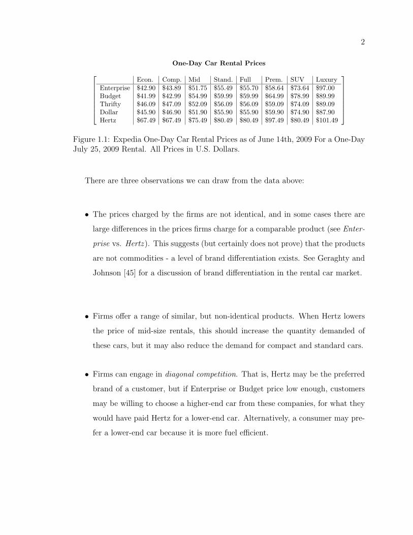
An example of such a car rental problem is renting a car from the Indianapolis,
IN aiport. On June 14th, 2009 a visitor to Expedia.com was presented the following
options for a one-day July 25, 2009 rental, in U.S. dollars:
2
One-Day Car Rental PricesEcon. Comp. Mid Stand. Full Prem. SUV Luxury
Enterprise $42.90 $43.89 $51.75 $55.49 $55.70 $58.64 $73.64 $97.00Budget $41.99 $42.99 $54.99 $59.99 $59.99 $64.99 $78.99 $89.99Thrifty $46.09 $47.09 $52.09 $56.09 $56.09 $59.09 $74.09 $89.09Dollar $45.90 $46.90 $51.90 $55.90 $55.90 $59.90 $74.90 $87.90Hertz $67.49 $67.49 $75.49 $80.49 $80.49 $97.49 $80.49 $101.49
Figure 1.1: Expedia One-Day Car Rental Prices as of June 14th, 2009 For a One-DayJuly 25, 2009 Rental. All Prices in U.S. Dollars.
There are three observations we can draw from the data above:
• The prices charged by the firms are not identical, and in some cases there are
large differences in the prices firms charge for a comparable product (see Enter-
prise vs. Hertz ). This suggests (but certainly does not prove) that the products
are not commodities - a level of brand differentiation exists. See Geraghty and
Johnson [45] for a discussion of brand differentiation in the rental car market.
• Firms offer a range of similar, but non-identical products. When Hertz lowers
the price of mid-size rentals, this should increase the quantity demanded of
these cars, but it may also reduce the demand for compact and standard cars.
• Firms can engage in diagonal competition. That is, Hertz may be the preferred
brand of a customer, but if Enterprise or Budget price low enough, customers
may be willing to choose a higher-end car from these companies, for what they
would have paid Hertz for a lower-end car. Alternatively, a consumer may pre-
fer a lower-end car because it is more fuel efficient.
3
1.1 Literature Review
There are two streams of research that have considered the problem of firms pricing
in an environment where there are multiple products. These include both the revenue
management literature and the oligopoly literature from microeconomics. Canonical
models in the existing revenue management literature do not model all of the three
observations mentioned earlier. For this reason, we look to the oligopolistic geometric
demand framework developed in microeconomics. This framework balances the need
for mathematical tractability with the need to create models that reflect real-world
revenue management challenges. As a consequence, a literature review of both areas
of study follows.
1.2 Introduction to Revenue Management Litera-
ture
One class of models, including Anderson and Wilson [5], Belobaba [10] and Wilson,
Anderson, and Kim [56] allows for multiple product classes. However they only allow
for a single firm and allow those firms to only alter booking limits, not prices. Oth-
ers such as Bell and Zhang [9] and Federgruen and Heching [38] allow for dynamic
pricing, but in a one-firm, one-product market. To accurately depict markets such
as the rental car industry a model that allows for multiple firms each selling multiple
products is required. This model should also include dynamic pricing as real-world
firms can currently alter their prices in real time.
A number of models of competition with dynamic pricing do exist, Perakis and
Sood [82] being a well-known example, but in these models each firm is only able
4
to offer a single-product class. Talluri [97] examines the equilibrium properties of
a two-firm/one-product per firm model where product differentiation exists between
the firms. A number of extensions to this model exist, including Levin, McGill and
Nediak [108], which allow consumers to exhibit strategic behaviour by waiting for
prices to fall. Cachon and Feldman [17], Jerath, Netessine and Veeraraghavan [58],
Liu and Zhang [67] and Parlakturk and Kabul [81] all allow customers to wait for
prices to fall. Marcotte, Savard and Zhu [80] consider the oligopoly problem in the
context of airline networks. Xu and Hopp [106] allow for a single inventory replen-
ishment and Mantin, Granot and Granot [7] create a duopoly model that uses the
one-arrival-per-period assumption.
Netessine and Shumsky’s [76] airline model allows for two firms and two product
classes, but only two of each and is a model of booking limits, not of dynamic pricing.
Song, Yuan and Mao [54] have an extension that allows for incomplete information.
A number of literature reviews exist in this area, including Talluri et. al. (2009)
[37], Phillips (2005) [83] and Talluri and van Ryzin (2004) [98]. Elmaghraby and
Keskinocak (2003) [35] provide a detailed literature review of revenue management
models. As a starting point, we will consider their literature review, before moving
on to articles which have appeared since their article was published.
When examining the dynamic pricing literature in revenue management, Elmaghraby
and Keskinocak “postulate that there are three main characteristics of a market envi-
ronment that influence the type of dynamic pricing problem a retailer faces.” Those
three characteristics, or dimensions, as identified by Elmaghraby and Keskinocak, are
as follows:
5
1. Replenishment vs. No Replenishment of Inventory (R/NR): Does the retailer
have the ability to re-order inventory during the sales period?
2. Dependent vs. Independent Demand over Time (I/D): Do past sales have an
impact on future sales?
3. Myopic vs. Strategic Customers (M/S): Do customers always purchase the good
immediately, or do they consider waiting for prices to drop?
(Note: Titles and abbreviations borrowed from Elmaghraby and Keskinocak).
Elmaghraby and Keskinocak find that the “bulk” of the dynamic pricing litera-
ture falls into two camps: NR-I (both NR-I-M and NR-I-S) and R-I-M (see earlier
definitions for ‘R’, ‘NR’, ‘I’, ‘M’ and ‘S’). Thus the major division in the literature,
according to Elmaghraby and Keskinocak, is between models where firms can re-order
inventory and ones where they cannot. First, we will examine models where no in-
ventory replenishment is possible.
1.2.1 No Inventory Replenishment
Elmaghraby and Keskinocak identify a number of models which study how pricing
decisions should be made in these markets. These include: Bitran, Caldentey, and
Mondschein (1998) [12]; Bitran and Mondschein (1997) [13]; Feng and Gallego (1995)
[39]; Gallego and van Ryzin (1994) [44]; Lazear (1986) [64]; Smith and Achabal (1998)
[94] and Zhao and Zheng (2000) [111]. One of the common demoninators is that firms
6
operate in a market of “imperfect competition (e.g. a monopolist)” [35]. There is no
competitive interaction between firms in these markets. We wish to develop a model
where competitive interaction is possible.
As well, Elmaghraby and Keskinocak indicate that all the papers they reviewed
on dynamic pricing in the N-I market consider the case where the firm only sells a
single product. Papers which consider simultaneously pricing multiple products do
so in a static setting, such as Reibstein and Gatignon (1984) [87].
Elmaghraby and Keskinocak identify a number of features which should be added
to NR-I models, in order to “bridge the gap” between theory and practice.
• Multiple products per firm: This is important when considering both substitute
products a firm might sell (two different sized bottles of ketchup) and comple-
mentary products (a top and the matching pair of pants).
• Multiple stores or multiple channels: Firms often sell the same product, from
the same inventory set, over multiple channels. An airport location of a car
rental firm sells its cars through its own website, through a third-party website
such as Expedia.com, to travel agents, and to walk-up-traffic.
• Initial inventory: The initial inventory a firm has is also often treated as given,
but in many situations it is a variable that the firm can control.
• Strategic customers: Customers may often “time” their purchases in order to
7
get the best possible price.
• Competitors’ Pricing Decisions: Elmaghraby and Keskinocak give an example
of how firms take this into account: “In a competitive business environment,
consumers’ purchasing decisions take into account prices offered by competing
firms. IT allows companies to automatically track competitors’ prices and in-
corporate that information into their pricing decisions. For example, Buy.com
Inc. developed technology using software “bots” to monitor prices on competing
sites such as Amazon.com and Best Buy (Heun 2001) [49]. Competitors’ prices,
along with other information, are then fed into the dynamic pricing software
from KhiMetrics, which suggests price changes on Buy.com Inc.”
Keeping in mind the features identified by Elmaghraby and Keskinocak, it is our
intention to make a major contribution to bridging this gap between theory and prac-
tice by developing a model that allows for dynamic pricing within the context of a
multiple-firm, multiple-product-per-firm environment.
1.2.2 Inventory Replenishment
Elmaghraby and Keskinocak find that the literature for models with inventory re-
plenishment fall into three broad categories, based on their modelling assumptions:
1. Markets where the firm’s demand is uncertain, faces convex production, holding
and ordering costs exist, and production quantity is unlimited. Papers in this
8
category include Federgruen and Heching (1999) [38], Thowsen (1975) [101] and
Zabel (1970) [110].
2. Markets as above with the addition of fixed ordering costs, as in Thomas (1970)
[100] and Chen and Simchi-Levi (2002) [18]. Chan, Simchi-Levi and Swann
(2002) [62] also incorporate limited production capacity.
3. Markets such as in number 1, expect the firm’s demand is deterministic, such
as Biller et. al. (2002) [89] and Rajan, Rakesh and Steinberg (1992) [1].
As with NR-I models, these models do not allow for retailers that sell multiple
products. Elmaghraby and Keskinocak see this as an area researchers need to con-
sider:
“One can argue that all products’ prices are somewhat interdependent and pric-
ing decisions should simultaneously consider all the products offered by a firm and
its competitors... One reasonable approach... is to identify families or categories of
products whose demands are significantly dependent on each other and simultane-
ously consider pricing decisions for products in the same family... Advances in IT
provide the retailer with the ability and the required data to optimize prices across
multiple products and, therefore, we see this as a research direction deserving imme-
diate attention.”
Diagonal competition is an important component of real-world industries of inter-
est to revenue managers.
9
1.2.3 Literature Post-Elmaghraby and Keskinocak
The pricing in revenue management literature has expanded since the publication of
Elmaghraby and Keskinocak.
The models in Elmaghraby and Keskinocak fall into two camps: NR-I (both NR-
I-M and NR-I-S) and R-I-M. These two camps have the independence assumption in
common. A number of recent models have been developed which allow for depen-
dent demand between periods. The models of Anderson and Wilson (2003) [5], Su
(2007) [96] and Wilson, Anderson and Kim (2006) [56] consider markets with strate-
gic consumers who may wait for the firm to offer a lower price. In Su, consumers can
purchase the good immediately or pay a fee to stay in the market and purchase at a
later date.
Another form of dependency between periods is caused by reference effects. Popescu
and Wu (2007) [84] examine how reference effects impact the choices made by con-
sumers:
“As customers revisit the firm, they develop price expectations, or reference prices,
which become the benchmark against which current prices are compared. Prices
above the reference price appear to be “high”, whereas prices below the reference
price are perceived as “low”... Adaptation level theory (Helson (1964) [48]) predicts
that customers respond to the current price of a product by comparing it to an inter-
nal standard formed based on past price exposures called the reference price... The
impact of the reference price on demand [is] called [the] reference effect...”
Popescu and Wu find that if reference prices are not taken into account, firms will
10
“systematically price too low and lose revenue.”
There are many variations in the structures of the models presented in the litera-
ture. In Bell and Zhang (2006) [9], firms have the ability to both alter the price they
charge and the quantity for sale. The market structure of Deng and Yano (2006) [29]
is that of a monopolist that has the abilities to set production levels, re-order and to
alter prices.
Dasci (2003) [24] considers a market with two firms where consumers, if not able
to purchase at their most-preferred firm (because they have run out of stock) attempt
to purchase from the other firm. Perakis and Sood (2006) [82] consider the pricing
problem in a market of multiple firms, each selling similar, but not identical goods.
Netessine and Shumsky (2006) [76] model a competitive airline market where each
firm allocates its seats between two booking classes. Each of these models considers
similar market structures to the one we wish to study and provide an excellent struc-
ture off of which to build.
Levin, McGill and Nediak [107] consider a scenario where a monopolist can choose
a price to charge but also issue consumers compensation if the price charged in the
future goes below the price the consumer paid today. Marcus and Anderson (2006)
[71] examine such pricing guarantees using a real options approach and find that in
practice firms likely do not benefit by issuing such guarantees.
Netessine, Savin and Xiao (2006) [90] model the scenario where firms ‘cross-sell’
products, that is they sell goods both individually and as part of a package. They
consider both what products should be bundled together and what price point to
charge for the bundles.
11
1.2.4 Lin and Sidbari
Lin and Sidbari (2008) [66] develop a model which allows for dynamic ‘real-time’
pricing of goods. There are N firms in the model, each of which sells one type of
good. Firms hold a limited quantity of each good and cannot re-order when sold out.
Following in the footsteps of Lautenbacher and Stidham (1999) [63], Subramanian et.
al. (1999) [55] and You (1999) [109], they assume that a single consumer arrives each
period with probability λ. We will adopt this assumption in our model as well.
The consumers see the products/brands as being different from one another and
make a purchase as to maximize their utility function (the utility function is in multi-
nomial logit form). Using a theorem in Vives [104], they show the game has a pure-
strategy Nash Equilibrium. They are unable, however, to prove that the equilibrium
is necessarily unique.
Interestingly, Lin and Sidbari find that for a given inventory level, prices are not
necessarily increasing over time, due to what they call ‘competition effects’.
1.2.5 Martinez de Albeniz and Talluri
Martinez-de-Albeniz and Talluri (2011) [28] create a dynamic pricing model with
multiple firms that sell a fixed number of goods over a finite number of periods. In
the base model there are two firms, each selling one class of product. Consumers
see the products as being identical and will always choose the lower priced good (if
prices are identical, consumers choose randomly). As with Lin and Sidbari (2008) [66]
12
each period a single consumer arrives with probability λ. They show for this model
a unique subgame-perfect equilibrium in pure strategies. The equilibrium is simply
the well-known Bertrand (1883) [11] result.
Martinez-de-Albeniz and Talluri [28] consider a number of extensions to the model,
including the case of N > 2 firms. They show a unique subgame-perfect equilibrium
for this model as well. The results, however, require firms selling only one type of
product, and no product/brand differentiation between firms.
A model of differentiated products is briefly considered and it is shown for some
functional forms, such as the logit choice function, it is often possible to obtain a
unique subgame-perfect Nash Equilibrium.
1.2.6 Lu
Lu (2009) [68] examines a market of N firms, each of which sells a limited inventory
of a single type of good. If firms run out of the good they leave the market for the
duration of the sales period. Although the model is described as a ‘price and inven-
tory’ game, re-orders are not possible.
As with previous papers, at most a single customer arrives each period with prob-
ability λ. Consumers do not act strategically or wait for higher prices.
Consumers do not see the products from firms as being identical. A lower price
(weakly) increases the quantity demanded of that good and (weakly) decreases de-
mand for the other goods.
13
Lu finds the existence of “a strategy that pushes customer to retailer 2, and hence
retailer 2 stocks out, after which retailer 1 becomes a monopolist.” In our model, we
will refer to such a strategy as a knockout strategy (Lu does not give it a name).
Lu shows that for the N = 2 case, a Nash Equilibrium in pure strategies need
not exist - it depends on the assumptions placed on demand. The N > 2 case is not
considered. Lu does also not consider firms that sell multiple products, but indicates
it as an area of future research, though it is not obvious from the thesis how the
model will be able to incorporate this.
1.2.7 Hu
A doctoral thesis by Hu (2009) [52] examines the N firm, 1 good type per firm dy-
namic pricing model but does so in continuous time, not discrete time, which is a
multi-firm extension of the Gallego and van Ryzin (1994) [44] model. Firms have a
finite period in which to sell their goods and assume the goods have no salvage value
and all other costs are fixed. They show that a subgame perfect equilibrium can be
constructed so long as the pricing options available to each firm are finite and discrete.
1.2.8 Isler and Imhof
Isler and Imhof (2008) [53] develop a two-firm/one-product-per-firm dynamic pricing
model in the context of airline ticket pricing. A parameter α is introduced which
models product differentiation. They find that when quantities are limited or some
product differentiation exists in the market, firms will price above marginal cost.
14
However, when both firms have a substantially large quantity and product differ-
entiation is assumed to be zero, Isler and Imhof obtain the Bertrand result of zero
economic profit. They do not consider the case of multiple seat classes per firm.
In order to formulate the best possible model to reflect real-world revenue man-
agement challenges, we next look to microeconomic models for guidance.
1.3 Introduction to Classic Microeconomics Mod-
els
Oligopoly theory has a long history in the study of microeconomics, particularly in
the field now known as Industrial Organization. Cournot’s [23] 1838 treatment re-
mains to this day standard undergraduate textbook fare. Many refinements have been
made over the years, from the price-competition model of Bertrand [11] to the spatial
competition model of Hotelling [51]. No one model has emerged as the benchmark
treatment of oligopoly in Industrial Organization - rather a toolbox full of approaches
which vary by the nature of competition (price, quantity, or other factor), assumption
used, and the amount of complexity in the model.
1.3.1 Bertrand Competition
Bertrand competition, as developed by Bertrand [11], is a 2-firm model of firm com-
petition where the firms face identical marginal costs and sell their good over one
period. Firms do not face capacity constraints and consumers purchase a fixed quan-
tity of goods from the lowest price firm, so long as the lowest price is below some
15
maximum-willingness-to-pay, leading to firms receiving zero economic profits. A log-
ical extension is to increase the number of periods under consideration, but playing a
Bertrand game with a finite number of periods yields the same zero economic profit
result, as shown by Friedman (1971) [41] and Friedman (1977) [42].
After the publication of Bertrand’s model in 1883, a number of extensions were
attempted in order to rid the model of the result that both firms price at marginal
cost. These extensions include, but are not limited to Fisher (1898) [40], Moore (1906)
[73], Schumpeter (1928) [91] and Stigler (1940) [95]. The extensions, and proofs of
the results, are available in many microeconomics texts. The results that follow are
available in Nichols [77] (2004) and Fudenberg and Tirole (1991) [43].
Fudenberg and Tirole point out a number of problems with the Bertrand model.
Firstly, the assumptions of the products being seen by consumers as identical, un-
limited quantity available, and wholly symmetric firms lead to the result that each
firm prices at marginal cost. Unfortunately, creating the assumption of firms facing
differing marginal costs yields the situation that only one firm serves the market.
Secondly, problems can be created if the assumption is made that marginal costs are
not constant. Allowing for increasing-returns to scale, that is that the marginal cost
of production declines as the level of production increases, involves further complica-
tions. In the case of homogenous goods, once again the result is that in equilibrium
the firms price at marginal cost. Since increasing returns to scale are allowed the
marginal cost of producing an additional unit of good is less than average cost - thus
this cannot be a Nash Equilibrium. Firms lose money by producing, thus are made
worse off by even participating in the game.
In order to get a result where firms do not price at marginal cost, it appears
16
necessary to introduce decreasing returns to scale into the model. Mathematically,
the most extreme version of decreasing returns to scale is one where the firms are
quantity constrained and cannot produce above a certain level (face an infinite cost
of production above a certain point). The quantity constrained version of Bertrand
is known as Bertrand-Edgeworth competition.
1.3.2 Bertrand-Edgeworth Competition
In order to create a scenario where firms price at higher than marginal cost, Edge-
worth [34] (1888) adds capacity constraints into the finitely repeated Bertrand game.
Unfortunately, pure-strategy equilibria do not exist under this scenario. The exten-
sion came to be known as Bertrand-Edgeworth competition (see Roll (1940) [88]).
Consider the following game:
Two firms sell identical products and face identical constant marginal costs. The
firms are capacity constrained, such that no single firm can meet the quantity de-
manded when price is set to marginal cost. The combined quantities of both firms,
however, exceed the quantity demanded at that price. As in the non-capacity con-
strained model, no Nash Equilibrium can exist where both firms price higher than
marginal cost. A firm can always improve its profitability by slightly undercutting
the other one. However, no Nash Equilibrium can exist where both firms price at
marginal cost. A firm could earn a strictly positive profit by pricing above marginal
cost, as it would capture the excess demand not satisfied by the lower priced firm.
Thus there is no Nash Equilibrium, as firms have an incentive to raise their prices
from marginal cost, yet they face an opposing incentive to lower their prices when
above marginal cost. Edgeworth believed that since an equilibrium would not exist,
17
prices would cycle from low to high to low again (known as an Edgeworth Cycle; see
Maskin and Tirole [72]).
A similar, but not identical, outcome to this model is that the firms will use mixed
strategies. Fortunately mixed-strategy Nash Equilibria exist in this game under very
weak conditions as shown by Dasgupta and Maskin (1988) [25]. However, the mixed-
strategies can be quite intricate and cumbersome.
Since some customers are prevented from purchasing from the lower priced firm,
a rationing rule must be used in this model to determine which customers will be
served by which firm (or at all). Fortunately, the existence of such an equilibrium
is invariant to the choice of rule. Unfortunately, the equilibrium (either in pure or
mixed strategies) can depend heavily on which rule is used to decide which customers
will receive goods when there is excess demand. As discussed in Tirole (1988) [102],
the two most common rules, the proportional rule and the surplus maximizing rule
can give very different results and there is generally no a priori reason to choose one
over the other (see also Davidson and Deneckere (1986) [26], Madden (1998) [69],
Osborne and Pitchik (1986) [79] and Vives (1993) [103]).
The Bertrand-Edgeworth model is widely used in the modelling of oligopoly prob-
lems (Allen and Helwig (1986) [3], Dixon (1990) [30] and Kruse et. al. (1994) [36]
are just three of many examples) particularly in cases where firms compete on price,
capacity constraints exist, and where the outcome of pure-strategy equilibrium is not
required.
18
1.3.3 Extensions of Bertrand-Edgeworth
There have been a number of extensions to the Bertrand-Edgeworth framework in
order to ensure the existence of Nash Equilibrium in pure strategies. Three such
examples are: Dudey (1992) [32], Levitan and Shubik (1972) [65] and Tasnadi (1999)
[99]. These models share a number of features. All three have two firms each selling
a single identical product. Firms in the models have a finite number of goods to sell
(no reorders are possible) and a finite selling horizon. In Tasnadi’s model each firm
simultaneously chooses the rationing rule it will use if it runs out of stock (this is
step 1 of the Tasnadi game). Firms choose price in the second stage and the overall
quantity demanded is responsive to price.
In contrast, Dudey’s model eliminates the rationing rule by assuming that only
one indivisible good can be sold per period; thus bypassing the excess demand prob-
lem. Unlike Tasnadi’s model, the market demand is constant no matter the price
charged by firms, so long as the prices stay within a specified range.
Levitan and Shubik consider a duopoly where the firms sell identical goods and
face identical capacity constraints. The firms simultaneously choose what price to
charge. Consumers purchase from the lowest price firm first and any excess demand
filters to the higher priced firm. They assume that the total demand is the maximum
of the high-price demand and the total available amount at the low price (since it is
all exhausted). Depending on the overall level of capacity relative to demand, Levitan
and Shubik show the final result can be anything between the Bertrand [11] and the
Cournot [23] solutions.
19
1.3.4 Spatial Competition
While Hotelling’s [51] (1929) model may at first glance seem significantly different
from a typical model of oligopolistic competition, it shares a number of features.
The most basic version of Hotelling’s model considers two ice cream vendors who
have set-up shop on a linear beach. Hotelling assumes that demand for ice cream
is distributed uniformly along the beach and each customer buys a single ice cream
cone. It is assumed that the ice cream is costless to produce. In the simple version
of the model we ignore price by assuming that each firm charges identical prices and
thus has the goal of maximizing market share. Since the products and prices are
identical, consumers purchase from the firm closest to their position on the beach.
In the two firm model, there is only one Nash Equilibrium in pure strategies - each
firm places its stand at the median point of the beach. For more than two firms a
pure-strategy Nash Equilibrium in the game cannot be assured. None exist in the
three firm case, for example.
The more robust version of Hotelling’s model has the firms choose both their
locations on the continuum and the price they will charge. Consumers pay a cost
proportional to the distance they travel, thus they purchase from the firm with the
lowest total cost.
Instead of a one-period game, this model is conducted in two stages: first the
choice of location, as before, and in the second stage the firms simultaneously choose
the price they will charge. Hotelling believed that the firms would invariably locate
close together, but unfortunately d’Aspremont, Gabszewicz, and Thisse (1997) [16]
showed that this could not lead to a Nash Equilibrium in pure strategies. A Nash
20
Equilibrium in pure strategies for this has yet to be found, but it also has not been
proven that one does not exist.
Despite the difficulties in obtaining pure strategy Nash Equilibria, Hotelling’s
model of spatial competition remains an important benchmark model in the study of
oligopoly.
1.3.5 Cournot
The Cournot [23] approach differs from many others in Industrial Organization, such
as ones based on Bertrand [11], as it considers competition over quantity, instead
of over price. Pure-strategy Nash Equilibria exist under fairly general conditions in
Cournot models (a sufficient, but not necessary condition is that the profit func-
tion for each firm be quasi-concave with respect to own output). For the multi-firm
Cournot model, the pure-strategy Nash Equilibrium provides for more output and
a lower price than under a monopoly, but for lower output and a higher price than
under perfect competition.
There have been a large number models of quantity competition since Cournot.
A particularly useful one for revenue management modelers is Manas [70], which is
cited frequently in the revenue management literature.
1.3.6 Manas
The model constructed by Manas [70] considers quantity, not price, competition in a
market with N firms. Specifically, the model has six basic features:
21
1. The goods produced by each firm are identical - there is no product differenti-
ation.
2. At the beginning of the game each firm decides what level of quantity to produce
- output is the only decision variable for each firm.
3. The equilibrium price for each good is a function of total market output -
specifically the equilibrium price is a linear function of overall output.
4. No collusion or cooperation is permitted/available to the firms.
5. All firms are rational profit maximizers.
6. Each firm faces a capacity constraint.
It can be shown that a pure-strategy Nash Equilibrium exists in the game with
the aid of a theorem by Nikaido and Isoda [78]. Nikaido and Isoda, through the de-
velopment of a fixed-point theorem, show that a game has at least one pure-strategy
Nash Equilibrium if all strategy spaces in the game are compact (the strategy space
is both closed and bounded) and convex (that is any convex combination of two al-
lowable strategies is also allowable), each payoff function is concave with respect to
that firm’s decision variable, and all payoff variables are concave. That holds in this
case, since the strategy spaces are both compact and convex (the real line spanning 0
to ki), the payoff functions are concave (linear), and all payoff variables are concave
(again, linear). Manas goes on to show that in this particular game, the Nash Equi-
librium is unique and gives an algorithm on how the Nash Equilibrium can be located.
While the cost and demand functions are relatively simplistic, the model develop-
ment by Manas provides a useful benchmark for models of quantity competition with
22
differentiated firms (but not products) and capacity constraints.
1.4 If Hertz Charges Twice What Enterprise Does,
Are They Competitors at All?
An important question we need to ask, given the data posted in the previous sec-
tion, is “Are low-price firms such as Dollar and Enterprise in the same market as
high-price firms such as Alamo and Hertz?” Dollar’s price for an economy rental is
only $5.15 above Enterprise’s, whereas the price differentials are $18.98, $43.22 and
$61.65 for Budget, Alamo and Hertz vis-a-vis Enterprise respectively. Renting a car
from Alamo could be significantly different than renting a car from Hertz, because
of the existence of fences, because they serve two completely separate demographic
markets or because of high levels of perceived firm differentiation among customers.
If this were the case, then the cross-elasticity between most, if not all brands would
be near zero. If cross-elasticity between most brands can be ignored, then we can
simply treat Enterprise’s optimization problem as a monopoly problem, or at worst a
duopoly problem between Enterprise and Dollar. Dollar need not concern itself with
how Budget prices its rental cars.
Without a published study or data on the cross-price elasticity between car rental
firms, we cannot say for certain if the elasticity between firms is non-zero. However,
there are markets, that share at least somewhat similar features to the car rental
market, that have been studied. Consider the market for spray glass cleaners. A 22
ounce bottle of Windex may sell for $2.49 whereas a 22 oz bottle of a private label
brand with a name such as Kwik-E-Mart Glass Cleaner with near identical formu-
23
lation may sell for $1.09, less than half the price of Windex. The name brand vs.
generic problem has been studied extensively in the marketing science literature, and
can provide insights on the dynamics of our market.
1.4.1 Sethuraman and Srinivasan
Sethuraman and Srinivasan [92] survey the marketing science literature and note sev-
eral studies which find that price reductions by high-price brands affect the demand
for low-price brands. Similarly price reductions by low-price brands affect the demand
for high-price brands. They indicate that the majority of these studies (including Al-
lenby and Rossi [4], Hardie, Johnson and Fader [6], Kamakura and Russell [59] and
Sivakumar and Raj [93]) find an asymmetric price effect - that is the demand for
low-price brand is more sensitive (as measured in terms of cross-price elasticity of
demand) to changes in high-price brand price than vice-versa. However, they note
that Bronnenberg and Wathieu [15] find that, in some instances, the effect can act in
reverse. A later paper by Dawes [27] also casts doubt on the asymmetric price effect
by concluding “once the size of the brands are controlled for, lower priced (store)
brands induce just as much ‘switching’ or purchase substitution from higher priced
(manufacturer) brands as do the higher priced brands induce switching from the lower
priced brands.” In the majority of cases examined the high price brands have larger
market shares, hence the need to control for the size of the brand.
Through both theory and empirics, Sethuraman and Srinivasan find that when
measured in terms of market share rather than price elasticity, the effect runs in re-
verse - that is price changes in the low-price brand have more impact on the market
share of the high-price brand than the converse. This discrepancy is due to the fact
24
that in many markets the high-price brands have larger market-shares than do low-
price brands.
In a related study Sethuraman, Srinivasan and Kim [85] find that when a brand
discounts its price, not all competing brands are affected equally. Specifically, that
the largest negative effect on the demand for a brand is a price reduction in the next-
higher priced brand. The second largest negative effect on the demand for a brand is
a price reduction in the next-lowest priced brand.
1.4.2 Batra and Sinha
Similar to Sethuraman and Srinivasan [92], Batra and Sinha [8] examine the question
of competition between national brands and private label or store brands. They find
that consumers are more likely to purchase a store brand, ceteris paribus, when:
• Consumers perceive smaller consequences to making a ‘mistake’ in their brand
choice.
• Purchase decisions are more based on search characteristics rather than expe-
rience characteristics. They borrow this distinction from Nelson [75], where
search characteristics of the products are those that can be verified ex-ante
whereas experience characteristics are ones that can only be verified after pur-
chase.
The second of the two points may be particularly important when it comes to
online purchases of rental cars. If online purchases are disproportionately made by
25
younger, more tech-savvy consumers, then online purchases may be associated with
less experienced rental car purchasers. Though as time goes on, the demographics of
online purchasers are converging to that of the general population.
1.4.3 Van Heerde, Gupta and Wittink
While buying an item of food at a grocery store is not identical to making an on-
line car rental reservation, the markets do share some characteristics. Most notably,
both markets involve large oligopolistic producers selling differentiated products. Van
Heerde, Gupta and Wittink [50] survey the marketing literature and find that cross-
elasticity accounts for the majority of total elasticity:
“Chiang (1991) [20], Chintagunta (1993) [21], and Bucklin, Gupta and
Siddarth (1998) [86] extend Gupta’s (1988) [47] approach, which Bell,
Chiang and Padmanabhan (1999) [31] then generalize to many categories
and brands. Across these decomposition studies, we find that, on average,
secondary demand effects (brand switching) account for the vast majority
(approximately 74 %) of total elasticity, which leaves 26% for primary
demand effects (purchase acceleration and quantity increases)... the per-
centage of secondary demand effects is never less than 40% (yogurt) and
is as high as 94% (margarine).”
1.4.4 Chevalier and Goolsbee
Chevalier and Goolsbee [19] consider price competition between online booksellers,
specifically Amazon.com and BarnesandNoble.com. In order to estimate sales data
26
for Amazon.com, the authors create a formula to translate sales rank data into sales.
They find high-levels of cross-price elasticity in the market, though the effect is rather
asymmetric:
“...[A] 1 % increase in the price at Amazon.com reduces quantity by about
0.5 % at Amazon.com but raises quantity at BN.com by 3.5 %. Given that
Amazon.com sells somewhere between three and 10 times as many books
as BN.com, this is very close to the same number of books, implying that
every customer lost by Amazon.com instead buys the book at BN.com...
The reverse is not true, however. Raising prices by 1 % at BN.com reduces
sales about 4 % but increases sales at Amazon.com by only about 0.2 %.
Many of the lost customers from BN.com evidently do not just go buy the
book from Amazon.com. [19]
While rental cars and books are two different markets, the Chevalier and Goolsbee
study does reveal the existence of cross-price elasticity in the online sphere.
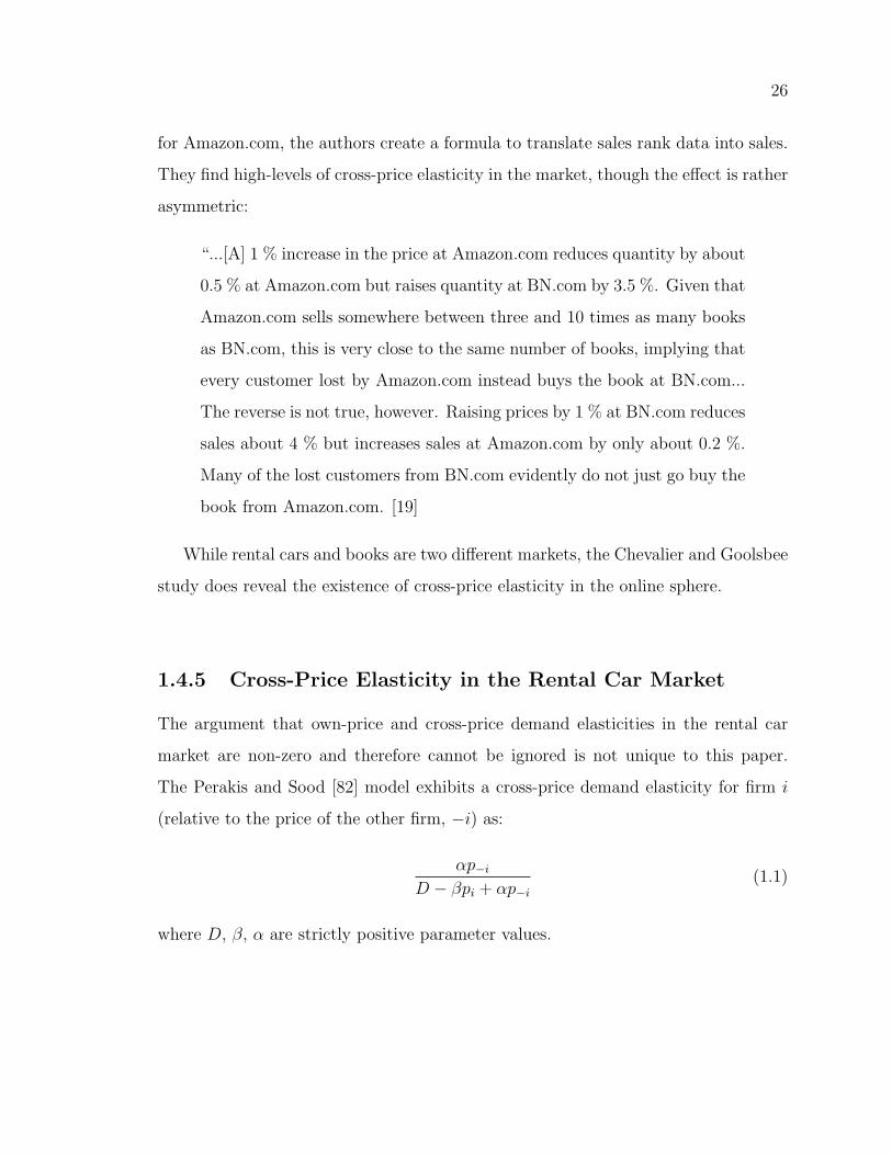
1.4.5 Cross-Price Elasticity in the Rental Car Market
The argument that own-price and cross-price demand elasticities in the rental car
market are non-zero and therefore cannot be ignored is not unique to this paper.
The Perakis and Sood [82] model exhibits a cross-price demand elasticity for firm i
(relative to the price of the other firm, −i) as:
αp−iD − βpi + αp−i
(1.1)
where D, β, α are strictly positive parameter values.
27
The existence of own price elasticity should not be in doubt, though the level of
own price-elasticity is not necessary constant between firms and brand classes. Dur-
ing a 2008 interview, car rental consultant Neil Abrams commented that ”[t]here is a
lot of elasticity in pricing [on the leisure side]; that is not true on the corporate side.”
[2].
A larger issue, however, is when firm X raises the price of one of its goods, how
much of the quantity demand loss goes to other goods (cross-elasticity) and how much
goes to consumers deciding to reduce their overall quantity purchased? While we are
unaware of any publicly-available study calculating these elasticities in the rental car
industry, there is a significant body of evidence suggesting that cross-elasticities are
significantly different than zero. The evidence would suggest that not all consumers
simply choose the non-purchase option, rather they choose to rent a car in another
class from the same firm or another car from a different firm.
1.4.6 References in the Literature to Cross-Price Elasticity
in the Rental Car Market
Although there have been no publicly released studies on cross-price elasticity in the
rental car market, so we do not know their magnitude. However, a number of recent
papers make references to the existence of this phenomenon. First consider Anderson,
Davison and Rasmussen [22]:
“The car rental industry is not as price sensitive as the airline industry.
Price changes do generate subtle changes in demand, but what is more
28
important is one car rental firm’s price against its competition’s.” [22]
Geraghty and Johnson [45] make a similar comment in their paper on revenue
management at National:
“The rental car market is extremely competitive. A price move that makes
the company more expensive than its competitors can damage utilization
levels.” [45]
Geraghty and Johnson add:
“Our initial analysis of National’s rate behavior indicated that competi-
tive positioning was the determining factor in its pricing decisions prior
to the revenue management program. At times of low demand, sensitivity
to competitor behavior is crucial. Utilization levels can suffer drastically
from poor rate positioning in the marketplace.” [45]
Additional evidence can be found in studies of consumer behaviour when purchas-
ing automobiles.
1.4.7 Cross-Price Elasticity in the Car Market
There have been at least two studies in peer-reviewed journals on cross-price elasticity
in the automobile market, both of which found strictly positive levels of cross-price
elasticity. Goldberg [46] finds that for automobile purchases:
29
“Consistent with utility maximization, and since consumers buy only one
car model, all cross price elasticities are positive. Furthermore, their mag-
nitude depends on the degree of similarity between products; automobiles
that belong to the same class and origin - and are therefore similar in
characteristics - exhibit on average higher cross price semi-elasticities than
products of different classes and origins.” [46]
Bordley [14] also finds that the level of cross-elasticity is dependent on how closely
related the two products are:
“The loyalty index is higher for higher priced products (as would be ex-
pected since higher income buyers are less price-sensitive).. economy car
buyers do not view non-economy cars as close substitutes, luxury car
buyers do not view non-luxury cars as closed substitutes... But note that
luxury car buyers are not, contrary to popular belief substantially less
price-sensitive than other buyers. This reflects how competitive the lux-
ury car market has become.” [14]
This second study suggests that although an industry (luxury cars) as a whole
may have low price-elasticity of demand, the price-elasticity of demand and cross-
price elasticity of demand for individual products may be significant.
While we do not have estimates of the exact level of cross-price elasticity in the
rental car market, the combined evidence of statements by practitioners on the im-
portance of cross-price elasticity in the rental car market, estimates of cross-price
30
elasticity in the car market and estimates of cross-price elasticity from scanner data
suggests that cross-price elasticities in the rental car market are likely to be signifi-
cantly different than zero.
1.5 Putting it Together
While more direct evidence of cross-price elasticity in the online car rental market is
needed, scanner based evidence from the marketing science literature shows that:
• Similar products can have sustainable long-term differences in prices through
perceived product differentiation.
• High-priced and low-priced brands are not ‘islands’ and significant cross-price
elasticity can exist between the two.
• The exact level of cross-price elasticity can vary depending on a number of fac-
tors, and may (though not necessarily) be higher for the low-priced brand.
1.6 Our Contribution
In this paper we create a dynamic pricing model that allows for N ×M product-firm
combinations using a repeated game framework. We share Vives’ [104] frustration in
the lack of progress made using repeated games to model oligopoly problems. Ex-
isting dynamic pricing models in revenue management are lacking as they do not
31
address the question of multiple firms selling multiple product classes, despite the
fact that most markets of interest to revenue managers have this feature. We do be-
lieve, however, that such a benchmark model can be established with a repeated game
model, as the choice of allocation rule for the “excess demand” problem which plagues
Bertrand-Edgeworth style capacity constrained models can be eliminated with a set
of assumptions which are plausible for many markets. The first key assumption is
that customers purchase at most one good at a time from at most one firm, which
is reasonable for many consumer markets such as the markets for durable goods and
rental cars. The second key assumption is that firms can change their prices instan-
taneously, which is currently the case in online markets such as Expedia and Orbitz.
The impact of the ability to dynamically change online pricing has been discussed for
some time now - Ariely (2000) [57], Kannan and Kopalle (2001) [60] and Wurman
(2001) [105] are three such examples. It will also likely be possible in the future at
retail stores thanks to the ongoing development of digital price displays. The use of
RFID (Radio Frequency IDentification) in dynamic digital pricing displays has been
heavily discussed - see Eckfeldt (1999) [33], Kourouthanassis and Roussos (2003) [61]
and Raza, Bradshaw and Hague (1999) [74] for examples. By introducing these as-
sumptions, we are able to guarantee the existence of Nash Equilibria, a feature which
is lacking in many models.
The final goal of this model is to provide a framework which describes price com-
petition in oligopolistic markets. We believe the game-theoretic model, using a geo-
metric representation of the potential market, can provide the benchmark model that
oligopoly theory in revenue management is lacking. We hope these ideas will strike a
chord with practioners, who will incorporate them into models used by industry, in
order to improve the bottom lines of their companies.
32
Considering cross-price elasticity and the strategic implications of the quantity
levels of all products in the market, firms can substantially increase their revenues.
If real world car rental firms are using existing pricing models from the revenue man-
agement literature, they are leaving a significant amount of revenue on the table. As
shown by Lu [68] there may be occasions where firms can increase their profits by
using a knockout strategy to eliminate a competitor product from the market.
33
Chapter 2
Creating and Solving NxM Pricing
Demand Models
2.1 Description of the Issue
In this chapter, a framework is created using geometry and the concept of ‘maximum-
willingness-to-pay’ to construct multivariate demand models. The result is the ability
to create mathematically tractable models with an unlimited number of product types.
The N firms with MN products pricing model allows for an accurate represen-
tation of the types of markets commonly seen in real-world revenue management
situations. Despite ‘multiple firm-multiple products per firm’ being included in the
‘future research’ of many revenue management pricing papers, there is very little lit-
erature in this area due to the complexity of the problem. However, we show that
it is possible to create models that allow for unlimited firms and unlimited prod-
ucts. The results hinge on a number of assumptions, the most important of which
is the ‘single-customer per period buys at most a single-product’ assumption which
34
is relatively common in the literature. Any pricing model also requires a demand
framework. A major contribution of this paper is it creates a geometric framework
that allows for the required mathematical tractability while still retaining a number
of useful properties. We show that we can be assured of the existence of pure strategy
subgame perfect Nash Equilibria. It is possible, in some instances, to show that the
Nash Equilibria are necessarily unique.
We then solve the NxM pricing model recursively, first for period T then for pe-
riods t < T . We then prove the existence of subgame-perfect Nash Equilibria for all
subgames. The result is the first ever solvable NxM revenue management model with
guaranteed existence of a solution (equilibria).
2.2 Assumptions of the Model
There are N competing firms in a market, each selling one or more differentiated
products. Specifically, firm n sells mn different products, for a total of MN brand-
product combinations in the market (MN ≥ N). There is no requirement that each
firm have the same number of products. The goods are sold over a finite selling
period. At the beginning of each period the firms simultaneously set their prices.
Firms have limited capacity and are unable to produce more goods. If a firm runs
out of a product that product is removed from consideration for the rest of the game.
Customers have a preferred brand, but will purchase one of their less preferred brand
if the price differential is high enough, or from no firm if all prices are too high.
One difficulty with capacity constrained models is the problem caused by excess
demand (the so called ‘excess demand’ problem). If the demand for a particular
35
product is higher in a given period than remaining inventory, we have to allocate that
excess demand somewhere else. This often causes the models to lack Nash Equilibria.
The lack of Nash Equilibria provides difficulties to the practitioner. A model that
cannot provide guidance in some scenarios is of little use to someone who wishes to
use it in practice.
To avoid the excess demand problem, assume that during any period only a single
customer arrives (with some probability λ) and she only demands one unit of one of
the goods from one of the firms. This eliminates the excess demand problem, because
any brand-product combinations remaining in the market will have at least one unit
available for sale. Any brand-product combinations that have run out of goods are
assumed to have dropped out of the market. This is similar to Lu (2009) [8], which
refers to such models as ‘price and inventory’ games. Thus, there can never be excess
demand in this model.
We follow the lead of Dudey (1992) [3], Lin and Sidbari (2008) [7], Martinez-de-
Albeniz and Talluri (2011) [2] and Lu (2009) [8] by using the at most one arrival/at
most one purchase assumption; an incredibly useful one that we believe is underuti-
lized in the literature. We deviate from Dudey and the subsequent papers by allowing
for more than 2 firms, product differentiation and market-level price elasticity of de-
mand. Further extensions are possible as well, such as multiple products per firm as
we see in the revenue management literature.
36
2.3 Introduction to the Oligopoly Pricing Game
Each firm begins the game with an initial inventory q1n,m, where q stands for quantity,
n ∈ [1, N ] for the firm, m ∈ [1,M ] for the product. The superscript 1 denotes that it
is the quantity at the start of the first period, where t ∈ [1, T ]. As with many models
in revenue management we will simplify the model, by treating all costs in the model
as sunk, thus they play no role in the analysis.
The timing of the game works as follows:
1. At the beginning of each period t ∈ [1, T ], every firm n ∈ [1, N ] with remaining
inventory of good m ∈ [1,M ] simultaneously sets a price ptn,m.
2. A customer arrives with probability λ. If a customer arrives, her preferences
are drawn randomly from a distribution ∆. Given this distribution, a customer
purchases good m from firm n with probability πtn,m(pt1,1, ..., ptN,M), where the
probability is a function of the prices currently offered by each remaining firm.
Thus the expected demand for product m from firm n in period t is given by
λπtn,m(pt1,1, ..., ptN,M).
There is also a chance that the consumer does not purchase any good, which
is denoted as πtNS(pt1,1, ..., ptN,M) (where NS stands for “no sale”). In further
analysis, we will drop the (pt1,1, ..., ptN,M) notation as it should be understood
that purchase probabilities are a function of price.
37
Assumption 1. We require that inside the range of prices [Ltn,m, Utn,m] our
demand space has the following properties:
(a) The sum of all purchase probabilities, including the probability of no sale,
given a customer’s arrival, to equal one.
(b) The probability function for a product is twice differentiable (in the interior
of the strategy space) with respect to own price.
(c) The probability functions are (weakly) decreasing in own price.
(d) The probability functions are (weakly) increasing in other product prices.
(e) The no-purchase probability is (weakly) increasing in the price of any prod-
uct.
(f) All probabilities are non-negative.
When a product is no longer for sale in the game, we will note it as having a
price U tn,m, which is the price at which there is no demand for that product. By
doing so we do not need to alter the probability functions whenever a product is
no longer available; ‘pricing’ the product at U tn,m allows it to fall away naturally.
If a customer chooses to purchase a particular good, she pays the price the firm
selling that good has offered. There is no negotiation. Thus the expected rev-
enue of firm n withM different products in period t is given by λ∑M
m=1 πtn,mp
tn,m.
3. At the end of the game, firms can sell their remaining inventory of each good
at the good-specific salvage value sTn,m. Other than 0 ≤ sTn,m < U tn,m we put
no restriction on the salvage value. It can be that sTn,m > Ltn,m and firms could
price below the salvage value, if they wished.
38
2.4 Demand Model
Consumers have a maximum-willingness-to-pay for each of the MN products. The
maximum-willingness-to-pay for each good m from firm n has a lower bound of
Ltn,m; any prices lower than Ltn,m will not increase quantity demanded. Similarly,
the maximum-willingness-to-pay for each good m from firm n has an upper bound of
U tn,m. At a price of U t
n,m or higher quantity demanded is zero. Thus our demand space
is a closed, compact MN -dimensional orthotope (hyperrectangle). For mathematical
tractability, we will assume that customers are identical with maximum-willingnesses-
to-pay uniformly distributed within the orthotope. The demand model in this section
will meet the necessary differentiability assumptions. Having a uniform distribution
is a sufficient condition, but it is not necessarily necessary; there may be other distri-
butions which meet the necessary conditions.
If only one product m from firm n existed in the market, the probability of sale
given one arrival and price ptn,m would be:
πtn,m =(U t
n,m − ptn,m)
(U tn,m − Ltn,m)
(2.1)
And the probability of no-sale, given arrival, equal to:
πtNS =(ptn,m − Ltn,m)
(U tn,m − Ltn,m)
(2.2)
Corollary 1 (Single Product Market Meets Demand Space Assumption). A
single product demand model meets all six demand space assumptions.
39
Proof. 1. All Probabilities Given Arrival Equal One:
(U tn,m − ptn,m)
(U tn,m − Ltn,m)
+(ptn,m − Ltn,m)
(U tn,m − Ltn,m)
=(U t
n,m − Ltn,m)
(U tn,m − Ltn,m)
= 1 (2.3)
2. Demand Probability Twice Differentiable:
∂πtn,m∂ptn,m
=−1
(U tn,m − Ltn,m)
,∂2πtn,m∂pt2n,m
= 0 (2.4)
3. Demand Probability Decreasing in Own Price: Met since the first deriva-
tive of the probability function with respect to price is negative.
∂πtn,m∂ptn,m
=−1
(U tn,m − Ltn,m)
(2.5)
4. Demand Probability Increasing in Other Product Prices: Irrelevant -
no other products in market.
5. No Purchase Probability Increasing in Prices: Met since the first deriva-
tive of the no-sale probability function with respect to price is positive.
∂πtNS∂ptn,m
=1
(U tn,m − Ltn,m)
(2.6)
6. Probabilities Non-Negative: Since our probability is decreasing in price, it
reaches a minimum at ptn,m = U tn,m. When ptn,m = U t
n,m, πtn,m = 0. Non-purchase
probability is increasing in price and thus reaches a minimum when ptn,m = Ltn,m.
When ptn,m = Ltn,m, πtNS = 0. The condition is met.
Therefore all six conditions are met.
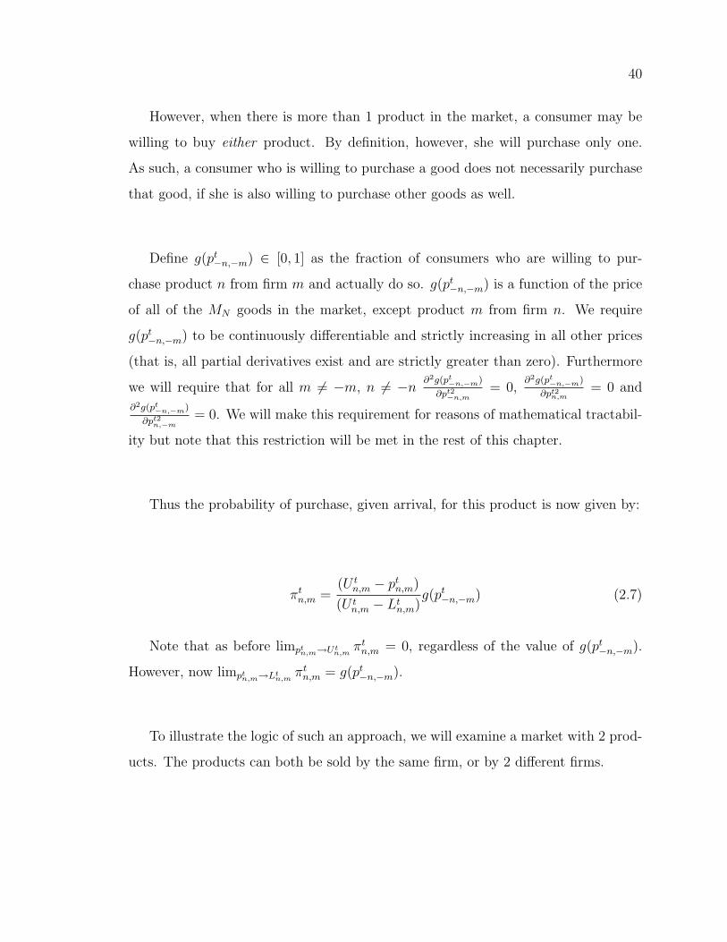
40
However, when there is more than 1 product in the market, a consumer may be
willing to buy either product. By definition, however, she will purchase only one.
As such, a consumer who is willing to purchase a good does not necessarily purchase
that good, if she is also willing to purchase other goods as well.
Define g(pt−n,−m) ∈ [0, 1] as the fraction of consumers who are willing to pur-
chase product n from firm m and actually do so. g(pt−n,−m) is a function of the price
of all of the MN goods in the market, except product m from firm n. We require
g(pt−n,−m) to be continuously differentiable and strictly increasing in all other prices
(that is, all partial derivatives exist and are strictly greater than zero). Furthermore
we will require that for all m 6= −m, n 6= −n ∂2g(pt−n,−m)
∂pt2−n,m
= 0,∂2g(pt
−n,−m)
∂pt2n,m
= 0 and
∂2g(pt−n,−m)
∂pt2n,−m
= 0. We will make this requirement for reasons of mathematical tractabil-
ity but note that this restriction will be met in the rest of this chapter.
Thus the probability of purchase, given arrival, for this product is now given by:
πtn,m =(U t
n,m − ptn,m)
(U tn,m − Ltn,m)
g(pt−n,−m) (2.7)
Note that as before limptn,m→Ut
n,mπtn,m = 0, regardless of the value of g(pt−n,−m).
However, now limptn,m→Lt
n,mπtn,m = g(pt−n,−m).
To illustrate the logic of such an approach, we will examine a market with 2 prod-
ucts. The products can both be sold by the same firm, or by 2 different firms.
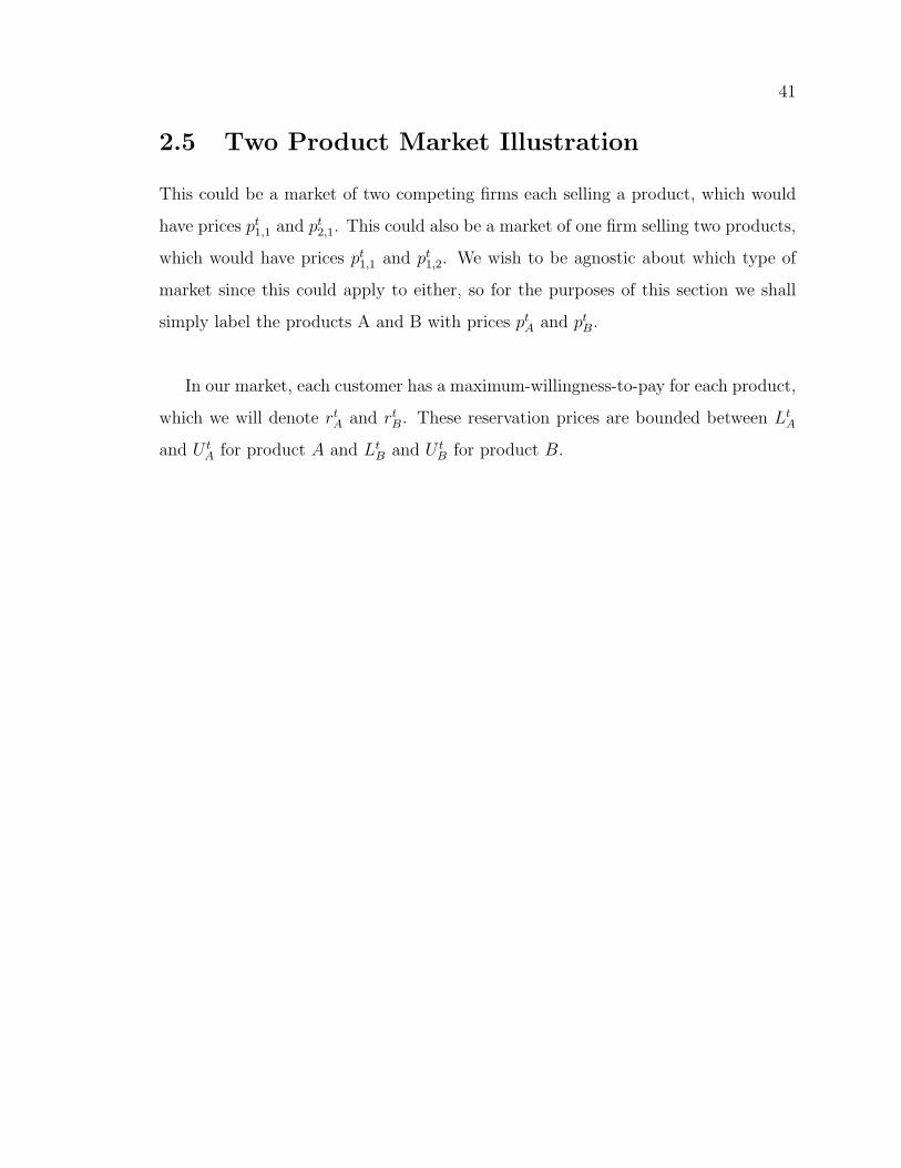
41
2.5 Two Product Market Illustration
This could be a market of two competing firms each selling a product, which would
have prices pt1,1 and pt2,1. This could also be a market of one firm selling two products,
which would have prices pt1,1 and pt1,2. We wish to be agnostic about which type of
market since this could apply to either, so for the purposes of this section we shall
simply label the products A and B with prices ptA and ptB.
In our market, each customer has a maximum-willingness-to-pay for each product,
which we will denote rtA and rtB. These reservation prices are bounded between LtA
and U tA for product A and LtB and U t
B for product B.
42
6
-00
ConsumerPreferences
LtB
rtB
U tB
LtArtA
U tA
Figure 2.1: Two-Dimensional demand space, with maximum-willingness-to-pay forgood A along the X-axis, and maximum-willingness-to-pay for good B along the Y -axis. All consumers’ maximum-willingnesses-to-pay exist within the rectangle marked‘Consumer Preferences’; there are no consumers outside the rectangle. Note that LtAand LtB are drawn as being strictly greater than zero. However, one or both of LtAand LtB can be equal to zero.
There is no benefit in setting the price of product A (ptA) below LtA as no consumers
have a maximum-willingness-to-pay below this value. Expected quantity demanded
would not increase relative to pricing at LtA and the firm would receive less revenue
per sale. Similarly, there is no incentive to price above U tA, as quantity demanded is
zero at U tA and for all values above this level. As such, we will restrict our analysis to
prices that are between (or equal to) LtA and U tA for firm A and LtB and U t
B for firm B.
Placing prices ptA and ptB on our figure gives us as follows:
43
6
-00
LtB
rtB
ptB
U tB
LtArtA
ptA U tA
A
XB
NS
Figure 2.2: Four Segments of a Two-Dimensional Demand Space, with maximum-willingness-to-pay for good A along the X-axis, and maximum-willingness-to-pay forgood B along the Y -axis. All consumers’ maximum-willingnesses-to-pay exist withinthe large rectangle; there are no consumers outside the rectangle. Note that LtA andLtB are drawn as being strictly greater than zero. However, one or both of LtA andLtB can be equal to zero.
In the NS area, consumers are unwilling to purchase either product, since their
maximum-willingness-to-pay for product A is below the price set for A (ptA) and the
same holds true for product B - their maximum-willingness-to-pay is set below the
market price for product B, ptB. In area A, customers are willing to buy product A
at the market price ptA. In area B, customers are willing to buy product B for the
price ptB. In the section labelled X, customers are willing to purchase either product.
Since consumers only purchase one good, we need a mechanism to assign customers
who are willing to buy either product to exactly one product.
We need a function that will apportion area X between the two products. One
obvious solution (but far from the only one) would be a proportional splitting rule
that is simply a straight line from (ptA, ptB) to U t
A, UtB.
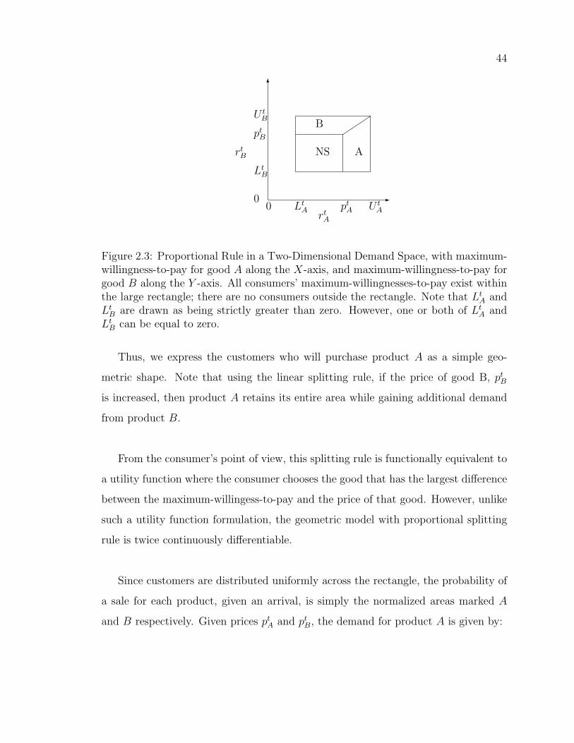
44
6
-00
LtB
rtB
ptB
U tB
LtArtA
ptA U tA
A
B
NS
���
Figure 2.3: Proportional Rule in a Two-Dimensional Demand Space, with maximum-willingness-to-pay for good A along the X-axis, and maximum-willingness-to-pay forgood B along the Y -axis. All consumers’ maximum-willingnesses-to-pay exist withinthe large rectangle; there are no consumers outside the rectangle. Note that LtA andLtB are drawn as being strictly greater than zero. However, one or both of LtA andLtB can be equal to zero.
Thus, we express the customers who will purchase product A as a simple geo-
metric shape. Note that using the linear splitting rule, if the price of good B, ptB
is increased, then product A retains its entire area while gaining additional demand
from product B.
From the consumer’s point of view, this splitting rule is functionally equivalent to
a utility function where the consumer chooses the good that has the largest difference
between the maximum-willingess-to-pay and the price of that good. However, unlike
such a utility function formulation, the geometric model with proportional splitting
rule is twice continuously differentiable.
Since customers are distributed uniformly across the rectangle, the probability of
a sale for each product, given an arrival, is simply the normalized areas marked A
and B respectively. Given prices ptA and ptB, the demand for product A is given by:
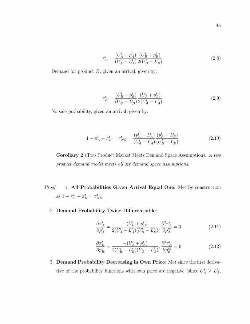
45
πtA =(U t
A − ptA)
(U tA − LtA)
(U tB + ptB)
2(U tB − LtB)
(2.8)
Demand for product B, given an arrival, given by:
πtB =(U t
B − ptB)
(U tB − LtB)
(U tA + ptA)
2(U tA − LtA)
(2.9)
No sale probability, given an arrival, given by:
1− πtA − πtB = πtNS =(ptA − LtA)
(U tA − LtA)
(ptB − LtB)
(U tB − LtB)
(2.10)
Corollary 2 (Two Product Market Meets Demand Space Assumption). A two
product demand model meets all six demand space assumptions.
Proof. 1. All Probabilities Given Arrival Equal One: Met by construction
as 1− πtA − πtB = πtNS.
2. Demand Probability Twice Differentiable:
∂πtA∂ptA
=−(U t
B + ptB)
2(U tA − LtA)(U t
B − LtB),∂2πtA∂pt2A
= 0 (2.11)
∂πtB∂ptB
=−(U t
A + ptA)
2(U tB − LtB)(U t
A − LtA),∂2πtB∂pt2B
= 0 (2.12)
3. Demand Probability Decreasing in Own Price: Met since the first deriva-
tive of the probability functions with own price are negative (since U tA ≥ LtA,
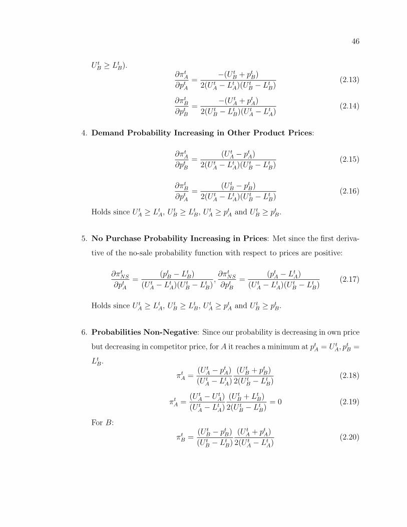
46
U tB ≥ LtB).
∂πtA∂ptA
=−(U t
B + ptB)
2(U tA − LtA)(U t
B − LtB)(2.13)
∂πtB∂ptB
=−(U t
A + ptA)
2(U tB − LtB)(U t
A − LtA)(2.14)
4. Demand Probability Increasing in Other Product Prices:
∂πtA∂ptB
=(U t
A − ptA)
2(U tA − LtA)(U t
B − LtB)(2.15)
∂πtB∂ptA
=(U t
B − ptB)
2(U tA − LtA)(U t
B − LtB)(2.16)
Holds since U tA ≥ LtA, U t
B ≥ LtB, U tA ≥ ptA and U t
B ≥ ptB.
5. No Purchase Probability Increasing in Prices: Met since the first deriva-
tive of the no-sale probability function with respect to prices are positive:
∂πtNS∂ptA
=(ptB − LtB)
(U tA − LtA)(U t
B − LtB),∂πtNS∂ptB
=(ptA − LtA)
(U tA − LtA)(U t
B − LtB)(2.17)
Holds since U tA ≥ LtA, U t
B ≥ LtB, U tA ≥ ptA and U t
B ≥ ptB.
6. Probabilities Non-Negative: Since our probability is decreasing in own price
but decreasing in competitor price, for A it reaches a minimum at ptA = U tA, p
tB =
LtB.
πtA =(U t
A − ptA)
(U tA − LtA)
(U tB + ptB)
2(U tB − LtB)
(2.18)
πtA =(U t
A − U tA)
(U tA − LtA)
(U tB + LtB)
2(U tB − LtB)
= 0 (2.19)
For B:
πtB =(U t
B − ptB)
(U tB − LtB)
(U tA + ptA)
2(U tA − LtA)
(2.20)
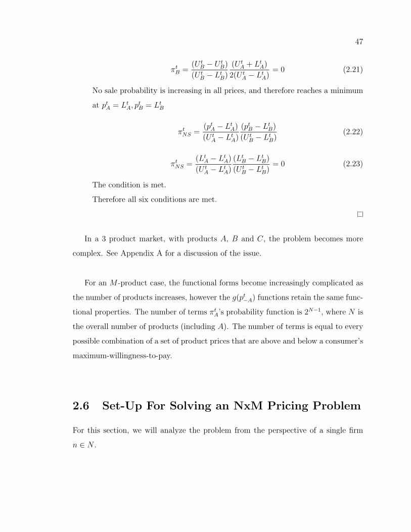
47
πtB =(U t
B − U tB)
(U tB − LtB)
(U tA + LtA)
2(U tA − LtA)
= 0 (2.21)
No sale probability is increasing in all prices, and therefore reaches a minimum
at ptA = LtA, ptB = LtB
πtNS =(ptA − LtA)
(U tA − LtA)
(ptB − LtB)
(U tB − LtB)
(2.22)
πtNS =(LtA − LtA)
(U tA − LtA)
(LtB − LtB)
(U tB − LtB)
= 0 (2.23)
The condition is met.
Therefore all six conditions are met.
In a 3 product market, with products A, B and C, the problem becomes more
complex. See Appendix A for a discussion of the issue.
For an M -product case, the functional forms become increasingly complicated as
the number of products increases, however the g(pt−A) functions retain the same func-
tional properties. The number of terms πtA’s probability function is 2N−1, where N is
the overall number of products (including A). The number of terms is equal to every
possible combination of a set of product prices that are above and below a consumer’s
maximum-willingness-to-pay.
2.6 Set-Up For Solving an NxM Pricing Problem
For this section, we will analyze the problem from the perspective of a single firm
n ∈ N .
48
In order to compute the optimal price each firm should charge in a given situation,
we need to first define our concept of equilibria. First we will assume that all firms
in the model are rational profit maximizers. Though, it is easy to adapt this model
to scenarios where one or more firms have committed to a different strategy, such as
a national advertising campaign that announces “rent a car for just 29.95!”.
Secondly, we will assume that firms do not engage in path-dependent strategies.
Thus all strategies in the game are Markovian as they only depend on the state. [1]
Here the state is simply the current quantity levels for each firm and the number of
periods remaining until the end of the game. We will use the game-theoretic concept
of Markov perfect equilibrium, if it exists, to determine each firm’s optimal pricing
strategy for each given state. First we need to define a few terms.
The definition of subgame and subgame perfect Nash Equilibria and Nash Equi-
librium used is adapted from Mas-Colell, Whinston, and Green [1]. The definition of
Markov perfect equilibrium is adapted from Fudenberg and Tirole [5].
Definition 1 (Subgame). A subgame begins with an information set containing a
single decision node, which contains all the decision nodes that are successors of this
node. Furthermore, it contains only those nodes which are successors.
In the case of the game developed here, every decision node is the initial point of
a subgame, including the entire game itself.
From that definition, we can define a subgame perfect Nash Equilibrium in this
49
context.
Definition 2 (Subgame Perfect Nash Equilibrium). A set of state contingent pricing
strategies for the N players in an N-player game is a subgame perfect Nash Equilib-
rium if it induces a Nash Equilibrium in every subgame of the game.
Where a Nash Equilibrium is defined as follows:
Definition 3 (Nash Equilibrium). Given a finite set of players 1, ..., I, and payoff
functions u = {u1()..uI()}, a strategy profile s = (s1, ..., sI) constitutes a Nash Equi-
librium of game ΓN = [I, {Si}, {ui()}] if for every i = 1, ..., I, ui(si, s−i) ≥ ui(s′i, s−i)
for all s′i ∈ Si.
A Markov perfect equilibrium takes the concept of a Subgame Perfect Nash Equi-
librium and applies it to situations where the firms are restricted to using only state-
dependent strategies.
Definition 4 (Markov Perfect Equilibrium). A Markov perfect equilibrium is a profile
of Markov strategies that yield a Nash Equilibrium in every subgame. Since the state
captures the influence of past play on the strategies and payoffs for each subgame,
if all of a player’s opponents use Markov strategies, that player has a best response
that is Markov as well. A Markov perfect equilibrium thus continues to be a perfect
equilibrium when the Markov restriction is dropped.
We can determine the Markov Perfect Equilibrium, if it exists, for the game
through backwards induction of a Markov decision process, where we examine the
50
subgames emanating from every possible combination of quantity levels and time re-
maining. Each firm’s optimal strategy is thus a set of state-contingent strategies for
each of these potential combinations.
2.7 Dynamic Programming Formulation
The objective of our Markov decision process is to maximize total profit over the
entire sales period, which is equivalent to maximizing our revenue if there are no
variable costs in the model. Since there are no variable costs in this model, we will
treat the problem as one of maximizing revenue. As discussed earlier, we can break
our multi-period planning problem into a series of single-period problems which are
solved through backwards induction.
A Markov decision process has four components:
• A set of states S.
• A set of actions a ∈ A.
• Pa(s, s′) = Pr(st+1 = s′|st = s, at = a), which is the probability that an action
a in state s at time t will lead to state s′ at time t+ 1.
• E[Ra(s, s′)] is the expected revenue received after transition to state s′ from
state s with probability Pa(s, s′).
51
It is necessary to define a few terms:
• The quantity of goods held by firm n at time t is denoted qtn, a vector of length
mtn. The quantity for a particular good is denoted qtn,m, and the quantity of
goods held by other firms is noted qt−n.
• The arrival rate of customers is given by λ.
• The end-of-game salvage value for a unit of good m held by firm n is sTn,m.
Our four components are then as follows:
• Our state space S at time t is simply the set of quantities of each good held by
every firm (not just firm n). Thus St = (qtn, qt−n).
• Our set of actions A at time t contains the prices we can set for each good m:
ptn,m ∈ [Ltn,m, Utn,m].
• The probability that we make a transition from state s in time t to state s′ in
time t+ 1 having one less of a given good m is equivalent to the probability of
sale of that good (expected demand) and given by λπtn,m. The probability that
we transition from state t to state t + 1 with a competitor j having one less
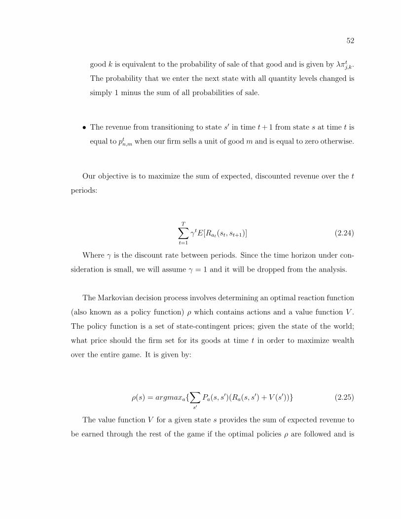
52
good k is equivalent to the probability of sale of that good and is given by λπtj,k.
The probability that we enter the next state with all quantity levels changed is
simply 1 minus the sum of all probabilities of sale.
• The revenue from transitioning to state s′ in time t+ 1 from state s at time t is
equal to ptn,m when our firm sells a unit of good m and is equal to zero otherwise.
Our objective is to maximize the sum of expected, discounted revenue over the t
periods:
T∑t=1
γtE[Rat(st, st+1)] (2.24)
Where γ is the discount rate between periods. Since the time horizon under con-
sideration is small, we will assume γ = 1 and it will be dropped from the analysis.
The Markovian decision process involves determining an optimal reaction function
(also known as a policy function) ρ which contains actions and a value function V .
The policy function is a set of state-contingent prices; given the state of the world;
what price should the firm set for its goods at time t in order to maximize wealth
over the entire game. It is given by:
ρ(s) = argmaxa{∑s′
Pa(s, s′)(Ra(s, s
′) + V (s′))} (2.25)
The value function V for a given state s provides the sum of expected revenue to
be earned through the rest of the game if the optimal policies ρ are followed and is
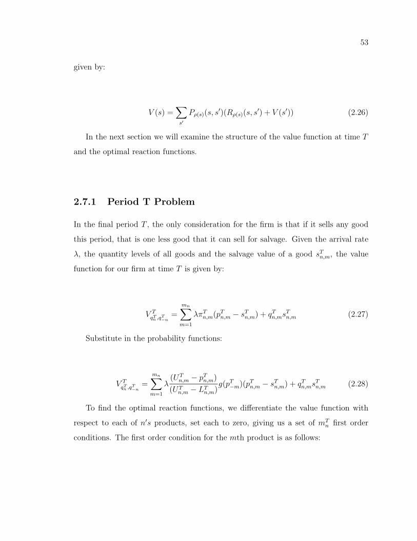
53
given by:
V (s) =∑s′
Pρ(s)(s, s′)(Rρ(s)(s, s
′) + V (s′)) (2.26)
In the next section we will examine the structure of the value function at time T
and the optimal reaction functions.
2.7.1 Period T Problem
In the final period T , the only consideration for the firm is that if it sells any good
this period, that is one less good that it can sell for salvage. Given the arrival rate
λ, the quantity levels of all goods and the salvage value of a good sTn,m, the value
function for our firm at time T is given by:
V TqTn ,q
T−n
=mn∑m=1
λπTn,m(pTn,m − sTn,m) + qTn,msTn,m (2.27)
Substitute in the probability functions:
V TqTn ,q
T−n
=mn∑m=1
λ(UT
n,m − pTn,m)
(UTn,m − LTn,m)
g(pT−m)(pTn,m − sTn,m) + qTn,msTn,m (2.28)
To find the optimal reaction functions, we differentiate the value function with
respect to each of n′s products, set each to zero, giving us a set of mTn first order
conditions. The first order condition for the mth product is as follows:
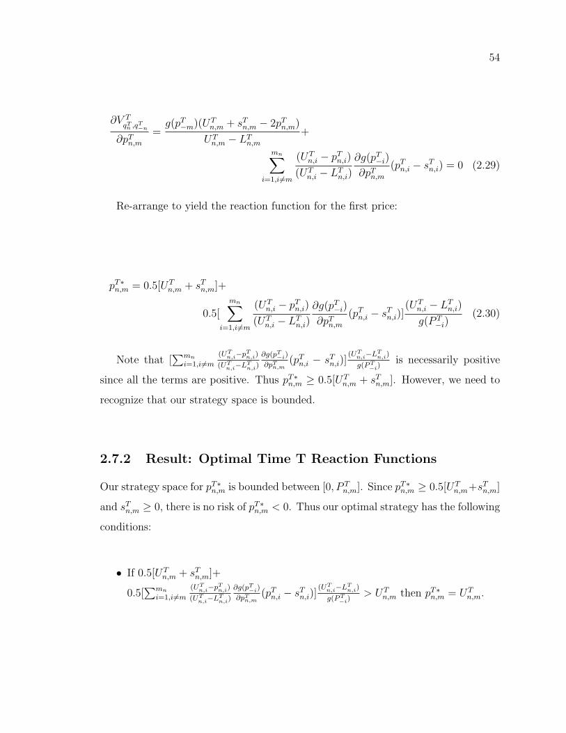
54
∂V TqTn ,q
T−n
∂pTn,m=g(pT−m)(UT
n,m + sTn,m − 2pTn,m)
UTn,m − LTn,m
+
mn∑i=1,i 6=m
(UTn,i − pTn,i)
(UTn,i − LTn,i)
∂g(pT−i)
∂pTn,m(pTn,i − sTn,i) = 0 (2.29)
Re-arrange to yield the reaction function for the first price:
pT∗n,m = 0.5[UTn,m + sTn,m]+
0.5[mn∑
i=1,i 6=m
(UTn,i − pTn,i)
(UTn,i − LTn,i)
∂g(pT−i)
∂pTn,m(pTn,i − sTn,i)]
(UTn,i − LTn,i)g(P T
−i)(2.30)
Note that [∑mn
i=1,i 6=m(UT
n,i−pTn,i)
(UTn,i−LT
n,i)
∂g(pT−i)
∂pTn,m
(pTn,i − sTn,i)](UT
n,i−LTn,i)
g(PT−i)
is necessarily positive
since all the terms are positive. Thus pT∗n,m ≥ 0.5[UTn,m + sTn,m]. However, we need to
recognize that our strategy space is bounded.
2.7.2 Result: Optimal Time T Reaction Functions
Our strategy space for pT∗n,m is bounded between [0, P Tn,m]. Since pT∗n,m ≥ 0.5[UT
n,m+sTn,m]
and sTn,m ≥ 0, there is no risk of pT∗n,m < 0. Thus our optimal strategy has the following
conditions:
• If 0.5[UTn,m + sTn,m]+
0.5[∑mn
i=1,i 6=m(UT
n,i−pTn,i)
(UTn,i−LT
n,i)
∂g(pT−i)
∂pTn,m
(pTn,i − sTn,i)](UT
n,i−LTn,i)
g(PT−i)
> UTn,m then pT∗n,m = UT
n,m.
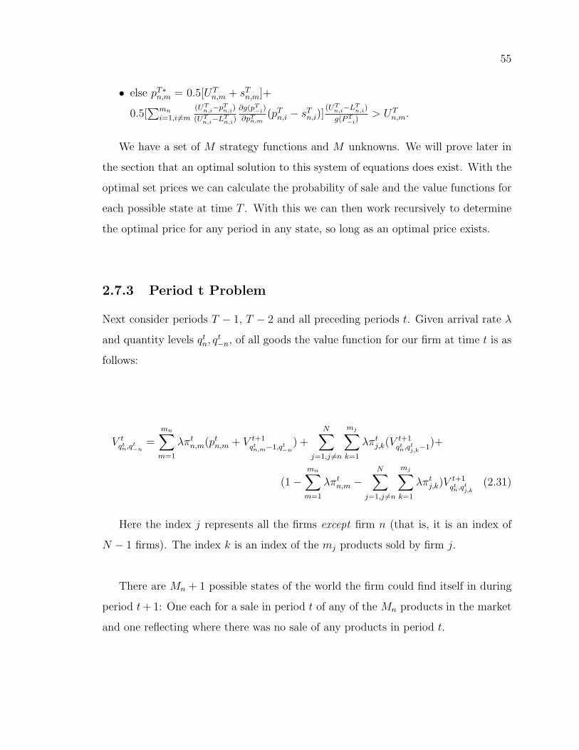
55
• else pT∗n,m = 0.5[UTn,m + sTn,m]+
0.5[∑mn
i=1,i 6=m(UT
n,i−pTn,i)
(UTn,i−LT
n,i)
∂g(pT−i)
∂pTn,m
(pTn,i − sTn,i)](UT
n,i−LTn,i)
g(PT−i)
> UTn,m.
We have a set of M strategy functions and M unknowns. We will prove later in
the section that an optimal solution to this system of equations does exist. With the
optimal set prices we can calculate the probability of sale and the value functions for
each possible state at time T . With this we can then work recursively to determine
the optimal price for any period in any state, so long as an optimal price exists.
2.7.3 Period t Problem
Next consider periods T − 1, T − 2 and all preceding periods t. Given arrival rate λ
and quantity levels qtn, qt−n, of all goods the value function for our firm at time t is as
follows:
V tqtn,q
t−n
=mn∑m=1
λπtn,m(ptn,m + V t+1qtn,m−1,qt
−n) +
N∑j=1,j 6=n
mj∑k=1
λπtj,k(Vt+1qtn,q
tj,k−1
)+
(1−mn∑m=1
λπtn,m −N∑
j=1,j 6=n
mj∑k=1
λπtj,k)Vt+1qtn,q
tj,k
(2.31)
Here the index j represents all the firms except firm n (that is, it is an index of
N − 1 firms). The index k is an index of the mj products sold by firm j.
There are Mn + 1 possible states of the world the firm could find itself in during
period t+ 1: One each for a sale in period t of any of the Mn products in the market
and one reflecting where there was no sale of any products in period t.
56
Re-arrange to yield:
V tqtn,q
t−n
=mn∑m=1
λπtn,m(ptn,m + V t+1qtn,m−1,qt
−n− V t+1
qtn,m,q
t−n
)+
N∑j=1,j 6=n
mj∑k=1
λπtj,k(Vt+1qtn,q
tj,k−1− V t+1
qtn,q
tj,k
) + V t+1qtn,q
t−n
(2.32)
To simplify, we define two functions:
ctn,m = V t+1qtn,m,q
t−n− V t+1
qtn,m−1,qt
−n(2.33)
ctn,m is the difference in the value functions between having quantity qt+1m,n = qtm,n−1
and qt+1m,n = qtm,n (that is, one more) of good qm,n in period t+ 1. Conceptually it can
be thought of as the opportunity cost of making a sale in period t. The opportunity
cost reflects the fact that if we sell a good now, that leaves us with one less good to
sell in the future.
The second function we define is as follows:
btj,k = V t+1qtn,q
tj,k−1− V t+1
qtn,q
tj,k
(2.34)
btj,k is the difference in the value functions between our competitor having qt+1j,k =
qtj,k and qt+1j,k = qtj,k−1 (that is, one less) of qtj,k in period t+1. Conceptually it can be
thought of as the benefit of our competitor making a sale in period t, leaving them
57
with one less good in period t+ 1. The benefit reflects the fact that a sale this period
increases the chance that our competitor will sell out of this particular good, leaving
us with one less competitor product with which to compete.
Substituting in the two functions provides:
V tqtn,q
t−n
=mn∑m=1
λπtn,m(ptn,m − ctn,m) +N∑
j=1,j 6=n
mj∑k=1
λπtj,k(btj,k) + V t+1
qtn,q
t−n
(2.35)
Substitute in the probability functions for each:
V tqtn,q
t−n
=mn∑m=1
λ(U t
n,m − ptn,m)
(U tn,m − Ltn,m)
g(pt−m)(ptn,m − ctn,m)+
N∑j=1,j 6=n
mj∑k=1
λ(U t
j,k − ptj,k)(U t
j,k − Ltj,k)g(ptj,−k)(b
tj,k) + V t+1
qtn,q
t−n
(2.36)
Note that g(pt−m) is a function of all other prices but the price for good m, in-
cluding both prices of goods sold by other firms and goods sold by our firm.
To find the optimal reaction functions, we differentiate the value function with
respect to each of n′s products, set each to zero, giving us a set of mN first order
conditions. The first order condition for the mth product is as follows:
58
∂V tqtn,q
t−n
∂ptn,m= λ
−1
(U tn,m − Ltn,m)
g(pt−m)(ptn,m − ctn,m)+
λ(U t
n,m − ptn,m)
(U tn,m − Ltn,m)
g(pt−m) +mn∑
i=1,i 6=m
λ(U t
n,i − ptn,i)(U t
n,i − Ltn,i)∂g(pt−i)
∂ptm(ptn,i − ctn,i)+
N∑j=1,j 6=n
mj∑k=1
λ(U t
j,k − ptj,k)(U t
j,k − Ltj,k)g(ptj,−k)
ptm(btj,k) = 0 (2.37)
Simplify to:
(U tn,m + ctn,m − 2ptn,m)
(U tn,m − Ltn,m)
g(pt−m)+
mn∑i=1,i 6=m
(U tn,i − ptn,i)
(U tn,i − Ltn,i)
∂g(pt−i)
∂ptm(ptn,i − ctn,i)+
N∑j=1,j 6=n
mj∑k=1
(U tj,k − ptj,k)
(U tj,k − Ltj,k)
∂g(ptj,−k)
ptn,m(btj,k) = 0 (2.38)
Note that no term in:
mn∑i=1,i 6=m
(U tn,i − ptn,i)
(U tn,i − Ltn,i)
∂g(pt−i)
∂ptm(ptn,i − ctn,i)+
N∑j=1,j 6=n
mj∑k=1
(U tj,k − ptj,k)
(U tj,k − Ltj,k)
∂g(ptj,−k)
ptn,m(btj,k) (2.39)
is a function of ptn,m. Define:
59
h(pt−m) =mn∑
i=1,i 6=m
(U tn,i − ptn,i)
(U tn,i − Ltn,i)
∂g(pt−i)
∂ptm(ptn,i − ctn,i)+
N∑j=1,j 6=n
mj∑k=1
(U tj,k − ptj,k)
(U tj,k − Ltj,k)
∂g(ptj,−k)
ptn,m(btj,k) (2.40)
then:
(U tn,m + ctn,m − 2ptn,m)
(U tn,m − Ltn,m)
g(pt−m) + h(pt−m) = 0 (2.41)
Re-arrange to yield:
pt∗n,m = 0.5[U tn,m + ctn,m +
h(pt−m)(U tn,m − Ltn,m)
g(pt−m)] (2.42)
2.7.4 Result: Optimal Time t Reaction Functions
Our strategy space for pt∗n,m is bounded between [0, P tn,m]. Thus our optimal strategy
has the following conditions:
• If 0.5[U tn,m + ctn,m +
h(pt−m)(Ut
n,m−Ltn,m)
g(pt−m)
] < 0, then pt∗n,m = 0.
• If 0.5[U tn,m + ctn,m +
h(pt−m)(Ut
n,m−Ltn,m)
g(pt−m)
] > U tn,m then pt∗n,m = U t
n,m.
• else pt∗n,m = 0.5[U tn,m + ctn,m +
h(pt−m)(Ut
n,m−Ltn,m)
g(pt−m)
].
60
We have a system of M equations and M unknowns. We can show that this
system of equations has a solution.
2.8 Five Factors in Optimal Pricing
Any optimal pricing revenue management model to price a good will consider own-
price elasticity, as does this one. It goes beyond, however, by implicitly (and simulta-
neously) considering five other factors, which we can see as we examine the optimal
pricing equation, given an interior solution, pt∗n,m = 0.5[U tn,m+ctn,m+
h(pt−m)(Ut
n,m−Ltn,m)
g(pt−m)
]:
1. Quantity Level of the Product: The ctn,m term in our pricing solution re-
flects that our good is being sold over a limited time period and re-orders are
not possible. A sale today means one less good to sell over the sales period (or
one less good to sell for salvage), leading to an opportunity cost of making a sale.
2. Quantity Levels of Firm’s Other Products: In the h(pt−m) equation we
have the term (ptn,i−ctn,i), which reflects that our other products have an oppor-
tunity cost as well. By changing the price of one good, we change the probability
of sale for our other goods. As these goods have an opportunity cost, we need
to take that into consideration when making our pricing decision.
3. Quantity Levels of Other Firms’ Products: In the h(pt−m) equation we
have the term (btj,k), which reflects the potential benefit to our competitor mak-
ing a sale. If our competitor makes a sale, this increases the probability that
they will run out of that good before the sales period is over. If the competitor
61
runs out of that product, that is one less competitor to price against.
4. Cannibalization, Cross-Price Elasticity and the Price of Our Other
Products: The terms g(pt−m),∂g(pt
−i)
∂ptm
and∂g(pt
j,−k)
ptn,m
contain the prices of our
other products. Thus the optimal price we set must consider the prices set for
our other goods and the cross-price elasticity of demand between our products.
5. Competition, Cross-Price Elasticity and the Price of Competitor Prod-
ucts: The terms g(pt−m),∂g(pt
−i)
∂ptm
and∂g(pt
j,−k)
ptn,m
also contain the prices of our com-
petitor’s products. Thus the optimal price we set must consider the prices other
firms are setting for their products and that raising our prices will see us losing
sales to our competitors.
We will see in the next two chapters how considering each factor increases the
revenue of the firm.
2.9 Result: Existence of a Solution
In this section we prove that an optimum solution exists.
Our strategy space is M dimensional, and bounded between [Ltn,m, Utn,m] in each
dimension. Nash [9] proved that the existence of a fixed-point in the strategy space
is necessary and sufficient for proving the existence of a Nash Equilibrium. We will
follow Nash’s lead and use Kakutani’s fixed point theorem to prove the existence of
62
a fixed-point (and thus the existence of a Nash Equilibrium).
Definition 5. Kakutani Fixed Point Theorem Let the strategy space S be a non-
empty, compact and convex subset of some Euclidean space Rn. Let φ be an upper
hemicontinuous set-valued function on S with the property that φ(x) is non-empty,
closed and convex for all x ∈ S. Then φ has a fixed point.
Convexity is guaranteed as our strategy space (the set of prices that can be charged
for each product) meets the following conditions.
Corollary 3 (Strategy Space of Pricing Game is Convex). The strategy space,
ρ, of our game is convex.
Proof. Take any two points within the strategy space, each denoted by anN -dimensional
vector [call them P (1) and P (2)]. Without loss of generality select the ith term of the
first vector pi(1) and the second point pi(2), where by definition ui ≥ pi(1) ≥ 0
and ui ≥ pi(2) ≥ 0. Pick any λ such that λ ∈ [0, 1]. Create a third vector
λP (1) + (1 − λ)P (2). The nth term of the vector is equal to λpi(1) + (1 − λ)pi(2).
The nth term is within the bounds 0 and ui since ui ≥ max{pi(1), pi(2)} ≥ λpi(1) +
(1−λ)pi(2) ≥ min{pi(1), pi(2)} ≥ 0. Since this holds for all i, then any linear combi-
nation of two points inside the strategy space is within the strategy space. Therefore
the strategy space is convex.
Since convexity is proven, we can prove the existence of a Subgame Perfect Nash
Equilibrium.
63
Corollary 4 (Existence of a Subgame Perfect Nash Equilibrium). Our game
has a Subgame Perfect Nash Equilibrium.
Proof. Our strategy set is non-empty so long as P tn,m > 0 ∀ n ∈ N , m ∈M , compact
and convex. Our Mn reaction functions are continuous, therefore upper hemicon-
tinuous, non-empty, closed and convex. The conditions of Kakutani’s Fixed Point
Theorem are met, therefore a Subgame Perfect Nash Equilibrium exists.
Result: Since our strategy space is convex, the conditions of Kakutani’s fixed
point theorem are met. A Subgame Perfect Nash Equilibrium exists guaranteeing the
existence of (at least) one solution to our NxM pricing model.
2.10 Uniqueness of a Solution
Uniqueness of a solution cannot be shown in general, but a unique solution exists in
many specific cases. A unique solution may not necessarily exist since the reaction
functions are not-necessarily monotonic, so there may be multiple fixed points. Two
methods that are well suited to showing the existence of a unique solution are the
functional forms we have chosen are the contraction mapping theorem and Rosen’s
uniqueness theorem.
Definition 6 (Rosen’s Uniqueness Theorem). If all the best response functions rm(s),
m ∈ M are twice continuously differentiable and if the Jacobian matrix J(g) of
g(s) ≡ r(s) − s is negative quasi-definite, then there is at most one Nash Equilib-
rium. Rosen (1965) [10]
64
The reaction functions by construction are twice continuously differentiable, so
that property is necessarily met. The second condition, however, is more cumber-
some to determine.
Definition 7 (Contraction Mapping Theorem). If the best reply function r is a con-
traction, then there exists a unique equilibrium. [4]. A contraction on a metric space
(M,d) is a function f from M to itself, with the property that there is some nonnega-
tive real number k < 1 such that for all x and y in M , d(f(x), f(y)) ≤ kd(x, y). Lang
(1968) [6].
For this game this may be easier to meet than Rosen’s theorem, since it does not
require any form of continuous differentiability. Furthermore, in the two-firm/one-
product-per-firm case, the best response function is naturally a contraction mapping
for two points on the same boundary (since the distance between them is zero).
However, we cannot show for all reasonable parameter values that the best-response
functions will always hold the contraction mapping property.
It is relatively straight-forward to illustrate the conditions required to have a
unique equilibrium in a model with two firms, each selling 1 type of product using
the proportional splitting rule. Consider the problem at time t from the perspective
of the firm selling product 1:
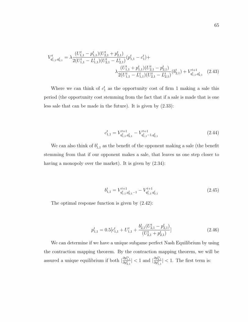
65
V tqt1,1,q
t2,1
= λ(U t
1,1 − pt1,1)(U t2,1 + pt2,1)
2(U t1,1 − Lt1,1)(U t
2,1 − Lt2,1)(pt1,1 − ct1)+
λ(U t
1,1 + pt1,1)(Ut2,1 − pt2,1)
2(U t1,1 − Lt1,1)(U t
2,1 − Lt2,1)(bt2,1) + V t+1
qt1,1,q
t2,1
(2.43)
Where we can think of ct1 as the opportunity cost of firm 1 making a sale this
period (the opportunity cost stemming from the fact that if a sale is made that is one
less sale that can be made in the future). It is given by (2.33):
ct1,1 = V t+1qt1,1,q
t2,1− V t+1
qt1,1−1,qt
2,1(2.44)
We can also think of bt1,1 as the benefit of the opponent making a sale (the benefit
stemming from that if our opponent makes a sale, that leaves us one step closer to
having a monopoly over the market). It is given by (2.34):
bt1,1 = V t+1qt1,1,q
t2,1−1
− V t+1qt1,1,q
t2,1
(2.45)
The optimal response function is given by (2.42):
pt1,1 = 0.5[ct1,1 + U t1,1 +
bt2,1(Ut2,1 − pt2,1)
(U t2,1 + pt2,1)
] (2.46)
We can determine if we have a unique subgame perfect Nash Equilibrium by using
the contraction mapping theorem. By the contraction mapping theorem, we will be
assured a unique equilibrium if both |∂pt∗1,1
∂pt2,1| < 1 and |∂p
t∗2,1
∂pt1,1| < 1. The first term is:
66
|∂pt∗1,1∂pt2,1
| < 1, |−2U t
2,1bt2,1
(U t2,1 + pt2,1)
2| = 1 (2.47)
This will hold for all values of pt2,1 ≥ 0 so long as U t2,1 > 2bt2,1. Thus as long as
both bt1,1 and bt2,1 are sufficiently small, we are guaranteed a unique equilibrium.
2.11 Results
In this section, a geometric demand framework was constructed that allows for math-
ematically tractable revenue management models with multiple firms selling multiple
classes of products. We have proven the existence of pure-strategy Nash Equilibria -
the first NxM revenue management model to do so, for any finite value of N and M .
67
Chapter 3
Two Optimal Dynamic Pricing
Examples
In this chapter we create two examples to illustrate the value of our approach. In
the first example, a two-firm/one-product-per-firm model illustrates the importance
of considering the quantity level of the product under consideration (factor 1 from
the previous chapter), the quantity level of the product sold by the other firm (factor
3) and the price of competitor products (factor 5). The second example is a two-
firm/three-products-per-firm rental car model. It considers all five factors, but pays
particular attention to cannibalization of demand (factor 4).
3.1 Example 1: Behaviour of the Model in a Real
World - 2 Firm, 1 Good Per Firm Scenario
This section illustrates through a numerical example the equilibrium properties of
the model. Our model does indeed produce the optimal price, making it superior to
68
any other pricing strategy provided that the firm makes an accurate assessment of
the state. The model generates a set of prices that shows on average optimal prices
are higher when firms have fewer goods remaining. One unusual strategy appears -
a knockout strategy where a firm will occasionally price high in order to temporarily
cede the market to the other firm. By doing so, it can force the other firm to run out
of goods, giving the firm that uses the knockout strategy a monopoly for the rest of
the game. The revenue increase from this approach indicates the value of considering
factor 3, the quantity level of competitor firms.
3.2 Description of the Problem
A simple two-firm/one-product-per-firm model is created. A numeric simulation is
used to illustrate the equilibrium properties of the model and to describe the strategies
used by firms.
3.3 Assumptions of the Model
To illustrate the pricing dynamics of the model and the value of optimal pricing
strategies, we will use the following numeric example with the following model spec-
ifications:
• There are two firms in the game, A and B.
• There are 50 periods in the game. The value of 50 is chosen such that there is
a reasonable variance in outcomes including selling out.
• Each firm begins the game with 10 items, which allows for a firm to sell out of
a good (but is far from a guarantee).
69
• A single person arrives each period, for a total of 50 arrivals. This is enough
arrivals such that there is a reasonable possibility that a firm will sell out of a
good before the end of the game.
• There is no salvage value for either firm for leftover goods.
• The two-dimensional uniform potential demand distribution has endpoints $0.00
and $100.00 for Firm A and $0.00 and $80.00 for Firm B.
Given these assumptions, there will be on average 40 arrivals. This may seem high,
given that there are only 20 goods between the two firms. However, many of these
arrivals will not wish to purchase from either firm, as their maximum-willingnesses-to-
pay are below the prices charged by each firm, so realized market quantity demanded
would be significantly less than 40 even with an unlimited supply of goods. The
number of periods was chosen such that there would be a reasonable probability that
the firms would sell out before the end of the sales period.
Using these model parameters, we investigate 22 different combinations of pricing
strategies. These involve situations where:
• Both firms behave optimally and consider factors 1, 3 and 5 in their pricing.
• One firm uses a fixed price strategy, the other knows this and prices optimally
based on that information. The fixed price strategies used can be to always set
a low price (the mean of the one-dimension distribution), always set a medium
price (75 percent of the one-dimensional distribution), or always set a high price
(90 percent of the one-dimension distribution).
70
• One firm uses a fixed price strategy, the other tries to price optimally but mis-
takenly assumes that the other firm is also trying to price optimally.
• Both firms commit to fixed price strategies, where the strategies can be fixed
prices that are low, medium, or high.
For Firm A, the low, medium, and high prices are 50, 75, and 90 respectively; for
Firm B they are 40, 60, and 72 respectively. We will denote the scenario where a firm
mistakenly assumes that their competitor is pricing optimally as Op(Mis).
For each scenario we calculated a set of 6050 state-contingent prices for each firm
based on each firm’s chosen strategy, though in the case where firms follow a fixed
price strategy the calculation was trivial. In all four scenarios each firm begins the
game with anywhere from 0-10 goods and there are 50 periods in each game. Once
again, this gives us a set of 6050 state-contingent prices for each firm in each scenario,
where the state is given by the number of periods remaining (1-50), the number of
goods Firm A has (0-10) and the number of goods Firm B has (0-10). When a firm
runs out of goods we have a monopoly and thus reduce the number of dimensions in
our model from 2 to 1. When both firms run out of goods before period T the game
is ended prematurely.
We ran 10,000 simulations using Palisade’s Risk package for each scenario and
recorded the mean revenue for both firms in each scenario, as well as the average
number of sales.
71
3.4 Determining the Optimal Price
In order to run the simulations, we need to know the price each firm should charge
in every state. The prices are determined analytically, through backward induction.
3.4.1 Both Firms Remaining
When both firms have quantity remaining, firm A’s value function at time t is given
by:
V tqtA,q
tB
= λπtA(ptA + V t+1qtA−1,qt
B) + λπtB(V t+1
qtA,q
tB−1
) + (1− λπtA − λπtB)V t+1qtA,q
tB
(3.1)
To simplify, we define two functions, first the cost function:
ctA = V t+1qtA,q
tB− V t+1
qtA−1,qt
B(3.2)
The second function we define is the benefit function:
btA = V t+1qtA,q
tB−1− V t+1
qtA,q
tB
(3.3)
Substituting in the two functions into our value function:
V tqtA,q
tB
= λπtA(ptA − ctA) + λπtB(btA) + V t+1qtA,q
tB
(3.4)
Finally, substitute in our probability functions:
72
V tqtA,q
tB
= λ(U t
A − ptA)(U tB + ptB)
2U tAU
tB
(ptA − ctA)+
λ(U t
A + ptA)(U tB − ptB)
2U tAU
tB
(btA) + V t+1qtA,q
tB
(3.5)
If firm A is pricing optimally, the optimal reaction function is obtained by taking
the first derivative with respect to ptA:
pt∗A = 0.5(U tA + ctA) +
(U tB − ptB)btA
2(U tB + ptB)
(3.6)
If B is using a fixed price strategy, we can substitute it into the above equation.
If B is pricing optimally, its reaction function is given by:
pt∗B = 0.5(U tB + ctB) +
(U tA − ptA)btB
2(U tA + ptA)
(3.7)
If both firms are pricing optimally, we can substitute pt∗B into A’s reaction function
to obtain the Nash Equilibrium prices. For A:
73
pt∗A =1
4(3U tB + ctB − btB)
∗
(√
((−3U tAU
tB − U t
ActB − 3U t
AbtB + 3U t
BctA + U t
BbtA + ctAc
tB − ctAbtB − ctBbtA + btAb
tB)2−
4(−6U tB − 2ctB + 2btB)(3(U t
A)2U tB + (U t
A)2ctB + (U tA)2btB + 3U t
AUtBc
tA+
U tAU
tBb
tA + U t
ActAc
tB + U t
ActAb
tB − U t
ActbbtA − U t
AbtAb
tB))−
3U tAU
tB − U t
ActB − 3U t
AbtB + 3U t
BctA + U t
BbtA + ctAc
tB − ctAbtB − ctBbtA + btAb
tB) (3.8)
3.4.2 Only A Remaining
When only A has inventory remaining, its value function at time t is given by:
V tqtA,0
= λπtA(ptA + V t+1qtA−1,0
) + (1− λπtA)V t+1qtA,0
(3.9)
As above, we substitute in our cost function (there is no benefit function, since
our opponent has no inventory) and then substitute in our probability functions:
V tqtA,0
= λ(U t
A − ptA)
U tA
(ptA − ctA) + V t+1qtA,q
tB
(3.10)
If firm A is pricing optimally, the optimal reaction function is obtained by taking
the first derivative with respect to ptA:
pt∗A = 0.5(U tA + ctA) (3.11)
In Appendix B, we give the optimal prices for firm A in periods T and T −1 when
B is also pricing optimally.
74
3.5 Simulation Results
Typically we would expect a firm to do better against a firm that is behaving sub-
optimally than one that is not. That holds under this experiment, with profits of up
to 2 percent higher for Firm A when B uses a fixed price strategy:
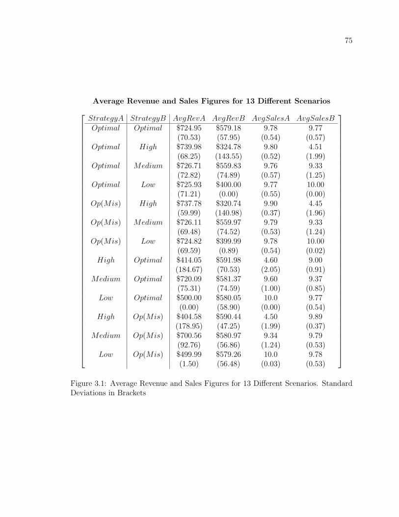
75
Average Revenue and Sales Figures for 13 Different Scenarios
StrategyA StrategyB AvgRevA AvgRevB AvgSalesA AvgSalesBOptimal Optimal $724.95 $579.18 9.78 9.77
(70.53) (57.95) (0.54) (0.57)Optimal High $739.98 $324.78 9.80 4.51
(68.25) (143.55) (0.52) (1.99)Optimal Medium $726.71 $559.83 9.76 9.33
(72.82) (74.89) (0.57) (1.25)Optimal Low $725.93 $400.00 9.77 10.00
(71.21) (0.00) (0.55) (0.00)Op(Mis) High $737.78 $320.74 9.90 4.45
(59.99) (140.98) (0.37) (1.96)Op(Mis) Medium $726.11 $559.97 9.79 9.33
(69.48) (74.52) (0.53) (1.24)Op(Mis) Low $724.82 $399.99 9.78 10.00
(69.59) (0.89) (0.54) (0.02)High Optimal $414.05 $591.98 4.60 9.00
(184.67) (70.53) (2.05) (0.91)Medium Optimal $720.09 $581.37 9.60 9.37
(75.31) (74.59) (1.00) (0.85)Low Optimal $500.00 $580.05 10.0 9.77
(0.00) (58.90) (0.00) (0.54)High Op(Mis) $404.58 $590.44 4.50 9.89
(178.95) (47.25) (1.99) (0.37)Medium Op(Mis) $700.56 $580.97 9.34 9.79
(92.76) (56.86) (1.24) (0.53)Low Op(Mis) $499.99 $579.26 10.0 9.78
(1.50) (56.48) (0.03) (0.53)
Figure 3.1: Average Revenue and Sales Figures for 13 Different Scenarios. StandardDeviations in Brackets
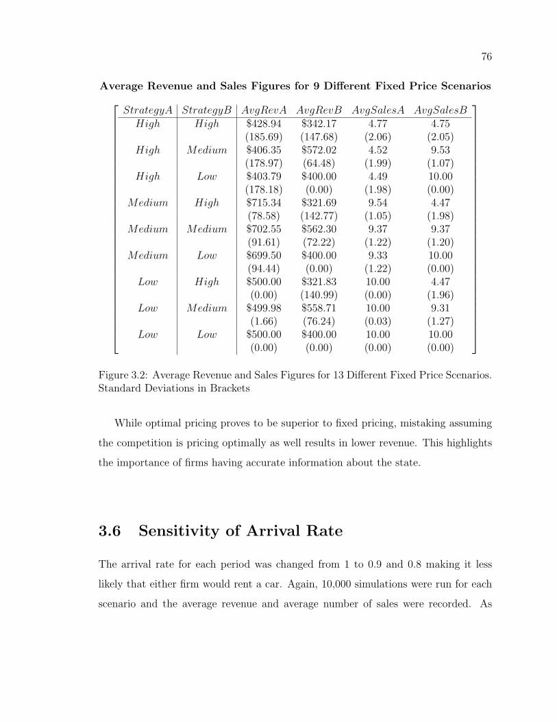
76
Average Revenue and Sales Figures for 9 Different Fixed Price Scenarios
StrategyA StrategyB AvgRevA AvgRevB AvgSalesA AvgSalesBHigh High $428.94 $342.17 4.77 4.75
(185.69) (147.68) (2.06) (2.05)High Medium $406.35 $572.02 4.52 9.53
(178.97) (64.48) (1.99) (1.07)High Low $403.79 $400.00 4.49 10.00
(178.18) (0.00) (1.98) (0.00)Medium High $715.34 $321.69 9.54 4.47
(78.58) (142.77) (1.05) (1.98)Medium Medium $702.55 $562.30 9.37 9.37
(91.61) (72.22) (1.22) (1.20)Medium Low $699.50 $400.00 9.33 10.00
(94.44) (0.00) (1.22) (0.00)Low High $500.00 $321.83 10.00 4.47
(0.00) (140.99) (0.00) (1.96)Low Medium $499.98 $558.71 10.00 9.31
(1.66) (76.24) (0.03) (1.27)Low Low $500.00 $400.00 10.00 10.00
(0.00) (0.00) (0.00) (0.00)
Figure 3.2: Average Revenue and Sales Figures for 13 Different Fixed Price Scenarios.Standard Deviations in Brackets
While optimal pricing proves to be superior to fixed pricing, mistaking assuming
the competition is pricing optimally as well results in lower revenue. This highlights
the importance of firms having accurate information about the state.
3.6 Sensitivity of Arrival Rate
The arrival rate for each period was changed from 1 to 0.9 and 0.8 making it less
likely that either firm would rent a car. Again, 10,000 simulations were run for each
scenario and the average revenue and average number of sales were recorded. As
77
expected, a lower arrival rate results in lower revenue and fewer sales. Otherwise the
results were quite similar to the higher arrival rate.
In all cases, the highest revenue was realized when a firm priced optimally against
a firm that was using fixed pricing. Having complete information was important as
making an incorrect assumption about the opponent’s pricing strategy resulted in
lower revenue.

78
Average Revenue and Sales Figures for 13 Different Scenarios - ArrivalRate 0.9
StrategyA StrategyB AvgRevA AvgRevB AvgSalesA AvgSalesBOptimal Optimal $693.28 $554.45 9.69 9.69
(78.07) (62.45) (0.66) (0.67)Optimal High $714.41 $286.60 9.74 3.98
(73.85) (136.85) (0.60) (1.90)Optimal Medium $697.08 $532.04 9.67 8.87
(80.48) (94.81) (0.68) (1.58)Optimal Low $693.89 $399.96 9.70 9.99
(77.72) (1.33) (0.65) (0.03)Op(Mis) High $711.13 $287.01 9.85 3.99
(64.12) (137.05) (0.46) (1.90)Op(Mis) Medium $695.45 $531.04 9.71 8.85
(76.64) (96.60) (0.63) (1.61)Op(Mis) Low $691.42 $399.94 9.69 10.00
(78.65) (2.36) (0.67) (0.06)High Optimal $369.68 $571.22 4.11 8.86
(173.78) (72.29) (1.93) (0.97)Medium Optimal $687.46 $557.66 9.12 9.16
(106.65) (77.80) (1.42) (0.96)Low Optimal $499.97 $555.11 10.0 9.70
(1.59) (63.11) (0.03) (0.63)High Op(Mis) $359.59 $569.19 4.00 9.85
(171.55) (51.25) (1.91) (0.45)Medium Op(Mis) $664.69 $556.20 8.86 9.73
(119.04) (60.49) (1.59) (0.63)Low Op(Mis) $499.88 $553.73 10.0 9.69
(3.43) (62.29) (0.07) (0.65)
Figure 3.3: Average Revenue and Sales Figures for 13 Different Scenarios. StandardDeviations in Brackets - Arrival Rate 0.9
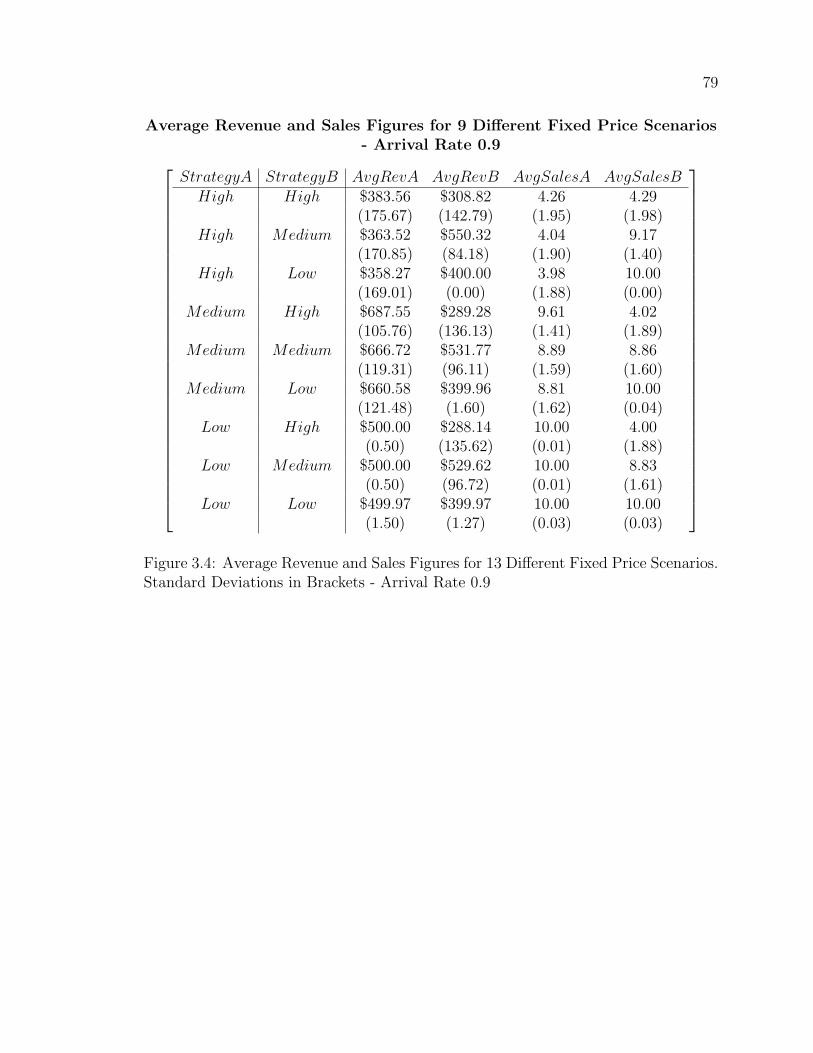
79
Average Revenue and Sales Figures for 9 Different Fixed Price Scenarios- Arrival Rate 0.9
StrategyA StrategyB AvgRevA AvgRevB AvgSalesA AvgSalesBHigh High $383.56 $308.82 4.26 4.29
(175.67) (142.79) (1.95) (1.98)High Medium $363.52 $550.32 4.04 9.17
(170.85) (84.18) (1.90) (1.40)High Low $358.27 $400.00 3.98 10.00
(169.01) (0.00) (1.88) (0.00)Medium High $687.55 $289.28 9.61 4.02
(105.76) (136.13) (1.41) (1.89)Medium Medium $666.72 $531.77 8.89 8.86
(119.31) (96.11) (1.59) (1.60)Medium Low $660.58 $399.96 8.81 10.00
(121.48) (1.60) (1.62) (0.04)Low High $500.00 $288.14 10.00 4.00
(0.50) (135.62) (0.01) (1.88)Low Medium $500.00 $529.62 10.00 8.83
(0.50) (96.72) (0.01) (1.61)Low Low $499.97 $399.97 10.00 10.00
(1.50) (1.27) (0.03) (0.03)
Figure 3.4: Average Revenue and Sales Figures for 13 Different Fixed Price Scenarios.Standard Deviations in Brackets - Arrival Rate 0.9
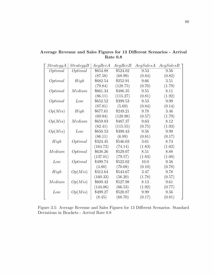
80
Average Revenue and Sales Figures for 13 Different Scenarios - ArrivalRate 0.8
StrategyA StrategyB AvgRevA AvgRevB AvgSalesA AvgSalesBOptimal Optimal $654.88 $524.02 9.53 9.56
(87.58) (68.99) (0.84) (0.82)Optimal High $682.54 $252.91 9.66 3.51
(79.84) (128.75) (0.70) (1.79)Optimal Medium $661.34 $486.35 9.55 8.11
(86.11) (115.27) (0.81) (1.92)Optimal Low $652.52 $399.53 9.53 9.99
(87.81) (5.69) (0.84) (0.14)Op(Mis) High $677.61 $249.21 9.78 3.46
(69.94) (128.98) (0.57) (1.79)Op(Mis) Medium $659.83 $487.37 9.63 8.12
(82.41) (115.55) (0.75) (1.93)Op(Mis) Low $650.53 $399.43 9.56 9.99
(86.11) (6.89) (0.81) (0.17)High Optimal $324.45 $546.03 3.61 8.74
(164.72) (74.14) (1.83) (1.02)Medium Optimal $638.26 $529.07 8.51 8.88
(137.01) (79.57) (1.83) (1.08)Low Optimal $499.74 $522.02 10.0 9.56
(4.80) (70.08) (0.10) (0.78)High Op(Mis) $312.64 $543.67 3.47 9.78
(160.33) (56.20) (1.78) (0.57)Medium Op(Mis) $609.42 $527.98 8.13 9.61
(144.06) (66.53) (1.92) (0.77)Low Op(Mis) $499.27 $520.87 9.99 9.56
(8.45) (68.70) (0.17) (0.81)
Figure 3.5: Average Revenue and Sales Figures for 13 Different Scenarios. StandardDeviations in Brackets - Arrival Rate 0.8
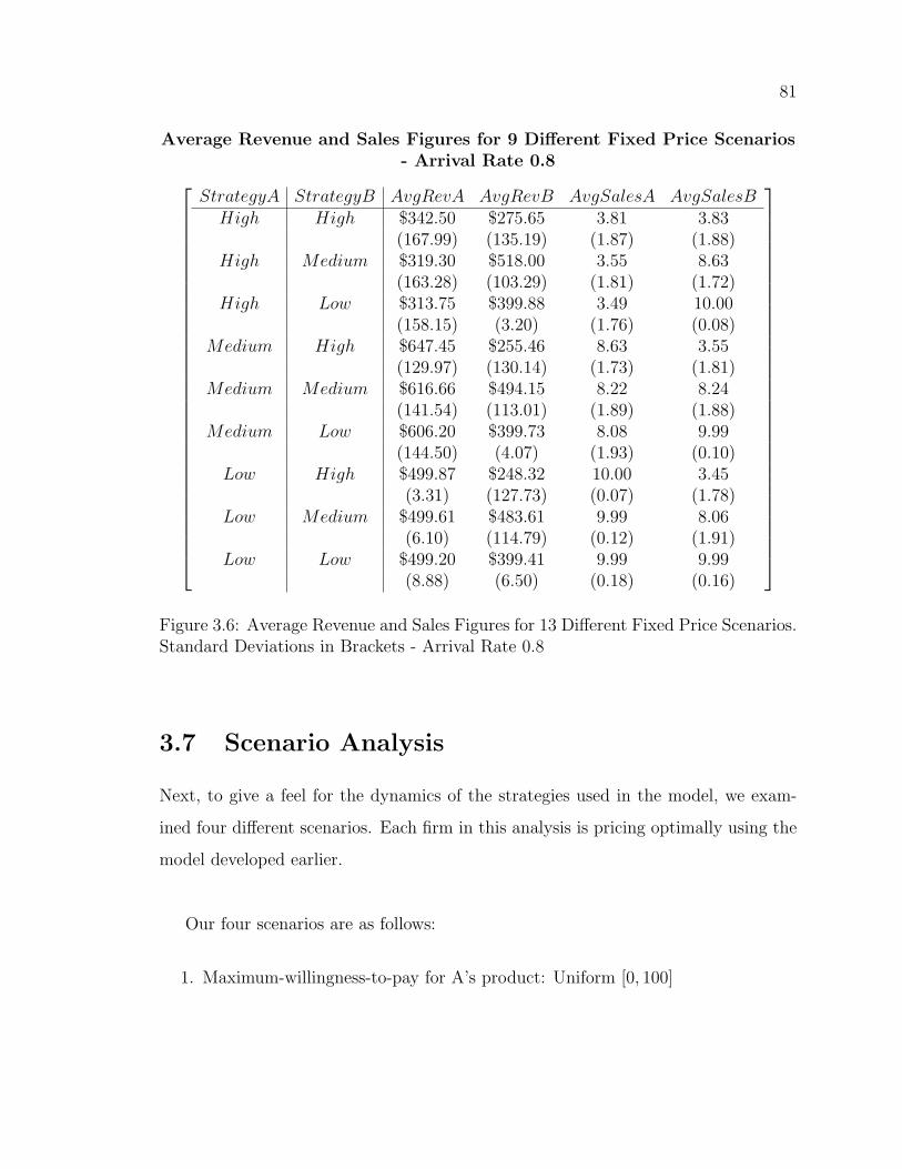
81
Average Revenue and Sales Figures for 9 Different Fixed Price Scenarios- Arrival Rate 0.8
StrategyA StrategyB AvgRevA AvgRevB AvgSalesA AvgSalesBHigh High $342.50 $275.65 3.81 3.83
(167.99) (135.19) (1.87) (1.88)High Medium $319.30 $518.00 3.55 8.63
(163.28) (103.29) (1.81) (1.72)High Low $313.75 $399.88 3.49 10.00
(158.15) (3.20) (1.76) (0.08)Medium High $647.45 $255.46 8.63 3.55
(129.97) (130.14) (1.73) (1.81)Medium Medium $616.66 $494.15 8.22 8.24
(141.54) (113.01) (1.89) (1.88)Medium Low $606.20 $399.73 8.08 9.99
(144.50) (4.07) (1.93) (0.10)Low High $499.87 $248.32 10.00 3.45
(3.31) (127.73) (0.07) (1.78)Low Medium $499.61 $483.61 9.99 8.06
(6.10) (114.79) (0.12) (1.91)Low Low $499.20 $399.41 9.99 9.99
(8.88) (6.50) (0.18) (0.16)
Figure 3.6: Average Revenue and Sales Figures for 13 Different Fixed Price Scenarios.Standard Deviations in Brackets - Arrival Rate 0.8
3.7 Scenario Analysis
Next, to give a feel for the dynamics of the strategies used in the model, we exam-
ined four different scenarios. Each firm in this analysis is pricing optimally using the
model developed earlier.
Our four scenarios are as follows:
1. Maximum-willingness-to-pay for A’s product: Uniform [0, 100]
82
Maximum-willingness-to-pay for B’s product: Uniform [0, 100]
Probability of customer arrival: .8
2. Maximum-willingness-to-pay for A’s product: Uniform [0, 100]
Maximum-willingness-to-pay for B’s product: Uniform [0, 80]
Probability of customer arrival: .8
3. Maximum-willingness-to-pay for A’s product: Uniform [0, 80]
Maximum-willingness-to-pay for B’s product: Uniform [0, 80]
Probability of customer arrival: .8
4. Maximum-willingness-to-pay for A’s product: Uniform [0, 100]
Maximum-willingness-to-pay for B’s product: Uniform [0, 100]
Probability of customer arrival: .5
3.7.1 Firm A has 1 Good
The following tables illustrate some of the pricing dynamics of the game as well as
the impact changing these parameter values has. We investigate the pricing strate-
gies for Firm A and Firm B in each of the four scenarios when B has anywhere from
1-10 goods, Firm A has exactly 1 good and the game is in period 46 (there are 5
periods left including the current period). First, Firm B’s pricing strategies in the
four scenarios.
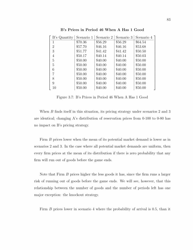
83
B’s Prices in Period 46 When A Has 1 Good
B’s Quantity Scenario 1 Scenario 2 Scenario 3 Scenario 41 $70.36 $56.29 $56.29 $64.542 $57.70 $46.16 $46.16 $53.683 $51.77 $41.42 $41.42 $50.504 $50.17 $40.14 $40.14 $50.035 $50.00 $40.00 $40.00 $50.005 $50.00 $40.00 $40.00 $50.006 $50.00 $40.00 $40.00 $50.007 $50.00 $40.00 $40.00 $50.008 $50.00 $40.00 $40.00 $50.009 $50.00 $40.00 $40.00 $50.0010 $50.00 $40.00 $40.00 $50.00
Figure 3.7: B’s Prices in Period 46 When A Has 1 Good
When B finds itself in this situation, its pricing strategy under scenarios 2 and 3
are identical; changing A’s distribution of reservation prices from 0-100 to 0-80 has
no impact on B’s pricing strategy.
Firm B prices lower when the mean of its potential market demand is lower as in
scenarios 2 and 3. In the case where all potential market demands are uniform, then
every firm prices at the mean of its distribution if there is zero probability that any
firm will run out of goods before the game ends.
Note that Firm B prices higher the less goods it has, since the firm runs a larger
risk of running out of goods before the game ends. We will see, however, that this
relationship between the number of goods and the number of periods left has one
major exception: the knockout strategy.
Firm B prices lower in scenario 4 where the probability of arrival is 0.5, than it
84
does in scenario 1 where the probability of arrival is 0.8. Once again, this is due to
the fact that the firm typically (but not always) prices higher when the probability
it will run out of goods before the game ends is higher. Thus, our model is very
responsive to changes in the state and takes market conditions into account.
3.7.2 Firm A has 10 Goods
Next we will examine the pricing dynamics for Firm A. Note that Firm A cannot
possibly run out of goods, given the fact we have assumed that it has 10 goods and
there are only 5 periods remaining.
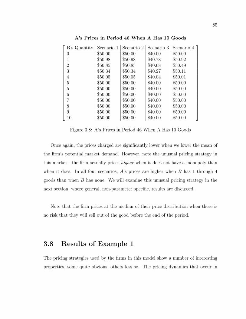
85
A’s Prices in Period 46 When A Has 10 Goods
B’s Quantity Scenario 1 Scenario 2 Scenario 3 Scenario 40 $50.00 $50.00 $40.00 $50.001 $50.98 $50.98 $40.78 $50.922 $50.85 $50.85 $40.68 $50.493 $50.34 $50.34 $40.27 $50.114 $50.05 $50.05 $40.04 $50.015 $50.00 $50.00 $40.00 $50.005 $50.00 $50.00 $40.00 $50.006 $50.00 $50.00 $40.00 $50.007 $50.00 $50.00 $40.00 $50.008 $50.00 $50.00 $40.00 $50.009 $50.00 $50.00 $40.00 $50.0010 $50.00 $50.00 $40.00 $50.00
Figure 3.8: A’s Prices in Period 46 When A Has 10 Goods
Once again, the prices charged are significantly lower when we lower the mean of
the firm’s potential market demand. However, note the unusual pricing strategy in
this market - the firm actually prices higher when it does not have a monopoly than
when it does. In all four scenarios, A’s prices are higher when B has 1 through 4
goods than when B has none. We will examine this unusual pricing strategy in the
next section, where general, non-parameter specific, results are discussed.
Note that the firm prices at the median of their price distribution when there is
no risk that they will sell out of the good before the end of the period.
3.8 Results of Example 1
The pricing strategies used by the firms in this model show a number of interesting
properties, some quite obvious, others less so. The pricing dynamics that occur in
86
this model are the result of the fact that a firm can run out of goods before the game
is over is taken into consideration. This means lost opportunities for sales for the firm
who runs out of goods and a change in market structure from duopoly to monopoly
for the firm that remains in the game.
All results in this section assume that the salvage value for each firm is set to
zero. These results are not altered in any significant way for strictly positive and
small salvage values, except for pricing when no firm has the possibility it will run
out of goods. Our model generates optimal prices that have the following general
characteristics.
1. All else being equal, prices for each firm are (weakly) higher in the amount of
time remaining in the game for each pair of quantity levels (qa, qb) for the firms.
This results from the fact that more periods remaining in the game increase the
probability that one or more firms may run out of goods before the game ends.
2. All else being equal, the higher the customer arrival rate, the (weakly) higher
each firm prices. Once again, this is because a higher arrival rate increases the
probability that one or more firms may run out of goods before the game ends.
3. If there is no possibility that all firms still in the game will run out of goods
(i.e. there are fewer periods remaining than goods left for each firm), then each
firm prices at the mean of its potential demand distribution, if the dimensions
of our overall potential market demand are independent (given our assumptions
on demand). This implies that if capacity is not a binding constraint, then the
87
price set is the same for a monopolist as a duopolist. However, the monopolist
has a higher probability of making a sale given a customer arrival, as he does
not lose potential sales to another firm.
4. Prices are typically (weakly) higher under a monopoly than under a duopoly.
Similarly, prices are typically increasing for both firms as the quantity level is
dropped for either firm, as the inventory level of each firm is taken into account.
However, there is one interesting exception to this, which we call the knockout
strategy.
The knockout strategy is employed when a firm, say Firm A, has very few goods,
typically one or two, with many periods left to go. In this situation, Firm B will set
its price very high, often close to the upper bound of its one-dimensional potential
demand distribution. It will do this in order to concede the market to Firm A during
this period, so Firm A will make a sale and thus run out of goods (be knocked out
of the game), allowing Firm B to have a monopoly for the rest of the game. Under
this situation, Firm A will typically price somewhat higher as well, but not so high as
to eliminate any chance of making a sale. Firm A knows that the longer it takes to
make a sale, the lower the price it will get, since prices, all else being equal, decline
as the number of periods remaining is reduced. By considering factor 3, the quantity
levels of competitor products, the firm can increase its revenue
Interestingly, Firm B will use the knockout strategy even if it cannot possibly run
out of goods, meaning that prices will not be any higher under a monopoly than under
a duopoly. A monopoly is still desirable to Firm B, since it raises the probability of a
sale under these conditions, so it will be able to sell goods that otherwise would not
88
garner any revenue.
3.9 Example 2: 2 x 3 Model - Rental Car Model
The importance of taking into consideration cross-price elasticities has been covered
extensively in the literature and has been demonstrated to be important in markets
of interest to revenue managers such as the rental car business. We show that it is
possible for a firm to reduce its profit using traditional revenue management tech-
niques that consider the pricing of each good in isolation and ignore factor 4. This
is caused by firms cannibalizing their high-end market by pricing their lower-end
products too low. Using a simultaneous optimization approach, firms achieve higher
profits by reducing cannibalization. In our simultaneous optimization model, prices
are typically higher for lower end products and lower for higher end products, than in
models where pricing decisions are made in isolation. This change in pricing increases
profits for the business using it.
3.10 Description of the Problem
The framework developed in this paper allows for the construction of models where
there are N firms each selling M similar, but not identical products. In this stylized
example we consider the case of 2 rental car brands, each offering 3 classes of cars for
rent. The agents in the model have heterogeneous preferences, but on average the
firms are seen as being identical in quality. The three different classes are described as,
in ascending value - compact, mid-sized, and full-sized. Due to the heterogeneity of
consumer preferences, some consumers may prefer, all else being equal, compact cars
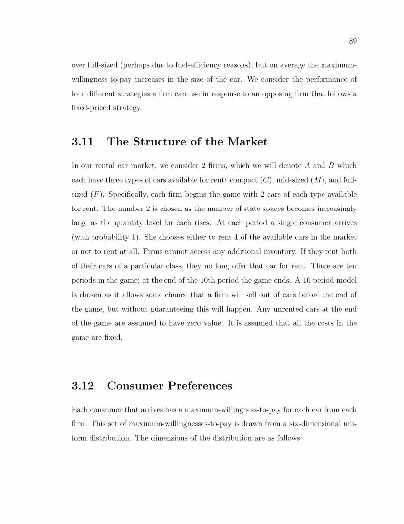
89
over full-sized (perhaps due to fuel-efficiency reasons), but on average the maximum-
willingness-to-pay increases in the size of the car. We consider the performance of
four different strategies a firm can use in response to an opposing firm that follows a
fixed-priced strategy.
3.11 The Structure of the Market
In our rental car market, we consider 2 firms, which we will denote A and B which
each have three types of cars available for rent: compact (C), mid-sized (M), and full-
sized (F ). Specifically, each firm begins the game with 2 cars of each type available
for rent. The number 2 is chosen as the number of state spaces becomes increasingly
large as the quantity level for each rises. At each period a single consumer arrives
(with probability 1). She chooses either to rent 1 of the available cars in the market
or not to rent at all. Firms cannot access any additional inventory. If they rent both
of their cars of a particular class, they no long offer that car for rent. There are ten
periods in the game; at the end of the 10th period the game ends. A 10 period model
is chosen as it allows some chance that a firm will sell out of cars before the end of
the game, but without guaranteeing this will happen. Any unrented cars at the end
of the game are assumed to have zero value. It is assumed that all the costs in the
game are fixed.
3.12 Consumer Preferences
Each consumer that arrives has a maximum-willingness-to-pay for each car from each
firm. This set of maximum-willingnesses-to-pay is drawn from a six-dimensional uni-
form distribution. The dimensions of the distribution are as follows:
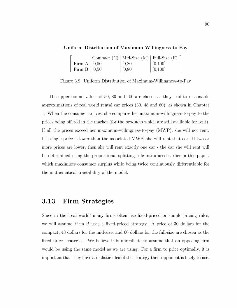
90
Uniform Distribution of Maximum-Willingness-to-Pay Compact (C) Mid-Size (M) Full-Size (F)Firm A [0,50] [0,80] [0,100]Firm B [0,50] [0,80] [0,100]
Figure 3.9: Uniform Distribution of Maximum-Willingness-to-Pay
The upper bound values of 50, 80 and 100 are chosen as they lead to reasonable
approximations of real world rental car prices (30, 48 and 60), as shown in Chapter
1. When the consumer arrives, she compares her maximum-willingness-to-pay to the
prices being offered in the market (for the products which are still available for rent).
If all the prices exceed her maximum-willingness-to-pay (MWP), she will not rent.
If a single price is lower than the associated MWP, she will rent that car. If two or
more prices are lower, then she will rent exactly one car - the car she will rent will
be determined using the proportional splitting rule introduced earlier in this paper,
which maximizes consumer surplus while being twice continuously differentiable for
the mathematical tractability of the model.
3.13 Firm Strategies
Since in the ’real world’ many firms often use fixed-priced or simple pricing rules,
we will assume Firm B uses a fixed-priced strategy. A price of 30 dollars for the
compact, 48 dollars for the mid-size, and 60 dollars for the full-size are chosen as the
fixed price strategies. We believe it is unrealistic to assume that an opposing firm
would be using the same model as we are using. For a firm to price optimally, it is
important that they have a realistic idea of the strategy their opponent is likely to use.
91
We consider 4 candidate strategies for Firm A:
1. Firm A follows the same fixed-price strategy as Firm B and ignores all five
factors.
2. Firm A follows an isolated optimization approach, where it determines the price
it will charge for each good without considering spill-over effects. It does not
consider the inventory levels of the other firm. This considers factors 1 and
5. It only partly considers factor 4. It recognizes that the price of the firm’s
other goods affects the demand for our good. However, it does not consider the
reverse. It treats the prices of the firm’s other products as a given which cannot
be changed. It also completely ignores factors 2 and 3.
3. Firm A follows a global optimization approach, where it determines the price
it will charge for all three goods simultaneously, in order to consider spill-over
effects. It does not consider the inventory levels of the other firm. This fully
considers factor 4 and adds factor 2 to the mix. All factors are now considered
other than factor 3.
4. Firm A follows a global optimization approach and considers the inventory level
of the other firm. This adds factor 3 and all five factors are now considered.
92
3.14 Solution Methodology
For each of the four strategy pairs, we compute a state-contingent set of prices through
backward induction. The state space is the current period and the inventory levels for
each product and firm. However, Firm A does not necessarily use all the information
from the state in making its decision. For the four-strategies, the states from A’s
perspective are as follows:
1. No state; every period identical to the last.
2. The current period and the inventory levels of only the product under consid-
eration.
3. The current period and the inventory levels of all Firm A’s products.
4. The current period and the inventory levels of all Firm A’s and Firm B’s prod-
ucts.
Once the state-contingent set of prices were obtained for the four different strate-
gies, 10,000 simulations were run for each strategy to obtain the average or expected
revenue for each firm. We used the results to investigate the differences in revenues
and booking rates between the four strategies.
3.15 Results of Example 2
The average profit for each firm in each strategy was as follows (note revenue and
profit in this model are functionally equivalent, as there are no explicit costs).
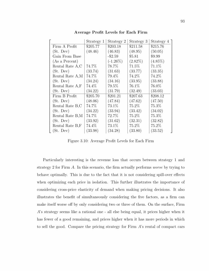
93
Average Profit Levels for Each Firm
Strategy 1 Strategy 2 Strategy 3 Strategy 4Firm A Profit $205.77 $203.18 $211.58 $215.76(St. Dev) (48.46) (46.83) (48.95) (50.05)Gain From Base -$2.59 $5.81 $9.99(As a Percent) (-1.26%) (2.82%) (4.85%)Rental Rate A,C 74.7% 78.7% 71.5% 71.1%(St. Dev) (33.74) (31.63) (33.77) (33.35)Rental Rate A,M 74.7% 79.4% 74.2% 74.2%(St. Dev) (34.24) (34.16) (33.95) (33.88)Rental Rate A,F 74.4% 79.5% 76.1% 76.0%(St. Dev) (34.22) (31.79) (32.49) (33.03)Firm B Profit $205.70 $201.21 $207.63 $208.12(St. Dev) (48.06) (47.84) (47.62) (47.50)Rental Rate B,C 74.7% 73.1% 75.2% 75.3%(St. Dev) (34.22) (33.94) (33.42) (34.02)Rental Rate B,M 74.7% 72.7% 75.2% 75.3%(St. Dev) (33.92) (31.62) (32.31) (32.82)Rental Rate B,F 74.4% 73.1% 75.2% 75.2%(St. Dev) (33.98) (34.28) (33.80) (33.52)
Figure 3.10: Average Profit Levels for Each Firm
Particularly interesting is the revenue loss that occurs between strategy 1 and
strategy 2 for Firm A. In this scenario, the firm actually performs worse by trying to
behave optimally. This is due to the fact that it is not considering spill-over effects
when optimizing each price in isolation. This further illustrates the importance of
considering cross-price elasticity of demand when making pricing decisions. It also
illustrates the benefit of simultaneously considering the five factors, as a firm can
make itself worse off by only considering two or three of them. On the surface, Firm
A’s strategy seems like a rational one - all else being equal, it prices higher when it
has fewer of a good remaining, and prices higher when it has more periods in which
to sell the good. Compare the pricing strategy for Firm A’s rental of compact cars
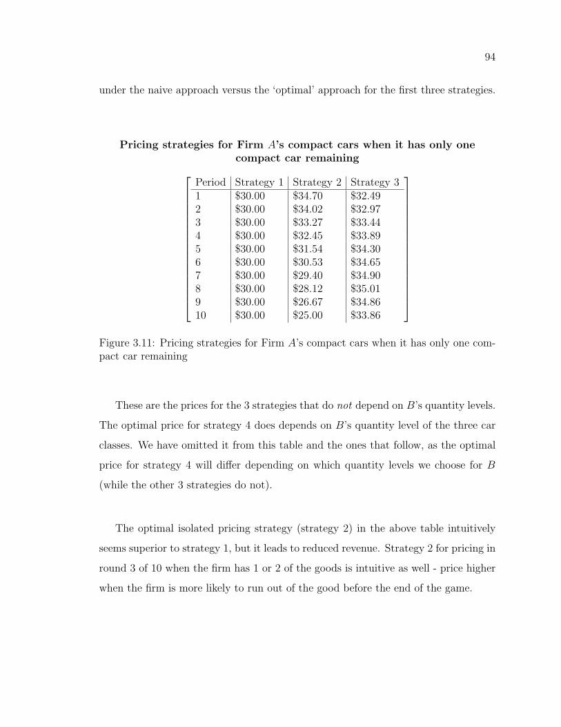
94
under the naive approach versus the ‘optimal’ approach for the first three strategies.
Pricing strategies for Firm A’s compact cars when it has only onecompact car remaining
Period Strategy 1 Strategy 2 Strategy 31 $30.00 $34.70 $32.492 $30.00 $34.02 $32.973 $30.00 $33.27 $33.444 $30.00 $32.45 $33.895 $30.00 $31.54 $34.306 $30.00 $30.53 $34.657 $30.00 $29.40 $34.908 $30.00 $28.12 $35.019 $30.00 $26.67 $34.8610 $30.00 $25.00 $33.86
Figure 3.11: Pricing strategies for Firm A’s compact cars when it has only one com-pact car remaining
These are the prices for the 3 strategies that do not depend on B’s quantity levels.
The optimal price for strategy 4 does depends on B’s quantity level of the three car
classes. We have omitted it from this table and the ones that follow, as the optimal
price for strategy 4 will differ depending on which quantity levels we choose for B
(while the other 3 strategies do not).
The optimal isolated pricing strategy (strategy 2) in the above table intuitively
seems superior to strategy 1, but it leads to reduced revenue. Strategy 2 for pricing in
round 3 of 10 when the firm has 1 or 2 of the goods is intuitive as well - price higher
when the firm is more likely to run out of the good before the end of the game.
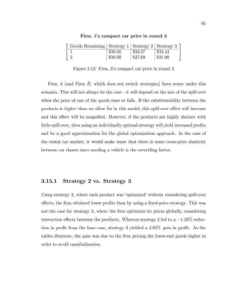
95
Firm A’s compact car price in round 3 Goods Remaining Strategy 1 Strategy 2 Strategy 31 $30.00 $33.27 $33.442 $30.00 $27.69 $31.90
Figure 3.12: Firm A’s compact car price in round 3
Firm A (and Firm B, which does not switch strategies) fares worse under this
scenario. This will not always be the case - it will depend on the size of the spill-over
when the price of one of the goods rises or falls. If the substitutability between the
products is higher than we allow for in this model, this spill-over effect will increase
and this effect will be magnified. However, if the products are highly distinct with
little spill-over, then using an individually optimal strategy will yield increased profits
and be a good approximation for the global optimization approach. In the case of
the rental car market, it would make sense that there is some cross-price elasticity
between car classes since needing a vehicle is the overriding factor.
3.15.1 Strategy 2 vs. Strategy 3
Using strategy 2, where each product was ‘optimized’ without considering spill-over
effects, the firm obtained lower profits than by using a fixed-price strategy. This was
not the case for strategy 3, where the firm optimizes its prices globally, considering
interaction effects between the products. Whereas strategy 2 led to a −1.26% reduc-
tion in profit from the base case, strategy 3 yielded a 2.82% gain in profit. As the
tables illustrate, the gain was due to the firm pricing the lower-end goods higher in
order to avoid cannibalization.
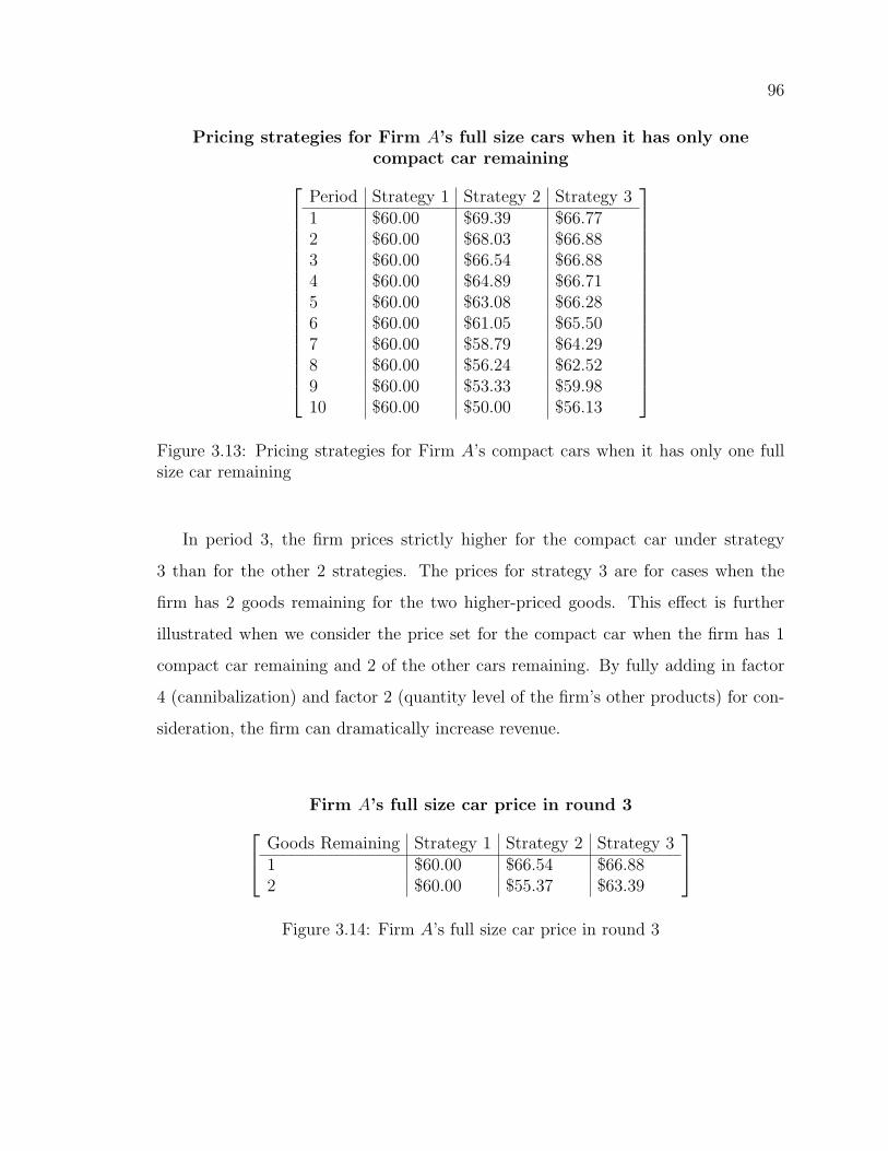
96
Pricing strategies for Firm A’s full size cars when it has only onecompact car remaining
Period Strategy 1 Strategy 2 Strategy 31 $60.00 $69.39 $66.772 $60.00 $68.03 $66.883 $60.00 $66.54 $66.884 $60.00 $64.89 $66.715 $60.00 $63.08 $66.286 $60.00 $61.05 $65.507 $60.00 $58.79 $64.298 $60.00 $56.24 $62.529 $60.00 $53.33 $59.9810 $60.00 $50.00 $56.13
Figure 3.13: Pricing strategies for Firm A’s compact cars when it has only one fullsize car remaining
In period 3, the firm prices strictly higher for the compact car under strategy
3 than for the other 2 strategies. The prices for strategy 3 are for cases when the
firm has 2 goods remaining for the two higher-priced goods. This effect is further
illustrated when we consider the price set for the compact car when the firm has 1
compact car remaining and 2 of the other cars remaining. By fully adding in factor
4 (cannibalization) and factor 2 (quantity level of the firm’s other products) for con-
sideration, the firm can dramatically increase revenue.
Firm A’s full size car price in round 3 Goods Remaining Strategy 1 Strategy 2 Strategy 31 $60.00 $66.54 $66.882 $60.00 $55.37 $63.39
Figure 3.14: Firm A’s full size car price in round 3
97
3.15.2 Strategy 3 vs. Strategy 4
In strategy 4, Firm A considers the inventory levels of each of the competitor’s three
products. Thus factor 2 consideration is added and all five factors are simultaneously
accounted for. In this strategy Firm A always prices all three types of goods higher,
ceteris paribus, when the firm has less of any good. In particularly, the prices are
raised when the opposing firm runs out of any product class. The difference in prices
tend to be small (less than a dollar), but they lead to a 4.85% increase in profit from
the base case and a nearly 2% increase over the case where the firm does not consider
the opposing firm’s inventory levels.
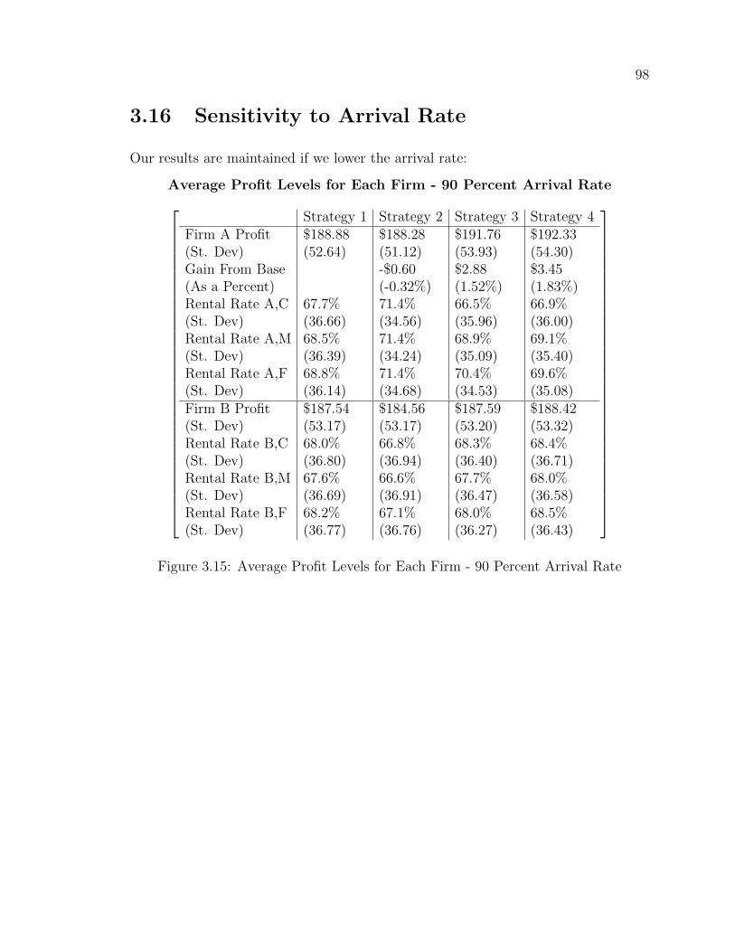
98
3.16 Sensitivity to Arrival Rate
Our results are maintained if we lower the arrival rate:
Average Profit Levels for Each Firm - 90 Percent Arrival Rate
Strategy 1 Strategy 2 Strategy 3 Strategy 4Firm A Profit $188.88 $188.28 $191.76 $192.33(St. Dev) (52.64) (51.12) (53.93) (54.30)Gain From Base -$0.60 $2.88 $3.45(As a Percent) (-0.32%) (1.52%) (1.83%)Rental Rate A,C 67.7% 71.4% 66.5% 66.9%(St. Dev) (36.66) (34.56) (35.96) (36.00)Rental Rate A,M 68.5% 71.4% 68.9% 69.1%(St. Dev) (36.39) (34.24) (35.09) (35.40)Rental Rate A,F 68.8% 71.4% 70.4% 69.6%(St. Dev) (36.14) (34.68) (34.53) (35.08)Firm B Profit $187.54 $184.56 $187.59 $188.42(St. Dev) (53.17) (53.17) (53.20) (53.32)Rental Rate B,C 68.0% 66.8% 68.3% 68.4%(St. Dev) (36.80) (36.94) (36.40) (36.71)Rental Rate B,M 67.6% 66.6% 67.7% 68.0%(St. Dev) (36.69) (36.91) (36.47) (36.58)Rental Rate B,F 68.2% 67.1% 68.0% 68.5%(St. Dev) (36.77) (36.76) (36.27) (36.43)
Figure 3.15: Average Profit Levels for Each Firm - 90 Percent Arrival Rate
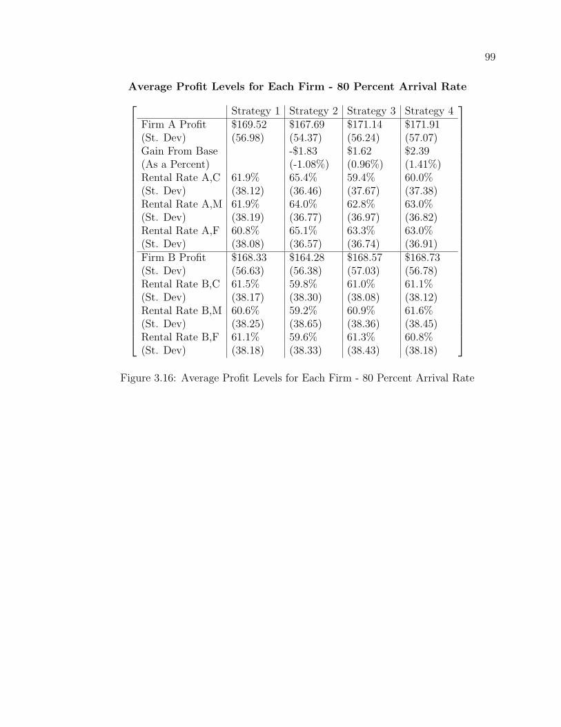
99
Average Profit Levels for Each Firm - 80 Percent Arrival Rate
Strategy 1 Strategy 2 Strategy 3 Strategy 4Firm A Profit $169.52 $167.69 $171.14 $171.91(St. Dev) (56.98) (54.37) (56.24) (57.07)Gain From Base -$1.83 $1.62 $2.39(As a Percent) (-1.08%) (0.96%) (1.41%)Rental Rate A,C 61.9% 65.4% 59.4% 60.0%(St. Dev) (38.12) (36.46) (37.67) (37.38)Rental Rate A,M 61.9% 64.0% 62.8% 63.0%(St. Dev) (38.19) (36.77) (36.97) (36.82)Rental Rate A,F 60.8% 65.1% 63.3% 63.0%(St. Dev) (38.08) (36.57) (36.74) (36.91)Firm B Profit $168.33 $164.28 $168.57 $168.73(St. Dev) (56.63) (56.38) (57.03) (56.78)Rental Rate B,C 61.5% 59.8% 61.0% 61.1%(St. Dev) (38.17) (38.30) (38.08) (38.12)Rental Rate B,M 60.6% 59.2% 60.9% 61.6%(St. Dev) (38.25) (38.65) (38.36) (38.45)Rental Rate B,F 61.1% 59.6% 61.3% 60.8%(St. Dev) (38.18) (38.33) (38.43) (38.18)
Figure 3.16: Average Profit Levels for Each Firm - 80 Percent Arrival Rate
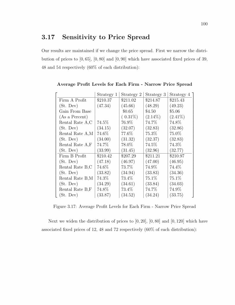
100
3.17 Sensitivity to Price Spread
Our results are maintained if we change the price spread. First we narrow the distri-
bution of prices to [0, 65], [0, 80] and [0, 90] which have associated fixed prices of 39,
48 and 54 respectively (60% of each distribution):
Average Profit Levels for Each Firm - Narrow Price Spread
Strategy 1 Strategy 2 Strategy 3 Strategy 4Firm A Profit $210.37 $211.02 $214.87 $215.43(St. Dev) (47.34) (45.66) (48.29) (49.23)Gain From Base $0.65 $4.50 $5.06(As a Percent) ( 0.31%) (2.14%) (2.41%)Rental Rate A,C 74.5% 76.9% 74.7% 74.8%(St. Dev) (34.15) (32.07) (32.83) (32.86)Rental Rate A,M 74.6% 77.6% 75.3% 75.0%(St. Dev) (34.00) (31.32) (32.37) (32.83)Rental Rate A,F 74.7% 78.0% 74.5% 74.3%(St. Dev) (33.99) (31.45) (32.96) (32.77)Firm B Profit $210.42 $207.29 $211.21 $210.97(St. Dev) (47.18) (46.97) (47.00) (46.95)Rental Rate B,C 74.6% 73.7% 74.9% 74.4%(St. Dev) (33.82) (34.94) (33.83) (34.36)Rental Rate B,M 74.3% 73.4% 75.1% 75.1%(St. Dev) (34.29) (34.61) (33.84) (34.03)Rental Rate B,F 74.8% 73.4% 74.7% 74.9%(St. Dev) (33.87) (34.52) (34.24) (33.75)
Figure 3.17: Average Profit Levels for Each Firm - Narrow Price Spread
Next we widen the distribution of prices to [0, 20], [0, 80] and [0, 120] which have
associated fixed prices of 12, 48 and 72 respectively (60% of each distribution):
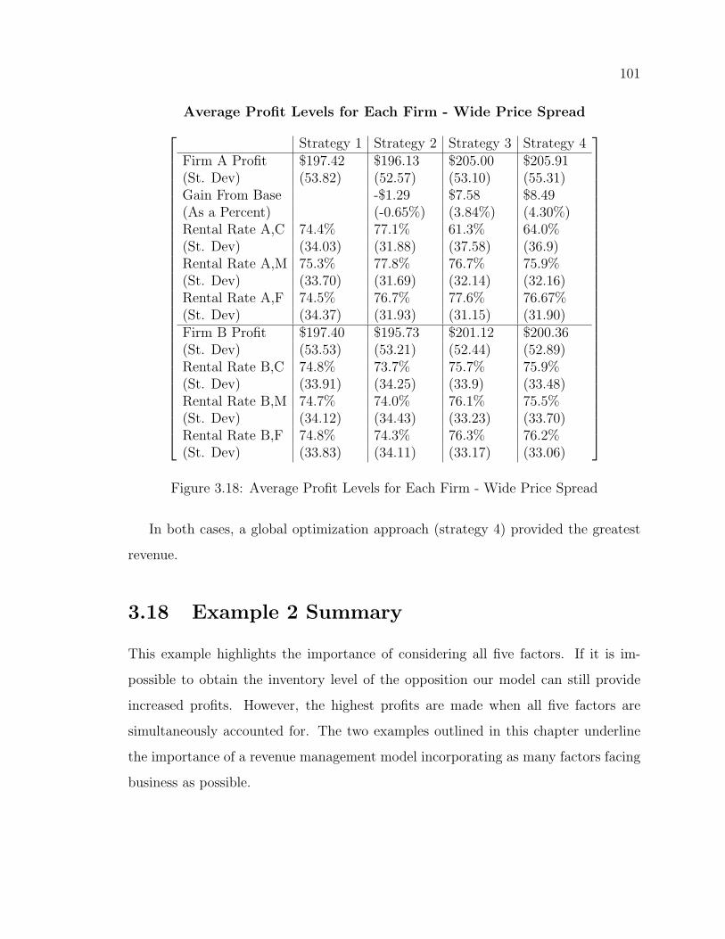
101
Average Profit Levels for Each Firm - Wide Price Spread
Strategy 1 Strategy 2 Strategy 3 Strategy 4Firm A Profit $197.42 $196.13 $205.00 $205.91(St. Dev) (53.82) (52.57) (53.10) (55.31)Gain From Base -$1.29 $7.58 $8.49(As a Percent) (-0.65%) (3.84%) (4.30%)Rental Rate A,C 74.4% 77.1% 61.3% 64.0%(St. Dev) (34.03) (31.88) (37.58) (36.9)Rental Rate A,M 75.3% 77.8% 76.7% 75.9%(St. Dev) (33.70) (31.69) (32.14) (32.16)Rental Rate A,F 74.5% 76.7% 77.6% 76.67%(St. Dev) (34.37) (31.93) (31.15) (31.90)Firm B Profit $197.40 $195.73 $201.12 $200.36(St. Dev) (53.53) (53.21) (52.44) (52.89)Rental Rate B,C 74.8% 73.7% 75.7% 75.9%(St. Dev) (33.91) (34.25) (33.9) (33.48)Rental Rate B,M 74.7% 74.0% 76.1% 75.5%(St. Dev) (34.12) (34.43) (33.23) (33.70)Rental Rate B,F 74.8% 74.3% 76.3% 76.2%(St. Dev) (33.83) (34.11) (33.17) (33.06)
Figure 3.18: Average Profit Levels for Each Firm - Wide Price Spread
In both cases, a global optimization approach (strategy 4) provided the greatest
revenue.
3.18 Example 2 Summary
This example highlights the importance of considering all five factors. If it is im-
possible to obtain the inventory level of the opposition our model can still provide
increased profits. However, the highest profits are made when all five factors are
simultaneously accounted for. The two examples outlined in this chapter underline
the importance of a revenue management model incorporating as many factors facing
business as possible.
102
Chapter 4
Booking Limits and Optimal
Pricing in a 2-Firm, 2 Class Airline
Model
Applying our model to the well-known Netessine and Shumsky problem yields sig-
nificantly increased revenues over the booking limits approach. Substantial gains to
revenue are available to firms when they have the ability to alter their prices in re-
sponse to changing market conditions. There are a number of features of the model
that lead to increased revenues. Instead of simply shutting off sales when demand
is high, firms can increase their price allowing for higher revenues per seat. When
demand is low, firms can lower their prices to assure they are not leaving with a
half-empty plane. Firms can also react to the quantity levels of their competitor
by employing the knockout strategy. Booking limits consider only quantity limits
(factors 1 through 3), while our optimal pricing model considers all five factors and
own price elasticity of demand. Optimal pricing provides the firm with more tactical
options than the on-off approach of booking limits, which allows the firm to increase
103
their revenues.
4.1 Description of the Problem
In this section, a 2-firm/2-seat class model is created following Netessine and Shumsky
[2] where the 2 classes of seat come from a shared inventory. Unlike Netessine and
Shumsky, each firm has the ability to alter its prices as well as close booking classes
(by setting a price for the class so high that quantity demanded falls to zero).
4.2 Netessine and Shumsky Market Structure
Consider the market structure discussed in Netessine and Shumsky (2005) [2]. They
consider the real-life problem of two competing airlines, flying the same route, each
with two booking classes.
“Consider an airline customer looking for an early-morning flight from
Rochester, NY, to Chicago in May 2003. The traveller can choose between
two airlines, American and United, which offer flights at nearly identical
times (6:00 A.M. and 6:10 A.M. respectively) at identical prices (both
charge $266 for 14-day and $315 for 7-day advance-purchase round-trip
tickets). Now suppose that the customer wishes to purchase American’s
14-day advance ticket. If the seats allocated to the 14-day fare class have
sold out, it is likely that the customer will attempt to purchase a ticket
in the same fare class on the United flight that departs 10 minutes later.”
[2]
104
In the Netessine and Shumsky framework, firms choose a booking limit on the
maximum number of sales they will allow into the lower class fare. Since this is a
competitive model and if the firms “do not collaborate on seat allocations,then the
decisions that arise out of the resulting game can differ significantly from the seat
allocations that would be optimal for a single decision maker with control over both
airlines”. Netessine and Shumsky describe the strategy set available to each airline.
“To maximize expected profits, the airline establishes a booking limit B
for low-fare seats. Note that the establishment of a booking limit is an
optimal policy for each airline – see Brumelle et al. (1990) [1]. Once the
booking limit is reached, the low fare is closed. Sales of high-fare tickets
are accepted until either the airplane is full or the flight departs.” [2]
We wish to expand the strategy set available to each firm. In the Netessine and
Shumsky model prices are taken as given and the firms have a set quantity of seats
which they can allocate between the two classes. We also allow seats to be allocated
in this manner, but we also allow the firm to change the price of each of its fare classes
in response to market conditions. This also allows us to have each firm dynamically
create booking limits, by raising the price of the lower fare class so high that the
probability of sale for that class is zero.
We go on to examine the use of the knockout strategy, where a firm should delib-
erately increase its price in order to increase the other firm’s probability of sale. That
is, the optimal price in equilibrium is higher than it normally would be, thanks to
this knockout effect. By using the knockout strategy when an opposing firm is close
to selling out, a firm can increase the chances that it will have a monopoly for the
rest of the period.
105
4.3 Model Specifications
There are two firms in this model, which we will refer to as Firm A and Firm B.
Each firm will offer two qualities of service: a business class denoted by an upper case
letter and a coach class which will be denoted by a lower case letter. Consumers see
the firms, as well as, the various firm classes being distinct.
To allow the model to be compatible with the Netessine and Shumsky [2] model
we use their assumption that coach class consumers purchase tickets before business
class customers. Specifically, for the first half of the game, only coach class consumers
arrive and for the second half, only business class consumers arrive. This is not neces-
sarily a realistic assumption, but is used to keep our model as close to Netessine and
Shumsky’s as possible. At each period of the game, each firm can set the price they
will charge to the type of consumer they expect to arrive that period (either coach
or business class). They can set a price so high that no consumer would purchase a
ticket for that class. This is analogous to the Netessine and Shumsky allowance that
a firm can close coach class sales so that the firm can have more seats available for
sale to business class customers, when they arrive.
The demand space for each class (first-class and coach) is described by a 2-
dimensional rectangle. Each dimension represents a range of maximum-willingnesses-
to-pay for the product offered in that class by each firm. For product i, this is
bounded between 0 and an upper bound ui, where uA > 0 and uB > 0. The only dif-
ference between first class and coach is that the upper-bound for the first class seats
is strictly higher than the upper-bound for the coach class seats. We assume that cus-
106
tomer maximum-willingnesses-to-pay are distributed uniformly within each rectangle.
We employ the proportional splitting rule for areas which are “claimed” by more
than one firm.
4.4 Decision variables and strategies employed by
each firm
At the beginning of period t, each firm simultaneously sets the price, pi, for each of
its fare classes, taking into account that a sale this period leaves one less available
seat next period. The firm, if it wishes, can choose to ‘close’ the fare class, by setting
the fare’s price to its upper bound, such that the probability of sale is zero.
We do not allow the airlines to ‘bump’ coach class seat holders in order to sell
additional business class seats.
We restrict the firms to Markovian strategies, so the strategies can depend only on
the state, which has three dimensions - the period, the quantity remaining for Firm
A, and the quantity remaining for Firm B. Restricting the problem to Markovian
strategies allows us to treat the problem as a dynamic program, where the solution
is a pure-strategy Markov Perfect Equilibrium.
107
4.5 Market level elasticity-of-demand, Strategies
employed by consumers and the nature of con-
sumer demand
At the beginning of each period, a single customer arrives with probability λ. For
the sake of simplicity, for the remainder of the section we will assume λ = 1. If it
is period 1 through T2
then a coach class consumer arrives; if it is period T2
+ 1 to
T then a business class consumer arrives. The consumer’s 2-dimensional vector of
maximum-willingness-to-pay is drawn randomly from the rectangle. Based on the
draw, they purchase one of the available seats or choose not to purchase at all. Since
the area of the ‘no purchase’ option expands as prices rise, the market does show
some level of price-elasticity-of-demand.
We assume consumers are myopic in this model. They do not have the option of
waiting to see if prices fall. They also do not attempt to cancel a reservation and
re-buy, if prices fall.
4.6 Firm A’s Optimization Problem
At time t, the firms have quantities qAt and qBt remaining respectively. We will refer
to product A’s probability of sale (given an arrival) as πA, which is a function of both
the prices in the market.
Given that the firm can enter three possible states of the world next period (one
where A has one less good, one where B has one less good, and one where both firms
108
continue to have the same number of goods), Firm A’s value function for period t
given quantity levels qAt and qBt is:
Vt(qAt , q
Bt ) =
λ ∗ πa(pa − Vt+1(qAt − 1, qBt ))+
λ ∗ (πB + πb) ∗ Vt+1(qAt , q
Bt − 1) + π0 ∗ Vt+1(q
At , q
Bt )
(4.1)
Where π0 is the probability that no firm makes a sale. This is given by:
1− λ(πA + πB) (4.2)
For Firm A, we place the constraints that 0 ≤ ptA ≤ uA and differentiate with
respect to ptA to obtain the firm’s best response function. Similarly for Firm B, we
differentiate with respect to ptB, to find the optimal reaction function for Firm B.
This gives us a system of two equations and two unknowns. Solving for this gives the
optimal price point for the firm at time t given the state of the world at the beginning
of the period.
4.7 Results for the 2x2 Airline Problem
In order to better illustrate the dynamics of the game, we created a number of simu-
lations. The parameter values used were as follows:
• The game had 30 rounds. In rounds 1 through 15 a single coach consumer
arrived with probability 1. In rounds 16 through 30 a single business class con-
sumer arrived with probability 1.
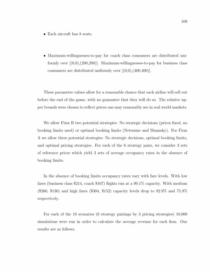
109
• Each aircraft has 8 seats.
• Maximum-willingnesses-to-pay for coach class consumers are distributed uni-
formly over [(0,0),(200,200)]. Maximum-willingnesses-to-pay for business class
consumers are distributed uniformly over [(0,0),(400,400)].
These parameter values allow for a reasonable chance that each airline will sell out
before the end of the game, with no guarantee that they will do so. The relative up-
per bounds were chosen to reflect prices one may reasonably see in real world markets.
We allow Firm B two potential strategies: No strategic decisions (prices fixed, no
booking limits used) or optimal booking limits (Netessine and Shumsky). For Firm
A we allow three potential strategies: No strategic decisions, optimal booking limits,
and optimal pricing strategies. For each of the 6 strategy pairs, we consider 3 sets
of reference prices which yield 3 sets of average occupancy rates in the absence of
booking limits.
In the absence of booking limits occupancy rates vary with fare levels. With low
fares (business class $214, coach $107) flights run at a 99.1% capacity. With medium
($260, $130) and high fares ($304, $152) capacity levels drop to 92.9% and 75.9%
respectively.
For each of the 18 scenarios (6 strategy pairings by 3 pricing strategies) 10,000
simulations were run in order to calculate the average revenue for each firm. Our
results are as follows.
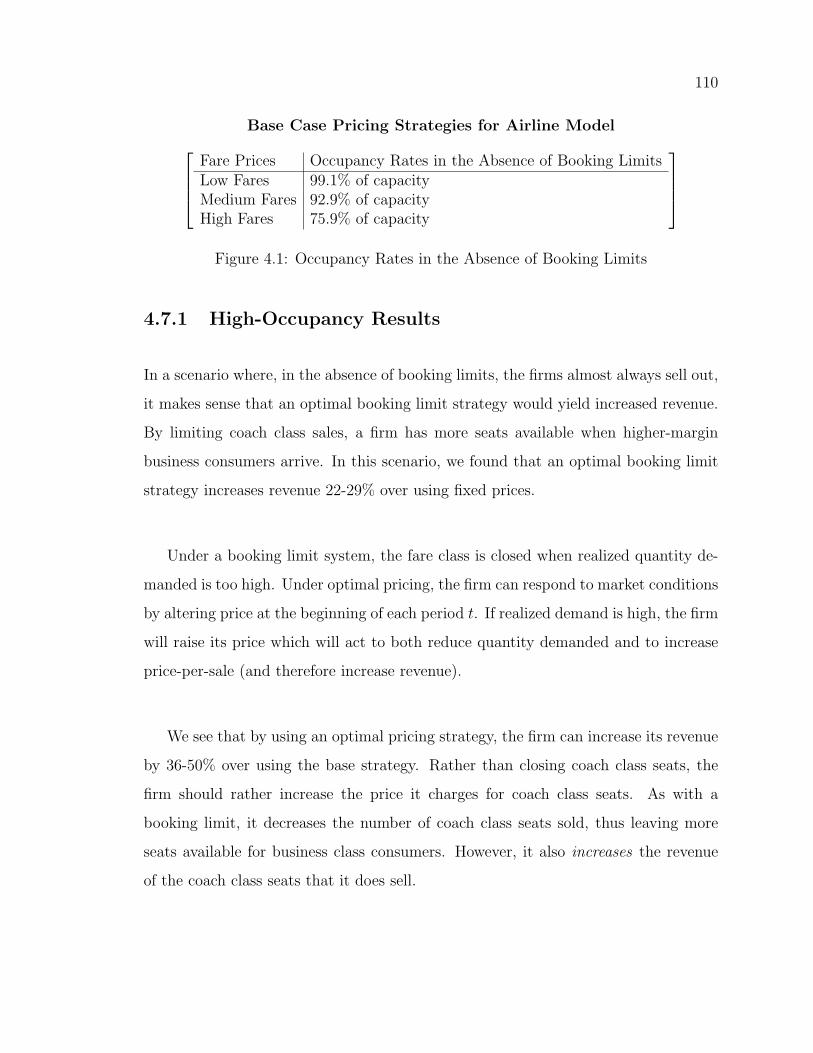
110
Base Case Pricing Strategies for Airline ModelFare Prices Occupancy Rates in the Absence of Booking LimitsLow Fares 99.1% of capacityMedium Fares 92.9% of capacityHigh Fares 75.9% of capacity
Figure 4.1: Occupancy Rates in the Absence of Booking Limits
4.7.1 High-Occupancy Results
In a scenario where, in the absence of booking limits, the firms almost always sell out,
it makes sense that an optimal booking limit strategy would yield increased revenue.
By limiting coach class sales, a firm has more seats available when higher-margin
business consumers arrive. In this scenario, we found that an optimal booking limit
strategy increases revenue 22-29% over using fixed prices.
Under a booking limit system, the fare class is closed when realized quantity de-
manded is too high. Under optimal pricing, the firm can respond to market conditions
by altering price at the beginning of each period t. If realized demand is high, the firm
will raise its price which will act to both reduce quantity demanded and to increase
price-per-sale (and therefore increase revenue).
We see that by using an optimal pricing strategy, the firm can increase its revenue
by 36-50% over using the base strategy. Rather than closing coach class seats, the
firm should rather increase the price it charges for coach class seats. As with a
booking limit, it decreases the number of coach class seats sold, thus leaving more
seats available for business class consumers. However, it also increases the revenue
of the coach class seats that it does sell.
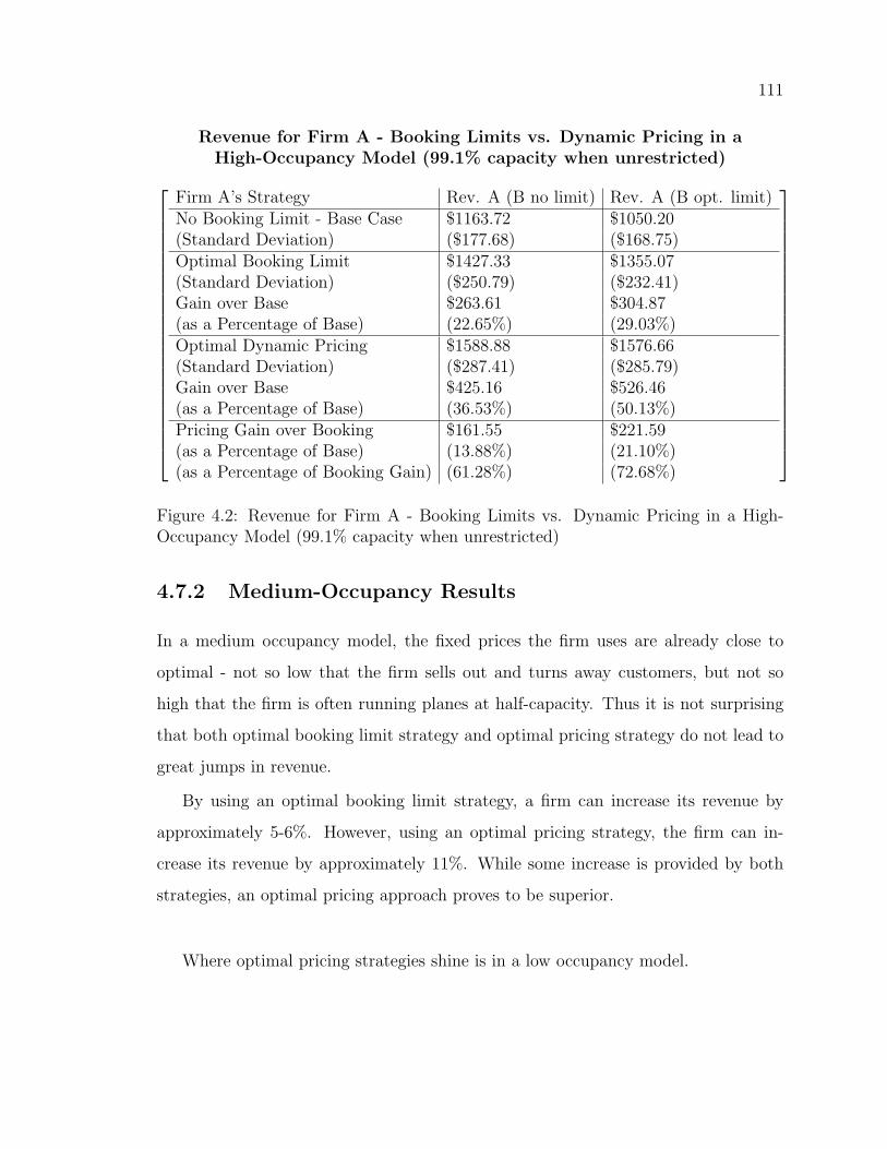
111
Revenue for Firm A - Booking Limits vs. Dynamic Pricing in aHigh-Occupancy Model (99.1% capacity when unrestricted)
Firm A’s Strategy Rev. A (B no limit) Rev. A (B opt. limit)No Booking Limit - Base Case $1163.72 $1050.20(Standard Deviation) ($177.68) ($168.75)Optimal Booking Limit $1427.33 $1355.07(Standard Deviation) ($250.79) ($232.41)Gain over Base $263.61 $304.87(as a Percentage of Base) (22.65%) (29.03%)Optimal Dynamic Pricing $1588.88 $1576.66(Standard Deviation) ($287.41) ($285.79)Gain over Base $425.16 $526.46(as a Percentage of Base) (36.53%) (50.13%)Pricing Gain over Booking $161.55 $221.59(as a Percentage of Base) (13.88%) (21.10%)(as a Percentage of Booking Gain) (61.28%) (72.68%)
Figure 4.2: Revenue for Firm A - Booking Limits vs. Dynamic Pricing in a High-Occupancy Model (99.1% capacity when unrestricted)
4.7.2 Medium-Occupancy Results
In a medium occupancy model, the fixed prices the firm uses are already close to
optimal - not so low that the firm sells out and turns away customers, but not so
high that the firm is often running planes at half-capacity. Thus it is not surprising
that both optimal booking limit strategy and optimal pricing strategy do not lead to
great jumps in revenue.
By using an optimal booking limit strategy, a firm can increase its revenue by
approximately 5-6%. However, using an optimal pricing strategy, the firm can in-
crease its revenue by approximately 11%. While some increase is provided by both
strategies, an optimal pricing approach proves to be superior.
Where optimal pricing strategies shine is in a low occupancy model.
112
Revenue for Firm A - Booking Limits vs. Dynamic Pricing in a MediumOccupancy Model (92.9% capacity when unrestricted)
Firm A’s Strategy Rev. A (B no limit) Rev. A (B opt. limit)No Booking Limit - Base Case $1411.15 $1383.33(Standard Deviation) ($252.09) ($243.47)Optimal Booking Limit $1481.77 $1461.10(Standard Deviation) ($295.02) ($307.32)Gain over Base $70.62 $77.77(as a Percentage of Base) (5.00%) (5.62%)Optimal Dynamic Pricing $1566.55 $1541.82(Standard Deviation) ($285.59) ($284.45)Gain over Base $155.40 $158.49(as a Percentage of Base) (11.01%) (11.46%)Pricing Gain over Booking $84.78 $80.72(as a Percentage of Base) (6.01%) (5.84%)(as a Percentage of Booking Gain) (120.05%) (103.79%)
Figure 4.3: Revenue for Firm A - Booking Limits vs. Dynamic Pricing in MediumOccupancy Model (92.9% capacity when unrestricted)
4.7.3 Low-Occupancy Results
In the following scenario, each airline runs at around 76% capacity when both airlines
do not use booking limits. Under such a scenario, there is little gained by using
booking limits.
If the firm does use booking limits under this scenario; the optimal booking limit
in all scenarios is to only allow 7 of the 8 seats to be sold to coach class consumers.
This increases revenue by about half of a percent.
An optimal pricing strategy shines in this scenario, since it allows the firm to
discount its prices if it appears that the plane will otherwise leave half-empty. By
using an optimal pricing strategy, the firm can obtain more than twenty times the
additional revenue of an optimal booking limit strategy.
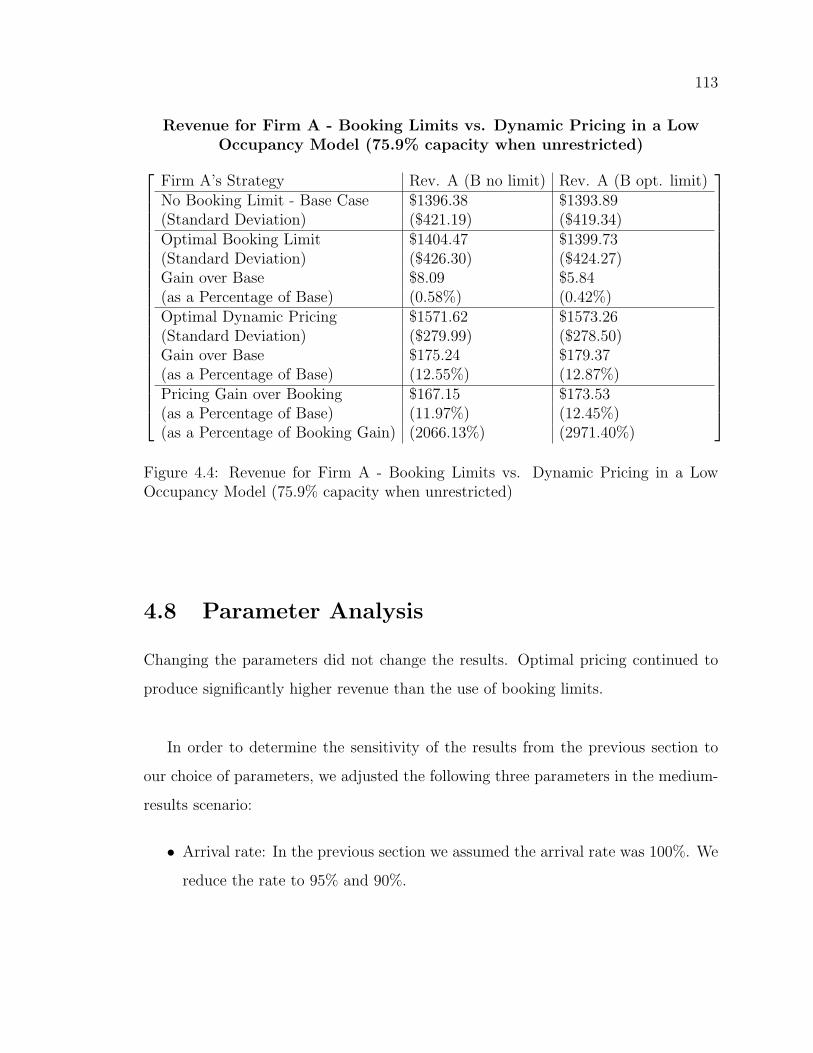
113
Revenue for Firm A - Booking Limits vs. Dynamic Pricing in a LowOccupancy Model (75.9% capacity when unrestricted)
Firm A’s Strategy Rev. A (B no limit) Rev. A (B opt. limit)No Booking Limit - Base Case $1396.38 $1393.89(Standard Deviation) ($421.19) ($419.34)Optimal Booking Limit $1404.47 $1399.73(Standard Deviation) ($426.30) ($424.27)Gain over Base $8.09 $5.84(as a Percentage of Base) (0.58%) (0.42%)Optimal Dynamic Pricing $1571.62 $1573.26(Standard Deviation) ($279.99) ($278.50)Gain over Base $175.24 $179.37(as a Percentage of Base) (12.55%) (12.87%)Pricing Gain over Booking $167.15 $173.53(as a Percentage of Base) (11.97%) (12.45%)(as a Percentage of Booking Gain) (2066.13%) (2971.40%)
Figure 4.4: Revenue for Firm A - Booking Limits vs. Dynamic Pricing in a LowOccupancy Model (75.9% capacity when unrestricted)
4.8 Parameter Analysis
Changing the parameters did not change the results. Optimal pricing continued to
produce significantly higher revenue than the use of booking limits.
In order to determine the sensitivity of the results from the previous section to
our choice of parameters, we adjusted the following three parameters in the medium-
results scenario:
• Arrival rate: In the previous section we assumed the arrival rate was 100%. We
reduce the rate to 95% and 90%.
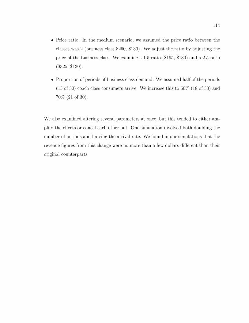
114
• Price ratio: In the medium scenario, we assumed the price ratio between the
classes was 2 (business class $260, $130). We adjust the ratio by adjusting the
price of the business class. We examine a 1.5 ratio ($195, $130) and a 2.5 ratio
($325, $130).
• Proportion of periods of business class demand: We assumed half of the periods
(15 of 30) coach class consumers arrive. We increase this to 60% (18 of 30) and
70% (21 of 30).
We also examined altering several parameters at once, but this tended to either am-
plify the effects or cancel each other out. One simulation involved both doubling the
number of periods and halving the arrival rate. We found in our simulations that the
revenue figures from this change were no more than a few dollars different than their
original counterparts.
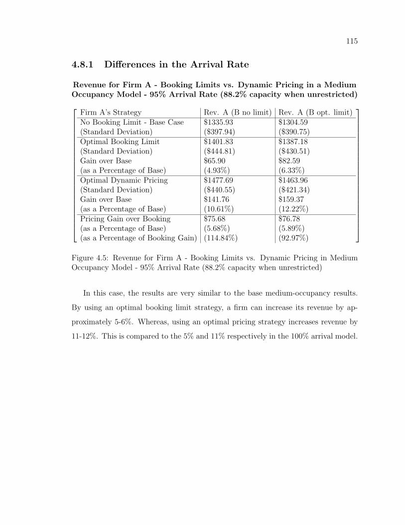
115
4.8.1 Differences in the Arrival Rate
Revenue for Firm A - Booking Limits vs. Dynamic Pricing in a MediumOccupancy Model - 95% Arrival Rate (88.2% capacity when unrestricted)
Firm A’s Strategy Rev. A (B no limit) Rev. A (B opt. limit)No Booking Limit - Base Case $1335.93 $1304.59(Standard Deviation) ($397.94) ($390.75)Optimal Booking Limit $1401.83 $1387.18(Standard Deviation) ($444.81) ($430.51)Gain over Base $65.90 $82.59(as a Percentage of Base) (4.93%) (6.33%)Optimal Dynamic Pricing $1477.69 $1463.96(Standard Deviation) ($440.55) ($421.34)Gain over Base $141.76 $159.37(as a Percentage of Base) (10.61%) (12.22%)Pricing Gain over Booking $75.68 $76.78(as a Percentage of Base) (5.68%) (5.89%)(as a Percentage of Booking Gain) (114.84%) (92.97%)
Figure 4.5: Revenue for Firm A - Booking Limits vs. Dynamic Pricing in MediumOccupancy Model - 95% Arrival Rate (88.2% capacity when unrestricted)
In this case, the results are very similar to the base medium-occupancy results.
By using an optimal booking limit strategy, a firm can increase its revenue by ap-
proximately 5-6%. Whereas, using an optimal pricing strategy increases revenue by
11-12%. This is compared to the 5% and 11% respectively in the 100% arrival model.
116
Revenue for Firm A - Booking Limits vs. Dynamic Pricing in a MediumOccupancy Model - 90% Arrival Rate (83.6% capacity when unrestricted)
Firm A’s Strategy Rev. A (B no limit) Rev. A (B opt. limit)No Booking Limit - Base Case $1270.81 $1239.65(Standard Deviation) ($488.91) ($470.64)Optimal Booking Limit $1335.02 $1313.05(Standard Deviation) ($535.82) ($522.94)Gain over Base $64.21 $73.40(as a Percentage of Base) (5.05%) (5.92%)Optimal Dynamic Pricing $1403.79 $1385.86(Standard Deviation) ($526.33) ($525.23)Gain over Base $132.98 $146.21(as a Percentage of Base) (10.46%) (11.79%)Pricing Gain over Booking $68.77 $72.81(as a Percentage of Base) (5.41%) (5.87%)(as a Percentage of Booking Gain) (107.10%) (99.20%)
Figure 4.6: Revenue for Firm A - Booking Limits vs. Dynamic Pricing in MediumOccupancy Model - 90% Arrival Rate (83.6% capacity when unrestricted)
Changing the arrival rate to 90% resulted in a revenue gain under booking limits
of 5% and under optimal pricing of 11%. The percentage gains in revenue remained
relatively constant under an arrival rate of 100%, 95% and 90% and optimal pricing
outperformed booking limits under each scenario.
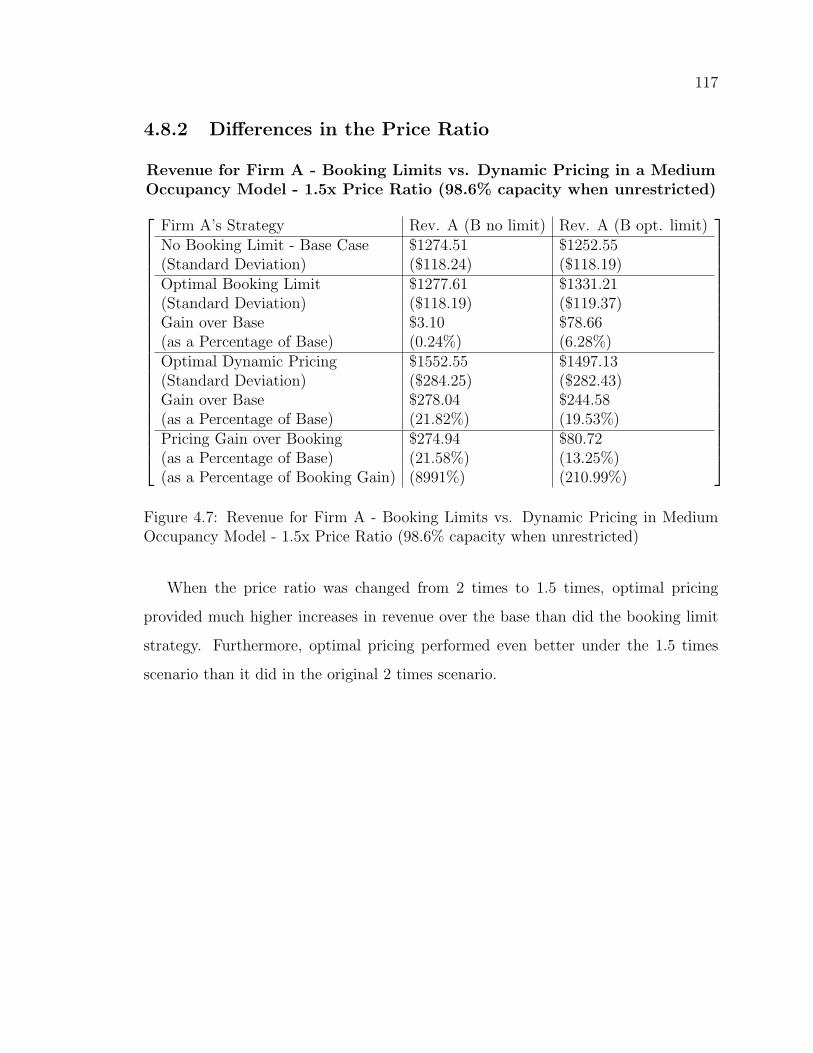
117
4.8.2 Differences in the Price Ratio
Revenue for Firm A - Booking Limits vs. Dynamic Pricing in a MediumOccupancy Model - 1.5x Price Ratio (98.6% capacity when unrestricted)
Firm A’s Strategy Rev. A (B no limit) Rev. A (B opt. limit)No Booking Limit - Base Case $1274.51 $1252.55(Standard Deviation) ($118.24) ($118.19)Optimal Booking Limit $1277.61 $1331.21(Standard Deviation) ($118.19) ($119.37)Gain over Base $3.10 $78.66(as a Percentage of Base) (0.24%) (6.28%)Optimal Dynamic Pricing $1552.55 $1497.13(Standard Deviation) ($284.25) ($282.43)Gain over Base $278.04 $244.58(as a Percentage of Base) (21.82%) (19.53%)Pricing Gain over Booking $274.94 $80.72(as a Percentage of Base) (21.58%) (13.25%)(as a Percentage of Booking Gain) (8991%) (210.99%)
Figure 4.7: Revenue for Firm A - Booking Limits vs. Dynamic Pricing in MediumOccupancy Model - 1.5x Price Ratio (98.6% capacity when unrestricted)
When the price ratio was changed from 2 times to 1.5 times, optimal pricing
provided much higher increases in revenue over the base than did the booking limit
strategy. Furthermore, optimal pricing performed even better under the 1.5 times
scenario than it did in the original 2 times scenario.
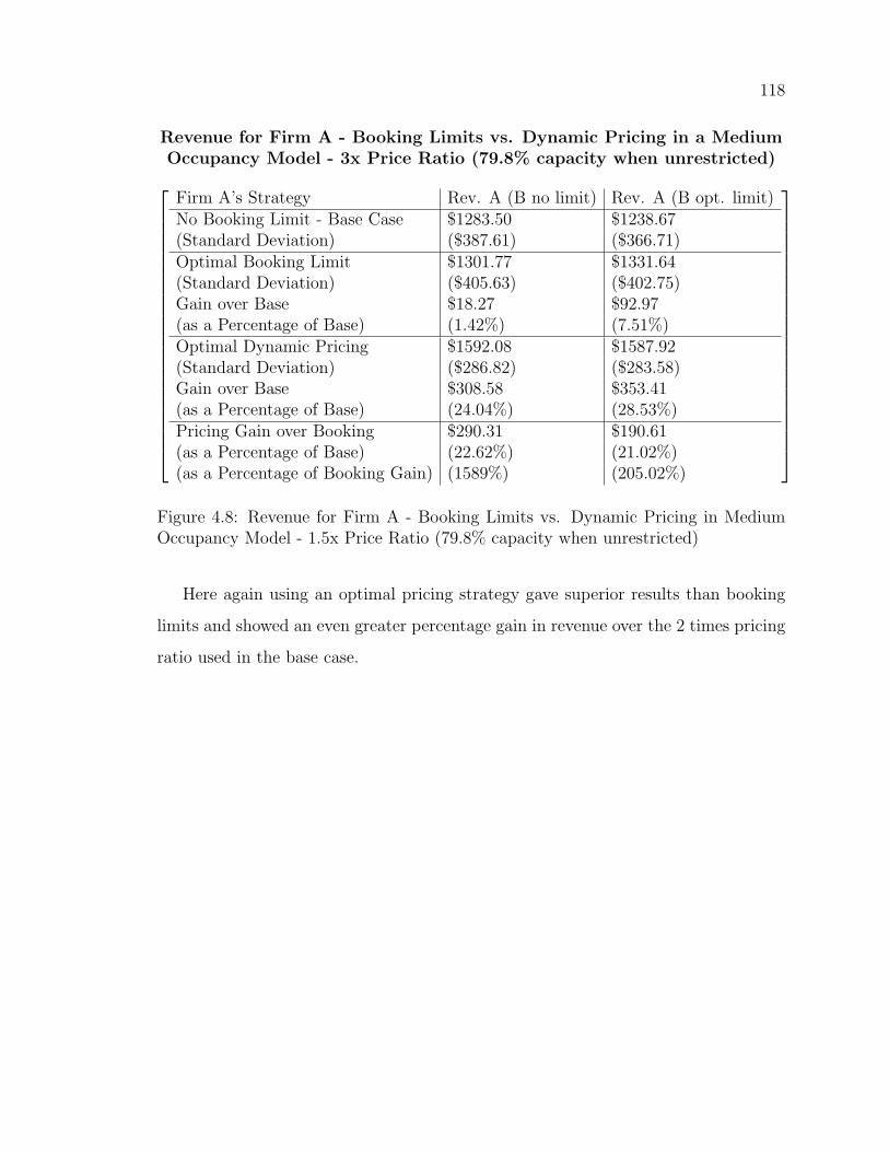
118
Revenue for Firm A - Booking Limits vs. Dynamic Pricing in a MediumOccupancy Model - 3x Price Ratio (79.8% capacity when unrestricted)
Firm A’s Strategy Rev. A (B no limit) Rev. A (B opt. limit)No Booking Limit - Base Case $1283.50 $1238.67(Standard Deviation) ($387.61) ($366.71)Optimal Booking Limit $1301.77 $1331.64(Standard Deviation) ($405.63) ($402.75)Gain over Base $18.27 $92.97(as a Percentage of Base) (1.42%) (7.51%)Optimal Dynamic Pricing $1592.08 $1587.92(Standard Deviation) ($286.82) ($283.58)Gain over Base $308.58 $353.41(as a Percentage of Base) (24.04%) (28.53%)Pricing Gain over Booking $290.31 $190.61(as a Percentage of Base) (22.62%) (21.02%)(as a Percentage of Booking Gain) (1589%) (205.02%)
Figure 4.8: Revenue for Firm A - Booking Limits vs. Dynamic Pricing in MediumOccupancy Model - 1.5x Price Ratio (79.8% capacity when unrestricted)
Here again using an optimal pricing strategy gave superior results than booking
limits and showed an even greater percentage gain in revenue over the 2 times pricing
ratio used in the base case.
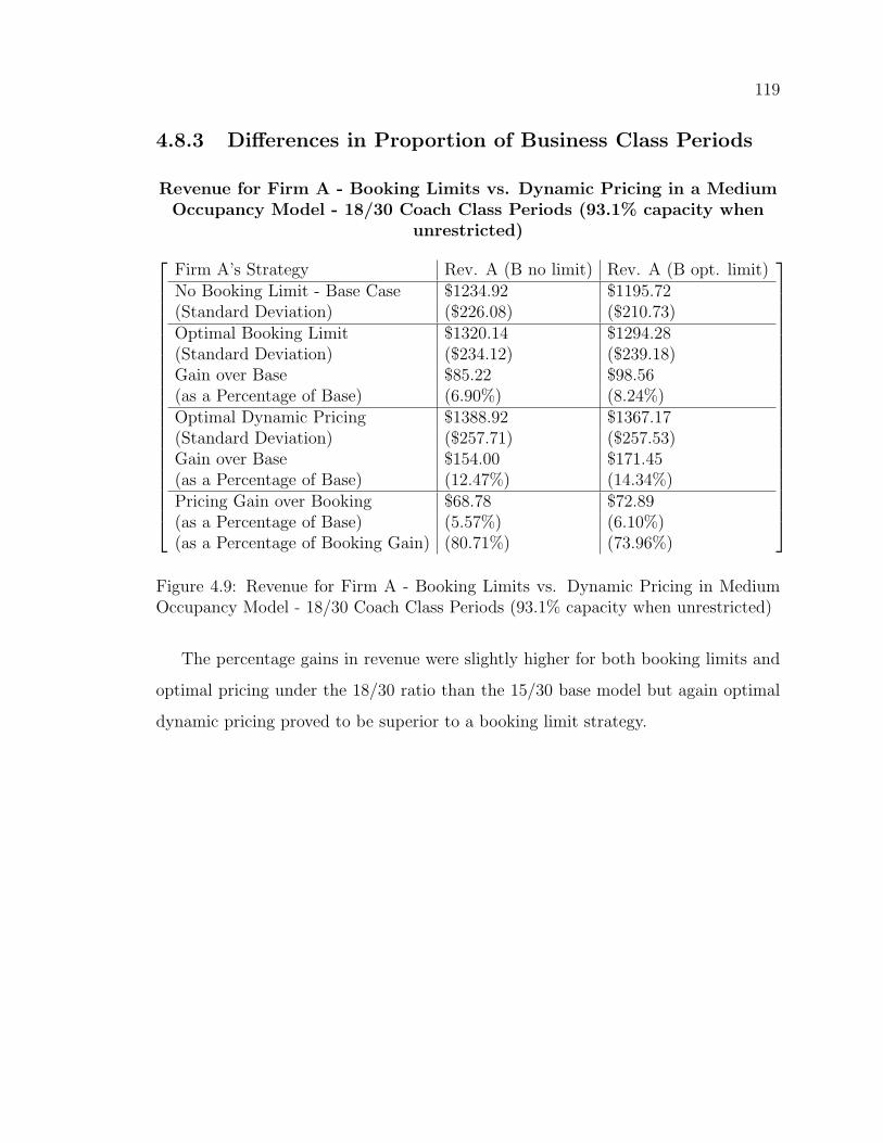
119
4.8.3 Differences in Proportion of Business Class Periods
Revenue for Firm A - Booking Limits vs. Dynamic Pricing in a MediumOccupancy Model - 18/30 Coach Class Periods (93.1% capacity when
unrestricted)
Firm A’s Strategy Rev. A (B no limit) Rev. A (B opt. limit)No Booking Limit - Base Case $1234.92 $1195.72(Standard Deviation) ($226.08) ($210.73)Optimal Booking Limit $1320.14 $1294.28(Standard Deviation) ($234.12) ($239.18)Gain over Base $85.22 $98.56(as a Percentage of Base) (6.90%) (8.24%)Optimal Dynamic Pricing $1388.92 $1367.17(Standard Deviation) ($257.71) ($257.53)Gain over Base $154.00 $171.45(as a Percentage of Base) (12.47%) (14.34%)Pricing Gain over Booking $68.78 $72.89(as a Percentage of Base) (5.57%) (6.10%)(as a Percentage of Booking Gain) (80.71%) (73.96%)
Figure 4.9: Revenue for Firm A - Booking Limits vs. Dynamic Pricing in MediumOccupancy Model - 18/30 Coach Class Periods (93.1% capacity when unrestricted)
The percentage gains in revenue were slightly higher for both booking limits and
optimal pricing under the 18/30 ratio than the 15/30 base model but again optimal
dynamic pricing proved to be superior to a booking limit strategy.
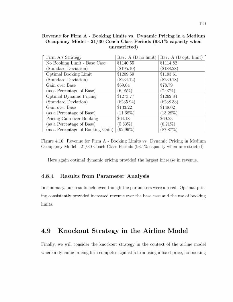
120
Revenue for Firm A - Booking Limits vs. Dynamic Pricing in a MediumOccupancy Model - 21/30 Coach Class Periods (93.1% capacity when
unrestricted)
Firm A’s Strategy Rev. A (B no limit) Rev. A (B opt. limit)No Booking Limit - Base Case $1140.55 $1114.82(Standard Deviation) ($195.10) ($188.28)Optimal Booking Limit $1209.59 $1193.61(Standard Deviation) ($234.12) ($239.18)Gain over Base $69.04 $78.79(as a Percentage of Base) (6.05%) (7.07%)Optimal Dynamic Pricing $1273.77 $1262.84(Standard Deviation) ($235.94) ($238.33)Gain over Base $133.22 $148.02(as a Percentage of Base) (11.68%) (13.28%)Pricing Gain over Booking $64.18 $69.23(as a Percentage of Base) (5.63%) (6.21%)(as a Percentage of Booking Gain) (92.96%) (87.87%)
Figure 4.10: Revenue for Firm A - Booking Limits vs. Dynamic Pricing in MediumOccupancy Model - 21/30 Coach Class Periods (93.1% capacity when unrestricted)
Here again optimal dynamic pricing provided the largest increase in revenue.
4.8.4 Results from Parameter Analysis
In summary, our results held even though the parameters were altered. Optimal pric-
ing consistently provided increased revenue over the base case and the use of booking
limits.
4.9 Knockout Strategy in the Airline Model
Finally, we will consider the knockout strategy in the context of the airline model
where a dynamic pricing firm competes against a firm using a fixed-price, no booking
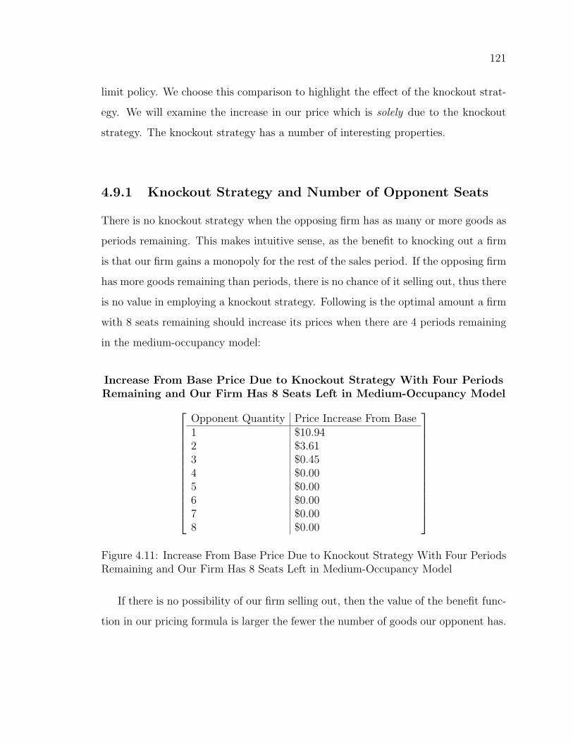
121
limit policy. We choose this comparison to highlight the effect of the knockout strat-
egy. We will examine the increase in our price which is solely due to the knockout
strategy. The knockout strategy has a number of interesting properties.
4.9.1 Knockout Strategy and Number of Opponent Seats
There is no knockout strategy when the opposing firm has as many or more goods as
periods remaining. This makes intuitive sense, as the benefit to knocking out a firm
is that our firm gains a monopoly for the rest of the sales period. If the opposing firm
has more goods remaining than periods, there is no chance of it selling out, thus there
is no value in employing a knockout strategy. Following is the optimal amount a firm
with 8 seats remaining should increase its prices when there are 4 periods remaining
in the medium-occupancy model:
Increase From Base Price Due to Knockout Strategy With Four PeriodsRemaining and Our Firm Has 8 Seats Left in Medium-Occupancy Model
Opponent Quantity Price Increase From Base1 $10.942 $3.613 $0.454 $0.005 $0.006 $0.007 $0.008 $0.00
Figure 4.11: Increase From Base Price Due to Knockout Strategy With Four PeriodsRemaining and Our Firm Has 8 Seats Left in Medium-Occupancy Model
If there is no possibility of our firm selling out, then the value of the benefit func-
tion in our pricing formula is larger the fewer the number of goods our opponent has.
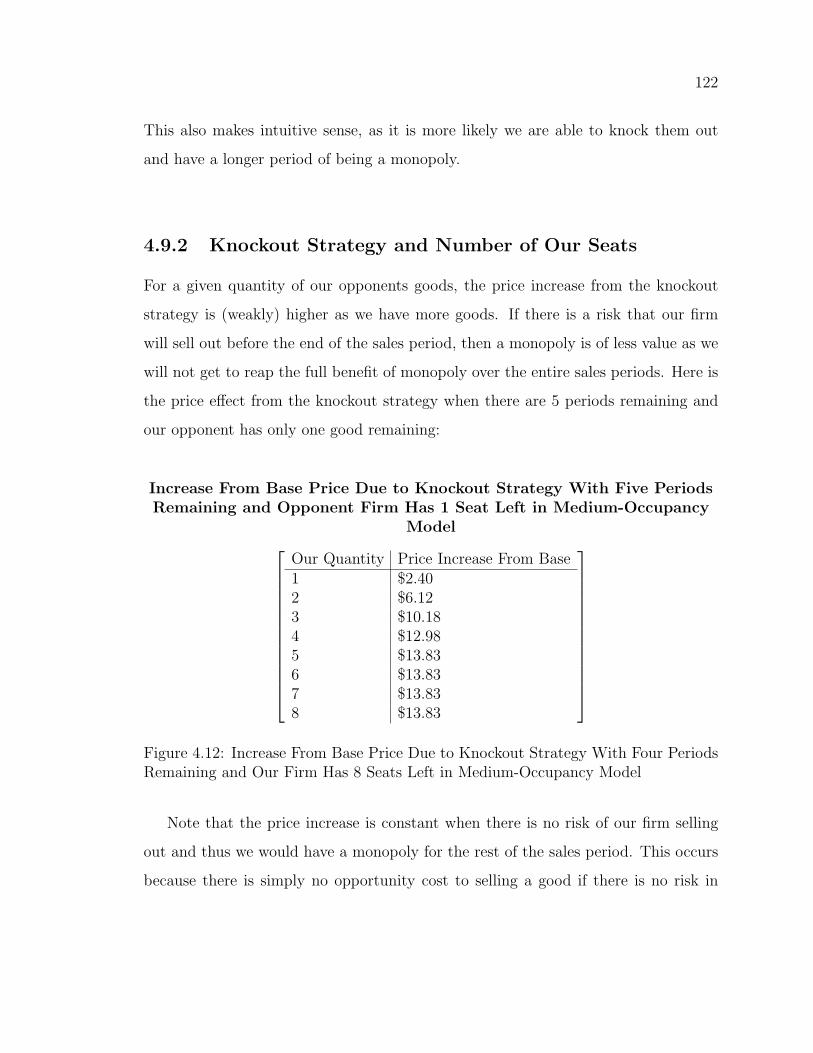
122
This also makes intuitive sense, as it is more likely we are able to knock them out
and have a longer period of being a monopoly.
4.9.2 Knockout Strategy and Number of Our Seats
For a given quantity of our opponents goods, the price increase from the knockout
strategy is (weakly) higher as we have more goods. If there is a risk that our firm
will sell out before the end of the sales period, then a monopoly is of less value as we
will not get to reap the full benefit of monopoly over the entire sales periods. Here is
the price effect from the knockout strategy when there are 5 periods remaining and
our opponent has only one good remaining:
Increase From Base Price Due to Knockout Strategy With Five PeriodsRemaining and Opponent Firm Has 1 Seat Left in Medium-Occupancy
Model
Our Quantity Price Increase From Base1 $2.402 $6.123 $10.184 $12.985 $13.836 $13.837 $13.838 $13.83
Figure 4.12: Increase From Base Price Due to Knockout Strategy With Four PeriodsRemaining and Our Firm Has 8 Seats Left in Medium-Occupancy Model
Note that the price increase is constant when there is no risk of our firm selling
out and thus we would have a monopoly for the rest of the sales period. This occurs
because there is simply no opportunity cost to selling a good if there is no risk in
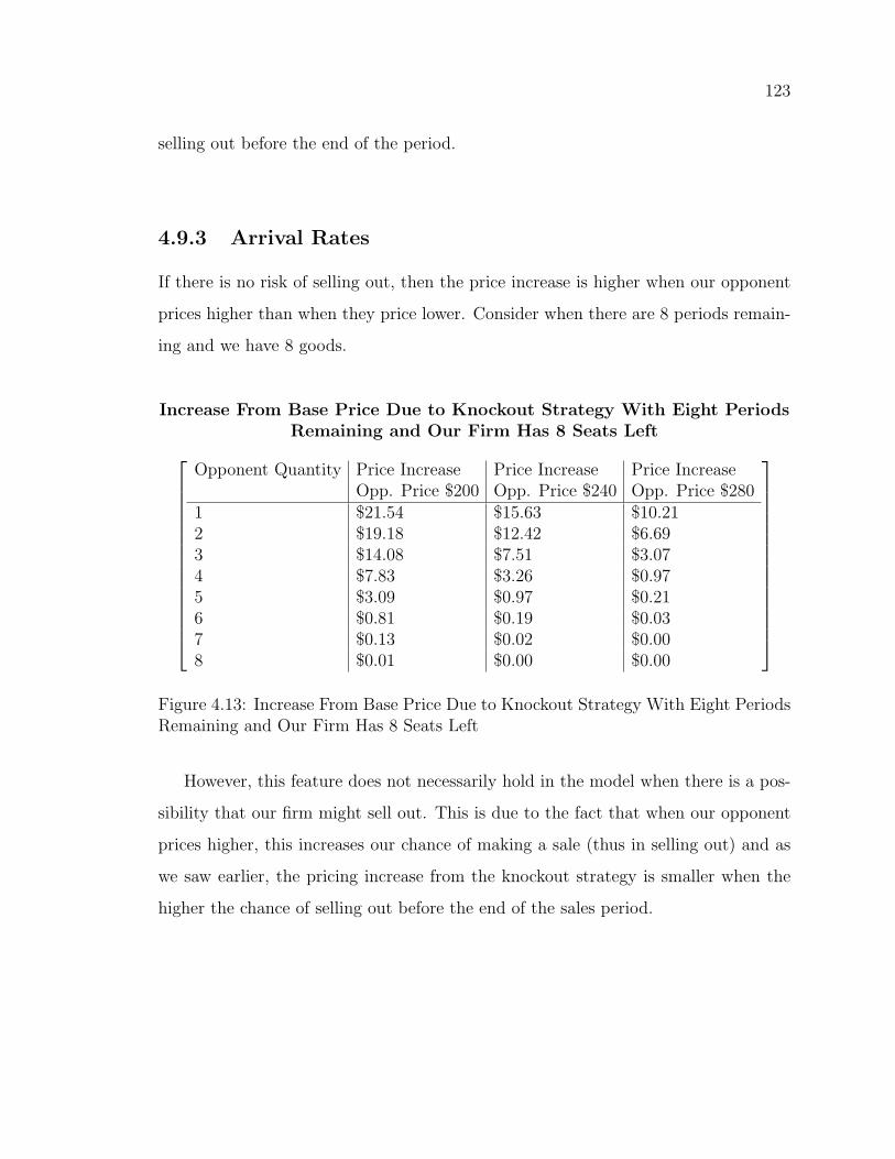
123
selling out before the end of the period.
4.9.3 Arrival Rates
If there is no risk of selling out, then the price increase is higher when our opponent
prices higher than when they price lower. Consider when there are 8 periods remain-
ing and we have 8 goods.
Increase From Base Price Due to Knockout Strategy With Eight PeriodsRemaining and Our Firm Has 8 Seats Left
Opponent Quantity Price Increase Price Increase Price IncreaseOpp. Price $200 Opp. Price $240 Opp. Price $280
1 $21.54 $15.63 $10.212 $19.18 $12.42 $6.693 $14.08 $7.51 $3.074 $7.83 $3.26 $0.975 $3.09 $0.97 $0.216 $0.81 $0.19 $0.037 $0.13 $0.02 $0.008 $0.01 $0.00 $0.00
Figure 4.13: Increase From Base Price Due to Knockout Strategy With Eight PeriodsRemaining and Our Firm Has 8 Seats Left
However, this feature does not necessarily hold in the model when there is a pos-
sibility that our firm might sell out. This is due to the fact that when our opponent
prices higher, this increases our chance of making a sale (thus in selling out) and as
we saw earlier, the pricing increase from the knockout strategy is smaller when the
higher the chance of selling out before the end of the sales period.
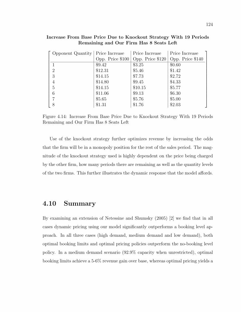
124
Increase From Base Price Due to Knockout Strategy With 19 PeriodsRemaining and Our Firm Has 8 Seats Left
Opponent Quantity Price Increase Price Increase Price IncreaseOpp. Price $100 Opp. Price $120 Opp. Price $140
1 $9.42 $3.25 $0.602 $12.31 $5.46 $1.423 $14.15 $7.73 $2.724 $14.80 $9.45 $4.335 $14.15 $10.15 $5.776 $11.06 $9.13 $6.307 $5.65 $5.76 $5.008 $1.31 $1.76 $2.03
Figure 4.14: Increase From Base Price Due to Knockout Strategy With 19 PeriodsRemaining and Our Firm Has 8 Seats Left
Use of the knockout strategy further optimizes revenue by increasing the odds
that the firm will be in a monopoly position for the rest of the sales period. The mag-
nitude of the knockout strategy used is highly dependent on the price being charged
by the other firm, how many periods there are remaining as well as the quantity levels
of the two firms. This further illustrates the dynamic response that the model affords.
4.10 Summary
By examining an extension of Netessine and Shumsky (2005) [2] we find that in all
cases dynamic pricing using our model significantly outperforms a booking level ap-
proach. In all three cases (high demand, medium demand and low demand), both
optimal booking limits and optimal pricing policies outperform the no-booking level
policy. In a medium demand scenario (92.9% capacity when unrestricted), optimal
booking limits achieve a 5-6% revenue gain over base, whereas optimal pricing yields a
125
11-12% gain. In high demand situations (99.1% capacity when unrestricted), optimal
booking limit policies substantially increase revenue (22-29% revenue gains over base)
but are significantly outperformed by optimal pricing policies (36-50% revenue gains
over base). Optimal booking limit policies are of marginal value in low demand sce-
narios (75.9% capacity when unrestricted) providing only a 0.4-0.6% gain in revenue.
Optimal pricing policies, however, continue to achieve significant revenue gains of
roughly 12-13%. Switching from optimal booking to optimal pricing yields significant
revenue increases under any demand scenario including one where our opponent has
few goods remaining. This situation allows the firm to further maximize revenue by
using the knockout strategy. Optimal pricing is a more nuanced strategy and takes
more factors into consideration, which leads to increased revenues for the firm.
126
Chapter 5
Conclusion and Future Research
5.1 Introduction - Background and Purpose
As discussed in the introduction to this thesis, there are three important pricing
properties of revenue management markets of interest:
• The prices charged by the firms are not identical, and in some cases there
are large differences in the prices firms charge for a comparable product (see
Enterprise vs. Hertz ). This suggests that the products are not commodities -
a level of brand differentiation exists.
• Firms offer a range of similar, but non-identical products. When Hertz lowers
the price of mid-size rentals, this should increase the quantity demanded of
these cars, but it may also reduce the demand for compact and standard cars.
• Firms can engage in diagonal competition. That is, Hertz may be the preferred
brand of a customer, but if Enterprise or Budget price low enough, customers
may be willing to choose a higher-end car from these companies, for what they
would have paid Hertz for a lower-end car.
127
However, typical revenue management models consider at most one of these prop-
erties and fails to address all three simultaneously. Revenue management has lacked
a model to adequately describe price competition in an oligopoly. The need for such
a model is well-known and appears in the “future research” section of many studies,
see Lu (2009) [5] as an example. Xavier Vives is quoted as saying:
“The question is, has oligopoly theory failed? ... Oligopolistic business
patterns have lacked a benchmark model of dynamic price formation. A
benchmark model could provide a counterpart to well-established static
models and some insight toward resolving dynamically the issue of an
appropriate game form. The model should be tractable and based on
plausible assumptions, and firms should use ‘simple’ strategies so that
the model can deliver relatively robust predictions. Such a result is not
possible with the repeated game model, which has probably received too
much attention.” [11]
While we share Vives’ frustration with the lack of progress in modeling oligopoly
problems in revenue management, our line of research illustrates that the repeated
game model can successfully be used to model the interactions between firms.
We have illustrated the importance of simultaneously considering five factors when
pricing a good in a revenue management context:
1. Quantity level of the product.
2. Quantity level of the firm’s other products.
3. Quantity level of other firms’ products.
4. Cannibalization, cross-price elasticity and the price of our firm’s other products.
128
5. Competition, cross-price elasticity and the price of competitor products.
While there is still much research to be completed in this area, this thesis maps
out an ambitious research agenda to create pricing models that adequately resemble
real-world markets.
5.2 Creating and Solving NxM Pricing Demand
Models
In Chapter 2, we create a twice continuously differentiable geometric demand frame-
work that allows for an unlimited (but finite) number of firms and products. This
allows for the creation of mathematically tractable optimal pricing models that have
multiple product classes from multiple firms. In Chapter 1 we saw how markets of
interest to revenue managers have multiple firms selling multiple classes of goods.
However, existing revenue management models allow for at most two of the following
three features: multiple firms, multiple goods, optimal pricing. Our framework allows
for all three simultaneously. There are two parts of our model that make this possi-
ble; a geometric demand model which is unique to this paper and a ‘single-customer
per period buys at most a single-product’ assumption which is relatively common in
the literature. We prove the existence of subgame perfect Nash Equilibria and then
solve the NxM model recursively. Unlike many models in the Bertrand-Edgeworth
competition literature, we can be assured that there is, in fact, a solution to any NxM
model. We cannot be assured that a unique solution will exist to all NxM models.
In general it is necessarily to solve the model recursively to find the optimal price in
each particular state in which it finds itself. We have not found a way to express the
optimal price in a particular state as a function of the variables in the model; it is
129
likely only possible to do so for the most trivial of models. We give two methods for
proving that a unique solution exists in a particular application of the model. We then
give conditions under which a solution will exist in a 2-firm/1-product-per-firm model.
The model created in the chapter considers own price elasticity of demand for
a product along with five factors: The quantity level of the product (factor 1), the
quantity level of the firm’s other products (factor 2), quantity level of the competi-
tor’s products (factor 3), cannibalization and cross-price elasticity between products
sold by the firm (factor 4) and cross-price elasticity between the firm’s product and
those of its competitors (factor 5).
5.2.1 Implications For Future Research
While we were able to prove the existence of Nash Equilibria, determining the condi-
tions to guarantee the existence of unique Nash Equilibria remains an area for future
research. We hope to show that the conditions for unique subgame perfect Nash
Equilibria are relatively flexible. While multiple equilibria do not render the model
useless, it may be difficult to advise a rental car company to “price their cars at
either $20.00 or $50.00”. Future research can also include studying when a number
of classic dynamic properties hold, such as under what conditions can we assure that
the optimal price is monotonic in the arrival rate.
130
5.3 Two Optimal Dynamic Pricing Examples
Chapter 3 contains two examples. A 2-firm/1-product-per-firm car rental model is
created. We show that if a firm does not take market structure into account (acts as if
it has a monopoly instead of a duopoly), it can do worse by trying to price optimally
instead of using a simple fixed-price pricing rule. A firm’s revenue will be reduced if
both factor 3 (opponent’s quantity) and factor 5 (competitive price effects) are not
considered. Although the model we develop assumes that firms know the quantity
levels of their competitors, we show that the firm can increase its revenues by consid-
ering spill-over effects and cross-elasticity, even if it is unaware of the quantity level
of the other firm in the market and must ignore factor 3. The highest revenues accrue
to the firm when it simultaneously considers all five factors. We show the existence of
a knockout strategy, stemming from factor 3, where a firm will price higher, in order
to give sales to the other firm. It does so in order to have that firm sell out of its
good, so the firm can have a monopoly for the rest of the sales period.
Later in the chapter a 2x3 rental car model is created. We show that a firm can
reduce its profit by using traditional revenue management techniques, that ignore
factor 4, to price its cars. This is due to existing models not considering spillover
effects between their brands. If spillover effects are ignored, firms will price their low
end cars too low which will cannibalize the sales of their higher-end/higher-margin
offerings. In our framework, prices are typically higher for lower end cars and lower
for higher end cars than in traditional revenue management models. Again, all five
factors must be considered simultaneously in order to maximize revenue.
131
5.3.1 Implications For Future Research
There are a great number of potential extensions for future research that would add
realism to the model. The first is a realization that not all bookings result in a final
sale, thus it is in the interest of the firm to overbook. A customer who books will be a
no-show by some probability τ , which can be incorporated into the model. It may be
possible to alter the model such that the firm can, in theory, accepted an unlimited
number of bookings, but pays a substantial cost for each overbooked customer it is
forced to compensate.
An important area for future applied research is determining reasonable estimates
for cross-price elasticity in revenue management markets of interest. While Anderson,
Davison and Rasmussen [1] and Geraghty and Johnson [4] indicate that substantial
cross-price elasticity exists in the rental car market, there are no published cross-price
elasticity parameter estimates. It is likely that such research will have to come with
the assistance of a rental car company in order to obtain the necessary data. Future
research should also consider alternative formulations of cross-price elasticity, as the
one used in this model may turn out not to be optimal for real-world applications.
However, the common assumption of constant cross-price elasticity may be inappro-
priate as well.
5.4 Booking Limits and Optimal Pricing in a 2-
Firm, 2 Class Airline Model
We consider the well-known 2-firm, 2-seat class Netessine and Shumsky [7] model
in Chapter 4. We recreate the model but allow our firm to use an optimal pricing
132
strategy rather than a booking limits strategy, to take advantage of factor 5 and own
price elasticity of demand, both of which are lacking in the Netessine and Shumsky
model. In a period of high demand (where the occupancy rate is 99.1% of capacity
in the absence of booking limits), a booking limit strategy provides a revenue in-
crease of 22-29% over having no strategy at all. However, an optimal pricing strategy
provides a 36-50% revenue increase over the no strategy case. We find that rather
than closing coach class seats, a firm should increase the price it charges for these
seats when demand is high. As with a booking limit, it will decrease the number
of seats sold, but do so at a much greater revenue-per-seat. We then test medium
demand (92.9% capacity) and low demand (75.9%) situations and find that an op-
timal pricing strategy significantly outperforms a booking limits strategy here as well.
5.4.1 Implications For Future Research
Elmaghraby and Keskinocak (2003) [3] discuss how a firm will often sell the same in-
ventory through different channels at different prices, such as through its own website,
through a third-party website such as Expedia.com, to travel agents, and to walk-up-
traffic. Future research should consider situations where a firm’s inventory is shared
through a number of different sales channels.
The ‘at most one arrival per period’ condition appears necessary to assure the
existence of Nash Equilibria - see Tirole (1988) [9], Davidson and Deneckere (1986)
[2], Madden (1998) [6], Osborne and Pitchik (1986) [8] and Vives (1993) [10]. It may
be possible to loosen the ‘an arrival purchases at most one good’ assumption to allow
for group bookings. One way may be as follows: Treat individual sales and sales of
a fixed size (e.g. four) to be two different product classes with a shared inventory.
133
Firms with enough inventory to cover the group booking set a price for both the group
and individual, whereas a firm with not enough inventory to cover a group booking
only sets a price for the individual booking. Each period a single customer who is
looking for either a group booking or an individual booking arrives with probability λ.
Similarly, in a real-world scenario one cannot avoid the issue of bundling of goods.
A customer purchases a bundle containing an airline seat to a destination and a re-
turn ticket. Online retailers such as Expedia and Orbitz allow the bundling of a car
rental, hotel stay and airline ticket for a single price. Length of stay/length of rental
can also be thought of as a bundle - a two-day stay in a hotel is a bundle of a room
rental for Tuesday night and a room rental for Wednesday night. An area for future
research is a dynamic pricing model that allows firms to price and bundle separate
goods and services together.
5.5 Final Thoughts
It is our hope that the contribution we have made to the study of modeling multiple-
firm/multiple-products per firm problems in revenue management will spark new
interest in this area of study and will stimulate the development of revenue manage-
ment models which are more realistic in this regard.
134
Bibliography for Chapter 1
[1] A. Rakesh A. Rajan and R. Steinberg. Dynamic pricing and ordering decisionsby a monopolist. Management Science, 38:240–262, 1992.
[2] N. Abrams. 5q with car rental consultant neil abrams. Travel Management,2008.
[3] B. Allen and M. Hellwig. Bertrand-edgeworth oligopoly in large markets. Reviewof Economic Studies, 53:175–204, 1986.
[4] G. Allenby and P. Rossi. Quality perceptions and asymmetric switching betweenbrands. Marketing Science, 10:185–204, 1991.
[5] C.K. Anderson and J.G. Wilson. Wait or buy? the strategic consumer: Pricingand profit implications. Journal of the Operations Research Society, 54:299–306,2004.
[6] E. Johnson B. Hardie and P. Fader. Modeling loss aversion and reference de-prendence effects on brand choice. Marketing Science, 12.4:378–394, 1993.
[7] D. Granot B. Mantin and F. Granot. A dynamic pricing model under duopolycompetition. 2007.
[8] R. Batra and I. Sinha. Consumer-level factors moderating the success of privatlabel brands. Journal of Retailing, 76.2:175–191, 2000.
[9] P.C. Bell and M. Zhang. Management decision-making in the single periodoptimum pricing problem. Journal of the Operations Research Society, 57:377–388, 2006.
[10] P.P. Belobaba. Application of a probabilistic decision model to airline seatinventory control. Operations Research, 37.2:183–197, 1989.
[11] J. Bertrand. Theorie mathematique de la richesse sociale. Journal des Savants,67:499–508, 1883.
135
[12] G.R. Bitran and S.V. Mondschein. An application of yield management to thehotel industry considering multiple day stays. Operations Research, 43:427–443,1995.
[13] G.R. Bitran and S.V. Mondschein. Periodic pricing of seasonal products inretailing. Management Science, 43:64–79, 1998.
[14] R.F. Bordley. Estimating automotive elasticities from segment elasticities andfirst choice / second choice data. Review of Economics and Statistics, 75.3:455–462, 1993.
[15] B. Bronnenberg and L. Wathieu. Asymmetric promotion effects and brandpositioning. Marketing Science, 15.4:379–394, 1996.
[16] J. Jaskold Gabszewicz C. d’Aspremont and J.F. Thisse. On hotelling’s stabilityin competition. Econometrica, 47.5:1145–1150, 1979.
[17] G.P. Cachon and P. Feldman. Is advance selling desirable with competition?Working Paper, University of Pennsylvania, 2010.
[18] X. Chen and D. Simchi-Levi. Coordinating inventory control and pricingstrategies with random demand and fixed ordering cost. Working Paper, Mas-sachusetts Institute of Technology, 2002.
[19] J. Chevalier and A. Goolsbee. Measuring prices and price competition online:Amazon.com and barnesandnoble.com. Quantitative Marketing and Economics,1:203–222, 2003.
[20] J. Chiang. A simultaneous approach to the whether, what, and how much tobuy questions. Marketing Science, 10.4:297–315, 1991.
[21] P.K. Chintagunta. Investigating purchase incidence, brand choice, and purchasequantity decisions of households. Marketing Science, 12.2:184–208, 1993.
[22] M. Davison C.K. Anderson and H. Rasmussen. Revenue management: A realoptions approach. Naval Research Logistics, 51.5:686–703, 2004.
[23] A.A. Cournot. Researches Into the Mathematical Principles of the Theory ofWealth - Translated by N.T. Bacon. Augustus Kelley, 1971.
[24] A. Dasci. Dynamic pricing of perishable assets under competition: a two-periodmodel. Working Paper, York University.
136
[25] P. Dasgupta and E. Maskin. The existence of equilibria in discontinuous eco-nomic games ii. Review of Economic Studies, 53:1–41, 1986.
[26] C. Davidson and R. Deneckere. Long-term competition in capacity, short-runcompetition in price, and the cournot model. Rand Journal of Economics,17:404–415, 1986.
[27] J. Dawes. Negative evidence of asymmetric brand substitution between man-ufacturer brands and lower priced store brands. Marketing Discoveries, pages259–263, 2003.
[28] V. Martinez de Albeniz and K. Talluri. dynamic pricing competition with fixedcapacities. Management Science, 2011.
[29] S. Deng and C. Yano. Joint production and pricing decisions with setup costsand capacity constraints. Management Science, 52:741–756, 2006.
[30] H. Dixon. Bertrand-edgeworth equilibria when firms avoid turning customersaway. Journal of Industrial Economics, 39.2:131–146, 1990.
[31] J. Chiang D.R. Bell and V. Padmanabhan. The decomposition of promotionalresponse: An empirical generalization. Marketing Science, 18.4:504–526, 1999.
[32] M. Dudey. Dynamic edgeworth-bertrand competition. Quarterly Journal ofEconomics, 107:1461–1477, 1992.
[33] B. Eckfeldt. What does rfid do for the consumer? Communications of theACM, 48.9:77–79, 2005.
[34] F.Y. Edgeworth. The mathematical theory of banking. Journal of the RoyalStatistics Society, 51:113–127, 1888.
[35] W. Elmaghraby and P. Keskinocak. Dynamic pricing in the presence of inven-tory considerations: Research overview, current practices, and future directions.Management Science, 49.10:1287–1309, 2003.
[36] J.B. Kruse et. al. Bertrand-edgeworth competition in experimental markets.Econometrica, 62.2:343–371, 1994.
[37] K. Talluri et. al. Revenue management: Models and methods. Proceedings of ofthe 2008 Winter Simulation Conference - Institute of Electrical and ElectornicsEngineering, Inc. (IEEE), 2008.
137
[38] A. Federgruen and A. Heching. Combined pricing and inventory control underuncertainty. Operations Research, 47(275-295), 1999.
[39] Y. Feng and G. Gallego. Optimal starting times for end-of-season sales andoptimal stopping times for promotional fares. Management Science, 41:1371–1391, 1995.
[40] I. Fisher. Cournot and monopoly economics. Quarterly Journal of Economics,12.2:119–138, 1898.
[41] J. Friedman. Non-cooperative equilibrium for supergames. Review of EconomicStudies, 38:1–12, 1971.
[42] J. Friedman. Oligopoly and the Theory of Games. North Holland, 1977.
[43] Drew Fudenberg and Jean Tirole. Game Theory. MIT Press, 1991.
[44] G. Gallego and G. van Ryzin. A multi-product dynamic pricing of inventorieswith stochastic demand over finite horizons. Management Science, 40:999–1020,1994.
[45] M.K. Geraghty and E. Johnson. Revenue management saves national car rental.Interfaces, 27:107–127, 1997.
[46] P.K. Goldberg. Product differentiation and oligopoly in international markets:The case of the u.s. automobile industry. Econometrica, 63.4:891–951, 1995.
[47] S. Gupta. Impact of sales promotion on when, what, and how much to buy.Journal of Marketing Research, 25:342–355, 1988.
[48] H. Helson. Adaptation Level Theory. Harper and Row, 1964.
[49] C.T. Heun. Dynamic pricing boosts bottom line. Information Week, October29, 2001.
[50] S. Gupta H.J. Van Heerde and D.R. Wittink. Edgeworth and modern oligopolytheory. European Economic Review, 37.2:463–476, 1993.
[51] H. Hotelling. Stability in competition. Economic Journal, 39:41–57, 1929.
[52] M. Hu. Dynamic Oligopoly Models in Revenue Management and Supply ChainManagement. Ph.D Thesis, Columbia University, 2009.
138
[53] K. Isler and H. Imhof. A game theoretic model for airline revenue manage-ment and competitive pricing. Journal of Revenue and Pricing Management,2008:384–396, 2008.
[54] Q. Yuan J. Song and Y. Mao. Two-player two-fare-class hotel revenue man-agement game with incomplete information of transferred customers. 2010 In-ternational Conference of Information Science and Management Engineering,pages 351–355, 2010.
[55] C.J. Lautenbacher J. Subramanian and S.J. Stidham. Yield management withoverbooking, cancellations and no shows. Transportation Science, 33:147–167,1999.
[56] C.K. Anderson J.G. Wilson and S.W. Kim. Optimal booking limits in the pres-ence of strategic consumer behavior. International Transactions in OperationalResearch, 13.2:99–110, 2006.
[57] J.G. Lynch Jr. and D. Ariely. Wine online: Search costs affect competition onprice, quality, and distribution. Marketing Science, 19.1:83–103, 2000.
[58] S. Netessine K. Jerath and S.K. Veeraraghavan. Revenue management withstrategic customers: Last-minute selling and opaque selling. Management Sci-ence, 56.3:430–448, 2010.
[59] W. Kamakura and G. Russell. A probabilistic choice model for market seg-mentation and elasticity structure. Journal of Marketing Research, 26:379–390,1989.
[60] P.K. Kannan and P.K. Kopalle. Dynamic pricing on the internet: Importanceand implications for consumer behavior. International Journal of ElectronicCommerce, 5.3:63–83, 2001.
[61] P. Kourouthanassis and G. Roussos. Pervasive computing. Applied Math at theUniversity of Western Ontario M.Sc. Thesis, 2.2:32–39, 2003.
[62] D. Simchi-Levi L. Chan and J. Swann. Dynamic pricing strategies for manufac-turing with stochastic demand and discretionary sales. Working Paper, GeorgiaInstitute of Technology, 2002.
[63] C.J. Lautenbacher and S.J. Stidham. The underlying markov decision processin the single-leg airline yield management problem. Transportation Science,33:136–146, 1999.
139
[64] E. Lazear. Retail pricing and clearance sales. American Economic Review,76.1:14–32, 1986.
[65] R. Levitan and M. Shubik. Price duopoly and capacity constraints. Interna-tional Economic Review, 13.1:111–122, 1972.
[66] K. Lin and S. Sidbari. Dynamic price competition with discrete customerchoices. European Journal of Operational Research, 197.3:969–980, 2009.
[67] Q. Liu and D. Zhang. Dynamic pricing competition and strategic customersunder vertical product differentiation. Working Paper, 2011.
[68] Y. Lu. Essays on Inventory, Pricing and Financial Trading Strategies. Ph.DThesis, Massachusetts Institute of Technology, 2009.
[69] P. Madden. Elastic demand, sunk costs and the kreps-scheinkman extension ofthe cournot model. Economic Theory, 12:199–212, 1998.
[70] M. Manas. A linear oligopoly game. Econometrica, 40.5:917–922, 1972.
[71] B.A. Marcus and C.K. Anderson. Online low price guarantees - a real optionsanalysis. Operations Research, 54:1041–1050, 2006.
[72] E. Maskin and J. Tirole. A theory of dynamic oligopoly ii: Price competi-tion, kinked demand curves, and edgeworth cycles. Econometrica, 56.3:571–599,1988.
[73] H. Moore. Paradoxes of competition. Quarterly Journal of Economics, 20.2:211–230, 1906.
[74] V. Bradshaw N. Raza and M. Hague. Applications of rfid technology. IEEEColloquium on RFID Technology, 1999/123, 1999.
[75] P. Nelson. Advertising as information. Journal of Political Economy, 82:729–754, 1974.
[76] S. Netessine and R.A. Shumsky. Revenue management games: horizontal andvertical competition. Management Science, 51.5, 2005.
[77] W. Nichols. Microeconomic Theory: Basic Principles and Extensions - 9thEdition. South-Western College Publications, 2004.
[78] H. Nikaido and K. Isoda. Note on non-cooperative convex games. PacificJournal of Mathematics, 5.S1:807–815, 1955.
140
[79] M.J. Osborne and C. Pitchik. Price competition in a capacity-constrainedduopoly. Journal of Economic Theory, 38.2, 1986.
[80] G. Savard P. Marcotte and D. Zhu. Mathematical structure of a bilevel strategicpricing model. European Journal of Operational Research, 193:552–566, 2009.
[81] A. Parlakturk and M.O. Kabul. The value of commitments when selling tostrategic customers: A supply chain perspective. Working Paper, University ofNorth Carolina, 2010.
[82] G. Perakis and A. Sood. Competitive multi-period pricing for perishable prod-ucts: A robust optimization approach. Mathematical Programming, 107:295–335, 2006.
[83] R. Phillips. Pricing and Revenue Optimization. Stanford University Press,2005.
[84] I. Popescu and Y. Wu. Dynamic pricing strategies with reference effects. Op-erations Research, Forthcoming, 2007.
[85] V. Srinivasan R. Sethuraman and D. Kim. Asymmetric and neighborhood cross-price effects: Some empirical generalizations. Marketing Science, 18.1:23–41,1999.
[86] S. Gupta R.E. Bucklin and S. Siddarth. Determining segmentation in salesresponse across consumer purchase behaviors. Journal of Marketing Research,35:189–197, 1998.
[87] D. Reibstein and H. Gatignon. Optimal product line pricing: The influence ofelasticities and cross-elasticities. Journal of Marketing Research, 21:259–267,1984.
[88] E. Roll. Social significance of recent trends in economic theory. CanadianJournal of Economics and Political Science, 6.3:448–459, 1940.
[89] D. Simchi-Levi S. Biller, L. Chan and J. Swann. Dynamic pricing and the direct-to-customer model in the automotive industry. Electronic Commerce Journal,2002.
[90] S. Savin s. Netessine and W. Xiao. Revenue management through dynamiccross selling in e-commerce retailing. Operations Research, 54:893–913, 2006.
[91] J. Schumpeter. Instability of capitalism. The Economics Journal, 38.151:361–386, 1928.
141
[92] R. Sethuraman and V. Srinivasan. The asymmetric share effect: An empiricalgeneralization on cross-price effects. Journal of Marketing Research, 39.3:379–386, 2002.
[93] K. Sivakumar and S. Raj. Quality-tier competition: How price changes influencebrand choice and category choice. Journal of Marketing, 61:71–84, 1997.
[94] S. Smith and D. Achabal. Clearance pricing and inventory policies for retailchains. Management Science, 44:285–300, 1998.
[95] J. Stigler. Notes on the theory of duopoly. Journal of Political Economy,48.4:521–541, 1940.
[96] X. Su. Intertemporal pricing with strategic consumer behavior. ManagementScience, 53:726–741, 2007.
[97] K. Talluri. On equilibria in duopolies with finite strategy spaces. TechnicalReport WP-701, Universitat Pompeu Fabra, 2003.
[98] K. Talluri and G. van Ryzin. The Theory and Practice of Revenue Management.Kluwer Academic Publishers, 2004.
[99] A. Tasnadi. A two-stage bertrand-edgeworth game. Economic Letters, 65:353–358, 1999.
[100] L. Thomas. Price-production decisions with deterministic demand. Manage-ment Science, 16:747–750, 1970.
[101] G.T. Thowsen. A dynamic nonstationary inventory problem for a price/quantitysetting firm. Naval Research Logistics Quarterly, 22:461–476, 1975.
[102] J. Tirole. The Theory of Industrial Organization. MIT Press, 1988.
[103] X. Vives. Edgeworth and modern oligopoly theory. European Economic Review,37.2:463–476, 1993.
[104] X. Vives. Oligopoly Pricing: Old Ideas and New Tools. MIT Press, 1999.
[105] P.R. Wurman. Dynamic pricing in the virtual marketplace. Internet Computing,5.2:36–42, 2001.
[106] X. Xu and W.J. Hopp. A monopolistic and oligopolistic stcohastic flow revenuemanagement model. Operations Research, 54.6:1098–1109, 2006.
142
[107] J. McGill Y. Levin and M. Nediak. Price guarantees in dynamic pricing andrevenue management. Operations Research, 55:75–97, 2007.
[108] J. McGill Y. Levin and M. Nediak. Dynamic pricing in the presence of strate-gic consumers and oligopolistic competition. Management Science, 55.1:32–46,2009.
[109] P.S. You. Dynamic pricing in airline seat management for flights with multiplelegs. Transportation Science, 33:192–206, 1999.
[110] E. Zabel. Monopoly and uncertainty. Review of Economic Studies, 37:205–219,1970.
[111] W. Zhao and Y. S. Zheng. Optimal dynamic pricing for perishable assets withnonhomogeneous demand. Management Science, 46.3:375–388, 2000.
143
Bibliography for Chapter 2
[1] M.D. Whinston A. Mas-Colell and J.R. Green. Microeconomic Theory. OxfordUniversity Press, 1995.
[2] V. Martinez de Albeniz and K. Talluri. dynamic pricing competition with fixedcapacities. Management Science, 2011.
[3] M. Dudey. Dynamic edgeworth-bertrand competition. Quarterly Journal ofEconomics, 107:1461–1477, 1992.
[4] J. Eichberger. Game Theory for Economists. Academic Press Inc., 1993.
[5] Drew Fudenberg and Jean Tirole. Game Theory. MIT Press, 1991.
[6] S. Lang. Analysis I. Addison-Wesley Publishing Company, 1968.
[7] K. Lin and S. Sidbari. Dynamic price competition with discrete customer choices.European Journal of Operational Research, 197.3:969–980, 2009.
[8] Y. Lu. Essays on Inventory, Pricing and Financial Trading Strategies. Ph.DThesis, Massachusetts Institute of Technology, 2009.
[9] J. Nash. Equilibrium points in n-person games. Proceedings of the NationalAcademy of Sciences of the United States of America, 36.1:48–49, 1950.
[10] J. Rosen. Existence and uniqueness of equilibrium points for concave n-persongames. Econometrica, 33:520–534, 1965.

144
Bibliography for Chapter 3
145
Bibliography for Chapter 4
[1] S.L. Brumelle and J.I. McGill. Airline seat allocation with nested fare classes.Operations Research, 41.1:127–137, 1993.
[2] S. Netessine and R.A. Shumsky. Revenue management games: horizontal andvertical competition. Management Science, 51.5, 2005.
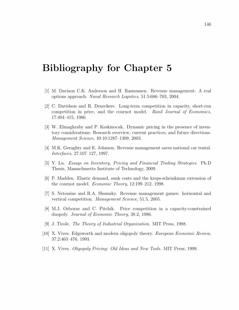
146
Bibliography for Chapter 5
[1] M. Davison C.K. Anderson and H. Rasmussen. Revenue management: A realoptions approach. Naval Research Logistics, 51.5:686–703, 2004.
[2] C. Davidson and R. Deneckere. Long-term competition in capacity, short-runcompetition in price, and the cournot model. Rand Journal of Economics,17:404–415, 1986.
[3] W. Elmaghraby and P. Keskinocak. Dynamic pricing in the presence of inven-tory considerations: Research overview, current practices, and future directions.Management Science, 49.10:1287–1309, 2003.
[4] M.K. Geraghty and E. Johnson. Revenue management saves national car rental.Interfaces, 27:107–127, 1997.
[5] Y. Lu. Essays on Inventory, Pricing and Financial Trading Strategies. Ph.DThesis, Massachusetts Institute of Technology, 2009.
[6] P. Madden. Elastic demand, sunk costs and the kreps-scheinkman extension ofthe cournot model. Economic Theory, 12:199–212, 1998.
[7] S. Netessine and R.A. Shumsky. Revenue management games: horizontal andvertical competition. Management Science, 51.5, 2005.
[8] M.J. Osborne and C. Pitchik. Price competition in a capacity-constrainedduopoly. Journal of Economic Theory, 38.2, 1986.
[9] J. Tirole. The Theory of Industrial Organization. MIT Press, 1988.
[10] X. Vives. Edgeworth and modern oligopoly theory. European Economic Review,37.2:463–476, 1993.
[11] X. Vives. Oligopoly Pricing: Old Ideas and New Tools. MIT Press, 1999.
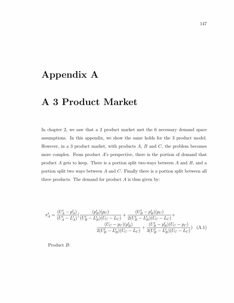
147
Appendix A
A 3 Product Market
In chapter 2, we saw that a 2 product market met the 6 necessary demand space
assumptions. In this appendix, we show the same holds for the 3 product model.
However, in a 3 product market, with products A, B and C, the problem becomes
more complex. From product A′s perspective, there is the portion of demand that
product A gets to keep. There is a portion split two-ways between A and B, and a
portion split two ways between A and C. Finally there is a portion split between all
three products. The demand for product A is thus given by:
πtA =(U t
A − ptA)
(U tA − LtA)
((ptB)(pC)
(U tB − LtB)(UC − LC)
+(U t
B − ptB)(pC)
2(U tB − LtB)(UC − LC)
+
(UC − pC)(ptB)
2(U tB − LtB)(UC − LC)
+(U t
B − ptB)(UC − pC)
3(U tB − LtB)(UC − LC)
) (A.1)
Product B:
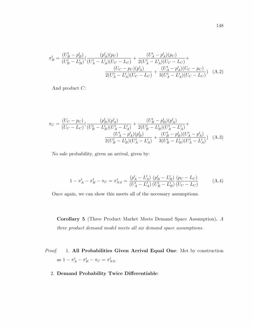
148
πtB =(U t
B − ptB)
(U tB − LtB)
((ptA)(pC)
(U tA − LtA)(UC − LC)
+(U t
A − ptA)(pC)
2(U tA − LtA)(UC − LC)
+
(UC − pC)(ptA)
2(U tA − LtA)(UC − LC)
+(U t
A − ptA)(UC − pC)
3(U tA − LtA)(UC − LC)
) (A.2)
And product C:
πC =(UC − pC)
(UC − LC)(
(ptB)(ptA)
(U tB − LtB)(U t
A − LtA)+
(U tB − ptB)(ptA)
2(U tB − LtB)(U t
A − LtA)+
(U tA − ptA)(ptB)
2(U tB − LtB)(U t
A − LtA)+
(U tB − ptB)(U t
A − ptA)
3(U tB − LtB)(U t
A − LtA)) (A.3)
No sale probability, given an arrival, given by:
1− πtA − πtB − πC = πtNS =(ptA − LtA)
(U tA − LtA)
(ptB − LtB)
(U tB − LtB)
(pC − LC)
(UC − LC)(A.4)
Once again, we can show this meets all of the necessary assumptions.
Corollary 5 (Three Product Market Meets Demand Space Assumption). A
three product demand model meets all six demand space assumptions.
Proof. 1. All Probabilities Given Arrival Equal One: Met by construction
as 1− πtA − πtB − πC = πtNS.
2. Demand Probability Twice Differentiable:
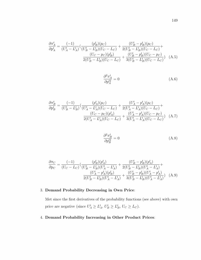
149
∂πtA∂ptA
=(−1)
(U tA − LtA)
((ptB)(pC)
(U tB − LtB)(UC − LC)
+(U t
B − ptB)(pC)
2(U tB − LtB)(UC − LC)
+
(UC − pC)(ptB)
2(U tB − LtB)(UC − LC)
+(U t
B − ptB)(UC − pC)
3(U tB − LtB)(UC − LC)
) (A.5)
∂2πtA∂pt2A
= 0 (A.6)
∂πtB∂ptB
=(−1)
(U tB − LtB)
((ptA)(pC)
(U tA − LtA)(UC − LC)
+(U t
A − ptA)(pC)
2(U tA − LtA)(UC − LC)
+
(UC − pC)(ptA)
2(U tA − LtA)(UC − LC)
+(U t
A − ptA)(UC − pC)
3(U tA − LtA)(UC − LC)
) (A.7)
∂2πtB∂pt2B
= 0 (A.8)
∂πC∂pC
=(−1)
(UC − LC)(
(ptB)(ptA)
(U tB − LtB)(U t
A − LtA)+
(U tB − ptB)(ptA)
2(U tB − LtB)(U t
A − LtA)+
(U tA − ptA)(ptB)
2(U tB − LtB)(U t
A − LtA)+
(U tB − ptB)(U t
A − ptA)
3(U tB − LtB)(U t
A − LtA)) (A.9)
3. Demand Probability Decreasing in Own Price:
Met since the first derivatives of the probability functions (see above) with own
price are negative (since U tA ≥ LtA, U t
B ≥ LtB, UC ≥ LC).
4. Demand Probability Increasing in Other Product Prices:
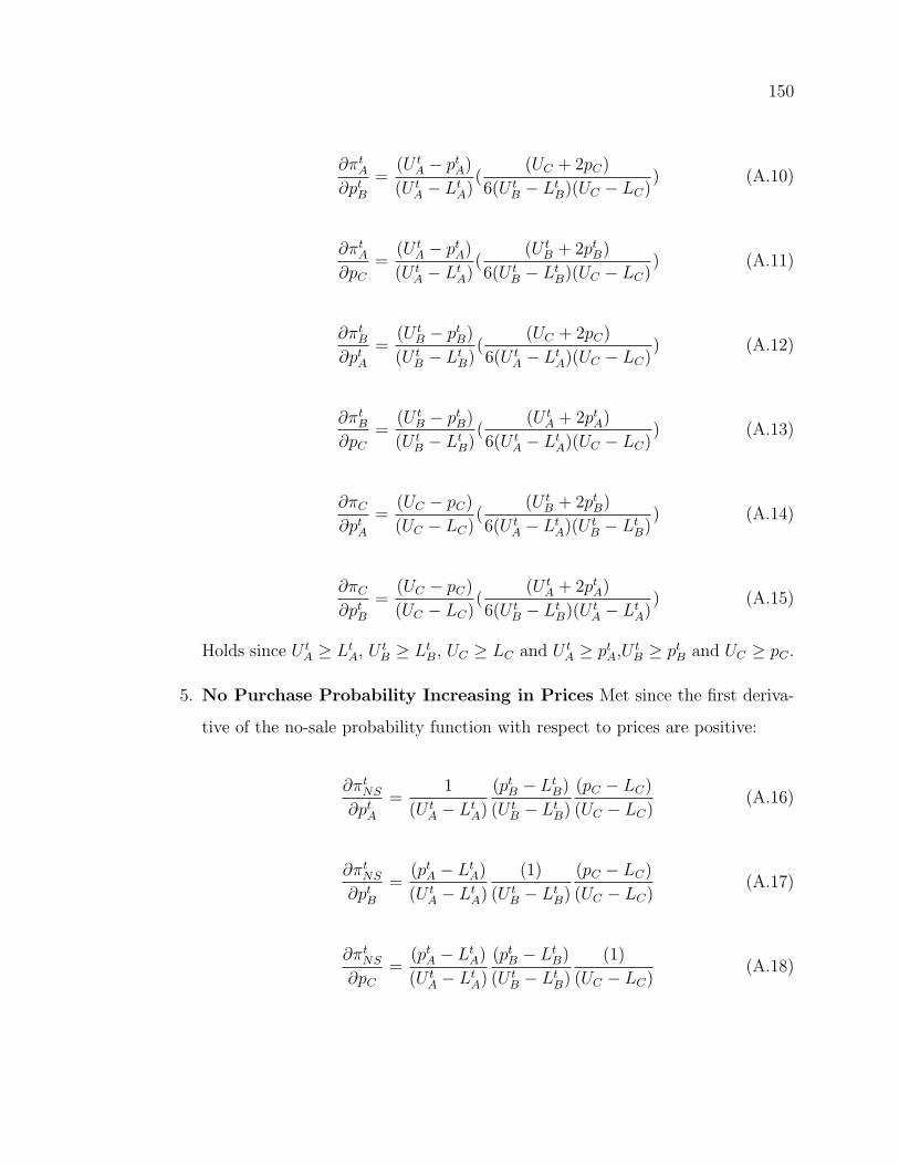
150
∂πtA∂ptB
=(U t
A − ptA)
(U tA − LtA)
((UC + 2pC)
6(U tB − LtB)(UC − LC)
) (A.10)
∂πtA∂pC
=(U t
A − ptA)
(U tA − LtA)
((U t
B + 2ptB)
6(U tB − LtB)(UC − LC)
) (A.11)
∂πtB∂ptA
=(U t
B − ptB)
(U tB − LtB)
((UC + 2pC)
6(U tA − LtA)(UC − LC)
) (A.12)
∂πtB∂pC
=(U t
B − ptB)
(U tB − LtB)
((U t
A + 2ptA)
6(U tA − LtA)(UC − LC)
) (A.13)
∂πC∂ptA
=(UC − pC)
(UC − LC)(
(U tB + 2ptB)
6(U tA − LtA)(U t
B − LtB)) (A.14)
∂πC∂ptB
=(UC − pC)
(UC − LC)(
(U tA + 2ptA)
6(U tB − LtB)(U t
A − LtA)) (A.15)
Holds since U tA ≥ LtA, U t
B ≥ LtB, UC ≥ LC and U tA ≥ ptA,U t
B ≥ ptB and UC ≥ pC .
5. No Purchase Probability Increasing in Prices Met since the first deriva-
tive of the no-sale probability function with respect to prices are positive:
∂πtNS∂ptA
=1
(U tA − LtA)
(ptB − LtB)
(U tB − LtB)
(pC − LC)
(UC − LC)(A.16)
∂πtNS∂ptB
=(ptA − LtA)
(U tA − LtA)
(1)
(U tB − LtB)
(pC − LC)
(UC − LC)(A.17)
∂πtNS∂pC
=(ptA − LtA)
(U tA − LtA)
(ptB − LtB)
(U tB − LtB)
(1)
(UC − LC)(A.18)
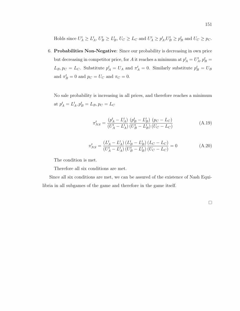
151
Holds since U tA ≥ LtA, U t
B ≥ LtB, UC ≥ LC and U tA ≥ ptA,U t
B ≥ ptB and UC ≥ pC .
6. Probabilities Non-Negative: Since our probability is decreasing in own price
but decreasing in competitor price, for A it reaches a minimum at ptA = U tA, p
tB =
LB, pC = LC . Substitute ptA = UA and πtA = 0. Similarly substitute ptB = UB
and πtB = 0 and pC = UC and πC = 0.
No sale probability is increasing in all prices, and therefore reaches a minimum
at ptA = LtA, ptB = LB, pC = LC
πtNS =(ptA − LtA)
(U tA − LtA)
(ptB − LtB)
(U tB − LtB)
(pC − LC)
(UC − LC)(A.19)
πtNS =(LtA − LtA)
(U tA − LtA)
(LtB − LtB)
(U tB − LtB)
(LC − LC)
(UC − LC)= 0 (A.20)
The condition is met.
Therefore all six conditions are met.
Since all six conditions are met, we can be assured of the existence of Nash Equi-
libria in all subgames of the game and therefore in the game itself.
152
Appendix B
Optimal Prices in the 2 Firm, 1
Good Per Firm Scenario
In this appendix, we examine the optimal prices in a 2 firm, 1 good per firm model,
to see how the state affects the optimal price for each good in the final 2 periods.
B.1 Time T
To simplify, we assume that UA and UB are constants and do not change from period
to period. As such, we can lose the time superscript.
B.1.1 Both Firm A and B Have One or More Goods
Optimal price for A:
pT∗A = 0.5(UA) (B.1)
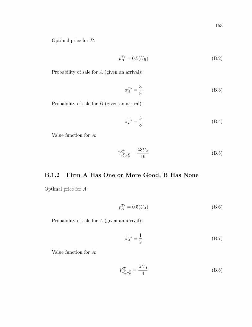
153
Optimal price for B:
pT∗B = 0.5(UB) (B.2)
Probability of sale for A (given an arrival):
πT∗A =3
8(B.3)
Probability of sale for B (given an arrival):
πT∗B =3
8(B.4)
Value function for A:
V TqTA,q
TB
=λ3UA
16(B.5)
B.1.2 Firm A Has One or More Good, B Has None
Optimal price for A:
pT∗A = 0.5(UA) (B.6)
Probability of sale for A (given an arrival):
πT∗A =1
2(B.7)
Value function for A:
V TqTA,q
TB
=λUA
4(B.8)
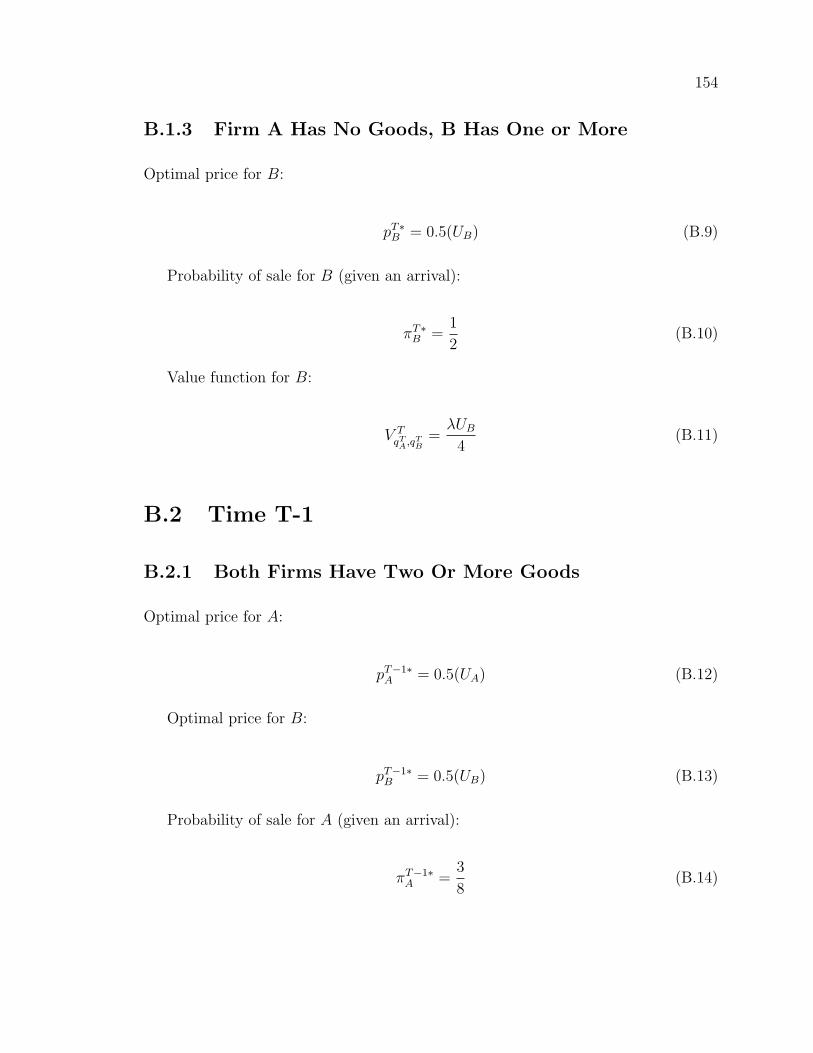
154
B.1.3 Firm A Has No Goods, B Has One or More
Optimal price for B:
pT∗B = 0.5(UB) (B.9)
Probability of sale for B (given an arrival):
πT∗B =1
2(B.10)
Value function for B:
V TqTA,q
TB
=λUB
4(B.11)
B.2 Time T-1
B.2.1 Both Firms Have Two Or More Goods
Optimal price for A:
pT−1∗A = 0.5(UA) (B.12)
Optimal price for B:
pT−1∗B = 0.5(UB) (B.13)
Probability of sale for A (given an arrival):
πT−1∗A =
3
8(B.14)
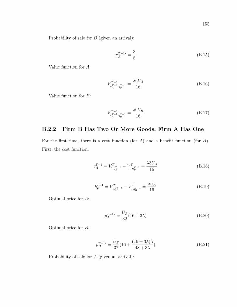
155
Probability of sale for B (given an arrival):
πT−1∗B =
3
8(B.15)
Value function for A:
V T−1
qT−1A ,qT−1
B
=λ6UA
16(B.16)
Value function for B:
V T−1
qT−1A ,qT−1
B
=λ6UB
16(B.17)
B.2.2 Firm B Has Two Or More Goods, Firm A Has One
For the first time, there is a cost function (for A) and a benefit function (for B).
First, the cost function:
cT−1A = V T
1,qT−1B− V T
0,qT−1B
=λ3UA
16(B.18)
bT−1B = V T
1,qT−1B− V T
0,qT−1B
=λUA16
(B.19)
Optimal price for A:
pT−1∗A =
UA32
(16 + 3λ) (B.20)
Optimal price for B:
pT−1∗B =
UB32
(16 +(16 + 3λ)λ
48 + 3λ) (B.21)
Probability of sale for A (given an arrival):
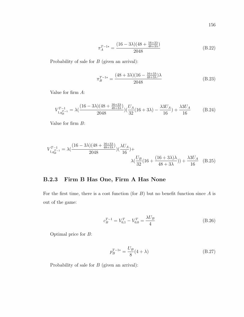
156
πT−1∗A =
(16− 3λ)(48 + 16+3λ48+3λ
)
2048(B.22)
Probability of sale for B (given an arrival):
πT−1∗B =
(48 + 3λ)(16− 16+3λ48+3λ
)λ
2048(B.23)
Value for firm A:
V T−1
1,qT−1B
= λ((16− 3λ)(48 + 16+3λ
48+3λ)
2048)(UA32
(16 + 3λ)− λ3UA16
) +λ3UA
16(B.24)
Value for firm B:
V T−1
1,qT−1B
= λ((16− 3λ)(48 + 16+3λ
48+3λ)
2048)(λUA16
)+
λ(UB32
(16 +(16 + 3λ)λ
48 + 3λ)) +
λ3UA16
(B.25)
B.2.3 Firm B Has One, Firm A Has None
For the first time, there is a cost function (for B) but no benefit function since A is
out of the game:
cT−1B = V T
0,1 − V T0,0 =
λUB4
(B.26)
Optimal price for B:
pT−1∗B =
UB8
(4 + λ) (B.27)
Probability of sale for B (given an arrival):
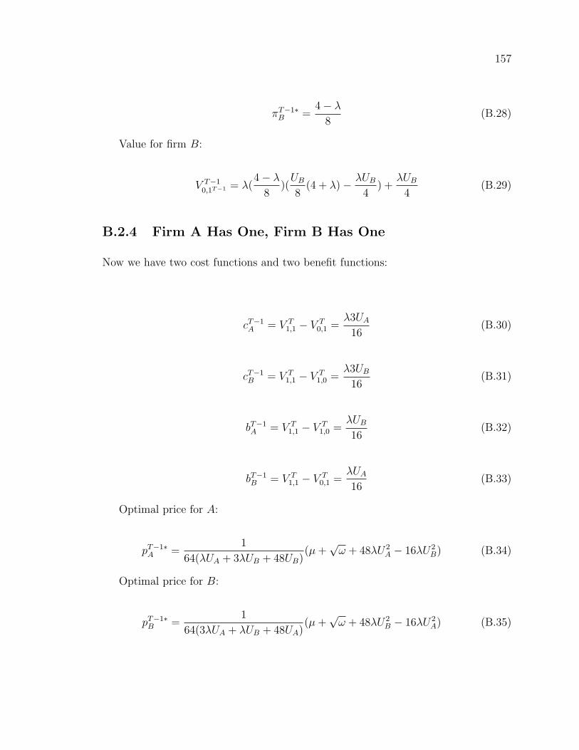
157
πT−1∗B =
4− λ8
(B.28)
Value for firm B:
V T−10,1T−1 = λ(
4− λ8
)(UB8
(4 + λ)− λUB4
) +λUB
4(B.29)
B.2.4 Firm A Has One, Firm B Has One
Now we have two cost functions and two benefit functions:
cT−1A = V T
1,1 − V T0,1 =
λ3UA16
(B.30)
cT−1B = V T
1,1 − V T1,0 =
λ3UB16
(B.31)
bT−1A = V T
1,1 − V T1,0 =
λUB16
(B.32)
bT−1B = V T
1,1 − V T0,1 =
λUA16
(B.33)
Optimal price for A:
pT−1∗A =
1
64(λUA + 3λUB + 48UB)(µ+
√ω + 48λU2
A − 16λU2B) (B.34)
Optimal price for B:
pT−1∗B =
1
64(3λUA + λUB + 48UA)(µ+
√ω + 48λU2
B − 16λU2A) (B.35)
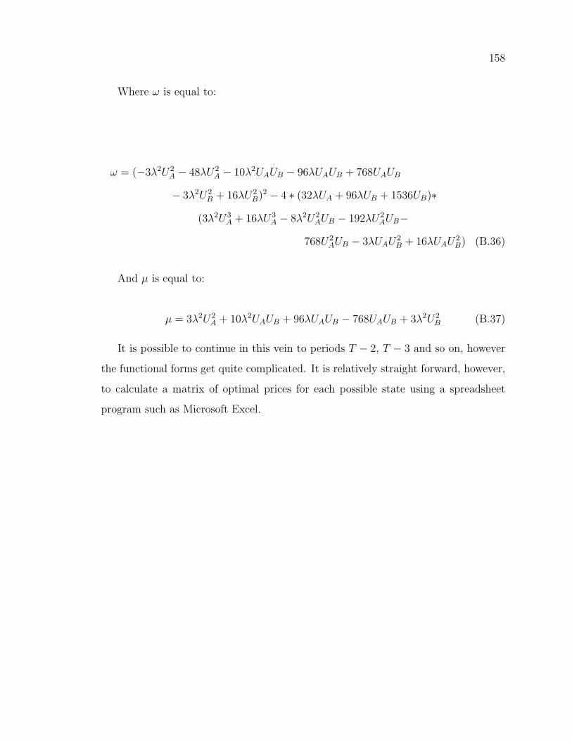
158
Where ω is equal to:
ω = (−3λ2U2A − 48λU2
A − 10λ2UAUB − 96λUAUB + 768UAUB
− 3λ2U2B + 16λU2
B)2 − 4 ∗ (32λUA + 96λUB + 1536UB)∗
(3λ2U3A + 16λU3
A − 8λ2U2AUB − 192λU2
AUB−
768U2AUB − 3λUAU
2B + 16λUAU
2B) (B.36)
And µ is equal to:
µ = 3λ2U2A + 10λ2UAUB + 96λUAUB − 768UAUB + 3λ2U2
B (B.37)
It is possible to continue in this vein to periods T − 2, T − 3 and so on, however
the functional forms get quite complicated. It is relatively straight forward, however,
to calculate a matrix of optimal prices for each possible state using a spreadsheet
program such as Microsoft Excel.
159
Curriculum Vitae
NAME: Michael Patrick Moffatt
PLACE OF BIRTH: London, Ontario
DATE OF BIRTH: March 14, 1977
POST-SECONDARYEDUCATION 1:
Richard Ivey School of BusinessLondon, OntarioPh.D.2003-2012
POST-SECONDARYEDUCATION 2:
University of RochesterRochester, New YorkM.A. Economics2000-2003
POST-SECONDARYEDUCATION 3:
University of Western OntarioLondon, OntarioHons B.A. Economics and Political Science1995-1999