Embed Size (px)
Citation preview

J Seismol (2010) 14:79–93DOI 10.1007/s10950-008-9147-6
ORIGINAL ARTICLE
Renewal models for earthquake predictability
E. Garavaglia · E. Guagenti ·R. Pavani · L. Petrini
Received: 11 December 2007 / Accepted: 23 December 2008 / Published online: 3 April 2009© Springer Science + Business Media B.V. 2009
Abstract The new Database of Italy’s Seismo-genic Sources (Basili et al. 2008) identifies areaswith a degree of homogeneity in earthquake gen-eration mechanism judged sufficiently high. Nev-ertheless, their seismic sequences show ratherlong and regular interoccurrence times mixedwith irregularly distributed short interoccurrencetimes. Accordingly, the following question couldnaturally arise: do sequences consist of nearlyperiodic events perturbed by a kind of noise; arethey Poissonian; or short interoccurrence timespredominate like in a cluster model? The rela-tive reliability of these hypotheses is at present
Electronic supplementary material The online versionof this article (doi: 10.1007/s10950-008-9147-6)contains supplementary material, which is availableto authorized users.
E. Garavaglia (B) · E. Guagenti · L. PetriniDepartment of Structural Engineering, Politecnicodi Milano, Piazza L. da Vinci 32, 20133, Milan, Italye-mail: [email protected]
E. Guagentie-mail: [email protected]
L. Petrinie-mail: [email protected]
R. PavaniDepartment of Mathematics, Politecnico di Milano,Piazza L. da Vinci 32, 20133, Milan, Italye-mail: [email protected]
a matter of discussion (Faenza et al., GeophysJ Int 155:521–531, 2003; Corral, Proc Geoph 12:89–100, 2005, Tectonophysics 424:177–193, 2006).In our regions, a statistical validation is not fea-sible because of the paucity of data. Moreover,the classical tests do not clearly suggest whichone among different proposed models must befavoured. In this paper, we adopt a model ofinteroccurrence times able to interpret the threedifferent hypotheses, ranging from exponential toWeibull distributions, in a scenario of increasingdegree of predictability. In order to judge whichone of these hypotheses is favoured, we adopt,instead of the classical tests, a more selective in-dicator measuring the error in respect to the cho-sen panorama of possible truths. The earthquakeprediction is here simply defined and calculatedthrough the conditional probability of occurrencedepending on the elapsed time t0 since the lastearthquake. Short-term and medium-term predic-tions are performed for all the Italian seismiczones on the basis of datasets built in the contextof the National Projects INGV-DPC 2004–2006,in the frame of which this research was devel-oped. The mathematical model of interoccurrencetimes (mixture of exponential and Weibull distri-butions) is justified in its analytical structure. Adimensionless procedure is used in order to re-duce the number of parameters and to make com-parisons easier. Three different procedures aretaken into consideration for the estimation of the

80 J Seismol (2010) 14:79–93
parameter values; in most of the cases, they givecomparable results. The degree of credibility ofthe proposed methods is evaluated. Their robust-ness as well as their sensitivity are discussed. Thecomparison of the probability of occurrence of aMaw >5.3 event in the next 5 and 30 years fromJanuary 1, 2003, conditional to the time elapsedsince the last event, shows that the relative rank-ing of impending rupture in 5 years is roughlymaintained in a 30-year perspective with higherprobabilities and large fluctuations betweensources belonging to the same macro region.
Keywords Renewal process · Hazard rate ·Earthquake predictability · Credibilityand robustness of the model · Italy
1 Introduction
One of the main issues in seismology and seis-mic engineering is reliable earthquake prediction.However, since earthquake occurrence dependson many random variables whose characteris-tics are often not well-defined, its prediction isstill a difficult matter. Several approaches havebeen presented, but it seems that none is clearlysuperior.
The degree of uncertainty, epistemic and sta-tistic, contained in the models leads to state-ments of this kind. “Although seismology hasintensively analysed the characteristics of singleearthquakes with great success, a clear descriptionof the properties of seismicity . . . is still lacking”(Corral 2006); “. . . test based on the likelihoodratios should be approached with caution. . . ” and“physical significance (of cyclic effects and cluster-ing) therefore remains questionable” (Vere-Jonesand Ozaki 1982); “. . . these results. . . could bevery relevant in the debate of seismic gap modelsversus clustering occurrence” (Corral 2005).
One of the major challenges is to interpret twoapparently opposite characteristics in recurrencetime models: temporal clustering and nearly peri-odic events. In Corral (2006), the author quotes“. . . results turn out to be in contradiction witheach other, from the paradigm of regular cyclesand characteristic earthquakes to the view of to-
tally random occurrence” and proposes a unifyingdescription of seismicity.
We do not have the pretension to enter in thedebate, but we propose an elementary model thatcould be a first step to incorporate quasi-periodicevents as well as Poissonian or clustered events.Moreover, we adopt an indicator, called credibil-ity, to compare the competing models.
The mathematical tool of the model consistsin a renewal process, already proposed by manyauthors in order to overcome the Poisson models.The renewal process is not free from criticism: (1)all past history, not only the last event, influencesthe earthquake generation; (2) the complexity ofItalian context makes debatable a complete en-ergy release after each earthquake followed by anew cycle; (3) the recurrence times are indepen-dent identically distributed (i.i.d.); (4) the sum ofmany causes of seismicity can suggest the Poissonprocess (this criticism being feeble because therenewal process includes the Poisson process as aparticular case).
Nevertheless, in the frame of the renewalprocesses, the role of the specific survivor func-tion (complementary distribution function) withthe implied hazard rate is crucial. The mix-ture exponential–Weibull distribution function wepropose has the capacity to incorporate in a prob-abilistic way three different behaviours (with dif-ferent kinds of energy release): to collapse into aPoisson process, to model characteristic or cluster-ing events.
The existence of characteristic or clusteringevents needs sound physical basis to be asserted;here the terms are used, for shortness, to indicate,respectively, the presence of rather regular tem-poral sequence (even if mixed with irregular shortinteroccurrence times) or the dominance of shortinteroccurrence times.
The main parameter responsible for making themixture suitable in the three mentioned cases isthe shape parameter α of the Weibull component.In general, its behaviour is as follows.
If α is greater than unity, the hazard rate comesout to be increasing until a peak value; it modelsa kind of seismic gap. If α is lesser than unity,the hazard rate comes out to be decreasing likein clustering events. If α is equal to unity, the pro-posed renewal process weakly differ from Poisson

J Seismol (2010) 14:79–93 81
process. Moreover, the renewal process can col-lapse precisely in a Poisson process, as shown inthe next sections.
In the SIS Intermediate Conference 2007 Riskand Prediction held in Venice in June 2007, sucha model was already presented (Garavaglia et al.2007) in a preliminary way; in this paper, it isstudied and applied to the Italian seismic zones.
During the last 12 years and at present, Ital-ian researchers are improving the earthquakecatalogues and proposing different seismogeneticmodels of the seismic source. Seismic zoning, aswell as the seismic catalogues, are again underrevision.
In the context of a research plan proposed byItalian Department of Civil Protection (DPC) andNational Institute of Geophysics and Vulcanol-ogy (INGV) (National Projects INGV-DPC 2004–2006) in the frame of which this work has beendeveloped, new databases were released with theaim of calculating the probability of occurrenceof strong events in the next 30 years. Earthquakesub-catalogues were obtained by the associationof the events of the Italian historic catalogueCPTI04 (Catalogo Parametrico dei TerremotiItaliani—Versione 2004, INGV, Bologna; CPTIWorking Group 2004) with seismogenetic sourceareas (SA; DISS03, INGV; DISS Working Group2006) that are sources having homogeneous be-haviour. For a lot of SAs, the number of events inthe sub-catalogues is inadequate for a significantstatistical analysis; therefore, the predictabilitycould not be applied to the whole Italian con-text. In order to overcome this problem, the SAshave been grouped in macro regions (MR; Basili2007) with the following characteristics: similarstyle of faulting and amount of deformation; thislast association permitted to have adequate inte-roccurrence times datasets. The approach hereinproposed was applied to these catalogues, as de-scribed in the following.
2 The interoccurrences time model
This paper is aimed at providing a model forearthquakes prediction, which takes into accountinteroccurrence time both for nearly periodic,
characteristic earthquakes and for clusters andother randomly occurring earthquakes having amagnitude greater than a selected threshold.
The procedure is purely probabilistic, but atleast three physical hypotheses are included:
1. a double behaviour in earthquake generation,as already said;
2. a dependence on the past history, expressedwith the use of a renewal process;
3. a stationary asymptotic behaviour of the haz-ard: a very long seismic silence in a zone couldbe reasonably interpreted as an energy releasehaving occurred somewhere else, rather than acontinuous enormous accumulation of energyin progress in the zone; so even in the case ofincreasing hazard rate, its limiting value is afinite quantity.
More precisely, property 2 means that the prob-ability of an earthquake occurrence depends onthe elapsed time t0 from the last event. Property 3means that, in case of α > 1, the hazard increaseswith t0 but, after a peak value, if the earthquakedoes not occur, it decreases and reaches a stablevalue, describing for every time increment a con-stant probability of an immediate occurrence.
In our regions, an exponential–Weibull (ex-w)mixture with the Weibull’s shape parameter α > 1appears to be suitable: it generally shows, after afirst phase of weakly decreasing hazard rate, a cen-tral phase of increasing hazard followed by a sta-tionary one. The exponential distribution mainlymodels the short interoccurrence times, related toclustering or random events, whilst the Weibulldistribution mainly models the interoccurrencetimes related to the characteristic earthquake.Nevertheless, both distributions are defined in [0,∞) without a threshold of separation between thetwo families of events. The weaker the character-istic earthquake is expressed, the more the tails ofthe two distributions overlap.
In any case, the mixture distribution overcomesthe drawback of a single distribution that ingeneral is not able to fit the entire class of interoc-currence times. In fact, what in general happensis that a distribution that fit well the short inte-roccurrence times does not fit the long interoccur-rence time and vice versa.

82 J Seismol (2010) 14:79–93
Moreover, note that the entire set of interoc-currence times has often coefficient of variation(COV) near to 1. So this property does not in-dicate a propensity towards characteristic earth-quake nor towards clustering. The preliminarycheck of the global COV simply would indicatethat the Poisson hypothesis is not rejectable. Abetter fitting is obtained through a mixture. Thecoefficient of aperiodicity (Matthews et al. 2002)of the resulting process can adequately fit se-quences with different degrees of regularity.
The choice of the two component distributionshere proposed for the mixture is the result ofinvestigations on different mix of distributions andon correspondence between the theoretical char-acteristic of the mixture and the physical aspect ofmodelled phenomenon (Guagenti Grandori et al.1990).
The ex-w survivor function, �τ (t0)=1−Fτ (t0),and the probability density function, fτ (t0), are,respectively (Cox 1962):
1−Fτ (t0)=(1− p) exp[−bt0
]+ p exp[− (ρ t0)α
],
(1)
fτ (t0) = (1 − p){b exp
[−bt0]}
+p{αρ (ρ t0)α−1 exp [−(ρ t0)α]
}. (2)
Let us call τ the interoccurrence time randomvariable, t0 being its generic value, i.e. the timesince the last event. The parameters involved inEq. 1 are p, which can be considered the weightof the characteristic earthquake portion of themodel; α, whose value governs the Weibull coeffi-cient of variation COVW:
COVw ={
�(1 + 2
α
)
[�
(1 + 1
α
) ] 2 − 1
} 12
; (3)
b and ρ that can be defined as functions of μ1
and μ2, which are the two return period compo-nents of the short interoccurrence times and of thecharacteristic earthquake interoccurrence times,respectively:
μ1 = 1
bμ2 = �
(1 + 1
α
)
ρ. (4)
Moreover, the COV of the mixture in the re-sulting process, called coefficient of aperiodicity,comes out to be:
COVex−w ={
(1− p)·2k21+ pk2
2
�(1+ 2
α
)
�2(1+ 1
α
) −1
}12
. (5)
The information about aperiodicity contained inEq. 5 differs from the information contained in thesample COV.
The mixture (1) models a wide class of earth-quake interoccurrence times; its hazard rate (HR),λ(t0), is defined as:
λ (t0) = fτ (t0)1 − Fτ (t0)
(6)
and it is shaped as required for property 3. Be-cause parameter p can assume different values,the distribution (1) can explore different degreesof characteristic earthquake evidence: increasingvalues of p means larger and larger evidence ofcharacteristic earthquake; p = 1 means lack of theirregular short interoccurrence times. In the twoextreme cases p = 0 and p = 1, the mixture dis-tribution (1) becomes, respectively, exponentialand Weibull and property 3 fails: when p = 0,the HR is constant in time and the predictabilityis missing; when p = 1, the HR is continuouslyincreasing until the certainty of an immediate oc-curring earthquake.
Equation 6 furnishes the prediction in a veryshort (infinitesimal) next time interval dt:
λ (t0) = lim�t0→0+
Pr {t0 < τ ≤ t0 + �t0 |τ > t0 }�t0
= fτ (t0)1 − Fτ (t0)
(7)
whilst the medium-term �t prediction is the prob-ability, at each t0 of an earthquake in the next �t:
P�t| t0 = Fτ (t0 + �t) − Fτ (t0)1 − Fτ (t0)
. (8)
In this context, prediction means, at each instant,the conditional probability of an earthquake withmagnitude greater than a specific value in the nexttime interval (dt or �t), given the length of thepreceding seismic gap.

J Seismol (2010) 14:79–93 83
The presence of four parameters is the maindrawback of Eq. 1 in the estimation procedure. Toavoid this shortcoming, we propose the followingtime scale transformation:
h = t0μ
(9)
where:
μ = (1 − p) μ1 + p μ2 (10)
is the global return period of the earthquakeprocess. Equation 9 transforms Eq. 1 into dimen-sionless terms as follows:
1 − F (h) = (1 − p) exp[− h
k1
]
+p exp{−
[�
(1 + 1
α
) hk2
]α}(11)
where k1 = μ1/μ, k2 = μ2/μ are the two returnperiod components, μ1 and μ2, expressed in di-mensionless terms.
Equation 11 offers the advantage of presentingthe range of a source’s possible earthquake behav-iour independently of the numerical value of therespective return periods. Then Eq. 10 becomes:
1 = (1 − p) k1 + p k2. (12)
The parameter p can now be estimated throughEq. 12 as follows:
p = 1 − k1
k2 − k1. (13)
Three parameters remain to be estimated inEq. 11. In order to make the estimate proce-dure easier and more stable, we proceed assumingα = constant with different trial values; then wechoose the best one in respect to likelihood func-tion. In this way, only k1 and k2 have to be esti-mated: they offer the advantage of being directlysuggested by the sample, at least if the ratio r =k2/k1 is large enough to ensure weak overlap ofthe two component densities. In this case, themean values of the interoccurrence times <1 andthe interoccurrence times >1 give empirical esti-mates of k1 and k2, respectively.
0 1 2 3 4 5h
02
4
6
8
10
12
14
1618
20
22λ
k2=1.2, alfa=4
p=0.1p=0.2p=0.3p=0.4p=0.5p=0.6p=0.7p=0.8Weibull
Fig. 1 Dimensionless HR for conjectural “truths” withk2 = 1.2 and α = 4
Varying k2 and k1, we obtain different familiesof earthquake processes, representing conjectural“truths”. In Figs. 1, 2, 3, 4 and 5, they are shown ina compact form through the dimensionless HR λ.
The assumed range [1.2–2] for k2 can be consid-ered exhaustive for a wide class of Italian seismiczones. The values of k1 are chosen between 0 and1 to give, from Eq. 13, equally spaced p values(0.1 ≤ p < 1/k2 with increment 0.1).
In the figures, the value of α is 4. Our largeset of numerical simulations show that larger orsmaller values of α lead to similar behaviourswith more or less pronounced peak relative tocharacteristic earthquake.
0 1 2 3 4 5 6 7 8 9 10 11h
0
1
2
3
4
5
6
7
8
9
10 k2=1.4, alfa=4
p=0.1p=0.2p=0.3p=0.4p=0.5p=0.6p=0.7Weibull
λ
Fig. 2 Dimensionless HR for conjectural “truths” withk2 = 1.4 and α = 4

84 J Seismol (2010) 14:79–93
0 1 2 3 4 5h
02
4
6
8
10
12
14
1618
20
22
k2=1.6, alfa=4
p=0.1p=0.2p=0.3p=0.4p=0.5p=0.6Weibull
44.258λ
Fig. 3 Dimensionless HR for conjectural “truths” withk2 = 1.6 and α = 4
Let us remember that all distributions (Eq. 11)have mean value = 1. If we want the prediction intime scale, we will use the relationships:
λ (h) = μ λ (t0) ; P�t|t0 = P�h| h with �t = μ �h,
(14)
F(h) = Fτ (t0) and f (h) = μ fτ (t0). (15)
Moreover, the asymptotic value of the hazard rateis given by λ∞ = 1/μ1 and its dimensionless formis given by λ∞ = 1/k1.
0 1 2 3 4 5
h
02
4
6
8
10
1214
16
18
20
22
k2=1.8, alfa=4
p=0.1p=0.2p=0.3p=0.4p=0.5Weibull
λ
Fig. 4 Dimensionless HR for conjectural “truths” withk2 = 1.8 and α = 4
0 1 2 3 4 5h
02
4
6
8
10
1214
16
18
20
22k2=2.0, alfa=4
p=0.1p=0.2p=0.3p=0.4Weibull
λ
Fig. 5 Dimensionless HR for conjectural “truths” withk2 = 2.0 and α = 4
3 Comparison between estimation procedures
We consider four different estimation proce-dures for conditional earthquake occurrenceprobability.
The first one assumes the mathematical model(Eq. 11) and it uses the classical method of max-imum likelihood (ML) for the estimation of theparameters k1 and k2 (Maybeck 1979).
A second method, proposed by us and calledthe threshold method (TR), assumes again themathematical model (Eq. 11) with the means ofinteroccurrence times less than and greater than 1taken as estimators of k1 and k2, respectively. Aswe will see in the following, if r assumes valuesaround 4 or more, the TR method is better than
0 1 2 3
h0
0.2
0.4
0.6
0.8
1F∗ (h)
1-F*(h)θ
−h
Fig. 6 Building of empirical value λ* as exposed in Eq. 13

J Seismol (2010) 14:79–93 85
the ML method: indeed, it is able to catch thecontribution of the few interoccurrence times inthe tail better than the ML, which is sensitiveto the total contribution of the interoccurrencetimes. On the other hand, the TR fails for lowvalues of r, i.e. if the tails of the two componentsof the mixture overlap.
A third method (ME) is based on the maxi-mum entropy principle that implies the use of ageneralised exponential distribution (Jaynes 1957;Akaike 1977; Tagliani 1989, 1990). Indeed, thisis the distribution function that incorporates onlythe information inherent in dataset (so maximis-ing the entropy of the distribution). This methoddoes not agree with our choice of limited λ∞,but it is useful in a qualitative sense because itis very sensitive to the dataset and is free fromthe characteristic earthquake or other interpretinghypothesis (Vere-Jones and Ozaki 1982).
Finally, an empirical method (EMP) consists inreading directly on the cumulative frequency poly-gon F* the values of λ* and P�h|h. Specifically, theempirical value λ* is:
λ∗ (h) = (tgθ)h
1 − F∗ (h)(16)
being (tgθ)h the tangent of that polygon F* sidewhich h belongs to (Fig. 6). Equation 16 becomesmeaningless at the end of the polygon, but, beforethe end, it offers an empirical rough predictiondirectly coming from the dataset, free from math-ematical model (apart the piecewise linearity ofthe polygon). Moreover, the dataset can suggestpossible variability of the hazard that the struc-ture of the chosen mathematical model cannotincorporate; typically, a possible multimodality ofthe hazard will be suggested from the empiricalmethod. Obviously, this rough empirical methodEMP cannot be considered as a reliable non-parametric procedure, but it may furnish comple-mentary qualitative information.
4 Procedure credibility
In previous papers (Grandori et al. 1998, 2003,2006; Guagenti et al. 2003, 2004), the credibilityof a procedure has been introduced: a measure ofthe error, with respect to a conjectural truth F◦,
when a target quantity A is estimated with thatprocedure. Let A◦ be the true value of A (in theconjectural truth) and As its estimator with theprocedure s. The credibility �◦
s of the procedure srelative to the truth F◦ (that here is simply a givendistribution) is defined as follows:
�◦s = Pr
{A◦ − kA◦ ≤ As ≤ A◦ + kA◦
}. (17)
In other words, �◦s is the probability to have (as
absolute value) a fractional (or relative) error notlarger than a given value k in the estimate of thequantity A. In this research, the target quantity Ais the prediction (λ or P�t|t0).
The merit of credibility �◦s is to focus atten-
tion on the target quantity A of interest, insteadof on the data fitting. This makes the credibilityspecifically useful to the aim of the research andmore selective than classic tests. For example,exponential, lognormal, gamma and Weibull dis-tributions, largely used for interoccurrence timemodel, can lead, with the classic tests, to similarlevels of significance; on the other hand, they leadto predictions drastically different.
It is remarkable that the credibility �◦s is not
based on the single sample given by the cataloguebut on “all samples” (i.e. 1,000 samples) that canbe drawn from F◦.
Because of definition (17) of credibility, com-peting models can be compared in the frame ofthe chosen conjectural truths. The values of � areobtained with Monte Carlo simulation.
In Tables 1 and 2, the � values are shown, rela-tive to the estimated quantity λ or P in respect tosome conjectural F◦ identified through their singleparameter k◦
2, being the comparison done with thesame values of p and α. The values p = 0.5 andα = 4 are assumed because they are frequentlyobserved in the studied zones; the parameter k◦
1is evaluated through Eq. 12.
Table 1 gives the credibilities of the estimate ofλ with the procedures ML and TR. Table 2 givesthe same credibilities for the estimate of P�h|h.The sample size is rather numerous in this firstanalysis: it is ν = 100. The threshold k is takenas equal to 0.3; a series of preliminary tests invarious hypothetical conditions confirmed a goodsensitivity of the method of comparison based onk = 0.3.

86 J Seismol (2010) 14:79–93
Table 1 Values of � =Pr
{∣∣∣ λ(h)−λ◦(h)
λ◦(h)
∣∣∣ < 0.3
}
with samples size v = 100
h Methods 0.5 1 1.5 2 2.5 hmax
k◦2
1.2 ML 0.99 0.89 0.94 0.49 0.87 0.890TR 1.00 0.02 0.22 ∼ 0.0 ∼ 0.0 ∼ 0.0
1.4 ML 0.96 0.93 0.81 0.74 0.45 0.50TR 1.00 0.76 0.67 0.93 ∼ 0.0 0.09
1.6 ML 0.92 0.93 0.76 0.73 0.74 0.82TR 1.00 0.94 0.84 0.83 0.88 0.87
1.8 ML 0.61 0.80 0.65 0.64 0.64 0.92TR 0.57 0.83 0.71 0.71 0.71 0.80
Table 2 Values of � =Pr
{∣∣∣ P(h)−P◦(h)
P◦(h)
∣∣∣ < 0.3
};
�h = 0.1 and withsamples size v = 100
h Methods 0.5 1 1.5 2 2.5 hmax
k2
1.2 ML 0.99 0.91 0.96 0.59 0.89 0.90TR 1.00 0.03 0.51 ∼ 0.00 ∼ 0.00 0.01
1.4 ML 0.97 0.93 0.86 0.80 0.53 0.53TR 1.00 0.75 0.75 0.98 ∼ 0.00 0.11
1.6 ML 0.92 0.91 0.79 0.84 0.85 0.88TR 1.00 0.93 0.87 0.90 0.95 0.97
1.8 ML 0.61 0.77 0.68 0.71 0.75 0.98TR 0.54 0.82 0.73 0.75 0.80 0.94
Table 3 Values of � =Pr
{∣∣∣ λ(h)−λ◦(h)
λ◦(h)
∣∣∣ < 0.3
}
with samples size v = 20
h Methods 0.5 1 1.5 2 2.5 hmax
k◦2
1.2 ML 0.71 0.57 0.57 0.19 0.50 0.49TR 0.91 0.21 0.37 ∼ 0.0 ∼ 0.0 ∼ 0.0
1.4 ML 0.67 0.61 0.46 0.38 0.25 0.36TR 0.91 0.65 0.54 0.68 0.14 0.70
1.6 ML 0.58 0.59 0.41 0.39 0.34 0.69TR 0.87 0.70 0.54 0.54 0.58 0.69
1.8 ML 0.33 0.41 0.36 0.34 0.34 0.43TR 0.38 0.49 0.38 0.38 0.40 0.57
Table 4 Values of � =Pr
{∣∣∣ P(h)−P◦(h)
P◦(h)
∣∣∣ < 0.3
};
�h = 0.1 and withsamples size v = 20
h Methods 0.5 1 1.5 2 2.5 hmax
k2
1.2 ML 0.78 0.58 0.59 0.24 0.51 0.49TR 0.90 0.20 0.37 ∼ 0.0 ∼ 0.0 ∼ 0.0
1.4 ML 0.70 0.58 0.53 0.45 0.28 0.28TR 0.92 0.63 0.55 0.68 0.14 0.70
1.6 ML 0.58 0.58 0.44 0.48 0.48 0.77TR 0.88 0.69 0.50 0.53 0.57 0.63
1.8 ML 0.32 0.41 0.34 0.34 0.38 0.79TR 0.41 0.50 0.36 0.35 0.36 0.59

J Seismol (2010) 14:79–93 87
Table 5 Values of�′
δ = Pr{λ (h) − 1 > 2
}
with samples size v = 20
h Methods 0.5 1 1.5 2 2.5 hmax
k2
1.2 ML 0.00 0.00 0.42 0.46 0.25 0.47TR 0.00 0.00 ∼ 0.0 0.79 0.68 0.71ME 0.01 0.08 0.28 0.21 0.24 0.15
1.4 ML 0.00 0.00 0.29 0.67 0.54 0.77TR 0.00 0.00 ∼ 0.0 0.74 0.84 0.88ME 0.02 0.04 ∼ 0.0 0.50 0.64 0.99
1.6 ML 0.00 0.00 0.12 0.54 0.74 0.87TR 0.00 0.00 ∼ 0.0 0.45 0.84 0.88ME 0.02 0.01 0.09 0.35 0.81 0.99
1.8 ML 0.00 0.00 ∼ 0.0 0.32 0.64 0.86TR 0.00 0.00 ∼ 0.0 0.21 0.58 0.76ME 0.01 0.01 0.04 0.18 0.50 1.00
0(exp) ML 0.00 0.00 0.00 0.00 0.00 0.00TR 0.00 0.00 0.00 0.00 0.00 0.00ME 0.05 0.04 0.04 0.05 0.04 0.00
The credibilities are time-dependent; hence,their values are calculated for different time in-stant h with steps of 0.5, i.e. 0.5 times the returnperiod μ. These step values allow determiningin which periods the prediction is more or lessreliable. The last column gives the mean value ofthe credibilities if the prediction is made when theelapsed time h is equal to the maximum observedinteroccurrence times.
In some cases, the tables show large differences.Which one must be judged more credible? Onthe basis of many numerical simulations, we cansay that the TR method is reliable when the ratior = k2/k1 is large (r > 4), as in the case of the thirdor fourth row. This behaviour can be explainedthanks to the meaning of the ratio r: its large val-ues (third and fourth cases) mean a weak overlapof the tails of the two component densities (ex andw) and the information coming from the largerIT is really interpreted as Weibull contribution,whilst small values of r mean that the role ofthe two components is not clearly separate in theinterpretation of short and long interoccurrencetimes.
The seismic zones in this study have muchfewer data than in this first simulation. So,Tables 3 and 4 give the credibilities when thesample has the more realistic size of 20 elements(ν = 20). The credibility values are obviouslyrather small, but they confirm the preceding trend.
With regard to the ME method, its credibilityis almost always around 0.25: a reliable prediction
cannot be based on it. Nevertheless, as alreadynoticed, from a qualitative point of view, it offersuseful information directly coming from data, freeof modelling error; therefore, it must be taken intoconsideration, especially when it appears largelydifferent from the assumed model.
All the methods are significantly reliable indeciding whether the Poissonian model could berejected. Indeed, in case of the Poisson model,HR = 1. If the credibility is aimed at testing thehypothesis HR = constant against any other timevarying HR, it becomes:
�δ = Pr{λ (h) − 1 < kδ
}. (18)
Equation 18 is the probability of an error notlarger than a given value kδ accepting the hypoth-esis HR = constant. Table 5 gives its complemen-tary values �′
δwith kδ = 2. Therefore, the tableshows the credibility of an HR more than threetimes the Poissonian constant HR. All the threemethods, even if the probability can be different,agree in judging the difference from the Poissonhypothesis, when it exists.
Table 6 Values of �expex−w for estimate with ML of λ and
P0.1|h; with samples size v = 20
h 0.5 1 1.5 2 2.5 hmax
λ 0.92 0.95 0.70 0.57 0.48 0.42P0.1|h 0.94 0.95 0.71 0.59 0.50 0.44
88 J Seismol (2010) 14:79–93
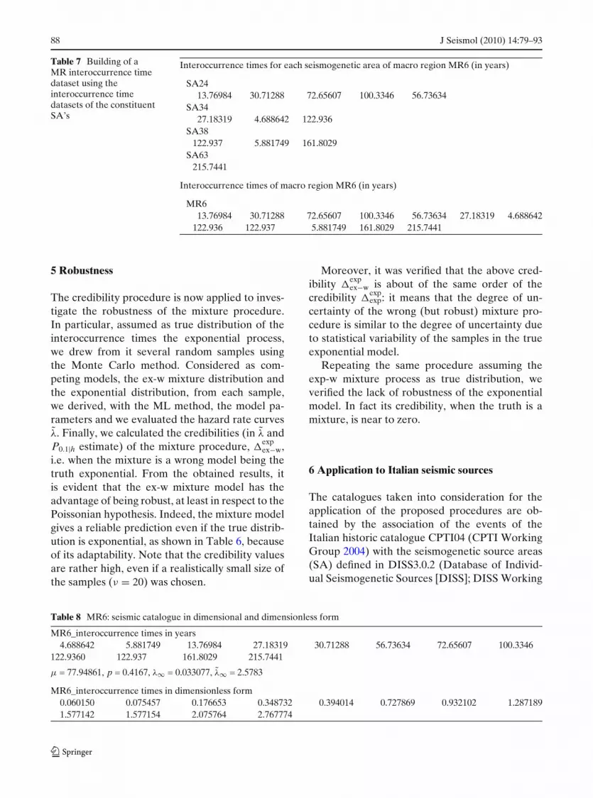
Table 7 Building of aMR interoccurrence timedataset using theinteroccurrence timedatasets of the constituentSA’s
Interoccurrence times for each seismogenetic area of macro region MR6 (in years)
SA2413.76984 30.71288 72.65607 100.3346 56.73634
SA3427.18319 4.688642 122.936
SA38122.937 5.881749 161.8029
SA63215.7441
Interoccurrence times of macro region MR6 (in years)
MR613.76984 30.71288 72.65607 100.3346 56.73634 27.18319 4.688642
122.936 122.937 5.881749 161.8029 215.7441
5 Robustness
The credibility procedure is now applied to inves-tigate the robustness of the mixture procedure.In particular, assumed as true distribution of theinteroccurrence times the exponential process,we drew from it several random samples usingthe Monte Carlo method. Considered as com-peting models, the ex-w mixture distribution andthe exponential distribution, from each sample,we derived, with the ML method, the model pa-rameters and we evaluated the hazard rate curvesλ. Finally, we calculated the credibilities (in λ andP0.1|h estimate) of the mixture procedure, �
expex−w,
i.e. when the mixture is a wrong model being thetruth exponential. From the obtained results, itis evident that the ex-w mixture model has theadvantage of being robust, at least in respect to thePoissonian hypothesis. Indeed, the mixture modelgives a reliable prediction even if the true distrib-ution is exponential, as shown in Table 6, becauseof its adaptability. Note that the credibility valuesare rather high, even if a realistically small size ofthe samples (ν = 20) was chosen.
Moreover, it was verified that the above cred-ibility �
expex−w is about of the same order of the
credibility �expexp: it means that the degree of un-
certainty of the wrong (but robust) mixture pro-cedure is similar to the degree of uncertainty dueto statistical variability of the samples in the trueexponential model.
Repeating the same procedure assuming theexp-w mixture process as true distribution, weverified the lack of robustness of the exponentialmodel. In fact its credibility, when the truth is amixture, is near to zero.
6 Application to Italian seismic sources
The catalogues taken into consideration for theapplication of the proposed procedures are ob-tained by the association of the events of theItalian historic catalogue CPTI04 (CPTI WorkingGroup 2004) with the seismogenetic source areas(SA) defined in DISS3.0.2 (Database of Individ-ual Seismogenetic Sources [DISS]; DISS Working
Table 8 MR6: seismic catalogue in dimensional and dimensionless form
MR6_interoccurrence times in years4.688642 5.881749 13.76984 27.18319 30.71288 56.73634 72.65607 100.3346
122.9360 122.937 161.8029 215.7441
μ = 77.94861, p = 0.4167, λ∞ = 0.033077, λ∞ = 2.5783
MR6_interoccurrence times in dimensionless form0.060150 0.075457 0.176653 0.348732 0.394014 0.727869 0.932102 1.2871891.577142 1.577154 2.075764 2.767774

J Seismol (2010) 14:79–93 89
0 1 2 3 4 5
h0
0.2
0.4
0.6
0.8
1F(h)
^
MLTRMEEMPEXP
a
0 1 2 3 4 5
h0123456789
10λ^ (h)
MLTRMEEMPEXP
b
Fig. 7 (a) MR6: estimation of F (h) in dimensionless form.(b) MR6: estimation of λ (h) in dimensionless form
Group 2006). In DISS, SAs are identified on thebasis of geological and geophysical characteristics(Basili 2007).
These new sub-catalogues have been madeavailable by the members of Task 1.1 of theINGV-DPC Project S2 (Slejko and Valensisecoord.). Each analysed catalogue involves events
with magnitude M defined in CTPI04 as Maw>5.3and having occurred from 1600 to 2002. Tobetter understand the results presented below,we have provided some supplementary elec-tronic material (the label “SEM”, included intable and figure references, will be used to identifyfurther supplementary electronic material associ-ated with this paper). In Figure 01SEM of theSupplementary Electronic Material, a plot of theSA’s labelled with the identification number usedin DISS3.0.2 is given.
As explained in the previous sections, the sam-ple size ν plays an important role on the reliabilityof a probabilistic analysis. Initial inspection of thecatalogues of the 74 SA Sources reveals imme-diately that the methods of this paper cannot beapplied successfully: many of the SA sources havetoo small a sample size v (zero to five events andzero to four interoccurrence times). We obtaineda set of sources having a sufficiently large set ofinteroccurrence times, using the new associationof source areas and related seismicity, groupingthe SA’s into eight macro regions (MR), on thebasis of geophysical aspects (Basili 2007). Theseare shown in Figure 02SEM of the SupplementaryElectronic Material; the MR coordinates are listedin Table 01SEM of the Supplementary ElectronicMaterial.
The combining of SAs in MR can lead to losethe proper identity of each SA. To maintain un-altered the characteristics of the interoccurrence
Table 9 MR6: probability of occurrence P�t| t0 for different �t and different approach of each SA
MR6 �t = 5 years �t = 10 years �t = 20 years �t = 30 years �t = 50 years �t = 100 years
SA24, t0 = 40ML 0.039451 0.096306 0.175295 0.237261 0.351327 0.627267TR 0.04145 0.088838 0.147305 0.195926 0.281847 0.580433ME 0.042291 0.106876 0.204251 0.286431 0.44201 0.721479
SA34, t0 = 22ML 0.056713 0.107703 0.207961 0.277258 0.392574 0.612508TR 0.058281 0.108403 0.200431 0.259055 0.350627 0.559674ME 0.049064 0.096063 0.198182 0.277916 0.428859 0.700014
SA38, t0 = 4ML 0.06687 0.136225 0.243931 0.323475 0.445231 0.636549TR 0.080004 0.148542 0.272828 0.349374 0.456243 0.607427ME 0.047855 0.101151 0.193301 0.271068 0.413136 0.682776
SA63, t0 = 92ML 0.038474 0.083398 0.16832 0.249702 0.435952 0.845912TR 0.032162 0.078694 0.150611 0.231663 0.429369 0.867464ME 0.057749 0.122077 0.233283 0.327149 0.504588 0.823986
90 J Seismol (2010) 14:79–93
0.00
0.10
0.20
0.30
0.40
0.50
0.60
0.70
0.80
0.90
1.00sa
22sa
23sa
02sa
07sa
48sa
61sa
62sa
64sa
66sa
67sa
01sa
08sa
09sa
11sa
12sa
18sa
20sa
27sa
30sa
31sa
32sa
39sa
44sa
46sa
47sa
49sa
51sa
25sa
26sa
28sa
37sa
40sa
41sa
56sa
03sa
04sa
05sa
58sa
59sa
75sa
79sa
84sa
89sa
24sa
34sa
38sa
63sa
15sa
16sa
19sa
53sa
55sa
68sa
80sa
14sa
17sa
21sa
35sa
42
MLTRME
MR1 MR2 MR3 MR4 MR5 MR6 MR7 MR8
P tΔ t0
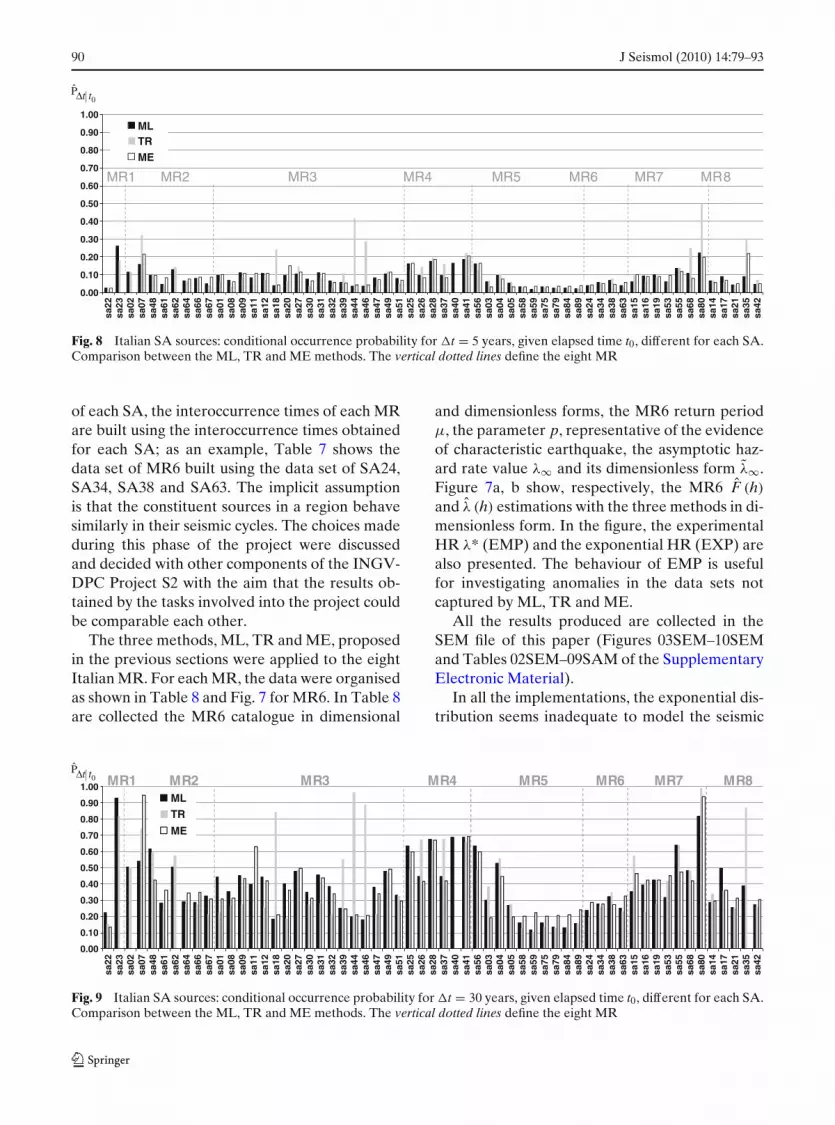
Fig. 8 Italian SA sources: conditional occurrence probability for �t = 5 years, given elapsed time t0, different for each SA.Comparison between the ML, TR and ME methods. The vertical dotted lines define the eight MR
of each SA, the interoccurrence times of each MRare built using the interoccurrence times obtainedfor each SA; as an example, Table 7 shows thedata set of MR6 built using the data set of SA24,SA34, SA38 and SA63. The implicit assumptionis that the constituent sources in a region behavesimilarly in their seismic cycles. The choices madeduring this phase of the project were discussedand decided with other components of the INGV-DPC Project S2 with the aim that the results ob-tained by the tasks involved into the project couldbe comparable each other.
The three methods, ML, TR and ME, proposedin the previous sections were applied to the eightItalian MR. For each MR, the data were organisedas shown in Table 8 and Fig. 7 for MR6. In Table 8are collected the MR6 catalogue in dimensional
and dimensionless forms, the MR6 return periodμ, the parameter p, representative of the evidenceof characteristic earthquake, the asymptotic haz-ard rate value λ∞ and its dimensionless form λ∞.Figure 7a, b show, respectively, the MR6 F (h)
and λ (h) estimations with the three methods in di-mensionless form. In the figure, the experimentalHR λ* (EMP) and the exponential HR (EXP) arealso presented. The behaviour of EMP is usefulfor investigating anomalies in the data sets notcaptured by ML, TR and ME.
All the results produced are collected in theSEM file of this paper (Figures 03SEM–10SEMand Tables 02SEM–09SAM of the SupplementaryElectronic Material).
In all the implementations, the exponential dis-tribution seems inadequate to model the seismic
sa22
sa23
sa02
sa07
sa48
sa61
sa62
sa64
sa66
sa67
sa01
sa08
sa09
sa11
sa12
sa18
sa20
sa27
sa30
sa31
sa32
sa39
sa44
sa46
sa47
sa49
sa51
sa25
sa26
sa28
sa37
sa40
sa41
sa56
sa03
sa04
sa05
sa58
sa59
sa75
sa79
sa84
sa89
sa24
sa34
sa38
sa63
sa15
sa16
sa19
sa53
sa55
sa68
sa80
sa14
sa17
sa21
sa35
sa42
P tΔ t0
0.00
0.10
0.20
0.30
0.40
0.50
0.60
0.70
0.80
0.90
1.00MLTR
ME
MR1 MR2 MR3 MR4 MR5 MR6 MR7 MR8
Fig. 9 Italian SA sources: conditional occurrence probability for �t = 30 years, given elapsed time t0, different for each SA.Comparison between the ML, TR and ME methods. The vertical dotted lines define the eight MR

J Seismol (2010) 14:79–93 91
0 0.2 0.4 0.6 0.8 1 1.2 1.4 1.6 1.8 2h
0
5
10
15
20
25 λ^ (h)
Fig. 10 Mixture-estimated λ (h) (in dimensionless form)for samples drawn from known distribution with increasinghazard rate (Weibull with α > 1)
renewal process, whilst the mixture ex-w, sup-ported by the proposed credibility analysis, seemsmore adequate.
The next step was the evaluation of the prob-ability P�t| t0 : it is the probability of occurrenceof an event of magnitude Maw>5.3 (accordingwith the events considered in the project) in thenext interval of time �t if a time t0 is passed fromthe last event occurring in each SA and the lastyear reported in CPTI04 (2002) assumed as dateof reference. Different intervals of time �t havebeen considered: 5, 10, 20, 30 50 and 100 years. Inparticular, the probability obtained for �t equal5 and 30 years are collected, both in tables andin maps, in Figures 11SEM–16SEM and Tables01_PSEM–08P_SEM of the Supplementary Elec-tronic Material of this paper. As example, Table 9shows the probability of occurrence connectedwith the SA classified in MR6.
Since the year 2002 (the end of our catalogue)until today, 5 years have already passed. The oc-currence probabilities shown in Table 9 are lowand the earthquake did not occur. Is this a con-firmation of the model goodness? Not at all. Itcan only be taken as a kind of consolation. Thedegree of goodness of the model is measured bythe above shown credibility that had explored the“complete” (1,000 samples) sequence of possibleevents.
Figures 8 and 9 collect and compare the prob-ability obtained in each SA with the three differ-
ent methods proposed for �t = 5 years and �t =30 years (in the Supplementary Electronic Mater-ial file, Figs. 8 and 9 are reported in larger formatand labelled as Figure 17SEM and Figure 18SEM,respectively). We may observe that, in most ofthe cases, the three methods give comparable re-sults. There are few cases in which the ML andME methods produce lower probabilities than theTR method. It could be due to the frame of the TRmethod more able to take into account the tail ofthe distribution when the ratio r is large, as pre-viously discussed: accordingly, the high value ofTR probability may indicate peaks in the hazardcurve not caught by ML and ME methods. In anycase, these situations should be investigated. How-ever, when the gap t0 is large (i.e. SA40 and SA11),the TR prediction cannot be done because theasymptotic behaviour of the hazard rate has beenreached. ME results mainly confirm the resultsof ML. On the other hand, being ME methodstrictly related to datasets, in few cases it gives dif-ferences or even lack of prediction. ConsideringML results for �t = 5 years, the highest hazardof occurrence are found in SA 23 (MR1-WesternAlps), in SA 80 (MR7-Calabrian Arc) and in theSA’s of the Central Northern Apennines (MR4).Increasing the interval of time up to 30 years,the hazard increases maintaining mainly the sameratio between the different areas. It indicates thatnot significant changes should be expected in the
0 1 2 3 4 5 6 7 8 9 10h
0
1
2
3
4
5
6
7λ^
(h)
Fig. 11 Mixture-estimated λ (h) (in dimensionless form)for samples drawn from known distribution with decreas-ing hazard rate (Weibull with α < 1)

92 J Seismol (2010) 14:79–93
hazard of the country increasing the expected timefrom 5 to 30 years, according to the ML and MEmethods. On the contrary, TR method underlinessome differences.
7 Discussion and conclusions
Within the context of earthquake prediction, ifit is admissible to assume that the generationof strong events depends primarily on the timeelapsed since the last event, at least in someseismic areas, and if, in this reduced context, itis reasonable to accept an asymptotic station-ary prediction, an exponential–Weibull mixturerenewal model, associated with an empirical cri-terion, leads to conditional probabilities of occur-rence having a rather good degree of credibility,at least for the Italian sources considered.
The proposed model appears flexible enoughto interpret different behaviours of earthquakeoccurrence, whose identification is up to this dayquestionable. It is a robust model; in particular, itcan give a statistic symptom of the dominant be-haviour in the analysed regions: clustering, seismicgap or Poissonian one.
The shape parameter α of the Weibull compo-nent is responsible for the increasing or decreasinghazard rate; the hazard rate being nearly constantwhen α is near to 1.
It is remarkable that the proposed mixturespontaneously fits the alternative behaviours witha good credibility. As an example, let us considersamples drawn from two known distributions withincreasing or decreasing hazard rate, respectively;precisely two Weibull distributions, respectivelywith α > 1 and α < 1 are assumed as conjec-tural truths. Figures 10 and 11 show the estimatedhazard rate with the ex-w mixture model. It isevident that, even if the mixture is a wrong modelin this case, it is able to catch the true increasingor decreasing behaviour of the hazard rate in thetwo assumed conjectural truths.
In the regions analysed in this paper, the modelleads to estimate values of α > 1. On the otherhand, we have to stress that the robustness of themixture model refers only to the explored distri-butions F◦. The panorama of conjectural truthsF◦ and the target quantities A should be properly
enriched; other models can enter in competition.Nevertheless, all the numerical experiments car-ried out up to now showed a remarkable robust-ness of the model, i.e. its adoption reduces theepistemic uncertainties.
The credibility �◦s can be a good tool to judge a
model in its structure in a panorama of conjecturaltruths, rather than to check a hypothesis upon asingle catalogue.
Acknowledgements This research has been developed inthe frame of the Project S2—Assessing the seismogeneticpotential and the probability of strong earthquakes inItaly (Slejko and Valensise coord.)—S2 Project has bene-fited from funding provided by the Italian Presidenza delConsiglio dei Ministri–Dipartimento della ProtezioneCivile (DPC). Scientific paper funded by DPC do not rep-resent its official opinion and policies. The authors wouldalso like to deeply thank both reviewers for their valuablecomments and suggestions in relation to the shortcomingsof the initially submitted work.
References
Akaike H (1977) On entropy maximization principle. In:Krishnaiah PR (ed) Proceedings of the symposium onapplication of statistics. Amsterdam, The Netherlands,pp 27–47
Basili R (2007) Organizzazione di un sistema di riferi-mento unitario per la valutazione della sismogenesi.Final report of Prj S2: valutazione del potenziale sis-mogenetetico e probabilità di forti terremoti in Italia,UR 1.1 report. Available at http://diss.rm.ingv.it/sismogenesi/S2_D1.2.html
Basili R, Valensise G, Vannoli P, Burrato P, FracassiU, Mariano S, Tiberti MM, Boschi E (2008) Thedatabase of individual seismogenic sources (DISS),version 3: summarizing 20 years of research onItaly’s earthquake geology. Tectonophysics 453:20–43.doi:10.1016/j.tecto.2007.04.014
Corral A (2005) Mixing of rescaled data and Bayesianinference for earthquake recurrence times. NonlinearProcess Geophys 12:89–100
Corral A (2006) Dependence of earthquake recurrencetimes and independence of magnitudes on seismic-ity history. Tectonophysics 424:177–193. doi:10.1016/j.tecto.2006.03.035
Cox DR (1962) Renewal theory. Methuen, London, UKCPTI Working Group (2004) Catalogo Parametrico dei
Terremoti Italiani–Versione 2004 (CPTI04) INGV,Bologna. Available at http://emidius.mi.ingv.it/CPTI04/
DISS Working Group (2006) Database of individual seis-mogenic sources (DISS), version 3.0.2: a compila-tion of potential sources for earthquakes larger than

J Seismol (2010) 14:79–93 93
M 5.5 in Italy and surrounding areas. Available athttp://www.ingv.it/DISS/
Faenza L, Marzocchi W, Boschi E (2003) A non-parametric hazard model to characterize the spatio-temporal occurrence of large earthquakes; anapplication to the Italian catalogue. Geophys J Int155:521–531. doi:10.1046/j.1365-246X.2003.02068.x
Garavaglia E, Guagenti E, Petrini L (2007) The earth-quake predictability in mixture renewal models. In:Editor Società Italiana di Statistica (ed) Proceed-ings of Società Italiana di Statistica, SIS interme-diate conference 2007 risk and prediction, Venezia,6–8 June, invited section. CLEUP, Venezia, vol I,pp 361–372
Grandori G, Guagenti E, Tagliani A (1998) A proposalfor comparing the reliabilities of alternative seis-mic hazard models. J Seismol 2:27–35. doi:10.1023/A:1009779806984
Grandori G, Guagenti E, Tagliani A (2003) Magnitudedistribution versus local seismic hazard. Bull SeismolSoc Am 93(3):1091–1098. doi:10.1785/0120010284
Grandori G, Guagenti E, Petrini L (2006) Earthquake cat-alogues and modelling strategies. A new testing proce-dure for the comparison between competing models. JSeismol 10(3):259–269. doi:10.1007/s10950-006-9015-1
Guagenti E, Garavaglia E, Petrini L (2003) Probabilistichazard models: is it possible a statistical validation? In:Bontempi F (ed) System-based vision for strategic andcreative design. Proceedings of ISEC02, 2nd interna-tional structural engineering and construction confer-
ence, Rome, Italy, U.E., 23–26 September. Balkema,Lisse, The Netherlands, vol II, pp 1211–1216
Guagenti E, Garavaglia E, Petrini L (2004) A proposito divalidazione. In: Lagomarsino S, Resemini S (eds) Pro-ceedings of ANIDIS04, XI Conv. Naz. “L’Ingegneriasismica in Italia”, Genova, 25–29 January. SGEditori-ali, Padova, CD-Rom
Guagenti Grandori E, Garavaglia E, Tagliani A (1990)Recurrence time distributions: a discussion. In: Pro-ceedings of the 9th ECEE European conference onearthquake engineering, Moscow, September 1990
Jaynes ET (1957) Information theory and statisticalmechanics. Phys Rev 106(4):620–630. doi:10.1103/PhysRev.106.620
Matthews MV, Ellsworth WL, Reasenberg PA (2002) ABrownian model for recurrent earthquakes. Bull Seis-mol Soc Am 92(6):2233–2250. doi:10.1785/0120010267
Maybeck PS (1979) Stochastic models, estimation, and con-trol, vols I and II. Academic, New York, NJ, USA
Tagliani A (1989) Principle of maximum entropy of prob-ability distributions: definition of applicability field.Probab Eng Mech 4(2):99–104
Tagliani A (1990) On the existence of maximum en-tropy distributions with four and more assigned mo-ments. Probab Eng Mech 5(4):167–170. doi:10.1016/0266-8920(90)90017-E
Vere-Jones D, Ozaki T (1982) Some examples of statisti-cal estimation applied to earthquake data—I. CyclicPoisson and self exciting models. Ann Inst Stat Math34(Part B):189–207