Embed Size (px)
Citation preview
Remote Sens. 2014, 6, 2514-2533; doi:10.3390/rs6032514
remote sensing ISSN 2072-4292
www.mdpi.com/journal/remotesensing
Article
Regional Water Balance Based on Remotely Sensed
Evapotranspiration and Irrigation: An Assessment of
the Haihe Plain, China
Yanmin Yang 1, Yonghui Yang
1,*, Deli Liu
2,3, Tom Nordblom
2,3, Bingfang Wu
4
and Nana Yan 4
1 Key Laboratory of Agricultural Water Resources, Center for Agricultural Resources Research,
Institute of Genetics and Developmental Biology, Chinese Academy of Sciences, 286 Huaizhong Road,
Shijiazhuang 050020, China; E-Mail: [email protected] 2
EH Graham Centre for Agricultural Innovation, Wagga Wagga, New South Wales 2650, Australia;
E-Mails: [email protected] (D.L); [email protected] (T.N.) 3
NSW Department of Primary Industry, Wagga Wagga Agricultural Institute, Pine Gully Road,
Wagga Wagga, NSW 2650, Australia 4
Key Lab. Of Digital Earth Sciences, Institute of Remote Sensing and Digital Earth Chinese
Academy of Science, P.O. Box 9718, No. 20, Datun Road, Olympic Science Park, Beijing 100101,
China; E-Mails: [email protected] (B.W.); [email protected] (N.Y.)
* Author to whom correspondence should be addressed; E-Mail: [email protected];
Tel.: +86-311-8581-4368.
Received: 6 January 2014; in revised form: 12 March 2014 / Accepted: 13 March 2014 /
Published: 20 March 2014
Abstract: Optimal planning and management of the limited water resources for maximum
productivity in agriculture requires quantifying the irrigation applied at a regional scale.
However, most efforts involving remote sensing applications in assessing large-scale
irrigation applied (IA) have focused on supplying spatial variables for crop models or
studying evapotranspiration (ET) inversions, rather than directly building a remote sensing
data-based model to estimate IA. In this study, based on remote sensing data, an IA
estimation model together with an ET calculation model (ETWatch) is set up to simulate
the spatial distribution of IA in the Haihe Plain of northern China. We have verified this as
an effective approach for the simulation of regional IA, being more reflective of regional
characteristics and of higher resolution compared to single site-specific results. The results
show that annual ET varies from 527 mm to 679 mm and IA varies from 166 mm to
OPEN ACCESS
Remote Sens. 2014, 6 2515
289 mm, with average values of 602 mm and 225 mm, respectively, from 2002 to 2007.
We confirm that the region along the Taihang Mountain in Hebei Plain has serious water
resource sustainability problems, even while receiving water from the South-North Water
Transfer (SNWT) project. This is due to the region’s intensive agricultural production and
declining groundwater tables. Water-saving technologies, including more timely and
accurate geo-specific IA assessments, may help reduce this threat.
Keywords: ETWatch; remote sensing technique; ET; irrigation requirement
1. Introduction
Competition for water resources in agriculture is increasing with water scarcity and becoming more
serious in the 21st century. The agricultural sector is one of the biggest consumers of water resources,
accounting for more than 70% of the world’s fresh water use from rivers and groundwater [1]. This
figure is even greater in Asia and the Pacific region, where it accounts for as much as 90% [1]. For
optimal planning and management of the limited water resources for maximum crop productivity in
agriculture, especially in arid and semi-arid regions of the world, techniques are required to quantify
the irrigation applied (IA) at regional scales.
Haihe Basin, located in North China, has especially severe water shortage problems. However, this
basin undertakes the heavy task of grain production to support a large proportion of the Chinese
population of this area. To sustain high-yield grain production, irrigation demand has been satisfied by
excessive groundwater pumping, which has caused sharply declining groundwater tables. To alleviate
water shortage problems in North China, the South-North Water Transfer (SNWT) project is under
construction. The transferred water will be mainly used to meet high priority domestic and industrial
demands. However, a large amount of surface water will then be released for agricultural use. The
problem of how to redistribute water among different sectors and how much will be available for
agricultural use will emerge with the completion of the project. Thus, the ability to accurately assess
the spatial distribution of irrigation demand is necessary.
The science of assessing IA on larger regional scales has undergone development from a focus on
statistical data to the present combination of techniques of crop growth simulation, a geographical
information system (GIS) and remote sensing [2]. Early methods applied to assess irrigation
requirements include water metering, questionnaires, water use coefficients, water rights, pumping
hours or electricity consumption [2]. For example, Boken et al. [3] used irrigation requirements (mm)
for cotton, peanut and maize measured at a limited number of sample sites combined with GIS and
geospatial techniques to estimate regional water use at a county level in Georgia. These methods are
direct and can be quite accurate, but are laborious and lacking in predictive capacity. Model-based
estimation for IA has been reported in many documents, mainly including the Food and Agriculture
Organization (FAO) Penman–Monteith method combining soil water balance models and crop growth
simulation models.
The FAO Penman-Monteith method [4] has been widely used to estimate IA. The method is the
internationally recommended standard for evapotranspiration (ET) estimation in both humid and arid
Remote Sens. 2014, 6 2516
environments [5]. Ozdogan et al. [6] used the CROPWAT system (S) (a computer program for irrigation
planning and management) to estimate water use in south-eastern Turkey, which computes
Penman-Monteith-based reference (potential) evapotranspiration (ETp) and then adjusts this generalized
variable for each crop using seasonal growth curves, or so-called Kc parameters. Leenhardt et al. [7]
applied a simulation platform called ADEAUMIS (an irrigation water demand assessment tool), which
mainly includes the FAO Penman-Monteith method and a spatial database to estimate IA. However,
FAO guidelines are often used to estimate crop evapotranspiration from observed or standard values of
crop development [7].
Crop models that dynamically simulate plant growth and the water demand of one or several crops
can provide quantitative contributions to the environmental impact assessment and be very useful for
water management [7]. One of the limitations of current crop simulation models is that they are site
specific. By combining with spatial data, crop models have been used by many scientists to estimate
IA at regional or global scales. Ines et al. [8] applied crop simulation models CERES-rice (Crop
Environment Resource Synthesis for rice), CERES-maize and CROPGRO-peanut (a process-oriented
model for crop growth of peanut) in DSSAT (Decision Support System for Agrotechnology Transfer)
version 3.0 coupled with GIS to the estimate irrigation needs for rice, maize and peanut, and then
water productivity in the Laoag River Basin in Ilocos Norte, Philippines. The cropping system model,
CROPGRO-Cotton, combined with kriging interpolation, was used to evaluate the spatial distribution
of monthly irrigation water use for cotton in the Coastal Plain region of Georgia [9]. Wriedt et al. [2]
estimated the spatial distribution of irrigation applied at a 10 × 10-km grid resolution in Europe with
the crop growth model, EPIC (Erosion Productivity Impact Calculator), combining available regional
statistics on crop distribution, crop-specific irrigated area and spatial data sources on soils, land use and
climate. The global scale water use of wheat was estimated by combining EPIC with GIS (geographic
information system) [10].
The shortage of geo-located data on agricultural practices was considered to be a limiting factor for
the operational use of crop models over large scales [11]. Fortunately, public domain Internet satellite
data and scientific development make remote sensing an attractive option for assessing irrigation
performance from individual fields to scheme or river basin scale [1]. One of the applications of remote
sensing in assessing irrigation performance is in providing information on some key variables of crop
production and, especially, variations in these over time and space. For example, Ozdogan et al. [6]
successfully estimated irrigated area with the aid of remote sensing to compute water use in
south-eastern Turkey, in the period 1993 to 2002. Ines et al. [12] estimated the distributed data, e.g.,
sowing dates, irrigation practices, soil properties, depth to groundwater and water quality, required as
inputs to regional modelling by minimizing the residuals between the distributions of field-scale ET
simulated by regional application of the SWAP (Soil, Water, Atmosphere and Plant) model and by
the surface energy balance algorithm for land (SEBAL) using pairs of Landsat-7 ETM+ images.
Another application of remote sensing in assessing irrigation performance was to estimate ET. The
satellite-based model SEBAL has been applied in more than 30 countries worldwide and is now an
operational instrument for targeting, monitoring and evaluating irrigation and drainage systems [13].
ETWatch is another ET monitoring system using remote sensing, which integrates SEBAL and SEBS
and is commonly used in North China [14].
Remote Sens. 2014, 6 2517
As stated above, most documents on RS applications for assessing irrigation water applied at larger
scales focused on providing spatial variables for crop models or studies on ET inversion. Little
literature is available on directly using RS to determine irrigation water requirements. The objectives
of the present study are to: (1) set up a model based on RS-based ETWatch and a soil water balance
model to evaluate irrigation water requirements; (2) analyse the spatial distribution of IA to evaluate
regional water sustainability.
2. Study Area
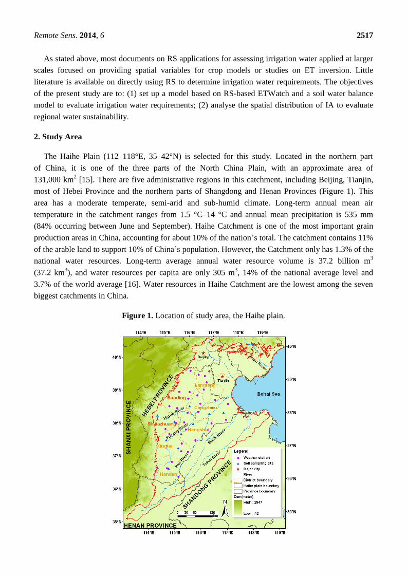
The Haihe Plain (112–118°E, 35–42°N) is selected for this study. Located in the northern part
of China, it is one of the three parts of the North China Plain, with an approximate area of
131,000 km2 [15]. There are five administrative regions in this catchment, including Beijing, Tianjin,
most of Hebei Province and the northern parts of Shangdong and Henan Provinces (Figure 1). This
area has a moderate temperate, semi-arid and sub-humid climate. Long-term annual mean air
temperature in the catchment ranges from 1.5 °C–14 °C and annual mean precipitation is 535 mm
(84% occurring between June and September). Haihe Catchment is one of the most important grain
production areas in China, accounting for about 10% of the nation’s total. The catchment contains 11%
of the arable land to support 10% of China’s population. However, the Catchment only has 1.3% of the
national water resources. Long-term average annual water resource volume is 37.2 billion m3
(37.2 km3), and water resources per capita are only 305 m
3, 14% of the national average level and
3.7% of the world average [16]. Water resources in Haihe Catchment are the lowest among the seven
biggest catchments in China.
Figure 1. Location of study area, the Haihe plain.
Remote Sens. 2014, 6 2518
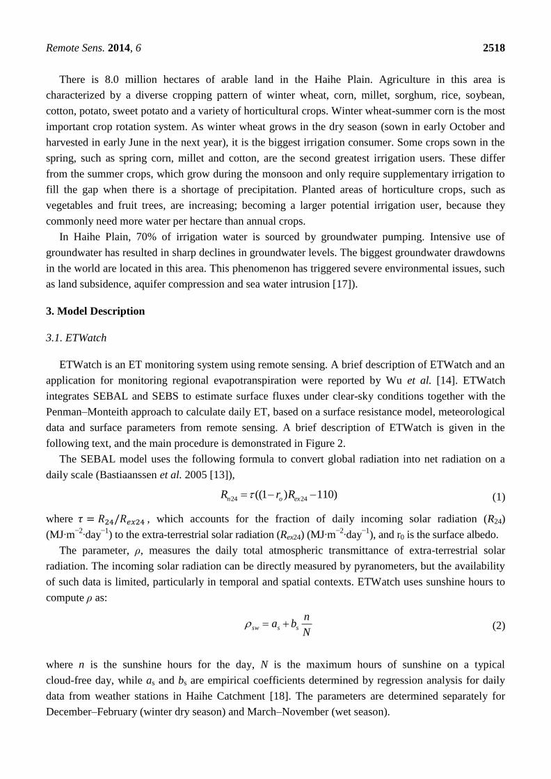
There is 8.0 million hectares of arable land in the Haihe Plain. Agriculture in this area is
characterized by a diverse cropping pattern of winter wheat, corn, millet, sorghum, rice, soybean,
cotton, potato, sweet potato and a variety of horticultural crops. Winter wheat-summer corn is the most
important crop rotation system. As winter wheat grows in the dry season (sown in early October and
harvested in early June in the next year), it is the biggest irrigation consumer. Some crops sown in the
spring, such as spring corn, millet and cotton, are the second greatest irrigation users. These differ
from the summer crops, which grow during the monsoon and only require supplementary irrigation to
fill the gap when there is a shortage of precipitation. Planted areas of horticulture crops, such as
vegetables and fruit trees, are increasing; becoming a larger potential irrigation user, because they
commonly need more water per hectare than annual crops.
In Haihe Plain, 70% of irrigation water is sourced by groundwater pumping. Intensive use of
groundwater has resulted in sharp declines in groundwater levels. The biggest groundwater drawdowns
in the world are located in this area. This phenomenon has triggered severe environmental issues, such
as land subsidence, aquifer compression and sea water intrusion [17]).
3. Model Description
3.1. ETWatch
ETWatch is an ET monitoring system using remote sensing. A brief description of ETWatch and an
application for monitoring regional evapotranspiration were reported by Wu et al. [14]. ETWatch
integrates SEBAL and SEBS to estimate surface fluxes under clear-sky conditions together with the
Penman–Monteith approach to calculate daily ET, based on a surface resistance model, meteorological
data and surface parameters from remote sensing. A brief description of ETWatch is given in the
following text, and the main procedure is demonstrated in Figure 2.
The SEBAL model uses the following formula to convert global radiation into net radiation on a
daily scale (Bastiaanssen et al. 2005 [13]),
24 24((1 ) 110)n o exR r R (1)
where , which accounts for the fraction of daily incoming solar radiation (R24)
(MJ∙m−2
∙day−1
) to the extra-terrestrial solar radiation (Rex24) (MJ∙m−2
∙day−1
), and r0 is the surface albedo.
The parameter, ρ, measures the daily total atmospheric transmittance of extra-terrestrial solar
radiation. The incoming solar radiation can be directly measured by pyranometers, but the availability
of such data is limited, particularly in temporal and spatial contexts. ETWatch uses sunshine hours to
compute ρ as:
N
nba sssw
(2)
where n is the sunshine hours for the day, N is the maximum hours of sunshine on a typical
cloud-free day, while as and bs are empirical coefficients determined by regression analysis for daily
data from weather stations in Haihe Catchment [18]. The parameters are determined separately for
December–February (winter dry season) and March–November (wet season).
Remote Sens. 2014, 6 2519
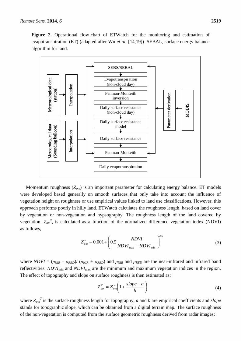
Figure 2. Operational flow-chart of ETWatch for the monitoring and estimation of
evapotranspiration (ET) (adapted after Wu et al. [14,19]). SEBAL, surface energy balance
algorithm for land.
Momentum roughness (Zom) is an important parameter for calculating energy balance. ET models
were developed based generally on smooth surfaces that only take into account the influence of
vegetation height on roughness or use empirical values linked to land use classifications. However, this
approach performs poorly in hilly land. ETWatch calculates the roughness length, based on land cover
by vegetation or non-vegetation and hypsography. The roughness length of the land covered by
vegetation, Zomv, is calculated as a function of the normalized difference vegetation index (NDVI)
as follows,
5.2
minmax
5.0001.0
NDVINDVI
NDVIZ v
om
(3)
where NDVI = (ρNIR – ρRED)/ (ρNIR + ρRED) and ρNIR and ρRED are the near-infrared and infrared band
reflectivities. NDVImin and NDVImax are the minimum and maximum vegetation indices in the region.
The effect of topography and slope on surface roughness is then estimated as:
b
aslopeZZ v
om
T
om 1
(4)
where ZomT is the surface roughness length for topography, a and b are empirical coefficients and slope
stands for topographic slope, which can be obtained from a digital terrain map. The surface roughness
of the non-vegetation is computed from the surface geometric roughness derived from radar images:
Daily evapotranspiration
Penman-Monteith
Daily surface resistance
Daily surface resistancemodel
Daily surface resistance(non-cloud day)
Penman-Monteithinversion
Evapotranspiration
(non-cloud day)
SEBS/SEBAL
Met
eoro
logic
al d
ata
(So
un
din
g b
allo
on
)
Par
amet
er d
eriv
atio
n
Met
eoro
logic
al d
ata
(sta
tio
n)
Inte
rpo
lati
on
Inte
rpo
lati
on
MO
DIS
Remote Sens. 2014, 6 2520
)(0906.0221.1)log( o
r
omZ (5)
where Zomr is the surface roughness of the non-vegetation fraction of the basin and σo is the backscatter
coefficient acquired from the Radarsat satellite image. The total basin roughness is finally computed as:
r
om
T
om
v
omom ZwZwZwZ 321 (6)
where w1, w2 and w3 are the weighted factors for vegetation, topography and bare-land on surface
roughness. The values of w1, w2 and w3 are 1.0, 1.0 and 0.25, respectively for the Hai Basin, which
were determined by using the empirical fitted ways [18].
Resistance for the days with clouds (RSunc) is computed as:
)()( min VPDmTmLAI
RSLAIRS
unc
clrclr
unc
(7)
where RSclr is the resistance for the cloudless day, LAIunc is the leaf area index for the day with clouds,
LAIclr is the leaf area index for cloud-free day and m(Tmin) and m(VPD) are the functions of minimum
temperatures and vapour pressures, respectively, which account for the effect of extreme temperature
and moisture on plant stomata.
3.2. Irrigation Applied (IA) Estimation Model
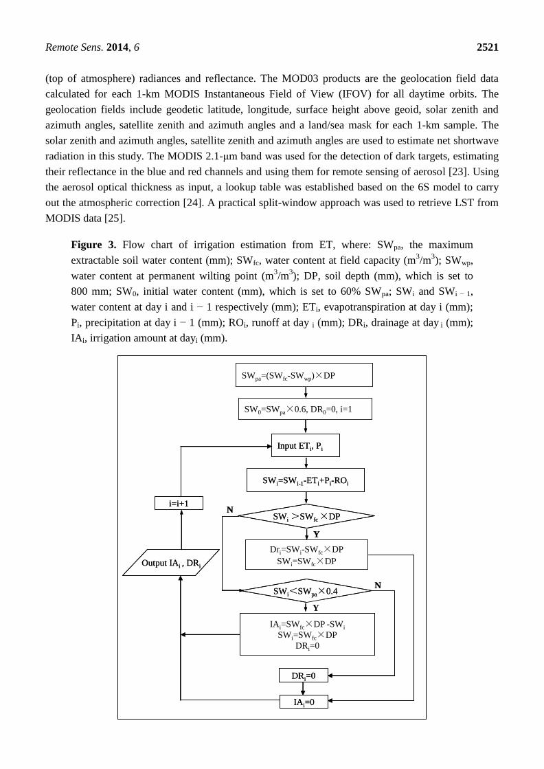
The sequence of calculations used to estimate IA is given in Figure 3. The model starts from the date
when a crop is sown. Several practical assumptions are made. The initial soil water content is set as 60%
of maximum plant available water (SWpa), which is generally used by farmers for crops to be sown. The
depth of soil profile is set as 80 cm. When soil water content is less than 40% SWpa, irrigation operation
is to be triggered. The irrigation applied is equal to the difference between field capacity (SWfc) and the
soil water content on the previous day (SWi−1). When there is precipitation on the day and the soil water
content is greater than field capacity, the amount of water in excess of field capacity is assumed to go to
deep drainage, and the current soil water content is set equal to field capacity. Since farmland in the
Haihe Plain is very flat and soils are deep, there is a large water holding capacity, especially in relation to
precipitation shortages; runoff (ROi) is minimal and may be ignored [20].
Water content at field capacity and permanent wilting point (SWfc and SWwp) are calculated by the
SPAW model [21]) using the basic soil texture parameters, including clay content (%), sand content (%)
and organic matter content (%). These soil parameters come from 76 representative sites in Haihe
Catchment. Precipitation data are collected from 46 meteorological stations. All these data are finally
interpolated into a 1-km2 grid and prepared for use in the above-mentioned spatial calculation procedures.
4. Data Collection
4.1. Remote Sensing Data
The MODIS data used in this study are the MOD021KM, MOD02QKM, MOD02HKM and
MOD03 products provided by the NASA Goddard Space Flight Center (GSFC) Level 1 and
Atmosphere Archive and Distribution System (LAADS) [22]. The MOD02QKM and MOD02HKM
products, including the 250-m and 500-m resolution bands, are aggregated to 1-km resolution TOA
Remote Sens. 2014, 6 2521
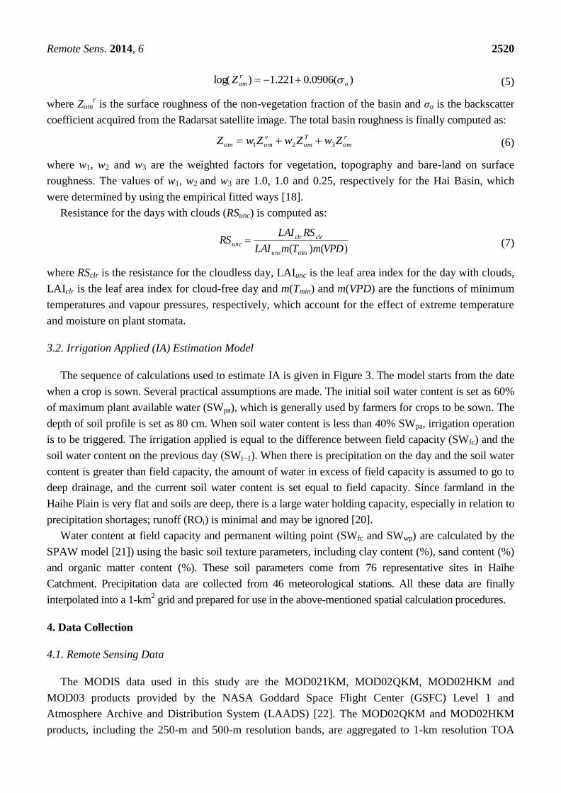
(top of atmosphere) radiances and reflectance. The MOD03 products are the geolocation field data
calculated for each 1-km MODIS Instantaneous Field of View (IFOV) for all daytime orbits. The
geolocation fields include geodetic latitude, longitude, surface height above geoid, solar zenith and
azimuth angles, satellite zenith and azimuth angles and a land/sea mask for each 1-km sample. The
solar zenith and azimuth angles, satellite zenith and azimuth angles are used to estimate net shortwave
radiation in this study. The MODIS 2.1-μm band was used for the detection of dark targets, estimating
their reflectance in the blue and red channels and using them for remote sensing of aerosol [23]. Using
the aerosol optical thickness as input, a lookup table was established based on the 6S model to carry
out the atmospheric correction [24]. A practical split-window approach was used to retrieve LST from
MODIS data [25].
Figure 3. Flow chart of irrigation estimation from ET, where: SWpa, the maximum
extractable soil water content (mm); SWfc, water content at field capacity (m3/m
3); SWwp,
water content at permanent wilting point (m3/m
3); DP, soil depth (mm), which is set to
800 mm; SW0, initial water content (mm), which is set to 60% SWpa; SWi and SWi − 1,
water content at day i and i − 1 respectively (mm); ETi, evapotranspiration at day i (mm);
Pi, precipitation at day i − 1 (mm); ROi, runoff at day i (mm); DRi, drainage at day i (mm);
IAi, irrigation amount at dayi (mm).
Y
Y
SWpa=(SWfc-SWwp)×DP
SW0=SWpa×0.6, DR0=0, i=1
SWi=SWi-1-ETi+Pi-ROi
IAi=SWfc×DP -SWi
SWi=SWfc×DP
DRi=0
N
N
Dri=SWi-SWfc×DP
SWi=SWfc×DP
SWi >SWfc×DP
SWi<SWpa×0.4
IAi=0
Output IAi , DRi
i=i+1
DRi=0
Input ETi, Pi
Y
Y
SWpa=(SWfc-SWwp)×DP
SW0=SWpa×0.6, DR0=0, i=1
SWi=SWi-1-ETi+Pi-ROi
IAi=SWfc×DP -SWi
SWi=SWfc×DP
DRi=0
N
N
Dri=SWi-SWfc×DP
SWi=SWfc×DP
SWi >SWfc×DP
SWi<SWpa×0.4
IAi=0
Output IAi , DRi
i=i+1
DRi=0
Input ETi, Pi
Remote Sens. 2014, 6 2522
Landsat TM images with Bands 2, 3, 4 and 5 at different periods from the years 2000–2001 at a spatial
scale of 1:100,000 were used to interpret land use data over the Haihe Plain. The work was done by another
group of ―land cover dynamic monitoring‖ of the Key Innovation Project (KZCX1-YW-08-03-04) of the
Chinese Academy of Sciences.
4.2. Meteorological Data
Daily meteorological data at 83 meteorological stations, including maximum and minimum air
temperature, sunshine duration, relative humidity, wind speed and air pressure (2002–2007), are
collected from the National Meteorological Bureau. The variables are interpolated into daily maps at
1-km resolution by the inverse distance squared method.
4.3. Lysimeter Data
Monthly ET and irrigation amount from large Lysimeter provided by Luangcheng Station (Chinese
Ecosystem Research Network).
5. Results
5.1. Verification
Validation of ET estimated from ETwatch was described in the documents of [14] and [26].
According to these reports, the ET result exhibited less error than the results produced by the earlier
method of constant-EF (evaporative factor). The mean absolute percent difference (MAPD) of
gap-filling approach is reasonable (22.5%), compared to MAPD produced by constant-EF (46.3%).
Alternatively, the gap-filling method used in ETWatch gives a 50% improvement in accuracy.
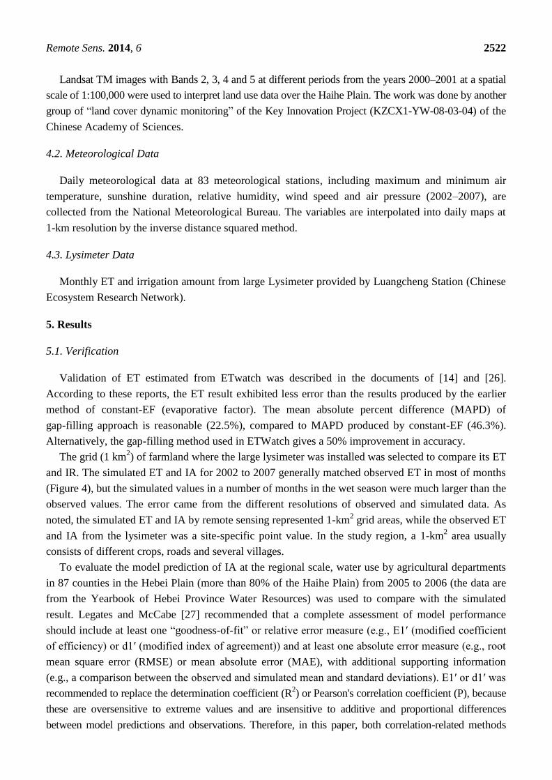
The grid (1 km2) of farmland where the large lysimeter was installed was selected to compare its ET
and IR. The simulated ET and IA for 2002 to 2007 generally matched observed ET in most of months
(Figure 4), but the simulated values in a number of months in the wet season were much larger than the
observed values. The error came from the different resolutions of observed and simulated data. As
noted, the simulated ET and IA by remote sensing represented 1-km2 grid areas, while the observed ET
and IA from the lysimeter was a site-specific point value. In the study region, a 1-km2 area usually
consists of different crops, roads and several villages.
To evaluate the model prediction of IA at the regional scale, water use by agricultural departments
in 87 counties in the Hebei Plain (more than 80% of the Haihe Plain) from 2005 to 2006 (the data are
from the Yearbook of Hebei Province Water Resources) was used to compare with the simulated
result. Legates and McCabe [27] recommended that a complete assessment of model performance
should include at least one ―goodness-of-fit‖ or relative error measure (e.g., E1′ (modified coefficient
of efficiency) or d1′ (modified index of agreement)) and at least one absolute error measure (e.g., root
mean square error (RMSE) or mean absolute error (MAE), with additional supporting information
(e.g., a comparison between the observed and simulated mean and standard deviations). E1′ or d1′ was
recommended to replace the determination coefficient (R2) or Pearson's correlation coefficient (P), because
these are oversensitive to extreme values and are insensitive to additive and proportional differences
between model predictions and observations. Therefore, in this paper, both correlation-related methods
Remote Sens. 2014, 6 2523
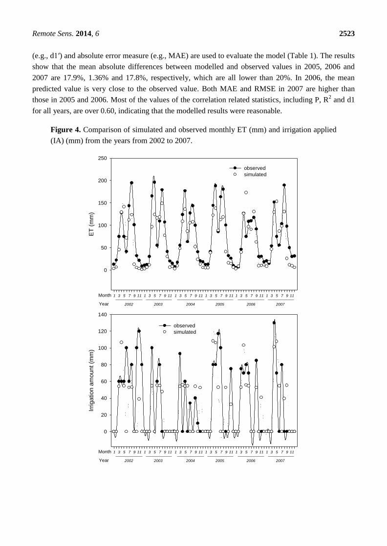
(e.g., d1′) and absolute error measure (e.g., MAE) are used to evaluate the model (Table 1). The results
show that the mean absolute differences between modelled and observed values in 2005, 2006 and
2007 are 17.9%, 1.36% and 17.8%, respectively, which are all lower than 20%. In 2006, the mean
predicted value is very close to the observed value. Both MAE and RMSE in 2007 are higher than
those in 2005 and 2006. Most of the values of the correlation related statistics, including P, R2 and d1
for all years, are over 0.60, indicating that the modelled results were reasonable.
Figure 4. Comparison of simulated and observed monthly ET (mm) and irrigation applied
(IA) (mm) from the years from 2002 to 2007.
ET
(m
m)
0
50
100
150
200
250
observed
simulated
2002 2003
111 3 5 7 9 111 3 5 7 9111 3 5 7 9 111 3 5 7 9 111 3 5 7 9 111 3 5 7 9
2004 2005 2006 2007
Month
Year
Irri
ga
tio
n a
mo
un
t (m
m)
0
20
40
60
80
100
120
140
observed
simulated
2002 2003
111 3 5 7 9 111 3 5 7 9111 3 5 7 9 111 3 5 7 9 111 3 5 7 9 111 3 5 7 9
2004 2005 2006 2007
Month
Year
Remote Sens. 2014, 6 2524
Table 1. Means and standard deviations of observed and simulated yearly irrigation
amount for county of Haihe Plain for the years of 2005, 2006 and 2007, and the statistics
comparing the observed and simulated values.
2005 2006 2007
Observed Modelled Observed Modelled Observed Modelled
Mean, mm 240 224 295 299 246 202
Standard deviation, mm 74 50 91 72 95 80
Mean absolute error, mm 38.88 39.75 52.05
Root mean square error, mm 53 55 71
Pearson’s correlation 0.73 0.80 0.81
Coefficient of determination 0.53 0.64 0.65
Modified index of agreement 0.61 0.68 0.68
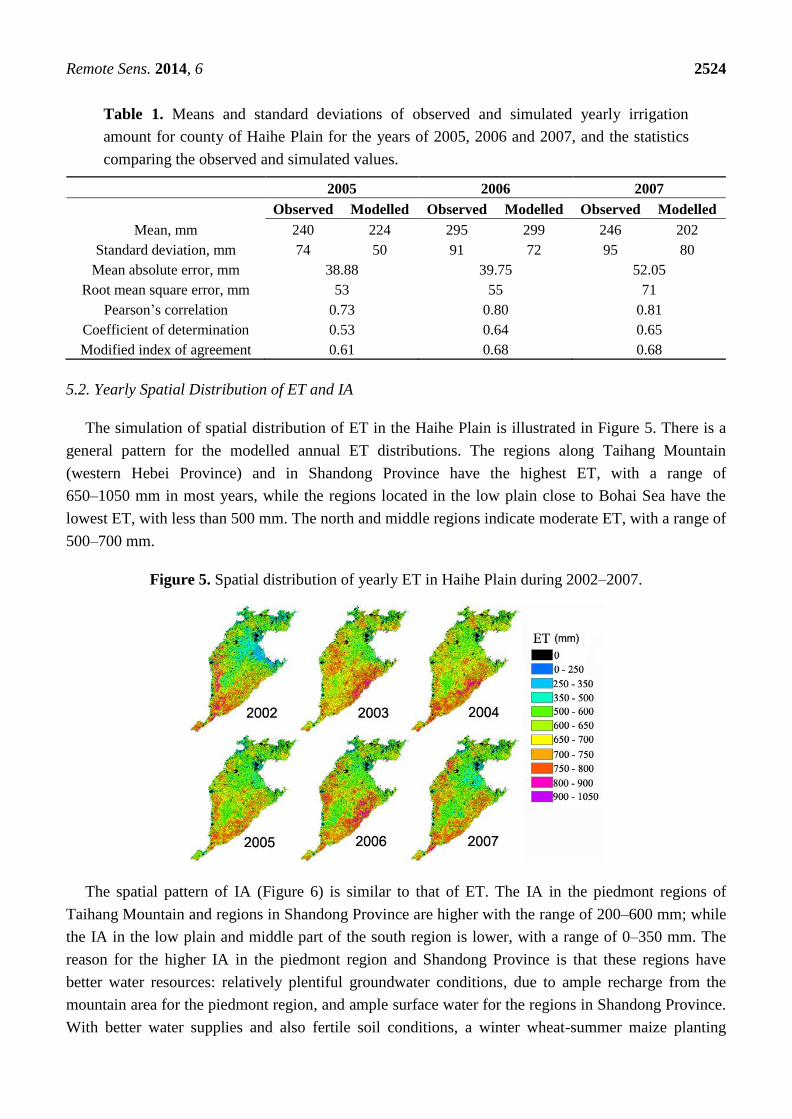
5.2. Yearly Spatial Distribution of ET and IA
The simulation of spatial distribution of ET in the Haihe Plain is illustrated in Figure 5. There is a
general pattern for the modelled annual ET distributions. The regions along Taihang Mountain
(western Hebei Province) and in Shandong Province have the highest ET, with a range of
650–1050 mm in most years, while the regions located in the low plain close to Bohai Sea have the
lowest ET, with less than 500 mm. The north and middle regions indicate moderate ET, with a range of
500–700 mm.
Figure 5. Spatial distribution of yearly ET in Haihe Plain during 2002–2007.
The spatial pattern of IA (Figure 6) is similar to that of ET. The IA in the piedmont regions of
Taihang Mountain and regions in Shandong Province are higher with the range of 200–600 mm; while
the IA in the low plain and middle part of the south region is lower, with a range of 0–350 mm. The
reason for the higher IA in the piedmont region and Shandong Province is that these regions have
better water resources: relatively plentiful groundwater conditions, due to ample recharge from the
mountain area for the piedmont region, and ample surface water for the regions in Shandong Province.
With better water supplies and also fertile soil conditions, a winter wheat-summer maize planting
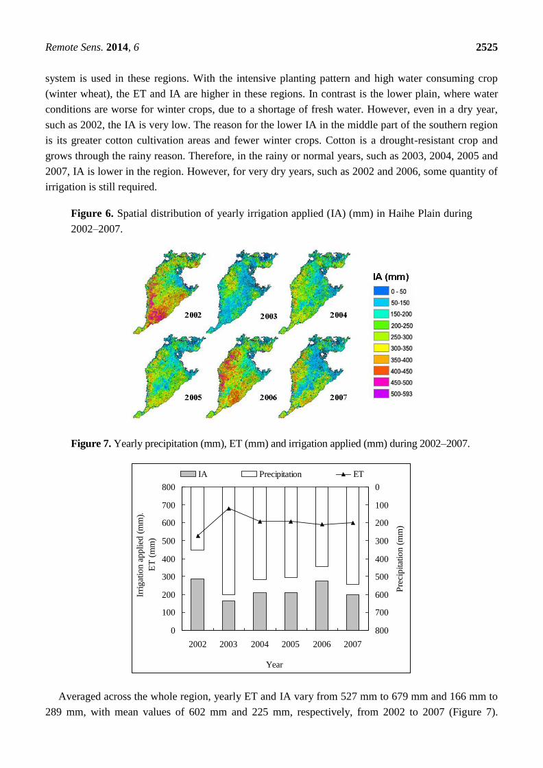
Remote Sens. 2014, 6 2525
system is used in these regions. With the intensive planting pattern and high water consuming crop
(winter wheat), the ET and IA are higher in these regions. In contrast is the lower plain, where water
conditions are worse for winter crops, due to a shortage of fresh water. However, even in a dry year,
such as 2002, the IA is very low. The reason for the lower IA in the middle part of the southern region
is its greater cotton cultivation areas and fewer winter crops. Cotton is a drought-resistant crop and
grows through the rainy reason. Therefore, in the rainy or normal years, such as 2003, 2004, 2005 and
2007, IA is lower in the region. However, for very dry years, such as 2002 and 2006, some quantity of
irrigation is still required.
Figure 6. Spatial distribution of yearly irrigation applied (IA) (mm) in Haihe Plain during
2002–2007.
Figure 7. Yearly precipitation (mm), ET (mm) and irrigation applied (mm) during 2002–2007.
Averaged across the whole region, yearly ET and IA vary from 527 mm to 679 mm and 166 mm to
289 mm, with mean values of 602 mm and 225 mm, respectively, from 2002 to 2007 (Figure 7).
0
100
200
300
400
500
600
700
800
2002 2003 2004 2005 2006 2007
Year
Irri
gat
ion a
pplied
(m
m).
.
ET
(m
m)
0
100
200
300
400
500
600
700
800
Pre
cipitat
ion (
mm
)...
IA Precipitation ET
Remote Sens. 2014, 6 2526
Yearly variations in ET and IA are highly related to precipitation, which varies from 351 mm to
601 mm, with a mean value of 493 mm from 2002 to 2007. ET is positively correlated to precipitation
and IA is negatively correlated to it. For example, in 2003, the precipitation is as high as 601 mm;
accordingly, the ET is the highest (679 mm); however, the IA is lowest (225 mm) in that year.
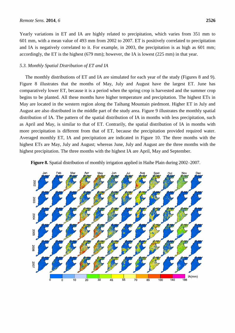
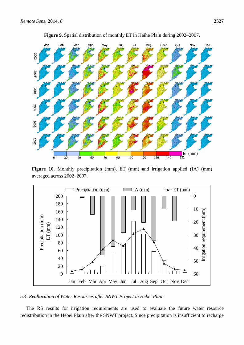
5.3. Monthly Spatial Distribution of ET and IA
The monthly distributions of ET and IA are simulated for each year of the study (Figures 8 and 9).
Figure 8 illustrates that the months of May, July and August have the largest ET. June has
comparatively lower ET, because it is a period when the spring crop is harvested and the summer crop
begins to be planted. All these months have higher temperature and precipitation. The highest ETs in
May are located in the western region along the Taihang Mountain piedmont. Higher ET in July and
August are also distributed in the middle part of the study area. Figure 9 illustrates the monthly spatial
distribution of IA. The pattern of the spatial distribution of IA in months with less precipitation, such
as April and May, is similar to that of ET. Contrarily, the spatial distribution of IA in months with
more precipitation is different from that of ET, because the precipitation provided required water.
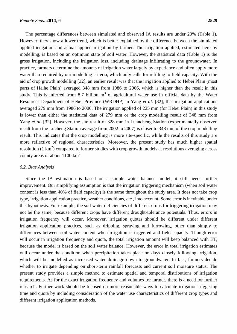
Averaged monthly ET, IA and precipitation are indicated in Figure 10. The three months with the
highest ETs are May, July and August; whereas June, July and August are the three months with the
highest precipitation. The three months with the highest IA are April, May and September.
Figure 8. Spatial distribution of monthly irrigation applied in Haihe Plain during 2002–2007.
Remote Sens. 2014, 6 2527
Figure 9. Spatial distribution of monthly ET in Haihe Plain during 2002–2007.
Figure 10. Monthly precipitation (mm), ET (mm) and irrigation applied (IA) (mm)
averaged across 2002–2007.
5.4. Reallocation of Water Resources after SNWT Project in Hebei Plain
The RS results for irrigation requirements are used to evaluate the future water resource
redistribution in the Hebei Plain after the SNWT project. Since precipitation is insufficient to recharge
0
20
40
60
80
100
120
140
160
180
200
Jan Feb Mar Apr May Jun Jul Aug Sep Oct Nov Dec
Pre
cipitat
ion (
mm
)..
ET
(m
m)
0
10
20
30
40
50
60
Irri
gat
ion r
equ
irem
ent (m
m).
.
Precipitation (mm) IA (mm) ET (mm)
Remote Sens. 2014, 6 2528
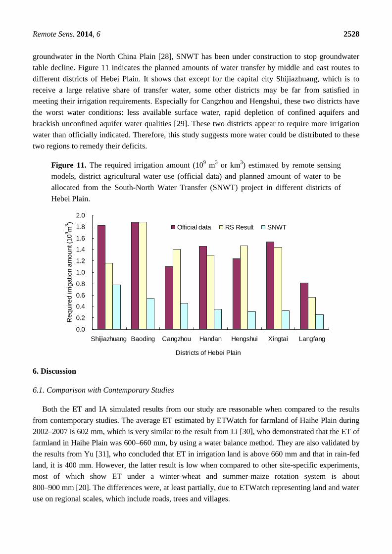
groundwater in the North China Plain [28], SNWT has been under construction to stop groundwater
table decline. Figure 11 indicates the planned amounts of water transfer by middle and east routes to
different districts of Hebei Plain. It shows that except for the capital city Shijiazhuang, which is to
receive a large relative share of transfer water, some other districts may be far from satisfied in
meeting their irrigation requirements. Especially for Cangzhou and Hengshui, these two districts have
the worst water conditions: less available surface water, rapid depletion of confined aquifers and
brackish unconfined aquifer water qualities [29]. These two districts appear to require more irrigation
water than officially indicated. Therefore, this study suggests more water could be distributed to these
two regions to remedy their deficits.
Figure 11. The required irrigation amount (109 m
3 or km
3) estimated by remote sensing
models, district agricultural water use (official data) and planned amount of water to be
allocated from the South-North Water Transfer (SNWT) project in different districts of
Hebei Plain.
6. Discussion
6.1. Comparison with Contemporary Studies
Both the ET and IA simulated results from our study are reasonable when compared to the results
from contemporary studies. The average ET estimated by ETWatch for farmland of Haihe Plain during
2002–2007 is 602 mm, which is very similar to the result from Li [30], who demonstrated that the ET of
farmland in Haihe Plain was 600–660 mm, by using a water balance method. They are also validated by
the results from Yu [31], who concluded that ET in irrigation land is above 660 mm and that in rain-fed
land, it is 400 mm. However, the latter result is low when compared to other site-specific experiments,
most of which show ET under a winter-wheat and summer-maize rotation system is about
800–900 mm [20]. The differences were, at least partially, due to ETWatch representing land and water
use on regional scales, which include roads, trees and villages.
0.0
0.2
0.4
0.6
0.8
1.0
1.2
1.4
1.6
1.8
2.0
Shijiazhuang Baoding Cangzhou Handan Hengshui Xingtai Langfang
Districts of Hebei Plain
Re
qu
ire
d irr
iga
tio
n a
mo
un
t (1
0 9m
3)
Official data RS Result SNWT
Remote Sens. 2014, 6 2529
The percentage differences between simulated and observed IA results are under 20% (Table 1).
However, they show a lower trend, which is better explained by the difference between the simulated
applied irrigation and actual applied irrigation by farmer. The irrigation applied, estimated here by
modelling, is based on an optimum state of soil water. However, the statistical data (Table 1) is the
gross irrigation, including the irrigation loss, including drainage infiltrating to the groundwater. In
practice, farmers determine the amounts of irrigation water largely by experience and often apply more
water than required by our modelling criteria, which only calls for refilling to field capacity. With the
aid of crop growth modelling [32], an earlier result was that the irrigation applied to Hebei Plain (most
parts of Haihe Plain) averaged 348 mm from 1986 to 2006, which is higher than the result in this
study. This is inferred from 8.7 billion m3 of agricultural water use in official data by the Water
Resources Department of Hebei Province (WRDHP) in Yang et al. [32], that irrigation applications
averaged 279 mm from 1986 to 2006. The irrigation applied of 225 mm (for Hebei Plain) in this study
is lower than either the statistical data of 279 mm or the crop modelling result of 348 mm from
Yang et al. [32]. However, the site result of 328 mm in Luancheng Station (experimentally observed
result from the Lucheng Station average from 2002 to 2007) is closer to 348 mm of the crop modelling
result. This indicates that the crop modelling is more site-specific, while the results of this study are
more reflective of regional characteristics. Moreover, the present study has much higher spatial
resolution (1 km2) compared to former studies with crop growth models at resolutions averaging across
county areas of about 1100 km2.
6.2. Bias Analysis
Since the IA estimation is based on a simple water balance model, it still needs further
improvement. Our simplifying assumption is that the irrigation triggering mechanism (when soil water
content is less than 40% of field capacity) is the same throughout the study area. It does not take crop
type, irrigation application practice, weather conditions, etc., into account. Some error is inevitable under
this hypothesis. For example, the soil water deficiencies of different crops for triggering irrigation may
not be the same, because different crops have different drought-tolerance potentials. Thus, errors in
irrigation frequency will occur. Moreover, irrigation quotas should be different under different
irrigation application practices, such as dripping, spraying and furrowing, other than simply to
differences between soil water content when irrigation is triggered and field capacity. Though error
will occur in irrigation frequency and quota, the total irrigation amount will keep balanced with ET,
because the model is based on the soil water balance. However, the error in total irrigation estimates
will occur under the condition when precipitation takes place on days closely following irrigation,
which will be modelled as increased water drainage down to groundwater. In fact, farmers decide
whether to irrigate depending on short-term rainfall forecasts and current soil moisture status. The
present study provides a simple method to estimate spatial and temporal distributions of irrigation
requirements. As for the exact irrigation frequency and volumes for farmer, there is a need for further
research. Further work should be focused on more reasonable ways to calculate irrigation triggering
time and quota by including consideration of the water use characteristics of different crop types and
different irrigation application methods.
Remote Sens. 2014, 6 2530
6.3. Suggestion for the Sustainability of Water Resources
Intensive agricultural production in Haihe Basin, especially Hebei Plain, makes the water shortage
situation more and more pressing. As 70% of irrigation comes from groundwater, the groundwater
table has declined drastically over several decades. According to the report from Yang et al. [33], an
approximate 100-mm irrigation application in cultivated land leads to about a 640-mm groundwater
decline. However, groundwater recharge is not sufficiently met by precipitation. Han et al. [28]
reported that precipitation recharge is only expected when a single or successive rainfall are in excess
of the minimum amount of 170 mm, a very rare condition in the piedmont region (Baoding,
Shijiazhuang, Xingtai and Handan districts). While in the coastal and middle area, Cangzhou and
Hengshui district, groundwater age has been found to exceed 10,000 years, this means there is only a
remote possibility of confined aquifer recharge in these districts [34].
Though SNWT aims to alleviate the water shortage problem, it may not completely meet water
demand in the study area (Figure 11). More strategies should be applied to stop ground water decline.
One of the ideal ways is to change the current double cropping system, winter wheat and summer corn,
to a single cropping system, corn. Winter wheat is the higher irrigation crop, because it is sown in the
dry season. However, the Chinese population is large and needs more food to feed itself. Therefore,
completely abandoning irrigated winter wheat production is impossible in the real world. The more
reasonable and feasible approach is to develop water-saving agricultural technologies. This should be
promoted by decision-makers, irrigation planners and agro-scientists. Hu et al. [35] suggested that a
29.2% or 135.7 mm reduction in irrigation could stop groundwater drawdown in the plain.
An additional 10% reduction in irrigation pumping (i.e., a total of 39.2% or 182.1 mm) would induce
groundwater recovery and restoration to the pre-development hydrologic conditions of 1956 in about
74 years. Total yield loss for wheat and maize under the appropriate irrigation timing and rate would
be less than 10%. However, this should be supplemented with strong political will, water-saving
incentives and water policy regulation and enforcement. The present study calculated IA based upon
soil water deficits, without regard to the values of different crops received by farmers in the various
districts, which translate into economic incentives for them. Where water quotas are limited, farmers
will have incentives to avoid waste by putting available water to its best possible use in their farms.
A market for water can provide further incentives for the most economically efficient use of this scarce
resource across different production zones.
7. Conclusions
An irrigation applied (IA) estimation model together with an ET-calculating model (ETWatch) was
set up to simulate the spatial distribution of IA in the Haihe Plain during the years from 2002–2007.
Through comparison with the regional observed values, simulated IA shows a reasonable result with
the correlation related statistics, including P, R2 and d1, all above 0.60. The present model is verified
as an effective and feasible approach to simulate regional irrigation requirements and has the
advantage of better reflecting local regional characteristics and at a higher resolution than the limited
site-specific results upon which earlier catchment-wide estimates have been made. The simulated
results show that annual ET and IA vary from 527 mm to 679 mm and 166 mm to 289 mm, with
Remote Sens. 2014, 6 2531
average values of 602 mm and 225 mm, respectively, over the years from 2002 to 2007. Regions along
Taihang Mountain and areas in Hebei Province have the highest ET and IA, with major problems in
water resource sustainability, because of their intensive agricultural production and declining
groundwater tables, even with new water expected from the SNWT project. Besides the need for more
SNWT water for this area, agricultural water saving techniques are urgently required to stop
groundwater decline. This study supports further development work to better integrate RS techniques,
land use information ground-truthing and tools, such as the ET-calculating model ETWatch. Such an
advance could provide a basis for the better understanding of the inescapable real-world trade-offs
among competing economic, social and environmental goals.
Acknowledgment
Financial support is by the National 973 Project (2010CB951002), the International Collaborative
Project (2012DFG90290) of the Ministry of Science and Technology and the Natural Science
Foundation Committee (41240010). We thank the supporting staff for the data collection and
organizational cooperation.
Author Contributions
Yanmin Yang, Yonghui Yang, Deli Liu and Tom Nordblom are principal authors contributing at
irrigation estimation. The order of the authors reflects their level of contribution. Yanmin Yang and
Yonghui Yang have written the majority of the manuscript and Deli Liu and Tom Nordblom are
responsible for the paper revision in English. Bingfang Wu and Nana Yan contributed in the ET
inversion by ET calculation model (ETWatch).
Conflicts of Interest
The authors declare no conflict of interest.
Reference
1. Ahmad, M.D.; Turral, H.; Nazeer, A. Diagnosing irrigation performance and water productivity
through satellite remote sensing and secondary data in a large irrigation system of Pakistan.
Agric. Water Manag. 2009, 96, 551–564.
2. Wriedt, G.; van der Velde, M.; Aloe, A.; Bouraoui, F. Estimating irrigation water requirements in
Europe. J. Hydrol. 2009, 373, 527–544.
3. Boken, V.K.; Hoogenboom, G.; Hook, J.E.; Thomas, D.L.; Guerra, L.C.; Harrison, K.A.
Agricultural water use estimation using geospatial modeling and a geographic information
system. Agric. Water Manag. 2004, 67, 185–199.
4. Allen, R.G. Using the FAO-56 dual crop coefficient method over an irrigated region as part of an
evapotranspiration intercomparison study. J. Hydrol. 2000, 229, 27–41.
5. Knox, J.W.; Weatherhead, K.; Loris, A.A.R. Assessing water requirements for irrigated
agriculture in Scotland. Water Int. 2007, 32, 133–144.
Remote Sens. 2014, 6 2532
6. Ozdogan, M.; Woodcock, C.E.; Salvucci, G.D.; Demir, H. Changes in summer irrigated crop area
and water use in Southeastern Turkey from 1993 to 2002: Implications for current and future
water resources. Water Resour. Manag. 2006, 20, 467–488.
7. Leenhardt, D.; Trouvat, J.L.; Gonzales, G.; Perarnaud, V.; Prats, S.; Bergez, J.E. Estimating
irrigation demand for water management on a regional scale II. Validation of ADEAUMIS.
Agric. Water Manag. 2004, 68, 233–250.
8. Ines, A.V.M.; Das Gupta, A.; Loof, R. Application of GIS and crop growth models in estimating
water productivity. Agric. Water Manag. 2002, 54, 205–225.
9. Guerra, L.C.; Garcia y Garcia, A.; Hook, J.E.; Harrison, K.A.; Thomas, D.L.; Stooksbury, D.E.;
Hoogenboom, G. Irrigation water use estimates based on crop simulation models and kriging.
Agric. Water Manag. 2007, 89, 199–207.
10. Liu, J.G.; Williams, J.R.; Zehnder, A.J.B.; Yang, H. GEPIC—Modelling wheat yield and crop
water productivity with high resolution on a global scale. Agric. Syst. 2007, 94, 478–493.
11. Hadria, R.; Duchemin, B.; Baup, F.; Le Toan, T.; Bouvet, A.; Dedieu, G.; Le Page, M. Combined
use of optical and radar satellite data for the detection of tillage and irrigation operations: Case
study in Central Morocco. Agric. Water Manag. 2009, 96, 1120–1127.
12. Ines, A.V.M.; Honda, K.; Das Gupta, A.; Droogers, P.; Clemente, R.S. Combining remote
sensing-simulation modeling and genetic algorithm optimization to explore water management
options in irrigated agriculture. Agric. Water Manag. 2006, 83, 221–232.
13. Bastiaanssen, W.G.M.; Noordman, E.J.M.; Pelgrum, H.; Davids, G.; Thoreson, B.P.; Allen, R.G.
SEBAL model with remotely sensed data to improve water-resources management under actual
field conditions. J. Irrig. Drain. Eng. Asce 2005, 131, 85–93.
14. Wu, B.; Xiong, J.; Yan, N.; Yang, L.; Du, X. ETWatch for monitoring regional evapotranspiration
with remote sensing. Adv. Water Sci. 2008, 19, 671–678.
15. Yang, G.Y.; Wang, Z.S.; Wagn, H.; Jia, Y.W. Potential evapotranspiration evolution rule and its
sensitivity analysis in Haihe River Basin. Adv. Water Sci. 2009, 20, 409–415.
16. Zheng, S.; Li, X. Study on water resources and its sustainable use in the Haihe River Basin.
South North Water Trans. Water Sci. Tech. 2009, 7, 45–77.
17. Liu, C.M. Environmental issues and the south-north water transfer scheme. China Q. 1998,
899–910.
18. Wu, B.; Yan, N.; Xiong, J.; Bastiaanssen, W.G.M.; Zhu, W.; Stein, A. Validation of ETWatch
using field measurements at diverse landscapes: A case study in Hai Basin of China. J. Hydrol.
2012, 436, 67–80.
19. Wu, B.X.; Xiong, J.; Yan, N.; Yang, L. ETWatch: An Operational ET Monitoring System with
Remote Sensing. In Proceedings of the 2008 ISPRS Workshop on Geo-information and Decision
Support Systems, Tehran, Iran, 6–7 January 2008.
20. Sun, H.; Shen, Y.; Yu, Q.; Flerchinger, G.N.; Zhang, Y.; Liu, C.; Zhang, X. Effect of precipitation
change on water balance and WUE of the winter wheat-summer maize rotation in the North China
Plain. Agric. Water Manag. 2010, 97, 1139–1145.
21. Saxton, K.; Rawls, W. Soil water characteristic estimates by texture and organic matter for
hydrologic solutions Soil Sci. Soc. Am. J. 2006, 70, 1569–1578.
Remote Sens. 2014, 6 2533
22. LAADS Web: Level 1 and Atmosphere Archive and Distribution System. Available online:
http://ladsweb.nascom.nasa.gov/data/search.html (accessed 3 March 2013).
23. Kaufman, Y.J.W.; Remer, L.A.; Gao, B.; Li, R.; Flynn, L. The MODIS 21 μm channel—Correlation
with visible reflectance for use in remote sensing of aerosol. IEEE Trans. Geosci. Remote Sens.
1997, 35, 1–13.
24. Vermote, E.F.; Tanre, D.; Deuze, J.L.; Herman, M.; Morcrette, J.J. Second simulation of the
satellite signal in the solar spectrum, 6S: An overview. IEEE Trans. Geosci. Remote Sens. 1997,
35, 675–686.
25. Mao, K.; Qin, Z.; Shi, J.; Gong, P. A practical split-window algorithm for retrieving land-surface
temperature from MODIS data. Int. J. Remote Sens. 2005, 26, 3181–3204.
26. Xiong, J.; Wu, B.; Yan, N.; Zeng, Y.; Liu, S. Estimation and validation of land surface
evaporation using remote sensing and meteorological data in North China. IEEE J. Sel. Top. Appl.
Earth Obs. Remote Sens. 2010, 3, 337–344.
27. Legates, D.R.; McCabe, G.J. Evaluating the use of ―goodness-of-fit‖ measures in hydrologic and
hydroclimatic model validation. Water Resour. Res. 1999, 35, 233–241.
28. Han, S.; Yang, Y.; Lei, Y.; Tang, C.; Moiwo, J.P. Seasonal groundwater storage anomaly and
vadose zone soil moisture as indicators of precipitation recharge in the piedmont region of
Taihang Mountain, North China Plain. Hydrol. Res. 2008, 39, 479–495.
29. Water Resources Department of Hebei Province. Yearbook of Hebei Province Water Resources
Statistic 1986–2006; Hebei Province Statistical Publishing House: Shijiazhuang, China, 2007.
(In Chinese)
30. Li, Y.D. Controlling ET to ensure the sustainable exploitation of water resources in Haihe
Catchment. Hydrol. Haihe Catch. 2007, 1, 4–8.
31. Yu, W.D. Water balance and water resources sustainable development in Haihe River Basin.
J. China Hydrol. 2008, 28, 79–82.
32. Yang, Y.; Yang, Y.; Moiwo, J.P.; Hu, Y. Estimation of irrigation requirement for sustainable
water resources reallocation in North China. Agric. Water Manag. 2010, 97, 1711–1721.
33. Yang, Y.; Watanabe, M.; Zhang, X.; Hao, X.; Zhang, J. Estimation of groundwater use by crop
production simulated by DSSAT-wheat and DSSAT-maize models in the piedmont region of the
North China Plain. Hydrol. Process. 2006, 20, 2787–2802.
34. Water Resources Department of Hebei Province. Report on Exploitation Planning for Hebei
Provincial Groundwater Resources; Hebei Province Statistical Publishing House: Shijiazhuang,
China, 1998. (In Chinese)
35. Hu, Y.; Moiwo, J.P.; Yang, Y.; Han, S.; Yang, Y. Agricultural water-saving and sustainable
groundwater management in Shijiazhuang Irrigation District, North China Plain. J. Hydrol. 2010,
393, 219–232.
© 2014 by the authors; licensee MDPI, Basel, Switzerland. This article is an open access article
distributed under the terms and conditions of the Creative Commons Attribution license
(http://creativecommons.org/licenses/by/3.0/).


