sics 62 (2007) 16–32www.elsevier.com/locate/jappgeo

Journal of Applied Geophy

Reducing ambiguities in vertical electrical soundinginterpretations: A geostatistical application

Dewashish Kumar 1, Shakeel Ahmed ⁎,1, N.S. Krishnamurthy 1, Benoit Dewandel 1

Indo-French Centre for Groundwater Research, National Geophysical Research Institute, Hyderabad-500007, India

Received 24 August 2005; accepted 2 July 2006

Abstract

The Vertical Electrical Sounding (VES) is the most widely used geophysical technique for groundwater prospecting. Howeverits interpretation has been subjected to several indistinctness and efforts are on to tackle them. Vertical Electrical Soundings werecarried out at 86 sites in a small watershed of about 60 km2 in a granitic terrain with the objective of delineating the aquifer layerparameters viz. weathered zone, fissured zone and depth to the bedrock. The thickness and resistivity of the weathered, fissuredzone and depth to bedrock were determined from VES data. Due to wide variation in resistivity and in the absence of goodresistivity contrast, the resolution has been less precise and thus the layer parameters interpreted could be ambiguous.

Based on the VES results and hydrogeological considerations, 25 wells were initially drilled and later on 8 more wells weredrilled intercepting through the bedrock. In addition, lithologs from 6 additional wells are available in the same watershed. Thuswith the help of lithologs from 39 wells, thicknesses of various layers and bedrock depths were determined. This set of data fromthe lithologs were analysed geostatistically and an estimation of these parameters was made at all the 86 locations using a finalvariogram obtained from the variographic analysis. This has provided a range for the estimated values of the above threeparameters using the standard deviation of the estimation error. The interpreted parameters from VES were compared with therange thus obtained in the above procedure. The interpreted VES results that could not be found within the stipulated rangeprovided by the geostatistical estimation, were categorized separately and a suitable reinterpretation was made for them by fittingsome parameters obtained from the nearby well data. After a few iterations, a large number of VES results were found falling in theestimated range and thus reduced the ambiguities in the VES results. The study has provided a new and additional method ofreducing the ambiguities in VES interpretation as well as providing a quality indicator to each interpretation.© 2006 Elsevier B.V. All rights reserved.

Keywords: VES; Resistivity; Nonuniqueness; Geostatistics; Variogram; Kriging; Hard rock; India

1. Introduction

Hard rock aquifers particularly in granitic terrain haveextremely different features than those of porous media as

⁎ Corresponding author. Tel.: +91 40 23434657; fax: +91 40 23434657.E-mail address: shakeelifcgr@gmail.com (S. Ahmed).

1 Tel.: +91 40 23434681, 23434657; fax: +91 40 23434657,23434651.

0926-9851/$ - see front matter © 2006 Elsevier B.V. All rights reserved.doi:10.1016/j.jappgeo.2006.07.001

the porosity and permeability are developed due to sec-ondary processes. Thus it introduces much more heter-ogeneity and variability. Hard rock aquifers generallyoccupy the first tens ofmeters belowground surface (Detayet al., 1989). The hydrogeological properties (e.g. hydraulicconductivity and storage) of the coveringweatheredmantle(saprolite) and the underlying bedrock derive primarilyfrom the geomorphic processes of deep weathering onemerged areas (Wyns et al., 1999; Taylor and Howard,

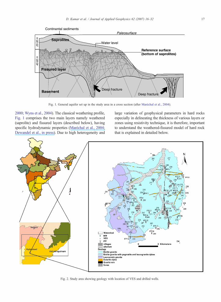
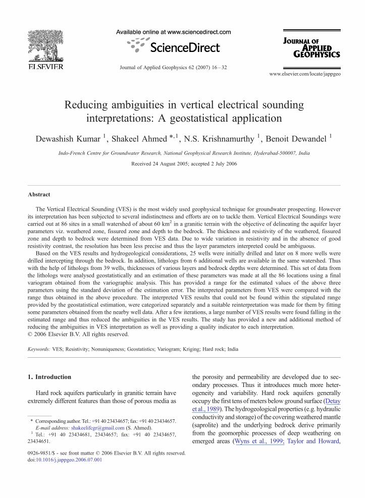
Fig. 1. General aquifer set up in the study area in a cross section (after Maréchal et al., 2004).

17D. Kumar et al. / Journal of Applied Geophysics 62 (2007) 16–32

2000; Wyns et al., 2004). The classical weathering profile,Fig. 1 comprises the two main layers namely weathered(saprolite) and fissured layers (described below), havingspecific hydrodynamic properties (Maréchal et al., 2004;Dewandel et al., in press). Due to high heterogeneity and

Fig. 2. Study area showing geology with

large variation of geophysical parameters in hard rocksespecially in delineating the thickness of various layers orzones using resistivity technique, it is therefore, importantto understand the weathered-fissured model of hard rockthat is explained in detailed below.

location of VES and drilled wells.

18 D. Kumar et al. / Journal of Applied Geophysics 62 (2007) 16–32

The saprolite, a clay-rich material is derived fromprolonged in situ decomposition of bedrock to a few tensof meters thickness (where this layer is not eroded). Thislayer is constituted by highly weathered parent rock withcoarse sand-size clasts texture (Eswaran and Bin, 1978;Acworth, 1987; Sharma and Rajamani, 2000; Chigira,2001). The fissured layer is generally characterized by adense horizontal fissuring in the first few meters and adepth decreasing density of subhorizontal and subverticalfissures (Houston and Lewis, 1988; Howard andKarundu, 1992; Dewandel et al., in press). Several pro-cesses such as cooling stresses in the magma, subsequenttectonic activity (Houston and Lewis, 1988) or lithostaticdecompression processes (Davis and Turk, 1964; Wright,1992) are invoked to explain the origin of the fissures.However, several works demonstrated that fissuringresults from the weathering process itself (Wyns et al.,1999, 2004). Fresh basement is permeable only locally,where tectonic fractures are present. The hydraulicproperties of such fractures have been investigated invarious studies (Pickens et al., 1987; Blomqvist, 1990;Walker et al., 2001; Kuusela-Lahtinen et al., 2003).

Locating the aquifers is not enough to solve thehydrogeological problem; one has to understand thecomplex system and for a quantitative evaluation, forwhich system parameters have to be determined with thehelp of a number of field and laboratory experiments.

To characterize this hard rock environment, acombined geostatistical–geophysical method was usedto delineate the layer parameters of the hard rock terrain.It is well known that the electrical geophysical method isa quite common technique in demarcating the differentsubsurface layers or zones both in terms of thickness andresistivity when compared with other geophysicalmethods. Despite its disadvantage in resolving the layersof low resistivity contrast, the technique is still widelyused in many applications such as groundwater pro-specting, hydrogeological, environmental and geotech-nical studies. A number of authors have described thesubject in detail e.g., (Zohdy, 1965, 1969; Zohdy et al.,1974; Flathe, 1976; Kelly, 1977).

The ultimate aim of a resistivity survey is to determinethe resistivity distribution with depth on the basis ofsurface measurements of the apparent resistivity(Muiuane and Pedersen, 2001) and to interpret it interms of geology or hydrogeology. Nevertheless, whenresistivity methods are used, limitations can be expectedif ground inhomogeneities and anisotropy are present(SenosMatias, 2002). Due to large variation in resistivityof the formations, as well as inherent nonuniqueness inthe interpretation techniques, this method sometimesresults in misinterpretation of the layer's parameters. The

ambiguous interpretation thus often makes the resultsunreliable and sometimes the geological logs after thedrilling provides very different results. It is thusnecessary to interpret the soundings data taking para-meters from other sources into consideration. However,it is important to interpret the VES results nearer to theactual subsurface situation as far as possible.

In the present study a geostatistical analysis usingOrdinary Kriging has therefore, been employed toobtain the limits of the estimated values at the pointwhere VES was carried out and verify that how manyresults of VES fall in the range provided by the krigingestimate of drilling data as well as their estimation error.The values not falling within the range are subject toreinterpretation using different combination of geophys-ical parameters. Such study has been useful in sortingthe VES interpretation having various degrees ofnonuniqueness and to check if they could be improvedwith a reinterpretation.

2. Study area

The study area (Maheshwaram watershed) that lieswithin the geographical coordinates between 170 06′ 20″to 170 11′ 00″ North latitude and 780 24′ 30″ to 780 29′00″ East longitude, covering an area of 60 km2 (Fig. 2)and situated at about 30 km south of Hyderabad is atypical watershed with outcrops, structural features andfissure systems. The average annual rainfall of the area is750mm.The area lies at an elevation of 600–670m abovemean sea level. The area consists of hard crystalline rocks,mainly pink and grey granites of Archaean age with foursets of joints. Major part of the basin is covered withpediplain having shallow weathering. Soil consisting ofclay loam, red loam and sandy loam with variablethicknesses (0–1 m) form the top layer (Hashimi andEngerrand, 1999). The general geological sequence of thearea is soil cover of about 1 m, followed by saprolite ofabout 12–18 m (morrum i.e., highly weathered granite)that is followed by fissured layer of about 15–20 m andthen the bedrock or basement rock. Moderate thicknessesof weathered rocks are present and thus a two tier systemviz., weathered and fissured aquifers co-exist almost in theentire area. Due to over-exploitation of the groundwaterresources, thewater level has gone down and presently thegroundwater occurrence is mainly in the fissured rockunder unconfined conditions (Maréchal et al., 2004).

3. Interpretation of VES data

In all the standard quantitative methods of VESinterpretation, certain assumptions are made with a view

Table 1Layer parameters obtained from lithologs (L) in meters

S. no. VES no. Well no. WT (L) FT (L) DBR (L)

1 219 IFP-1 18.3 19.2 37.52 216 IFP-2 18.0 2.0 20.03 209 IFP-3 11.5 12.0 23.54 208 IFP-4 17.5 4.5 22.05 282 IFP-5 22.5 13.5 36.06 253 IFP-6 23.0 9.2 32.27 257 IFP-7 18.0 0.5 18.58 256 IFP-8 18.3 4.6 22.99 252 IFP-9 19.7 13.8 33.510 261 IFP-10 14.3 7.7 22.011 265 IFP-11 15.8 21.7 37.512 232 IFP-12 23.8 13.7 37.513 271 IFP-13 36.2 9.5 45.714 246 IFP-14 14.6 9.2 23.815 247 IFP-15 12.0 11.7 23.716 244 IFP-16 10.0 26.6 36.617 245 IFP-17 20.7 9.8 30.518 270 IFP-18 18.2 4.6 22.819 229 IFP-19 2.3 38.8 41.120 206 IFP-20 13.8 7.3 21.121 241 IFP-21 13.8 7.3 21.122 215 IFP-22 9.2 31.8 41.023 227 IFP-23 19.2 19.8 39.024 223 IFP-24 22.9 4.6 27.525 274 IFP-25 16.0 26.0 42.026 – MW1 10.0 16.9 26.927 – MW2 17.0 14.4 31.428 – MW3 12.0 5.2 17.229 – OB1-1 10.0 10.3 20.330 – OB1-2 12.0 9.4 21.431 – OB1-3 15.0 6.4 21.432 – IFP1/1 15.5 19.5 35.033 – IFP1/2 22.5 7.7 30.234 – IFP1/3 17.1 11.9 29.035 – IFP9/2 33.0 4.2 37.236 – IFP11/2 27.0 5.3 32.337 – IFP11/3 33.0 2.2 35.238 – IFP26 21.6 17.4 39.039 – IFP27 25.5 7.5 33.0

WT (L) = weathered layer (saprolite) thickness.FT (L) = fissured layer thickness; DBR (L) = depth to bedrock.

19D. Kumar et al. / Journal of Applied Geophysics 62 (2007) 16–32

to make it possible to relate the geophysical anomalieswith the parameters of causative objects in a simple way.One of them is the assumption regarding the shapes ofobjects. Similarly, it is assumed that the causative objectshave uniform physical properties and have mathematicalphysical property boundaries (Bhimasankaram, 1990).Moreover, classical formulas for determining apparentelectrical resistivity and thickness assume homogeneity,and the potential field is smooth because of its highlydiffusive nature (Yeh et al., 2002). The electricalresistivity of geological media varies spatially due toinherent heterogeneous geological processes.

It is well known that the coefficient of anisotropy (λ) isexpressed as k ¼

ffiffiffiffiffiqtqL

r(Maillet, 1947; Zohdy et al., 1974);

where ρt is the transverse resistivity and ρL is the longi-tudinal resistivity respectively. For n layers, the averagetransverse resistivity is expressed as; qt ¼ T=H ¼Pn

i¼1hiqiPn

i¼1hi

while the average longitudinal resistivity as;

qL ¼ H=S ¼Pn

i¼1hiPn

i¼1

hiqi

; where the subscript i indicates the

position of the layer in the geoelectric section, T is totaltransverse resistance and S is total longitudinal conduc-tance. Values of λ generally range from 1.1 to 1.3 andvery rarely exceed 2.0 (Zohdy et al., 1974). They alsogave an example where the depths are overestimated bya factor equal to the coefficient of anisotropy, λ(example given for λ=1 and 2) when the sectionabove a poorly conductive bedrock consists of layers ofdifferent resistivities that cannot be resolved. In thepresent case, the surface layers are not highly conductiveand hence it is possible to resolve all the layers byconsidering the nearby geological information. In thegranitic terrain, the weathering is not uniform either invertical or in lateral direction of the formation and henceit is expected that the value of anisotropy also may benearer to 1.0. Since the geological information from thedrilled well is being considered while interpreting thesounding data, the depth to the poorly conductivebedrock can be estimated nearer to the real situation.Bhattacharya and Patra (1968) have also expressed thatany anisotropy in the plane of stratification is usuallyneglected as it is very small in most practical cases. Thiscould be justified given the fracturing and fissuring setsin the study area.

However, there are certain inherent ambiguities in allgeophysical interpretation techniques. These ambiguitiesare mainly of two types; 1. The possibility of differentinterpretations of the same result with regards toquantitative estimation of the parameters of causativebodies and 2. Lack of possibility in recognizing the

geological nature of the anomaly. The former ambiguitymay be of theoretical or practical in nature.

The theoretical ambiguity is inherent in all geophys-ical methods utilizing natural fields and in certainartificial methods. The theoretical ambiguity arisesbecause of the fact that while the direct problem ofcalculation of geophysical anomaly due to givendistribution of geological inhomogeneities can be solvedin a unique way, since the given object produces only onefully determined anomaly, the solution of inverseproblem of obtaining the parameters of the causativebody either by comparison or inversion techniques is

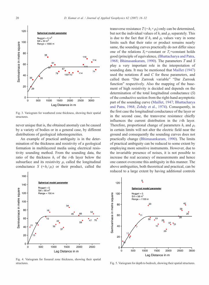
Fig. 3. Variogram for weathered zone thickness, showing their spatialstructures.

20 D. Kumar et al. / Journal of Applied Geophysics 62 (2007) 16–32

never unique that is, the obtained anomaly can be causedby a variety of bodies or in a general case, by differentdistributions of geological inhomogeneities.

An example of practical ambiguity is in the deter-mination of the thickness and resistivity of a geologicalformation in multilayered media using electrical resis-tivity sounding method. From the sounding data, theratio of the thickness hi of the i-th layer below thesubsurface and its resistivity ρi called the longitudinalconductance S (=hi /ρi) or their product, called the

Fig. 4. Variogram for fissured zone thickness, showing their spatialstructures.

transverse resistance T (=hi×ρi) only can be determined,but not the individual values of hi and ρi separately. Thisis due to the fact that if hi and ρi values vary in somelimits such that their ratio or product remains nearlysame, the sounding curves practically do not differ sinceone of the relations Si=constant or Ti=constant holdsgood (principle of equivalence, (Bhattacharya and Patra,1968; Bhimasankaram, 1990). The parameters T and Splay a very important role in the interpretation ofsounding data. It may be mentioned that Maillet (1947)used the notations R and C for these parameters, andcalled them “Dar Zarrouk variable” “Dar Zarroukfunction” respectively. Also the mapping of the base-ment of high resistivity is decided and depends on thedetermination of the total longitudinal conductance (S)of the conductive section from the right-hand asymptoticpart of the sounding curve (Maillet, 1947; Bhattacharyaand Patra, 1968; Zohdy et al., 1974). Consequently, inthe first case the longitudinal conductance of the layer orin the second case, the transverse resistance chieflyinfluences the current distribution in the i-th layer.Therefore, proportional change of parameters hi and ρiin certain limits will not alter the electric field near theground and consequently the sounding curves does notpractically change (Bhimasankaram, 1990). The limitsof practical ambiguity can be reduced to some extent byemploying more sensitive instruments. However, due tothe invariable presence of noises, it is not possible toincrease the real accuracy of measurements and henceone cannot overcome this ambiguity in this manner. Theabove ambiguities, both theoretical and practical, can bereduced to a large extent by having additional controls

Fig. 5. Variogram for depth to bedrock, showing their spatial structures.

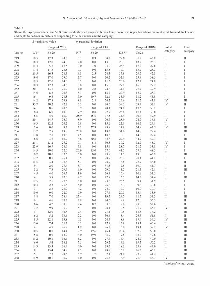
Table 2Shows the layer parameters from VES results and estimated range (with their lower bound and upper bound) for the weathered, fissured thicknessesand depth to bedrock in meters corresponding to VES number and the category

Z=estimated value σ standard deviation

Range of WT# Range of FT# Range of DBR# Initialcategory

Finalcategory

Ves no. WT⁎ Z±2σ FT⁎ Z±2σ DBR⁎ Z±2σ

219 16.5 12.3 24.3 13.1 8.3 30.2 29.6 31.2 43.8 III II216 18.3 12.0 24.0 2.0 0.0 13.0 20.3 13.7 26.3 II I209 11.4 5.5 17.5 12.0 1.0 23.0 23.4 17.2 29.8 I I208 17.4 11.5 23.5 0.3 0.0 15.5 17.7 15.7 28.3 III I282 21.5 16.5 28.5 16.3 2.5 24.5 37.8 29.7 42.3 I I253 19.4 17.0 29.0 12.7 0.0 20.2 32.1 25.9 38.5 II I257 19.5 12.0 24.0 0.5 0.0 11.5 20.0 12.2 24.8 III I256 18.3 12.3 24.3 8.8 0.0 15.5 27.1 16.5 29.2 III I252 20.1 13.7 25.7 14.0 2.8 24.8 34.1 27.2 39.9 III I261 14.6 8.3 20.3 8.3 0.0 18.7 22.9 15.7 28.3 III I265 16 9.8 21.8 19.0 10.7 32.6 35.0 31.2 43.8 I I232 14.2 17.8 29.8 8.8 2.8 24.7 29.6 31.2 43.8 IV III271 35.7 30.2 42.2 3.5 0.0 20.5 39.2 39.4 52.1 IV II246 14.1 8.6 20.6 9.9 0.0 20.1 24.0 17.5 30.1 II I247 8.4 6.0 18.0 7.9 0.8 22.7 23.8 17.4 30.0 III I244 8.5 4.0 16.0 25.9 15.6 37.5 34.4 30.3 42.9 II I245 20 14.7 26.7 8.9 0.0 20.7 28.9 24.2 36.8 IV I270 16.3 12.2 24.2 5.8 0.0 15.6 22.1 16.5 29.1 II I229 2.6 0.0 8.3 12.3 27.9 49.8 14.9 34.8 47.5 IV III206 13.2 7.8 19.8 20.8 0.0 18.3 34.0 14.8 27.4 II III241 13.8 7.8 19.8 4.5 0.0 18.3 18.3 14.8 27.4 I I215 8.6 3.2 15.2 13.8 20.8 42.8 22.9 34.7 47.3 II III227 21.1 13.2 25.2 10.1 8.8 30.8 39.2 32.7 45.3 IV I223 22.9 16.9 28.9 5.8 0.0 15.6 28.7 21.2 33.8 IV I274 14.3 10.0 22.0 26.9 15.0 37.0 41.2 35.7 48.3 III I201 6.7 10.0 37.5 5.0 0.0 23.9 11.7 19.0 43.9 III III202 17.2 0.0 26.4 8.5 0.0 28.9 25.7 20.4 44.1 I I203 11.5 3.4 31.6 5.3 0.0 28.9 16.8 22.7 48.0 III II204 9.1 2.0 27.4 3.7 0.0 31.5 12.8 19.0 41.7 III II205 3.2 7.3 29.9 6.0 0.0 29.0 15.2 21.5 42.1 II III207 4.5 4.0 26.7 11.9 0.0 26.4 16.4 10.9 31.5 II I210 4 5.8 27.0 9.7 0.0 22.9 13.7 14.7 34.4 III III211 17.5 2.5 27.6 6.0 0.0 23.5 23.5 9.4 31.9 III I212 10.3 2.3 25.5 5.0 0.0 26.6 15.3 9.8 30.8 III I213 3 2.3 23.9 14.2 0.0 24.0 17.3 10.9 30.7 II I214 10.6 0.0 22.0 9.9 0.0 27.4 20.5 13.4 33.9 II I217 1.8 7.0 28.4 22.4 0.0 19.5 24.2 11.5 31.3 III III218 6.1 4.6 30.3 3.8 0.0 24.6 9.9 12.0 35.3 III II220 6.6 4.2 30.8 2.4 0.7 33.5 9.0 28.8 52.6 II II221 7.2 9.9 35.9 5.3 0.0 28.1 12.5 21.7 45.1 IV III222 1.1 12.0 30.8 9.4 0.0 21.1 10.5 18.5 36.2 III III224 6.2 5.2 33.6 2.2 0.0 30.6 8.4 26.3 51.8 II II225 8.5 12.1 33.8 0.3 0.0 24.7 8.8 19.4 39.5 IV III226 15.6 7.4 31.7 0.3 0.0 27.9 15.9 18.1 40.4 III II228 4 4.7 26.7 11.9 0.0 26.2 16.0 19.1 39.2 IV III230 10.5 0.0 14.4 9.9 19.6 46.4 20.4 32.9 50.0 III III231 5.8 0.0 14.9 4.0 19.9 45.9 9.8 33.2 49.6 III III233 11.2 10.1 36.6 5.2 0.0 27.7 16.4 24.7 49.0 II II234 6.6 5.4 38.1 7.5 0.0 29.2 14.1 19.5 50.2 II II235 14.3 13.3 36.4 4.0 0.0 29.5 18.3 25.9 47.0 III II236 8 13.4 34.9 7.2 0.0 28.9 15.2 26.3 46.1 III III237 5.1 7.3 29.6 15.9 1.7 32.1 21.0 23.9 44.2 III III238 14.9 10.6 35.2 4.0 0.0 25.3 18.9 21.6 43.7 IV II

(continued on next page)

21D. Kumar et al. / Journal of Applied Geophysics 62 (2007) 16–32

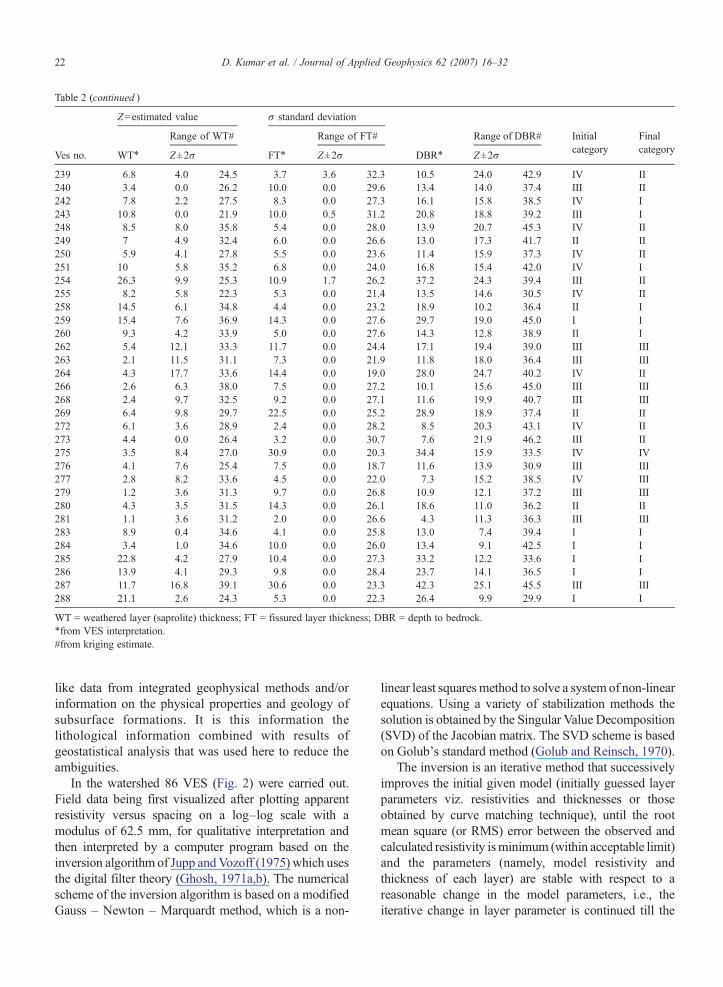
Table 2 (continued )

Z=estimated value σ standard deviation

Range of WT# Range of FT# Range of DBR# Initialcategory

Finalcategory

Ves no. WT⁎ Z±2σ FT⁎ Z±2σ DBR⁎ Z±2σ

239 6.8 4.0 24.5 3.7 3.6 32.3 10.5 24.0 42.9 IV II240 3.4 0.0 26.2 10.0 0.0 29.6 13.4 14.0 37.4 III II242 7.8 2.2 27.5 8.3 0.0 27.3 16.1 15.8 38.5 IV I243 10.8 0.0 21.9 10.0 0.5 31.2 20.8 18.8 39.2 III I248 8.5 8.0 35.8 5.4 0.0 28.0 13.9 20.7 45.3 IV II249 7 4.9 32.4 6.0 0.0 26.6 13.0 17.3 41.7 II II250 5.9 4.1 27.8 5.5 0.0 23.6 11.4 15.9 37.3 IV II251 10 5.8 35.2 6.8 0.0 24.0 16.8 15.4 42.0 IV I254 26.3 9.9 25.3 10.9 1.7 26.2 37.2 24.3 39.4 III II255 8.2 5.8 22.3 5.3 0.0 21.4 13.5 14.6 30.5 IV II258 14.5 6.1 34.8 4.4 0.0 23.2 18.9 10.2 36.4 II I259 15.4 7.6 36.9 14.3 0.0 27.6 29.7 19.0 45.0 I I260 9.3 4.2 33.9 5.0 0.0 27.6 14.3 12.8 38.9 II I262 5.4 12.1 33.3 11.7 0.0 24.4 17.1 19.4 39.0 III III263 2.1 11.5 31.1 7.3 0.0 21.9 11.8 18.0 36.4 III III264 4.3 17.7 33.6 14.4 0.0 19.0 28.0 24.7 40.2 IV II266 2.6 6.3 38.0 7.5 0.0 27.2 10.1 15.6 45.0 III III268 2.4 9.7 32.5 9.2 0.0 27.1 11.6 19.9 40.7 III III269 6.4 9.8 29.7 22.5 0.0 25.2 28.9 18.9 37.4 II II272 6.1 3.6 28.9 2.4 0.0 28.2 8.5 20.3 43.1 IV II273 4.4 0.0 26.4 3.2 0.0 30.7 7.6 21.9 46.2 III II275 3.5 8.4 27.0 30.9 0.0 20.3 34.4 15.9 33.5 IV IV276 4.1 7.6 25.4 7.5 0.0 18.7 11.6 13.9 30.9 III III277 2.8 8.2 33.6 4.5 0.0 22.0 7.3 15.2 38.5 IV III279 1.2 3.6 31.3 9.7 0.0 26.8 10.9 12.1 37.2 III III280 4.3 3.5 31.5 14.3 0.0 26.1 18.6 11.0 36.2 II II281 1.1 3.6 31.2 2.0 0.0 26.6 4.3 11.3 36.3 III III283 8.9 0.4 34.6 4.1 0.0 25.8 13.0 7.4 39.4 I I284 3.4 1.0 34.6 10.0 0.0 26.0 13.4 9.1 42.5 I I285 22.8 4.2 27.9 10.4 0.0 27.3 33.2 12.2 33.6 I I286 13.9 4.1 29.3 9.8 0.0 28.4 23.7 14.1 36.5 I I287 11.7 16.8 39.1 30.6 0.0 23.3 42.3 25.1 45.5 III III288 21.1 2.6 24.3 5.3 0.0 22.3 26.4 9.9 29.9 I I

WT = weathered layer (saprolite) thickness; FT = fissured layer thickness; DBR = depth to bedrock.⁎from VES interpretation.#from kriging estimate.

22 D. Kumar et al. / Journal of Applied Geophysics 62 (2007) 16–32

like data from integrated geophysical methods and/orinformation on the physical properties and geology ofsubsurface formations. It is this information thelithological information combined with results ofgeostatistical analysis that was used here to reduce theambiguities.

In the watershed 86 VES (Fig. 2) were carried out.Field data being first visualized after plotting apparentresistivity versus spacing on a log–log scale with amodulus of 62.5 mm, for qualitative interpretation andthen interpreted by a computer program based on theinversion algorithm of Jupp andVozoff (1975) which usesthe digital filter theory (Ghosh, 1971a,b). The numericalscheme of the inversion algorithm is based on a modifiedGauss – Newton – Marquardt method, which is a non-

linear least squares method to solve a system of non-linearequations. Using a variety of stabilization methods thesolution is obtained by the Singular Value Decomposition(SVD) of the Jacobian matrix. The SVD scheme is basedon Golub's standard method (Golub and Reinsch, 1970).

The inversion is an iterative method that successivelyimproves the initial given model (initially guessed layerparameters viz. resistivities and thicknesses or thoseobtained by curve matching technique), until the rootmean square (or RMS) error between the observed andcalculated resistivity isminimum (within acceptable limit)and the parameters (namely, model resistivity andthickness of each layer) are stable with respect to areasonable change in the model parameters, i.e., theiterative change in layer parameter is continued till the

Table 3Categorization of VES results before and after reinterpretation

Category No. of VES locations

Beforereinterpretation

After reinterpretation

No. % of total No. % of total

I 11 12.8 36 41.9II 20 23.2 24 27.9III 35 40.7 25 29.1IV 20 23.2 1 1.1

Table 4Shows the layer parameters from VES results in meters before andafter reinterpretation

VESno.

Result of VES beforereinterpretation

Result of VES afterreinterpretation

WT FT DBR WT FT DBR

219 6.8 13.1 29.5 16.5 13.1 29.6216 21.5 8.7 30.2 18.3 2.0 20.3209 7.5 14.6 22.1 11.4 12.0 23.4208 14.9 15.2 17.4 0.3 17.7282 21.5 16.3 37.8 21.5 16.3 37.8253 4.9 8.4 26.9 19.4 12.7 32.1257 2.4 26.4 19.5 0.5 20.0256 2.2 25.3 18.3 8.8 27.1252 6.8 27.3 20.1 14.0 34.1261 5.2 20.1 14.6 8.3 22.9265 11.7 30.6 42.3 16.0 19.0 35.0232 1.8 16.9 14.2 8.8 29.6271 5.0 21.7 26.7 35.7 3.5 39.2246 5.9 14.8 20.7 14.1 9.9 24.0247 7.6 36.9 44.5 8.4 7.9 23.8244 5.8 19.8 25.6 8.5 25.9 34.4245 11.2 7.3 18.5 20.0 8.9 28.9270 8.8 9.1 17.9 16.3 5.8 22.1229 2.8 13.5 16.3 2.6 12.3 14.9206 3.7 11.9 15.6 13.2 20.8 34.0241 13.0 12.9 26.0 13.8 4.5 18.3215 8.0 25.2 33.2 8.6 13.8 22.9227 1.4 24.5 21.1 10.1 39.2223 9.1 36.8 45.9 22.9 5.8 28.7274 4.4 15.5 19.9 14.3 26.9 41.2201 4.3 5.7 10.0 6.7 5.0 11.7202 17.2 8.5 25.7 17.2 8.5 25.7203 3.9 12.4 11.5 5.3 16.8204 6.0 11.4 9.1 3.7 12.8205 2.9 23.6 26.5 3.2 6.0 15.2207 2.7 14.1 16.8 4.5 11.9 16.4210 4.0 9.7 13.7 4.0 9.7 13.7211 2.1 20.2 17.5 6.0 23.5212 2.3 12.1 10.3 5.0 15.3213 3.0 17.3 3.0 14.2 17.3214 8.0 18.6 10.6 9.9 20.5217 1.8 22.9 1.8 22.4 24.2218 5.9 8.4 6.1 3.8 9.9220 6.6 2.4 9.0 6.6 2.4 9.0221 0.9 8.9 7.2 5.3 12.5222 1.4 11.2 12.6 1.1 9.4 10.5224 6.2 2.2 8.4 6.2 2.2 8.4225 3.6 10.0 8.5 0.3 8.8226 1.0 14.6 15.6 15.6 0.3 15.9228 1.4 6.7 4.0 11.9 16.0230 9.2 6.5 15.7 10.5 9.9 20.4231 0.4 7.6 5.8 4.0 9.8233 11.2 5.2 16.4 11.2 5.2 16.4234 7.6 5.1 12.7 6.6 7.5 14.1235 2.0 14.0 16.0 14.3 4.0 18.3236 8.0 7.2 15.2 8.0 7.2 15.2237 5.1 15.9 21.0 5.1 15.9 21.0238 3.6 17.1 14.9 4.0 18.9239 0.8 8.3 6.8 3.7 10.5

(continued on next page)

23D. Kumar et al. / Journal of Applied Geophysics 62 (2007) 16–32

RMS error is less than a fixed limit or there is no furtherchange in layer parameters. The initial model is selectedafter interpreting the field curves by curve matchingtechnique using master curves (Orellana and Mooney,1966; Rijkswaterstaat, 1969). Most of the soundingcurves show four and five layer cases and few are sixlayers. The weathered layer thickness varies from about ameter to about 35 m, the fissured layer thickness variesfrom less than a meter to about 30 m and the depth tobedrock varies from 4.3 m to 42.3 m. This shows a largevariation in subsurface layer parameters. Based on theresults of the interpretation and on hydrogeologicalconsiderations, 39 sites were drilled for experimentalstudy of the aquifer system (Krishnamurthy et al., 2000;Maréchal et al., 2004). These sites are so selected that theyare well distributed over the entire area (Fig. 2). Theseborewells were drilled up to a depth of 40–50 m. Theyield of these borewells varies from 300 lph to 21,000 lph,which is related to the number of fissures encountered(Maréchal et al., 2004). The layers encountered whiledrilling are saprolite and fissured layer followed byunfissured granite. Drilling data shows that using thelithologs of course, the thicknesses of individual layers donot match exactly with the VES interpretation neverthe-less the total depth to bedrock corroborates well with theVES results.

4. Geostatistical analysis of the drilling data

The Geostatistical technique was originally devel-oped (Matheron, 1965, 1971) to estimate regionalizedvariable such as the grade of an ore body at knownlocation in space, given a set of observed data. Re-gionalized variables are variables typical of a phenom-enon developing in space (and/or time) and possessing acertain structure. “Structure” refers to this spatialcorrelation which, of course is very different from onemagnitude to the other or from one aquifer to the next.Its application to groundwater hydrology has been

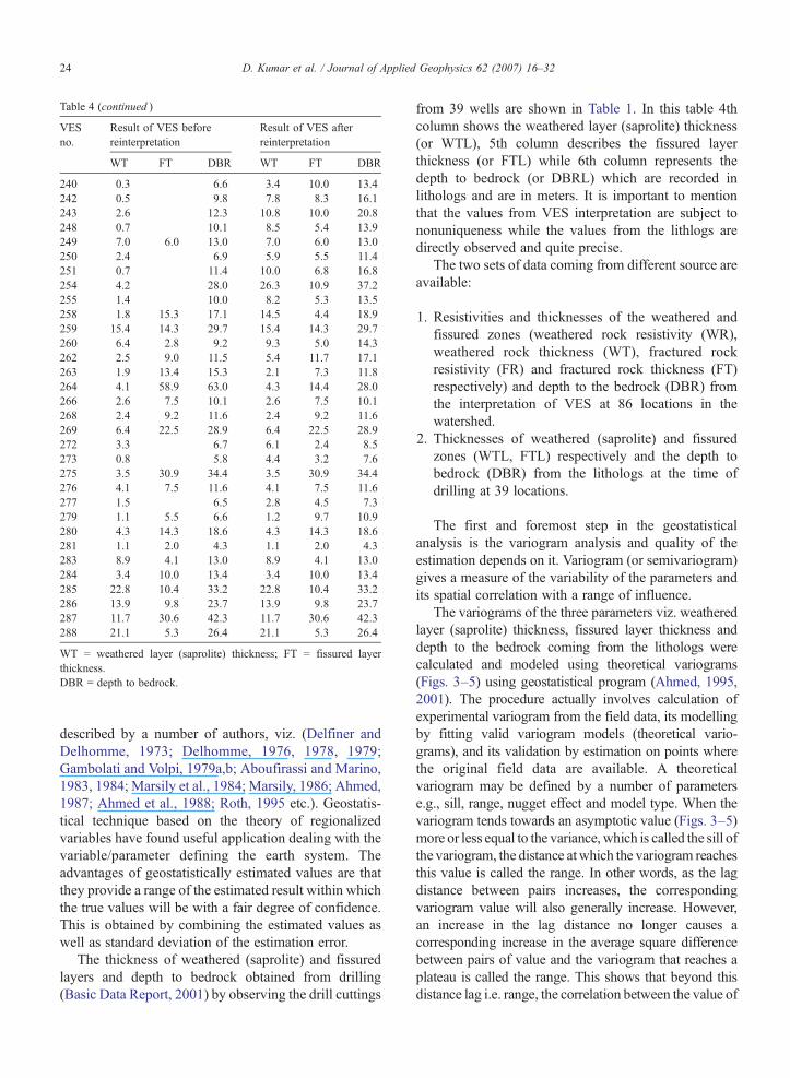
Table 4 (continued )

VESno.

Result of VES beforereinterpretation

Result of VES afterreinterpretation

WT FT DBR WT FT DBR

240 0.3 6.6 3.4 10.0 13.4242 0.5 9.8 7.8 8.3 16.1243 2.6 12.3 10.8 10.0 20.8248 0.7 10.1 8.5 5.4 13.9249 7.0 6.0 13.0 7.0 6.0 13.0250 2.4 6.9 5.9 5.5 11.4251 0.7 11.4 10.0 6.8 16.8254 4.2 28.0 26.3 10.9 37.2255 1.4 10.0 8.2 5.3 13.5258 1.8 15.3 17.1 14.5 4.4 18.9259 15.4 14.3 29.7 15.4 14.3 29.7260 6.4 2.8 9.2 9.3 5.0 14.3262 2.5 9.0 11.5 5.4 11.7 17.1263 1.9 13.4 15.3 2.1 7.3 11.8264 4.1 58.9 63.0 4.3 14.4 28.0266 2.6 7.5 10.1 2.6 7.5 10.1268 2.4 9.2 11.6 2.4 9.2 11.6269 6.4 22.5 28.9 6.4 22.5 28.9272 3.3 6.7 6.1 2.4 8.5273 0.8 5.8 4.4 3.2 7.6275 3.5 30.9 34.4 3.5 30.9 34.4276 4.1 7.5 11.6 4.1 7.5 11.6277 1.5 6.5 2.8 4.5 7.3279 1.1 5.5 6.6 1.2 9.7 10.9280 4.3 14.3 18.6 4.3 14.3 18.6281 1.1 2.0 4.3 1.1 2.0 4.3283 8.9 4.1 13.0 8.9 4.1 13.0284 3.4 10.0 13.4 3.4 10.0 13.4285 22.8 10.4 33.2 22.8 10.4 33.2286 13.9 9.8 23.7 13.9 9.8 23.7287 11.7 30.6 42.3 11.7 30.6 42.3288 21.1 5.3 26.4 21.1 5.3 26.4

WT = weathered layer (saprolite) thickness; FT = fissured layerthickness.DBR = depth to bedrock.

24 D. Kumar et al. / Journal of Applied Geophysics 62 (2007) 16–32

described by a number of authors, viz. (Delfiner andDelhomme, 1973; Delhomme, 1976, 1978, 1979;Gambolati and Volpi, 1979a,b; Aboufirassi and Marino,1983, 1984; Marsily et al., 1984; Marsily, 1986; Ahmed,1987; Ahmed et al., 1988; Roth, 1995 etc.). Geostatis-tical technique based on the theory of regionalizedvariables have found useful application dealing with thevariable/parameter defining the earth system. Theadvantages of geostatistically estimated values are thatthey provide a range of the estimated result within whichthe true values will be with a fair degree of confidence.This is obtained by combining the estimated values aswell as standard deviation of the estimation error.

The thickness of weathered (saprolite) and fissuredlayers and depth to bedrock obtained from drilling(Basic Data Report, 2001) by observing the drill cuttings

from 39 wells are shown in Table 1. In this table 4thcolumn shows the weathered layer (saprolite) thickness(or WTL), 5th column describes the fissured layerthickness (or FTL) while 6th column represents thedepth to bedrock (or DBRL) which are recorded inlithologs and are in meters. It is important to mentionthat the values from VES interpretation are subject tononuniqueness while the values from the lithlogs aredirectly observed and quite precise.

The two sets of data coming from different source areavailable:

1. Resistivities and thicknesses of the weathered andfissured zones (weathered rock resistivity (WR),weathered rock thickness (WT), fractured rockresistivity (FR) and fractured rock thickness (FT)respectively) and depth to the bedrock (DBR) fromthe interpretation of VES at 86 locations in thewatershed.

2. Thicknesses of weathered (saprolite) and fissuredzones (WTL, FTL) respectively and the depth tobedrock (DBR) from the lithologs at the time ofdrilling at 39 locations.

The first and foremost step in the geostatisticalanalysis is the variogram analysis and quality of theestimation depends on it. Variogram (or semivariogram)gives a measure of the variability of the parameters andits spatial correlation with a range of influence.

The variograms of the three parameters viz. weatheredlayer (saprolite) thickness, fissured layer thickness anddepth to the bedrock coming from the lithologs werecalculated and modeled using theoretical variograms(Figs. 3–5) using geostatistical program (Ahmed, 1995,2001). The procedure actually involves calculation ofexperimental variogram from the field data, its modellingby fitting valid variogram models (theoretical vario-grams), and its validation by estimation on points wherethe original field data are available. A theoreticalvariogram may be defined by a number of parameterse.g., sill, range, nugget effect and model type. When thevariogram tends towards an asymptotic value (Figs. 3–5)more or less equal to the variance, which is called the sill ofthe variogram, the distance atwhich the variogram reachesthis value is called the range. In other words, as the lagdistance between pairs increases, the correspondingvariogram value will also generally increase. However,an increase in the lag distance no longer causes acorresponding increase in the average square differencebetween pairs of value and the variogram that reaches aplateau is called the range. This shows that beyond thisdistance lag i.e. range, the correlation between the value of

25D. Kumar et al. / Journal of Applied Geophysics 62 (2007) 16–32

the parameters drops to zero. Theoretically a variogramshould pass from the origin but in the absence of smalldistance lags, the variograms are extrapolated towardsorigin and sometimes an extrapolation makes a clear

Fig. 6. Resistivity sounding curve — VES-245. (a) observed data, fitted curvmodel after reinterpretation.

intercept at the variogram axis. This intercept is known asnugget effect and this ismainly due to very high variabilityat small scale.Avariation of variogrambetween origin andrange is important and depending on this slope the

e and model before reinterpretation. (b) observed data, fitted curve and

26 D. Kumar et al. / Journal of Applied Geophysics 62 (2007) 16–32

variograms are modeled with different mathematicalfunctions called model type. In the present case all thethree variograms were fitted with spherical model.

It is often found that the theoretical and experimentalvariograms donot verywellmatch as the case in Figs. 3–5.

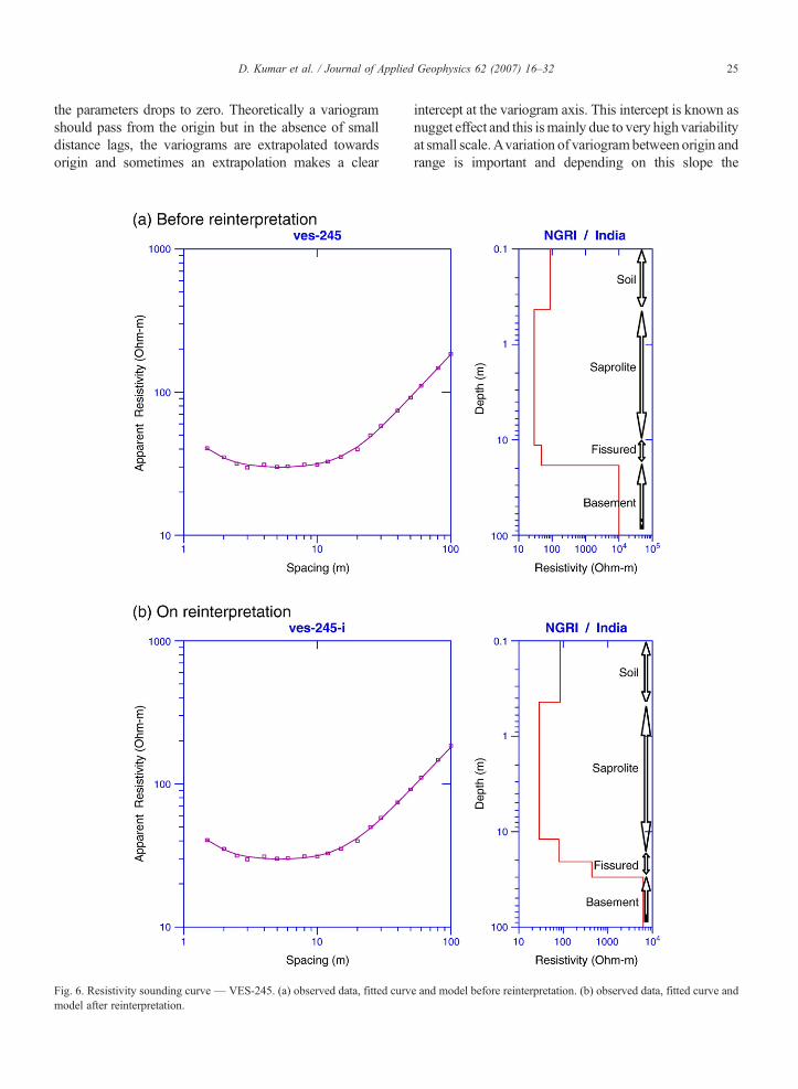
Fig. 7. Resistivity sounding curve — VES-271. (a) observed data, fitted curvmodel after reinterpretation.

This is basically due to the absence of sufficient data todetermine the true variability at one hand and restriction onthe case of limited theoretical model on the other hand.However, this ambiguity is successfully removed by cross-validation test (Ahmed and Gupta, 1989). The final (or

e and model before reinterpretation. (b) observed data, fitted curve and

27D. Kumar et al. / Journal of Applied Geophysics 62 (2007) 16–32

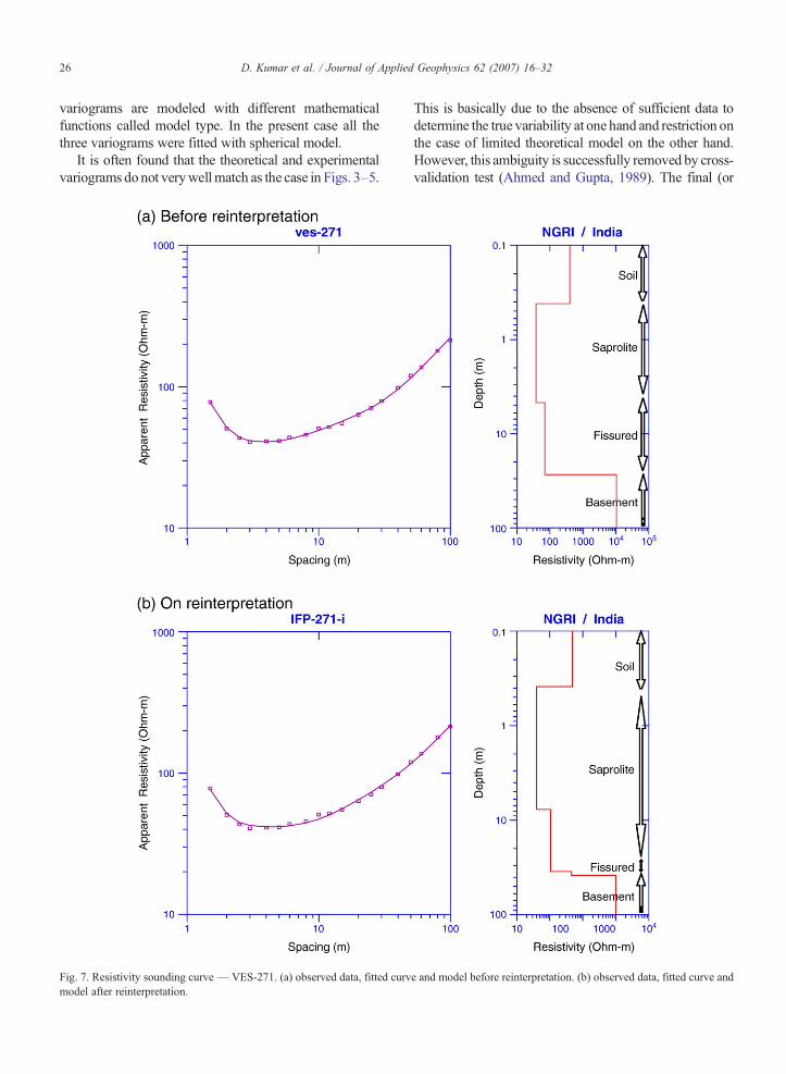
validated) variograms were used to estimate the threeparameters namely the weathered thickness, fissured rockthickness and depth to bedrock at the 86 VES locationsusing Ordinary Kriging. It is a well known type of kriginginterpolation technique of the kriging family that uses onlythe sampled primary variable to make estimates at un-

Fig. 8. Plot of VES number versus thicknesses from VES results

sampled locations. Kriging, or best linear unbiased esti-mation (BLUE) is an advanced interpolation procedurethat generates an estimated surface from an x–y scatteredset of points with z values (i.e., any regionalized variable).It is a weighted averaging method of interpolation derivedfrom the theory of regionalized variable, which assumes

and estimated values with their lower and upper bounds.

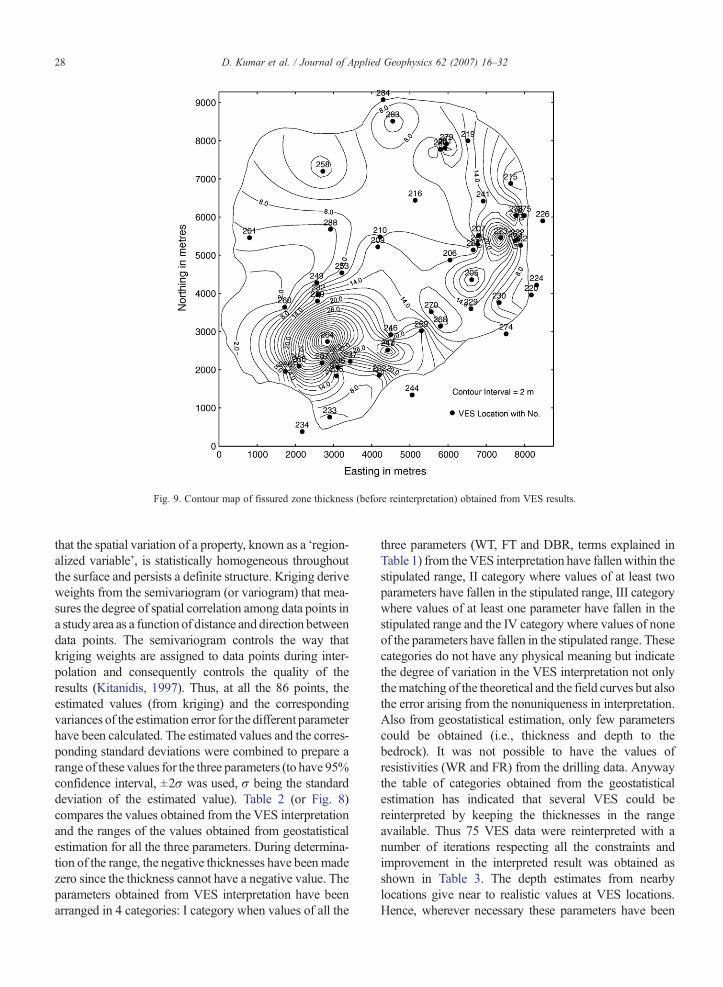
Fig. 9. Contour map of fissured zone thickness (before reinterpretation) obtained from VES results.

28 D. Kumar et al. / Journal of Applied Geophysics 62 (2007) 16–32

that the spatial variation of a property, known as a ‘region-alized variable’, is statistically homogeneous throughoutthe surface and persists a definite structure. Kriging deriveweights from the semivariogram (or variogram) that mea-sures the degree of spatial correlation among data points ina study area as a function of distance and direction betweendata points. The semivariogram controls the way thatkriging weights are assigned to data points during inter-polation and consequently controls the quality of theresults (Kitanidis, 1997). Thus, at all the 86 points, theestimated values (from kriging) and the correspondingvariances of the estimation error for the different parameterhave been calculated. The estimated values and the corres-ponding standard deviations were combined to prepare arange of these values for the three parameters (to have 95%confidence interval, ±2σ was used, σ being the standarddeviation of the estimated value). Table 2 (or Fig. 8)compares the values obtained from the VES interpretationand the ranges of the values obtained from geostatisticalestimation for all the three parameters. During determina-tion of the range, the negative thicknesses have been madezero since the thickness cannot have a negative value. Theparameters obtained from VES interpretation have beenarranged in 4 categories: I category when values of all the

three parameters (WT, FT and DBR, terms explained inTable 1) from theVES interpretation have fallenwithin thestipulated range, II category where values of at least twoparameters have fallen in the stipulated range, III categorywhere values of at least one parameter have fallen in thestipulated range and the IV category where values of noneof the parameters have fallen in the stipulated range. Thesecategories do not have any physical meaning but indicatethe degree of variation in the VES interpretation not onlythematching of the theoretical and the field curves but alsothe error arising from the nonuniqueness in interpretation.Also from geostatistical estimation, only few parameterscould be obtained (i.e., thickness and depth to thebedrock). It was not possible to have the values ofresistivities (WR and FR) from the drilling data. Anywaythe table of categories obtained from the geostatisticalestimation has indicated that several VES could bereinterpreted by keeping the thicknesses in the rangeavailable. Thus 75 VES data were reinterpreted with anumber of iterations respecting all the constraints andimprovement in the interpreted result was obtained asshown in Table 3. The depth estimates from nearbylocations give near to realistic values at VES locations.Hence, wherever necessary these parameters have been

29D. Kumar et al. / Journal of Applied Geophysics 62 (2007) 16–32

kept fixed while altering the resistivities only for the layersduring reinterpretation, such that the parameters S and Tare constant (as described in Interpretation of VES data).

5. Results and discussion

On comparing interpreted results at all the 86 locationswith the geostatistical estimation, it was found that someof the VES results are lying outside the geostatisticalestimation range (Table 2 (or Fig. 8), initial category)while few are completely falling within the range of theindividual parameters. Since using the variability of theparameters obtained from the lithological logs, the rangesof the estimated parameters are defined. Thus the VESvalues for the same parameter are expected to fall withinthe range respecting the 95% confidence interval.Therefore, it was thought to reinterpret the VES keepingin view of the drilling information as well as thegeological considerations of the area.

The number of locations where the parameters fromVES fall in different categories are shown in Table 3. It isseen from Table 3 that the parameters of VES at 20locations (initial interpretation) fall in category IV thatmeans not even a single parameter from these 20 locations

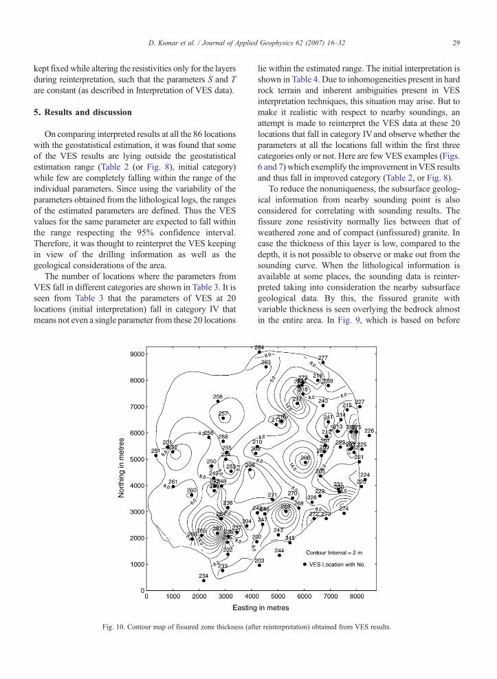
Fig. 10. Contour map of fissured zone thickness (aft

lie within the estimated range. The initial interpretation isshown in Table 4. Due to inhomogeneities present in hardrock terrain and inherent ambiguities present in VESinterpretation techniques, this situation may arise. But tomake it realistic with respect to nearby soundings, anattempt is made to reinterpret the VES data at these 20locations that fall in category IVand observe whether theparameters at all the locations fall within the first threecategories only or not. Here are few VES examples (Figs.6 and 7) which exemplify the improvement inVES resultsand thus fall in improved category (Table 2, or Fig. 8).

To reduce the nonuniqueness, the subsurface geolog-ical information from nearby sounding point is alsoconsidered for correlating with sounding results. Thefissure zone resistivity normally lies between that ofweathered zone and of compact (unfissured) granite. Incase the thickness of this layer is low, compared to thedepth, it is not possible to observe or make out from thesounding curve. When the lithological information isavailable at some places, the sounding data is reinter-preted taking into consideration the nearby subsurfacegeological data. By this, the fissured granite withvariable thickness is seen overlying the bedrock almostin the entire area. In Fig. 9, which is based on before

er reinterpretation) obtained from VES results.

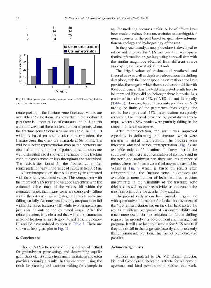
Fig. 11. Histogram plot showing comparison of VES results, beforeand after reinterpretation.

30 D. Kumar et al. / Journal of Applied Geophysics 62 (2007) 16–32

reinterpretation, the fracture zone thickness values areavailable at 52 locations. It shows that in the southwestpart there is concentration of contours and in the northand northwest part there are less number of points wherethe fracture zone thicknesses are available. In Fig. 10which is based on results after reinterpretation, thefracture zone thickness are available at 86 points, thiswill be a better representation map as the contours areobtained on more number of points, these contours arewell distributed and it shows the variation of the fracturezone thickness more or less throughout the watershed.The resistivities found for the fissured zone afterreinterpretation vary in the range of 120Ωm to 500Ωm.

After reinterpretation, the results were again comparedwith the kriging estimated values. This comparison withthe improved VES result shows good agreement with theestimated value, most of the values fall within theestimated range, that means some are completely fallingwithin the estimated range (category I) while some arefalling partially. At some locations only one parameter fallwithin the range (category III) while two parameters arejust near or outside the estimated range. After thereinterpretation, it is observed that while the parametersat 1(one) location fall in category IV, and those in categoryIII and IV have reduced as seen in Table 3. These areshown as histogram plot in Fig. 11.

6. Conclusions

Though,VES is themost common geophysical methodfor groundwater prospecting, and determining aquifergeometries etc., it suffers frommany limitations and oftenprovides nonunique results. In this condition, using theresult for planning and decision making for example in

aquifer modeling becomes unfair. A lot of efforts havebeen made to reduce these uncertainties and ambiguities/nonuniqueness in the past based on qualitative informa-tion on geology and hydrogeology of the area.

In the present study, a new procedure is developed torefine and improve the VES interpretation with quan-titative information on geology using borewell data withthe similar magnitude obtained from different sourceemploying the Geostatistical methods.

The kriged values of thickness of weathered andfissured zone as well as depth to bedrock from the drillingdata along with their corresponding estimation error haveprovided the range inwhich the true values should lie with95% confidence. Thus the VES interpreted results have tobe improved if they did not belong to these intervals. As amatter of fact almost 23% of VES did not fit initially(Table 3). However, by suitable reinterpretation of VEStaking the limits of the parameters from kriging, theresults have provided 42% interpretation completelyrespecting the interval provided by geostatistical tech-nique, whereas 58% results were partially falling in therange in different categories.

After reinterpretation, the result was improvedespecially in delineating thin fractures which weremissing in initial interpretation. The fracture zonethickness obtained before reinterpretation (Fig. 8) areavailable only at 52 locations. It shows that in thesouthwest part there is concentration of contours and inthe north and northwest part there are less number ofpoints where the fracture zone thicknesses are available.While in Fig. 9 which is based on results afterreinterpretation, the fracture zone thicknesses areavailable at more number of locations, thus reducinguncertainties in the variability of the fractured zonethickness as well as their resistivities as this zone is themost important one for aquifer flow studies.

The present study at one hand provided a guidelinewith quantitative information for further improvement ofthe VES reinterpretation and on the other hand sorted theresults in different categories of varying reliability andmuch more useful for site selection for further drillingrequired for groundwater development and managementprogram. It will also help to discard a few VES results ifthey do not fall in the range satisfactorily and to use onlythe remaining interpretation. This has not been otherwisepossible.

Acknowledgements

Authors are grateful to Dr. V.P. Dimri, Director,National Geophysical Research Institute for his encour-agements and kind permission to publish this work.

31D. Kumar et al. / Journal of Applied Geophysics 62 (2007) 16–32

Thanks toMr. S.C. Jain, Mr. B.A. Prakash, Mr. B.C. Negiand Dr. V. Ananda Rao who have been helpful at variousstages of this study. We are also thankful to the Indo-French Centre for Promotion of Advanced Research(IFCPAR), New Delhi for partially sponsoring the projectwork. The authors are thankful to both the anonymousreviewers for critically reviewing the manuscript and theeditor for their useful comments and suggestions forimproving the quality of the paper.

References

Aboufirassi, M., Marino, M.A., 1983. Kriging of water levels in Soussaquifer, Morocco. Math. Geol. 15 (4), 537–551.

Aboufirassi, M., Marino, M.A., 1984. Cokriging of aquifer transmis-sivities from field measurements of transmissivity and specificcapacity. Math. Geol. 16 (1), 19–35.

Acworth, R.I., 1987. The development of crystalline basement aquifersin a tropical environment. Q. J. Eng. Geol. 20, 265–272.

Ahmed, S., 1987. Estimation des transmissivités des aquifères parmethodes Géostatistique Multivariables et resolution du Pro-blème Inverse. Doctoral Thesis, Paris School of Mines, France,148 pp.

Ahmed, S., 1995. An interactive software for computing and modelinga variograms. In: Mousavi, Karamooz (Eds.), Proc. of a conferenceon “Water Resources Management (WRM'95)”, August 28–30.Isfahan University of Technology, Iran, pp. 797–808.

Ahmed, S., 2001. ProgramPLAYG, version 3.0, users guide,NGRI report.Ahmed, S., Gupta, C.P., 1989. Stochastic spatial prediction of

hydrogeologic parameters: role of cross-validation in krigings.International Workshop on “Appropriate Methodologies for Devel-opment and Management of Groundwater Resources in DevelopingCountries” Hyderabad, India, February 28–March 4, 1989, India,Oxford and IBH Publishing Co. Pvt. Ltd., IGW, Vol. III, 77–90.

Ahmed, S., Marsily, G. de, Talbot, A., 1988. Combined use ofhydraulic and electrical properties of an aquifer in a geostatisticalestimation of transmissivity. Groundwater 26 (1), 78–86.

Basic Data Report, 2001. BDR from AP Groundwater Department.Bhattacharya, P.K., Patra, H.P., 1968. Direct current geoelectric

sounding, principles and interpretation, methods in geochemistryand geophysics, series-9. Elsevier Publishing Company. 135 pp.

Bhimasankaram, V.L.S., 1990. Exploration geophysics, an outline.Association of Exploration Geophysicists. 98 pp.

Blomqvist, R.G., 1990. Deep groundwater in the crystalline basementin Finland, with implications for waste disposal studies. Geol.Foren. Stockh. Forh. 112 (4), 369–374.

Chigira, M., 2001. Micro-sheeting of granite and its relationship withlandsliding specially after the heavy rainstorm in June 1999,Hiroshima Prefecture, Japan. Eng. Geol. 59, 219–231.

Davis, S.N., Turk, L.J., 1964. Optimum depth of wells in crystallinerocks. Groundwater 2 (2), 6–11.

Delfiner, P., Delhomme, J.P., 1973. Optimum interpolation by kriging.In: Davis, J.C., McCullough, M.J. (Eds.), Display and Analysis ofSpatial Data. Wiley and Sons, London, pp. 96–114.

Delhomme, J.P., 1976. Application de la theorie des variables regionaliseesdans les sciences de l'eau, Doctoral Thesis, Ecole Des Mines De ParisFontainebleau, France.

Delhomme, J.P., 1978. Kriging in the hydrosciences. Adv.Water Resour.1 (5), 252–266.

Delhomme, J.P., 1979. Spatial variability and uncertainty ingroundwater flow parameters: a geostatistical approach. WaterResour. Res. 15 (2), 269–280.

Detay, M., Poyet, P., Emsellem, Y., Bernardi, A., Aubrac, G., 1989.Development of the saprolite reservoir and its state of saturation:influence on the hydrodynamic characteristics of drillings in crystallinebasement (in French). C. R. Acad. Sci. Paris II 309, 429–436.

Dewandel, B., Lachassagne, P.,Wyns, R.,Maréchal, J.C., Krishnamurthy,N.S., in press. A generalized 3-D geological and hydrogeologicalconceptual model of granite aquifers controlled by single ormultiphase weathering. Journal of Hydrology. doi:10.1016/j.jhydrol.2006.03.026.

Eswaran, H., Bin, W.C., 1978. A study of deep weathering profile ongranite in peninsular Malaysia: I. Physico-chemical and micro-morphological properties. J. Soil Sci. Soc. Am. 421, 144–149.

Flathe, H., 1976. The role of a geologic concept in geophysicalresearch work for solving hydrogeological problems. Geoexplora-tion 14, 195–206.

Gambolati, G., Volpi, G., 1979a. A conceptual deterministic analysis of thekriging technique in hydrology. Water Resour. Res. 15 (3), 625–629.

Gambolati, G., Volpi, G., 1979b. Groundwater contour mapping inVenice by Stochastic Interpolators, 1. Theory. Water Resour. Res.15 (2), 281–290.

Ghosh, D.P., 1971a. The application of linear filter theory to the directinterpretation of geoelectrical resistivity sounding measurements.Geophys. Prospect. 19, 192–217.

Ghosh, D.P., 1971b. Inverse filter coefficients for the computation ofapparent resistivity standard curves for a horizontally stratifiedEarth. Geophys. Prospect. 19, 769–775.

Golub, G.H., Reinsch, C., 1970. Singular value decomposition andleast-squares solutions. Numer. Math. 14, 403–420.

Hashimi, S.A.R., Engerrand, C., 1999. Groundwater status report forMaheshwaram Watershed, A.P., India, technical report of APGWD.

Houston, J.F.T., Lewis, R.T., 1988. TheVictoria Province drought reliefproject, II. Borehole yield relationships. Groundwater 26 (4),418–426.

Howard, KenW.F., Karundu, John, 1992. Constraints on the exploitationof basement aquifers in East Africa—water balance implications andthe role of the regolith. J. Hydrol. 139, 183–196.

Jupp, D.L.B., Vozoff, K., 1975. Stable iterative methods for the inversionof geophysical data. Geophys. J. R. Astron. Soc. 957–976.

Kelly, W.E., 1977. Geoelectric sounding for estimating aquifer hydraulicconductivity. Groundwater 15 (6), 420–425.

Kitanidis, P.K., 1997. Introduction to Geostatistics: Application toHydrogeology. Cambridge University Press, p. 249.

Krishnamurthy, N.S., Kumar, D., Negi, B.C., Jain, S.C., Dhar, R.L.,Ahmed, S., September 2000. Electrical Resistivity investigation inMaheshwaram Watershed, A.P., India, Technical Report No.NGRI-2000-GW-287.

Kuusela-Lahtinen, A., Niemi, A., Luukkonen, A., 2003. Flow dimensionas an indicator of hydraulic behaviour in site characterization offractured rock. Groundwater 41 (3), 33–341.

Maillet, R., 1947. The fundamental equations of electrical prospecting.Geophysics 12 (4), 529–556.

Maréchal, J.C., Dewandel, B., Subrahmanyam, K., 2004. Use ofhydraulic tests at different scales to characterize fracture networkproperties in the weathered–fractured layer of a hard rock aquifer.Water Resour. Res. 40 (W11508), 1–17.

Marsily, G. de., 1986. Quantitative Hydrogeology: Groundwaterhydrology for Engineers. Academic Press, pp. 203–206.

Marsily, G. de., Lavedan, G., Boucher, M., Fasanini, G., 1984.Interpretation of interference tests in a well field using

32 D. Kumar et al. / Journal of Applied Geophysics 62 (2007) 16–32

geostatistical techniques to fit the permeability distribution in areservoir model. In: Verly, G., et al. (Ed.), Geostatistics for NaturalResources Characterization, vol. 2. D. Reidel, Hingham, Mass, pp.831–849.

Matheron, G., 1965. Les variables regionalisèes et leur estimation.Masson, Paris.

Matheron, G., 1971. The theory of regionalized variables and itsapplication. Paris School of Mines, Cah. Cent. Morphologie Math.,5. Fontainebleau.

Muiuane, Elonio A., Pedersen, Laust B., 2001. 1D inversion of DCresistivity data using a quality-based truncated SVD. Geophys.Prospect. 49, 387–394.

Orellana, E., Mooney, H.M., 1966. Master tables and curves forvertical electrical sounding over layered structures, Interciencia,Madrid, Spain.

Pickens, J.F., Grisak, G.E., Avis, J.D., Belanger, D.W., Thury, M., 1987.Analysis and interpretation of borehole hydraulic tests in deepboreholes; principles model development and applications. WaterResour. Res. 23 (7), 1341–1375.

Rijkswaterstaat, 1969. Standard graphs for resistivity prospecting.European Association of Exploration Geophysicists, The Nether-lands, The Hague.

Roth, C., 1995. Contribution de la Geostatistique a la resolution duprobleme inverse en hydrogeologie. Doctoral Thesis, Paris Schoolof Mines, France, 195 pp.

Senos Matias, M.J., 2002. Square array anisotropy measurements andresistivity sounding interpretation. J. Appl. Geophys. 49 (3),185–194.

Sharma, A., Rajamani, V., 2000. Weathering of gneissic rocks in theupper reaches of Cauvery river, South India: implications toneotectonics of the region. Chem. Geol. 166, 203–233.

Taylor, R., Howard, K., 2000. A tectono-geomorphic model of thehydrogeology of deeply weathered crystalline rock: evidence fromUganda. Hydrogeol. J. 8 (3), 279–294.

Walker, D.D., Gylling, B., Strom, A., Selroos, J.O., 2001. Hydro-geologic studies for nuclear-waste disposal in Sweden. Hydrogeol.J. 9 (5), 419–431.

Wright, E.P., 1992. The hydrogeology of crystalline basement aquifersin Africa. In: Wright, E.P., Burgess, W.G. (Eds.), Hydrogeology ofcrystalline basement aquifers in AfricaLondon Spec Publ, vol. 66,pp. 1–27.

Wyns, R., Gourry, J.-C., Baltassat, J.M., Lebert, F., 1999. Caracterisa-tion multiparametres des horizons de subsurface (0–100 m) encontexte de socle altere, in 2eme Colloque GEOFCAN, edited by I.BRGM, IRD, UPMC, pp. 105–110, Orleans, France.

Wyns, R., Baltassat, J.M., Lachassagne, P., Legchenko, A., Vairon, J.,Mathieu, F., 2004. Application of SNMR soundings for ground-water reserves mapping in weathered basement rocks (Brittany,France). Bull. Soc. Géol. Fr. 175 (1), 21–34.

Yeh, T.-C. J., Liu, S., Glass, R. J., Baker, K., Brainard, J.R.,Alumbaugh, D., LaBrecque, D., 2002. A geostatistically basedinverse model for electrical resistivity surveys and its applicationsto vadose zone hydrology. Water Resour. Res. 38 (12), 1278, 14-1to 14-13, doi: 10.1029/2001WR001204.

Zohdy, A.A.R., 1965. The auxiliary point method of electricalsounding interpretation and its relationship to Dar Zarroukparameters. Geophysics 30 (4), 644–660.

Zohdy, A.A.R., 1969. The use of Schlumberger and equatorialsoundings in groundwater investigations near El Paso, Texas.Geophysics 34, 713–728.

Zohdy, A.A.R., Eaton, G.P., Mabey, D.R., 1974. Application of surfacegeophysics to groundwater investigation. Techniques of WaterResources Investigations. U.S. Geol. Surv. 116 pp.