Automated Impact Response Sounding for Accelerated

Brigham Young University Brigham Young University

BYU ScholarsArchive BYU ScholarsArchive

Theses and Dissertations

2018-07-01

Automated Impact Response Sounding for Accelerated Concrete Automated Impact Response Sounding for Accelerated Concrete

Bridge Deck Inspection Bridge Deck Inspection

Jacob Lynn Larsen Brigham Young University

Follow this and additional works at: https://scholarsarchive.byu.edu/etd

Part of the Electrical and Computer Engineering Commons

BYU ScholarsArchive Citation BYU ScholarsArchive Citation Larsen, Jacob Lynn, "Automated Impact Response Sounding for Accelerated Concrete Bridge Deck Inspection" (2018). Theses and Dissertations. 6989. https://scholarsarchive.byu.edu/etd/6989

This Thesis is brought to you for free and open access by BYU ScholarsArchive. It has been accepted for inclusion in Theses and Dissertations by an authorized administrator of BYU ScholarsArchive. For more information, please contact [email protected], [email protected].

http://home.byu.edu/home/

http://home.byu.edu/home/

https://scholarsarchive.byu.edu/

https://scholarsarchive.byu.edu/etd

https://scholarsarchive.byu.edu/etd?utm_source=scholarsarchive.byu.edu%2Fetd%2F6989&utm_medium=PDF&utm_campaign=PDFCoverPages

http://network.bepress.com/hgg/discipline/266?utm_source=scholarsarchive.byu.edu%2Fetd%2F6989&utm_medium=PDF&utm_campaign=PDFCoverPages

https://scholarsarchive.byu.edu/etd/6989?utm_source=scholarsarchive.byu.edu%2Fetd%2F6989&utm_medium=PDF&utm_campaign=PDFCoverPages

mailto:[email protected],%[email protected]

Automated Impact Response Sounding for Accelerated Concrete Bridge Deck Inspection

Jacob Lynn Larsen

A thesis submitted to the faculty of

Brigham Young University

in partial fulfillment of the requirements for the degree of

Master of Science

Brian A. Mazzeo, Chair

W. Spencer Guthrie

Gregory Nordin

Department of Electrical and Computer Engineering

Brigham Young University

Copyright © 2018 Jacob Lynn Larsen

All Rights Reserved

ABSTRACT

Automated Impact Response Sounding for Accelerated Concrete Bridge Deck Inspection

Jacob Lynn Larsen

Department of Electrical and Computer Engineering, BYU

Master of Science

Infrastructure deterioration is an international problem requiring significant attention.

One particular manifestation of this deterioration is the occurrence of sub-surface cracking

(delaminations) in reinforced concrete bridge decks. Of many techniques available for

inspection, air-coupled impact-echo testing, or sounding, is a non-destructive evaluation

technique to determine the presence and location of delaminations based upon the acoustic

response of a bridge deck when struck by an impactor. In this work, two automated air-coupled

impact-echo sounding devices were designed and constructed. Each device included fast and

repeatable impactors, moving platforms for traveling across a bridge deck, microphones for air-

coupled sensing, distance measurement instruments for keeping track of impact locations, and

signal processing modules. First, a single-channel automated sounding device was constructed,

followed by a multi-channel system that was designed and built from the findings of the single-

channel apparatus. The multi-channel device performed a delamination inspection in the same

manner as the single-channel device but could complete an inspection of an entire traffic lane in

one pass. Each device was tested on at least one concrete bridge deck and the delamination maps

produced by the devices were compared with maps generated from a traditional chain-drag

sounding inspection. The comparison between the two inspection approaches yielded high

correlations for bridge deck delamination percentages. Testing with the two devices was more

than seven and thirty times faster, respectively, than typical manual sounding procedures. This

work demonstrates a technological advance in which sounding can be performed in a manner

that makes complete bridge deck scanning for delaminations rapid, safe, and practical.

Keywords: acoustic response, concrete bridge deck, delamination, impact-echo testing

ACKNOWLEDGEMENTS

I gratefully acknowledge the Utah Department of Transportation and U.S. Army Dugway

Proving Ground for funding this research. BYU research assistants Jared Baxter, Joseph

McElderry, Jeff Barton, Mandy Bitnoff, Danny Flannery, Jaren Knighton, Aaron Smith, Eric

Sweat, Janelle Taysom, Tenli Waters, Lizzy Newbill, and David Young assisted with the field

work and data processing. I’d like to thank Dr. Mazzeo and Dr. Guthrie for bringing me into this

field as an undergraduate student with little experience. This research has shaped my career and

I would never have been involved if not for them. I’d also like to thank the Electrical and

Computer Engineering Department at Brigham Young University for the tuition assistance that

was provided throughout my studies. Most importantly I’d like to express my deep gratitude for

my wife, Jessica. She has spent countless hours taking care of our home and baby girl

throughout this process and has been a huge support over the last 3 years. I wouldn’t be where I

am today without her.

iv

TABLE OF CONTENTS

LIST OF TABLES .......................................................................................................................... v

LIST OF FIGURES ....................................................................................................................... vi

1 Introduction ............................................................................................................................. 1

1.1 Bridge Deck Deterioration ............................................................................................... 1

1.2 Impact-Echo Testing and Sounding ................................................................................. 2

1.3 Single-Channel Automated Sounding Device .................................................................. 4

1.4 Multi-Channel Automated Sounding Device ................................................................... 5

1.5 Publications Resulting from This Work ........................................................................... 5

1.6 Summary .......................................................................................................................... 6

2 Single-Channel Automated Sounding Device ......................................................................... 7

2.1 Apparatus Development ................................................................................................... 7

2.2 Field Demonstration ....................................................................................................... 12

2.3 Results and Discussion ................................................................................................... 14

2.4 Conclusions .................................................................................................................... 16

3 Multi-Channel Automated Sounding Device ........................................................................ 18

3.1 Apparatus Development ................................................................................................. 18

3.2 Field Demonstrations ..................................................................................................... 25


3.4 Conclusion ...................................................................................................................... 37

4 Conclusion and Future Work ................................................................................................. 39


4.2 Future Work ................................................................................................................... 40

4.3 Conclusion ...................................................................................................................... 41

References ..................................................................................................................................... 43

Appendix A. SCHEMATICS AND CODE .............................................................................. 46

v

LIST OF TABLES

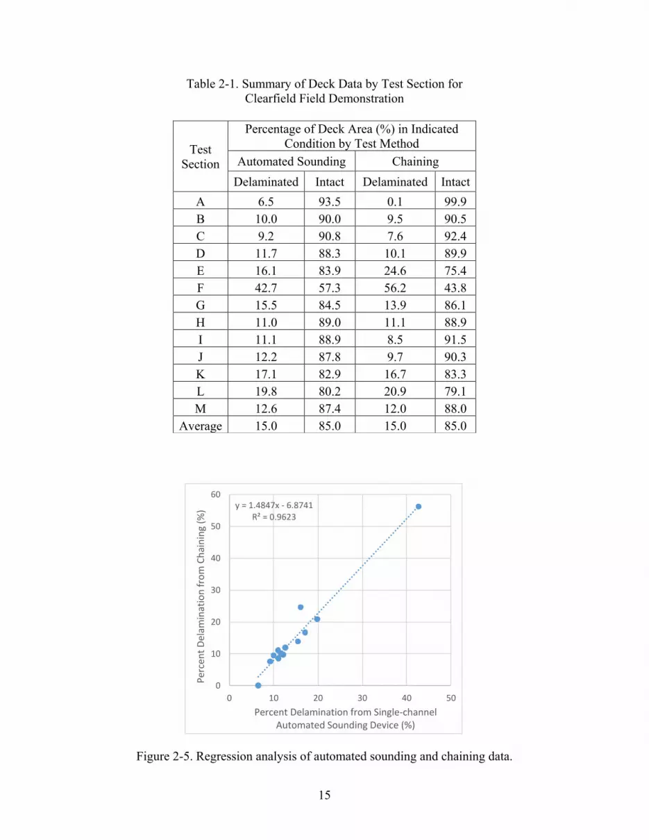
Table 2-1. Summary of Deck Data by Test Section for Clearfield Field Demonstration ............. 15

Table 3-1. Summary of Deck Data by Test Section for Clearfield Field Demonstration ............. 27

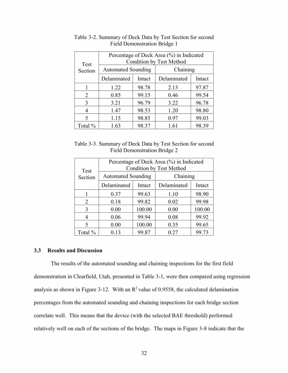
Table 3-2. Summary of Deck Data by Test Section for second Field Demonstration Bridge 1 ... 32

Table 3-3. Summary of Deck Data by Test Section for second Field Demonstration Bridge 2 ... 32

Table 3-4. Summary of Deck Data by Test Section from Two Sounding Devices for Clearfield

Field Demonstration .............................................................................................................. 34

vi

LIST OF FIGURES

Figure 2-1. Mallet impactor unit. .................................................................................................... 8

Figure 2-2. Automated sounding cart with power supply for impactor and laptop for

post-processing and recording. ................................................................................................ 9

Figure 2-3. Interior of the automated sounding cart. ...................................................................... 9

Figure 2-4. Automated sounding and chaining maps from the field demonstration. The

Bandlimited Acoustic Energy is calculated using the methods outlined in the text.............. 14

Figure 2-5. Regression analysis of automated sounding and chaining data. ................................ 15

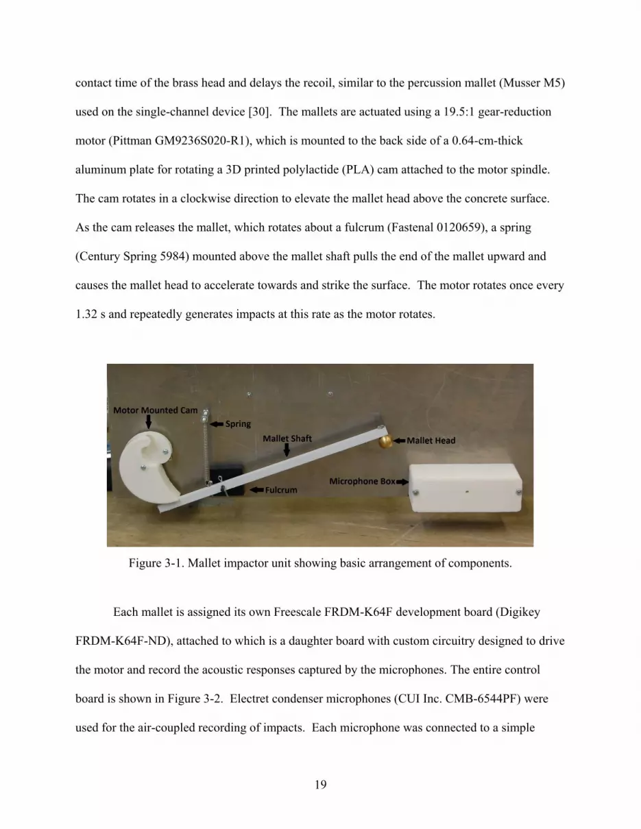
Figure 3-1. Mallet impactor unit showing basic arrangement of components. ............................ 19

Figure 3-2. Custom motor control and microphone amplification daughter board mounted on a

FRDM-K64F development board, with the ethernet cable and wires to the power source,

microphones, and rotation encoder shown. ........................................................................... 20

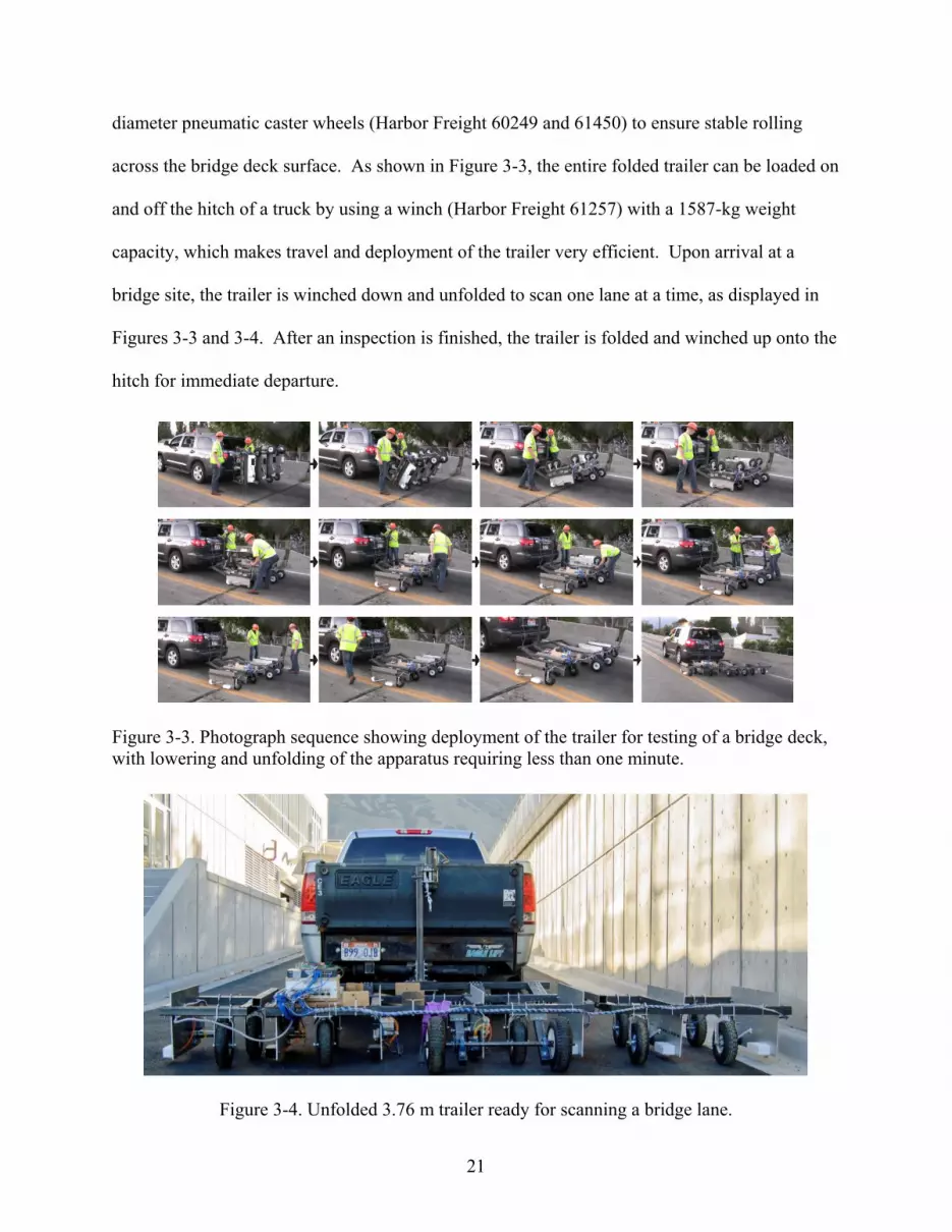
Figure 3-3. Photograph sequence showing deployment of the trailer for testing of a bridge deck,

with lowering and unfolding of the apparatus requiring less than one minute. ..................... 21

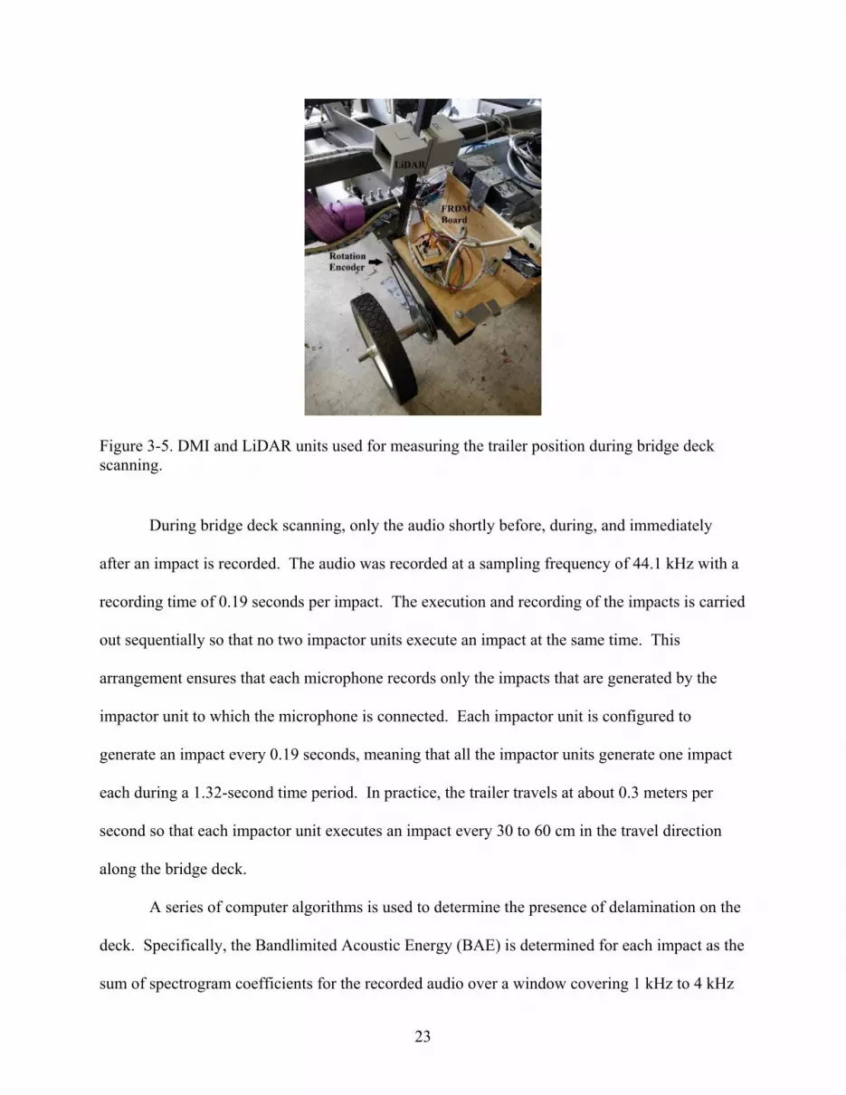
Figure 3-4. Unfolded 3.76 m trailer ready for scanning a bridge lane. ......................................... 21

Figure 3-5. DMI and LiDAR units used for measuring the trailer position during bridge deck

scanning. ................................................................................................................................ 23

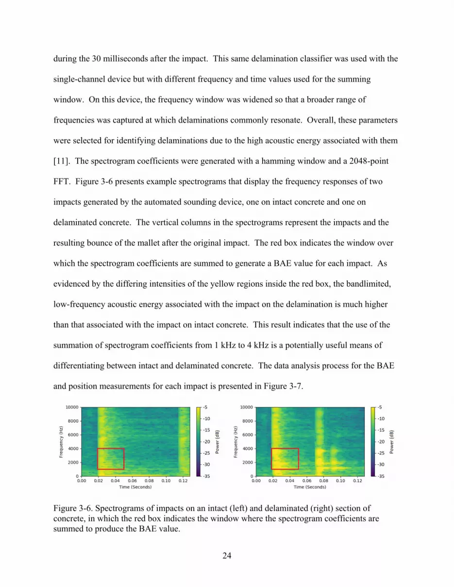
Figure 3-6. Spectrograms of impacts on an intact (left) and delaminated (right) section of

concrete, in which the red box indicates the window where the spectrogram coefficients are

summed to produce the BAE value. ...................................................................................... 24

Figure 3-7. Data analysis process for generating a delamination map from measurements of BAE

and position............................................................................................................................ 25

Figure 3-8. Multi-channel automated sounding trailer (top), single-mallet automated sounding

device not reported in this work (middle), and chaining (bottom) maps from the field

demonstration. ....................................................................................................................... 26

Figure 3-9. Maps for the automated sounding (top) and chaining data (bottom) from the first

bridge. .................................................................................................................................... 30

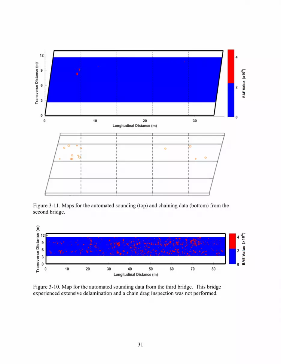
Figure 3-10. Map for the automated sounding data from the third bridge. This bridge

experienced extensive delamination and a chain drag inspection was not performed. ......... 31

Figure 3-11. Maps for the automated sounding (top) and chaining data (bottom) from the second

bridge. .................................................................................................................................... 31

Figure 3-12. Regression analysis of automated sounding and chaining data for first field

demonstration. ....................................................................................................................... 33

vii

Figure 3-13. Regression analysis for data from both automated sounding devices for the first

field demonstration. ............................................................................................................... 35

Figure 3-14. Regression analysis of automated sounding data and chain dragging data for the

first and second bridges in the second field demonstration. .................................................. 36

1

1 INTRODUCTION

In 2016, 9.1% of bridges in the United States were considered structurally deficient [1].

While this is a serious problem for the United States, infrastructure deterioration is a global

challenge. Trillions of dollars have been spent on the construction and maintenance of modern

infrastructure and even more will be spent on efforts to maintain and repair these expensive and

important investments. As has been documented in various media outlets, addressing

infrastructure deterioration is a major challenge, involving technical, economic, and political

considerations. Solutions to this problem require interdisciplinary work and expertise from

many different fields. To address one aspect of this global challenge, this thesis reports on

technological advances in civil infrastructure inspection by automation of an acoustic impact

response technique that is applied specifically to reinforced concrete bridge decks.

1.1 Bridge Deck Deterioration

One of the primary causes of structural deficiency in bridges, especially in colder regions,

is deterioration caused by the use of chloride-based deicing salts [2, 3]. The bridge deck, out of

all the elements of the structure, suffers the most from these deicing salts. It is also the hardest

part to inspect due to traffic. When the chloride ions in the deicing salts diffuse through concrete

bridge decks, corrosion of the embedded reinforcing steel can result [2]. As the corrosion

process leads to the formation of rust, the volume of the steel increases, causing an expansion of

the concrete from within the deck that eventually leads to a subsurface crack called a

2

delamination [4]. Delaminations are indicative of rapidly progressing deterioration and require

either repair or replacement of damaged sections. Locating these delaminations and quantifying

their extent is important for selecting appropriate maintenance and rehabilitation strategies to

minimize overall life-cycle costs of bridge decks.

1.2 Impact-Echo Testing and Sounding

In the 1980s, the National Institute of Standards and Technology pioneered the impact-

echo technique to identify delaminations in concrete surfaces [5, 6]. This traditional impact-echo

test involved the use of steel ball bearings for striking the concrete, and contact sensors

(accelerometers) used for measuring the echo and propagation of the pressure waves within the

concrete following an impact [7, 8, 9, 10]. Because these pressure waves propagate differently

in delaminated concrete than intact concrete, a Fast Fourier Transform was typically performed

on the recorded echo, and classifications of the material condition were made based on the

frequency spectra of the response signal. More recently, air-coupled techniques have been

employed to reduce the necessity of contacting the bridge deck surface to measure the impact

responses [11, 12, 13, 14, 15, 16, 17, 18]. Air-coupled impact-echo measurements are performed

using microphones suspended above the test surface and can produce results similar to those

obtained using contact sensors. Instead of directly measuring the pressure waves that propagate

within the concrete, the microphones capture leaky surface waves or, perhaps more imperfectly

in the case of concrete, flexural modes of the concrete that transmit acoustic energy through the

air. This method of detection works best for delaminations with a ratio of areal size to thickness

greater than five [19]. When the areal size is significantly greater than the thickness of the

delamination, the flexural modes dominate the acoustic response of the concrete, and the

delamination can be heard more easily.

3

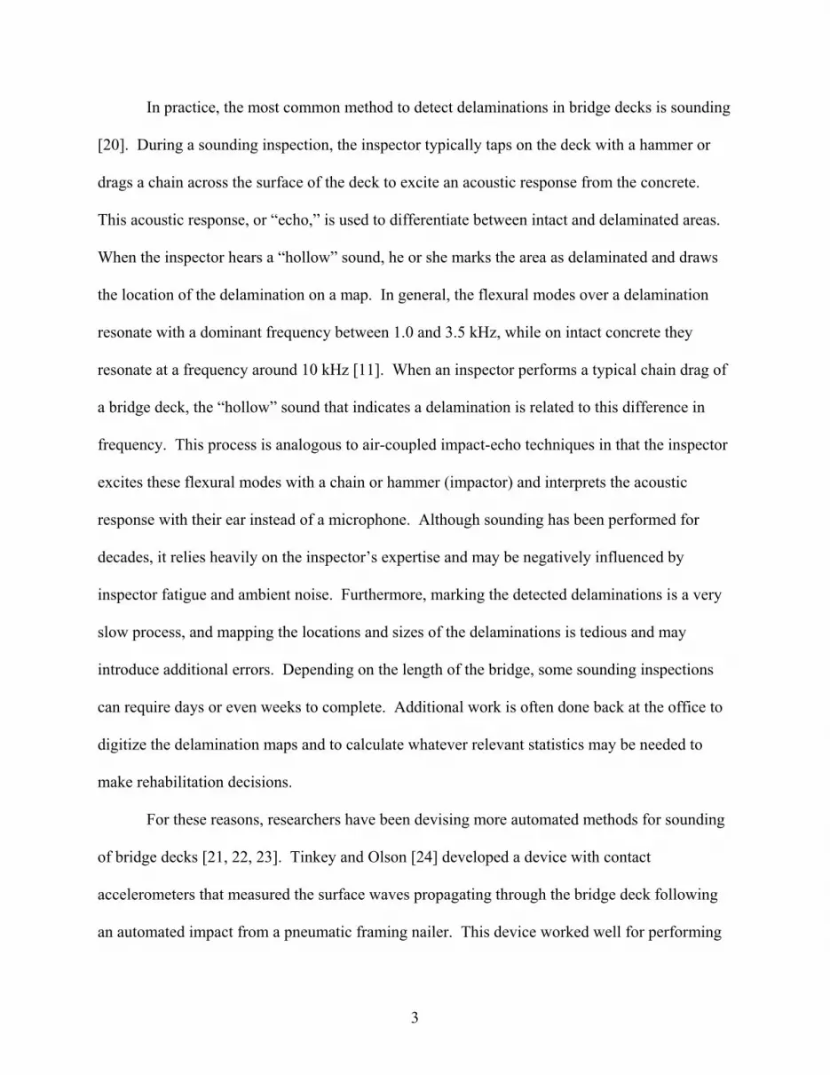
In practice, the most common method to detect delaminations in bridge decks is sounding

[20]. During a sounding inspection, the inspector typically taps on the deck with a hammer or

drags a chain across the surface of the deck to excite an acoustic response from the concrete.

This acoustic response, or “echo,” is used to differentiate between intact and delaminated areas.

When the inspector hears a “hollow” sound, he or she marks the area as delaminated and draws

the location of the delamination on a map. In general, the flexural modes over a delamination

resonate with a dominant frequency between 1.0 and 3.5 kHz, while on intact concrete they

resonate at a frequency around 10 kHz [11]. When an inspector performs a typical chain drag of

a bridge deck, the “hollow” sound that indicates a delamination is related to this difference in

frequency. This process is analogous to air-coupled impact-echo techniques in that the inspector

excites these flexural modes with a chain or hammer (impactor) and interprets the acoustic

response with their ear instead of a microphone. Although sounding has been performed for

decades, it relies heavily on the inspector’s expertise and may be negatively influenced by

inspector fatigue and ambient noise. Furthermore, marking the detected delaminations is a very

slow process, and mapping the locations and sizes of the delaminations is tedious and may

introduce additional errors. Depending on the length of the bridge, some sounding inspections

can require days or even weeks to complete. Additional work is often done back at the office to

digitize the delamination maps and to calculate whatever relevant statistics may be needed to

make rehabilitation decisions.

For these reasons, researchers have been devising more automated methods for sounding

of bridge decks [21, 22, 23]. Tinkey and Olson [24] developed a device with contact

accelerometers that measured the surface waves propagating through the bridge deck following

an automated impact from a pneumatic framing nailer. This device worked well for performing

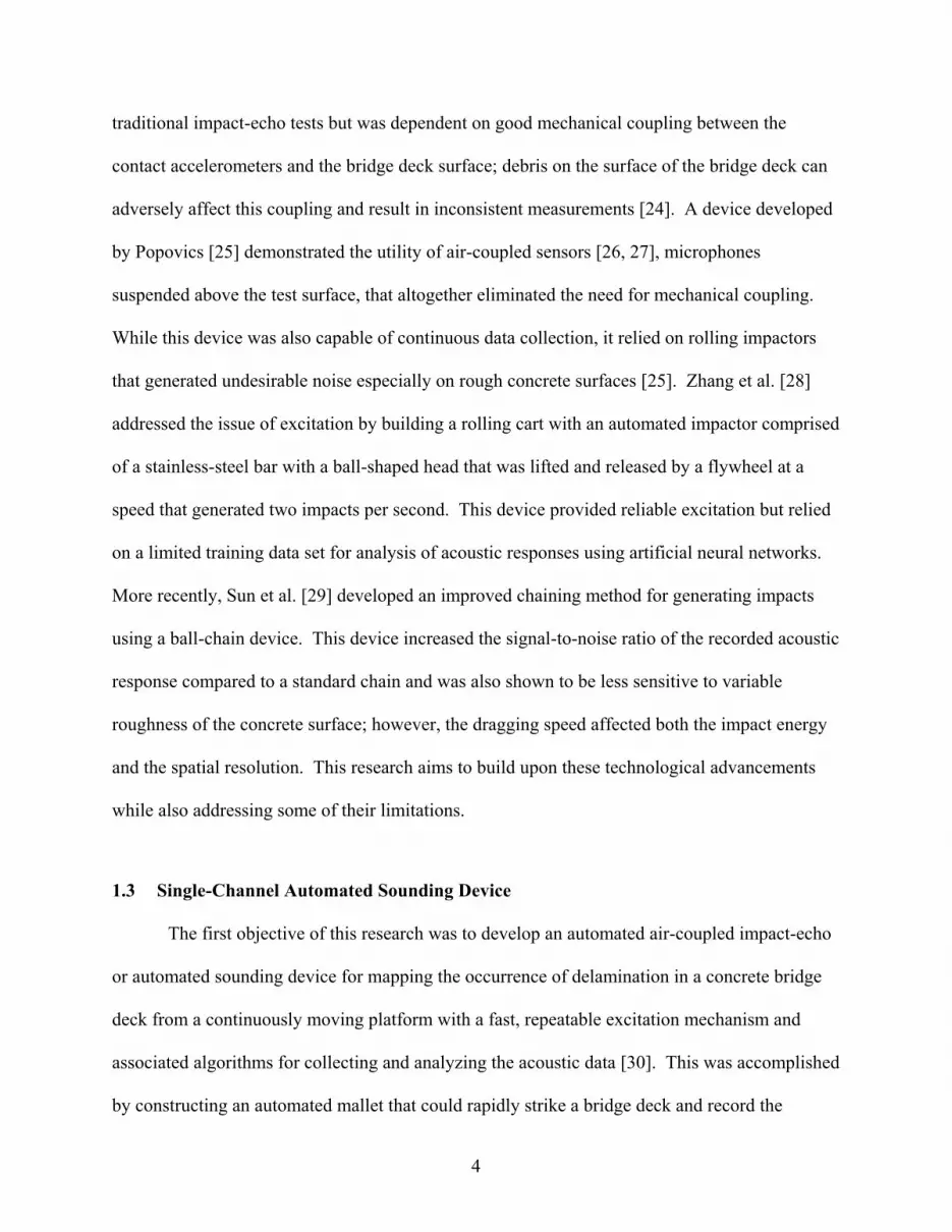
4

traditional impact-echo tests but was dependent on good mechanical coupling between the

contact accelerometers and the bridge deck surface; debris on the surface of the bridge deck can

adversely affect this coupling and result in inconsistent measurements [24]. A device developed

by Popovics [25] demonstrated the utility of air-coupled sensors [26, 27], microphones

suspended above the test surface, that altogether eliminated the need for mechanical coupling.

While this device was also capable of continuous data collection, it relied on rolling impactors

that generated undesirable noise especially on rough concrete surfaces [25]. Zhang et al. [28]

addressed the issue of excitation by building a rolling cart with an automated impactor comprised

of a stainless-steel bar with a ball-shaped head that was lifted and released by a flywheel at a

speed that generated two impacts per second. This device provided reliable excitation but relied

on a limited training data set for analysis of acoustic responses using artificial neural networks.

More recently, Sun et al. [29] developed an improved chaining method for generating impacts

using a ball-chain device. This device increased the signal-to-noise ratio of the recorded acoustic

response compared to a standard chain and was also shown to be less sensitive to variable

roughness of the concrete surface; however, the dragging speed affected both the impact energy

and the spatial resolution. This research aims to build upon these technological advancements

while also addressing some of their limitations.

1.3 Single-Channel Automated Sounding Device

The first objective of this research was to develop an automated air-coupled impact-echo

or automated sounding device for mapping the occurrence of delamination in a concrete bridge

deck from a continuously moving platform with a fast, repeatable excitation mechanism and

associated algorithms for collecting and analyzing the acoustic data [30]. This was accomplished

by constructing an automated mallet that could rapidly strike a bridge deck and record the

5

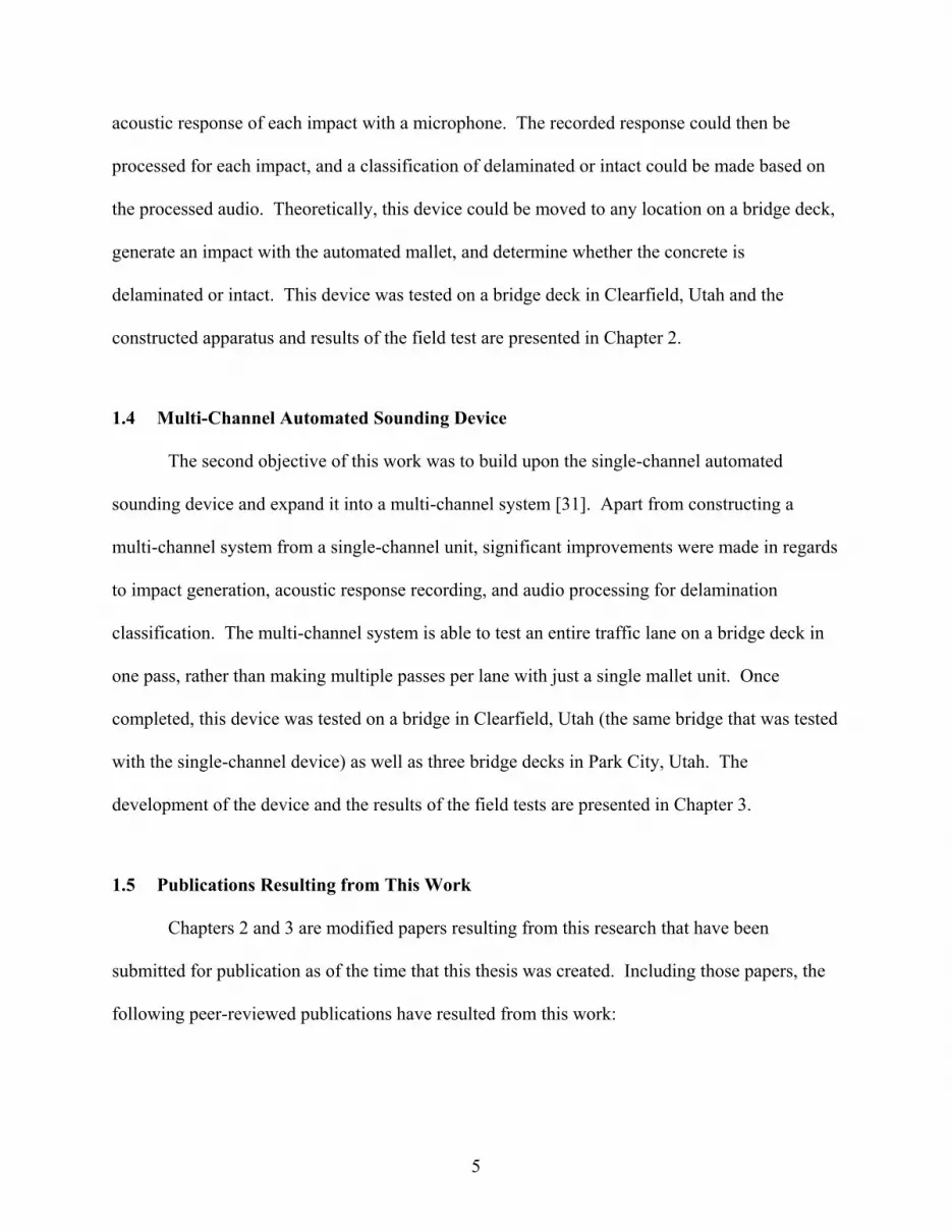
acoustic response of each impact with a microphone. The recorded response could then be

processed for each impact, and a classification of delaminated or intact could be made based on

the processed audio. Theoretically, this device could be moved to any location on a bridge deck,

generate an impact with the automated mallet, and determine whether the concrete is

delaminated or intact. This device was tested on a bridge deck in Clearfield, Utah and the

constructed apparatus and results of the field test are presented in Chapter 2.

1.4 Multi-Channel Automated Sounding Device

The second objective of this work was to build upon the single-channel automated

sounding device and expand it into a multi-channel system [31]. Apart from constructing a

multi-channel system from a single-channel unit, significant improvements were made in regards

to impact generation, acoustic response recording, and audio processing for delamination

classification. The multi-channel system is able to test an entire traffic lane on a bridge deck in

one pass, rather than making multiple passes per lane with just a single mallet unit. Once

completed, this device was tested on a bridge in Clearfield, Utah (the same bridge that was tested

with the single-channel device) as well as three bridge decks in Park City, Utah. The

development of the device and the results of the field tests are presented in Chapter 3.

1.5 Publications Resulting from This Work

Chapters 2 and 3 are modified papers resulting from this research that have been

submitted for publication as of the time that this thesis was created. Including those papers, the

following peer-reviewed publications have resulted from this work:

6

1. B. A. Mazzeo, J. Larsen, J. McElderry, and W. S. Guthrie, “Rapid multichannel impact-echo

scanning of concrete bridge decks from a continuously moving platform,” AIP Conference

Proceedings 1806, 080003, 2017.

2. W. S. Guthrie, J. Larsen, J. Baxter, B. A. Mazzeo, “Automated Air-Coupled Impact-Echo

Testing of a Concrete Bridge Deck from a Continuously Moving Platform,” Under Review.

3. J. Larsen, J. McElderry, W. S. Guthrie, B. A. Mazzeo, “Automated Sounding for Concrete

Bridge Deck Inspection through a Multi-Channel, Continuously Moving Platform,” Under

Review.

1.6 Summary

Automation of the sounding process with these devices significantly decreases the

standard bridge deck inspection time, eliminates the subjectivity associated with traditional

sounding techniques, and increases the safety of the inspection process by substantially reducing

the exposure of inspectors to live trafficking. Automation of traditional manual sounding

procedures with devices like those developed in this work can save Departments of

Transportation (DOT) significant amounts of time and money. Monitoring the structural

integrity of the nation’s bridges and execution of maintenance or rehabilitation can become more

efficient by implementing modern technology into our bridge management systems.

http://aip.scitation.org/author/Mazzeo%2C+Brian+A

http://aip.scitation.org/author/Larsen%2C+Jacob

http://aip.scitation.org/author/McElderry%2C+Joseph

http://aip.scitation.org/author/Guthrie%2C+W+Spencer

7

2 SINGLE-CHANNEL AUTOMATED SOUNDING DEVICE

The scope for the first stage of this research included designing and building the new

device, developing algorithms for processing the acoustic data, and determining a delamination

detection threshold by comparing the results obtained using the new device with those obtained

from traditional chain dragging in a field demonstration. The following sections provide a

description of the automated sounding device and associated algorithms developed in this work,

discussion of the results of the field demonstration, and conclusions and recommendations

derived from the findings.

2.1 Apparatus Development

The apparatus developed in this research included an impactor unit, a moving platform, a

microphone for air-coupled sensing, a distance measurement instrument (DMI), and signal

processing modules. The impactor unit designed for bridge deck testing in this research included

several individual elements as depicted in Figure 2-1. Based on previous work in which a softer

impact material was shown to improve excitation of flexural modes in concrete by facilitating a

longer contact time between the impactor and the concrete surface [32], a Musser M5 percussion

mallet was selected for the present work due to its shaft length and flexibility as well as its mallet

head size and composition. The mallet was actuated using a Pittman 19.5:1 gear-reduction

motor, which was mounted to the back side of an aluminum plate for rotating a cam shaft

8

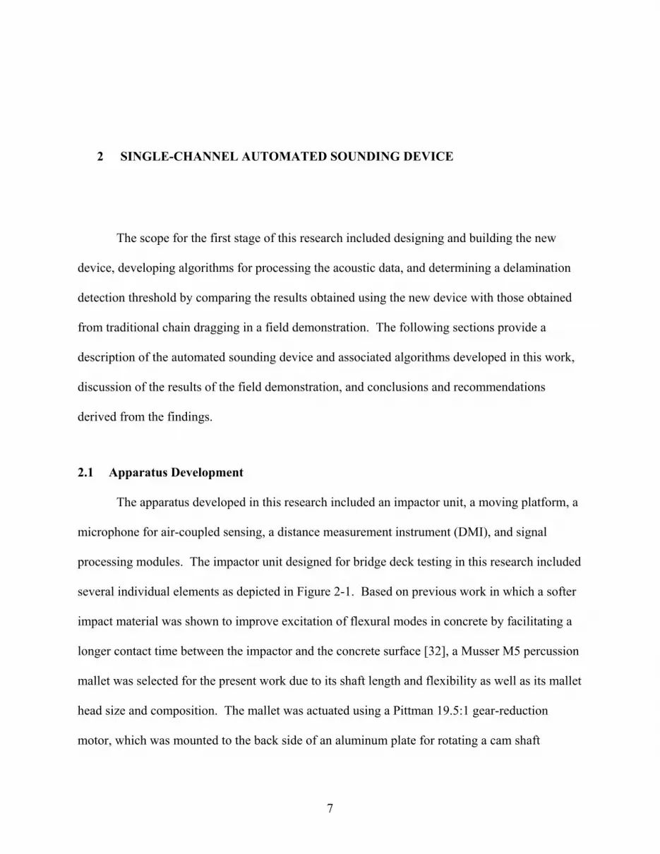
attached to the motor spindle. The cam shaft rotated in a clockwise direction, as viewed in

Figure 2-1, to elevate the mallet head above the concrete surface. As the cam shaft released the

mallet, which rotated about a pivot point, a spring mounted above the mallet shaft caused a

sudden downward motion of the mallet head. The mallet head then impacted the concrete

Figure 2-1. Mallet impactor unit.

surface. As the motor continued to rotate the cam shaft, consistent impacts were repeatedly

generated independent of the speed of the moving platform. A high impact rate on the order of

four impacts per second, which was twice as fast as that reported by Zhang et al. [28], was

achieved using a Tektronix PS280 power supply set to approximately 20 volts.

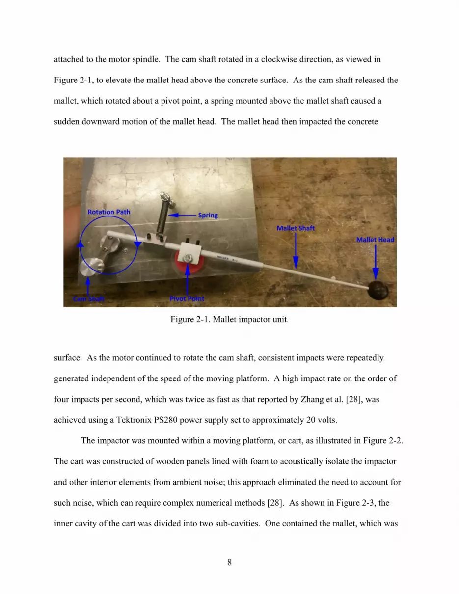
The impactor was mounted within a moving platform, or cart, as illustrated in Figure 2-2.

The cart was constructed of wooden panels lined with foam to acoustically isolate the impactor

and other interior elements from ambient noise; this approach eliminated the need to account for

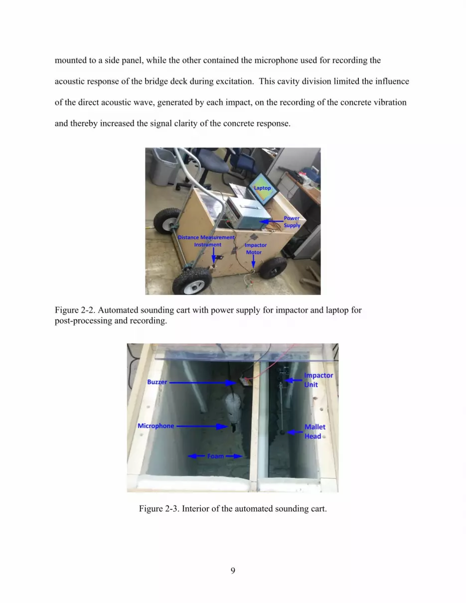
such noise, which can require complex numerical methods [28]. As shown in Figure 2-3, the

inner cavity of the cart was divided into two sub-cavities. One contained the mallet, which was

9

mounted to a side panel, while the other contained the microphone used for recording the

acoustic response of the bridge deck during excitation. This cavity division limited the influence

of the direct acoustic wave, generated by each impact, on the recording of the concrete vibration

and thereby increased the signal clarity of the concrete response.

Figure 2-2. Automated sounding cart with power supply for impactor and laptop for

post-processing and recording.

Figure 2-3. Interior of the automated sounding cart.

10

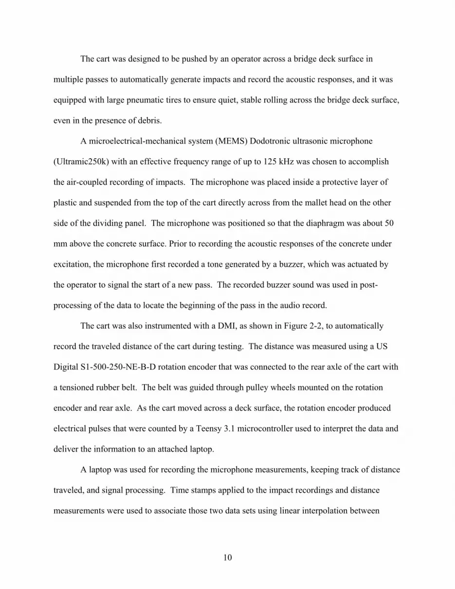
The cart was designed to be pushed by an operator across a bridge deck surface in

multiple passes to automatically generate impacts and record the acoustic responses, and it was

equipped with large pneumatic tires to ensure quiet, stable rolling across the bridge deck surface,

even in the presence of debris.

A microelectrical-mechanical system (MEMS) Dodotronic ultrasonic microphone

(Ultramic250k) with an effective frequency range of up to 125 kHz was chosen to accomplish

the air-coupled recording of impacts. The microphone was placed inside a protective layer of

plastic and suspended from the top of the cart directly across from the mallet head on the other

side of the dividing panel. The microphone was positioned so that the diaphragm was about 50

mm above the concrete surface. Prior to recording the acoustic responses of the concrete under

excitation, the microphone first recorded a tone generated by a buzzer, which was actuated by

the operator to signal the start of a new pass. The recorded buzzer sound was used in post-

processing of the data to locate the beginning of the pass in the audio record.

The cart was also instrumented with a DMI, as shown in Figure 2-2, to automatically

record the traveled distance of the cart during testing. The distance was measured using a US

Digital S1-500-250-NE-B-D rotation encoder that was connected to the rear axle of the cart with

a tensioned rubber belt. The belt was guided through pulley wheels mounted on the rotation

encoder and rear axle. As the cart moved across a deck surface, the rotation encoder produced

electrical pulses that were counted by a Teensy 3.1 microcontroller used to interpret the data and

deliver the information to an attached laptop.

A laptop was used for recording the microphone measurements, keeping track of distance

traveled, and signal processing. Time stamps applied to the impact recordings and distance

measurements were used to associate those two data sets using linear interpolation between

11

distance measurements. Impact events within the recording were identified at times when the

audio level exceeded a defined threshold. Signal processing was then performed on the data

corresponding to those times. As delaminations exhibit flexural vibrations that are lower in

vibration frequency than those exhibited by intact concrete under excitation [11, 33], a Fourier

transform was used for analyzing the frequency spectrum of the acoustic response to determine if

the concrete was intact or delaminated. More specifically, the following algorithm was

implemented in MATLAB. The acoustic waveform data had a representation in MATLAB that

ranged from -1 to 1 with a standard deviation of approximately 0.03 for most runs. To find times

when impacts occurred, time stamps were recorded when the signal deviated below its median

value by a value of at least 0.1. At those locations in the acoustic waveform record, 6001 audio

samples were then selected for further processing, representing about 24 ms of acoustic data. An

additional constraint was enforced that impacts were required to be at least 0.12 seconds apart to

ensure that single impacts were processed only once. The 6001 samples representing a single

impact were downsampled by a factor of 10 and then the MATLAB periodogram power spectral

density estimate with a rectangular window was computed using a 2048-point FFT. Bins 80 to

136, representing frequencies from 964 Hz to 1.65 kHz, were then summed to estimate the

bandlimited acoustic energy (BAE) over this selected time period after the impact. These

parameters were determined before comparison with the chaining data, however, these windows

of frequency and time were chosen for identifying delaminations due to the high acoustic energy

associated with them and are within the range of 0.5 to 5 kHz computed using semi-analytical

equations of resonance frequencies for square delaminations having a depth of 20 to 80 mm and

a width of 0.2 to 1.0 m [11]. Additionally, for the soft mallet impactor used in this study, this

range appeared to adequately capture the acoustic signature of delaminations. This approach of

12

summing a broad range of spectral energy captures variations naturally present in the depth and

extent of the delaminations on the deck.

2.2 Field Demonstration

After the apparatus was complete, a field demonstration was arranged on a concrete

bridge deck in northern Utah. The bridge carried one lane of eastbound traffic and one lane of

westbound traffic over several railroad tracks. With 11 spans, the bridge had a total length of

434 m, and the width of the bridge between the inside faces of the parapet walls was 8.7 m. The

bridge was constructed in 1972 using uncoated reinforcing steel, or black bar, and a 25-mm-thick

concrete overlay was placed in 1973. A nearly 10-mm-thick polymer surface treatment was

applied to the bridge deck approximately 30 years later. With an original cover depth of 50 mm

over the top mat of reinforcing steel, the average cover depth after these treatments was therefore

85 mm. At the time of the field demonstration in July 2014, the bridge was requiring weekly

pothole maintenance on especially the span over the railroad tracks.

The field demonstration involved automated sounding with the new device and chaining.

For testing, the deck was divided into sections in alphabetical order from A to M with increasing

longitudinal distance from east to west. These 13 sections corresponded to nine deck spans and

two long slab spans, one at each end of the bridge, with the slab spans being divided into two

sections each. A grid with 3-m spacing in the longitudinal direction and 1.2-m spacing in the

transverse direction was marked on the deck surface for spatial referencing.

Automated sounding was performed with the new device along each of 12 longitudinal

lines spaced 0.6 m apart in the transverse direction, excluding only the center line due to the

presence of traffic control equipment at that location during testing. The automated sounding

device delivered approximately four impacts per second, and the operator moved the device

13

along the line at a target speed of about 0.6 m per second. Each pass along the length of the

bridge required approximately 20 minutes, so that testing of the entire bridge deck was

completed in about 4-man hours. As described previously, a series of algorithms were then used

to process the data.

In the process of chaining the deck, the researchers recorded the occurrence of

delamination along each of the same 12 longitudinal lines evaluated using automated sounding

and also along the center line. The deck condition, delaminated or intact, was recorded at 0.3-m

intervals along each line. Each pass along the length of the bridge required an average of nearly

2.5-man hours, which equated to more than 30-man hours for the entire bridge deck.

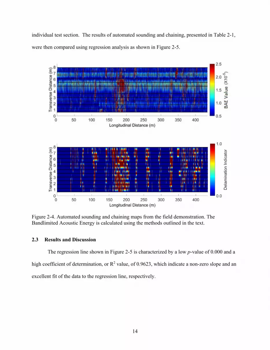
The results of the deck testing include maps showing the automated sounding data and

chaining data, as presented in Figure 2-4 (not drawn to scale). For display purposes, a cubic

interpolation function was used to generate values between the locations of the actual impacts

and chaining measurements, which are indicated by black dots that appear as lines in the maps

due to their close proximity to each other. In the automated sounding map, increasing BAE

values indicate an increasing likelihood of delamination. In the chaining map, delamination

indicator values of “0” and “1” indicate the absence and presence of delamination, respectively.

To determine if the span delamination percentages corresponded to observed differences

in the acoustic impact data by the new device, and because universal standards for acoustic

impact response are not yet established, a BAE threshold of 1.415x10-5 was selected to

distinguish intact from delaminated concrete. This threshold was chosen because it resulted in

the same delamination percentage for the entire bridge deck that was determined from chaining.

As a means of evaluating its suitability across a broad range of delamination percentages, the

same threshold of 1.415x10-5 was also used to compute the delamination percentage for each

14

individual test section. The results of automated sounding and chaining, presented in Table 2-1,

were then compared using regression analysis as shown in Figure 2-5.

Figure 2-4. Automated sounding and chaining maps from the field demonstration. The

Bandlimited Acoustic Energy is calculated using the methods outlined in the text.

2.3 Results and Discussion

The regression line shown in Figure 2-5 is characterized by a low p-value of 0.000 and a

high coefficient of determination, or R2 value, of 0.9623, which indicate a non-zero slope and an

excellent fit of the data to the regression line, respectively.

15

Table 2-1. Summary of Deck Data by Test Section for

Clearfield Field Demonstration

Figure 2-5. Regression analysis of automated sounding and chaining data.

y = 1.4847x - 6.8741R² = 0.9623

0

10

20

30

40

50

60

0 10 20 30 40 50

Per

cen

t D

elam

inat

ion

fro

m C

hai

nin

g (%

)

Percent Delamination from Single-channel Automated Sounding Device (%)

Test

Section

Percentage of Deck Area (%) in Indicated

Condition by Test Method

Automated Sounding Chaining

Delaminated Intact Delaminated Intact

A 6.5 93.5 0.1 99.9

B 10.0 90.0 9.5 90.5

C 9.2 90.8 7.6 92.4

D 11.7 88.3 10.1 89.9

E 16.1 83.9 24.6 75.4

F 42.7 57.3 56.2 43.8

G 15.5 84.5 13.9 86.1

H 11.0 89.0 11.1 88.9

I 11.1 88.9 8.5 91.5

J 12.2 87.8 9.7 90.3

K 17.1 82.9 16.7 83.3

L 19.8 80.2 20.9 79.1

M 12.6 87.4 12.0 88.0

Average 15.0 85.0 15.0 85.0

16

Although the deviation of the regression line from the line of equality in Figure 2-5

suggests that some bias may exist in the automated sounding testing approach used in this work,

the percentage of the deck area determined to be delaminated using automated sounding is within

3 percentage points of that determined to be delaminated using chaining for 10 of the 13 test

sections (test sections B, C, D, G, H, I, J, K, L, and M), which generally exhibit delamination

percentages ranging from 7 to 21 percent. Among the remaining three test sections, test section

A is characterized as having the lowest delamination percentage at less than 1 percent, while test

sections E and F are characterized as having the highest delamination percentages at greater than

24 percent according to the chaining results; the percentage of the deck area determined to be

delaminated using automated sounding is approximately 6 percentage points higher for test

section A and up to 14 percentage points lower for test sections E and F than the corresponding

percentages of the deck area determined to be delaminated using chaining. Such variations

between the results of the automated sounding and chaining tests may be partially attributed to

possible tracking differences along each of the longitudinal lines, exclusion of the center line

during the automated sounding tests, and/or minor distance measurement differences that may

have occurred between the two approaches.

2.4 Conclusions

The primary accomplishment of this part of the research is the development of a single-

channel automated sounding device for mapping the occurrence of delamination in a concrete

bridge deck from a continuously moving platform with a fast, repeatable excitation mechanism

and unsupervised algorithms for collecting and analyzing the acoustic data. The apparatus

included an impactor unit, a moving platform, a microphone for air-coupled sensing, a DMI, and

signal processing modules. Field testing of a concrete bridge deck with a length and width of

17

434 m and 8.7 m, respectively, required about 4-man hours using the new device compared to

more than 30-man hours required for chaining; therefore, testing with the new device was more

than seven times faster than chaining. A comparison of the automated sounding data with the

chaining data yielded a BAE detection threshold of 1.415x10-5, and the resulting percentage of

the deck area determined to be delaminated using automated sounding was within 3 percentage

points of that determined to be delaminated using chaining for 10 of the 13 test sections into

which the deck was divided. These test sections generally exhibited delamination percentages

ranging from 7 to 21 percent, demonstrating the utility of the new automated sounding testing for

evaluating concrete bridge decks with various amounts of delamination.

While the automated sounding device developed in this research incorporated only a

single channel, the apparatus could be readily expanded to a multi-channel system that would

allow even faster bridge deck testing. The development of such a device is detailed in the next

chapter. Nonetheless, given the typical threshold values for delamination percentages utilized

for bridge management, the data suggest that the new automated sounding device could be used

to generate results that would lead to similar maintenance and rehabilitation strategies as those

that would be recommended based on the results of chain dragging. Additional work to optimize

the use of the new acoustic data analysis algorithms presented in this work may provide even

better results; specifically, a larger frequency summing window may provide greater detection

capability.

18

3 MULTI-CHANNEL AUTOMATED SOUNDING DEVICE

The second stage of this research included the design and construction of the new multi-

channel device, improvement of the algorithms used for processing the acoustic data with the

single-channel device, and the determination of a delamination detection threshold by comparing

the results obtained using the multi-channel device with those obtained from traditional chain

dragging in field demonstrations. The following sections provide a description of the multi-

channel automated sounding device and associated algorithms used for processing, discussion of

the results of the field demonstrations, and conclusions and recommendations derived from the

findings.

3.1 Apparatus Development

The multi-channel automated sounding device includes seven replicated impactor and

recording units, a moving trailer platform, a distance measurement instrument (DMI), and signal

processing modules. The impactor unit from the single-channel device was improved upon for

the multi-channel device and comprises several individual elements as depicted in Figure 3-1.

As mentioned in Chapter 2, impact materials that are softer than steel have been shown to

improve excitation of flexural modes in concrete [32] due to the increased contact time they

exhibit during an impact [10]. Because of this, the mallets were constructed using a 38.1-cm

polypropylene shaft (UL 94HB) and a 2.54-cm-diameter brass head (Liberty Brass BAL132).

The polypropylene shaft is able to flex as the brass head contacts the surface, which increases the

19

contact time of the brass head and delays the recoil, similar to the percussion mallet (Musser M5)

used on the single-channel device [30]. The mallets are actuated using a 19.5:1 gear-reduction

motor (Pittman GM9236S020-R1), which is mounted to the back side of a 0.64-cm-thick

aluminum plate for rotating a 3D printed polylactide (PLA) cam attached to the motor spindle.

The cam rotates in a clockwise direction to elevate the mallet head above the concrete surface.

As the cam releases the mallet, which rotates about a fulcrum (Fastenal 0120659), a spring

(Century Spring 5984) mounted above the mallet shaft pulls the end of the mallet upward and

causes the mallet head to accelerate towards and strike the surface. The motor rotates once every

1.32 s and repeatedly generates impacts at this rate as the motor rotates.

Figure 3-1. Mallet impactor unit showing basic arrangement of components.

Each mallet is assigned its own Freescale FRDM-K64F development board (Digikey

FRDM-K64F-ND), attached to which is a daughter board with custom circuitry designed to drive

the motor and record the acoustic responses captured by the microphones. The entire control

board is shown in Figure 3-2. Electret condenser microphones (CUI Inc. CMB-6544PF) were

used for the air-coupled recording of impacts. Each microphone was connected to a simple

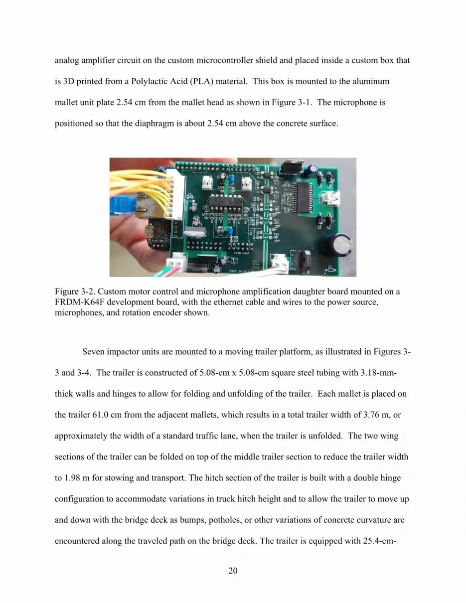
20

analog amplifier circuit on the custom microcontroller shield and placed inside a custom box that

is 3D printed from a Polylactic Acid (PLA) material. This box is mounted to the aluminum

mallet unit plate 2.54 cm from the mallet head as shown in Figure 3-1. The microphone is

positioned so that the diaphragm is about 2.54 cm above the concrete surface.

Seven impactor units are mounted to a moving trailer platform, as illustrated in Figures 3-

3 and 3-4. The trailer is constructed of 5.08-cm x 5.08-cm square steel tubing with 3.18-mm-

thick walls and hinges to allow for folding and unfolding of the trailer. Each mallet is placed on

the trailer 61.0 cm from the adjacent mallets, which results in a total trailer width of 3.76 m, or

approximately the width of a standard traffic lane, when the trailer is unfolded. The two wing

sections of the trailer can be folded on top of the middle trailer section to reduce the trailer width

to 1.98 m for stowing and transport. The hitch section of the trailer is built with a double hinge

configuration to accommodate variations in truck hitch height and to allow the trailer to move up

and down with the bridge deck as bumps, potholes, or other variations of concrete curvature are

encountered along the traveled path on the bridge deck. The trailer is equipped with 25.4-cm-

Figure 3-2. Custom motor control and microphone amplification daughter board mounted on a

FRDM-K64F development board, with the ethernet cable and wires to the power source,

microphones, and rotation encoder shown.

21

diameter pneumatic caster wheels (Harbor Freight 60249 and 61450) to ensure stable rolling

across the bridge deck surface. As shown in Figure 3-3, the entire folded trailer can be loaded on

and off the hitch of a truck by using a winch (Harbor Freight 61257) with a 1587-kg weight

capacity, which makes travel and deployment of the trailer very efficient. Upon arrival at a

bridge site, the trailer is winched down and unfolded to scan one lane at a time, as displayed in

Figures 3-3 and 3-4. After an inspection is finished, the trailer is folded and winched up onto the

hitch for immediate departure.

Figure 3-3. Photograph sequence showing deployment of the trailer for testing of a bridge deck,

with lowering and unfolding of the apparatus requiring less than one minute.

Figure 3-4. Unfolded 3.76 m trailer ready for scanning a bridge lane.

22

Figure 3-5 shows the DMI mounted to the back of the trailer. The DMI consists of two

25.4-cm-diameter rubber tires (Harbor Freight 90051) mounted to a fixed 2.54-cm steel axle,

together with a rotation encoder (CUI Inc. AMT203-V) that measures the rotation of the wheels

as they roll across the bridge deck. A rubber belt is stretched across two pulleys, one attached to

the axle and one attached to the rotation encoder, which ties the rotation of the encoder to the

rotation of the axle. The number of rotation encoder ticks is counted for a single rotation of the

DMI wheels, and the number of ticks per meter is computed using the circumference of the

wheel, which enables assignment of a specific longitudinal position for each impact event with

reference to a specific starting position on the bridge deck. Two light detection and ranging

(LiDAR) units (PulsedLight LiDAR Lite V2) are also mounted to the DMI to measure the trailer

distance from each parapet wall at all times during the inspection. The DMI and LIDAR

measurements, which effectively provide x and y coordinates, respectively, for each impact with

reference to a designated origin on the bridge deck, are recorded by another FRDM-K64F

development board. Compared to other global positioning schemes that could have been used,

the strategy utilized in this research enables more accurate relative positioning, on the order of 1

cm, during bridge deck testing without needing a static reference base station.

A connected laptop running a custom controller written in Python is used for controlling

the impactor units, receiving and storing the impact audio recordings and position information,

and signal processing. All impact audio recordings as well as DMI and LiDAR measurements

are sent to the laptop over a Transmission Control Protocol (TCP) ethernet network from the

individual impactor units and DMI modules used for data acquisition. Distance measurements

are assigned to individual impacts based on recorded time stamps that are controlled by a

common clock on the laptop.

23

Figure 3-5. DMI and LiDAR units used for measuring the trailer position during bridge deck

scanning.

During bridge deck scanning, only the audio shortly before, during, and immediately

after an impact is recorded. The audio was recorded at a sampling frequency of 44.1 kHz with a

recording time of 0.19 seconds per impact. The execution and recording of the impacts is carried

out sequentially so that no two impactor units execute an impact at the same time. This

arrangement ensures that each microphone records only the impacts that are generated by the

impactor unit to which the microphone is connected. Each impactor unit is configured to

generate an impact every 0.19 seconds, meaning that all the impactor units generate one impact

each during a 1.32-second time period. In practice, the trailer travels at about 0.3 meters per

second so that each impactor unit executes an impact every 30 to 60 cm in the travel direction

along the bridge deck.

A series of computer algorithms is used to determine the presence of delamination on the

deck. Specifically, the Bandlimited Acoustic Energy (BAE) is determined for each impact as the

sum of spectrogram coefficients for the recorded audio over a window covering 1 kHz to 4 kHz

24

during the 30 milliseconds after the impact. This same delamination classifier was used with the

single-channel device but with different frequency and time values used for the summing

window. On this device, the frequency window was widened so that a broader range of

frequencies was captured at which delaminations commonly resonate. Overall, these parameters

were selected for identifying delaminations due to the high acoustic energy associated with them

[11]. The spectrogram coefficients were generated with a hamming window and a 2048-point

FFT. Figure 3-6 presents example spectrograms that display the frequency responses of two

impacts generated by the automated sounding device, one on intact concrete and one on

delaminated concrete. The vertical columns in the spectrograms represent the impacts and the

resulting bounce of the mallet after the original impact. The red box indicates the window over

which the spectrogram coefficients are summed to generate a BAE value for each impact. As

evidenced by the differing intensities of the yellow regions inside the red box, the bandlimited,

low-frequency acoustic energy associated with the impact on the delamination is much higher

than that associated with the impact on intact concrete. This result indicates that the use of the

summation of spectrogram coefficients from 1 kHz to 4 kHz is a potentially useful means of

differentiating between intact and delaminated concrete. The data analysis process for the BAE

and position measurements for each impact is presented in Figure 3-7.

Figure 3-6. Spectrograms of impacts on an intact (left) and delaminated (right) section of

concrete, in which the red box indicates the window where the spectrogram coefficients are

summed to produce the BAE value.

25

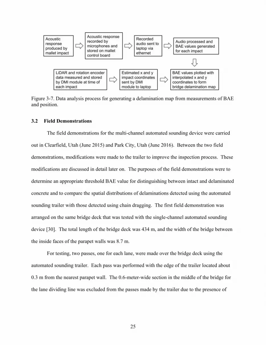
Figure 3-7. Data analysis process for generating a delamination map from measurements of BAE

and position.

3.2 Field Demonstrations

The field demonstrations for the multi-channel automated sounding device were carried

out in Clearfield, Utah (June 2015) and Park City, Utah (June 2016). Between the two field

demonstrations, modifications were made to the trailer to improve the inspection process. These

modifications are discussed in detail later on. The purposes of the field demonstrations were to

determine an appropriate threshold BAE value for distinguishing between intact and delaminated

concrete and to compare the spatial distributions of delaminations detected using the automated

sounding trailer with those detected using chain dragging. The first field demonstration was

arranged on the same bridge deck that was tested with the single-channel automated sounding

device [30]. The total length of the bridge deck was 434 m, and the width of the bridge between

the inside faces of the parapet walls was 8.7 m.

For testing, two passes, one for each lane, were made over the bridge deck using the

automated sounding trailer. Each pass was performed with the edge of the trailer located about

0.3 m from the nearest parapet wall. The 0.6-meter-wide section in the middle of the bridge for

the lane dividing line was excluded from the passes made by the trailer due to the presence of

26

traffic cones. Testing of the entire bridge deck was completed in about 1 hour. The chaining

inspection performed in July 2014 required more than 30-man hours.

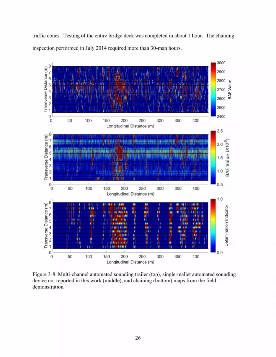
Figure 3-8. Multi-channel automated sounding trailer (top), single-mallet automated sounding

device not reported in this work (middle), and chaining (bottom) maps from the field

demonstration.

27

Maps generated from the multi-channel automated sounding trailer data, the single-mallet

automated sounding device data, and manual chaining data, are shown in Figure 3-8 (not drawn

to scale). The maps for the single-channel device data and chaining data are the same maps that

were presented in Chapter 2 and are included here for comparison to the multi-channel device.

For display and analysis purposes, a linear interpolation function was used to generate values

between the locations of the impacts and chaining measurements, which are indicated by black

dots appearing as lines in the maps due to their close proximity to each other. In the automated

sounding maps, increasing BAE values indicate an increasing probability of delamination. In the

chaining map, delamination indicator values of “0” and “1” indicate the absence and presence of

delamination, respectively.

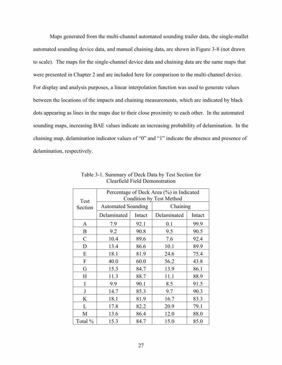
Table 3-1. Summary of Deck Data by Test Section for

Clearfield Field Demonstration

Test

Section





A 7.9 92.1 0.1 99.9

B 9.2 90.8 9.5 90.5

C 10.4 89.6 7.6 92.4

D 13.4 86.6 10.1 89.9

E 18.1 81.9 24.6 75.4

F 40.0 60.0 56.2 43.8

G 15.3 84.7 13.9 86.1

H 11.3 88.7 11.1 88.9

I 9.9 90.1 8.5 91.5

J 14.7 85.3 9.7 90.3

K 18.1 81.9 16.7 83.3

L 17.8 82.2 20.9 79.1

M 13.6 86.4 12.0 88.0

Total % 15.3 84.7 15.0 85.0

28

An important goal of this work was to determine if different delaminated and intact

regions could be distinguished reliably on a large deck by treating different sections of the deck

independently and then estimating their delamination percentages. Their individual delamination

percentages could then be used as a test for reliability of the method. To accomplish this, a BAE

threshold was selected that resulted in nearly the same total amount of delamination for the entire

bridge deck that was determined from chaining. This threshold, a BAE value of 2700, was then

used to compute the extent of delamination for each test section. The same 13 test sections (A

through M) used for analysis in our Chapter 2 are used here. Delamination percentages

calculated from both the automated sounding and chaining inspections for each test section are

presented in Table 3-1.

After the first field demonstration in Clearfield, Utah, the microphones on each mallet

were changed to a Knowles digital MEMS microphone (SPH0641LU4H-1). This was done

because the electret microphones broke easily and required custom power circuitry. Other

advantages to using MEMS microphones include small physical size, broad frequency

bandwidth, and high SNR [34]. Minor changes to the mallet control and audio processing code

were also made to accommodate this change in microphone. Specifically, the sampling

frequency was set to 3.75 MHz and the recording time for each impact was kept at 0.19 seconds.

The output of the microphone is a pulse-density modulated (PDM) signal which needed to be

converted to an analog audio signal before processing. In a PDM signal, the amplitude of the

wave is represented by the average pulse amplitude over time. Applying a low-pass filter to the

PDM signal essentially averages these pulses and returns an analog amplitude. To do this, a 2nd

order Butterworth filter was used with a cutoff frequency of 20 kHz. The analog signal was then

29

processed in the same way as was explained previously and a BAE value was generated for each

impact.

The second set of field tests with the automated sounding trailer was performed on three

bridges along U.S. Route 40 in Park City, Utah, in June 2016. The bridges, which had bare

concrete decks constructed using epoxy-coated rebar, were tested with the automated sounding

trailer and also inspected via manual chain dragging during the same night. The bridges were all

27 years old, located within 1.6 km of each other, and subject to the same climate and annual

average daily traffic. At the time of testing, the National Bridge Inventory ratings were 6, 7, and

6 for the first, second, and third bridge decks, respectively. Each of these bridges carried two

lanes of traffic, each heading in the same direction. Each of the two lanes on each bridge deck

was tested twice, with the second test in each lane occurring at a target distance of 30.5 cm

farther away from the parapet wall than the first test. This approach effectively doubled the

resolution of the collected data by evaluating points on a 30.5-cm interval in the transverse

direction rather than the fixed 61.0-cm spacing set by the mallet positions on the trailer.

Figures 3-9 and 3-10 present the resulting maps for the multi-mallet automated sounding

trailer and chaining tests for two of the bridge decks. The third bridge experienced extensive

delamination and the chain drag test was not completed due to the large amount of time it would

have required to perform accurately; indeed, a visual inspection indicated that some

delaminations had progressed to potholes on that deck, as evidenced by exposed rebar in some

locations. Figure 3-11 presents the delamination map that was produced by the multi-channel

device, but no comparison with a chain drag test is made for this bridge. The solid black lines in

the automated sounding maps represent the parapet walls and joints indicating the beginning and

end of the bridge deck. Because the microphones were changed between the first and second

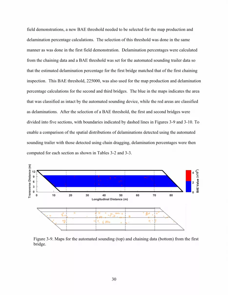
30

field demonstrations, a new BAE threshold needed to be selected for the map production and

delamination percentage calculations. The selection of this threshold was done in the same

manner as was done in the first field demonstration. Delamination percentages were calculated

from the chaining data and a BAE threshold was set for the automated sounding trailer data so

that the estimated delamination percentage for the first bridge matched that of the first chaining

inspection. This BAE threshold, 225000, was also used for the map production and delamination

percentage calculations for the second and third bridges. The blue in the maps indicates the area

that was classified as intact by the automated sounding device, while the red areas are classified

as delaminations. After the selection of a BAE threshold, the first and second bridges were

divided into five sections, with boundaries indicated by dashed lines in Figures 3-9 and 3-10. To

enable a comparison of the spatial distributions of delaminations detected using the automated

sounding trailer with those detected using chain dragging, delamination percentages were then

computed for each section as shown in Tables 3-2 and 3-3.

Figure 3-9. Maps for the automated sounding (top) and chaining data (bottom) from the first

bridge.

31

Figure 3-11. Maps for the automated sounding (top) and chaining data (bottom) from the

second bridge.

Figure 3-10. Map for the automated sounding data from the third bridge. This bridge

experienced extensive delamination and a chain drag inspection was not performed.

32

Table 3-2. Summary of Deck Data by Test Section for second

Field Demonstration Bridge 1

Test

Section





1 1.22 98.78 2.13 97.87

2 0.85 99.15 0.46 99.54

3 3.21 96.79 3.22 96.78

4 1.47 98.53 1.20 98.80

5 1.15 98.85 0.97 99.03

Total % 1.63 98.37 1.61 98.39

Table 3-3. Summary of Deck Data by Test Section for second

Field Demonstration Bridge 2

Test

Section





1 0.37 99.63 1.10 98.90

2 0.18 99.82 0.02 99.98

3 0.00 100.00 0.00 100.00

4 0.06 99.94 0.08 99.92

5 0.00 100.00 0.35 99.65

Total % 0.13 99.87 0.27 99.73


The results of the automated sounding and chaining inspections for the first field

demonstration in Clearfield, Utah, presented in Table 3-1, were then compared using regression

analysis as shown in Figure 3-12. With an R2 value of 0.9558, the calculated delamination

percentages from the automated sounding and chaining inspections for each bridge section

correlate well. This means that the device (with the selected BAE threshold) performed

relatively well on each of the sections of the bridge. The maps in Figure 3-8 indicate that the

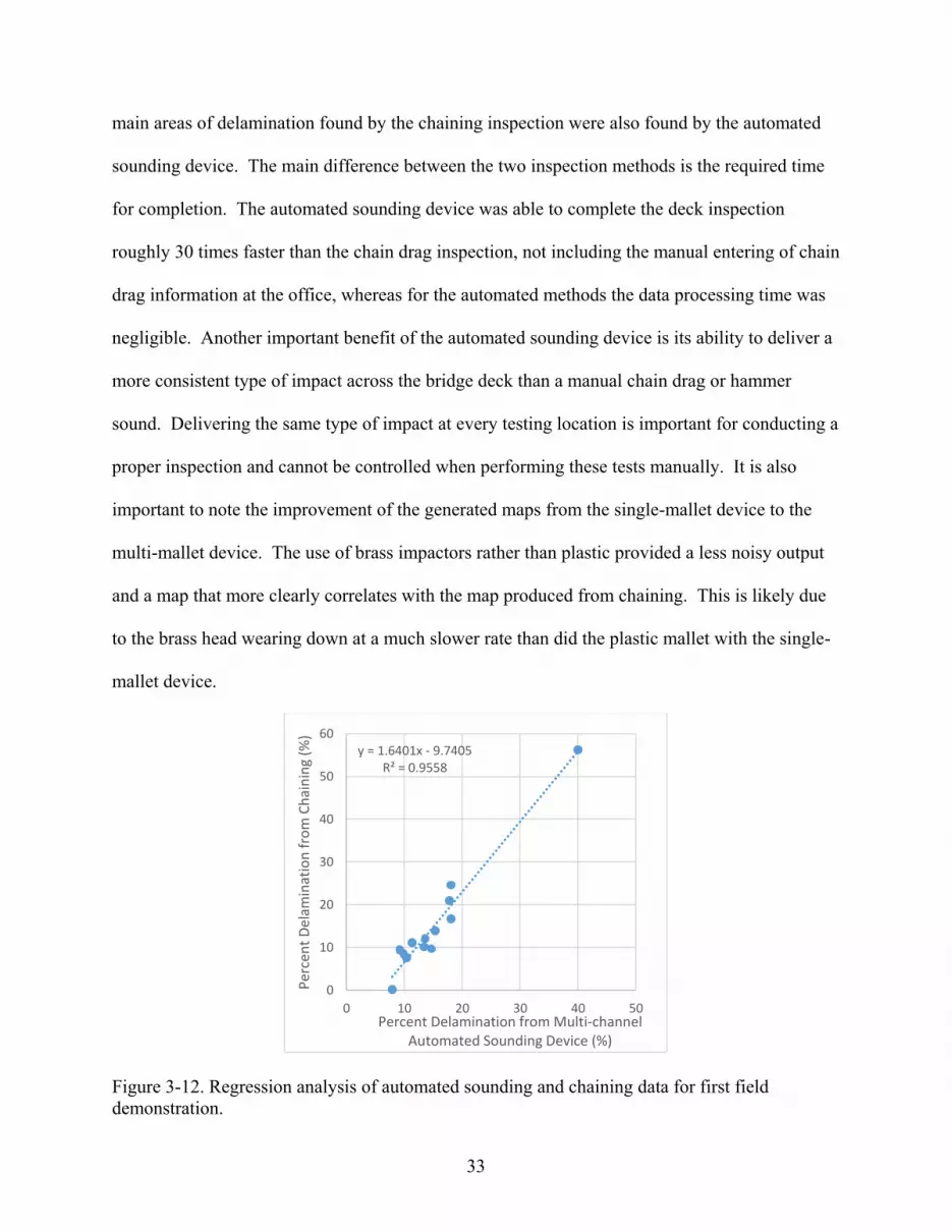
33

main areas of delamination found by the chaining inspection were also found by the automated

sounding device. The main difference between the two inspection methods is the required time

for completion. The automated sounding device was able to complete the deck inspection

roughly 30 times faster than the chain drag inspection, not including the manual entering of chain

drag information at the office, whereas for the automated methods the data processing time was

negligible. Another important benefit of the automated sounding device is its ability to deliver a

more consistent type of impact across the bridge deck than a manual chain drag or hammer

sound. Delivering the same type of impact at every testing location is important for conducting a

proper inspection and cannot be controlled when performing these tests manually. It is also

important to note the improvement of the generated maps from the single-mallet device to the

multi-mallet device. The use of brass impactors rather than plastic provided a less noisy output

and a map that more clearly correlates with the map produced from chaining. This is likely due

to the brass head wearing down at a much slower rate than did the plastic mallet with the single-

mallet device.

Figure 3-12. Regression analysis of automated sounding and chaining data for first field

demonstration.

y = 1.6401x - 9.7405R² = 0.9558

0

10

20

30

40

50

60

0 10 20 30 40 50

Per

cen

t D

elam

inat

ion

fro

m C

hai

nin

g (%

)

Percent Delamination from Multi-channel Automated Sounding Device (%)

34

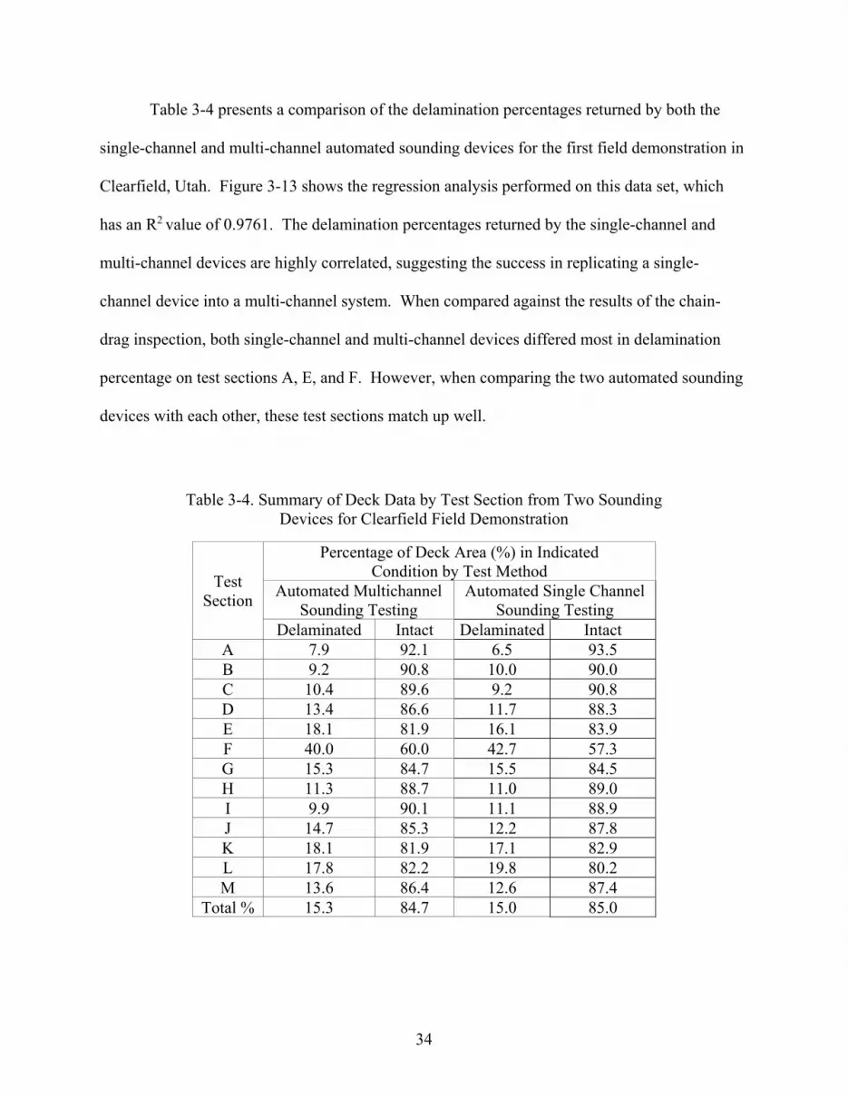
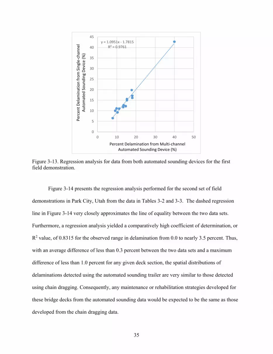
Table 3-4 presents a comparison of the delamination percentages returned by both the

single-channel and multi-channel automated sounding devices for the first field demonstration in

Clearfield, Utah. Figure 3-13 shows the regression analysis performed on this data set, which

has an R2 value of 0.9761. The delamination percentages returned by the single-channel and

multi-channel devices are highly correlated, suggesting the success in replicating a single-

channel device into a multi-channel system. When compared against the results of the chain-

drag inspection, both single-channel and multi-channel devices differed most in delamination

percentage on test sections A, E, and F. However, when comparing the two automated sounding

devices with each other, these test sections match up well.

Table 3-4. Summary of Deck Data by Test Section from Two Sounding

Devices for Clearfield Field Demonstration

Test

Section



Automated Multichannel

Sounding Testing

Automated Single Channel

Sounding Testing


A 7.9 92.1 6.5 93.5

B 9.2 90.8 10.0 90.0

C 10.4 89.6 9.2 90.8

D 13.4 86.6 11.7 88.3

E 18.1 81.9 16.1 83.9

F 40.0 60.0 42.7 57.3

G 15.3 84.7 15.5 84.5

H 11.3 88.7 11.0 89.0

I 9.9 90.1 11.1 88.9

J 14.7 85.3 12.2 87.8

K 18.1 81.9 17.1 82.9

L 17.8 82.2 19.8 80.2

M 13.6 86.4 12.6 87.4

Total % 15.3 84.7 15.0 85.0

35

Figure 3-13. Regression analysis for data from both automated sounding devices for the first

field demonstration.

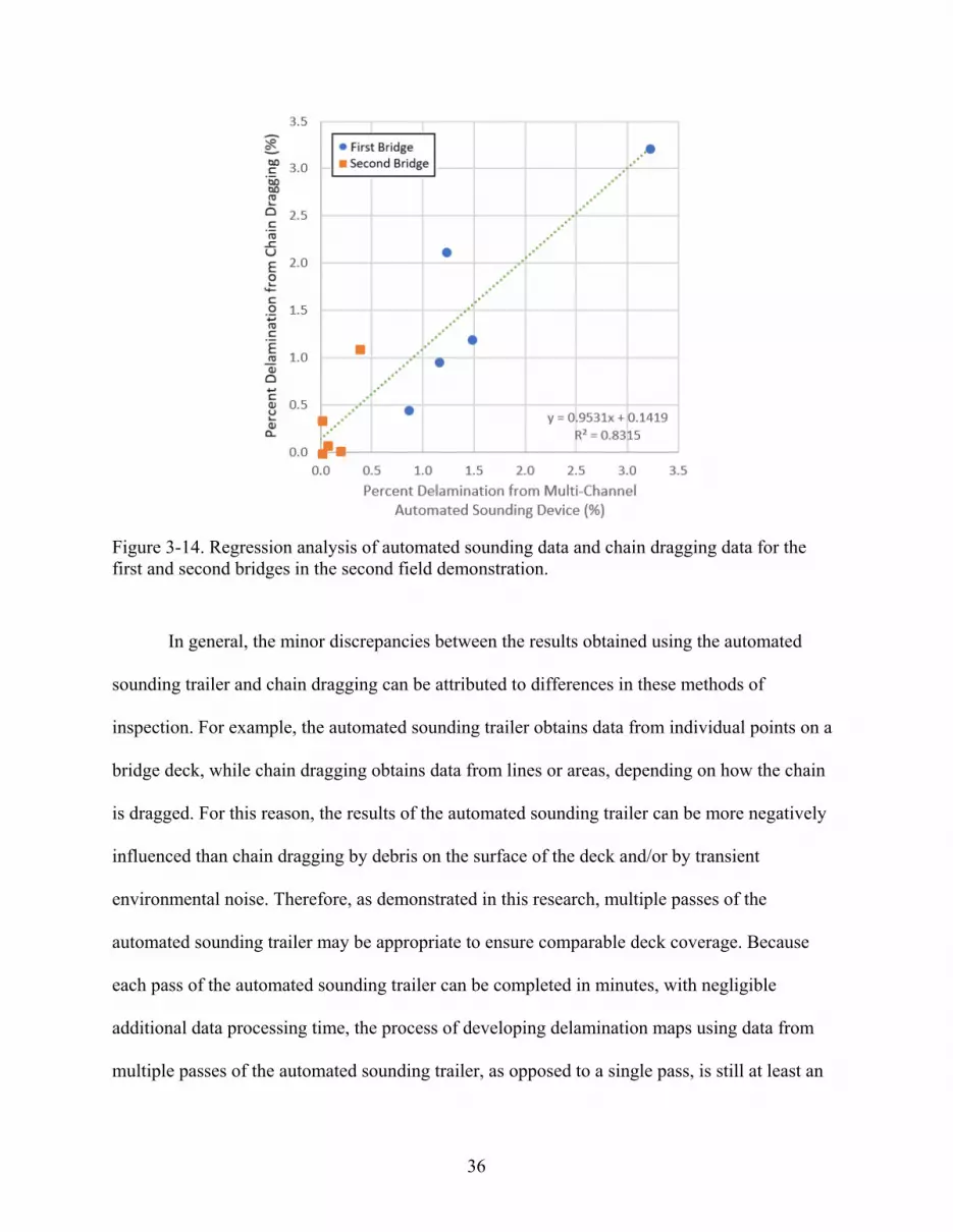
Figure 3-14 presents the regression analysis performed for the second set of field

demonstrations in Park City, Utah from the data in Tables 3-2 and 3-3. The dashed regression

line in Figure 3-14 very closely approximates the line of equality between the two data sets.

Furthermore, a regression analysis yielded a comparatively high coefficient of determination, or

R2 value, of 0.8315 for the observed range in delamination from 0.0 to nearly 3.5 percent. Thus,

with an average difference of less than 0.3 percent between the two data sets and a maximum

difference of less than 1.0 percent for any given deck section, the spatial distributions of

delaminations detected using the automated sounding trailer are very similar to those detected

using chain dragging. Consequently, any maintenance or rehabilitation strategies developed for

these bridge decks from the automated sounding data would be expected to be the same as those

developed from the chain dragging data.

y = 1.0951x - 1.7815R² = 0.9761

0

5

10

15

20

25

30

35

40

45

0 10 20 30 40 50

Per

cen

t D

elam

inat

ion

fro

m S

ingl

e-ch

ann

el

Au

tom

ated

So

un

din

g D

evic

e (%

)

Percent Delamination from Multi-channel Automated Sounding Device (%)

36

Figure 3-14. Regression analysis of automated sounding data and chain dragging data for the

first and second bridges in the second field demonstration.

In general, the minor discrepancies between the results obtained using the automated

sounding trailer and chain dragging can be attributed to differences in these methods of

inspection. For example, the automated sounding trailer obtains data from individual points on a

bridge deck, while chain dragging obtains data from lines or areas, depending on how the chain

is dragged. For this reason, the results of the automated sounding trailer can be more negatively

influenced than chain dragging by debris on the surface of the deck and/or by transient

environmental noise. Therefore, as demonstrated in this research, multiple passes of the

automated sounding trailer may be appropriate to ensure comparable deck coverage. Because

each pass of the automated sounding trailer can be completed in minutes, with negligible

additional data processing time, the process of developing delamination maps using data from

multiple passes of the automated sounding trailer, as opposed to a single pass, is still at least an

37

order of magnitude faster than that associated with chain dragging. In fact, as illustrated by the

third bridge evaluated in this research, the automated sounding trailer allows full mapping of

delaminations on bridge decks that are too deteriorated for chain dragging to even be completed

within a reasonable amount of time.

In this research, BAE thresholds were selected based on a comparison of the data

obtained using the automated sounding trailer with those obtained using chain dragging.

However, the selected threshold may not apply to all other bridge decks, as changes in deck

properties such as thickness and the presence of overlays would be expected to cause changes in

the acoustic responses associated with intact and delaminated areas. Because the magnitude of

variation in acoustic responses among different bridge decks is unknown, significant field testing

will be required to understand the universality of BAE thresholds. Furthermore, the use of

statistical methods may also be attractive for deriving BAE thresholds [35]. Finally, the

application of machine learning may prove to be an alternative classification scheme that allows

automated algorithms to rapidly classify an area of concrete as either delaminated or intact. The

apparatus described in this work is a platform with which these additional studies can be

completed.

3.4 Conclusion

In this work, a new multi-channel, air-coupled, automated, impact-echo sounding device

was designed, constructed, and demonstrated. The apparatus developed in this research includes

seven replicated impactor and recording units, a moving trailer platform, a DMI, and signal

processing modules. Each mallet is placed on the trailer 61.0 cm from the adjacent mallets,

which results in a total trailer width of 3.76 m, or approximately the width of a standard traffic

lane, when the trailer is unfolded. In practice, the trailer is towed at a speed of about 0.3 m/s so

38

that each impactor unit executes an impact every 30 to 60 cm in the travel direction along the

bridge deck. A series of computer algorithms is used to determine the presence of delamination

on the deck based on the BAE value computed from the acoustic response associated with each

impact.

Automation of the sounding process with this device significantly decreases the required

inspection time, eliminates the subjectivity associated with traditional sounding methods, and

increases safety by substantially reducing the exposure of inspectors to live traffic. Because each

pass of the automated sounding trailer can be completed in minutes, the process of developing

delamination maps using data from multiple passes of the automated sounding trailer is at least

an order of magnitude faster than that associated with chain dragging. In fact, as illustrated by

the third bridge of the second field demonstration, the automated sounding trailer allows full

mapping of delaminations on bridge decks that are too deteriorated for chain dragging to even be

completed within a reasonable amount of time.

For the first and second bridges evaluated in the second field demonstration of this

research, which exhibited a range in delamination from 0.0 to nearly 3.5 percent, the spatial

distributions of delaminations detected using the automated sounding trailer are very similar to

those detected using chain dragging, with an average difference of less than 0.3 percent between

the two data sets and a maximum difference of less than 1.0 percent for any given deck section.

Therefore, while additional field testing will be required to understand the universality of BAE

thresholds, use of the new automated sounding device is recommended for determining the

extent of delamination in the process of selecting appropriate maintenance and rehabilitation

strategies to maximize performance and minimize overall life-cycle costs of bridge decks.

39

4 CONCLUSION AND FUTURE WORK


In this work, two complete sounding devices were built and tested with the goal of

automating traditional manual sounding inspections that require significant amounts of time.

First, a single-channel device was built to test the ability to detect delaminations with an

automated mallet and microphone. After successfully locating delaminations on a bridge in

Clearfield, Utah, this device was expanded to a multi-channel system with 7 mallet units, each

spaced 61-cm apart on a trailer. This multi-channel device could be pulled across a bridge deck

and cover an entire traffic lane in one pass. This device was also tested on the same bridge in

Clearfield, Utah, as well as 3 other bridges in Park City, Utah. After selecting BAE thresholds

for both devices on each bridge, intact and delaminated concrete could be distinguished and

delamination percentages estimated for each bridge.

Both devices returned delamination percentage estimates that were highly correlated with

the chaining inspection for the first bridge in Clearfield, Utah. In Park City, Utah, only the

multi-channel device was used for the field demonstrations and the spatial distributions of

delaminations detected using the automated sounding trailer were very similar to those detected

using chain dragging. Consequently, any maintenance or rehabilitation strategies developed for

these bridge decks from the automated sounding data would be expected to be the same as those

developed from the chain dragging data.

40

In general, the minor discrepancies between the results obtained using the automated

sounding devices and chain dragging can be attributed to differences in these methods of

inspection. For example, the automated sounding devices obtain data from individual points on a

bridge deck, while chain dragging obtains data from lines or areas, depending on how the chain

is dragged. Because each pass of the automated sounding trailer can be completed in minutes,

with negligible additional data processing time, the process of developing delamination maps

using data from multiple passes of the automated sounding devices is at least an order of

magnitude faster than that associated with chain dragging. In fact, as illustrated by the third

bridge of the second field demonstration, the automated sounding trailer allows full mapping of

delaminations on bridge decks that are too deteriorated for chain dragging to even be completed

within a reasonable amount of time.

4.2 Future Work

Improvements that can be made to the automated sounding devices mostly deal with

accuracy in detecting delaminations. One such improvement would be to increase the number of

mallets that are mounted to the 12-foot-wide trailer of the multi-channel device. This would

decrease the spacing between each mallet from the current 2-foot spacing. This would mean that

small delaminations (less than 2 feet wide) could not as easily pass between the mallets on the

trailer and go undetected during the bridge inspection. While a chaining inspection would still

provide more comprehensive deck coverage, increasing the resolution of impacts that are

generated across the bridge deck would likely increase the accuracy of the delamination

percentage estimates.

41

In this research, BAE thresholds were selected based on a comparison of the data

obtained using the automated sounding trailer with those obtained using chain dragging.

However, the selected threshold may not apply to all other bridge decks, as changes in deck

properties such as thickness and the presence of overlays would be expected to cause changes in

the acoustic responses associated with intact and delaminated areas. Because the magnitude of

variation in acoustic responses among different bridge decks is unknown, significant field testing

will be required to understand the universality of BAE thresholds.

Another attractive approach for computer classification of delaminations is the

application of machine learning techniques. Neural networks could have potential for finding

other features in a recorded impact that would distinguish intact from delaminated concrete.

Implementing a machine learning approach would require a large training data set of recorded

impacts from a wide variety of bridges whose delaminations may have differing acoustic

properties. The multi-channel device developed in this work has the ability to collect these

impacts with which a training data set like this could be constructed.

4.3 Conclusion

The devices developed in this work demonstrate the utility of automation in current

bridge inspection processes. Both single-channel and multi-channel devices were able to excite

delaminations on bridge decks by means of automated mallets and record the acoustic responses

with microphones. The computer algorithms used for processing the acoustic data were able to

classify the concrete that was impacted as either intact or delaminated. The automated sounding

devices were able to complete the deck inspections at least 1 order of magnitude faster than the

chain drag inspections, not including the manual entering of chain drag information at the office.

42

Automation of traditional sounding techniques significantly decreases the standard bridge deck

inspection time, eliminates the subjectivity involved in current inspection methods, and increases

safety by substantially reducing the exposure of inspectors to live trafficking. Departments of

Transportation could save significant amounts of time and money by implementing automated

inspection technologies. The documented technology developed in this thesis demonstrates how

robotics, automation, and signal processing can be used to solve challenging problems in the

field of civil infrastructure.

43

REFERENCES

[1] 2017 ASCE Infrastructure Report Card, https://www.infrastructurereportcard.org/cat-

item/bridges/.

[2] J. Hema, W. S. Guthrie, and F. S. Fonseca, “Concrete Bridge Deck Condition Assessment

and Improvement Strategies.” Report UT-04.16. Utah Department of Transportation, Salt Lake

City, UT, November 2004.

[3] W.S. Guthrie, and R. S. Tuttle, “Condition Analysis of Concrete Bridge Decks in Utah.”

Report UT-06.01. Utah Department of Transportation, Salt Lake City, UT, February 2006.

[4] J. F. Young, S. Mindess, R. J. Gray, and A. Bentur, “The Science and Technology of Civil

Engineering Materials.” Upper Sadde River, NJ: Prentice-Hall, Inc. 1998.

[5] M. Sansalone, "Impact-echo: The complete story," ACI Structural Journal, vol. 94, pp. 777-

786, Nov-Dec 1997.

[6] M. Sansalone, and N. J. Carino, “Detecting Delaminations in Concrete Slabs with and

without Overlays Using the Impact-Echo Method,” ACI Materials Journal, vol. 86, No. 2, pp.

175-184, Mar-Apr 1989.

[7] C. M. Hsiao, C. C. Cheng, T. H. Liou, and Y. T. Juang, “Detecting flaws in concrete blocks

using the impact-echo method,” NDT&E International, vol. 41, pp. 98-107, Mar 2008.

[8] M. T. A. Chaudhary, “Effectiveness of Impact Echo testing in detecting flaws in prestressed

concrete slabs,” Construction and Building Materials, vol. 47, pp. 753-759, 2013.

[9] J. S. Popovics and J. L. Rose, "A new approach for the analysis of impact-echo data," Review

of Progress in Quantitative Nondestructive Evaluation, vol. 12, 1993.

[10] N. J. Carino, “The Impact-Echo Method: An Overview,” ASCE World Structural

Engineering Conference, May 2001.

[11] S. Kee and N. Gucunski, "Interpretation of Flexural Vibration Modes from Impact-Echo

Testing," J. Infrastruct. Syst., 04016009, 1-10, 2016.

[12] J. Y. Zhu and J. S. Popovics, “Non-contact detection of surface waves in concrete using an

air-coupled sensor,” AIP Conference Proceedings (2002); doi: 10.1063/1.1472940

[13] J. Y. Zhu and J. S. Popovics, “Air-Coupled Impact-Echo Method for NDT of Concrete,”

AIP Conference Proceedings (2006); doi: 10.1063/1.2184681

[14] J. Y. Zhu and J. S. Popovics, "Imaging concrete structures using air-coupled impact-echo,"

Journal of Engineering Mechanics-ASCE, vol. 133, pp. 628-640, Jun 2007.

https://www.infrastructurereportcard.org/cat-item/bridges/

https://www.infrastructurereportcard.org/cat-item/bridges/

44

[15] J. S. Popovics, T. Oh, and S. Ham, “Effective visualization of impact-echo data for bridge

deck NDE,” AIP Conference Proceedings, vol. 1430, pp. 1681-1688, 2012.

[16] S. W. Shin, J. S. Popovics, and T. Oh, “Cost Effective Air-Coupled Impact-Echo Sensing

for Rapid Detection of Delamination Damage in Concrete Structures,” Advances in Structural

Engineering, vol. 15, pp. 887-895, Jun 2012.

[17] S. H. Kee, T. Oh, J. S. Popovics, R. W. Arndt, and J. Y. Zhu, “Nondestructive Bridge Deck

Testing with Air-Coupled Impact-Echo and Infrared Thermography,” Journal of Bridge

Engineering, vol. 17, pp. 928-939, Nov-Dec 2012.

[18] D. Algernon, H. Ernst, and K. Dressler, “Signal Processing for Air-Coupled Impact-Echo

using Microphone Arrays,” presented at the 18th World Conference on Nondestructive Testing,

Durban, South Africa, 2012.

[19] T. Oh, “Defect Characterization in Concrete Elements Using Vibration Analysis and

Imaging,” Department of Civil Engineering – University of Illinois at Urbana-Champaign,

Dissertation, 2012.

[20] N. Gucunski, A. Imani, F. Romero, S. Nazarian, D. Yuan, and H. Wiggenhauser, et al.,

“Nondestructive testing to identify concrete bridge deck deterioration.” Washington, D.C. :

Transportation Research Board, 2013.

[21] B. A. Mazzeo, A. N. Patil, R. C. Hurd, J. M. Klis, T. T. Truscott, and W. S. Guthrie, "Air-

Coupled Impact-Echo Delamination Detection in Concrete Using Spheres of Ice for Excitation,"

Journal of Nondestructive Evaluation, pp. 1-10, 2013/12/07 2013.

[22] B. A. Mazzeo, A. N. Patil, and W. S. Guthrie, "Acoustic impact-echo investigation of

concrete delaminations using liquid droplet excitation," NDT&E International, vol. 51, pp. 41-

44, 2012.

[23] N. Gucunski, F. Romero, S. Kruschwitz, R. Feldmann, A. Abu-Hawash, and M. Dunn,

“Multiple Complementary Nondestructive Evaluation Technologies for Condition Assessment of

Concrete Bridge Decks,” Transportation Research Record, vol. 2201, pp. 34-44, 2010.

[24] Y. Tinkey, L. D. Olson, Olson Engineering, “Vehicle-Mounted Bridge Deck Scanner,”

Transportation Research Board: Highway IDEA Program, Project 132, Aug 2010.

[25] J. S. Popovics, “Investigation of a Full-Lane Acoustic Scanning Method for Bridge Deck

Nondestructive Evaluation,” Transportation Research Board: Highway IDEA Program, Project

134, Nov 2010.

[26] J. Y. Zhu and J. S. Popovics, "Imaging concrete structures using air-coupled impact-echo,"

Journal of Engineering Mechanics-ASCE, vol. 133, pp. 628-640, Jun 2007.

45

[27] S. W. Shin, J. S. Popovics, and T. Oh, “Cost Effective Air-Coupled Impact-Echo Sensing

for Rapid Detection of Delamination Damage in Concrete Structures,” Advances in Structural

Engineering, vol. 15, pp. 887-895, Jun 2012.

[28] G. Zhang, R. S. Harichandran, P. Ramuhalli, “An automatic impact-based delamination

detection system for concrete bridge decks,” NDT&E International, vol. 45, pp. 120-127, 2012.

[29] H. Sun, J. Zhu, S. Ham, “Acoustic evaluation of concrete delaminations using ball-chain

impact excitation,” The Journal of the Acoustical Society of America, vol. 141, May 2017.

[30] W. S. Guthrie, J. Larsen, J. Baxter, B. A. Mazzeo, “Automated Air-Coupled Impact-Echo

Testing of a Concrete Bridge Deck from a Continuously Moving Platform,” UNDER REVIEW.

[31] B. A. Mazzeo, J. Larsen, J. McElderry, and W. S. Guthrie, “Rapid multichannel impact-

echo scanning of concrete bridge decks from a continuously moving platform,” AIP Conference

Proceedings 1806, 080003, 2017.

[32] B. A. Mazzeo, T. T. Truscott, and W. S. Guthrie, "Signal processing of acoustic impact

response for reinforced concrete testing using paintballs and airsoft pellets for excitation," Audio

and Acoustic Signal Processing Technical Committee Newsletter, vol. 1, 2014.

[33] T. Oh, J. S. Popovics, and S. Sim, "Analysis of vibration for regions above rectangular

delamination defects in solids," Journal of Sound and Vibration, vol. 332, pp. 1766-1776, 4/1/

2013.

[34] S. Ham, J. S. Popovics, “Application of Micro-Electro-Mechanical Sensors Contactless

NDT of Concrete Structures,” Sensors, vol. 15, Issue 4, 10.3390/s150409078, Apr 2015.

[35] L. Hendricks, W. S. Guthrie, B. A. Mazzeo, “Implementing statistical analysis in multi-

channel acoustic impact-echo testing of concrete bridge decks: Determining thresholds for

delamination detection,” AIP Conference Proceedings 1949, 040005, 2018.


http://aip.scitation.org/author/Larsen%2C+Jacob

http://aip.scitation.org/author/McElderry%2C+Joseph

http://aip.scitation.org/author/Guthrie%2C+W+Spencer

https://dx.doi.org/10.3390%2Fs150409078


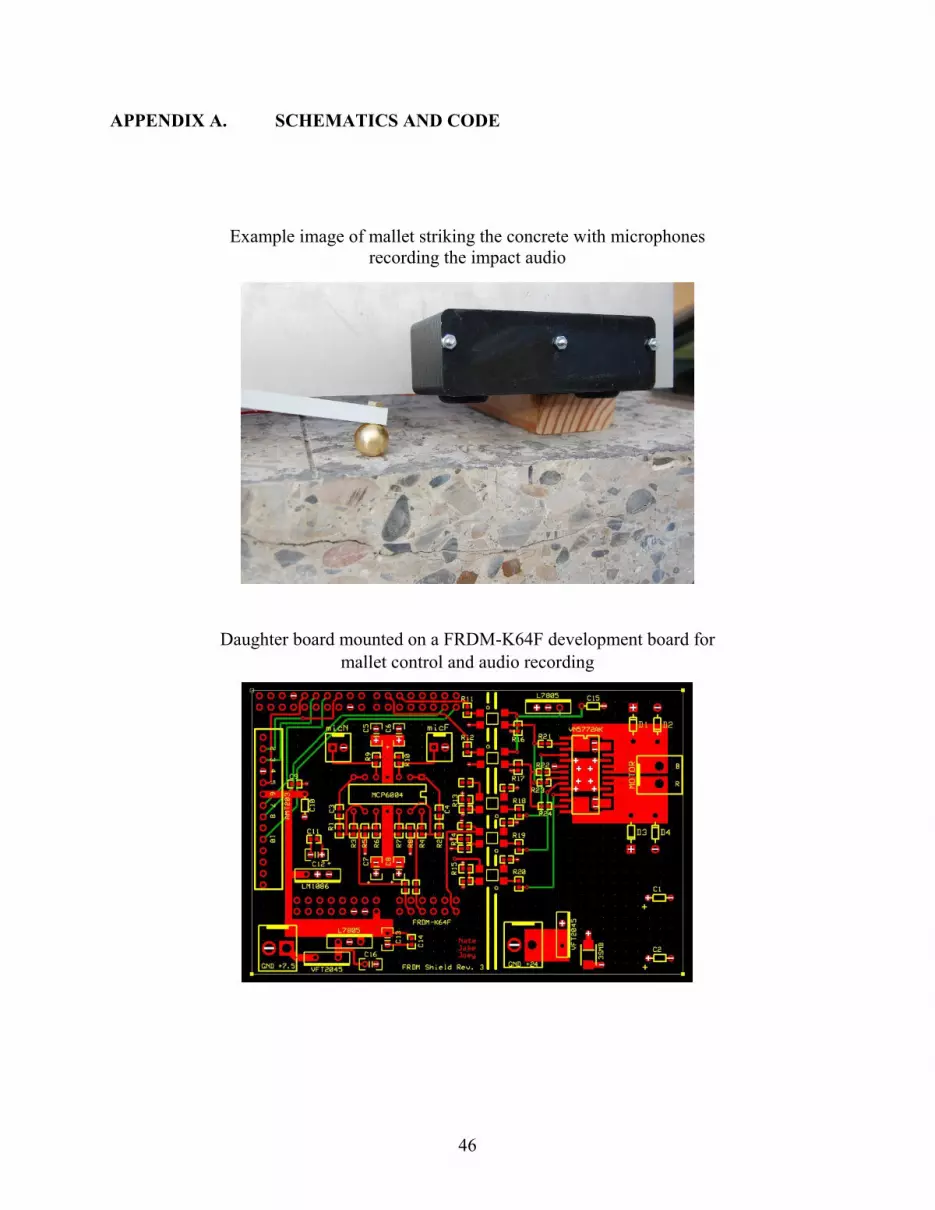
46

APPENDIX A. SCHEMATICS AND CODE

Example image of mallet striking the concrete with microphones

recording the impact audio

Daughter board mounted on a FRDM-K64F development board for

mallet control and audio recording

47

Parts list for daughter board mounted to FRDM-K64F

Part Digikey P/N Shield Reference Quantity

3.3V LDO LM1086IT-3.3/NOPB-ND LM1086 1

5V LDO 497-1443-5-ND L7805 2

H Bridge Motor Driver 497-11677-1-ND VN5772AK 1

Battery diode - 45V - 20A VFT2045BP-M3/4W-ND VFT2045 2

33V - 3W Zener Diode 3SMBJ5937BTPMSCT-ND 3SMB 1

Optoisolator 425-2108-1-ND PC3H71 5

FRDM-K64F FRDM-K64F-ND FRDM-K64F 1

600V - 1A Flyback diode 1N4005-TPMSCT-ND D1,D2,D3,D4 4

AMT203-V 102-2050-ND AMT203 1

Electret Condensor Mic 102-1722-ND micN,micF 2

Op Amp MCP6004-I/P-ND MCP6004 1

1A Fuse - 32 VDC F4191-ND

5A Fuse - 32 VDC F4197-ND

Resistors

10kOhm RES 0603 BYU Campus Shop R5,R6,R7,R8,R9,R10 6

31.6 kOhm RES 0603 BYU Campus Shop R3,R4 2

53kOhm RES 0603 BYU Campus Shop R1,R2 2

909 Ohm BYU Campus Shop R11,R12 2

0 ohm RES 0402 BYU Campus Shop R13,R14,R15 3

Decide later BYU Campus Shop R16,R17,R18,R19,R20 5

10k RES 0402 BYU Campus Shop R21,R22,R23,R24 4

Capacitors

0.1uF CAP BYU Campus Shop C5,C7

1uF 10V CAP 1276-1946-1-ND C3,C4 2

10uF CAP BYU Campus Shop C6,C8,C10,C9,C11

180uF CAP BYU Campus Shop C1,C2 2

Connectors

Large connector BYU Campus Shop 5v,24v,motor 3

Small connector BYU Campus Shop micN,micF 2

10 Position Vertical Header Connector A1925-ND

2 Position Connection Housing WM2100-ND

2 Position Vertical Header Connector WM4620-ND

2 Position Reception Connector A30994-ND

2 Position Vertical Header Connector A1921-ND

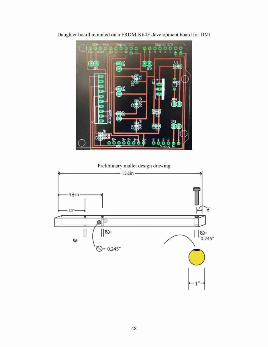
48

Daughter board mounted on a FRDM-K64F development board for DMI

Preliminary mallet design drawing

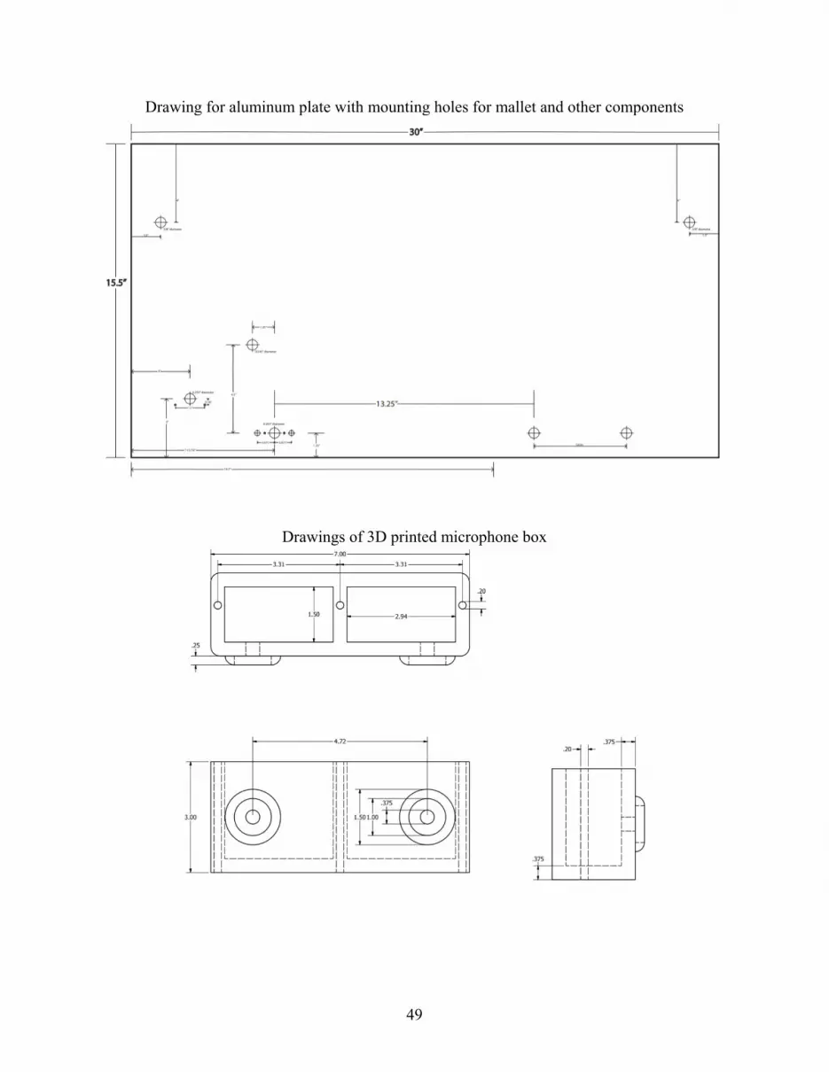
49

Drawing for aluminum plate with mounting holes for mallet and other components

Drawings of 3D printed microphone box

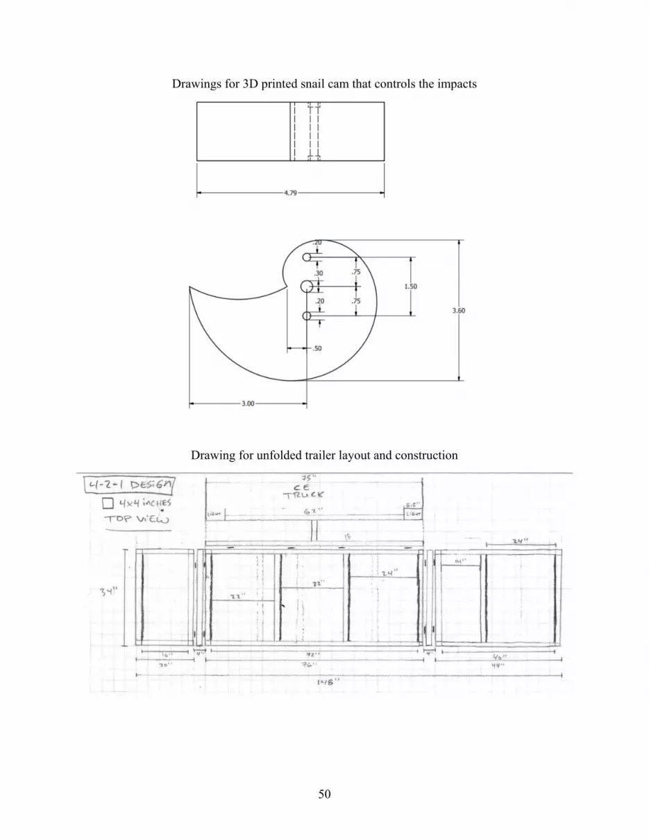
50

Drawings for 3D printed snail cam that controls the impacts

Drawing for unfolded trailer layout and construction

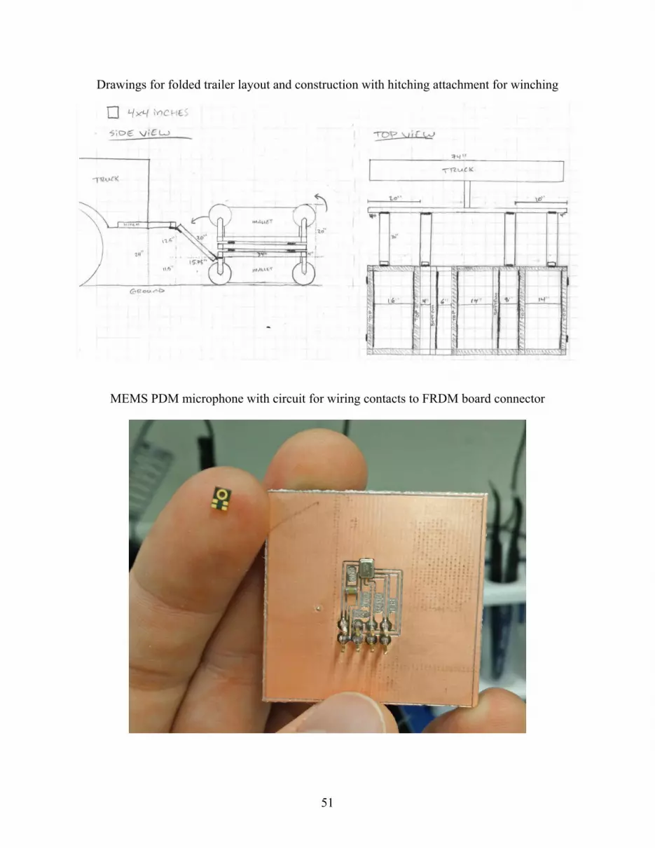
51

Drawings for folded trailer layout and construction with hitching attachment for winching

MEMS PDM microphone with circuit for wiring contacts to FRDM board connector

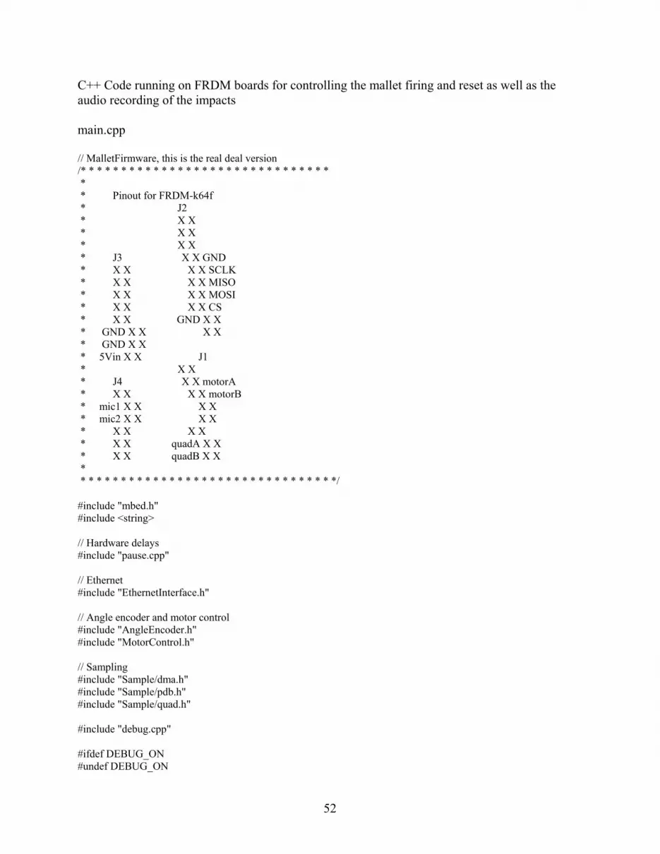
52

C++ Code running on FRDM boards for controlling the mallet firing and reset as well as the

audio recording of the impacts

main.cpp

// MalletFirmware, this is the real deal version

/* * * * * * * * * * * * * * * * * * * * * * * * * * * * * * *

*

* Pinout for FRDM-k64f

* J2

* X X

* X X

* X X

* J3 X X GND

* X X X X SCLK

* X X X X MISO

* X X X X MOSI

* X X X X CS

* X X GND X X

* GND X X X X

* GND X X

* 5Vin X X J1

* X X

* J4 X X motorA

* X X X X motorB

* mic1 X X X X

* mic2 X X X X

* X X X X

* X X quadA X X

* X X quadB X X

*

* * * * * * * * * * * * * * * * * * * * * * * * * * * * * * * */

#include "mbed.h"

#include <string>

// Hardware delays

#include "pause.cpp"

// Ethernet

#include "EthernetInterface.h"

// Angle encoder and motor control

#include "AngleEncoder.h"

#include "MotorControl.h"

// Sampling

#include "Sample/dma.h"

#include "Sample/pdb.h"

#include "Sample/quad.h"

#include "debug.cpp"

#ifdef DEBUG_ON

#undef DEBUG_ON

53

#endif

#define DEBUG_ON 1 // 1 or 0

// Settings for each mallet

#define MAX_CLIENTS 2 // set the max number of clients to at least 2 (first client is MATLAB, second is

the distance unit)

// Ethernet

#define LEN_PACKET 1460

#define NUM_PACKETS ((TOTAL_SAMPLES_MIC+TOTAL_SAMPLES_ANGLE)/LEN_PACKET)

#define GATEWAY "169.254.225.1" // set to match your computer

#define MASK "255.255.0.0" // set to match your computer (probably does already)

#define IP_LAPTOP "169.254.225.205"

#define IP_DMI "169.254.225.220"

#define SAMPLE_FREQ 3750000 // 3.75 MHz

// for debug purposes

Serial pc(USBTX, USBRX);

// motor control

MotorControl motor(PTC2, PTA2, 2000, 25); // cw, ccw, period_us, safetyPeriod_us

//DigitalOut sel(PTC12); // pull up resistor used instead

//DigitalIn temp_trigger(PTB2); // for simultaneous trigger

char buffer[LEN_PACKET]; // general purpose tx/rx buffer

char status[LEN_PACKET]; // tx buffer that contains the status for the entire mallet system

int NUM;

int PORT = 55000;

// Declaration of functions

void clearBuffer();

bool syncAngles();

void pdm_init();

int spi_start();

using namespace std;

int main() {

led_blue = 1;

led_green = 1;

led_red = 0;

if(SIM_UIDH == 0x001bffff && SIM_UIDML == 0x4d441504 && SIM_UIDL == 0x9013001C) NUM = 1;

else if(SIM_UIDH == 0x0016ffff && SIM_UIDML == 0x4d441504 && SIM_UIDL == 0x90110007) NUM =

2;

else if(SIM_UIDH == 0x0023ffff && SIM_UIDML == 0x4e453103 && SIM_UIDL == 0x70060023) NUM = 3;

else if(SIM_UIDH == 0x0010ffff && SIM_UIDML == 0x4e453103 && SIM_UIDL == 0x7006001f) NUM = 4;


5;


6;

else if(SIM_UIDH == 0x0015ffff && SIM_UIDML == 0x4e453103 && SIM_UIDL == 0x60010012) NUM = 7;

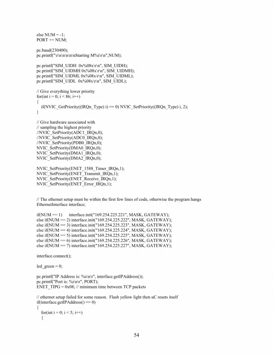
54

else NUM = -1;

PORT += NUM;

pc.baud(230400);

pc.printf("\r\n\n\n\n\nStarting M%i\r\n",NUM);

pc.printf("SIM_UIDH 0x%08x\r\n", SIM_UIDH);

pc.printf("SIM_UIDMH 0x%08x\r\n", SIM_UIDMH);

pc.printf("SIM_UIDML 0x%08x\r\n", SIM_UIDML);

pc.printf("SIM_UIDL 0x%08x\r\n", SIM_UIDL);

// Give everything lower priority

for(int i = 0; i < 86; i++)

{

if(NVIC_GetPriority((IRQn_Type) i) == 0) NVIC_SetPriority((IRQn_Type) i, 2);

}

// Give hardware associated with

// sampling the highest priority

//NVIC_SetPriority(ADC1_IRQn,0);

//NVIC_SetPriority(ADC0_IRQn,0);

//NVIC_SetPriority(PDB0_IRQn,0);

NVIC_SetPriority(DMA0_IRQn,0);



NVIC_SetPriority(ENET_1588_Timer_IRQn,1);

NVIC_SetPriority(ENET_Transmit_IRQn,1);

NVIC_SetPriority(ENET_Receive_IRQn,1);

NVIC_SetPriority(ENET_Error_IRQn,1);

// The ethernet setup must be within the first few lines of code, otherwise the program hangs

EthernetInterface interface;

if(NUM == 1) interface.init("169.254.225.221", MASK, GATEWAY);

else if(NUM == 2) interface.init("169.254.225.222", MASK, GATEWAY);






interface.connect();

led_green = 0;

pc.printf("IP Address is: %s\n\r", interface.getIPAddress());

pc.printf("Port is: %i\n\r", PORT);

ENET_TIPG = 0x08; // minimum time between TCP packets

// ethernet setup failed for some reason. Flash yellow light then uC resets itself

if(interface.getIPAddress() == 0)

{

for(int i = 0; i < 5; i++)

{

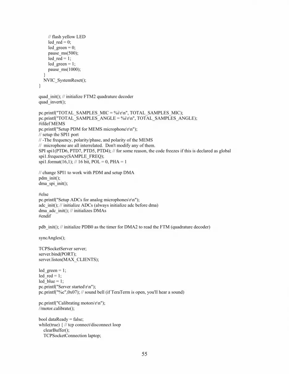
55

// flash yellow LED

led_red = 0;

led_green = 0;

pause_ms(500);

led_red = 1;

led_green = 1;

pause_ms(1000);

}

NVIC_SystemReset();

}

quad_init(); // initialize FTM2 quadrature decoder

quad_invert();

pc.printf("TOTAL_SAMPLES_MIC = %i\r\n", TOTAL_SAMPLES_MIC);

pc.printf("TOTAL_SAMPLES_ANGLE = %i\r\n", TOTAL_SAMPLES_ANGLE);

#ifdef MEMS

pc.printf("Setup PDM for MEMS microphone\r\n");

// setup the SPI1 port

// -The frequency, polarity/phase, and polarity of the MEMS

// microphone are all interrelated. Don't modify any of them.

SPI spi1(PTD6, PTD7, PTD5, PTD4); // for some reason, the code freezes if this is declared as global

spi1.frequency(SAMPLE_FREQ);

spi1.format(16,1); // 16 bit, POL = 0, PHA = 1

// change SPI1 to work with PDM and setup DMA

pdm_init();

dma_spi_init();

#else

pc.printf("Setup ADCs for analog microphones\r\n");

adc_init(); // initialize ADCs (always initialize adc before dma)

dma_adc_init(); // initializes DMAs

#endif

pdb_init(); // initialize PDB0 as the timer for DMA2 to read the FTM (quadrature decoder)

syncAngles();

TCPSocketServer server;

server.bind(PORT);

server.listen(MAX_CLIENTS);

led_green = 1;

led_red = 1;

led_blue = 1;

pc.printf("Server started\r\n");

pc.printf("%c",0x07); // sound bell (if TeraTerm is open, you'll hear a sound)

pc.printf("Calibrating motors\r\n");

//motor.calibrate();

bool dataReady = false;

while(true) { // tcp connect/disconnect loop

clearBuffer();

TCPSocketConnection laptop;

56

server.accept(laptop);

laptop.set_blocking(false, 9000); // timeout after 9s

bool ipVerified = true;

string ipAddress = laptop.get_address();

if(ipAddress != IP_LAPTOP) ipVerified = false;

int n;

while(true) { // rx/tx loop

n = laptop.receive(buffer,LEN_PACKET); // this operation times out after 1.5s

if(n <= 0) break; // exit rx/tx loop

if(!ipVerified){

clearBuffer();

sprintf(buffer,"Incorrect IP address");

n = laptop.send(buffer,LEN_PACKET);

pc.printf("%s\r\n");

break; // exit rx/tx loop

}

if(buffer[0] == ':' && ipVerified) {

switch(buffer[1])

{

// take sample

case 'M': // :M0.0000000000.0000000000 // yellow

case 2:

{

if( (buffer[2]-0x30) == NUM ) // has correct malletID number

{

led_green = 0;

led_red = 0;

if(!motor.getCalibration()){

clearBuffer();

sprintf(buffer,"Calibrate motor before attempting reset");


DEBUG printf("Calibrate motor before attempting reset\r\n");

break;

}


// update angle

bool success = syncAngles();

motor.releaseMallet();

// wait for mallet to fall a certain distance (max wait time is 40ms)

int start_height = quad_read();

for(int i = 0; i < 40; i++){

pause_ms(1);

if( (quad_read()-start_height) > 180 ) break;

}

DEBUG printf("Start %i\t Stop %i\r\n", start_height, quad_read());

}

}

case 'L':

case 'l':

57

{

// start sampling

pdb_start();

DEBUG printf("Start SPI\r\n");

//int returnVar = spi1.write(0x00f0);

int returnVar = spi_start();

// keep waiting for sampling to complete

for(int i = 0; i < 30; i++) { // timeout loop. sampling takes approx 137ms, this loop takes

30*5ms=150ms

if(dma_done) break;

pc.printf("sampling...\r\n");

pause_ms(5);

}

dataReady = true;

// reset mallet

DEBUG printf("ResetMallet\r\n");

motor.resetMallet();

// turn off all indicator LEDs

led_red = 1;

led_green = 1;

led_blue = 1;

break;

}

case 'N':

case 'n':

case 0:

{

clearBuffer();

sprintf(buffer,"M%i",NUM);


pc.printf("%s\r\n",buffer);

break;

}

/********************************************************************

* The code below is for testing and troubleshooting. Don't delete. *

********************************************************************/

case 'p':

case 13:

{

clearBuffer();

sprintf(buffer,"Resetting M%i",NUM);



pause_ms(200);

NVIC_SystemReset();

break;

}

case 'B':

case 'b':

case 6:

{

58

clearBuffer();

if(led_blue){

led_blue = 0;

sprintf(buffer,"LED blue = ON");

}

else {

led_blue = 1;

sprintf(buffer,"LED blue = OFF");

}



break;

}

case 'R':

case 'r':

case 7:

{

clearBuffer();

if(led_red){

led_red = 0;

sprintf(buffer,"LED red = ON");

}

else {

led_red = 1;

sprintf(buffer,"LED red = OFF");

}



break;

}

// test angle encoder

case 'W':

{

int16_t cow = 5;

double distance = 0.0;

distance = double(cow)*.393701;

clearBuffer();

sprintf(buffer, "Distance: %f in\r\n", distance);

}

case 'w': // reads 0 unless the counter is running

{

clearBuffer();

sprintf(buffer,"PDB: %i",PDB0_CNT);



break;

}

case 'A':

case 'a': // set zero

case 12:

{

clearBuffer();

if(angle_encoder.set_zero()) {

quad_update(0);

sprintf(buffer,"Zero set");

}

59

else sprintf(buffer,"Zero NOT set");



break;

}

case 'S':

case 's': // perform "no operation", which returns 0xa5

{

clearBuffer();

sprintf(buffer,"NOP: %x",angle_encoder.nop());



break;

}

case 'D':

case 'd': // read absolute and relative angles

case 5:

{

clearBuffer();

sprintf(buffer,"Angle: %i %i",angle_encoder.absolute_angle(),quad_read());



break;

}

case 'F':

case 'f':

{

clearBuffer();

sprintf(buffer,"Quad Cnt: %i", quad_read());



break;

}

case 'G':

case 'g': // sync relative angle with absolute angle

case 11:

{

clearBuffer();


if(success) sprintf(buffer,"Angles synchronized");

else sprintf(buffer,"Could not read absolute angle");



break;

}

// test motor

case 'Z':

case 'z': // release the mallet

case 8:

{

clearBuffer();

sprintf(buffer,"Release mallet");



60


if(success) {


pc.printf("Angles synchronized");

}

else pc.printf("Could not read absolute angle");

break;

}

case 'X':

case 'x': // reset the mallet

case 10:

{

clearBuffer();





break;

}

else {

sprintf(buffer,"Reset mallet");




}

break;

}

case 'C':

case 'c': // calibrate the mallet

case 1:

{

clearBuffer();


if(success){

sprintf(buffer,"Calibrate motor/cam reset");



motor.calibrate();

}

else{

sprintf(buffer,"Could not read absolute angle");



}

break;

}

case 'V':

case 'v': // release and reset the mallet

{

clearBuffer();




61


break;

}

sprintf(buffer,"Release/Reset mallet");




if(success) {


pause_us(TOTAL_SAMPLES_MIC*10);


}

else {

pc.printf("Could not read absolute angle");

break;

}

break;

} // end of this particular case

} // end switch(buffer)

} // end if(buffer[0] == ':')

if(n <= 0) break;

} // end while(true) rx/tx loop

} // end while(true) tcp connect/disconnect loop

} // end main

void pdm_init(){

// enable clocks for SPI ports

SIM_SCGC6 |= SIM_SCGC6_SPI0_MASK;



// Enable clock for PortB and PortD

SIM_SCGC5 |= SIM_SCGC5_PORTB_MASK; // SPI2

SIM_SCGC5 |= SIM_SCGC5_PORTD_MASK; // SPI0, SPI1

// check setting for "SMPL_PT"

SPI1_MCR |= 1;

SPI1_MCR |= SPI_MCR_MSTR_MASK | SPI_MCR_CONT_SCKE_MASK | SPI_MCR_HALT_MASK |

SPI_MCR_DIS_TXF_MASK | SPI_MCR_DIS_RXF_MASK; //master mode, continuous SCK, stopped (started

after initialization), TX fifo disabled, RX fifo disabled

SPI1_CTAR0 &= 0xfffcffff;

//SPI1_CTAR0 = SPI_CTAR_DBR_MASK | SPI_CTAR_FMSZ(15) | SPI_CTAR_PBR(2) | SPI_CTAR_ASC(2)

| SPI_CTAR_BR(2) | SPI_CTAR_CPHA_MASK; // baud = 4Mhz, frame size = 7+1 bits, CPOL = 0, CPHA = 1,

MSB first //0xB8020202

//SPI1_CTAR0 = SPI_CTAR_FMSZ(15) | SPI_CTAR_PBR(2) | SPI_CTAR_ASC(3) | SPI_CTAR_BR(2) |

SPI_CTAR_CPHA_MASK; // baud = 4Mhz, frame size = 7+1 bits, CPOL = 0, CPHA = 1, MSB first

//0xB8020202

SPI1_RSER = SPI_RSER_RFDF_RE_MASK | SPI_RSER_RFDF_DIRS_MASK; // enable requests, set

requests to DMA requests instead of interrupts

// Start SPI ports

SPI1_MCR &= ~SPI_MCR_HALT_MASK;

}

62

void clearBuffer() {

for(int i = 0; i < 100; i++) buffer[i] = 0;

}

//void clearFault() {

// for(int i = 100; i < 200; i++) buffer[i] = 0;

//}

bool syncAngles(){

for(int i = 0; i < 10; i++){ // timeout after 10 tries

int angle = angle_encoder.absolute_angle();

if(angle != 0x00ff0000) {

quad_update(angle);

return true;

}

}

return false;

}

#include "spi_api.h"

#include "cmsis.h"

#include "pinmap.h"

#include "mbed_error.h"

#include "fsl_clock_manager.h"

#include "fsl_dspi_hal.h"

#include "PeripheralPins.h"

int spi_start(){

// wait tx buffer empty

int timeout = 0xffff;

while(!DSPI_HAL_GetStatusFlag(SPI1_BASE, kDspiTxFifoFillRequest) && --timeout);

dspi_command_config_t command = {0};

command.isEndOfQueue = true;

command.isChipSelectContinuous = 0;

DSPI_HAL_WriteDataMastermode(SPI1_BASE, &command, (uint16_t)0x00f0);

DSPI_HAL_ClearStatusFlag(SPI1_BASE, kDspiTxFifoFillRequest);

// wait rx buffer full

timeout = 0xff;

while (!DSPI_HAL_GetStatusFlag(SPI1_BASE, kDspiRxFifoDrainRequest) && --timeout);

DSPI_HAL_ClearStatusFlag(SPI1_BASE, kDspiRxFifoDrainRequest);

return DSPI_HAL_ReadData(SPI1_BASE) & 0xff;

MotorControl.cpp

#include "MotorControl.h"

#ifdef DEBUG_ON

#undef DEBUG_ON

#endif

#define DEBUG_ON 1

63

DigitalOut led_red(LED_RED);

DigitalOut led_green(LED_GREEN);

DigitalOut led_blue(LED_BLUE);

// angle encoder

AngleEncoder angle_encoder(PTD2, PTD3, PTD1, PTD0, 8, 0, 1000000); // mosi, miso, sclk, cs, bit_width, mode,

hz

// constructor

MotorControl::MotorControl(PinName cw, PinName ccw, int period, int safetyPeriod) :

_cw(cw),

_ccw(ccw) {

// turn motor off

_cw = 0;

_ccw = 0;

_cw.period_us(period);

_ccw.period_us(period);

_period = period;

_safetyPeriod = safetyPeriod;

_calibrated = false;

}

void MotorControl::calibrate(){

off();

maxAngle = -5000;

minAngle = 5000;

int pastAngle;

int derivative;

int currAngle = angle_encoder.absolute_angle();

for(int i = 0; i < 150; i++){

pastAngle = currAngle;

currAngle = angle_encoder.absolute_angle();

if (currAngle > 2048 || currAngle < -2048) currAngle = angle_encoder.absolute_angle();

derivative = currAngle-pastAngle;

if(derivative > 50) {

printf("Dropped\r\n");

off();

_ccw = 0.7;

pause_us(2000);

off();

pause(0.5);

}

if(currAngle > maxAngle && currAngle != 0x00ff0000) maxAngle = currAngle;

if(currAngle < minAngle) minAngle = currAngle;

printf("C: %4i\tD: %4i\tMax: %4i\tMin: %4i\r\n",currAngle,derivative,maxAngle,minAngle);

_cw = 1;

pause_us(2000);

if(currAngle > 400){ // used in case the mallet is in a deep hole during calibration

pause_us(1000); // leave the motor on for a little longer

i -= 5;

printf("Calibration extended\r\n");

64

}

off();

pause_ms(40);

}

printf("\r\n\nMax: %i\r\nMin: %i\r\n",maxAngle,minAngle);

for(int i = 0; i < 40; i++) calibrationVar[i] = minAngle;

coarseThreshold = minAngle + 120; // 50

fallThreshold = minAngle + 220; // 80

fineMinThreshold = minAngle - 10; // -10 for extra margin, more negative would mean the reset mallet is

extra high, which dirt or anything on the mallet or cam might cause.

fineMaxThreshold = minAngle + 15; // 12

printf("CoarseThreshold: %i\r\n",coarseThreshold);

printf("FallThreshold: %i\r\n",fallThreshold);

printf("FineMinThreshold: %i\r\n",fineMinThreshold);

printf("FineMaxThreshold: %i\r\n",fineMaxThreshold);

// reset the mallet after calibration

off();

pause_ms(100);

resetMallet();

off();

_calibrated = true;

}

bool MotorControl::getCalibration(){

return _calibrated;

}

void MotorControl::releaseMallet() {

// make sure motor is off

off();

//int angle;

//int tempMinAngle = 2048;

// pulse clockwise to release mallet

_cw = 1;

pause_ms(10);

_cw = 0;

/*

for(int i = 0; i < 50; i++){ // pause 50 ms, max absolute read speed is 100kHz

angle = angle_encoder.absolute_angle();

if(angle < tempMinAngle && angle > -2048) tempMinAngle = angle;

}*/

pause_ms(50);

// pulse counter-clockwise to stop snail cam

_ccw = 0.7;

pause_ms(5);

_ccw = 0;


off();

//tempMinAngle -= 3; // the tempMinAngle tends to be higher than should be by 3.

//DEBUG printf("release angle: %i\r\n", tempMinAngle);

65

//if(tempMinAngle < minAngle-5 || tempMinAngle > minAngle + 5){

// DEBUG printf("Consider recalibrating this mallet\r\n");

//}

}

int MotorControl::resetMallet() {

led_red = 1;

led_blue = 1;

led_green = 1;

// while loop exits when the cam as settled in the window for 5 iterations

int set = 0;

int coarseResetCnt = 0;

int fineResetCnt = 0;

while(set < 5){


if(angle != 0x00ff0000){

DEBUG printf("set: %i\tangle: %i\r\n",set, angle);

// cam fell off during fineReset, so use coarseReset again

if(angle > fallThreshold && coarseResetCnt < 4) { // angle > fallThreshold

DEBUG printf("a\r\n");

coarseReset();

coarseResetCnt++;

set = 0;

fineResetCnt = 0;

}

// cam is within window, start counting iterations to make sure the cam is settled

else if(angle <= fineMaxThreshold && angle >= fineMinThreshold) {

set++;

DEBUG printf("b\r\n");

}

// use fineReset to finish moving cam to correct spot

else {

DEBUG printf("c\r\n");

int angle = fineReset();

fineResetCnt++;

if(fineResetCnt < 5){

_ccw = 0.2;

pause_us(_period);

off();

}

DEBUG printf("d\t angle: %i\r\n", angle_encoder.absolute_angle());

set = 2;

}

pause_ms(50);

}

}

DEBUG printf("e\r\n");

off();

led_red = 1;

66

led_blue = 1;

led_green = 1;

return 0;

}

void MotorControl::coarseReset() {

led_blue = 0;

//coarseThreshold = 50;

off();

for(int i = 0; i < 4; i++){

if(angle_encoder.absolute_angle() < coarseThreshold) break;

_cw = 1;

pause_ms(6);

off();

pause_ms(100);

}

pause_ms(100);

off();

}

int MotorControl::fineReset() {

led_red = 0;

//fineMaxThreshold = 12;

//fineMinThreshold = 0;

//fallThreshold = 80;


off();


int pastAngle;

int derivCnt = 0;

bool set = false;

double dutyCycle = 0.7;

double maxDutyCycle = 0.80;

double minDutyCycle = 0.50;

while(!set){

pastAngle = angle;

angle = angle_encoder.absolute_angle();

if(angle != 0x00ff0000){

if(angle == pastAngle){

derivCnt++;

}

else derivCnt = 0;

printf("A: %i, P: %i, D: %i, F: %f\r\n",angle, pastAngle, pastAngle-angle, dutyCycle);

if(angle > 100) maxDutyCycle = 0.68;

if((pastAngle-angle) == 0) dutyCycle += 0.05;

if((pastAngle-angle) > 20) dutyCycle -= 0.05;

if(dutyCycle < minDutyCycle) dutyCycle = minDutyCycle; //minimum duty cycle

if(dutyCycle > maxDutyCycle) dutyCycle = maxDutyCycle; // maximum duty cycle

// cam is in the correct window, so exit loop

if(angle <= fineMaxThreshold && angle >= fineMinThreshold) set = true;

67

// cam accidentally released the mallet again, exit loop so coarse reset can occur (this is important, b/c the

fine reset will attempt to rotate ccw and will break the motor)

/*else if(angle > fallThreshold) {

set = true;

}*/

// nudge cam either cw or ccw until it is positioned within the window

else{

if(angle > fineMaxThreshold) _cw = dutyCycle;

else if(angle < fineMinThreshold) { return 0; }

pause_us(2000);

off();

pause_ms(10);

}

}

}


off();

return angle_encoder.absolute_angle();

}

void MotorControl::off() {

_cw = 0;

_ccw = 0;

pause_us(_safetyPeriod);

}

/*

void MotorControl::clockwise(float dutyCycle) {

_ccw = 0;

_cw = dutyCycle;

}*/

pdb.cpp

#include "pdb.h"

#include "dma.h"

DigitalOut toggle_pdb(PTB23);

/* The PDB is setup to run continuous (when enabled) so it will

* periodically trigger the ADCs to sample and trigger DMA2 to

* save the quadrature angle. The PDB can be started and stopped. */

void pdb_init() {

// initialize the Programmable Delay Block

// turn on the clock to the PDB

SIM->SCGC6 |= SIM_SCGC6_PDB_MASK;

68

// set ADC trigger to PDB0

SIM_SOPT7 = SIM_SOPT7_ADC0TRGSEL(0);

// input frequency is 6 Mhz?

// Configure the Peripheral Delay Block (PDB):

//#define SLOW

#ifdef SLOW

PDB0_IDLY = 0; // need to trigger interrupt every counter reset which happens when modulus reached

PDB0_MOD = 0xffff;//0x257; // period of timer set to 10us

PDB0_CH0DLY0 = 0;

PDB0_CH0DLY1 = 0;

PDB0_CH1DLY0 = 0;

PDB0_CH1DLY1 = 0;

PDB0_CH0C1 = PDB_C1_EN(2) | PDB_C1_TOS(2); // channel 0 pretrigger 0 and 1 enabled and delayed


// Setup Staus and Control Register

PDB0_SC = 0; // clear register

PDB0_SC = PDB_SC_DMAEN_MASK // Enable DMA

| PDB_SC_PRESCALER(5) // Slow down the period of the PDB for testing

| PDB_SC_TRGSEL(0xf) // Trigger source is Software Trigger to be invoked in this file

| PDB_SC_PDBEN_MASK // PDB enabled

| PDB_SC_PDBIE_MASK // PDB Interrupt Enable

| PDB_SC_MULT(1) // Multiplication factor

| PDB_SC_CONT_MASK // Contintuous, rather than one-shot, mode

| PDB_SC_LDOK_MASK; // Need to ok the loading or it will not load certain regsiters!

#else

PDB0_IDLY = 0; // need to trigger interrupt every counter reset which happens when modulus reached

PDB0_MOD = 0x257; // period of timer set to 10us

PDB0_CH0DLY0 = 0;

PDB0_CH0DLY1 = 0;

PDB0_CH1DLY0 = 0;

PDB0_CH1DLY1 = 0;



// Setup Staus and Control Register

PDB0_SC = 0; // clear register

PDB0_SC = PDB_SC_DMAEN_MASK // Enable DMA

| PDB_SC_PRESCALER(1) // Slow down the period of the PDB for testing

| PDB_SC_TRGSEL(0xf) // Trigger source is Software Trigger to be invoked in this file

| PDB_SC_PDBEN_MASK // PDB enabled

| PDB_SC_PDBIE_MASK // PDB Interrupt Enable

| PDB_SC_MULT(0) // Multiplication factor

| PDB_SC_CONT_MASK // Contintuous, rather than one-shot, mode

| PDB_SC_LDOK_MASK; // Need to ok the loading or it will not load certain regsiters!

#endif

}

void pdb_start() {

dma_reset();

PDB0_SC |= PDB_SC_PDBEN_MASK; // PDB enabled

PDB0_SC |= PDB_SC_SWTRIG_MASK; // enable software trigger (start the PDB)

}

69

void pdb_stop() {

PDB0_SC &= ~PDB_SC_PDBEN_MASK; // PDB disabled

}

/* * * * * * * * * * * * * * For Debugging Purposes * * * * * * * * * * * * * * * * * * * * */

// Enables the interrupt for PDB0, which toggles PTB23.

// Scope PTB23 to verify the frequency.

void pdb_enable_interrupt() {

PDB0_SC &= ~PDB_SC_DMAEN_MASK; // disable DMA, this stops DMA2 from functioning

NVIC_SetVector(PDB0_IRQn, (uint32_t)&PDB0_IRQHandler);

NVIC_EnableIRQ(PDB0_IRQn);

}

void pdb_disable_interrupt() {

NVIC_DisableIRQ(PDB0_IRQn); // disable interrupt

PDB0_SC |= PDB_SC_DMAEN_MASK; // enable DMA (this lets DMA2 function)

}

void PDB0_IRQHandler() {

toggle_pdb = !toggle_pdb;

PDB0_SC &= ~PDB_SC_PDBIF_MASK; // clear interrupt flag

}

void pdb_print_registers() {

Serial debug2(USBTX,USBRX);

debug2.printf("PDB0_SC: %08x\r\n",PDB0_SC);

debug2.printf("PDB0_MOD: %08x\r\n",PDB0_MOD);

debug2.printf("PDB0_CNT: %08x\r\n",PDB0_CNT);

debug2.printf("PDB0_IDLY: %08x\r\n",PDB0_IDLY);

debug2.printf("PDB0_CH0C1: %08x\r\n",PDB0_CH0C1);

debug2.printf("PDB0_CH0S: %08x\r\n",PDB0_CH0S);

debug2.printf("PDB0_CH0DLY0: %08x\r\n",PDB0_CH0DLY0);


debug2.printf("PDB0_CH1C1: %08x\r\n",PDB0_CH1C1);

debug2.printf("PDB0_CH1S: %08x\r\n",PDB0_CH1S);



debug2.printf("PDB0_DACINTC0: %08x\r\n",PDB0_DACINTC0);

debug2.printf("PDB0_DACINT0: %08x\r\n",PDB0_DACINT0);

debug2.printf("PDB0_DACINTC1: %08x\r\n",PDB0_DACINTC1);

debug2.printf("PDB0_DACINT1: %08x\r\n",PDB0_DACINT1);

debug2.printf("PDB0_POEN: %08x\r\n",PDB0_POEN);

debug2.printf("PDB0_PO0DLY: %08x\r\n",PDB0_PO0DLY);

debug2.printf("PDB0_PO1DLY: %08x\r\n",PDB0_PO1DLY);

debug2.printf("PDB0_PO2DLY: %08x\r\n\n",PDB0_PO2DLY);

}

dma.cpp

/**

* Setup triggering for DMA2 and PortC

*/

70

#include "dma.h"

DigitalOut toggle_dma0(LED_RED);

DigitalOut toggle_dma1(LED_BLUE);

DigitalOut toggle_dma2(LED_GREEN);

Serial debug3(USBTX,USBRX);

int len_mic = TOTAL_SAMPLES_MIC;

int len_angle = TOTAL_SAMPLES_ANGLE;

uint16_t sample_array0[TOTAL_SAMPLES_MIC];

#ifndef MEMS

uint16_t sample_array1[TOTAL_SAMPLES_MIC];

#endif

uint16_t angle_array[TOTAL_SAMPLES_ANGLE];

bool dma_done = false;

bool dma_half_done = false;

uint32_t transmit_command = 0x80010000;

/*

*

* */

#ifdef MEMS

void dma_spi_init()

{

debug3.baud(230400);

toggle_dma0 = 1;

toggle_dma1 = 1;

// Enable clock for DMAMUX and DMA

SIM_SCGC6 |= SIM_SCGC6_DMAMUX_MASK | SIM_SCGC6_SPI1_MASK;

SIM_SCGC7 |= SIM_SCGC7_DMA_MASK;

SIM_SCGC6 |= SIM_SCGC6_FTM2_MASK; // make sure clock is enabled for FTM2

// SIM_SCGC3 = SPI2

// SIM_SCGC6 = SPI0, SPI1, DMAMUX

// SIM_SCGC7 = DMA

// Enable DMA channels and select MUX to the correct source (see page 95 of user manual)

// DMA0 reads from SPI1

// DMA1 does nothing, but can be used for a second microphone in the future if needs be

// DMA2 samples the FTM module (angle encoder)

// DMA3 writes to SPI1 to make it transmit, which also makes it receive data, which is recorded by DMA0

DMAMUX_CHCFG0 |= DMAMUX_CHCFG_ENBL_MASK | DMAMUX_CHCFG_SOURCE(16); // SPI1

//DMAMUX_CHCFG1 |= DMAMUX_CHCFG_ENBL_MASK | DMAMUX_CHCFG_SOURCE(17); // SPI2

DMAMUX_CHCFG2 |= DMAMUX_CHCFG_ENBL_MASK | DMAMUX_CHCFG_SOURCE(48); // Set

trigger source to PDB (Don't set DMA Trig Enable because that is for the PIT)

DMAMUX_CHCFG3 |= DMAMUX_CHCFG_ENBL_MASK | DMAMUX_CHCFG_SOURCE(16); // DMA to

transmit to SPI1

/*

Source Number (Page 95 of User Manual)

spi0_rx 14

spi0_tx 15

spi1 16

spi2 17

*/

71

// Enable request signal for channel 0

DMA_ERQ = DMA_ERQ_ERQ0_MASK | DMA_ERQ_ERQ2_MASK | DMA_ERQ_ERQ3_MASK;

// select round-robin arbitration priority

//DMA_CR |= DMA_CR_ERCA_MASK;

// Set memory address for source and destination for DMA0, DMA2, and DMA3

DMA_TCD0_SADDR = (uint32_t) &SPI1_POPR;

DMA_TCD0_DADDR = (uint32_t) sample_array0;

//DMA_TCD1_SADDR = (uint32_t) &SPI1_RXFR2;

//DMA_TCD1_DADDR = (uint32_t) sample_array1;

DMA_TCD2_SADDR = (uint32_t) &FTM2_CNT;

DMA_TCD2_DADDR = (uint32_t) angle_array;

DMA_TCD3_SADDR = (uint32_t) &transmit_command;

DMA_TCD3_DADDR = (uint32_t) &SPI1_PUSHR;

// Set an offset for source and destination address

DMA_TCD0_SOFF = 0x00; // Source address offset of 0 bits per transaction

DMA_TCD0_DOFF = 0x02; // Destination address offset of 2 bit per transaction (2 bytes)

//DMA_TCD1_SOFF = 0x00; // Source address offset of 0 bits per transaction

//DMA_TCD1_DOFF = 0x02; // Destination address offset of 2 bit per transaction


DMA_TCD2_DOFF = 0x02; // Destination address offset of 2 bit per transaction

DMA_TCD3_SOFF = 0;

DMA_TCD3_DOFF = 0;

// Set source and destination data transfer size

DMA_TCD0_ATTR = DMA_ATTR_SSIZE(1) | DMA_ATTR_DSIZE(1);

//DMA_TCD1_ATTR = DMA_ATTR_SSIZE(1) | DMA_ATTR_DSIZE(1);



// Number of bytes to be transfered in each service request of the channel

DMA_TCD0_NBYTES_MLNO = 0x02;

//DMA_TCD1_NBYTES_MLNO = 0x02;



// Current major iteration count

DMA_TCD0_CITER_ELINKNO = DMA_CITER_ELINKNO_CITER(len_mic);

DMA_TCD0_BITER_ELINKNO = DMA_BITER_ELINKNO_BITER(len_mic);

//DMA_TCD1_CITER_ELINKNO = DMA_CITER_ELINKNO_CITER(len_mic);

//DMA_TCD1_BITER_ELINKNO = DMA_BITER_ELINKNO_BITER(len_mic);

DMA_TCD2_CITER_ELINKNO = DMA_CITER_ELINKNO_CITER(len_angle);

DMA_TCD2_BITER_ELINKNO = DMA_BITER_ELINKNO_BITER(len_angle);



// Adjustment value used to restore the source and destination address to the initial value

// After reading 'len' number of times, the DMA goes back to the beginning by subtracting len*2 from the address

(going back to the original address)

DMA_TCD0_SLAST = 0; // Source address adjustment

DMA_TCD0_DLASTSGA = -len_mic*2; // Destination address adjustment

72

//DMA_TCD1_SLAST = 0; // Source address adjustment

//DMA_TCD1_DLASTSGA = -len_mic*2; // Destination address adjustment


DMA_TCD2_DLASTSGA = -len_angle*2; // Destination address adjustment

DMA_TCD3_SLAST = 0;

DMA_TCD3_DLASTSGA = 0;

// Setup control and status register

DMA_TCD0_CSR = 0;

//DMA_TCD1_CSR = 0;

DMA_TCD2_CSR = 0;

DMA_TCD3_CSR = 0;

// enable interrupt call at end of major loop

DMA_TCD0_CSR |= DMA_CSR_INTMAJOR_MASK | DMA_CSR_INTHALF_MASK;

//DMA_TCD1_CSR |= DMA_CSR_INTMAJOR_MASK | DMA_CSR_INTHALF_MASK;

DMA_TCD2_CSR |= DMA_CSR_INTMAJOR_MASK;

DMA_TCD3_CSR |= DMA_CSR_INTMAJOR_MASK | DMA_CSR_INTHALF_MASK;

// add interrupt handlers to interrupt vector table

NVIC_SetVector(DMA0_IRQn, (uint32_t)&DMA0_IRQHandler);

//NVIC_SetVector(DMA1_IRQn, (uint32_t)&DMA1_IRQHandler);

NVIC_SetVector(DMA2_IRQn, (uint32_t)&DMA2_IRQHandler);

//NVIC_SetVector(DMA3_IRQn, (uint32_t)&DMA3_IRQHandler);

// make sure all interrupt flags are cleared

DMA_CINT = DMA_CINT_CAIR_MASK;

//enable interrupts

NVIC_EnableIRQ(DMA0_IRQn);

//NVIC_EnableIRQ(DMA1_IRQn);


//NVIC_EnableIRQ(DMA3_IRQn);

}

/* DMA0 and DMA1 are triggered by ADC0 and ADC1 (which are triggered

* by the PDB). However, DMA2 is triggered directly by the PDB. This

* is becuase DMA2 is reading FTM2, which cannot trigger the DMA. */

#else

void dma_adc_init()

{

toggle_dma0 = 1;

toggle_dma1 = 1;

toggle_dma2 = 1;

// Enable clock for DMAMUX and DMA

SIM_SCGC6 |= SIM_SCGC6_DMAMUX_MASK;

SIM_SCGC7 |= SIM_SCGC7_DMA_MASK;

SIM_SCGC6 |= SIM_SCGC6_FTM2_MASK; // make sure clock is enabled for FTM2

// Enable DMA channels and select MUX to the correct source (see page 95 of user manual

DMAMUX_CHCFG0 |= DMAMUX_CHCFG_ENBL_MASK | DMAMUX_CHCFG_SOURCE(40); // ADC0

DMAMUX_CHCFG1 |= DMAMUX_CHCFG_ENBL_MASK | DMAMUX_CHCFG_SOURCE(41); // ADC1

DMAMUX_CHCFG2 |= DMAMUX_CHCFG_ENBL_MASK | DMAMUX_CHCFG_SOURCE(48); // Set

trigger source to PDB (Don't set DMA Trig Enable because that is for the PIT)

/* Source number Source module

73

40 ADC0

41 ADC1

48 PDB

*/

// Enable request signal for channel 0

DMA_ERQ = DMA_ERQ_ERQ0_MASK | DMA_ERQ_ERQ1_MASK | DMA_ERQ_ERQ2_MASK;

// select round-robin arbitration priority

DMA_CR |= DMA_CR_ERCA_MASK;

// Set memory address for source and destination for DMA0, DMA1, and DMA2

DMA_TCD0_SADDR = (uint32_t) &ADC0_RB;


DMA_TCD1_SADDR = (uint32_t) &ADC1_RA;


DMA_TCD2_SADDR = (uint32_t) &FTM2_CNT;

DMA_TCD2_DADDR = (uint32_t) angle_array;

// Set an offset for source and destination address







// Set source and destination data transfer size




// Number of bytes to be transfered in each service request of the channel




// Current major iteration count





DMA_TCD2_CITER_ELINKNO = DMA_CITER_ELINKNO_CITER(len_angle);

DMA_TCD2_BITER_ELINKNO = DMA_BITER_ELINKNO_BITER(len_angle);

// Adjustment value used to restore the source and destiny address to the initial value

// After reading 'len' number of times, the DMA goes back to the beginning by subtracting len*2 from the address

(going back to the original address)






DMA_TCD2_DLASTSGA = -len_angle*2; // Destination address adjustment

74

// Setup control and status register

DMA_TCD0_CSR = 0;

DMA_TCD1_CSR = 0;

DMA_TCD2_CSR = 0;

// enable interrupt call at end of major loop

//DMA_TCD0_CSR |= DMA_CSR_INTMAJOR_MASK | DMA_CSR_INTHALF_MASK;

DMA_TCD0_CSR |= DMA_CSR_INTMAJOR_MASK;

// add interrupt handlers to interrupt vector table

NVIC_SetVector(DMA0_IRQn, (uint32_t)&DMA_IRQHandler);

//enable interrupts


// dma_init takes 4.09us to run.

}

#endif

void dma_reset() {

dma_done = false;

dma_half_done = false;

// clear all DMA interrupts

DMA_CINT = DMA_CINT_CAIR_MASK;

DMA_ERQ |= DMA_ERQ_ERQ3_MASK;

//enable interrupts



}

/* The only DMA interrupt is from DMA0. The interrupts from DMA1 and DMA2

* are turned off because they all trigger at the same time. Actually

* DMA2 triggers just before DMA0 and DMA1, but it's a negligible amount

* of time. By the time the PDB is turned off, the ADCs will have already

* been triggered. */

void DMA0_IRQHandler() {

DMA_CINT |= DMA_CINT_CINT(0); // clear interrupt flag

if(!dma_half_done) {

dma_half_done = true;

//debug3.printf("half done\r\n");

return;

}

//PDB0_SC &= ~PDB_SC_PDBEN_MASK; // disable PDB

NVIC_DisableIRQ(DMA0_IRQn); // disable interrupt

dma_done = true;

DMA_ERQ &= ~DMA_ERQ_ERQ3_MASK;

//debug3.printf("DMA0 done\r\n");

}

void DMA2_IRQHandler() {

75

DMA_CINT |= DMA_CINT_CINT(2); // clear DMA2 interrupt flag

PDB0_SC &= ~PDB_SC_PDBEN_MASK; // disable PDB

NVIC_DisableIRQ(DMA2_IRQn); // disable DMA2 interrupt

//debug3.printf("DMA2 done\r\n");

}

/* * * * * * * * * * * * * * For Debugging Purposes * * * * * * * * * * * * * * * * * * * * */

void dma_print_registers() {

debug3.printf("SADDR0: 0x%08x\r\n",DMA_TCD0_SADDR);

debug3.printf("DADDR0: 0x%08x\r\n",DMA_TCD0_DADDR);





debug3.printf("CITER0: 0x%08x\r\n",DMA_TCD0_CITER_ELINKNO);

debug3.printf("BITER0: 0x%08x\r\n",DMA_TCD0_BITER_ELINKNO);





debug3.printf("DMA_CR: %08x\r\n", DMA_CR);

debug3.printf("DMA_ES: %08x\r\n", DMA_ES);

debug3.printf("DMA_ERQ: %08x\r\n", DMA_ERQ);

debug3.printf("DMA_EEI: %08x\r\n", DMA_EEI);

debug3.printf("DMA_CEEI: %02x\r\n", DMA_CEEI);

debug3.printf("DMA_SEEI: %02x\r\n", DMA_SEEI);

debug3.printf("DMA_CERQ: %02x\r\n", DMA_CERQ);

debug3.printf("DMA_SERQ: %02x\r\n", DMA_SERQ);

debug3.printf("DMA_CDNE: %02x\r\n", DMA_CDNE);

debug3.printf("DMA_SSRT: %02x\r\n", DMA_SSRT);

debug3.printf("DMA_CERR: %02x\r\n", DMA_CERR);

debug3.printf("DMA_CINT: %02x\r\n", DMA_CINT);

debug3.printf("DMA_INT: %08x\r\n", DMA_INT);

debug3.printf("DMA_ERR: %08x\r\n", DMA_ERR);

debug3.printf("DMA_HRS: %08x\r\n", DMA_HRS);

}

Python 2.7 Code for running the analysis of the impact audio data and obtaining BAE values for

each impact

import sys

import os, os.path, fnmatch

import numpy as np, pylab, scipy

import time

import Tkinter, tkFileDialog

import functions as func

76

import csv

from collections import defaultdict

start = time.clock()

FILETYPE = '.txt'

rootDir = "../DataFiles"

def runAnalysis1(rootDir):

analysisDir = rootDir + 'Analysis'

malletdirList = []

print analysisDir

# if analysis directory doesn't exist, create it

if not os.path.exists(analysisDir):

os.makedirs(analysisDir)

print 'Analysis directory created'

# get list of all the mallets

malletdirList = os.listdir(rootDir)

for d in malletdirList:

if not os.path.isdir(rootDir + d):

malletdirList.remove(d)

if 'Analysis' in malletdirList: malletdirList.remove('Analysis')

else: print 'Analysis directory not found'

if len(malletdirList) == 0: return # no mallet folders, so return

fileCnt = 0

for subDir in malletdirList:

currDir = rootDir + subDir

if os.path.isdir(currDir):

fileList = os.listdir(currDir)

fileCnt += len(fileList)

if fileCnt == 0: return #no impacts within the mallet folders, so return

#find the minimum distance (actually finds min value in timestamps of the impact file names) among the mallets

#in this scan file

distanceOffset = float("inf") #an arbitrary large number



if os.path.isdir(currDir):


if len(fileList) > 0:

minDistance = float(fileList[0][4:16])

#print minDistance

if minDistance < distanceOffset:

distanceOffset = minDistance

#print 'Min Distance Test:',distanceOffset #minimum distance recorded by DMI

# get bridge deck name and timestamp from directory name

if rootDir[len(rootDir)-1] == '\\' or rootDir[len(rootDir)-1] == '/':

rootDir = rootDir[0:len(rootDir)-1] #remove the slash at the end

deckStartTime = os.path.split(rootDir)[1] #the folder at the end of the directory is the

'optionalIdentifier__startTime'

deckName = os.path.split(os.path.split(rootDir)[0])[1] #the folder second from the end is the 'deckName'

77

#create analysis file in 'Analysis' folder

f = open(analysisDir + '/Analysis__' + deckName + '__' + deckStartTime + '.txt','w')

# traverse subfolders analyzing the files and writing to analysis file

rootDir = rootDir + '/'

minMallet = int(malletdirList[0][1])

maxMallet = int(malletdirList[len(malletdirList)-1][1])

print '\n\n'

print ' y'

print ' ^'

print ' |'

print ' |'

for x in range(1,8): #7 is the max number of mallets

#first line

if x == maxMallet: print ' mallet --- ',

else: print ' | ',

if x < minMallet or x > maxMallet: print '|-------|',

else: print '|M{0:d}-----|'.format(x),

if x < 2 or x > 5: print ''

else: print '|'

#second line

if x == maxMallet: print 'position | ',

else: print ' | ',

if x == 1 or x == 5: print ' # # '

elif x == 2 or x == 4: print '| |#|'

elif x == 3: print '| | |===='

elif x == 6: print '| |'

else: print ''

print ' |'

print ' +----|-----------------> x '

print ' start'

print ' distance'

print ''

print rootDir

print "Number of mallets: ", len(malletdirList)

print 'DeckName:', deckName

print 'StartTime:',deckStartTime

startDistance = raw_input('Enter start distance in DMI ticks (usually 0):')

startDistance = float(startDistance)# - distanceOffset #distanceOffset compensates for the DMI not starting at

exactly 0

startPosition = raw_input('Enter rightmost mallet start position (distance) in feet:')

startPosition = float(startPosition)

direction = raw_input('Increase or decreasing?:')

direction = direction.lower()

#this assumes the mallets sampling are neighboring

numMallets = len(malletdirList)

offset = maxMallet

78

if direction == 'increasing' or direction == 'i':

direction = 1.0

elif direction == 'decreasing' or direction == 'd':

direction = -1.0

else:

direction = 1.0

print 'Unrecognized input. Assuming direction is increasing'

minXpos = float("inf") # a ridiculously large number that will undoubtedly be replaced by the actual minimum

value

maxXpos = -float("inf") # a ridiculously small number that will undoubtedly be replaced by the actual maximum

value




if direction == -1.0: fileList = reversed(fileList)

for filename in fileList: #go through file in increasing direction, analyzing each one

marker1 = filename.find('__')

if marker1 == -1 or filename[-4:] != FILETYPE: print filename, ': improper file name format'

#elif (filename.find(subDir) == -1):print filename, ': wrong mallet name'

else:

filename_timestamp = float(filename[marker1+2:-4]) #get timestamp from the filename

filename_timestamp = '{0:12.3f}'.format(filename_timestamp)

y = (2*(offset - int(subDir[1]) ))*direction+startPosition #distance from parapet wall

x = float("inf") #set x to something recognizeable. it should be replaced with an actual value from the

DMI file

#search DMI file for distance along bridge

g = open(rootDir + 'DMI_File.txt')

for line in g:

timeStamp = line[0:12]

if filename_timestamp == timeStamp:

x = float(line[13:23])

break

g.close()

x = x+startDistance

#x = float(filename[marker1+2:marker2])*direction+startDistance

indicators = func.analyzeFile(currDir + '\\' + filename)

#replace 'blah' with 'indicators[2]' and delete the if/else statement

if indicators[3] == 4095:

blah = 0

print '*'

else: blah = indicators[3]

print '.',

#print "{0:11.6f} {1:11.6f} {2:14.6f} {3:11.6f} {4:11.6f} {5:11.6f} {6:11.6f}\r\n".format(x,

y,indicators[0], indicators[1], indicators[2], blah, indicators[4])

f.write("{0:f} {1:f} {2:f} {3:f} {4:f} {5:f} {6:f}\r".format(x, y,indicators[0], indicators[1],

float(filename_timestamp), blah, indicators[4]))

#f.write("{0:11.6f} {1:11.6f} {2:14.6f} {3:11.6f} {4:11.6f} {5:11.6f} {6:11.6f}\r".format(x,

y,indicators[0], indicators[1], indicators[2], blah, indicators[4]))

#x_coord y_coord delam_index wave_speed recoilHeight bounceTime

79

#print 'File:', filename, 'Y:', y, 'X:', x, 'Time:', float(filename_timestamp), 'Analysis:', indicators[0]

#wait = raw_input("Press <RETURN> key.")

#keep track of min and max distances

if x > maxXpos: maxXpos = x

if x < minXpos: minXpos = x

f.close()

print ''

print 'Min Distance:', minXpos

print 'Max Distance:', maxXpos

print 'Mallet Distance DelamIndex, WaveSpeed, RecoilHeight BounceTime'

print "Run time: ", (time.clock()-start)/60.0,'min'

########start of execution of program#########

root = Tkinter.Tk()

root.withdraw()

rootDir = tkFileDialog.askdirectory(parent=root,initialdir=rootDir,title='Please select a scan folder')

if rootDir == '': exit()

#rootDir = 'C:/Users/Joe/Desktop/TraverseTek/DataFiles/a_test/a__2016-03-03__08.49AM' #jkl;

#scan the selected directory for all log.txt files (because there is one log file per scan folder)

match = []

for root, dirnames, filenames in os.walk(rootDir):

for filename in fnmatch.filter(filenames, 'log.txt'):

match.append(root)

for i in match:

if i[len(i)-len('Analysis'):len(i)] == 'Analysis':# go back one directory

dir = i[0:len(i)-len('Analysis')]

runAnalysis1(dir)

print '\r\n\n\n\n\n\n'

#create a combined analysis file in root folder

match = []

for root, dirnames, filenames in os.walk(rootDir):

for filename in fnmatch.filter(filenames, 'Analysis*.txt'):

match.append(os.path.join(root,filename))

#open all the analysis files

mapVar = []

for path in match:

csv.register_dialect('space_delimited', delimiter=' ', skipinitialspace=True, quoting=csv.QUOTE_MINIMAL)

alist = []

with open(path, 'rU') as f:

reader = csv.reader(f,'space_delimited')

for row in reader:

alist.append([float(a) for a in row])

map_data=np.array(alist)

mapVar.append(map_data)

#create a set of all the channel distances

80

channelSet = set()

for singleMap in mapVar:

channelSet = channelSet | set(singleMap[:,1])

#separate the maps by channels

channels = []

for setVal in channelSet:

#print 'CurrChannel:',setVal

channels.append([])

for mapNum in range(len(mapVar)): #iterate through the maps

for rowNum in range(len(mapVar[mapNum])): #iterate through the rows

if mapVar[mapNum][rowNum][1] == setVal:

#print 'add',mapVar[mapNum][rowNum][1]

channels[-1].append(mapVar[mapNum][rowNum])

#for x in range(len(channels)):

# print [column[1] for column in channels[x]]

combinedAnalysisFilename = rootDir + '_map.txt'

print combinedAnalysisFilename

f = open(combinedAnalysisFilename,'w')

for x in range(len(channels)):

for y in range(len(channels[x])):

#print channels[x][y]

f.write('{0:11.6f} {1:11.6f} {2:11.6f} {3:11.6f} {4:11.6f} {5:11.6f} {6:11.6f}\r'.format(channels[x][y][0],

channels[x][y][1], channels[x][y][2], channels[x][y][3], channels[x][y][4], channels[x][y][5], channels[x][y][6]))

f.close()

exit()

Python 2.7 Code for plotting the impacts and their BAE values into a delamination map

import csv

import operator

from collections import defaultdict

import mpl_toolkits

import Tkinter, tkFileDialog

from matplotlib.mlab import griddata

import matplotlib.patches as mpatches

import matplotlib.pyplot as plt

import matplotlib.colors as mcolors

import numpy as np

import time

import scipy.signal as sp

def import_map(filename):

csv.register_dialect('space_delimited', delimiter=' ', skipinitialspace=True, quoting=csv.QUOTE_MINIMAL)

alist = []

with open(filename, 'rU') as f:

reader = csv.reader(f,'space_delimited')

for row in reader:

alist.append([float(a) for a in row])

81

map_data=np.array(alist)

#average duplicate enteries

#find duplicate distances

DupY = defaultdict(list)

for i,item in enumerate(map_data[:,1]):

DupY[item].append(i)

DupY = {k:v for k,v in DupY.items() if len(v)>1}

#print '1',DupY

#find duplicate mallets within duplicate distances

for i in DupY.iterkeys():

DupX = defaultdict(list)

for r,item in enumerate(map_data[DupY[i],0]):

DupX[item].append(r)

#print '2',DupY[i][r]

DupX = {k:v for k,v in DupX.items() if len(v)>1}

#average the enteries that contain both a duplicate distance and mallet

#print '****3',DupX

for j in DupX.iterkeys():

tempVar = np.zeros(len(map_data[0]))

tempVar1 = np.zeros(len(map_data[0]))

for m in range(len(DupX[j])):

#print '\t',DupX[j][m]

#print '\tA',DupY[i][DupX[j][m]]

#print '\t\t',map_data[DupY[i][DupX[j][m]]]

tempVar += map_data[DupY[i][DupX[j][m]]]

if m == (len(DupX[j])-1):

tempVar1 = map_data[DupY[i][DupX[j][m]]][4] #Holds onto last timestamp occurence of duplicates

map_data[DupY[i][DupX[j][m]]] = np.zeros(len(map_data[0]))

tempVar = tempVar/len(DupX[j])

map_data[DupY[i][DupX[j][m]]] = tempVar

#print map_data[DupY[i][DupX[j][m]]]

map_data[DupY[i][DupX[j][m]]][4] = tempVar1 #Avoids averaging for timestamp and instead saves the last

timestamp amongst the duplicate distances

#print map_data[DupY[i][DupX[j][m]]]

#print '\n'

# average the duplicates

length = len(map_data)

cnt = 0

while cnt < length:

if(map_data[cnt] == np.zeros(len(map_data[0]))).all():

map_data = np.delete(map_data,cnt,axis=0)

cnt = cnt - 1

cnt = cnt + 1

length = len(map_data)

x_data = map_data[:,0] #distance from edge (mallet channel)

y_data = map_data[:,1] #distance along bridge (DMI)

delamN_data = map_data[:,2] #reading from spectrogram

delamF_data = map_data[:,3]

time_stamp = map_data[:,4] #originally was wavespeed

recoil_data = map_data[:,5] #bounce height

bounce_data = map_data[:,6] #time between bounces

82

return (x_data, y_data, delamN_data, delamF_data, time_stamp, recoil_data, bounce_data, time_stamp,

time_stamp)

def import_DMI(filename):

time = []

distance = []

lidar_l = []

lidar_r = []

g = open(filename)

for line in g:

timeStamp = line[0:12]

ticks = line[12:23]

right = line[23:28] #Use these if the Lidar mount was flipped around during the scan.

left = line[28:33]

#left = line[23:28]

#right = line[28:33]

time.append(float(timeStamp))

distance.append(float(ticks))

lidar_l.append(float(left))

lidar_r.append(float(right))

g.close()

lidarLeftRaw = lidar_l

lidarRightRaw = lidar_r

filterLength = 350

#lidar_left = sp.medfilt(lidar_l,351)

#lidar_right = sp.medfilt(lidar_r,351)

#Pads ends of lidar arrays before filtering then truncates the filtered ends

leftHalf1 = lidar_l[0:filterLength/2]

leftHalf2 = lidar_l[(len(lidar_l)-filterLength/2):len(lidar_l)]

rightHalf1 = lidar_r[0:filterLength/2]

rightHalf2 = lidar_r[(len(lidar_r)-filterLength/2):len(lidar_r)]

newLidarL = []

newLidarR = []

for x in range(len(leftHalf1)):

newLidarL.append(leftHalf1[x])

newLidarR.append(rightHalf1[x])

for x in range(len(lidar_l)):

newLidarL.append(lidar_l[x])

newLidarR.append(lidar_r[x])

for x in range(len(leftHalf2)):

newLidarL.append(leftHalf2[x])

newLidarR.append(rightHalf2[x])

#Median Filtering

lidar_leftFull = sp.medfilt(newLidarL,filterLength+1)

lidar_rightFull = sp.medfilt(newLidarR,filterLength+1)

lidar_left = lidar_leftFull[filterLength/2:(len(lidar_leftFull)-filterLength/2)]

lidar_right = lidar_rightFull[filterLength/2:(len(lidar_rightFull)-filterLength/2)]

return (time, distance, lidar_left, lidar_right, lidarLeftRaw, lidarRightRaw)

def combineMap(list1,list2):

for x in range(len(list2)):

list1.append(list2[x])

83

return list1

def generateLevels(min,max,num):

#linear

levels = []

for x in range(num+1):

levels.append((max-min)*x/num+min)

#non linear

return levels

def make_colormap(seq):

"""Return a LinearSegmentedColormap

seq: a sequence of floats and RGB-tuples. The floats should be increasing

and in the interval (0,1).

"""

seq = [(None,) * 3, 0.0] + list(seq) + [1.0, (None,) * 3]

cdict = {'red': [], 'green': [], 'blue': []}

for i, item in enumerate(seq):

if isinstance(item, float):

r1, g1, b1 = seq[i - 1]

r2, g2, b2 = seq[i + 1]

cdict['red'].append([item, r1, r2])

cdict['green'].append([item, g1, g2])

cdict['blue'].append([item, b1, b2])

return mcolors.LinearSegmentedColormap('CustomMap', cdict)

###########################Start of code upon execution###########################################

root = Tkinter.Tk()

root.withdraw()

rootDir = "../DataFiles"

file_paths = []

dmi_file_paths = []

data = []

map_data = []

dmi_data = []

xCoords = []

yCoords = []

flip = []

bridgeLength = float(raw_input("\nHow long (in feet) was the bridge?: "))

bridgeWidth = float(raw_input("How wide (in feet) was the bridge?: "))

shoulders = float(raw_input("How wide (in feet) were the shoulders?: "))

mapCount = int(raw_input("How many scans do you want to plot together?: "))

for x in range(mapCount):

file_paths.append(tkFileDialog.askopenfilename(parent=root,initialdir=rootDir,title='Please select an \'Analysis\'

file'))

if file_paths[x] == '': exit()

print "\nFile ",x+1,": ", file_paths[x]

curFilePath = file_paths[x]

#Get file path for associated DMI file

for y in range(len(curFilePath)):

if (curFilePath[len(curFilePath)-y-1] == '/'):

new_file_path = curFilePath[0:len(curFilePath)-y]

84

break

dmi_file_paths.append(new_file_path + 'DMI_File.txt')

#print dmi_file_path

# import the map into the variable 'data'

data.append(import_map(curFilePath))

#print 'Map Size:',np.size(data)

# copy 'data' to 'map_data,' but change the data type to np.array (data is a 'tuple' and map_data is an 'np.array')

map_data.append(np.empty([11, len(data[x][0])])) #Don't make bigger than 11, for some reason this breaks things

for z in range(len(data[x])):

map_data[x][z] = data[x][z]

# import the dmi file into the variable 'dmi_data'

dmi_data.append(import_DMI(dmi_file_paths[x]))

#print 'DMI Size:',np.size(dmi_data)

xCoords.append(float(raw_input("Enter X coordinate of bottom left corner of scan (x in DMI ticks): ")))

yCoords.append(float(raw_input("Enter Y coordinate of bottom left corner of scan (mallet 7 distance in feet from

nearest parapet wall): ")))

flip.append(raw_input("Does this scan need to be flipped (y or n)?: "))

#Putting Lidar Measurement for corresponding timestamps into map_data matrix from dmi_data


for y in range(len(map_data[x][4])):

for z in range(len(dmi_data[x][0])):

if map_data[x][4][y] == dmi_data[x][0][z]:

map_data[x][7][y] = dmi_data[x][2][z]



#Saving Mallet# For Each Impact


for z in range(len(map_data[x][1])):

if float(map_data[x][1][z]) == float(0): map_data[x][10][z] = float(7)

elif float(map_data[x][1][z]) == float(2): map_data[x][10][z] = float(6)






else: map_data[x][10][z] = float(0)

#Adjusts x and y positions for plotting of each sample either with Lidar or fixed y distance

plotLidar = raw_input("\nDo you want to plot using the Lidar (y or n)?: ")

if plotLidar == "y":

lidarRatio = .393 #Multiply this by the Lidar measurement to get from cm to inches


plt.figure('Lidar Map',figsize=[20,12])

totalPlots = 1

pltCnt = 1

plt.subplot(totalPlots,1,pltCnt)

plt.title("Lidar Scan")

plt.hold(True)

plt.scatter(map_data[x][0],map_data[x][7],color='blue') #Left Lidar

plt.scatter(map_data[x][0],map_data[x][8],color='green') #Right Lidar

bluePatch = mpatches.Patch(color='blue', label='Left Lidar')

85

greenPatch = mpatches.Patch(color='green',label='Right Lidar')

plt.legend(handles = [bluePatch,greenPatch])

plt.tight_layout()

plt.show(block=False)

whichLidar = raw_input("Do you want to use the left or right lidar for plotting this scan (l or r)?: ")

#Right Lidar is about 3 inches to the left of mallet 4. Meaning it is about 21 inches to the right of Mallet 3.

#The Lidar units are about 3 inches apart from each other so Left Lidar is 18 inches to the right of Mallet 3

#and 6 inches to the left of Mallet 4

if whichLidar == "l":

for z in range(len(map_data[x][1])):

if float(map_data[x][1][z]) == float(0): map_data[x][1][z] = float(bridgeWidth -

(lidarRatio*map_data[x][7][z] + 78)/12) #Converts each left lidar measurement to feet for each mallet

elif float(map_data[x][1][z]) == float(2): map_data[x][1][z] = float(bridgeWidth -

(lidarRatio*map_data[x][7][z] + 54)/12)






(lidarRatio*map_data[x][7][z] - 18)/12)


(lidarRatio*map_data[x][7][z] - 42)/12) #Mallet 2 is originally indicated by a y axis value of 10


(lidarRatio*map_data[x][7][z] - 66)/12) #Mallet 1 is originally indicated by a y axis value of 12

else: map_data[x][1] = [y1+yCoords[x] for y1 in map_data[x][1]]

elif whichLidar == "r":

for z1 in range(len(map_data[x][1])):

if float(map_data[x][1][z1]) == float(0): map_data[x][1][z1] = float((lidarRatio*map_data[x][8][z1] -

75)/12) #Converts each right lidar measurement to feet for each mallet

elif float(map_data[x][1][z1]) == float(2): map_data[x][1][z1] = float((lidarRatio*map_data[x][8][z1] -

51)/12)


27)/12)


3)/12)

elif float(map_data[x][1][z1]) == float(8): map_data[x][1][z1] = float((lidarRatio*map_data[x][8][z1] +

21)/12)


45)/12) #Mallet 2 is originally indicated by a y axis value of 10


69)/12) #Mallet 1 is originally indicated by a y axis value of 12

else: map_data[x][1] = [y2+yCoords[x] for y2 in map_data[x][1]]

else: map_data[x][1] = [y+yCoords[x] for y in map_data[x][1]]

plt.close('all')

else:


map_data[x][1] = [y+yCoords[x] for y in map_data[x][1]]

#Adds starting coordinates for each scan position on the bridge


map_data[x][0] = [y+xCoords[x] for y in map_data[x][0]]

#Flip data for scans that need it


if flip[x] == 'y':

86

map_data[x][1] = [bridgeWidth-a for a in map_data[x][1]]

maxX = max(map_data[x][0])

map_data[x][0] = -1*map_data[x][0]

map_data[x][0] = [y+maxX for y in map_data[x][0]]

#Combining Maps

totalMap = []

totalX = []

totalY = []

totalDelamRatio = []

totalDelam = []

totalTime = []

totalRecoil = []

totalBounce = []

totalLidarLeft = []

totalLidarRight = []

totalMalletNumber = []


totalX = combineMap(totalX,map_data[x][0])


totalY = combineMap(totalY,map_data[x][1])


totalDelamRatio = combineMap(totalDelamRatio,map_data[x][2])


totalDelam = combineMap(totalDelam,map_data[x][3])


totalTime = combineMap(totalTime,map_data[x][4])


totalRecoil = combineMap(totalRecoil,map_data[x][5])


totalBounce = combineMap(totalBounce,map_data[x][6])


totalLidarLeft = combineMap(totalLidarLeft,map_data[x][7])


totalLidarRight = combineMap(totalLidarRight,map_data[x][8])


totalMalletNumber = combineMap(totalMalletNumber,map_data[x][10])

totalMap.append(totalX)

totalMap.append(totalY)

totalMap.append(totalDelamRatio)

totalMap.append(totalDelam)

totalMap.append(totalTime)

totalMap.append(totalRecoil)

totalMap.append(totalBounce)

totalMap.append(totalLidarLeft)

totalMap.append(totalLidarRight)

totalMap.append(totalMalletNumber)

'''

#Scales Axis to user entered Bridge Length

curMax = max(totalMap[0])

for z1 in range(len(totalMap[0])):

totalMap[0][z1] = (totalMap[0][z1]/curMax)*bridgeLength

'''

87

#Scales Axis to DMI measured Bridge Length --- 3583 DMI ticks = 1 foot

for z1 in range(len(totalMap[0])):

totalMap[0][z1] = (totalMap[0][z1]/3583)

bridgeLength = max(totalMap[0])

writeFile = raw_input("Do you want to write a total map file for this bridge (y or n)?: ")

if writeFile == 'y':

mapfile = open(rootDir +'/mapfile' + '.txt','w')

for index1 in range(len(totalMap[0])):

mapfile.write("{0:f} {1:f} {2:f} {3:f} {4:f} {5:f} {6:f}\r".format(totalMap[0][index1], totalMap[1][index1],

totalMap[3][index1], totalMap[4][index1], totalMap[7][index1], totalMap[8][index1], totalMap[9][index1]))

mapfile.close()

#Finds Max and Min Delam, Mallet, and Timestamp values of Map

indexMax, valueMax = max(enumerate(totalMap[3]), key=operator.itemgetter(1))

indexMin, valueMin = min(enumerate(totalMap[3]), key=operator.itemgetter(1))

print "\nMap Max Value and Index: ", valueMax, ", ", indexMax

print "Mallet of Max Value: ", 8-((totalMap[1][indexMax]-yCoords[0])/2 + 1)

print "Max TimeStamp: ", totalMap[4][indexMax]

print "\nMap Min Value and Index: ", valueMin, ", ", indexMin

print "Mallet of Min Value: ", 8-((totalMap[1][indexMin]-yCoords[0])/2 + 1)

print "Min TimeStamp: ", totalMap[4][indexMin]

print "\n"

xList = totalMap[0]

yList = totalMap[1]

# create a uniform grid of x and y points

i = 0

xi = np.linspace(min(totalMap[0]), max(totalMap[0]), 5000)

yi = np.linspace(min(totalMap[1]), max(totalMap[1]), 1000)

#create a uniform 3D graph for each of the indicators: delam index, wave speed, recoil height, and bounce time

interpolation = 'linear'

zi_delamRatio = griddata(xList, yList, totalMap[2], xi, yi, interp=interpolation)

zi_delamF = griddata(xList, yList, totalMap[3], xi, yi, interp=interpolation)

zi_recoil = griddata(xList, yList, totalMap[5], xi, yi, interp=interpolation)

zi_bounce = griddata(xList, yList, totalMap[6], xi, yi, interp=interpolation)

'''

#********************************* Plot the 3D graphs ***************************************

map_color = plt.cm.jet

map_color_r = plt.cm.jet_r

plt.figure('Bridge Maps',figsize=[20,12])

totalPlots = 2

pltCnt = 1

#Delam Raw


plt.title('Delamination Map')

cbar_title = 'Delamination Map'

v = np.arange(0, 700000, 10000)

CS_delam = plt.contourf(xi, yi, zi_delamF, v, cmap=map_color) #vmin = 0, vmax = 700000

plt.hold(True)

#plt.scatter(xList,yList, marker='o', c='b', s=2, zorder=10)

88

plt.colorbar(CS_delam)

plt.xlim(-bridgeLength/50,bridgeLength + bridgeLength/50)

plt.ylim(-bridgeWidth/10,bridgeWidth + bridgeWidth/10)

plt.plot([0,bridgeLength],[0,0],'k-',lw=3)

plt.plot([0,bridgeLength],[bridgeWidth,bridgeWidth],'k-',lw=3)

plt.xlabel('Bridge Length (ft)')

plt.ylabel('Bridge Width (ft)')

pltCnt += 1

'''

'''

#Delam Ratio


plt.title('Delam Ratio Map')

cbar_title = 'Delam Ratio Map'

w = np.linspace(0, 2, 3, endpoint = True)

CS_delamRatio = plt.contourf(xi, yi, zi_delamRatio, w, cmap=map_color) #vmin = 0, vmax = 700000

plt.hold(True)


plt.colorbar(CS_delamRatio)





plt.xlabel('Sample Distance (ft)')

plt.ylabel('Mallet Number (ft)')

pltCnt += 1

'''

'''

#Recoil Height


plt.title('Recoil Height')

cbar_title = 'Recoil Height'

CS_recoil = plt.contourf(xi,yi,zi_recoil, generateLevels(0,130,50), cmap=map_color_r)

plt.hold(True)

plt.scatter(xList,yList, marker='o', c='b', s=2, zorder=10)

plt.colorbar(CS_recoil)



pltCnt += 1

'''

'''

#Bounce Time


plt.title('Bounce Time')

cbar_title = 'Bounce Map'

CS_bounce = plt.contourf(xi, yi, zi_bounce, 50, cmap=map_color_r)

#CS_bounce = plt.contourf(xi, yi, zi_bounce, generateLevels(0,0.136,50), cmap=map_color_r)

#CS_bounce = plt.contourf(xi, yi, zi_bounce, [0, 0.06, 0.08, 0.15], cmap=map_color_r)

plt.hold(True)


plt.colorbar(CS_bounce)

plt.xlabel('Sample Distance (in)')


pltCnt += 1

'''

89

#plt.tight_layout()

#plt.show(block=False)

scatterPlot = raw_input("Do you want to plot with the scatter plot of impact locations (enter s)?: ")

if scatterPlot == "s":

plt.close('all')


totalPlots = 1

pltCnt = 1


plt.title('Delam Map')

cbar_title = 'Delam Map'

v = np.arange(0, 700000, 10000)

CS_delam = plt.contourf(xi, yi, zi_delamF, v, cmap=map_color) #vmin = 0, vmax = 700000

plt.hold(True)









plt.tight_layout()


thresholding = raw_input("Do you want to adjust plotting thresholds (y or n)?: ")

while thresholding == "y":

plt.close('all')


totalPlots = 2

pltCnt = 1


plt.title('Delamination Map')

cbar_title = 'Delamination Map'

low = float(raw_input("Enter 'not delaminated' max threshold: "))

medium = float(raw_input("Enter 'maybe delaminated' max threshold: "))

vmax = 700000

c = mcolors.ColorConverter().to_rgb

#rvb = make_colormap([c('blue'), c('yellow'), low, c('yellow'), medium, c('yellow'), c('red')]) #Faded Color Map

rvb = make_colormap([c('blue'),low/vmax, c('yellow'),medium/vmax, c('red')]) #Blocked Color Map

v = np.arange(0, vmax, 10000)

CS_delam = plt.contourf(xi, yi, zi_delamF, v, cmap=rvb) #vmin = 0, vmax = 700000

plt.hold(True)







plt.plot([22,28],[0,bridgeWidth],'k-',lw=3) #Approach Span joint lines for F540

plt.plot([bridgeLength-30,bridgeLength-24],[0,bridgeWidth],'k-',lw=3) #Approach Span joint lines for F540

#plt.plot([20,65],[bridgeWidth,0],'k-',lw=3) #Approach Span joint lines for F463

#plt.plot([bridgeLength-55,bridgeLength-15],[bridgeWidth,0],'k-',lw=3) #Approach Span joint lines for F463

plt.xlabel('Bridge Length (ft)')

90

plt.ylabel('Bridge Width (ft)')

plt.tight_layout()


thresholding = raw_input("Do you want to adjust plotting thresholds (y or n)?: ")

Documents

Automated Impact Response Sounding for Accelerated