RANDOM WALKS AND NON-LINEAR PATHS INMACROECONOMIC TIME SERIES:

Some Evidence and Implications

Franco BEVILACQUA0 , Adriaan van ZON0*

Maastricht, November 2001

Abstract

This paper investigates whether the inherent non-stationarity of macroeco-nomic time series is entirely due to a random walk or also to non-linear com-ponents. Applying the numerical tools of the analysis of dynamical systemsto long time series for the US, we reject the hypothesis that these series aregenerated solely by a linear stochastic process. Contrary to the Real BusinessCycle theory that attributes the irregular behavior of the system to exogenousrandom factors, we maintain that the ‡uctuations in the time series we exam-ined cannot be explained only by means of external shocks plugged into linearautoregressive models. A dynamical and non-linear explanation may be usefulfor the double aim of describing and forecasting more accurately the evolutionof the system.

Linear growth models that …nd empirical veri…cation on linear econometricanalysis, are therefore seriously called in question. Conversely non-linear dy-namical models may enable us to achieve a more complete information abouteconomic phenomena from the same data sets used in the empirical analysiswhich are in support of Real Business Cycle Theory.

We conclude that Real Business Cycle theory and more in general the unitroot autoregressive models are an inadequate device for a satisfactory under-standing of economic time series. A theoretical approach grounded on non-linearmetric methods, may however allow to identify non-linear structures that en-dogenously generate ‡uctuations in macroeconomic time series.

JEL Classi…cations: C22, E32.Keywords: Random Walks, Real Business Cycle Theory, Chaos.

0Laboratory of Economics and Management (L.E.M.), Sant’Anna School of AdvancedStudies, Pisa, Italy.

MERIT, Maastricht University, PO Box 616, 6200 MD Maastricht, The Netherlands, Tel.+31 (0)43 3883879, Email: f.bevilacqua@merit.unimaas.nl.

0* MERIT, Maastricht University, PO Box 616, 6200 MD Maastricht, The Netherlands,Tel. +31 (0)43 3883890, Email: Adriaan.vanZon@merit.unimaas.nl.

1

1 IntroductionThe aim of this paper is to identify the nature of the dynamics of macroeconomictime series. When time series are characterized by zero autocorrelation for allpossible leads and lags, the issue of distinguishing between deterministic andstochastic components becomes an impossible task when linear methods areused (Hommes 1998).

This impasse arises because linear methods are appropriate to detect regu-larities in time series like autocorrelations and dominant frequencies (Conover1971, Oppenheim and Schafer 1989), while ‡uctuations in real economic timeseries are generally characterized by zero autocorrelation and no dominant fre-quency. Economic ‡uctuations seem really similar to background noise, whichdoes not possess dominant frequencies and each noise impulse is not seriallycorrelated. The spectral analysis of economic ‡uctuations, seemingly as com-plex as noise, has lead many economists to consider ‡uctuations like identicallyindependently distributed (i.i.d.) events.

As a matter of fact the i.i.d. hypothesis is an obvious necessity for all linearmodels to describe, at least approximately, the irregularities in the observeddata. In the past two kind of linear economic models based on the i.i.d. hy-pothesis in the residuals have been presented. In the …rst model, known as thedeterministic trend model, variables evolve as a function in time along a lineartrend. In the second model (the stochastic trend model) variables evolve as afunction of their foregoing values and a shock shifts the value of the variablefrom the lagged value (Rappoport and Reichlin 1989). In this second case anyshock does evidently a¤ect the value of the variable at all leads and, therefore,it has a persistent e¤ect. Moreover the time series is entirely determined by theoccurrence of all past shocks (Fuller 1999, Maddala and Kim 1998).

Following the seminal article by Nelson and Plosser (1982), the empiricalevidence in the last twenty years has contradicted the linear trend models. Thestochastic trend model put forward by Nelson and Plosser seemed, instead, notto be contradicted by empirical results.

In this paper the Nelson and Plosser model will be called in question becauseit is based on the hypothesis that ‡uctuations are i.i.d. while they are not.The i.i.d. hypothesis, in our opinion, obscures existent non-linearities that maybe endogenized in non-linear models.

This article is organized as follows. In section 2 the main stylized facts o¤eredby the recent linear econometric analysis are presented. In section 3 it is shownhow neoclassical economic theory can be fully consistent with recent economet-ric results. In section 4 we put forward the hypothesis that non-linearities of thesystem may be a deterministic cause of the irregularities in economic time se-ries and we introduce a procedure, based on recent non-linear signal processingtechniques, that allows to identify the existence of non-linearities in the systemand, hopefully, to …lter out non-linearities (signals) from truly i.i.d. compo-nents (noise). In section 5 we present results obtained using arti…cial non-linearand autoregressive models; in particular we use the arsenal of tools from non-linear dynamics to identify the hidden deterministic structure that is underlying

2

the time series. In section 6 we present results obtained using non-linear met-ric techniques applied to monthly seasonally adjusted time series of some realmacroeconomic time series of the US (industrial production, employment, con-sumer price index, hourly wages, etc.). The common result that stands out fromthis analysis is that all the time series we have analyzed are also characterizedby non-random structures in the residuals and therefore the i.i.d. hypothesis issimply inconsistent with facts. The choice of assuming the residual componentsas random neglects the existence of a complex phenomenon. Instead, it is eventheoretically possible to reduce any stochastic component that perturbs unpre-dictably the system and thus peak the non-linear deterministic component. Insection 7 we conclude showing some theoretical implications that we can inferfrom our empirical results about the Real Business Cycle theory grounded onstochastic components with persistent e¤ects.

2 Empirical evidenceIn the last twenty years we have witnessed a huge progress in the statistical andeconometric analysis of time series which has given economists a far more pro-found knowledge about the relations between economic variables. The discoveryand the realization that time series do not show any tendency to evolve alonga deterministic log-linear growth trend and the cyclical reversible components,assumed in classical econometrics, do not exist at all, has deeply marked thedirection of the empirical research in the last two decades.

Recent econometric works have provided a solid empirical basis that is incontrast to the theoretical results of the early neoclassical growth models a laSolow (1956) and the Business Cycles models a la Lucas (1972, 1977 and 1980)based on monetary disturbances with transitory e¤ects. Nelson and Plosser(1982) have provided empirical evidence to the theoretical alternative of RealBusiness Cycle, despite the conventional wisdom of classical econometrics thatassumed ex-ante stationarity for all the economic variables. Nelson and Plosserhave shown that many macroeconomic time series1 are not stationary at all,and the stationary stochastic models developed in the ’70s do not actually …ndany empirical foundation2.

On the contrary, Nelson and Plosser have shown that the irregularity presentin macroeconomic time series could simply be explained by the introduction of

1Nelson and Plosser have analyzed fourteen macroeconomic time series for the US (withstarting date between 1860 and 1909 and with …nal date 1970). Among these there arereal GNP, nominal GNP, industrial production, employment, the unemployment rate, theconsumer index rate, nominal wages and real wages.

2 In the classical econometric works, time series were considered stationary along a deter-ministic trend, that is variables are a linear function of time:xt = ¯t + ®+ "twith "t i.i.d., ® and ¯ parameters, t time and xt a random variable x observed at time t.In this case the time series of the variable x is stationary along a time trend and each "t

has only temporary e¤ects. The short run component may be insulated regressing xt againsttime and assuming the regression line as the abscissa This procedure was approximately theone that was used in the ’70s to analyze short run cycles.

3

random shocks with persistent e¤ects as it happens in unit root processes3 .These results were in sharp contrast with the classic econometric works,

which a¢rmed that the irregularity in economic time series were due to transi-tory shocks, and have been crucial in moving the direction of research towardsthe theory of Real Business Cycle.

The acknowledged contribution of the Nelson and Plosser work was the dis-covery of the non-stationarity in the time series and the absence of any deter-ministic trend. More importantly, the introduction of random external shocksas the unique generator of the irregularity in the behavior of economic systems,did not contradict the results put forward by a modern version of neoclassicaltheory: the Real Business Cycle theory. Indeed, without the injection of exter-nal shocks, time series would move exactly in the direction that the neoclassicaltheory predicts. However in the presence of external shocks, economic systemsmove irregularly in the way that is described by the Real Business Cycle models(Prescott 1998).

In this article we try to move a step forward starting from this empiricalevidence. Our aim is to identify the process that generates the non-stationarityin time series without stating ex ante, contrary to Nelson and Plosser, that thenon-stationarity is the direct consequence of a stochastic process. Actually theremay be many possible non-linear deterministic alternatives to the stochasticexplanation to the non-stationarity in time series.

Treating economic ‡uctuations as endogenous non-linear process, and there-fore object of analysis, may contribute to a better understanding about thetemporal evolution of time series. Our purpose is to understand the dynamicsof ‡uctuations as the evolution of the system may depend entirely on them.We believe that assuming ‡uctuations as i.i.d. variables equivalent to noise isbasically wrong since, as we shall see in section 6, residuals are characterizedby a structure that is very di¤erent from noise and even from any other kindof random variable. These results will lead to conclude that it is feasible todiscover deterministic laws that shape the underlying non-linear structures.

2.1 Recent results from the Unit Root literature

Many recent related works have been published after the Nelson and Plosserpaper and their results di¤er mainly for the test function that has been used inthe veri…cation of the non-stationarity hypothesis.

Some papers simply con…rm that the non-stationarity of economic time seriesis a recurrent characteristic in many countries. Similarly to Nelson and Plosser,Lee and Siklos (1991) found that macroeconomic time series for Canada are

3 In the unit root processes, time series are not stationary and follow a random walk like:xt = ½xt¡1 + "t with "t i.i.d. and ½ = 1. This process is called ”unit” root because xt¡1

is multiplied by a parameter equal to one (or close to one). It is a ”root” because one isthe root of a characteristic equation (see Enders 1995, p. 25). Each "t has persistent e¤ectssince, as we can see, each ‡uctuation will not be reabsorbed in the future: xt = xt¡1 + "t =xt¡2 + "t¡1 + "t = ::: = "0 + "1 + :::+ "t¡1 + "t. The signal xt is therefore generated by thepast and present noise ". Since noise is an i.i.d. and exogenous variable, we conclude thatthe variable xt depends entirely on a variable which we don’t know anything about.

4

not stationary. Mills (1992) obtained basically the same results for the UK,McDougall (1995) for New Zealand, Rahman and Mustafa (1997) for the Asiancountries, Sosa for Argentina (1997), Gallegati (1996), de Haan and Zelhorst(1994) for Italy.

The macroeconomic variables that are more frequently analyzed are GDP,GNP, GDP and GNP per capita, industrial production, employment, unem-ployment rate and the consumer price index. Occasionally other variables likesavings (Coakley, Kulasi and Smith 1995), investments (Coorey 1991, Coakley,Kulasi and Smith 1995), wages (Coorey 1991), exchange rates (Durlauf 1993,Parikh 1994, Wu and Crato 1995, Serletis and Zimonopoulos 1997, Welivita1998), money and velocity of money (Al Bazai 1998, Serletis 1994) have beenanalyzed.

All these studies pointed out that almost every time series in any countryis characterized by the presence of a unit root, or equivalently by a stochasticprocess like a random walk4. The one exception to the existence of unit root inmacroeconomic time series is the unemployment rate. This non-conformity was…rst noticed by Nelson and Plosser and has been con…rmed by the majority ofunit roots researchers afterwards5.

In table 1 we list the main works that ascertained the existence of a unitroot in macroeconomic time series. For each author we mark with the ”+” signthe variable that was found to follow a random walk, and with the ”=” sign thevariable for which the results were mixed.

2.2 The broken trend hypothesis

Rappoport and Reichlin (1986, 1988, 1989) put forward the hypothesis thatthere could exist a broken deterministic trend that cannot be identi…ed by theDickey-Fuller test. Rappoport and Reichlin showed that in the case of a brokendeterministic trend the Dickey-Fuller test produces spurious results, since it isincapable to reject a false null hypothesis (the unit root hypothesis). Rappoportand Reichlin have moreover revealed empirical evidence concerning the existenceof a broken trend in many macroeconomic time series. They indeed rejected thehypothesis of a random walk for many real variables (like industrial production,real GNP, real per capita GNP and money supply) though not for all of them6 .

Perron (1989) as well as Rappoport and Reichlin showed that, when ‡uctu-ations are stationary along a broken trend, the Dickey-Fuller test is not able toreject the unit root hypothesis. Perron developed a test that allows to rejectthe unit root null hypothesis if the series is characterized by a broken trend.He applied his test to the same time series of the US that were used by Nelson

4This result also seems not to depend on the frequency of observation: Wells (1997),Osborn, Heravi and Birchenhall (1999) have found similar results using both quarterly andmonthly data.

5Except Banerjee et Al. (1992), Bresson and Celimene (1995), Dolado and Lopez (1996),Leybourne et al. (1999).

6The consumer price index and nominal wages for instance were found to follow a randomwalk.

5

and Plosser, after he arbitrarily assigned the date in which the structural breakoccurred. Perron concluded that the null unit root hypothesis could be rejectedalso at a high con…dence level for almost all the time series.

Similar results were obtained by Raj (1992) for the macroeconomic timeseries of Canada, France and Denmark , by Rudebusch (1992) for England, byLinden (1992) for Finland, by Wu and Chen (1995) for Taiwan and by Soejima(1995) for Japan.

Other authors looked also for a broken trend in speci…c time series. Dieboldand Rudebush (1989), Duck (1992), Zelhorst and de Haan (1993), Ben, Davidand Papell (1994), Alba and Papell (1995), McCoskey and Selden (1998) havefound a broken trend for the GDP in many countries. Alba and Papell (1995)for GDP per capita and Li (1995), Gil and Robinson (1997) found similar re-sults for industrial production, Simkins (1994) for wages in 8 OECD countriesand McCoskey and Selden (1998) for the G7 countries, Raj and Scottje (1994)for the US income distribution, Culver and Papell 1995, Leislie, Pu and Whar-ton (1995), and MacDonald (1996) for exchange rates. Given these results wecould check whether the broken trend hypothesis explains also the dynamics ofunemployment rate better than the unit root hypothesis. However Nelson andPlosser already found that the US unemployment rate tended to be stationary,and the works by Hansen (1991), Li (1995), Leslie, Pu and Warton (1995), Songand Wu (1997, 1998), Gil and Robinson (1997), Hylleberg and Engle (1996)simply con…rm the empirical evidence presented by Nelson and Plosser.

In table 2 we present the main works that support the hypothesis of a brokentrend in macroeconomic time series. For each author we mark with the ”-” signthe variable that was found stationary along a broken trend.

Criticisms to both the broken trend and the unit root hypothesis have beenput forward by several authors. Zivot and Andrews (1990, 1992) estimate theposition in time of the structural break and …nd that the existence of the brokentrend is not that clear in many of the time series that were analyzed by Perron.Cushing and McGarvey (1996) found that the ‡uctuations in the macroeconomictime series are more persistent compared to what stationary models indicate,but they are also less persistent than unit root models suggest. Mixed resultswere also obtained by Leybourne, McCabe and Tremayne (1996) for many USmacroeconomic time series, Krol (1992) for the production of many US sectors,and Crosby (1998) for the Australian GDP.

It seems therefore that not every time series are characterized by a unit root.What does this suggest? Are time series generated by a deterministic process orby chance? This issue has not been well formulated neither in the unit root norin the broken trend literature. The problem is that the idea according which anon-stationary process is a random walk process was implied in most of thesestudies. As we will see in section 4, not all the non-stationary processes follow arandom walk. Indeed, there may exist many deterministic non-linear processesthat are not stationary and become stationary after di¤erentiating with respectto time.

Since the results obtained by the broken trend literature are still open todiscussion in the sense that the studies hitherto published do not lead to a

6

general rejection of the random walk hypothesis, we question whether the brokentrend hypothesis provides the ultimate answer about the nature of economictime series. Moreover, as it will be shown in the next section, the random walkhypothesis has the great advantage that may be theoretically fully consistentwith the neoclassical framework once it is assumed that real changes occursrandomly.

3 The link between neoclassical growth theoryand the unit root literature

King, Rebelo and Plosser (1988b) showed that growth theory, which assumessteady growth, may be consistent with the highly irregular behavior of economictime series.

They considered the a one-commodity Solow (1956) and Swan (1956) model.The production function, the capital accumulation equation and the resourceconstraint are:

Yt = AtK1¡®t (NXt)

® 0 < ® < 1Kt+1 = I + (1 ¡ ±)Kt = sAtK

1¡®t (NXt)

® + (1 ¡ ±)Kt

Lt + N = 1Ct + It = Yt

where Yt is the output at time t, Kt is the capital stock available at time t, sthe saving rate, N is the labor input that is assumed constant at all time t, At

is a multiplier factor and its change corresponds to temporary changes of totalfactor productivity, XtN is the e¤ective labor units and changes of Xt modi…espermanently the performance of the system, Ct is the consumption at time t7.

Assume constant returns to scale in the production function, and constantlabor augmenting technical change rate ¢X

X. The dynamic equation for the

capital stock may be rewritten as:

¢Kt = sAtK1¡®t (NXt)

® ¡ ±Kt ! ¢Kt

N= sAtK1¡®

t (NXt)®¡±Kt

N

¢kt = sAtk1¡®t N1¡®N®¡1X®

t ¡ ±kt where kt = Kt

N .¢kt

kt= sAtk1¡®

t (Xt)®¡±kt

kt= sAtk

1¡®t (Xt)

®

kt¡ ± = °

where ° is the growth rate of the capital per capita.If sAtk1¡®

t (Xt)®

kt> ±, ¢kt

kt> 0, capital per capita grows.

Conversely, if sAtk1¡®t (Xt)

®

kt< ±, ¢kt

kt< 0, capital per capita decreases.

In steady state ¢kt

kt= 0 and Atk

1¡®t (Xt)

®

kt= Atk

¡®t (Xt)

® = ±s

is constant.In order that Atk

¡®t (Xt)

® is constant over time, kt and Xt must grow at the7Where the consumption decisions are based on a well behaved utility function U =

1Pt=0

¯tu (Ct; Lt) with ¯ < 1

where Lt is the leisure at time t, u the utility. 1 stands to indicate that the individual isthe in…nite lived representative.

7

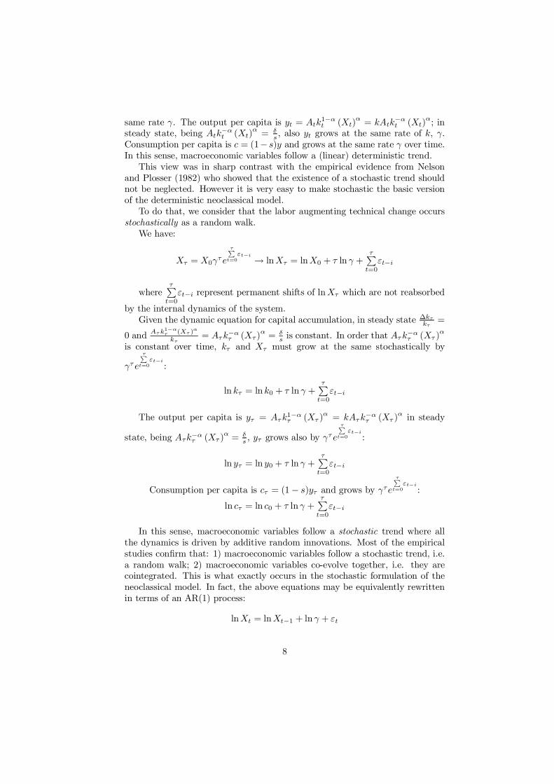
same rate °. The output per capita is yt = Atk1¡®t (Xt)

® = kAtk¡®t (Xt)

®; insteady state, being Atk

¡®t (Xt)

® = ±s, also yt grows at the same rate of k, °.

Consumption per capita is c = (1¡ s)y and grows at the same rate ° over time.In this sense, macroeconomic variables follow a (linear) deterministic trend.

This view was in sharp contrast with the empirical evidence from Nelsonand Plosser (1982) who showed that the existence of a stochastic trend shouldnot be neglected. However it is very easy to make stochastic the basic versionof the deterministic neoclassical model.

To do that, we consider that the labor augmenting technical change occursstochastically as a random walk.

We have:

X¿ = X0°¿e

¿Pt=0

"t¡i ! lnX¿ = lnX0 + ¿ ln ° +¿P

t=0"t¡i

where¿P

t=0"t¡i represent permanent shifts of lnX¿ which are not reabsorbed

by the internal dynamics of the system.Given the dynamic equation for capital accumulation, in steady state ¢k¿

k¿=

0 and A¿ k1¡®¿ (X¿ )®

k¿= A¿k¡®

¿ (X¿)® = ±s is constant. In order that A¿k¡®

¿ (X¿ )®

is constant over time, k¿ and X¿ must grow at the same stochastically by

°¿e

¿Pt=0

"t¡i

:

ln k¿ = ln k0 + ¿ ln ° +¿P

t=0"t¡i

The output per capita is y¿ = A¿k1¡®¿ (X¿ )® = kA¿k¡®

¿ (X¿ )® in steady

state, being A¿k¡®¿ (X¿ )® = ±

s , y¿ grows also by °¿e

¿Pt=0

"t¡i

:

ln y¿ = ln y0 + ¿ ln ° +¿P

t=0"t¡i

Consumption per capita is c¿ = (1 ¡ s)y¿ and grows by °¿e

¿Pt=0

"t¡i

:

ln c¿ = ln c0 + ¿ ln ° +¿P

t=0"t¡i

In this sense, macroeconomic variables follow a stochastic trend where allthe dynamics is driven by additive random innovations. Most of the empiricalstudies con…rm that: 1) macroeconomic variables follow a stochastic trend, i.e.a random walk; 2) macroeconomic variables co-evolve together, i.e. they arecointegrated. This is what exactly occurs in the stochastic formulation of theneoclassical model. In fact, the above equations may be equivalently rewrittenin terms of an AR(1) process:

lnXt = lnXt¡1 + ln ° + "t

8

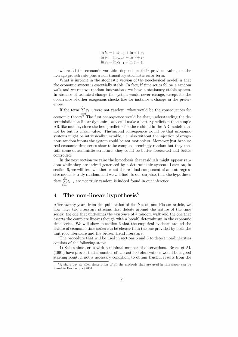
ln kt = ln kt¡1 + ln ° + "t

ln yt = ln yt¡1 + ln ° + "t

ln ct = ln ct¡1 + ln ° + "t

where all the economic variables depend on their previous value, on theaverage growth rate plus a non transitory stochastic error term.

What is implicit in the stochastic version of the neoclassical model, is thatthe economic system is essentially stable. In fact, if time series follow a randomwalk and we remove random innovations, we have a stationary stable system.In absence of technical change the system would never change, except for theoccurrence of other exogenous shocks like for instance a change in the prefer-ences.

If the term¿P

t=0"t¡i were not random, what would be the consequences for

economic theory? The …rst consequence would be that, understanding the de-terministic non-linear dynamics, we could make a better prediction than simpleAR like models, since the best predictor for the residual in the AR models can-not be but its mean value. The second consequence would be that economicsystems might be intrinsically unstable, i.e. also without the injection of exoge-nous random inputs the system could be not motionless. Moreover just becausereal economic time series show to be complex, seemingly random but they con-tain some deterministic structure, they could be better forecasted and bettercontrolled.

In the next section we raise the hypothesis that residuals might appear ran-dom while they are indeed generated by a deterministic system. Later on, insection 6, we will test whether or not the residual component of an autoregres-sive model is truly random, and we will …nd, to our surprise, that the hypothesis

that¿P

t=0"t¡i are not truly random is indeed found in our inference.

4 The non-linear hypothesis8

After twenty years from the publication of the Nelson and Plosser article, wenow have two literature streams that debate around the nature of the timeseries: the one that underlines the existence of a random walk and the one thatasserts the complete linear (though with a break) determinism in the economictime series. We will show in section 6 that the empirical evidence around thenature of economic time series can be clearer than the one provided by both theunit root literature and the broken trend literature.

The procedure that will be used in sections 5 and 6 to detect non-linearitiesconsists of the following steps:

1) Select time series with a minimal number of observations. Brock et Al.(1991) have proved that a number of at least 400 observations would be a goodstarting point, if not a necessary condition, to obtain trustful results from the

8A short but detailed description of all the methods that are used in this paper can befound in Bevilacqua (2001).

9

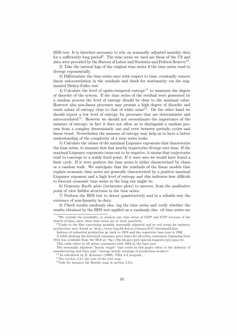
BDS test. It is therefore necessary to rely on seasonally adjusted monthly datafor a su¢ciently long period9. The time series we used are those of the US anddata were provided by the Bureau of Labor and Statistics and Federal Reserve10 .

2) Take the natural logs of the original time series if the time series tend todiverge exponentially.

3) Di¤erentiate the time series once with respect to time, eventually removelinear autocorrelation in the residuals and check for stationarity via the aug-mented Dickey-Fuller test.

4) Calculate the level of spatio-temporal entropy11 to measures the degreeof disorder of the system. If the time series of the residual were generated bya random process the level of entropy should be close to the maximal value.However also non-linear processes may present a high degree of disorder andreach values of entropy close to that of white noise12 . On the other hand weshould expect a low level of entropy for processes that are deterministic andautocorrelated13. However we should not overestimate the importance of themeasure of entropy; in fact it does not allow us to distinguish a random pro-cess from a complex deterministic one and even between periodic cycles andlinear trend. Nevertheless the measure of entropy may help us to have a betterunderstanding of the complexity of a time series looks.

5) Calculate the values of the maximal Liapunov exponents that characterizethe time series, to measure how fast nearby trajectories diverge over time. If themaximal Liapunov exponents turns out to be negative, it means that trajectoriestend to converge to a stable …xed point. If it were zero we would have found alimit cycle. If it were positive the time series is either characterized by chaosor a random walk. We anticipate that the residuals of the linear models thatexplain economic time series are generally characterized by a positive maximalLiapunov exponent and a high level of entropy and this indicates how di¢cultto forecast economic time series in the long run might be.

6) Generate Ruelle plots (recurrence plots) to uncover, from the qualitativepoint of view hidden structures in the time series.

7) Perform the BDS test to detect quantitatively and in a reliable way theexistence of non-linearity in data.

8) Check results randomly shu­ing the time series and verify whether theresults obtained by the BDS test applied on a randomly shu­ed time series are

9We exclude the possibility to analyze any time series of GDP and GNP because of thedearth of data, since these time series are at most quarterly.

10Links to the …les concerning monthly seasonally adjusted and in real terms for industryproductions were found at: http://www.bog.frb.fed.us/releases/G17/download2.htm

Indexes of industrial production go back to 1919 and the respective base year is 1992.A table showing the historical consumer price index for all urban consumers beginning from

1913 was available from the BLS at: ftp://ftp.bls.gov/pub/special.requests/cpi/cpiai.txt.This table refers to all urban consumers with 1982 as the base year.The seasonally adjusted ”hourly wages” time series in this paper refers to the industry of

manufacturing and data type ”average hourly earnings of production workers”.11As calculated by E. Kononov (1999), VRA 4.2 program.12See section 5.3.1 the case of the tent map.13Like for instance the Rossler map in section 5.3.2..

10

indeed di¤erent from the results obtained by the BDS test on the original timeseries14 . This veri…cation is extremely important since, if the two results turnout to be di¤erent, it means that the time order of the original time series issigni…cant and there exists causality in the data.

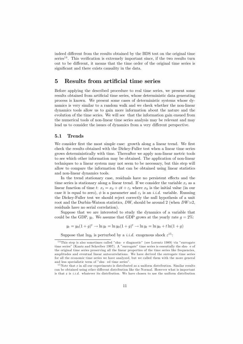
5 Results from arti…cial time seriesBefore applying the described procedure to real time series, we present someresults obtained from arti…cial time series, whose deterministic data generatingprocess is known. We present some cases of deterministic systems whose dy-namics is very similar to a random walk and we check whether the non-lineardynamics tools allow us to gain more information about the nature and theevolution of the time series. We will see that the information gain ensued fromthe numerical tools of non-linear time series analysis may be relevant and maylead us to consider the issues of dynamics from a very di¤erent perspective.

5.1 Trends

We consider …rst the most simple case: growth along a linear trend. We …rstcheck the results obtained with the Dickey-Fuller test when a linear time seriesgrows deterministically with time. Thereafter we apply non-linear metric toolsto see which other information may be obtained. The application of non-lineartechniques to a linear system may not seem to be necessary, but this step willallow to compare the information that can be obtained using linear statisticsand non-linear dynamics tools.

In the trend stationary case, residuals have no persistent e¤ects and thetime series is stationary along a linear trend. If we consider the variable xt as alinear function of time t: xt = x0 + Át + "t where x0 is the initial value (in ourcase it is equal to zero), Á is a parameter and "t is an i.i.d. variable. Runningthe Dickey-Fuller test we should reject correctly the null hypothesis of a unitroot and the Durbin-Watson statistics, DW, should be around 2 (when DW'2,residuals have no serial correlation).

Suppose that we are interested to study the dynamics of a variable thatcould be the GDP, yt. We assume that GDP grows at the yearly rate g = 2%:

yt = y0(1 + g)t ! ln yt = ln y0(1 + g)t ! ln yt = ln y0 + t ln(1 + g)

Suppose that lnyt is perturbed by a i.i.d. exogenous shock "15 :

14This step is also sometimes called ”shu­e diagnostic” (see Lorentz 1989) via ”surrogatetime series” (Kantz and Schreiber 1997). A ”surrogate” time series is essentially the shu­e ofthe original time series preserving all the linear properties of the time series like frequencies,amplitudes and eventual linear autocorrelations. We have derived the surrogate time seriesfor all the economic time series we have analyzed, but we called them with the more generaland less specialistic term of ”shu­ed time series”.

15Note that " in all our experiments is distributed as a uniform distribution. Similar resultscan be obtained using other di¤erent distribution like the Normal. However what is importantis that " is i.i.d. whatever its distribution. We have chosen to use the uniform distribution

11

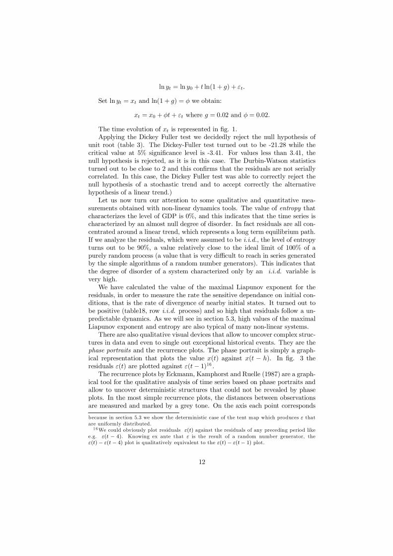
ln yt = ln y0 + t ln(1 + g) + "t:

Set ln yt = xt and ln(1 + g) = Á we obtain:

xt = x0 + Át + "t where g = 0:02 and Á = 0:02:

The time evolution of xt is represented in …g. 1.Applying the Dickey Fuller test we decidedly reject the null hypothesis of

unit root (table 3). The Dickey-Fuller test turned out to be -21.28 while thecritical value at 5% signi…cance level is -3.41. For values less than 3.41, thenull hypothesis is rejected, as it is in this case. The Durbin-Watson statisticsturned out to be close to 2 and this con…rms that the residuals are not seriallycorrelated. In this case, the Dickey Fuller test was able to correctly reject thenull hypothesis of a stochastic trend and to accept correctly the alternativehypothesis of a linear trend.)

Let us now turn our attention to some qualitative and quantitative mea-surements obtained with non-linear dynamics tools. The value of entropy thatcharacterizes the level of GDP is 0%, and this indicates that the time series ischaracterized by an almost null degree of disorder. In fact residuals are all con-centrated around a linear trend, which represents a long term equilibrium path.If we analyze the residuals, which were assumed to be i.i.d., the level of entropyturns out to be 90%, a value relatively close to the ideal limit of 100% of apurely random process (a value that is very di¢cult to reach in series generatedby the simple algorithms of a random number generators). This indicates thatthe degree of disorder of a system characterized only by an i.i.d. variable isvery high.

We have calculated the value of the maximal Liapunov exponent for theresiduals, in order to measure the rate the sensitive dependance on initial con-ditions, that is the rate of divergence of nearby initial states. It turned out tobe positive (table18, row i.i.d. process) and so high that residuals follow a un-predictable dynamics. As we will see in section 5.3, high values of the maximalLiapunov exponent and entropy are also typical of many non-linear systems.

There are also qualitative visual devices that allow to uncover complex struc-tures in data and even to single out exceptional historical events. They are thephase portraits and the recurrence plots. The phase portrait is simply a graph-ical representation that plots the value x(t) against x(t ¡ h). In …g. 3 theresiduals "(t) are plotted against "(t ¡ 1)16 .

The recurrence plots by Eckmann, Kamphorst and Ruelle (1987) are a graph-ical tool for the qualitative analysis of time series based on phase portraits andallow to uncover deterministic structures that could not be revealed by phaseplots. In the most simple recurrence plots, the distances between observationsare measured and marked by a grey tone. On the axis each point corresponds

because in section 5.3 we show the deterministic case of the tent map which produces " thatare uniformly distributed.

16We could obviously plot residuals "(t) against the residuals of any preceding period likee.g. "(t ¡ 4). Knowing ex ante that " is the result of a random number generator, the"(t) ¡ "(t ¡ 4) plot is qualitatively equivalent to the "(t) ¡ "(t¡ 1) plot.

12

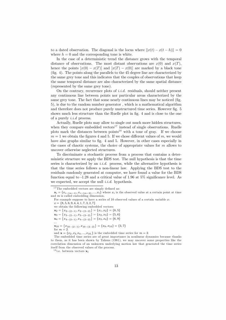
to a dated observation. The diagonal is the locus where kx(t) ¡ x(t ¡ h)k = 0where h = 0 and the corresponding tone is white.

In the case of a deterministic trend the distance grows with the temporaldistance of observations. The most distant observations are x(0) and x(T ),hence the points [x(0) ¡ x(T )] and [x(T ) ¡ x(0)] are marked by a black tone(…g. 4). The points along the parallels to the 45 degree line are characterized bythe same grey tone and this indicates that the couples of observations that keepthe same temporal distance are also characterized by the same spatial distance(represented by the same grey tone).

On the contrary, recurrence plots of i.i.d. residuals, should neither presentany continuous line between points nor particular areas characterized by thesame grey tone. The fact that some nearly continuous lines may be noticed (…g.5), is due to the random number generator , which is a mathematical algorithmand therefore does not produce purely unstructured time series. However …g. 5shows much less structure than the Ruelle plot in …g. 4 and is close to the oneof a purely i.i.d process.

Actually, Ruelle plots may allow to single out much more hidden structures,when they compare embedded vectors17 instead of single observations. Ruelleplots mark the distances between points18 with a tone of gray. If we choosem = 1 we obtain the …gures 4 and 5. If we chose di¤erent values of m, we wouldhave also graphs similar to …g. 4 and 5. However, in other cases especially inthe cases of chaotic systems, the choice of appropriate values for m allows touncover otherwise neglected structures.

To discriminate a stochastic process from a process that contains a deter-ministic structure we apply the BDS test. The null hypothesis is that the timeseries is characterized by an i.i.d. process, while the alternative hypothesis isthat the time series follows a non-linear law. Applying the BDS test to theresiduals randomly generated at computer, we have found a value for the BDSfunction equal to -1.28 and a critical value of 1.96 at 5% signi…cance level. Aswe expected, we accept the null i.i.d. hypothesis.

17The embedded vectors are simply de…ned as:xi = fxi¡(m¡1); xi¡(m¡2) ; :::; xig where xi is the observed value at a certain point at time

and m is called embedding dimension.For example suppose to have a series of 10 observed values of a certain variable x:x = f8; 5; 6; 9; 4; 4; 1; 7; 3; 2; 7gwe obtain the following embedded vectors:x2 =

©x2¡(2¡1); x2¡(2¡2)

ª= fx1; x2g = f8; 5g

x3 =©x3¡(2¡1); x3¡(2¡2)

ª= fx2; x3g = f5; 6g

x4 =©x4¡(2¡1); x4¡(2¡2)

ª= fx3; x4g = f6; 9g

...x10 =

©x10¡(2¡1); x10¡(2¡2)

ª= fx9; x10g = f3; 7g

for m = 2.and x = fx2; x3;x4; :::; x10;g is the embedded time series for m = 2.The embedded time series are of great importance in nonlinear dynamics because thanks

to them, as it has been shown by Takens (1981), we may uncover some properties like thecorrelation dimension of an unknown underlying motion law that generated the time seriesitself from the observed values of the process.

18 i.e. between vectors xi

13

From this simple exercise we have obtained the following results:- using the Dickey Fuller test we have correctly concluded that the time

series on levels is stationary and follows a deterministic trend.- the entropy indicates that the time series of levels is stable and the time

series of residuals is extremely unstable. The maximal Liapunov exponents ofresiduals is sharply positive, and this indicates that nearby trajectories divergeover time. Both the values of entropy and the maximal Liapunov exponent donot provide a de…nitive answer to the question as regards the nature of timeseries.

- recurrence plots and phase portraits allow to identify the existence ofstructures that are di¤erent from those of an i.i.d. process.

- the BDS test allows to better appreciate the importance of the timeorder in time series, that is to detect the existence of deterministic structures intime series. In this case we were not able to detect any deterministic structure inthe residuals since there weren’t any (except for the one of the random numbergenerator algorithm).

5.2 Random walks

We now analyze an other limit case: the random walk. The random walkhypothesis is not generally rejected by the unit root literature and it is at thecore of Real Business Cycle theory.

In the random walk case shocks, contrary to what happens in the case ofdeterministic trends, have persistent e¤ects and cumulate over time, withoutbeing reabsorbed even partially in the future. The time series is not stationary,does not follow a linear trend, but can still grow in a quite similar way to thecase of the deterministic trend. From a visual comparison between a series thatgrows like a random walk and a series that grows along a deterministic linearpath, it is often not possible to distinguish the nature of the two time series.The Dickey-Fuller test serves to single out which of the two time series followsa random walk.

In a random walk process, the value of the variable xt depends on its laggedvalue xt¡1 and a i.i.d. shock "t:

xt = xt¡1 + "t

Suppose now that we are interested in the dynamics of a variable y thatgrows yearly at the average rate of 2%, as an e¤ect of the cumulation of shocks:

ln yt = ln yt¡1 + "t ! ln yt ¡ ln yt¡1 = "t ! ln yt

yt¡1= "t ! yt = e"tyt¡1

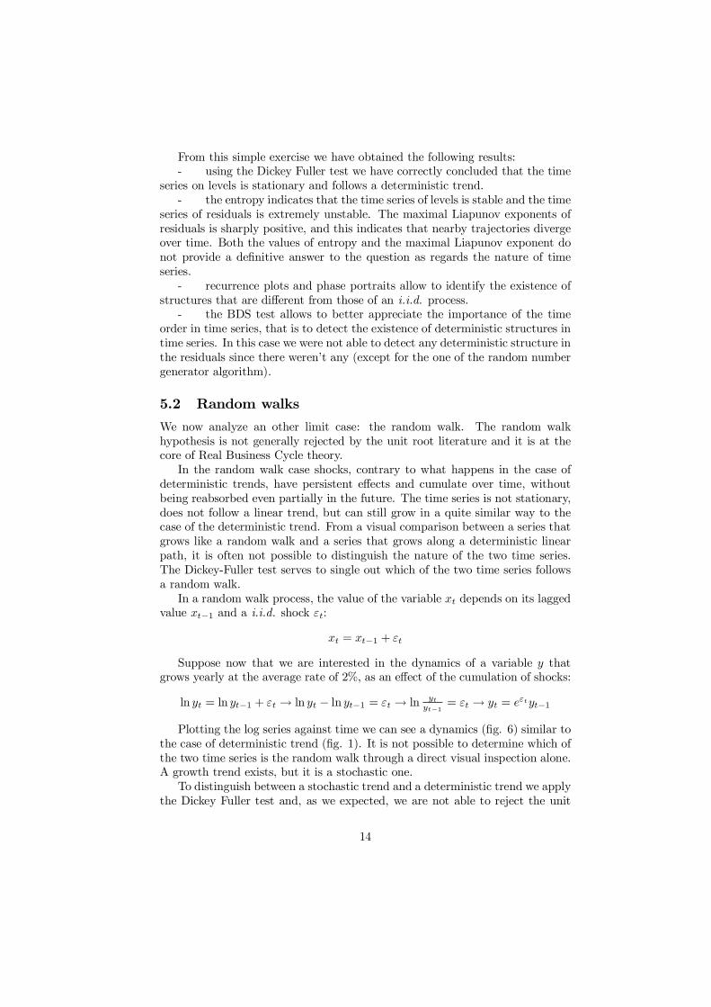
Plotting the log series against time we can see a dynamics (…g. 6) similar tothe case of deterministic trend (…g. 1). It is not possible to determine which ofthe two time series is the random walk through a direct visual inspection alone.A growth trend exists, but it is a stochastic one.

To distinguish between a stochastic trend and a deterministic trend we applythe Dickey Fuller test and, as we expected, we are not able to reject the unit

14

root hypothesis. The value of the test function turned out to be -1.98 while thecritical value is -3.41 at 5% signi…cance level (table 4). Residuals turned outnot to be serially correlated (Durbin-Watson statistic is 1.99).

The entropy level, the maximal Liapunov exponent, the BDS test and Ruelleplots of the residuals are exactly the same of those obtained for the deterministictrend case. Inasmuch as the aim of non-linear dynamics is to detect complexstructures in residuals, both in the case of stochastic growth and deterministicgrowth, residuals are stochastic and the tools of non-linear dynamics cannotbe used to detect linear determinism. The suitable instrument to detect lineardeterminism is indeed the Dickey-Fuller test.

5.3 Non-linear walks

5.3.1 Autoregressive tent map growth

We now apply the Dickey-Fuller test to an arti…cial time series where the valueof the variable depends on its lagged value and a deterministic non-linear shock.We will apply the BDS test and other tools of non-linear dynamics to identifythe deterministic structures that the Dickey-Fuller test is not able to detect.

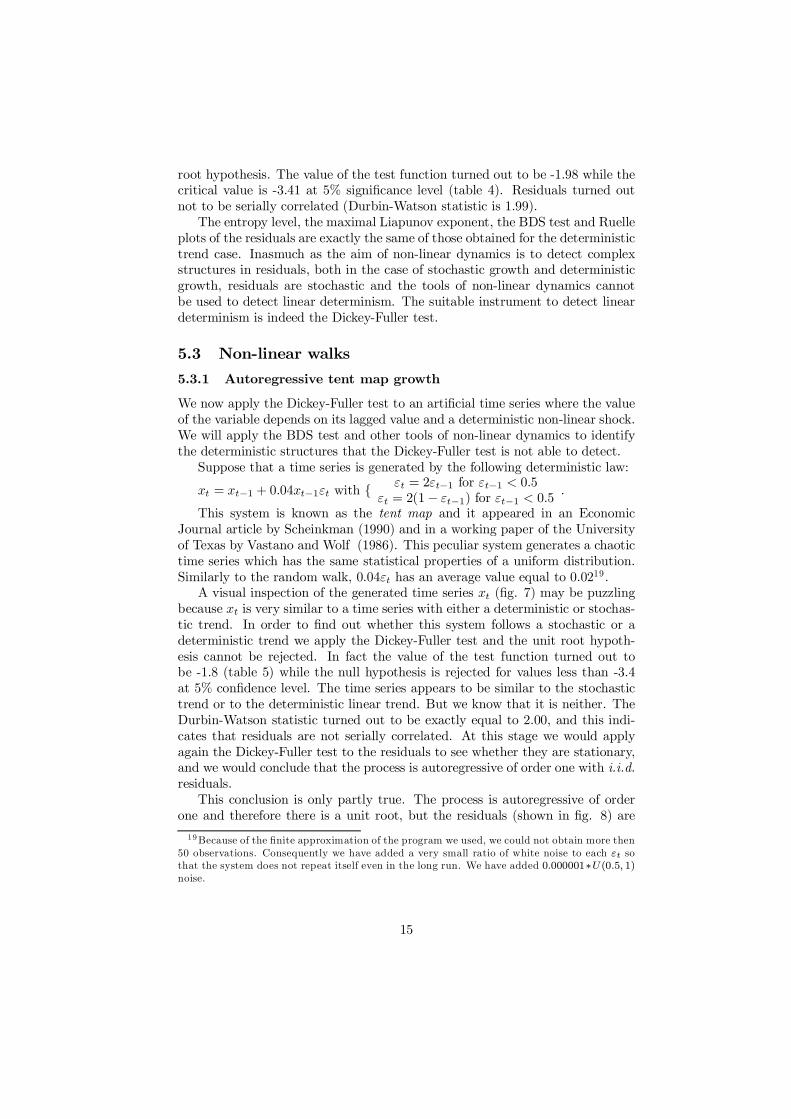
Suppose that a time series is generated by the following deterministic law:

xt = xt¡1 + 0:04xt¡1"t with f "t = 2"t¡1 for "t¡1 < 0:5"t = 2(1 ¡ "t¡1) for "t¡1 < 0:5

.

This system is known as the tent map and it appeared in an EconomicJournal article by Scheinkman (1990) and in a working paper of the Universityof Texas by Vastano and Wolf (1986). This peculiar system generates a chaotictime series which has the same statistical properties of a uniform distribution.Similarly to the random walk, 0:04"t has an average value equal to 0:0219.

A visual inspection of the generated time series xt (…g. 7) may be puzzlingbecause xt is very similar to a time series with either a deterministic or stochas-tic trend. In order to …nd out whether this system follows a stochastic or adeterministic trend we apply the Dickey-Fuller test and the unit root hypoth-esis cannot be rejected. In fact the value of the test function turned out tobe -1.8 (table 5) while the null hypothesis is rejected for values less than -3.4at 5% con…dence level. The time series appears to be similar to the stochastictrend or to the deterministic linear trend. But we know that it is neither. TheDurbin-Watson statistic turned out to be exactly equal to 2.00, and this indi-cates that residuals are not serially correlated. At this stage we would applyagain the Dickey-Fuller test to the residuals to see whether they are stationary,and we would conclude that the process is autoregressive of order one with i.i.d.residuals.

This conclusion is only partly true. The process is autoregressive of orderone and therefore there is a unit root, but the residuals (shown in …g. 8) are

19Because of the …nite approximation of the program we used, we could not obtain more then50 observations. Consequently we have added a very small ratio of white noise to each "t sothat the system does not repeat itself even in the long run. We have added 0:000001¤U (0:5; 1)noise.

15

deterministic and, knowing the law that generates the residuals, the process isperfectly predictable. In this case we must be very careful to read the resultsobtained with the Dickey-Fuller test. It suggests that it is not possible to refusethe null hypothesis of the existence of a unit root, i.e. the hypothesis of autore-gressive process of order one. However the residuals, as this case shows, can benon-stochastic. Consequently the Dickey-Fuller test is a tool that is not suitableto unveil whether the series follows a deterministic law, except for the specialcase that the series follows a deterministic linear trend. The acceptance of aunit root hypothesis and the presence of not serially correlated residuals doesnot authorize us to take the stochastic origin of the time series for granted.

From the values of entropy (78%) and the positive maximal Liapunov ex-ponent we may infer that the system is nearly unpredictable. However thesecharacteristics are typical of both stochastic and chaotic processes. In order toinfer the existence of non-linear structures we have performed the BDS test.The value of the BDS statistic (which asymptotically converges to normality)20

turned out 99.2 and this allows us to reject the null i.i.d. hypothesis with aminimal probability to be mistaken.

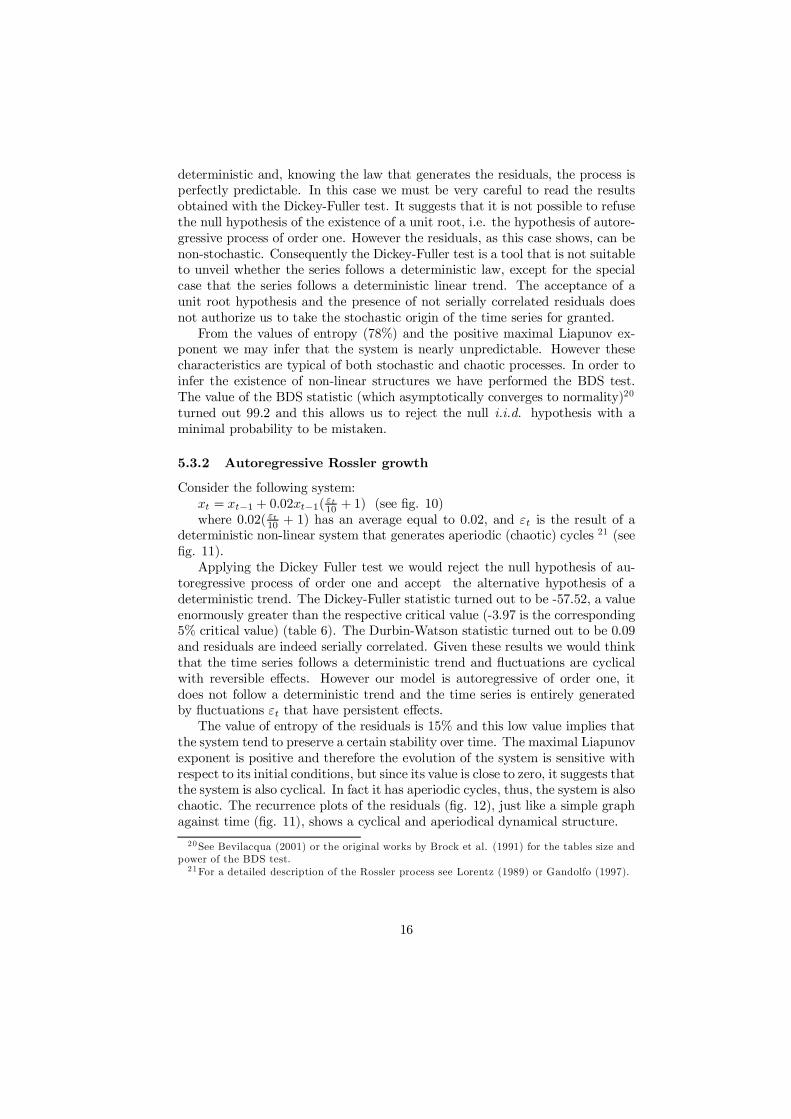
5.3.2 Autoregressive Rossler growth

Consider the following system:xt = xt¡1 + 0:02xt¡1(

"t

10 + 1) (see …g. 10)where 0:02( "t

10 + 1) has an average equal to 0:02, and "t is the result of adeterministic non-linear system that generates aperiodic (chaotic) cycles 21 (see…g. 11).

Applying the Dickey Fuller test we would reject the null hypothesis of au-toregressive process of order one and accept the alternative hypothesis of adeterministic trend. The Dickey-Fuller statistic turned out to be -57.52, a valueenormously greater than the respective critical value (-3.97 is the corresponding5% critical value) (table 6). The Durbin-Watson statistic turned out to be 0.09and residuals are indeed serially correlated. Given these results we would thinkthat the time series follows a deterministic trend and ‡uctuations are cyclicalwith reversible e¤ects. However our model is autoregressive of order one, itdoes not follow a deterministic trend and the time series is entirely generatedby ‡uctuations "t that have persistent e¤ects.

The value of entropy of the residuals is 15% and this low value implies thatthe system tend to preserve a certain stability over time. The maximal Liapunovexponent is positive and therefore the evolution of the system is sensitive withrespect to its initial conditions, but since its value is close to zero, it suggests thatthe system is also cyclical. In fact it has aperiodic cycles, thus, the system is alsochaotic. The recurrence plots of the residuals (…g. 12), just like a simple graphagainst time (…g. 11), shows a cyclical and aperiodical dynamical structure.

20See Bevilacqua (2001) or the original works by Brock et al. (1991) for the tables size andpower of the BDS test.

21For a detailed description of the Rossler process see Lorentz (1989) or Gandolfo (1997).

16

The support for the existence of non-linear structures in the time series fol-lows from the high value of the BDS statistic (table 6). The null i.i.d. hypothesisis rejected. Though the BDS test was able to detect correctly the existence ofnon-linear structures in the data also in this case, we may better appreciate itse¤ectiveness when residuals are not serially correlated, as in the cases of thetent map and seasonally adjusted real time series.

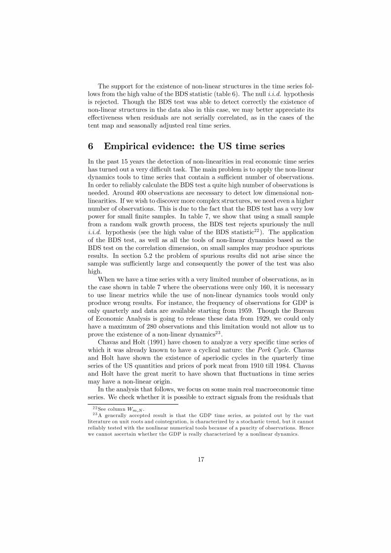
6 Empirical evidence: the US time seriesIn the past 15 years the detection of non-linearities in real economic time serieshas turned out a very di¢cult task. The main problem is to apply the non-lineardynamics tools to time series that contain a su¢cient number of observations.In order to reliably calculate the BDS test a quite high number of observations isneeded. Around 400 observations are necessary to detect low dimensional non-linearities. If we wish to discover more complex structures, we need even a highernumber of observations. This is due to the fact that the BDS test has a very lowpower for small …nite samples. In table 7, we show that using a small samplefrom a random walk growth process, the BDS test rejects spuriously the nulli.i.d. hypothesis (see the high value of the BDS statistic22). The applicationof the BDS test, as well as all the tools of non-linear dynamics based as theBDS test on the correlation dimension, on small samples may produce spuriousresults. In section 5.2 the problem of spurious results did not arise since thesample was su¢ciently large and consequently the power of the test was alsohigh.

When we have a time series with a very limited number of observations, as inthe case shown in table 7 where the observations were only 160, it is necessaryto use linear metrics while the use of non-linear dynamics tools would onlyproduce wrong results. For instance, the frequency of observations for GDP isonly quarterly and data are available starting from 1959. Though the Bureauof Economic Analysis is going to release these data from 1929, we could onlyhave a maximum of 280 observations and this limitation would not allow us toprove the existence of a non-linear dynamics23.

Chavas and Holt (1991) have chosen to analyze a very speci…c time series ofwhich it was already known to have a cyclical nature: the Pork Cycle. Chavasand Holt have shown the existence of aperiodic cycles in the quarterly timeseries of the US quantities and prices of pork meat from 1910 till 1984. Chavasand Holt have the great merit to have shown that ‡uctuations in time seriesmay have a non-linear origin.

In the analysis that follows, we focus on some main real macroeconomic timeseries. We check whether it is possible to extract signals from the residuals that

22See column Wm;N :23A generally accepted result is that the GDP time series, as pointed out by the vast

literature on unit roots and cointegration, is characterized by a stochastic trend, but it cannotreliably tested with the nonlinear numerical tools because of a paucity of observations. Hencewe cannot ascertain whether the GDP is really characterized by a nonlinear dynamics.

17

economic literature has assumed to be stochastic. What we want to ascertainwhether the residuals also contain a non-linear component together with a trulystochastic component. We try to …nd whether important temporal linkages arepresent between residuals. We will attempt to falsify the results of rejectionof the null i.i.d. hypothesis. We will proceed to a random shu­e of the timeseries in order to break any temporal link among data. Afterwards we will applynon-linear dynamics tools on the shu­ed time series. If the results of non-lineartest on both the original and the shu­ed time series are similar, it means thattime linkages are not important and the time series is generated by a stochasticprocess, otherwise there is evidence that time cannot be ruled out and thereexists a non-linear component.

6.1 Industrial production

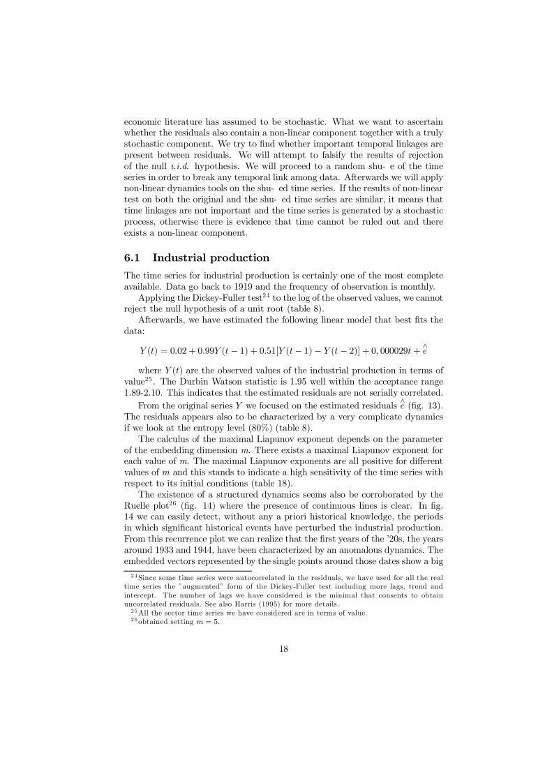
The time series for industrial production is certainly one of the most completeavailable. Data go back to 1919 and the frequency of observation is monthly.

Applying the Dickey-Fuller test24 to the log of the observed values, we cannotreject the null hypothesis of a unit root (table 8).

Afterwards, we have estimated the following linear model that best …ts thedata:

Y (t) = 0:02 + 0:99Y (t ¡ 1) + 0:51[Y (t ¡ 1) ¡ Y (t ¡ 2)] + 0; 000029t +^e

where Y (t) are the observed values of the industrial production in terms ofvalue25 . The Durbin Watson statistic is 1.95 well within the acceptance range1.89-2.10. This indicates that the estimated residuals are not serially correlated.

From the original series Y we focused on the estimated residuals^e (…g. 13).

The residuals appears also to be characterized by a very complicate dynamicsif we look at the entropy level (80%) (table 8).

The calculus of the maximal Liapunov exponent depends on the parameterof the embedding dimension m. There exists a maximal Liapunov exponent foreach value of m. The maximal Liapunov exponents are all positive for di¤erentvalues of m and this stands to indicate a high sensitivity of the time series withrespect to its initial conditions (table 18).

The existence of a structured dynamics seems also be corroborated by theRuelle plot26 (…g. 14) where the presence of continuous lines is clear. In …g.14 we can easily detect, without any a priori historical knowledge, the periodsin which signi…cant historical events have perturbed the industrial production.From this recurrence plot we can realize that the …rst years of the ’20s, the yearsaround 1933 and 1944, have been characterized by an anomalous dynamics. Theembedded vectors represented by the single points around those dates show a big

24Since some time series were autocorrelated in the residuals, we have used for all the realtime series the ”augmented” form of the Dickey-Fuller test including more lags, trend andintercept. The number of lags we have considered is the minimal that consents to obtainuncorrelated residuals. See also Harris (1995) for more details.

25All the sector time series we have considered are in terms of value.26obtained setting m = 5.

18

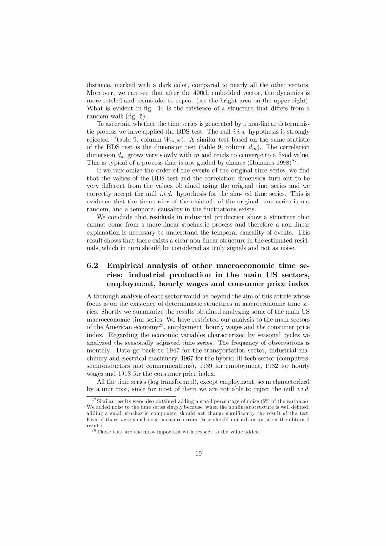
distance, marked with a dark color, compared to nearly all the other vectors.Moreover, we can see that after the 400th embedded vector, the dynamics ismore settled and seems also to repeat (see the bright area on the upper right).What is evident in …g. 14 is the existence of a structure that di¤ers from arandom walk (…g. 5).

To ascertain whether the time series is generated by a non-linear determinis-tic process we have applied the BDS test. The null i.i.d. hypothesis is stronglyrejected (table 9, column Wm;N). A similar test based on the same statisticof the BDS test is the dimension test (table 9, column dm). The correlationdimension dm grows very slowly with m and tends to converge to a …xed value.This is typical of a process that is not guided by chance (Hommes 1998)27.

If we randomize the order of the events of the original time series, we …ndthat the values of the BDS test and the correlation dimension turn out to bevery di¤erent from the values obtained using the original time series and wecorrectly accept the null i.i.d. hypothesis for the shu­ed time series. This isevidence that the time order of the residuals of the original time series is notrandom, and a temporal causality in the ‡uctuations exists.

We conclude that residuals in industrial production show a structure thatcannot come from a mere linear stochastic process and therefore a non-linearexplanation is necessary to understand the temporal causality of events. Thisresult shows that there exists a clear non-linear structure in the estimated resid-uals, which in turn should be considered as truly signals and not as noise.

6.2 Empirical analysis of other macroeconomic time se-ries: industrial production in the main US sectors,employment, hourly wages and consumer price index

A thorough analysis of each sector would be beyond the aim of this article whosefocus is on the existence of deterministic structures in macroeconomic time se-ries. Shortly we summarize the results obtained analyzing some of the main USmacroeconomic time series. We have restricted our analysis to the main sectorsof the American economy28, employment, hourly wages and the consumer priceindex. Regarding the economic variables characterized by seasonal cycles weanalyzed the seasonally adjusted time series. The frequency of observations ismonthly. Data go back to 1947 for the transportation sector, industrial ma-chinery and electrical machinery, 1967 for the hybrid Hi-tech sector (computers,semiconductors and communications), 1939 for employment, 1932 for hourlywages and 1913 for the consumer price index.

All the time series (log transformed), except employment, seem characterizedby a unit root, since for most of them we are not able to reject the null i.i.d.

27Similar results were also obtained adding a small percentage of noise (5% of the variance).We added noise to the time series simply because, when the nonlinear structure is well de…ned,adding a small stochastic component should not change signi…cantly the result of the test.Even if there were small i.i.d. measure errors these should not call in question the obtainedresults.

28Those that are the most important with respect to the value added.

19

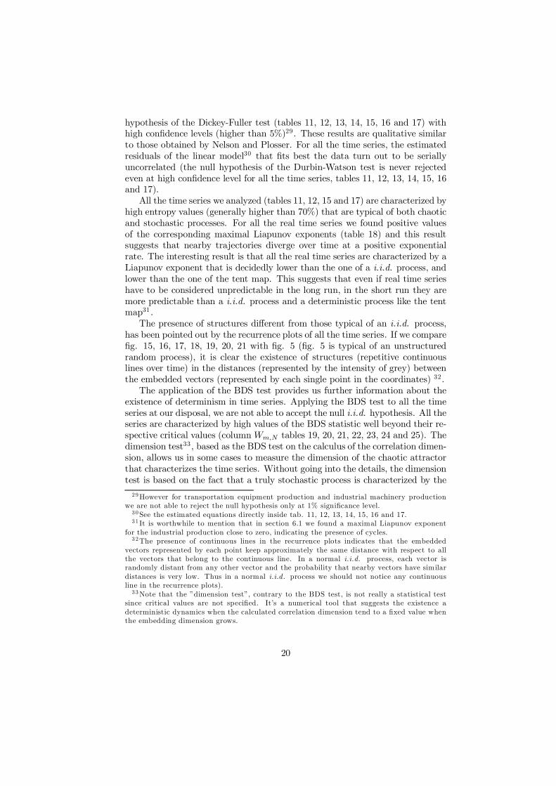
hypothesis of the Dickey-Fuller test (tables 11, 12, 13, 14, 15, 16 and 17) withhigh con…dence levels (higher than 5%)29. These results are qualitative similarto those obtained by Nelson and Plosser. For all the time series, the estimatedresiduals of the linear model30 that …ts best the data turn out to be seriallyuncorrelated (the null hypothesis of the Durbin-Watson test is never rejectedeven at high con…dence level for all the time series, tables 11, 12, 13, 14, 15, 16and 17).

All the time series we analyzed (tables 11, 12, 15 and 17) are characterized byhigh entropy values (generally higher than 70%) that are typical of both chaoticand stochastic processes. For all the real time series we found positive valuesof the corresponding maximal Liapunov exponents (table 18) and this resultsuggests that nearby trajectories diverge over time at a positive exponentialrate. The interesting result is that all the real time series are characterized by aLiapunov exponent that is decidedly lower than the one of a i.i.d. process, andlower than the one of the tent map. This suggests that even if real time serieshave to be considered unpredictable in the long run, in the short run they aremore predictable than a i.i.d. process and a deterministic process like the tentmap31 .

The presence of structures di¤erent from those typical of an i.i.d. process,has been pointed out by the recurrence plots of all the time series. If we compare…g. 15, 16, 17, 18, 19, 20, 21 with …g. 5 (…g. 5 is typical of an unstructuredrandom process), it is clear the existence of structures (repetitive continuouslines over time) in the distances (represented by the intensity of grey) betweenthe embedded vectors (represented by each single point in the coordinates) 32.

The application of the BDS test provides us further information about theexistence of determinism in time series. Applying the BDS test to all the timeseries at our disposal, we are not able to accept the null i.i.d. hypothesis. All theseries are characterized by high values of the BDS statistic well beyond their re-spective critical values (column Wm;N tables 19, 20, 21, 22, 23, 24 and 25). Thedimension test33, based as the BDS test on the calculus of the correlation dimen-sion, allows us in some cases to measure the dimension of the chaotic attractorthat characterizes the time series. Without going into the details, the dimensiontest is based on the fact that a truly stochastic process is characterized by the

29However for transportation equipment production and industrial machinery productionwe are not able to reject the null hypothesis only at 1% signi…cance level.

30See the estimated equations directly inside tab. 11, 12, 13, 14, 15, 16 and 17.31 It is worthwhile to mention that in section 6.1 we found a maximal Liapunov exponent

for the industrial production close to zero, indicating the presence of cycles.32The presence of continuous lines in the recurrence plots indicates that the embedded

vectors represented by each point keep approximately the same distance with respect to allthe vectors that belong to the continuous line. In a normal i.i.d. process, each vector israndomly distant from any other vector and the probability that nearby vectors have similardistances is very low. Thus in a normal i.i.d. process we should not notice any continuousline in the recurrence plots).

33Note that the ”dimension test”, contrary to the BDS test, is not really a statistical testsince critical values are not speci…ed. It’s a numerical tool that suggests the existence adeterministic dynamics when the calculated correlation dimension tend to a …xed value whenthe embedding dimension grows.

20

growth of the correlation dimension with the increase of the embedding dimen-sion, while a truly chaotic process is characterized by the correlation dimensiontending to settle to a constant value when the embedding dimension increases(Hommes 1998). This constant value represents the dimension of the chaoticattractor. In all the series we have analyzed the correlation dimension (columndm in tables19, 20, 21, 22, 23, 24 and 25) grows less than proportionally withrespect to ”m”, but in many cases we cannot detect a clear tendency of thecorrelation dimension to settle clearly to a constant value (column dm in tables19, 20, 21, 22, 23, 24, 25 and …g. 22). For all the time series we have analyzed,the BDS test suggests that the time series contain a deterministic structure,but it is not possible to quantify, via the dimension test, the dimension of theunderlying attractor of the time series34.

To check furthermore our results we have randomly ordered the real timeseries, applied BDS and calculated the dimension correlation of the shu­ed timeseries to see whether temporal linkages were relevant. In all the cases the valuesof the BDS and the dimension tests of the shu­ed time series were notablydi¤erent. We could not reject the null hypothesis of the BDS test for all theshu­ed time series and the correlation dimension also was also higher (tables26, 27, 28, 29, 30, 31, 32 and …g. 23) with respect to the original time series(tables 19, 20, 21, 22, 23, 24, 25 and …g. 22). This is a con…rmation thattemporal linkages between residuals are really important and therefore a mereprobabilistic hypothesis on the residuals of macroeconomic time series does nothave empirical ground.

7 Concluding remarksWe have …rst shown the theoretical possibility (section 4 and 5) and latter theempirical evidence (section 6) that in the serially uncorrelated residuals thereare present non-linear signals which, in the models with a deterministic (linearor broken) or stochastic trend, are assumed to be i.i.d., like white noise. Theapproach that we put forward is to separate the stochastic component (that isindeed present in the residuals) from the deterministic component and studythese two components separately. To be successful in this task we need a data…lter based on the concepts of non-linear dynamics. In this paper we have lim-ited our analysis to the detection of the existence of clear non-linearities in theresiduals of macroeconomic time series. We have detected non-linearities in allthe time series we analyzed. All the time series we have considered are thuscharacterized by determinism, notwithstanding all the series (except employ-ment) are non-stationary and residuals are serially uncorrelated. If all this is

34This phenomenon may be due to the presence of a stochastic component in the timeseries. It should be therefore important to …lter our data in order to separately analyzethe only deterministic component and to quantify the dimension of the chaotic attractor.The future application of …lters that allow us to reduce and hopefully remove the stochasticcomponent may allow us to detect the dimension of chaos for all the real time series for whichwe have already uncovered the presence of chaos.

21

true, in the short run, we may make better predictors than simple autoregressivemodels.

The problem of distinguishing between the two alternative hypothesis, deter-ministic trend or stochastic trend, was at the core of unit root and broken trendliterature (section 2), but for us it was not the …rst issue. Our aim was indeed todetect non-linear structures in those components that linear stochastic modelshave assumed as exogenous factors. As far as in linear stochastic models noiseplays the relevant role to make ”non-stationary” basically stationary processes,it was for us of primary importance, from the theoretical point of view, to checkwhether a component of what has been so far assumed noise might have anendogenous explanation. If this is the case as con…rmed in section 6, economicvariables may not follow a stationary path even in absence of external shocksand the observed non-stationarity may be the consequence of complex relationsbetween the economic variables.

Bibliography

Alba J. D. and Papell D. H., 1995, ”Trend breaks and the unit root hypothe-sis for newly industrializing and newly exporting countries”, Review of InternationalEconomics, 3, pp. 264-74.

Al Bazai H. S., 1998, ”The Saudi stock market and the monetary policy”, Journalof the Social Sciences, 26, pp. 91-106.

Banerjee A., Lumsdaine R. L. and Stock J. H., 1992, ”Recursive and sequentialtests of the unit root and trend break hypothesis: theory and international evidence”,Journal of Business and Economic Statistics, 10, pp.271-87.

Barro R. J. and Sala-i-Martin X. 1995, Economic Growth, Mc Graw Hill.Ben D. D., Lumsdaine R. L. and Papell D. H., 1996, ”Unit roots, postwar slow-

downs and long run growth: evidence from two structural breaks”, Tel Aviv SacklerInstitute of Economic Studies, WP 33.

Ben D. D., Lumsdaine R. L. and Papell D. H., 1996, The unit root hypothesis inlong-term output: evidence from two structural breaks for 16 countries, CEPR, DP.1336.

Ben D. D. and Papell D. H., 1994, ”The great crash, and the unit root hypothesis:some new evidence about an old stylized fact”, CEPR, DP. 965.

Bevilacqua F., 2001, ”Nonlinear dynamics in US macroeconomic time series”,Merit-Infonomics RM 2001-035.

Bohl M. T., 1998, ”Kovergenz westdeutscher regionen? Neue empirische ergebnisseauf derbasis von Panel-Einheitswurzeltests”, Konjunkturpolitik, 44, pp. 82-99.

Boswijk H. P., 1996, ”Unit roots and cointegration”, lecture notes, AmsterdamUniversity.

Bradley M. D. and Jansen D. W., 1995, ”Unit roots and infrequent large shocks:new international evidence on output growth”, Journal of Money, Credit and Banking,27, pp. 867-93.

22

Bresson G. and Celimene F., 1995, ”Hysteresis or persistence of the unemploymentrate: an econometric test in several Carribean countries”, Revue d’Economie Politique,105, pp. 965-98.

Brock W. A. and Dechert W. D., 1988, ”Theorems on distinguishing determin-istic from random systems”, in Barnett W. et al., Dynamic econometric modelling,Cambridge University Press.

Brock W. A., Dechert W.D. and Scheinkman J.A., 1987, ”A test for independencebased on the correlation integral”, University of Wisconsin-Madison.

Brock W. A., Hsieh D.A. and LeBaron B., 1991, Nonlinear Dynamics, Chaos, andInstability: Statistical Theory and Economic Evidence, MIT press.

Capitelli R. and Scjlegel A., 1991, ”Ist die Schweiz eine Zinsinsel?Eine multivariateuntersuchung uber den langfristigen internationalen realzinsausgleich”, Swiss Journalof Economic and Statistics, 127, pp. 647-64.

Caselli G. P. and Marinelli L., 1994, ”Italian GNP growth 1890-1992: a unit rootor segmented trend representation?”, Economic Notes, 23, pp. 53-73.

Chavas J. P. and Holt M. T., 1991, ”On nonlinear dynamics: the case of PorkCycle”, American Journal of Agricultural Economics, 73, pp. 819-28.

Chavas J. P. and Holt M. T., 1993, ”Market instability and nonlinear dynamics”,American Journal of Agricultural Economics, 75, pp. 113-20.

Chen B. and Tran K. C., 1994, ”Are we sure that the real exchange rate follows arandom walk?”, International Economic Journal, 8, pp. 33-44.

Cheung Y. W. and Chinn M. D., 1996, ”Further investigation of uncertain unitroot in GNP”, NBER, 206.

Choi I. and Yu B., 1997, ”A general framework for testing I(m) against I(m+k)”,Journal of Economic Theory and Econometrics, 3, pp. 103-38.

Coakley J., Kulasi F. and Smith R., 1995, ”Current account solvency and theFeldstein-Horioka puzzle”, Birkbeck College Discussion Paper London.

Conover W. J., 1971, Practical Nonparametric Statistics, Wiley, New York.Coorey S., 1991, ”The determinants of U.S. real interest rates in the long run”,

IMF WP 118.Crosby M., 1998, ”A note on the australian business cycle”, Economic Analysis

and Policy, 28, pp. 103-08.Culver S. E. and Papell D. H., 1995, ”Real exchanghe rates under the Gold Stan-

dard: can they be explained by the trend break model?”, Journal of InternationalMoney and Finance, 14, pp. 539-48.

Culver S. E. and Papell D. H., 1997, ”Is there a unit root in the in‡ation rate?Evidence from sequential break and Panel Data models”, Journal of Applied Econo-metrics, 12, pp. 435-44.

Cushing M. J. and Mc Garvey M. G., 1996, ”The persistence of shocks to macroe-conomic time series: some evidence from economic theory”, Journal of Business andEconomic Statistics, 14 pp. 179-87.

Dechert W. D., 1994, ”The correlation integral and the independence of gaussianand related processes”, SSRI W.P. 9412, University of Wisconsin.

Diebold F. X. and Rudebush G. D., 1989, ”Long memory and persistence in ag-gregate output”, Journal of Monetary Economics, 24, pp. 189-209.

23

Dickey D.A. and Fuller W.A., 1979, ”Distribution of the Estimators for Autoregres-sive Time Series with a Unit Root”, Journal of the American Statistical Association,74, pp. 427-431.

Dolado J. J. and Lopez S. J. D., 1996, ”Hysteresis and economic ‡uctuations(Spain, 1970-94)”, Centre for Economic Policy Research, Discussion Paper 1334.

Dolmas J., Raj B. and Scottje D. J., 1999, ”A peak through the structural breakwindow”, Economic Inquiry, 37, pp. 226-41.

Duck N. W., 1992, ”Evidence on breaking trend functions from nine countries”,University of Bristol WP 341.

Durlauf S. N., 1993, ”Time series properties of aggregate output ‡uctuations”,Journal of Econometrics, 56, pp. 39-56.

Eckmann J.P., Kamphorst O. and Ruelle D., 1987, ”Recurrence plots of dynamicalsystems”, Europhysic Letters, 4.

Enders W., 1995, Applied Econometric Time Series, Wiley.Fleissing A. R. and Strauss J., 1997, ”Unit root tests on real wage Panel Data for

the G7”, Economic Letters, 56, pp. 149-55.Frank, M. and Stengos T., 1988, ”International Chaos?”, European Economic Re-

view, 32, 1569-84.Franses P. H. and Kleibergen F., 1996, ”Unit roots in the Nelson Plosser data: do

they matter for forecasting?”, International Journal of Forecasting, 12, pp. 283-88.Fraser A. M. and Swinney H. L, 1986, ”Independent coordinates for strange at-

tractors from mutual information”, Phys. Review, 68.Fung H. G. and Lo W. C., 1992, ”Deviations from purchasing power parity”,

Financial Review, 27, 553-70.Fuller W.A. (1999), Introduction to Time Series, Wiley, New York.Gallegati M., 1996, ”Testing output through its supply components”, Economic

Notes, 25, pp. 249-60.Gamber E. N. and Sorensen R. L., 1994, ”Are net discount rates stationary?”,

Journal of Risk and Insurance, 61, pp. 503-12.Gil A. L. A. and Robinson P. M., 1997, ”Testing of unit roots and other nonsta-

tionary hypothesis in macroeconomic time series”, Journal of Econometrics, 80, pp.241-68.

Gokey T. C., 1990, ”Stationarity of nominal interest rates, in‡ation and real in-terest rates”, Oxford Applied Economics DP 105.

de Haan J. and Zelhorst D., 1993, ”The nonstationarity of German aggregateoutput”, Jahrbucher fur Nationalokonomie und Statistik, 212, pp. 410-18.

de Haan J., Zelhorst D., 1994, ”Testing for stationarity of output components:some results for Italy”, Economic Notes, 23, pp. 402-09.

de Haan J. and Zelhorst D., 1994, ”Testing for a break in output: new internationalevidence”, Oxford Economic Papers, 47, pp. 357-62.

Hansen G, 1991, ”Hysteresis and unemployment”, Jahrbucher fur Nationalokonomieund Statistik, 208, pp.272-98.

Harris R., 1995, Using Cointegration Analysis in Econometric Modelling, PrenticeHall, London.

Haslag J. and Nieswiadomy M., Slottje D. J., 1994, ”Are net discount rates sta-tionary? Some empirical evidence”, Journal of Risk and Insurance, 61, pp. 513-18.

24

Hylleberg S. and Engle R. F., 1996, ”Common seasonal features: global unemploy-ment”, Aarhus Department of Economics WP 13.

Hsieh D. A., 1991, ”Chaos and nonlinear dynamics: application to …nancial mar-kets”, Journal of Finance, 46, pp.1839-1877.

Hommes C. H., 1998, ”Nonlinear economic dynamics”, lecture notes, NAKE Utrecht.Johnston J., 1984, Econometric Methods, Mc Graw Hill.Kantz H. and Schreiber T., 1997, Nonlinear Time Series Analysis, Cambridge

University Press.Kennel M. B., Brown R. and Abarbanel H. D. I., 1992. ”Determining embedding

dimension for phase-space reconstruction using a geometrical construction”, PhysicsReview, 45, pp. 3403-3411.

King R. G., Plosser C. I. and Rebelo S. T., 1988a, ”Production, growth and busi-ness cycles I: the basic neoclassical model”, Journal of Monetary Economics, 21, 195-232.

King R. G., Plosser C. I. and Rebelo S. T., 1988b, ”Production, growth andbusiness cycles II: new directions”, Journal of Monetary Economics, 21, pp. 309-41.

Kononov E., 1999, ”Visual Recurrence Analysis 4.2 (software program)”,http://home.netcom.com/~eugenek/.Krol R., 1992, ”Trends, random walks and persistence: an empirical study of

disaggregated U.S. industrial production”, Review of Economics and Statistics, 74,pp. 154-59.

Lee H. S. and Siklos P. L., 1991, ”Unit roots and seasonal unit roots in macroeco-nomic time series: Canadian evidence”, Economic Letters, 35, pp. 273-77.

Lee J., 1996, ”Testing for a unit root in time series with trend breaks”, Journal ofMacroeconomics, 18, pp. 503-19.

Leislie D., Pu Y. and Wharton A, 1995, ”Hysteresis versus persistence in unem-ployment: a sceptical note on unit root tests”, Labour, 9, pp. 507-23.

Leybourne S. J. and Mc Cabe, B. P. M., 1999, ”Modi…ed stationary tests withdata dependent model selection rules”, Journal of Business and Economic Statistics,pp. 264-70.

Leybourne S. J., Mc Cabe, B. P. M. and Tremayne A. R., 1996, ”Can economic timeseries be di¤erenced to stationarity?”, Journal of Business and Economic Statistics,pp. 435-46.

Li H., 1995, ”A Reexamination of the Nelson-Plosser data set using recursive andsequential tests”, Empirical Economics, 20, pp. 501-18.

Linden M., 1992, ”Stochastic and deterministic trends in Finnish macroeconomictime series”, Finnish Economic Papers, pp. 110-16.

Lorentz H. W., 1989, Lecture Notes in Economics and Mathematical Systems,Springer Verlag.

Lucas R., 1972, ”Expectations and the neutrality of money”, Journal of EconomicTheory, 4, 103-24.

Lucas R., 1977, ”Understanding Business Cycles” in Brunner K., Meltzer eds, Sta-bilization of the domestic and international economy, Carnegie-Rochester ConferenceSeries on Pubblic Policy, 5, 7-29.

Lucas R., 1980, ”Methods and problems in Business Cycle Theory”, Journal ofMoney, Credit and Banking, 12, pp. 696-715.

25

Lumsdaine R. L. and Papell D. H., 1997, ”Multiple trend breaks and the unit roothypothesis”, Review of Economics and Statistics, 79, pp. 212-18.

MacDonald R., 1996, ”Panel unit root tests and real exchange rates”, EconomicLetters, 50, pp. 7-11.

Maddala G. S. and Kim I. M., 1998, Unit roots, cointegration and structural change,Cambridge University Press.

McCoskey S. K. and Selden T. M., 1998, ”Health care expenditures and GDP:panel data unit root test results”, Journal of Health Economics, 17, pp. 369-76.

McDougall R. S., 1995, ”The seasonal unit root structure in New Zealand macroe-conomic variables”, Applied Economics, 27, pp. 817-27.

Mills T., 1992, ”How robust is the …nding that innovations to UK output arepersistent”, Scottish Journal of Political Economy, 39, pp. 154-66.

Mills T. C. and Taylor M. P., 1992, ”Random walk components in output andexchange rates: some robust tests on UK data”, Bulletin of Economic Research, 41,pp. 123-35.

Mocan H. N., 1994, ”Is there a unit root in U.S. Real GNP ? A Re-assessment”,Economic Letters, 45, pp. 23-31.

Moosa I. A. and Bhatti R. H., 1996, ”Does real interest parity hold? Empiricalevidence from Asia”, Keio Economic Studies, 33, pp. 63-70.

Nelson C. R. and Plosser C. I., 1982, ”Trends and random walks in macroeconomictime series: some evidence and implications”, Journal of Monetary Economics, 10, pp.139-62.

Nunes L. C., Newbold P. and Kuan C. M., 1997, ”Testing for unit roots withbreaks: evidence on the great crash and the unit root hypothesis reconsidered”, OxfordBulletin of Economics and Statistics, 59, pp. 435-48.

Oppenheim, A.V. and Schafer R. W., 1989, Discrete-Time Signal Processing,Prentice-Hall, Englewood Cli¤s.

Osborn D. R., Heravi S. and Birchenhall C. R., 1999, ”Seasonal unit roots andforecasts of two digit European industrial production”, International Journal of Fore-casting, 15, pp.27-47.

Parikh A., 1994, ”Tests of real interest parity in international currency markets”,Journal of Economics, 59, pp. 167-91.

Perron P., 1989, ”The great crash, the oil price shock and the unit root hypothesis”,Econometrica, pp. 1361-1401.

Phillips P. C. B. and Xiao Z., 1998, ”A primer on unit root testing”, Journal ofEconomic Surveys, 12, pp. 423-69.

Prescott E., 1998, ”Notes on business cycle theory: methods and problems”, ISERdraft, Siena

Rahman M. and Mustafa M., 1997, ”Dynamics of real exports and real economicgrowths in 13 selected Asian countries”, Journal of Economic Development, pp. 81-95

Raj B., 1992, ”International evidence on persistence in output in the presence ofepisodic change”, Journal of Applied Econometrics, 7, pp. 281-93.

Raj B. and Scottje D. J., 1994, ”Are trend behavior of alternative income inequalitymeasures in the United States from 1947-1990 and the structural break”, Journal ofBusiness and Economic Statistics, 12, pp. 479-87.

26

Rappoport P. and Reichlin L., 1986, ”On broken trends, random walks and non-stationary cycles”, in Di-Matteo M., Goodwin R.M. and Vercelli A. eds., ”Technolog-ical and social factors in long term ‡uctuations”, Proceedings of ISER Workshop heldin Siena, Italy, December 16-18, 1986. Lecture Notes in Economics and MathematicalSystems series, no. 321, Springer, 1989, pp. 305-31.

Rappoport P. and Reichlin L., 1988, ”Segmented trends and nonstationary timeseries”, Federal Reserve Bank of New York.

Rappoport P. and Reichlin L. , 1989, ”Segmented trends and nonstationary timeseries”, Economic Journal 99, supplement, pp. 168-177.

Reichlin L., 1989, ”Structural change and unit root econometrics”, Economic Let-ters 31, 231-233.

Rudebusch G. D., 1990, ”Trends and random walks in macroeconomic time series:a re-examination”, Board of Governors of the Federal Reserve System Finance andEconomics Discussion Series, 139.

Rudebusch G. D., 1992, ”Trends and random walks in macroeconomic time series:a re-examination”, International Economic Review, 33, pp. 661-80.

Serletis A., 1994, ”Breaking trend functions in the velocity of money: evidencefrom the United States and Canada”, North American Journal of Economics andFinance, 5, pp. 201-08.

Serletis A. and Zimonopoulos G., 1997, ”Breaking trend functions in real exchangerates: evidence from seventeen OECD countries”, Journal of Macroeconomics, 19, pp.781-802.

Scheinkman J. A., 1990, ”Nonlinearities in Economic Dynamics”, Economic Jour-nal, 100, Supplement, 1990, pp. 33-48.

Simkins S. P., 1994, ”Business cycles, trends, and random walks in macroeconomictime series”, Southern Economic Journal, 60, pp. 977-88.

Soejima Y., 1995, ”A unit root test with structural change for Japanese macroe-conomic variables”, Monetary and Economic Studies 13, pp. 53-68.

Solow R, 1956, ”A contribution to the theory of economic growth”, QuarterlyJournal of Economics, 70, pp. 65-94.

Song F. M. and Wu Y. , 1998, ”Hysteresis in unemployment: evidence from 48U.S. States”, Economic Inquiry, 35, pp. 235-43.

Song F. M. and Wu Y. , 1998, ”Hysteresis in unemployment: evidence from OECDcountries”, Quarterly Review of Economics and Finance, 38, pp.181-92.

Sosa E. W., 1997, ”Testing for unit roots and trend breaks in Argentine real GDP”,Economica, 43, pp. 123-42.

Swan T. W., 1956, ”Economic growth and capital accumulation”, Economic Record,32, pp. 334-361.

Takens F., 1981, Detecting strange attractors in turbulence, Lecture Notes in Math-ematics, Springer.

Tong H., 1990, Non-linear Time Series: a Dynamical System Approach, ClarendonPress Oxford.

Tsay R.,1986, ”Nonlinearity tests for time series”, Biometrica, pp.461-466.Tsay W. J., 1998, ”On the power of Durbin-Watson statistic against fractionally

integrated processes”, Econometric Reviews, 17, pp. 361-86.

27

Vastano J.A. and Wolf A. (1986), ”Intermediate Length Scale E¤ects in LiapunovExponent Estimation”, Department of Physics and Center for Nonlinear Dynamics,University of Texas.

Welivita A., 1998, ”Cointegration tests and the long run purchasing power parity:examination of six currencies in Asia”, Journal of Economic Development, 21, pp.103-15.

Wells J. M., 1997, ”Modelling seasonal patterns and long run trends in U.S. timeseries”, International Journal of Forecasting, 13, pp. 407-20.

Wu J. L. and Chen S. L., 1995, ”Deterministic or stochastic trends: the empiricalevidence from Taiwan”, Taiwan Economic Review, 23, pp. 223-37.

Wu J. L. and Chen S. L., 1998, ”A re-examination of real interest rate parity”,Canadian Journal of Economics, 31, pp. 837-51.

Wu P. and Crato N., 1995, ”New tests for stationarity and parity reversion: evi-dence on New Zealand real exchange rates”, Empirical Economics, 20, pp. 599-613.

Wu Y. and Zhang H., 1996, ”Mean reversion in interest rates: new evidence froma panel of OECD countries”, Journal of Money, Credit and Banking, 28, pp. 604-21.

Wu Y, 1996, ”Are real exchange rates nonstationary? Evidence from a panel datatest”, Journal of Money, Credit and Banking, 28, pp. 54-63.

Zivot E. and Andrews D., 1990, ”Further evidence on the great crash, the oil priceshock, and the unit root hypothesis”, Yale Cowles Foundation DP 944.

Zivot E. and Andrews D., 1992, ”Further evidence on the great crash, the oil priceshock, and the unit root hypothesis”, Journal of Business and Economic Statistics,10, pp. 251-70.

28

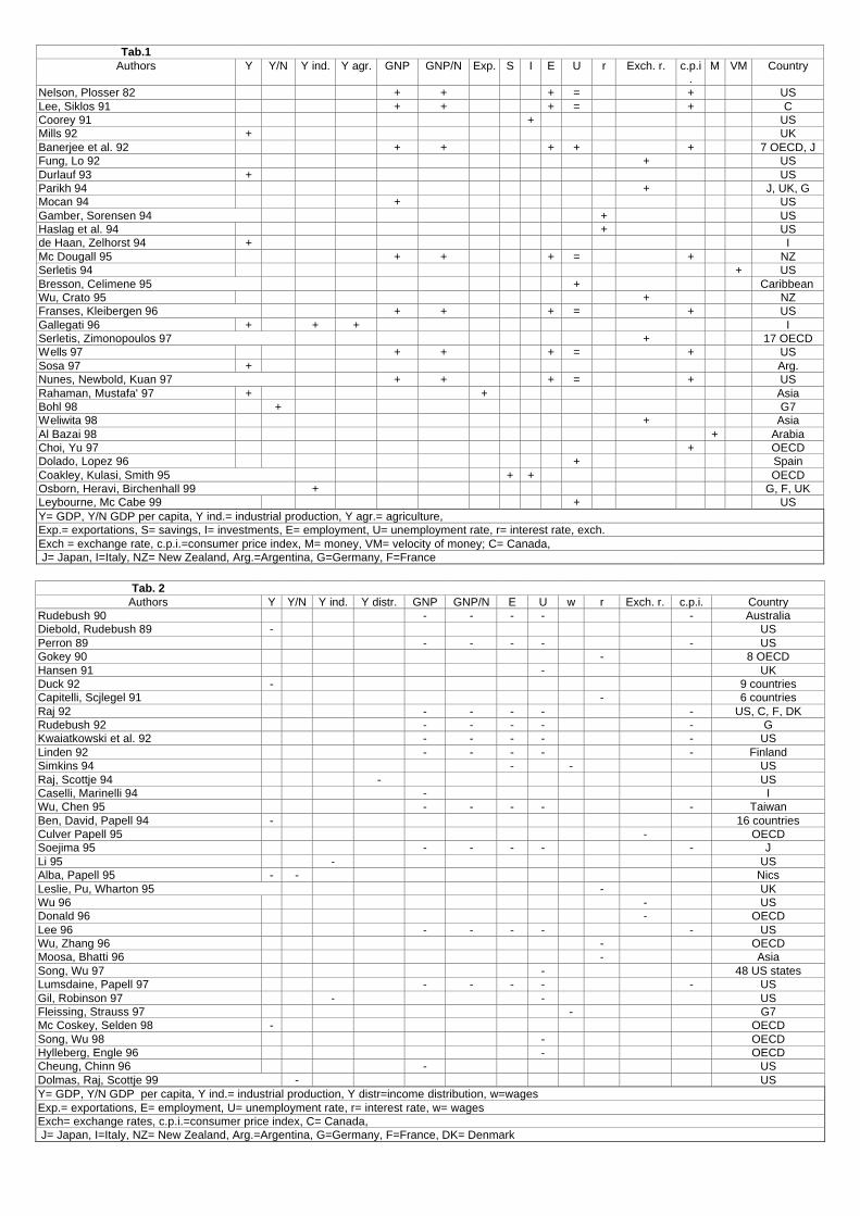
Tab.1 Authors Y Y/N Y ind. Y agr. GNP GNP/N Exp. S I E U r Exch. r. c.p.i

. M VM Country

Nelson, Plosser 82 + + + = + US Lee, Siklos 91 + + + = + C Coorey 91 + US Mills 92 + UK Banerjee et al. 92 + + + + + 7 OECD, J Fung, Lo 92 + US Durlauf 93 + US Parikh 94 + J, UK, G Mocan 94 + US Gamber, Sorensen 94 + US Haslag et al. 94 + US de Haan, Zelhorst 94 + I Mc Dougall 95 + + + = + NZ Serletis 94 + US Bresson, Celimene 95 + Caribbean Wu, Crato 95 + NZ Franses, Kleibergen 96 + + + = + US Gallegati 96 + + + I Serletis, Zimonopoulos 97 + 17 OECD Wells 97 + + + = + US Sosa 97 + Arg. Nunes, Newbold, Kuan 97 + + + = + US Rahaman, Mustafa' 97 + + Asia Bohl 98 + G7 Weliwita 98 + Asia Al Bazai 98 + Arabia Choi, Yu 97 + OECD Dolado, Lopez 96 + Spain Coakley, Kulasi, Smith 95 + + OECD Osborn, Heravi, Birchenhall 99 + G, F, UK Leybourne, Mc Cabe 99 + US Y= GDP, Y/N GDP per capita, Y ind.= industrial production, Y agr.= agriculture, Exp.= exportations, S= savings, I= investments, E= employment, U= unemployment rate, r= interest rate, exch. Exch = exchange rate, c.p.i.=consumer price index, M= money, VM= velocity of money; C= Canada, J= Japan, I=Italy, NZ= New Zealand, Arg.=Argentina, G=Germany, F=France

Tab. 2

Authors Y Y/N Y ind. Y distr. GNP GNP/N E U w r Exch. r. c.p.i. Country Rudebush 90 - - - - - Australia Diebold, Rudebush 89 - US Perron 89 - - - - - US Gokey 90 - 8 OECD Hansen 91 - UK Duck 92 - 9 countries Capitelli, Scjlegel 91 - 6 countries Raj 92 - - - - - US, C, F, DK Rudebush 92 - - - - - G Kwaiatkowski et al. 92 - - - - - US Linden 92 - - - - - Finland Simkins 94 - - US Raj, Scottje 94 - US Caselli, Marinelli 94 - I Wu, Chen 95 - - - - - Taiwan Ben, David, Papell 94 - 16 countries Culver Papell 95 - OECD Soejima 95 - - - - - J Li 95 - US Alba, Papell 95 - - Nics Leslie, Pu, Wharton 95 - UK Wu 96 - US Donald 96 - OECD Lee 96 - - - - - US Wu, Zhang 96 - OECD Moosa, Bhatti 96 - Asia Song, Wu 97 - 48 US states Lumsdaine, Papell 97 - - - - - US Gil, Robinson 97 - - US Fleissing, Strauss 97 - G7 Mc Coskey, Selden 98 - OECD Song, Wu 98 - OECD Hylleberg, Engle 96 - OECD Cheung, Chinn 96 - US Dolmas, Raj, Scottje 99 - US Y= GDP, Y/N GDP per capita, Y ind.= industrial production, Y distr=income distribution, w=wages Exp.= exportations, E= employment, U= unemployment rate, r= interest rate, w= wages Exch= exchange rates, c.p.i.=consumer price index, C= Canada, J= Japan, I=Italy, NZ= New Zealand, Arg.=Argentina, G=Germany, F=France, DK= Denmark

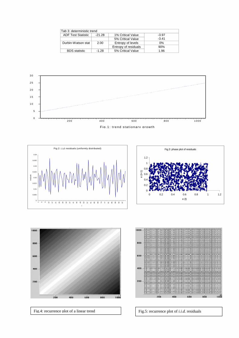
Tab 3: deterministic trend ADF Test Statistic -21.28 1% Critical Value

5% Critical Value -3.97 -3.41

Entropy of levels 0% Durbin-Watson stat 2.00 Entropy of residuals 90%

BDS statistic -1.28 5% Critical Value 1.96

Fig.2: i.i.d residuals (uniformly distributed)

0

0.005

0.01

0.015

0.02

0.025

0.03

0.035

0.04

1 5 9 13 17 21 25 29 33 37 41 45 49 53 57 61 65 69 73 77 81 85 89 93 97

t

resi

dual

s

0

5

1 0

1 5

2 0

2 5

3 0

2 0 0 4 0 0 6 0 0 8 0 0 1 0 0 0

F ig .1 : t rend s ta t i ona ry g rowth

Fig.3: phase plot of residuals

0

0.2

0.4

0.6

0.8

1

1.2

0 0.2 0.4 0.6 0.8 1 1.2

e (t)

e (t

+1)

Fig.4: recurrence plot of a linear trend Fig.5: recurrence plot of i.i.d. residuals

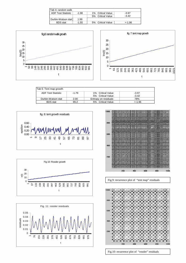
Tab 4: random walk ADF Test Statistic -1.98 1% Critical Value

5% Critical Value -3.97 -3.42

Durbin-Watson stat 1.99 BDS stat -1.55 5% Critical Value +-1.96

Tab 5: Tent map growth

ADF Test Statistic -1.79 1% Critical Value 5% Critical Value

-3.97 -3.42

Durbin-Watson stat 2.00 Entropy on residuals 78% BDS stat 99.2 5% Critical Value +-1.96

fig. 7: tent map growth

0

5

10

15

20

25

30

1 61 121

181

241

301

361

421

481

541

601

661

721

781

841

901

961

1021

t

lnx(

t)

fig.6: random walk growth

05

1015202530

1 50 99 148

197

246

295

344

393

442

491

540

589

638

687

736

785

834

883

932

981

t

lny(

t)

fig. 8: tent growth residuals

0.000.200.400.60

1 9 17 25 33 41 49 57 65 73 81 89 97

t

epsi

lon

Fig.9: recurrence plot of “tent map” residuals

Fig. 11: rossler residuals

0

0.01

0.02

0.03

0.04

0.05

1 76 151

226

301

376

451

526

601

676

751

826

901

976

t

resi

dual

s

Fig 10: Rossler growth

0

10

20

30

1 67 133

199

265

331

397

463

529

595

661

727

793

859

925

991

t

x(t)

Fig.10: recurrence plot of “rossler” residuals

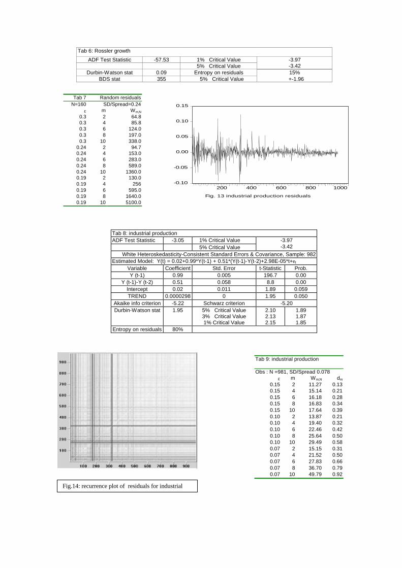
Tab 6: Rossler growth

ADF Test Statistic -57.53 1% Critical Value 5% Critical Value

-3.97 -3.42

Durbin-Watson stat 0.09 Entropy on residuals 15% BDS stat 355 5% Critical Value +-1.96

Tab 8: industrial production ADF Test Statistic -3.05 1% Critical Value

5% Critical Value -3.97 -3.42

White Heteroskedasticity-Consistent Standard Errors & Covariance, Sample: 982 Estimated Model: Y(t) = 0.02+0.99*Y(t-1) + 0.51*(Y(t-1)-Y(t-2)+2.98E-05*t+et

Variable Coefficient Std. Error t-Statistic Prob. Y (t-1) 0.99 0.005 196.7 0.00

Y (t-1)-Y (t-2) 0.51 0.058 8.8 0.00 Intercept 0.02 0.011 1.89 0.059 TREND 0.0000298 0 1.95 0.050

Akaike info criterion -5.22 Schwarz criterion -5.20 Durbin-Watson stat 1.95 5% Critical Value

3% Critical Value 1% Critical Value

2.10 2.13 2.15

1.89 1.87 1.85

Entropy on residuals 80%

-0.10

-0.05

0.00

0.05

0.10

0.15

200 400 600 800 1000

Fig. 13 industrial production residuals

Tab 7 Random residuals N=160 SD/Spread=0.24

ε m Wm,N

0.3 2 64.8 0.3 4 85.8 0.3 6 124.0 0.3 8 197.0 0.3 10 338.0

0.24 2 94.7 0.24 4 153.0 0.24 6 283.0 0.24 8 589.0 0.24 10 1360.0 0.19 2 130.0 0.19 4 256 0.19 6 595.0 0.19 8 1640.0 0.19 10 5100.0

Tab 9: industrial production Obs : N =981, SD/Spread 0.078

ε m Wm,N dm 0.15 2 11.27 0.13 0.15 4 15.14 0.21 0.15 6 16.18 0.28 0.15 8 16.83 0.34 0.15 10 17.64 0.39 0.10 2 13.87 0.21 0.10 4 19.40 0.32 0.10 6 22.46 0.42 0.10 8 25.64 0.50 0.10 10 29.49 0.58 0.07 2 15.15 0.31 0.07 4 21.52 0.50 0.07 6 27.83 0.66 0.07 8 36.70 0.79 0.07 10 49.79 0.92

Fig.14: recurrence plot of residuals for industrial

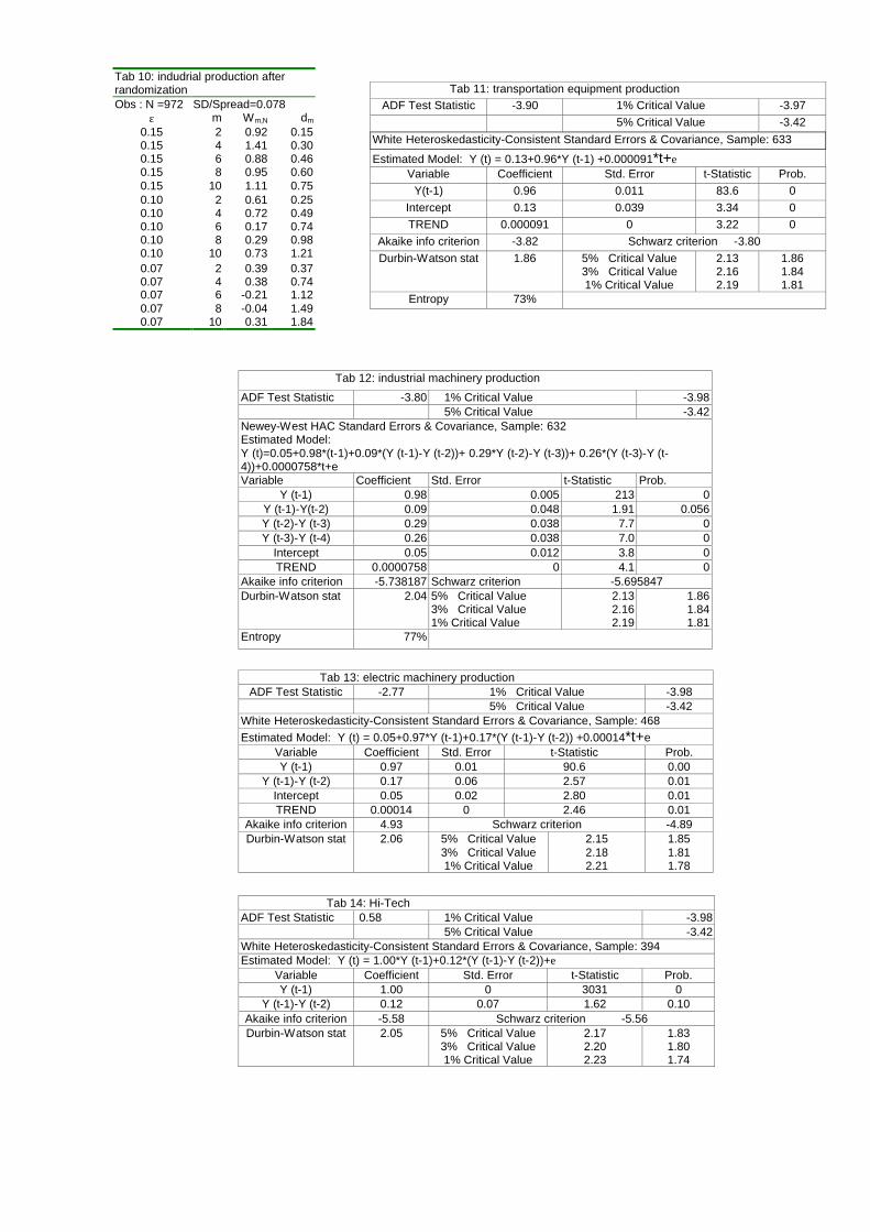
Tab 11: transportation equipment production ADF Test Statistic -3.90 1% Critical Value -3.97

5% Critical Value -3.42

White Heteroskedasticity-Consistent Standard Errors & Covariance, Sample: 633

Estimated Model: Y (t) = 0.13+0.96*Y (t-1) +0.000091*t+e Variable Coefficient Std. Error t-Statistic Prob.

Y(t-1) 0.96 0.011 83.6 0

Intercept 0.13 0.039 3.34 0

TREND 0.000091 0 3.22 0

Akaike info criterion -3.82 Schwarz criterion -3.80

Durbin-Watson stat 1.86 5% Critical Value 3% Critical Value 1% Critical Value

2.13 2.16 2.19

1.86 1.84 1.81

Entropy 73%

Tab 12: industrial machinery production

ADF Test Statistic -3.80 1% Critical Value -3.98 5% Critical Value -3.42

Newey-West HAC Standard Errors & Covariance, Sample: 632 Estimated Model: Y (t)=0.05+0.98*(t-1)+0.09*(Y (t-1)-Y (t-2))+ 0.29*Y (t-2)-Y (t-3))+ 0.26*(Y (t-3)-Y (t-4))+0.0000758*t+e Variable Coefficient Std. Error t-Statistic Prob.

Y (t-1) 0.98 0.005 213 0 Y (t-1)-Y(t-2) 0.09 0.048 1.91 0.056 Y (t-2)-Y (t-3) 0.29 0.038 7.7 0 Y (t-3)-Y (t-4) 0.26 0.038 7.0 0

Intercept 0.05 0.012 3.8 0 TREND 0.0000758 0 4.1 0

Akaike info criterion -5.738187 Schwarz criterion -5.695847 Durbin-Watson stat 2.04 5% Critical Value

3% Critical Value 1% Critical Value

2.13 2.16 2.19

1.86 1.84 1.81

Entropy 77%

Tab 13: electric machinery production ADF Test Statistic -2.77 1% Critical Value -3.98

5% Critical Value -3.42 White Heteroskedasticity-Consistent Standard Errors & Covariance, Sample: 468

Estimated Model: Y (t) = 0.05+0.97*Y (t-1)+0.17*(Y (t-1)-Y (t-2)) +0.00014*t+e Variable Coefficient Std. Error t-Statistic Prob. Y (t-1) 0.97 0.01 90.6 0.00

Y (t-1)-Y (t-2) 0.17 0.06 2.57 0.01 Intercept 0.05 0.02 2.80 0.01 TREND 0.00014 0 2.46 0.01

Akaike info criterion 4.93 Schwarz criterion -4.89 Durbin-Watson stat 2.06 5% Critical Value

3% Critical Value 1% Critical Value

2.15 2.18 2.21

1.85 1.81 1.78

Tab 14: Hi-Tech ADF Test Statistic 0.58 1% Critical Value -3.98

5% Critical Value -3.42 White Heteroskedasticity-Consistent Standard Errors & Covariance, Sample: 394 Estimated Model: Y (t) = 1.00*Y (t-1)+0.12*(Y (t-1)-Y (t-2))+e

Variable Coefficient Std. Error t-Statistic Prob. Y (t-1) 1.00 0 3031 0

Y (t-1)-Y (t-2) 0.12 0.07 1.62 0.10 Akaike info criterion -5.58 Schwarz criterion -5.56 Durbin-Watson stat 2.05 5% Critical Value

3% Critical Value 1% Critical Value

2.17 2.20 2.23

1.83 1.80 1.74

Tab 10: indudrial production after randomization Obs : N =972 SD/Spread=0.078

ε m Wm,N dm 0.15 2 0.92 0.15 0.15 4 1.41 0.30 0.15 6 0.88 0.46 0.15 8 0.95 0.60 0.15 10 1.11 0.75 0.10 2 0.61 0.25 0.10 4 0.72 0.49 0.10 6 0.17 0.74 0.10 8 0.29 0.98 0.10 10 0.73 1.21 0.07 2 0.39 0.37 0.07 4 0.38 0.74 0.07 6 -0.21 1.12 0.07 8 -0.04 1.49 0.07 10 0.31 1.84

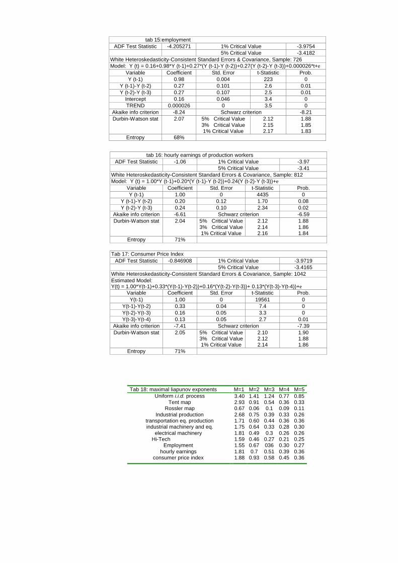
tab 16: hourly earnings of production workers ADF Test Statistic -1.06 1% Critical Value -3.97

5% Critical Value -3.41 White Heteroskedasticity-Consistent Standard Errors & Covariance, Sample: 812 Model: Y (t) = 1.00*Y (t-1)+0.20*(Y (t-1)-Y (t-2))+0.24(Y (t-2)-Y (t-3))+e

Variable Coefficient Std. Error t-Statistic Prob. Y (t-1) 1.00 0 4435 0

Y (t-1)-Y (t-2) 0.20 0.12 1.70 0.08 Y (t-2)-Y (t-3) 0.24 0.10 2.34 0.02

Akaike info criterion -6.61 Schwarz criterion -6.59 Durbin-Watson stat 2.04 5% Critical Value

3% Critical Value 1% Critical Value

2.12 2.14 2.16

1.88 1.86 1.84

Entropy 71%

Tab 17: Consumer Price Index ADF Test Statistic -0.846908 1% Critical Value -3.9719

5% Critical Value -3.4165 White Heteroskedasticity-Consistent Standard Errors & Covariance, Sample: 1042 Estimated Model: Y(t) = 1.00*Y(t-1)+0.33*(Y(t-1)-Y(t-2))+0.16*(Y(t-2)-Y(t-3))+ 0.13*(Y(t-3)-Y(t-4))+e

Variable Coefficient Std. Error t-Statistic Prob. Y(t-1) 1.00 0 19561 0

Y(t-1)-Y(t-2) 0.33 0.04 7.4 0 Y(t-2)-Y(t-3) 0.16 0.05 3.3 0 Y(t-3)-Y(t-4) 0.13 0.05 2.7 0.01

Akaike info criterion -7.41 Schwarz criterion -7.39 Durbin-Watson stat 2.05 5% Critical Value

3% Critical Value 1% Critical Value

2.10 2.12 2.14

1.90 1.88 1.86

Entropy 71%

tab 15:employment ADF Test Statistic -4.205271 1% Critical Value -3.9754

5% Critical Value -3.4182 White Heteroskedasticity-Consistent Standard Errors & Covariance, Sample: 726 Model: Y (t) = 0.16+0.98*Y (t-1)+0.27*(Y (t-1)-Y (t-2))+0.27(Y (t-2)-Y (t-3))+0.000026*t+e

Variable Coefficient Std. Error t-Statistic Prob. Y (t-1) 0.98 0.004 223 0

Y (t-1)-Y (t-2) 0.27 0.101 2.6 0.01 Y (t-2)-Y (t-3) 0.27 0.107 2.5 0.01

Intercept 0.16 0.046 3.4 0 TREND 0.000026 0 3.5 0

Akaike info criterion -8.24 Schwarz criterion -8.21 Durbin-Watson stat 2.07 5% Critical Value

3% Critical Value 1% Critical Value

2.12 2.15 2.17

1.88 1.85 1.83

Entropy 68%

Tab 18: maximal liapunov exponents M=1 M=2 M=3 M=4 M=5 Uniform i.i.d. process 3.40 1.41 1.24 0.77 0.85

Tent map 2.93 0.91 0.54 0.36 0.33 Rossler map 0.67 0.06 0.1 0.09 0.11

Industrial production 2.68 0.75 0.39 0.33 0.26 transportation eq. production 1.71 0.60 0.44 0.36 0.36 industrial machinery and eq. 1.75 0.64 0.33 0.28 0.30

electrical machinery 1.81 0.49 0.3 0.26 0.26 Hi-Tech 1.59 0.46 0.27 0.21 0.25

Employment 1.55 0.67 036 0.30 0.27 hourly earnings 1.81 0.7 0.51 0.39 0.36

consumer price index 1.88 0.93 0.58 0.45 0.36

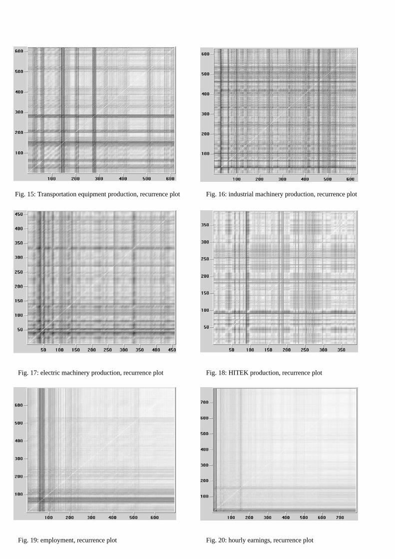
Fig. 15: Transportation equipment production, recurrence plot Fig. 16: industrial machinery production, recurrence plot

Fig. 17: electric machinery production, recurrence plot Fig. 18: HITEK production, recurrence plot

Fig. 19: employment, recurrence plot Fig. 20: hourly earnings, recurrence plot

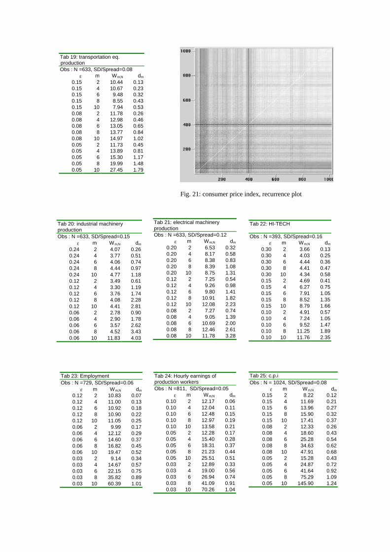
Fig. 21: consumer price index, recurrence plot

Tab 21: electrical machinery production Obs : N =633, SD/Spread=0.12

ε m Wm,N dm 0.20 2 6.53 0.32 0.20 4 8.17 0.58 0.20 6 8.38 0.83 0.20 8 8.39 1.08 0.20 10 8.75 1.31 0.12 2 7.25 0.54 0.12 4 9.26 0.98 0.12 6 9.80 1.41 0.12 8 10.91 1.82 0.12 10 12.08 2.23 0.08 2 7.27 0.74 0.08 4 9.05 1.39 0.08 6 10.69 2.00 0.08 8 12.46 2.61 0.08 10 11.78 3.28

Tab 22: HI-TECH Obs : N =393, SD/Spread=0.16

ε m Wm,N dm 0.30 2 3.66 0.13 0.30 4 4.03 0.25 0.30 6 4.44 0.36 0.30 8 4.41 0.47 0.30 10 4.34 0.58 0.15 2 4.69 0.41 0.15 4 6.27 0.75 0.15 6 7.91 1.05 0.15 8 8.52 1.35 0.15 10 8.79 1.66 0.10 2 4.91 0.57 0.10 4 7.24 1.05 0.10 6 9.52 1.47 0.10 8 11.25 1.89 0.10 10 11.76 2.35

Tab 23: Employment Obs : N =729, SD/Spread=0.06

ε m Wm,N dm 0.12 2 10.83 0.07 0.12 4 11.00 0.13 0.12 6 10.92 0.18 0.12 8 10.90 0.22 0.12 10 11.05 0.25 0.06 2 9.99 0.17 0.06 4 12.12 0.29 0.06 6 14.60 0.37 0.06 8 16.82 0.45 0.06 10 19.47 0.52 0.03 2 9.14 0.34 0.03 4 14.67 0.57 0.03 6 22.15 0.75 0.03 8 35.82 0.89 0.03 10 60.39 1.01

Tab 25: c.p.i Obs : N = 1024, SD/Spread=0.08

ε m Wm,N dm 0.15 2 8.22 0.12 0.15 4 11.69 0.21 0.15 6 13.96 0.27 0.15 8 15.90 0.32 0.15 10 17.41 0.37 0.08 2 12.33 0.26 0.08 4 18.60 0.43 0.08 6 25.28 0.54 0.08 8 34.63 0.62 0.08 10 47.91 0.68 0.05 2 15.28 0.43 0.05 4 24.87 0.72 0.05 6 41.64 0.92 0.05 8 75.29 1.09 0.05 10 145.90 1.24

Tab 24: Hourly earnings of production workers Obs : N =811, SD/Spread=0.05

ε m Wm,N dm 0.10 2 12.17 0.06 0.10 4 12.04 0.11 0.10 6 12.48 0.15 0.10 8 12.97 0.19 0.10 10 13.58 0.21 0.05 2 12.28 0.17 0.05 4 15.40 0.28 0.05 6 18.31 0.37 0.05 8 21.23 0.44 0.05 10 25.51 0.51 0.03 2 12.89 0.33 0.03 4 19.00 0.56 0.03 6 26.94 0.74 0.03 8 41.09 0.91 0.03 10 70.26 1.04

Tab 19: transportation eq. production Obs : N =633, SD/Spread=0.08

ε m Wm,N dm 0.15 2 10.44 0.13 0.15 4 10.67 0.23 0.15 6 9.48 0.32 0.15 8 8.55 0.43 0.15 10 7.94 0.53 0.08 2 11.78 0.26 0.08 4 12.98 0.46 0.08 6 13.05 0.65 0.08 8 13.77 0.84 0.08 10 14.97 1.02 0.05 2 11.73 0.45 0.05 4 13.89 0.81 0.05 6 15.30 1.17 0.05 8 19.99 1.48 0.05 10 27.45 1.79

Tab 20: industrial machinery production Obs : N =633, SD/Spread=0.15

ε m Wm,N dm 0.24 2 4.07 0.26 0.24 4 3.77 0.51 0.24 6 4.06 0.74 0.24 8 4.44 0.97 0.24 10 4.77 1.18 0.12 2 3.49 0.61 0.12 4 3.30 1.19 0.12 6 3.76 1.74 0.12 8 4.08 2.28 0.12 10 4.41 2.81 0.06 2 2.78 0.90 0.06 4 2.90 1.78 0.06 6 3.57 2.62 0.06 8 4.52 3.43 0.06 10 11.83 4.03

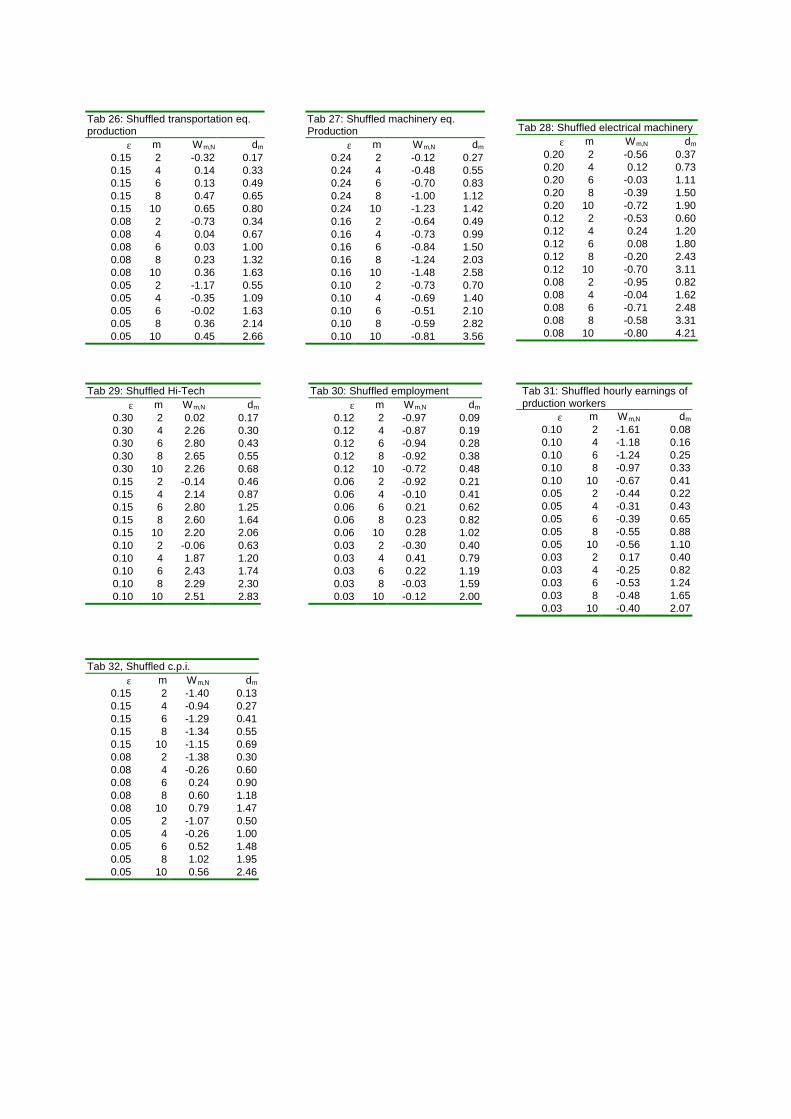
Tab 27: Shuffled machinery eq. Production

ε m Wm,N dm 0.24 2 -0.12 0.27 0.24 4 -0.48 0.55 0.24 6 -0.70 0.83 0.24 8 -1.00 1.12 0.24 10 -1.23 1.42 0.16 2 -0.64 0.49 0.16 4 -0.73 0.99 0.16 6 -0.84 1.50 0.16 8 -1.24 2.03 0.16 10 -1.48 2.58 0.10 2 -0.73 0.70 0.10 4 -0.69 1.40 0.10 6 -0.51 2.10 0.10 8 -0.59 2.82 0.10 10 -0.81 3.56

Tab 26: Shuffled transportation eq. production

ε m Wm,N dm 0.15 2 -0.32 0.17 0.15 4 0.14 0.33 0.15 6 0.13 0.49 0.15 8 0.47 0.65 0.15 10 0.65 0.80 0.08 2 -0.73 0.34 0.08 4 0.04 0.67 0.08 6 0.03 1.00 0.08 8 0.23 1.32 0.08 10 0.36 1.63 0.05 2 -1.17 0.55 0.05 4 -0.35 1.09 0.05 6 -0.02 1.63 0.05 8 0.36 2.14 0.05 10 0.45 2.66

Tab 28: Shuffled electrical machinery ε m Wm,N dm

0.20 2 -0.56 0.37 0.20 4 0.12 0.73 0.20 6 -0.03 1.11 0.20 8 -0.39 1.50 0.20 10 -0.72 1.90 0.12 2 -0.53 0.60 0.12 4 0.24 1.20 0.12 6 0.08 1.80 0.12 8 -0.20 2.43 0.12 10 -0.70 3.11 0.08 2 -0.95 0.82 0.08 4 -0.04 1.62 0.08 6 -0.71 2.48 0.08 8 -0.58 3.31 0.08 10 -0.80 4.21

Tab 29: Shuffled Hi-Tech ε m Wm,N dm

0.30 2 0.02 0.17 0.30 4 2.26 0.30 0.30 6 2.80 0.43 0.30 8 2.65 0.55 0.30 10 2.26 0.68 0.15 2 -0.14 0.46 0.15 4 2.14 0.87 0.15 6 2.80 1.25 0.15 8 2.60 1.64 0.15 10 2.20 2.06 0.10 2 -0.06 0.63 0.10 4 1.87 1.20 0.10 6 2.43 1.74 0.10 8 2.29 2.30 0.10 10 2.51 2.83

Tab 30: Shuffled employment ε m Wm,N dm

0.12 2 -0.97 0.09 0.12 4 -0.87 0.19 0.12 6 -0.94 0.28 0.12 8 -0.92 0.38 0.12 10 -0.72 0.48 0.06 2 -0.92 0.21 0.06 4 -0.10 0.41 0.06 6 0.21 0.62 0.06 8 0.23 0.82 0.06 10 0.28 1.02 0.03 2 -0.30 0.40 0.03 4 0.41 0.79 0.03 6 0.22 1.19 0.03 8 -0.03 1.59 0.03 10 -0.12 2.00

Tab 31: Shuffled hourly earnings of prduction workers

ε m Wm,N dm 0.10 2 -1.61 0.08 0.10 4 -1.18 0.16 0.10 6 -1.24 0.25 0.10 8 -0.97 0.33 0.10 10 -0.67 0.41 0.05 2 -0.44 0.22 0.05 4 -0.31 0.43 0.05 6 -0.39 0.65 0.05 8 -0.55 0.88 0.05 10 -0.56 1.10 0.03 2 0.17 0.40 0.03 4 -0.25 0.82 0.03 6 -0.53 1.24 0.03 8 -0.48 1.65 0.03 10 -0.40 2.07

Tab 32, Shuffled c.p.i. ε m Wm,N dm

0.15 2 -1.40 0.13 0.15 4 -0.94 0.27 0.15 6 -1.29 0.41 0.15 8 -1.34 0.55 0.15 10 -1.15 0.69 0.08 2 -1.38 0.30 0.08 4 -0.26 0.60 0.08 6 0.24 0.90 0.08 8 0.60 1.18 0.08 10 0.79 1.47 0.05 2 -1.07 0.50 0.05 4 -0.26 1.00 0.05 6 0.52 1.48 0.05 8 1.02 1.95 0.05 10 0.56 2.46