Embed Size (px)
Citation preview
Qualitative Spatial Configuration Queries
Towards Next Generation Access Methods for gis
Paolo Fogliaroni
Dissertation
zur Erlangung des Grades eines Doktors der
Ingenieurwissenschaften
— Dr.-Ing. —
Vorgelegt im Fachbereich 3 (Mathematik & Informatik)
der Universität Bremen
26 Juli 2012

Datum des Promotionskolloquiums:
Gutachter: Prof. Christian Freksa, Ph.D. (Universität Bremen)
Dieter Pfoser, Ph.D. (Research Center “athena”, Institute forthe Management of Information Systems)
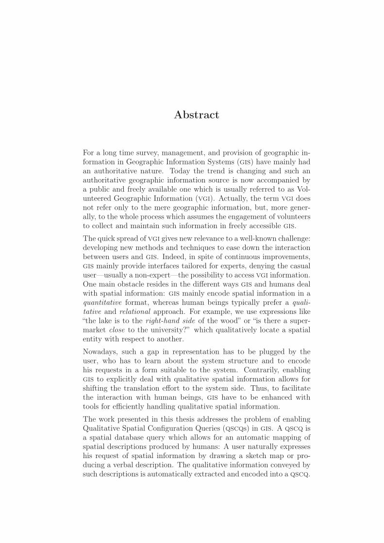
Abstract
For a long time survey, management, and provision of geographic in-formation in Geographic Information Systems (gis) have mainly hadan authoritative nature. Today the trend is changing and such anauthoritative geographic information source is now accompanied bya public and freely available one which is usually referred to as Vol-unteered Geographic Information (vgi). Actually, the term vgi doesnot refer only to the mere geographic information, but, more gener-ally, to the whole process which assumes the engagement of volunteersto collect and maintain such information in freely accessible gis.
The quick spread of vgi gives new relevance to a well-known challenge:developing new methods and techniques to ease down the interactionbetween users and gis. Indeed, in spite of continuous improvements,gis mainly provide interfaces tailored for experts, denying the casualuser—usually a non-expert—the possibility to access vgi information.One main obstacle resides in the different ways gis and humans dealwith spatial information: gis mainly encode spatial information in aquantitative format, whereas human beings typically prefer a quali-tative and relational approach. For example, we use expressions like“the lake is to the right-hand side of the wood” or “is there a super-market close to the university?” which qualitatively locate a spatialentity with respect to another.
Nowadays, such a gap in representation has to be plugged by theuser, who has to learn about the system structure and to encodehis requests in a form suitable to the system. Contrarily, enablinggis to explicitly deal with qualitative spatial information allows forshifting the translation effort to the system side. Thus, to facilitatethe interaction with human beings, gis have to be enhanced withtools for efficiently handling qualitative spatial information.
The work presented in this thesis addresses the problem of enablingQualitative Spatial Configuration Queries (qscqs) in gis. A qscq isa spatial database query which allows for an automatic mapping ofspatial descriptions produced by humans: A user naturally expresseshis request of spatial information by drawing a sketch map or pro-ducing a verbal description. The qualitative information conveyed bysuch descriptions is automatically extracted and encoded into a qscq.

The focus of this work is on two main challenges: First, the develop-ment of a framework that allows for managing in a spatial databasethe variety of spatial aspects that might be enclosed in a spatial de-scription produced by a human. Second, the conception of QualitativeSpatial Access Methods (qsams): algorithms and data structures tai-lored for efficiently solving qscqs. The main objective of a qsamis that of countering the exponential explosion in terms of storagespace—occurring when switching from a quantitative to a qualitativespatial representation—while keeping query response time acceptable.
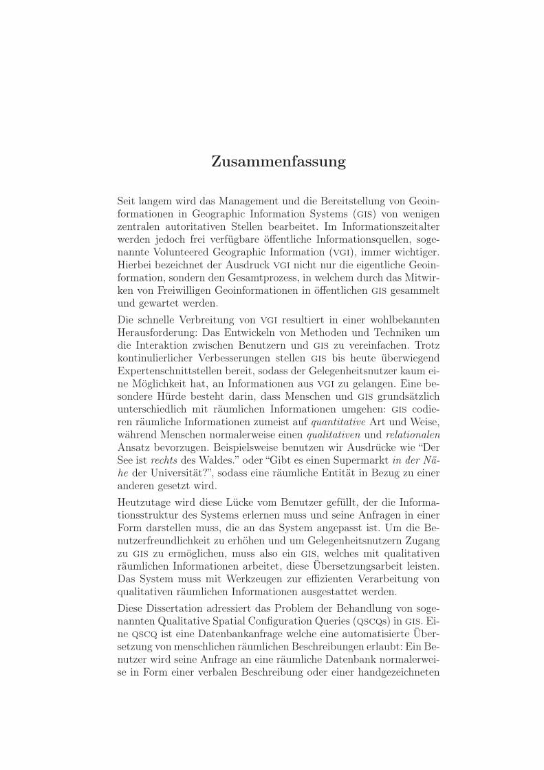
Zusammenfassung
Seit langem wird das Management und die Bereitstellung von Geoin-formationen in Geographic Information Systems (gis) von wenigenzentralen autoritativen Stellen bearbeitet. Im Informationszeitalterwerden jedoch frei verfügbare öffentliche Informationsquellen, soge-nannte Volunteered Geographic Information (vgi), immer wichtiger.Hierbei bezeichnet der Ausdruck vgi nicht nur die eigentliche Geoin-formation, sondern den Gesamtprozess, in welchem durch das Mitwir-ken von Freiwilligen Geoinformationen in öffentlichen gis gesammeltund gewartet werden.
Die schnelle Verbreitung von vgi resultiert in einer wohlbekanntenHerausforderung: Das Entwickeln von Methoden und Techniken umdie Interaktion zwischen Benutzern und gis zu vereinfachen. Trotzkontinulierlicher Verbesserungen stellen gis bis heute überwiegendExpertenschnittstellen bereit, sodass der Gelegenheitsnutzer kaum ei-ne Möglichkeit hat, an Informationen aus vgi zu gelangen. Eine be-sondere Hürde besteht darin, dass Menschen und gis grundsätzlichunterschiedlich mit räumlichen Informationen umgehen: gis codie-ren räumliche Informationen zumeist auf quantitative Art und Weise,während Menschen normalerweise einen qualitativen und relationalenAnsatz bevorzugen. Beispielsweise benutzen wir Ausdrücke wie “DerSee ist rechts des Waldes.” oder “Gibt es einen Supermarkt in der Nä-he der Universität?”, sodass eine räumliche Entität in Bezug zu eineranderen gesetzt wird.
Heutzutage wird diese Lücke vom Benutzer gefüllt, der die Informa-tionsstruktur des Systems erlernen muss und seine Anfragen in einerForm darstellen muss, die an das System angepasst ist. Um die Be-nutzerfreundlichkeit zu erhöhen und um Gelegenheitsnutzern Zugangzu gis zu ermöglichen, muss also ein gis, welches mit qualitativenräumlichen Informationen arbeitet, diese Übersetzungsarbeit leisten.Das System muss mit Werkzeugen zur effizienten Verarbeitung vonqualitativen räumlichen Informationen ausgestattet werden.
Diese Dissertation adressiert das Problem der Behandlung von soge-nannten Qualitative Spatial Configuration Queries (qscqs) in gis. Ei-ne qscq ist eine Datenbankanfrage welche eine automatisierte Über-setzung von menschlichen räumlichen Beschreibungen erlaubt: Ein Be-nutzer wird seine Anfrage an eine räumliche Datenbank normalerwei-se in Form einer verbalen Beschreibung oder einer handgezeichneten
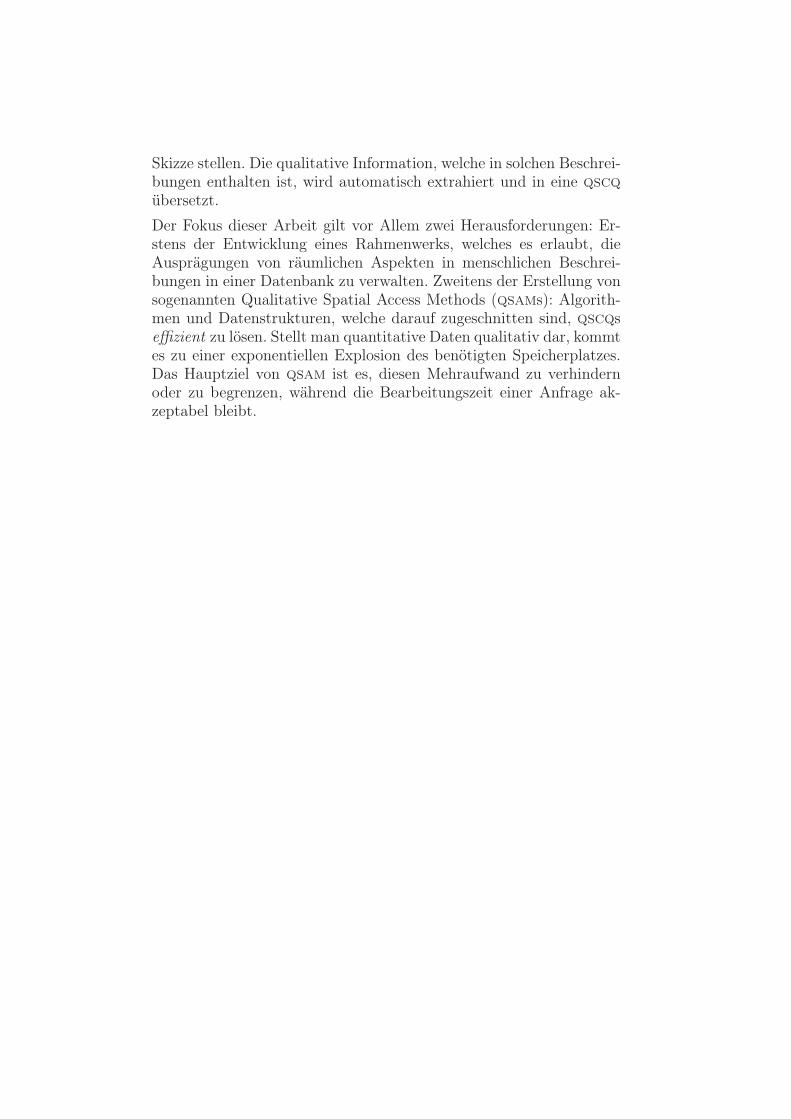
Skizze stellen. Die qualitative Information, welche in solchen Beschrei-bungen enthalten ist, wird automatisch extrahiert und in eine qscqübersetzt.
Der Fokus dieser Arbeit gilt vor Allem zwei Herausforderungen: Er-stens der Entwicklung eines Rahmenwerks, welches es erlaubt, dieAusprägungen von räumlichen Aspekten in menschlichen Beschrei-bungen in einer Datenbank zu verwalten. Zweitens der Erstellung vonsogenannten Qualitative Spatial Access Methods (qsams): Algorith-men und Datenstrukturen, welche darauf zugeschnitten sind, qscqseffizient zu lösen. Stellt man quantitative Daten qualitativ dar, kommtes zu einer exponentiellen Explosion des benötigten Speicherplatzes.Das Hauptziel von qsam ist es, diesen Mehraufwand zu verhindernoder zu begrenzen, während die Bearbeitungszeit einer Anfrage ak-zeptabel bleibt.
Sommario
La raccolta, la gestione e la fornitura di informazioni geografiche neiGeographic Information Systems (gis) ha avuto per un lungo periodouna natura prettamente autoritaria. Oggi la tendenza sta cambiandoe questa sorgente autoritaria di informazioni geografiche è ora accom-pagnata da una pubblica e liberamente disponibile a cui ci si riferisce,tipicamente, col nome di Volunteered Geographic Information (vgi).In realtà, con il termine vgi non ci si riferisce solo alle mere infor-mazioni geografiche, quanto piuttosto all’intero processo che assumel’impiego di volontari per il collezionamento ed il mantenimento ditali informazioni in gis liberamente accessibili.
La rapida diffusione del vgi da nuova rilevanza ad una ben nota sfi-da: sviluppare nuovi metodi e tecniche che facilitino l’interazione trautenti e gis. Infatti, malgrado i continui miglioramenti, i gis con-tinuano a fornire interfacce principalmente disegnate per esperti, ne-gando all’utente casuale—tipicamente un non esperto—la possibilitàdi accedere alle informazioni vgi. Uno degli ostacoli principali ri-siede nel diverso modo in cui gis ed esseri umani gestiscono le in-formazioni spaziali: mentre i gis codificano le informazioni spazialiprincipalmente in un formato quantitativo, gli esseri umani preferisco-no ricorrere, tipicamente, ad un approccio relazionale e qualitativo.Per esempio, ricorriamo ad espressioni quali “il lago si trova a de-stra del bosco” oppure ”il supermercato è vicino all’università?” chelocalizzano qualitativamente una entità spaziale rispetto ad un’altra.
Ad oggi, questo divario rappresentativo deve essere colmato dall’uten-te, il quale deve imparare a conoscere la struttura interna del sistemaed a codificare la sua richiesta in un formato che quest’ultimo possainterpretare. Viceversa, abilitare i gis al trattamento esplicito del-le informazioni spaziali qualitative permetterebbe di far ricadere losforzo di traduzione sul sistema piuttosto che sull’utente. Dunque,per facilitare l’interazione con gli esseri umani, i gis devono esserepotenziati con strumenti che permettano una gestione efficiente delleinformazioni qualitative spaziali.
Il lavoro presentato in questa tesi affronta il problema di abilitare leQualitative Spatial Configuration Queries (qscqs) nei gis. Una qscq

è un tipo di query ad un database spaziale che permette un map-ping automatico delle descrizioni spaziali prodotte dagli esseri uma-ni: un utente può esprimere la sua richiesta di informazioni spazialidisegnando delle sketch maps o producendo delle descrizioni verba-li. Le informazioni qualitative convogliate da tali descrizioni vengonoautomaticamente estratte e codificate in una qscq.
Questo lavoro si focalizza principalmente sulla risoluzione di due pro-blemi specifici. In primo luogo lo sviluppo di un framework che per-metta di gestire in un database la varietà di aspetti spaziali che pos-sono essere racchiusi in una descrizione prodotta da un essere umano.Successivamente l’attenzione è posta sull’ideazione di Qualitative Spa-tial Access Methods (qsams): algoritmi e strutture dati progettati perrisolvere efficientemente una qscq. L’obiettivo principale di un qsamè quello di contrastare l’esplosione esponenziale in termini di spaziodi memorizzazione—a cui si è soggetti quando si passa da una rap-presentazione spaziale quantitativa ad una qualitativa—mantenendo,contemporaneamente, un tempo di risposta delle query accettabile.

♦%&♦
" ♥&♥ ♥ ♦♠ &
♥♥ 1 ♣"&♦
♥ "♦ "♥

Acknowledgements
I gratefully acknowledge the Deutsche Forschungsgemeinschaft (dfg)which provided me with the financial support necessary to carry outmy research under the grant irtg grk 1498 Semantic Integration ofGeospatial Information.
Writing this dissertation took me considerably longer than I was ex-pecting. I have to admit that I have definitely underestimated theamount of work required to write a scientific text of this size in a lan-guage that is not my mother tongue. Luckily, many have supportedme during these months and helped me every time I was discouragedand tempted to admit a defeat. Well, it is time to thank all suchpeople without whom this dissertation, probably, would have nevercome to an end.
My first thought and most grateful thanks go to my supervisor, Prof.Christian Freksa. Thank you, Christian, for having given me theopportunity to work in your wonderful research group and for allowingme enough freedom to develop and pursue my ideas. Your commentshave been enlightening and they have often broadened my mind andgifted me with new perspectives on my work.
A special thank to the two post-docs who led me in the developmentof this work, Dr. Jan Oliver Wallgrün and Dr. Falko Schmid. Thankto Jan for the countless advices which helped me out in steering myresearch to the right direction, and thank to Falko who, with hisstronger pragmatism, allowed me to come to a realization of my ideasin a reasonable amount of time.
I also owe a sincere thank to all my colleagues in irtg, and especiallyto the Bremen sub-group which I have been daily in contact with.Thanks to Manfred Eppe, Torben Gerkensmeyer, Giorgio De Feliceand Jae Hee Lee for all the informal discussions and for having beenlistening to my fancy ideas. In particular, thanks to Giorgio, a long-time friend, who supported me during the dark periods and helpedme to find a way out of the countless pitfalls which I got stuck into.
I want to thank all my colleagues in the Cognitive Systems groupfor having provided me with a challenging and stimulant environmentwhere to grow my ideas. A special thank goes to Dr. Mehul Bhatt andto Dr. Diedrich Wolter. Mehul, you were always available for advis-ing and encouraging me: you taught me to trust more in my abilities.

Diedrich, your biting comments have been rumbling in my mind dur-ing the whole writing period: they helped me in being accurate in thedefinitions and picky in the descriptions.
Thanks also to all of them who accepted to revise and to proofreadpart of my thesis: Dr. Mehul Bhatt, Dr. Diedrich Wolter, Dr. FalkoSchmid, Dr. Thomas Barkowsky, Dr. Lutz Frommberger and Dr.Ana-Maria Olteteanu. And thanks again to Manfred Eppe and Tor-ben Gerkensmeyer for translating the abstract in German.
I cannot skip the administrative and technical staff: thanks to Ingrid,Gracia, Eva and Susanne for your help in deciphering and browsingthrough German bureaucracy as well as for your always happy good-mornings and your concerns about my health during the worst phasesof writing. You helped me in starting each day with the right step.Alexander, I owe you more than half of this thesis: thank for saving mefrom disk failure and for having never left me without the necessarytechnical means.
This dissertation would have never seen the daylight without the con-stant support of my family which kept believing in me every singlemoment of my life. Thank to my mother, Maddalena, and to mybrother, Andrea. This work is to reciprocate your endless supportand understanding, especially during those dark periods when I be-come intractable.
A special thank goes to my girlfriend Michela, thank you for hav-ing been at my side during this enterprise, for having listened to mespelling out my thoughts, and for having read and commented on mywriting style.
Thanks to my lifetime friends, who, similarly to my family, gave methe strength to not give up. Thanks to Andrea (Nano), Daniele(Sbrocceaux), Matteo (Naseaux), Giuseppe (Peppino), Jihad (Jax),Andrea (Gattaccio), Matteo (Ariel), Adriano (Donciò), Alessandro(Tobbino), Stefano (Senzacò), Samira (Mirasà) and Roberto (Lo Zio).Robby, this work is dedicated to your memory which will never dieout of my mind. Thank you for being my friend, and having taughtme the “secrets of life”.
Yet, thanks to the friends with whom I spent large part of my freetime here in Bremen, thanks to Sergio, Mitja, Lasse, Michael, Andachand Rami.
A final thank to all the people I met in these years, it was worth itto spending time together and sharing opinions on the most disparatetopics. You are too many to fit in such a small space, but all yournames reside in my heart.

Contents
List of Figures ix
List of Tables xi
List of Algorithms xiii
Notation and Symbols xv
Acronyms xvii
1 Introduction 1
1.1 Motivation . . . . . . . . . . . . . . . . . . . . . . . . . . . . . . . 21.2 Qualitative Spatial Relation Queries . . . . . . . . . . . . . . . . . 4
1.2.1 Natural Spatial Descriptions . . . . . . . . . . . . . . . . . 41.2.2 Qualitative Spatial Configuration Queries . . . . . . . . . . 5
1.3 Thesis and Contributions . . . . . . . . . . . . . . . . . . . . . . . 81.4 Outline of the Thesis . . . . . . . . . . . . . . . . . . . . . . . . . 9
2 Representation and Management of Spatial Information 11
2.1 Directed Hypergraphs . . . . . . . . . . . . . . . . . . . . . . . . 112.1.1 Basic Concepts . . . . . . . . . . . . . . . . . . . . . . . . 132.1.2 Connectedness . . . . . . . . . . . . . . . . . . . . . . . . . 13
2.2 Qualitative Spatial Representation and Reasoning . . . . . . . . . 162.2.1 On Qualitative Spatial Descriptions . . . . . . . . . . . . . 182.2.2 Qualitative Modeling: A World of Relations . . . . . . . . 182.2.3 Qualitative Reasoning: Relational Operations . . . . . . . 192.2.4 Classification of Qualitative Spatial Calculi . . . . . . . . . 22
2.2.4.1 Classification of Spatial Relations . . . . . . . . . 222.2.4.2 Frames of Reference, Acceptance Areas, and Re-
lation Arity . . . . . . . . . . . . . . . . . . . . . 232.2.4.3 Modeled Spaces and Spatial Primitives . . . . . . 242.2.4.4 Spatial Aspects . . . . . . . . . . . . . . . . . . . 26
2.2.5 Qualitative Constraint Networks . . . . . . . . . . . . . . . 292.2.6 Integration of Qualitative Models . . . . . . . . . . . . . . 312.2.7 On the Cognitive Adequacy of Qualitative Models . . . . . 32
vi Contents
2.3 Spatial Databases . . . . . . . . . . . . . . . . . . . . . . . . . . . 322.3.1 Spatial Data Modeling and Representation . . . . . . . . . 332.3.2 Spatial Data Management: Spatial Operators . . . . . . . 342.3.3 Spatial Queries and Indexes . . . . . . . . . . . . . . . . . 362.3.4 Spatial Access Methods . . . . . . . . . . . . . . . . . . . 372.3.5 Spatial Query Languages . . . . . . . . . . . . . . . . . . . 40
3 Qualitative Spatial Configuration Queries 43
3.1 Qualitative Spatial Relation Queries . . . . . . . . . . . . . . . . . 433.2 qscq Enablement . . . . . . . . . . . . . . . . . . . . . . . . . . . 45
3.2.1 Interpreting Natural Spatial Descriptions . . . . . . . . . . 463.2.2 Spatial Query Language Encoding . . . . . . . . . . . . . . 46
3.3 The qscq Problem . . . . . . . . . . . . . . . . . . . . . . . . . . 493.4 Solving qscqs . . . . . . . . . . . . . . . . . . . . . . . . . . . . . 51
3.4.1 Basic Retrieval Strategy . . . . . . . . . . . . . . . . . . . 533.5 Dataset Qualification . . . . . . . . . . . . . . . . . . . . . . . . . 55
3.5.1 Runtime Qualification . . . . . . . . . . . . . . . . . . . . 563.5.2 Pre-qualification . . . . . . . . . . . . . . . . . . . . . . . 57
3.6 Summary and Focus . . . . . . . . . . . . . . . . . . . . . . . . . 58
4 Qualitative Spatial Access Methods 61
4.1 Functional qsam . . . . . . . . . . . . . . . . . . . . . . . . . . . 624.2 Qualitative Storage Layer qsam . . . . . . . . . . . . . . . . . . . 634.3 Spatial Clustering qsams . . . . . . . . . . . . . . . . . . . . . . . 65
4.3.1 Background: Clustering Relations . . . . . . . . . . . . . . 654.3.2 Data Structure . . . . . . . . . . . . . . . . . . . . . . . . 674.3.3 Qualification . . . . . . . . . . . . . . . . . . . . . . . . . . 684.3.4 Retrieval . . . . . . . . . . . . . . . . . . . . . . . . . . . . 734.3.5 Final Remarks and Discussion . . . . . . . . . . . . . . . . 75
4.4 qsr-based qsam . . . . . . . . . . . . . . . . . . . . . . . . . . . 764.4.1 Background: the Inference Graph . . . . . . . . . . . . . . 76
4.4.1.1 Generating the Inference Graph . . . . . . . . . . 794.4.2 Data Structure . . . . . . . . . . . . . . . . . . . . . . . . 834.4.3 Qualification . . . . . . . . . . . . . . . . . . . . . . . . . . 834.4.4 Retrieval . . . . . . . . . . . . . . . . . . . . . . . . . . . . 944.4.5 Final Remarks and Discussion . . . . . . . . . . . . . . . . 94
4.5 Summary . . . . . . . . . . . . . . . . . . . . . . . . . . . . . . . 95
5 Developing Qualitative Spatial Access Methods 97
5.1 MyQual: an Extensible Development and Benchmark Framework 975.1.1 MyQual-Base . . . . . . . . . . . . . . . . . . . . . . . . . 995.1.2 MyQual-Toolbox . . . . . . . . . . . . . . . . . . . . . . . 1005.1.3 MyQual-Test: the Test Environment . . . . . . . . . . . . 1025.1.4 MyQual-App: the Production Environment . . . . . . . . 104
Contents vii
5.2 Implemented Spatial Clustering qsams . . . . . . . . . . . . . . . 1055.2.1 Grid -based Spatial Clustering qsam . . . . . . . . . . . . 1065.2.2 r∗-tree-based Spatial Clustering qsam . . . . . . . . . . . 109
5.3 Summary . . . . . . . . . . . . . . . . . . . . . . . . . . . . . . . 110
6 Empirical Evaluation 113
6.1 Evaluation Criteria and Experiments Setup . . . . . . . . . . . . . 1136.2 Evaluation Testbed . . . . . . . . . . . . . . . . . . . . . . . . . . 1146.3 Functional and Qualitative Storage Layer qsams . . . . . . . . . . 1166.4 Grid-based Spatial Clustering qsam . . . . . . . . . . . . . . . . . 1196.5 r∗-tree-based Spatial Clustering qsam . . . . . . . . . . . . . . . 1236.6 qsr-based qsam . . . . . . . . . . . . . . . . . . . . . . . . . . . 1286.7 A Real-World Experiment . . . . . . . . . . . . . . . . . . . . . . 1316.8 Summary and Comparison . . . . . . . . . . . . . . . . . . . . . . 133
7 Summary and Outlook 137
7.1 Summary of Results . . . . . . . . . . . . . . . . . . . . . . . . . 1377.2 Future Work . . . . . . . . . . . . . . . . . . . . . . . . . . . . . . 140
7.2.1 Minimum Qualitative Spatial Representation . . . . . . . . 1407.2.2 Empowering qsr-based qsam . . . . . . . . . . . . . . . . 1417.2.3 Other Qualitative Spatial Calculi and Inter-calculus qscqs 1427.2.4 Further Investigation on Spatial Clustering qsam . . . . . 1427.2.5 Mixed sc–qsr qsam . . . . . . . . . . . . . . . . . . . . . 1427.2.6 Dynamic and Parallel qsams . . . . . . . . . . . . . . . . 1437.2.7 Treating Disjunctive Relations and Inconsistency . . . . . 1437.2.8 Contributing Qualitative Spatial Information in vgi Projects144
References 145


List of Figures
1.1 OpenStreetMap dataset of the city of Bremen. . . . . . . . . . . . 31.2 Configuration solutions for the apartment-search example. . . . . 41.3 qscq: the space-time tradeoff. . . . . . . . . . . . . . . . . . . . . 7
2.1 Undirected, Directed, and Multi graphs. . . . . . . . . . . . . . . 122.2 Simple b-graph. . . . . . . . . . . . . . . . . . . . . . . . . . . . . 122.3 Hyperpaths, Components, and Condensation in hypergraphs. . . . 162.4 Allen temporal calculus and its application to the spatial domain. 172.5 Modeling direction relations by different frame of references. . . . 242.6 Frame of reference for extended objects. . . . . . . . . . . . . . . 252.7 Binary topological relations between extended objects. . . . . . . 262.8 Frame of reference of the Cardinal Direction Calculus. . . . . . . . 282.9 Qualitative representation of a spatial scene. . . . . . . . . . . . . 302.10 The geometric data type hierarchy. . . . . . . . . . . . . . . . . . 34
3.1 Natural spatial description queries: transformation flow. . . . . . 453.2 Logical scheme for the Bremen dataset. . . . . . . . . . . . . . . . 463.3 Multi-calculus Qualitative Constraint Network. . . . . . . . . . . 503.4 Solving a Qualitative Spatial Configuration Query (qscq). . . . . 523.5 Solving a qscq via subgraph matching. . . . . . . . . . . . . . . . 55
4.1 Clustering Relation. . . . . . . . . . . . . . . . . . . . . . . . . . . 664.2 Two possible tilesets over the same spatial dataset. . . . . . . . . 674.3 A spatial dataset and its rcc-qualification. . . . . . . . . . . . . . 774.4 Simple inference graph. . . . . . . . . . . . . . . . . . . . . . . . . 784.5 An inference path. . . . . . . . . . . . . . . . . . . . . . . . . . . 784.6 Three inference templates from the rcc reasoning tables. . . . . . 814.7 Instance of an inference graph of length l = 2. . . . . . . . . . . . 854.8 Relaxed Strongly Connected Components. . . . . . . . . . . . . . 884.9 Reducing the inference graph. . . . . . . . . . . . . . . . . . . . . 91
5.1 MyQual, logical framework overview . . . . . . . . . . . . . . . . 985.2 MyQual-Base, database schema. . . . . . . . . . . . . . . . . . . . 995.3 MyQual, interface screenshot. . . . . . . . . . . . . . . . . . . . . 1005.4 MyQual-Toolbox, database schema. . . . . . . . . . . . . . . . . . 1015.5 MyQual-Test, database schema. . . . . . . . . . . . . . . . . . . . 1025.6 Qualitative Spatial Configuration Query builder interface. . . . . . 104
x List of Figures
5.7 MyQual-App, database schema. . . . . . . . . . . . . . . . . . . . 1055.8 A spatial dataset clustered by means of two grids. . . . . . . . . . 1065.9 Grid-clustering with minimum bounding boxes. . . . . . . . . . . 1075.10 Database representation of a grid spatial clustering index. . . . . 1075.11 Database representation of an r∗-tree spatial clustering index. . . 109
6.1 A dataset from the qualification testbed. . . . . . . . . . . . . . . . 1156.2 qsl-qsam: spatial dataset qualification performance. . . . . . . . 1166.3 f-qsam: qscq execution performance. . . . . . . . . . . . . . . . 1176.4 qsl-qsam: qscq execution performance. . . . . . . . . . . . . . . 1186.5 grid -based sc-qsam: spatial dataset qualification performance. . . 1196.6 grid -based sc-qsam: qualification tuning. . . . . . . . . . . . . . 1206.7 grid -based sc-qsam: qscq execution performance. . . . . . . . . 1216.8 grid -based sc-qsam: qscq tuning. . . . . . . . . . . . . . . . . . 1226.9 r∗-tree-based sc-qsam: spatial dataset qualification performance. 1246.10 r∗-tree-based sc-qsam: qualification tuning. . . . . . . . . . . . . 1256.11 r∗-tree-based sc-qsam: qscq performance and tuning (rcc). . . 1266.12 r∗-tree-based sc-qsam: qscq performance and tuning (cdc). . . 1276.13 qsr-qsam: spatial dataset qualification performance. . . . . . . . 1296.14 Bremen: test dataset. . . . . . . . . . . . . . . . . . . . . . . . . . 131
List of Tables
2.1 Spatial operators. . . . . . . . . . . . . . . . . . . . . . . . . . . . 352.2 Most common spatial queries. . . . . . . . . . . . . . . . . . . . . 36
3.1 Classification of qualitative spatial relation queries. . . . . . . . . 44
4.1 Qualify-SC: execution over the dataset in Figure 4.2(a). . . . . 704.2 Qualify-SC: execution over the dataset in Figure 4.2(b). . . . . 724.3 Reasoning tables for rcc-8. . . . . . . . . . . . . . . . . . . . . . 804.4 Inference template tables. . . . . . . . . . . . . . . . . . . . . . . 834.5 Number of inference templates for rcc. . . . . . . . . . . . . . . . 93
6.1 Execution testbed. . . . . . . . . . . . . . . . . . . . . . . . . . . . 1156.2 Qualification performance for the Bremen dataset. . . . . . . . . . 1326.3 qscq execution performance for the Bremen dataset. . . . . . . . 1336.4 Comparison: average qualified dataset reduction. . . . . . . . . . 1346.5 Comparison: average dataset qualification time. . . . . . . . . . . 1356.6 Comparison: average qscq response time. . . . . . . . . . . . . . 135

List of Algorithms
3.1 Retrieve: Solves a given qscq Q via subgraph matching . . . . 543.2 ComputeRelationM: Computes which of the relations defined
in M holds over an a-tuple of spatial objects . . . . . . . . . . . . 564.1 ExtendPMatching-Functional: Extends the partial match-
ing (χ, ω) according to constraint ξ . . . . . . . . . . . . . . . . . 634.2 Qualify-QSL: Populates the relation tables in D with the rela-
tions induced by the spatial dataset . . . . . . . . . . . . . . . . . 644.3 ExtendPMatching-QSL: Extends the partial matching (χ, ω)
according to constraint ξ . . . . . . . . . . . . . . . . . . . . . . . 644.4 Qualify-SC: Populates the relation tables in D with the relations
induced by the spatial dataset and reduced according to the spatialclustering index I . . . . . . . . . . . . . . . . . . . . . . . . . . . 69
4.5 ExtendPMatching-SC: Extends the partial matching (χ, ω) ac-cording to constraint ξ and exploiting the index I . . . . . . . . . 73
4.6 Make-IG: Given a spatial dataset O and a spatial calculus M
constructs the inference graph IG of given length l. . . . . . . . . 844.7 Relaxed-Strongly-Connect: Computes the relaxed strongly
connected components for a given inference graph. . . . . . . . . . 894.8 GetSources: Computes a set of hyperpaths spanning the node
set of a given b-graph H and returns the source node set. . . . . . 904.9 Qualify-QSR: Populates the relation tables in D with the rela-
tions induced by the spatial dataset and reduced according to theinference graph IG of length l . . . . . . . . . . . . . . . . . . . . 92


Notation and Symbols
2S Power set of a set S,
a Arity of a generic qualitative relation or calculus,
A Arc set of a hypergraph H,
A Arity pool: set of arities of the calculi in P ,
b Cardinality of B,
B Relation pool: set of base relations of the calculi in P ,
B Cardinality of B,
B Set of base relations of a qualitative spatial calculus M,
c Number of spatial constraints in Q,
C Set of clusters associated with a spatial dataset O,
D Domain of a qualitative relation,
H A hierarchical spatial clustering index,
H A hypergraph,
I A spatial clustering index,
IG An inference graph,
IK An inference kernel,
IP An inference path,
M A qualitative spatial calculus,
N Cardinality of O,
N Node set of a hypergraph H,
O Set of spatial objects / Spatial dataset,
xvi Notation and Symbols
o A spatial object,
P Pool of available qualitative spatial calculi,
p Cardinality of P ,
Q A qualitative spatial configuration query,
r Generic qualitative spatial relation,
RM(O) Set of relations from M holding over a spatial set O,
rt A relation table,
t A tile,
T Tileset associated with a spatial dataset O,
tt A template table,
v Number of spatial variables in Q,
X Set of spatial variables in Q,
x A spatial variable,
Z Generic acceptance zone qualitative spatial relation,
ξ A spatial constraint,
Ξ Set of spatial constraints in Q,
Σ(Q) Solution of Q,
τ Sequence of tiles,
χ Sequence of spatial variables,
ω Sequence of spatial objects,

Acronyms
9-im 9-Intersection Model
ai Artificial Intelligence
cdc Cardinal Direction Calculus
csp Constraint Satisfaction Problem
dbms Database Management System
f-qsam Functional qsam
for frame of reference
gis Geographic Information System
gui Graphical User Interface
jepd jointly exhaustive and pairwise disjoint
jsp Joint Satisfaction Problem
lut Lookup table
mbr Minimum Bounding Rectangle
ogc OpenGIS Consortium
pqbe Pictorial Query-by-Example
qbe Query-by-Example
qbs Query-by-Sketch
qcn Qualitative Constraint Network
ql Query Language
qr Qualitative Reasoning
qsam Qualitative Spatial Access Method

xviii Acronyms
qscq Qualitative Spatial Configuration Query
qsl-qsam Qualitative Storage Layer qsam
qsr Qualitative Spatial Representation and Reasoning
qsr-qsam qsr-based qsam
rcc Region Connection Calculus
rdbms Relational Database Management System
sam Spatial Access Method
sc-qsam Spatial Clustering qsam
sql Structured Query Language
vgi Volunteered Geographic Information
Chapter 1
Introduction
The perception of space serves a fundamental role in everyday life. For this reasonwe have always tried to represent and store spatial information to the best of ourabilities. Beginning from geographic charts onwards, we investigated and devel-oped continuously more advanced spatial representation and analysis instrumentsthat help in easing down the process of making space-related decisions. For thispurpose, today, we use Geographic Information Systems (gis): complex com-puterized systems providing tools to store, manipulate, and analyze (geo)spatialdata.
For a long time survey, management, and provision of geographic informationin gis have mainly had an authoritative nature and the access to such informationhas been restricted to expert users. Today, thanks to the drop in the cost of surveyinstruments (mainly gps devices) and to the spread of information integrationand sharing tools characteristic of the Web 2.0, the trend is changing. The“old” authoritative geographic information source is now accompanied by a “new”,public and freely available one. Recently, Goodchild (2007) coined for it the termVolunteered Geographic Information (vgi): a particular form of user-generatedcontent that assumes the active engagement of volunteers to collect and providespatial data to be used in gis.
One main goal of vgi is to make geographic information freely available andusable. Probably the best known form of vgi is represented by web-based projectslike OpenStreetMap1, which aims at collaboratively producing a free editable mapof the world, and Wikimapia2, which furnishes spatial data that users are allowedto tag with textual information. Such projects provide web interfaces to let theusers interact with the spatial information stored in an underlying gis.
1http://www.openstreetmap.org/2http://wikimapia.org/
2 1 Introduction
1.1 Motivation
Albeit Web 2.0’s technologies allowed for bringing gis within general public’sreach, the expertise required to interact with them drastically reduce the numberof potential spatial data contributors and consumers. Indeed, in spite of continu-ous improvements, gis mainly provide interfaces tailored for experts, denying thecasual user—usually a non-expert—the possibility to fully exploit their poten-tials. The challenge of developing new methods and techniques to interact withgis in a more intuitive and natural way has been already tackled in the past (cf.Egenhofer, 1996, for example). Today, thanks to vgi, such a challenge gainednew relevance (cf. Pfoser, 2011, for example).
gis allow for performing a variety of spatial data manipulation and presen-tation for the most disparate tasks going from simple map visualization to pathplanning, to land usage examination, and to economical or criminal statistics.Nonetheless, most of these operations require a level of expertise that the casualuser does not possess. Accordingly, general public can exploit gis capabilitiesmainly by means of some web interfaces of the kind provided by OpenStreetMapor Wikimapia. According to Yao (1999), such interfaces restrict geographic dataconsumers to access spatial data in mainly two ways. (i) Location finding: de-tects a specific location and shows a map of the surrounding area; (ii) Routing:finds the shortest route between two locations. In both cases the user is requiredto specify the location(s) he is interested in either providing the specific name,the exact address or even the geographic coordinates.
Although such data access methods come in handy in many occasions, thereis an important type of access that today is largely unaccounted for. It concernscases in which we want to find a location on the basis of a set of spatial constraintsthat we specify. In such a case, most of the times we do not know the location apriori, hence we cannot specify an address or a name. From a certain perspectivethis kind of requests complements the previous ones in that the input consistssomehow of the spatial description of an entity and the expected output is theentity’s address, name, or geo-coordinates. Such a kind of requests can occur ineveryday life demands.
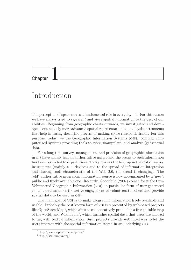
Example 1.1 (Apartment searching) - We are looking for an apartment to rent in the city
of Bremen, Germany. We obviously do not know the address in advance, but we have a
certain number of spatial constraints in our mind that the place has to satisfy. We want the
Apartment to be (i) located in between the main station and the university, (ii) in a walkingdistance from—i.e. close to—a Supermarket and (iii) a Tram- or a Bus- Stop. Lastly, (iv)we may want a Park to be visible from the Apartment. Figure 1.1 depicts the part of the
OpenStreetMap dataset of Bremen relevant for the request with icons showing entities of
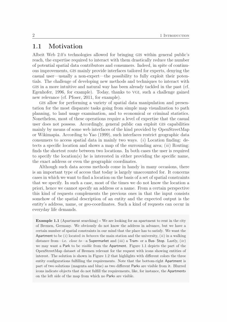
interest. The solution is shown in Figure 1.2 that highlights with different colors the three
entity configurations fulfilling the requirements. Note that the bottom-right Apartment is
part of two solutions (magenta and blue) as two different Parks are visible from it. Blurred
icons indicate objects that do not fulfill the requirements, like, for instance, the Apartments
on the left side of the map from which no Parks are visible.
1.1 Motivation 3
Flat for rent
Bus/Tram stop
Supermarket
Park
Main station
University
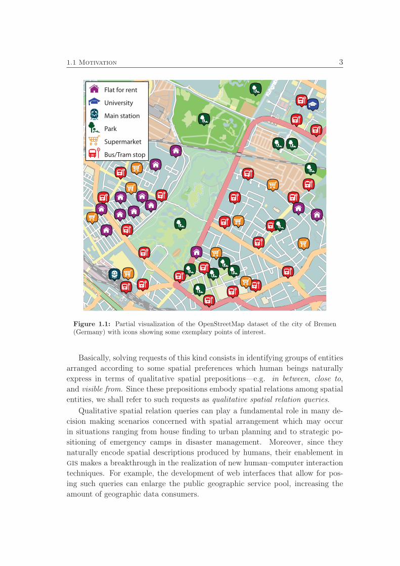
Figure 1.1: Partial visualization of the OpenStreetMap dataset of the city of Bremen(Germany) with icons showing some exemplary points of interest.
Basically, solving requests of this kind consists in identifying groups of entities
arranged according to some spatial preferences which human beings naturally
express in terms of qualitative spatial prepositions—e.g. in between, close to,
and visible from. Since these prepositions embody spatial relations among spatial
entities, we shall refer to such requests as qualitative spatial relation queries.
Qualitative spatial relation queries can play a fundamental role in many de-
cision making scenarios concerned with spatial arrangement which may occur
in situations ranging from house finding to urban planning and to strategic po-
sitioning of emergency camps in disaster management. Moreover, since they
naturally encode spatial descriptions produced by humans, their enablement in
gis makes a breakthrough in the realization of new human–computer interaction
techniques. For example, the development of web interfaces that allow for pos-
ing such queries can enlarge the public geographic service pool, increasing the
amount of geographic data consumers.
4 1 Introduction
Flat for rent
Bus/Tram stop
Supermarket
Park
Main station
University
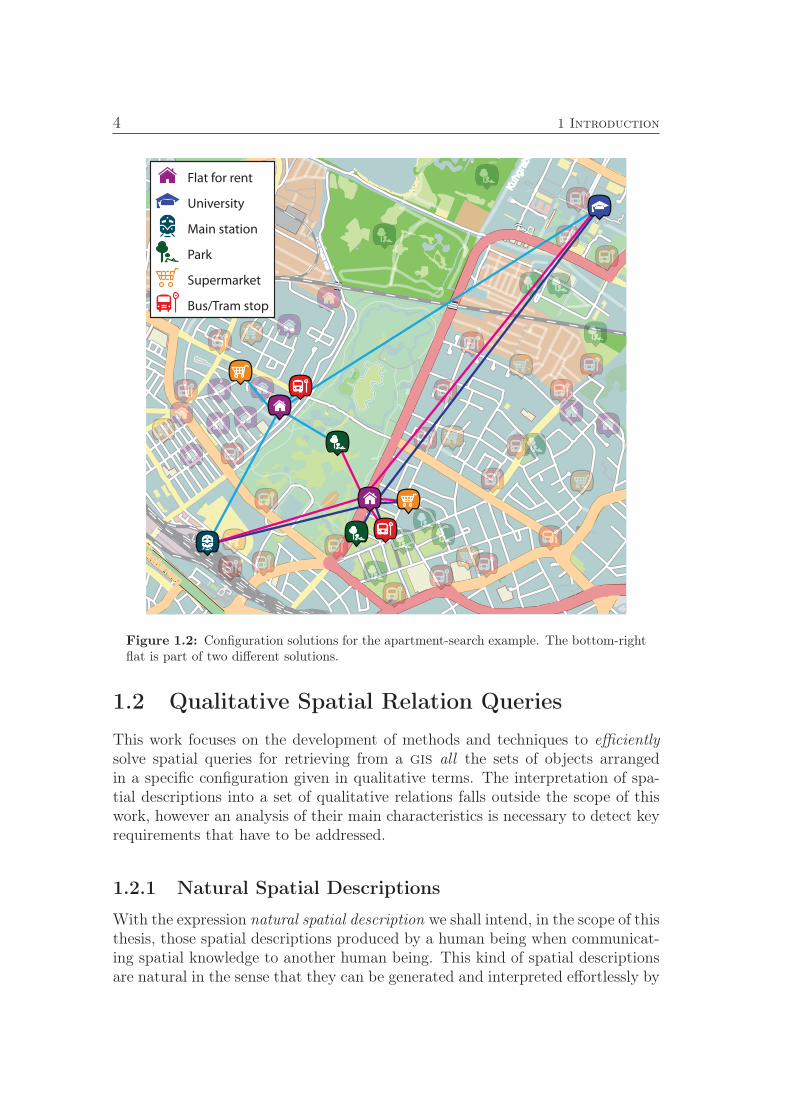
Figure 1.2: Configuration solutions for the apartment-search example. The bottom-rightflat is part of two different solutions.
1.2 Qualitative Spatial Relation Queries
This work focuses on the development of methods and techniques to efficientlysolve spatial queries for retrieving from a gis all the sets of objects arrangedin a specific configuration given in qualitative terms. The interpretation of spa-tial descriptions into a set of qualitative relations falls outside the scope of thiswork, however an analysis of their main characteristics is necessary to detect keyrequirements that have to be addressed.
1.2.1 Natural Spatial Descriptions
With the expression natural spatial description we shall intend, in the scope of thisthesis, those spatial descriptions produced by a human being when communicat-ing spatial knowledge to another human being. This kind of spatial descriptionsare natural in the sense that they can be generated and interpreted effortlessly by
1.2 Qualitative Spatial Relation Queries 5
the individuals involved in the communication process without the need to resortto further descriptive means than the description itself.
Natural spatial descriptions come mainly in two forms: verbal or pictorial. Inverbal forms a spatial entity is typically described using expressions that qual-itatively locate it with respect to one or more other objects in the scene, e.g.“The cinema is in between the university and the main station, close to the park”.Occasionally (e.g. when providing directions to a place) people likes to resortto pictorial descriptions, commonly known as sketches or sketch maps, as theyprovide a much more compact representation of spatial information. Sketch mapslook similar to real maps in that they report spatial entities in a geometric format.However, metric information is usually not intended to be reported in sketcheswhich, instead, correctly convey information about certain qualitative relationslike relative position, ordering, and connectedness. Qualitative relations, thus,are reliable pieces of information that can be extracted from both verbal and pic-torial spatial descriptions. As such, qualitative spatial relations are a key elementthat has to be considered in the development of solving techniques for queryingvia natural spatial descriptions.
A further important observation to consider when handling natural spatialdescriptions is that they usually convey information regarding several aspects ofspace. For example, the sentence “The cinema is in between the university andthe main station, close to the park” carries information about relative positionand distance. We can safely assume that for every domain/task there are someessential spatial aspects to take into account, while the others are usually irrele-vant. For instance, when giving directions to a place in a city, visibility can playan important role as the utilization of visual landmarks can allow for producingclearer instructions; similarly, relative directions might be preferable over cardi-nal ones. Contrarily, in a geographic description context in which one wants toexplain where the city of Bremen is located within Germany, cardinal directionsplay a significant role, while speaking about visual landmarks is pointless.
Heterogeneous composition of spatial descriptions and context–dependent di-versity of relevant spatial aspects are key issues to be considered to develop tech-niques that can realistically handle natural spatial descriptions. Accordingly, thiswork does not aim at treating selected aspects of space but, rather, pursues gen-eral and extensible solutions that allow for the integration of multiple qualitativespatial aspects.
1.2.2 Qualitative Spatial Configuration Queries
Usually a gis contains information about millions of real-world spatial entitieswhich are represented as geometric objects of different types, i.e. points, lines,polygons, or more complex combinations of these basic types. For example, atthe time of writing, the OpenStreetMap dataset of the Niedersachsen region, inGermany, contains nearly 1.300.000 geometric objects.
6 1 Introduction
Solving a qualitative spatial relation query is equivalent to searching for all thesets of objects in the gis arranged as described in the query. In other words, thequalitative spatial relations expressed in the query have to be matched againstthose raised by the spatial dataset.
Matching is as much easier as the number of objects uniquely specified in thequery increases: If one or more objects are specified by either their unique names,addresses, or geo-coordinates, the query difficulty scales down as the search canbe “anchored” on such entities. Similarly, specifying the category of searchedobjects allows for reducing the number of entities to be searched and, thus, thedifficulty of the query. Consequently, qualitative spatial relation queries can beclassified according to the degree of specification they provide.
Example 1.2 (Classes of qualitative spatial relation queries) - Answering the query “find
all the objects north of id”, where id identifies a certain object in the gis, consists in
checking which cardinal direction relation holds between any object o in the gis and id and
retrieving all the objects such that o is north of id.A more demanding query might be “find all the Supermarkets north of a Park”, where
Supermarket and Park are categories of spatial entities which the geometric object in the gis
are tagged with. Answering this query requires to check all the object pairs Supermarket-
Park in order to identify and retrieve those satisfying the expressed request.
This work focuses on the hardest class of qualitative spatial relation queries,namely that in which neither searched objects are fixed nor any kind of tag orcategorization that allows for reducing the search space is given. We shall referto such queries as Qualitative Spatial Configuration Queries (qscqs).
Efficiently Solving qscqs: Managing the Space-Time Tradeoff Whenswitching from the geometric objects to the qualitative spatial relations existingover them, the amount of data to be considered is subjected to a combinatorialexplosion: Let us assume, for simplicity, we are only interested in cardinal direc-tions, then every pair of objects from a spatial dataset raises one qualitative rela-tion. Hence, the Niedersachsen dataset gives rise to nearly (1.3 ·106)2 = 1.69 ·1012
cardinal direction relations. This number is doomed to augment in a realistic casewhen multiple spatial aspects have to be accounted for. Accordingly, one of themain challenges in solving a qscq is that of opportunely managing the access tosuch an enormous number of qualitative spatial relations.Qualitative spatial relations are not explicitly stored in a gis, thus, in order
to perform the matching required to solve a qscq, they have to be computedfrom a geographic dataset. Given the typical size of a geographic dataset such anoperation might require an amount of time unacceptable in a human-computerinteraction scenario: For instance, in the apartment searching scenario reported inExample 1.1 a user would expect to receive an answer to his request within a fewseconds whereas computing the qualitative relations might require hours, days oreven months according to the size of the geographic dataset under consideration.
1.2 Qualitative Spatial Relation Queries 7
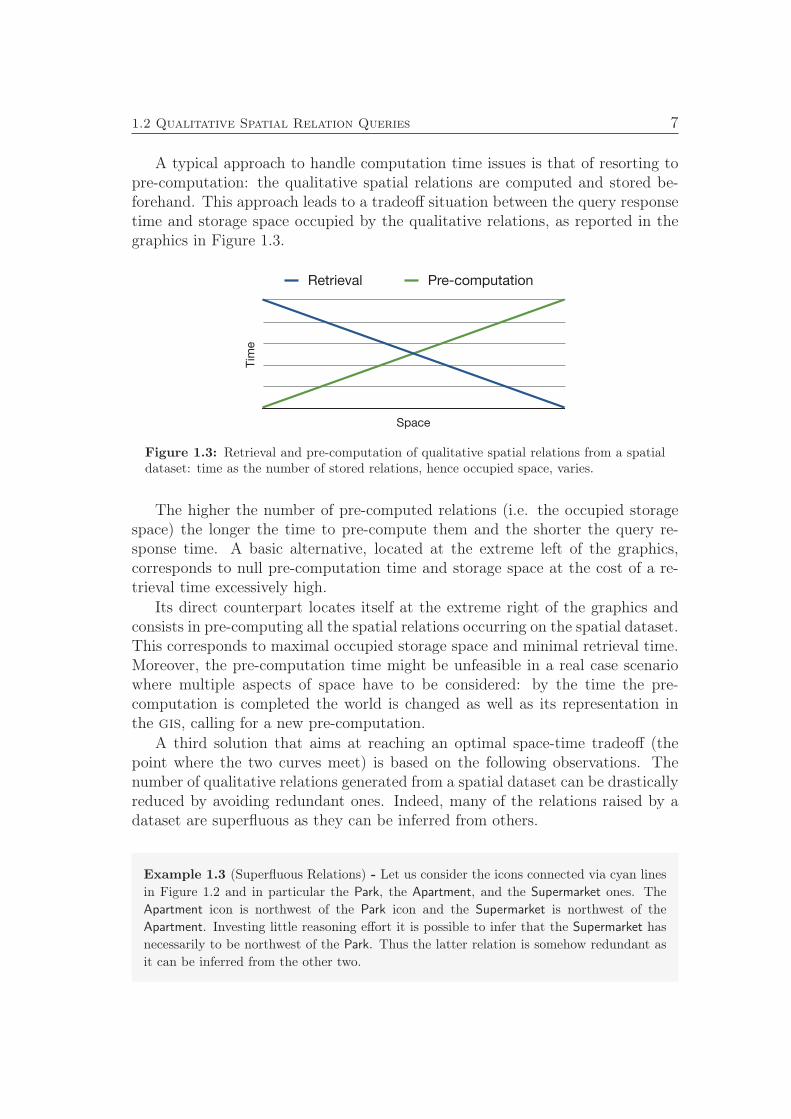
A typical approach to handle computation time issues is that of resorting topre-computation: the qualitative spatial relations are computed and stored be-forehand. This approach leads to a tradeoff situation between the query responsetime and storage space occupied by the qualitative relations, as reported in thegraphics in Figure 1.3.
Tim
e
Space
Retrieval Pre-computation
Figure 1.3: Retrieval and pre-computation of qualitative spatial relations from a spatialdataset: time as the number of stored relations, hence occupied space, varies.
The higher the number of pre-computed relations (i.e. the occupied storagespace) the longer the time to pre-compute them and the shorter the query re-sponse time. A basic alternative, located at the extreme left of the graphics,corresponds to null pre-computation time and storage space at the cost of a re-trieval time excessively high.
Its direct counterpart locates itself at the extreme right of the graphics andconsists in pre-computing all the spatial relations occurring on the spatial dataset.This corresponds to maximal occupied storage space and minimal retrieval time.Moreover, the pre-computation time might be unfeasible in a real case scenariowhere multiple aspects of space have to be considered: by the time the pre-computation is completed the world is changed as well as its representation inthe gis, calling for a new pre-computation.
A third solution that aims at reaching an optimal space-time tradeoff (thepoint where the two curves meet) is based on the following observations. Thenumber of qualitative relations generated from a spatial dataset can be drasticallyreduced by avoiding redundant ones. Indeed, many of the relations raised by adataset are superfluous as they can be inferred from others.
Example 1.3 (Superfluous Relations) - Let us consider the icons connected via cyan lines
in Figure 1.2 and in particular the Park, the Apartment, and the Supermarket ones. The
Apartment icon is northwest of the Park icon and the Supermarket is northwest of the
Apartment. Investing little reasoning effort it is possible to infer that the Supermarket has
necessarily to be northwest of the Park. Thus the latter relation is somehow redundant as
it can be inferred from the other two.
8 1 Introduction
A spatial dataset may give rise to many similar instances and it can be repre-sented by as many relations as necessary to infer all the omitted ones. Therefore,qualitative relation reduction strategies can be employed to keep memory con-sumption within an acceptable range, while search time efficiency can be obtainedby combining relation reconstruction strategies with indexing techniques.Now, it is clear that to efficiently enable qscqs it is not enough to device
“superficial” solutions to put on top of existing systems—like interfaces or accessfunctions. Rather, it is necessary to operate changes deep into the gis storagelayer, developing new algorithms and data structures that, combining spatialindexing techniques and qualitative relation reduction strategies, allow for main-taining spatial and temporal efficiency in the gis. Such data structures have tobe placed aside and designed to work synergistically with the existing ones.
1.3 Thesis and Contributions
This work aims at demonstrating the following thesis:
The synergistic interplay of spatial access methods and reductionstrategies is the key to enable and efficiently solve Qualitative SpatialConfiguration Queries in Geographic Information Systems.
In particular, the main contributions are:
• A special type of spatial queries, based on the notion of qualitative rela-tion, is defined that embraces and generalizes a variety of queries typicallyaccounted for separately in the literature. Consequentially, this allows forthe conception of generalized spatial indexing techniques.
• This work provides a theoretical and practical framework for the integrationof an open number of qualitative spatial calculi and spatial access meth-ods. The interplay of Qualitative Spatial Representation and Reasoning(qsr) and indexing techniques is identified as a suitable means to enablequalitative spatial queries in gis and to retain space-time efficiency.
• Based on the aforementioned framework, a variety of reduction/reconstruc-tion strategies for qualitative spatial relations are presented. They simulta-neously exploit the properties of standard spatial indexing techniques andqualitative spatial calculi. An algorithmic realization is given for each ofthem.
• A novel approach that allows for identifying minimal sets of qualitativespatial relations needed to describe a spatial scene is developed. As suchit provides a reduction strategy based on a general reduction theory thatexploits properties of reasoning tables provided with qualitative calculi butdoes not depend on any particular algebraic property.

1.4 Outline of the Thesis 9
1.4 Outline of the Thesis
The remainder of this thesis is organized as follows: In Chapter 2 different ap-proaches for the representation and management of spatial information are dis-cussed and some fundamental background concepts are introduced.
The problem of enabling Qualitative Spatial Configuration Queries in Geo-graphic Information Systems—and particularly in spatial databases—is detailedin Chapter 3. A set of necessary requirements is defined on top of which is de-signed a basic resolution method. Moreover, the issue of dataset qualification israised and formalized for which two straightforward—but inefficient—solutionsare discussed.
In Chapter 4 a theory of qualitative spatial relations indexing is developed.There, we define the concept of Qualitative Spatial Access Method (qsam) whichcan embody the basic resolution methods presented in the previous chapter aswell as more advanced indexing techniques. In particular, we introduce a familyof qsams based on a tile&cluster strategy and a generalized approach based onqsr techniques. Such qsams have been conceived in the scope of this work; theyare formalized and presented along with an algorithmic realization.
Chapter 5 is devoted to the development of a novel prototypical softwareframework. It provides an extension for an existing open-source Database Man-agement System (dbms) and a realization of the theoretical framework tracedalong the previous chapters.
Such a framework also provides a qsam development and benchmark environ-ment that has been used to evaluate the presented work. The results of such anevaluation are presented in Chapter 6. Finally, conclusions are drawn in Chap-ter 7 where also possible extensions and future work are outlined.

Chapter 2
Representation and Management of
Spatial Information
This chapter presents a review of the state–of–the–art on different techniques forthe representation and management of spatial information in computer systemsand Geographic Information Systems (gis). Section 2.1 introduces some back-ground concepts on graphs and hypergraphs, with a special focus on directedhypergraphs which are largely used in the next chapters. Section 2.2 narrowsdown to a specific field of knowledge representation called Qualitative SpatialRepresentation and Reasoning (qsr) that provides the formal ground and somecore techniques which ideas of this thesis have been stemmed from. Finally,in Section 2.3 a review of the state-of-the-art on spatial databases is presentedthat draws special attention on spatial queries, spatial indexes, and spatial querylanguages.
2.1 Directed Hypergraphs
A graph is a combinatorial structure widely used in mathematics and computerscience to represent sets of objects and binary connections over them. The repre-sented objects are abstracted into entities called nodes, whereas interconnectionsare node pairs called edges. If the edges are ordered pairs one speaks of directedgraphs and directed edges or, more simply, of digraphs and arcs. If multiple edges(resp. arcs) between the same node pair are admitted one speaks of multigraph(resp. multidigraph). Graphs lend themselves very well to be diagrammaticallyrepresented. As shown in Figure 2.1, nodes are represented by circles and edges(resp. arcs) by curves connecting the nodes.
12 2 Representation and Management of Spatial Information
n3
n1
n2
e1
(a)
n3
n1
n2
a1
a3
a2
(b)
n3
n1
n2
e1
e3
e2
(c)
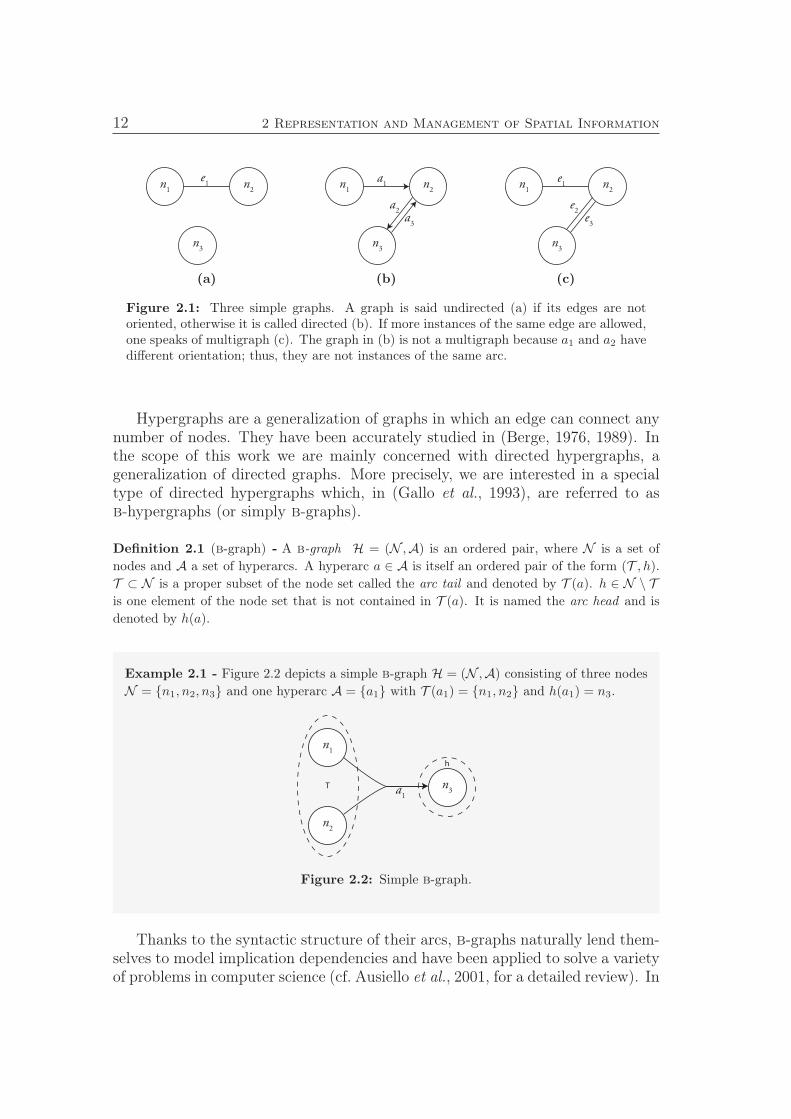
Figure 2.1: Three simple graphs. A graph is said undirected (a) if its edges are notoriented, otherwise it is called directed (b). If more instances of the same edge are allowed,one speaks of multigraph (c). The graph in (b) is not a multigraph because a1 and a2 havedifferent orientation; thus, they are not instances of the same arc.
Hypergraphs are a generalization of graphs in which an edge can connect anynumber of nodes. They have been accurately studied in (Berge, 1976, 1989). Inthe scope of this work we are mainly concerned with directed hypergraphs, ageneralization of directed graphs. More precisely, we are interested in a specialtype of directed hypergraphs which, in (Gallo et al., 1993), are referred to asb-hypergraphs (or simply b-graphs).
Definition 2.1 (b-graph) - A b-graph H = (N ,A) is an ordered pair, where N is a set of
nodes and A a set of hyperarcs. A hyperarc a ∈ A is itself an ordered pair of the form (T , h).
T ⊂ N is a proper subset of the node set called the arc tail and denoted by T (a). h ∈ N \ T
is one element of the node set that is not contained in T (a). It is named the arc head and is
denoted by h(a).
Example 2.1 - Figure 2.2 depicts a simple b-graph H = (N ,A) consisting of three nodes
N = n1, n2, n3 and one hyperarc A = a1 with T (a1) = n1, n2 and h(a1) = n3.
n2
n1
n3
T
h
a1
Figure 2.2: Simple b-graph.
Thanks to the syntactic structure of their arcs, b-graphs naturally lend them-selves to model implication dependencies and have been applied to solve a varietyof problems in computer science (cf. Ausiello et al., 2001, for a detailed review). In
2.1 Directed Hypergraphs 13
(Ausiello et al., 1983), for instance, b-graphs are used to represent functional de-pendencies1 in relational databases (cf. Elmasri & Navathe, 2008, for a thoroughintroduction to databases).
In the next two subsections we will review a series of useful hypergraph con-cepts that are necessary for a full comprehension of this work. Definitions aretaken and adapted from (Ausiello et al., 1983, 1986, 2001; Gallo et al., 1993); fora complete overview refer to these sources.
2.1.1 Basic Concepts
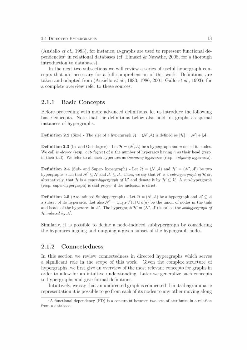
Before proceeding with more advanced definitions, let us introduce the followingbasic concepts. Note that the definitions below also hold for graphs as specialinstances of hypergraphs.
Definition 2.2 (Size) - The size of a hypergraph H = (N ,A) is defined as |H| = |N |+ |A|.
Definition 2.3 (In- and Out-degree) - Let H = (N ,A) be a hypergraph and n one of its nodes.
We call in-degree (resp. out-degree) of n the number of hyperarcs having n as their head (resp.
in their tail). We refer to all such hyperarcs as incoming hyperarcs (resp. outgoing hyperarcs).
Definition 2.4 (Sub- and Super- hypergraph) - Let H = (N ,A) and H′ = (N ′,A′) be two
hypergraphs, such that N ′ ⊆ N and A′ ⊆ A. Then, we say that H′ is a sub-hypergraph of H or,
alternatively, that H is a super-hypergraph of H′ and denote it by H′ ⊆ H. A sub-hypergraph
(resp. super-hypergraph) is said proper if the inclusion is strict.
Definition 2.5 (Arc-induced Subhypergraph) - Let H = (N ,A) be a hypergraph and A′ ⊆ A
a subset of its hyperarcs. Let also N ′ = ∪a∈A′T (a) ∪ h(a) be the union of nodes in the tails
and heads of the hyperarcs in A′. The hypergraph H′ = (N ′,A′) is called the subhypergraph ofH induced by A′.
Similarly, it is possible to define a node-induced subhypergraph by consideringthe hyperarcs ingoing and outgoing a given subset of the hypergraph nodes.
2.1.2 Connectedness
In this section we review connectedness in directed hypergraphs which servesa significant role in the scope of this work. Given the complex structure ofhypergraphs, we first give an overview of the most relevant concepts for graphs inorder to allow for an intuitive understanding. Later we generalize such conceptsto hypergraphs and give formal definitions.
Intuitively, we say that an undirected graph is connected if in its diagrammaticrepresentation it is possible to go from each of its nodes to any other moving along
1A functional dependency (FD) is a constraint between two sets of attributes in a relationfrom a database.
14 2 Representation and Management of Spatial Information
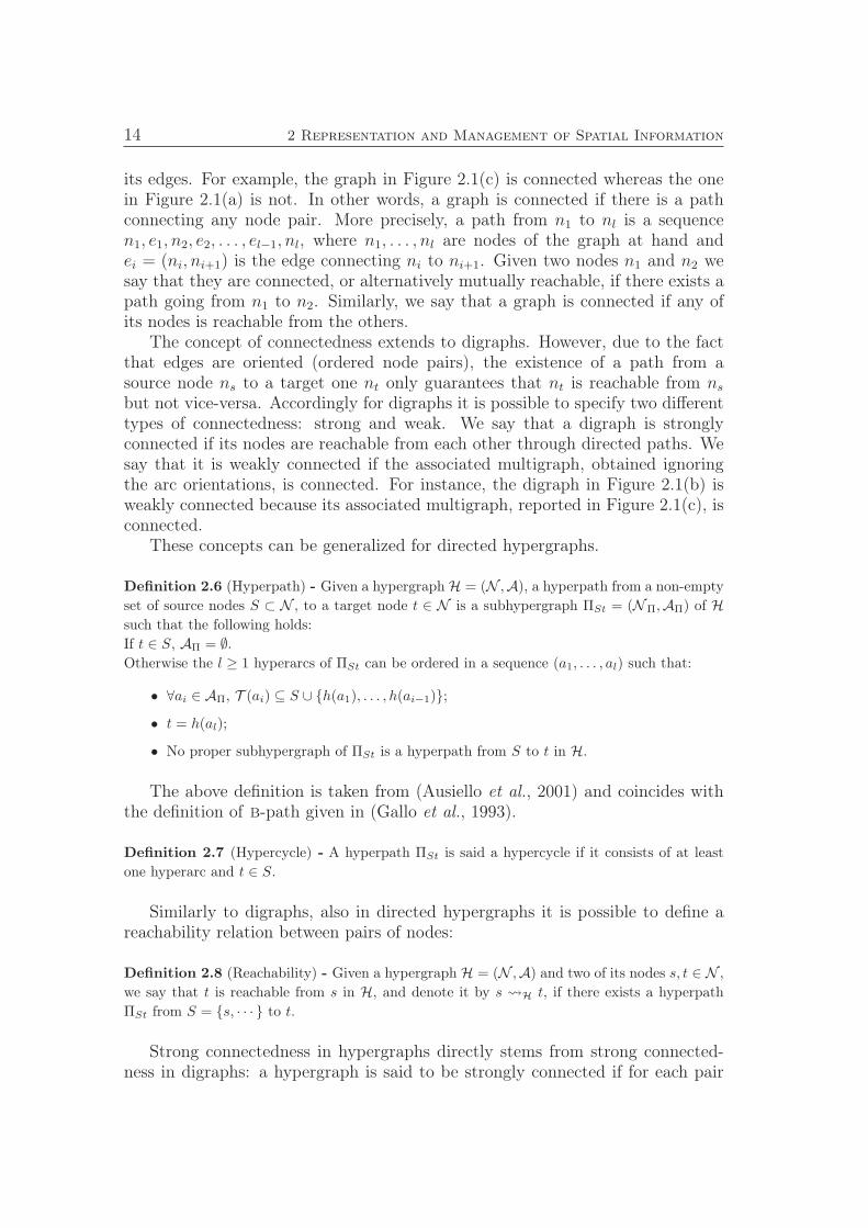
its edges. For example, the graph in Figure 2.1(c) is connected whereas the onein Figure 2.1(a) is not. In other words, a graph is connected if there is a pathconnecting any node pair. More precisely, a path from n1 to nl is a sequencen1, e1, n2, e2, . . . , el−1, nl, where n1, . . . , nl are nodes of the graph at hand andei = (ni, ni+1) is the edge connecting ni to ni+1. Given two nodes n1 and n2 wesay that they are connected, or alternatively mutually reachable, if there exists apath going from n1 to n2. Similarly, we say that a graph is connected if any ofits nodes is reachable from the others.
The concept of connectedness extends to digraphs. However, due to the factthat edges are oriented (ordered node pairs), the existence of a path from asource node ns to a target one nt only guarantees that nt is reachable from ns
but not vice-versa. Accordingly for digraphs it is possible to specify two differenttypes of connectedness: strong and weak. We say that a digraph is stronglyconnected if its nodes are reachable from each other through directed paths. Wesay that it is weakly connected if the associated multigraph, obtained ignoringthe arc orientations, is connected. For instance, the digraph in Figure 2.1(b) isweakly connected because its associated multigraph, reported in Figure 2.1(c), isconnected.
These concepts can be generalized for directed hypergraphs.
Definition 2.6 (Hyperpath) - Given a hypergraph H = (N ,A), a hyperpath from a non-empty
set of source nodes S ⊂ N , to a target node t ∈ N is a subhypergraph ΠSt = (NΠ,AΠ) of H
such that the following holds:
If t ∈ S, AΠ = ∅.
Otherwise the l ≥ 1 hyperarcs of ΠSt can be ordered in a sequence (a1, . . . , al) such that:
• ∀ai ∈ AΠ, T (ai) ⊆ S ∪ h(a1), . . . , h(ai−1);
• t = h(al);
• No proper subhypergraph of ΠSt is a hyperpath from S to t in H.
The above definition is taken from (Ausiello et al., 2001) and coincides withthe definition of b-path given in (Gallo et al., 1993).
Definition 2.7 (Hypercycle) - A hyperpath ΠSt is said a hypercycle if it consists of at least
one hyperarc and t ∈ S.
Similarly to digraphs, also in directed hypergraphs it is possible to define areachability relation between pairs of nodes:
Definition 2.8 (Reachability) - Given a hypergraph H = (N ,A) and two of its nodes s, t ∈ N ,
we say that t is reachable from s in H, and denote it by s H t, if there exists a hyperpath
ΠSt from S = s, · · · to t.
Strong connectedness in hypergraphs directly stems from strong connected-ness in digraphs: a hypergraph is said to be strongly connected if for each pair
2.1 Directed Hypergraphs 15
(s, t) of its nodes, there exists a hyperpath ΠSt and a hyperpath ΠTs, that is, itsnodes are mutually reachable from each other.
In fact, the reachability relation can be used to identify equivalence classes inthe node set of non-strongly connected hypergraphs.
Definition 2.9 (Strongly Connected Component) - Given a hypergraphH = (N ,A), a stronglyconnected component (scc) is a subhypergraph C = (NC ,AC) of H such that the following
conditions hold simultaneously:
• the nodes of C are pairwise mutually reachable: s C t and t C s ∀s, t ∈ NC ;
• C is maximal: there exists no scc C ′ that is a super-hypergraph of C.
Also for directed hypergraphs, there exists the concept of weak connectedness.A directed hypergraph is said weakly connected if its associated multi-digraph,obtained replacing each hyperarc with a series of arcs going from each node inthe tail to the head, is weakly connected.
Definition 2.10 (Weakly Connected Component) - Given a hypergraph H = (N ,A), a weaklyconnected component (wcc) is a subhypergraph C = (NC ,AC) of H such that the following
conditions hold simultaneously:
• C is weakly connected;
• C is maximal.
Above concepts are illustrated in the following:
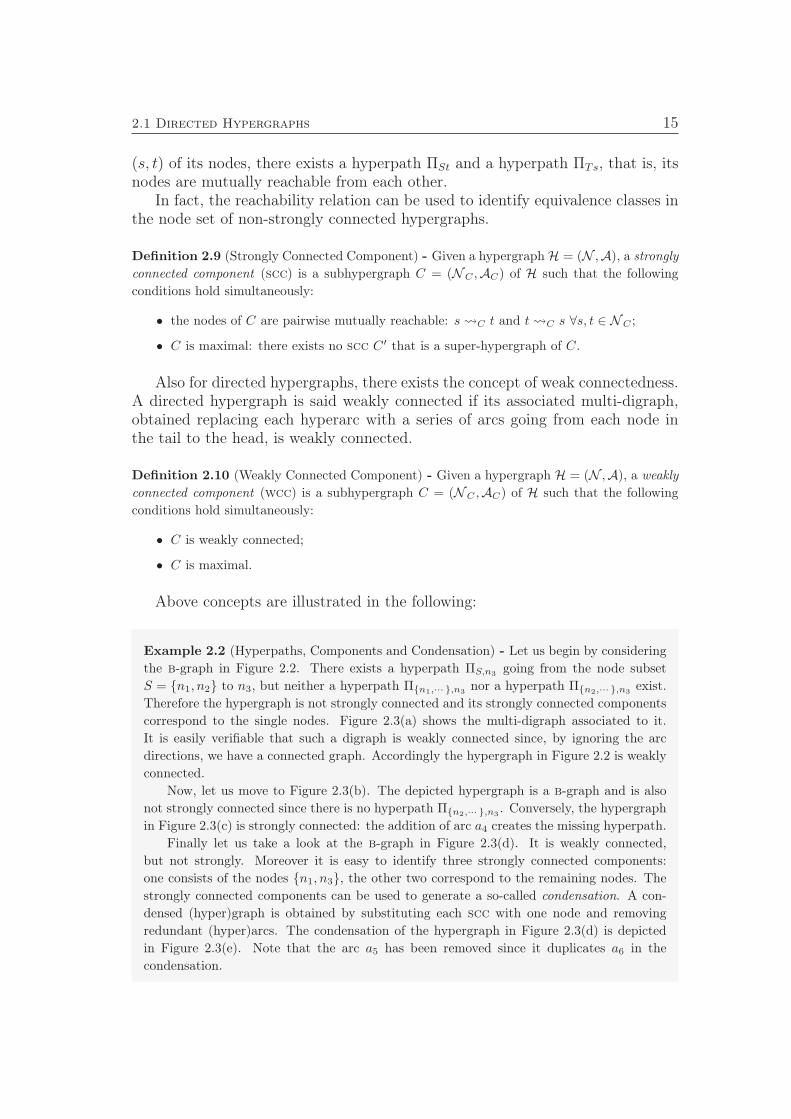
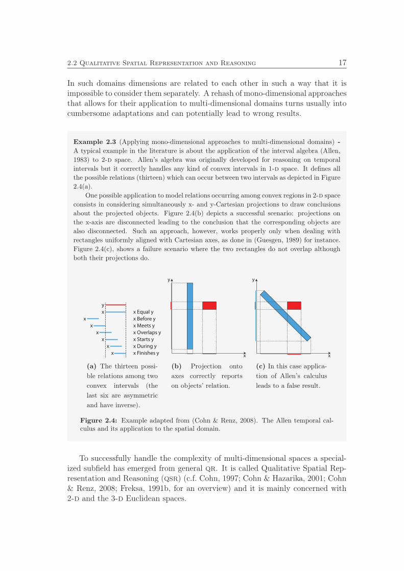
Example 2.2 (Hyperpaths, Components and Condensation) - Let us begin by considering
the b-graph in Figure 2.2. There exists a hyperpath ΠS,n3going from the node subset
S = n1, n2 to n3, but neither a hyperpath Πn1,··· ,n3nor a hyperpath Πn2,··· ,n3
exist.
Therefore the hypergraph is not strongly connected and its strongly connected components
correspond to the single nodes. Figure 2.3(a) shows the multi-digraph associated to it.
It is easily verifiable that such a digraph is weakly connected since, by ignoring the arc
directions, we have a connected graph. Accordingly the hypergraph in Figure 2.2 is weakly
connected.
Now, let us move to Figure 2.3(b). The depicted hypergraph is a b-graph and is also
not strongly connected since there is no hyperpath Πn2,··· ,n3. Conversely, the hypergraph
in Figure 2.3(c) is strongly connected: the addition of arc a4 creates the missing hyperpath.
Finally let us take a look at the b-graph in Figure 2.3(d). It is weakly connected,
but not strongly. Moreover it is easy to identify three strongly connected components:
one consists of the nodes n1, n3, the other two correspond to the remaining nodes. The
strongly connected components can be used to generate a so-called condensation. A con-
densed (hyper)graph is obtained by substituting each scc with one node and removing
redundant (hyper)arcs. The condensation of the hypergraph in Figure 2.3(d) is depicted
in Figure 2.3(e). Note that the arc a5 has been removed since it duplicates a6 in the
condensation.
16 2 Representation and Management of Spatial Information
n2
n1
n3
a2
a1
(a)
n2
n1
n3a
1
a2
a3
(b)
n2
n1
n3a
1
a2
a3
a4
(c)
n2
n1
n3a
1
a2
a3
n4
a4 a
6
a5
(d)
n2
a1
a2
n4
a4
n1 n
3
a6
(e)
Figure 2.3: Hyperpaths, Components, and Condensation in hypergraphs.
2.2 Qualitative Spatial Representation and Rea-
soning
Qualitative Reasoning (qr) (cf. Forbus, 2008, for an introduction) is a subfieldof Artificial Intelligence (ai) 1 that aims at abstracting from the continuous,infinitely precise, nature of the world into a discrete representation of it, providingsymbolic reasoning techniques.
Forbus, Nielsen & Faltings (1991) point out that one of the main strengths ofqr approaches is their minimality in representation. In other words, according toFreksa (1991b), qualitative representations allow for differentiating only as manyconcepts as necessary for the specific domain and task to achieve. Hence, qrturns particularly helpful when accurate measures (quantitative information) aremissing or when resorting to precise calculations is unnecessary or even undesir-able.
qr is usually concerned with scalar quantities, that is why it falls short whendealing with domains like the spatial one that are intrinsically multi-dimensional.
1For the interested reader, (Russell & Norvig, 2003) provides an excellent introduction toai.
2.2 Qualitative Spatial Representation and Reasoning 17
In such domains dimensions are related to each other in such a way that it isimpossible to consider them separately. A rehash of mono-dimensional approachesthat allows for their application to multi-dimensional domains turns usually intocumbersome adaptations and can potentially lead to wrong results.
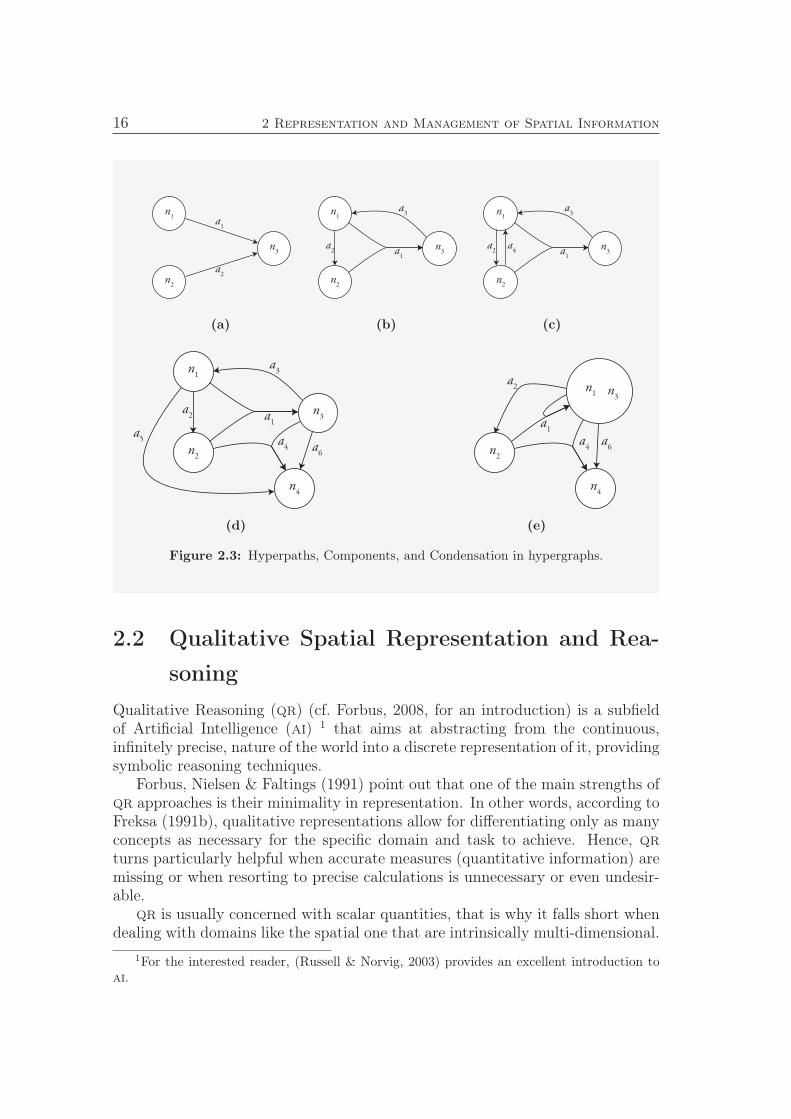
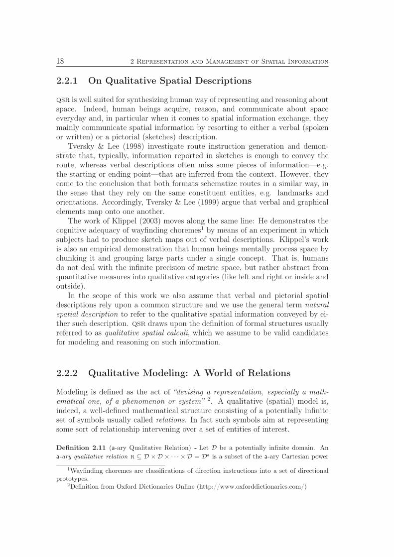
Example 2.3 (Applying mono-dimensional approaches to multi-dimensional domains) -
A typical example in the literature is about the application of the interval algebra (Allen,
1983) to 2-d space. Allen’s algebra was originally developed for reasoning on temporal
intervals but it correctly handles any kind of convex intervals in 1-d space. It defines all
the possible relations (thirteen) which can occur between two intervals as depicted in Figure
2.4(a).
One possible application to model relations occurring among convex regions in 2-d space
consists in considering simultaneously x- and y-Cartesian projections to draw conclusions
about the projected objects. Figure 2.4(b) depicts a successful scenario: projections on
the x-axis are disconnected leading to the conclusion that the corresponding objects are
also disconnected. Such an approach, however, works properly only when dealing with
rectangles uniformly aligned with Cartesian axes, as done in (Guesgen, 1989) for instance.
Figure 2.4(c), shows a failure scenario where the two rectangles do not overlap although
both their projections do.
x Before y
x Meets y
x Overlaps y
x Starts y
x During y
x Finishes y
x Equal y
y
x
x
x
x
x
x
x
(a) The thirteen possi-
ble relations among two
convex intervals (the
last six are asymmetric
and have inverse).
y
x
(b) Projection onto
axes correctly reports
on objects’ relation.
y
x
(c) In this case applica-
tion of Allen’s calculus
leads to a false result.
Figure 2.4: Example adapted from (Cohn & Renz, 2008). The Allen temporal cal-culus and its application to the spatial domain.
To successfully handle the complexity of multi-dimensional spaces a special-ized subfield has emerged from general qr. It is called Qualitative Spatial Rep-resentation and Reasoning (qsr) (c.f. Cohn, 1997; Cohn & Hazarika, 2001; Cohn& Renz, 2008; Freksa, 1991b, for an overview) and it is mainly concerned with2-d and the 3-d Euclidean spaces.
18 2 Representation and Management of Spatial Information
2.2.1 On Qualitative Spatial Descriptions
qsr is well suited for synthesizing human way of representing and reasoning aboutspace. Indeed, human beings acquire, reason, and communicate about spaceeveryday and, in particular when it comes to spatial information exchange, theymainly communicate spatial information by resorting to either a verbal (spokenor written) or a pictorial (sketches) description.
Tversky & Lee (1998) investigate route instruction generation and demon-strate that, typically, information reported in sketches is enough to convey theroute, whereas verbal descriptions often miss some pieces of information—e.g.the starting or ending point—that are inferred from the context. However, theycome to the conclusion that both formats schematize routes in a similar way, inthe sense that they rely on the same constituent entities, e.g. landmarks andorientations. Accordingly, Tversky & Lee (1999) argue that verbal and graphicalelements map onto one another.
The work of Klippel (2003) moves along the same line: He demonstrates thecognitive adequacy of wayfinding choremes1 by means of an experiment in whichsubjects had to produce sketch maps out of verbal descriptions. Klippel’s workis also an empirical demonstration that human beings mentally process space bychunking it and grouping large parts under a single concept. That is, humansdo not deal with the infinite precision of metric space, but rather abstract fromquantitative measures into qualitative categories (like left and right or inside andoutside).
In the scope of this work we also assume that verbal and pictorial spatialdescriptions rely upon a common structure and we use the general term naturalspatial description to refer to the qualitative spatial information conveyed by ei-ther such description. qsr draws upon the definition of formal structures usuallyreferred to as qualitative spatial calculi, which we assume to be valid candidatesfor modeling and reasoning on such information.
2.2.2 Qualitative Modeling: A World of Relations
Modeling is defined as the act of “devising a representation, especially a math-ematical one, of a phenomenon or system” 2. A qualitative (spatial) model is,indeed, a well-defined mathematical structure consisting of a potentially infiniteset of symbols usually called relations. In fact such symbols aim at representingsome sort of relationship intervening over a set of entities of interest.
Definition 2.11 (a-ary Qualitative Relation) - Let D be a potentially infinite domain. An
a-ary qualitative relation r ⊆ D × D × · · · × D = Da is a subset of the a-ary Cartesian power
1Wayfinding choremes are classifications of direction instructions into a set of directionalprototypes.
2Definition from Oxford Dictionaries Online (http://www.oxforddictionaries.com/)
2.2 Qualitative Spatial Representation and Reasoning 19
of the domain of interest. An element of an a-ary relation is an ordered multiset of a domain
elements called an a-tuple .
The domain of interest in the scope of this work is the set of regions embeddedin 2-d space. We adopt the typical interpretation of a region as a point-set sinceit is general enough to embrace lines and points as well—e.g. a point can be seenas a singleton point set. Then, an a-ary spatial relation r ⊆ (o1, . . . , oa) |oi ⊆R
2, i = 1, . . . , a is a subset of the infinite set consisting of any possible planeregion a-tuple.
The typical approach in qsr is to define a finite set of relations that is jointlyexhaustive and pairwise disjoint ( jepd).
Definition 2.12 (jepd set of qualitative relations) - A set B of a-ary qualitative relations is
called jointly exhaustive and pairwise disjoint if the following conditions hold simultaneously:
• B covers all the possible domain a-tuples:⋃
ri∈Bri = D
a;
• any domain a-tuple is contained in one, and only one, relation from B: ri ∩ rj = ∅
∀ ri,rj ∈ B with i 6= j.
The relations in a jepd set B are usually referred to as base relations, whereasthose belonging to the powerset 2B of B are called disjunctive relations. The setof disjunctive relations is obtained by considering all the possible unions of baserelations.
Given an a-tuple of domain object (o1, . . . , oa) ∈ Da we say that “the relation
r holds over o1, . . . , oa” or that “o1, . . . , oa are in the relation r” and we writer(o1, . . . , oa), to denote (o1, . . . , oa) ∈ r. For binary relations it is also possible touse the more intuitive notation o1ro2 to say that o1 is in relation r with o2.
Finally it has to be noted that, although different relations can have differentarities, a qualitative spatial model is typically defined over a set of relations ofuniform arity a, in which case one speaks of an a-ary model.
The definition of relations suffices for representation purposes, whereas theconception of a set of operations over the defined symbols provides the modelwith reasoning capabilities.
2.2.3 Qualitative Reasoning: Relational Operations
According to Cohn & Renz (2008, pag. 572), spatial reasoning is concerned with“[. . . ] deriving new knowledge from given information, checking consistency ofgiven information, updating the given knowledge, or finding a minimal represen-tation.”. In summary, reasoning consists in performing some sort of manipulationover given pieces of information to infer other (not necessarily new) pieces ofinformation.
Classical set-theoretic operations are commonly used in qsr. The union op-eration ∪ is a binary operation that can be used to adduce uncertainty (produce
20 2 Representation and Management of Spatial Information
disjunctive relations). Contrarily, the intersection operation ∩ allows for refin-
ing disjunctive relations and can be used to reduce uncertainty. Intersection can
also be used to check consistency over a set of given relations. Broadly speaking
(consistency checking is treated in more detail in Section 2.2.5), a relation set is
consistent if the relations of the set do not contradict each other, i.e. intersecting
any pair of relations does not yield the empty set. Finally, the complement is a
unary operation that can be used to express logical negation. E.g. to say that
objects o1 and o2 are not in relation r we write ¬r(o1, o2) that is equivalent to
the disjunction of all of the base relations but r.
Beyond standard set-theoretic operations, qualitative models are usually pro-
vided with two more kinds of operation that provide the main core for entailment:
permutation and composition.
Permutation Permutation is a unary operation that, given the relation ri,
holding over a domain element a-tuple (o1, . . . , oa), yields the relation rj holding
over a permutation of the element tuple. Accordingly, the number of possible
permutation operations depends on the arity a of the model and is equal to
a!− 1.
For binary relations it is possible to define only one permutation operation:
Definition 2.13 (Converse of a binary relation) - Let B be a jepd set of binary base relations
defined over a domain D and r ∈ 2B a disjunctive relation. The unary converse operation ()
is defined as:
r = (o2, o1) ∈ D2|(o1, o2) ∈ r
For the ternary case it is possible to distinguish up to five different permuta-
tions. A possible nomenclature for them is introduced in (Freksa & Zimmermann,
1992) and later reused in (Wallgrün et al., 2007):
Definition 2.14 (Permutations of a ternary relation) - Let B be a jepd set of ternary base rela-
tions defined over a domain D and r ∈ 2B a disjunctive relation. The five possible permutation
operations are defined as follows:
Shortcut: sc(r) = (o1, o3, o2)|(o1, o2, o3) ∈ r
Inverse: inv(r) = (o2, o1, o3)|(o1, o2, o3) ∈ r
Homing: hm(r) = (o2, o3, o1)|(o1, o2, o3) ∈ r
Shortcut inverse: sci(r) = (o3, o1, o2)|(o1, o2, o3) ∈ r
Homing inverse: hmi(r) = (o3, o2, o1)|(o1, o2, o3) ∈ r
2.2 Qualitative Spatial Representation and Reasoning 21
Composition Composition is a binary1 operation that, given the relationsholding over two overlapping a-tuples of domain elements, yields the relationholding over an a-tuple obtained from a concatenation of the given a-tuples. Forexample, given the binary relations ri(o1, o2) and rj(o2, o3), a possible compo-sition operation yields the relation rk(o1, o3). For a generic a-ary model it ispossible to define up to (a!)3 composition operations according to the permuta-tion of objects considered in the input and output relations.
For binary models it is commonly defined only one composition operation:
Definition 2.15 (Composition of binary relations) - LetB be a jepd set of binary base relations
defined over a domain D and ri,rj ∈ 2B two disjunctive relations. The binary compositionoperation is denoted by the symbol and is defined as follows:
ri rj = (o1, o3) ∈ D2|∃o2 ∈ D : (o1, o2) ∈ ri ∧ (o2, o3) ∈ rj
If the set of disjunctive relations 2B defined for a qualitative spatial modelis closed under intersection, union, complement, permutation, and compositionthen the model is commonly referred to as a qualitative calculus, to stress thefact that it also allows for symbolic reasoning beyond the mere representation.However, it is quite common that relations of spatial models are not closed atleast under some of the aforementioned operations. In this case it is necessaryto weaken the definition of the problematic operations in order to still be able toperform symbolic reasoning correctly. This is done by defining weak versions ofthe problematic operations: A weak operation yields the smallest relation in 2B
containing the result of the original operations.
Commonly the operation under which spatial calculi are not closed is thecomposition. Weak composition (cf. Düntsch et al., 2001; Renz & Ligozat, 2005)is defined as:
Definition 2.16 (Weak composition of binary relations) - Let B be a jepd set of binary
base relations defined over a domain D and ri,rj ∈ 2B two disjunctive relations. The weakcomposition operation is denoted by the symbol ⋄ and is defined as follows:
ri ⋄ rj = rk ∈ B|(ri rj) ∩ rk 6= ∅
Weak and strong composition can be defined for ternary calculi in a similarway. Moreover, the definitions of permutation and composition operations canalso be extended to generic a-ary models (cf. Condotta et al., 2006).
If a calculus is closed under permutation and composition (or a weak formof them) the application of such operations over a relation in 2B yields anotherrelation in 2B. Moreover, as the base relation set B is finite it is possible, and
1It is possible to define also higher-arity composition operations. Ternary composition, forexample is defined in (Condotta et al., 2006).
22 2 Representation and Management of Spatial Information
common, to provide tables summarizing precomputed results for any base re-lation (possibly also for disjunctive ones). In the literature, tables summarizingpermutation and composition operations are commonly referred to as permutationtables and composition tables, respectively. Since both types of tables allow forperforming qualitative reasoning, in the scope of this work we will use the genericterm reasoning tables to refer to either permutation or composition tables.
2.2.4 Classification of Qualitative Spatial Calculi
Research in qsr has led to the birth of a plethora of qualitative calculi. Theyvary widely with respect to features spanning from the modeled entities to thedevelopment techniques and underlying theory bases and to the modeled spatialaspects.
The research conducted so far has mainly focused on theoretical issues andthe majority of developed qualitative calculi is usually focused on a single aspectof space—e.g. topology, distance, and direction. The main aim has been that ofidentifying singularities and algebraic properties holding on accurately boundeddomains. However, according to (Egenhofer & Sharma, 1993; Renz & Nebel,2007; Sharma, 1996), when it comes to real applications it is mostly necessary tofocus on methods for dealing with multiple aspects simultaneously .
This section provides a survey and a classification of best known qualitativespatial calculi. The proposed sorting is similar in its nature to the work pre-sented in (Freksa & Röhrig, 1993), and, rather than being based on algebraicproperties of spatial calculi, aims at framing the spatial calculi within a catego-rizing coordinate system where axis dimensions represent useful characteristicsfor their utilization in a real-case scenario. The classification criteria are: quali-tative relation type, frame of reference, arity, modeled space, and modeled spatialaspect.
2.2.4.1 Classification of Spatial Relations
According to Clementini & Di Felice (1997) spatial relations can be classified intopological, projective, and metric. Topological relations express those geometricproperties that stay unchanged under a topological transformation. Technically,a topological transformation is a bicontinuous mapping1 from a topological spaceX to a subset of a topological space Y . Informally, a topological space is called a“rubber sheet” and a topological transformation can be imagined as a continuousdeformation of an object into another object obtained by a manipulation of such arubber sheet. The manipulation can consist in shrinking, stretching, and twistingbut not in cutting and glueing.
1A bicontinuous function is a continuous function admitting a continuous inverse.
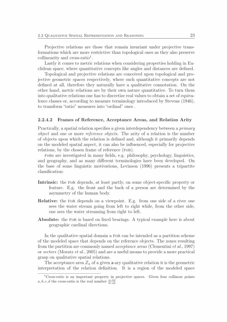
2.2 Qualitative Spatial Representation and Reasoning 23
Projective relations are those that remain invariant under projective trans-formations which are more restrictive than topological ones as they also preservecollinearity and cross-ratio1.
Lastly it comes to metric relations when considering properties holding in Eu-clidean space, where quantitative concepts like angles and distances are defined.
Topological and projective relations are conceived upon topological and pro-jective geometric spaces respectively, where such quantitative concepts are notdefined at all, therefore they naturally have a qualitative connotation. On theother hand, metric relations are by their own nature quantitative. To turn theminto qualitative relations one has to discretize real values to obtain a set of equiva-lence classes or, according to measure terminology introduced by Stevens (1946),to transform “ratio” measures into “ordinal” ones .
2.2.4.2 Frames of Reference, Acceptance Areas, and Relation Arity
Practically, a spatial relation specifies a given interdependency between a primaryobject and one or more reference objects. The arity of a relation is the numberof objects upon which the relation is defined and, although it primarily dependson the modeled spatial aspect, it can also be influenced, especially for projectiverelations, by the chosen frame of reference (for).
fors are investigated in many fields, e.g. philosophy, psychology, linguistics,and geography, and as many different terminologies have been developed. Onthe base of some linguistic motivations, Levinson (1996) presents a tripartiteclassification:
Intrinsic: the for depends, at least partly, on some object-specific property orfeature. E.g. the front and the back of a person are determined by theasymmetry of the human body.
Relative: the for depends on a viewpoint. E.g. from one side of a river onesees the water stream going from left to right while, from the other side,one sees the water streaming from right to left.
Absolute: the for is based on fixed bearings. A typical example here is aboutgeographic cardinal directions.
In the qualitative spatial domain a for can be intended as a partition schemeof the modeled space that depends on the reference objects. The zones resultingfrom the partition are commonly named acceptance areas (Clementini et al., 1997)or sectors (Moratz et al., 2005) and are a useful means to provide a more practicalgrasp on qualitative spatial relations.
The acceptance area Zr of a given a-ary qualitative relation r is the geometricinterpretation of the relation definition. It is a region of the modeled space
1Cross-ratio is an important property in projective spaces. Given four collinear pointsa, b, c, d the cross-ratio is the real number ac·bd
bc·ad
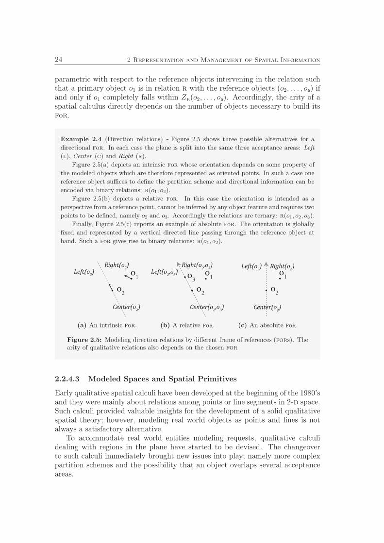
24 2 Representation and Management of Spatial Information
parametric with respect to the reference objects intervening in the relation suchthat a primary object o1 is in relation r with the reference objects (o2, . . . , oa) ifand only if o1 completely falls within Zr(o2, . . . , oa). Accordingly, the arity of aspatial calculus directly depends on the number of objects necessary to build itsfor.
Example 2.4 (Direction relations) - Figure 2.5 shows three possible alternatives for a
directional for. In each case the plane is split into the same three acceptance areas: Left(l), Center (c) and Right (r).
Figure 2.5(a) depicts an intrinsic for whose orientation depends on some property of
the modeled objects which are therefore represented as oriented points. In such a case one
reference object suffices to define the partition scheme and directional information can be
encoded via binary relations: r(o1, o2).
Figure 2.5(b) depicts a relative for. In this case the orientation is intended as a
perspective from a reference point, cannot be inferred by any object feature and requires two
points to be defined, namely o2 and o3. Accordingly the relations are ternary: r(o1, o2, o3).
Finally, Figure 2.5(c) reports an example of absolute for. The orientation is globally
fixed and represented by a vertical directed line passing through the reference object at
hand. Such a for gives rise to binary relations: r(o1, o2).
o1
o2
Left(o2)
Right(o2)
Center(o2)
(a) An intrinsic for.
o1
o2
o3
Left(o2,o3)Right(o
2,o3)
Center(o2,o3)
(b) A relative for.
o1
o2
Left(o2) Right(o
2)
Center(o2)
(c) An absolute for.
Figure 2.5: Modeling direction relations by different frame of references (fors). Thearity of qualitative relations also depends on the chosen for
2.2.4.3 Modeled Spaces and Spatial Primitives
Early qualitative spatial calculi have been developed at the beginning of the 1980’sand they were mainly about relations among points or line segments in 2-d space.Such calculi provided valuable insights for the development of a solid qualitativespatial theory; however, modeling real world objects as points and lines is notalways a satisfactory alternative.
To accommodate real world entities modeling requests, qualitative calculidealing with regions in the plane have started to be devised. The changeoverto such calculi immediately brought new issues into play; namely more complexpartition schemes and the possibility that an object overlaps several acceptanceareas.
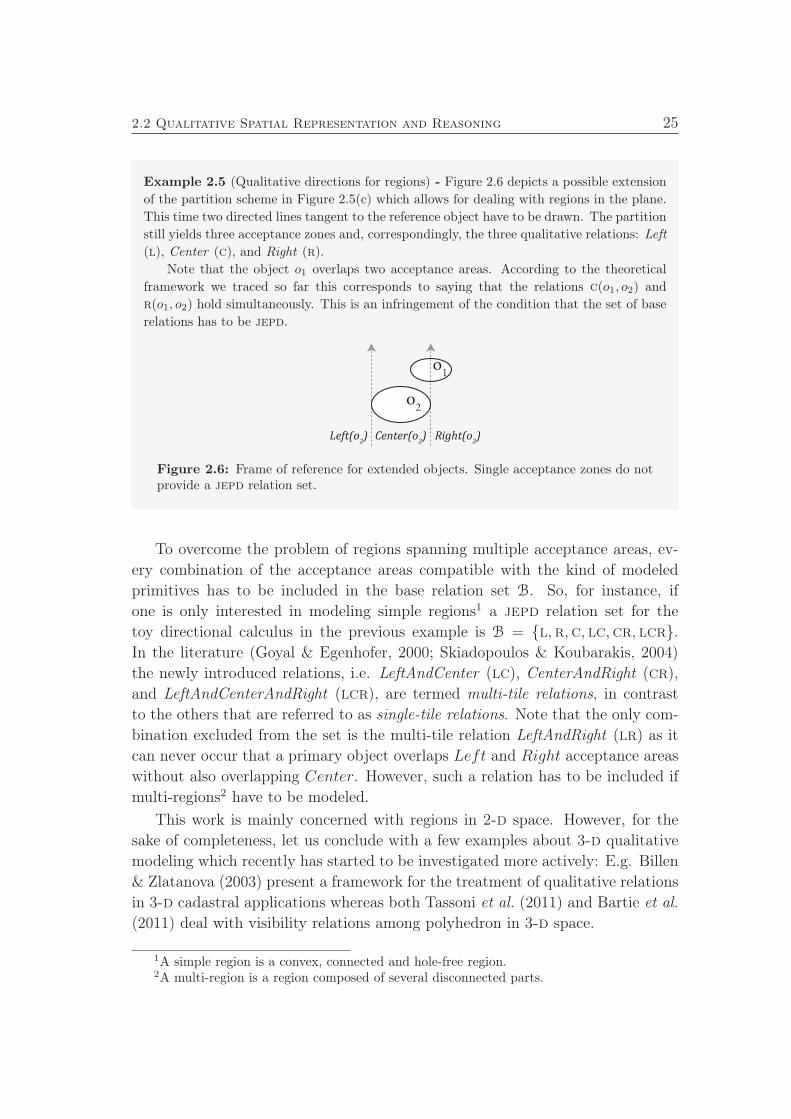
2.2 Qualitative Spatial Representation and Reasoning 25
Example 2.5 (Qualitative directions for regions) - Figure 2.6 depicts a possible extension
of the partition scheme in Figure 2.5(c) which allows for dealing with regions in the plane.
This time two directed lines tangent to the reference object have to be drawn. The partition
still yields three acceptance zones and, correspondingly, the three qualitative relations: Left(l), Center (c), and Right (r).
Note that the object o1 overlaps two acceptance areas. According to the theoretical
framework we traced so far this corresponds to saying that the relations c(o1, o2) and
r(o1, o2) hold simultaneously. This is an infringement of the condition that the set of base
relations has to be jepd.
o1
Left(o2) Right(o
2)Center(o
2)
o2
Figure 2.6: Frame of reference for extended objects. Single acceptance zones do notprovide a jepd relation set.
To overcome the problem of regions spanning multiple acceptance areas, ev-
ery combination of the acceptance areas compatible with the kind of modeled
primitives has to be included in the base relation set B. So, for instance, if
one is only interested in modeling simple regions1 a jepd relation set for the
toy directional calculus in the previous example is B = l,r,c, lc,cr, lcr.
In the literature (Goyal & Egenhofer, 2000; Skiadopoulos & Koubarakis, 2004)
the newly introduced relations, i.e. LeftAndCenter (lc), CenterAndRight (cr),
and LeftAndCenterAndRight (lcr), are termed multi-tile relations, in contrast
to the others that are referred to as single-tile relations. Note that the only com-
bination excluded from the set is the multi-tile relation LeftAndRight (lr) as it
can never occur that a primary object overlaps Left and Right acceptance areas
without also overlapping Center. However, such a relation has to be included if
multi-regions2 have to be modeled.
This work is mainly concerned with regions in 2-d space. However, for the
sake of completeness, let us conclude with a few examples about 3-d qualitative
modeling which recently has started to be investigated more actively: E.g. Billen
& Zlatanova (2003) present a framework for the treatment of qualitative relations
in 3-d cadastral applications whereas both Tassoni et al. (2011) and Bartie et al.
(2011) deal with visibility relations among polyhedron in 3-d space.
1A simple region is a convex, connected and hole-free region.2A multi-region is a region composed of several disconnected parts.
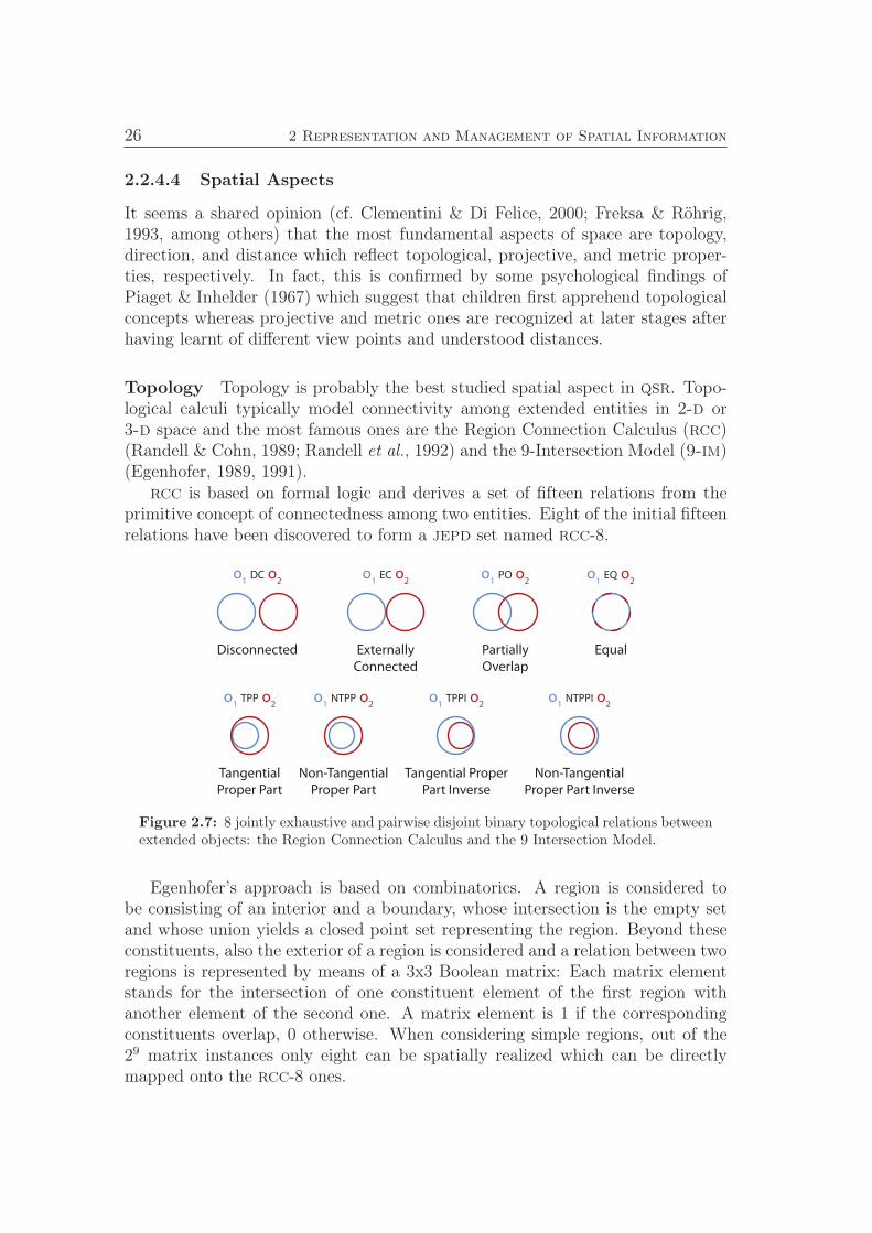
26 2 Representation and Management of Spatial Information
2.2.4.4 Spatial Aspects
It seems a shared opinion (cf. Clementini & Di Felice, 2000; Freksa & Röhrig,1993, among others) that the most fundamental aspects of space are topology,direction, and distance which reflect topological, projective, and metric proper-ties, respectively. In fact, this is confirmed by some psychological findings ofPiaget & Inhelder (1967) which suggest that children first apprehend topologicalconcepts whereas projective and metric ones are recognized at later stages afterhaving learnt of different view points and understood distances.
Topology Topology is probably the best studied spatial aspect in qsr. Topo-logical calculi typically model connectivity among extended entities in 2-d or3-d space and the most famous ones are the Region Connection Calculus (rcc)(Randell & Cohn, 1989; Randell et al., 1992) and the 9-Intersection Model (9-im)(Egenhofer, 1989, 1991).
rcc is based on formal logic and derives a set of fifteen relations from theprimitive concept of connectedness among two entities. Eight of the initial fifteenrelations have been discovered to form a jepd set named rcc-8.
o1 DC o
2
Disconnected
o1 TPP o
2
Tangential
Proper Part
o1 PO o
2
Partially
Overlap
o1 EC o
2
Externally
Connected
o1 EQ o
2
Equal
o1 NTPP o
2
Non-Tangential
Proper Part
o1 TPPI o
2
Tangential Proper
Part Inverse
o1 NTPPI o
2
Non-Tangential
Proper Part Inverse
Figure 2.7: 8 jointly exhaustive and pairwise disjoint binary topological relations betweenextended objects: the Region Connection Calculus and the 9 Intersection Model.
Egenhofer’s approach is based on combinatorics. A region is considered tobe consisting of an interior and a boundary, whose intersection is the empty setand whose union yields a closed point set representing the region. Beyond theseconstituents, also the exterior of a region is considered and a relation between tworegions is represented by means of a 3x3 Boolean matrix: Each matrix elementstands for the intersection of one constituent element of the first region withanother element of the second one. A matrix element is 1 if the correspondingconstituents overlap, 0 otherwise. When considering simple regions, out of the29 matrix instances only eight can be spatially realized which can be directlymapped onto the rcc-8 ones.
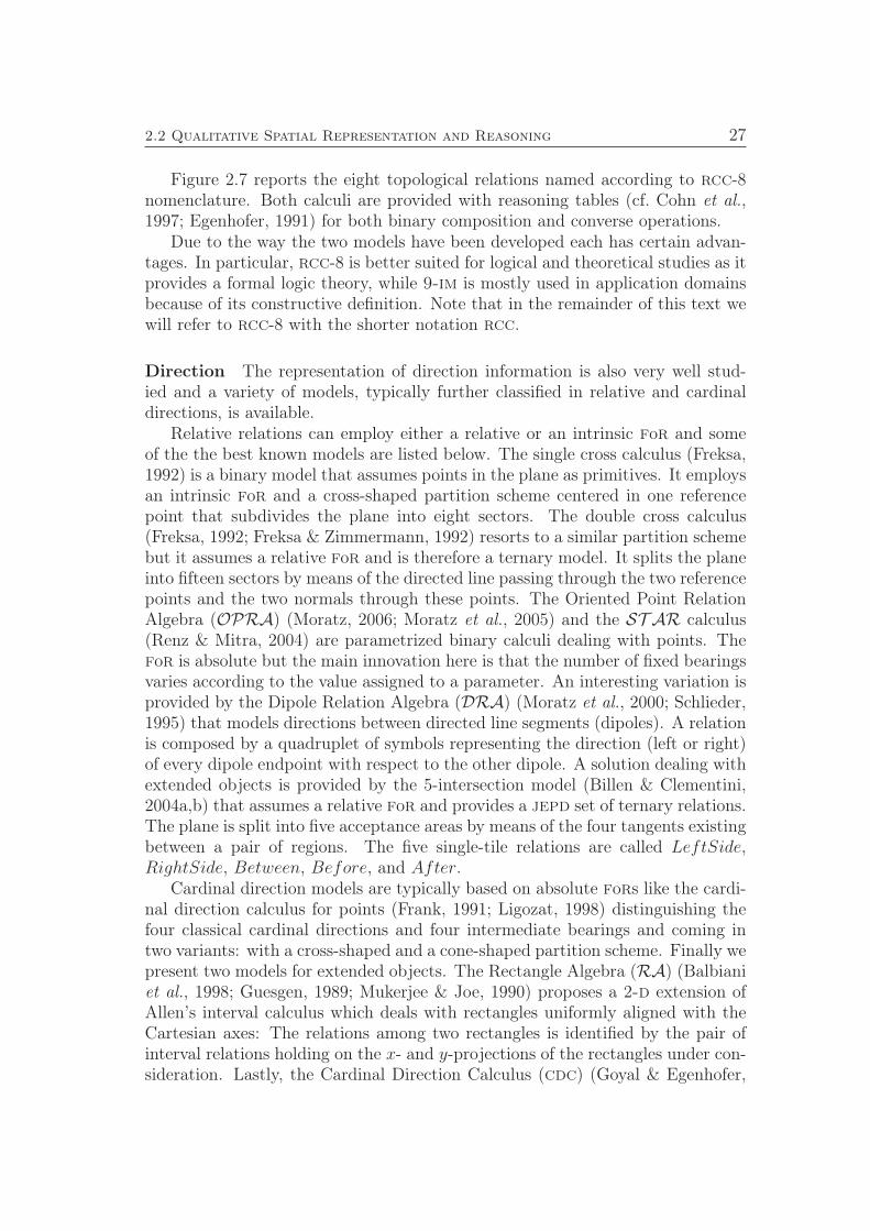
2.2 Qualitative Spatial Representation and Reasoning 27
Figure 2.7 reports the eight topological relations named according to rcc-8nomenclature. Both calculi are provided with reasoning tables (cf. Cohn et al.,1997; Egenhofer, 1991) for both binary composition and converse operations.
Due to the way the two models have been developed each has certain advan-tages. In particular, rcc-8 is better suited for logical and theoretical studies as itprovides a formal logic theory, while 9-im is mostly used in application domainsbecause of its constructive definition. Note that in the remainder of this text wewill refer to rcc-8 with the shorter notation rcc.
Direction The representation of direction information is also very well stud-ied and a variety of models, typically further classified in relative and cardinaldirections, is available.
Relative relations can employ either a relative or an intrinsic for and someof the the best known models are listed below. The single cross calculus (Freksa,1992) is a binary model that assumes points in the plane as primitives. It employsan intrinsic for and a cross-shaped partition scheme centered in one referencepoint that subdivides the plane into eight sectors. The double cross calculus(Freksa, 1992; Freksa & Zimmermann, 1992) resorts to a similar partition schemebut it assumes a relative for and is therefore a ternary model. It splits the planeinto fifteen sectors by means of the directed line passing through the two referencepoints and the two normals through these points. The Oriented Point RelationAlgebra (OPRA) (Moratz, 2006; Moratz et al., 2005) and the ST AR calculus(Renz & Mitra, 2004) are parametrized binary calculi dealing with points. Thefor is absolute but the main innovation here is that the number of fixed bearingsvaries according to the value assigned to a parameter. An interesting variation isprovided by the Dipole Relation Algebra (DRA) (Moratz et al., 2000; Schlieder,1995) that models directions between directed line segments (dipoles). A relationis composed by a quadruplet of symbols representing the direction (left or right)of every dipole endpoint with respect to the other dipole. A solution dealing withextended objects is provided by the 5-intersection model (Billen & Clementini,2004a,b) that assumes a relative for and provides a jepd set of ternary relations.The plane is split into five acceptance areas by means of the four tangents existingbetween a pair of regions. The five single-tile relations are called LeftSide,RightSide, Between, Before, and After.
Cardinal direction models are typically based on absolute fors like the cardi-nal direction calculus for points (Frank, 1991; Ligozat, 1998) distinguishing thefour classical cardinal directions and four intermediate bearings and coming intwo variants: with a cross-shaped and a cone-shaped partition scheme. Finally wepresent two models for extended objects. The Rectangle Algebra (RA) (Balbianiet al., 1998; Guesgen, 1989; Mukerjee & Joe, 1990) proposes a 2-d extension ofAllen’s interval calculus which deals with rectangles uniformly aligned with theCartesian axes: The relations among two rectangles is identified by the pair ofinterval relations holding on the x- and y-projections of the rectangles under con-sideration. Lastly, the Cardinal Direction Calculus (cdc) (Goyal & Egenhofer,
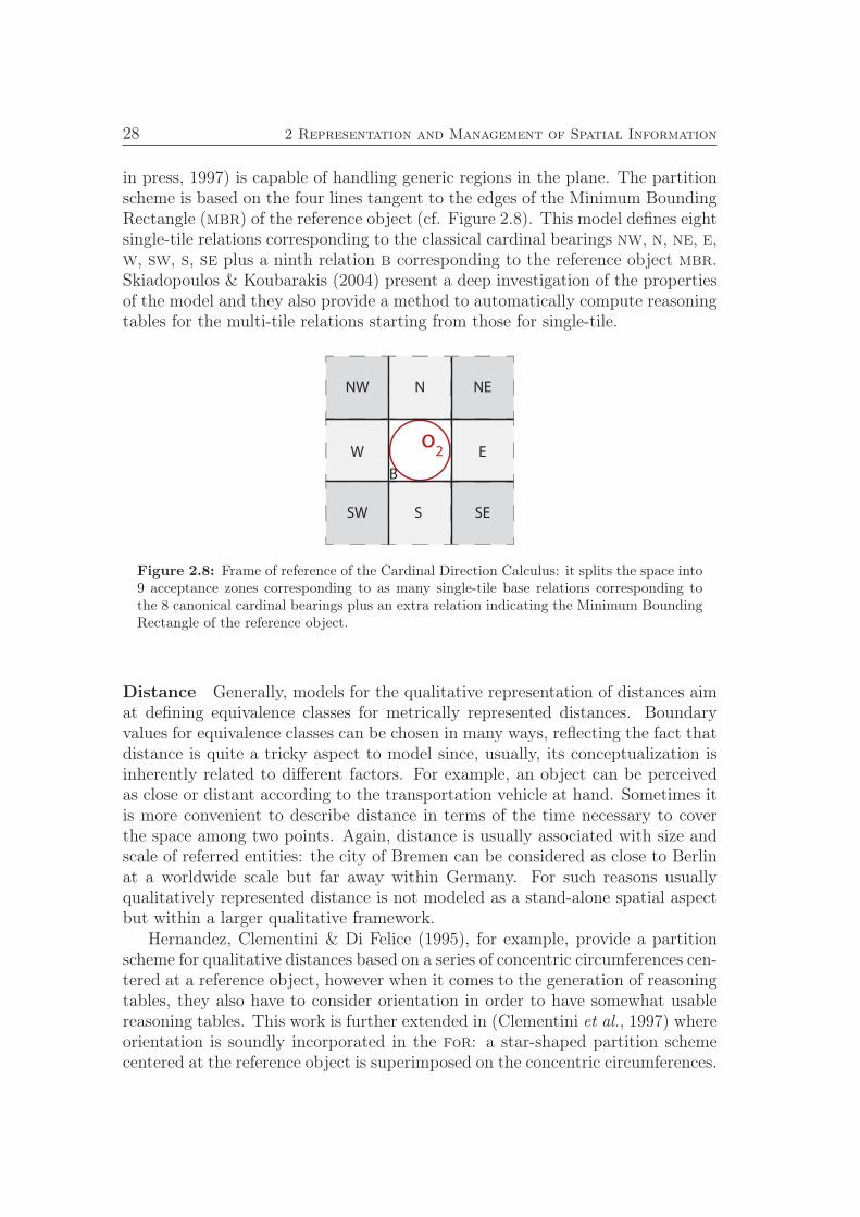
28 2 Representation and Management of Spatial Information
in press, 1997) is capable of handling generic regions in the plane. The partitionscheme is based on the four lines tangent to the edges of the Minimum BoundingRectangle (mbr) of the reference object (cf. Figure 2.8). This model defines eightsingle-tile relations corresponding to the classical cardinal bearings nw, n, ne, e,w, sw, s, se plus a ninth relation b corresponding to the reference object mbr.Skiadopoulos & Koubarakis (2004) present a deep investigation of the propertiesof the model and they also provide a method to automatically compute reasoningtables for the multi-tile relations starting from those for single-tile.
B
NW N NE
W E
SW S SE
o2
Figure 2.8: Frame of reference of the Cardinal Direction Calculus: it splits the space into9 acceptance zones corresponding to as many single-tile base relations corresponding tothe 8 canonical cardinal bearings plus an extra relation indicating the Minimum BoundingRectangle of the reference object.
Distance Generally, models for the qualitative representation of distances aimat defining equivalence classes for metrically represented distances. Boundaryvalues for equivalence classes can be chosen in many ways, reflecting the fact thatdistance is quite a tricky aspect to model since, usually, its conceptualization isinherently related to different factors. For example, an object can be perceivedas close or distant according to the transportation vehicle at hand. Sometimes itis more convenient to describe distance in terms of the time necessary to coverthe space among two points. Again, distance is usually associated with size andscale of referred entities: the city of Bremen can be considered as close to Berlinat a worldwide scale but far away within Germany. For such reasons usuallyqualitatively represented distance is not modeled as a stand-alone spatial aspectbut within a larger qualitative framework.
Hernandez, Clementini & Di Felice (1995), for example, provide a partitionscheme for qualitative distances based on a series of concentric circumferences cen-tered at a reference object, however when it comes to the generation of reasoningtables, they also have to consider orientation in order to have somewhat usablereasoning tables. This work is further extended in (Clementini et al., 1997) whereorientation is soundly incorporated in the for: a star-shaped partition schemecentered at the reference object is superimposed on the concentric circumferences.
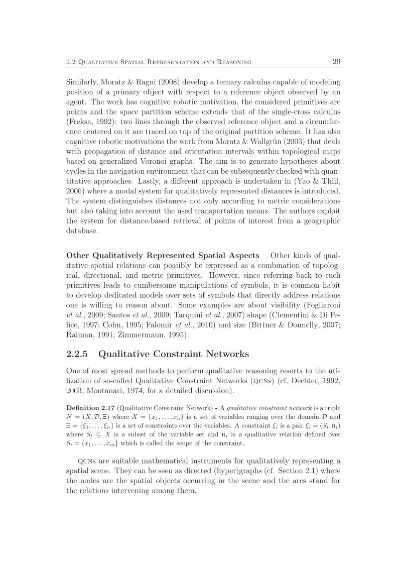
2.2 Qualitative Spatial Representation and Reasoning 29
Similarly, Moratz & Ragni (2008) develop a ternary calculus capable of modelingposition of a primary object with respect to a reference object observed by anagent. The work has cognitive robotic motivation, the considered primitives arepoints and the space partition scheme extends that of the single-cross calculus(Freksa, 1992): two lines through the observed reference object and a circumfer-ence centered on it are traced on top of the original partition scheme. It has alsocognitive robotic motivations the work from Moratz & Wallgrün (2003) that dealswith propagation of distance and orientation intervals within topological mapsbased on generalized Voronoi graphs. The aim is to generate hypotheses aboutcycles in the navigation environment that can be subsequently checked with quan-titative approaches. Lastly, a different approach is undertaken in (Yao & Thill,2006) where a modal system for qualitatively represented distances is introduced.The system distinguishes distances not only according to metric considerationsbut also taking into account the used transportation means. The authors exploitthe system for distance-based retrieval of points of interest from a geographicdatabase.
Other Qualitatively Represented Spatial Aspects Other kinds of qual-itative spatial relations can possibly be expressed as a combination of topolog-ical, directional, and metric primitives. However, since referring back to suchprimitives leads to cumbersome manipulations of symbols, it is common habitto develop dedicated models over sets of symbols that directly address relationsone is willing to reason about. Some examples are about visibility (Fogliaroniet al., 2009; Santos et al., 2009; Tarquini et al., 2007) shape (Clementini & Di Fe-lice, 1997; Cohn, 1995; Falomir et al., 2010) and size (Bittner & Donnelly, 2007;Raiman, 1991; Zimmermann, 1995).
2.2.5 Qualitative Constraint Networks
One of most spread methods to perform qualitative reasoning resorts to the uti-lization of so-called Qualitative Constraint Networks (qcns) (cf. Dechter, 1992,2003; Montanari, 1974, for a detailed discussion).
Definition 2.17 (Qualitative Constraint Network) - A qualitative constraint network is a tripleN = (X,D,Ξ) where X = x1, . . . , xn is a set of variables ranging over the domain D and
Ξ = ξ1, . . . , ξn is a set of constraints over the variables. A constraint ξi is a pair ξi = (Si,ri)
where Si ⊆ X is a subset of the variable set and ri is a qualitative relation defined over
Si = x1, . . . , xm which is called the scope of the constraint.
qcns are suitable mathematical instruments for qualitatively representing aspatial scene. They can be seen as directed (hyper)graphs (cf. Section 2.1) wherethe nodes are the spatial objects occurring in the scene and the arcs stand forthe relations intervening among them.
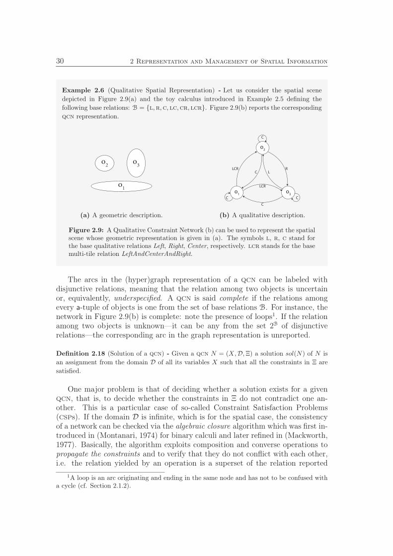
30 2 Representation and Management of Spatial Information
Example 2.6 (Qualitative Spatial Representation) - Let us consider the spatial scene
depicted in Figure 2.9(a) and the toy calculus introduced in Example 2.5 defining the
following base relations: B = l,r,c, lc,cr, lcr. Figure 2.9(b) reports the corresponding
qcn representation.
o1
o2
o3
(a) A geometric description.
o2
o1
o3
RL
LCR
C
LCR
C
C
C C
(b) A qualitative description.
Figure 2.9: A Qualitative Constraint Network (b) can be used to represent the spatialscene whose geometric representation is given in (a). The symbols l, r, c stand forthe base qualitative relations Left, Right, Center, respectively. lcr stands for the basemulti-tile relation LeftAndCenterAndRight.
The arcs in the (hyper)graph representation of a qcn can be labeled withdisjunctive relations, meaning that the relation among two objects is uncertainor, equivalently, underspecified. A qcn is said complete if the relations amongevery a-tuple of objects is one from the set of base relations B. For instance, thenetwork in Figure 2.9(b) is complete: note the presence of loops1. If the relationamong two objects is unknown—it can be any from the set 2B of disjunctiverelations—the corresponding arc in the graph representation is unreported.
Definition 2.18 (Solution of a qcn) - Given a qcn N = (X,D,Ξ) a solution sol(N) of N is
an assignment from the domain D of all its variables X such that all the constraints in Ξ are
satisfied.
One major problem is that of deciding whether a solution exists for a givenqcn, that is, to decide whether the constraints in Ξ do not contradict one an-other. This is a particular case of so-called Constraint Satisfaction Problems(csps). If the domain D is infinite, which is for the spatial case, the consistencyof a network can be checked via the algebraic closure algorithm which was first in-troduced in (Montanari, 1974) for binary calculi and later refined in (Mackworth,1977). Basically, the algorithm exploits composition and converse operations topropagate the constraints and to verify that they do not conflict with each other,i.e. the relation yielded by an operation is a superset of the relation reported
1A loop is an arc originating and ending in the same node and has not to be confused witha cycle (cf. Section 2.1.2).
2.2 Qualitative Spatial Representation and Reasoning 31
in the network. The algebraic closure algorithm can work with both strong andweak operations (cf. Section 2.2.3) and executes in O(n3) worst case time wheren is the number of variables in the network. In (Dylla & Moratz, 2004) the algo-rithm is further extended for ternary calculi, in which case the complexity risesup to O(n4).
2.2.6 Integration of Qualitative Models
It has been already recognized in the past (Egenhofer & Sharma, 1993; Renz& Nebel, 2007; Sharma, 1996) that, despite the investment of more than thirtyyears of research efforts in the field of qsr and the development of a vast andheterogeneous set of theoretical frameworks (cf. Section 2.2.4 for a classification),the application of the qualitative paradigm to tackle realistic problems remainsrelatively small.
One main reason is that human beings are generally capable of mixing severalaspects when communicating and reasoning about spatial knowledge. Therefore,the exploitation of qualitative reasoning to realistic applications calls for a moregeneral theory that can embrace the big variety of spatial features.
The poverty conjecture, initially enunciated for qualitative kinematics (Forbuset al., 1987) and later slightly modified (Forbus et al., 1991) to embrace spatialproperties in general, leaves few hopes for the development of such a general the-ory. The conjecture claims that “There is no purely qualitative, general-purposerepresentation of spatial properties” and is further elaborated by adducing someelucidations: (i) Qualitative spatial representations are useful in many cases andthey are fundamental to enable commonsense reasoning; however they must berelated to quantitative information. (ii) Qualitative models have to be designedin a task-specific manner.
An alternative to enable practical application of qsr draws upon the integra-tion of different qualitative models. This can be done in mainly two ways: (i)calculi fusion and (ii) inter–calculus reasoning.
The first approach consists in the combination of different calculi at both, arepresentational and reasoning level to obtain a new calculus. That is, severalaspects of space are considered simultaneously to represent more complex rela-tions and dedicated reasoning algorithms accounting for such complex aspectsare developed. The literature is full of examples for combining calculi. Some ofthem are about the integration of topology and direction (Hernandez, 1994; Pa-padias, 1994; Papadias & Sellis, 1994b; Papadias et al., 1995), topology and size(Gerevini & Renz, 1998, 2002), direction and distance (Clementini et al., 1997),or more complex combinations (Clementini & Di Felice, 1997; Sharma, 1996).
The second approach mainly grounds in the algebraic properties of qualitativecalculi. It consists in developing advanced reasoning techniques that allow forexploiting interdependencies between calculi. An example is provided by the JointSatisfaction Problem (jsp): the problem of deciding whether the joint networkobtained by merging two consistent qcns is itself consistent. Some works in this
32 2 Representation and Management of Spatial Information
direction are (Gerevini & Renz, 1998, 2002) that investigate the case of rcc-8with a newly defined calculus for size, (Li, 2007; Li & Cohn, 2009) consideringtopology, direction, and size, and (Liu et al., 2009) focusing on complexity issueswhen joining rcc-8 with two cardinal direction calculi: RA and cdc.
2.2.7 On the Cognitive Adequacy of Qualitative Models
Several studies have been carried on to assess the cognitive adequacy of quali-tative spatial models. Knauff et al. (1997) argue that “whether or not a formalapproach to qualitative spatial relations is a cognitively adequate model of humanspatial knowledge is in fact an empirical question and can be answered only on thebasis of empirical results”. Therefore they conducted experiments to assess thecognitive adequacy of rcc and 9-im (cf. section 2.2.4.4). The results outlinedthat such models correctly reflect human way of dealing with topological rela-tions. No equally sound results have been provided for other aspect of space like,for example, cardinal directions. However, much research supports the assump-tion that people usually reason about directions differentiating among a small setof qualitative directions (from four up to eight according to the level of accuracyrequired), therefore legitimating the underlying assumption that qualitative di-rectional models can suitably encode this kind of spatial information. Similarlyin the context of this work we generalize such an assumption and assume thatqualitative models, if adequately designed, can provide a suitable means to repre-sent human spatial knowledge; proving cognitive adequacy of qualitative modelsis not the aim of this work though.
2.3 Spatial Databases
A Geographic Information System (gis) is a system of hardware and softwareelements that allows for surveying, storing, analyzing, manipulating, retrieving,sharing, mapping1, and, more generally, presenting geographic data. At the coreof a gis is the storage layer, that is, a support to persistently represent data in acomputer. Storing can be done by means of standard files—e.g. shapefiles (ESRI,1998). Nonetheless, the usage of a database in this role can notably improve dataretrieval and analysis performance. Databases allow for storing many dimensionsof data, but they are not designed to manage multidimensional data as a whole.Therefore, given its multidimensional nature, spatial information cannot be easilyhandled by plain databases without a so-called “spatial extension”.
Spatial databases are databases extended with data types and proceduresfor inserting, deleting, manipulating, and retrieving spatial information. Tech-nically, a gis needs to deal with geographically referenced spatial information,therefore one usually makes a further differentiation between spatial databases
1Mapping in this context is intended as the action of producing a map.
2.3 Spatial Databases 33
and geospatial databases (or simply geodatabases). Geodatabases are primarilyspatial databases that offer support for geo-referencing spatial objects. However,although the findings presented in this text have been prompted by motivationsof geographic nature, they completely disregard the geographic component andare general enough to work with spatial information in general. Therefore, in thereminder of this text we focus on the more general spatial databases.
2.3.1 Spatial Data Modeling and Representation
In the geographic domain one is interested in modeling real and fictitious entities.Real entities comprise physical objects, natural or artificial, that actually exist inthe world, e.g. a lake or a building, whereas fictitious entities are those entitiesthat are not physically distinguishable from surrounding ones, e.g. administra-tive districts or countries. Rather, boundaries of fictitious entities are definedartificially by humans, e.g. the borderline between two countries is an imageryline decided according to some political issues. An ontological perspective on thisissue is taken by Smith (1995) who distinguishes between entities with bona fideand fiat boundaries, respectively.
Modeling spatial information can be done mainly following two approachesthat in the literature (Longley et al., 2005; Worboys & Duckham, 2004) are typi-cally referred to as field-based and object-based. The field-based approach looksat the properties that have to be modeled as continuous fields and discretizes themvia the superimposition of a—typically regular—geometric structure, e.g. a grid.With every cell of the structure a value is associated that summarizes features—e.g. the average—of the modeled property ranging over the points contained inthe cell. This kind of representation is commonly referred to as raster.
The object-based approach is diametrically opposite to the field-based ap-proach since the main focus is on the spatial entities which are modeled asfirst order objects. The typical resulting representation is referred to as vector–based since boundaries of spatial entities of interest are geometrically describedby means of directed line segments called vectors. A vector is defined by thespecification of its end points in terms of geometric coordinates.
Rasters and vectors are generated from different sources, are different at therepresentational level, they better lend themselves to different modeling purposes,and have to be managed differently.
Rasters present a good solution for modeling values varying continuously overspace—e.g. digital elevation modeling—they are very similar to bitmap imagesand, indeed, are typically generated from satellite pictures. Some of the mostimportant types of data management operations are: identification of spatialentities from satellite pictures (raw pixel sets), clustering and interpolation ofrecorded values, and statistical operations over given areas.
Vector representations are usually obtained from digitalization of charts, fromvectorization of raster data, or from the direct collection of real–world entitycoordinates—e.g. through gps receivers. In such representations objects are
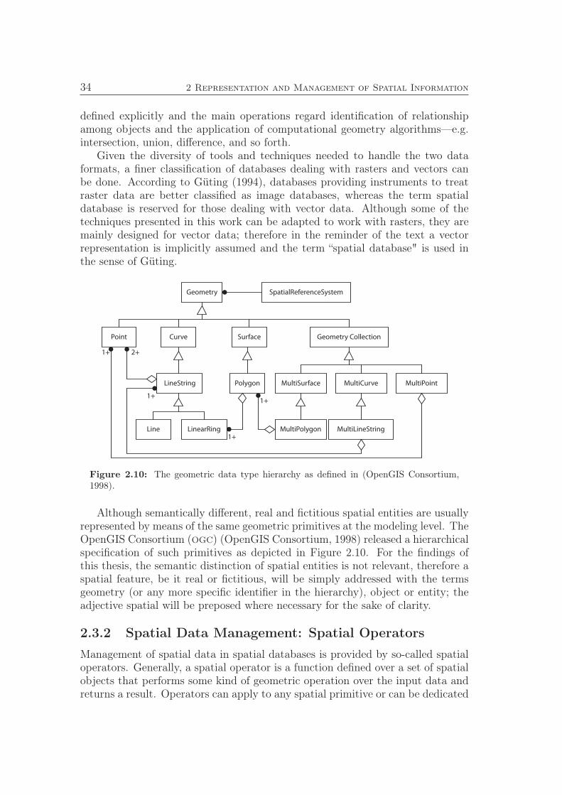
34 2 Representation and Management of Spatial Information
defined explicitly and the main operations regard identification of relationshipamong objects and the application of computational geometry algorithms—e.g.intersection, union, difference, and so forth.
Given the diversity of tools and techniques needed to handle the two dataformats, a finer classification of databases dealing with rasters and vectors canbe done. According to Güting (1994), databases providing instruments to treatraster data are better classified as image databases, whereas the term spatialdatabase is reserved for those dealing with vector data. Although some of thetechniques presented in this work can be adapted to work with rasters, they aremainly designed for vector data; therefore in the reminder of the text a vectorrepresentation is implicitly assumed and the term “spatial database" is used inthe sense of Güting.
Geometry SpatialReferenceSystem
Curve SurfacePoint Geometry Collection
PolygonLineString MultiSurface MultiCurve MultiPoint
Line LinearRing MultiPolygon MultiLineString
1+
1+1+
1+
2+
Figure 2.10: The geometric data type hierarchy as defined in (OpenGIS Consortium,1998).
Although semantically different, real and fictitious spatial entities are usuallyrepresented by means of the same geometric primitives at the modeling level. TheOpenGIS Consortium (ogc) (OpenGIS Consortium, 1998) released a hierarchicalspecification of such primitives as depicted in Figure 2.10. For the findings ofthis thesis, the semantic distinction of spatial entities is not relevant, therefore aspatial feature, be it real or fictitious, will be simply addressed with the termsgeometry (or any more specific identifier in the hierarchy), object or entity; theadjective spatial will be preposed where necessary for the sake of clarity.
2.3.2 Spatial Data Management: Spatial Operators
Management of spatial data in spatial databases is provided by so-called spatialoperators. Generally, a spatial operator is a function defined over a set of spatialobjects that performs some kind of geometric operation over the input data andreturns a result. Operators can apply to any spatial primitive or can be dedicated
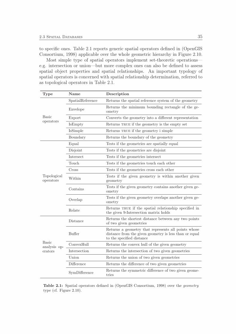
2.3 Spatial Databases 35
to specific ones. Table 2.1 reports generic spatial operators defined in (OpenGISConsortium, 1998) applicable over the whole geometric hierarchy in Figure 2.10.
Most simple type of spatial operators implement set-theoretic operations—e.g. intersection or union—but more complex ones can also be defined to assessspatial object properties and spatial relationships. An important typology ofspatial operators is concerned with spatial relationship determination, referred toas topological operators in Table 2.1.
Type Name Description
Basicoperators
SpatialReference Returns the spatial reference system of the geometry
EnvelopeReturns the minimum bounding rectangle of the ge-ometry
Export Converts the geometry into a different representation
IsEmpty Returns true if the geometry is the empty set
IsSimple Returns true if the geometry i simple
Boundary Returns the boundary of the geometry
Topologicaloperators
Equal Tests if the geometries are spatially equal
Disjoint Tests if the geometries are disjoint
Intersect Tests if the geometries intersect
Touch Tests if the geometries touch each other
Cross Tests if the geometries cross each other
WithinTests if the given geometry is within another givengeometry
ContainsTests if the given geometry contains another given ge-ometry
OverlapTests if the given geometry overlaps another given ge-ometry
RelateReturns true if the spatial relationship specified inthe given 9-Intersection matrix holds
Basicanalysis op-erators
DistanceReturns the shortest distance between any two pointsof two given geometries
BufferReturns a geometry that represents all points whosedistance from the given geometry is less than or equalto the specified distance
ConvexHull Returns the convex hull of the given geometry
Intersection Returns the intersection of two given geometries
Union Returns the union of two given geometries
Difference Returns the difference of two given geometries
SymDifferenceReturns the symmetric difference of two given geome-tries
Table 2.1: Spatial operators defined in (OpenGIS Consortium, 1998) over the geometrytype (cf. Figure 2.10).
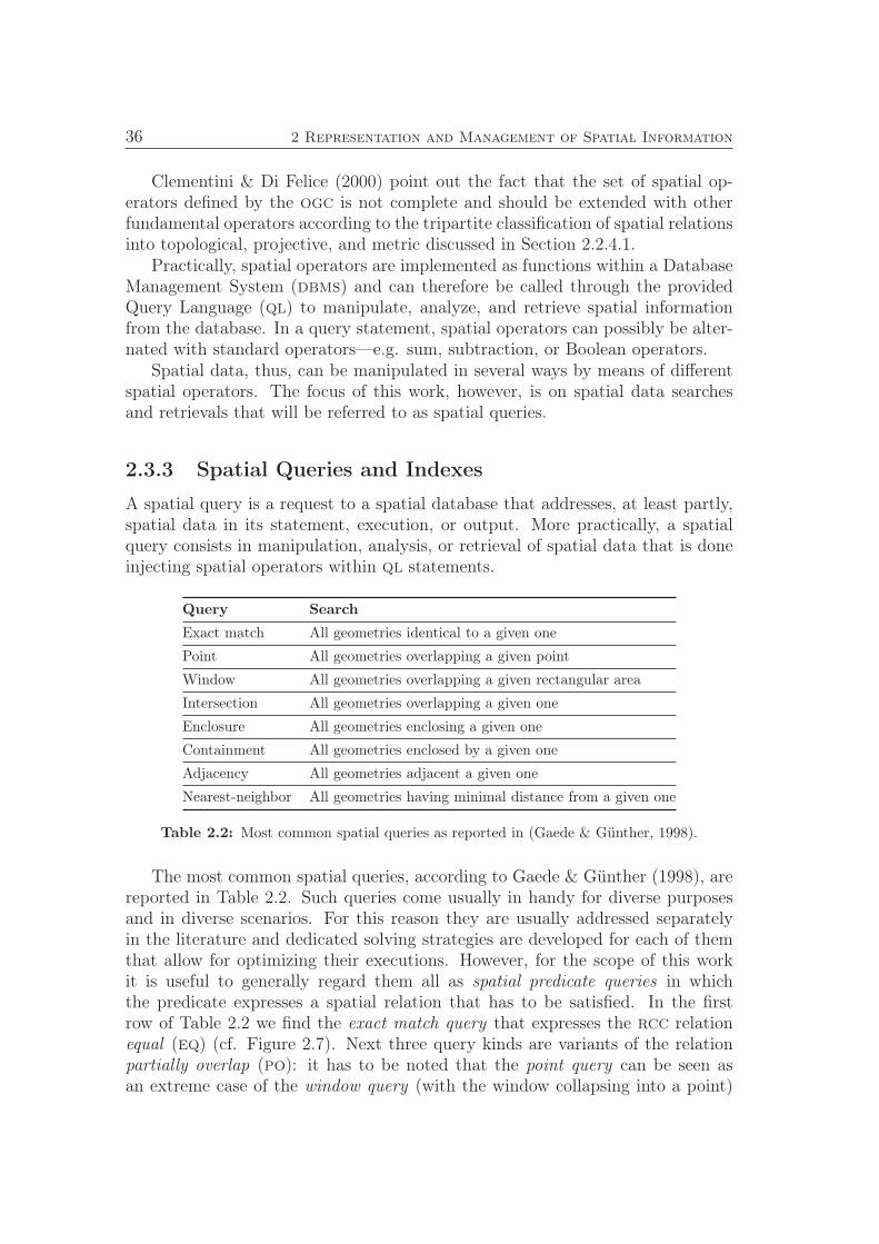
36 2 Representation and Management of Spatial Information
Clementini & Di Felice (2000) point out the fact that the set of spatial op-erators defined by the ogc is not complete and should be extended with otherfundamental operators according to the tripartite classification of spatial relationsinto topological, projective, and metric discussed in Section 2.2.4.1.
Practically, spatial operators are implemented as functions within a DatabaseManagement System (dbms) and can therefore be called through the providedQuery Language (ql) to manipulate, analyze, and retrieve spatial informationfrom the database. In a query statement, spatial operators can possibly be alter-nated with standard operators—e.g. sum, subtraction, or Boolean operators.
Spatial data, thus, can be manipulated in several ways by means of differentspatial operators. The focus of this work, however, is on spatial data searchesand retrievals that will be referred to as spatial queries.
2.3.3 Spatial Queries and Indexes
A spatial query is a request to a spatial database that addresses, at least partly,spatial data in its statement, execution, or output. More practically, a spatialquery consists in manipulation, analysis, or retrieval of spatial data that is doneinjecting spatial operators within ql statements.
Query Search
Exact match All geometries identical to a given one
Point All geometries overlapping a given point
Window All geometries overlapping a given rectangular area
Intersection All geometries overlapping a given one
Enclosure All geometries enclosing a given one
Containment All geometries enclosed by a given one
Adjacency All geometries adjacent a given one
Nearest-neighbor All geometries having minimal distance from a given one
Table 2.2: Most common spatial queries as reported in (Gaede & Günther, 1998).
The most common spatial queries, according to Gaede & Günther (1998), arereported in Table 2.2. Such queries come usually in handy for diverse purposesand in diverse scenarios. For this reason they are usually addressed separatelyin the literature and dedicated solving strategies are developed for each of themthat allow for optimizing their executions. However, for the scope of this workit is useful to generally regard them all as spatial predicate queries in whichthe predicate expresses a spatial relation that has to be satisfied. In the firstrow of Table 2.2 we find the exact match query that expresses the rcc relationequal (eq) (cf. Figure 2.7). Next three query kinds are variants of the relationpartially overlap (po): it has to be noted that the point query can be seen asan extreme case of the window query (with the window collapsing into a point)
2.3 Spatial Databases 37
which, in turn, is a special case of the more general intersection query. Therefore,the first four listed query types, together with the enclosure, containment, andadjacency queries, can be categorized as topological predicate queries or, simply,as topological queries. Nearest-neighbor queries, are distance predicate queries.Lastly Gaede & Günther (1998) report a further type of query referred to as spatialjoin. Such kind of queries are also spatial predicate queries but the emphasis hereis posed on the join operation to be performed between two different datasets.Spatial queries make use of spatial operators (cf. Table 2.1) that have alreadybeen recognized not to be exhaustive (cf. Section 2.3.2). Similarly the spatialqueries reported in Table 2.2 do not cover all of the possible requests one may beinterested in—e.g. directional queries are missing.
Usage of spatial operators makes the syntax of spatial query statements similarto that of non-spatial ones. However, issues related to spatial data manipulationdo not exhaust themselves with simple definition of spatial primitives and opera-tors. There are at least two more main issues that have to be accounted for: thedevelopment of query and visualization languages suitable to human users andthe conception of methods to speed up spatial data access. The former is a bigtopic in itself that falls largely beyond the scope of this work but will be partlyaddressed in section 2.3.5. The latter instead is the central theme of the nextsection.
2.3.4 Spatial Access Methods
One main concern of dbmss is to provide fast access to data stored in secondarymemory. Only a small part of data present in a database can be loaded intomain memory and, despite technological improvements guaranteeing increasinglybetter performance, accessing secondary memory remains the bottleneck in infor-mation systems. For this reason, historically, dbmss are furnished with auxiliarydata structures designed to reduce the number of secondary memory accesses.Such structures are referred to as indexes or access methods and keep data or-ganized in such a way that it is not necessary to perform a complete scan of adataset when executing a search. Instead the index file, typically much smallerthan data file, can be completely loaded into main memory and used to find thesecondary memory blocks containing the searched data.
Example 2.7 (Phone book) - One of the best known examples of index is the phone book.
A phone book contains thousands of entries and it would be impossible to use if they
would not be organized in a certain manner. A typical scenario consists in looking for the
phone number of a person whose name and surname are known. Given that there are more
duplicated first names rather than surnames, entries in a phone book are alphabetically
ordered by surname. This simple artifice makes manual search possible because it allows
to quickly direct the search to the right book section.
38 2 Representation and Management of Spatial Information
Typically an index is designed to work properly only for certain data typesand for a specific set of queries—e.g. the organization of entries in a phone book isnot suitable for searching the owner of a known phone number. Spatial data typesand the kind of queries one might be willing to perform on them are inherentlydifferent from scalar types and queries, therefore a variety of dedicated indexingtechniques have been devised: they are referred to as spatial indexes or SpatialAccess Methods ( sams).
At a general level, spatial indexing approaches can be divided into hash coding,hierarchical approaches, and space-filling curves. Given that no total order existsin the spatial domain, hash functions are realized by means of a partition of theworking space. Hierarchical approaches resort to tree-like structures similar toB-trees (Comer, 1979). Lastly, space-filling curves are well determined curveswith recurrent patterns that aim at traversing the working space, this way a totalorder can be specified according to the sequential intersection of the space-fillingcurves with spatial objects.
Spatial indexes have to be small to fit into main memory. For this reason in-dexing data structures usually maintain approximations of spatial objects ratherthan a representation of the objects themselves—e.g. a polygon can be approx-imated by its centroid or by its Minimum Bounding Rectangle (mbr). In con-trast to actual objects, approximations usually need a fixed, known, and smalleramount of memory to be represented. Accordingly representing approximationsallows for producing more compact data structures and more efficient algorithmsfor their management.
Indexes that encode approximations are generally subject to search processesconsisting of two phases. (i) The filter phase consists in searching index entriesto obtain a superset of the actual query results. Indeed, by considering approx-imations, the search produces a set of candidate results containing both actualresults and false hits. False hits are later ruled out through a (ii) refinement stepwhen actual geometries are retrieved from the stored data and are tested againstthe requested spatial predicates.
A short summary of spatial access methods relevant for this work is givenbelow. For a complete review refer to (Gaede & Günther, 1998; Samet, 2006).
Grid-based Approaches Some of the easiest and most powerful spatial index-ing techniques are based on space tessellation by means of uniform grids (Bentley& Friedman, 1979; Franklin, 1978, 1984, 1989).
The space which the objects are embedded into, is partitioned via the super-imposition of a grid and a correspondence is created among an object and thegrid cells it overlaps.
Grid-based approaches are wonderful candidates to treat any typology of spa-tial queries, topological, projective, and metric, since the regularity of the gridstructure allows for quickly restricting the search space. To answer a windowquery, for example, it is possible to check which grid cells overlap the given
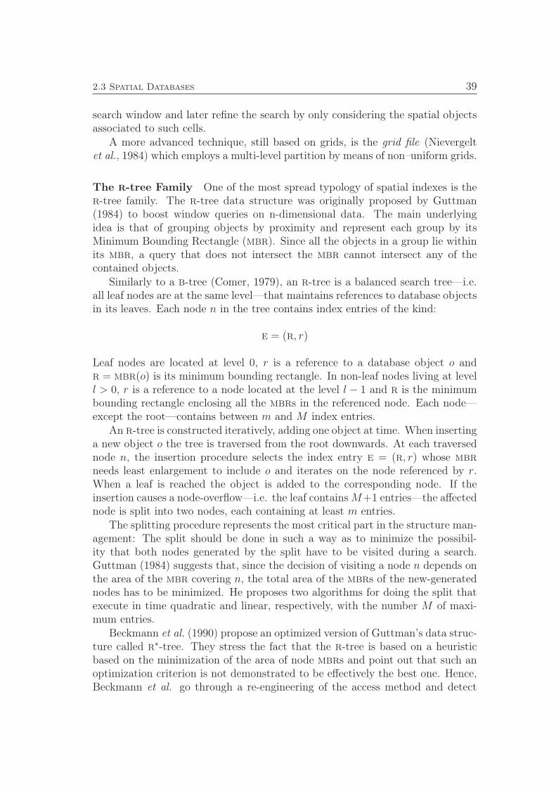
2.3 Spatial Databases 39
search window and later refine the search by only considering the spatial objectsassociated to such cells.
A more advanced technique, still based on grids, is the grid file (Nievergeltet al., 1984) which employs a multi-level partition by means of non–uniform grids.
The r-tree Family One of the most spread typology of spatial indexes is ther-tree family. The r-tree data structure was originally proposed by Guttman(1984) to boost window queries on n-dimensional data. The main underlyingidea is that of grouping objects by proximity and represent each group by itsMinimum Bounding Rectangle (mbr). Since all the objects in a group lie withinits mbr, a query that does not intersect the mbr cannot intersect any of thecontained objects.
Similarly to a b-tree (Comer, 1979), an r-tree is a balanced search tree—i.e.all leaf nodes are at the same level—that maintains references to database objectsin its leaves. Each node n in the tree contains index entries of the kind:
e = (r, r)
Leaf nodes are located at level 0, r is a reference to a database object o andr = mbr(o) is its minimum bounding rectangle. In non-leaf nodes living at levell > 0, r is a reference to a node located at the level l − 1 and r is the minimumbounding rectangle enclosing all the mbrs in the referenced node. Each node—except the root—contains between m and M index entries.
An r-tree is constructed iteratively, adding one object at time. When insertinga new object o the tree is traversed from the root downwards. At each traversednode n, the insertion procedure selects the index entry e = (r, r) whose mbrneeds least enlargement to include o and iterates on the node referenced by r.When a leaf is reached the object is added to the corresponding node. If theinsertion causes a node-overflow—i.e. the leaf containsM+1 entries—the affectednode is split into two nodes, each containing at least m entries.
The splitting procedure represents the most critical part in the structure man-agement: The split should be done in such a way as to minimize the possibil-ity that both nodes generated by the split have to be visited during a search.Guttman (1984) suggests that, since the decision of visiting a node n depends onthe area of the mbr covering n, the total area of the mbrs of the new-generatednodes has to be minimized. He proposes two algorithms for doing the split thatexecute in time quadratic and linear, respectively, with the number M of maxi-mum entries.
Beckmann et al. (1990) propose an optimized version of Guttman’s data struc-ture called r∗-tree. They stress the fact that the r-tree is based on a heuristicbased on the minimization of the area of node mbrs and point out that such anoptimization criterion is not demonstrated to be effectively the best one. Hence,Beckmann et al. go through a re-engineering of the access method and detect
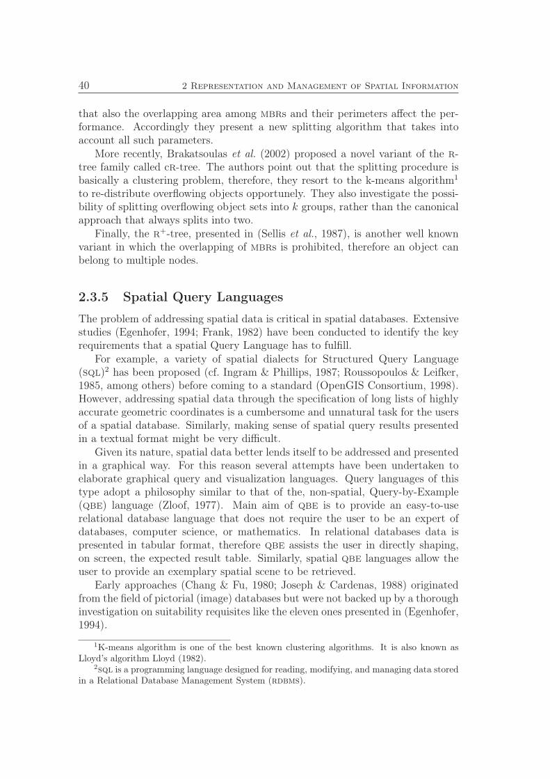
40 2 Representation and Management of Spatial Information
that also the overlapping area among mbrs and their perimeters affect the per-formance. Accordingly they present a new splitting algorithm that takes intoaccount all such parameters.
More recently, Brakatsoulas et al. (2002) proposed a novel variant of the r-tree family called cr-tree. The authors point out that the splitting procedure isbasically a clustering problem, therefore, they resort to the k-means algorithm1
to re-distribute overflowing objects opportunely. They also investigate the possi-bility of splitting overflowing object sets into k groups, rather than the canonicalapproach that always splits into two.
Finally, the r+-tree, presented in (Sellis et al., 1987), is another well knownvariant in which the overlapping of mbrs is prohibited, therefore an object canbelong to multiple nodes.
2.3.5 Spatial Query Languages
The problem of addressing spatial data is critical in spatial databases. Extensivestudies (Egenhofer, 1994; Frank, 1982) have been conducted to identify the keyrequirements that a spatial Query Language has to fulfill.
For example, a variety of spatial dialects for Structured Query Language(sql)2 has been proposed (cf. Ingram & Phillips, 1987; Roussopoulos & Leifker,1985, among others) before coming to a standard (OpenGIS Consortium, 1998).However, addressing spatial data through the specification of long lists of highlyaccurate geometric coordinates is a cumbersome and unnatural task for the usersof a spatial database. Similarly, making sense of spatial query results presentedin a textual format might be very difficult.
Given its nature, spatial data better lends itself to be addressed and presentedin a graphical way. For this reason several attempts have been undertaken toelaborate graphical query and visualization languages. Query languages of thistype adopt a philosophy similar to that of the, non-spatial, Query-by-Example(qbe) language (Zloof, 1977). Main aim of qbe is to provide an easy-to-userelational database language that does not require the user to be an expert ofdatabases, computer science, or mathematics. In relational databases data ispresented in tabular format, therefore qbe assists the user in directly shaping,on screen, the expected result table. Similarly, spatial qbe languages allow theuser to provide an exemplary spatial scene to be retrieved.
Early approaches (Chang & Fu, 1980; Joseph & Cardenas, 1988) originatedfrom the field of pictorial (image) databases but were not backed up by a thoroughinvestigation on suitability requisites like the eleven ones presented in (Egenhofer,1994).
1K-means algorithm is one of the best known clustering algorithms. It is also known asLloyd’s algorithm Lloyd (1982).
2sql is a programming language designed for reading, modifying, and managing data storedin a Relational Database Management System (rdbms).
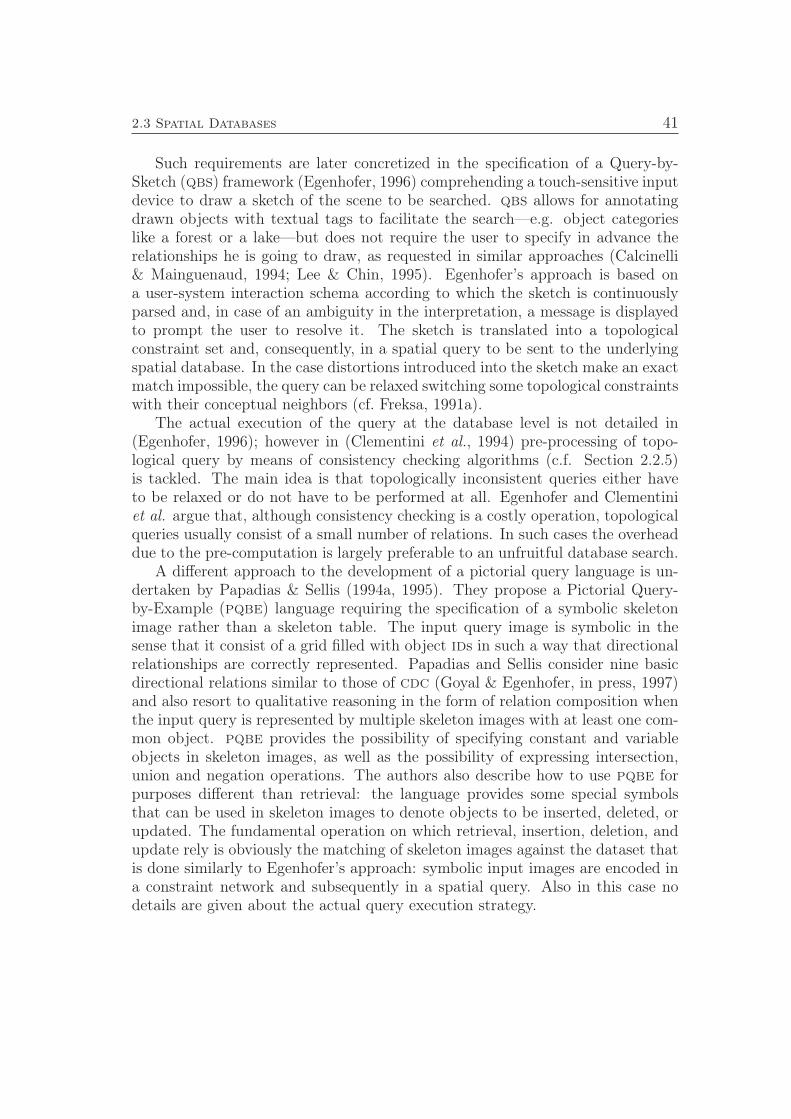
2.3 Spatial Databases 41
Such requirements are later concretized in the specification of a Query-by-Sketch (qbs) framework (Egenhofer, 1996) comprehending a touch-sensitive inputdevice to draw a sketch of the scene to be searched. qbs allows for annotatingdrawn objects with textual tags to facilitate the search—e.g. object categorieslike a forest or a lake—but does not require the user to specify in advance therelationships he is going to draw, as requested in similar approaches (Calcinelli& Mainguenaud, 1994; Lee & Chin, 1995). Egenhofer’s approach is based ona user-system interaction schema according to which the sketch is continuouslyparsed and, in case of an ambiguity in the interpretation, a message is displayedto prompt the user to resolve it. The sketch is translated into a topologicalconstraint set and, consequently, in a spatial query to be sent to the underlyingspatial database. In the case distortions introduced into the sketch make an exactmatch impossible, the query can be relaxed switching some topological constraintswith their conceptual neighbors (cf. Freksa, 1991a).
The actual execution of the query at the database level is not detailed in(Egenhofer, 1996); however in (Clementini et al., 1994) pre-processing of topo-logical query by means of consistency checking algorithms (c.f. Section 2.2.5)is tackled. The main idea is that topologically inconsistent queries either haveto be relaxed or do not have to be performed at all. Egenhofer and Clementiniet al. argue that, although consistency checking is a costly operation, topologicalqueries usually consist of a small number of relations. In such cases the overheaddue to the pre-computation is largely preferable to an unfruitful database search.
A different approach to the development of a pictorial query language is un-dertaken by Papadias & Sellis (1994a, 1995). They propose a Pictorial Query-by-Example (pqbe) language requiring the specification of a symbolic skeletonimage rather than a skeleton table. The input query image is symbolic in thesense that it consist of a grid filled with object ids in such a way that directionalrelationships are correctly represented. Papadias and Sellis consider nine basicdirectional relations similar to those of cdc (Goyal & Egenhofer, in press, 1997)and also resort to qualitative reasoning in the form of relation composition whenthe input query is represented by multiple skeleton images with at least one com-mon object. pqbe provides the possibility of specifying constant and variableobjects in skeleton images, as well as the possibility of expressing intersection,union and negation operations. The authors also describe how to use pqbe forpurposes different than retrieval: the language provides some special symbolsthat can be used in skeleton images to denote objects to be inserted, deleted, orupdated. The fundamental operation on which retrieval, insertion, deletion, andupdate rely is obviously the matching of skeleton images against the dataset thatis done similarly to Egenhofer’s approach: symbolic input images are encoded ina constraint network and subsequently in a spatial query. Also in this case nodetails are given about the actual query execution strategy.


Chapter 3
Qualitative Spatial Configuration Queries
In this chapter we introduce, discuss, analyze, and devise solutions to the Quali-tative Spatial Configuration Query (qscq) problem.
3.1 Qualitative Spatial Relation Queries
In Section 2.3.3 spatial queries have been defined and the most common typeshave been discussed. It has been outlined that, despite their semantic differences,spatial queries share a ground commonality: they all encode spatial predicatesthat, typically, embody some sort of qualitative spatial relation. Accordingly, thetotality of such spatial queries can be generally referred to as qualitative spatialrelation queries.
Qualitative spatial relation queries can be classified according to the “degreeof indetermination” of the spatial predicates involved, namely according to theelements of the spatial predicate that are left unspecified. Let us consider queriesinvolving only one binary predicate of the form
(primary object, spatial relation, reference object)
Moreover, let us assume that the spatial predicate is taken from a set of B quali-tative relations and that the query is defined over a spatial dataset of cardinalityN—i.e. containing N objects. Then, Table 3.1 shows a possible categorizationand nomenclature.
Given the typical size N of a spatial dataset, we can safely assume that B≪ N.Hence, Table 3.1 also lists the different types of qualitative spatial queries orderedaccording to the number of checks to be performed to resolve any query. A relationretrieval query, for instance, has to be checked against (in the worst case) allthe B available spatial predicates in order to find out the one holding among
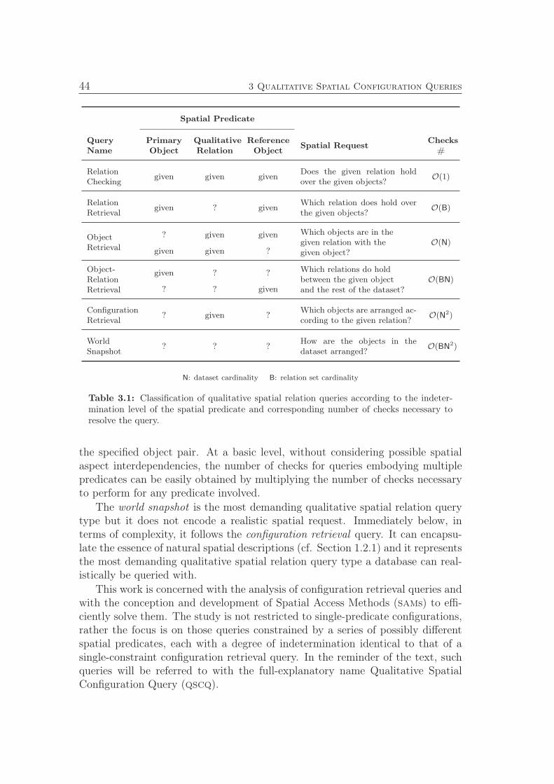
44 3 Qualitative Spatial Configuration Queries
Spatial Predicate
Query
Name
Primary
Object
Qualitative
Relation
Reference
ObjectSpatial Request
Checks
#
Relation
Checkinggiven given given
Does the given relation hold
over the given objects?O(1)
Relation
Retrievalgiven ? given
Which relation does hold over
the given objects?O(B)
? given givenObject
Retrieval given given ?
Which objects are in the
given relation with the
given object?
O(N)
Object-
Relation
Retrieval
given ? ? Which relations do hold
between the given object
and the rest of the dataset?
O(BN)? ? given
Configuration
Retrieval? given ?
Which objects are arranged ac-
cording to the given relation?O(N2)
World
Snapshot? ? ?
How are the objects in the
dataset arranged?O(BN2)
N: dataset cardinality B: relation set cardinality
Table 3.1: Classification of qualitative spatial relation queries according to the indeter-mination level of the spatial predicate and corresponding number of checks necessary toresolve the query.
the specified object pair. At a basic level, without considering possible spatialaspect interdependencies, the number of checks for queries embodying multiplepredicates can be easily obtained by multiplying the number of checks necessaryto perform for any predicate involved.
The world snapshot is the most demanding qualitative spatial relation querytype but it does not encode a realistic spatial request. Immediately below, interms of complexity, it follows the configuration retrieval query. It can encapsu-late the essence of natural spatial descriptions (cf. Section 1.2.1) and it representsthe most demanding qualitative spatial relation query type a database can real-istically be queried with.
This work is concerned with the analysis of configuration retrieval queries andwith the conception and development of Spatial Access Methods (sams) to effi-ciently solve them. The study is not restricted to single-predicate configurations,rather the focus is on those queries constrained by a series of possibly differentspatial predicates, each with a degree of indetermination identical to that of asingle-constraint configuration retrieval query. In the reminder of the text, suchqueries will be referred to with the full-explanatory name Qualitative SpatialConfiguration Query (qscq).
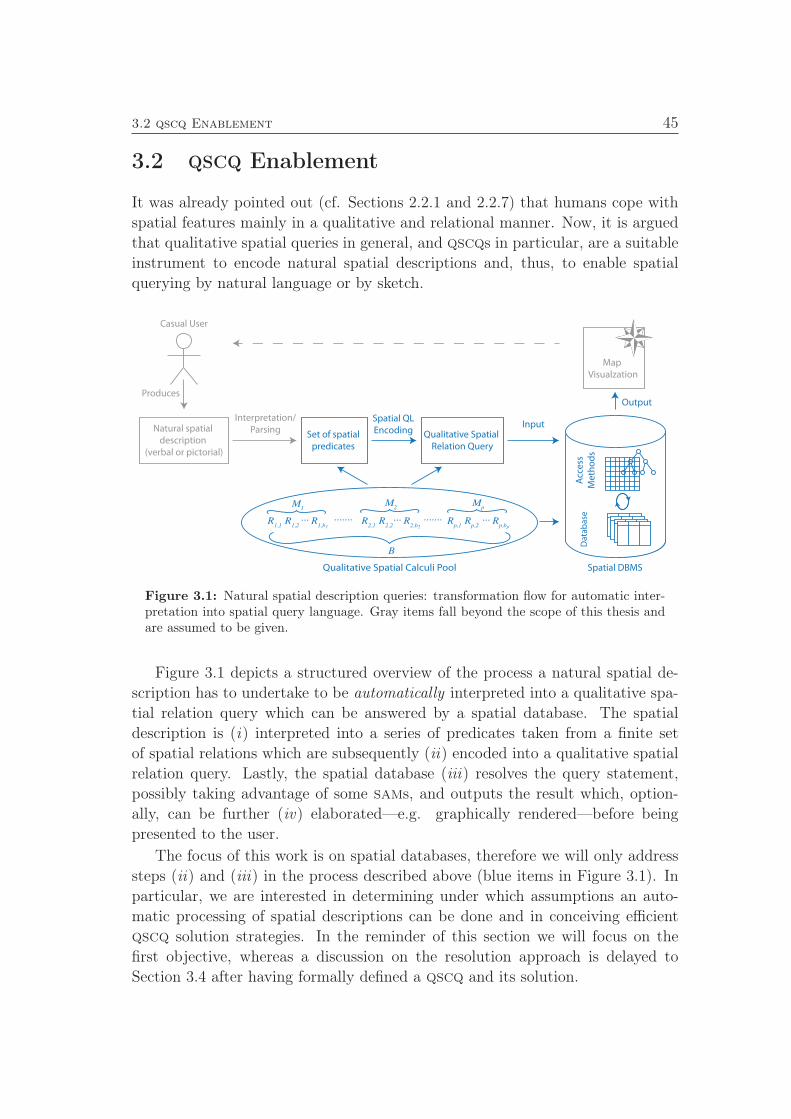
3.2 qscq Enablement 45
3.2 qscq Enablement
It was already pointed out (cf. Sections 2.2.1 and 2.2.7) that humans cope with
spatial features mainly in a qualitative and relational manner. Now, it is argued
that qualitative spatial queries in general, and qscqs in particular, are a suitable
instrument to encode natural spatial descriptions and, thus, to enable spatial
querying by natural language or by sketch.
Produces
Natural spatial
description
(verbal or pictorial)
Set of spatial
predicates
Qualitative Spatial
Relation Query
Spatial QL
Encoding
Qualitative Spatial Calculi Pool
B
R2,1
R2,2
... R2,b2
Rp,1
Rp,2
... Rp,bp
R1,1
R1,2
... R1,b1
M1
M2
Mp
....... .......
Da
tab
ase
Acc
ess
Me
tho
ds
Spatial DBMS
Map
Visualzation
Output
InputInterpretation/
Parsing
Casual User
Figure 3.1: Natural spatial description queries: transformation flow for automatic inter-pretation into spatial query language. Gray items fall beyond the scope of this thesis andare assumed to be given.
Figure 3.1 depicts a structured overview of the process a natural spatial de-
scription has to undertake to be automatically interpreted into a qualitative spa-
tial relation query which can be answered by a spatial database. The spatial
description is (i) interpreted into a series of predicates taken from a finite set
of spatial relations which are subsequently (ii) encoded into a qualitative spatial
relation query. Lastly, the spatial database (iii) resolves the query statement,
possibly taking advantage of some sams, and outputs the result which, option-
ally, can be further (iv) elaborated—e.g. graphically rendered—before being
presented to the user.
The focus of this work is on spatial databases, therefore we will only address
steps (ii) and (iii) in the process described above (blue items in Figure 3.1). In
particular, we are interested in determining under which assumptions an auto-
matic processing of spatial descriptions can be done and in conceiving efficient
qscq solution strategies. In the reminder of this section we will focus on the
first objective, whereas a discussion on the resolution approach is delayed to
Section 3.4 after having formally defined a qscq and its solution.
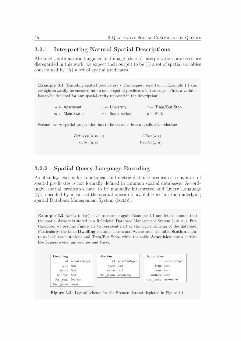
46 3 Qualitative Spatial Configuration Queries
3.2.1 Interpreting Natural Spatial Descriptions
Although, both natural language and image (sketch) interpretation processes aredisregarded in this work, we expect their output to be (i) a set of spatial variablesconstrained by (ii) a set of spatial predicates.
Example 3.1 (Encoding spatial predicates) - The request reported in Example 1.1 can
straightforwardly be encoded into a set of spatial predicates in two steps. First, a variable
has to be declared for any spatial entity reported in the description:
a← Apartment u← University t← Tram/Bus Stop
m← Main Station s← Supermarket p← Park
Second, every spatial proposition has to be encoded into a qualitative relation:
Between(a,m, u) Close(a, t)
Close(a, s) V isible(p, a)
3.2.2 Spatial Query Language Encoding
As of today, except for topological and metric distance predicates, semantics ofspatial predicates is not formally defined in common spatial databases. Accord-ingly, spatial predicates have to be manually interpreted and Query Language(ql)-encoded by means of the spatial operators available within the underlyingspatial Database Management System (dbms).
Example 3.2 (qscq today) - Let us resume again Example 1.1 and let us assume that
the spatial dataset is stored in a Relational Database Management System (rdbms). Fur-
thermore, we assume Figure 3.2 to represent part of the logical schema of the database.
Particularly, the table Dwelling contains houses and Apartments, the table Station main-
tains both train stations and Tram/Bus Stops while the table Amenities stores entities
like Supermarkets, universities and Parks.
Dwelling
id: serial integer
type: text
name: text
address: text
for_rent: boolean
the_geom: point
Station
id: serial integer
type: text
name: text
the_geom: geometry
Amenities
id: serial integer
type: text
name: text
address: text
the_geom: geometry
Figure 3.2: Logical scheme for the Bremen dataset depicted in Figure 1.1.

3.2 qscq Enablement 47
Then the request in Example 1.1 can possibly be encoded into a spatially-extended
sql language. The absence of appropriate spatial operators to express all of the required
spatial constraints (cf. Section 2.3.2) forces the database user to geometrically interpret
the spatial description and to elaborate a cumbersome query statement like the one shown
in Listing 3.1. Since no formal semantics is provided for the requested predicates, several
assumptions have been made. (i) The relation Between(a,m, u) has been considered satis-
fied by all those Apartments a located within an ellipse, with eccentricity equal to 23 , whose
foci are m and u (cf. lines 15-19). (ii) Similarly, the qualitative distance relation Close has
been interpreted as “less than 2 units away” (cf. lines 20 and 21), whatever a unit means.
(iii) Lastly, the visibility constraint has been heavily approximated with the condition thatno dwelling lies in between the searched Apartment and a Park (cf. lines 22-28).
Listing 3.1: Possible SQL encoding of the spatial request in Example 1.1
1 SELECT
2 a.the_geom, m.the_geom, u.the_geom,
3 s.the_geom, t.the_geom, p.the_geom
4 FROM
5 Dwelling AS d,
6 Dwelling AS a, Station AS m, Amenities AS u,
7 Amenities AS s, Station AS t, Amenities AS p
8 WHERE
9 a.type = "Apartment" AND a.for_rent = true
10 AND m.type = "Main Station"
11 AND u.type = "University"
12 AND s.type = "Supermarket"
13 AND t.type = "Tram/Bus Stop"
14 AND p.type = "Park"
15 AND (distance(a.the_geom,m.the_geom) +
16 distance(a.the_geom,u.the_geom))
17 <=
18 (distance(m.the_geom,u.the_geom) +
19 (distance(m.the_geom,u.the_geom)/2))
20 AND distance(a.the_geom,s.the_geom) < 2
21 AND distance(a.the_geom,t.the_geom) < 2
22 AND NOT intersect(
23 set_difference(
24 convex_hull(union(a.the_geom,p.the_geom)),
25 union(a.the_geom,p.the_geom)
26 ),
27 d.the_geom
28 )
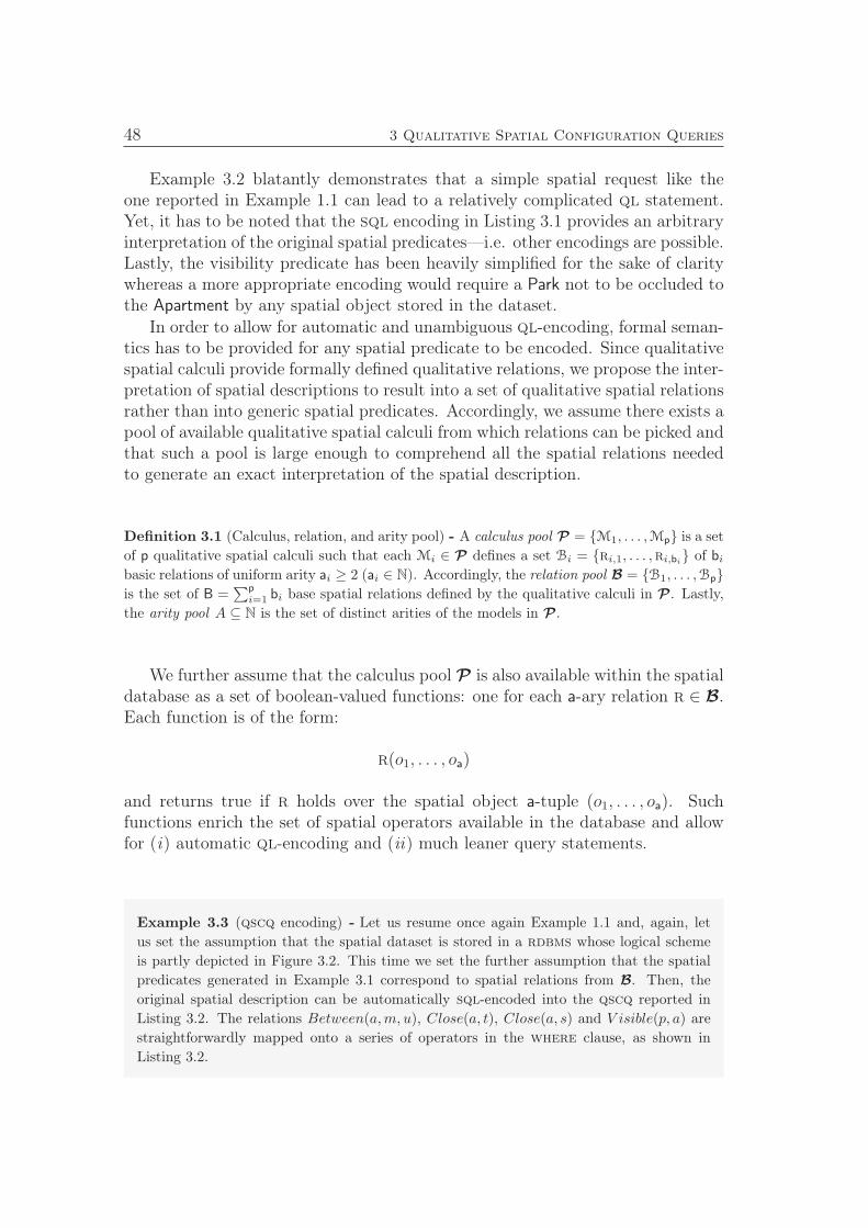
48 3 Qualitative Spatial Configuration Queries
Example 3.2 blatantly demonstrates that a simple spatial request like theone reported in Example 1.1 can lead to a relatively complicated ql statement.Yet, it has to be noted that the sql encoding in Listing 3.1 provides an arbitraryinterpretation of the original spatial predicates—i.e. other encodings are possible.Lastly, the visibility predicate has been heavily simplified for the sake of claritywhereas a more appropriate encoding would require a Park not to be occluded tothe Apartment by any spatial object stored in the dataset.
In order to allow for automatic and unambiguous ql-encoding, formal seman-tics has to be provided for any spatial predicate to be encoded. Since qualitativespatial calculi provide formally defined qualitative relations, we propose the inter-pretation of spatial descriptions to result into a set of qualitative spatial relationsrather than into generic spatial predicates. Accordingly, we assume there exists apool of available qualitative spatial calculi from which relations can be picked andthat such a pool is large enough to comprehend all the spatial relations neededto generate an exact interpretation of the spatial description.
Definition 3.1 (Calculus, relation, and arity pool) - A calculus pool P = M1, . . . ,Mp is a set
of p qualitative spatial calculi such that each Mi ∈ P defines a set Bi = ri,1, . . . ,ri,bi of bibasic relations of uniform arity ai ≥ 2 (ai ∈ N). Accordingly, the relation pool B = B1, . . . ,Bp
is the set of B =∑p
i=1 bi base spatial relations defined by the qualitative calculi in P . Lastly,
the arity pool A ⊆ N is the set of distinct arities of the models in P .
We further assume that the calculus pool P is also available within the spatialdatabase as a set of boolean-valued functions: one for each a-ary relation r ∈ B.Each function is of the form:
r(o1, . . . , oa)
and returns true if r holds over the spatial object a-tuple (o1, . . . , oa). Suchfunctions enrich the set of spatial operators available in the database and allowfor (i) automatic ql-encoding and (ii) much leaner query statements.
Example 3.3 (qscq encoding) - Let us resume once again Example 1.1 and, again, let
us set the assumption that the spatial dataset is stored in a rdbms whose logical scheme
is partly depicted in Figure 3.2. This time we set the further assumption that the spatial
predicates generated in Example 3.1 correspond to spatial relations from B. Then, the
original spatial description can be automatically sql-encoded into the qscq reported in
Listing 3.2. The relations Between(a,m, u), Close(a, t), Close(a, s) and V isible(p, a) are
straightforwardly mapped onto a series of operators in the where clause, as shown in
Listing 3.2.
3.3 The qscq Problem 49
Listing 3.2: qscq encoding of the spatial request in Example 1.1
1 SELECT
2 a.the_geom, m.the_geom, u.the_geom,
3 s.the_geom, t.the_geom, p.the_geom
4 FROM
5 Dwelling AS a, Station AS m, Amenities AS u,
6 Amenities AS s, Station AS t, Amenities AS p
7 WHERE
8 a.type = "Apartment" AND a.for_rent = true
9 AND m.type = "Main Station"
10 AND u.type = "University"
11 AND s.type = "Supermarket"
12 AND t.type = "Tram/Bus Stop"
13 AND p.type = "Park"
14 AND Between(a,m,u)
15 AND Close(a,t)
16 AND Close(a,s)
17 AND Visible(p,a)
3.3 The qscq Problem
So far we described the challenge of enabling qualitative spatial relation queries
in a rather conceptual way to illustrate all involved constituents more clearly.
Yet, now that all the components involved in the game have been introduced and
an analysis of qscq solving procedure is to be carried out, a formalization of the
concepts of qscq and of its solution is necessary.
Definition 3.2 (Qualitative Spatial Configuration Query) - Given a calculus pool P and a
spatial dataset O. A Qualitative Spatial Configuration Query defined over (O,P) is a pair
Q = (X,Ξ) where X is a set of v variables ranging over O and Ξ is a set of c spatial constraints.
Each constraint ξ ∈ Ξ is, in turn, a pair ξ = (R, χ) where R ⊆ B is the set of relations of
uniform arity a defined over the same variable a-sequence χ ∈ Xa. The relationship between
the variable set and the constraint set is expressed by the following rule:
X = c⋃
i=1
χ(ξi)
where χ(ξi) is the spatial variable a-sequence constrained by ξi
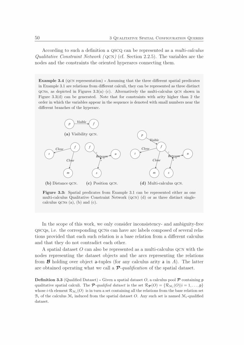
50 3 Qualitative Spatial Configuration Queries
According to such a definition a qscq can be represented as a multi-calculus
Qualitative Constraint Network (qcn) (cf. Section 2.2.5). The variables are the
nodes and the constraints the oriented hyperarcs connecting them.
Example 3.4 (qcn representation) - Assuming that the three different spatial predicates
in Example 3.1 are relations from different calculi, they can be represented as three distinct
qcns, as depicted in Figures 3.3(a)–(c). Alternatively the multi-calculus qcn shown in
Figure 3.3(d) can be generated. Note that for constraints with arity higher than 2 the
order in which the variables appear in the sequence is denoted with small numbers near the
different branches of the hyperarc.
fpVisible
(a) Visibility qcn.
f
t
m
Close
Close
(b) Distance qcn.
f
s
uBetween
3
2
1
(c) Position qcn.
s
uBetween
f
t
m
Close
Close
p
Visible
3
2
1
(d) Multi-calculus qcn.
Figure 3.3: Spatial predicates from Example 3.1 can be represented either as onemulti-calculus Qualitative Constraint Network (qcn) (d) or as three distinct single-calculus qcns (a), (b) and (c).
In the scope of this work, we only consider inconsistency- and ambiguity-free
qscqs, i.e. the corresponding qcns can have arc labels composed of several rela-
tions provided that each such relation is a base relation from a different calculus
and that they do not contradict each other.
A spatial dataset O can also be represented as a multi-calculus qcn with the
nodes representing the dataset objects and the arcs representing the relations
from B holding over object a-tuples (for any calculus arity a in A). The latter
are obtained operating what we call a P-qualification of the spatial dataset.
Definition 3.3 (Qualified Dataset) - Given a spatial dataset O, a calculus pool P containing p
qualitative spatial calculi. The P-qualified dataset is the set RP(O) = RMi(O)|i = 1, . . . , p
whose i-th elementRMi(O) is in turn a set containing all the relations from the base relation set
Bi of the calculus Mi induced from the spatial dataset O. Any such set is named Mi-qualified
dataset.
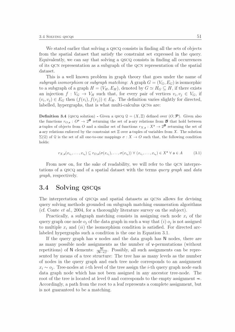
3.4 Solving qscqs 51
We stated earlier that solving a qscq consists in finding all the sets of objectsfrom the spatial dataset that satisfy the constraint set expressed in the query.Equivalently, we can say that solving a qscq consists in finding all occurrencesof its qcn representation as a subgraph of the qcn representation of the spatialdataset.
This is a well known problem in graph theory that goes under the name ofsubgraph isomorphism or subgraph matching : A graphG = (VG, EG) is isomorphicto a subgraph of a graph H = (VH , EH), denoted by G ≃ HG ⊆ H, if there existsan injection f : VG → VH such that, for every pair of vertices vi, vj ∈ VG, if(vi, vj) ∈ EG then (f(vi), f(vj)) ∈ EH . The definition varies slightly for directed,labelled, hypergraphs, that is what multi-calculus qcns are:
Definition 3.4 (qscq solution) - Given a qscq Q = (X,Ξ) defined over (O,P). Given also
the functions rO,a : Oa → 2B returning the set of a-ary relations from B that hold between
a-tuples of objects from O and a similar set of functions rX,a : Xa → 2B returning the set of
a-ary relations enforced by the constraint set Ξ over a-tuples of variables from X. The solution
Σ(Q) of Q is the set of all one-to-one mappings σ : X → O such that, the following condition
holds:
rX,a(xi1 , . . . , xia) ⊆ rO,a(σ(xi1), . . . , σ(xia)) ∀ (xi1 , . . . , xia) ∈ Xa ∀ a ∈ A (3.1)
From now on, for the sake of readability, we will refer to the qcn interpre-tations of a qscq and of a spatial dataset with the terms query graph and datagraph, respectively.
3.4 Solving qscqs
The interpretation of qscqs and spatial datasets as qcns allows for devisingquery solving methods grounded on subgraph matching enumeration algorithms(cf. Conte et al., 2004, for a thoroughly literature survey on the subject).
Practically, a subgraph matching consists in assigning each node xi of thequery graph one node oj of the data graph in such a way that (i) oj is not assignedto multiple xi and (ii) the isomorphism condition is satisfied. For directed arc-labeled hypergraphs such a condition is the one in Equation 3.1.
If the query graph has v nodes and the data graph has N nodes, there areas many possible node assignments as the number of v-permutations (withoutrepetitions) of N elements: N!
(N−v)!. Possibly, all such assignments can be repre-
sented by means of a tree structure: The tree has as many levels as the numberof nodes in the query graph and each tree node corresponds to an assignmentxi ∼ oj. Tree-nodes at i-th level of the tree assign the i-th query graph node eachdata graph node which has not been assigned in any ancestor tree-node. Theroot of the tree is located at level 0 and corresponds to the empty assignment ≁.Accordingly, a path from the root to a leaf represents a complete assignment, butis not guaranteed to be a matching.
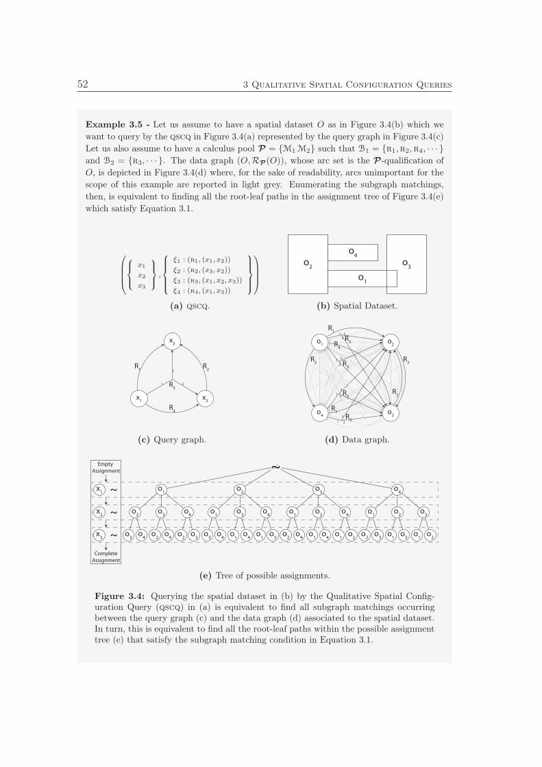
52 3 Qualitative Spatial Configuration Queries
Example 3.5 - Let us assume to have a spatial dataset O as in Figure 3.4(b) which we
want to query by the qscq in Figure 3.4(a) represented by the query graph in Figure 3.4(c)
Let us also assume to have a calculus pool P = M1 M2 such that B1 = r1,r2,r4, · · ·
and B2 = r3, · · · . The data graph (O,RP(O)), whose arc set is the P-qualification of
O, is depicted in Figure 3.4(d) where, for the sake of readability, arcs unimportant for the
scope of this example are reported in light grey. Enumerating the subgraph matchings,
then, is equivalent to finding all the root-leaf paths in the assignment tree of Figure 3.4(e)
which satisfy Equation 3.1.
x1
x2
x3
,
ξ1 : (r1, (x1, x2))
ξ2 : (r2, (x3, x2))
ξ3 : (r3, (x1, x2, x3))
ξ4 : (r4, (x1, x3))
(a) qscq.
o1
o3
o4
o2
(b) Spatial Dataset.
x2
x1
x3
R1
R2
R4
R3
1
2
3
(c) Query graph.
o2
o1
o3
o4
R1
R2
R2
R4
R2
R1
R3
R3
1
2
3
1 2
3
R3
1 2
3
R3
1
2
3
(d) Data graph.
o3
o4
o2
o3
o2
o4
x3
o3
o4
o1
o3
o1
o4
o2
o4
o1
o2
o1
o4
o2
o3
o1
o2
o1
o3
~x1
o4
o1
o3
o2
x2
o2
o3
o4
o3
o4
o1
o4
o1
o2
o3
o1
o2
~Empty
Assignment
Complete
Assignment
~
~
(e) Tree of possible assignments.
Figure 3.4: Querying the spatial dataset in (b) by the Qualitative Spatial Config-uration Query (qscq) in (a) is equivalent to find all subgraph matchings occurringbetween the query graph (c) and the data graph (d) associated to the spatial dataset.In turn, this is equivalent to find all the root-leaf paths within the possible assignmenttree (e) that satisfy the subgraph matching condition in Equation 3.1.
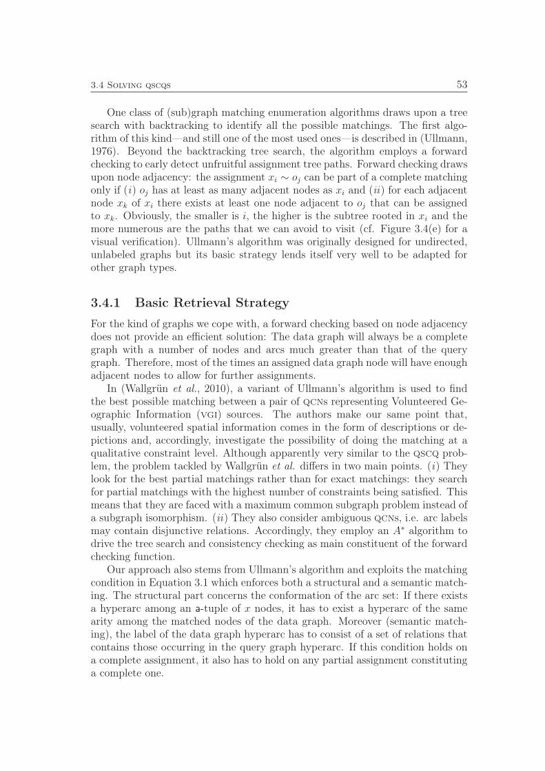
3.4 Solving qscqs 53
One class of (sub)graph matching enumeration algorithms draws upon a treesearch with backtracking to identify all the possible matchings. The first algo-rithm of this kind—and still one of the most used ones—is described in (Ullmann,1976). Beyond the backtracking tree search, the algorithm employs a forwardchecking to early detect unfruitful assignment tree paths. Forward checking drawsupon node adjacency: the assignment xi ∼ oj can be part of a complete matchingonly if (i) oj has at least as many adjacent nodes as xi and (ii) for each adjacentnode xk of xi there exists at least one node adjacent to oj that can be assignedto xk. Obviously, the smaller is i, the higher is the subtree rooted in xi and themore numerous are the paths that we can avoid to visit (cf. Figure 3.4(e) for avisual verification). Ullmann’s algorithm was originally designed for undirected,unlabeled graphs but its basic strategy lends itself very well to be adapted forother graph types.
3.4.1 Basic Retrieval Strategy
For the kind of graphs we cope with, a forward checking based on node adjacencydoes not provide an efficient solution: The data graph will always be a completegraph with a number of nodes and arcs much greater than that of the querygraph. Therefore, most of the times an assigned data graph node will have enoughadjacent nodes to allow for further assignments.
In (Wallgrün et al., 2010), a variant of Ullmann’s algorithm is used to findthe best possible matching between a pair of qcns representing Volunteered Ge-ographic Information (vgi) sources. The authors make our same point that,usually, volunteered spatial information comes in the form of descriptions or de-pictions and, accordingly, investigate the possibility of doing the matching at aqualitative constraint level. Although apparently very similar to the qscq prob-lem, the problem tackled by Wallgrün et al. differs in two main points. (i) Theylook for the best partial matchings rather than for exact matchings: they searchfor partial matchings with the highest number of constraints being satisfied. Thismeans that they are faced with a maximum common subgraph problem instead ofa subgraph isomorphism. (ii) They also consider ambiguous qcns, i.e. arc labelsmay contain disjunctive relations. Accordingly, they employ an A∗ algorithm todrive the tree search and consistency checking as main constituent of the forwardchecking function.
Our approach also stems from Ullmann’s algorithm and exploits the matchingcondition in Equation 3.1 which enforces both a structural and a semantic match-ing. The structural part concerns the conformation of the arc set: If there existsa hyperarc among an a-tuple of x nodes, it has to exist a hyperarc of the samearity among the matched nodes of the data graph. Moreover (semantic match-ing), the label of the data graph hyperarc has to consist of a set of relations thatcontains those occurring in the query graph hyperarc. If this condition holds ona complete assignment, it also has to hold on any partial assignment constitutinga complete one.
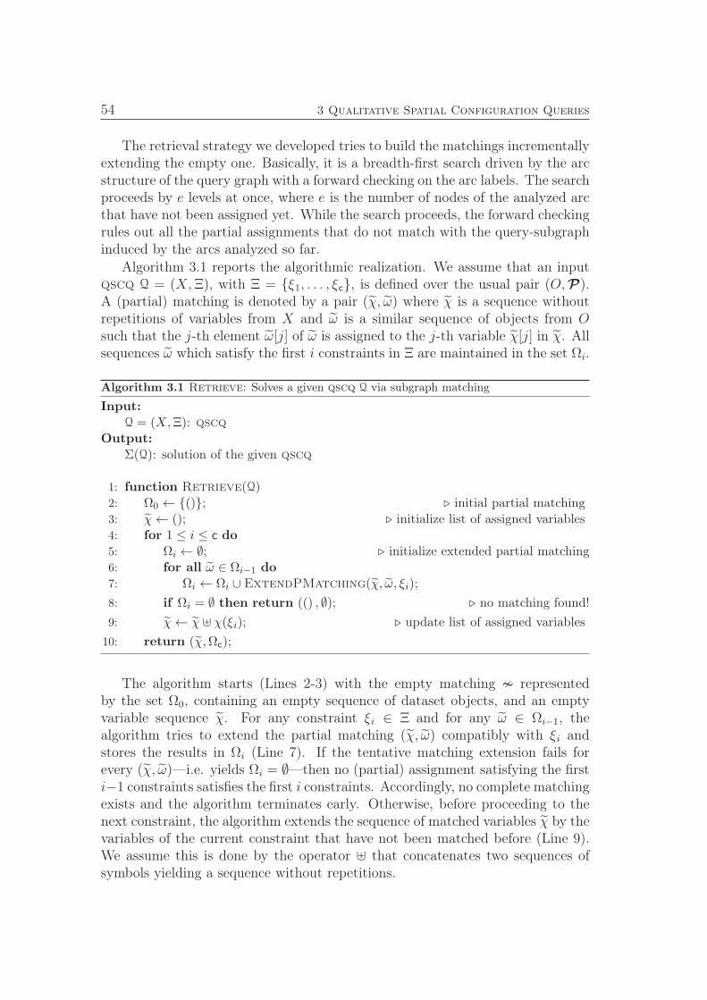
54 3 Qualitative Spatial Configuration Queries
The retrieval strategy we developed tries to build the matchings incrementallyextending the empty one. Basically, it is a breadth-first search driven by the arcstructure of the query graph with a forward checking on the arc labels. The searchproceeds by e levels at once, where e is the number of nodes of the analyzed arcthat have not been assigned yet. While the search proceeds, the forward checkingrules out all the partial assignments that do not match with the query-subgraphinduced by the arcs analyzed so far.
Algorithm 3.1 reports the algorithmic realization. We assume that an inputqscq Q = (X,Ξ), with Ξ = ξ1, . . . , ξc, is defined over the usual pair (O,P).A (partial) matching is denoted by a pair (χ, ω) where χ is a sequence withoutrepetitions of variables from X and ω is a similar sequence of objects from Osuch that the j-th element ω[j] of ω is assigned to the j-th variable χ[j] in χ. Allsequences ω which satisfy the first i constraints in Ξ are maintained in the set Ωi.
Algorithm 3.1 Retrieve: Solves a given qscq Q via subgraph matching
Input:
Q = (X,Ξ): qscq
Output:
Σ(Q): solution of the given qscq
1: function Retrieve(Q)2: Ω0 ← (); ⊲ initial partial matching3: χ← (); ⊲ initialize list of assigned variables4: for 1 ≤ i ≤ c do
5: Ωi ← ∅; ⊲ initialize extended partial matching6: for all ω ∈ Ωi−1 do
7: Ωi ← Ωi ∪ ExtendPMatching(χ, ω, ξi);
8: if Ωi = ∅ then return (() , ∅); ⊲ no matching found!
9: χ← χ ⊎ χ(ξi); ⊲ update list of assigned variables
10: return (χ,Ωc);
The algorithm starts (Lines 2-3) with the empty matching ≁ representedby the set Ω0, containing an empty sequence of dataset objects, and an emptyvariable sequence χ. For any constraint ξi ∈ Ξ and for any ω ∈ Ωi−1, thealgorithm tries to extend the partial matching (χ, ω) compatibly with ξi andstores the results in Ωi (Line 7). If the tentative matching extension fails forevery (χ, ω)—i.e. yields Ωi = ∅—then no (partial) assignment satisfying the firsti−1 constraints satisfies the first i constraints. Accordingly, no complete matchingexists and the algorithm terminates early. Otherwise, before proceeding to thenext constraint, the algorithm extends the sequence of matched variables χ by thevariables of the current constraint that have not been matched before (Line 9).We assume this is done by the operator ⊎ that concatenates two sequences ofsymbols yielding a sequence without repetitions.
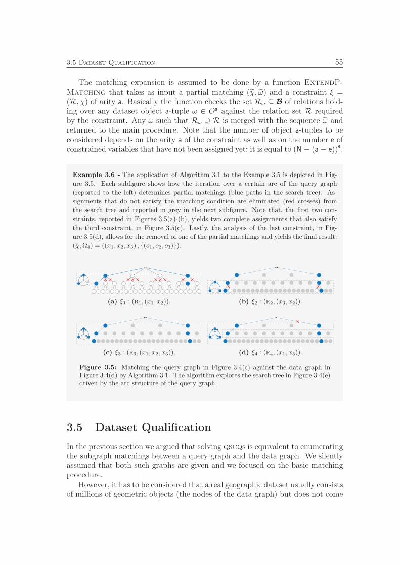
3.5 Dataset Qualification 55
The matching expansion is assumed to be done by a function ExtendP-Matching that takes as input a partial matching (χ, ω) and a constraint ξ =(R, χ) of arity a. Basically the function checks the set Rω ⊆ B of relations hold-ing over any dataset object a-tuple ω ∈ Oa against the relation set R requiredby the constraint. Any ω such that Rω ⊇ R is merged with the sequence ω andreturned to the main procedure. Note that the number of object a-tuples to beconsidered depends on the arity a of the constraint as well as on the number e ofconstrained variables that have not been assigned yet; it is equal to (N− (a− e))e.
Example 3.6 - The application of Algorithm 3.1 to the Example 3.5 is depicted in Fig-
ure 3.5. Each subfigure shows how the iteration over a certain arc of the query graph
(reported to the left) determines partial matchings (blue paths in the search tree). As-
signments that do not satisfy the matching condition are eliminated (red crosses) from
the search tree and reported in grey in the next subfigure. Note that, the first two con-
straints, reported in Figures 3.5(a)-(b), yields two complete assignments that also satisfy
the third constraint, in Figure 3.5(c). Lastly, the analysis of the last constraint, in Fig-
ure 3.5(d), allows for the removal of one of the partial matchings and yields the final result:
(χ,Ω4) = ((x1, x2, x3) , (o1, o2, o3)).
~
(a) ξ1 : (r1, (x1, x2)).
~
(b) ξ2 : (r2, (x3, x2)).
~
(c) ξ3 : (r3, (x1, x2, x3)).
~
(d) ξ4 : (r4, (x1, x3)).
Figure 3.5: Matching the query graph in Figure 3.4(c) against the data graph inFigure 3.4(d) by Algorithm 3.1. The algorithm explores the search tree in Figure 3.4(e)driven by the arc structure of the query graph.
3.5 Dataset Qualification
In the previous section we argued that solving qscqs is equivalent to enumeratingthe subgraph matchings between a query graph and the data graph. We silentlyassumed that both such graphs are given and we focused on the basic matchingprocedure.
However, it has to be considered that a real geographic dataset usually consistsof millions of geometric objects (the nodes of the data graph) but does not come
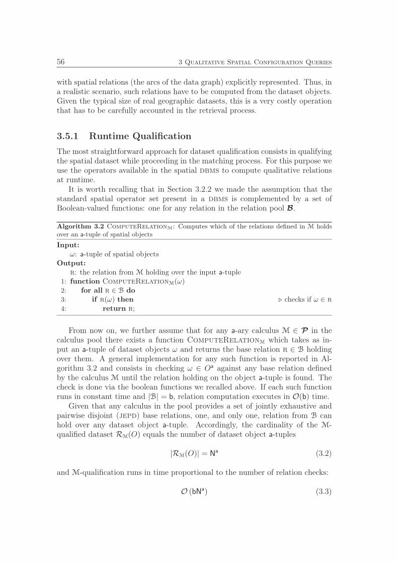
56 3 Qualitative Spatial Configuration Queries
with spatial relations (the arcs of the data graph) explicitly represented. Thus, ina realistic scenario, such relations have to be computed from the dataset objects.Given the typical size of real geographic datasets, this is a very costly operationthat has to be carefully accounted in the retrieval process.
3.5.1 Runtime Qualification
The most straightforward approach for dataset qualification consists in qualifyingthe spatial dataset while proceeding in the matching process. For this purpose weuse the operators available in the spatial dbms to compute qualitative relationsat runtime.
It is worth recalling that in Section 3.2.2 we made the assumption that thestandard spatial operator set present in a dbms is complemented by a set ofBoolean-valued functions: one for any relation in the relation pool B.
Algorithm 3.2 ComputeRelationM: Computes which of the relations defined in M holdsover an a-tuple of spatial objects
Input:
ω: a-tuple of spatial objectsOutput:
r: the relation from M holding over the input a-tuple1: function ComputeRelationM(ω)2: for all r ∈ B do
3: if r(ω) then ⊲ checks if ω ∈ r
4: return r;
From now on, we further assume that for any a-ary calculus M ∈ P in thecalculus pool there exists a function ComputeRelationM which takes as in-put an a-tuple of dataset objects ω and returns the base relation r ∈ B holdingover them. A general implementation for any such function is reported in Al-gorithm 3.2 and consists in checking ω ∈ Oa against any base relation definedby the calculus M until the relation holding on the object a-tuple is found. Thecheck is done via the boolean functions we recalled above. If each such functionruns in constant time and |B| = b, relation computation executes in O(b) time.
Given that any calculus in the pool provides a set of jointly exhaustive andpairwise disjoint (jepd) base relations, one, and only one, relation from B canhold over any dataset object a-tuple. Accordingly, the cardinality of the M-qualified dataset RM(O) equals the number of dataset object a-tuples
|RM(O)| = Na (3.2)
and M-qualification runs in time proportional to the number of relation checks:
O (bNa) (3.3)
3.5 Dataset Qualification 57
Given that, in the worst case, a qscq involves relations from any calculus inthe pool P , runtime qualification affects the time of each qscq retrieval by afactor:
O
(∑
M∈P
b(M)Na(M)
)(3.4)
where b(M) and a(M) stand for the number of base relations defined in M andthe arity of the calculus, respectively. Such a temporal cost is definitely unfeasiblewhen considering real geospatial datasets, even for a small calculus pool.
Clementini et al. (1994), showed that for the 9-Intersection Model (9-im)(Egenhofer, 1989, 1991) the relation computation time can be drastically reducedby performing the checks according to the relation-occurrence-frequency order.However, such heuristics only works for models with highly unbalanced relation-occurence-frequencies, e.g. nearly 90% of pairs of objects from a real geospatialdataset are Disconnected.
A further drawback of this approach is that it does not allow for exploitingand integrating purely qualitative information into the system, that is, spatialinformation directly coming in qualitative terms rather than computed from aquantitative dataset—e.g. the kind of information that can be derived fromnatural spatial descriptions.
3.5.2 Pre-qualification
A typical approach used in computer science to cope with intensive computationaltasks consists in resorting to Lookup Tables (luts): data structures designed toaccommodate the results of a certain computation, which allow to replace theruntime calculation with a faster lookup operation.
Accordingly, a different approach to tackle the dataset qualification consistsin extending the underlying spatial dbms with a qualitative storage layer, namelyenriching the database schema by some luts dedicated to accommodate qualita-tive spatial relations. We call such tables relation tables. This solution achievesthe double effect of (i) reducing qscq retrieval time and (ii) enabling the dbmsto deal with a mix of qualitative and geometric information pieces.
Having a place to store qualitative relations allows for P-qualifying the spatialdataset only once. Moreover, the relation tables can be indexed with standardtechniques—i.e. b-tree (Comer, 1979) or hashing (Fagin et al., 1979; Litwin,1980)—allowing for sub-linear access times. Assuming we employ an index whichguarantees logarithmic access time, the computational overhead for qscq re-trievals reported in Equation 3.4 becomes:
O
(∑
M∈P
log(Na(M)
))
(3.5)
58 3 Qualitative Spatial Configuration Queries
The downside of this approach lies in the amount of extra storage space re-quired to store the qualified dataset; according to Equation 3.2 it is proportionalto:
|RP(O)| =∑
M∈P
|RM(O)| =∑
M∈P
Na(M) (3.6)
Moreover, similarly to the previous approach, the time required for the pre-qualification depends on the cardinality N of the spatial dataset and on the arityand the number of relations in P . Although the latter ones are very small withrespect to the former, the dependency from the dataset cardinality represents animportant issue when dealing with real geographic datasets.
Example 3.7 - Let us consider the Bremen OpenStreetMap1 dataset—a small dataset for
geographic standards—with N ≈ 7 × 10⁴ objects. Let us assume that the calculus pool
P = cdc only consists of the Cardinal Direction Calculus (cdc) (Goyal & Egenhofer,
in press, 1997) and that the spatial dataset contains only simple regions. cdc is a binary
calculus—i.e. a(cdc) = 2—which for simple regions, only defines b(cdc) = 218 jepd base
relations. Then, according to Equation 3.6, the qualified dataset RP(Bremen) contains a
number of relations in the range of (7× 10⁴)2 = 4.9× 10⁹ and, according to Equation 3.3,
the qualification process can require up to approximately 218 · (7 × 104)2 = 1.06 × 10¹²
relation checks.
A final drawback of having such a big amount of extra stored informationregards the maintenance of consistency in the dataset. For example, the removalor the update of a spatial object has to be propagated along the whole qualifieddataset which, given the size of the latter, may be a very costly operation.
3.6 Summary and Focus
In this chapter we defined a generalization for spatial predicate queries that allowsfor looking at them as a single query type. We classified them according to thelevel of indeterminacy of the encoded spatial predicates and identified the classhardest to solve: Qualitative Spatial Configuration Queries (qscqs).
We argued that, if the semantics of spatial predicates is described formallyand available in a dbms, qualitative spatial queries represent a valuable meansto automatically encode natural spatial descriptions. Therefore they are a keyelement for the design of more natural human-Geographic Information System(gis) interfaces: qualitative spatial queries can be used for both, contributinginformation into a spatial database as well as “questioning” it. We raised thepoint that qualitative spatial calculi provide the necessary semantics and thatverbal (and/or pictorial) spatial descriptions can be interpreted into a series of
1www.openstreetmap.org/
3.6 Summary and Focus 59
spatial predicates. Then we assumed to have available a pool of qualitative spatialcalculi providing as many relations as necessary to capture the semantics of allthe spatial predicates resulting from the interpretation of any natural spatialdescription. We concluded that, having such a calculus pool encoded as a seriesof operators in a spatial dbms allows for a straightforward and automatic ql-encoding of natural spatial descriptions.
Drawing upon this assumption, we focused on qscq solving. We provided aformal definition and noted that a qscq can be represented as a multi-calculusqcn which we named query graph. Similarly a spatial dataset can also be seenas a huge qcn: the data graph. Accordingly, we showed that solving a qscqis equivalent to enumerate all the subgraph isomorphisms occurring between thetwo networks and we designed a simple graph matching procedure which exploitsproperties of this kind of graphs.
Matching algorithms have to rely on the arc set—i.e. qualitative relations—ofboth graphs and we pointed out that assuming the data graph to be given is atoo strong hypothesis because of the following motivations. (i) Usually spatialdatasets come in a geometric representation, i.e. qualitative relations occurringon the geometric set are not explicit. (ii) Given the typical cardinality of spa-tial datasets, the qualification process is a very costly operation which heavilyaffects the overall matching time and, therefore, cannot be disregarded in qscq-retrievals. Accordingly, we presented two basic approaches to tackle the datasetqualification problem. Runtime qualification is straightforwardly realizable buthighly inefficient since it requires to compute relations occurring over the wholedataset at any qscq-retrieval. The pre-qualification allows for qualifying thedataset only once and even for indexing the resulting qualified dataset. Accord-ingly this constitutes the best choice to maintain reasonable retrieval times but,on the other hand, requires an enormous quantity of extra storage space.
In agreement with this summary, the remainder of this work is focused on twomain investigations: (i) How dataset qualification can be done to obtain a goodtradeoff between storage space and qscq-retrieval time. (ii) How the assumptionthat the calculus pool contains enough qualitative calculi can be realized.
Efficient execution of spatial queries is achieved in spatial dbms through theexploitation of so-called Spatial Access Methods (sams) (cf. Section 2.3.4). InChapter 4, we design a series of sams tailored for solving qscqs; we term themQualitative Spatial Access Methods (qsams). They draw upon a combination ofluts and Qualitative Spatial Representation and Reasoning (qsr) techniques tomaintain a good trade-off between the space occupied by the dataset qualificationand qscq retrieval time.
The variety of expressions occurring in natural spatial descriptions does notallow for deciding in advance which spatial relations will be necessary for theencoding: Neither one can predict what spatial aspects—i.e. topological vs.directional—will be reported, nor which type of spatial calculi will be more suit-able for the encoding—i.e. cardinal vs. relative directions. Consequently, theassumption that the calculus pool has to provide enough qualitative relations

60 3 Qualitative Spatial Configuration Queries
to encode any spatial description, is better realized allowing for an extendablepool. This shift of perspective calls for a practical approach: In Chapter 5 anovel prototypical software framework is developed that provides a solution fora readily integration of qualitative spatial calculi as well as a development andbenchmarking tool for qsams.
Chapter 4
Qualitative Spatial Access Methods
In Section 3.4 we designed a basic strategy for solving a Qualitative Spatial Con-figuration Query (qscq) that is basically a subgraph isomorphism procedure. Thegraphs to be matched are Qualitative Constraint Networks (qcns) representingthe given qscq and the spatial dataset being queried.
In a user-computer interaction scenario, a qscq results from the interpretationof a spatial description produced by a human being. In a realistic case, it is licit toassume that such a description does not convey more than a few tens of qualitativespatial constraints. In this work, we do not cope with the interpretation processand assume that a spatial description comes already interpreted into a qscq.
In contrast, spatial datasets typically consist of millions of geometric objects,that is, the arcs of the qcn representing the dataset are not explicitly available.Thus a dataset qualification (cf. Definition 3.3) has to be performed in orderto be able to resolve a qscq. Given the typical size of a spatial dataset, a fulldataset qualification is a very costly operation that have to be carefully takeninto account in the qscq solving strategy.
In Sections 3.5.1 and 3.5.2 two basic strategies for the dataset qualificationhave been analyzed: runtime qualification and pre-qualification. The first onedoes not require any extra storage space to be used but is highly inefficient forwhat concerns the retrieval time. The second one calls for a database schemaextension—named qualitative storage layer—where the qualified dataset can bestored explicitly. This allows for fast retrievals but has two main drawbacks:(i) It requires an enormous quantity of extra storage space. (ii) Given that thetemporal cost of a full pre-qualification is extremely high, such a solution canhardly manage real world dynamism. That is, by the time the pre-computationis done, the changes that have occurred, for instance, in a city and reported inthe corresponding spatial dataset are not reflected in the qualified dataset, callingfor a new qualification.
62 4 Qualitative Spatial Access Methods
In this chapter we propose an alternative to improve the above-mentionedapproaches. The main underlying idea is to extend the spatial database witha qualitative storage layer but only pre-compute a targeted subset of the wholequalified dataset. The missing relations have to be rebuildable at retrieval time,ideally without resorting to a full dataset qualification. For doing this we suggestto resort to a relation reduction/reconstruction paradigm to be applied in thequalification and retrieval phase.
Reduction and reconstruction operations can be directly encoded within Spa-tial Access Methods (sams) specifically designed to optimize qscq executions:
Definition 4.1 (Qualitative Spatial Access Method) - Given a spatial dataset O and a calculus
pool P , a Qualitative Spatial Access Method (qsam) over (O,P) is a triple (q,D, r) such that
q : (O,P) → D is a dataset qualifier function which, given the spatial dataset, populates theset of data structures D underlying the qsam. r : (D,P) → Σ(Q) is a retriever function thatexploits the information stored in D to solve a given qscq.
A qsam is characterized by a reduction and a reconstruction strategy thatdetermine the main features of the qualifier and retriever functions, as well as theconstitution of the data structure set.
In the remainder of this chapter four different typologies of qsams are pre-sented together with a discussion on the provided space-time tradeoff. In Sec-tions 4.1 and 4.2 two qsams are developed that embody the basic strategiesof runtime qualification and pre-qualification, respectively. Section 4.3 is dedi-cated to the design of a qsam family drawing upon a spatial clustering reductionstrategy, whereas in Section 4.4 is devised a solution whose main idea is to usestandard Qualitative Spatial Representation and Reasoning (qsr) techniques torebuild missing relations. Finally, Section 4.5 concludes the chapter with a sum-mary.
4.1 Functional qsam
According to Definition 4.1, the runtime qualification strategy presented in Sec-tion 3.5.1 is a qsam of the form
(−,−,Retrieve-Functional)
where the qualifier function q is void as well as the set D of data structures.The algorithmic realization of the retriever function, Retrieve-Functional,is identical to the one in Algorithm 3.1 with the function ExtendPMatchingrealized as in Algorithm 4.1.
The function fetches all the necessary information about the constraints, i.e.the set of enforced relations R, the variable sequence χ, the arity a, and theset of calculi Pξ which the relations in R belong to. Then, it iterates over allthe dataset object a-tuples compatible with the input—cf. Example 4.1. If therelations Rω from Pξ holding over the object a-tuple ω at hand equal those in

4.2 Qualitative Storage Layer qsam 63
R, ω is merged with the sequence ω of objects already matched and is added tothe set of extended matchings Ωξ.
Example 4.1 - Let us assume that the variables χ = (x1, x2) are already assigned the
objects ω = (o5, o7) and that the constraint ξ is defined over the variables χ = (x2, x3).
Then, only object pairs (oi, oj) with oi = o7 are compatible with the input.
Note that the number of object a-tuples to be considered depends on the aritya of the constraint as well as on the number e of constrained variables that havenot been assigned yet; it is equal to (N− (a− e))e where N is the cardinality ofthe spatial dataset O.
Algorithm 4.1 ExtendPMatching-Functional: Extends the partial matching (χ, ω) ac-cording to constraint ξ
Input:
(χ, ω): partial matchingξ = (R, χ): constraint to satisfy
Output:
Ωξ: set of matchings extended from (χ, ω) and satisfying constraint ξ
1: function ExtendPMatching-Functional(χ, ω, ξ)2: Ωξ ← ∅; ⊲ initialize constraint matching set3: (R, χ)← ξ; ⊲ get the relation set and the variable sequence of ξ4: a← |χ|; ⊲ get the arity of ξ5: Pξ ← ∅ ⊲ initialize set of calculi for ξ6: for all r ∈ R do
7: Pξ ← Pξ
⋃M(r); ⊲ add to Pξ the calculus r belongs to
8: for all ω ∈ Oa|ω[i] = ω[i] ∀ i s.t. χ[i] ∈ χ do ⊲ for each compatible ω9: Rω ← ∅; ⊲ initialize the set of relations holding on ω10: for all M ∈ Pξ do
11: Rω ← Rω
⋃ComputeRelationM(ω);
12: if Rω = R then
13: Ωξ ← Ωξ ∪ ω ⊎ ω;
14: return Ωξ;
4.2 Qualitative Storage Layer qsam
The pre-qualification approach presented in Section 3.5.2 is a qsam of the form
(Qualify-QSL,Dqsl,Retrieve-QSL)
The set of data structures Dqsl = rti|∀ i ∈ A is a set of |A| Lookup Tables(luts) named relation tables where A is the arity pool (cf. Definition 3.1). The

64 4 Qualitative Spatial Access Methods
i-th relation table rti contains entries of the form
(rω, ω)
where ω is an i-tuple of dataset objects and rω is an i-ary relation from therelation pool B.
The qualifier function, Qualify-QSL, P-qualifies the whole spatial dataset,accommodating each relation in the appropriate relation table according to itsarity. The algorithmic realization of Qualify-QSL is reported in Algorithm 4.2.
Algorithm 4.2 Qualify-QSL: Populates the relation tables in D with the relations inducedby the spatial dataset
Input:
O: Spatial setP : Calculus pool
Output:
luts in D are filled with relations from the P-qualified dataset RP(O)
1: function Qualify-QSL(O,P)2: for all M ∈ P do
3: a← a(M); ⊲ get the arity of the calculus at hand4: for all ω ∈ Oa do
5: rω ← ComputeRelationM(ω);6: rta ← rta
⋃(rω, ω);
Also in this case, the retriever function, Retrieve-QSL, is identical to theone in Algorithm 3.1 with the function ExtendPMatching realized as in Al-gorithm 4.3: It gets the arity a of the constraint ξ and calls the function Selectthat retrieves from the relation table rta all the entries (rω, ω) with rω ⊆ R andthe object a-tuple compatible with the partial matching (χ, ω) in input.
Algorithm 4.3 ExtendPMatching-QSL: Extends the partial matching (χ, ω) according toconstraint ξ
Input:
(χ, ω): partial matchingξ = (R, χ): constraint to satisfy
Output:
Ωξ: set of matchings extended from (χ, ω) and satisfying constraint ξ
1: function ExtendPMatching-QSL(χ, ω, ξ)2: (R, χ)← ξ; ⊲ get the relation set and the variable sequence of ξ3: a← |χ|; ⊲ get the arity of ξ4: return Select(R, χ, χ, ω,rta);
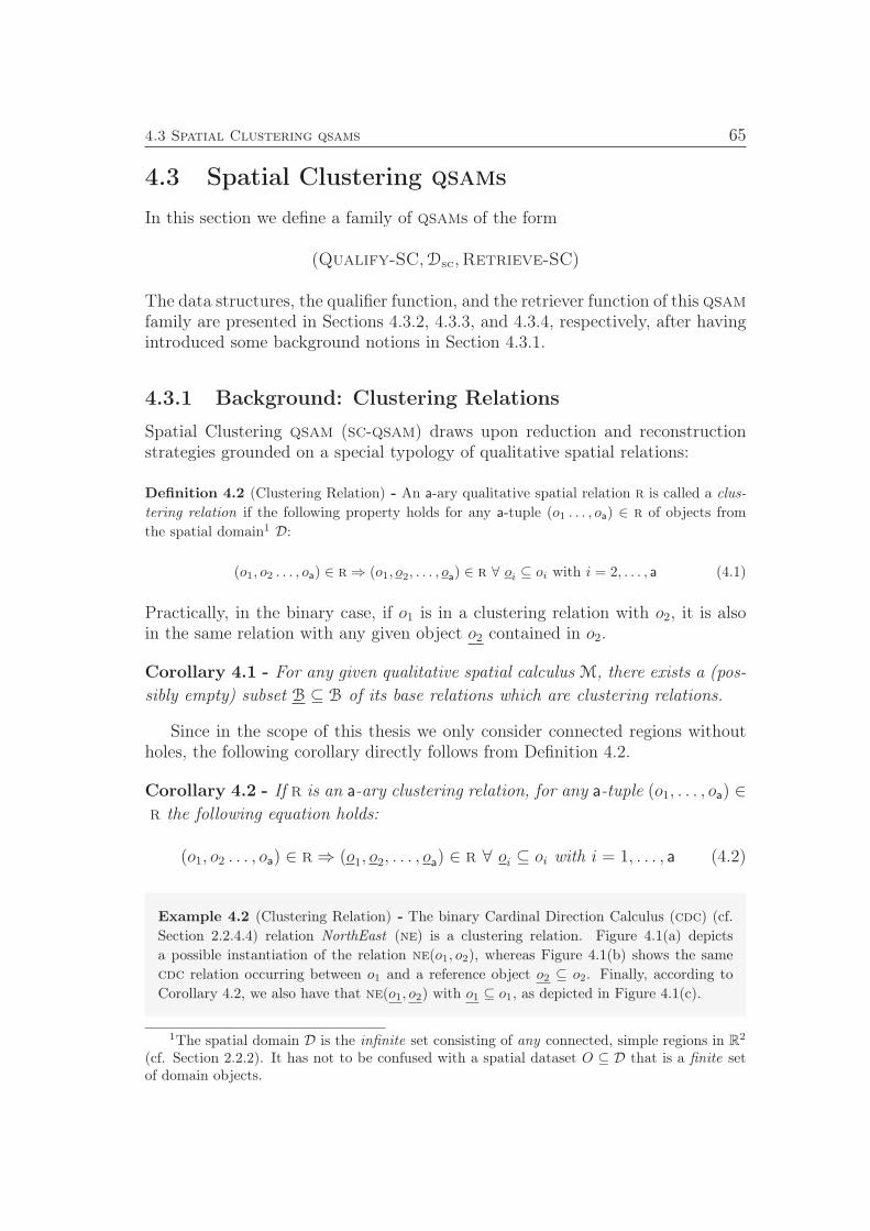
4.3 Spatial Clustering qsams 65
4.3 Spatial Clustering qsams
In this section we define a family of qsams of the form
(Qualify-SC,Dsc,Retrieve-SC)
The data structures, the qualifier function, and the retriever function of this qsamfamily are presented in Sections 4.3.2, 4.3.3, and 4.3.4, respectively, after havingintroduced some background notions in Section 4.3.1.
4.3.1 Background: Clustering Relations
Spatial Clustering qsam (sc-qsam) draws upon reduction and reconstructionstrategies grounded on a special typology of qualitative spatial relations:
Definition 4.2 (Clustering Relation) - An a-ary qualitative spatial relation r is called a clus-tering relation if the following property holds for any a-tuple (o1 . . . , oa) ∈ r of objects from
the spatial domain1 D:
(o1, o2 . . . , oa) ∈ r⇒ (o1, o2, . . . , oa) ∈ r ∀ oi ⊆ oi with i = 2, . . . , a (4.1)
Practically, in the binary case, if o1 is in a clustering relation with o2, it is alsoin the same relation with any given object o2 contained in o2.
Corollary 4.1 - For any given qualitative spatial calculus M, there exists a (pos-
sibly empty) subset B ⊆ B of its base relations which are clustering relations.
Since in the scope of this thesis we only consider connected regions withoutholes, the following corollary directly follows from Definition 4.2.
Corollary 4.2 - If r is an a-ary clustering relation, for any a-tuple (o1, . . . , oa) ∈
r the following equation holds:
(o1, o2 . . . , oa) ∈ r⇒ (o1, o2, . . . , oa) ∈ r ∀ oi ⊆ oi with i = 1, . . . , a (4.2)
Example 4.2 (Clustering Relation) - The binary Cardinal Direction Calculus (cdc) (cf.
Section 2.2.4.4) relation NorthEast (ne) is a clustering relation. Figure 4.1(a) depictsa possible instantiation of the relation ne(o1, o2), whereas Figure 4.1(b) shows the same
cdc relation occurring between o1 and a reference object o2 ⊆ o2. Finally, according to
Corollary 4.2, we also have that ne(o1, o2) with o1 ⊆ o1, as depicted in Figure 4.1(c).
1The spatial domain D is the infinite set consisting of any connected, simple regions in R2
(cf. Section 2.2.2). It has not to be confused with a spatial dataset O ⊆ D that is a finite setof domain objects.
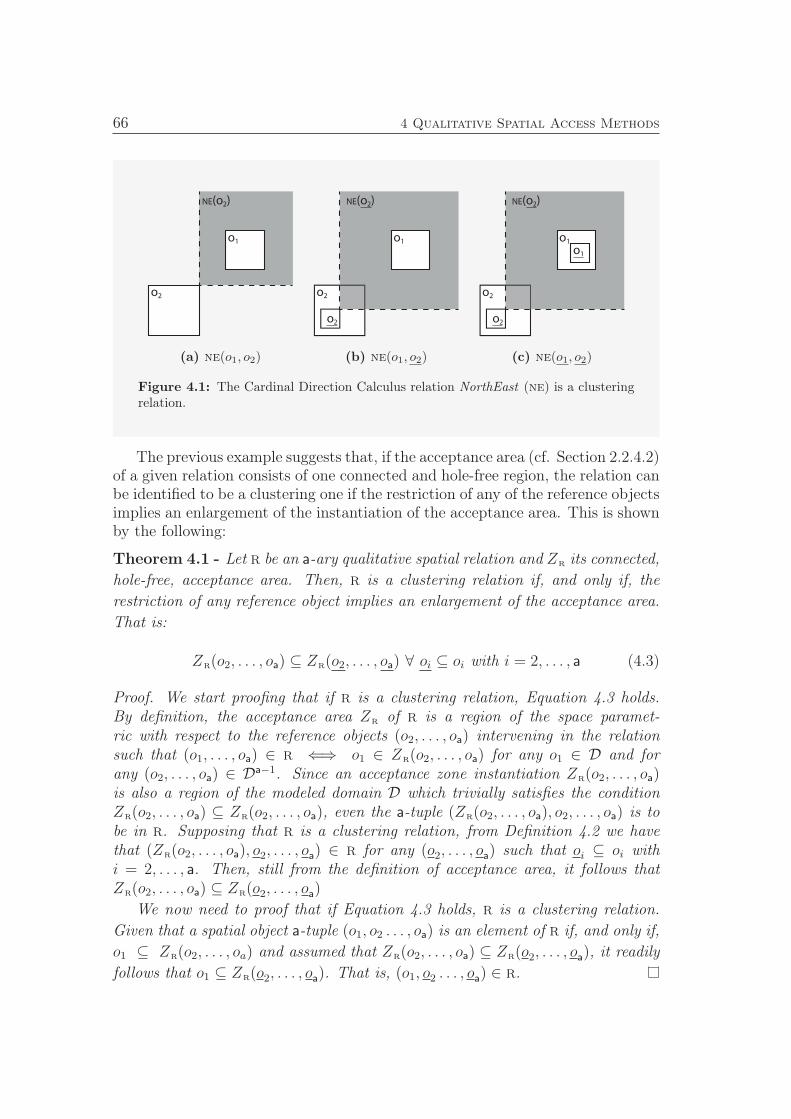
66 4 Qualitative Spatial Access Methods
NE(o2)
o2
o1
(a) ne(o1, o2)
o2
o2
NE(o2)
o1
(b) ne(o1, o2)
o2
o2
NE(o2)
o1
o1
(c) ne(o1, o2)
Figure 4.1: The Cardinal Direction Calculus relation NorthEast (ne) is a clusteringrelation.
The previous example suggests that, if the acceptance area (cf. Section 2.2.4.2)of a given relation consists of one connected and hole-free region, the relation canbe identified to be a clustering one if the restriction of any of the reference objectsimplies an enlargement of the instantiation of the acceptance area. This is shownby the following:
Theorem 4.1 - Let r be an a-ary qualitative spatial relation and Zr its connected,
hole-free, acceptance area. Then, r is a clustering relation if, and only if, the
restriction of any reference object implies an enlargement of the acceptance area.
That is:
Zr(o2, . . . , oa) ⊆ Zr(o2, . . . , oa) ∀ oi ⊆ oi with i = 2, . . . , a (4.3)
Proof. We start proofing that if r is a clustering relation, Equation 4.3 holds.By definition, the acceptance area Zr of r is a region of the space paramet-ric with respect to the reference objects (o2, . . . , oa) intervening in the relationsuch that (o1, . . . , oa) ∈ r ⇐⇒ o1 ∈ Zr(o2, . . . , oa) for any o1 ∈ D and forany (o2, . . . , oa) ∈ D
a−1. Since an acceptance zone instantiation Zr(o2, . . . , oa)is also a region of the modeled domain D which trivially satisfies the conditionZr(o2, . . . , oa) ⊆ Zr(o2, . . . , oa), even the a-tuple (Zr(o2, . . . , oa), o2, . . . , oa) is tobe in r. Supposing that r is a clustering relation, from Definition 4.2 we havethat (Zr(o2, . . . , oa), o2, . . . , oa) ∈ r for any (o2, . . . , oa) such that oi ⊆ oi withi = 2, . . . , a. Then, still from the definition of acceptance area, it follows thatZr(o2, . . . , oa) ⊆ Zr(o2, . . . , oa)
We now need to proof that if Equation 4.3 holds, r is a clustering relation.
Given that a spatial object a-tuple (o1, o2 . . . , oa) is an element of r if, and only if,
o1 ⊆ Zr(o2, . . . , oa) and assumed that Zr(o2, . . . , oa) ⊆ Zr(o2, . . . , oa), it readily
follows that o1 ⊆ Zr(o2, . . . , oa). That is, (o1, o2 . . . , oa) ∈ r.
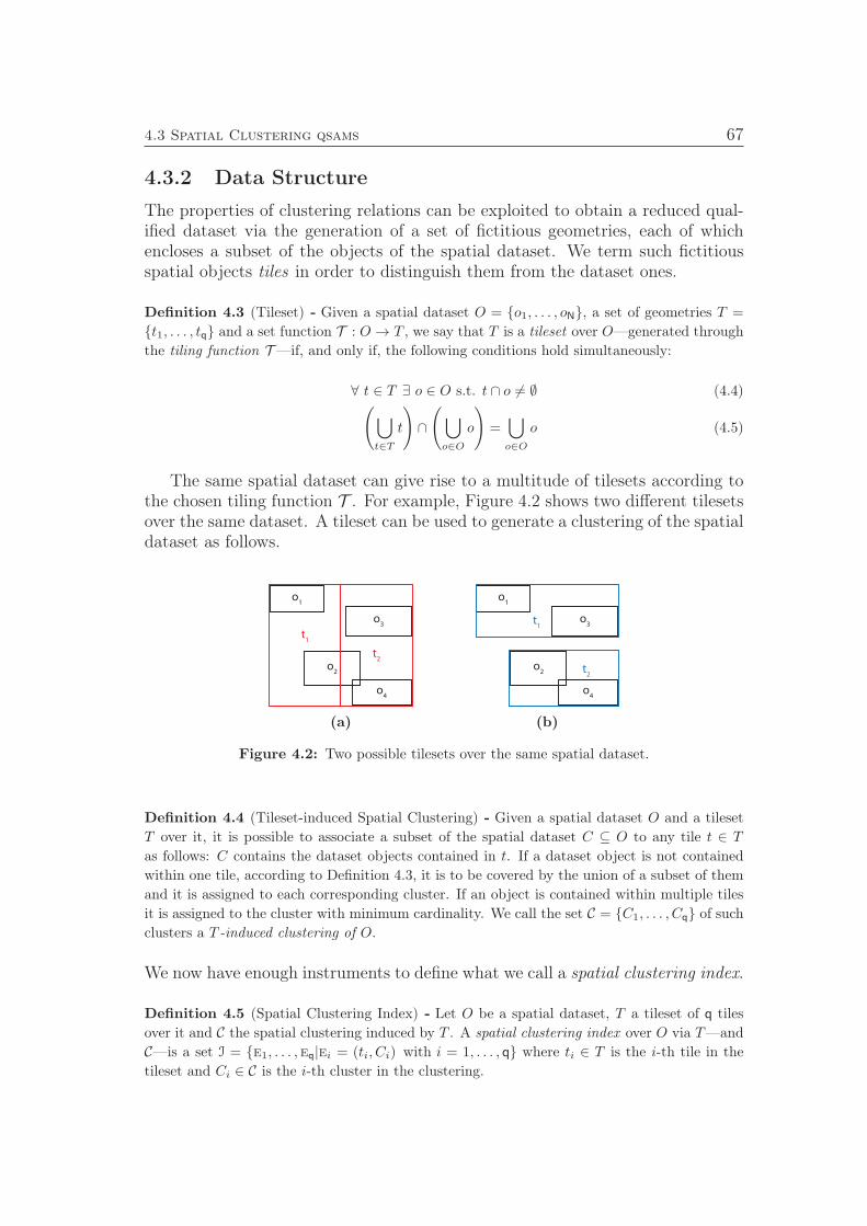
4.3 Spatial Clustering qsams 67
4.3.2 Data Structure
The properties of clustering relations can be exploited to obtain a reduced qual-ified dataset via the generation of a set of fictitious geometries, each of whichencloses a subset of the objects of the spatial dataset. We term such fictitiousspatial objects tiles in order to distinguish them from the dataset ones.
Definition 4.3 (Tileset) - Given a spatial dataset O = o1, . . . , oN, a set of geometries T =
t1, . . . , tq and a set function T : O → T , we say that T is a tileset over O—generated throughthe tiling function T—if, and only if, the following conditions hold simultaneously:
∀ t ∈ T ∃ o ∈ O s.t. t ∩ o 6= ∅ (4.4)(⋃
t∈T
t
)∩
(⋃
o∈O
o
)=⋃
o∈O
o (4.5)
The same spatial dataset can give rise to a multitude of tilesets according tothe chosen tiling function T . For example, Figure 4.2 shows two different tilesetsover the same dataset. A tileset can be used to generate a clustering of the spatialdataset as follows.
o1
o2
o4
o3
t1
t2
(a)
o1
o2
o4
o3
t1
t2
(b)
Figure 4.2: Two possible tilesets over the same spatial dataset.
Definition 4.4 (Tileset-induced Spatial Clustering) - Given a spatial dataset O and a tileset
T over it, it is possible to associate a subset of the spatial dataset C ⊆ O to any tile t ∈ T
as follows: C contains the dataset objects contained in t. If a dataset object is not contained
within one tile, according to Definition 4.3, it is to be covered by the union of a subset of them
and it is assigned to each corresponding cluster. If an object is contained within multiple tiles
it is assigned to the cluster with minimum cardinality. We call the set C = C1, . . . , Cq of such
clusters a T -induced clustering of O.
We now have enough instruments to define what we call a spatial clustering index.
Definition 4.5 (Spatial Clustering Index) - Let O be a spatial dataset, T a tileset of q tiles
over it and C the spatial clustering induced by T . A spatial clustering index over O via T—andC—is a set I = e1, . . . ,eq|ei = (ti, Ci) with i = 1, . . . , q where ti ∈ T is the i-th tile in the
tileset and Ci ∈ C is the i-th cluster in the clustering.
68 4 Qualitative Spatial Access Methods
For the sake of notation it is convenient to define a set of operators to easilyrefer to the index elements.
Definition 4.6 - Given an entry e = (t, C) from a spatial clustering index I, we say that t(e) = t
is the tile associated with e and that C(e) = C is the cluster associated with e. Similarly, givenan a-tuple of index entries ǫ = (e1, . . . ,ea), we say that τ(ǫ) = (t(e1), . . . , t(ea)) is the tilea-tuple associated with ǫ and that σ(ǫ) = (C(e1), . . . , C(ea)) is the cluster a-tuple associatedwith ǫ.
A spatial clustering index together with a set of relation tables provide thedata structures underlying a spatial clustering qsam. Note that, in this case,a relation table contains entries pointing either at dataset objects or at indexentries.
4.3.3 Qualification
The qualification procedure for sc-qsam resorts to a spatial clustering index toproduce a reduced set of spatial relations. Before going through the algorithm,it is convenient, for the sake of exposition, to introduce the following concept.
Definition 4.7 - Given a dataset O indexed by a spatial clustering index I, any a-tuple of
index entries ǫ = (e1, . . . ,ea) gives rise to a set Ωǫ of dataset object a-tuples having the i-th
term taken from the cluster C(ei) associated with the i-th entry in ǫ. We say that Ωǫ is inducedby ǫ and, if |C(ei)| = Ni, we have that:
|Ωǫ| =a∏
i=1
Ni
Given a dataset O indexed by a spatial clustering index I = (T , C) and acalculus pool P , the dataset qualification procedure, reported in Algorithm 4.4,resorts to the tileset T to exploit the properties of clustering relations.
For any a-ary calculus in the pool M ∈ P , the procedure iterates over everya-tuple ǫ of entries from I. If the relation rǫ, holding over the tile a-tuple τ(ǫ)associated with a given ǫ, is a clustering relation—i.e. rǫ ∈ B(M)—then, accord-ing to Equation 4.2, the same relation occurs over every object a-tuple ω ∈ Ωǫ
induced by ǫ. Accordingly, computing the relations holding over any ω ∈ Ωǫ issuperfluous and we can simply store rǫ in the relation table rta. Conversely, ifrǫ is not a clustering relation, it is necessary to compute and store the relationsoccurring over all the object a-tuples mentioned above. Note that, if the tile τ isan a-tuple having all terms equal we simply compute the relations occurring overall the objects in the corresponding cluster by resorting to the qualifier functionQualify-QSL described in Section 4.2.
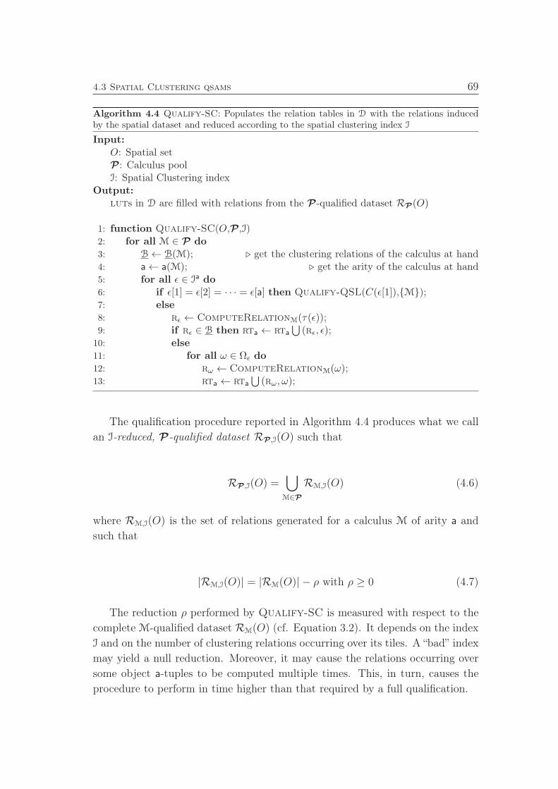
4.3 Spatial Clustering qsams 69
Algorithm 4.4 Qualify-SC: Populates the relation tables in D with the relations inducedby the spatial dataset and reduced according to the spatial clustering index I
Input:
O: Spatial setP : Calculus poolI: Spatial Clustering index
Output:
luts in D are filled with relations from the P-qualified dataset RP(O)
1: function Qualify-SC(O,P ,I)2: for all M ∈ P do
3: B← B(M); ⊲ get the clustering relations of the calculus at hand4: a← a(M); ⊲ get the arity of the calculus at hand5: for all ǫ ∈ Ia do
6: if ǫ[1] = ǫ[2] = · · · = ǫ[a] then Qualify-QSL(C(ǫ[1]),M);7: else
8: rǫ ← ComputeRelationM(τ(ǫ));9: if rǫ ∈ B then rta ← rta
⋃(rǫ, ǫ);
10: else
11: for all ω ∈ Ωǫ do
12: rω ← ComputeRelationM(ω);13: rta ← rta
⋃(rω, ω);
The qualification procedure reported in Algorithm 4.4 produces what we call
an I-reduced, P-qualified dataset RP,I(O) such that
RP,I(O) =⋃
M∈P
RM,I(O) (4.6)
where RM,I(O) is the set of relations generated for a calculus M of arity a and
such that
|RM,I(O)| = |RM(O)| − ρ with ρ ≥ 0 (4.7)
The reduction ρ performed by Qualify-SC is measured with respect to the
complete M-qualified dataset RM(O) (cf. Equation 3.2). It depends on the index
I and on the number of clustering relations occurring over its tiles. A “bad” index
may yield a null reduction. Moreover, it may cause the relations occurring over
some object a-tuples to be computed multiple times. This, in turn, causes the
procedure to perform in time higher than that required by a full qualification.
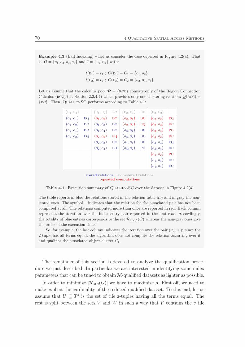
70 4 Qualitative Spatial Access Methods
Example 4.3 (Bad Indexing) - Let us consider the case depicted in Figure 4.2(a). That
is, O = o1, o2, o3, o4 and I = e1, e2 with:
t(e1) = t1 ; C(e1) = C1 = o1, o2
t(e2) = t2 ; C(e2) = C2 = o2, o3, o4
Let us assume that the calculus pool P = rcc consists only of the Region Connection
Calculus (rcc) (cf. Section 2.2.4.4) which provides only one clustering relation: B(rcc) =
dc. Then, Qualify-SC performs according to Table 4.1:
(e1, e1) – (e1, e2) ec (e2, e1) ec (e2, e2) –
(o1, o1) eq (o1, o2) dc (o2, o1) dc (o2, o2) eq
(o1, o2) dc (o1, o3) dc (o2, o2) eq (o2, o3) dc
(o2, o1) dc (o1, o4) dc (o3, o1) dc (o2, o4) po
(o2, o2) eq (o2, o2) eq (o3, o2) dc (o3, o2) dc
(o2, o3) dc (o4, o1) dc (o3, o3) eq
(o2, o4) po (o4, o2) po (o3, o4) dc
(o4, o2) po
(o4, o3) dc
(o4, o4) eq
stored relations non-stored relations
repeated computations
Table 4.1: Execution summary of Qualify-SC over the dataset in Figure 4.2(a)
The table reports in blue the relations stored in the relation table rt2 and in gray the non-
stored ones. The symbol – indicates that the relation for the associated pair has not been
computed at all. The relations computed more than once are reported in red. Each column
represents the iteration over the index entry pair reported in the first row. Accordingly,
the totality of blue entries corresponds to the set Rrcc,I(O) whereas the non-gray ones give
the order of the execution time.
So, for example, the last column indicates the iteration over the pair (e2,e2): since the
2-tuple has all terms equal, the algorithm does not compute the relation occurring over it
and qualifies the associated object cluster C1.
The remainder of this section is devoted to analyze the qualification proce-
dure we just described. In particular we are interested in identifying some index
parameters that can be tuned to obtainM-qualified datasets as lighter as possible.
In order to minimize |RM,I(O)| we have to maximize ρ. First off, we need to
make explicit the cardinality of the reduced qualified dataset. To this end, let us
assume that U ⊆ T a is the set of tile a-tuples having all the terms equal. The
rest is split between the sets V and W in such a way that V contains the v tile
4.3 Spatial Clustering qsams 71
a-tuples in a clustering relation. Then, according to Algorithm 4.4 we have that
|RM,I(O)| =∑
τ j∈U
a∏
k=1
Nj,k + v +∑
τ j∈W
a∏
k=1
Nj,k (4.8)
where Nj,k is assumed to be the cardinality of the object cluster Cj,k associatedwith the k-th term of the j-th tile a-tuple τ j.
To assess the reduction amount, it is convenient to express |RM(O)| as afunction of the sets U , V and W . Given a partition of the spatial dataset, thiscan be done easily (cf. Example 4.3 for an empirical demonstration). However,since we did not impose any restriction on the way the index I is generated, theclustering C may or may not provide a partition of the spatial dataset O. Thatis, the summation of the cardinality of its object clusters exceeds the cardinalityof the spatial dataset of a quantity e ≥ 0. Nonetheless, given the clustering C =
C1, . . . , Cq, it is always possible to stem from it a partition C = C1, . . . , Cqof O such that:
Ci =
Ci if i = 1
Ci \⋃i−1
j=1 Cj if 2 ≤ i ≤ q
If we denote with Ni the cardinality of the i-th cluster Ci we have that Ni−Ni = eiand, consequently, that
e =
q∑
i=1
ei
Then, it is possible to rewrite Equation 3.2 as follows:
|RM(O)| =∑
τ j∈U
a∏
k=1
Nj,k +∑
τ j∈V
a∏
k=1
Nj,k +∑
τ j∈W
a∏
k=1
Nj,k (4.9)
where Nj,k is assumed to be the cardinality of the object cluster Cj,k associatedwith the k-th term of the j-th tile a-tuple τ j.
Lastly, let us define the following symbols which allow for a leaner notationand a smoother analysis:
ρU =∑
τ j∈U
a∏
k=1
(Nj,k)−a∏
k=1
Nj,k
ρV =∑
τ j∈V
a∏
k=1
(Nj,k)− v
ρW =∑
τ j∈W
a∏
k=1
(Nj,k)−a∏
k=1
Nj,k
Hence, from Equations 4.7, 4.8, and 4.9, the reduction performed by Algorithm 4.4
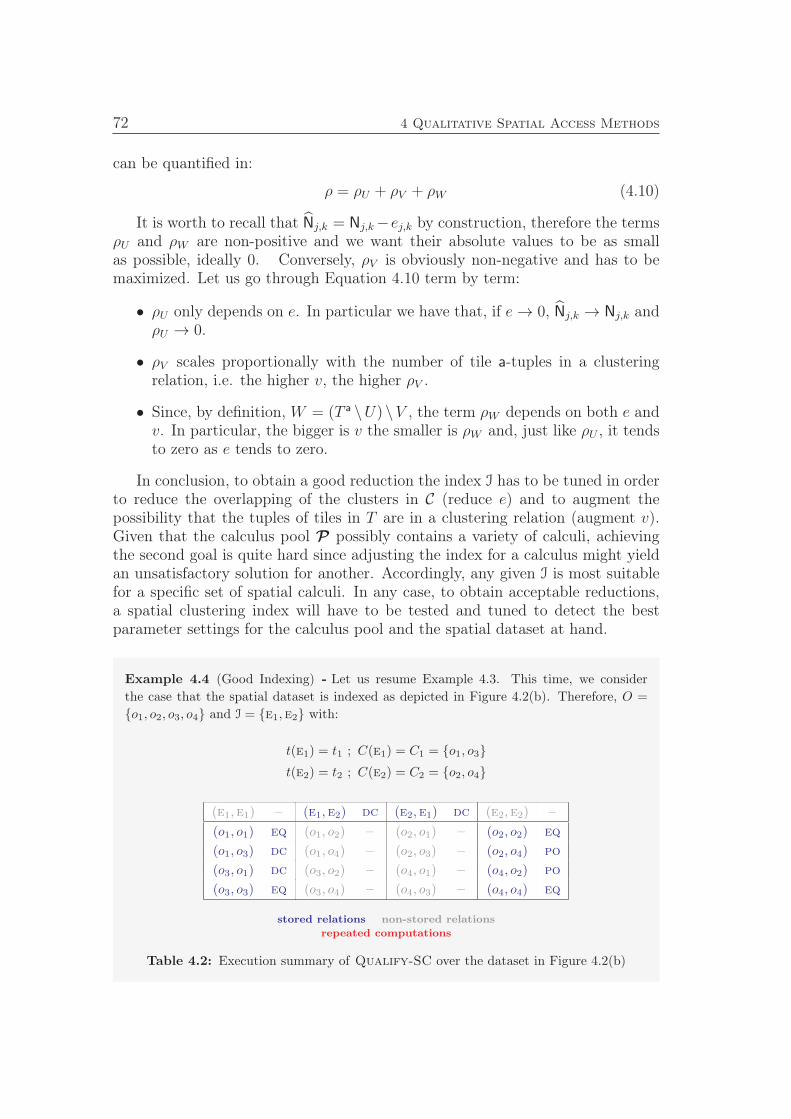
72 4 Qualitative Spatial Access Methods
can be quantified in:
ρ = ρU + ρV + ρW (4.10)
It is worth to recall that Nj,k = Nj,k−ej,k by construction, therefore the termsρU and ρW are non-positive and we want their absolute values to be as smallas possible, ideally 0. Conversely, ρV is obviously non-negative and has to bemaximized. Let us go through Equation 4.10 term by term:
• ρU only depends on e. In particular we have that, if e→ 0, Nj,k → Nj,k andρU → 0.
• ρV scales proportionally with the number of tile a-tuples in a clusteringrelation, i.e. the higher v, the higher ρV .
• Since, by definition, W = (T a \U) \V , the term ρW depends on both e andv. In particular, the bigger is v the smaller is ρW and, just like ρU , it tendsto zero as e tends to zero.
In conclusion, to obtain a good reduction the index I has to be tuned in orderto reduce the overlapping of the clusters in C (reduce e) and to augment thepossibility that the tuples of tiles in T are in a clustering relation (augment v).Given that the calculus pool P possibly contains a variety of calculi, achievingthe second goal is quite hard since adjusting the index for a calculus might yieldan unsatisfactory solution for another. Accordingly, any given I is most suitablefor a specific set of spatial calculi. In any case, to obtain acceptable reductions,a spatial clustering index will have to be tested and tuned to detect the bestparameter settings for the calculus pool and the spatial dataset at hand.
Example 4.4 (Good Indexing) - Let us resume Example 4.3. This time, we consider
the case that the spatial dataset is indexed as depicted in Figure 4.2(b). Therefore, O =
o1, o2, o3, o4 and I = e1, e2 with:
t(e1) = t1 ; C(e1) = C1 = o1, o3
t(e2) = t2 ; C(e2) = C2 = o2, o4
(e1, e1) – (e1,e2) dc (e2, e1) dc (e2, e2) –
(o1, o1) eq (o1, o2) – (o2, o1) – (o2, o2) eq
(o1, o3) dc (o1, o4) – (o2, o3) – (o2, o4) po
(o3, o1) dc (o3, o2) – (o4, o1) – (o4, o2) po
(o3, o3) eq (o3, o4) – (o4, o3) – (o4, o4) eq
stored relations non-stored relations
repeated computations
Table 4.2: Execution summary of Qualify-SC over the dataset in Figure 4.2(b)
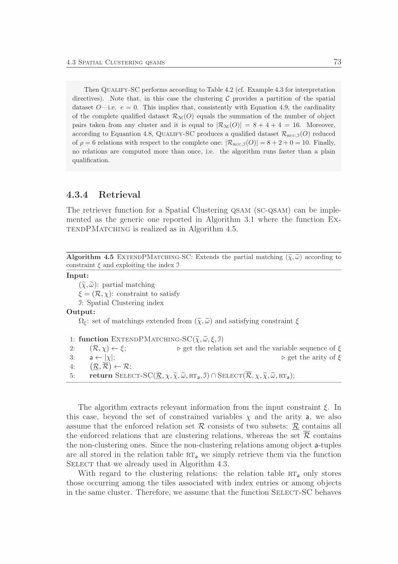
4.3 Spatial Clustering qsams 73
Then Qualify-SC performs according to Table 4.2 (cf. Example 4.3 for interpretation
directives). Note that, in this case the clustering C provides a partition of the spatial
dataset O—i.e. e = 0. This implies that, consistently with Equation 4.9, the cardinality
of the complete qualified dataset RM(O) equals the summation of the number of object
pairs taken from any cluster and it is equal to |RM(O)| = 8 + 4 + 4 = 16. Moreover,
according to Equantion 4.8, Qualify-SC produces a qualified dataset Rrcc,I(O) reduced
of ρ = 6 relations with respect to the complete one: |Rrcc,I(O)| = 8 + 2 + 0 = 10. Finally,
no relations are computed more than once, i.e. the algorithm runs faster than a plain
qualification.
4.3.4 Retrieval
The retriever function for a Spatial Clustering qsam (sc-qsam) can be imple-mented as the generic one reported in Algorithm 3.1 where the function Ex-tendPMatching is realized as in Algorithm 4.5.
Algorithm 4.5 ExtendPMatching-SC: Extends the partial matching (χ, ω) according toconstraint ξ and exploiting the index I
Input:
(χ, ω): partial matchingξ = (R, χ): constraint to satisfyI: Spatial Clustering index
Output:
Ωξ: set of matchings extended from (χ, ω) and satisfying constraint ξ
1: function ExtendPMatching-SC(χ, ω, ξ, I)2: (R, χ)← ξ; ⊲ get the relation set and the variable sequence of ξ3: a← |χ|; ⊲ get the arity of ξ4:
(R,R
)← R;
5: return Select-SC(R, χ, χ, ω,rta, I) ∩ Select(R, χ, χ, ω,rta);
The algorithm extracts relevant information from the input constraint ξ. Inthis case, beyond the set of constrained variables χ and the arity a, we alsoassume that the enforced relation set R consists of two subsets: R contains allthe enforced relations that are clustering relations, whereas the set R containsthe non-clustering ones. Since the non-clustering relations among object a-tuplesare all stored in the relation table rta we simply retrieve them via the functionSelect that we already used in Algorithm 4.3.
With regard to the clustering relations: the relation table rta only storesthose occurring among the tiles associated with index entries or among objectsin the same cluster. Therefore, we assume that the function Select-SC behaves
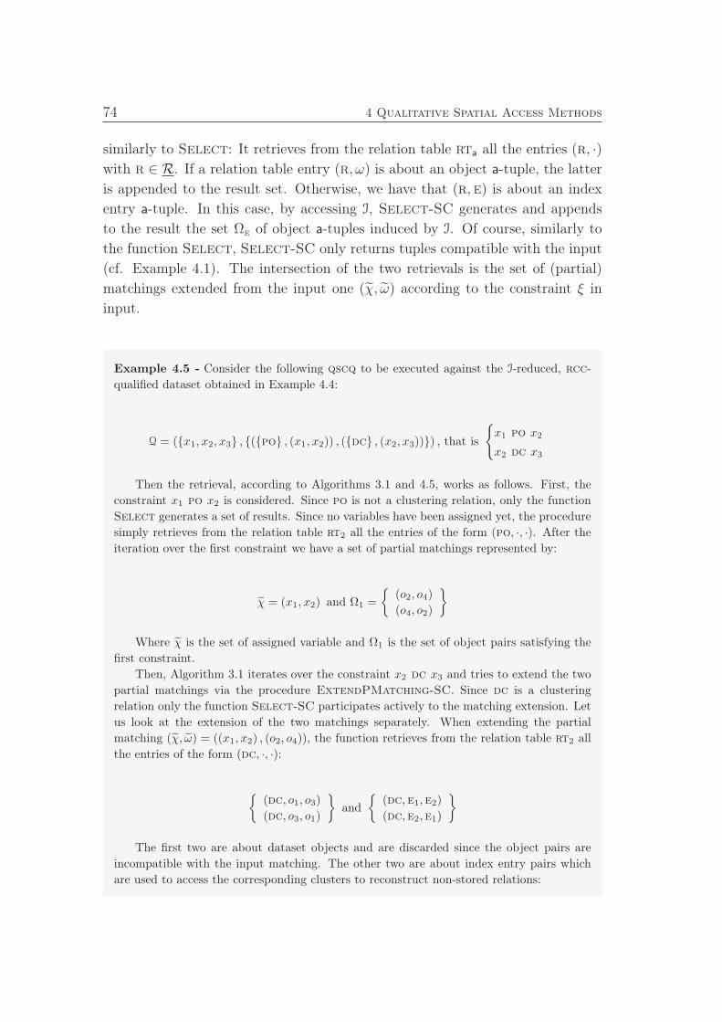
74 4 Qualitative Spatial Access Methods
similarly to Select: It retrieves from the relation table rta all the entries (r, ·)
with r ∈ R. If a relation table entry (r, ω) is about an object a-tuple, the latter
is appended to the result set. Otherwise, we have that (r,e) is about an index
entry a-tuple. In this case, by accessing I, Select-SC generates and appends
to the result the set Ωe of object a-tuples induced by I. Of course, similarly to
the function Select, Select-SC only returns tuples compatible with the input
(cf. Example 4.1). The intersection of the two retrievals is the set of (partial)
matchings extended from the input one (χ, ω) according to the constraint ξ in
input.
Example 4.5 - Consider the following qscq to be executed against the I-reduced, rcc-
qualified dataset obtained in Example 4.4:
Q = (x1, x2, x3 , (po , (x1, x2)) , (dc , (x2, x3))) , that is
x1 po x2
x2 dc x3
Then the retrieval, according to Algorithms 3.1 and 4.5, works as follows. First, the
constraint x1 po x2 is considered. Since po is not a clustering relation, only the function
Select generates a set of results. Since no variables have been assigned yet, the procedure
simply retrieves from the relation table rt2 all the entries of the form (po, ·, ·). After the
iteration over the first constraint we have a set of partial matchings represented by:
χ = (x1, x2) and Ω1 =
(o2, o4)
(o4, o2)
Where χ is the set of assigned variable and Ω1 is the set of object pairs satisfying the
first constraint.
Then, Algorithm 3.1 iterates over the constraint x2 dc x3 and tries to extend the two
partial matchings via the procedure ExtendPMatching-SC. Since dc is a clustering
relation only the function Select-SC participates actively to the matching extension. Let
us look at the extension of the two matchings separately. When extending the partial
matching (χ, ω) = ((x1, x2) , (o2, o4)), the function retrieves from the relation table rt2 all
the entries of the form (dc, ·, ·):
(dc, o1, o3)
(dc, o3, o1)
and
(dc,e1, e2)
(dc,e2, e1)
The first two are about dataset objects and are discarded since the object pairs are
incompatible with the input matching. The other two are about index entry pairs which
are used to access the corresponding clusters to reconstruct non-stored relations:
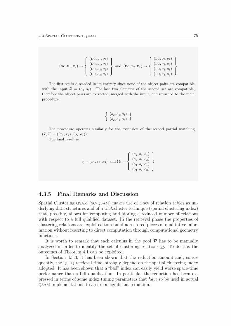
4.3 Spatial Clustering qsams 75
(dc,e1, e2)→
(dc, o1, o2)
(dc, o1, o4)
(dc, o3, o2)
(dc, o3, o4)
and (dc, e2, e1)→
(dc, o2, o1)
(dc, o2, o3)
(dc, o4, o1)
(dc, o4, o3)
The first set is discarded in its entirety since none of the object pairs are compatible
with the input ω = (o2, o4). The last two elements of the second set are compatible,
therefore the object pairs are extracted, merged with the input, and returned to the main
procedure:
(o2, o4, o1)
(o2, o4, o3)
The procedure operates similarly for the extension of the second partial matching
(χ, ω) = ((x1, x2) , (o2, o4)).
The final result is:
χ = (x1, x2, x3) and Ω2 =
(o2, o4, o1)
(o2, o4, o3)
(o4, o2, o1)
(o4, o2, o3)
4.3.5 Final Remarks and Discussion
Spatial Clustering qsam (sc-qsam) makes use of a set of relation tables as un-derlying data structures and of a tile&cluster technique (spatial clustering index)that, possibly, allows for computing and storing a reduced number of relationswith respect to a full qualified dataset. In the retrieval phase the properties ofclustering relations are exploited to rebuild non-stored pieces of qualitative infor-mation without resorting to direct computation through computational geometryfunctions.
It is worth to remark that each calculus in the pool P has to be manuallyanalyzed in order to identify the set of clustering relations B. To do this theoutcomes of Theorem 4.1 can be exploited.
In Section 4.3.3, it has been shown that the reduction amount and, conse-quently, the qscq retrieval time, strongly depend on the spatial clustering indexadopted. It has been shown that a “bad” index can easily yield worse space-timeperformance than a full qualification. In particular the reduction has been ex-pressed in terms of some index tuning parameters that have to be used in actualqsam implementations to assure a significant reduction.
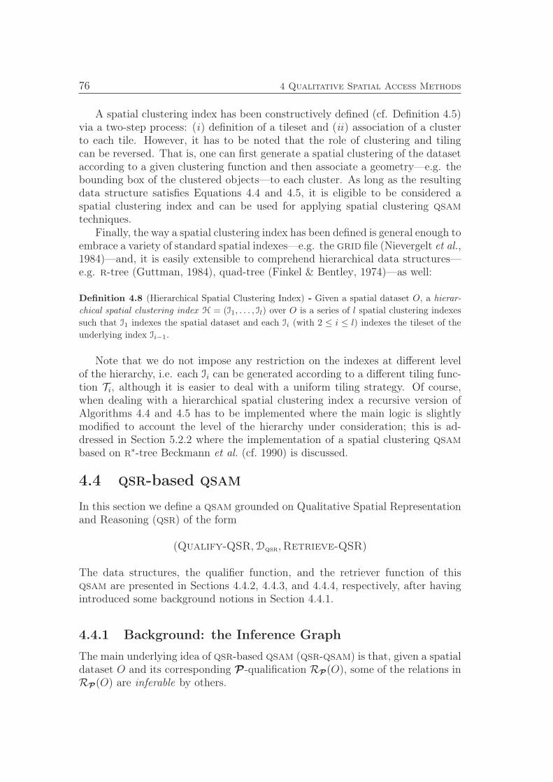
76 4 Qualitative Spatial Access Methods
A spatial clustering index has been constructively defined (cf. Definition 4.5)via a two-step process: (i) definition of a tileset and (ii) association of a clusterto each tile. However, it has to be noted that the role of clustering and tilingcan be reversed. That is, one can first generate a spatial clustering of the datasetaccording to a given clustering function and then associate a geometry—e.g. thebounding box of the clustered objects—to each cluster. As long as the resultingdata structure satisfies Equations 4.4 and 4.5, it is eligible to be considered aspatial clustering index and can be used for applying spatial clustering qsamtechniques.
Finally, the way a spatial clustering index has been defined is general enough toembrace a variety of standard spatial indexes—e.g. the grid file (Nievergelt et al.,1984)—and, it is easily extensible to comprehend hierarchical data structures—e.g. r-tree (Guttman, 1984), quad-tree (Finkel & Bentley, 1974)—as well:
Definition 4.8 (Hierarchical Spatial Clustering Index) - Given a spatial dataset O, a hierar-chical spatial clustering index H = (I1, . . . , Il) over O is a series of l spatial clustering indexes
such that I1 indexes the spatial dataset and each Ii (with 2 ≤ i ≤ l) indexes the tileset of the
underlying index Ii−1.
Note that we do not impose any restriction on the indexes at different levelof the hierarchy, i.e. each Ii can be generated according to a different tiling func-tion Ti, although it is easier to deal with a uniform tiling strategy. Of course,when dealing with a hierarchical spatial clustering index a recursive version ofAlgorithms 4.4 and 4.5 has to be implemented where the main logic is slightlymodified to account the level of the hierarchy under consideration; this is ad-dressed in Section 5.2.2 where the implementation of a spatial clustering qsambased on r∗-tree Beckmann et al. (cf. 1990) is discussed.
4.4 qsr-based qsam
In this section we define a qsam grounded on Qualitative Spatial Representationand Reasoning (qsr) of the form
(Qualify-QSR,Dqsr,Retrieve-QSR)
The data structures, the qualifier function, and the retriever function of thisqsam are presented in Sections 4.4.2, 4.4.3, and 4.4.4, respectively, after havingintroduced some background notions in Section 4.4.1.
4.4.1 Background: the Inference Graph
The main underlying idea of qsr-based qsam (qsr-qsam) is that, given a spatialdataset O and its corresponding P-qualification RP(O), some of the relations inRP(O) are inferable by others.
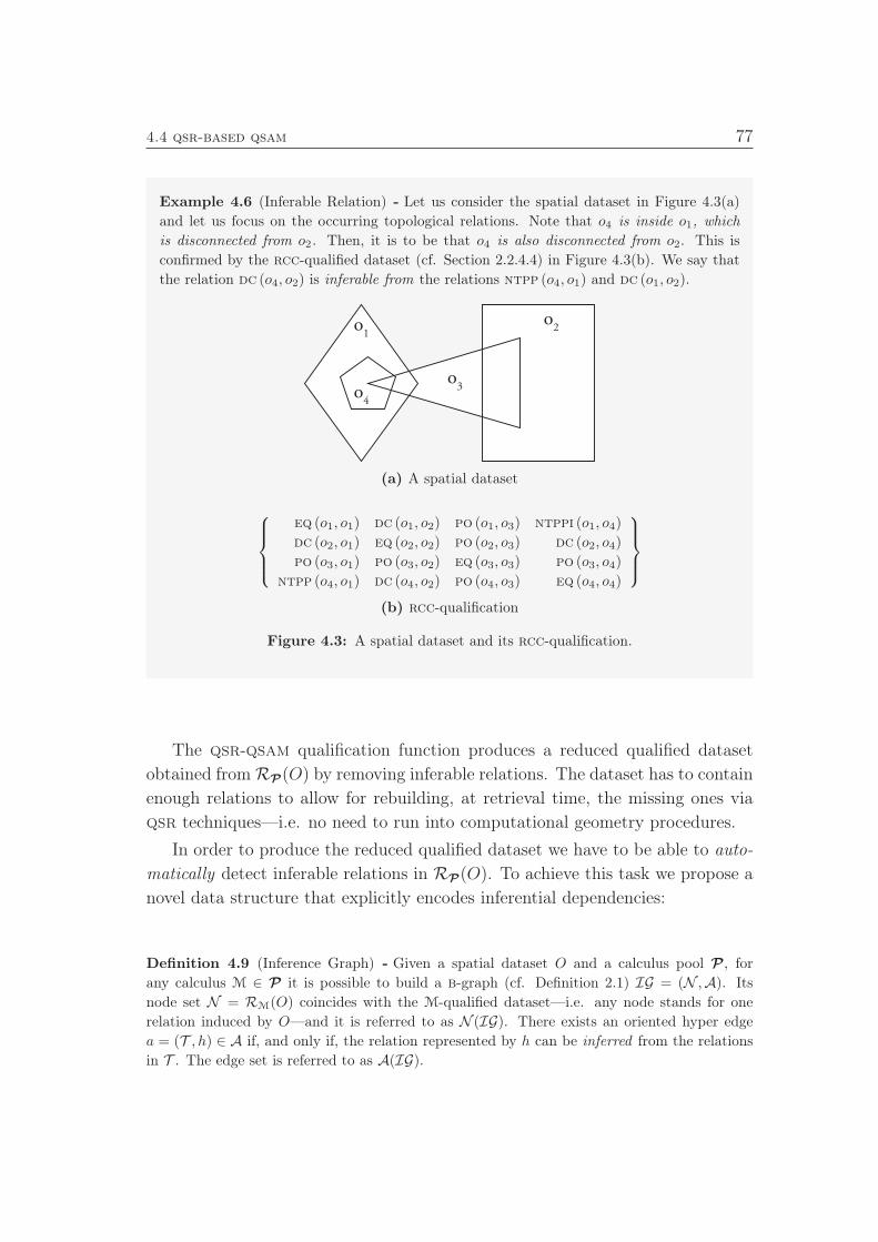
4.4 qsr-based qsam 77
Example 4.6 (Inferable Relation) - Let us consider the spatial dataset in Figure 4.3(a)
and let us focus on the occurring topological relations. Note that o4 is inside o1, whichis disconnected from o2. Then, it is to be that o4 is also disconnected from o2. This is
confirmed by the rcc-qualified dataset (cf. Section 2.2.4.4) in Figure 4.3(b). We say that
the relation dc (o4, o2) is inferable from the relations ntpp (o4, o1) and dc (o1, o2).
o1
o2
o3
o4
(a) A spatial dataset
eq (o1, o1) dc (o1, o2) po (o1, o3) ntppi (o1, o4)
dc (o2, o1) eq (o2, o2) po (o2, o3) dc (o2, o4)
po (o3, o1) po (o3, o2) eq (o3, o3) po (o3, o4)
ntpp (o4, o1) dc (o4, o2) po (o4, o3) eq (o4, o4)
(b) rcc-qualification
Figure 4.3: A spatial dataset and its rcc-qualification.
The qsr-qsam qualification function produces a reduced qualified dataset
obtained fromRP(O) by removing inferable relations. The dataset has to contain
enough relations to allow for rebuilding, at retrieval time, the missing ones via
qsr techniques—i.e. no need to run into computational geometry procedures.
In order to produce the reduced qualified dataset we have to be able to auto-
matically detect inferable relations in RP(O). To achieve this task we propose a
novel data structure that explicitly encodes inferential dependencies:
Definition 4.9 (Inference Graph) - Given a spatial dataset O and a calculus pool P , for
any calculus M ∈ P it is possible to build a b-graph (cf. Definition 2.1) IG = (N ,A). Its
node set N = RM(O) coincides with the M-qualified dataset—i.e. any node stands for one
relation induced by O—and it is referred to as N (IG). There exists an oriented hyper edge
a = (T , h) ∈ A if, and only if, the relation represented by h can be inferred from the relationsin T . The edge set is referred to as A(IG).
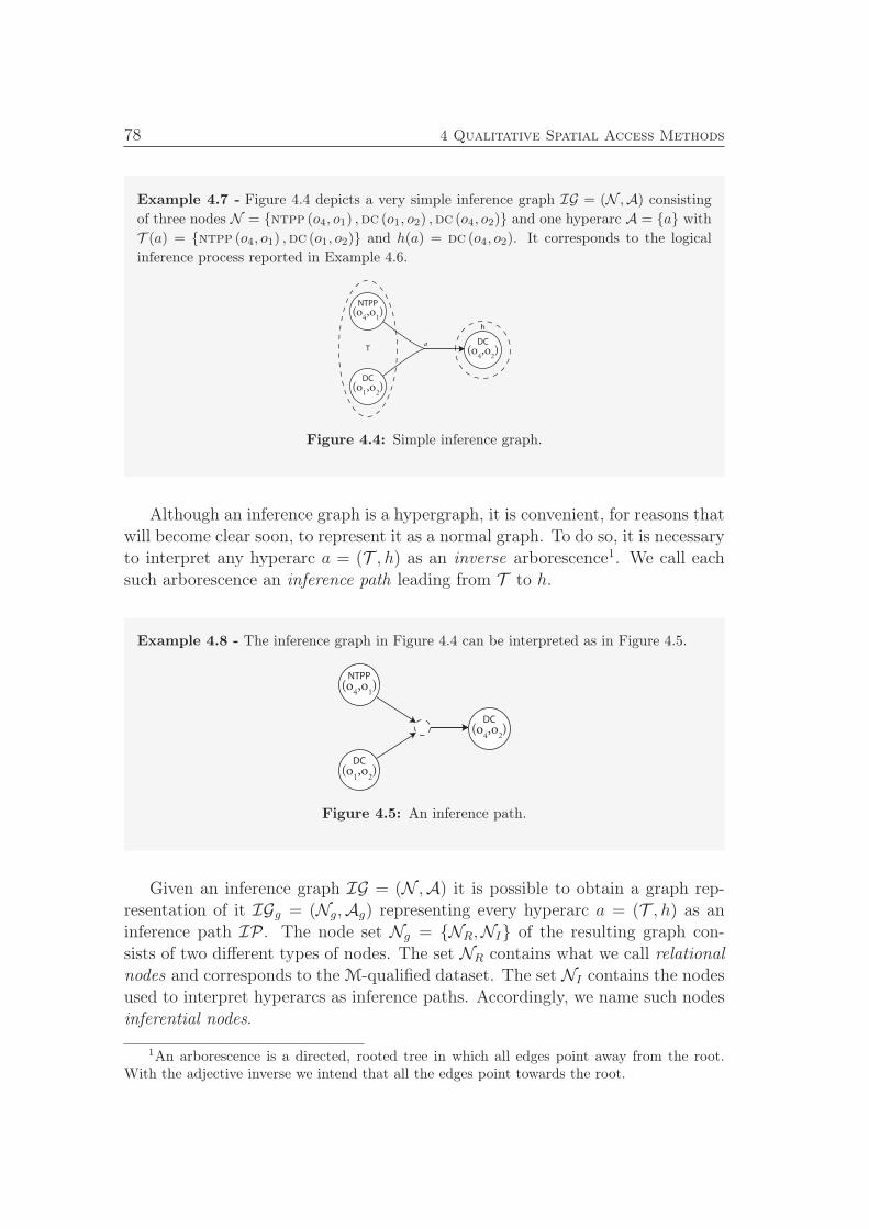
78 4 Qualitative Spatial Access Methods
Example 4.7 - Figure 4.4 depicts a very simple inference graph IG = (N ,A) consisting
of three nodes N = ntpp (o4, o1) ,dc (o1, o2) ,dc (o4, o2) and one hyperarc A = a with
T (a) = ntpp (o4, o1) ,dc (o1, o2) and h(a) = dc (o4, o2). It corresponds to the logical
inference process reported in Example 4.6.
DC
(o1,o
2)
NTPP
(o4,o
1)
DC
(o4,o
2)T
h
a
Figure 4.4: Simple inference graph.
Although an inference graph is a hypergraph, it is convenient, for reasons thatwill become clear soon, to represent it as a normal graph. To do so, it is necessaryto interpret any hyperarc a = (T , h) as an inverse arborescence1. We call eachsuch arborescence an inference path leading from T to h.
Example 4.8 - The inference graph in Figure 4.4 can be interpreted as in Figure 4.5.
DC
(o1,o
2)
NTPP
(o4,o
1)
DC
(o4,o
2)
Figure 4.5: An inference path.
Given an inference graph IG = (N ,A) it is possible to obtain a graph rep-resentation of it IGg = (Ng,Ag) representing every hyperarc a = (T , h) as aninference path IP . The node set Ng = NR,NI of the resulting graph con-sists of two different types of nodes. The set NR contains what we call relationalnodes and corresponds to the M-qualified dataset. The set NI contains the nodesused to interpret hyperarcs as inference paths. Accordingly, we name such nodesinferential nodes.
1An arborescence is a directed, rooted tree in which all edges point away from the root.With the adjective inverse we intend that all the edges point towards the root.
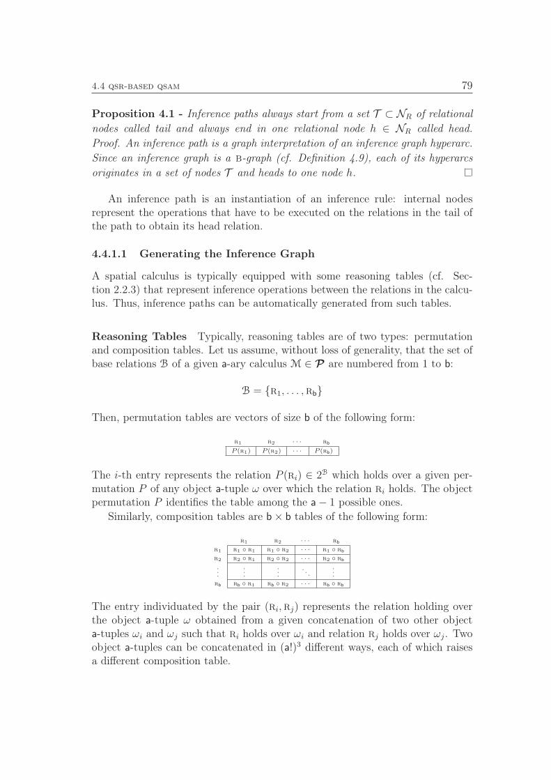
4.4 qsr-based qsam 79
Proposition 4.1 - Inference paths always start from a set T ⊂ NR of relational
nodes called tail and always end in one relational node h ∈ NR called head.
Proof. An inference path is a graph interpretation of an inference graph hyperarc.
Since an inference graph is a b-graph (cf. Definition 4.9), each of its hyperarcs
originates in a set of nodes T and heads to one node h.
An inference path is an instantiation of an inference rule: internal nodesrepresent the operations that have to be executed on the relations in the tail ofthe path to obtain its head relation.
4.4.1.1 Generating the Inference Graph
A spatial calculus is typically equipped with some reasoning tables (cf. Sec-tion 2.2.3) that represent inference operations between the relations in the calcu-lus. Thus, inference paths can be automatically generated from such tables.
Reasoning Tables Typically, reasoning tables are of two types: permutationand composition tables. Let us assume, without loss of generality, that the set ofbase relations B of a given a-ary calculus M ∈ P are numbered from 1 to b:
B = r1, . . . ,rb
Then, permutation tables are vectors of size b of the following form:
r1 r2 · · · rb
P (r1) P (r2) · · · P (rb)
The i-th entry represents the relation P (ri) ∈ 2B which holds over a given per-mutation P of any object a-tuple ω over which the relation ri holds. The objectpermutation P identifies the table among the a− 1 possible ones.
Similarly, composition tables are b× b tables of the following form:
r1 r2 · · · rb
r1 r1 r1 r1 r2 · · · r1 rb
r2 r2 r1 r2 r2 · · · r2 rb
.
.
.
.
.
.
.
.
.
...
.
.
.
rb rb r1 rb r2 · · · rb rb
The entry individuated by the pair (ri,rj) represents the relation holding overthe object a-tuple ω obtained from a given concatenation of two other objecta-tuples ωi and ωj such that ri holds over ωi and relation rj holds over ωj. Twoobject a-tuples can be concatenated in (a!)3 different ways, each of which raisesa different composition table.
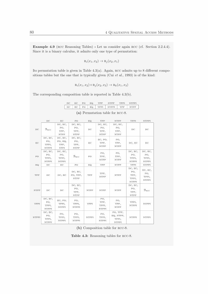
80 4 Qualitative Spatial Access Methods
Example 4.9 (rcc Reasoning Tables) - Let us consider again rcc (cf. Section 2.2.4.4).
Since it is a binary calculus, it admits only one type of permutation:
ri(x1, x2)→ rj(x2, x1)
Its permutation table is given in Table 4.3(a). Again, rcc admits up to 8 different compo-
sitions tables but the one that is typically given (Cui et al., 1993) is of the kind:
ri(x1, x2) ⋄ rj(x2, x3)→ rk(x1, x3)
The corresponding composition table is reported in Table 4.3(b).
dc ec po eq tpp ntpp tppi ntppi
dc ec po eq tppi ntppi tpp ntpp
(a) Permutation table for rcc-8.
dc ec po eq tpp ntpp tppi ntppi
dc Brcc
dc, ec,po,tpp,ntpp
dc, ec,po,tpp,ntpp
dc
dc, ec,po,tpp,ntpp
dc, ec,po,tpp,ntpp
dc dc
ec
dc, ec,po,
tppi,ntppi
dc, ec,po, eq,tpp,tppi
dc, ec,po,tpp,ntpp
ec
ec, po,tpp,ntpp
po,tpp,ntpp
dc, ec dc
po
dc, ec,po,
tppi,ntppi
dc, ec,po,
tppi,ntppi
Brcc po
po,tpp,ntpp
po,tpp,ntpp
dc, ec,po,
tppi,ntppi
dc, ec,po,
tppi,ntppi
eq dc ec po eq tpp ntpp tppi ntppi
tpp dc dc, ec
dc, ec,po, tpp,ntpp
tpptpp,ntpp
ntpp
dc, ec,po,tpp,tppi,ntppi
dc, ec,po,
tppi,ntppi
ntpp dc dc
dc, ec,po,tpp,ntpp
ntpp ntpp ntpp
dc, ec,po,tpp,ntpp
Brcc
tppi
dc, ec,po,
tppi,ntppi
ec, po,tppi,ntppi
po,tppi,ntppi
tppi
po,tpp,tppi,ntppi
po,tpp,ntpp
tppi,ntppi
ntppi
ntppi
dc, ec,po,
tppi,ntppi
po,tppi,ntppi
po,tppi,ntppi
ntppi
po,tppi,ntppi
po, tpp,eq, ntpp,
tppi,ntppi
ntppi ntppi
(b) Composition table for rcc-8.
Table 4.3: Reasoning tables for rcc-8.
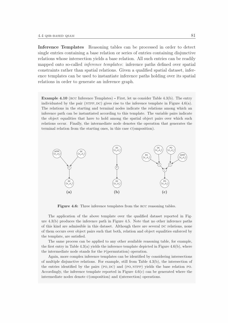
4.4 qsr-based qsam 81
Inference Templates Reasoning tables can be processed in order to detect
single entries containing a base relation or series of entries containing disjunctive
relations whose intersection yields a base relation. All such entries can be readily
mapped onto so-called inference templates: inference paths defined over spatial
constraints rather than spatial relations. Given a qualified spatial dataset, infer-
ence templates can be used to instantiate inference paths holding over its spatial
relations in order to generate an inference graph.
Example 4.10 (rcc Inference Templates) - First, let us consider Table 4.3(b). The entry
individuated by the pair (ntpp,dc) gives rise to the inference template in Figure 4.6(a).
The relations in the starting and terminal nodes indicate the relations among which an
inference path can be instantiated according to this template. The variable pairs indicate
the object equalities that have to hold among the spatial object pairs over which such
relations occur. Finally, the intermediate node denotes the operation that generates the
terminal relation from the starting ones, in this case c(omposition).
C
DC
(x1,x
2)
NTPP
(x1,x
3)
DC
(x3,x
2)
(a)
DC
(x1,x
2)
DC
(x2,x
1)
P
(b)
I
PO
(x1,x
3)
DC
(x3,x
2)
PO
(x1,x
4)
NTPP
(x4,x
2)
CC
PO
(x1,x
2)
(c)
Figure 4.6: Three inference templates from the rcc reasoning tables.
The application of the above template over the qualified dataset reported in Fig-
ure 4.3(b) produces the inference path in Figure 4.5. Note that no other inference paths
of this kind are admissible in this dataset. Although there are several dc relations, none
of them occurs over object pairs such that both, relation and object equalities enforced by
the template, are satisfied.
The same process can be applied to any other available reasoning table, for example,
the first entry in Table 4.3(a) yields the inference template depicted in Figure 4.6(b), where
the intermediate node stands for the p(permutation) operation.
Again, more complex inference templates can be identified by considering intersections
of multiple disjunctive relations. For example, still from Table 4.3(b), the intersection of
the entries identified by the pairs (po,dc) and (po,ntpp) yields the base relation po.
Accordingly, the inference template reported in Figure 4.6(c) can be generated where the
intermediate nodes denote c(omposition) and i(ntersection) operations.
82 4 Qualitative Spatial Access Methods
As seen in the above example, inferential nodes can be of three different types.
• Permutational: generated from permutation table, they have fixed in-degree and out-degree equal to 1. Incoming edges always originate in arelational node whereas outgoing edges always head toward intersection orrelational nodes.
• Compositional: generated from composition table, they have fixed in-degree and out-degree: the first equal to 2, the latter to 1. Incoming edgesalways originate in a relational node whereas outgoing edges always headtoward intersection or relational nodes.
• Intersection: generated from intersection of disjunctive relations that, inturn, result from composition or permutation operations. They have fixedin-degree and out-degree: the first equal to 2, the latter to 1. Incomingedges can originate in any kind of inferential node. Outgoing edges alwayshead toward intersection or relational nodes.
According to such properties we have that any inference template (resp. path)is structured as follows: Moving from any tail node to the head, the first non-relational node encountered is either permutational or compositional. It neces-sarily follows a series of intersection nodes and, finally, the head of the inferencetemplate (resp. path).
Definition 4.10 (Length of an Inference Graph) - An inference template (resp. path) is said
to be of length l if l is the maximal number of inferential nodes encountered when moving from
any relational node n ∈ T in its tail to its head h. Accordingly, an inference graph is said of
length l if its longest inference path has length equal to l.
From the properties of the inferential nodes and from the above definition itreadily follows the following:
Proposition 4.2 - An inference template (resp. path) of length l contains l − 1
intersection nodes and the cardinality of its tail |T | is such that: l ≤ |T | ≤ 2l.
Finally, we have that:
Proposition 4.3 - Given a calculus M ∈ P defining b = |B| base relations no
inference templates (resp. paths) longer than l = b exists. Proof. A disjunctive
relation consists at most of the disjunction of b base relations. As such a relation
results from a permutational or compositional node, then, we need at most b− 1
intersection nodes to filter out all but one base relation.
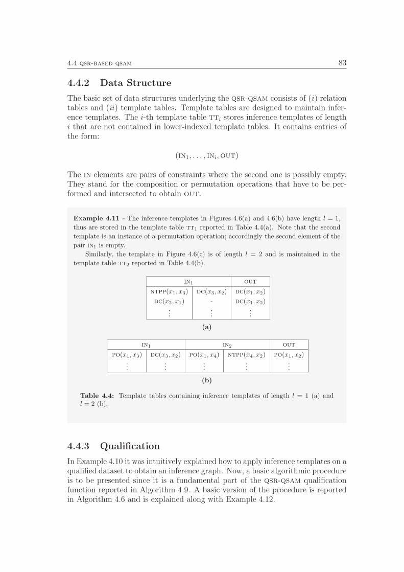
4.4 qsr-based qsam 83
4.4.2 Data Structure
The basic set of data structures underlying the qsr-qsam consists of (i) relationtables and (ii) template tables. Template tables are designed to maintain infer-ence templates. The i-th template table tti stores inference templates of lengthi that are not contained in lower-indexed template tables. It contains entries ofthe form:
(in1, . . . , ini,out)
The in elements are pairs of constraints where the second one is possibly empty.They stand for the composition or permutation operations that have to be per-formed and intersected to obtain out.
Example 4.11 - The inference templates in Figures 4.6(a) and 4.6(b) have length l = 1,
thus are stored in the template table tt1 reported in Table 4.4(a). Note that the second
template is an instance of a permutation operation; accordingly the second element of the
pair in1 is empty.
Similarly, the template in Figure 4.6(c) is of length l = 2 and is maintained in the
template table tt2 reported in Table 4.4(b).
in1 out
ntpp(x1, x3) dc(x3, x2) dc(x1, x2)
dc(x2, x1) - dc(x1, x2)...
......
(a)
in1 in2 out
po(x1, x3) dc(x3, x2) po(x1, x4) ntpp(x4, x2) po(x1, x2)...
......
......
(b)
Table 4.4: Template tables containing inference templates of length l = 1 (a) andl = 2 (b).
4.4.3 Qualification
In Example 4.10 it was intuitively explained how to apply inference templates on aqualified dataset to obtain an inference graph. Now, a basic algorithmic procedureis to be presented since it is a fundamental part of the qsr-qsam qualificationfunction reported in Algorithm 4.9. A basic version of the procedure is reportedin Algorithm 4.6 and is explained along with Example 4.12.
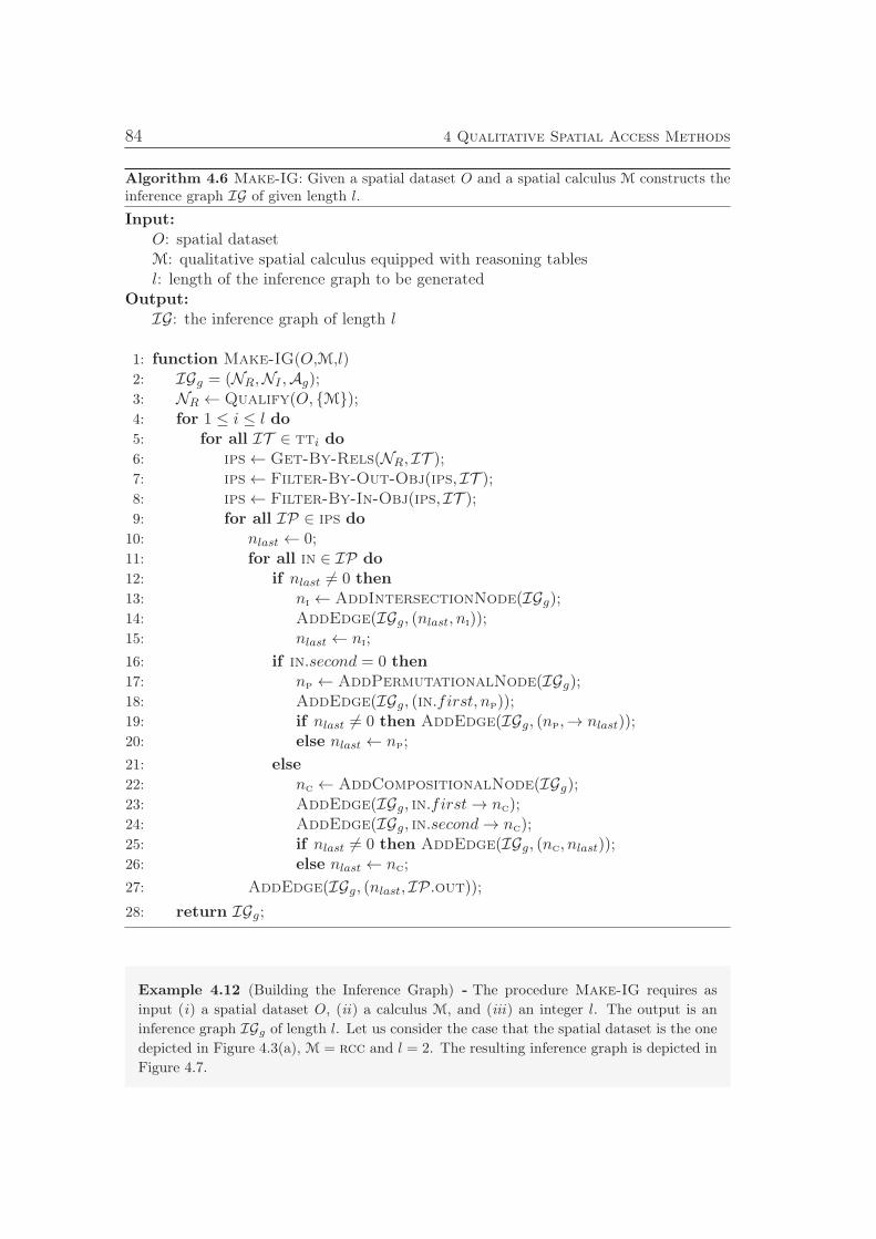
84 4 Qualitative Spatial Access Methods
Algorithm 4.6 Make-IG: Given a spatial dataset O and a spatial calculus M constructs theinference graph IG of given length l.
Input:
O: spatial datasetM: qualitative spatial calculus equipped with reasoning tablesl: length of the inference graph to be generated
Output:
IG: the inference graph of length l
1: function Make-IG(O,M,l)2: IGg = (NR,NI ,Ag);3: NR ← Qualify(O, M);4: for 1 ≤ i ≤ l do
5: for all IT ∈ tti do
6: ips← Get-By-Rels(NR, IT );7: ips← Filter-By-Out-Obj(ips, IT );8: ips← Filter-By-In-Obj(ips, IT );9: for all IP ∈ ips do
10: nlast ← 0;11: for all in ∈ IP do
12: if nlast 6= 0 then
13: ni ← AddIntersectionNode(IGg);14: AddEdge(IGg, (nlast, ni));15: nlast ← ni;
16: if in.second = 0 then
17: np ← AddPermutationalNode(IGg);18: AddEdge(IGg, (in.first, np));19: if nlast 6= 0 then AddEdge(IGg, (np,→ nlast));20: else nlast ← np;
21: else
22: nc ← AddCompositionalNode(IGg);23: AddEdge(IGg, in.first→ nc);24: AddEdge(IGg, in.second→ nc);25: if nlast 6= 0 then AddEdge(IGg, (nc, nlast));26: else nlast ← nc;
27: AddEdge(IGg, (nlast, IP.out));
28: return IGg;
Example 4.12 (Building the Inference Graph) - The procedure Make-IG requires as
input (i) a spatial dataset O, (ii) a calculus M, and (iii) an integer l. The output is aninference graph IGg of length l. Let us consider the case that the spatial dataset is the one
depicted in Figure 4.3(a), M = rcc and l = 2. The resulting inference graph is depicted in
Figure 4.7.
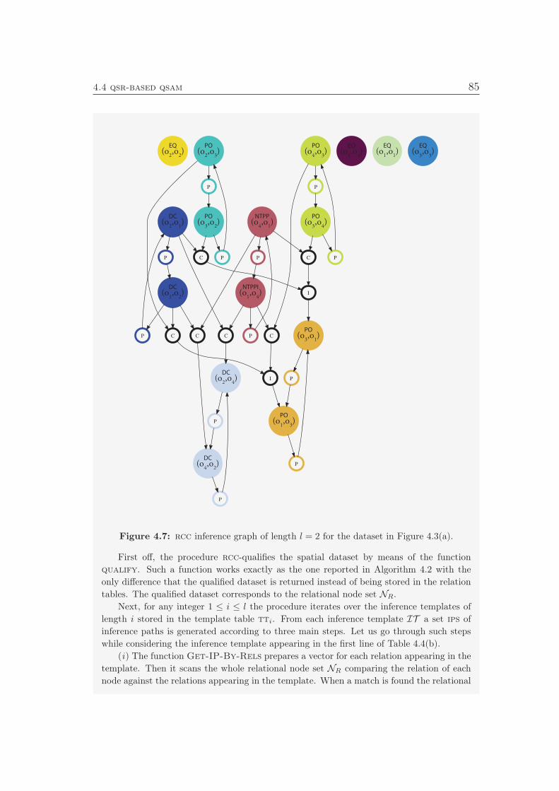
4.4 qsr-based qsam 85
EQ(o
2,o
2)
DC(o
2,o
4)
P
DC(o
2,o
1)
P
C
C
PO(o
2,o
3)
P
C
DC(o
4,o
2)
P
EQ(o
4,o
4)
NTPP(o
4,o
1)
C
CP
PO(o
4,o
3)
P
C
DC(o
1,o
2)
P
NTPPI(o
1,o
4)
P
EQ(o
1,o
1)
PO(o
1,o
3)
P
PO(o
3,o
2)
P
PO(o
3,o
4)
P
PO(o
3,o
1)
P
EQ(o
3,o
3)
I
I
Figure 4.7: rcc inference graph of length l = 2 for the dataset in Figure 4.3(a).
First off, the procedure rcc-qualifies the spatial dataset by means of the function
qualify. Such a function works exactly as the one reported in Algorithm 4.2 with the
only difference that the qualified dataset is returned instead of being stored in the relation
tables. The qualified dataset corresponds to the relational node set NR.
Next, for any integer 1 ≤ i ≤ l the procedure iterates over the inference templates of
length i stored in the template table tti. From each inference template IT a set ips of
inference paths is generated according to three main steps. Let us go through such steps
while considering the inference template appearing in the first line of Table 4.4(b).
(i) The function Get-IP-By-Rels prepares a vector for each relation appearing in thetemplate. Then it scans the whole relational node set NR comparing the relation of each
node against the relations appearing in the template. When a match is found the relational
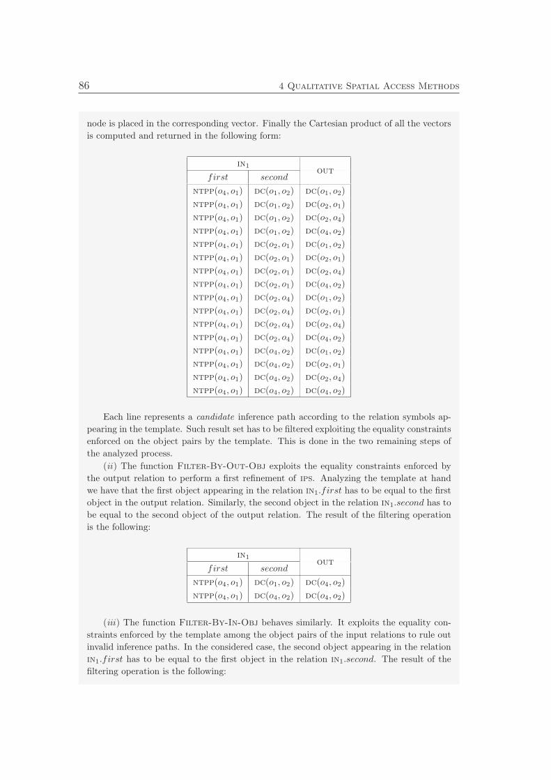
86 4 Qualitative Spatial Access Methods
node is placed in the corresponding vector. Finally the Cartesian product of all the vectors
is computed and returned in the following form:
in1
first secondout
ntpp(o4, o1) dc(o1, o2) dc(o1, o2)
ntpp(o4, o1) dc(o1, o2) dc(o2, o1)
ntpp(o4, o1) dc(o1, o2) dc(o2, o4)
ntpp(o4, o1) dc(o1, o2) dc(o4, o2)
ntpp(o4, o1) dc(o2, o1) dc(o1, o2)
ntpp(o4, o1) dc(o2, o1) dc(o2, o1)
ntpp(o4, o1) dc(o2, o1) dc(o2, o4)
ntpp(o4, o1) dc(o2, o1) dc(o4, o2)
ntpp(o4, o1) dc(o2, o4) dc(o1, o2)
ntpp(o4, o1) dc(o2, o4) dc(o2, o1)
ntpp(o4, o1) dc(o2, o4) dc(o2, o4)
ntpp(o4, o1) dc(o2, o4) dc(o4, o2)
ntpp(o4, o1) dc(o4, o2) dc(o1, o2)
ntpp(o4, o1) dc(o4, o2) dc(o2, o1)
ntpp(o4, o1) dc(o4, o2) dc(o2, o4)
ntpp(o4, o1) dc(o4, o2) dc(o4, o2)
Each line represents a candidate inference path according to the relation symbols ap-pearing in the template. Such result set has to be filtered exploiting the equality constraints
enforced on the object pairs by the template. This is done in the two remaining steps of
the analyzed process.
(ii) The function Filter-By-Out-Obj exploits the equality constraints enforced bythe output relation to perform a first refinement of ips. Analyzing the template at hand
we have that the first object appearing in the relation in1.first has to be equal to the first
object in the output relation. Similarly, the second object in the relation in1.second has to
be equal to the second object of the output relation. The result of the filtering operation
is the following:
in1
first secondout
ntpp(o4, o1) dc(o1, o2) dc(o4, o2)
ntpp(o4, o1) dc(o4, o2) dc(o4, o2)
(iii) The function Filter-By-In-Obj behaves similarly. It exploits the equality con-straints enforced by the template among the object pairs of the input relations to rule out
invalid inference paths. In the considered case, the second object appearing in the relation
in1.first has to be equal to the first object in the relation in1.second. The result of the
filtering operation is the following:
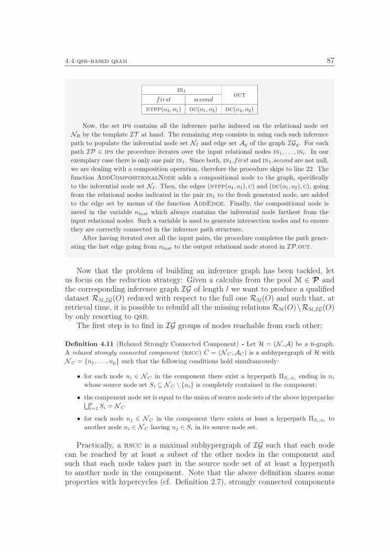
4.4 qsr-based qsam 87
in1
first secondout
ntpp(o4, o1) dc(o1, o2) dc(o4, o2)
Now, the set ips contains all the inference paths induced on the relational node set
NR by the template IT at hand. The remaining step consists in using each such inference
path to populate the inferential node set NI and edge set Ag of the graph IGg. For each
path IP ∈ ips the procedure iterates over the input relational nodes in1, . . . , ini. In our
exemplary case there is only one pair in1. Since both, in1.first and in1.second are not null,
we are dealing with a composition operation, therefore the procedure skips to line 22. The
function AddCompositionalNode adds a compositional node to the graph, specifically
to the inferential node set NI . Then, the edges (ntpp(o4, o1),c) and (dc(o1, o2),c), going
from the relational nodes indicated in the pair in1 to the fresh generated node, are added
to the edge set by means of the function AddEdge. Finally, the compositional node is
saved in the variable nlast which always contains the inferential node farthest from the
input relational nodes. Such a variable is used to generate intersection nodes and to ensure
they are correctly connected in the inference path structure.
After having iterated over all the input pairs, the procedure completes the path gener-
ating the last edge going from nlast to the output relational node stored in IP.out.
Now that the problem of building an inference graph has been tackled, letus focus on the reduction strategy: Given a calculus from the pool M ∈ P andthe corresponding inference graph IG of length l we want to produce a qualifieddataset RM,IG(O) reduced with respect to the full one RM(O) and such that, atretrieval time, it is possible to rebuild all the missing relations RM(O)\RM,IG(O)by only resorting to qsr.
The first step is to find in IG groups of nodes reachable from each other:
Definition 4.11 (Relaxed Strongly Connected Component) - Let H = (N ,A) be a b-graph.
A relaxed strongly connected component (rscc) C = (NC ,AC) is a subhypergraph of H with
NC = n1, . . . , np such that the following conditions hold simultaneously:
• for each node ni ∈ NC in the component there exist a hyperpath ΠSi,niending in ni
whose source node set Si ⊆ NC \ ni is completely contained in the component;
• the component node set is equal to the union of source node sets of the above hyperpaths:⋃p
i=1 Si = NC
• for each node nj ∈ NC in the component there exists at least a hyperpath ΠSi,nito
another node ni ∈ NC having nj ∈ Si in its source node set.
Practically, a rscc is a maximal subhypergraph of IG such that each nodecan be reached by at least a subset of the other nodes in the component andsuch that each node takes part in the source node set of at least a hyperpathto another node in the component. Note that the above definition shares someproperties with hypercycles (cf. Definition 2.7), strongly connected components
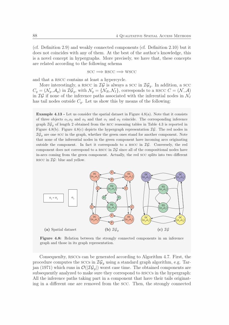
88 4 Qualitative Spatial Access Methods
(cf. Definition 2.9) and weakly connected components (cf. Definition 2.10) but itdoes not coincides with any of them. At the best of the author’s knowledge, thisis a novel concept in hypergraphs. More precisely, we have that, these conceptsare related according to the following schema
scc =⇒ rscc =⇒ wscc
and that a rscc contains at least a hypercycle.More interestingly, a rscc in IG is always a scc in IGg. In addition, a scc
Cg = (Ng,Ag) in IGg, with Ng = NR,NI, corresponds to a rscc C = (N ,A)in IG if none of the inference paths associated with the inferential nodes in NI
has tail nodes outside Cg. Let us show this by means of the following:
Example 4.13 - Let us consider the spatial dataset in Figure 4.8(a). Note that it consists
of three objects o1,o2 and o3 and that o1 and o2 coincide. The corresponding inference
graph IGg of length 2 obtained from the rcc reasoning tables in Table 4.3 is reported in
Figure 4.8(b). Figure 4.8(c) depicts the hypergraph representation IG. The red nodes in
IGg are one scc in the graph, whether the green ones stand for another component. Note
that none of the inferential nodes in the green component have incoming arcs originating
outside the component. In fact it corresponds to a rscc in IG. Conversely, the red
component does not correspond to a rscc in IG since all of the compositional nodes have
in-arcs coming from the green component. Actually, the red scc splits into two different
rscc in IG: blue and yellow.
o1 = o
2o
3
(a) Spatial dataset
EQ
(o1,o
2)
EQ
(o2,o
1)
P P
C C
C C
P
PDC
(o3,o
1)
DC
(o1,o
3)
P
PDC
(o3,o
2)
DC
(o2,o
3)
(b) IGg
EQ
(o1,o
2)
EQ
(o2,o
1)
DC
(o3,o
2)
DC
(o2,o
3)
DC
(o3,o
1)
DC
(o1,o
3)
(c) IG
Figure 4.8: Relation between the strongly connected components in an inferencegraph and those in its graph representation.
Consequenlty, rsccs can be generated according to Algorithm 4.7. First, theprocedure computes the sccs in IGg using a standard graph algorithm, e.g. Tar-jan (1971) which runs in O(|IGg|) worst case time. The obtained components aresubsequently analyzed to make sure they correspond to rsccs in the hypergraph:All the inference paths taking part in a component that have their tails originat-ing in a different one are removed from the scc. Then, the strongly connected
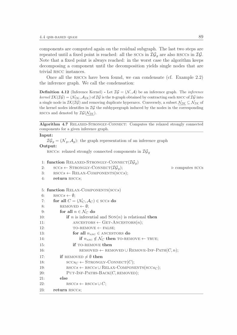
4.4 qsr-based qsam 89
components are computed again on the residual subgraph. The last two steps arerepeated until a fixed point is reached: all the sccs in IGg are also rsccs in IG.Note that a fixed point is always reached: in the worst case the algorithm keepsdecomposing a component until the decomposition yields single nodes that aretrivial rscc instances.
Once all the rsccs have been found, we can condensate (cf. Example 2.2)the inference graph. We call the condensation:
Definition 4.12 (Inference Kernel) - Let IG = (N ,A) be an inference graph. The inferencekernel IK(IG) = (NIK,AIK) of IG is the b-graph obtained by contracting each rscc of IG into
a single node in IK(IG) and removing duplicate hyperarcs. Conversely, a subset NIK ⊆ NIK of
the kernel nodes identifies in IG the subhypergraph induced by the nodes in the corresponding
rsccs and denoted by IG(NIK).
Algorithm 4.7 Relaxed-Strongly-Connect: Computes the relaxed strongly connectedcomponents for a given inference graph.
Input:
IGg = (N g,Ag): the graph representation of an inference graphOutput:
rsccs: relaxed strongly connected components in IGg
1: function Relaxed-Strongly-Connect(IGg)2: sccs← Strongly-Connect(IGg); ⊲ computes sccs3: rsccs← Relax-Components(sccs);4: return rsccs;
5: function Relax-Components(sccs)6: rsccs← ∅;7: for all C = (NC ,AC) ∈ sccs do
8: removed← ∅;9: for all n ∈ NC do
10: if n is inferential and Son(n) is relational then
11: ancestors← Get-Ancestors(n);12: to-remove← false;13: for all nanc ∈ ancestors do
14: if nanc /∈ NC then to-remove← true;
15: if to-remove then
16: removed← removed ∪Remove-Inf-Path(C, n);
17: if removed 6= ∅ then
18: sccsC ← Strongly-Connect(C);19: rsccs← rsccs ∪Relax-Components(sccsC);20: Put-Inf-Paths-Back(C,removed);21: else
22: rsccs← rsccs ∪ C;
23: return rsccs;

90 4 Qualitative Spatial Access Methods
Now, it has to be noted that, given an inference kernel hyperarc a = (T , h) ∈AIK, we have that all the relations corresponding to the nodes in IG(h) can be
inferred through reasoning operations by the relational nodes in IG(T ). Accord-ingly, given a series of hyperpaths spanning the whole kernel node set NIK, thesource node sets of such hyperpaths suffice to infer all the other nodes. To find
the source nodes we propose Algorithm 4.8 that runs in O(|IG|).
Algorithm 4.8 GetSources: Computes a set of hyperpaths spanning the node set of a givenb-graph H and returns the source node set.
Input:
H = (N ,A): b-graphOutput:
S: set of source nodes from which is possible to reach all the others
1: function GetSources(H)2: S; ⊲ global array3: ToVisit; ⊲ global array of size |N |4: on; ⊲ array of nodes ordered according to the number of outgoing arcs5: while on is not empty do
6: s← on.pop();7: if ToVisit[s] then
8: S.push(s);9: Visit(s,H)
10: return S;
11: function Visit(n,H)12: ToVisit[n]← false;13: for all outgoing ao do
14: if ToVisit[h(ao)] and h(ao) /∈ S then
15: for all nt ∈ T (ao) \ n do
16: if ToVisit[nt] and nt /∈ S then
17: S.push(nt);
18: Visit(h(ao),H);
19: return ;
The same principle applies to each source rscc: it is possible to find a set of
source relational nodes that reach all the other nodes in the component. Accord-
ingly, storing only the relation corresponding to such nodes is enough to rebuild,
at runtime, (i) the relation corresponding to the nodes in the same component
and (ii) the other components.
The whole qualification procedure, as explained above, is reported in Algo-
rithm 4.9. Example 4.14 traces the execution for the inference graph obtained
from the previous examples.
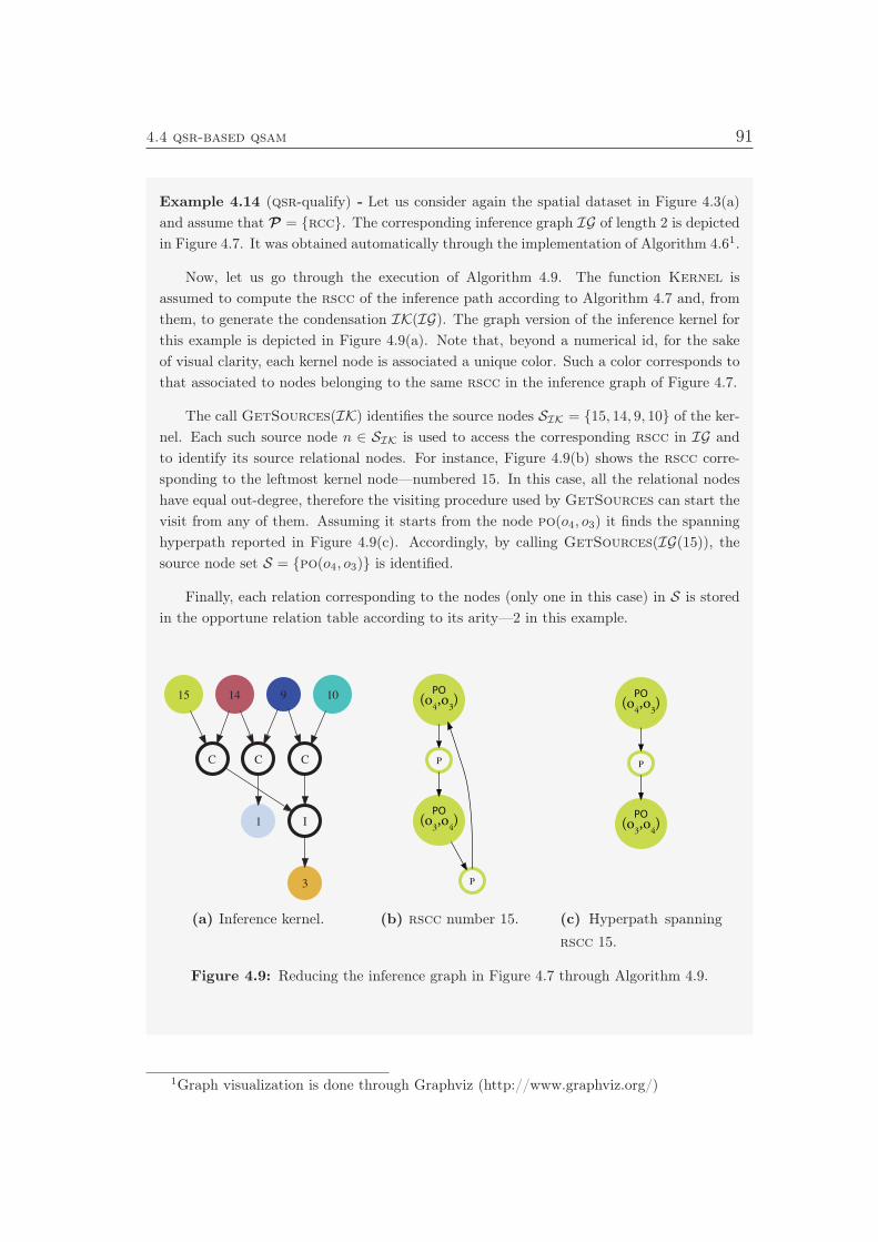
4.4 qsr-based qsam 91
Example 4.14 (qsr-qualify) - Let us consider again the spatial dataset in Figure 4.3(a)
and assume that P = rcc. The corresponding inference graph IG of length 2 is depicted
in Figure 4.7. It was obtained automatically through the implementation of Algorithm 4.61.
Now, let us go through the execution of Algorithm 4.9. The function Kernel is
assumed to compute the rscc of the inference path according to Algorithm 4.7 and, from
them, to generate the condensation IK(IG). The graph version of the inference kernel for
this example is depicted in Figure 4.9(a). Note that, beyond a numerical id, for the sake
of visual clarity, each kernel node is associated a unique color. Such a color corresponds to
that associated to nodes belonging to the same rscc in the inference graph of Figure 4.7.
The call GetSources(IK) identifies the source nodes SIK = 15, 14, 9, 10 of the ker-
nel. Each such source node n ∈ SIK is used to access the corresponding rscc in IG and
to identify its source relational nodes. For instance, Figure 4.9(b) shows the rscc corre-
sponding to the leftmost kernel node—numbered 15. In this case, all the relational nodes
have equal out-degree, therefore the visiting procedure used by GetSources can start the
visit from any of them. Assuming it starts from the node po(o4, o3) it finds the spanning
hyperpath reported in Figure 4.9(c). Accordingly, by calling GetSources(IG(15)), the
source node set S = po(o4, o3) is identified.
Finally, each relation corresponding to the nodes (only one in this case) in S is stored
in the opportune relation table according to its arity—2 in this example.
1
9
C C
14
C
1015
3
I
(a) Inference kernel.
PO
(o4,o
3)
P
PO
(o3,o
4)
P
(b) rscc number 15.
PO
(o4,o
3)
P
PO
(o3,o
4)
(c) Hyperpath spanning
rscc 15.
Figure 4.9: Reducing the inference graph in Figure 4.7 through Algorithm 4.9.
1Graph visualization is done through Graphviz (http://www.graphviz.org/)
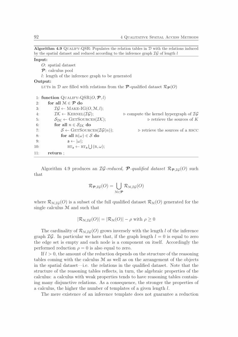
92 4 Qualitative Spatial Access Methods
Algorithm 4.9 Qualify-QSR: Populates the relation tables in D with the relations inducedby the spatial dataset and reduced according to the inference graph IG of length l
Input:
O: spatial datasetP : calculus pooll: length of the inference graph to be generated
Output:
luts in D are filled with relations from the P-qualified dataset RP(O)
1: function Qualify-QSR(O,P , l)2: for all M ∈ P do
3: IG ←Make-IG(O,M, l);4: IK ← Kernel(IG); ⊲ compute the kernel hypergraph of IG5: SIK ← GetSources(IK); ⊲ retrieve the sources of K6: for all n ∈ SIK do
7: S ← GetSources(IG(n)); ⊲ retrieve the sources of a rscc
8: for all r(ω) ∈ S do
9: a← |ω|;10: rta ← rta
⋃(r, ω);
11: return ;
Algorithm 4.9 produces an IG-reduced, P-qualified dataset RP,IG(O) suchthat
RP,IG(O) =⋃
M∈P
RM,IG(O)
where RM,IG(O) is a subset of the full qualified dataset RM(O) generated for thesingle calculus M and such that
|RM,IG(O)| = |RM(O)| − ρ with ρ ≥ 0
The cardinality of RM,IG(O) grows inversely with the length l of the inferencegraph IG. In particular we have that, if the graph length l = 0 is equal to zerothe edge set is empty and each node is a component on itself. Accordingly theperformed reduction ρ = 0 is also equal to zero.
If l > 0, the amount of the reduction depends on the structure of the reasoningtables coming with the calculus M as well as on the arrangement of the objectsin the spatial dataset—i.e. the relations in the qualified dataset. Note that thestructure of the reasoning tables reflects, in turn, the algebraic properties of thecalculus: a calculus with weak properties tends to have reasoning tables contain-ing many disjunctive relations. As a consequence, the stronger the properties ofa calculus, the higher the number of templates of a given length l.
The mere existence of an inference template does not guarantee a reduction
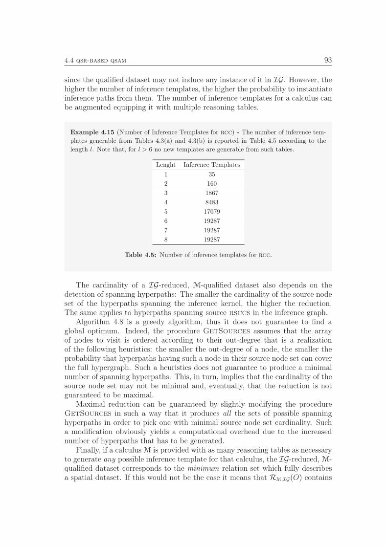
4.4 qsr-based qsam 93
since the qualified dataset may not induce any instance of it in IG. However, thehigher the number of inference templates, the higher the probability to instantiateinference paths from them. The number of inference templates for a calculus canbe augmented equipping it with multiple reasoning tables.
Example 4.15 (Number of Inference Templates for rcc) - The number of inference tem-
plates generable from Tables 4.3(a) and 4.3(b) is reported in Table 4.5 according to the
length l. Note that, for l > 6 no new templates are generable from such tables.
Lenght Inference Templates
1 35
2 160
3 1867
4 8483
5 17079
6 19287
7 19287
8 19287
Table 4.5: Number of inference templates for rcc.
The cardinality of a IG-reduced, M-qualified dataset also depends on thedetection of spanning hyperpaths: The smaller the cardinality of the source nodeset of the hyperpaths spanning the inference kernel, the higher the reduction.The same applies to hyperpaths spanning source rsccs in the inference graph.
Algorithm 4.8 is a greedy algorithm, thus it does not guarantee to find aglobal optimum. Indeed, the procedure GetSources assumes that the arrayof nodes to visit is ordered according to their out-degree that is a realizationof the following heuristics: the smaller the out-degree of a node, the smaller theprobability that hyperpaths having such a node in their source node set can coverthe full hypergraph. Such a heuristics does not guarantee to produce a minimalnumber of spanning hyperpaths. This, in turn, implies that the cardinality of thesource node set may not be minimal and, eventually, that the reduction is notguaranteed to be maximal.
Maximal reduction can be guaranteed by slightly modifying the procedureGetSources in such a way that it produces all the sets of possible spanninghyperpaths in order to pick one with minimal source node set cardinality. Sucha modification obviously yields a computational overhead due to the increasednumber of hyperpaths that has to be generated.
Finally, if a calculus M is provided with as many reasoning tables as necessaryto generate any possible inference template for that calculus, the IG-reduced, M-qualified dataset corresponds to the minimum relation set which fully describesa spatial dataset. If this would not be the case it means that RM,IG(O) contains
94 4 Qualitative Spatial Access Methods
relations that can be inferred from other relations. This is obviously impossiblegiven that the algorithm is designed to detect all the inferable relations.
4.4.4 Retrieval
The basic retrieval function for qsr-qsam draws upon standard qsr techniques.Given its constructive properties, the IG-reduced, P-qualified dataset RP,IG(O)contains enough spatial relations to rebuild all the missing ones by only applyingsymbolic reasoning.
Accordingly, the algorithm to solve a qscq consists of two main steps: foreach calculus M involved in the query (i) run the algebraic closure algorithm (cf.Section 2.2.5) on RM,IG(O) to rebuild the full qualified dataset RM(O). (ii) Solvethe query with the basic retrieval procedure reported in Algorithm 3.1 with thefunction ExtendPMatching realized as in Algorithm 4.3
4.4.5 Final Remarks and Discussion
qsr-based qsam (qsr-qsam) makes use of the inference graph (cf. Definition 4.9)to identify inferential dependencies among the relations in a full qualified datasetRP(O). Inferable relations are not stored since they can be rebuilt at retrievaltime via qualitative reasoning techniques.
In Section 4.4.3 a basic qualification procedure has been presented that pro-duces reduced, but not minimum, qualified dataset. It was pointed out that sucha procedure can be slightly modified to compute any possible set of spanninghyperpaths. This would allow for selecting the set with the smallest source nodeset and, thus, for producing minimal qualified datasets.
The problem of finding minimum qualitative representations has been raised,for example, in (Egenhofer & Sharma, 1992, 1993) where it is claimed that con-sistency checking algorithms can be used to find minimum topological represen-tations. The idea of Egenhofer & Sharma is to remove the arcs of a completeQualitative Constraint Network (qcn) one by one until it becomes ambiguous.In this way it is possible to identify the smallest possible set of relations form-ing a consistent description for the scene. In (Egenhofer & Sharma, 1993) theidentification of minimal relation set is obtained as a side-product of consistencyand the algorithm to find it is obviously not optimized. The qualification proce-dure we presented, instead, is purposely designed for reducing a qualified dataset,i.e. the arcs in a qcn. In Section 4.4.3 it was also argued that, if a calculus isprovided with as many reasoning tables as necessary to generate any possibleinference template, Qualify-QSR generates a qualified dataset with absoluteminimal cardinality, i.e. a minimum qualitative representation.
In Section 4.4.1.1 it was shown how inference templates can be automaticallygenerated from reasoning tables. However, it has to be noted that the set ofinference templates can be enriched with manually-defined ones. In this way,for example, one can introduce inter-calculi inferential dependencies that allow
4.5 Summary 95
for unifying inference graphs generated for different calculi and, accordingly, forproducing even more compact P-qualified datasets. For example, one mightobserve that if o1 is North of o2 then it has to be that o1 and o2 are Disconnected :n(o1, o2) → dc(o1, o2) and n(o1, o2) → dc(o2, o1). Of course this requires todefine new types of inferential nodes. For example, in this case one might definea new type named implication and manually add to the template tables a series oftemplates based on this operation. In his Ph.D thesis, Sharma (1996) developeda series of inter-calculus reasoning tables that can be exploited for this purpose.
Lastly, it is worth to remark that the strategies presented in the previoussections are basic strategies that can be improved in several ways. For example,the set of data structures underlying the qsam can be extended to allow formemorizing which inference templates are used to perform the reduction. Theretrieval approach can exploit this information to “guide” the algebraic closurealgorithm during the reconstruction phase.
4.5 Summary
In this chapter we defined Qualitative Spatial Access Methods (qsams): a ty-pology of Spatial Access Method (sam) suited for solving Qualitative SpatialConfiguration Queries (qscqs). A qsam has been formalized (cf. Definition 4.1)as a triple (q,D, r) where q is a dataset qualifier function that populates the set Dof data structures underlying the qsam and r is a retriever function that exploitsthe information stored in D to solve a given qscq.
Four kinds of qsams have been developed: Functional qsam (f-qsam), Quali-tative Storage Layer qsam (qsl-qsam), Spatial Clustering qsam (sc-qsam), andqsr-based qsam (qsr-qsam). They all draw upon the basic retrieval strategypresented in Section 3.4.1, but tackle differently the dataset qualification problem(cf. Section 3.5).
f-qsam (cf. Section 4.1) encodes the runtime qualification strategy presentedin Section 3.5.1. Accordingly, it has a void qualifier function and an empty set ofdata structures. The retriever function qualifies the dataset at qscq executiontime. Such a solution provides the best option in terms of storage space but isextremely costly with respect to retrieval time.
qsl-qsam (cf. Section 4.2) encodes the pre-qualification strategy presentedin Section 3.5.2. The qualifier function performs a full qualification of the spatialdataset and stores the resulting qualitative relations into a set of appositely de-signed Lookup Tables (luts) called relation tables. Such an approach allows fortransforming qscq solving into a series of look-up operations. Although allowingfor high retrieval time performance, this solution presents two main drawbacks:(i) It requires an enormous quantity of extra storage space needed to maintainthe qualified dataset. (ii) The high computational cost demanded by a full pre-qualification makes hard to deal with the dynamism of the real world. Indeed,
96 4 Qualitative Spatial Access Methods
by the time a spatial dataset is qualified, the produced qualified dataset mightbe already out-of-date, calling for a new pre-qualification.
The sc-qsam family is introduced in Section 4.3. It draws upon the jointexploitation of a special type of spatial relations called Clustering Relations to-gether with a spatial clustering index (cf. Definition 4.5). If opportunely tuned,the spatial clustering index produces a subdivision of the spatial dataset thatallows the qualifier function to compute and store a reduced number of qualita-tive relations. Beyond the relation tables, the set of data structures underlyinga sc-qsam contains other data structures designed to represent the spatial clus-tering index used to make the subdivision. At qscq execution time, the retrieverfunction exploits the index structure to rebuild the qualitative relations missingin the relation tables. This approach provides a valuable compromise betweenthe previous solutions: it shorten the retrieval time with respect to f-qsam aswell as the pre-qualification time and produces more compact qualified datasets.The main shortcoming of this approach is that it requires a careful calibrationof the spatial clustering index parameters. Indeed, as shown in Section 4.3.3, a“bad” index may yield worse space-time performance than a full pre-qualification.Consequently this solution requires a mindful tuning of the index parameters thatalso depends on the spatial calculi in the calculus pool P .
Finally qsr-qsam is presented in Section 4.4. It exploits a novel data struc-ture named inference graph (cf. Definition 4.9) to obtain a reduced qualifieddataset from which it is possible to infer back all the missing relations by onlyresorting to symbolic reasoning. The advantages of this strategy are that it isindependent of the spatial calculus and it might be used to produce the minimumset of qualitative relations needed to describe a spatial dataset (cf. discussion onthe reduction at the end of Section 4.4.3). The main drawbacks are that, in or-der to perform the reduction, qsr-qsam requires a full pre-qualification plus theinstantiation of an inference graph. This is a very costly operation, that makethis solution unsuitable for being applied on a full spatial dataset.
A possible alternative that takes advantage of both sc-qsam and qsr-qsamis described in the Outlook section of Chapter 7.
Chapter 5
Developing and Benchmarking
Qualitative Spatial Access Methods
In this chapter we tackle the problem of developing and benchmarking QualitativeSpatial Access Methods (qsams) from a practical perspective. The chapter issplit into two main parts: Section 5.1 introduces a software framework calledMyQual whose main purpose is to provide a development, testing, and productionenvironment for Spatial Access Methods (sams) suited for qualitative spatialqueries, with a particular focus on qsams and Qualitative Spatial ConfigurationQueries (qscqs). MyQual has been used to implement, test and compare all ofthe qsams presented in Chapter 4 (cf. Chapter 6 for the experimental results).
As explained in the previous chapter, the Spatial Clustering qsam (sc-qsam)family (cf. Section 4.3) requires a careful choice of the spatial clustering indexas well as a mindful tuning of its parameters according to the spatial calculi thathave to be treated. Section 5.2 is devoted to present the implementation of twoinstances of the sc-qsam family.
5.1 MyQual: an Extensible Development and Bench-
mark Framework
MyQual is a novel software framework realized in the scope of this thesis tofacilitate the development of sams for qualitative spatial queries (cf. Section 3.1).It has been designed as an extension for spatially-enabled PostgreSQL1 databases
1http://www.postgresql.org/
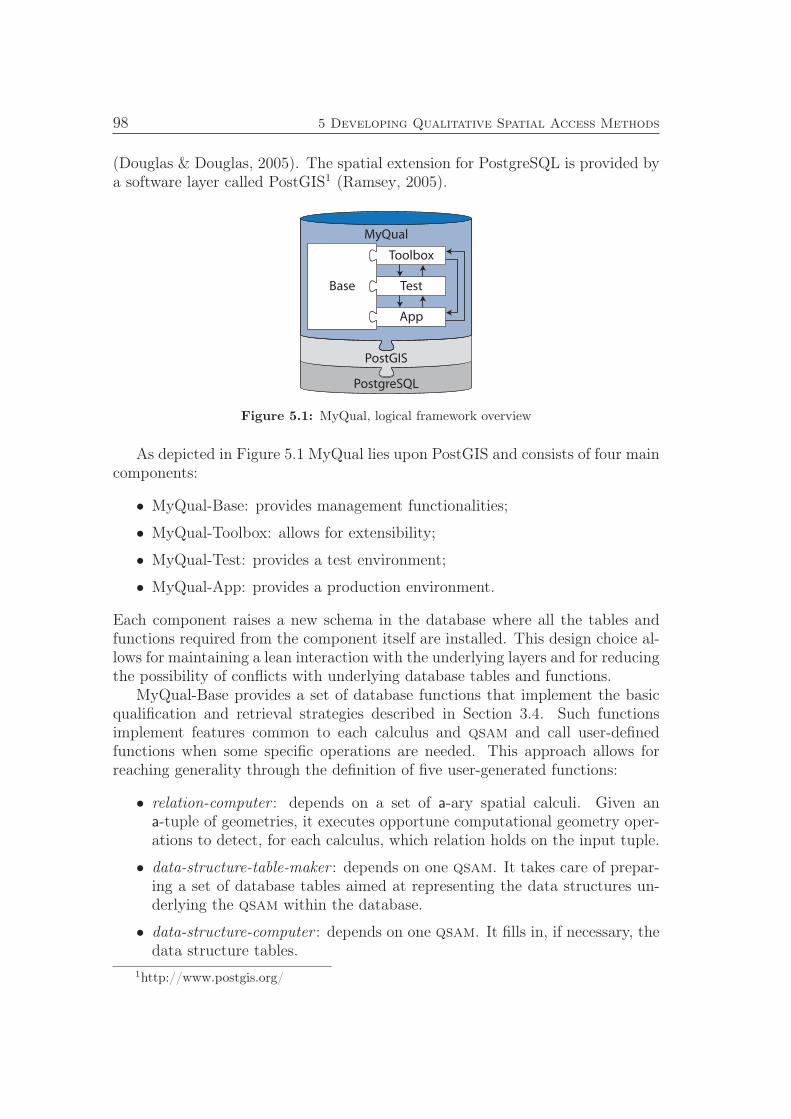
98 5 Developing Qualitative Spatial Access Methods
(Douglas & Douglas, 2005). The spatial extension for PostgreSQL is provided bya software layer called PostGIS1 (Ramsey, 2005).
PostGIS
PostgreSQL
MyQual
Toolbox
Test
App
Base
Figure 5.1: MyQual, logical framework overview
As depicted in Figure 5.1 MyQual lies upon PostGIS and consists of four maincomponents:
• MyQual-Base: provides management functionalities;
• MyQual-Toolbox: allows for extensibility;
• MyQual-Test: provides a test environment;
• MyQual-App: provides a production environment.
Each component raises a new schema in the database where all the tables andfunctions required from the component itself are installed. This design choice al-lows for maintaining a lean interaction with the underlying layers and for reducingthe possibility of conflicts with underlying database tables and functions.
MyQual-Base provides a set of database functions that implement the basicqualification and retrieval strategies described in Section 3.4. Such functionsimplement features common to each calculus and qsam and call user-definedfunctions when some specific operations are needed. This approach allows forreaching generality through the definition of five user-generated functions:
• relation-computer : depends on a set of a-ary spatial calculi. Given ana-tuple of geometries, it executes opportune computational geometry oper-ations to detect, for each calculus, which relation holds on the input tuple.
• data-structure-table-maker : depends on one qsam. It takes care of prepar-ing a set of database tables aimed at representing the data structures un-derlying the qsam within the database.
• data-structure-computer : depends on one qsam. It fills in, if necessary, thedata structure tables.
1http://www.postgis.org/
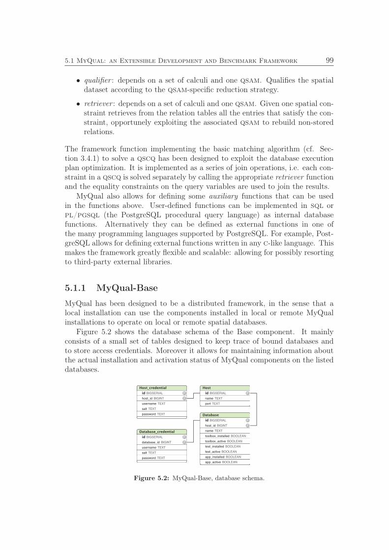
5.1 MyQual: an Extensible Development and Benchmark Framework 99
• qualifier : depends on a set of calculi and one qsam. Qualifies the spatialdataset according to the qsam-specific reduction strategy.
• retriever : depends on a set of calculi and one qsam. Given one spatial con-straint retrieves from the relation tables all the entries that satisfy the con-straint, opportunely exploiting the associated qsam to rebuild non-storedrelations.
The framework function implementing the basic matching algorithm (cf. Sec-tion 3.4.1) to solve a qscq has been designed to exploit the database executionplan optimization. It is implemented as a series of join operations, i.e. each con-straint in a qscq is solved separately by calling the appropriate retriever functionand the equality constraints on the query variables are used to join the results.
MyQual also allows for defining some auxiliary functions that can be usedin the functions above. User-defined functions can be implemented in sql orpl/pgsql (the PostgreSQL procedural query language) as internal databasefunctions. Alternatively they can be defined as external functions in one ofthe many programming languages supported by PostgreSQL. For example, Post-greSQL allows for defining external functions written in any c-like language. Thismakes the framework greatly flexible and scalable: allowing for possibly resortingto third-party external libraries.
5.1.1 MyQual-Base
MyQual has been designed to be a distributed framework, in the sense that alocal installation can use the components installed in local or remote MyQualinstallations to operate on local or remote spatial databases.
Figure 5.2 shows the database schema of the Base component. It mainlyconsists of a small set of tables designed to keep trace of bound databases andto store access credentials. Moreover it allows for maintaining information aboutthe actual installation and activation status of MyQual components on the listeddatabases.
Host_credential
id BIGSERIAL P
host_id BIGINT F
username TEXT
salt TEXT
password TEXT
Database_credential
id BIGSERIAL P
database_id BIGINT F
username TEXT
salt TEXT
password TEXT
Database
id BIGSERIAL P
host_id BIGINT F
name TEXT
toolbox_installed BOOLEAN
toolbox_active BOOLEAN
app_installed BOOLEAN
test_installed BOOLEAN
app_active BOOLEAN
test_active BOOLEAN
Host
id BIGSERIAL P
name TEXT
port TEXT
Figure 5.2: MyQual-Base, database schema.
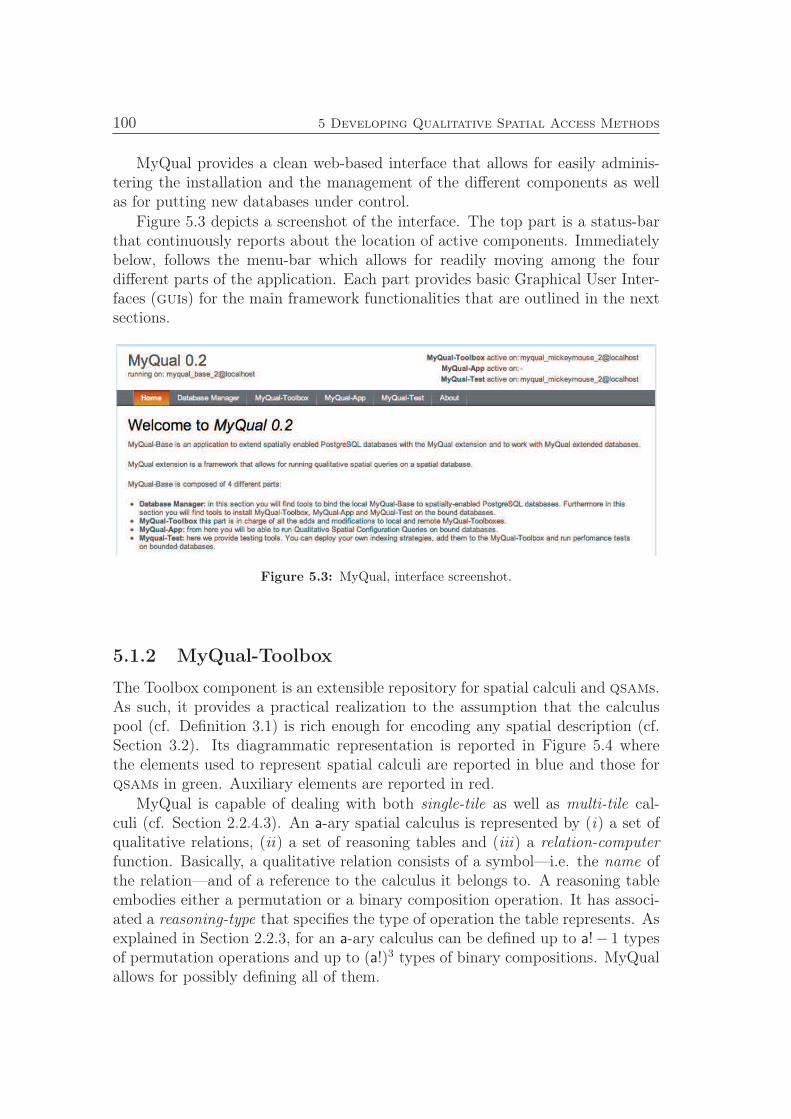
100 5 Developing Qualitative Spatial Access Methods
MyQual provides a clean web-based interface that allows for easily adminis-tering the installation and the management of the different components as wellas for putting new databases under control.
Figure 5.3 depicts a screenshot of the interface. The top part is a status-barthat continuously reports about the location of active components. Immediatelybelow, follows the menu-bar which allows for readily moving among the fourdifferent parts of the application. Each part provides basic Graphical User Inter-faces (guis) for the main framework functionalities that are outlined in the nextsections.
Figure 5.3: MyQual, interface screenshot.
5.1.2 MyQual-Toolbox
The Toolbox component is an extensible repository for spatial calculi and qsams.As such, it provides a practical realization to the assumption that the calculuspool (cf. Definition 3.1) is rich enough for encoding any spatial description (cf.Section 3.2). Its diagrammatic representation is reported in Figure 5.4 wherethe elements used to represent spatial calculi are reported in blue and those forqsams in green. Auxiliary elements are reported in red.
MyQual is capable of dealing with both single-tile as well as multi-tile cal-culi (cf. Section 2.2.4.3). An a-ary spatial calculus is represented by (i) a set ofqualitative relations, (ii) a set of reasoning tables and (iii) a relation-computerfunction. Basically, a qualitative relation consists of a symbol—i.e. the name ofthe relation—and of a reference to the calculus it belongs to. A reasoning tableembodies either a permutation or a binary composition operation. It has associ-ated a reasoning-type that specifies the type of operation the table represents. Asexplained in Section 2.2.3, for an a-ary calculus can be defined up to a!− 1 typesof permutation operations and up to (a!)3 types of binary compositions. MyQualallows for possibly defining all of them.
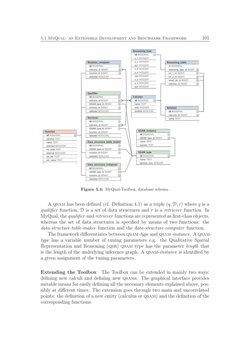
5.1 MyQual: an Extensible Development and Benchmark Framework 101
QSAM_type
id BIGSERIAL P
name TEXT
params_num INTEGER
Relation_computer
id BIGSERIAL P
calculus_id BIGINT F
function_id BIGINT F
selected BOOLEAN
Relation
id BIGSERIAL P
calculus_id BIGINT F
name TEXT
Data_structure_computer
id BIGSERIAL P
QSAM_type_id BIGINT F
function_id BIGINT F
selected BOOLEAN
Function
id BIGSERIAL P
schema TEXT
name TEXT
selected BOOLEAN
for_what TEXT
external BOOLEAN
ext_file TEXT
ext_name TEXT
Reasoning_table
id BIGSERIAL
reasoning_type_id BIGINT F
rel_1_id BIGINT F
rel_2_id BIGINT F
result_rel_id BIGINT F
calculus_id BIGINT F
Retriever
id BIGSERIAL P
calculus_id BIGINT F
QSAM_type_id BIGINT F
function_id BIGINT
selected BOOLEAN
Qualifier
id BIGSERIAL P
calculus_id BIGINT F
QSAM_type_id BIGINT F
function_id BIGINT F
selected BOOLEAN
Data_structure_table_maker
id BIGSERIAL P
QSAM_type_id BIGINT F
function_id BIGINT F
selected BOOLEAN
Calculus
id BIGSERIAL P
name TEXT
arity INTEGER
multitile BOOLEAN
Reasoning_type
id BIGSERIAL P
x_1 INTEGER
y_1 INTEGER
z_1 INTEGER
x_2 INTEGER
y_2 INTEGER
z_2 INTEGER
x_3 INTEGER
y_3 INTEGER
z_3 INTEGER
QSAM_instance
id BIGSERIAL P
QSAM_type_id BIGINT F
name TEXT
params TEXT
Figure 5.4: MyQual-Toolbox, database schema.
A qsam has been defined (cf. Definition 4.1) as a triple (q,D, r) where q is aqualifier function, D is a set of data structures and r is a retriever function. InMyQual, the qualifier and retriever functions are represented as first-class objects,whereas the set of data structures is specified by means of two functions: thedata-structure-table-maker function and the data-structure-computer function.
The framework differentiates between qsam-type and qsam-instance. A qsam-type has a variable number of tuning parameters e.g. the Qualitative SpatialRepresentation and Reasoning (qsr) qsam type has the parameter length thatis the length of the underlying inference graph. A qsam-instance is identified bya given assignment of the tuning parameters.
Extending the Toolbox The Toolbox can be extended in mainly two ways:defining new calculi and defining new qsams. The graphical interface providessuitable means for easily defining all the necessary elements explained above, pos-sibly at different times. The extension goes through two main and uncorrelatedpoints: the definition of a new entity (calculus or qsam) and the definition of thecorresponding functions.
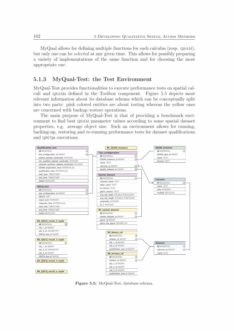
102 5 Developing Qualitative Spatial Access Methods
MyQual allows for defining multiple functions for each calculus (resp. qsam),but only one can be selected at any given time. This allows for possibly preparinga variety of implementations of the same function and for choosing the mostappropriate one.
5.1.3 MyQual-Test: the Test Environment
MyQual-Test provides functionalities to execute performance tests on spatial cal-culi and qsams defined in the Toolbox component. Figure 5.5 depicts mostrelevant information about its database schema which can be conceptually splitinto two parts: pink colored entities are about testing whereas the yellow onesare concerned with backup/restore operations.
The main purpose of MyQual-Test is that of providing a benchmark envi-ronment to find best qsam parameter values according to some spatial datasetproperties, e.g. average object size. Such an environment allows for running,backing-up, restoring and re-running performance tests for dataset qualificationsand qscqs executions.
BK_QSCQ_result_3_tuple
id BIGSERIAL P
obj_1_id BIGINT
obj_2_id GEOMETRY
obj_3_id BIGINT
QSCQ_test_id BIGINT
BK_QSCQ_result_n_tuple
QSCQ_test
id BIGSERIAL P
test_configuration_id BIGINT F
QSCQ TEXT
result_num INTEGER
response_time INTERVAL(6)
start_time TIMESTAMP
end_time TIMESTAMP
tested BOOLEAN
BK_QSCQ_result_4_tuple
Qualification_test
id BIGSERIAL P
test_configuration_id BIGINT F
spatial_dataset_cardinality INTEGER
full_qualified_dataset_cardinality INTEGER
reduced_qualified_dataset_cardinality INTEGER
QSAM_preparation_time INTERVAL(6)
qualification_time INTERVAL(6)
start_time TIMESTAMP
end_time TIMESTAMP
tested BOOLEAN
BK_ternary_rel
id BIGSERIAL P
relation_id BIGINT F
obj_1_id BIGINT
obj_2_id BIGINT
obj_3_id BIGINT
qualification_test_id BIGINT
BK_QSCQ_result_2_tuple
id BIGSERIAL P
obj_1_id BIGINT
obj_2_id GEOMETRY
QSCQ_test_id BIGINTBK_binary_rel
id BIGSERIAL P
relation_id BIGINT F
obj_1_id BIGINT
obj_2_id BIGINT
qualification_test_id BIGINT
Relation
id BIGSERIAL P
calculus_id BIGINT F
name TEXT
BK_QSAM_instance
BK_spatial_dataset
id BIGSERIAL P
spatial_dataset_id BIGINT F
geom_id BIGINT
geom_the_geom GEOMETRY
QSAM_instance
id BIGSERIAL P
QSAM_type_id BIGINT
name TEXT
params TEXT
Test_configuration
id BIGSERIAL P
QSAM_instance_id BIGINT F
name TEXT
calculus_id BIGINT F
spatial_dataset_id BIGINT F
Calculus
id BIGSERIAL P
name TEXT
arity INTEGER
multitile BOOLEAN
Spatial_dataset
id BIGSERIAL P
schema_name TEXT
table_name TEXT
id_column TEXT
geom_column TEXT
avg_obj_width DOUBLE PRECISION
avg_obj_heigth DOUBLE PRECISION
cardinality INTEGER
id_1 INTEGER
Figure 5.5: MyQual-Test, database schema.
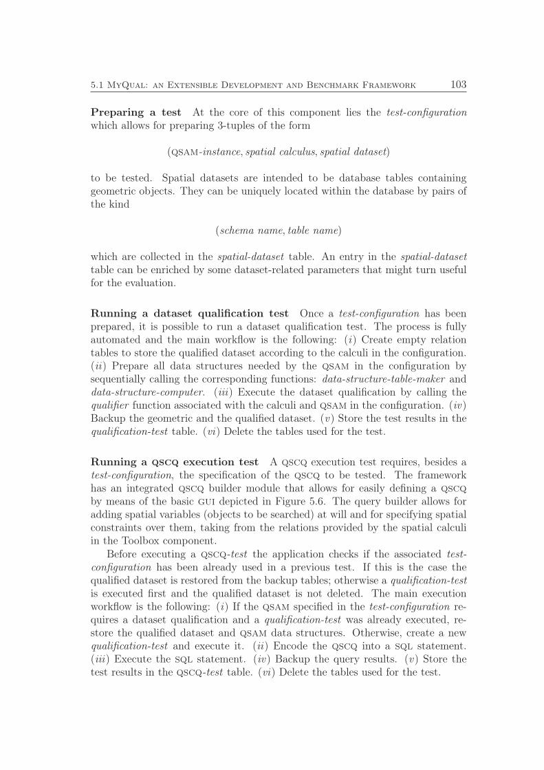
5.1 MyQual: an Extensible Development and Benchmark Framework 103
Preparing a test At the core of this component lies the test-configurationwhich allows for preparing 3-tuples of the form
(qsam-instance, spatial calculus, spatial dataset)
to be tested. Spatial datasets are intended to be database tables containinggeometric objects. They can be uniquely located within the database by pairs ofthe kind
(schema name, table name)
which are collected in the spatial-dataset table. An entry in the spatial-datasettable can be enriched by some dataset-related parameters that might turn usefulfor the evaluation.
Running a dataset qualification test Once a test-configuration has beenprepared, it is possible to run a dataset qualification test. The process is fullyautomated and the main workflow is the following: (i) Create empty relationtables to store the qualified dataset according to the calculi in the configuration.(ii) Prepare all data structures needed by the qsam in the configuration bysequentially calling the corresponding functions: data-structure-table-maker anddata-structure-computer. (iii) Execute the dataset qualification by calling thequalifier function associated with the calculi and qsam in the configuration. (iv)Backup the geometric and the qualified dataset. (v) Store the test results in thequalification-test table. (vi) Delete the tables used for the test.
Running a qscq execution test A qscq execution test requires, besides atest-configuration, the specification of the qscq to be tested. The frameworkhas an integrated qscq builder module that allows for easily defining a qscqby means of the basic gui depicted in Figure 5.6. The query builder allows foradding spatial variables (objects to be searched) at will and for specifying spatialconstraints over them, taking from the relations provided by the spatial calculiin the Toolbox component.
Before executing a qscq-test the application checks if the associated test-configuration has been already used in a previous test. If this is the case thequalified dataset is restored from the backup tables; otherwise a qualification-testis executed first and the qualified dataset is not deleted. The main executionworkflow is the following: (i) If the qsam specified in the test-configuration re-quires a dataset qualification and a qualification-test was already executed, re-store the qualified dataset and qsam data structures. Otherwise, create a newqualification-test and execute it. (ii) Encode the qscq into a sql statement.(iii) Execute the sql statement. (iv) Backup the query results. (v) Store thetest results in the qscq-test table. (vi) Delete the tables used for the test.
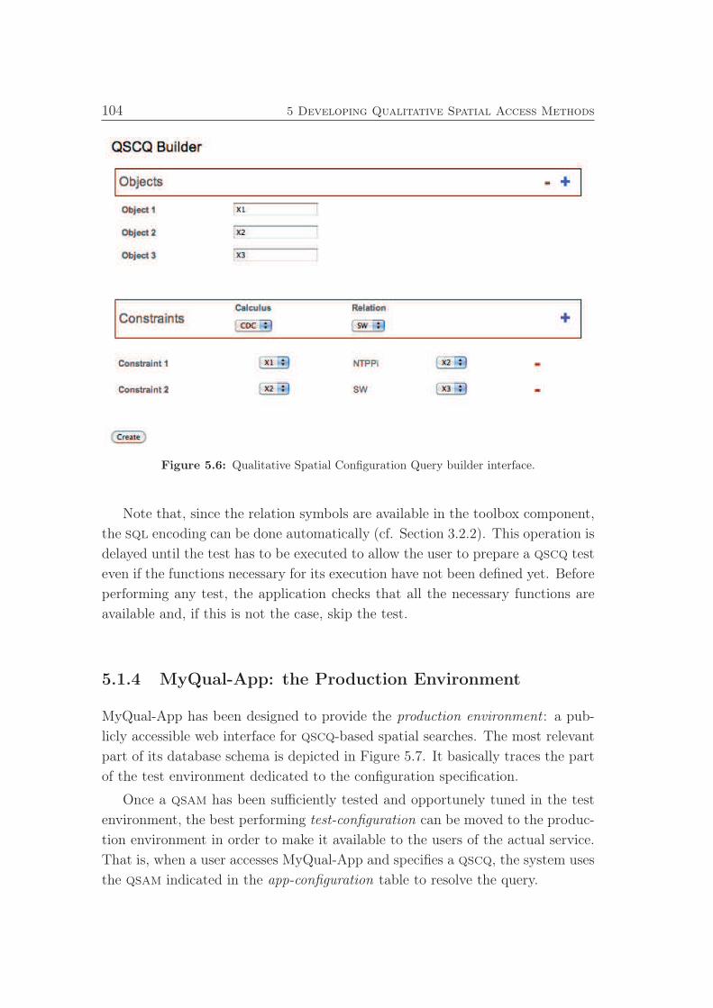
104 5 Developing Qualitative Spatial Access Methods
Figure 5.6: Qualitative Spatial Configuration Query builder interface.
Note that, since the relation symbols are available in the toolbox component,
the sql encoding can be done automatically (cf. Section 3.2.2). This operation is
delayed until the test has to be executed to allow the user to prepare a qscq test
even if the functions necessary for its execution have not been defined yet. Before
performing any test, the application checks that all the necessary functions are
available and, if this is not the case, skip the test.
5.1.4 MyQual-App: the Production Environment
MyQual-App has been designed to provide the production environment : a pub-
licly accessible web interface for qscq-based spatial searches. The most relevant
part of its database schema is depicted in Figure 5.7. It basically traces the part
of the test environment dedicated to the configuration specification.
Once a qsam has been sufficiently tested and opportunely tuned in the test
environment, the best performing test-configuration can be moved to the produc-
tion environment in order to make it available to the users of the actual service.
That is, when a user accesses MyQual-App and specifies a qscq, the system uses
the qsam indicated in the app-configuration table to resolve the query.
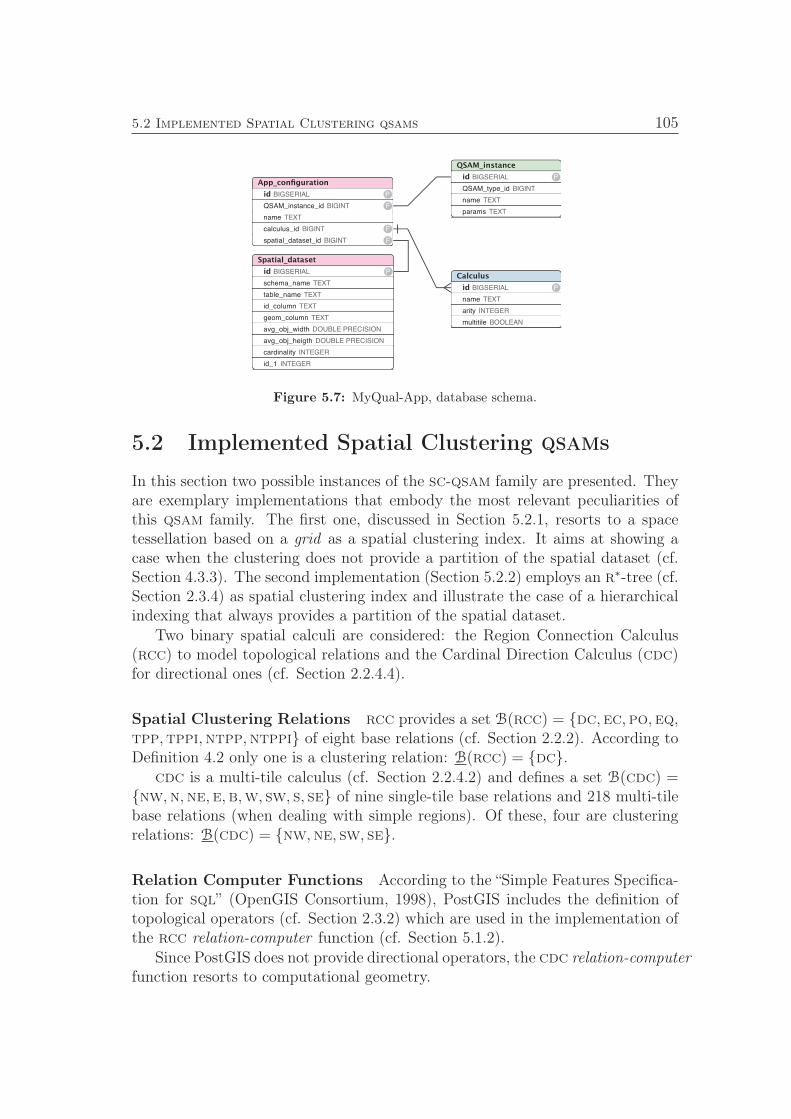
5.2 Implemented Spatial Clustering qsams 105
QSAM_instance
id BIGSERIAL P
QSAM_type_id BIGINT
name TEXT
params TEXT
App_configuration
id BIGSERIAL P
QSAM_instance_id BIGINT F
name TEXT
calculus_id BIGINT F
spatial_dataset_id BIGINT F
Calculus
id BIGSERIAL P
name TEXT
arity INTEGER
multitile BOOLEAN
Spatial_dataset
id BIGSERIAL P
schema_name TEXT
table_name TEXT
id_column TEXT
geom_column TEXT
avg_obj_width DOUBLE PRECISION
avg_obj_heigth DOUBLE PRECISION
cardinality INTEGER
id_1 INTEGER
Figure 5.7: MyQual-App, database schema.
5.2 Implemented Spatial Clustering qsams
In this section two possible instances of the sc-qsam family are presented. Theyare exemplary implementations that embody the most relevant peculiarities ofthis qsam family. The first one, discussed in Section 5.2.1, resorts to a spacetessellation based on a grid as a spatial clustering index. It aims at showing acase when the clustering does not provide a partition of the spatial dataset (cf.Section 4.3.3). The second implementation (Section 5.2.2) employs an r∗-tree (cf.Section 2.3.4) as spatial clustering index and illustrate the case of a hierarchicalindexing that always provides a partition of the spatial dataset.
Two binary spatial calculi are considered: the Region Connection Calculus(rcc) to model topological relations and the Cardinal Direction Calculus (cdc)for directional ones (cf. Section 2.2.4.4).
Spatial Clustering Relations rcc provides a set B(rcc) = dc,ec,po,eq,tpp,tppi,ntpp,ntppi of eight base relations (cf. Section 2.2.2). According toDefinition 4.2 only one is a clustering relation: B(rcc) = dc.
cdc is a multi-tile calculus (cf. Section 2.2.4.2) and defines a set B(cdc) =nw,n,ne,e,b,w, sw, s, se of nine single-tile base relations and 218 multi-tilebase relations (when dealing with simple regions). Of these, four are clusteringrelations: B(cdc) = nw,ne, sw, se.
Relation Computer Functions According to the “Simple Features Specifica-tion for sql” (OpenGIS Consortium, 1998), PostGIS includes the definition oftopological operators (cf. Section 2.3.2) which are used in the implementation ofthe rcc relation-computer function (cf. Section 5.1.2).
Since PostGIS does not provide directional operators, the cdc relation-computerfunction resorts to computational geometry.
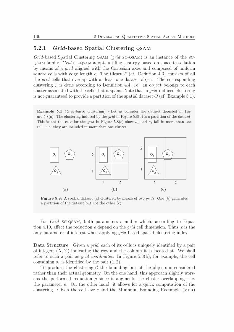
106 5 Developing Qualitative Spatial Access Methods
5.2.1 Grid-based Spatial Clustering qsam
Grid -based Spatial Clustering qsam (grid sc-qsam) is an instance of the sc-qsam family. Grid sc-qsam adopts a tiling strategy based on space tessellationby means of a grid aligned with the Cartesian axes and composed of uniformsquare cells with edge length c. The tileset T (cf. Defintion 4.3) consists of allthe grid cells that overlap with at least one dataset object. The correspondingclustering C is done according to Definition 4.4, i.e. an object belongs to eachcluster associated with the cells that it spans. Note that, a grid -induced clusteringis not guaranteed to provide a partition of the spatial dataset O (cf. Example 5.1).
Example 5.1 (Grid -based clustering) - Let us consider the dataset depicted in Fig-
ure 5.8(a). The clustering induced by the grid in Figure 5.8(b) is a partition of the dataset.This is not the case for the grid in Figure 5.8(c) since o1 and o3 fall in more than one
cell—i.e. they are included in more than one cluster.
o1
o2
o3
(a)
o1
o2
o32
1
1 2
(b)
o1
o2
o3
2
1
1 2
(c)
Figure 5.8: A spatial dataset (a) clustered by means of two grids. One (b) generatesa partition of the dataset but not the other (c).
For Grid sc-qsam, both parameters e and v which, according to Equa-tion 4.10, affect the reduction ρ depend on the grid cell dimension. Thus, c is theonly parameter of interest when applying grid -based spatial clustering index.
Data Structure Given a grid, each of its cells is uniquely identified by a pairof integers (X, Y ) indicating the row and the column it is located at. We shallrefer to such a pair as grid-coordinates. In Figure 5.8(b), for example, the cellcontaining o1 is identified by the pair (1, 2).
To produce the clustering C the bounding box of the objects is consideredrather than their actual geometry. On the one hand, this approach slightly wors-ens the performed reduction ρ since it augments the cluster overlapping—i.e.the parameter e. On the other hand, it allows for a quick computation of theclustering. Given the cell size c and the Minimum Bounding Rectangle (mbr)
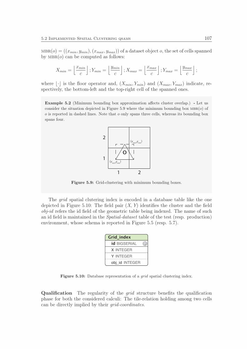
5.2 Implemented Spatial Clustering qsams 107
mbr(o) = ((xmin, ymin), (xmax, ymax)) of a dataset object o, the set of cells spannedby mbr(o) can be computed as follows:
Xmin =⌊xmin
c
⌋;Ymin =
⌊ymin
c
⌋;Xmax =
⌊xmax
c
⌋;Ymax =
⌊ymax
c
⌋;
where ⌊·⌋ is the floor operator and, (Xmin, Ymin) and (Xmax, Ymax) indicate, re-spectively, the bottom-left and the top-right cell of the spanned ones.
Example 5.2 (Minimum bounding box approximation affects cluster overlap.) - Let us
consider the situation depicted in Figure 5.9 where the minimum bounding box mbr(o) of
o is reported in dashed lines. Note that o only spans three cells, whereas its bounding box
spans four.
o
2
1
1 2
(xmin,y
min)
(xmax,y
max)
Figure 5.9: Grid-clustering with minimum bounding boxes.
The grid spatial clutering index is encoded in a database table like the onedepicted in Figure 5.10: The field pair (X,Y) identifies the cluster and the fieldobj-id refers the id field of the geometric table being indexed. The name of suchan id field is maintained in the Spatial-dataset table of the test (resp. production)environment, whose schema is reported in Figure 5.5 (resp. 5.7).
Grid_index
id BIGSERIAL P
X INTEGER
Y INTEGER
obj_id INTEGER
Figure 5.10: Database representation of a grid spatial clustering index.
Qualification The regularity of the grid structure benefits the qualificationphase for both the considered calculi: The tile-relation holding among two cellscan be directly implied by their grid-coordinates.
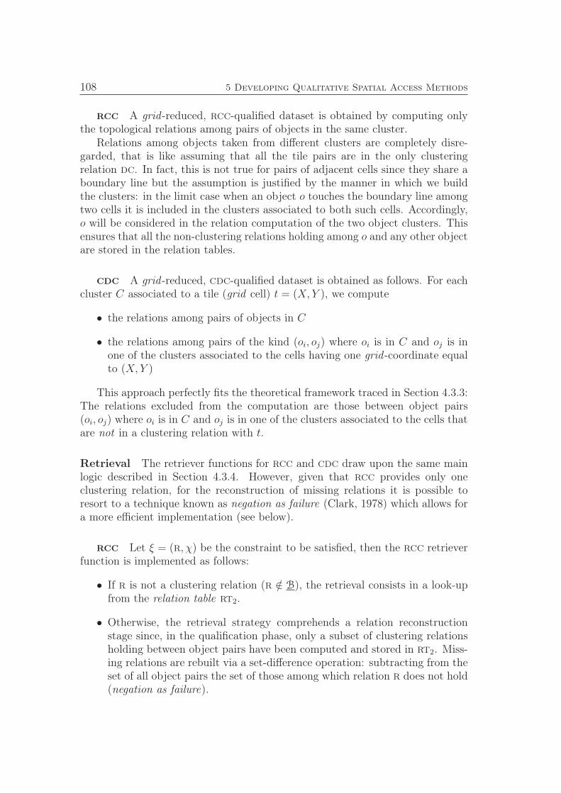
108 5 Developing Qualitative Spatial Access Methods
rcc A grid -reduced, rcc-qualified dataset is obtained by computing onlythe topological relations among pairs of objects in the same cluster.
Relations among objects taken from different clusters are completely disre-garded, that is like assuming that all the tile pairs are in the only clusteringrelation dc. In fact, this is not true for pairs of adjacent cells since they share aboundary line but the assumption is justified by the manner in which we buildthe clusters: in the limit case when an object o touches the boundary line amongtwo cells it is included in the clusters associated to both such cells. Accordingly,o will be considered in the relation computation of the two object clusters. Thisensures that all the non-clustering relations holding among o and any other objectare stored in the relation tables.
cdc A grid -reduced, cdc-qualified dataset is obtained as follows. For eachcluster C associated to a tile (grid cell) t = (X, Y ), we compute
• the relations among pairs of objects in C
• the relations among pairs of the kind (oi, oj) where oi is in C and oj is inone of the clusters associated to the cells having one grid -coordinate equalto (X, Y )
This approach perfectly fits the theoretical framework traced in Section 4.3.3:The relations excluded from the computation are those between object pairs(oi, oj) where oi is in C and oj is in one of the clusters associated to the cells thatare not in a clustering relation with t.
Retrieval The retriever functions for rcc and cdc draw upon the same mainlogic described in Section 4.3.4. However, given that rcc provides only oneclustering relation, for the reconstruction of missing relations it is possible toresort to a technique known as negation as failure (Clark, 1978) which allows fora more efficient implementation (see below).
rcc Let ξ = (r, χ) be the constraint to be satisfied, then the rcc retrieverfunction is implemented as follows:
• If r is not a clustering relation (r /∈ B), the retrieval consists in a look-upfrom the relation table rt2.
• Otherwise, the retrieval strategy comprehends a relation reconstructionstage since, in the qualification phase, only a subset of clustering relationsholding between object pairs have been computed and stored in rt2. Miss-ing relations are rebuilt via a set-difference operation: subtracting from theset of all object pairs the set of those among which relation r does not hold(negation as failure).
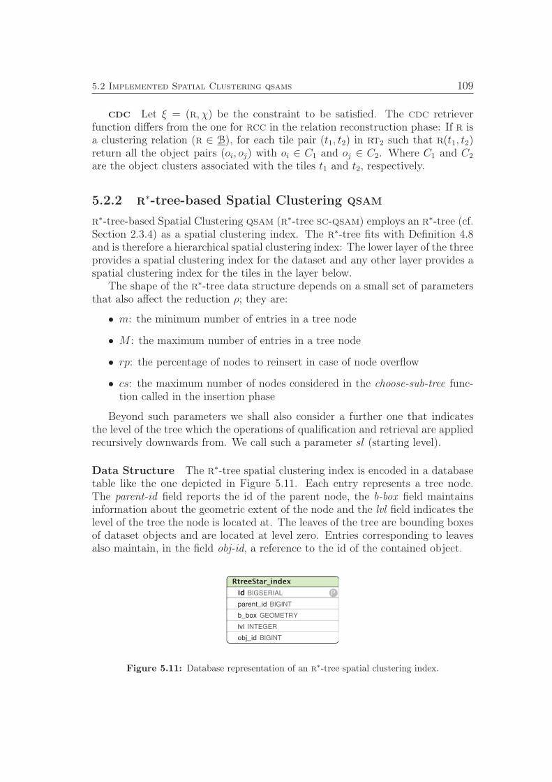
5.2 Implemented Spatial Clustering qsams 109
cdc Let ξ = (r, χ) be the constraint to be satisfied. The cdc retrieverfunction differs from the one for rcc in the relation reconstruction phase: If r isa clustering relation (r ∈ B), for each tile pair (t1, t2) in rt2 such that r(t1, t2)return all the object pairs (oi, oj) with oi ∈ C1 and oj ∈ C2. Where C1 and C2
are the object clusters associated with the tiles t1 and t2, respectively.
5.2.2 r∗-tree-based Spatial Clustering qsam
r∗-tree-based Spatial Clustering qsam (r∗-tree sc-qsam) employs an r∗-tree (cf.Section 2.3.4) as a spatial clustering index. The r∗-tree fits with Definition 4.8and is therefore a hierarchical spatial clustering index: The lower layer of the threeprovides a spatial clustering index for the dataset and any other layer provides aspatial clustering index for the tiles in the layer below.
The shape of the r∗-tree data structure depends on a small set of parametersthat also affect the reduction ρ; they are:
• m: the minimum number of entries in a tree node
• M : the maximum number of entries in a tree node
• rp: the percentage of nodes to reinsert in case of node overflow
• cs: the maximum number of nodes considered in the choose-sub-tree func-tion called in the insertion phase
Beyond such parameters we shall also consider a further one that indicatesthe level of the tree which the operations of qualification and retrieval are appliedrecursively downwards from. We call such a parameter sl (starting level).
Data Structure The r∗-tree spatial clustering index is encoded in a databasetable like the one depicted in Figure 5.11. Each entry represents a tree node.The parent-id field reports the id of the parent node, the b-box field maintainsinformation about the geometric extent of the node and the lvl field indicates thelevel of the tree the node is located at. The leaves of the tree are bounding boxesof dataset objects and are located at level zero. Entries corresponding to leavesalso maintain, in the field obj-id, a reference to the id of the contained object.
RtreeStar_index
id BIGSERIAL P
parent_id BIGINT
b_box GEOMETRY
lvl INTEGER
obj_id BIGINT
Figure 5.11: Database representation of an r∗-tree spatial clustering index.
110 5 Developing Qualitative Spatial Access Methods
Qualification Differently than a grid, the construction process of an r∗-treeis data-driven and its final structure depends on, besides the index parameters,the spatial arrangement of the indexed dataset. Accordingly, it is not possible toknow in advance what the relation among two tiles (directory rectangles of thetree nodes) is.
The qualifier functions for rcc and cdc realize a recursive variant of thegeneral procedure described in Algorithm 4.4 (Section 4.3.3). Namely, the ba-sic qualification is applied on the tiles at the starting level sl. The procedurecomputes the relation r holding on each tile pair (ti, tj) in the current level. Ifr ∈ B is a clustering relation, all the children of the tree node corresponding toti are to be in the same relation r with all the children of tj. Then the qualifierfunction store the relation r(ti, tj) in the relation table rt2. Otherwise, if thelevel in consideration is not the leaf one and r /∈ B is not a clustering relation,the procedure recurses on the lower level, only considering the tree nodes havingti or tj as parent node. Note that the relations holding on objects at the leaf levelare computed using the actual geometries of the dataset objects instead of theirbounding box.
Retrieval Similarly to the qualifier functions, the retriever functions for rccand cdc realize a recursive variant of the general procedure described in Algo-rithm 4.5 (Section 4.3.4). Let ξ = (r, χ) be the constraint to be satisfied, thenthe retriever function is implemented as follows:
• If r is not a clustering relation (r /∈ B), the retrieval consists in a look-upfrom the relation table rt2.
• Otherwise, for each level lvl ≤ sl and for each tile pair (t1, t2) in rt2 suchthat t1 and t2 are at level lvl of the tree and such that r(t1, t2), retrieve allthe children leaf nodes of t1 and t2. Return all the object pairs (oi, oj) withoi being a child of t1 and oj being a child of t2.
Note that, as for grid -based sc-qsam, also in this case for the rcc retrieverfunction the reconstruction phase can be empowered by applying negation asfailure technique.
5.3 Summary
In this chapter a novel software framework called MyQual has been presented .Its main purpose is to provide a development, test and production environmentfor sams for qualitative spatial queries, with a particular focus on qsams andqscqs.
MyQual has been designed as an extension for PostGIS-enabled PostgreSQLdatabases and is logically divided in four parts: MyQual-Base, MyQual-Toolbox,
5.3 Summary 111
MyQual-Test and MyQual-App. Each part, when installed in a database, pro-duces a dedicated schema where all the tables, functions and indexes used by thecomponent are kept separated from the rest of the database.
MyQual-Base encodes all the basic functionalities of the framework whichcomprehend the management of bound databases. All the other components canbe installed separately and can be used from different instances of MyQual-Base.
MyQual-Toolbox is an extensible repository for qualitative spatial calculi andqsams. It provides both a realization of the assumption that the calculus pool(cf. Definition 3.1) is rich enough for encoding any natural spatial description(cf. Section 3.2) and a development environment for qsams.
MyQual-Test is the test environment where different configurations of qsamsand spatial calculi can be tested upon different spatial datasets. It providestwo main test typologies: qualification tests and qscq execution tests. Theenvironment provides guis to readily prepare and run such tests. The results areautomatically backed-up to allows for comparison and reproduction. qscqs canbe generated via a web-form gui.
MyQual-App has been thought as the production environment where mostpromising qsams and spatial calculi can be made available to casual users willingto execute qualitative spatial queries.
MyQual achieves generality by being grounded in the definition of five user-defined functions. Such functions depends on spatial calculi and qsams and canbe implemented in a variety of programming languages.
The second part of the chapter has been devoted to present the implementa-tion of two instances of sc-qsam within MyQual. The first instance presented,resorts to a simple grid as spatial clustering index and serves as an example ofthe case in which the clustering does not provide a dataset partition. The secondimplementation grounds in the r∗-tree data structure and provides an exemplarycase of hierarchical spatial clustering index.

Chapter 6
Empirical Evaluation
This chapter provides an empirical evaluation of the Qualitative Spatial AccessMethods (qsams) presented in Chapter 4. In Section 6.1 the main evaluationcriteria are outlined. Section 6.2 is devoted to testbed definition. Section 6.3discusses experiments on Functional qsam and Qualitative Storage Layer qsam.Performance of grid -based and r∗-tree-based Spatial Clustering qsam are ana-lyzed in Sections 6.4 and 6.5, respectively; whereas qsr-based qsam is discussedin Section 6.6. Section 6.7 is devoted to a comparison of the most promisingqsams on a real geospatial dataset. The chapter ends with a comparison of theresults in Section 6.8.
6.1 Evaluation Criteria and Experiments Setup
In order to assess the qsams presented in Chapter 4, we are interested in eval-uating the following features as the cardinality of the addressed spatial datasetchanges: (i) dataset qualification time, (ii) space occupancy of the qualifieddataset, and (iii) Qualitative Spatial Configuration Query (qscq) execution time.
Qualified dataset occupancy directly depends on the number of pre-computedrelations, which is independent of the characteristics of the hosting machine.Accordingly, we measure point (ii) in terms of the cardinality of the producedqualified datasets.
qscq retrieval time scales with the output size, i.e. the number of returnedconfigurations. This, in turn, depends on the number and on the type of relationsencoded in the qscq. Accordingly, we also discuss the correlation between theretrieval time of a given qscq and the size of its output.
MyQual (cf. Section 5.1) has been used to implement and test all the qsamspresented in this work (cf Chapter 4 and Section 5.2) with two binary qualitative
114 6 Empirical Evaluation
spatial calculi:the Region Connection Calculus (rcc) and the Cardinal DirectionCalculus (cdc).
Experiments have been run in two main stages: spatial dataset qualificationand qscq execution. The qualification stage is executed first. MyQual automati-cally backs up the qualified dataset and the data structures underlying the testedqsam, if any, in order to allow for reproducing the experiment. Once backed up,these items are deleted from the database. For each qscq execution the qualifieddataset and the qsam data structures are restored from the backup tables, thenthe qscq is resolved and timed. Also in this case MyQual automatically backs upthe results of the query and deletes all the restored items. Note that, if two qscqshave to be tested against the same qualified dataset, the latter is restored anddeleted twice (even if the executions are consequential). This is done to reduce tothe minimum the interference of the optimization instruments of the underlyingDatabase Management System (dbms) in the timing: A freshly restored table istreated as a new object by the dbms, i.e. no statistics are available for the queryoptimizer that can be used to boost the execution of a query.
Finally, note that the relation tables, where qualified datasets are stored, havebeen purposely designed and implemented without any indexing technique in or-der to reduce to the minimum the interference of dbms optimization componentson the outcomes. However, as claimed in Section 3.5.2 one of the advantages ofpre-qualification is that the resulting dataset can be indexed by means of standardindexing techniques such as b-trees that allow to further shorten qscq responsetimes.
The reported computing times refer to an Apple iMac mounting a 2.7 ghzIntel Core i5 (4 cores) processor and a 12 gb 1333 mhz ddr3 ram unit.
6.2 Evaluation Testbed
Most of the qsams have been tested over a common testbed in order to allow for adirect comparison of the results. When a different testbed has been used, becauseof some qsam-specific features, it is specified in the corresponding section.
We shall discriminate the testbed according to the two experiment types:The qualification testbed consists of a set of randomly generated spatial datasets.Each dataset consists of convex polygons1 uniformly distributed in a D × D =500 × 500 fixed-size workspace. The dataset cardinality N ranges over the set100, 250, 500, 750, 1000. Figure 6.1(a) depicts a random dataset with N = 1000.The average dataset object extent on each dimension (x- and y- projection) dvaries over the set 7.5, 15—refer to Figure 6.1(b) for a pictorial explanation.The qualification testbed consists of 10 dataset instances for every pair (N, d) ∈100, 250, 500, 750, 1000 × 7.5, 15, for a total of 100 randomly generated
1The polygons have a variable number of vertices ranging between 3 and 8. Note, however,that the number of vertices is unimportant in the scope of this evaluation since it does notaffect the outcomes of the experiments.
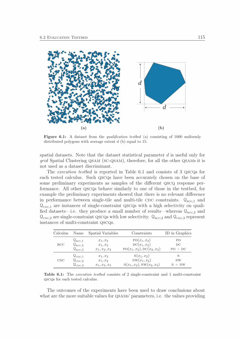
6.2 Evaluation Testbed 115
(a)
d
d
(b)
Figure 6.1: A dataset from the qualification testbed (a) consisting of 1000 uniformlydistributed polygons with average extent d (b) equal to 15.
spatial datasets. Note that the dataset statistical parameter d is useful only forgrid Spatial Clustering qsam (sc-qsam), therefore, for all the other qsams it isnot used as a dataset discriminant.
The execution testbed is reported in Table 6.1 and consists of 3 qscqs foreach tested calculus. Such qscqs have been accurately chosen on the base ofsome preliminary experiments as samples of the different qscq response per-formance. All other qscqs behave similarly to one of those in the testbed, forexample the preliminary experiments showed that there is no relevant differencein performance between single-tile and multi-tile cdc constraints. Qrcc,1 andQcdc,1 are instances of single-constraint qscqs with a high selectivity on quali-fied datasets—i.e. they produce a small number of results—whereas Qrcc,2 andQcdc,2 are single-constraint qscqs with low selectivity. Qrcc,3 and Qcdc,3 representinstances of multi-constraint qscqs.
Calculus Name Spatial Variables Constraints ID in Graphics
rccQrcc,1 x1, x2 po(x1, x2) poQrcc,2 x1, x2 dc(x1, x2) dcQrcc,3 x1, x2, x3 po(x1, x2),dc(x2, x3) po + dc
cdcQcdc,1 x1, x2 n(x1, x2) nQcdc,2 x1, x2 nw(x1, x2) nwQcdc,3 x1, x2, x3 n(x1, x2),nw(x2, x3) n + nw
Table 6.1: The execution testbed consists of 2 single-constraint and 1 multi-constraintqscqs for each tested calculus.
The outcomes of the experiments have been used to draw conclusions aboutwhat are the more suitable values for qsams’ parameters, i.e. the values providing
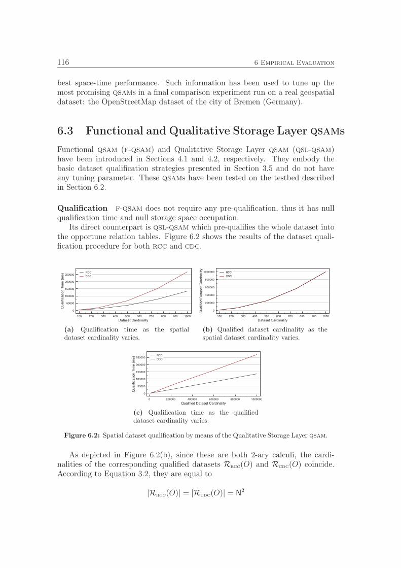
116 6 Empirical Evaluation
best space-time performance. Such information has been used to tune up themost promising qsams in a final comparison experiment run on a real geospatialdataset: the OpenStreetMap dataset of the city of Bremen (Germany).
6.3 Functional and Qualitative Storage Layer qsams
Functional qsam (f-qsam) and Qualitative Storage Layer qsam (qsl-qsam)have been introduced in Sections 4.1 and 4.2, respectively. They embody thebasic dataset qualification strategies presented in Section 3.5 and do not haveany tuning parameter. These qsams have been tested on the testbed describedin Section 6.2.
Qualification f-qsam does not require any pre-qualification, thus it has nullqualification time and null storage space occupation.
Its direct counterpart is qsl-qsam which pre-qualifies the whole dataset intothe opportune relation tables. Figure 6.2 shows the results of the dataset quali-fication procedure for both rcc and cdc.
100 200 300 400 500 600 700 800 900 1000
Dataset Cardinality
0
50000
100000
150000
200000
250000
Qualifi
cation T
ime (
ms) RCC
CDC
(a) Qualification time as the spatialdataset cardinality varies.
100 200 300 400 500 600 700 800 900 1000
Dataset Cardinality
0
200000
400000
600000
800000
1000000
Qualifi
ed D
ata
set C
ard
inalit
y
RCC
CDC
(b) Qualified dataset cardinality as thespatial dataset cardinality varies.
0 200000 400000 600000 800000 1000000
Qualified Dataset Cardinality
0
50000
100000
150000
200000
250000
Qualifi
cation T
ime (
ms) RCC
CDC
(c) Qualification time as the qualifieddataset cardinality varies.
Figure 6.2: Spatial dataset qualification by means of the Qualitative Storage Layer qsam.
As depicted in Figure 6.2(b), since these are both 2-ary calculi, the cardi-nalities of the corresponding qualified datasets Rrcc(O) and Rcdc(O) coincide.According to Equation 3.2, they are equal to
|Rrcc(O)| = |Rcdc(O)| = N2
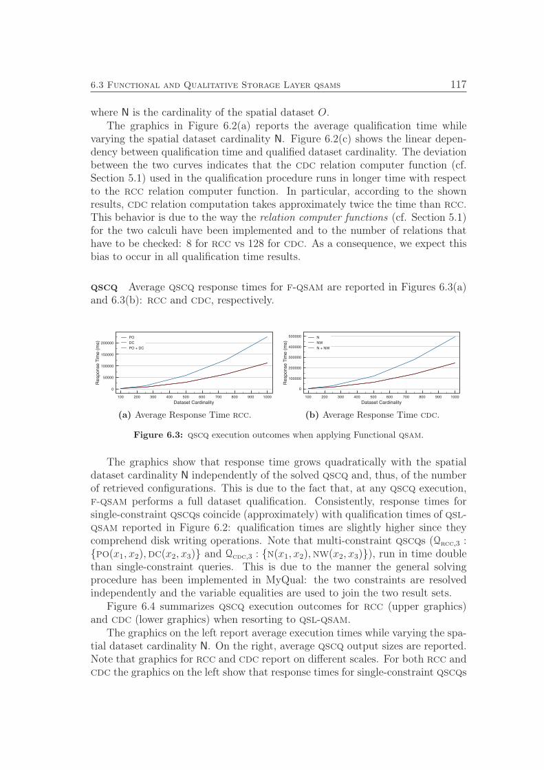
6.3 Functional and Qualitative Storage Layer qsams 117
where N is the cardinality of the spatial dataset O.The graphics in Figure 6.2(a) reports the average qualification time while
varying the spatial dataset cardinality N. Figure 6.2(c) shows the linear depen-dency between qualification time and qualified dataset cardinality. The deviationbetween the two curves indicates that the cdc relation computer function (cf.Section 5.1) used in the qualification procedure runs in longer time with respectto the rcc relation computer function. In particular, according to the shownresults, cdc relation computation takes approximately twice the time than rcc.This behavior is due to the way the relation computer functions (cf. Section 5.1)for the two calculi have been implemented and to the number of relations thathave to be checked: 8 for rcc vs 128 for cdc. As a consequence, we expect thisbias to occur in all qualification time results.
qscq Average qscq response times for f-qsam are reported in Figures 6.3(a)and 6.3(b): rcc and cdc, respectively.
100 200 300 400 500 600 700 800 900 1000
Dataset Cardinality
0
50000
100000
150000
200000
Response T
ime (
ms)
PO
DC
PO + DC
(a) Average Response Time rcc.
100 200 300 400 500 600 700 800 900 1000
Dataset Cardinality
0
100000
200000
300000
400000
500000
Response T
ime (
ms)
N
NW
N + NW
(b) Average Response Time cdc.
Figure 6.3: qscq execution outcomes when applying Functional qsam.
The graphics show that response time grows quadratically with the spatialdataset cardinality N independently of the solved qscq and, thus, of the numberof retrieved configurations. This is due to the fact that, at any qscq execution,f-qsam performs a full dataset qualification. Consistently, response times forsingle-constraint qscqs coincide (approximately) with qualification times of qsl-qsam reported in Figure 6.2: qualification times are slightly higher since theycomprehend disk writing operations. Note that multi-constraint qscqs (Qrcc,3 :po(x1, x2),dc(x2, x3) and Qcdc,3 : n(x1, x2),nw(x2, x3)), run in time doublethan single-constraint queries. This is due to the manner the general solvingprocedure has been implemented in MyQual: the two constraints are resolvedindependently and the variable equalities are used to join the two result sets.
Figure 6.4 summarizes qscq execution outcomes for rcc (upper graphics)and cdc (lower graphics) when resorting to qsl-qsam.
The graphics on the left report average execution times while varying the spa-tial dataset cardinality N. On the right, average qscq output sizes are reported.Note that graphics for rcc and cdc report on different scales. For both rcc andcdc the graphics on the left show that response times for single-constraint qscqs
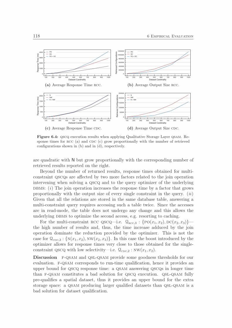
118 6 Empirical Evaluation
100 200 300 400 500 600 700 800 900 1000
Dataset Cardinality
0
1000
2000
3000
4000
Response T
ime (
ms)
PO
DC
PO + DC
(a) Average Response Time rcc.
100 200 300 400 500 600 700 800 900 1000
Dataset Cardinality
0
200000
400000
600000
800000
1000000
1200000
Retr
ieved C
onfigura
tions PO
DC
PO + DC
(b) Average Output Size rcc.
100 200 300 400 500 600 700 800 900 1000
Dataset Cardinality
0
500
1000
1500
2000
Response T
ime (
ms)
N
NW
N + NW
(c) Average Response Time cdc.
100 200 300 400 500 600 700 800 900 1000
Dataset Cardinality
0
50000
100000
150000
200000
250000
Retr
ieved C
onfigura
tions N
NW
N + NW
(d) Average Output Size cdc.
Figure 6.4: qscq execution results when applying Qualitative Storage Layer qsam. Re-sponse times for rcc (a) and cdc (c) grow proportionally with the number of retrievedconfigurations shown in (b) and in (d), respectively.
are quadratic with N but grow proportionally with the corresponding number ofretrieved results reported on the right.
Beyond the number of returned results, response times obtained for multi-constraint qscqs are affected by two more factors related to the join operationintervening when solving a qscq and to the query optimizer of the underlyingdbms: (i) The join operation increases the response time by a factor that growsproportionally with the output size of every single constraint in the query. (ii)Given that all the relations are stored in the same database table, answering amulti-constraint query requires accessing such a table twice. Since the accessesare in read-mode, the table does not undergo any change and this allows theunderlying dbms to optimize the second access, e.g. resorting to caching.
For the multi-constraint rcc qscq—i.e. Qrcc,3 : po(x1, x2),dc(x2, x3)—the high number of results and, thus, the time increase adduced by the joinoperation dominate the reduction provided by the optimizer. This is not thecase for Qcdc,3 : n(x1, x2),nw(x2, x3). In this case the boost introduced by theoptimizer allows for response times very close to those obtained for the single-constraint qscq with low selectivity—i.e. Qcdc,2 : nw(x1, x2).
Discussion f-qsam and qsl-qsam provide some goodness thresholds for ourevaluation. f-qsam corresponds to run-time qualification, hence it provides anupper bound for qscq response time: a qsam answering qscqs in longer timethan f-qsam constitutes a bad solution for qscq execution. qsl-qsam fullypre-qualifies a spatial dataset, thus it provides an upper bound for the extrastorage space: a qsam producing larger qualified datasets than qsl-qsam is abad solution for dataset qualification.
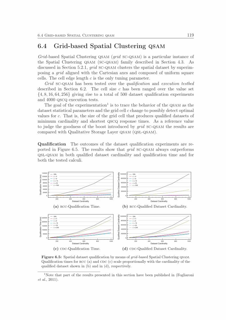
6.4 Grid-based Spatial Clustering qsam 119
6.4 Grid-based Spatial Clustering qsam
Grid -based Spatial Clustering qsam (grid sc-qsam) is a particular instance ofthe Spatial Clustering qsam (sc-qsam) family described in Section 4.3. Asdiscussed in Section 5.2.1, grid sc-qsam clusters the spatial dataset by superim-posing a grid aligned with the Cartesian axes and composed of uniform squarecells. The cell edge length c is the only tuning parameter.
Grid sc-qsam has been tested over the qualification and execution testbeddescribed in Section 6.2. The cell size c has been ranged over the value set4, 8, 16, 64, 256 giving rise to a total of 500 dataset qualification experimentsand 4000 qscq execution tests.
The goal of the experimentation1 is to trace the behavior of the qsam as thedataset statistical parameters and the grid cell c change to possibly detect optimalvalues for c. That is, the size of the grid cell that produces qualified datasets ofminimum cardinality and shortest qscq response times. As a reference valueto judge the goodness of the boost introduced by grid sc-qsam the results arecompared with Qualitative Storage Layer qsam (qsl-qsam).
Qualification The outcomes of the dataset qualification experiments are re-ported in Figure 6.5. The results show that grid sc-qsam always outperformsqsl-qsam in both qualified dataset cardinality and qualification time and forboth the tested calculi.
200 400 600 800 1000
Dataset Cardinality
0
20000
40000
60000
80000
100000
120000
140000
Qualifi
cation T
ime (
ms) QSL
c = 4
c = 8
c = 16
c = 64
c = 256
(a) rcc-Qualification Time.
200 400 600 800 1000
Dataset Cardinality
0
200000
400000
600000
800000
1000000
Qualifi
ed D
ata
set C
ard
inalit
y
QSL
c = 4
c = 8
c = 16
c = 64
c = 256
(b) rcc-Qualified Dataset Cardinality.
200 400 600 800 1000
Dataset Cardinality
0
50000
100000
150000
200000
250000
Qualifi
cation T
ime (
ms) QSL
c = 4
c = 8
c = 16
c = 64
c = 256
(c) cdc-Qualification Time.
200 400 600 800 1000
Dataset Cardinality
0
200000
400000
600000
800000
1000000
Qualifi
ed D
ata
set C
ard
inalit
y
QSL
c = 4
c = 8
c = 16
c = 64
c = 256
(d) cdc-Qualified Dataset Cardinality.
Figure 6.5: Spatial dataset qualification by means of grid -based Spatial Clustering qsam.Qualification times for rcc (a) and cdc (c) scale proportionally with the cardinality of thequalified dataset shown in (b) and in (d), respectively.
1Note that part of the results presented in this section have been published in (Fogliaroniet al., 2011).
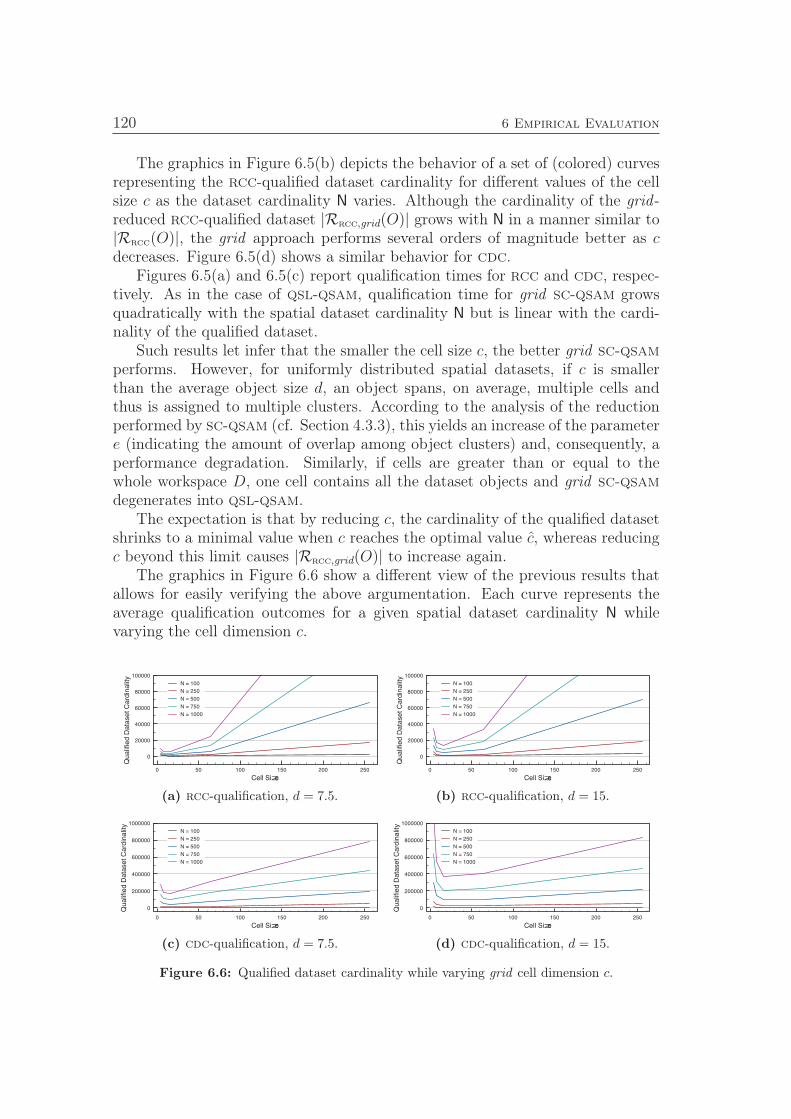
120 6 Empirical Evaluation
The graphics in Figure 6.5(b) depicts the behavior of a set of (colored) curvesrepresenting the rcc-qualified dataset cardinality for different values of the cellsize c as the dataset cardinality N varies. Although the cardinality of the grid -reduced rcc-qualified dataset |Rrcc,grid(O)| grows with N in a manner similar to|Rrcc(O)|, the grid approach performs several orders of magnitude better as cdecreases. Figure 6.5(d) shows a similar behavior for cdc.
Figures 6.5(a) and 6.5(c) report qualification times for rcc and cdc, respec-tively. As in the case of qsl-qsam, qualification time for grid sc-qsam growsquadratically with the spatial dataset cardinality N but is linear with the cardi-nality of the qualified dataset.
Such results let infer that the smaller the cell size c, the better grid sc-qsamperforms. However, for uniformly distributed spatial datasets, if c is smallerthan the average object size d, an object spans, on average, multiple cells andthus is assigned to multiple clusters. According to the analysis of the reductionperformed by sc-qsam (cf. Section 4.3.3), this yields an increase of the parametere (indicating the amount of overlap among object clusters) and, consequently, aperformance degradation. Similarly, if cells are greater than or equal to thewhole workspace D, one cell contains all the dataset objects and grid sc-qsamdegenerates into qsl-qsam.
The expectation is that by reducing c, the cardinality of the qualified datasetshrinks to a minimal value when c reaches the optimal value c, whereas reducingc beyond this limit causes |Rrcc,grid(O)| to increase again.
The graphics in Figure 6.6 show a different view of the previous results thatallows for easily verifying the above argumentation. Each curve represents theaverage qualification outcomes for a given spatial dataset cardinality N whilevarying the cell dimension c.
0 50 100 150 200 250
Cell Size
0
20000
40000
60000
80000
100000
Qualifi
ed D
ata
set C
ard
inalit
y
N = 100
N = 250
N = 500
N = 750
N = 1000
(a) rcc-qualification, d = 7.5.
0 50 100 150 200 250
Cell Size
0
20000
40000
60000
80000
100000
Qualifi
ed D
ata
set C
ard
inalit
y
N = 100
N = 250
N = 500
N = 750
N = 1000
(b) rcc-qualification, d = 15.
0 50 100 150 200 250
Cell Size
0
200000
400000
600000
800000
1000000
Qualifi
ed D
ata
set C
ard
inalit
y
N = 100
N = 250
N = 500
N = 750
N = 1000
(c) cdc-qualification, d = 7.5.
0 50 100 150 200 250
Cell Size
0
200000
400000
600000
800000
1000000
Qualifi
ed D
ata
set C
ard
inalit
y
N = 100
N = 250
N = 500
N = 750
N = 1000
(d) cdc-qualification, d = 15.
Figure 6.6: Qualified dataset cardinality while varying grid cell dimension c.
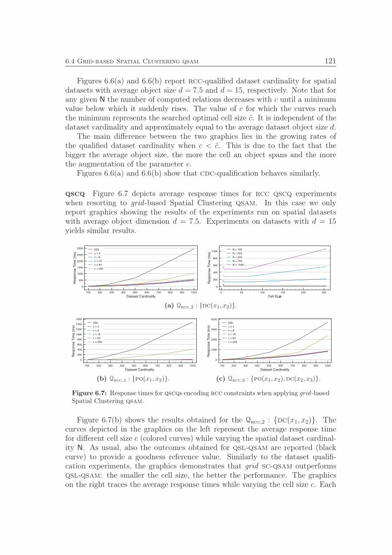
6.4 Grid-based Spatial Clustering qsam 121
Figures 6.6(a) and 6.6(b) report rcc-qualified dataset cardinality for spatialdatasets with average object size d = 7.5 and d = 15, respectively. Note that forany given N the number of computed relations decreases with c until a minimumvalue below which it suddenly rises. The value of c for which the curves reachthe minimum represents the searched optimal cell size c. It is independent of thedataset cardinality and approximately equal to the average dataset object size d.
The main difference between the two graphics lies in the growing rates ofthe qualified dataset cardinality when c < c. This is due to the fact that thebigger the average object size, the more the cell an object spans and the morethe augmentation of the parameter e.
Figures 6.6(a) and 6.6(b) show that cdc-qualification behaves similarly.
qscq Figure 6.7 depicts average response times for rcc qscq experimentswhen resorting to grid -based Spatial Clustering qsam. In this case we onlyreport graphics showing the results of the experiments run on spatial datasetswith average object dimension d = 7.5. Experiments on datasets with d = 15yields similar results.
100 200 300 400 500 600 700 800 900 1000
Dataset Cardinality
0
500
1000
1500
2000
2500
3000
Response T
ime (
ms)
QSL
c = 4
c = 8
c = 16
c = 64
c = 256
0 50 100 150 200 250
Cell Size
0
200
400
600
800
1000
Response T
ime (
ms)
N = 100
N = 250
N = 500
N = 750
N = 1000
(a) Qrcc,2 : dc(x1, x2).
100 200 300 400 500 600 700 800 900 1000
Dataset Cardinality
0
200
400
600
800
1000
1200
1400
1600
Response T
ime (
ms)
QSL
c = 4
c = 8
c = 16
c = 64
c = 256
(b) Qrcc,1 : po(x1, x2).
100 200 300 400 500 600 700 800 900 1000
Dataset Cardinality
0
1000
2000
3000
4000
Response T
ime (
ms)
QSL
c = 4
c = 8
c = 16
c = 64
c = 256
(c) Qrcc,3 : po(x1, x2),dc(x2, x3).
Figure 6.7: Response times for qscqs encoding rcc constraints when applying grid -basedSpatial Clustering qsam.
Figure 6.7(b) shows the results obtained for the Qrcc,2 : dc(x1, x2). Thecurves depicted in the graphics on the left represent the average response timefor different cell size c (colored curves) while varying the spatial dataset cardinal-ity N. As usual, also the outcomes obtained for qsl-qsam are reported (blackcurve) to provide a goodness reference value. Similarly to the dataset qualifi-cation experiments, the graphics demonstrates that grid sc-qsam outperformsqsl-qsam: the smaller the cell size, the better the performance. The graphicson the right traces the average response times while varying the cell size c. Each
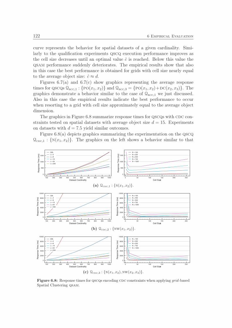
122 6 Empirical Evaluation
curve represents the behavior for spatial datasets of a given cardinality. Simi-larly to the qualification experiments qscq execution performance improves asthe cell size decreases until an optimal value c is reached. Below this value theqsam performance suddenly deteriorates. The empirical results show that alsoin this case the best performance is obtained for grids with cell size nearly equalto the average object size: c ≈ d.
Figures 6.7(a) and 6.7(c) show graphics representing the average responsetimes for qscqs Qrcc,1 : po(x1, x2) and Qrcc,3 = po(x1, x2)+dc(x2, x3). Thegraphics demonstrate a behavior similar to the case of Qrcc,1 we just discussed.Also in this case the empirical results indicate the best performance to occurwhen resorting to a grid with cell size approximately equal to the average objectdimension.
The graphics in Figure 6.8 summarize response times for qscqs with cdc con-straints tested on spatial datasets with average object size d = 15. Experimentson datasets with d = 7.5 yield similar outcomes.
Figure 6.8(a) depicts graphics summarizing the experimentation on the qscqQcdc,1 : n(x1, x2). The graphics on the left shows a behavior similar to that
100 200 300 400 500 600 700 800 900 1000
Dataset Cardinality
0
500
1000
1500
Response T
ime (
ms)
QSL
c = 4
c = 8
c = 16
c = 64
c = 256
0 50 100 150 200 250
Cell Size
0
500
1000
1500
Response T
ime (
ms)
N = 100
N = 250
N = 500
N = 750
N = 1000
(a) Qcdc,1 : n(x1, x2).
100 200 300 400 500 600 700 800 900 1000
Dataset Cardinality
0
2000
4000
6000
8000
10000
Response T
ime (
ms)
QSL
c = 4
c = 8
c = 16
c = 64
c = 256
0 50 100 150 200 250
Cell Size
0
2000
4000
6000
8000
10000
Response T
ime (
ms)
N = 100
N = 250
N = 500
N = 750
N = 1000
(b) Qcdc,2 : nw(x1, x2).
100 200 300 400 500 600 700 800 900 1000
Dataset Cardinality
0
2000
4000
6000
8000
10000
Response T
ime (
ms)
QSL
c = 4
c = 8
c = 16
c = 64
c = 256
0 50 100 150 200 250
Cell Size
0
2000
4000
6000
8000
10000
Response T
ime (
ms)
N = 100
N = 250
N = 500
N = 750
N = 1000
(c) Qcdc,3 : n(x1, x2),nw(x2, x3).
Figure 6.8: Response times for qscqs encoding cdc constraints when applying grid -basedSpatial Clustering qsam.
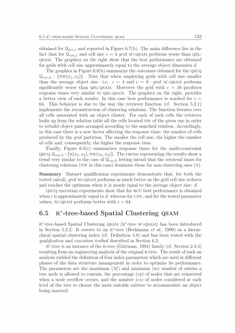
6.5 r∗-tree-based Spatial Clustering qsam 123
obtained for Qrcc,1 and reported in Figure 6.7(b). The main difference lies in thefact that for Qcdc,1 and cell size c = 4 grid sc-qsam performs worse than qsl-qsam. The graphics on the right show that the best performance are obtainedfor grids with cell size approximately equal to the average object dimension d.
The graphics in Figure 6.8(b) summarize the outcomes obtained for the qscqQcdc,2 : nw(x1, x2). Note that when employing grids with cell size smallerthan the average object size—i.e. c = 4 and c = 8—grid sc-qsam performssignificantly worse than qsl-qsam. Moreover the grid with c = 16 producesresponse times very similar to qsl-qsam. The graphics on the right, providesa better view of such results: In this case best performance is reached for c =64. This behavior is due to the way the retriever function (cf. Section 5.2.1)implements the reconstruction of clustering relations: The function iterates overall cells associated with an object cluster. For each of such cells the retrieverlooks up from the relation table all the cells located nw of the given one in orderto rebuild object pairs arranged according to the searched relation. Accordingly,in this case there is a new factor affecting the response time: the number of cellsproduced by the grid partition. The smaller the cell size, the higher the numberof cells and, consequently, the higher the response time.
Finally, Figure 6.8(c) summarizes response times for the multi-constraintqscq Qcdc,3 : n(x1, x2),nw(x2, x3). The curves representing the results show atrend very similar to the case of Qcdc,2 letting intend that the retrieval times forclustering relations (nw in this case) dominate those for non-clustering ones (n).
Summary Dataset qualification experiments demonstrate that, for both thetested calculi, grid sc-qsam performs as much better as the grid cell size reducesand reaches the optimum when it is nearly equal to the average object size: d.
qscq execution experiments show that for rcc best performance is obtainedwhen c is approximately equal to d, whereas for cdc, and for the tested parametervalues, sc-qsam performs better with c = 64.
6.5 r∗-tree-based Spatial Clustering qsam
r∗-tree-based Spatial Clustering qsam (r∗-tree sc-qsam) has been introducedin Section 5.2.2. It resorts to an r∗-tree (Beckmann et al., 1990) as a hierar-chical spatial clustering index (cf. Definition 4.8) and has been tested with thequalification and execution testbed described in Section 6.2.
r∗-tree is an instance of the r-tree (Guttman, 1984) family (cf. Section 2.3.4)resulting from an engineering analysis of the original r-tree. The result of such ananalysis yielded the definition of four index parameters which are used in differentphases of the data structure management in order to optimize its performance.The parameters are the maximum (M) and minimum (m) number of entries atree node is allowed to contain, the percentage (rp) of nodes that are reinsertedwhen a node overflow occurs, and the number (cs) of nodes considered at eachlevel of the tree to choose the most suitable subtree to accommodate an objectbeing inserted.
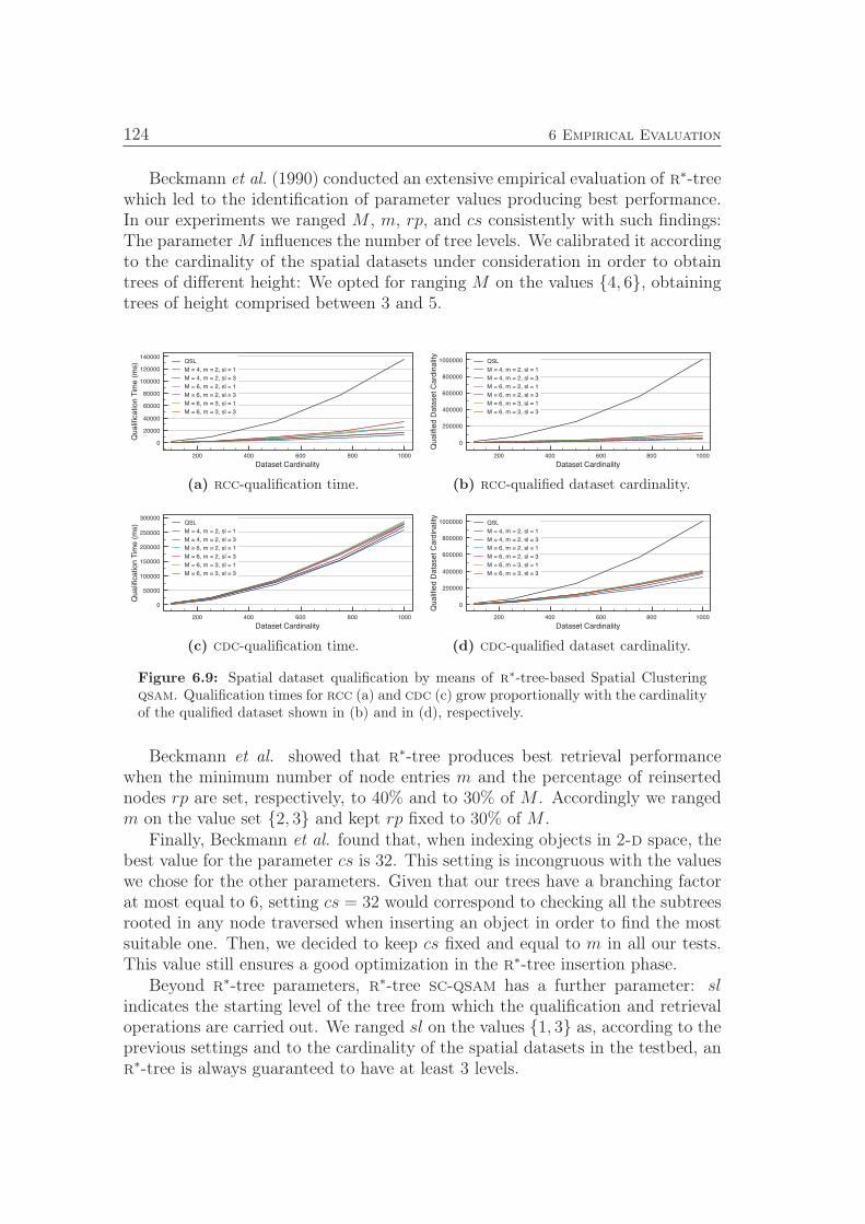
124 6 Empirical Evaluation
Beckmann et al. (1990) conducted an extensive empirical evaluation of r∗-treewhich led to the identification of parameter values producing best performance.In our experiments we ranged M , m, rp, and cs consistently with such findings:The parameter M influences the number of tree levels. We calibrated it accordingto the cardinality of the spatial datasets under consideration in order to obtaintrees of different height: We opted for ranging M on the values 4, 6, obtainingtrees of height comprised between 3 and 5.
200 400 600 800 1000
Dataset Cardinality
0
20000
40000
60000
80000
100000
120000
140000
Qualifi
cation T
ime (
ms) QSL
M = 4, m = 2, sl = 1
M = 4, m = 2, sl = 3
M = 6, m = 2, sl = 1
M = 6, m = 2, sl = 3
M = 6, m = 3, sl = 1
M = 6, m = 3, sl = 3
(a) rcc-qualification time.
200 400 600 800 1000
Dataset Cardinality
0
200000
400000
600000
800000
1000000
Qualifi
ed D
ata
set C
ard
inalit
y
QSL
M = 4, m = 2, sl = 1
M = 4, m = 2, sl = 3
M = 6, m = 2, sl = 1
M = 6, m = 2, sl = 3
M = 6, m = 3, sl = 1
M = 6, m = 3, sl = 3
(b) rcc-qualified dataset cardinality.
200 400 600 800 1000
Dataset Cardinality
0
50000
100000
150000
200000
250000
300000
Qualifi
cation T
ime (
ms) QSL
M = 4, m = 2, sl = 1
M = 4, m = 2, sl = 3
M = 6, m = 2, sl = 1
M = 6, m = 2, sl = 3
M = 6, m = 3, sl = 1
M = 6, m = 3, sl = 3
(c) cdc-qualification time.
200 400 600 800 1000
Dataset Cardinality
0
200000
400000
600000
800000
1000000
Qualifi
ed D
ata
set C
ard
inalit
y
QSL
M = 4, m = 2, sl = 1
M = 4, m = 2, sl = 3
M = 6, m = 2, sl = 1
M = 6, m = 2, sl = 3
M = 6, m = 3, sl = 1
M = 6, m = 3, sl = 3
(d) cdc-qualified dataset cardinality.
Figure 6.9: Spatial dataset qualification by means of r∗-tree-based Spatial Clusteringqsam. Qualification times for rcc (a) and cdc (c) grow proportionally with the cardinalityof the qualified dataset shown in (b) and in (d), respectively.
Beckmann et al. showed that r∗-tree produces best retrieval performancewhen the minimum number of node entries m and the percentage of reinsertednodes rp are set, respectively, to 40% and to 30% of M . Accordingly we rangedm on the value set 2, 3 and kept rp fixed to 30% of M .
Finally, Beckmann et al. found that, when indexing objects in 2-d space, thebest value for the parameter cs is 32. This setting is incongruous with the valueswe chose for the other parameters. Given that our trees have a branching factorat most equal to 6, setting cs = 32 would correspond to checking all the subtreesrooted in any node traversed when inserting an object in order to find the mostsuitable one. Then, we decided to keep cs fixed and equal to m in all our tests.This value still ensures a good optimization in the r∗-tree insertion phase.
Beyond r∗-tree parameters, r∗-tree sc-qsam has a further parameter: slindicates the starting level of the tree from which the qualification and retrievaloperations are carried out. We ranged sl on the values 1, 3 as, according to theprevious settings and to the cardinality of the spatial datasets in the testbed, anr∗-tree is always guaranteed to have at least 3 levels.
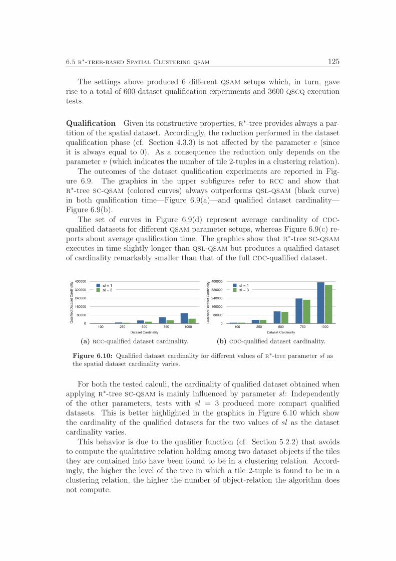
6.5 r∗-tree-based Spatial Clustering qsam 125
The settings above produced 6 different qsam setups which, in turn, gaverise to a total of 600 dataset qualification experiments and 3600 qscq executiontests.
Qualification Given its constructive properties, r∗-tree provides always a par-tition of the spatial dataset. Accordingly, the reduction performed in the datasetqualification phase (cf. Section 4.3.3) is not affected by the parameter e (sinceit is always equal to 0). As a consequence the reduction only depends on theparameter v (which indicates the number of tile 2-tuples in a clustering relation).
The outcomes of the dataset qualification experiments are reported in Fig-ure 6.9. The graphics in the upper subfigures refer to rcc and show thatr∗-tree sc-qsam (colored curves) always outperforms qsl-qsam (black curve)in both qualification time—Figure 6.9(a)—and qualified dataset cardinality—Figure 6.9(b).
The set of curves in Figure 6.9(d) represent average cardinality of cdc-qualified datasets for different qsam parameter setups, whereas Figure 6.9(c) re-ports about average qualification time. The graphics show that r∗-tree sc-qsamexecutes in time slightly longer than qsl-qsam but produces a qualified datasetof cardinality remarkably smaller than that of the full cdc-qualified dataset.
0
80000
160000
240000
320000
400000
100 250 500 750 1000
Qualif
ied
Data
set
Card
inalit
y
Dataset Cardinality
sl = 1sl = 3
(a) rcc-qualified dataset cardinality.
0
80000
160000
240000
320000
400000
100 250 500 750 1000
Qualif
ied
Data
set
Card
inalit
y
Dataset Cardinality
sl = 1sl = 3
(b) cdc-qualified dataset cardinality.
Figure 6.10: Qualified dataset cardinality for different values of r∗-tree parameter sl asthe spatial dataset cardinality varies.
For both the tested calculi, the cardinality of qualified dataset obtained whenapplying r∗-tree sc-qsam is mainly influenced by parameter sl: Independentlyof the other parameters, tests with sl = 3 produced more compact qualifieddatasets. This is better highlighted in the graphics in Figure 6.10 which showthe cardinality of the qualified datasets for the two values of sl as the datasetcardinality varies.
This behavior is due to the qualifier function (cf. Section 5.2.2) that avoidsto compute the qualitative relation holding among two dataset objects if the tilesthey are contained into have been found to be in a clustering relation. Accord-ingly, the higher the level of the tree in which a tile 2-tuple is found to be in aclustering relation, the higher the number of object-relation the algorithm doesnot compute.
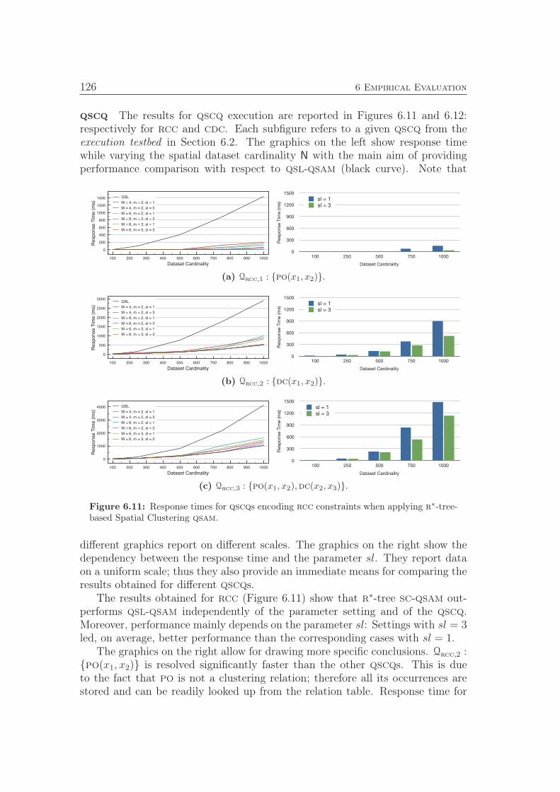
126 6 Empirical Evaluation
qscq The results for qscq execution are reported in Figures 6.11 and 6.12:respectively for rcc and cdc. Each subfigure refers to a given qscq from theexecution testbed in Section 6.2. The graphics on the left show response timewhile varying the spatial dataset cardinality N with the main aim of providingperformance comparison with respect to qsl-qsam (black curve). Note that
100 200 300 400 500 600 700 800 900 1000
Dataset Cardinality
0
200
400
600
800
1000
1200
1400
Response T
ime (
ms)
QSL
M = 4, m = 2, sl = 1
M = 4, m = 2, sl = 3
M = 6, m = 2, sl = 1
M = 6, m = 2, sl = 3
M = 6, m = 3, sl = 1
M = 6, m = 3, sl = 3
0
300
600
900
1200
1500
100 250 500 750 1000
Resp
on
se T
ime (m
s)
Dataset Cardinality
sl = 1sl = 3
(a) Qrcc,1 : po(x1, x2).
100 200 300 400 500 600 700 800 900 1000
Dataset Cardinality
0
500
1000
1500
2000
2500
3000
Response T
ime (
ms)
QSL
M = 4, m = 2, sl = 1
M = 4, m = 2, sl = 3
M = 6, m = 2, sl = 1
M = 6, m = 2, sl = 3
M = 6, m = 3, sl = 1
M = 6, m = 3, sl = 3
0
300
600
900
1200
1500
100 250 500 750 1000
Resp
on
se T
ime (m
s)
Dataset Cardinality
sl = 1sl = 3
(b) Qrcc,2 : dc(x1, x2).
100 200 300 400 500 600 700 800 900 1000
Dataset Cardinality
0
1000
2000
3000
4000
Response T
ime (
ms)
QSL
M = 4, m = 2, sl = 1
M = 4, m = 2, sl = 3
M = 6, m = 2, sl = 1
M = 6, m = 2, sl = 3
M = 6, m = 3, sl = 1
M = 6, m = 3, sl = 3
0
300
600
900
1200
1500
100 250 500 750 1000
Resp
onse T
ime (m
s)
Dataset Cardinality
sl = 1sl = 3
(c) Qrcc,3 : po(x1, x2),dc(x2, x3).
Figure 6.11: Response times for qscqs encoding rcc constraints when applying r∗-tree-based Spatial Clustering qsam.
different graphics report on different scales. The graphics on the right show thedependency between the response time and the parameter sl. They report dataon a uniform scale; thus they also provide an immediate means for comparing theresults obtained for different qscqs.
The results obtained for rcc (Figure 6.11) show that r∗-tree sc-qsam out-performs qsl-qsam independently of the parameter setting and of the qscq.Moreover, performance mainly depends on the parameter sl: Settings with sl = 3led, on average, better performance than the corresponding cases with sl = 1.
The graphics on the right allow for drawing more specific conclusions. Qrcc,2 :po(x1, x2) is resolved significantly faster than the other qscqs. This is dueto the fact that po is not a clustering relation; therefore all its occurrences arestored and can be readily looked up from the relation table. Response time for
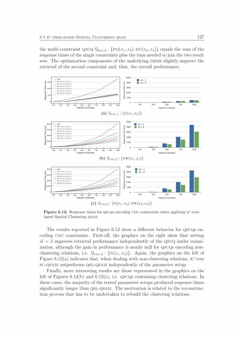
6.5 r∗-tree-based Spatial Clustering qsam 127
the multi-constraint qscq Qrcc,3 : po(x1, x2),dc(x2, x3) equals the sum of theresponse times of the single constraints plus the time needed to join the two resultsets. The optimization components of the underlying dbms slightly improve theretrieval of the second constraint and, thus, the overall performance.
100 200 300 400 500 600 700 800 900 1000
Dataset Cardinality
0
500
1000
1500
Response T
ime (
ms)
QSL
M = 4, m = 2, sl = 1
M = 4, m = 2, sl = 3
M = 6, m = 2, sl = 1
M = 6, m = 2, sl = 3
M = 6, m = 3, sl = 1
M = 6, m = 3, sl = 3
0
1200
2400
3600
4800
6000
100 250 500 750 1000
Resp
on
se T
ime (m
s)
Dataset Cardinality
sl = 1sl = 3
(a) Qcdc,1 : n(x1, x2).
100 200 300 400 500 600 700 800 900 1000
Dataset Cardinality
0
2000
4000
6000
8000
Response T
ime (
ms)
QSL
M = 4, m = 2, sl = 1
M = 4, m = 2, sl = 3
M = 6, m = 2, sl = 1
M = 6, m = 2, sl = 3
M = 6, m = 3, sl = 1
M = 6, m = 3, sl = 3
0
1200
2400
3600
4800
6000
100 250 500 750 1000
Resp
onse T
ime (m
s)
Dataset Cardinality
sl = 1sl = 3
(b) Qcdc,2 : nw(x1, x2).
100 200 300 400 500 600 700 800 900 1000
Dataset Cardinality
0
2000
4000
6000
8000
Response T
ime (
ms)
QSL
M = 4, m = 2, sl = 1
M = 4, m = 2, sl = 3
M = 6, m = 2, sl = 1
M = 6, m = 2, sl = 3
M = 6, m = 3, sl = 1
M = 6, m = 3, sl = 3
0
1200
2400
3600
4800
6000
100 250 500 750 1000
Resp
onse T
ime (m
s)
Dataset Cardinality
sl = 1sl = 3
(c) Qcdc,3 : n(x1, x2),nw(x2, x3).
Figure 6.12: Response times for qscqs encoding cdc constraints when applying r∗-tree-based Spatial Clustering qsam.
The results reported in Figure 6.12 show a different behavior for qscqs en-coding cdc constraints. First-off, the graphics on the right show that settingsl = 3 improves retrieval performance independently of the qscq under exami-nation, although the gain in performance is nearly null for qscqs encoding non-clustering relations, i.e. Qcdc,2 : n(x1, x2). Again, the graphics on the left ofFigure 6.12(a) indicates that, when dealing with non-clustering relations, r∗-treesc-qsam outperforms qsl-qsam independently of the parameter setup.
Finally, more interesting results are those represented in the graphics on theleft of Figures 6.12(b) and 6.12(c), i.e. qscqs containing clustering relations. Inthese cases, the majority of the tested parameter setups produced response timessignificantly longer than qsl-qsam. The motivation is related to the reconstruc-tion process that has to be undertaken to rebuild the clustering relations.
128 6 Empirical Evaluation
Best performance is obtained for parameter setups with having M = 6 andsl = 3. This behavior is probably due to the parameter M : Allowing for a highernumber of entries in each tree node yields an r∗-tree with a smaller number oflevels and tiles. Consequently the retriever function performs a reduced numberof loops in the reconstruction phase.
Summary Dataset qualification experiments demonstrate that, for both thetested calculi, r∗-tree sc-qsam performs as much better as the parameter slis higher. In our tests best results have been obtained for sl = 3. The otherparameters do not affect the performance significantly. Note, however, that r∗-tree sc-qsam performs cdc-qualification in time slightly longer than qsl-qsam,obtaining more compact qualified datasets though.
qscq execution experiments showed that the best performance is obtainedfor sl = 3. For queries encoding rcc constraints r∗-tree sc-qsam always outper-forms qsl-qsam, independently of the other parameters.
For queries encoding cdc spatial clustering relations best performance is ob-tained with parameter setups with M = 6.
6.6 qsr-based qsam
qsr-based qsam (qsr-qsam) has been introduced in Section 4.4. It is groundedin a novel data structure named inference graph (cf. Section 4.4.1) that aimsat highlighting the inference patterns existing among the qualitative relationsholding on a spatial dataset O. Each node of an inference graph IG representsa relation in the qualified dataset RP(O) where P is the pool of calculi underconsideration. A hyperarc a in IG is called inference path; it always originatesin a set of nodes T (the tail of the path) and heads to one node h (the headof the path). An inference path of length l represents a series of l reasoningoperations that have to be undertaken to infer h from T . An inference pathis an instantiation of an inference template which, in turn, is generated fromthe reasoning tables (cf. Section 2.2.3) of the calculus under consideration. Aninference graph of length l does not contain inference paths longer than l.
The length l of the inference path is the only parameter of qsr-qsam andis bounded above by the number of base relations in the calculus. Generatingan inference graph of length l for a calculus M requires to check every inferencetemplate of length smaller or equal to l against the relations of the full qualifieddataset RM(O).
To build the inference templates we implemented a template generator. Forrcc the generation of inference templates of any length from the reasoning tablesreported in Table 4.3 took approximately 5 seconds. The number of generatedtemplates as the length l varies is reported in Table 4.5.
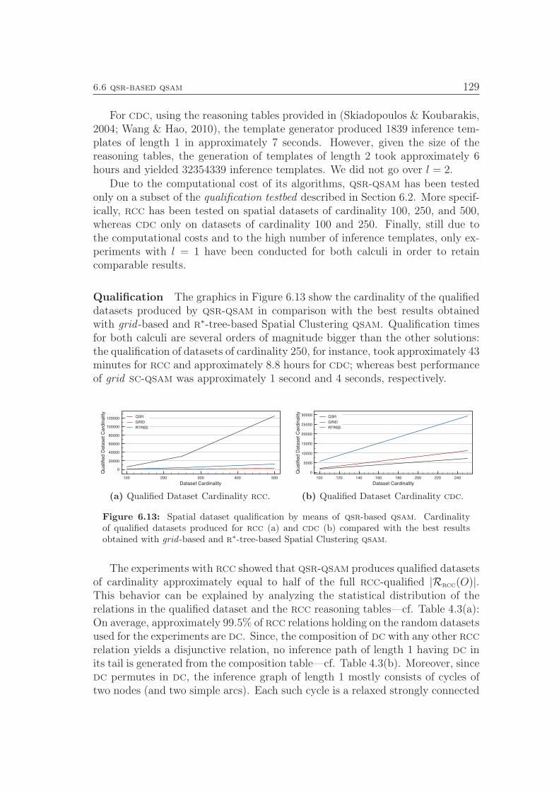
6.6 qsr-based qsam 129
For cdc, using the reasoning tables provided in (Skiadopoulos & Koubarakis,2004; Wang & Hao, 2010), the template generator produced 1839 inference tem-plates of length 1 in approximately 7 seconds. However, given the size of thereasoning tables, the generation of templates of length 2 took approximately 6hours and yielded 32354339 inference templates. We did not go over l = 2.
Due to the computational cost of its algorithms, qsr-qsam has been testedonly on a subset of the qualification testbed described in Section 6.2. More specif-ically, rcc has been tested on spatial datasets of cardinality 100, 250, and 500,whereas cdc only on datasets of cardinality 100 and 250. Finally, still due tothe computational costs and to the high number of inference templates, only ex-periments with l = 1 have been conducted for both calculi in order to retaincomparable results.
Qualification The graphics in Figure 6.13 show the cardinality of the qualifieddatasets produced by qsr-qsam in comparison with the best results obtainedwith grid -based and r∗-tree-based Spatial Clustering qsam. Qualification timesfor both calculi are several orders of magnitude bigger than the other solutions:the qualification of datasets of cardinality 250, for instance, took approximately 43minutes for rcc and approximately 8.8 hours for cdc; whereas best performanceof grid sc-qsam was approximately 1 second and 4 seconds, respectively.
100 200 300 400 500
Dataset Cardinality
0
20000
40000
60000
80000
100000
120000
Qualifi
ed D
ata
set C
ard
inalit
y
QSR
GRID
RTREE
(a) Qualified Dataset Cardinality rcc.
100 120 140 160 180 200 220 240
Dataset Cardinality
0
5000
10000
15000
20000
25000
30000
Qualifi
ed D
ata
set C
ard
inalit
y
QSR
GRID
RTREE
(b) Qualified Dataset Cardinality cdc.
Figure 6.13: Spatial dataset qualification by means of qsr-based qsam. Cardinalityof qualified datasets produced for rcc (a) and cdc (b) compared with the best resultsobtained with grid -based and r∗-tree-based Spatial Clustering qsam.
The experiments with rcc showed that qsr-qsam produces qualified datasetsof cardinality approximately equal to half of the full rcc-qualified |Rrcc(O)|.This behavior can be explained by analyzing the statistical distribution of therelations in the qualified dataset and the rcc reasoning tables—cf. Table 4.3(a):On average, approximately 99.5% of rcc relations holding on the random datasetsused for the experiments are dc. Since, the composition of dc with any other rccrelation yields a disjunctive relation, no inference path of length 1 having dc inits tail is generated from the composition table—cf. Table 4.3(b). Moreover, sincedc permutes in dc, the inference graph of length 1 mostly consists of cycles oftwo nodes (and two simple arcs). Each such cycle is a relaxed strongly connected
130 6 Empirical Evaluation
component (cf. Definition 4.11) having only one source node that is the onestored by the qualification procedure.
The graphics in Figure 6.13(a) shows that both grid r∗-tree sc-qsam andr∗-tree sc-qsam outperform qsr-qsam by producing rcc-qualified datasets ofcardinalities much smaller than those generated by qsr-qsam.
The experiments run on cdc show a completely different behavior: the graph-ics in Figure 6.13(b) indicates that qsr-qsam produces very compact cdc-qualified datasets, outperforming both grid r∗-tree sc-qsam and r∗-tree sc-qsam. Again this is due to the statistical distribution of the relations in thequalified dataset and to the cdc reasoning tables (cf. Skiadopoulos & Koubarakis,2004; Wang & Hao, 2010): The datasets used in the experiments gave rise to awell-variegated set of cdc relations and the constitution of the reasoning tablesallow for producing an inference graph with a complex hyperarc structure. This,in turn, allowed for identifying strongly connected components consisting of sev-eral nodes, eventually yielding a higher reduction of the qualified datasets.
qscq The retriever function for qsr-qsam has been implemented as follows:First it applies algebraic closure algorithm (cf. Section 2.2.5) to rebuild the fullqualified dataset which is stored in the relation tables and queried via the retrieverfunction of qsl-qsam. Note that in case of multi-constraint qscqs, given thecomputational cost of algebraic closure algorithm, the reconstruction is executedonly when resolving the first constraint.
The results of the experiments showed that in the retrieval phase qsr-qsamperforms largely worse than all the other discussed solutions, f-qsam included.On spatial datasets of cardinality N = 250, for instance, all the qscqs in thetestbed encoding rcc constraints have been resolved in approximately 1 minute,against the nearly 7 seconds taken by f-qsam. cdc performed even worse: all ofthe cdc qscqs in the testbed have been answered in approximately 1 hour.
The huge time difference occurring between rcc and cdc is mainly relatedto the different number of base relations provided by the two models (8 vs 218)and thus to the size of the reasoning tables that are used in the algebraic closureto perform the reasoning.
These results yield the main conclusion that a plain application of qsr-qsamon a full spatial dataset is definitely unsuitable in terms of query response times.
Summary Dataset qualification experiments showed that for rcc qsr-qsamproduces reduced qualified datasets of cardinality approximately equal to halfof the cardinality of a full qualified dataset. For cdc the reduction was muchgreater. The obtained qualified datasets are extremely compact, outperformingall the qsams presented before. However, the qualification time is extremelyhigh, making this qsam unsuited for being used on complete datasets.
qscq execution experiments showed that for both calculi the retrieval timeis definitely too high. This is due to the high computational cost of algebraicclosure algorithm. However it has to be considered that in this work we tested
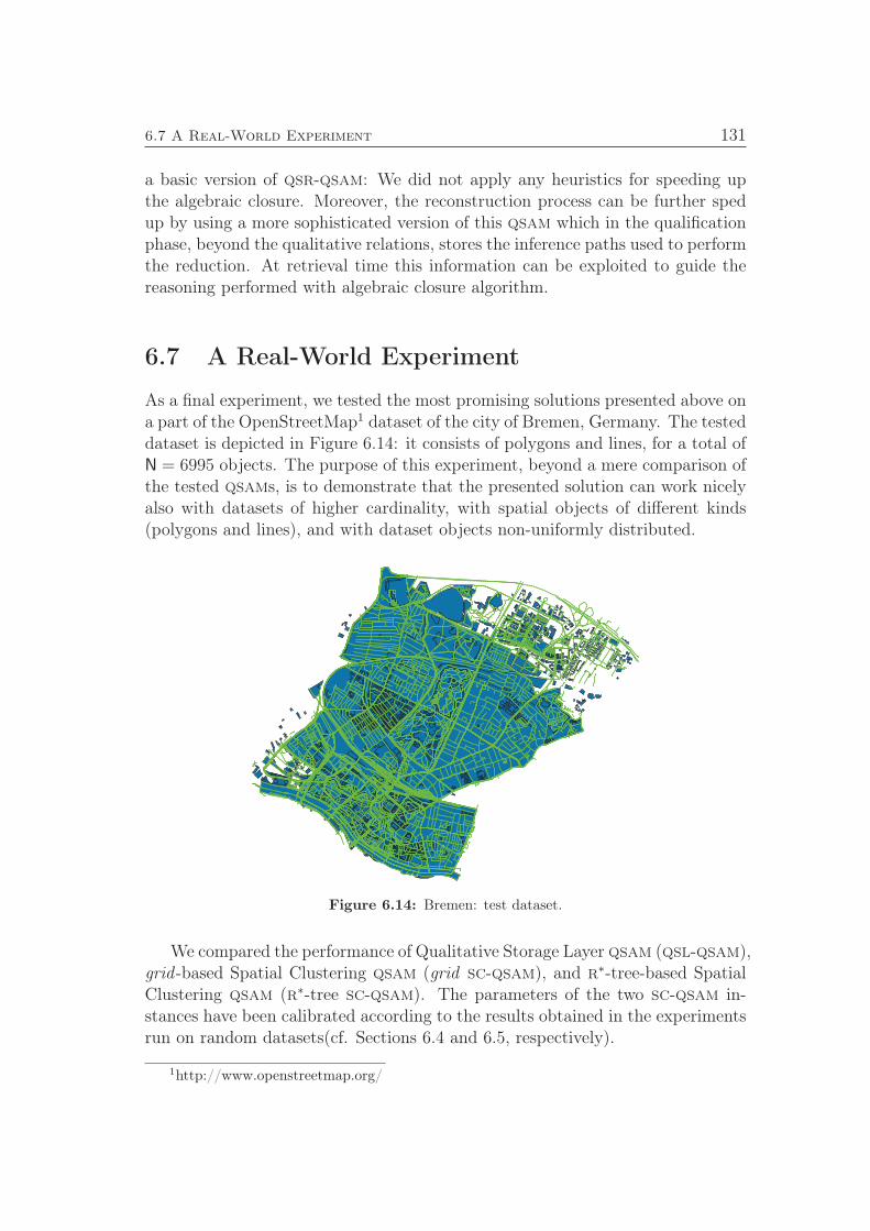
6.7 A Real-World Experiment 131
a basic version of qsr-qsam: We did not apply any heuristics for speeding upthe algebraic closure. Moreover, the reconstruction process can be further spedup by using a more sophisticated version of this qsam which in the qualificationphase, beyond the qualitative relations, stores the inference paths used to performthe reduction. At retrieval time this information can be exploited to guide thereasoning performed with algebraic closure algorithm.
6.7 A Real-World Experiment
As a final experiment, we tested the most promising solutions presented above ona part of the OpenStreetMap1 dataset of the city of Bremen, Germany. The testeddataset is depicted in Figure 6.14: it consists of polygons and lines, for a total ofN = 6995 objects. The purpose of this experiment, beyond a mere comparison ofthe tested qsams, is to demonstrate that the presented solution can work nicelyalso with datasets of higher cardinality, with spatial objects of different kinds(polygons and lines), and with dataset objects non-uniformly distributed.
Figure 6.14: Bremen: test dataset.
We compared the performance of Qualitative Storage Layer qsam (qsl-qsam),grid -based Spatial Clustering qsam (grid sc-qsam), and r∗-tree-based SpatialClustering qsam (r∗-tree sc-qsam). The parameters of the two sc-qsam in-stances have been calibrated according to the results obtained in the experimentsrun on random datasets(cf. Sections 6.4 and 6.5, respectively).
1http://www.openstreetmap.org/
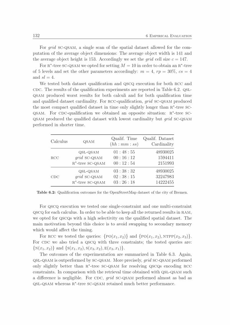
132 6 Empirical Evaluation
For grid sc-qsam, a single scan of the spatial dataset allowed for the com-
putation of the average object dimensions: The average object width is 141 and
the average object height is 153. Accordingly we set the grid cell size c = 147.
For r∗-tree sc-qsam we opted for settingM = 10 in order to obtain an r∗-tree
of 5 levels and set the other parameters accordingly: m = 4, rp = 30%, cs = 4
and sl = 4.
We tested both dataset qualification and qscq execution for both rcc and
cdc. The results of the qualification experiments are reported in Table 6.2. qsl-
qsam produced worst results for both calculi and for both qualification time
and qualified dataset cardinality. For rcc-qualification, grid sc-qsam produced
the most compact qualified dataset in time only slightly longer than r∗-tree sc-
qsam. For cdc-qualification we obtained an opposite situation: r∗-tree sc-
qsam produced the qualified dataset with lowest cardinality but grid sc-qsam
performed in shorter time.
Calculus qsamQualif. Time(hh : mm : ss)
Qualif. DatasetCardinality
rccqsl-qsam 01 : 48 : 55 48930025
grid sc-qsam 00 : 16 : 12 1594411r∗-tree sc-qsam 00 : 12 : 54 2151993
cdcqsl-qsam 03 : 38 : 32 48930025
grid sc-qsam 02 : 38 : 15 32247983r∗-tree sc-qsam 03 : 26 : 18 14222455
Table 6.2: Qualification outcomes for the OpenStreetMap dataset of the city of Bremen.
For qscq execution we tested one single-constraint and one multi-constraint
qscq for each calculus. In order to be able to keep all the returned results in ram,
we opted for qscqs with a high selectivity on the qualified spatial dataset. The
main motivation beyond this choice is to avoid swapping to secondary memory
which would affect the timing.
For rcc we tested the queries: po(x1, x2) and po(x1, x2),ntpp(x2, x3).For cdc we also tried a qscq with three constraints; the tested queries are:
n(x1, x2) and s(x1, x2), s(x3, x2),e(x3, x1).
The outcomes of the experimentation are summarized in Table 6.3. Again,
qsl-qsam is outperformed by sc-qsam. More precisely, grid sc-qsam performed
only slightly better than r∗-tree sc-qsam for resolving qscqs encoding rcc
constraints. In comparison with the retrieval time obtained with qsl-qsam such
a difference is negligible. For cdc, grid sc-qsam performed almost as bad as
qsl-qsam whereas r∗-tree sc-qsam retained much better performance.
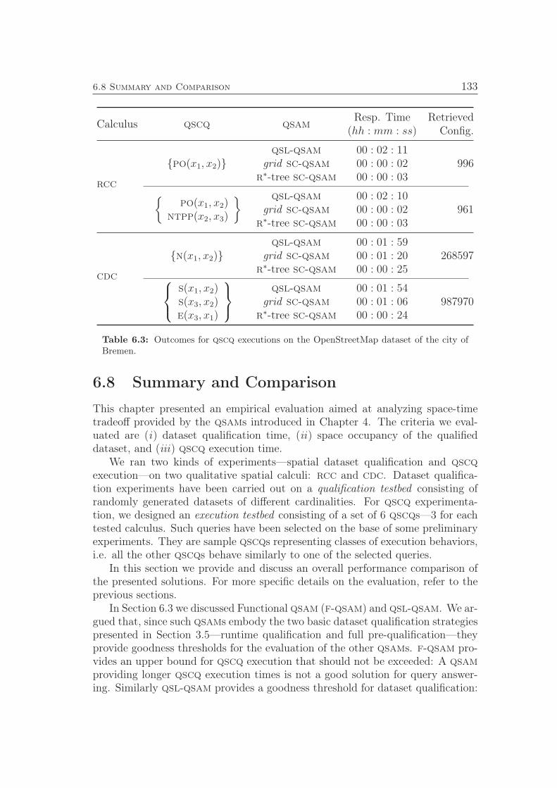
6.8 Summary and Comparison 133
Calculus qscq qsamResp. Time
(hh : mm : ss)Retrieved
Config.
rcc
po(x1, x2)qsl-qsam 00 : 02 : 11
996grid sc-qsam 00 : 00 : 02r∗-tree sc-qsam 00 : 00 : 03
po(x1, x2)
ntpp(x2, x3)
qsl-qsam 00 : 02 : 10961grid sc-qsam 00 : 00 : 02
r∗-tree sc-qsam 00 : 00 : 03
cdc
n(x1, x2)qsl-qsam 00 : 01 : 59
268597grid sc-qsam 00 : 01 : 20r∗-tree sc-qsam 00 : 00 : 25
s(x1, x2)s(x3, x2)e(x3, x1)
qsl-qsam 00 : 01 : 54987970grid sc-qsam 00 : 01 : 06
r∗-tree sc-qsam 00 : 00 : 24
Table 6.3: Outcomes for qscq executions on the OpenStreetMap dataset of the city ofBremen.
6.8 Summary and Comparison
This chapter presented an empirical evaluation aimed at analyzing space-timetradeoff provided by the qsams introduced in Chapter 4. The criteria we eval-uated are (i) dataset qualification time, (ii) space occupancy of the qualifieddataset, and (iii) qscq execution time.
We ran two kinds of experiments—spatial dataset qualification and qscqexecution—on two qualitative spatial calculi: rcc and cdc. Dataset qualifica-tion experiments have been carried out on a qualification testbed consisting ofrandomly generated datasets of different cardinalities. For qscq experimenta-tion, we designed an execution testbed consisting of a set of 6 qscqs—3 for eachtested calculus. Such queries have been selected on the base of some preliminaryexperiments. They are sample qscqs representing classes of execution behaviors,i.e. all the other qscqs behave similarly to one of the selected queries.
In this section we provide and discuss an overall performance comparison ofthe presented solutions. For more specific details on the evaluation, refer to theprevious sections.
In Section 6.3 we discussed Functional qsam (f-qsam) and qsl-qsam. We ar-gued that, since such qsams embody the two basic dataset qualification strategiespresented in Section 3.5—runtime qualification and full pre-qualification—theyprovide goodness thresholds for the evaluation of the other qsams. f-qsam pro-vides an upper bound for qscq execution that should not be exceeded: A qsamproviding longer qscq execution times is not a good solution for query answer-ing. Similarly qsl-qsam provides a goodness threshold for dataset qualification:
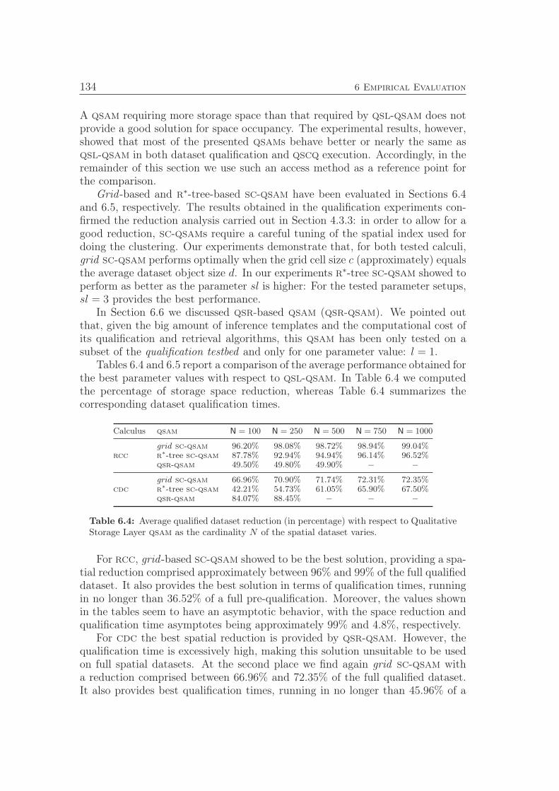
134 6 Empirical Evaluation
A qsam requiring more storage space than that required by qsl-qsam does notprovide a good solution for space occupancy. The experimental results, however,showed that most of the presented qsams behave better or nearly the same asqsl-qsam in both dataset qualification and qscq execution. Accordingly, in theremainder of this section we use such an access method as a reference point forthe comparison.
Grid -based and r∗-tree-based sc-qsam have been evaluated in Sections 6.4and 6.5, respectively. The results obtained in the qualification experiments con-firmed the reduction analysis carried out in Section 4.3.3: in order to allow for agood reduction, sc-qsams require a careful tuning of the spatial index used fordoing the clustering. Our experiments demonstrate that, for both tested calculi,grid sc-qsam performs optimally when the grid cell size c (approximately) equalsthe average dataset object size d. In our experiments r∗-tree sc-qsam showed toperform as better as the parameter sl is higher: For the tested parameter setups,sl = 3 provides the best performance.
In Section 6.6 we discussed qsr-based qsam (qsr-qsam). We pointed outthat, given the big amount of inference templates and the computational cost ofits qualification and retrieval algorithms, this qsam has been only tested on asubset of the qualification testbed and only for one parameter value: l = 1.
Tables 6.4 and 6.5 report a comparison of the average performance obtained forthe best parameter values with respect to qsl-qsam. In Table 6.4 we computedthe percentage of storage space reduction, whereas Table 6.4 summarizes thecorresponding dataset qualification times.
Calculus qsam N = 100 N = 250 N = 500 N = 750 N = 1000
rcc
grid sc-qsam 96.20% 98.08% 98.72% 98.94% 99.04%r∗-tree sc-qsam 87.78% 92.94% 94.94% 96.14% 96.52%
qsr-qsam 49.50% 49.80% 49.90% − −
cdc
grid sc-qsam 66.96% 70.90% 71.74% 72.31% 72.35%r∗-tree sc-qsam 42.21% 54.73% 61.05% 65.90% 67.50%
qsr-qsam 84.07% 88.45% − − −
Table 6.4: Average qualified dataset reduction (in percentage) with respect to QualitativeStorage Layer qsam as the cardinality N of the spatial dataset varies.
For rcc, grid -based sc-qsam showed to be the best solution, providing a spa-tial reduction comprised approximately between 96% and 99% of the full qualifieddataset. It also provides the best solution in terms of qualification times, runningin no longer than 36.52% of a full pre-qualification. Moreover, the values shownin the tables seem to have an asymptotic behavior, with the space reduction andqualification time asymptotes being approximately 99% and 4.8%, respectively.
For cdc the best spatial reduction is provided by qsr-qsam. However, thequalification time is excessively high, making this solution unsuitable to be usedon full spatial datasets. At the second place we find again grid sc-qsam witha reduction comprised between 66.96% and 72.35% of the full qualified dataset.It also provides best qualification times, running in no longer than 45.96% of a
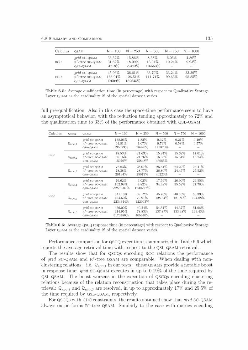
6.8 Summary and Comparison 135
Calculus qsam N = 100 N = 250 N = 500 N = 750 N = 1000
rcc
grid sc-qsam 36.52% 15.86% 8.58% 6.05% 4.86%r∗-tree sc-qsam 31.62% 18.09% 13.04% 10.24% 9.93%
qsr-qsam 4718% 29423% 116553% − −
cdc
grid sc-qsam 45.96% 36.61% 33.79% 33.24% 33.39%r∗-tree sc-qsam 165.91% 126.51% 111.71% 99.63% 95.85%
qsr-qsam 17609% 182645% − − −
Table 6.5: Average qualification time (in percentage) with respect to Qualitative StorageLayer qsam as the cardinality N of the spatial dataset varies.
full pre-qualification. Also in this case the space-time performance seem to havean asymptotical behavior, with the reduction tending approximately to 72% andthe qualification time to 33% of the performance obtained with qsl-qsam.
Calculus qscq qsam N = 100 N = 250 N = 500 N = 750 N = 1000
rcc
Qrcc,1
grid sc-qsam 138.06% 1.82% 0.32% 0.21% 0.19%r∗-tree sc-qsam 64.81% 1.67% 0.74% 0.58% 0.57%
qsr-qsam 195099% 78420% 143870% − −
Qrcc,2
grid sc-qsam 78.53% 21.63% 15.84% 15.62% 17.01%r∗-tree sc-qsam 86.16% 21.76% 16.35% 15.54% 16.74%
qsr-qsam 15070% 25848% 46085% − −
Qrcc,3
grid sc-qsam 72.83% 28.07% 26.51% 24.22% 25.41%r∗-tree sc-qsam 78.38% 28.77% 26.80% 24.45% 25.52%
qsr-qsam 28194% 25073% 46223% − −
cdc
Qcdc,1
grid sc-qsam 76.62% 3.02% 17.59% 26.90% 26.55%r∗-tree sc-qsam 102.98% 4.82% 34.48% 35.52% 27.78%
qsr-qsam 22278687% 1730227% − − −
Qcdc,2
grid sc-qsam 641.18% 39.12% 45.76% 40.16% 50.39%r∗-tree sc-qsam 424.60% 79.91% 128.34% 121.80% 134.88%
qsr-qsam 2234344% 422093% − − −
Qcdc,3
grid sc-qsam 456.00% 40.24% 54.51% 44.37% 51.98%r∗-tree sc-qsam 314.95% 78.83% 137.87% 133.48% 139.43%
qsr-qsam 3173486% 405640% − − −
Table 6.6: Average qscq response time (in percentage) with respect to Qualitative StorageLayer qsam as the cardinality N of the spatial dataset varies.
Performance comparison for qscq execution is summarized in Table 6.6 whichreports the average retrieval time with respect to the qsl-qsam retrieval.
The results show that for qscqs encoding rcc relations the performanceof grid sc-qsam and r∗-tree qsam are comparable. When dealing with non-clustering relations—i.e. Qrcc,1 in our tests—these qsams provide a notable boostin response time: grid sc-qsam executes in up to 0.19% of the time required byqsl-qsam. The boost worsens in the execution of qscqs encoding clusteringrelations because of the relation reconstruction that takes place during the re-trieval: Qrcc,2 and Qrcc,3 are resolved, in up to approximately 17% and 25.5% ofthe time required by qsl-qsam, respectively.
For qscqs with cdc constraints, the results obtained show that grid sc-qsamalways outperforms r∗-tree qsam. Similarly to the case with queries encoding

136 6 Empirical Evaluation
rcc relations, the performance boost provided by the qsam is higher when deal-ing with non-clustering relations than with clustering relations.
In conclusion, the result of the conducted experiments show that grid sc-qsam provides the best performance on random generated datasets for both rccand cdc and for both dataset qualification and qscq execution. However, theexperimentation conducted on the OpenStreetMap dataset of Bremen (cf. Sec-tion 6.7) showed that r∗-tree qsam behaves better in terms of spatial reduction(cf. Table 6.2) as well as in qscq retrievals (cf. Table 6.3). The motivation isthat the higher the cardinality of the spatial dataset, the more relevant the roleplayed by the hierarchical structure of r∗-tree.
As explained before, qsr-qsam, in the basic version presented in this work,does not provide a suitable solution for real applications. More sophisticatedversions of this qsam can be developed and tested which we expect to lead tobetter performance.
Chapter 7
Summary and Outlook
This chapter concludes the thesis with a summary and a discussion of the resultsachieved. Additionally it outlines some possible directions for future investiga-tions stemming from the presented work.
7.1 Summary of Results
Despite continuous improvements, Geographic Information Systems (gis) keeplacking instruments for interpreting and coping with spatial queries expressedin a human-friendly format, i.e. qualitative spatial descriptions. They provideinterfaces mainly tailored for experts, denying the casual user the possibility toexploit their potentials and, consequently, drastically reducing the number ofpotential spatial data contributors and consumers.
As of today the casual user can exploit gis capabilities mainly by resortingto some pre-defined interfaces which allow for accessing spatial information in alimited number of ways. One typology of access to spatial information, todaylargely unaccounted for, concerns the cases in which one wants to retrieve spatialinformation on the basis of a set of spatial constraints. In this work we faced thechallenge of filling this gap.
Human beings have a natural predisposition for acquiring, reasoning on, andcommunicating spatial information that allows them to deal with spatial mattersin a quite effortless manner. The processes underlying spatial reasoning in hu-mans, mainly draws upon qualitative spatial representation. Qualitative SpatialRepresentation and Reasoning (qsr) is a well established field that also findsapplications in gis in that most typologies of spatial queries encode some sortof qualitative spatial relation: a predicate that spatial entities have to satisfy.Typically, in the literature, queries encoding different spatial predicates are stud-ied separately and specialized solving strategies are developed for each type. In
138 7 Summary and Outlook
this thesis we stressed the fact that all such spatial queries can be regarded asa single query type that we named Qualitative Spatial Relation Query. We pre-sented a classification and a nomenclature of these queries. The classification isbased on the level of indeterminacy of the spatial predicates encoded in a querywhereas the nomenclature reflects the type of spatial request. Moreover, Quali-tative Spatial Relation Queries have been ranked according to the computationalcost required to resolve any of their instances. We decided to focus our workon the type hardest to solve that we named Qualitative Spatial ConfigurationQueries (qscqs).
qscqs can encode constraints from different qualitative spatial calculi, there-fore they can be interpreted as a multi-calculus Qualitative Constraint Network(qcn), which, in turn can be represented as a directed hypergraph. The quali-tative spatial relations among the objects in a spatial dataset can be computedinto a so-called qualified dataset which can also be interpreted as a multi-calculusqcn (cf. Example 3.4). Accordingly, the problem of solving a qscq is equivalentto finding all the isomorphisms between the hypergraph representing the qscqand that representing the qualified dataset.
Initially, we assumed that the hypergraph representation of both the qscq andthe spatial dataset were given and we derived from Ullmann’s famous algorithma basic matching procedure (cf. Section 3.4.1) suited for the special type ofhypergraphs we treat.
Later on, we pointed out that, given the typical size of a real spatial dataset,the qualification operation required to generate a qualified dataset is computa-tionally too onerous. Therefore, assuming that the hypergraph representationof the spatial dataset is given is not a reasonable hypothesis. Rather, datasetqualification has to be carefully accounted for in the qscq resolution process.
We presented two basic dataset qualification strategies (cf. Section 3.5): run-time qualification and pre-qualification. Runtime qualification is a purely func-tional approach that executes the qualification at retrieval time. It does notrequire any extra storage space but is highly inefficient for what concerns qscqretrieval time. Pre-qualification requires to extend the schema of the underlyingspatial database with a set of Lookup Tables (luts) designed to accommodate thequalified dataset. We called such luts relation tables and the schema extensionqualitative storage layer. Pre-qualification allows for significantly speeding up theretrievals but requires an enormous amount of space to store the qualified dataset.Moreover the elevated time required by qualification operation makes hard to dealwith the dynamism of the real world: by the time the pre-qualification is com-pleted the world has changed as well as its representation in the spatial database,calling for a new qualification.
In Chapter 4 we introduced the concept of Qualitative Spatial Access Method(qsam). A qsam (cf. Definition 4.1) is a special class of spatial access methodswhich applies a qualitative relation reduction/reconstruction paradigm to opti-mize the space-time tradeoff inevitably adduced by qscq solving strategies. Themain purpose of a qsam is to provide a solving strategy that takes into account
7.1 Summary of Results 139
the dataset qualification problem by extending the spatial database with a qual-itative storage layer and by only pre-computing a targeted subset of the wholequalified dataset. Non-stored relations have to be rebuildable at qscq executiontime.
More specifically, a qsam is composed of three elements: a qualifier function,a set of data structures, and a retriever function. The qualifier function takescare of qualifying the spatial dataset into a set of relation tables and, possibly, ofstoring some additional bits of information summarizing the strategy adopted toperform the reduction (if any). The retriever function exploits the informationstored in the set of data structures to resolve a given qscq, possibly rebuildingmissing qualitative spatial relations.
Four kinds of qsams have been proposed: Functional qsam (f-qsam), Qual-itative Storage Layer qsam (qsl-qsam), Spatial Clustering qsam (sc-qsam),and qsr-based qsam (qsr-qsam). They all resort to hypergraph matching tosolve a qscq but tackle differently the dataset qualification problem.
f-qsam and qsl-qsam (cf Sections 4.1 and 4.2, respectively) encode runtimequalification and full pre-qualification, respectively. As such, they provide good-ness reference values to assess other qsams: A qscq retrieval should not takelonger than the time employed by f-qsam. Similarly, a qsam producing a qual-ified dataset larger than that produced by qsl-qsam does not provide a goodapproach for qualification.
sc-qsam (cf. Section 4.3) is a family of qsams that resorts to a tile&clusterapproach: It jointly exploits a special type of qualitative spatial relations calledclustering relations (cf. Definition 4.2) together with a spatial clustering index(cf. Definition 4.5) to produce a reduced qualified dataset. If opportunely tuned,the spatial clustering index produces a subdivision of the spatial dataset that al-lows the qualifier function to compute and store a reduced number of qualitativerelations. This approach provides a valuable compromise between the previoussolutions: it shorten the retrieval time with respect to f-qsam and produces morecompact qualified datasets in a shorter time with respect to qsl-qsam. At qscqexecution time, the retriever function exploits the structure of the spatial clus-tering index to rebuild qualitative relations missing in the relation tables. Themain shortcoming of this approach is that it requires a careful calibration of thespatial clustering index. Otherwise sc-qsam might lead worse qualification andretrieval performance than those obtained with qsl-qsam and f-qsam, respec-tively. In this work we presented two special instances of sc-qsam: (i) grid -basedsc-qsam (cf. Section 5.2.1) employs a uniform grid as a spatial clustering index.(ii) r∗-tree-based sc-qsam (cf. Section 5.2.2) resorts to r∗-tree.
qsr-qsam (cf. Section 4.4) exploits a novel data structure named inferencegraph (cf. Definition 4.9) to obtain a reduced qualified dataset from which itis possible to infer back all the missing relations by only resorting to symbolicreasoning. The advantages of this qsam are that it is independent of the spatialcalculus and it might be used to produce the minimum set of qualitative relationsneeded to describe a spatial dataset (cf. discussion on the reduction at the end
140 7 Summary and Outlook
of Section 4.4.3). However, the temporal costs required by the qualifier andretriever functions makes qsr-qsam unsuitable for being applied on a wholespatial dataset. Note that, in this work we have been mainly interested in drawingthe foundations of this qsam by defining the inference graph and a basic version ofthe reduction and reconstruction strategies. As will be discussed in Section 7.2.2,such basic strategies leave ample room for improvement.
In Chapter 5 we presented MyQual: a software framework for developingand benchmarking qsams. MyQual has been used to implement and test allthe qsams introduced in this thesis, providing an empirical demonstration of itsusefulness.
MyQual Toolbox is one of the four components provided by MyQual: it isan extensible repository for qualitative spatial calculi and qsams. As such, itprovides a practical realization of a fundamental assumption of this work: Weassumed the existence of a pool of qualitative relations rich enough to contain allthe relations necessary to encode any qualitative spatial description produced byhumans into a qualitative spatial relation query. Given the variety of expressionstypical of spatial descriptions produced by humans, it is impossible to predictwhich relations will be needed. Contrarily, having an extensible repository ofspatial calculi allows for enriching the pool at will when necessary.
Beyond being a development environment, MyQual aims at providing a dis-tributed tool for bringing at the casual user reach the possibility of querying agis in a more intuitive way, i.e. via Qualitative Spatial Relation Queries.
In conclusion, the presented theoretical findings and the empirical results,prove that an accurate interplay of spatial access methods and a qualitative reduc-tion/reconstruction paradigm is fundamental for enabling and efficiently solvingQualitative Spatial Configuration Queries in Geographic Information Systems.In particular, the empirical results indicated the Spatial Clustering qsam familyto be the most promising solution.
7.2 Future Work
The work presented in this thesis can be extended in several ways. In the followingsections we outline some of the most attractive perspectives.
7.2.1 Minimum Qualitative Spatial Representation
The inference graph has been introduced in Section 4.4.1. We showed how itcan be generated from the reasoning tables of a given qualitative spatial calcu-lus and how it can be used to detect a reduced number of qualitative relationsdescribing a spatial scene. We also provided a qualitative analysis of the reduc-tion properties provided by this data structure and argued that it can be used toproduce the minimum set of qualitative relations necessary to describe a spatialscene. A further investigation is required to formally verify the validity of thisargumentation and to detect under which conditions a maximum reduction—i.e.a minimum description—is possible.
7.2 Future Work 141
7.2.2 Empowering qsr-based qsam
As demonstrated by the empirical evaluation carried out in Section 6.6 the pre-sented version of qsr-qsam is highly inefficient for what concern dataset qualifica-tion and qscq retrieval times. However, the presented solution can be empoweredin several ways:
• The definition of Relaxed Strongly Connected Component (cf. Defini-tion 4.11) can be modified to allow for the specification of a maximal lengththat the spanning hyperpaths connecting the nodes of each relaxed com-ponent do not have to exceed. This provides a certain control on the timerequired for the computation of the components. Defining such a maximallength allows for avoiding the exploration of long paths that, at the end,might not be relevant for computing a component. Of course, fixing themaximal allowed length at a too small value will produce components con-sisting of a reduced number of nodes, and consequently affect the overallreduction. Therefore, a more careful investigation has to be undertaken inorder to define the best value for this new parameter.
• The inference paths used for doing the reduction, can be stored in an ap-posite data structure. Such information can be used in the retrieval phaseas a sort of “reasoning map” to guide the reasoning operations performedby the algebraic closure algorithm: When iterating over a certain relationr(oi, oj) the algorithm can access the stored inference paths to immediatelydetect the relations which r(oi, oj) has to be composed with in order tore-generate one of the missing relations. Of course, also in this case thereis a space-time tradeoff that has to be accounted for. The storage of infer-ence paths allows for speeding up the relation reconstruction phase, and,thus, the qscq response time, but on the other hand requires an increasedamount of storage space. This tradeoff has to be investigated to detectwhat is the percentage of inference path that can be stored without leadingto an excessive worsening of the storage performance.
• The actual reduction and reconstruction phases allow for using inter-calculiinference templates. That is, new inference rules connecting relations fromdifferent calculi can be used in the dataset qualification and in the qscqexecution phases. For example one might note that, if an object oi is to thenorth of and object oj then it follows that oi is also disconnected from oj.This inference rule can be encoded as an inter-calculus inference template.Some work in this direction has been done, for example, by Sharma (1996)who developed a series of inter-calculus reasoning tables. Inter-calculus tem-plates allow for instantiating inference paths that connect inference graphsotherwise disconnected—i.e. generated from different calculi. It is of specialinterest to investigate how such a connection influences the reduction andthe reconstruction performed by qsr-qsam.

142 7 Summary and Outlook
7.2.3 Other Qualitative Spatial Calculi and Inter-calculus
qscqs
One main objective of this work was to develop a theoretical framework general
enough to deal with qualitative spatial calculi of any arity. Moreover, the frame-
work also allows for dealing with qualitative relation queries encoding simulta-
neously relations concerning multiple spatial aspects—i.e. belonging to different
calculi.
In this work, we limited ourselves to implementations of basic cases: we only
dealt with two binary calculi—the Region Connection Calculus (rcc) and the
Cardinal Direction Calculus (cdc)—and with qscqs encoding relations from
the same calculus. Further investigations may concern the implementation of
other calculi, possibly of higher arity, and the experimentation of the presented
techniques on queries encoding relations from multiple calculi.
7.2.4 Further Investigation on Spatial Clustering qsam
The Spatial Clustering qsam (sc-qsam) family has been introduced in Sec-
tion 4.3. In this work we presented and implemented two possible instances
of such a family: one based on a grid index, the other on an r∗-tree. Further
investigations can be carried out that aim at analyzing other sc-qsam instances,
that is, the employment of other data structures and space partitioning methods
to be used as a spatial clustering index.
Moreover, of special interest is the development of techniques to automatically
detect spatial clustering relations among those provided by a qualitative spatial
calculus. For this investigation, the results of Theorem 4.1 can be used as a
starting point.
7.2.5 Mixed sc–qsr qsam
It was pointed out in the discussion of qsr-based qsam (qsr-qsam) (and con-
firmed by the empirical evaluation) that the high temporal cost required by the
qualification and retrieval functions, make qsr-qsam not suited for being applied
to whole spatial datasets. A possible solution to overcome this inconvenience is
that of developing a mixed Spatial Clustering–qsr qsam. Dataset qualification
consists in applying first Spatial Clustering qsam (sc-qsam) to exploit cluster-
ing relations for computing a reduced number of inter-cluster object relations.
Then, applying qsr-qsam on each object cluster allows for reducing the number
of in-cluster relations. qscq execution can be done by applying algebraic closure
on each cluster and subsequently calling the sc-qsam retriever function.
7.2 Future Work 143
7.2.6 Dynamic and Parallel qsams
In Section 3.1 we introduced a generalization for queries encoding spatial pred-
icates that allow for looking at them as a single query type. We called such a
generalization qualitative spatial relation query and presented Qualitative Spatial
Access Methods (qsams) in Chapter 4: a class of Spatial Access Methods (sams)
tailored for solving the hardest variant of qualitative spatial relation query. In
this thesis we investigated how to efficiently access qualitative spatial informa-
tion from a spatial database, restricting ourselves to the consideration of static
datasets, i.e. we only focused on insert and search operations. In order to make
the presented solutions practically usable, they have to be provided with algo-
rithms for dealing with dynamic datasets, that is functions for taking into account
deletion and update operations have to be developed.
A further possible investigation direction concerns the parallelization of the
algorithmic framework we presented. In Chapter 5 we discussed MyQual, a soft-
ware framework for the development of qsams. MyQual has been designed to be
a distributed framework, in the sense that a local installation can use tools located
on a remote bounded machine and simultaneously provide tools to be used by re-
mote installations of MyQual. So far, the hardware and computational resources
required for the execution of a certain operation, are provided by the machine
hosting the tool being used. The parallelization of the algorithmic framework
would allow to further enhance the distributed fashion of MyQual, allowing for
moving a step towards cloud computing: the computation required by a certain
method can be split and distributed over the network of MyQual installations.
7.2.7 Treating Disjunctive Relations and Inconsistency
This work focused on the definition of a theoretical framework and on the devel-
opment of basic methods and techniques for the resolution of Qualitative Spatial
Configuration Queries (qscqs). To allow for a lean analysis we set the assump-
tion that the qscqs under consideration were consistent—i.e. they do not encode
spatial relations conflicting with each other. Moreover, we narrowed down our
investigation to the case in which the relations encoded in a qscq were base
relations—i.e. no disjunction of relations appears in a query.
A further extension of the presented solutions consists in the development
of techniques that can deal with uncertainty and inconsistency. Some work have
already been conducted on these issues (cf. Clementini et al., 1994; Wallgrün et al.,
2010, for instance). A possible research direction, then, concerns the integration
of previous work with the results presented in this thesis in order to develop qscq
solving techniques capable of dealing with queries encoding disjunctive relations
and of opportunely handling inconsistency.
144 7 Summary and Outlook
7.2.8 Contributing Qualitative Spatial Information in vgi
Projects
Volunteered Geographic Information (vgi) is a particular form of user-generatedcontent in that it assumes the involvement of volunteers to collect and disseminatespatial information. Probably, the most known form of vgi, is represented by web-based projects like OpenStreetMap1, which aims at collaboratively producing afree editable map of the world.
There are several ways a volunteer can contribute spatial information into aweb gis. One of the easiest consists in surveying spatial data by means of aGlobal Positioning System (gps) device and uploading it to the server hostingthe gis.
However, the number of real contributors is strongly affected by the techno-logical barriers risen by such a method: (i) Although gps technology is spreadingvery fast, not everyone posseses a device with a gps antenna. (ii) Not everyonehaving a gps device knows how to use it. (iii) In order to be uploaded, the sur-veyed data has to be cleaned and tagged. This requires a certain level of expertisein gis.
As discussed in (Fogliaroni et al., 2010), providing the casual user with thepossibility of contributing geographic information via natural spatial descriptions(cf. Sections 1.2.1 and 2.2.1) would allow for overcome such technological barriers.
MyQual, the software framework we developed for enabling qscqs, can servea fundamental role in this perspective: It provides the basic components to allowthe underlying spatial database to store and retrieve qualitative spatial infor-mation. As a consequence, it also provides basic methods for inputting spatialinformation given in a qualitative form. That is, a volunteer can give a textualor pictorial description of the spatial entities he wants to contribute on, relatingthem to a set of entities in the spatial database underlying a gis. The givenspatial description can be encoded into a qualitative spatial relation query whosesingle relations can be stored in the qualitative storage layer. Although not hav-ing geometries associated, the new spatial entities are now present in the databaseand can be retrieved via a qualitative spatial relation query.
Therefore, the ideas presented in this thesis can be used as a base for develop-ing a new contribution form of spatial information that can be used to empoweralready established vgi projects like OpenStreetMap.
1http://www.openstreetmap.org/
References
Allen, J. (1983). Maintaining knowledge about temporal intervals. Communications of the
ACM , 26(11), 832–843. (17)
Ausiello, G., D’Atri, A. & Saccà, D. (1983). Graph algorithms for functional dependency
manipulation. Journal of the ACM (JACM), 30(4), 752–766. (13)
Ausiello, G., D’Atri, A. & Saccà, D. (1986). Minimal representation of directed hyper-
graphs. SIAM Journal on Computing , 15(2), 418–431. (13)
Ausiello, G., Franciosa, P. & Frigioni, D. (2001). Directed hypergraphs: Problems,
algorithmic results, and a novel decremental approach. In A. Restivo, S. Della Rocca &
L. Roversi, eds., Theoretical Computer Science, vol. 2202 of Lecture Notes in Computer
Science, 312–328, Springer-Verlag. (12, 13, 14)
Balbiani, P., Condotta, J. & Del Cerro, L. (1998). A model for reasoning about bidi-
mensional temporal relations. In A.G. Cohn, L. Schubert & S.S. C., eds., Proceedings of the
Sixth International Conference on Principles of Knowledge Representation and Reasoning ,
124–130, Morgan Kaufmann. (27)
Bartie, P., Reitsma, F., Clementini, E. & Kingham, S. (2011). Referring expres-
sions in location based services: The case of the ‘opposite’ relation. In O. De Troyer,
C. Bauzer Medeiros, R. Billen, P. Hallot, A. Simitsis & H. Van Mingroot, eds., Advances in
Conceptual Modeling. Recent Developments and New Directions, vol. 6999 of Lecture Notes
in Computer Science, 231–240, Springer-Verlag. (25)
Beckmann, N., Kriegel, H.P., Schneider, R. & Seeger, B. (1990). The r∗-tree: An
efficient and robust access method for points and rectangles. In Proceedings of the 1990
ACM SIGMOD International Conference on Management of Data, SIGMOD ’90, 322–331,
ACM. (39, 76, 123, 124)
Bentley, J.L. & Friedman, J.H. (1979). Data structures for range searching. ACM Com-
puting Surveys (CSUR), 11(4), 397–409. (38)
Berge, C. (1976). Graphs and hypergraphs, vol. 6. Elsevier. (12)
Berge, C. (1989). Hypergraphs: Combinatorics of finite sets, vol. 45. North-Holland. (12)
Billen, R. & Clementini, E. (2004a). Introducing a reasoning system based on ternary
projective relations. In P. Fisher, ed., Developments in Spatial Data Handling , 381–394,
Springer-Verlag. (27)
146 References
Billen, R. & Clementini, E. (2004b). A model for ternary projective relations between
regions. In E. Bertino, S. Christodoulakis, D. Plexousakis, V. Christophides, M. Koubarakis,
K. Böhm & E. Ferrari, eds., Advances in Database Technology – EDBT 2004 , vol. 2992 of
Lecture Notes in Computer Science, 537–538, Springer-Verlag. (27)
Billen, R. & Zlatanova, S. (2003). 3d spatial relationships model: A useful concept for 3d
cadastre? Computers, Environment and Urban Systems, 27(4), 411–425. (25)
Bittner, T. & Donnelly, M. (2007). A formal theory of qualitative size and distance re-
lations between regions. In Proceedings of the 21st International Workshop on Qualitative
Reasoning . (29)
Brakatsoulas, S., Pfoser, D. & Theodoridis, Y. (2002). Revisiting r-tree construction
principles. In Y. Manolopoulos & P. Návrat, eds., Advances in Databases and Information
Systems, vol. 2435 of Lecture Notes in Computer Science, 17–24, Springer-Verlag. (40)
Calcinelli, D. & Mainguenaud, M. (1994). Cigales, a visual query language for geograph-
ical information system: The user interface. Journal of Visual Languages and Computing ,
5(2), 113–132. (41)
Chang, N. & Fu, K. (1980). Query-By-Pictorial-Example. IEEE Transactions on Software
Engineering(6), 519–524. (40)
Clark, K.L. (1978). Negation as failure. In Logic and Databases, vol. 1, 293–322, Plenum
Publishing Corporation. (108)
Clementini, E. & Di Felice, P. (1997). A global framework for qualitative shape description.
GeoInformatica, 1(1), 11–27. (22, 29, 31)
Clementini, E. & Di Felice, P. (2000). Spatial operators. SIGMOD Record , 29(3), 31–38.
(26, 36)
Clementini, E., Sharma, J. & Egenhofer, M.J. (1994). Modelling topological spatial
relations: Strategies for query processing. Computers & Graphics, 18(6), 815–822. (41, 57,
143)
Clementini, E., Di Felice, P. & Hernández, D. (1997). Qualitative representation of
positional information. Artificial Intelligence, 95(2), 317–356. (23, 28, 31)
Cohn, A.G. (1995). A hierarchical representation of qualitative shape based on connection
and convexity. In A. Frank & W. Kuhn, eds., Spatial Information Theory A Theoretical
Basis for GIS , vol. 988 of Lecture Notes in Computer Science, 311–326, Springer-Verlag,
10.1007/3-540-60392-1_20. (29)
Cohn, A.G. (1997). Qualitative spatial representation and reasoning techniques. In G. Brewka,
C. Habel & B. Nebel, eds., Proceedings of the 21st Annual German Conference on Artificial
Intelligence: Advances in Artificial Intelligence, vol. 1303 of Lecture Notes in Computer
Science, 1–30, Springer-Verlag. (17)
References 147
Cohn, A.G. & Hazarika, S.M. (2001). Qualitative spatial representation and reasoning: An
overview. Fundamenta Informaticae, 46(1-2), 1–29. (17)
Cohn, A.G. & Renz, J. (2008). Qualitative spatial representation and reasoning. In V.L.
Frank van Harmelen & B. Porter, eds., Handbook of Knowledge Representation, vol. 3 of
Foundations of Artificial Intelligence, 551–596, Elsevier. (17, 19)
Cohn, A.G., Bennett, B., Gooday, J. & Gotts, N.M. (1997). Qualitative spatial repre-
sentation and reasoning with the region connection calculus. GeoInformatica, 1(3), 275–316.
(27)
Comer, D. (1979). Ubiquitous b-tree. ACM Computing Surveys (CSUR), 11(2), 121–137. (38,
39, 57)
Condotta, J., Ligozat, G. & Saade, M. (2006). A generic toolkit for n-ary qualitative
temporal and spatial calculi. In TIME 2006. Proceedings of the Thirteenth International
Symposium on Temporal Representation and Reasoning , vol. 6, 78–86. (21)
Conte, D., Foggia, P., Sansone, C. & Vento, M. (2004). Thirty years of graph matching
in pattern recognition. International journal of pattern recognition and artificial intelligence,
18(3), 265–298. (51)
Cui, Z., Cohn, A.G. & Randell, D.A. (1993). Qualitative and topological relationships in
spatial databases. In D. Abel & B. Chin Ooi, eds., Proceedings of the Third International
Symposium on Advances in Spatial Databases, vol. 692 of Lecture Notes in Computer Science,
296–315, Springer-Verlag. (80)
Dechter, R. (1992). Constraint networks. In S.C. Shapiro, ed., Encyclopedia of Artificial
Intelligence (2nd Edition), vol. 1, 276–285, John Wiley & Sons, Inc. (29)
Dechter, R. (2003). Constraint processing . The Morgan Kaufmann Series in Artificial Intel-
ligence, Morgan Kaufmann. (29)
Douglas, K. & Douglas, S. (2005). PostgreSQL. A comprehensive guide to building, pro-
gramming, and administering PostgreSQL databases (2nd Edition). Sams Publishing. (98)
Düntsch, I., Wang, H. & McCloskey, S. (2001). A relation–algebraic approach to the
region connection calculus. Theoretical Computer Science, 255(1-2), 63–83. (21)
Dylla, F. & Moratz, R. (2004). Empirical complexity issues of practical qualitative spatial
reasoning about relative position. In Workshop on Spatial and Temporal Reasoning at ECAI
2004 . (31)
Egenhofer, M. (1996). Spatial-Query-By-Sketch. In W. Citrin & M. Burnett, eds., Proceed-
ings of the 1996 IEEE Symposium on Visual Languages, 60–67. (2, 41)
148 References
Egenhofer, M. & Sharma, J. (1992). Topological consistency. In P. Bresnahan, E. Corwin &
D. Cowen, eds., Proceeding of the Fifth International Symposium on Spatial Data Handling ,
vol. 2, 335–343. (94)
Egenhofer, M. & Sharma, J. (1993). Assessing the consistency of complete and incomplete
topological information. Geographical Systems, 1(1), 47–68. (22, 31, 94)
Egenhofer, M.J. (1989). A formal definition of binary topological relationships. In W. Litwin
& H.J. Schek, eds., 3rd International Conference, FODO 1989 on Foundations of Data Orga-
nization and Algorithms, vol. 367 of Lecture Notes in Computer Science, 457–472, Springer-
Verlag. (26, 57)
Egenhofer, M.J. (1991). Reasoning about binary topological relations. In O. Günther &
H.J. Schek, eds., Proceedings of the Second International Symposium on Advances in Spatial
Databases, vol. 525 of Lecture Notes in Computer Science, 143–160, Springer-Verlag. (26,
27, 57)
Egenhofer, M.J. (1994). Spatial sql: A query and presentation language. IEEE Transactions
on Knowledge and Data Engineering , 6(1), 86–95. (40)
Elmasri, R. & Navathe, S. (2008). Fundamentals of database systems, vol. 2. Pearson Edu-
cation India. (13)
ESRI (1998). Shapefile technical description. Tech. rep., Environmental Systems Research In-
stitute, Inc. (32)
Fagin, R., Nievergelt, J., Pippenger, N. & Strong, H.R. (1979). Extendible hashing:
A fast access method for dynamic files. ACM Transactions on Database Systems (TODS),
4(3), 315–344. (57)
Falomir, Z., Martí, I., Viana, W., Museros, L. & Escrig, M.T. (2010). A pragmatic
approach for qualitative shape and qualitative colour similarity matching. In R. Alquézar,
A. Moreno & J. Aguilar, eds., Artificial Intelligence Research and Development – Proceedings
of the 13th International Conference of the Catalan Association for Artificial Intelligence,
vol. 220 of Frontiers in Artificial Intelligence and Applications, 281–290, IOS Press. (29)
Finkel, R.A. & Bentley, J.L. (1974). Quad-trees a data structure for retrieval on composite
keys. Acta Informatica, 4, 1–9. (76)
Fogliaroni, P., Wallgrün, J.O., Clementini, E., Tarquini, F. & Wolter, D. (2009).
A qualitative approach to localization and navigation based on visibility information. In K.S.
Hornsby, C. Claramunt, M. Denis & G. Ligozat, eds., Proceedings of the 9th International
Conference on Spatial Information Theory , COSIT’09, 312–329, Springer-Verlag. (29)
Fogliaroni, P., De Felice, G. & Wallgrün, J.O. (2010). A qualitative perspective on
volunteered geographic information. InGIScience 2010 - Workshop on the Role of Volunteered
Geographic Information in Advancing Science. (144)
References 149
Fogliaroni, P., De Felice, G., Schmid, F. & Wallgrün, J.O. (2011). Managing quali-
tative spatial information to support Query-by-Sketch. In J. Wang, Bölemann, M. Chipofya,
A. Schwering & J.O. Wallgrün, eds., Understanding and Processing Sketch Maps (COSIT’11),
vol. 42 of ifgiPrints, 21 – 32, IOS Press. (119)
Forbus, K.D. (2008). Qualitative modeling. In V.L. Frank van Harmelen & B. Porter, eds.,
Handbook of Knowledge Representation, vol. 3 of Foundations of Artificial Intelligence, 361–
393, Elsevier. (16)
Forbus, K.D., Nielsen, P. & Faltings, B. (1987). Qualitative kinematics: A framework.
In Proceedings of the 10th International Joint Conference on Artificial Intelligence - Volume
1 , IJCAI’87, 430–435, Morgan Kaufmann Publishers Inc. (31)
Forbus, K.D., Nielsen, P. & Faltings, B. (1991). Qualitative spatial reasoning: The
CLOCK project. Artificial Intelligence, 51(1-3), 417–471. (16, 31)
Frank, A.U. (1982). mapquery: Data base query language for retrieval of geometric data
and their graphical representation. ACM SIGGRAPH Computer Graphics , 16(3), 199–207.
(40)
Frank, A.U. (1991). Qualitative spatial reasoning with cardinal directions. In H. Kaindl, ed.,
Proceedings of the 7th Austrian Conference on Artificial Intelligence, ÖGAI , vol. 287 of
Informatik-Fachberichte, 157–167, Springer-Verlag. (27)
Franklin, W.R. (1978). Combinatorics of hidden surface algorithms. Ph.D. thesis, Center for
research in computing technology, Harvard University. (38)
Franklin, W.R. (1984). Adaptive grids for geometric operations. Cartographica: The Inter-
national Journal for Geographic Information and Geovisualization, 21(2-3), 160–167. (38)
Franklin, W.R. (1989). Uniform grids: A technique for intersection detection on serial
and parallel machines. In Proceedings of the Ninth International Symposium on Computer-
Assisted Cartography , 100–109, American Congress on Surveying and Mapping. (38)
Freksa, C. (1991a). Conceptual neighborhood and its role in temporal and spatial reasoning. In
M.G. Singh & L. Travé-Massuyès, eds., Decision Support Systems and Qualitative Reasoning ,
181–187, North-Holland. (41)
Freksa, C. (1991b). Qualitative spatial reasoning. In D.M. Mark & A.U. Frank, eds., Cognitive
and linguistic aspects of geographic space, 361–372. (16, 17)
Freksa, C. (1992). Using orientation information for qualitative spatial reasoning. In A. Frank,
I. Campari & U. Formentini, eds., Theories and Methods of Spatio-Temporal Reasoning in
Geographic Space, vol. 639 of Lecture Notes in Computer Science, 162–178, Springer-Verlag.
(27, 29)
150 References
Freksa, C. & Röhrig, R. (1993). Dimensions of qualitative spatial reasoning. In P. Car-
reté & M. Singh, eds., Proceedings of Qualitative reasoning and decision technologies
(QUARDET’93), 483–492. (22, 26)
Freksa, C. & Zimmermann, K. (1992). On the utilization of spatial structures for cognitively
plausible and efficient reasoning. In Proceedings of the IEEE International Conference on
Systems, Man and Cybernetics, 261–266, IEEE. (20, 27)
Gaede, V. & Günther, O. (1998). Multidimensional access methods. ACM Computing Sur-
veys (CSUR), 30(2), 170–231. (36, 37, 38)
Gallo, G., Longo, G., Pallottino, S. & Nguyen, S. (1993). Directed hypergraphs and
applications. Discrete Applied Mathematics, 42(2-3), 177–201. (12, 13, 14)
Gerevini, A. & Renz, J. (1998). Combining topological and qualitative size constraints for
spatial reasoning. In M. Maher & J.F. Peugeot, eds., Proceedings of the 4th International
Conference on Principles and Practice of Constraint Programming , Lecture Notes in Com-
puter Science, 220–234, Springer-Verlag. (31, 32)
Gerevini, A. & Renz, J. (2002). Combining topological and size information for spatial
reasoning. Artificial Intelligence, 137(1-2), 1–42. (31, 32)
Goodchild, M.F. (2007). Citizens as sensors: The world of volunteered geography. GeoJour-
nal , 69(4), 211–221. (1)
Goyal, R. & Egenhofer, M. (2000). Consistent queries over cardinal directions across dif-
ferent levels of detail. In Proceedings of the 11th International Workshop on Database and
Expert System Applications, 876–880, IEEE Computer Society. (25)
Goyal, R. & Egenhofer, M. (in press). Cardinal directions between extended spa-
tial objects. IEEE Transactions on Knowledge and Data Engineering , available at
http://www.spatial.maine.edu/∼max/RJ36.html. (27, 41, 58)
Goyal, R.K. & Egenhofer, M.J. (1997). The direction-relation matrix: A representation
for directions relations between extended spatial objects. In The Annual Assembly and the
Summer Retreat of University Consortium for Geographic Information Systems Science. (28,
41, 58)
Guesgen, H. (1989). Spatial reasoning based on Allen’s temporal logic. Tech. Rep. TR-89-049,
International Computer Science Institute at Berkley, California, 1989. (17, 27)
Güting, R. (1994). An introduction to spatial database systems. The VLDB Journal , 3(4),
357–399. (34)
Guttman, A. (1984). r-trees: A dynamic index structure for spatial searching. In Proceedings
of the 1984 ACM SIGMOD International Conference on Management of Data, SIGMOD
’84, 47–57, ACM. (39, 76, 123)
References 151
Hernandez, D. (1994). Qualitative representation of spatial knowledge, vol. 804 of Lecture
Notes in Computer Science. Springer-Verlag. (31)
Hernandez, D., Clementini, E. & Di Felice, P. (1995). Qualitative distances. In A. Frank
& W. Kuhn, eds., Spatial Information Theory A Theoretical Basis for GIS , vol. 988 of Lecture
Notes in Computer Science, 45–57, Springer-Verlag. (28)
Ingram, K.J. & Phillips, W.W. (1987). Geographic information processing using a sql-
based query language. In N.R. Chrisman, ed., Proceedings of the 8th International Symposium
on Computer-Assisted Cartography , 326–335, American Congress on Surveying and Mapping.
(40)
Joseph, T. & Cardenas, A. (1988). picquery: A high level query language for pictorial
database management. IEEE Transactions on Software Engineering , 14(5), 630–638. (40)
Klippel, A. (2003). Wayfinding choremes. In W. Kuhn, M. Worboys & S. Timpf, eds., Spatial
Information Theory. Foundations of Geographic Information Science, vol. 2825 of Lecture
Notes in Computer Science, 301–315, Springer-Verlag. (18)
Knauff, M., Rauh, R. & Renz, J. (1997). A cognitive assessment of topological spatial
relations: Results from an empirical investigation. In S. Hirtle & A. Frank, eds., Proceedings
of the International Conference on Spatial Information Theory: A Theoretical Basis for GIS ,
vol. 1329 of Lecture Notes in Computer Science, 193–206, Springer-Verlag. (32)
Lee, Y. & Chin, F. (1995). An iconic query language for topological relationships in gis.
International Journal of Geographical Information Systems, 9(1), 25–46. (41)
Levinson, S.C. (1996). Frames of reference and Molyneux’s question: Crosslinguistic evidence.
In P. Bloom, M.A. Peterson, L. Nadel & M.F. Garrett, eds., Language and Space, 109–169,
MIT Press. (23)
Li, S. (2007). Combining topological and directional information for spatial reasoning. In Pro-
ceedings of the 20th international joint conference on Artifical intelligence, IJCAI’07, 435–
440, Morgan Kaufmann Publishers Inc. (32)
Li, S. & Cohn, A.G. (2009). Reasoning with topological and directional spatial information.
CoRR, abs/0909.0122. (32)
Ligozat, G. (1998). Reasoning about cardinal directions. Journal of Visual Languages and
Computing , 9(1), 23–44. (27)
Litwin, W. (1980). Linear hashing: A new tool for file and table addressing. In Proceedings of
the sixth international conference on Very Large Data Bases - Volume 6 , VLDB ’80, 212–223,
VLDB Endowment Inc. (57)
Liu, W., Li, S. & Renz, J. (2009). Combining rcc-8 with qualitative direction calculi:
Algorithms and complexity. In Proceedings of the 21st International Joint Conference on
Artifical Intelligence, 854–859, Morgan Kaufmann Publishers Inc. (32)
152 References
Lloyd, S. (1982). Least squares quantization in PCM. IEEE Transactions on Information
Theory , 28(2), 129–137. (40)
Longley, P., Goodchild, M., Maguire, D. & Rhind, D. (2005). Geographic Information
Systems and Science. John Wiley & Sons, Ltd. (33)
Mackworth, A. (1977). Consistency in networks of relations. Artificial Intelligence, 8(1),
99–118. (30)
Montanari, U. (1974). Networks of constraints: Fundamental properties and applications to
picture processing. Information Science, 7(2), 95–132. (29, 30)
Moratz, R. (2006). Representing relative direction as a binary relation of oriented points. In
Proceedings of the 2006 conference on ECAI 2006: 17th European Conference on Artificial
Intelligence August 29 – September 1, 2006, Riva del Garda, Italy , 407–411, IOS Press. (27)
Moratz, R. & Ragni, M. (2008). Qualitative spatial reasoning about relative point position.
Journal of Visual Languages & Computing , 19(1), 75 – 98. (29)
Moratz, R. & Wallgrün, J.O. (2003). Propagation of distance and orientation intervals. In
Proceedings of 2003 IEEE/RSJ International Conference on Intelligent Robots and Systems
(IROS), vol. 4, 3245–3250. (29)
Moratz, R., Renz, J. & Wolter, D. (2000). Qualitative spatial reasoning about line seg-
ments. In W. Horn, ed., Proceedings of the 14th European Conference on Artificial Intelli-
gence, ECAI 2000 , 234–238, IOS Press. (27)
Moratz, R., Dylla, F. & Frommberger, L. (2005). A relative orientation algebra with
adjustable granularity. In Proceedings of the Workshop on Agents in Real-Time and Dynamic
Environments (IJCAI 05). (23, 27)
Mukerjee, A. & Joe, G. (1990). A qualitative model for space. In Proceedings of the eighth
National conference on Artificial intelligence - Volume 1 , AAAI’90, 721–727, AAAI Press.
(27)
Nievergelt, J., Hinterberger, H. & Sevcik, K.C. (1984). The grid file: An adaptable,
symmetric multikey file structure. ACM Trans. Database Syst., 9(1), 38–71. (39, 76)
OpenGIS Consortium (1998). OpenGIS simple features specification for sql. Tech. rep.,
OpenGIS Consortium (OGC). (34, 35, 40, 105)
Papadias, D. (1994). Relation-based representation of spatial knowledge. Ph.D. thesis, National
Technical University of Athens. (31)
Papadias, D. & Sellis, T. (1994a). A pictorial language for the retrieval of spatial relations
from image databases. In the Proceedings of the 6th International Symposium on Spatial Data
Handling (SDH), Taylor Francis. (41)
References 153
Papadias, D. & Sellis, T. (1994b). Qualitative representation of spatial knowledge in two-
dimensional space. The VLDB Journal , 3, 479–516. (31)
Papadias, D. & Sellis, T. (1995). A pictorial Query-By-Example language. Journal of Visual
Languages & Computing , 6(1), 53–72. (41)
Papadias, D., Sellis, T., Theodoridis, Y. & Egenhofer, M.J. (1995). Topological re-
lations in the world of minimum bounding rectangles: A study with r-trees. In Proceedings
of the 1995 ACM SIGMOD international conference on Management of data, SIGMOD ’95,
92–103, ACM. (31)
Pfoser, D. (2011). On user-generated geocontent. In D. Pfoser, Y. Tao, K. Mouratidis,
M. Nascimento, M. Mokbel, S. Shekhar & Y. Huang, eds., Advances in Spatial and Temporal
Databases, vol. 6849 of Lecture Notes in Computer Science, 458–461, Springer-Verlag. (2)
Piaget, J. & Inhelder, B. (1967). The child’s conception of space. Routledge. (26)
Raiman, O. (1991). Order of magnitude reasoning. Artificial Intelligence, 51(1-3), 11–38. (29)
Ramsey, P. (2005). PostGIS manual . Refractions Research Coroporation. (98)
Randell, D.A. & Cohn, A.G. (1989). Modelling topological and metrical properties of phys-
ical processes. In R.J. Brachman, H.J. Levesque & R. Reiter, eds., Proceedings of the 1st In-
ternational Conference on Principles of Knowledge Representation and Reasoning (KR’89),
357–368, Morgan Kaufmann. (26)
Randell, D.A., Cui, Z. & Cohn, A. (1992). A spatial logic based on regions and connection.
In B. Nebel, C. Rich & W. Swartout, eds., Principles of Knowledge Representation and
Reasoning: Proceedings of the Third International Conference (KR’92), 165–176, Morgan
Kaufmann. (26)
Renz, J. & Ligozat, G. (2005). Weak composition for qualitative spatial and temporal rea-
soning. In P. van Beek, ed., Principles and Practice of Constraint Programming (CP 2005),
vol. 3709 of Lecture Notes in Computer Science, 534–548, Springer-Verlag. (21)
Renz, J. & Mitra, D. (2004). Qualitative direction calculi with arbitrary granularity. In
C. Zhang, H. W. Guesgen & W.K. Yeap, eds., PRICAI 2004: Trends in Artificial Intelligence,
vol. 3157 of Lecture Notes in Computer Science, 65–74, Springer-Verlag. (27)
Renz, J. & Nebel, B. (2007). Qualitative spatial reasoning using constraint calculi. In
M. Aiello, I. Pratt-Hartmann & J. Benthem, eds., Handbook of Spatial Logics, 161–215,
Springer-Verlag. (22, 31)
Roussopoulos, N. & Leifker, D. (1985). Direct spatial search on pictorial databases us-
ing packed r-trees. In Proceedings of the 1985 ACM SIGMOD international conference on
Management of data, SIGMOD ’85, 17–31, ACM. (40)
154 References
Russell, S.J. & Norvig, P. (2003). Artificial Intelligence: A modern approach. Pearson
Education. (16)
Samet, H. (2006). Foundations of multidimensional and metric data structures. Morgan Kauf-
mann. (38)
Santos, P., Dee, H. & Fenelon, V. (2009). Qualitative robot localisation using information
from cast shadows. Proceedings of the 2009 IEEE International Conference on Robotics and
Automation, 220–225. (29)
Schlieder, C. (1995). Reasoning about ordering. In A.U. Frank & W. Kuhn, eds., Proceedings
of the 3rd International Conference on Spatial Information Theory (COSIT’95), 341–349.
(27)
Sellis, T.K., Roussopoulos, N. & Faloutsos, C. (1987). The r+tree: A dynamic index
for multi-dimensional objects. In Proceedings of the 13th International Conference on Very
Large Data Bases, VLDB ’87, 507–518, Morgan Kaufmann Publishers Inc. (40)
Sharma, J. (1996). Integrated spatial reasoning in geographic information systems: Combining
topology and direction. Ph.D. thesis, University of Maine. (22, 31, 95, 141)
Skiadopoulos, S. & Koubarakis, M. (2004). Composing cardinal direction relations. Arti-
ficial Intelligence, 152(2), 143–171. (25, 28, 129, 130)
Smith, B. (1995). On drawing lines on a map. Spatial Information Theory: A Theoretical Basis
for GIS , 475–484. (33)
Stevens, S.S. (1946). On the theory of scales of measurement. Science, 103(2684), 677–680.
(23)
Tarjan, R. (1971). Depth-first search and linear graph algorithms. In Proceedings of 12th
Annual Symposium on Switching and Automata Theory , 114 –121. (88)
Tarquini, F., De Felice, G., Fogliaroni, P. & Clementini, E. (2007). A qualitative
model for visibility relations. In J. Hertzberg, M. Beetz & R. Englert, eds., KI 2007: Advances
in Artificial Intelligence, vol. 4667 of Lecture Notes in Computer Science, 510–513, Springer-
Verlag. (29)
Tassoni, S., Foliaroni, P., Bhatt, M. & De Felice, G. (2011). Toward a qualitative
model of 3d visibility. In 25th International Workshop on Qualitative Reasoning (IJCAI
2011), (position paper). (25)
Tversky, B. & Lee, P. (1998). How space structures language. In C. Freksa, C. Habel &
K. Wender, eds., Spatial Cognition, vol. 1404 of Lecture Notes in Computer Science, 157–175,
Springer-Verlag. (18)
References 155
Tversky, B. & Lee, P.U. (1999). Pictorial and verbal tools for conveying routes. In Proceed-
ings of the International Conference on Spatial Information Theory (COSIT’99), Lecture
Notes in Computer Science, 51–64, Springer-Verlag. (18)
Ullmann, J. (1976). An algorithm for subgraph isomorphism. Journal of the ACM (JACM),
23(1), 31–42. (53, 138)
Wallgrün, J.O., Frommberger, L., Wolter, D., Dylla, F. & Freksa, C. (2007).
Qualitative spatial representation and reasoning in the SparQ-toolbox. Spatial Cognition V
Reasoning, Action, Interaction, 39–58. (20)
Wallgrün, J.O., Wolter, D. & Richter, K.F. (2010). Qualitative matching of spatial
information. In Proceedings of the 18th SIGSPATIAL International Conference on Advances
in Geographic Information Systems, 300–309, ACM. (53, 143)
Wang, M. & Hao, Z. (2010). Reasoning about the inverse of cardinal direction relation.
Information Technology Journal , 9(9), 935–941. (129, 130)
Worboys, M. & Duckham, M. (2004). gis: A computing perspective (2nd edition). CRC
Press, Inc. (33)
Yao, X. (1999). Qualitative geo-referencing for web-based gis. In B. Li, ed., Geoinformatics
and Socioinformatics, vol. 19, 1–15. (2)
Yao, X. & Thill, J.C. (2006). Spatial queries with qualitative locations in spatial information
systems. Computers, Environment and Urban Systems, 30(4), 485–502. (29)
Zimmermann, K. (1995). Measuring without measures: The delta calculus. In W.K. A Frank,
ed., Spatial Information Theory: a theoretical basis for GIS , vol. 988 of Lecture Notes in
Computer Science, 59–68, Springer-Verlag. (29)
Zloof, M.M. (1977). Query-By-Example: A data base language. IBM systems Journal , 16(4),
324–343. (40)


