Proof-Guided Test Selection from First-Order Specifications with Equality

Proof-Guided Test Selection from First-Order

Specifications with Equality

Delphine Longuet1 Marc Aiguier2 Pascale Le Gall2

1 Laboratoire Specification et Verification, ENS de Cachan61 avenue du President Wilson, F-94235 Cachan Cedex

[email protected]

2 Laboratory of Mathematics Applied to Systems (MAS), Ecole Centrale ParisGrande Voie des Vignes, F-92295 [email protected], [email protected]

Abstract

This paper deals with test case selection from axiomatic specifications whoseaxioms are quantifier-free first-order formulas with equality. We first prove theexistence of an ideal exhaustive test set to start the selection from. We then pro-pose an extension of the test selection method called axiom unfolding, originallydefined for algebraic specifications, to quantifier-free first-order specifications withequality. This method basically consists of a case analysis of the property undertest (the test purpose) according to the specification axioms. It is based on aproof search for the different instances of the test purpose. Since the calculus issound and complete, this allows us to provide a full coverage of this property.The generalisation we propose allows to deal with any kind of predicate (not onlyequality) and with any form of axiom and test purpose (not only equations orHorn clauses). Moreover, it improves our previous works with efficiently dealingwith the equality predicate, thanks to the paramodulation rule.Keywords. Specification-based testing, quantifier-free first-order specifications,selection criteria, test purpose, axiom coverage, unfolding, proof tree normalisa-tion.

Introduction

Testing. Testing is a very common practice in the software development process. Itis used at different steps of development to detect failures in a software system. Theaim is not to prove the correctness of the system but only to ensure a certain confidencedegree in its quality.

The principle of software testing is to execute the system on a finite subset of itspossible inputs. The testing process is usually decomposed into three phases:

1. The selection of a relevant subset of the set of all possible inputs of the system,called a test set

2. The submission of this test set to the system

1

3. The decision of the success or the failure of the test set submission, also knownas the “oracle problem”.

Different strategies may be used to select test sets, thus defining several approachesto testing. The selection method called black-box testing is based on the use of a (formalor informal) specification as a reference object describing the intended behaviour of thesystem, without any knowledge of the implementation [7, 11, 8, 18]. This allows inparticular to use the same test set at different steps of the system development, if thespecification does not change. Moreover, when the specification is formal, i.e. writtenin a mathematical formalism, both the selection phase and the oracle problem becomeeasier to answer. On one hand, the specification of the different system behaviours(as axioms or paths for example) allows to select relevant test sets, by coverage ofthose behaviours. On the other hand, the oracle problem can be more easily solvedsince the result of a test can be deduced or even computed from the specification. Thedecision of the success of the test submission is then possible provided that there existsa means to compare the submission result and the expected output. Depending on thechosen formalism, if the system specification is executable for example, the selectionand decision phases can even be automated.

Formal framework. The formalisation of the testing process allowed by the use offormal specifications requires some hypotheses and observability restrictions, concern-ing both the system under test and tests themselves. Test hypotheses on the systemunder test state that its behaviour can be described by a formal model. Moreover, itis assumed that test cases can be represented by formal objects that the system is ableto understand. For instance in Tretmans’ framework [31], since the specification is anInput Output Labelled Transition System (IOLTS), the system under test is assumedto be an IOLTS as well, in order to be able to compare the behaviours they bothdescribe. Test cases are then traces, that are sequences of inputs and outputs, chosenfrom the specification and which the system must be able to perform.

Sometimes, observability restrictions are used to select test cases that can be inter-preted as successful or not when performed by the system under test. For instance, inthe framework of testing from equational specifications, where test cases are equations,the oracle problem comes from the distance between the abstract level of data typespecification and concrete implementations. Intuitively, data types can be implementedaccording to concrete data representations such that it becomes difficult to state theappropriate abstraction/concretisation relation between the specified data types andimplemented ones. The most common way to deal with this difficulty is to base thedecision procedure of the success/failure only on the equality procedures provided inthe programming language used to implement the system. Such sorts provided witha decidable predefined equality procedure are called observable. If we suppose thatthe implementation provides all the operations of the specification with an appropriateprofile, then all ground terms used in the specification can be translated into compu-tations within the implementation under test. These two assumptions explain that inthe algebraic testing setting, test cases are usually represented as particular formulas,called observable formulas to refer to the oracle problem. These formulas are builtfrom ground equations over observable sorts.

When such conditions (test hypotheses on the system and observability restrictions)are precisely stated, it becomes possible to formally define the testing activity [31,19, 14, 17]. In particular, the notion of correctness of a system with respect to itsspecification can be defined up to these conditions, as well as important properties on

2

test sets connecting the correctness to the success of a test set submission. A test setmust at least not reject correct systems. Conversely, a test set should ideally rejectany incorrect system. Unfortunately, it is well-known that in practice, testing is avery partial validation process: only few incorrect systems are rejected by a given testset. Nevertheless, if one would indefinitely continue to add new well-chosen test cases,one would expect that asymptotically any incorrect system could be rejected. In ourframework, when testing from logical specifications, such an ideal test set is calledexhaustive and is the starting point to the selection of a finite test set to submit to thesystem. In the approach called partition testing, the selection phase consists first insplitting an exhaustive test set into what we could call behavioural equivalence classes,and then in choosing one test case in each of these classes, thus building a finite testset which covers these behaviours. The first step is the definition of selection criteriacharacterising equivalence classes of behaviours, while the second step is the generationof test cases representing each of these behaviours. The assumption here, called theuniformity hypothesis, is that test cases in a class all are equivalent to make the systemfail with respect to the behaviour they characterise.

Contribution. This paper addresses the definition of selection criteria in the frame-work of testing from first-order specifications with equality. Such specifications areclassically used to specify standard software, i.e. software which computes resultsby manipulating complex data structures but with quite simple control structures.1

Testing from algebraic specifications2 has already been extensively studied [7, 19, 14,6, 25, 5, 23, 24, 4, 1, 3]. Selection issues in particular have been investigated. Themost popular selection method which has been studied is the one called axiom un-folding [6, 7, 25, 1]. It consists in dividing the exhaustive set into subsets accordingto criteria derived from the specification axioms. The fundamental idea behind thismethod is to use the well-known and efficient proof techniques of algebraic specifi-cations for selecting test cases. Test cases must be consequences of the specificationaxioms, so they must be able to be proved as theorems in the theory defined by thespecification. In other words, they can be deduced from the specification axioms usingthe calculus associated to the specification formalism. The idea behind axiom unfold-ing is to refine the initial exhaustive test set, replacing the initial property under testby the set of its different instances that can be deduced from the specification axioms.Intuitively, it consists of a case analysis. These particular cases of the initial propertycan themselves be unfolded and so on, leading to a finer and finer partition of theexhaustive test set. One must then prove that the obtained test set is as powerful asthe initial one, that is no test is lost (the strategy is then said to be sound) and no testis added (the strategy is complete).

In this paper, we propose to extend the test selection method based on axiomunfolding to a larger class of axiomatic specifications: quantifier-free first-order spec-ifications with equality. Compared to other works on axiom unfolding [25, 1], theenlargement is twofold. First, we do not reduce atomic formulas to equations but alsoconsider any kind of predicates. Secondly, formulas are not restricted to Horn clauses

1In this sense, standard software differentiate from reactive systems, that are often characterised bythe fact that they do not compute a result but rather maintain an interaction with their environment.Manipulated data structures are often very simple while control is very complex (parallel execution. . . ).Many works have been dedicated to testing reactive and communicating systems, among which [20,27, 31, 30, 12, 13].

2Algebraic specifications are a restriction of first-order specifications where the only predicate isequality and axioms are only equations or universal Horn clauses.

3

(called conditional positive formulas when dealing with equational logic).This extension allows us to answer one of the main drawbacks of test selection

methods for algebraic specifications: the very strong condition on systems needed toensure the existence of an exhaustive test set. We actually proved in [3] that, whendealing with conditional positive specifications (i.e. equational specifications whereaxioms are under the form of a conjunction of equations implying an equation) andwhen test cases are equations only, an exhaustive test set only exists under a conditionwe called initiality, which requires the system under test to behave like the specificationon the equations appearing in the premises of the axioms.3 Since the system undertest is supposed to be hidden in this framework of black-box testing, this condition cannever be verified. We will show in this paper that when dealing with quantifier-freefirst-order specifications and ground first-order formulas as test cases, no condition onsystems is needed to ensure the existence of an exhaustive test set.

Our first goal was to consider the whole classical first-order language. However, weshowed in [3] that proving the existence of an exhaustive test set for such specificationsboiled down to show the correctness of the system under test itself. Testing a formulaof the form ∃X,ϕ(X) would actually amount to exhibit a witness value a such thatϕ(X) is interpreted as true by the system when substituting X by a. Of course, thereis no general way to exhibit such a pertinent value, but notice that astonishingly,exhibiting such a value would amount to simply prove the system with respect to theinitial property. Thus, generally speaking, existential properties are not testable.

Related works. Other approaches of collaborations between proof and testing haverecently been studied. For instance, testing can complement proof when a completeformal proof of the program correctness is not available [21]. Testing the weak partsof the proof, like pending lemmas, helps to gain confidence in the correctness of theprogram. In this approach, the testing process is not studied on its own, but rather asa complementary pragmatic approach to formal proof. Thus, exhaustivity or selectioncriteria are not investigated since the properties to test are given by the missing partsof the proof.

Closer to our own approach are the works [11, 25, 8, 10, 9]. The properties undertest are directly derived from the axioms of the specification. A property under test isrewritten into a set of elementary properties, so that testing each of these propertiesseparately is equivalent to testing the initial property. Intuitively, the rewriting of theinitial property comes down to making a case analysis. This case analysis gives riseto a partition of the test set, such that at least a test case will be selected in eachsubset of the partition. For instance, either Boolean expressions are transformed intoequivalent disjunctive normal forms, each conjunction becoming a set of the partition,or conditional axioms are reduced to equations by keeping only variable substitutionsvalidating preconditions. In general, the family of elementary properties covers all theinstances of the initial property, thus proving the soundness and the completeness ofthe selection criteria defined by the rewriting procedure for a given property. However,for all these works, axioms are necessarily the starting point of the testing process andmore complicated properties involving several axioms are not considered. Since theaim of testing is to make the program under test fail, it is important to cover as manydifferent behaviours as possible to have a hope to detect a failure. What we providehere is a more general approach allowing any formula to be tested, not only axiomsand with non restricted form, given a quantifier-free first-order specification.

3See [3] for a complete presentation of this result.

4

Some works on specification-based testing [23, 22] have already considered a similarclass of formulas. They propose a mixed approach combining black-box and white-boxtesting to deal with the problem of non-observable data types. From the selectionpoint of view, they do not propose any particular strategy, but only the substitutionof axiom variables for some arbitrarily chosen data. On the contrary, following thespecification-based testing framework proposed in [19], we characterise an exhaustivetest set for such specifications. Moreover, by extending the unfolding-based selectioncriteria family defined for conditional positive equational specifications, we define asound and complete unfolding procedure devoted to the coverage of quantifier-freefirst-order axioms.

Structure of the paper. The organisation of the paper follows the framework de-fined in [19], that we instantiate with the formalism of quantifier-free first-order logic.Section 1 recalls standard notations of quantifier-free first-order logic and gives thesequent calculus our selection method is based on. It also provides the example whichis going to be used all along the paper. Section 2 sets the formal framework for testingfrom logical specifications: the underlying test hypotheses and observability restric-tions are given, the notion of correctness of a system with respect to its specification isdefined and an exhaustive test set for quantifier-free first-order specifications is charac-terised. In Section 3, the selection method by means of selection criteria is presented.We present our own selection method by axiom unfolding in Section 4 and prove itssoundness and completeness.

This paper is an extension of [2] where we defined a test selection method basedon axiom unfolding for first-order specifications but where equality was handled asany other predicate. We were thus loosing the natural, concise and efficient reasoningassociated to equality: the replacement of equal by equal. We solve this problem hereby using an additional inference rule called paramodulation. The paramodulation ruleoriginally belongs to a calculus used as a refutational theorem proving method for first-order logic with equality [29]. Following the same principles that lead to resolution,Robinson and Wos introduced the paramodulation rule to replace several steps ofresolution by an instantiation and the replacement of a subterm. In this paper, wethen propose to define our test selection method based on axiom unfolding using asequent calculus enriched by paramodulation.

1 Preliminaries

1.1 Quantifier-free first-order specifications with equality

Syntax. A (first-order) signature Σ = (S, F, P, V ) consists of a set S of sorts, a set Fof operation names each one equipped with an arity in S∗×S, a set P of predicate nameseach one equipped with an arity in S+ and an S-indexed set of variables V . In thesequel, an operation name f of arity (s1 . . . sn, s) will be denoted by f : s1×. . .×sn → s,and a predicate name p of arity (s1 . . . sn) will be denoted by p : s1 × . . .× sn.

Given a signature Σ = (S, F, P, V ), TΣ(V ) and TΣ are both S-indexed sets of termswith variables in V and ground terms, respectively, freely generated from variablesand operations in Σ and preserving arity of operations. A substitution is any mappingσ : V → TΣ(V ) that preserves sorts. Substitutions are naturally extended to termswith variables.

5

Σ-atomic formulas are formulas of the form t = t′ with t, t′ ∈ TΣ(V )s or p(t1, . . . , tn)with p : s1×. . .×sn and ti ∈ TΣ(V )si

for each i, 1 ≤ i ≤ n. A Σ-formula is a quantifier-free first-order formula built from atomic formulas and Boolean connectives ¬, ∧, ∨ and⇒. As usual, variables of quantifier-free formulas are implicitly universally quantified.A Σ-formula is said ground if it does not contain variables. Let us denote For(Σ) theset of all Σ-formulas.

A specification Sp = (Σ, Ax) consists of a signature Σ and a set Ax of quantifier-freeformulas built over Σ. Formulas in Ax are often called axioms.

Semantics. A Σ-model M is an S-indexed set M = (Ms)s∈S equipped for eachf : s1 × . . . × sn → s ∈ F with a mapping fM : Ms1 × . . . ×Msn

→ Ms and for eachpredicate p : s1 × . . . × sn with an n-ary relation pM ⊆ Ms1 × . . . ×Msn . Mod(Σ) isthe set of all Σ-models.

Given a Σ-model M, a Σ-assignment in M is any mapping ν : V → M preservingsorts, i.e. ν(Vs) ⊆Ms. Assignments are naturally extended to terms with variables. AΣ-modelM satisfies for an assignment ν a Σ-atomic formula p(t1, . . . , tn) if and only if(ν(t1), . . . , ν(tn)) ∈ pM. The satisfaction of a Σ-formula ϕ for an assignment ν byM,denoted byM |=ν ϕ, is inductively defined on the structure of ϕ from the satisfactionfor ν of atomic formulas of ϕ and using the classic semantic interpretation of Booleanconnectives. M validates a formula ϕ, denoted by M |= ϕ, if and only if for everyassignment ν : V →M , M |=ν ϕ.

Given Ψ ⊆ For(Σ) and two Σ-modelsM andM′,M is Ψ-equivalent toM′, denotedbyM≡Ψ M′, if and only if we have: ∀ϕ ∈ Ψ, M |= ϕ⇐⇒M′ |= ϕ.

Given a specification Sp = (Σ, Ax), a Σ-model M is an Sp-model if for everyϕ ∈ Ax,M |= ϕ. Mod(Sp) is the subset of Mod(Σ) whose elements are all Sp-models.A Σ-formula ϕ is a semantic consequence of a specification Sp = (Σ, Ax), denoted bySp |= ϕ, if and only if for every Sp-model M, we have M |= ϕ. Sp• is the set of allsemantic consequences.

Herbrand model. Given a set of quantifier-free formulas Ψ ⊆ For(Σ), let us denoteHTΣ the Σ-model, classically called the Herbrand model of Ψ,

• defined by the Σ-algebra

– whose carrier is TΣ/≈ where ≈ is the congruence on terms in TΣ defined byt ≈ t′ if and only if Ψ |= t = t′

– whose operation meaning is defined for every operation f : s1 × . . .× sn →s ∈ F by the mapping fHTΣ : ([t1], . . . , [tn]) 7→ [f(t1, . . . , tn)]

• such that ([t1], . . . , [tn]) ∈ pHTΣ if and only if Ψ |= p(t1, . . . , tn).

This structure is valid since by definition, ≈ is a congruence (i.e. compatible withoperations and predicates). It is easy to show that Ψ |= ϕ ⇔ HTΣ |= ϕ for everyground formula ϕ, and then HTΣ ∈ Mod((Σ,Ψ)).

Calculus. A calculus for quantifier-free first-order specifications is defined by thefollowing inference rules, where Γ ` ∆ is a sequent such that Γ and ∆ are two multisetsof quantifier-free first-order formulas:

6

Γ, ϕ ` ∆, ϕTaut Γ ` ∆ Ax (Γ ` ∆ ∈ Ax ) Γ ` ∆, t = tRef

Γ ` ∆, s = t Γ′ ` ∆′, ϕ[r]σ(Γ), σ(Γ′) ` σ(∆), σ(∆′), σ(ϕ[t]) Para

(σ mgu of s and r,r not a variable)

Γ ` ∆, ϕΓ,¬ϕ ` ∆ Left-¬ Γ, ϕ ` ∆

Γ ` ∆,¬ϕRight-¬

Γ, ϕ, ψ ` ∆Γ, ϕ ∧ ψ ` ∆ Left-∧ Γ ` ∆, ϕ Γ ` ∆, ψ

Γ ` ∆, ϕ ∧ ψ Right-∧

Γ, ϕ ` ∆ Γ, ψ ` ∆Γ, ϕ ∨ ψ ` ∆ Left-∨ Γ ` ∆, ϕ, ψ

Γ ` ∆, ϕ ∨ ψ Right-∨

Γ ` ∆, ϕ Γ, ψ ` ∆Γ, ϕ⇒ ψ ` ∆ Left-⇒ Γ, ϕ ` ∆, ψ

Γ ` ∆, ϕ⇒ ψRight-⇒

Γ ` ∆σ(Γ) ` σ(∆) Subs

Γ ` ∆, ϕ Γ′, ϕ ` ∆′

Γ,Γ′ ` ∆,∆′ Cut

Since we only consider quantifier-free formulas, rules for the introduction of quan-tifiers are useless.

Normalisation of sequents. Since the inference rules associated to Boolean con-nectives are reversible, they can be used from bottom to top to transform any sequent` ϕ, where ϕ is a quantifier-free formula, into a set of sequents Γi ` ∆i where everyformula in Γi and ∆i is atomic. Such sequents will be called normalised sequents.

This transformation is very useful, since we can show that every proof tree canbe transformed into a proof tree of same conclusion and such that Para, Cut andSubs rules never occur under rule instances associated to Boolean connectives. Thisonly holds under the assumption that axioms and tautologies introduced as leaves arenormalised sequents. Then, all the sequents manipulated at the top of the proof treeare normalised, while the bottom of the proof tree only consists in applying rules tointroduce Boolean connectives.

This transformation is obtained from basic transformations defined as rewritingrules where Ã is the rewriting relation between elementary proof trees. For instance,the following rewriting rule allows to make any instance of the Cut rule go over aninstance of the Left-¬ rule occurring on its left-hand side:

Γ ` ∆, ψ, ϕΓ,¬ϕ ` ∆, ψ Left-¬Γ′, ψ ` ∆′

Γ,Γ′,¬ϕ ` ∆,∆′ Cut ÃΓ ` ∆, ψ, ϕ Γ′, ψ ` ∆′

Γ,Γ′ ` ∆,∆′, ϕCut

Γ,Γ′,¬ϕ ` ∆,∆′ Left-¬

The other basic transformations are defined in the same way. Therefore, using proofterms for proofs, with a recursive path ordering >rpo to order proofs induced by thewell-founded relation (precedence) > on rule instances

Ax, Taut > Para, Cut, Subs > Left-@, Right-@, where @ ∈ ¬,∧,∨,⇒we show that the transitive closure of Ã is contained in the relation >rpo, and thusthat Ã is terminating.

This last result states that every sequent is equivalent to a set of normalised se-quents, which allows to only deal with normalised sequents. Therefore, in the following,we will suppose that the specification axioms are given under the form of normalisedsequents.

7

Remark. The normalised sequents can obviously be transformed into formulas inclausal form. Then the Cut rule can be replaced by the rule

ϕ ∪ ¬Γ ∪∆ ¬ϕ ∪ ¬Γ′ ∪∆′

¬Γ ∪ ¬Γ′ ∪∆ ∪∆′

We can easily show that in a proof tree, the substitution rule can always be appliedjust before the cut rule instead of just after, since it does not change the proof:

Γ ` ∆, ϕ Γ′, ϕ ` ∆′

Γ,Γ′ ` ∆,∆′ Cut

σ(Γ), σ(Γ′) ` σ(∆), σ(∆′) Subs ÃΓ ` ∆, ϕ

σ(Γ) ` σ(∆), σ(ϕ) SubsΓ′, ϕ ` ∆′

σ(Γ′), σ(ϕ) ` σ(∆′) Subs

σ(Γ), σ(Γ′) ` σ(∆), σ(∆′) Cut

It is then possible to combine the substitution and the cut rules to obtain the classicalresolution rule:

ϕ ∪ ¬Γ ∪∆ ¬ϕ′ ∪ ¬Γ′ ∪∆′

σ(¬Γ ∪ ¬Γ′ ∪∆ ∪∆′)

where σ is a unifier of ϕ and ϕ′.Actually, as we will see afterwards, this is the rule of resolution which is imple-

mented in our unfolding algorithm. However, we believe that using the sequent calculusmakes the completeness proof easier.

The soundness and completeness of the resolution calculus with paramodulationis well-known [29]. Therefore, the sequent calculus presented above is also soundand complete. Thus, for a given set of formulas, the set of syntactic and semanticconsequences of these formulas coincide: theorems for this set of formulas are exactlyits semantic consequences. From now on, we will then speak about theorems andsemantic consequences without making any difference, in the framework of first-orderlogic.

1.2 Running example

By way of illustration, we give a specification of sorted lists of positive rationals, usingthe notations from the algebraic specification language Casl [26].

We first give a specification of naturals, built from constructors 0 and successor s.The addition add and the multiplication mult on naturals are specified as usual, as wellas the predicate “less than” ltn. The constructor operation / then builds rationalsfrom pairs of naturals. Two rationals x/y and u/v are equal if x × v = u × y. Sincewe consider only positive rationals, x/y is less than u/v (ltr predicate) if x× v is lessthan u× y.

Lists of rationals are then built from constructors [ ] and :: as usual. The inser-tion insert of a rational in a sorted list needs to consider four cases: the list is empty,then the rational becomes the only element of the list; the first element of the list isequal to the rational to insert, then the element is not repeated; the first element ofthe list is greater than the rational to insert, then it is inserted at the head; the firstelement of the list is less than the rational to insert, then the insertion is tried in therest of the list. The membership predicate isin is specified saying that there is noelement in the empty list, and that searching for an element in a non-empty list comesdown to finding it at the head of the list or to searching it in the rest of the list.

8

spec RatList =types Nat ::= 0 | s(Nat)

Rat ::= / (Nat ,Nat)List ::= [ ] | :: (Rat ,List)

ops add : Nat ×Nat → Natmult : Nat ×Nat → Natinsert : Rat × List → List

preds ltn : Nat ×Natltr : Rat × Ratisin : Rat × List

vars x, y, u, v: Nat ; e: Rat ; l: List• add(x, 0) = x• add(x, s(y)) = s(add(x, y))• mult(x, 0) = 0• mult(x, s(y)) = add(x,mult(x, y))• ltn(0, s(x))• ¬ltn(x, 0)• ltn(s(x), s(y))⇔ ltn(x, y)• x/s(y) = u/s(v)⇔ mult(x, s(v)) = mult(u, s(y))• ltr(x/s(y), u/s(v))⇔ ltn(mult(x, s(v)),mult(u, s(y)))• insert(x/s(y), [ ]) = x/s(y) :: [ ]• x/s(y) = e⇒ insert(x/s(y), e :: l) = e :: l• ltr(x/s(y), e)⇒ insert(x/s(y), e :: l) = x/s(y) :: e :: l• ltr(e, x/s(y))⇒ insert(x/s(y), e :: l) = e :: insert(x/s(y), l)• ¬isin(x/s(y), [ ])• isin(x/s(y), e :: l)⇔ x/s(y) = e ∨ isin(x/s(y), l)

end

Axioms are then transformed into normalised sequents, as explained above. Forexample, the normalisation of the right-to-left implication of the axiom

isin(x/s(y), e :: l)⇔ x/s(y) = e ∨ isin(x/s(y), l)

leads to the two normalised sequents 19 and 20 (see below) thanks to the followingproof tree:

x/s(y) = e ` isin(x/s(y), e :: l) isin(x/s(y), l) ` isin(x/s(y), e :: l)x/s(y) = e ∨ isin(x/s(y), l) ` isin(x/s(y), e :: l) Left-∨` x/s(y) = e ∨ isin(x/s(y), l) ⇒ isin(x/s(y), e :: l) Right-⇒

Using the same transformation, the normalisation of the specification axioms leads tothe following 20 sequents:

9

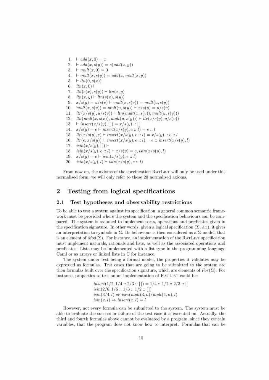
1. ` add(x, 0) = x2. ` add(x, s(y)) = s(add(x, y))3. ` mult(x, 0) = 04. ` mult(x, s(y)) = add(x,mult(x, y))5. ` ltn(0, s(x))6. ltn(x, 0) `7. ltn(s(x), s(y)) ` ltn(x, y)8. ltn(x, y) ` ltn(s(x), s(y))9. x/s(y) = u/s(v) ` mult(x, s(v)) = mult(u, s(y))

10. mult(x, s(v)) = mult(u, s(y)) ` x/s(y) = u/s(v)11. ltr(x/s(y), u/s(v)) ` ltn(mult(x, s(v)),mult(u, s(y)))12. ltn(mult(x, s(v)),mult(u, s(y))) ` ltr(x/s(y), u/s(v))13. ` insert(x/s(y), [ ]) = x/s(y) :: [ ]14. x/s(y) = e ` insert(x/s(y), e :: l) = e :: l15. ltr(x/s(y), e) ` insert(x/s(y), e :: l) = x/s(y) :: e :: l16. ltr(e, x/s(y)) ` insert(x/s(y), e :: l) = e :: insert(x/s(y), l)17. isin(x/s(y), [ ]) `18. isin(x/s(y), e :: l) ` x/s(y) = e, isin(x/s(y), l)19. x/s(y) = e ` isin(x/s(y), e :: l)20. isin(x/s(y), l) ` isin(x/s(y), e :: l)

From now on, the axioms of the specification RatList will only be used under thisnormalised form, we will only refer to these 20 normalised axioms.

2 Testing from logical specifications

2.1 Test hypotheses and observability restrictions

To be able to test a system against its specification, a general common semantic frame-work must be provided where the system and the specification behaviours can be com-pared. The system is assumed to implement sorts, operations and predicates given inthe specification signature. In other words, given a logical specification (Σ,Ax ), it givesan interpretation to symbols in Σ. Its behaviour is then considered as a Σ-model, thatis an element of Mod(Σ). For instance, an implementation of the RatList specificationmust implement naturals, rationals and lists, as well as the associated operations andpredicates. Lists may be implemented with a list type in the programming languageCaml or as arrays or linked lists in C for instance.

The system under test being a formal model, the properties it validates may beexpressed as formulas. Test cases that are going to be submitted to the system arethen formulas built over the specification signature, which are elements of For(Σ). Forinstance, properties to test on an implementation of RatList could be:

insert(1/2, 1/4 :: 2/3 :: [ ]) = 1/4 :: 1/2 :: 2/3 :: [ ]isin(2/6, 1/6 :: 1/3 :: 1/2 :: [ ])isin(3/4, l)⇒ isin(mult(3, n)/mult(4, n), l)isin(x, l)⇒ insert(x, l) = l

However, not every formula can be submitted to the system. The system must beable to evaluate the success or failure of the test case it is executed on. Actually, thethird and fourth formulas above cannot be evaluated by a program, since they containvariables, that the program does not know how to interpret. Formulas that can be

10

evaluated by the system under test are called observable formulas. Test cases then arechosen among observable formulas. When dealing with first-order specifications, theonly requirement is that test cases must not contain non-instantiated variables. Testcases for the third and fourth properties above must then be ground instances of theseformulas:

isin(3/4, 1/2 :: 3/4 :: [ ])⇒ isin(mult(3, 5)/mult(4, 5), 1/2 :: 3/4 :: [ ])isin(3/4, 12/16 :: [ ])⇒ isin(mult(3, 4)/mult(4, 4), 12/16 :: [ ])isin(3/5, [ ])⇒ insert(3/5, [ ]) = [ ]isin(2/6, 1/6 :: 1/3 :: [ ])⇒ insert(2/6, 1/6 :: 1/3 :: [ ]) = 1/6 :: 1/3 :: [ ]

Observable formulas then are all ground formulas. The set of observable formulas isdenoted by Obs.

We suppose in this paper that all sorts are observable, i.e. provided with a reli-able decidable equality procedure in the system under test. Dealing with non observ-able sorts adds technical issues which would make the paper more difficult to read.Actually, two facts should be taken into account [15]: non observable equalities areobserved through successive applications of functions leading to an observable result,usually called observable contexts; more embarrassing, one cannot in a pure black-boxtesting approach rely on some information based on non-observable equalities whoseoccurrences are in premisses of conditional equational formulas or more generally innegative positions in the axioms [22].

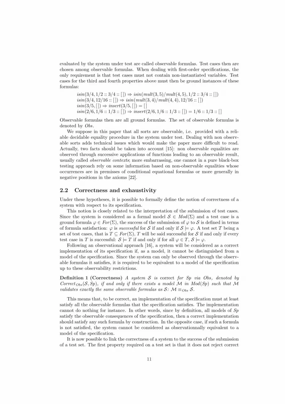
2.2 Correctness and exhaustivity

Under these hypotheses, it is possible to formally define the notion of correctness of asystem with respect to its specification.

This notion is closely related to the interpretation of the submission of test cases.Since the system is considered as a formal model S ∈ Mod(Σ) and a test case is aground formula ϕ ∈ For(Σ), the success of the submission of ϕ to S is defined in termsof formula satisfaction: ϕ is successful for S if and only if S |= ϕ. A test set T being aset of test cases, that is T ⊆ For(Σ), T will be said successful for S if and only if everytest case in T is successful: S |= T if and only if for all ϕ ∈ T , S |= ϕ.

Following an observational approach [16], a system will be considered as a correctimplementation of its specification if, as a model, it cannot be distinguished from amodel of the specification. Since the system can only be observed through the observ-able formulas it satisfies, it is required to be equivalent to a model of the specificationup to these observability restrictions.

Definition 1 (Correctness) A system S is correct for Sp via Obs, denoted byCorrectObs(S,Sp), if and only if there exists a model M in Mod(Sp) such that Mvalidates exactly the same observable formulas as S: M≡Obs S.

This means that, to be correct, an implementation of the specification must at leastsatisfy all the observable formulas that the specification satisfies. The implementationcannot do nothing for instance. In other words, since by definition, all models of Spsatisfy the observable consequences of the specification, then a correct implementationshould satisfy any such formula by construction. In the opposite case, if such a formulais not satisfied, the system cannot be considered as observationnally equivalent to amodel of the specification.

It is now possible to link the correctness of a system to the success of the submissionof a test set. The first property required on a test set is that it does not reject correct

11

systems. For instance, a correct implementation of RatList would be rejected by testcases like ltr(1/2, 1/3) or isin(2/5, [ ]) which do not hold for the specification. It couldalso be rejected by a test case like insert(1/2, 3/4 :: 1/3 :: [ ]) = 1/2 :: 3/4 :: 1/3 :: [ ]which is not part of the specification (the operation insert is not specified for unsortedlists). Therefore, such test cases are not wanted. A test set that does not reject correctsystems is called unbiased. Thus, if a system fails for an unbiased test set, it is provedto be incorrect.

Conversely, if a test set rejects any incorrect system (but perhaps also correct ones),it is called valid. Then if a system passes a valid test set, it is proved to be correct.Incorrect implementations would not be rejected by tautologies like 1/2 = 1/2 forinstance. As another example, an incorrect implementation of the operation isin forwhich isin(x, l) always holds would not be rejected by test cases like isin(3/4, 3/4 :: [ ])or isin(1/2, 1/3 :: 1/2 :: [ ]), that do not cover all the specified behaviours. Such testsets are not sufficient to reject incorrect systems, they cannot form a valid test set.

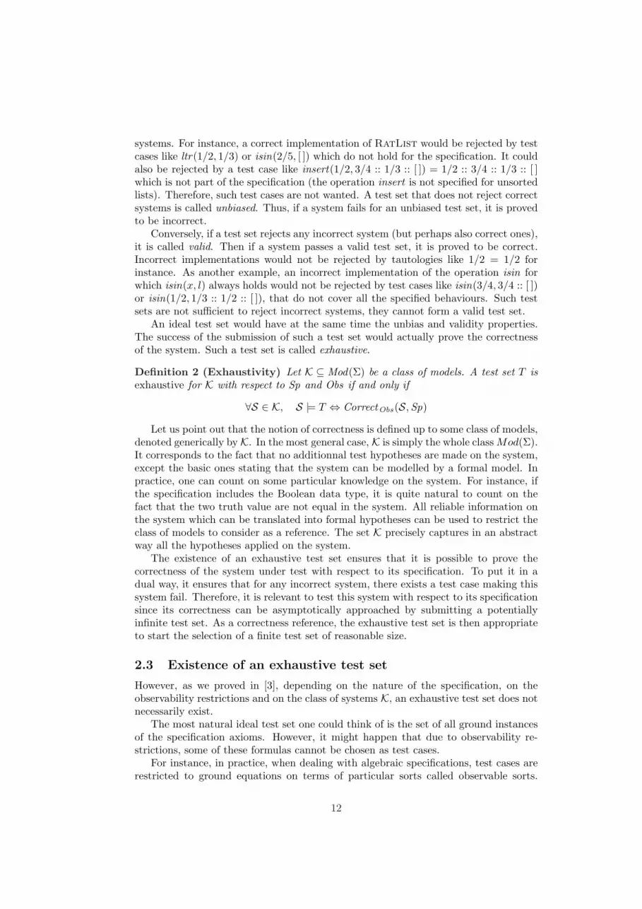
An ideal test set would have at the same time the unbias and validity properties.The success of the submission of such a test set would actually prove the correctnessof the system. Such a test set is called exhaustive.

Definition 2 (Exhaustivity) Let K ⊆ Mod(Σ) be a class of models. A test set T isexhaustive for K with respect to Sp and Obs if and only if

∀S ∈ K, S |= T ⇔ CorrectObs(S,Sp)

Let us point out that the notion of correctness is defined up to some class of models,denoted generically by K. In the most general case, K is simply the whole classMod(Σ).It corresponds to the fact that no additionnal test hypotheses are made on the system,except the basic ones stating that the system can be modelled by a formal model. Inpractice, one can count on some particular knowledge on the system. For instance, ifthe specification includes the Boolean data type, it is quite natural to count on thefact that the two truth value are not equal in the system. All reliable information onthe system which can be translated into formal hypotheses can be used to restrict theclass of models to consider as a reference. The set K precisely captures in an abstractway all the hypotheses applied on the system.

The existence of an exhaustive test set ensures that it is possible to prove thecorrectness of the system under test with respect to its specification. To put it in adual way, it ensures that for any incorrect system, there exists a test case making thissystem fail. Therefore, it is relevant to test this system with respect to its specificationsince its correctness can be asymptotically approached by submitting a potentiallyinfinite test set. As a correctness reference, the exhaustive test set is then appropriateto start the selection of a finite test set of reasonable size.

2.3 Existence of an exhaustive test set

However, as we proved in [3], depending on the nature of the specification, on theobservability restrictions and on the class of systems K, an exhaustive test set does notnecessarily exist.

The most natural ideal test set one could think of is the set of all ground instancesof the specification axioms. However, it might happen that due to observability re-strictions, some of these formulas cannot be chosen as test cases.

For instance, in practice, when dealing with algebraic specifications, test cases arerestricted to ground equations on terms of particular sorts called observable sorts.

12

These sorts are those equipped with an equality predicate in the programming lan-guage used to implement the system under test. In general, basic sorts like Booleansor integers are observable, but more complex data types like lists, trees or sets are not.Therefore, an axiom that would be an equation between terms of non-observable sortcannot be submitted as a test case since the oracle problem cannot be solved by thesystem under test. A classical answer to this problem is to assume that non-observablesorts are observable through observable contexts. For instance, a list L may be com-pared to another list L′ by first comparing their first element head(L) and head(L′),then their second one head(tail(L)) and head(tail(L′)), and so on. Then lists are mostof the time observed through contexts head(tailn(•)) which is, in general, sufficient.

Another problem arises when specification axioms are not themselves equations, butfor instance positive conditional formulas, that are a conjunction of equations implyingan equation. In this case, axioms cannot be directly submitted as test cases, since theydo not have the required form for test cases. A condition then has to be imposedto the system under test to ensure that the satisfaction of test cases as equations bythe system is sufficient to prove the satisfaction of axioms. This condition is calledinitiality and imposes that the system under test behaves like the initial algebra (andso like the specification) on premises of axioms. The class K must then be restrictedto systems satisfying this initiality condition. The interested reader may refer to [3] toa full study of conditions ensuring exhaustivity for algebraic specifications.

Moreover, as mentioned in the introduction, since the aim of testing is to make thesystem fail, the larger the exhaustive test set is, the better and the finer the detectionof failures will be.

Among all possible test sets, the largest one is the set of semantic consequences ofthe specification. As a matter of fact, to be correct, the system under test must beobservationally equivalent to a model of the specification, it must then satisfy exactlythe same observable formulas as this model does. Now, formulas satisfied by all themodels of a specification are by definition the semantic consequences of this specifica-tion, which set is denoted by Sp•. The system must then satisfy exactly the semanticconsequences of the specification which are observable, i.e. formulas in Sp• ∩Obs.

We show here that considering a specification Sp with quantifier-free first-orderaxioms and the set of all ground first-order formulas as the set of observable formulasObs, the exhaustivity of Sp• ∩Obs holds without conditions on the system under test,that is K = Mod(Σ).

Theorem 1 Let Sp = (Σ, Ax) be a quantifier-free first-order specification and Obs bethe set of all ground first-order formulas. Then Sp• ∩Obs is exhaustive for Mod(Σ).

Proof (⇒) Let S be a system, i.e. S ∈ Mod(Σ), such that S |= Sp• ∩ Obs. Let usshow that CorrectObs(S,Sp).

Define Th(S) = ϕ ∈ Obs | S |= ϕ. Let HTΣ ∈ Mod(Σ) be the Herbrandmodel of Th(S). By definition, we have that S ≡Obs HTΣ . Let us then show thatHTΣ ∈ Mod(Sp). Let ϕ be an axiom of Sp. Let ν : V → HTΣ be an assignment. Bydefinition, ν(ϕ) is a ground formula. By hypothesis, S |= ν(ϕ) and then HTΣ |= ν(ϕ).We conclude that HTΣ |=ν ϕ.

(⇐) Suppose that there existsM∈ Mod(Sp) such thatM≡Obs S. Let ϕ ∈ Sp•∩Obs.By hypothesis, M |= ϕ, then S |= ϕ as well. ¤

In [3], we generalised Theorem 1 by distinguishing observable and non-observablesorts. This requires a syntactical condition on the specification, where non-observable

13

atomic formulas must only appear at “positive” positions in the axioms (ϕ is at apositive position and ψ at a negative position in ϕ ∧ ¬ψ or in ψ ⇒ ϕ for instance).See [3] for a complete presentation of this result. We do not consider non-observablesorts here for sake of simplicity.

3 Selection criteria

When it exists, the exhaustive test set is the starting point for the selection of apractical test set. In practice, experts apply selection criteria on a reference test set inorder to extract a test set of reasonable size to submit to the system. The underlyingidea is that all the test cases satisfying a certain selection criterion allow to detect thesame class of incorrect systems. A selection criterion can then be seen as representinga fault model.

A selection criterion can be defined with respect to the size of the input data forinstance, or with respect to the different specified behaviours of a given functionality.As an example, let us consider an implementation of the operation computing themultiplication of two square matrices of size n × n, n ≥ 0. One can consider that, ifthe implementation is not correct, it can be detected for small values of n, let say lessthan 5. For n ≥ 5, it can be assumed that the implementation will behave in a uniformway. This selection criteria is called the regularity hypothesis [7]. The implementationis assumed to behave in a uniform way for all input data of size greater than a givenvalue. Therefore, in our example, it is sufficient to submit one test case for each valueof n between 1 and 4, and one test case for n ≥ 5, for instance with n = 7.

To give an example of another selection criterion, let us consider a function whosebehaviour depends on a given threshold value t for one of its argument a. This functionhas three distinct behaviours, for a < t, a = t and a > t. One can consider thatthe implementation of this function will behave in a uniform way for each of thesesets of values. This selection criterion is called the uniformity hypothesis [7]. Theimplementation is assumed to behave in a uniform way for all input data respecting agiven constraint. In other words, this hypothesis states that the test sets defined bythese constraints form equivalent classes of behaviours, then submitting one test casefor each of these classes is sufficient. Therefore, it is sufficient to submit one test casewith a < t, one with a = t and one with a > t to test the function of our example.

These two hypotheses are very classical since [7]. They have been used in andadapted to other contexts, for instance in the framework of conformance testing forreactive systems [28]. Most of the existing selection methods are based on them.The selection method presented in this paper is in particular based on the uniformityhypothesis. It is obvious that this hypothesis makes more sense for small test sets thanfor very large ones. The aim then is to divide the initial exhaustive test set into smallersets, so that this hypothesis can be applied in a meaningful way.

A classical method for selecting test sets with respect to a selection criterion Cconsists in dividing a reference test set T into a family of test subsets Tii∈IC(T ) insuch a way to preserve all test cases, i.e. T =

⋃i∈IC(T )

Ti. The application of a selectioncriterion associates a family of test sets to a given test set. All test cases in a test setTi are supposed to be equivalent to detect systems which are incorrect with respect tothe fault model captured by Ti. The application of a selection criterion to a given testset T allows to refine this test set. The obtained test subsets are more “specialised”than the initial test set, they correspond to more precise fault models than the oneassociated with T .

14

Definition 3 (Selection criterion) Let Exh be an exhaustive test set. A selectioncriterion C is a mapping4 P(Exh)→ P(P(Exh)).

For all T ⊆ Exh, C(T ) being a family of test sets Tii∈IC(T ) where IC(T ) is the setof indexes associated with the application of criterion C to T , we denote by |C(T )| theset

⋃

i∈IC(T )

Ti.

The construction of a test set relevant to a selection criterion must benefit from thedivision obtained by the application of this criterion. Test cases must be chosen so asnot to loose any of the cases captured by the criterion.

Definition 4 (Satisfaction of a selection criterion) Let T ⊆ Exh be a test setand C be a selection criterion. A test set T ′ satisfies the criterion C applied to T ifand only if:

T ′ ⊆ |C(T )| ∧ ∀i ∈ IC(T ), Ti 6= ∅ ⇒ T ′ ∩ Ti 6= ∅

A test set satisfying a selection criterion contains at least one test case of eachsubset Ti of the initial test set, when Ti is not empty. A selection criterion may thenbe considered as a coverage criterion, according to the way it divides the initial testset. It can be used to cover a particular aspect of the specification. In this paper, thedefinition of selection criteria will be based on the coverage of the specification axioms.This selection method is called partition testing.

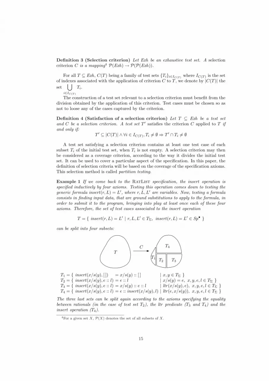
Example 1 If we come back to the RatList specification, the insert operation isspecified inductively by four axioms. Testing this operation comes down to testing thegeneric formula insert(r, L) = L′, where r, L, L′ are variables. Now, testing a formulaconsists in finding input data, that are ground substitutions to apply to the formula, inorder to submit it to the program, bringing into play at least once each of these fouraxioms. Therefore, the set of test cases associated to the insert operation

T = insert(r, L) = L′ | r, L, L′ ∈ TΣ, insert(r, L) = L′ ∈ Sp•

can be split into four subsets:

T1 T2 T3

T4CT

T1 = insert(x/s(y), [ ]) = x/s(y) :: [ ] | x, y ∈ TΣ T2 = insert(x/s(y), e :: l) = e :: l | x/s(y) = e, x, y, e, l ∈ TΣ T3 = insert(x/s(y), e :: l) = x/s(y) :: e :: l | ltr(x/s(y), e), x, y, e, l ∈ TΣ T4 = insert(x/s(y), e :: l) = e :: insert(x/s(y), l) | ltr(e, x/s(y)), x, y, e, l ∈ TΣ

The three last sets can be split again according to the axioms specifying the equalitybetween rationals (in the case of test set T2), the ltr predicate (T3 and T4) and theinsert operation (T4).

4For a given set X, P(X) denotes the set of all subsets of X.

15

The relevance of a selection criterion is determined by the link between the initialtest set and the family of test sets obtained by the application of this criterion.

Definition 5 (Properties) Let C be a selection criterion and T be a test set.

• C is said sound for T if and only if |C(T )| ⊆ T• C is said complete for T if and only if |C(T )| ⊇ T

These properties are essential for the definition of an appropriate selection criterion.The soundness of a criterion ensures that test cases are really selected among the initialtest set. The application of the criterion does not add any new test case. Additionaltest cases may actually bias the test set, making a correct system fail. Reciprocally,if the selection criterion is complete, no test case of the initial test set is lost. If sometest cases are missing, an incorrect system may pass the test set, while it should havefailed on the missing test cases. A sound and complete selection criterion then has theproperty to preserve exactly all the test cases of the test set it divides, and then topreserve the unbias and the validity (and so the exhaustivity) of the initial test set.

4 Axiom unfolding

Building a test set to submit to the system consists in defining a method for dividing theinitial test set into subsets and then, assuming the uniformity hypothesis, in choosingone test case in each of the obtained subsets. We will here present our method fordefining relevant selection criteria in order to guide the final choice of the test cases.The application of the selection criteria will allow to refine the initial test set bycharacterising test subsets which respect given constraints on the input data.

4.1 Test sets for quantifier-free first-order formulas

The selection method we are going to present is called axiom unfolding and is basedon a case analysis of the specification. This procedure was first defined for positiveconditional specifications [6, 7, 25, 1], i.e. axioms are formulas where a conjunction ofequations implies another equation. In this setting, test cases are only equations. Theexhaustive test set is the set of equations of the form f(t1, . . . , tn) = t where f is anoperation of the signature, t1, . . . , tn, t are ground terms and such that this equation isa semantic consequence of the specification. To divide this initial test set comes downto dividing each test set associated to a given operation of the signature. The equationf(t1, . . . , tn) = t characterising this test set (when f is given) is called a test purpose.The operation f is specified by a certain number of axioms in the specification, whichdefine the behaviour of this operation by cases, according to the different values of itsinputs. The set of test cases for f will then be divided according to these different cases,that are the different axioms specifying this operation, as we showed in the previoussection in Example 1.

Here, we generalise this procedure to quantifier-free first-order specifications. Sincea test case may be any quantifier-free first-order formula, dividing the initial exhaustivetest set comes down to dividing each test set associated to a given formula, chosen tobe a test purpose. The test set associated to a formula naturally is the set of groundinstances of this formula which are consequences of the specification.

16

Definition 6 (Test set for a formula) Let Sp = (Σ,Ax ) be a quantifier-free first-order specification. Let ϕ be a quantifier-free first-order formula, called test purpose.The test set for ϕ, denoted by Tϕ, is the following set:

Tϕ = ρ(ϕ) | ρ : V → TΣ, ρ(ϕ) ∈ Sp• ∩Obs

Note that the formula taken as a test purpose may be any formula, not necessarilya semantic consequence of the specification. However, only substitutions ρ such thatρ(ϕ) is a semantic consequence of Sp will be built at the generation step.

Example 2 Here are some test purposes for the signature of the specification RatList,with examples of associated test cases.

add(x, 0) = x. Since add(x, 0) = x is an axiom, all ground instances of this formulaare test cases: add(0, 0) = 0, add(6, 0) = 6, etc.

ltr(u, v). This predicate is under-specified, the case where a rational is of the form x/0is not taken into account, so there cannot be tests on this case. Test cases maybe: ltr(1/3, 1/2), ltr(4/8, 4/6), etc.

add(m,n) = mult(m, 2). Only cases where m = n are semantic consequences of thespecification, such as add(2, 2) = mult(2, 2), add(5, 5) = mult(5, 2), etc.

insert(r, l) = [ ]. The formula is never satisfied for any ground instance of r and l, sothere is no possible test case.

As we showed on Example 1, the test set for a formula is divided into subsets,that are themselves test sets for different instances of the initial test purpose, undercertain constraints. Each of these test subsets can be characterised by a substitutionσ, allowing to map the initial test purpose to its corresponding instance, and a set ofconstraints C. For instance, the test set T2 of Example 1

T2 = insert(x/s(y), e :: l) = e :: l | x/s(y) = e, x, y, e, l ∈ TΣ

may be characterised by the pair (C, σ) where

C = x/s(y) = e σ : r 7→ x/s(y)L 7→ e :: lL′ 7→ e :: l

These test subsets, obtained by the application of a criterion, will be called constrainedtest sets.

Definition 7 (Constrained test set) Let Sp = (Σ,Ax ) be a quantifier-free first-order specification. Let ϕ be a quantifier-free first-order formula. Let C be a set ofquantifier-free first-order formulas called Σ-constraints and σ : V → TΣ(V ) be a sub-stitution. A test set for ϕ constrained by C and σ, denoted by T(C,σ),ϕ, is the followingset of ground formulas:

T(C,σ),ϕ = ρ(σ(ϕ)) | ρ : V → TΣ, ρ(σ(ϕ)) ∈ Sp• ∩Obs,∀ψ ∈ C, ρ(ψ) ∈ Sp• ∩Obs

The pair ((C, σ), ϕ) is called a constrained test purpose.

17

Note that the test purpose of Definition 6 can be seen as the constrained testpurpose ((ϕ, Id), ϕ).

Example 3 Examples of constrained test purposes may be the following:(

( ∅ , σ : x 7→ s(u) ), add(x, 0) = x)

(( ltn(3, x) , Id ), add(x, 0) = x

)

(( ltn(x, z) , σ : u 7→ x/s(y) ), ltr(u, v)

)v 7→ z/s(y)

As another example, to come back to Example 1 where we split the test set associatedto insert(r, L) = L′ into four subsets, we can express each of them as constrained testpurposes as follows:

(( ∅ , σ1 : r 7→ x/s(y) ), insert(r, L) = L′

)L 7→ [ ]L′ 7→ x/s(y) :: [ ]

(( x/s(y) = e , σ2 : r 7→ x/s(y) ), insert(r, L) = L′

)L 7→ e :: lL′ 7→ e :: l

(( ltr(x/s(y), e) , σ3 : r 7→ x/s(y) ), insert(r, L) = L′

)L 7→ e :: lL′ 7→ x/s(y) :: e :: l

(( ltr(e, x/s(y)) , σ4 : r 7→ x/s(y) ), insert(r, L) = L′

)L 7→ e :: lL′ 7→ e :: insert(x/s(y), l)

Only this kind of constrained test purposes, built from a case analysis of the specificationaxioms, will be of interest. The aim of the unfolding procedure we will introduce in thenext section is to build such test sets.

4.2 Unfolding procedure

In practice, the initial test purpose is not constrained. The aim of the unfoldingprocedure is to replace it with a set of constrained test purposes, using the specificationaxioms. This procedure is an algorithm with the following inputs:

• a quantifier-free first-order specification Sp = (Σ,Ax ) where axioms of Ax havebeen transformed into normalised sequents

• a quantifier-free first-order formula ϕ seen as the initial test purpose.

As we already said, the initial test purpose ϕ can be seen as the constrained testpurpose ((ϕ, Id), ϕ), or even ((C0, Id), ϕ) where C0 is the set of normalised sequentsobtained from ϕ. Let Ψ0 be the set containing the initial constraints of test purposeϕ, the pair (C0, Id). Constrained test sets for formulas are naturally extended to setsof pairs Ψ as follows:

TΨ,ϕ =⋃

(C,σ)∈Ψ

T(C,σ),ϕ

18

The initial test set Tϕ then is the set TΨ0,ϕ.The aim of the procedure is to divide this set according to the different cases in

which formula ϕ holds. These cases correspond to the different instances of ϕ that canbe proved as theorems, i.e. that can be deduced from the specification axioms usingthe calculus we gave in Section 1. So basically, the procedure searches for those prooftrees that allow to deduce (instances of) the initial test purpose from the specificationaxioms. However, the aim is not to build the complete proofs of these instances of ϕ,but only to make a partition of TΨ0,ϕ increasingly fine. A first step in the constructionof the proof tree of each instance will give us pending lemmas, constraints remainingto prove that, together with the right substitution, characterise each instance of ϕ.We will thus be able to replace Ψ0, which contains only one constraint, with a set ofconstraints Ψ1 characterising each instance of ϕ that can be proved from the axioms.The set Ψ1 can itself be replaced with a bigger set Ψ2 obtained from a second step inthe construction of the previous proof trees, and so on. The procedure can be stoppedat any moment, as soon as the tester is satisfied with the obtained partition.

Note that the procedure only intends to divide the test set associated to a givenformula, by returning a set of constraints which characterise each set of the partition.The generation phase, not handled in this paper, consists in choosing one test case ineach set of the partition (assuming the uniformity hypothesis) by solving the constraintsassociated to each set (which might be an issue in itself, due to the nature of theseconstraints).

The general case. As already explained, the procedure tries to divide the initialtest set associated to a test purpose ϕ into test subsets by searching for proof trees ofdifferent instances of ϕ from the specification axioms. To achieve this purpose, it triesto unify the test purpose with an axiom, or more precisely, it tries to unify a subset ofthe test purpose’s subformulas with a subset of an axiom’s subformulas. Hence, if thetest purpose is a normalised sequent of the form

γ1, . . . , γp, . . . , γm ` δ1, . . . , δq, . . . , δnthe procedure tries to unify a subset of γ1, . . . , γm, δ1, . . . , δn with a subset of theformulas of an axiom. Then it looks for a specification axiom of the form

ψ1, . . . , ψp, ξ1, . . . , ξl ` ϕ1, . . . , ϕq, ζ1, . . . , ζk

such that it is possible to unify ψi and γi for all i, 1 ≤ i ≤ p, and ϕi and δi for all i,1 ≤ i ≤ q.

Now we have to ensure that it is actually possible to prove (an instance of) thetest purpose from this axiom. The inference rule which is fundamental at this stage isthe Cut rule. It allows at the same time to delete the subformulas of the axiom thatcannot be unified with subformulas of the test purpose, and to add the subformulas ofthe test purpose that do not exist in the axiom. To give a general picture, we have thefollowing matching between the two formulas:

to delete to delete

Axiom ψ1, . . . , ψp︸︷︷︸,︷︸︸︷ξ1, . . . , ξl `ϕ1, . . . , ϕq︸︷︷︸,

︷︸︸︷ζ1, . . . , ζk

unification unification

Test purpose︷︸︸︷γ1, . . . , γp, γp+1, . . . , γm︸︷︷︸`

︷︸︸︷δ1, . . . , δq, δq+1, . . . , δn︸︷︷︸

to add to add

19

The additional formulas of the axiom and the missing formulas of the test purpose willbe added or deleted thanks to applications of the cut rule. The proof will then consistof two steps.

1. First, we apply to the axiom the substitution σ that allows the unification.

2. Then, we cut one by one each formula of the axiom that cannot be unified witha subformula of the test purpose. This gives us a set of lemmas (the proof treeleaves) needed to complete the proof, the constraints. The last subformula to becut also allows to add the missing subformulas. This is possible because in thepremises of the rule, Γ, ∆ and Γ′, ∆′ may be different.

The unifying substitution σ and the set of constraints given by the pending lemmasthus define a constrained test set characterising the instance of the test purpose wemanage to prove.

If we denote by Γ the set of formulas γ1, . . . , γp, Γ′ the set γp+1, . . . , γm, ∆ theset δ1, . . . , δq and ∆′ the set δq+1, . . . , δn, we get a proof tree of the following form:

...σ(Γ′) ` σ(ξl), σ(∆′)

...` σ(ξ1)

STσ(Γ), σ(ξ2), . . . , σ(ξl)`σ(∆)Cut

... Cut

σ(Γ), σ(ξl) ` σ(∆) Cut

σ(Γ), σ(Γ′) ` σ(∆), σ(∆′) Cut

where ST is the following subtree:

SubsΓ, ξ1, . . . , ξl ` ∆, ζ1, . . . , ζk

Ax

σ(Γ), σ(ξ1), . . . , σ(ξl) ` σ(∆), σ(ζ1), . . . , σ(ζk)

...σ(ζ1) `

σ(Γ), σ(ξ1), . . . , σ(ξl) ` σ(ζ2), . . . , σ(ζk), σ(∆) Cut

... Cut

σ(Γ), σ(ξ1), . . . , σ(ξl) ` σ(∆), σ(ζk)Cut

...σ(ζk) `

σ(Γ), σ(ξ1), . . . , σ(ξl) ` σ(∆) Cut

As this proof tree shows, after having applied the substitution unifying some subfor-mulas of the axiom with some subformulas of the test purpose (the formula to prove),l+k applications of the Cut rule allow to delete the l subformulas of the left-hand sideof the axiom and the k subformulas of its right-hand side, and moreover, allow to addthe formulas of Γ′ and ∆′.

The case of equality. In order to deal more efficiently with equality, this is theparamodulation rule that is used. When an axiom contains an equation, it can be usedto replace a subterm of a formula with another subterm, equal to it according to thisaxiom. This rule makes the procedure more efficient to handle equality than standardfirst-order calculus, since it allows to use the replacement of equal by equal principle.So the procedure tries to unify a subterm of a subformula of the test purpose with oneof the members of an equation in an axiom. Hence, if the test purpose is a normalisedsequent of the form

γ1, . . . , γp, . . . , γm ` δ1, . . . , δq, . . . , δn

20

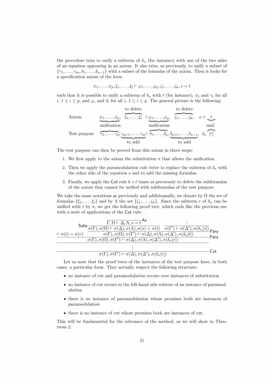
the procedure tries to unify a subterm of δn (for instance) with one of the two sidesof an equation appearing in an axiom. It also tries, as previously, to unify a subset ofγ1, . . . , γm, δ1, . . . , δn−1 with a subset of the formulas of the axiom. Then it looks fora specification axiom of the form

ψ1, . . . , ψp, ξ1, . . . , ξl ` ϕ1, . . . , ϕq, ζ1, . . . , ζk, s = t

such that it is possible to unify a subterm of δn with t (for instance), ψi and γi for alli, 1 ≤ i ≤ p, and ϕi and δi for all i, 1 ≤ i ≤ q. The general picture is the following:

to delete to delete

Axiom ψ1, . . . , ψp︸︷︷︸,︷︸︸︷ξ1, . . . , ξl `ϕ1, . . . , ϕq︸︷︷︸,

︷︸︸︷ζ1, . . . , ζk, s = t︸︷︷︸

unification unification unif.

Test purpose︷︸︸︷γ1, . . . , γp, γp+1, . . . , γm︸︷︷︸`

︷︸︸︷δ1, . . . , δq, δq+1, . . . , δn−1︸︷︷︸, δn

︷︸︸︷[r]

to add to add

The test purpose can then be proved from this axiom in three steps:

1. We first apply to the axiom the substitution σ that allows the unification.

2. Then we apply the paramodulation rule twice to replace the subterm of δn withthe other side of the equation s and to add the missing formulas.

3. Finally, we apply the Cut rule k+ l times as previously to delete the subformulasof the axiom that cannot be unified with subformulas of the test purpose.

We take the same notations as previously and additionnally, we denote by Ω the set offormulas ξ1, . . . , ξl and by Λ the set ζ1, . . . , ζk. Since the subterm r of δn can beunified with t by σ, we get the following proof tree, which ends like the previous onewith a serie of applications of the Cut rule:

` σ(t) = σ(r)

SubsΓ,Ω ` ∆,Λ, s = t

Ax

σ(Γ), σ(Ω) ` σ(∆), σ(Λ), σ(s) = σ(t)

...σ(Γ′) ` σ(∆′), σ(δn[s])

σ(Γ), σ(Ω), σ(Γ′) ` σ(∆), σ(Λ), σ(∆′), σ(δn[t])Para

σ(Γ), σ(Ω), σ(Γ′) ` σ(∆), σ(Λ), σ(∆′), σ(δn[r])Para

...σ(Γ), σ(Γ′) ` σ(∆), σ(∆′), σ(δn[r])

Cut

Let us note that the proof trees of the instances of the test purpose have, in bothcases, a particular form. They actually respect the following structure:

• no instance of cut and paramodulation occurs over instances of substitution

• no instance of cut occurs in the left-hand side subtree of an instance of paramod-ulation

• there is no instance of paramodulation whose premises both are instances ofparamodulation

• there is no instance of cut whose premises both are instances of cut.

This will be fundamental for the relevance of the method, as we will show in Theo-reom 2.

21

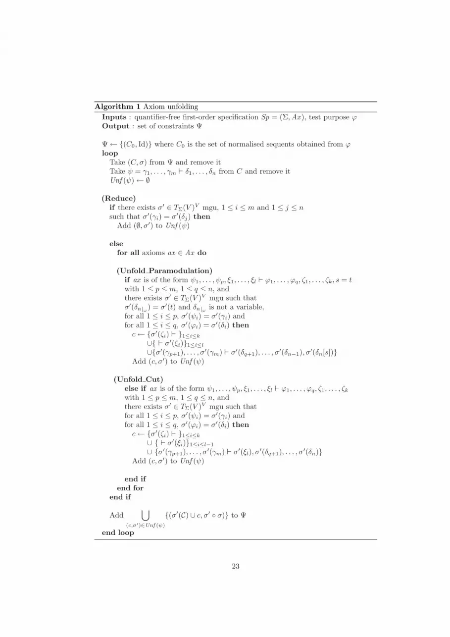
The algorithm. The unfolding procedure is formally described by the followingalgorithm.5 What it unfolds is a constraint ψ from a set of constraints C associatedto some substitution σ in a pair of constraints (C, σ). The first set of constraints C0only containing the initial test purpose, the procedure starts with unfolding this testpurpose. It builds a set Unf (ψ) representing the unfolding of ψ and containing all thepairs of constraints and substitution obtained by unfolding. Then it will unfold theconstraints obtained from the unfolding of the test purpose, which will be consideredthemselves as test purposes, and so on. Given a constraint ψ = γ1, . . . , γm ` δ1, . . . , δn,the algorithm can be synthesised in the following way.

(Reduce) The first verification to make is whether some instances of the constraint aretautologies. If it is possible to unify some γi with some δj thanks to a substitutionσ, then σ(ψ) always holds and is useless. σ(ψ) is then removed from the set ofconstraints associated to the corresponding instance of the test purpose.

(Unfold Paramodulation) This is the part of the algorithm dealing with equality.If a subterm of a formula in the constraint can be unified with one of the membersof an equation appearing in an axiom, and a subset of the other formulas of theconstraint can be unified with a subset of the other formulas of the axiom, thenit is possible to prove the constraint from this axiom with two applications ofthe paramodulation rule and a certain number of applications of the Cut rule.In this case, the set of constraints that is built is the set of all σ′(ζi) ` for ibetween 1 and k and all ` σ′(ξi) for i between 1 and l, to which is added thelemma σ′(γp+1), . . . , σ′(γm) ` σ′(δq+1), . . . , σ′(δn−1), σ′(δn[s]) needed to applythe paramodulation rule. It simply means that if a subterm of δn can be unifiedwith t thanks to a substitution σ′, then this subterm can be replaced with s inσ′(δn).

(Unfold Cut) If the paramodulation rule cannot be used to unfold the constraint ψ,it is checked whether the Cut rule can be used alone. As explained before, if a partof the constraint can be unified with a part of an axiom, then we know that theconstraint can be proved from this axiom with a certain number of applicationsof the Cut rule where, as in the previous case, each σ′(ζi) ` for i between 1and k and each ` σ′(ξi) for i between 1 and l is a lemma remaining to prove.One of those lemmas must bring the missing formulas, so σ′(ξl) is in the contextσ′(γp+1), . . . , σ′(γm) ` σ′(ξl), σ′(δq+1), . . . , σ′(δn).

Then the procedure replaces the initial constraint ψ with each of the sets of constraintsin Unf (ψ). Each unification with an axiom leads to a pair (c, σ′), so the initial con-straint ψ is replaced with as many sets of formulas as there are axioms with whichit can be unified. The definition of Unf (ψ) being based on unification, this set iscomputable if the specification has finitely many axioms.

Termination of the unfolding procedure is unlikely, since it is not checked, duringits execution, whether the formula ϕ is a semantic consequence of the specificationor not. Actually, this will be done during the generation phase, not handled in thispaper. As we already explained, the aim of the unfolding procedure is not to find thecomplete proof of formula ϕ, but to make a partition of Tϕ increasingly fine. Hence theprocedure can be stopped at any moment, when the obtained partition is fine enoughaccording to the judgement or the needs of the tester. The idea is to stretch further

5In the algorithm, δn|ω is the subterm appearing at position ω in δn, where positions in terms aredefined by words over naturals, following the standard numbering of tree nodes.

22

Algorithm 1 Axiom unfoldingInputs : quantifier-free first-order specification Sp = (Σ,Ax ), test purpose ϕOutput : set of constraints Ψ

Ψ← (C0, Id) where C0 is the set of normalised sequents obtained from ϕloop

Take (C, σ) from Ψ and remove itTake ψ = γ1, . . . , γm ` δ1, . . . , δn from C and remove itUnf (ψ)← ∅

(Reduce)if there exists σ′ ∈ TΣ(V )V mgu, 1 ≤ i ≤ m and 1 ≤ j ≤ nsuch that σ′(γi) = σ′(δj) then

Add (∅, σ′) to Unf (ψ)

elsefor all axioms ax ∈ Ax do

(Unfold Paramodulation)if ax is of the form ψ1, . . . , ψp, ξ1, . . . , ξl ` ϕ1, . . . , ϕq, ζ1, . . . , ζk, s = twith 1 ≤ p ≤ m, 1 ≤ q ≤ n, andthere exists σ′ ∈ TΣ(V )V mgu such thatσ′(δn|ω ) = σ′(t) and δn|ω is not a variable,for all 1 ≤ i ≤ p, σ′(ψi) = σ′(γi) andfor all 1 ≤ i ≤ q, σ′(ϕi) = σ′(δi) thenc← σ′(ζi) ` 1≤i≤k∪ ` σ′(ξi)1≤i≤l∪σ′(γp+1), . . . , σ′(γm) ` σ′(δq+1), . . . , σ′(δn−1), σ′(δn[s])

Add (c, σ′) to Unf (ψ)

(Unfold Cut)else if ax is of the form ψ1, . . . , ψp, ξ1, . . . , ξl ` ϕ1, . . . , ϕq, ζ1, . . . , ζkwith 1 ≤ p ≤ m, 1 ≤ q ≤ n, andthere exists σ′ ∈ TΣ(V )V mgu such thatfor all 1 ≤ i ≤ p, σ′(ψi) = σ′(γi) andfor all 1 ≤ i ≤ q, σ′(ϕi) = σ′(δi) thenc← σ′(ζi) ` 1≤i≤k∪ ` σ′(ξi)1≤i≤l−1

∪ σ′(γp+1), . . . , σ′(γm) ` σ′(ξl), σ′(δq+1), . . . , σ′(δn)Add (c, σ′) to Unf (ψ)

end ifend for

end if

Add⋃

(c,σ′)∈Unf (ψ)

(σ′(C) ∪ c, σ′ σ) to Ψ

end loop

23

the execution of the procedure in order to make increasingly big proof trees whoseremaining lemmas are constraints. If ϕ is not a semantic consequence of Sp, thenthis means that, among remaining lemmas, some of them do not hold, and then theassociated test set is empty.

Given a formula ψ, the unfolding procedure defines the selection criterion Cψ whichmaps T(C,σ),ϕ to the family of test sets T(σ′(Crψ)∪c,σ′σ),ϕ for each (c, σ′) in Unf (ψ)if ψ belongs to C, and to itself otherwise. To ensure the relevance of this selectioncriterion, it must be shown that its application does not add new test cases to T(C,σ),ϕ

(soundness) or remove test cases from it (completeness). These results are proved inthe next subsection.

Coverage of the exhaustive test set. Here, our unfolding procedure has beendefined in order to cover behaviours of one test purpose, represented by the formulaϕ. When we are interested in covering more widely the exhaustive set Sp• ∩ Obs, astrategy consists in ordering quantifier-free first-order formulas with respect to theirlength, as follows:

Φ0 =

` p(x1, . . . , xn),` f(x1, . . . , xn) = y

p : s1 × . . .× sn ∈ P,f : s1 × . . .× sn → s ∈ F,∀i, 1 ≤ i ≤ n, xi ∈ Vsi , y ∈ Vs

Φn+1 =

p(x1, . . . , xn),Γ ` ∆,f(x1, . . . , xn) = y,Γ ` ∆,

Γ ` ∆, p(x1, . . . , xn),Γ ` ∆, f(x1, . . . , xn) = y

Γ ` ∆ ∈ Φn,p : s1 × . . .× sn ∈ P,f : s1 × . . .× sn → s ∈ F,∀i, 1 ≤ i ≤ n, xi ∈ Vsi , y ∈ Vs

Then, to manage the size (often infinite) of Sp•∩Obs, we start by choosing k ∈ N, andthen we apply for every i, 1 ≤ i ≤ k, the above unfolding procedure to each formulabelonging to Φi. Of course, this requires that signatures are finite so that each set Φiis finite too.

Example 4 First, to show the handling of equality with the paramodulation rule, westart with the formula of Example 1: insert(r, L) = L′. The associated constrained testpurpose for this formula is

((` insert(r, L) = L′, Id), insert(r, L) = L′)

We denote by Ψ0 the set containing this first pair of constraints. After a loop of thealgorithm, where the chosen constraint ψ is necessarily ` insert(r, L) = L′, we obtainthe following set Ψ1 (each pair is labelled by the number of the axiom used for theunfolding of the initial formula):

Ψ1 = ( ` x0/s(y0) :: [ ] = L′ , σ1 : r 7→ x0/s(y0) ) (13)L 7→ [ ]

( ` x0/s(y0) = e0, , σ2 : r 7→ x0/s(y0) ) (14)` e0 :: l0 = L′ L 7→ e0 :: l0

( ` ltr(x0/s(y0), e0), , σ3 : r 7→ x0/s(y0) ) (15)` x0/s(y0) :: e0 :: l0 = L′ L 7→ e0 :: l0

( ` ltr(e0, x0/s(y0)), , σ4 : r 7→ x0/s(y0) ) (16)` e0 :: insert(x0/s(y0), l0) = L′ L 7→ e0 :: l0

24

We get the same four sets as in Examples 1 and 3, although they are expressed a bitdifferently. The four sets of Example 3 are what we would have obtained with theapplication of the (Unfold Cut) part of the algorithm. We can see here that usingparamodulation results in simpler substitutions and more constraints, which allows tounfold more finely the initial formula. For instance, the last constraint in the fourthset ` e0 :: insert(x0/s(y0), l0) = L′ was kept implicit in the substitution given in thefourth set of Example 3, which prevents from unfolding it as we can do here.

Actually, we now show the unfolding of this last constraint. We get the followingset, which replaces the fourth set above (the new substitution is already composed withthe previous one):

( ` ltr(e0, x0/s(y0)), , σ′1 : r 7→ x0/s(y0) ) (13)` e0 :: x0/s(y0) :: [ ] = L′ L 7→ e0 :: [ ]

( ` ltr(e0, x0/s(y0)), , σ′2 : r 7→ x0/s(y0) ) (14)` x0/s(y0) = e1, L 7→ e0 :: e1 :: l1` e0 :: e1 :: l1 = L′

( ` ltr(e0, x0/s(y0)), , σ′3 : r 7→ x0/s(y0) ) (15)` ltr(x0/s(y0), e1), L 7→ e0 :: e1 :: l1` e0 :: x0/s(y0) :: e1 :: l1 = L′

( ` ltr(e0, x0/s(y0)), , σ′4 : r 7→ x0/s(y0) ) (16)` ltr(e1, x0/s(y0)), L 7→ e0 :: e1 :: l1` e0 :: e1 :: insert(x0/s(y0), l1) = L′

To see that these sets correspond to what we expect from the procedure, we can writethem in a more natural way:

insert(x0/s(y0), e0 :: [ ]) = e0 :: x0/s(y0) :: [ ] | ltr(e0, x0/s(y0))insert(x0/s(y0), e0 :: e1 :: l1) = e0 :: e1 :: l1 | ltr(e0, x0/s(y0))

x0/s(y0) = e1insert(x0/s(y0), e0 :: e1 :: l1) = e0 :: x0/s(y0) :: e1 :: l1 | ltr(e0, x0/s(y0))

ltr(x0/s(y0), e1)insert(x0/s(y0), e0 :: e1 :: l1) = e0 :: e1 :: insert(x0/s(y0), l1) | ltr(e0, x0/s(y0))

ltr(e1, x0/s(y0))We could have unfolded any other constraint of one of the first four sets, according tothe axioms specifying the predicates over rationals for instance.

Example 5 To show a complete example where cut and paramodulation are used, wetake the formula isin(r, L) ⇒ insert(r, L) = L′. This formula does not hold for everysubstitution of the variables. If L is not the empty list, the instances where L = L′

only are consequences of the specification (as well as instances where isin(r, L) does nothold, but these one are of no interest for our purpose). The unfolding of this formulawill then lead to two kinds of constraints: those where L = L′ that will actually becometest cases since they are consequences of the specification, and those where L 6= L′ thatwill not lead to test cases. The procedure cannot distinguish between these two kinds ofconstraints. However, before being submitted to the system, a ground substitution ρ isapplied to constrained test purposes. Since by definition, ρ(ϕ) has to be a consequenceof the specification, the constraints where L 6= L′ will not be submitted as test cases tothe system.

25

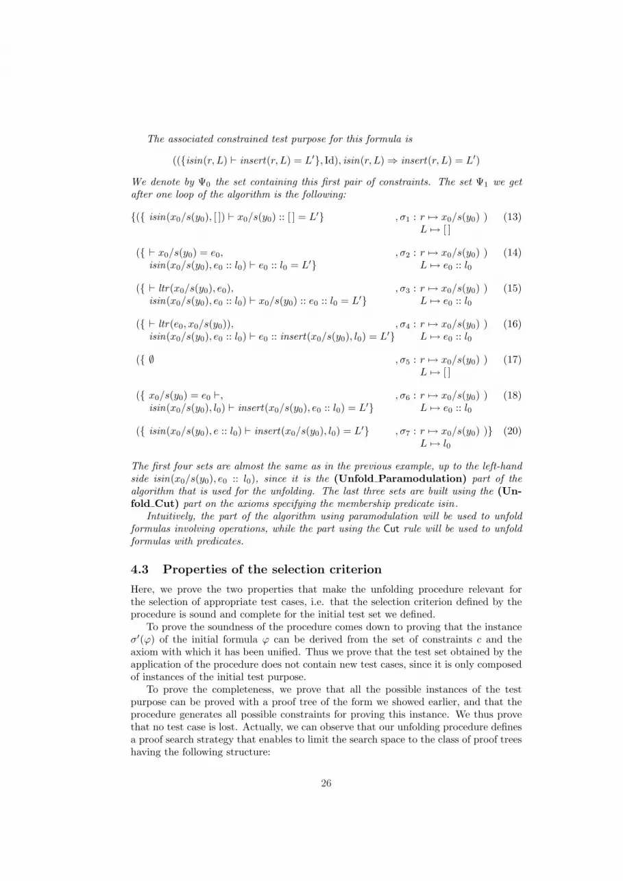
The associated constrained test purpose for this formula is

((isin(r, L) ` insert(r, L) = L′, Id), isin(r, L)⇒ insert(r, L) = L′)

We denote by Ψ0 the set containing this first pair of constraints. The set Ψ1 we getafter one loop of the algorithm is the following:

( isin(x0/s(y0), [ ]) ` x0/s(y0) :: [ ] = L′ , σ1 : r 7→ x0/s(y0) ) (13)L 7→ [ ]

( ` x0/s(y0) = e0, , σ2 : r 7→ x0/s(y0) ) (14)isin(x0/s(y0), e0 :: l0) ` e0 :: l0 = L′ L 7→ e0 :: l0

( ` ltr(x0/s(y0), e0), , σ3 : r 7→ x0/s(y0) ) (15)isin(x0/s(y0), e0 :: l0) ` x0/s(y0) :: e0 :: l0 = L′ L 7→ e0 :: l0

( ` ltr(e0, x0/s(y0)), , σ4 : r 7→ x0/s(y0) ) (16)isin(x0/s(y0), e0 :: l0) ` e0 :: insert(x0/s(y0), l0) = L′ L 7→ e0 :: l0

( ∅ , σ5 : r 7→ x0/s(y0) ) (17)L 7→ [ ]

( x0/s(y0) = e0 `, , σ6 : r 7→ x0/s(y0) ) (18)isin(x0/s(y0), l0) ` insert(x0/s(y0), e0 :: l0) = L′ L 7→ e0 :: l0

( isin(x0/s(y0), e :: l0) ` insert(x0/s(y0), l0) = L′ , σ7 : r 7→ x0/s(y0) ) (20)L 7→ l0

The first four sets are almost the same as in the previous example, up to the left-handside isin(x0/s(y0), e0 :: l0), since it is the (Unfold Paramodulation) part of thealgorithm that is used for the unfolding. The last three sets are built using the (Un-fold Cut) part on the axioms specifying the membership predicate isin.

Intuitively, the part of the algorithm using paramodulation will be used to unfoldformulas involving operations, while the part using the Cut rule will be used to unfoldformulas with predicates.

4.3 Properties of the selection criterion

Here, we prove the two properties that make the unfolding procedure relevant forthe selection of appropriate test cases, i.e. that the selection criterion defined by theprocedure is sound and complete for the initial test set we defined.

To prove the soundness of the procedure comes down to proving that the instanceσ′(ϕ) of the initial formula ϕ can be derived from the set of constraints c and theaxiom with which it has been unified. Thus we prove that the test set obtained by theapplication of the procedure does not contain new test cases, since it is only composedof instances of the initial test purpose.

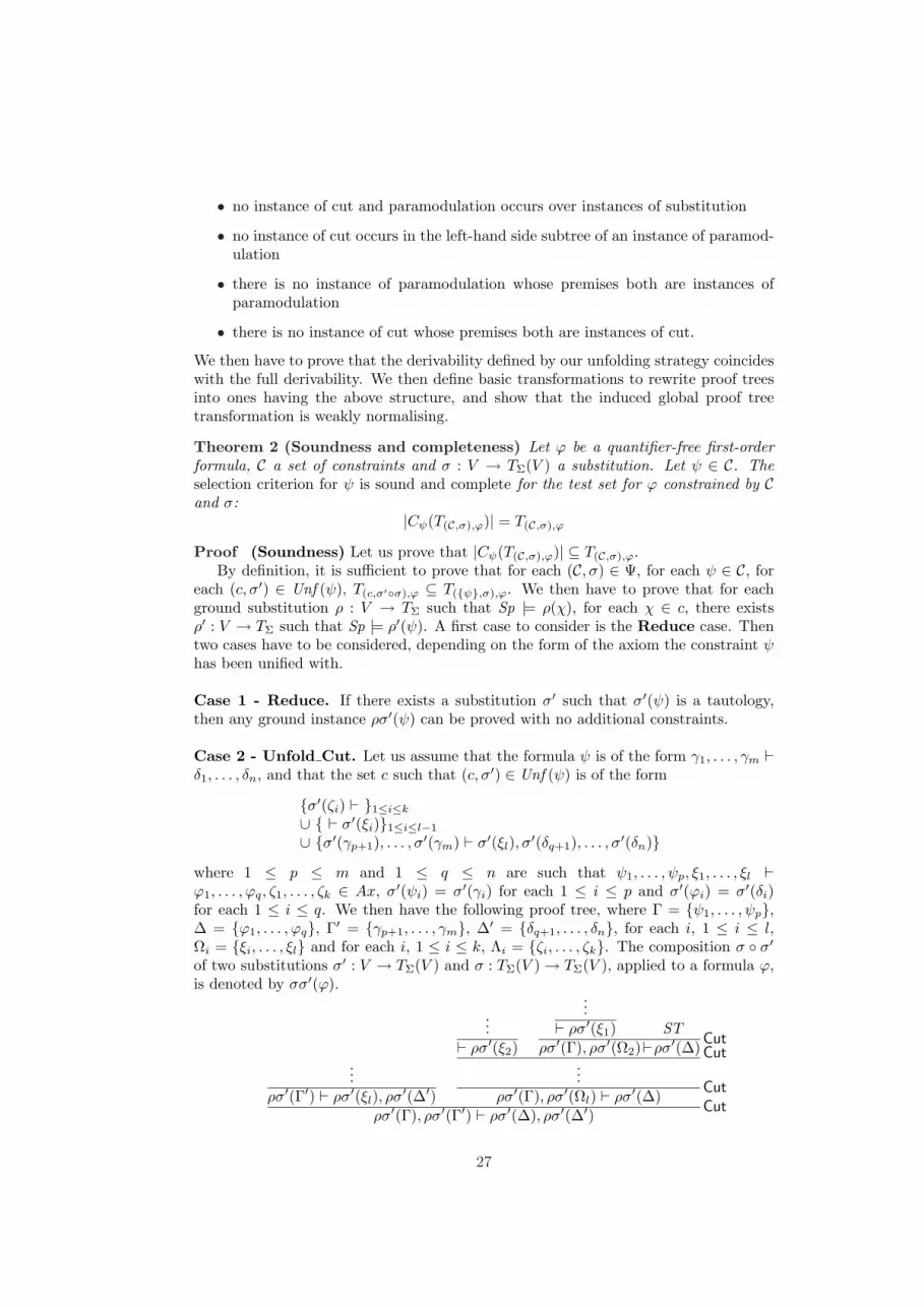
To prove the completeness, we prove that all the possible instances of the testpurpose can be proved with a proof tree of the form we showed earlier, and that theprocedure generates all possible constraints for proving this instance. We thus provethat no test case is lost. Actually, we can observe that our unfolding procedure definesa proof search strategy that enables to limit the search space to the class of proof treeshaving the following structure:

26





We then have to prove that the derivability defined by our unfolding strategy coincideswith the full derivability. We then define basic transformations to rewrite proof treesinto ones having the above structure, and show that the induced global proof treetransformation is weakly normalising.

Theorem 2 (Soundness and completeness) Let ϕ be a quantifier-free first-orderformula, C a set of constraints and σ : V → TΣ(V ) a substitution. Let ψ ∈ C. Theselection criterion for ψ is sound and complete for the test set for ϕ constrained by Cand σ:

|Cψ(T(C,σ),ϕ)| = T(C,σ),ϕ

Proof (Soundness) Let us prove that |Cψ(T(C,σ),ϕ)| ⊆ T(C,σ),ϕ.By definition, it is sufficient to prove that for each (C, σ) ∈ Ψ, for each ψ ∈ C, for

each (c, σ′) ∈ Unf (ψ), T(c,σ′σ),ϕ ⊆ T(ψ,σ),ϕ. We then have to prove that for eachground substitution ρ : V → TΣ such that Sp |= ρ(χ), for each χ ∈ c, there existsρ′ : V → TΣ such that Sp |= ρ′(ψ). A first case to consider is the Reduce case. Thentwo cases have to be considered, depending on the form of the axiom the constraint ψhas been unified with.

Case 1 - Reduce. If there exists a substitution σ′ such that σ′(ψ) is a tautology,then any ground instance ρσ′(ψ) can be proved with no additional constraints.

Case 2 - Unfold Cut. Let us assume that the formula ψ is of the form γ1, . . . , γm `δ1, . . . , δn, and that the set c such that (c, σ′) ∈ Unf (ψ) is of the form

σ′(ζi) ` 1≤i≤k∪ ` σ′(ξi)1≤i≤l−1

∪ σ′(γp+1), . . . , σ′(γm) ` σ′(ξl), σ′(δq+1), . . . , σ′(δn)where 1 ≤ p ≤ m and 1 ≤ q ≤ n are such that ψ1, . . . , ψp, ξ1, . . . , ξl `ϕ1, . . . , ϕq, ζ1, . . . , ζk ∈ Ax, σ′(ψi) = σ′(γi) for each 1 ≤ i ≤ p and σ′(ϕi) = σ′(δi)for each 1 ≤ i ≤ q. We then have the following proof tree, where Γ = ψ1, . . . , ψp,∆ = ϕ1, . . . , ϕq, Γ′ = γp+1, . . . , γm, ∆′ = δq+1, . . . , δn, for each i, 1 ≤ i ≤ l,Ωi = ξi, . . . , ξl and for each i, 1 ≤ i ≤ k, Λi = ζi, . . . , ζk. The composition σ σ′of two substitutions σ′ : V → TΣ(V ) and σ : TΣ(V )→ TΣ(V ), applied to a formula ϕ,is denoted by σσ′(ϕ).

...ρσ′(Γ′) ` ρσ′(ξl), ρσ′(∆′)

...` ρσ′(ξ2)

...` ρσ′(ξ1) ST

ρσ′(Γ), ρσ′(Ω2)`ρσ′(∆)Cut

...

Cut

ρσ′(Γ), ρσ′(Ωl) ` ρσ′(∆) Cut

ρσ′(Γ), ρσ′(Γ′) ` ρσ′(∆), ρσ′(∆′) Cut

27


Γ,Ω1 ` Λ1,∆Ax

ρσ′(Γ), ρσ′(Ω1) ` ρσ′(Λ1), ρσ′(∆) Subs

...ρσ′(ζ1) `

ρσ′(Γ), ρσ′(Ω1) ` ρσ′(Λ2), ρσ′(∆) Cut

...ρσ′(ζ2) `

...

Cut

ρσ′(Γ), ρσ′(Ω1) ` ρσ′(∆) Cut

Case 3 - Unfold Paramodulation. Let us assume that the formula ψ is of the formγ1, . . . , γm ` δ1, . . . , δn, and that the set c such that (c, σ′) ∈ Unf (ψ) is of the form

σ′(ζi) ` 1≤i≤k∪ ` σ′(ξi)1≤i≤l∪σ′(γp+1), . . . , σ′(γm) ` σ′(δq+1), . . . , σ′(δn−1), σ′(δn[s])

where 1 ≤ p ≤ m and 1 ≤ q ≤ n are such that ψ1, . . . , ψp, ξ1, . . . , ξl `ϕ1, . . . , ϕq, ζ1, . . . , ζk, s = t ∈ Ax, σ′(δn|ω ) = σ′(t), σ′(ψi) = σ′(γi) for each 1 ≤ i ≤ pand σ′(ϕi) = σ′(δi) for each 1 ≤ i ≤ q. We then have the following proof tree, wherewe follow the same notations as previously except that ∆′ is the set δq+1, . . . , δn−1:

...` ρσ′(ξl)

...` ρσ′(ξ2)

...` ρσ′(ξ1) ST

ρσ′(Γ), ρσ′(Γ′), ρσ′(Ω2)`ρσ′(∆), ρσ′(∆′), ρσ′(δn[r])Cut

...

Cut

ρσ′(Γ), ρσ′(Γ′), ρσ′(Ωl) ` ρσ′(∆), ρσ′(∆′), ρσ′(δn[r])Cut

ρσ′(Γ), ρσ′(Γ′) ` ρσ′(∆), ρσ′(∆′), ρσ′(δn[r])Cut


ST ′

...ρσ′(ζ1) `

ρσ′(Γ), ρσ′(Γ′), ρσ′(Ω1) ` ρσ′(Λ2), ρσ′(∆), ρσ′(∆′), ρσ′(δn[r])Cut

...ρσ′(ζ2) `

...

Cut

ρσ′(Γ), ρσ′(Γ′), ρσ′(Ω1) ` ρσ′(∆), ρσ′(∆′), ρσ′(δn[r])Cut

and ST’ is the following subtree:

ρσ′(t)=ρσ′(r)

SubsΓ,Ω1`Λ1,∆,s=t

Ax

ρσ′(Γ),ρσ′(Ω1)`ρσ′(Λ1),ρσ′(∆),ρσ′(s)=ρσ′(t)

...ρσ′(Γ′)`ρσ′(∆′),ρσ′(δn[s])

ρσ′(Γ),ρσ′(Γ′),ρσ′(Ω1)`ρσ′(Λ1),ρσ′(∆),ρσ′(∆′),ρσ′(δn[t])

Para

ρσ′(Γ),ρσ′(Γ′),ρσ′(Ω1)`ρσ′(Λ1),ρσ′(∆),ρσ′(∆′),ρσ′(δn[r])

Para

(Completeness) Let us prove that T(C,σ),ϕ ⊆ |Cψ(T(C,σ),ϕ)|.By definition, it is sufficient to prove that T(ψ,σ),ϕ ⊆

⋃

(c,σ′)∈Unf (ψ)

T(c,σ′σ),ϕ. We

then have to prove that for each ground substitution ρ : V → TΣ such that Sp |= ρ(ψ),there exists (c, σ′) ∈ Unf (ψ) such that there exists ρ′ : V → TΣ such that Sp |= ρ′(χ)for each χ ∈ c. In other words, we have to prove that ρ(ψ) can be deduced fromspecification Sp if there exists (c, σ′) ∈ Unf (ψ), and ρ′ : V → TΣ such that Sp |= ρ′(χ)for each χ ∈ c.

28

If ρ(ψ) is a tautology, it is a ground instance of a tautology σ′(ψ). Therefore, thereexists a pair (∅, σ′) ∈ Unf (ψ) build by the (Reduce) part of the algorithm.

If it is not a tautology, let show that there exists a pair (c, σ′) ∈ Unf (ψ) and asubstitution ρ′ such that ρ(ψ) can be deduced from the set of all ρ′(χ) for χ ∈ c.

First, let us note that the unfolding procedure defines a strategy which boundsthe search space for proof trees to a class of trees having a specific structure. Theprocedure defines a proof search strategy which selects proof trees where:





We then have to prove that there exists a proof tree having the structure we justdescribed and of conclusion ρ(ψ). We are actually going to prove a stronger result: weare going to define elementary transformations of proof trees, which allow to rewriteelementary combinations of inference rules, and then we will prove that the resultingglobal proof trees transformation is weakly normalizing and normal forms are prooftrees with the above structure.

We give here the elementary transformations of basic proof trees. For instance,when an instance of the cut rule occurs over an instance of the substitution rule, wehave the following rewriting rule to make the instance of substitution go over theinstance of cut:

Γ ` ∆, ϕ Γ′, ϕ ` ∆′

Γ,Γ′ ` ∆,∆′ Cut

σ(Γ), σ(Γ′) ` σ(∆), σ(∆′) Subs ÃΓ ` ∆, ϕ

σ(Γ) ` σ(∆), σ(ϕ) SubsΓ′, ϕ ` ∆′

σ(Γ′), σ(ϕ) ` σ(∆′) Subs

σ(Γ), σ(Γ′) ` σ(∆), σ(∆′) Cut

The case where an instance of substitution occurs over an instance of paramodu-lation:

Γ ` ∆, s = t Γ′ ` ∆′, ϕ[r]σ(Γ), σ(Γ′) ` σ(∆), σ(∆′), σ(ϕ[t]) Para

ρ(σ(Γ)), ρ(σ(Γ′)) ` ρ(σ(∆)), ρ(σ(∆′)), ρ(σ(ϕ[t])) Subs Ã

Γ ` ∆, s = tρ(σ(Γ)) ` ρ(σ(∆), ρ(σ(s)) = ρ(σ(t)) Subs

Γ′ ` ∆′, ϕ[r]ρ(σ(Γ′) ` ρ(σ(∆′), ρ(σ(ϕ[r]))Subs

ρ(σ(Γ)), ρ(σ(Γ′)) ` ρ(σ(∆)), ρ(σ(∆′)), ρ(σ(ϕ[t])) Para

We know from the paramodulation in the initial proof tree that σ(r) = σ(s), thereforewe also have ρ(σ(r)) = ρ(σ(s)).

The case where an instance of cut occurs in the left-hand side of an instance ofparamodulation:6

6We omit the contexts for the sake of readability.

29

` ψ ψ ` s = t` s = t

Cut ` ϕ[r]` σ(ϕ[t]) Para Ã

ψ ` s = t ` ϕ[r]σ(ψ) ` σ(ϕ[t]) Para

` ψ` σ(ψ) Subs

` σ(ϕ[t]) Cut

The case where two instances of paramodulation occur over an instance ofparamodulation:7

` u = v ` s = t[x]` σ(s) = σ(t[v]) Para

` r = z ` ϕ[w]` σ′(ϕ[z]) Para

` σ′′(σ′(ϕ[σ(t[v])])) Para Ã

` r = z` σ′(r) = σ′(z)Subs

` u = v ` s = t[x]` σ(s) = σ(t[v]) Para

` σ′′(σ′(r)) = σ′′(σ(t[v])) Para` ϕ[w]` σ′(ϕ[w]) Subs

` σ′′(σ′(ϕ[σ(t[v])])) Para

From the three instances of paramodulation in the initial tree, we know that: (1)σ(x) = σ(u), (2) σ′(w) = σ′(r), (3) σ′′(σ′(z)) = σ′′(σ(s)). In the resulting proof tree,we use these unifications in the order (1), (3) and (2).

The case of two cuts over a third one has to be divided into four cases, accordingto the position of the last cut formula in the premises of the two cuts of the top.

The case where ϕ is in both left premises:

Γ1`∆1,ϕ1,ϕ Γ′1,ϕ1`∆′1Γ1,Γ

′1`∆1,∆

′1,ϕ

CutΓ2,ϕ`∆2,ϕ2 Γ′2,ϕ2`∆′2

Γ2,Γ′2,ϕ`∆2,∆

′2

Cut

Γ1,Γ′1,Γ2,Γ

′2`∆1,∆

′1,∆2,∆

′2

Cut

Ã

Γ1`∆1,ϕ1,ϕ Γ2,ϕ`∆2,ϕ2

Γ1,Γ2`∆1,∆2,ϕ1,ϕ2

Cut

Γ′2,ϕ2`∆′2Γ1,Γ2,Γ

′2`∆1,∆2,∆

′2,ϕ1

Cut

Γ′1,ϕ1`∆′1Γ1,Γ

′1,Γ2,Γ

′2`∆1,∆

′1,∆2,∆

′2

Cut

The case where ϕ is in both right premises:

Γ1`∆1,ϕ1 Γ′1,ϕ1`∆′1,ϕ

Γ1,Γ′1`∆1,∆

′1,ϕ

CutΓ2`∆2,ϕ2 Γ′2,ϕ2,ϕ`∆′2

Γ2,Γ′2,ϕ`∆2,∆

′2

Cut

Γ1,Γ′1,Γ2,Γ

′2`∆1,∆

′1,∆2,∆

′2

Cut

Ã Γ1`∆1,ϕ1

Γ′1,ϕ1`∆′1,ϕ

Γ2`∆2,ϕ2 Γ′2,ϕ2,ϕ`∆′2Γ2,Γ

′2,ϕ`∆2,∆

′2

Cut

Γ′1,Γ2,Γ′2,ϕ1`∆′1,∆2,∆

′2

Cut

Γ1,Γ′1,Γ2,Γ

′2`∆1,∆

′1,∆2,∆

′2

Cut

The case where ϕ is in the left premise of the left cut, and in the right premise ofthe right cut:

Γ1`∆1,ϕ1,ϕ Γ′1,ϕ1`∆′1Γ1,Γ

′1`∆1,∆

′1,ϕ

CutΓ2`∆2,ϕ2 Γ′2,ϕ2,ϕ`∆′2

Γ2,Γ′2,ϕ`∆2,∆

′2

Cut

Γ1,Γ′1,Γ2,Γ

′2`∆1,∆

′1,∆2,∆

′2

Cut

7We omit the contexts for the sake of readability.

30

Ã Γ2`∆2,ϕ2

Γ1`∆1,ϕ1,ϕ Γ′1,ϕ1`∆′1Γ1,Γ

′1`∆1,∆

′1,ϕ

Cut

Γ′2,ϕ2,ϕ`∆′2Γ1,Γ

′1,Γ

′2,ϕ2`∆1,∆

′1,∆

′2

Cut

Γ1,Γ′1,Γ2,Γ

′2`∆1,∆

′1,∆2,∆

′2

Cut

The case where ϕ is in the right premise of the left cut, and in the left premise ofthe right cut:

Γ1`∆1,ϕ1 Γ′1,ϕ1`∆′1,ϕ

Γ1,Γ′1`∆1,∆

′1,ϕ

CutΓ2,ϕ`∆2,ϕ2 Γ′2,ϕ2`∆′2

Γ2,Γ′2,ϕ`∆2,∆

′2

Cut

Γ1,Γ′1,Γ2,Γ

′2`∆1,∆

′1,∆2,∆

′2

Cut

Ã Γ1`∆1,ϕ1

Γ′1,ϕ1`∆′1,ϕ

Γ2,ϕ`∆2,ϕ2 Γ′2,ϕ2`∆′2Γ2,Γ

′2,ϕ`∆2,∆

′2

Cut

Γ′1,Γ2,Γ′2,ϕ1`∆′1,∆2,∆

′2

Cut

Γ1,Γ′1,Γ2,Γ

′2`∆1,∆

′1,∆2,∆

′2

Cut

Let us define the measure of a proof tree π by:

m

(π1 π2

Γ1,Γ2 ` ∆1,∆2Cut

)=

1 +m(π1) +m(π2) if each πi =πi1 πi2Γi ` ∆i

Cut i = 1, 2

m(π1) +m(π2) otherwise

m

(π1 π2

Γ1,Γ2 ` ∆1,∆2Para

)=

1 +m(π1) if π1 =π11 π12

Γ1 ` ∆1Cut

1 +m(π1) +m(π2) if each πi =πi1 πi2Γi ` ∆i

Para i = 1, 2

m(π1) +m(π2) otherwise

A proof tree π is in normal form if and only if m(π) = 0. A proof tree π =π1 π2

ϕis called maximal if and only if π1 and π2 are in normal form but π is not. Therefore,by applying the strategy which consists in reducing first maximal proof trees, we showthat the measure m decreases for each basic transformation given above.

Since by hypothesis, Sp |= ρ(ψ), and ψ is not a tautology, there necessarily existseither an axiom

ψ1, . . . , ψp, ξ1, . . . , ξl ` ϕ1, . . . , ϕq, ζ1, . . . , ζk

or an axiomψ1, . . . , ψp, ξ1, . . . , ξl ` ϕ1, . . . , ϕq, ζ1, . . . , ζk, s = t

and a ground substitution ρ′ such that

• ρ′(ψi) = ρ′(γi) for each 1 ≤ i ≤ p• ρ′(ϕi) = ρ′(δi) for each 1 ≤ i ≤ q• ρ′(δn|ω ) = ρ′(t).

Hence ρ′ is a unifier of each ψi and γi, of each ϕi and δi and of δn|ω and t. So thereexists a proof tree resulting of the transformation defined above, of conclusion ρ(ψ)where ρ = ρ′, and of the form:

31

...ρ(Γ′) ` ρ(ξl), ρ(∆′)

...` ρ(ξ2)

...` ρ(ξ1) STρ(Γ), ρ(Ω2)`ρ(∆)Cut

...

Cut

ρ(Γ), ρ(Ωl) ` ρ(∆) Cut

ρ(Γ), ρ(Γ′) ` ρ(∆), ρ(∆′) Cut


Γ,Ω1 ` Λ1,∆Ax

ρ(Γ), ρ(Ω1) ` ρ(Λ1), ρ(∆)Subs

...ρ(ζ1) `

ρ(Γ), ρ(Ω1) ` ρ(Λ2), ρ(∆) Cut

...ρ(ζ2) `

...

Cut

ρ(Γ), ρ(Ω1) ` ρ(∆) Cut

or of the form:

...ρ(Γ′) ` ρ(ξl), ρ(∆′)

...` ρ(ξ2)

...` ρ(ξ1) ST

ρ(Γ), ρ(Ω2)`ρ(∆), ρ(δn[r])Cut

...

Cut

ρ(Γ), ρ(Ωl) ` ρ(∆), ρ(δn[r])Cut

ρ(Γ), ρ(Γ′) ` ρ(∆), ρ(∆′), ρ(δn[r])Cut


ρ(t)=ρ(r)

SubsΓ,Ω1`Λ1,∆,s=t

Ax

ρ(Γ),ρ(Ω1)`ρ(Λ1),ρ(∆),ρ(s)=ρ(t)

...ρ(Γ′)`ρ(∆′),ρ(δn[s])

ρ(Γ),ρ(Ω1),ρ(Γ′)`ρ(Λ1),ρ(∆),ρ(∆′),ρ(δn[t])

Para

ρ(Γ),ρ(Ω1),ρ(Γ′)`ρ(Λ1),ρ(∆),ρ(∆′),ρ(δn[r])

Para

...ρ(ζ1)`

ρ(Γ),ρ(Ω1)`ρ(Λ2),ρ(∆),ρ(δn[r])Cut

...ρ(ζ2)`

...Cut

ρ(Γ),ρ(Ω1)`ρ(∆),ρ(δn[r])Cut

and where Γ = ψ1, . . . , ψp, ∆ = ϕ1, . . . , ϕq, Γ′ = γp+1, . . . , γm, ∆′ =δq+1, . . . , δn, for each i, 1 ≤ i ≤ l, Ωi = ξi, . . . , ξl and for each i, 1 ≤ i ≤ k,Λi = ζi, . . . , ζk.

¤

5 Unfolding and structural induction

5.1 Structural induction

One of the testing hypotheses states that the signature Σ of the specification defines thevisible (public) interface of the system under test. When the operations implementedin the system are exactly those of the signature (i.e. no operation of the signature issupposed to be hidden), then we can assume that the first-order structure S associatedto the system under test is reachable, which means that all the values manipulated by

32

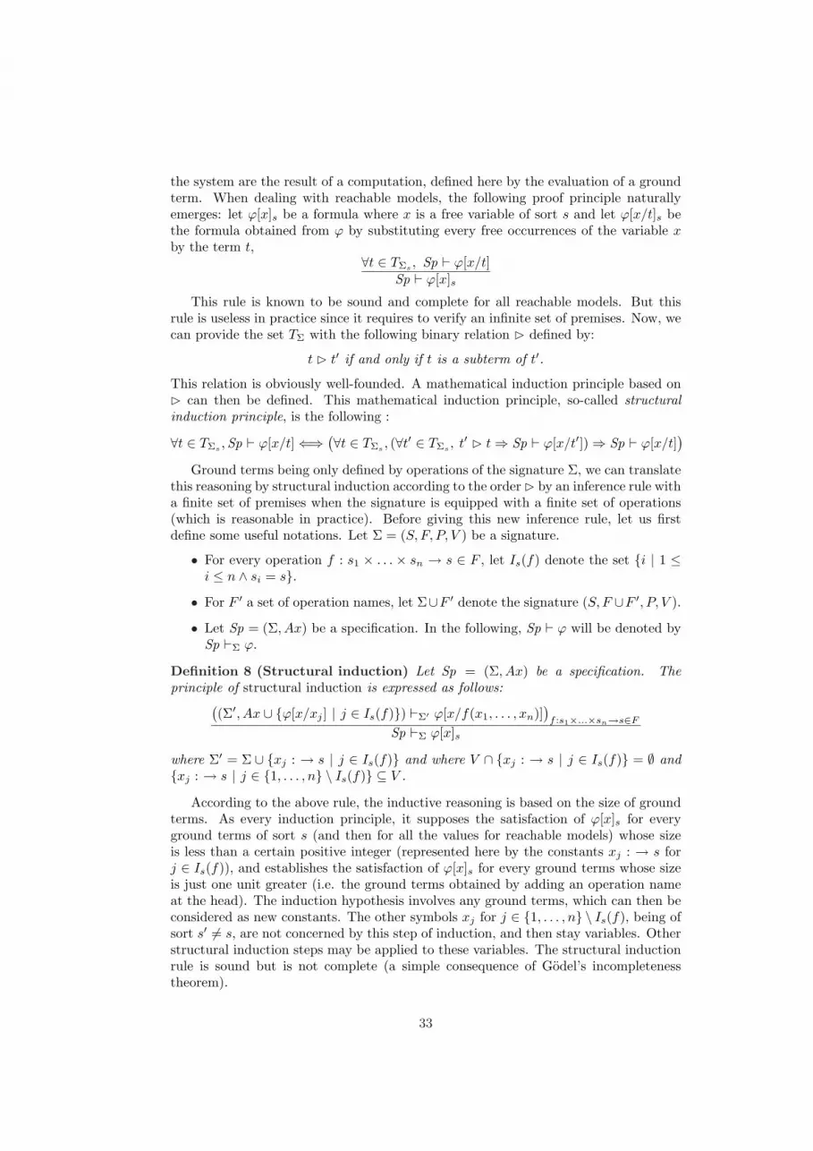
the system are the result of a computation, defined here by the evaluation of a groundterm. When dealing with reachable models, the following proof principle naturallyemerges: let ϕ[x]s be a formula where x is a free variable of sort s and let ϕ[x/t]s bethe formula obtained from ϕ by substituting every free occurrences of the variable xby the term t,

∀t ∈ TΣs , Sp ` ϕ[x/t]Sp ` ϕ[x]s

This rule is known to be sound and complete for all reachable models. But thisrule is useless in practice since it requires to verify an infinite set of premises. Now, wecan provide the set TΣ with the following binary relation B defined by:

t B t′ if and only if t is a subterm of t′.

This relation is obviously well-founded. A mathematical induction principle based onB can then be defined. This mathematical induction principle, so-called structuralinduction principle, is the following :

∀t ∈ TΣs ,Sp ` ϕ[x/t]⇐⇒ (∀t ∈ TΣs , (∀t′ ∈ TΣs , t′ B t⇒ Sp ` ϕ[x/t′])⇒ Sp ` ϕ[x/t]

)

Ground terms being only defined by operations of the signature Σ, we can translatethis reasoning by structural induction according to the order B by an inference rule witha finite set of premises when the signature is equipped with a finite set of operations(which is reasonable in practice). Before giving this new inference rule, let us firstdefine some useful notations. Let Σ = (S, F, P, V ) be a signature.

• For every operation f : s1 × . . . × sn → s ∈ F , let Is(f) denote the set i | 1 ≤i ≤ n ∧ si = s.

• For F ′ a set of operation names, let Σ∪F ′ denote the signature (S, F ∪F ′, P, V ).

• Let Sp = (Σ, Ax) be a specification. In the following, Sp ` ϕ will be denoted bySp `Σ ϕ.

Definition 8 (Structural induction) Let Sp = (Σ, Ax) be a specification. Theprinciple of structural induction is expressed as follows:

((Σ′, Ax ∪ ϕ[x/xj ] | j ∈ Is(f)) `Σ′ ϕ[x/f(x1, . . . , xn)]

)f :s1×...×sn→s∈F

Sp `Σ ϕ[x]s

where Σ′ = Σ ∪ xj : → s | j ∈ Is(f) and where V ∩ xj : → s | j ∈ Is(f) = ∅ andxj : → s | j ∈ 1, . . . , n \ Is(f) ⊆ V .

According to the above rule, the inductive reasoning is based on the size of groundterms. As every induction principle, it supposes the satisfaction of ϕ[x]s for everyground terms of sort s (and then for all the values for reachable models) whose sizeis less than a certain positive integer (represented here by the constants xj : → s forj ∈ Is(f)), and establishes the satisfaction of ϕ[x]s for every ground terms whose sizeis just one unit greater (i.e. the ground terms obtained by adding an operation nameat the head). The induction hypothesis involves any ground terms, which can then beconsidered as new constants. The other symbols xj for j ∈ 1, . . . , n \ Is(f), being ofsort s′ 6= s, are not concerned by this step of induction, and then stay variables. Otherstructural induction steps may be applied to these variables. The structural inductionrule is sound but is not complete (a simple consequence of Godel’s incompletenesstheorem).

33

Example 6 Let us suppose the specification Sp of the arithmetic defined by

• the signature Σ = (S, F, P, V ) where

– S = Nat,– F = 0 : → Nat , s : Nat → Nat , + : Nat ×Nat → Nat,– V = x, y,

• the set of axioms Ax

– x+ 0 = x

– x+ s(y) = s(x+ y)

It is well-known that when the set of algebras is restricted to reachable algebras, theformula 0+x = x can be proved by structural induction. Indeed, applying the inferencerule of the structural induction gives these three cases to prove:

1. Sp `Σ 0 + 0 = 0

2. Sp ∪ 0 + x1 = x1 `Σ∪x1: →Nat 0 + s(x1) = s(x1)

3. Sp ∪ 0 + xi = xi | i = 1, 2 `Σ∪xi: →Nat, i=1,2 0 + (x1 + x2) = x1 + x2

This is the general case, where each f(x1, . . . , xn) possibly denotes a different value.A particular case comes from the presence of constructors, which are operations thatgenerate the set of all possible values for a given sort. Here for instance, 0 and sgenerate all the natural numbers. Hence, the operation + is completely defined by thesetwo operations, and the last case given by the application of the structural inductionrule is redundant with the two first.

5.2 Test selection and structural induction

The induction rule presented in the previous subsection is independent of any calculus.It can then be added to the sequent calculus our unfolding procedure is based on, con-sidering the formula ϕ in the induction rule as a sequent. In this setting, the inductionrule leads to a new step in the unfolding algorithm. In the unfolding procedure, thisnew step comes just after the loop involving all axioms. It comes as another way tounfold the constraint, independently of the axioms. Before presenting the unfoldingstep for induction, let us recall that a normalised sequent ψ = γ1, . . . , γm ` δ1, . . . , δnhas been chosen in a set C of Ψ. To simplify the presentation, we will use the inter-pretation of ψ in first-order logic ψ′ = γ1 ∧ · · · ∧ γm ⇒ δ1 ∨ · · · ∨ δn on which we willmake a normalisation step after having made an induction step on it (see below). Theunfolding for induction is then defined by:

(Unfold Induction)if x is a variable of sort s in ψ s.t. ¬labelled(x) thenc← ψ[x/cste] | cste : → s

∪ Normalise(( ∧

i∈Is(f) ψ′[x/xi]

)⇒ ψ′[x/f(x1, . . . , xn)])

| f ∈ F, ∀i ∈ Is(f), xi is a fresh variableFor each fresh variable xi added in the previous step labelled(xi)Add (c, Id) to Unf (ψ)

34

end if

We assume the initialisation ¬labelled(x) for each variable x of the test purpose ϕ.The Normalise function allows to transform any formula into a normalised sequent, asexplained in Section 1.

Considered as a new constraint, the normalisation of the formula

( ∧

i∈Is(f)

ψ′[x/xi])⇒ ψ′[x/f(x1, . . . , xn)]

allows to link together the variables xi in each ψ′[x/xi] and ψ′[x/f(x1, . . . , xn)]. Indeed,as we have already explained in the previous subsection, each xi in the induction ruleplays the role of a constant. Hence, the induction hypothesis and the general caserepresented here by each ψ′[x/xi] and ψ′[x/f(x1, . . . , xn)], respectively, are groundterms over the signature Σ′ = Σ∪xi | i ∈ Is(f). This prevents the system under testto directly interpret them, because it does not know how to interpret each constant xi.Now, by the theorem of deduction which holds in first-order logic, we equivalently havethe formula

(∧i∈Is(f) ψ

′[x/xi]) ⇒ ψ′[x/f(x1, . . . , xn)]. By definition, this formula is

correct for any value that can be associated to each constant xi. Under this form,each xi can then be a variable, it can be substituted during the inference steps thatfollow. When they are substituted by ground terms, generated constraints can then beinterpreted by the system under test. Labelling these new variables in the algorithmallows not to apply some induction steps on these fresh variables, and then to avoidendless inductions.

Adding this induction step in the unfolding algorithm preserves the correctness ofthe algorithm. On the other hand, this does not allow to preserve its completeness. Thereason is that the new constraints defined by the general cases can require in their proofto make some other induction steps. This is, for instance, the case of the second generalcase to prove in Example 6. Indeed, proving the formula 0+ (x1 +x2) = x1 +x2 needsthe associativity of + which itself is proved by structural induction from the axiomsgiven in Example 6.

The problem comes from the fact that formulas which need to be proved by struc-tural induction are not, by definition, consequences (by using the other rules of thecalculus) of axioms, and then require human intervention to be generated. Such for-mulas can syntactically be identified. More formally, the completeness of thealgorithm would be satisfied if both cut and paramodulation rules would go over in-duction. However, this does not hold in general.

Since the unfolding procedure is not complete anymore when induction is added,some constraints generated by the algorithm will not be able to be unfolded. Theseconstraints are those which cannot be unified with any axiom, and so which needto be proved by structural induction. Such a constraint cannot be unfolded if aninduction step has already been performed and the variables of the sort to involve inthe induction are already labelled. In this case, it is the tester’s choice how to deal withthis constraint. The tester may decide to keep it as a constraint, or to try to unfoldit more. If he decides to unfold it, he has to provide himself the theorems neededto prove the constraint as new axioms of the specification. In the case we alreadymentioned, if the constraint is the formula 0+(x1 +x2) = x1 +x2, the theorem to addto the specification is the associativity of the operation +: x+ (y + z) = (x+ y) + z.

35

This theorem can be taken as a new test purpose, to be unfolded from the initialspecification and tested, to increase the confidence in its validity.

Conclusion

In this paper, we extended the test selection method known as axiom unfolding toquantifier-free first-order specifications with equality. We first proved the existenceof an exhaustive test set, namely the set of observable semantic consequences of thespecification, without any condition on the system under test. As it has originallybeen defined in the algebraic specifications setting, our unfolding procedure consists individing the initial test set for a formula into test subsets, characterising the differentinstances of this formula that can be proved from the specification axioms. The gener-ation of a test set for this formula then arises from the selection of one test case in eachresulting subset. We improved our previous works on this procedure by handling theequality predicate in an efficient way, thanks to the paramodulation rule. We provedthis procedure to be sound and complete, so that exhaustivity for a given formula ispreserved at each step. We finally proposed a strategy to cover the exhaustive test set.

The definition of test selection criteria is the first step towards the construction ofa practical test set to submit to the system. The next step is the generation of a testset satisfying these criteria. In our framework, the generation consists in applying theuniformity hypothesis to the constrained test sets obtained by unfolding an initial testpurpose. It actually comes down to solve the constraints associated to each constrainedtest purpose, in order to build one test case corresponding to this purpose. Note thatfor a constrained test set T(C,σ),ϕ where C is empty, any instantiation of the variablesdefines a test case. However, since we are interested in generating only one test caseper constrained test set, a complete unfolding procedure is useless. It suffices to solvethe constraints on the fly, during the unfolding procedure. A strategy is then neededto choose at each step which constraint in the current set C should be unfolded inorder to reduce the remaining set C to the empty set and then to be able to computea test case. Obviously, as the current set of constraints may be unsatisfiable, the testcase generation also requires some backtracking steps. To be efficient, such a strategyof test case generation should be based on some heuristics (e.g. the choice of thenext constraint to be unfolded may be based on syntactic criteria, like constraintswith the fewest variables or constraints unifying with the fewest axioms) or applied tospecifications written according to some predefined restricted form [25, 1]. To completethe work of this paper, we plan to study the definition of an efficient algorithm of testcase generation for a subclass of quantifier-free first-order specification.

Ongoing research is also to be continued on structuration aspects. Axiomatic spec-ifications can be structured via operators allowing to rename, to reduce or to enricha specification for instance, or to make the union of two specifications. Integrationtesting, that is testing the composition of several modules or program units, deals withtesting the new properties arising from the composition of those modules but thatdid not exist in the individual modules. Our goal then is to propose a framework offunctional testing with selection criteria including structuration primitives, followingfor instance [23, 24].

36

References

[1] Marc Aiguier, Agnes Arnould, Clement Boin, Pascale Le Gall, and Bruno Marre.Testing from algebraic specifications: test data set selection by unfolding axioms.In Formal Approaches to Testing of Software (FATES’05), volume 3997 of LectureNotes in Computer Science, pages 203–217, 2005.

[2] Marc Aiguier, Agnes Arnould, Pascale Le Gall, and Delphine Longuet. Test se-lection criteria from quantifier-free first-order specifications. In Fundamentals ofSoftware Engineering (FSEN’07), volume 4767 of Lecture Notes in Computer Sci-ence, pages 144–159, 2007.

[3] Marc Aiguier, Agnes Arnould, Pascale Le Gall, and Delphine Longuet.Exhaustive test sets for algebraic specification correctness. Technical re-port, IBISC, Universite d’Evry Val d’Essonne, 2008. Submitted, available athttp://www.epigenomique.genopole.fr/∼aiguier/publications/communications/exhaust.pdf.

[4] Agnes Arnould and Pascale Le Gall. Test de conformite : une approche algebrique.Technique et Science Informatiques, Test de logiciel, 21:1219–1242, 2002.

[5] Agnes Arnould, Pascale Le Gall, and Bruno Marre. Dynamic testing from boundeddata type specifications. In Dependable Computing - EDCC-2, volume 1150 ofLecture Notes in Computer Science, pages 285–302, 1996.

[6] Gilles Bernot. Testing against formal specifications: a theoretical view. In Theoryand Practice of Software Development (TAPSOFT’91), volume 494 of LectureNotes in Computer Science, pages 99–119, 1991.

[7] Gilles Bernot, Marie-Claude Gaudel, and Bruno Marre. Software testing basedon formal specifications: a theory and a tool. Software Engineering Journal,6(6):387–405, 1991.

[8] Achim D. Brucker and Burkhart Wolff. Symbolic test case generation for primi-tive recursive functions. In Formal Approaches to Software Testing (FATES’04),volume 3395 of Lecture Notes in Computer Science, pages 16–32, 2004.

[9] Matthieu Carlier and Catherine Dubois. Functional testing in the Focal environ-ment. In Tests and Proofs (TAP’08), volume 4966 of Lecture Notes in ComputerScience, pages 84–98, 2008.

[10] Koen Claessen and John Hughes. QuickCheck: a lightweight tool for randomtesting of Haskell programs. ACM SIGPLAN Notices, 35(9):268–279, 2000.

[11] Jeremy Dick and Alain Faivre. Automating the generation and sequencing oftest cases from model-based specifications. In Formal Methods Europe (FME’93),volume 670 of Lecture Notes in Computer Science, pages 268–284, 1993.

[12] Lars Frantzen, Jan Tretmans, and Tim A. C. Willemse. Test generation based onsymbolic specifications. In Formal Approaches to Software Testing (FATES’04),volume 3395 of Lecture Notes in Computer Science, pages 1–15, 2004.

[13] Christophe Gaston, Pascale Le Gall, Nicolas Rapin, and Assia Touil. Symbolicexecution techniques for test purpose definition. In Testing of CommunicatingSystems (TestCom’06), volume 3964 of Lecture Notes in Computer Science, pages1–18, 2006.

37

[14] Marie-Claude Gaudel. Testing can be formal, too. In Theory and Practice ofSoftware Development (TASPOFT’95), volume 915 of Lecture Notes in ComputerScience, pages 82–96, 1995.

[15] Marie-Claude Gaudel and Pascale Le Gall. Testing data types implementationsfrom algebraic specifications. In Robert M. Hierons, Jonathan P. Bowen, and MarkHarman, editors, Formal Methods and Testing, volume 4949 of Lecture Notes inComputer Science, pages 209–239. Springer, 2008.

[16] Rolf Hennicker, Martin Wirsing, and Michel Bidoit. Proof systems for struc-tured specifications with observability operators. Theoretical Computer Science,173(2):393–443, 1997.

[17] Claude Jard and Thierry Jeron. TGV: theory, principles and algorithms. a tool forthe automatic synthesis of conformance test cases for non-deterministic reactivesystems. Software Tools for Technology Transfer (STTT), 6, 2004.

[18] Pieter W. M. Koopman, Artem Alimarine, Jan Tretmans, and Marinus J. Plasmei-jer. GAST: Generic automated software testing. In Implementation of FunctionalLanguages, volume 2670 of Lecture Notes in Computer Science, pages 84–100,2002.

[19] Pascale Le Gall and Agnes Arnould. Formal specification and test: correctnessand oracle. In 11th Workshop on Algebraic Development Techniques (WADT’96),volume 1130 of Lecture Notes in Computer Science, pages 342–358, 1996.

[20] David Lee and Mihalis Yannakakis. Principles and methods of testing finite statemachines - A survey. In Proceedings of the IEEE, volume 84, pages 1090–1126,1996.

[21] Guillaume Lussier and Helene Waeselynck. Proof-guided test: an experimentalstudy. In International Computer Software and Applications Conference (COMP-SAC’04), pages 528–533. IEEE Computer Society, 2004.

[22] Patrıcia Machado. On oracles for interpreting test results against algebraic spec-ifications. In Algebraic Methodology and Software Technology, volume 1548 ofLecture Notes in Computer Science. Springer-Verlag, 1999.

[23] Patrıcia Machado. Testing from structured algebraic specifications. In AlgebraicMethodology and Software Technology (AMAST’00), volume 1816 of Lecture Notesin Computer Science, pages 529–544, 2000.

[24] Patrıcia Machado and Donald Sannella. Unit testing for Casl architectural spec-ifications. In Mathematical Foundations of Computer Science, volume 2420 ofLecture Notes in Computer Science, pages 506–518, 2002.

[25] Bruno Marre. LOFT : a tool for assisting selection of test data sets from algebraicspecifications. In Theory and Practice of Software Development (TAPSOFT’95),volume 915 of Lecture Notes in Computer Science, pages 799–800, 1995.

[26] Peter D. Mosses. CASL Reference Manual, The Complete Documentation of theCommon Algebraic Specification Language, volume 2960 of Lecture Notes in Com-puter Science. Springer, 2004.

38

[27] Alexandre Petrenko, Sergiy Boroday, and Roland Groz. Confirming configurationsin EFSM. In Formal Methods for Protocol Engineering and Distributed Systems(FORTE’99), volume 156 of IFIP Conference Proceedings, pages 5–24, 1999.

[28] Marc Phalippou. Relations d’implantation et hypotheses de test sur les automatesa entrees et sorties. PhD thesis, Universite de Bordeaux, 1994.

[29] George A. Robinson and Larry Wos. Paramodulation and theorem proving infirst-order theories with equality. Machine Intelligence, 4:133–150, 1969.

[30] Vlad Rusu, Lydie du Bousquet, and Thierry Jeron. An approach to symbolictest generation. In 2nd International Workshop on Integrated Formal Method(IFM’00), volume 1945 of Lecture Notes in Computer Science, pages 338–357,2000.

[31] Jan Tretmans. Testing labelled transition systems with inputs and outputs. InInternational Workshop on Protocols Test Systems (IWPTS’95), 1995.

39

Documents

Proof-Guided Test Selection from First-Order Specifications with Equality