Embed Size (px)
Citation preview

Probability & Statistics
for Engineers &; Scientists
Probability & Statistics for Engineers & Scientists
E I G H T H E D I T I O N
Ronald E. Walpole Roanoke College
Raymond H. Myers Virginia Polytechnic Institute and State University
Sharon L. Myers Radford University
Keying Ye University of Texas at San Antonio
Pearson Education International
PEARSON
Prentice Hall

If you purchased this book within the United States or Canada you should be aware that it has been wrongfully imported without the approval of the Publisher or Author.
Editor in Chief: Sally Yagun Production Editor: Lynn Savino Wendel Senior Managing Editor: Linda Mihatov Belmms Assistant Managing Editor: Bayani Mendoza de Leon Executive Managing Editor: Kathleen Schiaparelli Manufacturing Buyer: Maura Zaldivar Manufacturing Manager: Alexis Heydt-Long Marketing Manager: Halee Dinsey Marketing Assistant: Jennifer de Leeuwcrk Director of Marketing: Patrice Jones Editorial Assistant/Print Supplements Editor: Jennifer Urban Art Editor: Thomas Benfatti Art Director: Heather Scott Creative Director: Juan R. Lopez Director of Creative Services: Paul Belfanti Cover Photo: Corbis Royalty Free Art Studio: Laser-words
PEARSON
Prentice Hall
© 2007, 2002, 1998. 1993, 1989, 1985, 1978, 1972 Pearson Education, Inc. Pearson Prentice Hall Pearson Education, Inc. Upper Saddle River, N.I 07458
All rights reserved. No part, of tins book may be reproduced, in any form or by any means, without permission in writing from the publisher.
Pearson Prentice Hall™ is a trademark of Pearson Education, Inc. 1 0 9 8 7 6 5 4 3
ISBN 0 - 1 3 - 2 0 4 7 6 7 - 5
Pearson Education LTD., London Pearson Education Australia PTY. Limited, Sydney Pearson Education Singapore, Pte. Ltd. Pearson Education North Asia Ltd., Hong Kong Pearson Education Canada, Ltd.. Toronto Pearson Education de Mexico, S.A. de C.V. Pearson Education-Japan, Tokyo Pearson Education Malaysia, Pte. Ltd. Pearson Education, Upper Saddle River, New Jersey

This book is dedicated to
Billy and Julie
R.H.M. and S.L.M.
Limin K.Y.
Contents
Preface xv
1 Introduction to Statistics and Data Analysis 1 1.1 Overview: Statistical Inference, Samples, Populations and Exper
imental Design 1
1.2 The Hole of Probability 4
1.3 Sampling Procedures; Collection of Data 7
1.4 Measures of Location: The Sample Mean and Median 11
Exercises 13
1.5 Measures of Variability 1 •! Exercises 17
1.0 Discrete and Continuous Data 17
1.7 Statistical Modeling, Scientific Inspection, and Graphical Diagnostics ]!)
J .8 Graphical Methods and Data Description 20
1.9 General Types of Statistical Studies: Designed Experiment, Observational Study, and Retrospective Study 25
Exercises 28
2 Probability 31 2.1 Sample Space 31
2.2 Events 34 Exercises 38
'2.3 Counting Sample Points 40 Exercises 47
2.4 Probability of an Event 48 2.5 Additive Rules 52
Exercises 55 2.6 Conditional Probability 58 2.7 Multiplicative Rules 61
Exercises 65
Vlll Contents
2.8 Bayes' Rule 68 Exercises 72
Review Exercises 73
3 Random Variables and Probability Distributions 77 3.1 Concept of a Random Variable 77
3.2 Discrete Probability Distributions 80
3.3 Continuous Probability Distributions 84
Exercises 88 3.4 Joint Probability Distributions 91
Exercises 101 Review Exercises 103
3.5 Potential Misconceptions and Hazards; Relationship to Material
in Other Chapters 106
4 Mathematical Expectation 107 4.1 Mean of a Random Variable 107
Exercises 113 4.2 Variance and Covariance of Random Variables 115
Exercises 122 4.3 Means and Variances of Linear Combinations of Random Variables 123
4.4 Chebyshov's Theorem 131
Exercises 134 Review Exercises 136
4.5 Potential Misconceptions and Hazards; Relationship to Material in Other Chapters 138
5 Some Discrete Probability Distributions 141 5.1 Introduction and Motivation 141 5.2 Discrete Uniform Distribution 141 5.3 Binomial and Multinomial Distributions 143
Exercises 150
5.4 Hypergeometric Distribution 152 Exercises 157
5.5 Negative Binomial and Geometric Distributions 158 5.6 Poisson Distribution and the Poisson Process 161
Exercises 165
Review Exercises 167 5.7 Potential Misconceptions and Hazards: Relationship to Material
in Other Chapters 169
Contents IX
6 Some Continuous Probability Distributions 171 6.1 Continuous Uniform Distribution 171
6.2 Normal Distribution 172
6.3 Areas under the Normal Curve 176
6.4 Applications of the Normal Distribution 182
Exercises 185
6.5 Normal Approximation to the Binomial 187
Exercises 19;}
6.6 Gamma and Exponential Distributions 194
6.7 Applications of the Exponential and Gamma Distributions 197
6.8 Chi-Squared Distribution 200
6.9 Lognormal Distribution 201
6.10 VVeibull Distribution (Optional) 202
Exercises 205
Review Exercises 206
6.1 1 Potential Misconceptions and Hazards: Relationship to Material
in Other Chapters 209
7 Functions of Random Variables (Optional).. 211 7.1 Introduction 211
7.2 Transformations of Variables 211
7.3 Moments and Moment-Generating Functions 219
Exercises 226
8 Fundamental Sampling Distributions and Data Descriptions 229 8.1 Random Sampling 229
8.2 Some Important Statistics 231
Exercises 23 1
8.3 Data Displays and Graphical Methods 236
8.4 Sampling Distributions 243
8.5 Sampling Distribution of Means 244
Exercises 251
8.6 Sampling Distribution of S 251
8.7 ^-Distribution 257
8.8 F-Distribution 261
Exercises 265
Review Exercises 266
8.9 Potential Misconceptions and Hazards; Relationship to Material
in Other Chapters 268
Contents
9 One- and Two-Sample Estimation Problems 269 9.1 Introduction 269 9.2 Statistical Inference 269
9.3 Classical Methods of Estimation 270 9.4 Single Sample: Estimating the Mean 274
9.5 Standard Error of a Point Estimate 280 9.6 Prediction Intervals 281
9.7 Tolerance Limits 283 Exercises 285
9.8 Two Samples: Estimating the Difference between Two Means . . . 288
9.9 Paired Observations 294
Exercises 297 9.10 Single Sample: Estimating a Proportion 299 9.11 Two Samples: Estimating the Difference between Two Proportions 302
Exercises 304
9.12 Single Sample: Estimating the Variance 306
9.13 Two Samples: Estimating the Ratio of Two Variances 308
Exercises 310
9.14 Maximum Likelihood Estimation (Optional) 310
Exercises 315 Review Exercises 315
9.15 Potential Misconceptions and Hazards; Relationship to Material
in Other Chapters 319
10 One- and Two-Sample Tests of Hypotheses 321 10.1 Statistical Hypotheses: General Concepts 321
10.2 Testing a Statistical Hypothesis 323 10.3 One- and Two-Tailed Tests 332
10.4 The Use of P-Values for Decision Making in Testing Hypotheses. 334
Exercises 336 10.5 Single Sample: Tests Concerning a Single Mean (Variance Known) 338 10.6 Relationship to Confidence Interval Estimation 341 10.7 Single Sample: Tests on a Single Mean (Variance Unknown) 342 10.8 Two Samples: Tests on Two Means 345 10.9 Choice of Sample Size for Testing Means 350 10.10 Graphical Methods for Comparing Means 355
Exercises 357 10.11 One Sample: Test on a Single Proportion 361 10.12 Two Samples: Tests on Two Proportions 364
Exercises 366 10.13 One- and Two-Sample Tests Concerning Variances 367
Contents xi
Exercises 370
10.14 Goodness-of-Fit Test 371 10.15 Test for Independence (Categorical Data) 374 10.16 Test for Homogeneity 377
10.17 Testing for Several Proportions 378 10.18 Two-Sample Case Study 380
Exercises 383 Review Exercises 385
10.19 Potential Misconceptions and Hazards; Relationship to Material in Other Chapters 387
11 Simple Linear Regression and Correlation.. 389 11.1 Introduction to Linear Regression 389
11.2 The Simple Linear Regression Model 390
11.3 Least Squares and the Fitted Model 394
Exercises 397
11.4 Properties of the Least Squares Estimators 400 11.5 Inferences Concerning the Regression Coefficients 402 11.6 Prediction 409
Exercises 412
11.7 Choice of a Regression Model 414
11.8 Analysis-of-Variance Approach 415
11.9 Test for Linearity of Regression: Data with Repeated Observations 417
Exercises 423 11.10 Data Plots and Transformations 425 11.11 Simple Linear Regression Case Study 430
11.12 Correlation 432
Exercises 438 Review Exercises 438
11.13 Potential Misconceptions and Hazards; Relationship to Material in Other Chapters 443
12 Multiple Linear Regression and Certain Nonlinear Regression Models 445 12.1 Introduction 445
12.2 Estimating the Coefficients 446 12.3 Linear Regression Model Using Matrices (Optional) 449
Exercises 452 12.4 Properties of the Least Squares Estimators 456 12.5 Inferences in Multiple Linear Regression 458
Exercises 464
xii Contents
12.6 Choice of a Fitted Model through Hypothesis Testing 465
12.7 Special Case of Orthogonality (Optional) 469
Exercises 473
12.8 Categorical or Indicator Variables 474
Exercises 478
12.9 Sequential Methods for Model Selection 479
12.10 Study of Residuals and Violation of Assumptions 485
12.11 Cross Validation, C;), and Other Criteria for Model Selection 490
Exercises 496
12.12 Special Nonlinear Models for Nonideal Conditions 499
Review Exercises 503
12.13 Potential Misconceptions and Hazards; Relationship to Material
in Other Chapters 508
13 One-Factor Experiments: General 511 13.1 Analysis-of-Variance Technique 511
13.2 The Strategy of Experimental Design 512
13.3 One-Way Analysis of Variance: Completely Randomized Design
(One-Way ANOVA) 513
13.4 Tests for the Equality of Several Variances 518
Exercises 521
13.5 Single-Dcgree-of-Freedom Comparisons 523
13.6 Multiple Comparisons 527
13.7 Comparing Treatments with a Control 531
Exercises 533
13.8 Comparing a Set of Treatments in Blocks 535
13.9 Randomized Complete Block Designs 537
13.10 Graphical Methods and Model Checking 544
13.11 Data Transformations In Analysis of Variance) 547
13.12 Latin Squares (Optional) 549
Exercises 551
13.13 Random Effects Models 555
13.14 Power of Analysis-of-Variance Tests 559
13.15 Case Study 563
Exercises 565
Review Exercises 567
13.16 Potential Misconceptions and Hazards; Relationship to Material in Other Chapters 571
Contents xiii
14 Factorial Experiments (Two or More Factors) 573 14.1 Introduction 573
14.2 Interaction in the Two-Factor Experiment 574
14.3 Two-Factor Analysis of Variance 577 Exercises 587
14.4 Three-Factor Experiments 590 Exercises 597
14.5 Model II and III Factorial Experiments 600 14.6 Choice of Sample Size 603
Exercises 605 Review Exercises 607
14.7 Potential Misconceptions and Hazards; Relationship to Material in Other Chapters 609
15 2k Factorial Experiments and Fractions 611 15.1 Introduction 611
15.2 The 2fc Factorial: Calculation of Effects and Analysis of Variance 612 15.3 Nonreplicated 2k Factorial Experiment 618 15.4 Injection Molding Case Study 619
Exercises 622
15.5 Factorial Experiments in a Regression Setting 625 15.6 The Orthogonal Design 631 15.7 Factorial Experiments in Incomplete Blocks 639
Exercises 645
15.8 Fractional Factorial Experiments 647 15.9 Analysis of Fractional Factorial Experiments 653
Exercises 656 15.10 Higher Fractions and Screening Designs 657
15.11 Construction of Resolution III and IV Designs 658
15.12 Other Two-Level Resolution III Designs; The Plackett-Burman Designs 660
15.13 Robust Parameter Design 661 Exercises 666 Review Exercises 667
15.14 Potential Misconceptions and Hazards: Relationship to Material in Other Chapters 669
16 Nonparametric Statistics 671 16.1 Nonparametric Tests 671 16.2 Signed-Rank Test 676
xiv Contents
Exercises 679 16.3 Wilcoxon Rank-Sum Test 681
16.4 Kruskal-Wallis Test 684 Exercises 686
1G.5 Runs Test. 687 16.6 Tolerance Limits 690 16.7 Rank Correlation Coefficient 690
Exercises 693 Review Exercises 695
17 Statistical Quality Control 697 17.1 Introduction 697 17.2 Nature of the Control Limits 699 17.3 Purposes of the Control Chart 699 17.4 Control Charts for Variables 700 17.5 Control Charts for Attributes 713 17.6 Cusum Control Charts 721
Review Exercises 722
18 Bayesian Statistics (Optional) 725 18.1 Bayesian Concepts 725 18.2 Bayesian Inferences 726 18.3 Bayes Estimates Using Decision Theory Framework 732
Exorcises 734
Bibliography 737
A Statistical Tables and Proofs 741
B Answers to Odd-Numbered Non-Review Exercises 795
Index 811
Preface
General Approach and Mathematical Level
The general goals for the eighth edition remain the same as those in recent editions. We feel as if it is important to retain a balance between theory and applications. Engineers and physical scientists as well as computer scientists are trained in calculus and thus mathematical support is given when we feel as if the pedagogy-is enhanced by it. This approach prohibits the material from becoming a collection of tools with no mathematical roots. Certainly students with a mathematical background of calculus, and, in a few cases, linear algebra, have the capability to understand the concepts more thoroughly and use the resulting tools more intelligently. Otherwise there is a clear danger that, the student will only be able to apply the material within very narrow bounds.
The new edition contains a substantially larger number of exercises. These exercises challenge the student to be able to use concepts from the text to solve problems dealing with many real-life scientific and engineering situations. The data sets involved in the exercises are available for download from website at http://www.prenhaU.com.. The increase in the quantity of exercises results in a much broader spectrum of areas of applications, including biomedical, biocngi-neering, business problems, computer issues, and many others. Even the chapters that deal in introductory probability theory contain examples and exercises that carry a broad range of applications that students of science and engineering will easily recognize as important. As in past editions, the use of calculus is confined to elementary probability theory and probability distributions. These topics are discussed in Chapters 2. 3, 1, 6, and 7. Chapter 7 is an optional chapter that includes transformations of variables and moment generating functions. Matrix algebra is used only a, modest amount in linear regression material in Chapters 11 and 12. For those who desire the use of more substantial support with matrices, an optional section in Chapter 12 is available. The instructor who wishes to minimize the use of matrices may bypass this section with no loss of continuity. Students using this text should have completed the equivalent of one semester of differential and integral calculus. An exposure to matrix algebra would be helpful but not necessary if the course context excludes I he aforementioned optional section given in Chapter 12.
xvi Preface
Content and Course Planning This text is designed for either a one- or two-semester course. A reasonable curriculum for a one-semester course might include Chapters 1 through 10. Many instructors desire for students to be exposed in some degree to simple linear regression in a one semester course. Thus one may choose to include a portion of Chapter 11. On the other hand, some instructors wish to teach a portion of analysis of variance, in which case Chapters 11 and 12 may be excluded in favor of some portion of Chapter 13, which features one factor analysis of variance. In order to provide sufficient time for one or perhaps even both of these topics, the instructor may wish to eliminate Chapter 7 and/or certain specialized topics in Chapters 5 and 6 (for example, treatment on the gamma, lognormal, and Weibull distributions, or material on the negative binomial and geometric distributions). Indeed, some instructors find that in a one-semester course in which regression analysis and analysis of variance are of primary interest, there may be topics in Chapter 9 on estimation that may be removed (e.g., maximum likelihood, prediction intervals, and/or tolerance limits). We feel as if the flexibility exists that allows a one-semester course given any priorities set down by the instructor.
Chapter 1 is an elementary overview of statistical inference designed for the beginner. It contains material on sampling and data analysis and contains many-examples and exercises for motivation. Indeed, some very rudimentary aspects of experimental design are included along with an appreciation of graphic techniques and certain vital characteristics of data collection. Chapters 2, 3, and 4 deal with basic probability as well as discrete and continuous random variables. Chapters 5 and 6 cover specific discrete and continuous distributions with illustrations of their use and relationships among them. In addition, a substantial number of examples and exercises are given that illustrate their use. Chapter 7 is an optional chapter that treats transformation of random variables. An instructor may wish to cover this material only if he or she is teaching a more theoretical course. This chapter is clearly the most mathematical chapter in the text. Chapter 8 contains additional material on graphical methods as well as a very important introduction to the notion of a sampling distribution. Probability plotting is discussed. The material on sampling distribution is reinforced by a thorough discussion of the central limit theorem as well as the distribution of a sample variance under normal i.i.d. (independently and identically distributed) sampling. The t and F distributions are introduced along with motivation regarding their use in chapters that follow. Chapters 9 and 10 contain material on one and two sample point and interval estimation and hypothesis testing. Material on confidence intervals, prediction intervals, tolerance intervals, and maximum likelihood estimation in Chapter 9 offeis the instructor considerable flexibility regarding what might be excluded in a one-semester course. A section on Bayes estimation that was available in the seventh edition in Chapter 9 has been removed. More attention will be given to this topic in the "New to This Edition" section that follows.
Chapters 11 through 17 contain ample material for a second semester. Simple and multiple linear regression are contained in Chapters 8 and 12, respectively. Chapter 12 also contains material on logistic regression, which finds applications in many areas of engineering and the biological sciences. The material covered in multiple linear regression is quite extensive and thus provides flexibility for the
Preface xvii
instructor. Among the "special topics" to which an instructor has access are the special case of orthogonal rcgressors, categorical or indicator variables, sequential methods for model selection, study of residuals and violation of assumptions, cross validation and the use of PRESS and C,„ and, of course, logistic regression. Chapters 13 through 17 contain topics in analysis of variance, design of experiments, nonparametric statistics, and quality control. Chapter 15 treats two-level factorials (with and without blocking) and fractional factorials, and again flexibility is abundant because of the many "special topics" offered in this chapter. Topics beyond the standard 2k and fractional 2* designs include blocking and partial confounding, special higher fractions and screening designs, Plackett-Burman designs, and robust parameter design.
All chapters contain a large number of exercises, considerably more than what was offered in the seventh edition. More information on exercises will be given in the "New To This Edition" section.
Case Studies and Computer Software The topical material in two-sample hypothesis testing, multiple linear regression, analysis of variance, and the use of two-level factorial experiments is supplemented by case studies that feature computer printout and graphical material. Both SAS and MINFTAB are featured. The use of the computer printout underscores our feeling that the students should have the experience of reading and interpreting computer printout and graphics, even if that which is featured in the text is not what is used by the instructor. Exposure to more than one type of software can broaden the experience base for the student. There is no reason to believe that the software in the course will be that which he or she will be called upon to use in practice following graduation. Many examples and case studies in the text are supplemented, where appropriate, by various types of residual plots, quantile plots, normal probability plots, and others. This is particularly prevalent in the material used in Chapters 11 through 15.
New to This Edition
General
1. There arc 15 20% new problem sets incorporated, with many new applications demonstrated in engineering as well as biological, physical, and computer science.
2. There is new and end-ofLchapter review material where appropriate. This material emphasizes key ideas as well as risks and hazards that the user of material covered in the chapter must be aware of. This material will also provide demonstration of how it is influenced by material in other chapters.
3. A new mini (and optional) chapter on Bayesian statistics has been incorporated. The chapter will be a practical offering with applications emphasized in many fields.
4. There are extensive additional changes made throughout, based on need perceived by authors and reviewers. The following outlines some specifics.
xviii Preface
Chapter 1: Introduction to Statistics and Data Analysis
Chapter 1 contains a substantial amount of new material. There is new exposition on the difference between discrete and continuous measurements. Many illustrations are given with particular real life applications of discrete measurements (e.g., numbers of radioactive particles, the number of personnel responsible for a particular port facility, and the number of oil tankers arriving each day at a port city). Special attention is given to situations associated with binary data. Examples are given in the biomedical field as well as quality control.
New concepts (for this text) are discussed in Chapter 1 which deal with properties of a distribution or sample other than those that characterize central tendency and variability. Quartiles and, more generally, quantiles are defined and discussed.
The importance of experimental design and the advantages that it offers is expanded beyond that of the seventh addition. In this development important notions that are treated include randomization, reduction of process variability, and interaction among factors.
The readers are exposed in the first chapter to different types of statistical studies: the designed experiment, the observational study, and the retrospective study. Examples are given of each type and advantages and disadvantages are discussed. The chapter continues to emphasize graphical procedures and where they apply.
Nineteen new exercises were added to Chapter 1. Some make use of data from studies conducted at the Virginia Tech consulting center and some are taken from engineering journals and others involve historical data. This chapter now contains 30 exercises.
Chapter 2: Probability
There are new examples and new exposition to better demonstrate the notion of conditional probability. Chapter 2 offers 136 total exercises. All new exercises involve direct applications in science and engineering.
Chapter 3: Random Variables and Probability Distributions
There is new exposition on the notion of "dummy" variables that, play an important role in the Bernoulli and binomial distributions. There are many more exercises with new applications. The new review at the end of the chapter introduces the connection between material in Chapter 3 with the concept of distribution parameters and specific probability distributions discussed in future chapters.
Topics for new exercises include particle size distribution for missile fuel, measurement errors in scientific systems, studies of time to failure for manufactured washing machines, the production of electron tubes on an assembly line, arrival time problems at certain big city intersections, shelf life of a product, passenger congestion problems in airports, problems with impurities in batches of chemical product, failure in systems of electronic components working in parallel, and many others. There are now 82 exercises in this chapter.
Preface x j x
Chapter 4: Mathematical Expectation
Several more exercises were added to Chapter 4. Rules for expectations and variances of linear functions were expanded to cover approximations for nonlinear functions. Examples are given to illustrate the use of these rules. The review at the end of Chapter 4 reveals possible difficulties and hazards with practical applications of the material since most examples and exercises assume parameters (mean and variance) are known and in true applications these parameters would be estimated. Reference is made to Chapter 9, where estimation is discussed. There are now 103 exercises in this chapter.
Chapter 5: Some Discrete Probability Distributions
New exercises representing various applications of the Poisson distribution have been added. Additional exposition has been added that deals with the Poisson probability function.
New exercises include real life applications of the Poisson, binomial, and hy-pergeometric distributions. Topics for new exercises include flaws in manufactured copper wire, highway potholes in need of repair, patient traffic in an urban hospital, airport luggage screening, homeland security detection of incoming missiles, and many others. In addition, plots are given that provide the reader with a clear indication about the nature of both the Poisson and the binomial distribution as parameters change. There are now 105 exercises in this chapter.
Chapter 6: Some Continuous Probability Distributions
Many more examples and exercises dealing in both the exponential and the gamma distribution have been added. The "lack of memory" property of the exponential distribution is now discussed at length and related to the bond between the exponential and Poisson distributions. The section on the Weibull distribution is greatly improved and expanded. The extensions presented focus on the measuring and interpretation of the failure rate or "hazard rate" and how knowledge of the parameters of the Weibull allow the user to learn how machines wear or even get stronger over time. More exercises are given that involve the Weibull and lognormal distributions. Caution is expressed in the review much like that in Chapter 5. In practical situations, guesses or estimates of process parameters of the gamma distribution in, say, failure rate problems or parameters of either a gamma or Weibull distribution, may be unstable, thereby introducing errors in calculations. There are now 84 exercises in this chapter.
Chapter 7: Functions of Random Variables (optional)
No major changes are included in this optional chapter.
Chapter 8: Fundamental Distributions and Data Description
There is additional exposition on the central limit theorem as well as the general concept of sampling distributions. There are many new exercises. The summary
xx Preface
provides important information on t. \2-. and F. including how they are used and what assumptions are involved.
More attention is given in Chapter 8 to normal probability plotting. In addition, the central limit theorem is discussed in more detail in order that the reader can gain more insight about what size n must be before normality can be invoked. Plots are given to illustrate this.
Additional exposition is given regarding the normal approximation to the binomial distribution and how it works in practical situations. The presentation presents an intuitive argument that connects the normal approximation of the binomial to the central limit theorem. The number of exercises in this chapter is now 75.
Chapter 9: One- and Two-Sample Estimation Problems
Many new applications are revealed in new exercises in this chapter. The summary gives rationale and hazards associated with the so-called large sample confidence interval. The importance of the assumption of normality and the conditions under which it is assumed are discussed.
Early in the chapter the development of confidence intervals offers a pragmatic discussion about why one must begin with the "known er' case. It is suggested that these kinds of situations do not actually occur in practice but consideration of the known s case initially provides a structure that allows the more useful "unknown CT" to be understood more easily by students.
One-sided bounds of all types are now presented and discussion is given as to when they are used as opposed to the two-sided counterparts. New examples are given which require the use of the one-sided intervals. These include confidence intervals, prediction intervals, and tolerance intervals. The concept of a mean squared error of an estimator is discussed. Thus the notion of bias and variance can be brought together in the general comparison of estimators. Twenty-seven new exercises are included in Chapter 9. There are now 111 exercises in this chapter.
Chapter 10: One- and Two-Sided Tests of Hypotheses
We have an entirely restructured exposition on the introduction to hypothesis testing. It is designed to help the student have a clear picture of what is being accomplished and not being accomplished in hypothesis testing. The notion that we rarely, if ever, "accept the null hypothesis'' is discussed with illustrations. There is also a thorough discussion with examples, of how one should structure or set up the null and alternative hypotheses. The notion that rejection implies "sample evidence refutes HQ" and that HQ is actually the logical complement to Hi is discussed precisely with several examples. Much is said about the concept of "fail to reject HQ'1 and what it means in practical situations. The summary produces "misconceptions and hazards" which reveals problems in drawing the wrong conclusions when the analyst "fails to reject" the null hypothesis. In addition, "robustness" is discussed, which deals with the nature of the sensitivity of various tests of hypotheses to the assumption of normality. There are now 115 exercises in this chapter.
Preface xx i
Chapter 11: Simple Linear Regression
Many new exercises are added in simple linear regression. Special exposition is given to the pitfalls in the use of R2, the coefficient of determination. Much additional emphasis is given to graphics and diagnostics dealing in regression. The summary deals with hazards that one may encounter if diagnostics are not used. It is emphasized that diagnostics provide "checks" on the validity of assumptions. These diagnostics include data plots, plots of student.ized residuals, and normal probability plots of residuals.
An important presentation is made early in the chapter about the nature of linear models in science and engineering. It is pointed out that these are often empirical models that are simplifications of more complicated and unknown structures.
More emphasis is given in this chapter on data plotting. "Regression through the origin'' is discussed in an exercise. More discussion is given on what it means when H0: /? = 0 is rejected or not rejected. Plots are used for illustration. There are now 68 exercises in this chapter.
Chapter 12: Multiple Linear Regression
Additional treatment is given in this chapter on the pitfalls of R2. The discussion centers around the need to compromise between the attempt to achieve a "good fit" to the data and the inevitable loss in error degrees of freedom that is experienced when one "overfits." In that regard the "adjusted R2"' is defined and discussed with examples. In addition, the CV (coefficient of variation) is discussed and interpreted as a measure that can be used to compare competing models. Several new exercises are present to provide the reader experience in comparing competing models using real data sets. Additional treatment is given to the topic of "categorical regressors" with graphical tools used to support the underlying concepts. Additional exercises are given to illustrate practical uses of logistic regression in both industrial and biomedical research areas. There are now 72 exercises in this chapter.
Chapter 13: One-Factor Experiments: General
The discussion of Tukey's test on multiple comparisons is expanded considerably. More is presented on the notion of error rate and o>values in the context of simultaneous confidence intervals.
A new and important section is given on "Data Transformation in Analysis of Variance." A contrast is made with the discussion in Chapters 11 and 12 dealing with transformation to produce a good fit in regression. A brief presentation is given regarding the robustness of analysis of variance to the assumption of homogeneous variance. This discussion is connected to previous sections on diagnostic plots to detect violations in assumptions.
Additional mention is made of the root causes of violation of the homogeneous variance assumption and how it is often a natural occurrence when the variance is a function of the mean. Transformations are discussed that can be used to accommodate the problem. Examples and exercises are used for illustration. Several new exercises were added. The total number of exercises in this chapter is 67.
xxn Preface
Chapter 14: Factorial Experiments (Two or More Factors)
Considerable attention is given to the concept, of interaction and interaction plots quite early in the chapter. Examples are given in which scientific interpretations of interaction are given using graphics. New exercises highlight the use of graphics including diagnostic plots of residuals. Several new exercises appear in this chapter. All include experimental data from chemical and biological sciences and all include emphasis on graphical analysis. There are 43 exercises in this chapter.
Chapter 15: 2k Factorial Experiments and Fractions
Early in this chapter new material has been added to highlight and illustrate the role of two-level designs as screening experiments. In this regard they are often part of a sequential plan in which the scientist or engineer is attempting to learn about the process, assess the role of the candidate factors, and give insight that will aid in determining the most fruitful region of experimentation. The notion of fractional factorial designs is motivated early.
The motivation of the notion of "effects" and the graphical procedures that are used in determining "active effects" are discussed in more detail with examples. The chapter uses considerably more graphical illustrations and geometric displays to motivate the concepts for both full and fractional factorials. In addition, graphical depictions are used to illustrate the available lack-of-fit information when one augments the two-level design with center runs.
In the development and discussion of fractional factorial designs, the procedure for constructing the fraction is greatly simplified and made much more intuitively appealing. "Added columns" that are selected according to the desired alias structure are used with several examples. We feel as if the reader can now gain a better understanding of what is gained (and lost) by using fractions. This represents a major simplification from the previous edition. For the first time a substantial table is given that allows the reader to construct two-level designs of resolution HI and IV. Eighteen new exercises were added to this chapter. The total number of exercises in this chapter is now 50.
Chapter 16: Nonparametric Statistics
No major changes are included. The total number of exercises is 41.
Chapter 17: Statistical Quality Control
No major changes are included. The total number of exercises is 10.
Chapter 18: Bayesian Statistics (optional)
This chapter is completely new in the eighth edition. The material on Bayesian statistics in the seventh edition (in Chapter 9) was removed in favor of featuring this subject in a new self-contained chapter.
This chapter treats the pragmatic and highly useful elements of Bayesian statistics of which students in science and engineering should be aware. The chapter

Preface xxiii
presents the important concept of subjective probability in conjunction with the notion that in many applications population parameters are truly not constant but should be treated as random variables. Point and interval estimation is treated from a Bayesian point of view and practical examples are displayed, This chapter is relatively short (ten pages) and contains 9 examples and 11 exercises.
Acknowledgements
We are indebted to those colleagues who reviewed the previous editions of this book and provided many helpful suggestions for this edition. They are: Andre Adler, Illinois institute of Technology. Georgiana Baker, University of South Carolina-, Barbara Bonnie, University of Minnesota-. Nirmal Devi, Embry Riddle; Ruxu Du, University of Miami; Stephanie Edwards. Demidji State University. Charles McAllister, Louisiana State University; Judith Miller, Georgetown University, Timothy Raymond, Bucknell University; Dennis Webster, Louisiana State University; Blake Whitten, University of Iowa; Michael Zabarankin, Stevens Institute of Technology.
We would like to thank the editorial and production services provided by numerous people from Prentice Hall, especially the editor in chief Sally Yagan, production editor Lynn Savino Wcndel, and copy editor Patricia Daly. Many useful comments, suggestions and proof-readings by Richard Charnigo. Jr., Michael Anderson, Joleen Beltrami and George Lobcll are greatly appreciated. We thank the Virginia Tech Statistical Consulting Center which was the source of many real-life data sets. In addition we thank Linda Douglas who worked hard in helping the preparation of the manuscript.
R.H.M. S.L.M. K.Y.
Chapter 1
Introduction to Statistics and Data Analysis
1.1 Overview: Statistical Inference, Samples, Populations, and Experimental Design
Beginning in the 1980s and continuing into the twenty-first century: an inordinate amount of attention has been focused on improvement of quality in American industry. Much has been said and written about the Japanese "industrial miracle," which began in the middle of the twentieth century. The Japanese were able to succeed where we and other countries had failed-namely, to create an atmosphere that allows the production of high-quality products. Much of the success of the Japanese has been attributed to the use of statistical methods and statistical thinking among management personnel.
Use of Scientific Da ta
The use of statistical methods in manufacturing, development of food products, computer software, pharmaceutical, and many other areas involves the gathering of information or scientific data. Of course, the gathering of data is nothing new. It has been done for well over a thousand years. Data have been collected, summarized, reported, and stored for perusal. However, there is a profound distinction between collection of scientific information and inferential statistics. It is the latter that has received rightful attention in recent decades.
The offspring of inferential statistics has been a large "toolbox" of statistical methods employed by statistical practitioners. These statistical methods are designed to contribute to the process of making scientific: judgments in the face of uncertainty and variation. The product density of a particular material from a manufacturing process will not always be the same. Indeed, if the process involved is a batch process rather than continuous, there will be variation in material density between not only the batches (batch-to-batch variation) that come off the line, but also within-batch variation. Statistical methods are used to analyze data from a process such as this one in order to gain more sense of where in the prr cess changes may be made to improve the quality of the process. In this, qur"
Chapter 1 Introduction to Statistics and Data Analysis
may well be defined in relation to closeness to a target density value in harmony with what portion of the time this closeness criterion is met. An engineer may be concerned with a specific instrument that is used to measure sulfur monoxide in the air during pollution studies. If the engineer has doubts about the effectiveness of the instrument, there are two sources of variation that must be dealt with. The first is the variation in sulfur monoxide values that are found at the same locale on the same day. The second is the variation between values observed and the true sulfur monoxide that is in the air at the time. If either of these two sources of variation is exceedingly large (according to some standard set by the engineer), the instrument may need to be replaced. In a biomedical study of a new drug that reduces hypertension, 85% of patients experienced relief while it is generally recognized that the current or "old drug" brings relief to 80% of patients that have chronic hypertension. However, the new drug is more expensive to make and may result in certain side effects. Should the new drug be adopted? This is a problem that is encountered (often with much more complexity) frequently by pharmaceutical firms in harmony with the FDA (Federal Drug Administration). Again, the consideration of variation needs to be taken into account. The "85%" value is based on a certain number of patients chosen for the study. Perhaps if the study were repeated with new patients the observed number of "successes" would be 75%! It is the natural variation from study to study that must be taken into account in the decision process. Clearly this variation is important since variation from patient to patient is endemic to the problem.
Variability in Scientific Da ta
In the problems discussed above the statistical methods used involve dealing with variability and in each case the variability to be studied is that encountered in scientific data. If the observed product density in the process is always the same and is always on target, there would be no need for statistical methods. If the device for measuring sulfur monoxide always gives the same value and the value is accurate (i.e., it is correct), no statistical analysis is needed. If there was no patient-to-patient variability inherent in the response to the drug (i.e., it either always brings relief or not), life would be simple for scientists in the pharmaceutical firms and FDA and no statistician would be needed in the decision process. Inferential statistics has produced an enormous number of analytical methods that allow for analysis of data from systems like those described above. This reflects the true nature of the science that we call inferential statistics, namely that of using techniques that allow us to go beyond merely reporting data but, rather, allow the drawing of conclusions (or inferences) about the scientific system. Statisticians make use of fundamental laws of probability and statistical inference to draw conclusions about scientific systems. Information is gathered in the form of samples, or collections of observations. The process of sampling is introduced in Chapter 2 and the discussion continues throughout the entire book.
Samples are collected from populations that are collections of all individuals or individual items of a particular type. At times a population signifies a scientific system. For example, a manufacturer of computer boards may wish to eliminate defects. A sampling process may involve collecting information on 50 computer boards sampled randomly from the process. Here, the population is all computer
1.1 Overview: Statistical Inference, Samples, Populations and Experimental Design 3
boards manufactured by the firm over a specific period of time. In a drug experiment, a sample of patients is taken and each is given a specific drug to reduce blood pressure. The interest is focused on drawing conclusions about the population of those who suffer from hypertension. If an improvement is made in the computer board process and a second sample of boards is collected, any conclusions drawn regarding the effectiveness of the change in process should extend to the entire population of computer boards produced under the "improved process."
Often, it is very important to collect scientific data in a systematic way, with planning being high on the agenda. At times the planning is, by necessity, quite limited. We often focus only on certain properties or characteristics of the items or objects in the population. This characteristic has particular engineering or, say, biological importance to the "customer," the scientist or engineer who seeks to learn about the population. For example, in one of the illustrations above the quality of the process had to do with the product density of the output of a process. An engineer may need to study the effect of process conditions, temperature, humidity, amount of a particular ingredient, and so on. He or she can systematically move these factors to whatever levels are suggested according to whatever prescription or experimental design is desired. However, a forest scientist who is interested in a study of factors that influence wood density in a certain kind of tree cannot necessarily design an experiment. In this case it may require an observational study in which data are collected in the field but factor levels could not be preselected. Both of these types of studies lend themselves to methods of statistical inference. In the former, the quality of the inferences will depend on proper planning of the experiment. In the latter, the scientist is at the mercy of what can be gathered. For example, it is sad if an agronomist is interested in studying the effect of rainfall on plant yield and the data are gathered during a drought.
One should gain an insight into the importance of statistical thinking by managers and the use of statistical inference by scientific personnel. Research scientists gain much from scientific data. Data provide understanding of scientific phenomena. Product and process engineers learn more in their off-line efforts to improve the process. They also gain valuable insight by gathering production data (online monitoring) on a regular basis. This allows for determination of necessary modifications in order to keep the process at a desired level of quality.
There are times when a scientific practitioner wishes only to gain some sort of summary of a set of data represented in the sample. In other words, no inferential statistics are used. Rather a set of single-number statistics or descriptive statistics is helpful. These numbers give a sense of center of location of the data, variability in the data, and the general nature of the distribution of observations in the sample. Though no specific statistical methods leading to statistical inference are incorporated, much can be learned. At times, descriptive statistics are accompanied by graphics. Modern statistical software packages allow for computation of means, medians, standard deviations, and other single-number statistics as well as produce graphs that show a "footprint" of the nature of the sample. Definitions and illustrations of the single-number statistics, as well as descriptions of graphical methods including histograms, stem-and-leaf plots, dot plots, and box plots, will be given in sections that follow.
Chapter 1 Introduction to Statistics and Data Analysis
1.2 The Role of Probability
In this book, Chapters 2 to 6 deal with fundamental notions of probability. A thorough grounding in these concepts allows the reader to have a better understanding of statistical inference. Without some formalism in probability, the student cannot appreciate the true interpretation of data analysis through modern statistical methods. It is quite natural to study probability prior to studying statistical inference. Elements of probability allow us to quantify the strength or "confidence" in our conclusions. In this sense, concepts in probability form a major component that supplements statistical methods and help gauge the strength of the statistical inference. The discipline of probability, then, provides the transition between descriptive statistics and inferential methods. Elements of probability allow the conclusion to be put into the language that the science or engineering practitioners require. An example follows that enables the reader to understand the notion of a P-value, which often provides the "bottom line" in the interpretation of results from the use of statistical methods.
Example 1.1:1 Suppose that an engineer encounters data from a manufacturing process in which 100 items are sampled and 10 are found to be defective. It is expected and anticipated that occasionally there will be defective items. Obviously these 100 items represent the sample. However, it has been determined that in the long run, the company can oidy tolerate 5% defective in the process. Now, the elements of probability allow the engineer to determine how conclusive the sample information is regarding the nature of the process. In this case the population conceptually represents all possible items from the process. Suppose we learn that if the process is acceptable, that is, if it does produce items no more than 5% of which are defective, there is a probability of 0.0282 of obtaining 10 or more defective items in a random sample of 100 items from the process. This small probability suggests that the process does, indeed, have a long-run percent defective that exceeds 5%. In other words, under the condition of an acceptable process, the sample information obtained would rarely occur. However, it did occur! Clearly, though, it would occur with a much higher probability if the process defective rate exceeded 5% by a significant amount. J
From this example it becomes clear that the elements of probability aid in the translation of sample information into something conclusive or inconclusive about the scientific system. In fact, what was learned likely is alarming information to the engineer or manager. Statistical methods (which we will actually detail in Chapter 10) produced a P-value of 0.0282. The result suggests that the process very likely is not acceptable. The concept of a P-value is dealt with at length in succeeding chapters. The example that follows provides a second illustration.
Example 1.2:1 Often the nature of the scientific study will dictate the role that probability and deductive reasoning play in statistical inference. Exercise 9.40 on page 297 provides data associated with a study conducted at the Virginia Polytechnic Institute and State University on the development, of a relationship between the roots of trees and the action of a fungus. Minerals are transferred from the fungus to the trees and sugars from the trees to the fungus. Two samples of 10 northern red oak seedlings
1.2 The Role of Probability
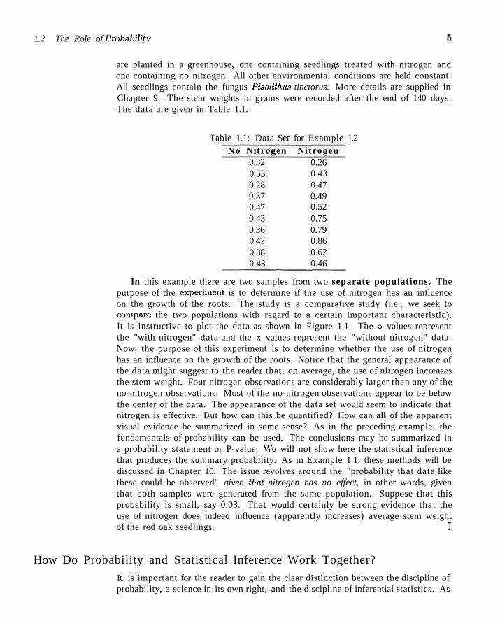
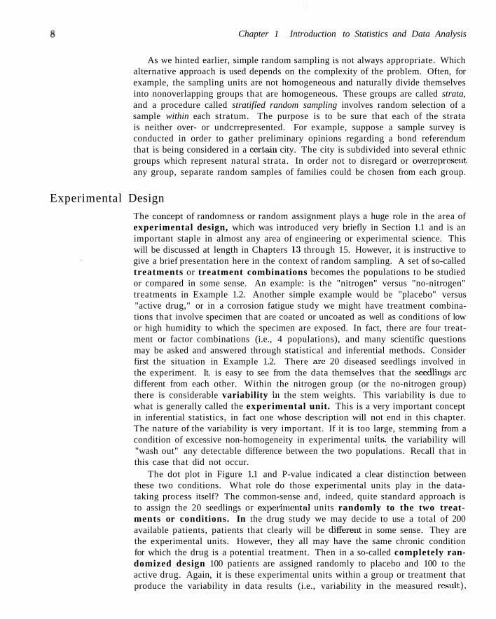
are planted in a greenhouse, one containing seedlings treated with nitrogen and one containing no nitrogen. All other environmental conditions are held constant. All seedlings contain the fungus Pisolithus tinctorus. More details are supplied in Chapter 9. The stem weights in grams were recorded after the end of 140 days. The data are given in Table 1.1.
Table 1.1: Data Set for Example 1.2 No Nitrogen
0.32 0.53 0.28 0.37 0.47 0.43 0.36 0.42 0.38 0.43
Nitrogen 0.26 0.43 0.47 0.49 0.52 0.75 0.79 0.86 0.62 0.46
In this example there are two samples from two separate populations. The purpose of the experiment is to determine if the use of nitrogen has an influence on the growth of the roots. The study is a comparative study (i.e.. we seek to compare the two populations with regard to a certain important characteristic). It is instructive to plot the data as shown in Figure 1.1. The o values represent the "with nitrogen" data and the x values represent the "without nitrogen" data. Now, the purpose of this experiment is to determine whether the use of nitrogen has an influence on the growth of the roots. Notice that the general appearance of the data might suggest to the reader that, on average, the use of nitrogen increases the stem weight. Four nitrogen observations are considerably larger than any of the no-nitrogen observations. Most of the no-nitrogen observations appear to be below the center of the data. The appearance of the data set would seem to indicate that nitrogen is effective. But how can this be quantified? How can all of the apparent visual evidence be summarized in some sense? As in the preceding example, the fundamentals of probability can be used. The conclusions may be summarized in a probability statement or P-value. Wc will not show here the statistical inference that produces the summary probability. As in Example 1.1, these methods will be discussed in Chapter 10. The issue revolves around the "probability that data like these could be observed" given that nitrogen has no effect, in other words, given that both samples were generated from the same population. Suppose that this probability is small, say 0.03. That would certainly be strong evidence that the use of nitrogen does indeed influence (apparently increases) average stem weight of the red oak seedlings. J
How Do Probability and Statistical Inference Work Together?
It. is important for the reader to gain the clear distinction between the discipline of probability, a science in its own right, and the discipline of inferential statistics. As
Chapter 1 Introduction to Statistics and Data Analysis
§ o
0.25 0.30 0.35 0.40 0.45 0.50 0.55 0.60 0.65 0.70 0.75 0.80 0.85 0.90
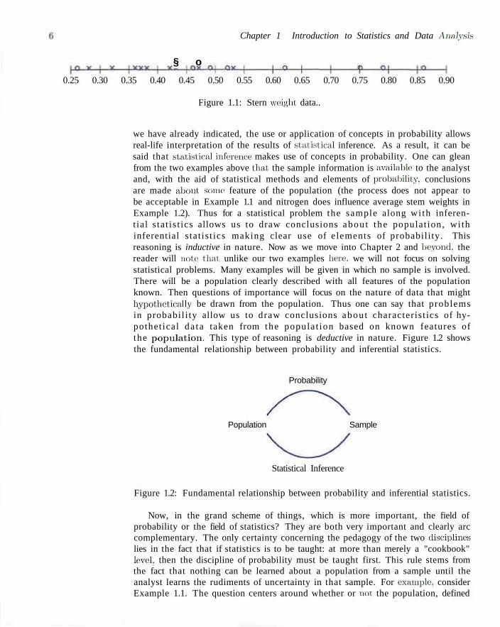
Figure 1.1: Stern weight data..
we have already indicated, the use or application of concepts in probability allows real-life interpretation of the results of statistical inference. As a result, it can be said that statistical inference makes use of concepts in probability. One can glean from the two examples above that, the sample information is available; to the analyst and, with the aid of statistical methods and elements of probability, conclusions are made about, some feature of the population (the process does not appear to be acceptable in Example 1.1 and nitrogen does influence average stem weights in Example 1.2). Thus for a statistical problem the sample along wi th inferent ial s ta t is t ics allows us to draw conclusions abou t t he populat ion, wi th inferential s tat is t ics making clear use of elements of probabili ty. This reasoning is inductive in nature. Now as we move into Chapter 2 and beyond, the reader will note' thai unlike our two examples here, we will not focus on solving statistical problems. Many examples will be given in which no sample is involved. There will be a population clearly described with all features of the population known. Then questions of importance will focus on the nature of data that might hypothetical]}' be drawn from the population. Thus one can say that problems in probabil i ty allow us to draw conclusions abou t characterist ics of hypothet ical da ta taken from the popula t ion based on known features of the populat ion. This type of reasoning is deductive in nature. Figure 1.2 shows the fundamental relationship between probability and inferential statistics.
Probability
Population Sample
Statistical Inference
Figure 1.2: Fundamental relationship between probability and inferential statistics.
Now, in the grand scheme of things, which is more important, the field of probability or the field of statistics? They are both very important and clearly arc complementary. The only certainty concerning the pedagogy of the two disciplines lies in the fact that if statistics is to be taught: at more than merely a "cookbook" level, then the discipline of probability must be taught first. This rule stems from the fact that nothing can be learned about a population from a sample until the analyst learns the rudiments of uncertainty in that sample. For example, consider Example 1.1. The question centers around whether or not the population, defined
1.3 Sampling Procedures; Collection of Data
by the process, is no more than 5% defective. In other words the conjecture is that on t he average 5 out of 100 items are defective. Now, the sample contains 100 items and 10 are defective. Does this support the conjecture or refute it? On the surface it would appear to be a refutation of the conjecture because. 10 out of 100 seem to be "a bit much." But without elements of probability, how do we know'.' Only through the study of materia] in future chapters will we learn that under the condition that the process is acceptable (5% defective), the probability of obtaining 10 or more defective items in a sample of 100 is 0.0282.
We have given two examples where the elements of probability provide a summary that the scientist or engineer can use as evidence on which to build a decision. The bridge between the data and the conclusion is, of course, based on foundations of statistical inference, distribution theory, and sampling distributions discussed in future; chapters.
1.3 Sampling Procedures; Collection of Data
In Section 1.1 we discussed very briefly the notion of sampling and the sampling process. While sampling appears to be a simple concept, the complexity of the questions that must be answered about the population or populations necessitates that the sampling process be very complex at times. While the notion of sampling is discussed in a technical way in Chapter 8, we shall endeavor here to give: some common sense notions of sampling, This is a natural transition to a discussion of the concept of variability.
Simple Random Sampling
The importance of proper sampling revolves around the degree of confidence with which the analyst is able to answer the questions being asked. Let us assume that only a single population exists in the problem. Recall that in Example 1.2 two populations were involved. Simple r andom sampl ing implies that any particular sample: of a specified sample size has the same chance of being selected as any other sample of the same size. The term sample size simply means the number of elements in the sample. Obviously, a table of random numbers can be utilized in sample selection in many instances. The virtue of simple random sampling is that it aids in the elimination of the problem of having the sample reflect a different (possibly more confined) population than the one about which inferences need to be made. For example, a sample is to be chosen to answer certain questions regarding political preferences in a. certain state in the United States. The sample involves the choice of, say, 1000 families and a survey is to be conducted. Now, suppose it turns out that random sampling is not used. Rather, all or nearly all of the 1000 families chosen live in an urban setting. It is believed that political preferences in rural areas differ from those in urban areas. In other words, the sample drawn actually confined the population and thus the inferences need to be confined to the "limited population," and in this case confining may be undesirable. If, indeed, the inferences need to be made about the state as a whole, the sample of size 1000 described here is often referred to as a. biased sample.
Chapter 1 Introduction to Statistics and Data Analysis
As we hinted earlier, simple random sampling is not always appropriate. Which alternative approach is used depends on the complexity of the problem. Often, for example, the sampling units are not homogeneous and naturally divide themselves into nonoverlapping groups that are homogeneous. These groups are called strata, and a procedure called stratified random sampling involves random selection of a sample within each stratum. The purpose is to be sure that each of the strata is neither over- or undcrrepresented. For example, suppose a sample survey is conducted in order to gather preliminary opinions regarding a bond referendum that is being considered in a certain city. The city is subdivided into several ethnic groups which represent natural strata. In order not to disregard or overrepreseut any group, separate random samples of families could be chosen from each group.
Experimental Design
The concept of randomness or random assignment plays a huge role in the area of experimental design, which was introduced very briefly in Section 1.1 and is an important staple in almost any area of engineering or experimental science. This will be discussed at length in Chapters 13 through 15. However, it is instructive to give a brief presentation here in the context of random sampling. A set of so-called treatments or treatment combinations becomes the populations to be studied or compared in some sense. An example: is the "nitrogen" versus "no-nitrogen" treatments in Example 1.2. Another simple example would be "placebo" versus "active drug," or in a corrosion fatigue study we might have treatment combinations that involve specimen that are coated or uncoated as well as conditions of low or high humidity to which the specimen are exposed. In fact, there are four treatment or factor combinations (i.e., 4 populations), and many scientific questions may be asked and answered through statistical and inferential methods. Consider first the situation in Example 1.2. There arc 20 diseased seedlings involved in the experiment. It. is easy to see from the data themselves that the seedlings arc different from each other. Within the nitrogen group (or the no-nitrogen group) there is considerable variability in the stem weights. This variability is due to what is generally called the experimental unit. This is a very important concept in inferential statistics, in fact one whose description will not end in this chapter. The nature of the variability is very important. If it is too large, stemming from a condition of excessive non-homogeneity in experimental units, the variability will "wash out" any detectable difference between the two populations. Recall that in this case that did not occur.
The dot plot in Figure 1.1 and P-value indicated a clear distinction between these two conditions. What role do those experimental units play in the data-taking process itself? The common-sense and, indeed, quite standard approach is to assign the 20 seedlings or experimental units randomly to the two treatments or conditions. In the drug study we may decide to use a total of 200 available patients, patients that clearly will be different in some sense. They are the experimental units. However, they all may have the same chronic condition for which the drug is a potential treatment. Then in a so-called completely randomized design 100 patients are assigned randomly to placebo and 100 to the active drug. Again, it is these experimental units within a group or treatment that produce the variability in data results (i.e., variability in the measured result).
1.3 Sampling Procedures; Collection of Data 9
say blood pressure, or whatever drug efficacy value is important. In the corrosion fatigue study the experimental units are the specimen that are the subjects of the corrosion.
Why Assign Experimental Units Randomly?
What is the possible negative impact of not randomly assigning experimental units to the treatments or treatment combinations? This is seen most clearly in the case of the drug study. Among the characteristics of the patients that produce variability in the results are age, gender, weight, and others. Suppose merely by chance the placebo group contains a sample of people that are predominately heavier than those in the treatment group. Perhaps heavier individuals have a tendency to have a higher blood pressure. This clearly biases the result and, indeed, any result obtained through the application of statistical inference may have little to do with the drug but more to do with differences in weights among the two samples of patients.
We should emphasize the attachment of importance to the term variability. Excessive variability among experimental units "camouflages" scientific findings. In future sections we attempt to characterize and quantify measures of variability. In sections that follow we introduce and discuss specific quantities that can be computed in samples; the quantities give a sense of the nature of the sample with respect to center of location of the data and variability in the data, A discussion of several of these single number measures serves to provide a preview of wdiat statistical information will be important components of the statistical methods that are used in Chapters 8 through 15. These measures that help characterize the nature of the data set fall into the category of descriptive statistics. This material is a prelude to a brief presentation of pictorial and graphical methods that go even further in characterization of the data set. The reader should understand that the statistical methods illustrated here will be used throughout the text. In order to offer the reader a clearer picture of what is involved in experimental design studies, we offer Example 1.3.
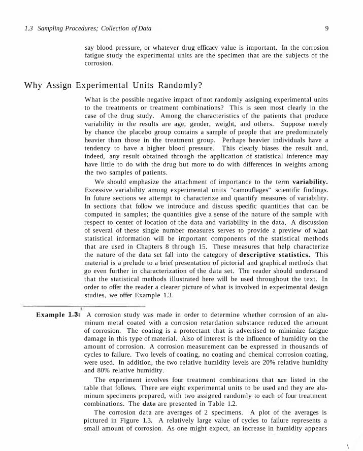
Example 1.3:1 A corrosion study was made in order to determine whether corrosion of an aluminum metal coated with a corrosion retardation substance reduced the amount of corrosion. The coating is a protectant that is advertised to minimize fatigue damage in this type of material. Also of interest is the influence of humidity on the amount of corrosion. A corrosion measurement can be expressed in thousands of cycles to failure. Two levels of coating, no coating and chemical corrosion coating, were used. In addition, the two relative humidity levels are 20% relative humidity and 80% relative humidity.
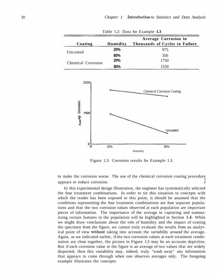
The experiment involves four treatment combinations that axe listed in the table that follows. There are eight experimental units to be used and they are aluminum specimens prepared, with two assigned randomly to each of four treatment combinations. The data are presented in Table 1.2.
The corrosion data are averages of 2 specimens. A plot of the averages is pictured in Figure 1.3. A relatively large value of cycles to failure represents a small amount of corrosion. As one might expect, an increase in humidity appears
\
10 Chapter 1 Introduction to Statistics and Data Analysis
Table 1.2: Data for Example 1.3
Average Corrosion in Coating Humidity Thousands of Cycles to Failure
Uncoated
Chemical Corrosion
20% 80% 20%
80%
975
350 1750
1550
2000
O 1000 <D
I
Chemical Corrosion Coating
Uncoated
20% 80% Humidity
Figure 1.3: Corrosion results for Example 1.3.
to make the corrosion worse. The use of the chemical corrosion coating procedure appears to reduce corrosion. J
In this experimental design illustration, the engineer has systematically selected the four treatment combinations. In order to tie this situation to concepts with which the reader has been exposed to this point, it should be assumed that the conditions representing the four treatment combinations are four separate populations and that the two corrosion values observed at each population are important pieces of information. The importance of the average in capturing and summarizing certain features in the population will be highlighted in Section 1.4. While we might draw conclusions about the role of humidity and the impact of coating the specimen from the figure, we cannot truly evaluate the results from an analytical point of view without taking into account the variability around the average. Again, as we indicated earlier, if the two corrosion values at each treatment combination are close together, the picture in Figure 1.3 may be an accurate depiction. But if each corrosion value in the figure is an average of two values that are widely dispersed, then this variability may, indeed, truly "wash away" any information that appears to come through when one observes averages only. The foregoing example illustrates the concepts:
1.4 Measures of Location: The Sample Mean and Median 11
(1) random assignment of treatment combinations (coating/humidity) to experimental units (specimens)
(2) the use of sample averages (average corrosion values) in summarizing sample information
(3) the need for consideration of measures of variability in the analysis of any sample or sets of samples
This example suggests the need for what follows in Sections 1.4 and 1.5, namely, descriptive statistics that indicate measures of center of location in a set of data, and those that measure variability.
1.4 Measures of Location: The Sample Mean and Median
Location measures in a data set are designed to provide the analyst some quantitative measure of where the data center is in a sample. In Example 1.2 it appears as if the center of the nitrogen sample clearly exceeds that of the no-nitrogen sample. One obvious and very useful measure is the sample mean. The mean is simply a numerical average.
Definition 1.1: Suppose that the observations in a sample are x
denoted by x is
_ _ v^ x% _ an + %i + • f-i n. n
I . . - C 2 , . .
• + X„
, xn. The sample mean,
There are other measures of central tendency that are discussed in detail in future chapters. One important measure is the sample median. The purpose of the sample median is to reflect the central tendency of the sample in such a way that it is uninfluenced by extreme values or outliers. Given that the observations in a sample are xj, X2> • • •, xn, arranged in increasing order of magnitude, the sample median is
- _ J •r("+i)/2: if n is odd, X =
$(xn/2 + En/2+l)5 n n i s c v c n -
For example, suppose the data set is the following: 1.7, 2.2, 3.9, 3.11, and 14.7. The sample mean and median are, respectively,
£ = 5.12, £ = 3.9.
Clearly, the mean is influenced considerably by the presence of the extreme observation, 14.7, whereas the median places emphasis on the true "center" of the data set. In the case of the two-sample data set of Example 1.2, the two measures of
12 Chapter 1 Introduction to Statistics and Data Analysis
central tendency for the individual samples are
X (no nitrogen) = 0.399 gram, . , . , 0.38 + 0.42 x (no nitrogen) — = 0.400 gram,
X (nitrogen) = 0.5G5 gram, 0,19 + 0.52
x (nitrogen) = = 0.505 gram.
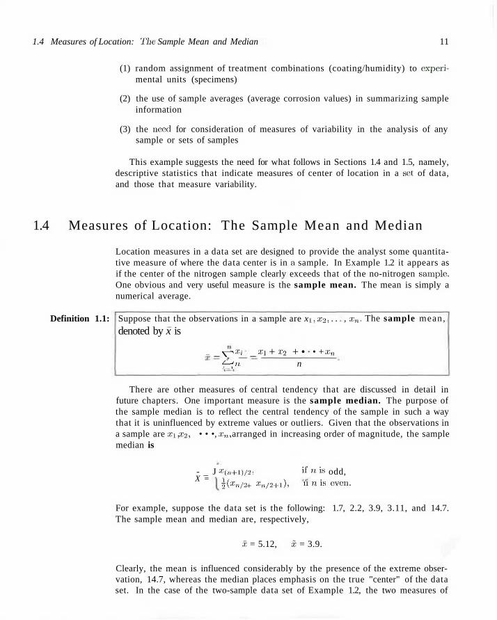
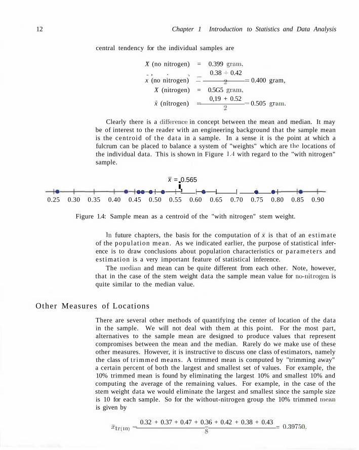
Clearly there is a difference in concept between the mean and median. It may be of interest to the reader with an engineering background that the sample mean is the centroid of the da ta in a sample. In a sense it is the point at which a fulcrum can be placed to balance a system of "weights" which are the locations of the individual data. This is shown in Figure 1.4 with regard to the "with nitrogen" sample.
x = 0.565
i • • - • + - • — H H » — I 1 • •+-0.25 0.30 0.35 0.40 0.45 0.50 0.55 0.60 0.65 0.70 0.75 0.80 0.85 0.90
Figure 1.4: Sample mean as a centroid of the "with nitrogen" stem weight.
In future chapters, the basis for the computation of x is that of an es t imate of the populat ion mean. As we indicated earlier, the purpose of statistical inference is to draw conclusions about population characteristics or pa ramete r s and es t imat ion is a very important feature of statistical inference.
The median and mean can be quite different from each other. Note, however, that in the case of the stem weight data the sample mean value for no-nitrogen is quite similar to the median value.
Other Measures of Locations
There are several other methods of quantifying the center of location of the data in the sample. We will not deal with them at this point. For the most part, alternatives to the sample mean are designed to produce values that represent compromises between the mean and the median. Rarely do we make use of these other measures. However, it is instructive to discuss one class of estimators, namely the class of t r immed means. A trimmed mean is computed by "trimming away" a certain percent of both the largest and smallest set of values. For example, the 10% trimmed mean is found by eliminating the largest 10% and smallest 10% and computing the average of the remaining values. For example, in the case of the stem weight data we would eliminate the largest and smallest since the sample size is 10 for each sample. So for the without-nitrogen group the 10% trimmed mean is given by
0.32 + 0.37 + 0.47 + 0.36 + 0.42 + 0.38 + 0.43 xtr(10) = 5 = 0.39(50.
Exercises 13
Exercises
and for the 10% trimmed mean for the with-nitrogen group we have
0.43 + 0.47 + 0.49 + 0.52 + 0.75 + 0.79 + 0.62 + 0.46 ^trcio) —
8 = 0.56625.
Note t h a t in this case, as expected, the t r immed means are close to both the mean and median for the individual samples. The t r immed mean approach is, of course, more insensitive to outliers than the sample mean but not as insensitive as the median. On the other hand the t r immed mean approach makes use of more information. Note t ha t the sample median is, indeed, a special case of the tr immed mean in which all of the sample da ta are eliminated apar t from the middle one or two observations.
1.1 The following measurements were recorded for the drying time, in hours, of a certain brand of latex paint.
3.4 2.5 4.8 2.9 3.6 2.8 3.3 5.6 3.7 2.8 4.4 4.0 5.2 3.0 4.8
Assume that the measurements are a simple random sample. (a) What is the sample size for the above sample?
(b) Calculate the sample mean for this data. (c) Calculate the sample median. (d) Plot the data by way of a dot plot. (e) Compute the 20% trimmed mean for the above
data set.
1.2 According to the journal Chemical Engineering, an important property of a fiber is its water ab-sorbency. A random sample of 20 pieces of cotton fiber is taken and the absorbency on each piece was measured. The following are the absorbency values:
18.71 21.41 20.72 21.81 19.29 22.43 20.17 23.71 19.44 20.50 18.92 20.33 23.00 22.85 19.25 21.77 22.11 19.77 18.04 21.12.
(a) Calculate the sample mean and median for the above sample values.
(b) Compute the 10% trimmed mean. (c) Do a dot plot of the absorbency data.
1.3 A certain polymer is used for evacuation systems for aircraft. It is important that the polymer be resistant to the aging process. Twenty specimens of the polymer were used in an experiment. Ten were assigned randomly to be exposed to the accelerated batch aging process that involved exposure to high temperatures for 10 days. Measurements of tensile strength of
218 229 215 204
217 228 211 201
225 221 209 205
the specimens were made and the following data were recorded on tensile strength in psi.
No aging: 227 222 218 216
Aging: 219 214 218 203
(a) Do a dot plot of the data. (b) From your plot, does it appear as if the aging pro
cess has had an effect on the tensile strength of this polymer? Explain.
(c) Calculate the sample mean tensile strength of the two samples.
(d) Calculate the median for both. Discuss the similarity or lack of similarity between the mean and median of each group.
1.4 In a study conducted by the Department of Me> chanical Engineering at Virginia Tech, the steel rods supplied by two different companies were compared. Ten sample springs were made out of the steel rods supplied by each company and a measure of flexibility was recorded for each. The data are as follows:
Company A: 9.3 8.8 6.8 8.7 8.5 6.7 8.0 6.5 9.2 7.0
Company B: 11.0 9.8 9.9 10.2 10.1 9.7 11.0 11.1 10.2 9.6
(a) Calculate the sample mean and median for the data for the two companies.
(b) Plot the data for the two companies on the same line and give your impression.
1.5 Twenty adult males between the ages of 30 and 40 were involved in a study to evaluate the effect of a specific health regimen involving diet and exercise on the blood cholesterol. Ten were randomly selected to be a control group and ten others were assigned to take
Control group:
Treatment group:
7 5
- 6 12
3 22
5 37
- 4 — 7
9 5
11 9 4 3
2.07 2.05 2.52 1.99
2.14 2.18 2.15 2.42
2.22 2.09 2.49 2.08
2.03 2.14 2.03 2.42
2.21 2.11 2.37 2.29
2.03 2.02 2.05 2.01
14 Chapter 1 Introduction to Statistics and Data Analysis
part in the regimen as the treatment group for a period to be a function of curing temperature. A study was of 6 months. The following data show the reduction in carried out in which samples of 12 specimens of the rub-cholesterol experienced for the time period for the 20 ber were prepared using curing temperatures of 20° C subjects: and 45° C. The data below show the tensile strength
values in megapascals.
20° C:
45° C:
(a) Do a dot plot of the data for both groups on the same graph. (a) Show a dot plot of the data with both low and high
(b) Compute the mean, median, and 10% trimmed temperature tensile strength values. means for both groups. (b) Compute sample mean tensile strength for both
(c) Explain why the difference in the mean suggests samples. one conclusion about the effect of the regimen, (c) Docs it appear as if curing temperature has an in-while the difference in medians or trimmed means fluence on tensile strength based on the plot? Com-suggests a different conclusion. ment further.
(d) Does anything else appear to be influenced by an 1.6 The tensile strength of silicone rubber is thought increase in cure temperature? Explain.
1.5 Measures of Variability
Sample variability plays an important role in da t a analysis. Process and product variability is a fact of life in engineering and scientific: systems: The control or reduction of process variability is often a source of major difficulty. More and more process engineers and managers are learning tha t product quality, and as a result, profits tha t are derived from manufactured products are very much a function of p r o c e s s v a r i a b i l i t y . As a result, much of Chapters 9 through 15 deal with da ta analysis and modeling procedures in which sample variability plays a major role. Even in small da ta analysis problems, the success of a particular statistical method may depend on the magnitude of the variability among the observations in the sample. Measures of location in a sample do not provide a proper summary of the nature of a da ta set. For instance, in Example 1.2 we cannot conclude tha t the use of nitrogen enhances growth without taking sample variability into account.
While the details of the analysis of this type of da ta set are deferred to Chapter 9, it should be clear from Figure 1.1 t ha t variability among the "no-nitrogen" observations and variability among the "with-nitrogen" observations are certainly of some consequence. In fact, it appears that the variability within the nitrogen sample is larger than that of the no-nitrogen sample. Perhaps there is something about the inclusion of nitrogen that not only increases the stem height (x of 0.565 gram compared to an x of 0.399 gram for the no-nitrogen sample) but also increases the variability in stem height (i.e., renders the stem height more inconsistent).
As another example, contrast the two da ta sets below. Each contains two samples and the difference in the means is roughly the same for the two samples: Da ta set B seems to provide a much sharper contrast between the two populations from which the samples were taken. If the purpose of such an experiment, is to detect distinction between the two populations, the task is accomplished in the case of da t a set B. However, in da ta set A the large variability within the two samples creates difficulty. In fact, it is not clear tha t there is a distinction bet-ween
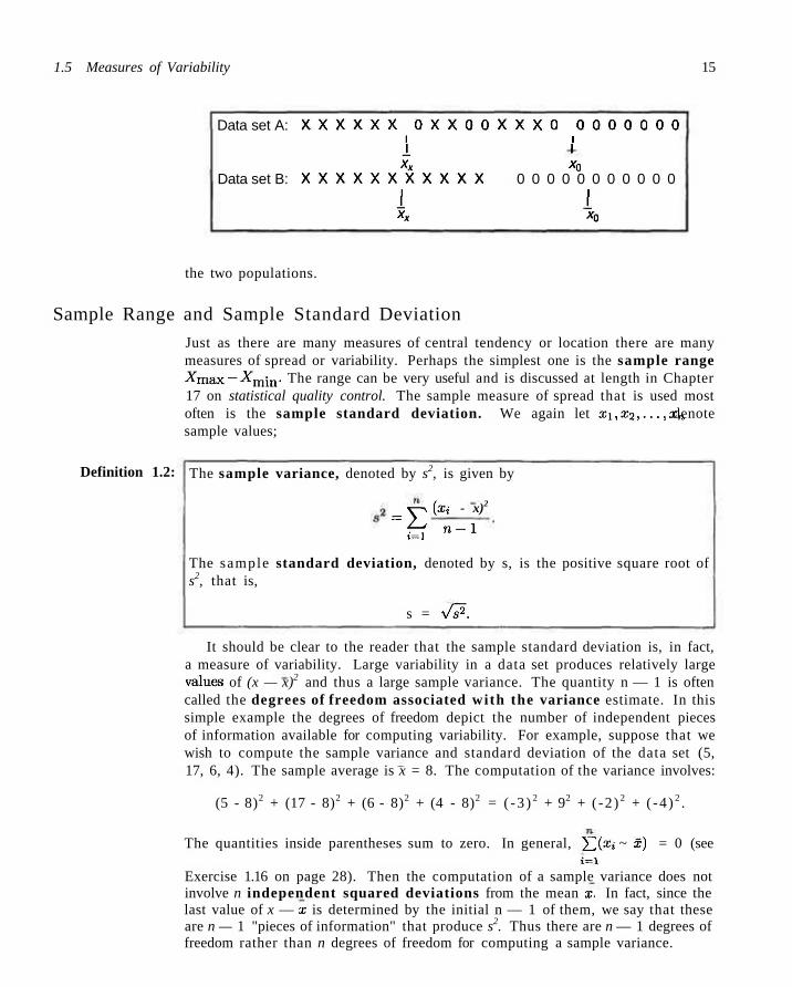
1.5 Measures of Variability 15
Data set A:
Data set B:
X X X X X X O X X O O X X X O O O O O O O O i i
1 I xx x0
X X X X X X X X X X X 0 0 0 0 0 0 0 0 0 0 0 1 1
J. J_ *x X0
the two populations.
Sample Range and Sample Standard Deviation
Just as there are many measures of central tendency or location there are many measures of spread or variability. Perhaps the simplest one is the sample range ^ m a x - ^ m i n . The range can be very useful and is discussed at length in Chapter 17 on statistical quality control. The sample measure of spread that is used most often is the sample standard deviation. We again let Xi,X2,...,xn denote sample values;
Definition 1.2: The sample variance, denoted by s2, is given by
(Xi - x)2
=£ i = i
n - 1
The sample standard deviation, denoted by s, is the positive square root of s2, that is,
s = Vs2.
It should be clear to the reader that the sample standard deviation is, in fact, a measure of variability. Large variability in a data set produces relatively large values of (x — x)2 and thus a large sample variance. The quantity n — 1 is often called the degrees of freedom associated with the variance estimate. In this simple example the degrees of freedom depict the number of independent pieces of information available for computing variability. For example, suppose that we wish to compute the sample variance and standard deviation of the data set (5, 17, 6, 4). The sample average is x = 8. The computation of the variance involves:
(5 - 8)2 + (17 - 8)2 + (6 - 8)2 + (4 - 8)2 = ( -3 ) 2 + 92 + ( -2) 2 + ( -4 ) 2 .
The quantities inside parentheses sum to zero. In general, Yl (xi ~ &) = 0 (see t=t
Exercise 1.16 on page 28). Then the computation of a sample variance does not involve n independent squared deviations from the mean x. In fact, since the last value of x — x is determined by the initial n — 1 of them, we say that these are n — 1 "pieces of information" that produce s2. Thus there are n — 1 degrees of freedom rather than n degrees of freedom for computing a sample variance.
16 Chapter 1 Introduction to Statistics and Data Analysis
Example 1.4:1 In an example discussed extensively in Chapter 10, an engineer is interested in testing the "bias" in a pH meter. Data arc collected on the meter by measuring the pH of a neutral substance (pH — 7.0). A sample of size 10 is taken with results given by
7.07 7.00 7.10 6.97 7.00 7.03 7.01 7.01 6.98 7.08.
The sample mean x is given by
. = 7 . 0 7 + 7 . 0 0 + 7 . 1 0 + - + 7.08 = ? ^
The sample variance s2 is given by
s2 =I[(7.07 - 7.025)2 + (7.00 - 7.025)2 + (7.10 - 7.025)2
+ • • • + (7.08 - 7.025)2] = 0.001939.
As a result, the sample standard deviation is given by
s = \/0.00193 = 0.044.
So the sample standard deviation is 0.0440 with n — 1 = 9 degrees of freedom. J
Units for Standard Deviation and Variance
It should be apparent from Definition 1.2 that the variance is a measure of the average squared deviation from the mean x. We use the term average squared deviation even though the definition makes use of a division by degrees of freedom n — 1 rather than n. Of course, if n is large the difference in the denominator is inconsequential. As a result, the sample variance possesses units that are the square of the units in the observed data whereas the sample standard deviation is found in linear units. As an example, consider the data of Example 1.2. The stem weights are measured in grams. As a result, the sample standard deviations are in grams and the variances are measured in grams . In fact, the individual standard deviations are 0.0728 grams for the no-nitrogen case and 0.1867 grams for the nitrogen group. Note that the variability as characterized by the standard deviation does indicate considerably larger variability in the nitrogen sample. This condition was noted from Figure 1.1.
Which Variability Measure Is More Important?
As we indicated earlier the sample range has applications in the area of statistical quality control. It may appear to the reader that the use of both the sample variance and the sample standard deviation is redundant. Both measures reflect the same concept in measuring variability but the sample standard deviation measures variability in linear units whereas the sample variance is measured in squared units. Both play huge roles in the use of statistical methods. Much of what is
Exercises ] 7
accomplished in the context: of statistical inference involves drawing conclusions about, characteristics of populations. Among these characteristics arc constants which are1 called p o p u l a t i o n p a r a m e t e r s . Two important parameters are the p o p u l a t i o n m e a n and the p o p u l a t i o n variance . The sample variance plays an explicit role in the statistical methods used to draw inferences about the population variance. The sample; s tandard deviation has an impor tant role along with the sample mean in inferences tha t are made about the population mean. In general, the variance is considered more in inferential theory, while the s tandard deviation is used more in applications.
Exercises
1.7 Consider the drying time data for Exercise 1.1 1.10 For the data of Exercise 1.4 on page 13. com-on page 13. Compute the sample-variance and sample pute both the mean and variance in 'flexibility" for standard deviation, berth company A and company B.
1.8 Compute the sample variance: and standard devi- i . n Consider the data in Exercise 1.5 on page 13. ation for the water absorbency data of Exercise 1.2 on Compute the sample variance and the sample standard page 13. deviation for both the control and treatment groups.
1.9 Exercise 1.3 on page 13 showed samples of tensile 1.12 Rjr Exercise 1.6 em page 14, compute the sample strength data, one for specimens that were exposed to standard deviation in tensile strength for the samples an aging process and one in which there was no ag- separately for the two temperatures. Does it. appear as ing of the specimens. Calculate the sample variance as if a r , i„ c r c a so in temperature influences the variability well as standard deviation in tensile strength for both m (ensile strength? Explain. samples.
1.6 Discrete and Continuous Data
Statistical inference through the analysis of observational studies or designed experiments is used in many scientific areas. T h e data gathered may be d i s c r e t e or cont inuous , depending on the area of application. For example1, a chemical engineer may be interested in conducting an experiment that will lead to conditions where yield is maximized. Here, of course, the yield may be in percent, or g rams/pound, measured on a continuum. On the other hand, a toxicologist conducting a combination drug experiment may encounter da ta that are binary in nature (i.e., the patient either responds or not) .
Great distinctions arc made between discrete and continuous data in the probability theory tha t allow us to draw statistical inferences. Often applications of statistical inference are found when the da ta are count, data. For example, an engineer may be interested in studying the number of radioactive particles passing through a counter in, say, 1 millisecond. Personnel responsible for the1 efficiency of a port facility may be interested in the characteristics of the number of oil tankers arriving each day at a certain port: city, In Chapter 5, several distinct scenarios, leading to different ways of handling da ta arc discussed for situations with count da ta .
Special a t tent ion even at this early stage of the textbook should be paid to some details associated with binary data . Applications requiring statistical analysis of
18 Chapter 1 Introduction to Statistics and Data Analysis
binary data are voluminous. Often the measure that is used in the analysis is the sample proportion. Obviously the binary situation involves two categories. If there are n units involved in the data and x is defined as the number that fall into category 1, then n — x fall into category 2. Thus, x/n is the sample proportion in category 1 and 1 — x/n is the sample proportion in category 2. In the biomedical application, 50 patients may represent the sample units and if 20 out of 50 experienced an improvement in a stomach ailment (common to all 50) after all were given the drug, then |g = 0.4 is the sample proportion for which the drug was a success and 1 — 0.4 = 0.6 is the sample proportion for which the drug was not successful. Actually the basic numerical measurement for binary data is generally denoted by either 0 or 1. For example, in our medical example, a successful result is denoted by a 1 and a nonsuccess a 0. As a result, the sample proportion is actually a sample mean of the ones and zeros. For the successful category,
xi + x2 + • • • + x50 _ 1 + 1 + 0 + - - + 0 + 1 _ 20 50 ~ 50 ~ 50 ~ ' '
What Kinds of Problems Are Solved in Binary Data Situations?
The kinds of problems facing scientists and engineers dealing in binary data are not a great deal unlike those seen where continuous measurements are of interest. However, different techniques are used since the statistical properties of sample proportions are quite different from sample means that result from averages taken from continuous populations. Consider the example data in Exercise 1.6 on page 14. The statistical problem underlying this illustration focuses on whether an intervention, say, on increase in cure temperature, will alter the population mean tensile strength associated with the silicone rubber process. On the other hand, in a quality control area suppose an automobile tire manufacturer reports that a shipment of 5000 tires selected randomly from the process results in 100 of them showing blemishes. Here the sample proportion is §^§j = 0.02. Following a change in the process designed to reduce blemishes, a second sample of 5000 is taken and 90 tires are blemished. The sample proportion has been reduced to gg§j, = 0.018. The question arises, "Is the decrease in the sample proportion from 0.02 to 0.018 substantial enough to suggest a real improvement in the population proportion?" Both of these illustrations require the use of the statistical properties of sample averages-one from samples from a continuous population, and the other from samples from a discrete (binary) population. In both cases the sample mean is an estimate of a population parameter, a population mean in the first illustration (i.e., mean tensile strength), and a population proportion (i.e., proportion of blemished tires in the population), in the second case. So here we have sample estimates used to draw scientific conclusions regarding population parameters. As we indicated in Section 1.4, this is the general theme in many practical problems using statistical inference.
1.7 Statistical Modeling, Scientific Inspection, and Graphical Diagnostics 19
1.7 Statistical Modeling, Scientific Inspection, and Graphical Diagnostics
Often the end result of a statistical analysis is the estimation of parameters of a postulated model. This is natural for scientists and engineers since they often deal in modeling. A statistical model is not deterministic but, rather, must entail some probabilistic: aspects. A model form is often the foundation of assumpt ions that are made by the analyst. For example, in our Example 1.2 the scientist may wish to draw some level of distinction between the "nitrogen" and "no-nitrogen" populations through the sample information. The analysis may require a certain model for the data, for example, that the two samples conic: from normal or Gaussian dis t r ibut ions . See Chapter 6 for a discussion of the normal distribution.
At times the model postulated may take on a somewhat more complicated form. Consider, for example, a textile manufacturer who designs an experiment where cloth specimens are being produced that contain various percentages of cotton. Consider the data in Table 1.3.
Table 1.3: Tensile Strength
Cot ton Percentage Tensile S t r eng th
15 20 25 30
7, 7, 9, 8, 10 19, 20, 21, 20, 22 21, 21, 17, 19, 20 8, 7, 8, 9, 10
Five cloth specimens are manufactured for each of the four cotton percentages. In this case both the model for the experiment and the type of analysis used should take into account the goal of the experiment and important input from the textile scientist. Some simple graphics can shed important light, on the clear distinction between the samples. Sec Figure 1.5; the sample means and variability are depicted nicely in the data plot. One possible goal of this experiment is simply to determine whic:h cotton percentages are truly distinct from the others. In other words, as in the case of the nitrogen/no-nitrogen data, for which cotton percentages are there clear distinctions between the populations or, more specifically, between the population means? In this case, perhaps a reasonable: model is that each sample comes from a normal distribution. Here the goal is very much like that of the nitrogen/iio-iiitrogen data except that more samples are involved. The formalism of the analysis involves notions of hypothesis testing discussed in Chapter 10. Incidentally, this formality is perhaps not necessary in light of the diagnostic plot. But does this describe the real goal of the experiment and hence the proper approach to data analysis? It is likely that the scientist anticipates the existence of a maximum, population mean tensile strength in the range of cotton concentration in the experiment. Here the analysis of the data should revolve around a different type of model, one that postulates a type of structure relating the population
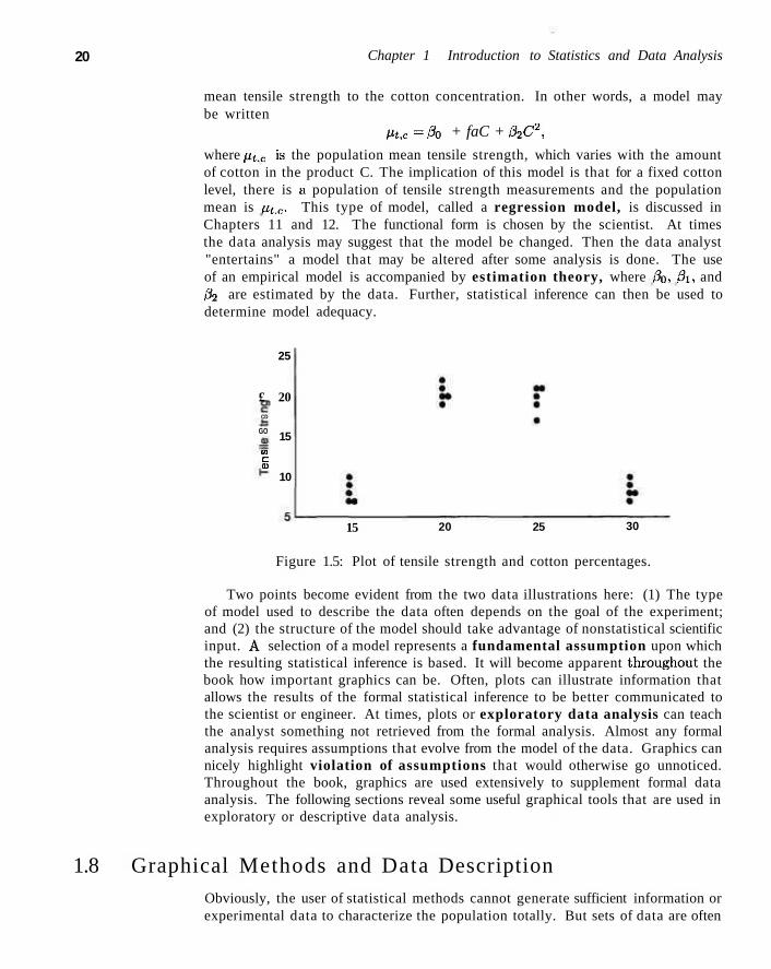
20 Chapter 1 Introduction to Statistics and Data Analysis
mean tensile strength to the cotton concentration. In other words, a model may be written
»t,c = .3o + faC + i32c2,
where fit.c is the population mean tensile strength, which varies with the amount of cotton in the product C. The implication of this model is that for a fixed cotton level, there is a population of tensile strength measurements and the population mean is ut.r.- This type of model, called a regression model, is discussed in Chapters 11 and 12. The functional form is chosen by the scientist. At times the data analysis may suggest that the model be changed. Then the data analyst "entertains" a model that may be altered after some analysis is done. The use of an empirical model is accompanied by estimation theory, where 3Q, 8\, and P2 are estimated by the data. Further, statistical inference can then be used to determine model adequacy.
25
£ 20 CD
GO
W c a
15
10
15 20 25 30
Figure 1.5: Plot of tensile strength and cotton percentages.
Two points become evident from the two data illustrations here: (1) The type of model used to describe the data often depends on the goal of the experiment; and (2) the structure of the model should take advantage of nonstatistical scientific input. xA selection of a model represents a fundamental assumption upon which the resulting statistical inference is based. It will become apparent throughout the book how important graphics can be. Often, plots can illustrate information that allows the results of the formal statistical inference to be better communicated to the scientist or engineer. At times, plots or exploratory data analysis can teach the analyst something not retrieved from the formal analysis. Almost any formal analysis requires assumptions that evolve from the model of the data. Graphics can nicely highlight violation of assumptions that would otherwise go unnoticed. Throughout the book, graphics are used extensively to supplement formal data analysis. The following sections reveal some useful graphical tools that are used in exploratory or descriptive data analysis.
1.8 Graphical Methods and Data Description Obviously, the user of statistical methods cannot generate sufficient information or experimental data to characterize the population totally. But sets of data are often
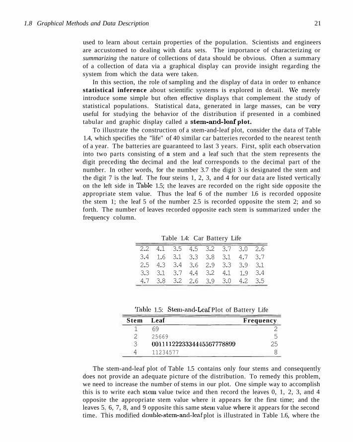
1.8 Graphical Methods and Data Description 21
used to learn about certain properties of the population. Scientists and engineers are accustomed to dealing with data sets. The importance of characterizing or summarizing the nature of collections of data should be obvious. Often a summary of a collection of data via a graphical display can provide insight regarding the system from which the data were taken.
In this section, the role of sampling and the display of data in order to enhance statistical inference about scientific systems is explored in detail. We merely introduce some simple but often effective displays that complement the study of statistical populations. Statistical data, generated in large masses, can be very useful for studying the behavior of the distribution if presented in a combined tabular and graphic display called a stem-and-leaf plot.
To illustrate the construction of a stem-and-leaf plot, consider the data of Table 1.4, which specifies the "life" of 40 similar car batteries recorded to the nearest tenth of a year. The batteries are guaranteed to last 3 years. First, split each observation into two parts consisting of a stem and a leaf such that the stem represents the digit preceding the decimal and the leaf corresponds to the decimal part of the number. In other words, for the number 3.7 the digit 3 is designated the stem and the digit 7 is the leaf. The four steins 1, 2, 3, and 4 for our data are listed vertically on the left side in Table 1.5; the leaves are recorded on the right side opposite the appropriate stem value. Thus the leaf 6 of the number 1.6 is recorded opposite the stem 1; the leaf 5 of the number 2.5 is recorded opposite the stem 2; and so forth. The number of leaves recorded opposite each stem is summarized under the frequency column.
Table 1.4: Car Battery Life
2.2 3.4 2.5 3.3 4.7
4.1 1.6 4.3 3.1 3.8
3.5 3.1 3.4 3.7 3.2
4.5 3.3 3.6 4.4 2.6
3.2 3.8 2.9 3.2 3.9
3.7 3.1 3.3 4.1 3.0
3.0 4.7 3.9 1.9 4.2
2.6 3.7 3.1 3.4 3.5
Table 1.5: Stem-and-Leaf Plot of Battery Life
Stem Leaf Frequency 1 2 3 4
69 25669 0011112223334445507778899 11234577
2 5 25 8
The stem-and-leaf plot of Table 1.5 contains only four stems and consequently does not provide an adequate picture of the distribution. To remedy this problem, we need to increase the number of stems in our plot. One simple way to accomplish this is to write each stein value twice and then record the leaves 0, 1, 2, 3, and 4 opposite the appropriate stem value where it appears for the first time; and the leaves 5. 6, 7, 8, and 9 opposite this same stein value wdiere it appears for the second time. This modified double-stem-and-leaf plot is illustrated in Table 1.6, where the
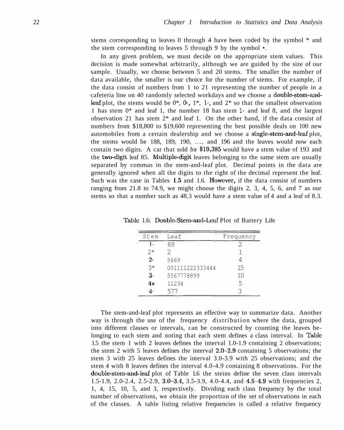
22 Chapter 1 Introduction to Statistics and Data Analysis
stems corresponding to leaves 0 through 4 have been coded by the symbol * and the stem corresponding to leaves 5 through 9 by the symbol •.
In any given problem, we must decide on the appropriate stem values. This decision is made somewhat arbitrarily, although we are guided by the size of our sample. Usually, we choose between 5 and 20 stems. The smaller the number of data available, the smaller is our choice for the number of stems. For example, if the data consist of numbers from 1 to 21 representing the number of people in a cafeteria line on 40 randomly selected workdays and we choose a double-stem-and-leaf plot, the stems would be 0*, 0-, 1*, 1-, and 2* so that the smallest observation 1 has stem 0* and leaf 1, the number 18 has stem 1- and leaf 8, and the largest observation 21 has stem 2* and leaf 1. On the other hand, if the data consist of numbers from $18,800 to $19,600 representing the best possible deals on 100 new automobiles from a certain dealership and we choose a single-stem-and-leaf plot, the stems would be 188, 189, 190, . . . , and 196 and the leaves would now each contain two digits. A car that sold for 819,385 would have a stem value of 193 and the two-digit leaf 85. Multiple-digit leaves belonging to the same stem are usually separated by commas in the stem-and-leaf plot. Decimal points in the data are generally ignored when all the digits to the right of the decimal represent the leaf. Such was the case in Tables 1.5 and 1.6. However, if the data consist of numbers ranging from 21.8 to 74.9, we might choose the digits 2, 3, 4, 5, 6, and 7 as our stems so that a number such as 48.3 would have a stem value of 4 and a leaf of 8.3.
Table 1.6: Double-Stem-and-Leaf Plot of Battery Life
Stem 1-2* 2-3* 3 4* 4-
Leaf 69 2 5669 001111222333444 5567778899 11234 577
Frequency 2 1 4 15 10 5 3
The stem-and-leaf plot represents an effective way to summarize data. Another way is through the use of the frequency dis t r ibut ion where the data, grouped into different classes or intervals, can be constructed by counting the leaves belonging to each stem and noting that each stem defines a class interval. In Table 1.5 the stem 1 with 2 leaves defines the interval 1.0-1.9 containing 2 observations; the stem 2 with 5 leaves defines the interval 2.0-2.9 containing 5 observations; the stem 3 with 25 leaves defines the interval 3.0-3.9 with 25 observations; and the stem 4 with 8 leaves defines the interval 4.0-4.9 containing 8 observations. For the double-stem-and-leaf plot of Table 1.6 the steins define the seven class intervals 1.5-1.9, 2.0-2.4, 2.5-2.9, 3.0-3.4, 3.5-3.9, 4.0-4.4, and 4.5-4.9 with frequencies 2, 1, 4, 15, 10, 5, and 3, respectively. Dividing each class frequency by the total number of observations, we obtain the proportion of the set of observations in each of the classes. A table listing relative frequencies is called a relative frequency
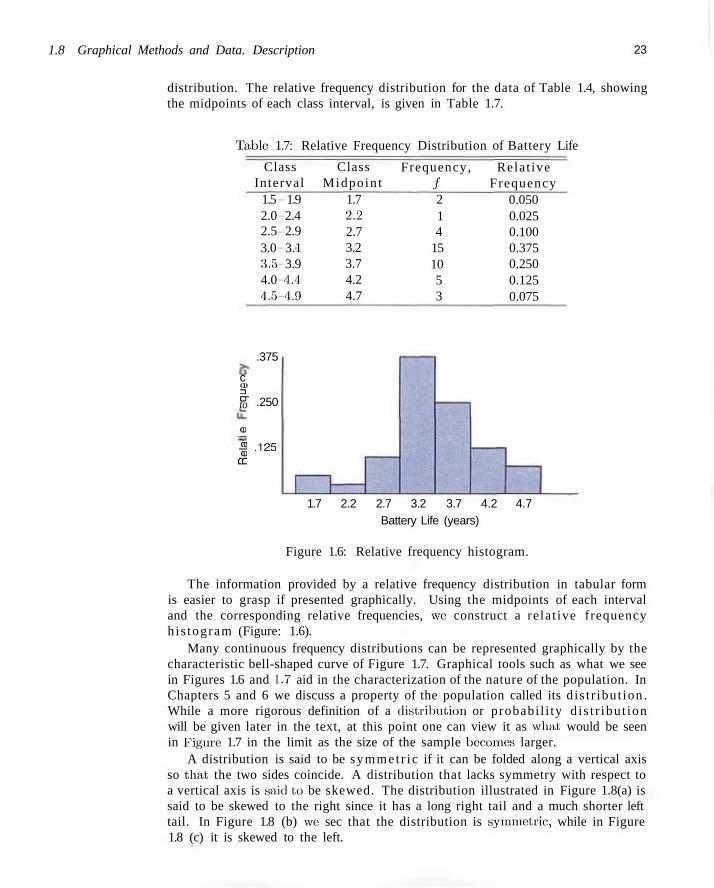
1.8 Graphical Methods and Data. Description 23
distribution. The relative frequency distribution for the data of Table 1.4, showing the midpoints of each class interval, is given in Table 1.7.
Table 1.7: Relative Frequency Distribution of Battery Life
Class Interval
1.5 1.9 2.0 2.4 2.5 2.9 3.0 3.1 3.5 3.9 4.0 •1.1 4.5-4.9
Class Midpoin t
1.7 2.2 2.7 3.2 3.7 4.2 4.7
Frequency, / 2 1 4
15 10 5 3
Relat ive Frequency
0.050 0.025 0.100 0.375 0.250 0.125 0.075
.375
c CD 3 cr to
a) >
.250
I -125 PC
1.7 2.2 2.7 3.2 3.7 4.2 Battery Life (years)
4.7
Figure 1.6: Relative frequency histogram.
The information provided by a relative frequency distribution in tabular form is easier to grasp if presented graphically. Using the midpoints of each interval and the corresponding relative frequencies, we construct a relat ive frequency h is togram (Figure: 1.6).
Many continuous frequency distributions can be represented graphically by the characteristic bell-shaped curve of Figure 1.7. Graphical tools such as what we see in Figures 1.6 and L.7 aid in the characterization of the nature of the population. In Chapters 5 and 6 we discuss a property of the population called its d is t r ibut ion. While a more rigorous definition of a distribution or probabi l i ty d is t r ibut ion will be given later in the text, at this point one can view it as what, would be seen in Figme 1.7 in the limit as the size of the sample becomes larger.
A distribution is said to be symmet r i c if it can be folded along a vertical axis so that, the two sides coincide. A distribution that lacks symmetry with respect to a vertical axis is said to be skewed. The distribution illustrated in Figure 1.8(a) is said to be skewed to the right since it has a long right tail and a much shorter left tail. In Figure 1.8 (b) we sec that the distribution is symmetric, while in Figure 1.8 (c) it is skewed to the left.
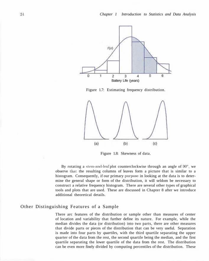
Chapter 1 Introduction to Statistics and Data Analysis
2 3 4 Battery Life (years)
Figure 1.7: Estimating frequency distribution.
Figure 1.8: Skewness of data.
By rotating a stem-and-leaf plot counterclockwise through an angle of 90°, we observe that the resulting columns of leaves form a picture that is similar to a histogram. Consequently, if our primary purpose: in looking at the data is to determine the general shape or form of the distribution, it will seldom be necessary to construct a relative frequency histogram. There are several other types of graphical tools and plots that are used. These are discussed in Chapter 8 after we introduce additional theoretical details.
Other Distinguishing Features of a Sample
There arc features of the distribution or sample other than measures of center of location and variability that further define its nature. For example, while the median divides the data (or distribution) into two parts, there are other measures that divide parts or pieces of the distribution that can be very useful. Separation is made into four parts by quartiles, with the third qnartile separating the upper quarter of the data from the rest, the second qnartile being the median, and the first quartile separating the lower quartile of the data from the rest. The distribution can be even more finely divided by computing percentiles of the distribution. These
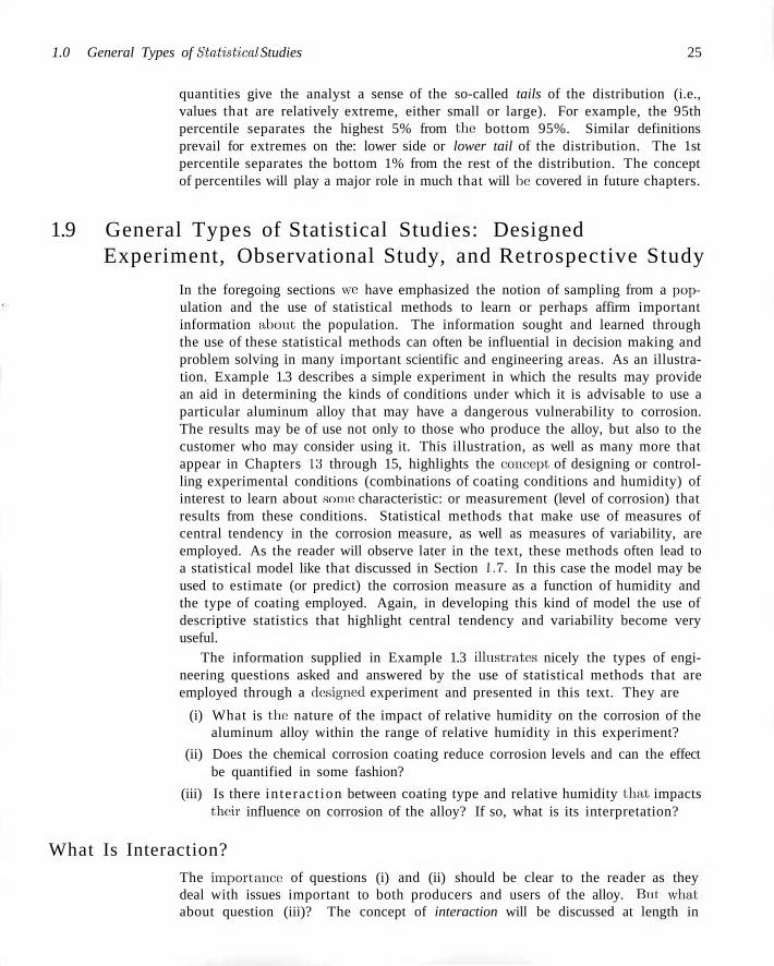
1.0 General Types of Statistical Studies 25
quantities give the analyst a sense of the so-called tails of the distribution (i.e., values that are relatively extreme, either small or large). For example, the 95th percentile separates the highest 5% from the: bottom 95%. Similar definitions prevail for extremes on the: lower side or lower tail of the distribution. The 1st percentile separates the bottom 1% from the rest of the distribution. The concept of percentiles will play a major role in much that will be covered in future chapters.
1.9 General Types of Statistical Studies: Designed Experiment, Observational Study, and Retrospective Study
In the foregoing sections we have emphasized the notion of sampling from a population and the use of statistical methods to learn or perhaps affirm important information about the population. The information sought and learned through the use of these statistical methods can often be influential in decision making and problem solving in many important scientific and engineering areas. As an illustration. Example 1.3 describes a simple experiment in which the results may provide an aid in determining the kinds of conditions under which it is advisable to use a particular aluminum alloy that may have a dangerous vulnerability to corrosion. The results may be of use not only to those who produce the alloy, but also to the customer who may consider using it. This illustration, as well as many more that appear in Chapters 13 through 15, highlights the concept of designing or controlling experimental conditions (combinations of coating conditions and humidity) of interest to learn about some characteristic: or measurement (level of corrosion) that results from these conditions. Statistical methods that make use of measures of central tendency in the corrosion measure, as well as measures of variability, are employed. As the reader will observe later in the text, these methods often lead to a statistical model like that discussed in Section 1.7. In this case the model may be used to estimate (or predict) the corrosion measure as a function of humidity and the type of coating employed. Again, in developing this kind of model the use of descriptive statistics that highlight central tendency and variability become very useful.
The information supplied in Example 1.3 illustrates nicely the types of engineering questions asked and answered by the use of statistical methods that are employed through a designed experiment and presented in this text. They are
(i) What is the nature of the impact of relative humidity on the corrosion of the aluminum alloy within the range of relative humidity in this experiment?
(ii) Does the chemical corrosion coating reduce corrosion levels and can the effect be quantified in some fashion?
(iii) Is there in teract ion between coating type and relative humidity that impacts thc:ir influence on corrosion of the alloy? If so, what is its interpretation?
What Is Interaction?
The importance: of questions (i) and (ii) should be clear to the reader as they deal with issues important to both producers and users of the alloy. But. what about question (iii)? The concept of interaction will be discussed at length in
26 Chapter 1 Introduction to Statistics and Data Analysis
Chapters 14 and 15. Consider the plot in Figure 1.3. This is an illustration of the detection of interaction between two factors in a simple designed experiment. Note that the lines connecting the sample means are not parallel. Parallelism would have indicated that the effect (seen as a result of the slope of the lines) of relative humidity is the same, namely a negative effect, for both an uncoated condition and the chemical corrosion coating. Recall the "negative" slope implies that corrosion becomes more pronounced as humidity rises. Lack of parallelism implies an interaction between coating type and relative humidity. The nearly "flat" line for the corrosion coating as opposed to a steeper slope for the uncoated condition suggests that not only is the chemical corrosion coating beneficial (note the displacement between the lines), but the presence of the coating renders the effect of humidity negligible. Clearly all these questions are very important to the effect of the two individual factors and to the interpretation of the interaction, if it is present.
Statistical models are extremely useful in answering questions as those listed in (i), (ii), and (iii), where the data come from a designed experiment. But one does not always have the luxury or resources that allow the employment of a designed experiment. For example, there are many instances in which the conditions of interest to the scientist or engineer cannot be implemented simply because the important factors cannot be controlled. In Example 1.3, the relative humidity and coating type (or lack of coating) are quite easy to control. This of course is the defining feature of a designed experiment. In many fields, factors that need to be studied cannot be controlled for any one of various reasons. Tight control as in Example 1.3 allows the analyst to be confident that any differences found (for example, in corrosion levels) are due to the factors under control. As a second illustration, consider Exercise 1.6 on page 14. Suppose in this case 24 specimens of silicone rubber are selected and 12 assigned to each of the cure temperature levels. The temperatures are controlled carefully and thus this is an example of a designed experiment with a single factor being cure temperature. Differences found in the mean tensile strength would be assumed to be attributed to the different cure temperatures.
What if Factors Are Not Controlled?
Suppose there are no factors controlled and no random assignment of fixed treatments to experimental units and yet there is a need to glean information from a data set. As an illustration, a study is done in which interest centers around the relationship between blood cholesterol levels and the amount of sodium measured in the blood. A group of individuals were monitored over time and both blood cholesterol and sodium were monitored. Certainly some useful information can be gathered from such a data set. However, it should be clear that there certainly can be no strict control of blood sodium levels. Ideally, the subject should be divided randomly into two groups with one group assigned a specific "high level" of blood sodium and another a specific "low level" of blood sodium. Obviously this cannot be done. Clearly changes in cholesterol can be experienced because of changes in one of a number of other factors that were not controlled. This kind of study, without factor control, is called an observational study. Much of the time it involves a situation in which subjects are observed across time.
1.9 General Types of Statistical Studies 27
Biological and biomedical studies are often by necessity observational studies. However, observational studies are not confined to those areas. For example, consider a study that is designed to determine the influence of ambient temperature on the electric power consumed by a chemical plant. Clearly, levels of ambient temperature cannot be controlled and thus the data structure can only be a monitoring of the data from the plant over time,
It should be apparent that the striking difference between a well designed experiment and observational studies is the difficulty in determination of true cause and effect with the latter. Also, differences found in the fundamental response (e.g., corrosion levels, blood cholesterol, plant electric power consumption) may be due to other underlying factors that were not controlled. Ideally in a designed experiment the nuisance factors would be equalized via the randomization process. Certainly changes in blood cholesterol could be due to fat intake or exercise activity, and so on. Electric power consumption could be affected by the amount of product produced or even the purity of the product produced.
Another often ignored disadvantage in an observational study when compared to carefully designed experiments is that unlike the latter, observational studies are at the mercy of nature, environmental or other uncontrolled circumstances that impact the ranges of factors of interest. For example, in the biomedical study regarding the influence of blood sodium levels on blood cholesterol, it is possible that there is indeed a strong influence but the particular data set used did not involve enough observed variation in sodium levels because of the nature of the subjects chosen. Of course, in a designed experiment, the analyst chooses and controls ranges of factors.
A third type of statistical study which can be very useful but has clear disadvantages when compared to a designed experiment is a retrospective study. This type of study uses strictly historical data, data taken over a specific period of time. One obvious advantage with retrospective data is that there is no cost in collecting the data. However, as one might expect, there are clear disadvantages.
(i) Validity and reliability of historical data are often in doubt.
(ii) If time is an important aspect of the structure of the data, there may be data missing.
(iii) There may be errors in collection of the data that are not known.
(iv) Again, as is the case of observational data, there is no control on the ranges of the measured variables (the factors in a study). Indeed, the ranges found in historical data may not be relevant for current studies.
Studies Not to Derive Relationships among Variables
In Section 1.7 some attention was given to modeling of relationships among variables. We introduced the notion of regression analysis, which is covered in Chapters 11 and 12 and is illustrated as a form of data analysis for designed experiments discussed in Chapters 14 and 15. In Section 1.7, a model relating population mean tensile strength of cloth to percentages of cotton was used for illustration where 20 specimens of cloth represented the experimental units. In that case, the data came from a simple designed experiment where the individual cotton percentages were selected by the scientist.
28 Chapter 1 Introduction to Statistics and Data Analysis
Often both observational data and retrospective da ta are used for the purpose of observing relationships among variables through model building procedures discussed in Chapters 11 and 12. While the advantages of designed experiments certainly apply when the goal is statistical model building, there are many areas in which designing of experiments is not possible. Thus, observational or historical data must be used. We refer here to a historical data set that is found in Exercise 12.9 on page 454. The goal is to build a model that will result in an equation or relationship that relates monthly electric power consumed to average ambient tempera ture Xi, the: number of days in the month SBJ, the average product purity x-3, and the tons of product produced :i:,|. The da ta are the past year's historical data .
Exercises
1.13 A manufacturer of electronic components is interested in determining the lifetime of a certain type of battery. A sample, in hour's of life, is as follows:
123,116,122,110,175, 120,125, 111, 118, 117.
(a) Find the sample mean and median. (b) What feature in this data set is responsible for the
substantial difference between the two?
1.14 A tire manufacturer wants to determine the inner diameter of a certain grade of tire. Ideally, the diameter would be 570 mm. The data are as follows:
572,572,573,568,569,575,565,570.
(a) Find the sample mean and median. (b) Find the sample variance, standard deviation, and
range. (c) Using the calculated statistics in parts (a) and (b),
can you comment on the quality of the tires?
1.15 Five independent coin tosses result in HIIHHII. It turns out that if the coin is fair the probability of this outcome is ( l / 2 ) s = 0.03125. Does this produce strong evidence that the coin is not fair? Comment and use the concept of P-value discussed in Section 1.2.
1.16 Show that the n pieces of information in £ (i"i —
x) ai'e n ° t independent: that, is, show that,
B* 0.
1.17 A study of the effects of smoking on sleep patterns is conducted. The measure observed is the time. in minutes, that it takes to fall asleep. These data are obtained:
Smokers:
Nonsmokers:
69.3 53.2 60.2 28.6 29.8 30.6 36.0
56.0 48.1 43.8 25.1 28.4 31.8 37.9
22.1 52.7 23.2 26.4 38.5 41.6 13.9
47.6 34.4 13.8 34.9 30.2 21.1
(a) Find the sample mean for each group. (b) Find the sample standard deviation for each group. (c) Make a dot plot of the data sets A and B on the
same line.
(d) Comment on what kind of impact smoking appears to have on the time required to fall asleep.
1.18 The following scores represent the final examination grade for an elementary statistics course:
23 60 79 32 57 74 52 70 82 95 41 65 92 85 64 75 78 25 80 71 83 54 64 72 60 78 89 76 84 79 34 67 17 82 85 61
(a) Construct a stem-and-leaf plot for the examhiation grades in which the stems are 1, 2, 3 , . . . . 9.
(b) Set up a relative frequency distribution. (c) Construct a relative frequency histogram, draw an
estimate of the graph of the distribution and discuss the skewness of the distribution.
(d) Compute the sample mean, sample median, and sample standard deviation.
1.19 The following data represent the length of life in years, measured to the nearest tenth, of 39 similar fuel pumps:
36 55 98 88 48 69
80 76 81 62 84 74
77 52 67 74 90 i;:;
81 10 41 43 15 80
Exercises
2.0 0.2 1.5 4.5 1.0
3.0 6.0 4.0 0.3 6.0
0.3 5.5 5.9 1.5 5.6
3.3 6.5 1.8 0.5 6.0
1.3 0.2 4.7 2.5 1.2
0.4 2.3 0.7 5.0 0.2
(a) Construct a stem-and-leaf plot for the life in years of the fuel pump using the digit to the left of the decimal point as the stem for each observation.
(b) Set up a relative frequency distribution. (c) Compute the sample mean, sample range, and sam
ple standard deviation.
1.20 The following data represent the length of life, in seconds, of 50 fruit flies subject to a new spray in a controlled laboratory experiment:
17 20 10 9 23 13 12 19 18 24 12 14 6 9 13 6 7 10 13 7 16 18 8 13 3 32 9 7 10 II 13 7 18 7 10 4 27 19 16 8 7 10 5 14 15 10 9 6 7 15
(a) Construct a double-stem-and-leaf plot for the life span of the fruit flies using the stems 0*, 0-, 1*, 1-, 2*, 2-, and 3* such that stems coded by the symbols * and • are associated, respectively, with leaves 0 through 4 and 5 through 9.
(b) Set up a relative frequency distribution. (c) Construct a relative frequency histogram. (d) Find the median.
1.21 The nicotine contents, in milligrams, for 40 cigarettes of a certain brand were recorded as follows:
1.09 1.92 2.31 1.79 2.28 1.74 1.47 1.97 0.85 1.24 1.58 2.03 1.70 2.17 2.55 2.11 1.86 1.90 1.68 1.51 1.64 0.72 1.69 1.85 1.82 1.79 2.46 1.88 2.08 1.67 1.37 1.93 1.40 1.64 2.09 1.75 1.63 2.37 1.75 1.69
(a) Find the sample mean and sample median. (b) Find the sample standard deviation.
1.22 The following data are the measures of the diameters of 36 rivet heads in 1/100 of an inch.
6.72 6.77 6.82 6.70 6.78 6.70 6.62 6.75 6.66 6.66 6.64 6.76 6.73 6.80 6.72 6.76 6.76 6.68 6.66 6.62 6.72 6.76 6.70 6.78 6.76 6.67 6.70 6.72 6.74 6.81 6.79 6.78 6.66 6.76 6.76 6.72
(a) Compute the sample mean and sample standard deviation.
(b) Construct a relative frequency histogram of the data.
29
(c) Comment on whether there is any clear indication or not that the sample came from a population that depicts a bell-shaped distribution.
1.23 The hydrocarbon emissions at idling speed in parts per million (ppm) for automobiles of 1980 and 1990 are given for 20 randomly selected cars.
1980 models: 141 359 247 940 882 494 306 210 105 880 200 223 188 940 241 190 300 435 241 380
1990 models: 140 160 20 20 223 60 20 95 360 70 220 400 217 58 235 380 200 175 85 65
(a) Construct a dot plot as in Figure 1.1. (b) Compute the sample means for the two years and
superimpose the two means on the plots. (c) Comment on what the dot plot indicates regarding
whether or not the population emissions changed from 1980 to 1990. Use the concept of variability in you comments.
1.24 The following are historical data on staff salaries (dollars per pupil on 30 schools sampled in the eastern part of the United States in the early 1970s).
3.79 2.99 2.77 2.91 3.10 1.84 2.52 3.22 2.45 2.14 2.67 2.52 2.71 2.75 3.57 3.85 3.36 2.05 2.89 2.83 3.13 2.44 2.10 3.71 3.14 3.54 2.37 2.68 3.51 3.37
(a) Compute the sample mean and sample standard deviation.
(b) Construct a relative frequency histogram of the data.
(c) Construct a stem-and-leaf display of the data.
1.25 The following data set is related to that in Exercise 1.24. It gives the percent of the families that are in the upper income level at the same individual schools in the same order as in Exercise 1.24.
72.2 31.9 26.5 29.1 27.3 8.6 22.3 26.5 20.4 12.8 25.1 19.2 24.1 58.2 68.1 89.2 55.1 9.4 14.5 13.9 20.7 17.9 8.5 55.4 38.1 54.2 21.5 26.2 59.1 43.3
(a) Calculate the sample mean. (b) Calculate the sample median. (c) Construct a relative frequency histogram of the
data. (d) Compute the 10% trimmed mean. Compare with
the results in (a) and (b) and comment.
1.26 Suppose it is of interest to use the data sets in Exercises 1.24 and 1.25 to derive a model that would predict staff salaries as a function of percent of families
30 Chapter 1 Introduction to Statistics and Data Analysis
in a high income level for current school systems. Comment on any disadvantage in carrying out this type of analysis.
1.27 A study is done to determine the influence of the wear, y, of a bearing as a function of the load, a;, on the bearing. A designed experiment is used for this study. Three levels of load were used, 700 lb, 1000 lb, and 1300 lb. Four specimens were used at each level and the sample means were, respectively, 210, 325, and 375.
(a) Plot average of wear against load.
(b) From the plot in (a), does it appear as if a relationship exists between wear and load?
(c) Suppose we look at the individual wear values for each of the four specimens at each load level.
y^ 3/7 y* Vi
700 145 105 260 330
1000 250 195 375 480
1300 150 180 420 750
j/i = 210 y2 = 325 ya = 375 Plot the wear results for all specimens against the three load values.
(d) From your plot in (c), does it appear as if a clear relationship exists? If your answer is different from that in (b), explain why.
1.28 Many manufacturing companies in the United States and abroad use molded parts as components of a process. Shrinkage is often a major problem. Thus a molded die for a part is built larger than nominal to allow for part shrinkage. In an injection molding study it is known that the shrinkage is influenced by many factors, among which are the injection velocity in ft/sec and mold temperature in °C. The following two data sets show the results of a designed experiment in which injection velocity held at two levels (say "low" and "high") and mold temperature was held constant at a "low" level. The shrinkage is measured in cm X 104.
Shrinkage values at low injection velocity: 72.68 72.62 72.58 72.48 73.07 72.55 72.42 72.84 72.58 72.92
Shrinkage values at high injection velocity:
71.62 71.68 71.74 71.48 71.55 71.52 71.71 71.56 71.70 71.50
(a) Construct a dot plot of both data sets on the same graph. Indicate on the plot both shrinkage means, that for low injection velocity and high injection velocity.
(b) Based on the graphical results in (a), using the location of the two means and your sense of variability, what is your conclusion regarding the effect of injection velocity on shrinkage at "low" mold temperature?
1.29 Consider the situation of Exercise 1.28. But now use the following data set in which shrinkage is measured once again at low injection velocity and high injection velocity. However, this time the mold temperature is raised to a "high" level and held constant.
Shrinkage values at low injection velocity:
76.20 76.09 75.98 76.15 76.17 75.94 76.12 76.18 76.25 75.82
Shrinkage values at high injection velocity:
93.25 93.19 92.87 93.29 93.37 92.98 93.47 93.75 93.89 91.62
(a) As in Exercise 1.28, construct a dot plot with both data sets on the same graph and identify both means (i.e., mean shrinkage for low injection velocity and for high injection velocity).
(b) As in Exercise 1.28, comment on the influence of injection velocity on shrinkage for high mold temperature. Take into account the position of the two means and the variability around each mean.
(c) Compare your conclusion in (b) with that in (b) of Exercise 1.28 in which mold temperature was held at a low level. Would you say that there is an interaction between injection velocity and mold temperature? Explain.
1.30 Use the results of Exercises 1.28 and 1.29 to create a plot that illustrates the interaction evident from the data. Use the plot in Figure 1.3 in Example 1.3 as a guide. Could the type of information found in Exercises 1.28, 1.29, and 1.30 have been found in an observational study in which there was no control on injection velocity and mold temperature by the analyst? Explain why or why not.
Chapter 2
Probability
2.1 Sample Space
In the study of statistics we arc concerned basically with the presentation and interpretation of chance outcomes that occur in a planned study or scientific investigation. For example, we may record the number of accidents that occur monthly at the intersection of Driftwood Lane and Royal Oak Drive, hoping to justify the installation of a traffic, light; we might classify items coining off an assembly line as "defective" or "nondefective"; or we may be interested in the volume of gas released in a chemical reaction when the concentration of an acid is varied. Hence, the statistician is often dealing with either experimental data, representing counts or measurements, or perhaps with categorical d a t a that can be classified according to some criterion.
We shall refer to any recording of information, whether it be numerical or categorical, as an observation. Thus the numbers 2, 0, 1, and 2, representing the number of accidents that occurred for each month from January through April during the past year at the intersection of Driftwood Lane and Royal Oak Drive, constitute a set of observations. Similarly, the categorical data N, D, N, N, and D, representing the items found to be defective or nondefective when five items are inspected, are recorded as observations.
Statisticians use the word exper iment to describe any process that generates a set of data. A simple example of a statistical experiment is the tossing of a coin. In this experiment there are only two possible outcomes, heads or tails. Another experiment might be the launching of a missile and observing its velocity at specified times. The opinions of voters concerning a new sales tax can also be considered as observations of an experiment. We are particularly interested in the observations obtained by repeating the experiment several times. In most cases the outcomes will depend on chance and, therefore, cannot, be predicted with certainty. If a chemist runs an analysis several times under the same conditions, he or she will obtain different measurements, indicating an element of chance in the experimental procedure. Even when a coin is tossed repeatedly, we cannot be certain that a given toss will result in a head. However, we know the entire set of possibilities for each toss.
Given the discussion in Section 1.9, we should deal with the breadth of the term experiment Three types of statistical studies were reviewed and several examples were given of each. In each of the three cases, designed experiments, observational studies, and retrospective studies, the end result was a set of data that of course is
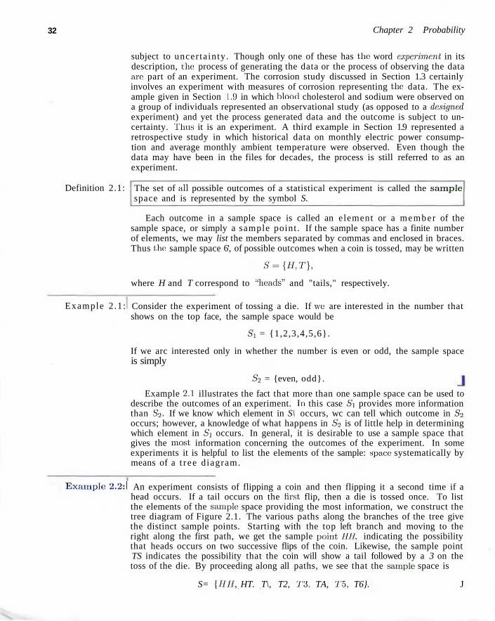
32 Chapter 2 Probability
subject to uncertainty. Though only one of these has the word experiment, in its description, the: process of generating the data or the process of observing the data are part of an experiment. The corrosion study discussed in Section 1.3 certainly involves an experiment with measures of corrosion representing the: data. The example given in Section 1.9 in which blood cholesterol and sodium were observed on a group of individuals represented an observational study (as opposed to a designed experiment) and yet the process generated data and the outcome is subject to uncertainty. Tims it is an experiment. A third example in Section 1.9 represented a retrospective study in which historical data on monthly electric power consumption and average monthly ambient temperature were observed. Even though the data may have been in the files for decades, the process is still referred to as an experiment.
Definition 2.1: The set of all possible outcomes of a statistical experiment is called the sample space and is represented by the symbol S.
Each outcome in a sample space is called an element or a member of the sample space, or simply a sample point . If the sample space has a finite number of elements, we may list the members separated by commas and enclosed in braces. Thus the: sample space 6', of possible outcomes when a coin is tossed, may be written
S={H,T),
where H and T correspond to "heads" and "tails," respectively.
Example 2.1: Consider the experiment of tossing a die. If wc are interested in the number that shows on the top face, the sample space would be
Si = {1,2,3,4,5,6}.
If we arc interested only in whether the number is even or odd, the sample space is simply
S2 = {even, odd}.
Example 2.1 illustrates the fact that more than one sample space can be used to describe the outcomes of an experiment. In this case Si provides more information than S2. If we know which element in S\ occurs, wc can tell which outcome in S2 occurs; however, a knowledge of what happens in S2 is of little help in determining which element in Si occurs. In general, it is desirable to use a sample space that gives the most information concerning the outcomes of the experiment. In some experiments it is helpful to list the elements of the sample: space systematically by means of a t r ee diagram.
Example 2.2:1 An experiment consists of flipping a coin and then flipping it a second time if a head occurs. If a tail occurs on the first, flip, then a die is tossed once. To list the elements of the sample space providing the most information, we construct the tree diagram of Figure 2.1. The various paths along the branches of the tree give the distinct sample points. Starting with the top left branch and moving to the right along the first path, we get the sample point HH, indicating the possibility that heads occurs on two successive flips of the coin. Likewise, the sample point TS indicates the possibility that the coin will show a tail followed by a 3 on the toss of the die. By proceeding along all paths, we see that the sample space is
S= {IIH. HT. T\, T2, T3, TA, T5, T6}. J
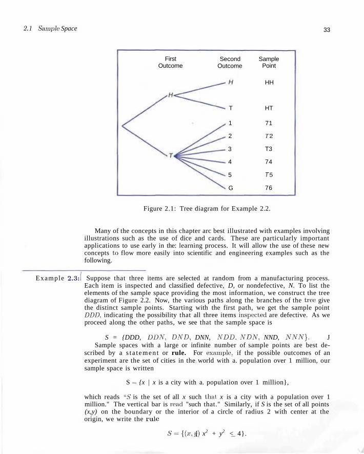
2.1 Sample Space 33
First Outcome
Second Outcome
Sample Point
HH
T
1
2
3
4
5
G
HT
71
72
T3
74
75
76
Figure 2.1: Tree diagram for Example 2.2.
Many of the concepts in this chapter arc best illustrated with examples involving illustrations such as the use of dice and cards. These are particularly important applications to use early in the: learning process. It will allow the use of these new concepts to flow more easily into scientific and engineering examples such as the following.
Example 2.3:1 Suppose that three items are selected at random from a manufacturing process. Each item is inspected and classified defective, D, or nondefective, N. To list the elements of the sample space providing the most information, we construct the tree diagram of Figure 2.2. Now, the various paths along the branches of the tree give the distinct sample points. Starting with the first path, we get the sample point DDD. indicating the possibility that all three items inspected are defective. As we proceed along the other paths, we see that the sample space is
S = {DDD, DDN, DND, DNN, NDD, NDN, NND, NNN}. J Sample spaces with a large or infinite number of sample points are best de
scribed by a s t a t emen t or rule. For example, if the possible outcomes of an experiment are the set of cities in the world with a. population over 1 million, our sample space is written
S = {x | x is a city with a. population over 1 million},
which reads "S is the set of all x such that x is a city with a population over 1 million." The vertical bar is read "such that." Similarly, if S is the set of all points (x,y) on the boundary or the interior of a circle of radius 2 with center at the origin, we write the rule
S={(x,y) [ x2 + y2 < 4}.
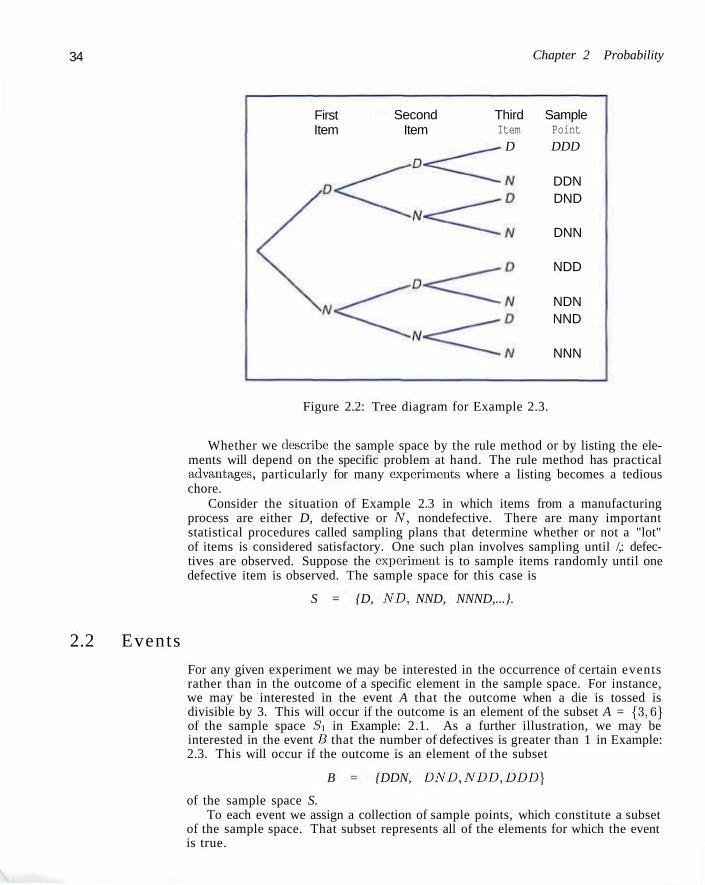
34 Chapter 2 Probability
First Item
Second Item
Third Sample Item Point
D DDD
DDN DND
DNN
NDD
NDN NND
NNN
Figure 2.2: Tree diagram for Example 2.3.
Whether we describe: the sample space by the rule method or by listing the elements will depend on the specific problem at hand. The rule method has practical advantages, particularly for many experiments where a listing becomes a tedious chore.
Consider the situation of Example 2.3 in which items from a manufacturing process are either D, defective or Ar, nondefective. There are many important statistical procedures called sampling plans that determine whether or not a "lot" of items is considered satisfactory. One such plan involves sampling until /,: defectives are observed. Suppose the experiment is to sample items randomly until one defective item is observed. The sample space for this case is
S = {D, ND, NND, NNND,...}.
2.2 Events
For any given experiment we may be interested in the occurrence of certain events rather than in the outcome of a specific element in the sample space. For instance, we may be interested in the event A that the outcome when a die is tossed is divisible by 3. This will occur if the outcome is an element of the subset A = {3,6} of the sample space Si in Example: 2.1. As a further illustration, we may be interested in the event B that the number of defectives is greater than 1 in Example: 2.3. This will occur if the outcome is an element of the subset
B = {DDN, DND,NDD,DDD}
of the sample space S. To each event we assign a collection of sample points, which constitute a subset
of the sample space. That subset represents all of the elements for which the event is true.
2.2 Events 35
Definition 2.2: An event is a subset of a sample space.
Example 2.4:1 Given the sample space S = {t | t > 0}, where t is the life in years of a certain electronic component, then the event A that the component fails before the end of the fifth year is the subset A = {t | 0 < t < 5}. J
It is conceivable that an event may be a subset that includes the entire sample space S, or a subset of S called the null set and denoted by the symbol ©, which contains no elements at all. For instance, if we let A be the event of detecting a microscopic organism by the naked eye in a biological experiment, then .4 = d>. Also, if
B = {x | x is an even factor of 7},
then B must be the null set, since the only possible factors of 7 are the odd numbers 1 and 7.
Consider an experiment where the smoking habits of the employees of a manufacturing firm arc recorded. A possible sample space might classify an individual as a nonsmoker, a light smoker, a moderate smoker, or a heavy smoker. Let the subset of smokers be some event. Then all the: nonsmokers correspond to a different event, also a subset of S, which is called the complement of the set of smokers.
Definition 2.3: The complement of an event A with respect to S is the subset of all elements of S that are not in A. We denote the complement, of A by the symbol A'.
Example 2.5:1 Let R be the event that a red card is selected from an ordinary deck of 52 playing cards, and let S be the entire: deck. Then R' is the event that the card selected from the deck is not a red but a black card. J
Example 2.6:1 Consider the sample space
Definition 2.4:
S = {book, catalyst, cigarette:, precipitate, engineer, rivet}.
Let A = {catalyst, rivet, book, cigarette}. Then the complement of A is A' =
{precipitate, engineer}. J We now consider certain operations with events that will result in the formation
of new events. These new events will be subsets of the same sample: space as the given events. Suppose that A and B arc two events associated with an experiment. In other words, A and B are subsets of the same sample space S. For example, in the tossing of a die wc: might let A be the event that an even number occurs and B the event that a number greater than 3 shows. Then the subsets A — {2,4,6} and B = {4, 5,6} are subsets of the same sample space
S = {1,2,3,4,5,6}.
Note that both. A and B will occur on a given toss if the outcome is an element of the subset {4,6}, which is just, the intersect ion of A and B.
The intersect ion of two events A and B, denoted by the symbol A D B, is the event containing all elements that are common to A and B.
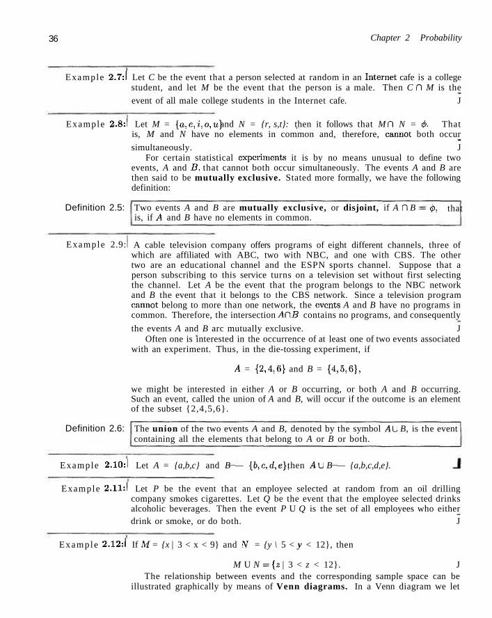
36 Chapter 2 Probability
Example 2.7:1 Let C be the event that a person selected at random in an Internet cafe is a college student, and let M be the event that the person is a male. Then C D M is the
event of all male college students in the Internet cafe. J
Example 2.8:1 Let M = {a.e./i.o,u} and N = {r, s,t}: then it follows that M f\ N = tj>. That is, M and N have no elements in common and, therefore, cannot both occur
simultaneously. J For certain statistical experiments it is by no means unusual to define two
events, A and B, that cannot both occur simultaneously. The events A and B are then said to be mutually exclusive. Stated more formally, we have the following definition:
Definition 2.5: Two events A and B are mutually exclusive, or disjoint, if A n B is, if A and B have no elements in common.
<t>, that
Example 2.9: A cable television company offers programs of eight different channels, three of which are affiliated with ABC, two with NBC, and one with CBS. The other two are an educational channel and the ESPN sports channel. Suppose that a person subscribing to this service turns on a television set without first selecting the channel. Let A be the event that the program belongs to the NBC network and B the event that it belongs to the CBS network. Since a television program cannot belong to more than one network, the events A and B have no programs in common. Therefore, the intersection A(~\B contains no programs, and consequently
the events A and B arc mutually exclusive. J Often one is interested in the occurrence of at least one of two events associated
with an experiment. Thus, in the die-tossing experiment, if
A = {2,4,6} and B = {4,5,6},
we might be interested in either A or B occurring, or both A and B occurring. Such an event, called the union of A and B, will occur if the outcome is an element of the subset {2,4,5,6}.
Definition 2.6: The union of the two events A and B, denoted by the symbol AU B, is the event containing all the elements that belong to A or B or both.
Example 2.10:1 Let A = {a,b,c} and B — {b,c,d,e}; then AU B — {a,b,c,d,e}.
Example 2.11:1 Let P be the event that an employee selected at random from an oil drilling company smokes cigarettes. Let Q be the event that the employee selected drinks alcoholic beverages. Then the event P U Q is the set of all employees who either drink or smoke, or do both. J
Example 2.12:1 If M = {x | 3 < x < 9} and <V = {y \ 5 < y < 12}, then
M U N = [z | 3 < z < 12}. J The relationship between events and the corresponding sample space can be
illustrated graphically by means of Venn diagrams. In a Venn diagram we let
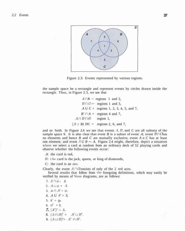
2.2 Events 37
Figure 2.3: Events represented by various regions.
the sample space be a rectangle and represent events by circles drawn inside the rectangle. Thus, in Figure 2.3, we see that
A(l B = regions 1 and 2, B(lC — regions 1 and 3, A U C = regions 1, 2, 3, 4, 5, and 7,
B' n A = regions 4 and 7, AtlBnC = region 1,
(A U B) DC = regions 2, 6, and 7,
and so forth. In Figure 2.4 we see that events A, B, and C are all subsets of the sample space S. It is also clear that event B is a subset of event .4; event Bf)C has no elements and hence B and C are mutually exclusive; event A n C has at least one element; and event A U B — A. Figure 2.4 might, therefore, depict a situation where we select a card at random from an ordinary deck of 52 playing cards and observe whether the following events occur:
.4: the card is red, B: I he card is the jack, queen, or king of diamonds,
C: the card is an ace-
Clearly, the event Af\C consists of only of the 2 red aces. Several results that follow from the foregoing definitions, which may easily be
verified by means of Venn diagrams, are as follows: 1. AC\Q = 6.
2. . l U e j = A.
3. .4 H A' = (p.
4. .4 U A' = S.
5. S' = (p.
6. <!/ = S.
7. (AJ = A. 8. (Ar\B)' = A'UB'. 9. {A\JB)' = A' C\B'.
38 Chapter 2 Probability
Figure 2.4: Events of the sample space S.
Exercises
2.1 List the elements of each of the following sample spaces: (a) the set of integers between 1 and 50 divisible by 8:
(b) the set S = {x | x2 + 4x - 5 = 0}; (c) the set of outcomes when a coin is tossed until a
tail or three heads appear: (d) the set S = {x | a; is a continent}; (e) the set. S = {x \ 2x - 4 > 0 and X < 1}.
2.2 Use the rule method to describe the sample space S consisting of all points in the first quadrant inside a circle of radius 3 with center at the origin.
2.3 Which of the following events are equal?
(a) A = {1,3}; (b) B = {x | x is a number on a die}:
(c) C ={x\x2 -4x + 3 = 0}; (d) D = {x | x is the number of heads when six coins
are tossed}.
2.4 An experiment involves tossing a pair of dice, 1 green and 1 red. and recording the numbers that come up. If ,-r equals the outcome on the green die and y the outcome on the red die, describe the sample space S (a) by listing the elements {x,y)\ (b) by using the rule method.
2 .5 An experiment, consists of tossing a die and then flipping a coin once if the number on the: die is even. If the number on the die is odcl, the coin is flipped twice. Using the notation 4 / / , for example, to denote the outcome that the die comes up 4 and then the coin comes
up heads, and 3HT to denote the outcome that the die comes up 3 followed by a head and then a tail on the coin, construct a tree diagram to show the 18 elements of the sample space S.
2.6 Two jurors are selected from 4 alternates to serve at a murder trial. Using ttie notation .4IA;J, for example, to denote the simple event that alternates 1 and 3 are selected, list the 0 elements of the sample space S.
2.7 Four students are selected at random from a chemistry class and classified as male or female. List the elements of the sample space Si using the letter M for "male" and F for "female." Define a second sample space S-2 where the elements represent the number of females selected.
2.8
(a)
(b)
(d) («) (0 (g)
For the sample space of Exercise 2.4:
list the elements corresponding to the event A that the sum is greater than 8; list the elements corresponding to the event B that a 2 occurs on either die; list the elements corresponding to the event C that a number greater than 4 comes up on the green die list the elements corresponding to the event AnC list the elements corresponding to the event AC\B
list the elements corresponding to the event BC\C construct a Venn diagram to illustrate the intersections and unions of the events A. B. and C.
2.9 For the sample space of Exercise 2.5, (a) list the elements corresponding to the event A that
a number less than :i occurs on the die; (b) list the elements corresponding to the event B that
Exercises 39
2 tails occur; (c) list the elements corresponding to the event A';
(d) list the elements corresponding to the event A'nB;
(e) list the elements corresponding to the event A U B.
2.10 An engineering firm is hired to determine if certain waterways in Virginia are safe for fishing. Samples are taken from three rivers.
(a) List the elements of a sample space S, using the letters F for "safe to fish" and N for "not safe to fish."
(b) List the elements of S corresponding to event E that at least two of the rivers are safe for fishing.
(c) Define aii event that has as its elements the points
{FFF, NFF, FFN, NFN}.
2.11 The resumes of 2 male applicants for a college teaching position in chemistry are placed in the same file as the resumes of 2 female applicants. Two positions become available and the first, at the rank of assistant professor, is filled by selecting 1 of the 4 applicants at random. The second position, at the rank of instructor, is then filled by selecting at random one of the remaining 3 applicants. Using the notation M2F1, for example, to denote the simple event that the first position is filled by the second male applicant and the second position is then filled by the first female applicant,
(a) list the elements of a sample space S;
(b) list the elements of S corresponding to event A that the position of assistant professor is filled by a male applicant;
(c) list the elements of S corresponding to event B that exactly 1 of the 2 positions was filled by a male applicant;
(d) list the elements of S corresponding to event C that neither position was filled by a male applicant;
(e) list the elements of S corresponding to the event AH 5 ;
(f) list the elements of S corresponding to the event A DC:
(g) construct a Venn diagram to illustrate the intersections and unions of the events A, B, and C.
2.12 Exercise and diet are being studied as possible substitutes for medication to lower blood pressure. Three groups of subjects will be used to study the effect of exercise. Group one is sedentary while group two walks and group three swims for 1 hour a day. Half of each of the three exercise groups will be on a salt-free diet. An additional group of subjects will not exercise nor restrict their salt, but will take the stan
dard medication. Use Z for sedentary, W for walker, S for swimmer, Y for salt, JV for no salt, M for medication, and F for medication free. (a) Show all of the elements of the sample space S.
(b) Given that A is the set of nonmedicated subjects and B is the set of walkers, list the elements of A UB.
(c) List the elements of A n B.
2.13 Construct a Venn diagram to illustrate the possible intersections and unions for the following events relative to the sample space consisting of all automobiles made in the United States.
F: Four door, S: Sun roof, P: Power steering.
2.14 If S = {0,1,2,3,4,5,6,7,8,9} and A = {0,2,4,6,8}, B = {1,3,5,7,9}, C = {2,3,4,5}, and D = {1,6, 7}, list the elements of the sets corresponding to the following events: (a) A U C;
(b) A n B; (c) C; (d) (C nD)uB; (e)(SnC)'; (f) A n C n D'.
2.15 Consider the sample space S={copper, sodium, nitrogen, potassium, uranium, oxygen, zinc}, and the events
A = {copper, sodium, zinc},
B = {sodium, nitrogen, potassium},
C = {oxygen}.
List the elements of the sets corresponding to the following events: (a) A';
(b) AUC;
(c) (A 0 B') U C;
(d) B' n C"; (e) A n B n C; (f) (A'uB')n(A'nC).
2.16 If S = {x I 0 < x < 12}, M = {x I 1 < x < 9}, and N = {x | 0 < a: < 5}, find (a) M U N; (b) M n N;
(c) M' n N'.
2.17 Let A. B, and C be events relative to the sample space S. Using Venn diagrams, shade the areas representing the following events:
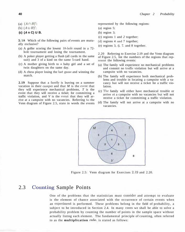
40 Chapter 2 Probability
(a) (ACBY; ( b ) ( A u B ) ' ; (c) (.4 n C) U B.
2.18 Which of the following pairs of events are mutually exclusive? (a) A golfer scoring the lowest 18-hole round in a 72-
hole tournament and losing the tournament. (b) A poker player getting a flush (all cards in the same
suit) and 3 of a kind on the same 5-card hand. (c) A mother giving birth to a baby girl and a set of
twin daughters on the same day. (d) A chess player losing the last game and winning the
match.
2.19 Suppose that a family is leaving on a summer vacation in their camper and that M is the event that they will experience mechanical problems, T is the event that they will receive a ticket; for committing a traffic violation, and V is the event: that they will arrive at a campsite with no vacancies. Referring to the Venn diagram of Figure 2.5, state in words the events
represented by the following regions: (a) region 5:
(b) region 3; (c) regions 1 and 2 together: (d) regions 4 and 7 together; (e) regions 3, (i. 7. and 8 together.
2.20 Referring to Exercise 2.19 and the Venn diagram of Figure 2.5, list the numbers of the regions that represent, the following events:
(a) The family will experience no mechanical problems and commit no traffic violation but will arrive at a campsite with no vacancies.
(b) The family will experience both mechanical problems and trouble in locating a campsite with a vacancy but will not receive a ticket for a traffic violation.
(c) The family will either have mechanical trouble or arrive at a campsite with no vacancies but will not receive a ticket for committing a traffic violation.
(d) The family will not arrive at a campsite with no vacancies.
Figure 2.5: Venn diagram for Exercises 2.19 and 2.20.
2.3 Counting Sample Points
One of the problems tha t the statistician must consider and a t tempt to evaluate is the element of chance associated with the occurrence of certain events when an experiment is performed. These problems belong in the field of probability, a subject to be introduced in Section 2.4. In many cases we shall be able to solve a probability problem by counting the number of points in the sample space without actually listing each element. The fundamental principle of counting, often referred to as the mul t ip l i ca t ion rule, is s ta ted as follows:
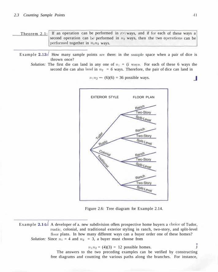
2.3 Counting Sample Points 41
Theorem 2.1: If an second fierfori
operation can operation can
ned together in
be be
performed performed
nin2 ways.
in in
r>\ 11.2
ways, ways,
and if foi then the
each :wo o
of these icrations
ways a can be
Example 2.13:1 How many sample points are: there: in the sample: space when a pair of dice is thrown once?
Solution: The first die can land in any one of nj = (i ways. For each of these 6 ways the second die can also laud in n% = 6 ways. Therefore, the pair of dice can land in
iiirio — (6)(6) = 36 possible ways.
EXTERIOR STYLE FLOOR PLAN
Figure 2.6: Tree diagram for Example 2.14.
Example 2.14:1 A developer of a. new subdivision offers prospective home buyers a choice of Tudor, rustic:, colonial, and traditional exterior styling in ranch, two-story, and split-level iloor plans. In how many different ways can a buyer order one of these homes?
Solution: Since »i = 4 and n% = 3, a buyer must choose from
" i"2 = (4)(3) = 12 possible homes. J The answers to the two preceding examples can be verified by constructing
free diagrams and counting the various paths along the branches. For instance,
42 Chapter 2 Probability
in Example 2.14 there will be m = 4 branches corresponding to the different exterior styles, and then there will be «2 = 3 branches extending from each of these 4 branches to represent the different floor plans. This tree diagram yields the ni«2 = 12 choices of homes given by the paths along the branches as illustrated in Figure 2.6.
The multiplication rule of Theorem 2.1 may be extended to cover any number of operations. Suppose, for instance, that a customer wishes to install an AT&T™ telephone and can choose from m = 10 decorator colors, which we shall assume are available in any of n? = 3 optional cord lengths with n-j — 2 types of dialing, namely, rotary or touch-tone. These three classifications result in niri2^3 = (10)(3)(2) = 60 different ways for a customer to order one of these phones. The generalized mult ipl ication rule covering k operations is stated in the following theorem.
Theorem 2.2: If an operation can be performed in n\ ways, and if for each of these a second operation can be performed in n2 ways, and for each of the first two a third operation can be performed in n$ ways, and so forth, then the sequence of k operations can be performed in n\H2- • -nk ways.
Example 2.15:1 Sam is going to assemble a computer by himself. He: has the choice of ordering chips from two brands, a hard drive from four, memory from three, and an accessory bundle from five local stores. How many different, ways can Sam order the parts?
Solution: Since n\ = 2, n? = 4, n,\ = 3, and m = 5, there are
n.i x "2 x «3 x 11.4 = 2 x 4 x 3 x 5 = 120
different ways to order the parts. J!
Example 2.16:1 How many even four-digit numbers can be formed from the digits 0, 1, 2, 5, 6, and 9 if each digit can be used only once?
Solution: Since the number must be even, we have only 7/.1 = 3 choices for the units position. However, for a four-digit number the thousands position cannot be 0. Hence we consider the units position by two parts, 0 or not 0. If the units position is 0 (i.e., n\ = 1), we have no — 5 choices for the thousands position, B3 = 4 for the hundreds position, and n.4 = 3 for the tens position. Therefore, in this case we have a total of
uln2n;j7?.-i = (l)(5)(4)(3) = 60
even four-digit numbers. On the other hand, if the units position is not 0 (i.e., 711 = 2), we have no = 4 choices for the thousands position, rc.3 = 4 for the hundreds position, and n\ — 3 for the tens position. In this situation there are a total of
ninanan4 = (2)(4)(4)(3) = 96
even four-digit numbers. Since the above two cases are mutually exclusive of each other, the total number
of even four-digit numbers can be calculated by 60 + 96 = 156. J
2.3 Counting Sample Points 43
Frequently, we are interested in a sample space that contains elements as all possible orders or arrangements of a group of objects. For example, we may want to know how many different arrangements are possible for sitting 6 people around a table, or we may ask how many different orders are possible for drawing 2 lottery tickets from a total of 20. The different arrangements are called pe rmuta t ions .
Definition 2.7: A permutation is an arrangement of all or part of a set of objects.
Consider the three letters a, b, and c. The possible permutations are ohc, acb, bac, bca, cab, and cba. Thus we see that there are 6 distinct arrangements. Using Theorem 2.2 we could arrive at the answer 6 without actually listing the different orders. There are ni = 3 choices for the first position, then n2 = 2 for the second, leaving only n^ = 1 choice for the last position, giving a total of
7)in2;»3 = (3)(2)(1) = 6 permutations.
In general, n distinct objects can be arranged in
n(n - l)(n - 2) • • • (3)(2)(1) ways.
We represent this product by the symbol n\, which is read "n factorial." Three objects can be arranged in 3! = (3)(2)(1) = 6 ways. By definition, l! = 1. Also we define 0! = 1.
Theorem 2.3: The number of permutations of n objects is n!.
The number of permutations of the four letters a, b, c, and d will be 4! = 24. Now consider the number of permutations that are possible by taking two letters at a time from four. These would be ab, ac, ad, ba, be, bd, ca, cb, cd, da, db, and dc. Using Theorem 2.1 again, we have two positions to fill with m = 4 choices for the first and then m = 3 choices for the second for a total of
nm-2 = (4) (3) = 12
permutations. In general, n distinct objects taken r at a time can be arranged in
n{n- l ) ( n - 2 ) - - - ( n - r + 1)
ways. We represent this product by the symbol
1,1 r (n - I - ) ! '
As a result we have the theorem that follows.
Theorem 2.4: The number of permutation of n distinct objects taken r at a time is
n! n* r — (n — r)! '
44 Chapter 2 Probability
Example 2.17:1 In one year, three awards (research, teaching, and service) will be given for a class of 25 graduate students in a statistics department. If each student can receive at most one award, how many possible selections are there?
Solution: Since the awards are distinguishable, it is a permutation problem. The total number of sample points is
2 ^ - 7 ^ y _ = ^ - ^ m ) ( 2 3 ) = 13,800. j
Example 2.18:1 A president and a treasurer are to be chosen from a student club consisting of 50 people. How many different choices of officers are possible if
(a) there are no restrictions;
(b) A will serve only if he is president;
(c) B and C will serve together or not at all:
(d) D and E will not serve together?
Solution: (a) The total number of choices of the officers, if there are no restrictions, is
5C.A = ~ = (50)(49) = 2450.
(b) Since A will serve only if he is the president, we have two situations here: (i) A is selected as the president, wdiich yields 49 possible outcomes; or (ii) Officers are selected from the remaining 49 people which has the number of choices 49P2 = (49)(48) = 2352. Therefore, the total number of choices is 49 4- 2352 = 2401.
(c) The number of selections when B and C serve together is 2. The number of selections when both B and C are not chosen is 43^2 = 2256. Therefore, the total number of choices in this situation is 2 + 2256 = 2258.
(d) The number of selections when D serves as an officer but not E is (2) (48) = 96, where 2 is the number of positions D can take and 48 is the number of selections of the other officer from the remaining people in the club except E. The number of selections when E serves as an officer but not D is also (2)(48) = 96. The number of selections when both D and E are not chosen is 4 8 P 2 = 2256. Therefore, the total number of choices is (2)(96) + 2256 = 2448. This problem also has another short solution: Since D and E can only serve together in 2 ways, the answer is 2450 - 2 = 2448. I
Permutations that occur by arranging objects in a circle are called circular pe rmuta t ions . Two circular permutations arc not considered different unless corresponding objects in the two arrangements are preceded or followed by a different object as we proceed in a clockwise direction. For example, if 4 people are playing bridge, we do not have a new permutation if they all move one position in a clockwise direction. By considering one person in a fixed position and arranging the other three in 3! ways, we find that there are 6 distinct arrangements for the bridge game.
2.3 Counting Sample Points 45
Theorem 2.5: The number of permutations of n objects arranged in a circle is (n — 1)!.
So far we have considered permutations of distinct objects. That is, all the objects were completely different or distinguishable. Obviously, if the letters 6 and c are both equal to x, then the 6 permutations of the letters a, b, and c become axx, axx, xax, xax, xxa, and xxa, of which only 3 are distinct. Therefore, with 3 letters, 2 being the same, we have 3!/2! = 3 distinct permutations. With 4 different letters a, b, c, and d, we have 24 distinct permutations. If we let a = b = x and c — d = y, we can list only the following distinct permutations: xxyy, xyxy, yxxy, yyxx, xyyx, and yxyx. Thus we have 4!/(2! 2!) = 6 distinct permutations.
Theorem 2.6: The number of distinct permutations of n things of which n\ are of one kind, n2 of a second kind,. . . , n^ of a fcth kind is
n< n\\U2 Ira,! • • n-k}-
Example 2.19:1 In a college football training session, the defensive coordinator needs to have 10 players standing in a row. Among these 10 players, there are 1 freshman, 2 sophomores, 4 juniors, and 3 seniors, respectively. How many different ways can they be arranged in a row if only their class level will be distinguished?
Solution: Directly using Theorem 2.6, the total number of arrangements is
10!
1! 2! 4! 3! = 12.600.
Often we are concerned with the number of ways of partitioning a set of n objects into r subsets called cells. A partition has been achieved if the intersection of every possible pair of the r subsets is the empty set <p and if the union of all subsets gives the original set. The order of the elements within a cell is of no importance. Consider the set {a, e, i, o, u}. The possible partitions into two cells in which the first cell contains 4 elements and the second cell 1 element are
{(a, e,i. o), (TJ.)}, {(a, i ,o,u), (e)}, {(e, i, o, a), (a)}, {(a, e, o, u), (i)}, {(a,e, i,u), (o)}.
We see that there are 5 such ways to partition a set of 4 elements into two subsets or cells containing 4 elements in the first cell and 1 clement in the second.
The number of partitions for this illustration is denoted by the symbol
w 5!
4 , 1 / 4! 1!
where the top number represents the total number of elements and the bottom numbers represent the number of elements going into each cell, We state this more generally in the following theorem.
46 Chapter 2 Probability
Theorem 2.7: The number of ways of partitioning a set of n objects into r cells with n\ elements in the first cell, n2 elements in the second, and so forth, is
( n \ — n ' \n i , r? .2 , . . . ,n r / n i (no
where m + n2 + • • • + nr n.
Example 2.20:1 In how many ways can 7 graduate students be assigned to one triple and two double hotel rooms during a conference?
Solution: The total number of possible partitions would be
3,2.2 7!
= 210. 3! 2! 2! " " " J
In many problems we are interested in the number of ways of selecting r objects from n without regard to order. These selections are called combinations. A combination is actually a partition with two cells, the one cell containing the r objects selected and the other cell containing the (n — r) objects that are left. The number of such combinations, denoted by
1, is usually shortened to ( r.n — rj \r
since the number of elements in the second cell must be n — r.
Theorem 2.8: The number of combinations of n distinct objects taken r at a time is
fn\ _ n! \rj rl(n — r)\
Example 2.21:1 A young boy asks his mother to get five Game-Boy™ cartridges from his collection of 10 arcade and 5 sports games. How many ways are there that his mother will get 3 arcade and 2 sports games, respectively?
Solution: The number of ways of selecting 3 cartridges from 10 is
W 3! 10!
= 120. ( 1 0 - 3 ) !
The number of ways of selecting 2 cartridges from 5 is
' 5 \ 5! 2! 3!
= 10.
Using the multiplication rule of Theorem 2.1 with m = 120 and ri2 — 10, there are (120)(10) = 1200 ways. J
Exercises 47
E x a m p l e 2.22:1 How many different letter arrangements can be made from the letters in the word of STATISTICS?
Solution: Using the same argument as of discussion for Theorem 2.8, in this example we can actually apply Theorem 2.7 to obtain
Exercises
10
3 . 3 , 2 , 1 , 1
10!
3! 3! 2! 1! 1! = 50.400.
Here we have tota l 10 letters, while 2 letters (S , T) appear 3 times each, letter /
appears twice, and letters A and C appear once each. J !
2.21 Registrants at a large convention are offered 6 sightseeing tours on each of 3 days. In how many-ways can a person arrange to go on a sightseeing tour planned by this convention?
2.22 In a medical study patients are classified in 8 ways according to whether they have blood type AB+, AB~, A+, A~, B+, B~, 0+, or 0~, and also according to whether their blood pressure is low, normal, or high. Find the number of ways in which a patient can be classified.
2 .23 If an experiment consists of throwing a die and then drawing a letter at random from the English alphabet, how many points are there in the sample space?
2.24 Students at a private liberal arts college are classified as being freshmen, sophomores, juniors, or seniors, and also according to whether they are male or female. Find the total number of possible classifications for the students of that college.
2.25 A certain shoe conies in 5 different styles with each style available in 4 distinct colors. If the store wishes to display pairs of these shoes showing all of its various styles and colors, how many different pairs would the store have on display?
2.26 A California study concluded that by following 7 simple health rules a man's life can be extended by 11 years on the average and a woman's life by 7 years. These 7 rules are as follows: no smoking, regular exercise, use alcohol moderately, get, 7 to 8 hours of sleep, maintain proper weight, eat. breakfast, and do not eat between meals. In how many ways can a person adopt five of these rules to follow (a) If the person presently violates all 7 rules?
(b) If the person never drinks and fast?
always eats break-
2.27 A developer of a new subdivision offers a prospective home buyer a choice of 4 designs, 3 different heating systems, a garage or carport, and a patio or screened porch. How many different, plans are available to this buyer?
2.28 A drug for the relief of asthma can be purchased from 5 different, manufacturers in liquid, tablet, or capsule form, all of which come in regular and extra strength. How many different ways can a doctor prescribe the drug for a patient suffering from asthma?
2.29 In a fuel economy study, each of 3 race cars is tested using 5 different brands of gasoline at 7 test sites located in different regions of the country. If 2 drivers are used in the study, and test runs are made once under each distinct set of conditions, how many tost, runs are needed?
2.30 In how many different ways can a true-false test consisting of 9 questions be answered?
2.31 If a multiple-choice test consists of 5 questions each with 4 possible answers of which only 1 is correct, (a) In how many different ways can a student check off
one answer to each question? (b) In how many ways can a student, check off one
answer to each question and get all the answers wrong ?
(a) How many distinct permutations can be lade from the letters of the word columns?
(b) How many of these permutations start with the let-
2.32 made
ter mi
48 Chapter 2 Probability
2.33 A witness to a hit-and-run accident told the police that the license number contained the letters RLH followed by 3 digits, the first of which is a 5. If the witness cannot recall the last 2 digits, but is certain that all 3 digits are different, find the maximum number of automobile registrations that the police may have to check.
2.34 (a) In how many ways can 6 people be lined up to get on a bus?
(b) If 3 specific persons, among 6, insist on following each other, how many ways are possible?
(c) If 2 specific persons, among 6, refuse to follow each other, how many ways are possible?
2.35 A contractor wishes to build 9 houses, each different in design. In how many ways can he place these houses on a street if 6 lots are on one side of the street and 3 lots are on the opposite side?
2.36 (a) How many three-digit numbers can be formed from the digits 0, 1, 2, 3, 4, 5, and 6, if each digit can be used only once?
(b) How many of these are odd numbers? (c) How many are greater than 330?
2.37 In how many ways can 4 boys and 5 girls sit in a row if the boys and girls must alternate?
2.38 Four married couples have bought 8 scats in the same row for a concert. In how many different ways can they be seated (a) With no restrictions? (b) If each couple is to sit together? (c) If all the men sit together to the right of all the
women?
2.39 In a regional spelling bee, the 8 finalists consist of 3 boys and 5 girls. Find the number of sample points in the sample space S for the number of possible orders at the conclusion of the contest for (a) all 8 finalists;
(b) the first 3 positions.
2.40 In how many ways can 5 starting positions on a basketball team be filled with 8 men who can play any of the positions?
2.41 Find the number of ways that 6 teachers can be assigned to 4 sections of an introductory psychology course if no teacher is assigned to more than one section.
2.42 Three lottery tickets for first, second, and third prizes are drawn from a group of 40 tickets. Find the number of sample points in S for awarding the 3 prizes if each contestant holds only 1 ticket.
2.43 In how many ways can 5 different trees be planted in a circle?
2.44 In how many ways can a caravan of 8 covered wagons from Arizona be arranged in a circle?
2.45 How many distinct permutations can be made from the letters of the word infinity?
2.46 In how many ways can 3 oaks, 4 pines, and 2 maples be arranged along a property line if one does not distinguish among trees of the same kind?
2.47 A college plays 12 football games during a season. In how many ways can the team end the season with 7 wins, 3 losses, and 2 ties?
2.48 Nine people are going on a skiing trip in 3 cars that hold 2, 4, and 5 passengers, respectively. In how many ways is it possible to transport the 9 people to the ski lodge, using all cars?
2.49 How many ways are there to select 3 candidates from 8 equally qualified recent graduates for openings in an accounting firm?
2.50 How many ways are there that no two students will have the same birth date in a size of 60 class?
2.4 Probability of an Event
Perhaps it was humankind's unquenchable thirst for gambling tha t led to the early development of probability theory. In an effort to increase their winnings, gamblers called upon mathematicians to provide opt imum strategies for various games of chance. Some of the mathematicians providing these strategies were Pascal, Leibniz, Fermat, and James Bernoulli. As a result of this development of probability theory, statistical inference, with all its predictions and generalizations, has branched out far beyond games of chance to encompass many other fields as-
2.4 Probability of an Event 49
Definition 2.8:
sociated with chance occurrences, such as politics, business, weather forecasting, and scientific research. For these predictions and generalizations to be reasonably accurate, an understanding of basic probability theory is essential.
What clo we mean when we make the statements "John will probably win the tennis match," or "I have a fifty-fifty chance: of getting an even number when a die is tossed." or "I am not likely to win at bingo tonight." or "Most of our graduating class will likely be married within 3 years?" In each case we are expressing an outcome of which we are not certain, but owing to past information or from an understanding of the: structure of the experiment, we have some: degree of confidence in the validity of the statement.
Throughout the remainder of this chapter we consider only those experiments for which the sample space contains a finite number of elements. The likelihood of the occurrence of an event resulting from such a statistical experiment is evaluated by means of a set of real numbers called weights or probabil i t ies ranging from 0 to 1. l b every point in the sample space we assign a. probability such that the sum of all probabilities is I. If we have reason to believe that a certain sample point is quite likely to occur when the experiment is conducted, the probability assigned should be close to 1. On the other hand, a probability closer to zero is assigned to a .sample point that is not likely to occur. In many experiments, such as tossing a coin or a die, all the sample points have the same chance of occurring and arc assigned equal probabilities. For points outside the sample: space, that is, for simple events that cannot possibly occur, we assign a probability of zero.
To find the probability of an event .4, we sum all the probabilities assigned to the sample points in A. This sum is called the probability of A and is denoted by P(A).
The probability of an event A. Therefore,
Fm t her more
P(,
0 < P(A) < 1
if A,, A>. A3,..
Ii U A2 U A3 U -
4 is the
P(4>)
. is a scqi
••) = P(
sum
= 0,
lencc
of the
and
weight
P
of mutu;
4.1)+ P{A; »H
(S)
illy
P(
3 of all
= 1.
sample ]
exclusive events
4a) + •
joints
, then
in
Example 2.23:1 A coin is tossed twice. What is the probability that at least one head occurs? Solution: The sample space; for this experiment is
S= {IIII, NT. Til, TT}.
If the coin is balanced, each of these outcomes would be equally likely to occur. Therefore, we assign a probability of x1 to each sample point. Then iu = 1, or u> — 1/4. If A represents the event of at least one1 head occurring, then
A = {HILHT,TII} and P(A) = - -f I I
50 Chapter 2 Probability
Example 2.24:1 A die is loaded in such a way that an even number is twice as likely to occur as an odd number. If E is the event that a number less than 4 occurs on a single toss of the die, find P(E).
Solution: The sample space is S = {1.2.3.4.5.6}. We assign a probability of w to each odd number and a. probability of 2w to each even number. Since the sum of the probabilities must be 1, we have 9w = 1 or w = 1/9. Hence probabilities of 1/9 and 2/9 are assigned to each odd and even number, respectively. Therefore,
E = {1,2,3} and P(E) = 2 1
+ 9 + 9
Example 2.25:1 In Example 2.24, let A be the event that an even number turns up and let B be the event, that, a number divisible by 3 occurs. Find P(A U B) and P{A l~l B).
Solution: For the events A = {2,4,6} and B = {3,6} we have
AuB- {2,3,4,6] and A R B = {6}.
By assigning a probability of 1/9 to each odd number and 2/9 to each even number, we have
P f / l U 6 ) ^ + ^ + ^ and P(AP.B) = 9 J
If the sample space Cor an experiment contains N elements, all of which are equally likely to occur, we assign a probability equal to l/N to each of the N points. The probability of any event A containing n of these Ar sample points is then the ratio of the number of elements in A to the number of elements in S.
Theorem 2.9: If an experiment can result in any one of N different equally likely outcomes, and if exactly n of these outcomes correspond to event A, then the probability of event A is
P(A) n = N
Example 2.26:1 A statistics e:lass for engineers consists of 25 industrial, 10 mechanical, 10 electrical, and 8 civil engineering students. If a person is randomly selected by the instructor to answer a question, find the probability that the student chosen is (a) an industrial engineering major, (b) a civil engineering or an electrical engineering major.
Solution: Denote by /. M, E, and C the students majoring in industrial, mechanical, electrical, and civil engineering, respectively. The total number of students in the class is 53. all of which arc equally likely to be selected.
(a) Since 25 of the 53 students are majoring in industrial engineering, the probability of the event /, selecting an industrial engineering at random, is
* < " = § •
2.4 Probability of an Event 51
(b) Since 18 of the 53 students are civil or electrical engineering majors, it follows that
1 Q
P(CUE) = - . j
Example 2.27:1 In a poker hand consisting of 5 cards, find the probability of holding 2 aces and 3 jacks.
Solution: The number of ways of being dealt 2 aces from 4 is
' 4 \ 4! = 6, ©-/!} 2! 2!
and the number of ways of being dealt 3 jacks from 4 is
' 4 \ 4! 3! 1!
= 4.
By the multiplication rule of Theorem 2.1, there are n — (6)(4) = 24 hands with 2 aces and 3 jacks. The total number of 5-card poker hands, all of which are equally likely, is
/ 5 2 \ 52! A r = ( 5 j = 5 T ^ ! = 2 ' 5 9 8 ' 9 6 0 -
Therefore, the probability of event C of getting 2 aces and 3 jacks in a 5-card poker hand is
F ^ = 2 ^ 9 | l l 6 0 = 0 - 9 X l 0 " r ' J If the outcomes of an experiment are not equally likely to occur, the probabili
ties must be assigned on the basis of prior knowledge or experimental evidence. For example, if a coin is not balanced, we could estimate the probabilities of heads and tails by tossing the coin a large number of times and recording the outcomes. According to the relative frequency definition of probability, the true probabilities would be the fractions of heads and tails that occur in the long run.
To find a numerical value that represents adequately the probability of winning at tennis, we must depend on our past performance at the game as well as that of our opponent and, to some extent, in our belief in being able to win. Similarly, to find the probability that a horse will win a race, we must arrive at a probability based on the previous records of all the horses entered in the race as well as the records of the jockeys riding the horses. Intuition would undoubtedly also play a part in determining the size of the bet that we might be willing to wager. The use of intuition, personal beliefs, and other indirect information in arriving at probabilities is referred to as the subject ive definition of probability.
In most of the applications of probability in this book the relative frequency interpretation of probability is the operative one. Its foundation is the statistical experiment rather than subjectivity. It is best viewed as the l imiting relat ive frequency. As a result, many applications of probability in science and engineering must be based on experiments that can be repeated. Less objective notions of
52 Chapter 2 Probability
probability are encountered when we assign probabilities based on prior information and opinions. As an example, "there is a good chance that the Lions will lose the Super Bowl." When opinions and prior information differ from individual to individual, subjective probability becomes the relevant resource.
2.5 Additive Rules
Often it is easier to calculate the probability of some event from known probabilities of other events. This may well be true if the event in question can be represented as the union of two other events or as the complement of some event. Several important laws that frequently simplify the computation of probabilities follow. The: first, called the additive rule, applies to unions of events.
Theorem 2.10: If A and B are two events, then
P(A UB) = P(A) + P(B) - P(A n B).
Proof: Consider the Venn diagram in Figure 2.7. The P(A U B) is the sum of the probabilities of the sample points in A U B. Now P(A) + P{B) is the stun of all the1 probabilities in A plus the sum of all the probabilities in B. Therefore, we have added the probabilities in (A fl B) twice:. Since these probabilities add up to P(A D B), we must subtract this probability once to obtain the sum of the probabilities in A U 13. J
Figure 2.7: Additive rule of probability.
Corollary 2.1: If A and B are mi it ually exclusive.
P(A U B)
then
= P(A) + P(B).
Corollary 2.1 is an immediate result of Theorem 2.10, since if A and B are mutually exclusive. A n B = 0 and then P(A fl B) = P((b) = 0. In general,wc write:
2.5 Additive Rules
Corollary 2.2: If Ai, A2, • • • •. An are mutually exclusive, then
P(Aj U A-2 U • • • U An) = P(Ai) + P(y\2) + ••• + P{A„)
A collection of events [A\, A%,... A„ } of a sample space S is called a par t i t ion of S if A], A-2, • • •, A„ arc mutually exclusive and A1 U A2 U • • • U An = S. Thus we1
have
Corollary 2.3: If Ai, A2, • • • • An is a partition of sample space S, then
P{A^ U A2 U • • • U An) = P{A,) + P(A2) + • • • + P(4») = P(S) = 1.
As one might expect, Theorem 2.10 extends in an analogous fashion.
Theorem 2.11: For three events A,
P(A UBuC)
B, and C.
= P{A)+P(B)-rP(C) - P(A n B) -- P ( A n C ) - - P(B n C) + P{A n B n C).
Example 2.28:1 John is going to graduate from an industrial engineering department in a university by the end of the semester. Alter being interviewed at two companies he likes, he assesses that his probability of get ting an offer from company A is 0.8, and the probability that he gets an offer from company B is O.C. If. on the other hand, he believes that the probability that he will get offers from both companies is 0.5, what is the probability that he will get at least one offer from these two companies?
Solution: Using the additive rule, we have
P(A U B) = P(A) + P(B) - P(A fl B) = 0.8 + 0.6 - 0.5 = 0.9. J
Example 2.29:1 What is the probability of getting a total of 7 or 11 when a pair of fair dice are tossed?
Solution: Let A be the event that 7 occurs and B the event that 11 comes up. Now, a total of 7 occurs for 6 of the 30 sample points and a total of 11 occurs for only 2 of the sample points. Since all sample* points are equally likely, we have P{A) = 1/6 and P(B) = 1/18. The events A and B are mutually exclusive, since a total of 7 and 11 cannot both occur on the same toss. Therefore,
P(A U B) = P(A) + P(B) = ]- + ± = j .
This result could also have been obtained by counting the total number of points for the event A U B, namely 8, and writing
™=M4 ,
54 Chapter 2 Probability
Theorem 2.10 and its three corollaries should help the reader gain more insight into probability and its interpretation. Corollaries 1 and 2 suggest the very intuitive result dealing with the probability of occurrence of at least one of a number of events, no two of which can occur simultaneously. The probability that at least one occurs is the sum of the probabilities of occurrence of the individual events. The third corollary simply states that the highest value of a probability (unity) is assigned to the entire sample space S.
Example 2.30:1 If the probabilities are, respectively, 0.09, 0.15, 0.21, and 0.23 that a person purchasing a new automobile will choose the color green, white, red, or blue, what is the probability that a given buyer will purchase a new automobile that comes in one of those colors?
Solution: Let G, W, R, and B be the events that a buyer selects, respectively, a green, white, red, or blue automobile. Since these four events are mutually exclusive, the probability is
P{G U W U R U B) = P(G) + P(W) + P{R) + P{B)
= 0.09 + 0.15 + 0.21 + 0.23 = 0.68. J Often it is more difficult to calculate the probability that an event occurs than
it is to calculate the probability that the event does not occur. Should this be the case for some event A, wc simply find P(A') first and then, using Theorem 2.10, find P(A) by subtraction.
Theorem 2.12: If A and A' are complementary events, then
P(A) + P(A') = 1.
Proof: Since A U A' = S and the sets A and A' are disjoint, then
1 = P(S) = P(A U A') = P(A) + P(A').
Example 2.31:1 If the probabilities that an automobile mechanic will service 3, 4, 5, 6, 7, or 8 or more cars on any given workday are, respectively, 0.12, 0.19, 0.28, 0.24, 0.10, and 0.07, what is the probability that he will service at least 5 cars on his next day at work?
Solution: Let E be the event that at least 5 cars are serviced. Now, P(E) = 1 — P(E'), where E' is the event that fewer than 5 cars are serviced. Since
P ( £ ' ) = 0.12+ 0.19 = 0.31,
it follows from Theorem 2.12 that
P(E) = 1 - 0.31 = 0.69. J
Example 2.32:1 Suppose the manufacturer specifications of the length of a certain type of computer cable are 2000 ± 10 millimeters. In this industry, it is known that small cable is just as likely to be defective (not meeting specifications) as large cable. That is, the probability of randomly producing a cable with length exceeding 2010 millimeters
Exercises oo
is equal to the probability of producing a cable with length smaller than 1990 millimeters. The probability that the production procedure meets specifications is known to be 0.99.
(a) What is the probability that a cable selected randomly is too large?
(b) What is the probability that a randomly selected cable is larger than 1990 millimeters?
Solution: Let M be the event that a cable meets specifications. Let S and L be the events that the cable is too small and too large, respectively. Then
(a) P(M) = 0.99 and P{S) = P(L) = ± ^ p = 0.005.
(b) Denoting by X the length of a randomly selected cable, we have
P(1990 < X < 2010) = P{M) = 0.99.
Since P(X > 2010) = P(L) = 0.005 then
P(X > 1990) = P(M) + P(L) = 0.995.
This also can be solved by using Theorem 2.12:
P(X > 1990) + P(X < 1990) = 1.
Thus, P{X > 1990) = 1 - P{S) = 1 - 0.005 = 0.995. J
Exercises
2.51 Find the errors in each of the following statements: (a) The probabilities that an automobile salesperson
will sell 0, 1, 2, or 3 cars on any given day in February are, respectively, 0.19, 0.38, 0.29, and 0.15.
(b) The probability that it will rain tomorrow is 0.40 and the probability that it will not rain tomorrow is 0.52.
(c) The probabilities that a printer will make 0, 1, 2, 3, or 4 or more mistakes in setting a document are, respectively, 0.19,0.34, -0.25,0.43, and 0.29.
(d) On a single draw from a deck of playing cards the probability of selecting a heart is 1/4, the probability of selecting a black card is 1/2, and the probability of selecting both a heart and a black card is 1/8.'
2.52 Assuming that all elements of S in Exercise 2.8 on page 38 are equally likely to occur, find (a) the probability of event A: (b) the probability of event C; (c) the probability of event A DC.
2.53 A box contains 500 envelopes of which 75 contain $100 in cash, 150 contain $25, and 275 contain $10. An envelope may be purchased for $25. What is the sample space for the different amounts of money? Assign probabilities to the sample points and then find the probability that the first envelope purchased contains less than $100.
2.54 Suppose that in a senior college class of 500 students it is found that 210 smoke, 258 drink alcoholic beverages, 216 eat between meals, 122 smoke and drink alcoholic beverages, 83 eat between meals and drink alcoholic beverages, 97 smoke and eat between meals, and 52 engage in all three of these bad health practices. If a member of this senior class is selected at random, find the probability that the student (a) smokes but does not drink alcoholic beverages; (b) eats between meals and drinks alcoholic beverages
but does not smoke; (c) neither smokes nor eats between meals.
2.55 The probability that an American industry will locate in Shanghai, China is 0.7, the probability that it
56 Chapter 2 Probability
will locate in Beijing, China is 0.4, and the probability that it will locate in cither Shanghai or Beijing or both is 0.8. What is the probability that the industry will locate (a) in both cities? (b) in neither city?
2.56 From past experiences a stockbroker believes that under present economic conditions a customer will invest in tax-free bonds with a probability of 0.6, will invest in mutual funds with a probability of 0.3, and will invest in both tax-free bonds and mutual funds with a probability of 0.15. At this time, find the probability that a customer will invest
(a) in either tax-free bonds or mutual funds: (b) in neither tax-free bonds nor mutual funds.
2.57 If a letter is chosen at random from the English alphabet, find the probability that the letter (a) is a vowel exclusive of y;
(b) is listed somewhere ahead of the letter j \
(c) is listed somewhere after the letter g.
2.58 An automobile manufacturer is concerned about a possible recall of its best-selling four-door sedan. If there were a recall, there is 0.25 probability that a defect is in the brake system, 0.18 in the transmission, 0.17 in the fuel system, and 0.40 in some other area.
(a) What is the probability that the defect is the brakes or the fueling system if the probability of defects in both systems simultaneously is 0.15?
(b) What is the probability that there are no defects in either the brakes or the fueling system?
2.59 If each coded item in a catalog begins with 3 distinct letters followed by 4 distinct nonzero digits, find the probability of randomly selecting one of these coded items with the first letter a vowel and the last digit even.
2.60 A pair of fair dice is tossed. Find the probability of getting (a) a total of 8; (b) at most a total of 5.
2.61 Two cards are drawn in succession from a deck without replacement. What is the probability that both cards are greater than 2 and less than 8?
2.62 If 3 books are picked at random from a shelf containing 5 novels, 3 books of poems, and a dictionary, what is the probability that (a) the dictionary is selected?
(b) 2 novels and 1 book of poems are selected?
2.63 In a poker hand consisting of 5 cards, find the probability of holding (a) 3 aces;
(b) 4 hearts and 1 club.
2.64 In a game of Yahtzee, where 5 dice are tossed simultaneously, find the probability of getting 4 of a kind.
2.65 In a high school graduating class of 100 students, 54 studied mathematics, 69 studied history, and 35 studied both mathematics and history. If one of these students is selected at random, find the probability that
(a) the student took mathematics or history;
(b) the student did not take either of these subjects; (c) the student took history but not mathematics.
2.66 Dom's Pizza Company uses taste testing and statistical analysis of the data prior to marketing any new product. Consider a study involving three types of crusts (thin, thin with garlic and oregano, and thin with bits of cheese). Dom's is also studying three sauces, (standard, a new sauce with more garlic, and a new sauce with fresh basil).
(a) How many combinations of crust and sauce are involved?
(b) What is the probability that a judge will get a plain thin crust with a standard sauce for his first taste test?
2.67 According to Consumer Digest (July/August 1996), the. probable location of personal computers (PC) in the home is as follows:
Adult bedroom: 0.03 Child bedroom: 0.15 Other bedroom: 0.14 Office or den: 0.40 Other rooms: 0.28
(a) What is the probability that a PC is in a bedroom? (b) What is the probability that it is not in a bedroom? (c) Suppose a household is selected at random from
households with a PC; in what room would you expect to find a PC?
2.68 Interest centers around the life of an electronic component. Suppose it is known that the probability that the component survives for more than 6000 hours is 0.42. Suppose also that the probability that the component survives no longer than 4000 hours is 0.04.
Exercises 57
(a) What is the probability that the life of the component is less than or equal to 6000 hours?
(b) What is the probability that the life is greater than 4000 hours?
2.69 Consider the situation of Exercise 2.68. Let A be the event that the component fails a particular test and B be the event that the component displays strain but does not actually fail. Event A occurs with probability 0.20 and event B occurs with probability 0.35. (a) What is the probability that the component does
not fail the test? (b) What, is the probability that a component works
perfectly well (i.e., neither displays strain nor fails the test)?
(c) What is the probability that the component either fails or shows strain in the test?
2.70 Factory workers are constantly encouraged to practice zero tolerance when it comes to accidents in factories. Accidents can occur because the working environment or conditions themselves are unsafe. On the other hand, accidents can occur due to carelessness or so-called human error. In addition, the worker's shift 7:00 A.M.-3:00 P.M. (day shift), 3:00 P.M.-11:00 P.M. (evening shift), and 11:00 P.M.-7:00 A.M. (graveyard shift) may be a factor. During the last year, 300 accidents have occurred. The percentages of the accidents for the condition combinations are as follows:
Unsafe H u m a n Shift Cond i t ions E r r o r Day 5% 32% Evening 6% 25% Graveyard 2% 30%
If an accident report is selected randomly from the 300 reports, (a) What is the probability that the accident occurred
on the graveyard shift? (b) What is the probability that the accident occurred
due to human error? (c) What is the probability that the accident occurred
due to unsafe conditions? (d) What is the probability that the accident occurred
on either the evening or graveyard shift?
2.71 Consider the situation of Example 2.31 on page 54. (a) What is the probability that no more than 4 cars
will be serviced by the mechanic? (b) What is the probability that he will service fewer
than 8 cars? (c) What is the probability that lie will service either
3 or 4 cars?
2.72 Interest centers around the nature of an oven purchased at a particular department store. It can be either a gas or electric oven. Consider the decision made by six distinct customers.
(a) Suppose that the probability is 0.40 that at most, two of these individuals purchase an electric oven. What is the probability that at least three purchase the electric oven?
(b) Suppose it is known that the probability that all six purchase the electric oven is 0.007 while 0.104 is the probability that all six purchase the gas oven. What is the probability that at least one of each type is purchased?
2.73 It is common in many industrial areas to use a filling machine to fill boxes full of product. This occurs in the food industry as well as other areas in which the product is used in the home, for example, detergent. These machines are not perfect, and, indeed they may A, fill to specification, B, underfill, and C, overfill. Generally, the practice of underfilling is that which one hopes to avoid. Let P(B) = 0.001 while P(A) = 0.990.
(a) Give P{C). (b) What is the probability that the machine does not
underfill?
(c) What is the probability that the machine either overfills or underfills?
2.74 Consider the situation of Exercise 2.73. Suppose 50,000 boxes of detergent are produced per week and suppose also that those underfilled are "sent back" with customers requesting reimbursement of purchase price. Suppose also that the ''cost" of production is known to be $4.00 per box while the purchase price is $4.50 per box.
(a) What is the weekly profit under the condition of no defective boxes?
(b) What is the loss in profit expected due to underfilling?
2.75 As the situation of Exercise 2.73 might suggest, statistical procedures are often used for control of quality (i.e., industrial quality control). At times, the weight of a product is an important variable to control. Specifications are given for the weight, of a certain packaged product and a package is rejected if it is either too light or too heavy. Historical data suggest that 0.95 is the probability that the product meets weight specifications whereas 0.002 is the probability that the product is too light. For each single packaged product the manufacturer invests $20.00 in production and the purchase price by the consumer is $25.00.
(a) What is the probability that a package chosen randomly from the production line it too heavy?
58 Chapter 2 Probability
(b) For each 10,000 packages sold, what profit is received by the manufacturer if all packages meet weight specification?
(c) Assuming that all "defective" packages are rejected and rendered worthless, how much is the profit reduced on 10,000 packages due to failure to meet
weight specification?
2.76 Prove that
P(A' n B') = 1 + P{A r i f l ) - P(A) - P{B).
2.6 Conditional Probability
The probability of an event B occurring wdien it is known that some event A has occurred is called a conditional probability and is denoted by P(P|A). The symbol P ( P | A) is usually read "the probability that B occurs given that A occurs" or simply "the probability of B, given A."
Consider the event B of getting a perfect square when a die is tossed. The die is constructed so that the even numbers are twice as likely to occur as the odd numbers. Based on the sample space S = {1,2,3,4,5,6}, with probabilities of 1/9 and 2/9 assigned, respectively, to the odd and even numbers, the probability of B occurring is 1/3. Now suppose that it is known that the toss of the die resulted in a number greater than 3. We are now dealing with a reduced sample space A = {4,5,6}, wdiich is a subset of S. To find the probability that B occurs, relative to the space A, we must first assign new probabilities to the elements of A proportional to their original probabilities such that their sum is 1. Assigning a probability of w to the odd number in A and a probability of 2w to the two even numbers, we have ow = 1 or w = 1 / 5 . Relative to the space A, we find that B contains the single element 4. Denoting this event by the symbol P|A, we write P|A = {4}, and hence
P{B\A) = \.
This example illustrates that events may have different probabilities when considered relative to different sample spaces.
We can also write
P,2?IA) 2 2 / 9 P{Af]B) P{BlA} ~ 5 ~ 5/9 ~ P(A) ;
where P(A n B) and P(A) are found from the original sample space S. In other words, a conditional probability relative to a subspace A of S may be calculated directly from the probabilities assigned to the elements of the original sample space S.
Definition 2.9: The conditional probability of B, given A, denoted by P(P|A) is defined by
P{A H B) P{B\A)
P{A) provided P{A) > 0.
As an additional illustration, suppose that our sample space S is the population of adults in a small town who have completed the requirements for a college degree.
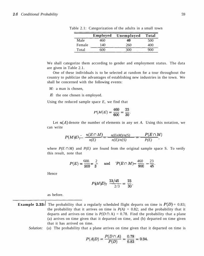
2.6" Conditional Probability 59
Table 2.1: Categorization of the adults in a small town
Male Female Total
Employed 460 140 600
Unemployed 40 260 300
Total 500 400 900
We shall categorize them according to gender and employment status. The data are given in Table 2.1.
One of these individuals is to be selected at random for a tour throughout the country to publicize the advantages of establishing new industries in the town. We shall be concerned with the following events:
M: a man is chosen,
E: the one chosen is employed.
Using the reduced sample space E, we find that
P ( A i | £ , ) - 6 0 0 _ 3 0 '
Let n(A) denote the number of elements in any set A. Using this notation, we can write
P(M\F\ - <E^M) n(EnM)/n(S) PjEHM) K ' ' n(E) n{E)/n{S) P(E) '
where P(E n M) and P(E) are found from the original sample space S. To verify this result, note that
„ , „ 600 2 j „ . „ w . 460 23 P ^ = 9 0 0 = 3 a n d P ^ n M ) = 900 = 45"
Hence
p,M\E) = 23/45 = 23 1 ' ' 2/3 30'
as before.
Example 2.33:1 The probability that a regularly scheduled flight departs on time is P{D) = 0.83; the probability that it arrives on time is P(A) = 0.82; and the probability that it departs and arrives on time is P{D D A) = 0.78. Find the probability that a plane (a) arrives on time given that it departed on time, and (b) departed on time given that it has arrived on time.
Solution: (a) The probability that a plane arrives on time given that it departed on time is
60 Chapter 2 Probability
(b) The probability that a plane departed on time given that it has arrived on time is
In the die-tossing experiment discussed on page 58 we note that P{B\A) = 2/5 whereas P{B) = 1/3. That is, P(B\A) ^ P{B), indicating that B depends on A. Now consider an experiment in which 2 cards are drawn in succession from an ordinary deck, with replacement. The events are defined as
A: the first card is an ace,
B: the second card is a spade.
Since the first card is replaced, our sample space for both the first and second draws consists of 52 cards, containing 4 aces and 13 spades. Hence
13 1 13 1
P{B\A) = ~ = 4 and P(B) = ~ = ^ v ' ' 52 4 v ; 52 4
4'
That is, P(i?|A) = P(B). When this is true, the events A and B are said to be independent.
The notion of conditional probability provides the capability of reevaluating the idea of probability of an event in light, of additional information, that is, when it is known that another event has occurred. The probability P(A|P) is an "updating" of P{A) based on the knowledge that event B has occurred. In Example 2.33 it is important to know the probability that the flight arrives on time. One is given the information that the flight did not depart on time. Armed with this additional information, the more pertinent probability is P(A|D'), that is, the probability that it arrives on time, given that it did not depart on time. In many situations the conclusions drawn from observing the more important conditional probability change the picture entirely. In this example the computation of P(A|£>') is
As a result, the probability of an on-time arrival is diminished severely in the presence of the additional information.
Example 2.34:1 The concept of conditional probability has countless applications in both industrial and biomedical applications. Consider an industrial process in the textile industry in which strips of a particular type of cloth are being produced. These strips can be defective in two ways, length and nature of texture. For the case of the latter, the process of identification is very complicated. It is known from historical information on the process that 10% of strips fail the length test, 5% fail the texture test, and only 0.8% fail both tests. If a strip is selected randomly from the process and a quick measurement identifies it as failing the length test, what is the probability that it is texture defective?
Solution: Consider the events
L : length defective, T : texture defective
2.7 Multiplicative Rules til
Thus, given that the strip is length defective:, the probability that this strip is texture defective is given by
n m l r . P{TC\L) 0.008 P(T\L) = „ , , , ' TTT- = 0.08.
P(L) 0,
Thus, the knowledge given by the conditional probability provides considerably more information than merely knowing P{T). J
Independent Events
Definition 2.10:
Although conditional probability allows for an alteration of the probability of an event in the light of additional material, it also enables us to understand better the very important concept of independence or, in the present context, independent events. In the airport illustration in Example 2.33, P(A\D) differs from P{A). This suggests that the occurrence of D influenced A and this is certainly expected in this illustration. However, consider the situation where we have events A and B and
P{A\B) = P(A).
In other words, the occurrence of B had no impact on the odds of occurrence of A. Here the occurrence of A is independent of the occurrence of B. The importance of the concept of independence cannot be overemphasized. It plays a vital role in material in virtually all chapters in this book and in all areas of applied statistics.
Two events A and B are- independent if and only if
P(B\A) = P(B) or P(A\B) - P{A),
provided the existences of the conditional probabilities. Otherwise. A and B are dependent .
The condition P{B\A) = P{B) implies that P{A\B) = P(A), and conversely. For the card-drawing experiments, where we showed that P(B\A) = P(B) = 1/4, we also can see that P{A\B) = P{A) = 1/13.
2.7 Multiplicative Rules
Multiplying the formula of Definition 2.9 by P(A), wc obtain the following important multiplicative rule, which enables us to calculate the probability that two events will both occur.
Theorem 2.13: If in an experiment the events A and B can both occur, then
P(Anfl) = P(A)P(B\A). provided P(A) > 0.
Thus the probability that both A and B occur is equal to the probability that A occurs multiplied by the conditional probability that B occurs, given that A
62 Chapter 2 Probability
occurs. Since the events AC\B and BCiA are equivalent, it follows from Theorem 2.13 that we can also write
P{A n B) = P{B n A) = P(5)P(A|B) .
In other words, it does not matter which event is referred to as A and which event is referred to as B.
Example 2.35:1 Suppose that we have a fuse box containing 20 fuses, of which 5 are defective. If 2 fuses are selected at random and removed from the box in succession without replacing the first, what is the probability that both fuses are defective?
Solution: We shall let A be the event that the first fuse is defective and B the event that the second fuse is defective; then we interpret A fl B as the event that A occurs, and then B occurs after A has occurred. The probability of first removing a defective fuse is 1/4; then the probability of removing a second defective fuse from the remaining 4 is 4/19. Hence
™-(;)Gi>H-Example 2.36:1 One bag contains 4 white balls and 3 black balls, and a second bag contains 3 white
balls and 5 black balls. One ball is drawn from the first bag and placed unseen in the second bag. What is the probability that a ball now drawn from the second bag is black?
Solution: Let Bi, B2, and W\ represent, respectively, the drawing of a black ball from bag 1, a black ball from bag 2, and a white ball from bag 1. We are interested in the union of the mutually exclusive events B\ n B2 and W\ <~\ Bi- The various possibilities and their probabilities are illustrated in Figure 2.8. Now
P[(Bi n Bo) or (Wi n B2)\ = P{B1 n B2) + P(Wi H B2)
= P(Bl)P(B2\Bl) + P(Wl)P(B2\W1)
j) (I)+ (I) (i)= I- J If, in Example 2.35, the first fuse is replaced and the fuses thoroughly rear
ranged before the second is removed, then the probability of a defective fuse on the second selection is still 1/4; that is, P(i?|A) = P(B) and the events A and B are independent. When this is true, we can substitute P(B) for P(P |A) in Theorem 2.13 to obtain the following special multiplicative rule.
Theorem 2.14: Two events A and B are independent if and only if
P{A n B) = P(A)P(B).
Therefore, to obtain the probability that two independent events will both occur, we simply find the product of their individual probabilities.
Example 2.37:1 A small town has one fire engine and one ambulance available for emergencies. The probability that the fire engine is available when needed is 0.98, and the
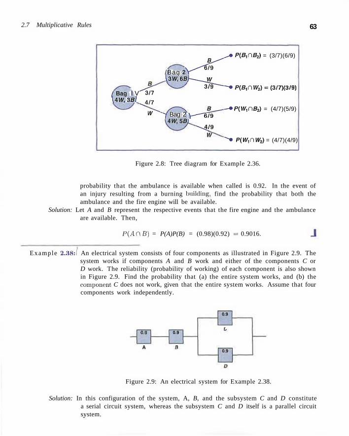
2.7 Multiplicative Rules 63
/Bag l V 14IV, Sal
""3/7
^ 4 / 7
W ^
/Bag 2V"" 13IV, 6B/—
7 Bag 2 y -
B^^ - - ^ / 9
-_JV 3/9~~~-
— 6 / 9
•--4/9
^ • P ( S 1 n B 2 ) = (3/7)(6/9)
- ^ P ^ n ^ ^ f S ^ K S / S )
- • P(W^DB2) = (4/7)(5/9)
•"""• P(IV,niV2) = (4/7)(4/9)
Figure 2.8: Tree diagram for Example 2.36.
probability that the ambulance is available when called is 0.92. In the event of an injury resulting from a burning building, find the probability that both the ambulance and the fire engine will be available.
Solution: Let A and B represent the respective events that the fire engine and the ambulance are available. Then,
P ( A n B ) = P(A)P(B) = (0.98)(0.92) = 0.9016.
Example 2.38:1 An electrical system consists of four components as illustrated in Figure 2.9. The system works if components A and B work and either of the components C or D work. The reliability (probability of working) of each component is also shown in Figure 2.9. Find the probability that (a) the entire system works, and (b) the component C does not work, given that the entire system works. Assume that four components work independently.
0.9
A
0.9
R
0.9
r.
0.9
Figure 2.9: An electrical system for Example 2.38.
Solution: In this configuration of the system, A, B, and the subsystem C and D constitute a serial circuit system, whereas the subsystem C and D itself is a parallel circuit system.
64 Chapter 2 Probability
(a) Clearly the probability that the entire system works can be calculated as the following:
P(A n Bn(C U D)) = P(A)P(B)P(C U D)
= P(A)P(J3)[1 - P ( C ' n D ' ) ]
= F(A)P(B)[1 - P(C')P(D')}
= ( 0 . 9 ) ( 0 . 9 ) [ l - ( l - 0 . 8 ) ( l - 0 . 8 ) ]
- 0.7776.
The equalities above hold because of the independence among the four components.
(b) To calculate the conditional probability in this case, notice that
P(the system works but C docs not work) P = P(the system works)
P(A DBnC'nD) (0.9)(0.9)( 1 - 0.8)(0.8)
P(the system works) 0.7770 = 0.1667.
Theorem 2.15: If, in an experiment, the events Ai, A2,... ,Ak can occur, then
P(Ai n A2 n • ••••• n A*.)
= P(A1)P(A2 |Ai)P(A ; i |Ai n A2) • • • P(Ak\Ai n A2 n • •
If the events A\, A2, • • • ,Ak are independent, then
P(AI n A2 n • • • n Ak) = P(A,)P(A2) • • • P(Ak).
•nAA._i).
Example 2.39:1 Three cards arc drawn in succession, without replacement, from an ordinary deck of playing cards. Find the probability that the event A\C\ A2C\ A3 occurs, where Ai is the event that the first card is a red ace, A2 is the event that the second card is a 10 or a jack, and A3 is the event that the third card is greater than 3 but less than 7.
Solution: First we define: the events
A\\ the first card is a red ace,
A2: the. second card is a 10 or a jack,
A-y. the third card is greater than 3 but less than 7.
Now
P{AX 52
2 , P(A2 |Ai) = ~ , P( Aa I Ai n A,) = ^ , 51 50
and hence, by Theorem 2.15,
P(Ai n A, n A3) = P(A,)P(A2 |A1)P(A3|A ] n A2)
- ) ( - ) ( - ) = — • 52) V 5 1 / \ 5 0 / 5525
Exercises 65
E x a m p l e 2.40:1 A coin is biased so tha t a head is twice as likely to occur as a tail. If the coin is tossed 3 t imes, what is the probability of get t ing 2 tails and 1 head?
Solution: The sample space for the experiment consists of the 8 elements,
S = {HHH, HHT, HTH, THE, HTT, THT, TTH, TTT).
However, with an unbalanced coin it is no longer possible to assign equal probabilities to each sample point. It is easy to see t h a t P(H) = 2 / 3 and P(T) = 1/3 for one toss since a head is twice as likely to occur as a tail . Now let A be the event of gett ing 2 tails and 1 head in the 3 tosses of the coin. Then,
A = {TTH,THT, HTT},
and since the outcomes on each of the 3 tosses are independent, it follows from Theorem 2.15 tha t
P{TTH) = P(T)P(T)P{H) = ( I ) ( I ) ( | ) = 2.
Similarly, P{THT) = P{HTT) = 2/27, and hence P(A) = 2 /27 + 2 /27 + 2 /27 =
2/9. J
Exercises
2.77 If R is the event that a convict committed armed robbery and D is the event that the convict pushed dope, state in words what probabilities are expressed by (a) P(R\D); (b) P(D'\R);
(c) P(R'\D').
2.78 A class in advanced physics is comprised of 10 juniors, 30 seniors, and 10 graduate students. The final grades show that 3 of the juniors, 10 of the seniors, and 5 of the graduate students received an A for the course. If a student is chosen at random from this class and is found to have earned an .4, what is the probability that he or she is a senior?
2.79 A random sample of 200 adults are classified below by sex and their level of education attained.
Education Male Female Elementary 38 4!) Secondary 28 50 College " 22 17
If a person is picked at random from this group, find the probability that (a) the person is a male, given that the person has a
secondary education; (b) the person does not have a college degree, given
that the person is a female.
2.80 In an experiment to study the relationship of hypertension and smoking habits, the following data are collected for 180 individuals:
Moderate Heavy Nonsmokers Smokers Smokers
H 21 36 30 NH 48 26 19
where H and NH in the table stand for Hypertension and Nonhypertension, respectively. If one of these individuals is selected at random, find the probability that the person is (a) experiencing hypertension, given that the person is
a heavy smoker; (b) a nonsmoker, given that the person is experiencing
no hypertension.
2.81 In the senior year of a high school graduating class of 100 students, 42 studied mathematics, 68 studied psychology, 54 studied history, 22 studied both mathematics and history, 25 studied both mathematics and psychology, 7 studied history but neither mathe-
66 Chapter 2 Probabil i ty
matics nor psychology, 10 studied all three subjects, and 8 did not take any of the three. If a student is selected at random, find the probability that (a) a person enrolled in psychology takes all three sub
jects; (b) a person not taking psychology is taking both his
tory and mathematics.
2.82 A manufacturer of a flu vaccine is concerned about the quality of its flu serum. Batches of serum are processed by three different departments having rejection rates of 0.10, 0.08, and 0.12, respectively. The inspections by the three departments are sequential and independent.
(a) What is the probability that a batch of serum survives the first departmental inspection but is rejected by the second department?
(b) What is the probability that a batch of serum is rejected by the third department?
2.83 In USA Today (Sept. 5, 1996) the results of a survey involving the use of sleepwear while traveling were listed as follows:
Male Female Total Underwear Nightgown Nothing Pajamas T-shirt Other
0.220 0.002 0.160 0.102 0.046 0.084
0.024 0.180 0.018 0.073 0.088 0.003
0.244 0.182 0.178 0.175 0.134 0.087
(a) What is the probability that a traveler is a female who sleeps in the nude?
(b) What is the probability that a traveler is male? (c) Assuming the traveler is a male, what is the prob
ability that he sleeps in pajamas? (d) What is the probability that a traveler is male if he
sleeps in pajamas or a T-shirt?
2.84 The probability that an automobile being filled with gasoline will also need an oil change is 0.25; the probability that it needs a new oil filter is 0.40; and the probability that both the oil and filter need changing is 0.14.
(a) If the oil had to be changed, what is the probability that a new oil filter is needed?
(b) If a new oil filter is needed, what is the probability that the oil has to be changed?
2.85 The probability that a married man watches a certain television show is 0.4 and the probability that a married woman watches the show is 0.5. The probability that a man watches the show, given that his wife does, is 0.7. Find the probability that
(a) a married couple watches the show; (b) a wife watches the show given that her husband
does; (c) at least 1 person of a married couple will watch the
show.
2.86 For married couples living in a certain suburb, the probability that the husband will vote on a bond referendum is 0.21, the probability that his wife will vote in the referendum is 0.28, and the probability that both the husband and wife will vote is 0.15. What is the probability that (a) at least one member of a married couple will vote? (b) a wife will vote, given that her husband will vote? (c) a husband will vote, given that his wife does not
vote?
2.87 The probability that a vehicle entering the Lu-ray Caverns has Canadian license plates is 0.12; the probability that it is a camper is 0.28; and the probability that it is a camper with Canadian license plates is 0.09. What is the probability that
(a) a camper entering the Luray Caverns has Canadian license plates?
(b) a vehicle with Canadian license plates entering the Luray Caverns is a camper?
(c) a vehicle entering the Luray Caverns does not have Canadian plates or is not a camper?
2.88 The probability that the head of a household is home when a telemarketing representative calls is 0.4. Given that the head of the house is home, the probability that goods will be bought from the company is 0.3. Find the probability that the head of the house is home and goods being bought from the company.
2.89 The probability that a doctor correctly diagnoses a particular illness is 0.7. Given that the doctor makes an incorrect diagnosis, the probability that the patient enters a law suit is 0.9. What is the probability that the doctor makes an incorrect diagnosis and the patient sues?
2.90 In 1970, 11% of Americans completed four years of college; 43% of them were woman. In 1990, 22% of Americans completed four years of college; 53% of them were women (Time, Jan. 19, 1996). (a) Given that a person completed four years of college
in 1970, what is the probability that the person was a women?
(b) What is the probability that a woman would finish four years of college in 1990?
(c) What is the probability that in 1990 a man would not finish college?
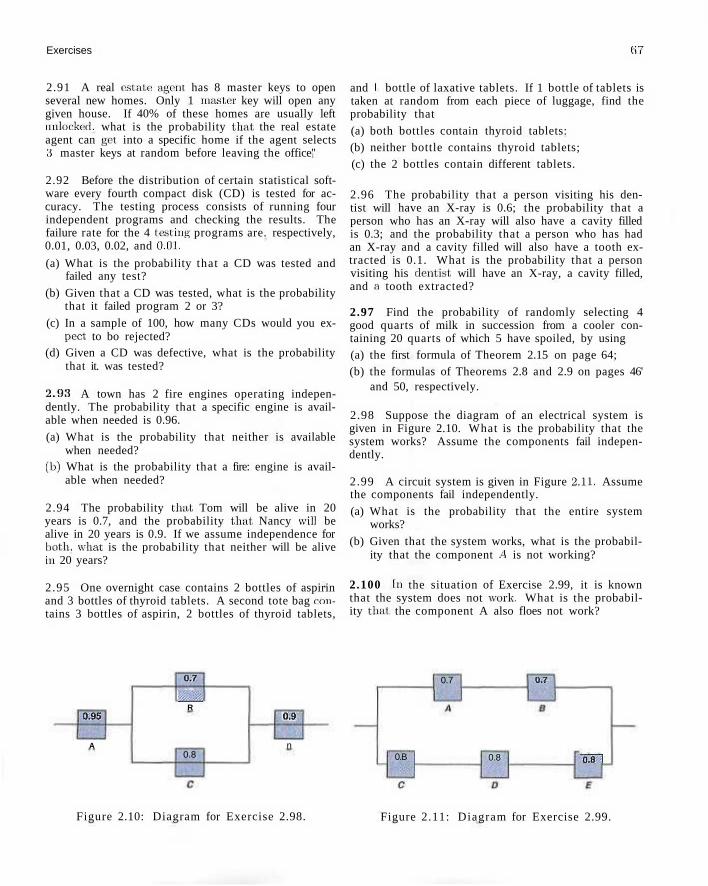
Exercises 07
2.91 A real estate agent has 8 master keys to open several new homes. Only 1 master key will open any given house. If 40% of these homes are usually left unlocked, what is the probability that the real estate agent can get into a specific home if the agent selects 15 master keys at random before leaving the office''
2.92 Before the distribution of certain statistical software every fourth compact disk (CD) is tested for accuracy. The testing process consists of running four independent programs and checking the results. The failure rate for the 4 testing programs are. respectively, 0.01, 0.03, 0.02, and 0.01.
(a) What is the probability that a CD was tested and failed any test?
(b) Given that a CD was tested, what is the probability that it failed program 2 or 3?
(c) In a sample of 100, how many CDs would you expect to bo rejected?
(d) Given a CD was defective, what is the probability that it. was tested?
2.93 A town has 2 fire engines operating independently. The probability that a specific engine is available when needed is 0.96.
(a) What is the probability that neither is available when needed?
(Ii) What is the probability that a fire: engine is available when needed?
2.94 The probability that Tom will be alive in 20 years is 0.7, and the probability that Nancy will be alive in 20 years is 0.9. If we assume independence for both, what is the probability that neither will be alive hi 20 years?
2.95 One overnight case contains 2 bottles of aspirin and 3 bottles of thyroid tablets. A second tote bag contains 3 bottles of aspirin, 2 bottles of thyroid tablets,
and I bottle of laxative tablets. If 1 bottle of tablets is taken at random from each piece of luggage, find the probability that
(a) both bottles contain thyroid tablets: (b) neither bottle contains thyroid tablets; (c) the 2 bottles contain different tablets.
2.96 The probability that a person visiting his dentist will have an X-ray is 0.6; the probability that a person who has an X-ray will also have a cavity filled is 0.3; and the probability that a person who has had an X-ray and a cavity filled will also have a tooth extracted is 0.1. What is the probability that a person visiting his dentist, will have an X-ray, a cavity filled, and a tooth extracted?
2.97 Find the probability of randomly selecting 4 good quarts of milk in succession from a cooler containing 20 quarts of which 5 have spoiled, by using (a) the first formula of Theorem 2.15 on page 64; (b) the formulas of Theorems 2.8 and 2.9 on pages 46'
and 50, respectively.
2.98 Suppose the diagram of an electrical system is given in Figure 2.10. What is the probability that the system works? Assume the components fail independently.
2.99 A circuit system is given in Figure 2.11. Assume the components fail independently.
(a) What is the probability that the entire system works?
(b) Given that the system works, what is the probability that the component A is not working?
2.100 In the situation of Exercise 2.99, it is known that the system does not work. What is the probability that the component A also floes not work?
0.95
A
0-7
^H R
0.8
0.9
n
0.7 0.7;
0.B 0.8 "bin
Figure 2.10: Diagram for Exercise 2.98. Figure 2.11: Diagram for Exercise 2.99.
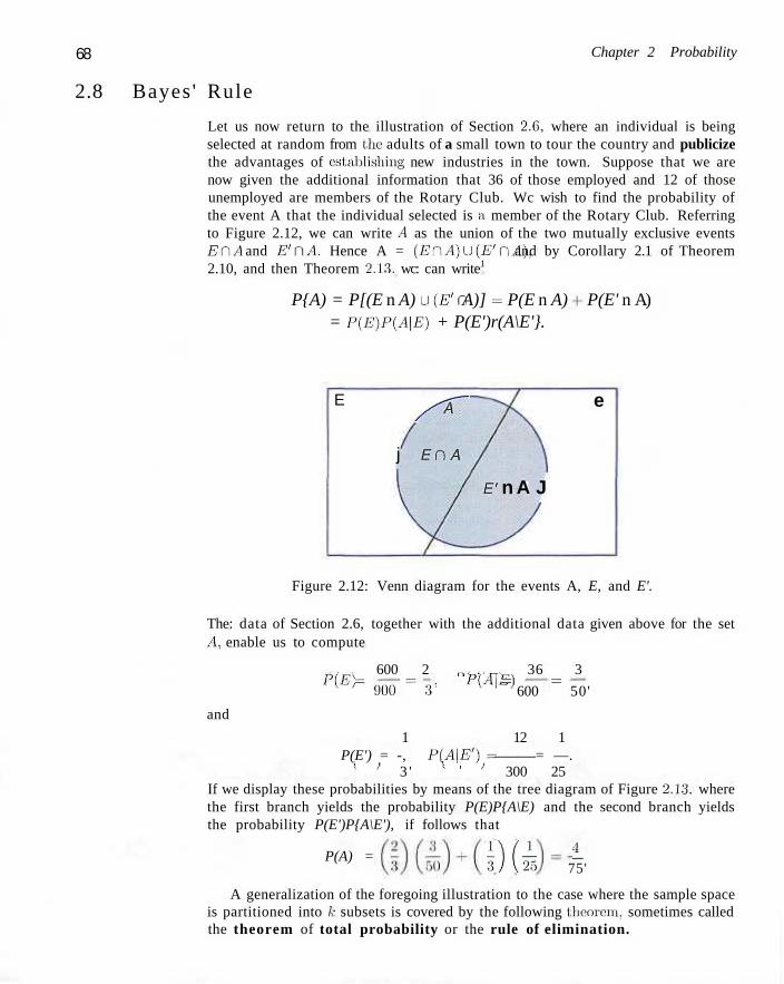
68 Chapter 2 Probability
2.8 Bayes ' Rule
Let us now return to the illustration of Section 2.C, where an individual is being selected at random from the adults of a small town to tour the country and publicize the advantages of establishing new industries in the town. Suppose that we are now given the additional information that 36 of those employed and 12 of those unemployed are members of the Rotary Club. Wc wish to find the probability of the event A that the individual selected is a member of the Rotary Club. Referring to Figure 2.12, we can write A as the union of the two mutually exclusive events EDA and E ' f l A Hence A = {EnA)U{E'r\A), and by Corollary 2.1 of Theorem 2.10, and then Theorem 2.13. wc: can write1
P{A) = P[(E n A) u(E'n A)] = P(E n A) = P(E)P(A\E) + P(E')r(A\E'}.
P(E' n A)
E /-^A~
j EDA
£' n A J
e
Figure 2.12: Venn diagram for the events A, E, and E'.
The: data of Section 2.6, together with the additional data given above for the set A, enable us to compute
„ , „ , 600 2 „ , . . „ . 36 3 P ^ = 900 = 3 ' PiAE) - 600 = 50'
and
1 12 1 P(E') = -, P(A|J5') = = —.
k ' 3 ' v ' ' 300 25 If we display these probabilities by means of the tree diagram of Figure 2.13. where the first branch yields the probability P(E)P{A\E) and the second branch yields the probability P(E')P{A\E'), if follows that
P(A) = \M 4_
75'
A generalization of the foregoing illustration to the case where the sample space is partitioned into k subsets is covered by the following theorem, sometimes called the theorem of total probability or the rule of elimination.
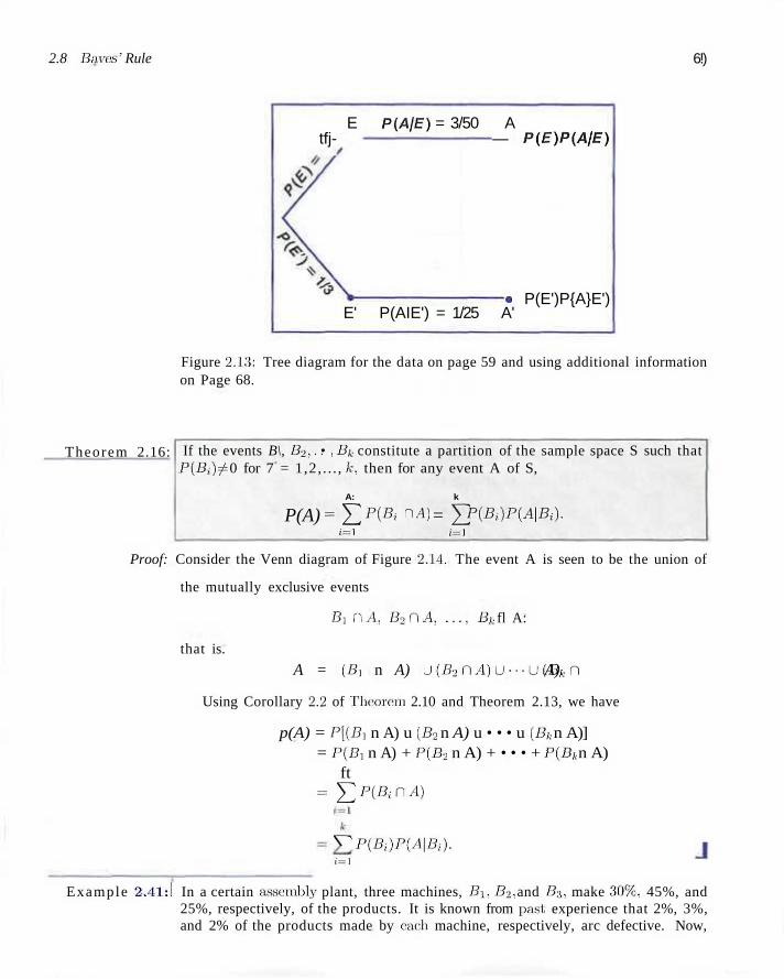
2.8 Baves' Rule 6!)
E P(AjE) = 3/50 A tfj- — P{E)P(A(E)
E' P(AIE') = 1/25 A' • P(E')P{A}E')
Figure 2.13: Tree diagram for the data on page 59 and using additional information on Page 68.
Theorem 2.16: If the events B\, B2,.. • ,Bk constitute a partition of the sample space S such that P(Bi) ^ 0 for 7 = 1,2,. . . , k, then for any event A of S,
A: k
P(A) = Y, P(B> n -4) = E P(Bi)P{A\Bt). i = i j = i
Proof: Consider the Venn diagram of Figure 2.14. The event A is seen to be the union of
the mutually exclusive events
Pi DA, B2<lA, . . . , Bk fl A:
that is.
A = (Pi n A) u(B2nA)u---u(Bkn A).
Using Corollary 2.2 of Theorem 2.10 and Theorem 2.13, we have
p(A) = P[(P, n A) u (£2 n A) u • • • u (Bk n A)] = P(P, n A) + P{B2 n A) + • • • + P(Bk n A)
ft = ^ P ( / i ; n A )
V^r> 1 = 1
P(Bi)P{A\Bi).
Example 2.41:1 In a certain assembly plant, three machines, Bi, B2, and P3, make 30%:, 45%, and 25%, respectively, of the products. It is known from past, experience that 2%, 3%, and 2% of the products made by each machine, respectively, arc defective. Now,
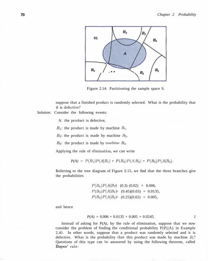
70 Chapter 2 Probability
01
s * / .
K Bz
J A
• • ^
BJ
\ S e
s4
1 B5
Figure 2.14: Partitioning the sample space S.
suppose that a finished product is randomly selected. What is the probability that if is defective?
Solution: Consider the following events:
A: the product, is defective,
P i : the product is made by machine P i ,
B2: the product is made by machine B2,
B$: the product is made by machine: P3.
Applying the rule of elimination, we can write
P(A) = P(Pi )P(A|Pi ) + P (P 2 )P (A |P , ) + P(B3)P(AjP : t).
Referring to the tree diagram of Figure 2,15, we find that the three branches give the probabilities
P(Bl)P(A\Bl) = (0.3) (0.02) = 0.006.
P{B2)P(A\B2) = (0.45)(0.03) = 0.0135,
P{B3)P(A\B3) = (0.25)(0.02) = 0.005,
and hence
P(A) = 0.006 + 0.0135 + 0.005 = 0.0245. J
Instead of asking for P(A), by the rule of elimination, suppose that we now consider the problem of finding the conditional probability P(Pj|A) in Example 2.41. In other words, suppose that a product was randomly selected and it is defective. What is the probability that, this product was made by machine P,? Questions of this type can lie answered by using the following theorem, called Bayes ' rule:
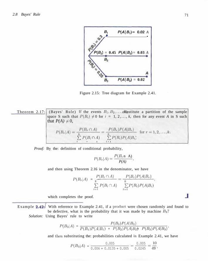
2.8 Bayes' Rule 71
B, P(A\B,) = 0.02 A «b * •
P(B2) = 0.45 P(A\B2) = 0.03 A
P(A|B3) = 0.02
Figure 2.15: Tree diagram for Example 2.41.
Theorem 2.17: (Bayes' Rule) If the events B\,B2,...,Bk constitute a partition of the sample space S such that P(Pi) ^ 0 for i = 1, 2 , . . . , k, then for any event A in S such that P(A) £ 0,
E W n . e ) E i>(B,)P(4|B() 1 = 1 2 = 1
Proof: By the: definition of conditional probability,
P(Br n A) P(P, |A)
P(A)
and then using Theorem 2.16 in the denominator, we have
P ( P , O A ) P(P, .)P(A|B r) P(P,.|A) = -
\ZP{Bif)A) £ P(Bi)P(A\Bi) i = i i'=i
which completes the proof.
Example 2.42:1 With reference to Example 2.41, if a product were chosen randomly and found to be defective, what is the probability that it was made by machine £3?
Solution: Using Bayes' rule to write
P(B:i|A) = P(B-,)P(A\B:i
P(B} )P(A|P,) + P(B2)P(A\B2) + P(P3)P(A|P,3) ;
and them substituting the: probabilities calculated in Example 2.41, we have
0.005 0.005 10 P(P.l|A) =
0.006 + 0.0135 + 0.005 0.0245 49 '
72 Chapter 2 Probability
In view of the fact that a defective product was selected, this result suggests that
it probably was not made by machine B3. J
E x a m p l e 2.43:1 A manufacturing firm employs three analytical plans for the design and development of a particular product. For cost reasons, all three are used at varying times. In fact, plans 1, 2, and 3 are used for 30%,, 20%, and 50% of the products respectively. The "defect rate:" is different for the three procedures as follows:
P(D\Pi)=0M, P{D\P2) = 0.03. P ( D | P 3 ) = 0.02,
where P(D\Pj) is the probability of a, defective product, given plan j. If a random product was observed and found to be defective, which plan was most likely used and thus responsible?
Solution: From the statement, of the problem
PiPi) = 0.30. P(P2) = 0.20, and P(P:i) = 0.50,
we must find P(Pj\D) for j = 1,2,3. Bayes' rule from Theorem 2.17 shows
P ( P ! ) P ( D | P l )
Exercises
P(Pi\D) P(Pi)P(D|P,) + P(P2)P(D\P2) + P(P3)P(D\P3) (0.30)(0.01) 0.003 _
(0.3)(0.01) + (0.20)(0.03) + (0.50)(0.02) ~~ 0.019 " 0.158.
Similarly,
w ) = ( 0 ! 3 £ - 2 0 ) = Q - 3 1 6 - I P(P3\D) = m m . = 0.019 0.019
The conditional probability of a defect given plan 3 is the largest of the three; thus a defective for a random product is most, likely the result of the use of plan 3. J
Using Bayes' rule, a statistical methodology, called the Bayesian method, has attracted a lot of attention in applications. An introduction to Bayesian method will be discussed in Chapter 18.
2.101 In a certain region of the country it is known from (last, experience that the: probability of selecting an adult over 40 years of age: with cancer is 0.05, If the probability of a doctor correctly diagnosing a person with cancer as having the disease is 0.78 and the: probability of incorrectly diagnosing a person without cancer as having the disease is 0.1)6, what is the probability that, a person is diagnosed as having cancer?
2.102 Police plan to enforce speed limits by using radar traps at 4 different locations within the city limits. The radar traps at each of the locations L\, E>,
L:u and L4 are operated 40%, 30%, 20%, and 30% of the time, and if a person who is speeding on his way to work has probabilities of 0.2, 0.1, 0.5, and 0.2, respectively, of passing through these locations, what is the probability that he will receive a spcuxling ticket?
2.103 Referring to Exercise 2.101, what, is the probability that a person diagnosed as having cancer actually has the disease?
2.104 If in Exercise 2.102 the person received a speeding ticket on his way to work, what is the probability
Review Exercises 73
that he passed through the radar trap located at Li?
2.105 Suppose that the four inspectors at a film factory are supposed to stamp the expiration date on each package of film at the end of the assembly line. John, who stamps 20% of the packages, fails to stamp the expiration date once in every 200 packages: Tom, who stamps 60% of the packages, fails to stamp the expiration date once in every 100 packages; Jeff, who stamps 15% of the packages, fails to stamp the expiration date once in every 90 packages; and Pat, who stamps 5% of the packages, fails to stamp the expiration date once in every 200 packages. If a customer complains that her package of film does not show the expiration date, what is the probability that it was inspected by John?
2.106 A regional telephone company operates three identical relay stations at different locations. During a one year period, the number of malfunctions reported by each station and the causes are shown below.
Station A B C Problems with electricity supplied Computer malfunction Malfunctioning electrical equipment Caused by other human errors
Suppose that a malfunction was reported and it was found to be caused by other human errors. What is the probability that it came from station C?
2 4 5 7
1 3 4 7
1 2 2 5
2.107 Pollution of the rivers in the United States has been a problem for many years. Consider the following events:
A= (The river is polluted.}
B— {A sample of water tested detects pollution.}
C= {Fishing permitted.}
Assume P(A) = 0.3. P(B|A) = 0.75, P (P |A ' ) = 0.20, P ( q A n P ) = 0.20, P(C|A'nP) = 0.15, P(C|Ans ' ) = 0.80, and P(C|A' n B') = 0.90. (a) Find P ( A n B n C ) . (b) Find P (B 'nC) . (c) Find P(C). (d) Find the probability that the river is polluted, given
that fishing is permitted and the sample tested did not detect pollution.
2.108 A paint-store chain produces and sells latex and semigloss paint. Based on long-range sales, the probability that a customer will purchase latex paint is 0.75. Of those that purchase latex paint, 60% also purchase rollers. But only 30% of semigloss paint buyers purchase rollers. A randomly selected buyer purchases a roller and a can of paint. What is the probability that the paint is latex?
Review Exercises
2.109 A truth serum has the property that 90% of the guilty suspects are properly judged while, of course, 10% of guilty suspects are improperly found innocent. On the other hand, innocent suspects are misjudged 1% of the time. If the suspect was selected from a group of suspects of which only 5% have ever committed a crime, and the serum indicates that he is guilty, what is the probability that he is innocent?
2.110 An allergist, claims that 50% of the patients she tests are allergic to some type of weed. What, is the probability that
(a) exactly 3 of her next 4 patients are allergic to weeds?
(b) none of her next 4 patients is allergic to weeds?
2.111 By comparing appropriate regions of Venn diagrams, verify that (a) (AD B) LI (An B') = A; (b) A' n (B' uC) = (A' n B') u (A' n C).
2.112 The probabilities that a service station will pump gas into 0, 1, 2, 3, 4, or 5 or more cars during a certain 30-minute period are 0.03, 0.18, 0.24, 0.28, 0.10, and 0.17, respectively. Find the probability that in this 30-minute period
(a) more than 2 cars receive gas;
(b) at most 4 cars receive gas; (c) 4 or more cars receive gas.
2.113 How many bridge hands are possible containing 4 spades, 6 diamonds, 1 club, and 2 hearts?
2.114 If the probability is 0.1 that a person will make a mistake on his or her state income tax return, find the probability that (a) four totally unrelated persons each make a mistake; (b) Mr. Jones and Ms. Clark both make a mistake,
and Mr. Roberts and Ms. Williams do not make a mistake.
2.115 A large industrial firm uses 3 local motels to
74 Chapter 2 Probability
provide overnight accommodations for its clients. From past experience it is known that 20%: of the clients are assigned rooms at the Ramada Inn, 50% at. the Sheraton, and 30% at the Lake view Motor Lodge. If the plumbing is faulty in 5% of the rooms at the Ramada Inn, in 4% of the rooms at the Sheraton, and in 8% of the rooms at the Lakeview Motor Lodge, what, is the probability that
(a) a client will be assigned a room with faulty plumbing?
(b) a person with a room having faulty plumbing was assigned accommodations at the Lakeview Motor Lodge?
2.116 From a group of 4 men and 5 women, how many committees of size 3 are possible
(a) with no restrictions? (b) with 1 man and 2 women? (c) with 2 men and I woman if a certain man must be
on the committee?
2.117 The probability that a patient recovers from a delicate heart operation is 0.8. What is the probability that (a) exactly 2 of the next 3 patients who have this op
eration survive? (b) all of the next 3 patients who have this operation
survive?
2.118 In a certain federal prison it is known that 2/3 of the inmates are under 25 years of age. It is also known that 3/5 of the inmates are male and that 5/8 of the inmates are female or 25 years of age or older. What is the probability that a prisoner selected at random from this prison is female and at least 25 years old?
2.119 From 4 red, 5 green, and 6 yellow apples, how many selections of 9 apples are possible if 3 of each color are to be selected?
2.120 From a box containing 6 black balls and 4 green balls, 3 balls are drawn in succession, each ball being replaced in the box before the next draw is made. What is the probability that
(a) all 3 are the same color? (b) each color is represented?
2.121 A shipment of 12 television sets contains 3 defective sets. In how many ways can a hotel purchase 5 of these sets and receive at least 2 of the defective sets?
2.122 Electrical, chemical, industrial, and mechanical engineering curricula were studied. It was found
that some students took no statistics, some took one semester, and others took two semesters. Consider the following events:
A: Some statistics is taken B: Electrical and industrial engineers C: Chemical engineers
Use Venn diagrams and shade the areas representing the following events:
( a ) ( A n P ) ' ;
(b) (A u BY; (c) (AHC)UB.
2.123 A certain federal agency employs three consulting firms (A, B, and C) with probabilities 0.40, 0.35, and 0.25, respectively. From past experience it is known that the probability of cost overruns for the firms are 0.05, 0.03, and 0.15, respectively. Suppose a cost overrun is experienced by the agency.
(a) What, is the probability that the consulting firm involved is company C?
(b) What is the probability that it is company A?
2.124 A manufacturer is studying the effects of cooking temperature, cooking time, and type of cooking oil for making potato chips. Three different temperatures, 4 different cooking times, and 3 different oils are to be used.
(a) What is the total number of combinations to be studied?
(b) How many combinations will be used for each type of oil?
(c) Discuss why permutations are not an issue in this exercise.
2.125 Consider the situation in Exercise 2.124, and suppose that the manufacturer can try only two combinations in a day. (a) What is the probability that any given set of 2 runs
is chosen? (b) What is the probability that the highest tempera
ture is used in either of these 2 combinations?
2.126 A certain form of cancer is known to be found in women over 60 with probability 0.07. A blood test exists for the detection of the disease but the test is not infallible. In fact, it is known that 10% of the time the test gives a false negative (i.e., the test incorrectly gives a negative result) and 5% of the time the test, gives a false positive (i.e., incorrectly gives a positive result). If a woman over 60 is known to have taken the test and received a favorable (i.e., a negative result), what is the probability that she has the disease?
Review Exercises 75
2.127 A producer of a certain type of electronic component ships to suppliers in lots of twenty. Suppose that 60% of all such lots contain no defective components, 30% contain one defective component, and 10% contain two defective components. A lot is selected and two components from the lot are randomly selected and tested and neither is defective.
(a) What is the probability that zero defective components exist in the lot?
(b) What is the probability that one defective exists in the lot?
(c) What is the probability that two defectives exist in the lot?
2.128 A rare disease exists in which only 1 in 500 are affected. A test for the disease exists but of course it is not infallible. A correct positive result (patient actually has the disease) occurs 95% of the time while a false positive result (patient does not have the disease) occurs 1% of the time. If a randomly selected individual is tested and the result is positive, what is the probability that the individual has the disease?
2.129 A construction company employs 2 sales engineers. Engineer 1 does the work in estimating cost for 70% of jobs bid by the company. Engineer 2 does the work for 30% of jobs bid by the company. It is known that the error rate for engineer 1 is such that 0.02 is the probability of an error when he does the work, whereas the probability of an error in the work of engineer 2 is 0.04. Suppose a bid arrives and a serious error occurs in estimating cost. Which engineer would you guess did the work? Explain and show all work.
2.130 In the field of quality control the science of statistics is often used to determine if a process is "out of control." Suppose the process is, indeed, out of control and 20% of items produced are defective.
(a) If three items arrive off the process line in succession, what is the probability that all three are defective?
(b) If four items arrive in succession, what is the probability that three are defective?
2.131 An industrial plant is conducting a study to determine how quickly injured workers are back on the job following injury. Records show that 10% of all injured workers are admitted to the hospital for treatment and 15% are back on the job the next day. In addition, studies show that 2% are both admitted for hospital treatment and back on the job the next day. If a worker is injured, what is the probability that the worker will either be admitted to a hospital or back on
the job the next day or both?
2.132 A firm is accustomed to training operators who do certain tasks on a production line. Those operators who attend the training course are known to be able to meet their production quotas 90% of the time. New operators who do not take the training course only meet their quotas 65%. of the time. Fifty percent of new operators attend the course. Given that a new operator meets his production quota, what is the probability that he (or she) attended the program?
2.133 A survey of those using a particular statistical software system indicated that 10% were dissatisfied. Half of those dissatisfied purchased the system from vender A. It is also known that 20%> of those surveyed purchased from vendor A. Given that the software package was purchased from vendor ,4, what is the probability that that particular user is dissatisfied?
2.134 During bad economic times, industrial workers are dismissed and are often replaced by machines. The history of 100 workers whose loss of employment is attributable to technological advances is reviewed. For each of these individuals, it was determined if he or she was given an alternative job within the same company, found a job with another company but is working in the same field, found a job in a new field, or has been unemployed for 1 year. In addition, the union status of each worker is recorded. The following table summarizes the results.
Union Nonunion Same Company New Company (same field) New Field Unemployed
(a) If the selected workers found a job with a new company in the same field, what is the probability that the worker is a union member?
(b) If the worker is a union member, what is the probability that the worker has been unemployed for a
2.135 There is a 50-50 chance that the queen carries the gene of hemophilia. If she is a carrier, then each prince has a 50-50 chance of having hemophilia independently. If the queen is not a carrier, the prince will not have the disease. Suppose the queen has had three princes without the disease, what is the probability the queen is a carrier?
2.136 What is the probability that no two students will have the same birth date in a size of 60 class? (See Exercise 2.50.)
40 13 A 2
15 10 11 5
Chapter 3
Random Variables and Probability Distributions
3.1 Concept of a Random Variable
Definition 3.1:
Statistics is concerned with making inferences about populations and population characteristics. Experiments are conducted with results that are subject to chance. The testing' of a number of electronic components is an example of a s tat is t ical exper iment , a term that is used to describe any process by which several chance observations arc generated. It is often important to allocate a numerical description to the outcome. For example, the sample space giving a. detailed description of each possible outcome when three electronic components are tested may be written
S = {NNN, NND, NDN, DNN, NDD, DND, DDN, DDD},
where AT denotes "nondefective" and D denotes "defective." One is naturally concerned with the: number of defectives that occur. Thus each point in the sample space will be assigned a numerical value of 0, 1, 2, or 3. These values are, of course, random quantities determined by the outcome of the experiment. They may be viewed as values assumed by the random variable X, the number of defective items when three electronic components are tested.
A random variable is a function that associates a. real number with each element in the sample space.
We shall use a capital letter, say X, to denote a random variable and its corresponding small letter, x in this case, for one of its values. In the electronic: component testing illustration above, we notice that the random variable X assumes the value 2 for all elements in the subset
E = {DDN, DND, NDD}
of the sample space S. That is. each possible value of A' represents an event that is a subset of the sample space for the given experiment.
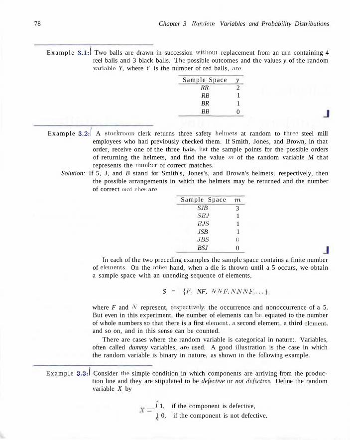
78 Chapter 3 Random. Variables and Probability Distributions
Example 3.1:1 Two balls are drawn in succession without replacement from an urn containing 4 reel balls and 3 black balls. The possible outcomes and the values y of the random variable: Y, where V is the number of red balls, are
Sample Space y RR RB BR BB
2 1 1 0
Example 3.2:1 A stockroom clerk returns three safety helmets at random to three steel mill employees who had previously checked them. If Smith, Jones, and Brown, in that order, receive one of the three hats, list the sample points for the possible orders of returning the helmets, and find the value in of the random variable M that represents the number of correct matches.
Solution: If 5, J, and B stand for Smith's, Jones's, and Brown's helmets, respectively, then the possible arrangements in which the helmets may be returned and the number of correct mat dies are
Sample Space SJB SB.I HIS JSB JUS BSJ
rn 3 1 1 1 (i
0
In each of the two preceding examples the sample space contains a finite number of elements. On the other hand, when a die is thrown until a 5 occurs, we obtain a sample space with an unending sequence of elements,
S = {F. NF, NNF, NNNF,...},
where F and Ar represent, respectively, the occurrence and nonoccurrence of a 5. But even in this experiment, the number of elements can Vic equated to the number of whole numbers so that there is a first element, a second element, a third clement, and so on, and in this sense can be counted.
There are cases where the random variable is categorical in nature:. Variables, often called dummy variables, are used. A good illustration is the case in which the random variable is binary in nature, as shown in the following example.
Example 3.3:1 Consider the simple condition in which components are arriving from the production line and they are stipulated to be defective or not defective. Define the random variable X by
J 1, if the component is defective,
1 0, if the component is not defective.
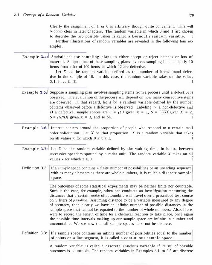
3.1 Concept of a Random Variable 79
Clearly the assignment of 1 or 0 is arbitrary though quite convenient. This will become clear in later chapters. The random variable in which 0 and 1 arc chosen to describe the two possible values is called a Bernoull i r andom variable. J
Further illustrations of random variables are revealed in the following four examples.
Example 3.4:1 Statisticians use sampling plans to either accept or reject batches or lots of material. Suppose one of these sampling plans involves sampling independently 10 items from a lot of 100 items in which 12 are defective.
Let X be the random variable defined as the number of items found defective in the sample of 10. In this case, the random variable takes on the values 0,1,2, . . . ,9 ,10 . J
Example 3.5:1 Suppose a sampling plan involves sampling items from a process until a defective is observed. The evaluation of the process will depend on how many consecutive items are observed. In that regard, let X be; a random variable defined by the number of items observed before a defective is observed. Labeling Ar a non-defective and D a defective, sample spaces are S = (D) given X = 1, S = (ND) given X = 2. S = (NND) given X = 3, and so on. J
Example 3.6:1 Interest centers around the proportion of people who respond to a certain mail order solicitation. Let X be that proportion. X is a random variable that takes on all values x for which 0 < x < 1. J
Example 3.7:1 Let X be the random variable defined by the: waiting time, in hours, between successive speeders spotted by a radar unit. The random variable X takes on all values x for which z > 0. J
Definition 3.2: If a sample space contains a finite number of possibilities or an unending sequence with as many elements as there are whole numbers, it is called a discrete sample space.
The outcomes of some statistical experiments may be neither finite nor countable. Such is the case, for example, when one conducts an investigation measuring the distances that a certain make of automobile will travel over a prescribed test course on 5 liters of gasoline. Assuming distance to be a variable measured to any degree of accuracy, then clearly we have an infinite number of possible distances in the sample space that cannot be. equated to the number of whole numbers. Also, if one-were to record the length of time for a chemical reaction to take place, once again the possible time intervals making up our sample space are infinite in number and uncountable. We see now that all sample spaces need not be discrete.
Definition 3.3: If a sample space contains an infinite number of possibilities equal to the number of points on a line segment, it is called a cont inuous sample space.
A random variable: is called a discrete r a n d o m variable if its set. of possible outcomes is countable. The random variables in Examples 3.1 to 3.5 are discrete
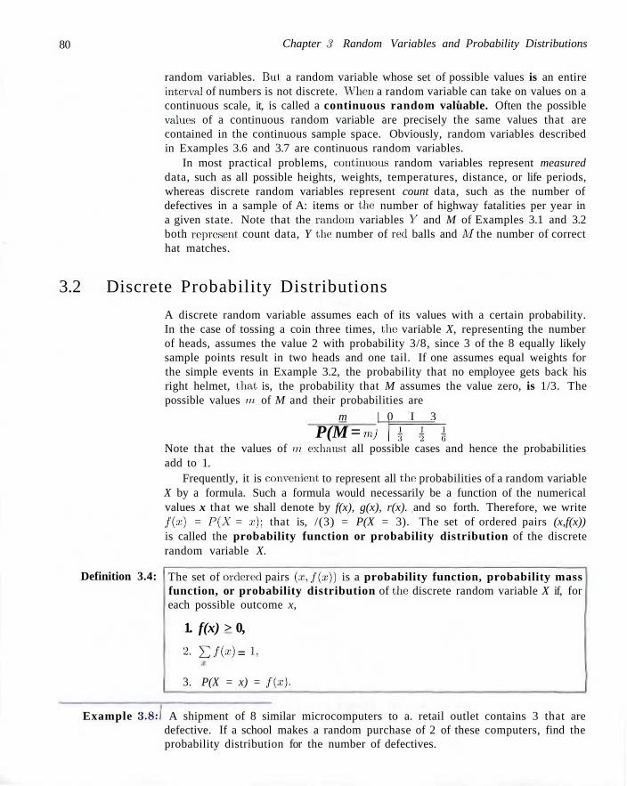
80 Chapter 3 Random Variables and Probability Distributions
random variables. But a random variable whose set of possible values is an entire interval of numbers is not discrete. When a random variable can take on values on a continuous scale, it, is called a continuous random valuable. Often the possible values of a continuous random variable are precisely the same values that are contained in the continuous sample space. Obviously, random variables described in Examples 3.6 and 3.7 are continuous random variables.
In most practical problems, continuous random variables represent measured data, such as all possible heights, weights, temperatures, distance, or life periods, whereas discrete random variables represent count data, such as the number of defectives in a sample of A: items or the; number of highway fatalities per year in a given state. Note that the random variables 1' and M of Examples 3.1 and 3.2 both represent count data, Y the number of red balls and M the number of correct hat matches.
3.2 Discrete Probability Distributions
A discrete random variable assumes each of its values with a certain probability. In the case of tossing a coin three times, the variable X, representing the number of heads, assumes the value 2 with probability 3/8, since 3 of the 8 equally likely sample points result in two heads and one tail. If one assumes equal weights for the simple events in Example 3.2, the probability that no employee gets back his right helmet, that is, the probability that M assumes the value zero, is 1/3. The possible values rn of M and their probabilities are
m | 0 I 3
P(M = m) | ~ m Note that the values of in exhaust all possible cases and hence the probabilities add to 1.
Frequently, it is convenient to represent all the probabilities of a random variable X by a formula. Such a formula would necessarily be a function of the numerical values x that we shall denote by f(x), g(x), r(x). and so forth. Therefore, we write /(:<:) = P(X = x); that is, /(3) = P(X = 3). The set of ordered pairs (x,f(x)) is called the probability function or probability distribution of the discrete random variable X.
Definition 3.4: The set of ordered pairs (aJ,/(a:)) is a probability function, probability mass function, or probability distribution of the discrete random variable X if, for each possible outcome x,
1. f(x) > 0,
2- £ / (* ) = !>
3. P(X = x) = /(.r).
Example 3.8:1 A shipment of 8 similar microcomputers to a. retail outlet contains 3 that are defective. If a school makes a random purchase of 2 of these computers, find the probability distribution for the number of defectives.
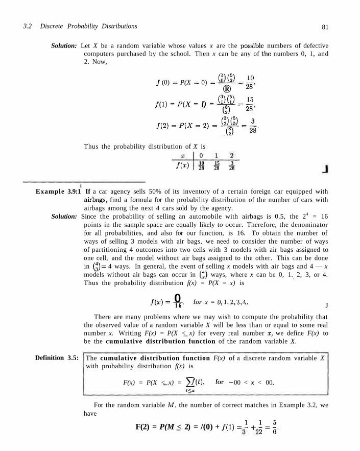
3.2 Discrete Probability Distributions 81
Solution: Let X be a random variable whose values x are the possible numbers of defective computers purchased by the school. Then x can be any of the numbers 0, 1, and 2. Now,
/ (0) = P(X = 0) =
f(l) = P(X = l) =
(g)(5) _"> ® 28'
( t)( t) _ 15
© 28' /(2) = P(X = 2) = S | ) = | .
Thus the probability distribution of X is 0
/ (*) 10 15 3 28 28 28
Example 3.9:1 If a car agency sells 50% of its inventory of a certain foreign car equipped with airbags. find a formula for the probability distribution of the number of cars with airbags among the next 4 cars sold by the agency.
Solution: Since the probability of selling an automobile with airbags is 0.5, the 24 = 16 points in the sample space are equally likely to occur. Therefore, the denominator for all probabilities, and also for our function, is 16. To obtain the number of ways of selling 3 models with air bags, we need to consider the number of ways of partitioning 4 outcomes into two cells with 3 models with air bags assigned to one cell, and the model without air bags assigned to the other. This can be done in (4)= 4 ways. In general, the event of selling x models with air bags and 4 — x models without air bags can occur in ( r) ways, where x can be 0, 1. 2, 3, or 4. Thus the probability distribution f(x) = P(X = x) is
/(*)=» 0 for x = 0,1,2,3,4. 1 6 ' '""" - » - ' - ' • " - • J
There are many problems where we may wish to compute the probability that the observed value of a random variable X will be less than or equal to some real number x. Writing F(x) = P(X < x) for every real number x, we define F(x) to be the cumulative distribution function of the random variable X.
Definition 3.5: The cumulative distribution function F(x) of a discrete random variable X with probability distribution f(x) is
F(x) = P(X < x) = Y /(*). for - 00 < x < 00. «<a;
For the random variable M, the number of correct matches in Example 3.2, we have
F(2) = P(M < 2) = /(0) + /(l) = 1 + 1='^.
82 Chapter 3 Random Variables and Probability Distributions
The cumulative distribution function of M is
for rn < 0,
, ;r, for 0 < rn < 1, F(m.) = < i 1 §, for 1 < m < 3,
1, for rn > 3.
One should pay particular notice to the fact that the cumulative distribution function is a monotone nonclecreasing function defined not only for the values assumed by the given random variable but for all real numbers.
Example 3.10:1 Find the cumulative distribution function of the random variable X in Example 3.9. Using F(x), verify that /(2) = 3/8.
Solution: Direct calculations of the probability distribution of Example 3.9 give / (0 )= 1/16, / ( l ) = 1/4, / (2 )= 3/8, / (3 )= 1/4, and / (4 )= 1/16. Therefore,
F(0) = /(0) = 16'
F(l) = f(0) + /(!) = 16 :
11 i r(2) = /(0) + / ( l ) + /(2) = ~ ,
F(3) = /(0) + / ( l ) + / (2) + /(3) = | | ,
F(4) = /(0) + / ( l ) + /(2) + /(3) + /(4) = 1.
Hence
F(x) = {
10' _5_ 16' n l!i ' 15 16'
1
for x < 0,
for 0 < x < 1,
for 1 < ,-r < 2,
for 2 < ,T < 3,
for 3 < x < 4,
for :r > 4.
Now,
/(2) = F(2) F(1) = ii_A = 3. w 16 16 8
It is often helpful to look at a probability distribution in graphic form. One might plot the points (x, f(x)) of Example 3.9 to obtain Figure 3.1. By joining the points to the x axis either with a dashed or solid line, we obtain what is commonly called a bar chart. Figure 3.1 makes it easy to see what values of X are most likely to occur, and it also indicates a perfectly symmetric situation in this case.
Instead of plotting the points (x, f(x)), we more frequently construct rectangles, as in Figure 3.2. Here the rectangles are constructed so that their bases of equal width are centered at each value x and their heights are equal to the corresponding
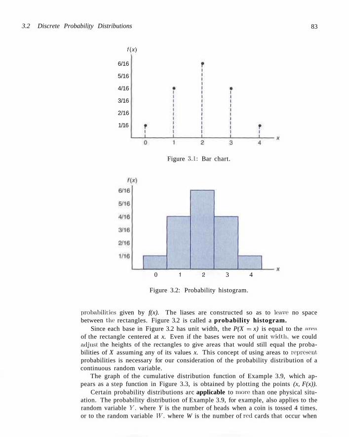
3.2 Discrete Probability Distributions 83
f'x)
6/16
5/16
4/16
3/16
2/16
1/16
Figure 3.1: Bar chart.
0 1 2 3 4
Figure 3.2: Probability histogram.
probabilities given by f(x). The liases are constructed so as to leave no space between the rectangles. Figure 3.2 is called a probability histogram.
Since each base in Figure 3.2 has unit width, the P(X = x) is equal to the area, of the rectangle centered at x. Even if the bases were not of unit width, we could adjust the heights of the rectangles to give areas that would still equal the probabilities of X assuming any of its values x. This concept of using areas to represent probabilities is necessary for our consideration of the probability distribution of a continuous random variable.
The graph of the cumulative distribution function of Example 3.9, which appears as a step function in Figure 3.3, is obtained by plotting the points (x, F(x)).
Certain probability distributions arc applicable to more than one physical situation. The probability distribution of Example 3.9, for example, also applies to the random variable Y, where Y is the number of heads when a coin is tossed 4 times. or to the random variable W, where W is the number of red cards that occur when
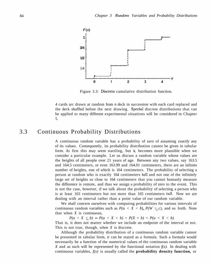
84 Chapter 3 Random Variables and Probability Distributions
F(x)
1
3/4
1/2
1/4
. •
• '
f ' i i
. 1
0 1 2 3 4
Figure 3.3: Discrete cumulative distribution function.
4 cards arc drawn at random from a deck in succession with each card replaced and the deck shuffled before the next drawing. Special discrete distributions that can be applied to many different experimental situations will be considered in Chapter 5.
3.3 Continuous Probability Distributions
A continuous random variable has a probability of zero of assuming exactly any of its values. Consequently, its probability distribution cannot be given in tabular form. At first this may seem startling, but it, becomes more plausible when we consider a particular example. Let us discuss a random variable whose values are the heights of all people over 21 years of age. Between any two values, say 163.5 and 164.5 centimeters, or even 163.99 and 164.01 centimeters, there are an infinite number of heights, one of which is 164 centimeters. The probability of selecting a person at random who is exactly 164 centimeters tall and not one of the infinitely large set of heights so close to 164 centimeters that you cannot humanly measure the difference is remote, and thus we assign a probability of zero to the event. This is not the case, however, if we talk about the probability of selecting a person who is at least 163 centimeters but not more than 165 centimeters tall. Now we are dealing with an interval rather than a point value of our random variable.
We shall concern ourselves with computing probabilities for various intervals of continuous random variables such as P(a < X < b), P(W > c), and so forth. Note that when X is continuous,
P(a < X < b) = P(a < X < b) + P(X = b) = P(a < X < b). That is, it does not matter whether we include an endpoint of the interval or not. This is not true, though, when X is discrete.
Although the probability distribution of a continuous random variable cannot be presented in tabular form, it can be stated as a formula. Such a formula would necessarily be a function of the numerical values of the continuous random variable X and as such will be represented by the functional notation f(x). In dealing with continuous variables, f(x) is usually called the probability density function, or
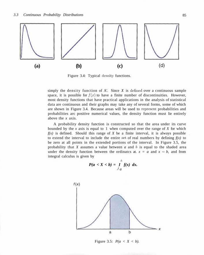
3.3 Continuous Probability Distributions 85
(a) (b) (c) (d)
Figure 3.4: Typical density functions.
simply the densi ty function of A'. Since X is defined over a continuous sample space, it is possible for f(x) to have a finite number of discontinuities. However, most density functions that have practical applications in the analysis of statistical data are continuous and their graphs may take any of several forms, some of which are shown in Figure 3.4. Because areas will be used to represent probabilities and probabilities arc positive numerical values, the density function must lie entirely above the x axis.
A probability density function is constructed so that the area under its curve bounded by the x axis is equal to 1 when computed over the range of X for which f(x) is defined. Should this range of X be a finite interval, it is always possible to extend the interval to include the entire sot of real numbers by defining f(x) to be zero at all points in the extended portions of the interval. In Figure 3.5, the probability that X assumes a value between a and /; is equal to the shaded area under the density function between the ordinatcs at. x = a and x = b, and from integral calculus is given by
P(a < X < b) = I f(x) dx. J a
Figure 3.5: P(a < X < b).
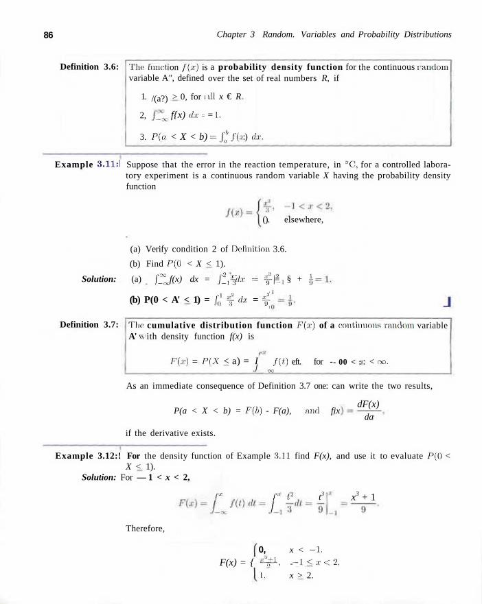
86 Chapter 3 Random. Variables and Probability Distributions
Definition 3.6: The: funct variable A
1.
2,
3.
/(a?)
J—OC
PU>
on /(.r) is ", defined
> 0, for i
f{x) dx =
< X < b)
a probability density function over the set of real numbers R, if
ill x € R
= 1.
-£/& :) (fe.
for the continuous i andoni
Example 3.11:1 Suppose that the error in the reaction temperature, in °C, for a controlled laboratory experiment is a continuous random variable X having the probability density function
(). elsewhere,
(a) Verify condition 2 of Definition 3.6.
(b) Find P(Q < X < 1).
Solution: (a) [^ f(x) dx = £ f c/.r = ^ = § + } i
(b) P(0 < A' < 1) = ./;,' Jf da; = £
Definition 3.7: The A' w
cumulative distribution function F(a:) of a continuous random ith density function f(x) is
F(a) = PLX < a) = I / ( / ) eft. for -— oo
- 00 < : : < co.
variable
As an immediate consequence of Definition 3.7 one: can write the two results,
dF(x) P(a < X < b) = F(b) - F(a), and fix
if the derivative exists.
da
Example 3.12:! For the density function of Example 3.11 find F(x), and use it to evaluate F(0 < X < 1).
Solution: For — 1 < x < 2,
r /••' /,- t3 x3 + 1
Therefore,
F(x) = { 0, x < - 1 ,
- 1 < J
x > 2. * # * , - l < a r < 2 ,
l.
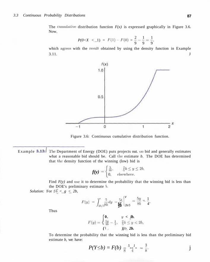
3.3 Continuous Probability Distributions 87
The cumulative: distribution function F(x) is expressed graphically in Figure 3.6. Now.
P(0<X < 1) = F ( l ) - F ( 0 ) = 2 1 1
9 9 9 which agrees with the result obtained by using the density function in Example
3.11. J
- 1 0 1 2
Figure 3.6: Continuous cumulative distribution function.
Example 3.13:1 The Department of Energy (DOE) puts projects out. on bid and generally estimates what a reasonable bid should be. Call the estimate b. The DOE has determined that the density function of the winning (low) bid is
f(y) gfc, \b<y<2b, 0. elsewhere.
Find F(y) and use it to determine the probability that the winning bid is less than the DOE's preliminary estimate /;.
Solution: For fb < g < 2b,
v ru r} r^ F[V) = U »* = §6 2b/5
5y _ 1 86 ~ 4 '
Thus
f 0. y < lb.
{ I • ))> 2b.
To determine the probability that the winning bid is less than the preliminary bid estimate b, we: have:
P(Y<b) = F(b) = 5--1- = l j
Chapter 3 Random Variables and Probability Distributions
Exercises
3.1 Classify the following random variables as discrete or continuous:
X: the number of automobile accidents per year in Virginia.
Y: the length of time to play 18 holes of golf.
M: the amount of milk produced yearly by a particular cow.
N: the number of eggs laid each month by a hen.
P: the number of building permits issued each month in a certain city.
Q: the weight of grain produced per acre.
3.7 The total number of hours, measured in units of 100 hours, that a family runs a vacuum cleaner over a period of one year is a continuous random variable X that has the density function
/(*) 0 < x < 1 ,
x, 1 < x < 2, elsewhere.
Find the probability that over a period of one year, a family runs their vacuum cleaner (a) less than 120 hours; (b) between 50 and 100 hours,
3.2 An overseas shipment of 5 foreign automobiles contains 2 that have slight paint blemishes. If an agency receives 3 of these automobiles at random, list the elements of the sample space S using the letters B and Ar for blemished and nonblemished, respectively; then to each sample point assign a value x of the random variable X representing the number of automobiles purchased by the agency with paint blemishes.
3.3 Let W be a random variable giving the number of heads minus the number of tails in three tosses of a coin. List the elements of the sample space S for the three tosses of the coin and to each sample point assign a value w of W.
3.4 A coin is flipped until 3 heads in succession occur. List only those elements of the sample space that require 6 or less tosses. Is this a discrete sample space? Explain.
3.5 Determine the value c so that each of the following functions can serve as a probability distribution of the discrete random variable X:
(a) f(x) = c(x2 + 4), for a: = 0,1,2,3;
(b)f(x) = c(l)(3*x),Iorx - 0 , 1 , 2 .
3.6 The shelf life, in days, for bottles of a certain prescribed medicine is a random variable having the density function
f{*) f 20,1)00
i (aT+Toop 10,
a : > 0 ,
elsewhere.
Find the probability that a bottle of this medicine will have a shell life of (a) at least 200 days; (b) anywhere from 80 to 120 days.
3.8 Find the probability distribution of the random variable W in Exercise 3.3. assuming that the coin is biased so that a head is twice as likely to occur as a tail.
3.9 The proportion of people who respond to a certain mail-order solicitation is a continuous random variable X that has the density function
/(*) = ^ , 0 < x < l , 0, elsewhere.
(a) Show that P(0 < X < 1) = 1. (b) Find the probability that more than 1/4 but fewer
than 1/2 of the people contacted will respond to this type of solicitation.
3.10 Find a formula for the probability distribution of the random variable X representing the outcome when a single die is rolled once.
3.11 A shipment of 7 television sets contains 2 defective sets. A hotel makes a random purchase of; 3 of the sets. If x is the number of defective sets purchased by the hotel, find the probability distribution of X. Express the results graphically as a probability histogram.
3.12 An investment firm offers its customers municipal bonds that mature after varying numbers of years. Given that the cumulative distribution function of T, the number of years to maturity for a randomly selected bond, is,
F(t) =
t< 1, 1 < t < 3, 3 < t <5 , 5 < t < 7, t>7,
Exercises 89
find ( a ) P ( T = 5); (b) P(T > 3); (c) P(1.4 < T < 6).
3.13 The probability distribution of A, the number of imperfections per 10 meters of a synthetic fabric in continuous rolls of uniform width, is given by
0 1 2 3 4 ~J{~x) 0.41 0.37 0.16 0.05 0.01
Construct the cumulative distribution function of X.
3.14 The waiting time, in hours, between successive speeders spotted by a radar unit is a continuous random variable with cumulative distribution function
F(x) x < 0, x > 0.
Find the probability of waiting less than 12 minutes between successive speeders
(a) using the cumulative distribution function of X;
(b) using the probability density function of X.
3.15 Find the cumulative distribution function of the random variable X representing the number of defectives in Exercise 3.11. Then using F(x), find
(a) P(X = 1); (b) P(0 < X < 2).
3.16 Construct a graph of the cumulative distribution function of Exercise 3.15.
3.17 A continuous random variable X that can assume values between x = 1 and x = 3 has a density function given by f(x) = 1/2. (a) Show that the area under the curve is equal to 1. (b) Find P(2 < X < 2.5). (c) Find P(X < 1.6).
3.18 A continuous random variable X that can assume values between x = 2 and x = 5 has a density function given by f(x) = 2(1 + a;)/27. Find (a) P(X < 4);
(b) P(3 < X < 4).
3.19 For the density function of Exercise 3.17, find F(x). Use it to evaluate P(2 < X < 2.5).
3.20 For the density function of Exercise 3.18, find F(x), and use it to evaluate P(3 < X < 4).
3.21 Consider the density function
< X < 1,
elsewhere.
(a) Evaluate k.
(b) Find F(x) and use it to evaluate
P(0.3 < X < 0.6).
3.22 Three cards are drawn in succession from a deck without replacement. Find the probability distribution for the number of spades.
3.23 Find the cumulative distribution function of the random variable W in Exercise 3.8. Using F(w), find (a) P(W > 0); (b) P ( - l < W < 3 ) .
3.24 Find the probability distribution for the number of jazz CDs when 4 CDs are selected at random from a collection consisting of 5 jazz CDs, 2 classical CDs, and 3 rock CDs. Express your results by means of a formula.
3.25 From a box containing 4 dimes and 2 nickels, 3 coins are selected at random without replacement. Find the probability distribution for the total T of the 3 coins. Express the probability distribution graphically as a probability histogram.
3.26 From a box containing 4 black balls and 2 green balls, 3 balls are drawn in succession, each ball being replaced in the box before the next draw is made. Find the probability distribution for the number of green balls.
3.27 The time to failure in hours of an important piece of electronic equipment used in a manufactured DVD player has the density function
/ ( , ) = jsoc 2000 e X P t " •a:/2000), x > 0, x < 0 .
(a) Find F(x). (b) Determine the probability that the component (and
thus the DVD player) lasts more than 1000 hours before the component needs to be replaced.
(c) Determine the probability that the component fails before 2000 hours.
3.28 A cereal manufacturer is aware that the weight of the product in the box varies slightly from box to box. In fact, considerable historical data has allowed the determination of the density function that describes the probability structure for the weight (in
90 Chapter 3 Random Variables and Probability Distribxdions
ounces). In fact, letting X be the random variable weight, in ounces, the density function can be described as
/ ( Ho1, 23.75 < x < 26.25, elsewhere.
(a) Verify that this is a valid density function. (b) Determine the probability that the weight is
smaller than 24 ounces. (c) The company desires that the weight exceeding 26
ounces is an extremely rare occurrence. What is the probability that this "rare occurrence" does actually occur?
3.29 An important factor in solid missile fuel is the particle size distribution. Significant problems occur if the particle sizes are too large. From production data in the past, it has been determined that the particle size (in micrometers) distribution is characterized by
/ ( ] 10, e) > 1,
elsewhere.
(a) Verify that this is a valid density function.
(b) Evaluate F(x).
(c) What is the probability that a random particle from the manufactured fuel exceeds 4 micrometers?
3.30 Measurements of scientific systems are always subject to variation, some more than others. There are many structures for measurement error and statisticians spend a great deal of time modeling these errors. Suppose the measurement error X of a certain physical quantity is decided by the density function
/(• x) = { fc(3 0.
x2), - 1 < x < 1, elsewhere.
(a) Determine k that renders f(x) a valid density function.
(b) Find the probability that a random error in measurement is less than 1/2.
(c) For this particular measurement, it is undesirable if the magnitude of the error (i.e., |a:|), exceeds 0.8. What is the probability that this occurs?
3.31 Based on extensive testing, it is determined by the manufacturer of a washing machine that the time Y (in years) before a major repair is required is characterized by the probability density function
fix) lo, -»/•! y > 0 ,
elsewhere.
(a) Critics would certainly consider the product a bargain if it is unlikely to require a major repair before the sixth year. Comment on this by determining P(Y > 6).
(b) What is the probability that a major repair occurs in the first year?
3.32 The proportion of the budgets for a certain type of industrial company that is allotted to environmental and pollution control is coming under scrutiny. A data collection project determines that the distribution of these proportions is given by
/ (») • < > = r
y)\ 0 < y < l , elsewhere.
(a) Verify that the above is a valid density. (b) What is the probability that a company chosen at
random expends less than 10% of its budget on environmental and pollution controls?
(c) What is the probability that a company selected at random spends more than 50% on environmental and pollution control?
3.33 Suppose a special type of small data processing firm is so specialized that some have difficulty making a profit in their first year of operation. The pdf that characterizes the proportion Y that make a profit is given by
/ («) ( i - ? / ) 3 0 < y < 1,
elsewhere.
(a) What is the value of k that renders the above a valid density function?
(b) Find the probability that at most 50% of the firms make a profit in the first year.
(c) Find the probability that at least 80% of the firms make a profit in the first year.
3.34 Magnetron tubejs are produced from an automated assembly line. A sampling plan is used periodically to assess quality on the lengths of the tubes. This measurement is subject to uncertainty. It is thought that the probability that a random tube meets length specification is 0.99. A sampling plan is used in which the lengths of 5 random tubes are measured. (a) Show that the probability function of Y, the num
ber out of 5 that meet length specification, is given by the following discrete probability function
/(?/) = ^ h ^ ! ( 0 - 9 9 ) y ( a o i ) 5 _ v ' for y = 0.1,2,3,4,5.
3.4 Joint Probability Distributions 91
(b) Suppose random selections arc made off the line section. and 3 are outside specifications. Use /(•</) above (b) F i n d t h e probability that only 2 cars arrive, either to support or refute the conjecture that the probability is 0.99 that a single tube meets specifi- „ „_ ^ , , . ., , cations ^ n a laboratory assignment, if the equipment is
working, the density function of the observed outcome, X is
3.35 Suppose it is known from large amounts of historical data that X, the number of cars that arrive at a specific intersection during a 20 second time period, ,/ •, _ f 2(1 — x), 0 < x < 1, is characterized by the following discrete probability J\ ) — ^Q_ otherwise, function
/(x) = e " 6 - , x = 0,1.2, . . . . (a) Calculate P(A < 1/3). x\ (b) What is the probability that X will exceed 0.5?
(a) Find the probability that in a specific 20-second (c) Given that X > 0.5, what is the probability that time period, more than 8 cars arrive at the inter- X will be less than 0.75?
3.4 Joint Probability Distributions
Our study of random variables and their probability distributions in the preceding sections is restricted to one-dimensional sample spaces, in that we recorded outcomes of an experiment as values assumed by a single random variable. There will be situations, however, where we may find it desirable to record the simultaneous outcomes of several random variables. For example, we might measure the amount of precipitate P and volume V of gas released from a controlled chemical experiment, giving rise to a two-dimensional sample space consisting of the outcomes (p, ?;), or we might be interested in the hardness H and tensile strength T of cold-drawn copper resulting in the outcomes (h, t). In a study to determine the likelihood of success in college, based on high school data, we might use a three-dimensional sample space and record for each individual his or her aptitude test score, high school rank in class, and grade-point average at the end of the freshman year in college.
If X and Y are two discrete random variables, the probability distribution for their simultaneous occurrence can be represented by a function with values f(x,y) for any pair of values (x, y) within the range of the random variables X and Y. It is customary to refer to this function as the joint probability distribution of X and Y.
Hence, in the discrete case,
f(x,y) = P(X = x,Y = yy,
that is, the values f(x, y) give the probability that outcomes x and y occur at the same time. For example, if a television set is to be serviced and X represents the age to the nearest year of the set and Y represents the number of defective tubes in the set, then / (5,3) is the probability that the television set is 5 years old and needs 3 new tubes.
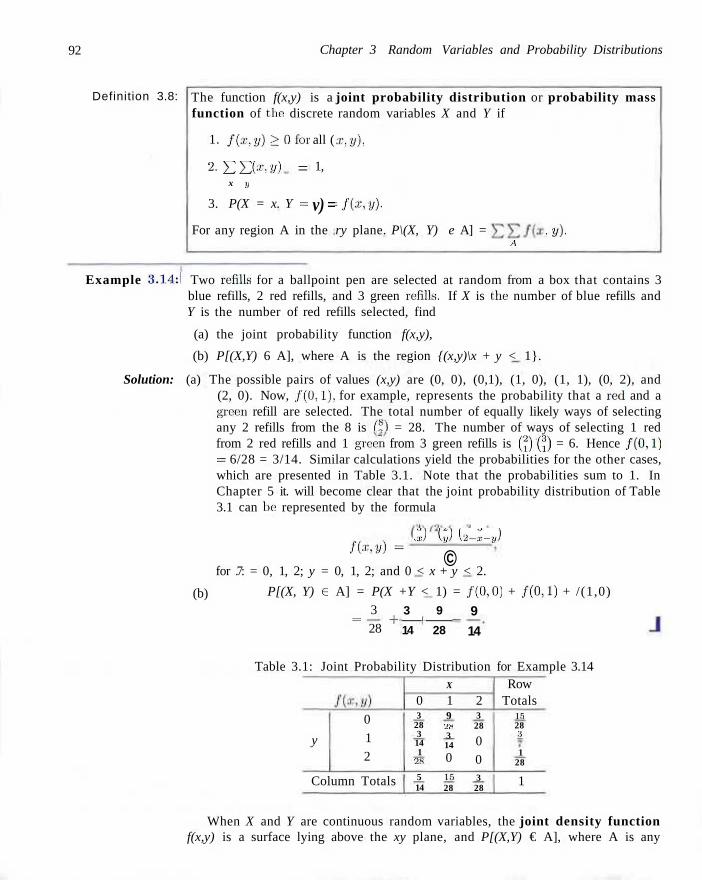
92 Chapter 3 Random Variables and Probability Distributions
Definition 3.8: The function f(x,y) is a function of the discrete
1. / ( . r , y ) > 0 f o r
2. ZZf (*-.») = x y
3. P(X = x. Y =
For any region A in
all (
1,
v) = the
joint probability distribution or random variables X and Y if
•T.y),
-f{x,y).
ry plane. P\(X, Y) e A] = A
probability
• y).
mass
Example 3.14:1 Two refills for a ballpoint pen are selected at random from a box that contains 3 blue refills, 2 red refills, and 3 green refills. If X is the number of blue refills and Y is the number of red refills selected, find
(a) the joint probability function f(x,y),
(b) P[(X,Y) 6 A], where A is the region {(x,y)\x + y < 1}.
Solution: (a) The possible pairs of values (x,y) are (0, 0), (0,1), (1, 0), (1, 1), (0, 2), and (2, 0). Now, /(0,1) , for example, represents the probability that a red and a greem refill are selected. The total number of equally likely ways of selecting any 2 refills from the 8 is LI = 28. The number of ways of selecting 1 red from 2 red refills and 1 green from 3 green refills is ( ) (j) = 6. Hence /(0,1) = 6/28 = 3/14. Similar calculations yield the probabilities for the other cases, which are presented in Table 3.1. Note that the probabilities sum to 1. In Chapter 5 it. will become clear that the joint probability distribution of Table 3.1 can be represented by the formula
\.x) \y) \2-x-y) f(x,y) = ©
(b)
for .7: = 0, 1, 2; y = 0, 1, 2; and 0 < x + y < 2.
P[(X, Y) e A] = P(X +Y < 1) = /(0,0) + /(0,1) + /(1,0) 3
= 28 +
3 9 L —
14 28
9
14
Table 3.1: Joint Probability Distribution for Example 3.14
y
0 1 2
Column Totals
X
0 3
28 3 14 1
28
5 14
1 9 28 3 14
0
18 28
2 3 28
0 0 3 28
Row Totals
in 28 3
1 28
1
When X and Y are continuous random variables, the joint density function f(x,y) is a surface lying above the xy plane, and P[(X,Y) € A], where A is any
3.4 Joint Probability Distributions 93
region in the xy plane, is equal to the volume of the right cylinder bounded by the base A and the surface.
Definition 3.9: The function f(x,y) is a joint density function of the continuous random variables X and Y if
1- / ( * , » ) > 0, for all (x,y),
2. f?00JZ0Hx,y)dxdy = l,
3. P[(X, Y) £ A] = / JA f(x, y) dx dy,
for any region A in the xy plane.
Example 3.15:1 A candy company distributes boxes of chocolates with a mixture of creams, toffees, and nuts coated in both light and dark chocolate. For a randomly selected box, let X and Y, respectively, be the proportions of the light and dark chocolates that are creams and suppose that the joint density function is
ftz . ) = ( § ( 2 a f + 3»). 0 < x < 1,0 < ?y < 1, 10, elsewhere.
(a) Verify condition 2 of Definition 3.9.
(b) Find P[(X, Y £ A], where A = {{x,y)\0 < x < ±, ± < y < ±}.
Solution: (a) f f f(x,y)dxdy= I f \{2x + 3y) dx dy J-oc J-oo JO JO °
2 3 , = 5 + 5 = L
(b) P[(X,Y)eA] = P(0<X<l-,±<Y<1-)
= //4 (To + f) dy = {TO + %
10 [ \ 2 + 4
:c=l/2
dy x=0
1/2
11/4
1 _3_ 4 + 16
13 Too'
Given the joint probability distribution f(x,y) of the discrete random variables X and Y, the probability distribution </(x) of X alone is obtained by summing f(x, y) over the values of Y. Similarly, the probability distribution h(y) of Y alone is obtained by summing f(x,y) over the values of X. We define g(x) and h(y) to be the marginal distributions of X and Y, respectively. When X and Y are continuous random variables, summations are replaced by integrals. Wre can now make the following general definition.
94 Chapter 3 Random Variables and Probability Distributions
Definition 3.10: The marginal distributions of X alone and of Y alone
9(x) = ^2f(x,y) V
for the discrete case, and
/•OO
.</(» = / f(x, y) dy J — oc
for the continuous case.
and
and
h(y)
h(y) ••
X
= r /(< J —oc
are
2/),
,y) dx,
The term marginal is used here because, in the discrete case, the values of g(x) and h(y) are just the marginal totals of the respective columns and rows when the values of /(.r, y) are displayed in a rectangular table.
Example 3.16:1 Show that the column and row totals of Table 3.1 give the marginal distribution of X alone and of Y alone.
Solution: For the random variable X, we see that
ff(0) = /(0,0) + / ( 0 , l ) + / (0,2) = | + A + l = A
f f(l) = / ( l , 0 ) + / ( l , l ) + / ( l , 2 ) = ! + ^ - r O = ! ,
and
g(2) = f(2,0) + f(2,1) + /(2,2) = 1 + 0 + 0 = 1 ,
which are just the column totals of Table 3.1. In a similar manner we could show-that the values of h(y) are given by the row totals. In tabular form, these marginal distributions may be written as follows:
$(x) 1 V
14 28 28 h(y) 0 1 2
15—3—Z~~ • 28 7 28 J
Example 3.17:1 Find g(x) and h(y) for the joint density function of Example 3.15. Solution: By definition,
4x + 3
y=0
for 0 < i < 1, and .g(.r) = 0 elsewhere. Similarly,
%) = r ° /(*, y) dx = / |(2x + 3y) dx = 2 (1t3?V)
J-oc JO O °
for 0 < y < 1, and ft(t/) = 0 elsewhere. J The fact that the marginal distributions g(x) and h(y) are indeed the proba
bility distributions of the individual variables X and Y alone can be verified by
3.4 Joint Probability Distributions 95
showing that the conditions of Definition 3.4 or Definition 3.6 are satisfied. For example, in the continuous case
Definition 3.11:
/
OC /»00 l>OC
g(x) dx = / f(x,y) dy dx = l, •CO •' — oo ./ —oo and
P(a<X <b) = P(a<X < b, - o c < Y < oo) rb poc rb
= f(x> v) dydx - / s(x) dx. Jo. 'I—oo Ja
In Section 3.1 we state that the value x of the random variable X represents an event that is a subset of the sample space. If we use the definition of conditional probability as stated in Chapter 2,
P ( A n S ) P(B\A) =
P(A) P(A) > 0,
where A and B are now the events defined by X = x and Y = y, respectively, then
P(X = x,Y = y) f(x,y) P(Y = y\X = x)
P(X = x) ff(x) g(x) > 0,
where X and Y are discrete random variables. It is not difficult to show that the function f(x, y)/g{x), which is strictly a func
tion of y with x fixed, satisfies all the conditions of a probability distribution. This is also true when f(x, y) and g(x) are the joint density and marginal distribution, respectively, of continuous random variables. As a result, it is extremely important that we make use of the special type of distribution of the form f(x,y)/g(x) in order to be able to effectively compute conditional probabilities. This type of distribution is called a conditional probability distribution; the formal definition follows.
Let X and Y be two random variables, discrete or continuous. The conditional distribution of the random variable Y given that X = x is
f{y\x) = / (x ,y) g(x) > 0.
Similarly the conditional distribution of the random variable X given that Y = y is
f(x\y) = f(x,y)
h(y) ' h(y) > 0.
If we wish to find the probability that the discrete random variable X falls between a and b when it is known that the discrete variable Y = y, we evaluate
P(a<X<b\Y = y)= ] T f(x\y),
where the summation extends over all values'<8TC^ between a and b. When X and Y are continuous, we evaluate
P(a <X<b\Y = y)= f f(x\y) dx.
96 Chapter 3 Random Variables and Probability Distributions
Example 3.18:1 Referring to Example 3.14, find the conditional distribution of A", given that Y =\, and use it to determine P(X = 0|V = 1).
Solution: We need to find ((x\y), where y — 1. First, we find that
Now,
Therefore,
x=0
/ W « - ^ - £ / < « . » . "0,1.2-
f(2\l)={j\f(2,l)=(J\(0) = 0,
and the conditional distribution of X, given that Y = 1, is 0 1 2 "T r 0 7Ni)
Finally,
P(x = o|r=i) = /(o|i) = i. Therefore, if it is known that 1 of the 2 pen refills selected is red, we have a probability equal to 1/2 that the other refill is not blue. J
Example 3.19:1 The joint density for the random variables (X, Y), where X is the unit temperature change and Y is the proportion of spectrum shift that a certain atomic particle produces, is
/(x,y) flOxt/2, 0 <x < y < 1,
10, elsewhere.
(a) Find the marginal densities g(x), h.(y), and the conditional density f(y\x).
(b) Find the probability that the spectrum shifts more than half of the total observations, given that the temperature is increased to 0.25 unit.
Solution: (a) By definition,
9(x) = / f{x,y) dy= lOxy2 dy J — oo J X
= — x(l - x J ) , 0 < X < 1, 10 o -^-xyJ
3 y y=X
h(y) = f f(x, y) dx = fJ lOxy2 dx = ox^2^ = 5y\ 0 < y < 1. J-oo JO
3.4 Joint Probability Distributions 97
Now
f(y\x) = f{x..y) _ lOxy2
9{x)
3;V2
fx(l -x*) 1-x* 0 <x <y <1.
(b) Therefore,
P ( y > 2 X = 0.2o) = / f(y\x = 0.25)dy
7i/2 1 - 0.25 253 dy = 9'
Example 3.20:1 Given the joint density function
f(x,y) ^ 2 L i , 0 < x- < 2, 0 < y < 1,
0, elsewhere,
find g(x), h(y), f(x\y), and evaluate P(\ < X < \\Y = 1). Solution: By definition,
9(x) = / /(a-', y)dy= — ./-oo Jo
_ (xy_ xy ~~ \ 4 4
+ 3y2) dy
. , , 3 \ i J / = 1
0 < a: < 2,
and
= f°° f(x,y)dx= f ./-oo ^0
/:r2 3x 2 y 2 \
2 i ( l + 3 y 2 ) cirr.
1 + 3y 2
, 0 < y < l .
Therefore,
and
A I W /i,(y) ( l + 3y2)/2 2' u < x < 2 '
/ l 1 1 \ / , 1 / 2a; _3_ 64'
Statistical Independence If f(x\y) does not depend on y, as is the case for Example 3.20, then f(x\y) = g(x) and / (x , y) = g(x)h(y). The proof follows by substituting
/(a;, y) = /(x|y)/*(y)
98 Chapter 3 Random. Variables and Probability Distributions
into the marginal distribution of X. That is,
/
oo rx..
f{x,y)dy= / f(x\y)h{y) dy. -OO */ —OO
If f{x\y) does not, depend on ;;, wc may write
.</(•<•) = f(x\!l) f h(y) dy. J — oo
Now
/ h(y) dy = 1, J — oc
since h(y) is the probability density function of Y. Therefore:.
.</(•'•) = /(x|y) and then f(x,y) = g(x)h(y).
Definition 3.12:
It should make sense to the reader that if f(x\y) does not depend on y, then of course the outcome of the random variable Y has no impact, on the outcome of the random variable X. In other words, we say that X and Y are independent random variables. We now offer the following formal definition of statistical independence.
Let X and Y be two random variables, discrete or continuous, with joint probability distribution f(x,y) and marginal distributions g(x) and h(y), respectively. The random variables X and Y are said to be statist ically independent if and only if
f(x,y) = g(x)h(y)
for all (x, y) within their range.
The continuous random variables of Example 3.20 arc statistically independent, since the product of the two marginal distributions gives the joint density function. This is obviously not the case, however, for the continuous variables of Example 3.19. Checking for statistical independence of discrete random variables requires a more thorough investigation, since it is possible to have the product of the marginal distributions equal to the joint probability distribution for some but not all combinations of (x.y). If you can find any point (x,y) for which f(x,y) is defined such that f(x,y) r1 g(x)h(y), the discrete variables X and Y are not statistically independent.
Example 3.21:1 Show that the random variables of Example 3.14 are not statistically independent.
Proof: Let us consider the point (0, I). From Table 3.1 we find the three probabilities
3.4 Joint Probability Distributions 99
/ (0 ,1) , y(0), andh ( l ) to be
mu-£. 3 3 1
»(o) = E / ( M - ^ + S + s - S ;y=o
2
28 14 28 14'
Clearly,
fc<i)=£/(*.i>-n+n+0-|-x=0
/ ( 0 , l ) ^ y ( 0 ) M l ) ,
and therefore X and y are not statistically independent. J All the preceding definitions concerning two random variables can be generalized to the case of n random variables. Let f(xi,x2,.. • ,xn) be the joint probability function of the random variables X\,X2,..., X„. The marginal distribution of X\, for example, is
9{xi) = E " E / ( X 1 . X 2 , • • •,Xn) J:? X„
for the discrete case, and
/
OC rOC
•• f(xi,x2,..., xn) dx2 dx3 • • • dxn
•OC- J—OO for the continuous case. We can now obtain joint marginal distributions such as g(x\,x2), where
{52 "' 52 /(a'i»X2, • • •. xn), (discrete case),
/-oo ' ' ' I^oc / ( x i , a;2,... ,x n ) da^ da;4 • • • dx„, (continuous case). We could consider numerous conditional distributions. For example, the joint conditional distribution of X\, X2, and X-$, given that X.\ = x4, X5 = x 5 , . . . , Xn = xn , is written
,, , x / ( x i , x 2 , . . . , x „ ) J\,X\,X2,X-s\X4.X5, ... ,xn) = — -,
y(x4 ,x5 , ...,xn)
where g(x4,x&,... ,xn) is the joint marginal distribution of the random variables X4,Xr,,. .., Xn.
A generalization of Definition 3.12 leads to the following definition for the mutual statistical independence of the variables Xi,X2,..., Xn.
100 Chapter 3 Random Variables and Probability Distributions
Definition 3.13: Let X\, X2,..., Xn be n random variables, discrete or continuous, with joint probability distribution f(x\.x2.... .xu) and marginal distribution /i( : , :i )i /2(x2), • • •, fn(•>'„), respectively, The random variables X\,X2,..., Xu are said to be mutually statistically independent if and only if
/(a'!, X2, ..., Xn) = /l O'-'l )/a(X2) ' ' ' fn (x„ )
for all (xi, x2,..., xa) within their range.
Example 3.22:1 Suppose that the shelf life, in years, of a certain perishable: food product packaged in cardboard containers is a random variable whose probability density function is given by
fix) = e~x, x > 0,
0, elsewhere.
Let Xi, X2, and A3 represent the shelf lives for three of these containers selected independently and find P(X^ < 2.1 < X2 < 3,X3 > 2).
Solution: Since the containers were selected independently, we can assume that the random variables Ari, X2, and X^ are statistically independent, having the joint probability density
/ (x i , x 2 , x 3 ) = f(xi)f(x2)f(x3) = e - * e - » e - » —Xl— X3-X3
for Xi > 0, :).'2 > 0, x-.i > 0, and f(x.\,x2,x3) = 0 elsewhere. Hence
.3 ,.2
P(Xi < 2, 1 < X2 < 3, A':, > 2) = / / / e ^ 1 - * 2 - * 3 dxi dx2 dx:i
= (1 - e.-2)(e.-1 - e~3)e-'- = 0.0372.
What Are Important Characteristics of Probability Distributions and Where Do They Come From?
This is an important point in the text to provide the reader a transition into the next three; chapters. We: have given illustrations in both examples and exercises of practical scientific and engineering situations in which probability distributions and their properties are used to solve important problems. These probability distributions, either discrete or continuous, were introduced through phrases like "it is known that" or "suppose that" or even in some cases "historical evidence suggests that." These arc situations in which the nature of the distribution and even a good estimate of the probability structure can be determined through historical data, data from long-term studies, or even large amounts of planned data. The reader should remember the discussion of the use of histograms in Chapter 1 and from that recall how frequency distributions arc: estimated from the histograms. However, not all probability functions and probability density functions are derived from large amounts of historical data. There are a substantial number of situations in which the nature of the scientific scenario suggests a distribution
Exercises 101
type. Indeed many of these are reflected in exercises in bo th Chapters 2 and 3. When independent repeated observations are binary in na ture (e.g., "defective or not," "survive or not," "allergic or not") with observations 0 or 1, the distribution covering this situation is called the b i n o m i a l d i s t r i b u t i o n and the probability function is known and will be demonstrated in its generality in Chapter 5. Exercise 3.34 in Section 3.3 and Review Exercise 3.82 are examples and there are others tha t the reader should recognize. The scenario of a continuous distribution in "time to failure" as in Review Exercise 3.71 or Exercise 3.27 on page 89 often suggests a distribution type called the e x p o n e n t i a l d i s t r ibut ion . These types of illustrations are merely two of many so-called s t andard distributions tha t are used extensively in real world problems because the scientific scenario that gives rise to each of them is recognizable and occurs often in practice. Chapters 5 and 6 cover many of these types along with some underlying theory concerning their use.
A second part, of this transition to material in future chapters deals with the notion of p o p u l a t i o n p a r a m e t e r s or d i s t r i b u t i o n a l p a r a m e t e r s . Recall in Chapter 1 we discussed the need to use data to provide information about these parameters . We went to lengths in discussing the notion of a m e a n and variance and provided a vision for the concepts in the context of a population. Indeed the population mean and variance are easily found from the probability function for the discrete case or probability density function for the continuous case. These parameters and their importance in the solution of many types of real world problems will provide much of the material in Chapters 8 through 17.
Exercises
3.37 Determine the values of c so that the following functions represent joint probability distributions of the random variables A" and Y:
(a) f(x, y) — cxy, for x = 1, 2, 3; y = 1, 2,3; (b) f(x, y) = c\x - y\, for a: = - 2 , 0 , 2 ; y = - 2 , 3 .
3.38 If the joint probability distribution of X and Y is given by
f(x, y) = 2 ± E , for ,.. = o, 1, 2,3; y = (1, 1, 2,
find (a) P(X <2,Y = 1); (b) P(X > 2,Y < 1);
(c) P(X > Y); (d) P(X + Y = 4).
3.39 From a sack of fruit containing 3 oranges, 2 apples, and 3 bananas, a random sample of 4 pieces of fruit is selected. If X is the number of oranges and Y is the number of apples in the sample:, find
(a) the joint probability distribution of A' and Y; (b) P[(X, Y) € .4], where A is the region that is given
by {(x,y) h r + y < 2 } .
3.40 A privately owned liquor store operates both a drive-in facility and a walk-in facility. On a randomly selected day, let A" and Y, respectively, be the proportions of the time that the drive-in and walk-in facilities are in use, and suppose that the joint density function of these random variables is
f(x,y) l o , + 2y), 0 < : c < 1, 0 < y < 1,
elsewhere.
(a) Find the marginal density of X.
(b) Find the marginal density of Y. (c) Find the probability that the drive-in facility is
busy less than one-half of the time.
3.41 A candy company distributes boxes of chocolates with a mixture of creams, toffees, and cordials. Suppose that the weight of each box is 1 kilogram, but the individual weights of the creams, toffees, and cordials vary from box to box. For a randomly selected box, let X and Y represent the weights of the creams and the toffees, respectively, and suppose that, the joint
102 Chapter 3 Random Variables and Probability Distributions
density function of these variables is
(24xy, 0 < a ; < l , 0 < y < l , x+y < 1, elsewhere.
(a) Find the probability that in a given box the cordials account for more than 1/2 of the weight.
(b) Find the marginal density for the weight of the creams.
(c) Find the probability that the weight of the toffees in a box is less than 1/8 of a kilogram if it is known that creams constitute 3/4 of the weight.
3.42 Let X and Y denote the lengths of life, in years, of two components in an electronic system. If the joint density function of these variables is
-O+v) f(x,y) = {l
findP(0<X< 1 \Y = 2).
x > 0, y > elsewhere.
0,
3.43 Let X denote the reaction time, in seconds, to a certain stimulus and Y denote the temperature (°F) at which a certain reaction starts to take place. Suppose that two random variables X and Y have the joint density
f(x
Find
(a) P(0 (b) P(X
Hr < X < i and
<Y).
0<x< 1, elsewhere.
4 — ' — 2
0<y<
);
l
3.44 Each rear tire on an experimental airplane is supposed to be filled to a pressure of 40 pound per square inch (psi). Let X denote the actual air pressure for the right tire and Y denote the actual air pressure for the left tire. Suppose that X and Y are random variables with the joint density
f{x,y) =
'k(x2+y2),
c0,
30 < a: < 50; 30 < y < 50, elsewhere.
(a) Find k.
(b) Find P(30 < X < 40 and 40 < Y < 50). (c) Find the probability that both tires are underfilled.
3.45 Let X denote the diameter of an armored electric cable and V denote the diameter of the ceramic mold that makes the cable. Both X and Y are scaled
so that they range between 0 and 1. Suppose that X and Y have the joint density
1 0, elsewhere.
Find P(X + Y> 1/2).
3.46 Referring to Exercise 3.38, find (a) the marginal distribution of X; (b) the marginal distribution of Y.
3.47 The amount of kerosene, in thousands of liters, in a tank at the beginning of any day is a random amount Y from which a random amount X is sold during that day. Suppose that the tank is not resupplied during the day so that x < y, and assume that the joint density function of these variables is
f(xy) = l2' Q<x<y n 'V> \ 0 , elsewhere.
< 1 ,
(a) Determine if X and Y are independent. (b) Find P ( l / 4 < X < 1/2 | Y = 3/4).
3.48 Referring to Exercise 3.39, find (a) f(y\2) for all values of y;
(b) P(Y = 0 | X = 2).
3.49 Let X denote the number of times a certain numerical control machine will malfunction: 1, 2, or 3 times on any given day. Let Y denote the number of times a technician is called on an emergency call. Their joint probability distribution is given as
/ (« ,» ) 1
y 2 3
1 0.05 0.05
0
x 2
0.05 0.1 0.2
3 0.1 0.35 0.1
(a) Evaluate the marginal distribution of X. (b) Evaluate the marginal distribution of V. (c) Find P(Y = 3 | X = 2).
3.50 Suppose that X and Y have the following joint probability distribution:
x f(x,y) 2 4
0.10 0.20 0.10
0.15 0.30 0.15
(a) Find the marginal distribution of A. (b) Find the marginal distribution of Y.
Review Exercises 103
3.51 Consider an experiment that consists of 2 rolls of a balanced die. If X is the number of 4s and Y is the number of os obtained in the 2 rolls of the die, find (a) the joint probability distribution of A and V; (b) P[(X, Y) € A], where A is the region {(x,y) \ 2x +
V < 3}.
3.52 Let X denote the: number of heads and Y the number of heads minus the number of tails when 3 coins are tossed. Find the joint probability distribution of X and Y.
3.53 Three cards are drawn without replacement from the 12 face cards (jacks, queens, and kings) of an ordinary deck of 52 playing cards. Let X be the number of kings selected and Y the number of jacks. Find
(a) the joint probability distribution of X and Y;
(b) P[(X,Y) e A), where A is the region given by {(x,y) \x + y>2}.
3.54 A coin is tossed twice. Let Z denote the number of heads on the first toss and W the total number of heads on the 2 tosses. If the coin is unbalanced and a head has a 40% chance of occurring, find (a) the joint probability distribution of W and Z; (b) the marginal distribution of W\ (c) the marginal distribution of Z;
(d) the probability that at least 1 head occurs.
3.55 Given the joint density function
' ^ p , 0 < z < 2 , 2 < ? ; < 4 , f(x, y) {cT elsewhere,
find P ( l < Y < 3 | X = 1).
3.56 Determine whether the two random variables of Exercise 3.49 are dependent or independent.
3.57 Determine whether the two random variables of Exercise 3.50 are dependent or independent.
3.58 The joint density function of the random variables X and Y is
fix, y) (6x,
"to, 0 < x < 1, 0 < y < 1 elsewhere.
x,
(a) Show that X and V are not independent. (b) Find P(X > 0.3 | Y = 0.5).
3.59 Let X, Y, and Z have the joint probability density function
f(x, y, z) { kxy2z,
0 , '
0<x,y< 1; 0< z <2, elsewhere.
(a) Find k.
(b) F i n d P ( A < } , y > | , l < 2 < 2 ) .
3.60 Determine whether the two random variables of Exercise 3.43 are dependent or independent.
3.61 Determine whether the two random variables of Exercise 3.44 are dependent or independent.
3.62 The joint probability density function of the random variables X, Y, and Z is
ixyz* f(x,y,z)=i a
Find
0 <x,y< 1; 0< z < 3, elsewhere.
(a) the joint marginal density function of Y and Z: (b) the marginal density of Y;
(c) P ( i < A < i , V > A, KZ<2);
( d ) P ( 0 < A < i | y = i , 2 = 2).
Review Exercises
3.63 A tobacco company produces blends of tobacco with each blend containing various proportions of Turkish, domestic, and other tobaccos. The proportions of Turkish and domestic in a blend are random variables with joint density function (X = Turkish and Y = domestic)
fix.y) _ (24xy, 0 < x,y < 1: x + y < 1,
\ 0 , elsewhere.
(a) Find the probability that in a given box the Turkish tobacco accounts for over half the blend.
(b) Find the marginal density function for the proportion of the domestic tobacco.
(c) Find the probability that the proportion of Turkish tobacco is less than 1/8 if it is known that the blend contains 3/4 domestic tobacco.
3.64 An insurance company offers its policyholders a
104 Chapter 3 Random. Variables and Probability Distributions
number of different premium payment options. For a randomly selected policyholder, let X be the number of months between successive payments. The cumulative distribution function of X is
F(x) = {
0, i f x < l , 0.4, if 1 < x < 3, 0.6, if 3 < x < 5, 0.8, if 5 < x < 7, 1.0, if x > 7.
(a) What is the probability mass function of X?
(b) Compute P(4 < X < 7).
3.65 Two electronic components of a missile system work in harmony for the success of the total system. Let X and Y denote the life in hours of the two components. The joint density of X and Y is
fix,y) -{ ye-yll+*)t x,y>0,
0, elsewhere.
(a) Give the marginal density functions for both random variables.
(b) What is the probability that both components will exceed 2 hours?
3.66 A service facility operates with two service lines. On a randomly selected day, let X be the proportion of time that the first line is in use whereas Y is the proportion of time that the second line is in use. Suppose that the joint probability density function for (A, V) is
fix •»>-r §(.t:2 + i/2), 0<x,y<\, elsewhere.
(a) Compute the probability that neither line is busy more than half the time.
(b) Find the probability that the first line is busy more than 75% of the time.
3.67 Let the number of phone calls received by a switchboard during a 5-minute interval be a random variable X with probability function
/ ( * )« e - 2 2 x
for x = 0 ,1,2, .
(a) Determine the probability that X equals 0, 1, 2, 3, 4, 5, and 6.
(b) Graph the probability mass function for these values of x.
(c) Determine the cumulative distribution function for these values of X.
3.68 Consider the random variables X and Y with joint density function
fix, y) {o x + y, 0 < x,y < 1,
elsewhere.
(a) Find the marginal distributions of X and Y.
(b) F i n d P ( A > 0 . 5 , y >0.5) .
3.69 An industrial process manufactures items that can be classified as either defective or not defective. The probability that an item is defective is 0.1. An experiment is conducted in which 5 items are drawn randomly from the process. Let the random variable X be the number of defectives in this sample of 5. What is the probability mass function of X?
3.70 Consider the following joint probability density function of the random variables X and Y:
f{x,y) { -jx-u
0 , "
1 < x < 3, 1 < y < 2, elsewhere.
(a) Find the marginal density functions of X and Y.
(b) Are X and Y independent? (c) Find P(X > 2).
3.71 The life span in hours of an electrical component is a random variable with cumulative distribution function
F(x) {;-x > 0, eleswhere.
(a) Determine its probability density function. (b) Determine the probability that the life span of such
a component will exceexl 70 hours.
3.72 Pairs of pants are being produced by a particular outlet facility. The pants are "checked" by a group of 10 workers. The workers inspect pairs of pants taken randomly from the production line. Each inspector is assigned a number from 1 through 10. A buyer selects a pair of pants for purchase. Let the random variable X be the inspector number.
(a) Give a reasonable probability mass function for X.
(b) Plot the cumulative distribution function for X.
3.73 The shelf life of a product is a random variable that is related to consumer acceptance. It turns out that the shelf life Y in days of a certain type of bakery product has a density function
fiv) - » / 2 0 < y < oc,
elsewhere.
Review Exercises 105
What fraction of the loaves of this product, stocked today would you expect to be sellable 3 days from now?
3.74 Passenger congestion is a service problem in airports. Trains are installed within the airport to reduce the congestion. With the use of the train, the time X that it takes in minutes to travel from the main terminal to a particular concourse has density function
fix) 10, 0 < -T < 10, elsewhere.
(a) Show that the pdf above is a valid density function.
(b) Find the probability that the time it takes a passenger to travel from the main terminal to the concourse will not exceed 7 minutes.
3.75 Impurities in the batch of final product of a chemical process often reflect a serious problem. From considerable plant data gathered, it is known that the proportion Y of impurities in a batch has a density function given by
Aw-fr-"1 0 < y < 1, elsewhere.
(a) Verify that the above is a valid density function. (b) A batch is considered not sellable and then not-
acceptable if the percentage of impurities exceeds 60%. With the current quality of the process, what is the percentage of batches that are not acceptable?
3.76 The time Z in minutes between calls to an electrical supply system has the probability density function
/(*) \ 0 ,
-z/10 0 < z < oo, elsewhere.
(a) What is the probability that there are no calls within a 20-minute time interval?
(b) What is the probability that the first call comes within 10 minutes of opening?
3.77 A chemical system that results from a chemical reaction has two important components among others in a blend. The joint distribution describing the proportion A'i and X2 of these two components is given by
, , , / 2 , 0 < an < x2 < 1, f(xi,x2)=<
(0, elsewhere.
(a) Give the marginal distribution of Ai . (b) Give the marginal distribution of X2.
(c) What, is the probability that component proportions produce the results Ai < 0.2 and X2 > 0.5?
(d) Give the conditional distribution fXl | X , (x i \ x 2 ) .
3.78 Consider the situation of Review Exercise 3.77. But suppose the joint distribution of the two proportions is given by
f(x. T a ) = /6:r2 , 0 < x X2 < Xl < 1, here.
(a) Give the marginal distribution / * , (xi) of the proportion Xi and verify that it is a valid density function.
(b) What is the probability that proportion X2 is less than 0.5 given that Xi" is 0.7?
3.79 Consider the random variables X and Y that represent the number of vehicles that arrive at 2 separate street corners during a certain 2-tninute period. These street corners arc fairly close together so it is important that traffic engineers deal with them jointly if necessary. The joint distribution of X and Y is known to be
ft \ - JL _ ! _ J\.x,y) - l g • A{x+yY.
for x = 0 , 1 , 2 , . . . , and y = 0 , 1 , 2 , . . . . (a) Are the two random variables X and Y indepen
dent? Explain why or why not. (b) What is the probability that during the time pe
riod in question less than 4 vehicles arrive at the two street corners?
3.80 The behavior of series of components play a huge role in scientific and engineering reliability problems. The reliability of the entire system is certainly no better than the weakest component in the series. In a series system, the components operate independently of each other. In a particular system containing three components the probability of meeting specification for components 1, 2, and 3, respectively, are 0.95, 0.99, and 0.92. What is the probability that the entire system works?
3.81 Another type of system that is employed in engineering work is a group of parallel components or a parallel system. In this more conservative approach, the probability that the system operates is larger than the probability that any component operates. The system fails only when all systems fail. Consider a situation in which there are 4 independent components in a parallel system with probability of operation given by
Component 1: 0.95; Component 2: 0.94:
Component 3: 0.90; Component 4: 0.97.
What is the probability that the system does not fail?
106 Chapter S Random Variables and Probability Distributions
3.82 Consider a system of components in which there does have a redundancy built in such that it does not ;ire five independent components, each of which pos- fail if 3 out of the 5 components are operational. What sesses an operational probability of 0.92. The system is the probability that the total system is operational?
3.5 Potential Misconceptions and Hazards; Relationship to Material in Other Chapters
In future chapters it will become apparent that probability distributions represent the: structure through which probabilities that are computed aid in the evaluation and understanding of a process. For example, in Review Exercise 3.67, the probability distribution that quantifies the probability of a heavy load during certain time periods can be very useful in planning for any changes in the system. Review Exercise 3.71 describes a scenario in which the life span of an electronic: component is studied. Knowledge of the probability structure for the component will contribute significantly toward an understanding of the reliability of a large system of which the component is a part. In addition, an understanding of the general nature of probability distributions will enhance the understanding of the concept of a P-value which was introduced briefly in Chapter 1 and will play a major role: beginning in Chapter 10 and extending throughout the balance of the text.
Chapters 4, 5, and 6 depend heavily on the material in this chapter. In Chapter 4 we discuss the meaning of important pa rame te r s in probability distributions. These important parameters quantify notions of central tendency and variability in a system. In fact, knowledge of these quantities themselves, quite apart from the complete distribution, can provide insight into the nature of the system. Chapters 5 and 6 will deal with engineering, biological, or general scientific scenarios that, identify special types of distributions. For example, the structure of the probability function in Review Exercise 3.67 will easily be identified under certain assumptions discussed in Chapter 5. The same holds for the scenario of Review Exercise 3.71. This is a special type of t ime to failure problem for which the probability density function will be diseaissed in Chapter 6.
As far as potential hazards with the use of material in this chapter, the "warning" to the reader is not to read more into the material than is evident. The general nature of the probability distribution for a specific scientific: phenomenon is not obvious from what is learned in this chapter. The purpose of this chapter is to learn how to manipulate a probability distribution, not to learn how to identify a specific type. Chapters 5 and 6 go a long way toward identification according to the general nature of the scientific system.
Chapter 4
Mathematical Expectation
4.1 Mean of a Random Variable
If two coins are tossed 16 times and X is the number of heads that occur per toss, then the values of X can be 0, 1. and 2. Suppose that the experiment yields no heads, one: head, and two heads a total of 4, 7, and 5 times, respectively. The average number of heads per toss of the two coins is then
(0)(4) + Q)(7) + (2)(5) = l M
Hi
This is an average value and is not necessarily a possible outcome for the experiment. For instance, a salesman's average monthly income is not likely to be equal to any of his monthly paychecks.
Let us now restructure our computation for the average number of heads so as to have the following equivalent form:
< o > ( T 9 + ( i ) G y + ( 2 ) G 9 = i m
The numbers 4/16, 7/16, and 5/16 arc the fractions of the total tosses resulting in 0, 1. and 2 heads, respectively. These fractions are also the relative frequencies for the different values of X in our experiment. In fact, then, we can calculate the mean or average of a set. of data by knowing the distinct values that occur and their relative frequencies, without any knowledge of the-: total number of observations in our set of data. Therefore, if 1/16 or 1/4 of the tosses result in no heads. 7/16 of the tosses result in one head, and 5/16 of the tosses result in two heads, the mean number of heads per toss would be 1.06 no matter whether the total number of tosses was 16, 1000, or even 10,000.
Let us now use this method of relative: frequencies to calculate the average number of heads per toss of two coins that we might expect in the long run. We shall refer to this average value as the m e a n of t h e r a n d o m variable X or the mean of the probabi l i ty d is t r ibut ion of X and write it as a.,- or simply as p. when it is clear to which random variable we refer. It is also common among
108 Chapter 4 Mathematical Expectation
statisticians to refer to this mean as the mathematical expectation or the expected value of the random variable X and denote it as E(X).
Assuming that two fair coins were tossed, we find that the sample space for our experiment is
S = {HH,HT,TH,TT}.
Since the 4 sample points are all equally likely, it follows that
P(X = 0) = P(TT) = -, P(X = 1) = P(TH) + P(HT) = ^, T: /•
and
Definition 4.1:
P(X = 2) = P(HH) = -,
where a typical element, say TH, indicates that the first toss resulted in a tail followed by a head on the second toss. Now, these probabilities are just the relative frequencies for the given events in the long run. Therefore,
, t - / ' ; ( X ) ^ ( G ) ( i ) 4 (!) GM8-This result means that a person who tosses 2 coins over and over again will, on the average, get 1 head per toss.
The method described above for calculating the expected number of heads per toss of 2 coins suggests that the mean or expected value of any discrete random variable may be obtained by multiplying each of the values Xi,x2,. • • ,xn of the random variable X by its corresponding probability /(xi),/(a;2),.. • , / (^n) and summing the products. This is true, however, only if the random variable is discrete. In the case of continuous random variables, the definition of an expected value is essentially the same with summations replaced by integrations.
Let X be a random variable with probability distribution f(x). The mean or expected value of X is
u = £(X) = 5>/(*)
if X is discrete, and
if X is continuous.
/
oo xf(x) dx
-oo
Example 4.1:1 A lot containing 7 components is sampled by a quality inspector; the lot contains 4 good components and 3 defective components. A sample of 3 is taken by the inspector. Find the expected value of the number of good components in this sample.
•1.1 Mean of a Random Variable 109
Solution: Let X represent the number of good components in the sample. The probability distribution of X is
Of :! ) /(•'') = — T = T — , •'• = 0,1,2,3.
A few simple calculations yield /(0) = 1/35, f(l) = 12/35, ,/'(2) = 18/35, and ,/'(3) = 4/35. Therefore.
-w-m(i) + w(S)+(«(i)+m(A)-H_,, Thus, if a sample of size 3 is selected at random over and over again from a lot of 4 good components and 3 defective components, it would contain, on average, 1.7 good components. J
Example 4.2:1 In a gambling game a man is paid $5 if he gets all heads or all tails when three coins are tossed, and he will pay out $3 if cither one or two heads show. What, is his expected gain?
Solution: The sample space for the possible outcomes when three coins are tossed simultaneously, or, equivalently, if 1 coin is tossed three times, is
S = {IIHII, HUT, IVTIl, THH, HTT, THT, TTII. TTT}.
One can argue that each of these possibilities is equally likely and occurs with probability equal to 1/8. An alternative approach would be to apply flic multiplicative rule of probability for independent events to each element of S. For example,
P(IIHT) = P(H)P(H)P(T) = (jj Q ) (~\ = \.
The random variable of interest is Y, the amount the gambler can win; and the possible values of 1' are $5 if event E\ = {HHH,TTT} occurs and —$3 if event.
E2 = {HUT. IITII, THH, HTT, THT, TTH}
occurs. Since E\ and E% occur with probabilities 1/4 and 3/4, respectively, it follows that
u = E(Y) = (5)(j\+(-3)(jj = - 1 .
In this game the gambler will, on average, lose $1 per toss of the: three coins. A game is considered "fair" if the gambler will, on average, come out even. Therefore, an expected gain of zero defines a. fair game. J
Examples 4.1 and 4.2 arc designed to allow the reader to gain some insight info what we mean by the expected value of a random variable. In both cases the random variables are discrete. We follow with an example of a continuous random variable where an engineer is interested in the mean life of a certain type of electronic device. This is an illustration of a time to failure problem that occurs
110 Chapter 4 Mathematical Expectation
often in practice. The expected value of the life of the device is an important parameter for its evaluation.
Example 4.3:1 Let X be the random variable that denotes the life in hours of a certain electronic device. The probability density function is
(20.000 ^ , . i n n
0, elsewhere.
Find the expected life of this type of device. Solution: Using Definition 4.1, we have
„ , „ . r ° 20,000, f00 20,000 J u = E(X) = / x ' dx = / 2 dx = 200. J100 X JM) X
Therefore, we can expect this type of device to last, on average, 200 hours. J Now let us consider a new random variable g(X), which depends on X; that is,
each value of g(X) is determined by knowing the values of X. For instance, g(X) might be X2 or 3X - 1, so that whenever X assumes the value 2, g(X) assumes the value g(2). In particular, if X is a discrete random variable with probability distribution f(x), for x = —1,0,1,2, and g(X) = X2 then
P[g(X) . 0] - P(X = 0) = /(0) ,
P[g(X) - 1] = P(X = - 1 ) + P(X = 1) = / ( - l ) + / ( l ) ,
P[ff(X) = 4] = P(X = 2) = / (2) ,
so that the probability distribution of g(X) may be written 9ix)
P[g(X) = g(x)] 0 1 4
/(0) / ( - ! ) + /(!) /(2) By the definition of an expected value of a random variable, we obtain
ug(x) = E[g(x)} = 0/(0) + l [ / ( - l ) + / ( l ) ] + 4/(2)
= (-l)V(-l) + (0)2/(0) + (1)2/(1) + (2)2/(2) = 52g(x)f(x). X
This result is generalized in Theorem 4.1 for both discrete and continuous random variables.
Theorem 4 .1 : Let X be a random variable with probability distribution f(x). The expected value of the random variable g(X) is
ug{x)=E[g(X)} = £ g(x)f(x) X
if X is discrete, and
/
oo g(x)f(x) dx
-oo
if X is continuous.
4.1 Mean of a Random Variable 111
Example 4.4:1 Suppose that the number of cars X that pass through a car wash between 4:00 P.M. and 5:00 P.M. on any sunny Friday has the following probability distribution:
P(X = x) 4 6 8 9
"X X I 1 1 T~ 12 12 1 4 6 CI
Let g(X) = 2X - 1 represent the amount of money in dollars, paid to the attendant by the manager. Find the attendant's expected earnings for this particular time period.
Solution: By The:orcin 4.1, the attendant can expect to receive
E\g(X)] =E(2X - 1 ) = £ ( 2 x - I)./'(:. X = 'l
+ (15) (j\ + (17) f~ ) I" . ' ,
Example 4.5:1 Let X be a random variable with density function
fix) - 1 <x < 2,
elsewhere:.
Find the expected value of g(X) = 4X + 3. Solution: By Theorem 4.1, wc have
Definition 4.2:
E(4X + 3) (4.r + 3):c:2
l.r (4a;3 + 3:r2) dx = 8. -i 3 3./_, J
We shall now extend our concept of mathematical expectation to the case of two random variables X and Y with joint probability distribution f(x,y).
Let X and Y bo random variables with joint probability distribution f(x, y). The mean or expected value of the random variable g(X, Y) is
ug(XiY) = E[g(X,Y)} =Y,T,9ix>V)f(x,v)
if X and Y are discrete, and
/'v(-v.v)
if X and Y are continuous.
E[g(X,Y)}= j j g J — oc J — oc
(x,y)f(x,y) dx dy
Generalization of Definition 4.2 for the calculation of mathematical expectations of functions of several random variables is straightforward.
112 Chapter 4 Mathematical Expectation
Example 4.6:1 Let X and Y be the random variables with joint probability distribution indicated in Table 3.1 on page 92. Find the expected value of g(X, Y) = XY. The table is reprinted here for convenience.
fix, y)
y
0 1 2
Column Totals
X
0 3
28 3 14 1
28
5 14
1 9
28 3 14
0
15 28
2 3
28
0 0
3 28
Row Totals
15 28 3 7 1
28
1
Solution: By Definition 4.2, we write
2 2
E(XY) = £ £ xyf(x, y) = (0)(0)/(0,0) + (0)(1)/(0,1)
+ (1)(0)/(1,0) + (1)(1)/(1,1) + (2)(0)/(2,0)
-/<u>-£. Example 4.7:1 Find E(Y/X) for the density function
10, elsewhere.
Solution: We have
Y -ff Jo Jo
•1/(1 + 3y2) dx dy
Jo XJ JQ J0 4
Note that if g(X. Y) = X in Definition 4.2, we have
'.V + 3J/3 , 5 — d v = o-
E(X) J2T,xf(x,ij) = T,xg(x), (discrete case), x y x
•f-oo I^L xfix, y) dy dx = JTX xg(x) dx, (continuous cases),
where g(x) is the marginal distribution of A'. Therefore, in calculating E(X) over a two-dimensional space, one may use either the joint probability distribution of X and Y or the marginal distribution of X. Similarly, we define
Y,Y.yfix^j) = Y,vHy), (discrete case), E(Y) = { V^x y
I^oo S~x yf(x>y} dx dy - J-X yhiy) d-y-. (continuous cases),
where h(y) is the marginal distribution of the random variable Y.
Exercises
Exercises
113
4 .1 Assume that two random variables (X, V) arc uniformly distributed on a circle with radius a. Then the joint probability density function is
Jy J> \ o , otherwise.
Find the expected value of X, fix-
4.2 The probability distribution of the discrete random variable X is
/(:'•! «
0.1,2,3.
Find the mean of X.
4 .3 Find the mean of the random variable T representing the total of the three coins of Exercise 3.25 on page 89.
4.4 A coin is biased so that a bead is three time:s as likely to occur as a tail. Find the expected number of tails when this coin is tossed twice.
4 .5 The probability distribution of X, the number of imperfections per 10 meters of a synthetic fabric in continuous rolls of uniform width, is given in Exercise 3.13 on page 89 as
x I 0 1 2 3 4 f(x) | 0.41 1137 016 (TOE 0.01
Find the average number of imperfections per 10 meters of this fabric.
4.6 An attendant at a car wash is paid according to the number of cars that pass through. Suppose the probabilities are 1/12, 1/12, 1/4, 1/4, 1/6, and 1/6, respectively, that the attendant receives $7, $9, $11, $13, $15, or $17 between 4:00 P.M. and 5:00 P.M. on any sunny Friday. Find the attendant's expected earnings for this particular period.
4.7 By investing in a particular stock, a person can make a profit in one year of $4000 with probability 0.3 or take a loss of $1000 with probability 0.7. What is this person's expected gain?
4 .8 Suppose that an antique jewelry dealer is interested in purchasing a gold necklace for which the probabilities are 0.22, 0.36, 0.28, and 0.14. respectively, that she will be able to sell it, for a profit of $250, sell it for a profit of $150, break even, or sell it for a loss of $150. What is her expected profit?
4.9 In a gambling game a woman is paid $3 if she draws a jack eir a queen and $5 if she draws a king or an ace from an ordinary deck of 52 playing cards. If she draws any other card, she loses. How much should she pay to play if the game is fair?
4.10 Two tire-quality experts examine stacks of tires and assign quality ratings to each tire on a 3-point scale. Let X denote the grade given by expert A and Y denote the grade given by B. The following table gives the joint, distribution for A' and Y.
f(*,v) 1
.7.' 2 3
l o.to 0.10 0.03
y 2
0.05 0.35 0.10
3 0.02 0.05 0.20
Find fix a n d fiy.
4.11 A private pilot wishes to insure his airplane for $200,000. The insurance company estimates that a total loss may occur with probability 0.002, a 50% loss with probability 0.01, and a 25% loss with probability 0.1. Ignoring all other partial losses, what premium should the insurance company charge each year to realize an average profit of $500?
4.12 If a dealer's profit, in units of $5000, on a new automobile can bo looked upon as a random variable X having the density function
fix] f2( 2(1 - x ) , 0<sr < 1,
elsewhere,
find the average profit per automobile.
4 .13 The density function of coded measurements of pitch diameter of threads of a fitting is
\o (Xx < 1, elsewhere.
Find the expected value of X.
4.14 What, proportion of individuals can be expected to respond to a certain mail-order solicitation if the proportion X has the density function
fix) p , 0 <x < 1. elsewhere.
114 Chapter 4 Mathematical Expectation
4.15 The density function of the continuous random variable X, the total number of hours, in units of 100 hours, that a family runs a vacuum cleaner over a period of one year, is given in Exercise 3.7 on page 88 as
( x, 0 < x < 1,
2-x, 1 < x < 2, 0, elsewhere.
Find the average number of hours per year that families run their vacuum cleaners.
4.16 Suppose that you are inspecting a lot of 1000 light bulbs, among which 20 are defectives. Choose two light bulbs randomly from the lot without replacement. Let
X f the 1st light bulb is defective,
otherwise, \ 0 , c
v f 1, if the 2nd light bulb is defective. X2
= \ 1 0, otherwise,
Find the probability that at least one light bulb chosen is defective. [Hint: Compute P(Xi + X2 — 1).]
4.17 Let X be a random variable with the following probability distribution:
TfrT - 3 6 9 1/6 1 / 2 T J S
Find na{x), where g(X) = (2X + l ) 2 .
4.18 Find the expected value of the random variable g(X) = X 2 , where X has the probability distribution of Exercise 4.2.
4.19 A large industrial firm purchases several new word processors at the end of each year, the exact number depending on the frequency of repairs in the previous year. Suppose that the number of word processors, X, that are purchased each year has the following probability distribution:
0 1 2 3 3/10
x 7£5
T/TO 3/10 2/5 I/o
If the cost of the desired model will remain fixed at $1200 throughout this year and a discount of 50X2
dollars is credited toward any purchase, how much can this firm expect to spend on new word processors at the end of this year?
4.20 A continuous random variable X has the density function
Find the expected value of g(X) = e 2 X / 3 .
x>0, elsewhere.
4.21 What is the dealer's average profit per automobile if the profit on each automobile is given by g(X) = X 2 , where X is a random variable having the density function of Exercise 4.12?
4.22 The hospital period, in days, for patients following treatment for a certain typo of kidney disorder is a random variable Y = X + 4, where X has the density function
x>0,
10, elsewhere.
Find the average number of days that a person is hospitalized following treatment for this disorder.
4.23 Suppose that X and Y have the following joint probability function:
fix,y) 1
y 3 5
X
2 4 0.10 0.15 0.20 0.30 0.10 0.15
(a) Find the expected value of g(X,Y) = XY2.
(b) Find ux and iiy.
4.24 Referring to the random variables whose joint probability distribution is given in Exercise 3.39 on page 101, (a) nnd E(X2Y - 2XY);
(b) find ux - ay.
4.25 Referring to the random variables whose joint probability distribution is given in Exercise 3.53 on page 103, find the mean for the total number of jacks and kings when 3 cards are drawn without replacement from the 12 face cards of an ordinary deck of 52 playing cards.
4.26 Let X and Y be random variables with joint densitv function
f(x,y) (4xy, 0 < x, y < 1, (0, elsewhere.
Find the expected value of Z = y/X2 + Y2.
4.27 In Exercise 3.27 on page 89, a density function is given for the time to failure of an important component of a DVD player. Find the mean number of hours to failure of the component and thus the DVD.
4.2 Variance and Covariance of Random Variables 115
4.28 Consider the information of Exercise 3.28 on page 89. The problem deals with the weight in ounces of the product in a, cereal box with
/ ( H . 23.75 < . T (0, elsewhere.
< 26.25,
(a) Plot, the density function.
(b) Compute the expected value or mean weight in oune:e:s.
(c) Are you surprised at your answers in (b)? Explain why or why not..
4.29 In Exercise 3.29 on page 90, we were dealing with an important particle size distribution with the distribution of the particle size characterized by
fix) f"3x-4, z > 1. \ o . elsewhere.
(a) Plot the density function. (b) Give the mean particle size.
4.30 In Exercise 3.31 on page 90, the distribution of time before a major repair of a washing machine was
-»/4
M = {f What is the population mean "time to repair?"
.'/ > 0. elsewhere:.
4.31 Consider Exercise 3.32 on page 90.
(a) What is the mean proportion of the budget, allocated to environmental and pollution control?
(b) What is the probability that a company selected at random will have a proportion allocated to environmental and pollution control that exceeds the population mean given in (a)?
4.32 In Exercise 3.13 on page 89, the distribution of the number of imperfections per 10 meters of synthetic fabric is given by
x 1 0 I 2 3 4 Q.().r 0.01 f(x) I 0.41 037 016
(a) Plot the probability function. (b) Find the expected number of imperfections.
E(X) = /,..
(c) Find E(X2).
4.2 Variance and Covariance of Random Variables The mean or expected value of a random variable X is of special importance in statistics because it describes where the probability distribution is centered. By itself, however, the mean does not give adequate description of the shape of the distr ibution. Wc need to characterize the variability in the distribution. In Figure 4.1 we have the histograms of two discrete probability distr ibutions with the same moan /;. = 2 that differ considerably in the variability or dispersion of their observations about the mean.
2
(a)
2
(b)
Figure 4 .1: Distributions with equal means and unequal dispersions.
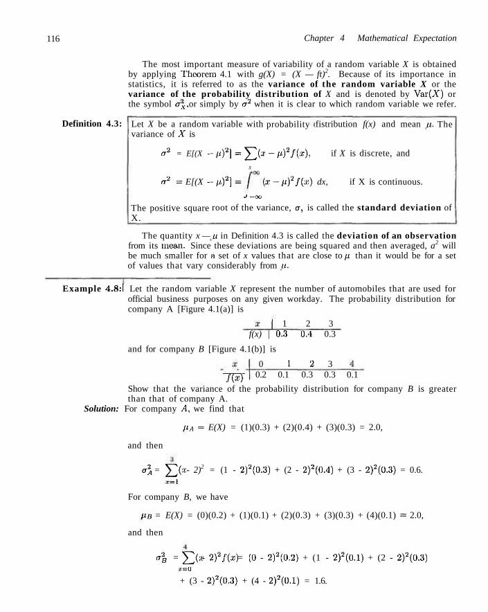
116 Chapter 4 Mathematical Expectation
The most important measure of variability of a random variable X is obtained by applying Theorem 4.1 with g(X) = (X — ft)2. Because of its importance in statistics, it is referred to as the variance of the random variable X or the variance of the probability distribution of X and is denoted by Var(X) or the symbol ax, or simply by a2 when it is clear to which random variable we refer.
Definition 4.3: Let X be a random variance of X is
CT2 = E[(X -
o-2 = E[(X -
The positive square X.
variable with
-li?\
-l>)2]
-B" X
= (
J —OO
probability
-V-ffix),
X-(lff(x)
fistribution f(x) and mean u.
if X is discrete, and
dx, if X is continuous.
The
root of the variance, er, is called the standard deviation of
The quantity x — u in Definition 4.3 is called the deviation of an observation from its mean. Since these deviations are being squared and then averaged, a2 will be much smaller for a set of x values that are close to fi than it would be for a set of values that vary considerably from u.
Example 4.8:1 Let the random variable X represent the number of automobiles that are used for official business purposes on any given workday. The probability distribution for company A [Figure 4.1(a)] is
1 2 3 f(x) | 0.3 0.4 0.3
and for company B [Figure 4.1(b)] is
0 1 2 3
HxJ 0.2 0.1 0.3 0.3 0.1
Show that the variance of the probability distribution for company B is greater than that of company A.
Solution: For company A, we find that
uA = E(X) = (1)(0.3) + (2)(0.4) + (3)(0.3) = 2.0,
and then
a\ = YJKX - 2)2 = (1 - 2)2(0.3) + (2 - 2)2(0.4) + (3 - 2)2(0.3) = 0.6. r = l
For company B, we have
uB = E(X) = (0)(0.2) + (1)(0.1) + (2)(0.3) + (3)(0.3) + (4)(0.1) = 2.0,
and then
er2B = £ > - 2?f{x) = (0 - 2)2(0.2) + (1 - 2)2(0.1) + (2 - 2)2(0.3) x=Q
+ (3 - 2)2(0.3) + (4 - 2)2(0.1) = 1.6.
4.2 Variance and Covariance of Random Variables 117
Clearly, the variance of the number of automobiles that are used for official business
purposes is greater for company B than for company A. J An alternative and preferred formula for finding a2, which often simplifies the
calculations, is stated in the following theorem.
Theorem 4.2: The variance of a random variable X is
a2 = E(X2) - ,i2.
Proof: For the discrete case we can write
o1 = ^ix-tx)*f(x) = Y,(x*-2ux + tj?)f(x) X X
= Y, ,'2/(,') - 2/, £ xf(x) + „2 Y, fix). x x X
Since p. = Ylxfix) by definition, and ]C/( X ) = 1 f° r an.Y discrete probability X X
distribution, it follows that
e x 2 = £ : r V M - , r = £ ( X 2 ) - , r . , x —*
For the continuous case the proof is step by step the same, with summations replaced by integrations.
Example 4.9:1 Let the random variable X represent the number of defective parts for a machine when 3 parts are sampled from a production line and tested. The following is the probability distribution of X,
0 1 2 3 fix)
Using Theorem 4.2, calculate a Solution: First, we compute
0.51 0.38 0.10 0.01 2
u = (0)(0.51) + (1)(0.38) - (2)(0.10) + (3)(0.01) = 0.61.
Now
E(X2) = (0)(0.51) - (1)(0.38) - (4)(0.10) J- (9)(0.01) = 0.87.
Therefore,
a2 = 0 . 8 7 - (0.61)2 = 0.4979. J
Example 4.10:1 The weekly demand for Pepsi, in thousands of liters, from a local chain of efficiency stores, is a continuous random variable X having the probability density
. f 2 ( , - - l ) , X<x<2, n ' [0, elsewhere.
Find the mean and variance of X. Solution: r / r . „ f , . . . 5
/i = E(X) = 2 j x(x- I) dx = - ,
118 Chapter 4 Mathematical Expectation
Theorem 4.3:
and
Therefore,
E(X ! ) = 2 / 2 x (x l)dx=j.
6 V 3 / 18 At this point the variance or standard deviation only has meaning when we com
pare two or more distributions that have the same units of measurement. Therefore, we could compare the variances of the distributions of contents, measured in liters, for two companies bottling orange juice, and the larger value would indicate the company whose product is more variable or less uniform. It would not be meaningful to compare the variance of a distribution of heights to the variance of a distribution of aptitude scores. In Section 4.4 we show how the standard deviation can be used to describe a single distribution of observations.
We shall now extend our concept of the variance of a random variable X to also include random variables related to X. For the random variable fir(X), the variance will be denoted by er2,A-, and is calculated by means of the following theorem.
Let X be a random variable with probability distribution fix). The variance of the random variable giX) is
oi(x) = E{[g(X) - ug{X)}2} = 5 > ( z ) - ug{x))
2f(x) X
if X is discrete, and
/
oo \ffix) - ug{x)]
2f(x) dx •oo
if X is continuous.
Proof: Since giX) is itself a random variable with mean Mg(X) a s defined in Theorem 4.1, it follows from Definition 4.3 that
°%(X) =E{\9{X)-fia(X))}'
Now, applying Theorem 4.1 again to the random variable [g(X) — ug(Xy\2, the proof
is complete. J
Example 4.11:1 Calculate the variance of g(X) = 2X + 3, where X is a random variable with probability distribution
a: 1 0 1 2 3 f(x) I I I I -
J W I 4 8 2 8 Solution: First let us find the mean of the random variable 2X + 3. According to Theorem
4.1.
M2X+3 - E(2X + 3) = Yi2x + 3 ) / ( x ) = 6-x=0
4.2 Variance and Covariance of Random Variables 119
Now, using Theorem 4.3, we have
4 v + a = E{[(2X + 3) - Wx+z]2} = E[(2X + 3 - 6)2] :i
= E(4X2 - 12X + 9) = ]T(4ar2 - 12a: - 0)/(x) 2?=()
Example 4.12:1 Let X be a random variable having the density function given in Example 4.5 on page 111. Find the variance of the random variable g(X) = 4X + 3.
Solution: In Example 4.5 we found that IM.\+3 = 8. Now, using Theorem 4.3,
4 v + 3 = E{[(4X - 3) - 8]2} = E[(4X - 5)2]
" (4s - 5)2^-ob: = - l (16a:4 - 40.-r3 + 25x2) da: = —. i 3 3 ,/-i 5
If g(X.Y) = (X-(ix)(Y-uY). where /cA- = E(X) and / i v = E(Y), Definition 4.2 yields an expected value called the covariance of X and Y, which we denote by (Txy or Cov(X, Y).
Definition 4.4: Let X and Y be random variables with joint probability distribution f(x, y). The covariance of X and Y is
trXY = E[(X - fi.x)(Y - uY)\ = Y X> ~ Mx)(|/ - %)/(*, v) x y
if X and Y are discrete, and
er.vv- = E[{X - us)(Y - fly)) = / / (;r - fix)(y - /%)/(£, y) dx dy .1 — oo J —oc
if X and Y arc continuous.
The covariance between two random variables is a measurement of the nature of the association between the two. If large values of X often result in large values of Y or small values of X result in small values of Y. positive X — fix will often result-in positive Y — //.,- and negative A' — fi.x will often result in negative Y — fiY. Thus the product (X — fix)(Y — fiY) will tend to be positive. On the other hand, if large A' values often result in small Y values, the product (X — fi\)(Y — fiY) will tend to be negative. Thus the sign of the covariance indicates whether the relationship between two dependent random variables is positive or negative. When X and Y are statistically independent, it can be shown that the covariance is zero (see Corollary 4.5). The converse, however, is not generally true. Two variables may have zero covariance and still not be statistically independent. Note that the covariance only describes the linear relationship between two random variabilis. Therefore, if a covariance between X and Y is zero, X and Y may have a nonlinear relationship, which means that they are not necessarily independent.
The alternative and preferred formula for aXY is stated by Theorem 4.4.
120 Chapter 4 Mathematical Expectation
Theorem 4.4: The covariance of two random variables X and Y with means ux and uY, respectively, is given by
O-XY =E(XY)- flXflY.
Proof: For the discrete case we can write
VXY -Y,12(x ~ flx^y ~ ^-)fix-- y) x y
= Y YSxy ~ VxV - l'yx + MxMv)f(x, y) x y
= YY xyfix> y) - /x-v Y Y vf(x>y) x y x y
- Mv Y Y xffay}+iixfw Y Y f(x-- y)' x y x y
Since
ux = ^ .T/(a: , j / ) and uY = ^ 2 / / ( x . y ) X y
by definition, and in addition
x y
for any joint discrete distribution, it follows that,
aw- = E(XY) - fixuY - uYux + uxuY - E(XY) - uxuY.
For the continuous case the proof is identical with summations replaced by integrals. J
Example 4.13:1 Example 3.14 on page 92 describes a situation involving the number of blue refills X and the number of red refills Y. Two refills for a ballpoint pen are selected at random from a certain box, the following is the joint probability distributions.
fix,y) 0
V i 2
gix)
0
28 3 14 1 28 5 14
X
1 9 28 3 14
0 15 28
2 3 28
0 0 3 28
Kv) 15 28 3 7 1 28 1
Find the covariance of X and Y. Solution: From Example 4.6, we see that E(XY) = 3/14. Now
" « - 1 > < * > - <•» ( n ) + ( 1 ) (I)+<2> ( 1 ) 4
4.2 Variance and Covariance of Random Variables 121
and
p.Y = Y!M.'i) = (a) w=o
+ (1) + (2) •2s
Therefore,
E(XY)-uxur = II
9_
56'
Example 4.14:1 The fraction X of male runners and the fraction Y of female runners who compete in marathon races arc described by the joint density function
fix,!)) Sxy, 0 < y < x < 1, 0, elsewhere1.
Find the covariance of X and Y. Solution: We first compute the marginal density functions. They are
4:r3, 0 < x < 1, 0. elsewhere,
and
Hy
9ix)
_ / 4 y ( I - r ) , ( ) < / / < ! , (I. elsewhere.
From the marginal density functions given above, wc compute
ux = E(X] 4s dx = - , and (iy = / 4 y ( l - y ) dy = n Jo 15
From the joint density functions given, we have -1 /• I
E(XY) 8x'y dx dy= -.
Then
rXY = E(XY)-uxuY=-8_\ _ _4_
•'V \15J ~ 225' J Although the covariance between two random variables does provide informa
tion regarding the nature of the relationship, the magnitude of Cxy does not indicate anything regarding the strength, of the relationship, since <TXY is not scale-free. Its magnitude will depend on the units measured for both X and Y. There is a scale-free version of the covariance called the correlat ion coefficient that is used widely in statistics.
Definition 4.5: Let ox
X and Y be ra and aY, respect.
ldom vely.
variables The corrc
wii lat
h covariance crvv ; ion coefficient of X
0-X Y
axaY
md sta and Y
ndai is
d deviations
It should be clear to the reader that pXY is free of the units of X and Y. The correlation coefficient satisfies the inequality — 1 < pXY < 1. It assumes a value of
122 Chapter 4 Mathematical Expectation
Exercises
zero when <TVV = 0. Where there is an exact linear dependency, say Y = a + bX, pxy ss 1 if I) > 0 and pxy = —1 if b < 0. (See Exercise 4.48.) The correlation coefficient is the subject of more discussion in Chapter 12, where we deal with linear regression.
4 .33 L"se Definition 4.3 on page 116 to find the variance of the random variable X of Exercise 4.7 on page 113.
4 .34 Let X be a random variable with the following probability distribution:
a;
fix) —2 0.3
3 0.2
5 0.5
Find the standard deviation of X.
4.35 The random variable X, representing the number of errors per 100 lines of software code, has the following probability distribution:
2 3 4 5 6
1W 0.01 0.25 0.4 0.3 0.04
Using Theorem 4.2, find the variance of X.
4.36 Suppose that the probabilities are 0.4. 0.3, 0.2, and 0.1, respectively, that 0, 1, 2. or 3 power failures will strike a certain subdivision in any given year. Find the mean and variance of the random variable X representing the number of power failures striking this subdivision.
4.37 A dealer's profit, in units of S5000, on a new automobile is a random variable X having the density function given in Exercise 4.12 on page 113. Find the variance of A".
4.38 The proportion of people who respond to a certain mail-order solicitation is a random variable X having the density function given in Exercise 4.14 on page 113. Find the variance of X.
4.39 The total number of hours, in units of 100 hours, that a family runs a vacuum cleaner over a period of one year is a random variable X having the density function given in Exercise 4.15 on page 114. Find the variance of X.
4.40 Referring to Exercise 4.14 on page 113, find Ta(X) for the function g(X) = 3A2 + 4.
4 .41 Find the standard deviation of the random variable g(X) = (2X + l ) 2 in Exercise 4.17 on page 114.
4.42 Using the results of Exercise 4.21 on page 114,
find the variance of g(X) = A'2, where X is a random variable having the density function given in Exercise: 4.12 on page 113,
4.43 The length of time, in minutes, for an airplane to obtain clearance for take off at a certain airport is a random variable Y = 3X — 2, where X has the density function
/(*) - {J -x/4 x > 0
elsewhere.
Find the mean and variance of the random variable Y.
4.44 Find the covariance of the random variables A' and Y of Exercise 3.39 on page 101.
4.45 Find the covariance of the random variables X and Y of Exercise 3.49 on page 102.
4.46 Find the covariance of the random variables A' and Y of Exercise 3.44 on page 102.
4.47 Referring to the random variables whose joint density function is given in Exercise 3.40 on page 101, find the covariance of X and Y.
4.48 Given a random variable A, with standard deviation <T,Y and a random variable Y = a + bX, show that if b < 0, the correlation coefficient pXY = —1, and if b > 0, f>xv = 1.
4.49 Consider the situation in Exercise 4.32 on page 115. The distribution of the number of imperfections per 10 meters of synthetic failure is given by
x 1 0 1 2 3 4 f{x) I 0.41 037 0T6 (105 OuT~
Find the variance and standard deviation of the number of imperfections.
4.50 On a laboratory assignment, if the equipment is working, the density function of the observed outcome, X. is
Find the variance and standard deviation of X.
(2(1 -x), 0 < x < 1, otherwise.
4.3 Means and Variances of Linear Combinations of Random VariabJes 123
4.3 Means and Variances of Linear Combinations of Random Variables
We now develop some useful properties that will simplify the calculations of means and variances of random variables that appear in later chapters. These properties will permit us to deal with expectations in terms of other parameters that are either known or are easily computed. All the results that we present here are valid for both discrete and continuous random variables. Proofs are given only for the continuous case. We begin with a theorem and two corollaries that should be, intuitively, reasonable to the reader.
Theorem 4.5: If a and b are constants, then
E(aX + b) = aEiX) + b.
Proof: By the definition of an expected value,
/
OO /-OC i>00
(ax + b)f(x) dx = a xf(x) dx + b I f(x) dx. -oo J—oc J—oo
The first integral on the right is E(X) and the second integral equals 1. Therefore, we have
E(aX + b) = aE(X) + b. J
Corollary 4 .1 : Setting a = 0, we see that E(b) = b.
Corollary 4.2: Setting 6 = 0, we see that E(aX) = aE(X).
Example 4.15:1 Applying Theorem 4.5 to the discrete random variable f(X) = 2X — 1, rework Example 4.4.
Solution: According to Theorem 4.5, we can write
E(2X - 1) = 2E(X) - 1.
Now
fi = E(X) = Yxf{x)
= (4)(iL) + ( 5 )(l) + (6)(l)+(r)(l) + ( 8 )Q)+ ( 9 )( i ) . 41_ 6 '
Therefore,
as before.
M2X-1 = (2) (j) - 1 = $12.67,
124 Chapter 4 Mathematical Expectation
Example 4.16:1 Applying Theorem 4.5 to the continuous random variable g(X) = 4X + 3, rework Example 4.5.
Solution: In Example 4.5 we may use Theorem 4.5 to write
Now
Therefore,
£(4X + 3) = 4E(X) + 3.
"^-/!'(£)*-£ J*-i
E(4X + S) = (4)| j ] + 3 = S,
as before.
Thmrsm 4.fi: The expected value of the sum or difference of two or more functions of a random variable X is the sum or difference of the expected values of the functions. That is,
E[g(X) ± h(X)} = E[g(X)\ ± E[h(X)\.
Proof: By definition,
/
oo [g(x) ± h(x)]f(x) dx
-OO
/
OO fOG
g(x)f(x)dx± h(x)f(x)dx •OO J — DC
= E\g(X)} ± E[h(X)}.
Example 4.17:1 Let X be a random variable with probability distribution as follows: 0 l " 2 3
~i r fix) 0 Find the expected value of Y = (X — l)2.
Solution: Applying Theorem 4.6 to the function Y = (X — l)2 , we can write
E\(X - l)2] = E(X2 - 2X + 1) = E(X2) - 2E(X) + E(l).
From Corollary 4.1, E(l) = 1, and by direct computation,
EiX) = (0) ( - (1) { - ) +(2)(0) + (3)
and
E(X2) = (0){ ^)-i(i) G) + (4)(0) + (9)
© = ''
4.3 Means and Variances of Linear Combinations of Random Variables 12?
Hence
£ [ ( X - 1 ) 2 ] = 2 - (2 ) (1 ) + 1 = 1.
Example 4.18:1 The weekly demand for a certain drink, in thousands of liters, at a chain of convenience stores is a continuous random variable g(X) = X + X — 2, where X has the density function
/ ( * : 2 ( 1 - 1 } , 1 < x < 2, 0, elsewhere.
Find the expected value for the weekly demand of the drink. Solution: By Theorem 4.6. we write
E(X2 + X - 2) = E(X2) + E(X) - E(2).
From Corollary 4.1. .£7(2) = 2. and by direct integration,
E(X\ 2 s { s - l ) d.:> - > ! > -
'•') dx = -,
and
Now
E(X2) = I 2.r'(x - 1) dx = 2 / ( s 3 - .r2) ds = y .
so that the average weekly demand for the drink from this chain of eflic:iency stores is 2500 lifers. J
Suppose that we have two random variables X and Y with joint probability distribution f(x,y). Two additional properties that will be very useful in succeeding chapters involve the expected values of the sum, difference, and product of these two random variables. First, however, let us prove a theorem on the expected value of the sum or difference of functions of the given variables. This, of course, is merely an extension of Theorem 4.6,
Theorem 4.7: The expected value of the sum or difference of two or more functions of the random variables X and Y is the sum or difference of the expected values of the functions. That is,
E[g(X, Y) ± h(X, Y)] = E[g(X, Y)} ± E\h(X, Y)}.
Proof: By Definition 4.2.
E[g(X, Y) ± h(X, Y)]= f j [g(x. y) ± h(x, y)]f{x, y) dx dy
/
OC /*00 /'OC if*OG
/ g{x,y)f{x,y) dx dy± I Ii.(x,y)f(x,y)dxdy •OC >i — CO iZ-flOt/-
=E[g(X,Y)]±E[h(X,Y)}.
126 Chapter 4 Mathematical Expectation
Corollary 4.3: Setting g(X, Y) = g(X) and h(X, Y) = h(Y), we see that
E[g(X) ±h(Y)) = E[g(X)} ± E{h(Y)}.
Corollary 4.4: Setting g(X, Y) = X and h[X, Y) - Y, we see that
E[X ± Y] = E[X] ± E[Y\.
If X represents the daily production of some item from machine A and Y the daily production of the same kind of item from machine B, then X + Y represents the total number of items produced daily by both machines. Corollary 4.4 states that the average daily production for both machines is equal to the sum of the average daily production of each machine.
Theorem 4.8: Let X and Y be two independent random variables. Then
E(XY) m E(X)E(Y).
Proof: By Definition 4.2,
/
OO /"OO / xyf(x,y) dx dy.
•oc J—oc
Since X and Y are independent, we may write
f(x,y) =g(x)h(y),
where g(x) and h(y) are the marginal distributions of X and Y, respectively. Hence
/
OO /-OO /"OO /.so
/ xyg(x)h(y) dx dy = / xg(x) dx I yh(y) •oo J—oo J—oc J—oc
dy
= E(X)E(Y). J
Theorem 4.8 can be illustrated for discrete variables by considering the experiment of tossing a green die and a red die. Let the random variable X represent the outcome on the green die and the random variable Y represent the outcome on the red die. Then XY represents the product of the numbers that occur on the pair of dice. In the long run, the average of the products of the numbers is equal to the product of the average number that occurs on the green die and the average number that occurs on the red die.
Corollary 4.5: Let X and Y be two independent random variables. Then crXY = 0.
Proof: The proof can be seen by using Theorems 4.4 and 4.8.
Example 4.19:1 In producing gallium-arsenide microchips, it is known that the ratio between gallium and arsenide is independent of producing a high percentage of workable wafers, which are the main components of microchips. Let X denote the ratio of
4.3 Means and Variances of Linear Combinations of Random Variables 127
gallium to arsenide and Y denote the percentage of workable microwafers retrieved during a 1-hour period. X and Y are independent random variables with the joint density being known as
/ ( a , , ) = J * ^ r A 0 < x < 2 , 0 < y < l , 10, elsewhere.
Illustrate that E(XY) = E(X)E(Y), as Theorem 4.8 suggests. Solution: By definition.
E(XY) = [ f xyf(x,y) dx dy = f f X y ( 1 + 3 y 1 dx dy Jo Jo Jo Jo 4
Jo i z ;c=o JO
n l 2 y ( l + 3ya) 5 3 V 6 !
E(X) = f [ xf(x,y) dxdy= f f ^ ^ ^ dx dy Jo Jo Jo Jo 4
Jo L* x = 0 JO
"l2(l + 3y2)A 4
~ " 5 — d y = s '
E(Y) = f !\fix,y) dx dy = f1 f s ^ + V ) dx dy Jo Jo Jo Jo 4
fl x2-> x2y(l + 3y2) 8
dy= / x=0 JO
,y{14^*v-l Hence
«xwn-(J)(|)-|-«xy). _, We conclude this section by proving two theorems that are useful for calculating
variances or standard deviations.
Theorem 4.9: If a and b are constants, then
°lx+b = «2** = <*2*2.
Proof: By definition,
Now
TaX+6 = £?{[(aJC + b) - uaX+b}2}.
P-aX+b = E(aX + b) = ap + b
by Theorem 4.5. Therefore,
o-lx+b = E[(aX +b-au- b)2} = a2E[(X - p)2) = a2cr2.
128 Chapter 4 Mathematical Expectation
Corollary 4.fi: Setting a = 1, we see that
2. . _ „i = ni °~x+b = at = a*
Corollary 4.7: Setting b = 0, we see that
°lx = «M ~ a2<72.
Corollary 4.6 states that the variance is unchanged if a constant is added to or subtracted from a random variable. The addition or subtraction of a constant simply shifts the values of X to the right or to the left but does not change their variability. However, if a random variable is multiplied or divided by a constant, then Corollary 4.7 states that the variance is multiplied or divided by the square of the constant.
Theorem 4.10: If X and Y are random variables with joint probability distribution f(x, y), then
alx+bY = «2<7x + h2(Tl + 2abaXY.
Proof: By definition,
Now
°lx+bY = E{[(aX + bY) - p.ax+l>Y}2}.
PaX+bY = E(oX + bY) = aE(X) + bE(Y) = apx + bpY,
by using Corollary 4.4 followed by Corollary 4.2. Therefore,
°lx+bY = E{[a(X -px)+ b(Y - py)}2}
= a2E[(X - px)2\ + b2E[(Y - pYf] + 2abE[(X - px)(Y - pY)}
= a2 a2 + b2al + 2abaXY.
Corollary 4.8; If X and Y are independent random variables, then
<r2x+6y = a 2 4 + &2<4-
The result stated in Corollary 4.8 is obtained from Theorem 4.10 by invoking Corollarv 4.5.
Corollary 4.9: If X and Y are independent random variables, then 2 2 2
°~aX-bY = ° <*x ,2 _ „ 2 _ 2 + b 2 ( r 2
Corollary 4.9 follows by replacing b by —b in Corollary 4.8. Generalizing to a linear combination of n independent random variables, we write
4.3 Means and Variances of Linear Combinations of Random Variables 129
Corollary 4.10: If X i , X 2 , . . . , X n are independent random variables, then
<41Xi+a2X2+..+anXn = 01*4, + al°X3 + ••• + <lloXn
Example 4.20:1 If A' and Y are random variables with variances ox = 2, o2 = 4, and covariance CT.VV = - 2 , find the variance of the random variable Z = 3X - 4Y + 8.
Solution: °"z ~ ffzx-4Y+e = °3X-4V (by Theorem 4.9)
= 9er2 + 16c72 - 24o\x-v (by Theorem 4.10)
= (9) (2)+( lG)(4) - (24) ( -2) = 130.
Example 4.21:1 Let A' and Y denote the amount of two different types of impurities in a batch of a certain chemical product. Suppose that X and Y are independent random variables with variances a\ = 2 arid aY = 3. Find the variance of the random variable Z = 3X - 21' + 5.
Solution: = °fx-2Y+5 = °3X-2Y ihY Theorem 4.9)
= 9cr2 + Aa'l (by Corollary 4.9)
= (9)(2) + (4)(3)=30.
What if the Function Is Nonlinear? In that which has preceded this section, we deal with properties of linear functions of random variables for very important reasons. From Chapter 8 through 15, much of what, is discussed and illustrated are practical and real world problems in which the analyst is constructing a linear mode l to describe a data set and thus to describe or explain the behavior of a certain scientific phenomenon. Thus, it is natural that expected values and variances of linear combinations of random variables are encountered. However, there are situations in which properties of nonlinear functions of random variables become important. Certainly there are many scientific: phenomena that are nonlinear and certainly statistical modeling using nonlinear functions is very important. In fact, in Chapter 12, we deal with the modeling of what have become certain standard nonlinear models. Indeed, even a simple function of random variables, say Z = X/Y, occurs quite frequently in practice and yet unlike the rules given earlier in this section for the expected value of linear combinations of random variables, there is no simple general rule. For example,
E{Z) = E(X/Y) * E(X)/E(Y),
except in very special circumstances. The material provided by Theorem 4.5 through Theorem 4.10 and the various
corollaries are extremely useful in that there are no restrictions on the form of the density or probability functions, apart from the property of independence when it is required as in the corollaries following Theorem 4.10. To illustrate, consider Example 4.21; the variance of Z = 3A' - 2Y -f- 5 does not require restrictions on the distributions of the amounts X and Y of the two types of impurities. Only independence between X and Y is required. Now, we do have at our disposal the capacity to find pg{x) a n c ' al(X) ^or a m / f u n c t i o n <?(") fr°m m ' s t principles established in Theorem 4.1 and 4.3, where it, is assumed that the corresponding
130 Chapter 4 Mathematical Expectation
distribution f(x) is known. Exercises 4.40, 4.41, and 4.42, among others, illustrate the use of these theorems. Thus, if the function g(x) is nonlinear and the density function (or probability function in the discrete case) is known, pg(X) a n d o~2
g(X) can be evaluated exactly. But, like the rules given for linear combinations, are there rules for nonlinear functions that can be used when the form of the distribution of the pertinent random variables is not known?
In general, suppose X is a random variable and Y = gix). The general solution for E(Y) or Var(Y) can be difficult and depends on the complexity of the function g(-). However, there are approximations available that depend on a linear approximation of the function g(x). For example, suppose we denote E(X) as p and Var(X) = o2. Then a Taylor series approximation of g(x) around X = px
gives
9ix)=9iux)-rd-3{x)
dx [x-px) +
d2gix)
x=nx dx2
ix-Px)2
+ •• =Mx
As a result, if we truncate with the linear term and take the expected value of both sides, we obtain E[g(X)] « gipx), which is certainly intuitive and in some cases gives a reasonable approximation. However, if we include the second-order term of the Taylor series, then we have a second order adjustment for this first-order approximation as
Approximation of E[9iX)} E{g(X)}K9(px) +
02g(x) dx2
=fx 2
Example 4.22:1 Given the random variable X with mean px and variance o\, give the second-order approximation to E(ex).
Solution: Since %• = ex and ^ = ex, we obtain E(ex) « e>lx (1 + a2.(2). J
Similarly, we can develop an approximation for Var[ej(s)] by taking the variance of both sides of the first order Taylor series expansion of g(x).
Approximation of Var[g(x)\ Var[g(X)\
dx =Mx
Example 4.23:1 Given the random variable X as in Example 4.22, give an approximate formula for Var[g(x)].
Solution: Again %- = ex; thus Var(X) « e2"-vc72 . J These approximations can be extended to nonlinear functions of more than one
random variable. Given a set of independent random variables Xi, X 2 , . . . , X/t with means px,p2,...,pk
and variances o\,G2,...,a\, respectively, let
Y = h(XuX2,...,Xk)
be a nonlinear function; then the following are approximations for E(Y) and
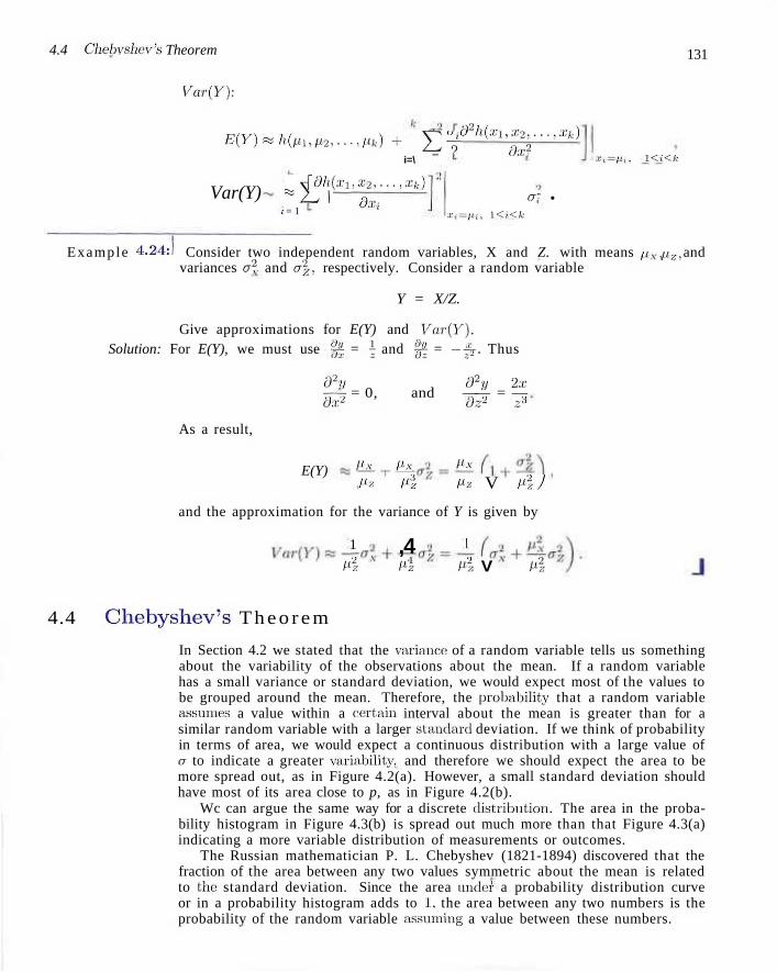
4.4 Chebvshev's Theorem 131
Var(Y):
E(Y)tok(pup2,...,pk) + YT
Var(Y) ^Yr
i=\
02h(xi,x2,...,xk) Ox2
'x,=Hi. l<i<k
rdli(xl.x2,...,xk)~"
; = 1 dx, 0-7 •
x,=;t i , l<i<fc
Example 4.24:1 Consider two independent random variables, X and Z. with means px, pz. and variances a2 and of,, respectively. Consider a random variable
Y = X/Z.
Give approximations for E(Y) and Var(Y). Solution: For E(Y), we must use §f = \ and §f = - f i - Thus
e92</ c92jr 2.x-- - ^ = 0, and —— = — ox1 oz1 zA
As a result,
E(Y) Its , Mx Mx
Uz l4 l*z V Ml/
and the approximation for the variance of Y is given by
1 ,4 1
Mi /4 Ml V Ml
4.4 Chebyshev 's T h e o r e m
In Section 4.2 we stated that the variance of a random variable tells us something about the variability of the observations about the mean. If a random variable has a small variance or standard deviation, we would expect most of the values to be grouped around the mean. Therefore, the probability' that a random variable assumes a value within a certain interval about the mean is greater than for a similar random variable with a larger standard deviation. If we think of probability in terms of area, we would expect a continuous distribution with a large value of a to indicate a greater variability, and therefore we should expect the area to be more spread out, as in Figure 4.2(a). However, a small standard deviation should have most of its area close to p, as in Figure 4.2(b).
Wc can argue the same way for a discrete distribution. The area in the probability histogram in Figure 4.3(b) is spread out much more than that Figure 4.3(a) indicating a more variable distribution of measurements or outcomes.
The Russian mathematician P. L. Chebyshev (1821-1894) discovered that the fraction of the area between any two values symmetric about the mean is related to the standard deviation. Since the area under a probability distribution curve or in a probability histogram adds to 1, the area between any two numbers is the probability of the random variable assuming a value between these numbers.
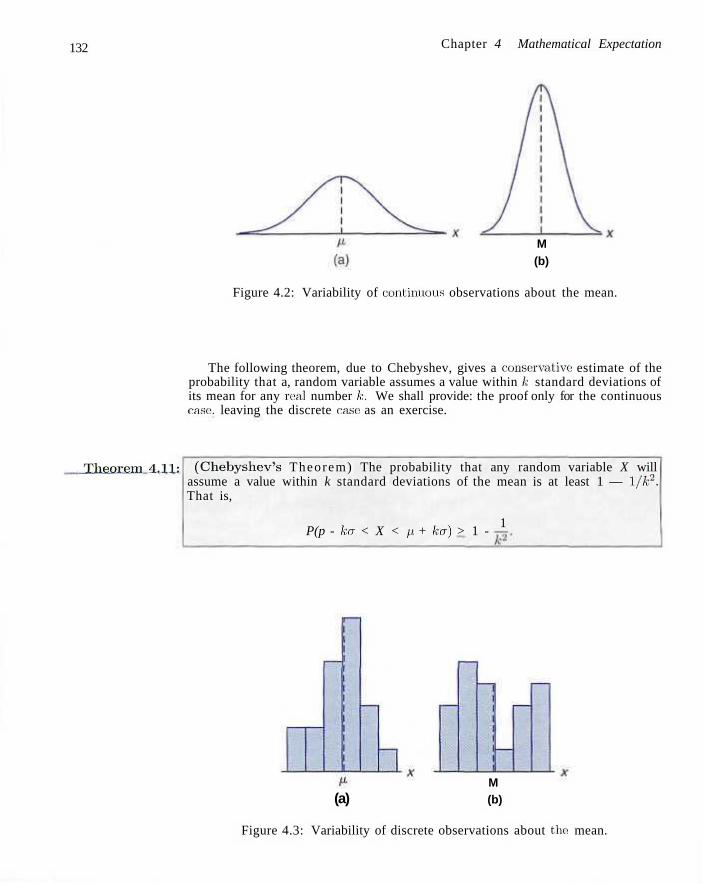
132 Chapter 4 Mathematical Expectation
M (b)
Figure 4.2: Variability of continuous observations about the mean.
The following theorem, due to Chebyshev, gives a conservative estimate of the probability that a, random variable assumes a value within /,: standard deviations of its mean for any real number /.:. We shall provide: the proof only for the continuous case, leaving the discrete case as an exercise.
-Theorem 4,11; (Chebyshev 's Theorem) The probability that any random variable X will assume a value within k standard deviations of the mean is at least 1 — 1/fc2. That is,
P(p - ko < X < \i + ko) > 1 -1
(a) M (b)
Figure 4.3: Variability of discrete observations about the: mean.
4.4 Chebyshev's Theorem 133
Proof: By our previous definition of the variance of A', we can write
a2=E[(X-p)2]= f ° ( s - M ) V ( s ) d s J — OC
/•// —fc<7 /•/!-)-riTT = / {x - p)2f(x) dx + / (s - ,y)2/(s) ds
J — OC .I/i — krT
+ I (x - pff(x) dx J/,+ 1.(7
(x - p)2f(x) dx + (x- u)2f(x) dx, •oc J/i + kir
since the second of the three integrals is nonnegative. Now, since |s — fi\ > ka wherever s > p + ka or x < p - ka, we have (x - p)2 > k2a2 in both remaining integrals. It follows that
/
'fi — ktr />oo
A-V/(.r) dx + / k2a2f{x) dx, -oo Jfi+ko and that
Hence
/
fi — ka rOC -t
f(x)dx+ f(x)dx<-, J/i+ka '>
r/t+ko | P(p - ka < X < p. + ka) = / f(x) dx > 1
A : 2 '
and the theorem is established. J For A: = 2 the theorem states that the random variable X has a probability of
at least 1 — 1/22 = 3/4 of falling within two standard deviations of the mean. That is, three-fourths or more of the observations of any distribution lie in the interval p ± 2a. Similarly, the theorem says that at least eight-ninths of the observations of any distribution fall in the interval p ± 3a.
Solution:
Example 4.25:1 A random variable A' has a mean p = 8, a variance CT2 = 9, and an unknown probability distribution, Find
(a) P(-4 < X < 20).
(b) P ( ] X - 8 | > 6 ) .
(a) P ( - 4 < X < 20) = P[8 - (4) (3) < X < 8 + (4)(3)] > if.
(b) P( |X - 8| > 6) = 1 - P(\X ~ 8 | < 6) « 1 - P ( - 6 < X - 8 < (i)
= I - P[8 - (2)(3) < X < 8 + (2)(3)] < j .
Chebyshev's theorem holds for any distribution of observations and, for this reason, the results are usually weak. The value given by the theorem is a lower bound only. That is, wc know that the probability of a random variable falling within two standard deviations of the mean can be no less than 3/4, but we never
134 Chapter 4 Mathematical Expectation
Exercises
know how much more it might actually be. Only when the probability distribution is known can we determine exact probabilities. For this reason we call the theorem a distribution-free result. When specific: distributions are assumed as in future chapters, the results will be less conservative. The use of Chebyshevs theorem is relegated to situations where the form of the distribution is unknown.
4.51 Referring to Exercise 4.35 on page 122, find the mean and variance of the discrete random variable Z = 3X — 2, when X represents the number of errors per 100 lines of code.
4.52 Using Theorems 4.5 and 4.9, find the mean and variance of the random variable Z = 5A + 3, where X has the probability distribution of Exercise 4.30 on page 122.
4.53 Suppose that a grocery store purchases 5 cartons of skim milk at the wholesale price of $1.20 per carton and retails the milk at $1.65 per carton. After the expiration date, the unsold milk is removed from the shelf and the grocer receives a credit from the distributor equal to three-fourths of the wholesale price. If the probability distribution of the random variable X, the number of cartons that are sold from this lot, is
x
fix) 0 l
IS
1 -2. 15
2 •2 15
3 a
"ir>
4 4 IS
5
15
find the expected profit.
4.54 Repeat Exercise 4.43 on page 122 by applying Theorems 4.5 and 4.9.
4.55 Let X be a random variable with the following probability distribution:
/(«) - 3
Find E(X) and E(X2) and then, evaluate £((2X + 1)2].
using these values,
4.57 If a random variable X is defined such that
E[(X - I)2] = 10, E[(X - 2)2] = 6,
find p, and a .
4.58 Suppose that X and Y are independent random variables having the joint probability distribution
fix,y) l
V 3 5
X
2 4 0.10 0.15 0.20 0.30 0.10 0.15
Find
(a) E(2X - ZY);
(b) E(XY).
4.59 Use Theorem 4.7 to evaluate £ (2XY 2 - X 2 K) for the joint probability distribution shown in Table 3.1 on page 92.
4.60 Seventy new jobs are opening up at an automobile manufacturing plant, but 1000 applicants show up for the 70 positions. To select the best 70 from among the applicants, the company gives a test that covers mechanical skill, manual dexterity, and mathematical ability. The mean grade on this test turns out to be 60, and the scores have a standard deviation 6. Can a person who has an 84 score count on getting one of the jobs? [Hint Use Chebyshev's theorem.] Assume that the distribution is symmetric about the mean.
4.56 The total time, measured in units of 100 hours, that a teenager runs her stereo set over a period of one year is a continuous random variable A that has the density function
!
x, 0 < x < 1,
2 - x, 1 < x < 2, 0, elsewhere.
Use Theorem 4.6 to evaluate the mean of the random variable Y = 60X~ -f- 39X, where Y is equal to the number of kilowatt hours expended annually.
4.61 An electrical firm manufactures a 100-watt light bulb, which, according to specifications written on the package, has a mean life of 900 hours with a standard deviation of 50 hours. At most, what percentage of tfie bulbs fail to last even 700 hours? Assume that the distribution is symmetric about the mean.
4.62 A local company manufactures telephone wire. The average length of the wire is 52 inches with a standard deviation of 6.5 inches. At most, what percentage of the: telephone wire from this company exceeds 71.5 inches? Assume that the distribution is symmetric about the mean.
Exercises 135
4.63 Suppose that you roll a fair 10-sided die ( 0 , 1 , 2 , . . . , 9) 500 times. Using Chebyshev's theorem, compute the probability that the sample mean, X, is between 4 and 5.
4.64 If X and Y are independent random variables with variances a 5 and at = 3. find the variance of the random variable Z = - 2 X + 4Y - 3.
4 .65 Repeat Exercise 4.64 if X and Y are not independent and aXy = 1.
4.66 A random variable X has a mean p ~ 12, a variance a2 = 9, and an unknown probability distribution. Using Chebyshev's theorem, estimate (a) P(6 < X < 18); (b) P(3 < X < 21).
4.67 A random variable X has a mean p = 10 and a variance a2 = 4. Using Chebyshev's theorem, find (a) P(\X - 10| > 3); ( b ) P ( | X - 1 0 | < 3 ) ; (c) P(b < X < 15); (d) the value of the constant c such that
P(\X - 10| > c) < 0.04.
4.68 Compute P(p - 2er < X < p, + 2a), where X has the density function
fix) f6:r(l -x), 0 < a ; < l ,
elsewhere
and compare with the result given in Chebyshev's theorem.
4.69 Let X represent the number that occurs when a red die is tossed and Y the number that occurs when a green die is tossed. Find (a)E(X + Y); (b) E(X - Y); (c) E(XY).
4.70 Suppose that X and Y are independent random variables with probability densities and
9{x) = / £ . x>2 \ 0 , elsew! elsewhere,
and
Find the expected value of Z = XY
< 2 / < 1, elsewhere.
4.71 by
If the joint density function of X and Y is given
fix,y) ix + 2y), 0<x < 1,
elsewhere. K V < 2,
find the expected value of g(X, Y) = ys + X2Y.
4.72 Let X represent the number that occurs when a green die is tossed and Y the number that occurs when a red die is tossed. Find the variance of the random variable (a) 2X - Y;
(b) X + 3 F - 5.
4.73 Consider a random variable X with density function
10, elsewhere.
(a) Find p = E(X) and a2 = E[(X - p)2].
(b) Demonstrate that Chebyshev's theorem holds for k = 2 and k = 3.
4 .74 The power P in watts which is dissipated in an electric circuit with resistance R is known to be given by P = I2R, where / is current in amperes and R is a fixed constant at 50 ohms. However, / is a random variable with pj = 15 amperes and a2 = 0.03 amperes2. Give numerical approximations to the mean and variance of the power P.
4.75 Consider Review Exercise 3.79 on page 105. The random variables X and V represent the number of vehicles that arrive at two separate street corners during a certain 2-minute period in the day. The joint distribution is
fix,y) - 4{x+y) • 1 6 ,
for x = 0 , 1 , 2 , . . . , and y = 0 , 1 , 2 , . . . . (a) Give E(X), E(Y), Var(X), and Var(Y). (b) Consider Z = X + Y, the sum of the two.
E(Z) and Var(Z). Find
4.76 Consider Review Exercise 3.66 on page 104. There are two service lines. The random variables X and Y are the proportion of time that line 1 and line 2 are in use respectively. The joint probability density function for (X, Y) is given by
fiz,y) \o Ux2 + y2), 0<x,y< 1,
elsewhere.
136 Chapter 4 Mathematical Expectation
(a) Determine whether or not X and Y are independent.
(b) It is of interest to know something about, the proportion of Z = X 4- Y. the sum of the two proportions. Find E(X-rY). Also find E(XY).
(c) Find Var(X) , Var(Y), and Cov(X.Y).
(d) Find Var(X + Y).
4.77 The length of time Y in minutes required to generate a human reflex to tear gas has density function
fiy) '{I -v/4 0 < y < oc,
elsewhere.
(a) What is the mean time to reflex?
(b) Find E(Y2) and Var(Y).
4.78 A manufacturing company has developed a fuel-efficient machine for cleaning carpet because it delivers carpet cleaner so rapidly. Of interest is a random variable Y, the amount in gallons per minute delivered. It is known that the density function is given by
fiy) - J 1 - 7
\ 0 , el
< >J < 8, elsewhere.
(a) Sketch the density function.
(b) Give E(Y), E(Y2), and Var(Y).
4.79 For the situation in Exercise 4.78, compute E(e' ) using Theorem 4.1, that is, by using
E(eY)= j\*f(y)dy.
Then compute £(eY ) by not using f(y), but rather by using the second-order adjustment to the first-order approximation of E(eY). Comment.
4.80 Consider again the situation of Exercise 4.78. It is required to find Var(eY). Use Theorems 4.2 and 4.3 and define Z = eY. Thus, use the conditions of Exercise 4.79 to find
Var(Z) E(Z2) [E(Z)f
Then do it by not using f(y) but rather use the first order Taylor series approximation to Var(e'1 ). Comment!
Review Exercises
4.81 Prove Chebyshev's theorem when X is a discrete random variable.
4.82 Find the covariance of the random variables X and Y having the joint, probability density function.
f(xv)-tx + y' °<x<hO<y nX,y,~\Q, elsewhere.
< 1,
4.83 Referring to the random variables whose joint probability density function is given in Exercise 3.47 on page 102, find the average amount of kerosene left in the tank at the end of the day.
4.84 Assume the length X in minutes of a particular type of telephone conversation is a random variable with probability density function
/(.)-{£ . I / 5 x > 0, elsewhere.
(a) Determine the mean length JE(X) of this type of telephone conversation.
(b) Find the variance and standard deviation of X.
(c) Find E[(X + 5)2].
4.85 Referring to the random variables whose joint density function is given in Exercise 3.41 on page 101, find the covariance between the weight of the creams and the weight of the toffees in these boxes of chocolates.
4.86 Referring to the random variables whose joint probability density function is given in Exercise 3.41 on page 101, find the expected weight for the sum of the creams and toffees if one purchased a box of these chocolates.
4.87 Suppose it is known that the life X of a particular compressor in hours has the density function
fix) {uoo 0,
' ^ 9 0 0 , a : > 0 , elsewhere.
(a) Find the mean life of the compressor.
(b) F i n d £ ( X 2 ) . (c) Find the variance and standard deviation of the
random variable X.
Review Exercises 137
4.88 Referring to the random variables whose joint density function is given in Exercise 3.40 on page 101, (a) find px and fiy;
(b) find E[(X 4- V)/2],
4.89 Show that Cov(aX,by) = ab Cov(X,V).
4.90 Consider the density function of the Review Exercise 4.87. Demonstrate that Chebyshev's theorem holds for k. = 2 and k = 3.
4.91 Consider the joint density function
'm, x>2,0<y<l, f(x,y) {? elsewhere.
Compute the correlation coefficient pXY.
4.92 Consider random variables X and Y of Exercise 4.65 on page 135. Compute pXY.
4.93 A dealer's profit in units of $5000 on a new automobile is a random variable A" having density function
fix {I 2(1 -x), 0 < . T < 1 ,
elsewhere.
(a) Find the variance of the dealer's profit. (b) Demonstrate that Chebyshev's inequality holds for
k = 2 with the density function above. (c) What is the probability that the profit exceeds
$500?
4.94 Consider Exercise 4.10 page 113. Can it, be said that the grades given by the two experts are independent? Explain why or why not.
4 .95 A company's marketing and accounting departments have determined that if the company markets its newly developed product, the contribution of the product to the firm's profit during the next 6 months is described by the following:
Profit Contribution Probability -85,000 (loss) 0.2 $10,000 0.5 $30,000 0.3
What is the company's expected profit?
4.96 An important system acts in support of a vehicle in our space program. A single crucial component works only 85% of the time. In order to enhance the reliability of the system, it is decided that 3 components will be installed in parallel such that the system fails only if they all fail. Assume the components act independently and that they are equivalent in the sense
that all 3 of them have an 85% success rate. Consider the random variable X as the number of components out of 3 that fail. (a) Write out a probability function for the random
variable X. (b) What is E(X) (i.e., the mean number of compo
nents out of 3 that fail)? (c) What is Var(X)?
(d) What is the probability that the entire system is successful?
(e) What is the probability that the system fails?
(f) If the desire is to have the system be successful with probability 0.99, are three components sufficient? If not, how many are required?
4.97 In business it is important to plan and carry on research in order to anticipate what will occur at the end of the year. Research suggests that the profit (loss) spectrum is as follows with corresponding probabilities.
Profit Probability -$15,000
SO $15,000 S25,000 $40,000 $50,000
$100,000 8150,000 $200,000
0.05 0.15 0.15 0.30 0.15 0.10 0.05 0.03 0.02
(a) What is the expected profit? (b) Give the standard deviation of the profit.
4.98 It is known through data collection and considerable research that the amount of time in seconds that. a certain employee of a company is late for work is a random variable X with density function
fix) = lf^ (502 - x2), - 5 0 < x < 50,
elsewhere.
In other words, he is not only slightly late at times, but also can be early to work. (a) Find the expected value of the time in seconds that
he: is late. (b) Find E(X2).
(c) What, is the standard deviation of the time he is late?
4.99 A delivery truck travels from point A to point B and back using the same route each clay. There are four traffic lights on the route. Let Xi denote the number of red lights the truck encounters going from A to B and X2 denote the number encountered on the return
138 Chapter 4 Mathematical Expectation
trip. Data collected over a long period suggest that the given by joint probability
XL
0 1 2 3 4
disl
0 .01 .03 .03 .02 .01
ribution for
1 .01 .05 .11 .07 .06
X2
2
.03
.08
.15
.10
.(),'!
( X i . A , ) is.
3 4 .07 .01 .03 .02 .01 .01 .03 .01 .01 .01
(a) Give the marginal density of A'i. (b) Give the marginal density of X2. (c) Give the conditional density distribution of A'i
given A'J = 3.
(d) Give E(Xi). fc) Give E(X2).
(f) Give E(X\\Xz = 3 ) . (g) Give the standard deviation of Xt.
4.100 A convenience store has two separate locations in the store where customers can be: checked out as they leave. These locations both have: two cash registers and have two employees that check out customers. Let X be the number of cash registers being used at a particular time for location L and Y the number being used at the same: time period for location 2. The joint probability function is given by
0 1
0 1 2
0.12 0.08 0.06
0.04 0.19 0.12
0.04 0.05 0.30
(a) Give the marginal density of both X and Y as well as the probability distribution of A" given V = 2.
(b) Give E(X) and Var(X). (c) Give E(X\Y = 2) and Var(X[Y = 2).
he joint distribution of X and V is given by x
y 0 l 2 3 4 5
Compute the expec
0 0.01 0.03 0.03 0.07 0.12 0.08
•ted pi
1 0.01 0.08 0.06 0.07 0.04 0.06
ofit for
2 0.03 0.07 0.06 0.13 0.03 0.02
the fen
4.102 As we shall illustrate in Chapter 12, statistical methods associated with linear and nonlinear models are very important. In fact, exponential functions are often used in a wide variety of scientific and engineering problems. Consider a model that is fit to a set of data involving measured values k\ and k2 and a certain re?-sponse Y to the measurements. The model postulated is
Y = Jio+iikl+Ms
where Y denotes e s t ima ted value of Y. ki and k,2 are fixed values and &o, l>\, and b2 are e s t ima tes of constants and hence are random variables. Assume that these random variables are independent and use the approximate formula. For the variance of a non-linear function of more than one variable. Give an expression for Var(Y). Assume that the means of bo, bi, and bo are known and are tio, 0i< and <32 and assume that the variances of bo, bi and b> are known and are OQ, a2, and (Tj.
4.103 Consider Review Exercise 3.75 on page 105. It involved Y, the proportion of impurities in a batch and the density function is given by
fiy) {I 0(1 -yf, 0 <-u < l. 0. elsewhere.
Find the- expected percentage of impurities. 4 .101 Consider a ferry that can carry both buses and cars on a trip across a waterway. Each trip costs the ( b ) Find the expected value of the proportion of quality owner approximately 810. The fee for cars is $3 and the fee for buses is $8. Let X and Y denote the number of buses and cars, respectively, carried on a given trip. * '
material (i.e., find E(l — Y)). Find the' variance of the random variable Z = 1 — Y.
4.5 Potential Misconceptions and Hazards; Relationship to Material in Other Chapters
The material in this chapter is extremely fundamental in nature, much like that in Chapter 3. Whereas in Chapter 3 we a t tempted to feature general characteristics of a probability distribution, in this chapter we define important quantities or parameters tha t characterize the general nature of the system. The m e a n of a
4-5 Potential Misconceptions and Hazards 139
distribution reflects central tendency, and the variance or standard deviation reflects variability in the system. In addition, a covariance reflects the tendency for two random variables to "move together" in a system. These important parameters will remain fundamental to all that follows in this text.
The reader should understand that the distribution type is often dictated by the scientific scenario. However, the parameter values need to be estimated from scientific data. For example, in the case of Review Exercise 4.87 the manufacturer of the compressor may know (material that will be presented in Chapter 6) from experience gained through the knowledge of the type of compressor that the nature of the distribution is as indicated in the exercise. But the mean p = 900 would be estimated from experimentation on the machine. Though the parameter value of 900 is given as known here it will not be known in real-life situations without the use of experimental data. Chapter 9 is dedicated to estimation.
Chapter 5
Some Discrete Probability Distributions
5.1 Introduction and Motivation
No matter whether a discrete probability distribution is represented graphically by a histogram, in tabular form, or by means of a formula, the behavior of a random variable is described. Often, the observations generated by different statistical experiments have the same general type of behavior, Consequently, discrete random variables associated with these experiments can be described by essentially the same probability distribution and therefore: can be represented by a single formula. In fact, one needs only a handful of important probability distributions to describe many of the: discrete random variables encountered in practice.
Such a handful of distributions actually describe several real life random phenomena. For instance, in a study involving testing the: effectiveness of a new drug, the number of cured patients among all the patients who use such a drug approximately follows a binomial distribution (Section 5.3). In an industrial example, when a sample of items selected from a. batch of production is tested, the number of defective items in the sample usually can be modeled as a. hypergeometric random variable (Section 5.4). In a statistical quality control problem, the experimenter will signal a shift of the process mean when observational data exceed certain limits. The number of samples required to produce: a false alarm follows a. geometric distribution which is a special case of the negative binomial distribution (Section 5.5). On the other hand, the number of white cells from a fixed amount of an individual's blood sample is usually random and may be: described by a Poisson distribution (Section 5.6). In this chapter, we are going to present these commonly used distributions with various examples.
5.2 Discrete Uniform Distribution
The simplest of all discrete probability distributions is one where the random variable assumes each of its values with an equal probability. Such a probability
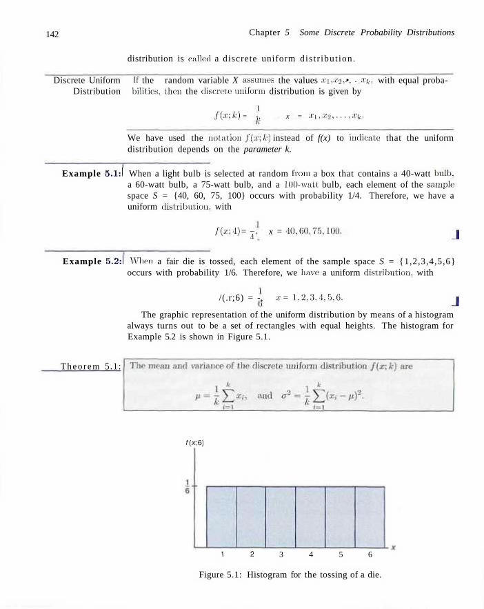
142 Chapter 5 Some Discrete Probability Distributions
distribution is called a discrete uniform dis t r ibut ion.
Discrete Uniform If the random variable X assumes the values xi,x2.- •. • SEfc, with equal proba-Distribution bilities, them the discrete unil'orni distribution is given by
I f{.r;k) = -, x = Xi,X2,-.-,Xk-
We have used the notation f(x;k) instead of f(x) to indicate: that the uniform distribution depends on the parameter k.
Example 5.1:1 When a light bulb is selected at random from a box that contains a 40-watt bulb, a 60-watt bulb, a 75-watt bulb, and a 100-watt bulb, each element of the sample1
space S = {40, 60, 75, 100} occurs with probability 1/4. Therefore, we have a uniform distribution, with
f(x;4) = j , x = 40,60,75,100. j
Example 5.2:1 When a fair die is tossed, each element of the sample space S = {1,2,3,4,5,6} occurs with probability 1/6. Therefore, we have a uniform distribution, with
/(.r;6) = -, £ = 1,2,3,4,5,6. j
The graphic representation of the uniform distribution by means of a histogram always turns out to be a set of rectangles with equal heights. The histogram for Example 5.2 is shown in Figure 5.1.
Theorem 5.1:
f(x;6)
1 2 3 4 5 6
Figure 5.1: Histogram for the tossing of a die.
5.3 Binomial and Multinomial Distributions 143
Proof: By definition
P = E(X) = £ *</fa;*) = E f = £l>« i=i ;=i i=\
k k
a2 = E\(X - p.)2} = Yixi - H?fiXi;k) = i J > , - ')2' I i = l i = l - *
Example 5.3:1 Referring to Example 5.2, we find that
1 + 24-3 + 4 + 5 + 6 p = = 3.5
<r2 = i [ ( l - 3 . 5 ) 2 + ( 2 - 3 . 5 ) 2 + . - . + ( 6 - 3 . 5 ) 2 ] = = i ^ = | = 2.92. j
5.3 Binomial and Multinomial Distributions
An experiment often consists of repeated trials, each with two possible outcomes that may be labeled success or failure. The most obvious application deals with the testing of items as they come off an assembly line, where each test or trial may indicate a defective or a nondefective item. We may choose to define either outcome as a success. The process is referred to as a Bernoul l i process. Each trial is called a Bernoull i trial . Observe, for example, if one were drawing cards from a deck, the probabilities for repeated trials change if the cards are not replaced. That, is, the probability of selecting a heart, on the first draw is 1/4, but on the second draw it is a conditional probability having a value of 13/51 or 12/51, depending on whether a heart appeared on the first draw: this, then, would no longer be considered a set of Bernoulli trials.
The Bernoulli Process
Strictly speaking, the Bernoulli process must possess the following properties:
1. The experiment consists of n repeated trials.
2. Each trial results in an outcome that may be classified as a. success or a failure.
3. The probability of success, denoted by p, remains constant from trial to trial.
4. The repeated trials arc independent.
Consider the set of Bernoulli trials where three items are selected at random from a manufacturing process, inspected, and classified as defective or nondefective. A defective item is designated a success. The number of successes is a random variable X assuming integral values from zero through 3. The eight possible outcomes and the corresponding values of X are
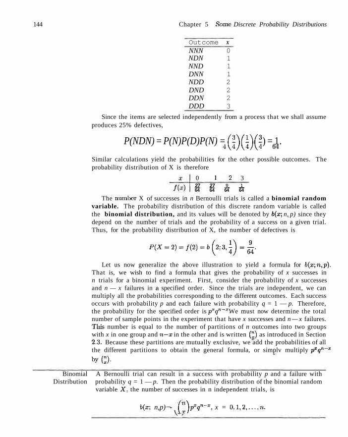
144 Chapter 5 Some Discrete Probability Distributions
Outcome NNN NDN NND DNN NDD DND DDN DDD
X
0 1 1 1 2 2 2 3
Since the items are selected independently from a process that we shall assume produces 25% defectives,
P(NDN) = P(N)P(D)P(N) = (?) ( J ) (f ) = 1.
Similar calculations yield the probabilities for the other possible outcomes. The probability distribution of X is therefore
0 1 2 3 27 27 JL J_ 64 64 64 64
The number X of successes in n Bernoulli trials is called a binomial random variable. The probability distribution of this discrete random variable is called the binomial distribution, and its values will be denoted by b(x; n, p) since they depend on the number of trials and the probability of a success on a given trial. Thus, for the probability distribution of X, the number of defectives is
P ( * - 2 ) - / ( 2 ) - 6 ( 2 ; 3 , i ) - £ .
Let us now generalize the above illustration to yield a formula for b(x;n,p). That is, we wish to find a formula that gives the probability of x successes in n trials for a binomial experiment. First, consider the probability of x successes and n — x failures in a specified order. Since the trials are independent, we can multiply all the probabilities corresponding to the different outcomes. Each success occurs with probability p and each failure with probability q = 1 — p. Therefore, the probability for the specified order is pxqn~x. We must now determine the total number of sample points in the experiment that have x successes and n — x failures. This number is equal to the number of partitions of n outcomes into two groups with x in one group and n—x in the other and is written (") as introduced in Section 2.3. Because these partitions are mutually exclusive, we add the probabilities of all the different partitions to obtain the general formula, or simplv multiply pxqn~x
by(" ) -
Binomial A Bernoulli trial can result in a success with probability p and a failure with Distribution probability q = 1 — p. Then the probability distribution of the binomial random
variable X, the number of successes in n independent trials, is
b(x; n,p) - (]pxqn~x, x = 0,1,2,. . . ,n.
5.3 Binomial and Multinomial Distributions
Note that when n = 3 and p = 1/1, the probability distribution of X, the number of defectives, may be written as
M*;3.41=$ a m r , «-o...«. rather than in the tabular form on page 144.
Example 5.4:1 The probability that a certain kind of component will survive a shoe:k test is 3/4. Find the probability that exactly 2 of the next. 4 components tested survive.
Solution: Assuming that the: tests are independent and -p = 3/4 for each of the 4 tests, we obtain
2 1 4 / \ 4 / V2! 2! / \4.4J 128
Where Does the Name Binomial Come From?
The binomial distribution derives its name from the fact that, the u + 1 terms in the binomial expansion of (q+p)n correspond to the various values of b(x;n, p) for ar = 0 , l , 2 , . . . , n . That is,
= b[(): n, p) + b( I; n, p) + b(2; n, p) + • • • + (>(n: n, p).
Sinc:c: p -|- q = 1, we sec that
Tl
Ybix\n,p)= I. 1 = 0
a condition that must hold for any probability distribution. Frequently, we are interested in problems where it is necessary to find P(X < r)
or P(a < X < b). Fortunately, binomial sums
/• B(i-,n,p) = Ybi:'"-n-P)
.r=(J
are available and are given Table A.l of the Appendix for n = 1,2,..., 20, and selected values of/; from 0.1 to 0.9. We illustrate the use of Table A.l with the following example.
Example 5.5:1 The probability that a. patient recovers from a rare blood disease is 0.4. If 15 people are known to have contracted this disease, what is the probability that (a) at least 10 survive, (b) from 3 to 8 survive, and (c) exactly 5 survive?
146 Chapter 5 Some Discrete Probability Distributions
Solution: Let X be the number of people that survive.
9
(a) P(X > 10) = 1 - P(X < 10) = 1 - Y bix' 15> °-4) = l ~ ° '9 6 6 2
x=0
= 0.0338 8 8 2
(b) P(3 < X < 8) = Y bix>15< °-4) = Y, 6(x; 15' °'4) ~ S *(*'15' °'4) x=3 *=() x=0
= 0.9050 - 0.0271 = 0.8779 5 4
(c) P(X = 5) = 6(5; 15,0.4) = ]T] b(x\ 15,0.4) - ^ b(x\ 15,0.4) x=0 x=0
= 0.4032-0.2173 = 0.1859 J
Example 5.6:1 A large chain retailer purchases a certain kind of electronic device from a manufacturer. The manufacturer indicates that the defective rate of the device is 3%.
(a) The inspector of the retailer randomly picks 20 items from a shipment. What is the probability that there will be at least one defective item among these 20?
(b) Suppose that the retailer receives 10 shipments in a month and the inspector randomly tests 20 devices per shipment. What is the probability that there will be 3 shipments containing at least one defective device?
Solution: (a) Denote by X the number of defective devices among the 20. This X follows a 6(x;20,0.03) distribution. Hence
P(X > 1) = 1 - P(X = 0) = 1 - 6(0; 20,0.03)
= 1 - 0.03°(1 - 0.03)20-0 = 0.4562.
(b) In this case, each shipment can either contain at least one defective item or not. Hence, testing the result of each shipment can be viewed as a Bernoulli trial with p = 0.4562 from part (a). Assuming the independence from shipment to shipment and denoting by Y the number of shipments containing at least one defective item Y follows another binomial distribution b(y; 10,0.4562). Therefore, the answer to this question is
= » = ( > P(Y = 3) = 0.4562J(1 - 0.4562)7 = 0.1602
Areas of Application
From Examples 5.4, 5.5, and 5.6, it should be clear that the binomial distribution finds applications in many scientific fields. An industrial engineer is keenly interested in the "proportion defective" in an industrial process. Often, quality control measures and sampling schemes for processes are based on the binomial distribution. The binomial applies for any industrial situation where an outcome of a process is dichotomous and the results of the process are independent, with
5.3 Binomial and Multinomial Distributions 147
the probability of a success being constant from trial to trial. The binomial distribution is also used extensively for medical and military applications. In both cases, a success or failure result is important. For example, "cure" or "no cure" is important in pharmaceutical work, while "hit" or "miss" is often the interpretation of the result of firing a guided missile.
Since the probability distribution of any binomial random variable depends only on the values assumed by the parameters n, p, and q, it would seem reasonable to assume that the mean and variance of a binomial random variable also depend on the values assumed by these parameters. Indeed, this is true, and in Theorem 5.2 we derive general formulas as functions of n, p. and q that can be used to compute the mean and variance of any binomial random variable.
Theorem 5.2: The mean and variance of the binomial distribution b(x;n,p) are
p — np, and a2 = npq.
Proof: Let the outcome on the j th trial be represented by a Bernoulli random variable Ij, which assumes the values 0 and 1 with probabilities q and p, respectively. Therefore, in a binomial experiment the number of successes can be written as the sum of the n independent indicator variables. Hence
X = h+h + ••• + / „ .
The mean of any Ij is E(Ij) = (0)(ey) + (l)(p) = P- Therefore, using Corollary 4.4, the mean of the binomial distribution is
p = E(X) = E(h) + E(I2) + ••• + E(In ) = p + p + - - - + p = np.
n terms
The variance of any Ij is
o\ = EKlj - p)2} = E(I2) -p2 = (0)2(q) + (l)2(p) - p2 = p(l - p ) = pq.
By extending Corollary 4.10 to the case of n independent variables, the variance of the binomial distribution is
ax - °"2, + °~\ + • • • + CT/„ =pq + pq + ---+pq= npq.
n terms J
Example 5.7:1 Find the mean and variance of the binomial random variable of Example 5.5, and then use Chebyshev's theorem (on page 132) to interpret the interval p ± 2o.
Solution: Since Example 5.5 was a binomial experiment with n = 15 and p = 0.4, by Theorem 5.2, we have
p = (15)(0.4) = 6, and er2 = (15)(0.4)(0.6) = 3.6.
Taking the square root of 3.6, we find that a — 1.897. Hence the required interval is 6±(2)(1.897), or from 2.206 to 9.794. Chebyshev's theorem states that the number
148 Chapter 5 Some Discrete Probability Distributions
of recoveries among 15 patients subjected to the given disease has a probability of at least 3/4 of falling between 2.206 and 9.794, or, because the data are discrete, between 3 and 9 inclusive. J
Example 5.8:1 It is conjectured that an impurity exists in 30% of all drinking wells in a certain rural community. In order to gain some insight on this problem, it is determined that some tests should be made. It is too expensive to test all of the many wells in the area, so 10 were randomly selected for testing.
(a) Using the binomial distribution, what is the probability that exactly three wells have the impurity assuming that the conjecture is correct?
(b) What is the probability that more than three wells are impure?
Solution: (a) We require
6(3; 10,0.3) = P(X = 3) = Y bix-10' °-3) ~ £ bix'10^ °-3) •i.—O x=0
= 0.6496 - 0.3828 = 0.2668.
(b) In this case wc need P(X > 3) = 1 - 0.6496 = 0.3504. J
There are solutions in which the computation of binomial probabilities may allow us to draw inference about a scientific population after data are collected. An illustration is given in the next example.
Example 5.9:1 Consider the situation of Example 5.8. The "30% arc impure" is merely a conjecture put forth by the area water board. Suppose 10 wells are randomly selected and 6 are found to contain the impurity. What does this imply about the conjecture? Use a probability statement.
Solution: We must first ask: "If the conjecture is correct, is it likely that we could have found 6 or more impure wells?"
10 5
P(X > 6) = Y bix> 10< °'3) ~ £ 2 b(:,;; 10' °'3) = 1 ~ ° ' 9 5 2 7 = °-0473-:r=0 X=0
As a result, it is very unlikely (4.7% chance) that 6 or more wells would be found impure if only 30% of all are impure. This casts considerable doubt on the conjecture and suggests that the impurity problem is much more severe. J
As the reader should realize by now, in many applications there are more than two possible outcomes. To borrow an example from the field of genetics, the color of guinea pigs produced as offspring may be red. black, or white. Often the "defective" or "not defective" dichotomy in engineering situations is truly an oversimplification. Indeed, there are often more than two categories that characterize items or parts coming off an assembly line.
Multinomial Experiments
The binomial experiment becomes a multinomial experiment if we let each trial have more than 2 possible outcomes. Hence the classification of a manufactured product as being light, heavy, or acceptable and the recording of accidents at a
5.3 Binomial and Multinomial Distributions 149
certain intersection according to the day of the week constitute multinomial experiments. The drawing of a card from a deck with replacement is also a multinomial experiment if the 4 suits are the outcomes of interest.
In general, if a given trial can result in any one of k possible outcomes E\, E2, •. •, Ek with probabilities p\,p2-,- • • -.Pk, then the multinomial distribution will give the probability that E\ occurs x\ times, E2 occurs x2 times, . . . , and Ek occurs 2,-fc times in n independent trials, where
X\ + x2 -\ + Xk = n.
We shall denote this joint probability distribution by
f(xi, x2, ...,xk;pi,p2,...,pk, n).
Clearly, p\ + p2 + • • • + Pk = 1 > since the result of each trial must be one of the k possible outcomes.
General Form for Multinomial Probabilities
To derive the general formula, we proceed as in the binomial case. Since the trials are independent, any specified order yielding x\ outcomes for E\, x2 for E2,. ..,Xk for Ek will occur with probability pXlp2
2 • • -p^". The total number of orders yielding similar outcomes for the n trials is equal to the number of partitions of n items into k groups with X\ in the first group; x2 in the second group,.. . ; and Xk in the Arth group. This can be done in
n
vTi, X2, .... XkJ XX\ X2\ • • • .Tfc! ways. Since all the partitions are mutually exclusive and occur with equal probability, we obtain the multinomial distribution by multiplying the probability for a specified order by the total number of partitions.
Multinomial If a given trial can result in the k outcomes Ei,E2,... ,Ek with probabili-Distribution ties p\,p2,... ,pk, then the probability distribution of the random variables
X\,X2, • • •,Xk, representing the number of occurrences for E\,E2,..., Ek in n independent trials is
f(x1,x2,...,xk\Pi,P2,...,Pk,n) - f ' jPi'pf2•••?**> \Xl,X2,...,XkJ
with
k k
/]xj = n, and / J Pi = 1. i=l t = l
The multinomial distribution derives its name from the fact that the terms of the multinomial expansion of (pi +p2+ • • •+Pfc)n correspond to all the possible values Of f(x\,X2, . . . ,Xk\P\,P2: • • • ,Pk,n).
Example 5.10:1 The complexity of arrivals and departures into an airport are such that computer simulation is often used to model the "ideal" conditions. For a certain airport
150 Chapter 5 Some Discrete Probability Distributions
containing three runways it is known that in the ideal setting the following are the: probabilities that the individual runways arc accessed by a randomly arriving commercial jet:
Runway 1: p\ = 2 /9 , Runway 2: p2 = 1/6, Runway 3: y;;j = 11/18.
Wha t is the probability that 6 randomly arriving airplanes arc distributed in the following fashion?
Runway 1: 2 airplanes, Runway 2: 1 airplane, Runway 3: 3 airplanes
Solution: Using the multinomial distribution, we have
fl 2,1,3^,1,^6 9 ' 6 18 '
Exercises
A' -) -2,\,3) \9J \GJ \IS
6! 22 1 l l 3 2!1!3! 92 6 183 = 0.1127.
5.1 An employee is selected from a staff of 10 to supervise a certain project by selecting a tag at random from a box containing 10 tags numbered from 1 to 10. Find the formula for the probability distribution of X representing the number on the tag that, is drawn. What is the probability that the number drawn is less than 4?
5.2 Twelve people: are given two identical speakers to listen to for differences, if any. Suppose that these people answered by guessing only. Find the probability that three people claim to have heard a difference between the two speakers.
5.3 Find the mean and variance of the random variable A' of Exercise 5.1.
5.4 In a certain city district the need for money to buy drugs is stated as the: reason for 75% of all thefts. Find the probability that among the next 5 theft cases reported in this district, (a) exactly 2 resulted from the need for money to buy
drugs; (b) at most 3 resulled from the need for money to buy
drugs.
5.5 According to Chemical Engineermi/ Progress (Nov. 1990), approximately 30% of all pipework failures in chemical plants are caused by operator error. (a) What is the probability that out of the next 20
pipework failures at least 10 are due to operator error?
(b) What is the probability that no more than 4 out of 20 such failures are due to operator error?
(c) Suppose, for a particular plant, that, out of the random sample of 20 such failures, exactly 5 are operational errors. Do you feel that the 30% figure stated above applies to this plant? Comment.
5.6 .According to a survey by the Administrative Management Society, one-half of U.S. companies give employees 4 weeks of vacation after they have been with the company for 15 years. Find the probability that among G companies surveyed at random, the number that give employees 4 weeks of vacation after 15 years of employment is
(a) anywhere from 2 to 5; (b) fewer than 3.
5.7 One prominent physician claims that 70% of those with lung cancer are chain smokers. If his assertion is correct, (a) find the: probability that of 10 such patients re
cently admitted to a hospital, fewer than half are chain smokers:
(b) find the probability that of 20 such patients recently admitted to a hospital, fewer than half are chain smokers.
5.8 According to a study published by a group of University of Massachusetts sociologists, approximately 60% of the Valium users in the state of Massachusetts
Exercises 151
first took Valium for psychological problems. Find the probability that among the next 8 users interviewed from this state,
(a) exactly 3 began taking Valium for psychological problems;
(b) at least 5 began taking Valium for problems that were not psychological.
5.9 In testing a certain kind of truck tire over a rugged terrain, it is found that 25% of the trucks fail to complete the test run without a blowout. Of the next 15 trucks tested, find the probability that
(a) from 3 to 6 have blowouts; (b) fewer than 4 have blowouts: (c) more than 5 have blowouts.
5.10 A nationwide survey of seniors by the University of Michigan reveals that almost 70% disapprove of daily pot smoking, according to a report in Parade. If 12 seniors are selected at random and asked their opinion, find the probability that the number who disapprove of smoking pot daily is
(a) anywhere from 7 to 9: (b) at most 5; (c) not less than 8.
5.11 The probability that a patient recovers from a delicate heart operation is 0.9. What is the probability that exactly 5 of the next 7 patients having this operation survive?
5.12 A traffic control engineer reports that. 75% of the vehicles passing through a checkpoint are from within the state. What is the probability that fewer than 4 of the next 9 vehicles arc from out of state?
5.13 A study examined national attitudes about antidepressants. The study revealed that approximately 70% believe "antidepressants do not really cure anything, they just cover up the real trouble." According to this study, what is the probability that at least 3 of the next 5 people selected at random will be of this opinion?
5.14 It is known that the percentage of wins for the Chicago Bulls basketball team going into the playoffs for the 1996-97 season was 87.7. Round the 87.7 to 90 in order to use Table A.l.
(a) What is the probability that the Bulls will sweep (4-0) in the initial best-of-7 playoff series?
(b) What is the probability that the Bulls would tain the initial best-of-7 playoff series?
(c) What very important assumption is made for answering parts (a) and (b)?
5.15 It is known that 60% of mice inoculated with a serum are protected from a certain disease. If 5 mice are inoculated, find the probability that (a) none contracts the disease;
(b) fewer than 2 contract the disease; (c) more than 3 contract the disease.
5.16 Suppose that airplane engines operate independently and fail with probability equal to 0.4. Assuming that a plane makes a safe flight if at least one-half of its engines run, determine whether a 4-engine plane or a 2-engine plane has the higher probability- for a successful flight.
5.17 If X represents the number of people in Exercise 5.13 who believe that antidepressants do not cure but only cover up the real problem, find the mean and variance of X when 5 people are selected at random and then use Chebyshev's theorem to interpret the interval /j. ±2 a.
5.18 (a) In Exercise 5.9, how many of the 15 trucks would you expect to have blowouts?
(b) According to Chebyshev's theorem, there is a probability of at least 3/4 that the number of trucks among the next 15 that have blowouts will fall in what interval?
5.19 As a student drives to school, he encounters a traffic signal. This traffic signal stays green for 35 seconds, yellow for 5 seconds, and red for 60 seconds. Assume that the student goes to school each weekday between 8:00 and 8:30. Let A'i be the number of times he encounters a green light, X2 be the number of times he encounters a yellow light, and X;i be the number of times he encounters a red light. Find the joint distribution of Xi , Xa, and X3.
5.20 According to USA Today (March 18,1997), of 4 million workers in the general workforce, 0.8% tested positive for drugs. Of those testing positive, 22.5% were cocaine users and 54.4% marijuana users.
(a) What is the probability that of 10 workers testing positive, 2 are cocaine users, 0 marijuana users, and 3 users of other drugs?
(b) What is the probability that of 10 workers testing positive, all are marijuana users?
(c) What is the probability that of 10 workers testing positive, none are cocaine users?
5.21 The surface of a circular dart board has a small center circle called the bull's-eye and 20 pie-shaped regions numbered from 1 to 20. Each of the pioshaped regions is further divided into three parts such that a
152 Chapter 5 Some Discrete Probability Distributions
person throwing a dart that lands on a specified number scores the value of the number, double the number, or triple the number, depending on which of the three parts the dart falls. If a pe:rson hits the bull's-eye with probability 0.01. hits a double with probability 0.10, hits a triple with probability 0.05, and misses the dart, board with probability 0.02, what is the probability that 7 throws will result in no bull's-eyes, no triples, a double twice, and a complete miss once?
5.22 According to a genetics theory, a certain cross of guinea pigs will result in red, black, and white offspring in the ratio 8:4:4. Find the probability that among 8 offspring 5 will be red, 2 black, and I white.
5.23 The probabilities are 0.4, 0.2, 0.3, and 0.1, respectively, that a delegate to a certain convention arrived by air, bus. automobile, or train. What is the probability that among 9 delegates randomly selected at this convention, 3 arrived by air, 3 arrived by bus, 1 arrived by automobile, and 2 arrived by train?
5.24 A safety engineer claims that only 40% of all workers wear safety helmets when they eat lunch at the workplace. Assuming that his claim is right, find the probability that 4 of 6 workers randomly chosen will be wearing their helmets while having lunch at the workplace.
5.25 Suppose that for a very large shipment of integrated-circuit chips, the probability of failure for any one chip is 0.10. Assuming that the assumptions
underlying the binomial distributions are met, find the probability that at most 3 chips fail in a random sample1
of 20.
5.26 Assuming that 6 in 10 automobile accidents are due mainly to a speed violation, find the probability that, among 8 automobile accidents 6 will be due mainly to a speed violation
(a) by using the formula for the binomial distribution;
(b) by using the binomial table.
5.27 If the probability that a fluorescent light has a useful life of at least 800 hours is 0.9, find the probabilities that among 20 such lights
(a) exactly 18 will have a useful life of at least 800 hours;
(b) at. least 15 will have a useful life of at least 800 hours;
(c) at least 2 will not have a useful life of at least 800 hours.
5.28 A manufacturer knows that on the average 20% of the elect ric toasters which lie makes will require repairs within 1 year after they are sold. When 20 toasters are randomly selected, find appropriate numbers x and y such that
(a) the probability that at least x of them will require repairs is less than 0.5;
(b) the probability that at least y of them will not require repairs is greater than 0.8.
5.4 Hypergeometric Distribution
The simplest way to view the distinction between the binomial distribution of Section 5.3 and the hypergeometric distribution lies in the way the sampling is clone. The types of applications of the hypergeometric arc very similar to those of the binomial distribution. We are interested in computing probabilities for the number of observations that fall into a particular category. But in the case of the binomial, independence among trials is required. As a result, if the binomial is applied to. say, sampling from a lot of items (deck of cards, batch of production items), the sampling must be clone w i t h r e p l a c e m e n t of each item after it is observed. On the other hand, flic hypergeometric distribution does not require independence and is based on the: sampling done w i t h o u t r e p l a c e m e n t .
Applications for the hypergeometric distribution are found in many areas, with heavy uses in acceptance sampling, electronic testing, and quality assurance. Obviously, for many of these fields testing is done at the expense of the item being tested. That is, the item is destroyed and hence cannot be replaced in the sample. Thus sampling without replacement is necessary. A simple example: with playing cards will serve as our first illustration.
If we wish to find the: probability of observing 3 red cards in 5 draws from an
5.4 Hypergeometric Distribution 153
ordinary deck of 52 playing cards, the binomial distribution of Section 5.3 does not apply unless each card is replaced and the deck reshuffled before the next drawing-is made. To solve the problem of sampling without replacement, let. us restate the problem. If 5 cards are drawn at random, we are interested in the probability of selecting 3 red cards from the 26 available and 2 black cards from the 26 black cards available in the deck. There are (23
<i) ways of selecting 3 red cards, and for each of these ways wc can choose 2 black cards in (2
26) ways. Therefore, the total
number of ways to select 3 red and 2 black cards in 5 draws is the product (23e) (2^).
The total number of ways to select any 5 cards from the 52 that are available is (°5
2). Hence the probability of selecting 5 cards without replacement of which 3 are red and 2 are black is given by
(23i)(22'
i) _ (261/3123!)(26!/2! 24!) = Q ^ (<*) 521/5! 47!
In general, we are interested in the probability of selecting x successes from the A" items labeled successes and n — x failures from the Ar — k items labeled failures when a random sample of size n is selected from AT items. This is known as a hypergeometric experiment, that is, one that possesses the following two properties:
1. A random sample of size n is selected without replacement from N items.
2. k of the Ar items may be classified as successes and N — k are classified as failures.
The number X of successes of a hypergeometric experiment is called a hypergeometric random variable. Accordingly, the probability distribution of the hypergeometric variable is called the hypergeometric distribution, and its values will be denoted by h(x; N, n, A:), since they depend on the number of successes k in the set N from which we select n items.
Hypergeometric Distribution In Acceptance Sampling
As in the case of the binomial distribution, the hypergeometric distribution finds applications in acceptance sampling where lots of material or parts are sampled in order to determine whether or not the entire lot is accepted.
Example 5.11:1 A particular part that is used as an injection device is sold in lots of 10. The producer feels that the lot is deemed acceptable if no more than one defective is in the lot. Some lots are sampled and the sampling plan involves random sampling and testing 3 of the parts out of 10. If none of the 3 is defective, the lot is accepted. Comment on the utility of this plan.
Solution: Let us assume that the lot is truly unacceptable (i.e., that 2 out of 10 are defective). The probability that our sampling plan finds the lot acceptable is
(olffl P(X = 0) = - ^ f - = 0.467.

154 Chapter 5 Some Discrete Probability Distributions
Thus, if the lot is truly unacceptable with 2 defective parts, this sampling plan will allow acceptance roughly 47% of the time. As a result, this plan should be considered faulty. J
Let us now generalize in order to find a formula for h(x;N,ti,k). The total number of samples of size n chosen from A7 items is (*J(). These samples are assumed to be equally likely. There are (£) ways of selecting x successes from the A* that are available, and for each of these ways we can choose the n — x failures in (*V-*) w ay s > Thus the total number of favorable samples among the (*') possible samples is given by (*) ( „ r* ) ' Hence we have the following definition.
Hypergeometric The probability distribution of the hypergeometric random variable X, the Distribution number of successes in a random sample of size n selected from Ar items of
which k are labeled success and N — k labeled failure, is
h(x; N, n, k) = )£~x , max{0, n - (N - k)} <x< min{n, k}. \n)
The range of x can be determined by the three binomial coefficients in the definition, where x and n — x are no more than k and AT — A:, respectively; and both of them cannot be less than 0. Usually, when both k (the number of successes) and Ar - k (the number of failures) are larger than the sample size n, the range of a hypergeometric random variable will be x = 0 , 1 , . . . ,n.
Example 5.12:1 Lots of 40 components each are called unacceptable if they contain as many as 3 defectives or more. The procedure for sampling the lot is to select 5 components at random and to reject the lot if a defective is found. What is the probability that exactly 1 defective is found in the sample if there are 3 defectives in the entire lot?
Solution: Using the hypergeometric distribution with n = 5, N = 40, k — 3, and x = 1, we find the probability of obtaining one defective to be
(DCY) (?) / i ( l ;40,5,3)= V.IQX =0.3011.
Once again this plan is likely not desirable since it detects a bad lot (3 defectives)
only about 30% of the time. -I
Theorem 5.3: The mean and variance of the hypergeometric distribution h(x; N, n, A;) are
nk , 9 N — n k / k\ p = - , and ex = J^-J • n • - ( l - - j .
The proof for the mean is shown in Appendix A.25.
Example 5.13:1 Let us now reinvestigate Example 3.9. The purpose of this example was to illustrate the notion of a random variable and the corresponding sample space. In the example, we have a lot of 100 items of which 12 are defective. What is the probability that in a sample of 10, 3 are defective?
5.4 Hypergeometric Distribution 155
Solution: Using the hypergeometric probability function we have
/i(3; 100,10,12) = ±% ($(7) C)
0.08.
Example 5.14:1 Find the mean and variance of the random variable of Example 5.12 and then use Chebyshev's theorem to interpret the interval //. ± 2er.
Solution: Since Example 5.12 was a hypergeometric experiment, with Ar = 40, u = 5, and k = 3, then by Theorem 5.3 we have
• ( 5 ) ( 3 ) = ? =0.375. 40
and
er2 = 40
39 v l v - h ) " " •
Taking the square root of 0.3113, we find that a = 0.558. Hence the required interval is 0.375 ± (2)(0.558), or from -0.741 to 1.491. Chebyshev's theorem states that the number of defectives obtained when 5 components are selected at random from a lot of 40 components of which 3 are defective has a probability of at least 3/4 of falling between —0.741 and 1.491. That is, at, least three-fourths of
the time, the 5 components include: less than 2 defectives. J
Relationship to the Binomial Distribution
In this chapter wc discuss several important discrete distributions that have wide applicability. Many of these distributions relate nicely to each other. The beginning student should gain a clear understanding of these relationships. There is an interesting relationship between the: hypergeometric and the binomial distribution. As one might expect, if n is small compared to N, the nature of the N items changes very little in each draw. So a binomial distribution can be used to approximate the hypergeometric distribution when n is small, compared to N. In fact, as a rule of thumb the approximation is good when jq < 0.05.
Thus the quantity £ plays the role of the binomial parameter p. As a result, the binomial distribution may be viewed as a large population edition of the hypergeometric: distributions. The mean and variance then come from the formulas
n-p nk k
C T - = ? ? w = n . _ M _ _
Comparing those formulas with those of Theorem 5.3, we see that the mean is the same whereas the variance differs by a correction factor of (N — n)/(N — 1), which is negligible when n is small relative to AT.
Example 5.15:1 A manufacturer of automobile tires reports that among a shipment of 5000 sent to a local distributor, 1000 are slightly blemished. If one purchases 10 of these tires at random from the distributor, what, is the probability that exactly 3 are blemished?
156 Chapter 5 Some Discrete Probability Distributions
Solution: Since N = 5000 is large relative to the sample size n = 10, we shall approximate the desired probability by using the binomial distribution. The probability of obtaining a blemished tire is 0.2. Therefore, the probability of obtaining exactly 3 blemished tires is
3 2
h(3; 5000,10,1000) « &(3; 10.0.2) = Y b(x\ 1[}; °-
2) - Y b^x'-10' °'2) x=0 x=0
= 0.8791-0.6778 = 0.2013.
On the other hand, the exact probability is /?(3; 5000,10.1000) = 0.2015. J The hypergeometric distribution can be extended to treat the case where the
N items can be partitioned into A: cells A\, A2, ...,Ak with ciy elements in the first cell, a2 elements in the second cell Uk elements in the feth cell. We are now interested in the: probability that a random sample of size n yields Xi elements from A\, X2 elements from A2, . . . , and Xk elements from Ak- Let us represent this probability by
f(xi. x-2, Xk: fl] ,fto Ofc, N, n).
To obtain a general formula, we note that the total number of samples that can be chosen of size n from N items is still f ). There are (f
(M) ways of selecting
X\ items from the items in A\, and for each of these we can choose x2 items from the items in Ai in (°a) ways. Therefore, we can select x\ items from A\ and x2
items from A<> in ("')("2,) ways. Continuing in this way, we can select all n items consisting of X\ from Ax, x2 from A2,. . . , and Xk from Ai, in
ei] \ a2
xj \X2 ways.
The required probability distribution is now defined as follows.
Multivariate: If N items can be partitioned into the A: cells A], A2,..., Afc with at, a.2,..., ak
Hypergeometric elements, respectively, then the probability distribution of the random variables Distribution A*i,X2,..., X ,, representing the number of elements selected from A] ,A2,. • •, Ak
in a random sample' of size n, is
f(xi ,x2,.... Xk;ai , 02 , . . . ,Ofe,iV, n) = oc:)-!::)
k k with J2 xi = n and J^ a,- = A'.
1 = 1 ( = 1
Example 5.16:1 A group of 10 individuals is used for a biological case study. The group contains 3 people with blood type O, 4 with blood type A, and 3 with blood type B. What is the probability that a random sample of 5 will contain I person with blood type O, 2 people with blood type A, and 2 people with blood type 13?
Exercises 157
Solution: Using the extension of the hypergeometric distribution with x\ = 1, x2 = 2, £3 = 2, aI = 3. (7,2 = 4, «3 = 3, iV = 10, and n = 5, we find t h a t the desired probabili ty is
/ ( l , 2 ,2 ; 3 , 4 , 3 , 1 0 , 5 ) : ('5°)
14
Exercises
5.29 If 7 cards are dealt from an ordinary deck of 52 playing cards, what is the probability that (a) exactly 2 of them will be face cards?
(b) at least 1 of them will be a queen?
5.30 To avoid detection at customs, a traveler places 6 narcotic tablets in a bottle containing 9 vitamin pills that are similar in appearance. If the customs official selects 3 of the tablets at random for analysis, what is the probability that the traveler will be arrested for illegal possession of narcotics?
5.31 A homeowner plants 6 bulbs selected at random from a box containing 5 tulip bulbs and 4 daffodil bulbs. What is the probability that he planted 2 daffodil bulbs and 4 tulip bulbs?
5.32 From a lot of 10 missiles, 4 are selected at random and fired. If the lot contains 3 defective missiles that will not fire, what is the probability that (a) all 4 will fire?
(b) at most 2 will not. fire?
5.33 A random committee of size 3 is selected from 4 doctors and 2 nurses. Write a formula for the probability distribution of the random variable X representing the number of doctors on the committee. Find P(2 < X < 3).
5.34 What is the probability that a waitress will refuse to serve alcoholic beverages to only 2 minors if she randomly checks the IDs of 5 students from among 9 students of which 4 arc not of legal age?
5.35 A company is interested in evaluating its current inspection procedure on shipments of 50 identical items. The procedure is to take a sample of 5 and pass the shipment if no more than 2 are found to be defective. What proportion of 20% defective shipments will be accepted?
5.36 A manufacturing company uses an acceptance scheme on production items before they are shipped. The plan is a two-stage one. Boxes of 25 are readied
for shipment and a sample of 3 is tested for defectives. If any defectives are found, the entire box is sent back for 100% screening. If no defectives are found, the box is shipped.
(a) What is the probability that a box containing 3 defectives will be shipped?
(b) What is the probability that a box containing only 1 defective will be sent back for screening?
5.37 Suppose that the manufacturing company of Exercise 5.36 decides to change its acceptance scheme. Under the new scheme an inspector takes one at random, inspects it, and then replaces it in the box; a second inspector does likewise. Finally, a third inspector goes through the same procedure. The box is not shipped if any of the three find a defective. Answer Exercise 5.36 under this new plan.
5.38 In Exercise 5.32, how many defective missiles might we expect to be included among the 4 that are selected? Use Chebyshev's theorem to describe the variability of the number of defective missiles included when 4 are selected from several lots each of size 10 containing 3 defective missiles.
5.39 If a person is dealt 13 cards from an ordinary deck of 52 playing cards several times, how many hearts per hand can he expect? Between what two values would you expect the number of hearts to fall at least 75% of the time?
5.40 It is estimated that 4000 of the 10,000 voting residents of a town are against a new sales tax. If 15 eligible voters are selected at random and asked their opinion, what is the probability that at most 7 favor the new tax?
5.41 An annexation suit is being considered against a county subdivision of 1200 residences by a neighboring city. If the occupants of half the residences object to being annexed, what is the probability that in a random sample of 10 at least 3 favor the annexation suit?
5.42 Among 150 IRS employees in a large city, only 30 are women. If 10 of the applicants are chosen at ran-
158 Chapter 5 Some Discrete Probability Distributions
elom to provide free: fax assistance for the residents of this city, use the binomial approximation to the hypergeometric to find the probability that at. least 3 women arc selected.
5.43 A nationwide survey of 17,000 seniors by the University of Michigan revealed that almost 70% disapprove of daily pot smoking. If 18 of these seniors are selected at random and asked their opinions, what is the probability that more than 9 but less than 14 disapprove of smoking pot?
5.44 Find the probability of being dealt a bridge hand of 13 cards containing 5 spades, 2 hearts. 3 diamonds, and 3 clubs.
5.45 A foreign student club lists as its members 2 Canadians, 3 Japanese, 5 Italians, and 2 Germans. If a committee of 4 is selected at random, find the probability that
(a) all nationalities are represented;
(b) all nationalities except the Italians are represented.
5.46 An urn contains 3 green balls, 2 blue balls, and 4 red balls. In a random sample: of 5 balls, find the probability that both bine balls and at. least 1 reel ball are selected.
5.47 Population studies of biology and the environment often tag and release subjects in order to estimate size and degree: of certain features in the population. Ten animals of a certain population thought to be extinct (or near extinction) are caught, tagged and released in a certain region. After a period of time a random sample of 15 of this type of animal is selected
in the region. What is the probability that 5 of those selected are tagged animals if there are 25 animals of this type in the region?
5.48 A large company has an inspection system for the batches of small compressors purchased from vendors. A batch typically contains 15 compressors. In the inspection system a random sample of 5 is selected and all are tested. Suppose there arc 2 faulty compressors in the batch of 15.
(a) What, is the probability that for a given sample there will be I faulty compressor?
(b) What, is the probability that inspection will discover both faulty compressors?
5.49 A government task force suspects that some manufacturing companies are in violation of federal pollution regulations with regard to dumping a certain type of product. Twenty firms are under suspicion but all cannot be inspected. Suppose that 3 of the firms are; in violation.
(a) What is the probability that inspection of 5 firms finds no violations?
(b) What is the probability that the plan above will find two violations?
5.50 Every hour, 10,000 cans of soda are filled by a machine, among which 300 underfilled cans are produced. Each hour a sample of 30 cans is randomly selected and the number of ounces of soda per can is checked. Denote: by A' the number of cans selected that are underfilled. Find the probability that at, least one underfilled can will be among those sampled.
5.5 Negative Binomial and Geometric Distributions
Let us consider an experiment where the properties are the same as those listed for a binomial experiment, with the exception that the trials will be repeated until a fixed number of successes occur. Therefore, instead of finding the probability of x successes in n trials, where n is fixed, we are now interested in the probability that, the A'th success occurs on the- .rth trial. Experiments of this kind are called n e g a t i v e b i n o m i a l e x p e r i m e n t s .
As an illustration, consider the use of a drug that is known to be effective in 60% of the cases where it is used. The use of the drug will be considered a success if it is effective in bringing some degree of relief to the patient. We are interested in finding the probability that, the fifth patient to experience relief is the seventh patient, to receive the drug during a given week. Designating a success by S and a failure by F, a possible order of achieving the desired result is SFSSSFS, which occurs with probability
(0.6)(0.4)(0.6)(0.6)(0.6)(0.4)(0.6) = (0.6)r)(0,l)
5.5 Negative Binomial and Geometric Distributions 159
Wc could list all possible orders by rearranging the F's and S's except for the last outcome, which must be the fifth success. The total number of possible orders is equal to the number of partitions of the first six trials into two groups with 2 failures assigned to the one group and the 4 successes assigned to the other group. This can be done in (®) = 15 mutually exclusive ways. Hence, if X represents the outcome on which the fifth success occurs, then
P(X = 7) - (J J (0.6)5(0.4)2 = 0.1866.
Wha t Is the Negative Binomial Random Variable?
The number X of trials to produce k successes in a negative binomial experiment is called a negative binomial random variable, and its probability distribution is called the negative binomial distribution. Since its probabilities depend on the number of successes desired and the probability of a success on a given trial, we shall denote them by the symbol b*(x;k,p). To obtain the general formula for b*(x;k,p), consider the probability of a success on the xtn trial preceded by A: — 1 successes and x — k failures in some specified order. Since the trials are independent, we can multiply all the probabilities corresponding to each desired outcome. Each success occurs with probability p and each failure with probability q = 1 — p. Therefore, the probability for the specified order ending in success is
pk~1qx~kp = pkqx~k.
The total number of sample points in the experiment ending in a success, after the occurrence of A: — 1 successes and x — k failures in any order, is equal to the number of partitions of a;— 1 trials into two groups with A:— 1 successes corresponding to one group and x — k failures corresponding to the other group. This number is specified by the term i^l\)-, each mutually exclusive and occurring with equal probability pkgX-k yre obtain the general formula by multiplying pkqx~k by (lZ])-
Negative If repeated independent trials can result in a success with probability p and a Binomial failure with probability ej —1—p, then the probability distribution of the random
Distribution variable X, the number of the trial on which the A:th success occurs, is
b*(x;k,p)= U I p V - * , x = k,k+l,k + 2,....
Example 5.17:1 In an NBA (National Basketball Association) championship series, the team who wins four games out. of seven will be the winner. Suppose that team A has probability 0.55 of winning over team B and both teams A and B face each other in the championship games.
(a) What is the probability that team A will win the series in six games?
(b) What is the probability that team A will win the series?
(c) If both teams face each other in a regional playoff series and the winner is decided by winning three out of five games, what is the probability that team A will win a playoff?
160 Chapter 5 Some Discrete Probability Distributions
Solution: (a) 6*(6;4,0.55) = (g)0.554(l - 0.55)G~4 = 0.1853.
(b) P(team A wins the championship series) is
b* (4; 4,0.55) + b* (5; 4,0.55) + b*(6; 4,0.55) + b"(7; 4,0.55)
= 0.0915 + 0.1647 + 0.1853 + 0.1668 = 0.6083.
(c) P(team A wins the playoff) is
b* (3; 3.0.55) + b" (4; 3,0.55) + b* (5; 3,0.55)
= 0.1664 + 0.2246 + 0.2021 = 0.5931. J
The negative binomial distribution derives its name from the fact that each term in the expansion of pk(l — q)~k corresponds to the values of b*(x;k,p) for x = A:, k + 1, k + 2, . . . . If we consider the special case of the negative binomial distribution where k — 1, we have a probability distribution for the number of trials required for a single success. An example would be the tossing of a coin until a head occurs. We might be interested in the probability that the first head occurs on the fourth toss. The negative binomial distribution reduces to the form
b*(x:l,p) = pqx-1, x= 1 ,2,3, . . . .
Since the successive terms constitute a geometric progression, it is customary to refer to this special case as the geometric distribution and denote its values by 9ix\p).
Geometric If repeated independent trials can result in a success with probability p and Distribution a failure with probability q = 1 — p, then the probability distribution of the
random variable X, the number of the trial on which the first success occurs, is
g(x;p)=pqx~\ x = 1,2,3,....
Example 5.18:1 In a certain manufacturing process it is known that, on the average, 1 in every 100 items is defective. What is the probability that the fifth item inspected is the first defective item found?
Solution: Using the geometric distribution with x — 5 and p — 0.01, we have
fl(5;0.01) = (0.01)(0.99)' = 0.0096. J
Example 5.19:1 At "busy time" a telephone exchange is very near capacity, so callers have difficulty placing their calls. It may be of interest to know the number of attempts necessary in order to gain a connection. Suppose that we let p = 0.05 be the probability of a connection during busy time. We are interested in knowing the probability that 5 attempts are necessary for a successful call.
Solution: Using the geometric distribution with x = 5 and p = 0.05 yields
P(X = x)= g(5:0.05) = (0.05)(0.95)4 = 0.041. J
Quite often, in applications dealing with the geometric distribution, the mean and variance are important. For example, in Example 5.19 the expected number
5.6 Poisson Distribution and the Poisson Process 161
of calls necessary to make a connection is quite important. The following states without proof the mean and variance of the geometric distribution.
Theorem 5.4: The are
mean and variance of a random variable following the geometric distribution
' 1 2 1 - P P P2
Applications of Negative Binomial and Geometric Distributions
Areas of application for the negative binomial and geometric distributions become obvious when one focuses on the examples in this section and the exercises devoted to these distributions at the end of Section 5.6. In the case of the geometric distribution, Example 5.19 depicts a situation where engineers or managers are attempting to determine how inefficient a telephone exchange system is during busy periods of time. Clearly in this case, trials occurring prior to a success represent a cost. If there is a high probability of several attempts prior to a connection, then plans should be made to redesign the system.
Applications of the negative binomial are similar in nature. Attempts are costly in some sense and they are occurring in sequence. A high probability of requiring a "large" number of attempts to experience a fixed number of successes is not beneficial to the scientist or engineer. Consider the scenarios of the Review Exercises 5.94 and 5.95. In Exercise 5.95 the oil driller defines a certain level of success from sequentially drilling locations for oil. If only six attempts have been made at the point where the second success is experienced, the profits appear to dominate substantially the investment incurred by the drilling.
5.6 Poisson Distribution and the Poisson Process
Experiments yielding numerical values of a random variable X, the number of outcomes occurring during a given time interval or in a specified region, are called Poisson experiments. The given time interval may be of any length, such as a minute, a day, a week, a month, or even a year. Hence a Poisson experiment can generate observations for the random variable X representing the number of telephone calls per hour received by an office, the number of days school is closed due to snow during the winter, or the number of postponed games due to rain during a baseball season. The specified region could be a line segment, an area, a volume, or perhaps a piece of material. In such instances X might represent the number of field mice per acre, the number of bacteria in a given culture, or the number of typing errors per page. A Poisson experiment is derived from the Poisson process and possesses the following properties:
Properties of Poisson Process 1. The number of outcomes occurring in one time interval or specified region is
independent of the number that occurs in any other disjoint time interval or region of space. In this way wc say that the Poisson process has no memory.
162 Chapter 5 Some Discrete Probability Distributions
2. The probability that a single outcome will occur during a very short time interval or in a small region is proportional to the length of the time interval or the size of the region and does not depend on the number of outcomes occurring outside this time interval or region.
3. The probability that more than one outcome will occur in such a short time interval or fall in such a small region is negligible.
The number X of outcomes occurring during a Poisson experiment is called a Poisson random variable, and its probability distribution is called the Poisson distribution. The mean number of outcomes is computed from p = Xt, where t is the specific "time," "distance," "area," or "volume" of interest. Since its probabilities depend on A, the rate of occurrence of outcomes, we shall denote them by the symbol p(x; Xt). The derivation of the formula for p(x; Xt), based on the three properties of a Poisson process listed above, is beyond the scope of this book. The following concept is used for computing Poisson probabilities.
Poisson The probability distribution of the Poisson random variable X, representing Distribution the number of outcomes occurring in a given time interval or specified region
denoted by t, is e~Xt(Xt)x
p(x;Xt) = x<
-, a: = 0,1,2,.
where A is the average number of outcomes per unit time, distance, area, or volume, and e = 2.71828 • • •.
Table A.2 contains Poisson probability sums
r
P(r;Xt) = Ypix'Xt)-x=0
for a few selected values of At ranging from 0.1 to 18. We illustrate the use of this table with the following two examples.
Example 5.20:1 During a laboratory experiment the average number of radioactive particles passing through a counter in 1 millisecond is 4. What is the probability that 6 particles enter the counter in a given millisecond?
Solution: Using the Poisson distribution with x = 6 and Xt = 4 and Table A.2, we have
e _ 44 6 6 5
p(6;4) = — — = Ypix'4) ~ Yp(x'-4^ = 0.8893-0.7851 = 0.1042. x=0 x=0
Example 5.21:1 Ten is the average number of oil tankers arriving each day at a certain port city. The facilities at the port can handle at most 15 tankers per day. What is the probability that on a given day tankers have to be turned away?
Solution: Let X be the number of tankers arriving each day. Then, using Table A.2, we have
ID
P(X > 15) = 1 - P(X < 15) = 1 - Ypix'> 10) = 1 - 0.9513 = 0.0487. x = 0
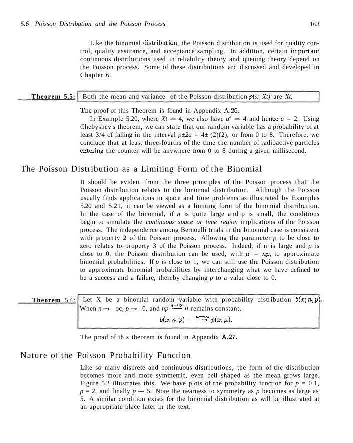
5.6 Poisson Distribution and the Poisson Process 163
Like the binomial distribution, the Poisson distribution is used for quality control, quality assurance, and acceptance sampling. In addition, certain important continuous distributions used in reliability theory and queuing theory depend on the Poisson process. Some of these distributions arc discussed and developed in Chapter 6.
Theorem 5.5: Both the mean and variance of the Poisson distribution p(x; Xt) are Xt.
The proof of this Theorem is found in Appendix A.26. In Example 5.20, where Xt — 4, we also have a2 — 4 and hence a = 2. Using
Chebyshev's theorem, we can state that our random variable has a probability of at least 3/4 of falling in the interval p±2a = 4± (2)(2), or from 0 to 8. Therefore, we conclude that at least three-fourths of the time the number of radioactive particles entering the counter will be anywhere from 0 to 8 during a given millisecond.
The Poisson Distribution as a Limiting Form of the Binomial
It should be evident from the three principles of the Poisson process that the Poisson distribution relates to the binomial distribution. Although the Poisson usually finds applications in space and time problems as illustrated by Examples 5.20 and 5.21, it can be viewed as a limiting form of the binomial distribution. In the case of the binomial, if n is quite large and p is small, the conditions begin to simulate the continuous space or time region implications of the Poisson process. The independence among Bernoulli trials in the binomial case is consistent with property 2 of the Poisson process. Allowing the parameter p to be close to zero relates to property 3 of the Poisson process. Indeed, if n is large and p is close to 0, the Poisson distribution can be used, with p = np, to approximate binomial probabilities. If p is close to 1, we can still use the Poisson distribution to approximate binomial probabilities by interchanging what we have defined to be a success and a failure, thereby changing p to a value close to 0.
Theorem 5.6: Let X be a binomial random variable with probability distribution b(x;n,p). When n —> oc, p —> 0, and np "—* p remains constant,
b(x\n,p) n=^>p(x;p).
The proof of this theorem is found in Appendix A.27.
Nature of the Poisson Probability Function Like so many discrete and continuous distributions, the form of the distribution becomes more and more symmetric, even bell shaped as the mean grows large. Figure 5.2 illustrates this. We have plots of the probability function for p = 0.1, p = 2, and finally p — 5. Note the nearness to symmetry as p becomes as large as 5. A similar condition exists for the binomial distribution as will be illustrated at an appropriate place later in the text.
164 Chapter 5 Some Discrete Probability Distributions
1.0
0.75
*. 0.5
0.25
a
/u = 0.1
0.30
0.20
0.10
0
M = 2
0.30
0.20
0.10
0
M = 5
0 2 4 6 8 1 0 0 2 4 6 8 1 0 0 2 4 6 8 1 0
Figure 5.2: Poisson density functions for different means.
Example 5.22:1 In a certain industrial facility accidents occur infrequently. It is known that the probability of an accident on any given day is 0.005 and accidents are independent of each other.
(a) What, is the probability that in any given period of 400 days there will be an accident on one day?
(b) What is the probability that there are at most three days with an accident?
Solution: Let. X be a binomial random variable with n = 400 and p = 0.005. Thus np = 2. Using the Poisson approximation,
(a) P(X = 1) = c—21 = 0.271. and 3
(b) P{X < 3) = £ c-'J2'7;c! = 0.857. . i=o J
Example 5.23:1 In a manufacturing process where glass products arc produced, defects or bubbles occur, occasionally rendering the piece undesirable: for marketing. It is known that, on average, 1 in every 1000 of these items produced has one or more bubbles. What is the probability that a random sample of 8000 will yield fewer than 7 items possessing bubbles?
Solution: This is essentially a binomial experiment with n = 8000 and /; = 0.001. Since p is very close to zero and n is quite large, we shall approximate with the Poisson distribution using
p= (800Q)(0.001) = 8.
Hence, if X represents the number of bubbles, we have
P(X < 7) = V & ( s ; 8000,0.001) «p(x ;8) = 0.3134 x=0
Exercises
Exercises
165
5.51 The probability that a person, living in a certain city, owns a dog is estimated to be 0.3. Find the probability that the tenth person randomly interviewed in that city is the fifth one to own a dog.
5.52 A scientist inoculates several mice, one at a time, with a disease germ until he finds 2 that have contracted the disease. If the probability of contracting the disease is 1/6, what is the probability that 8 mice are required?
5.53 An inventory study determines that, on average, demands for a particular item at a warehouse are made 5 times per day. What is the probability that on a given day this item is requested (a) more than 5 times?
(b) not at all?
5.54 Find the probability that a person flipping a coin gets (a) the third head on the seventh flip;
(b) the first head on the fourth flip.
5.55 Three people toss a fair coin and the odd man pays for coffee. If the coins all turn up the same, they are tossed again. Find the probability that fewer than 4 tosses are needed.
5.56 According to a study published by a group of University of Massachusetts sociologists, about two-thirds of the 20 million persons in this country who take Valium are women. Assuming this figure to be a valid estimate, find the probability that on a given day the fifth prescription written by a doctor for Valium is
(a) the first prescribing Valium for a woman;
(b) the third prescribing Valium for a woman.
5.57 The probability that a student pilot passes the written test for a private pilot's license is 0.7. Find the probability that the student will pass the test (a) on the third try; (b) before the fourth try.
5.58 On average a certain intersection results in 3 traffic accidents per month. What is the probability that for any given month at this intersection (a) exactly 5 accidents will occur? (b) less than 3 accidents will occur? (c) at least 2 accidents will occur?
5.59 A secretary makes 2 errors per page, on average. What is the probability that on the next page he or she will make
(a) 4 or more errors? (b) no errors?
5.60 A certain area of the eastern United States is, on average, hit by 6 hurricanes a year. Find the probability that for a given year that area will be hit by
(a) fewer than 4 hurricanes;
(b) anywhere from 6 to 8 hurricanes.
5.61 Suppose the probability is 0.8 that any given person will believe a tale about the transgressions of a famous actress. What is the probability that (a) the sixth person to hear this tale is the fourth one
to believe it? (b) the third person to hear this tale is the first one to
believe it?
5.62 The average number of field mice per acre in a 5-acre wheat field is estimated to be 12. Find the probability that fewer than 7 field mice are found (a) on a given acre; (b) on 2 of the next 3 acres inspected.
5.63 A restaurant chef prepares a tossed salad containing, on average, 5 vegetables. Find the probability that the salad contains more than 5 vegetables (a) on a given day; (b) on 3 of the next 4 days;
(c) for the first time in April on April 5.
5.64 The probability that a person will die from a certain respiratory infection is 0.002. Find the probability that fewer than 5 of the next 2000 so infected will die.
5.65 Suppose that, on average, 1 person in 1000 makes a numerical error in preparing his or her income tax return. If 10,000 forms are selected at random and examined, find the probability that 6, 7, or 8 of the forms contain an error.
5.66 The probability that a student fails the screening test for scoliosis (curvature of the spine) at a local high school is known to be 0.004. Of the next 1875 students who are screened for scoliosis, find the probability that
(a) fewer than 5 fail the test;
166 Chapter 5 Some Discrete Probability Distributions
(b) 8, 9, or 10 fail the test.
5.67 (a) Find the mean and variance in Exercise 5.64 of the random variable X representing the number of persons among 2000 that die from the respiratory infection.
(b) According to Chebyshev's theorem, there is a probability of at least 3/4 that the number of persons to die among 2000 persons infected will fall within what interval?
5.68 (a) Find the mean and variance in Exercise 5.65 of the random variable X representing the number of persons among 10,000 who make an error in preparing their income tax returns.
(b) According to Chebyshev's theorem, there is a probability of at least 8/9 that the number of persons who make errors in preparing their income tax returns among 10,000 returns will be within what interval?
5.69 An automobile manufacturer is concerned about a fault in the braking mechanism of a particular model. The fault can, on rare occasions, cause a catastrophe at high speed. The distribution of the number of cars per year that will experience the fault is a Poisson random variable with A = 5.
(a) What is the probability that at most 3 cars per year will experience a catastrophe?
(b) What is the probability that more than 1 car per year will experience a catastrophe?
5.70 Changes in airport procedures require considerable planning. Arrival rates of aircraft are important factors that must be taken into account. Suppose small aircraft arrive at a certain airport, according to a Poisson process, at the rate of 6 per hour. Thus the Poisson parameter for arrivals for a period of hours is p. = 6t.
(a) What is the probability that exactly 4 small aircraft arrive during a 1-hour period?
(b) What is the probability that at least 4 arrive during a 1-hour period?
(c) If we define a working day as 12 hours, what is the probability that at least 75 small aircraft arrive during a day?
5.71 The number of customers arriving per hour at a certain automobile service facility is assumed to follow a Poisson distribution with mean A = 7. (a) Compute the probability that more than 10 cus
tomers will arrive in a 2-hour period. (b) What is the mean number of arrivals during a 2-
hour period?
5.72 Consider Exercise 5.66. What is the mean number of students who fail the test?
5.73 The probability that a person dies when he contracts a virus infection is 0.001. Of the next 4000 so infected, what is the mean number that will die?
5.74 A company purchases large lots of a certain kind of electronic device. A method is used that rejects a lot if 2 or more defective units are found in a random sample of 100 units.
(a) What is the mean number of defective units found in a sample of 100 units if the lot is 1% defective?
(b) What is the variance?
5.75 In the case of a certain type of copper wire, it is known that, on the average, 1.5 flaws occur per millimeter. Assuming that the number of flaws is a Poisson random variable, what is the probability that no flaws occur in a certain portion of wire of length 5 millimeters? What is the mean number of flaws in a portion of length 5 millimeters?
5.76 Potholes on a highway can be a serious problem and are in constant need of repair. With a particular type of terrain and make of concrete, past experience suggests that there are, on the average, 2 potholes per mile after a certain amount of usage. It is assumed that the Poisson process applies to the random variable "number of potholes."
(a) What is the probability that no more than one pothole will appear in a section of one mile?
(b) What is the probability that no more than 4 pot holes will occur in a given section of 5 miles?
5.77 Hospital administrators in large cities anguish about problems with traffic in emergency rooms in hospitals. For a particular hospital in a large city, the staff on hand cannot accommodate the patient traffic if there are more than 10 emergency cases in a given hour. It is assumed that patient arrival follows a Poisson process and historical data suggest that, on the average, 5 emergencies arrive per hour. (a) What is the probability that in a given hour the
staff can no longer accommodate the traffic? (b) What is the probability that more than 20 emer
gencies arrive during a 3-hour shift of personnel?
5.78 In airport luggage screening it is known that 3% of people screened have questionable objects in their luggage. What is the probability that a string of 15 people pass through successfully before an individual is caught with a questionable object? What is the expected number in a row that pass through before an individual is stopped?
Review Exercises 167
5.79 Computer technology has produced an environment in which "robots" operate with the use of microprocessors. The probability that a robot fails during any 6 hour shift is 0.10. What is the probability that a robot will operate at most 5 shifts before it fails?
5.80 Refusal rate in telephone polls is known to be ap
proximately 20%. A newspaper report indicates that 50 people were interviewed before the first refusal. (a) Comment, on the validity of the report. Use a prob
ability in your argument. (b) What is the expected number of people interviewed
before a refusal?
Review Exercises
5.81 During a manufacturing process 15 units are randomly selected each day from the production line to check the percent defective. From historical information it is known that the probability of a defective unit is 0.05. Any time that two or more defectives are found in the sample of 15, the process is stopped. This procedure is used to provide a signal in case the probability of a defective has increased.
(a) What is the probability that on any given day the production process will be stopped? (Assume 5% defective.)
(b) Suppose that the probability of a defective has increased to 0.07. What is the probability that on any given day the production process will not be stopped?
5.82 An automatic welding machine is being considered for production. It will be considered for purchase if it is successful for 99% of its welds. Otherwise, it will not be considered efficient. A test is conducted on a prototype that is to perform 100 welds. The machine will be accepted for manufacture if it misses no more than 3 welds.
(a) What is the probability that a good machine will be rejected?
(b) What is the probability that an inefficient machine with 95% welding success will be accepted?
5.83 A car rental agency at a local airport has available 5 Fords, 7 Chcvrolets, 4 Dodges, 3 Hondas, and 4 Toyotas. If the agency randomly selects 9 of these cars to chauffeur delegates from the airport to the downtown convention center, find the probability that 2 Fords. 3 Chevrolets, 1 Dodge, 1 Honda, and 2 Toyotas are used.
5.84 Service calls come to a maintenance center ac-cording to a Poisson process and, on the average, 2.7 calls come per minute. Find the probability that (a) no more than 4 calls come in any minute; (b) fewer than 2 calls come in any minute; (c) more than 10 calls come in a 5-minute period.
5.85 An electronics firm claims that the proportion of defective units of a certain process is 5%. A buyer has a standard procedure of inspecting 15 units selected randomly from a large lot. On a particular occasion, the buyer found 5 items defective.
(a) What is the probability of this occurrence, given that the claim of 5% defective is correct?
(b) What would be your reaction if you were the buyer?
5.86 An electronic switching device occasionally malfunctions and may need to be replaced. It is known that the device is satisfactory if it makes, on the average, no more than 0.20 error per hour. A particular 5-hour period is chosen as a "test" on the device. If no more than 1 error occurs, the device is considered satisfactory.
(a) What is the probability that a satisfactory device will be considered unsatisfactory on the basis of the rest? Assume that a Poisson process exists.
(b) What is the probability that a device will be accepted as satisfactory when, in fact, the mean number of errors is 0.25? Again, assume that a Poisson process exists.
5.87 A company generally purchases large lots of a certain kind of electronic device. A method is used that rejects a lot if two or more defective units are found in a random sample of 100 units. (a) What is the probability of rejecting a lot that is 1%.
defective? (b) What is the probability of accepting a lot that is
5% defective?
5.88 A local drugstore owner knows that, on average, 100 people per hour stop by his store. (a) Find the probability that in a given 3-minutc pe
riod nobody enters the store. (b) Find the probability that in a given 3-minute pe
riod more than 5 people enter the store.
5.89 (a) Suppose that you throw 4 dice, probability that you get at least one 1.
Find the
168 Chapter 5 Some Discrete Probability Distributions
(b) Suppose that you throw 2 dice 24 times. Find the probability that you get at least one (1, 1), that is, you roll "snake;-eyes." [Note: The probability of part (a) is greater than the probability of part (b).]
5.90 Suppose that 500 lottery tickets are sold. Among them, 200 tickets pay off at least the cost of the ticket. Now suppose that you buy 5 tickets. Find the probability that you will win back at least the cost of 3 tickets.
5.91 Imperfections in computer circuit boards and computer chips lend themselves to statistical treatment. For a particular type of board the probability of a diode failure is 0.03. Suppose a circuit board contains 200 diodes. (a) What is the mean number of failures among the
diodes? (b) What is the variance? (c) The board will work if there are no defective diodes.
What is the probability that a board will work?
5.92 The potential buyer of a particular engine re-quires (among other things) that the engine start successfully 10 consecutive times. Suppose the probability of a successful start is 0.990. Let us assume that the outcomes of attempted starts are independent.
(a) What is the probability that the engine is accepted after only 10 starts?
(b) What is the probability that 12 attempted starts are made during the acceptance process?
5.93 The acceptance scheme for purchasing lots containing a large number of batteries is to test no more than 75 randomly selected batteries and to reject a lot if a single battery fails. Suppose the probability of a failure is 0.001.
(a) What is the probability that a lot is accepted? (b) What is the probability that a lot is rejected on the
20th test? (c) What is the probability that it is rejected in 10 or
less trials?
5.94 An oil drilling company ventures into various locations, and its success or failure is independent from one location to another. Suppose the probability of a success at any specific location is 0.25. (a) What is the probability that a driller drills 10 lo
cations and finds 1 success? (b) The driller feels that he will go bankrupt if he drills
10 times before the first success occurs. What are the driller's prospects for bankruptcy?
5.95 Consider the information of Review Exercise 5.94. The driller feels that he will "hit it big" if the second success occurs on or before the sixth attempt. What is the probability that the driller will "hit it big?"
5.96 A couple decides they will continue to have children until they have two males. Assuming that P(male) = 0.5, what is the probability that their second male is their fourth child?
5.97 It is known by researchers that 1 in 100 people carry a gene that leads to the inheritance of a certain chronic disease. From a random sample of 1000 individuals, what is the probability that fewer than 7 individuals carry the gene? Use a Poisson approximation. Using the approximation, what is the approximate mean number of people out of 1000 carrying the gene?
5.98 A production process produces electronic component, parts. It has presumably been established that the probability of a defective part is 0.01. During a test of this presumption, 500 items are sampled randomly and 15 defective out of the 500 were observed.
(a) What is your response to the presumption that the process is 1% defective? Be sure that a computed probability accompanies your comment.
(b) Under the presumption of a 1% defective process, what is the probability that only 3 would be found defective?
(c) Do (a) and (b) again using the Poisson approximation.
5.99 A production process produces items in lots of 50. Sampling plans exist in which lots are pulled aside periodically and exposed to a certain type of inspection. It is usually assumed that the proportion defective in the process is very small. It is also important to the company that lots containing defects be a rare event. Currently the inspection plan by the company is to periodically sample randomly 10 out of the 50 in a lot and if none are defective, no intervention into the process is done.
(a) Suppose in a lot chosen at random, 2 out of 50 are defective. What is the probability that at least 1 in the sample of 10 from the lot is defective?
(b) From your answer in (a), comment about the quality of this sampling plan.
(c) What is the mean number of defects found out of 10?
5.100 Consider the situation of Review Exercise 5.99. It has been determined that the sampling plan should be extensive enough so that there is a high probability, say 0.9, that if as many as 2 defects exist in the lot of 50 being sampled, at least. 1 will be found in the
. 7 Potential Misconceptions and Hazards 169
.sampling. With these restrictions, how many of the 50 should be sampled?
5.101 Homeland Security and missile defense technology make it paramount that we be able to detect incoming projectiles or missiles. To make the defense successful, multiple radar screens are: required. Suppose it is determined that three independent screens are to be operated and the probability that, any one screen will detect an incoming missile is 0.8. Obviously, if no screens detect an incoming projectile, the system is unworthy and must be improved.
(a) What is the probability that an incoming missile will not be detected by any of the three screens?
(b) What is the probability that the missile will be detected by only one screen?
(e:) What is the probability that it. will lie detected by at least two out of throe screens?
5.102 Consider Review Exercise 5.101. Suppose if is important, that the overall system be as near perfect as possible. Assuming the: quality of the screens are: as indicated in Review Exercise 5.101,
(a) how many are needed to insure that the probability that the missile gets through undetected is 0.0001?
(b) Suppose it is decided to stay with only 3 screens and attempt to improve the screen detection ability. What must be the individual screen effectiveness (i.e.- probability of detection), in order to achieve the effectiveness required from (a)?
5.103 Co back to Review Exercise 5.99(a). Recompute the probability using the binomial distribution. Comment.
5.104 There are two vacancies in a certain statistics department in the United States. Five individuals apply. Two have expertise in linear models and one has expertise in applied probability. The search committee is instructed to choose the two members randomly.
(a) What is the probability that the two e:liosen are those with expertise in linear models?
(b) What is the probability that from the two chosen, one: has expertise: in linear models and one has expertise in applied probability?
5.105 The manufacturer of a tricycle for children has received complaints about defective: brakes in the product. According to the design of the product and considerable: preliminary testing, it had been determined that the probability of the kind of defect in the complaint was 1 in 10000 (i.e., .0001). After a thorough investigation of the complaints, it was determined that, during a certain period of time, 200 products were randomly chosen from production and 5 experienced defective brakes.
(a) Comment on the "1 in 10,000" claim by the manufacturer. Use a probabilistic argument. Use the binomial distribution for your calculations.
(b) Do the work using the Poisson approximation.
5.7 Potential Misconceptions and Hazards; Relationship to Material in Other Chapters
The discrete distributions discussed in this chapter occur with great frequency in engineering and the biological and physical sciences. The exercises and examples certainly suggest this. In the case of the binomial and Poisson distributions, industrial sampling plans and much engineering judgment arc made based on these two distributions. This is also the case for the hypergeometric distribution. While the geometric and negative: binomial distr ibutions are used to a somewhat lesser extent, they also find applications. In particular, a negative binomial random variable can be viewed as a mixture of Poisson and gamma random variables (gamma distribution will be discussed in Chapter 6).
Despite the rich heritage tha t these distr ibutions find in real-life applications, they can be misused unless the scientific practit ioner is prudent and cautious. Of course, any probability calculation for the distr ibutions discussed in this chapter are made under the assumption that the parameter value: is known. Real-world applications often result in a parameter value tha t may "move around" clue to factors tha t arc: difficult to control in the process or because of interventions in
170 Chapter 5 Some Discrete Probability Distributions
the process that are not taken into account. For example, in Review Exercise 5.81, "historical information" is used. But is the process that exists now the same process as that under which the historical data were collected? The use of the Poisson distribution can suffer even more from this difficulty. For example, consider Review Exercise 5.84. The questions on (a), (b), and (c) are based on the use of p = 2.7 calls per minute. Based on historical records, this is the number of calls that occur "on the average." But in this and many other applications of the Poisson distribution there are "slow times" and "busy times" so it is expected that there are times in which the conditions for the Poisson process may appear to hold when in fact they do not. Thus the probability calculations may be incorrect. In the case of the binomial the assumption that may fail in certain applications (in addition to nonconstancy of p) is the independence assumption, stating that the Bernoulli trials must be independent.
One of the most famous misuses of the binomial distribution occurred in the 1961 baseball season, when Mickey Mantle and Roger Maris were engaged in a friendly battle to break Babe Ruth's all time record of 60 home runs, A famous magazine article made a prediction based on probability theory and predicted that Mantle would break the record based on a higher probability calculation with the use of the binomial distribution. The classic error made was the choice of estimations of the parameter p (one for each player) based on relative historical frequency of home runs throughout their careers. Maris, unlike Mantle, had not been a prodigious home run hitter prior to 1961. As a result, his "estimate" of p was quite low. As a result the calculated probability of breaking the record was quite high for Mantle and low for Maris. The end result: Mantle failed to break the record and Maris succeeded.
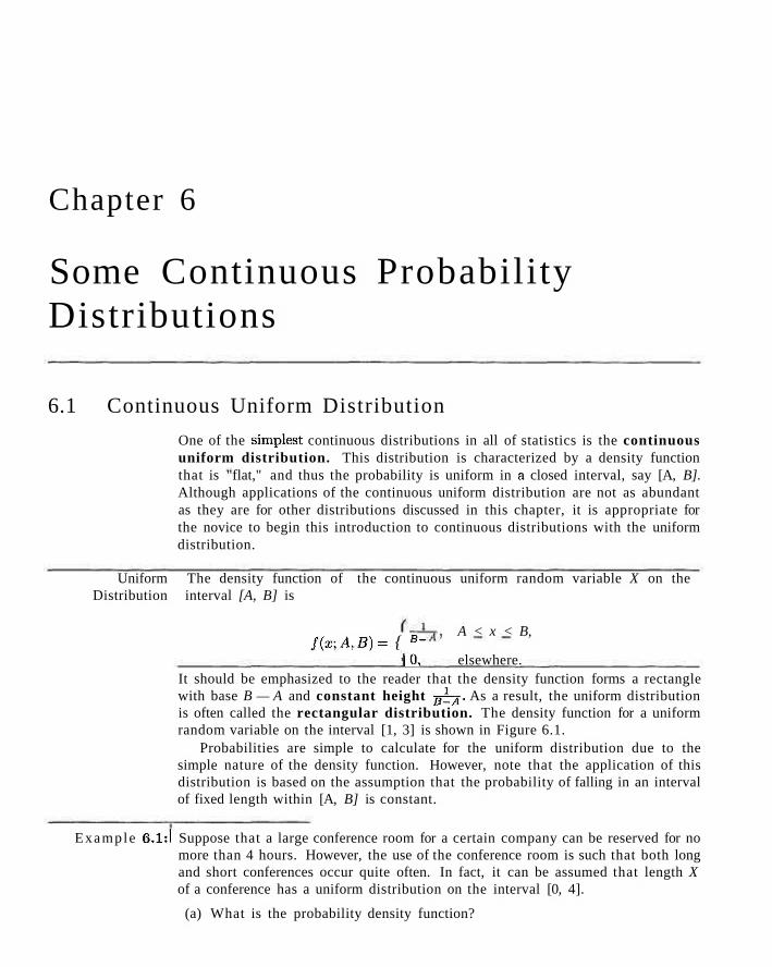
Chapter 6
Some Continuous Probability Distributions
6.1 Continuous Uniform Distribution
One of the simplest continuous distributions in all of statistics is the continuous uniform distribution. This distribution is characterized by a density function that is "flat," and thus the probability is uniform in a closed interval, say [A, B]. Although applications of the continuous uniform distribution are not as abundant as they are for other distributions discussed in this chapter, it is appropriate for the novice to begin this introduction to continuous distributions with the uniform distribution.
Uniform The density function of the continuous uniform random variable X on the Distribution interval [A, B] is
A < x < B, f(x-A.B) = { B~
10, elsewhere. It should be emphasized to the reader that the density function forms a rectangle with base B — A and constant height -g^j- As a result, the uniform distribution is often called the rectangular distribution. The density function for a uniform random variable on the interval [1, 3] is shown in Figure 6.1.
Probabilities are simple to calculate for the uniform distribution due to the simple nature of the density function. However, note that the application of this distribution is based on the assumption that the probability of falling in an interval of fixed length within [A, B] is constant.
Example 6.1:1 Suppose that a large conference room for a certain company can be reserved for no more than 4 hours. However, the use of the conference room is such that both long and short conferences occur quite often. In fact, it can be assumed that length X of a conference has a uniform distribution on the interval [0, 4].
(a) What is the probability density function?
172 Chapter 6 Some Continuous Probability Distributions
0 1 3
Figure 6.1: The density function for a random variable on the interval [1,3].
(b) What is the probability that any given conference lasts at least 3 hours? Solution: (a) The appropriate density function for the uniformly distributed random vari
able X in this situation is
fix) = j , 0 < ; r < 4 .
0, elsewhere.
Theorem 6.1:
(b) P[X>3]=f^dx = \.
The mean and variance of the uniform distribution are
A-rB 2 (B~A)2
p = — - — . and o = — . ' 2 12
The proofs of the: theorems are left to the reader. See Exercise 6.20 on page 187.
6.2 Normal Distribution The most important, continuous probability distribution in the entire field of statistics is the normal distr ibution. Its graph, called the normal curve, is the bell-shaped curve: of Figure 6.2, which describes approximately many phenomena that occur in nature, industry, and research. Physical measurements in areas such as meteorological experiments, rainfall studies, and measurements of manufactured parts are often more than adequately explained with a normal distribution. In addition, errors in scientific measurements are extremely well approximated by a normal distribution. In 1733, Abraham DeMoivre developed the mathematical equation of the normal curve. It provided a basis for which much of the theory of inductive statistics is founded. The normal distribution is often referred to as the Gaussian dis tr ibut ion, in honor of Karl Fricdrich Gauss (1777-1855), who also derived its equation from a study of errors in repeated measurements of the same quantity.
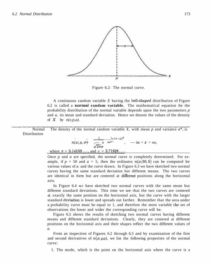
6.2 Normal Distribution 173
Figure 6.2: The normal curve.
A continuous random variable X having the bell-shaped distribution of Figure 6.2 is called a normal random variable. The mathematical equation for the probability distribution of the normal variable depends upon the two parameters p and a, its mean and standard deviation. Hence we denote the values of the density of AT by n(x;p,a).
Normal The density of the normal random variable X, with mean p and variance a2, is Distribution
, , 1 krix—ut3
n(x;u,a) = ,— e 2 »* , — co < re < oo, s/2na
where n = 3.14159..., and e = 2.71828....
Once p and a are specified, the normal curve is completely determined. For example, if p = 50 and a = 5, then the ordinates n(x; 50,5) can be computed for various values of a: and the curve drawn. In Figure 6.3 we have sketched two normal curves having the same standard deviation but different means. The two curves are identical in form but are centered at different positions along the horizontal axis.
In Figure 6.4 wc have sketched two normal curves with the same mean but different standard deviations. This time we see that the two curves are centered at. exactly the same position on the horizontal axis, but the curve with the larger standard deviation is lower and spreads out farther. Remember that the area under a probability curve must be equal to 1, and therefore the more variable the set of observations the lower and wider the corresponding curve will be.
Figure 6.5 shows the results of sketching two normal curves having different means and different standard deviations. Clearly, they are centered at different positions on the horizontal axis and their shapes reflect the two different values of a.
From an inspection of Figures 6.2 through 6.5 and by examination of the first and second derivatives of n(x:p, a), we list the following properties of the normal curve:
1. The mode, which is the point on the horizontal axis where the curve is a
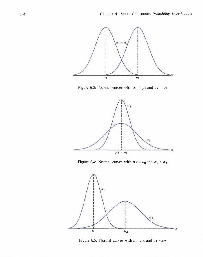
174 Chapter 6 Some Continuous Probability Distributions
Mi Ma
Figure 6.3: Normal curves with pi < p2 and a\ = a2.
P>\ = M2
Figure: 6.4: Normal curves with p.\ ~ p2 and 0\ < a2
AM M2
Figure 6.5: Normal curves with p.\ <p2 and a^ <a2
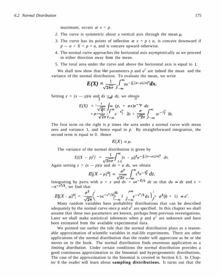
6.2 Normal Distribution 175
maximum, occurs at x = p.
2. The curve is symmetric about a vertical axis through the mean p.
3. The curve has its points of inflection at x = p ± a, is concave downward if p — a < X < p + a, and is concave upward otherwise.
4. The normal curve approaches the horizontal axis asymptotically as we proceed in either direction away from the mean.
5. The total area under the curve and above the horizontal axis is equal to 1.
We shall now show that the parameters p and a2 are indeed the mean and the variance of the normal distribution. To evaluate the mean, we write
E(X) = -=L- P Xe-^x-ri/°f dx. s/2na J-oo
Setting z = (x — p)/a and dx = a dz, we obtain
E(X) = -j=J (p, + oz)e-^dz 1 fx _ ^ , a /,oc _ ^ J
= p~~/= / e * dz + —j= j ze 2 dz. \j2lt '-oc V 2lt J-oc
The first term on the right is p times the area under a normal curve with mean zero and variance 1, and hence equal to p. By straightforward integration, the second term is equal to 0. Hence
E(X) = u.
The variance of the normal distribution is given by
E[(X - p)2] = -jL- fX (x - M)2e-5i(--">/-]2 dx.
V2TTCT J-X Again setting z = (x — p)/a and dx = a dz, we obtain
E[(X-p)2] = -?L ^ z2e-^ dz.
Integrating by parts with u = z and dv = ze~z I2 dz so that du = dz and v = —e~z I2, we find that
2 / oc r°° \ E[(X - p)2\ = -j= ( -Ze-zl/2\_x + I c-*2'2 dz) = a2(0 + 1) - a2.
Many random variables have probability distributions that can be described adequately by the normal curve once p and a2 are specified. In this chapter we shall assume that these two parameters are known, perhaps from previous investigations. Later we shall make statistical inferences when p and a2 are unknown and have been estimated from the available experimental data.
We pointed out earlier the role that the normal distribution plays as a reasonable approximation of scientific variables in real-life experiments. There are other applications of the normal distribution that the reader will appreciate as he or she moves on in the book. The normal distribution finds enormous application as a limiting distribution. Under certain conditions the normal distribution provides a good continuous approximation to the binomial and hypergeometric distributions. The case of the approximation to the binomial is covered in Section 6.5. In Chapter 8 the reader will learn about sampling distributions. It turns out that the
176 Chapter 6 Some Continuous Probability Distributions
limiting distribution of sample averages is normal. This provides a broad base for statistical inference that proves very valuable to the data analyst interested in estimation and hypothesis testing. The important areas of analysis of variance (Chapters 13, 14, and 15) and quality control (Chapter 17) have their theory based on assumptions that make use of the normal distribution.
In much of what follows in Section 6.3, examples are given which demonstrate the use of tables of the normal distribution. Section 6.4 follows with examples of applications of the normal distribution.
6.3 Areas under the Normal Curve
The curve of any continuous probability distribution or density function is constructed so that the area under the curve bounded by the two ordinatos x — x\ and x — x2 equals the probability that the random variable X assumes a value between x = x\ and x = x2. Thus, for the normal curve in Figure 6.6,
P(x\ < X < x2) = / n(x;p.o)dx = / • Jx, \l2ixa JXl
is represented by the area of the shaded region.
r<B-*> dx,
Figure 6.6: P(x.\ < X < x2) = area of the shaded region.
In Figures 6.3, 6.4, and 6.5 we saw how the normal curve is dependent on the mean and the standard deviation of the distribution under investigation. The area under the curve between any two ordinates must then also depend on the values p and a. This is evident in Figure 6.7, where we have shaded regions corresponding to P(xi < X < x-2) for two curves with different means and variances. The P{x\ < X < x2), where X is the random variable describing distribution A, is indicated by the darker shaded area. If X is the random variable describing distribution B, then P(x.\ < X < x2) is given by the entire shaded region. Obviously, the two shaded regions are different in size; therefore, the probability associated with each distribution will be different for the two given values ol X.
The difficulty encountered in solving integrals of normal density functions necessitates the tabulation of normal curve areas for quick reference. However, it
6.3 Areas under the Normal Curve 177
x, x2
Figure 6.7: P(.V] < X < x2) for different normal curves.
Definition 6.1:
would be a hopeless task to attempt to set up separate tables for every conceivable values of p and er. Fortunately, we are able to transform all the observations of any normal random variable X to a new set of observations of a normal random variable Z with mean 0 and variance 1. This can be done bv means of the transformation
Z = ^ » . o
Whenever X assumes a value x, the corresponding value of Z is given by z = (x — p)/o. Therefore, if A' falls between the values x — x\ and x = x2, the random variable Z will fall between the corresponding values z\ = (xi — p)jo and z2 — (x2 — p)/o. Consequently, we may write
P(xi < X <x2) = 1 f
Jx,
d*~H) dx = 1
2TT
-L V^OJX,
n(2;0, l) dz = P(z\ < Z < z2)
f dz
where Z is seen to be a normal random variable with mean 0 and variance 1.
The distribution of a normal random variable with mean 0 and variance 1 is called a standard normal distribution.
The original and transformed distributions are illustrated in Figure 6.8. Since all the values of X falling between x\ and x2 have corresponding z values between z\ and z2, the area under the X-curve between the ordinates x = x\ and x = x2 in Figure 6.8 equals the area under the Z-curve between the transformed ordinates z = z\ and z — z2.
We have now reduced the required number of tables of normal-curve areas to one, that of the standard normal distribution. Table A.3 indicates the area under the standard normal curve corresponding to P(Z < z) for values of z ranging from —3.49 to 3.49. To illustrate the use of this table, let us find the probability that Z is less than 1.74. First, we locate a value of z equal to 1.7 in the left column, then move across the row to the column under 0.04, where we read 0.9591. Therefore, P(Z < 1.74) = 0.9591. To find a z value corresponding to a given probability, the process is reversed. For example, the z value leaving an area of 0.2148 under the curve to the left of z is seen to be —0.79.
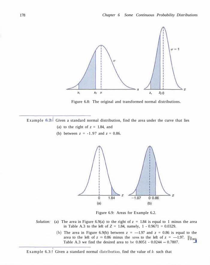
178 Chapter 6 Some Continuous Probability Distributions
X, x2 M z, z2o
Figure 6.8: The original and transformed normal distributions.
Example 6.2:1 Given a standard normal distribution, find the area under the curve that lies
(a) to the right of z = 1.84, and
(b) between z = -1.97 and z = 0.86.
Figure 6.9: Areas for Example 6.2.
Solution: (a) The area in Figure 6.9(a) to the right of z = 1.84 is equal to 1 minus the area in Table A.3 to the left of Z = 1.84, namely, 1 - 0.9671 = 0.0329.
(b) The area in Figure 6.9(b) between z = —1.97 and z = 0.86 is equal to the area to the left of z = 0.86 minus the area to the left of z = —1.97. Fre Table A.3 we find the desired area to be 0.8051 - 0.0244 = 0.7807.
rroni
Example 6.3:! Given a standard normal distribution, find the value of A- such that
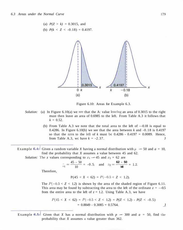
6.3 Areas under the Normal Curve L79
(a) P(Z > k) = 0.3015, and
(b) P(k < Z < -0.18) = 0.4197.
Figure 6.10: Areas for Example 6.3.
Solution: (a) In Figure 6.10(a) we see that the A: value leaving an area of 0.3015 to the right must then leave an area of 0.6985 to the left. From Table A.3 it follows that k = 0.52.
(b) From Table A.3 we note that the total area to the left of —0.18 is equal to 0.4286. In Figure 6.10(b) we see that the area between k and -0.18 is 0.4197 so that the area to the left, of k must be 0.4286 - 0.4197 = 0.0089. Hence, from Table A.3, wc have k = -2.37. J
Example 6.4:1 Given a random variable X having a normal distribution with )i. — 50 and a = 10, find the probability that X assumes a value between 45 and 62.
Solution: The z values corresponding to x\ — 45 and x2 = 62 are
z\ 45 - 50
10 = -0 .5 and
62 - 50
Ml = 1.2.
Therefore,
P(45 < X < 62) = P ( - 0 . o < Z < 1.2).
The P(—0.5 < Z < 1.2) is shown by the area of the shaded region of Figure 6.11. This area may be found by subtracting the area to the left of the ordinate z = —0.5 from the entire area to the left of z = 1.2. Using Table A.3, we have
P(45 < X < 62) = P ( -0 .5 < Z < 1.2) = P(Z < 1.2) - P(Z < -0.5)
= 0.8849 - 0.3085 = 0.5764. J
Example 6.5:1 Given that X has a normal distribution with p — 300 and a = 50, find the: probability that X assumes a value greater than 362.
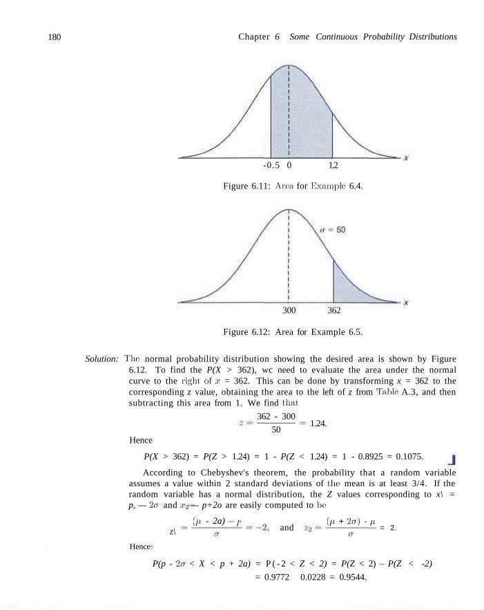
180 Chapter 6 Some Continuous Probability Distributions
-0.5 0 1.2
Figure 6.11: Area for Example: 6.4.
300 362
Figure 6.12: Area for Example 6.5.
Solution: The1 normal probability distribution showing the desired area is shown by Figure 6.12. To find the P(X > 362), wc need to evaluate the area under the normal curve to the right of;?: = 362. This can be done by transforming x = 362 to the corresponding z value, obtaining the area to the left of z from Tabic A.3, and then subtracting this area from 1. We find that
362 - 300
50 1.24.
Hence
P(X > 362) = P(Z > 1.24) = 1 - P(Z < 1.24) = 1 - 0.8925 = 0.1075.
According to Chebyshev's theorem, the probability that a random variable assumes a value within 2 standard deviations of flic: mean is at least 3/4. If the random variable has a normal distribution, the Z values corresponding to x\ = p, — 2(7 and x2 — p+2o are easily computed to be:
z\ (p. - 2a) /' and
(//. + 2cr) - p.
Hence
P(p - 2cr < X < p + 2a) = P ( - 2 < Z < 2) = P(Z < 2)
= 0.9772 - 0.0228 = 0.9544.
= 2.
P(Z < -2)
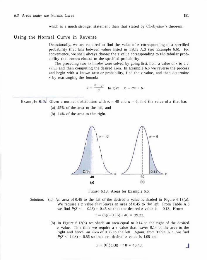
6.3 Areas under the Normal Curve 181
which is a much stronger statement than that stated by Chebyshev's theorem.
Using the Normal Curve in Reverse
Occasionally, we are required to find the value of z corresponding to a specified probability that falls between values listed in Table A.3 (see Example 6.6). For convenience, we shall always choose: the z value corresponding to the tabular probability that comes closest, to the specified probability.
The preceding two examples were solved by going first; from a value of x to a z value and then computing the desired area. In Example 6.6 we reverse the process and begin with a known area or probability, find the z value, and then determine x by rearranging the formula.
M to give: x =CTZ + p.
Example 6.6:1 Given a normal distribution with //. = 40 and a = 6, find the value of x that has
(a) 45% of the area to the left, and
(b) 14% of the area to the: right.
/
y 0.45
1 \ 1 \
i \ i \ i \ i \ i \
i \ 1 1 i i
= 6
40
(a)
Figure1 6.13: Areas for Example 6.6.
Solution: (a) An area of 0.45 to the left of the desired x value is shaded in Figure 6.13(a). We require a z value that leaves an area of 0.45 to the left. From Table A.3 we find P(Z < —0.13) = 0.45 so that the desired z value is —0.13. Hence:
.,:= (6)(-0.13) + 40 = 39.22.
(b) In Figure 6.13(b) we shade an area equal to 0.14 to the right of the desired x value. This time we require a z value that leaves 0.14 of the area to the right and hence: an area of 0.86 to the left. Again, from Table A.3, we find P(Z < 1.08) = 0.86 so that the- desired z value is 1.08 and
(6)( 1.08) + 4 0 = 46.48.
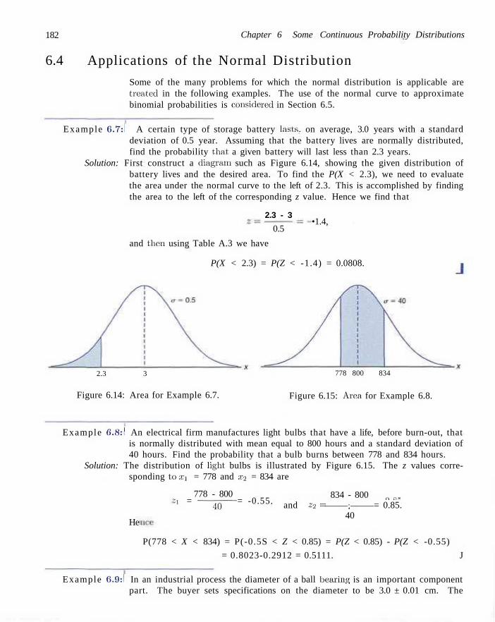
182 Chapter 6 Some Continuous Probability Distributions
6.4 Applications of the Normal Distribution
Some of the many problems for which the normal distribution is applicable are treated in the following examples. The use of the normal curve to approximate binomial probabilities is considered in Section 6.5.
Example 6.7:1 A certain type of storage battery lasts, on average, 3.0 years with a standard deviation of 0.5 year. Assuming that the battery lives are normally distributed, find the probability that a given battery will last less than 2.3 years.
Solution: First construct a diagram such as Figure 6.14, showing the given distribution of battery lives and the desired area. To find the P(X < 2.3), we need to evaluate the area under the normal curve to the left of 2.3. This is accomplished by finding the area to the left of the corresponding z value. Hence we find that
2.3 - 3
0.5 •1.4,
and then using Table A.3 we have
P(X < 2.3) = P(Z < -1.4) = 0.0808.
2.3 3
Figure 6.14: Area for Example 6.7.
778 800 834
Figure 6.15: Area for Example 6.8.
Example 6.8:1 An electrical firm manufactures light bulbs that have a life, before burn-out, that is normally distributed with mean equal to 800 hours and a standard deviation of 40 hours. Find the probability that a bulb burns between 778 and 834 hours.
Solution: The distribution of light bulbs is illustrated by Figure 6.15. The z values corresponding to X] = 778 and .T2 = 834 are
778 - 800 A = — j g - = -0.55.
834 - 800 n M
and z2 = : = 0.85. 40
He
P(778 < X < 834) = P(-0.5S < Z < 0.85) = P(Z < 0.85) - P(Z < -0.55)
= 0.8023-0.2912 = 0.5111. J
Example 6.9:1 In an industrial process the diameter of a ball bearing is an important component part. The buyer sets specifications on the diameter to be 3.0 ± 0.01 cm. The
6.4 Applications of the Normal Distribution 183
implication is that no part falling outside these specifications will be accepted. It is known that in the process the diameter of a ball bearing has a normal distribution with mean p. = 3.0 and standard deviation a = 0.005. On the average, how many manufactured ball bearings will be: scrapped?
Solution: The distribution of diameters is illustrated by Figure 6.16. The values corresponding to the specification limits are X\ = 2.99 and x2 = 3.01. The corresponding z values are
2.99 - 3.0 „ „ , 3.01 - 3.0 -i = —^7^— = - 2 - 0 ' and «2 = = +2.0.
0.005 0.005 Hence
P(2.99 < X < 3.01) = P ( -2 .0 < Z < 2.0).
From Table A.3, P(Z < -2.0) = 0.0228. Due to symmetry of the normal distribution, we find that
P(Z < -2.0) + P(Z > 2.0) = 2(0.0228) = 0.0456.
As a result, it is anticipated that on the average, 4.56% of manufactured ball bearings will be scrapped. J
0.005
2.99 3.0 3.01
Figure 6.16: Area for Example 6.9.
0.0228 0.025 X
1.108 1.500 1.892
Figure 6.17: Specifications for Example 6,10.
Example 6.10:1 Gauges are used to reject all components where a certain dimension is not within the specification l.50±d. It is known that this measurement is normally distributed with mean 1.50 and standard deviation 0.2. Determine the value d such that the specifications "cover"' 95% of the measurements.
Solution: From Table A.3 we know that:
Therefore.
from which we obtain
P ( - 1 . 9 6 < Z < 1.96) = 0.95.
(1.S0 + d) - 1.50 1.96
0.2
d= (0.2)(1.96) = 0.392.
An illustration of the specifications is shown in Figure 6.17.
184 Chapter 6 Some Continuous Probability Distributions
Example 6.11:1 A certain machine makes electrical resistors having a mean resistance of 40 ohms and a standard deviation of 2 ohms. Assuming that the resistance follows a normal distribution and can be measured to any degree of accuracy, what percentage of resistors will have a resistance exceeding 43 ohms'?
Solution: A percentage is found by multiplying the relative frequency by 100%. Since the relative frequency for an interval is equal to the probability of falling in the interval, we must find the area to the right of x = 43 in Figure 6.18. This can be done by transforming x = 43 to the corresponding ; value, obtaining the area to the left of z from Table: A.3, and then subtracting this area from 1. We find
43-40 = 1.5.
Therefore,
P(X > 43) = P(Z > 1.5) = I - P(Z < 1.5) = 1 - 0.9332 = 0.0668.
Hence, 6.68%. of the resistors will have a resistance exceeding 43 ohms. J
43.5
Figure 6.18: Area for Example: 6.11. Figure 6,19: Area for Example: 6.11
Example 6.12:1 Find the percentage of resistances exceeding 43 ohms for Example 6.11 if resistance is measured to the nearest ohm.
Solution: This problem differs from Example 6.11 in that we now assign a measurement of 43 ohms to all resistors whose resistances are greater than 42.5 and less than 43.5. We are actually approximating a discrete distribution by means of a continuous normal distribution. The required area is the region shaded to the right of 43.5 in Figure 6.19. We now find that
43.5 - 40
2 = 1.75.
Hence
P(X > 43.5) = P(Z > 1.75) = 1 - P(Z < 1.75) = 1 - 0.9599 = 0.0401.
Therefore, 4.01% of the resistances exceed 43 ohms when measured to the nearest ohm. The difference 6.68% - 4.01% = 2.67%: between this answer and that or Example 6.11 represents all those resistors having a resistance greater than 43 and less than 43.5 that are now being recorded as 43 ohms. J
Exercises 185
Example 6.13:1 The average grade for an exam is 74, and the standard deviation is 7. If 12%; of the class is given A's, and the grades are curved to follow a normal distribution, what is the lowest possible A and the highest possible B?
Solution: In this example we begin with a known area of probability, find the z value, and then determine x from the formula x = az + p.. An area of 0.12, corresponding to the fraction of students receiving A's, is shaded in Figure 6.20. Wc require a z value that leaves 0.12 of the area to the right and hence, an area of 0.88 to the left. From Table A.3, P(Z < 1.18) has the closest value to 0.88, so that, the desired z value is 1.18. Hence
.i:= (7)(1.18) + 74 = 82.26.
Therefore, the lowest A is 83 and the highest. B is 82. J
74 DR
Figure 6.20: Area for Example 6.13. Figure 6.21: Area for Example 6.14.
Example 6.14:1 Refer to Example 6.13 and find the sixth decile. Solution: The sixth decile, written Da, is the x value: that leaves 60% of the area to the left
as shown in Figure 6.21. From Table A.3 we find P(Z < 0.25) =a 0.6, so that the desired z value is 0.25. Now x = (7)(0.25) + 74 = 75.75. Hence D(i = 75.75. That
Exercises
is, 60%. of the grades are 75 or less.
C.l Given a standard normal distribution, find the normal curve area under the curve which lies (a) to the left of a = 1.43; (b) to the right of z = -0.89: (c) between z = —2.16 and z = — 0.65; (el) te> the left of ; = -1.39; (e) to the: right of z = 1.90: (T) between z = -0.48 and z = 1.74.
6.2 Find the value of z if the area under a standard
(a) to the right, of z is 0.:!022; (b) to the left of a is 0.1131; (c) between 0 and z, with z > 0, is 0.4838; (d) between —z and z, with z > 0, is 0.9500.
6.3 Given a standard normal distribution, value of k such that (a) P(Z < k) = 0.0427; (b) P(Z > /,•) = 0.2946;
find the
186 Chapter 6 Some Continuous Probability Distributions
(c) P ( -0 .93 < Z < k) = 0.7235.
6.4 Given a normal distribution with p = 30 and a — 6, find (a) the normal-curve area to the right of x = 17; (b) the normal-curve area to the left of x = 22;
(c) the normal-curve area between x = 32 and x = 41; (d) the value of a: that has 80% of the normal-curve
area to the left; (e) the two values of x that contain the middle 75% of
the normal-curve area.
6.5 Given the normally distributed variable X with mean 18 and standard deviation 2.5, find (a) P(X < 15): (b) the value of k such that P(X < k) = 0.2236; (c) the value of k such that P(X > k) = 0.1814; (d) P(17 < X < 21).
6.6 According to Chebyshev's theorem, the probability that any random variable assumes a value within 3 standard deviations of the mean is at least 8/9. If it is known that the probability distribution of a random variable X is normal with mean p, and variance a2, what is the exact value of P(p, — 3a- < X < p + 3a)?
6.7 A research scientist reports that mice will live an average of 40 months when their diets are sharply restricted and then enriched with vitamins and proteins. Assuming that the lifetimes of such mice are normally distributed with a standard deviation of 6.3 months, find the probability that a given mouse will live
(a) more than 32 months; (b) less than 28 months;
(c) between 37 and 49 months.
6.8 The loaves of rye bread distributed to local stores by a certain bakery have an average length of 30 centimeters and a standard deviation of 2 centimeters. Assuming that the lengths are normally distributed, what percentage of the loaves are
(a) longer than 31.7 centimeters? (b) between 29.3 and 33.5 centimeters in length? (c) shorter than 25.5 centimeters?
6.9 A soft-drink machine is regulated so that it discharges an average of 200 milliliters per cup. If the amount of drink is normally distributed with a standard deviation equal to 15 milliliters, (a) what fraction of the cups will contain more than
224 milliliters? (b) what is the probability that a cup contains between
191 and 209 milliliters? (c) how many cups will probably overflow if 230-
milliliter cups are used for the next 1000 drinks? (d) below what value do we get the smallest 25% of the
drinks?
6.10 The finished inside diameter of a piston ring is normally distributed with a mean of 10 centimeters and a standard deviation of 0.03 centimeter.
(a) What proportion of rings will have inside diameters exceeding 10.075 centimeters?
(b) What is the probability that a piston ring will have an inside diameter between 9.97 and 10.03 centimeters?
(c) Below what value of inside diameter will 15% of the piston rings fall?
6.11 A lawyer commutes daily from his suburban home to his midtown office. The average time for a one-way trip is 24 minutes, with a standard deviation of 3.8 minutes. Assume the distribution of trip times to be normally distributed.
(a) What is the probability that a trip will take at least 1/2 hour?
(b) If the office opens at 9:00 A.M. and he leaves his house at 8:45 A.M. daily, what percentage of the time is he late for work?
(c) If he leaves the house at 8:35 A.M. and coffee is served at the office from 8:50 A.M. until 9:00 A.M., what is the probability that he misses coffee?
(d) Find the length of time above which we find the slowest 15% of the trips.
(e) Find the probability that 2 of the next 3 trips will take at least 1/2 hour.
6.12 In the November 1990 issue of Chemical Engineering Progress, a study discussed the percent purity of oxygen from a certain supplier. Assume that the mean was 99.61 with a standard deviation of 0.08. Assume that the distribution of percent purity was approximately normal.
(a) What percentage of the purity values would you expect to be between 99.5 and 99.7?
(b) What purity value would you expect to exceed exactly 5% of the population?
6.13 The average life of a certain type of small motor is 10 years with a standard deviation of 2 years. The manufacturer replaces free all motors that fail while under guarantee. If he is willing to replace only 3% of the motors that fail, how long a guarantee should he offer? Assume that the lifetime of a motor follows a normal distribution.
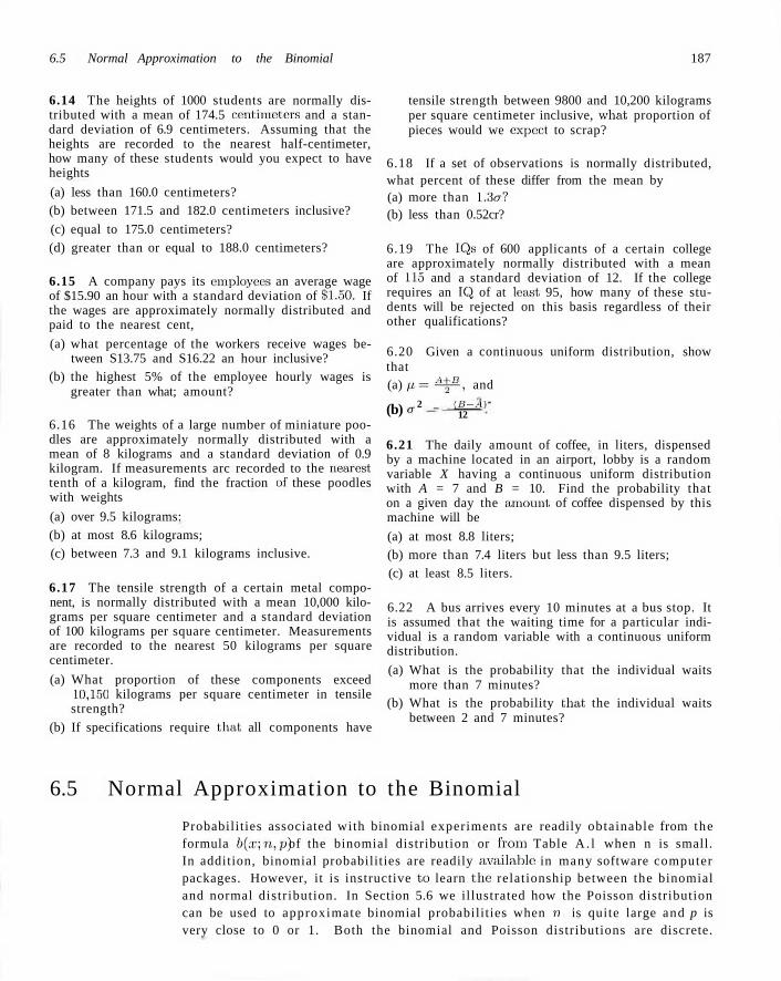
6.5 Normal Approximation to the Binomial 187
6.14 The heights of 1000 students are normally distributed with a mean of 174.5 centimeters and a standard deviation of 6.9 centimeters. Assuming that the heights are recorded to the nearest half-centimeter, how many of these students would you expect to have heights
(a) less than 160.0 centimeters? (b) between 171.5 and 182.0 centimeters inclusive?
(c) equal to 175.0 centimeters? (d) greater than or equal to 188.0 centimeters?
6.15 A company pays its employees an average wage of $15.90 an hour with a standard deviation of $1.50. If the wages are approximately normally distributed and paid to the nearest cent,
(a) what percentage of the workers receive wages between S13.75 and S16.22 an hour inclusive?
(b) the highest 5% of the employee hourly wages is greater than what; amount?
6.16 The weights of a large number of miniature poodles are approximately normally distributed with a mean of 8 kilograms and a standard deviation of 0.9 kilogram. If measurements arc recorded to the nearest tenth of a kilogram, find the fraction or these poodles with weights
(a) over 9.5 kilograms: (b) at most 8.6 kilograms; (c) between 7.3 and 9.1 kilograms inclusive.
6.17 The tensile strength of a certain metal component, is normally distributed with a mean 10,000 kilograms per square centimeter and a standard deviation of 100 kilograms per square centimeter. Measurements are recorded to the nearest 50 kilograms per square centimeter.
(a) What proportion of these components exceed 10,150 kilograms per square centimeter in tensile strength?
(b) If specifications require that all components have
tensile strength between 9800 and 10,200 kilograms per square centimeter inclusive, what, proportion of pieces would we expect to scrap?
6.18 If a set of observations is normally distributed, what percent of these differ from the mean by (a) more than 1.3c? (b) less than 0.52cr?
6.19 The IQs of 600 applicants of a certain college are approximately normally distributed with a mean of 115 and a standard deviation of 12. If the college requires an IQ of at least 95, how many of these students will be rejected on this basis regardless of their other qualifications?
6.20 Given a continuous uniform distribution, show that (a) p = ^ - , and
(b) tr 2 _ (D-A)-12
6.21 The daily amount of coffee, in liters, dispensed by a machine located in an airport, lobby is a random variable X having a continuous uniform distribution with A = 7 and B = 10. Find the probability that on a given day the amount, of coffee dispensed by this machine will be
(a) at most 8.8 liters; (b) more than 7.4 liters but less than 9.5 liters; (c) at least 8.5 liters.
6.22 A bus arrives every 10 minutes at a bus stop. It is assumed that the waiting time for a particular individual is a random variable with a continuous uniform distribution.
(a) What is the probability that the individual waits more than 7 minutes?
(b) What is the probability that the individual waits between 2 and 7 minutes?
6.5 Normal Approximation to the Binomial
Probabilities associated with binomial experiments are readily obtainable from the formula b(x;n,p) of the binomial distribution or from Table A . l when n is small. In addition, binomial probabilities are readily available in many software computer packages. However, it is instructive to learn the relationship between the binomial and normal distr ibution. In Section 5.6 we illustrated how the Poisson distribution can be used to approximate binomial probabilities when 77 is quite large and p is very close to 0 or 1. Both the binomial and Poisson distributions are discrete.
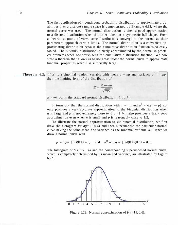
188 Chapter 6 Some Continuous Probability Distributions
Theorem 6.2:
The first application of a continuous probability distribution to approximate probabilities over a discrete sample space is demonstrated by Example 6.12, where the normal curve was used. The normal distribution is often a good approximation to a discrete distribution when the latter takes on a symmetric bell shape. From a theoretical point, of view, some distributions converge to the normal as their parameters approach certain limits. The normal distribution is a convenient approximating distribution because the cumulative distribution function is so easily tabled. The binomial distribution is nicely approximated by the normal in practical problems when one works with the cumulative distribution function. We now state a theorem that allows us to use areas under the normal curve to approximate binomial properties when n is sufficiently large.
If A'' is a binomial random variable with mean p then the limiting form of the distribution of
X — np
np and variance a2 = npq,
as n —* oo, is the standard normal distribution 11,(2; 0,1).
It turns out that the normal distribution with p = np and a2 = np(l — p) not only provides a very accurate approximation to the binomial distribution when n is large and p is not extremely close to 0 or 1 but also provides a fairly good approximation even when n is small and p is reasonably close to 1/2.
To illustrate the normal approximation to the binomial distribution, we first draw the histogram for b(x; 15,0.4) and then superimpose the particular normal curve having the same mean and variance as the binomial variable X. Hence we draw a normal curve with
p = np = (15)(0.4) = 6, and a2 = npq = (15)(0.4)(0.6) = 3.0.
The histogram of b(x; 15, 0.4) and the corresponding superimposed normal curve, which is completely determined by its mean and variance, are illustrated by Figure 6.22.
0 1 2 3 4 5 6 7 8 9 1 1 1 3 1 5
Figure 6.22: Normal approximation of b(x; 15,0.4).
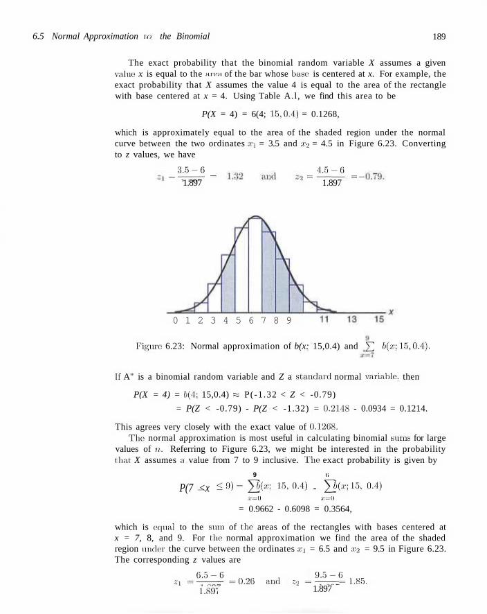
6.5 Normal Approximation u> the Binomial 189
The exact probability that the binomial random variable X assumes a given value: x is equal to the area of the bar whose base: is centered at x. For example, the exact probability that X assumes the value 4 is equal to the area of the rectangle with base centered at x = 4. Using Table A.l, we find this area to be
P(X = 4) = 6(4; 15,0.4) = 0.1268,
which is approximately equal to the area of the shaded region under the normal curve between the two ordinates x\ = 3.5 and x2 = 4.5 in Figure 6.23. Converting to z values, we have
= 3^zJ? = _ = 4J5-6 = 1.897 " 1.897
0 1 2 3 4 5 6 7 8 9
Figure 6.23: Normal approximation of b(x: 15,0.4) and Y^ b(x;15,0.4).
If A" is a binomial random variable and Z a .standard normal variable, then
P(X = 4) = b(4; 15,0.4) % P(-1.32 < Z < -0.79)
= P(Z < -0.79) - P(Z < -1.32) = 0.2118 - 0.0934 = 0.1214.
This agrees very closely with the exact value of 0.1268. The: normal approximation is most useful in calculating binomial sums for large
values of n. Referring to Figure 6.23, we might be interested in the probability that X assumes a value from 7 to 9 inclusive. The exact probability is given by
9 (i
P(7 <x <Q) = Y &(«; 15> 0-4) - Y b(x'<15> °-4) x=Q ,r=()
= 0.9662 - 0.6098 = 0.3564,
which is eepial to the sum of the areas of the rectangles with bases centered at x = 7, 8, and 9. For the normal approximation we find the area of the shaded region tinclt:r the curve between the ordinates xi = 6.5 and asa = 9.5 in Figure 6.23. The corresponding z values are
^1 = 5^5-6 = 0 < 2 6 aml C2 = ^ « = 1_85_ vmi 1.897
190 Chapter 6 Some Continuous Probability Distributions
Now,
P(7 < X < 9) ftf P(0.26 < Z < 1.85) = P(Z < 1.85) - P(Z < 0.26)
= 0.9678 - 0.6026 = 0.3652.
Once again, the normal-curve approximation provides a value that agrees very closely with the exact value of 0.3564. The degree of accuracy, which depends on how well the curve fits the histogram, will increase as n increases. This is particularly true when p is not very close to 1/2 and the histogram is no longer symmetric. Figures 6.24 and 6.25 show the histograms for fo(a;;6,0.2) and b(x; 15,0.2), respectively. It is evident that a normal curve would fit the histogram when n — 15 considerably better than when n = 6.
0 1 2 3 4 5 6 7 8 9 11 13 15
Figure 6.24: Histogram for b(x: 6, 0.2). Figure 6.25: Histogram for b(x; 15,0.2).
In our illustrations of the normal approximation to the binomial, it became apparent that if we seek the area under the normal curve to the left of, say, x it is more accurate to use x + 0.5. This is a correction to accommodate the fact, that a discrete distribution is being approximated by a continuous distribution. The correction + 0 . 5 is called a continuity correction. From the foregoing discussion we give the following formal normal approximation to the binomial.
Normal Let X be a binomial random variable with parameters n and p. Then X has Approximation to approximately a normal distribution with p = np and a2 = npq = np(l — p)
the Binomial and Distribution
P(X<x) = Yb(k>n'P) fe=0 area, under normal curve to the left of x + 0.5
. < £ L ± 0 : 5 - V
and the approximation will be good if np and n(\ —p) are greater than or equal to 5.
As we indicated earlier, the quality of the approximation is quite good for large n. If p is close to 1/2, a moderate or small sample size will be sufficient for a reasonable approximation. We offer Table 6.1 as an indication of the quality of the
6.5 Normal Approximation to the Binomial 191
approximation. Both the normal approximation and the true binomial cumulative probabilities are given. Notice that at p = 0.05 and p = 0.10, the approximation is fairly crude for n = 10. However, even for n = 10, note the improvement for p = 0.50. On the other hand, when p is fixed at p = 0.05, note the improvement of the approximation as we go from n — 20 to n = 100.
Table 6.1: Normal Approximation and True Cumulative Binomial Probabilities
r 0 1 2 3 4 5 6 7 8 9
10
r 0 1 2 3 4 5 6 7 8 9
10
p = 0.05 Binomial
0.5987 0.9139 0.9885 0.9990 1.0000
n = Binomial
0.3585 0.7358 0.9245 0.9841 0.9974 0.9997 1.0000
, n = 10 Normal 0.5000 0.9265 0.9981 1.0000 1.0000
• 20 Normal 0.3015 0.6985 0.9382 0.9948 0.9998 1.0000 1.0000
p = 0.1C Binomial
0.3487 0.7361 0.9298 0.9872 0.9984 1.0000
P = n =
Binomial 0.0769 0.2794 0.5405 0.7604 0.8964 0.9622 0.9882 0.9968 0.9992 0.9998 1.0000
i, n = 10 Normal 0.2981 0.7019 0.9429 0.9959 0.9999 1.0000
0.05 = 50
Normal 0.0968 0.2578 0.5000 0.7422 0.9032 0.9744 0.9953 0.9994 0.9999 1.0000 1.0000
p = 0.50 Binomial
0.0010 0.0107 0.0547 0.1719 0.3770 0.6230 0.8281 0.9453 0.9893 0.9990 1.0000
n — Binomial
0.0059 0.0371 0.1183 0.2578 0.4360 0.6160 0.7660 0.8720 0.9369 0.9718 0.9885
, n = 10 Normal 0.0022 0.0136 0.0571 0.1711 0.3745 0.6255 0.8289 0.9429 0.9864 0.9978 0.9997
100 Normal
0.0197 0.0537 0.1251 0.2451 0.4090 0.5910 0.7549 0.8749 0.9463 0.9803 0.9941
Example 6.15:1 The probability that a patient recovers from a rare blood disease is 0.4. If 100 people are known to have contracted this disease, what is the probability that less than 30 survive?
Solution: Let the binomial variable X represent the number of patients that survive. Since n = 100, we should obtain fairly accurate results using the normal-curve approximation with
/i = np=(100) (0 .4 )=40 ,
and
= v/npc7 = \/(100)(0.4)(0.6) = 4.899.
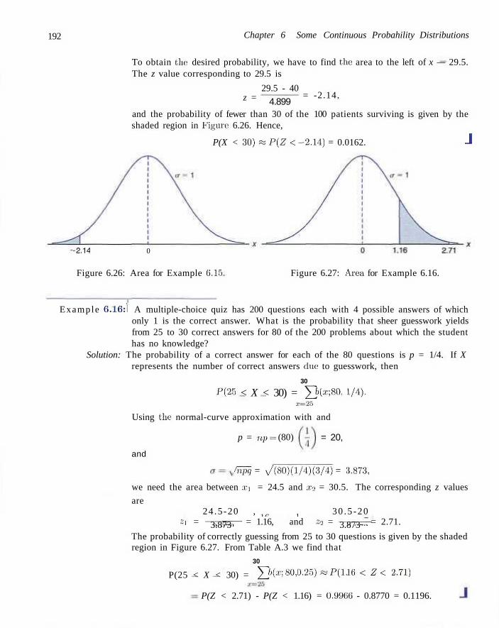
192 Chapter 6 Some Continuous Probahility Distributions
To obtain the: desired probability, we have to find the area to the left of x — 29.5. The z value corresponding to 29.5 is
29.5 - 40 z = 4.899
= -2.14.
and the probability of fewer than 30 of the 100 patients surviving is given by the shaded region in Figure: 6.26. Hence,
P(X < 30) « P ( Z < -2.14) = 0.0162. J
-2.14 0
Figure 6.26: Area for Example 6.15 Figure 6.27: Area for Example 6.16.
Example 6.16:1 A multiple-choice quiz has 200 questions each with 4 possible answers of which only 1 is the correct answer. What is the probability that sheer guesswork yields from 25 to 30 correct answers for 80 of the 200 problems about which the student has no knowledge?
Solution: The probability of a correct answer for each of the 80 questions is p = 1/4. If X represents the number of correct answers due to guesswork, then
30
P(25 < X < 30) = Y l'ix' 80< ]/4). s=25
Using the normal-curve approximation with and
p = np = (80)
and
= 20,
(npq = v/(80)(l/4)(3/4) = 3.873,
we need the area between Xj = 24.5 and x2 = 30.5. The corresponding z values
are 24 .5 -20 , „„ , 30 .5 -20
z\ = - ^ — ^ — = 1.16, and z2 = —r^r = 2.71. 3.873 3.873 The probability of correctly guessing from 25 to 30 questions is given by the shaded region in Figure 6.27. From Table A.3 we find that
30
P(25 < X < 30) = Y bix'>80' ° '25) ~ P ( L JC < Z < 2 ' 7 1 )
P(Z < 2.71) - P(Z < 1.16) = 0.996G - 0.8770 = 0.1196.
Exercises
Exercises
193
6.23 Evaluate P ( l < X < 4) for a binomial variable with n = 15 and p = 0.2 by using
(a) Table A.l in the Appendix; (b) the normal-curve approximation.
6.24 A coin is tossed 400 times. Use the normal-curve approximation to find the probability of obtaining
(a) between 185 and 210 heads inclusive; (b) exactly 205 heads;
(c) less than 176 or more than 227 heads.
6.25 A process for manufacturing an electronic component is 1% defective. A quality control plan is to select 100 items from the process, and if none are defective, the process continues. Use the normal approximation to the binomial to find
(a) the probability that the process continues for the sampling plan described;
(b) the probability that the process continues even if the process has gone bad (i.e., if the frequency of defective components has shifted to 5.0% defective).
6.26 A process yields 10% defective items. If 100 items are randomly selected from the process, what is the probability that the number of defectives
(a) exceeds 13? (b) is less than 8?
6.27 The probability that a patient recovers from a delicate heart operation is 0.9. Of the next 100 patients having this operation, what is the probability that (a) between 84 and 95 inclusive survive? (b) fewer than 86 survive?
6.28 Researchers at George Washington University and the National Institutes of Health claim that approximately 75% of the people believe "tranquilizers work very well to make a person more calm and relaxed." Of the next 80 people interviewed, what is the probability that (a) at least 50 are of this opinion? (b) at most 56 are of this opinion?
6.29 If 20% of the residents in a U.S. city prefer a white telephone over any other color available, what is the probability that among the next 1000 telephones installed in that city (a) between 170 and 185 inclusive will be white?
(b) at least 210 but not more than 225 will be white?
6.30 A drug manufacturer claims that a certain drug cures a blood disease, on the average, 80% of the time. To check the claim, government testers used the drug on a sample of 100 individuals and decided to accept the claim if 75 or more were cured. (a) What is the probability that, the claim will be re
jected when the cure probability is, in fact, 0.8?
(b) What is the probability that the claim will be accepted by the government when the cure probability is as low as 0.7?
6.31 One-sixth of the male freshmen entering a large state school are out-of-state students. If the students are assigned at random to the dormitories, 180 to a building, what is the probability that in a given dormitory at least one-fifth of the students are from out of state?
6.32 A pharmaceutical company knows that approximately 5% of its birth-control pills have an ingredient that is below the minimum strength, thus rendering the pill ineffective. What is the probability that fewer than 10 in a sample of 200 pills will be ineffective?
6.33 Statistics released by the National Highway Traffic Safety Administration and the National Safety Council show that on an average weekend night, 1 out of every 10 drivers on the road is drunk. If 400 drivers are randomly checked next Saturday night, what is the probability that the number of drunk drivers will be
(a) less than 32? (b) more than 49? (c) at least 35 but less than 47?
6.34 A pair of dice is rolled 180 times. What is the probability that a total of 7 occurs
(a) at least 25 times? (b) between 33 and 41 times inclusive? (c) exactly 30 times?
6.35 A company produces component parts for an engine. Parts specifications suggest that 95% of items meet specifications. The parts are shipped to customers in lots of 100. (a) What is the probability that more than 2 items will
be defective in a given lot? (b) What is the probability that more than 10 items
will be defective in a lot?
194 Chapter 6 Some Continuous Probability Distributions
6.36 A commonly used practice of airline companies is to sell more tickets than actual seats to a particular flight because customers who buy tickets do not always show up for the flight. Suppose that the percentage of no-shows at flight time is 2%. For a particular flight with 197 seats, a total of 200 tickets was sold. What is the probability that the airline overbooked this flight?
6.37 The serum cholesterol level X in 14-year-old boys has approximately a normal distribution with mean 170 and standard deviation 30.
(a) Find the probability that the serum cholesterol level of a randomly chosen 14-year-old boy exceeds 230.
(b) In a middle school there are 300 14-year-old boys. Find the probability that at least 8 boys have a
serum cholesterol level that exceeds 230.
6.38 A tele-marketing company has a special letter-opening machine that opens and removes the contents of an envelope. If the envelope is fed improperly into the machine, the contents of the envelope may not be removed or may be damaged. In this case we say that, the machine has "failed."
(a) If the machine has a probability of failure of 0.01, what is the probability of more than 1 failure occurring in a batch of 20 envelopes?
(b) If the probability of failure of the machine is 0.01 and a batch of 500 envelopes is to be opened, what is the probability that more than 8 failures will occur?
6.6 Gamma and Exponential Distributions
Although the normal distribution can be used to solve many problems in engineering and science, there are still numerous situations tha t require different types of density functions. Two such density functions, the g a m m a and e x p o n e n t i a l d i s tr ibut ions , are discussed in this section.
It turns out that the exponential is a special case of the gamma distribution. Both find a large number of applications. The exponential and gamma distributions play an important role in both queuing theory and reliability problems. Time between arrivals at service facilities, and time to failure of component parts and electrical systems, often are nicely modeled by the exponential distribution. The relationship between the gamma and the exponential allows the gamma to be involved in similar types of problems. More details and illustrations will be supplied in Section 6.7.
The gamma distribution derives its name from the well-known g a m m a funct ion, studied in many areas of mathematics . Before we proceed to the: gamma distribution, let us review this function and some of its important properties.
Definition 6.2: The g a m m a funct ion is defined by
F (a ) = / xn-le~x dx, for a > 0. Jo
Integrating by par ts with TJ = x° l and dv — e •' dx, we obtain
r(ct) = -e~x xn~] | ~ + / e~x(a - l)xa~2 dx = (a - 1) / xa-2e~x
Jo Jo
for a > 1, which yields the recursion formula
T(a) = (a-l)T(a-l).
Repeated application of the recursion formula gives
T(a) = (a - 1 ) (Q - 2 ) r ( a - 2) = (a - l ) ( a - 2 ) (a - 3 )F(a - 3),
dx,
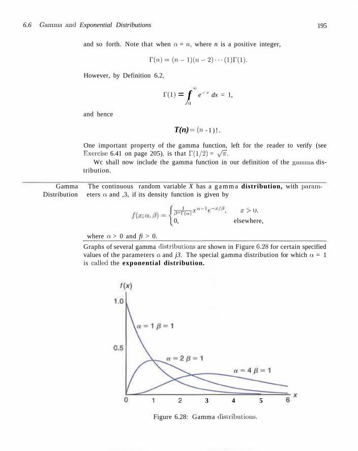
6.6 Gamma and Exponential Distributions 195
and so forth. Note that when a = n, where n is a positive integer,
r(n)-(n-l)(n-2)-..(l)r(l).
However, by Definition 6.2.
r(i) = f Jo
and hence
T(n)
e x dx = 1,
- 1 ) ! .
One important property of the gamma function, left for the reader to verify (see Exercise 6.41 on page 205). is that T(l/2) = \pK.
Wc shall now include the gamma function in our definition of the gamma distribution.
Gamma The continuous random variable X has a g a m m a distribution, with param-Distribution eters a and ,3, if its density function is given by
par{a)x , X>U,
0, elsewhere,
where a > 0 and fi > 0.
Graphs of several gamma distributions are shown in Figure 6.28 for certain specified values of the parameters a and j3. The special gamma distribution for which a = 1 is called the exponential distribution.
1 2 3 4 5
Figure 6.28: Gamma distributions.
196 Chapter 6 Some Continuous Probability Distributions
Exponential The continuous random variable X has an exponential distribution, with Distribution parameter 3, if its density function is given by
Theorem 6.3;
fix; 3) '^c-x'a, x > 0 ,
0, elsewhere,
where 0 > 0.
The following theorem and corollary give the mean and variance of the gamma and exponential distributions.
The mean and variance of the gamma distribution are
p = ctfl, and a2=ad2.
The proof of this theorem is found in Appendix A.28.
Corollary 6.1: The mean and variance of the exponential distribution are
p = B, and a2 = 02.
Relationship to the Poisson Process
We shall pursue applications of the exponential distribution and then return to the gamma distribution. The most important applications of the exponential distribution are situations where the Poisson process applies (see Chapter 5). The reader should recall that the Poisson process allows for the use of the discrete distribution called the Poisson distribution. Recall that the Poisson distribution is used to compute the probability of specific numbers of "events" during a particular •period of time or space. In many applications, the time period or span of space is the random variable. For example, an industrial engineer may be interested in modeling the time T between arrivals at a congested intersection during rush hour in a large city. An arrival represents the Poisson event.
The relationship between the exponential distribution (often called the negative exponential) and the Poisson process is quite simple. In Chapter 5 the Poisson distribution was developed as a single-parameter distribution with parameter A, wdiere X may be interpreted as the mean number of events per unit "time." Consider now the random variable described by the time required for the first event to occur. Using the Poisson distribution, we find that the probability of no events occurring in the span up to time f. is given by
p(0; Xt) ,-xt (A*)0
0! = e -xt
We can now make use of the above and let X be the time to the first Poisson event. The probability that the length of time until the first event will exceed x is
6.7 Applications of the Exponential and Gamma Distributions 197
the same as the probability that no Poisson events will occur in x. The latter, of course, is given by e~ . As a result,
P(X > x) = erXx.
Thus the cumulative distribution function for X is given by
P(0<X <x) = \-e-Xx.
Now, in order that we recognize the presence of the exponential distribution, we may differentiate the cumulative distribution function above to obtain the density function
f(x) = Xe-Xx,
which is the density function of the exponential distribution with A = 1/0.
6.7 Applications of the Exponential and Gamma Distributions
In the foregoing we provided the foundation for the application of the exponential distribution in "time to arrival" or time to Poisson event problems. We will display illustrations here and then proceed to discuss the role of the gamma distribution in these modeling applications. Notice that the mean of the exponential distribution is the parameter 0, the reciprocal of the parameter in the Poisson distribution. The reader should recall that it is often said that the Poisson distribution has no memory, implying that, occurrences in successive time periods are independent. The important parameter 0 is the mean time between events. In reliability theory, where equipment failure: often conforms to this Poisson process, 0 is called mean t ime between failures. Many equipment breakdowns do follow the Poisson process, and thus the exponential distribution does apply. Other applications include survival times in biomedical experiments and computer response time.
In the following example we show a simple application of the exponential distribution to a problem in reliability. The binomial distribution also plays a role in the solution.
Example 6.17:1 Suppose that a system contains a certain type of component whose time, in years, to failure is given by T. The random variable T is modeled nicely by the exponential distribution with mean time to failure /? = 5. If 5 of these components are installed in different systems, what is the probability that at least. 2 are still functioning at the end of 8 years?
Solution: The probability that a given component is still functioning after 8 years is given by
P(T > 8) = \ j e-'lu dt = e - 8 / 5 M 0.2.
5 .Is Let X represent the number of components functioning after 8 years. Then using the binomial distribution,
5 1
P(X >2) = Y b(x\ 5.0-2) = 1 " Y b{-'"- 5' °'2) = X ~ 0 7 3 7 3 = °-2627- J x=2
198 Chapter 6 Some Continuous Probability Distributions
There are exercises and examples in Chapter 3 where the reader has already-encountered the exponential distribution. Others involving waiting time and reliability problems can be found in Example 6.24 and in exercises and review exercises at the end of this chapter.
The Memoryless Property and Its Effect on the Exponential Distribution
The types of applications of the exponential distribution in reliability and component or machine lifetime problems is influenced by the memoryless (or lack-of-memory) property of the exponential distribution. For example, in the case of, say, an electronic component where distribution of lifetime has an exponential distribution, the probability that the component lasts, say t hours, that is, P(X > t), is the same as the conditional probability
P(X>t0 + t | X>tQ).
So if the component "makes it" to to hours, the probability of lasting an additional t hours is the same as the probability of lasting t hours. So there is no "punishment" through wear that may have ensued for lasting the first to hours. Thus, the exponential distribution is more appropriate when the memoryless property is justified. But if the failure of the component is a result of gradual or slow wear (as in mechanical wear), then the exponential does not apply and either the gamma or Weibull distribution (Section 6.10) may be more appropriate.
The importance of the gamma distribution lies in the fact that it defines a family of which other distributions are special cases. But the gamma itself has important applications in waiting time and reliability theory. Whereas the exponential distribution describes the time until the occurrence of a Poisson event (or the time between Poisson events), the time (or space) occurring until a specified number of Poisson events occur is a random variable whose density function is described by that of the gamma distribution. This specific number of events is the parameter a in the gamma density function. Thus it becomes easy to understand that when a = 1, the special case of the exponential distribution occurs. The gamma density can be developed from its relationship to the Poisson process in much the same manner as we developed the exponential density. The details are left to the reader. The following is a numerical example of the use of the gamma distribution in a waiting-time application.
Example 6.18:1 Suppose that telephone calls arriving at a particular switchboard follow a Poisson process with an average of 5 calls coming per minute. What is the probability that up to a minute will elapse until 2 calls have come in to the switchboard?
Solution: The Poisson process applies with time until 2 Poisson events following a gamma distribution with 0 = 1/5 and a = 2. Denote by X the time in minutes that transpires before 2 calls come. The required probability is given by
P(X < 1) = / ]pxe~X/fi dx = 2 5 / xe~5X dx = i~ e"5(l + 5) = 0.96. -
While the origin of the gamma distribution deals in time (or space) until the occurrence of a Poisson events, there are many instances where a gamma distribution works very well even though there is no clear Poisson structure. This is
6.7 Applications of the Exponential and Gamma Distributions 199
particularly true for survival t ime problems in both engineering and biomedical applications.
Example 6.19:1 In a biomedical study with rats, a dose-response investigation is used to determine the effect of the dose of a toxicant on their survival time. The toxicant is one that is frequently discharged into the atmosphere from jet fuel. For a certain dose of the toxicant the study determines that the survival time, in weeks, has a gamma distribution with a: = 5 and 0 = 10. What is the probability that a rat survives no longer than 60 weeks?
Solution: Let the random variable X be the survival time (time to death). The required probability is
60 _ a - l . i r x x/0
r(5) dx.
The integral above can be solved through the use of the incomplete gamma function, which becomes the cumulative distribution function for the gamma distribution. This function is written as
f va~1e~v
F(x;a)= / lTrT-dy.
Jo ria)
If we let y = x/0, so x = 0y, we have
P{X < 60) = f Jo
ye
r(5) dy,
which is denoted as F(6: 5) in the table of the incomplete gamma function in Appendix A.24. Note that this allows a quick computation of probabilities for the gamma distribution. Indeed, for this problem the probability that the rat survives no longer than 60 days is given by
P(X < 60) = F(6; 5) = 0.715. J
Example 6.20:1 It is known, from previous data, that the length of time in months between customers1 complaints about a certain product is a gamma distribution with a = 2 and 3 = 4. Changes were made that involve a tightening of quality control requirements. Following these changes, it took 20 months before the first complaint. Does it appear as if the quality control tightening was effective?
Solution: Let X be the time to the first complaint, which, under conditions prior to the changes, follows a gamma distribution with a = 2 and 0 = 4. The question centers around how rare is X > 20 given that a and 3 remain at values 2 and 4, respectively. In other words, under the prior conditions is a "time to complaint" as large as 20 months reasonable? Thus we need, following the solution to Example 6.19,
P ( X > 2 0 ) = l - i ^ 2
Again, using y = x/0, we have
'"20 xa~le"x/!i
r(a) dx.
P(X > 20) Jo
ye » r(2)
dy = 1 - F(5; 2) = 1 - 0.96 = 0.04,
200 Chapter 6 Some Continuous Probability Distributions
where F(5; 2) = 0.9G is found from Table A.24. As a result, we could conclude that the conditions of the gamma distribution
with a = 2 and 0 = 4 are not supported by the data that an observed time to complaint is as large as 20 months. As a result, it. is reasonable to conclude that the finality control work was effective. J
Example 6.21:1 Consider Exercise 3.31 on page 90. Based on extensive testing it is determined that the time Y in years before a major repair is required for a certain washing machine is characterized by the density function
10. elsewhere.
Note this is an exponential with p = 4 years. The machine is considered a bargain if it is unlikely to require a major repair before the sixth year. Thus, what is the probability P(Y > 6)? Also, what is the probability that a major repair occurs in the first year?
Solution: Consider the cumulative distribution function F(y) for the: exponential distribution
F(y) = - f e-1'0 dt= l-e~v' P Jo
-via ' "" 0 J0 ' - * "
So
P(Y > 6) = 1 - F{6) = e _ 3 / a = 0.2231.
Thus, the probability that it will require major repair after year six is 0.223. Of course, it will require: the: repair before year six with probability 0.777. Thus, one might conclude the machine is not really a bargain. The probability that a. major repair occurs in the first year is
P(Y < 1) = 1- c"l/"1 = I -0 .779 = 0.221. J
6.8 Chi-Squared Distribution
Another very important special case of the gamma distribution is obtained by letting o = v/2 and 0 = 2. where v is a positive: integer. The: result is called the chi-squared distr ibut ion. The distribution has a. single parameter, v, called the degrees of freedom.
Chi-Squared The continuous random variable: X has a chi-squared distribution, with v degrees Distribution of freedom, if its density function is given by
xvj2-ie-x/2 X>Q
f(x;v) = {*"3rW*r 10. elsewhere,
where v is a positive integer.
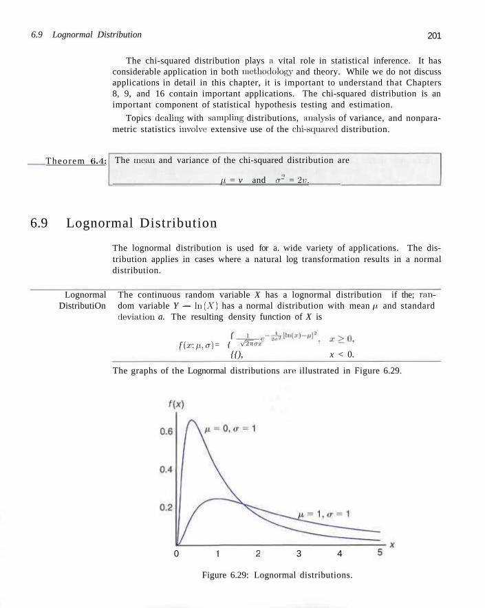
6.9 Lognormal Distribution 201
The chi-squared distribution plays a vital role in statistical inference. It has considerable application in both methodology and theory. While we do not discuss applications in detail in this chapter, it is important to understand that Chapters 8, 9, and 16 contain important applications. The chi-squared distribution is an important component of statistical hypothesis testing and estimation.
Topics dealing with sampling distributions, analysis of variance, and nonparametric statistics involve1 extensive use of the chi-squared distribution.
Theorem 6.4: The mean and variance of the chi-squared distribution are
//. = v and er" = 2-t'.
6.9 Lognormal Distribution
The lognormal distribution is used for a. wide variety of applications. The distribution applies in cases where a natural log transformation results in a normal distribution.
Lognormal The continuous random variable X has a lognormal distribution if the; ran-DistributiOn dom variable Y — hi (A) has a normal distribution with mean p. and standard
deviation a. The resulting density function of X is
f(x.;ii,a) = { V^trx {{), x < 0.
The graphs of the Lognormal distributions are illustrated in Figure 6.29.
0 1 2 3 4
Figure 6.29: Lognormal distributions.
202 Chapter 6 Some Continuous Probability Distributions
Theorem 6.5:
The cumulative distribution function is quite simple due to its relationship to the normal distribution. The use of the distribution function is illustrated by the following example.
Example 6.22:1 Concentration of pollutants produced by chemical plants historically are known to exhibit behavior that resembles a lognormal distribution. This is important when one considers issues regarding compliance to government regulations. Suppose it is assumed that the concentration of a certain pollutant, in parts per million, has a lognormal distribution with parameters p = 3.2 and a — 1. What is the probability that the concentration exceeds 8 parts per million?
Solution: Let. the random variable X be pollutant concentration
P(X > 8) = 1 - P(X < 8).
Since bx(X) has a normal distribution with mean p. = 3.2 and standard deviation (7 = 1,
PiX < 8) = <l> ln(8) - 3.2
1 #(-1.12) = 0.1314.
Here, we use the <3> notation to denote the cumulative distribution function of the standard normal distribution. As a result, the probability that the pollutant concentration exceeds 8 parts per million is 0.1314. J
Example 6.23:1 The life, in thousands of miles, of a certain type of electronic control for locomotives has an approximate lognormal distribution with p — 5.149 and a — 0.737. Find the 5th percentile of the life of such a locomotive.
Solution: From Table A.3 we know that P(Z < —1.645) = 0.05. Denote by A' the life of such a locomotive. Since ln(A') has a normal distribution with mean p = 5.149 and a = 0.737, the 5th percentile of X can be calculated as
ln(.r) = 5.149+ (0.737)(-1.045) = 3.937.
Hence, ,?;=51.265. This means that only 5% of the locomotives will have lifetime less than 51.265 thousand miles. J
6.10 Weibull Distribution (Optional)
Modern technology has enabled us to design many complicated systems whose operation, or perhaps safety, depends on the reliability of the various components making up the systems. For example, a fuse may burn out, a steel column may buckle, or a heat-sensing device may fail. Identical components subjected to identical environmental conditions will fail at different and unpredictable: times. Wc
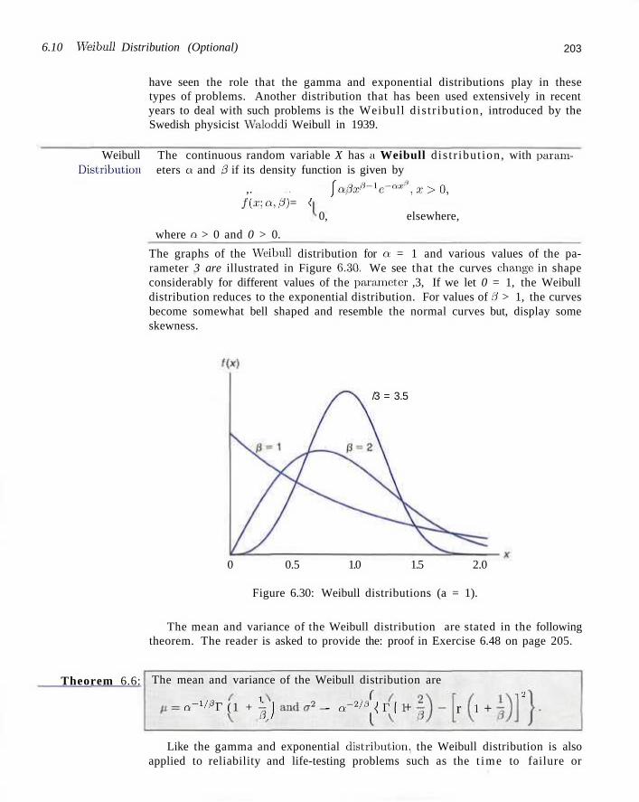
6.10 WeHmll Distribution (Optional) 203
have seen the role that the gamma and exponential distributions play in these types of problems. Another distribution that has been used extensively in recent years to deal with such problems is the Weibull d is t r ibut ion, introduced by the Swedish physicist Waloddi Weibull in 1939.
Weibull The continuous random variable X has a Weibull d is t r ibut ion, with parain-Distribution eters a and 0 if its density function is given by
,. . ja0x')-'e-"x", x>0, f(x:a,3) = <
0, elsewhere,
where a > 0 and 0 > 0.
The graphs of the Weibull distribution for a = 1 and various values of the parameter 3 are illustrated in Figure 6.30. We see that the curves change in shape considerably for different values of the parameter ,3, If we let 0 = 1, the Weibull distribution reduces to the exponential distribution. For values of 0 > 1, the curves become somewhat bell shaped and resemble the normal curves but, display some skewness.
/3 = 3.5
0 0.5 1.0 1.5 2.0
Figure 6.30: Weibull distributions (a = 1).
The mean and variance of the Weibull distribution are stated in the following theorem. The reader is asked to provide the: proof in Exercise 6.48 on page 205.
Theorem 6.6: The mean and variance of the Weibull distribution are
1 Q - i / 3 r ( 1 + ^ 1 2 - a'2!3 {T\l + r i +
n 2
Like the gamma and exponential distribution, the Weibull distribution is also applied to reliability and life-testing problems such as the t ime to failure or
204 Chapter 6 Some Continuous Probability Distributions
life length of a component, measured from some specified time until it fails. Let us represent this time to failure by the continuous random variable T, with probability density function f(t), where f(t) is the Weibull distribution. The Weibull distribution has the inherent flexibility that does not require the lack of memory property of the exponential distribution. The cumulative distribution function (cdf) for the Weibull can be written in closed form and certainly is useful in computing probabilities.
cdf for Weibull The cumulative distribution function for the Weibull distribution is given by Distribution
F(aO = l - e - a i r ' \ f o r ; r > 0 .
for a > 0 and 0 > 0.
Example 6.24:1 The length of life X in hours of an item in the machine shop has a Weibull distribution with o = 0.01 and 0=2. What is the probability that it fails before eight hours of usage?
Solution: P(X < 8) = F(8) = 1 - e^ 0 0 1 ) 8* = 1 - 0.527 = 0.473. J
The Failure Rate for the Weibull Distribution
When the Weibull distribution applies, it is often helpful to determine the failure rate (sometimes called hazard rate) in order to get a sense of wear or deterioration of the component. Let us first define the reliability of a component or product as the probability that it will function properly for at least a specified time under specified experimental conditions. Therefore, if R(t) is defined to be the reliability of the given component at time t, we may write
/•OO R(t) = P(T>t) = / f(t) dt = l- F(t),
where F(t) is the cumulative distribution function of T. The conditional probability that a component will fail in the interval from T = t to T = t + At, given that it survived to time t, is
F(t + At) - F(t) R(t)
Dividing this ratio by At and taking the limit as At —» 0, we get the failure rate, denoted by Z(t). Hence
Z(t) = lim F{t + At) ~F{t) 1 - F'{t) - f{t) - fit)
At-+o At R(t) R(t) R(t) l - F ( t ) '
which expresses the failure rate in terms of the distribution of the time to failure. Since Z(t) = f(t)/[l — F(t)], then the failure rate is given as the following:
Failure Rate for The failure rate at time t for the Weibull distribution is given by Weibull
Distribution Z(t) = a0tP~l, t > 0.
Exercises 205
Interpretation of the Failure Rate
The quanti ty Z(t) is aptly named as a failure rate since it docs quantify the rate of change over t ime of the conditional probabili ty tha t the component lasts an additional At given that it has lasted to time t. T h e ra te of decrease (or increase) with time is important . The following are crucial points.
(a) If 0 — 1, the failure ra te = a, a constant . This, as indicated earlier, is the special case of the exponential distribution in which lack of memory prevails.
(b) If 0 > 1, Z(t) is an increasing function of t which indicates tha t the component wears over time.
(c) If 0 < 1, Z(t) is a decreasing function of t ime and hence the component s trengthens or hardens over time.
For example, the item in the machine shop in Example 6.24 possesses 0 = 2 and hence it wears over time. In fact, the failure ra te function is given by Z(t) = .Q2t. On the other hand, suppose the parameters were 0 = 3/4 and a = 2. Z(t) = 1.5/f1
and hence the component gets stronger over t ime.
Exercises
6.39 If a random variable X has the gamma distribution with a = 2 and 0 = 1, find P(1.8 < X < 2.4).
6.40 In a certain city, the daily consumption of water (in millions of liters) follows approximately a gamma distribution with Q = 2 and 0 = 3. If the daily capacity of that city is 9 million liters of water, what is the probability that on any given day the water supply is inadequate?
6.41 Use the gamma function with y = \/2x to show that T(l/2) =s/n.
6.42 Suppose that the time, in hours, taken to repair a heat pump is a random variable X having a gamma distribution with parameters a =2 and 3 =1/2 . What is the probability that the next service call will require (a) at most 1 hour to repair the heat pump? (b) at least 2 hours to repair the heat pump?
6.43 (a) Find the mean and variance of the daily water consumption in Exercise 6.40.
(b) According to Chebyshev's theorem, there is a probability of at least 3/4 that the water consumption on any given day will fall within what interval?
6.44 In a certain city, the daily consumption of electric power, in millions of kilowatt-hours, is a random variable X having a gamma distribution with mean fi = 6 and variance a2 = 12.
(a) Find the values of a and 0. (b) Find the probability that on any given day the daily
power consumption will exceed 12 million kilowatt-hours.
6.45 The length of time for one individual to be served at a cafeteria is a random variable having an exponential distribution with a mean of 4 minutes. What is the probability that a person is served in less than 3 minutes on at least 4 of the next 6 days?
6.46 The life, in years, of a certain type of electrical switch has an exponential distribution with an average life 0 = 2. If 100 of these switches are installed in different systems, what is the probability that at most 30 fail during the first year?
6.47 Suppose that the service life, in years, of a hearing aid battery is a random variable having a Weibull distribution with a = 1/2 and B = 2. (a) How long can such a battery be expected to last? (b) What is the probability that such a battery will be
operating after 2 years?
6.48 Derive the mean and variance of the Weibull distribution.
6.49 The lives of a certain automobile seal have the Weibull distribution with failure rate Z(t) =\/\fi. Find the probability that such a seal is still intact after 4 years.
206 Chapter 6 Some Continuous Probability Distributions
6.50 The continuous random variable X has the beta distribution with parameters a and 3 if its density function is given by
fix) = J r(a)i \ 0 ,
+3) ^ - ' ( l - x ) ' ' 0 < x < 1,
elsewhere,
where a > 0 and 0 > 0. If the proportion of a brand of television set requiring service during the first year of operation is a random variable having a beta distribution with a = 3 and 3 = 2, what is the probability that at least 80% of the new models sold this year of this brand will require service during their first year of operation?
6.51 In a biomedical research activity it was determined that the survival time, in weeks, of an animal when subjected to a certain exposure of gamma radiation has a gamma distribution with a =5 and 3 =10.
(a) What is the mean survival time of a randomly selected animal of the type used in the experiment?
(b) What is the standard deviation of survival time? (c) What is the probability that an animal survives
more than 30 weeks?
6.52 The lifetime, in weeks, of a certain type of transistor is known to follow a gamma distribution with mean 10 weeks and standard deviation \/50 weeks. (a) What is the probability that the transistor will last
at most 50 weeks? (b) What is the probability that the transistor will not
survive the first 10 weeks?
6.53 Computer response time is an important application of the gamma and exponential distributions. Suppose that a study of a certain computer system reveals that the rasponse time, in seconds, has an exponential distribution with a mean of 3 seconds.
(a) What is the probability that response time exceeds 5 seconds?
(b) What is the probability that response time exceeds 10 seconds?
6.54 Rate data often follow a lognormal distribution. Average power usage (dB per hour) for a particular company is studied and is known to have a lognormal distribution with parameters fi = 4 and a =2. What is the probability that the company uses more than 270 dB during any particular hour?
6.55 For Exercise 6.54, what is the mean power usage (average dBs per hour)? What is the variance?
6.56 The number of automobiles that arrive at a certain intersection per minute has a Poisson distribution with a mean of 5. Interest centers around the time that elapses before 10 automobiles appear at the intersection.
(a) What is the probability that more than 10 automobiles appear at the intersection during any given minute of time?
(b) What is the probability that more than 2 minutes are required before 10 cars arrive?
6.57 Consider the information in Exercise 6.56. (a) What is the probability that more than 1 minute
elapses between arrivals?
(b) What is the mean number of minutes that elapse between arrivals?
6.58 Show that the failure-rate function is given by
Z(t) = a,3t0~l, t>0,
if and only if the time to failure distribution is the Weibull distribution
f(t)=a3t!i~le-atl', t>0.
Review Exercises
6.59 According to a study published by a group of sociologists at the University of Massachusetts, approximately 49% of the Valium users in the state of Massachusetts are white-collar workers. What is the probability that between 482 and 510, inclusive, of the next 1000 randomly selected Valium users from this state would be white-collar workers?
6.60 The exponential distribution is frequently applied to the waiting times between successes in a Pois
son process. If the number of calls received per hour by a telephone answering service is a Poisson random variable with parameter X = 6, we know that the time, in hours, between successive calls has an exponential distribution with parameter 0 =1/6. What is the probability of waiting more than 15 minutes between any two successive calls?
6.61 When a is a positive integer n, the gamma distribution is also known as the Erlang distribution.
Review Exercises 207
Setting a = n in the gamma distribution on page 195, the Erlang distribution is
fix) ) 3n(n-l)< '
\0, x > 0,
elsewhere.
It can be shown that if the times between successive events are independent, each having an exponential distribution with parameter 3, then the total elapsed waiting time X until all n events occur has the Erlang distribution. Referring to Review Exercise 6.60, what is the probability that the next 3 calls will be received within the next 30 minutes?
6.62 A manufacturer of a certain type of large machine wishes to buy rivets from one of two manufacturers. It is important that the breaking strength of each rivet exceed 10,000 psi. Two manufacturers (A and B) offer this type of rivet and both have rivets whose breaking strength is normally distributed. The mean breaking strengths for manufacturers A and B are 14,000 psi and 13,000 psi, respectively. The standard deviations are 2000 psi and 1000 psi, respectively. Which manufacturer will produce, on the average, the fewest number of defective rivets?
6.63 According to a recent census, almost 65% of all households in the United States were composed of only one or two persons. Assuming that this percentage is still valid today, what is the probability that between 590 and 625, inclusive, of the next 1000 randomly selected households in America will consist of either one or two persons?
6.64 The life of a certain type of device has an advertised failure rate of 0.01 per hour. The failure rate is constant and the exponential distribution applies. (a) What is the mean time to failure? (b) What is the probability that 200 hours will pass
before a failure is observed?
6.65 In a chemical processing plant it is important that the yield of a certain type of batch product stay above 80%. If it stays below 80% for an extended period of time, the company loses money. Occasional defective manufactured batches are of little concern. But if several batches per day are defective, the plant shuts down and adjustments are made. It is known that the yield is normally distributed with standard deviation 4%.
(a) What is the probability of a "false alarm" (yield below 80%) when the mean yield is 85%?
(b) What is the probability that a manufactured batch will have a yield that exceeds 80% when in fact the mean yield is 79%?
6.66 Consider an electrical component failure rate of once every 5 hours. It is important to consider the time that it takes for 2 components to fail. (a) Assuming that the gamma distribution applies,
what is the mean time that it takes for failure of 2 components?
(b) What is the probability that 12 hours will elapse before 2 components fail?
6.67 The elongation of a steel bar under a particular load has been established to be normally distributed with a mean of 0.05 inch and a = 0.01 inch. Find the probability that the elongation is
(a) above 0.1 inch; (b) below 0.04 inch; (c) between 0.025 and 0.065 inch.
6.68 A controlled satellite is known to have an error (distance from target) that is normally distributed with mean zero and standard deviation 4 feet. The manufacturer of the satellite defines a "success" as a firing in which the satellite comes within 10 feet of the target. Compute the probability that the satellite fails.
6.69 A technician plans to test a certain type of resin developed in the laboratory to determine the nature of the time it takes before bonding takes place. It is known that the mean time to bonding is 3 hours and the standard deviation is 0.5 hour. It will be considered an undesirable product if the bonding time is either less than 1 hour or more than 4 hours. Comment on the utility of the resin. How often would its performance be considered undesirable? Assume that time to bonding is normally distributed.
6.70 Consider the information in Review Exercise 6.64. What is the probability that less than 200 hours will elapse before 2 failures occur?
6.71 For Review Exercise 6.70 what is the mean and variance of the time that elapses before 2 failures occur?
6.72 The average rate of water usage (thousands of gallons per hour) by a certain community is known to involve the lognormal distribution with parameters p = 5 and a = 2. It is important for planning purposes to get a sense of periods of high usage. What is the probability that, for any given hour, 50,000 gallons of water are used?
6.73 For Review Exercise 6.72, what is the mean of the average water usage per hour in thousands of gallons?
6.74 In Exercise 6.52 on page 206, the lifetime of a
208 Chapter 6 Some Continuous Probability Distributions
transistor is assumed to have a gamma distribution with mean 10 weeks and standard deviation V50 weeks. Suppose that the gamma distribution assumption is incorrect. Assume that the distribution is normal. (a) What is the probability that the transistor will last
at most 50 weeks? (b) What is the probability that the transistor will not
survive for the first 10 weeks? (c) Comment on the difference between your results
here and those found in Exercise 6.52 on page 206.
6.75 Consider Exercise 6.50 on page 206. The beta distribution has considerable application in reliability problems in which the basic random variable is a proportion in the practical scenario illustrated in the example. In that regard, consider Review Exercise 3.75 on page 105. Impurities in the batch of product of a chemical process reflect a serious problem. It is known that the proportion of impurities Y in a batch has the density function
fiy) = J10*1 -yf 0 < y < l , elsewhere.
(a) Verify that the above is a valid density function. (b) What is the probability that a batch is considered
not acceptable (i.e., Y > 0.6)? (c) What are the parameters a and 0 of the beta dis
tribution illustrated here? (d) The mean of the beta distribution is ^pj. What is
the mean proportion of impurities in the batch?
(e) The variance of a beta distributed random variable is
a2 = a0 (a + 0)*(a + 0+1)'
What is the variance of Y in this problem?
6.76 Consider now Review Exercise 3.76 on page 105. The density function of the time Z in minutes between calls to an electrical supply store is given by
/(*) \o, -z/10 0 < z < co,
elsewhere.
(a) What is the mean time between calls? (b) What is the variance in the time between calls? (c) What is the probability that the time between calls
exceeds the mean?
6.77 Consider Review Exercise 6.76. Given the assumption of the exponential distribution, what is the mean number of calls per hour? What is the variance in the number of calls per hour?
6.78 In a human factor experimental project, it has been determined that the reaction time of a pilot to a visual stimulus is normally distributed with a mean of 1/2 second and standard deviation of 2/5 seconds.
(a) What is the probability that a reaction from the pilot takes more than 0.3 seconds?
(b) What reaction time is that which is exceeded 95% of the time?
6.79 The length of time between breakdowns of an essential piece of equipment is important in the decision of the use of auxiliary equipment. An engineer thinks that the best "model" for time between breakdowns of a generator is the exponential distribution with a mean of 15 days. (a) If the generator has just broken down, what is the
probability that it will break down in the next 21 days?
(b) What is the probability that the generator will operate for 30 days without a breakdown?
6.80 The length of life, in hours, of a drill bit in a mechanical operation has a Weibull distribution with a = 2 and 0 = 50. Find the probability that the bit will fail before 10 hours of usage.
6.81 Derive the cdf for the Weibull distribution. [Hint: In the definition of a cdf, make the transformation z = j/3 .]
6.82 In Review Exercise 6.80, explain why the nature of the scenario would likely not lend itself to the exponential distribution.
6.83 Form the relationship between the chi-squared random variable and the gamma random variable, prove that the mean of the chi-squared random variable is v and the variance is 2v.
6.84 The length of time, in seconds, that a computer user reads his (or her) e-mail is distributed as a log-normal random variable with p = 1.8 and a2 = 4.0. (a) What is the probability that the user reads the mail
for more than 20 seconds? More than a minute? (b) What is the probability that the user reads the mail
for a length of time that is equal to the mean of the underlying lognormal distribution?
6.11 Potential Misconceptions and Hazards; Relationship to Material in Other Chapters 209
6.11 Potential Misconceptions and Hazards; Relationship to Material in Other Chapters
Many of the hazards in the use of material in this chapter are quite similar to those of Chapter 5. One of the biggest: misuses of statistics is the assumption of an underlying normal distribution in carrying out a type of statistical inference: when indeed it is not normal. The reader will be exposed to tests of hypotheses in Chapters 10 through 15 in which the normality assumption is made. In addition, however, the reader will be reminded that, there are t es t s of goodness of fit as well as graphical routines discussed in Chapters 8 and 10 that allow for "chee;ks" on data to determine if the normality assumption is reasonable.
Chapter 7
Functions of Random Variables (Optional)
7.1 Introduction
This chapter contains a broad spectrum of material. Chapters 5 and 6 deal with specific: types of distributions, both discrete and continuous. These arc: distributions that find use in many subject matter applications, including reliability, quality control, and acceptance sampling. In the present chapter wc begin with a more general topic:, that of distributions of functions of random variables. General techniques are introduced and illustrated by examples. This is followed by a related concept, moment-generating functions, which can be helpful in [earning about distributions of linear functions of random variables.
In standard statistical methods, the result of statistical hypothesis testing, estimation, or even statistical graphics does not involve a single random variable but, rather, functions of one or more random variables. As a result, statistical inference requires the distributions of the>se functions. For example, the use of averages of r andom variables is common. In addition, sums and more general linear combinations are important. We are often interested in the distribution of sums of squares of random variables, particularly in the use of analysis of variance techniques discussed in Chapters 11 14.
7.2 Transformations of Variables
Frequently in statistics, one encounters the need to derive the probability distribution of a function of one: or more random variables. Fbr example, suppose that X is a discrete random variable with probability distribution f(x), and suppose further that Y = u(X) defines a one-to-one transformation between the values of X and Y. We wish to find the probability distribution of Y. It is important to note that the one-to-one transformation implies that each value x is related to one, and only one, value y = u(x) and that each value y is related to one, and only one:, value x = w(y), where w(y) is obtained by solving y = u(x) for x in terms of y.
212 Chapter 7 Functions of Random Variables (Optional)
From our discussion of discrete probability distributions in Chapter 3, it is clear that the random variable Y assumes the value y when X assumes the value w(y). Consequently, the probability distribution of Y is given by
g(y) = P(Y = y) = P[X = w(y)} = f[w(y)].
Theorem 7.1: Suppose that X is a discrete random variable with probability distribution fix). Let Y = u(X) define a one-to-one transformation between the values of X and y so that the equation y = u(x) can be uniquely solved for x in terms of y, say x = w(y). Then the probability distribution of Y is
giv) = f[w(y)].
Example 7.1:1 Let X be a geometric random variable with probability distribution
m" /(r) ^ 4 U J ' •7: = 1'2'3""--Find the probability distribution of the random variable Y = X2.
Solution: Since the values of X are all positive, the transformation defines a one-to-one correspondence between the x and y values, y = x2 and x = ^/y. Hence
g{v) = _ |7(VJ/) = ! Q ) ^ \ ?/ = i,4,9,...,
10, elsewhere. J
Consider a problem where Xx and X2 are two discrete random variables with joint probability distribution f(x\,x2) and we wish to find the joint probability distribution g(yi,y2) of the two new random variables,
Yx = ux(X\, Xt) and Y2 = u2(Xx,X2),
which define a one-to-one transformation between the set of points (xi, x2) and (2/1.2/2)- Solving the equations y\ = u\(x\,x2) and y2 = u2(x\,x2) simultaneously, we obtain the unique inverse solution
xx = wx (2/1 ,y2), and x2 = w2 (yx ,y2)-
Hence the random variables Yi and Y2 assume the values y\ and y2, respectively, when A'i assumes the value wx (j/i, 2/2) and X2 assumes the value w2 = (yi, y2). The joint probability distribution of Yi and Y2 is then
5(1/1,2/2) = P\Yx = y\,Y2 = 2/2) = P[X\ = wi(yx,y2),X2 = w2(yx,y2)]
= f[miyi,V2),w2iyx,m)]-
7.2 Transformations of Variables 213
Theorem 7.2: Suppose that A'i and X2 are discrete random variables with joint probability distribution f(xx,x2)- Let Yi = uxiXx,X2) and Y2 = u2(Xx,X2) define a one-to-one transformation between the points (xx,x2) and (2/1,2/2) so that the equations
2/i = ux(xx,x2) and 2/2 = u2(xx,x2)
may be uniquely solved for xx and x2 in terms of 2/1 and y2, say xx = 1^1(2/1,2/2) and X2 = ^2(51,52)- Then the joint probability distribution of Yi and Y2 is
5(2/1,2/2) = f[m(yu 2/2), 1^2(2/1, lte)].
Theorem 7.2 is extremely useful for finding the distribution of some random variable Y] = ui(Xx,X2), where X\, and X2 are discrete random variables with joint probability distribution f(x\,x2). We simply define a second function, say Y2 = u2(Xx,X2), maintaining a one-to-one correspondence between the points (xx,x2) and (2/1,2/2), and obtain the joint probability distribution 5(2/1,2/2)- The distribution of Yi is just the marginal distribution of 5(2/1,2/2), found by summing over the 2/2 values. Denoting the distribution of Y] by h(y\), we can then write
M2/1) = ^.9(2/i ,2/2) •
Example 7.2:1 Let Xi and X2 be two independent random variables having Poisson distributions with parameters p\ and p2, respectively. Find the distribution of the random variable Yx = Xx + X2.
Solution: Since Xi and X2 arc independent, we can write
fixx,x2) = f(xi)f(x2) = - ' " / 4 1 e-' '2P22
zi l .r2!
e-(^+«*)pXlpx*
.Tl!x2!
where Xx = 0 ,1 ,2 , . . . , and x2 = 0,1,2, Let us now define a second random variable, say Y2 = X2. The inverse functions arc given by x\ = 2/1 —2/2 and x2 —y2. Using Theorem 7.2, we find the joint probability distribution of Yi and Y2 to be
5(2/1 • 2/2) = e-Ou+wO^vi-i t t^
(2/1 - 52)152!
where 2/1 = 0 ,1 ,2 , . . . , and y2 = 0 ,1 ,2 , . . .,y\. Note that since x\ > 0, the transformation Xi = j/i — x-2 implies that y2 and hence x2 must always be less than or equal to 2/1 • Consequently, the marginal probability distribution of Y] is
Vi VI
% . ) = Y 5(5i,52) = e- ( '"+"a ) Y TTTZ 11-2=0 t/2=0 W
,-(fl+K2) Jli. y i (
Mi1"w/4f 52)152!
51!
-(M1+M2)
E » ' ' ,,!/l -1/2 ,,.V2
_ 0 5 2 ! ( 5 , - 5 2 ) ! / i l M2
5i 3/2=0 V W 2 /
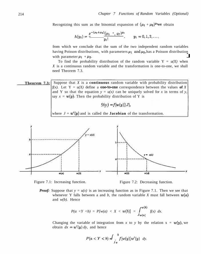
214 Chapter 7 Functions of Random Variables (Optional)
Recognizing this sum as the binomial expansion of (px + p2)yi we obtain
e - O l + / i 2 ) ( u . + uo)yi
M ' 5 i ) = f g l ; • 2 / 1 - 0 , 1 , 2 , . . . ,
from which we conclude that the sum of the two independent random variables having Poisson distributions, with parameters px and p2, has a Poisson distribution with parameter px + p2- J
To find the probability distribution of the random variable Y = u(X) when X is a continuous random variable and the transformation is one-to-one, we shall need Theorem 7.3.
Theorem 7.3: Suppose that X is a continuous random variable with probability distribution f(x). Let Y = u(X) define a one-to-one correspondence between the values of X and Y so that the equation y = u(x) can be uniquely solved for x in terms of y, say x = w(y). Then the probability distribution of Y is
9iy) = fHy)]\J\,
where J = w'(y) and is called the Jacobian of the transformation.
w(a) w(b)
Figure 7.1: Increasing function.
b
\ y = "(x)
vv(fi) w{a)
Figure 7.2: Decreasing function.
Proof: Suppose that y = u(x) is an increasing function as in Figure 7.1. Then we see that whenever Y falls between a and b, the random variable X must fall between w(a) and w(b). Hence
rw(b)
P(a <Y <b) = P[w(a) < X < w(b)] = / f(x) dx. Jw(a)
Changing the variable of integration from x to y by the relation x = w(y), we obtain dx = w'(y) dy, and hence
P(a<Y<b)= f f[w(y)]w'(y) dy. J a
7.2 Transformations of Variables 215
Since the integral gives the desired probability for every a < b within the permissible set of y values, then the probability distribution of Y is
9iv) = f[wiy)]v/iy) = f[w(y)]J.
If wc recognize ./ = u:'(y) as the reciprocal of the slope of the tangent line to the curve of the increasing function y = u(x), it is then obvious that J = \J\. Hence
9iv) = f[w(y)]\J\.
Suppose that y = u(x) is a decreasing function as in Figure 7.2. Then we write
P(a <Y<b) = P[w(b) < X < w(o)\ = / f(x) dx.
Again changing the variable of integration to y, wc: obtain
P(a < Y <b)= I f[w(y)}w'(y) dy = - / f[iv(y)\w'(g) dy, •I i, J„
from which wc conclude that
9iv) = -fMy)]w'(y) = -f[w(y)]J.
In this case the slope of the curve is negative and .7 = —1./|. Hence
g(y) = f\w(y)}\J\,
as before. J
Example 7.3:1 Let X be a continuous random variable with probability distribution
/'(a:) = J &' 1 < :': < 5' l o , elsewhere.
Find the probability distribution of the random variable V" = 2X — 3. Solution: The inverse solution of y = 2x — 3 yields x = (y + 3)/2, from which we obtain
J = w'(y) = dx/dy = 1/2. Therefore, using Theorem 7.3, we find the density function of Y to be
rM|iZ2(i) = ^ - 1 < , < 7 , </(v) = <n '- y~' , , I
10, elsewhere. To find the joint probability distribution of the: random variables Y\ = u\ (A'i, X2) and Y2 = u2(X\,X2) when X\ and X2 arc: continuous and the transformation is one-to-one, we need an additional theorem, analogous to Theorem 7.2. which we state without proof.
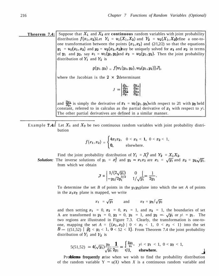
216 Chapter 7 Functions of Random Variables (Optional)
Theorem 7.4: Suppose that A'i and X2 are continuous random variables with joint probability distribution f(xi,x2). Let Yx = u i p f i , X2) and Y2 = u2(Xi,X2) define a one-to-one transformation between the points (xi,X2) and (2/1,2/2) so that the equations 2/1 = ui(xi,X2) and y2 = u2(xx,x2) may be uniquely solved for xi and X2 in terms of 2/1 and 2/2, say xi = w\(yi,y2) and X2 = tf2(5i,52)- Then the joint probability distribution of Yi and Y2 is
5(51,52) = /K(2/i,52),W2(5i,52)]|J|,
where the Jacobian is the 2 x 2 determinant
J = dx,
& Ox 1 dy2
6x3 9V2
and g j 1 is simply the derivative of xx = wi(yx,y2) with respect to 2/1 with y2 held constant, referred to in calculus as the partial derivative of xi with respect to y\. The other partial derivatives are defined in a similar manner.
Example 7.4:1 Let Xx and X2 be two continuous random variables with joint probability distribution
J l> i ,x 2 ) = 4xix2 , 0 < xi < 1, 0 < x2 < 1,
0, elsewhere.
Find the joint probability distribution of Yi = X2 and Y2 = XxX2. Solution: The inverse solutions of j/i = x2 and y2 = xxx2 are xi = ^fyl and x2 = y2j yfy[,
from which we obtain
,7 = 1 / ( 2 ^ ) 0
-y2j2y\12 Ify/yi
1
2'5i'
To determine the set B of points in the y\y2 plane into which the set A of points in the X1X2 plane is mapped, we write
Xx = y/m and x2 = y2/v/m
and then setting X\ = 0, X2 = 0, X] = 1, and X2 = 1, the boundaries of set A are transformed to yi = 0, y2 = 0, 2/1 = 1, and 2/2 — \/5i or y\ = yx- The two regions are illustrated in Figure 7.3. Clearly, the transformation is one-to-one, mapping the set A = {(xi,X2) | 0 < xi < 1, 0 < x2 < 1} into the set B — {(51,52) I 52 < 5i < 1, 0 < 52 < 1}. From Theorem 7.4 the joint probability distribution of Yi and Y2 is
52 1 f2 , 122/1 [0,
y\ < 2/1 < 1, 0 < 2/2 < 1, elsewhere.
5(51,52) =4(y/yi~)
iblems frequently z of the random variable Y = u(X) when X is a continuous random variable and
\fy~\2y\ l [J, elsewhere. 1
Problems frequently arise when we wish to find the probability distribution
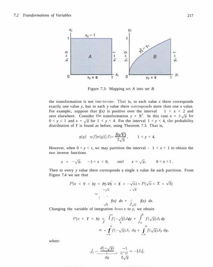
7.2 Transformations of Variables 217
x2 = 0 y2 = 0
Figure 7.3: Mapping set A into set B.
the transformation is not one-to-one. That, is, to each value x there corresponds exactly one value y, but to each y value there corresponds more than one x value. For example:, suppose that f(x) is positive over the interval — 1 < x < 2 and zero elsewhere. Consider the transformation y = X2. In this case x = ±*/l7 for 0 < y < 1 and x = ,Jy for 1 < y < 4. For the interval 1 < y < 4, the probability distribution of Y is found as before, using Theorem 7.3. That is,
giv) = fHvW\ fis/V) - \ /5 '
1 < y < 4.
However, when 0 < y < t, wc may partition the interval — 1 < x < 1 to obtain the two inverse functions
x = -y/y, 1 < x < 0, . 'uiel x = y/y, 0 < x < l .
Then to every y value there corresponds a single x value for each partition. From Figure 7.4 we see that
P(u. < Y < b) = P(-Vb < X < - V o ) + P(v /a < X < Vb)
/
- v/77 /• </b
fix) dx + / f(x) dx. -Vb JjTi.
Changing the variable of integration from x to y, we obtain
P(n < Y < b) = f f(-y/y)Ji dy + I f(y/y)J» dy J I, J a
= - f f(-yfi)J\ dy+ j f{y/y)J2dy,
when
, gc-yy) - i Jl ~ i = TT^=
dv 2\/y
218 Chapter 7 Functions of Random Variables (Optional)
y = x*
-1 -v6~ -Va Va VF 1
Figure 7.4: Decreasing and increasing function.
and
* / 2yf
Hence we can write
P(« <Y<b)= I \f(-Jy-)\Jy\ + f{y/y)\J2\] dy, J a
and then
5(5) = fi-Vv)\Ji\ + f{y/v)\h\ = / ( Vfl + /(vfl 0 L 2^/j/
The probability distribution of Y for 0 < y < 4 may now be written
/(-v*yv*>, 0<2/<l, 4 4£f , ' 1< v, < 4,
0, elsewhere.
This procedure for finding g(y) when 0 < y < 1 is generalized in Theorem 7.5 for k inverse functions. For transformations not one-to-one of functions of several variables, the reader is referred to Introduction to Mathematical. Statistics by Hogg and Craig (see the Bibliography).
7.3 Moments and Moment-Generating Functions 219
Theorem 7.5: Suppose that X is a continuous random variable with probability distribution fix). Let Y = u(X) define a transformation between the value of X and Y that is not one-to-one. If the interval over which X is defined can be partitioned into k mutually disjoint sets such that each of the inverse functions
xx = w\iv)> x2 =w2(y), Xk = Wk(y)
of y = u(x) defines a one-to-one correspondence, then the probability distribution of Y is
9(y) = Yf[mivWil 4 = 1
where Ji = w'^y), i = 1,2,.. . , k.
Example 7.5:1 Show that Y = (X — p)2/o2 has a chi-squared distribution with 1 degree of freedom when A' has a normal distribution with mean p and variance a2.
Solution: Let Z = (X — p)/a, where the random variable Z has the standard normal distribution
/(*) = 1 -z2/2
'2it —oo < z < oo.
We shall now find the distribution of the random variable Y = Z2. The inverse solutions of y = z2 are z = ±\/j7' ^ w e designate z\ = — Vy and z2 — \/y, then J\ = —l/2yfy and J2 = 1/2V/Ty. Hence, by Theorem 7.5, we have
giy) = -!/ /2
2^5 - y / 2
'2-n 2VP yi/a-ie-ir/2, 5 > 0 .
Since g(y) is a density function, it follows that
/2K Jo i /a-ie-s/a rf,J = d5
£(1/2) o yX/2-Xe-y/2 _ F(l/2)
v/2r(l/2) w " v^ ' /2) f°° j /V ' - ' e " SF ./,, v
/2r( i y
the integral being the area under a gamma probability curve with parameters o = 1/2 and 0 = 2. Therefore, ^px = r ( l / 2 ) and the probability distribution of Y is given by
1 . . .1/2-1 -?/ /2 > n
7Hwi)5 . 5>0, 0, elsewhere,
which is seen to be: a chi-squared distribution with 1 degree of freedom. _l
7.3 Moments and Moment-Generating Functions
In this section we concentrate on applications of moment-generating functions. The obvious purpose of the moment-generating function is in determining moments
220 Chapter 7 Functions of Random Variables (Optional)
Definition 7.1:
of random variables. However, the most important contribution is to establish distributions of functions of random variables.
lig(X) = X1' for r = 0 ,1 ,2 ,3 , . . . , Definition 7.1 yields an expected value called the rth moment abou t the origin of the random variable X, which we denote by p'r.
The rth momen t about the origin of the random variable X is given by
J2xrf(x), if X is discrete, //,. = E(Xr)
J_ xrf(x) dx, if A' is continuous.
Since the first and second moments about the origin are given by p.] = E(X) and p2 = E(X2), we can write the mean and variance of a random variable as
p = p. and p2 - pr
Although the moments of a random variable can be determined directly from Definition 7.1, an alternative procedure exists. This procedure requires us to utilize a moment-genera t ing function.
Definition 7.2: The moment-genera t ing function of the random variable X is given by E(etx) and is denoted by Mx(t). Hence
Mx(t) = E(et*) £ e * " / ( x ) , if X is discrete,
f(x) dx, if X is continuous.
Moment-generating functions will exist only if the sum or integral of Definition 7.2 converges. If a moment-generating function of a random variable X does exist, it can be used to generate all the moments of that variable. The method is described in Theorem 7.0.
Theorem 7.G: Let AT be a random variable with moment-generating function A/y(r). Then
drMx(t)
dtr = Mr (=0
Proof: Assuming that wc: can differentiate inside summation and integral signs, we obtain
drMX (f) j T, Xretxf(x), if X is discrete,
dfV \ IZo xre'xf(x) dx, if X is continuous.
Setting t = 0, wc: see that both cases reduce to 7i'(Xr) = pr. J
Example 7.6:1 Find the moment-generating function of the binomial random variable X and then use it to verify that //. = np and o2 = npq.
7.3 Moments and Moment-Generating Functions 221
Solution: From Definition 7.2 we have:
MX(t)=5>te(")pv-* = Y ("W)v-*. :i: = t> ^ ' x-0 \ * /
Recognizing this last sum as the binomial expansion of (pe* + q)", wc obtain
Mxit) = (pet + q)n.
Now
dMx(t) I i ~\n—l„„t
dt = n(pe' +q)"~lpe
d2Mx(t) _ dt?
Setting t = 0, we get
np[c'(n - l)(pe' + q)n-2pel + (pe1 + ey)"" V]
and
Therefore.
p, = np
p2 = np[(n- l)p + 1].
and
p = Px~ "P
o2 = p2 - P2 = np(\ - p) = npq,
which agrees with the results obtained in Chapter 5.
Example 7.7:1 Show that the moment-generating function of the random variable X having a normal probability distribution with mean p and variance a1 is given by
Mx(l)=v.xp(pi+^a2tA .
Solution: From Definition 7.2 the moment-generating function of the normal random variable X is
-^--jy^HM dx
J^x \/2TT exp
x2 - 2(p + ta2)x + p
2a'2 dx.
222 Chapter 7 Functions of Random Variables (Optional)
Completing the square in the exponent, we can write
x2 - 2(p + ta2)x + p2 = [x - (p. + ta2)}2 - 2pto2 - t2o4
and then
*«-£?c-'{-"-»""t-»--*> -W £)£7feM- f c Jss s a t}*
Let w = [x - (p + £<72)]/CT; then dx = er eiwi and
Mx (t) = exp htf + \<J2t2\ j -j=e-w^2 dw = exp (pet + ^<T2*2) ,
since the last integral represents the area under a standard normal density curve and hence equals 1. J
Example 7.8:1 Show that the moment-generating function of the random variable X having a chi-squared distribution with v degrees of freedom is Mx(r-) = (1 — 2t)~vf2.
Solution: The chi-squared distribution was obtained as a special case of the gamma distribution by setting a = v/2 and 3 = 2. Substituting for f(x) in Definition 7.2, we obtain
r°° l Adx(t) = / etx - xv/2~1e~x/2 dx
x[> Jo 2*/2r(l!/2)a; ax
- I f rv/2-l -x(X-2t)/2 d
Writing y = x(l - 2t)/2 and cix = [2/(1 - 2t)} dy, we get for t < ±,
1 f°° f 2v \v/2~i 2
" r W 2 K l ^ l" v"",e" * = (1"2,)""2 '
since the last integral equals r(u/2) . J
Although the method of transforming variables provides an effective way of finding the distribution of a function of several variables, there is an alternative and often preferred procedure when the function in question is a linear combination of independent random variables. This procedure utilizes the properties of moment-generating functions discussed in the following four theorems. In keeping with the mathematical scope of this book, we state Theorem 7.7 without proof.
7.3 Moments and Moment-Generating Functions 223
Theorem 7.7: (Uniqueness Theorem) Let X and Y be two random variables with moment-generating functions Mxit) and My(t), respectively. If Mx(t) = My-(£) for all values of t, then X and Y have the same probability distribution.
Theorem 7.8: Mx+a(t) = eatMx(t).
Proof: Mx+ait) = E[etiX+")\ = eatE(elX) = e<"Mx(t).
Theorem 7.9: Maxit) = Mxiat).
Proof: MaX(t) = E[ei{-"x^\ = E\eia^x] = Mxiat).
Theorem 7.10: If X i , X 2 , . . . , X n are independent random variables with moment-generating functions MXl it), M . Y 2 ( 0 , • • •, Mx„ it), respectively, and Y = Xi + X2 + r Xn, then
Mr(t) = MXl {t)Mx2(t) • • • MXn it).
,X2,..., xn) dx\ dx2 • • • dx„.
Proof: For the continuous case
MYit) = E(etY) = E[et{Xi+x*+-+x")}
/
OO /»GQ
• " / #**+*+™+x4f{s1,x •oc J—oc
Since the variables are independent, we have
f(xux2,. • ., Xn) = fxixi )f2(x2) • • • /„(xr,.)
and then
/
OO rC>Cl /-OC
e^fxixi) dxx / e,x\f2(x2) dx2 • • • / ete» fn(xn) dxn - CO J—OC J — DC'
= MXl(t)MX2(t)---MxJt). j The proof for the discrete case is obtained in a similar manner by replacing integrations with summations.
Theorems 7.7 through 7.10 are vital for understanding moment-generating functions. An example follows to illustrate. There are many situations in which we need to know the distribution of the sum of random variables. We may use Theorems 7.7 and 7.10 and the result of Exercise 7.19 following this section to find the distribution of a sum of two independent Poisson random variables with moment-generating functions given by
MXl it) = e - „/'l (<>'-!) Mx.2(t) = e'l'l-ei-1\
224 Chapter 7 Functions of Random Variables (Optional)
respectively. According to Theorem 7.10, the moment-generating function of the random variable Y\ — Xx + X2 is
MYl(t) = MXl(t)MxAt) = e/M«'-i)e/'2(e«-i) = etMi+^Ke'-i)
which we immediately identify as the moment-generating function of a random variable having a Poisson distribution with the parameter pi + p2- Hence, according to Theorem 7.7, we again conclude that the sum of two independent random variables having Poisson distributions, with parameters pi and p2, has a Poisson distribution with parameter pi + p2-
Linear Combinations of Random Variables
In applied statistics one frequently needs to know the probability distribution of a linear combination of independent normal random variables. Let us obtain the distribution of the random variable Y = a iXi +02X2 when Xi is a normal variable with mean px and variance o2 and X2 is also a normal variable but independent of Xi with mean p2 and variance cr2. First, by Theorem 7.10, we find
MY(t) = MaiXl(t)Ma2X2(t),
and then, using Theorem 7.9,
My(t) = Mx,iaxt)MX2(a2t).
Substituting axt for t and then a2t for t in a moment-generating function of the normal distribution derived in Example 7.7, we have
My(t) = exp(axpit + d\a2t2/2 + a2p2t + a\o\t2 j2)
= exp[(aipi + a2p2)t + (ajaj + ala2)t2/2],
which we recognize as the moment-generating function of a distribution that is normal with mean aipi + CI2P2 and variance a2cT2 + a\o~\.
Generalizing to the case of n independent normal variables, we state the following result,
Theorem 7.11: If X l , X 2 , . . . , with means px dom variable
xn ,M2,
are independent random variables having normal distributions ...,p„ and variances a\,o\,...,on, respectively, then the ran-
Y = - axXx + 02X2 + •
has a normal distribution with mean
and variance
VY
a\
= flipi +a2p2 +
2 2 1 2 2 , = a\a\ + a\a2 + •
• • + anXn
••+ anpn
••+<&£•
It is now evident that the Poisson distribution and the normal distribution possess a reproductive property in that the sum of independent random variables
7.3 Moments and Moment-Generating Functions 225
having either of these: distributions is a random variable that also has the same type of distribution. This reproductive property is also possessed by the chi-squared distribution.
Theorem 7.12: If A'i, A ro,. . . , Xn arc mutually independent random variables that have, respectively, chi-squared distributions with vx, v2,..., vn degrees of freedom, then the random variable
Y = Xx + X2 + • • • + X„
has a chi-squared distribution with v = V\ + v2 + • • • + vn degrees of freedom.
Proof: By Theorem 7.10,
My(l) = Mxl(t)MX2(l.)---MxJt).
From Example 7.8.
,U.v,(/) = ( l - 2 / . ) - " ' / 2 , i= l ,2 , . . . ,n . ]
Therefore,
MY(t) = (1 - 2/,)-' : i /2(l - 2/.)-"- /2 • . - ( I - 2t)-v^2
= (1 - 2/:)~("1+"-+"'+"")/'2,
which we recognize as the moment-generating function of a chi-squared distribution
with v — V\ + i»2 + • • • + vn degrees of freedom. J
Corollary 7.1: If Xi, X 2 , . . . , X„ are independent random variables having identical normal distributions with mean p and variance a2, then the random variable
r-T, i=l
Xi - p
has a chi-squared distribution with v = n degrees of freedom.
This corollary is an immediate consequence of Example 7.5, which states that each of the n independent random variables [(A",; — p)/a]2, i — 1,2, . . . , n , has a chi-squared distribution with 1 degree of freedom. This corollary is extremely important. It establishes a relationship between the very important chi-squared distribution and the normal distribution. It also should provide the reader a clear idea of what wc mean by the parameter that wc; call degrees of freedom. As we move into future chapters, the notion of degrees of freedom plays an increasingly important role. We see from Corollary 7.1 that if Z\,Z2,... ,Zn are independent
" standard normal random variables, then J^ Zf has a chi-squared distribution and
the single parameter, v, the degrees of freedom, is n, the number of standard normal variates. Furthermore, if each normal random variable in the Xi, in Corollary 7.1 has different mean and variance, wc can have the following result.
226 Chapter 7 Functions of Random Variables (Optional)
C o r o l l a r y 7.2: If X ] , X2, • • •, X n are independent random variables and X; follows a normal distribution with mean p.j and variance a2 for i = 1,2, . . . , n , then the random variable
Y £ Xt - fa
at
has a chi-squared distribution with v = n degrees of freedom.
Exercises
7.1 Let X be a random variable with probability
' 4 , 85 = 1,2,3, elsewhere. / ( * :
• f t Find the probability distribution of the random variable Y = 2 X - 1 .
7.2 Let X be a binomial random variable with probability distribution
Show that the random variable Y = —2 In A' has a chi-squared distribution with 2 degrees of freedom.
7.6 Given the random variable X with probability distribution
/ (*) = 2x, 0 < x < 1, 0. elsewhere.
/w = {air (i)". x = 0,1,2,3, elsewhere.
Find the probability distribution of the random variable Y = X2.
7.3 Let Xi and X2 be discrete random variables with the joint multinomial distribution
find the probability distribution of Y = 8X3 .
7.7 The speed of a molecule in a uniform gas at equilibrium is a random variable V whose probability distribution is given by
/ (x i .xa )
Xl,X2, 2 — X\ — x2
/(«) = 0. 0 > 0, elsewhere.
for x\ = 0,1,2; £2 = 0,1,2; x\ + x2 < 2; and zero elsewhere. Find the joint probability distribution of Yx = Xi + X2 and y2 = Xx - X2.
7.4 Let Xi and Xi be discrete random variables with joint probability distribution
where k is an appropriate constant and b depends on the absolute temperature and mass of the molecule. Find the probability distribution of the kinetic energy of the molecule W, where W = mV2 /2.
7.8 A dealer's profit, in units of $5000, on a new automobile is given by Y = X 2 , where X is a random variable having the density function
fixi,x2) 16
o, zi = 1,2; X2 = 1,2,3, elsewhere. *> - { * - * 0 < x< 1,
elsewhere.
Find the probability distribution of the random variable Y = Xi.X-2.
7.5 Let X have the probability distribution
/ ( * ) -1, 0 < x < 1. 0, elsewhere.
(a.) Find the probability density function of the random variable Y.
(b) Using the density function of Y, find the probability that the profit will be less than S500 on the next new automobile sold by this dealership.
Exercises 227
7.9 The hospital period, in days, for patients following treatment for a certain type of kidney disorder is a random variable Y = X + 4, where X has the density function
If the resistance varies independently of the current according to the probability distribution
fix. -{ 9ir)
(x+4)* '
0,
x>0,
elsewhere.
_ f 2r, 0 < ~~ \0, else
r < I, elsewhere,
(a) Find the probability density function of the random variable Y.
(b) Using the density function of Y, find the probability that the hospital period for a patient following this treatment will exceed 8 days.
7.10 The random variables X and Y, representing the weights of creams and toffees in 1-kilogram boxes of chocolates containing a mixture of creams, toffees, and cordials, have the joint density function
find the probability distribution for the power W = I2R watts.
7.14 Let X be a random variable with probability distribution
(0, elsewhere.
Find the probability distribution of the random variable Y = X2.
fix, y) = '24xy,
.0,
0 < x < 1 , 0 < x + y< 1, elsewhere.
< 1,
7.15 Let X have the probability distribution
fix) -flr t11, -\<x<2, elsewhere.
(a) Find the probability density function of the random variable Z = X + Y.
(b) Using the density function of Z, find the probability that in a given box the sum of the creams and toffees accounts for at least 1/2 but less than 3/4 of the total weight.
7 .11 The amount of kerosene, in thousands of liters, in a tank at the beginning of any day is a random amount Y from which a random amount X is sold during that day. Assume that the joint density function of these variables is given by
fix,y) - f t
0 < x < y, 0 < y < 1, elsewhere.
Find the probability density function for the amount of kerosene left in the tank at the end of the day.
7.12 Let Xi and X2 be independent random variables each having the probability distribution
fix
Find the probability distribution of the random variable Y = X2.
7.16 Show that the r th moment about the origin of the gamma distribution is
' 0'T(a + r)
[Hint: Substitute y = x/Q in the integral defining pr' and then use the gamma function to evaluate the integral]
7.17 A random variable X has the discrete uniform distribution
/(x;fc) = / * ' x~l,2,...,k,
Jy ' \ 0 , elsewhere.
Show that the moment-generating function of X is
e{(l - e*') x > 0 , elsewhere.
Mx(t) = fe(l - el)
Show that the random variables Yi and Y2 are independent when Yi = Xi + X2 and Y2 - X\j(X\ +X2).
7.13 A current of I amperes flowing through a resistance of R ohms varies according to the probability distribution
7.18 A random variable X has the geometric distribution g(x;p) = pqx~^ for x = 1,2, 3 Show that the moment-generating function of X is
Mx(t) = pe \-qe*
t <\nq.
/(») = f 6 t ( l - t ) , 0 < i < 1, \ 0 , elsewhere.
and then use Mx(t) to find the mean and variance of the geometric distribution.
228 Chapter 7 Functions of Random Variables (Optional)
7.19 A random variable X has the Poisson distribution p(x; u) = e~'xpx/x\ for x = 0,1,2, Show that the moment-generating function of X is
Mx(t) = e" ( e , _ 1 ) .
Using Mx(t), find the mean and variance of the Poisson distribution.
7.20 The moment-generating function of a certain Poisson random variable X is given by
Mx(t) = e^e'-l).
Find P(p - 2CT < X < fi + 2a).
7.21 Using the moment-generating function of Example 7.8, show that the mean and variance of the chi-squared distribution with v degrees of freedom are, respectively, v and 2v.
7.22 Dy expanding etx in a Maclaurin series and integrating term by term, show that
/ . ' Mx(t) = / etxf(x) dx
• t2 > f = 1 + pi + fl2y + • • • + Pr-J + • •
7.23 If both A' and Y, distributed independently, follow exponential distributions with mean parameter 1. find the distributions of (a) U = X + Y, and (b) V = X/(X + Y).
Chapter 8
Fundamental Sampling Distributions and Data Descriptions
8.1 Random Sampling
The outcome of a statistical experiment may be recorded either as a numerical value or as a descriptive representation. When a pair of dice: is tossed and the total is the outcome of interest, we record a numerical value. However, if the students of a certain school arc: given blood tests and the typo of blood is of interest, then a descriptive representation might be the most useful. A person's blood can be classified in 8 ways: AB, A, B, or O, with a plus or minus sign, depending on the presence or absence of the Eh antigen.
In this chapter wc focus ou sampling from distributions or populations and study such important quantities as the sample mean and sample variance, which are of vital importance in future chapters. In addition, we attempt to give the reader an introduction to the role that the sample mean and variance will play in later chapters in statistical inference. The use of the modern high-speed computer allows the scientist or engineer to greatly enhance his or her use of formal statistical inference with graphical techniques. Much of the time formal inference appears quite dry and perhaps even abstract to the practitioner or the manager who wishes to let statistical analysis be a guide to decision-making.
Populations and Samples
We begin this section by discussing the notions of populations and samples. Both are mentioned in a broad fashion in Chapter 1. However, much more needs to be discussed about them here, particularly in the context of the concept of random variables. The totality of observations with which wc: arc: concerned, whether their number be finite or infinite, constitutes what we call a popula t ion . There was a time when the word population referred to observations obtained from statistical studies about people. Today, the statistician uses the term to refer to observations relevant to anything of interest, whether it be groups of people, animals, or all possible outcomes from some complicated biological or engineering system.
230 Chapter 8 Fundamental Sampling Distributions and Data Descriptions
Definition 8.1:
Definition 8.2:
A populat ion consists of the totality of the observations with which we are concerned.
The number of observations in the population is defined to be the size of the population. If there are 600 students in the school that we classified according to blood type, we say that we have a population of size 600. The numbers on the cards in a deck, the heights of residents in a certain city, and the lengths of fish in a particular lake are examples of populations with finite size. In each case the total number of observations is a finite number. The observations obtained by measuring the atmospheric pressure every day from the past on into the future, or all measurements on the depth of a lake from any conceivable position, are examples of populations whose sizes are infinite. Some finite populations are so large that in theory we assume them to be infinite. This is true if you consider the population of lifetimes of a certain type of storage battery being manufactured for mass distribution throughout the country.
Each observation in a population is a value of a random variable X having some probability distribution fix). If one is inspecting items coming off an assembly line for defects, then each observation in the population might, be a value 0 or 1 of the Bernoulli random variable X with probability distribution
b(x:l,p)=pxq1- 0,1,
where 0 indicates a nondefective item and 1 indicates a defective item. Of course, it is assumed that p, the probability of any item being defective, remains constant from trial to trial. In the blood-type experiment the random variable X represents the type of blood by assuming a value from 1 to 8. Each student is given one of the values of the discrete random variable. The lives of the storage batteries are values assumed by a continuous random variable having perhaps a normal distribution. When we refer hereafter to a "binomial population," a "normal population," or, in general, the "population f(x)," we shall mean a population whose observations are values of a random variable having a binomial distribution, a normal distribution, or the probability distribution fix). Hence the mean and variance of a random variable or probability distribution are also referred to as the mean and variance of the corresponding population.
In the field of statistical inference the statistician is interested in arriving at conclusions concerning a population when it is impossible or impractical to observe the entire set of observations that make up the population. For example, in attempting to determine the average length of life of a certain brand of light bulb, it would be impossible to test all such bulbs if we are to have any left to sell. Exorbitant costs can also be a prohibitive factor in studying the entire population. Therefore, we must depend on a subset of observations from the population to help us make inferences concerning that same population. This brings us to consider the notion of sampling.
A sample is a subset of a population.
If our inferences from the sample to the population are to be valid, we must obtain samples that are representative of the population. All too often we are
8.2 Some Important Statistics 231
tempted to choose a sample by selecting the most convenient members of the population. Such a procedure may lead to erroneous inferences concerning the population. Any sampling procedure that produces inferences that consistently overestimate or consistently underestimate some characteristic of the population is said to be biased. To eliminate any possibility of bias in the sampling procedure, it is desirable to choose a r a n d o m sample in the sense that the observations are made independently and at random.
In selecting a random sample of size n from a population f(x), let us define the random variable X;, i = 1,2, . . . , n , to represent the ith measurement or sample value that we observe. The random variables X i , X 2 , . . . ,Xn will then constitute a random sample from the population f(x) with numerical values x\,x2,... ,xn if the measurements are obtained by repeating the experiment n independent times under essentially the same conditions. Because of the identical conditions under which the elements of the sample are selected, it is reasonable to assume that the n random variables Xj , X2,..., X„ are independent and that, each has the same probability distribution fix). That is, the probability distributions of X i , X 2 , . . . , X n
are, respectively, fixx),f(x2),...,f(xn) and their joint probability distribution is f(xx,x2,...,xn) = fixi)f(x2)---f(xn). The concept of a random sample is described formally by the following definition.
Definition 8.3: Let Xy,X2,...,Xn be n independent random variables, each having the same probability distribution f(x). Define X i , X 2 , . . . , Xn to be a r andom sample of size n from the population f(x) and write its joint probability distribution as
f(xi,x2,...,xn) = f(xi)f(x2)- •• f{xn).
If one makes a random selection of n = 8 storage batteries from a. manufacturing process, which has maintained the same specification, and records the length of life for each battery with the first measurement X\ being a value of X\, the second measurement x2 a value of X2, and so forth, then x\,x2,... ,x$ are the values of the random sample Xi, X 2 , . . . , X§. If we assume the population of battery lives to be normal, the possible values of any X,;, i = 1,2, . . . , 8, will be precisely the same as those in the original population, and hence X, has the same identical normal distribution as X.
8.2 Some Important Statistics
Our main purpose in selecting random samples is to elicit information about the unknown population parameters. Suppose, for example, that we wish to arrive at a conclusion concerning the proportion of coffee-drinking people in the United States who prefer a certain brand of coffee. It would be impossible to question every coffee-drinking American in order to compute the value of the parameter p representing the population proportion. Instead, a large random sample is selected and the proportion p of people in this sample favoring the brand of coffee in question is calculated. The value p is now used to make an inference concerning the true proportion p.
Now, p is a function of the observed values in the random sample; since many
232 Chapter 8 Fundamental Sampling Distributions and Data Descriptions
Definition 8.4:
random samples arc possible from the same population, we would expect p to vary somewhat from sample to sample. That is, p is a value of a random variable that we represent by P. Such a random variable is called a statist ic.
Any function of the random variables constituting a random sample is called a stat ist ic.
Central Tendency in the Sample; the Sample Mean
In Chapter 4 we introduced the two parameters p and a2, which measure the center of location and the variability of a probability distribution. These are constant population parameters and are in no way affected or influenced by the observations of a random sample. We shall, however, define sonic important statistics that describe corresponding measures of a random sample. The most commonly used statistics for measuring the center of a set of data, arranged in order of magnitude, are the mean, median, and mode. All of these statistics arc defined in Chapter 1. The mean will be defined again here.
Definition 8.5: If X i , X 2 , . . . ,X„ represent a random sample of size n, then the sample mean is defined by the statistic
I x = ^]Tx„
; = i
Note that the statistic X assumes the value .i: = •- J2 '•''' when X] assumes the " i = i
value x%, X2 assumes the value x2, and so forth. In practice the value of a statistic is usually given the: same name as the statistic. For instance, the term sample mean is applied to both the statistic X and its computed value x.
There is an earlier reference made to the sample mean in Chapter 1. Examples were given that illustrated the computation of a sample mean.
As we suggested in Chapter 1, a measure of central tendency in the sample does not by itself give a clear indication of the nature of the sample. Thus a measure of variability in the sample must also be considered.
The Sample Variance
The variability in the sample should display how the observations spread out from the average. The reader is referred to Chapter 1 for more discussion. It is possible to have two sets of observations with the same mean or median that differ considerably in the variability of their measurements about the average.
Consider the following measurements, in liters, for two samples of orange juice bottled by companies A and B:
Sample A Sample B
0.97 1.06
1.00 1.01
0.94 0.88
1.03 0.91
1.06 1.14
Both samples have the same mean. 1.00 liter. It is obvious that company A bottles orange juice: with a more uniform content than company B. Wc say that
8.2 Some Important Statistics 233
Definition 8.6:
the variability or the dispersion of the observations from the average is less for sample A than for sample B. Therefore, in buying orange juice, we would feel more confident that the bottle we select will be closer to the advertised average if we buy from company A.
In Chapter 1 we introduced several measures of sample variability including the sample variance and sample range. In this chapter we will focus on the sample variance.
If X] , X2,..., X„ represent a random sample of size n, then the sample variance is defined by the statistic
/ ' = I
The computed value of S2 for a given sample is denoted by s2. Note that S2 is essentially defined to be the average of the squares of the deviations of the observations from their mean. The reason for using n — 1 as a divisor rather than the more obvious choice n will become apparent, in Chapter 9.
Example 8.1:1 A comparison of coffee prices at 4 randomly selected grocery stores in San Diego showed increases from the previous month of 12, 15, 17, and 20 cents for a 1-pound bag. Find the: variance of this random sample of price increases.
Solution: Calculating the sample mean, we get
12 + 15 + 17 + 20 ,„ x = • = 16 cents.
Therefore,
(12-16) 2 - f i£(*i-ie)a
(-4)2 + ( - l ) 2 + (l)2 + (4)2
1 6 ) 2 + ( I 7 - 16)2 + ( 2 0 - 1 6 ) s
34 3" 3 3 ' J
Whereas the expression for the sample variance in Definition 8.6 best illustrates that S2 is a measure of variability, an alternative expression does have some merit and thus the reader should be aware of it and the following theorem contains this expression.
Theorem 8.1:
Proof: By definition,
i = l
234 Chapter 8 Fundamental Sampling Distributions and Data Descriptions
i= l
£x2-2X]Tx, : + ;zX2
n - 1 1=1 i = l
Replacing X by ^ Xi/n and multiplying numerator and denominator by n. we
Definition 8.7:
i=\
obtain the more useful computational formula of Theorem 8.1.
The s a m p l e s t a n d a r d dev ia t ion , denoted by S, is the positive square root of the sample variance.
E x a m p l e 8.2:1 Find the variance of the da ta 3, 4, 5, 6, 6, and 7, representing the number of t rout caught by a random sample of 6 fishermen on June 19, 1996, at Lake Muskoka.
6 6 Solution: We find that J2 x2 = 171, J^ Xf = 31 , n — 6. Hence
i - l i=\
s2 = (6M [ ( 6 ) ( 1 7 1 ) - ( 3 1 ) 2 ] = f-Thus the sample s tandard deviation s = \ / l 3 / 6 = 1.47.
Exercises
8.1 Define suitable populations from which the following samples are selected: (a) Persons in 200 homes are called by telephone in the
city of Richmond and asked to name the candidate that they favor for election to the school board.
(b) A coin is tossed 100 times and 34 tails are recorded. (c) Two hundred pairs of a new type of tennis shoe
were tested on the professional tour and, on the average, lasted 4 months.
(d) On five different occasions it took a lawyer 21, 26, 24, 22, and 21 minutes to drive from her suburban home to her midtown office.
8.2 The number of tickets issued for traffic violations by 8 state troopers during the Memorial Day weekend are 5, 4, 7, 7, 6, 3, 8, and 6. (a) If these values represent the number of tickets is
sued by a random sample of 8 state troopers from Montgomery County in Virginia, define a suitable population.
(b) If the values represent the number of tickets issued by a random sample of 8 state troopers from South Carolina, define a suitable population.
8.3 The numbers of incorrect answers on a true-false competency test for a random sample of 15 students were recorded as follows: 2, 1, 3, 0, 1, 3, 6, 0, 3. 3. 5, 2, 1, 4, and 2. Find
(a) the mean; (b) the median; (c) the mode.
8.4 The lengths of time, in minutes, that 10 patients waited in a doctor's office before receiving treatment were recorded as follows: 5, 11, 9, 5, 10, 15. 6, 10, 5, and 10. Treating the data as a random sample, find (a) the mean;
(b) the median; (c) the mode.
8.5 The reaction times for a random sample of 9 subjects to a stimulant were recorded as 2.5, 3.6, 3.1, 4.3, 2.9. 2.3, 2.6, 4.1, and 3.4 seconds. Calculate (a) the mean; (b) the median.
Exercises 235
8.6 According to ecology writer Jacqueline Killeen, phosphates contained in household detergents pass right through our sewer systems, causing lakes to turn into swamps that eventually dry up into deserts. The following data show the amount of phosphates per load of laundry, in grams, for a random sample of various types of detergents used according to the prescribed directions:
Laundry Phosphates per Load Detergent (grains) A & P Blue Sail Dash Concentrated All Cold Water All Breeze Oxydol Ajax Seaxs Fab Cold Power Bold Rinso
For the given phosphate data, (a) the mean: (b) the median; (c) tile mode.
48 47 42 42 41 34 31 30 29 29 29 26
find
8.7 A random sample of employees from a local manufacturing plant pledged the following donations, in dollars, to the United Fund: 100, 40, 75. 15, 20, 100, 75, 50, 30, 10, 55, 75, 25, 50, 90, 80, 15, 25, 45, and 100. Calculate
(a) the mean:
(b) the mode.
8.8 Find the mean, median, and mode for the sample whose observations, 15, 7, 8, 95. 19, 12, 8, 22, and 14, represent the number of sick days claimed on 9 federal income tax returns. Which value appears to be the best measure of the center of our data? State reasons for j'our preference.
8.9 With reference to the lengths of time that 10 patients waited in a doctor's office before receiving treatment in Exercise 8.4, find
(a) the range; (b) the standard deviation.
8.10 With reference to the sample of reaction times for the 9 subjects receiving the stimulant in Exercise
8.5, calculate (a) the range;
(b) the variance using the formula of Definition 8.6.
8.11 With reference to the random sample of incorrect answers on a true-false competency test for the 15 students in Exercise 8.3, calculate the variance using the formula
(a) of Definition 8.6; (b) of Theorem 8.1.
8.12 The tar contents of 8 brands of cigarettes selected at random from the latest list released by the Federal Trade Commission are as follows: 7.3, 8.6, 10.4, 16.1, 12.2, 15.1, 14.5, and 9.3 milligrams. Calculate (a) the mean; (b) the variance.
8.13 The grade-point averages of 20 college seniors selected at random from a graduating class are as follows:
3.2 2.9 1.8 3.2
1.9 3.8 2.5 2.3
2.7 3.0 3.7 2.1
2.4 2.5 2.8 2.5
2.8 3.3 2.0 1.9
Calculate the standard deviation.
8.14 (a) Show that the sample variance is unchanged if a constant c is added to or subtracted from each value in the sample.
(b) Show that the sample variance becomes c2 times its original value if each observation in the sample is multiplied by c.
8.15 Verify that the variance of the sample 4, 9, 3, 6, 4, and 7 is 5.1, and using this fact along with the results of Exercise 8.14, find (a) the variance of the sample 12, 27, 9, 18, 12, and 21; (b) the variance of the sample 9, 14, 8, 11, 9, and 12.
8.16 In the season of 2004-05, the football team of University of South California had the following score differences for its 13 games played.
11 49 32 3 6 38 38 30 8 40 31 5 36
Find (a) the mean score differences: (b) the median score difference.
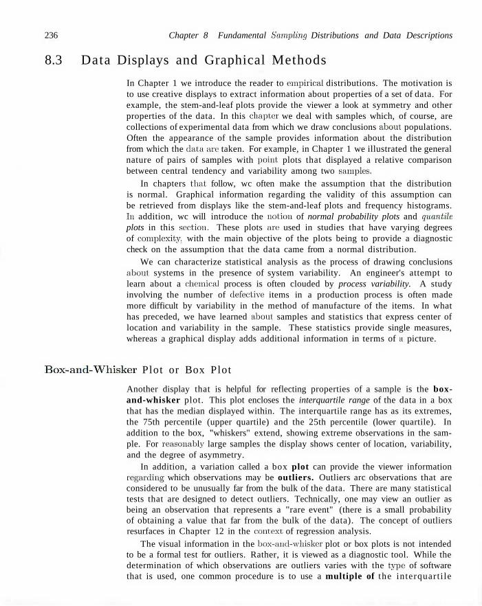
236 Chapter 8 Fundamental Sampling Distributions and Data Descriptions
8.3 Data Displays and Graphical Methods
In Chapter 1 we introduce the reader to empirical distributions. The motivation is to use creative displays to extract information about properties of a set of data. For example, the stem-and-leaf plots provide the viewer a look at symmetry and other properties of the data. In this chapter we deal with samples which, of course, are collections of experimental data from which we draw conclusions about populations. Often the appearance of the sample provides information about the distribution from which the data, arc taken. For example, in Chapter 1 we illustrated the general nature of pairs of samples with point plots that displayed a relative comparison between central tendency and variability among two samples.
In chapters that follow, wc often make the assumption that the distribution is normal. Graphical information regarding the validity of this assumption can be retrieved from displays like the stem-and-leaf plots and frequency histograms. In addition, wc will introduce the notion of normal probability plots and quantile plots in this section. These plots are used in studies that have varying degrees of complexity, with the main objective of the plots being to provide a diagnostic check on the assumption that the data came from a normal distribution.
We can characterize statistical analysis as the process of drawing conclusions about systems in the presence of system variability. An engineer's attempt to learn about a chemical process is often clouded by process variability. A study involving the number of defective items in a production process is often made more difficult by variability in the method of manufacture of the items. In what has preceded, we have learned about samples and statistics that express center of location and variability in the sample. These statistics provide single measures, whereas a graphical display adds additional information in terms of a picture.
Box-and-Whisker Plot or Box Plot
Another display that is helpful for reflecting properties of a sample is the box-and-whisker plot. This plot encloses the interquartile range of the data in a box that has the median displayed within. The interquartile range has as its extremes, the 75th percentile (upper quartile) and the 25th percentile (lower quartile). In addition to the box, "whiskers" extend, showing extreme observations in the sample. For reasonably large samples the display shows center of location, variability, and the degree of asymmetry.
In addition, a variation called a box plot can provide the viewer information regarding which observations may be outliers. Outliers arc observations that are considered to be unusually far from the bulk of the data. There are many statistical tests that are designed to detect outliers. Technically, one may view an outlier as being an observation that represents a ''rare event" (there is a small probability of obtaining a value that far from the bulk of the data). The concept of outliers resurfaces in Chapter 12 in the context of regression analysis.
The visual information in the box-and-whisker plot or box plots is not intended to be a formal test for outliers. Rather, it is viewed as a diagnostic tool. While the determination of which observations are outliers varies with the typo of software that is used, one common procedure is to use a multiple of the interquart i le
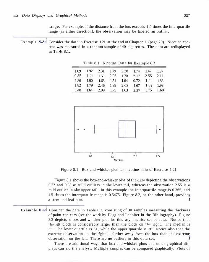
8.3 Data Displays and Graphical Methods 237
range. For example, if the distance from the box exceeds 1.5 times the interquartile range (in either direction), the observation may be labeled an outlier.
Example 8.3:1 Consider the data in Exercise 1.21 at the end of Chapter I (page 29). Nicotine content was measured in a random sample of 40 cigarettes. The data are redisplayed in Table 8.1.
Table 8.1: Nicotine Data for Example 8.3
1.09 0.85 1.86 1.82 1.40
1.92 1.24 1.90 1.79 1.64
2.31 1.58 1.68 2.46 2.09
1.79 2.03 1.51 1.88 1.75
2.28 1.70 1.64 2.08 1.63
1.74 2.17 0.72 1.67 2.37
1.47 2.55 1.69 1.37 1.75
1.97 2.11 1.85 1.93 l.fiy
O O Q
1.0 1.5 2.0 Nicotine
2.5
Figure 8.1: Box-and-whisker plot for nicotine data of Exercise 1.21.
Figure 8.1 shows the box-and-whisker plot, of the data depicting the observations 0.72 and 0.85 as mild outliers in the lower tail, whereas the observation 2.55 is a mild outlier in the upper tail. In this example the interquartile range is 0.365, and 1.5 times the interquartile range is 0.5475. Figure 8.2, on the other hand, provides a stem-and-leaf plot. J
Example 8.4:1 Consider the data in Table 8.2, consisting of 30 samples measuring the thickness of paint can ears (see the work by Hogg and Ledolter in the Bibliography). Figure 8.3 depicts a box-and-whisker plot for this asymmetric: set of data. Notice that the left block is considerably larger than the block on flic: right. The median is 35. The lower quartile is 31, while the upper quartile is 36. Notice also that the extreme observation on the right is farther away from the box than the extreme observation on the left. There are no outliers in this data set. J
There are additional ways that box-and-whisker plots and other graphical displays can aid the analyst. Multiple samples can be compared graphically. Plots of
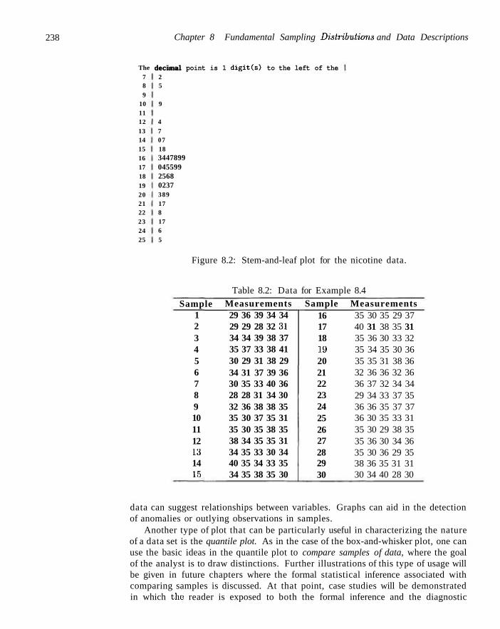
238 Chapter 8 Fundamental Sampling Distributions and Data Descriptions
decimal point is 1 digit(s) to the left of the The 7 8 9
10 11 12 13 14 15 16 17 18 19 20 21 22 23 24 25
decimal 2 5
9
4 7 07 18 3447899 045599 2568 0237 389 17 8 17 6 5
Figure 8.2: Stem-and-leaf plot for the nicotine data.
Table 8.2: Data for Example 8.4
Sample 1 2 3 4 5 6 7 8 9 10 11 12 13 14 15
Measurements 29 36 39 34 34 29 29 28 32 31 34 34 39 38 37 35 37 33 38 41 30 29 31 38 29 34 31 37 39 36 30 35 33 40 36 28 28 31 34 30 32 36 38 38 35 35 30 37 35 31 35 30 35 38 35 38 34 35 35 31 34 35 33 30 34 40 35 34 33 35 34 35 38 35 30
Sample 16 17 18 19 20 21 22 23 24 25 26 27 28 29 30
Measurements 35 30 35 29 37 40 31 38 35 31 35 36 30 33 32 35 34 35 30 36 35 35 31 38 36 32 36 36 32 36 36 37 32 34 34 29 34 33 37 35 36 36 35 37 37 36 30 35 33 31 35 30 29 38 35 35 36 30 34 36 35 30 36 29 35 38 36 35 31 31 30 34 40 28 30
data can suggest relationships between variables. Graphs can aid in the detection of anomalies or outlying observations in samples.
Another type of plot that can be particularly useful in characterizing the nature of a data set is the quantile plot. As in the case of the box-and-whisker plot, one can use the basic ideas in the quantile plot to compare samples of data, where the goal of the analyst is to draw distinctions. Further illustrations of this type of usage will be given in future chapters where the formal statistical inference associated with comparing samples is discussed. At that point, case studies will be demonstrated in which the reader is exposed to both the formal inference and the diagnostic
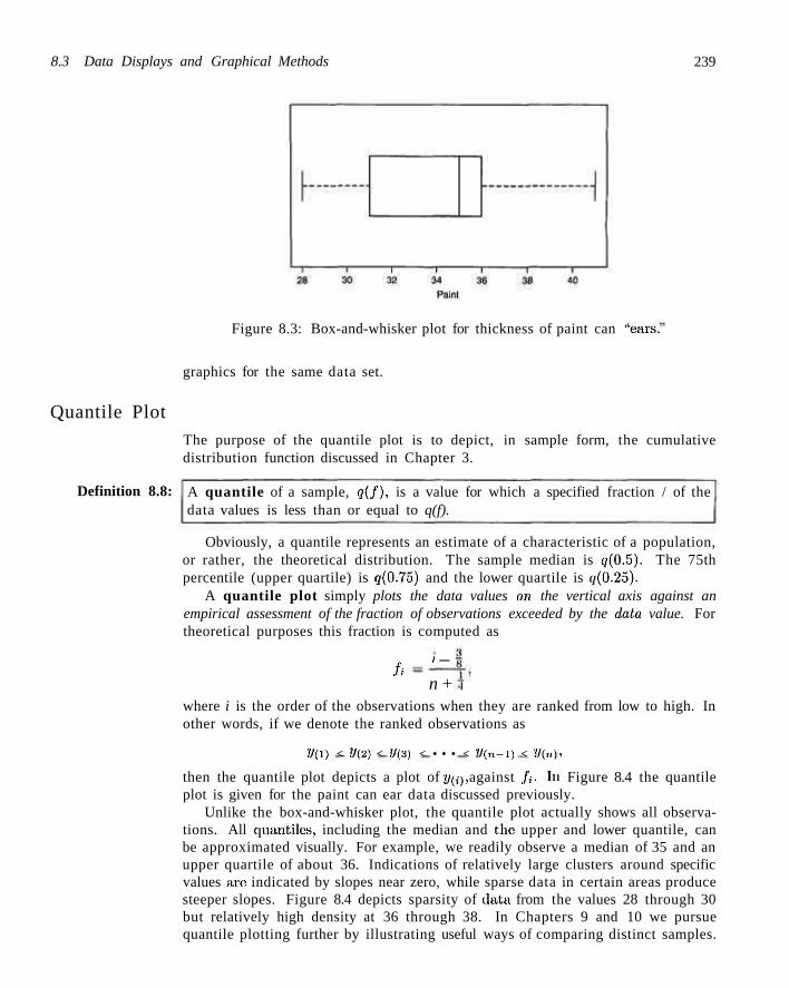
8.3 Data Displays and Graphical Methods 239
Figure 8.3: Box-and-whisker plot for thickness of paint can "ears.
graphics for the same data set.
Quantile Plot
Definition 8.8:
The purpose of the quantile plot is to depict, in sample form, the cumulative distribution function discussed in Chapter 3.
A quantile of a sample, e7(/), is a value for which a specified fraction / of the data values is less than or equal to q(f).
Obviously, a quantile represents an estimate of a characteristic of a population, or rather, the theoretical distribution. The sample median is cy(0.5). The 75th percentile (upper quartile) is ey(0.75) and the lower quartile is g(0.25).
A quantile plot simply plots the data values on the vertical axis against an empirical assessment of the fraction of observations exceeded by the data value. For theoretical purposes this fraction is computed as
fi i —
n + where i is the order of the observations when they are ranked from low to high. In other words, if we denote the ranked observations as
2/(1) < 9(2) < 2/(3) < • • • < 2/(n-l) < ?/(«)'
then the quantile plot depicts a plot of y^), against /*. In Figure 8.4 the quantile plot is given for the paint can ear data discussed previously.
Unlike the box-and-whisker plot, the quantile plot actually shows all observations. All quantilcs, including the median and the upper and lower quantile, can be approximated visually. For example, we readily observe a median of 35 and an upper quartile of about 36. Indications of relatively large clusters around specific values are indicated by slopes near zero, while sparse data in certain areas produce steeper slopes. Figure 8.4 depicts sparsity of data from the values 28 through 30 but relatively high density at 36 through 38. In Chapters 9 and 10 we pursue quantile plotting further by illustrating useful ways of comparing distinct samples.
240 Chapter 8 Fundamental Sampling Distributions and Data Descriptions
40
38
36 *
1" 32
30
28
^ —
™"•
-
• —
~ •
—
0.0 0.2 0.4 0.6
Fraction, /
0.8 1.0
Figure 8.4: Quantile plot for paint data.
Detection of Deviations from Normality
It should be somewhat evident to the reader that detection of whether or not a data set came from a normal distribution can be an important tool for the data analyst. As we indicated earlier in this section, we often make the assumption that all or subsets of observations in a data set are realizations of independent identically distributed normal random variables. Once again, the diagnostic plot can often nicely augment (for display purposes) a formal goodness-of-fit test on the data. Goodness-of-fit tests are discussed in Chapter 10. For the reader of a scientific paper or report, diagnostic information is much clearer, less dry, and perhaps not boring. In later chapters (Chapters 9 through 13), we focus again on methods of detecting deviations from normality as an augmentation of formal statistical inference. These types of plots are useful in detection of distribution types. There are also situations in both model building and design of experiments in which the plots are used to detect important model terms or effects that are active. In other situations they are used to determine whether or not the underlying assumptions made by the scientist or engineer in building the model are reasonable. Many examples with illustrations will be encountered in Chapters 11, 12, and 13. The following subsection provides a discussion and illustration of a diagnostic plot called the normal quantile-quantile plot.
Normal Quantile-Quantile Plot
The normal quantile-quantile plot takes advantage of what is known about the quantiles of the normal distribution. The methodology involves a plot of the em-
8.3 Data Displays and Graphical Methods 241
pirical quantiles recently discussed against the corresponding quantile of the normal distribution. Now, the expression for a quantile of an N(p,a) random variable is very complicated. However, a good approximation is given by
%Af) = V + a{4.91[/° ' u - (1 - f)ou]}.
The expression in brackets (the multiple of er) is the approximation for the corresponding quantile for the N(0, 1) random variable, that is,
go,i(/) = 4 . 9 1 [ / 0 1 4 - ( l - / ) 0 1 4 ] .
Definition 8.9: The normal quantile-quantile plot is a plot of y^) (ordered observations) ; _ 3
against <fo,i(/i), where /* = ^ + .
A nearly straight-line relationship suggests that the data came from a normal distribution. The intercept on the vertical axis is an estimate of the population mean p and the slope is an estimate of the standard deviation a. Figure 8.5 shows a normal quantile-quantile plot for the paint can data.
40
38
* 36
| 34 O
32
30
28
• fl • •
—~~
—
_ "
^ ^
• • • •
•
- 2 2 1 - 2 2
Standard Normal Quantile, qfo.iiV)
Figure 8.5: Normal quantile-quantile plot for paint data.
Normal Probability Plotting
Notice how the deviation from normality becomes clear from the appearance of the plot. The asymmetry exhibited in the data results in changes in the slope.

242 Chapter 8 Fundamental Sampling Distributions and Data Descriptions
The ideas of probability plotting are manifested in plots other than the normal quantile-quantile plot discussed here. For example, much attention is given to the so-called normal probabili ty plot, in which the vertical axis contains / plotted on special paper and the scale used results in a straight line when plotted against the ordered data values. In addition, an alternative plot makes use of the expected values of the ranked observations for the normal distribution and plots the ranked observations against their expected value, under the assumption of data from N(p,a). Once again, the straight line is the graphical yardstick used. We continue to suggest that the foundation in graphical analytical methods developed in this section aid in the illustration of formal methods of distinguishing between distinct samples of data.
Example 8.5:1 Consider the data in Exercise 10.41 on page 359 in Chapter 10. In a study, Nutrient Retention and Macro Invertebrate Community Response to Sewage Stress in a Stream Ecosystem, conducted in the Department of Zoology at the Virginia Polytechnic Institute and State University, data were collected on density measurements (number of organisms per square meter) at two different collecting stations. Details are given in Chapter 10 regarding analytical methods of comparing samples to determine if both are from the same N(p,a) distribution. The data are given in Table 8.3.
Table 8.3: Data for Example 8.5
N u m b e r of Organisms pe r Square M e t e r Station 1
5,030 13.700 10.730 11.400
860 2.200 4,250 15,040
4,980 11,910 8,130 26.850 17.660 22,800 1.130 1.690
Station 2 2,800 4.670 6,890 7,720 7,030 7,330
2.810 1.330 3.320 1.230 2.130 2,190
Construct a normal quantile-quantile plot and draw conclusions regarding whether or not it is reasonable to assume that the two samples are from the same n(x; p, a) distribution.
Solution: Figure 8.6 shows the normal quantile-quantile plot for the density measurements. The plot shows an appearance that is far from a single straight line. In fact, the data from station 1 reflect a few values in the lower tail of the distribution and several in the upper tail. The "clustering" of observations would make it seem unlikely that the two samples came from a common N(p, a) distribution. _l
Although we have concentrated our development and illustration on probability plotting for the normal distribution, wc could focus on any distribution. We would merely need to compute quantities analytically for the theoretical distribution in question.
8.4 Sampling Distributions 243
25,000
20,000
CO
| 15,000 en
10,000
5,000
**>
.^° o ++' >++o'T
o Station 1 + Station 2
- 2 - 1 0 1 2 Standard Normal Quantile, q0A{f)
Figure 8.6: Normal quantile-quantile plot, for density data of Example 8.5.
8.4 Sampling Distributions
The field of statistical inference is basically concerned with generalizations and predictions. For example, we might claim, based on the opinions of several people interviewed on the street, that in a forthcoming election 60% of the eligible voters in the city of Detroit favor a certain candidate. In this case we are dealing with a random sample of opinions from a very large finite population. As a second illustration we might state that the average cost to build a residence in Charleston, South Carolina, is between 8230,000 and $235,000, based on the estimates of 3 contractors selected at random from the 30 now building in this city. The population being sampled here is again finite but very small. Finally, let us consider a soft-drink dispensing machine in which the average amount of drink dispensed is being held to 240 milliliters. A company official computes the mean of 40 drinks to obtain x = 236 milliliters and on the basis of this value decides that the machine is still dispensing drinks with an average content of p = 240 milliliters. The 40 drinks represent a sample from the infinite population of possible drinks that will be dispensed by this machine.
Inference about the Population from Sample Information
In each of the examples above we have computed a statistic from a sample selected from the population, and from these statistics we made various statements concerning the values of population parameters that may or may not be true. The company official made the decision that the soft-drink machine dispenses drinks with an average content of 240 milliliters, even though the sample mean was 236 milliliters, because he knows from sampling theory that such a sample value is likely to occur. In fact, if he ran similar tests, say every hour, he would expect the values of x to fluctuate above and below p. = 240 milliliters. Only wdien the value
244 Chapter 8 Fundamental Sampling Distributions and Data Descriptions
of x is substantially different from 240 milliliters will the company official initiate action to adjust the machine.
Since a statistic is a random variable that depends only on the observed sample, it must have a probability distribution.
Definition 8.10: The probability distribution of a statistic is called a sampling distribution.
The probability distribution of X is called the sampling distribution of the mean.
The sampling distribution of a statistic depends on the size of the population, the size of the samples, and the method of choosing the samples. For the remainder of this chapter we study several of the more important sampling distributions of frequently used statistics. Applications of these sampling distributions to problems of statistical inference are considered throughout most of the remaining chapters.
What Is the Sampling Distribution of XI
Wc should view the sampling distributions of X and S2 as the mechanisms from which we are eventually to make inferences on the parameters p and a2. The .sampling distribution of X with sample size n is the distribution that results when an experiment is conducted over and over (always with sample size n) and the many values of X result. This sampling distribution, then, describes the variability of sample averages around the population mean p. In the case of the soft-drink machine, knowledge of the: sampling distribution of X arms the analyst with the knowledge of a "typical" discrepancy between an observed x value and true //.. The same principle applies in the case of the distribution of S2. The sampling distribution produces information about the variability of s2 values around a2 in repeated experiments.
8.5 Sampling Distribution of Means
The first important sampling distribution to be considered is that of the mean X. Suppose that a random sample of n observations is taken from a normal population with mean p and variance a2. Each observation Xi, i = 1,2. . . . ,n, of the random sample: will then have the same normal distribution as the population being sampled. Hence, by the reproductive property of the normal distribution established in Theorem 7.11. we conclude that
X = -(Xx+X2 + --- + Xn) n
has a normal distribution with mean 1,
px = -jp + p + • • • + p) = p.,
and variance
II terms
1 / 2 •-> •>•. °" -s (a- + a2 + ---+a2) = —. n2 "> *• ' n
n terms
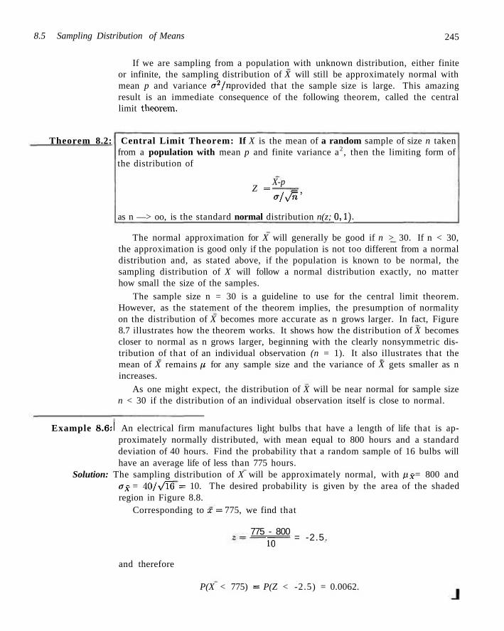
8.5 Sampling Distribution of Means 245
Theorem 8.2:
If we are sampling from a population with unknown distribution, either finite or infinite, the sampling distribution of X will still be approximately normal with mean p and variance o2/n provided that the sample size is large. This amazing result is an immediate consequence of the following theorem, called the central limit theoi'em.
Central Limit Theorem: If X is the mean of a random sample of size n taken from a population with mean p and finite variance a2 , then the limiting form of the distribution of
Z = X-p
a/vn'
as n —> oo, is the standard normal distribution n(z; 0,1).
The normal approximation for X will generally be good if n > 30. If n < 30, the approximation is good only if the population is not too different from a normal distribution and, as stated above, if the population is known to be normal, the sampling distribution of X will follow a normal distribution exactly, no matter how small the size of the samples.
The sample size n = 30 is a guideline to use for the central limit theorem. However, as the statement of the theorem implies, the presumption of normality on the distribution of X becomes more accurate as n grows larger. In fact, Figure 8.7 illustrates how the theorem works. It shows how the distribution of X becomes closer to normal as n grows larger, beginning with the clearly nonsymmetric distribution of that of an individual observation (n = 1). It also illustrates that the mean of X remains p for any sample size and the variance of X gets smaller as n increases.
As one might expect, the distribution of X will be near normal for sample size n < 30 if the distribution of an individual observation itself is close to normal.
Example 8.6:1 An electrical firm manufactures light bulbs that have a length of life that is approximately normally distributed, with mean equal to 800 hours and a standard deviation of 40 hours. Find the probability that a random sample of 16 bulbs will have an average life of less than 775 hours.
Solution: The sampling distribution of X will be approximately normal, with px = 800 and ax = 40/ \ / l6 = 10. The desired probability is given by the area of the shaded region in Figure 8.8.
Corresponding to x = 775, we find that
775 - 800 io = -2.5.
and therefore
P(X < 775) = P(Z < -2.5) = 0.0062.
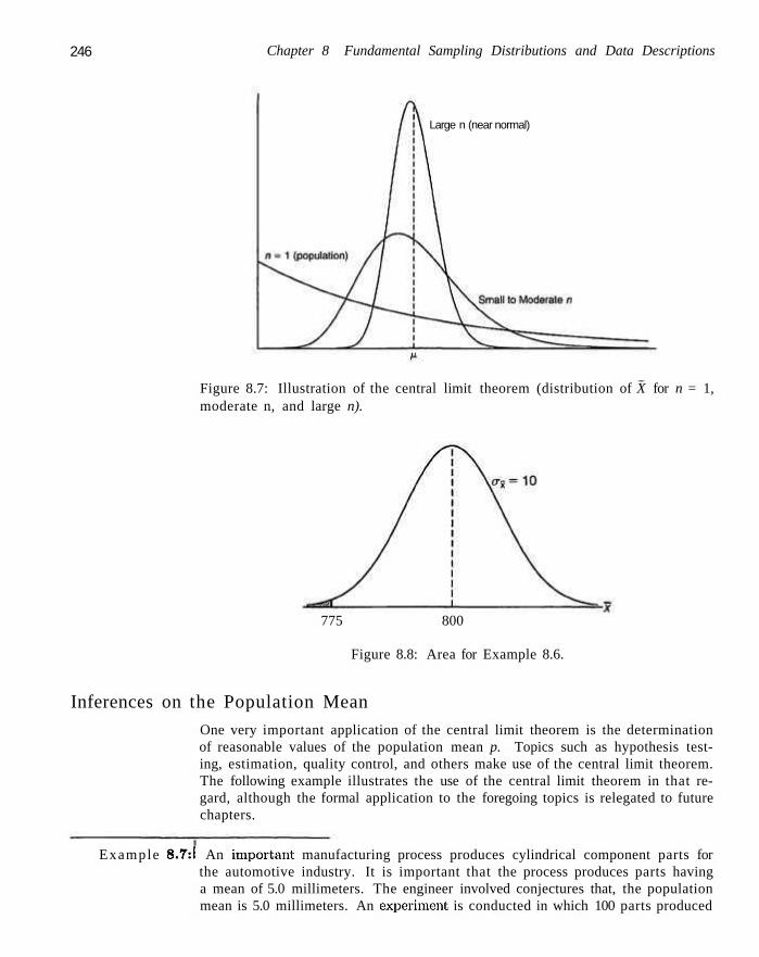
246 Chapter 8 Fundamental Sampling Distributions and Data Descriptions
Large n (near normal)
Figure 8.7: Illustration of the central limit theorem (distribution of X for n = 1, moderate n, and large n).
775 800
Figure 8.8: Area for Example 8.6.
Inferences on the Population Mean
One very important application of the central limit theorem is the determination of reasonable values of the population mean p. Topics such as hypothesis testing, estimation, quality control, and others make use of the central limit theorem. The following example illustrates the use of the central limit theorem in that regard, although the formal application to the foregoing topics is relegated to future chapters.
Example 8.7:1 An important manufacturing process produces cylindrical component parts for the automotive industry. It is important that the process produces parts having a mean of 5.0 millimeters. The engineer involved conjectures that, the population mean is 5.0 millimeters. An experiment is conducted in which 100 parts produced
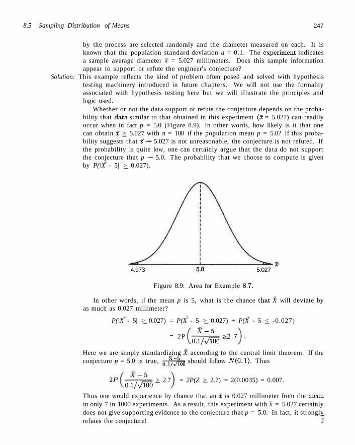
8.5 Sampling Distribution of Means 247
by the process are selected randomly and the diameter measured on each. It is known that the population standard deviation a = 0.1. The experiment indicates a sample average diameter x = 5.027 millimeters. Does this sample information appear to support or refute the engineer's conjecture?
Solution: This example reflects the kind of problem often posed and solved with hypothesis testing machinery introduced in future chapters. We will not use the formality associated with hypothesis testing here but we will illustrate the principles and logic used.
Whether or not the data support or refute the conjecture depends on the probability that data similar to that obtained in this experiment (x = 5.027) can readily occur when in fact p = 5.0 (Figure 8.9). In other words, how likely is it that one can obtain x > 5.027 with n = 100 if the population mean p = 5.0? If this probability suggests that x — 5.027 is not unreasonable, the conjecture is not refuted. If the probability is quite low, one can certainly argue that the data do not support the conjecture that p — 5.0. The probability that we choose to compute is given by P(\X - 5| > 0.027).
4.973 5.027
Figure 8.9: Area for Example 8.7.
In other words, if the mean p is 5, what is the chance that X will deviate by as much as 0.027 millimeter?
P(\X - 5| > 0.027) = P(X - 5 > 0.027) + P(X - 5 < -0.027)
X - 5 = 2P
O.l/vlOO >2.7
Here we are simply standardizing X according to the central limit theorem. If the conjecture p = 5.0 is true, u~/°im should follow Ar(0,1). Thus
2P > 2.7 = 2P(Z > 2.7) = 2(0.0035) = 0.007. ,0.1/v/lOO
Thus one would experience by chance that an x is 0.027 millimeter from the mean in only 7 in 1000 experiments. As a result, this experiment with x = 5.027 certainly does not give supporting evidence to the conjecture that p = 5.0. In fact, it strongly refutes the conjecture! J
248 Chapter 8 Fundamental Sampling Distributions and Data Descriptions
Sampling Distribution of the Difference between Two Averages
The illustration in Example 8.7 deals with notions of statistical inference on a single mean p. The engineer was interested in supporting a conjecture regarding a single population mean. A far more important application involves two populations. A scientist or engineer is interested in a comparative experiment in which two manufacturing methods, 1 and 2, are to be compared. The basis for that comparison is pi — p2, the difference in the population means.
Suppose that we have two populations, the first with mean p\ and variance a2, and the second with mean p2 and variance o\. Let the statistic A'i represent the mean of a random sample of size n\ selected from the first population, and the statistic X2 represent the mean of a random sample of size n2 selected from the second population, independent of the sample from the first population. What can we say about the sampling distribution of the difference A'i — X2 for repeated samples of size nx and n2? According to Theorem 8.2, the variables Xx and X2
are both approximately normally distributed with means px and p2 and variances af/nx and a2/n2, respectively. This approximation improves as n\ and n2 increase. By choosing independent samples from the two populations the variables Xx and X2 will be independent, and then using Theorem 7.11, with ax = 1 and a2 = —1, we can conclude that Xx - X2 is approximately normally distributed with mean
Mx,-x2 = Pxt ~ l'x2 = Mi - P2
and variance
ax1-x2 -ax, +ax7 - n\ n2
Theorem 8.3: If independent samples of size ni and n2 are drawn at random from two populations, discrete or continuous, with means pi and p2, and variances o\ and respectively, then the sampling distribution of the differences of means, A'i is approximately normally distributed with mean and variance given by
' 2 '
x2,
PXx-X2 = P l - ^ 2 , and X\—X2
°2
nx n2
= ^ +
Hence
Z = (Xx - X2) - (px - p2)
y/ici/nx) + ial/n2)
is approximately a standard normal variable.
If both ni and n2 are greater than or equal to 30, the normal approximation for the distribution of A'i — X2 is very good when the underlying distributions are not too far away from normal. However, even when nx and n2 are less than 30, the normal approximation is reasonably good except when the populations are decidedly nonnormal. Of course, if both populations are normal, then A'i — X2 has a normal distribution no matter what the sizes are of nx and n2.
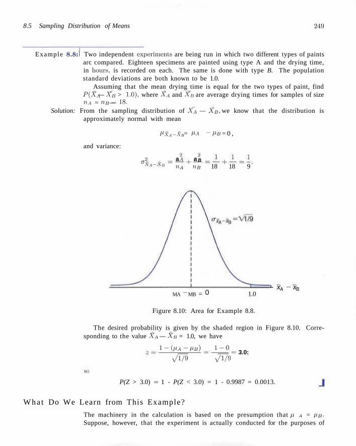
8.5 Sampling Distribution of Means 249
Example 8.8:1 Two independent experiments are being run in which two different types of paints arc compared. Eighteen specimens are painted using type A and the drying time, in hours, is recorded on each. The same is done with type B. The population standard deviations are both known to be 1.0.
Assuming that the mean drying time is equal for the two types of paint, find P(XA — XB > 1-0), where XA and XB are average drying times for samples of size ".•1 = nB — 18.
Solution: From the sampling distribution of XA — XB, we know that the distribution is approximately normal with mean
and variance:
l'xA-xB = AM -fiB = 0 ,
a a nA nB 18 18 9
B
L *A - *B MA - MB = 0 1.0
Figure 8.10: Area for Example 8.8.
The desired probability is given by the shaded region in Figure 8.10. Corresponding to the value XA — XB = 1.0, we have
i-iflA-ps) 1 -0 3.0:
so
v/1/9 y/1/9
P(Z > 3.0) = 1 - P(Z < 3.0) = 1 - 0.9987 = 0.0013.
What Do We Learn from This Example?
The machinery in the calculation is based on the presumption that ft A = PB-Suppose, however, that the experiment is actually conducted for the purposes of
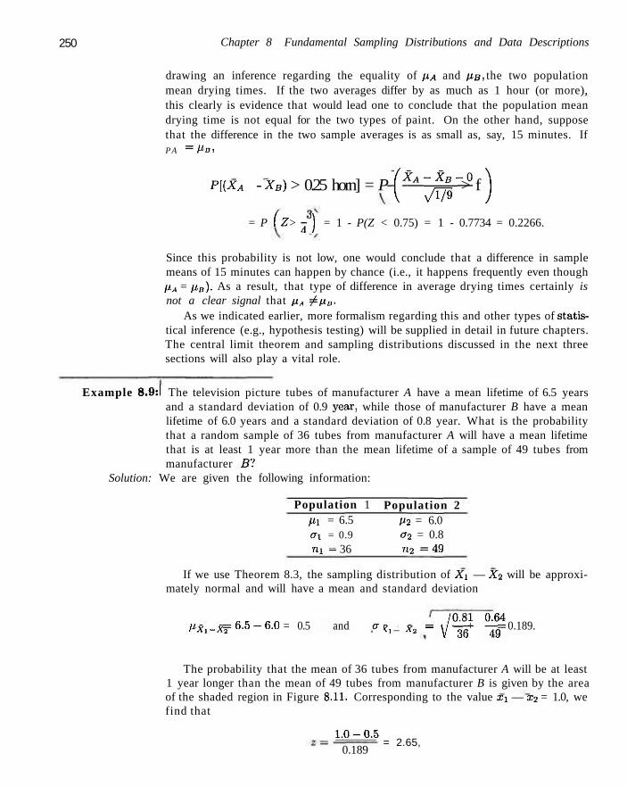
250 Chapter 8 Fundamental Sampling Distributions and Data Descriptions
drawing an inference regarding the equality of PA and pB, the two population mean drying times. If the two averages differ by as much as 1 hour (or more), this clearly is evidence that would lead one to conclude that the population mean drying time is not equal for the two types of paint. On the other hand, suppose that the difference in the two sample averages is as small as, say, 15 minutes. If P A = M B I
P[(XA - XB) > 0.25 horn] = P (*A~J^~° > f )
= P (Z > j } = 1 - P(Z < 0.75) = 1 - 0.7734 = 0.2266.
Since this probability is not low, one would conclude that a difference in sample means of 15 minutes can happen by chance (i.e., it happens frequently even though pA = fiD). As a result, that type of difference in average drying times certainly is not a clear signal that pA ^ pB.
As we indicated earlier, more formalism regarding this and other types of statistical inference (e.g., hypothesis testing) will be supplied in detail in future chapters. The central limit theorem and sampling distributions discussed in the next three sections will also play a vital role.
Example 8.9:1 The television picture tubes of manufacturer A have a mean lifetime of 6.5 years and a standard deviation of 0.9 year, while those of manufacturer B have a mean lifetime of 6.0 years and a standard deviation of 0.8 year. What is the probability that a random sample of 36 tubes from manufacturer A will have a mean lifetime that is at least 1 year more than the mean lifetime of a sample of 49 tubes from manufacturer BI
Solution: We are given the following information:
Population 1 px = 6.5 <7i = 0.9 ni = 36
Population 2 p2 = 6.0 a2 = 0.8 n2 = 4 9
If we use Theorem 8.3, the sampling distribution of A'i — X2 will be approximately normal and will have a mean and standard deviation
pXl_Xa - 6 . 5 - 6 . 0 = 0.5 and a ? ] _ Az - \ j ^ + ^ = 0.189.
The probability that the mean of 36 tubes from manufacturer A will be at least 1 year longer than the mean of 49 tubes from manufacturer B is given by the area of the shaded region in Figure 8.11. Corresponding to the value xi — x2 = 1.0, we find that
1 .0-0.5 0.189
= 2.65,
Exercises 251
crJf l_%= 0.189
0.5 1.0
Figure 8.11: Area for Example 8.9.
x, - x2
and hence
P(Xx - X2 > 1.0) = P(Z > 2.65) = 1 - P(Z < 2.65)
= 1 - 0.9960 = 0.0040. J
More on Sampling Distribution of Means - Normal Approximation to Binomial
In Section 6.5 much was discussed regarding the normal approximation to the binomial distribution. Conditions were given on the parameters n and p for which the distribution of a binomial random variable can be approximated by the normal distribution. Examples and exercises reflected the importance of the tool we refer to as the "normal approximation/' It turns out that the central limit theorem sheds even more light on how and why this approximation works. We certainly know that a binomial random variable is the number X of successes in n independent trials, where the outcome of each trial is binary. We also illustrated in Chapter 1 that the proportion computed in such an experiment is an average of a set of 0s and Is. Indeed, while the proportion X/n is an average, X is the sum of this set of 0s and Is, and both X and X/n are approximately normal if n is sufficiently large. Of course, from wdiat we learned in Chapter 6, there are conditions on n and p that affect the quality of the approximation, namely np > 5 and nq > 5.
Exercises
8.17 If all possible samples of size 16 are drawn from a normal population with mean equal to 50 and standard deviationequal to 5, what is the probability that a sample mean X will fall in the interval from p% — 1.9ax to px ~ 0.4<Tjf ? Assume that the sample means can be measured to any degree of accuracy.
8.18 Given the discrete uniform population
/ ( " " f t a: = 2,4, 6, elsewhere,
find the probability that a random sample of size 54, selected with replacement, will yield a sample mean greater than 4.1 but less than 4.4. Assume the means
252 Chapter 8 Fundamental Sampling Distributions and Data Descriptions
to be measured to the nearest tenth.
8.19 A certain type of thread is manufactured with a mean tensile strength of 78.3 kilograms and a standard deviation of 5.6 kilograms. How is the variance of the sample mean changed when the sample size is (a) increased from 64 to 196?
(b) decreased from 784 to 49?
8.20 If the standard deviation of the mean for the sampling distribution of random samples of size 36 from a large or infinite population is 2, how large must the size of the sample become if the standard deviation is to be reduced to 1.2?
8.21 A soft-drink machine is being regulated so that the amount of drink dispensed averages 240 milliliters with a standard deviation of 15 milliliters. Periodically, the machine is checked by taking a sample of 40 drinks and computing the average content. If the mean of the 40 drinks is a value within the interval px ± 2a x , the machine is thought to be operating satisfactorily; otherwise, adjustments are made. In Section 8.4, the company official found the mean of 40 drinks to be x = 236 milliliters and concluded that the machine needed no adjustment. Was this a reasonable decision?
8.22 The heights of 1000 students are approximately normally distributed with a mean of 174.5 centimeters and a standard deviation of 6.9 centimeters. If 200 random samples of size 25 are drawn from this population and the means recorded to the nearest tenth of a centimeter, determine
(a) the mean and standard deviation of the sampling distribution of X;
(b) the number of sample means that fall between 172.5 and 175.8 centimeters inclusive;
(c) the number of sample means falling below 172.0 centimeters.
8.23 The random variable X, representing the number of cherries in a cherry puff, has the following probability distribution:
X
P(X = x) 4
0.2 5
0.4 6
0.3 7
0.1
(a) Find the mean p. and the variance a2 of X.
(b) Find the mean px, and the variance a\ of the mean X for random samples of 36 cherry puffs.
(c) Find the probability that the average number of cherries in 36 cherry puffs will be less than 5.5.
8.24 If a certain machine makes electrical resistors having a mean resistance of 40 ohms and a standard deviation of 2 ohms, what is the probability that a random sample of 36 of these resistors will have a com
bined resistance of more than 1458 ohms?
8.25 The average life of a bread-making machine is 7 years, with a standard deviation of 1 year. Assuming that the lives of these machines follow approximately a normal distribution, find
(a) the probability that the mean life of a random sample of 9 such machines falls between 6.4 and 7.2 years;
(b) the value of a; to the right of which 15% of the means computed from random samples of size 9 would fall.
8.26 The amount of time that a drive-through bank teller spends on a customer is a random variable with a mean p = 3.2 minutes and a standard deviation a = 1.6 minutes. If a random sample of 64 customers is observed, find the probability that their mean time at the teller's counter is
(a) at most 2.7 minutes: (b) more than 3.5 minutes; (c) at least 3.2 minutes but less than 3.4 minutes.
8.27 In a chemical process the amount of a certain type of impurity in the output is difficult to control and is thus a random variable. Speculation is that the population mean amount of the impurity is 0.20 grams per gram of output. It is known that the standard deviation is 0.1 grams per gram. An experiment is conducted to gain more insight regarding the speculation that p = 0.2. The process was run on a lab scale 50 times and the sample average x turned out to be 0.23 grams per gram. Comment on the speculation that the mean amount of impurity is 0.20 grams per gram. Make use of the central limit theorem in your work.
8.28 A random sample of size 25 is taken from a normal population having a mean of 80 and a standard deviation of 5. A second random sample of size 36 is taken from a different normal population having a mean of 75 and a standard deviation of 3. Find the probability that the sample mean computed from the 25 measurements will exceed the sample mean computed from the 36 measurements by at least 3.4 but less than 5.9. Assume the difference of the means to be measured to the nearest tenth.
8.29 The distribution of heights of a certain breed of terrier dogs has a mean height of 72 centimeters and a standard deviation of 10 centimeters, whereas the distribution of heights of a certain breed of poodles has a mean height of 28 centimeters with a standard deviation of 5 centimeters. Assuming that the sample means can be measured to any degree of accuracy, find the probability that the sample mean for a random sample
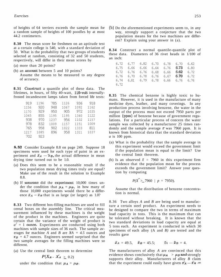
Exercises 253
of heights of 64 terriers exceeds the sample mean for a random sample of heights of 100 poodles by at most 44.2 centimeters.
8.30 The mean score for freshmen on an aptitude test at a certain college is 540, with a standard deviation of 50. What is the probability that two groups of students selected at random, consisting of 32 and 50 students, respectively, will differ in their mean scores by
(a) more than 20 points? (b) an amount between 5 and 10 points?
Assume the means to be measured to any degree of accuracy.
8.31 Construct a quantile plot of these data. The lifetimes, in hours, of fifty 40-watt. 110-volt internally-frosted incandescent lamps taken from forced life tests:
(b)
919 1156 1170 1045 938 978 765 1217 702
1196 920 929 855 970 832 958 1085 923
785 948 950 1195 1237 1009 902 896
1126 1067 905 1195 956 1157 1022 958
936 1092 972 1340 1102 1151 1333 1311
918 1162 1035 1122 1157 1009 811 1037
8.32 Consider Example 8.8 on page 249. Suppose 18 specimens were used for each type of paint in an experiment and XA — XB, the actual difference in mean drying time turned out to be 1.0.
(a) Does this seem to be a reasonable result if the two population mean drying times truly are equal? Make use of the result in the solution to Example 8.8.
(b) If someone did the experiment 10,000 times under the condition that PA = p-B, in how many of those 10,000 experiments would there be a difference XA —XB that is as large (or larger) as 1.0?
8.33 Two different box-filling machines are used to fill cereal boxes on the assembly line. The critical measurement influenced by these machines is the weight of the product in the machines. Engineers are quite certain that the variance of the weight of product is a2 = 1 ounce. Experiments are conducted using both machines with sample sizes of 36 each. The sample averages for machine A and B are XA = 4.5 ounces and XB = 4.7 ounces. Engineers seemed surprised that the two sample averages for the filling machines were so different.
(a) Use the central limit theorem to determine
P(XB - XA > 0.2)
under the condition that PA = PB-
Do the aforementioned experiments seem to, in any way, strongly support a conjecture that the two population means for the two machines are different? Explain using your answer in (a).
8.34 Construct a normal quantile-quantile plot of these data. Diameters of 36 rivet heads in 1/100 of an inch:
6.72 6.75 6.72 6.76 6.74 6.72
6.77 6.66 6.76 6.70 6.81
6.82 6.66 6.76 6.78 6.79
6.70 6.64 6.68 6.76 6.78
6.78 6.76 6.66 6.67 6.66
6.70 6.73 6.62 6.70 6.76
6.62 6.80 6.72 6.72 6.76
8.35 The chemical benzene is highly toxic to humans. However, it is used in the manufacture of many medicine dyes, leather, and many coverings. In any production process involving benzene, the water in the output of the process must not exceed 7950 parts per million (ppm) of benzene because of government regulations. For a particular process of concern the water sample was collected by a manufacturer 25 times randomly and the sample average x was 7960 ppm. It is known from historical data that the standard deviation a is 100 ppm.
(a) What is the probability that the sample average in this experiment would exceed the government limit if the population mean is equal to the limit? Use the central limit theorem.
(b) Is an observed x = 7960 in this experiment firm evidence that the population mean for the process exceeds the government limit? Answer your question by computing
P(X > 7960 | p = 7950).
Assume that the distribution of benzene concentration is normal.
8.36 Two alloys A and B are being used to manufacture a certain steel product. An experiment needs to be designed to compare the two in terms of maximum load capacity in tons. This is the maximum that can be tolerated without breaking. It is known that the two standard deviations in load capacity are equal at 5 tons each. An experiment is conducted in which 30 specimens of each alloy (A and B) are tested and the results gave
XA = 49.5, xo = 45.5; XA — XB = 4.
The manufacturers of alloy A are convinced that this evidence shows conclusively that ft,A > PB and strongly supports their alloy. Manufacturers of alloy B claim that the experiment could easily have given XA — XB —
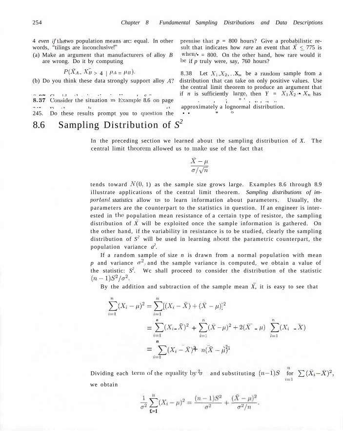
254 Chapter 8 Fundamental Sampling Distributions and Data Descriptions
4 even iflhe two population means arc: equal. In other premise that p = 800 hours? Give a probabilistic rewords, "tilings are inconclusive!" suit that indicates how rare an event that X < 775 is (a) Make an argument that manufacturers of alloy B w h o n /'• = 800. On the other hand, how rare would it
are wrong. Do it by computing he if p truly were, say, 760 hours?
P(XA - XB > 4 | pA = pa). 8.38 Let Xi, X2,..., X„ be a random sample from a (b) Do you think these data strongly support alloy A! distribution that can take on only positive values. Use
the central limit theorem to produce an argument that „ „_ r, . , .. ., ,. • ,, , 0 ,, if n is sufficiently large, then Y = X\X2-- • Xn has 8.37 Consider the situation in example 8.6 on page . , ; ° ' , ,. , ., .. „ . . T^ ^L ^ ., approximately a lognormal distribution. 245. Do these results prompt you to question the • • * °
8.6 Sampling Distribution of S2
In the preceding section we learned about the sampling distribution of X. The central limit theorem allowed us to make use of the fact tha t
X-p
a/sfn.
tends toward A'(0, 1) as the sample size grows large. Examples 8.6 through 8.9 illustrate applications of the central limit theorem. Sampling distributions of important statistics allow us to learn information about parameters. Usually, the parameters are the counterpart to the statistics in question. If an engineer is interested in the population mean resistance of a certain type of resistor, the sampling distribution of X will be exploited once the sample information is gathered. On the other hand, if the variability in resistance is to be studied, clearly the sampling distribution of S2 will be used in learning about the parametric counterpart , the population variance a2.
If a random sample of size n is drawn from a normal population with mean p and variance a2, and the sample variance is computed, we obtain a value of the statistic: S2. Wc shall proceed to consider the distribution of the statistic (n-l)S2/o2.
By the addition and subtraction of the sample mean X, it is easy to see that
Y(Xi-ti2=Yttxi-x)+(x-ri? n ii ii
= Y(*i - x? + £ ( * - /')2+2(A- - it) Yi-X'i - x) n
= YiXi-X)i + n(X-p)i
t= i i = i
\2
Dividing each term of the equality by a and substi tut ing ( n - l ) 5 for Y^iXj-X)2, ;=i
we obtain
*?> £=1
a2/n
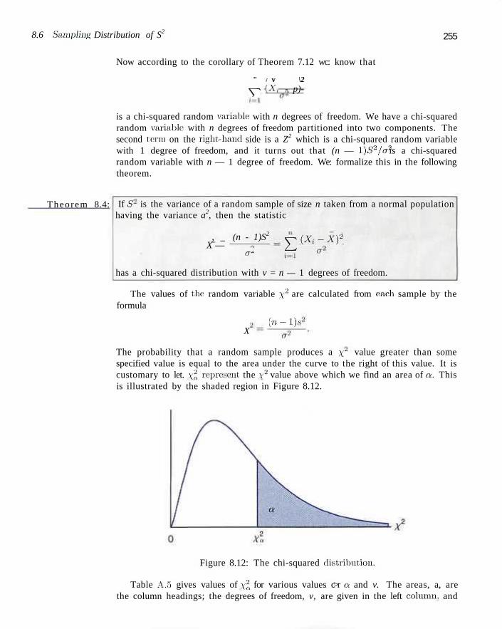
8.6 Sampling Distribution of S2 255
Now according to the corollary of Theorem 7.12 wc: know that
" i v \2 y - (A,- - p)-
is a chi-squared random variable with n degrees of freedom. We have a chi-squared random variable: with n degrees of freedom partitioned into two components. The second term on the right-hand side is a Z2 which is a chi-squared random variable with 1 degree of freedom, and it turns out that (n — l)S2/a2 is a chi-squared random variable with n — 1 degree of freedom. We: formalize this in the following theorem.
Theorem 8.4: If S is the variance of a random sample of size n taken from a normal population having the variance a2, then the statistic
, _ (n - 1)S2
X — a*
£ 1.x,-xf
has a chi-squared distribution with v = n — 1 degrees of freedom.
The values of the random variable x2 are calculated from each sample by the formula
X ( n - l p
The probability that a random sample produces a ,\;~ value greater than some specified value is equal to the area under the curve to the right of this value. It is customary to let. y2, represent the y2 value above which we find an area of a. This is illustrated by the shaded region in Figure 8.12.
Figure 8.12: The chi-squared distribution.
Table A.5 gives values of y^ for various values c>r a and v. The areas, a, are the column headings; the degrees of freedom, v, are given in the left column, and
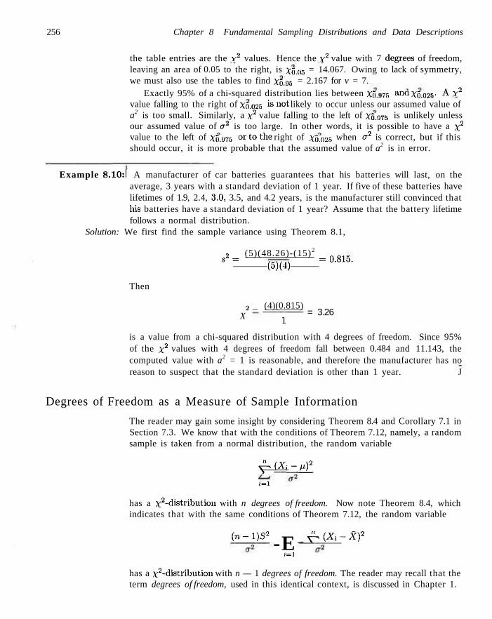
256 Chapter 8 Fundamental Sampling Distributions and Data Descriptions
the table entries are the Y2 values. Hence the y2 value with 7 degrees of freedom, leaving an area of 0.05 to the right, is x0_ng = 14.067. Owing to lack of symmetry, we must also use the tables to find X0.95 = 2.167 for v = 7.
Exactly 95% of a chi-squared distribution lies between X0.075 a i M Xo.025- A Y2
value falling to the right of X0.025 is n o t likely to occur unless our assumed value of a2 is too small. Similarly, a x2 value falling to the left of ^0,975 is unlikely unless our assumed value of er2 is too large. In other words, it is possible to have a \ 2
value to the left of Xo.375 o r t 0 the right of X0.025 when <r2 is correct, but if this should occur, it is more probable that the assumed value of a2 is in error.
Example 8.10:1 A manufacturer of car batteries guarantees that his batteries will last, on the average, 3 years with a standard deviation of 1 year. If five of these batteries have lifetimes of 1.9, 2.4, 3.0, 3.5, and 4.2 years, is the manufacturer still convinced that his batteries have a standard deviation of 1 year? Assume that the battery lifetime follows a normal distribution.
Solution: We first find the sample variance using Theorem 8.1,
2 (5)(48.26)-(15)2
' " (5X4) = °-81°-
Then
a _ (4)(0.815) X 1
= 3.26
is a value from a chi-squared distribution with 4 degrees of freedom. Since 95% of the x2 values with 4 degrees of freedom fall between 0.484 and 11.143, the computed value with a2 = 1 is reasonable, and therefore the manufacturer has no reason to suspect that the standard deviation is other than 1 year. J
Degrees of Freedom as a Measure of Sample Information
The reader may gain some insight by considering Theorem 8.4 and Corollary 7.1 in Section 7.3. We know that with the conditions of Theorem 7.12, namely, a random sample is taken from a normal distribution, the random variable
^jXj-p)2
i=X
has a ^-distribution with n degrees of freedom. Now note Theorem 8.4, which indicates that with the same conditions of Theorem 7.12, the random variable
(n-l)S2 _^(X,-Xf -E j = i
has a ^-distribution with n — 1 degrees of freedom. The reader may recall that the term degrees of freedom, used in this identical context, is discussed in Chapter 1.
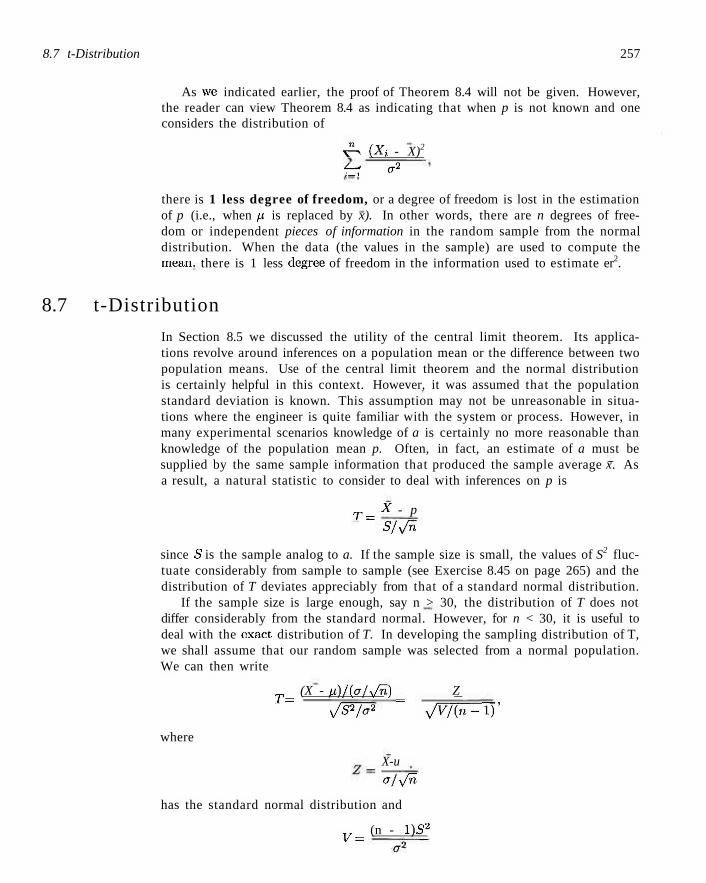
8.7 t-Distribution 257
As we indicated earlier, the proof of Theorem 8.4 will not be given. However, the reader can view Theorem 8.4 as indicating that when p is not known and one considers the distribution of
v ^ {Xj - X)2
f-f «2
there is 1 less degree of freedom, or a degree of freedom is lost in the estimation of p (i.e., when p is replaced by x). In other words, there are n degrees of freedom or independent pieces of information in the random sample from the normal distribution. When the data (the values in the sample) are used to compute the mean, there is 1 less degree of freedom in the information used to estimate er2.
8.7 t-Distribution
In Section 8.5 we discussed the utility of the central limit theorem. Its applications revolve around inferences on a population mean or the difference between two population means. Use of the central limit theorem and the normal distribution is certainly helpful in this context. However, it was assumed that the population standard deviation is known. This assumption may not be unreasonable in situations where the engineer is quite familiar with the system or process. However, in many experimental scenarios knowledge of a is certainly no more reasonable than knowledge of the population mean p. Often, in fact, an estimate of a must be supplied by the same sample information that produced the sample average x. As a result, a natural statistic to consider to deal with inferences on p is
T = X - p S/s/n~
since 5 is the sample analog to a. If the sample size is small, the values of S2 fluctuate considerably from sample to sample (see Exercise 8.45 on page 265) and the distribution of T deviates appreciably from that of a standard normal distribution.
If the sample size is large enough, say n > 30, the distribution of T does not differ considerably from the standard normal. However, for n < 30, it is useful to deal with the exact, distribution of T. In developing the sampling distribution of T, we shall assume that our random sample was selected from a normal population. We can then write
T = (X - p)/(a/Vrl,) = Z
x/57^2 y/V/(n-iy
where
X-u o/sfh.
has the standard normal distribution and
v = (n - 1)S2
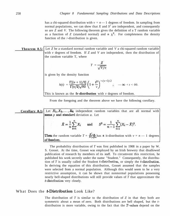
258 Chapter 8 Fundamental Sampling Distributions and Data Descriptions
Theorem 8.5:
Corollary 8.1:
has a chi-squared distribution with v = n — 1 degrees of freedom. In sampling from normal populations, we can show that X and S2 are independent, and consequently so are Z and V. The following theorem gives the definition of a T random variable as a function of Z (standard normal) and a x2- For completeness the density function of the /-distribution is given.
Let Z be a standard normal random variable and V a chi-squared random variable with v degrees of freedom. If Z and V are independent, then the distribution of the random variable T, where
T =
is given by the density function
r[(« + i)/2] h(t) =
; \ v
-(v+l)/2 — OC < t < 00.
Y(V/2)JKV
This is known as the fr-distribution with v degrees of freedom.
From the foregoing and the theorem above we have the following corollary.
Let Xx,X2,...,Xn be independent random variables that are all normal with mean p and standard deviation a. Let
» = i t = i
Then the random variable T = J V £ has a it-distribution with v = n — 1 degrees offreedom.
The probability distribution of T was first published in 1908 in a paper by W. S. Gosset. At the time, Gosset was employed by an Irish brewery that disallowed publication of research by members of its staff. To circumvent this restriction, he published his work secretly under the name "Student." Consequently, the distribution of T is usually called the Student /.-distribution, or simply the /-distribution. In deriving the equation of this distribution, Gosset assumed that the samples were selected from a normal population. Although this would seem to be a very restrictive assumption, it can be shown that nonnormal populations possessing nearly bell-shaped distributions will still provide values of T that approximate the /-distribution very closely.
W h a t Does the ^-Distribution Look Like?
The distribution of T is similar to the distribution of Z in that they both are symmetric about a mean of zero. Both distributions are bell shaped, but the t-distribution is more variable, owing to the fact that the T-values depend on the
8.7 t-Distribution 259
fluctuations of two quantities. X and S2, whereas the Z-values depend only on the changes of X from sample to sample. The distribution of T differs from that of Z in that the variance of T depends on the sample size n and is always greater than 1. Only when the sample size n —» oo will the two distributions become the same. In Figure 8.13 we show the relationship between a standard normal distribution (v = oo) and /-distributions with 2 and 5 degrees of freedom. The percentage points of the /-distribution are given in Table A.4.
Figure 8.13: The ^-distribution curves for v = 2,5, Figure 8.14: Symmetry property of the t-and oc. distribution.
It is customary to let Z„ represent the /-value above which we find an area equal to a. Hence, the /-value with 10 degrees of freedom leaving an area of 0.025 to the right is / = 2.228. Since the /-distribution is symmetric about a mean of zero, we have Zi_a = —ta; that is, the /-value leaving an area of 1 - a to the right and therefore an area of Q to the left is equal to the negative /-value that leaves an area of a in the right tail of the distribution (see Figure 8.14). That is, /0.95 = — fo.05i i0 U9 = —/0.oi and so forth.
Example 8.11:1 The /-value with v = 14 degrees of freedom that leaves an area of 0.025 to the left and therefore an area of 0.975 to the right, is
t<),975 = — *0.025 = —2.145. J
Example 8.12:1 Find P(-t0.025 < T < Z0.05). Solution: Since Z0.05 leaves an area of 0.05 to the right, and —/0.025 leaves an area of 0.025
to the left, wc find a total area of
1 - 0.05 - 0.025 = 0.925
between — Z0.025 and Zo.os- Hence
P(-to.oas < T < Z,u,o) = 0.925.
Example 8.13:1 Find k such that P(k < T < —1.761) = 0.045 for a random sample of size 15
selected from a normal distribution and i~fc.
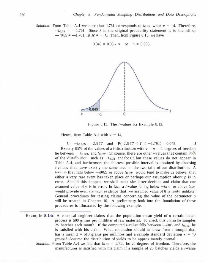
260 Chapter 8 Fundamental Sampling Distributions and Data Descriptions
Solution: From Table A.4 we note that 1.761 corresponds to Z0.05 when v = 14. Therefore, —Z005 = —1.761. Since k in the original probability statement is to the left of — '0.05 = —1.761, let A' = — ta. Then, from Figure 8.15, we have
0.045 = 0.05 - a or a = 0.005.
Figure 8.15: The /-values for Example 8.13.
Hence, from Table A.4 with v — 14,
k = -to.oos = -2.977 and P(-2.977 < T < -1.761) = 0.045. J Exactly 95%. of the values of a /-distribution with v = n — 1 degrees of freedom
lie between — Zn.02!j and /Q.025. Of course, there are other /-values that contain 95%, of the distribution, such as —/0.02 and fco.03, but these values do not appear in Table A.4, and furthermore the shortest possible interval is obtained by choosing /-values that leave exactly the same area in the two tails of our distribution. A /-value that falls below —/0.025 or above Z0.025 would tend to make us believe: that either a very rare event has taken place or perhaps our assumption about p is in error. Should this happen, we shall make the latter decision and claim that our assumed value of p is in error. In fact, a /-value falling below —/y.oi or above /QOI would provide even stronger evidence that our assumed value of ft is quite: unlikely. General procedures for testing claims concerning the value of the parameter p will be treated in Chapter 10. A preliminary look into the foundation of these procedures is illustrated by the following example.
Example 8.14:1 A chemical engineer claims that the population mean yield of a certain batch process is 500 grams per milliliter of raw material. To check this claim he samples 25 batches each month. If the computed /-value falls between —/0.05 and to.05, he is satisfied with his claim. What conclusion should he draw from a sample that has a mean x = 518 grams per milliliter and a sample standard deviation ,s = 40 grams? Assume the distribution of yields to be approximately normal.
Solution: From Table A.4 we find that to.05 = 1-711 for 24 degrees of freedom. Therefore, the manufacturer is satisfied with his claim if a sample of 25 batches yields a /-value
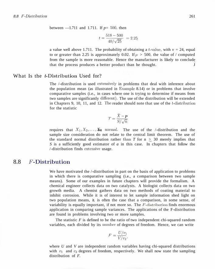
8.8 F-Distribution 261
between —1.711 and 1.711. If p= 500, then
t_ 5 1 8 - 5 0 0 = 2 2 5
40/\/25
a value well above 1.711. The probability of obtaining a /-value, with v = 24, equal to or greater than 2.25 is approximately 0.02. If p > 500. the value of / computed from the sample is more reasonable. Hence the manufacturer is likely to conclude that the process produces a better product than he thought. J
What Is the ^-Distribution Used for?
The /-distribution is used extensively in problems that deal with inference about the population mean (as illustrated in Example 8.14) or in problems that involve comparative samples (i.e., in cases where one is trying to determine if means from two samples are significantly different). The use of the distribution will be extended in Chapters 9, 10, 11, and 12. The reader should note that use of the '-distribution for the statistic
T = X - P S/VT,
requires that Xx,X2,...,Xn be normal. The use of the /-distribution and the sample size consideration do not relate to the central limit theorem. The use of the standard normal distribution rather than T for n > 30 merely implies that S is a sufficiently good estimator of a in this case. In chapters that follow the /-distribution finds extensive usage.
8.8 F-Distribution
We have motivated the /-distribution in part on the basis of application to problems in which there is comparative sampling (i.e., a comparison between two sample means). Some of our examples in future chapters will provide the formalism. A chemical engineer collects data on two catalysts. A biologist collects data on two growth media. A chemist gathers data on two methods of coating material to inhibit corrosion. While it is of interest to let sample information shed light on two population means, it. is often the case that a comparison, in some sense, of variability is equally important, if not more so. The F-distribntion finds enormous application in comparing sample variances. The applications of the F-distribution are found in problems involving two or more samples.
The statistic F is defined to be the ratio of two independent chi-squared random variables, each divided by its number of degrees of freedom. Hence, we can write
F = U/vi V/V-2 '
where U and V are independent random variables having chi-squared distributions with V\ and v2 degrees of freedom, respectively. We shall now state the sampling distribution of F.
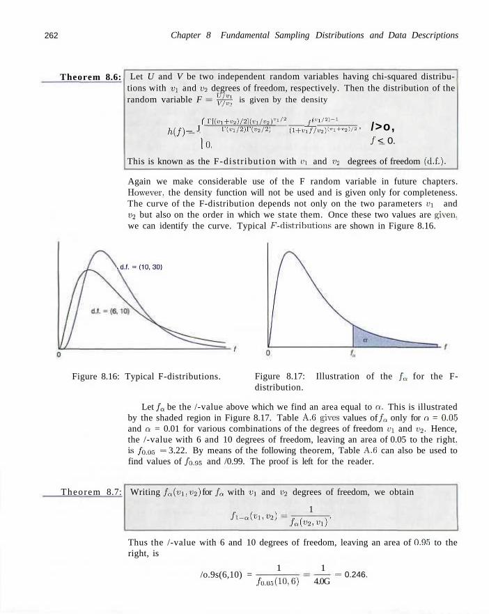
262 Chapter 8 Fundamental Sampling Distributions and Data Descriptions
Theorem 8.6: Let U and V be two independent random variables having chi-squared distributions with Vi and v2 degrees of freedom, respectively. Then the distribution of the random variable F •TTT^ is given by the density
(r\(vi+V2)/2](vi/v2Vl/2
htf\ _ J F(cl/2)rC«2/2)
b, Jll ( > - l / 2 ) - l
(l+t.l//u2)(^l+"2)/2 ' />o, / < 0.
This is known as the F-distr ibution with Ui and V2 degrees of freedom (d.f).
Again we make considerable use of the F random variable in future chapters. However, the density function will not be used and is given only for completeness. The curve of the F-distribution depends not only on the two parameters t>x and v2 but also on the order in which we state them. Once these two values are given, we can identify the curve. Typical F-distribtitions are shown in Figure 8.16.
,d.f. = (10,30)
Figure 8.16: Typical F-distributions. Figure 8.17: Illustration of the /„ for the F-distribution.
Let fa be the /-value above which we find an area equal to a. This is illustrated by the shaded region in Figure 8.17. Table A.6 gives values of fa only for a = 0.05 and Q = 0.01 for various combinations of the degrees of freedom t'i and v2. Hence, the /-value with 6 and 10 degrees of freedom, leaving an area of 0.05 to the right. is /o.Oo = 3.22. By means of the following theorem, Table A.6 can also be used to find values of /0.95 and /0.99. The proof is left for the reader.
Theorem 8.7: Writing fa{vx,v2) for fa with vi and v2 degrees of freedom, we obtain
1 /i_„(i. 'i,t>2) faiv2,Vl)'
Thus the /-value with 6 and 10 degrees of freedom, leaving an area of 0.95 to the right, is
1 1 /o.9s(6,10) =
/o.o5(10:6) 4.0G = 0.246.
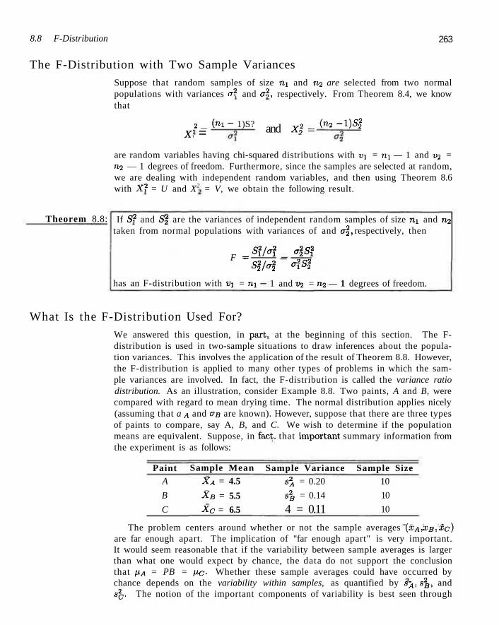
8.8 F-Distribution 263
The F-Distribution with Two Sample Variances
Suppose that random samples of size m and n2 are selected from two normal populations with variances er2 and cr2, respectively. From Theorem 8.4, we know that
, _ ( ! > ! - 1)S? x- = and XI = (U2 - 1)5g
are random variables having chi-squared distributions with vx = nx — 1 and i>2 = U2 — 1 degrees of freedom. Furthermore, since the samples are selected at random, we are dealing with independent random variables, and then using Theorem 8.6 with X 2 = U and X2 = V, we obtain the following result.
Theorem 8.8: If S 2 and S2 are the variances of independent random samples of size nx and n2
taken from normal populations with variances of and o\, respectively, then
F = Sf>2 _ 4SI Si/a2
has an F-distribution with vx = nx
o\S*2
1 and v2 = n2 — 1 degrees of freedom.
What Is the F-Distribution Used For?
We answered this question, in part, at the beginning of this section. The F-distribution is used in two-sample situations to draw inferences about the population variances. This involves the application of the result of Theorem 8.8. However, the F-distribution is applied to many other types of problems in which the sample variances are involved. In fact, the F-distribution is called the variance ratio distribution. As an illustration, consider Example 8.8. Two paints, A and B, were compared with regard to mean drying time. The normal distribution applies nicely (assuming that a A and crB are known). However, suppose that there are three types of paints to compare, say A, B, and C. We wish to determine if the population means are equivalent. Suppose, in fact, that important summary information from the experiment is as follows:
Paint A
B
C
Sample Mean XA = 4.5
XB = 5.5
Xc = 6.5
Sample Variance s2
A = 0.20
s% = 0.14
4 = 0.11
Sample Size 10
10
10
The problem centers around whether or not the sample averages (XA, XB, XC) are far enough apart. The implication of "far enough apart" is very important. It would seem reasonable that if the variability between sample averages is larger than what one would expect by chance, the data do not support the conclusion that PA = PB = PC- Whether these sample averages could have occurred by chance depends on the variability within samples, as quantified by sA, s2
B, and S"Q. The notion of the important components of variability is best seen through
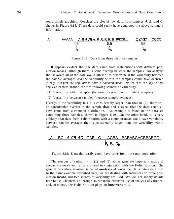
264 Chapter 8 Fundamental Sampling Distributions and Data Descriptions
some simple graphics. Consider the plot of raw data from samples A, B, and C, shown in Figure 8.18. These data could easily have generated the above summary information.
A AAAAA ARAAR A R R R R R FPTTR CCCC COCO 4.5 5.5 6.5
*A XB *C
Figure 8.18: Data from three distinct samples.
It appears evident that the data came from distributions with different population means, although there is some overlap between the samples. An analysis that involves all of the data would attempt to determine if the variability between the sample averages and the variability within the samples could have occurred jointly if in fact the populations have a common mean. Notice that the key to this analysis centers around the two following sources of variability.
(1) Variability within samples (between observations in distinct samples)
(2) Variability between samples (between sample averages)
Clearly, if the variability in (1) is considerably larger than that in (2), there will be considerable overlap in the sample data and a signal that the data could all have come from a common distribution. An example is found in the data set containing three samples, shown in Figure 8.19. On the other hand, it is very unlikely that data from a distribution with a common mean could have variability between sample averages that is considerably larger than the variability within samples.
A BC ACBAC CAB C ACBA BABABCACBBABCC ± 1 1 *A * C XB
Figure 8.19: Data that easily could have come from the same population.
The sources of variability in (1) and (2) above generate important ratios of sample variances and ratios are used in conjunction with the F-distribution. The general procedure involved is called analysis of variance. It is interesting that in the paint example described here, we are dealing with inferences on three population means, but two sources of variability are used. We will not supply details here but in Chapters 13 through 15 we make extensive use of analysis of variance, and, of course, the F-distribution plays an important role.
E:i 265
Exercises
8.39 For a chi-squared distribution find
(a) X'o.025 when v = 15:
(b) Xo.oi when v = 7:
(c) xl.nr> when e = 24.
8.40 For a chi-sc|iiarc:cl distribution find the following:
(a) Xo.oo5 w l | en v = 5;
(b) Xo.05 when v = 19:
(c) Xo.oi when v = 12.
8.41 For a chi-squared distribution find \ „ .such that
(a) P(X3 > \i) = 0.99 when v = 4;
(b) /'(A'- > xl) = 0.025 when « = 19: (c) P(37.652 < A'2 < xi) = 0-M5 when i> = 25.
8.42 For a chi-squared distribution find Xa such that
(a) F(A"-' > \l) = 0.01 when o = 21:
(b) lJ(X2 < xl) = 0-95 when v = 6;
('') P(Xo < A'2 < 23.209) = 0.015 when v = 10.
8.43 Find the probability that a random sample of 25 observations, from a normal population with variance a" = 6, will have a variance s
(a) greater than !). I; (b) between 3.462 and 10.745.
Assume the sample variances to be continuous measurements.
8.44 The scores on a placement test given to college freshmen for the past five years are approximately normally distributed with a mean //. = 71 and a variance a2 = 8. Would you still consider a2 = 8 to be a valid value of the variance if a random sample or 20 students who take this placement test this year obtain a value of .s2 = 20?
8.45 Show that the variance of S for random samples of size n. from a normal population decreases as n becomes largo. [Hint: First, find the variance of (n - 1 ) 5 > 2 . ]
8.46 (a) Find i0.oas when v = 14. (h) Find —to.io when v = 10. (c) Find ta.nm when v = 7.
8.47 (a) Find P(T < 2.3G5) when v = 7.
(b) Find P(T > 1.318) when v = 24.
(c) Find F( —J-356 < T < 2.179) when v = 12. (d) Find P(T > -2.567) when r = 17.
8.48 (a) Find P(-to.oos < T < iu.en) for v = 20. (b) Find P(T> -tojou).
8.49 Given a random sample of size 21 from a normal distribution, find k such that (a) P(-2.069 < T < k) = 0.965; (b) P{k <T< 2.807) = 0.095; (c) P(-Jfc < T < k) = 0.90.
8.50 A manufacturing firm claims that the batteries used in their electronic games will last an average of 30 hours. To maintain this average. L6 batteries are tested each month. If the computed /-value falls between —fo.02S and to.OBBi '-he firm is satisfied with its claim. What conclusion should the firm draw from a sample that has a mean x = 27.5 hours and a standard deviation a = 5 hours? Assume the distribution of battery lives to be approximately normal.
8.51 A normal population with unknown variance has a mean of 20. Is one likely to obtain a random sample of size !) from this population with a mean of 24 and a standard deviation of 4.1? If not, what conclusion would you draw?
8.52 A maker of a certain brand of low-fat cereal bars claims that their average saturated fat content is 0.5 gram. In a random sample of 8 cereal bars of this brand the saturated fat. content was 0.6. 0.7. 0.7. 0.3. 0.4. 0.5, 0.4, and 0.2. Would you agree with the claim? Assume a normal distribution.
8.53 For an F-distribution find
(a) /(i.o5 with vi = 7 and v2 = 15;
(b) /ei.ci.-i with vi = 15 and v2 = 7: (c) /o.oi with f.'i = 24 and v2 = 19; (el) /o.ss with vt = li) and ua = 24; (e) /o.BB with Ui = 28 and v2 = 12.
8.54 Pull-strength tests on 10 soldered leads for a semi conductor device yield the following results in pounds force required to rupture the bond:
19.8 12.7 13.2 16.9 10.6 18.8 11.1 143 17.0 12.5
Another set, of 8 leads was tested after encapsulation to determine whether the pull strength has been increased by encapsulation of the device, with the following results:
266 Chapter 8 Fundamental Sampling Distributions and Data Descriptions
24.9 22.8 23.6 22.1 20.4 21.6 21.8 22.5 Comment on the evidence available concerning equality of the two population variances.
8.55 Consider the following measurements of the heat producing capacity of the coal produced by two mines
(in millions of calories per ton): Mine 1: 8260 8130 8350 8070 8340 Mine 2: 7950 7890 7900 8140 7920 7840
Can it be concluded that the two population variances are equal?
Review Exercises
8.56 Consider the data displayed in Exercise 1.20 on page 29. Construct a box-and-whisker plot, and comment on the nature of the sample. Compute the sample mean and sample standard deviation.
8.57 If Xi, X2,..., X„ are independent random variables having identical exponential distributions with parameter 6, show that the density function of the random variable Y = X\ +X2+- • -+Xn is that of a gamma distribution with parameters a = n and 3 = 0.
8.58 In testing for carbon monoxide in a certain brand of cigarette, the data, in milligrams per cigarette, were coded by subtracting 12 from each observation. Use the results of Exercise 8.14 on page 235 to find the standard deviation for the carbon monoxide contents of a random sample of 15 cigarettes of this brand if the coded measurements are 3.8, —0.9. 5.4, 4.5. 5.2. 5.6. 2.7, - 0 . 1 . - 0 . 3 , -1 .7 . 5.7, 3.3. 4.4, -0 .5 , and 1.9.
8.59 If S2 and S2 represent the variances of independent random samples of size m = 8 and n2 = 12, taken from normal populations with equal variances, find the P(SJ7S| < 4.89).
8.60 A random sample of 5 bank presidents indicated annual salaries of $395,000, $521,000, $483,000, $479,000, and 8510,000. Find the variance of this set.
8.61 If the number of hurricanes that hit. a certain area of the eastern United States per year is a random variable having a Poisson distribution with p = 6, find the probability that this area will be hit by (a) exactly 15 hurricanes in 2 years;
(b) at most 9 hurricanes in 2 years.
8.62 A taxi company tests a random sample of 10 steel-belted radial tires of a certain brand and recorded the following tread wear: 48,000, 53,000. 45,000. 61,000, 59,000, 56,000, 63,000, 49,000, 53,000, and 54,000 kilometers. Use the results of Exercise 8.14 on page 235 to find the standard deviation of this set of data by first dividing each observation by 1000 and then subtracting 55.
8.63 Consider the data of Exercise 1.19 on page 28. Construct a box-and-whisker plot. Comment. Compute the sample mean and sample standard deviation.
8.64 If A"? and Sf represent the variances of independent random samples of size n\ = 25 and n2 — 31, taken from normal populations with variances a2 = 10 and erf = 15, respectively, find
P(S\/Sl > 1.26).
8.65 Consider Exercise 1.21 on page 29. on any outliers.
Comment
8.66 Consider Review Exercise 8.56. any outliers in the data.
Comment on
8.67 The breaking strength A" of a certain rivet used in a machine engine has a mean 5000 psi and standard deviation 400 psi. A random sample of 36 rivets is taken. Consider the distribution of X, the sample mean breaking strength.
(a) What is the probability that the sample mean falls between 4800 psi and 5200 psi?
(b) What sample n would be necessary in order to have
P(4900 < X < 5100) = 0.99?
8.68 Consider the situation of Review Exercise 8.62. If the population from which the sample was taken has population mean p = 53,000 kilometers, does the sample information here seem to support that claim? In your answer, compute
_ x - 53, 000 s/VW
and determine from Table A.4 (with 9 d.f.) if the computed <-value is reasonable or does it appear to be a rare event?
8.9 Potential Misconceptions and Hazards 267
8.69 Two distinct solid fuel propellants, type A and type B, are being considered in a space program activity. Burning rates on the propellant are crucial. Random samples of 20 specimens of the two propellants are taken with sample means given by 20.5 cm/sec for propellant A and 24.50 cm/sec for propellant B. It is generally assumed that the variability in burning rate is roughly the same for the two propellants and is given by a population standard deviation of 5 cm/sec. Assume that the burning rates for each propellant are approximately normal and hence make use of the central limit theorem. Nothing is known about the two population mean burning rates and it is hoped that this experiment might shed some light.
(a) If, indeed PA = PB, what is P(XB — XA > 4.0)? (b) Use your answer in (a) to shed some light on the
proposition that PA = PB-
8.70 The concentration of an active ingredient in the output of a chemical reaction is strongly influenced by the catalyst that is used in the reaction. It is felt that when catalyst A is used, the population mean concentration exceeds 65%. The standard deviation is known to be a = 5%. A sample of outputs from 30 independent experiments gives the average concentration of XA = 64.5%.
(a) Does this sample information with an average concentration of XA = 64.5% provide disturbing information that perhaps pA is not 65%, but less than 65%? Support your answer with a probability statement.
(b) Suppose a similar experiment is done with the use of another catalyst, catalyst B. The standard deviation a is still assumed to be 5% and XB turns out to be 70%. Comment on whether or not the sample information on catalyst B seems to give strong information that suggests that \IB is truly greater than PA- Support your answer by computing
P(XB - XA > 5.5 | pB = PA).
(c) Under the condition that PA = PB = 65%, give the approximate distribution of the following quantities (with mean and variance of each). Make use of the central limit theorem.
\)XB; ii)A\, - XB:
compute (assuming pa = 65%)
P(XB > 70).
8.72 Given a normal random variable X with mean 20 and variance 9, and a random sample of size ;i taken from the distribution, what sample size n is necessary in order that
P(19.9 < X < 20.1) = 0.95?
8.73 In Chapter 9 the concept of parameter estimation will be discussed at length. Suppose A is a random variable with mean p and variance a2 = 1.0. Suppose also that a random sample of size n is to be taken and x is to be used as an estimate of p. When the data are taken and the sample mean is measured, we wish it to be within 0.05 units of the true mean with probability 0.99. That is, we want, there to be a good chance that the computed x from the sample is "very close" to the population mean (wherever it is!), so we wish
P(\X -p\< 0.05) = 0.99.
What sample size is required?
8.74 Suppose a filling machine is used to fill cartons with a liquid product. The specification that is strictly enforced for the filling machine is 9 ± 1.5 oz. If any carton is produced with weight outside these bounds, it is considered by the supplier to be a defective. It is hoped that at least 99% of cartons will meet these specifications. With the conditions p, = 9 and a = 1, what proportion of cartons from the process are defective? If changes are made to reduce variability, what must a be reduced to in order to meet specifications with probability 0.99? Assume a normal distribution for the weight.
8.75 Consider the situation in Review Exercise 8.74. Suppose a considerable quality effort is conducted to "tighten'' the variability in the system. Following the effort, a random sample of size 40 is taken from the new assembly line and the sample variance s" = 0.188 ounces2. Do we have strong numerical evidence that a2
has been reduced below 1.0? Consider the probability
P(S2 < 0.188 | a2 = 1.0).
8.71 From the information in Review Exercise 8.70. and give conclusion.
268 Chapter 8 Fundamental Sampling Distributions and. Data Descriptions
8.9 Potential Misconceptions and Hazards; Relationship to Material in Other Chapters
The central limit theorem is one of the most powerful tools in all statistics, and even though this chapter is relatively short, it contains a wealth of fundamental information that, is laced with tools that will lie used throughout the balance of the text.
The: notion of a sampling distribution is one of the most important fundamental concepts in all of statistics, and the student at this point in his or her training should gain a clear understanding before proceeding beyond this chapter. All chapters that follow will make considerable use of sampling distributions. Suppose one wants to use the statistic X to draw inferences about the population mean //. It will be done by using the observed value X from a single sample of size it. Then any inference made must be accomplished by taking into account not-just the single value but rather the theoretical structure or dis t r ibut ion of all x values tha t could be observed from samples of size n. Thus the term sampling distribution is introduced. This distribution is the basis for the central limit theorem. The /., \ 2 , and F-distributions arc also used in the context of sampling distributions. For example, the {-distribution, pictured in Figure 8.13, represents the structure that occurs if all of the values of '',~C- arc formed, where x and S are taken from samples of size n from a n(x;p,a) distribution. Similar remarks can be made about, x a,nd F, and the reader should not forget, that the sample information forming the statistics for all of these distributions is the normal. So it can be said t ha t where there is a t, F, or \ 2 , t he source was a sample from a normal dis tr ibut ion.
The three distributions described above may appear to be introduced in a rather self-contained fashion with no indication of what they are about. However, they will appear in practical problem-solving throughout the: balance of the text.
Now, there are things that one must bear in mind lest confusion set in regarding these fundamental sampling distributions:
(i) One cannot use the central limit theorem unless er is known. When a is not known, it should be replaced by s. the sample standard deviation, in order to use the central limit theorem.
(ii) The Tstatistic is not a result, of the central limit theorem and X\,x2,.. • ,xn
must come from a n(x: p. a) distribution in order that fj-f= be a f-distribution. and s is, of course, merely an estimate of a.
(iii) While the notion of degrees of freedom is new at this point, the concept should be very intuitive since it. is reasonable that the nature of the distribution of S and also f should depend on the amount of information in the sample x\,x2,... ,xn.
Chapter 9
One- and Two-Sample Estimation Problems
9.1 Introduction
In previous chapters we emphasized sampling properties of the sample mean and sample: variance. We also emphasized displays of data in various forms. The purpose of these: presentations is to build a foundation that allows statisticians to draw conclusions about, the population parameters from experimental data. For example, the central limit theorem provides information about the distribution of the sample mean X. The distribution involves the population mean //.. Thus any conclusions drawn concerning p from an observed sample average must depend on knowledge of this sampling distribution. Similar comments could apply for S2 and a2. Clearly, any conclusions wc draw about the variance of a normal distribution would likely involve the sampling distribution of S2.
In this chapter we begin by formally outlining the purpose of statistical inference. We follow this by discussing the problem of es t imat ion of popula t ion paramete r s . We confine our formal developments of specific estimation procedures to problems involving one and two samples.
9.2 Statistical Inference
In Chapter 1 wc discuss the general philosophy of formal statistical inference:. The theory of s tat is t ical inference consists of those methods by which one makes inferences or generalizations about a population. The trend of today is to distinguish between the classical me thod of estimating a population parameter, whereby inferences arc based strictly on information obtained from a random sample selected from the population, and the Bayesian me thod , which utilizes prior subjective knowledge about the probability distribution of the unknown parameters in conjunction with the information provided by the sample data. Throughout most of this chapter we shall use classical methods to estimate unknown population parameters such as the mean, proportion, and the variance by computing statistics
270 Chapter 9 One- and Two-Sample Estimation Problems
from random samples and applying the theory of sampling distributions, much of which was covered in Chapter 8. Bayesian estimation will be discussed in Chapter 18.
Statistical inference may be divided into two major areas: est imation and tes ts of hypotheses. We treat these two areas separately, dealing with theory and applications of estimation in this chapter and hypothesis testing in Chapter 10. To distinguish clearly between the two areas, consider the following examples. A candidate for public office may wish to estimate the true proportion of voters favoring him by obtaining the opinions from a random sample of 100 eligible voters. The fraction of voters in the sample favoring the candidate could be used as an estimate of the true proportion in the population of voters. A knowledge of the sampling distribution of a proportion enables one to establish the degree of accuracy of our estimate. This problem falls in the area of estimation.
Now consider the case in which one is interested in finding out whether brand A floor wax is more sc;uff-resistant than brand B floor wax. He or she might hypothesize that brand A is better than brand B and, after proper testing, accept or reject this hypothesis. In this example we do not attempt to estimate a parameter, but instead we try to arrive at a correct decision about a prestated hypothesis. Once again we are dependent on sampling theory and the use of data to provide us with some measure of accuracy for our decision.
9.3 Classical Methods of Estimation
A point es t imate of some population parameter 0 is a single value 8 of a statistic: 0. For example, the value x of the statistic X, computed from a sample of size n, is a point estimate of the population parameter p. Similarly, p = x/n is a point estimate of the true proportion p for a binomial experiment.
An estimator is not expected to estimate the population parameter without error. We do not expect X to estimate p exactly, but we certainly hope that it is not far off. For a particular sample it is possible to obtain a closer estimate of p by using the sample median X as an estimator. Consider, for instance, a sample consisting of the values 2, 5, and 11 from a population whose mean is 4 but supposedly unknown. We would estimate p to be x = 6, using the sample mean as our estimate, or x — 5, using the sample median as our estimate. In this case the estimator X produces an estimate closer to the true parameter than that of the estimator X. On the other hand, if our random sample contains the values 2, 6, and 7, then x = 5 and x = 6, so that X is now the better estimator. Not knowing the true value of ft, we must decide in advance whether to use X or X as our estimator.
Unbiased Est imator
What are the desirable properties of a "good" decision function that would influence us to choose one estimator rather than another? Let 0 be an estimator whose value 0 is a point estimate of some unknown population parameter 6. Certainly, we would like the sampling distribution of 0 to have a mean equal to the parameter estimated. An estimator possessing this property is said to be unbiased.
9.3 Classical Methods of Estimation 271
Definition 9.1: A statistic 0 is said to be an unbiased estimator of the parameter 0 if
Pe = F(0 ) = 6.
Example 9.1:1 Show that S2 is an unbiased estimator of the: parameter a2. Solution: Let us write
; = i
i = l
Now
nE(X - p.
^iK"^ However,
Therefore,
ox. = a2 for i = 1,2,.
E(S2) =
a n
n.a — n— n — 1 \ II
a2.
Y(x,-x)2 = Ytix>-i''>-(x-iiW t> n
= Yi*> - I'f - 2(* - p) YiXi - I') + "iX ~ I'f
n
^YiX'-rf-oiX-l'f-
Although S2 is an unbiased estimator of a2, S, cm the other hand, is a biased estimator of a with the bias becoming insignificant for large samples. This example illustrates why we divide by n — 1 rather than n when the variance is estimated.
Variance of a Point Es t imator
If 0 i and 02 arc1 two unbiased estimators of the: same population parameter 0, we would choose the estimator whose sampling distribution has the smaller variance. Hence, if er? < a'j , we say that 0 i is a more efficient es t imator of 0 than 02-
If I rV-J
Definition 9.2: If wc consider all possible unbiased estimators of some parameter 0, the: one with the smallest variance is called the most efficient es t imator of 8.
In Figure 9.1 we illustrate the sampling distributions of 3 different estimators 01 , 02, and 0.j. all estimating 9. It is clear that only 0 1 : and 02 are unbiased,
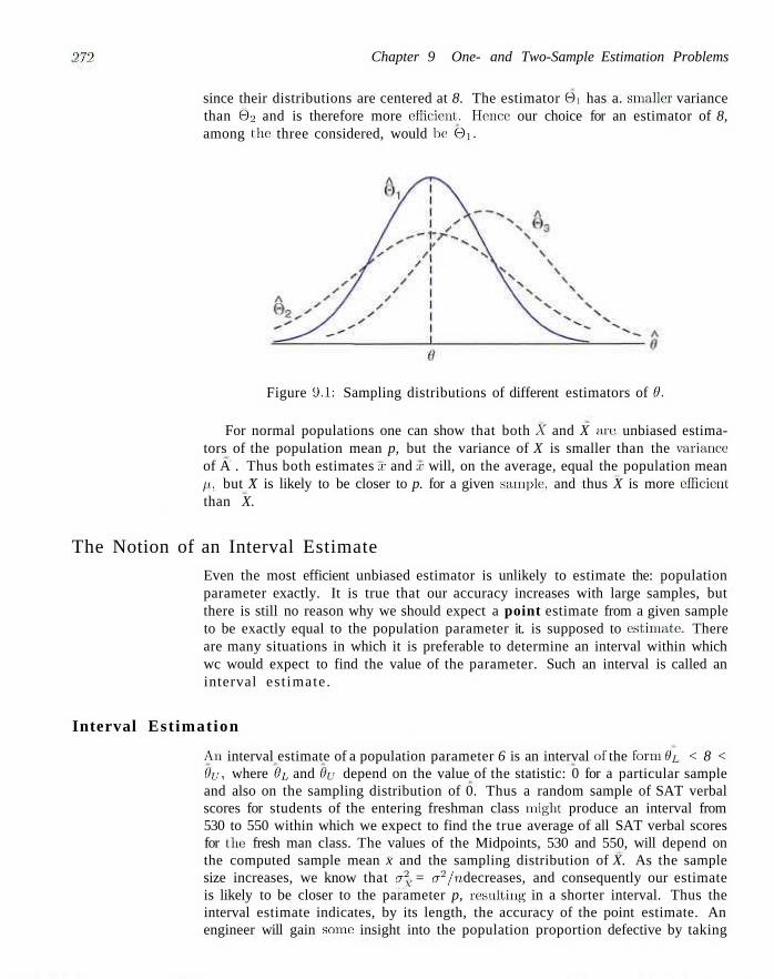
').7-> Chapter 9 One- and Two-Sample Estimation Problems
since their distributions are centered at 8. The estimator B | has a. smaller variance than 02 and is therefore more efficient. Hence our choice for an estimator of 8, among the three considered, would be 0 ] .
Figure 9.1: Sampling distributions of different estimators of 6.
For normal populations one can show that both X and X are1 unbiased estimators of the population mean p, but the variance of X is smaller than the variance of A . Thus both estimates x and x will, on the average, equal the population mean //.. but X is likely to be closer to p. for a given sample:, and thus X is more efficient than X.
The Notion of an Interval Estimate
Even the most efficient unbiased estimator is unlikely to estimate the: population parameter exactly. It is true that our accuracy increases with large samples, but there is still no reason why we should expect a point estimate from a given sample to be exactly equal to the population parameter it. is supposed to estimate. There are many situations in which it is preferable to determine an interval within which wc would expect to find the value of the parameter. Such an interval is called an interval es t imate.
Interval Est imation
An interval estimate of a population parameter 6 is an interval of the form 81, < 8 < ()ij, where 6L and By depend on the value of the statistic: 0 for a particular sample and also on the sampling distribution of 0. Thus a random sample of SAT verbal scores for students of the entering freshman class might produce an interval from 530 to 550 within which we expect to find the true average of all SAT verbal scores for the: fresh man class. The values of the Midpoints, 530 and 550, will depend on the computed sample mean x and the sampling distribution of X. As the sample size increases, we know that a\ = a2fn decreases, and consequently our estimate is likely to be closer to the parameter p, resulting in a shorter interval. Thus the interval estimate indicates, by its length, the accuracy of the point estimate. An engineer will gain some insight into the population proportion defective by taking
9.3 Classical Methods of Estimation 273
a sample and computing the sample proportion defectives. But an interval estimate might be more informative.
Interpretation of Interval Estimates
Since different samples will generally yield different, values of 0 and, therefore, different values 81, and 8u, these cndpoints of the interval are values of corresponding random variables 0/, and 0(.:. From the sampling distribution of 0 we shall be able to determine 0/, and 0/y such that the P(&L < 8 < 0 y ) is equal to any positive fractional value wc care to specify. If, for instance, we find 0/ , and ©jy such that
F ( 0 t < 8 < &u) = 1 - a
for 0 < a < 1, then we have a probability of 1 —a of selecting a random sample that will produce an interval containing 0. The interval 0/, < 9 < 8u, computed from the selected sample, is then called a 100(1 —a)% confidence interval, the fraction 1 — a is called the confidence coefficient or the degree of confidence, and the endpoints, 8i, and 8a, are called the lower and upper confidence l imits. Thus, when a = 0.05, we have a 95% confidence interval, and when a = 0.01 we obtain a wider 99% confidence interval. The wider the confidence interval is, the more confident we can be that the given interval contains the unknown parameter. Of course, it is better to be 95% confident that the average life of a certain television transistor is between 6 and 7 years than to be 99% confident that it is between 3 and 10 years. Ideally, we prefer a short interval with a high degree of confidence. Sometimes, restrictions on the size of our sample prevent us from achieving short intervals without sacrificing some of our degree of confidence.
In the sections that follow we pursue the notions of point and interval estimation, with each section representing a different special case. The reader should notice that while point and interval estimation represent different approaches to gain information regarding a parameter, they are related in the sense that confidence interval estimators are based on point estimators. In the following section, for example, we should see that the estimator X is a very reasonable point estimator of p. As a result, the important confidence interval estimator of p depends on knowledge of the sampling distribution of X.
Wc begin in the following section with the simplest case of a confidence interval. The scenario is simple and yet unrealistic. We are interested in estimating a population mean p and yet a is known. Clearly if p is unknown, it is quite unlikely that a is known. Any historical information that produced enough information to allow the assumption that a is known would likely have produced similar information about p. Despite this argument, we begin with this case because the concepts and indeed the resulting mechanics associated with confidence interval estimation remain the same when more realistic situations surface later in Section 9.4 and beyond.
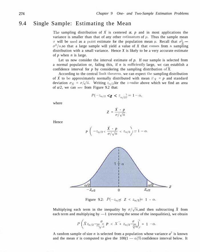
274 Chapter 9 One- and Two-Sample Estimation Problems
9.4 Single Sample: Estimating the Mean
The sampling distribution of X is centered at. p and in most applications the variance is smaller than that of any other estimators of /<. Thus the sample mean .i: will be used as a point estimate for the population mean p. Recall that ay — a2/n, so that a large sample will yield a value of X that comes from a sampling distribution with a small variance. Hence X is likely to be a very accurate estimate of p when n is large.
Let us now consider the interval estimate of p. If our sample is selected from a normal population or, failing this, if n is sufficiently large, wc can establish a confidence interval for p by considering the sampling distribution of X.
According to the central limit theorem, we can expect the- sampling distribution of X to be approximately normally distributed with mean // y = p and standard deviation cry = of s/Tt. Writing zai2 lor the z-varue above which we find an area of a/2, we can se:c from Figure 9.2 that:
Pi- <-al2 <z < •af2) 1
where
Hence
Z = X - p
P -Za/2 <
a/yTr'
X - p o/sfTt < Za/2 ) — 1 ~ 0!.
-za/2 0
Figure 9.2: P(-zo/2 < Z < za/2) = 1 - a.
Multiplying each term in the inequality by a/^/n, and then subtracting X from each term and multiplying by —1 (reversing the sense of the inequalities), we obtain
P[X- ZQ/2-7= < P < X + Za /2-4= ) = 1 - Q.
A random sample of size n is selected from a population whose variance a2 is known and the mean x is computed to give the 100(1 — a)% confidence interval below. It
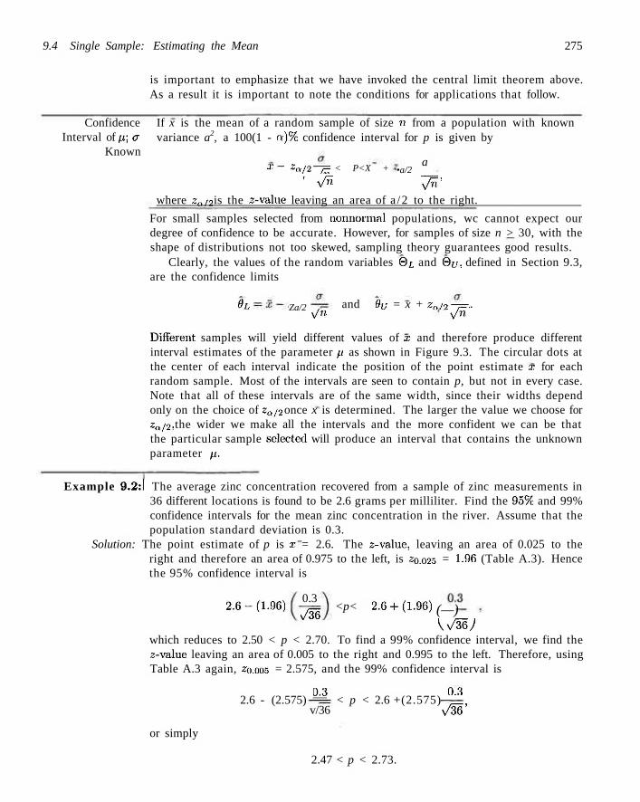
9.4 Single Sample: Estimating the Mean 275
is important to emphasize that we have invoked the central limit theorem above. As a result it is important to note the conditions for applications that follow.
Confidence Interval of p\ <r
Known
If x is the mean of a random sample of size n from a population with known variance a2, a 100(1 - o)% confidence interval for p is given by
X- za/2-?= < P<X +
' \/n •a/2
a
7^' where za/2 is the 3-value leaving an area of a /2 to the right.
For small samples selected from nonnormal populations, wc cannot expect our degree of confidence to be accurate. However, for samples of size n > 30, with the shape of distributions not too skewed, sampling theory guarantees good results.
Clearly, the values of the random variables @L and 0 y , defined in Section 9.3, are the confidence limits
0L Za/2 yfn and 8y = x + za i2 —=.
v^n"
Different samples will yield different values of x and therefore produce different interval estimates of the parameter // as shown in Figure 9.3. The circular dots at the center of each interval indicate the position of the point estimate x for each random sample. Most of the intervals are seen to contain p, but not in every case. Note that all of these intervals are of the same width, since their widths depend only on the choice of zQ/2 once x is determined. The larger the value we choose for za/2, the wider we make all the intervals and the more confident we can be that the particular sample selected will produce an interval that contains the unknown parameter p.
Example 9.2:1 The average zinc concentration recovered from a sample of zinc measurements in 36 different locations is found to be 2.6 grams per milliliter. Find the 95% and 99% confidence intervals for the mean zinc concentration in the river. Assume that the population standard deviation is 0.3.
Solution: The point estimate of p is x = 2.6. The 2-value, leaving an area of 0.025 to the right and therefore an area of 0.975 to the left, is zo.025 = 1-96 (Table A.3). Hence the 95% confidence interval is
2.6-(1.96) 0.3
\/36 <p< 2.6+(1.96) (—)
\V3QJ which reduces to 2.50 < p < 2.70. To find a 99% confidence interval, we find the z-value leaving an area of 0.005 to the right and 0.995 to the left. Therefore, using Table A.3 again, 20.005 = 2.575, and the 99% confidence interval is
2.6 - (2.575) 0.3
v/36 < p < 2.6 +(2.575) ° "
vW or simply
2.47 < p < 2.73.
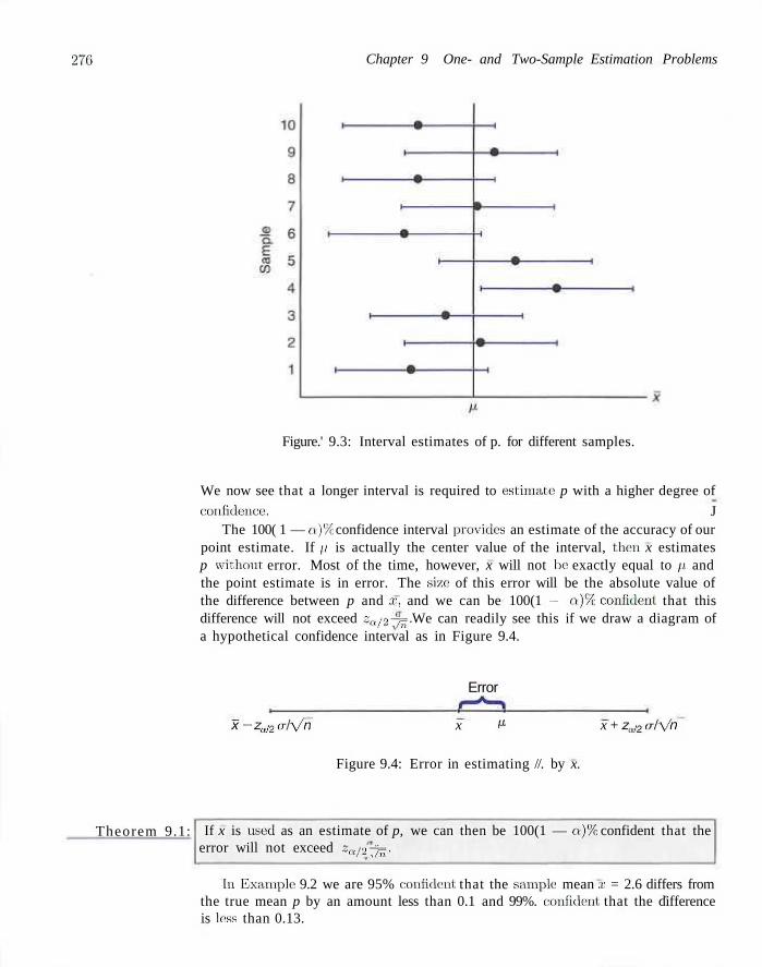
270 Chapter 9 One- and Two-Sample Estimation Problems
Figure.' 9.3: Interval estimates of p. for different samples.
We now see that a longer interval is required to estimate: p with a higher degree of
confidence. J The 100( 1 — a)% confidence interval provides an estimate of the accuracy of our
point estimate. If // is actually the center value of the interval, then x estimates p without error. Most of the time, however, x will not be exactly equal to p. and the point estimate is in error. The size of this error will be the absolute value of the difference between p and x, and we can be 100(1 — a)% confident that this difference will not exceed za/2-j=. We can readily see this if we draw a diagram of a hypothetical confidence interval as in Figure 9.4.
Error
x-zal2al\/n x p- x + z„i2<rl\/n
Figure 9.4: Error in estimating //. by x.
Theorem 9.1: If x is used as an estimate of p, we can then be 100(1 — a)% confident that the error will not exceed Zaj2-ns,
In Example 9.2 we are 95% confident that the sample1 mean x = 2.6 differs from the true mean p by an amount less than 0.1 and 99%. confident that the difference is less than 0.13.
9.4 Single Sample: Estimating the Mean
Theorem 9.2:
Frequently, we wish to know how large a sample is necessary to ensure that the error in estimating ft will be less than a specified amount e. By Theorem 9.1 this means that we must choose n such that -0/2-7= = e> Solving this equation gives the following formula for 11.
If x is used as an estimate of p, we can be 100(1 — «•)% confident that the error will not exceed a specified amount e when the sample size is
" = ( e ) '
When solving for the: sample size, n, all fractional values arc rounded up to the next whole number. By adhering to this principle, we can be sure that our degree of confidence never falls below 100(1 - n)%.
Strictly speaking, the formula in The:orem 9.2 is applicable only if we know the variance of the population from which we are to select our sample. Lacking this information, we could take a preliminary sample of size n > 30 to provide an estimate of a. Them, using ,s as an approximation for a in Theorem 9.2 we could determine approximately how many observations are needed to provide the desired degree of accuracy.
Example 9.3:1 How large a sample is required in Example 9.2 if we want to be 95% confident that our estimate of p. is off by less than 0.057
Solution: The population standard deviation is a = 0.3. Then, by Theorem 9.2,
(1.96)(0.3) O.O:
= 138.3.
Therefore, we can be 95% confident that a random sample of size 139 will provide an estimate x differing from //. by an amount less than 0.05. J
One-Sided Confidence Bounds
The confidence intervals and resulting confidence bounds discussed thus far are two-sided in nature (i.e., both tipper and lower bounds are given). However, there are many applications in which only one bound is sought. For example, if the measurement of interest is tensile strength, the engineer receives more information from a lower bound only. This bound communicates the "worst case" scenario. On the other hand, if the measurement is something for which a relatively large value of p is not profitable or desirable, then an upper confidence bound is of interest. An example would be a case: in which inferences need to be made concerning the mean mercury composition in a river. An upper bound is very informative in this case.
One-sided confidence bounds are developed in the: same fashion as two-sided intervals. However, the source is a one-sided probability statement that makes use of the central limit theorem
P X I' a/y/n. < z, = 1
278 Chapter 9 One- and Two-Sample Estimation Problems
One can then manipulate the probability statement much like before and obtain
P(p > X - 2Qcr/Vn) = 1 - Q.
Similar manipulation of P ( .~j~ > — za J = 1 — a gives
P(p < X + zao/sfn) - I - a .
As a result, the upper and lower one-sided bounds follow.
One-Sided If X is the mean of a random sample of size n from a population with variance Confidence a2, the one-sided 100(1 - a)% confidence bounds for p are given by-
Bounds on p; a Known upper one-sided bound: x + Zo,a/y/n;
lower one-sided bound: x — zao/\frt..
Example 9.4:1 In a psychological testing experiment, 25 subjects are selected randomly and their reaction time, in seconds, to a particular experiment, is measured. Past experience suggests that the variance in reaction time to these types of stimuli are 4 sec2 and that reaction time is approximately normal. The average time for the subjects was 6.2 seconds. Give an upper 95% bound for the mean reaction time.
Solution: The upper 95% bound is given by
x + zaa/s/n = 6.2 + (1.645)^/4/25 = 6.2 + 0.658
= 6.858 seconds.
Hence, we arc 95% confident that the mean reaction is less than 6.858 seconds. -I
The Case of a Unknown
Frequently, wc are attempting to estimate the mean of a population when the variance is unknown. The reader should recall that in Chapter 8 we learned that if we have a random sample from a normal distribution, then the random variable
S/Jn has a Student t-distribution with n — 1 degrees of freedom. Here S is the sample standard deviation. In this situation with a unknown, T can be used to construct a confidence interval on p. The procedure is the same as that with known a except that a is replaced by S and the standard normal distribution is replaced by the ^-distribution. Referring to Figure 9.5, we can assert that
P(-ta/2 < T < ta/2) = 1 - a,
where tai2 is the (-value with n — 1 degrees of freedom, above which we find an area of a /2 . Because of symmetry, an equal area of a /2 will fall to the left of-tQy2-Substituting for T, we write
X-p \
~ta/2 < ~sm< ta/2)=
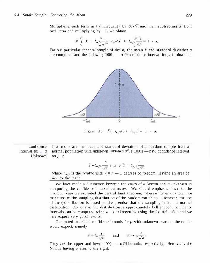
9.4 Single Sample: Estimating the Mean 279
Multiplying each term in the inequality by S/y/ti, and then subtracting X from each term and multiplying by —1, we obtain
P [ X - ta/s-7= <p<X + tai2-j= V" Vn
1 - a.
For our particular random sample of size n, the mean x and standard deviation s are computed and the following 100(1 — a)% confidence interval for p. is obtained.
Figure 9.5: P(-ta/2 <T< ta/2) = 1 - a.
Confidence Interval for p.; a
Unknown
If x and s are the mean and standard deviation of a. random sample from a normal population with unknown variance a2, a 100(1 — n)% confidence interval for p is
s s x - Wz~7= < M < •'*•' + ta/2-7=:
where ta/2 is the (-value with v = n — 1 degrees of freedom, leaving an area of o/2 to the right.
We have made a distinction between the cases of a known and a unknown in computing the confidence interval estimates. Wc should emphasize that for the a known case we exploited the central limit theorem, whereas for er unknown we made use of the sampling distribution of the random variable T. However, the use of the (-distribution is based on the premise that the sampling is from a normal distribution. As long as the distribution is approximately bell shaped, confidence intervals can be computed when a2 is unknown by using the (-distribution and we may expect very good results.
Computed one-sided confidence bounds for p with unknown a are as the reader would expect, namely
s and •t
They are the upper and lower 100(1 — a)% (-value having a area to the right.
s/n
respectively. Here ta is the
280 Chapter 9 One- and Two-Sample Estimation Problems
Concept of a Large-Sample Confidence Interval
Often statisticians recommend that even when normality cannot be assumed, a unknown, and n > 30, s can replace er and the confidence interval
s
Vn
may be used. This is often referred to as a large-sample confidence interval. The justification lies only in the presumption that with a sample as large as 30 and the population distribution not too skewed, s will be very close to the true a and thus the central limit theorem prevails. It should be emphasized that this is only an approximation and the quality of the approach becomes better as the sample size grows larger.
Example 9.5:1 The contents of 7 similar containers of sulfuric acid are 9.8, 10.2, 10.4, 9.8, 10.0, 10.2, and 9.6 liters. Find a 95% confidence interval for the mean of all such containers, assuming an approximate normal distribution.
Solution: The sample mean and standard deviation for the given data are
x = 10.0 and s = 0.283.
Using Table A.4, we find (0.025 = 2.447 for v = 6 degrees of freedom. Hence the 95%. confidents interval for p. is
10 .0 - (2.447) ( ^ ) < M < 10.0 + (2.447) ( ^
which reduces to 9.74 < p < 10.20. J
9.5 Standard Error of a Point Estimate
We have made a rather sharp distinction between the goals of point estimates and confidence interval estimates. The former supplies a single number extracted from a set of experimental data, and the latter provides an interval given the experimental, data that is reasonable for the parameter; that is, 100(1 — a)% of such computed intervals "cover" the parameter.
These two approaches to estimation are related to each other. The "common thread" is the sampling distribution of the point estimator. Consider, for example, the estimator X of p with a known. We indicated earlier that a measure of quality of an unbiased estimator is its variance. The variance of X is
2 °~ ax = —.
n Thus the standard deviation of AT or standard error of X is a/s/n. Simply put, the standard error of an estimator is its standard deviation. For the case of X, the computed confidence limit
a x ± zty f2—~=, is written as x ± za/2 s.e.(x),
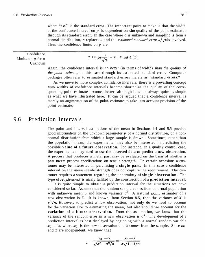
9.6 Prediction Intervals 281
where ils.e." is the standard error. The important point to make is that the width of the confidence interval on p. is dependent on the quality of the point estimator through its standard error. In the case where a is unknown and sampling is from a normal distribution, s replaces a and the estimated standard error s/^/n is involved. Thus the confidence limits on p are
Confidence s
Limits on p for a x ± t a / 2 77^ = x ± ia/2S-e-(a;) Unknown
Again, the confidence interval is no better (in terms of width) than the quality of the point estimate, in this case through its estimated standard error. Computer packages often refer to estimated standard errors merely as "standard errors.1'
As we move to more complex confidence intervals, there is a prevailing concept that, widths of confidence intervals become shorter as the quality of the corresponding point estimate becomes better, although it is not always quite as simple as what we have illustrated here. It can be argued that a confidence interval is merely an augmentation of the point, estimate to take into account precision of the point estimate.
9.6 Prediction Intervals
The point and interval estimations of the mean in Sections 9.4 and 9.5 provide good information on the unknown parameter p of a normal distribution, or a non-normal distribution from which a large sample is drawn. Sometimes, other than the population mean, the experimenter may also be interested in predicting the possible value of a future observation. For instance, in a quality control case, the experimenter may need to use the observed data to predict a new observation. A process that produces a metal part may be evaluated on the basis of whether a part meets process specifications on tensile strength. On certain occasions a customer may be interested in purchasing a single part. In this case a confidence interval on the mean tensile strength does not capture the requirement. The customer requires a statement regarding the uncertainty of single observation. The type of requirement, is nicely fulfilled by the construction of a prediction interval.
It is quite simple to obtain a prediction interval for the situations we have considered so far. Assume that the random sample comes from a normal population with unknown mean p and known variance a2. A natural point, estimator of a new observation is X. It is known, from Section 8.5, that the variance of X is a2jn. However, to predict a new observation, not only do we need to account for the variation clue to estimating the mean, but also should we account for the variation of a future observation. From the assumption, we know that the variance of the random error in a new observation is a2. The development of a prediction interval is best displayed by beginning with a normal random variable XQ — x, where XQ is the new observation and x comes from the sample. Since XQ and x are independent, we know that
XQ — x xo — x z = s/a2 + a2/n ay/l + 1/n
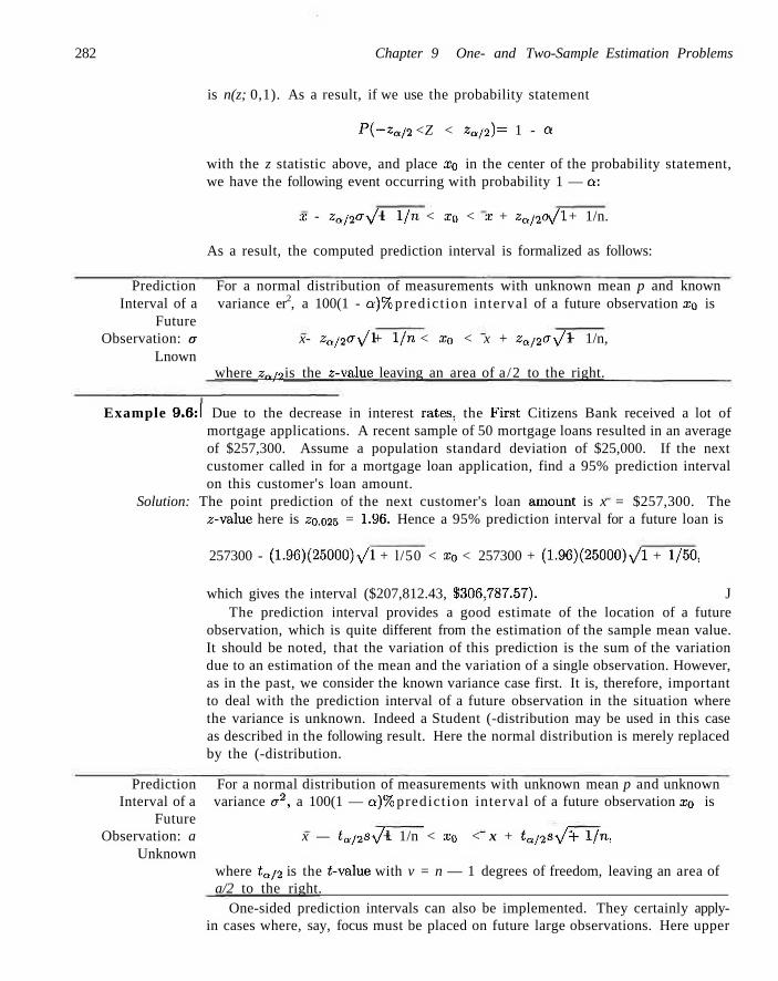
282 Chapter 9 One- and Two-Sample Estimation Problems
is n(z; 0,1). As a result, if we use the probability statement
Pi-Za/2 <Z < za/2) = 1 - a
with the z statistic above, and place .To in the center of the probability statement, we have the following event occurring with probability 1 — a:
x - zaj2ayj\ + 1/n < x0 < x + za/2a \Jl + 1/n.
As a result, the computed prediction interval is formalized as follows:
Prediction For a normal distribution of measurements with unknown mean p and known Interval of a variance er2, a 100(1 - a)% predict ion interval of a future observation xo is
Future Observation: a x- zaj2o\J\ + l/n < xa < x + za/2ay/l + 1/n,
Lnown where za/2 is the z-value leaving an area of a /2 to the right.
Example 9.6:1 Due to the decrease in interest rates, the First Citizens Bank received a lot of mortgage applications. A recent sample of 50 mortgage loans resulted in an average of $257,300. Assume a population standard deviation of $25,000. If the next customer called in for a mortgage loan application, find a 95% prediction interval on this customer's loan amount.
Solution: The point prediction of the next customer's loan amount is x = $257,300. The z-value here is zo.025 = 1-96. Hence a 95% prediction interval for a future loan is
257300 - (1.96)(25000)v/l + l/50 < x0 < 257300 + (1.96)(25000)>/l + 1/50,
which gives the interval ($207,812.43, $306,787.57). J The prediction interval provides a good estimate of the location of a future
observation, which is quite different from the estimation of the sample mean value. It should be noted, that the variation of this prediction is the sum of the variation due to an estimation of the mean and the variation of a single observation. However, as in the past, we consider the known variance case first. It is, therefore, important to deal with the prediction interval of a future observation in the situation where the variance is unknown. Indeed a Student (-distribution may be used in this case as described in the following result. Here the normal distribution is merely replaced by the (-distribution.
Prediction For a normal distribution of measurements with unknown mean p and unknown Interval of a variance cr2, a 100(1 — a)% predict ion interval of a future observation XQ is
Future Observation: a x — ta/2s\/l + 1/n < XQ < x + ta/2sy/l + l/n,
Unknown where ta/2 is the i-value with v = n — 1 degrees of freedom, leaving an area of a/2 to the right.
One-sided prediction intervals can also be implemented. They certainly apply-in cases where, say, focus must be placed on future large observations. Here upper
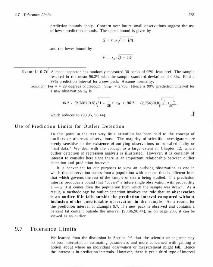
9.7 Tolerance Limits 283
prediction bounds apply. Concern over future small observations suggest the use of lower prediction bounds. The upper bound is given by
and the lower bound by
x + tas>/l + l/n
x — tnsy 1 + 1/n.
Example 9.7:1 A meat inspector has randomly measured 30 packs of 95%. lean beef. The sample resulted in the mean 96.2% with the sample standard deviation of 0.8%. Find a 99% prediction interval for a new pack. Assume normality.
Solution: For v = 29 degrees of freedom, (Q.OUS = 2.756. Hence a 99% prediction interval for a new observation .TQ is
96.2 - (2.756) (0.8)^1 - ^ < a* < 96.2 + (2.756)(0.8) J l + ±,
which reduces to (93.96, 98.44).
Use of Prediction Limits for Outlier Detection
To this point in the text very little attention has been paid to the concept of out l iers or aberrant, observations. The majority of scientific investigators are keenly sensitive to the existence of outlying observations or so called faulty or "bad data." We deal with the concept to a large extent in Chapter 12. where outlier detection in regression analysis is illustrated. However, it is certainly of interest to consider here since there is an important relationship between outlier detection and prediction intervals.
It is convenient for our purposes to view an outlying observation as one in which that observation conies from a population with a mean that is different from that which governs the rest of the sample of size n being studied. The prediction interval produces a bound that "covers" a future single observation with probability 1 — Q if it comes from the population from which the sample was drawn. As a result, a methodology for outlier detection involves the rule that an observation is an outlier if it falls outside the prediction interval computed without inclusion of the quest ionable observation in the sample. As a result, for the prediction interval of Example 9.7, if a new pack is observed and contains a percent fat content outside the interval (93.96,98.44), as on page 283, it can be viewed as an outlier.
9.7 Tolerance Limits We learned from the discussion in Section 9.6 that the scientist or engineer may be* less interested in estimating parameters and more concerned with gaining a notion about where an individual observation or measurement might fall. Hence the interest is in prediction intervals. However, there is yet a third type of interval
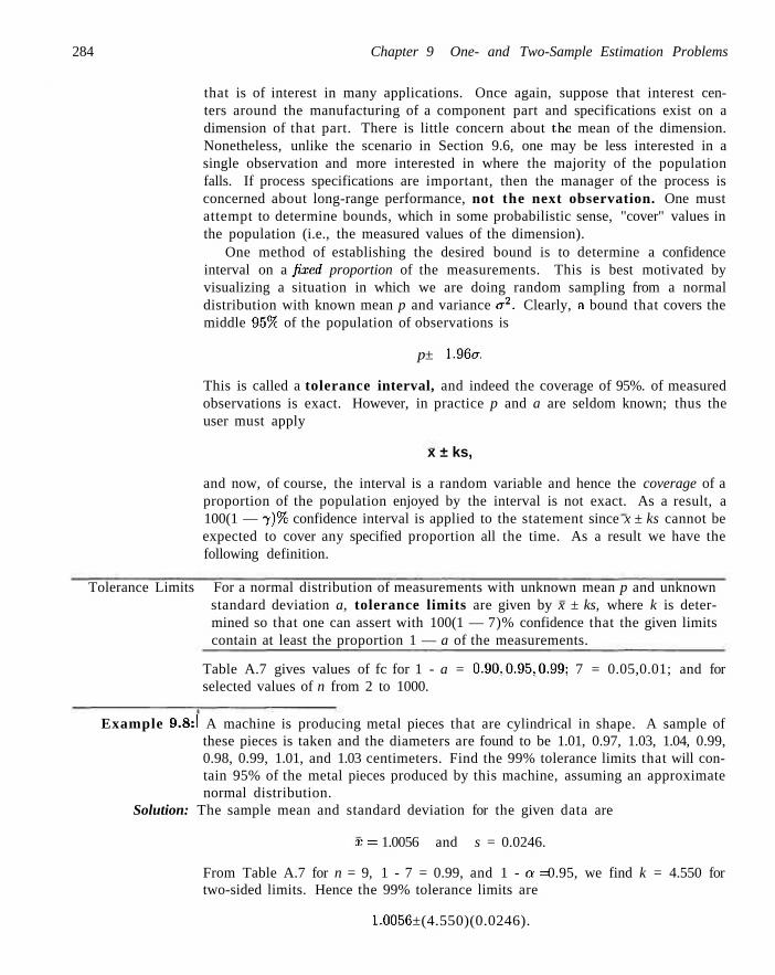
284 Chapter 9 One- and Two-Sample Estimation Problems
that is of interest in many applications. Once again, suppose that interest centers around the manufacturing of a component part and specifications exist on a dimension of that part. There is little concern about the mean of the dimension. Nonetheless, unlike the scenario in Section 9.6, one may be less interested in a single observation and more interested in where the majority of the population falls. If process specifications are important, then the manager of the process is concerned about long-range performance, not the next observation. One must attempt to determine bounds, which in some probabilistic sense, "cover" values in the population (i.e., the measured values of the dimension).
One method of establishing the desired bound is to determine a confidence interval on a fixed proportion of the measurements. This is best motivated by visualizing a situation in which we are doing random sampling from a normal distribution with known mean p and variance cr2. Clearly, a bound that covers the middle 95% of the population of observations is
p± 1.96er.
This is called a tolerance interval, and indeed the coverage of 95%. of measured observations is exact. However, in practice p and a are seldom known; thus the user must apply
x ± ks,
and now, of course, the interval is a random variable and hence the coverage of a proportion of the population enjoyed by the interval is not exact. As a result, a 100(1 — 7)% confidence interval is applied to the statement since x ± ks cannot be expected to cover any specified proportion all the time. As a result we have the following definition.
Tolerance Limits For a normal distribution of measurements with unknown mean p and unknown standard deviation a, tolerance limits are given by x ± ks, where k is determined so that one can assert with 100(1 — 7)% confidence that the given limits contain at least the proportion 1 — a of the measurements.
Table A.7 gives values of fc for 1 - a = 0.90,0.95,0.99; 7 = 0.05,0.01; and for selected values of n from 2 to 1000.
Example 9.8:1 A machine is producing metal pieces that are cylindrical in shape. A sample of these pieces is taken and the diameters are found to be 1.01, 0.97, 1.03, 1.04, 0.99, 0.98, 0.99, 1.01, and 1.03 centimeters. Find the 99% tolerance limits that will contain 95% of the metal pieces produced by this machine, assuming an approximate normal distribution.
Solution: The sample mean and standard deviation for the given data are
. T = 1.0056 and s = 0.0246.
From Table A.7 for n = 9, 1 - 7 = 0.99, and 1 - a= 0.95, we find k = 4.550 for two-sided limits. Hence the 99% tolerance limits are
1.0056 ±(4.550)(0.0246).
Exercises 285
Tha t is, wc are 99% confident that the tolerance interval from 0.894 to 1.117 will contain 95% of the metal pieces produced by this machine. It is interesting to note that the corresponding 99% confidence: interval for //. (see Exercise 9.13 on page 286) has a lower limit of 0.978 and an upper limit, of 1.033, verifying our earlier statement, tha t a tolerance interval must necessarily be longer than a confidence interval with the same degree of confidence. J
Distinction among Confidence Intervals, Prediction Intervals, and Tolerance Intervals
It is important to reempbnsize the difference among the three types of intervals discussed and illustrated in the preceding sections. The computat ions are straightforward but interpretation can be confusing. In real-life applications these intervals are not interchangeable because their interpretat ions are quite distinct.
In the case of the confidence intervals discussed, one is only at tent ive to the p o p u l a t i o n m e a n . For example, in Exercise 9.15 on page 286 there is an engineering process that produces the sheering pins. A specification will be set on Rockwe:ll hardness below which a customer will not accept any pins. Here, a population parameter must take a backseat. It is important tha t the engineer know where the> majority of the values of Rockwell hardness are going to be. Thus, tolerance limits should be used. Surely when tolerance limits on any process output are tighter than process specifications then the news is good for the process manager.
It is true t ha t the tolerance limit interpretation is somewhat related to the confidence interval. The 100(1—a)% tolerance interval on, say, the proportion 0.95 can be viewed as a confidence interval on t h e m i d d l e 9 5 % of the corresponding normal distribution. One-sided tolerance limits are also relevant. In the case of the Rockwell hardness problem, it is desirable to have a lower bound of the form x — ks such tha t we arc "99% confident that at least 99%, of Rockwell hardness values will exceed the computed value."
Prediction limits are applicable when it is important to determine a bound on a s ing l e v a l u e . The mean is not the issue and the location of the majority of the population is not the direct issue. Rather, the location of a single new observation is required.
Exercises
9.1 Let ns define A"'2 = £ ( A ; - X)2/n. Show that. 9 - 3 Show that the estimator P' of Exercise: 9.2(b) be-;=: comes unbiased as n —> oo.
E(S' ) = [(» - l)/njff , 9.4 An electrical firm manufactures light bulbs that „ _ have a length of life that, is approximately normally
and hence S ' is a biased estimator for a~. distributed with a standard deviation of 40 hours. If a sample of 30 bulbs lias an average life of 780 hours, (hid a 9695 confidence interval for the population mean
(a) P = X/n is an unbiased estimator of p; of all bulbs produced by this firm.
9.2 ff A' is a binomial random variable, show that
K/n is a
(b) P' = x --fiip is a biased estimator of p. 9.5 Many cardiac patients wear implanted pacemakers to control their heartbeat. A plastic connector
286 Chapter 9 One- and Two-Sample Estimation Problems
module mounts on the top of the pacemaker. Assuming a standard deviation of 0.0015 and an approximate normal distribution, find a 95% confidence interval for the mean of all connector modules made by a certain manufacturing company. A random sample of 75 modules has an average of 0.310 inch.
9.6 The heights of a random sample of 50 college students showed a mean of 174.5 centimeters and a standard deviation of 6.9 centimeters. (a) Construct a 98% confidence interval for the mean
height of all college students.
(b) What can we assert with 98% confidence about the possible size of our error it we estimate the mean height of all college students to be 174.5 centimeters?
9.7 A random sample of 100 automobile owners shows that, in the state of Virginia, an automobile is driven on the average 23,500 kilometers per year with a standard deviation of 3900 kilometers. Assume the distribution of measurements to be approximately normal.
(a) Construct a 99% confidence interval for the average number of kilometers an automobile is driven annually in Virginia.
(b) What can we assert with 99% confidence about the possible size of our error if we estimate the average number of kilometers driven by car owners in Virginia to be 23.500 kilometers per year?
9.8 How large a sample is needed in Exercise 9.4 if we wish to be 96% confident that our sample mean will be within 10 hours of the true mean?
9.9 How large a sample is needed in Exercise 9.5 if we wish to be 95% confident that our sample mean will be within 0.0005 inch of the true mean?
9.10 An efficiency expert wishes to determine the average time that it takes to drill three holes in a certain metal clamp. How large a sample will he need to be 95% confident that his sample mean will be within 15 seconds of the true mean? Assume that it is known from previous studies that a = 40 seconds.
9.11 A UCLA researcher claims that the life span of mice can be extended by as much as 25% when the calories in their food are reduced by approximately 40% from the time they are weaned. The restricted diets are enriched to normal levels by vitamins and protein. Assuming that it is known from previous studies that a = 5.8 months, how many mice should be included in our sample if we wish to be 99% confident that the mean life span of the sample will be within 2 months of the population mean for all mice subjected to this reduced diet?
9.12 Regular consumption of presweetened cereals contributes to tooth decay, heart disease, and other degenerative diseases, according to studies conducted by Dr. W. H. Bowen of the National Institute of Health and Dr. J. Yudben, Professor of Nutrition and Dietetics at the University of London. In a random sample of 20 similar single servings of Alpha-Bits, the average sugar content was 11.3 grams with a standard deviation of 2.45 grams. Assuming that the sugar contents are normally distributed, construct a 95% confidence interval for the mean sugar content for single servings of Alpha-Bits.
9.13 A machine is producing metal pieces that are cylindrical in shape. A sample of pieces is taken and the diameters are 1.01, 0.97, 1.03, 1.04, 0.99, 0.98, 0.99, 1.01, and 1.03 centimeters. Find a 99% confidence interval for the mean diameter of pieces from this machine, assuming an approximate normal distribution.
9.14 A random sample of 10 chocolate energy bars of a certain brand has, on average, 230 calories with a standard deviation of 15 calories. Construct a 99% confidence interval for the true mean calorie content of this brand of energy bar. Assume that the distribution of the calories is approximately normal.
9.15 A random sample of 12 shearing pins is taken in a study of the Rockwell hardness of the head on the pin. Measurements on the Rockwell hardness were made for each of the 12, yielding an average value of 48.50 with a sample standard deviation of 1.5. Assuming the measurements to be normally distributed, construct a 90% confidence interval for the mean Rockwell hardness.
9.16 A random sample of 12 graduates of a certain secretarial school typed an average of 79.3 words per minute with a standard deviation of 7.8 words per minute. Assuming a normal distribution for the number of words typed per minute, find a 95% confidence interval for the average number of words typed by all graduates of this school.
9.17 A random sample of 25 bottles of buffered aspirin contain, on average, 325.05 mg of aspirin with a standard deviation of 0.5 mg. Find the 95% tolerance limits that will contain 90% of the aspirin contents for this brand of buffered aspirin. Assume that the aspirin content is normally distributed.
9.18 The following measurements were recorded for the drying time, in hours, of a certain brand of latex paint:
3.4 2.5 4.8 2.9 3.6 2.8 3.3 5.6 3.7 2.8 4.4 4.0 5.2 3.0 4.8
Assuming that the measurements represent a random
Exercises 287
sample from a normal population, find the 99% tolerance limits that will contain 95%. of the drying times.
9.19 Referring to Exercise 9.7, construct a 99% tolerance interval containing 99% of the miles traveled by automobiles annually in Virginia.
9.20 Referring to Exercise 9.15, construct, a 95% tolerance interval containing 90% of the measurements.
9.21 In Section 9.3 wc emphasized the notion of "most efficient estimator" by comparing the variance of two unbiased estimators ©i and ©2. However this does not take into account bias in case one or both estimators are not unbiased. Consider the quantity
MSE = E(Q - B),
where MSE denotes m e a n s q u a r e d error . The MSE is often used to compare two estimators ©i and 02 of 6 when either or both is unbiased because (i) it is intuitively reasonable and (ii) it accounts for bias. Show that MSE can be written
MSE = E{& - E(<3>)]2 + [£(© - 6))2
= Var(Q) + [Bias(e)]2.
9.22 Consider Exercise 9.1 and S'2, the estimator of <r". Analysts often use S'2 rather than dividing
n 52 (Xi — X)2 by n — 1, the degrees of freedom in the i = i
sample.
(a) What is the bias of S"2?
(b) Show that the bias of S'2 approaches zero as n —> oo.
9.23 Compare S2 and S'2 (see Exercise 9.1), the two estimators of a2, to determine which is more efficient. Assume they are estimators found using Xi, X2,...,Xn, independent random variables from n(x:p,a). Which estimator is more efficient considering only the variance of the estimators? [Hint Make use of Theorem 8.4 and Section 6.8 in which we learned that, the variance of a xl is 2v.]
9.24 Consider Exercise 9.23. Use the MSE discussed in Exercise 9.21 to determine which estimator is more efficient. In fact, write out
MSE(S2) MSE(S'2)'
9.25 Consider Exercise 9.12. Compute a 95% prediction interval for the sugar content for the next single serving of Alpha-Bits.
9.26 Consider Exercise 9.16. Compute the 95% prediction interval for the next observed number of words per minute typed by a member of the secretarial school.
9.27 Consider Exercise 9.18. Compute a 95% prediction interval on a new observed measured drying time for the latex paint.
9.28 Consider the situation of Exercise 9.13. Estimation of the mean diameter, while important, is not nearly as important as trying to "pin down" the location of the majority of the distribution of diameters. To that, end, find the 95%. tolerance limits that contain 95% of the diameters.
9.29 In a study conducted by the Department of Zoology at Virginia Tech. fifteen "samples" of water were collected from a certain station in the James River in order to gain some insight regarding the amount of orthophosphorous in the river. The concentration of the chemical is measured in milligrams per liter. Let us suppose that the mean at the station is not as important as the upper extremes of the distribution of the chemical at the station. Concern centers around whether the concentrations at these extremes are too large. Readings for the fifteen water samples gave a sample mean of 3.84 milligrams per liter and sample standard deviation of 3.07 milligrams per liter. Assume that the readings are a random sample from a normal distribution. Calculate a prediction interval (upper 95% prediction limit) and a tolerance limit (95% upper tolerance limit that exceeds 95% of the population of value). Interpret both; that is, tell what each communicates to us about the upper extremes of the distribution of orthophosphorous at the sampling station.
9.30 A type of thread is being studied for its tensile strength properties. Fifty pieces were tested under similar conditions and the results showed an average tensile strength of 78.3 kilograms and a standard deviation of 5.6 kilograms. Assuming a normal distribution of tensile strength, give a lower 95% prediction interval on a single observed tensile strength value. In addition, give a lower 95% tolerance limit that is exceeded by 99% of the tensile strength values.
9.31 Refer to Exercise 9.30. Why are the quantities requested in the exercise likely to be more important to the manufacturer of the thread than say a confidence interval on the mean tensile strength?
9.32 Refer to Exercise 9.30 once again. Suppose that specifications by a buyer of the thread are that the tensile strength of the material must be at least 62 kilograms. The manufacturer is satisfied if at most 5%
288 Chapter 9 Ouey and Two-Sample Estimation Problems
of manufactured pieces have tensile strength less than 62 kilograms. Is there cause for concern? This time use a one-sided 99%) tolerance limit that is exceeded by 95%) of the tensile strength values.
9.33 Consider the drying time measurements in Exercise 9.18. Suppose the 15 observations in the data se;t also included a 16th value of 6.9 hours. In the con
text of the original 15 observations, is the 16th value an outlier? Show work.
9.34 Consider the data in Exercise 9.15. Suppose the manufacturer of the shearing pins insists that the Rockwell hardness of the product will be as low, or lower than a value: of 44.0 only 5%, of the time. What is your reaction? Use a tolerance limit calculation to determine your judgment.
9.8 Two Samples: Estimating the Difference between Two Means
If we have two populations with means p\ and p2 and variances 07 and erf, respectively, a point estimator of the difference between p.\ and p2 is given by the statistic X\—X2. Therefore, to obtain a point estimate of p.\ — p2, we shall select two independent random samples, one: from each population, of size -ti\ and n2, and compute the difference X\ — x2, of the sample means. Clearly, we must consider the sampling distributions of Xj — X2.
According to Theorem 8.3, we can expect the sampling distribution of X% — X2 to be approximately normally distributed with mean f*jp,_ j j . = ft] — p2 and s tandard deviation oXi_Xn — \fo\jii\ +o2/n2- Therefore, we can assert with a probability of 1 — n that the s tandard normal variable
Z {Xi -X2) - (//,, -p2)
\/o-2/»i + a\/n2
will fall between —Za/2 and za/2. Referring once again to Figure 9.2. we write
P{-za/2 < Z < Za/2) = 1 - a .
Substituting for Z, we: s tate equivaleutly tha t
P -: Xi -X2)- (/M -p2) \
= < Za/2 ) = 1 _ CV, \J a\l ni +a\/n2
which leads to the following 100(1 — <v)% confidence interval for p\ — p2.
Confidence If .i:t and x2 are means of independent random samples of sizes m and n2
Interval for from populations with known variances a\ and a2, respectively, a 100(2 — a ) % P\ — P>\ a2 and confidence interval for p.\ — p2 is given by
a2. Known
(xi - x2) tar az , .
za/2\l — + —<px- P2 < {xi - x a ) + z. " ill n2
n / 2 V m +
where za,-2 is the --value leaving an area of a / 2 to the right.
The degree of confidence is exact when samples are selected from normal populations. For nonnoriual populations the central limit theorem allows for a good approximation for reasonable size samples.
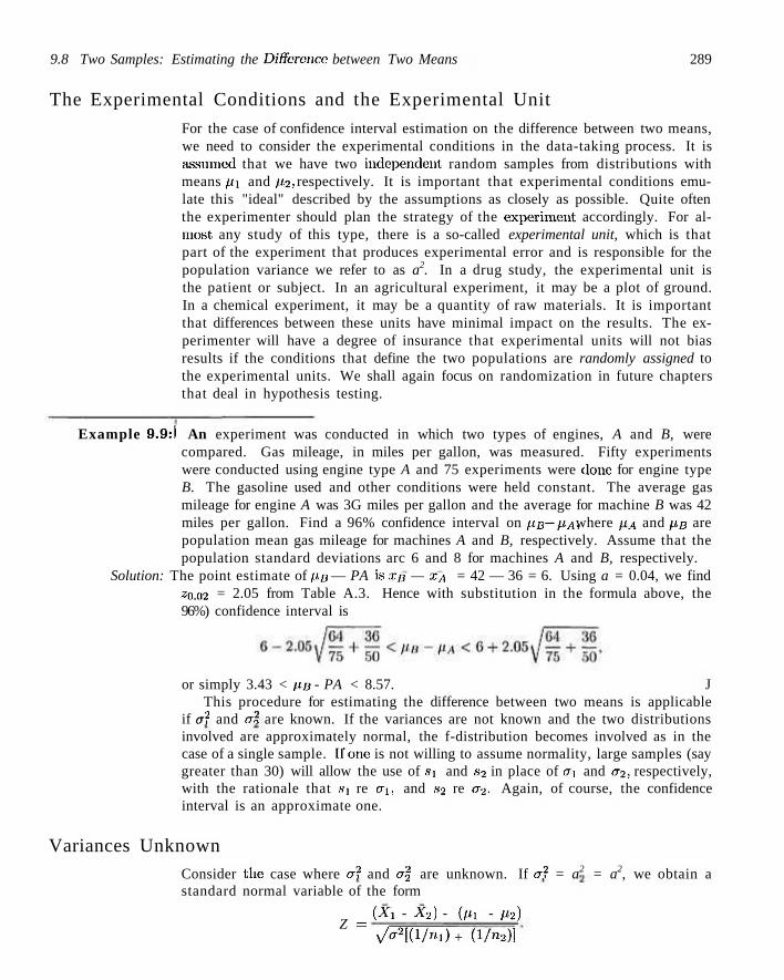
9.8 Two Samples: Estimating the Difference between Two Means 289
The Experimental Conditions and the Experimental Unit
For the case of confidence interval estimation on the difference between two means, we need to consider the experimental conditions in the data-taking process. It is assumed that we have two independent random samples from distributions with means pi and p2, respectively. It is important that experimental conditions emulate this "ideal" described by the assumptions as closely as possible. Quite often the experimenter should plan the strategy of the experiment accordingly. For almost any study of this type, there is a so-called experimental unit, which is that part of the experiment that produces experimental error and is responsible for the population variance we refer to as a2. In a drug study, the experimental unit is the patient or subject. In an agricultural experiment, it may be a plot of ground. In a chemical experiment, it may be a quantity of raw materials. It is important that differences between these units have minimal impact on the results. The experimenter will have a degree of insurance that experimental units will not bias results if the conditions that define the two populations are randomly assigned to the experimental units. We shall again focus on randomization in future chapters that deal in hypothesis testing.
Example 9.9:1 An experiment was conducted in which two types of engines, A and B, were compared. Gas mileage, in miles per gallon, was measured. Fifty experiments were conducted using engine type A and 75 experiments were done for engine type B. The gasoline used and other conditions were held constant. The average gas mileage for engine A was 3G miles per gallon and the average for machine B was 42 miles per gallon. Find a 96% confidence interval on pB ~PA, where PA and ps are population mean gas mileage for machines A and B, respectively. Assume that the population standard deviations arc 6 and 8 for machines A and B, respectively.
Solution: The point estimate of PB — PA is XB — %A = 42 — 36 = 6. Using a = 0.04, we find zo.m = 2.05 from Table A.3. Hence with substitution in the formula above, the 96%) confidence interval is
or simply 3.43 < PB - PA < 8.57. J This procedure for estimating the difference between two means is applicable
if a2 and a2 are known. If the variances are not known and the two distributions involved are approximately normal, the f-distribution becomes involved as in the case of a single sample. Hone is not willing to assume normality, large samples (say greater than 30) will allow the use of S\ and s2 in place of ai and a2, respectively, with the rationale that si re CTI, and ,s2 re a2. Again, of course, the confidence interval is an approximate one.
Variances Unknown
Consider the case where a2 and <r| are unknown. If a2 = a2 = a2, we obtain a standard normal variable of the form
{Xi - X2) - (px - p2) Z =
v/ff2[(l/ni) + ( l /n2)]
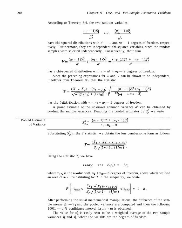
290 Chapter 9 One- and Two-Sample Estimation Problems
According to Theorem 8.4, the two random variables
'"' -,"S? a„d OozM oz a2-
have chi-squared distributions with n\ — 1 and n2 — 1 degrees of freedom, respectively. Furthermore, they are independent chi-squared variables, since the random samples were selected independently. Consequently, their sum
y = (m - 1)5? | (n2 - 1)522 = (n, - 1)5? + (n2 - 1)52
2
a2 a2 a2
has a chi-squared distribution with v = n\ + n2 — 2 degrees of freedom. Since the preceding expressions for Z and V can be shown to be independent,
it follows from Theorem 8.5 that the statistic
(Xi - X2) ~ jpi - P2) , {ni-l)S$ + (;n2-\)S2
v/<72[(l/ni) + (l/n2)] ' V ff2(»i + "2 " 2)
has the ^-distribution with v = ni + n2 — 2 degrees of freedom. A point estimate of the unknown common variance a2 can be obtained by
pooling the sample variances. Denoting the pooled estimator by S2, we write
Pooled Estimate 2 _ (m - 1)5? + (n2 - 1 )5 | of Variance br ~ n i + n 2 _ 2 '
Substituting S2 in the T statistic, we obtain the less cumbersome form as follows:
T ^ (Xx - X2) - (pi - p2)
S p v W m ) + (l/«2) '
Using the statistic T, we have
Pi-ta/2 <T< ta/2) = l-a,
where ta/2 is the t-value with nx + n2 — 2 degrees of freedom, above which we find an area of a /2 . Substituting for T in the inequality, we write
, . JXx ~ x2) -jpi - P2) , .
SPy/(l/ni) + (l/n2) = l - a .
After performing the usual mathematical manipulations, the difference of the sample means $i — x2 and the pooled variance are computed and then the following 100(1 — a)% confidence interval for px - p2 is obtained.
The value for s2 is easily seen to be a weighted average of the two sample variances s2 and s2, where the weights are the degrees of freedom.
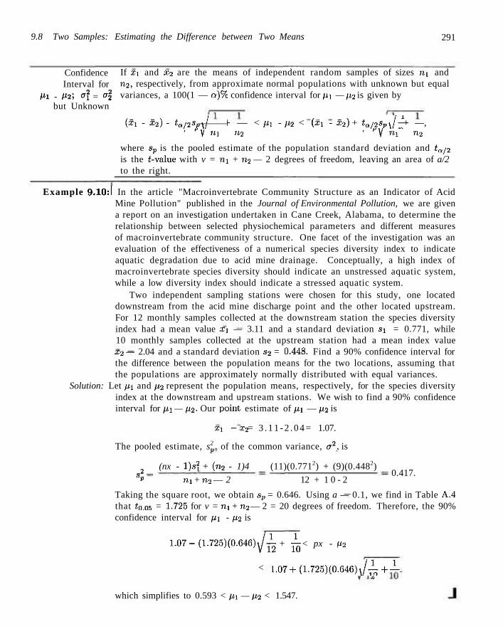
9.8 Two Samples: Estimating the Difference between Two Means 291
Confidence Interval for
Pi - P25 o\ = al but Unknown
If xi and x2 are the means of independent random samples of sizes rti and n2, respectively, from approximate normal populations with unknown but equal variances, a 100(1 — Q ) % confidence interval for pi — p2 is given by
(xx - x2) - tQ/2spJ h — < pi - p2 < (xx - x2) + ta/2SpJ— + —, ' ¥ V 'M n2 ' y V «-i n2
where sp is the pooled estimate of the population standard deviation and ta/2
is the f-value with v = nx + n2 — 2 degrees of freedom, leaving an area of a/2 to the right.
Example 9.10:1 In the article "Macroinvertebrate Community Structure as an Indicator of Acid Mine Pollution" published in the Journal of Environmental Pollution, we are given a report on an investigation undertaken in Cane Creek, Alabama, to determine the relationship between selected physiochemical parameters and different measures of macroinvertebrate community structure. One facet of the investigation was an evaluation of the effectiveness of a numerical species diversity index to indicate aquatic degradation due to acid mine drainage. Conceptually, a high index of macroinvertebrate species diversity should indicate an unstressed aquatic system, while a low diversity index should indicate a stressed aquatic system.
Two independent sampling stations were chosen for this study, one located downstream from the acid mine discharge point and the other located upstream. For 12 monthly samples collected at the downstream station the species diversity index had a mean value xi — 3.11 and a standard deviation sx = 0.771, while 10 monthly samples collected at the upstream station had a mean index value x2 — 2.04 and a standard deviation s2 = 0.448. Find a 90% confidence interval for the difference between the population means for the two locations, assuming that the populations are approximately normally distributed with equal variances.
Solution: Let p\ and p2 represent the population means, respectively, for the species diversity index at the downstream and upstream stations. We wish to find a 90% confidence interval for p\ — p2. Our point, estimate of pi — p2 is
xx -x2 = 3 . 1 1 - 2 . 0 4 = 1.07.
The pooled estimate, s2 of the common variance, a2, is
(nx - l ) s 2 + (n2 - 1)4 (11)(0.7712) + (9)(0.4482) 4 = ni + n2 — 2 12 + 1 0 - 2
0.417.
Taking the square root, we obtain sp = 0.646. Using a — 0.1, we find in Table A.4 that fo.os = 1-725 for v = ni + n2 — 2 = 20 degrees of freedom. Therefore, the 90% confidence interval for p.j - p2 is
1 . 0 7 - ( 1 . 7 2 5 ) ( 0 . 6 4 6 ) ^ + ^ < px - p2
< 1,07+(1.725K0.(M(S)\/-L + -L
which simplifies to 0.593 < p\ — p2 < 1.547.
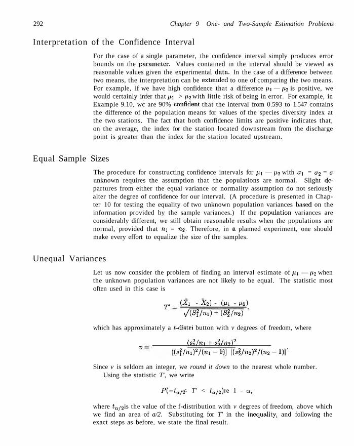
292 Chapter 9 One- and Two-Sample Estimation Problems
Interpretation of the Confidence Interval
For the case of a single parameter, the confidence interval simply produces error bounds on the parameter. Values contained in the interval should be viewed as reasonable values given the experimental data. In the case of a difference between two means, the interpretation can be extended to one of comparing the two means. For example, if we have high confidence that a difference p\ — p2 is positive, we would certainly infer that px > p2 with little risk of being in error. For example, in Example 9.10, wc are 90% confident that the interval from 0.593 to 1.547 contains the difference of the population means for values of the species diversity index at the two stations. The fact that both confidence limits are positive indicates that, on the average, the index for the station located downstream from the discharge point is greater than the index for the station located upstream.
Equal Sample Sizes
The procedure for constructing confidence intervals for pi — p2 with CTJ = o2 = a unknown requires the assumption that the populations are normal. Slight departures from either the equal variance or normality assumption do not seriously alter the degree of confidence for our interval. (A procedure is presented in Chapter 10 for testing the equality of two unknown population variances based on the information provided by the sample variances.) If the population variances are considerably different, we still obtain reasonable results when the populations are normal, provided that n\ = n2. Therefore, in a planned experiment, one should make every effort to equalize the size of the samples.
Unequal Variances
Let us now consider the problem of finding an interval estimate of pi — p2 when the unknown population variances are not likely to be equal. The statistic most often used in this case is
T, _ JXx - X2) - (pi - p2)
x/(5?/n1) + (522/n2) '
which has approximately a £-distri button with v degrees of freedom, where
is2i/nx+sl/n2)2
" lisynx)2/{nx-l)} + [(s2/n2)2/(n2-l)Y
Since v is seldom an integer, we round it down to the nearest whole number. Using the statistic T', we write
P(-tQ/2 < T' < ta/2) re 1 - a,
where taj2 is the value of the f-distribution with v degrees of freedom, above which we find an area of a/2. Substituting for T' in the inequality, and following the exact steps as before, we state the final result.
9.8 Two Samples: Estimating the Difference between Two Means 293
Confidence If x\ and s2, and x2 and s2 are the means and variances of independent random Interval for samples of sizes m and n2, respectively, from approximate normal populations
Pi — P2\ <r2 ¥" °~2 w l th unknown and unequal variances, an approximate 100(1 — o)% confidence and Unknown interval for pi — p2, is given by
(ail -x2) - f Q / 2 \ / — + — < Pi - p2 < {xi -x2) + tQ/2\ — + -2-,
where tQ/2 is the f-value with
(jf/ni +s\/n2)2
l(s2/nx)2/(ni - 1)] + [(s2/n2f/(n2 - 1)]
degrees of freedom, leaving an area a /2 to the right.
Note that the value v above involves random variables and thus it represents an estimate of the degrees of freedom, In applications this estimate will not be a whole number, and thus the analyst must round down to the nearest integer to achieve desired confidence.
Before we illustrate the confidence interval above with an example, we should point out that all the confidence intervals on pi — p2 are of the same general form as those on a single mean; namely, they can be written
point estimate ± ta/2 sTe.(point estimate)
or
point estimate ± za/2 s.e.(point estimate).
For example, in the case where &i = er2 = er, the estimated standard error of Si — x2 is Spy/l/nx + l /n 2 . For the case where a2 ^ o\.
s.e.(.Ti - x2) = -*• + -*•. ni n2
Example 9.11:1 A study was conducted by the Department of Zoology at the Virginia Polytechnic Institute and State University to estimate the difference in the amount of the chemical orthophosphorus measured at two different stations on the James River. Or-thophosphorus is measured in milligrams per liter. Fifteen samples were collected from station 1 and 12 samples were obtained from station 2. The 15 samples from station 1 had an average orthophosphorus content of 3.84 milligrams per liter and a standard deviation of 3.07 milligrams per liter, while the 12 samples from station 2 had an average content of 1.49 milligrams per liter and a standard deviation of 0.80 milligram per liter. Find a 95% confidence interval for the difference in the true average orthophosphorus contents at these two stations, assuming that the observations came from normal populations with different variances.
Solution: For station 1 we have xi = 3.84, s\ = 3.07, and ni = 15. For station 2, 5:2 = 1.49, s2 = 0.80, and n2 = 12. We wish to find a 95% confidence interval for pj — p2.
294 Chapter 9 One- and Two-Sample Estimation Problems
Since the population variances are assumed to be unequal, we can only find an approximate 95% confidence interval based on the ("-distribution with v degrees of freedom, where
(3.072/15 + 0.802/12)2 _ i r o - i r 1 [(3.072/15)2/14] + [(0.802/12)2/H] ~
Our point estimate of p\ - p2 is
xx -x2 = 3.84 - 1 . 4 9 = 2.35.
Using a = 0.05, we find in Table A.4 that £0.025 = 2.120 for v = 16 degrees of freedom. Therefore, the 95% confidence interval for pi — p2 is
3.072 0.802 „ „ /3.072 0.802
2.35 - 2.120^ - ^ - + -r^-<px-p2< 2.35 + 2.120^ " J g - + ,,,
which simplifies to 0.60 < px — p2 < 4.10. Hence we are 95% confident that the interval from 0.60 to 4.10 milligrams per liter contains the difference of the true average orthophosphorus contents for these two locations. J
9.9 Paired Observations
At this point we shall consider estimation procedures for the difference of two means when the samples are not independent and the variances of the two populations are not necessarily equal. The situation considered here deals with a very special experimental situation, namely that of paired observations. Unlike the situation described earlier, the conditions of the two populations are not assigned randomly to experimental units. Rather, each homogeneous experimental unit receives both population conditions; as a result, each experimental unit has a pair of observations, one for each population. For example, if we run a test on a new diet using 15 individuals, the weight before and after going on the diet form the information for our two samples. These two populations are '"before" and "after" and the experimental unit is the individual. Obviously, the observations in a pair have something in common. To determine if the diet is effective, we consider the differences dx,d2,... ,dn in the paired observations. These differences are the values of a random sample Di,D2,... ,Dn from a population of differences that we shall assume to be normally distributed with mean pD = pi — p2 and variance a2
D. We estimate a2,, by s2
d, the variance of the differences that constitute our sample. The point estimator of pD is given by D.
When Should Pairing Be Done?
Pairing observations in an experiment is a strategy that can be employed in many fields of application. The reader will be exposed to this concept in material related to hypothesis testing in Chapter 10 and experimental design issues in Chapters 13 and 15. By selecting experimental units that are relatively homogeneous (within the units) and allowing each unit to experience both population conditions, the
9.9 Paired Observations 295
effective "experimental error variance" (in this case a2D) is reduced.The reader
may visualize that the ith pair consists of the measurement
Di = Xu — X2i.
Since the two observations are taken on the sample experimental unit, they are not independent and, in fact,
Var(Di) = Var(Xu - X2i) =o\ + a\- 2Cov(Xu,X2i).
Now, intuitively, it is expected that er2 should be reduced because of the similarity in nature of the "errors" of the two observations within an experimental unit, and this comes through in the expression above. One certainly expects that if the unit is homogeneous, the covariance is positive. As a result, the gain in quality of the confidence interval over that of not pairing will be greatest when there is homogeneity within units and large differences as one goes from unit to unit. One should keep in mind that the performance of the confidence interval will depend on the standard error of D, which is, of course, oD/\/n, where n is the number of pairs. As we indicated earlier, the intent of pairing is to reduce aD.
Tradeoff between Reducing Variance and Losing Degrees of Freedom
In comparing the paired confidence interval situation against that of the unpaired, it is apparent that there is a "tradeoff" involved. Although pairing should indeed reduce variance and hence reduce the standard error of the point estimate, the degrees of freedom are reduced by reducing the problem to a one-sample problem. As a result, the taj2 point attached to the standard error is adjusted accordingly. Thus pairing may be counterproductive. This would certainly be the case if one experiences only a modest reduction in variance (through er2) by pairing.
Another illustration of pairing might involve the choice of n pairs of subjects with each pair having a similar characteristic, such as IQ, age, breed, and so on; then for each pair one member is selected at random to yield a value of X\, leaving the other member to provide the value of X2. In this case Xx and X2 might represent the grades obtained by two individuals of equal IQ when one of the individuals is assigned at random to a class using the conventional lecture approach while the other individual is assigned to a class using programmed materials.
A 100(1 — Q ) % confidence interval for pD can be established by writing
P(-ta/2 <T< ttt/2) = 1 - a,
where T = D~^ and tn/2, as before, is a value of the ^-distribution with n — 1 degrees of freedom.
It is now a routine procedure to replace T by its definition in the inequality above and carry out the mathematical steps that lead to the following 100(1 — Q ) % confidence interval for pi — p2 = pD-
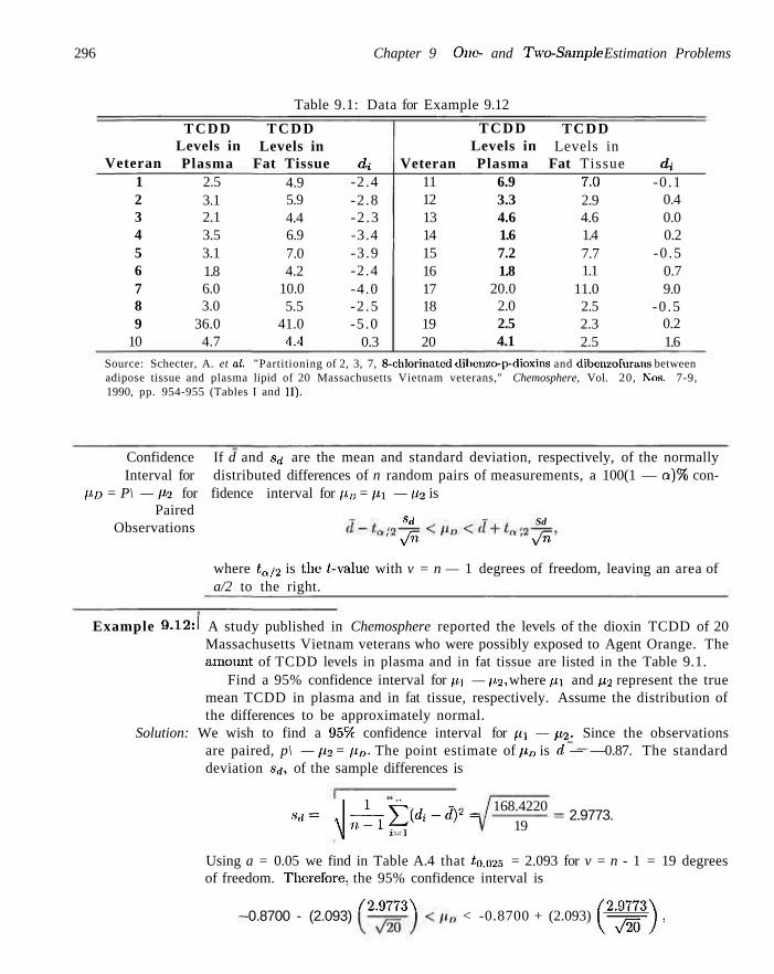
296 Chapter 9 One- and Two-Sample Estimation Problems
Veteran 1 2 3 4 5 6 7 8 9
10
TCDD Levels in Plasma
2.5 3.1 2.1 3.5 3.1 1.8 6.0 3.0
36.0 4.7
Table 9.1: Data for Example 9.12
T C D D Levels in
Fat Tissue 4.9 5.9 4.4 6.9 7.0 4.2
10.0 5.5
41.0 4.4
di -2.4 -2.8 -2 .3 -3.4 -3 .9 -2.4 -4.0 -2 .5 -5.0
0.3
Veteran 11 12 13 14 15 16 17 18 19 20
TCDD Levels in Plasma
6.9 3.3 4.6 1.6 7.2 1.8
20.0 2.0 2.5 4.1
TCDD Levels in
Fat Tissue 7.0 2.9 4.6 1.4 7.7 1.1
11.0 2.5 2.3 2.5
di -0 .1
0.4 0.0 0.2
-0 .5 0.7 9.0
-0 .5 0.2 1.6
Source: Schecter, A. et ai. "Partitioning of 2, 3, 7, 8-chlorinated clibenzo-p-dioxins and dibenzofurans between adipose tissue and plasma lipid of 20 Massachusetts Vietnam veterans," Chemosphere, Vol. 20, Nos. 7-9, 1990, pp. 954-955 (Tables I and II).
Confidence If d and Sd are the mean and standard deviation, respectively, of the normally Interval for distributed differences of n random pairs of measurements, a 100(1 — Q ) % con-
po = P\ — P2 for fidence interval for pD = px — p2 is Paired
Observations Sd Sd
' \/n ' -y/n
where ta/2 is the ('-value with v = n — 1 degrees of freedom, leaving an area of a/2 to the right.
Example 9.12:1 A study published in Chemosphere reported the levels of the dioxin TCDD of 20 Massachusetts Vietnam veterans who were possibly exposed to Agent Orange. The amount of TCDD levels in plasma and in fat tissue are listed in the Table 9.1.
Find a 95% confidence interval for pi — p2, where pi and p2 represent the true mean TCDD in plasma and in fat tissue, respectively. Assume the distribution of the differences to be approximately normal.
Solution: We wish to find a 95% confidence interval for pi — p2. Since the observations are paired, p\ — p2 = pD. The point estimate of pD is d — —0.87. The standard deviation Srf, of the sample differences is
— ^ g c * - - " > • -168.4220
19 2.9773.
Using a = 0.05 we find in Table A.4 that £0.025 = 2.093 for v = n - 1 = 19 degrees of freedom. Therefore, the 95% confidence interval is
-0.8700 - (2.093) /2.9773X
< -0.8700 + (2.093) /2 .9773\
I v ^ O / '
Exercises 297
Exercises
or .simply —2.2634 < //.,, < 0.5234. from which we can conclude that there- is no
significant, difference between the mean T C D D level in plasma and the mean T C D D
level in fat. tissue. J
9.35 A random sample of size m = 25 taken from a normal population with a standard deviation <TI = 5 has a mean $x = 80. A second random sample of size 7)2 = 36, taken from a different normal population with a standard deviation a2 = 3, has a mean x2 = 75. Find a 94% confidence interval for p\ — /i2.
9.36 Two kinds of thread are being compared for strength. Fifty pieces of each type of thread are tested under similar conditions. Brand A had an average: tensile strength of 78.3 kilograms with a standard deviation of 5.6 kilograms, while brand B had an average tensile strength of 87.2 kilograms with a standard deviation of 6.3 kilograms. Construct a 95% confidence interval for the difference of the population means.
9.37 A study was conducted to determine if a certain metal treatment has any effect on the amount of metal removed in a pickling operation. A random sample of 100 pieces was immersed in a bath for 24 hours without the treatment, yielding an average of 12.2 millimeters of metal removed and a sample standard deviation of 1.1 millimeters. A second sample of 200 pieces was exposed to the treatment, followed by the 24-hour immersion in the bath, resulting in an average: removal of 9.1 millimeters of metal with a sample standard deviation of 0.9 millimeter. Compute a 98% confidence interval estimate for the difference between the population means. Docs the treatment appear to reduce the mean amount of metal removed?
9.38 In a hatch chemical process, two catalysts arc being compared for their effect on the output of the process reaction. A sample of 12 batches was prepared using catalyst 1 and a sample of 10 batches was obtained using catalyst 2. The 12 batches for which catalyst 1 was used gave an average yield of 85 with a sample standard deviation of 4, and the second sample gave an average of 81 and a sample standard deviation of 5. Find a 90% confidence interval for the difference between the population means, assuming thai, the: populations art: approximately normally distributed with equal variances.
9.39 Students may choose between a 3-semcstcr-hour course in physics without, labs and a 4-semester-liour course with labs. The final written examination is the same for each section. If 12 students in the section with
labs made an average examination grade of 84 with a standard deviation of 4, and 18 students in the section without labs made an average: grade of 77 with a standard deviation of 6, find a 99%. confidence interval for the difference between the average grades for the two courses. Assume the populations to be approximately normally distributed with equal variances.
9.40 Ilia study conducted at (lie Virginia Polytechnic: Institute: and State University on the development of ectomycorrhizal. a symbiotic relationship between the roots of trees and a fungus in which minerals are transferred from the fungus to the trees and sugars from the trees to the fungus, 20 northern red oak seedlings with the fungus Pisolithus tinctortts were grown in a greenhouse. All seedlings were planted in the same type of soil and received the same amount of sunshine and water. Half received no nitrogen at planting time: to serve as a control and the other half ree;eived 368 ppm of nitrogen in the form NaNO:i. The stem weights, recorded in grams, at the end of 140 days were recorded as follows:
No Ni t rogen N i t r o g e n 0.32 0.53 0.28 0.37 0.47 0.43 0.30 0.42 0.38 0.43
0.26 0.43 0.47 0.49 0.52 0.75 0.79 0.86 0.62 0.46
Construct a 95% confidence interval for the difference in the mean stem weights between seedlings that receive no nitrogen and those: that receive 308 ppm of nitrogen. Assume the populations to be normally distributed with equal variances.
9.41 The: following data, recorded in days, represent the length of time to recovery for patients randomly treated with one of two medications to clear up severe bladder infections:
Med ica t i on 1 Medica t ion 2 ni = 14 x'i = 17 ai = 1.5
112 = 16
Xi = 19 4 = 1.8
298 Chapter 9 One- and Two-Sample Estimation Problems
lows:
Find a 99% confidence interval for the difference ft2—pi in the mean recovery time for the two medications, assuming normal populations with equal variances.
9.42 An experiment reported in Popular Science compared fuel economics for two types of similarly equipped diesel mini-trucks. Let us suppose that 12 Volkswagen and 10 Toyota trucks are: used in 90-kilometer per hour steady-spaced tests. If the 12 Volkswagen trucks average 16 kilometers per liter with a standard deviation of 1.0 kilometer per liter and the 10 Toyota trucks average 11 kilometers per liter with a standard deviation of 0.8 kilometer per liter, construct a 90% confidence interval for the difference between the average kilometers per liter of these two mini-trucks. Assume that the distances per liter for each truck model are approximately normally distributed with equal variances.
9.43 A taxi company is trying to decide: whether to purchase brand .4 or brand B tires for its fleet of taxis. To estimate the difference in the two brands, an experiment is conducted using 12 of each brand. The tires are run until they wear out. The results are
Brand .4: xi — 36,300 kilometers, s\ = 5,000 kilometers.
Brand B: x2 = 38,100 kilometers, s2 = 6.100 kilometers.
Compute a 95% confidence interval for /I.A — pa assuming the populations to be approximately normally distributed. You may not assume that the variances are equal.
9.44 Referring to Exercise 9.43, find a 99% confidence interval for pi — p2 if a tire from each company is assigned at random to the rear wheels of 8 taxis and the following distance, in kilometers, recorded:
Taxi Brand A Brand B 1 2 3 4 5 6 7 8
34.400 45.500 36,700 32.000 48,400 32.800 38.100 30,100
36.700 46.800 37.700 31.100 47.800 36,400 38,900 31,500
Assume that the differences of the distances are approximately normally distributed.
9.45 The government awarded grants to the agricultural departments of 9 universities to test the yield capabilities of two new varieties of wheat. Each variety was planted on plots of equal area at each university and the yields, in kilograms per plot, recorded as fol-
University
Variety 1 2 4 8 9 1 38 23 35 41 44 29 37 31 38 2 45 25 31 38 50 33 36 40 43
Find a 95% confidence interval for the mean difference between the yields of the two varieties, assuming the differences of yields to be approximately normally distributed. Explain why pairing is necessary in this problem.
9.46 The following data represent the running times of films produced by two motion-picture companies.
Company Time (minutes) t II
103 97
94 82
no 123
87 92
98 175 88 118
Compute a 90% confidence interval for the difference between the average running times of films produced by the two companies. Assume that the running-time differences are approximately normally distributed with unequal variances.
9.47 From Fortune magazine (March 1997), 10 of the 431 companies studied are listed below. The total returns for the 10 year's prior to 1996 and also for 1996 are listed. Find a 95% confidence interval for the mean change in percent return to investors.
Company Coca-Cola Mirage Resorts Merck Microsoft Johnson & Johnson Intel Pfizer Procter & Gamble Berkshire Hathawav S&P 500
Total Return to Investors
1986-96 29.8% 27.9% 22.1% 44.5% 22.2% 43.8% 21.7% 21.9% 28.3% 11.8%
1996 43.3% 25.4% 24.0% 88.3% 18.1%
131.2% 34.0% 32.1% 6.2%
20.3%
9.48 An automotive company is considering two types of batteries for its automobile. Sample information on the life of the battery is being used. Twenty batteries of type A and twenty batteries of type B are being used. The summary statistics are XA = 32.91, XB = 30.47, SA = 1-57, and SB — 1.74. Assume the data on each battery are normally distributed and assume a A = &B-
(a) Find a 95% confidence interval on PA — PB. (b) Draw some conclusion from (a) that provides some
insight into whether A o r f i should be adopted.
9.10 Single Sample: Estimating a Proportion 299
9.49 Two different brands of latex paint are being-considered for use. Drying time in hours is being measured on specimen samples of the use of the two paints. Fifteen specimens for each were selected and the drying times are as follows:
Pa in t A Pa in t B 3.5 2.7 3.9 4.2 3.6 2.7 3.3 5.2 4.2 2.9 4.4 5.2 4.0 1.1 3.4
4.7 3.D 4.5 5.5 4.0 5.3 4.3 6.0 5.2 3.7 5.5 6.2 5.1 5.4 4.8
Assume the drying time is normally distributed with a A = VB- Find a 95% confidence interval on pn — PA
where PA and /;« are mean drying times.
9.50 Two levels (low and high) of insulin doses are given to two groups of diabetic rats tea check the insulin-binding capacity, yielding the following data:
Low dose:: Hi =8 X\ — 1.98 «i = 0.51 High dose: n2 = 13 £ 2 = 1.30 8a = 0.35
Assume that both variances are equal. Give a 95% confidence interval for the difference of the true average insulin-binding capacity between two samples.
9.10 Single Sample: Estimating a Proportion
A point est imator of the proportion p in a binomial experiment is given by the statistic P = X/n, where X represents the number of successes in n trials. Therefore, the sample proportion p = x/n will be used as the pom! estimate of the parameter /;.
If the unknown proportion p is not expected to be too close to zero or 1. we can establish a confidence interval for p by considering the sampling distr ibution of P. Designating a failure in each binomial trial by the value 0 and a success by the value 1, the number of successes, x, can be interpreted as the sum of n values consisting only of zeros and ones, and p is just the sample mean of these it values. Hence, by the central limit theorem, for n sufficiently large, P is approximately normally distributed with mean
pp = E(P) = E X up
= P
and variance
2 2 _ °~x _ "P'l _ PQ
Therefore, we can assert that
P(-za/2 < Z < zn/2) = 1 - a,
Aievc
Z = P-p
s/pq/'
and za/2 is the value of the s tandard normal curve above which we find an area of a/2. Subst i tut ing for Z, we write
( P-P \ P -Za/2 < —j== < za/2 = 1 - a.
V vWn /
300 Chapter 9 One- and Two-Sample Estimation Problems
Multiplying each term of the inequality by y/pq/n, and then subtracting P and multiplying by —1, we obtain
?<»<'+v.,/5i--* It is difficult to manipulate the inequalities so as to obtain a random interval whose end points are independent of p, the unknown parameter. When n is large, very little error is introduced by substituting the point estimate p = x/n for the p under the radical sign. Then we can write
P\P-zal2^<p<P + za/2^jS\^l-a.
For our particular random sample of size n, the sample proportion p = x/n is computed, and the following approximate 100(1 — a)% confidence interval for p is obtained.
Large-Sample If p is the proportion of successes in a random sample of size n, and q = 1 — p, Confidence an approximate 100(1 — a)% confidence interval for the binomial parameter p
Interval for p is given by
P9 ^ ^ . , Iffl — <p<p + za/2\ —, n ' V n
where za/2 is the g-yalue leaving an area of o/2 to the right.
When n is small and the unknown proportion p is believed to be close to 0 or to 1, the confidence-interval procedure established here is unreliable and, therefore, should not. be used. To be on the safe side, one should require both np or nq to be greater than or equal to 5. The method for finding a confidence interval for the binomial parameter p is also applicable when the binomial distribution is being used to approximate the hypergeometric distribution, that is, when n is small relative to N, as illustrated by Example 9.13.
Example 9.13:1 In a random sample of n = 500 families owning television sets in the city of Hamilton, Canada, it is found that x = 340 subscribed to HBO. Find a 95% confidence interval for the actual proportion of families in this city who subscribe to HBO.
Solution: The point estimate of p is p = 340/500 = 0.68. Using Table A.3, we find that zo.025 = 1-96. Therefore, the 95% confidence interval for p is
which simplifies to 0.64 < p < 0.72. J If p is the center value of a 100(1 - a)% confidence interval, then p estimates p
without error. Most of the time, however, /; will not be exactly equal to p and the point estimate is in error. The size of this error will be the positive difference that
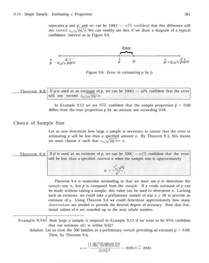
9.10 Single Sample: Estimating a Proportion 301
separates p and p, and wc can be 100(1 — o)% confident that this difference will not exceed zai2 y/pq/n. We can readily see this if we draw a diagram of a typical confidence: interval as in Figure 9.6.
Error
A /A A
P -ZaizVP qtn A
P P+z, •a/2Vp Q'n
Figure 9.6: Error in estimating p by p.
Theorem 9.3: If -p is used as an estimate of p, we can be 100(1 — a)% confident that the error will not exceed za/2y/pq/n.
In Example 9.13 we are 95%. confident that the sample proportion p = 0.68 differs from the true proportion p by an amount not exceeding 0.04.
Choice of Sample Size
Let us now determine how large a sample is necessary to ensure that the error in estimating p will be less than a specified amount e. By Theorem 9.3, this means we must choose n such that z„/2 y/pq/n = e.
Theorem 9.4: If p is will be
used as an less than a
estimate of p, we specified amount
n =
can be 100( e when the s
*l/m e2 '
l—,ot)% confident that the error ample size is approximately
Theorem 9.4 is somewhat misleading in that we must use p to determine the sample size n, but p is computed from the sample. If a crude estimate of p can be made without taking a sample, this value can be used to determine n. Lacking such an estimate, we could take a preliminary sample of size n > 30 to provide an estimate of p. Using Theorem 9.4 we could determine approximately how many observations are needed to provide the desired degree of accuracy. Note that fractional values of n arc rounded up to the next whole number.
Example 9.14:1 How large a sample is required in Example 9.13 if we want to be 95% confident that our estimate of/; is within 0.02?
Solution: Let us treat the 500 families as a preliminary sample providing an estimate p = 0.68. Then, by Theorem 9.4,
(1.96)2 (0.68) (0.32)
"'= — ^ a o 2 ) ^ — = 2 0 8 9 - 8 ~ 2 0 9 ° -
302 Chapter 9 One- and Two-Sample Estimation Problems
Therefore, if we base our estimate of p on a random sample of size 2090, wc can be 95% confident that our sample proportion will not differ from the true proportion by more than 0.02. J
Occasionally, it will be impractical to obtain an estimate of p to be used for determining the sample size for a specified degree of confidence. If this happens, an upper bound for n is established by noting that pq = p(l — /5), which must be at most equal to 1/4, since p must lie between 0 and 1. This fact may be verified by completing the square. Hence
P(l - P) = - ( / r - P ) = ~ ~ (P* ~P+ ~) = - ~ l P ~ -
which is always less than 1/4 except when p = 1/2 and then pq = 1/4. Therefore, if we substitute p = 1/2 into the formula for n in Theorem 9.4, when, in fact, p actually differs from 1/2, then n will turn out to be larger than necessary for the specified degree of confidence and as a result our degree of confidence will increase.
Theorem 9.5: If p is used as an estimate of p, we can be at least 100(1 - o)% confident that the error will not exceed a specified amount e when the sample size is
~2 Za/2
" = 4 ^ -
Example 9.15:1 How large a sample is required in Example 9.13 if we want to be at least 95% confident that our estimate of p is within 0.02?
Solution: Unlike Example 9.14. wc: shall now assume that no preliminary sample has been taken to provide an estimate of p. Consequently, we can be at least 95% confident that our sample proportion will not differ from the true proportion by more than 0.02 if we choose a sample of size
- - <L 9 6»2 = 2 4 0 , . (.1)(0.(I2)2
Comparing the results of Examples 9.14 and 9.15, information concerning p. provided by a preliminary sample, or perhaps from past experience, enables us to choose a smaller sample while maintaining our required degree of accuracy. _l
9.11 Two Samples: Estimating the Difference between Two Proportions
Consider the problem where we wish to estimate the difference between two binomial parameters p\ and p2. For example, we might let p\ be the proportion of smokers with lung cancer and p2 the proportion of nonsmokers with lung cancer. Our problem, then, is to estimate the difference between these two proportions. First, we select independent random samples of size nx and 712 from the two binomial populations with means niPi and n2p2 and variances nxPx°x a n d n2p2q2,
9.11 Two Samples: Estimating the Difference between Two Proportions 303
respectively, then determine the numbers x\ and x2 of people in each sample with lung cancer, and form the proportions px — xx/n, and p2 = x2/n. A point estimator of the difference between the two proportions, pi — p2, is given by the statistic Pi — P2. Therefore, the difference of the sample proportions, px — p2, will be used as the point estimate of pi — p2.
A confidence interval for pi — p2 can be established by considering the sampling distribution of Pi — P2. From Section 9.10 we know that A and P2 are each approximately normally distributed, with means pi and p2 and variances pxqx/n-x and p2q2/n2, respectively. By choosing independent samples from the two populations, the variables Pi and P2 will be independent, and then by the reproductive property of the normal distribution established in Theorem 7.11, we conclude that Pi — P2 is approximately normally distributed with mean
P p j - p , = P i - P 2
and variance
2 _ Plgl P2(?2 A - A ni n2
Therefore, we can assert that
P( -2a /2 < Z < Za/2) = 1 - Q',
where
z_ ( A - P 2 ) - ( P 1 - P 2 )
\ /Pi9i /ni +p2q2/n2 '
and zay2 is a value of the standard normal curve above wdiich we find an area of a /2 . Substituting for Z, we write
„ ( P i - P 2 ) - ( p i - p 2 ) „ -Za/2 < / , , , - < Zct/2
y/PiQx/nx +p2q2/n2 = 1 - a.
After performing the usual mathematical manipulations, we replace pi, p2, Qi, ande72 under the radical sign by their estimates pi = xi/ni,p2 = x2/n2, qx = 1—pi, and 92 = 1 — p2, provided that n-ipi, nitji, U2p2. and r).2e72, are all greater than or equal to 5, and the following approximate 100(1 — Q ) % confidence interval for Pi — P2 is obtained.
Large-Sample If pi and p~2 are the proportions of successes in random samples of size n-i and Confidence n2, respectively, qi = 1 —pi, and 172 = 1 — p2, an approximate 100(1 — Q ) % Interval for confidence interval for the difference of two binomial parameters pi — P2. is
Pi - P2 given by
, - . x Pill . P292 . (pi - p2) - za/2 d 1 < Pi - P2
" nx n2 ^ t- - i , P1^1 , P2(l2
< Pi -P2) + Za/2 \ + ,
' V nx n2
wdiere za/2 is the 3-value leaving an area of a/2 to the right.
304 Chapter 9 One- and Two-Sample Estimation Problems
E x a m p l e 9.16:1 A certain change in a. process for manufacture of component parts is being considered. Samples are taken using both the existing and the: new procedure so as to determine if the new process results in an improvement. If 75 of 1500 items from the existing procedure were found to be defective and 80 of 2000 items from the new procedure were found to be defective, find a, 90%: confidence interval for the t rue difference in the fraction of defectives between the existing and the new process.
Solution: Let p\ and p2 be the true proportions of defectives for the existing and new procedures, respectively. Hence ;3, = 75/1500 = 0.05 and f>2 = 80/2000 = 0.04, and the point estimate of pi — p2 is
px - p2 = 0 . 0 5 - 0 . 0 4 = 0.01.
Using Table A.3, we find Zo.oa = 1.645. Therefore, substi tuting into the formula, with
/(0.05)(0.95) (0.04)(0.96)
V 1500 2000
we: obtain the 90%, confidence interval to be -0 .0017 < p\ -p2 < 0.0217. Since the interval contains the value 0, there is no reason to believe that the new procedure produced a significant decrease in the: proportion of defectives over the existing
method, J Up to this point all confidence intervals presented were of the form
Exercises
point estimate ± K s.e.(point estimate),
where K is a constant (cither t or normal percent point). This is the case when the parameter is a mean, difference between means, proportion, or difference between proportions, due to the symmetry of the /. and Z distributions. However, it does not, extend to variances and ratios of variances that will be discussed in Sections 9.12 and 9.13.
9.51 (a) A random .sample of 200 voters is selected and 114 are found to support, an annexation suit. Find the 96% confidence interval for the fraction of the voting population favoring the suit.
(b) What can we assert with 90% confidence about the possible size of our error if we estimate the fraction of voters favoring the annexation suit to be 0.57?
9.52 A manufacturer of compact disk players uses a set of comprehensive tests to access the electrical function of its product. All compact disk players must pass all tests prior to being sold. A random sample of 500 disk players resulted in 15 failing one or more tests.
Find a 90% confidence intt compact disk players from tests.
tcrval for the proportion of the: population that pass all
9.53 In a random sample of 1000 homes in a certain city, it is found that 228 are heated by oil. Find the 99%, confidence interval for the: proportion of homes in this city that are heated by oil.
9.54 Compute a 98% confidence interval for the proportion of defective items in a process when it is found that a sample of si^e 100 yields 8 defectives.
Exercises 305
9.55 A new rocket-launching system is being considered for deployment of small, short-range rockets. The existing system has p = 0.8 as the probability of a successful launch. A sample of 40 experimental launches is made with the new system and 34 are successful.
(a) Construct a 95% confidence interval for p.
(b) Would you conclude that the new system is better?
9.56 A geneticist is interested in the proportion of African males that have a certain minor blood disorder. In a. random sample of 100 African males, 24 are found to be afflicted.
(a) Compute a 99% confidence interval for the proportion of African males that have this blood disorder.
(b) What can we assert with 99% confidence about the possible size of our error if we estimate the proportion of African males with this blood disorder to be 0.24?
9.57 (a) According to a report in the Roanoke Times & World-News, approximately 2/3 of the 1600 adults polled by telephone said they think the space shuttle program is a good investment for the country. Find a 95% confidence interval for the proportion of American adults who think the space shuttle program is a good investment for the country.
(b) What can we assert with 95% confidence about the possible size of our error if we estimate the proportion of American adults who think the space shuttle program is a good investment to be 2/3?
9.58 In the newspaper article referred to in Exercise 9.57, 32% of the 1600 adults polled said the U.S. space program should emphasize scientific exploration. How large a sample of adults is needed in the poll if one wishes to be 95% confident that the estimated percentage will be within 2% of the true percentage?
9.59 How large a sample is needed in Exercise 9.51 if we wish to be 96% confident that our sample proportion will be within 0.02 of the true fraction of the voting population?
9.60 How large a sample is needed in Exercise 9.53 if wo wish to be 99% confident that our sample proportion will be within 0.05 of the true proportion of homes in this city that are heated by oil?
9 .61 How large a sample is needed in Exercise 9.54 if we wish to be 98% confident that our sample proportion will be within 0.05 of the true proportion defective?
9.62 A study is to be made to estimate the percentage of citizens in a town who favor having their water fluoridated. How large a sample is needed if one wishes
to be at least 95% confident that our estimate is within 1% of the true percentage?
9.63 A conjecture by a faculty member in the microbiology department at Washington University School of Dental Medicine in St. Louis states that a couple of cups of either green or oolong tea each day will provide sufficient fluoride to protect your teeth from decay. How large a sample is needed to estimate the percentage of citizens in a certain town who favor having their water fluoridated if one wishes to be at least 99% confident that the estimate is within 1% of the true percentage?
9.64 A study is to be made to estimate the proportion of residents in a certain city and its suburbs who favor the construction of a nuclear power plant. How large a sample is needed if one wishes to be at least 95% confident that the estimate is within 0.04 of the true proportion of residents in this city and its suburbs that favor the construction of the nuclear power plant?
9.65 A certain geneticist is interested in the proportion of males and females in the population that have a certain minor blood disorder. In a random sample of 1000 males, 250 are found to be afflicted, whereas 275 of 1000 females tested appear to have the disorder. Compute a 95% confidence interval for the difference between the proportion of males and females that have the blood disorder.
9.66 Ten engineering schools in the United States were surveyed. The sample contained 250 electrical engineers, 80 being women; 175 chemical engineers, 40 being women. Compute a 90% confidence interval for the difference between the proportion of women in these two fields of engineering. Is there a significant difference between the two proportions?
9.67 A clinical trial is conducted to determine if a certain type of inoculation has an effect on the incidence of a certain disease. A sample of 1000 rats was kept in a controlled environment for a period of 1 year and 500 of the rats were given the inoculation. Of the group not given the drug, there were 120 incidences of the disease, while 98 of the inoculated group contracted it. If we call pi the probability of incidence of the disease in uninoculated rats and p2 the probability of incidence after receiving the drug, compute a 90% confidence interval for pi — p2.
9.68 In a study. Germination and Emergence of Broccoli, conducted by the Department of Horticulture at Virginia Polytechnic Institute and State University, a researcher found that at 5CC, 10 seeds out of 20 germinated, while at 15CC, 15 out of 20 seeds germinated. Compute a 95% confidence interval for the difference
30G Chapter 9 One- and Two-Sample Estimation Problems
between the proportion of germination at the two different temperatures and decide if there is a significant difference.
9.G9 A survey of 1000 students concluded that 274 students chose a professional baseball team. .4. as his or her favorite team. In 1991, the same survey was conducted involving 760 students. It concluded that 240 eif them also chose team A as their favorite. Compute a 95% confidence interval for the difference between the proportion oT students favoring team .4 between the two surveys. Is there a significant difference?
9.70 According to <7S'.4 Today (March 17. 1997), women made up 33.7% of the editorial staff at. local TV stations in 1990 and 36.2% in 1994. Assume 20 new employees were: hired as editorial staff. (a) Estimate the number that would have been women
in each year, respectively. (b) Compute a 95% confidence interval to see if there is
evidence that the proportion of women hired as editorial stall' in 1994 was higher than the proportion hired in 1990.
9.12 Single Sample: Estimating the Variance
If a sample size of n is drawn from a normal population with variance a2, and the sample variance s2 is computed, we obtain a value of the statistic S2. This computed sample variance will be used as a point estimate of a2. Hence the statistic S2 is called an estimator of a2.
An interval estimate of a2 can be established by using the statistic
X •2 (n-l)S2
According to Theorem 8.4, the statistic A'2 has a chi-squared distribution with n — 1 degrees of freedom when samples arc chosen from a normal population. We may write (see Figure 9 7 )
P ( A " - O / 2 < A ' 2 < ^ / 2 ) = 1 - « '
where x\-a/2 a n ^ X2
a/2 a r e values of the chi-squared distribution with n— 1 degrees
of freedom, leaving areas of 1 —a/2 and a / 2 , respectively, to the right. Substituting for X2, we write
„ ( » - l ) 5 2 ^ 2
Xl-a/2 " 2 Vv/2 = I - a.
Dividing each term in the inequality by (n — 1 )S 2 , and then inverting each term (thereby changing the sense of the inequalities), we obtain
(n - 1)S2 a (u-l)S2
< a < — x Y 2
Xl-a/I = 1-Q!,
For our particular random sample of size n, the .sample variance s2 is computed, and the following 100(1 — a)% confidence interval for cr2 is obtained.
9.12 Single Sample: Estimating the Variance 307
Figure: 9.7: P( v2 < A'2 < v;2 ) = , _ a .
Confidence If S is the variance of a random sample of size: n from a normal population, a Interval for er2 100(1 — ot)% confidence interval for tr2 is
( n - l ) . s 2 _ , ^ (n-l)s* < a < • — T ; ,
Y 2
Art/2 X I - Q / 2
where: Xa/2 a n d -Y.'i_,> •'•' a r c X -values with v = n — 1 degrees of freedom, leaving
areas of a /2 and 1 — a/2 , respectively, to the right.
An approximate 100(1 — n)% confidence interval for er is obtained by taking the square root of each endpoint of the interval for a2.
Example 9.17:1 The following are the weights, in decagrams, of 10 packages of grass seed distributed by a. certain company: 46.4, 46.1, 45.8, 47.0, 46.1, 45.9, 45.8, 46.9, 45.2, and 46.0. Find a 95% confidence interval for the variance of all such packages of grass seed distributed by this company, assuming a normal population.
Solution: First we find
n£z?-(X» 2
; = 1 i=l
n(n- 1) (10)(21. 273.12)- (4G1.2)2
(10)(9) 0.286.
To obtain a 95%, confidence interval, we choose a = 0.05. Then, using Table A.5 with v = 9 degrees of freedom, we find X0.025 = 19.023 and A'u.975 = 2.700. Therefore, the 95%: confidence interval for a2 is
(9)(0.286) o (9)(0.286) 19.023 "" 2.700 '
or simply 0.135 < a1 < 0.953. J
308
9.13
Chapter 9 One- and Two-Sample Estimation Problems
Two Samples: Estimating the Ratio of Two Variances
A point estimate of the ratio of two population variances o'j/a2 is given by the ratio s\/s\ of the sample variances. Hence the statistic S2/S2 is called an estimator of al/al }
If a\ and a\ are the variances of normal populations, we can establish an interval estimate of a\/a\ by using the statistic
„ °$s2
arSr,
According to Theorem 8.8, the random variable F has an F-distribution with Vi — n\ — I and v2 — vt2 — 1 degrees of freedom. Therefore, we may write (see Figure 9.8)
P{fx-a/iivx,v2) < F < fQ/2(vx,v2)] = 1 - a.
where fx-a/ii^U '<-!2) and ftt/2{i'i'V2) arc the values of the F-distribution with Vx and t'2 degrees of freedom, leaving areas of 1 — ct/2 and a /2 , respectively, to the right. Substituting for F. we write
P a2S2
/ l -«/2( f , l -1 '2) < - | -=J < fa/2ivtiV2) T a2S2 1 - a.
Multiplying each term in the inequality by S2/S2, and then inverting each term (again changing the sense of the inequalities), we obtain
P a2 S2
< - 3 < aS S2 fa/2(vx,V2) ar, S2 / ,_, t/2(vi,v2) = 1 - a.
The results of Theorem 8.7 enable us to replace the quantity fx-a/2ivi>v2) by 1/fa/2(v2,V]). Therefore,
P Si I S2 fa/2{m, v2) a\ St
••> ,.2 al bX J! I \
< zs < -&Lfiin,vx) 1 - a .
For any two independent random samples of size nx and n2 selected from two normal populations, the ratio of the sample variances sj/s2, is computed and the following 100(1 — a)% confidence interval for a2/a2, is obtained.
Confidence If s\ and Sj are the variances of independent samples of size »i and n2, re-Interval for a2/a2 spectively, from normal populations, then a 100(1 — a)% confidence interval for
2 / 2 • 0\/02 IS
< ~k < 4/a/a(«3i»l) i s\ fa/2ivx,V2) ar,
where fa/2{vx,v2) is an /-value with v\ = ii\ — 1 and v2 = n2 — 1 degrees of freedom leaving an area of a /2 to the right, and fa/2iv2> <-'i) is a similar /-value with v2 = i>2 — I arid v\ = nx — 1 degrees of freedom.
9.13 Two Samples: Estimating the Ratio of Two Variances 309
'1 - o H (r,'2
Figure 9.8: P[/i_Q/2(vi,V2) < F < / , / 2 ( " i , r2)] = 1 - a.
As in Section 9.12. an approximate 100(1 — a)% confidence interval for oi/a2 is obtained by taking the square root of each cndpoint of the interval for a2/a2,.
Example 9.18:1 A confidence interval for the difference in the mean orthophosphorus contents, measured in milligrams per liter, at two stations on the James River was constructed in Example 9.1 I on page 293 by assuming the normal population variance to be unequal. Justify this assumption by constructing a 98% confidence interval for a\/a2 and for a\/a2, where a\ and a2 are the variances of the populations of orthophosphorus contents at station I and station 2, respectively,
Solution: Prom Example 9.11, wc: have nx = 15, n2 = 12, s\ = 3.07, and s2 = 0.80. For a 98% confidence interval, a = 0.02. Interpolating in Table A.6, we find /o.oi (14, U) fts 4.30 and /o.oi(ll, 14) w 3.87. Therefore, the 98%. confidence interval for a\/a\ is
3.(J7-
0.802 1
430 < <S(3.87),
0.802^ "
which simplifies to 3.425 < ^i < 56.991. Taking square roots of the confidence limits, we: find that a 98%; confidence interval for ai/a2 is
1.851 < — < 7.549. 0*2
Since this interval does not allow for the- possibility of Oi/a2 being equal to 1, we
were correct in assuming that ai ^ a-., or a2 •£ a\ in Example 9.11. J
310
Exercises
Chapter 9 One- and Two-Sample Estimation Problems
9.71 A manufacturer of car batteries claims that his batteries will last, on average, 3 years with a variance of 1 year. If 5 of these batteries have lifetimes of 1.9, 2.4, 3.0, 3.5, and 4.2 years, construct a 95% confidence interval for a2 and decide if the manufacturer's claim that a" = 1 is valid. Assume the population of battery lives to be approximately normally distributed.
9.72 A random sample of 20 students obtained a mean of x = 72 and a variance of s~ = 16 on a college placement, test in mathematics. Assuming the scores to be normally distributed, construct a 98% confidence interval for o~.
9.73 Construct, a 95% confidence interval for a in Exercise 9.12 on page 286.
9.74 Construct a 99% confidence interval for er in Exercise 9.13 on page 286.
9.75 Construct a 99%. confidence intcrvi crcise 9.14 on page 286.
for a in Ex-
9.76 Construct: a 90%. confidence interval for ex in Exercise 9.15 on page 286.
9.77 Construct a 98% confidence interval for oi/aj in Exercise 9.42 on page 298, where <7i and o2 are, respectively, the standard deviations for the distances obtained per liter of fuel by the Volkswagen and Toyota mini-trucks.
9.78 Construct a 90% confidence interval for a\ja\ in Exercise 9.43 on page 298. Were we justified in assuming that a\ ^ a2 when we constructed our confidence interval for /ii — p2?
9.79 Construct a 90% confidence interval for aj/rr]t
in Exercise 9.46 on page 298. Should we have assumed ai = of/ in constructing our confidence interval for / ' ; - / ' ; ;?
9.80 Construct a 95% confidence interval for ex^/er^ in Exercise 9.49 on page 298. Should the equal-variance assumption be used?
9.14 Maximum Likelihood Estimation (Optional)
Often the estimators of parameters have been those that, appeal to intuition. The estimator X certainly seems reasonable as an est imator of a population mean p. The virtue of S2 as an estimator of a2 is underscored through the discussion of unbiasedness in Section 9.3. The estimator for a binomial parameter p is merely a sample proportion, which of course is an average and appeals to common sense. But there are many situations in which it is not at all obvious what the proper estimator should be. As a result, there is much to be learned by the student in statistics concerning different philosophies tha t produce different methods of estimation. In this section we deal with the m e t h o d of m a x i m u m l ike l ihood .
Maximum likelihood estimation represents one of the most, important approaches to estimation in all of statistical inference. We will not give a thorough development of the method. Rather, we will a t t empt to communicate the philosophy of maximum likelihood and illustrate with examples tha t relate to other estimation problems discussed in this chapter.
The Likelihood Function
As the name implies, the method of maximum likelihood is that for which the likelihood function is maximized. The likelihood function is best illustrated through the use of an example with a discrete distribution and a single parameter. Denote by Xi, X2,..., X„ the independent, random variables taken from a discrete probability distribution represented by f(x, 9), where 9 is a single parameter of the:
9.14 Maximum Likelihood Estimation (Optional) 311
distribution. Now
L(.r,i, x2,..., x„; 8) = /(:e.'i, :i:2, . . . . x„; (?)
= f{xx,8)f(x2,8)--.f{xn,8)
is the joint distribution of the random variables. This is often referred to as the likelihood function. Note that the variable of the likelihood function is 9, not the x. Denote by xi, x2,.... xn the observed values in a sample. In the case of a discrete random variable the interpretation is very clear. The quantity L(xx, x2,..., xn; 9), the likelihood, of the sample, is the following joint probability:
P(Xi=xi.X2=x2....,X„=x„\0).
which is the probability of obtaining the sample values x\.x2,... ,xn. For the discrete case the maximum likelihood estimator is one that results in a maximum value for this joint probability or maximizes the likelihood of the sample.
Consider a fictitious example where three items from an assembly line are inspected. The items are ruled either defective or nondefective and thus the Bernoulli process applies. Testing the three items results in two nondefective items followed by a. defective item. It is of interest to estimate p, the proportion nondefective in the process. The likelihood of the sample for this illustration is given by
.3 p.p.q = p q V
where q = 1 — p. Maximum likelihood estimation would give an estimate of p for which the: likelihood is maximized. It is clear that if we differentiate the likelihood with respect to p, set the derivative to zero, and solve, wc: obtain the value
9
? 3 = 3 -
Now, of course, in this situation p = 2/3 is the sample: proportion defective and is thus a reasonable estimator of the probability of a defective. The reader slienikl attempt to understand that the philosophy of maximum likelihood estimation evolves from the notion that the reasonable estimator of a parameter based on sample information is that parameter value that produces tin largest probability of obtaining the sample. This is, indeed, the interpretation for the discrete case, since the likelihood is the probability of jointly observing the values in the sample.
Xow. while the interpretation of the likelihood function as a joint, probability is confined to the discrete case, the notion of maximum likelihood extends to the estimation of parameters of a continuous distribution. We now present a formal definition of maximum likelihood estimation.
Definition 9.3: Given independent observations x.i,x2,... ,xu from a probability density function (continuous case) or probability mass function (discrete case) f(x,\0), the maximum likelihood estimator 8, is that which maximizes the likelihood function
L(xx,x2,...,xn;8) = f(xx,8)fix2,8)---f(xnt8).
Quite often it, is convenient to work with the natural log of the likelihood function in finding the maximum of the likelihood function. Consider the following example dealing with the parameter p of a Poisson distribution.
312 Chapter 9 One-and Two-Sample Estimation Problems
Example 9.19:1 Consider a Poisson distribution with probability mass function
f{x\p)=E—£- a;-0,1,2,
Suppose that a random sample x\,x2,...,x„ is taken from the distribution. What is the maximum likelihood estimate of pi
Solution: The likelihood function is
Lixx ,x2 x„; p) = YI fixi\u) = -=5 j -—j ,:=i ll»=i-1'-
Now consider
n
\nL(x,i,x2,...,xn;p) - —np + ^ Xj hi p - l n j ^ a : , ! i=[
n
i.= I i-1
d In L(xx,x2,...,xn;p)
di1 r-f P-» = i
Solving for p, the maximum likelihood estimator involves setting the derivative to zero and solving for the parameter. Thus
n
p= > — = X.
f-f n i = i
Since p is the mean of the Poisson distribution (Chapter 5), the sample average
would certainly seem like a reasonable estimator. J The following example shows the use of the method of maximum likelihood for
finding estimates of two parameters. We simply find the values of the parameters that maximize (jointly) the likelihood function.
Example 9.20:1 Consider a random sample xx,x2,... ,xn from a normal distribution N(p,a). Find the maximum likelihood estimators for p and er2.
Solution: The likelihood function for the normal distribution is
L(xi,x2,...,xn;p,a2) = ^ J ^ ^ exp j - | g ( ^ )
Taking logarithms gives us
1 " / \ ' \\\L(xi,x2,...,xn;p,a2) = - - ln(27t) - T^hier2- - ^ (——^ j
j = 1 \ G J
Hence
c91nL _ Y ^ (xi — P dp =4-i \ a
! = 1
9.14 Maximum Likelihood Estimation (Optional) 313
and
dhxL n 1 >—>. 2
" e ^ 2 " = -2o~2 + 2^)2 2>'';'' - ll> 1 = 1
Setting both derivatives to zeroes, we obtain
2~] Xj — np = 0 and no2 = 2_]ixi — p)2-; = 1 t = l
Thus the maximum likelihood estimator of p is given by
1 " = - V Xj = x,
n *-^ P
n i= l
which is a pleasing result since x has played such an important role in this chapter as a point estimate of p. On the other hand, the maximum likelihood estimator of CT 2 i s
a> = ± £>-*)*. t = i
Checking the second order partial derivative matrix confirms that the solutions
resulting maximum of the likelihood function. J It is interesting to note the distinction between the maximum likelihood esti
mator of er2 and the unbiased estimator S2 developed earlier in this chapter. The numerator is identical, of course, and the denominator is the "degrees of freedom1' n — 1 for the unbiased estimator and n for the maximum likelihood estimator. Maximum likelihood estimators do not necessarily enjoy the property of unbiasedness. However, the maximum likelihood estimators do have very important asymptotic properties.
Example 9.21:1 Suppose 10 rats are used in a biomedical study where the rats are injected with cancer cells and given a cancer drug that is designed to increase their survival rate. The survival times, in months, are 14, 17, 27, 18, 12, 8, 22, 13, 19, and 12. Assume that the exponential distribution applies. Give a maximum likelihood estimate of mean survival.
Solution: From Chapter 6 we know that the probability density function for the exponential random variable X is
10, elsewhere.
Thus the log likelihood of the data given (n = 10) is
10 lnL(xx,x2,...,xi0;B) = - 1 0 1 n / 9 - ^ Y, xi-
' i=\
314 Chapter 9 One- and Two-Sample Estimation Problems
Setting
dlnL 10 1 ^
da a a2 ._ i
implies that
1 10
3= TT-^Xi = x = 16.2. t = i
The second derivative of the log likelihood evaluated at the value p above yields a negative value. As a result, the estimator of the parameter 8 the population mean is the sample average x. J
The following example shows the maximum likelihood estimator for a distribution that does not appear in previous chapters.
Example 9.22:1 It is known that a sample of 12, 11.2, 13.5, 12.3, 13.8, and 11.9 comes from a population with the density function
f(x:8) = +T-. X > \ ,
0, elsewhere,
where 8 > 0. Find the maximum likelihood estimate of 8. Solution: The likelihood function of n observations from this population be written as
L(xx,x2,... ,x10;8) = 1 1 - ^ = rrjn Ae+1,
which implies that
n
lnL(xl,x2,...,Xio;8) = n\n(8) - (9 + 1) ^ l n (x>) -
Setting 0 = Q^ = § - £ ln(Xi) results in
! = 1
1 = 1
n
E ln(xi) i= i
6 = = 0 3970
ln(12) + ln(11.2) + ln(13.5) + ln(12.3) + ln(13.8) + ln(11.9) u - o t " u -
Since the second derivative of L is —n/82, which is always negative, the likelihood
function does achieve its maximum value at 8. J
Exercises 315
Additional Comments Concerning Maximum Likelihood Est imat ion
A thorough discussion of the properties of maximum likelihood estimation is beyond the scope of this book and is usually a major topic of a course in the theory of statistical inference. The method of maximum likelihood allows the analyst to make use of knowledge of the distribution in determining an appropr ia te estimator. The method of maximum likelihood cannot be applied without knowledge of the underlying distribution. We learned in Example 9.20 tha t the maximum likelihood est imator is not necessarily unbiased. The maximum likelihood est imator is unbiased asymptotically or in the limit; tha t is, the amount of bias approaches zero as the sample size becomes large. Earlier in this chapter the notion of efficiency was discussed, efficiency being linked to the variance property of an estimator. Maximum likelihood estimators possess desirable variance properties in the limit. T h e reader should consult Lehmann's book for details.
Exercises
9.81 Suppose that there are n trials X\,x2,... ,xn
from a Bernoulli process with parameter p, the probability of a success. That is, the probability of r successes is given by (")p '( l — p)n~'. Work out the maximum likelihood estimator for the parameter p.
9.82 Consider a sample of x\,x2,... ,xn, observations from a Weibull distribution with parameters a and 8 and density function
fix) ^ (adx^e"***
\0, a ; > 0 , elsewhere,
for a, 3 > 0. (a) Write out the likelihood function. (b) Write out the equations which when solved give the
maximum likelihood estimators of a and ,3.
9.83 Consider the lognormal distribution with the density function given in Section 6.9. Suppose we have a sample x\, x2,... ,xn from a lognormal distribution. (a) Write out the likelihood function. (b) Develop the maximum likelihood estimators of p
and a2.
9.84 Consider the observations xi,x2,...,xn from the gamma distribution discussed in Section 6.6. (a) Write out the likelihood function. (b) Write out a set of equations which when solved give
the maximum likelihood estimators of a and 8.
9.85 Consider a hypothetical experiment where a man with a fungus uses an antifungal drug and is cured. Consider this, then, a sample of one from a Bernoulli distribution with probability function
fix) = pV 0 ,1 ,
where p is the probability of a success (cure) and q = 1 — p. Now, of course, the sample information gives x = 1. Write out a development that shows that p = 1.0 is the maximum likelihood estimator of the probability of cure.
9.86 Consider the observation X from the negative binomial distribution given in Section 5.5. Find the maximum likelihood estimator for p, given k known.
Review Exercises
9.87 Consider two estimators of a2 in a sample the maximum likelihood estimator CT2 = £ £ ( x i - ; r ) 2 . x\,x2,...,xn, which is drawn from a normal distri- i=i bution with mean // and variance a2. The estimators Discuss the variance properties of these two estimators.
are the unbiased estimator s 2 = - ^ £ (x, - x)2, and 9 8 8 I t i s d a i m e d t h a t a n e w d i e t w i l l r e d u c e a p e r .
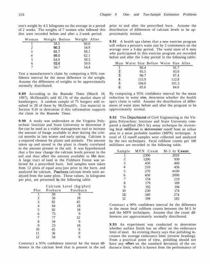
316 Chapter 9 One- and Two-Sample Estimation Problems
son's weight by 4.5 kilograms on the average in a period of 2 weeks. The weights of 7 women who followed this diet were recorded before and after a 2-week period.
W o m a n 1 2 3 4 5 6 7
Weight Before 58.5 60.3 61.7 69.0 64.0 62.6 56.7
Weight After 60.0 54.9 58.1 62.1 58.5 59.9 54.4
Test a manufacturer's claim by computing a 95% confidence interval for the mean difference in the weight. Assume the differences of weights to be approximately normally distributed.
9.89 According to the Roanoke Times (March 16, 1997), McDonald's sold 42.1% of the market share of hamburgers. A random sample of 75 burgers sold resulted in 28 of them by McDonald's. Use material in Section 9.10 to determine if this information supports the claim in the Roanoke Times.
9.90 A study was undertaken at the Virginia Polytechnic Institute and State University to determine if fire can be used as a viable management tool to increase the amount of forage available to deer during the critical months in late winter and early spring. Calcium is a required element for plants and animals. The amount taken up and stored in the plant is closely correlated to the amount present in the soil. It was hypothesized that a fire may change the calcium levels present in the soil and thus affect the amount available to the deer. A large tract of land in the Fishburn Forest was selected for a prescribed burn. Soil samples were taken from 12 plots of equal area just prior to the burn, and analyzed for calcium. Postburn calcium levels were analyzed from the same plots. These values, in kilograms per plot, are presented in the following table:
Calc ium Level (kg /p lo t ) P lo t P r e b u r n P o s t b u r n
1 2 3 4 5 6 7 8 9
10 11 12
50 50 82 64 82 73 77 54 23 45 36 54
9 18 45 18 18 9
32 9
18 9 9 9
prior to and after the prescribed burn. Assume the distribution of differences of calcium levels to be approximately normal.
9.91 A health spa claims that a new exercise program will reduce a person's waist size by 2 centimeters on the average over a 5-day period. The waist sizes of 6 men who participated in this exercise program are recorded before and after the 5-day period in the following table:
M a n Wais t Size Before Wais t Size After 90.4 95.5 98.7
115.9 104.0 85.6
91.7 93.9 97.4
112.8 101.3 84.0
By computing a 95% confidence interval for the mean reduction in waist size, determine whether the health spa's claim is valid. Assume the distribution of differences of waist sizes before and after the program to be approximately normal.
9.92 The Department of Civil Engineering at the Virginia Polytechnic Institute and State University compared a modified (M-5 hr) assay technique for recovering fecal coliforms in storrnwater runoff from an urban area to a most probable number (MPN) technique. A total of 12 runoff samples were collected and analyzed by the two techniques. Fecal coliform counts per 100 milliliters are recorded in the following table.
Sample 1 2 3 4 5 6 7 8 9
10 11 12
M P N C o u n 2300 1200 450 210 270 450 154 179 192 230 340 194
t M-5 hr Count 2010
930 400 436
4100 2090
219 169 194 174 274 183
Construct a 95% confidence interval for the mean difference in the calcium level that is present in the soil
Construct a 90% confidence interval for the difference in the mean fecal coliform counts between the M-5 hr and the MPN techniques. Assume that the count differences are approximately normally distributed.
9.93 An experiment was conducted to determine whether surface finish has an effect on the endurance limit of steel. An existing theory says that polishing increases the average endurance limit (reverse bending). From a practical point of view, polishing should not have any effect on the standard deviation of the endurance limit, which is known from the performance of
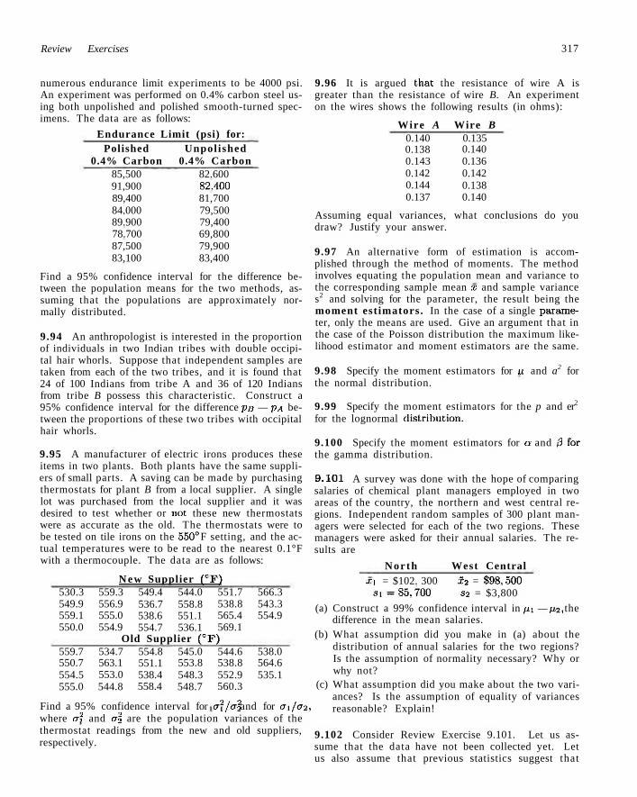
Review Exercises 317
numerous endurance limit experiments to be 4000 psi. An experiment was performed on 0.4% carbon steel using both unpolished and polished smooth-turned specimens. The data are as follows:
Endurance Limit (psi) for: Polished Unpol ished
0.4% Carbon 0.4% Carbon 85,500 91,900 89,400 84.000 89.900 78.700 87,500 83,100
82.600 82,400 81,700 79,500 79,400 69,800 79,900 83,400
Find a 95% confidence interval for the difference between the population means for the two methods, assuming that the populations are approximately normally distributed.
9.94 An anthropologist is interested in the proportion of individuals in two Indian tribes with double occipital hair whorls. Suppose that independent samples are taken from each of the two tribes, and it is found that 24 of 100 Indians from tribe A and 36 of 120 Indians from tribe B possess this characteristic. Construct a 95% confidence interval for the difference pa — PA between the proportions of these two tribes with occipital hair whorls.
9.95 A manufacturer of electric irons produces these items in two plants. Both plants have the same suppliers of small parts. A saving can be made by purchasing thermostats for plant B from a local supplier. A single lot was purchased from the local supplier and it was desired to test whether or not these new thermostats were as accurate as the old. The thermostats were to be tested on tile irons on the 550° F setting, and the actual temperatures were to be read to the nearest 0.1°F with a thermocouple. The data are as follows:
N e w Supplier (CF) 530.3 549.9 559.1 550.0
559.7 550.7 554.5 555.0
559.3 556.9 555.0 554.9
549.4 536.7 538.6 554.7
544.0 558.8 551.1 536.1
551.7 538.8 565.4 569.1
Old Supplier (CF) 534.7 563.1 553.0 544.8
554.8 551.1 538.4 558.4
545.0 553.8 548.3 548.7
544.6 538.8 552.9 560.3
566.3 543.3 554.9
538.0 564.6 535.1
Find a 95% confidence interval for a2/a2 and for aifa2, where a2 and a\ are the population variances of the thermostat readings from the new and old suppliers, respectively.
9.96 It is argued that the resistance of wire A is greater than the resistance of wire B. An experiment on the wires shows the following results (in ohms):
Wire A 0.140 0.138 0.143 0.142 0.144 0.137
Wire B 0.135 0.140 0.136 0.142 0.138 0.140
Assuming equal variances, what conclusions do you draw? Justify your answer.
9.97 An alternative form of estimation is accomplished through the method of moments. The method involves equating the population mean and variance to the corresponding sample mean x and sample variance s2 and solving for the parameter, the result being the moment estimators. In the case of a single parameter, only the means are used. Give an argument that in the case of the Poisson distribution the maximum likelihood estimator and moment estimators are the same.
9.98 Specify the moment estimators for u. and a2 for the normal distribution.
9.99 Specify the moment estimators for the p and er2
for the lognormal distribution.
9.100 Specify the moment estimators for a and 8 for the gamma distribution.
9.101 A survey was done with the hope of comparing salaries of chemical plant managers employed in two areas of the country, the northern and west central regions. Independent random samples of 300 plant managers were selected for each of the two regions. These managers were asked for their annual salaries. The results are
North West Central x,i = $102. 300 S2 = $98,500
s , = S 5 , 7 0 0 s2 = $3,800
(a) Construct a 99% confidence interval in pi — p2, the difference in the mean salaries.
(b) What assumption did you make in (a) about the distribution of annual salaries for the two regions? Is the assumption of normality necessary? Why or why not?
(c) What assumption did you make about the two variances? Is the assumption of equality of variances reasonable? Explain!
9.102 Consider Review Exercise 9.101. Let us assume that the data have not been collected yet. Let us also assume that previous statistics suggest that
318 Chapter 9 One- and Two-Sample Estimation Problems
a\ = o2 = $4000. Are the sample sizes in Review Exercise 9.101 sufficient to produce a 95% confidence interval on p\ —p2 having a width of only $1000? Show all work.
9.103 A specific labor union is becoming defensive about gross absenteeism by its members. The union decided to check this by monitoring a random sample of its members. The union leaders had always claimed that in a typical month, 95% of its members are absent less than 10 hours per month. Use the data to respond to this claim. Use a one-sided tolerance limit and choose the confidence level to be 99%. Be sure to interpret what you learned from the tolerance limit calculation. The number of members in this sample was 300. The number of hours absent was recorded for each of the 300 members. The results were x = 6.5 hours and s = 2.5 hours.
9.104 A random sample of 30 firms dealing in wireless products were selected to determine the proportion of such firms that have implemented new software to improve productivity. It turned out that eight of the 30 have implemented such software. Find a 95% confidence interval on p, the true proportion of such firms that have implemented new software.
9.105 Refer to Review Exercise 9.104. Suppose there is concern about whether or not the point estimate p = 8/30 is accurate enough because the confidence interval around p is not sufficiently narrow. Using p as our estimate of p, how many companies would need to be sampled in order to have a 95% confidence interval with a width of only 0.05?
9.106 A manufacturer turns out a product item that is labeled either "defective" or "not defective." In order to estimate the proportion defective, a random sample of 100 items is taken from production and 10 are found to be defective. Following the implementation of a quality improvement program, the experiment was conducted again. A new sample of 100 is taken and this time only 6 are found defective.
(a) Give a 95% confidence interval on p\ — p2, where pi is the population proportion defective before improvement, and p2 is the proportion defective after improvement.
(b) Is there information in the confidence interval found in (a) that would suggest that pi > p21 Explain.
9.107 A machine is used to fill boxes of product in an assembly line operation. Much concern centers around the variability in the number of ounces of product in the box. The standard deviation in weight of product is known to be 0.3 ounces. An improvement is implemented after which a random sample of 20 boxes are
selected and the sample variance is found to be 0.045 ounces. Find a 95% confidence interval on the variance in the weight of the product. Does it appear from the range of the confidence interval that the improvement of the process enhanced quality as far as variability is concerned? Assume normality on the distribution of weight of product.
9.108 A consumer group is interested in comparing operating costs for two different types of automobile engines. The group is able to find 15 owners whose cars have engine type A and 15 who have engine type B. All 30 owners bought their cars at roughly the same time and all have kept good records for a certain 12 month period. In addition, owners were found that drove roughly the same mileage. The cost statistics are yA = $87.00/1,000 miles, yB = $75.00/1,000 miles, SA = $5.99, and SB — $4.85. Compute a 95% confidence interval to estimate PA — PB, the difference in the mean operating costs. Assume normality and equal variance.
9.109 Consider the statistic Sp, the pooled estimate of er2. The estimator is discussed in Section 9.8. It is used when one is willing to assume that o\ = o\ = a2. Show that the estimator is unbiased for a2 (i.e., show that E(S2) = a2). You may make use of results from any theorem or example in Chapter 9.
9.110 A group of human factor researchers are concerned about reaction to a stimulus by airplane pilots with a certain cockpit arrangement. An experiment was conducted in a simulation laboratory and 15 pilots were used with average reaction time 3.2 seconds and sample standard deviation 0.6 seconds, It is of interest to characterize extremes (i.e., worst case scenario). To that end, answer the following:
(a) Give a particular important one-sided 99% confidence bound on the mean reaction time. What assumption, if any, must you make on the distribution of reaction time?
(b) Give a 99% one-sided prediction interval and give an interpretation of what it means. Must you make an assumption on the distribution of reaction time to compute this bound?
(c) Compute a one-sided tolerance bound with 99% confidence that involves 95% of reaction times. Again, give interpretation and assumption on distribution if any. [Note: The one-sided tolerance limit values are also included in Table A.7].
9. I l l A certain supplier manufactures a type of rubber mat that is sold to automotive companies. In the application, the pieces of material must have certain hardness characteristics. Defective mats are occasionally discovered and rejected. The supplier claims that
9.15 Potential Misconceptions and Hazards 319
the proportion defective is 0.05. A challenge was marie- the proportion defective. by one of the clients who purchased the product. Thus (b) Compute an appropriate 95% one-sided confidence an experiment, was conducted in which 400 mats are interval on the proportion defective. tested and 17 were found defective. / , . . . . , r , . , , , ,, , ,
(c) Interpret both of these in (a) and (b) and comment (a) Compute a 95% two-sided confidence interval on o n t n e c | a i m l n a d e b y t n e . suppiior .
9.15 Potential Misconceptions and Hazards; Relationship to Material in Other Chapters
The concept of a large-sum pie confidence internal on a population is often confusing to the beginning student. It is based on the prescription that even when a is unknown and one is not convinced that the distribution being sampled is normal, then a confidence interval on p. can be computed from
* ± za,2^-=. • \/ii
In practice this is often used when the sample is too small. The genesis of this large sample interval is, of course, the central limit theorem (CUT), under which normality is not: necessary. Here the CLT requires a known a, of which s is only an estimate. Thus the requirement is made that n must be at least as large as 30 and the underlying distribution is close to symmetric, in which case the interval is still an approximation.
There are instances in which the practical application of material in Chapter 9 must be couched in the context of material in the chapter. One very important illustration is the use of (-distribution for the confidence interval on p when a is unknown. Strictly speaking, the use of the (-distribution requires that the distribution sampled from is normal. However, it is well known that any application of the (-distribution is reasonably insensitive (i.e., robust ) to the normality assumption. This represents one of those fortunate situations in which do occur often in the field of statistics in which a basic assumption does not hold and yet ''everything turns out alright!" However, one population from which the sample is drawn cannot deviate' substantially from normal. Thus, normal probability plots discussed in Chapter 8 and goodncss-of-fit tests introduced in Chapter 10 will often be called upon here to ascertain some sense of ''nearness to normality." This idea of "robustness to normality51 will reappear in Chapter 10.
It is our experience that one of the most serious "misuses of statistics" in practice evolves from confusion about distinction between the interpretation of the types of statistical intervals. Thus the subsection in this chapter where differences among the three types of intervals are discussed. It is very likely that in practice the confidence interval is heavily overused. That, is, it is used when there is really no interest in the mean. Rather, there arc: often questions of the type, "Where is the next observation going to fall?" Or often, more importantly, "Where is the large bulk of the distribution?" These are crucial questions that are not answered by computing an interval on the mean. A confidence interval is commonly misused as an interval such that the probability of the parameter falls in this interval is, say
320 Chapter 9 One- and Two-Sample Estimation Problems
95%, which is a correct interpretation of a Bayesian posterior interval (readers are referred to Chapter 18 for more information on Bayesian inference). Confidence interval merely suggests that if the experiment or data is observed again and again, about 95% of such intervals will contain the true parameter. Any beginning student of practical statistics should be very clear on the difference among these statistical intervals.
Another potential serious misuse of statistics centers around the use of the \2-distribution for a confidence interval on a single variance. Again, normality on the distribution from which the sample is drawn is assumed. Unlike the use of the t-distribution, the use of x2 test for this application is not robust to the normality assumption (i.e., the sampling distribution of ai— deviates far away from \2
if the underlying distribution is not normal). Thus, strict use of goodness-of-fit (Chapter 10) tests and/or normal probability plotting can be extremely important here. More information about this general issue will be given in future chapters.
Chapter 10
One- and Two-Sample Tests of Hypotheses
10.1 Statistical Hypotheses: General Concepts
Often, the problem confronting the scientist or engineer is not so much the estimation of a population parameter as discussed in Chapter 9, but rather the formation of a data-based decision procedure that, can produce a. conclusion about sonic scientific system. For example, a medical researcher may decide on the basis of experimental evidence whether coffee drinking increases the risk of cancer in humans; an engineer might have to decide on the basis of sample data whether there is a difference between the accuracy of two kinds of gauges; or a sociologist might wish to collect, appropriate data to enable him or her to decide whether a person's blood type and eye color are independent variables. In each of these cases the scientist or engineer postulates or conjectures something about a system. In addition, each must involve the use of experimental data and decision-making that is based on the data. Formally, in each case, the conjecture can be put in the form of a statistical hypothesis. Procedures that lead to the acceptance or rejection of statistical hypotheses such as these comprise a major area of statistical inference. First, let us define precisely what we mean by a s tat is t ical hypothesis .
Definition 10.1: A statist ical hypothesis is an assertion or conjecture concerning one or more populations.
The truth or falsity of a statistical hypothesis is never known with absolute certainty unless we examine the entire population. This, of course, would be impractical in most situations. Instead, we take a random sample from the population of interest and use the data contained in this sample to provide evidence that either supports or does not support the hypothesis. Evidence from the sample that is inconsistent with the stated hypothesis leads to a rejection of the hypothesis.
322 Chapter 10 One- and Two-Sample Tests of Hypotheses
The Role of Probability in Hypothesis Testing
It should be made clear to the reader that the decision procedure must be done with the awareness of the probability of a wrong conclusion. For example, suppose that the hypothesis postulated by the engineer is that the fraction defective p in a certain process is 0.10. The experiment is to observe a random sample of the product in question. Suppose that 100 items are tested and 12 items are found defective. It is reasonable to conclude that this evidence does not refute the condition p — 0.10, and thus it may lead one not to reject the hypothesis. However, it also does not refute p = 0.12 or perhaps even p = 0.15. As a result, the reader must be accustomed to understanding that the rejection of a hypothesis implies that the sample evidence refutes it. Put another way, rejection means that there is a small probability of obtaining the sample information observed when, in fact, the hypothesis is true. For example, in our proportion-defective hypothesis, a sample of 100 revealing 20 defective items is certainly evidence of rejection. Why? If, indeed, p — 0.10, the probability of obtaining 20 or more defectives is approximately 0.002. With the resulting small risk of a wrong conclusion, it would seem safe to reject the hypothesis that p = 0.10. In other words, rejection of a hypothesis tends to all but "rule out" the hypothesis, On the other hand, it is very important to emphasize that the acceptance or. rather, failure to reject, does not rule out other possibilities. As a result, the firm conclusion is established by the data analyst when a hypothesis is rejected.
The formal statement of a hypothesis is often inliuenced by the structure of the probability of a wrong conclusion. If the scientist is interested in strongly supporting a contention, he or she hopes to arrive at the contention in the form of rejection of a hypothesis. If the medical researcher wishes to show strong evidence in favor of the contention that coffee drinking increases the risk of cancer, the hypothesis tested should be of the form "there is no increase in cancer risk produced by drinking coffee." As a result, the contention is reached via a rejection. Similarly, to support the claim that one kind of gauge is more accurate than another, the engineer tests the hypothesis that there is no difference in the accuracy of the two kinds of gauges.
The foregoing implies that when the data analyst formalizes experimental evidence on the basis of hypothesis testing, the formal statement of the hypothesis is very important.
The Null and Alternative Hypotheses
The structure of hypothesis testing will be formulated with the use of the term null hypothesis. This refers to any hypothesis we wish to test and is denoted by H[). The rejection of Ho leads to the acceptance of an alternative hypothesis, denoted by Hi. An understanding of the different, roles played by the null hypothesis (Ho) and the alternative hypothesis (Hi) is crucial to one's understanding of the rudiments of hypothesis testing. The alternative hypothesis Hi usually represents the question to be answered, the theory to be tested and thus its specification is crucial. The null hypothesis Ho nullifies or opposes Hi and is often the logical complement to H\. As the reader gains more understanding of hypothesis testing, he or she should note that the analyst, arrives at one of the two following
10.2 Testing a Statistical Hypothesis 323
conclusions:
reject HQ: in favor of Hi because of sufficient evidence in the data.
fail to -reject HQ: because of insufficient evidence in the data.
Note that the conclusions do not involve a formal and literal "accept HQ." The statement of Ho often represents "status quo" in opposition to the new idea, conjecture, and so on, stated in Hi, while failure to reject HQ represents the proper conclusion. In our binomial example, the practical issue may come from a concern that the historical defective probability of 0.10 no longer is true. Indeed the conjecture may be that it exceeds 0.10. We may then state
H0: p = 0.10,
HI: p > 0.10.
Now 12 defective items out of 100 does not refute a p = 0.10 so the conclusion is "fail to reject ffo" However, if the data produce 20 out of 100 defective items, then the conclusion is "reject Ho" in favor of Hi: p > 0.10.
Though the applications of hypothesis testing are quite abundant in scientific and engineering work, perhaps the best illustration for a novice lies in the predicament encountered in a jury trial. The null and alternative hypotheses are
H0: defendant is innocent,
Hi: defendant is guilty.
The indictment comes because of suspicion of guilt. The hypothesis Ho (status quo) stands in opposition to Hi and is maintained unless flj is supported by evidence "beyond a reasonable doubt." However, "failure to reject HQ" in this case does not imply innocence, but merely that the evidence was insufficient to convict. So the jury does not necessarily accept. HQ but fails to reject Ho-
10.2 Testing a Statistical Hypothesis
To illustrate the concepts used in testing a statistical hypothesis about a population, consider the following example. A certain type of cold vaccine is known to be only 25% effective after a period of 2 years. To determine if a new and somewhat more expensive vaccine is superior in providing protection against the same virus for a longer period of time, suppose that 20 people are chosen at random and inoculated. In an actual study of this type the participants receiving the new vaccine might number several thousand. The number 20 is being used here only to demonstrate the basic steps in carrying out a statistical test. If more than 8 of those receiving the new vaccine surpass the 2-year period without contracting the virus, the new vaccine will be considered superior to the one presently in use. The requirement that the number exceed 8 is somewhat arbitrary but appears reasonable in that it: represents a modest gain over the 5 people that could be expected to receive protection if the 20 people had been inoculated with the vaccine already in use. We are essentially testing the null hypothesis that the new vaccine is equally effective after a period of 2 years as the one now commonly used. The alternative
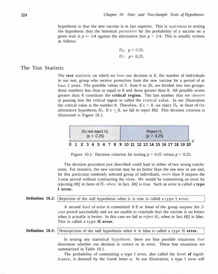
324 Chapter 10 One- and Two-Sample Tests of Hypotheses
hypothesis is that the new vaccine is in fart superior. This is equivalent to testing the hypothesis that the binomial parameter for the probability of a success on a given trial is p — 1/4 against the alternative that p > 1/4. This is usually written as follows:
HQ: p = 0.25,
Hx: p> 0.25.
The Test Statistic The test s tat is t ic on which we base our decision is X, the number of individuals in our test, group who receive protection from the new vaccine for a period of at least 2 years. The possible values of X, from 0 to 20, are divided into two groups: those numbers less than or equal to 8 and those greater than 8. All possible scores greater than 8 constitute the critical region. The last number that we observe in passing into the critical region is called the critical value. In our illustration the critical value is the number 8. Therefore, if x > 8, we reject Ho in favor of the: alternative hypothesis Hi. If x < 8, we fail to reject HQ. This decision criterion is illustrated in Figure 10.1.
Do not reject H0
(p = 0.25) 1
Reject H0
(p > 0.25)
0 1 2 3 4 5 6 7 8 9 10 11 12 13 14 15 16 17 18 19 20
Figure 10.1: Decision criterion for testing p = 0.25 versus p > 0.25.
The decision procedure just described could lead to either of two wrong conclusions. For instance, the new vaccine may be no better than the one now in use and, for this particular randomly selected group of individuals, more than 8 surpass the 2-year period without contracting the virus. Wc would be committing an error by rejecting HQ in favor of Hi when, in fact, HQ is true. Such an error is called a type I error.
Definition 10.2:
Definition 10.3:
Rejection of the null hypothesis when it is true is called a type I error.
A second kind of error is committed if 8 or fewer of the group surpass the 2-ycar period successfully and we are unable to conclude that the vaccine is no better when it actually is better. In this case we fail to reject HQ when in fact HQ is false:. This is called a type II error.
Nonrejection of the null hypothesis when it is false is called a type II error.
In testing any statistical hypothesis, there are four possible situations that determine whether our decision is correct or in error. These four situations are summarized in Table 10.1.
The probability of committing a type I error, also called the level of significance, is denoted by the Greek letter a. In our illustration, a type I error will
10.2 Testing a Statistical Hypothesis 325
Table 10.1: Possible Situations for Testing a Statistical Hypothesis
Do not reject Ho Reject HQ
HQ is true HQ is false Correct decision Type II error Type I error Correct decision
occur when more than 8 individuals surpass the 2-year period without contracting the virus using a new vaccine that is actually equivalent to the one in use. Hence, if X is the number of individuals who remain free of the virus for at least 2 years,
a = P(type I error) = P (X > 8 when p = - j = ^ b (x; 20, - j
= 1 - £ 6 ( x; 20, j J = 1 - 0.9591 = 0.0409. x=0 ^ '
We say that the null hypothesis, p = 1/4, is being tested at the a = 0.0409 level of significance. Sometimes the level of significance is called the size of the test. A critical region of size 0.0409 is very small and therefore it is unlikely that a type I error will be committed. Consequently, it would be most unusual for more than 8 individuals to remain immune to a virus for a 2-year period using a new vaccine that is essentially equivalent to the one now on the market.
The Probability of a Type II Error
The probability of committing a type II error, denoted by ,8, is impossible to compute unless we have a specific alternative hypothesis. If we test the null hypothesis that p = 1/4 against the alternative hypothesis that p = 1/2, then we are able to compute the probability of not rejecting HQ, when it is false. We simply find the probability of obtaining 8 or fewer in the group that surpass the 2-year period when p — 1/2. In this case
,3 = P(type II error) = P (X < 8 when p = - j
= J2b(x;20,^] =0.2517.
This is a rather high probability, indicating a test procedure in which it is quite likely that we shall reject the new vaccine when, in fact, it is superior to what now in use. Ideally, we like to use a test procedure for which the type I and type II error probabilities are both small.
It is possible that the director of the testing program is willing to make a type II error if the more expensive vaccine is not significantly superior. In fact, the only time he wishes to guard against the type II error is when the true value of p is at
326 Chapter 10 One-and Two-Sample Tests of Hypotheses
least 0.7. If p — 0.7, this test procedure gives
3 = P(type II error) = P(X < 8 when p = 0.7) 8
= ^ o ( x ; 20,0.7) = 0.0051. x=0
With such a small probability of committing a type II error, it is extremely unlikely that the new vaccine would be rejected when it is 70% effective after a period of 2 years. As the alternative hypothesis appioaches unity, the value of 3 diminishes to zero.
The Role of a, /3, and Sample Size
Let us assume that the director of the testing program is unwilling to commit a type II error when the alternative hypothesis p = 1/2 is true even though we have found the probability of such an error to be 3 = 0.2517. A reduction in 3 is always possible!^- increasing the size of the critical region. For example, consider what happens to the values of a and 3 when we change our critical value to 7 so that all scores greater than 7 fall in the critical region and those less than or equal to 7 fall in the nonrejection region. Now, in testing p = 1/4 against the alternative hypothesis that p — 1/2, we find that
a = j S ( Z; 20, J ) = 1 - J^eb (x;20, j J =1-0.8982 = 0.1018, x=8 ^ ' x=0 \ '
and
3 = j^bfx;20,^ j =0.1316. .T=0
By adopting a new decision procedure, we have reduced the probability of committing a type II error at the expense of increasing the probability of committing a type I error. For a fixed sample size, a decrease in the probability of one error will usually result in an increase in the probability of the other error. Fortunately, the probability of committing both types of error can be reduced by increasing the sample size. Consider the same problem using a random sample of 100 individuals. If more than 36 of the group surpass the 2-year period, we reject the null hypothesis that p — 1/4 and accept the alternative hypothesis that p > 1/4. The critical value is now 36. All possible scores above 36 constitute the critical region and all possible scores less than or equal to 36 fall in the acceptance region.
To determine the probability of committing a type I error, we shall use the normal-curve approximation with
fj, = np = (100) f ^ j = 2 5 , and a = y/rrpq = v/(100)(l/4)(3/4) = 4.33.
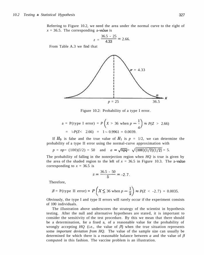
10.2 Testing a Statistical Hypothesis 327
Referring to Figure 10.2, we need the area under the normal curve to the right of x = 36.5. The corresponding z-value is
36.5 - 25 z = 4.33
2.66.
From Table A.3 we find that
a = 4.33
p = 25 36.5
Figure 10.2: Probability of a type I error.
a = P(type I error) = P
= \-P(Z< 2.66) = 1
X > 36 when p — -4
- 0.9961 = 0.0039.
P(Z > 2.66)
If Ho is false and the true value of Hi is p = 1/2, we can determine the probability of a type II error using the normal-curve approximation with
p = np= (100)(l/2) = 50 and a = Jnpq = v/(100)(l/2)(l/2) = 5.
The probability of falling in the nonrejection region when HQ is true is given by the area of the shaded region to the left of x = 36.5 in Figure 10.3. The z-value corresponding to x = 36.5 is
36.5 - 50 -2.7.
Therefore,
8 = P(type II error) = P(X < 36 when p — P(Z < -2.7) = 0.0035.
Obviously, the type I and type II errors will rarely occur if the experiment consists of 100 individuals.
The illustration above underscores the strategy of the scientist in hypothesis testing. After the null and alternative hypotheses are stated, it is important to consider the sensitivity of the test procedure. By this we mean that there should be a determination, for a fixed a, of a reasonable value for the probability of wrongly accepting HQ (i.e., the value of 8) when the true situation represents some important deviation from HQ. The value of the sample size can usually be determined for which there is a reasonable balance between a and the value of 8 computed in this fashion. The vaccine problem is an illustration.
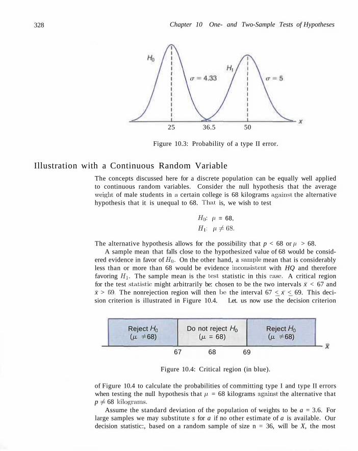
328 Chapter 10 One- and Two-Sample Tests of Hypotheses
25 36.5 50
Figure 10.3: Probability of a type II error.
Illustration with a Continuous Random Variable The concepts discussed here for a discrete population can be equally well applied to continuous random variables. Consider the null hypothesis that the average weight of male students in a certain college is 68 kilograms against the alternative hypothesis that it is unequal to 68. That, is, we wish to test
HQ\ p = 68,
Hi: p#68.
The alternative hypothesis allows for the possibility that p < 68 or ft > 68. A sample mean that falls close to the hypothesized value of 68 would be consid
ered evidence in favor of HQ- On the other hand, a sample mean that is considerably less than or more than 68 would be evidence inconsistent with HQ and therefore favoring Hx. The sample mean is the test, statistic in this case:. A critical region for the test statistic; might arbitrarily be: chosen to be the two intervals x < 67 and x > 69. The nonrejection region will then be: the interval 67 < x < 69. This decision criterion is illustrated in Figure 10.4. Let. us now use the decision criterion
Reject H0
(p. * 68) Do not reject H0
(p. = 68) Reject HQ (p, * 68)
67 68 69
Figure 10.4: Critical region (in blue).
of Figure 10.4 to calculate the probabilities of committing type I and type II errors when testing the null hypothesis that //. = 68 kilograms against the alternative that p y^ 68 kilograms.
Assume the standard deviation of the population of weights to be a = 3.6. For large samples we may substitute s for a if no other estimate of a is available. Our decision statistic:, based on a random sample of size n = 36, will be X, the most
10.2 Testing a Statistical Hypothesis 329
efficient, estimator of p. From the central limit theorem, we: know that the sampling distribution of X is approximately normal with standard deviation crx = o/yfn = 3.6/6 = 0.6.
The probability of committing a type I error, or the level of significance of our test, is equal to the sum of the areas that have been shaded in each tail of the distribution in Figure 10.5. Therefore,
a = P(X < 67 when p = 68) + P(X > 69 when p. = OS).
67 p. = 68
Figure: 10.5: Critical region for testing p. — 08 versus p ^ 68.
The 2-va.lues corresponding to x\ — 67 and x2 = 69 when HQ is true are
<J7 - 68 n „„ , 69 - 08 Z] — ——— = —l.oc and Z2 = ——-— 1.67. 0.6 0.6
Therefore.
Q = P(Z < -1.67) + P(Z > 1.67) = 2P(Z < -1.67) = 0.0950.
Thus 9.5% of all samples of size 36 would lead us to reject p. = 68 kilograms when, in fact, it is true. To reduce a, we have a, choice: of increasing the sample size or widening the fail-to-rejection region. Suppose that we increase the sample size to n = 64. Then 0% = 3.6/8 = 0.45. Now
Z l = ^ 6 8 = - 2 . 2 2 and z2 = ^ = 2.22. 0.45 0.45
Hence
ct = P(Z < -2.22) + P(Z > 2.22) = 2P(Z < -2.22) = 0.0264.
The reduction in a is not sufficient, by itself to guarantee a good testing procedure. Wc must also evaluate 3 for various alternative hypotheses. If it is important to reject Ho when the true mean is some value p. > 70 or p < 66, then the probability of committing a type II error should be computed and examined for the alternatives p = 66 and p = 70. Because of symmetry, it is only necessary to
330 Chapter 10 One- and Two-Sample Tests of Hypotheses
consider the probability of not rejecting the null hypothesis that p = 68 when the alternative p. = 70 is true. A type II error will result when the sample mean x falls between 67 and 69 when Hi is true. Therefore, referring to Figure 10.6, we find that
Q = P(67 < X < 69 when p. = 70).
Figure 10.6: Probability of type II error for testing // = 68 versus p. — 70.
The z-values corresponding to aSj = 67 and x2 = 69 when H\ is true are
6 7 - 7 0 r „ _ 69 - 70 Z\ = „ , r = -6.67 and z2 = - = -2.22.
0.45 0.45
Therefore.
3 = P(-6 .67 < Z < -2.22) = P(Z < -2.22) - P(Z < -6.67)
= 0.0132-0.0000 = 0.0132.
If the true value of p is the alternative p = 66, the value of 8 will again be 0.0132. For all possible values of fi < 66 or p > 70, the value of 8 will be even smaller when n = 64, and consequently there would be little chance of not rejecting HQ when it is false.
The probability of committing a type II error increases rapidly when the true value of // approaches, but is not equal to, the hypothesized value. Of course, this is usually the situation where we do not mind making a type II error. For example, if the alternative hypothesis p — 68.5 is true, we do not mind committing a type II error by concluding that the true answer is p = 68. The probability of making such an error will be high when n = 64. Referring to Figure 10.7, we have
8 = P(67 < X < 69 when //. = 68.5).
The z-values corresponding to :ci = 67 and x-2 = 69 when p = 68.5 are
10.2 Testing a Statistical Hypothesis 331
67 68 68.5 69
Figure 10.7: Type II error for testing p. = 68 versus p = 68.5.
67 - 68.5 69 - 68.5 :i = = —3.33 and z-> = = 1.11.
0.45 " 0.45 Therefore,
3 = P ( -3 .33 < Z < 1.11)= P ( Z < l . l l ) - P ( Z < -3.33)
= 0.8665-0.0004 = 0.8661.
The preceding examples illustrate the following important properties:
Important Properties of a
Test, of Hypothesis
1. The type I error and type II error are related. A decrease in the probability of one generally results in an increase in the probability of the other.
2. The size of the critical region, and therefore the probability of committing a type I error, can always be reduced by adjusting the critical value(s).
3. An increase in the sample size n will reduce a and 3 simultaneously.
4. If the null hypothesis is false, 13 is a maximum when the true value of a parameter approaches the hypothesized value. The greater the distance between the true value and the hypothesized value, the smaller 3 will be.
One very important concept that relates to error probabilities is the notion of the power of a test.
Definition 10.4: The power of a test is the probability of rejecting HQ given th, native is true.
at a specific alte
The power of a test can be computed as 1 — 8. Often different types of tes ts are compared by contrast ing power properties. Consider the previous illustration in which we were testing HQ: p = 68 and H\i p ^ 68. As before, suppose we are interested in assessing the sensitivity of the test. The test is governed by the rule that we do not reject HQ if 67 < x < 69. Wc seek the capability of the test for properly rejecting HQ when indeed p = 68.5. WTe have seen that the probability of a type II error is given by 8 — 0-8661. Thus the power of the test is 1 — 0.8661 = 0.1339. In a sense, the power is a more succinct measure of how
332 Chapter 10 One- and Two-Sample Tests of Hypotheses
sensitive the test is for "detecting differences" between a mean of 68 and 68.5. In this case, if p is truly 68.5, the test as described will properly reject Ho only 13.39% of the time. As a result, the test would not be a good one if it is important that the analyst have a reasonable chance of truly distinguishing between a mean of 68.0 (specified by HQ) and a mean of 68.5. From the foregoing, it is clear that to produce a desirable power (say, greater than 0.8), one must either increase a or increase the sample size.
In what has preceded in this chapter, much of the text on hypothesis testing revolves around foundations and definitions. In the sections that follow we get more specific and put hypotheses in categories as well as discuss tests of hypotheses on various parameters of interest. We begin by drawing the distinction between a one-sided and two-sided hypothesis.
10.3 One- and Two-Tailed Tests
A test of any statistical hypothesis, where the alternative is one sided, such as
HQ: 9 — 6Q,
H\: 9 > 8Q,
or perhaps
HQ: 8 = 8Q,
Hi: 8 < 8Q,
is called a one-tailed test. In Section 10.2, we refer to the test statistic for a hypothesis. Generally, the critical region for the alternative hypothesis 8 > 8Q lies in the right tail of the distribution of the test statistic, while the critical region for the alternative hypothesis 8 < 8Q lies entirely in the left tail. In a sense, the inequality symbol points in the direction where the critical region lies. A one-tailed test is used in the vaccine experiment of Section 10.2 to test the hypothesis p = 1/4 against the one-sided alternative p > 1/4 for the binomial distribution. The one-tailed critical region is usually obvious. For understanding, the reader should visualize the behavior of the test statistic and notice the obvious signal that would produce evidence supporting the alternative hypothesis.
A test of any statistical hypothesis where the alternative is two sided, such as
HQ: 9 — 8Q,
Hi: 8 + 8Q,
is called a two-tailed test, since the critical region is split into two parts, often having equal probabilities placed in each tail of the distribution of the test statistic. The alternative hypothesis 8 / 8Q states that either 9 < 90 or 9 > 90. A two-tailed test was used to test the null hypothesis that p — 68 kilograms against the two-sided alternative p ^ 68 kilograms for the continuous population of student weights in Section 10.2.
10.3 One- and Two-Tailed Tests 333
How Are the Null and Alternative Hypotheses Chosen?
The null hypothesis HQ will often be stated using the equality sign. With this approach, it is clear how the probability of type I error is controlled. However, there are situations in which the application suggests that "do not reject HQ''- implies that the parameter 9 might be any value defined by the natural complement to the alternative hypothesis. For example, in the vaccine example where the alternative hypothesis is Hi: p > 1/4, it is quite possible that a non-rejection of Ho cannot rule out a value of p less than 1/4. Clearly though, in the case of one-tailed tests, the statement of the alternative is the most important, consideration.
Whether one sets up a one-tailed or a two-tailed test will depend on the conclusion to be drawn if Ho is rejected. The location of the critical region can be determined only after Hi has been stated. For example, in testing a new drug, one sets up the hypothesis that it is no better than similar drugs now on the market and tests this against the alternative hypothesis that the new drug is superior. Such an alternative hypothesis will result in a one-tailed test with the critical region in the right tail. However, if we wish to compare a new teaching technique with the conventional classroom procedure, the alternative hypothesis should allow for the new approach to be either inferior or superior to the conventional procedure. Hence the test is two-tailed with the critical region divided equally so as to fall in the extreme left and right tails of the distribution of our statistic.
Example 10.1:1 A manufacturer of a certain brand of rice cereal claims that the average saturated fat content does not exceed 1.5 grams. State the null and alternative hypotheses to be used in testing this claim and determine where the critical region is located.
Solution: The manufacturer's claim should be rejected only if p is greater than 1.5 milligrams and should not be rejected if p is less than or equal to 1.5 milligrams. We test
H0: p = 1.5,
Hi: p > 1.5,
the nonrejection of HQ does not rule out values less than 1.5 milligrams. Since we have a one-tailed test, the greater than symbol indicates that the critical region lies entirely in the right tail of the distribution of our test statistic X. J
Example 10.2:1 A real estate agent claims that 60%, of all private residences being built today are 3-bedroom homes. To test this claim, a large sample of new residences is inspected: the proportion of these homes with 3 bedrooms is recorded and used as our test statistic. State the null and alternative hypotheses to be used in this test and determine the location of the critical region.
Solution: If the test statistic is substantially higher or lower than p = 0.6, we would reject the agent's claim. Hence we should make the hypothesis
HQ: p = 0.6,
H I : p ^ 0 . 6 .
The alternative hypothesis implies a two-tailed test with the critical region divided equally in both tails of the distribution of P. our test statistic. J
334 Chapter 10 One- and Two-Sample Tests of Hypotheses
10.4 The Use of P-Values for Decision Making in Testing Hypotheses
In testing hypotheses in which the test statistic is discrete, the critical region may be chosen arbitrarily and its size determined. If a is too large, it can be reduced by making an adjustment in the critical value. It may be necessary to increase the sample size to offset the decrease that occurs automatically in the power of the test.
Over a number of generations of statistical analysis, it had become customary to choose an a of 0.05 or 0.01 and select the critical region accordingly. Then, of course, strict rejection or nonrejection of Ho would depend on that critical region. For example, if the test is two tailed and a is set at the 0.05 level of significance and the test statistic involves, say, the standard normal distribution, then a z-value is observed from the data and the critical region is
z>1 .96 or z < - 1 . 9 8 ,
where the value 1.96 is found as Zo.025 in Table A.3. A value of z in the critical region prompts the statement, "The value of the test statistic: is significant." We can translate that into the user's language. For example, if the hypothesis is given by
H0: p = 10,
Hi: p^ 10.
one might say: "The mean differs significantly from the value 10."
Preselection of a Significance Level
This preselection of a significance level a has its roots in the philosophy that the maximum risk of making a. type I error should be controlled. However, this approach docs not account for values of test statistics that are "close" to the critical region. Suppose, for example, in the illustration with HQ: p = 10: versus Hi : p ^ 10, a value of z = 1.87 is observed; strictly speaking, with a = 0.05 the value is not significant. But the risk of committing a type I error if one rejects HQ in this case could hardly be considered severe. In fact, in a two-tailed scenario one can quantify this risk as
P = 2P(Z > 1.87 when //. = 10) = 2(0.0307) = 0.0614.
As a result, 0.0614 is the probability of obtaining a value of z as large or larger (in magnitude) than 1.87 when in fact p = 10. Although this evidence against Ho is not as strong as that which would result from a rejection at an a = 0.05 level, it is important information to the user. Indeed, continued use of a = 0.05 or 0.01 is only a result of what standards have been passed through the generations. The P-value approach has been adopted extensively by users in applied stat ist ics. The approach is designed to give the user an alternative (in terms of a probability) to a mere "reject" or "do not reject" conclusion. The P-value computation also gives the user important information wdien the z-value falls well
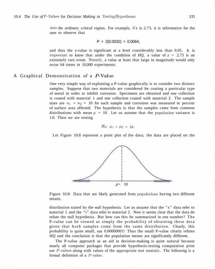
10.4 The Use of P-Values for Decision Making in Testing Hypotheses 335
into the ordinary critical region. For example, if z is 2.73, it is informative for the user to observe that
P = 2(0.0032) = 0.0064,
and thus the z-value is significant at a level considerably less than 0.05. It. is important to know that under the condition of HQ, a value of z = 2.73 is an extremely rare event. Namely, a value at least that large in magnitude would only occur 64 times in 10,000 experiments.
A Graphical Demonstra t ion of a P-Value
One very simple way of explaining a P-value graphically is to consider two distinct samples. Suppose that two materials are considered for coating a particular type of metal in order to inhibit corrosion. Specimens are obtained and one collection is coated with material 1 and one collection coated with material 2. The sample sizes are ??.i = n2 = 10 for each sample and corrosion was measured in percent of surface area affected. The hypothesis is that the samples came from common distributions with mean p = 10. Let us assume that the population variance is 1.0. Then we are testing
HQ: PX = Pa = 10.
Let Figure 10.8 represent a point plot of the data; the data are placed on the
p= 10
Figure 10.8: Data that are likely generated from populations having two different means.
distribution stated by the null hypothesis. Let us assume that the "x" data refer to material 1 and the "o" data refer to material 2. Now it seems clear that the data do refute the null hypothesis. But how can this be summarized in one number? The P-value can be viewed as simply the probabi l i ty of obta in ing these da t a given t h a t b o t h samples come from the same dis t r ibut ion. Clearly, this probability is quite small, say 0.00000001! Thus the small P-value clearly refutes HQ and the conclusion is that the population means are significantly different.
The P-value approach as an aid in decision-making is quite natural because nearly all computer packages that provide hypothesis-testing computation print out P-values along with values of the appropriate test statistic. The following is a formal definition of a P-valuc.
336 Chapter 10 One- and Two-Sample Tests of Hypotheses
Definition 10.5: A P-value is the lowest level (of significance) at which the observed value of the lesl statistic is significant,
How Does the Use of P-Values Differ from Classic Hypothesis Testing?
If is tempting at this point to summarize the procedures associated with testing, say. Ho: 9 = 9Q. However, the student who is a, novice in this area should understand there arc differences in approach and philosophy between the classic fixed a approach tha t is climaxed with either the "reject Ho" or "do not reject Ho" conclusion and the P-value approach. In the latter, no fixed o is determined and conclusions are drawn on the basis of the size of the P-value in harmony with the subjective judgment of the engineer or scientist. While modern computer software will output P-values, nevertheless it is important that readers understand both approaches in order to appreciate the totali ty of the concepts. Thus we offer a brief list of procedural steps for both the classical and P-value approach.
Approach to Hypothesis
Testing with Fixed Probability
of Type I Error
1. State the null and alternative hypotheses. 2. Choose a fixed significance level a. 3. Choose an appropriate test statistic and establish the critical region based on cv. 4. From the computed test statistic, reject HQ if the test statistic is in the critical region. Otherwise, do not reject. 5. Draw scientific or engineering conclusions.
Significance 1. S ta te null and alternative hypotheses. Testing (P-Value 2. Choose: an appropriate test statistic.
Approach) 3. Compute P-value based on computed value of test statistic. 4. Use judgment based on P-value and knowledge of scientific system.
In the sections in this chapter and chapters that, follow, many examples and exercises emphasize the P-value approach to drawing scientific conclusions.
Exercises
10.1 Suppose that mi allergist wishes to test the hypothesis that at least 30% of the public is allergic to some cheese products. Explain how the allergist could commit (a) a type I error; (b) a type II error.
10.2 A sociologist is concerned about the effectiveness of a training course designed to get more drivers to use seat, belts in automobiles.
(a) What hypothesis Is she testing if she commits a type I error by erroneously concluding that the
training course: is ineffective? (b) What hypothesis is she testing if she commits a
type II error by erroneously concluding that the training course is effective?
10.3 A large manufacturing firm is being charged with discrimination in its hiring practices. (a) What hypothesis is being tested if a jury commits
a type I error by dueling the firm guilty? (b) What hypothesis is being tested if a jury commits
a type II error by finding the firm guilty?
Exercises 337
10.4 The proportion of adults living in a small town who are college graduates is estimated to be p = 0.6. To test this hypothesis, a random sample of 15 adults is selected. If the number of college graduates in our sample is anywhere from 6 to 12, we shall not reject the null hypothesis that p = 0.6; otherwise, we shall conclude that p ^ 0.6.
(a) Evaluate a assuming that p = 0.6. Use the binomial distribution.
(b) Evaluate 8 for the alternatives p = 0.5 and p — 0.7. (c) Is this a good test procedure?
10.5 Repeat. Exercise 10.4 when 200 adults are selected and the fail to reject region is defined to be 110 < x < 130, where x is the number of college graduates in our sample. Use the normal approximation.
10.6 A fabric manufacturer believes that the proportion of orders for raw material arriving late is p = 0.6. If a random sample of 10 orders shows that 3 or fewer arrived late, the hypothesis that p = 0.6 should be rejected in favor of the alternative p < 0.6. Use the binomial distribution.
(a) Find the probability of committing a type I error if the true proportion is p = 0.6.
(b) Find the probability of committing a type II error for the alternatives p = 0.3, p — 0.4, and p = 0.5.
10.7 Repeat Exercise 10.6 when 50 orders are selected and the critical region is defined to be x < 24, where x is the number of orders in our sample that arrived late. Use the normal approximation.
10.8 A dry cleaning establishment claims that a new-spot remover will remove more than 70% of the spots to which it is applied. To check this claim, the spot remover will be used on 12 spots chosen at random. If fewer than 11 of the spots are removed, we shall not reject the null hypothesis that p = 0.7: otherwise, we conclude that p > 0.7.
(a) Evaluate a, assuming that p = 0.7. (b) Evaluate 8 for the alternative p = 0.9.
10.9 Repeat Exercise 10.8 when 100 spots are treated and the critical region is defined to be x > 82, where x is the number of spots removed.
10.10 In the publication Relief from Arthritis by Tliorsons Publishers, Ltd., John E. Croft claims that over 40% of the sufferers from osteoarthritis received measurable relief from an ingredient produced by a particular species of mussel found off the coast, of New Zealand. To test this claim, the mussel extract is to be given to a group of 7 osteoarthritic patients. If 3 or more of the patients receive relief, we shall not re
ject the null hypothesis that p = 0.4; otherwise, we conclude that p < 0.4.
(a) Evaluate a, assuming that p = 0.4.
(b) Evaluate 8 for the alternative p = 0.3.
10.11 Repeat Exercise 10.10 when 70 patients are given the mussel extract and the critical region is defined to be x < 24, where x is the number of osteoarthritic patients who receive relief.
10.12 A random sample of 400 voters in a certain city are asked if they favor an additional 4% gasoline sales tax to provide badly needed revenues for street repairs. If more than 220 but fewer than 260 favor the sales tax, we shall conclude that 60% of the voters are for it.
(a) Find the probability of committing a type I error if 60% of the voters favor the increased tax.
(b) What is the probability of committing a type II error using this test procedure if actually only 48% of the voters are in favor of the additional gasoline tax?
10.13 Suppose, in Exercise 10.12, we conclude that 60% of the voters favor the gasoline sales tax if more than 214 but fewer than 266 voters in our sample favor it. Show that this new critical region results in a smaller value for a at the expense of increasing /?.
10.14 A manufacturer has developed a new fishing line, which he claims has a mean breaking strength of 15 kilograms with a standard deviation of 0.5 kilogram. To test the hypothesis that, p = 15 kilograms against the alternative that p < 15 kilograms, a random sample of 50 lines will be tested. The critical region is defined to be x < 14.9.
(a) Find the probability of committing a type I error when Ha is true.
(b) Evaluate 8 for the alternatives p — 14.8 and p = 14.9 kilograms.
10.15 A soft-drink machine at a steak house is regulated so that the amount of drink dispensed is approximately normally distributed with a mean of 200 milliliters and a standard deviation of 15 milliliters. The machine is checked periodically by taking a sample of 9 drinks and computing the average content. If x falls in the interval 191 < x < 209, the machine is thought to be operating satisfactorily; otherwise, we conclude that p ^ 200 milliliters.
(a) Find the probability of committing a type I error when p. = 200 milliliters.
(b) Find the probability of committing a type II error when //. = 215 milliliters.
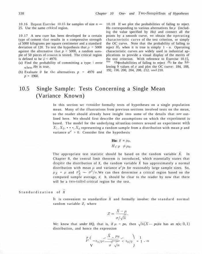
338 Chapter 10 One- and Two-Sample Tests of Hypotheses
10.16 Repeat Exercise: 10.15 for samples of size n — 10.18 If we plot the probabilities of failing to reject. 25. Use the same critical region. Ho corresponding to various alternatives for ft (includ
ing the value specified by Ho) and connect all the 10.17 A new cure has been developed for a certain points by a smooth curve, we obtain the ope ra t ing type of cement that results in a compressive strength charac ter i s t ic curve of the test criterion, or simply of 5000 kilograms per square centimeter and a standard the OC curve. Note that the probability of failing to deviation of 120. To test the hypothesis that p = 5000 reject Ho when it is true is simply 1 - o. Operating against the alternative that p < 5000, a random sam- characteristic curves are widely used in industrial apple of 50 pieces of cement is tested. The critical region plications to provide a visual display of the merits of is defined to be z < 4970. the test criterion. With reference to Exercise 10.15, (a) Find the probability of committing a type \ error filld thc probabilities of failing to reject Ha for the fol-
when Hn is true. lowing 9 values of /; and plot the OC curve: 184, 188,
(b) Evaluate 0 for the alternatives p = 4970 and p = 1960.
192, 196, 200, 204, 208. 212. and 210.
10.5 Single Sample: Tests Concerning a Single Mean (Variance Known)
In this section wc consider formally tests of hypotheses on a single population mean. Many of the illustrations from previous sections involved tests on the mean, so the reader should already have insight into some of the details tha t are outlined here. We should first describe the assumptions on which the experiment is based. The model for the underlying situation centers around an experiment with A'i, A'2, • • •, Xn representing a random sample from a distribution with mean p and variance a'2 > 0. Consider first the hypothesis
Ho: // = po, HI: p ^ po.
The appropriate test statistic should be based on the random variable X. In Chapter 8, the central limit theorem is introduced, which essentially states tha t despite the distribution of X, the random variable X has approximately a normal distribution with mean p. and variance a2 jn for reasonably large sample sizes. So, / /y = // and a2y — a2/n. We can then determine a critical region based on the computed sample average, x. It. should be clear to the reader by now that there will be a two-tailed critical region for the test.
S t a n d a r d i z a t i o n o f X
It is convenient to standardize X and formally involve: the s t a n d a r d n o r m a l random variable Z, where
z = =A a/^/rt
Wc: know that under HQ, t ha t is, if p = po, then ^/n.(X — po)/a has an n(x; 0,1) distribution, and hence the expression
P ( ^ % ~ ll° ^ >\ 1 P -Za/2 < 7-7=- < Za/2 = 1 - Q
V 0- yfn }
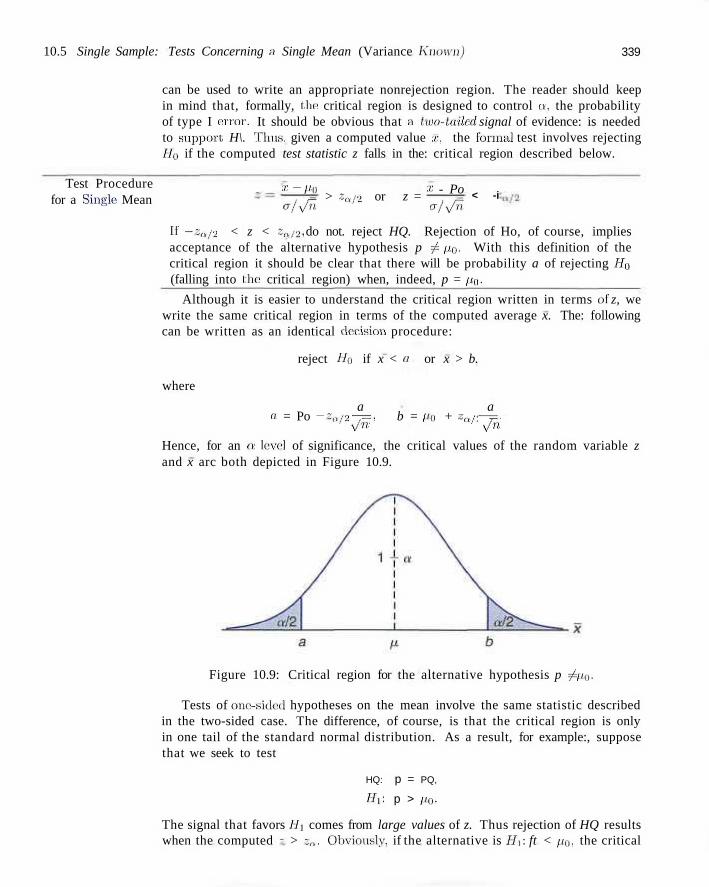
10.5 Single Sample: Tests Concerning a Single Mean (Variance Known) 339
can be used to write an appropriate nonrejection region. The reader should keep in mind that, formally, the critical region is designed to control n, the probability of type I error. It should be obvious that a two-toiled signal of evidence: is needed to support, H\. Thus, given a computed value ii:, the formal test involves rejecting Ho if the computed test statistic z falls in the: critical region described below.
Test Procedure for a Single Mean
•'' ~ Po cr/y/n
> za/2 or z = x - Po a/y/n
< -i
If —Za/2 < z < za/2, do not. reject HQ. Rejection of Ho, of course, implies acceptance of the alternative hypothesis p ^ p.0. With this definition of the critical region it should be clear that there will be probability a of rejecting HQ (falling into the: critical region) when, indeed, p = po-
Although it is easier to understand the critical region written in terms of z, we write the same critical region in terms of the computed average x. The: following can be written as an identical decision procedure:
where
reject Ho if x < <t or x > b.
a a a = Po - za/2-7=, b = po + zn/2 —j=.
y/n v/n
Hence, for an a level of significance, the critical values of the random variable z and x arc both depicted in Figure 10.9.
Figure 10.9: Critical region for the alternative hypothesis p ^ fi0.
Tests of one-sided hypotheses on the mean involve the same statistic described in the two-sided case. The difference, of course, is that the critical region is only in one tail of the standard normal distribution. As a result, for example:, suppose that we seek to test
HQ: p = PQ,
H I : p > po.
The signal that favors Hi comes from large values of z. Thus rejection of HQ results when the computed - > ~a. Obviously, if the alternative is Hi: ft < po, the critical
340 Chapter 10 One- and Two-Sample Tests of Hypotheses
region is entirely in the lower tail and thus rejection results from z < —Za. Although in a one-sided testing case the null hypothesis can be written as HQ : p. < pa or Ho: p > PQ, it is usually written as Ho: p. = PQ.
The following two examples illustrate tests on means for the case in which er is known.
Example 10.3:1 A random sample of 100 recorded deaths in the United States during the past year showed an average life span of 71.8 years. Assuming a population standard deviation of 8.9 years, does this seem to indicate that the: mean life span today is greater than 70 years? Use a 0.05 level of significance.
Solution: 1. HQ: p - 70 years.
2. H\: 11 > 70 years.
3. a = 0.05.
4. Critical region: z > 1.645, where z
5. Computations: x = 71.8 years, a =
zJisi o . '?:
.9 years, and 2 = Ji=^ = 2.02.
6. Decision: Reject HQ and conclude that the mean life span today is greater than 70 years.
In Example 10.3 the P-value corresponding to z = 2.02 is given by the area of the shaded region in Figure 10.10.
Figure 10.10: P-value for Example 10.3.
Using Table A.3, we have
P = P(Z > 2.02) = 0.0217.
As a result, the evidence in favor of Hi is even stronger than that suggested by a 0.05 level of significance. J
Example 10.4:1 A manufacturer of sports equipment has developed a new synthetic fishing line that he: claims has a mean breaking strength of 8 kilograms with a standard deviation of 0.5 kilogram. Test the hypothesis that p = 8 kilograms against the alternative that p ^ 8 kilograms if a random sample of 50 lines is tested and found to have a mean breaking strength of 7.8 kilograms. Use a 0.01 level of significance.
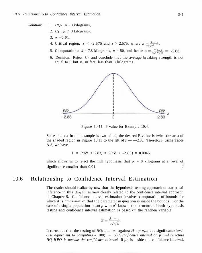
10.6' Relationship to Confidence Interval Estimation 341
Solution: l. HQ-. p = 8 kilograms,
2. H[: ft -£ 8 kilograms.
3. Q =0 .01 .
4. Critical region: z < -2.575 and z > 2.575, where z = ^&.
5. Computations: x = 7.8 kilograms, n = 50, and hence . 7.8-8 -2.83. 0.5/V50
6. Decision: Reject //(! and conclude that the average breaking strength is not equal to 8 but is, in fact, less than 8 kilograms.
Figure 10.11: P-value for Example 10.4.
Since the test in this example is two tailed, the desired P-value is twice: the area of the shaded region in Figure 10.11 to the left of z — —2.83. Therefore, using Table A.3, we have
P = P(\Z\ > 2.83) = 2P(Z < -2.83) = 0.0046.
which allows us to reject the null hypothesis that p. = 8 kilograms at a. level of
significance smaller than 0.01. J
10.6 Relationship to Confidence Interval Estimation
The reader should realize by now that the hypothesis-testing approach to statistical inference in this chapter is very closely related to the confidence interval approach in Chapter 9. Confidence interval estimation involves computation of bounds for which it is "reasonable" that the parameter in question is inside the bounds. For the case of a single: population mean p with a2 known, the structure of both hypothesis testing and confidence interval estimation is based on the random variable
X I' o/y/n"
It turns out that the testing of HQ: p — po against II\: p / po at a significance level a is equivalent to computing a 100(1 — a)% confidence interval on p and rejecting HQ if PO is outside the confidence internal. If PQ is inside the confidence interval.
342 Chapter 10 One- and Two-Sample Tests of Hypotheses
the hypothesis is not, rejected. The equivalence is very intuitive and quite simple to illustrate. Recall that with an observed value x failure to reject Ho at significance level a implies that
. x - po — Za/2 S T~/= S Zr.v/2:
' aj s/n which is equivalent to
a a x ~ za/2—j= < IH) < X + Za!2—=.
' yfll ' s/n The confidence interval equivalence to hypothesis testing extends to differences
between two means, variances, ratios of variances, and so on. As a result, the student of statistics should not consider confidence interval estimation and hypothesis testing as separate forms of statistical inference. For example, consider Example 9.2 on page 275. The: 95% confidence interval on the mean is given by the bounds (2.50, 2.70). Thus, with the same sample information, a two-sided hypothesis on p involving any hypothesized value between 2.50 and 2.70 will not be rejected. As we turn to different areas of hypothesis testing, the equivalence to the confidence interval estimation will continue to be exploited.
10.7 Single Sample: Tests on a Single Mean (Variance Unknown)
One would certainly suspect that tests on a. population mean p with a2 unknown, like confidence interval estimation, should involve the use of Student, f-distribution. Strictly speaking, the application of Student f for both confidence intervals and hypothesis testing is developed under the following assumptions. The random variables Xi,X2.... ,Xn represent a random sample from a normal distribution with unknown p. and a2. Then the random variable y/n(X — p)/S has a Student's it-distribution with n—1 degrees of freedom. The structure of the test is identical to that for the case of a known with the exception that the value a in the test statistic is replaced by the computed estimate S and the standard normal distribution is replaced by a /-distribution. As a result., for the two-sided hypothesis
Ho: p = po,
H\: ft / p o ,
rejection of Ho, at significance level O' results when a computed /-statistic
The /.-Statistic for a Test on a
Single Mean _ x — p 0
(Variance s/y/n Unknown)
exceeds ZQ/2,„-i or is less than —ta/2.„-\- The reader should recall from Chapters 8 and 9 that the: /-distribution is symmetric around the value zero. Thus, this two-tailed critical region applies in a fashion similar to that for the case of known a.
10.7 Single Sample: Tests on a Single Mean (Variance Unknown) 343
For the two-sided hypothesis at significance level a, the two-tailed critical regions apply. For H\: p > pa, rejection results when t > r„,T,_|. For H i : p < p.0, the critical region is given by / < — tfa,n_i.
Example 10.5:1 The Edison Electric Institute has published figures on the annual number of kilowatt hours expended by various home appliances. It is claimed that a vacuum cleaner expends an average of 46 kilowatt hours per year. If a random sample of 12 homes included in a planned study indicates that vacuum cleaners expend an average of 42 kilowatt hours per year with a standard deviation of 11.9 kilowatt hours, does this suggest at the 0.05 level of significance that vacuum cleaners expend, on the average, less than 46 kilowatt hours annually? Assume the population of kilowatt hours to be normal.
Solution: 1. HQ: p = 46 kilowatt hours.
2. Hi: p < 46 kilowatt hours.
3. a = 0.05.
4. Critical region: t < —1.796, where t = JT/T= with 11 degrees of freedom.
5. Computations: x = 42 kilowatt hours, s = 11.9 kilowatt hours, and n = 12. Hence
t 4 2 - 4 6
11.9/\/l2 = -1.16, P = P(T< -1.16) w 0.135.
6. Decision: Do not reject Ho and conclude that the average number of kilowatt, hours expended annually by home vacuum cleaners is not significantly less than 46. J
C o m m e n t o n t h e S i n g l e - S a m p l e T-Tes t
The reader has probably noticed that the equivalence of the two-tailed t-test for a single mean and the computation of a confidence interval on p with a replaced by s is maintained. For example, consider Example 9.5 on page 280. Essentially, we can view that computation as one in which we have found all values of po, the hypothesized mean volume of containers of sulfuric acid, for which the hypothesis Ho : p = po will not be rejected at o = 0.05. Again, this is consistent with the statement: "Based on the sample information, values of the population mean volume between 9.74 and 10.26 liters are not unreasonable."
Comments regarding the normality assumption are worth emphasis at this point. We have indicated that when a is known, the central limit theorem allows for the use of a test statistic or a confidence interval which is based on Z, the standard normal random variable. Strictly speaking, of course, the central limit theorem and thus the use of the standard normal does not apply unless a is known. In Chapter 8, the development of the ^-distribution is given. At that point it was stated that normality on Xy,X2,..., Xn was an underlying assumption. Thus, strictly speaking, the Student's /-tables of percentage points for tests or confidence intervals should not be used unless it is known that the sample comes from a normal population. In practice, a can rarely be assumed known. However,
344 Chapter 10 One-and Two-Sample Tests of Hypotheses
a very good estimate may be available from previous experiments. Many statistics textbooks suggest that one can safely replace a by s in the test statistic
_ x - po ajy/n '
when n > 30 and still use the Z-tables for the appropriate critical region. The implication here is that the central limit theorem is indeed being invoked and one is relying on the fact that swcr. Obviously, when this is done the results must be viewed as being approximate. Thus a computed P-value (from the Z-distribution) of 0.15 may be 0.12 or perhaps 0.17, or a computed confidence interval may be a 93% confidence interval rather than a 95% interval as desired. Now wdiat about situations where n < 30? The user cannot rely on s being close to a, and in order to take into account the inaccuracy of the estimate, the confidence interval should be wider or the critical value larger in magnitude. The /-distribution percentage points accomplish this but are correct only when the sample is from a normal distribution. Of course, normal probability plots can be used to ascertain some sense of the deviation of normality in a data set.
For small samples, it is often difficult to detect deviations from a normal distribution. (Goodness-of-fit tests are discussed in a later section of this chapter.) For bell-shaped distributions of the random variables Xx,X2,...,Xn, the use of the /-distribution for tests or confidence intervals is likely to be quite good. When in doubt, the user should resort to nonparametric procedures which are presented in Chapter 16.
Annotated Computer Printout for Single-Sample T-Test
It should be of interest for the reader to see annotated computer printout showing the result of a single-sample t-test. Suppose that an engineer is interested in testing the bias in a pH meter. Data are collected on a neutral substance (pH = 7.0). A sample of the measurements were taken with the data as follows:
7.07 7.00 7.10 6.97 7.00 7.03 7.01 7.01 6.98 7.08
It is, then, of interest to test
H0: p = 7.0,
Hi: p ^ 7.0.
In this illustration we use the computer package MINITAB to illustrate the analysis of the data set above. Notice the key components of the printout shown in Figure 10.12. Of course, the mean y — 7.0250, StDev is simply the sample standard deviation s = 0.044, and SE Mean is the estimated standard error of the mean and is computed as s/y/n = 0.0139. The i-value is the ratio
(7.0250-7)/0.0139= 1.80.
The P-value of 0.106 suggests results that are inconclusive. There is not a strong rejection of HQ (based on an a of 0.05 or 0.10), yet one certainly cannot
10.8 Two Samples: Tests on Two Means 345
pH-meter 7.07 7.00 7.10 6.97 7.00 7.03 7.01 7.01 6.98 7.08
MTB > Onet 'pH-meter ' ; SUBO Test 7.
One-Sample T: pH-meter Test of mu = 7 vs not = 7 Variable N Mean StDev SE Mean 95% CI T P pH-meter 10 7.02500 0.04403 0.01392 (6.99350. 7.05650) 1.80 0.106
Figure 10.12: MINITAB printout for one sample r-test for pH meter.
truly conclude that the pH meter is unbiased. Notice that the sample size of 10 is rather small. An increase in sample size (perhaps another experiment) may sort things out. A discussion regarding appropriate sample size appears in Section 10.9.
10.8 Two Samples: Tests on Two Means
The reader has already come to understand the relationship between tests and confidence intervals and can rely largely on details supplied by the confidence interval material in Chapter 9. Tests concerning two means represent a set of very important analytical tools for the scientist or engineer. The experimental setting is very much like that described in Section 9.8. Two independent random samples of size «i and n2, respectively, are drawn from two populations with means pi and p2 and variances o2 and a\. We know that the random variable
\/o\jnx + a\jn2
has a standard normal distribution. Here we are assuming that nx and n2 are sufficiently large that the central limit theorem applies. Of course, if the two populations are normal, the statistic above has a standard normal distribution even for small nx and n2. Obviously, if we can assume that ai — o2 = a, the statistic above reduces to
z = (Ag - X2) - (pi - p2)
o-y/l/nx + l / n 2
The two statistics above serve as a basis for the development of the test procedures involving two means. The confidence interval equivalence and the ease in the transition from the case of tests on one mean provide simplicity.
The two-sided hypothesis on two means can be written generally as
H0: pi - p2 = do-Obviously, the alternative can be two sided or one sided. Again, the distribution used is the distribution of the test statistic under Ho. Values xx and x2 are computed and, for CTI and CT2 known, the test statistic is given by
_ (xi - x2) - d0
s/a\/m +a\/n2
346 Chapter 10 One- and Two-Sample Tests of Hypotheses
with a two-tailed critical region in the case of a two-sided alternative. That is, reject Ho in favor of Hi: pi — p2 7 do if z > zai2 or z < —za/2. One-tailed critical regions are used in the case of the one-sided alternatives. The reader should, as before, study the test statistic and be satisfied that for, say, Hi : pi — p2 > do, the signal favoring Hi comes from large values of z. Thus the upper-tailed critical region applies.
Unknown But Equal Variances
The more prevalent situations involving tests on two means are those in which variances are unknown. If the scientist involved is willing to assume that both distributions are normal and that ox — o2 = a, the pooled t-test (often called the two-sample /-test) may be used. The test statistic (see Section 9.8) is given by the following test procedure.
Two-Sample Pooled T-Test t =
(xi - x2) - do
Spy/1/ni + \/n2
where
2__ s\(nx - \) + s\{n2 - I) Sp nx + n2 - 2
The /-distribution is involved and the two-sided hypothesis is not rejected when
—ta/2,nl+n-2-2 <t< £n/2,ni +n2-2-
Recall from material in Chapter 9 that the degrees of freedom for the /-distribution are a result of pooling of information from the two samples to estimate a2. Onesided alternatives suggest one-sided critical regions, as one might expect. For example, for H\\ p\ — p2 > do, reject H\: pi - p2 = do when / > r.Q:„1+„2_2.
Example 10.6:1 An experiment was performed to compare the abrasive wear of two different laminated materials. Twelve pieces of material 1 were tested by exposing each piece to a machine measuring wear. Ten pieces of material 2 were similarly tested. In each case, the depth of wear was observed. The samples of material 1 gave an average (coded) wear of 85 units with a sample standard deviation of 4, while the samples of material 2 gave an average of 81 and a sample standard deviation of 5. Can we conclude at the 0.05 level of significance that the abrasive wear of material 1 exceeds that of material 2 by more than 2 units? Assume the populations to be approximately normal with equal variances.
Solution: Let. pi and p2 represent, the population means of the abrasive wear for material 1 and material 2, respectively.
1. H0: pi - p2 = 2.
2. Hf.pi -p2>2.
3. a = 0.05.
4. Critical region: t > 1.725. where / = (a.1~a2)~d° with v = 20 degrees of spS/X/n\+l/n2
freedom.
10.8 Two Samples: Tests on Two Means 347
5. Computations:
Xx = 85, si = 4 , nx = 12,
.f:2 = 81, s2 = 5, n2 = 10.
Hence
(ll)(16) + (9)(25) V 12+10-2 '*'
t = ( 8 5 7 8 1 ) - 2 = 1.04, 4.478^/1/12 + 1/10
P = P(T > 1.04) w 0.16. (See Table A.4.)
6. Decision: Do not reject Ho. We are unable to conclude that the abrasive wear of material 1 exceeds that of material 2 by more than 2 units. J
Unknown But Unequal Variances
There are situations where the analyst is not able to assume that cri = er2. Recall from Chapter 9 that, if the populations are normal, the statistic
T, _ (A'i - X2) - do
y/s\/nx + s\/n2
has an approximate /-distribution with approximate degrees of freedom
js'{/ni + s\/n2)2
V (s2/m)2/(m -l) + (s2/n2)2/(n2 - 1)•
As a result, the test procedure is to not reject HQ when
~ta/2,v <t < ta/2tV,
with v given as above. Again, as in the case of the pooled t-test, one-sided alternatives suggest one-sided critical regions.
Paired Observations
When the student of statistics studies the two-sample t-test or confidence interval on the difference between means, he or she should realize that some elementary notions dealing in experimental design become relevant and must be addressed. Recall the discussion of experimental units in Chapter 9, where it is suggested at that point that the condition of the two populations (often referred to as the two treatments) should be assigned randomly to the experimental units. This is done to avoid biased results due to systematic differences between experimental units. In other words, in terms of hypothesis-testing jargon, it is important that the significant difference found (or not found) between means be due to the different conditions of the populations and not due to the experimental units in the study. For example, consider Exercise 9.40 in Section 9.9. The 20 seedlings play the role
348 Chapter 10 One-and Two-Sample Tests of Hypotheses
of the experimental units. Ten of them are to be treated with nitrogen and 10 with no nitrogen. It may be very important that this assignment to the "nitrogen" and "no-nitrogen" treatment be random to ensure that systematic differences between the seedlings do not interfere with a valid comparison between the means.
In Example 10.6, time of measurement, is the most likely choice of the experimental unit. The 22 pieces of material should be measured in random order. We need to guard against the possibility that wear measurements made close together in time might tend to give similar results. Systemat ic (nonrandom) differences in exper imenta l units are not expected. However, random assignments guard against the problem.
References to planning of experiments, randomization, choice of sample size, and so on, will continue to influence much of the development in Chapters 13, 14, and 15. Any scientist or engineer whose interest lies in analysis of real data should study this material. The pooled /-test is extended in Chapter 13 to cover more than two means.
Testing of two means can be accomplished when data are in the form of paired observations as discussed in Chapter 9. In this pairing structure, the conditions of the two populations (treatments) are assigned randomly within homogeneous units. Computation of the confidence interval for pi - p 2 in the situation with paired observations is based on the random variable
T ._ D ~ PD S,i/ \fn '
where D and S,i are random variables representing the sample mean and standard deviations of the differences of the observations in the experimental units. As in the case of the pooled t-test, the assumption is that the observations from each population are normal. This two-sample problem is essentially reduced to a one-sample problem by using the computed differences d\, d2,..., dn. Thus the hypothesis reduces to
Ho: po — dQ.
The computed test statistic is then given by
a - do t.=
Sd/y/n'
Critical regions are constructed using the t-distribution with n — 1 degrees of freedom.
Example 10.7:1 In a study conducted in the forestry and wildlife department at Virginia Polytechnic Institute and State University, J. A. Wesson examined the influence of the drug succinylcholine on the circulation levels of androgens in the blood. Blood samples from wild, free-ranging deer were obtained via the jugular vein immediately after an intramuscular injection of succinylcholine using darts and a capture gun. Deer were bled again approximately 30 minutes after the injection and then released. The levels of androgens at time of capture and 30 minutes later, measured in nanograms per milliliter (ng/ml), for 15 deer are given in Table 10.2.
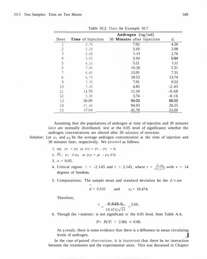
1 2 3 4 5 ii 7 8 9 10 11 12 13 14 15
2.76 5.18 2.68 3.05 4.10 7.05 6.60 4,79 7,39 7.30 11.78 3.90
26.00 67.48 17.04
10.8 Two Samples: Tests on Two Means 349
Table 10.2: Data, for Example 10.7
Androgen (ng/ml) Deer Time of Injection 30 Minutes after Injection d;
7.02 4.26 3.10 2.08 5.44 2.76 3.99 0.94 5.21 1.11
10.26 3.21 13.91 7.31 18.53 13.74
7.91 0.52 4.85 -2.45
11.10 -0.68 3.74 -0.16
94.03 68.03 94.03 26.55 41.70 24.66
Assuming that the populations of androgen at time of injection and 30 minutes later are normally distributed, test at the 0.05 level of significance whether the androgen concentrations are altered after 30 minutes of restraint.
Solution: Let pi and p2 be the average androgen concentration at the time of injection and 30 minutes later, respectively. We proceed as follows:
1. HQ: px = Pa or PD = Pi - P-2 = 0.
2. Hi; px ^ p-2 or pp = p\ - p2 ^ 0.
3. a = 0.05.
4. Critical region: / < -2.145 and /. > 2.145, where t = - M f e with v = 14
degrees of freedom.
5. Computations: The sample mean and standard deviation for the dj's are
d = 9.848 and sd = 18.474.
Therefore,
= 9.848-0 =
18.474/ v/15 6. Though the /-statistic: is not significant at. the 0.05 level, from Table A.4,
P= P(\T\ > 2.06) = 0.06.
As a result, there is some evidence that there is a difference in mean circulating levels of androgen.
In the case of paired observations, it is important that there be no interaction between the treatments and the experimental units. This was discussed in Chapter
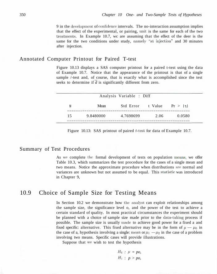
350 Chapter 10 One- and Two-Sample Tests of Hypotheses
9 in the development of confidence intervals. The no-interaction assumption implies that the effect of the experimental, or pairing, unit is the same for each of the two treatments. In Example 10.7, wc are assuming that the effect of the deer is the same for the two conditions under study, namely "at, injection'' and 30 minutes after injection.
Annotated Computer Printout for Paired T-test
Figure 10.13 displays a SAS computer printout for a paired t-test using the data of Example 10.7. Notice that the appearance of the printout is that of a single sample /-test and, of course, that is exactly what is accomplished since the test seeks to determine if d is significantly different from zero.
Analysis Variable : Diff
N Mean Std Error t Value Pr > It I
15 9.8480000 4.7698699 2.06 0.0580
Figure 10.13: SAS printout of paired /-test for data of Example 10.7.
Summary of Test Procedures
As wc complete the1 formal development of tests on population means, we offer Table 10.3, which summarizes the test procedure for the cases of a single mean and two means. Notice the approximate procedure when distributions are normal and variances are unknown but not assumed to be equal. This statistic was introduced in Chapter 9,
10.9 Choice of Sample Size for Testing Means
In Section 10.2 we demonstrate how the: analyst can exploit relationships among the sample size, the significance level o, and the power of the test to achieve a certain standard of quality. In most practical circumstances the experiment should be planned with a choice of sample size made prior to the data-taking process if possible. The sample size is usually made: to achieve good power for a fixed a and fixed specific: alternative. This fixed alternative may be in the form of p — po in the case of a, hypothesis involving a single: mean or ft\ — p,2 in the case of a problem involving two means. Specific cases will provide illustrations.
Suppose that wc wish to test the hypothesis
HQ : p = po,
H] : p > po,
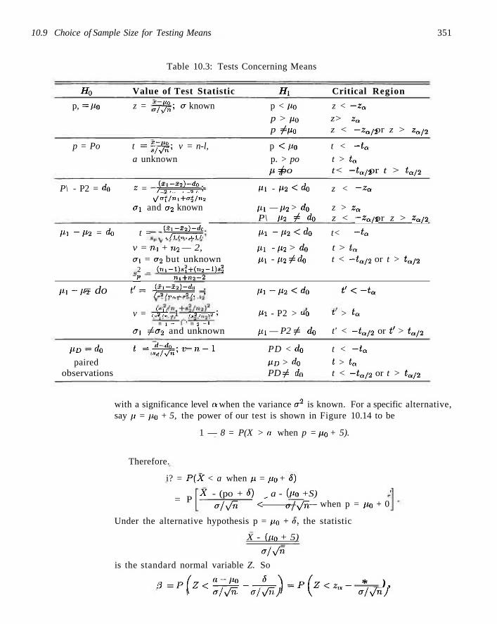
10.9 Choice of Sample Size for Testing Means 351
Table 10.3: Tests Concerning Means
Ho Value of Test Statistic Hi Critical Region
p, = po z = */!%'-, a known p < po z < —za
p > po z> za
p ^ po z < -zQ/2 or z > za/2
p = Po t = 2=J&; v = n-l, p <Po t < -ta
a unknown p. > po t > ta
p^ po t< -ta/2 or t > taj2
P\ - P2 = do z = }xl~S2)~t°, ; Pi - P2<d0 z < -za \Z"l/ni+<T^./n-2
CTI and a2 known pi — p2 > do z > za
P\ ~ P-2 ¥" do z < -za/2 or z > za/2
P! -1*2 = do t = (a;~g2)~d/0 ~ Pi -P2<dQ t< -ta
v = m + n2 — 2, px - p2 > do t > tn
ai = a2 but unknown pi - p2 ^ do t < —ta/2 or t > ta/2
2 _ ( n i - l ) g | + ( n a - l ) « l Jl »i+«2-2
p1-p2 = do t'= f'~g2)"2d; ; pi-p2<do t'<-ta
v = rjrr ,1 , i , i i ; Pi - P2 > «o r > t a n 1 — 1 ' n 2 - 1
<T[ ^ <r2 and unknown Pi — P2 ¥= do t' < —ta/2 or i ' > £Q/2
P D = d 0 < = ~ ^ ; v = n - l PD < d0 t < -tQ
paired P D > do t > ta
observations PD f^ do t < —ta/2 or t > ta/2
with a significance level a when the variance cr2 is known. For a specific alternative, say p = po + 5, the power of our test is shown in Figure 10.14 to be
1 — 8 = P(X > a when p = p0 + 5).
Therefore.
i? = P(X < a when /t = p 0 + 0)
= P A" - (po + &) ^ a - (pa +S) '
< / _ — when p = po + 0 cr/T/n ajy/n
Under the alternative hypothesis p = po + o, the statistic
X - (PQ + 5)
ajy/n-
is the standard normal variable Z. So
3 = p ( z < t ^ - * ) = P ( Z < Z a - * ) , \ a/yfn cr/y/n) \ <r/y/nj
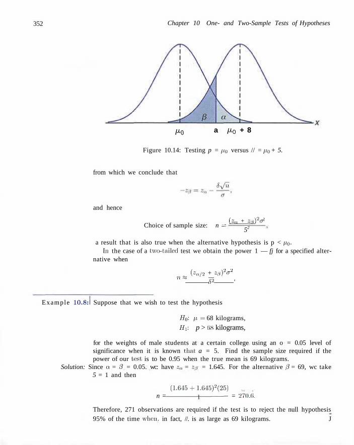
352 Chapter 10 One- and Two-Sample Tests of Hypotheses
^ 0 a pi0 + 8
Figure 10.14: Testing p = //o versus // = pu + 5.
from which we conclude that
Sy/n
and hence
2~2 Choice of sample size: n =
(Zg + Z(i)20
52
a result that is also true when the alternative hypothesis is p < PQ. In the case of a two-tailed test we obtain the power 1 — fj for a specified alter
native when
iZa/2 + Z,3)202
U * c^ '
Example 10.8:1 Suppose that we wish to test the hypothesis
Ho: p. = 68 kilograms,
H[-. p > 08 kilograms,
for the weights of male students at a certain college using an o = 0.05 level of significance when it is known that a = 5. Find the sample size required if the power of our test is to be 0.95 when the true mean is 69 kilograms.
Solution: Since a = 8. = 0.05. wc: have za = Zp = 1.645. For the alternative 8 = 69, wc take 5 = 1 and then
(1.645 +1.645)2(25) _ „ . n = ——- = 2/().f).
Therefore, 271 observations are required if the test is to reject the null hypothesis 95% of the time when, in fact, //. is as large as 69 kilograms. J
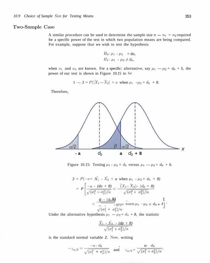
10.9 Choice of Sample Size for Testing Means 353
Two-Sample Case
A similar procedure can be used to determine the sample size n — nx = n2 required for a specific power of the test in which two population means are being compared. For example, suppose that we wish to test the hypothesis
H0: px - 11-2 = do,
Hi: pi - p2 ^ d0,
when cT| and er2 are known. For a specific: alternative, say //.j — p2 = do + S, the power of our test is shown in Figure 10.15 to lie
1 — 3 = P(\Xi — X2\ > a when p.] - p2 = do + 8.
Therefore,
- a d0 a d0 + 8
Figure 10.15: Testing p\ - p2 = do versus pi — p2 = do + 6.
3 = P(-(t < A', - A'2 < a when px - p2 = d0 + 8)
= P -a - (do + 8) (Xi - X2) - (d0 + 8)
y/Wl+oD/n y/Wi + o%)/n
a -(da+ 8) 1 < i, •> ,?7= w n e n Ml - P2 = do + 8\
s/(a[ + a2) /n Under the alternative hypothesis px — p2 = c/o + 8, the statistic
Xx - X-2 - (dp + 8)
\/(a2+al)/n
is the standard normal variable Z. New, writing
*a/2 - « - do , a- do
and z,t/2 = y/ia'i + al)/n y/(a2+a2)/n
354 Chapter 10 One- and Two-Sample Tests of Hypotheses
we have
3 = P -ZQ/2 ========= < Z < ZQ/2 -y/ial + o^/n ~a,z y/io(+oi)jn
from which we conclude that
-zg «= za/2 -y/Taf+aJ)J7i'
and hence
iza/2 + zg)2(a\ + a\) n ^ :
62
For the one-tailed test, the expression for the required sample size when n = ni = n2 is
iza + zg)2ia2 + a2) Choice of sample size: n —
82
When the population variance (or variances in the two-sample situation) is unknown, the choice of sample size is not straightforward. In testing the hypothesis p = po when the true value is p = po + <5, the statistic
X-(p0+8)
S/y/n
does not follow the ^-distribution, as one might expect, but instead follows the noncentral ^-distribution. However, tables or charts based on the noncentral ^-distribution do exist for determining the appropriate sample size if some estimate of a is available or if 8 is a multiple of a. Table A.8 gives the sample sizes needed to control the values of a and 0 for various values of
A = =J£1 _ \P ~ PQ\ a a
for both one- and two-tailed tests. In the case of the two-sample i-test in which the variances are unknown but assumed equal, we obtain the sample sizes n = rai = n2
needed to control the values of a and 0 for various values of
A = M _ iMi - P 2 - d 0 | a a
from Table A.9.
Example 10.9:1 In comparing the performance of two catalysts on the effect of a reaction yield, a two-sample t-test is to be conducted with a = 0.05. The variances in the yields are considered to be the same for the two catalysts. How large a sample for each catalyst is needed to test the hypothesis
Ho: pi = p 2 ,
Hi: pi ^ p2,
10.10 Graphical Methods for Comparing Means 355
if it is essential to detect a difference of O.Ser between the catalysts with probability 0.9?
Solution: From Table A.9, with o = 0.05 for a two-tailed test, 0 = 0.1, and
jO.Scrl A = - = 0.8,
we find the required sample size to be n = 34. J It is emphasized that in practical situations it might be difficult to force a
scientist or engineer to make a commitment on information from which a value of A can be found. The reader is reminded that the A-value quantifies the kind of difference between the means that the scientist considers important, that is, a difference considered significant, from a scientific, not a statistical, point of view. Example 10.9 illustrates how this choice is often made, namely, by selecting a fraction of a. Obviously, if the sample size is based on a choice of \8\ that, is a small fraction of a, the resulting sample size may be quite large compared to what the study allows.
10.10 Graphical Methods for Comparing Means
In Chapter 1 considerable attention is directed toward displaying data in graphical form. Stem-and-leaf plot displays and, in Chapter 8, box-and-whisker, quantile plots, and quantile-quantile normal plots are used to provide a "picture" to summarize a set of experimental data. Many computer software packages produce graphical displays. As we proceed to other forms of data analysis (e.g., regression analysis and analysis of variance). graphical methods become even more informative.
Graphical aids used in conjunction with hypothesis testing arc not used as a replacement of the test procedure. Certainly, the value of the test statistic indicates the proper type of evidence in support of HQ or Hi. However, a pictorial display provides a good illustration and is often a better communicator of evidence to the beneficiary of the analysis. Also, a picture will often clarify why a significant difference was found. Failure of an important assumption may be exposed by a summary type of graphical display.
For the comparison of means, side-by-side box-and-whisker plots provide a telling display. The reader should recall that these plots display the 25th percentile, 75th percentile, and the median in a data set. In addition, the whiskers display the extremes in a data set. Consider Exercise 10.40 following this section. Plasma ascorbic acid levels were measured in two groups of pregnant women, smokers and nonsmokers. Figure 10.16 shows the box-and-whisker plots for both groups of women. Two things are very apparent. Taking into account variability, there: appears to be a negligible difference in the sample moans. In addition, the variability in the two groups appears to be somewhat different. Of course, the analyst must keep in mind the rather sizable differences between the sample sizes in this case.
Consider Exercise 9.40 in Section 9.9. Figure 10.17 shows the multiple box-and-whisker plot for the data of 10 seedlings, half given nitrogen and half given no nitrogen. The display reveals a smaller variability for the group containing no
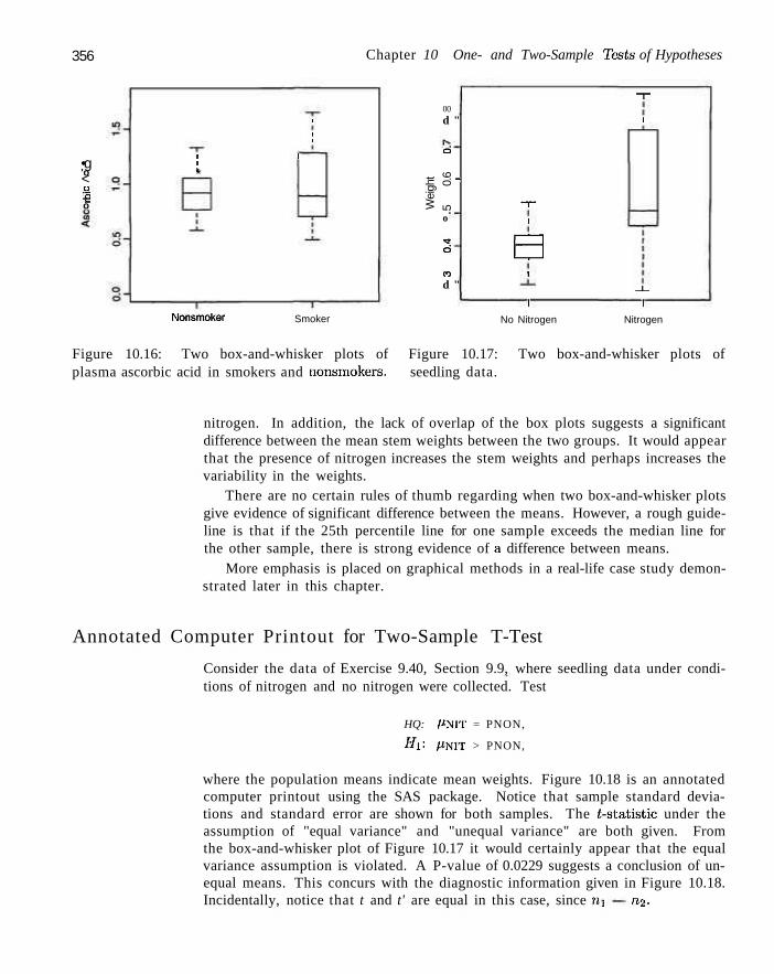
356 Chapter 10 One- and Two-Sample Tests of Hypotheses
•g 'o < o '•£ o
i
i i
i I i i *
00
d "
ci
Wei
ght
5 0.
6 i
o
•a-ci
CO
d "
-r i
B i
i
-r-
i
_ i _
1 Nonsmoker Smoker No Nitrogen Nitrogen
Figure 10.16: Two box-and-whisker plots of Figure 10.17: Two box-and-whisker plots of plasma ascorbic acid in smokers and nonsmokers. seedling data.
nitrogen. In addition, the lack of overlap of the box plots suggests a significant difference between the mean stem weights between the two groups. It would appear that the presence of nitrogen increases the stem weights and perhaps increases the variability in the weights.
There are no certain rules of thumb regarding when two box-and-whisker plots give evidence of significant difference between the means. However, a rough guideline is that if the 25th percentile line for one sample exceeds the median line for the other sample, there is strong evidence of a difference between means.
More emphasis is placed on graphical methods in a real-life case study demonstrated later in this chapter.
Annotated Computer Printout for Two-Sample T-Test
Consider the data of Exercise 9.40, Section 9.9, where seedling data under conditions of nitrogen and no nitrogen were collected. Test
HQ: PNIT = PNON,
H I : PNIT > PNON,
where the population means indicate mean weights. Figure 10.18 is an annotated computer printout using the SAS package. Notice that sample standard deviations and standard error are shown for both samples. The i-statistic under the assumption of "equal variance" and "unequal variance" are both given. From the box-and-whisker plot of Figure 10.17 it would certainly appear that the equal variance assumption is violated. A P-value of 0.0229 suggests a conclusion of unequal means. This concurs with the diagnostic information given in Figure 10.18. Incidentally, notice that t and t' are equal in this case, since nx — n2.
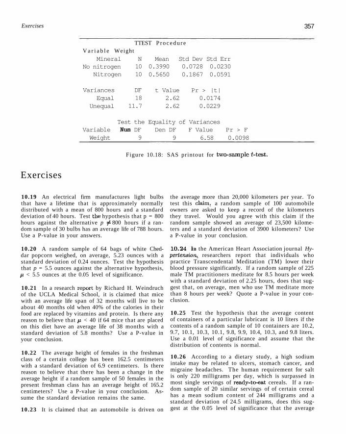
Exercises 357
TTEST P r o c e d u r e V a r i a b l e Weight
Mineral No nitrogen
Nitrogen
Variances Equal
Unequal
N 10 10
DF 18
11.7
Test the Variable Num DF Weight 9
Mean Std Dev Std Err 0.3990 0.0728 0.0230 0.5650 0.1867 0.0591
t Value Pr > |t| 2.62 0.0174 2.62 0.0229
Equality of Variances Den DF F Value Pr > F
9 6.58 0.0098
Figure 10.18: SAS printout for two-sample t-test.
Exercises
10.19 An electrical firm manufactures light bulbs that have a lifetime that is approximately normally distributed with a mean of 800 hours and a standard deviation of 40 hours. Test tbe hypothesis that p = 800 hours against the alternative p ^ 800 hours if a random sample of 30 bulbs has an average life of 788 hours. Use a P-value in your answers.
10.20 A random sample of 64 bags of white Cheddar popcorn weighed, on average, 5.23 ounces with a standard deviation of 0.24 ounces. Test the hypothesis that p = 5.5 ounces against the alternative hypothesis, p < 5.5 ounces at the 0.05 level of significance.
10.21 In a research report by Richard H. Weindruch of the UCLA Medical School, it is claimed that mice with an average life span of 32 months will live to be about 40 months old when 40% of the calories in their food are replaced by vitamins and protein. Is there any reason to believe that /z < 40 if 64 mice that are placed on this diet have an average life of 38 months with a standard deviation of 5.8 months? Use a P-value in your conclusion.
10.22 The average height of females in the freshman class of a certain college has been 162.5 centimeters with a standard deviation of 6.9 centimeters. Is there reason to believe that there has been a change in the average height if a random sample of 50 females in the present freshman class has an average height of 165.2 centimeters? Use a P-value in your conclusion. Assume the standard deviation remains the same.
10.23 It is claimed that an automobile is driven on
the average more than 20,000 kilometers per year. To test this claim, a random sample of 100 automobile owners are asked to keep a record of the kilometers they travel. Would you agree with this claim if the random sample showed an average of 23,500 kilometers and a standard deviation of 3900 kilometers? Use a P-value in your conclusion.
10.24 In the American Heart Association journal Hypertension, researchers report that individuals who practice Transcendental Meditation (TM) lower their blood pressure significantly. If a random sample of 225 male TM practitioners meditate for 8.5 hours per week with a standard deviation of 2.25 hours, does that suggest that, on average, men who use TM meditate more than 8 hours per week? Quote a P-value in your conclusion.
10.25 Test the hypothesis that the average content of containers of a particular lubricant is 10 liters if the contents of a random sample of 10 containers are 10.2, 9.7, 10.1, 10.3, 10.1, 9.8, 9.9, 10.4, 10.3, and 9.8 liters. Use a 0.01 level of significance and assume that the distribution of contents is normal.
10.26 According to a dietary study, a high sodium intake may be related to ulcers, stomach cancer, and migraine headaches. The human requirement for salt is only 220 milligrams per day, which is surpassed in most single servings of ready-to-eat cereals. If a random sample of 20 similar servings of of certain cereal has a mean sodium content of 244 milligrams and a standard deviation of 24.5 milligrams, does this suggest at the 0.05 level of significance that the average
358 Chapter 10 One- and Two-Sample Tests of Hypotheses
sodium content for a single serving of such cereal is greater than 220 milligrams? Assume the distribution of sodium contents to be normal.
10.27 A study at the University of Colorado at Boulder shows that running increases the percent resting metabolic rate (RMR) in older women. The average RMR of 30 elderly women runners was 34.0% higher than the average RMR of 30 sedentary elderly women and the standard deviations were reported to be 10.5% and 10.2%, respectively. Was there a significant increase in RMR of the women runners over the sedentary women? Assume the populations to be approximately normally distributed with equal variances. Use a P-value in your conclusions.
10.28 According to Chemical Engineering an important property of fiber is its water absorbency. The average percent absorbency of 25 randomly selected pieces of cotton fiber was found to be 20 with a standard deviation of 1.5. A random sample of 25 pieces of acetate yielded an average percent of 12 with a standard deviation of 1.25. Is there strong evidence that the population mean percent absorbency for cotton fiber is significantly higher than the mean for acetate. Assume that the percent absorbency is approximately normally distributed and that the population variances in percent absorbency for the two fibers are the same. Use a significance level of 0.05.
10.29 Past experience indicates that the time for high school seniors to complete a standardized test is a normal random variable with a mean of 35 minutes. If a random sample of 20 high school seniors took an average of 33.1 minutes to complete this test with a standard deviation of 4.3 minutes, test the hypothesis at the 0.05 level of significance that p = 35 minutes against the alternative that p < 35 minutes.
10.30 A random sample of size m = 25, taken from a normal population with a standard deviation eri = 5.2, has a mean xi = 81. A second random sample of size ri2 = 36, taken from a different normal population with a standard deviation a2 = 3.4, has a mean x2 = 76. Test the hypothesis that p\ — p2 against the alternative pi i^ pi- Quote a P-value in your conclusion.
10.31 A manufacturer claims that the average tensile strength of thread A exceeds the average tensile strength of thread B by at least 12 kilograms. To test his claim, 50 pieces of each type of thread are tested under similar conditions. Type A thread had an average tensile strength of 86.7 kilograms with known standard deviation of a A = 6.28 kilograms, while type B thread had an average tensile strength of 77.8 kilograms with known standard deviation of an = 5.61 kilograms. Test the manufacturer's claim a ta = 0.05.
10.32 Amstat News (December 2004) lists median salaries for associate professors of statistics at research institutions and at liberal arts and other institutions in the United States. Assume a sample of 200 associate professors from research institutions having an average salary of $70,750 per year with a standard deviation of S6000. Assume also a sample of 200 associate professors from other types of institutions having an average salary of $65,200 with a standard deviation of $5000. Test the hypothesis that the mean salary for associate professors in research institutions is $2000 higher than for those in other institutions. Use a 0.01 level of significance. Assume equal variances.
10.33 A study is made to see if increasing the substrate concentration has an appreciable effect on the velocity of a chemical reaction. With a substrate concentration of 1.5 moles per liter, the reaction was run 15 times with an average velocity of 7.5 micromoles per 30 minutes and a standard deviation of 1.5. With a substrate concentration of 2.0 moles per liter, 12 runs were made, yielding an average velocity of 8.8 micro-moles per 30 minutes and a sample standard deviation of 1.2. Is there any reason to believe that this increase in substrate concentration causes an increase in the mean velocity by more than 0.5 micromole per 30 minutes? Use a 0.01 level of significance and assume the populations to be approximately normally distributed with equal variances.
10.34 A study was made to determine if the subject matter in a physics course is better understood when a lab constitutes part of the course. Students were randomly selected to participate in either a 3-semester-hour course without labs or a 4-semester-hour course with labs. In the section with labs, 11 students made an average grade of 85 with a standard deviation of 4.7, and in the section without labs, 17 students made an average grade of 79 with a standard deviation of 6.1. Would you say that the laboratory course increases the average grade by as much as 8 points? Use a P-value in your conclusion and assume the populations to be approximately normally distributed with equal variances.
10.35 To find out whether a new serum will arrest leukemia, 9 mice, all with an advanced stage of the disease, are selected. Five mice receive the treatment and 4 do not. Survival times, in years, from the time the experiment commenced are as follows:
Treatment No Treatment
2.1 5.3 1.4 4.6 0.9 1.9 0.5 2.8 3.1
At the 0.05 level of significance can the serum be said to be effective? Assume the two distributions to be normally distributed with equal variances.
10.36 A large automobile manufacturing company is
Exercises 359
trying to decide whether to purchase brand A or brand B tires for its new models. To help arrive at a decision, an experiment is conducted using 12 of each brand. The tires are run until they wear out. The results are
Brand A: xi = 37, 900 kilometers,
si = 5,100 kilometers.
Brand B: xi = 39,800 kilometers,
,S2 = 5, 900 kilometers.
Test the hypothesis that there is no difference in the average wear of 2 brands of tires. Assume the populations to be approximately normally distributed with equal variances. Use a P-value.
10.37 In Exercise 9.42 on page 298, test the hypothesis that Volkswagen mini-trucks, on the average, exceed similarly equipped Toyota mini-trucks by 4 kilometers per liter. Use a 0.10 level of significance.
10.38 A UCLA researcher claims that the average life span of mice can be extended by as much as 8 months when the calories in their food are reduced by approximately 40% from the time they are weaned. The restricted diets are enriched to normal levels by vitamins and protein. Suppose that a random sample of 10 mice are fed a normal diet and live an average life span of 32.1 months with a standard deviation of 3.2 months, while a random sample of 15 mice are fed the restricted diet and live an average life span of 37.6 months with a standard deviation of 2.8 months. Test the hypothesis at the 0.05 level of significance that the average life span of mice on this restricted diet is increased by 8 months against the alternative that the increase is less than 8 months. Assume the distributions of life spans for the regular and restricted diets are approximately normal with equal variances.
10.39 The following data represent the running times of films produced by 2 motion-picture companies:
Company Time (minutes) 1 102 86 98 109 92 2 81 165 97 134 92 87 114
Test the hypothesis that the average running time of films produced by company 2 exceeds the average running time of films produced by company 1 by 10 minutes, against the one-sided alternative that the difference is less than 10 minutes. Use a 0.1 level of significance and assume the distributions of times to be approximately normal with unequal variances.
10.40 In a study conducted at the Virginia Polytechnic Institute and State University, the plasma ascorbic acid levels of pregnant women were compared for smokers versus nonsmokers. Thirty-two women in the last
three months of pregnancy, free of major health disorders, and ranging in age from 15 to 32 years, were selected for the study. Prior to the collection of 20 ml of blood, the participants were told to avoid breakfast, forgo their vitamin supplements, and avoid foods high in ascorbic acid content. From the blood samples, the following plasma ascorbic acid values of each subject were determined in milligrams per 100 milliliters:
Plasma Ascorbic Acid Values Nonsmokers 0.97 0.72 1.00 0.81 0.62 1.32 1.24 0.99 0.90 0.74 0.88 0.94
1.16 0.86 0.85 0.58 0.57 0.64 0.98 1.09 0.92 0.78 1.24 1.18
Smokers 0.48 0.71 0.98 0.68 1.18 1.36 0.78 1.64
Is there sufficient evidence to conclude that there is a difference between plasma ascorbic acid levels of smokers and nonsmokers? Assume that the two sets of data came from normal populations with unequal variances. Use a P-value.
10.41 A study was conducted by the Department of Zoology at the Virginia Polytechnic Institute and State University to determine if there is a significant difference in the density of organisms at two different sta-tions located on Cedar Run, a secondary stream located in the Roanoke River drainage basin. Sewage from a sewage treatment plant and overflow from the Federal Mogul Corporation settling pond enter the stream near its headwaters. The following data give the density measurements, in number of organisms per square meter, at the two different collecting stations:
Number of Organisms per Square Station
5030 13,700 10,730 11,400
860 2200 4250
15,040
1 4980
11,910 8130
26,850 17,660 22,800
1130 1690
M e t e r Station 2
2800 4670 6890 7720 7030 7330
2810 1330 3320 1230 2130 2190
Can we conclude, at the 0.05 level of significance, that the average densities at the two stations are equal? Assume that the observations come from normal populations with different variances.
10.42 Five samples of a ferrous-type substance are to
360 Chapter 10 One- and Two-Sample Tests of Hypotheses
be used to determine if there is a difference between a laboratory chemical analysis and an X-ray fluorescence analysis of the iron content. Each sample was split into two subsamples and the two types of analysis were applied. Following are the coded data showing the iron content analysis:
Analysis X-ray
Chemical
1 2.0 2.2
Sample 2 3 4
2.0 2.3 2.1 1.9 2.5 2.3
5 2.4 2.4
Assuming that the populations are normal, test at the 0.05 level of significance whether the two methods of analysis give, on the average, the same result.
10.43 A taxi company manager is trying to decide whether the use of radial tires instead of regular belted tires improves fuel economy. Twelve cars were equipped with radial tires and driven over a prescribed test course. Without changing drivers, the same cars were then equipped with regular belted tires and driven once again over the test course. The gasoline consumption, in kilometers per liter, was recorded as follows:
Kilometers per Liter Car
1 2 3 4 5 6 7 8 9 10 11 12
Radial T i res 4.2 4.7 6.6 7.0 6.7 4.5 5.7 6.0 7.4 4.9 6.1 5.2
Belted Tires 4.1 4.9 6.2 6.9 6.8 4.4 5.7 5.8 6.9 4.7 6.0 4.9
Can we conclude that cars equipped with radial tires give better fuel economy than those equipped with belted tires? Assume the populations to be normally distributed. Use a P-valne in your conclusion.
10.44 In Exercise 9.88 on page 315, use the t-distribution to test the hypothesis that the diet reduces a person's weight by 4.5 kilograms on the average against the alternative hypothesis that the mean difference in weight is less than 4.5 kilograms. Use a P-value.
10.45 According to the published reports, practice under fatigued conditions distorts mechanisms which govern performance. An experiment was conducted using 15 college males who were trained to make a continuous horizontal right-to-left arm movement from a microswitch to a barrier, knocking over the barrier coincident with the arrival of a clock sweephand to the
6 o'clock position. The absolute value of the difference between the time, in milliseconds, that it took to knock over the barrier and the time for the sweephand to reach the 6 o'clock position (500 msec) was recorded. Each participant performed the task five times under prefatigue and postfatigue conditions, and the sums of the absolute differences for the five performances were recorded as follows:
Absolute Time Differences Subject
1 2 3 4 5 6 7 8 9
10 11 12 13 14 15
Prefatigue 158 92 05 98 33 89
148 58
142 117 74 66
109 57 85
Postfatigue 91 59
215 226 223 91 92
177 134 116 153 219 143 164 100
An increase in the mean absolute time differences when the task is performed under postfatigue conditions would support the claim that practice under fatigued conditions distorts mechanisms that govern performance. Assuming the populations to be normally distributed, test this claim.
10.46 In a study conducted by the Department of Human Nutrition and Foods at the Virginia Polytechnic Institute and State University the following data on the comparison of sorbic acid residuals in parts per million in ham immediately after dipping in a sorbate solution and after 60 days of storage were recorded:
Sorbic Acid Residuals in Ham Slice
1 2 3 4 5 6 7 8
Before Storage 224 270 400 444 590 660
1400 680
After Storage 116 96
239 329 437 597 689 576
Assuming the populations to be normally distributed, is there sufficient evidence, at the 0.05 level of significance, to say that the length of storage influences sorbic acid residual concentrations?
10.47 How large a sample is required in Exercise 10.20 if the power of our test is to be 0.90 when the
10.11 One Sample: Test on a Single Proportion 3G1
true mean is 5.20? Assume: that a = 0.24.
10.48 I f the distribution of life spans in Exercise: 10.21 is approximately normal, how large a sample: is required in order that the probability of committing a type 11 error be 0.1 when the true mean is 35.9 months? Assume that a = 5.8 months.
10.49 How large a sample: is required in Exercise 10.22 if the power of our test is to be 0.95 when the true average height differs from J62.5 by 3.1 centimeters? Use: a = 0.02.
10.50 How large should the samples be in Exercise 10.31 if the power of our test is to be 0.95 vvlie:n the true difference between thread types A and B is 8 kilo-
Dog Knife S t r e n g t h 1 1 2 2 3 3 4 4 5 5 6 6 7 7 8 8
Hot Cold Hot:
Cold Hot,
Cold Hot
Cold Hot
Cold Hot
Cold Hot
Cold Hot.
Cold
5120 8200
10000 8000
10000 9200
10000 6200
10000 10000 7900 5200
510 885
1020 4G0
10.51 How large a sample is required in Exercise 10.24 if the power of our test is to be 0.8 when the true mean meditation time exceeds the hypothesized value by L.2ff? Use a = 0.05.
10.52 On testing
Ho: p = 14, Hi: P ? M 4 ,
an Q = 0.05 level t-test is being considered. What sample size is necessary in order that the probability is 0.1 of falsely failing to reject Ho when the true population mean differs from 14 by 0.5? From a preliminary sample we estimate er to be 1.25.
10.53 A study was conducted at the Department of Veterinary Medicine at Virginia Polytechnic Institute and State University to determine if the "strength" of a wound from surgical incision is affected by the temperature of the knife. Eight dogs were used in the experiment. The incision was performed in the abdomen of the animals. A "hot" and "cold" incision was made on each dog and the strength was measured. The resulting data appear below.
(a) Write1 an appropriate: hypothesis to determine if there is a significant difference in strength between the hot and cold incisions.
(b) Test the hypothesis using a paired /-test. Use a P-valne in your conclusion.
10.54 Nine subjects were ust:el in an experiment to determine if an atmosphere involving exposure to carbon monoxide has an impact on breathing capability. The data were collected by personnel in the Health and Physical Education Department at Virginia Polytechnic Institute and State University. The data were analyzed in the Statistics Consulting Center at Hokie Land. The subjects were exposed to breathing chambers, one of which contained a high concentration of CO. Several breathing measures were made for each subject for each chamber. The: subjects were exposed to the breathing chambers in random sequence. The data give the breathing frequency in number of breaths taken per minute. Make a one-sided test of the hypothesis that mean breathing frequency is the same for the two environments. Use a = 0.05. Assume that breathing frequency is approximately normal.
Subject 1 2 3 4 5 6 7 8 1)
W i t h C O 30 45 26 25 34 51 16 :V2 30
W i t h o u t C O 30 40 25 23 30 19
41 35 28
10.11 One Sample: Test on a Single Proportion
Tests of hypotheses concerning proportions are required in many areas. The politician is certainly interested in knowing what fraction of the voters will favor him in the next election. All manufacturing firms tiro concerned about the proportion of
362 Chapter 10 One-and Two-Sample Tests of Hypotheses
defective items when a shipment is made. The gambler depends on a knowledge of the proportion of outcomes that he or she considers favorable.
We shall consider the problem of testing the hypothesis that the proportion of successes in a binomial experiment equals some specified value. That is, we are testing the null hypothesis HQ that p = po, where p is the parameter of the binomial distribution. The alternative hypothesis may be one of the usual one-sided or two-sided alternatives:
p < po, p> po, or p jt po.
The appropriate random variable on which we base our decision criterion is the binomial random variable X, although we could just as well use the statistic p = X/n. Values of X that are far from the mean p = npo will lead to the rejection of the null hypothesis. Because AT is a discrete binomial variable, it is unlikely that a critical region can be established whose size is exactly equal to a prespecified value of Q. For this reason it is preferable, in dealing with small samples, to base our decisions on P-values. To test the hypothesis
HQ: p = Po,
Hi: p<p0,
we use the binomial distribution to compute the P-value
P = P(X < x when p = p0).
The value x is the number of successes in our sample of size n. If this P-value is less than or equal to a, our test is significant at the a level and we reject H0 in favor of Hi. Similarly, to test the hypothesis
HQ: P = Pu,
Hi: p > po,
at the ei-level of significance, we compute
P = P(X > x when p = po)
and reject Ho in favor of Hi if this P-value is less than or equal to a. Finally, to test the hypothesis
H0: P = Po,
Hi: p^po, at the Q-level of significance, we compute
P = 2P(X < x when p — po) if x < npo, or
P = 2P(X > x when p — p0) if x > npo
and reject Ho in favor of H\ if the computed P-value is less than or equal to a. The steps for testing a null hypothesis about a proportion against various al
ternatives using the binomial probabilities of Table A.l are as follows:
10.11 One Sample: Test on a Single Proportion 363
Testing a 1. HQ: p = p0-Proportion: 2. One of the alternatives H\: p < pn, p > po, or p ^ po-
Small Samples 3. Choose a level of significance equal to a. 4. Test statistic: Binomial variable X with p = p0 . 5. Computations: Find x, the number of successes, and compute the appropriate P-value. 6. Decision: Draw appropriate conclusions based on the P-value.
Example 10.10:1 A builder claims that heat pumps are installed in 70% of all homes being constructed today in the city of Richmond, Virginia. Would you agree with this claim if a random survey of new homes in this city shows that 8 out of 15 had heat pumps installed? Use a 0.10 level of significance.
Solution: 1. HQ: p = 0.7.
2. Hi: p 7^0.7.
3. o = 0 . 1 0 .
4. Test statistic: Binomial variable X with p = 0.7 and n = 15.
5. Computations: x — 8 and np0 = (15)(0.7) = 10.5. Therefore, from Table A.l, the computed P-value is
8
P = 2P(X < 8 when p = 0.7) = 2 ^ b(x; 15,0.7) = 0.2622 > 0.10. x=0
6. Decision: Do not reject HQ. Conclude that there is insufficient reason to doubt the builder's claim. J
In Section 5.3. we saw that binomial probabilities were obtainable from the actual binomial formula or from Table A.l when n is small. For large n, approximation procedures are required. When the hypothesized value po is very close to 0 or 1, the Poisson distribution, with parameter p = npo, may be used. However, the normal-curve approximation, with parameters p = npo, and a2 = npoqo, is usually preferred for large n and is very accurate as long as po is not extremely close to 0 or to 1. If we use the normal approximation, the z-value for t es t ing p= po is given by
x - npo p-po
y/nPoqo y/poqo/n
which is a value of the standard normal variable Z. Hence, for a two-tailed test at the o-level of significance, the critical region is z < —2Q/o or z > za/2. For the one-sided alternative p < po, the critical region is z < —za, and for the alternative p > po, the critical region is z > za.
Example 10.11:1 A commonly prescribed drug for relieving nervous tension is believed to be only 60% effective. Experimental results with a new drug administered to a random sample of 100 adults who were suffering from nervous tension show that 70 received relief. Is this sufficient evidence to conclude that the new drug is superior to the one commonly prescribed? Use a 0.05 level of significance.
364 Chapter 10 One- and Two-Sample Tests of Hypotheses
Solution: 1. HQ: p = 0.6.
2. Hi: p > 0 . 6 .
3. a = 0.05.
4. Critical region: 2 > 1.645.
5. Computations: x = 70. n = 100. p = 70/100 = 0.7, and
= 2.04, P = P(Z > 2.04) < 0.0207. v/(0.(i)(0.4)/10(J
6. Decision: Reject Ho and conclude that the new drug is superior.
10.12 Two Samples: Tests on Two Proportions
Situations often arise where we wish to test the hypothesis that two proportions are equal. For example, we might try to show evidence that the proportion of doctors who are pediatricians in one state is equal to the proportion of pediatricians in another state. A person may decide to give up smoking only if he or she is convinced that the proportion of smokers with lung cancer exceeds the proportion of nonsmokers with lung cancer.
In general, we wish to test the: null hypothesis that two proportions, or binomial parameters, are equal. That: is, we are testing pi = p2 against one of the alternatives p\ < p2, pi > p2, or p\ ^ -p2- Of course, this is equivalent to testing the null hypothesis that, p\ — p2 = 0 against one of the alternatives pi — P2 < 0, Pi ~ Pa > 0, or pi — po T 0- The statistic on which we base our decision is the random variable Pi — P2. Independent samples of size n\ and n2 are selected at random from two binomial populations and the proportion of successes P] and P2 for the two samples is computed.
In our construction of confidence intervals for pi and P2 wc noted, for »i and n2
sufficiently large, that the point estimator P] minus P2 was approximately normally distributed with mean
P-p, - A ~Pi ~P2
and variance
2 P1Q1 , P2Q2 a
P,-iX = — + — • ' 1 ' - nx ii2
Therefore, our critical region(s) can be established by using the standard normal variable
z _ ( A - P 3 ) - ( P l - P 2 )
\/pt f / i /»i +P2q->/i>2
When HQ is true, we can substitute pi = p2 = p and c/i = c/2 = q (where p and q are the common values) in the preceding formula for Z to give the form
z= h~h
y/pq(\/ni + \/n.2)
10.12 Two Samples: Tests on Two Proportions 365
To compute a value of Z, however, we must estimate the parameters p and q that appear in the radical. Upon pooling the data from both samples, the pooled estimate of the proportion p is
P = xx + 3:2
»i + n2'
where xx and x2 arc the number of successes in each of the two samples. Substituting p for p and q — 1 — p for q, the «-value for testing pi = p2 is determined from the formula
Pi - P2
y/pq(l/m + I/77.2)
The critical regions for the appropriate alternative hypotheses are set up as before using critical points of the standard normal curve. Hence, for the alternative Pi f^ P2 at the Q-levcl of significance, the critical region is z < —za/2, or z > za/2. For a test where the alternative is pi < P2, the critical region is z < —za, and when the alternative is pi > p2, the critical region is z > za.
Example 10.12:1 A vote is to be taken among the residents of a town and the surrounding county to determine whether a proposed chemical plant should be constructed. The construction site is within the town limits, and for this reason many voters in the county feel that the proposal will pass because of the large proportion of town voters who favor the construction. To determine if there is a significant difference in the proportion of town voters and county voters favoring the proposal, a poll is taken. If 120 of 200 town voters favor the proposal and 240 of 500 county residents favor it, would you agree that the proportion of town voters favoring the proposal is higher than the proportion of county voters? Use an a = 0.05 level of significance.
Solution: Let pi and p2 be the true proportion of voters in the town and county, respectively, favoring the proposal.
1. H0: Px =P2-
2. Hi: pi >p2.
3. a = 0.05.
4. Critical region: 2 > 1.645.
5. Computations:
240 Pi = £i = i^= 0 .60,
771 200
p
P2
120 + 240
X2
n2 500 = 0.48, and
Xl +x2
m + n2 200 + 500 = 0.51.
Therefore.
0.60 - 0.48 z =
v/(0.51)(0.49)(l/200-
P = P(Z > 2.9) = 0.0019.
1/500) = 2.9.
6. Decision: Reject HQ and agree that, the proportion of town voters favoring the proposal is higher than the proportion of county voters. J j
366
Exercises
Chapter 10 One- and Two-Sample Tests of Hypotheses
10.55 A marketing expert for a pasta-making company believes that 40% of pasta lovers prefer lasagna. If 9 out of 20 pasta lovers choose lasagna over other pastas, what can be concluded about the expert's claim? Use a 0.05 level of significance.
10.56 Suppose that, in the past, 40% of all adults favored capital punishment. Do we have reason to believe that the proportion of adults favoring capital punishment today has increased if, in a random sample of 15 adults, 8 favor capital punishment? Use a 0.05 level of significance.
10.57 A coin is tossed 20 times, resulting in 5 heads. Is this sufficient evidence to reject the hypothesis that tile coin is balanced in favor of the alternative that heads occur less than 50% of the time? Quote a P-value.
10.58 It is believed that at least 60% of the residents in a certain area favor an annexation suit by a neighboring city. What conclusion would you draw if only 110 in a sample of 200 voters favor the suit? Use a 0.05 level of significance.
10.59 A fuel oil company claims that one-fifth of the homes in a certain city are heated by oil. Do we have reason to believe that fewer than 1/5 are heated by oil if, in a random sample of 1000 homes in this city, it is found that 136 are heated by oil? Use a P-value in your conclusion.
10.60 At. a certain college it is estimated that at most 25% of the students ride bicycles to class. Does this seem to be a valid estimate if, in a random sample of 90 college students, 28 are found to ride bicycles to class? Use a 0.05 level of significance.
10.61 A new radar device is being considered for a certain defense missile system. The system is checked by experimenting with actual aircraft in which a kill or a no kill is simulated. If in 300 trials, 250 kills occur, accept or reject, at the 0.04 level of significance, the claim that the probability of a kill with the new system does not exceed the 0.8 probability of the existing device.
10.62 In a controlled laboratory experiment, scientists at the University of Minnesota discovered that 25% of a certain strain of rats subjected to a 20% coffee bean diet and then force-fed a powerful cancer-causing
chemical later developed cancerous tumors. Would we have reason to believe that the proportion of rats developing tumors when subjected to this diet has increased if the experiment were repeated and 16 of 48 rats developed tumors? Use a 0.05 level of significance.
10.63 In a study to estimate the proportion of residents in a certain city and its suburbs who favor the construction of a nuclear power plant, it is found that 63 of 100 urban residents favor the construction while only 59 of 125 suburban residents are in favor. Is there a significant difference between the proportion of urban and suburban residents who favor construction of the nuclear plant? Make use of a P-value.
10.64 In a study on the fertility of married women conducted by Martin O'Connell and Carolyn C. Rogers for the Census Bureau in 1979, two groups of childless wives aged 25 to 29 were selected at random and each wife was asked if she eventually planned to have a child. One group was selected from among those wives married less than two years and the other from among those wives married five years. Suppose that 240 of 300 wives married less than two years planned to have children some day compared to 288 of the 400 wives married five years. Can we conclude that the proportion of wives married less than two years who planned to have children is significantly higher than the proportion of wives married five years? Make use of a P-value.
10.65 An urban community would like to show that the incidence of breast cancer is higher than in a nearby-rural area. (PCB levels were found to be higher in the soil of the urban community.) If it is found that 20 of 200 adult women in the urban community have breast cancer and 10 of 150 adult women in the rural community have breast cancer, can we conclude at the 0.05 level of significance that breast cancer is more prevalent in the urban community?
10.66 In a winter of an epidemic flu, 2000 babies were surveyed by a well-known pharmaceutical company to determine if the company's new medicine was effective after two days. Among 120 babies who had the flu and were given the medicine, 29 were cured within two days. Among 280 babies who had the flu but were not given the medicine, 56 were cured within two days. Is there any significant indication that supports the company's claim of the effectiveness of the medicine?
10.13 One- and Two-Sample Tests Concerning Variances 367
10.13 One- and Two-Sample Tests Concerning Variances
In this section we arc concerned with testing hypotheses concerning population variances or standard deviations. One:- and two-sample tests on variances arc certainly not difficult to motivate. Engineers and scientists are constantly confronted with studies in which they arc: required to demonstrate: that measurements involving products or processes fall inside .specifications set by consumers. The specifications are often met if the process variance is sufficiently small. Attention is also focused on comparative experiments between methods or processes where inherent reproducibility or variability must formally be compared, hi addition, a test comparing two variances is often applied prior to conducting a t-test on two means. The goal is to determine if the equal variance assumption is violated.
Lot. us first consider the problem of testing the null hypothesis HQ that the population variance o2 equals a specified value: CT(
2 against one of the usual alternatives o~ < CTQ, a2 > (TQ, or a~ /• e7t
2. The appropriate statistic: on which we base our decision is the same chi-squareel statistic of Theorem 8.1 that is used in Chapter 9 to construe:! a confidence interval for a-. Therefore, if we assume that the distribution of the population being sampled is normal, the chi-squared value for testing a = OQ is given by
2 _ (71 - 1).S2
X — 2 '
where n is the sample si/.c, s2 is the sample variance, and a'2, is the: value of a2 given by the null hypothesis, If ffo is true, x'2 is a value of the chi-squared distribution with t: = 77 — 1 degrees of freedom. Hence, for a two-tailecl test at the a-levcl of significance, the critical region is v'2 < x\-a/2
o r K2 > Xa/2' For the onesided alternative a2 < ofi, the critical region is ,\2 < x'f-a
a l K ' f°r t ' i e one-sided alternative <r2 > a\, the critical region is \2 > \ '- .
Robustness of %2-Test to Assumption of Normali ty
The reader may have discerned that various tests depend, at least, theoretically, on the assumption of normality. In general, many procedures in applied statistics have theoretical underpinnings that depend on the normal distribution. These procedures vary in the degree of their dependency on the assumption of normality. A procedure that is reasonably insensitive to the assumption is called a robus t p rocedure (i.e., robust to normality). The \2-fest on a single: variance is very noni'obiist to normality (i.e., the practical success of the procedure depends on normality). As a result, the P-value computed may be appreciably different from the actual P-value if the population sampled is not normal. Indeed, it is quite feasible that a statistically significant P-valuc may not truly signal Hi: a ^ exo, but. rather, a significant value may be a result of the violation of the normality assumptions. Therefore, the analyst should approach the use of this particular X2-test with caution.
Example 10.13:1 A manufacturer of car batteries claims that the life of his batteries is approximately normally distributed with a standard deviation equal to 0.9 year. If a random
368 Chapter 10 One- and Two-Sample Tests of Hypotheses
sample of 10 of these batteries has a standard deviation of 1.2 years, do you think that a > 0.9 year? Use a 0.05 level of significance.
Solution: 1- HQ\ a2 = 0.81.
2. Hi: <72>0.81.
3. a = 0.05.
4. Critical region: From Figure 10.19 we see that the null hypothesis is rejected
when x2 > 16.919, where x2 = ^"~5 ) s , with v = 9 degrees of freedom.
16.919
Figure 10.19: Critical region for the alternative hypothesis a > 0.9.
5. Computations: s2 = 1.44, n = 10, and
(9)(1.44) x2 = 0.81
= 16.0, P % 0.07.
6. Decision: The x2-statistic is not significant at the 0.05 level. However, based on the P-value 0.07, there is evidence that a > 0.9. J
Now let. us consider the problem of testing the equality of the variances a2 and a2 of two populations. That is, we shall test the null hypothesis HQ that a2
against one of the usual alternatives
2 _ „ 2
~2 , J2. ai < a2,
> CTo or *? * A For independent random samples of size 77] and n2, respectively, from the two populations, the /-value for test ing a\ — a2 is the ratio
/ =
where s2 and s\ are the variances computed from the two samples. If the two populations are approximately normally distributed and the null hypothesis is true, according to Theorem 8.8 the ratio / = s\/s\ is a value of the F-distribution with t'i = 7 7 i — l and v2 — n2 — 1 degrees of freedom. Therefore, the critical regions of size a corresponding to the one-sided alternatives a\ < a\ and <r2 > a\ are, respectively. / < f\-nivx,v2) and / > fa(vi,v2). For the two-sided alternative a2 j£ a2., the critical region is / < fi-a/2(vx,v2) or / > fQ/2ivx,v2).
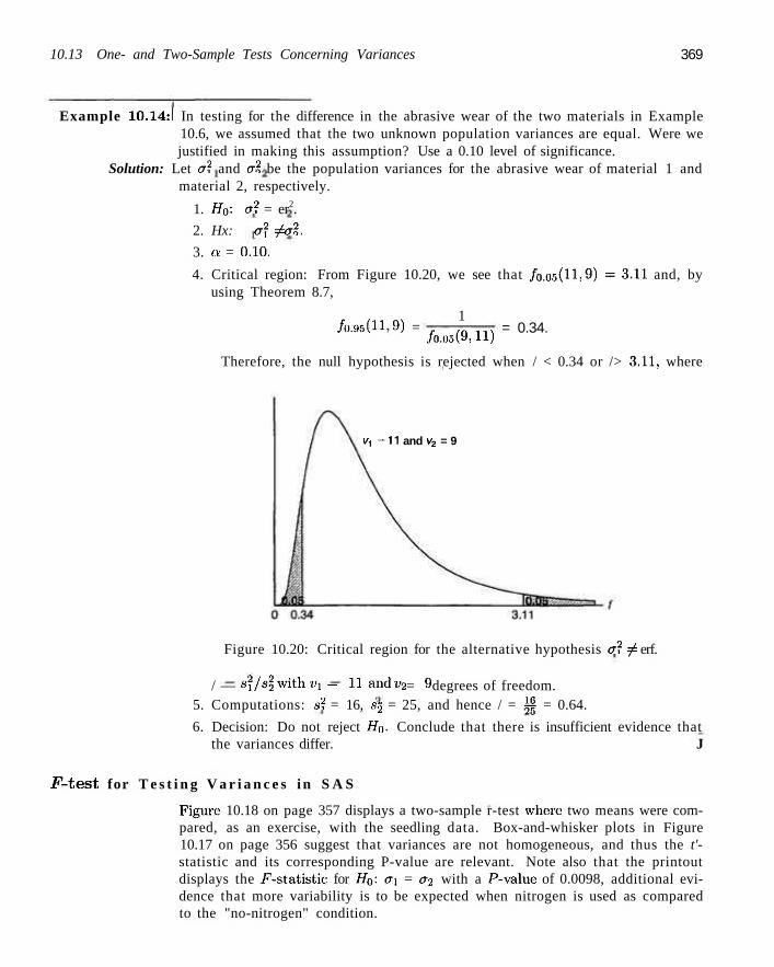
10.13 One- and Two-Sample Tests Concerning Variances 369
Example 10.14:1 In testing for the difference in the abrasive wear of the two materials in Example 10.6, we assumed that the two unknown population variances are equal. Were we justified in making this assumption? Use a 0.10 level of significance.
Solution: Let a2 and a2 be the population variances for the abrasive wear of material 1 and material 2, respectively.
1. H0: a2 = er2.
2. Hx: a2^ a2.
3. a = 0.10.
4. Critical region: From Figure 10.20, we see that /o.oo(H ;9) = 3 . 1 1 and, by using Theorem 8.7,
1 /o.95(H,9) = = 0.34.
/u.oo(9,ll)
Therefore, the null hypothesis is rejected when / < 0.34 or /> 3.11, where
1/1 = 11 and v2 = 9
Figure 10.20: Critical region for the alternative hypothesis a2 ^ erf.
/ — s i / s l ^'ith ?'i — 11 a n d v2 = 9 degrees of freedom. 5. Computations: s2 = 16, s2 = 25, and hence / = ±| = 0.64.
6. Decision: Do not reject H0. Conclude that there is insufficient evidence that the variances differ. J
.F-test for T e s t i n g V a r i a n c e s i n S A S
Figure 10.18 on page 357 displays a two-sample r-test where two means were compared, as an exercise, with the seedling data. Box-and-whisker plots in Figure 10.17 on page 356 suggest that variances are not homogeneous, and thus the t'-statistic and its corresponding P-value are relevant. Note also that the printout displays the F-statistic for H0: ax = 02 with a P-value of 0.0098, additional evidence that more variability is to be expected when nitrogen is used as compared to the "no-nitrogen" condition.
370
Exercises
Chapter 10 One- and Two-Sample Tests of Hypotheses
10.67 The volume of containers of a particular lubricant is known to be normally distributed with a variance of 0.03 liter, Test the hypothesis that a2 = 0.03 against tbe alternative that a2 7 0.03 for the random sample of 10 containers in Exercise 10.25 011 page 357. Use a P-value in your conclusions.
10.68 Past experience indicates that the time required for high school seniors to complete a standardized test is a normal random variable with a standard deviation of 6 minutes. Test, the hypothesis thai 0 = 6 against the alternative that, IT < 6 if a random sample of 20 high school seniors has a standard deviations s = 4.51. Use a 0.05 level of significance.
10.69 Allotoxins produced by mold on peanut crops in Virginia must be monitored. A sample of 61 batches of peanuts reveals levels of 24.17 ppm, on average, with a variance of 4.25 ppm. Test the hypothesis that a2 = 4.2 ppm with the alternative that a ^ 4.2 ppm. Use a P-value in your conclusions.
10.70 Past data indicate that, the amount of money contributed by the working residents of a large city to a volunteer rescue squad is a normal random variable with a standard deviation of St.40. It has been suggested that the contributions to the rescue squad from just the employees of the sanitation department are much more variable. If the contributions of a random sample of 12 employees from the sanitation department had a standard deviation of $1.75, can we conclude at the 0.01 level of significance that the standard deviation of the contributions of all sanitation workers is greater than that of all workers living in this city?
10.71 A soft-drink dispensing machine is said to be out of control if the variance of the contents exceeds 1.15 deciliters. If a random sample of 25 drinks from this machine has a variance of 2.03 deciliters, does this indicate at the 0.05 level of significance that the machine is out of control? Assume that the contents are approximately normally distributed.
10.72 Large-Sample Test of a2 = rr0: When n > 30 we can test the null hypothesis that a = a2, or a — (To, by computing
S - CT(]
ero /y/2n'
which is a value of a random variable whose sampling distribution is approximately the standard normal distribution. (a) With reference to Example 10.5, test, at, the 0.05
level of significance whether a = 10.0 years against the alternative that <r / 10.0 years.
(b) It is suspected that, the variance of the distribution of distances in kilometers achieved per 5 liters of fuel by a new automobile model eejuipped with a diesel engine is less than the variance of the distribution of distances achieved by the same model equipped with a six-cylinder gasoline engine, which is known to be a2 = 6.25. If 72 test runs in the diesel model have a variance of 4.41, can we conclude at the 0.05 level of significance that the variance of the distances achieved by the: diesel model is less than that of the gasoline model?
10.73 A study is conducted to compare the length of time between men and women to assemble a certain product. Past experience indicates that the distribution of times for both men and women is approximately normal but the variance of the times for women is less than that for men. A random sample of times for 11 men and 14 women produced the following data:
M e n W o m e n 7H = I I si =6 .1
712 = W
Test the hypothesis that a'i = a2 against the alternative that ai > a2. Use a P-valuc in your conclusion.
10.74 In Exercise 10.41 on page 359, test the hypothesis at the 0.05 level of significance that a1 = <T| against the alternative that, a2 ^ a2, where aj and a2 are the variances for the number of organisms per square meter at the two different locations on Cedar Run.
10.75 With reference: to Exercise I0..'{9 on page 359, test the hypothesis that a\ = a\ against the alternative that a\ 7 a\, where a\ and a2 are: the variances for the running times of films produced by company 1 and company 2, respectively. Use a P-value.
10.76 Two types of instruments for measuring the amount of sulfur monoxide in the atmosphere are being compared in an air-pollution experiment. It is desired to determine whether the two types of instruments yield measurements having the same variability. The following readings were recorded for the two instruments:
Sulfur Monoxide I n s t r u m e n t A I n s t r u m e n t B
0.86 0.82 0.75 0.61
0.87 0.74 0.63 0.55
10.14 Goodncss-of-Fit Test 371
Sulfur Monox ide Instrument A
0.89 0.64 0.81 0.68 0.65
Instrument B 0.76 0.70 0.69 0.57 0.53
Assuming the populations of measurements to be approximately normally distributed, test the hypothesis that a A = a a against the alternative that CT.-I ^ ae-Use a P-value.
10.77 An experiment was conducted to compare the alcohol contents in a soy sauce at two different production lines. Production was monitored eight times a day. The data are shown here.
Production line 1: 0.48 0.39 0.42 0.52 0.40 0.48 0.52 0.52
Production line 2: 0.38 0.37 0.39 0.41 0.38 0.39 0.40 0.39
Assume both populations arc normal. It is suspected
that production line 1 is not producing as consistently as production line 2 in terms of alcohol contents. Test the hypothesis that eri = a2 against the alternative that ai ^ a2. Use a P-value.
10.78 The hydrocarbon emissions are known to have decreased dramatically during the 1980s. A study was conducted to compare the hydrocarbon emissions at idling speed, in parts per million (ppm), for automobiles of 1980 and 1990. Twenty cars of each year model were randomly selected and their hydrocarbon emission levels were recorded. The data are as follows:
1980 models: 141 359 247 940 882 494 306 210 105 880 200 223 188 940 241 190 300 435 241 380
1990 models: 140 160 20 20 223 60 20 95 360 70 220 400 217 58 235 380 200 175 85 65
Test the hypothesis that en = a2 against the alternative that o\ ^ a2. Assume both populations are norma]. Use a P-value.
10.14 Goodness-of-Fit Test
Throughout this chapter we have been concerned with the testing of statistical hypotheses about single population parameters such as p, a2, and p. Now we shall consider a test to determine if a population has a specified theoretical distribution. T h e test is based on how good a fit we have between the frequency of occurrence of observations in an observed sample and the expected frequencies obtained from the hypothesized distribution.
Tabic 10.4: Observed and Expected Frequencies of 120 Tosses of a Die
Face: Observed Expected
1 20 20
2 22 20
3 17 20
4 18 20
5 19 20
6 24 20
To illustrate, consider the tossing of a die. We hypothesize t ha t the die is honest, which is equivalent to testing the hypothesis t ha t the distribution of outcomes is the discrete uniform distribution
fix) = 1
x = 1,2, . . . ,6.
Suppose tha t the die is tossed 120 times and each outcome is recorded. Theoretically, if the die is balanced, we would expect, each face to occur 20 times. The results are given in Table 10.4. By comparing the observed frequencies with the corresponding expected frequencies, wc must decide whether these discrepancies are likely to occur as a result, of sampling fluctuations and the die is balanced, or the die is not honest and the distribution of outcomes is not uniform. It is common
372 Chapter 10 One- and Two-Sample Tests of Hypotheses
practice to refer to each possible outcome of an experiment as a cell. Hence, in our illustration, we have 6 cells. The appropriate statistic on which we base our decision criterion for an experiment involving k cells is defined by the following theorem.
Goodness-of-Fit A goodness-of-fit test between observed and expected frequencies is based Test on the quantity
2 _ V ^ iOi ~ Gj)2
*' = £ where x2 iS a value of a random variable whose sampling distribution is approximated very closely by the chi-squared distribution with v = k — 1 degrees of freedom. The symbols o, and e; represent the observed and expected frequencies, respectively, for the ith cell.
The number of degrees of freedom associated with the chi-squared distribution used here is equal to k — 1, since there are only k — 1 freely determined cell frequencies. That is, once k — 1 cell frequencies are determined, so is the frequency for the kth cell.
If the observed frequencies are close to the corresponding expected frequencies, the x2-value will be small, indicating a good fit. If the observed frequencies differ considerably from the expected frequencies, the x2"vahie will be large and the fit is poor. A good fit leads to the acceptance of HQ whereas a poor fit leads to its rejection. The critical region will, therefore, fall in the right tail of the chi-squared distribution. For a level of significance equal to a, we find the critical value xa
from Table A.5, and then \ 2 > Xa constitutes the critical region. The decision criterion described here should not be used unless each of the expected frequencies is at least equal to 5. This restriction may require the combining of adjacent cells resulting in a reduction in the number of degrees of freedom.
From Table 10.4, we find the x2-value to be
2 _ (20 - 20)2 (22 - 20)2 ( 1 7 - 2 0 ) 2
X ~ 20 + 20 + 20 ( 1 8 - 2 0 ) 2 ( 1 9 - 2 0 ) 2 ( 2 4 - 2 0 ) 2
20 20 20
Using Table A.5, we find xij.05 = 11-070 for v — 5 degrees of freedom. Since 1.7 is less than the critical value, we fail to reject HQ. We conclude that there is insufficient evidence that the die is not balanced.
As a second illustration, let us test the hypothesis that the frequency distribution of battery lives given in Table 1.7 on page 23 may be approximated by a normal distribution with mean p = 3.5 and standard deviation a = 0.7. The expected frequencies for the 7 classes (cells), listed in Table 10.5, are obtained by computing the areas under the hypothesized normal curve that fall between the various class boundaries.
For example, the 2-values corresponding to the boundaries of the fourth class are
2 .95-3 .5 n m , 3 .45-3 .5 zi = — = -0.79 and z2 = — = -0.07,
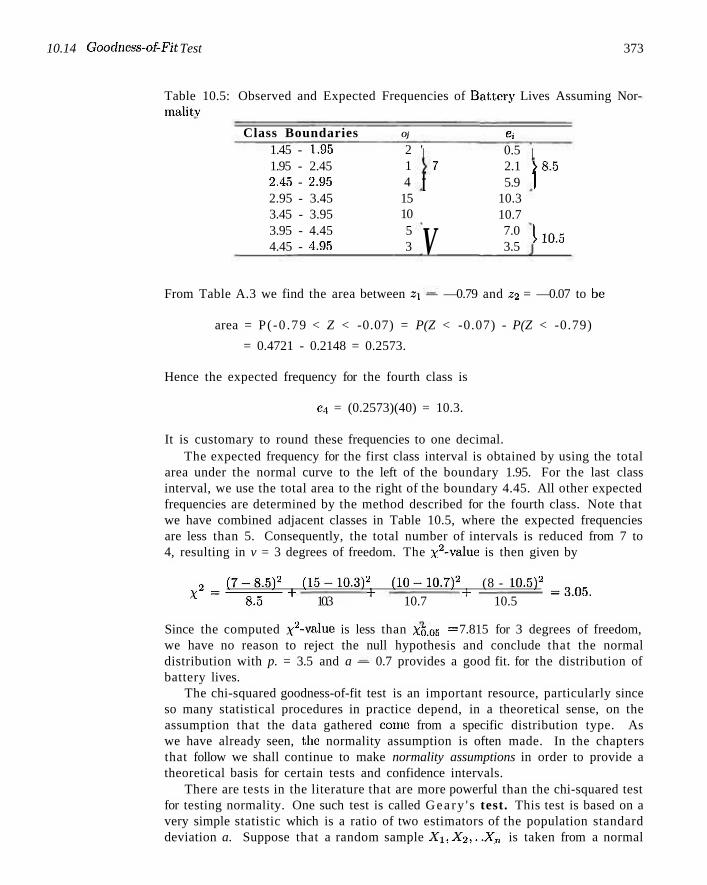
10.14 Goodness-of-Fit Test 373
Table 10.5: Observed and Expected Frequencies of Battery Lives Assuming Nor-malitv
Class Boundaries 1.45 - 1.95 1.95 - 2.45 2.45 - 2.95 2.95 - 3.45 3.45 - 3.95 3.95 - 4.45 4.45 - 4.95
Oj
2 ' 1 4
15 10 5 3
| 7
f
V
ei
0.5 2.1 5.9
10.3 10.7 7.0 3.5
| >8.5 1
110.5
From Table A.3 we find the area between zx — —0.79 and z2 = —0.07 to be
area = P(-0 .79 < Z < -0.07) = P(Z < -0.07) - P(Z < -0.79)
= 0.4721 - 0.2148 = 0.2573.
Hence the expected frequency for the fourth class is
e4 = (0.2573)(40) = 10.3.
It is customary to round these frequencies to one decimal. The expected frequency for the first class interval is obtained by using the total
area under the normal curve to the left of the boundary 1.95. For the last class interval, we use the total area to the right of the boundary 4.45. All other expected frequencies are determined by the method described for the fourth class. Note that we have combined adjacent classes in Table 10.5, where the expected frequencies are less than 5. Consequently, the total number of intervals is reduced from 7 to 4, resulting in v = 3 degrees of freedom. The x2-value is then given by
2 ( 7 - 8 . 5 ) 2 (15-10 .3) 2 (10-10 .7) 2 (8 - 10.5)2
X ^S-o—-^ 10.3 + 10.7 + 10.5 = 3 " 0 5 -
Since the computed x2-value is less than Xo.os = 7.815 for 3 degrees of freedom, we have no reason to reject the null hypothesis and conclude that the normal distribution with p. = 3.5 and a — 0.7 provides a good fit. for the distribution of battery lives.
The chi-squared goodness-of-fit test is an important resource, particularly since so many statistical procedures in practice depend, in a theoretical sense, on the assumption that the data gathered come from a specific distribution type. As we have already seen, the normality assumption is often made. In the chapters that follow we shall continue to make normality assumptions in order to provide a theoretical basis for certain tests and confidence intervals.
There are tests in the literature that are more powerful than the chi-squared test for testing normality. One such test is called Geary ' s test. This test is based on a very simple statistic which is a ratio of two estimators of the population standard deviation a. Suppose that a random sample Xx,X2,..., X„ is taken from a normal
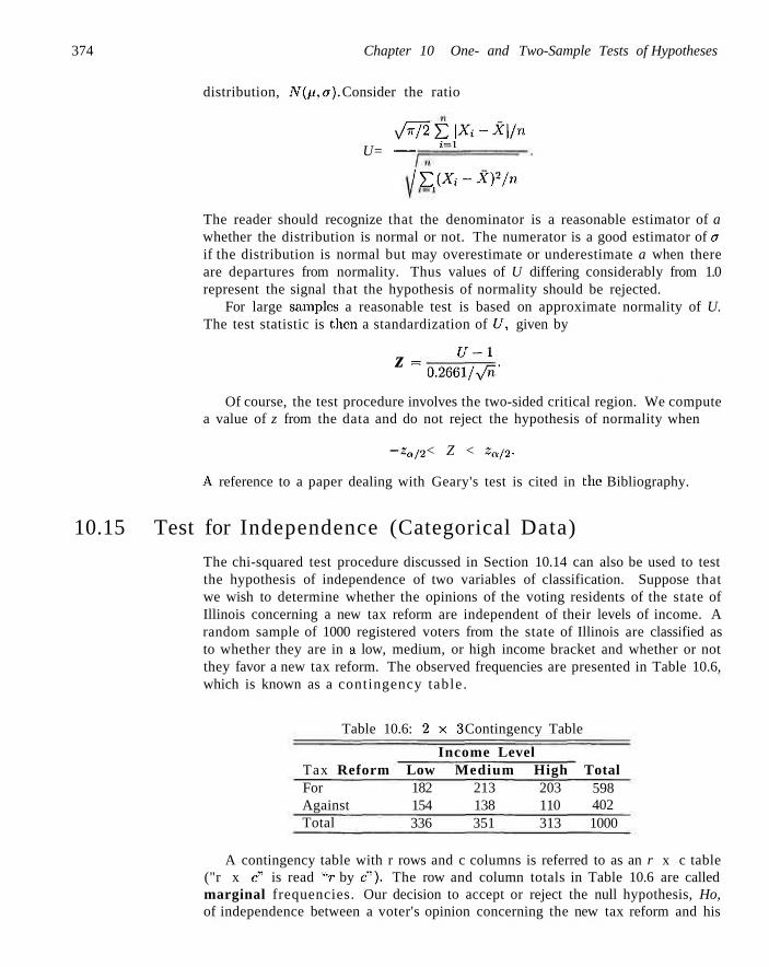
374 Chapter 10 One- and Two-Sample Tests of Hypotheses
distribution, N(p,o). Consider the ratio
y/^j2zZ\Xi-X\/n U= — i=l
IZiXt-Xp/n
The reader should recognize that the denominator is a reasonable estimator of a whether the distribution is normal or not. The numerator is a good estimator of cr if the distribution is normal but may overestimate or underestimate a when there are departures from normality. Thus values of U differing considerably from 1.0 represent the signal that the hypothesis of normality should be rejected.
For large samples a reasonable test is based on approximate normality of U. The test statistic is then a standardization of U, given by
z = u'1
0.2661/v/rT'
Of course, the test procedure involves the two-sided critical region. We compute a value of z from the data and do not reject the hypothesis of normality when
-za/2 < Z < za/2.
A reference to a paper dealing with Geary's test is cited in the Bibliography.
10.15 Test for Independence (Categorical Data)
The chi-squared test procedure discussed in Section 10.14 can also be used to test the hypothesis of independence of two variables of classification. Suppose that we wish to determine whether the opinions of the voting residents of the state of Illinois concerning a new tax reform are independent of their levels of income. A random sample of 1000 registered voters from the state of Illinois are classified as to whether they are in a low, medium, or high income bracket and whether or not they favor a new tax reform. The observed frequencies are presented in Table 10.6, which is known as a contingency table.
Table 10.6: 2 x 3 Contingency Table
Tax Reform For Against Total
Income Level Low Medium High 182 213 203 154 138 110 336 351 313
Total 598 402 1000
A contingency table with r rows and c columns is referred to as an r x c table ("r x c" is read "r by c"). The row and column totals in Table 10.6 are called marginal frequencies. Our decision to accept or reject the null hypothesis, Ho, of independence between a voter's opinion concerning the new tax reform and his
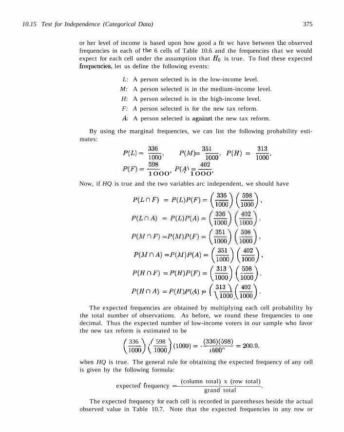
10.15 Test for Independence (Categorical Data) 375
or her level of income is based upon how good a fit wc have between the observed frequencies in each of the 6 cells of Table 10.6 and the frequencies that we would expect for each cell under the assumption that Ho is true. To find these expected frequencies, let us define the following events:
L: A person selected is in the low-income level.
M: A person selected is in the medium-income level.
H: A person selected is in the high-income level.
F: A person selected is for the new tax reform.
A: A person selected is against the new tax reform.
By using the marginal frequencies, we can list the following probability estimates:
^ > = Tffir p ^ = » p<ff> = S ! ' 1000' v ' 1000'
Now, if HQ is true and the two variables arc independent, we should have
^ - ^ . ( H ) ( - ) ,
™=™,=(fi)(^), ^ - P , * ™ - ( £ ) ( £ ) . p(tfn.4)=p(«)P(WiiiN)(ie.y k ; v / v 7 yWQ0j i^ioooy
The expected frequencies are obtained by multiplying each cell probability by the total number of observations. As before, we round these frequencies to one decimal. Thus the expected number of low-income voters in our sample who favor the new tax reform is estimated to be
/ 336 N / 598 \
Vioooy V IOOO) ( 1 0 0 0 ) . < « » - 2 0 0 . 9 ,
when HQ is true. The general rule for obtaining the expected frequency of any cell is given by the following formula:
, „ (column total) x (row total) expected frequency = : : .
grand total
The expected frequency for each cell is recorded in parentheses beside the actual observed value in Table 10.7. Note that the expected frequencies in any row or
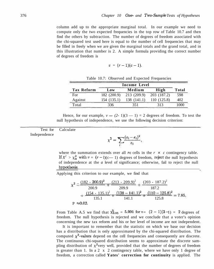
376 Chapter 10 One- and Two-Sample Tests of Hypotheses
column add up to the appropriate marginal total. In our example we need to compute only the two expected frequencies in the top row of Table 10.7 and then find the others by subtraction. The number of degrees of freedom associated with the chi-squared test used here is equal to the number of cell frequencies that may be filled in freely when we are given the marginal totals and the grand total, and in this illustration that number is 2. A simple formula providing the correct number of degrees of freedom is
u = ( r - l ) ( c - l ) .
Table 10.7: Observed and Expected Frequencies
Income Level Tax Reform Low Medium High For 182 (200.9) 213 (209.9) 203 (187.2) Against 154 (135.1) 138 (141.1) 110 (125.8) Total 336 351 313
Total 598 402 1000
Hence, for our example, v — (2- 1)(3 — 1) = 2 degrees of freedom. To test the null hypothesis of independence, we use the following decision criterion:
Test for Calculate Independence
2 V^ i0i ~ e'')2
*2 = £ where the summation extends over all re cells in the r x c contingency table. If X2 > Xa w i * n v = (r— l)(c— 1) degrees of freedom, reject the null hypothesis of independence at the a level of significance; otherwise, fail to reject the null hypothesis.
Applying this criterion to our example, we find that
a _ (182 - 200.9)2 (213 - 209.9)2 (203 - 187.2)2
200.9 209.9 187.2 , (154 - 135.1)2 (138-141.1)2 (110-125.8)2
+ 135.1 + 141.1 + 125.8 P w0.02.
From Table A.5 we find that Xom = 5 - 9 9 1 f o r v = (2 ~ ! ) ( 3 - 1) = 2 degrees of freedom. The null hypothesis is rejected and we conclude that a voter's opinion concerning the new tax reform and his or her level of income are not independent.
It is important to remember that the statistic on which we base our decision has a distribution that is only approximated by the chi-squared distribution. The computed x2-values depend on the cell frequencies and consequently are discrete. The continuous chi-squared distribution seems to approximate the discrete sampling distribution of \2 very well, provided that the number of degrees of freedom is greater than 1. In a 2 x 2 contingency table, where we have only 1 degree of freedom, a correction called Yates' correction for continuity is applied. The
10.16 Test for Homogeneity 377
corrected formula then becomes
X2(corrected) = ^ ( | o ^ e i | - ° - 5 ) 2 .
e% t
If the expected cell frequencies are large, the corrected and uncorrected results are almost the same. When the expected frequencies are between 5 and 10, Yates' correction should be applied. For expected frequencies less than 5, the Fisher-Irwin exact test should be used. A discussion of this test may be found in Basic Concepts of Probability and Statistics by Hodges and Lehmann (see the Bibliography). The Fisher-Irwin test may be avoided, however, by choosing a larger sample.
10.16 Test for Homogeneity
When we tested for independence in Section 10.15, a random sample of 1000 voters was selected and the row and column totals for our contingency table were determined by chance. Another type of problem for which the method of Section 10.15 applies is one in which either the row or column totals are predetermined. Suppose, for example, that we decide in advance to select 200 Democrats, 150 Republicans, and 150 Independents from the voters of the state of North Carolina and record whether they are for a proposed abortion law, against it, or undecided. The observed responses are given in Table 10.8.
Table 10.8: Observed and Expected Frequencies
Political Affiliation Abortion Law Democrat Republican Independent For 82 70 62 Against 93 62 67 Undecided 25 18 21 Total 200 150 150
Total 214 222 64 500
Now, rather than test for independence, we test the hypothesis that the population proportions within each row are the same. That is, we test the hypothesis that the proportions of Democrats, Republicans, and Independents favoring the abortion law are the same; the proportions of each political affiliation against the law are the same: and the proportions of each political affiliation that are undecided are the same. We are basically interested in determining whether the three categories of voters arc homogeneous with respect to their opinions concerning the proposed abortion law. Such a test is called a test for homogeneity.
Assuming homogeneity, we again find the expected cell frequencies by multiplying the corresponding row and column totals and then dividing by the grand total. The analysis then proceeds using the same chi-squared statistic as before. We illustrate this process in the following example for the data of Table 10.8.
Example 10.15:1 Referring to the data of Table 10.8, test the hypothesis that the opinions concerning the proposed abortion law are the same within each political affiliation. Use a 0.05 level of significance.
378 Chapter 10 One- and Two-Sample Tests of Hypotheses
Solution: 1. HQ: For each opinion the proportions of Democrats, Republicans, and Independents are the same.
2. Hi: For at least one opinion the: proportions of Democrats, Republicans, and Independents are not the same.
3. o = 0.05.
4. Critical region: \'2 > 9.488 with o = 4 degrees of freedom.
5. Computations: Using the expected cell frequency formula on page 375, we need to compute the 4 cell frequencies. All other frequencies are found by subtraction. The observed and expected cell frequencies are displayed in Table 10.9.
Table 10.9: Observed and Expected Frequencies
Abor t ion Law For Against Undecided Total
Democra t 82 (85.6) 93 (88.8) 25 (25.6)
200
Political Affiliai Republican
70 (64.2) 62 (66.6) 18 (19.2)
150
don Independent
62 (64.2) 67 (66.6) 21 (19.2)
150
Total 214 222 64
500
Now.
, _ (82-85.6)- (70 - 64.2)2 i (02 - 64.2)2
+
+
85.6 64.2 64.2 (93 - 88.8)2 (62 - 66.6)-' (67 - 66.6)2
88.8 ~6fi.(i 66.6 (25-25.6)'-' (18 - 19.2)- (21 - 19.2)2
25.6 19.2 19.2 1.53.
6. Decision: Do not reject HQ. There is insufficient evidence to conclude that the proportion of Democrats, Republicans, and Independents differs for each stated opinion. J
10.17 Testing for Several Proportions
The chi-squared statistic for testing for homogeneity is also applicable when testing the hypothesis that k binomial parameters have the same value. This is. therefore, an extension of the: test presented in Section 10.12 for determining differences between two proportions to a test for determining differences among k proportions. Hence wc are interested in testing the mill hypothesis
HQ : pi P-2 = Pk
against the alternative hypothesis, Hi, that the population proportions are not till equal. Tb perform this test, we first observe independent random samples of
10.17 Testing for Several Proportions 379
Table 10.10:
Sample: Successes Failures
k Indepe
1 xx
111 ~ Xl
nclent Binomial Samples
2 x2
n2 -x2 ••
k
Xk
nk - Xk
size iii,n2,... ,nk from the A: populations and arrange the data as in the 2 x k contingency table. Tabic 10.10.
Depending on whether the sizes of the random samples were predetermined or occurred at random, the test procedure is identical to the test for homogeneity or the test for independence. Therefore, the expected cell frequencies are calculated as before and substituted together with the observed frequencies into the chi-squared statistic
2 _ V^ i°i ~ d)2
X ^ et ' >
with
v = (2 - l)(k - 1) = k - 1
degrees of freedom. By selecting the appropriate upper-tail critical region of the form \ 2 > x L w e
can now reach a decision concerning HQ.
Example 10.16:1 In a shop study, a set of data was collected to determine whether or not the proportion of defectives produced by workers was the same for the day, evening, or night shift worked. The data were collected and shown in Table 10.11.
Table 10.11:
Shift: Defectives Nondefectives
Data for Example
Day Evening 45 55
905 890
10.16
Night 70
870
Use a 0.025 level of significance to determine if the proportion of defectives is the same for all three shifts.
Solution: Let /Ji,P2, and p% represent the true proportion of defectives for the day, evening, and night shifts, respectively.
1. HQ: pi = p2 - p3 .
2. Hi : p\,p2, and pa arc not all equal.
3. a = 0.025.
4. Critical region: \2 > 7.378 for v = 2 degrees of freedom.
5. Computations: Corresponding to the observed frequencies oi = 45 and 02 = 55, we find
(950) (170) (945)(170) e i = 2835 = 5 ' - ° a n d C2 = 2835 = ^ ^
380 Chapter 10 One- and Two-Sample Tests of Hypotheses
All other expected frequencies are found by subtraction and are displayed in Table 10.12.
Table 10.12: Observed and Expected Frequencies
Shift: Defectives Nondefectives Total
Day 45 (57.0)
905 (893.0) 950
Evening 55 (56.7)
890 (888.3) 945
Night 70 (56.3)
870 (883.7) 940
Total 170
2665 2835
Now
4 5 - 5 7 . 0 ) 2 , (55-50.7) 2 (70-56.3) 2
+ 57.0 56.7 56.3 (905 - 893.0)2 (890-888.3)2 (870 - 883.7)2
893.0 888.3 883. P «0.0I.
= 6.29.
6. Decision: We do not reject HQ at a — 0.025. Nevertheless, with the above P-value computed, it would certainly be dangerous to conclude that the proportion of defectives produced is the same for all shifts.
10.18 Two-Sample Case Study
In this section we consider a study where we show a thorough analysis using both graphical and formal analysis along with annotated computer printout and conclusions. In a data analysis study conducted by personnel at the Statistics Consulting Center at Virginia Tech, two different materials, say alloy A and alloy B, were compared in terms of breaking strength. Alloy B is more expensive, but it should certainly be adopted if it can be demonstrated that it is stronger than alloy A. The consistency of performance of the two alloys should also be taken into account.
Random samples of beams for each alloy were selected and the strength was measured in a 0.001-inch deflection as a fixed force was applied at both ends of the beam. Twenty specimens were used for each of the two alloys. The data are given in Table 10.13.
It is important that the engineer compare the two alloys. Of concern is average strength and reproducibility. It is of interest to determine if there is a severe violation of the normality assumption required of both the r- and P-tests. Figures 10.21 and 10.22 are normal quantile-quantile plots of the samples for the two alloys.
There does not appear to be any serious violation of the normality assumption. In addition, Figure 10.23 shows two box-and-whisker plots on the same graph. The box-and-whisker plots would suggest that there is no appreciable difference in the variability of deflection for the two alloys. Howrevcr, it seems that the mean of alloy B is significantly smaller, suggesting at feast graphically that alloy B is stronger. The sample means and standard deviations are
f/A = 83.55, sA = 3.663; yB = 79.70. sB = 3.097.
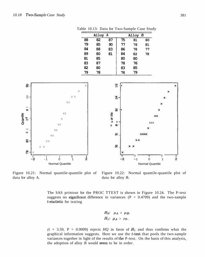
10.18 Two-Sample Case Study 381
Table 10.13: Data for Two-Sample Case Study
88 79 84 89 81 83 82 79
Alloy A 82 85 88 80 85 87 80 78
87 90 83 81
75 77 86 84 80 78 83 76
Alloy B 81 80 78 81 78 77 82 78 80 76 85 79
o _
8-
to _ CO
t= "* -ra co
o CM _
co
CO
CO X
1
X X
XX
1
XX
XX
X
X X
XX
XX
X
XX
1 1
X
1
CO ^
co
CM _ CO ^
c = o a co'
co _
<o _
- 1 0 1
Normal Quantile
xxx
T T -1 0 1
Normal Quantile
Figure 10.21: Normal quantile-quantile plot of Figure 10.22: Normal quantile-quantile plot of data for alloy A. data for alloy B.
The SAS printout for the PROC TTEST is shown in Figure 10.24. The P-test suggests no significant difference in variances (P = 0.4709) and the two-sample t-statistic for testing
Ho- PA = PB,
Hi- PA > PB-.
(t = 3.59, P = 0.0009) rejects HQ in favor of Hi and thus confirms what the graphical information suggests. Here we use the t-test that pools the two-sample variances together in light of the results of the P-test. On the basis of this analysis, the adoption of alloy B would seern to be in order.
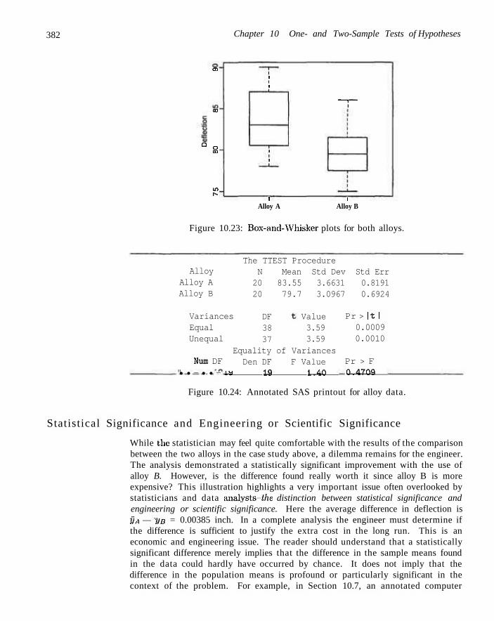
382 Chapter 10 One- and Two-Sample Tests of Hypotheses
Q
CJ>
CO
o en
in N
l
l
l
~T~
1
1 i Alloy A Alloy B
Figure 10.23: Box-and-Whisker plots for both alloys.
Alloy Alloy A Alloy B
Variances Equal Unequal
Num DF "• • - • • — 19
The TTEST Procedure N Mean Std Dev Std Err 20 83.55 3.6631 0.8191 20 79.7 3.0967 0.6924
DF 38 37
Value 3.59 3.59
Equality of Variances Den DF F Value
IS J^IO
Pr > It I 0.0009 0.0010
Pr > F 0.4709
Figure 10.24: Annotated SAS printout for alloy data.
Statistical Significance and Engineering or Scientific Significance
While the statistician may feel quite comfortable with the results of the comparison between the two alloys in the case study above, a dilemma remains for the engineer. The analysis demonstrated a statistically significant improvement with the use of alloy B. However, is the difference found really worth it since alloy B is more expensive? This illustration highlights a very important issue often overlooked by statisticians and data analysts-f/ie distinction between statistical significance and engineering or scientific significance. Here the average difference in deflection is §A — VB = 0.00385 inch. In a complete analysis the engineer must determine if the difference is sufficient to justify the extra cost in the long run. This is an economic and engineering issue. The reader should understand that a statistically significant difference merely implies that the difference in the sample means found in the data could hardly have occurred by chance. It does not imply that the difference in the population means is profound or particularly significant in the context of the problem. For example, in Section 10.7, an annotated computer
Exercises 383
printout is used to show evidence tha t a pH meter was, in fact, biased. T h a t is, it does not demonstra te a mean pH of 7.00 for the material on which it was tested. But the variability among the observations in the sample is very small. The engineer may decide tha t the small deviations from 7.0 render the pH meter adequate.
Exercises
10.79 A die is tossed 180 times with the following results:
X
f 1 28
2 36
3 36
4 30
5 27
6 23
Is this a halanced die? Use a 0.01 level of significance.
10.80 In 100 tosses of a coin, 63 heads and 37 tails are ohserved. Is this a balanced coin? Use a 0.05 level of significance.
10.81 A machine is supposed to mix peanuts, hazelnuts, cashews, and pecans in the ratio 5:2:2:1. A can containing 500 of these mixed nuts was found to have 269 peanuts, 112 hazelnuts, 74 cashews, and 45 pecans. At the 0.05 level of significance, test the hypothesis that the machine is mixing the nuts in the ratio 5:2:2:1.
10.82 The grades in a statistics course for a particular semester were as follows:
Grade
/ A 14
B 18
C 32
D 20
F 16
Test the hypothesis, at the 0.05 level of significance, that the distribution of grades is uniform.
10.83 Three cards are drawn from an ordinary deck of playing cards, with replacement, and the number Y of spades is recorded. After repeating the experiment 64 times, the following outcomes were recorded:
y f
0 21
1 31
2 12
3 0
Test the hypothesis of 0.01 level of significance that the recorded data may be fitted by the binomial distribution b(y;3,1/4), y = 0 ,1,2,3. '
10.84 Three marbles are selected from an urn containing 5 red marbles and 3 green marbles. After recording the number X of red marbles, the marbles are replaced in the urn and the experiment repeated 112 times. The results obtained are as follows:
0 1 2 3 1 31 55 25
Test the hypothesis at the 0.05 level of significance that the recorded data may be fitted by the hypergeometric
distribution h(x; 8,3, 5), x = 0 ,1 , 2, 3.
10.85 A coin is thrown until a head occurs and the number X of tosses recorded. After repeating the experiment 256 times, we obtained the following results:
X
f 1 136
2 60
3 34
4 12
5 9
6 1
7 3
8 1
Test the hypothesis at, the 0.05 level of significance that the observed distribution of X may be fitted by the geometric distribution g(x; 1/2), x = 1,2,3,
10.86 Repeat Exercise 10.83 using a new set of data obtained by actually carrying out the described experiment 64 times.
10.87 Repeat Exercise 10.85 using a new set of data obtained by performing the described experiment 256 times.
10.88 In Exercise 1.18 on page 28, test the goodness of fit between the observed class frequencies and the corresponding expected frequencies of a normal distribution with p = 65 and a = 21, using a 0.05 level of significance.
10.89 In Exercise 1.19 on page 28, test the goodness of fit between the observed class frequencies and the corresponding expected frequencies of a normal distribution with p = 1.8 and a = 0.4, using a 0.01 level of significance.
10.90 In an experiment to study the dependence of hypertension on smoking habits, the following data were taken on 180 individuals:
Non- Moderate Heavy smokers Smokers Smokers
Hypertension 21 36 30 No Hypertension 48 26 19
Test the hypothesis that the presence or absence of hypertension is independent of smoking habits. Use a 0.05 level of significance.
10.91 A random sample of 90 adults is classified according to gender and the number of hours they watch
384 Chapter 10 One- and Two-Sample Tests of Hypotheses
television during a week:
Gender Male Female
Over 25 hours Under 25 hours
15 27
29 19
Use a 0.01 level of significance and test the hypothesis that the time spent watching television is independent of whether the viewer is male or female.
10.92 A random sample of 200 married men, all retired, were classified according to education and number of children:
Education Elementary Secondary College
Number of Children 0-1 2 - 3 14 37 19 42 12 17
Over 3 32 17 10
Test the hypothesis, at the 0.05 level of significance, that the size of a family is independent of the level of education attained by the father.
10.93 A criminologist conducted a survey to determine whether the incidence of certain types of crime varied from one part of a large city to another. The particular crimes of interest were assault, burglary, larceny, and homicide. The following table shows the numbers of crimes committed in four areas of the city during the past year.
Type of Crime District Assault Burglary Larceny Homicide 1~~ 162 118 451 18 2 310 196 996 25 3 258 193 458 10 4 280 175 390 19
Can we conclude from these data at the 0.01 level of significance that the occurrence of these types of crime is dependent on the city district?
10.94 A college infirmary conducted an experiment to determine the degree of relief provided by three cough remedies. Each cough remedy was tried on 50 students and the following data recorded:
Cough Remedy NyQuil Robitussin Triaminic
No relief Some relief Total relief
11 32 7
13 28 9
9 27 14
Test the hypothesis that the three cough remedies are equally effective. Use a P-value in your conclusion.
10.95 To determine current attitudes about prayers in public schools, a survey was conducted in 4 Virginia counties. The following table gives the attitudes
of 200 parents from Craig County, 150 parents from Giles County. 100 parents from Franklin County, and 100 parents from Montgomery County:
County Att i tude Craig Giles Franklin Mont. Favor Oppose No opinion
65 42 93
66 30 54
40 33 27
34 42 24
Test for homogeneity of attitudes among the 4 counties concerning prayers in the public schools. Use a P-value in your conclusion.
10.96 According to a Johns Hopkins University study published in the American Journal of Public Health, widows live longer than widowers. Consider the following survival data collected on 100 widows and 100 widowers following the death of a spouse:
Years Lived Widow Widower Less than 5 5 to 10 More than 10
25 42 33
39 40 21
Can wc conclude at the 0.05 level of significance that the proportions of widows and widowers are equal with respect to the different time periods that a spouse survives after the death of his or her mate?
10.97 The following responses concerning the standard of living at the time of an independent opinion poll of 1000 households versus one year earlier seems to be in agreement with the results of a study published in Across the Board (June 1981):
Standard of Living
Period
1980: Jan. May
Sept. 1981: Jan.
Somewhat Better
72 63 47 40
Same
144 135 100 105
Not as Good Total
84 300 102 300 53 200 55 200
Test, the hypothesis that the proportions of households within each standard of living category are the same for each of the four time periods. Use a P-value.
10.98 A survey was conducted in Indiana, Kentucky, and Ohio to determine the attitude of voters concerning school busing. A poll of 200 voters from each of these states yielded the following results:
Voter Attitude Do Not
State Support Support Undecided
Indiana 82 97 21 Kentucky 107 66 27 Ohio 93 74 33
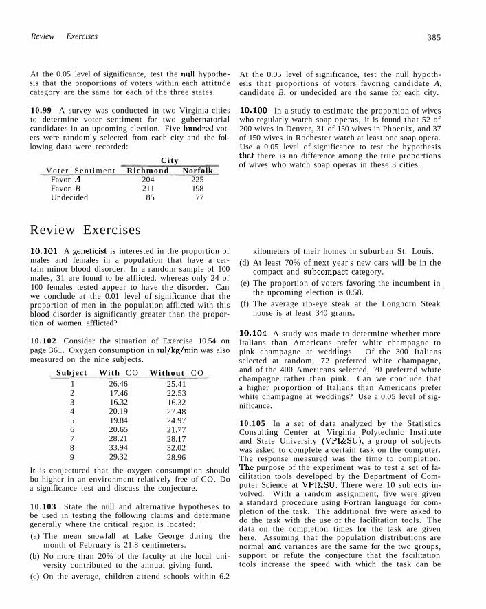
Review Exercises 385
At the 0.05 level of significance, test the null hypothesis that the proportions of voters within each attitude category are the same for each of the three states.
10.99 A survey was conducted in two Virginia cities to determine voter sentiment for two gubernatorial candidates in an upcoming election. Five hundred voters were randomly selected from each city and the following data were recorded:
Voter Sen t iment Favor A Favor B Undecided
City Richmond Norfolk
204 225 211 198 85 77
At the 0.05 level of significance, test the null hypothesis that proportions of voters favoring candidate A, candidate B, or undecided are the same for each city.
10.100 In a study to estimate the proportion of wives who regularly watch soap operas, it is found that 52 of 200 wives in Denver. 31 of 150 wives in Phoenix, and 37 of 150 wives in Rochester watch at least one soap opera. Use a 0.05 level of significance to test the hypothesis that there is no difference among the true proportions of wives who watch soap operas in these 3 cities.
Review Exercises
10.101 A geneticist is interested in the proportion of males and females in a population that have a certain minor blood disorder. In a random sample of 100 males, 31 are found to be afflicted, whereas only 24 of 100 females tested appear to have the disorder. Can we conclude at the 0.01 level of significance that the proportion of men in the population afflicted with this blood disorder is significantly greater than the proportion of women afflicted?
10.102 Consider the situation of Exercise 10.54 on page 361. Oxygen consumption in ml/kg/min was also measured on the nine subjects.
Subject 1 2 3 4 5 6 7 8 9
With C O 26.46 17.46 16.32 20.19 19.84 20.65 28.21 33.94 29.32
Without CO 25.41 22.53 16.32 27.48 24.97 21.77 28.17 32.02 28.96
It is conjectured that the oxygen consumption should bo higher in an environment relatively free of CO. Do a significance test and discuss the conjecture.
10.103 State the null and alternative hypotheses to be used in testing the following claims and determine generally where the critical region is located:
(a) The mean snowfall at Lake George during the month of February is 21.8 centimeters.
(b) No more than 20% of the faculty at the local university contributed to the annual giving fund.
(c) On the average, children attend schools within 6.2
kilometers of their homes in suburban St. Louis. (d) At least 70% of next year's new cars will be in the
compact and subcompact category. (e) The proportion of voters favoring the incumbent in
the upcoming election is 0.58. (f) The average rib-eye steak at the Longhorn Steak
house is at least 340 grams.
10.104 A study was made to determine whether more Italians than Americans prefer white champagne to pink champagne at weddings. Of the 300 Italians selected at random, 72 preferred white champagne, and of the 400 Americans selected, 70 preferred white champagne rather than pink. Can we conclude that a higher proportion of Italians than Americans prefer white champagne at weddings? Use a 0.05 level of significance.
10.105 In a set of data analyzed by the Statistics Consulting Center at Virginia Polytechnic Institute and State University (VPI&SU), a group of subjects was asked to complete a certain task on the computer. The response measured was the time to completion. The purpose of the experiment was to test a set of facilitation tools developed by the Department of Computer Science at VPI&SU. There were 10 subjects involved. With a random assignment, five were given a standard procedure using Fortran language for completion of the task. The additional five were asked to do the task with the use of the facilitation tools. The data on the completion times for the task are given here. Assuming that the population distributions are normal and variances are the same for the two groups, support or refute the conjecture that the facilitation tools increase the speed with which the task can be
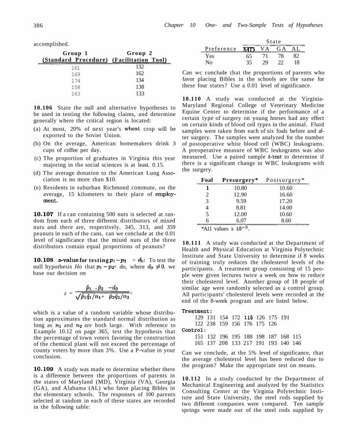
386 Chapter 10 One- and Two-Sample Tests of Hypotheses
accomplished.
Group 1 (Standard Procedure)
161 169 174 158 163
Group 2 (Facilitation Tool)
132 162 134 138 133
10.106 State the null and alternative hypotheses to be used in testing the following claims, and determine generally where the critical region is located:
(a) At most, 20% of next year's wheat, crop will be exported to the Soviet Union.
(b) On the average, American homemakers drink 3 cups of coffee per day.
(c) The proportion of graduates in Virginia this year majoring in the social sciences is at least. 0.15.
(d) The average donation to the American Lung Association is no more than $10.
(e) Residents in suburban Richmond commute, on the average, 15 kilometers to their place of emploj'-ment.
10.107 If a can containing 500 nuts is selected at random from each of three different distributors of mixed nuts and there are, respectively, 345, 313, and 359 peanuts in each of the cans, can we conclude at the 0.01 level of significance that the mixed nuts of the three distributors contain equal proportions of peanuts?
10.108 a-value for testing pi —p-2 = <4>: To test the null hypothesis Ho that p\—p2 = do, where do ^ 0, we base our decision on
z = p~\ - j>i - do
y/piqi/ni + p2</2/n2
which is a value of a random variable whose distribution approximates the standard normal distribution as long as m and n2 are both large. With reference to Example 10.12 on page 365, test the hypothesis that the percentage of town voters favoring the construction of the chemical plant will not exceed the percentage of county voters by more than 3%. Use a P-value in your conclusion.
10.109 A study was made to determine whether there is a difference between the proportions of parents in the states of Maryland (MD), Virginia (VA), Georgia (GA), and Alabama (AL) who favor placing Bibles in the elementary schools. The responses of 100 parents selected at random in each of these states are recorded in the following table:
P re fe rence Yes No
MD 65 35
S t a t e VA G A 71 78 29 22
AL 82 18
Can wc conclude that the proportions of parents who favor placing Bibles in the schools are the same for these four states? Use a 0.01 level of significance.
10.110 A study was conducted at the Virginia-Maryland Regional College of Veterinary Medicine Equine Center to determine if the performance of a certain type of surgery on young horses had any effect on certain kinds of blood ceil types in the animal. Fluid samples were taken from each of six foals before and after surgery. The samples were analyzed for the number of postoperative white blood cell (WBC) leukograms. A preoperative measure of WBC leukograms was also measured. Use a paired sample t-test to determine if there is a significant change in WBC leukograms with the surgery.
Foal Presurgery* 1 10.80 2 12.90 3 9.59 4 8.81 5 12.00 6 6.07
*A11 values x KT3 .
Pos t su rge ry* 10.60 16.60 17.20 14.00 10.60 8.60
10.111 A study was conducted at the Department of Health and Physical Education at Virginia Polytechnic Institute and State University to determine if 8 weeks of training truly reduces the cholesterol levels of the participants. A treatment group consisting of 15 people were given lectures twice a week on how to reduce their cholesterol level. Another group of 18 people of similar age were randomly selected as a control group. All participants' cholesterol levels were recorded at the end of the 8-week program and are listed below.
Treatment: 129 131 154 172 115 126 175 191 122 238 159 156 176 175 126
Control: 151 132 196 195 188 198 187 168 115 165 137 208 133 217 191 193 140 146
Can we conclude, at the 5% level of significance, that the average cholesterol level has been reduced due to the program? Make the appropriate test on means.
10.112 In a study conducted by the Department of Mechanical Engineering and analyzed by the Statistics Consulting Center at the Virginia Polytechnic Institute and State University, the steel rods supplied by two different companies were compared. Ten sample springs were made out of the steel rods supplied by
10.19 Potential Misconceptions and Hazards 387
each company and the "bounciness" was studied. The data are as follows:
Company A: 9.3 8.8 6.8 Company B: 11.0 9.8 9.9 10.2
8.7 8.5 6.7 8.0 6.5 9.2 7.0
10.1 9.7 11.0 11.1 10.2 9.6
Can you conclude that there is virtually no difference in means between the steel rods supplied by the two companies? Use a P-value to reach your conclusion. Should variances be pooled here?
10.113 In a study conducted by the Water Resources Center and analyzed by the Statistics Consulting Center at the Virginia Polytechnic Institute and State University, two different wastewater treatment plants are compared. Plant A is located where the median household income is below S22,000 a year, and plant B is located where the median household income is above $60,000 a year. The amount of wastewater treated at, each plant (thousand gallons/day) was randomly sampled for 10 days. The data are as follows:
Plant A: 21 19 20 23 22 28 32 19 13 18
Plant B: 20 39 24 33 30 28 30 22 33 24
Can we conclude, at the 5% level of significance, that the average amount of wastewater treated at the high-income neighborhood is more than that from the low-income area? Assume normality.
10.114 The following data show the number of defects in 100,000 lines of code in a particular type of software program made in the United States and Japan. Is there enough evidence to claim that there is a significant difference between the programs of the two countries? Test on means. Should variances be pooled?
U.S. 48 39 42 52 40 48 52 52 54 48 52 55 43 46 48 52
Japan 50 48 42 40 43 48 50 46 38 38 36 40 40 48 48 45
10.115 Studies show that the concentration of PCBs is much higher in malignant breast tissue than in normal breast tissue. If a study of 50 women with breast cancer reveals an average PCB concentration of 22.8 x 10 - '1 gram, with a standard deviation of 4.8 x 10- '1 gram, is the mean concentration of PCBs less than 24 x 10 - '1 gram?
10.19 Potential Misconceptions and Hazards; Relationship to Material in Other Chapters
One of the easiest ways to misuse statistics relates to the final scientific, conclusion drawn wdien the analyst does not reject the null hypothesis Ho- In this text we have a t t empted to make it clear what the null hypothesis means and wdiat the alternative means, and that in a large sense, the alternative hypothesis is much more important . Pu t in the form of an example, if the engineer is a t tempt ing to compare two gauges and a two-sample f-test is used, and H0 is "the gauges are equivalent" while Hi is "the gauges are not equivalent," not rejecting H0 does not lead to the conclusion of equivalent gauges. In fact, a case can be made for never writing or saying "Accept HQ\" Not rejecting HQ merely implies insufficient evidence. Depending on the nature of the hypothesis, a lot of possibilities are still not ruled out.
As in the case of the large-sample confidence interval discussed in Chapter 9, a large-sample 2-t.est tha t uses
z = sls/n.
with s replacing a is risky to use for n < 30. If n > 30 and the distribution is not normal bu t somehow close to normal, the central limit theorem is being called upon and one is relying on the fact tha t with n > 30, s « a.

388 Chapter 10 One- and Two-Sample Tests of Hypotheses
Of course, any t-test is accompanied with the concomitant assumption of normality. As in the case of confidence intervals, the t-test is relatively robust to normality. However, one should still use normal probability plotting, goodness-of-fit tests, or other graphical procedures wdien the sample is not too small.
Chapter 11
Simple Linear Regression and Correlation
11.1 Introduction to Linear Regression
Often, in practice, one is called upon to solve problems involving sets of variables when it is known that there exists some inherent relationship among the variables. For example, in an industrial situation it may be known that the tar content in the outlet stream in a chemical process is related to the inlet temperature. It may be of interest to develop a method of prediction, that is, a procedure for estimating the tar content for various fuels of the inlet temperature from experimental information. Now, of course, it is highly likely that for many example runs in which the inlet temperature is the same, say 130°C, the outlet tar content will not be the same. This is much like what happens it we study several automobiles with the same engine volume. They will not all have the same gas mileage. If we consider houses in the same part of the country that have the same square footage of living space, this does not mean then all will be sold for the same price. Tar content, gas mileage (nipg), and the price of houses (in thousands of dollars) are natural dependent variables or responses in these three scenarios. Inlet temperature, engine volume (cubic feet), and square feet of living space are, respectively, natural independent variables or regressors. A reasonable form of a relationship between the response Y and the regressor x is the linear relationship
Y = a + 0x,
where, of course, a is the intercept and 0 is the slope. The relationship is illustrated in Figure 11.1.
If the relationship is exact, then it is a deterministic relationship between two scientific variables and there is no random or probabilistic component, to it. However, in the examples listed above, as well as in countless other scientific and engineering phenomena, the relationship is not deterministic (i.e., a given x does not always give the same value for Y). As a result, important problems here are probabilistic in nature since the relationship above cannot be viewed as being exact. The concept of regression analysis deals with finding the best relationship
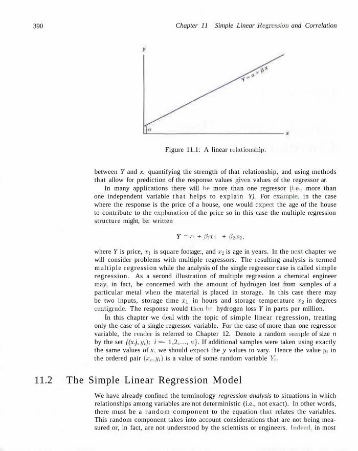
390 Chapter 11 Simple Linear Regression and Correlation
Figure 11.1: A linear relationship.
between Y and x. quantifying the strength of that relationship, and using methods that allow for prediction of the response values given values of the regressor ar.
In many applications there will be more than one regressor (i.e., more than one independent variable t ha t helps to explain Y). For example, in the case where the response is the price of a house, one would expect the age of the house to contribute to the explanation of the price so in this case the multiple regression structure might, be: written
Y = a + 0i X\ + 0\x2,
where Y is price, xi is square footage:, and x2 is age in years. In the next chapter we will consider problems with multiple regressors. The resulting analysis is termed multiple regression while the analysis of the single regressor case is called simple regression. As a second illustration of multiple regression a chemical engineer may, in fact, be concerned with the amount of hydrogen lost from samples of a particular metal when the material is placed in storage. In this case there may be two inputs, storage time xn in hours and storage temperature x2 in degrees centigrade. The response would then be: hydrogen loss Y in parts per million.
In this chapter we deal with the topic of simple linear regression, treating only the case of a single regressor variable. For the case of more than one regressor variable, the render is referred to Chapter 12. Denote a random sample of size n by the set {(x.j, yi); i — 1,2,..., n}. If additional samples were taken using exactly the same values of x. we should expect the y values to vary. Hence the value j / , in the ordered pair (.r,-, y,) is a value of some random variable Y,.
11.2 The Simple Linear Regression Model
We have already confined the terminology regression analysis to situations in which relationships among variables are not deterministic (i.e., not exact). In other words, there must be a random component to the equation that, relates the variables. This random component takes into account considerations that are not being measured or, in fact, are not understood by the scientists or engineers. Indeed, in most
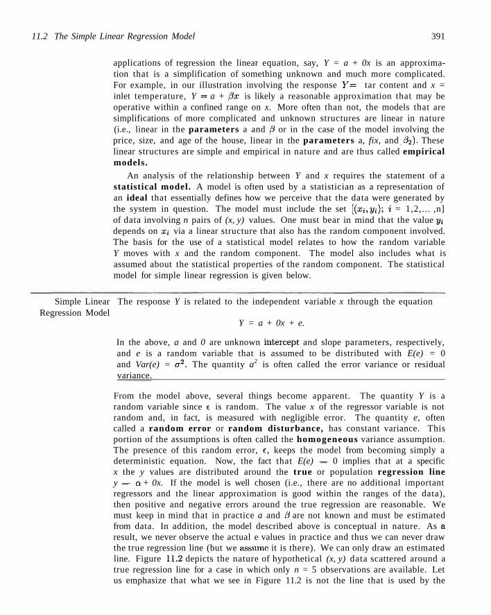
11.2 The Simple Linear Regression Model 391
applications of regression the linear equation, say, Y = a + 0x is an approximation that is a simplification of something unknown and much more complicated. For example, in our illustration involving the response Y— tar content and x = inlet temperature, Y = a + 0-x is likely a reasonable approximation that may be operative within a confined range on x. More often than not, the models that are simplifications of more complicated and unknown structures are linear in nature (i.e., linear in the parameters a and 3 or in the case of the model involving the price, size, and age of the house, linear in the parameters a, fix, and 02). These linear structures are simple and empirical in nature and are thus called empirical models.
An analysis of the relationship between Y and x requires the statement of a statistical model. A model is often used by a statistician as a representation of an ideal that essentially defines how we perceive that the data were generated by the system in question. The model must include the set [(x;,yj); i = 1,2,... ,n] of data involving n pairs of (x, y) values. One must bear in mind that the value yi depends on ,T,- via a linear structure that also has the random component involved. The basis for the use of a statistical model relates to how the random variable Y moves with x and the random component. The model also includes what is assumed about the statistical properties of the random component. The statistical model for simple linear regression is given below.
Simple Linear The response Y is related to the independent variable x through the equation Regression Model
Y = a + 0x + e.
In the above, a and 0 are unknown intercept and slope parameters, respectively, and e is a random variable that is assumed to be distributed with E(e) = 0 and Var(e) = a2. The quantity a2 is often called the error variance or residual variance.
From the model above, several things become apparent. The quantity Y is a random variable since e is random. The value x of the regressor variable is not random and, in fact, is measured with negligible error. The quantity e, often called a random error or random disturbance, has constant variance. This portion of the assumptions is often called the homogeneous variance assumption. The presence of this random error, e, keeps the model from becoming simply a deterministic equation. Now, the fact that E(e) — 0 implies that at a specific x the y values are distributed around the true or population regression line y — a + 0x. If the model is well chosen (i.e., there are no additional important regressors and the linear approximation is good within the ranges of the data), then positive and negative errors around the true regression are reasonable. We must keep in mind that in practice a and 0 are not known and must be estimated from data. In addition, the model described above is conceptual in nature. As a result, we never observe the actual e values in practice and thus we can never draw the true regression line (but we asstune it is there). We can only draw an estimated line. Figure 11.2 depicts the nature of hypothetical (x, y) data scattered around a true regression line for a case in which only n = 5 observations are available. Let us emphasize that what we see in Figure 11.2 is not the line that is used by the
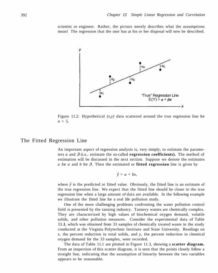
392 Chapter 11 Simple Linear Regression and Correlation
scientist or engineer. Rather, the picture merely describes what the assumptions mean! The regression that the user has at his or her disposal will now be described.
True" Regression Line E(Y) = a + f3x
Figure 11.2: Hypothetical (x,y) data scattered around the true regression line for n = 5.
The Fitted Regression Line
An important aspect of regression analysis is, very simply, to estimate the parameters a and 0 (i.e., estimate the so-called regression coefficients). The method of estimation will be discussed in the next section. Suppose we denote the estimates a for a and b for ,6\ Then the estimated or fitted regression line is given by
y = a + bx,
where y is the predicted or fitted value. Obviously, the fitted line is an estimate of the true regression line. We expect that the fitted line should be closer to the true regression line when a large amount of data are available. In the following example we illustrate the fitted line for a real life pollution study.
One of the more challenging problems confronting the water pollution control field is presented by the tanning industry. Tannery wastes are chemically complex. They are characterized by high values of biochemical oxygen demand, volatile solids, and other pollution measures. Consider the experimental data of Table 11.1, which was obtained from 33 samples of chemically treated waste in the study conducted at the Virginia Polytechnic Institute and State University. Readings on x, the percent reduction in total solids, and y, the percent reduction in chemical oxygen demand for the 33 samples, were recorded.
The data of Table 11.1 are plotted in Figure 11.3, showing a scatter diagram. From an inspection of this scatter diagram, it is seen that the points closely follow a straight line, indicating that the assumption of linearity between the two variables appears to be reasonable.
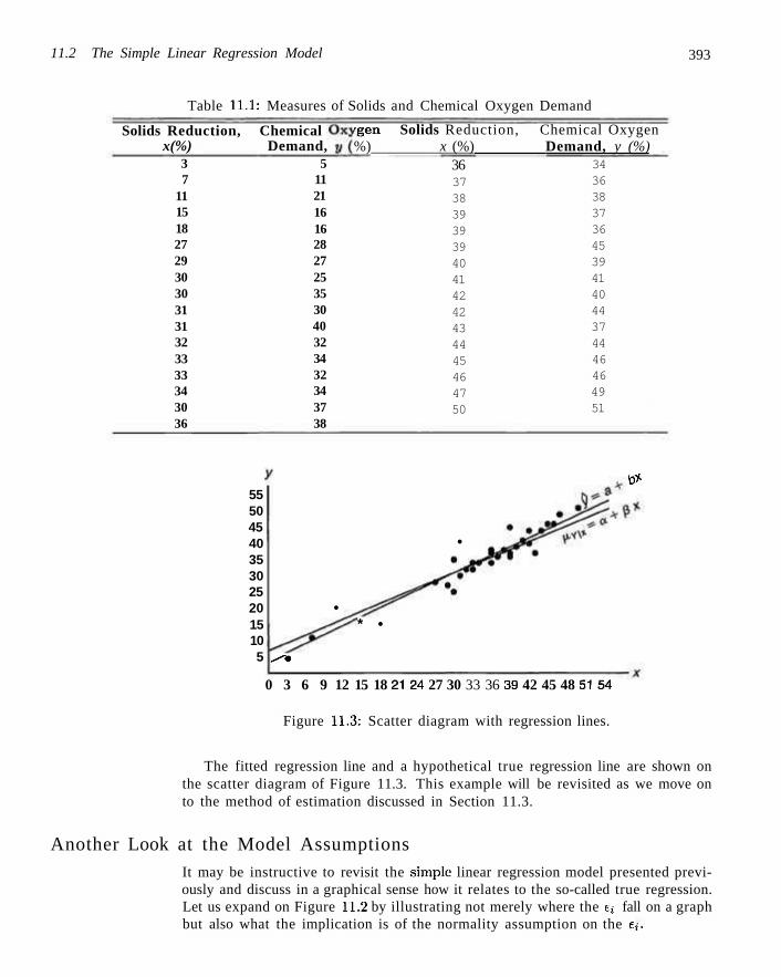
11.2 The Simple Linear Regression Model 393
Table 11.1: Measures of Solids and Chemical Oxygen Demand
rgen Solids Reduction, Chemical Oxygen %) x (%) Demand, y (%)
Solids Reduction, x(%)
3 7
11 15 18 27 29 30 30 31 31 32 33 33 34 30 36
Chemical Demand,
5 11 21 16 16 28 27 25 35 30 40 32 34 32 34 37 38
36 37 38 39 39 39 40 41 42 42 43 44 45 46 47 50
34 36 38 37 36 45 39 41 40 44 37 44 46 46 49 51
& 55 50 45 40 35 30 25 20 15 10 5 ^ »
• * •
•
0 3 6 9 12 15 18 2124 27 30 33 36 39 42 45 48 5154
Figure 11.3: Scatter diagram with regression lines.
The fitted regression line and a hypothetical true regression line are shown on the scatter diagram of Figure 11.3. This example will be revisited as we move on to the method of estimation discussed in Section 11.3.
Another Look at the Model Assumptions It may be instructive to revisit the simple linear regression model presented previously and discuss in a graphical sense how it relates to the so-called true regression. Let us expand on Figure 11.2 by illustrating not merely where the e* fall on a graph but also what the implication is of the normality assumption on the e,.
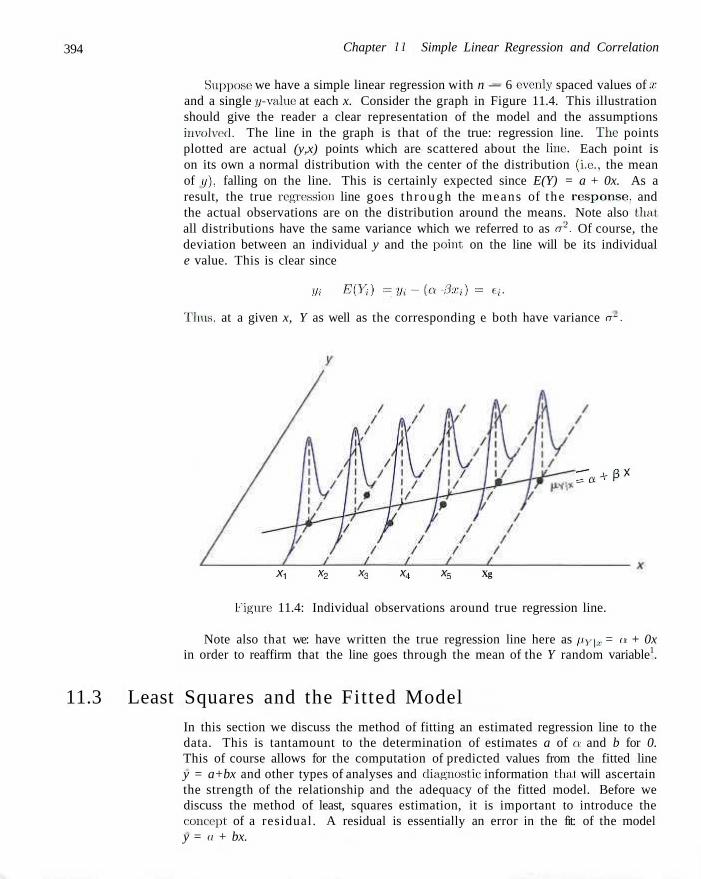
394 Chapter 11 Simple Linear Regression and Correlation
Suppose we have a simple linear regression with n — 6 evenly spaced values of a; and a single y-value at each x. Consider the graph in Figure 11.4. This illustration should give the reader a clear representation of the model and the assumptions involved. The line in the graph is that of the true: regression line. The points plotted are actual (y,x) points which are scattered about the line:. Each point is on its own a normal distribution with the center of the distribution (i.e., the mean of (/), falling on the line. This is certainly expected since E(Y) = a + 0x. As a result, the true regression line goes th rough the means of the response, and the actual observations are on the distribution around the means. Note also that all distributions have the same variance which we referred to as a2. Of course, the deviation between an individual y and the point, on the line will be its individual e value. This is clear since
yi - E(Y,) =•!,;-(a+ 0xi) = ei.
Tims, at a given x, Y as well as the corresponding e both have variance a~.
r«+p*
Xi X2 X3 X4 X5 Xg
Figure 11.4: Individual observations around true regression line.
Note also that we: have written the true regression line here as py\x = a + 0x in order to reaffirm that the line goes through the mean of the Y random variable1.
11.3 Least Squares and the Fitted Model In this section we discuss the method of fitting an estimated regression line to the data. This is tantamount to the determination of estimates a of a and b for 0. This of course allows for the computation of predicted values from the fitted line y = a+bx and other types of analyses and diagnostic information that will ascertain the strength of the relationship and the adequacy of the fitted model. Before we discuss the method of least, squares estimation, it is important to introduce the concept of a residual. A residual is essentially an error in the fit: of the model y = a + bx.
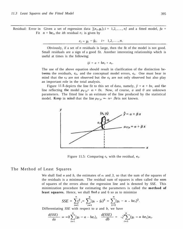
11.3 Least Squares and the Fitted Model 395
Residual: Error in Given a set of regression data [(XJ,yi);i = 1,2, Fit a + bxi, the ith residual e» is given by
, n] and a fitted model, fa =
a = yi i= 1,2.
Obviously, if a set of n residuals is large, then the fit of the model is not good. Small residuals are a sign of a good fit. Another interesting relationship which is useful at times is the following:
iji = a + bxj + Ci.
The use of the above equation should result in clarification of the distinction between the residuals, Ci, and the conceptual model errors, e,. One must bear in mind that the et are not observed but the e, are not only observed but also play an important role in the total analysis.
Figure 11.5 depicts the line fit to this set of data, namely, y = a + bx, and the line reflecting the model pY\x = a + 0x. Now, of course, a and 0 are unknown parameters. The fitted line is an estimate of the line produced by the statistical model. Keep in mind that the line pyw. — a + 0x is not known.
Figure 11.5: Comparing Cj with the residual, e*.
The Method of Least Squares
We shall find a and b, the estimates of ci and 3, so that the sum of the squares of the residuals is a minimum. The residual sum of squares is often called the sum of squares of the errors about the regression line and is denoted by SSE. This minimization procedure for estimating the parameters is called the method of least squares. Hence, we shall find a and 6 so as to minimize
ti. n u
SSE = £ e? = J2iVi - in)2 = J2iVi ~ a - bXi)2.
i=X i=\ i= l Differentiating SSE with respect to a and b, we have
d(SSE) da
- 2XXy ' -«-k*t), d(SSE)
db = -2 22iyi -a- bXi)Xi.
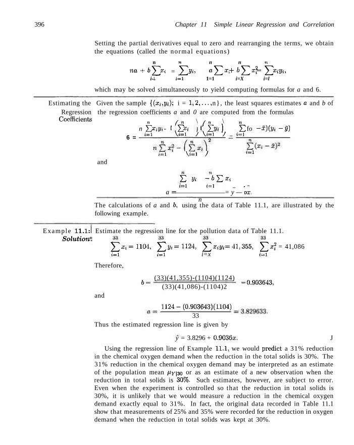
396 Chapter 11 Simple Linear Regression and Correlation
Setting the partial derivatives equal to zero and rearranging the terms, we obtain the equations (called the normal equations)
n n n n u
na + b'Yj Xi = ] P yi, aY^Xi + bY^x2 = ^2 xrt)h i-\ j=l 1=1 i=X i=l
which may be solved simultaneously to yield computing formulas for a and 6.
Estimating the Given the sample {(:(;;. j/i); i = 1,2,.. . , n} , the least squares estimates a and b of Regression the regression coefficients a and 0 are computed from the formulas
Coefficients „ / " \ / " \ n £ xm - I £ Xi I £ yi) £ fo - z)(j/i - V)
»=i \ »= i / \ t = i / _ j=i 6 =
i=i \ i = i / i = i
and
£ Vi -bT,xi t=i i= i _ .
a = = y — ox. n
The calculations of a and tb, using the data of Table 11.1, are illustrated by the following example.
Example 11.1:1 Estimate the regression line for the pollution data of Table 11.1. SolutioTi *
^ ; c t = 1104, ^ j / i = 1124, ^ 2 - ^ = 41,355, ^ a r ? = 41,086 »=i ;=i i=x i=i
Therefore,
(33)(41,355)-(1104)(1124) 6 = (33)(41,086)-(1104)2 = ° - 9 0 3 6 4 3 '
and
1124-(0.903643)(1104) 33
Thus the estimated regression line is given by
y = 3.8296 + 0.9036a;. J
Using the regression line of Example 11.1. we would predict a 31% reduction in the chemical oxygen demand when the reduction in the total solids is 30%. The 31% reduction in the chemical oxygen demand may be interpreted as an estimate of the population mean py|3o or as an estimate of a new observation when the reduction in total solids is 30%. Such estimates, however, are subject to error. Even when the experiment is controlled so that the reduction in total solids is 30%, it is unlikely that we would measure a reduction in the chemical oxygen demand exactly equal to 31%. In fact, the original data recorded in Table 11.1 show that measurements of 25% and 35% were recorded for the reduction in oxygen demand when the reduction in total solids was kept at 30%.
Exercises 397
What Is Good about Least Squares?
It should be noted that the least squares criterion is designed to provide a fitted line that results in a "closeness" between the line and the plotted points. There are many ways of measuring closeness. For example, one may wish to determine a
n n and b for which £ |y; - T/;| is minimized or for which £ \yt - y^1 '5 is minimized.
•;=i »=i These are both viable and reasonable methods. Note that both of these as well as the least squares procedure result in forcing residuals to be "small" in some sense. One should remember that the residuals are the empirical counterpart to the e values. Figure 11.6 illustrates a set of residuals. One should note that the fitted line has predicted values as points on the line and hence the residuals are vertical deviations from points to the line. As a result, the least squares procedure produces a line that minimizes the sum of squares of vertical deviations from the points to the line.
Exercises
Figure 11.6: Residuals as vertical deviations.
11.1 A study conducted at. VP1&SU to determine if certain static arm-strength measures have an influence on the "dynamic lift" characteristics of an individual. Twenty-five individuals were subjected to strength tests and then were asked to perform a weight-lifting test in which weight was dynamically lifted overhead. The data are given here. (a) Estimate a and 0 for the linear regression curve
fiY\x = a + 0x. (b) Find a point estimate of /Xy|3(). (c) Plot the residuals versus the Xa (arm strength).
Comment.
Ind iv idua l 1 2 3 4 5 6 7 8 9
10 11 12
A r m S t r e n g t h , x
17.3 19.3 19.5 19.7 22.9 23.1 26.4 26.8 27.6 28.1 28.2 28.7
D y n a m i c Lift, y
71.7 48.3 88.3 75.0 91.7
100.0 73.3 65.0 75.0 88.3 68.3 96.7
398 Chapter 11 Simple Linear Regression and Correlation
Individual 13 14 15 16 17 18 19 20 21 22 23 24 25
Arm Strength, x
29.0 29.6 29.9 29.9 30.3 31.3 36.0 39.5 40.4 44.3 44.6 50.4 55.9
Dynamic Lift, y
76.7 78.3 60.0 71.7 85.0 85.0 88.3
100.0 100.0 100.0 91.7
100.0 71.7
11.2 The grades of a class of 9 students on a midterm report (x) and on the final examination (y) are as follows:
.X
y 77 50 71 72 81 94 96 99 67 82 66 78 34 47 85 99 99 68
(a) Estimate the linear regression line. (b) Estimate the final examination grade of a student
who received a grade of 85 on the midterm report.
11.3 A study was made on the amount of converted sugar in a certain process at various temperatures. The data were coded and recorded as follows:
Temperature, x Converted Sugar, y 1.0 1.1 1.2 1.3 1.4 1.5 1.6 1.7 1.8 1.9 2.0
8.1 7.8 8.5 9.8 9.5 8.9 8.6
10.2 9.3 9.2
10.5
(a) Estimate the linear regression line. (b) Estimate the mean amount of converted sugar pro
duced when the coded temperature is 1.75. (c) Plot the residuals versus temperature. Comment.
11.4 In a certain type of metal test specimen, the normal stress on a specimen is known to be functionally related to the shear resistance. The following is a set of coded experimental data on the two variables:
Normal Stress,a: Shear Resistance,?/ 26.8 25.4 28.9 23.6
26.5 27.3 24.2 27.1
Normal Stress,x 27.7 23.9 24.7 28.1 26.9 27.4 22.6 25.6
Shear Resistance,;/ 23.6 25.9 26.3 22.5 21.7 21.4 25.8 24.9
(a) Estimate the regression line ny\x = a + ,3x. (b) Estimate the shear resistance for a normal stress of
24.5 kilograms per square centimeter.
11.5 The amounts of a chemical compound y, which dissolved in 100 grams of water at various temperature, .r, were recorded as follows:
x (°C) y (grams) 0 15 30 45 60 75
8 12 25 31 44 48
6 10 21 33 39 51
8 14 24 28 42 44
(a) Find the equation of the regression line. (b) Graph the line on a scatter diagram.
(c) Estimate the amount of chemical that will dissolve in 100 grams of water at 50°C.
11.6 A mathematics placement test is given to all entering freshmen at a small college. A student who receives a grade below 35 is denied admission to the regular mathematics course and placed in a remedial class. The placement test scores and the final grades for 20 students who took the regular course were recorded as follows:
Placement Test Course Grade 50 35 35 40 55 65 35 60 90 35 90 80 60 60 60 40 55 50 65 50
53 41 61 56 68 36 11 70 79 59 54 91 48 71 71 47 53 68 57 79
Exercises 399
(a) Plot a scatter diagram. (b) Find the equation of the regression line to predict
course grades from placement test scores. (c) Graph the line on the scatter diagram. (d) If 60 is the minimum passing grade, below which
placement test score should students in the future be denied admission to this course?
11.7 A study was made by a retail merchant to determine the relation between weekly advertising expenditures and sales. The following data were recorded:
Adver t i s ing Cos t s ($) Sales ($) 40 20 25 20 30 50 40 20 50 40 25 50
385 400 395 365 475 440 490 420 560 525 480 510
(a) Plot a scatter diagram. (b) Find the equation of the regression line to predict
weekly sales from advertising expenditures. (c) Estimate the weekly sales when advertising costs
are $35. (d) Plot the residuals versus advertising costs. Com
ment.
11.8 The following data were collected to determine the relationship between pressure and the corresponding scale reading for the purpose of calibration.
Pressure, x (lb/sq in.) 10 10 to 10 10 50 50 50 50 50
Scale Reading, y 13 18 16 15 20 86 90 88 88 92
(a) Find the equation of the regression line. (b) The purpose of calibration in this application is to
estimate pressure from an observed scale reading-Estimate the pressure for a scale reading of 54 using x = (54 — a)/b.
11.9 A study of the amount of rainfall and the quan
tity of air pollution removed produced the following data:
Daily Rainfall, Particulate Removed, x (0.01
4.3 4.5 5.9 5.6 6.1 5.2 3.8 2.J 7.5
cm) y (Mg/m3)
126 121 116 118 114 118 132 141 108
(a) Find the equation of the regression line to predict, the particulate removed from the amount of daily rainfall.
(b) Estimate the amount of particulate removed when the daily rainfall is x- = 4.8 units.
11.10 The following data are the selling prices 2 of a certain make and model of used car w years old:
w (years) z (dollars) 1 2 2 3 a 5
6350 5695 5750 5395 4985 4895
Fit a curve of the form /i-|„, = ~id'" by means of the nonlinear sample regression equation z = cd'". [Hint Write In z = In c + (In d)w = a + bw.]
11.11 The thrust of an engine (y) is a function of exhaust temperature (x) in °F when other important variables arc held constant. Consider the following data.
y 4300 4650 3200 3150 4950
X
1760 1652 1485 1390 1820
y 4010 3810 4500 3008
X
1665 1550 1700 1270
(a) Plot the data. (b) Fit a simple linear regression to the data and plot
the line through the data.
11.12 A study was done to study the effect of ambient temperature x on the electric power consumed by a chemical plant, y. Other factors were held constant and the data were collected from an experimental pilot plant.
(a) Plot the data. (b) Estimate the slope and intercept in a simple linear
400 Chapter 11 Simple Linear Regression and Correlation
regression model.
(c) Predict power consumption for an ambient temperature of 65°F.
y (BTU) 250 285 320 295
x (°F) 27 45 72 58
y (BTU) 265 298 267 321
x (°F)
31 60 3 1 71
11.13 The following is a portion of a classic data set called the "pilot plot data" in Fitting Equations to Data by Daniel and Wood, published in L971. The response y is the acid content of material produced by titration whereas the regressor X is the organic acid content produced by extraction and weighing.
y 76 62 66 58 ss
X
123 55 100 75 159
y 70 37 82 88 43
X
109 48 138 164 28
(a) Plot the data; does it appear that a simple linear regression will be a suitable model?
(b) Fit a simple linear regression; estimate a slope and intercept.
(c) Graph the regression fine on the plot in (a).
11.14 A professor in the School of Business in a university polled a dozen colleagues about the number of professional meetings professors attended in the past five years (X) and the number of papers submitted by those1 to refereed journals (Y) during the same period. The: summary data are given as follows:
n= 1.2, 1 = 4, y - 12, ii n
^ . i - ? = 2 3 2 . YxiVi = 318.
Fit a simple linear regression model between x and y by finding out the estimates of intercept and slope. Comment whether attending professional meetings would result in publishing more papers.
11.4 Properties of the Least Squares Estimators In addition to the assumptions that, the error term in the model
Y, = a + 0Xj + e-,
is a random variable with mean zero and constant variance a2, suppose tha t wc: make the further assumption that t \, t2, • •., e„. arc independent from run to run in the experiment. This provides a foundation for finding the means and variances for the estimators of a and 0.
It is important to remember that our values of a and b, based on a given sample of n observations, are only est imates of true parameters cv and 3. If the experiment is repeated over and over again, each time using the same fixed values of x, the resulting estimates of a and 0 will most likely differ from experiment to experiment. These: different estimates may be viewed as values assumed by the: random variables A and B, while a. and b arc specific realizations.
Since the values of x remain fixed, the values of A and B depend on the variations in the values of y or, more precisely, on tho values of the random variables, Yx,Y2,..., Yn. The distributional assumptions imply that the Yi's, 2 = 1 ,2 , . . . , n, are also independently distributed, with mean py\xi = a + 0x.j and equal variances ex"; that is.
>YU 1,2,
Mean and Variance of Est imators
In what follows we show that the estimator B is unbiased for 0 and demonstrate the variances of both A and B. This will begin a series of developments tha t lead
11.4 Properties of the Least Squares Estimators 401
to hypothesis testing and confidence interval estimation on the intercept and slope. Since the estimator
B
Y,(xi-x)(Yi-Y) Eto-xjy* t = l _ i = l
J2 (X{ - X)2 Y. ixi ~ X)2
»=i ?=i
is of the form YI <HYi'. where i=x
Xi ~ x . , ?. = 1,2, . . . , n ,
Zixi-x)* t = i
we may conclude from Corollary 4.4 that
£ (x^ - x)E(Yi) £) fa - *)(a + 0Xi) pB = E(B) = i=L. = i=i— =a,
Eixi-x)2 E(^-s)2
«=1 i = l
and then, using Corollary 4.10,
t,iXi-S)20Yl 2 2 i = l "
oB = 2 2 £(.r,-x)2l Efe-*)2
,:=1 J ' = 1
It can be shown (Exercise 11.15 on page 412) that the random variable A has the mean
n
PA — a and variance d\ = —^—- a2. n J2 ixt - x)2
i = l
From the foregoing results, it is apparent that the least squares estimators for a and 0 are both unbiased estimators.
Part i t ion of Total Variability and Est imation of a2
To draw inferences on a and 0, it becomes necessary to arrive at an estimate of the parameter a2 appearing in the two preceding variance formulas for A and B. The parameter a2, the model error variance, reflects random variation or experimental error variation around the regression line. In much of what follows it is advantageous to use the notation
n ii n
Sxx = Y2(Xi ~ x)2' Svv = Y2(yi~y^' Sxy = Y2ixi-x)(yi-y).
102 Chapter 11 Simple Linear Regression and Correlation
Now we may write: the error sum of squares as follows:
SSE = Y^iVi - a - bxi)2 = Y2\(Vi ~V)~ &fa - *)f
n n n
= Yfr- v? - » X > " " x](!J> ~ ® +1;1 !DX* ~ x)2
i = l i = l i = l = .'/.'/ — 2bbxy + 0 DXx — Syy — 0SXy,
the final step following from the fact that b — Sxy/S,„x.
Theorem 11.1: An unbiased estimate of a2 is
2 _ SSE _ A (iji - y,)2 _
~ n - 2 ~ ^ vi - 2 i = i
Syy VOxy
n - 2 '
The proof of Theorem 11.1 is left as an exercise (see Review Exercise 11.CI).
The Est imator of a2 as a Mean Square Error
One should observe: the result of Theorem 11.1 in order to gain sonic intuition about the estimator of a2. The parameter a2 measures variance or squared deviations between Y values and their mean given by jiy x (he., squared deviations between Y and a + 0x). Of course, the a + 0x is estimated by y = a+bx. Thus it would make sense that the variance a2 is best depicted as a squared deviation of the typical observation tjj from the estimated mean, iji, which is the corresponding point on the fitted line. Thus the (yi — iji)- values reveal the appropriate variance, much like (-iji — y)2 values measure variance: when one is sampling in a nonregression scenario. In other words, y estimates the mean in the latter simple situation whereas y-L estimates the mean of y, in a regression structure. Now, what about the divisor n — 2? In future sections we shall note that these are the degrees of freedom associated with the estimator s2 of a2. Whereas in the standard normal i.i.d. scenario, one degree of freedom is .subtracted from n in the denominator and a reasonable explanation is that one parameter is estimated, namely, the mean p by say y, but in the regression problem, two pa ramete r s are est imated, namely a and 0 by a and b. Thus the important parameter a2, estimated by
>)
s2 = £(.iy/-.i/;)V('»-2), i= i
is called a mean squared error, depicting a type of mean (division by n — 2) of the squared residuals.
11.5 Inferences Concerning the Regression Coefficients
Aside from merely estimating the linear relationship between x and Y for purposes of prediction, the experimenter may also be interested in drawing certain inferences
11.5 Inferences Concerning the Regression Coefficients 403
about, the slope and intercept. In order to allow for the testing of hypotheses and the construction of confidence intervals on a and 0, one must be willing to make the further assumption that each Cj, i — 1,2,..., n, is normally distributed. This assumption implies that Yi,Y2,...,Yn are also normally distributed, each with probability distribution n(i/;;o + 0x,,a). Since A and B are linear functions of independent normal variables, we may now deduce from Theorem 7.11 that A and B are normally distributed with probability distributions n(a; Q,CT^) and n(b; 0,0/3), respectively.
It turns out that under the normality assumption, a result very much analogous to that given in Theorem 8.4 allows us to conclude that (n—2)52/cr2 is a chi-squared variable with n — 2 degrees of freedom, independent of the random variable B. Theorem 8.5 then assures us that the statistic
T=iB-0)/io/y/$xZ) _ B-0 S/a S/^/S^
has a f-distribution with 11 — 2 degrees of freedom. The statistic T can be used to construct a 100(1 — a)% confidence interval for the coefficient 0.
Confidence Interval A 100(1 - a)% confidence interval for the parameter ,3 in the regression line for ,3 PY\X — a + 3x is
b - t,v/2 r-— < 0 <b + ttt/2-&XX V °xx
where tn/2 is a value of the (-distribution with n — 2 degrees of freedom.
Example 11.2:1 Find a 95% confidence interval for 0 in the regression line pY\x = ot + 3x, based on the pollution data of Table 11.1.
Solution: From the results given in Example 11.1 we find that
Sxx = 4152.18, Sxy = 3752.09.
In addition, we find that Syy = 3713.88. Recall that b = 0.903643. Hence,
g2 = Syy - bSxy = 3713.88 - (0.903643)(3752.09) = 1Q m Q
n — 2 31
Therefore, taking the square root, we obtain s = 3.2295. Using Table A.4, we find £0.025 ~ 2.045 for 31 degrees of freedom. Therefore, a 95% confidence interval for 0\s
0.903643 - i ^ £ E = a < 0 < 0.903643 + £ 0 * 2 2 ^ . \/4152.18 V4152.18
which simplifies to
0.8012 < 0 < 1.0061. J
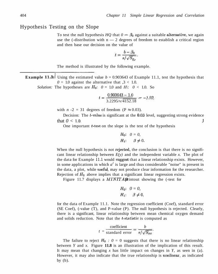
404 Chapter 11 Simple Linear Regression and Correlation
Hypothesis Testing on the Slope
To test the null hypothesis HQ that 0 — 0o against a suitable alternative, we again use the (-distribution with n — 2 degrees of freedom to establish a critical region and then base our decision on the value of
'x.r s/y/S~x
The method is illustrated by the following example.
Example 11.3:1 Using the estimated value b = 0.903643 of Example 11.1, test the hypothesis that 0 = 1.0 against the alternative that ,3 < 1.0.
Solution: The hypotheses are //(): 0 = 1.0 and H\: 0 < 1.0. So
t_ 0.903643-1.0 _ _ 1 C ) ( ?
3.2295/v/4152.18
with n -2 = 31 degrees of freedom (P « 0.03). Decision: The t-value is significant at the 0.03 level, suggesting strong evidence
that 0 < 1.0. J One important f-test on the slope is the test of the hypothesis
HQ: 0 = 0,
Hi: 0^0.
When the null hypothesis is not rejected, the conclusion is that there is no significant linear relationship between E(y) and the independent variable x. The plot of the data for Example 11.1 would suggest that a linear relationship exists. However, in some applications in which a2 is large and thus considerable "noise" is present in the data, a plot, while useful, may not produce clear information for the researcher. Rejection of Ho above implies that a significant linear regression exists.
Figure 11.7 displays a MINITAB printout showing the (-test for
H0: 0 = 0, Hi: 0^0,
for the data of Example 11.1. Note the regression coefficient (Coef), standard error (SE Coef), (-value (T), and P-value (P). The null hypothesis is rejected. Clearly, there is a significant, linear relationship between mean chemical oxygen demand and solids reduction. Note that the (-statistic is computed as
coefficient b t = standard error
The failure to reject H0 : 0 = 0 suggests that there is no linear relationship between Y and x. Figure 11.8 is an illustration of the implication of this result. It may mean that changing x has little impact on changes in Y, as seen in (a). However, it may also indicate that the true relationship is nonlinear, as indicated by (b).
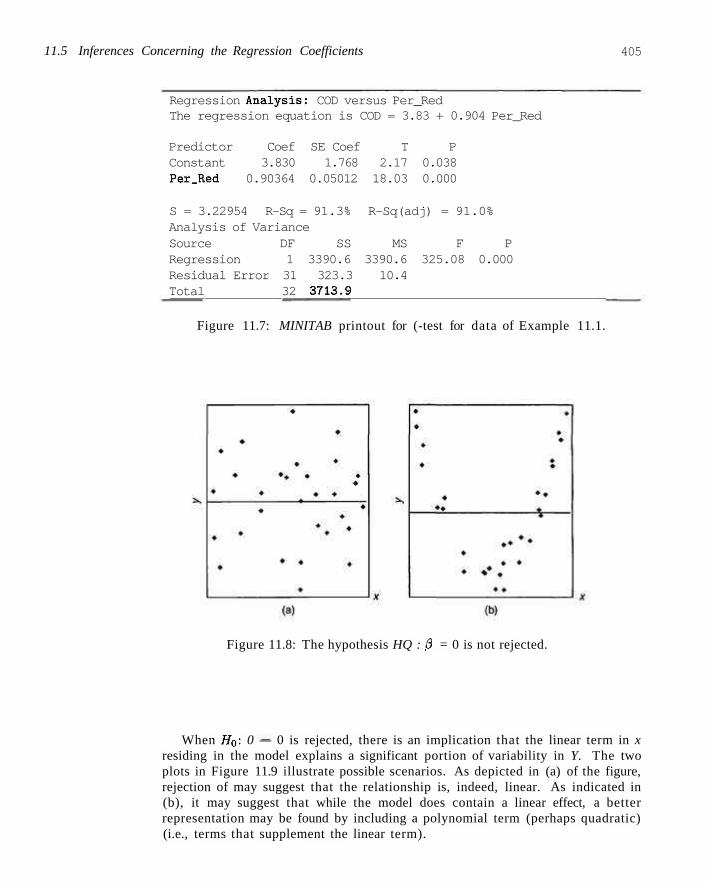
11.5 Inferences Concerning the Regression Coefficients 405
Regression Analysis: COD versus Per_Red The regression equation is COD = 3.83 + 0.904 Per_Red
Predictor Coef SE Coef T P Constant 3.830 1.768 2.17 0.038 Per.Red 0.90364 0.05012 18.03 0.000
S = 3.22954 R-Sq = 91.3% R-Sq(adj) = 91.0% Analysis of Variance Source DF SS MS F P Regression 1 3390.6 3390.6 325.08 0.000 Residual Error 31 323.3 10.4 Total 32 3713.9
Figure 11.7: MINITAB printout for (-test for data of Example 11.1.
Figure 11.8: The hypothesis HQ : ,3 = 0 is not rejected.
When Ho: 0 — 0 is rejected, there is an implication that the linear term in x residing in the model explains a significant portion of variability in Y. The two plots in Figure 11.9 illustrate possible scenarios. As depicted in (a) of the figure, rejection of may suggest that the relationship is, indeed, linear. As indicated in (b), it may suggest that while the model does contain a linear effect, a better representation may be found by including a polynomial term (perhaps quadratic) (i.e., terms that supplement the linear term).
406 Chapter 11 Simple Linear Regression and Correlation
Figure 11.9: The hypothesis Ho : 0 = 0 is rejected.
Statistical Inference on the Intercept
Confidence intervals and hypothesis testing on the coefficient a may be established from the fact that A is also normally distributed. It is not difficult to show that
T = A- a
SJZx*/(nSxx)
has a (-distribution with n — 2 degrees of freedom from which we may construct a 100(1 - a)% confidence interval for a.
Confidence Interval A 100(1 — a)% confidence interval for the parameter a in the regression line for a PY\X — a + 0x is
a - (a/2 ; „ < a <a + ta Vm%. y/noxx
where ta/2 is a value of the (-distribution with n — 2 degrees of freedom.
Note that the symbol a is used here in two totally unrelated ways, first as the level of significance and then as the intercept of the regression line.
Example 11.4:1 Find a 95% confidence interval for a in the regression line py\x = a + 0x, based on the data of Table 11.1.
Solution: In Examples 11.1 and 11.2 we found that
Svx = 4152.18 and s = 3.2295.
21.5 Inferences Concerning the Regression Coefficients 407
From Example 11.1 wc: had
V xj = 41,086 and a = 3.829633. i = i
Using Table A.4, we find (0.(125 « 2.045 for 31 degrees of freedom. Therefore, a 95% confidence interval for n is
(2.045) (3.2295) v/41,086 3.829633 - i • ,V = <o < 3.829633
v/(33)(4152.18) (2.045)(3.229.r))y/41.U86
v/(33)(4152.l8)
which simplifies to 0.2132 < a < 7.4 161. J To test the null hypothesis Ho that a = ao against a suitable alternative, we
can use the (-distribution with n — 2 degrees of freedom to establish a critical region and then base our decision 011 the: value of
sJT,xf/{nSxx]
Example 11.5:1 Using the estimated value a = 3.829640 of Example 11.1, test the hypothesis that (\ = 0 at the 0.05 loved of significance' against the alternative that er ^ 0.
Solution: The hypotheses are Ho', n = 0 and Hi', a / 0. So
_ 3.829633 - 0 _ 9
~ 3.2295v/41,086/((33)(4152.18)) ' ;
with 31 degrees of freedom. Thus P = P-value « 0.038 and wc conclude that a =fi 0. Note that this is merely Coef/StDev, as wc sec in the MINITAB printout
in Figure 11.7. The SE Coef is the standard error of the estimated intercept. J
A Measure of Quality of Fit : Coefficient of Determinat ion
Note in Figure 11.7 that an item denoted by R-Sq is given with a value of 91.3%. This quantity, R2, is called the coefficient of de te rmina t ion . This quantity is a measure of the propor t ion of variability explained by the fitted model . In Section 11.8 we slnill introduce the notion of an analysis of variance approach to hypothesis testing in regression. The analysis of variance approach makes use of the
error sum of squares SSE = YI iVi — lli)2 a n ( ' the to ta l corrected sum of squares ;=i
u SST — Y2iVi —iii)2- The latter represents the variation in the response values that
i= i ideally would be explained by the model. The SSE value is the variation due to error, or variat ion unexplained. Clearly, if SSE = 0, all variation is explained. The quantity that represents variation explained is SSI1 — SSE. The Rr is
,., ... ,. , , . . n2 ., 00E Coeff. of determination: Rr = 1 — .
408 Chapter 11 Simple Linear Regression and Correlation
Note that if the fit is perfect, all residuals are zero, and thus R2 = 1.0. But if SSE is only slightly smaller than SST, R2 « 0. Note from the printout in Figure 11.7 that the coefficient of determination suggests that the model fit to the data explains 91.3% of the variability observed in the response, the chemical oxygen demand.
The plots in Figure 11.10 provide an illustration of a good fit (P 2 « 1.0) for plot (a) and a poor fit (P 2 « 0) for plot (b).
(a) R? a 1.0 (b) fl2a0
Figure 11.10: Plots depicting a very good fit and a poor fit.
Pitfalls in the Use of B?
Analysts quote values of R2 quite often, perhaps due to its simplicity. However there are pitfalls in its interpretation. The reliability of P2 is a function of the size of the regression data set and the type of applications. Clearly, 0 < P2 < 1 and the upper bound is achieved when the fit to the data is perfect (i.e., all of the residuals are zero). What is an acceptable value for P 2 ? This is a difficult question to answer. A chemist, charged with doing a linear calibration of a high-precision piece of equipment, certainly expects to experience a very high P2-value (perhaps exceeding 0.99) while a behavioral scientist, dealing in data impacted by variability in human behavior, may feel fortunate to experience an P2 as large as 0.70. An experienced model fitter senses when a value is large enough, given the situation confronted. Clearly, some scientific phenomena lend themselves to modeling with more precision than others.
The P2 criterion is dangerous to use for comparing competing models for the same data set. When one adds additional terms to the model (e.g., an additional regressor), it decreases SSE and thus increases P2 (at least not decrease it). This implies that R2 can be made artificially high by an unwise practice of overfltting (i.e., the inclusion of too many model terms). Thus, the inevitable increase in
11.6 Prediction 409
P2 enjoyed by adding an additional term does not imply the additional term was needed. In fact, the simple model may be superior for predicting response values. The role of overfitting and its influence on prediction capability will be discussed at length in Chapter 12 as we visit the notion of models involving more than a single regressor. Suffice it to say at this point that one should not subscribe to a model selection process that solely involves the consideration of R2.
11.6 Prediction
There are several reasons for building a linear regression. One, of course, is to predict response values at one or more values of the independent variable. In this section the focus is on errors associated with prediction.
The equation y = a+bx may be used to predict or estimate the mean response P-Y\x0
a t x = XQ, where .To is not necessarily one of the prechosen values, or it may be used to predict a single value j/o of the variable YQ, when x = XQ. We would expect, the error of prediction to be higher in the case of a single predicted value than in the case where a mean is predicted. This, then, will affect the width of our intervals for the values being predicted.
Suppose that the experimenter wishes to construct a confidence interval for PY\X0- ^ e s n a ^ u s e the point estimator YQ = A + Bx0, to estimate py\Xo = a+0x. It can be shown that the sampling distribution of YQ is normal with mean
pY,xo = E(Y0) = E(A + BXQ) = a + 0xo = py \x0
and variance
2 2 2 2 ""Vo = aA+Bx0 ~ aY+B(x0-&) ~ ° n S-
21
the latter following from the fact that Cov(Y,B) = 0 (see Exercise 11.16 on page 412). Thus a 100(1 - a)% confidence interval on the mean response py\Xa can now be constructed from the statistic
T = YQ - PY\x0
S^l/n+ixo-xY/Sj
which has a (-distribution with n — 2 degrees of freedom.
Confidence Interval A 100(1 — a)% confidence interval for the mean response py\Xo is for py\Xli
/ l (x0-x)2 „ / l (xo-x)2
;</o -ta/2s\ - + 5 <VY\XU < 2/0 + ta/2S\ ~ + 5 ' y n J I J y ^ oXx
where tQ/2 is a value of the (-distribution with n — 2 degrees of freedom.
Example 11.6:1 Using the data of Table 11.1, construct a 95% confidence limits for the mean response py\Xo-
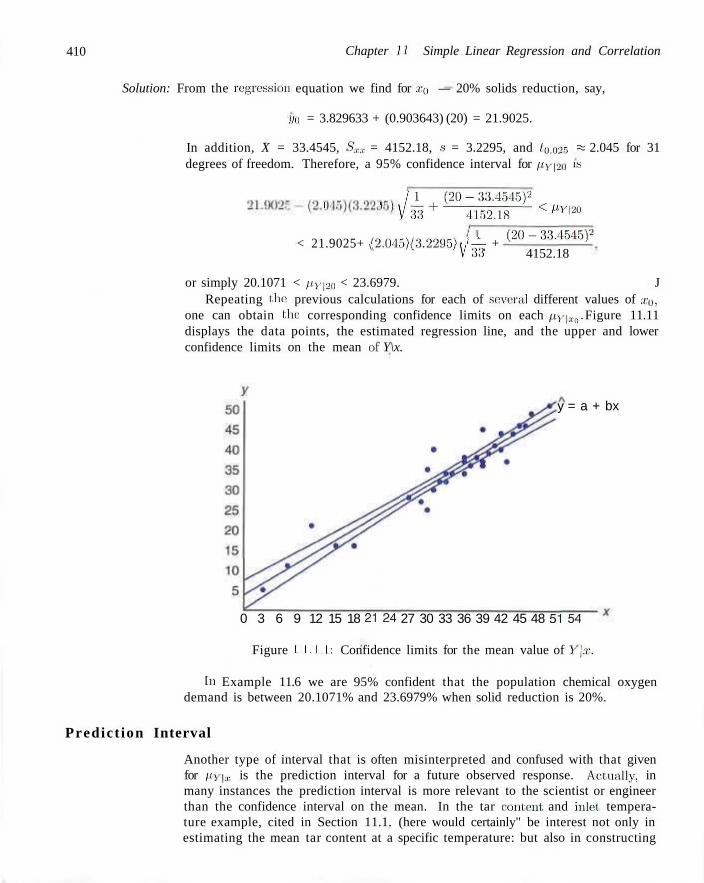
410 Chapter 11 Simple Linear Regression and Correlation
Solution: From the regression equation we find for XQ — 20% solids reduction, say,
.1/0 = 3.829633 + (0.903643) (20) = 21.9025.
In addition, X = 33.4545, Sxx = 4152.18, s = 3.2295, and i0.036 « 2.045 for 31 degrees of freedom. Therefore, a 95% confidence interval for //>|2o 1S
< ! ' \/4+(2\L52,^'5)2<^l2"
< 21.9025+ (2.045)(3.2295)t/- + ( 2 ° ~ 3 3 ' 4 5 4 5 ) 2 v " ; V 3 3 4152.18
or simply 20.1071 < / / r | 2 0 < 23.6979. J Repeating the1 previous calculations for each of several different values of a,'0,
one can obtain the corresponding confidence limits on each py^. Figure 11.11 displays the data points, the estimated regression line, and the upper and lower confidence limits on the mean of Y\x.
y = a + bx
0 3 6 9 12 15 18 2124 27 30 33 36 39 42 45 48 5154
Figure I I. I I: Confidence limits for the mean value of Y\x.
fn Example 11.6 we are 95% confident that the population chemical oxygen demand is between 20.1071% and 23.6979% when solid reduction is 20%.
Predict ion Interval
Another type of interval that is often misinterpreted and confused with that given for /(y-|.,. is the prediction interval for a future observed response. Actually, in many instances the prediction interval is more relevant to the scientist or engineer than the confidence interval on the mean. In the tar content and inlet temperature example, cited in Section 11.1. (here would certainly" be interest not only in estimating the mean tar content at a specific temperature: but also in constructing
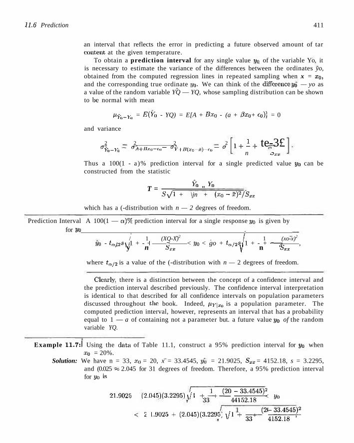
22.6' Prediction 411
an interval that reflects the error in predicting a future observed amount of tar content at the given temperature.
To obtain a prediction interval for any single value r/n of the variable Yo, it is necessary to estimate the variance of the differences between the ordinates yo, obtained from the computed regression lines in repeated sampling when x = xo, and the corresponding true ordinate y0. We can think of the difference yo — yo as a value of the random variable YQ — YQ, whose sampling distribution can be shown to be normal with mean
Py-0_y-0 = E(YQ - YQ) = E[A + BXQ - (a + 0xo + e0)] = 0
and variance
2 2 2 2 aY0-Y0 — aA+Bxa-to ~ °~?+B{x0-x)-(.u ~ ° 1 + I + te-3£
n oxx
Thus a 100(1 - a )% prediction interval for a single predicted value y0 can be constructed from the statistic
T = ^° " Y° Sy/\ + \jn + (xQ-x)2/Sxx
which has a (-distribution with n — 2 degrees of freedom.
Prediction Interval A 100(1 — Q ) % prediction interval for a single response yo is given by for y0 .
/ 1 (XQ-X)2 . / 1 (xo-x)2
2/o - ta/2SA 1 + - H - < y0 < go + ta/2Si 1 + - + — 5 , ' y n Sxx Y n 5XX
where ta/2 is a value of the (-distribution with n — 2 degrees of freedom.
Clearly, there is a distinction between the concept of a confidence interval and the prediction interval described previously. The confidence interval interpretation is identical to that described for all confidence intervals on population parameters discussed throughout the book. Indeed, py\Xo is a population parameter. The computed prediction interval, however, represents an interval that has a probability equal to 1 — a of containing not a parameter but. a future value yo of the random variable YQ.
Example 11.7:1 Using the data of Table 11.1, construct a 95% prediction interval for j/o when XQ = 20%.
Solution: We have n = 33, x0 = 20, x = 33.4545, yo = 21.9025, Sxx = 4152.18, s = 3.2295, and (0.025 ~ 2.045 for 31 degrees of freedom. Therefore, a 95% prediction interval for yo is
21.9025 - (2.045,(3.2295) V<T + 1 + ( 2 ° = j f ^ < »o
< ? 1.9025 + (2.045)(3.2205) y/l + g + ^ J ^ ^ -
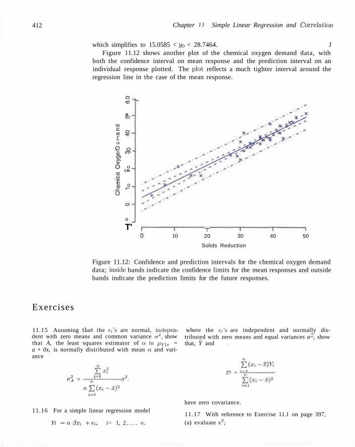
412 Chapter 11 Simple Linear Regression and Correlation
which simplifies to 15.0585 < y0 < 28.7464. J Figure 11.12 shows another plot of the chemical oxygen demand data, with
both the confidence interval on mean response and the prediction interval on an individual response plotted. The plot, reflects a much tighter interval around the regression line in the case of the mean response.
o _ CD ^
o
O 7D C a £ CD
Q c S -a> co cs> >. x O o . _ CM CO o
% o .
O
o
T' T 10 30 20
Solids Reduction
40 50
Figure 11.12: Confidence and prediction intervals for the chemical oxygen demand data; inside bands indicate the confidence limits for the mean responses and outside bands indicate the prediction limits for the future responses.
Exercises
11.15 Assuming that, the e,'s are normal, indepen- where the it's are independent and normally dis-dent with zero means and common variance a2, show that A, the least squares estimator of a in /.iy|x. = a + 0x, is normally distributed with mean a and variance
a\ = i = l
nJ^ixi-S)3
i = l
11.16 For a simple linear regression model
Yi =a+ pXi +€i, i= 1, 2 . . . . . ii.
tributed with zero means and equal variances a~, show that, Y and
2? = £0»»
1 = 1
x)Yi
1=1
have zero covariance.
11.17 With reference to Exercise 11.1 on page 397, (a) evaluate s ,
Exercises 413
(b) test; the hypothesis that 3 = 0 against the alternative that 0 ,£ 0 at the 0.05 level of significance and interpret the resulting decision.
11.18 With reference to Exercise 11.2 on page 398,
(a) evaluate s2; (b) construct a 95% confidence interval for a;
(c) construct a 95% confidence interval for 0.
11.19 With reference to Exercise 11.3 on page 398,
(a) evaluate s2; (b) construct a 95% confidence interval for a;
(c) construct a 95% confidence interval for 3.
11.20 With reference to Exercise 11.4 on page 398, (a) evaluate s2;
(b) construct a 99% confidence interval for a; (c) construct a 99%. confidence interval for 3.
11.21 With reference to Exercise 11.5 on page 398,
(a) evaluate s2;
(b) construct a 99% confidence interval for a;
(c) construct a 99% confidence interval for 0.
11.22 Test the hypothesis that a = 10 in Exercise 11.6 on page 398 against the alternative that a < 10. Use a 0.05 level of significance.
11.23 Test the hypothesis that 0 = 6 in Exercise 11.7 on page 399 against the alternative that 3 < 6. Use a 0.025 level of significance.
11.24 Using the value of s2 found in Exercise 11.18(a), construct a 95% confidence interval for /ly-isa in Exercise 11.2 on page 398.
11.25 With reference to Exercise 11.4 on page 398, use the value of s2 found in Exercise 11.20(a) to compute (a) a 95% confidence interval for the menu shear resis
tance when x = 24.5; (b) a 95% prediction interval for a single predicted
value of the shear resistance when x = 24.5.
11.26 Using the value of s2 found in Exercise 11.19(a), graph the regression line and the 95% confidence bands for the mean response py\x for the data of Exercise 11.3 on page 398.
11.27 Using the value of s2 found in Exercise 11.19(a), construct a 95% confidence interval for the amount of converted sugar corresponding to x = 1.6 in
Exercise 11.3 on page 398.
11.28 With reference to Exercise 11.5 on page 398, use the value of sa found in Exercise 11.21(a) to compute (a) a 99% confidence interval for the average amount
of chemical that will dissolve in 100 grams of water at 50° C;
(b) a 99% prediction interval for the amount of chemical that will dissolve in 100 grams of water at 50°C.
11.29 Consider the regression of mileage for certain automobiles, measured in miles per gallon (mpg) on their weight in pounds (wt). The data are from Consumer Reports (April 1997). Part of the SAS output from the procedure is shown in Figure 11.13. (a) Estimate the mileage for a vehicle weighing 4000
pounds. (b) Suppose that the Honda engineers claim that, on
average, the Civic (or any other model car weighing 2440 pounds) gets more than 30 mpg. Based on the results of the regression analysis, would you believe that claim? Why or why not?
(c) The design engineers for the Lexus ES300 targeted 18 mpg as being ideal for this model (or any other model weighing 3390 pounds) although it is expected that some variation will be experienced. Is it likely that this target value is realistic? Discuss.
11.30 Show that in the case of a least, squares fit to the simple linear regression model
Yi = a + 0xi + ei, i = 1 ,2 . . . . . n,
that Y. iVi - 2/0 = £ e< = 0. » = i ; = i
11.31 Consider the situation of Exercise 11.30 but suppose n = 2 (i.e., only two data points are available). Give an argument that the least squares regression line will result in (t/i — i/t) = (y2 — y2) = 0. Also show that for this case R2 = 1.0.
11.32 There are important applications in which due to known scientific constraints, the regression line must go through the origin (i.e., the intercept must be zero). In other words, the model should read
Yi = 3xi+f.i, 1.2, •, n,
and only a simple parameter requires estimation. The model is often called the regression through the origin model. (a) Show that the least squares estimator of the slope
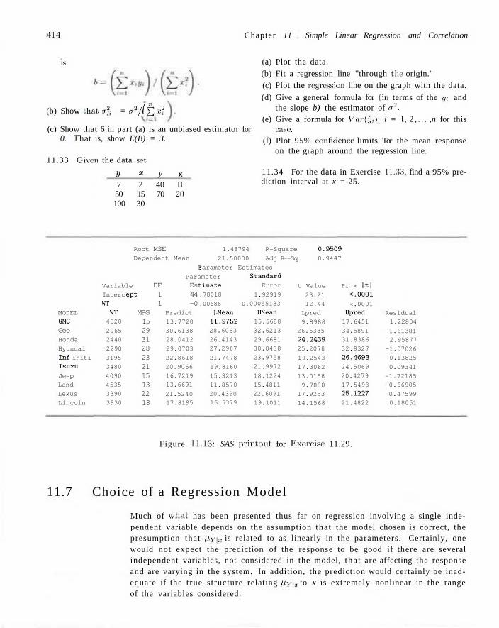
I l l Chapter 11 Simple Linear Regression and Correlation
is
(b) Show that er% = a2/ ( jr x'f
(c) Show that 6 in part (a) is an unbiased estimator for 0. That is, show E(B) = 3.
11.33 Given the data set
y x y x 7 2 40 10 50 15 70 2(1 100 30
(a) Plot the data. (b) Fit a regression line ''through the origin." (c) Plot the regression line on the graph with the data.
(d) Give a general formula for (in terms of the ?/,• and the slope b) the estimator of a2.
(e) Give a formula for V"«r(t/,); i = I, 2 , . . . ,n for this case:.
(I) Plot 95% confidence limits Tor the mean response on the graph around the regression line.
11.34 For the data in Exercise 11.33. find a 95% prediction interval at x = 25.
MODEL
GHC Geo Honda
Hyundai
Inf. initi
Isuzu
Jeep
Land
Lexus
Lincoln
Root MSE Dependent Mean
Variable
Interc
WT WT 4520
2065
2440
2290
3195
3480
4090
4535
3390
3930
cpt
MPG 15 29 31 28 23 21 15 13 22 18
DF 1 1
:
1.48794
21.50000
R-Square 0.9509
Adj R-
Parameter Estimates
Parameter
Es 44 -0
Predict
13.7720
30.6138
28.0412
29.0703
22.8618
20.9066
16.7219
13.6691
21.5240
17.8195
timate
.78018
.00686 0.
LMean
11.9752
28.6063
26.4143
27.2967
21.7478
19.8160
15.3213
11.8570
20.4390
16.5379
Standard
Error
1.92919
00055133
UMoan 15.5688
32.6213
29.6681
30.8438
23.9758
21.9972
18.1224
15.4811
22.6091
19.1011
-Sq 0.9447
t Value
23.21
-12.44
Lpred
9.8988
26.6385
24.2439
25.2078
19.2543
17.3062
13.0158
9.7888
17.9253
14.1568
Pr > Itl
<.0001
<.0001 Upred
17.6451
34.5891
31.8386
32.9327
26.4693
24.5069
20.4279
17.5493
25.1227
21.4822
Residual
1.22804
-1.61381
2.95877
-1.07026
0.13825
0.09341
-1.72185
-0.66905
0.47599
0.18051
Figure 11.13: SAS printout for Exercise 11.29.
11.7 Choice of a Regression Model
Much of what has been presented thus far on regression involving a single independent variable depends on the assumption that the model chosen is correct, the presumption that p.y\x is related to as linearly in the parameters. Certainly, one would not expect the prediction of the response to be good if there are several independent variables, not considered in the model, t ha t are affecting the response and are varying in the system. In addition, the prediction would certainly be inadequate if the t rue structure relating py\x to x is extremely nonlinear in the range of the variables considered.
11.8 Analysis-of-Variance Ap;)ioach 415
Often the simple linear regression model is used even though it is known that the model is something other than linear or that the true structure is unknown. This approach is often sound, particularly when the range of a; is narrow. Thus the model used becomes an approximating function that one hopes is an adequate rep-resentation of the true: picture in the region of interest. One should note, however, the effect of an inadequate model on the results presented thus far. For example, if the true model, unknown to the experimenter, is linear in more than one x, say,
P>Y\xuxi = Oi + 0iX] +fcx2,
then the ordinary least squares estimate b = Sxj)/Sxx, calculated by only considering .t'i in the experiment, is, under general circumstances, a biased estimate of the coefficient p\, the bias being a function of the additional coefficient 02 (see Exercise 11.37 on page 423). Also, the estimate sa for a2 is biased due to the additional variable.
11.8 Analysis-of-Variance Approach
Often the problem of analyzing the quality of the estimated regression line is handled by an analysis-of-variance (ANOVA) approach: a procedure whereby the total variation in the dependent variable: is subdivided into meaningful components that arc then observed and treated in a systematic: fashion. The analysis of variance, discussed in Chapter 13, is a powerful resource that is used for many applications.
Suppose that wc have n experimental data points in the usual form (x-i.-yi) and that the regression line is estimated. In our estimation of a2 in Section 11.4 we establish the identity
Syy = bSxy + SSE.
Aii alternative and perhaps more informative formulation is
n n it
X > - v)2 = X > - a)2 + ]T> - fc)a-; = i i = i ?.=i
So we have achieved a partitioning of the to ta l corrected sum of squares of y info two components that should reflect particular meaning to the experimenter. Wc: shall indicate this partitioning symbolically as
SST = SSR + SSE.
The first component of the right, SSR, is called the regression sum of squares and it reflects the amount of variation in the //-values explained by the model , in this case the postulated straight, line. The second component is the familiar error sum of squares, which reflects variation about the regression line.
Suppose thai; we arc interested in testing the hypothesis
HQ: /S = 0,
HI: 0^0,
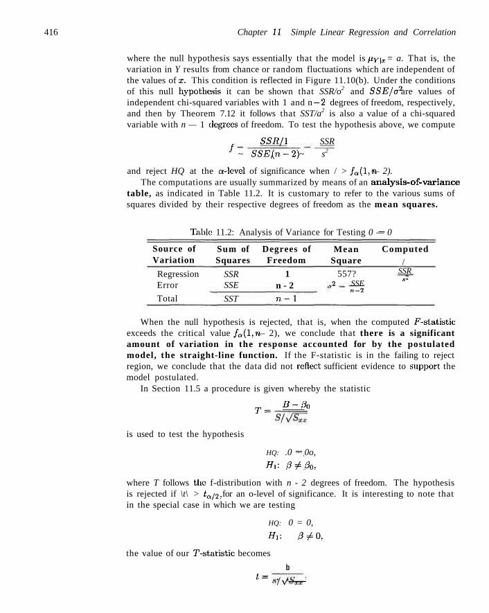
416 Chapter 11 Simple Linear Regression and Correlation
where the null hypothesis says essentially that the model is py\x = a. That is, the variation in Y results from chance or random fluctuations which are independent of the values of a:. This condition is reflected in Figure 11.10(b). Under the conditions of this null hypothesis it can be shown that SSR/o2 and SSE/a2 are values of independent chi-squared variables with 1 and n —2 degrees of freedom, respectively, and then by Theorem 7.12 it follows that SST/a2 is also a value of a chi-squared variable with n — 1 degrees of freedom. To test the hypothesis above, we compute
557?./1 SSR i ~ SSE/ (n-2) ~ s2
and reject HQ at the en-level of significance when / > fa(l,n — 2). The computations are usually summarized by means of an analysis-of-variance
table, as indicated in Table 11.2. It is customary to refer to the various sums of squares divided by their respective degrees of freedom as the mean squares.
Tabic 11.2: Analysis of Variance for Testing 0 — 0
Source of Variation
Regression Error
Total
Sum of Squares
SSR SSE
SST
Degrees of Freedom
1 n - 2
n - 1
Mean Square
557? „2 _ SSE
71—2
Computed /
SSR a-
When the null hypothesis is rejected, that is, when the computed F-statistic exceeds the critical value fQ(l,n — 2), we conclude that there is a significant amount of variation in the response accounted for by the postulated model, the straight-line function. If the F-statistic is in the failing to reject region, we conclude that the data did not reflect sufficient evidence to support the model postulated.
In Section 11.5 a procedure is given whereby the statistic
r__ B-0Q
is used to test the hypothesis
HQ: .0 = 0o,
Hi: ,6V 3 0 ,
where T follows the f-distribution with n - 2 degrees of freedom. The hypothesis is rejected if \t\ > taj2, for an o-level of significance. It is interesting to note that in the special case in which we are testing
HQ: 0 = 0,
Hi: 0^0,
the value of our [/""-statistic becomes
b t= . ,
11.9 Test for Linearity of Regression: Data with Repeated Observations 417
and the hypothesis under consideration is identical to that being tested in Table 11.2. Namely, the null hypothesis states that the variation in the response is due merely to chance. The analysis of variance uses the F-distribution rather than the (-distribution. For the two-sided alternative, the two approaches are identical. This we can see by writing
.2 _ " SXx OOxy Solx
' ~^2~~~s^~~ ~P~'
which is identical to the /-value used in the analysis of variance. The basic relationship between the (-distribution with v degrees of freedom and the F-distribution with 1 and v degrees of freedom is
t2 = f(l,v).
Of course, the (-test allows for testing against a one-sided alternative while the F-test is restricted to testing against a two-sided alternative.
Annotated Computer Printout for Simple Linear Regression
Consider again the chemical oxygen demand data of Table 11.1. Figures 11.14 and 11.15 show more complete annotated computer printouts. Again the we illustrate it with MINITAB PC software. The (-ratio column indicates tests for null hypotheses of zero values on the parameter. The term "Fit" denotes y-values, often called fitted values. The term :'SE Fit" is used in computing confidence intervals on mean response. The item R2 is computed as (SSR/SST) x 100 and signifies the proportion of variation in y explained by the straight-line regression. Also shown are confidence intervals on the mean response and prediction intervals on a new observation.
11.9 Test for Linearity of Regression: Data with Repeated Observations
For certain kinds of experimental situations the researcher has the capability of obtaining repeated observations on the response for each value of x. Although it is not necessary to have these repetitions in order to estimate a and 0, nevertheless repetitions enable the experimenter to obtain quantitative information concerning the appropriateness of the model. In fact, if repeated observations are generated, the experimenter can make a significance test to aid in determining whether or not the model is adequate.
Let us select a random sample of n observations using k distinct values of x, say xx, x2,..., xn, such that, the sample contains n\ observed values of the random variable Yx corresponding to xx, n2 observed values of Y2 corresponding to x2,...,
k nk observed values of Yt,- corresponding to x/,-. Of necessity, n = 2~2ni-
418 Chapter 11 Simple Linear Regression and Correlation
The regression equat Predictor Constant Per Red 0.
S = 3.22954
Source Regression Res:
ion is COD =3.83 Coef SE Coef
3.830 90364 C R-Sq =
Analysis DF 1
Ldual Error 31 Total
Obs 1 2 3 4 5 6 7 8 9 10 11 12 13 14 15 16 17 18 19 20 21 22 23 24 25 26 27 28 29 30 31 32 33
Per Red 3.0
36.0 7.0
37.0 11.0 38.0 15.0 39.0 18.0 39.0 27.0 39.0 29.0 40.0 30.0 41.0 30.0 42.0 31.0 42.0 31.0 43.0 32.0 44.0 33.0 45.0 33.0 46.0 34.0 47.0 36.0 50.0 36.0
32
COD 5.000
34.000 11.000 36.000 21.000 38.000 16.000 37.000 16.000 36.000 28.000 45.000 27.000 39.000 25.000 41.000 35.000 40.000 30.000 44.000 40.000 37.000 32.000 44.000 34.000 46.000 32.000 46.000 34.000 49.000 37.000 51.000 38.000
1.768 '.05012 91.3'/.
T 2.17 0. 18.03 0. R-Sq(adi)
; of Variance SS
3390.6 323.3 3713.9
Fit 6.541
36.361 10.155 37.264 13.770 38.168 17.384 39.072 20.095 39.072 28.228 39.072 30.035 39.975 30.939 40.879 30.939 41.783 31.843 41.783 31.843 42.686 32.746 43.590 33.650 44.494 33.650 45.397 34.554 46.301 36.361 49.012 36.361
MS
I + 0.904 Per P
038 000 = 91.0%
F P 3390.6 325.08 0.000 10.4
SE Fit 1.627 0.576 1.440 0.590 1.258 0.607 1.082 0.627 0.957 0.627 0.649 0.627 0.605 0.651 0.588 0.678 0.588 0.707 0.575 0.707 0.575 0.738 0.567 0.772 0.563 0.807 0.563 0.843 0.563 0.881 0.576 1.002 0.576
Residual St -1.541 -2.361 0.845 -1.264 7.230 -0.168 -1.384 -2.072 -4.095 -3.072 -0.228 5.928 -3.035 -0.975 -5.939 0.121 4.061 -1.783 -1.843 2.217 8.157 -5.686 -0.746 0.410 0.350 1.506 -1.650 0.603 -0.554 2.699 0.639 1.988 1.639
.Red
Resid -0.55 -0.74 0.29 -0.40 2.43 -0.05 -0.45 -0.65 -1.33 -0.97 -0.07 1.87 -0.96 -0.31 -1.87 0.04 1.28 -0.57 -0.58 0.70 2.57 -1.81 -0.23 0.13 0.11 0.48 -0.52 0.19 -0.17 0.87 0.20 0.65 0.52
Figure 11.14: MINITAB printout of simple linear regression for chemical oxygen demand data; part I.
We define
ijij = the j th value of the random variable Y-,. m
Vi. =Ti. = YlVi^ j=l
Tt Hi
11.9 Test for Linearity of Regression: Data with Repeated Observations 419
Obs 1 2 3 4 5 6 7 8 9 10 11 12 13 14 15 16 17 18 19 20 21 22 23 24 25 26 27 28 29 30 31 32 33
6 36 10 37 13 38 17 39 20 39 28 39 30 39 30 40 30 41 31 41 31 42 32 43 33 44 33 45 34 46 36 49 36
Fit 541 361 155 264 770 168 384 072 095 072 228 072 035 975 939 879 939 783 843 783 843 686 746 590 650 494 650 397 554 301 361 012 361
SE Fit 1.627 0.576 1.440 0.590 1.258 0.607 1.082 0.627 0.957 0.627 0.649 0.627 0.605 0.651 0.588 0.678 0.588 0.707 0.575 0.707 0.575 0.738 0.567 0.772 0.563 0.807 0.563 0.843 0.563 0.881 0.576 1.002 0.576
95'/, 3.223
35.185 7.218
36.062 11.204 36.931 15.177 37.793 18.143 37.793 26.905 37.793 28.802 38.648 29.739 39.497 29.739 40.341 30.669 40.341 30.669 41.181 31.590 42.016 32.502 42.848 32.502 43.677 33.406 44.503 35.185 46.969 35.185
CI 9.858)
37.537) 13.092) 38.467) 16.335) 39.405) 19.592) 40.351) 22.047) 40.351) 29.551) 40.351) 31.269) 41.303) 32.139) 42.261) 32.139) 43.224) 33.016) 43.224) 33.016) 44.192) 33.902) 45.164) 34.797) 46.139) 34.797) 47.117) 35.701) 48.099) 37.537) 51.055) 37.537)
95'/. ( -0.834 (29.670 ( 2.943 (30.569 ( 6.701 (31.466 (10.438 (32.362 (13.225 (32.362 (21.510 (32.362 (23.334 (33.256 (24.244 (34.149 (24.244 (35.040 (25.152 (35.040 (25.152 (35.930 (26.059 (36.818 (26.964 (37.704 (26.964 (38.590 (27.868 (39.473 (29.670 (42.115 (29.670
PI 13.916) 43.052) 17.367) 43.960) 20.838) 44.870) 24.331) 45.781) 26.965) 45.781) 34.946) 45.781) 36.737) 46.694) 37.634) 47.609) 37.634) 48.525) 38.533) 48.525) 38.533) 49.443) 39.434) 50.362) 40.336) 51.283) 40.336) 52.205) 41.239) 53.128) 43.052) 55.908) 43.052)
Figure 11.15: MINITAB printout of simple linear regression for chemical oxygen demand data; part II.
Hence, if 11,4 = 3, measurements of Y are made corresponding to x indicate these observations by 2/41,2/42, and 1/43. Then
.T4, we would
Pi. =2/41 +2/42 + 2/. -13-
Concept of Lack of Fit
The error sum of squares consists of two parts: the amount due to the variation between the values of Y within given values of x and a component that is normally called the lack-of-fit contribution. The first component reflects mere random variation or p u r e exper imenta l error , while the second component is a measure of the systematic variation brought about by higher-order terms. In our case these are terms in x other than the linear or first-order contribution. Note that in choosing a linear model we are essentially assuming that this second component does not exist and hence our error sum of squares is completely due to random errors. If this should be the case, then s2 = SSE/(n — 2) is an unbiased estimate
420 Chapter 11 Simple Linear Regression and Correlation
of a2. However, if the model does not adequately fit the data, then the error sum of squares is inflated and produces a biased estimate of a2. Whether or not the model fits the data, an unbiased estimate of a can always be obtained when we have repeated observations simply by computing
zZiyij-Vi.)2
2 _ i= i A\ = ; i=l,2,...,k„ m - I
for each of the k distinct values of x and then pooling these variances we have
,1. 12 E("i-1)«? E E f c ' f e ) , 2 = i= l i = i j = i
n — k n — k
The numerator of s2 is a measure of the pure experimental error. A computational procedure for separating the error sum of squares into the two components representing pure error and lack of fit is as follows:
Computation of 1. Compute the pure error sum of squares Lack-of-Fit Sum of
bquares v^V~^/ - ^ Z^l^hlij-Vi.)'-7 = 1 j = l
This sum of squares has n — k degrees of freedom associated with it and the resulting mean square is our unbiased estimate s2 of a2. 2. Subtract the pure error sum of squares from the error sum of squares SSE, thereby obtaining the sum of squares due to lack of fit. The degrees of freedom for lack of fit arc also obtained by simply subtracting (n — 2) — (n — k) = k — 2.
The computations required for testing hypotheses in a regression problem with repeated measurements on the response may be summarized as shown in Table 11.3.
Table 11.3: Analysis of Variance for Testing Linearity of Regression
Source of Variation
Sum of Squares
Degrees of Mean Freedom Square
Computed /
Regression Error
Lack of fit
Pure error
Total
557? SSE
1 n - 2
(SSE-SSE (pure) jk-2
^SSE (pure) \n - k
SST n-1
5S7?
SSE- SSE( pure) fc-2
2 ssa(pure)
SSR
ssE-ssE(pure) S2(fc-2)
S" = n-fc
Figures 11.16 and 11.17 display the sample points for the "correct model" and "incorrect model" situations. In Figure 11.16, where the py<x fall on a straight line,
11.9 Test for Linearity of Regression: Data with Repeated Observations 421
there is no lack of fit when a linear model is assumed, so that the sample variation around the regression line is a pure error resulting from the variation that occurs among repeated observations. In Figure 11.17, where the py\x clearly do not fall on a straight line, the lack of fit from erroneously choosing a linear model accounts for a large portion of the variation around the regression line in addition to the pure error.
Xi X2 X3 X4 X5 XQ
Figure 11.16: Correct linear model with no lack-of-nt component.
^ P *
Xl X2 X3 X4 X5 Xg
Figure 11.17: Incorrect linear model with lack-of-fit component.
W h a t Is the Importance in D e t e c t i n g Lack of Fi t?
The concept of lack of fit is extremely important in applications of regression analysis. In fact, the need to construct or design an experiment that will account for lack of fit becomes more critical as the problem and the underlying mechanism involved become more complicated. Surely, one cannot always be certain that his
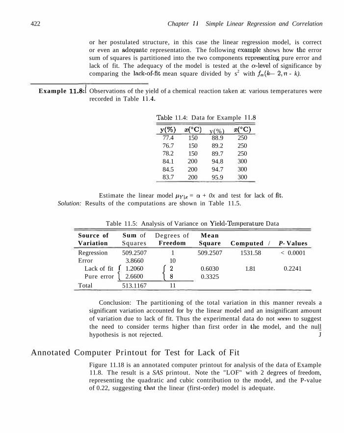
422 Chapter 11 Simple Linear Regression and Correlation
or her postulated structure, in this case the linear regression model, is correct or even an adequate representation. The following example shows how the error sum of squares is partitioned into the two components representing pure error and lack of fit. The adequacy of the model is tested at the a-level of significance by comparing the lack-of-fit mean square divided by s2 with fn(k — 2,n - k).
Example 11.8:1 Observations of the yield of a chemical reaction taken at: various temperatures were recorded in Table 11.4.
Table 11.4: Data for Example 11.8
y(%) 77.4 76.7 78.2 84.1 84.5 83.7
*(°C) 150 150 150 200 200 200
y(%) 88.9 89.2 89.7 94.8 94.7 95.9
x(°C) 250 250 250 300 300 300
Estimate the linear model py\x = a + 0x and test for lack of fit. Solution: Results of the computations are shown in Table 11.5.
Table 11.5: Analysis of Variance on Yield-Temperature Data
Source of Variation
Regression Error
Lack of fit Pure error
Total
Sum of Squares
509.2507 3.8660
f 1.2060 \ 2.6600
513.1167
Degrees of Freedom
1 10
{I 11
Mean Square
509.2507
0.6030 0.3325
Computed /
1531.58
1.81
P- Values
< 0.0001
0.2241
Conclusion: The partitioning of the total variation in this manner reveals a significant variation accounted for by the linear model and an insignificant amount of variation due to lack of fit. Thus the experimental data do not seem to suggest the need to consider terms higher than first order in the model, and the null hypothesis is not rejected. J
Annotated Computer Printout for Test for Lack of Fit Figure 11.18 is an annotated computer printout for analysis of the data of Example 11.8. The result is a SAS printout. Note the "LOF" with 2 degrees of freedom, representing the quadratic and cubic contribution to the model, and the P-value of 0.22, suggesting that the linear (first-order) model is adequate.
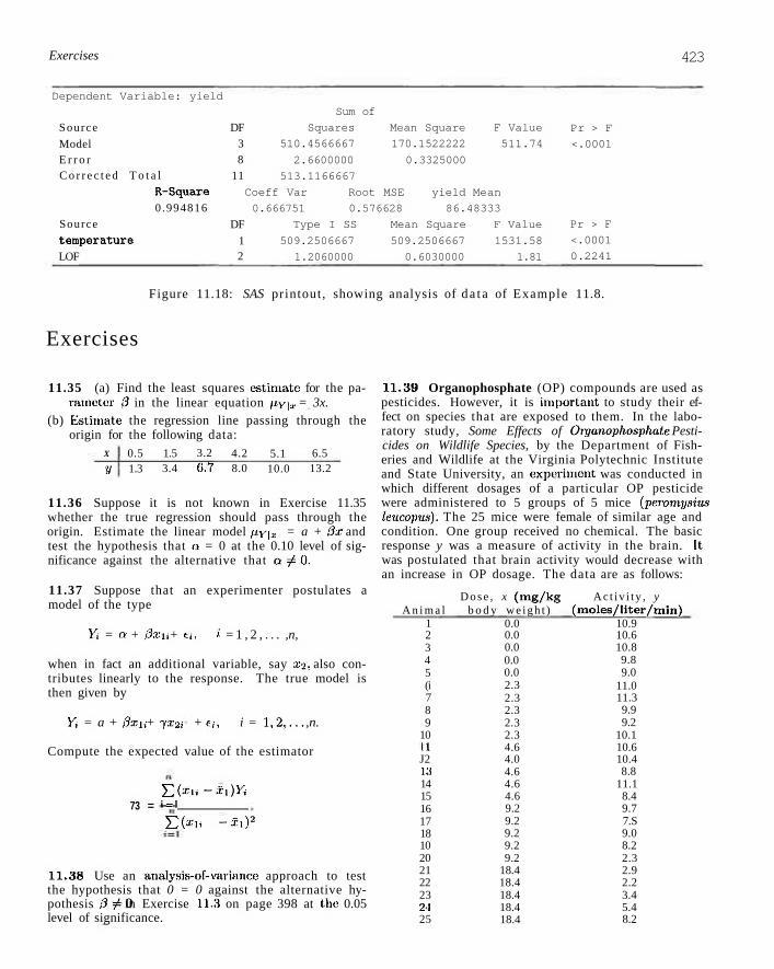
Exercises 423
Dependent Variable: yield
Source
Model E r r o r C o r r e c t e d T o t a l
R-Square
0 .994816 Source t e m p e r a t u r e
LOF
DF 3 8
11
DF
1 2
Sum of
Squares Mean Square F Value
510.4566667 170.1522222 511.74
2.6600000 0.3325000
513.1166667
Coeff Var Root MSE yield Mean
0.666751 0.576628 86.48333
Type I SS Mean Square F Value
509.2506667 509.2506667 1531.58
1.2060000 0.6030000 1.81
Pr > F
<.0001
Pr > F
<.0001
0.2241
Figure 11.18: SAS printout, showing analysis of da t a of Example 11.8.
Exercises
11.35 (a) Find the least squares estimate for the parameter 0 in the linear equation py\x = 3x.
(b) Estimate the regression line passing through the origin for the following data:
X
V
0.5 1.3
1.5 3.4
3.2 0.7
4.2 8.0
5.1 10.0
6.5 13.2
11.36 Suppose it is not known in Exercise 11.35 whether the true regression should pass through the origin. Estimate the linear model fJ.y\x = a + 3x and test the hypothesis that a = 0 at the 0.10 level of significance against the alternative that a / 0 ,
11.37 Suppose that an experimenter postulates a model of the type
Yi = a + 0xu + a, i = 1 , 2 , . . . ,n,
when in fact an additional variable, say x2, also contributes linearly to the response. The true model is then given by
Yi = a + 0xn + -yx-2, + <=,-, i = 1,2,. . . ,n.
Compute the expected value of the estimator
73 = Eixu~xi)Yi i = l
E ( * H ~Xl)2
11.38 Use an analysis-of-variance approach to test the hypothesis that 0 = 0 against the alternative hypothesis 3^0 in Exercise 11.3 on page 398 at the 0.05 level of significance.
11.39 Organophosphate (OP) compounds are used as pesticides. However, it is important to study their effect on species that are exposed to them. In the laboratory study, Some Effects of Oiyanophosphate Pesticides on Wildlife Species, by the Department of Fisheries and Wildlife at the Virginia Polytechnic Institute and State University, an experiment was conducted in which different dosages of a particular OP pesticide were administered to 5 groups of 5 mice (peromysius leucopus). The 25 mice were female of similar age and condition. One group received no chemical. The basic response y was a measure of activity in the brain. It was postulated that brain activity would decrease with an increase in OP dosage. The data are as follows:
A n i m a l 1 2 3 4 5 (i 7 8 9
10 It J2 13 14 15 16 17 18 10 20 21 22 23 2-1 25
D o s e , x ( m g / k g b o d y w e i g h t )
0.0 0.0 0.0 0.0 0.0 2.3 2.3 2.3 2.3 2.3 4.6 4.0 4.6 4.6 4.6 9.2 9.2 9.2 9.2 9.2
18.4 18.4 18.4 18.4 18.4
Ac t iv i t y , y ( m o l e s / I i t e r / m i n )
10.9 10.6 10.8 9.8 9.0
11.0 11.3 9.9 9.2
10.1 10.6 10.4 8.8
11.1 8.4 9.7 7.S 9.0 8.2 2.3 2.9 2.2 3.4 5.4 8.2
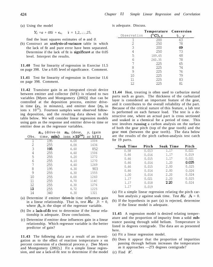
424 Chapter 11 Simple Linear Regression and Correlation
(a) Using the model
Yt =a + 0Xi + Ci, * = 1,2,.
is adequate. Discuss.
,25, Temperature Conversion
find the least squares estimates of a and 0. (b) Construct an analysis-of-variance table in which
the lack of fit and pure error have been separated. Determine if the lack of fit is significant at the 0.05 level. Interpret the results.
11.40 Test for linearity of regression in Exercise 11.5 on page 398. Use a 0.05 level of significance. Comment.
11.41 Test for linearity of regression in Exercise 11.6 on page 398. Comment.
11.42 Transistor gain in an integrated circuit device between emitter and collector (hFE) is related to two variables [Myers and Montgomery (2002)] that can be controlled at the deposition process, emitter drive-in time (SBI, in minutes), and emitter dose (x2, in ions x 1014). Fourteen samples were observed following deposition, and the resulting data shown in the table below. We will consider linear regression models using gain as the response and emitter drive-in time or emitter dose as the regressor variables.
ati, (drive-in X2, (dose, y, (gain Obs . t ime , min) ions x lO 1 4 ) or h F E ) 1 2 3 4 5 6 7 8 9 10 11 12 13 14
195 255 195 255 255 255 255 195 255 255 255 255 255 340
4.00 4.00 4.60 4.60 4.20 4.10 4.60 4.30 4.30 4.00 4.70 4.30 4.72 4.30
1004 1636 852 1506 1272 1270 1269 903 1555 1260 114C 1276 1225 1321
(a) Determine if emitter drive-in time influences gain in a linear relationship. That is, test Ho: 3\ = 0, where 0i, is the slope of the regressor variable.
(b) Do a lack-of-fit test to determine if the linear relationship is adequate. Draw conclusions.
(c) Determine if emitter dose influences gain in a linear relationship. Which regressor variable is the better predictor of gain?
11.43 The following data are a result of an investigation as to the effect of reaction temperature x on percent conversion of a chemical process y. [See Myers and Montgomery (2002).] Fit a simple linear regression, and use a lack-of-fit test to determine if the model
Observation 1 2 3 4 5 6 7 8 9 10 11 12
(°C), x 200 250 200 250
189.65 260.35 225 225 225 225 225 225
%, y 43 78 09 73 48 78 65 74 76 79 83 81
11.44 Heat, treating is often used to carburize metal parts such as gears. The thickness of the carburized layer is considered an important feature of the gear, and it contributes to the overall reliability of the part. Because of the critical nature of this feature, a lab test is performed on each furnace load. The test is a destructive one, where an actual part is cross sectioned and soaked in a chemical for a period of time. This test involves runriing a carbon analysis on the surface of both the gear pitch (top of the gear tooth) and the gear root (between the gear teeth). The data below are the results of the pitch carbon-analysis test catch for 19 parts.
Soak Time Pitch Soak Time Pitch 0.58 0.66 0.66 0.66 0.66 0.66 1.00 1.17 1.17 1.17
0.013 0.016 0.015 0.016 0.015 0.016 0.014 0.021 0.018 0.019
1.17 1.17 1.17 1.20 2.00 2.00 2.20 2.20 2.20
0.021 0.019 0.021 0.025 0.025 0.026 0.024 0.025 0.024
(a) Fit a simple linear regression relating the pitch carbon analysis y against soak time. Test Ho: 0i = 0.
(b) If the hypothesis in part (a) is rejected, determine if the linear model is adequate.
11.45 A regression model is desired relating temperature and the proportion of impurity from a solid substance passing through solid helium. Temperature is listed in degrees centigrade. The data are as presented here. (a) Fit a linear regression model. (b) Does it appear that the proportion of impurities
passing through helium increases the temperature as it approaches —273 degrees centigrade?
(c) Find R2.
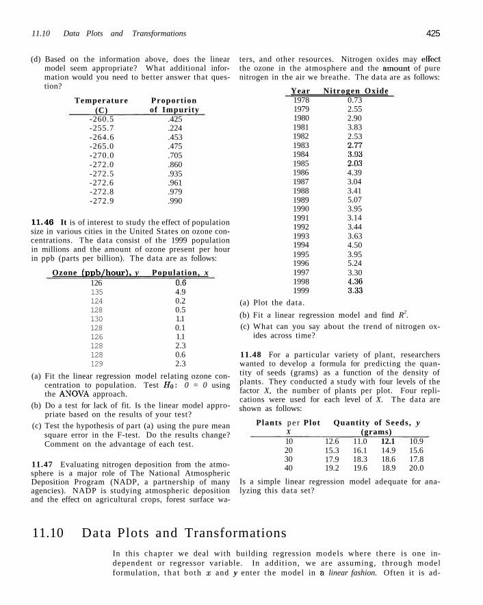
11.10 Data Plots and Transformations 425
(d) Based on the information above, does the linear model seem appropriate? What additional information would you need to better answer that question?
Temperature (C)
-260.5 -255.7 -264.6 -265.0 -270.0 -272.0 -272.5 -272.6 -272.8 -272.9
Proportion of Impurity
.425
.224
.453
.475
.705
.860
.935
.961
.979
.990
11.46 It is of interest to study the effect of population size in various cities in the United States on ozone concentrations. The data consist of the 1999 population in millions and the amount of ozone present per hour in ppb (parts per billion). The data are as follows:
Ozone (ppb/hour) , y Population, x 126 135 124 128 130 128 126 128 128 129
0.6 4.9 0.2 0.5 1.1 0.1 1.1 2.3 0.6 2.3
(a) Fit the linear regression model relating ozone concentration to population. Test Ho: 0 = 0 using the ANOVA approach.
(b) Do a test for lack of fit. Is the linear model appropriate based on the results of your test?
(c) Test the hypothesis of part (a) using the pure mean square error in the F-test. Do the results change? Comment on the advantage of each test.
11.47 Evaluating nitrogen deposition from the atmosphere is a major role of The National Atmospheric Deposition Program (NADP, a partnership of many agencies). NADP is studying atmospheric deposition and the effect on agricultural crops, forest surface wa
ters, and other resources. Nitrogen oxides may effect the ozone in the atmosphere and the amount of pure nitrogen in the air we breathe. The data are as follows:
Year Nitrogen Oxide 1978 1979 1980 1981 1982 1983 1984 1985 1986 1987 1988 1989 1990 1991 1992 1993 1994 1995 1996 1997 1998 1999
0.73 2.55 2.90 3.83 2.53 2.77 3.93 2.03 4.39 3.04 3.41 5.07 3.95 3.14 3.44 3.63 4.50 3.95 5.24 3.30 4.36 3.33
(a) Plot the data.
(b) Fit a linear regression model and find R2.
(c) What can you say about the trend of nitrogen oxides across time?
11.48 For a particular variety of plant, researchers wanted to develop a formula for predicting the quantity of seeds (grams) as a function of the density of plants. They conducted a study with four levels of the factor X, the number of plants per plot. Four replications were used for each level of X. The data are shown as follows:
Plants p e r X
10 20 30 40
Plot Quantity of Seeds, y
12.6 15.3 17.9 19.2
(grams) 11.0 12.1 10.9 16.1 14.9 15.6 18.3 18.6 17.8 19.6 18.9 20.0
Is a simple linear regression model adequate for analyzing this data set?
11.10 Data Plots and Transformations In this chapter we deal with building regression models where there is one independent or regressor variable. In addition, we are assuming, through model formulation, t h a t both a; and y enter the model in a linear fashion. Often it is ad-
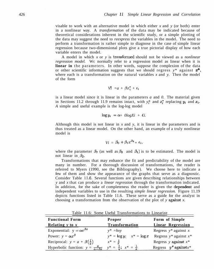
426 Chapter 11 Simple Linear Regression and Correlation
visable to work with an alternative model in which either x and y (or both) enter in a nonlinear way. A transformation of the data may be indicated because of theoretical considerations inherent in the scientific study, or a simple plotting of the data may suggest the need to reexpress the variables in the model. The need to perform a transformation is rather simple to diagnose in the case of simple linear regression because two-dimensional plots give a true pictorial display of how each variable enters the model.
A model in which x or y is transformed should not be viewed as a nonlinear regression model. Wc normally refer to a regression model as linear when it is linear in t he parameters . In other words, suppose the complexion of the data or other scientific information suggests that we should regress y* against x*, where each is a transformation on the natural variables x and y. Then the model of the form
Vi =a + 3x* + Ej
is a linear model since it is linear in the parameters a and 0. The material given in Sections 11.2 through 11.9 remains intact, with y* and x* replacing y^ and Xi. A simple and useful example is the log-log model
logj/i =a + 0logXi + €i.
Although this model is not linear in x and y, it is linear in the parameters and is thus treated as a linear model. On the other hand, an example of a truly nonlinear model is
Vi = 0o + A s * + ei,
where the parameter 02 (as well as f% and 0\) is to be estimated. The model is not linear in 32.
Transformations that may enhance the fit and predictability of the model are many in number. For a thorough discussion of transformations, the reader is referred to Myers (1990, see the Bibliography). We choose here to indicate a few of them and show the appearance of the graphs that serve as a diagnostic. Consider Table 11.6. Several functions are given describing relationships between y and x that can produce a linear regression through the transformation indicated. In addition, for the sake of completeness the reader is given the dependent and independent variables to use in the resulting simple linear regression. Figure 11.19 depicts functions listed in Table 11.6. These serve as a guide for the analyst in choosing a transformation from the observation of the plot of y against x.
Table 11.6: Some Useful Transformations to Linearize
Functional Form Proper Form of Simple Relating y to x Transformation Linear Regression Exponential: y = ae- y* =hxy Regress y* against x
Power: y = ax3 y* = logy; x* = logo: Regress y* against x*
Reciprocal: y = a + 0 [-) x* = 1 Regress y against x*
Hyperbolic function: y = af3x y* = \\ x* = j Regress y*against x*
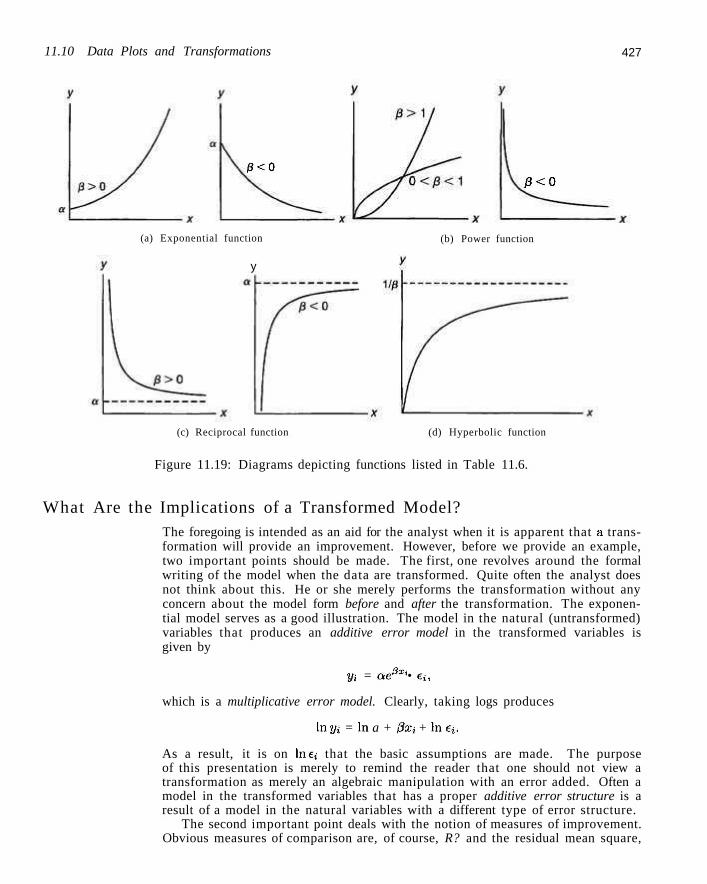
11.10 Data Plots and Transformations 427
;3<0 0<O
(a) Exponential function
y
(b) Power function
(c) Reciprocal function (d) Hyperbolic function
Figure 11.19: Diagrams depicting functions listed in Table 11.6.
What Are the Implications of a Transformed Model? The foregoing is intended as an aid for the analyst when it is apparent that a transformation will provide an improvement. However, before we provide an example, two important points should be made. The first, one revolves around the formal writing of the model when the data are transformed. Quite often the analyst does not think about this. He or she merely performs the transformation without any concern about the model form before and after the transformation. The exponential model serves as a good illustration. The model in the natural (untransformed) variables that produces an additive error model in the transformed variables is given by
Vi = ae3xi • ei,
which is a multiplicative error model. Clearly, taking logs produces
In yi = In a + 0Xi + In e*.
As a result, it is on lnei that the basic assumptions are made. The purpose of this presentation is merely to remind the reader that one should not view a transformation as merely an algebraic manipulation with an error added. Often a model in the transformed variables that has a proper additive error structure is a result of a model in the natural variables with a different type of error structure.
The second important point deals with the notion of measures of improvement. Obvious measures of comparison are, of course, R? and the residual mean square,
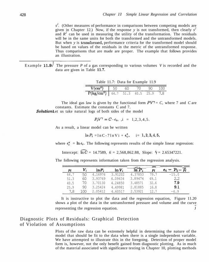
428 Chapter 11 Simple Linear Regression and Correlation
s2. (Other measures of performance in comparisons between competing models are given in Chapter 12.) Now, if the response y is not transformed, then clearly s2
and R2 can be used in measuring the utility of the transformation. The residuals will be in the same units for both the transformed and the untransformed models. But when y is transformed, performance criteria for the transformed model should be based on values of the residuals in the metric of the untransformed response. Thus comparisons that are made are proper. The example that follows provides an illustration.
Example 11.9:1 The pressure P of a gas corresponding to various volumes V is recorded and the data are given in Table 11.7.
Table 11.7: Data for Example 11.9
V(cm a) P(kg/cm^)
50 64.7
60 51.3
70 40.5
90 25.9
100 7.8
The ideal gas law is given by the functional form PV7 = C, where 7 and C are constants. Estimate the constants C and 7.
Solution: Let us take natural logs of both sides of the model
PiV^C-ti, ,i = l ,2 ,3 ,4 ,5 .
As a result, a linear model can be written
lnPi = l n C - 7 l n V i + e*, i= 1,2,3,4,5,
where e* = lne*. The following represents results of the simple linear regression:
Intercept: hiC = 14.7589, 6 = 2,568,862.88, Slope: 7 = 2.65347221.
The following represents information taken from the regression analysis.
Pi 64.7 51.3 40.5 25.9 7.8
Vi 50 60 70 90 100
\nPi 4.16976 3.93769 3.70130 3.25424 2.05412
InVi 3.91202 4.09434 4.24850 4.49981 4.60517
-—;-In Pi
4.37853 3.89474 3.48571 2.81885 2.53921
Z?=Z
Pi 79.7 49.1 32.6 16.8 12.7
Si — ij
-15.0 2.2 7.9 9.1
-4.9
— Pi
It is instructive to plot the data and the regression equation, Figure 11.20 shows a plot of the data in the untransformed pressure and volume and the curve representing the regression equation. J
Diagnostic Plots of Residuals: of Violation of Assumptions
Graphical Detection
Plots of the raw data can be extremely helpful in determining the nature of the model that should be fit to the data when there is a single independent variable. We have attempted to illustrate this in the foregoing. Detection of proper model form is, however, not the only benefit gained from diagnostic plotting. As in much of the material associated with significance testing in Chapter 10, plotting methods
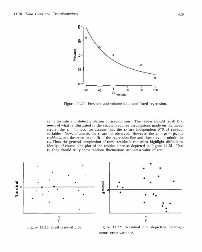
11.10 Data Plots and Transformations 429
o . co
o . eo
3 0) o <n TJ- '
8-1
50 - r -
60 -r 70
80
Volume
90 - 1 100
Figure 11.20: Pressure and volume data and fitted regression.
can illustrate and detect violation of assumptions. The reader should recall that much of what is illustrated in the chapter requires assumptions made on the model errors, the e». In fact, we assume that the e are independent N(0, a) random variables. Now, of course, the e, are not observed. However, the e* = yi — &, the residuals, are the error in the fit of the regression line and thus serve to mimic the ti. Thus the general complexion of these residuals can often highlight difficulties. Ideally, of course, the plot of the residuals are as depicted in Figure 11.21. That is, they should truly show random fluctuations around a value of zero.
(0 3 S 0 to
as er
•
•
•
• •
•
•
• •
• •
•
•
•
•
• •
•
CO
o) n 0) u DC
A
y A
y
Figure 11.21: Ideal residual plot. Figure 11.22: Residual plot depicting heteroge
neous error variance.
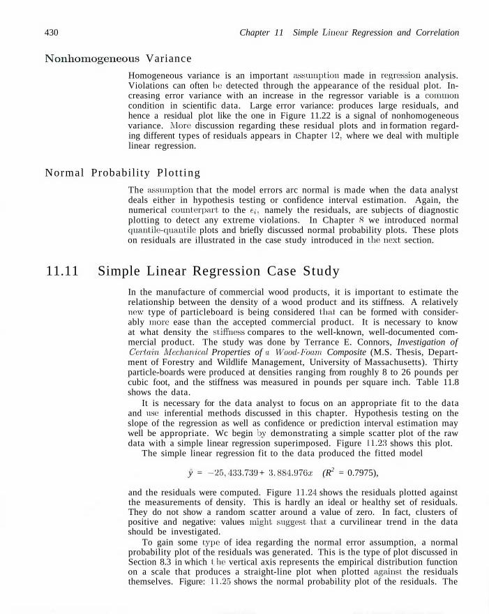
430 Chapter 11 Simple Linear Regression and Correlation
Nonhomogeneous Variance
Homogeneous variance is an important assumption made in regression analysis. Violations can often be detected through the appearance of the residual plot. Increasing error variance with an increase in the regressor variable is a common condition in scientific data. Large error variance: produces large residuals, and hence a residual plot like the one in Figure 11.22 is a signal of nonhomogeneous variance. More discussion regarding these residual plots and in formation regarding different types of residuals appears in Chapter L2, where we deal with multiple linear regression.
Normal Probabili ty Plot t ing
The assumption that the model errors arc normal is made when the data analyst deals either in hypothesis testing or confidence interval estimation. Again, the numerical counterpart to the E,-, namely the residuals, are subjects of diagnostic plotting to detect any extreme violations. In Chapter 8 we introduced normal quantile-quantile plots and briefly discussed normal probability plots. These plots on residuals are illustrated in the case study introduced in the next section.
11.11 Simple Linear Regression Case Study
In the manufacture of commercial wood products, it is important to estimate the relationship between the density of a wood product and its stiffness. A relatively new type of particleboard is being considered that can be formed with considerably more ease than the accepted commercial product. It is necessary to know at what density the .stiffness compares to the well-known, well-documented commercial product. The study was done by Terrance E. Connors, Investigation of Certain. Mechanical Properties of a Wood-Foam Composite (M.S. Thesis, Department of Forestry and Wildlife Management, University of Massachusetts). Thirty particle-boards were produced at densities ranging from roughly 8 to 26 pounds per cubic foot, and the stiffness was measured in pounds per square inch. Table 11.8 shows the data.
It is necessary for the data analyst to focus on an appropriate fit to the data and use: inferential methods discussed in this chapter. Hypothesis testing on the slope of the regression as well as confidence or prediction interval estimation may well be appropriate. Wc begin lay demonstrating a simple scatter plot of the raw data with a simple linear regression superimposed. Figure 11.23 shows this plot.
The simple linear regression fit to the data produced the fitted model
y = -25,133.739 + 3,884.976:r (R2 = 0.7975),
and the residuals were computed. Figure 11.24 shows the residuals plotted against the measurements of density. This is hardly an ideal or healthy set of residuals. They do not show a random scatter around a value of zero. In fact, clusters of positive and negative: values might suggest that a curvilinear trend in the data should be investigated.
To gain some type of idea regarding the normal error assumption, a normal probability plot of the residuals was generated. This is the type of plot discussed in Section 8.3 in which I he vertical axis represents the empirical distribution function on a scale that produces a straight-line plot when plotted against the residuals themselves. Figure: 11.25 shows the normal probability plot of the residuals. The
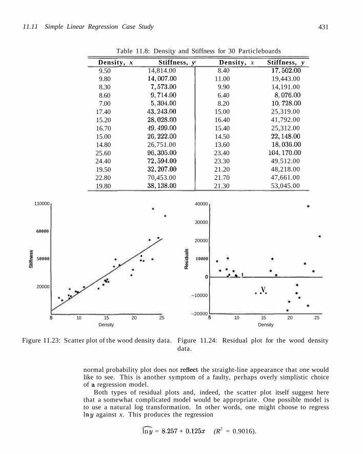
11.11 Simple Linear Regression Case Study 431
Table 11.8: Density and Stiffness for 30 Particleboards
Density, x 9.50 9.80 8.30 8.60 7.00
17.40 15.20 16.70 15.00 14.80 25.60 24.40 19.50 22.80 19.80
Stiffness, y 14,814.00 14,007.00 7,573.00 9,714.00 5,304.00
43,243.00 28.028.00 49.499.00 26.222.00 26.751.00 96,305.00 72,594.00 32,207.00 70,453.00 38,138.00
Density, x 8.40
11.00 9.90 6.40 8.20
15.00 16.40 15.40 14.50 13.60 23.40 23.30 21.20 21.70 21.30
Stiffness, y 17.502.00 19,443.00 14,191.00 8.076.00
10.728.00 25.319.00 41,792.00 25,312.00 22,148.00 18,036.00
104,170.00 49.512.00 48,218.00 47,661.00 53,045.00
110000
60000
c 50000
20000
10 15 20 Density
25
40000
30000
20000
2 10000
-10000
-20000
.» » !
V • • •
10 15 20 25
Density
Figure 11.23: Scatter plot of the wood density data. Figure 11.24: Residual plot for the wood density data.
normal probability plot does not reflect, the straight-line appearance that one would like to see. This is another symptom of a faulty, perhaps overly simplistic choice of a regression model.
Both types of residual plots and, indeed, the scatter plot itself suggest here that a somewhat complicated model would be appropriate. One possible model is to use a natural log transformation. In other words, one might choose to regress In j / against x. This produces the regression
In j / = 8.257 + 0.125a; (R2 = 0.9016).
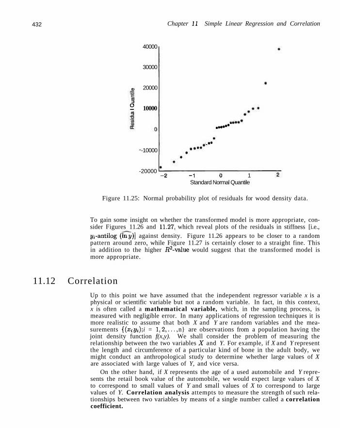
432 Chapter 11 Simple Linear Regression and Correlation
40000
30000
u 20000
3 2 10000 CO
-10000
-20000
.~*'
_••
- 2 - 1 0 1 Standard Normal Quantile
Figure 11.25: Normal probability plot of residuals for wood density data.
To gain some insight on whether the transformed model is more appropriate, consider Figures 11.26 and 11.27, which reveal plots of the residuals in stiffness [i.e., yrantilog (Inj/)] against density. Figure 11.26 appears to be closer to a random pattern around zero, while Figure 11.27 is certainly closer to a straight fine. This in addition to the higher i?2-value would suggest that the transformed model is more appropriate.
11.12 Correlation Up to this point we have assumed that the independent regressor variable x is a physical or scientific variable but not a random variable. In fact, in this context, x is often called a mathematical variable, which, in the sampling process, is measured with negligible error. In many applications of regression techniques it is more realistic to assume that both X and Y are random variables and the measurements {(xi, y,); i = 1,2,..., n} are observations from a population having the joint density function f(x,y). We shall consider the problem of measuring the relationship between the two variables A" and Y. For example, if X and Y represent the length and circumference of a particular kind of bone in the adult body, we might conduct an anthropological study to determine whether large values of X are associated with large values of Y, and vice versa.
On the other hand, if X represents the age of a used automobile and Y represents the retail book value of the automobile, we would expect large values of X to correspond to small values of Y and small values of X to correspond to large values of Y. Correlation analysis attempts to measure the strength of such relationships between two variables by means of a single number called a correlation coefficient.
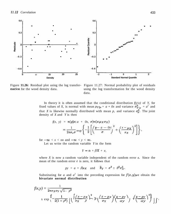
11.12 Correlation 433
0.6
0.3
-0.3
-0.6
•
•
«
•
•
* •
•
•• •
• • •
•
• •
•
•
• • •
•
*
•
•
•
10 15 Density
20 25
0.6
0.3
-0.3
-0.6
- 2 - 1 0 1 Standard Normal Quantile
Figure 11.26: Residual plot using the log transfer- Figure 11.27: Normal probability plot of residuals mation for the wood density data. using the log transformation for the wood density
data.
In theory it is often assumed that the conditional distribution f(y\x) of Y, for fixed values of X, is normal with mean p.y\x = a + 0x and variance Oy<x = a2 and
that X is likewise normally distributed with mean p, and variance a2. The joint density of X and Y is then
f(x, y) = n(y\x; a + 0x, a)n(x; px, ax)
(y — a — 0x\ ( x 1 2itaxa exp
Px o~x
for —oo < x < oo and —oc < y < ex. Let us write the random variable Y in the form
Y = a + BX + e,
where X is now a random variable independent of the random error e. Since the mean of the random error e is zero, it follows that
py = a + 0px and ay = a2 + 02a\.
Substituting for a and a2 into the preceding expression for fix,y), we obtain the bivariate normal distribution
fix,y) = 1
27TCT,Yay y/\ — O2
x exp f l \(x-px\2 _ 2 fx-px\ (y-PY\ (V-PYV] 1 \ 2(l-(fi)[\ ax J P \ crx J\ ay J + { ay )\f>
434 Chapter 11 Simple Linear Regression and Correlation
for —oo < x < oo and —oo < y < oc, where
p2 = ! _ £_ = , 2fi ^ Oy Oy'
The constant /? (rho) is called the population correlation coefficient and plays a major role in many bivariate data analysis problems. It is important for the reader to understand the physical interpretation of this correlation coefficient and the distinction between correlation and regression. The term regression still has meaning here. In fact, the straight line given by py\x = a + 0x is still called the regression line as before, and the estimates of a and ,3 are identical to those given in Section 11.3. The value of p is 0 when 0 = 0, which results when there essentially is no linear regression; that is, the regression line is horizontal and any knowledge of X is useless in predicting Y. Since aY > a2, we must have p2 < 1 and hence -1 < p < 1. Values of p — ±1 only occur when er2 = 0, in which case we have a perfect linear relationship between the two variables. Thus a value of p equal to +1 implies a perfect linear relationship with a positive slope, while a value of p equal to —1 results from a perfect linear relationship with a negative slope. It might be said, then, that sample estimates of p close to unity in magnitude imply good correlation or linear association between X and Y, whereas values near zero indicate little or no correlation.
To obtain a sample estimate of p, recall from Section 11.4 that the error sum of squares is
o*jii = *-*yy boXy-
Dividing both sides of this equation by Syy and replacing Sxy by bSxx, we obtain the relation
,2 Jxx . SoE -q — I o • °yy Jyy
The value of b2Sxx/Syy is zero when 6 = 0, which will occur when the sample points show no linear relationship. Since Syy > SSE, we conclude that b2Sxx/Sxy
must be between 0 and 1. Consequently, by/Sxx/Syy must range from -1 to +1 , negative values corresponding to lines with negative slopes and positive values to lines with positive slopes. A value of -1 or +1 will occur when SSE = 0, but this is the case where all sample points lie in a straight line. Hence a perfect linear relationship appears in the sample data when by/Sxx/Syy = ±1 . Clearly, the quantity by/Sxx/Syy, which we shall henceforth designate as r, can be used as an estimate of the population correlation coefficient, p. It is customary to refer to the estimate r as the Pearson product-moment correlation coefficient or simply the sample correlation coefficient.
Correlation The measure p of linear association between two variables X and Y is estimated Coefficient by the sample correlation coefficient r, where
r - t V ~ " " ' - ^ ^ / O ^ x O ] yy
For values of r between —1 and +1 we must be careful in our interpretation. For example, values of r equal to 0,3 and 0.6 only mean that we have two positive
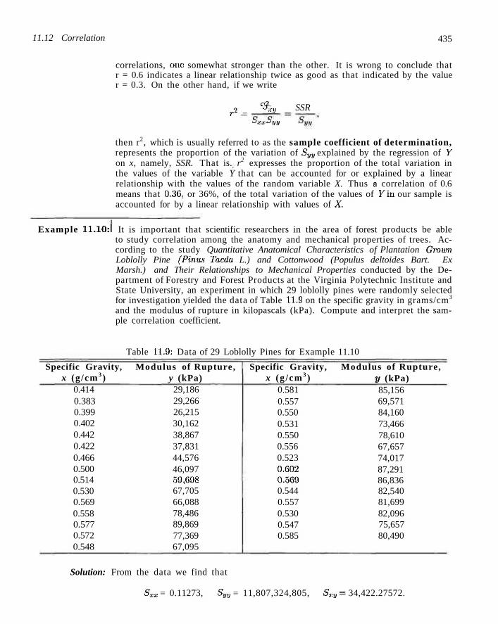
11.12 Correlation 435
correlations, one somewhat stronger than the other. It is wrong to conclude that r = 0.6 indicates a linear relationship twice as good as that indicated by the value r = 0.3. On the other hand, if we write
c2 ?.2 _ °xy SSR
-~>XX'~'yy
then r2, which is usually referred to as the sample coefficient of determination, represents the proportion of the variation of Syy explained by the regression of V on x, namely, SSR. That is. r2 expresses the proportion of the total variation in the values of the variable Y that can be accounted for or explained by a linear relationship with the values of the random variable X. Thus a correlation of 0.6 means that 0.36, or 36%, of the total variation of the values of Kin our sample is accounted for by a linear relationship with values of X
Example 11.10:1 It is important that scientific researchers in the area of forest products be able to study correlation among the anatomy and mechanical properties of trees. According to the study Quantitative Anatomical Characteristics of Plantation Grown Loblolly Pine (Pinus Taeda L.) and Cottonwood (Populus deltoides Bart. Ex Marsh.) and Their Relationships to Mechanical Properties conducted by the Department of Forestry and Forest Products at the Virginia Polytechnic Institute and State University, an experiment in which 29 loblolly pines were randomly selected for investigation yielded the data of Table 11.9 on the specific gravity in grams/cm3
and the modulus of rupture in kilopascals (kPa). Compute and interpret the sample correlation coefficient.
Specific Gravity, x (g /cm 3 )
0.414 0.383 0.399 0.402 0.442 0.422 0.466 0.500 0.514 0.530 0.569 0.558 0.577 0.572 0.548
Table 11.9: Data of 29 Loblolly Pines for Example
Modulus of Rupture, y (kPa) 29,186 29,266 26,215 30,162 38,867 37,831 44,576 46,097 59,098 67,705 66,088 78,486 89,869 77,369 67,095
Specific Gravity, x (g /cm 3 )
0.581 0.557 0.550 0.531 0.550 0.556 0.523 0.602 0.569 0.544 0.557 0.530 0.547 0.585
11.10
Modulus of Rupture, V (kPa)
85,156 69,571 84,160 73,466 78,610 67,657 74,017 87,291 86,836 82,540 81,699 82,096 75,657 80,490
Solution: From the data we find that
Sxx = 0.11273, Syy = 11,807,324,805, Sxy = 34,422.27572.
436 Chapter 11 Simple Linear Regression and Correlation
Therefore,
r= , 3 4 > 4 2 2 ' 2 7 5 7 2 = Q.9435.
v/(0.11273)(ll,807,3241805)
A correlation coefficient of 0.9435 indicates a good linear relationship between X and Y. Since r2 = 0.8902, we can say that approximately 89% of the variation in
the values of Y is accounted for by a linear relationship with X. J A test of the special hypothesis p = 0 versus an appropriate alternative is
equivalent to testing ,3 = 0 for the simple linear regression model and therefore the procedures of Section 11.8 using either the ^-distribution with n — 2 degrees of freedom or the F-distribution with 1 and n — 2 degrees of freedom are applicable. However, if one wishes to avoid the analysis-of-variance procedure and compute only the sample correlation coefficient, it can be verified (see Exercise 11.51 on page 438) that the i-value
t =
can also be written as
ry/n — 2
y/T^r2
which, as before, is a value of the statistic T having a ^-distribution with n — 2 degrees of freedom.
Example 11.11:1 For the data of Example 11.10, test the hypothesis that there is no linear association among the variables.
Solution: 1. HQ: p = 0.
2. Hx: p/^0. 3. a = 0.05. 4. Critical region: /; < -2.052 or t > 2.052.
5 . Computations: t = j ^ " ^ = 14.79, P < 0.0001.
6. Decision: Reject the hypothesis of no linear association. J A test of the more general hypothesis p = po against a suitable alternative is
easily conducted from the sample information. If X and Y follow the bivariate normal distribution, the quantity
H&) is a value of a random variable that follows approximately the normal distribution with mean ^ In j ^ and variance l / (n — 3). Thus the test procedure is to compute
yfn z = — ^ l n ( i ± i V h / 1 + ^ V ^ 3 i n (l + r)(l-po)
l-rj \l-po)\ 2 l(l-r)(l + p0)
and compare it with the critical points of the standard normal distribution.
Example 11.12:1 For the data of Example 11.10, test the null hypothesis that p = 0.9 against the alternative that p > 0.9. Use a 0.05 level of significance.
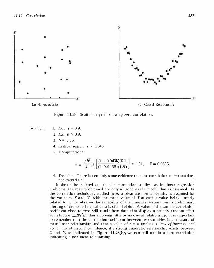
11.12 Correlation 437
• •
{a) No Association (b) Causal Relationship
Figure 11.28: Scatter diagram showing zero correlation.
Solution: 1. HQ: p = 0.9.
2. Hx: p > 0.9.
3. a = 0.05.
4. Critical region: z > 1.645.
5. Computations:
z = V^6
In (1 + 0.9435)(0.1) (1-0.9435)(1.9)
= 1.51. F = 0.0655.
6. Decision: There is certainly some evidence that the correlation coefficient does not exceed 0.9. J
It should be pointed out that in correlation studies, as in linear regression problems, the results obtained are only as good as the model that is assumed. In the correlation techniques studied here, a bivariate normal density is assumed for the variables X and Y, with the mean value of Y at each z-value being linearly related to x. To observe the suitability of the linearity assumption, a preliminary plotting of the experimental data is often helpful. A value of the sample correlation coefficient close to zero will result from data that display a strictly random effect as in Figure 11.28(a), thus implying little or no causal relationship. It is important to remember that the correlation coefficient between two variables is a measure of their linear relationship and that a value of r = 0 implies a lack of linearity and not a lack of association. Hence, if a strong quadratic relationship exists between X and F, as indicated in Figure 11.28(b), we can still obtain a zero correlation indicating a nonlinear relationship.
438
Exercises
Chapter 11 Simple Linear Regression and Correlation
11.49 Compute and interpret the correlation coefficient for the following grades of 6 students selected at random:
Mathematics grade English grade
70 92 80 74 65 83
74 84 63 87 78 90
11.50 Test the hypothesis that p = 0 in Exercise 11.49 against the alternative that p ^ 0. Use a 0.05 level of significance.
11.51 Show the necessary steps in converting the
equation r = s/ssr; to the equivalent form / _ .-yAT^S
11.52 The following data were obtained in a study of the relationship between the weight and chest size of infants at birth:
Weight (kg) Ches t Size (cm) 27T5 29J> 2.15 26.3 4.41 32.2 5.52 36.5 3.21 27.2 4.32 27.7 2.31 28.3 4.30 30.3 3.71 28.7
(a) Calculate r.
(b) Test the null hypothesis that p = 0 against the alternative that p > 0 at the 0.0i level of significance.
(c) What percentage of the variation in the infant chest sizes is explained by difference in weight?
11.53 With reference to Exercise 11.1 on page 397, assume that x and y are random variables with a bi-variate normal distribution: (a) Calculate r.
(b) Test the hypothesis that p = 0 against the alternative that p 7 0 at the 0.05 level of significance.
11.54 With reference to Exercise 11.9 on page 399, assume a bivariate normal distribution for x and y.
(a) Calculate r. (b) Test the null hypothesis that p = —0.5 against the
alternative that p < —0.5 at the 0.025 level of significance.
(c) Determine the percentage of the variation in the amount of particulate removed that is due to changes in the daily amount of rainfall.
Review Exercises
11.55 With reference to Exercise 11.6 on page 398, conclusions, construct (a) a 95% confidence interval for the average course
grade of students who make a 35 on the placement test;
(b) a 95% prediction interval for the course grade of a student who made a 35 on the placement test.
11.56 The Statistics Consulting Center at Virginia Polytechnic Institute and State University analyzed data on normal woodchucks for the Department of Veterinary Medicine. The variables of interest were body-weight in grams and heart weight in grams. It was also of interest to develop a linear regression equation in order to determine if there is a significant linear relationship between heart weight and total body weight. Use heart weight as the independent variable and body weight as the dependent variable and fit a simple linear regression using the following data. In addition, test the hypothesis HQ: 3 = 0 versus Hi: 0 •£ 0. Draw
Body Weight grains) 4050 2465 3120 5700 2595 3640 2050 4235 2935 4975 3690 2800 2775 2170 2370 2055 2025 2645 2675
Heart Weight (grams) 11.2 12.4 10.5 13.2 9.8 11.0 10.8 10.4 12.2 11.2 10.8 14.2 12.2 10.0 12.3 12.5 11.8 16.0 13.8
Review Exercises 439
11.57 The amounts of solids removed from a particular material when exposed to drying periods of different lengths are as shown.
x (hours) y (grams) 4.4 4.5 4.8 5.5 5.7 5.9 6.3 6.9 7.5 7.8
13.1 9.0
10.4 13.8 12.7 9.9
13.8 16.4 17.6 18.3
14.2 11.5 11.5 14.8 15.1 12.7 16.5 15.7 16.9 17.2
(a) Estimate the linear regression line.
(b) Test at the 0.05 level of significance whether the linear model is adequate.
11.58 With reference to Exercise 11.7 on page 399, construct
(a) a 95% confidence interval for the average weekly-sales when $45 is spent on advertising;
(b) a 95% prediction interval for the weekly sales when 845 is spent on advertising.
11.59 An experiment was designed for the Department of Materials Engineering at Virginia Polytechnic Institute and State University to study hydrogen ein-brittlement properties based on electrolytic hydrogen pressure measurements. The solution used was 0.1 N NaOH, the material being a certain type of stainless steel. The cathodic charging current density was controlled and varied at four levels. The effective hydrogen pressure was observed as the response. The data follow.
Run 1 2 3 4 5 6 7 8 9
10 11 12 13 14 L5
Charging Current Density, x ( m A / c m 2 )
0.5 0.5 0.5 0.5 1.5 1.5 1.5 2.5 2.5 2.5 2.5 3.5 3.5 3.5 3.5
Effective Hydrogen
Pressure, y (atm) 86.1 92.1 64.7 74.7
223.6 202.1 132.9 413.5 231.5 466.7 365.3 493.7 382.3 447.2 563.8
(b) Compute the pure error sum of squares and make a test for lack of fit.
(c) Does the information in part (b) indicate a need for a model in x beyond a first-order regression? Explain.
11.60 The following data represent the chemistry grades for a random sample of 12 freshmen at a certain college along with their scores on an intelligence test administered while they were still seniors in high school:
Student 1 2 3 4 5 6 7 8 9
10 11 12
Test Score, x
65 50 55 65 55 70 65 70 55 70 50 55
Chemistry Grade, y
85 74 76 90 85 87 94 98 81 91 76 74
(a) Run a simple linear regression of y against x.
(a) Compute and interpret the sample correlation coefficient.
(b) State necessary assumptions on random variables.
(c) Test the hypothesis that p = 0.5 against the alternative that p > 0.5. Use a P-value in the conclusion.
11.61 For the simple linear regression model, prove that E(s2) = a'1.
11.62 The business section of the Washington Times in March of 1997 listed 21 different used computers and printers and their sale prices. Also listed was the average hover bid. Partial results from the regression analysis using SAS software are shown in Figure 11.29 on page 440.
(a) Explain the difference between the confidence interval on the mean and the prediction interval.
(b) Explain why the standard errors of prediction vary from observation to observation.
(c) Which observation has the lowest standard error of prediction? Why?
11.63 Consider the vehicle data in Figure 11.30 from Consumer Reports. Weight is in tons, mileage in miles per gallon, and drive ratio is also indicated. A regression model was fitted relating weight x to mileage y. A partial SAS printout in Figure 11.30 on page 441 shows some of the results of that regression analysis and Fig-
440 Chapter 11 Simple Linear Regression and Correlation
ure 11.31 on page 442 gives plot of the residuals and (b) Fit the model by replacing weight with log weight. weight for each vehicle. (a) From the analysis and the residual plot, does it ap
pear that an improved model might be found by using a transformation? Explain.
Comment on the results, (c) Fit a model by replacing mpg with gallons per 100
miles traveled, as mileage is often reported in other countries. Which of the three models is preferable? Explain.
R-Square Coeff Vax 0.967472 7.923338
Parameter Estimate In te rcep t 59.93749137 Buyer 1.04731316
Root MSE Pr ice Mean 70.83841
Standard Error
38.34195754
product Buyer IBM PS/1 486/66 420MB IBM ThinkPad 500 IBM Think-Dad 755CX AST Pentium 90 540MB Dell Pentium 75 1GB Gateway 486/75 320MB Clone 586/133 1GB Compaq Contura 4/25 120MB Compaq Deskpro P90 1.2GB Micron P75 810MB Micron P100 1.2GB Mac Quadra 840AV 500MB Mac Performer 6116 700MB PouerBook 540c 320MB PowerBook 5300 500MB Power Mac 7500/100 1GB NEC Versa 486 340MB Toshiba 1960CS 320MB Toshiba 4800VCT 500MB HP Laser j e t I I I Apple Laser Writer Pro 63
325 450
1700 800 650 700 500 450 BOO 800 900 450 700
1400 1350 1150 800 700
1000 350 750
0.04405635
Pr ice 375 625
1850 875 700 750 600 600 850 675 975 575 775
1500 1575 1325
900 825
1150 475 800
Predic t Value
400.31 531.23
1840.37 897.79 740.69 793.06 583.59 531.23 897.79 897.79
1002.52 531.23 793.06
1526.18 1473.81 1264.35 897.79 793.06
1107.25 426.50 845.42
894.0476
t Value 1.56
23.77
Pr > | t | 0.1345 <.0001
Std Err Lower 95'/, Upper 95V. Predict 25.8906 21.7232 42.7041 15.4590 16.7503 16.0314 20.2363 21.7232 15.4590 15.4590 16.1176 21.7232 16.0314 30.7579 28.8747 21.9454 15.4590 16.0314 17.8715 25.0157 15.5930
Mean 346.12 485.76
1750.99 865.43 705.63 759.50 541.24 485.76 865.43 865.43 968.78 485.76 759.50
1461.80 1413.37 1218.42 865.43 759.50
1069.85 374.14 812.79
Mean 454.50 576.70
1929.75 930.14 775.75 826.61 625.95 576.70 930.14 930.14
1036.25 576.70 826.61
1590.55 1534.25 1310.28 930.14 826.61
1144.66 478.86 878.06
Lower 95'/, Upper 95'/. Predic t
242.46 376.15
1667.25 746.03 588.34 641.04 429.40 376.15 746.03 746.03 850.46 376.15 641.04
1364.54 1313.70 1109.13 746.03 641.04 954.34 269.26 693.61
Predic t 558.17 686.31
2013.49 1049.54 893.05 945.07 737.79 686.31
1049.54 1049.54 1154.58 686.31 945.07
1687.82 1633.92 1419.57 1049.64 945.07
1260.16 583.74 997.24
Figure 11.29: SAS printout, showing partial analysis of data of Review Exercise 11.62.
11.64 Observations on the yield of a chemical reaction taken at various temperatures were recorded as follows:
s ( °C) y(%) x(°C) y(%) 150 150 200 250 250 300
75.4 81.2 85.5 89.0 90.5 96.7
150 200 200 250 300 300
77.7 84.4 85.7 89.4 94.8 95.3
(a) Plot the data. (b) Does it appear from the plot as if the relation
ship is linear? (c) Fit a simple linear regression and test for lack
of fit.
(d) Draw conclusions based on your result in (c).
11.65 Physical fitness testing is an important as
pect of athletic training. A common measure of the magnitude of cardiovascular fitness is the maximum volume of oxygen uptake during a strenuous exercise. A study was conducted on 24 middle-aged men to study the influence of the time it takes to complete a two mile run. The oxygen uptake measure was accomplished with standard laboratory methods as the subjects performed on a treadmill. The work was published in "Maximal Oxygen Intake Prediction in Young and Middle Aged Males," Journal of Sports Medicine 9, 1969, 17-22. The data are as presented here.
Subject 1 2 3 4 5
y, Maximum Volume of O2
42.33 53.10 42.08 50.06 42.45
x, Time in Seconds
918 805 892 962 968
Review Exercises 441
Obs 1 2 3 4 5 6 7 8 9
10 11 12 13 14 15 16 17 18 19 20 21 22 23 24 25 26 27 28 29 30 31 32 33 34 35 36 37 38
ft-
Model Buick E s t a t e Wagon
WT 4 . 3 6 0
Ford Country Squire Wagon 4 . 0 5 4 Chevy Ma l i b u Wagon Chrys ler LeBaron Wagon C h e v e t t e Toyota Corona Datsun 510 Dodge Omni Audi 5000 Volvo 240 CL Saab 99 GLE Peugeot 694 SL Buick Century S p e c i a l Mercury Zephyr Dodge Aspen AMC Concord D/L Chevy Caprice C l a s s i c Ford LTP Mercury Grand Marquis Dodge St Reg i s Ford Mustang 4 Ford Mustang Ghia Macda GLC Dodge Col t AMC S p i r i t VW S c i r o c c o Honda Accord LX Buick Skylark Chevy C i t a t i o n Olds Omega P o n t i a c Phoenix Plymouth Horizon Datsun 210 F i a t S trada VW Dasher Datsun 810 BMW 3 2 0 i VW Rabbit
-Square Coeff Var 0 .817244 11 .46010
Parame s t er Es t imate I n t e r c e p t 48 .67928080 WT - 8 . 3 6 2 4 3 1 4 1
3 . 6 0 5 3 . 9 4 0 2 . 1 5 5 2 . 5 6 0 2 . 3 0 0 2 . 2 3 0 2 . 8 3 0 3 . 1 4 0 2 . 7 9 5 3 . 4 1 0 3 . 3 8 0 3 . 0 7 0 3 . 6 2 0 3 . 4 1 0 3 . 8 4 0 3 . 7 2 5 3 . 9 5 5 3 . 8 3 0 2 . 5 8 5 2 . 9 1 0 1 .975 1 .915 2 . 6 7 0 1 .990 2 . 1 3 5 2 . 5 7 0 2 . 5 9 5 2 . 7 0 0 2 . 5 5 6 2 . 2 0 0 2 . 0 2 0 2 . 1 3 0 2 . 1 9 0 2 . 8 1 5 2 . 6 0 0 1 .925
Root MSE 2 . 8 3 7 5 8 0
Standard Error
1 .94053995 0 .65908398
MPG DR.RATI0 1 6 . 9 1 5 . 5 1 9 . 2 1 8 . 5 3 0 . 0 2 7 . 5 2 7 . 2 3 0 . 9 2 0 . 3 1 7 . 0 2 1 . 6 1 6 . 2 2 0 . 6 2 0 . 8 1 8 . 6 1 8 . 1 1 7 . 0 1 7 . 6 1 6 . 5 1 8 . 2 2 6 . 5 2 1 . 9 3 4 . 1 3 5 . 1 2 7 . 4 3 1 . 5 2 9 . 5 2 8 . 4 2 8 . 8 2 6 . 8 3 3 . 5 3 4 . 2 3 1 . 8 3 7 . 3 3 0 . 5 2 2 . 0 2 1 . 5 3 1 . 9 MPG Mean 2 4 . 7 6 0 5 3
t Value 2 5 . 0 9
- 1 2 . 6 9
2 . 7 3 2 . 2 6 2 . 5 6 2 . 4 5 3 . 7 0 3 . 0 5 3 . 5 4 3 . 3 7 3 . 9 0 3 . 5 0 3 . 7 7 3 . 5 8 2 . 7 3 3 . 0 8 2 . 7 1 2 . 7 3 2 . 4 1 2 . 2 6 2 . 2 6 2 . 4 5 3 . 0 8 3 . 0 8 3 . 7 3 2 .97 3 . 0 8 3 . 7 8 3 . 0 5 2 . 5 3 2 . 6 9 2 . 8 4 2 . 6 9 3 . 3 7 3 . 7 0 3 . 1 0 3 . 7 0 3 . 7 0 3 . 6 4 3 . 7 8
Pr > Itl <.0001 <.0001
Figure 11.30: SAS printout, showing partial analysis of data of Review Exercise 11.63.
Subject 6 7 8 9
10 11 12 13 14 15
y> Maximum Volume of O2
42.46 47.82 49.92 36.23 49.66 41.49 46.17 46.18 43.21 51.81
x, Time in Seconds
907 770 743
1045 810 927 813 858 860 760
Subject 16 17 18 19 20 21 22 23 24
y, Maximum Volume of O2
53.28 53.29 47.18 56.91 47.80 48.65 53.67 60.62 56.73
x, Time in Seconds
747 743 803 683 844 755 700 748 775
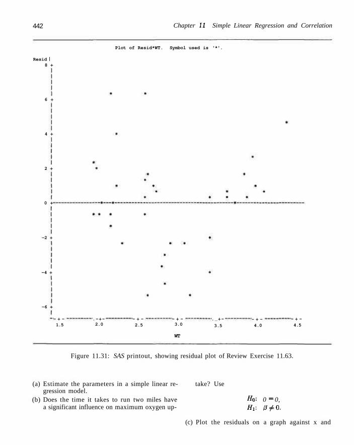
442 Chapter 11 Simple Linear Regression and Correlation
Resid I 8 +
6 +
4 +
2 +
0 +
-2 +
-4 +
-6 +
— + — 1.5
Plot of Resid*WT. Symbol used is '*'.
.-+— 2.0
— + — 2.5
— + — 3.0
WT
._+—
3.5
— + — 4.0
— + — 4.5
Figure 11.31: SAS printout, showing residual plot of Review Exercise 11.63.
(a) Estimate the parameters in a simple linear re- take? Use gression model.
(b) Does the time it takes to run two miles have Ho'- 0 = 0, a significant influence on maximum oxygen up- Hi: 0^0.
(c) Plot the residuals on a graph against x and
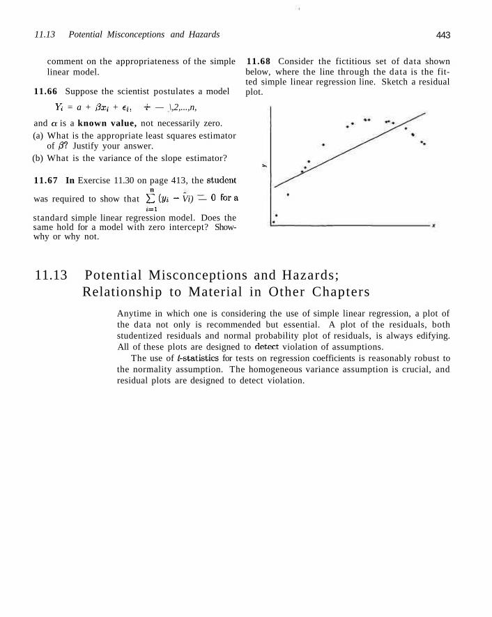
11.13 Potential Misconceptions and Hazards 443
comment on the appropriateness of the simple 11.68 Consider the fictitious set of data shown linear model.
11.66 Suppose the scientist postulates a model
Yi = a + 0Xi + ti, -i — \,2,...,n,
and a is a known value, not necessarily zero. (a) What is the appropriate least squares estimator
of 01 Justify your answer. (b) What is the variance of the slope estimator?
11.67 In Exercise 11.30 on page 413, the student n
was required to show that YL iVi ~ Vi) — 0 f° r a
i=i standard simple linear regression model. Does the same hold for a model with zero intercept? Show-why or why not.
below, where the line through the data is the fitted simple linear regression line. Sketch a residual plot.
11.13 Potential Misconceptions and Hazards; Relationship to Material in Other Chapters
Anytime in which one is considering the use of simple linear regression, a plot of the data not only is recommended but essential. A plot of the residuals, both studentized residuals and normal probability plot of residuals, is always edifying. All of these plots are designed to detect violation of assumptions.
The use of ^-statistics for tests on regression coefficients is reasonably robust to the normality assumption. The homogeneous variance assumption is crucial, and residual plots are designed to detect violation.
Chapter 12
Multiple Linear Regression and Certain Nonlinear Regression Models
12.1 Introduction
In most research problems where regression analysis is applied, more than one independent variable is needed in the regression model. The complexity of most scientific mechanisms is such that in order to be able to predict an important response, a multiple regression model is needed. When this model is linear in the coefficients, it is called a multiple linear regression model. For the case of A:independent variables.'1:1,0:2,. •• ,Xk, the mean of Y~|a;i,.T2, • • • ,Xk is given by the multiple linear regression model
PY\x,,x-j xh =00 + 0lXi H h 0kXk,
and the estimated response is obtained from the sample regression equation
g = 60 + M l +"- + bkXk,
where each regression coefficient 0t is estimated by &,: from the sample data using the method of least squares. As in the case of a single independent variable, the multiple linear regression model can often be an adequate representation of a more complicated structure within certain ranges of the independent variables.
Similar least squares techniques can also be applied in estimating the coefficients when the linear model involves, say, powers and products of the independent variables. For example, when k — 1. the experimenter may feel that the means py\x do not fall on a straight lino but are more appropriately described by the polynomial regression model
PY\x = 00 + 0\X + 02x2 + h 0rx'\
and the estimated response is obtained from the polynomial regression equation
y = b0 + bxx + b2x? + h brxr.
446 Chapter 12 Multi-pie Linear Regression and Certain Nonlinear Regression Models
Confusion arises occasionally when we speak of a polynomial model as a linear model. However, statisticians normally refer to a linear model as one in which the parameters occur linearly, regardless of how the independent variables enter the model. An example of a nonlinear model is the exponential relat ionship
PY\X = <*&*,
which is estimated by the regression equation
y = abx.
There are many phenomena in science and engineering that are inherently nonlinear in nature and, when the true structure is known, an attempt should certainly be made to fit the actual model. The literature on estimation by least squares of nonlinear models is voluminous. While we do not attempt to cover nonlinear regression in any rigorous fashion in this text, we do cover certain specific types of nonlinear models in Section 12.12. The nonlinear models discussed in this chapter deal with nonideal conditions in which the analyst is certain that the response and hence the response model error are not normally distributed but, rather, have a binomial or Poisson distribution. These situations do occur extensively in practice.
A student who wants a more general account of nonlinear regression should consult Classical and Modern- Regression with Applications by Myers (see the Bibliography).
12.2 Estimating the Coefficients
In this section we obtain the least squares estimators of the parameters 0Q, 0\,..., 0k by fitting the multiple linear regression model
Mri*i,*2 xk = A) + p\xi + • • • + 3kxk
to the data points
{(xu,X2i,...,xki,yi), i = l , 2 , . . . , n and n > k},
where j/* is the observed response to the values xn, X2i, • • •, Xki of the k independent variablesXi,x2 , . . . ,xk- Each observation (xn,x2{,... ,Xki, yi) is assumed to satisfy the following equation
Multiple Linear Vi = 00 + 0ixu + 02x2i + ••• + ffixiti + U,
Regression Model or
Vi = Vi + Ci = b0 + byxii + b2x2i H h bkxki + e»,
where Ci and e, are the random error and residual, respectively, associated with the response yi and fitted value yi-
As in the case of simple linear regression, it is assumed that the e,; are independent, identically distributed with mean zero and common variance a2.
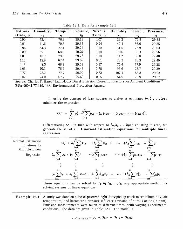
12.2 Estimating the Coefficients 447
Table 12.1: Data for Example 12.1
Nitrous Oxide, y
0.90 0.91 0.96 0.89 1.00 1.10 1.15 1.03 0.77 1.07
Humidity, xx
72.4 41.6 34.3 35.1 10.7 12.9 8.3
20.1 72.2 24.0
Temp., X2
76.3 70.3 77.1 68.0 79.0 67.4 66.8 76.9 77.7 67.7
Pressure, x-s
29.18 29.35 29.24 29.27 29.78 29.39 29.69 29.48 29.09 29.60
Nitrous Oxide, y
1.07 0.94 1.10 1.10 1.10 0.91 0.87 0.78 0.82 0.95
Humidity, Xl
23.2 47.4 31.5 10.6 11.2 73.3 75.4 96.6
107.4 54.9
Temp., X2
76.8 86.6 76.9 86.3 86.0 76.3 77.9 78.7 86.8 70.9
Pressure, X3
29.38 29.35 29.63 29.56 29.48 29.40 29.28 29.29 29.03 29.37
Source: Charles T. Hare, EPA-600/2-77-116. U.S.
"Light-Duty Diesel Emission Correction Factors for Ambient Conditions," Environmental Protection Agency.
In using the concept of least squares to arrive at estimates bo,bi,...,bk, we minimize the expression
SSE = ^Te? = Z^iVi -b0- bixii - b2x2i bkXki)2
i = \ 1 = 1
Differentiating SSE in turn with respect to bo,bi,...,bk, and equating to zero, we generate the set of k + 1 normal estimation equations for multiple linear regression.
nbo + bx 22xii +b2^x2i + ••• +bk^*** = ^ V i Normal Estimation
Equations for Multiple Linear
Regression 6o £ > „ + 6, £ Ai +h £ xux2i + +bk £ xuxki = £ xxw
; = i ; = i j = i i = l
i = l i = l i = l j = l i = l
bo ^2 XM + 6 l 1>2 XkiXxi+b2 ^2 Xk%x2i + ••• +bk \\2,xli = ^ XfciJ/i j = 1 i=1
These equations can be solved for b0,bi,b2,...,bk by any appropriate method for solving systems of linear equations.
Example 12.1:1 A study was done on a diesel-powered-light-duty pickup truck to see if humidity, air temperature, and barometric pressure influence emission of nitrous oxide (in ppm). Emission measurements were taken at different times, with varying experimental conditions. The data are given in Table 12.1. The model is
M V . T po + 3ia-i + 02x2 + 03x3,
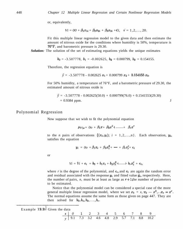
448 Chapter 12 Multiple Linear Regression and Certain Nonlinear Regression Models
or, equivalently,
Vi = 00 + PlXli + 02X2i + 03X3i +€i, 2 = 1,2,..., 20.
Fit this multiple linear regression model to the given data and then estimate the amount of nitrous oxide for the conditions where humidity is 50%, temperature is 76°F, and barometric pressure is 29.30.
Solution: The solution of the set of estimating equations yields the unique estimates
b0 = -3.507778, bi = -0.002625, b2 = 0.000799, b3 = 0.154155.
Therefore, the regression equation is
y = -3.507778 - 0.002625 xx + 0.000799 x2 + 0.154155 x3.
For 50% humidity, a temperature of 76°F, and a barometric pressure of 29.30, the estimated amount of nitrous oxide is
y = -3.507778 - 0.002625(50.0) + 0.000799(76.0) + 0.1541553(29.30)
= 0.9384 ppm. J
Polynomial Regression
Now suppose that we wish to fit the polynomial equation
PY\X = 0o + 0\x + 02x2 H + 0rx
r
to the n pairs of observations {(x;,2/t); i = 1 ,2 , . . . ,n} . Each observation, yt, satisfies the equation
yi = 0o + plXi + 02x\ + ••• + 0rxr + €i
or
Vi = Vi + &i = b0 + biXi + b2x2 -t r brx
r{ + et,
where r is the degree of the polynomial, and u, and e* are again the random error and residual associated with the response yi and fitted value yi, respectively. Here, the number of pairs, n, must be at least as large as r+1, the number of parameters to be estimated.
Notice that the polynomial model can be considered a special case of the more general multiple linear regression model, where we set xi = x, x2 — x2,..., xr =xr. The normal equations assume the same form as those given on page 447. They are then solved for bo,b\,b2,...,br.
Example 12.2:1 Given the data X
y
0 9.1
l 7.3
2 3.2
3 4.6
4 4.8
5 2.9
6 5.7
7 7.1
8 8.8
9 10.2
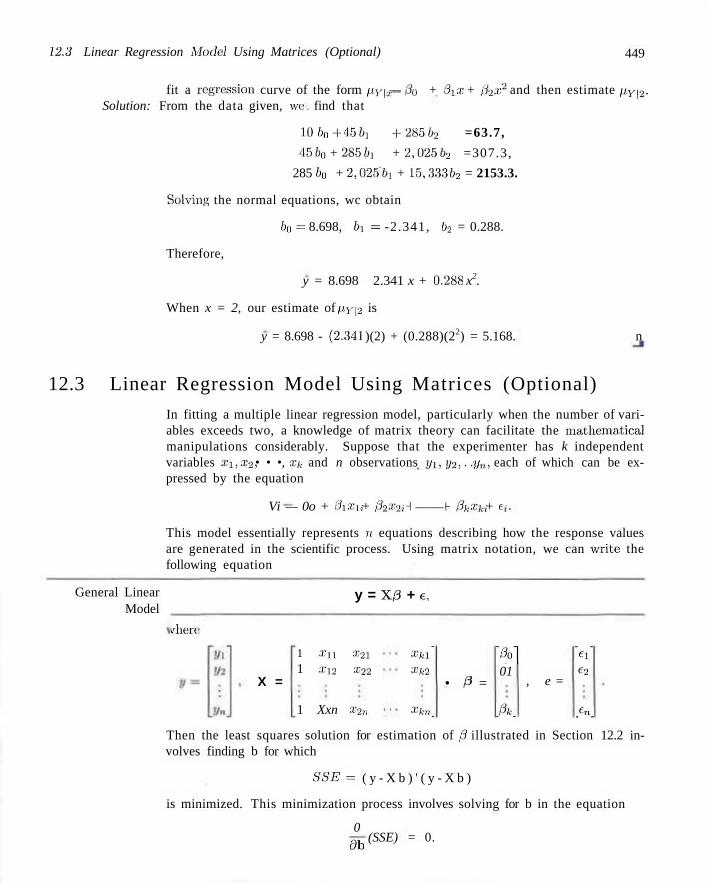
12.3 Linear Regression Model Using Matrices (Optional) 449
fit a regression curve of the form pY\x — f% + 3yx + 02x2 and then estimate py\2.
Solution: From the data given, we> find that
10 b0+ 45lh +285()2 =63.7,
456o + 285fri + 2,025/>2 =307.3,
285 UQ + 2,02511! + 15,333 b2 = 2153.3.
Solving the normal equations, wc obtain
6o= 8.698, bi = -2.341, b2 = 0.288.
Therefore,
y = 8.698 - 2.341 x + 0.288 x2.
When x = 2, our estimate of fiy\2 is
y = 8.698 - (2.341 )(2) + (0.288)(22) = 5.168. n
12.3 Linear Regression Model Using Matrices (Optional)
In fitting a multiple linear regression model, particularly when the number of variables exceeds two, a knowledge of matrix theory can facilitate the mathematical manipulations considerably. Suppose that the experimenter has k independent variables X\,x2, • • •, xk and n observations i/i, y2,..., yn, each of which can be expressed by the equation
Vi — 0o + 0ixn + 02x2i H 1- 0kxki + Ci-
This model essentially represents n equations describing how the response values are generated in the scientific process. Using matrix notation, we can wrrite the following equation
General Linear Model
y = X/3 + e,
/here
X =
1 ajii x2X
1 xx2 x22
1 Xxn X2„
Xkl~
Xk2
Xkn.
• P =
~0o] 01
A.
, e =
"«l"
e-2
. e".
Then the least squares solution for estimation of 0 illustrated in Section 12.2 involves finding b for which
SSE = ( y - X b ) ' ( y - X b )
is minimized. This minimization process involves solving for b in the equation
0
db (SSE) = 0.
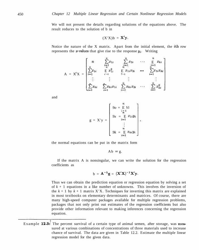
450 Chapter 12 Multiple Linear Regression and Certain Nonlinear Regression Models
We will not present the details regarding solutions of the equations above. The result reduces to the solution of b in
(X'X)b = X'y-
Notice the nature of the X matrix. Apart from the initial element, the tth row represents the x-values that give rise to the response y%. Writing
A = X X =
and
E xu J2 x2i
n n YI Xki YI XkiXu Y2 XkiX2i
<-i=l i=\
E xki
E X1i E X\i E XliX2i ••• E XliXki 1 = 1 t '= l 7 = 1 i=X
i - l "fci
g = X'y =
9o = E Vi ; = 1
9x = E xuVi s = l
9k = E xkiVi
the normal equations can be put in the matrix form
A b = g.
If the matrix A is nonsingular, we can write the solution for the regression coefficients as
b = A- X g = ( X ' X ^ X ' y .
Thus we can obtain the prediction equation or regression equation by solving a set of k + 1 equations in a like number of unknowns. This involves the inversion of the k + 1 by k + 1 matrix X'X. Techniques for inverting this matrix are explained in most textbooks on elementary determinants and matrices. Of course, there are many high-speed computer packages available for multiple regression problems, packages that not only print out estimates of the regression coefficients but also provide other information relevant to making inferences concerning the regression equation.
Example 12.3:1 The percent survival of a certain type of animal semen, after storage, was measured at various combinations of concentrations of three materials used to increase chance of survival. The data are given in Table 12.2. Estimate the multiple linear regression model for the given data.
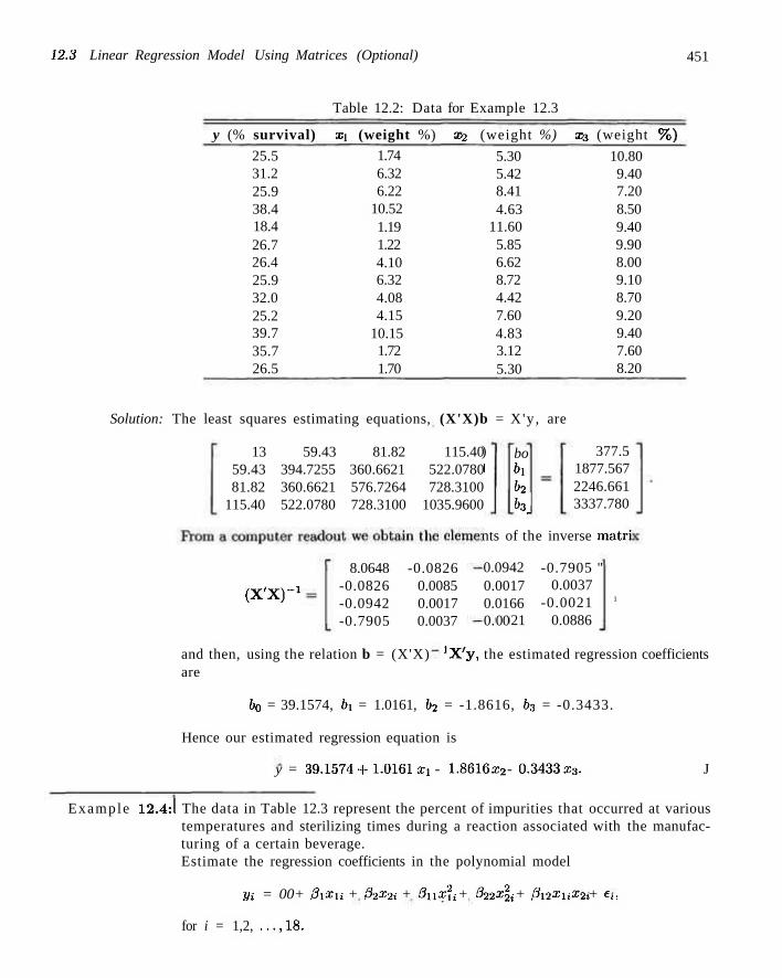
12.3 Linear Regression Model Using Matrices (Optional) 451
Table 12.2: Data for Example 12.3
y (% survival) 25.5 31.2 25.9 38.4 18.4 26.7 26.4 25.9 32.0 25.2 39.7 35.7 26.5
xi (weight %)
1.74 6.32 6.22
10.52 1.19 1.22 4.10 6.32 4.08 4.15
10.15 1.72 1.70
X2 (weight %)
5.30 5.42 8.41 4.63
11.60 5.85 6.62 8.72 4.42 7.60 4.83 3.12 5.30
x3 (weight %)
10.80 9.40 7.20 8.50 9.40 9.90 8.00 9.10 8.70 9.20 9.40 7.60 8.20
Solution: The least squares estimating equations, (X'X)b = X'y , are
13 59.43 81.82 115.40 59.43 394.7255 360.6621 522.0780 81.82 360.6621 576.7264 728.3100
115.40 522.0780 728.3100 1035.9600
( X ' X ) - 1
8.0648 -0.0826 -0.0826 0.0085 -0.0942 0.0017 -0.7905 0.0037
) 1
bo bi b2
b3\
377.5 1877.567 2246.661 3337.780
nts of the inverse matri
0.0942 0.0017 0.0166 0. 00 21
-0.7905 " 0.0037
-0.0021 0.0886
1
and then, using the relation b = (X'X) 'X 'y , the estimated regression coefficients are
b0 = 39.1574, h = 1.0161, b2 = -1.8616, b3 = -0.3433.
Hence our estimated regression equation is
y = 39.1574 + 1.0161 xi - 1.8616 x2 - 0.3433 x3. J
Example 12.4:1 The data in Table 12.3 represent the percent of impurities that occurred at various temperatures and sterilizing times during a reaction associated with the manufacturing of a certain beverage. Estimate the regression coefficients in the polynomial model
Vi = 00+ 0lXxi + 32X2i + 0llX2i + 022x\i + 0l2XUX2i + £»,
for i = 1,2, . . . , 1 8 .
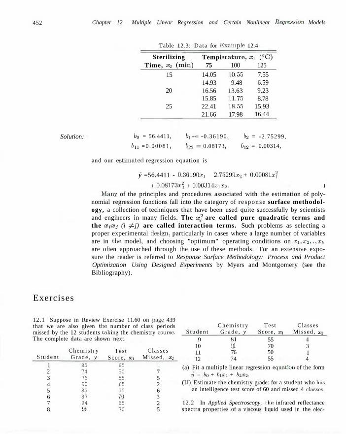
452 Chapter 12 Multiple Linear Regression and Certain Nonlinear Regression. Models
Table 12.3: Data for Example 12.4
Exercises
Sterilizing Time, x2 (min)
15
20
25
Tempi 75
14.05 14.93 16.56 15.85 22.41 21.66
srature, 100
10.55 9.48
13.63 1L.75 18.55 17.98
xx (CC) 125
7.55 6.59 9.23 8.78
15.93 16.44
Solution: bo = 56.4411,
bu = 0 . 0 0 0 8 1 ,
bi --
099
-0 .36190.
0.08173,
b2 = -2.75299,
bv2 = 0.00314,
and our estimated regression equation is
y =56.4411 - 0.30190x1 - 2.75299x9 + O.OOOSlxf
+ 0.08173a;| + 0.00314xiiE2. J Many of the principles and procedures associated with the estimation of poly
nomial regression functions fall into the category of response surface methodology, a collection of techniques that have been used quite successfully by scientists and engineers in many fields. The x2 are called pure quadratic terms and the XjXj (i ^ j) are called interaction terms. Such problems as selecting a proper experimental design, particularly in cases where a large number of variables are in the model, and choosing "optimum" operating conditions on xx,x2,... ,Xk are often approached through the use of these methods. For an extensive exposure the reader is referred to Response Surface Methodology: Process and Product Optimization Using Designed Experiments by Myers and Montgomery (see the Bibliography).
12.1 Suppose in Review Exercise 11.60 on page 439 that we are also given the number of class periods missed by the 12 students taking the chemistry course. The complete data are shown next.
S tuden t
1 2 3 4 5 6 7 8
Chemis t ry Grade , y
Test Score, xi
Classes Missed, x2
85 74 76 90 85 87 94 !>«
65 50 55 65 55 Til
65 70
I 7 5 2 6 3 2 5
C h e m i s t r y Test Classes S tuden t G r a d e , y Score, xi Missed, x2
9 10 11 12
81 !)l 76 74
55 70 50 55
3 1 4
(a) Fit a multiple linear regression equation of the form y = 60 + biXi + b2x2.
(IJ) Estimate the chemistry grade: for a student who has an intelligence test score of 60 and missed 4 classes.
12.2 In Applied Spectroscopy, the infrared reflectance spectra properties of a viscous liquid used in the clec-
Exercises 453
tronics industry as a lubricant were studied. The designed experiment consisted of the effect of band frea-quency Xi and film thickness x2 on optical density y using a Perkin-Elmer Model 621 infrared spectrometer. [Source: Pachansky, J., England, C. D., and Wattman, R. "Infrared spectroscopic studies of poly (perflouro-propyleneoxide) on gold substrate. A classical dispersion analysis for the refractive index." Applied Spectroscopy, Vol. 40, No. 1, Jan. 1986, p. 9, Table 1.]
X i X2
0.231 0.107 0.053 0.129 0.069 0.030 1.005 0.559 0.321 2.948 1.633 0.934
740 740 740 805 805 805 980 980 980
1,235 1,235 1,235
1.10 0.62 0.31 1.10 0.62 0.31 1.10 0.62 0.31 1.10 0.62 0.31
Estimate the multiple linear regression equation y = bo + bixi + b2x2.
12.3 A set of experimental runs was made to determine a way of predicting cooking time y at various levels of oven width x i , and flue temperature x2. The coded data were recorded as follows:
X l X2
6.40 15.05 18.75 30.25 44.85 48.94 51.55 61.50
100.44 111.42
1.32 2.69 3.56 4.41 5.35 6.20 7.12 8.87 9.80
10.65
1.15 3.40 4.10 8.75
14.82 15.15 15.32 18.18 35.19 40.40
Estimate the multiple linear regression equation Myi^ ,^ =0o + 0\xi + 02X2.
12.4 An experiment was conducted to determine if the weight of an animal can be predicted after a given period of time on the basis of the initial weight of the animal and the amount of feed that was eaten. The following data, measured in kilograms, were recorded:
Final Weight, y
95 77 80
100 97
Initial Weight, xi
42 33 33 45 39
Feed Weight, X2
272 226 259 292 311
Final Weight, y
70 50 80 92 84
Initial Weight, Xi
36 32 41 40 38
Feed Weight, X2
183 173 236 230 235
(a) Fit a multiple regression equation of the form
PY\x = 00 + 0ixx + 02x2.
(b) Predict the final weight of an animal having an initial weight of 35 kilograms that is fed 250 kilograms of feed.
12.5 (a) Fit a multiple regression equation of the form pY\x = 0Q+ 0m + 0\x2 to the data of Example 11.8.
(b) Estimate the yield of the chemical reaction for a temperature of 225° C.
12.6 An experiment was conducted on a new model of a particular make of an automobile to determine the stopping distance at various speeds. The following data were recorded.
Speed, v (km/hr) 35 50 65 80 95 110 Stopping Distance, d(m) 16 26 41 62 88 119
(a) Fit a multiple regression curve of the form up\v = 0O + 0W+02V2.
(b) Estimate the stopping distance when the car is traveling at 70 kilometers per hour.
12.7 An experiment was conducted in order to determine if cerebral blood flow in human beings can be predicted from arterial oxygen tension (millimeters of mercury). Fifteen patients were used in the study and the following data were observed:
Blood Flow, y
84.33 87.80 82.20 78.21 78.44 80.01 83.53 79.46 75.22 76.58 77.90 78.80 80.67 86.60 78.20
Arterial Oxygen Tension, x
603.40 582.50 556.20 594.60 558.90 575.20 580.10 451.20 404.00 484.00 452.40 448.40 334.80 320.30 350.30
454 Chapter 12 Multiple Linear Regression and Certain Nonlinear Regression A4odels
Estimate the quadratic regression equation
PY\x = 3o + 0ix + 02X2.
12 .8 The following is a set of coded experimental data on the compressive strength of a particular alloy at various values of the concentration of some additive:
scores of four tests. The data are as follows:
Concentration, X
10.0 15.0 20.0 25.0 30.0
Compressive
25.2 29.8 31.2 31.7 29.4
Strength, y
27.3 28.7 31.1 27.8 32.6 29.7 30.1 32.3 30.8 32.8
(a) Estimate the quadratic regression equation py\x = 0o + 0iX + p\x2.
(b) Test for lack of fit of the model.
12.9 The electric power consumed each month by a chemical plant is thought to be related to the average ambient temperature x i , the number of days in the month x2, the average product purity X3, and the tons of product produced X4. The past year's historical data are available and are presented in the following table.
X ] X2 ak X ]
240 236 290 274 301 316 300 296 267 276 288 261
25 31 45 60 65 72 80 84 75 60 50 38
24 21 24 25 25 26 25 25 24 25 25 23
91 90 88 87 91 94 87 86 88 91 90 89
100 95 110 88 94 99 97 96 110 105 100 98
(a) Fit a multiple linear regression model using the above data set.
(b) Predict power consumption for a month in which xi = 75°F, x2 = 24 days, x3 = 90%, and x4 = 98 tons.
12.10 Given the data
X
y
0 l
l 4
2 5
3 3
4 2
5 3
6 4
(a) Fit the cubic model fiy\x = 30 +0ix+02x2 + 03x*.
(b) Predict Y when x = 2.
12.11 The personnel department of a certain industrial firm used 12 subjects in a study to determine the relationship between job performance rating (y) and
y Xl X2 X.]
11.2 14.5 17.2 17.8 19.3 24.5 21.2 16.9 14.8 20.0 13.2 22.5
56.5 59.5 69.2 74.5 81.2 88.0 78.2 69.0 58.1 80.5 58.3 84.0
71.0 72.5 76.0 79.5 84.0 86.2 80.5 72.0 68.0 85.0 71.0 87.2
38.5 38.2 42.5 43.4 47.5 47.4 44.5 41.8 42.1 48.1 37.5 51.0
43.0 44.8 49.0 56.3 60.2 62.0 58.1 48.1 46.0 60.3 47.1 65.2
Estimate the regression coefficients in the model
y = bo + bixi + b2x2 + b3x3 + &4X4.
12.12 The following data reflect information taken from 17 U.S. Naval hospitals at various sites around the world. The regressors are workload variables, that is, items that result in the need for personnel in a hospital installation. A brief description of the variables is as follows:
y = monthly labor-hours,
xi = average daily patient load,
X2 = monthly X-ray exposures,
X3 = monthly occupied bed-days,
X4 = eligible population in the area/1000,
i s = average length of patient's stay, in days.
Site xi X2 X3 Xl X 5 y 1 2 3 4 5 6 7 8 9 10 11 12 13 14 15 16 17
15.57 44.02 20.42 18.74 49.20 44.92 55.48 59.28 94.39 128.02 96.00 131.42 127.21 252.90 409.20 463.70 510.22
2463 2048 3940 6505 5723 11520 5779 5969 8461
20106 13313 10771 15543 36194 34703 39204 86533
472.92 1339.75 620.25 568.33 1497.60 1365.83 1687.00 1639.92 2872.33 3655.08 2912.00 3921.00 3865.67 7684.10
12446.33 14098.40 15524.00
18.0 9.5 12.8 36.7 35.7 24.0 43.3 46.7 78.7 180.5 60.9 103.7 126.8 157.7 169.4 331.4 371.6
4.45 6.92 4.28 3.90 5.50 4.60 5.62 5.15 6.18 6.15 5.88 4.88 5.50 7.00 10.75 7.05 6.35
566.52 696.82 1033.15 1003.62 1611.37 1613.27 1854.17 2160.55 2305.58 3503.93 3571.59 3741.40 4026.52 10343.81 11732.17 15414.94 18854.45
The goal here is to produce an empirical equation that will estimate (or predict) personnel needs for Naval hospitals. Estimate the multiple linear regression equa-
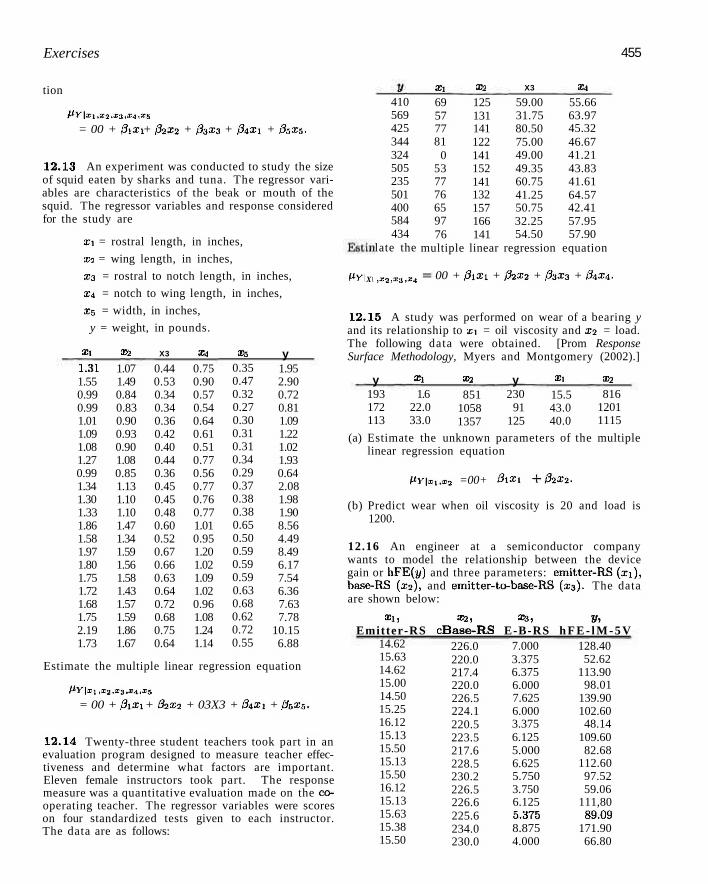
Exercises 455
tion
PY\xi,X2.X3,I4,x$
= 00 + 0Hl + 02X2 + 03X3 + 0AXI + 05X5-
12.13 An experiment was conducted to study the size of squid eaten by sharks and tuna. The regressor variables are characteristics of the beak or mouth of the squid. The regressor variables and response considered for the study are
xi = rostral length, in inches,
x2 = wing length, in inches,
X3 = rostral to notch length, in inches,
X4 = notch to wing length, in inches,
X5 = width, in inches,
y = weight, in pounds.
Xl X 2 X3 X4
Xl X2 X3 X4 Xs y 1.31 1.55 0.99 0.99 1.01 1.09 1.08 1.27 0.99 1.34 1.30 1.33 1.86 1.58 1.97 1.80 1.75 1.72 1.68 1.75 2.19 1.73
1.07 1.49 0.84 0.83 0.90 0.93 0.90 1.08 0.85 1.13 1.10 1.10 1.47 1.34 1.59 1.56 1.58 1.43 1.57 1.59 1.86 1.67
0.44 0.53 0.34 0.34 0.36 0.42 0.40 0.44 0.36 0.45 0.45 0.48 0.60 0.52 0.67 0.66 0.63 0.64 0.72 0.68 0.75 0.64
0.75 0.90 0.57 0.54 0.64 0.61 0.51 0.77 0.56 0.77 0.76 0.77 1.01 0.95 1.20 1.02 1.09 1.02 0.96 1.08 1.24 1.14
0.35 0.47 0.32 0.27 0.30 0.31 0.31 0.34 0.29 0.37 0.38 0.38 0.65 0.50 0.59 0.59 0.59 0.63 0.68 0.62 0.72 0.55
1.95 2.90 0.72 0.81 1.09 1.22 1.02 1.93 0.64 2.08 1.98 1.90 8.56 4.49 8.49 6.17 7.54 6.36 7.63 7.78
10.15 6.88
410 569 425 344 324 505 235 501 400 584 434
late the
69 57 77 81
0 53 77 76 65 97 76
multiple
125 131 141 122 141 152 141 132 157 166 141
linear
59.00 31.75 80.50 75.00 49.00 49.35 60.75 41.25 50.75 32.25 54.50
55.66 63.97 45.32 46.67 41.21 43.83 41.61 64.57 42.41 57.95 57.90
regression equation
f*Y\ X\ ,X2,X\1 P^4 00 + /3lXl + 02X2 + /33X3 + 04X4.
12.15 A study was performed on wear of a bearing y and its relationship to xi = oil viscosity and X2 = load. The following data were obtained. [Prom Response Surface Methodology, Myers and Montgomery (2002).]
y Xl X2 y Xl X2
193 172 113
1.6 22.0 33.0
851 1058 1357
230 91
125
15.5 43.0 40.0
816 1201 1115
Estimate the multiple linear regression equation
l^Y\x\ ,X2IX3,X4,25
= 00 + 3\Xl + 02X2 + 03X3 + /?4Xl + 05X5.
12.14 Twenty-three student teachers took part in an evaluation program designed to measure teacher effectiveness and determine what factors are important. Eleven female instructors took part. The response measure was a quantitative evaluation made on the cooperating teacher. The regressor variables were scores on four standardized tests given to each instructor. The data are as follows:
(a) Estimate the unknown parameters of the multiple linear regression equation
f.Y\xi,x2 =00+ 0\X\ +02X2-
(b) Predict wear when oil viscosity is 20 and load is 1200.
12.16 An engineer at a semiconductor company wants to model the relationship between the device gain or hFE(y) and three parameters: emitter-RS (xi), base-RS (X2), and emitter-to-base-RS (X3). The data are shown below:
X i , X2, X3, y , Emitter-RS cBase-RS E-B-RS h F E - l M - 5 V
14.62 15.63 14.62 15.00 14.50 15.25 16.12 15.13 15.50 15.13 15.50 16.12 15.13 15.63 15.38 15.50
226.0 220.0 217.4 220.0 226.5 224.1 220.5 223.5 217.6 228.5 230.2 226.5 226.6 225.6 234.0 230.0
7.000 3.375 6.375 6.000 7.625 6.000 3.375 6.125 5.000 6.625 5.750 3.750 6.125 5.375 8.875 4.000
128.40 52.62
113.90 98.01
139.90 102.60 48.14
109.60 82.68
112.60 97.52 59.06
111,80 89.09
171.90 66.80

456 Chapter 12 Multiple Linear Regression and Certain Nonlinear Regression. Models
xi, x2, x3, y, Emitter-RS cBase-RS E-B-RS hFE-lM-5V
14.25 14.50 14.62
224.3 240.5 223.7
8.000 10.870 7.375
157.11) 208.40 133.40
(a) Fit a multiple linear regression to the data. (b) Predict hFE when x3 = 14. x2 = 220, and i::i
[Data from Myers and Montgomery (2002)].
12.4 Properties of the Least Squares Estimators
The means and variances of the estimators bo, bx,..., bk are readily obtained under certain assumptions on the random errors ej, e2,..., ck that are identical to those made in the case of simple linear regression. When we assume these errors to be independent, each with zero mean and variance er", it can then be shown that bo,b\,... ,bk arc. respectively, unbiased estimators of the regression coefficients 0o, 0x, • • • ,3k- In addition, the variances of b's are obtained through the elements of the inverse of the A matrix. Note that the off-diagonal elements of A = X'X represent sums of products of elements in the columns of X, while the diagonal elements of A represent sums of squares of elements in the columns of X. The inverse matrix, A - 1 , apart from the multiplier a2, represents the variance-covariance mat r ix of the estimated regression coefficients. That is, the elements of the matrix A_1er display the variances of bo, b], . . . , bk on the main diagonal and covariances on the off-diagonal. For example, in a A- = 2 multiple linear regression problem, we might write
(X'X)-
with the elements below the main diagonal determined through the symmetry of the matrix. Then we can write
of. = cao2, i = 0,1,2,
Ob^bj = Cov(bi,bj)= CijO2, i ^ j .
Of course, the estimates of the variances and hence flic standard errors of these estimators are obtained by replacing er2 with the appropriate estimate obtained through experimental data. An unbiased estimate of a2 is once again defined in terms of the error stun of squares, which is computed using the formula established in Theorem 12.1. In the theorem we are making the assumptions on the e-, described above.
coo ClO
C20
CQl
C - l l
cai
C02
Cl2
C22
Theorem 12.1: Fo
an
r the linear regression
unbiased estimate of o
2 8 =
SSE n - k - l
equation
y =
2 is given
where
X3 +
by the
SSE--
e,
error
n
=£ ?:=i
or
el
residual
= £> i = i
mean
-Vi?
sepi ire
We can see that Theorem 12.1 represents a generalization of Theorem 11.1
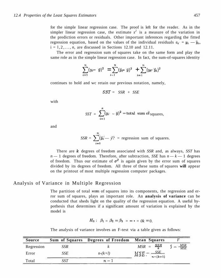
12.4 Properties of the Least Squares Estimators 457
for the simple linear regression case. The proof is left for the reader. As in the simpler linear regression case, the estimate s2 is a measure of the variation in the prediction errors or residuals. Other important inferences regarding the fitted regression equation, based on the values of the individual residuals e^ = yi — yi, i = l , 2 , . . . , n, are discussed in Sections 12.10 and 12.11.
The error and regression sum of squares take on the same form and play the same role as in the simple linear regression case. In fact, the sum-of-squares identity
£ > " V? = £ > - V? + f > - Vi? i—l 2 = 1 ;'.= 1
continues to hold and wc retain our previous notation, namely,
SST = SSR + SSE
with
n
SST = 2_,iy> ~ y? = t'0*8-! s u m OI squares, i = i
and
SSR = ^Jfj/i — y? = regression sum of squares. ; = i
There are A; degrees of freedom associated with SSR and, as always, SST has n — 1 degrees of freedom. Therefore, after subtraction, SSE has n — k — 1 degrees of freedom. Thus our estimate of er2 is again given by the error sum of squares divided by its degrees of freedom. All three of these sums of squares will appear on the printout of most multiple regression computer packages.
Analysis of Variance in Mult iple Regression
The partition of total sum of squares into its components, the regression and error sum of squares, plays an important role. An analysis of variance can be conducted that sheds light on the quality of the regression equation. A useful hypothesis that determines if a significant amount of variation is explained by the model is
#o : 0i = 02 = 1% = •• • = 0k = 0.
The analysis of variance involves an F-test via a table given as follows:
Source
Regression
Error
Total
Sum of Squares
SSR
SSE
SST
Degrees of Freedom
k
n-(k+l)
n - 1
Mean Squares
MSR = ^f2
HfQf? SSE MSL - n _ ( f c + 1 )
F f _ MSR •> MSE
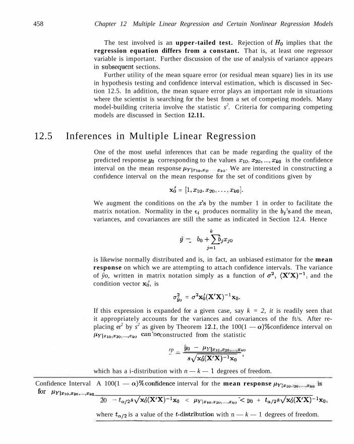
458 Chapter 12 Multiple Linear Regression and Certain Nonlinear Regression Models
The test involved is an upper-tailed test. Rejection of H0 implies that the regression equation differs from a constant. That is, at least one regressor variable is important. Further discussion of the use of analysis of variance appears in subsequent sections.
Further utility of the mean square error (or residual mean square) lies in its use in hypothesis testing and confidence interval estimation, which is discussed in Section 12.5. In addition, the mean square error plays an important role in situations where the scientist is searching for the best from a set of competing models. Many model-building criteria involve the statistic s2. Criteria for comparing competing models are discussed in Section 12.11.
12.5 Inferences in Multiple Linear Regression
One of the most useful inferences that can be made regarding the quality of the predicted response yo corresponding to the values arm, X2Q, ..., Xko is the confidence interval on the mean response py\Xw,x.Jt Xka- We are interested in constructing a confidence interval on the mean response for the set of conditions given by
xo = [1,xio,X2ot •••-.Xka}-
We augment the conditions on the x's by the number 1 in order to facilitate the matrix notation. Normality in the £{ produces normality in the bjS and the mean, variances, and covariances are still the same as indicated in Section 12.4. Hence
k
y - b°+YI bJxj° J = I
is likewise normally distributed and is, in fact, an unbiased estimator for the mean response on which we are attempting to attach confidence intervals. The variance of yo, written in matrix notation simply as a function of cr2, ( X ' X ) - 1 , and the condition vector Xrj, is
0$, = c72x(J(X'X)-1x0.
If this expression is expanded for a given case, say k = 2, it is readily seen that it appropriately accounts for the variances and covariances of the ft/s. After replacing er2 by s2 as given by Theorem 12.1, the 100(1 — a)% confidence interval on Mv|a;io.x2o....,2to c a n oe constructed from the statistic
rp _ VO — llY\x,0,X20,--,Xk0
Vxd(X'X)-1x0 '
which has a i-distribution with n — k — 1 degrees of freedom.
Confidence Interval A 100(1 — a)% confidence interval for the mean response py\xm_, for PY\xla,xm,...,Xk0
2/0 - iQ/2S\/x6(X'X)-1Xo < PY\xw,xM,...,xku <V0 + ta/2Sy/x6(X'X)-lK0,
where ta/2 is a value of the ^-distribution with n — k — 1 degrees of freedom.
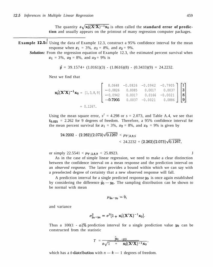
22.5 Inferences in Multiple Linear Regression 459
The quantity sy'x<5(X'X)~1x0 is often called the standard error of prediction and usually appears on the printout of many regression computer packages.
Example 12.5:1 Using the data of Example 12.3, construct a 95% confidence interval for the mean response when xx = 3%. x2 = 8%, and x3 = 9%.
Solution: From the regression equation of Example 12.3, the estimated percent survival when xx = 3%, x2 = 8%, and x3 = 9% is
y = 39.1574+ (1.0161)(3) - (1.8616)(8) - (0.3433)(9) = 24.2232.
Next we find that
x 0(X'X)-1x 0 = [1,3,8,9]
8.0648 -0.0826 -0.0942 -0.7905 -0.0826 0.0085 0.0017 0.0037 -0,0942 0.0017 0.0166 -0.0021 -0.7905 0.0037 -0.0021 0.0886
= 0.1267.
Using the mean square error, s2 = 4.298 or s = 2.073, and Table A.4, we see that £0.025 = 2.262 for 9 degrees of freedom. Therefore, a 95% confidence interval for the mean percent survival for xx = 3%, x2 = 8%, and X3 = 9% is given by
24.2232 - (2.262)(2.073)\/0.1267 < py\3,s,c,
< 24.2232 + (2.262)(2.073)V0.1267,
or simply 22.5541 < MV|3,8,9 < 25.8923. J As in the case of simple linear regression, we need to make a clear distinction
between the confidence interval on a mean response and the prediction interval on an observed response. The latter provides a bound within which we can say with a preselected degree of certainty that a new observed response will fall.
A prediction interval for a single predicted response yo is once again established by considering the difference y0 — y0. The sampling distribution can be shown to be normal with mean
^Oo-yo ~ 0,
and variance
<£-*,» ^[l + xftX'X)-1*,].
Thus a 100(1 - a)% prediction interval for a single prediction value yo can be constructed from the statistic
T = Vo -yo Sy/l + x6(X'X)-W
which has a t-distribution with n — k — 1 degrees of freedom.
460 Chapter 12 Multiple Linear Regression and Certain Nonlinear Regression Models
Prediction Interval A 100(1 — a)% prediction interval for a single response i/o is given by for j/o
2/0 " <Q/2*\/l+X($(X'X)-1Xo < 2/0 < VO + ta/2SV'l + X<J(X'X)-1Xo>
where ta/2 is a value of the t-distribution with n — k — 1 degrees of freedom.
Example 12.6:1 Using the data of Example 12.3, construct a 95% prediction interval for an individual percent survival response when xx = 3%, x2 = 8%, and x3 = 9%.
Solution: Referring to the results of Example 12.5, we find that the 95% prediction interval for the response yo, when xx = 3%, x2 = 8%., and X3 = 9%, is
24.2232 - (2.262)(2.073)\/1.1267 <y0< 24.2232
+ (2.262)(2.073)\/l.l267,
which reduces to 19.2459 < 2/0 < 29.2005. Notice, as expected, that the prediction interval is considerably wider than the confidence interval for mean percent survival in Example 12.5. J
A knowledge of the distributions of the individual coefficient estimators enables the experimenter to construct confidence intervals for the coefficients and to test hypotheses about them. Recall from Section 12.4 that the b,'s (j = 0,1,2,.. ,,k) are normally distributed with mean 0j and variance Cjja2. Thus we can use the statistic
t = _ bj - 0jp
s./c 33
with n — k — I degrees of freedom to test hypotheses and construct confidence intervals on 0j. For example, if we wish to test
#0: 0j = 0jo> Hi'. 0j ^ 0JO,
we compute the above i-statistic and do not reject HQ if -ta/2 < t < ta/2, where taj2 has n — k — 1 degrees of freedom.
Example 12.7:1 For the model of Example 12.3, test the hypothesis that 02 = -2 .5 at the 0.05 level of significance against the alternative that 02 > —2.5.
Solution: H0: 02 = -2 .5 ,
Hi: 32 > -2 .5 .
Computations:
t = b2 - 02O = -1-8616 + 2.5 = 2 3 g o
sy/c^ 2.073 VQ.0166 ' '
P = P(T > 2.390) = 0.04.
Decision: Reject Ho and conclude that 02 > —2.5.
12.5 Inferences in Multiple Linear Regression 461
Individual T-Tests for Variable Screening
The i-tcst most often used in multiple regression is the one which tests the importance of individual coefficients (i.e., H$j — 0 against the alternative Hi: 0j ^ 0). These tests often contribute to what is termed variable screening where the analyst attempts to arrive at the most useful model (i.e., the choice of wdiich regressors to use). It should be emphasized here that if a coefficient is found insignificant (i.e., the hypothesis H0: 0j = 0 is not rejected), the conclusion drawn is that the variable is insignificant (i.e., explains an insignificant amount, of variation in y), in the presence of the other regressors in the model. This point will be reaffirmed in a future discussion.
Annotated Printout for Data of Example 12.3
Figure 12.1 shows an annotated computer printout for a multiple linear regression fit to the data of Example 12.3. The package used is 5.45.
Note the model parameter estimates, the standard errors, and the i-statistics shown in the output. The standard errors are computed from square roots of diagonal elements of (X'X)~1s2. In this illustration the variable x3 is insignificant in the presence of xx and x2 based on the i-test and the corresponding P-value = 0.5916. The terms CLM and CLI are confidence intervals on mean response and prediction limits on an individual observation, respectively. The /-test in the analysis of variance indicates that a significant amount of variability is explained. As an example of the interpretation of CLM and CLI, consider observation 10. With an observation of 25.2 and a predicted value of 26.068, we are 95% confident that the mean response is between 24.502 and 27.633, and a new observation will fall between 21.124 and 31.011 with probability 0.95. The R2 value of 0.9117 implies that the model explains 91.17% of the variability in the response. More discussion about i£2-appears in Section 12.6.
More on Analysis of Variance in Multiple Regression (Optional)
In Section 12.4 we discussed briefly the partition of the total sum of squares
YI iVi — 'V? m t ° its two components, the regression model and error sums of squares »=i (illustrated in Figure 12.1). The analysis of variance leads to a test of
Ho: 0i=02=03 = --- = 0k = 0.
Rejection of the null hypothesis has an important interpretation for the scientist or engineer. (For those who are interested in more treatment of the subject using matrices, it is useful to discuss the development of these sums of squares used in ANOVA.)
First recall from the definition of y, X, and 0 in Section 12.3, as well as b, the vector of least squares estimators given by
b = (X'X) - ' X ' y .
462 Chapter 12 Multiple Linear Regression and Certain Nonlinear Regression Models
Source
Model
Error
Corrected Total
Root MSE Dependent Mean
Coeff Var
Variable DF
Intercept 1
xl x2 x3
1 1 1
Sum of Mean
DF Squares Square F Value Pr >
3 399.45437 133.:
F 15146 30.98 <.0001
9 38.67640 4.29738
12 438.13077
2.07301 R-Square
29.03846 Adj R-Sq
7.13885
Parameter
Estimate
39.15735
1.01610
-1.86165
-0.34326
Dependent Predicted Std Error
Obs 1 2 3 4 5 6 7 8 9 10 11 12 13
Variable
25.5000
31.2000
25.9000
38.4000
18.4000
26.7000
26.4000
25.9000
32.0000
25.2000
39.7000
35.7000
26.5000
Value Mean Predict
27.3514 1.4152
32.2623 0.7846
27.3495 1.3588
38.3096 1.2818
15.5447 1.5789
26.1081 1.0358
28.2532 0.8094
26.2219 0.9732
32.0882 0.7828
26.0676 0.6919
37.2524 1.3070
32.4879 1.4648
28.2032 0.9841
0.9117
0.8823
Standard
Error
5.88706
0.19090
0.26733
0.61705
95'/. CL
24.1500
30.4875
24.2757
35.4099
11.9730
23.7649
26.4222
24.0204
30.3175
24.5024
34.2957
29.1743
25.9771
t Value
6.65
5.32
-6.96
-0.56
Mean
30.5528
34.0371
30.4234
41.2093
19.1165
28.4512
30.0841
28.4233
33.8589
27.6329
40.2090
35.8015
30.4294
Pr > Itl <,0001
0.0005
<.0001
0.5916
95'/, CL
21 27 21 32 9 20 23 21 27 21 31 26 23
.6734
.2482
.7425
.7960
.6499
.8658
.2189
.0414
.0755
.1238
.7086
.7459
.0122
Predict
33.0294
37.2764
32.9566
43.8232
21.4395
31.3503
33.2874
31.4023
37.1008
31.0114
42.7961
38.2300
33.3943
Residual
-1.8514
-1.0623
-1.4495
0.0904
2.8553
0.5919
-1.8532
-0.3219
-0.0882
-0.8676
2.4476
3.2121
-1.7032
Figure 12.1: 5.45 printout for data in Example 12.3.
A partition of the uncorrected sum of squares
y'y = X>2 j = i
into two components is given by
y'y = b 'X 'y + (y'y - b 'X'y)
= y 'X(X 'X) - 1 X'y + [y'y - y 'X(X 'X) - l X'y] .
The second term (in brackets) on the right-hand side is simply the error sum of n
squares Y2 iVi —Vi)2- The reader should see that an alternative expression for the ; = i
error sum of squares is
SSE = y'[I„ - X(X'X)-1X']y.
12.5 Inferences in Multiple Linear Regression 463
The term y ' X ( X ' X ) - X'y is called the regression sum of squares. However, n
it is not the expression YI iVi ~ V? used for testing the "importance" of the terms i=[
bx, b2,..., bk but, rather,
y'X(X'XrxX'y = I>? 2 i >
i = l
which is a regression sum of squares uncorrected for the mean. As such it would only be used in testing if the "regression equation differs significantly from zero." That is,
H0: 0o=0i=02 = ---=0k = 0.
In general, this is not as important as testing
HQ: 0i=02 = --- = 0k = 0,
since the latter states that the mean response is a constant, not necessarily zero.
Degrees of Freedom
Thus the partition of sums of squares and degrees of freedom reduces to
Source Sum of Squares d.f.
Regression £ y2 = y ' X ( X ' X ) - 1 X ' y fe + 1 i-l
Error YZilH ~ m? = y'fc. - X(X'X)- 1 X']y n-(k + 1) i = l
Total £ yf = y'y n i = l
Hypothesis of Interest
Now, of course, the hypotheses of interest for an ANOVA must eliminate the role of the intercept in that described previously. Strictly speaking, if Ho : 0x = 02 = • • • — 0k — 0, then the estimated regression line is merely y; = y. As a result, we are actually seeking evidence that the regression equation "varies from a constant." Thus, the total and regression sums of squares must be "corrected for the mean." As a result, we have
;=1 i = l i = l
In matrix notation this is simply
y ' [In - l f l ' l V ^ l ' l y = y ' [ X ( X ' X ) - 1 X ' - l f l ' l j - ^ y
+ y ' ( I „ - X ( X ' X ) - 1 X ' ] y .
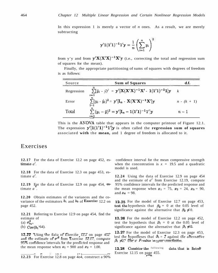
464 Chapter 12 Multiple Linear Regression and Certain Nonlinear Regression Models
In this expression 1 is merely a vector of n ones. As a result, we are merely subtracting
y ' l ( l ' l ) - 1 l ' y = i ^ ^ )
from y 'y and from y 'X(X 'X) _ 1 X'y (i.e., correcting the total and regression sum of squares for the mean).
Finally, the appropriate partitioning of sums of squares with degrees of freedom is as follows:
Source Sum of Squares d.f.
Regression £ (ft - y)2 = y T X f X ' X ) - ^ ' - l ( l ' l ) - 1 l ] y k i=i
Error £ (yt - y{)2 = y '[In - X(X'X)" 1 X']y n - (k + 1)
1=1
Total £ ( 2 / i -y ) 2 =y ' [ I n - l ( l / l ) - 1 l ' ] y n - 1 i=\
This is the ANOVA table that appears in the computer printout of Figure 12.1. The expression y ' [ l ( l ' l ) - 1 l ' ] y is often called the regression sum of squares associated with the mean, and 1 degree of freedom is allocated to it.
Exercises
12.17 For the data of Exercise 12.2 on page 452, es- confidence interval for the mean compressive strength timate a2. when the concentration is x = 19.5 and a quadratic
model is used. 12.18 For the data of Exercise 12.3 on page 453, estimate a2. 12.24 Using the data of Exercise 12.9 on page 454
and the estimate of a2 from Exercise 12.19, compute 12.19 For the data of Exercise 12.9 on page 454, es- 95% confidence intervals for the predicted response and timate a . the mean response when xi = 75, x2 = 24, x3 = 90,
and X4 = 98. 12.20 Obtain estimates of the variances and the co-variance of the estimators bx and b2 of Exercise 12.2 on 1 2 . 2 5 For the model of Exercise 12.7 on page 453, page 452. t e s t t h e hypothesis that 02 = 0 at the 0.05 level of
significance against the alternative that 02 ^ 0. 12.21 Referring to Exercise 12.9 on page 454, find the estimate of 1 2 . 2 6 For the model of Exercise 12.2 on page 452, (a) a2
2, test the hypothesis that 0i = 0 at the 0.05 level of (b) Cov(bi 64). significance against the alternative that 0i / 0,
, . . , „ , i U , . r „ ,„ . . , . 1 2 . 2 7 For the model of Exercise 12.3 on page 453, 12.22 Using the data of Exercise 12.2 on page 452 . . .. , ., .. . a „ . . ., ,. .<.•
j .1. ... j. e 2c -^ • -in,-. test the hypotheses that 3\ = 2 against the alternative and the estimate of er" from Exercise 12.17. compute ,, , 0 ,,„„ „ D , „,„„ . „ „ . „„„„,„• „ r n r „ , . t , , , ,. t , K , pi * 2. Use a /•'-value in your conclusion. 95% confidence intervals for the predicted response and ' the mean response when xi = 900 and x2 = 1.00. 1 2 2 8 Q ^ ^ t h e f o l l o w i n g d a U t h a t ig l i s t e d f a
„ „ . „ „ ,_ . -, Exercise 12.15 on page 455. 12.23 For Exercise 12.8 on page 4o4, construct a 90% H b
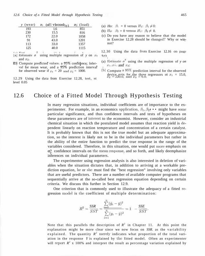
y (wear) 193 230 172 91
113 125
Xi ( o 1 viscosii 1.6
15.5 22.0 43.0 33.0 40.0
ty) x< (load) 851 816
1058 1201 1357 1115
12.6 Choice of a Fitted Model through Hypothesis Testing 465
(a) Ho: 01 = 0 versus // , : 3i # 0; (b) H0: 02 = 0 versus Hi: 32 5* 0. (c) Do you have any reason to believe that the model
in Exercise 12.28 should be changed? Why or win-not?
, , , - , , . 2 ... , , 12.30 Using the data from Exercise 12.16 on page (aj Estimate er using multiple regression of y on ;r:i . r ,
and x2. ' „ ,, , „ ,. , , „,fw „ , . . (a) Estimate o using the multiple regression of y on ID) Compute predicted values, a 95% confidence; inter- , , e i n,n/ i- • i xi. Xi. and 2:3:
val tor mean wear, and a 95% prediction interval for observed wear if xi = 20 and x2 = 1000. (u) Compute a 95%. prediction interval for the observed
device gain for the three regressors tit Xi = 15.0, 12.29 Using the data from Exercise 12.28, teat, tit. X2 = 2 2 0 ' 0 ' a i l d x* = 6*0,
level 0.05
12.6 Choice of a Fitted Model Through Hypothesis Testing
In many regression situations, individual coefficients are of importance to the experimenter. For example, in an economics application, 0x,p\, • • • might have some particular significance, and thus confidence intervals and tests of hypotheses on these parameters are of interest to the economist. However, consider an industrial chemical situation in which the postulated model assumes that reaction yield is dependent linearly on reaction temperature and concentration of a certain catalyst. It is probably known that this is not the true model but an adequate approximation, so the interest is likely not to be in the individual parameters but rather in the ability of the entire function to predict the true response in the range of the variables considered. Therefore, in this situation, one would put more emphasis on er? confidence intervals on the mean response, and so forth, and likely deemphasize inferences on individual parameters.
The experimenter using regression analysis is also interested in deletion of variables when the situation dictates that, in addition to arriving at a workable prediction equation, he or she: must find the ''best regression" involving only variables that are useful predictors. There are a number of available computer programs that sequentially arrive at the so-called best regression equation depending on certain criteria. We discuss this further in Section 12.9.
One criterion that is commonly used to illustrate the adequacy of a fitted regression model is the coefficient of mult iple de te rmina t ion :
SSR g ,<» ' - T J ) 2 SSE
" « " • " £ < » - « • " ~ s s r
/ - - 1
Note tha t this parallels the description of R2 in Chapter 11. At this point the explanation might be more clear since we now focus on SSR. as the v a r i a b i l i t y e x p l a i n e d . The quanti ty R2 merely indicates what proportion of the total variation in the response Y is explained by the fitted model. Often an experimenter will report R2 x 100% and interpret the result as percentage variation explained by
466 Chapter 12 Multiple Linear Regression and Certain Nonlinear Regression Models
the postulated model. The square root of R2 is called the multiple correlation coefficient between Kand the set x\,x2,..., Xk- In Example 12.3, the value of R2
indicating the proportion of variation explained by the three independent variables Xi, x2, and x3 is found to be
55H = 399:45 = 1 SST 438.13 J
which means that 91.17% of the variation in percent survival has been explained by the linear regression model.
The regression sum of squares can be used to give some indication concerning whether or not the model is an adequate explanation of the true situation. We can test the hypothesis HQ that the regression is not significant by merely forming the ratio
SSR/k SSR/k } ~ SSE/{n-k-\)~ s2
and rejecting Ho at the a-level of significance when / > fa{k, n — k — 1). For the data of Example 12.3 we obtain
' 4.298
From the printout of Figure 12.1 the P-value is less than 0.0001. This should not be misinterpreted. Although it does indicate that the regression explained by the model is significant, this does not rule out the possibility that
1. The linear regression model in this set of x's is not the only model that can be used to explain the data; indeed, there may be other models with transformations on the x's that may give a larger value of the F-statistic.
2. The model may have been more effective with the inclusion of other variables in addition to Xi, x2, and x3 or perhaps with the deletion of one or more of the variables in the model, say x3, which displays P = 0.5916.
The reader should recall the discussion in Section 11.5 regarding the pitfalls in the use of R2 as a criterion for comparing competing models. These pitfalls are certainly relevant in multiple linear regression. In fact, the dangers in its employment in multiple regression are even more pronounced since the temptation to overfit is so great. One should always keep in mind the fact an R? « 1.0 can always be achieved at the expense of error degrees of freedom when an excess of model terms is employed. However, an R2 = 1, describing a model with a near perfect fit, does not always result in a model that predicts well.
The Adjusted Coefficient of Determination (Adjusted R2)
In Chapter 11 several figures displaying computer printout from both SAS and MINITAB featured a statistic called adjusted R? or adjusted coefficient of determination. Adjusted R? is a variation on R? that provides an adjustment for degrees of freedom. The coefficient of determination as defined on page 407 cannot decrease as terms are added to the model. In other words. R2 does not
12.6 Choice of a Fitted Model through Hypothesis Testing 467
decrease as the error degrees of freedom n — A: — 1 are reduced, the latter result being produced by an increase in k, the number of model terms. Adjusted R2
is computed by dividing SSE and SST by their respective values of degrees of freedom (i.e., adjusted R2 is as follows).
Adlui i idP? SSE/jn-k-1) adj SST/(n-l) '
To illustrate the use of R2d<, Example 12.3 is revisited.
How Are R2 and i?^dj Affected by Removal of a;3?
The t (or corresponding F) test for £3, the weight percent of ingredient 3, would certainly suggest that a simpler model involving only Xx and x2 may well be an improvement. In other words, the complete model with all the regressors maybe an overfitted model. It is certainly of interest to investigate R2 and R2
dt for both the full (xx,x2,x3) and restricted (x\,x2) models. We already know that HfM = 0.9117 by Figure 12.1. The SSE for the reduced model is 40.01 and thus ^restricted = 1 — .i38°i3 = 0-9087. Thus more variability is explained with 2:3 in the model. However, as wre have indicated, this will occur even if the model is an overfitted model. Now, of course, R\Ai is designed to provide a statistic that punishes an overfitted model so we might expect to favor the restricted model. Indeed, for the full model
2 38.6764/9 4.2974 K»d> - l ~ 438.1308/12 " l ~ 3U5109 " °M26,
whereas for the reduced model (deletion of x3)
2 40.01/10 4.001 n o n n i R°*> = * " 438.1308/12 = l ~ 36^109 = °-8 9°4-
Thus R2d- does indeed favor the restricted model and, indeed confirms the evidence
produced by the t- and F-tests that suggests that the reduced model is preferable to the model containing all three regressors. The reader may expect that other statistics may suggest the rejection of the overfitted model. See Exercise 12.40 on page 474.
Tests on Subsets and Individual Coefficients
The addition of any single variable to a regression system -will increase the regression sum squares and thus reduce the error sum of squares. Consequently, we must decide whether the increase in regression is sufficient to warrant using it in the model. As we might expect, the use of unimportant variables can reduce the effectiveness of the prediction equation by increasing the variable of the estimated response. We shall pursue this point further by considering the importance of £3 in Example 12.3. Initially, we can test
H0: 03 = O,
Hi: 03^O
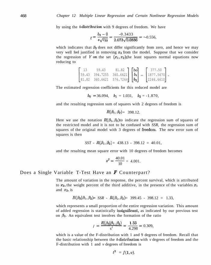
468 Chapter 12 Multiple Linear Regression and Certain Nonlinear Regression Models
by using the (-distribution with 9 degrees of freedom. We have
6 3 - O -0.3433 t Sy/^sl 2.073v
/0l)886 -0.556,
which indicates that p\ does not differ significantly from zero, and hence we may very well feel justified in removing x3 from the model. Suppose that we consider the regression of y o n the set (xi,x2), the least squares normal equations now reducing to
13 59.43 81.82 59.43 394.7255 360.6621 81.82 360.6621 576.7264
bo 61 b2
=
377.50 1877.5670 2246.6610
The estimated regression coefficients for this reduced model are
/>o = 36.094, bx = 1.031, b2 = -1.870,
and the resulting regression sum of squares with 2 degrees of freedom is
Ri0i,02) = 398.12.
Here we use the notation R(0x,02) to indicate the regression sum of squares of the restricted model and it is not to be confused with SSR, the regression sum of squares of the original model with 3 degrees of freedom. The new error sum of squares is then
SST - R(0x,02) = 438.13 - 398.12 = 40.01,
and the resulting mean square error with 10 degrees of freedom becomes
, 40.01 10
= 4.001.
Does a Single Variable T-Test Have an JF Counterpar t?
The amount of variation in the response, the percent survival, which is attributed to x3, the weight percent of the third additive, in the presence of the variables xx and x2, is
Ri03\0\,02) = SSR - R(3i,02) = 399.45 - 398.12 = 1.33,
which represents a small proportion of the entire regression variation. This amount of added regression is statistically insignificant, as indicated by our previous test on 03. An equivalent test involves the formation of the ratio
/ RiM^M = 1-33
s2 4.298 0.309.
which is a value of the F-distribution with 1 and 9 degrees of freedom. Recall that the basic relationship between the (-distribution with v degrees of freedom and the F-distribution with 1 and v degrees of freedom is
t2 = f(l,v),
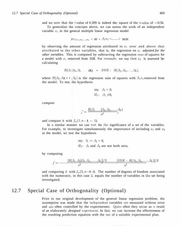
12.7 Special Case of Orthogonality (Optional) 469
and we note that the /-value of 0.309 is indeed the: square of the (-value of —0.56. To generalize the concepts above, we can assess the work of an independent
variable ;r, in the general multiple linear regression model
/ ' >> , ,X3,...,Xk = 00 + 0lX\ + r- 0kXk
by observing the amount of regression attributed to Xi over and above tha t a t t r i bu t ed to the o ther variables, that is, the regression on Xi adjusted for the other variables. This is computed by subtracting the regression sum of squares for a model with x; removed from SSR. For example, we say that as] is assessed by-calculating
R{0i\02,0:i 0k) = SSR - R(02,3:i, ...,0k.),
where R(02Jh, • • • ,3k) is the regression sum of squares with p\xi removed from the model. To test, the hypothesis
HQ: 0I = 0.
Hi: 0i+ 0,
compute
R.(0i \32,0:i,...,0k) J _9 !
and compare it with / „ ( l , n - k — 1). In a similar manner we can test, for the significance of a set of the variables.
For example, to investigate simultaneously the importance of including x\ and x2
in the model, wc test the hypothesis
HQ: 3i — 02 = 0,
Hi'. 0i and 0\ are not both zero,
by computing
. [R.(0i,02\03-.04,-..:0k)}/2 [SSR-R(03,34,...,0k)}/2 J s2 ,s2
and comparing il with fa(2,n—k — l). The number of degrees of freedom associated with the numerator, in this case 2, equals the number of variables in the set being investigated.
12.7 Special Case of Orthogonality (Optional)
Prior to our original development of the general linear regression problem, the assumption was made that the independent variables arc measured without error and arc often controlled by the experimenter. Quite often they occur as a result of an elaborately designed experiment. In fact, wc can increase the effectiveness of the resulting prediction equation with the use of a suitable experimental plan.
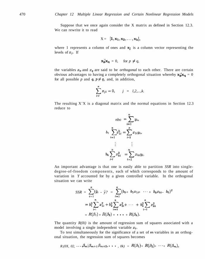
470 Chapter 12 Multiple Linear Regression and Certain Nonlinear Regression Models
Suppose that we once again consider the X matrix as defined in Section 12.3. We can rewrite it to read
X = [ l ,X 1 (X2,. . . ,X k ] ,
where 1 represents a column of ones and Xj is a column vector representing the levels of Xj. If
XpXq = 0, for p + q,
the variables xv and xq are said to be orthogonal to each other. There are certain obvious advantages to having a completely orthogonal situation whereby x,Jxq = 0 for all possible p and q,p + q, and, in addition,
n
^ £ j i = 0 , j = l,2,...,k. i=l
The resulting X 'X is a diagonal matrix and the normal equations in Section 12.3 reduce to
nbo = \V^yi, t = i
n n
&i YI x i ' = ]L xuyu
i=X i=X
bkJ2Xli =YsXkiyi' i=l i=X
An important advantage is that one is easily able to partition SSR into single-degree-of-freedom components , each of which corresponds to the amount of variation in Y accounted for by a given controlled variable. In the orthogonal situation we can write
n n
SSR = ]T(& - y? = Y^ib° + bixu + •'• + hxki - b0)2
t = i i = i n n n
= b2YJx\i+blY,x22i + --- + b2
k^4i i=\ r= l i = l
= R(0i) + R(02) + • • • + R(0k)-
The quantity R(0i) is the amount of regression sum of squares associated with a model involving a single independent variable Xi.
To test simultaneously for the significance of a set of m variables in an orthogonal situation, the regression sum of squares becomes
R.(0X, 02, -•-, 0m\0m+l, 0m+2, • • • , 0k) = Ri0x) + Ri02) + •" + «(/?m),
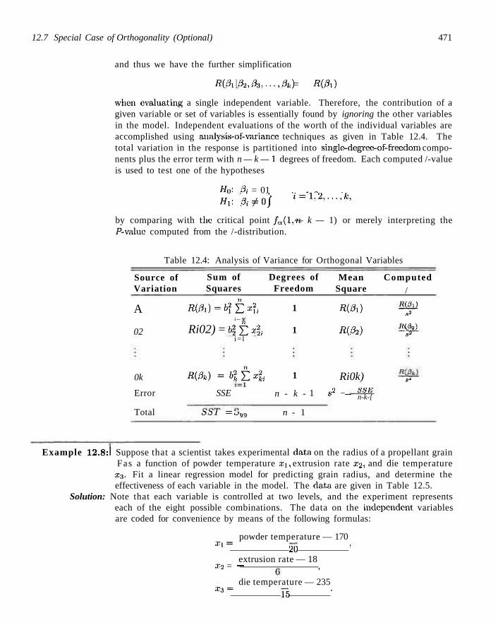
12.7 Special Case of Orthogonality (Optional) 471
and thus we have the further simplification
R(0i\02,03,...,0k) = Ri0i)
when evaluating a single independent variable. Therefore, the contribution of a given variable or set of variables is essentially found by ignoring the other variables in the model. Independent evaluations of the worth of the individual variables are accomplished using analysis-of-variance techniques as given in Table 12.4. The total variation in the response is partitioned into single-degree-of-freedom components plus the error term with n — k — 1 degrees of freedom. Each computed /-value is used to test one of the hypotheses
HQ: 3i = 01 . _ . „ , Hi: A ' ^ O j ' - 1 ^ - - - ^ -
by comparing with the critical point fa(\,n — k — 1) or merely interpreting the F-value computed from the /-distribution.
Table 12.4: Analysis of Variance for Orthogonal Variables
Source of Variation
A
02
0k
Error
Total
Sum of Squares
Rifii)=b\t*2u i=X
Ri02) = b2±x2., i= l
RiM = b\±xl SSE
»50i = iJyy
Degrees of Freedom
1
1
1
n - k -
n - 1
1
Mean Square
R(9x)
R{02)
Ri0k) n2 _ SSE b ~ n-k-[
Computed /
R(fli) s2
R(32) >
8*
Example 12.8:1 Suppose that a scientist takes experimental data on the radius of a propellant grain Fas a function of powder temperature x\, extrusion rate x2, and die temperature x3. Fit a linear regression model for predicting grain radius, and determine the effectiveness of each variable in the model. The data are given in Table 12.5.
Solution: Note that each variable is controlled at two levels, and the experiment represents each of the eight possible combinations. The data on the independent variables are coded for convenience by means of the following formulas:
powder temperature — 170 X, = 20 '
extrusion rate — 18 x2 = - ,
die temperature — 235 X3 = 15 •
472 Chapter 12 Multiple Linear Regression and Certain Nonlinear Regression Models
Table 12.5: Data for Example 12.8
Grain Radius
82 93
114 124 111 129 157 164
Powder Temperature
150 190 150 150 190 190 150 190
(-1) (+1) (-1) (-1) (+1) (+1) (-1) (+1)
Extrusion Rate
12 12 24 12 24 12 24 24
(-1) (-1) (+1) (-1) (+1) (-1) (+1) (+1)
Die Temperature
220 (-1) 220 (-1) 220 (-1) 250 (+1) 220 (-1) 250 (+1) 250 (+1) 250 (+1)
The resulting levels of Xx, x2, and x3 take on the values -1 and +1 as indicated in the table of data. This particular experimental design affords the orthogonality that we are illustrating here. A more thorough treatment of this type of experimental layout is discussed in Chapter 15. The X matrix is
X =
1 - ] 1 1 1 - ] 1 -1 1 1 1 ] 1 - ] 1 1
[ - 1 I - 1 I 1 1 - 1 1 1 [ - 1 1 1 i 1
- 1 - 1 - 1
1 - 1
1 1 1
and the orthogonality conditions are readily verified. We can now compute coefficients
6° = 5 X > = 12L75' 6l = \ !>«» = T = 2-5' t = i ? ' = 1
3 2 =
8
YI x-aVi i=l 118
14.75.
8
2-i X'iiVi 1 _ .
so in terms of the coded variables, the prediction equation is
y = 121.75 +2.5 Xi + 14.75 x2 + 21.75 £3.
The analysis-of-variance Table 12.6 shows independent contributions to SSR for each variable. The results, when compared to the /o.05(l-4) critical point of 7.71, indicate that £1 does not contribute significantly at the 0.05 level, whereas variables £2 and £3 are significant. In this example the estimate for a2 is 23.1250. As for the single-independent-variable case, it is pointed out that this estimate does not solely contain experimental error variation unless the postulated model is correct. Otherwise, the estimate is "contaminated" by lack of fit in addition to pure
Exercises 473
Table 12.6: Analysis of Variance for Grain Radius Data
Source of Sum of Degrees of Mean Computed Variation Squares Freedom Square / P- Value
01
02
03 Error
Total
(2.5)2(8) = 50
(14.75)2(8) = 1740.50
(21.75)2(8) = 3784.50
92.5
5667.50
1
1
1
4
7
50
1740.50
3784.50
23.1250
2.16
75.26
163.65
0.2156
0.0010
0.0002
Exercises
error, and the lack of fit can be separated only if we obtain multiple experimental observations at the various (xi,x2,x3) combinations.
Since £i is not significant, it can simply be eliminated from the model without altering the effects of the other variables. Note that £2 and £3 both impact the grain radius in a positive fashion, with £3 being the more important factor based on the smallness of the P-value. J j
12.31 Compute and interpret the coefficient of multiple determination for the variables of Exercise 12.3 on page 453.
12.32 Test whether the regression explained by the model in Exercise 12.3 on page 453 is significant at the 0.01 level of significance.
12.33 Test whether the regression explained by the model in Exercise 12.9 on page 454 is significant at the 0.01 level of significance.
12.34 For the model of Exercise 12.11 on page 454, test the hypothesis
H0: 0i=0i= 0, Hy. 0i and 02 are not both zero.
12.35 Repeat Exercise 12.26 on page 464 using an F-statistic.
12.36 A small experiment was conducted to fit a multiple regression equation relating the yield y to temperature xi, reaction time x2, and concentration of one of the reactants 23. Two levels of each variable were chosen and measurements corresponding to the coded independent variables were recorded as follows:
y 7.6 8.4 9.2
10.3 9.8
11.1 10.2 12.6
Xl
—1
— 1 — 1
— 1
* 2
- 1 - 1
1 - 1
1 - 1
1 1
x3 - 1 - 1 - 1
1 - 1
1 1 1
(a) Using the coded variables, estimate the multiple linear regression equation
V-Ylxx 00 + 0\Xl + 82X2 + 03X3.
(b) Partition SSR, the regression sum of squares, into three single-degree-of-freedom components attributable to £1, X2, and x3, respectively. Show an analysis-of-variance table, indicating significance tests on each variable.
12.37 Consider the electric power data of Exercise 12.9 on page 454. Test Ho '• 0i = 02 = 0 making use of Ri0i, 32\03,04). Give a P-value, and draw conclusions.
12.38 Consider the data for Exercise 12.36. Compute the followings
R(0i\0o), R(0i\0o,02,03),
R(02\0o,3i), R(02\0o,0i,03),
R(03\3o,0l,02).
474 Chapter 12 Multiple Linear Regression and Certain Nonlinear Regression Models
Comment.
12.39 Consider the data of Exercise 11.63 on page 439. Fit a regression model using weight and drive ratio as explanatory variables. Compare this model with the SLR (simple linear regression) model using weight alone. Use R2, R2^j, and any I- (or F)-statistics you may need to compare the SLR with the multiple regression model.
12.40 Consider Example 12.3. Figure 12.1 on page 462 displays a SAS printout of an analysis of the model containing variables xi, x2, and £3. Focus on the confidence interval of the mean response fiy at the (xi,x2,x3) locations representing the 13 data points. Consider an item in the printout indicated by C.V. This is the coefficient of variation, which is defined by
C.V. = - • 100. y
where s = y/s^ is the root mean squared error. The coefficient of variation is often used as yet another criterion for comparing competing models. It is a scale-free quantity which expresses the estimate of a, namely s, as a percent of the average response y. In competition for the "best" among a group of competing models, one strives for the model with a "small" value of C.V. Do a regression analysis of the data set shown in Example 12.3 but eliminate x3. Compare the full (xi,x2,x3) model with the restricted model (a.-), x2) and focus on two criteria: (i) C.V.; (ii) the widths of the confidence intervals on fiy- For the second criterion you may want to use the average width. Comment.
12.41 Consider Example 12.4 on page 451. Compare the two competing models
First order: yi = 0o + 0ixu + 02x2i + £>,
Second order: j/j = 0o + 0ixu + 82x21
+ 0\\X2u + 822x\i + 0\2XliX2i + et.
Use i?adj in your comparison in addition to testing Ho : 0n = 022 = 0n = 0. In addition, use C.V. discussed in Exercise 12.40.
12.42 In Example 12.8 on page 471 a case is made for eliminating x\, powder temperature, from the model since the P-value based on the .F-test is 0.2154 while P-values for x2 and £3 are near zero.
(a) Reduce the model by eliminating xi, thereby producing a full and restricted (or reduced) model and compare them on the basis of R2
d}.
(b) Compare the full and restricted models using the width of the 95% prediction intervals on a new observation. The "best" of the two models would be that with the "tightened" prediction intervals. Use the average of the width of the prediction intervals.
12.43 Consider the data of Exercise 12.15 on page 455. Can the response, wear, be explained adequately by a single variable (either viscosity or load) in an SLR rather than with the full two-variable regression? Justify your answer thoroughly through tests of hypotheses as well as the comparison of three competing models.
12.44 For the data set given in Exericise 12.16 on page 455, can the response be explained adequately by any two regressor variables? Discuss.
12.8 Categorical or Indicator Variables
An extremely important special case application of multiple linear regression occurs when one or more of the regressor variables are categorica l or indicator variables . In a chemical process the engineer may wish to model the process yield against regressors such as process temperature and reaction time. However, there is interest in using two different catalysts and somehow including "the catalyst" in the model. The catalyst effect cannot be measured on a continuum and is hence a categorical variable. An analyst may wish to model the price of homes against regressors tha t include square feet of living space £1 , the land acreage x2, and age of the house £3. These regressors are clearly continuous in nature. However, it is clear tha t cost of homes may vary substantially from one area of the country to another. Thus, da ta may be collected on homes in the east, midwest, south, and west. As a result, we have an indicator variable with four categories . In the chemical process example, if two catalysts are used, we have an indicator variable with two categories. In a biomedical example a drug is to be compared to a
12.8 Categorical or Indicator Variables 475
placebo and all subjects have several continuous measurements such as age, blood pressure, and so on, observed as well as gender, which of course is categorical with two categories. So, included along with the continuous variables are two indicator variables, treatment at two categories (active drug and placebo) and gender at two categories (male and female).
Model with Categorical Variables
Let us use the chemical processing example to illustrate how indicator variables are involved in the model. Suppose y = yield and xx = temperature and £2 = reaction time. Now let us denote the indicator variable by z. Let z = 0 for catalyst 1 and z = 1 for catalyst 2. The assignment of the (0,1) indicator to the catalyst is arbitrary. As a result, the model becomes
Vi = 0o + 0ix\i + 02x2i + 03Zi + ti, i - 1 ,2 , . . . ,n .
Three Categories
The estimation of coefficients by the method of least squares continues to apply. In the case of three levels or categories of a single indicator variable, the model will include two regressors, say zx and z2, where the (0,1) assignment is as follows:
"1 1
1
0
0
0
0
22 0 0
0
1
1
0
0
In other words, if there are t categories, the model includes £ — 1 actual model terms.
It may be instructive to look at a graphical appearance of the model with 3 categories. For the sake of simplicity, let us assume a single continuous variable x. As a result, the model is given by
Vi = '00 + 0\Xi + 32zii + 03z2i + €i.
Thus Figure 12.2 reflects the nature of the model. The following are model expres-
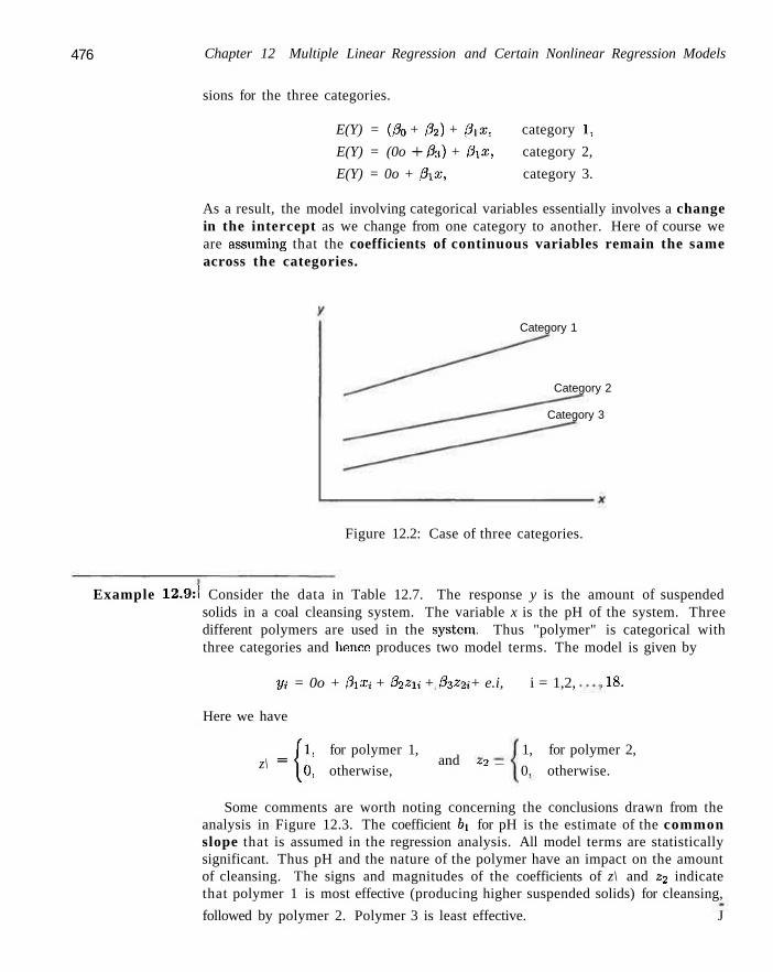
476 Chapter 12 Multiple Linear Regression and Certain Nonlinear Regression Models
sions for the three categories.
E(Y) = (0o + 02) + 0ix, category 1,
E(Y) = (0o +1%) + 0xx, category 2,
E(Y) = 0o + 0ix, category 3.
As a result, the model involving categorical variables essentially involves a change in the intercept as we change from one category to another. Here of course we are assuming that the coefficients of continuous variables remain the same across the categories.
Category 1
Category 2
Category 3
Figure 12.2: Case of three categories.
Example 12.9:1 Consider the data in Table 12.7. The response y is the amount of suspended solids in a coal cleansing system. The variable x is the pH of the system. Three different polymers are used in the system. Thus "polymer" is categorical with three categories and hence produces two model terms. The model is given by
Vi = 0o + 0\Xi + 02zxi + 33z2i + e.i, i = 1,2, .18.
Here we have
z\ • f t
for polymer 1,
otherwise, and <-2 —
1, for polymer 2,
0. otherwise.
Some comments are worth noting concerning the conclusions drawn from the analysis in Figure 12.3. The coefficient bi for pH is the estimate of the common slope that is assumed in the regression analysis. All model terms are statistically significant. Thus pH and the nature of the polymer have an impact on the amount of cleansing. The signs and magnitudes of the coefficients of z\ and z2 indicate that polymer 1 is most effective (producing higher suspended solids) for cleansing,
followed by polymer 2. Polymer 3 is least effective. J
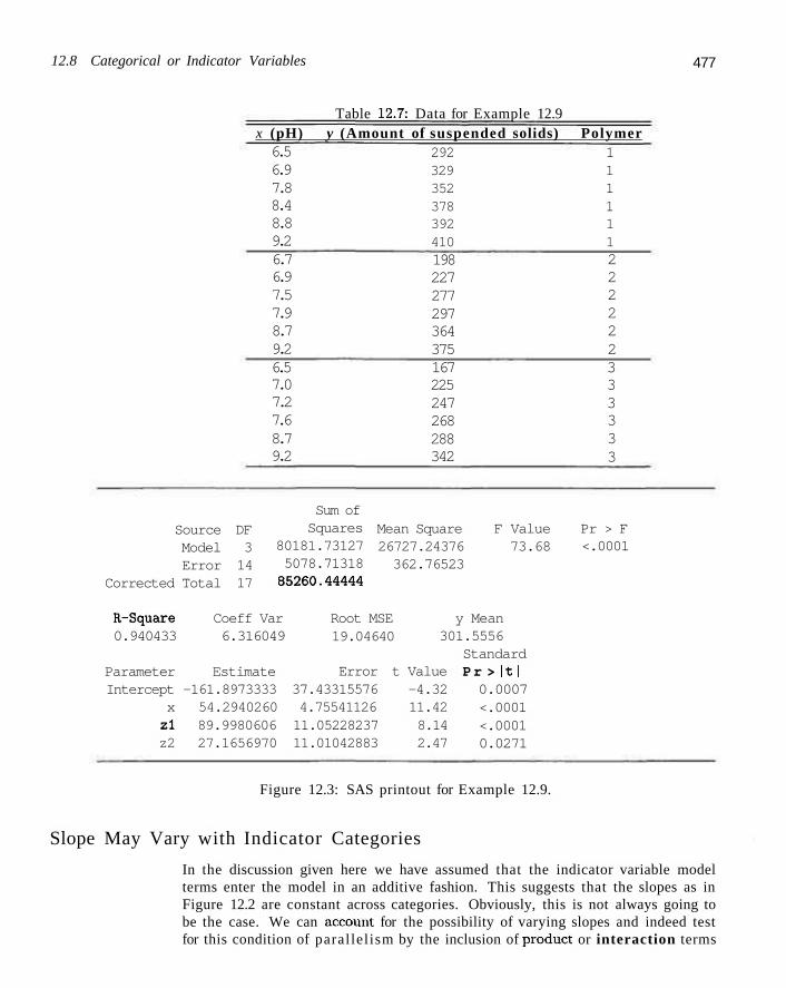
12.8 Categorical or Indicator Variables 477
Table 12.7: Data for Example 12.9 x (pH) y (Amount of suspended solids) Polymer 6.5 6.9 7.8 8.4 8.8 9.2
292 1 329 1 352 1 378 1 392 1 410 1
6.7 6.9 7.5 7.9 8.7 9.2 6.5 7.0 7.2 7.6 8.7 9.2
198 227 277 297 364 375 167 225 247 268 288 342
2 2 2 2 2 2 3 3 3 3 3 3
Source DF Model 3 Error 14
Corrected Total 17
Sum of Squares
80181.73127 5078.71318 85260.44444
Mean Square 26727.24376 362.76523
F Value 73.68
Pr > F <.0001
R-Square 0.940433
Coeff Var 6.316049
Parameter Estimate Intercept -161.8973333
x 54.2940260 zl 89.9980606 z2 27.1656970
Root MSE 19.04640
Error t Value 37.43315576 -4.32 4.75541126 11.42 11.05228237 8.14 11.01042883 2.47
y Mean 301.5556
Standard Pr > It I 0.0007 <.0001 <.0001 0.0271
Figure 12.3: SAS printout for Example 12.9.
Slope May Vary with Indicator Categories
In the discussion given here we have assumed that the indicator variable model terms enter the model in an additive fashion. This suggests that the slopes as in Figure 12.2 are constant across categories. Obviously, this is not always going to be the case. We can account for the possibility of varying slopes and indeed test for this condition of parallelism by the inclusion of product or interaction terms
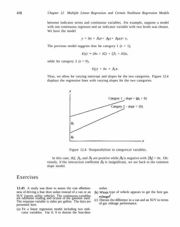
478 Chapter 12 Multiple Linear Regression and Certain Nonlinear Regression Models
between indicator terms and continuous variables. For example, suppose a model with one continuous regressor and an indicator variable with two levels was chosen. We have the model
y = 0o + 0xx + 02z + 03xz + e,
The previous model suggests that for category 1 (z = 1),
Eiy) = (0o + 02) + i0x + 03)x,
while for category 2 (z = 0),
E(y) = 0o + 0xx.
Thus, we allow for varying intercept and slopes for the two categories. Figure 12.4 displays the regression lines with varying slopes for the two categories.
Category 1 - slope = (/3, + ft)
Category 2 - slope = (ft)
Exercises
Figure 12.4: Nonparallelism in categorical variables.
In this case, 0Q, 0\, and 02 are positive while 33 is negative with \03\ < 0x. Obviously, if the interaction coefficient 03 is insignificant, we are back to the common slope model.
12.45 A study was done to assess the cost effectives- sedan. ness of driving a four door sedan instead of a van or an (b) Which type of vehicle appears to get the best gas SUV (sports utility vehicle). The continuous variables mileage?* are odometer reading and octane of the gasoline used The response variable is miles per gallon. The data are presented here. (a) Fit a linear regression model including two indi
cator variables. Use 0, 0 to denote the four-door
(c) Discuss the difference in a van and an SUV in terms of gas mileage performance.
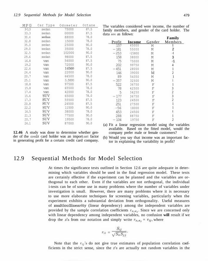
12.9 Sequential Methods for Model Selection 479
MPG 3 1.5 33.3 30.4 32.8 35.0 29.0 32.5 29.6 16.8 19.2 22.6 24.4 20.7 25.1 18.8 15.8 17.4 15.6 17.3 20.8 22.2 16.5 21.3 20.7 24.1
Car Type sedan sedan sedan sedan sedan sedan sedan sedan van van van van van van van van van SUV SUV SUV SUV SUV SUV SUV SUV
Odometer 75000 00000 88000 15000 25000 35000 102000 98000 56000 72000 11500 22000 66500 3.5000 97500 65500 42000 65000 55500 26500 11500 38000 77500 19500 87000
Octane 87.5 87.5 78.0 78.0 90.0 78.0 90.0 87.5 87.5 90.0 87.5 90.0 78.0 90.0 87.5 78.0 78.0 78.0 87.5 87.5 90.0 78.0 90.0 78.0 90.0
12.46 A study was done to determine whether gender of the credit card holder was an import ant factor in generating profit for a certain credit card company.
The variables considered were income, the number of family members, and gender of the card holder. The data are as follows:
Family Profit Income Gender Members
2 I 3 1
4 1 2 1 I 1 3 2 3 2 1 1 I 1 2
(a) Fit a linear regression model using the variables available. Based on the fitted model, would the company prefer male or female customers?
(b) Would you say that income was an important factor in explaining the variability in profit?
157 181 253 158 75 202 451 146 89 357 522 78 5
177 123 251 -56 453 288 104
45000 55000 15800 38000 75000 99750 28000 39000 54350 32500 36750 42500 34250 36750 24500 27500 18000 24500 88750 19750
M M M M M M M M M M F F F F F F F F F F
12.9 Sequential Methods for Model Selection
At times the significance tests outlined in Section 12.6 are quite adequate in determining which variables should be used in the final regression model. These tests are certainly effective if the experiment can be planned and the variables are orthogonal to each other. Even if the variables are not orthogonal, the individual i-tests can be of some use in many problems where the number of variables under investigation is small. However, there are many problems where it is necessary to use more elaborate techniques for screening variables, particularly when the experiment exhibits a substantial deviation from orthogonality. Useful measures of multicollinearity (linear dependency) among the independent variables are provided by the sample correlation coefficients rXiXi. Since we are concerned only with linear dependency among independent variables, no confusion will result if we drop the afs from our notation and simply write rXiXj = rij, where
rn = y/SitSj
Note that the ry 's do not give true estimates of population correlation coefficients in the strict sense, since the x's are actually not random variables in the
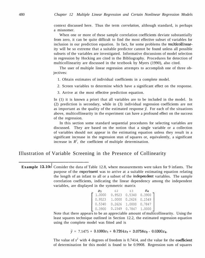
480 Chapter 12 Multiple Linear Regression and Certain Nonlinear Regression Models
context discussed here. Thus the term correlation, although standard, is perhaps a misnomer.
When one or more of these sample correlation coefficients deviate substantially from zero, it can be quite difficult to find the most effective subset of variables for inclusion in our prediction equation. In fact, for some problems the multicollinear-ity will be so extreme that a suitable predictor cannot be found unless all possible subsets of the variables are investigated. Informative discussions of model selection in regression by Hocking are cited in the Bibliography. Procedures for detection of multicollinearity are discussed in the textbook by Myers (1990), also cited.
The user of multiple linear regression attempts to accomplish one of three objectives:
1. Obtain estimates of individual coefficients in a complete model.
2. Screen variables to determine which have a significant effect on the response.
3. Arrive at the most effective prediction equation.
In (1) it is known a priori that all variables are to be included in the model. In (2) prediction is secondary, while in (3) individual regression coefficients are not as important as the quality of the estimated response y. For each of the situations above, multicollinearity in the experiment can have a profound effect on the success of the regression.
In this section some standard sequential procedures for selecting variables are discussed. They are based on the notion that a single variable or a collection of variables should not appear in the estimating equation unless they result in a significant increase in the regression stun of squares or, equivalently, a significant increase in R2, the coefficient of multiple determination.
Illustration of Variable Screening in the Presence of Collinearity
Example 12.10:1 Consider the data of Table 12.8, where measurements were taken for 9 infants. The purpose of the experiment was to arrive at a suitable estimating equation relating the length of an infant to all or a subset of the independent variables. The sample correlation coefficients, indicating the linear dependency among the independent variables, are displayed in the symmetric matrix
Xx 1.0000 0.9523 0.5340 0.3900
£2
0.9523 1.0000 0.2626 0.1549
£3
0.5340 0.2626 1.0000 0.7847
£ 4
0.3900 0.1549 0.7847 1.0000
Note that there appears to be an appreciable amount of multicollinearity. Using the least squares technique outlined in Section 12.2, the estimated regression equation using the complete model was fitted and is
y = 7.1475 + 0.1000£i + 0.7264.T2 + 3.0758£3 - 0.0300£4.
The value of s2 with 4 degrees of freedom is 0.7414, and the value for the coefficient of determination for this model is found to be 0.9908. Regression sum of squares
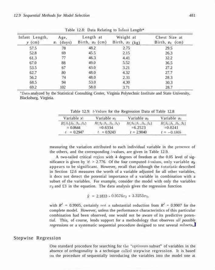
12.9 Sequential Methods for Model Selection 481
Table 12.8: Data Relating to Infant Length*
Infant Length, y (cm)
57.5 52.8 61.3 67.0 53.5 62.7 56.2 68.5 69.2
Age, Xx (days)
78 69 77 88 67 80 74 94
102
Length at Bi r th , x2 (cm)
48.2 45.5 46.3 49.0 43.0 48.0 48.0 53.0 58.0
Weight Bi r th , a:.i
2.75 2.15 4.41 5.52 3.21 4.32 2.31 4.30 3.71
a t (kg)
Chest Size at Bi r th , XA (cm)
29.5 26.3 32.2 36.5 27.2 27.7 28.3 30.3 28.7
*Data analyzed by the Statistical Consulting Center, Virginia Polytechnic Institute and State University, Blacksburg, Virginia.
Table 12.9: t-Values for the Regression Data of Table 12.8
Variable x\ Variable x2 Variable 0:3 Variable £i R(0i\02,8a,0.i) R(32\0i,03,3i) R(0-A\0i,02,0.i) R(04\0i,02,03)
= 0.0644 =0.6334 =6.2523 =0.0241 I. = 0.2947 I. = 0.9243 t = 2.9040 t = -0.1805
measuring the variation attributed to each individual variable in the presence of the others, and the corresponding /-values, are given in Table 12.9.
A two-tailed critical region with 4 degrees of freedom at the 0.05 level of significance is given by \t\ > 2.776. Of the four computed /-values, only variable £3 appears to be significant. However, recall that although the /-statistic described in Section 12.6 measures the worth of a variable adjusted for all other variables, it docs not detect the potential importance of a variable in combination with a subset of the variables. For example, consider the model with only the variables x2 and £3 in the equation. The data analysis gives the regression function
j) = 2.1833 - 0.9576.T2 + 3.3253£3,
with R2 = 0.9905, certainly not a substantial reduction from R2 = 0.9907 for the complete model. However, unless the performance characteristics of this particular combination had been observed, one would not be aware of its predictive potential. This, of course, lends support for a methodology that observes all possible regressions or a systematic sequential procedure designed to test several subsctsJ
Stepwise Regression
One standard procedure for searching for the "optimum subset'' of variables in the absence of orthogonality is a technique calleel s tepwise regression. It is based on the procedure of sequentially introducing the variables into the model one at
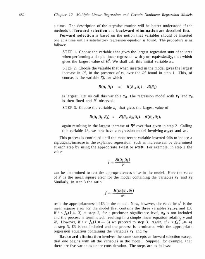
482 Chapter 12 Multiple Linear Regression and Certain Nonlinear Regression Models
a time. The description of the stepwise routine will be better understood if the methods of forward selection and backward elimination are described first.
Forward selection is based on the notion that variables should be inserted one at a time until a satisfactory regression equation is found. The procedure is as follows:
STEP 1. Choose the variable that gives the largest regression sum of squares when performing a simple linear regression with y or, equivalently, that wdiich gives the largest value of R2. We shall call this initial variable £i.
STEP 2. Choose the variable that when inserted in the model gives the largest increase in R2, in the presence of x\, over the R2 found in step 1. This, of course, is the variable Xj, for which
R(0j\0x) = R(0i,0j)-R(0x)
is largest. Let us call this variable x2. The regression model with Xi and x2
is then fitted and R2 observed.
STEP 3. Choose the variable Xj that gives the largest value of
Ri0i\0x,02) = Ri0i,S2,0i) - Ri0i,02),
again resulting in the largest increase of R.2 over that given in step 2. Calling this variable £3, we now have a regression model involving x\, x2, and £3,
This process is continued until the most recent variable inserted fails to induce a significant increase in the explained regression. Such an increase can be determined at each step by using the appropriate F-test or i-test. For example, in step 2 the value
RiMh) 1 s2
can be determined to test the appropriateness of x2 in the model. Here the value of s2 is the mean square error for the model containing the variables X\ and x2. Similarly, in step 3 the ratio
. _ - R ( W , & ) sz
tests the appropriateness of £3 in the model. Now, however, the value for s2 is the mean square error for the model that contains the three variables xi, x2, and £3. If / < fa(l,n — 3) at step 2, for a prechosen significance level, x2 is not included and the process is terminated, resulting in a simple linear equation relating y and X\, However, if / > / Q ( l , n — 3) we proceed to step 3. Again, if / < fa(l,n — 4) at step 3, £3 is not included and the process is terminated with the appropriate regression equation containing the variables xx and x2.
Backward elimination involves the same concepts as forward selection except that one begins with all the variables in the model. Suppose, for example, that there are five variables under consideration. The steps are as follows:
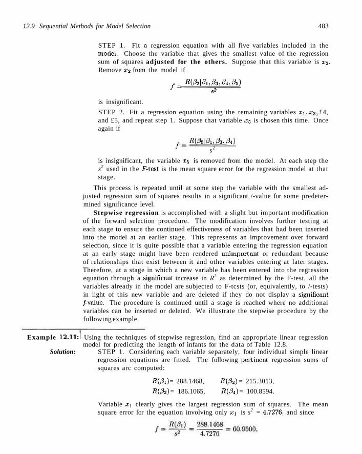
12.9 Sequential Methods for Model Selection 483
STEP 1. Fit a regression equation with all five variables included in the model. Choose the variable that gives the smallest value of the regression sum of squares adjusted for the others. Suppose that this variable is x2. Remove x2 from the model if
,_- f t ( f t | f t ,&, /?4,&) } s2
is insignificant.
STEP 2. Fit a regression equation using the remaining variables xi, x3, £4, and £5, and repeat step 1. Suppose that variable £5 is chosen this time. Once again if
Rj05\0i,03,.04) J s2
is insignificant, the variable X5 is removed from the model. At each step the s2 used in the F-test is the mean square error for the regression model at that stage.
This process is repeated until at some step the variable with the smallest adjusted regression sum of squares results in a significant /-value for some predetermined significance level.
Stepwise regression is accomplished with a slight but important modification of the forward selection procedure. The modification involves further testing at each stage to ensure the continued effectiveness of variables that had been inserted into the model at an earlier stage. This represents an improvement over forward selection, since it is quite possible that a variable entering the regression equation at an early stage might have been rendered unimportant or redundant because of relationships that exist between it and other variables entering at later stages. Therefore, at a stage in which a new variable has been entered into the regression equation through a significant increase in R2 as determined by the F-test, all the variables already in the model are subjected to F-tcsts (or, equivalently, to /-tests) in light of this new variable and are deleted if they do not display a significant /•value. The procedure is continued until a stage is reached where no additional variables can be inserted or deleted. We illustrate the stepwise procedure by the following example.
Example 12.11:1 Using the techniques of stepwise regression, find an appropriate linear regression model for predicting the length of infants for the data of Table 12.8.
Solution: STEP 1. Considering each variable separately, four individual simple linear regression equations are fitted. The following pertinent regression sums of squares arc computed:
R(0i) = 288.1468, R(02) = 215.3013,
R(03) = 186.1065, R(04) = 100.8594.
Variable xi clearly gives the largest regression sum of squares. The mean square error for the equation involving only £1 is s2 = 4.7276, and since
484 Chapter 12 Multiple Linear Regression and Certain Nonlinear Regression Models
which exceeds /o.oo(l,7) = 5.59. the variable x\ is entered into the model.
STEP 2. Three regression equations are fitted at this stage, all containing xx. The important results for the combinations (£i,£2), (£i,£3) and (£i,£\i) are
Rifa\0i) = 23.8703, Ri03\0i) = 29.3086, R(04\0x) = 13.8178.
Variable £3 displays the largest regression sum of squares in the presence of xx- The regression involving £1 and £3 gives a new value of s2 = 0.6307, and since
R(03\0x) _ 29-3086 1 " s2 0.6307 ~ '
which exceeds /o.os(L6) = 5.99, the variable £3 is included along with £x in the model. Now we must subject xi in the presence of £3 to a significance test. We find that Ri0x\03) = 131.349, and hence
R{0i\jh) 131.349 f - — ^ ~ 0.6307 - 2 ° 8 - 2 6 '
which is highly significant. Therefore, £1 is retained along with £3.
STEP 3. With £1 and £3 already in the model, we now require R(32\0x,03) and R(04\0i,03) in order to determine which, if any, of the remaining two variables is entered at this stage. From the regression analysis using £2 along with x.x and £3, we find R(02\0i,03) = 0.7948, and when £4 is used along with £1 and £3, we obtain R(04\0x,03) = 0.1855. The value of s2 is 0.5979 for the (£i,£2,£3) combination and 0.7198 for the (£i,£2,£4) combination. Since neither /-value is significant at the a = 0.05 level, the final regression model includes only the variables £1 and £3. The estimating equation is found to be
y = 20.1084 + 0.4136.£i + 2.0253£3,
and the coefficient of determination for this model is R2 = 0.9882.
Although (£^£3) is the combination chosen by stepwise regression, it is not necessarily the combination of two variables that gives the largest value of R2. In fact, we have already observed that the combination (£2, £3) gives an R? = 0.9905. Of course, the stepwise procedure never actually observed this combination. A rational argument could be made that there is actually a negligible difference in performance between these two estimating equations, at least in terms of percent variation explained. It is interesting to observe, however, that the backward elimination procedure gives the combination (x2,x3) in the final equation (see Exercise
12.49 on page 496). J
Summary The main function of each of the procedures explained in this section is to expose the variables to a systematic methodology designed to ensure the eventual inclusion of the best combinations of the variables. Obviously, there is no assurance that this
12.10 Study of Residuals and Violation of Assumptions 485
will happen in all problems, and, of course, it is possible that the multicollinearity is so extensive that one has no alternative but to resort to estimation procedures other than least squares. These estimation procedures arc discussed in Myers (1990), listed in the Bibliography.
The sequential procedures discussed here represent three of many such methods that have been put forth in the literature and appear in various regression computer packages that are available. These methods are: designed to be computationally efficient but, of course, do not give results for all possible subsets of the variables. As a result, the procedures are most effective in data sets that involve a large number of variables. In regression problems involving a relatively small number of variables, modern regression computer packages allow for the computation and summarization of quantitative information on all models for every possible subset of the variables. Illustrations are provided in Section 12.11.
12.10 Study of Residuals and Violation of Assumptions (Model Checking)
It was suggested earlier in this chapter that, the residuals, or errors in the regression fit, often carry information that can be very informative to the data analyst. The ei — Vi — Vh i = \,2,...,n, which are the numerical counterpart to the Cj's, the model errors, often shed light on the possible: violation of assumptions or the presence of "suspect" data points. Suppose that wc: let the vector x; denote the values of the regressor variables corresponding to the v'th data point, supplemented by a 1 in the initial position. That is,
X; = {l,XU,X2i,-..,Xki}-
Consider the quantity
hu = x'i(X'X)-1xi, i. = 1,2,...,n.
The reader should recognize that hu is used in the computation of the confidence intervals on the mean response in Section 12.5. Apart from er2, hu represents the variance of the fitted value y\. The hu values are the diagonal elements of the HAT matrix
H = X ( X ' X ) _ 1 X ' ,
which plays an important role in any study of residuals and in other modern aspects of regression analysis (see the reference to Myers, 1990, listed in the Bibliography). The term HAT matrix is derived from the fact that H generates the il?/-hats" or the fitted values when multiplied by the vector y of observed responses. That is, y = Xb and thus
y = X ( X ' X ) - 1 X ' y = Hy,
where y is the vector whose ith element is y.,.
486 Chapter 12 Multiple Linear Regression and Certain Nonlinear Regression Models
If we make the usual assumptions that the £j's are independent and normally distributed with zero mean and variance er2, the statistical properties of the residuals are readily characterized. Then
E(et) = E(yi - m) = 0, and a2 - (1 - hu)a2,
for i = 1,2,.. . , n. (See the Myers, 1990, reference for details.) It can be shown that the HAT diagonal values are bounded according to the inequality
- < hu < I-n
n
In addition, Y2 hii — k + 1. the number of regression parameters. As a result, any t = i
data point whose HAT diagonal element is large, that is, well above the average value of (A; + l ) /n , is in a position in the data set where the variance of y< is relatively large, and the variance of a residual is relatively small. As a result, the data analyst can gain some insight on how large a residual may become before its deviation from zero can be attributed to something other than mere chance. Many of the commercial regression computer packages produce the set of studentized residuals.
Studentized „ _ e» • _ , 0 „ Residual sy/l - hu '
Here each residual has been divided by an es t imate of its s t andard deviation, creating a t-like statistic that is designed to give the analyst a scale-free quantity that provides information regarding the size of the residual. In addition, standard computer packages often provide values of another set of studentized-type residuals, called the il-Student values.
^-Student Residual . _ e» • _ -, 0 H — H , • <• — 1, 4, . . . |T»
S-iy/1 - hu where s_j is an estimate of the error standard deviation, calculated with the ith data point deleted.
There are three types of violations of assumptions that are readily detected through use of residuals or residual plots. While plots of the raw residuals, the ei, can be helpful, it is often more informative to plot the studentized residuals. The three violations are as follows:
1. Presence of outliers
2. Heterogeneous error variance
3. Model misspecification
In case 1, we choose to define an outlier as a data point where there is a deviation from the usual assumption E(ti) = 0 for a specific value of i. If there is a reason to believe that a specific data point is an outlier exerting a large influence on the fitted model, r-j or ti may be informative. The E-Student values can be expected to be more sensitive to outliers than the r,- values.
In fact, under the condition that F(ej) = 0, U is a value of a random variable following a /-distribution with n— l — (k+l) = n — k — 2 degrees of freedom. Thus
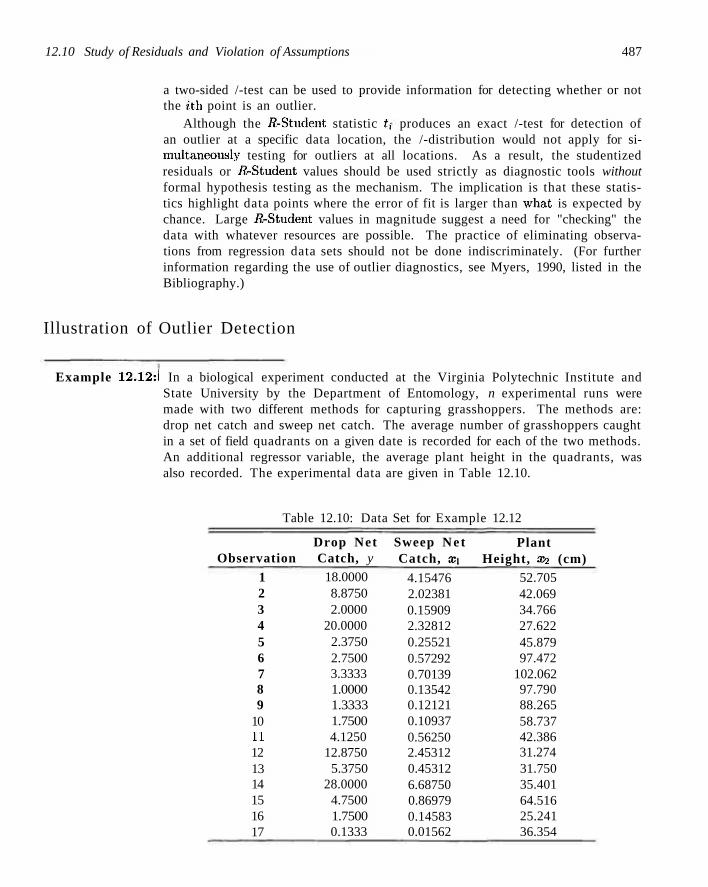
12.10 Study of Residuals and Violation of Assumptions 487
a two-sided /-test can be used to provide information for detecting whether or not the tth point is an outlier.
Although the /2-Student statistic /, produces an exact /-test for detection of an outlier at a specific data location, the /-distribution would not apply for simultaneously testing for outliers at all locations. As a result, the studentized residuals or /{-Student values should be used strictly as diagnostic tools without formal hypothesis testing as the mechanism. The implication is that these statistics highlight data points where the error of fit is larger than wdiat is expected by chance. Large /{-Student values in magnitude suggest a need for "checking" the data with whatever resources are possible. The practice of eliminating observations from regression data sets should not be done indiscriminately. (For further information regarding the use of outlier diagnostics, see Myers, 1990, listed in the Bibliography.)
Illustration of Outlier Detection
Example 12.12:1 In a biological experiment conducted at the Virginia Polytechnic Institute and State University by the Department of Entomology, n experimental runs were made with two different methods for capturing grasshoppers. The methods are: drop net catch and sweep net catch. The average number of grasshoppers caught in a set of field quadrants on a given date is recorded for each of the two methods. An additional regressor variable, the average plant height in the quadrants, was also recorded. The experimental data are given in Table 12.10.
Table 12.10: Data Set for Example 12.12
Observation 1 2 3 4 5 6 7 8 9
10 11 12 13 14 15 16 17
Drop Net Catch, y
18.0000 8.8750 2.0000
20.0000 2.3750 2.7500 3.3333 1.0000 1.3333 1.7500 4.1250
12.8750 5.3750
28.0000 4.7500 1.7500 0.1333
Sweep Net Catch, xi
4.15476 2.02381 0.15909 2.32812 0.25521 0.57292 0.70139 0.13542 0.12121 0.10937 0.56250 2.45312 0.45312 6.68750 0.86979 0.14583 0.01562
Plant Height, £2 (cm)
52.705 42.069 34.766 27.622 45.879 97.472
102.062 97.790 88.265 58.737 42.386 31.274 31.750 35.401 64.516 25.241 36.354
488 Chapter 12 Multiple Linear Regression and Certain Nonlinear Regression Models
The goal is to be able to estimate grasshopper catch by using only the sweep net method, which is less costly. There was some concern about the validity of the fourth data point. The observed catch that was reported using the net drop method seemed unusually high given the other conditions and, indeed, it was felt that the figure might be erroneous. Fit a model of the type
Pi =0O+0lXx + f%X2
to the 17 data points and study the residuals to determine if data point 4 is an outlier.
Solution: A computer package generated the fitted regression model
y = 3.6870 + 4.1050.fi - 0.0367£2
along with the statistics R2 = 0.9244 and s2 = 5.580. The residuals and other diagnostic information were also generated and recorded in Table 12.11.
Table 12.11: Residual Information for the Data Set of Example 12.12
Obs.
1 2 3 4 5 6 7 8 9
10 11 12 13 14 15 16 17
Vi
18.000 8.875 2.000
20.000 2.375 2.750 3.333 1.000 1.333 1.750 4.125
12.875 5.375
28.000 4.750 1.750 0.133
Vi 18.809 10.452 3.065
12.231 3.052 2.464 2.823 0.656 0.947 1.982 4.442
12.610 4.383
29.841 4.891 3.360 2.418
Vi - Vi -0.809 -1.577 -1.065
7.769 -0.677
0.286 0.510 0.344 0.386
-0.232 -0.317
0.265 0.992
-1.841 -0.141 -1.610 -2.285
hu
0.2291 0.0766 0.1364 0.1256 0.0931 0.2276 0.2669 0.2318 0.1691 0.0852 0.0884 0.1152 0.1339 0.6233 0.0699 0.1891 0.1386
Sy/1 — hu
2.074 2.270 2.195 2.209 2.250 2.076 2.023 2.071 2.153 2.260 2.255 2.222 2.199 1.450 2.278 2.127 2.193
n -0.390 -0.695 -0.485
3.517 -0.301
0.138 0.252 0.166 0.179
-0.103 -0.140
0.119 0.451
-1.270 -0.062 -0.757 -1.042
U
-0.3780 -0.6812 -0.4715
9.9315 -0.2909
0.1329 0.2437 0.1601 0.1729
-0.0989 -0.1353
0.1149 0.4382
-1.3005 -0.0598 -0.7447 -1.0454
As expected, the residual at the fourth location appears to be unusually high, namely, 7.769. The vital issue here is whether or not this residual is larger than one would expect by chance. The residual standard error for point 4 is 2.209. The R-Student value t4 is found to be 9.9315. Viewing this as a value of a random variable having a /-distribution with 13 degrees of freedom, one would certainly conclude that the residual of the fourth observation is estimating something greater than 0 and that the suspected measurement error is supported by the study of residuals. Notice that no other residual results in an /{-Student value that produces any cause for alarm. J
12.10 Study of Residuals and Violation of Assumptions 489
Plot t ing Residuals
In Chapter 11 wc discuss, in some detail, the usefulness of plotting residuals in regression analysis. Violation of model assumptions can often be detected through these plots. In multiple regression normal probability plotting of residuals or plots of residuals against y may be useful. However, it is often preferable to plot studentized residuals.
Keep in mind that the preference of the studentized residuals over ordinary residuals for plotting purposes stems from the fact that since the variance of the ith residual depends on the ith HAT diagonal, variances of residuals will differ if there is a dispersion in the HAT diagonals. Thus the appearance of a plot of residuals may depict heterogeneity because the residuals themselves do not behave, in general, in an ideal way. The purpose of using studentized residuals is to provide a standardization. Clearly, if a were known, then under ideal conditions (i.e., a correct model and homogeneous variance), we have
E [oy/T^hTi)
= 0, and Var ay/\ — hi
= 1.
So the studentized residuals produce a set of statistics that behave in a standard way under ideal conditions. Figure 12.5 shows a plot of the /{-Student values for the grasshopper data of Example 12.12. Note how the value for observation 4 stands out from the rest. The /{-Student plot was generated by SAS software. The plot shows the residual against the y-values.
T 10 15 20
Predicted Value of Y
T 25 30
Figure 12.5: /{-Student values plotted against predicted values for grasshopper data of Example 12.12.
490 Chapter 12 Multiple Linear Regress ion. and Certain Nonlinear Regression Models
Normality Checking
The reader should recall the importance of normality checking through the use of normal probability plotting as discussed in Chapter 11. The: same recommendation holds for the case of multiple linear regression. Normal probability plots can be generated using standard regression software. Again, however, they can be more effective when one does not use ordinary residuals but, rather, studentized residuals or /{-Student values.
12.11 Cross Validation, Cp, and Other Criteria for Model Selection
For many regression problems the experimenter must choose between various alternative models or model forms that are developed from the same data set. Quite often, in fact, the model that best predicts or estimates mean response is required. The experimenter should fake into account the relative sizes of the .s,2-values for the candidate models and certainly the general nature of the confidence intervals on the mean response. One must also consider how well the model predicts response values that were not used in building the candidate models. The models should be subjected to cross validation. What, is required, then, are cross-validation errors rather than fitting errors. Such errors in prediction are the PRESS residuals
Si = Vi ~§i,-i, i = 1,2,
where ?/,;._,• is the prediction of the ith data point by a model that did not. make use of the ith point in the calculation of the coefficients. These PRESS residuals are calculated from the formula
fc-i-Ar-. i=l,2,...,n, 1 - li.,t
(The derivation can be found in the regression textbook by Myers, 1990).
Use of the PRESS Statistic
The motivation for PRESS and the utility of PRESS residuals is very simple to understand. The purpose of extracting or setting aside data, points one at a time is to allow the use; of separate methodologies for fitting and assessment of a specific model. For assessment of a model the "—f indicates that the PRESS residual gives a prediction error where the observation being predicted is independent of the model, fit.
Criteria that make use of the PRESS residuals are given by
Y,\5i\ and PRESS = J^«f. 2 = 1
The term PRESS is an acronym for the prediction sum of squares. We suggest that both of these criteria be used. It is possible for PRESS to be dominated by one
12.11 Cross Validation, Cp, and Other Criteria for Model Selection 491
n or only a few large PRESS residuals. Clearly, the criteria YI \°i\ }S l e s s sensitive
i = l to a small number of large values.
In addition to the PRESS statistic itself, the analyst can simply compute an "R2-hke" statistic reflecting prediction performance. The statistic is often called R2
d and is given as follows:
R? of Prediction Given a fitted model with a specific value for PRESS, R2red is given by
PRESS R2 - 1 •"•pred ±
Zivi-v)2
i=X
Note that. /{2 (1 is merely the ordinary R2 statistic with SSE replaced by the
PRESS statistic. In the following example a "case-study" illustration is provided in which many-
candidate models are fit to a set of data and the best model is chosen. The sequential procedures described in Section 12.9 are not used. Rather, the role of the PRESS residuals and other statistical values in selecting the best regression equation is illustrated.
Example 12.13:1 Case S tudy Leg strength is a necessary ingredient of a successful punter in American football. One measure of the quality of a good punt is the "hang time." This is the time that the ball hangs in the air before being caught by the punt returner. To determine what leg strength factors influence hang time and to develop an empirical model for predicting this response, a study on The Relationship Between Selected Physical Performance Variables and Football Punting Ability was conducted by the Department of Health, Physical Education, and Recreation at the Virginia Polytechnic Institute and State University. Thirteen punters were chosen for the experiment and each punted a football 10 times. The average hang time, along with the strength measures used in the analysis, were recorded in Table 12.12.
Each regressor variable is defined as follows:
1. RLS, right leg strength (pounds)
2. LLS, left leg strength (pounds)
3. RHF, right hamstring muscle flexibility (degrees)
4. LHF, left hamstring muscle flexibility (degrees)
5. Power, Overall leg strength (foot-pounds)
Determine the most appropriate model for predicting hang time. Solution: In the search for the "best" of the candidate models for predicting hang time, the
information in Table 12.13 was obtained from a regression computer package. The models are ranked in ascending order of the values of the PRESS statistic. This display provides enough information on all possible models to enable the user to eliminate from consideration all but a few models. The model containing x2 and £5 (LL5and Power), denoted by £2£s, appears to be superior for predicting punter
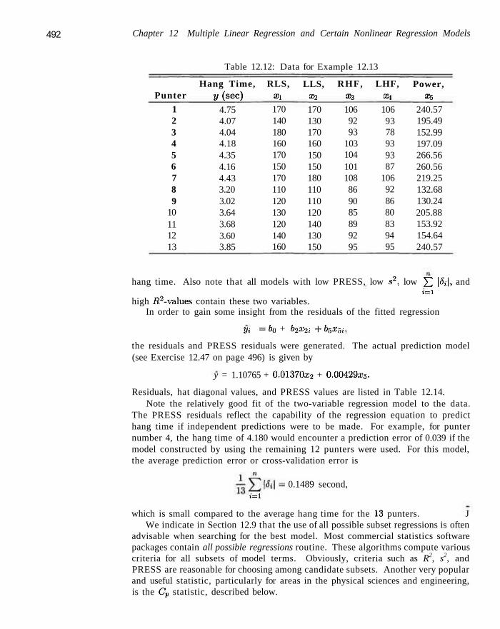
492 Chapter 12 Multiple Linear Regression and Certain Nonlinear Regression Models
Table 12.12: Data for Example 12.13
Punter
1 2 3 4 5 6 7 8 9
10 11 12 13
Hang Time, V (sec)
4.75 4.07 4.04 4.18 4.35 4.16 4.43 3.20 3.02 3.64 3.68 3.60 3.85
RLS, Xx 170 140 180 160 170 150 170 110 120 130 120 140 160
LLS, X2
170 130 170 160 150 150 180 110 110 120 140 130 150
RHF, x3
106 92 93
103 104 101 108 86 90 85 89 92 95
LHF, £4
106 93 78 93 93 87
106 92 86 80 83 94 95
Power, £5
240.57 195.49 152.99 197.09 266.56 260.56 219.25 132.68 130.24 205.88 153.92 154.64 240.57
hang time. Also note that all models with low PRESS, low .s2, low Y2 \^i\, and t= i
high /{2-values contain these two variables. In order to gain some insight from the residuals of the fitted regression
Pi =bo + b2x2i +b5x5i,
the residuals and PRESS residuals were generated. The actual prediction model (see Exercise 12.47 on page 496) is given by
y = 1.10765 + 0.01370.X-2 + 0.00429£5.
Residuals, hat diagonal values, and PRESS values are listed in Table 12.14. Note the relatively good fit of the two-variable regression model to the data.
The PRESS residuals reflect the capability of the regression equation to predict hang time if independent predictions were to be made. For example, for punter number 4, the hang time of 4.180 would encounter a prediction error of 0.039 if the model constructed by using the remaining 12 punters were used. For this model, the average prediction error or cross-validation error is
1=1
0.1489 second,
which is small compared to the average hang time for the 13 punters. J We indicate in Section 12.9 that the use of all possible subset regressions is often
advisable when searching for the best model. Most commercial statistics software packages contain all possible regressions routine. These algorithms compute various criteria for all subsets of model terms. Obviously, criteria such as R2, s2, and PRESS are reasonable for choosing among candidate subsets. Another very popular and useful statistic, particularly for areas in the physical sciences and engineering, is the Cp statistic, described below.
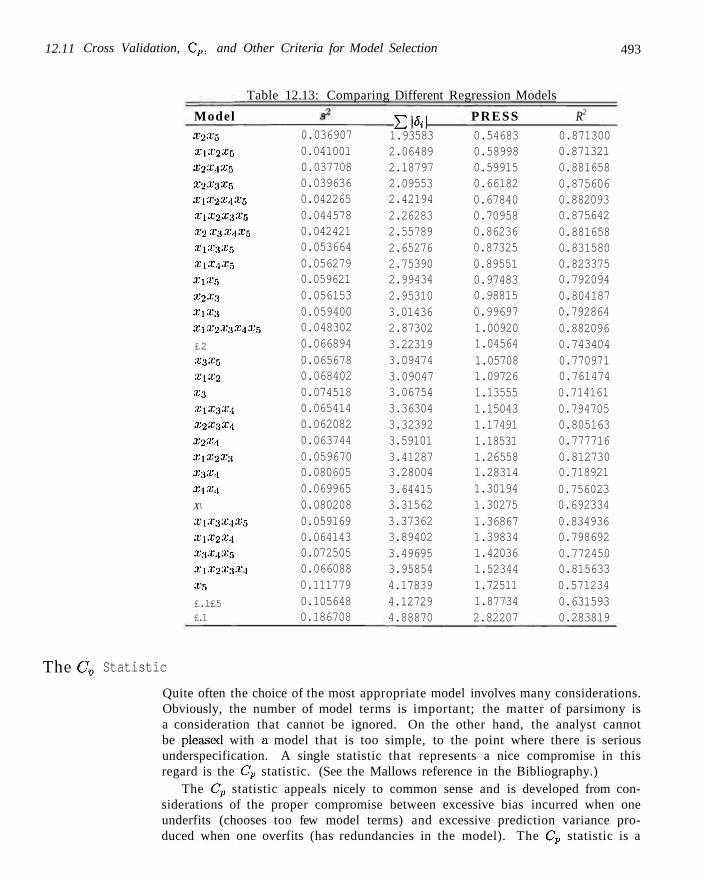
12.11 Cross Validation, C,,, and Other Criteria for Model Selection 493
Table 12.13: Comparing Different Regression Models
Model £1*1 PRESS R2
The Cv
X2X5
£l£'2£5
X2X4X$
x2x3x5
XiX2X.lX5
£ l £ 3 £ 3 £ 5
£2 £3 £4^5
£l £3.1:5
£l £.l£5
Xixr, x2x3
XiX3
XxX2X3X4Xs
£2
£3*5
£l£2
x3
£l£3£.-l
£2«3X4
X2X,i
X\X2X3
X3X<\
X1X4
X\
£ 1£ 3£4£ 3
£l£2£4
£3£.l£5
£l£2£3£4
£5
£.l£5
£.1
Statistic
0.036907 0.041001 0.037708 0.039636 0.042265 0.044578 0.042421 0.053664 0.056279 0.059621 0.056153 0.059400 0.048302 0.066894 0.065678 0.068402 0.074518 0.065414 0.062082 0.063744 0.059670 0.080605 0.069965 0.080208 0.059169 0.064143 0.072505 0.066088 0.111779 0.105648 0.186708
1.93583 2.06489 2.18797 2.09553 2.42194 2.26283 2.55789 2.65276 2.75390 2.99434 2.95310 3.01436 2.87302 3.22319 3.09474 3.09047 3.06754 3.36304 3.32392 3.59101 3.41287 3.28004 3.64415 3.31562 3.37362 3.89402 3.49695 3.95854 4.17839 4.12729 4.88870
0.54683 0.58998 0.59915 0.66182 0.67840 0.70958 0.86236 0.87325 0.89551 0.97483 0.98815 0.99697 1.00920 1.04564 1.05708 1.09726 1.13555 1.15043 1.17491 1.18531 1.26558 1.28314 1.30194 1.30275 1.36867 1.39834 1.42036 1.52344 1.72511 1.87734 2.82207
0.871300 0.871321 0.881658 0.875606 0.882093 0.875642 0.881658 0.831580 0.823375 0.792094 0.804187 0.792864 0.882096 0.743404 0.770971 0.761474 0.714161 0.794705 0.805163 0.777716 0.812730 0.718921 0.756023 0.692334 0.834936 0.798692 0.772450 0.815633 0.571234 0.631593 0.283819
Quite often the choice of the most appropriate model involves many considerations. Obviously, the number of model terms is important; the matter of parsimony is a consideration that cannot be ignored. On the other hand, the analyst cannot be pleased with a model that is too simple, to the point where there is serious underspecification. A single statistic that represents a nice compromise in this regard is the Cp statistic. (See the Mallows reference in the Bibliography.)
The Cv statistic appeals nicely to common sense and is developed from considerations of the proper compromise between excessive bias incurred when one underfits (chooses too few model terms) and excessive prediction variance produced when one overfits (has redundancies in the model). The Cp statistic is a
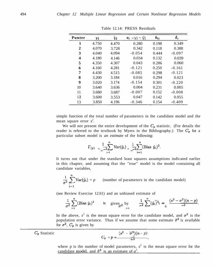
494 Chapter 12 Multiple Linear Regression and Certain Nonlinear Regression Models
Table 12.14: PRESS Residuals
Punter 1 2 3 4 5 6 7 8 9
10 11 12 13
Vi 4.750 4.070 4.040 4.180 4.350 4.160 4.430 3.200 3.020 3.640 3.680 3.600 3.850
Vi 4.470 3.728 4.094 4.146 4.307 4.281 4.515 3.184 3.174 3.636 3.687 3.553 4.196
e* =Vi ~ Vi 0.280 0.342
-0.054 0.034 0.043
-0.121 -0.085
0.016 -0.154
0.004 -0.007
0.047 -0.346
hu 0.198 0.118 0.444 0.132 0.286 0.250 0.298 0.294 0.301 0.231 0.152 0.142 0.154
Si
0.349 0.388
-0.097 0.039 0.060
-0.161 -0.121
0.023 -0.220
0.005 -0.008
0.055 -0.409
simple function of the total number of parameters in the candidate model and the mean square error s2.
We will not present the entire development of the Cp statistic. (For details the reader is referred to the textbook by Myers in the Bibliography.) The Cp for a particular subset model is an estimate of the following:
i n 1 n
r(p) = ^ £ V a r ^ ) + 3 E ( B i a s &¥• i= l t=l
It turns out that under the standard least squares assumptions indicated earlier in this chapter, and assuming that the "true" model is the model containing all candidate variables.
1 -— Y j Var(yi) = p (number of parameters in the candidate model)
t = i
(see Review Exercise 12.61) and an unbiased estimate of
- l ^ B i a s y , ) 2 is given by ±fffi* yt? = ^JZSf^A. i=l i=l
In the above, s2 is the mean square error for the candidate model, and CJ2 is the population error variance. Thus if we assume that some estimate a2 is available for er2, Cp is given by
Cp Statistic (s2 - a2)(n - p) Cp = p+ ^2 ,
where p is the number of model parameters, s2 is the mean square error for the candidate model, and CT2 is an estimate of a2.
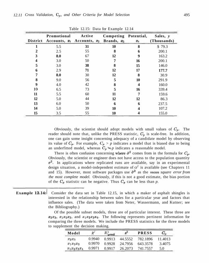
12.11 Cross Validation, Cp, and Other Criteria for Model Selection 495
Table 12.15: Data for Example 12.14
District 1 2 3 4 5 6 7 8 9
10 11 12 13 14 15
Promotional Accounts, £i
5.5 2.5 8.0 3.0 3.0 2.9 8.0 9.0 4.0 6.5 5.5 5.0 6.0 5.0 3.5
Active Accounts, x2
31 55 67 50 38 71 30 56 42 73 60 44 50 39 55
Competing Brands, x3
10 8
12 7 8
12 12 5 8 5
11 12 6
10 10
Potential, X\
8 6 9
16 15 17 8
10 4
16 7
12 6 4 4
Sales, y (Thousands)
$ 79.3 200.1 163.2 200.1 146.0 177.7 30.9
291.9 160.0 339.4 159.6 86.3
237.5 107.2 155.0
Obviously, the scientist should adopt models with small values of Cp. The reader should note that, unlike the PRESS statistic, Cp is scale-free. In addition, one can gain some insight concerning adequacy of a candidate model by observing its value of Cp. For example, Cp > p indicates a model that is biased due to being an underfitted model, whereas Cp ~ p indicates a reasonable model.
There is often confusion concerning wdiere d2 comes from in the formula for Cp. Obviously, the scientist or engineer does not have access to the population quantity <j2. In applications where replicated runs are available, say in an experimental design situation, a model-independent estimate of cr2 is available (see Chapters 11 and 15). However, most software packages use cr2 as the mean square error from the most complete model. Obviously, if this is not a good estimate, the bias portion of the Cp statistic can be negative. Thus Cp can be less than p.
Example 12.14:1 Consider the data set in Table 12.15, in which a maker of asphalt shingles is interested in the relationship between sales for a particular year and factors that influence sales. (The data were taken from Neter, Wassermann, and Kutner; see the Bibliography.)
Of the possible subset models, three are of particular interest. These three are £2£3, £i£2£3, and £i£2£3£4- The following represents pertinent information for comparing the three models. We include the PRESS statistics for the three models to supplement the decision making.
Model R2 R? PRESS
£ 2 £ 3
£ l £ 2 * 3 XXX2X3X4
0.9940 0.9970 0.9971
0.9913 0.9928 0.9917
44.5552 24.7956 26.2073
782.1896 643.3578 741.7557
11.4013 3.4075 5.0
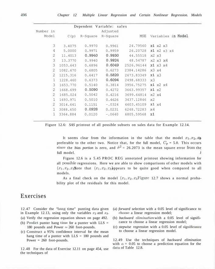
496 Chapter 12 Multiple Linear Regression and Certain Nonlinear Regression. Models
Dependent V a r i a b l e : s a l e s Number in
Model
3 4 2 3 3 2 2 1 3 2 2 1 2 1 1
C(p)
3.4075 5.0000
11.4013
13.3770
1053.643
1082.670
1215.316
1228.460
1653.770
1668.699
1685.024
1693.971
3014.641
3088.650 3364.884
R-Square
0.9970
0.9971
0.9940
0.9940
0.6896
0.6805
0.6417
0.6373
0.5140
0.5090
0.5042
0.5010
0.1151
0.0928 0.0120
Adjusted
R-Square
0.9961 0.9959
0.9930
0.9924
0.6049
0.6273
0.5820
0.6094
0.3814
0.4272
0.4216
0.4626 -.0324
0.0231
-.0640
MSE
24.79560
26.20728
44.55518
48.54787
2526.96144
2384.14286
2673.83349
2498.68333
3956.75275
3663.99357
3699.64814
3437.12846
6603.45109
6248.72283
6805.59568
Variables i
xl xl x2 x2 xl x3 xl x3 xl xl x2 x2 xl x4 xl
x2 x2 x3 x3 x3 x4 x3
x2 x2 x4
x4
x3 x3 x4
x4 x4
x4
Figure 12.6: SAS printout of all possible subsets on sales da ta for Example 12.14.
It seems clear from the information in the table that the model xi,x2,x3 is preferable to the other two. Notice that , for the full model, Cp = 5.0. This occurs since the bias portion is zero, and a2 = 26.2073 is the mean square error from the full model. J
Figure 12.6 is a 5.45 PROC REG annotated printout showing information for all possible regressions. Here we are able to show comparisons of other models with (xi,x2,x3). Note that (xi,X2,Xs) appears to be quite good when compared to all models.
As a final check on the model (xi>X2,X3), Figure 12.7 shows a normal probability plot of the residuals for this model.
Exercises
12.47 Consider the "hang time" punting data given in Example 12.13, using only the variables x2 and x3.
(a) Verify the regression equation shown on page 492. (b) Predict punter hang time for a punter with LLS =
180 pounds and Power = 260 foot-pounds. (c) Construct a 95% confidence interval for the mean
hang time of a punter with LLS = 180 pounds and Power = 260 foot-pounds.
12.48 For the data of Exercise 12.11 on page 454, use the techniques of
(a) forward selection with a 0.05 level of significance to choose a linear regression model;
(b) backward eliniinalion with a 0.05 level of significance to choose a linear regression model;
(c) stepwise regression with a 0.05 level of significance to choose a linear regression model.
12.49 Use the techniques of backward elimination with a = 0.05 to choose a prediction equation for the data of Table 12.8.
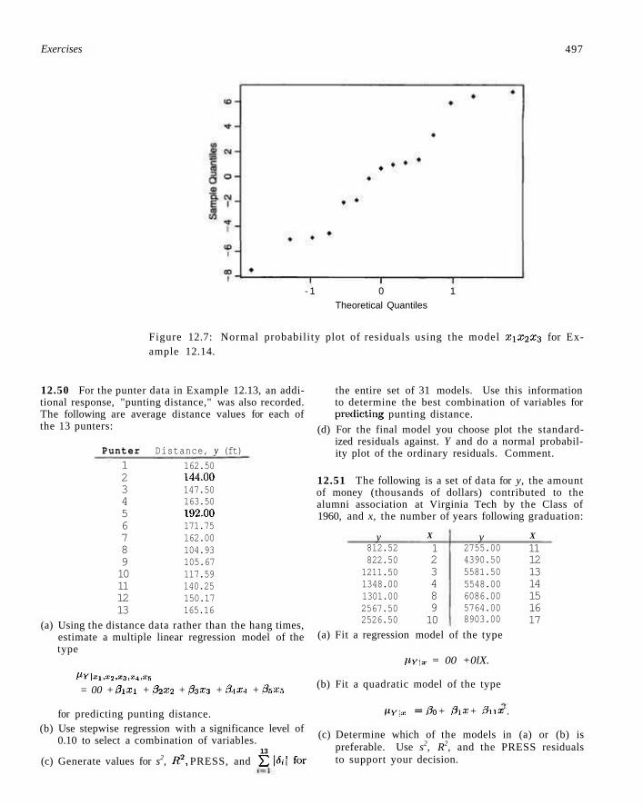
Exercises 497
- 1 0 1
Theoretical Quantiles
Figure 12.7: Normal probability plot of residuals using the model £i£2£3 for Example 12.14.
12.50 For the punter data in Example 12.13, an additional response, "punting distance," was also recorded. The following are average distance values for each of the 13 punters:
Punter
1 2 3 4 5 6 7 8 9 10 11 12 13
Distance, y (ft)
162.50 144.00 147.50 163.50 192.00 171.75 162.00 104.93 105.67 117.59 140.25 150.17 165.16
(a) Using the distance data rather than the hang times, estimate a multiple linear regression model of the type
PY\xi,X2,X3,x4,X5
= 00 + j3lXl + 32^2 + 03X3 + #ia\] + 05X3
for predicting punting distance. (b) Use stepwise regression with a significance level of
0.10 to select a combination of variables. 13
(c) Generate values for s2, R2, PRESS, and YI l&l f o r
the entire set of 31 models. Use this information to determine the best combination of variables for predicting punting distance.
(d) For the final model you choose plot the standardized residuals against. Y and do a normal probability plot of the ordinary residuals. Comment.
12.51 The following is a set of data for y, the amount of money (thousands of dollars) contributed to the alumni association at Virginia Tech by the Class of 1960, and x, the number of years following graduation:
y 812.52 822.50 1211.50 1348.00 1301.00 2567.50 2526.50
X
1 2 3 4 8 9 10
y 2755.00 4390.50 5581.50 5548.00 6086.00 5764.00 8903.00
X
11 12 13 14 15 16 17
(a) Fit a regression model of the type
PY\x = 00 +0lX.
(b) Fit a quadratic model of the type
HY\x =0o + 0\x + 3nx .
(c) Determine which of the models in (a) or (b) is preferable. Use s2, R2, and the PRESS residuals to support your decision.
498 Chapter 12 Multiple Linear Regression and Certain Nonlinear Regression Models
12.52 For the model of Exercise 12.50(a), test the hypothesis
Ho: 34 = 0,
Hi: 3,i # 0.
Use a P-value in your conclusion.
12.53 For the quadratic model of Exercise 12.51(b), give estimates of the variances and covariances of the estimates of 0\ and 0i i.
12.54 In an effort to model executive compensation for the year 1979, 33 firms were selected, and data were gathered on compensation, sales, profits, and employment. Consider the model
yt =0o + 0i lnrnii + 02 \nx2i
+ 03\nx3i + ei, i = 1,2 33.
(a) Fit the regression with the model above. (b) Is a model with a subset of the variables preferable
to the full model?
12.55 Rayon whiteness is an important factor for scientists dealing in fabric quality. Whiteness is affected by pulp quality and other processing variables. Some of the variables include acid bath temperature, °C (xi); cascade acid concentration, % (a^); water temperature, °C (x3); sulfide concentration, % (aii); amount of chlorine bleach, lb/min (xs)\ blanket finish temperature, °C (.%). A set of data taken on rayon specimens is given here. The response, y, is the measure of whiteness.
(a) Use the criteria MSE, Cp, and PRESS to give the best model from among all subset models.
(b) Do a normal probability plot of residuals for the "best" model. Comment.
Firm 1 2 3 4 5 6 7 8 9
10 11 12 13 14 15 16 17 18 19 20 21 22 23 24 25 26 27 28 29 30 31 32 33
Compensation, y Sales, xi
(thousands) (millions) $450 387 368 277 676 454 507 496 487 383 311 271 524 498 343 354 324 225 254 208 518 406 332 340 698 306 613 302 540 293 528 456 417
$4,600.6 9,255.4 1,526.2 1,683.2 2. 752.8 2.205.8 2.384.6 2.746.0 1,434.0
470.6 1,508.0
464.4 9,329.3 2,377.5 1,174.3
409.3 724.7 578.9 966.8 591.0
4,933.1 7,613.2 3,457.4
545.3 22,862.8
2,361.0 2,614.1 1,013.2 4,560.3
855.7 4,211.6 5, 440.4 1.229.9
Profits, x2 (millions)
$128.1 783.9 136.0 179.0 231.5 329.5 381.8 237.9 222.3
63.7 149.5 30.0
577.3 250.7
82.6 61.5 90.8 63.3 42.8 48.5
310.6 491.6 228.0
54.6 3011.3
203.0 201.0 121.3 194.6 63.4
352.1 655.2
97.5
Employment , x3
48. 000 55.900 13.783 27.765 34.000 26.500 30.800 41.000 25.900 8.600
21.075 6,874
39,000 34,300 19.405 3.586 3.905 4.139 6,255
10,605 65, 392 89,400 55, 200
7,800 337.119
52, 000 50, 500 18, 625 97,937 12,300 71,800 87, 700 14,600
y X\ X2 £ l X.l X5 X6
88.7 89.3 75.5 92.1 83.4 44.8 50.9 78.0 86.8 47.3 53.7 92.0 87.9 90.3 94.2 89.5
43 42 47 46 52 50 43 49 51 51 48 46 43 45 53 47
0.211 0.604 0.450 0.641 0.370 0.526 0.486 0.504 0.609 0.702 0.397 0.488 0.525 0.486 0.527 0.601
85 89 87 90 93 85 83 93 90 80 92 88 85 84 87 95
0.243 0.237 0.198 0.194 0.198 0.221 0.203 0.279 0.220 0.198 0.231 0.211 0.199 0.189 0.245 0.208
0.606 0.600 0.527 0.500 0.485 0.533 0.510 0.489 0.462 0.478 0.411 0.387 0.437 0.499 0.530 0.500
48 55 61 6a 54 60 57 49 64 63 61 88 63 58 65 67
12.56 A client from the Department of Mechanical Engineering approached the Consulting Center at Virginia Polytechnic Institute and State University for help in analyzing an experiment dealing with gas turbine engines. Voltage output of engines was measured at various combinations of blade speed and voltage measuring sensor extension. The data are as follows:
y (volts)
1.95 2.50 2.93 1.69 1.23 3.13 1.55 1.94 2.18 2.70 1.32 1.60 1.89
Speed , £i (in. / sec )
6336 7099 8026 6230 5369 8343 6522 7310 7974 8501 6646 7384 8000
Extension, X2 ( in . )
0.000 0.000 0.000 0.000 0.000 0.000 0.006 0.006 0.006 0.006 0.012 0.012 0.012
12.12 Special Nonlinear Models for Nonidenl Conditions 499
(a) Fit a regression model using all independent variables.
(b) Use stepwise regression with input significance level 0.25 and removal significance level 0.05. Give your final model.
(c) Use all possible regression models and compute R.~, Cv, s~, adjusted R~ for all models.
(d) Give final model.
(e) For your model in part (d), plot studentized residuals (or fl-Student) and comment.
y (volts)
2.15 1.09 1.26 1.57 1.92
Speed, xi ( in . /sec)
8545 6755 7362 7934 8554
Ex tens ion , xj ( in . )
0.012 0.018 0.018 0.018 0.018
(a) Fit a multiple linear regression to the data, (h) Compute (-tests on coefficients. Give P-values. (c) Comment on the quality of the fined mode:!.
12.57 The pull strength of a wire bond is an inipor- 1 2 5 8 F()|. B x ( T c i s ( , l 2 .57, test H0: 0i = f% = 0. Give taut, characteristic. rIhe table below gives Information p.values and comment on pull strength y, die height xi, post height x2, loop height Xi, wire length a*, bond width on the die xr,, 12.59 In Exercise- 12.28, page 464, we have the fol-anel bond width on the post x6. [Data from Myers and lowing data concerning wear of a bearing: .Montgomery (2002).]
y (wear) £j (oil viscosity) x2 ( load) 1. Ei x- ^ ^1 S 5 L _ 193 1.0 851
230 15.5 816 172 22.0 1058 91 43.0 1201
113 33.0 1357 125 40.0 1115
(a) The following model may be considered to describe this data:
yi = 00 + 0\Xl, + ,32X21 + 0\2XUX2i + «,,
8.0 8.3 8.5 8.8 9.0 9.3 9.3 9.5 9.8
10.0 10.3 10.5 10.8 11.0 11.:', 11.5 11.8 12.3 12.5
5.2 5.2 5.8 6.4 5.8 5.2 5.6 6.0 5.2 5.8 0.4 6.0 6.2 6.2 6.2 5.6 6.0 5.8 5.6
19.6 19.8 19.6 19.4 18.6 18.8 20.4 19.0 20.8 19.9 18.0 20.6 20.2 20.2 19.2 17.0 19.8 18.8 18.6
29.6 32.4 31.0 32.4 28.6 30.6 32.4 32.6 32.2 31.8 32.6 33.4 31.8 32.4 31.4 33.2 35.4 34.0 34.2
94.9 89.7 96.2 95.6 86.5 84.5 88.8 85.7 93.6 86.0 87.1 93.1 83.4 94.5 83.4 85.2 84.1 80.9 83.0
2.1 2.1 2.0 2.2 2.0 2.1 2.2 2.1 2.3 2.1 2.0 2.1 2.2 2.1 1.9 2.1 2.0 2.1 1.9
2.3 1.8 2.0 2.1 1.8 2.1 1.9 1.9 2.1 1.8 1.(1 2.1 2.1 1.9 1.8 2.1 1.8 1.8 2.0
for i = 1 ,2 , . . . ,6 . The %\X2 is an "interaction"' term. Fit this model and estimate the parameters.
(b) Use the models (x\), (£1,12), (x2). (xi ,£2,£i£a) and compute PRESS, Cp, and s" to determine the 'best'' model.
12.12 Special Nonlinear Models for Nonideal Conditions
In much of the preceding material in this chapter and in Chapter 11 wc have benefited substantially from the assumption tha t the model errors, the ei, are normal with mean zero and constant variance o . However, there are many real-life situations in which the response is clearly nonnormal. For example, a wealth of applications exist where the r e s p o n s e is b i n a r y (0 or 1) and hence Bernoulli in nature . In the1 social sciences the problem may be to develop a model to predict whether or not an individual is a good credit risk or not (0 or 1) as a function of certain socioeconomic regressors such as income, ago, gender and level of education. In a biomedical drug trial the response is often whether or not the patient responds positively to a drug while regressors may include drug dosage as well as biological factors such us age, weight, and blood pressure. Again the response is binary
500 Chapter 12 Multiple Linear Regression and Certain Nonlinear Regression Models
in nature. Applications are also abundant in manufacturing areas where certain controllable factors influence whether a manufactured item is defective or not.
A second type of nonnormal application on which we will touch briefly has to do with count data. Here the assumption of a Poisson response is often convenient. In biomedical applications the number of cancer cell colonies may be the response which is modeled against drug dosages. In the textile industry the number of imperfections per yard of cloth may be a reasonable response which is modeled against certain process variables.
Nonhomogeneous Variance
The reader should note the comparison of the ideal (i.e., the normal response) situation with that of the Bernoulli (or binomial) or the Poisson response. We have become accustomed to the fact that the normal case is very special in that the variance is independent of the mean. Clearly this is not the case for either Bernoulli or Poisson responses. For example, if the response is 0 or 1, suggesting a Bernoulli response, then the model is of the form
p = f(x.0),
where p is the probability of a success (say response = 1). The parameter p plays the role of py\x in the normal case. However, the Bernoulli variance is »(1 - p), which, of course, is also a function of the regressor x. As a result, the variance is not constant. This rules out the use of standard least squares that we have utilized in our linear regression work up to this point. The same is true for the Poisson case since the model is of the form
X = fix,0),
with Var(y) = uv = A. which varies with x.
Binary Response (Logistic Regression)
The most popular approach to modeling binary responses is a technique entitled logistic regression. It is used extensively in the biological sciences, biomedical research, and engineering. Indeed, even in the social sciences binary responses are found to be plentiful. The basic distribution for the response is either Bernoulli or binomial. The former is found in observational studies where there are no repeated runs at each regressor level while the latter will be the case when an experiment is designed. For example, in a clinical trial in which a new drug is being evaluated the goal might be to determine the dose of the drug that provides efficacy. So certain doses will be employed in the experiment and more than one subject will be used for each dose. This case is called the grouped case.
W h a t Is the Model for Logistic Regression?
In the case of binary responses the mean response is a probability. In the preceding clinical trial illustration, we might say that we wish to estimate the probability that
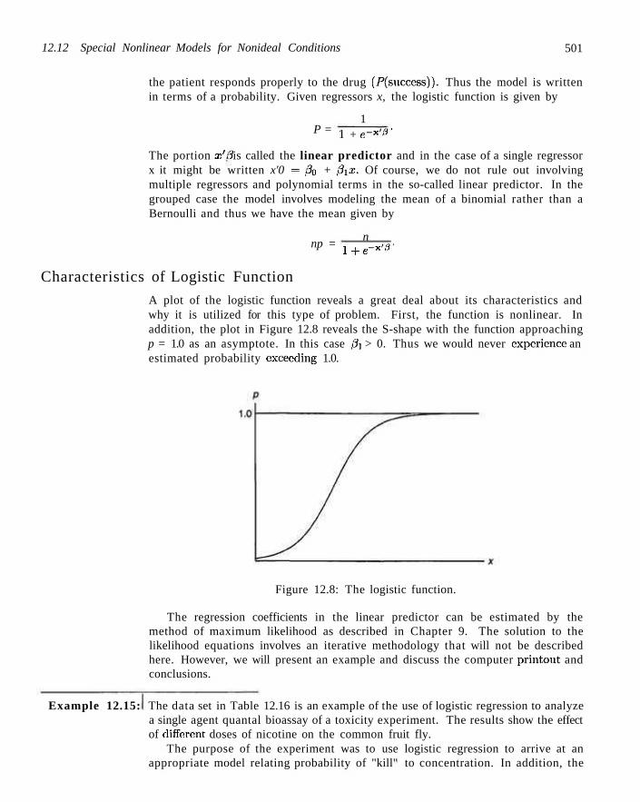
12.12 Special Nonlinear Models for Nonideal Conditions 501
the patient responds properly to the drug (P(success)). Thus the model is written in terms of a probability. Given regressors x, the logistic function is given by
P = 1
1 + e-* '" '
The portion x'3 is called the linear predictor and in the case of a single regressor x it might be written x'0 = 0O + 0ix. Of course, we do not rule out involving multiple regressors and polynomial terms in the so-called linear predictor. In the grouped case the model involves modeling the mean of a binomial rather than a Bernoulli and thus we have the mean given by
np = n
1+e -x'3'
Characteristics of Logistic Function
A plot of the logistic function reveals a great deal about its characteristics and why it is utilized for this type of problem. First, the function is nonlinear. In addition, the plot in Figure 12.8 reveals the S-shape with the function approaching p = 1.0 as an asymptote. In this case 0i > 0. Thus we would never experience an estimated probability exceeding 1.0.
Figure 12.8: The logistic function.
The regression coefficients in the linear predictor can be estimated by the method of maximum likelihood as described in Chapter 9. The solution to the likelihood equations involves an iterative methodology that will not be described here. However, we will present an example and discuss the computer printout and conclusions.
Example 12.15: The data set in Table 12.16 is an example of the use of logistic regression to analyze a single agent quantal bioassay of a toxicity experiment. The results show the effect of different doses of nicotine on the common fruit fly.
The purpose of the experiment was to use logistic regression to arrive at an appropriate model relating probability of "kill" to concentration. In addition, the
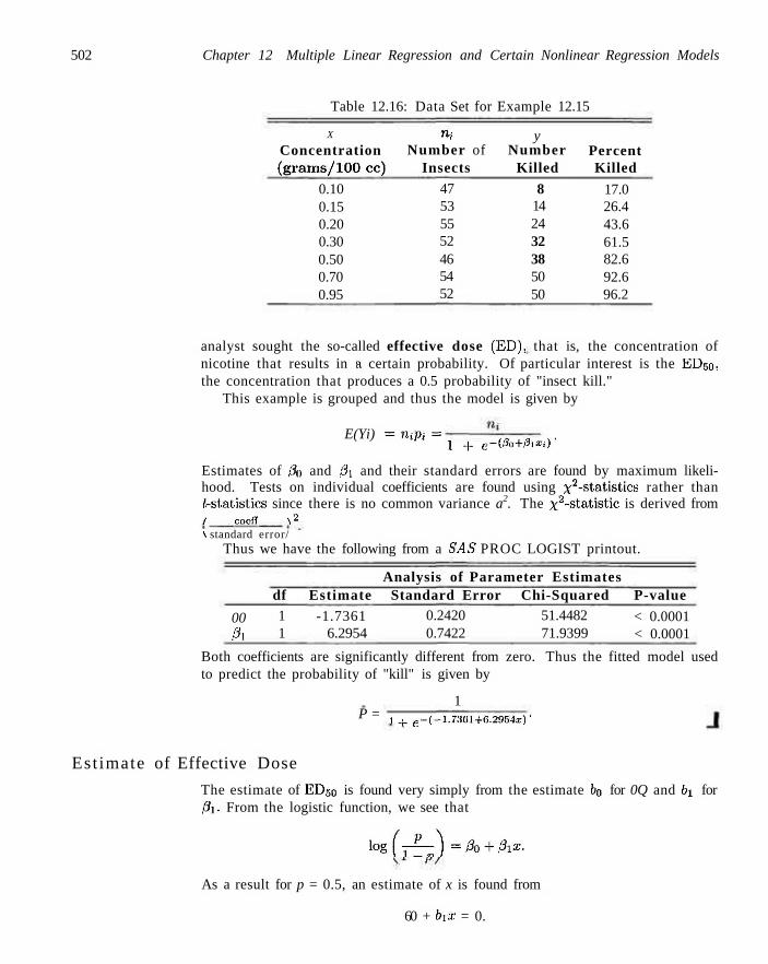
502 Chapter 12 Multiple Linear Regression and Certain Nonlinear Regression Models
Table 12.16: Data Set for Example 12.15
X
Concentration (g rams/100
0.10 0.15 0.20 0.30 0.50 0.70 0.95
cc)
iy Number of
Insects 47 53 55 52 46 54 52
y Number
Killed
8 14 24 32 38 50 50
Percent Killed
17.0 26.4 43.6 61.5 82.6 92.6 96.2
analyst sought the so-called effective dose (ED), that is, the concentration of nicotine that results in a certain probability. Of particular interest is the ED50, the concentration that produces a 0.5 probability of "insect kill."
This example is grouped and thus the model is given by
E(Yi) = mpi = 1 4. e-(%+&\Xi)'
Estimates of 0Q and 0\ and their standard errors are found by maximum likelihood. Tests on individual coefficients are found using x2-statistics rather than ^-statistics since there is no common variance a2. The x2-statistic is derived from / coeff \ 2
\ standard error/ Thus we have the following from a SMS PROC LOGIST printout.
00 01
df 1 1
Estimate -1.7361
6.2954
Analysis of Parameter Estimates Standard Error Chi-Squared
0.2420 51.4482 0.7422 71.9399
P-value
< 0.0001 < 0.0001
Both coefficients are significantly different from zero. Thus the fitted model used to predict the probability of "kill" is given by
1 P = 1 _|_ e-(-1.73(il+0.2954x) '
Est imate of Effective Dose
The estimate of ED50 is found very simply from the estimate 60 for 0Q and 61 for 0x. From the logistic function, we see that
\og(-^-\=0Q+0xx.
As a result for p = 0.5, an estimate of x is found from
60 + bxx = 0.
Review Exercises 503
Thus the ED50 is given by
x = - ( ~ j = 0.276 grams/100 cc.
Concept of Odds Ratio
Another form of inference tha t is conveniently accomplished using logistic regression is derived from the use of the odds rat io. The odds rat io is designed to
Definition 12.1:
determine how the o d d s of succes s = j ^ — increases as certain changes in regressor values occur. For example, in the case of Example 12.15 we may wish to know how the odds increases if one were to increase dosage by, say, 0.2 gram/lOOcc.
In to
logistic regression that of condition
an odds ratio is 1 in the regressort
b/(i-b/U-
the ratio of odds of , that is,
P)h p)W
success at condition 2
This allows the analyst to ascertain a sense of the utility of changing the regressor
by a certain number of units. Now since ( j ^ - ) = eth+f>\--r^ (-uen for o u r Example
12.15, the rat io reflecting the increase in odds of success when dosage of nicotine is increased by 0.2 grams/100 cc is given by
gO.26, _ e(0.2)(6.2954) _ 3 ^2.
The implication of an odds ratio of 3.522 is t ha t the odds of success is enhanced by a factor of 3.522 when the nicotine dose is increased by 0.2 g rams/100 cc.
Review Exercises
12.60 In the Department of Fisheries and Wildlife at Virginia Polytechnic Institute and State University, an experiment was conducted to study the effect of stream characteristics on fish biomass. The regressor variables are as follows: average depth (of 50 cells) (xi): area of in-stream cover (i.e., undercut banks, logs, boulders, etc.) (as); percent canopy cover (average of 12) (x3); area> 25 centimeters in depth (x4). The response is y, the fish biomass. The data are as follows:
Obs . y Xl X2 Xa X.l
1 2 3 4 5 6 7 8
100 388 755
1288 230
0 551 345
14.3 19.1 54.6 28.8 16.1 10.0 28.5 13.8
15.0 29.4 58.0 42.6 15.9 56.4 95.1 60.6
12.2 26.0 24.2 26.1 31.6 23.3 13.0 7.5
48.0 152.2 469.7 485.9
87.6 6.9
192.9 105.8
Obs. V Xi X2 Xi X l
9 0 10.7 35.2 40.3 0.0 10 348 25.9 52.0 40.3 116.6
(a) Fit a multiple linear repression including all four regression variables.
(b) Use Cp , R2, and s to determine the best subset of variables. Compute these statistics for all possible subsets.
(c) Compare the appropriateness of the models in parts (a) and (b) for predicting fish biomass.
12.61 Show that, in a multiple linear regression data set,
53 /j« = ?'•
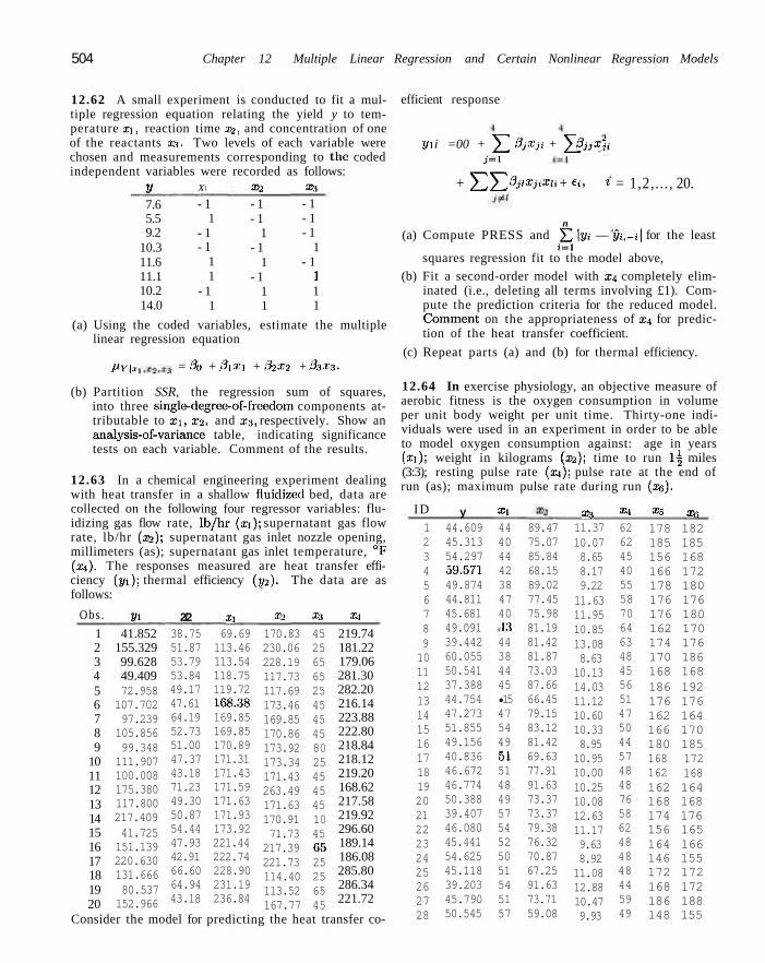
504 Chapter 12 Multiple Linear Regression and Certain Nonlinear Regression Models
12.62 A small experiment is conducted to fit a multiple regression equation relating the yield y to temperature Xi, reaction time x2, and concentration of one of the reactants xs. Two levels of each variable were chosen and measurements corresponding to the coded independent variables were recorded as follows:
y X\ 3>2 X3
efficient response
7.6 5.5 9.2
10.3 11.6 11.1 10.2 14.0
- 1 1
- 1 - 1
1 1
- 1 1
- 1 - 1
1 - 1
1 - 1
1 1
- 1 - 1 - 1
1 - 1
1 1 1
(a) Using the coded variables, estimate the multiple linear regression equation
UY\x = 3a + 01-t'l + 02'-t2 + 53J3.
(b) Partition SSR, the regression sum of squares, into three single3-degree-of-freedom components attributable to x i , 2-2, and x3, respectively. Show an analysis-of-variance table, indicating significance tests on each variable. Comment of the results.
12.63 In a chemical engineering experiment dealing with heat transfer in a shallow fluidized bed, data are collected on the following four regressor variables: flu-idizing gas flow rate, lb/hr (xi); supernatant gas flow rate, lb/hr (X2); supernatant gas inlet nozzle opening, millimeters (as); supernatant gas inlet temperature, °F (x4). The responses measured are heat transfer efficiency (yi): thermal efficiency (1/2). The data are as follows:
Obs . 2/i 2/2 Xl X-2 X.l XA
1 2 3 4 5 6 7 8 9
10 11 12 13 14 15 16 17 18 19 20
41.852 155.329 99.628 49.409 72.958 107.702 97.239 105.856 99.348 111.907 100.008 175.380 117.800 217.409 41.725 151.139 220.630 131.666 80.537 152.966
38.75 51.87 53.79 53.84 49.17 47.61 64.19 52.73 51.00 47.37 43.18 71.23 49.30 50.87 54.44 47.93 42.91 66.60 64.94 43.18
69.69 113.46 113.54 118.75 119.72 168.38 169.85 169.85 170.89 171.31 171.43 171.59 171.63 171.93 173.92 221.44 222.74 228.90 231.19 236.84
170.83 230.06 228.19 117.73 117.69 173.46 169.85 170.86 173.92 173.34 171.43 263.49 171.63 170.91 71.73 217.39 221.73 114.40 113.52 167.77
45 25 65 65 25 45 45 45 80 25 45 45 45 10 45 65 25 25 65 45
219.74 181.22 179.06 281.30 282.20 216.14 223.88 222.80 218.84 218.12 219.20 168.62 217.58 219.92 296.60 189.14 186.08 285.80 286.34 221.72
l/i i =00 + 5 3 0jXji + ^ 0}jX2i J = l
+ 5 3 5 Z PiiXii*" + e«"> « = 1,2,.. . , 20.
n (a) Compute PRESS and YI \yt — yt,-i\ for the least
i—l squares regression fit to the model above,
(b) Fit a second-order model with x4 completely eliminated (i.e., deleting all terms involving £1). Compute the prediction criteria for the reduced model. Comment on the appropriateness of x4 for prediction of the heat transfer coefficient.
(c) Repeat parts (a) and (b) for thermal efficiency.
12.64 In exercise physiology, an objective measure of aerobic fitness is the oxygen consumption in volume per unit body weight per unit time. Thirty-one individuals were used in an experiment in order to be able to model oxygen consumption against: age in years (11); weight in kilograms (as); time to run l | miles (3:3); resting pulse rate (x4); pulse rate at the end of run (as); maximum pulse rate during run (2$).
ID y Xl x3 214 XQ xa
Consider the model for predicting the heat transfer co-
1 2 3 4 5 6 7 8 9 10 11 12 13 14 15 16 17 18 19 20 21 22 23 24 25 26 27 28
44.609 45.313 54.297 59.571 49.874 44.811 45.681 49.091 39.442 60.055 50.541 37.388 44.754 47.273 51.855 49.156 40.836 46.672 46.774 50.388 39.407 46.080 45.441 54.625 45.118 39.203 45.790 50.545
44 40 44 42 38 47 40 13 44 38 44 45 •15 47 54 49 51 51 48 49 57 54 52 50 51 54 51 57
89.47 75.07 85.84 68.15 89.02 77.45 75.98 81.19 81.42 81.87 73.03 87.66 66.45 79.15 83.12 81.42 69.63 77.91 91.63 73.37 73.37 79.38 76.32 70.87 67.25 91.63 73.71 59.08
11.37 10.07 8.65 8.17 9.22 11.63 11.95 10.85 13.08 8.63 10.13 14.03 11.12 10.60 10.33 8.95 10.95 10.00 10.25 10.08 12.63 11.17 9.63 8.92 11.08 12.88 10.47 9.93
62 62 45 40 55 58 70 64 63 48 45 56 51 47 50 44 57 48 48 76 58 62 48 48 48 44 59 49
178 182 185 185 156 168 166 172 178 180 176 176 176 180 162 170 174 176 170 186 168 168 186 192 176 176 162 164 166 170 180 185 168 162
172 168
162 164 168 168 174 176 156 165 164 166 146 155 172 172 168 172 186 188 148 155
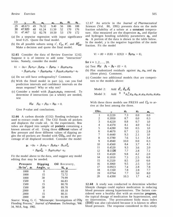
Review Exercises 505
ID y Xl x2 X-s XA X$
29 48.673 30 47.920 31 47.467
49 48 52
76.32 61.24 82.78
9.40 11.50 10.50
xe 56 186 188 52 170 176 53 170 172
(a) Do a stepwise regression with input significance level 0.25. Quote the final model.
(b) Do all possible subsets using s2, Cp, R2, and JR^JJ. Make a decision and quote the final model.
12.67 An article in the Journal of Pharmaceutical Sciences (Vol. 80, 1991) presents data on the mole fraction solubility of a solute at a constant temperature. Also measured are the dispersion a;i, and dipolar and hydrogen bonding solubility parameters as, and 3:3. A portion of the data is shown in the table below. In the model, y is the negative logarithm of the mole fraction. Fit the model
12.65 Consider the data of Review Exercise 12.62. Suppose it is of interest to add some "interaction" terms. Namely, consider the model
Vi = 0o+ 0iXu + 32X2i + 03X3i + 0\2xiiX2i
+ 013'XliX3i + 023X2iX3i + 0l23XliX2iX3i + Ci-
(a) Do we still have orthogonality? Comment.
(b) With the fitted model in part (a), can you find prediction intervals and confidence intervals on the mean response? Why or why not?
(c) Consider a model with ,6"i23a:ia:2.T3 removed. To determine if interactions (as a whole) are needed, test
Ho'- 0\1 = A3 = #23 = 0.
Give P-value and conclusions.
12.66 A carbon dioxide (CO2) flooding technique is used to extract crude oil. The CO2 floods oil pockets and displaces the crude oil. In the experiment, flow tubes are dipped into sample oil podcets containing a known amount of oil. Using three different values of flow pressure and three different values of dipping angles the oil pockets are flooded with CO2, and the percentage of oil displaced recorded. Consider the model
2/t =0o + 0\Xu + 02x2i + 0nx2u
+ 022X2i + 0l2XuX2i + €,.
Fit the model above to the data, and suggest any model editing that may be needed.
Pressure lb / in 2 , xi
1000 1000 1000 1500 1500 1500 2000 2000 2000
Source: Wang, G. Flooding Process,"
Dipping Angle,
0 15 30 0
15 30 0
15 30
X2
C. "Microscopic
Oil Recovery,
%, v 60.58 72.72 79.99 66.83 80.78 89.78 69.18 80.31 91.99
: Investigations of ' Journal of Petroleum Technology,
Vi = 00 + 0\Xli + 02X2i + 33X3i + €i,
fori = 1,2, . . . , 20.
(a) Test H0: 0i = p\ = 03 = 0. (b) Plot studentized residuals against xi, x2, and X3
(three plots). Comment. (c) Consider two additional models that are competi
tors to the models above:
Model 2:
Model 3:
Add Xi, x2, x3
Add Xi,x2,x3,xix2,xiX3,X2X3.
With these three models use PRESS and Cv to arrive at the best among the three.
Obs. y Xl X2 x3
1 2 3 4 5 6 7 8 9
10 11 12 13 14 15 16 17 18 19 20
0.2220 0.3950 0.4220 0.4370 0.4280 0.4670 0.4440 0.3780 0.4940 0.4560 0.4520 0.1120 0.4320 0.1010 0.2320 0.3060 0.0923 0.1160 0.0764 0.4390
7.3 8.7 8.8 8.1 9.0 8.7 9.3 7.6
10.0 8.4 9.3 7.7 9.8 7.3 8.5 9.5 7.4 7.8 7.7
10.3
0.0 0.0 0.7 4.0 0.5 1.5 2.1 5.1 0.0 3.7 3.6 2.8 4.2 2.5 2.0 2.5 2.8 2.8 3.0 1.7
0.0 0.3 1.0 0.2 1.0 2.8 1.0 3.4 0.3 4.1 2.0 7.1 2.0 6.8 6.6 5.0 7.8 7.7 8.0 4.2
34, N0.8, Aug. 1982.
12.68 A study was conducted to determine whether lifestyle changes could replace medication in reducing blood pressure among hypertensives. The factors considered were a healthy diet with an exercise program, the typical dosage of medication for hypertension, and no intervention. The pretreatment body mass index (BMI) was also calculated because it is known to affect blood pressure. The response considered in this study
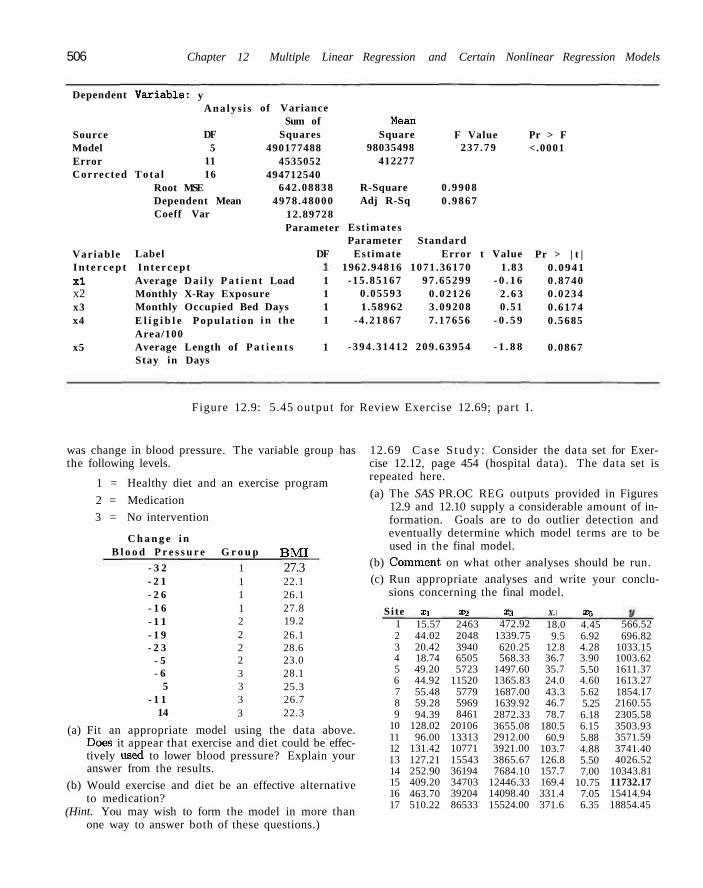
506 Chapter 12 Multiple Linear Regression and Certain Nonlinear Regression Models
Dependent
Source Model Error Corrected
Var iable
Var iab le : y A n a l y s i s
DF 5
11 Tota l 16
Root MSE Dependent Mean Coeff Var
Label I n t e r c e p t I n t e r c e p t x l x2 x3 x4
x5
of Variance Sum of
Squares 490177488
4535052 494712540
642 .08838 4978.48000
12.89728 Parameter
DF
Average D a i l y P a t i e n t Load 1 Monthly X-Ray Exposure 1 Monthly Occupied Bed Days 1 E l i g i b l e Popula t ion Area/100
i n the 1
Average Length of P a t i e n t s 1 Stay in Days
Mean Square
98035498 412277
R-Square Adj R-Sq
Est imates
F Value 237 .79
0 .9908 0 .9867
Parameter Standard Estimate Error t Value
1962.94816 1071.36170 1 .83 -15 .85167
0 .05593 1.58962
-4 .2 1 8 6 7
97 .65299 - 0 . 1 6 0 .02126 2 . 6 3 3 .09208 0 .51 7 .17656 - 0 . 5 9
-394 .31412 209 .63954 - 1 . 8 8
Pr > F <.0001
Pr > | t | 0 .0941 0 .8740 0 .0234 0 .6174 0 .5685
0 .0867
Figure 12.9: 5.45 output for Review Exercise 12.69; part I.
was change in blood pressure. The variable group has the following levels.
1 = Healthy diet and an exercise program
2 = Medication
3 = No intervention
C h a n g e i n B l o o d P r e s s u r e
- 3 2 - 2 1 - 2 6 - 1 6 - 1 1 - 1 9 - 2 3
- 5 - 6
5 - 1 1
14
G r o u p
1 1 1 1 2 2 2 2 3 3 3 3
BMI 27.3 22.1 26.1 27.8 19.2 26.1 28.6 23.0 28.1 25.3 26.7 22.3
(a) Fit an appropriate model using the data above. Doess it appear that exercise and diet could be effectively useid to lower blood pressure? Explain your answer from the results.
(b) Would exercise and diet be an effective alternative to medication?
(Hint. You may wish to form the model in more than one way to answer both of these questions.)
12.69 Case S tudy : Consider the data set for Exercise 12.12, page 454 (hospital data). The data set is repeated here.
(a) The SAS PR.OC REG outputs provided in Figures 12.9 and 12.10 supply a considerable amount of information. Goals are to do outlier detection and eventually determine which model terms are to be used in the final model.
(b) Comment, on what other analyses should be run. (c) Run appropriate analyses and write your conclu
sions concerning the final model.
Site xi X2 X3 X.\ 3 5 1 2 3 4 5 6 7 8 9
10 11 12 13 14 15 16 17
15.57 44.02 20.42 18.74 49.20 44.92 55.48 59.28 94.39
128.02 96.00
131.42 127.21 252.90 409.20 463.70 510.22
2463 2048 3940 6505 5723
11520 5779 5969 8461
20106 13313 10771 15543 36194 34703 39204 86533
472.92 1339.75 620.25 568.33
1497.60 1365.83 1687.00 1639.92 2872.33 3655.08 2912.00 3921.00 3865.67 7684.10
12446.33 14098.40 15524.00
18.0 9.5
12.8 36.7 35.7 24.0 43.3 46.7 78.7
180.5 60.9
103.7 126.8 157.7 169.4 331.4 371.6
4.45 6.92 4.28 3.90 5.50 4.60 5.62 5.25 6.18 6.15 5.88 4.88 5.50 7.00
10.75 7.05 6.35
566.52 696.82
1033.15 1003.62 1611.37 1613.27 1854.17 2160.55 2305.58 3503.93 3571.59 3741.40 4026.52
10343.81 11732.17 15414.94 18854.45
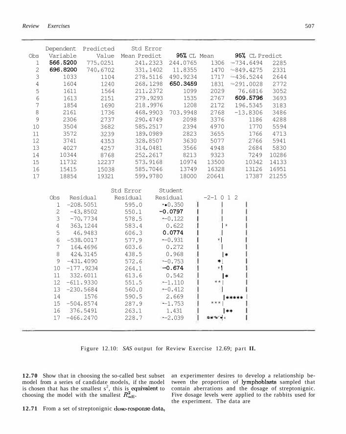
Review Exercises 507
Obs 1 2 3 4 5 6 7 8 9 10 11 12 13 14 15 16 17
Dependent Variable 566.5200 696.8200
1033 1604 1611 1613 1854 2161 2306 3504 3572 3741 4027 10344 11732 15415 18854
Predicted Value
775 740
0251 6702 1104 1240 1564 2151 1690 1736 2737 3682 3239 4353 4257 8768 12237 15038 19321
Obs Residual 1 -208 2 -43 3 -70 4 363 5 46 6 -538 7 164 8 424 9 -431 10 -177 11 332 12 -611 13 -230 14 15 -504 16 376 17 -466
5051 8502 7734 1244 9483 0017 4696 3145 4090 .9234 6011 9330 5684 1576 8574 5491 2470
Std Error Mean Predict
241 331 278 268 211 279 218 468 290 585 189 328 314 252 573 585 599
Std Error Residual
595.0 550.1 578.5 583.4 606.3 577.9 603.6 438.5 572.6 264.1 613.6 551.5 560.0 590.5 287.9 263.1 228.7
2323 1402 5116 1298 2372 .9293 .9976 9903 4749 2517 0989 8507 0481 2617 9168 7046 9780
95% CL 244.0765 11.8355 490.9234 650.3459
1099 1535 1208
703.9948 2098 2394 2823 3630 3566 8213 10974 13749 18000
Student Residual
•0.350 -0.0797 -0.122 0.622 0.0774 -0.931 0.272 0.968 -0.753 -0.674 0.542 -1.110 -0.412 2.669 -1.753 1.431 -2.039
Mean 1306 1470 1717 1831 2029 2767 2172 2768 3376 4970 3655 5077 4948 9323 13500 16328 20641
-2-1 0 1
1 *
* 1
1* * i * 1 1*
**|
95'/, CL Predict -734.6494 -849.4275 -436.5244 -291.0028 76.6816 609.5796 196.5345 -13.8306
1186 1770 1766 2766 2684 7249 10342 13126 17387
2
|***** | ***|
|*« T *l* T* " 1
2285 2331 2644 2772 3052 3693 3183 3486 4288 5594 4713 5941 5830 10286 14133 16951 21255
Figure 12.10: SAS output for Review Exercise 12.69; pa r t II.
12.70 Show that in choosing the so-called best subset model from a series of candidate models, if the model is chosen that has the smallest s2, this is equivalent to choosing the model with the smallest R2
vi\.
12.71 From a set of streptonignic dosorcsponse data.
an experimenter desires to develop a relationship between the proportion of lymphoblasts sampled that contain aberrations and the dosage of streptonignic. Five dosage levels were applied to the rabbits used for the experiment. The data are
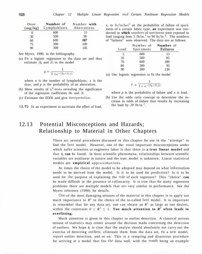
508 Chapter 12 Multiple Linear Regression and Certain Nonlinear Regression Models
Dose ( m g / k g )
0 30 60 75 90
Number of Lymphoblas t s
600 500 600 300 300
N u m b e r with A b e r r a t i o n s
15 96
187 100 145
See Myers, 1990, in the bibliography. (a) Fit a logistic regression to the data set and thus
estimate 0o and 0i in the model
1 1 + e-O3„+0iz) '
where n is the number of lymphoblasts, x is the dose, and p is the probability of an aberration.
(b) Show results of x2-tests revealing the significance of the regression coefficients 0o and 3\.
(c) Estimate the ED50 and give interpretation.
12.72 In an experiment to ascertain the effect of load,
x, in lb/inches on the probability of failure of specimens of a certain fabric type, an experiment was conducted in which numbers of specimens were exposed to load ranging from 5 lb/in.2 to 90 lb/in. . The numbers of ''failures" were observed. The data are as follows:
Load
5 35 70 80 90
N u m b e r of Specimens
600 500 600 300 300
Number of Failures
13 95
189 95
130
(a) Use: logistic regression to fit the model
1 !' = 1 4- e-(jSb+j8i«) '
where p is the probability of failure and x is load. (b) Use the odds ratio concept to determine the in
crease in odds of failure that results by increasing the load by 20 lb/in.2.
12.13 Potential Misconceptions and Hazards; Relationship to Material in Other Chapters
There arc several procedures discussed in this chapter for use in the "at tempt" to find the best model. However, one of the: most important misconceptions under which naive scientists or engineers labor is tha t there is a t rue linear m o d e l and that it, can be found. In most scientific phenomena, relationships between scientific variables are nonlinear in nature and the true: model is unknown. Linear statistical models are: empir ica l a p p r o x i m a t i o n s .
At times the choice of the model to be adopted may depend on what information needs to be derived from the model. Is it to be used for prediction? Is it to be used for the purpose of explaining the role of each regressor? This ''choice" can be made difficult in the presence of collincarity. It is true that for many regression problems there are multiple models that arc very similar in performance. See the Myers reference (1990) for details.
One of the most damaging misuses of the material in this chapter is to apply too much importance to R2 in the choice of the so-called best model. It is important to remember that for any da ta set, one can obtain an R2 as large as one desires, within the constraint 0 < R2 < 1. Too m u c h a t t e n t i o n to R2 of ten leads to overfitt ing.
Much attention is given in this chapter to outlier detection. A classical serious misuse of statistics may center around the decision made concerning the detection of outliers. We hope it, is clear that the analyst should absolutely not carry out the exercise of detecting outliers, eliminate them from the da ta set, fit a new model, report outlier detection, and so on. This is a tempting and disastrous procedure for arriving at a model that fits the data well, with the result, being an example

12.13 Potential Misconceptions and Hazards 509
of how to lie with statistics. If an outlier is detected, the history of the data should be checked for possible clerical or procedural error before it is eliminated from the data set. One must remember that an outlier by definition is a data point that the model did not fit well. The problem may not be in the data but rather in the model selection. A changed model may result in the point not being detected as an outlier.
Chapter 13
One-Factor Experiments: General
13.1 Analysis-of-Variance Technique
In the estimation and hypotheses testing material covered in Chapters 9 and 10, we arc restricted in each case to considering no more than two population parameters. Such was the case, for example, in testing for the equality of two population means using independent samples from normal populations with common but unknown variance, where it was necessary to obtain a pooled estimate of a2.
This material dealing in two-sample inference represents a special case of what we call the one-factor problem. For example, in Exercise 35, Section 10.8, the survival time is measured for two samples of mice where one sample received a new serum for leukemia treatment and the other sample received no treatment. In this case we say that there is one factor, namely treatment, and the factor is at two levels. If several competing treatments were being used in the sampling process, more samples of mice would be necessary. In this case the problem would involve one factor with more than two levels and thus more than two samples.
In the fe > 2 sample problem, it will be assumed that there are k samples from k populations. One very common procedure used to deal with testing population means is called the analysis of variance, or ANOVA.
The analysis of variance is certainly not a new technique if the reader has followed the material on regression theory. We used the analysis-of-variance approach to partition the total sum of squares into a portion due to regression and a portion due to error.
Suppose in an industrial experiment that an engineer is interested in how the mean absorption of moisture in concrete varies among 5 different concrete aggregates. The samples are exposed to moisture: for 48 hours. It, is decided that 6 samples are to be tested for each aggregate, requiring a total of 30 samples to be tested. The data are recorded in Table 13.1.
The model for this situation is considered as follows. There are 6 observations taken from each of 5 populations with means jti,fi2- • • • , Ms- respectively. We may wish to test
H Q : i n = 1 1 - 2 = • - • = / ' 5 ,
II [-. At least two of the means are not equal.
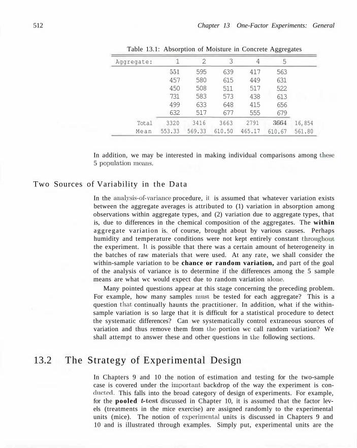
512 Chapter 13 One-Factor Experiments: General
Table 13.1: Absorption of Moisture in Concrete Aggregates
Aggregate:
Total Mean
1
551 457 450 731 499 632
3320 553.33
2
595 580 508 583 633 517
3416 569.33
3
639 615 511 573 648 677
3663 610.50
4
417 449 517 438 415 555
2791 465.17
5
563 631 522 613 656 679
3064 610.67
16,854 561.80
In addition, we may be interested in making individual comparisons among these 5 population means.
Two Sources of Variability in the Data
In the analysis-of-variance procedure, i! is assumed that whatever variation exists between the aggregate averages is attributed to (1) variation in absorption among observations within aggregate types, and (2) variation due to aggregate types, that is, due to differences in the chemical composition of the aggregates. The within aggregate variation is. of course, brought about by various causes. Perhaps humidity and temperature conditions were not kept entirely constant throughout the experiment. It is possible that there was a certain amount of heterogeneity in the batches of raw materials that were used. At any rate, we shall consider the within-sample variation to be chance or random variation, and part of the goal of the analysis of variance is to determine if the differences among the 5 sample means are what wc would expect due to random variation alone.
Many pointed questions appear at this stage concerning the preceding problem. For example, how many samples must be tested for each aggregate? This is a question that continually haunts the practitioner. In addition, what if the within-sample variation is so large that it is difficult for a statistical procedure to detect the systematic differences? Can we systematically control extraneous sources of variation and thus remove them from the portion wc call random variation? We shall attempt to answer these and other questions in the: following sections.
13.2 The Strategy of Experimental Design
In Chapters 9 and 10 the notion of estimation and testing for the two-sample case is covered under the important backdrop of the way the experiment is conducted. This falls into the broad category of design of experiments. For example, for the pooled M,est discussed in Chapter 10, it is assumed that the factor levels (treatments in the mice exercise) are assigned randomly to the experimental units (mice). The notion of experimental units is discussed in Chapters 9 and 10 and is illustrated through examples. Simply put, experimental units are the
13.3 One- Way Analysis of Variance: Completely Randomized Design 513
units (mice, patients, concrete specimens, time) that provide t h e heterogeneity t ha t leads to exper imenta l error in a scientific investigation. The random assignment eliminates bias that could result by systematic assignment. The goal is to distribute uniformly among the factor levels the risks brought about by the heterogeneity of the experimental units. A random assignment best simulates the conditions that are assumed by the model. In Section 13.8 we discuss blocking in experiments. The notion of blocking is presented in Chapters 9 and 10, when comparisons between means was accomplished with pairing, that is, the division of the experimental units into homogeneous pairs called blocks. The factor levels or treatments are then assigned randomly within blocks. The purpose of blocking is to reduce the effective experimental error. In this chapter we naturally extend the pairing to larger block sizes, with analysis of variance being the primary analytical tool.
13.3 One-Way Analysis of Variance: Completely Randomized Design (One-Way ANOVA)
Random samples of size n are selected from each of k populations. The k different populations are classified on the basis of a single criterion such as different treatments or groups. Today the term t r e a t m e n t is used generally to refer to the various classifications, whether they be different aggregates, different analysts, different fertilizers, or different regions of the country.
Assumptions and Hypotheses in One-Way ANOVA
It is assumed that the k populations are independent and normally distributed with means fix,Pi »P-k a i l (l common variance a2. As indicated in Section 13.2, these assumptions are made more palatable by randomization. We wish to derive appropriate methods for testing the hypothesis
Ho' in = / ' 2 = ••• = Pk-.
H\: At least two of the means arc not equal.
Let. yij denote the j th observation from the ith treatment and arrange the data as in Table 13.2. Here, Y',. is the total of all observations in the sample from the ith treatment, y,, is the mean of all observations in the sample from the ith treatment, Y„ is the total of all nk observations, and y_. is the mean of all nk observations.
M o d e l for O n e - W a y A N O V A
Each observation may be written in the form
Yij = IM. + t ' J '
where £y measures the deviation of the jth observation of the ith sample from the corresponding treatment mean. The ey-term represents random error and plays the same role as the error terms in the regression models. An alternative and
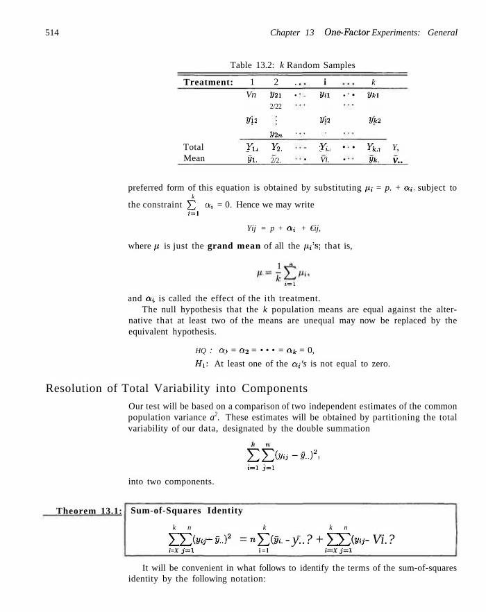
514 Chapter 13 One-Factor Experiments: General
Table 13.2: k Random Samples
Treatment:
Total Mean
1 Vn
J/12
S/ln Vi.
Si.
2 . 2/21 •
2/22
2/2n '
Y2. 2/2.
i - S/»i •
2/i2
2/tn - Y. • • Vi. •
k
• Vki
Vk2
Vkn • Yk. 2/fc.
Y,
v..
preferred form of this equation is obtained by substituting m = p. + ai, subject to k
the constraint Y^, on = 0. Hence we may write f=i
Yij = p + Oti + €ij,
where p. is just the grand mean of all the /i,'s; that is,
1 *
t = i
and ait is called the effect of the ith treatment. The null hypothesis that the k population means are equal against the alter
native that at least two of the means are unequal may now be replaced by the equivalent hypothesis.
HQ : a, = o2 = • • • = afr = 0,
Hi: At least one of the a, 's is not equal to zero.
Resolution of Total Variability into Components
Our test will be based on a comparison of two independent estimates of the common population variance a2. These estimates will be obtained by partitioning the total variability of our data, designated by the double summation
EBi*-*..)8, t = i j = i
into two components.
Theorem 13.1: Sum-of-Squares Identity
k n k k n
E J > y - V-? = n£>i. - y..? + E J > y - Vi.? i=X j ' = l i = l i—X j '= l
It will be convenient in what follows to identify the terms of the sum-of-squares identity by the following notation:
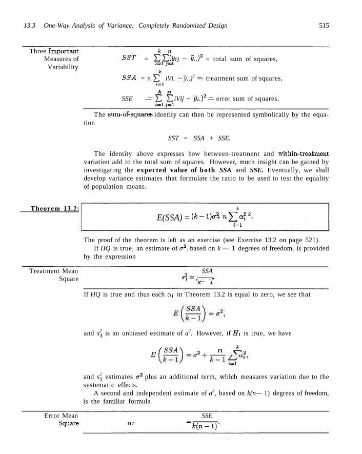
13.3 One-Way Analysis of Variance: Completely Randomized Design 515
Three Important k n Measures of SST = £ E iVij ~ V..)2 = total sum of squares,
Variability '~ J~
SSA = n 2~2 iVi. ~ y..)2 — treatment sum of squares. »=i
k n
SSE — ^Z YI iVij ~ Vi-? — error sum of squares. i = l j ' = l
The sum-of-squares identity can then be represented symbolically by the equation
SST = SSA + SSE.
The identity above expresses how between-treatment and within-treatment variation add to the total sum of squares. However, much insight can be gained by investigating the expected value of both SSA and SSE. Eventually, we shall develop variance estimates that formulate the ratio to be used to test the equality of population means.
Theorem 13.2: k 2 E(SSA) = (k-l)a2 + nY,°<'2i
f = i
The proof of the theorem is left as an exercise (see Exercise 13.2 on page 521). If HQ is true, an estimate of a2, based on k — 1 degrees of freedom, is provided
by the expression
Treatment Mean SSA Square s i = , _ . •
If HQ is true and thus each Q,- in Theorem 13.2 is equal to zero, we see that
and s2 is an unbiased estimate of a2. However, if Hi is true, we have
r,fSSA\ 2 n ^ 2
i = i
and s2 estimates a2 plus an additional term, wdiich measures variation due to the systematic effects.
A second and independent estimate of a2, based on k(n— 1) degrees of freedom, is the familiar formula
Error Mean SSE S c i u a r e fi2 = k(n-lY
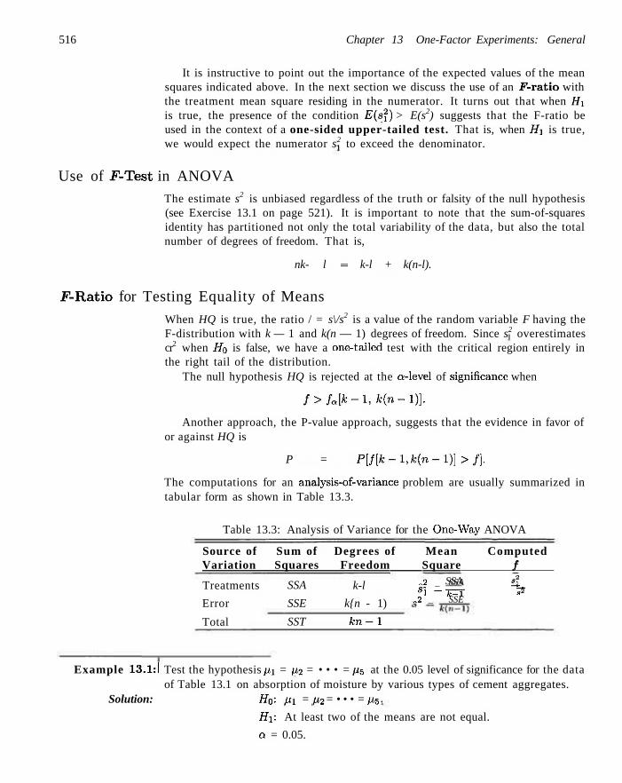
516 Chapter 13 One-Factor Experiments: General
It is instructive to point out the importance of the expected values of the mean squares indicated above. In the next section we discuss the use of an F-ratio with the treatment mean square residing in the numerator. It turns out that when Hi is true, the presence of the condition E(s2) > E(s2) suggests that the F-ratio be used in the context of a one-sided upper-tailed test. That is, when Hi is true, we would expect the numerator s2 to exceed the denominator.
Use of F-Test in ANOVA
The estimate s2 is unbiased regardless of the truth or falsity of the null hypothesis (see Exercise 13.1 on page 521). It is important to note that the sum-of-squares identity has partitioned not only the total variability of the data, but also the total number of degrees of freedom. That is,
nk- l = k-l + k(n-l).
F-Ratio for Testing Equality of Means
When HQ is true, the ratio / = s\/s2 is a value of the random variable F having the F-distribution with k — 1 and k(n — 1) degrees of freedom. Since s2 overestimates cr2 when H0 is false, we have a one-tailed test with the critical region entirely in the right tail of the distribution.
The null hypothesis HQ is rejected at the Q-level of significance when
/ > / * [ * - 1 , * ( « - ! ) ] •
Another approach, the P-value approach, suggests that the evidence in favor of or against HQ is
P = P[f[k-l,k(n-l)]>f}.
The computations for an analysis-of-variance problem are usually summarized in tabular form as shown in Table 13.3.
Table 13.3: Analysis of Variance for the One-Way ANOVA
Source of Sum of Degrees of Mean Computed Variation Squares Freedom Square /
SSA £? k-X ^
Treatments
Error
Total
SSA
SSE
SST
k-l
k{n - 1)
kn-1
„2 _ SSA s i - ¥=T
„2 _ SSE
Example 13.1:1 Test the hypothesis pi = u2 = • • • = pt, at the 0.05 level of significance for the data of Table 13.1 on absorption of moisture by various types of cement aggregates.
Solution: H0: Ux = u2 = • • • = /X5.
Hi: At least two of the means are not equal.
Q = 0.05.
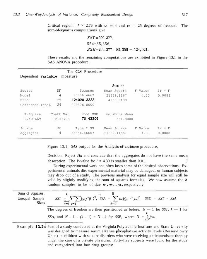
13.3 One-Way Analysis of Variance: Completely Randomized Design 517
Critical region: / > 2.76 with t'i sum-of-squarcs computations give
4 and v2 = 25 degrees of freedom. The
55P=209,377,
554=85,356,
55£=209,377 - 85,356 = 124,021.
These results and the remaining computations are exhibited in Figure 13.1 in the SAS ANOVA procedure.
The GLH Procedure Dependent Var iable : moisture
Source
Model
Error
Corrected Total
R-Square
0.407669
Source
aggregate
DF 4 25 29
Coeff Var
12.53703
DF 4
Squares
85356.4667
124020.3333
209376.8000
Root MSE
70.43304
Type I SS
85356.46667
Sum of
Mean Square F Value
21339.1167 4.30
4960.8133
moisture Mean
561.8000
Mean Square F Value
21339.11667 4.30
Pr > F
0.0088
Pr > F
0.0088
Figure 13.1: SAS output for the Analysis-of-variance procedure.
Decision: Reject Ho and conclude that the aggregates do not have the same mean
absorption. The P-value for / = 4.30 is smaller than 0.01. J During experimental work one often loses some of the desired observations. Ex
perimental animals die, experimental material may be damaged, or human subjects may drop out of a study. The previous analysis for equal sample size will still be valid by slightly modifying the sum of squares formulas. We now assume the A: random samples to be of size rix,n2,..., nk, respectively.
Sum of Squares; je, „,. ft Unequal Sample SST = *T ^(Vij - y..)2, SSA = J^m(y i . - y..)2, SSE = SST - SSA
Sizes f=i j = i
The degrees of freedom are then partitioned as before: N — 1 for SST, k — 1 for k
SSA, and N - 1 - (k - 1) = N - k for SSE, where N = £ n;. t = i
Example 13.2:1 Part of a study conducted at the Virginia Polytechnic Institute and State University was designed to measure serum alkaline phosphatase activity levels (Bessey-Lowry Units) in children with seizure disorders who were receiving anticonvulsant therapy under the care of a private physician. Forty-five subjects were found for the study and categorized into four drug groups:
518 Chapter 13 One-Factor Experiments: General
G-l: Control (not receiving anticonvulsants and having no history of seizure disorders)
G-2: Phenobaibilal
G-3: Carbamazepine
G-4: Other anticonvulsants
From blood samples collected on each subject the serum alkaline phosphatase activity level was determined and recorded as shown in Table 13.4. Test the hypothesis at the 0.05 level of significance that the average serum alkaline phosphatase activity level is the same for the four drug groups.
Table 13.4: Serum Alkaline: Phosphatase Activity Level
G-49.20 44.54 45.80 95.84 30.10 30.50 82.30 87.85
105.00 95.22
1 97.50
105.00 58.05 86.60 58.35 72.80
116.70 45.15 70.35 77.40
G-2 97.07 73.40 68.50 91.85
106.60 0.57 0.79 0.77 0.81
G-3 62.10 94.95
142.50 53.00
175.00 79.50 29.50 78.40
127.50
G-4 110.60 57.10
117.60 77.71
150.00 82.90
111.50
Solution: HQ : pi = p2 = p3 = fi4,
Hi: At least two of the means are not equal.
cv = 0.05.
Critical region: / > 2.836, by interpolating in Tabic A.6. Computations: V',. = 1460.25, Y2. = 440.36, F3. = 842.45, Y4. = 707.41 and Y = 3450.47. The analysis of variance is shown in the MINITAB output of Figure 13.2. Decision: Reject Ho and conclude that i he average serum alkaline phosphatase activity levels for the four drug groups are not all the same. The P-value is 0.02J
In concluding our discussion on the analysis of variance for the one-way classification, we state the advantages of choosing equal sample sizes over the choice of unequal sample sizes. The first advantage is that the /-ratio is insensitive to slight departures from the assumption of equal variances for the k populations when the samples are of equal size. Second, the choice of equal sample size minimizes the probability of committing a type II error.
13.4 Tests for the Equality of Several Variances
Although the /-ratio obtained from the: analysis-of-variance procedure is insensitive to departures from the assumption of equal variances for the k normal populations
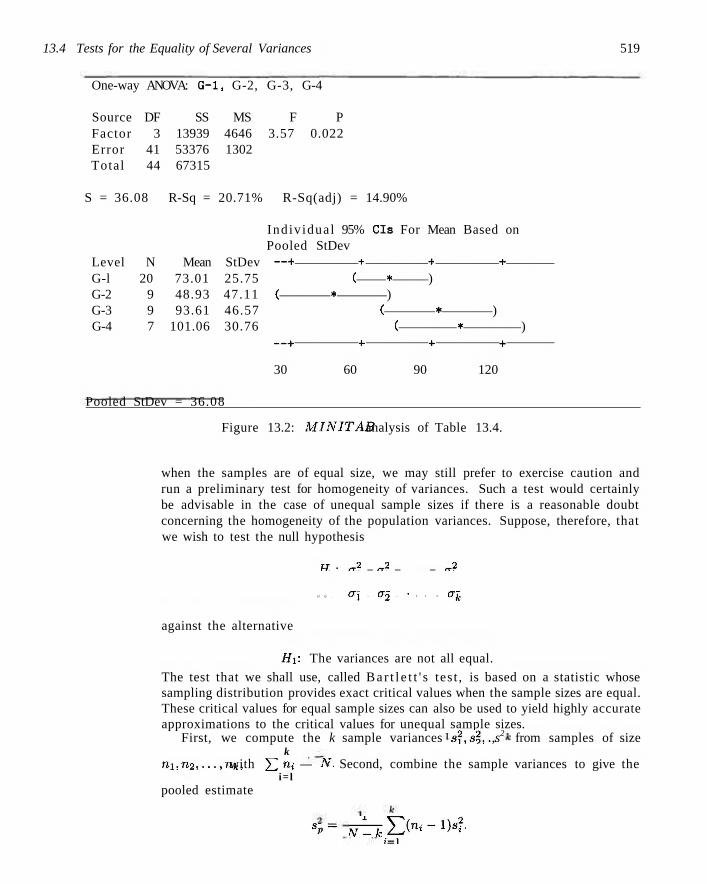
13.4 Tests for the Equality of Several Variances 519
One-way ANOVA: G-l, G-2, G-3, G-4
Source DF SS MS F P Factor 3 13939 4646 3.57 0.022 Error 41 53376 1302 Total 44 67315
S = 36.08 R-Sq = 20.71% R-Sq(adj) = 14.90%
Indiv idual 95% CIs For Mean Based on Pooled StDev
Level N Mean StDev —+ + + + G-l 20 73.01 25.75 ( * ) G-2 9 48.93 47.11 ( * ) G-3 9 93.61 46.57 ( * ) G-4 7 101.06 30.76 ( * )
—+ + + +
30 60 90 120
Pooled StDev = 36.08
Figure 13.2: MINITAB analysis of Table 13.4.
when the samples are of equal size, we may still prefer to exercise caution and run a preliminary test for homogeneity of variances. Such a test would certainly be advisable in the case of unequal sample sizes if there is a reasonable doubt concerning the homogeneity of the population variances. Suppose, therefore, that we wish to test the null hypothesis
W . „2 _ „2 _ _ „2
H Q . O X - a 2 - • • • = a k
against the alternative
Hi: The variances are not all equal.
The test that we shall use, called Ba r t l e t t ' s tes t , is based on a statistic whose sampling distribution provides exact critical values when the sample sizes are equal. These critical values for equal sample sizes can also be used to yield highly accurate approximations to the critical values for unequal sample sizes.
First, we compute the k sample variances s2,s2,.. .,s2 from samples of size k
nx,n2,...,nk, with YI n* — ^- Second, combine the sample variances to give the i= l
pooled estimate
S P = ^ m ^ ( n < - 1 ) ^ ' t•=l
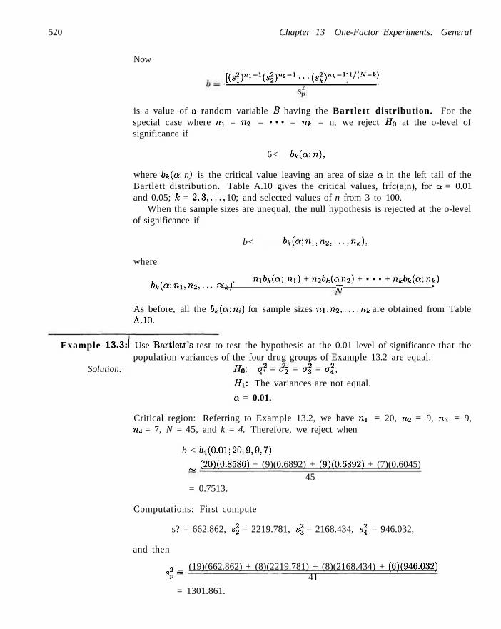
520 Chapter 13 One-Factor Experiments: General
Now
[(^)"--i(^r2-i'--(4)nfc-1]1/(-v-fe)
s2
is a value of a random variable B having the Bartlett distribution. For the special case where m = 712 = • • • = "A- = n, we reject Ho at the o-level of significance if
6< bkia;n),
where 0^(0; n) is the critical value leaving an area of size a in the left tail of the Bartlett distribution. Table A.10 gives the critical values, frfc(a;n), for a = 0.01 and 0.05; k = 2 , 3 , . . . , 10; and selected values of n from 3 to 100.
When the sample sizes are unequal, the null hypothesis is rejected at the o-level of significance if
b< bkia;ni.n2,...,nk),
where
, , v n-xbkia; ni) + n2bk(a; n2) + • • • + nkbk(a;nk) bk(a;ni,n2,...,nk) « r-r •
As before, all the bk(a; m) for sample sizes m , n 2 , . . . , nk are obtained from Table A.10.
Example 13.3:1 Use Bartlett's test to test the hypothesis at the 0.01 level of significance that the population variances of the four drug groups of Example 13.2 are equal.
Solution: Ho'- a2 = a2 = a\ = a\,
Hi: The variances are not equal.
a = 0.01.
Critical region: Referring to Example 13.2, we have n.j = 20, n2 = 9, ri3 = 9, n4 = 7, N = 45, and k = 4. Therefore, we reject when
b < 64(0.01; 20,9,9,7)
_ (20)(0.8586) + (9)(0.6892) + (9)(0.6892) + (7)(0.6045) 45
= 0.7513.
Computations: First compute
s? = 662.862, s\ = 2219.781, s | = 2168.434, s2, = 946.032,
and then
2 _ (19)(662.862) + (8)(2219.781) + (8)(2168.434) + (6)(946.032) SP- 41
= 1301.861.
Exercises 521
Now
b = [(662.862) 19(2219.781)8(2168.434)8(946.032)c]1/41
1301.861 0.8557.
Decision: Do not reject the hypothesis, and conclude that the population variances
of the four drug groups are not significantly different. _l Although Bartlett's test is most often used for testing of homogeneity of vari
ances, other methods are available. A method due to Cochran provides a computationally simple procedure, but it is restricted to situations in which the sample sizes are equal. Cochran's test is particularly useful for detecting if one variance is much larger than the others. The statistic that is used is
G = largest Sf
k '
ESf i-l
and the hypothesis of equality of variances is rejected if g > gQ where the value of ga is obtained from Table A.11.
To illustrate Cochran's test, let us refer again to the data of Table 13.1 on moisture absorption in concrete aggregates. Were we justified in assuming equal variances when we performed the analysis of variance of Example 13.1? We find that
,2 si = 12,134, si = 2303, s^ = 3594, si = 3319, s£ = 3455.
Exercises
Therefore.
12,134 24,805
= 0.4892,
which does not exceed the table value #0.05 = 0.5065. Hence we conclude that the assumption of equal variances is reasonable.
13.1 Show that the mean square error
2 _ SSE 8 - f c ( n - l )
for the analysis of variance in a one-way classification is an unbiased estimate of a2.
13.2 Prove Theorem 13.2.
13.3 Six different machines are being considered for use in manufacturing rubber seals. The machines are being compared with respect, to tensile strength of the product. A random sample of 4 seals from each machine is used to determine whether the mean tensile
strength varies from machine to machine. The following are the tensile-strength measurements in kilograms per square centimeter x 10~':
Machine 1
17.5 16.9 15.8 18.G
2 16.4 19.2 17.7 15.4
3 20.3 15.7 17.8 18.9
4 14.6 16.7 20.8 18.9
5 17.5 19.2 16.5 20.5
6 18.3 16.2 17.5 20.1
Perform the analysis of variance at the 0.05 level of significance and indicate whether or not the mean tensile strengths differ significantly for the 6 machines.
13.4 The data in the following table represent the
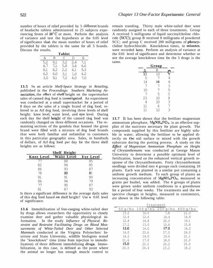
522 Chapter 13 One-Factor Experiments: General
number of hours of relief provided by 5 different brands of headache tablets administered to 25 subjects experiencing fevers of 38°C or more. Perforin the: analysis of variance and test the hypothesis at the 0.05 level of significance that, the mean number of hours of relief provided by the tablets is the same for all 5 brands. Discuss the results.
Tablet A 5.2 4.7 8.1 6.2 3.0
B 9.1 7.1 8.2 6.0 9.1
C 3.2 5.8 2.2 3.1 7.2
D 2.4 3.4 4.1 1.0 4.0
E 7.1 6.6 9.3 4.2 7.0
13.5 In an article Shelf-Space Strategy in Retailing, published in the Proceedings: Southern Marketing Association, the effect of shelf height on the supermarket sales of canned dog food is investigated. An experiment was conducted at a small supermarket for a period of 8 days on the sales of a single brand of clog food, referred to as Arf dog food, involving three levels of shelf height: knee level, waist level, and eye level. During each day the shelf height of the canned clog food was randomly changed on three different occasions. The remaining sections of the gondola that housed the given brand were filled with a mixture of dog food brands that were both familiar and unfamiliar to customers in this particular geographic area. Sales, in hundreds of dollars, of Arf dog food per day for the three shelf heights are as follows:
Shelf Height Knee Level Waist Level Eye Level
77 82 86 78 81 86 77 81
88 94 93 90 91 94 90 87
85 85 87 81 80 79 87 93
Is there a significant difference in the average daily sales of this dog food based on shelf height? Use a, 0.01 level of significance.
13.6 Immobilization of free-ranging white-tailed deer by drugs allows researchers the opportunity to closely examine deer and gather valuable physiological information. In the study Influence of Physical. Restraint and Restraint Facilitating Drugs on Blood Measurements of White-Tailed Deer and Other Selected Mammals conducted at the Virginia Polytechnic Institute and State University, wildlife biologists tested the "knockdown" time (time from injection to immobilization) of three different immobilizing drugs. Immobilization, in this case, is defined as the point where the animal no longer has enough muscle control to
remain standing. Thirty male white-tailed deer were randomly assigned to each of three treatments. Group A received 5 milligrams of liquid succinylcholine chloride (SCC); group B received 8 milligrams of powdered SCC; and group C received 200 milligrams of phency-clidine hydrochloride. Knockdown times, in minutes, were recorded here. Perform an analysis of variance at the 0.01 level of significance and determine whether or not the average knockdown time for the 3 drugs is the same.
Group
A ll 5 14 7 10 7 23 4 11 11
B 10 7 16 7 7 5 10 10 6 12
c 4 4 6 3 5 C 8 3 7 3
13.7 It has been shown that the fertilizer magnesium ammonium phosphate, MgNH^POi, is an effective supplier of the nutrients necessary for plant growth. The compounds supplied by this fertilizer are highly soluble in water, allowing the fertilizer to be applied directly on the soil surface or mixed with the growth substrate during the potting process. A study on the Effect, of Magnesium Ammonium Phosphate on Height of Chrysanthemums was conducted at George Mason University to determine a possible optimum level of fertilization, based on the enhanced vertical growth response of the chrysanthemums. Forty chrysanthemum seedlings were divided into 4 groups each containing 10 plants. Each was planted in a similar pot containing a uniform growth medium. To each group of plants an increasing concentration of .\lgNH4PO4, measured in grains per bushel, was added. The 4 groups of plants were grown under uniform conditions in a greenhouse for a period of four weeks. The treatments and the respective changes in heights, measured in centimeters, are shown in the following table:
Treatment 50 g/bu 100 g/bu 200 g/bu 400 g/bu
13.2 12.4 12.8 17.2 13.0 14.0 14.2 21.6 15.0 20.0
16.0 12.6 14.8 13.0 14.0 23.6 14.0 17.0 22.2 24.4
7.8 14.4 20.0 15.8 17.0 27.0 19.6 18.0 20.2 23.2
21.0 14.8 19.1 15.8 18.0 26.0 21.1 22.0 25.0 18.2
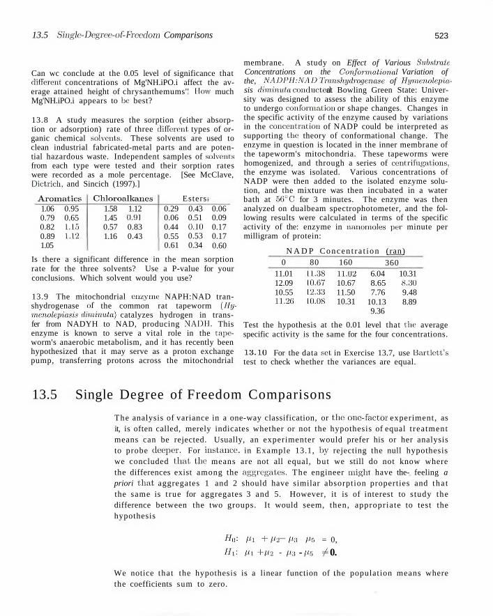
13.5 Single-Degree-of-Freedom Comparisons 523
Can wc conclude at the 0.05 level of significance that different concentrations of Mg'NH.iPO.i affect the average attained height of chrysanthemums'' How much Mg'NH.iPO.i appears to be best?
13.8 A study measures the sorption (either absorption or adsorption) rate of three different types of organic chemical solvents. These solvents are used to clean industrial fabricated-metal parts and are potential hazardous waste. Independent samples of solvents from each type were tested and their sorption rates were recorded as a mole percentage. [See McClave, Dietrich, and Sincich (1997).]
Aroma t i c s 1.06 0.95 0.79 0.65 0.82 1.15 0.89 1.12 1.05
Chloroalkanes 1.58 1.12 1.45 0.91 0.57 0.83 1.16 0.43
0.29 0.06 0.44 0.55 0.61
Esters 0.43 0.51 0.10 0.53 0.34
0.06 0.09 0.17 0.17 0.60
Is there a significant difference in the mean sorption rate for the three solvents? Use a P-value for your conclusions. Which solvent would you use?
13.9 The mitochondrial enzyme NAPH:NAD tran-shydrogenase of the common rat tapeworm (lly-menolepiasis diminuta) catalyzes hydrogen in transfer from NADYH to NAD, producing NADH. This enzyme is known to serve a vital role in the tapeworm's anaerobic metabolism, and it has recently been hypothesized that it may serve as a proton exchange pump, transferring protons across the mitochondrial
membrane. A study on Effect of Various Substrate Concentrations on the Conformational Variation of the, NADPII:NAD Transhydrogenase of Hymenolepia-sis diminutaconducted at Bowling Green State: University was designed to assess the ability of this enzyme to undergo conformation or shape changes. Changes in the specific activity of the enzyme caused by variations in the concentration of NADP could be interpreted as supporting the theory of conformational change. The enzyme in question is located in the inner membrane of the tapeworm's mitochondria. These tapeworms were homogenized, and through a series of centrifugations, the enzyme was isolated. Various concentrations of NADP were then added to the isolated enzyme solution, and the mixture was then incubated in a water bath at 56°C for 3 minutes. The enzyme was then analyzed on dualbeam spectrophotometer, and the following results were calculated in terms of the specific activity of the: enzyme in nanomoles per minute per milligram of protein:
N A D P Concen t r a t i on (ran) 0
11.01 12.09 10.55 11.26
80 11.38 10.07 12.33 10.08
160 11.02 10.67 11.50 10.31
360 6.04 10.31 8.65 8..'it) 7.76 9.48
10.13 8.89 9.36
Test the hypothesis at the 0.01 level that the: average specific activity is the same for the four concentrations.
13.10 For the data set in Exercise 13.7, use Bartlett's test to check whether the variances are equal.
13.5 Single Degree of Freedom Comparisons
The analysis of variance in a one-way classification, or tho one-factor experiment, as it, is often called, merely indicates whether or not the hypothesis of equal t reatment means can be rejected. Usually, an experimenter would prefer his or her analysis to probe deeper. For instance, in Example 13.1, by rejecting the null hypothesis we concluded tha t the means are not all equal, but we still do not know where the differences exist among the aggregates. The engineer might have the- feeling a priori t h a t aggregates 1 and 2 should have similar absorption properties and tha t the same is t rue for aggregates 3 and 5. However, it is of interest to s tudy the difference between the two groups. It would seem, then, appropriate to test the hypothesis
H 0 : px +fi2 - / / / j
Hi: pi + ft2 - //,!
- M6 = 0,
- pr, ? 0.
We notice that the hypothesis is a linear function of the population means where the coefficients sum to zero.
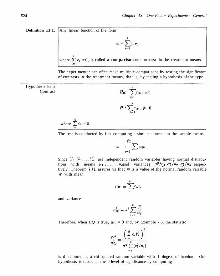
524 Chapter 13 One-Factor Experiments: General
Definition 13.1: Any linear function
k
where YI Ci = 0 , is i = i
of the form
k
t = i
called a comparison
Pi,
or contrast in the treatment means.
The experimenter can often make multiple comparisons by testing the significance of contrasts in the treatment means, that is, by testing a hypothesis of the type
Hypothesis for a Contrast HQ: 22 c*A*j = 0,
i = l
k
Hi: Y^ ciP-i ¥> °i ( = i
where YI ci — 0. » = i
The test is conducted by first computing a similar contrast in the sample means,
fc '«•' = ^Cilji..
i-l
Since Y\,,Y2.,... ,Yk. are independent random variables having normal distributions with means p.i,p.2,...,pk and variances a2/nx,o2/n2,... ,o2/nk, respectively, Theorem 7.11 assures us that w is a value of the normal random variable W with mean
Pw = 22 CiP{
i=i
and variance
J2 _ _2 V ^ Ci
i = l
Therefore, when HQ is true, u\y = 0 and, by Example 7.5, the statistic
W2 £ ciY. i = i
°w *2£(c?M) i=X
is distributed as a chi-squared random variable with 1 degree of freedom. Our hypothesis is tested at the o-level of significance by computing
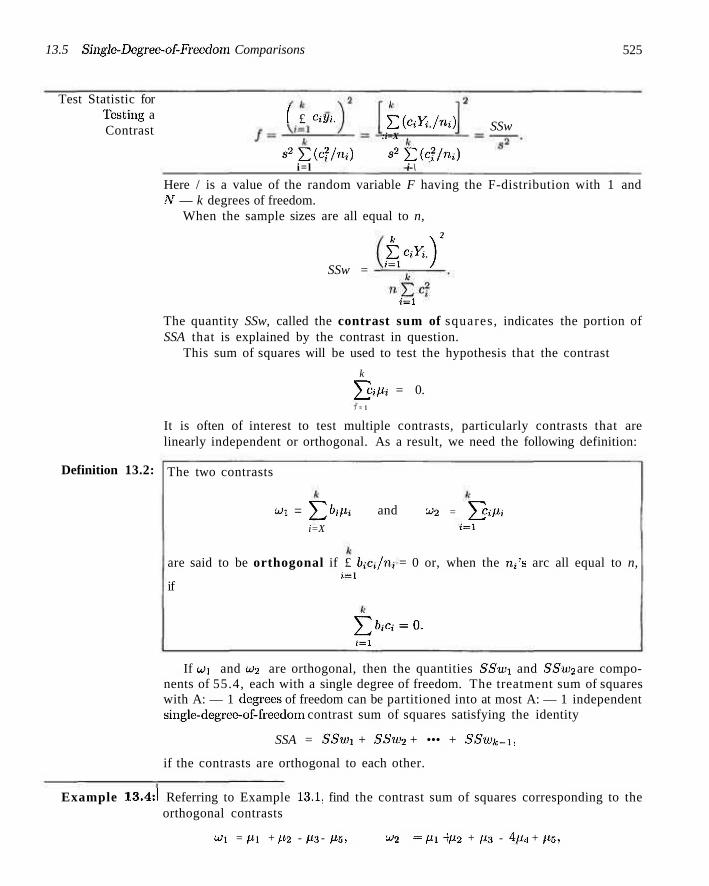
13.5 Single-Degree-of-Freedom Comparisons 525
Test Statistic for Testing a Contrast
YH^/m) :i=X
Definition 13.2:
f £ Civ,.
s2Zic2/n,) S2 £ ( c ? / n 0
i= l i-\
SSw
Here / is a value of the random variable F having the F-distribution with 1 and Ar — k degrees of freedom.
When the sample sizes are all equal to n, 2
SSw = kc'n)' t = l
The quantity SSw, called the contrast sum of squares, indicates the portion of SSA that is explained by the contrast in question.
This sum of squares will be used to test the hypothesis that the contrast
k
^ dpi = 0. 7 = 1
It is often of interest to test multiple contrasts, particularly contrasts that are linearly independent or orthogonal. As a result, we need the following definition:
The two contrasts
wi = \V2 biPi and ^ 2 = ^ CiPi
i=X t = l
are said to be orthogonal if £ biCi/n, = 0 or, when the n;'s arc all equal to n, i-l
if
^ f c ; c ; = 0. ; = i
If W] and LJ2 are orthogonal, then the quantities 55u'i and SSw2 are components of 55.4, each with a single degree of freedom. The treatment sum of squares with A: — 1 degrees of freedom can be partitioned into at most A: — 1 independent single-degrec-of-freedom contrast sum of squares satisfying the identity
SSA = SSwi + SSw2 + ••• + SSwk-i,
if the contrasts are orthogonal to each other.
Example 13.4:1 Referring to Example 13.1, find the contrast sum of squares corresponding to the orthogonal contrasts
Wi = fix + fl2 - p3 - P5, U>2 = pi+ fi2 + ps - 4u4 + fl-5,
526 Chapter 13 One-Factor Experiments: General
and carry out appropriate tests of significance. In this case it is of interest a priori, to compare the two groups (1,2) and (3,5). An important and independent contrast is the comparison between the set of aggregates (1,2,3,5) and aggregate 4.
Solution: It is obvious that the two contrasts are orthogonal, since
(1)(1) + (1)(1) + (-1)(1) + (0)(-4) + (-1)(1) = 0.
The second contrast indicates a comparison between aggregates (1,2,3, and 5) and aggregate 4. We can write two additional contrasts orthogonal to the first two, namely:
w.3 — IH — P2 (aggregate 1 versus aggregate 2),
OJ4 = p-i - Pb (aggregate 3 versus aggregate 5).
From the data of Table 13.1, we have
(3320 + 3416 - 3663 - 3664)2 1 , r r o
SSWi = 6[(l)» + (l)* + ( - l )» + ( - l ) ] = M ' d d 3 :
_ [3320 + 3416 + 3663 + 3664 - 4(2791)]2 _ A " " Q[(l)2 + (l)2 + (l)2 + (l)2 + (-4y\ ~ W^°-
A more extensive analysis-of-variance table is shown in Table 13.5. We note that the two contrast sum of squares account for nearly all the aggregate sum of squares. There is a significant difference between aggregates in their absorption properties, and the contrast U/'i is marginally significant. However, the /-value of 14.12 for u}2
is more significant and the hypothesis
HQ: px + p2 + p3 + (is = 4p4
is rejected.
Table 13.5: Analysis of Variance Using Orthogonal Contrasts
Source of Variation Aggregates (1,2) vs. (3,5) (1,2,3,5) vs. 4
Error Total
Sum of Squares
85,356 J 14,553 \ 70,035
124,021 209,377
Degrees of Freedom
4
l: 25 29
Mean Square 21,339
J14,533 j70,035
4,961
Computed /
4.30 2.93
14.12
Orthogonal contrasts allow the practitioner to partition the treatment variation into independent components. There are several choices available in selecting the orthogonal contrasts except for the last one. Normally, the experimenter would have certain contrasts that are of interest to him or her. Such was the ease in our example, where a priori considerations suggest, that aggregates (1,2) and (3,5)
13.6 Multiple Comparisons 527
constitute distinct groups with different absorption properties, a postulation that was not strongly supported by the significance test. However, the second comparison supports the conclusion that aggregate 4 seems to ilstand out" from the rest. In this case the complete partitioning of 55.4 was not necessary, since two of the four possible independent comparisons accounted for a majority of the variation in treatments.
Figure: 13.3 shows a 5.45 GLM procedure that displays a complete set of orthogonal contrasts. Note that the sum of squares for the four contrasts adds to the aggregate sum of squares, Also, that the latter two contrasts (1 versus 2, 3 versus 5) reveal insignificant comparisons. J
Dependent Variable
Source
Model Error
Corrected
R-0.
Source
aggregate
Source
aggregate
Contrast
(1,2,3,5)
(1,2) vs.
1 vs. 2
3 vs. 5
Total
-Square
.407669
vs. 4
(3,5)
The GLM Procedure
: moisture
DF 4 25 29
C
DF 4
DF 4
DF 1 1 1 1
Sum of Squares
85356.4667
124020.3333 209376.8000
loeff Var
12.53703
Type I SS
85356.46667
Type III SS
85356.46667
Contrast SS
70035.00833
14553.37500
768.00000
0.08333
Mean Square F
21339.1167 4960.8133
Value Pr > F 4.30 0.0088
Root MSE moisture Mean
70.43304
Mean Square
21339.11667
Mean Square
21339.11667
Mean Square
70035.00833
14553.37500
768.00000 0.08333
561.8000
F Value
4.30
F Value
4.30
F Value
14.12
2.93
0.15
0.00
Pr > F
0.0088
Pr > F
0.0088
Pr > F
0.0009
0.0991
0.6973
0.9968
Figure 13.3: A set of orthogonal procedures
13.6 Multiple Comparisons
The analysis of variance is a powerful procedure for testing the homogeneity of a set of means. However, if we reject the null hypothesis and accept the stated alternative that the means are not all equal wc still do noi know which of the population means are equal and which arc different.
In Section 13.5 we describe the use of orthogonal contrasts to make comparisons among sets of factor levels or treatments. The: notion of orthogonality allows the analyst to make tests involving independent contrasts. Thus the variation
528 Chapter 13 One-Factor Experiments: General
among treatments, 55/1, can be partitioned into single-degree-of-freedom components, and then proportions of this variation can be attributed to specific contrasts. However, there are situations in which the use of contrasts is not an appropriate approach. Often it is of interest to make several (perhaps all possible) paired comparisons among the treatments. Actually, a paired comparison may be viewed as a simple contrast, namely, a test of
H0: fn - p.j = 0,
Hf. pi - p.j ji 0,
for all i 7 j. All possible paired comparisons among the means can be very beneficial when particular complex contrasts are not known a priori. For example, in the aggregate data of Table 13.1, suppose that we wish to test
HQ: pi - u$ = 0,
Hi: pi - ps 7^0,
The test is developed through use of an F, t, or a confidence interval approach. Using the t. we have
where s is the square root of the mean square error and n = 6 is the sample size per treatment, In this case
553.33-610.67 , „ t = — . = -1 .41 .
^/4lm^Sl/3 The P-value for the <-test with 25 degrees of freedom is 0.17. Thus there is not sufficient evidence to reject HQ.
Relationship between t and F
In the foregoing we displayed the use of a pooled t-test along the lines of that discussed in Chapter 10. The pooled estimate comes from the mean square error in order to enjoy the degrees of freedom that are pooled across all five samples. In addition, we have tested a contrast. The reader should note that if the lvalue is squared, the result is exactly of the form of the value of / for a test on a contrast discussed in the preceding section. In fact,
, _ im.-Vs.)2 __ (553.33-610.67)2
1 *2(l/6 + l/6) 4961(1/3) '
which, of course, is t2.
Confidence Interval Approach to a Paired Comparison
It is straightforward to solve the same problem of a paired comparison (or a contrast) using a confidence interval approach. Clearly, if we compute a 100(1 — o)%
13.6 Multiple Comparisons 529
confidence interval on pi — p$, we have
Si. -So . ±tD t«/2S\j-,
where tn/2 is the upper 100(1 - a/2)% point of a /.-distribution with 25 degrees of freedom (degrees of freedom coming from s2). This straightforward connection between hypothesis testings and confidence intervals should be obvious from discussions in Chapters 9 and 10. The test of the simple contrast u-x - Po involves no more than observing whether or not the confidence interval above covers zero. Substituting the numbers, we have as the 95% confidence interval
(553.33 - 610.67) ± 2.060\/496Ti/i = -57.34 ± 83.77.
Thus, since the interval covers zero, the contrast is not significant. In other words, we do not. find a significant difference between the means of aggregates 1 and 5.
Experiment-Wise Error Rate
Tukey's Test
We have demonstrated that a simple contrast (i.e., a comparison of two means) can be made through an F-test as demonstrated in Section 13.5, a i-test, or by computing a confidence interval on the difference between the two means. However, serious difficulties occur when the analyst attempts to make many or all possible paired comparisons. For the case of k means, there will be, of course, r — k(k — l ) /2 possible paired comparisons. Assuming independent comparisons, the experiment-wise error rate (i.e., the probability of false rejection of at least one of the hypotheses) is given by 1 — (1 — a)r, where a is the selected probability of type I error for a specific comparison. Clearly, this measure of experiment-wise type I error can be quite large. For example, even if there are only 6 comparisons, say, in the case of 4 means, and o = 0.05, the experiment-wise rate is
1 - (0.95)6 ss 0.26.
With the task of testing many paired comparisons there is usually the need to make the effective contrast on a single comparison more conservative. That is, using the confidence interval approach, the confidence intervals would be much wider than the ±ta/2s\/2/n used for the case where only a single comparison is being made.
There are several standard methods for making paired comparisons that sustain the credibility of the type I error rate. We shall discuss and illustrate two of thern here. The first one, called Tukey's procedure, allows formation of simultaneous 100(1 — a)% confidence intervals for all paired comparisons. The method is based on the studentized range distribution. The appropriate percentile point is a function of a, k, and v = degrees of freedom for s2. A list of upper percentage points for Q = 0.05 is shown in Table A. 12. The method of paired comparisons by Tukey involves finding a significant difference between means i and j (i ^ j) if |jfe. — y~jm\
exceeds 17(0-, k, v] J -.
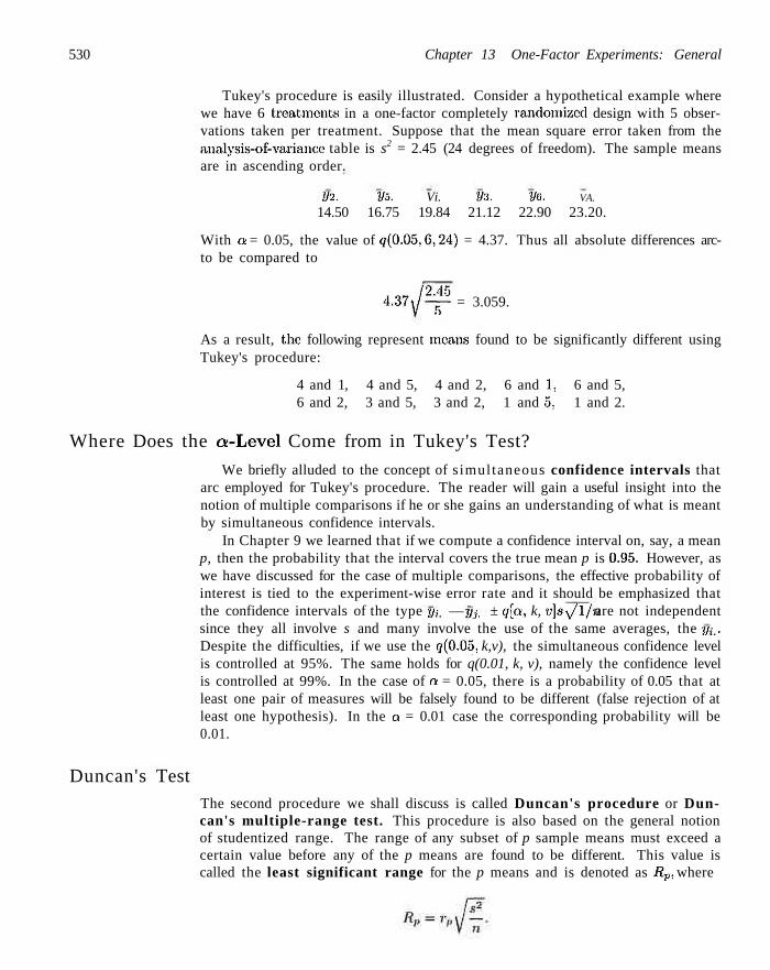
530 Chapter 13 One-Factor Experiments: General
Tukey's procedure is easily illustrated. Consider a hypothetical example where we have 6 treatments in a one-factor completely randomized design with 5 observations taken per treatment. Suppose that the mean square error taken from the analysis-of-variance table is s2 = 2.45 (24 degrees of freedom). The sample means are in ascending order.
])2. Vo. Vi. V'i. Ve. VA.
14.50 16.75 19.84 21.12 22.90 23.20.
With a = 0.05, the value of <7(0.05,6,24) = 4.37. Thus all absolute differences arc-to be compared to
4 . 3 7 1 / - ^ = 3.059.
As a result, the following represent moans found to be significantly different using Tukey's procedure:
4 and 1, 4 and 5, 4 and 2, 6 and 1, 6 and 5, 6 and 2, 3 and 5, 3 and 2, 1 and 5, 1 and 2.
Where Does the a-Level Come from in Tukey's Test?
We briefly alluded to the concept of s imultaneous confidence intervals that arc employed for Tukey's procedure. The reader will gain a useful insight into the notion of multiple comparisons if he or she gains an understanding of what is meant by simultaneous confidence intervals.
In Chapter 9 we learned that if we compute a confidence interval on, say, a mean p, then the probability that the interval covers the true mean p is 0.95. However, as we have discussed for the case of multiple comparisons, the effective probability of interest is tied to the experiment-wise error rate and it should be emphasized that the confidence intervals of the type y,. — fjj. ± q[a, k, v]sy/l/n are not independent since they all involve s and many involve the use of the same averages, the pi,. Despite the difficulties, if we use the q(0.05. k,v), the simultaneous confidence level is controlled at 95%. The same holds for q(0.01, k, v), namely the confidence level is controlled at 99%. In the case of a = 0.05, there is a probability of 0.05 that at least one pair of measures will be falsely found to be different (false rejection of at least one hypothesis). In the a = 0.01 case the corresponding probability will be 0.01.
Duncan's Test The second procedure we shall discuss is called Duncan's procedure or Duncan's multiple-range test. This procedure is also based on the general notion of studentized range. The range of any subset of p sample means must exceed a certain value before any of the p means are found to be different. This value is called the least significant range for the p means and is denoted as Rp, where
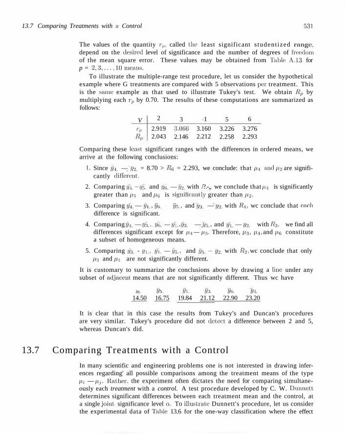
13.7 Comparing Treatments with a Control 531
The values of the quantity rp, called the1 least significant s tudent ized range, depend on the desired level of significance and the number of degrees of freedom of the mean square error. These values may be obtained from Tabic A.13 for p = 2 , 3 , . . . 11.0 means.
To illustrate the multiple-range test procedure, let us consider the hypothetical example where G treatments are compared with 5 observations per treatment. This is the same example as that used to illustrate Tukey's test. We obtain R.v by multiplying each rp by 0.70. The results of these computations are summarized as follows:
V
l'l>
2
2.919 2.043
3
3.06G 2.146
1
3.160 2.212
5
3.226 2.258
6
3.276 2.293
Comparing these least: significant ranges with the differences in ordered means, we arrive at the following conclusions:
1. Since v/4. — f/2. = 8.70 > /?Q = 2.293, we conclude: that //,[ and p2 are significantly differenl.
2. Comparing y4, - 1/5. and i/,;. — y2, with /?.-,, we conclude that ft,\ is significantly greater than fir, and fio is significantly greater than p2.
3. Comparing y4, — yi., j/y. — j/5., and y-j, — y2. with R4, wc conclude that each difference is significant.
4. Comparing j/4, — y-.i,. yo, — yi,, fj-.i. — v/r,., and 1/1. — [/•>. with R.-.i, we find all differences significant except for m — p3. Therefore, fi3, p4, and po constitute a subset of homogeneous means.
5. Comparing y:!. - [/],. yi, — yr,., and §5. — S2. with R2- wc conclude that only ps and ft-i are not significantly different.
It is customary to summarize the conclusions above by drawing a lino under any subset of adjacent means that are not significantly different. Thus wc have
in. TJTJ. S I . S3. Se. Vi. 14.50 16.75 19.84 21.12 22.90 23.20
It is clear that in this case the results from Tukey's and Duncan's procedures are very similar. Tukey's procedure did not detect a difference between 2 and 5, whereas Duncan's did.
13.7 Comparing Treatments with a Control
In many scientific and engineering problems one is not interested in drawing inferences regarding' all possible comparisons among the treatment means of the type Pi — fij. Rather, the experiment often dictates the need for comparing simultaneously each treatment with a control. A test procedure developed by C. W. Dunnett determines significant differences between each treatment mean and the control, at a single joint, significance level a. To illustrate Dunnett's procedure, let us consider the experimental data of Tabic 13.6 for the one-way classification where the effect
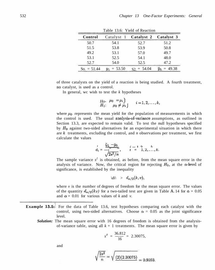
532 Chapter 13 One-Factor Experiments: General
Table 13.6: Yield of Reaction
Control 50.7 51.5 49.2 53.1 52.7
So. = 51.44
Catalyst 1
Si.
54.1 53.8 53.1 52.5 54.0
= 53.50
Catalyst 2
S2.
52.7 53.9 57.0 54.1 52.5
= 54.04
Catalyst 3
2/3
51.2 50.8 49.7 48.0 47.2
= 49.38
of three catalysts on the yield of a reaction is being studied. A fourth treatment, no catalyst, is used as a control.
In general, wc wish to test the k hypotheses
Ho- Po = pA i = 1 ) 2 ) . . . ) j f c ) Hi: po^Pi)
where po represents the mean yield for the population of measurements in which the control is used. The usual analysis-of-variance assumptions, as outlined in Section 13.3, are expected to remain valid. To test the null hypotheses specified by Ho against two-sided alternatives for an experimental situation in which there are A: treatments, excluding the control, and n observations per treatment, we first calculate the values
, Vi. - SO. . - i n I, di = —; , t = 1,2,...,K.
y/2^Jn The sample variance s2 is obtained, as before, from the mean square error in the analysis of variance. Now, the critical region for rejecting Ho, at the a-level of significance, is established by the inequality
\di\ > da/2(k,v),
where v is the number of degrees of freedom for the mean square error. The values of the quantity dn/2(k, v) for a two-tailed test are given in Table A. 14 for o = 0.05 and a = 0.01 for various values of k and v.
Example 13.5:1 For the data of Table 13.6, test hypotheses comparing each catalyst with the control, using two-sided alternatives. Choose a = 0.05 as the joint significance level.
Solution: The mean square error with 16 degrees of freedom is obtained from the analysis-of-variance table, using all k + 1 treatments. The mean square error is given by
, 36.812 s2 = —— = 2.30075,
16
and
m?om=0i9593>
Exercises 333
Hence
, 5 3 . 5 0 - 5 1 . 4 4 (h= 0.9593 =2M'<
«fe- 5 4 - ° 4 - . 5 . 1 - 4 4 = 2.710, 0.9593
49.38 - 51.44 -2.147.
0.9593
From Table A. 14 the critical value for a = 0.05 is found to be
do.025(3,16) = 2.59.
Since \dx\ < 2.59, and \d3\ < 2.59, wc conclude that only the mean yield for catalyst
2 is significantly different from the mean yield of the reaction using the control. J Many practical applications dictate the need for a one-tailed test for comparing
t reatments with a control. Certainly, when a pharmacologist is concerned with the comparison of various dosages of a drug on the effect, of reducing cholesterol level, and his control is zero dosage, it. is of interest to determine if each dosage produces a significantly larger reduction than that of the control. Table A. 15 shows the critical values o{d„(k,v) for one-sided alternatives.
Exercises
13.11 Consider the data of Review Exercise 13.58 on page 568. Make significance tests on the following contrasts:
(a) B versus A, C, and D;
(b) C versus A and D\
(c) A versus D.
13.12 The study Loss of Nitrogen Through Sweat by Preadolescent Boys Consuming Three Levels of Dietary Protein was conducted by the Department of Human Nutrition and Foods at the Virginia Polytechnic Institute and State University to determine perspiration nitrogen loss at, various dietary protein levels. Twelve preadolescent boys ranging in age from 7 years, 8 months to !) years, 8 months, and judged to be clinically healthy, were used in the experiment. Each boy was subjected to one of three controlled diets in which 29. 54, or 84 grams of protein per day were: consumed. The following data represent, the body perspiration nitrogen loss, in milligrams, collected during the last two days of the experimental period:
P r o t e i n Level 29 G r a m s
190 266 270
54 G r a m s 318 295 271 438
84 G r a m s 390 321 390 399
(a) 402
Perform an analysis of variance at the 0.05 level of significance: to show that the mean perspiration nitrogen losses at the three protein levels arc different. Use a single' degree-of-freedom contrast with a = 0.05 to compare the mean perspiration nitrogen loss for boys who consume 29 grams of protein per day versus boys who consume 54 and 84 grams of protein.
13.13 The purpose of the study The Incorporation of a. Chelating Agent into a Flame Retardant Finish of a Cotton Flannelette and the Evaluation of Selected Fabric Properties conducted at the Virginia Polytechnic Institute and State University was to evaluate: the use of a chelating agent as part of the flamc-ictardant finish of cotton flannelette by determining its effects upon
534 Chapter 13 One-Factor Experiments: General
flammability after the fabric is laundered under specific conditions. Two baths were prepared, one with car-boxyinethyl cellulose and one without. Twelve pieces of fabric were laundered 5 times in bath I, and 12 other pieces of fabric were laundered 10 times in bath I. This was repeated using 24 additional pieces of cloth in bath II. After the washings the lengths of fabric: that burned and the burn times were measured. For convenience, let us define the following treatments:
Treatment 1: 5 launderings in bath I,
Treatment 2: 5 launderings in bath II,
Treatment 3: 10 launderings in bath I,
Treatment 4: 10 launderings in bath II.
Burn times, in seconds, were recorded as follows:
Treatment
Blend
1 13.7 23.0 15.7 25.5 15.8 14.8 14.0 29.4 9.7
14.0 12.3 12.3
2 6.2 5.4 5.0 4.4 5.0 3.3
16.0 2.5 1.6 3.9 2.5 7.1
3 27.2 16.8 12.9 14.9 17.1 13.0 10.8 13.5 25.5 14.2 27.4 11.5
4 18.2 8.8
14.5 14.7 17.1 13.9 10.6 5.8 7.3
17.7 18.3 9.9
(a) Perforin an analysis of variance using a 0.01 level of significance and determine whether there are any significant differences among the treatment means.
(b) Use single-degree-of-freedom contrasts with a = 0.01 to compare the mean burn time of treatment 1 versus treatment 2 and also treatment 3 versus treatment 4.
13.14 Use Tukey's test, with a 0.05 level of significance, to analyze the means of the 5 different brands of headache tablets in Exercise 13.4 on page 521.
13.15 For the data used in Review Exercise 13.58 on page 568, perform Tukey's test with a 0.05 level of significance to determine which laboratories differ, on average, in their analysis.
13.16 An investigation was conducted to determine the source of reduction in yield of a certain chemical product. It was known that the loss in yield occurred in the mother liquor, that is. the material removed at the filtration stage. It was felt that different blends of the original material may result in different yield reductions at the mother liquor stage. The following are results of the percent reduction for 3 batches at each of 4 preselected blends:
25.0 24.3 27.9
25.2 28.6 24.7
20.8 26.7 22.2
31.6 29.8 34.3
(a) Perform the analysis of variance at the a = 0.05 level of significance.
(b) Use Duncan's multiple-range test to determine which blends differ.
(c) Do part, (b) using Tukey's test.
13.17 In the study An Evaluation of the Removal Method for Estimating Benthic Populations and Diversity conducted by the Virginia Polytechnic Institute and State University on the Jackson River, 5 different sampling procedures were used to determine the species count. Twenty samples were selected at random and each of the 5 sampling procedures were repeated 4 times. The species counts were recorded as follows:
Sampling Procedure
Depletion 85 55 40 77
Modified Hess
75 45 35 67
Surber 31 20 9
37
Substrate Removal Kick-Kicknet net
43 17 21 10 15 8 27 15
(a) Is there a significant difference in the average species count for the different sampling procedures? Use a P-value in your conclusion.
(b) Use Tukey's test with a = 0.05 to find which sampling procedures differ.
13.18 The following data are values of pressure (psi) in a torsion spring for several settings of the angle be-tween the legs of the spring in a free position:
Angle (°) 67 83 85
71 84 85 85 86 86 87
75 86 87 87 87 88 88 88 88 88 89 90
79 89 90 90 91
83 90 92
Compute a one-way analysis of variance for this experiment and state your conclusion concerning the effect of angle on the pressure in the spring. (C. R. Hicks, Fundamental Concepts in the Design of Experiments, Holt, Rinebart and Winston, New York, 1973.)
13.19 In the following biological experiment 4 concentrations of a certain chemical are used to enhance the growth of a certain type of plant over time. Five
13.8 Comparing a Set of Treatments in Blocks 535
plants are used at each concentration and the growth in each plant is measured in centimeters. The following growth data are taken. A control (no chemical) is also applied.
Concen t r a t i on Con t r
6.8 7.3 6.3 0.9 7.1
ol 1 8.2 8.7 9.4 9.2 8.6
2 7.7 8.4 8.6 8.1 8.0
3 6.9 5.8 7.2 6.8 7,1
4 5.9 6.1 ( i . ' . i
5.7 6.1
Use Dunnett's two-sided icance to simultaneously with the control.
test at the 0.05 level of signif-compare the concentrations
13.20 The following table (A. Ilald, Statistical. Theory with Engineering Applications. John Wiley fc Sons. New York. 1952) gives tensile1 si lengths of deviations from 340 for wires taken from nine cables to be used for a high-voltage network. Each cable is made from 12 wires. We want to know whether the mean strengths of the wires in the nine cables are the same. If the cables are different, which ones differ? Use a /'-value in your analysis of variance.
Cable Tensile S t r e n g t h
1 2 • 3 4-5 6 7 8 9
5 -- 1 1 -
0--12
7 1
- 1 - 1
2
-13 -13 -1.0-
4 1 0 0 0 6
- 5 - 8 -15-
2 5
- 5 2 7 7
- 2 -8
-12 10 0
- 4 I 5 8
-III - 3 -- 2 - 5 10
- 1 - 4 III 15
- 6 -12-- 8 - 8 -
6 0 2 8
11
- 5 -12 -- 5 -12
5 2 7 1
—7
0 - 3 2 -10 5 - 6 -
0 - 4 - 1 0 - 5 - 3 2 0 - 1 -5 1 - 2 5 1 0 2 - 3 6 7 10 7
- 7 -12-—5 -- 3
-10 6
- 4 0 8
—5 -10 -11
0 _2
7 2 5 I
13.21 The printout information in Figure 13.4 on page 530 gives Duncan's test using PROC GLM in SAS for the aggregate data in Example 13.1. Give conclusions regarding paired comparisons using Duncan's test results.
13.22 The financial structure of a firm refers to the way the firm's assets are divided by equity and debt, and the financial leverage refers to the percentage of assets financed by debt. In the paper The Effect of Financial Leverage on Return, Tai Ma of the Virginia
Polytechnic Institute: and State University claims that financial leverage can be used to increase the rate of return on equity. To say it another way, stockholders can receive higher returns on equity with the same amount, of investment by the use: of financial leverage. The following data show the rates of return on equity using 3 different levels of financial leverage' and a control level (zero debt) for 24 randomly selected firms:
F inanc ia l Leverage Con t r
2.1 5.6 3.0 7.8 5.2 2.6
ol Low 6.2 4.0 8.4 2.8 4.2 5.0
M e d i u m 9.6 8.0 5.5
12.6 7.0 7.8
High 10.3 6.9 7.8 5.8 7.2
12.0 Source: Standard & Poor's Machinery Industry Survey, 1975.
(a) Perform the analysis of variance at the 0.05 level of significance. Use Dunnett's test at the 0.01 level of significance to determine whether the mean rates of return on equity at the low, medium, and high levels of financial leverage are higher than at the control level.
(b
13.23 It is suspected that the environmental temperature in which batteries are: activated affects their life. Thirty homogeneous batteries were tested, six at each of five temperatures, and the data are shown below (activated life in seconds). Analyze and interpret the data. (C. R. Hicks, Fundamental Concepts in Design, of Experiments, Holt. Rinehart and Winston. New York, 1973.)
T e m p e r a t u r e (°C) 0 55 55 57 54 54 56
25 60 61 60 60 60 60
50 70 72 72 08 77 77
75 72 72 72 70 68 69
100 65 66 60 64 65 65
13.24 Do Duncan's test for paired comparisons for the data of Exercise 13.8 on page 523. Discuss the results.
13.8 Comparing a Set of Treatments in Blocks
In Section 13.2 we discuss the idea of blocking, tha t is, isolating sets of experimental units that arc reasonably homogeneous and randomly assigning t reatments to these units. This is an extension of the "pairing" concept that is discussed in Chapters
536 Chapter 13 One-Factor Experiments: General
The GLM Procedure Duncan's Multiple Range Test for moisture
NOTE: This t e s t cont ro l s the Type I comparisonwise e r ro r r a t e , not the experimentwise e r ro r r a t e .
Alpha 0.05 Error Degrees of Freedom 25 Error Mean Square 4960.813
Number of Means 2 3 4 5 C r i t i c a l Range 83.75 87.97 90.69 92.61
Means with the same l e t t e r a re not s i g n i f i c a n t l y d i f f e r e n t . Duncan Grouping Mean N aggregate
A 610.67 6 5 A A 610.50 6 3 A A 569.33 6 2 A A 553.33 6 1
B 465.17 6 4
Figure 13.4: SAS printout for Exercises 13.21.
9 and 10 and is done to reduce experimental error, since the units in blocks have characteristics that are more common than units that are in different blocks.
The reader should not view blocks as a second factor, although this is a tempting way of visualizing the design. In fact, the main factor (treatments) still carries the major thrust of the experiment. Experimental units are still the source of error, just as in the completely randomized design. We merely treat sets of these units more systematically when blocking is accomplished. In this way, we say there are restrictions in randomization. For example, for a chemical experiment designed to determine if there is a difference in mean reaction yield among four catalysts, samples of materials to be tested are drawn from the same batches of raw materials, while other conditions, such as temperature and concentration of reactants, are held constant. In this case the time of day for the experimental runs might represent the experimental units, and if the experimenter feels that, there could possibly be a slight time effect, he or she would randomize the assignment of the catalysts to the runs to counteract the possible trend. This type of experimental strategy is the completely randomized design. As a second example of such a design, consider an experiment to compare four methods of measuring a particular physical property of a fluid substance. Suppose the sampling process is destructive; that is, once a sample of the substance has been measured by one method, it cannot be measured again by any of the other methods. If it is decided that 5 measurements are to be taken for each method, then 20 samples of the material are selected from a large
13.9 Randomized Complete Block Designs 537
batch at random and are used in the experiment to compare the four measuring devices. The experimental units are the randomly selected samples. Any variation from sample to sample will appear in the error variation, as measured by s2 in the analysis.
What Is the Purpose of Blocking4!
If the variation due to heterogeneity in experimental units is so large that the sensitivity of detecting treatment differences is reduced due to an inflated value of s2, a better plan might be to "block off" variation due to these units and thus reduce the extraneous variation to that accounted for by smaller or more homogeneous blocks. For example, suppose that in the previous catalyst illustration it is known a priori that there definitely is a significant, day-to-day effect on the yield and that we can measure the yield for four catalysts on a given day. Rather than assign the 4 catalysts to the 20 test runs completely at random, we choose, say, 5 days and run each of the 4 catalysts on each day, randomly assigning the catalysts to the runs within days. In this way the day-to-day variation is removed in the analysis and consequently the experimental error, which still includes any time trend within days, more accurately represents chance variation. Each day is referred to as a block.
The most straightforward of the randomized block designs is one in which we randomly assign each treatment, once to every block. Such an experimental layout is called a randomized complete block design, each block constituting a single replication of the treatments.
13.9 Randomized Complete Block Designs
A typical layout for the randomized complete block design (RCB) using 3 measurements in 4 blocks is as follows:
Block 1 Block 2 Block 3 Block 4
t2
u h
tx h t2
t3
t2
tx
t2
tx h
The t's denote the assignment to blocks of each of the 3 treatments. Of course, the true allocation of treatments to units within blocks is done at random. Once the experiment has been completed, the data can be recorded as in the following 3 x 4 array:
Treatment 1 2 3
Block: 1
Vn J/21
2/31
2
2/12
2/22
2/32
3
2/13
2/23
2/33
4
2/14
2/24
J/34
where yn represents the response obtained by using treatment 1 in block 1, yi2
represents the response obtained by using treatment 1 in block 2, . . . , and y34
represents the response obtained by using treatment 3 in block 4.
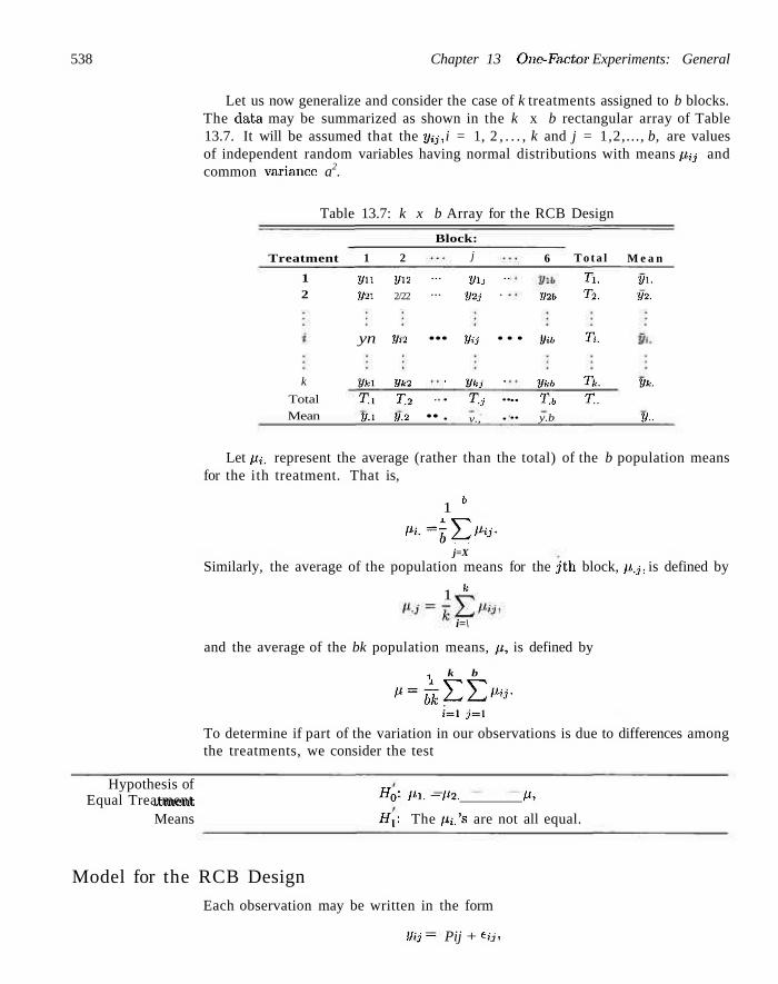
538 Chapter 13 One-Factor Experiments: General
Let us now generalize and consider the case of k treatments assigned to b blocks. The data may be summarized as shown in the k x b rectangular array of Table 13.7. It will be assumed that the y^, i = 1, 2 , . . . , k and j = 1,2,..., b, are values of independent random variables having normal distributions with means p-ij and common variance a2.
Table 13.7: k x b Array for the RCB Design
Treatment
1 2
1
2/ii
2/21
2
J/12
2/22
Block: j
... yij ..
... y2j . .
6
V2b
T o t a l
Ti.
T-2.
M e a n
2/i. y-2.
yn yt2 ••• yu • • • y*b T.
k
Total
Mean
2/fci
Ti
V-i
2/fc2 T2 ..
y.2 ••
' 2/fej '
• T.j ••
• v., •
ykb
•• T.b
•• y.b
Tk.
T. Vk.
V-
Let pi. represent the average (rather than the total) of the b population means for the ith treatment. That is,
1 b
^-= 1^2^' j=X
Similarly, the average of the population means for the j th block, p.j, is defined by
1 k
i=\
and the average of the bk population means, u, is defined by
1 k b
^=^EE^-»=i j = i
To determine if part of the variation in our observations is due to differences among the treatments, we consider the test
Hypothesis of ttment Means Hx: The /Zj.'s are not all equal.
Equal Treatment H*' (l1- ~ f'2- **»
Model for the RCB Design
Each observation may be written in the form
Vij — Pij + eij)
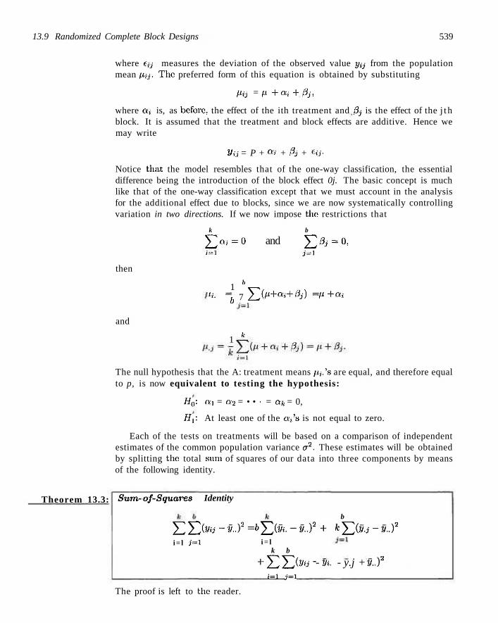
13.9 Randomized Complete Block Designs 539
where e-,j measures the deviation of the observed value yy from the population mean pij. The preferred form of this equation is obtained by substituting
Pij = p + ai + 0j,
where ct< is, as before, the effect of the ith treatment and 3j is the effect of the j t h block. It is assumed that the treatment and block effects are additive. Hence we may write
Vij = P + a> + Pj + Uy
Notice that the model resembles that of the one-way classification, the essential difference being the introduction of the block effect 0j. The basic concept is much like that of the one-way classification except that we must account in the analysis for the additional effect due to blocks, since we are now systematically controlling variation in two directions. If we now impose the restrictions that
k b
] T o , = 0 and ^ ^ = 0 , ;=1 j=\
then
and
1 b
ii. = 7 E ^ + ai + "•>) = fl + Q '» b
1 k
The null hypothesis that the A: treatment means //,.'s are equal, and therefore equal to p, is now equivalent to testing the hypothesis:
H0: ai = a2 = • • • = ak = 0,
H\: At least one of the Q,'S is not equal to zero.
Each of the tests on treatments will be based on a comparison of independent estimates of the common population variance a2. These estimates will be obtained by splitting the total sum of squares of our data into three components by means of the following identity.
Theorem 13.3: Sum- of-Squares Identity
EI>-3-) 2
i= l j = l =&X>'-^")2
i = l k b
+EE(^-i=i j=\
b
+ kY,iy~3-y-)2
- m. - y.j + y..f
The proof is left to the reader.
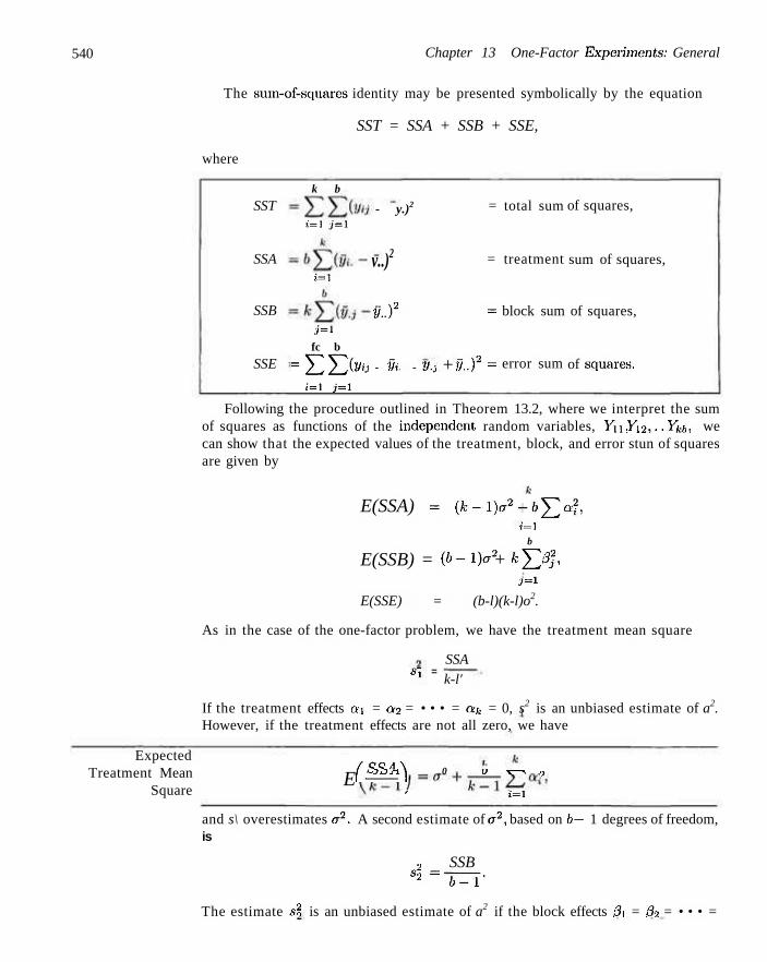
540 Chapter 13 One-Factor Experiments: General
The sum-of-sqtiares identity may be presented symbolically by the equation
SST = SSA + SSB + SSE,
where
SST
SSA
SSB
SSE
k b
i=i j = i
i = i
i=i fc b
-ED* i = l j=l
- y.)2
v..)2
y.f
- Hi. - V-3 + v..?
= total sum
= treatment
= block sum
= error sum
of squares,
sum of squares,
of squares,
of squares.
Following the procedure outlined in Theorem 13.2, where we interpret the sum of squares as functions of the independent random variables, Yu, Yi2,..., Y^i,, we can show that the expected values of the treatment, block, and error stun of squares are given by
E(SSA) = (k-l)o2+bJ2a2, i = i
b
E(SSB) = (b-l)o2 + kJ2 3], j = i
E(SSE) = (b-l)(k-l)o2.
As in the case of the one-factor problem, we have the treatment mean square
S, = SSA k-l'
If the treatment effects Qi = a2 = • • • = a*, = 0, s2 is an unbiased estimate of a2. However, if the treatment effects are not all zero, we have
Expected Treatment Mean
Square E
fSSA\ W / l \ 0 O V—v 9
' i = i
and s\ overestimates er2. A second estimate of a2, based on b— 1 degrees of freedom, is
2 SSB S2 = b^T'
The estimate .s2, is an unbiased estimate of a2 if the block effects 3i = b\ = • • • =
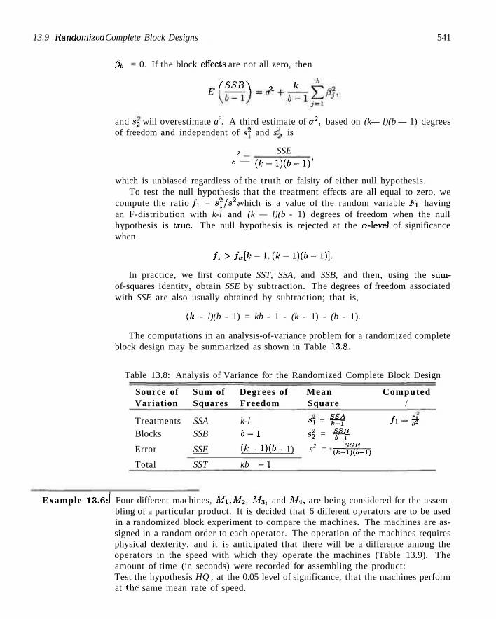
13.9 Randomized Complete Block Designs 541
,3i, = 0. If the block effects are not all zero, then
_{SSB\ 9 k E
and s2 will overestimate a2. A third estimate of <72, based on (k— l)(b — 1) degrees of freedom and independent of s2 and s2, is
2 SSE s — (k-l)(b-l)-
which is unbiased regardless of the truth or falsity of either null hypothesis. To test the null hypothesis that the treatment effects are all equal to zero, we
compute the ratio f\ = s2/s2, which is a value of the random variable Fi having an F-distribution with k-l and (k — l)(b - 1) degrees of freedom when the null hypothesis is true. The null hypothesis is rejected at the a-Ievel of significance when
/ i > / « [ f c - l , ( * - l ) ( 6 - l ) ] .
In practice, we first compute SST, SSA, and SSB, and then, using the sum-of-squares identity, obtain SSE by subtraction. The degrees of freedom associated with SSE are also usually obtained by subtraction; that is,
(A: - l)(b - 1) = kb - 1 - (k - 1) - (b - 1).
The computations in an analysis-of-variance problem for a randomized complete block design may be summarized as shown in Table 13.8.
Table 13.8: Analysis of Variance for the Randomized Complete Block Design
Source of Sum of Degrees of Mean Computed Variation Squares Freedom Square /
Treatments SSA k-l *i = f r f / i = f* Blocks SSB 6 - 1 s\ = | f f
Error SSE (fe - l)(b - 1) s2 = ( j d r f h )
Total SST kb -1
Example 13.6:1 Four different machines, Mi, M2, M3, and M4, are being considered for the assembling of a particular product. It is decided that 6 different operators are to be used in a randomized block experiment to compare the machines. The machines are assigned in a random order to each operator. The operation of the machines requires physical dexterity, and it is anticipated that there will be a difference among the operators in the speed with which they operate the machines (Table 13.9). The amount of time (in seconds) were recorded for assembling the product: Test the hypothesis HQ , at the 0.05 level of significance, that the machines perform at the same mean rate of speed.
542 Chapter 13 One-Factor Experiments: General
Table 13.9: Time, in Seconds, to Assemble Product
Operator Machine
1 2 3 4
Total
1
42.5 39.8 40.2 41.3 1G3.8
2
39.3 40.1 40.5 42.2
162.1
3
39.6 40.5 41.3 43.5
164.9
4
39.9 42.3 43.4 44.2
169.8
5
42.9 42.5 44.9 45.9 176.2
6
43.6 43.1 45.1 42.3
174.1
Total 247.8 248.3 255.4 259.4
1010.9
Solution: HQ: O] = o_2 = 0 3 = a4 = 0 (machine effects are zero),
Hi: At least one of the Oj's is not equal to zero.
The sum-of-squares formulas shown on page 540 and the degrees of freedom are used to produce the analysis of variance in Table 13.10. The value / = 3.34 is significant at P = 0.048. If we use a = 0.05 as at least an approximate yardstick, we conclude that the machines do not perform at the same mean rate of speed. _l
Table 13.10: Analysis of Variance for the Data of Table 13.9
Source of Variation
Machines Operators Error
Total
Sum of Squares
15.93 42.09 23.84
81.86
Degrees of Freedom
3 5
15 23
Mean Square
5.31 8.42 1.59
Computed /
3.34
Further Comments Concerning Blocking
In Chapter 10 we present a procedure for comparing means when the observations were paired. The procedure involved "subtracting out" the effect due to the homogeneous pair and thus working with differences. This is a special case of a randomized complete block design with k = 2 treatments. The n homogeneous units to which the treatments were assigned take on the role of blocks.
If there is heterogeneity in the experimental units, the experimenter should not be misled into believing that it is always advantageous to reduce the experimental error through the use of small homogeneous blocks. Indeed, there may be instances where it would not be desirable to block. The purpose in reducing the error variance is to increase the sensitivity of the test for detecting differences in the treatment means. This is reflected in the power of the test procedure. (The power of the analysis-of-variance test procedure is discussed more extensively in Section 13.13.) The power for detecting certain differences among the treatment means increases with a decrease in the error variance. However, the power is also affected by the degrees of freedom with which this variance is estimated, and blocking reduces the degrees of freedom that are available from k(b — 1) for the one-way classification
13.9 Randomized Complete Block Designs 543
CD
C O
CL O 0_
Block 1
h
Treatments (a)
c CO CD
C o Block 2 ts
C L O
Block 1
Block 2
h Treatments
(b)
Figure 1.3.5: Population means for (a) additive results, and (b) interacting effects.
to (k — l)(b — 1). So one could lose power by blocking if there is not a significant reduction in the error variance.
Interaction between Blocks and Treatments Another important assumption that is implicit in writing the moelol for a randomized complete block design is that the treatment and block effects are assumed to be additive. This is equivalent to stating that
tHj - fHj' = I'fj - Pi'j' Pij ~ Pi'j = Pi p « 3
for every value of i, /', j , and j ' . That is, the difference between the population means for blocks j and f is the same for every treatment and the difference between the population means for treatments i and i! is the same for every block. The parallel lines of Figure 13.5(a) illustrate a Bet of mean responses lor which the treatment and block effects are additive, whereas the intersecting lines of Figure 13.5(b) show a situation in which treatment and block effects arc said to interact . Referring to Example L3.6, if operator 3 is 0.5 seconds faster on the average than operator 2 when machine 1 is used, then operator 3 will still be 0.5 seconds faster on the average than operator 2 when machine 2, 3, or 4 is used. In many experiments the assumption of additivity does not hold and the analysis of Section 13.9 leads to erroneous conclusions. Suppose, for instance, that operator 3 is 0.5 seconds faster on the average than operator 2 when machine: 1 is used but is 0.2 second slower on the average than operator 2 when machine 2 is used. The operators and machines are now interacting.
An inspection of Table 13.9 suggests the presence of possible interaction. This apparent interaction may be real or it may be due to experimental error. The analysis of Example 13.G was based on the assumption that the apparent interaction was due entirely to experimental error. If the total variability of our data was in part due to an interaction effect, this source of variation remained a part of the error sum of squares, causing the mean square e r ror to overes t imate er2,
544 Chapter 13 One-Factor Experiments: General
and thereby increasing the probability of committing a type II error. We have, in fact, assumed an incorrect model. If we let (c\3)jj denote the interaction effect of the rth treatment and the j th block, we can write a more appropriate model in the form
yij = p +cn + 8j + (a8)ij + eij,
on which we impose the additional restrictions
k I,
J>/?)«i = £ > ; % = 0. (=i j=\
We can now readily verify that
SSE E
( 6 - l ) ( * - l )
1 k t>
(6-D(*-uEEMft-
Thus the mean square error is seen to be a biased es t imate of a2 when existing interaction has been ignored. It would seem necessary at this point to arrive at a procedure for the detection of interaction for cases where there is suspicion that it exists. Such a procedure requires the availability of an unbiased and independent estimate of er2. Unfortunately, the randomized block design docs not lend itself to such a test unless the experimental setup is altered. This subject is discussed extensively in Chapter 14.
13.10 Graphical Me thods and Model Checking
In several chapters we make reference to graphical procedures displaying data and analytical results. In early chapters we used stem-and-leaf and box-and-whisker plots as visuals that aid in summarizing samples. We use similar diagnostics to better understand the data in two sample problems in Chapters 9 and 10. In Chapter 9 we introduce the notion of residual plots (ordinary and studentized residuals) to detect violations of standard assumptions. In recent years much attention in data analysis has centered on graphical methods . Like regression, analysis of variance lends itself to graphics that aid in summarizing data as well as detecting violations. For example, a simple plotting of the raw observations around each treatment mean can give the analyst a feel for variability between sample means and within samples, Figure 13.6 depicts such a plot, for the aggregate data of Table 13.1. By the appearance of the plot one might even gain a graphical insight about, which aggregates (if any) stand out from the others. It is clear that aggregate 4 stands out from the others. Aggregates 3 and 5 certainly form a homogeneous group, as do aggregates 1 and 2.
As in the case of regression, residuals can be helpful in analysis of variance in providing a diagnostic that may detect violations of assumptions. To form the residuals, we merely need to consider the model of the one-factor problem, namely
ijij =pi + eij.
13.10 Graphical Methods and Model Checking 545
/t>v
700
650
| 600
o 550 5
500 450
400
*
*
+y^
•
t
•
hz • «
* t +y3
•
*
•
•
?4 + • •
• t *
ys+ •
*
1 2 3 4 5
Aggregate
Figure 13.6: Plot of data around the mean for the aggregate data of Table 13.1.
(0 - g u> a>
CC
200
150
100
50
0
-50
-100
-150
Aggregate
Figure 13.7: Plots of residuals for five aggregates, using data in Table 13.1.
It is straightforward to determine that the estimate of pi is y~i.. Hence the ijth residual is y~i. — ij... This is easily extendable to the randomized complete block model. It may be instructive to have the residuals plotted for each aggregate in order to gain some insight regarding the homogeneous variance assumption. This plot is shown in Figure 13.7.
Trends in plots such as these may reveal difficulties in some situations, particularly when the violation of a particular assumption is graphic. In the case of Figure 13.7, the residuals seem to indicate that the within-treatment variances are reasonably homogeneous apart from aggregate 1. There is some graphical evidence that the variance for aggregate 1 is larger than the rest.
What Is a Residual for a RCB Design? The randomized complete block is another experimental situation in which graphical displays can make the analyst feel comfortable with an "ideal picture," or
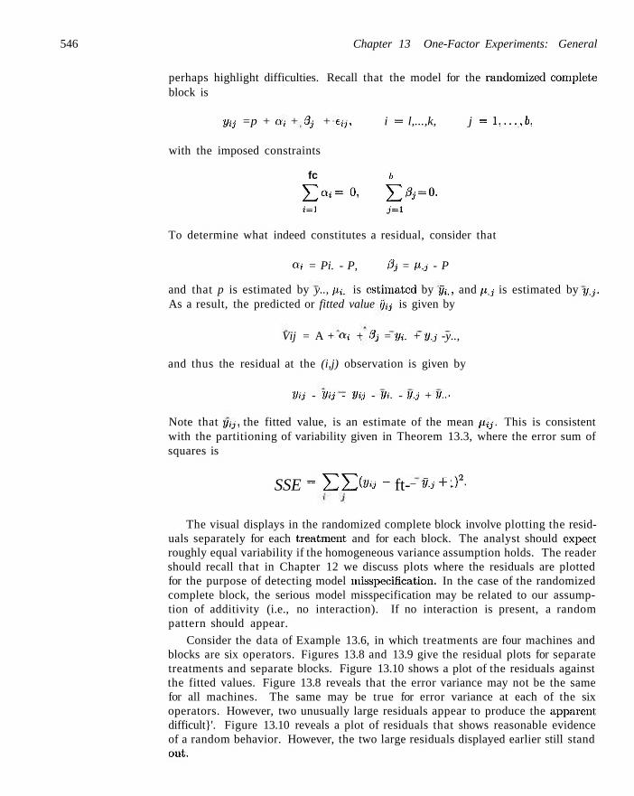
546 Chapter 13 One-Factor Experiments: General
perhaps highlight difficulties. Recall that the model for the randomized complete block is
Vij =p + a, + 33- + e,j, i = l,...,k, j = l,...,b,
with the imposed constraints
fc /,
£a, = 0, E ^ = 0-i=i j=i
To determine what indeed constitutes a residual, consider that
Qi = Pi. - P, 8j = P.j - P
and that p is estimated by y.., fn. is estimated by j / , . , and p.j is estimated by y.j. As a result, the predicted or fitted value tjij is given by
Vij = A + ®i + 3j = yi. + y.j -y..,
and thus the residual at the (i,j) observation is given by
Vij - Vij - Vij - vi. - y.j + y..-
Note that y,j, the fitted value, is an estimate of the mean u, j . This is consistent with the partitioning of variability given in Theorem 13.3, where the error sum of squares is
SSE = EE<»« - ft-_ y-i+v -)2-
The visual displays in the randomized complete block involve plotting the residuals separately for each treatment, and for each block. The analyst should expect roughly equal variability if the homogeneous variance assumption holds. The reader should recall that in Chapter 12 we discuss plots where the residuals are plotted for the purpose of detecting model misspecification. In the case of the randomized complete block, the serious model misspecification may be related to our assumption of additivity (i.e., no interaction). If no interaction is present, a random pattern should appear.
Consider the data of Example 13.6, in which treatments are four machines and blocks are six operators. Figures 13.8 and 13.9 give the residual plots for separate treatments and separate blocks. Figure 13.10 shows a plot of the residuals against the fitted values. Figure 13.8 reveals that the error variance may not be the same for all machines. The same may be true for error variance at each of the six operators. However, two unusually large residuals appear to produce the apparent difficult}'. Figure 13.10 reveals a plot of residuals that shows reasonable evidence of a random behavior. However, the two large residuals displayed earlier still stand out.
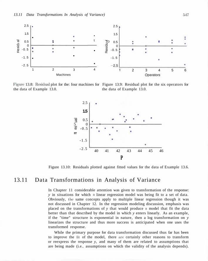
13.11 Data Transformations In Analysis of Variance) 547
IS 3
'55 ti) rr
2.5
1.5
0.5 0
- 0 . 5
- 1 . 5
- 2 . 5
*
•
* *
•
1
•
2
Machines
*
*
•
3
•
t
•
• 4
TO
'55
CC
2.5
1.5
0.5 0
-0 .5
- 1 . 5
-?fi 2 3 4 5 6
Operators
Figure 13.8: Residual plot for the: four machines for Figure 13.9: Residual plot for the six operators for the data of Example 13.0. the data of Example 13.0.
2.5
1.5
"§ 0.5 5 0 tu -0 .5 rr
-1 .5
-2 .5 40 41 42 43 44 45 46
P Figure 13.10: Residuals plotted against fitted values for the data of Example 13.6.
13.11 Data Transformations in Analysis of Variance
In Chapter 11 considerable attention was given to transformation of the response: y in situations for which a linear regression model was being fit to a set of data. Obviously, the same concepts apply to multiple linear regression though it was not discussed in Chapter 12. In the regression modeling discussion, emphasis was placed on the transformations of y that would produce a model that fit the data better than that described by the model in which y enters linearly. As an example, if the "time" structure is exponential in nature, then a log transformation on y linearizes the structure and thus more success is anticipated when one uses the transformed response.
While the primary purpose for data transformation discussed thus far has been to improve the lit of the model, there arc certainly other reasons to transform or reexpress the response y, and many of them are related to assumptions that are being made (i.e.. assumptions on which the validity of the analysis depends).
548 Chapter 13 One-Factor Experiments: General
One very important assumption in analysis of variance is the homogeneous variance assumption discussed quite early in Section 13.4. We assume a common variance ex2. If the variance differs a great deal from treatment to treatment and we perform the standard ANOVA discussed in this chapter (and future chapters), the results can be substantially flawed. In other words, the analysis of variance is not robust to the assumption of homogeneous variance. As we have discussed thus far, this is the center piece of motivation for the residual plots discussed in last section and illustrated in Figures 13.8, 13.9, and 13.10. These plots allow us to detect nonhomogeneous variance problems. However, what do we do about them? How can we accommodate them?
Where Does Nonhomogeneous Variance Come From?
Often, but not always, nonhomogeneous variance in ANOVA is present because of the distribution of the responses. Now, of course we assume normality in the response. But there certainly are situations in which tests on means are needed even though the distribution of the response is one of those nonnormal distributions discussed in Chapters 5 and 6, e.g., Poisson, lognormal. exponential, gamma, and so on. ANOVA-type problems certainly exist with count data, time to failure data and so on.
Wc demonstrated in Chapters 5 and 6 that, apart from the normal case, the variance of a distribution will often be a function of the mean, say a2 = g(pi)- For example, in the Poisson case Var(Yi) = pi = a2 (i.e., the variance is equal to the mean). In the case of the exponential distribution, the Var(Yj) — a2 — p2 (i.e., the variance is equal to the square of the m.ean). For the case of the lognormal a log transformation produces a normal distribution with constant variance a2.
The same concepts that we used in Chapter 4 to determine the variance of a nonlinear function can be used as an aid to determine the nature of the variance stabilizing transformation g(yt). Recall from the first order Taylor Series expansion 0 1 oiVi) around j/,- = p, when g'(pi) — %'"' . The transformation function
I »* liji=iii
g(y) must be independent of p in order that it suffice as the variance stabilizing transformation. From the above
Var[g(Ui)} = [g'(pi)}2af.
As a result, g(yi) must be such that g'ipi) oc £. Thus, if we suspect that the
response is Poisson distributed, ai = uj , so g'(fii) ex - ^ j . Thus the variance t*i
stabilizing transformation becomes g(yi) = yi . From this illustration and similar manipulation for the exponential and gamma distributions, we have the following.
Distribution Variance Stabilizing Transformations Poisson g(y) = y1/2
Exponential g(y) = lnt/ Gamma g(y) = lny
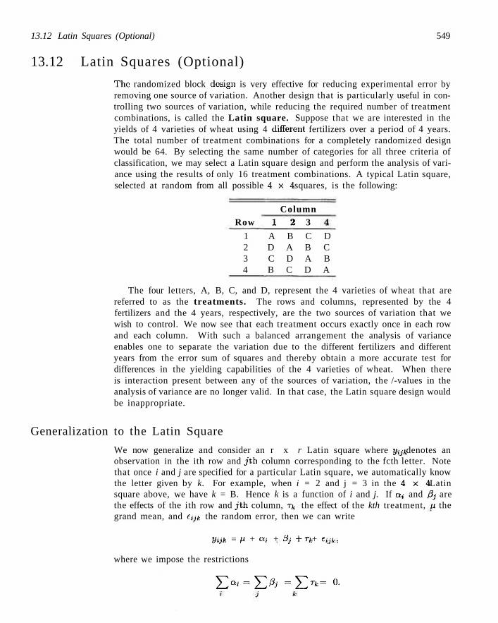
13.12 Latin Squares (Optional) 549
13.12 Latin Squares (Optional)
The randomized block design is very effective for reducing experimental error by removing one source of variation. Another design that is particularly useful in controlling two sources of variation, while reducing the required number of treatment combinations, is called the Latin square. Suppose that we are interested in the yields of 4 varieties of wheat using 4 different fertilizers over a period of 4 years. The total number of treatment combinations for a completely randomized design would be 64. By selecting the same number of categories for all three criteria of classification, we may select a Latin square design and perform the analysis of variance using the results of only 16 treatment combinations. A typical Latin square, selected at random from all possible 4 x 4 squares, is the following:
Column Row 1 2 3
1 A B C D 2 D A B C 3 C D A B 4 B C D A
The four letters, A, B, C, and D, represent the 4 varieties of wheat that are referred to as the treatments. The rows and columns, represented by the 4 fertilizers and the 4 years, respectively, are the two sources of variation that we wish to control. We now see that each treatment occurs exactly once in each row and each column. With such a balanced arrangement the analysis of variance enables one to separate the variation due to the different fertilizers and different years from the error sum of squares and thereby obtain a more accurate test for differences in the yielding capabilities of the 4 varieties of wheat. When there is interaction present between any of the sources of variation, the /-values in the analysis of variance are no longer valid. In that case, the Latin square design would be inappropriate.
Generalization to the Latin Square
We now generalize and consider an r x r Latin square where y^ denotes an observation in the ith row and j t h column corresponding to the fcth letter. Note that once i and j are specified for a particular Latin square, we automatically know the letter given by k. For example, when i = 2 and j = 3 in the 4 x 4 Latin square above, we have k = B. Hence k is a function of i and j. If a» and 0j are the effects of the ith row and j t h column, TA, the effect of the kth treatment, u the grand mean, and e;jfc the random error, then we can write
Vijk = p + on + 3j +rk + djk,
where we impose the restrictions
T,^ = J2^ = E^ =
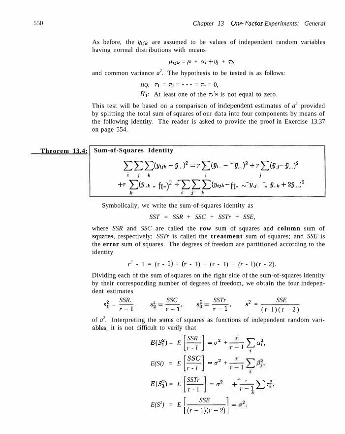
550 Chapter 13 One-Factor Experiments: General
As before, the yjjk are assumed to be values of independent random variables having normal distributions with means
Pijk = fl + Cti+ 0j + Tk
and common variance a2. The hypothesis to be tested is as follows:
HQ: Ti = r2 = • • • = r r = 0,
Hi: At least one of the r;'s is not equal to zero.
This test will be based on a comparison of independent estimates of a2 provided by splitting the total sum of squares of our data into four components by means of the following identity. The reader is asked to provide the proof in Exercise 13.37 on page 554.
Theorem 13.4: Sum-of-Squares Identity
EEEfow*-&. . ) a = r E(f t - " y-)2+rJ2^- -ft-)2
1 j k i j
+r E(ft* - ft-)2 + /)2'Y2E^y* - ft- ~ y-j- - y-k+2^-)2
Symbolically, we write the sum-of-squares identity as
SST = SSR + SSC + SSTr + SSE,
where SSR and SSC are called the row sum of squares and column sum of squares, respectively; SSTr is called the treatment sum of squares; and SSE is the error sum of squares. The degrees of freedom are partitioned according to the identity
r2 - 1 = (r - 1) + (r - 1) + (r - 1) + (r - l)(r - 2).
Dividing each of the sum of squares on the right side of the sum-of-squares identity by their corresponding number of degrees of freedom, we obtain the four independent estimates
SSR. , SSC - SSTr , SSE s2 =
r-l' r-l r-l" s2 =
( r - l ) ( r - 2 )
of a2. Interpreting the sums of squares as functions of independent random variables, it is not difficult to verify that
E(S2) = E
E(Sl) = E
E(S2) = E
E(S2) = E
SSR
r - l
SSC
r - l
SSTr
= a2 +
= a2 +
T E«*
r - l
SSE
3
= - +—iX<T^
L(r- l )(r-2)J
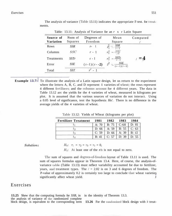
Exercises 551
The analysis of variance (Tabic 13.11) indicates the appropriate F-test. for treatments.
Table: 13.11: Analysis of Variance for an r x r Latin Square
Source of Variation
Rows
Columns
Treatments
Error
Total
Stun of Squares
SSR
SSC
SSTr
SSE
SST
Degrees of Freedom
r- I
r - 1
r - l
( r - l ) ( r -
r2 - 1
-2)
M e a n Square
.2 SSR •st - 7 = T „2 _ SSC S2 - ,-1
•2 _ SSTr \ ' i - , _ |
„2 _ SSE " - (r-l)t>-2)
C o m p u t e d /
/ = 4
Example 13.7:1 To illustrate the analysis of a Latin square design, let us return to the experiment where the letters A, B, C. and D represent 1 varieties of wheat: the rows represent 4 different fertilizers; and the columns account for 4 different, years. The data in Table 13.12 arc the yields for the 4 varieties of wheat, measured in kilograms per plot. It is assumed that the various sources of variation do not interact. Using a 0.05 level of significance, test the hypothesis Ho'. There is no difference in the average yields of the 4 varieties of wheat.
Table 13.12: Yields of Wheat (kilograms per plot)
Fertilizer Treatment 1981 1982 1983 1984 h t-2 h h
A: 70 D: 66 C: 59 B: 41
B: 75 A: 59 D: 66 C: 57
C:68 B: 55 A: 39 D: 39
D: 81 C: 63 B: 12 D: 55
Solution: HQ: TI = r2 = r3 = T, = 0,
Hi'. At least one of the n's is not equal to zero.
The sum of squares and degrees-of-freedom layout of Table 13.11 is used. The sum of squares formulas appear in Theorem 13.4. Here, of course, the analysis-of-variance tabic (Table 13.13) must reflect variability accounted for due to fertilizer, years, and treatment types. The / = 2.02 is on 3 and 6 degrees of freedom. The P-value of approximately 0.2 is certainly too large to conclude that wheat varieties significantly affect wheat yield. J
Exercises
13.25 Show that the computing formula for SSB, in in the identity of Theorem 13.3. the analysis of variance of the randomized complete block design, is equivalent to the corresponding term 13.26 For the randomized block design with k treat-
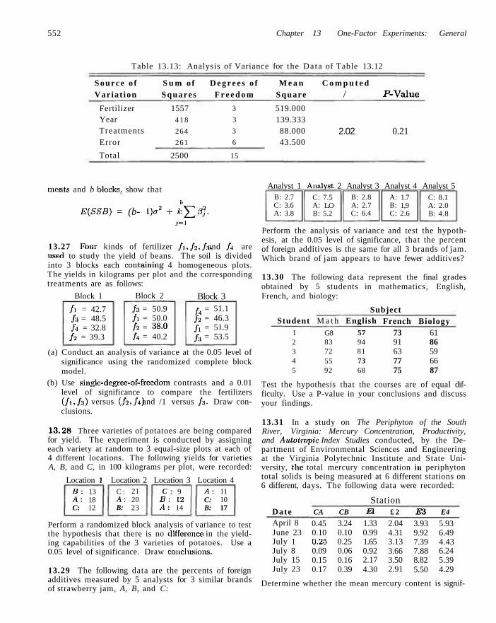
552 Chapter 13 One-Factor Experiments: General
Table 13.13: Analysis of Variance for the Da ta of Table 13.12
Source o f S u m o f D e g r e e s o f M e a n Variat ion Squares F r e e d o m Square
C o m p u t e d / P-Value
Fertilizer Year Treatments Error
Total
1557 4 1 8
264
261
2500
3
3
3
6
15
519.000 139.333 88.000 43.500
2.02 0.21
ments and b blocks, show that
i,
E(SSB) = (b- l)o2 + k^2$• j = i
13.27 Four kinds of fertilizer f\,f2,fa, and f4 are usesd to study the yield of beans. The soil is divided into 3 blocks each containing 4 homogeneous plots. The yields in kilograms per plot and the corresponding treatments are as follows:
Analyst 1 Analyst. 2 Analyst 3 Analyst 4 Analyst 5
Block 1 Block 2
fi = 42.7 h = 48.5 /., = 32.8 f2 = 39.3
h = 50.9 h = 50.0 h = 38.0 h = 40.2
Block 3
u h h h
= 51.1 = 46.3 = 51.9 = 53.5
(a) Conduct an analysis of variance at the 0.05 level of significance using the randomized complete block model.
(b) Use single-degree-of-freedom contrasts and a 0.01 level of significance to compare the fertilizers (/1./3) versus (f2,f4) and /1 versus /3- Draw conclusions.
13.28 Three varieties of potatoes are being compared for yield. The experiment is conducted by assigning each variety at random to 3 equal-size plots at each of 4 different locations. The following yields for varieties A, B, and C, in 100 kilograms per plot, were recorded:
Location 1 Location 2 Location 3 Location 4 B; A: C:
13 18 12
C : A: B:
21 20 23
C B: A:
9 12 14
A: C: B:
11 10 17
Perform a randomized block analysis of variance to test the hypothesis that there is no difference in the yielding capabilities of the 3 varieties of potatoes. Use a 0.05 level of significance. Draw conclusions.
13.29 The following data are the percents of foreign additives measured by 5 analysts for 3 similar brands of strawberry jam, A, B, and C:
B: C: A:
2.7 3.6 3.8
C: A: B:
7.5 L.O 5.2
B: A: C:
2.8 2.7 6.4
A: B: C:
1.7 1,9 2.6
C: A: B:
8.1 2.0 4.8
Perform the analysis of variance and test the hypothesis, at the 0.05 level of significance, that the percent of foreign additives is the same for all 3 brands of jam. Which brand of jam appears to have fewer additives?
13.30 The following data represent the final grades obtained by 5 students in mathematics, English, French, and biology:
Subject Student
1 2 3 4 5
M a t h
G8 83 72 55 92
English 57 94 81 73 68
French Biology 73 61 91 86 63 59 77 66 75 87
Test the hypothesis that the courses are of equal difficulty. Use a P-value in your conclusions and discuss your findings.
13.31 In a study on The Periphyton of the South River, Virginia: Mercury Concentration, Productivity, and Autoimpic Index Studies conducted, by the Department of Environmental Sciences and Engineering at the Virginia Polytechnic Institute and State University, the total mercury concentration in periphyton total solids is being measured at 6 different stations on 6 different, days. The following data were recorded:
Station Date April 8 June 23 July 1 July 8 July 15 July 23
CA
0.45 0.10 0.25 0.09 0.15 0.17
CB
3.24 0.10 0.25 0.06 0.16 0.39
El
1.33 0.99 1.65 0.92 2.17 4.30
£ 2
2.04 4.31 3.13 3.66 3.50 2.91
E3
3.93 9.92 7.39 7.88 8.82 5.50
E4
5.93 6.49 4.43 6.24 5.39 4.29
Determine whether the mean mercury content is signif-
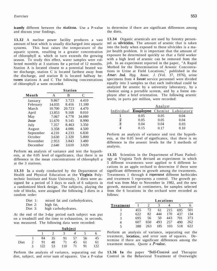
Exercises 553
icantly different between the stations, and discuss your findings.
Use a P-value
13.32 A nuclear power facility produces a vast amount of heat which is usually discharged into aquatic systems. This heat raises the temperature of the aquatic system, resulting in a greater concentration of chlorophyll o, which in turn extends the growing season. To study this effect, water samples were collected monthly at 3 stations for a period of 12 months. Station A is located closest to a potential heated water discharge, station C is located farthest away from the discharge, and station B is located halfway between stations A and C The following concentrations of chlorophyll a were recorded.
Station Month
January February March April May June July August September October November December
A
9.867 14.035 10.700 13.853 7.067
11.670 7.357 3.358 4.210 3.630 2.953 2.640
B
3.723 8.416
20.723 9.168 4.778 9.145 8.463 4.086 4.233 2.320 3.843 3.610
C
4.410 11.100 4.470 8.010
34.080 8.990 3.350 4.500 6.830 5.800 3.480 3.020
Perform an analysis of variance and test the hypothesis, at the 0.05 level of significance, that there is no difference in the mean concentrations of chlorophyll a at the 3 stations.
13.33 In a study conducted by the Department of Health and Physical Education at the Virginia Polytechnic Institute and State University, 3 diets were assigned for a period of 3 days to each of 6 subjects in a randomized block design. The subjects, playing the role of blocks, were assigned the following 3 diets in a random order:
Diet 1: mixed fat and carbohydrates, Diet 2: high fat, Diet 3: high carbohydrates.
At the end of the 3-day period each subject was put on a treadmill and the time to exhaustion, in seconds, was measured. The following data were recorded:
Subject
Diet
Perform the analysis of variance, separating out the diet, subject, and error sum of squares. Use a P-value
1 2 3
1 84 91
122
2 35 48 53
3 91 71
110
4 57 45 71
5 56 61 91
6 45 61
122
to determine if there are significant differences among the diets.
13.34 Organic arsenicals are used by forestry personnel as silvicides. The amount of arsenic that is taken into the body when exposed to these silvicides is a major health problem. It is important that the amount of exposure be determined quickly so that a field worker with a high level of arsenic can be removed from the job. In an experiment reported in the paper, "A Rapid Method for the Determination of Arsenic Concentrations in Urine at Field Locations," published in the Amer. Ind. Hyg. Assoc. J. (Vol. 37, 1976), urine specimens from 4 forest service personnel were divided equally into 3 samples so that each individual could be analyzed for arsenic by a university laboratory, by a chemist using a portable system, and by a forest employee after a brief orientation. The following arsenic levels, in parts per million, were recorded:
Ana lys t Ind iv idua l E m p l o y e e C h e m i s t L a b o r a t o r y
0.05 0.05 0.04 0.15
0.05 0.05 0.04 0.17
0.04 0.04 0.03 0.10
Perform an analysis of variance and test the hypothesis, at the 0.05 level of significance, that there is no difference in the arsenic levels for the 3 methods of analysis.
13.35 Scientists in the Department of Plant Pathology at Virginia Tech devised an experiment in which 5 different treatments were applied to 6 different locations in an apple orchard to determine if there were significant differences in growth among the treatments. Treatments 1 through 4 represent different herbicides and treatment 5 represents a control. The growth period was from May to November in 1982, and the new growth, measured in centimeters, for samples selected from the 6 locations in the orchard were recorded as follows:
Treatment 1 2 3 4 5
Perform an analysis of variance, separating out the treatment, location, and error sum of squares. Determine if there are significant differences among the treatment means. Quote a P-valuc.
13.36 In the paper "Self-Control and Therapist Control in the Behavioral Treatment of Overweight
1 455 622 695 607 388
2 72 82 56
650 263
Locations 3 61
444 50
493 185
4 215 170 443 257 103
5 695 437 701 490 518
6 501 134 373 262 622
554 Chapter 13 One-Factor Experiments: General
Women," published in Behavioral Research and Therapy (Vol. 10, 1972), two reduction treatments and a control treatment were studied lor their effects on the weight change of obese women. The two reduction treatments involved were, respectively, a self-induced weight reduction program and a therapist-controlled reduction program. Each of 10 subjects were assigns*! to the 3 treatment programs in a random order and measured for weight loss. The following weight changes were recorded:
Treatment Subject Control Self-induced Therapist Worker
13.40 A manufacturing firm wants to investigate the effects of 5 color additives on the setting time of a new concrete mix. Variations in the setting times can be expected from day-to-day changes in temperature and humidity and also from the different workers who prepare the test molds. To eliminate these extraneous sources of variation, a 5 x 5 Latin square design was used in which the letters A, B, C, D, and E represent the 5 additives. The setting times, in hours, for the 25 molds are shown in the following table.
Day
1 2 3 4 5 6 7 8 9
10
1.00 3.75 0.00
-0.25 -2.25 -1.00 -1.00
3.75 1.50 0.50
-2.25 -6.00 -2.00 -1.50 -3.25 -1.50
-10.75 -0.75
0.00 -3.75
-10.50 -13.50
0.75 -4.50 -6.00
4.00 -12.25
-2.75 -6.75 -7.00
Perform an analysis of variance and test the hypothesis, at the 0.01 level of significance, that there is no difference in the mean weight losses for the 3 treatments. Which treatment was best?
13.37 Verify the sum-of-squares identity of Theorem 13.4 on page 550.
13.38 For the r x r Latin square design, show that
E(SSTr) = (r l)cr2 + r ^ r l .
13.39 The mathematics department of a large university wishes to evaluate the teaching capabilities of 4 professors. In order to eliminate any effects due to different mathematics courses and different times of the day, it was decided to conduct an experiment using a Latin square design in which the letters A, B, C, and D represent the 4 different professors. Each professor taught one section of each of 4 different courses scheduled at each of 4 different times during the day. The following data show the grades assigned by these professors to 16 students of approximately equal ability. Use a 0.05 level of significance to test the hypothesis that different professors have no effect on the grades.
Course Time
1 2 3 4
Algebra A: 84 B: 91 C:59 D: 75
Geometry B: 79 C: 82 D: 70 A: 91
Statistics C: 63 D: 80 A: 77 B: 75
Calculus D: 97 A: 93 B: 80 C: 68
D: 10.7 E: 10.3 E:11.3 C:10.5 A: 11.8 B:10.9 B: 14.1 A: 11.6 C: 14.5 D:11.5
B: 11.2 D:12.0 C: 10.5 E: 11.0 A: 11.5
A: 10.9 C: 10.5 B:11.5 A: 10.3 D:11.3 E: 7.5 G11.7 D:11.5 E: 12.7 B: 10.9
At the 0.05 level of significance, can we say that the color additives have any effect on the setting time of the concrete mix?
13.41 In the book Design of Experiments for the Quality Improvement published by the Japanese Standards Association (1989), a study on the amount of dye needed to get the best color for a certain type of a fabric was conducted. The three amounts of dye, \% wof ( 1 % of the weight of a fabric), 1% wof, and 3% wof, were each administered at two different plants. The color density of a fabric was then observed four times for each level of dye at each plant.
Plant 1
Plant 2
1/3% 5.2 6.0 5.9 5.9 6.5 5.5 6.4 5.9
Amount of Dye 1% " 3%
12.3 10.5 12.4 10.9 14.5 11.8 16.0 13.6
22.4 17.8 22.5 18.4 29.0 23.2 29.7 24.0
Perform an analysis of variance to test the hypothesis, at the 0.05 level of significance, that there is no difference in the color density of a fabric for the three levels of dye. Consider plants to be blocks.
13.42 An experiment was conducted to compare three types of coating materials for copper wire. The purpose of the coating is to eliminate "flaws" in the wire. Ten different specimens of length five millimeters were randomly assigned to receive each coating process and the thirty specimens were subjected to an abrasive wear type process. The number of flaws was measured for each and the results are as follows:
Material 1 2 3
6 7 7
8 7 8
4 9
5 6
3 2 4
3 4 3
5 4
4 5
12 18 8
8 6 5
7 7
14 18
13.13 Random Effects Models 555
Show whatever findings suggest a conclusion. Suppose it is assumed that the Poisson process applies (c) Do a plot of the residuals and comment, and thus the model is Ytj = fit + ey. where fn is the (d) G i v e t h e p u r p o S e 0f your data transformation, mean of a Poisson distribution and at = «;. , , ,,., , .. . , . . , , t.
*•' (ej What additional assumption is made here that may (a) Do an appropriate transformation on the data and not have been completely satisfied by your trans-
perform an analysis of variance. formation? (b) Determine whether or not there is sufficient evi- (f) Comment on (e) after doing a normal probability
dence to choose one coating material over the other. plot on the residuals.
13.13 Random Effects Models
Throughout this chapter we deal with analysis-of-variance procedures in which the primary goal is to study the effect on some response of certain fixed or predetermined treatments. Experiments in which the treatments or treatment levels are preselected by the experimenter as opposed to being chosen randomly are called fixed effects experiments or model I experiments. For the fixed effects model, inferences are made only on those particular treatments used in the experiment.
It is often important that the experimenter be able to draw inferences about a population of treatments by means of an experiment in which the treatments used are chosen randomly from the population. For example, a biologist may be interested in whether or not there is a significant variance in some physiological characteristic due to animal type. The animal types actually used in the experiment are then chosen randomly and represent the treatment effects. A chemist may be interested in studying the effect of analytical laboratories on the chemical analysis of a substance. He is not concerned with particular laboratories but rather with a large population of laboratories. He might then select a group of laboratories at random and allocate samples to each for analysis. The statistical inference would then involve (1) testing whether or not the laboratories contribute a nonzero variance to the analytical results, and (2) estimating the variance due to laboratories and the variance within laboratories.
Model and Assumptions for Random Effects Model
The one-way random effects model, often referred to as model II, is written like the fixed effects model but with the terms taking on different meanings. The response
Vij= p + CM + tij
is now a value of the random variable
Yij =fi + Ai + Eij,
with i = 1,2,... ,k and j = 1,2,... ,n where the A»'s are normally and independently distributed with mean zero and variance a2 and are independent of the Eij's. As for the fixed effects model, the Ey's are also normally and independently-distributed with mean zero and variance a2. Note that for a model II experiment,
556 Chapter 13 One-Factor Experiments: General
Theorem 13.5:
k k the random variable ^ Ai assumes the value J2 ai'-> anc^ the constraint that these
t'=l i = l
Q,'s sum to zero no longer applies.
For the one-way random effects analysis-of-variance model,
E(SSA) = (k- l)a2 + n(k - l)o£ and E(SSE) = k(n - 1)<T2.
Table 13.14 shows the expected mean squares for both a model I and a model II experiment. The computations for a model II experiment are carried out in exactly the same way as for a model I experiment. That is, the sum-of-squares, degrees-of-freedom, and mean-square columns in an analysis-of-variance table are the same for both models.
Table 13.14: Expected Mean Squares for the One-Factor Experiment
Source of Variation Treatments
Error Total
Degrees of Freedom
k-l
k{n - 1) nk - 1
Mean Squares
4 s2
Expected Mean Squares Model I Model II
*2 + F ^ £ ° ? o2+na2a
i
a2 a2
For the random effects model, the hypothesis that the treatment effects are all zero is written as follows:
Hypothesis for a Model II
Experiment
HQ: a2a = 0,
Hi: oifiO.
This hypothesis says that the different treatments contribute nothing to the variability of the response. It is obvious from Table 13.14 that s2 and s2 are both estimates of a2 when HQ is true and that the ratio
s4
is a value of the random variable F having the F-distribution with k—l and k(n — 1) degrees of freedom. The null hypothesis is rejected at the a-level of significance wdien
/>/Q[fc-l ,fc(n-l)] .
In many scientific and engineering studies, interest is not centered on the jF-test. The scientist knows that the random effect does, indeed, have a significant effect. What is more important is estimation of the various variance components. This produces a sense of ranking in terms of what factors produce the most variability and by how much. In the present context it may be of interest to quantify how much larger the single-factor variance component is than that produced by chance (random variation).
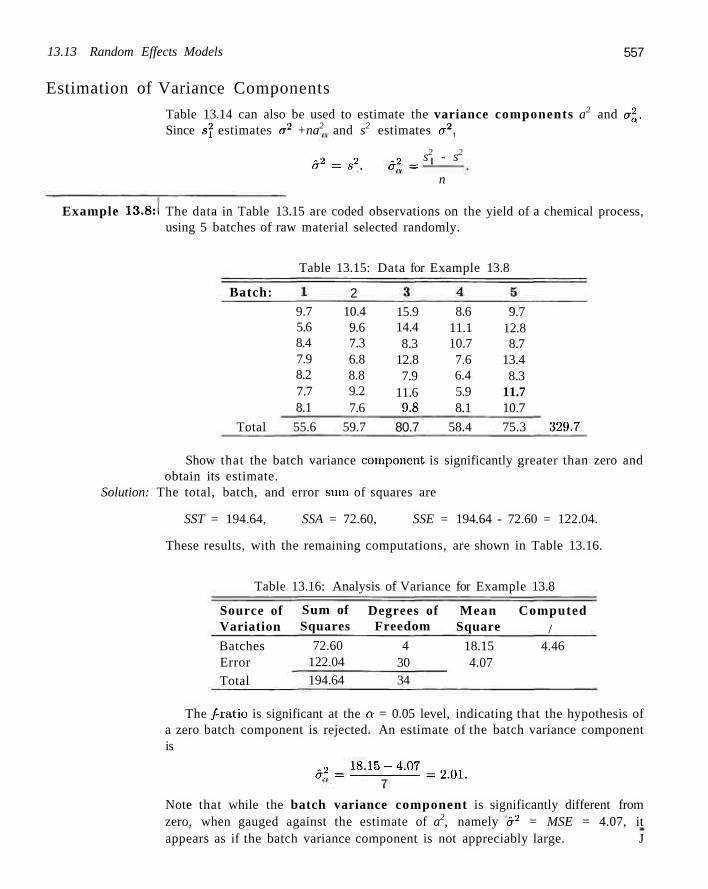
13.13 Random Effects Models 557
Estimation of Variance Components
Table 13.14 can also be used to estimate the variance components a2 and a2^. Since s\ estimates a2 +na2 and s2 estimates a2,
a2 = s2. a2 = s2 - s2
n
Example 13.8:1 The data in Table 13.15 are coded observations on the yield of a chemical process, using 5 batches of raw material selected randomly.
Table 13.15: Data for Example 13.8
Batch: 2 9.7 5.6 8.4 7.9 8.2 7.7 8.1
10.4 9.6 7.3 6.8 8.8 9.2 7.6
15.9 14.4 8.3
12.8 7.9
11.6 9.8
8.6 11.1 10.7 7.6 6.4 5.9 8.1
9.7 12.8 8.7
13.4 8.3
11.7 10.7
Total 55.6 59.7 80.7 58.4 75.3 329.7
Show that the batch variance component is significantly greater than zero and obtain its estimate.
Solution: The total, batch, and error stun of squares are
SST = 194.64, SSA = 72.60, SSE = 194.64 - 72.60 = 122.04.
These results, with the remaining computations, are shown in Table 13.16.
Table 13.16: Analysis of Variance for Example 13.8
Source of Variation
Batches Error Total
Sum of Squares
72.60 122.04 194.64
Degrees of Freedom
4 30 34
Mean Square
18.15 4.07
Computed /
4.46
The /-ratio is significant at the a = 0.05 level, indicating that the hypothesis of a zero batch component is rejected. An estimate of the batch variance component is
<f>-=»=M.-uz. Note that while the batch variance component is significantly different from zero, when gauged against the estimate of a2, namely a2 = MSE = 4.07, it appears as if the batch variance component is not appreciably large. J
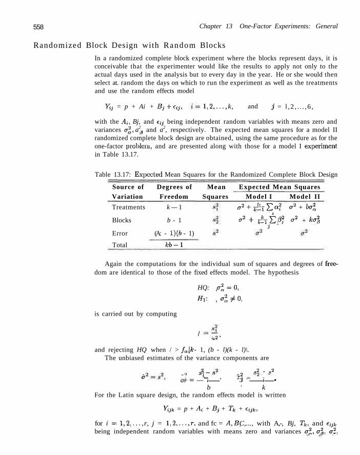
558 Chapter 13 One-Factor Experiments: General
Randomized Block Design with Random Blocks
In a randomized complete block experiment where the blocks represent days, it is conceivable that the experimenter would like the results to apply not only to the actual days used in the analysis but to every day in the year. He or she would then select at. random the days on which to run the experiment as well as the treatments and use the random effects model
Yij = p + Ai + Bj+eij, 1,2,... , k, and j = l , 2 , . . . , 6 ,
with the Ai, Bj, and etj being independent random variables with means zero and variances a2, a2, and a2, respectively. The expected mean squares for a model II randomized complete block design are obtained, using the same procedure as for the one-factor problem, and are presented along with those for a model I experiment in Table 13.17.
Table 13.17: Expected Mean Squares for the Randomized Complete Block Design
Source of Degrees of Mean Expected Mean Squares Variation Freedom Squares Model I Model II
Treatments k — 1
Blocks b - 1
Error (A: - 1)(6 - 1)
a2 + '-l2Zaf a2 + ba2a
°2 + £itp* a2 + ka\
Total kb-l
Again the computations for the individual sum of squares and degrees of freedom are identical to those of the fixed effects model. The hypothesis
HQ: a2x=0,
Hi: a2^0,
is carried out by computing
/ .•2'
and rejecting HQ when / > fa[k - 1, (b - l)(k - l)\. The unbiased estimates of the variance components are
a2 „1 Si
ai = — r? _ 9? - «2
~i ' "3 ~ i • b ' k
For the Latin square design, the random effects model is written
Yijk = p + Af + Bj + Tk + eijk,
for i = 1,2,. . . , r, j = 1,2,.. . ,r, and fc = A,B, C,..., with A,-, Bj, Tk, and eyfe being independent random variables with means zero and variances a2, a'i, a2,
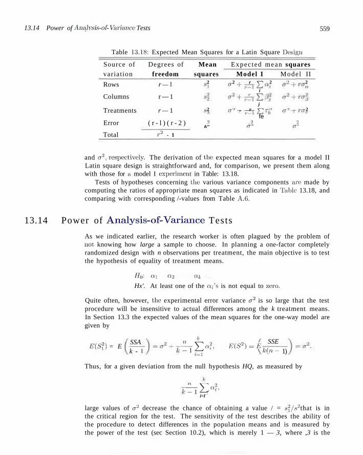
13.14 Power of Analysis-of-Variance Tests 559
Table 13.18: Expected Mean Squares for a Latin Square Dewign
Source of Degrees of Mean Expec ted mean squares variat ion freedom squares Model I Model II
2 2 i r V^ 2 } i 2
i
j 2 ^ , r " i '> , 2
fe 2 — 2 2
A'" r r - CT
Rows r — I
Columns r — 1
Treatments r — 1
Error ( r - l ) ( r - 2 )
Total T* - 1
and a2, respectively. The derivation of the expected mean squares for a model II Latin square design is straightforward and, for comparison, we present them along with those for a model I experiment in Table: 13.18.
Tests of hypotheses concerning the various variance components arc made by computing the ratios of appropriate mean squares as indicated in Tabic 13.18, and comparing with corresponding /-values from Table A.6.
13.14 Power of Analysis-of-Variance Tests
As we indicated earlier, the research worker is often plagued by the problem of not knowing how large a sample to choose. In planning a one-factor completely randomized design with n observations per treatment, the main objective is to test the hypothesis of equality of treatment means.
H Q : e i ' i = a 2 = • • • O k = 0 ,
Hx'. At least one of the a,-'s is not equal to zero.
Quite often, however, the experimental error variance a2 is so large that the test procedure will be insensitive to actual differences among the k treatment means. In Section 13.3 the expected values of the mean squares for the one-way model are given by
E(S2) = E SSA k - I
^Y.o2. E(S2)=E ? = i
SSE
kin- 1)
Thus, for a given deviation from the null hypothesis HQ, as measured by
n ^ ., • 3 T 2 > '
i=l
large values of a2 decrease the chance of obtaining a value / = s2/s2 that is in the critical region for the test. The sensitivity of the test describes the ability of the procedure to detect differences in the population means and is measured by the power of the test (sec Section 10.2), which is merely 1 — 3, where ,3 is the
560 Chapter 13 One-Factor Experiments: General
probability of accepting a false hypothesis. We can interpret the power of our analysis-of-variance tests, then, as the probability that the F-statistic is in the critical region when, in fact, the null hypothesis is false and the treatment means do differ. For the one-way analysis-of-variance test, the power, 1 — 3, is
l-0 = P S2
-^ > faivuv-i) when Hx is true
S2 k
^ > faivi,v2) when ^ a f = 0 i=\
The term fa(v\, v2) is, of course, the upper-tailed critical point of the F-distribution k
with vx and v2 degrees of freedom. For given values of ]T ct2/(k - 1) and a2, the t = i
power can be increased by using a larger sample size n. The problem becomes one of designing the experiment with a value of n so that the power requirements
k are met. For example, we might require that for specific values of 52 a2 =£ 0 and
j = i
a2, the hypothesis be rejected with probability 0.9. When the power of the test is low, it severely limits the scope of the inferences that can be drawn from the experimental data.
Fixed Effects Case
In the analysis of variance the power depends on the distribution of the F-ratio under the alternative hypothesis that the treatment means differ. Therefore, in the case of the one-way fixed effects model, we require the distribution of S2/S2
when, in fact.
5>^0' i=\
Of course, when the null hypothesis is true, a; = 0 for i = 1,2, ...,k, and the statistic follows the F-distribution with k — 1 and N — k degrees of freedom. If
k 53 a2 T 0, the ratio follows a noncentral F-distribution. i = l
The basic random variable of the noncentral Fis denoted by F . Let fa(vx, v2, A) be a value of F with parameters Vi, v2, and A. The parameters vi and v2 of the distribution are the degrees of freedom associated with S2 and S2, respectively, and A is called the noncentrality parameter. When A = 0, the noncentral F simply reduces to the ordinary F-distribution with vi and v2 degrees of freedom.
For the fixed effects, one-way analysis of variance with sample sizes m, n2,..., n/t we define
1 k
= ^ 2 £ n ^ ' 2er2
i= i
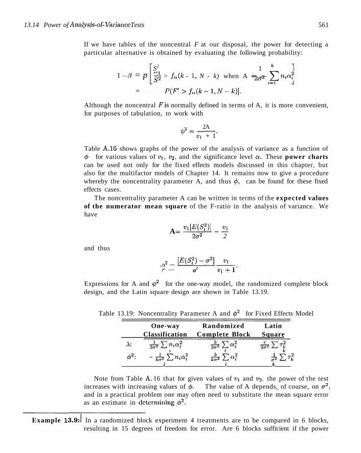
13.14 Power of Analysis-of-Variance Tests 561
If we have tables of the noncentral F at our disposal, the power for detecting a particular alternative is obtained by evaluating the following probability:
i - a = p S2 1 k
•^ > faik - I, N - k) when A = — ^ m a 2
i=i
= P(F'>fa(k.-l,N-k)}.
Although the noncentral F is normally defined in terms of A, it is more convenient, for purposes of tabulation, to work with
2 2A V Vi + 1
Table A.16 shows graphs of the power of the analysis of variance as a function of (f> for various values of t'i, v2, and the significance level a. These power charts can be used not only for the fixed effects models discussed in this chapter, but also for the multifactor models of Chapter 14. It remains now to give a procedure whereby the noncentrality parameter A, and thus d>, can be found for these fixed effects cases.
The noncentrality parameter A can be written in terms of the expected values of the numerator mean square of the F-ratio in the analysis of variance. We have
and thus
Expressions for A and 4>2 for the one-way model, the randomized complete block design, and the Latin square design are shown in Table 13.19.
Table 13.19: Noncentrality Parameter A and <p2 for Fixed Effects Model
One-way Randomized Latin Classification Complete Block Square
°2'- ktztnta2 ^ £ « ? ^£T2
i i k
Note from Table A. 16 that for given values of vi and t'2, the power of the test increases with increasing values of <f>. The value of A depends, of course, on a2, and in a practical problem one may often need to substitute the mean square error as an estimate in determining o2.
A
^2 v —
vi\E(S2)\ 2er2
[E(S2)-a2\ a2 i
Vl
2
Vl
' i + l
Example 13.9:1 In a randomized block experiment 4 treatments are to be compared in 6 blocks, resulting in 15 degrees of freedom for error. Are 6 blocks sufficient if the power
562 Chapter 13 One-Factor Experiments: General
of our test for detecting differences among the treatment means, at the 0.05 level of significance, is to be at least 0.8 when the true means are p\. = 5.0, p2. = 7.0, p3, = 4.0, and p4. = 4.0? An estimate of a2 to be used in the computation of the power is given by a2 = 2.0.
Solution: Recall that the treatment means are given by pi. = p. + a;. If we invoke the 4
restriction that 52 o» = 0- w e have «=i
-I
M= j ^2 Hi. =5 .0 , <=i
and then Q] = 0, 02 = 2.0, a3 = —1.0, and a4 = —1.0. Therefore,
2 b ^ 2 (6)(6)
1 = 1
from wdiich we obtain <b = 2.121. Using Table A. 16, the power is found to be approximately 0.89, and thus the power requirements are met. This means that if
<i
the value of 52 of = 6 and a2 = 2.0, the use of 6 blocks will result in rejecting the i=l
hypothesis of equal treatment means with probability 0.89. J
Random Effects Case
In the fixed effects case, the computation of power requires the use of the noncentral F-distribution. Such is not, the case in the random effects model. In fact, the power is computed very simply by the use of the standard F-tables. Consider, for example, the one-way random effects model, n observations per treatment, with the hypothesis
H0: crl = 0,
Hi: o**0.
When H\ is true, the ratio
SSA/[(k-l)(a2 + na2a)] s2
f SSE/[k(n - l)a2] s 2(! + nal/a2)
is a value of the random variable F having the F-distribution with k— 1 and k(n— 1) degrees of freedom. The problem becomes one, then, of determining the probability of rejecting Ho under the condition that the true treatment variance component a2 j£ 0. We have then
1 - 0 = p | | | > fa[k - 1,k(n - 1)] when Hi is t rue!
S2 s /a[fc-l,fc(n-l)n = P{-
\S ,2(l-rner2v/CT2) l + na2/a2
I 1 + nalja2 J
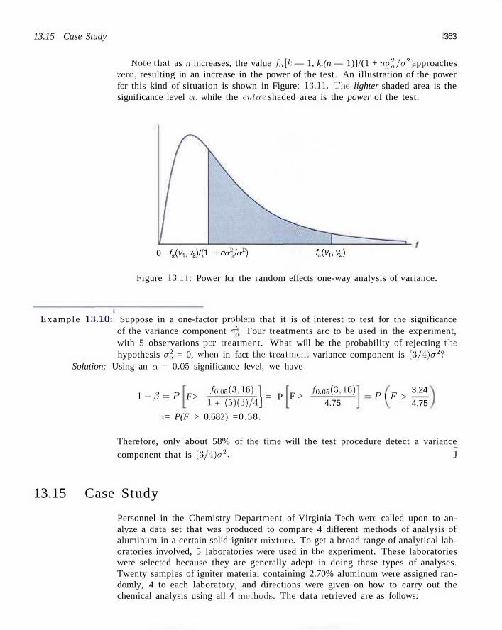
13.15 Case Study 363
Note that, as n increases, the value /a[fe — 1, k.(n — 1)]/(1 + no2./a2) approaches zero, resulting in an increase in the power of the test. An illustration of the power for this kind of situation is shown in Figure; 13.11. The lighter shaded area is the significance level a, while the entire shaded area is the power of the test.
0 fa(v„ „2)/<1 +nar*fo*) 4(vi, vz)
Figure 13.11: Power for the random effects one-way analysis of variance.
Example 13.10:1 Suppose in a one-factor problem that it is of interest to test for the significance of the variance component a2. Four treatments arc to be used in the experiment, with 5 observations pe r treatment. What will be the probability of rejecting the hypothesis a2 = 0, when in fact the treatment variance component is (3/4)<r2?
Solution: Using an a = 0.05 significance level, we have
1-3-P F> /o.or,(3,16)
l + (5)(3)/4j
= P(F > 0.682) =0.58.
= P F > ./0.Q5(3,16)
4.75 P[F>
3.24
4.75
Therefore, only about 58% of the time will the test procedure detect a variance
component that is (3/4)ff2. J
13.15 Case Study
Personnel in the Chemistry Department of Virginia Tech were called upon to analyze a data set that was produced to compare 4 different methods of analysis of aluminum in a certain solid igniter mixture. To get a broad range of analytical laboratories involved, 5 laboratories were used in the experiment. These laboratories were selected because they are generally adept in doing these types of analyses. Twenty samples of igniter material containing 2.70% aluminum were assigned randomly, 4 to each laboratory, and directions were given on how to carry out the chemical analysis using all 4 methods. The data retrieved are as follows:
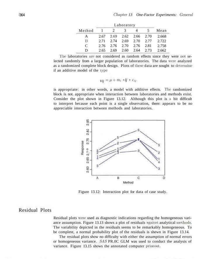
364 Chapter 13 One-Factor Experiments: General
Labora tory
Me thod
A IS C D
1
2.67 2.71 2.76 2.65
2
2.69 2.74 2.76 2.69
3
2.62 2.69 2.70 2.60
4
2.66 2.70 2.76 2.64
5
2.70 2.77 2.81 2.73
Mean
2.668 2.722 2.758 2.662
The laboratories are not considered as random effects since they were not selected randomly from a larger population of laboratories. The data were analyzed as a randomized complete block design. Plots of these data are sought to determine if an additive model of the type
Vij nii +lj + e-,j
is appropriate: in other words, a model with additive effects. The randomized block is not. appropriate when interaction between laboratories and methods exist. Consider the plot shown in Figure 13.12. Although this plot is a bit difficult to interpret because each point is a single observation, there: appears to be no appreciable interaction between methods and laboratories.
co .
o oo.
o r- . cxi
B C
Method
Residual Plots
Figure 13.12: Interaction plot for data of case study.
Residual plots were used as diagnostic indications regarding the homogeneous variance assumption. Figure 13.13 shows a plot of residuals against analytical methods. The variability depicted in the residuals seems to be remarkably homogeneous. To be complete, a normal probability plot of the residuals is shewn in Figure 13.14.
The residual plots show no difficulty with either the assumption of normal errors or homogeneous variance. SAS PR.0C GLM was used to conduct the analysis of variance. Figure 13.15 shows the annotated computer printout.
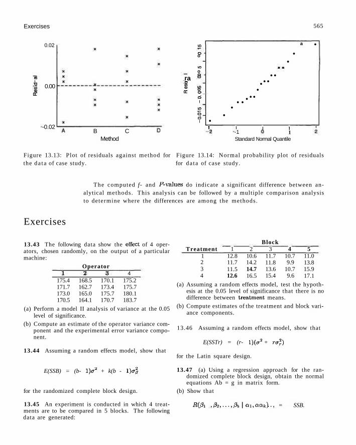
Exercises 565
0.02
CO 3 •g a>
er 0.00
-0.02 B C
Method
ra ^ o
er
in
o -o
i n o o -
o o _ d I
in
o _ a 1 •
1
• •
•
1
• • • •
•
• • • • •
•
1 I
•
a •
1
-1 1 Standard Normal Quantile
Figure 13.13: Plot of residuals against method for Figure 13.14: Normal probability plot of residuals the da t a of case study. for da ta of case study.
The computed f- and P-values do indicate a significant difference between analytical methods. This analysis can be followed by a multiple comparison analysis to determine where the differences are among the methods.
Exercises
13.43 The following data show the effect of 4 operators, chosen randomly, on the output of a particular machine:
Operator
Block
4 175.4 168.5 170.1 175.2 171.7 162.7 173.4 175.7 173.0 165.0 175.7 180.1 170.5 164.1 170.7 183.7
(a) Perform a model II analysis of variance at the 0.05 level of significance.
(b) Compute an estimate of the operator variance component and the experimental error variance component.
13.44 Assuming a random effects model, show that
E(SSB) = (b- l)o-2 + k(b - l)a}
for the randomized complete block design.
13.45 An experiment is conducted in which 4 treatments are to be compared in 5 blocks. The following data are generated:
Treatment 1 2 3 4
1 12.8 11.7 11.5 12.6
2 10.6 14.2 14.7 16.5
3 11.7 11.8 13.6 15.4
4 10.7 9.9
10.7 9.6
5 11.0 13.8 15.9 17.1
(a) Assuming a random effects model, test the hypothesis at the 0.05 level of significance that there is no difference between treatment means.
(b) Compute estimates of the treatment and block variance components.
13.46 Assuming a random effects model, show that
E(SSTr) = (r- l)(a2 + rcr2)
for the Latin square design.
13.47 (a) Using a regression approach for the randomized complete block design, obtain the normal equations Ab = g in matrix form.
(b) Show that
R(,3i ,82,...,,3h\ai,a2,..., ak) = SSB.
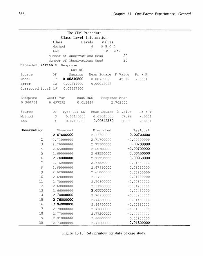
566 Chapter 13 One-Factor Experiments: General
The GLM Procedure Class Level Information
Class Levels Values
Dependen
Source
Model
Error
Method
Lab 4 A B C D
5 1 2 3 4!
Number of Observations Read
Number of Observations Used
t Variable: Response Sum of
DF Squares
7 0.05340500
12 0.00217000
Corrected Total 19 0.05557500
R-Square
0.960954
Source
Method
Lab
Observat: ion 1 2 3 4 5 6 7 8 9 10 11 12 13 14 15 16 17 18 19 20
Coeff Var Root
Mean Square F
0.00762929
0.00018083
MSE Response
5 20 20
Value Pr > F
42.19 <.0001
Mean
0.497592 0.013447 2.702500
DF Type III SS
3 0.03145500
4 0.02195000
Observed
2.67000000
2.71000000
2.76000000
2.65000000 2.69000000
2.74000000
2.76000000
2.69000000
2.62000000
2.69000000
2.70000000 2.60000000 2.66000000
2.70000000
2.76000000 2.64000000
2.70000000 2.77000000
2.81000000
2.73000000
Mean Square
0.01048500
0.00548750
Predicted
2.66300000
2.71700000
2.75300000
2.65700000 2.68550000
2.73950000
2.77550000
2.67950000
2.61800000
2.67200000
2.70800000 2.61200000 2.65550000
2.70950000
2.74550000 2.64950000
2.71800000 2.77200000
2.80800000
2.71200000
F Value Pr > F
57.98 <.0001
30.35 <.0001
Residual
0.00700000
-0.00700000
0.00700000 -0.00700000
0.00450000
0.00050000
-0.01550000
0.01050000
0.00200000 0.01800000
-0.00800000 -0.01200000 0.00450000
-0.00950000
0.01450000 -0.00950000 -0.01800000
-0.00200000
0.00200000
0.01800000
Figure 13.15: SAS printout for data of case study.
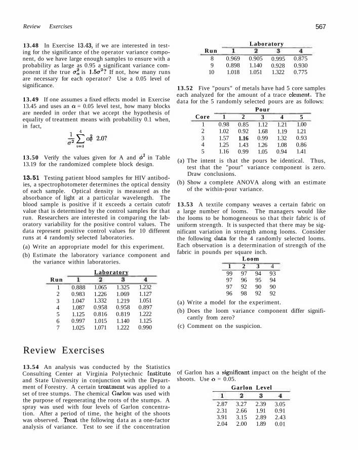
Review Exercises 567
13.48 In Exercise 13.43, if we are interested in testing for the significance of the operator variance component, do we have large enough samples to ensure with a probability as large as 0.95 a significant variance component if the true a\ is 1.5ej2? If not, how many runs are necessary for each operator? Use a 0.05 level of significance.
13.49 If one assumes a fixed effects model in Exercise 13.45 and uses an a = 0.05 level test, how many blocks are needed in order that we accept the hypothesis of equality of treatment means with probability 0.1 when, in fact,
±±a2 = 2.0? t = i
13.50 Verify the values given for A and o2 in Table 13.19 for the randomized complete block design.
13.51 Testing patient blood samples for HIV antibodies, a spectrophotometer determines the optical density of each sample. Optical density is measured as the absorbance of light at a particular wavelength. The blood sample is positive if it exceeds a certain cutofr value that is determined by the control samples for that run. Researchers are interested in comparing the laboratory variability for the positive control values. The data represent positive control values for 10 different runs at 4 randomly selected laboratories.
(a) Write an appropriate model for this experiment. (b) Estimate the laboratory variance component and
the variance within laboratories.
Run Laboratory
Laboratory Run
1 2 3 4 5 6 7
0.888 0.983 1.047 1.087 1.125 0.997 1.025
1.065 1.226 1.332 0.958 0.816 1.015 1.071
1.325 1.069 1.219 0.958 0.819 1.140 1.222
1.232 1.127 1.051 0.897 1.222 1.125 0.990
8 9
10
0.969 0.898 1.018
0.905 1.140 1.051
0.995 0.928 1.322
0.875 0.930 0.775
13.52 Five "pours" of metals have had 5 core samples each analyzed for the amount of a trace element. The data for the 5 randomly selected pours are as follows:
Pour Core
1 2 3 4 5
1 0.98 1.02 1.57 1.25 1.16
2 0.85 0.92 1.16 1.43 0.99
3 1.12 1.68 0.99 1.26 1.05
4 1.21 1.19 1.32 1.08 0.94
5 1.00 1.21 0.93 0.86 1.41
(a) The intent is that the pours be identical. Thus, test that the "pour" variance component is zero. Draw conclusions.
(b) Show a complete ANOVA along with an estimate of the within-pour variance.
13.53 A textile company weaves a certain fabric on a large number of looms. The managers would like the looms to be homogeneous so that their fabric is of uniform strength. It is suspected that there may be significant variation in strength among looms. Consider the following data for the 4 randomly selected looms. Each observation is a determination of strength of the fabric in pounds per square inch.
Loom 1
99 97 97 96
2 97 96 92 98
3 94 95 90 92
4 93 94 90 92
(a) Write a model for the experiment. (b) Does the loom variance component differ signifi
cantly from zero? (c) Comment on the suspicion.
Review Exercises
13.54 An analysis was conducted by the Statistics Consulting Center at Virginia Polytechnic Institute and State University in conjunction with the Department of Forestry. A certain treatment was applied to a set of tree stumps. The chemical Garlon was used with the purpose of regenerating the roots of the stumps. A spray was used with four levels of Garlon concentration. After a period of time, the height of the shoots was observed. TVeat the following data as a one-factor analysis of variance. Test to see if the concentration
of Garlon has a significant impact on the height of the shoots. Use a = 0.05.
Garlon Level
2.87 2.31 3.91 2.04
3.27 2.66 3.15 2.00
2.39 1.91 2.89 1.89
3.05 0.91 2.43 0.01
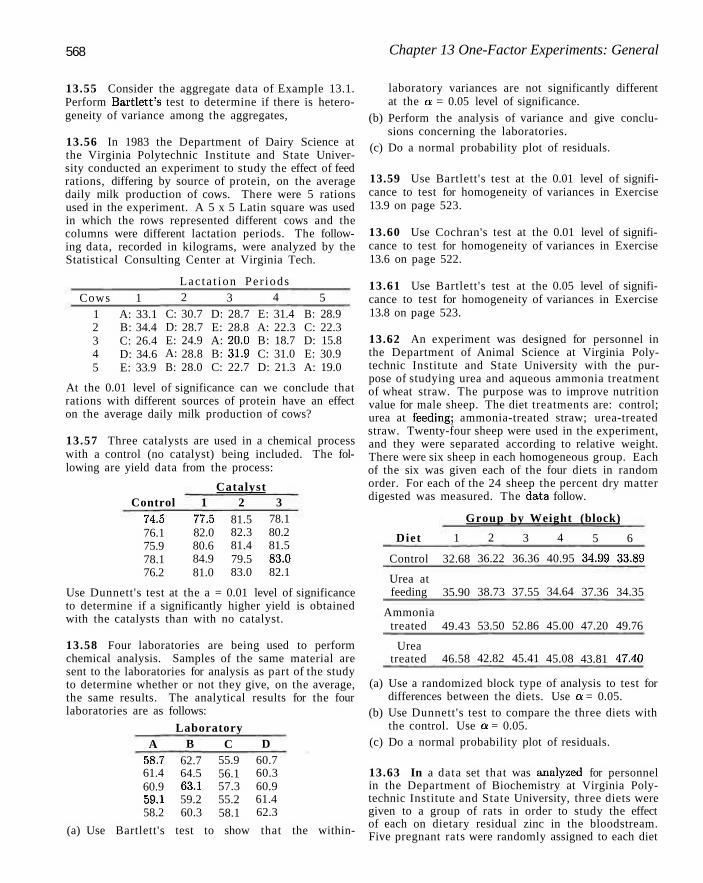
568 Chapter 13 One-Factor Experiments: General
13.55 Consider the aggregate data of Example 13.1. Perform Bartlett's test to determine if there is heterogeneity of variance among the aggregates,
13.56 In 1983 the Department of Dairy Science at the Virginia Polytechnic Institute and State University conducted an experiment to study the effect of feed rations, differing by source of protein, on the average daily milk production of cows. There were 5 rations used in the experiment. A 5 x 5 Latin square was used in which the rows represented different cows and the columns were different lactation periods. The following data, recorded in kilograms, were analyzed by the Statistical Consulting Center at Virginia Tech.
Lac ta t ion Pe r iods Cows
1 2 3 4 5
1 A: 33.1 B: 34.4 C: 26.4 D: 34.6 E: 33.9
C: D: E: A: B:
2 30.7 28.7 24.9 28.8 28.0
3 D: 28.7 E: 28.8 A: 20.0 B: 31.9 C: 22.7
4 E: 31.4 A: 22.3 B: 18.7 C: 31.0 D: 21.3
B: C: D: E: A:
5 28.9 22.3 15.8 30.9 19.0
At the 0.01 level of significance can we conclude that rations with different sources of protein have an effect on the average daily milk production of cows?
13.57 Three catalysts are used in a chemical process with a control (no catalyst) being included. The following are yield data from the process:
Catalyst Control
74.5 76.1 75.9 78.1 76.2
1 77.5 82.0 80.6 84.9 81.0
2 81.5 82.3 81.4 79.5 83.0
3 78.1 80.2 81.5 83.0 82.1
Use Dunnett's test at the a = 0.01 level of significance to determine if a significantly higher yield is obtained with the catalysts than with no catalyst.
13.58 Four laboratories are being used to perform chemical analysis. Samples of the same material are sent to the laboratories for analysis as part of the study to determine whether or not they give, on the average, the same results. The analytical results for the four laboratories are as follows:
A 58.7 61.4 60.9 59.1 58.2
Laboratory B
62.7 64.5 63.1 59.2 60.3
C 55.9 56.1 57.3 55.2 58.1
D 60.7 60.3 60.9 61.4 62.3
laboratory variances are not significantly different at the Q = 0.05 level of significance.
(b) Perform the analysis of variance and give conclusions concerning the laboratories.
(c) Do a normal probability plot of residuals.
13.59 Use Bartlett's test at the 0.01 level of significance to test for homogeneity of variances in Exercise 13.9 on page 523.
13.60 Use Cochran's test at the 0.01 level of significance to test for homogeneity of variances in Exercise 13.6 on page 522.
13.61 Use Bartlett's test at the 0.05 level of significance to test for homogeneity of variances in Exercise 13.8 on page 523.
13.62 An experiment was designed for personnel in the Department of Animal Science at Virginia Polytechnic Institute and State University with the purpose of studying urea and aqueous ammonia treatment of wheat straw. The purpose was to improve nutrition value for male sheep. The diet treatments are: control; urea at feeding: ammonia-treated straw; urea-treated straw. Twenty-four sheep were used in the experiment, and they were separated according to relative weight. There were six sheep in each homogeneous group. Each of the six was given each of the four diets in random order. For each of the 24 sheep the percent dry matter digested was measured. The data follow.
Group by Weight (block)
Diet
Control
Urea at feeding
Ammonia treated
Urea treated
1
32.68
35.90
49.43
46.58
2
36.22
38.73
53.50
42.82
3
36.36
37.55
52.86
45.41
4
40.95
34.64
45.00
45.08
5
34.99
37.36
47.20
43.81
6
33.89
34.35
49.76
47.40
(a) Use Bartlett's test to show that the within-
(a) Use a randomized block type of analysis to test for differences between the diets. Use a = 0.05.
(b) Use Dunnett's test to compare the three diets with the control. Use a = 0.05.
(c) Do a normal probability plot of residuals.
13.63 In a data set that was analyze*! for personnel in the Department of Biochemistry at Virginia Polytechnic Institute and State University, three diets were given to a group of rats in order to study the effect of each on dietary residual zinc in the bloodstream. Five pregnant rats were randomly assigned to each diet
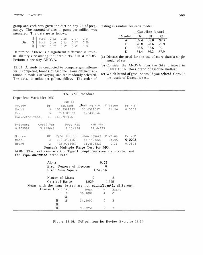
Review Exercises 569
group and each was given the diet on day 22 of pregnancy. The amount of zinc in parts per million was measured. The data are as follows:
Diet 0.50 0.42 1.06
0.42 0.40 0.82
0.65 0.73 0.72
0.47 0.47 0.72
0.44 0.69 0.82
Determine if there is a significant difference in residual dietary zinc among the three diets. Use a- = 0.05. Perform a one-way ANOVA.
13.64 A study is conducted to compare gas mileage for 3 competing brands of gasoline. Four different automobile models of varying size are randomly selected. The data, in miles per gallon, follow. The order of
testing is random for each model.
Gasol ine b r a n d M o d e l
A 32A3513 387 B 28.8 28.6 29.9 C 36.5 37.6 39.1 D 34.4 36.2 37.9
(a) Discuss the need for the use of more than a single model of car.
(b) Consider the ANOVA from the SAS printout in Figure 13.16. Does brand of gasoline matter?
(c) Which brand of gasoline would you select? Consult the result of Duncan's test.
The GLM Procedure Dependent Variable: MPG
Source Model Error Corrected
R-Square 0.953591
Source Model Brand
Sum of DF Squares 1 5 153.2508333 6 7.4583333
Total 11 160.7091667
Coeff Var Root MSE 3.218448 1.114924
DF Type III SS 3 130.3491667 2 22.9016667
<ean Square F 30.6501667 1.2430556
MPG Mean 34.64167
Mean Square F 43.4497222 11.4508333
Value 24.66
Value 34.95 9.21
Pr > F 0.0006
Pr > F 0.0003 0.0148
Duncan's Mult iple Range Test for MPG NOTE: This t e s t cont ro ls the Type I comparisonwise e r ro r r a t e , not the experimentwise e r ro r r a t e .
Alpha 0.05 Error Degrees of Freedom 6 Error Mean Square 1.243056
Number of Means 2 3 C r i t i c a l Range 1.929 1.999
Means with the same l e t t e r are not s i g n i f i c a n t l y d i f f e r e n t . Duncan Grouping
A Mean
36.4000
34.5000
33.0250
N 4
4
4
Brand C
B
A
Figure 13.16: SAS pr intout for Review Exercise 13.64.
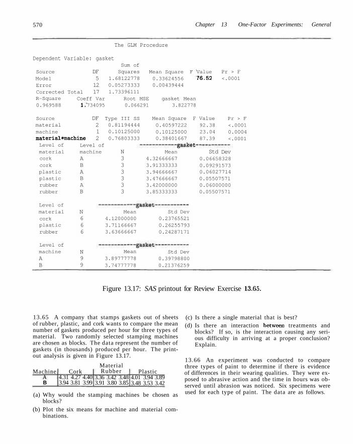
570 Chapter 13 One-Factor Experiments: General
The GLM Procedure
Dependent Variable: gasket
Source Model Error Corrected R-Square 0.969588
Source material machine
Total
DF 5 12 17
Sum of Squares
1.68122778 0.05273333 1.73396111
Mean Square F 0.33624556 0.00439444
Coeff Var Root MSE gasket Mean 1.
material*machine Level of material cork cork plastic plastic rubber rubber
Level of material cork plastic rubber
Level of machine A B
734095 0.066291 3.822778
DF 2 1 2
Type III SS 0.81194444 0.10125000 0.76803333
Level of machine A B A B A B
N 6 6 6
N 9 9
N 3 3 3 3 3 3
Mean Square F 0.40597222 0.10125000 0.38401667
, 4 .
Mean 4.32666667 3.91333333 3.94666667 3.47666667 3.42000000 3.85333333
Mean 4.12000000 3.71166667 3.63666667
Std Dev 0.23765521 0.26255793 0.24287171
Mean 3.89777778 3.74777778
Std Dev 0.39798800 0.21376259
Value 76.52
Value 92.38 23.04 87.39
Std
Pr > F <.0001
Pr > F <.0001 0.0004 <.0001
Dev 0.06658328 0.09291573 0.06027714 0.05507571 0.06000000 0.05507571
Figure 13.17: SAS printout for Review Exercise 13.65.
13.65 A company that stamps gaskets out of sheets of rubber, plastic, and cork wants to compare the mean number of gaskets produced per hour for three types of material. Two randomly selected stamping machines are chosen as blocks. The data represent the number of gaskets (in thousands) produced per hour. The printout analysis is given in Figure 13.17.
Machine
B
Cork 4.31 4.27 4.40 3.94 3.81 3.99
Material Rubber
3.36 3.42 3.48 3.91 3.80 3.85
Plastic 4.01 3.94 3.89 3.48 3.53 3.42
(a) Why would the stamping machines be chosen as blocks?
(b) Plot the six means for machine and material combinations.
(c) Is there a single material that is best? (d) Is there an interaction between treatments and
blocks? If so, is the interaction causing any serious difficulty in arriving at a proper conclusion? Explain.
13.66 An experiment was conducted to compare three types of paint to determine if there is evidence of differences in their wearing qualities. They were exposed to abrasive action and the time in hours was observed until abrasion was noticed. Six specimens were used for each type of paint. The data are as follows.
13.16 Potential. Misconceptions and Hazards 571
Pa in t Type 2
158 97 282 315 220 115
515 ,ri5.r)
264 330
544 525
317 536
662 175
213 614
(a) Do an analysis of variance to determine if the evidence suggests that, wearing quality differs for the 3 paints. Use a P-value in your conclusion.
(b) If significant differences are found, characterize what they are. Is there one paint that stands out? Discuss your findings.
(c) Do whatever graphical analysis you need t.ei determine if assumptions used in (a) arc valid. Discuss your findings.
(d) Suppose it is determined that the data for each treatment follows an exponential distribution. Does this suggest an alternative analysis? If so, do the alternative analysis and give findings.
13.67 Four different locations in the northeast are used for collecting ozone measurements in parts per million. Amounts of ozone were collected in 5 samples at each location.
1 0.09 0.10 0.08 0.08 0.1.1
Location 2
0.15 0.12 0.17 0.18 0.14
3 0.10 0.13 0.08 0.08 0.09
4 0.10 0.07 0.05 0.08 0.09
(a) Is then: sufficient information here to suggest that there are differences in the mean ozone levels across locations? Be guided by a P-value.
(b) If significant tlifferences are found in (a), characterize the nature of the differences. Use whatever methods yon have learned.
13.16 Potential Misconceptions and Hazards; Relationship to Material in Other Chapters
As in either procedure's covered in previous chapters, the analysis of variance is reasonably robust, to the normality assumption but less robust to the homogeneous variance assumption.
Bar t le t t ' s test for equal variance is extremely nonrobust to normality.
Chapter 14
Factorial Experiments (Two or More Factors)
14.1 Introduction
Consider a situation where it is of interest to study the effect of two factors, A and B, on some response. For example, in a chemical experiment we would like to vary simultaneously the reaction pressure and reaction time and study the effect of each on the yield. In a biological experiment, it is of interest to study the effect of drying time and temperature on the amount of solids (percent by weight) left in samples of feast. As in Chapter 13, the term factor is used in a general sense to denote any feature of the experiment such as temperature, time, or pressure that may be varied from trial to trial. We define the levels of a factor to be the actual values used in the experiment.
For each of these cases it is important to determine not only if the two factors each has an influence on the response, but also if there is a significant interaction between the two factors. As far as terminology is concerned, the experiment described here is a two-factor experiment and the experimental design may be either a completely randomized design, in which the various treatment combinations are assigned randomly to all the experimental units, or a randomized complete block design, in which factor combinations are assigned randomly to blocks. In the case of the yeast example, the various treatment combinations of temperature and drying time would be assigned randomly to the samples of yeast if we are using a completely randomized design.
Many of the concepts studied in Chapter 13 are extended in this chapter to two and three factors. The main thrust of this material is the use of the completely randomized design with a factorial experiment. A factorial experiment in two factors involves experimental trials (or a single trial) at all factor combinations. For example, in the temperature-drying-time example with, say, three levels of each and n = 2 runs at each of the nine combinations, we have a two-factor factorial in a completely randomized design. Neither factor is a blocking factor; we are interested in how each influence percent solids in the samples and whether or not they interact. The: biologist would then have available 18 physical samples of
374 Chapter 14 Factorial Experiments (Two or More Factors)
material which are: experimental units. These: would then be assigned randomly to the 18 combinations (nine treatment combinations, each duplicated).
Before we launch into analytical details, sums of squares, and so on, it maybe of interest for the reader to observe the obvious connection between what we have described and flic situation with the one-factor problem. Consider the yeast experiment. Explanation of degrees of freedom aids the reader or the analyst in visualizing the extension. We should initially view the 9 treatment combinations as if they represent one factor with 0 levels (8 degrees of freedom). Thus an initial look at degrees of freedom gives
Treatment combinations 8 Error 0 Total 1 •
Main Effects and Interaction
Actually, the experiment could be analyzed as dcscribcel in the above table. However, the F-tcst for combinations would probably not give the analyst the information he or she desires, namely, that which considers the role of temperature and drying time. Three drying times have 2 associated degrees of freedom, three temperatures have 2 degrees of freedom. The main factors, temperature and drying time, are called main effects. The main effects represent 4 of the 8 degrees of freedom for factor combinations. The additional 4 degrees of freeelom are associated with interaction between the two factors. As a result, the analysis involves
Combinations Temperature Drying time Interaction
Error
2 2 4
8
9 Total 17
Recall from Chapter 13 that, factors in an analysis of variance may be viewed as fixed or random, depending on the type1 eif inference desired and how the levels were chosen. Here wc must consider fixeel effects, random effects, and even cases where e:ffccts are mixed. Most, attention will be drawn toward expected mean squares when we advance to these topics. In the following section we focus on the concept of interaction.
14.2 Interaction in the Two-Factor Experiment
In the randomized block model discussed previously it was assumed that one observation on each treatment is taken in each block. If the model assumption is correct, that is, if blocks and treatments are the only real effects and interaction does not exist, the expected value of the mean square error is the experimental error variance a2. Suppose, however, that there is interaction occurring between treatments and blocks as indicated by the model
IJij = fl+ O; + 0j + (np)ij + f.jj
14.2 Interaction in the Two-Factor Experiment 575
of Section 13.9. The expected value of the mean square error was then given as
k b SSE
(b-l)(k-l) *2 + (OT^E£(^-^ ' ^ * i=i i = i
The treatment and block effects do not appear in the expected mean square error, but the interaction effects do. Thus, if there is interaction in the model, the mean square error reflects variation due to experimental error plus an interaction contribution and, for this experimental plan, there is no way of separating them.
Interaction and the Interpretation of Main Effects
From an experimenter's point of view it should seem necessary to arrive at a significance test on the existence of interaction by separating true error variation from that due to interaction. The main effects, A and B, take on a different meaning in the presence of interaction. In the previous biological example the effect that drying time has on the amount of solids left in the yeast might very well depend on the temperature to which the samples are exposed. In general, there could be experimental situations in which factor A has a positive effect on the response at one level of factor B, while at a different level of factor B the effect of A is negative. We use the term positive effect here to indicate that the yield or response increases as the levels of a given factor increase according to some defined order. In the same sense a negative effect corresponds to a decrease in yield for increasing levels of the factor.
Consider, for example, the following data on temperature (factor A at levels t\, t2, and t3 in increasing order) and drying time dx, d2, and d3 (also in increasing order). The response is percent solids. These data are completely hypothetical and given to illustrate a point.
A
h t2
t3
di
4.4 7.5 9.7
B
d2
8.8 8.5 7.9
dz 5.2 2.4 0.8
Total 18.4 18.4 18.4
Total 21.6 25.2 8.4 55.2
Clearly the effect of temperature is positive on percent solids at the low drying time di but negative for high drying time d3. This clear interaction between temperature and drying time is obviously of interest to the biologist but, based on the totals of the responses for temperature t\, t2, and t3, the temperature sum of squares, 55.4, will yield a value of zero. We say then that the presence of interaction is masking the effect of temperature. Thus if we consider the average effect of temperature, averaged over drying time, there is no effect. This then defines the main effect. But, of course, this is likely not what is pertinent to the biologist.
Before drawing any final conclusions resulting from tests of significance on the main effects and interaction effects, the experimenter should first observe whether or not the test for interaction is significant. If interaction is
576 Chapter 14 Factorial Experiments (Two or More Factors)
not significant, then the results of the tests on the main effects are meaningful. However, if interaction should be significant, then only those tests on the main effects that turn out to be significant are meaningful. Nonsignificant main effects in the presence of interaction might well be a result of masking and dictate the need to observe the influence of each factor at fixed levels of the other.
A Graphical Look at Interaction
The presence of interaction as well as its scientific impact can be interpreted nicely through the use of interaction plots. The plots clearly give a pictorial view of the tendency in the data to show the effect of changing one factor as one moves from one level to another of a second factor. Figure 14.1 illustrates the strong temperature by drying time interaction. The interaction is revealed in nonparallel lines.
8
a.
Temperature
Figure 14.1: Interaction plot for temperature-drying time data.
The relatively strong temperature effect on percent solids at the lower drying time is reflected in the steep slope at di. At the middle drying time d2 the temperature has very little effect while at the high drying time d3 the negative slope illustrates a negative effect of temperature. Interaction plots such as this set give the scientist a quick and meaningful interpretation of the interaction that is present. It should be apparent that parallelism in the plots signals an absence of interaction.
Need for Multiple Observations
Interaction and experimental error are separated in the two-factor experiment only if multiple observations are taken at the various treatment combinations. For maximum efficiency, there should be the same number n of observations at each combination. These should be true replications, not just repeated measurements. For
14.3 Two-Factor Analysis of Variance 577
example, in the yeast, illustration, if we take n = 2 observations at each combination of temperature and drying time, there should be two separate samples and not merely repeated measurements on the same sample. This allows variability due to experimental units to appear in "error," so the variation is not merely measurement error.
14.3 Two-Factor Analysis of Variance
To present general formulas lor the analysis of variance of a two-factor experiment using repeated observations in a completely randomized design, we shall consider the case of n replications of the treatment combinations determined by o levels of factor A and b levels of factor B. The observations may be classified by means of a rectangular array where the rows represent the levels of factor A and the columns represent the levels of factor B. Each treatment combination defines a cell in our array. Thus we have ah cells, each cell containing n observations. Denoting the A:th observation taken at the ith level of factor A and the j th level of factor B by yijk, the abn observations are shown in Table 14.1.
Tabic 14.1: Two-Factor Experiment with n Replications B
1 2 ••• b Total M e a n
zmi 2/112
.1/1 In
y-211
2/212
J/121
2/122
J/12n
1/221
J/222
Vxbi
l/U-2
Vlbn
y-m V2b2
Yi.
Y2..
Vl..
2/2..
2/2 In l)22n V2bn
Wall
Ha 12
Vail Va22
Vabl
v<ii<2
Ya.. Va..
Total Mean
Vain Y.i.
P.l.
2/u2n
Y.2. V.2.
Vabn YM.
y.b.
The observations in the (*j)th roll constitute a random sample of size n from a population that is assumed to be normally distributed with mean pij and variance er-. All ab populations are assumed to have the same variance a2. Let us define
580 Chapter 14 Factorial Experiments (Two or More Factors)
squares as functions of the independent random variables ym, J/112, • • • -. 27a(m, it is not difficult to verify that
E(S!) = E
E(Sl) = E
E(Sl) = E
E(S2) = E
SSA
a - 1
SSB b-l
SS(AB)
0 lib -C—v n
."."it* = CT" +
| > - 1 ) ( 6 - 1 ) S5£
j = l
n
(a-D(*-l)feft n E D ^ ' = ff , . a b ( n - l ) .
from which we immediately observe that all four estimates of a2 are unbiased when HQ, HQ, and H0 are true.
To test the hypothesis HQ, that the effects of factors A are all equal to zero, we compute the ratio
F-Test for Factor A f - Sl
s*
which is a value of the random variable Fi having the F-distribution with a - 1 and ab(n — 1) degrees of freedom when H0 is true. The null hypothesis is rejected at the a-level of significance when / ] > fa[a — l,ab(n — 1)]. Similarly, to test the hypothesis H0 that the effects of factor B are all equal to zero, we compute the ratio
F-Test for Factor B h
s 2 s 2
which is a value of the random variable F2 having the F-distribution with 5—1 and ab(n — 1) degrees of freedom when Hu is true. This hypothesis is rejected at the a-level of significance when f2 > fa[b- 1, ab(n— 1)]. Finally, to test the hypothesis HQ , that the interaction effects are all equal to zero, we compute the ratio
F-Test for Interaction f — -2.
2 '
which is a value of the random variable F3 having the F-distribution with (a. — l)(b — 1) and ab(n — 1) degrees of freedom when HQ is true. We conclude that interaction is present when f3 > /Q[(a — 1)(5 — l),a6(n — 1)].
As indicated in Section 14.2, it is advisable to interpret the test for interaction before attempting to draw inferences on the main effects. If interaction is not significant, there is certainly evidence that the tests eni main effects are interpretable. Rejection of hypothesis 1 on page 578 implies that the response means at the levels of factor A are significantly different while rejection of hypothesis 2 implies a similar condition for the means at levels of factor B. However, a significant interaction could very well imply that the data should be analyzed in a somewhat, different manner-perhaps observing the effect of factor A at fixed levels of factor B. and so forth.
14.3 Two-Factor Analysis of Variance 581
The computations in an analysis-of-variance problem, for a two-factor experiment with n replications, are usually summarized as in Table 14.2.
Table 14.2: Analysis of Variance for the Two-Factor Experiment with n Replications
Example 14.1:1
Source of Variation Main effect
A
B
Two-factor interactions
AB
Error
Total
In an experiment
Sum of Squares
SSA
SSB
SS(AB)
SSE
SST
Degrees of Freedom
a - 1
6 - 1
( a - l ) ( 6 - l )
ab(n - 1)
abn — 1
conducted to determine w
Mean Square
„2 _ SSA Sl - a -1 „2 _ SSB «2 - T=T
2 _ SS(AB) S3 - (a- l ) (6- l ) „2 _ SSE b ~ ab(n-l)
Computed
/i = f* h-$
h-i
hich of 3 different missile system; preferable, the propellant burning rate for 24 static firings was measured. Four different propellant types were used. The experiment yielded duplicate observations of burning rates at each combination of the treatments.
The data, after coding, are given in Table 14.3. Test the following hypotheses: (a) HQ-. there is no difference in the mean propellant burning rates when different missile systems are used, (b) H0: there is no difference in the mean propellant burning rates of the 4 propellant types, (c) HQ : there is no interaction between the different missile systems and the different propellant types.
Table 14.3: Propellant Burning Rates
Missile System
ax
a2
a-A
bx 34.0 32.7 32.0 33.2 28.4 29.3
Propellant Type
62
30.1 32.8 30.2 29.8 27.3 28.9
63 64
29.8 29.0 26.7 28.9 28.7 27.6 28.1 27.8 29.7 28.8 27.3 29.1
Solution: 1. (a) HQ-. ax = a2 = a3 = 0. (b) HQ: ,3X =02 = 03 = 04 = 0. (c) HQ': (a0)n = (a0)12 = ••• = (a0)34 = 0.
2. (a) H^: At least one of the a^s is not equal to zero, (b) Hi : At least one of the 0j !s is not equal to zero.
582 Chapter 14 Factorial Experiments (Two or More Factors)
(c) Hx : At least one of the (a/3)y's is not equal to zero.
The sum-of-squares formula is used as described in Theorem 14.1. The analysis of variance is shown in Table 14.4,
Table 14.4: Analysis of Variance for the Data of Table 14.3
Source of Sum of Degrees of Mean Computed Variat ion Squares Freedom Square /
Missile system Propellant type Interaction Error
Total
14.52 40.08 22.16 14.91
91.68
2 3 6
12
23
7.26 13.36 3.69 1.24
5.84 10.75 2.97
The reader is directed to a SAS GLM Procedure (General Linea Models) for analysis of the burning rate data in Figure 14.2. Note how the "model" (11 degrees of freedom) is initially tested and the system, type, and system by type interaction are tested separately. The /-test on model (P = 0.0030) is testing the accumulation of the two main effects and the interaction.
(a) Reject H0 and conclude that different missile systems result in different mean propellant burning rates. The P-value is approximately 0.017.
(b) Reject H0 and conclude that the mean propellant burning rates are not the same for the four propellant types. The P-value is smaller than 0.0010.
(c) Interaction is barely insignificant at the 0.05 level, but the P-value of approximately 0.0512 would indicate that interaction must be taken seriously.
The GLM P r o c e d u r e Dependent V a r i a b l e : r a t e
Source Model E r r o r
DF 11 12
C o r r e c t e d T o t a l 23
R-Square 0.837366
Source sys tem t y p e sys tem*type
Coeff Var 3 .766854
DF 2 3 6
Sum of Squa res
76 .76833333 14.91000000 91 .67833333
Root MSE 1.114675
Type I I I SS 14.52333333 40.08166667 22.16333333
Mean Square 6 .97893939 1.24250000
r a t e Mean 29 .59167
Mean Square F 7 .26166667
13.36055556 3.69388889
F Value 5 .62
Value 5 .84
10 .75 2 . 9 7
Pr > F 0 .0030
Pr > F 0 .0169 0 .0010 0 .0512
Figure 14.2: SAS Printout of the analysis of the propellant rate data of Table 14.3.
At this point we should draw some type of interpretation of the interaction. It should be emphasized that statistical significance of a main effect merely implies
14.3 Two-Factor Analysis of Variance 583
that marginal means are significantly different. However, consider the two-way-table of averages in Table: 14.5.
Ol
a2
a3
Averc
Tabl
Lge
• 14.5:
6i 33.35 32.60 28.85 31. GO
Interpre
b2
31.45 30.00 28.10 29.85
station of Interne
b3
28.25 28.40 28.50 28.38
04
28.95 27.70 28.95 28.53
tion
Average
30.50 29.68 28.60
It is apparent that more important information exists in the body of the table-trends that are inconsistent with the trend depicted by marginal averages. Table 14.5 certainly suggests that the effect of propellant type depends on the system being used. For example, for system 3 the propellant-type effect does not appear to be important, although it does have a large effect if either system 1 or system 2 is used. This explains the "significant" interaction between these two factors. More will be revealed subsequently concerning this interaction. J
Example 14.2:1 Referring to Example 14.1, choose two orthogonal contrasts to partition the sum of squares for the missile systems into single-degree-of-freedom components to be used in comparing systems I and 2 with 3 and system 1 versus system 2.
Solution: The contrast for comparing systems 1 and 2 with 3 is
wj = px. + )i-2. - 2p.A..
A second contrast, orthogonal to u,'i, for comparing system 1 with system 2, is given by UJ-> = pi. — p2.. The single-degree-of-freedom sums of squares are
[244.0 + 237.4 - (2)(228.8)]2
ss^= (mir-- ay + (-m =1L80'
and
(244.0-237.4)2
SStJ2 ~ (8)[(1)3+ (-!)*] - 2J2-
Notice that SSwx +SSw% = SSA, as expected. The computed /-values corresponding to u.'i and JJ2 are. respectively,
f, = £ ? = 9-5 and f2 = £ £ = 2.2. •' 1.24 1.21
Compared to the critical value /o.o5(li 12) = 4.75, we find /1 to be- significant. In fact, the P-value is less than 0.01. Thus the first contrast indicates that the hypothesis
HQ: -(pi. + p-2.) =/ ' ;s .
is rejected. Since f2 < 4.75, the mean binning rates of the first and second systems
are not significantly different. J
584 Chapter 14 Factorial Experiments (Two or More Factors)
Impact of Significant Interaction in Example 14.1
If the hypothesis of no interaction in Example 14.1 is true, we could make the general comparisons of Example 14.2 regarding our missile systems rather than separate comparisons for each propellant. Similarly, we might make general comparisons among the propellants rather than separate comparisons for each missile system. For example, we could compare propellants 1 and 2 with 3 and 4 and also propellant 1 versus propellant 2. The resulting /-ratios, each with 1 and 12 degrees of freedom, turn out to be 24.86 and 7.41, respectively, and both are quite significant at the 0.05 level.
From propellant averages there appears to be evidence that propellant 1 gives the highest mean burning rate. A prudent experimenter might be somewhat cautious in making overall conclusions in a problem such as this one, where the /-ratio for interaction is barely below the 0.05 critical value. For example, the overall evidence, 31.60 versus 29.85 on the average for the two propellants, certainly indicates that propellant 1 is superior, in terms of a higher burning rate, to propellant 2. However, if we restrict ourselves to system 3, where we have an average of 28.85 for propellant 1 as opposed to 28.10 for propellant 2, there appears to be little or no difference between these two propellants. In fact, there appears to be a stabilization of burning rates for the different propellants if we operate with system 3. There is certainly overall evidence which indicates that system 1 gives a higher burning rate than system 3. but if we restrict ourselves to propellant 4, this conclusion does not appear to hold.
The analyst can conduct a simple t-test using average burning rates at system 3 in order to display conclusive evidence that interaction is producing considerable difficulty in allowing broad conclusions on main effects. Consider a comparison of propellant 1 against propellant 2 only using system 3. Borrowing an estimate of a2 from the overall analysis, that is, using s2 = 1.24 with 12 degrees of freedom, we can use
0.75 0.75 f. = ; = - = = = 0.67.
^/W/n y/iHi which is not even close to being significant. This illustration suggests that one must be cautious about strict interpretation of main effects in the presence of interaction.
Graphical Analysis for the Two-Factor Problem of Example 14.1
Many of the same types of graphical displays that were suggested in the one-factor problems certainly apply in the two-factor case. Two-dimensional plots of cell means or treatment combination means can provide an insight into the presence of interactions between the two factors. In addition, a plot of residuals against fitted values may well provide an indication of whether or not the homogeneous variance assumption holds. Often, of course, a violation of the homogeneous variance assumption involves an increase in the error variance as the response numbers get larger. As a result, this plot may point out the violation.
Figure 14.3 shows the plot of cell means in the case of the missile system propellant illustration in Example 14.1. Notice how graphic (in this case) the lack of parallelism shows through. Note the flatness of the part of the figure showing
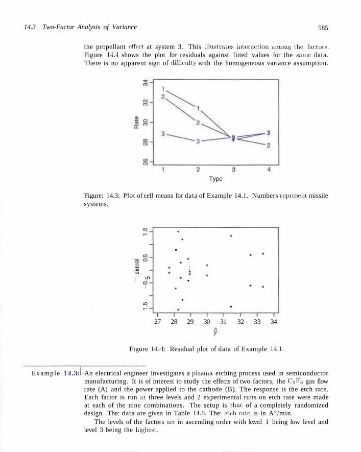
14.3 Two-Factor Analysis of Variance 585
the propellant effect at system 3. This illustrates interaction among the1 factors. Figure 11.4 shows the plot for residuals against fitted values for the same data. There is no apparent sign of difficulty with the homogeneous variance assumption.
Type
Figure: 14.3: Plot of cell means for data of Example 14.1. Numbers represent missile systems.
in
-g '(/> | *
lO T—
I
+
•
:
• *
• •
27 28 29 30 31 32 33 34
Figure l-l. I: Residual plot of data of Example 14.1.
Example 14.3:1 An electrical engineer investigates a plasma, etching process used in semiconductor manufacturing. It is of interest to study the effects of two factors, the C2F(i gas flow rate (A) and the power applied to the cathode (B). The response is the etch rate. Each factor is run at three levels and 2 experimental runs on etch rate were made at each of the nine combinations. The setup is that, of a completely randomized design. The: data are given in Table 14.6. The: etch rate- is in A°/min.
The levels of the factors arc in ascending order with le:ve:l 1 being low level and level 3 being the highest.
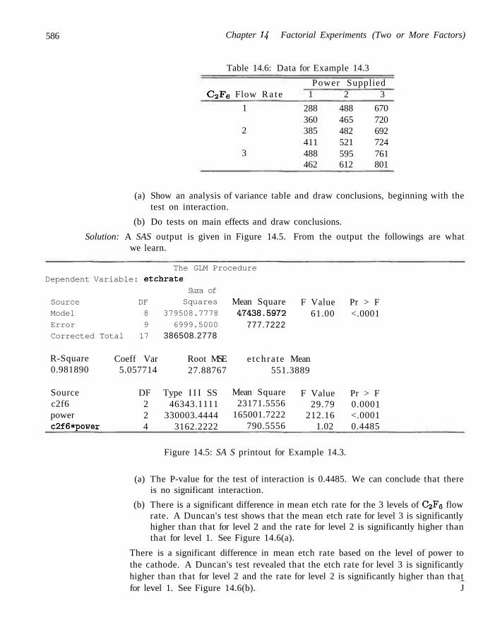
586 Chapter IJ, Factorial Experiments (Two or More Factors)
Table 14.6: Data for Example 14.3
C 2 F 6 Flow R a t e
1
2
3
Power Supplied 1
288 360 385 411 488 462
2 3
488 670 465 720 482 692 521 724 595 761 612 801
(a) Show an analysis of variance table and draw conclusions, beginning with the test on interaction.
(b) Do tests on main effects and draw conclusions.
Solution: A SAS output is given in Figure 14.5. From the output the followings are what we learn.
The GLM Procedure
Dependent Variable: etchrate
Source DF
Model 8
Error 9
Corrected Total 17
Sura of
Squares
379508.7778
6999.5000
386508.2778
Mean Square 47438.5972
777.7222
F Value Pr > F 61.00 <.0001
R-Square 0.981890
Coeff Var 5.057714
Root MSE 27.88767
e tch ra te Mean 551.3889
Source c2f6 power c2f6*power
DF Type I I I SS 2 46343.1111 2 330003.4444 4 3162.2222
Mean Square 23171.5556
165001.7222 790.5556
F Value Pr > F 29.79 0.0001
212.16 <.0001 1.02 0.4485
Figure 14.5: SA S printout for Example 14.3.
(a) The P-value for the test of interaction is 0.4485. We can conclude that there is no significant interaction.
(b) There is a significant difference in mean etch rate for the 3 levels of C2Fo flow rate. A Duncan's test shows that the mean etch rate for level 3 is significantly higher than that for level 2 and the rate for level 2 is significantly higher than that for level 1. See Figure 14.6(a).
There is a significant difference in mean etch rate based on the level of power to the cathode. A Duncan's test revealed that the etch rate for level 3 is significantly higher than that for level 2 and the rate for level 2 is significantly higher than that for level 1. See Figure 14.6(b). J
Exercises 587
Duncan Grouping A B C
Mean N c2f6 6 1 9 . 8 3 6 3 535 .83 6 2 498 .50 6 1
(a)
Duncan Grouping A B C
Mean 7 2 8 . 0 0 527 .17 399 .00
N 6 6 6
power 3 2 1
(b)
Figure 14.6: (a) SAS output , dealing with Example 14.3 (Duncan's teat on gas flow rate) : (b) SAS output , for Example 14.3 (Duncan's test on power),
Exercises
14.1 An experiment was conducted to study the effect of temperature and type of oven on the life of a particular component being tested. Four types of ovens and 3 temperature levels were used in the experiment. Twenty-four pieces were assigned randomly, 2 to each combination of treatments, and the following results recorded.
T e m p e r a t u r e Oven (Degrees)
500
550
o, 227 221 187 208
o2 214 259 181 179
Oa
225 236 232 198
o4 200 229 246 273
600
Using a 0.05 level that
174 198 178 206 202 194 213 219
of significance, test the hypothesis
(a) different temperatures have no effect on the life of the component:
(b) different ovens have no effect, on the life of the component;
(c) the type of oven and temperature elo not interact.
14.2 To ascertain the stability of vitamin C in reconstituted frozen orange juice concentrate stored in a refrigerator for a period of up to one week, the study Vitamin C Retention, in Reconstituted Frozen Orange Juice was conducted by the Department of Human Nutrition and Foods at the Virginia Polytechnic Institute and State University. Three types of frozen orange juice concentrate were tested using 3 different time periods. The time periods refer to the number of days from when the orange juice was blended until it was tested. The results, in milligrams of ascorbic acid per liter, were recorded. Use a 0.05 level of significance to test the hypothesis that (a) there is no difference in ascorbic acid contents
among the different brands of orange juice concentrate:
(b) there is no difference in ascorbic acid contents for the different time periods;
(c) the brands of orange juice concentrate and the number of days from the time the juice was blended until it is testcel do not interact.
T i m e (days) B r a n d
Richfood
Sealed-Sweet
Minute Maid
0 52.6 49.8 56.0 49.6 52.5 51.8
54.2 46.5 48.0 48.4 52.0 53.6
3 49.4 42.8 48.8 44.0 48.0 48.2
49.2 53.2 44.0 42.4 47.0 49.6
t
42.7 40.4
49.2 42.0 48.5 45.2
7
48.8 47.6 44.0 43.2 43.3 47.6
14.3 Three strains of rats were studied under 2 environmental conditions for their performance in a maze test. The error scores for the 48 rats were recorded as follows:
S t ra in E n v i r o n m e n t Br igh t Mixed Dull
Free 28 12 33 83 101 94~~ 22 23 36 14 33 56 25 10 41 76 122 83 36 86 22 58 35 23
Res t r i c t ed 72 32 60 89 136 120 48 93 35 126 38 153 25 31 83 110 64 128 91 19 99 118 87 140
Use a 0.01 level of significance to test the hypothesis that (a) there is no difference in error scores for different
environments; (b) there is no difference in error scores for different
strains; (c) the environments and strains of rats do not inter
act.
14.4 Corrosion fatigue in metals has been defined as
588 Chapter 14 Factorial Experiments (Two or More Factors)
the simultaneous action of cyclic stress and chemical attack on a metal structure. A widely used technique for minimizing corrosion-fatigue damage in aluminum involves the application of a protective coating. In a study conducted by the Department of Mechanical Engineering at the Virginia Polytechnic Institute and State University, different levels of humidity-
Low: 20-25% relative humidity Medium: 55-60% relative humidity High: 86-91% relative humidity
and 3 types of surface coatings Uncoated: no coating
Anodized: sulfuric acid anodic oxide coating
Conversion: chromate chemical conversion coating
were used. The corrosion-fatigue data, expressed in thousands of cycles to failure, were recorded as follows:
Relative Humidity Coating Low Medium High
Uncoated
Anodized
361 466 1069
114 1236 533
469 937 1357
1032 92 211
314 244 261 322 306 68
522 739 134 471 130 398
1344 1027 1011
78 387 130
1216 1097 1011
466 107 327
130 1482 252 874 586 524 Conversion 841 529 105 755 402 751
1595 754 847 573 846 529
(a) Perform an analysis of variance with a = 0.05 to test for significant main and interaction effects.
(b) Use Duncan's multiple-range test at the 0.05 level of significance to determine which humidity levels result in different corrosion-fatigue damage.
14.5 To determine which muscles need to be subjected to a conditioning program in order to improve one's performance on the flat serve used in tennis, a study was conducted by the Department of Health, Physical Education and Recreation at the Virginia Polytechnic Institute and State University. Five different muscles
anterior deltoid
pectorial major
posterior deltoid
4: middle deltoid
triceps
were tested on each of 3 subjects, and the experiment was carried out 3 times for each treatment combination. The electromyographic data, recorded during the serve, are presented here. Use a 0.01 level of significance to test the hypothesis that (a) different subjects have equal electromyographic
measurements:
(b) different muscles have no effect on electromyograhic measurements;
(c) subjects and types of muscle do not interact.
Muscle Subject ~ 2 3 4~ 5~
1
2
32 59 38 63 60 50
5 1.5 2 10 9 7
58 61 66 64 78 78
10 10 14 45 61 71
19 20 23 43 61 42
3 43 41 26 63 61 54 43 29 46 85 47 42 23 55 95
14.6 An experiment was conducted to increase the adhesiveness of rubber products. Sixteen products were made with the new additive and another 16 without the new additive. The observed adhesiveness is recorded below.
Without Additives
Temperature
50 2.3 2.9 3.1 3.2
60 3.4 3.7 3.6 3.2
70 3.8 3.9 4.1 3.8
(°C) 80 3.9 3.2 3.0 2.7
With Additives 4.3 3.8 3.9 3.5 3.9 3.8 4.0 3.6 3.9 3.9 3.7 3.8 4.2 3.5 3.6 3.9
Perform an analysis of variance to test for significant main and interaction effects.
14.7 The extraction rate of a certain polymer is known to depend on the reaction temperature and the amount of catalyst used. An experiment was conducted at four levels of temperature and five levels of the catalyst, and the extraction rate was recorded in the following table.
50° C
60° C
70° C
0.5% 38 41
44 43 44 47
Amount of Catalyst
0.6% 45 47 56 57
56 60
0.7%
57 59
70 69 70 67
0.8%
59 61
73 72
73 61
0.9%
57 58
61 58 61 59
80° C 49 47
62 65
70 55
62 69
53 58
Perform an analysis of variance, main and interaction effects.
Test for significant
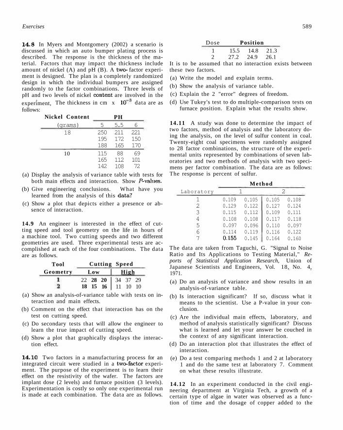
Exercises 589
14.8 In Myers and Montgomery (2002) a scenario is discussed in which an auto bumper plating process is described. The response is the thickness of the material. Factors that may impact the thickness include amount of nickel (A) and pH (B). A t w o factor experiment is designed. The plan is a completely randomized design in which the individual bumpers are assigned randomly to the factor combinations. Three levels of pH and two levels of nickel content are involved in the
Dose Position
experiment, follows:
The thickness in cm x 10 data are as
Nickel Content PH (grams)
18 5 250 195 188
5.5 211 172 165
6 221 150 170
115 165 142
88 112 108
69 101 72
10
(a) Display the analysis of variance table with tests for both main effects and interaction. Show P-values.
(b) Give engineering conclusions. What have you learned from the analysis of this data?
(c) Show a plot that depicts either a presence or absence of interaction.
14.9 An engineer is interested in the effect of cutting speed and tool geometry on the life in hours of a machine tool. Two cutting speeds and two different geometries are used. Three experimental tests are accomplished at each of the four combinations. The data are as follows.
Tool Geometry
Cutting Speed Low
22 18
28 15
20 16
High 34 11
37 10
29 10
(a) Show an analysis-of-variance table with tests on interaction and main effects.
(b) Comment on the effect that interaction has on the test on cutting speed.
(c) Do secondary tests that will allow the engineer to learn the true impact of cutting speed.
(d) Show a plot that graphically displays the interaction effect.
14.10 Two factors in a manufacturing process for an integrated circuit were studied in a two-factor experiment. The purpose of the experiment is to learn their effect on the resistivity of the wafer. The factors are implant dose (2 levels) and furnace position (3 levels). Experimentation is costly so only one experimental run is made at each combination. The data are as follows.
1 15.5 14.8 21.3 2 27.2 24.9 26.1
It is to be assumed that no interaction exists between these two factors. (a) Write the model and explain terms. (b) Show the analysis of variance table. (c) Explain the 2 "error" degrees of freedom. (d) Use Tukey's test to do multiple-comparison tests on
furnace position. Explain what the results show.
14.11 A study was done to determine the impact of two factors, method of analysis and the laboratory doing the analysis, on the level of sulfur content in coal. Twenty-eight coal specimens were randomly assigned to 28 factor combinations, the structure of the experimental units represented by combinations of seven laboratories and two methods of analysis with two specimens per factor combination. The data are as follows: The response is percent of sulfur.
Method Laboratory
1 2 3 4 5 6 7
0.109 0.129 0.115 0.108 0.097 0.114 0.155
1 0.105 0.122 0.112 0.108 0.096 0.119 0.145
2 0.105 0.127 0.109 0.117 0.110 0.116 0.164
0.108 0.124 0.111 0.118 0.097 0.122 0.160
The data are taken from Taguchi, G. "Signal to Noise Ratio and Its Applications to Testing Material," Reports of Statistical Application Research, Union of Japanese Scientists and Engineers, Vol. 18, No. 4, 1971.
(a) Do an analysis of variance and show results in an analysis-of-variance table.
(b) Is interaction significant? If so, discuss what it means to the scientist. Use a P-value in your conclusion.
(c) Are the individual main effects, laboratory, and method of analysis statistically significant? Discuss what is learned and let your answer be couched in the context of any significant interaction.
(d) Do an interaction plot that illustrates the effect of interaction.
(e) Do a test comparing methods 1 and 2 at laboratory 1 and do the same test at laboratory 7. Comment on what these results illustrate.
14.12 In an experiment conducted in the civil engineering department at Virginia Tech, a growth of a certain type of algae in water was observed as a function of time and the dosage of copper added to the
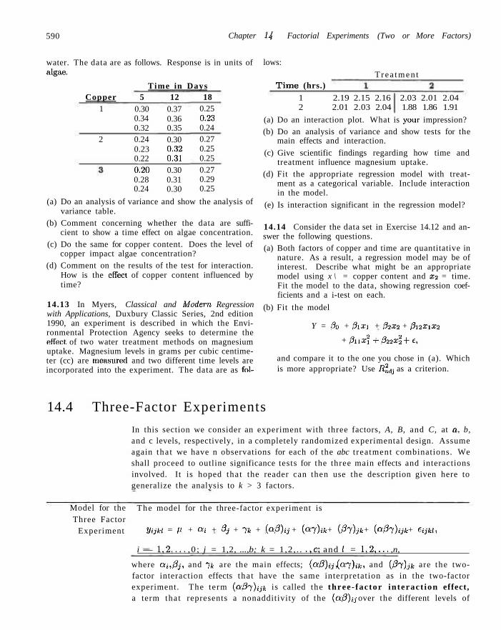
590 Chapter 14 Factorial Experiments (Two or More Factors)
water. The data are as follows. Response is in units of algae.
Time in Days Copper 5 12 18
lows:
T r e a t m e n t
1
2
0.30 0.34 0.32 0.24 0.23 0.22
0.37 0.36 0.35 0.30 0.32 0.31
0.25 0.23 0.24 0.27 0.25 0.25
0.20 0.28 0.24
0.30 0.31 0.30
0.27 0.29 0.25
(a) Do an analysis of variance and show the analysis of variance table.
(b) Comment concerning whether the data are sufficient to show a time effect on algae concentration.
(c) Do the same for copper content. Does the level of copper impact algae concentration?
(d) Comment on the results of the test for interaction. How is the effect of copper content influenced by time?
14.13 In Myers, Classical and Modern Regression with Applications, Duxbury Classic Series, 2nd edition 1990, an experiment is described in which the Environmental Protection Agency seeks to determine the effect of two water treatment methods on magnesium uptake. Magnesium levels in grams per cubic centimeter (cc) are measurexl and two different time levels are incorporated into the experiment. The data are as fol-
Time (hrs.) 1 2.19 2.15 2.16 2.03 2.01 2.04 2 2.01 2.03 2.04 1.88 1.86 1.91
(a) Do an interaction plot. What is your impression? (b) Do an analysis of variance and show tests for the
main effects and interaction.
(c) Give scientific findings regarding how time and treatment influence magnesium uptake.
(d) Fit the appropriate regression model with treatment as a categorical variable. Include interaction in the model.
(e) Is interaction significant in the regression model?
14.14 Consider the data set in Exercise 14.12 and answer the following questions. (a) Both factors of copper and time are quantitative in
nature. As a result, a regression model may be of interest. Describe what might be an appropriate model using x \ = copper content and x2 = time. Fit the model to the data, showing regression coefficients and a i-test on each.
(b) Fit the model
Y = 0o + /?ixi + 32x2 + 3\2Xix2
+ 3nX2i +022x1 + 6,
and compare it to the one you chose in (a). Which is more appropriate? Use R2
dj as a criterion.
14.4 Three-Factor Experiments
In this section we consider an experiment with three factors, A, B, and C, at a, b, and c levels, respectively, in a completely randomized experimental design. Assume again tha t we have n observations for each of the abc t reatment combinations. We shall proceed to outline significance tests for the three main effects and interactions involved. It is hoped that the reader can then use the description given here to generalize the analysis to k > 3 factors.
Model for the Three Factor
Experiment
The model for the three-factor experiment is
Vijki = P + o-'i + 3j + 7fc + (c\3)ij + (a-y)ik + (0"f)jk + ic*0l)ijk + e y « ,
i — 1 ,2 . . . . ,0 ; j = 1,2, ...,b; k = 1,2, . . . , c ; and I = 1 ,2 , . . . ,n,
where ai, pj, and jk are the main effects; (a0)ij, (07)^, , and (0~y)jk are the two-factor interaction effects tha t have the same interpretation as in the two-factor experiment. The term (a/?7),jfc is called the three- factor interact ion effect, a term that represents a nonadditivity of the (a0)ij over the different levels of
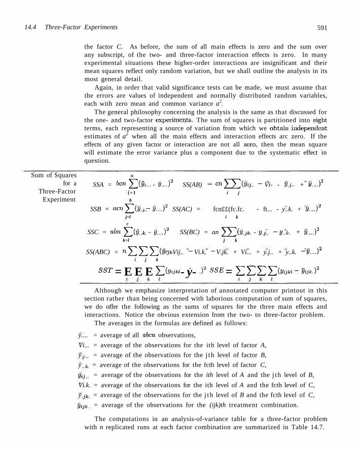
14.4 Three-Factor Experiments 591
Sum of Squares for a
Three-Factor Experiment
the factor C. As before, the sum of all main effects is zero and the sum over any subscript, of the two- and three-factor interaction effects is zero. In many experimental situations these higher-order interactions are insignificant and their mean squares reflect only random variation, but we shall outline the analysis in its most general detail.
Again, in order that valid significance tests can be made, we must assume that the errors are values of independent and normally distributed random variables, each with zero mean and common variance a2.
The general philosophy concerning the analysis is the same as that discussed for the one- and two-factor experiments. The sum of squares is partitioned into eight terms, each representing a source of variation from which we obtain independent estimates of a2 when all the main effects and interaction effects arc zero. If the effects of any given factor or interaction are not all zero, then the mean square will estimate the error variance plus a component due to the systematic effect in question.
a
SSA = ben J2iVi... - fj...f SS(AB) = cnJ2 £ ( f l y . . " Vi- - V-i- + V-f (=1 i j
b
SSB = acnJ2iV.j.. - V-f SS(AC) = fcn££(fc.fc. - ft... - y..k. + V...f j=l i k c
SSC = aim Y,iV..k. - j/....)2 SS(BC) = an £ J > . j f c . - y.j.- " V-k- + V..-)2
k=l j k
SS(ABC) = n-Y^YlY^iyijk. ~ Vij.. - Vi.k. - V.jk. + Vi... + y.j.. + y..k. - y....f i j k
SST = E E E E t o - y- ")2 SSE = E E E£<«* Vijk.)2
Although we emphasize interpretation of annotated computer printout in this section rather than being concerned with laborious computation of sum of squares, we do offer the following as the sums of squares for the three main effects and interactions. Notice the obvious extension from the two- to three-factor problem.
The averages in the formulas are defined as follows:
y.... = average of all aben observations,
Vi... = average of the observations for the ith level of factor A,
y j = average of the observations for the j th level of factor B,
y k = average of the observations for the fcth level of factor C,
y^ = average of the observations for the ith level of A and the j t h level of B,
Vi.k. = average of the observations for the ith level of A and the fcth level of C,
y j k = average of the observations for the j t h level of B and the fcth level of C,
fjijk = average of the observations for the (ijk)th treatment combination.
The computations in an analysis-of-variance table for a three-factor problem with n replicated runs at each factor combination are summarized in Table 14.7.
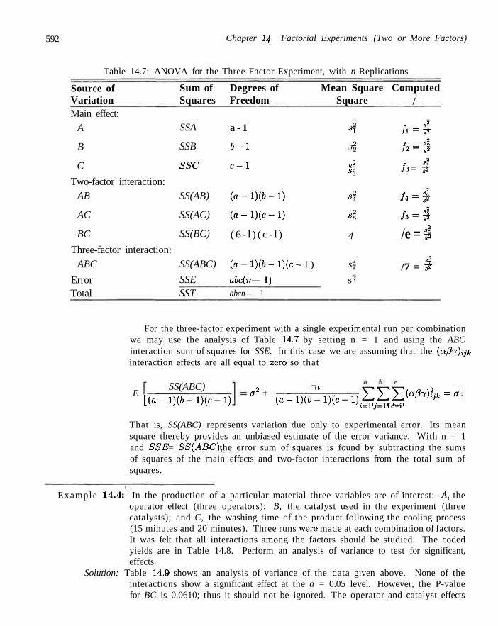
592 Chapter 14 Factorial Experiments (Two or More Factors)
Table 14.7: ANOVA for the Three-Factor Experiment, with n Replications
Source of Variation Main effect:
A
B
C
Two-factor interaction: AB
AC
BC
Three-factor interaction: ABC
Error Total
Sum of Squares
SSA
SSB
SSC
SS(AB)
SS(AC)
SS(BC)
SS(ABC)
SSE SST
Degrees of Freedom
a - 1
b-1
c - 1
( a - l ) ( 6 - l )
( o - l ) ( c - l )
( 6 - l ) ( c - l )
(o- l ) (6- l ) (c -
abc(n — 1)
abcn— 1
Mean Square Square
• si
s-2
R2
s 3
«2 s4
<i2
•s5
4
- 1 ) s2
S"
Computed /
h-i A-s
s2
h = 3$
/4-i
/ 5=f l
/e = fl
/7 = fl
For the three-factor experiment with a single experimental run per combination we may use the analysis of Table 14.7 by setting n = 1 and using the ABC interaction sum of squares for SSE. In this case we are assuming that the (adf)ijk interaction effects are all equal to zero so that
E SS(ABC)
L(o- l ) (6- l ) (c - l ) a2 + RraR^(^"' »=i j = i f c = i
That is, SS(ABC) represents variation due only to experimental error. Its mean square thereby provides an unbiased estimate of the error variance. With n = 1 and SSE = SS(ABC), the error sum of squares is found by subtracting the sums of squares of the main effects and two-factor interactions from the total sum of squares.
Example 14.4:1 In the production of a particular material three variables are of interest: A, the operator effect (three operators): B, the catalyst used in the experiment (three catalysts); and C, the washing time of the product following the cooling process (15 minutes and 20 minutes). Three runs were made at each combination of factors. It was felt that all interactions among the factors should be studied. The coded yields are in Table 14.8. Perform an analysis of variance to test for significant, effects.
Solution: Table 14.9 shows an analysis of variance of the data given above. None of the interactions show a significant effect at the a = 0.05 level. However, the P-value for BC is 0.0610; thus it should not be ignored. The operator and catalyst effects
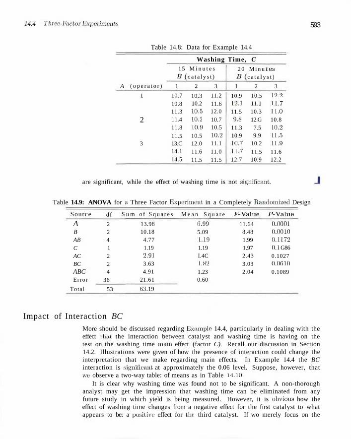
14.4 Three-Factor Experiments 593
Table 14.8: Data for Example 14.4
Washing Time, C
A ( o p e r a t o r )
1
2
3
1 5 M i n u t e s
B( 1
10.7 10.8 11.3 11.4 11.8
11.5 13.C 14.1 14.5
c a t a l y s t )
2
10.3 10.2 10.5 10.2 10.9
10.5 12.0 11.6 11.5
3
11.2 11.6 12.0 10.7 10.5 10.2 11.1 11.0 11.5
2 0 M i n u i B\
1
10.9 12.1 11.5 9.8
11.3 10.9 10.7 1 1.7 12.7
e-s c a t a l y s t )
2
10.5 11.1 10.3 12.G 7.5 9.9
10.2
11.5 10.9
3
12.2 1 1.7 1 1.0 10.8 10.2 11.5 1.1.9 11.6 12.2
are significant, while the effect of washing time is not significant.
Table 14.9: ANOVA for a Three Factor Experiment in a Completely Randomized Design
Source
A B AB
C AC BC ABC Error
Total
d f
2 2 4 1 2 2 4
36
53
S u m o f S q u a r e s
13.98 10.18 4.77 1.19 2.91 3.63 4.91
21.61
63.19
M e a n S q u a r e
0.99 5.09 1.19 1.19 I.4C 1.82 1.23 0.60
F - V a l u e
11.64 8.48 1.99 1.97 2.43 3.03 2.04
P - V a l u e
0.0001 (1.0010 0.1172 0.1 G86 0.1027 O.0G10 0.1089
Impact of Interaction BC
More should be discussed regarding Example 14.4, particularly in dealing with the effect that the interaction between catalyst and washing time is having on the test on the washing time main effect (factor C). Recall our discussion in Section 14.2. Illustrations were given of how the presence of interaction could change the interpretation that we make regarding main effects. In Example 14.4 the BC interaction is significant at approximately the 0.06 level. Suppose, however, that we observe a two-way table: of means as in Table 14.10.
It is clear why washing time was found not to be significant. A non-thorough analyst may get the impression that washing time can be eliminated from any future study in which yield is being measured. However, it is obvious how the effect of washing time changes from a negative effect for the first catalyst to what appears to be: a positive effect for the third catalyst. If wo merely focus on the
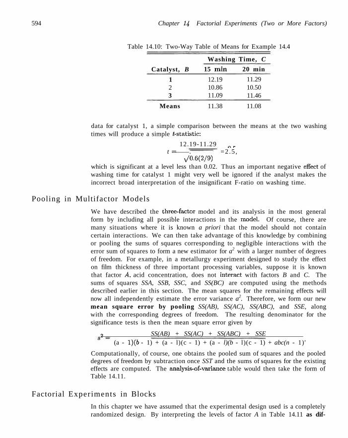
594 Chapter 14 Factorial Experiments (Two or More Factors)
Table 14.10: Two-Way Table of Means for Example 14.4
Catalyst, B
1 2 3
Washing
15 min
12.19 10.86 11.09
Time, C
20 min
11.29 10.50 11.46
Means 11.38 11.08
data for catalyst 1, a simple comparison between the means at the two washing times will produce a simple ^-statistic:
12.19-11.29 „ „ t = . =2 .5 ,
>/0.6(2/9) which is significant at a level less than 0.02. Thus an important negative effect of washing time for catalyst 1 might very well be ignored if the analyst makes the incorrect broad interpretation of the insignificant F-ratio on washing time.
Pooling in Multifactor Models
We have described the three-factor model and its analysis in the most general form by including all possible interactions in the model. Of course, there are many situations where it is known a priori that the model should not contain certain interactions. We can then take advantage of this knowledge by combining or pooling the sums of squares corresponding to negligible interactions with the error sum of squares to form a new estimator for a2 with a larger number of degrees of freedom. For example, in a metallurgy experiment designed to study the effect on film thickness of three important processing variables, suppose it is known that factor A, acid concentration, does not interact with factors B and C. The sums of squares SSA, SSB, SSC, and SS(BC) are computed using the methods described earlier in this section. The mean squares for the remaining effects will now all independently estimate the error variance a2. Therefore, we form our new mean square error by pooling SS(AB), SS(AC), SS(ABC), and SSE, along with the corresponding degrees of freedom. The resulting denominator for the significance tests is then the mean square error given by
2 SS(AB) + SS(AC) + SS(ABC) + SSE ~ (a - 1)(6 - 1) + (a - l)(c - 1) + (a - l)(b - l)(c - 1) + abc(n - 1)'
Computationally, of course, one obtains the pooled sum of squares and the pooled degrees of freedom by subtraction once SST and the sums of squares for the existing effects are computed. The analysis-of-variance table would then take the form of Table 14.11.
Factorial Experiments in Blocks
In this chapter we have assumed that the experimental design used is a completely randomized design. By interpreting the levels of factor A in Table 14.11 as dif-
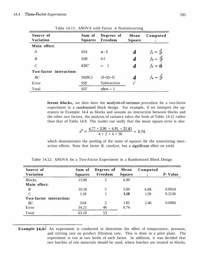
14.4 Three-Factor Experiments 595
Table 14.11: ANOVA with Factor .4 Noninteracting
Source of Variation
Main effect:
A
B
C
Two-factor interaction:
BC
Error
Total
Sum of Squares
SSA
SSB
SSC
SS(BC)
SSE
SST
Degrees of Freedom
a - 1
b-l
c- 1
(b-l)(c-l)
Subtraction
abcn — 1
Mean Square
4 4 4
4 s2
Computed /
/i = fl h = $ /3 = fl
/4 = S
ferent blocks, we then have the analysis-of-variance procedure for a two-factor experiment in a randomized block design. For example, if we interpret the operators in Example 14.4 as blocks and assume no interaction between blocks and the other two factors, the analysis of variance takes the form of Table 14.12 rather than that of Table 14.9. The reader can verify that the mean square error is also
4.77 + 2.91 + 4.91 + 21.61 4 + 2 + 4 + 36
= 0.74.
which demonstrates the pooling of the sums of squares for the nonexisting interaction effects. Note that factor B, catalyst, has a significant effect on yield.
Table 14.12: ANOVA for a Two-Factor Experiment in a Randomized Block Design
Source of Variation
Blocks Main effect:
B C
Two-factor interaction: BC
Error
Total
Sum of Squares
13.98
10.18 1.18
3.64 34.21
63.19
Degrees of Freedom
2
2 1
2 46
53
Mean Square
6.99
5.09 1.18
1.82 0.74
Computed /
6.88 1.59
2.46
P- Value
0.0024 0.2130
0.0966
Example 14.5:1 An experiment is conducted to determine the effect of temperature, pressure, and stirring rate on product filtration rate. This is done in a pilot plant. The experiment is run at two levels of each factor. In addition, it was decided that two batches of raw materials should be used, where batches are treated as blocks.
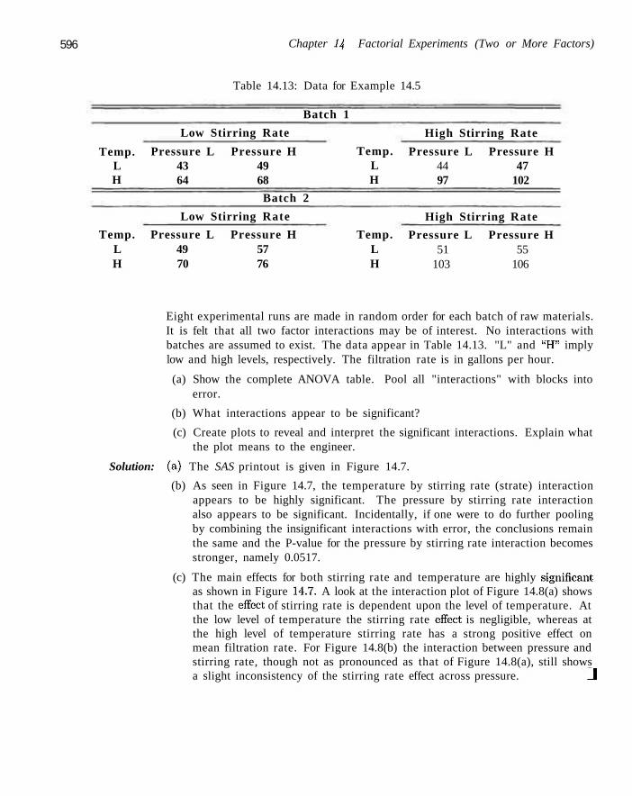
596 Chapter 14 Factorial Experiments (Two or More Factors)
Table 14.13: Data for Example 14.5
Batch 1
Temp. L H
Low Stirring Rate
Pressure L Pressure H 43 49 64 68
Temp. L H
High Stirring Rate
Pressure L Pressure H 44 47 97 102
Batch 2
Temp. L H
Low Stirring Rate
Pressure L Pressure H 49 57 70 76
Temp. L H
High Stirring Rate
Pressure L Pressure H 51 55
103 106
Eight experimental runs are made in random order for each batch of raw materials. It is felt that all two factor interactions may be of interest. No interactions with batches are assumed to exist. The data appear in Table 14.13. "L" and "H" imply low and high levels, respectively. The filtration rate is in gallons per hour.
(a) Show the complete ANOVA table. Pool all "interactions" with blocks into error.
(b) What interactions appear to be significant?
(c) Create plots to reveal and interpret the significant interactions. Explain what the plot means to the engineer.
Solution: (a) The SAS printout is given in Figure 14.7.
(b) As seen in Figure 14.7, the temperature by stirring rate (strate) interaction appears to be highly significant. The pressure by stirring rate interaction also appears to be significant. Incidentally, if one were to do further pooling by combining the insignificant interactions with error, the conclusions remain the same and the P-value for the pressure by stirring rate interaction becomes stronger, namely 0.0517.
(c) The main effects for both stirring rate and temperature are highly significant as shown in Figure 14.7. A look at the interaction plot of Figure 14.8(a) shows that the effect of stirring rate is dependent upon the level of temperature. At the low level of temperature the stirring rate effect is negligible, whereas at the high level of temperature stirring rate has a strong positive effect on mean filtration rate. For Figure 14.8(b) the interaction between pressure and stirring rate, though not as pronounced as that of Figure 14.8(a), still shows a slight inconsistency of the stirring rate effect across pressure. J
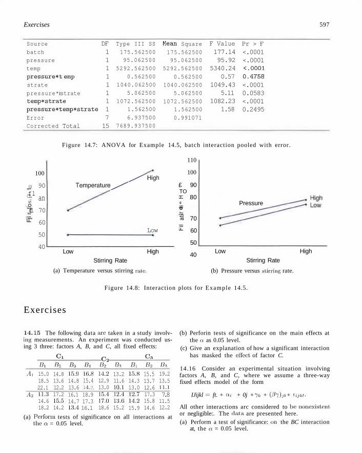
Exercises
Source
batch
pressure
temp
pressure*!; emp
strate
pressure* strate temp*strate
pressure*temp*strate
Error
Corrected Total
DF 1 1 1 1 1 1 1 1 7 15
Type III SS
175.562500 95.062500
5292.562500
0.562500
1040.062500
5.062500
1072.562500 1.562500
6.937500
7689.937500
Mean Square
175.562500 95.062500
5292.562500
0.562500
1040.062500
5.062500
1072.562500 1.562500
0.991071
F Value 177.14 95.92
5340.24 0.57
1049.43 5.11
1082.23 1.58
Pr > F <.0001 <.0001 •c.OOOl 0.4758 <.0001 0.0583 <.0001 0.2495
597
100
(1)
fl CL E O (fl •— li.
90
an
70
60
50
40
Figure 14.7: ANOVA for Example 14.5, batch interaction pooled with error.
110
100
Temperature^-'"''' /-""'High
Low
Low High
Stirring Rate
(a) Temperature versus stirring rate.
80
£ 90 TO
CC c o
'a 70
E 60
50
40
Pressure
Low High
Stirring Rate
(b) Pressure versus stirring rate.
Figure 14.8: Interaction plots for Example 14.5.
Exercises
14.15 The following data are taken in a study involving measurements. An experiment was conducted using 3 three: factors A, B, and C, all fixed effects:
-4i
Bi
15.0 18.5 22.1
Ci
B-, 14.8 13.6 12.2
Bs
15.9 14.8 13.6
Bi
16.8 15.4 1-1. :>,
c2 B2
14.2 12.9 13.0
Ih
13.2 11.6 10.1
Si 15.8 14.3 13.0
C:l B2 15.5 13.7 12.6
Bi
19.2 13.5 11.1
M
(a) Perform tests of significance on all interactions at the a = 0.05 level.
11.3 14.6 18.2
17.2 15.5 14.2
16.1 18.9 14.7 17.3 13.4 16.1
15,1 17.0 18.6
12.1 13.6 15.2
12.7 14.2 15.9
17.3 15.8 14.6
7.8 11.5 12.2
(b) Perforin tests of significance on the main effects at the Q as 0.05 level.
(c) Give an explanation of how a significant interaction has masked the effect of factor C.
14.16 Consider an experimental situation involving factors A, B, and C, where we assume a three-way fixed effects model of the form
IJijkl a= ft. + OH + 0j + ft, + (0rt)jk + Uikl.
All other interactions arc considered to be nonexistent or negligible:. The elata are presented here. (a) Perform a test of significance: e>n the BC interaction
at, the a = 0.05 level.
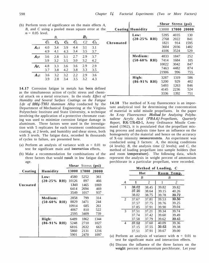
598 Chapter 14 Factorial Experiments (Two or More Factors)
(b) Perform tests of significance on the main effects A, B, and C using a pooled mean square error at the a = 0.05 level.
B, Bo
An
A2:
Ar.
Ci
4.0 4.9
3.6 3.9
4.8 3.7
c2 3.4 4.1
2.8 3.2
3.3 3.8
C3
3.9 4.3
3.1 3.5
3.6 4.2
Ci
4.4 3.4
2.7 3.0
3.6 3.8
C2
3.1 3.5
2.9 3.2
2.9 3.3
O,
3.1 3.7
3.7 4.2
2.9 3.5
3.6 3.9
3.2 2.8
3.2 3.4
2.2 3.5
2.9 3.2
3.6 4.3
14.17 Corrosion fatigue in metals has been defined as the simultaneous action of cyclic stress and chemical attack on a metal structure. In the study Effect of Humidity and Several Surface Coatings on the Fatigue Life of 2024-T351 Aluminum Alloy conducted by the Department of Mechanical Engineering at the Virginia Polytechnic Institute and State University, a technique involving the application of a protective chromate coating was used to minimize corrosion fatigue damage in aluminum. Three factors were used in the investigation with 5 replicates for each treatment combination: coating, at 2 levels, and humidity and shear stress, both with 3 ievels. The fatigue data, recordeel in thousands of cycles to failure, are presented here.
(a) Perform an analysis of variance with a = 0.01 to test for significant main and interaction effects,
(b) Make a recommendation for combinations of the three factors that would result in low fatigue damage.
Coating
Uncoated
Humidity
Low: (20-25% RH)
Medium: (50-60% RH)
High: (86-91% RH)
Shear Stress
13000
4580 10126
1341 6414 3549
2858 8829
10914 4067 2595
6489 5248 6816 5860 5901
17000
5252 897
1465 2694 1017
799 3471
685 810
3409
1862 2710 2632 2131 2470
(psi)
20000
361 466
1069 469 937
314 244 261 522 739
1344 1027 663
1216 1097
Coating
Chromated
Humidity
Low: (20-25% RH)
Medium: (50-60% RH)
High: (86-91% RH)
Shear Stress
13000
5395 2768 1821 3604 4106
4833 7414
10022 7463
21906
3287 5200 5493 4145 3336
17000
4035 2022
914 2036 3524
1847 1684 3042 4482
996
1319 929
1263 2236 1392
(psi)
20000
130 841
1595 1482 529
252 105 847 874 755
586 402 846 524 751
14.18 The method of X-ray fluorescence is an important analytical tool for determining the concentration of material in solid missile propellants. In the paper An X-ray Fluorescence Method for Analyzing Polybu-tadiene Acrylic Acid (PBAA) Propellants, Quarterly Report, RK-TR-62-1, Army Ordinance Missile Command (1962), it is postulated that the propellant mixing process and analysis time have an influence on the homogeneity of the material and hence on the accuracy of X-ray intensity measurements. An experiment was conducted using 3 factors: A, the mixing conditions (4 levels); B, the analysis time (2 levels); and C, the method of loading propellant into sample holders (hot and room temperature). The following data, which represent the analysis in weight percent of ammonium perchlorate in a particular propellant, were recorded.
Method of Loading, C Hot R o o m Temp.
A
1
2
3
4
B 1
38.62 37.20 38.02 37.67 37.57 37.85 37.51 37.74 37.58 37.52 37.15 37.51
2
38.45 38.64 38.75 37.81 37.75 37.91 37.21 37.42 37.79 37.60 37.55 37.91
1 39.82 39.15 39.78 39.53 39.76 39.90 39.34 39.60 39.62 40.09 39.63 39.67
B 2
39.82 40.26 39.72 39.56 39.25 39.04 39.74 39.49 39.45 39.36 39.38 39.00
(a) Perform an analysis of variance with a = 0.01 to test for significant main and interaction effects.
(b) Discuss the influence of the three factors on the weight, percent of ammonium perchlorate. Let your
Exercises 599
discussion involve the role of any significant interaction.
14.19 Electronic copiers make copies by gluing black ink on paper, using static electricity. Heating and gluing the ink on the paper comprise the final stage of the copying process. The gluing power during this final process determines the quality of the copy. It is postulated that temperature, surface state of gluing the roller, and hardness of the press roller influence the gluing power of the copier. An experiment is run with treatments consisting of a combination of these three factors at each of three levels. The following data show the gluing power for each treatment combination. Perform an analysis of variance with a = 0.05 to test for significant main and interaction effects.
Surface S t a t e of Gluing Roller
H a r d n e s s of t h e P r e s s Rol ler
20 40 60
Low T e m p .
Soft: 0.52 0.57
0.44 0.53
M e d i u m : 0.64 0.58
HaTai UBT 0.74
0.59 0.64 0.77 0.65
M e d i u m Soft: 0.46 0.40 T e m p . 0.58 0.37
M e d i u m : 0.60 0.43 0.62 0.61
Hard : 0.53 0.66
0.65 0.56
High T e m p .
Soft: 0.52 0.57
M e d i u m : 0.53 0.66
"0\4T 0.47
0.44 0.53 u\6o 0.56
HaTcTT 1TM 0.44
0.54 0.65
0.52 0.56
0.79 0.79
0.73 0.78
058 0.57 0.59
0.31 0.48
0.49 0.66
0.66 0.72
0.57 0.56
0.53 0.59
0.45 0.47
0.54 0.65
0.52 0.56
0.59 7X4T 0.47
048 0.43
(131 0.27
0.60 0.78
0.55 0.68
0.49 0.74
0.48 0.50
0.55 0.57
~D\65 0.58
.56
.49 0.42 0.49
"054" 0.56
56 71
0.66 0.67
.65
.65 0.49 0.52
0.50 55 57
0.65 0.58
14.20 For a study of the hardness of gold dental fillings, five randomly chosen dentists were assigned combinations of three methods of condensation and two types of gold. The hardness was measured. [See Hoaglin, Mosteller, and Tukey (1991).] The data are presented here. Let the dentists play the role of blocks. (a) State the appropriate model with the assumptions. (b) Is there a significant interaction between method
of condensation and type of gold filling material? (c) Is there one method of condensation that seems to
be best? Explain.
Block T y p e Den t i s t
1
2
3
4
M e t h o d 1 2 3 1 2 3 1 2 3 1 2 3
Gold Foil 792 772 782
803 752 715 715 792 762
673 657 690
Golden t 824 772 803 803 772 707 724 715 606 946 743 245
1 2 3
634 649 724
715 724 627
14.21 Consider combinations of three factors in the removal of dirt from standard loads of laundry. The first factor is the brand of the detergent, X, Y, or Z. The second factor is the type of detergent, liquid or powder. The third factor is the temperature of the water, hot or warm. The experiment was replicated three times. Response is percent dirt removal. The data are as follows:
B r a n d T y p e T e m p e r a t u r e
X
Y
Powder
Liquid
Powder
Liquid
Hot Warm Hot
Warm Hot
Warm Hot
Warm
85 88 80 82 83 85 78 75 72 75 75 73 90 92 92 88 86 88 78 76 70 76 77 76
Powder
Liquid
Hot Warm
Hot Warm
85 76 60 55
87 74 70 57
88 78 68 54
(a) Are there significant interaction effects at the a = 0.05 level?
(b) Are there significant differences between the three brands of detergent?
(c) Which combination of factors would you prefer to use?
14.22 A scientist collects experimental data on the radius of a propellant grain, y, as a function of powder temperature, extrusion rate, and die temperature. The three factor experiment is as follows:
GOO Chapter 14 Factorial Experiments (Two or More Factors)
P o w d e r T e m p
R a t e 12 24
Die T e m p 150
220 250 82 124
114 157
Die T e m p 190
220 250 88 129
121 164
Resources were not, available to take repeated experimental trials at the eight combinations of factors. It is felt as if extrusion rate does not interact, with die temperature and that the three-factor interaction should be negligible. Thus, these two interactions may be pooled to produce a 2 d.f. "error" term.
(a) Do an analysis of variance that includes the three main effects and two two-factor interactions. Determine what effects influence radius of the propellant grain.
(b) Construct interaction plots for the powder temperature by die temperature and powder temperature by extrusion rate interactions.
(c) Comment on the consistency between the appearance of the interaction plots and the tests on the two interactions in the ANOVA.
14.23 In the book Design of Experiments for Quality Improvement, published by the Japanese Standards Association (1989), a study is reported on the extraction of polyethylene by using a solvent and how the
amount of gel (proportion) is influenced by three factors, the type of solvent, extraction temperature, and extraction time. A factorial experiment was designed and the following data were collected 011 proportion of gel.
T i m e Solvent. T e m p
17*1 1 1 2 0 Ethano l
80 ™ . 120 l o l u e n e
80
4 94.0, 94.0 95.3, 95.1 94.6, 94.5 95.4, 95,1
8 93.8, 94.2 94.9, 95.3 93.6, 94.1 95.6, 96.0
16 91.1, 90.5 92.5, 92.4 91.1. 91.0 92.1, 92.1
(a) Do an analysis of variance and determine what factors and interactions influence the proportion of gel.
(b) Construe:! an interaction plot, for any two factor interaction that is significant. In addition, explain what conclusion can be drawn from the presence of the interaction.
(c) Do a normal probability plot of residuals and comment .
14.24 Consider the data set in Exercise 14.19. (a) Construct an interaction plot for any two factor
interaction that is significant.
(b) Do a normal probability plot of residuals and comment .
14.5 Model II and III Factorial Experiments
In a two-factor experiment with random effects wc have model II:
Yijk =ft + Ai + Bj + (AB)ij + eijk,
for i — 1 ,2 , . . . , o.\ j = 1,2,..., b; and k = 1 .2 , . . . , n, where the Ai, Bj, (AB)ij, and eyfe are independent, random variables with zero moans and variances a~., a\, a2a, and a2, respectively. The sum of squares for model II experiments are computed in exactly the same way as for model I experiments. Wc are now interested in testing hypotheses of the form
H0:
H't:
oi = o> <^o,
ft
ff0: H'[:
a2 = 0,
4*o, H, 0 • 'a0 0.
f^0,
where the denominator in the /-ratio is not necessarily the mean square error. The appropriate denominator can be determined by examining the expected values of the various mean squares. These are shown in Table 14.14.
From Table 14.14 we see that HQ and H0 are tested by using s | in the denominator of the /-ratio, whereas H0 is tested using s in the denominator. The unbiased estimates of the variance components are
bn " 2 a0
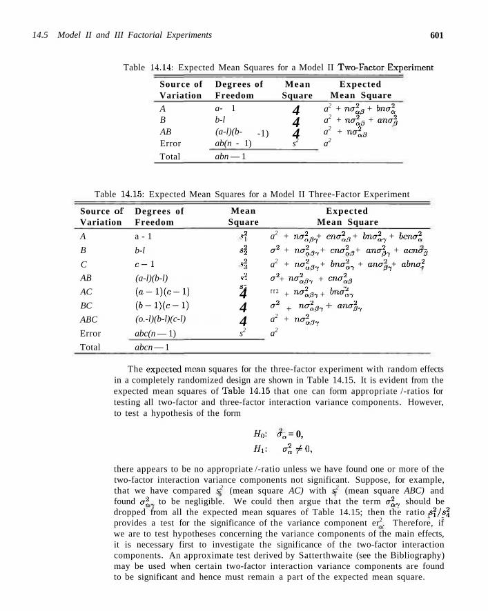
14.5 Model II and III Factorial Experiments 601
Table 14.14: Expected Mean Squares for a Model II Two-Factor Experiment
Source of Degrees of Mean Variation Freedom Square
Expected Mean Square
A B AB Error
Total
a- 1 b-l (a-l)(b-ab(n - 1)
abn — 1
-1)
4 4 4 s2
a2 + na2a3 + bna2
a
a2 + na2a3 + ana2
3
a2 + na2a3
a2
Table 14.15: Expected Mean Squares for a Model II Three-Factor Experiment
Source of Variation
A
B
C
AB
AC
BC
ABC
Error
Total
Degrees of Freedom
a - 1
b-l
c-l
(a-l)(b-l)
( a - l ) ( c - l ) ( 6 - l ) ( c - l ) (o.-l)(b-l)(c-l)
abc(n — 1)
abcn — 1
Mean Square
Q 2
<i2 h2
i2
s2
s4 4 4 4 s2
Expected Mean Square
a2 + na\ai + cna1^ + bna^. + bcna2a
a2 + na23,t + cna2
3 + ana2^ + acna3
a2 + na2a3l + bna2^ + ana^ + abna2
^ + n°~U-y + cncr2^ f f 2 + n < 3 7 + i n f f « 7
a2 + n°lfh- + anali a2 + na2
afh.
a2
The expected mean squares for the three-factor experiment with random effects in a completely randomized design are shown in Table 14.15. It is evident from the expected mean squares of Table 14.15 that one can form appropriate /-ratios for testing all two-factor and three-factor interaction variance components. However, to test a hypothesis of the form
Ho'- aa = 0, Hi: a2
a^0,
there appears to be no appropriate /-ratio unless we have found one or more of the two-factor interaction variance components not significant. Suppose, for example, that we have compared s2 (mean square AC) with s2 (mean square ABC) and found a2 to be negligible. We could then argue that the term cr2., should be dropped from all the expected mean squares of Table 14.15; then the ratio s2/s2
provides a test for the significance of the variance component er2. Therefore, if we are to test hypotheses concerning the variance components of the main effects, it is necessary first to investigate the significance of the two-factor interaction components. An approximate test derived by Satterthwaite (see the Bibliography) may be used when certain two-factor interaction variance components are found to be significant and hence must remain a part of the expected mean square.
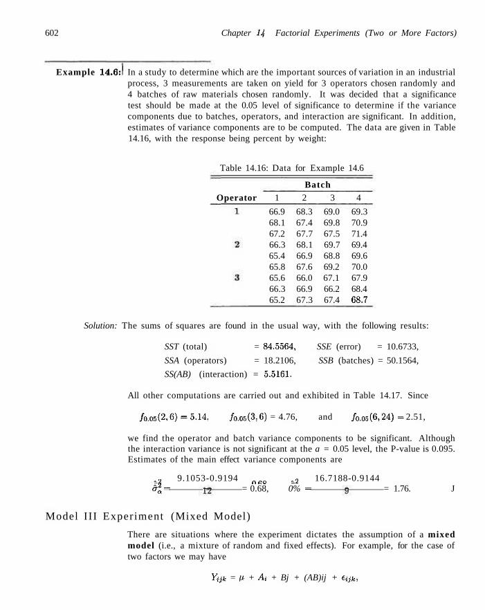
602 Chapter 14 Factorial Experiments (Two or More Factors)
Example 14.6:1 In a study to determine which are the important sources of variation in an industrial process, 3 measurements are taken on yield for 3 operators chosen randomly and 4 batches of raw materials chosen randomly. It was decided that a significance test should be made at the 0.05 level of significance to determine if the variance components due to batches, operators, and interaction are significant. In addition, estimates of variance components are to be computed. The data are given in Table 14.16, with the response being percent by weight:
Table 14.16: Data for Example 14.6
Batch Operator 1 2 3 4
66.9 68.3 69.0 69.3 68.1 67.4 69.8 70.9 67.2 67.7 67.5 71.4 66.3 68.1 69.7 69.4 65.4 66.9 68.8 69.6 65.8 67.6 69.2 70.0 65.6 66.0 67.1 67.9 66.3 66.9 66.2 68.4 65.2 67.3 67.4 68.7
Solution: The sums of squares are found in the usual way, with the following results:
SST (total) = 84.5564, SSE (error) = 10.6733,
SSA (operators) = 18.2106, SSB (batches) = 50.1564,
SS(AB) (interaction) = 5.5161.
All other computations are carried out and exhibited in Table 14.17. Since
/o.o5(2,6)=5.14, /o.05(3,6) = 4.76, and /o.os(6,24) = 2.51,
we find the operator and batch variance components to be significant. Although the interaction variance is not significant at the a = 0.05 level, the P-value is 0.095. Estimates of the main effect variance components are
„2 9.1053-0.9194 n „Q _2 16.7188-0.9144 ai = - = 0.68, 0% = - = 1.76. J
Model III Experiment (Mixed Model)
There are situations where the experiment dictates the assumption of a mixed model (i.e., a mixture of random and fixed effects). For example, for the case of two factors we may have
Yijk = p + Ai + Bj + (AB)ij + eiik.
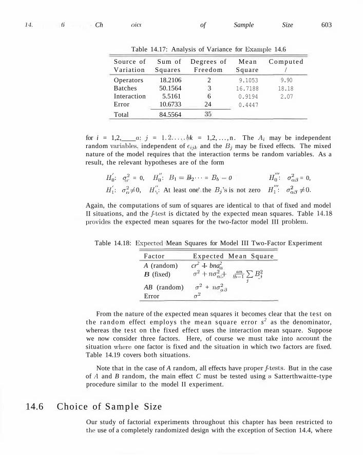
11. (1 Ch oict i of Sample Size 603
Table 14.17: Analysis of Variance for Example 14.6
Source of Sum of Degrees of Mean C o m p u t e d Variat ion Squares Freedom Square /
Operators 18.2106 2 Batches 50.1564 3 Interaction 5.5161 6 Error 10.6733 24
9.1053 16.7188 0.9194 0.4447
9.90 18.18 2.07
Total 84.5564
for i = 1,2, u: j = l.'2,....b: k = 1,2, . . . , n . The A; may be independent random variables, independent of etjk and the Bj may be fixed effects. The mixed nature of the model requires that the interaction terms be random variables. As a result, the relevant hypotheses are of the form
H'0: a2 = 0, H'0\ Bl=B2 = --- = B/, = 0 HQ": a2a3 = 0,
H[: ol ^ 0, tl": At least one' the Sj ' s is not zero H'i": a2a3 ^ 0.
Again, the computations of sum of squares are identical to that of fixed and model II situations, and the /-test is dictated by the expected mean squares. Table 14.18 preivides the expected mean squares for the two-factor model III problem.
Table 14.18: Expecteel Mean Squares for Model III Two-Factor Experiment
Factor Expec ted M e a n Square A (random) cr2 -I- bna2
B (fixed) ^+nal3 + M^Y.B2
j AB (random) a2 + na2
3
Error a2
From the nature of the expected mean squares it becomes clear that the tes t on the r andom effect employs t he mean square error s2 as the denominator, whereas the tes t on t he fixed effect uses the interaction mean square. Suppose we now consider three factors. Here, of course we must take into account the situation where; one factor is fixed and the situation in which two factors are fixed. Table 14.19 covers both situations.
Note that in the case of A random, all effects have proper/tests. But in the case of A and B random, the main effect C must be tested using a Satterthwaitte-type procedure similar to the model II experiment.
14.6 Choice of Sample Size
Our study of factorial experiments throughout this chapter has been restricted to the use of a completely randomized design with the exception of Section 14.4, where
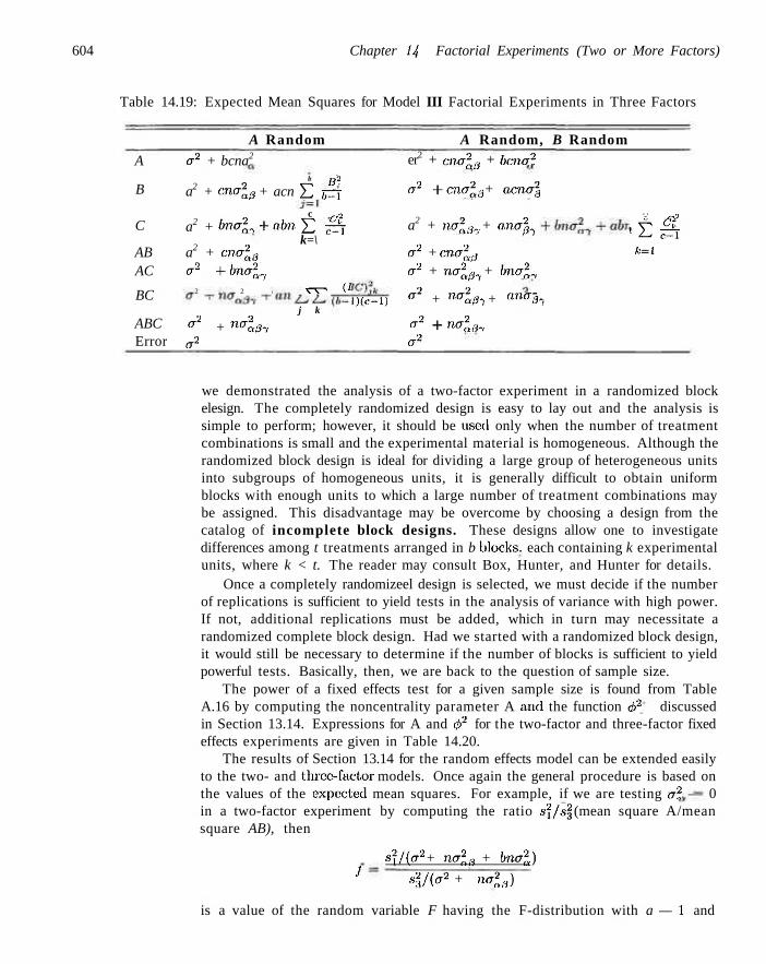
604 Chapter Ut Factorial Experiments (Two or More Factors)
Table 14.19: Expected Mean Squares for Model III Factorial Experiments in Three Factors
A Random A Random, B Random
'-' r-2
> E & A . - = l
A
B
C
AB AC
BC
ABC Error
er2 + bcna2
b B„>
a2 + cna2a0 + acn J2 tT=T
c , , 2
a2 + bna2^ +abn-2~2 ^d\ k=\
a2 + cna2k3
a2 +bna2y
2 i 2 i ^ * - ' ( ^
j k
V1 + 1K3y a2
l ) ( c - l )
er2 + c-/ie72,v + bcna2
a2 +cna23 + acna\
a2 + na23,. + a.na2^
or2 + cn.a2ali
a2 + na2a3l + bna2^.
°"2 + nalfi-, + ana3-f
°2 + 'K^ a2
we demonstrated the analysis of a two-factor experiment in a randomized block elesign. The completely randomized design is easy to lay out and the analysis is simple to perform; however, it should be usctl only when the number of treatment combinations is small and the experimental material is homogeneous. Although the randomized block design is ideal for dividing a large group of heterogeneous units into subgroups of homogeneous units, it is generally difficult to obtain uniform blocks with enough units to which a large number of treatment combinations may be assigned. This disadvantage may be overcome by choosing a design from the catalog of incomplete block designs. These designs allow one to investigate differences among t treatments arranged in b blocks, each containing k experimental units, where k < t. The reader may consult Box, Hunter, and Hunter for details.
Once a completely randomizeel design is selected, we must decide if the number of replications is sufficient to yield tests in the analysis of variance with high power. If not, additional replications must be added, which in turn may necessitate a randomized complete block design. Had we started with a randomized block design, it would still be necessary to determine if the number of blocks is sufficient to yield powerful tests. Basically, then, we are back to the question of sample size.
The power of a fixed effects test for a given sample size is found from Table A.16 by computing the noncentrality parameter A anel the function <t>2 discussed in Section 13.14. Expressions for A and e£2 for the two-factor and three-factor fixed effects experiments are given in Table 14.20.
The results of Section 13.14 for the random effects model can be extended easily to the two- and three-factor models. Once again the general procedure is based on the values of the expected mean squares. For example, if we are testing a2 — 0 in a two-factor experiment by computing the ratio s2/s3 (mean square A/mean square AB), then
s2l(a2 + na2a3 + bnal)
J s2/(a2 + nal3)
is a value of the random variable F having the F-distribution with a — I and
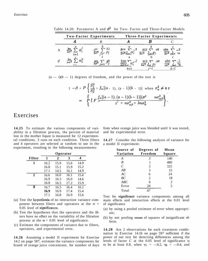
Exercises 605
Table 14.20: Parameter A and 4>2 for Two- Factor and Three-Factor Models
T w o - F a c t o r E x p e r i m e n t s T h r e e - F a c t o r E x p e r i m e n t s
A B A B C
A
tf
MrT a2
(=1 a
- ^ E a i i=\
an V 1 fl2 2 ^ 2^ Pj
j=l b
#E/$ }=l
ben v> _,2 acn V"1 ol abn V^ „,2 2^ L,ai 2^2 lu Pj 2 ? L Ifc t = l fc=l
a b c fcen v-> ,,.2 acn V"* ,<l2 abn V ..2 ^ 2 - ai b^ 2^ Pj 75* L. Ik
t=l j=l k=l
(a — l)(b — 1) degrees of freedom, and the power of the test is
1 - 0 = P { | i > falia - 1), (a - l)(fi - 1)] when e r 2 ^ 0 J
= P{F> fa[(a-l),(a-l)(b-l)}(a2 + nal3)
s2 + nalfi + bnal
Exercises
14.25 To estimate the various components of variability in a filtration process, the percent of material lost in the mother liquor is measured for 12 experimental conditions. 3 runs on each condition. Three filters and 4 operators are selected at random to use in the experiment, resulting in the following measurements:
Operator Filter
1
2
1 16.2 16.8 17.1 16.6 16.9 16.8
2 15.9 15.1 14.5 16.0 16.3 16.5
3 15.6 15.9 16.1 16.1 16.0 17.2
4 14.9 15.2 14.9 15.4 14.6 15.9
16.7 16.5 16.9 16.9 17.1 16.8
16.4 17.4 16.9
16.1 15.4 15.6
(a) Test the hypothesis of no interaction variance component between filters and operators at the a = 0.05 level of significance.
(b) Test the hypotheses that the operators and the filters have no effect on the variability of the filtration process at the a = 0.05 level of significance.
(c) Estimate the components of variance due to filters, operators, and experimental error.
14.26 Assuming a model II experiment for Exercise 14.2 on page 587, estimate the variance components for brand of orange juice concentrate, for number of days
from when orange juice was blended until it was tested, and for experimental error.
14.27 Consider the following analysis of variance for a model II experiment:
Source of Variation
A B C AB AC BC ABC Error Total
Degrees of Freedom
3 1 2 3 6 2 6
24 47
Mean Square
140 480 325
15 24 18 2 5
Test for significant variance components among all main effects and interaction effects at the 0.01 level of significance (a) by using a pooled estimate of error when appropri
ate; (b) by not pooling sums of squares of insignificant ef
fects.
14.28 Are 2 observations for each treatment combination in Exercise 14.16 on page 597 sufficient if the power of our test for detecting differences among the levels of factor C at the 0.05 level of significance is to be at least 0.8. when 71 = —0.2, 72 = —0.4, and
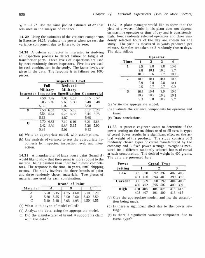
606 Chapter 14 Factorial Experiments (Two or More Factors)
73 = —0.2? Use the same pooled estimate of a2 that was used in the analysis of variance.
14.29 Using the estimates of the variance components in Exercise 14.25, evaluate the power when we test the variance component due to filters to be zero.
14.30 A defense contractor is interested in studying an inspection process to detect failure or fatigue of transformer parts. Three levels of inspections are used by three randomly chosen inspectors, Five lots are used for each combination in the study. The factor levels are given in the data. The response is in failures per 1000 pieces.
Inspection Level Full Reduced
Military Military Inspector Inspection Specification Commercial
A
B
7.50 5.85 5.35 7.58 6.54 5.12
7.42 5.89
6.52 5.64
7.08 6.17 5.65 5.30 5.02 7.68 5.86 5.28 5.38 4.87
6.15 5.52 5.48 5.48 5.98 6.17 6.20 5.44 5.75 5.68
7.70 6.42 5.35
6.82 5.39
7.19 5.85 5.01
6.19 5.35
6.21 5.36 6.12
5.66 5.90
c
(a) Write an appropriate model, with assumptions. (b) Use analysis of variance to test the appropriate hy
pothesis for inspector, inspection level, and interaction.
14.31 A manufacturer of latex house paint (brand A) would like to show that their paint is more robust to the material being painted than their two closest competitors. The response is the time, in years, until chipping occurs. The study involves the three brands of paint and three randomly chosen materials. Two pieces of material are used for each combination.
Ma te r i a l A B C
Brand of Paint A
5.50 5.15 5.60 5.55 5.40 5.48
B
4.75 4.60 5.50 5.60 5.05 4.95
C 5.10 5.20 5.40 5.50 4.50 4.55
(a) What is this type of model called? (b) Analyze the data, using the appropriate model. (c) Did the manufacturer of brand A support its claim
with the data?
14.32 A plant manager would like to show that the yield of a woven fabric in his plant does not depend on machine operator or time of day and is consistently high. Four randomly selected operators and three randomly selected hours of the day are chosen for the study. The yield is measured in yards produced per minute. Samples are taken on 3 randomly chosen days. The data follow:
Operator Time
1
2
1 9.5 9.8
10.0 10.2 9.9 9.5
2 9.8
10.1 9.6
10.1 9.8 9.7
3 9.8
10.3 9.7
10.2 9.8 9.7
4 10.0 9.7
10.2 10.3 10.1 9.9
10.5 10.2 9.3
10.4 10.2 9.8
9.9 10.3 10.2
10.0 10.1 9.7
(a) Write the appropriate model. (b) Evaluate the variance components for operator and
time. (c) Draw conclusions.
14.33 A process engineer wants to determine if the power setting on the machines used to fill certain types of cereal boxes results in a significant effect on the actual weight of the product. The study consists of 3 randomly chosen types of cereal manufactured by the company and 3 fixed power settings. Weight is measured for 4 different randomly selected boxes of cereal at each combination. The desired weight is 400 grams. The data are presented here.
Power Cereal Type Sett ing
Low
Current
1 395 390 401 400 396 399 400 402
2 392 392 394 401 390 392 395 502
3 402 405 399 399 404 403 400 399
High 410 408 404 406 415 412 408 407 401 400 413 415
(a) Give the appropriate model, and list the assumption being made.
(b) Is there a significant effect due to the power setting?
(c) Is there a significant variance component due to cereal type?
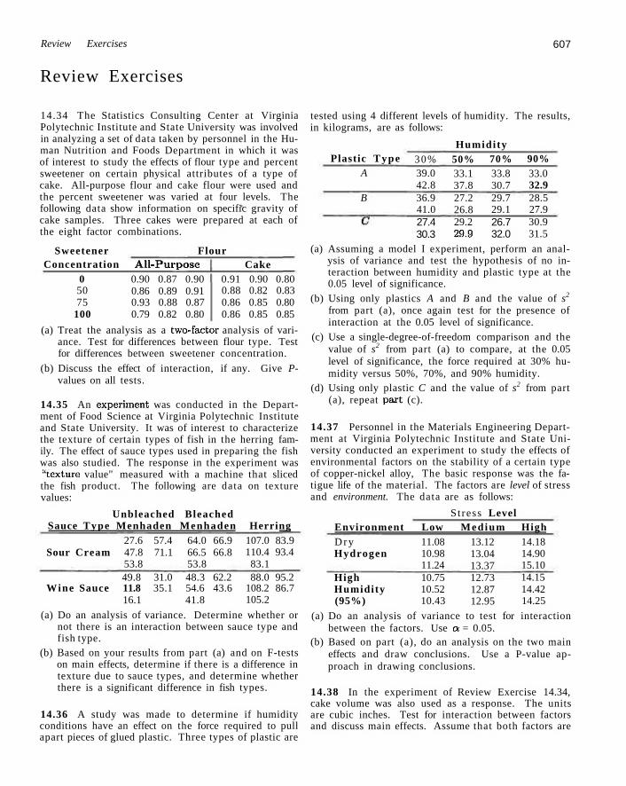
Review Exercises 607
Review Exercises
14.34 The Statistics Consulting Center at Virginia Polytechnic Institute and State University was involved in analyzing a set of data taken by personnel in the Human Nutrition and Foods Department in which it was of interest to study the effects of flour type and percent sweetener on certain physical attributes of a type of cake. All-purpose flour and cake flour were used and the percent sweetener was varied at four levels. The following data show information on specific gravity of cake samples. Three cakes were prepared at each of the eight factor combinations.
Sweetener Flour Concentration
0 50 75
100
All-Purpose 0.90 0.87 0.90 0.86 0.89 0.91 0.93 0.88 0.87 0.79 0.82 0.80
Cake 0.91 0.90 0.80 0.88 0.82 0.83 0.86 0.85 0.80 0.86 0.85 0.85
(a) Treat the analysis as a two-factor analysis of variance. Test for differences between flour type. Test for differences between sweetener concentration.
(b) Discuss the effect of interaction, if any. Give P-values on all tests.
14.35 An experiment was conducted in the Department of Food Science at Virginia Polytechnic Institute and State University. It was of interest to characterize the texture of certain types of fish in the herring family. The effect of sauce types used in preparing the fish was also studied. The response in the experiment was "texture value" measured with a machine that sliced the fish product. The following are data on texture values:
Unbleached Bleached Sauce Type Menhaden Menhaden Herring
27.6 Sour Cream 47.8
53.8
57.4 71.1
64.0 66.9 66.5 66.8 53.8
107.0 83.9 110.4 93.4 83.1
49.8 Wine Sauce 11.8
16.1
31.0 35.1
48.3 62.2 54.6 43.6 41.8
88.0 95.2 108.2 86.7 105.2
(a) Do an analysis of variance. Determine whether or not there is an interaction between sauce type and fish type.
(b) Based on your results from part (a) and on F-tests on main effects, determine if there is a difference in texture due to sauce types, and determine whether there is a significant difference in fish types.
14.36 A study was made to determine if humidity conditions have an effect on the force required to pull apart pieces of glued plastic. Three types of plastic are
tested using 4 different levels of humidity. The results, in kilograms, are as follows:
Humidity Plastic Type
A
B
3 0 % 39.0 42.8 36.9 41.0
50% 33.1 37.8 27.2 26.8
70% 33.8 30.7 29.7 29.1
90% 33.0 32.9 28.5 27.9
27.4 30.3
29.2 29.9
26.7 32.0
30.9 31.5
(a) Assuming a model I experiment, perform an analysis of variance and test the hypothesis of no interaction between humidity and plastic type at the 0.05 level of significance.
(b) Using only plastics A and B and the value of s2
from part (a), once again test for the presence of interaction at the 0.05 level of significance.
(c) Use a single-degree-of-freedom comparison and the value of s2 from part (a) to compare, at the 0.05 level of significance, the force required at 30% humidity versus 50%, 70%, and 90% humidity.
(d) Using only plastic C and the value of s2 from part (a), repeat part (c).
14.37 Personnel in the Materials Engineering Department at Virginia Polytechnic Institute and State University conducted an experiment to study the effects of environmental factors on the stability of a certain type of copper-nickel alloy, The basic response was the fatigue life of the material. The factors are level of stress and environment. The data are as follows:
S t ress Level Environment Low Medium High D r y Hydrogen
11.08 10.98 11.24
13.12 13.04 13.37
14.18 14.90 15.10
10.75 10.52 10.43
12.73 12.87 12.95
14.15 14.42 14.25
High Humidity (95%)
(a) Do an analysis of variance to test for interaction between the factors. Use a = 0.05.
(b) Based on part (a), do an analysis on the two main effects and draw conclusions. Use a P-value approach in drawing conclusions.
14.38 In the experiment of Review Exercise 14.34, cake volume was also used as a response. The units are cubic inches. Test for interaction between factors and discuss main effects. Assume that both factors are
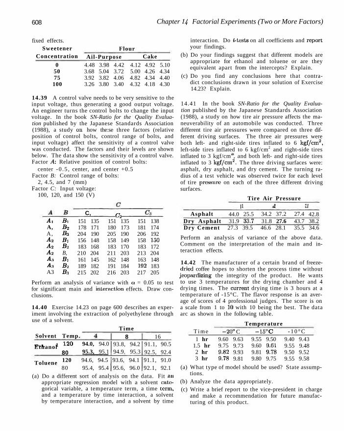
608 Chapter 14 Factorial Experiments (Two or More Factors)
fixed effects. Sweetener
Concentration Flour
Ail-Purpose Cake 0 4.48 3.98 4.42 4.12 4.92 5.10
50 3.68 5.04 3.72 5.00 4.26 4.34 75 3.92 3.82 4.06 4.82 4.34 4.40 100 3.26 3.80 3.40 4.32 4.18 4.30
14.39 A control valve needs to be very sensitive to the input voltage, thus generating a good output voltage. An engineer turns the control bolts to change the input voltage. In the book SN-Ratio for the Quality Evaluation published by the Japanese Standards Association (1988), a study 011 how the:se three factors (relative position of control bolts, control range of bolts, and input voltage) affect the sensitivity of a control valve was conducted. The factors and their levels are shown below. The data show the sensitivity of a control valve. Factor A: Relative position of control bolts:
center -0 .5 , center, and center +0.5 Factor B: Control range of bolts:
2, 4.5, and 7 (mm) Factor C: Input voltage:
100, 120, and 150 (V)
C, c2 Ai A, A, A2
A2
A2
A3 A3
A3
Bi B2
B3
Bi B2
B, Bi B2
B3
151 135 178 171 204 190 156 148 183 168 210 204 161 145 189 182 215 202
151 135 180 173 205 190 158 149 183 170 211 203 162 148 191 184 216 203
151 138 181 174 206 192 158 150 183 172 213 204 163 148 192 183 217 205
Perform an analysis of variance with a = 0.05 to test for significant main and interaction effects. Draw conclusions.
14.40 Exercise 14.23 on page 600 describes an experiment involving the extraction of polyethylene through use of a solvent.
Time Solvent Temp.
i?4.u 1 ! 2 0 Ethanol 80
94.0, 94.0 95.3, 95.1
Toluene
8 93.8, 94.2 94.9. 95.3
16 91.1, 90.5 92.5, 92.4
120 94.6, 94.5 93.6, 94.1 91.1, 91.0 80 95.4, 95.4 95.6, 96.0 92.1, 92.1
(a) Do a different sort of analysis on the data. Fit an appropriate regression model with a solvent cate> gorical variable, a temperature term, a time term, and a temperature by time interaction, a solvent by temperature interaction, and a solvent by time
interaction. Do f-tests on all coefficients and report your findings.
(b) Do your findings suggest that different models are appropriate for ethanol and toluene or are they equivalent apart from the intercepts? Explain.
(c) Do you find any conclusions here that contradict conclusions drawn in your solution of Exercise 14.23? Explain.
14.41 In the book SN-Ratio for the Quality Evaluation published by the Japanese Standards Association (1988), a study on how tire air pressure affects the maneuverability of an automobile was conducted. Three different tire air pressures were compared on three different driving surfaces. The three air pressures were both left- and right-side tires inflated to 6 kgf/cm2, left-side tires inflated to 6 kgf/cm2 and right-side tires inflated to 3 kgf/cm", and both left- and right-side tires inflated to 3 kgf/cm2. The three driving surfaces were: asphalt, dry asphalt, and dry cement. The turning radius of a test vehicle was observed twice for each level of tire pressure on each of the three different driving surfaces.
Tire Air Pressure
Asphalt Dry Asphalt
]
44.0 31.9
1 25.5 33.7
« 34.2 31.8
i 37.2 27.6
27.4 43.7
1
42.8 38.2
Dry Cement 27.3 39.5 46.6 28.1 35.5 34.6
Perform an analysis of variance of the above data. Comment on the interpretation of the main and interaction effects.
14.42 The manufacturer of a certain brand of freeze-dried coffee hopes to shorten the process time without jeopardizing the integrity of the product. He wants to use 3 temperatures for the drying chamber and 4 drying times. The current drying time is 3 hours at a temperature of -15°C. The flavor response is an average of scores of 4 professional judges. The score is on a scale from 1 to 10 with 10 being the best. The data arc as shown in the following table.
Temperature T i m e -20° C - 1 5 ° C - 1 0 ° C 1 hr
1.5 hr 2 hr 3 hr
9.60 9.75 9.82 9.78
9.63 9.73 9.93 9.81
9.55 9.60 9.81 9.80
9.50 9.61 9.78 9.75
9.40 9.55 9.50 9.55
9.43 9.48 9.52 9.58
(a) What type of model should be used? State assumptions.
(b) Analyze the data appropriately. (c) Write a brief report to the vice-president in charge
and make a recommendation for future manufacturing of this product.
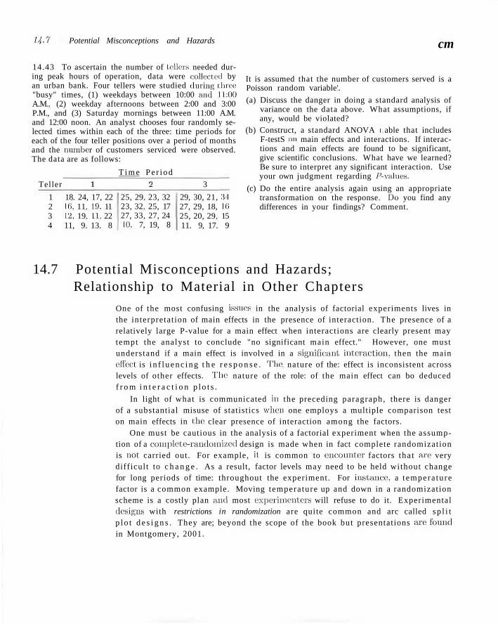
14-7 Potential Misconceptions and Hazards cm
14.43 To ascertain the number of tellers needed during peak hours of operation, data were collected by an urban bank. Four tellers were studied during three "busy" times, (1) weekdays between 10:00 anel 11:00 A.M.. (2) weekday afternoons between 2:00 and 3:00 P.M., and (3) Saturday mornings between 11:00 A.M. and 12:00 noon. An analyst chooses four randomly selected times within each of the three: time periods for each of the four teller positions over a period of months and the number of customers serviced were observed. The data are as follows:
T i m e Pe r iod
Teller 1 2 3
1 18. 24, 17, 22 2 16, 11. 19, 11 3 12, 19. 11, 22 4 11, 9. 13. 8
25, 29. 23, 32 23, 32. 25, 17 27, 33, 27, 24 10. 7, 19, 8
29, 30, 21, 31 27, 29, 18, 16 25, 20, 29. 15 11. 9, 17. 9
It is assumed that the number of customers served is a Poisson random variable'.
(a) Discuss the danger in doing a standard analysis of variance on the data above. What assumptions, if any, would be violated?
(b) Construct, a standard ANOVA I able that includes F-testS on main effects and interactions. If interactions and main effects are found to be significant, give scientific conclusions. What have we learned? Be sure to interpret any significant interaction. Use your own judgment regarding P-values.
(c) Do the entire analysis again using an appropriate transformation on the response. Dei you find any differences in your findings? Comment.
14.7 Potential Misconceptions and Hazards; Relationship to Material in Other Chapters
One of the most confusing issues in the analysis of factorial experiments lives in the interpretat ion of main effects in the presence of interaction. The presence of a relatively large P-value for a main effect when interactions are clearly present may tempt the analyst to conclude "no significant main effect." However, one must understand if a main effect is involved in a signifie'riiit. interaction, then the main effect is i n f l u e n c i n g t h e r e s p o n s e . The1 nature of the: effect is inconsistent across levels of other effects. The: nature of the role: of the main effect can bo deduced f r o m i n t e r a c t i o n p l o t s .
In light of what is communicated in the preceding paragraph, there is danger of a substantial misuse of statistics when one employs a multiple comparison test on main effects in the clear presence of interaction among the factors.
One must be cautious in the analysis of a factorial experiment when the assumption of a complete-randomized design is made when in fact complete randomization is not carried out. For example, it is common to encounter factors tha t are very difficult to c h a n g e . As a result, factor levels may need to be held without change for long periods of time: throughout the experiment. For installed, a t empera ture factor is a common example. Moving tempera ture up and down in a randomization scheme is a costly plan auel most experimenters will refuse to do it. Experimental elcsigns with restrictions in randomization are quite common and arc called sp l i t p lo t d e s i g n s . They are; beyond the scope of the book but presentations arc found in Montgomery, 2001.
Chapter 15
2k Factorial Experiments and Fractions
15.1 Introduction
We have already been exposed to certain experimental design concepts. The sampling plan for the simple i-test on the mean of a normal population and also the analysis of variance involve randomly allocating pre-chosen treatments to experimental units. The randomized block design, where treatments are assigned to units within relatively homogeneous blocks, involves restricted randomization.
In this chapter we give special attention to experimental designs in which the experimental plan calls for the study of the effect on a response of k factors, each at two levels, These are commonly known as 2fe factorial experiments. We often denote the levels as "high" and "low" even though this notation may be arbitrary in the case of qualitative variables. The complete factorial design requires that each level of every factor occur with each level of every other factor, giving a total of 2k treatment combinations.
Factor Screening and Sequential Experimentation
Often when experimentation is conducted either on a research or development level, a well-planned experimental design is a stage of what is truly a sequential plan of experimentation. More often than not, the scientists and engineers at the outset of a study may not be aware of which factors are important nor what are appropriate ranges in the potential factors in which experimentation should be conducted. For example, in the text Response Surface Methodology by Myers and Montgomery (2002), one example is given of an investigation of a pilot plant experiment in which four factors-temperature, pressure, concentration of formaldehyde, and steering rate-are varied in order that their influence on the response, filtration rate of a certain chemical product, be established. Even at the pilot plant level the scientists are not certain if all four factors should be involved in the model. In addition, the eventual goal is to determine the proper settings of contributing factors that maximize the filtration rate. Thus there is a need to determine the
612 Chapter 15 2k Factorial Experiments and Fractions
proper region of exper imentat ion. The: questions can be answered only if the total experimental plan is done .sequentially. Many experimental endeavors are plans that feature iterative learning, the type of learning that is consistent with the scientific method, with the word iterative implying stage-wise experimentation.
Generally, the initial stage of the ideal sequential plan is variable or factor screening, a procedure that involves an inexpensive experimental design involving the candidate factors. This is particularly important when the plan involves a complex system like: a manufacturing process. The information received from the results of a screening design are used to design one eir more subsequent experiments in which adjustments in the important factors are made, the adjustments that provide improvements in the system or proe:ess.
The 2fc factorial experiments and fractions of the 2k are powerful tools that are ideal screening designs. Thew are simple, practical and intuitively appealing. Many of the general concepts discussed in Chapter 14 continue to apply. However, there are graphical methods that provide useful intuition in the analysis of the two level designs.
Screening Designs for Large Number of Factors
When A: is small, say k = 2 or even A: = 3, the utility of the 2k factorial for factor screening is clear. Both analysis of variance and/or regression analysis as diseuissed and illustrated in Chapters 12, 13, and 14 remain useful as tools. In addition, graphical approaches will become apparent.
If A* is large, say as large as 6. 7, or 8, the number of factor combinations and thus experimental runs will often become prohibitive. For example, suppose one is interested in carrying out a screening design involving A: = 8 factors. There may be interest in gaining information on all k = 8 main effects as well as the ".,"" = 28 two-factor interactions. However, 28 = 25G runs would appear to be much too large and wasteful for studying 28 + 8 = 36 effects. But as we will illustrate in future sections, when A: is large we can gain considerable information in an efficient manner by using only a fraction of the complete 2 factorial experiment:. This class of designs is the class of fractional factorial designs. The goal is to retain high quality information on main effects and interesting interactions even though the size of the design is reduced considerably.
15.2 T h e 2k Factorial: Calculation of Effects and Analysis of Variance
Consider initially a 22 factorial with factors A and B and n experimental observations per factor combination. It is useful to use the symbols (1), a, b, anel ab to signify the design points, where the presence of a lowercase letter implies that the factor ( 1 or B) is at the high level. Thus, absence of the lower case implies that the factor is at the low level. So ab is the design point (+, +) , a is (+, —), b is ( —, +) and (1) is ( —, —). There are situations in the foregoing in which the notation also stands for the response data at, the design point in question. As an introduction into the calculation of important effects that aid in the determination of the in-
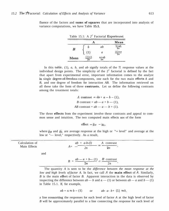
15.2 The2k Factorial: Calculation of Effects and Analysis of Variance 613
fluence of the factors and sums of squares that are incorporated into analysis of variance computations, we have Table 15.1.
Table 15.1: A 22 Factorial Experiment
A Mean ab
a
a+ab In
b—at> 2«
(D-fa 2r,
In this table, (1), a, b, and ab signify totals of the ??. response values at the individual design points. The simplicity of the 22 factorial is defined by the fact that apart from experimental error, important information comes to the analyst in single degree-of-freedoni components, one each for the two main effects A and B, and one degree of freedom for interaction AB. The information retrieved on all these take the form of three contrasts. Let us define the following contrasts among the treatment totals:
.4 contrast = a o + a - / i - ( l ) ,
B contrast = ab — a + b — (1),
AB contrast = ab — a — b + (1).
The three effects from the experiment involve these contrasts and appeal to common sense and intuition. The two computed main effects are of the form
effect = fin -y~L,
where j/u and ?//, are average response at the high or "+ level" and average at the low or "— level," respectively. As a result,
Calculation of ab + a-b-(l) A contrast Main Effects A= —
and
B =
2n 2-n
ab — a + b— (1) _ JB contrast 2~rt. ~ 2n '
The quantity A is seen to be the difference between the mean response at the low and high levels of factor A. In fact, we call A the main effect of A. Similarly, B is the main effect, of factor B. Apparent interaction in the data is observed by inspecting the difference between ab — b and a — (1) or between ab — a and b — (1) in Table 15.1. If, for example,
o f t - a « 6 - ( l ) or ab- a- b+ (1) « 0.
a line connecting the responses for each level of factor A at the high level of factor B will be approximately parallel to a line connecting the response for each level of
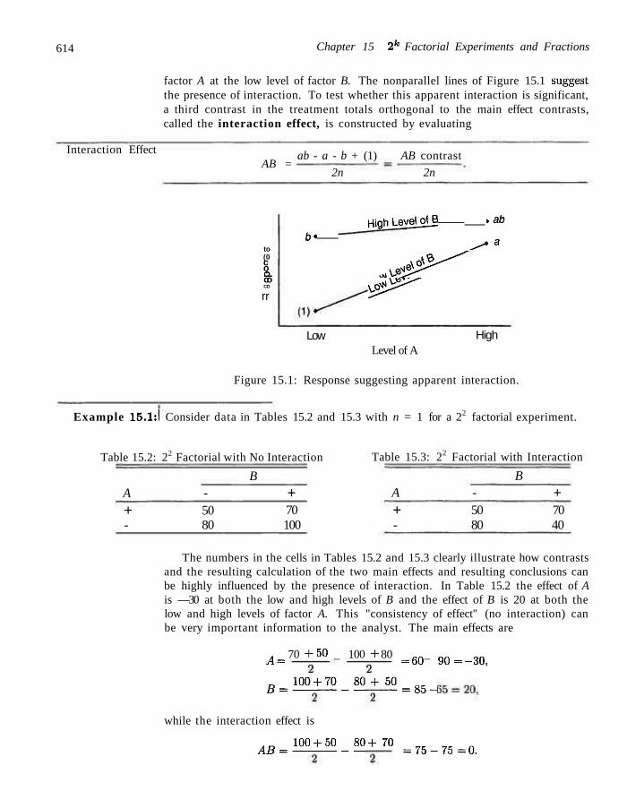
614 Chapter 15 2k Factorial Experiments and Fractions
factor A at the low level of factor B. The nonparallel lines of Figure 15.1 suggest the presence of interaction. To test whether this apparent interaction is significant, a third contrast in the treatment totals orthogonal to the main effect contrasts, called the interaction effect, is constructed by evaluating
Interaction Effect AB =
ab - a - b + (1) AB contrast
2n 2n
to (0 c o a. co CD
rr
b* HigM-eveWtfJ
. , ^ ^ \ ^ > ^
>ab
^-""* a
Low High Level of A
Figure 15.1: Response suggesting apparent interaction.
Example 15.1:1 Consider data in Tables 15.2 and 15.3 with n = 1 for a 22 factorial experiment.
Table 15.2: 22 Factorial with No Interaction Table 15.3: 22 Factorial with Interaction
A + -
-50 80
B + 70 100
A
+ -
-50 80
B + 70 40
The numbers in the cells in Tables 15.2 and 15.3 clearly illustrate how contrasts and the resulting calculation of the two main effects and resulting conclusions can be highly influenced by the presence of interaction. In Table 15.2 the effect of A is —30 at both the low and high levels of B and the effect of B is 20 at both the low and high levels of factor A. This "consistency of effect" (no interaction) can be very important information to the analyst. The main effects are
^ = 70 + 50 _ 100 + 80 = 6 Q _ 9 Q = _ 3 0 >
B = i g o + 7 0 _ 8 0 + w = 8 B _
while the interaction effect is
^ = 1 0 C + 5 0 _ 8 0 + 70 = 7 5 _ 7 5 = a
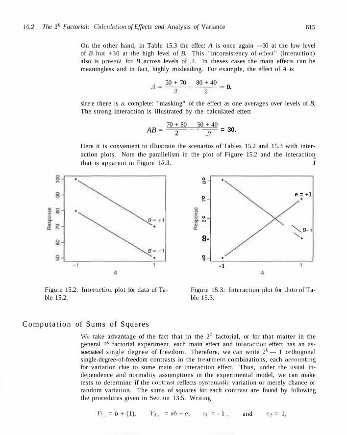
1-5.2 The 2k Factorial: Calculation of Effects and Analysis of Variance 615
On the other hand, in Table 15.3 the effect A is once again —30 at the low level of B but +30 at the high level of B. This "inconsistency of effect" (interaction) also is present for B across levels of ,4. In theses cases the main effects can be meaningless and in fact, highly misleading. For example, the effect of A is
50 + 70 80 + 40 0.
sine:e there is a. complete: "masking" of the effect as one averages over levels of B. The strong interaction is illustrated by the calculated effect
AB = 70 + 80 50 + 40
2 ~ . = 30.
Here it is convenient to illustrate the scenarios of Tables 15.2 and 15.3 with interaction plots. Note the parallelism in the plot of Figure 15.2 and the interaction that is apparent in Figure 15.3. J
o _ CO
o _
o CD
8-
o _
•
•
e = +1
< ^\B= - 1
•
-1
Figure 15.2: Interaction plot for data of Table 15.2.
Figure 15.3: Interaction plot for data of Table 15.3.
Computat ion of Sums of Squares
Wc take advantage of the fact that in the 22 factorial, or for that matter in the general 2k factorial experiment, each main effect and interactiem effect has an as-soe:iateel single degree of freedom. Therefore, we can write 2k — 1 orthogonal single-degree-of-freedom contrasts in the treatment combinations, each acceiunting for variation clue to some main or interaction effect. Thus, under the usual independence and normality assumptions in the experimental model, we can make tests to determine if the contrast reflects systematic variation or merely chance or random variation. The sums of squares for each contrast are found by following the procedures given in Section 13.5. Writing
Vi., = b + (1). Y2.. = ob + a, C] = - 1 , and c2 = 1,
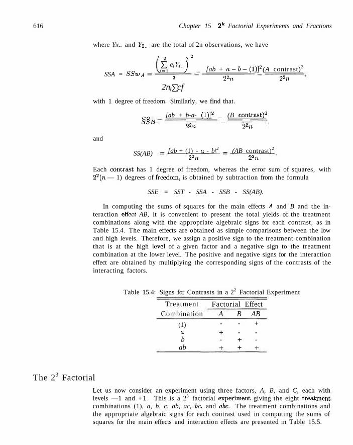
616 Chapter 15 2k Factorial Experiments and Fractions
where Yx.. and Y2„ are the total of 2n observations, we have
' '2 \ 2
J S °iYi") _ [ab + g-b-(l)}2 _ (A contrast)2
SSA = SSw A 2 22n 22n
2n £ cf
with 1 degree of freedom. Similarly, we find that.
c c [ab + b-a- (I)]2 _ (B contrast)2
bbB ~ ¥7t. " ¥n :
and
[ab + (1) - a - b\2 (AB contrast)2 SS(AB)
22n 22n
Each contrast has 1 degree of freedom, whereas the error sum of squares, with 22(n — 1) degrees of freedom, is obtained by subtraction from the formula
SSE = SST - SSA - SSB - SS(AB).
In computing the sums of squares for the main effects A and B and the interaction effect AB, it is convenient to present the total yields of the treatment combinations along with the appropriate algebraic signs for each contrast, as in Table 15.4. The main effects are obtained as simple comparisons between the low and high levels. Therefore, we assign a positive sign to the treatment combination that is at the high level of a given factor and a negative sign to the treatment combination at the lower level. The positive and negative signs for the interaction effect are obtained by multiplying the corresponding signs of the contrasts of the interacting factors.
Table 15.4: Signs for Contrasts in a 22 Factorial Experiment
Treatment Combination
(1) a b
ab
Factorial Effect A -+ -+
B --+ +
AB + --+
The 23 Factorial
Let us now consider an experiment using three factors, A, B, and C, each with levels —1 and + 1 . This is a 23 factorial experiment, giving the eight treatment, combinations (1), a, b, c, ab, ac, be, and abc. The treatment combinations and the appropriate algebraic signs for each contrast used in computing the sums of squares for the main effects and interaction effects are presented in Table 15.5.
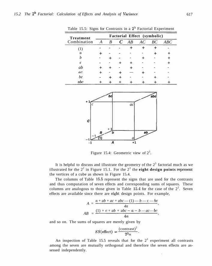
15.2 The 2k Factorial: Calculation of Effects and Analysis of Varianci 617
Table 15.5: Signs for Contrasts in a 2'! Factorial Experiment
Treatment Factorial Effect (symbolic)
Combination
(1) o. b c
ab ac be
abc
A -+ --+ + -+
B --+ -+ -
+ +
C ---+ -
+ + +
AB + --
+ + — -
+
AC + -+ --
+ -
+
BC + + ----
+ +
ABC -
+ + + ---
+
+ 1 c
B.
'be
+ 1
ac
a
^s^abc
ab^'
-1 +1
Figure 15.4: Geometric view of 23
It is helpful to discuss and illustrate the geometry of the 23 factorial much as we illustrated for the 22 in Figure 15.1. For the 23 the eight design points represent the vertices of a cube as shown in Figure 15.4.
The columns of Table 15.5 represent the signs that are used for the contrasts and thus computation of seven effects and corresponding sums of squares. These columns are analogous to those given in Table 15,4 for the case of the 22. Seven effects are available since there are eight, design points. For example,
A =
AB =
a + ab + ac + abc — (1) — b — c — be 4n
(1) + c + ab + abc b — ac— be
4« and so on. The sums of squares are merely given by
(contrast)2
^(effect) = 23n
An inspection of Table 15.5 reveals that for the 23 experiment all contrasts among the seven are mutually orthogonal and therefore the seven effects are assessed independently.
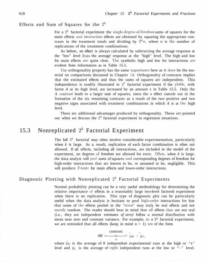
618 Chapter 15 2h Factorial Experiments and Fractions
Effects and Sum of Squares for the 2k
For a 2 factorial experiment the single-degree-of-freedom sums of squares for the main effects and interaction effects are obtained by squaring the appropriate contrasts in the treatment totals and dividing by 2*n, where n is the number of replications of the treatment combinations.
As before:, an effee:t is always calculated by subtracting the average response at the "low" level from the average' response at the "high" level. The high and low for main effects are: quite clear. The- symbolic high and low for interactions are evident from information as in Table 15.5.
The orthogonality property has the same importance here as it eloes for the material on comparisons discussed in Chapter 13. Orthogonality of contrasts implies that the estimated effects and thus the sums of squares arc independent. This independence is readily illustrated in 23 factorial experiment if the yields, with factor A at its high level, are increased by an amount x in Table 15.5. Only the A contrast leads to a larger sum of squares, since the x effect cancels out in the formation of the six remaining contrasts as a result of the two positive and two negative signs associated with treatment combinations in which A is at the1 high level.
There arc additional advantages produced by orthogonality. These are pointed out when we discuss the 2k factorial experiment in regression situations.
15.3 Nonreplicated 2k Factorial Experiment
The full 2 factorial may often involve considerable experimentation, particularly when k is large. As a. result, replication of each factor combination is often not allowed. If all effects, including all interactions, are included in the model of the experiment, no degrees eif freedom are allowed for error. Often, when k is large. the data analyst will pool sums of squares anel corresponding degrees of freedom for high-order interactions that arc known to be, or assumed to be, negligible. This will produce F-tests for main effects and lower-order interactions.
Diagnostic Plot t ing with Nonreplicated 2k Factorial Experiments
Normal probability plotting can be a very useful methodology for determining the relative importance e>f effects in a reasonably large two-level factored experiment when there is no replication. This type of diagnostic plot can be particularly useful when the data analyst is hesitant to pool high-order interactions for fear that some of the effects pooled in the "error" may truly be real effects and not merely random. The reader should bear in mind that all effects that, are not real (i.e., they are independent estimates of zero) follow a normal distribution with mean near zero and constant variance. For example, in a 2 factorial experiment, we are reminded that all effects (keep in mind n = 1) are of the form
contrast AB = = yH - yL.
o
where yu is the average of 8 independent experimental runs at the high or "+" level and ///. is the average of eight independent runs at the low or "—" level.
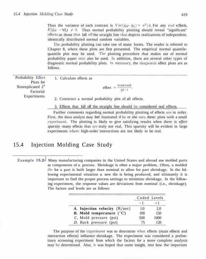
15.4 Injection Molding Case Study 619
Thus the variance of each contrast is Var(yH - yL) = a2/4. For any real e:ffects, E{ljH - VL) r 0. Thus normal probability plotting should reveal "significant" effects as those thai; fall off the straight line that depicts realizations of independent. identically distributed normal random variables.
The probability plotting can take one of many forms. The reader is referred to Chapter 8, where these plots are first presented. The empirical normal quantile-quantile plot may be used. The plotting procedure that makes use of normal probability paper may also be used. In addition, there are several other types of diagnostic normal probability plots. In summary, the diagnostic effect plots are as follows.
Probability Effect Plots for
Nonreplicated 24
Factorial Experiments
1. Calculate effects as
effect = contrast
ok-1 '
2. Construct a normal probability plot of all effects.
3. Effects that fall off the straight line should be considered real effects.
Further comments regarding normal probability plotting of effects are in order. First, the data analyst may feel frustrated if he or she uses these: plots with a small experiment. The plotting is likely to give satisfying results when there is effect sparsity -many effects that arc truly not real. This sparsity will be evident in large experiments where- high-order interactions are not likely to be real.
15.4 Injection Molding Case Study
Example 15.2:1 Many manufacturing companies in the United States and abroad use molded parts as components of a. process. Shrinkage is often a major problem, Often, a molded elie for a part is built larger than nominal to allow for part shrinkage. In the following experimental situation a. new die is being produced, and ultimately it is important to find the proper process settings to minimize shrinkage. In the following experiment, the response values are deviations from nominal (i.e., shrinkage). The factors and levels are as follows:
A. Injection velocity (ft /sec) B. Mold temperature (°C) C. Mold pressure (psi) D. Back pressure (psi)
Coded Levels - 1
1.0 100 500
75
+ 1 2.0 150
1000 120
The purpose of the experiment was to determine what, effects (main effee:ts and interaction effects) influence shrinkage. The experiment was considered a preliminary screening experiment from which the factors for a more complete analysis may be determined. Also, it was hoped that some insight, into how the important
620 Chapter 15 2k Factorial Experiments and Fractions
factors impact shrinkage might be determined. The data from a non-replicated 2"' factorial experiment are given in Table 15.6.
Table 15.6: Data for Example 15.2
Factor Combination
(1) a. b ab e ac be abc
Response (cm x 104)
72.68 71.74 76.09 93.19 71.25 70.59 70.92
104.96
Factor Combination
d ad bd abd cd acd bed abed
Response (cm x 104)
73.52 75.97 74.28 92.87 79.34 75.12 79.67 97.80
Initially, effects were calculated and placed on a normal probability plot. The calculated effects are as follows:
A = 10.5613, BD = -2.2787, B = 12.4463, C = 2.4138, D = 2.1438, 4 5 = 11.4038,
AC = 1.2613, AD = -1.8238, BC = 1.8163, CD = 1.4088, ABC = 2.8588, ABD = -1.7813,
ACD = -3.0438, BCD = -0.4788, ABCD = -1.3063.
The normal probability plot is shown in Figure 15.5. The plot seems to imply that effects A, B, and AB stand out as being important. The signs of the important effects indicate that the preliminary conclusions are as follows:
1. An increase in injection velocity from 1.0 to 2.0 increases shrinkage.
2. An increase in mold temperature from 100°C to 150°C increases shrinkage.
3. There is an interaction between injection velocity and mold temperature; although both main effects are important, it is crucial that we understand the impact of the two-factor interaction. J
Analysis with Pooled Mean Square Error: Annotated Computer Printout
It may be of interest to observe an analysis of variance of the injection molding data with high-order interactions pooled to form an mean square error. Interactions of ordea- three and four are pooled. Figure 15.6 shows a 5/lS'PR.OC GLM printout. The analysis of variance reveals essentially the same conclusion as that of the normal probability plot.
The tests and P-valties shown in Figure 15.6 require interpretation. A significant P-value suggests that the effect differs significantly from zero. The tests on main effects (which in the presence of interactions may be regarded as the effects averaged over the levels of the other factors) indicate significance for effects A and
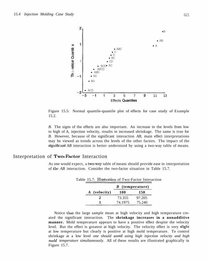
15.4 Injection Molding Case Study 621
CO
eu
CD
O m 0
o CD
•B
• AB
• A
• BCD • ABCD
• ABD • AD
• BO
• ACD
• ABC • C • D • BC • CD • AC
- 3 - 1 1 3 5 7 Effects Quantiles
11 13
Figure 15.5: Normal quantile-quantile plot of effects for case study of Example 15.2.
B. The signs of the effects are also important. An increase in the levels from low to high of A, injection velocity, results in increased shrinkage. The same is true for B. However, because of the significant interaction AB, main effect interpretations may be viewed as trends across the levels of the other factors. The impact of the significant AB interaction is better understood by using a two-way table of means.
Interpretation of Two-Factor Interaction As one would expect, a two-way table of means should provide ease in interpretation of the AB interaction. Consider the two-factor situation in Table 15.7.
Table 15.7: Illustration of Two-Factor Interaction
A (velocity) 2 1
B (temperature) 100 150
73.355 97.205 74.1975 75.240
Notice that the large sample mean at high velocity and high temperature created the significant interaction. The shrinkage increases in a nonadditive manner. Mold temperature appears to have a positive effect despite the velocity level. But the effect is greatest at high velocity. The velocity effect is very slight at low temperature but clearly is positive at high mold temperature. To control shrinkage at a low level one should avoid using high injection velocity and high m.old temperature simultaneously. All of these results are illustrated graphically in Figure 15.7.
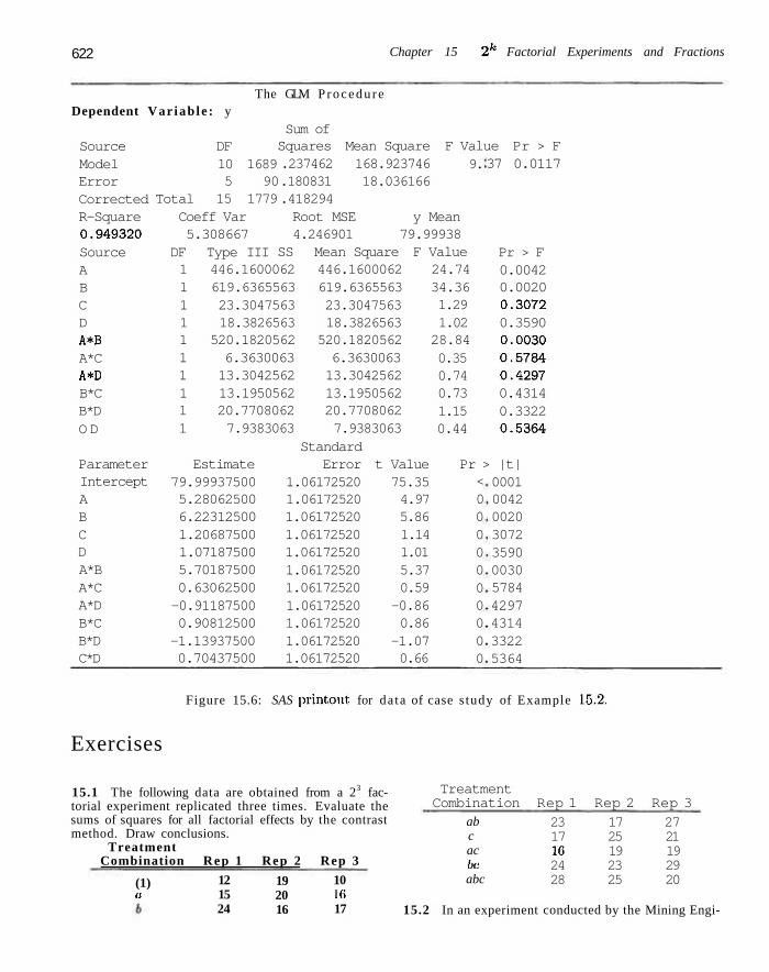
622 Chapter 15 2k Factorial Experiments and Fractions
The GLM P r o c e d u r e Dependent Var iab le : y
Source Model Error Corrected R-Square 0.949320 Source A B C D A*B A*C A*D B*C B*D O D
Parameter Intercept A B C D A*B A*C A*D B*C B*D C*D
DF 10 1689 5 90
Total 15 1779 Coeff Var 5.308667
DF Type III
Sum of Squares Mean Square .237462 168.923746 .180831 18.036166 .418294
F Value Pr > F 9.
Root MSE y Mean 4.246901 79.99938
SS Mean Square F Value 1 446.1600062 446.1600062 24.74 1 619.6365563 619.6365563 34.36 1 23.3047563 23.3047563 1 18.3826563 18.3826563
1.29 1.02
1 520.1820562 520.1820562 28.84 1 6.3630063 6.3630063 1 13.3042562 13.3042562 1 13.1950562 13.1950562 1 20.7708062 20.7708062 1 7.9383063 7.9383063
Estimate 79.99937500 5.28062500 6.22312500 1.20687500 1.07187500 5.70187500 0.63062500 -0.91187500 0.90812500 -1.13937500 0.70437500
Standard Error t Value
1.06172520 75.35 1.06172520 4.97 1.06172520 5.86 1.06172520 1.14 1.06172520 1.01 1.06172520 5.37 1.06172520 0.59 1.06172520 -0.86 1.06172520 0.86 1.06172520 -1.07 1.06172520 0.66
0.35 0.74 0.73 1.15 0.44
37 0.0117
Pr > F 0.0042 0.0020 0.3072 0.3590 0.0030 0.5784 0.4297 0.4314 0.3322 0.5364
Pr > |t| < 0 0 0 0 0 0 0 0 0 0
0001 0042 0020 3072 3590 0030 5784 4297 4314 3322 5364
Figure 15.6: SAS printout, for da ta of case s tudy of Example 15.2,
Exercises
15.1 The following data are obtained from a 23 factorial experiment replicated three times. Evaluate the sums of squares for all factorial effects by the contrast method. Draw conclusions.
Treatment Combination Rep 1 Rep 2 Rep 3
(1) a
12 15 24
19 20 16
10 l(i 17
Treatment Combination
ab c ac be abc
Rep 1
23 17 10 24 28
Rep 2
17 25 19 23 25
Rep 3
27 21 19 29 20
15.2 In an experiment conducted by the Mining Engi-
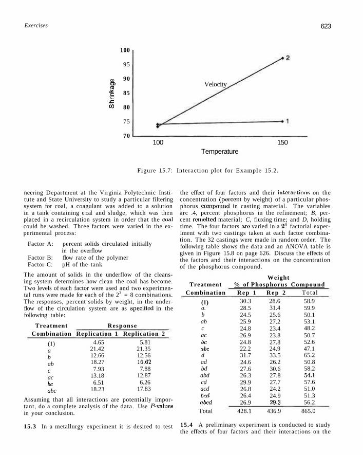
Exercises 623
CD
e? j * : c *\_ x: ty)
100
95
90
85
80
75
70
Velocity
100 150 Temperature
Figure 15.7: Interaction plot for Example 15.2.
neering Department at the Virginia Polytechnic Institute and State University to study a particular filtering system for coal, a coagulant was added to a solution in a tank containing e:oal and sludge, which was then placed in a recirculation system in order that the coal could be washed. Three factors were varied in the experimental process:
Factor A: percent solids circulated initially in the overflow
Factor B: flow rate of the polymer Factor C: pH of the tank
The amount of solids in the underflow of the cleansing system determines how clean the coal has become. Two levels of each factor were used and two experimental runs were made for each of the 23 = 8 combinations. The responses, percent solids by weight, in the underflow of the circulation system are as specified in the following table:
Response Treatment Combination Replication 1 Replication 2
(1) a b ab c ac be abc
4.65 21.42 12.66 18.27 7.93
13.18 6.51
18.23
5.81 21.35 12.56 16.62 7.88
12.87 6.26
17.83
Assuming that all interactions are potentially important, do a complete analysis of the data. Use P-values in your conclusion.
15.3 In a metallurgy experiment it is desired to test
the effect of four factors and their interactions on the concentration (percent by weight) of a particular phosphorus compound in casting material. The variables arc .4, percent phosphorus in the refinement; B, percent remelted material; C, fluxing time; and D, holding time. The four factors arc varied in a 2 factorial experiment with two castings taken at each factor combination. The 32 castings were made in random order. The following table shows the data and an ANOVA table is given in Figure 15.8 on page 626. Discuss the effects of the factors and their interactions on the concentration of the phosphorus compound.
Weight Treatment % of Phosphorus Compound
Combination
(1) a. b ab c ac be abc d ad bd abd cd acd bed abed
Rep 1 30.3 28.5 24.5 25.9 24.8 26.9 24.8 22.2 31.7 24.6 27.6 26.3 29.9 26.8 26.4 26.9
Rep 2 28.6 31.4 25.6 27.2 23.4 23.8 27.8 24.9 33.5 26.2 30.6 27.8 27.7 24.2 24.9 29.3
Tota l 58.9 59.9 50.1 53.1 48.2 50.7 52.6 47.1 65.2 50.8 58.2 54.1 57.6 51.0 51.3 56.2
Total 428.1 436.9 865.0
15.4 A preliminary experiment is conducted to study the effects of four factors and their interactions on the
624 Chapter 15 2k Factorial Experiments and Fractions
output of a certain machining operation. Two runs are made at each of the treatment combinations in order to supply a measure of pure experimental error. Two levels of each factor are used, resulting in the data shown here. Make tests on all main effects and interactions at the 0.05 level of significance. Draw conclusions.
Treatment Combination Replicate 1 Replicate 2
(T) 7 3 9l5 a 9.1 10.2 b 8.6 5.8 c 10.4 12.0 d 7.1 8.3 ab 11.1 12.3 ac 16.4 15.5 ad 7.1 8.7 be 12.6 15.2 bd 4.7 5.8 cd 7.4 10.9 abc 21.9 21.9 abd 9.8 7.8 acd 13.8 11.2 bed 10.2 11.1 abed 12.8 14.3
15.5 In the study An X-Ray Fluorescence Method for Analyzing Polybutadiene-Acrylic Acid (PBAA) Propellants, Quarterly Reports, RK-TR-62-1, Army Ordnance Missile Command, an experiment was conducted to determine whether or not there is a significant difference in the amount of aluminum achieved in the analysis between certain levels of certain processing variables. The data given in the table were recorded.
Phys . Mixing Blade Nitrogen Obs. State Time Speed Condition Aluminum
1 2 3 4 5 6 7 8 9 10 11 12 13 14 15 16
The
.4:
2 2 2 2 2 2 2 2
1 2 1 2 1 2 2 1 1 2 1 2 1 2 2 1
variables are given
mixing time level 1 level 2
-2 hours -4 hours
2 2 1 1 1 I 2 2 2 2 1 1 1 1 2 2
below.
2 2 1 2 2 1 1 1 2 2 1 2 2 1 1 1
10.3 16.0 16.2 16.1 16.0 16.0 15.5 15.9 10.7 16.1 16.3 15.8 15.9 15.9 15.6 15.8
B: blade speed level 1-36 rpin level 2-78 rpin
C: condition of nitrogen passed over propellant level 1-dry level 2-72% relative humidity
D: physical state of propellant level 1-uncured level 2-cured
Assuming all three- and four-factor interactions to be negligible, analyze the data. Use a 0.05 level of significance. Write a brief report summarizing the findings.
15.6 It is important to study the effect of concentration of the reactant and the feed rate on the viscosity of the product from a chemical process. Let the reactant concentration be factor A at levels 15% and 25%. Let the feed rate be factor B with the levels being 20 lb/hr and 30 lb/hr. The experiment, involves 2 experimental runs at each of the four combinations (L = low and H = high). The viscosity readings are as follows.
B
H
L
132 137
145 147
L
149 152
154 150
H
(a) Assuming a model containing two main effects and an interaction, calculate the three effects. Do you have any interpretation at this point?
(b) Do an analysis of variance and test for interaction. Give conclusions.
(c) Test for main effects and give final conclusions regarding the importance of all these effects.
15.7 Consider Exercise 15.3. It is of interest to the researcher to learn not only that AD, BC, and possibly AB arc important. But there is also interest in what they mean scientifically. Show two-dimensional interaction plots for all three and give interpretation.
15.8 Consider Exercise 15.3 once again. Three-factor interactions are often not significant and, even if they are, they are difficult to interpret. The interaction ABD appears to be important. To gain some sense of interpretation, show two AD interaction plots, one for B = —1 and the other for B = +1. From the appearance of these, give an interpretation of the ABD interaction.
15.5 Factorial Experiments in a Regression Setting 625
15.9 Consider Exercise 15.6. Use a "-4-1" and "—1" scaling for '-high" and "low,'- respectively, and do a multiple linear regression with the model
Y, = 3a + (lixu + ;hx2i +0i2Xux%i + ei,
with xu = reactant. concentration (—1. +1) anil xa = feed rate ( -1 .+1) . (a) Compute regression coefficients. (b) How do the coefficients bi, b2, and 612 relate to the
effects you found in Exercise 15.6(a)? (c) In your regression analysis do /-tests oil 61, l>s. and
b\>- how do these test results relate to those in Exercise 15.6(b) and (e:)?
15.10 Consider Exercise 15.5. Compute all 15 effects and do normal probability plots of the effects. (a) Docs it appear as if your assumption of negligible
three- and four-factor interactions has merit?
(b) Are the results of the effect plots consistent with what you communicated about, the importance of main effects and two-factor interactions in your summary report?
15.11 In Myers and Montgomery (2002), a data set. is discussed in which a 23 factorial is used by an engineer to study the effects of cutting speed (A), tool geometry (B). and cutting angle (C) on the life (in hours) of a machine tool. Two levels of each factor are chosen, and duplicates were run at, each design point with the: order of the runs being random. The data are presented here.
(a) Calculate all seven effects. Which appear, based on their magnitude, to be important?
(b) Do an analysis of variance and observe P-values.
(c) Do your results in (a) and (b) agree? (d) The engineer felt confident, that cutting speed and
cutting angle should interact. If this interaction is
significant, draw an interaction plot and discuss the engineering meaning of the interaction.
B Life
(1) a b
ab c
ac he
abc
— + -+ -+ --
— — i + — — + —
— — — — + -+ +
22. 31 32, 43 35. 34 35. 47 44, 45 40. 37 60, 50 39, 41
15.12 Consider Exercise 15.11. Suppose there was some experimental difficulty in making the runs. In fact, the total experiment had to be halted after only 4 runs. As a result, the abbreviated experiment is given by
Life
a 43 I) 35 c 44
abc 39
With only these runs we have the signs for contrasts given by
A B C AB AC BC ABC
+ + + r +
+
a b
abc + +
Comment. In your comments, determine whether or not the: contrasts are orthogonal. Which are and which are not? Are main effects orthogonal to each other? In this abbreviated experiment (entitled a fractional factorial,) can we study interactions independent of main effects? Is it a useful experiment if we are convinced that interactions are negligible? Explain.
15.5 Factorial Experiments in a Regression Setting
In much of Chapter 15 we: have thus far confmed our discussion of analysis of the data for a 2* factorial to the method of analysis of variance. The only reference to an alternative analysis resides in Exercise 15.9 on page; 624. Indeed, this exercise certainly introduces much of what motivates the present section. There are situations in which model fitting is important a n d the: factors under s tudy c a n be c o n t r o l l e d . For example', a biologist may wish to s tudy the growth of a certain type of algae in the water and thus a model tha t relates units of algae as a function of the amount of a pollutant and, say, time, woulel be- very helpful. Thus the study involves a factorial experiment in a laboratory sett ing in which concentration of the pollutant and time arc the factors. As we shall discuss later in this section,
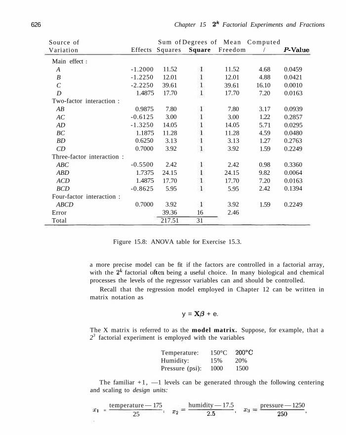
626 Chapter 15 2k Factorial Experiments and Fractions
Source of Variation
Sum of Degrees of Mean Compu ted Effects Squares Square Freedom / P-Value
Main effect A B C D
Two-factor AB AC AD BC BD CD
interaction :
Three-factor interaction : ABC ABD ACD BCD
Four-factor ABCD
Error Total
interaction :
-1.2000 -1.2250 -2.2250
1.4875
0.9875 -0.6125 -1.3250
1.1875 0.6250 0.7000
-0.5500 1.7375 1.4875
-0.8625
0.7000
11.52 12.01 39.61 17.70
7.80 3.00
14.05 11.28 3.13 3.92
2.42 24.15 17.70 5.95
3.92 39.36 217.51
16 31
11.52 12.01 39.61 17.70
7.80 3.00
14.05 11.28 3.13 3.92
2.42 24.15 17.70 5.95
3.92 2.46
4.68 4.88
16.10 7.20
3.17 1.22 5.71 4.59 1.27 1.59
0.98 9.82 7.20 2.42
1.59
0.0459 0.0421 0.0010 0.0163
0.0939 0.2857 0.0295 0.0480 0.2763 0.2249
0.3360 0.0064 0.0163 0.1394
0.2249
Figure 15.8: ANOVA table for Exercise 15.3.
a more precise model can be fit if the factors are controlled in a factorial array, with the 2k factorial often being a useful choice. In many biological and chemical processes the levels of the regressor variables can and should be controlled.
Recall that the regression model employed in Chapter 12 can be written in matrix notation as
y = X/3 + e.
The X matrix is referred to as the model matrix. Suppose, for example, that a 23 factorial experiment is employed with the variables
Temperature: 150°C 200°C Humidity: 15% 20% Pressure (psi): 1000 1500
The familiar +1 , —1 levels can be generated through the following centering and scaling to design units:
Xl = temperature — 175
25 : x2
humidity — 17.5 2J5 '
x-.i pressure — 1250
250 '
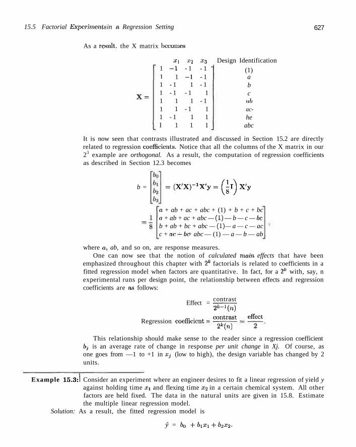
15.5 Factorial Experiments in a Regression Setting 627
As a result, the X matrix becomes
1 1 1 1 1 1 1 I
Xi
-I 1
- 1 - 1
1 1
- 1 1
X-2
- 1 - I
1 - 1
1 - 1
1 1
X-i
- 1 " - 1 - 1
1 - 1
1 1 1
Design Identification
(1) a b c
ttb ache
abc
It is now seen that contrasts illustrated and discussed in Section 15.2 are directly related to regression coefficients. Notice that all the columns of the X matrix in our 23 example are orthogonal. As a result, the computation of regression coefficients as described in Section 12.3 becomes
b = = (X'X)-1X'y=Ql)x'y
a + ab + ac + abc + (1) + b + c + bc a + ab + ac + abc — (1) — b — c — be b + ab + bc + abc — (I) — a — c — ac c + acJ-bc + abc — (1) — a — b — ab
where a, ab, and so on, are response measures. One can now see that the notion of calculated main effects that have been
emphasized throughout this chapter with 2k factorials is related to coefficients in a fitted regression model when factors are quantitative. In fact, for a 2fe with, say, n experimental runs per design point, the relationship between effects and regression coefficients are as follows:
Effect =
Regression coefficient;
contrast 2k~1(n) contrast
2k(n)
effect
This relationship should make sense to the reader since a regression coefficient bj is an average rate of change in response per unit change in Xj. Of course, as one goes from —1 to +1 in Xj (low to high), the design variable has changed by 2 units.
Example 15.3:1 Consider an experiment where an engineer desires to fit a linear regression of yield y against holding time xi and flexing time x2 in a certain chemical system. All other factors are held fixed. The data in the natural units are given in 15.8. Estimate the multiple linear regression model.
Solution: As a result, the fitted regression model is
y = bo + bixi +b2x2.
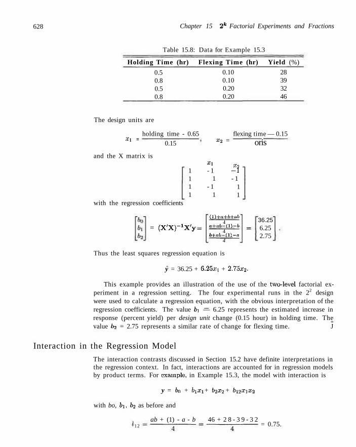
628 Chapter 15 2k Factorial Experiments and Fractions
Table 15.8: Data for Example 15.3
Holding Time (hr) Flexing Time (hr) Yield (%)
0.5 0.8 0.5 0.8
0.10 0.10 0.20 0.20
28 39 32 46
The design units are
holding time - 0.65 X l =
and the X matrix is
0.15 x2 = flexing time — 0.15
oris
1 1 1 1
Xl
- 1 1
- 1 1
x2 -I - 1
1 1
with the regression coefficients
= (X'X^X'y
(l)+<i+b+ab' 4 a+al>-(l)-b 4
b+ati-{l)-a 4
36.25 6.25 2.75
Thus the least squares regression equation is
y = 36.25 + 6.25*1 + 2.75.T2.
This example provides an illustration of the use of the two-level factorial experiment in a regression setting. The four experimental runs in the 22 design were used to calculate a regression equation, with the obvious interpretation of the regression coefficients. The value bi — 6.25 represents the estimated increase in response (percent yield) per design unit change (0.15 hour) in holding time. The value b2 = 2.75 represents a similar rate of change for flexing time. J
Interaction in the Regression Model
The interaction contrasts discussed in Section 15.2 have definite interpretations in the regression context. In fact, interactions are accounted for in regression models by product terms. For example, in Example 15.3, the model with interaction is
y = bn + bixi + b2x2 + bx2xix2
with bo, bx, b2 as before and
ab + (1) - a - b 46 + 2 8 - 3 9 - 3 2 '12 = 0.75.
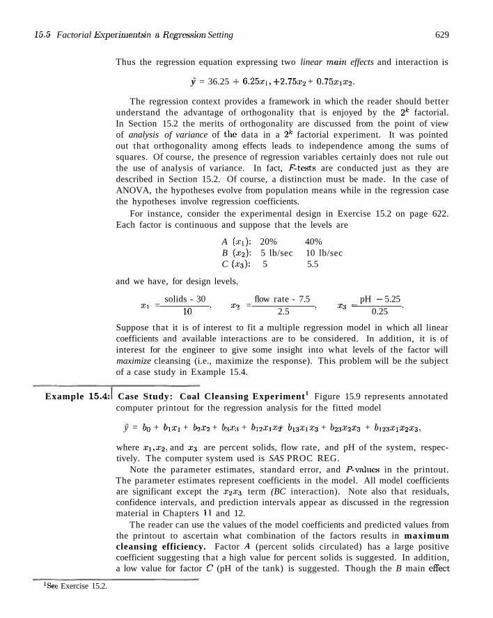
15.5 Factorial Experiments in a Regression Setting 629
Thus the regression equation expressing two linear main effects and interaction is
y = 36.25 -I- 6.25x1, +2.75x2 + 0.75xix2.
The regression context provides a framework in which the reader should better understand the advantage of orthogonality that is enjoyed by the 2k factorial. In Section 15.2 the merits of orthogonality are discussed from the point of view of analysis of variance of the data in a 2k factorial experiment. It was pointed out that orthogonality among effects leads to independence among the sums of squares. Of course, the presence of regression variables certainly does not rule out the use of analysis of variance. In fact, F-tests are conducted just as they are described in Section 15.2. Of course, a distinction must be made. In the case of ANOVA, the hypotheses evolve from population means while in the regression case the hypotheses involve regression coefficients.
For instance, consider the experimental design in Exercise 15.2 on page 622. Each factor is continuous and suppose that the levels are
A (xi): 20% 40% B (x2): 5 lb/sec 10 lb/sec C (x3): 5 5.5
and we have, for design levels.
solids - 30 flow rate - 7.5 pH - 5.25 Xi = . Xo = . .?;•! = .
10 2.5 3 0.25
Suppose that it is of interest to fit a multiple regression model in which all linear coefficients and available interactions are to be considered. In addition, it is of interest for the engineer to give some insight into what levels of the factor will maximize cleansing (i.e., maximize the response). This problem will be the subject of a case study in Example 15.4.
Example 15.4:1 Case Study: Coal Cleansing Experiment1 Figure 15.9 represents annotated computer printout for the regression analysis for the fitted model
y = b0 + bixx + b2x2 + b:ix:i + bi2xix2 + bi3Xix3 + 623X2X3 + 6123X1X2X3,
where x\, x2, and X3 are percent solids, flow rate, and pH of the system, respectively. The computer system used is SAS PROC REG.
Note the parameter estimates, standard error, and P-values in the printout. The parameter estimates represent coefficients in the model. All model coefficients are significant except the x2X3 term (BC interaction). Note also that residuals, confidence intervals, and prediction intervals appear as discussed in the regression material in Chapters 11 and 12.
The reader can use the values of the model coefficients and predicted values from the printout to ascertain what combination of the factors results in maximum cleansing efficiency. Factor A (percent solids circulated) has a large positive coefficient suggesting that a high value for percent solids is suggested. In addition, a low value for factor C (pH of the tank) is suggested. Though the B main effect
'See Exercise 15.2.
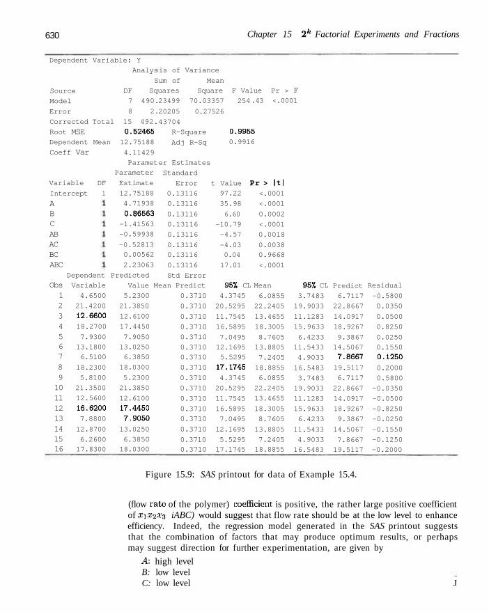
630 Chapter 15 2k Factorial Experiments and Fractions
Dependent Variable: Y
Source
Model
Error
Analys is of Variance
Sum of Mean
DF Squares Square F Value Pr >
7 490.
8 2.
Corrected Total 15 492.
Root MSE Dependent Mean
Coeff Var
Variable DF
Intercept 1
A B C AB AC BC ABC
0.52465
12.75188
4.11429
Paramet
Parameter
Estimate
12.75188
4.71938
0.86563
-1.41563
-0.59938
-0.52813
0.00562
2.23063
Dependent Predicted
Obs 1 2 3 4 5 6 7 8 9 10 11 12 13 14 15 16
Variable
4.6500
21.4200
12.6600
18.2700
7.9300
13.1800
6.5100
18.2300
5.8100
21.3500
12.5600
16.6200
7.8800
12.8700
6.2600
17.8300
23499 70.03357 254
20205 0.27526
43704
R-Square
Adj R-Sq
er Estimates
Standard
Error
0.13116
0.13116
0.13116
0.13116
0.13116
0.13116
0.13116
0.13116
Std Error
Value Mean Predict
5.2300
21.3850
12.6100
17.4450
7.9050
13.0250
6.3850
18.0300
5.2300
21.3850
12.6100
17.4450
7.9050
13.0250
6.3850
18.0300
0.3710
0.3710
0.3710
0.3710
0.3710
0.3710
0.3710
0.3710
0.3710
0.3710
0.3710
0.3710
0.3710
0.3710
0.3710
0.3710
F .43 <.0001
0.9955
0.9916
t Value
97.22
35.98
6.60
-10.79
-4.57
-4.03
0.04
17.01
Pr > |tl <.0001
<.0001
0.0002
<.0001
0.0018
0.0038
0.9668
<.0001
95'/. CL Mean
4.3745
20.5295
11.7545
16.5895
7.0495
12.1695
5.5295
17.1745
4.3745
20.5295
11.7545
16.5895
7.0495
12.1695
5.5295
17.1745
6.0855
22.2405
13.4655
18.3005
8.7605
13.8805
7.2405
18.8855
6.0855
22.2405
13.4655
18.3005
8.7605
13.8805
7.2405
18.8855
957. CL
3.7483
19.9033
11.1283
15.9633
6.4233
11.5433
4.9033
16.5483
3.7483
19.9033
11.1283
15.9633
6.4233
11.5433
4.9033
16.5483
Predict
6.7117
22.8667
14.0917
18.9267
9.3867
14.5067
7.8667
19.5117
6.7117
22.8667
14.0917
18.9267
9.3867
14.5067
7.8667
19.5117
Residual
-0.5800
0.0350
0.0500
0.8250
0.0250
0.1550
0.1250
0.2000
0.5800
-0.0350
-0.0500
-0.8250
-0.0250
-0.1550
-0.1250
-0.2000
Figure 15.9: SAS printout for data of Example 15.4.
(flow rate of the polymer) coefficient, is positive, the rather large positive coefficient of £1X2X3 iABC) would suggest that flow rate should be at the low level to enhance efficiency. Indeed, the regression model generated in the SAS printout suggests that the combination of factors that may produce optimum results, or perhaps may suggest direction for further experimentation, are given by
A: high level B: low level C: low level J
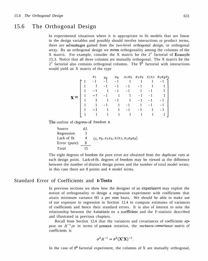
15.6 The Orthogonal Design 631
15.6 The Orthogonal Design
In experimental situations where it is appropriate to fit models that are linear in the design variables and possibly should involve interactions or product terms, there are advantages gained from the two-level orthogonal design, or orthogonal array. By an orthogonal design we mean orthogonality among the columns of the X matrix. For example, consider the X matrix for the 22 factorial of Examine 15.3. Notice that all three columns are mutually orthogonal. The X matrix for the 23 factorial also contains orthogonal columns. The 2'? factorial with interactions would yield an X matrix of the type
x =
outline of cleg
Source Regression Lack of fit Error (pure)
Total
" 1 1 1 1 1 1 1 1
rees e
d.f. 3 4 8 15
Xl
- 1 :i
- l - l
l l
- l :i
x2 - 1 - 1
1 - 1
1 - 1
1 1
Df freedom is
(x, X 2 ,X lX3
x-i - 1 - 1 - 1
1 - 1
1 1 1
X2X3
X[X 2 X1X3
1 1 - 1 - 1 - 1 1
1 - 1 1 - 1
- 1 1 - 1 - 1
1 1
x1X2X3)
X2X3
1 1
- 1 - 1 - 1 - 1
1 1
X1X2
- 1 1 1 1
- 1 - 1 - 1
1
The eight degrees of freedom for pure error are obtained from the duplicate runs at each design point. Lack-of-fit. degrees of freedom may be viewed as the difference between the number of distinct design points and the number of total model terms; in this case there are 8 points and 4 model terms.
Standard Error of Coefficients and t-Tests
In previous sections we show how the designer of an experiment may exploit the notion of orthogonality to design a regression experiment with coefficients that attain minimum variance 011 a per cost basis. We should be able to make use of our exposure to regression in Section 12.4 to compute estimates of variances of coefficients and hence their standard errors. It is also of interest to note the relationship between the f-statistic on a coefficient, and the F-statistic described and illustrated in previous chapters.
Recall from Section 12.4 that the variances and covariances of coefficients appear on A~l, or in terms of present, notation, the variance-covariance matrix of coefficients is
^ i - ' ^ ' f X ' X ) " 1 .
In the case of 2k factorial experiment, the columns of X are mutually orthogonal,
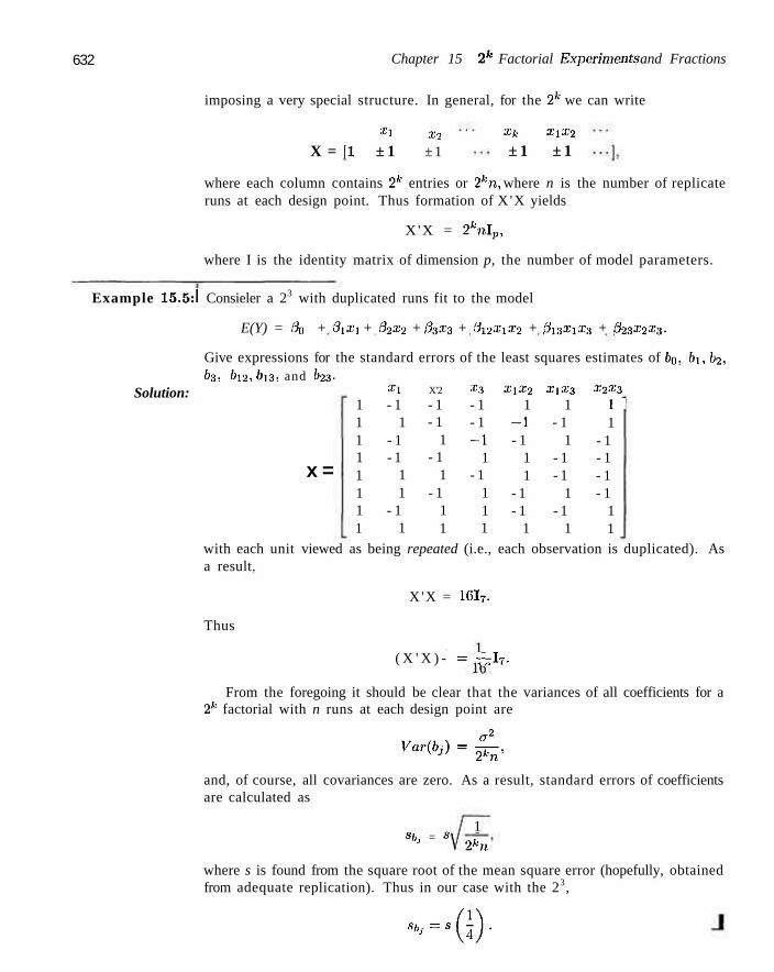
632 Chapter 15 2k Factorial Experiments and Fractions
imposing a very special structure. In general, for the 2k we can write
Xl
X = fl ± 1 x2
± 1 Xk XlX 2
± 1 ± 1
where each column contains 2fr entries or 2kn, where n is the number of replicate runs at each design point. Thus formation of X 'X yields
X 'X = 2knlp,
where I is the identity matrix of dimension p, the number of model parameters.
Example 15.5:1 Consieler a 23 with duplicated runs fit to the model
E(Y) = t% + 3ixi + Q2x2 + f%xz + Sx2xx%2 + SxiXxx-i + Q2zx2xz.
Give expressions for the standard errors of the least squares estimates of bo, bi, b2, &3: b\2, bi3, and b23.
Solution: 1 1 1 1 1 1 1 1
Xi
- 1 1
- 1 - 1
1 1
- 1 1
X'2
- 1 - 1
1 - 1
1 - 1
1 1
x-.i - 1 - 1 - 1
1 - 1
1 1 1
XiX2
1 - 1 - 1
1 1
- 1 - 1
1
X1X3
1 - 1
1 - 1 - 1
1 - 1
1
£2X3 1 " 1
- 1 - 1 - 1 - 1
1 1
x =
with each unit viewed as being repeated (i.e., each observation is duplicated). As a result.
X 'X = I6I7.
Thus
( X ' X ) - = - I 7 .
From the foregoing it should be clear that the variances of all coefficients for a 2k factorial with n runs at each design point are
"«%> = £ . and, of course, all covariances are zero. As a result, standard errors of coefficients are calculated as
Sbj = s 1
2kn
where s is found from the square root of the mean square error (hopefully, obtained from adequate replication). Thus in our case with the 23,
« * = • ( * ) •
15.6 The Orthogonal Design 633
Example 15.6:1 Consider the metallurgy experiment Exercise 15.3 on page1 623. Suppose that the fitted model is
E(Y) =3o + 3i.ri + 32x2 + p\xz + Ai£-i + finxix2 - f\z,x\x^
+ 0X4XXX4 + /323X2X3 + 324X2X4 + 3MXJX4-
What are the standard errors of the least squares regression coefficients? Solution: Standard errors of all coefficients for the 2k factorial are equal and are
n~
which in this illustration is
sbi (16)(2)
In this case the pure mean square error is given by s = 2.46 (16 degrees of freedom). Thus
sbi = 0.28.
The: standard errors of coefficients can be used to construct ^-statistics on all coefficients. These t-values arc related to the ^-statistics in the analysis of variance. We have already demonstrated that an F-statistic on a inefficient, using the 2k
factorial, is
(contrast)2
(2k)(„.)s2 •
This is the form of the F-statistics em page 620 for the metallurgy experiment. (Exercise 15.3). It is easy to verify that if we write
bj contrast. t = —. where bj = —-; ,
shi ' '' 2kn
then
2 (contrast)2
'" = s22kn ~ J As a result, the- usual relationship holds between ^-statistics on coefficients and the F-values. As we might expect, the only- difference in the use of the t or F in assessing significance lies in the fact that the /-statistic indicates the sign or direction of the effect of the coefficient.
It would appear that the 2 ' factorial plan would handle: many practical situations in which regression models are fit. It can accommodate linear and interaction terms, providing optimal estimates of all coefficients (from a variance point, of view). However, when /,: is large, the number of design points required is very large. Often, portions of the total design can lie used and still allow orthogonality with all its advantages. The'se designs are discussed in Section 15.8, which follows.
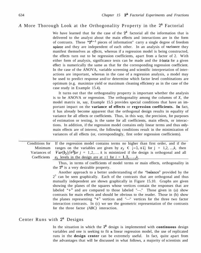
634 Chapter 15 2k Factorial Experiments and Fractions
A More Thorough Look at the Orthogonality P roper ty in the 2h Factorial
We have learned that for the case of the 2* factorial all the information that is delivered to the analyst about the main effects and interactions are in the form of contrasts. These "2 fc_1 pieces of information" carry a single degree of freedom apiece and they are independent of each other. In an analysis of variance they manifest themselves as effects, whereas if a regression model is being constructed, the effects turn out to be regression coefficients, apart from a factor of 2. With either form of analysis, significance tests can be made and the f-tests for a given effect is numerically the same as that for the corresponding regression coefficient. In the case of the ANOVA, variable screening and scientific interpretation of interactions are important, whereas in the case of a regression analysis, a model may be used to predict response and/or determine which factor level combinations are optimum (e.g. maximize yield or maximum cleaning efficiency as in the case of the case study in Example 15.4).
It turns out that the orthogonality property is important whether the analysis is to be ANOVA or regression. The orthogonality among the columns of X, the model matrix in, say, Example 15.5 provides special conditions that have an important impact on the variance of effects or regression coefficients. In fact, it has already become apparent that the orthogonal design results in equality of variance for all effects or coefficients. Thus, in this way, the precision, for purposes of estimation or testing, is the same for all coefficients, main effects, or interactions. In addition, if the regression model contains only linear terms and thus only-main effects are of interest, the following conditions result in the minimization of variances of all effects (or, correspondingly, first order regression coefficients).
Conditions for If the regression model contains terms no higher than first order, and if the Minimum ranges on the variables are given by Xj € [—1,-1-1] for j = 1,2, ...,k, then
Variances of Var(bj)/a2, for j = 1,2,.. . . k is minimized if the design is orthogonal and all Coefficients Xj levels in the design are at ±1 for i = 1,2,. . . , k.
Thus, in terms of coefficients of model terms or main effects, orthogonality in the 2k is a very desirable property.
Another approach to a better understanding of the "balance" provided by the 23 can be seen graphically. Each of the contrasts that are orthogonal and thus mutually independent are shown graphically in Figure 15.10. Graphs are given showing the planes of the squares whose vertices contain the responses that are labeled "+" and are compared to those labeled "—." Those given in (a) show contrasts for main effects and should be obvious to the reader. Those in (b) show the planes representing "+" vertices and "—" vertices for the three two factor interaction contrasts. In (c) we see the geometric representation of the contrasts for the three factor (ABC) interaction.
Center Runs with 2fc Designs
In the situation in which the 2k design is implemented with continuous design variables and one is seeking to fit a linear regression model, the use of replicated runs in the design center can be extremely useful. In fact, quite apart from the advantages that will be discussed in what follows, a majority of scientists and
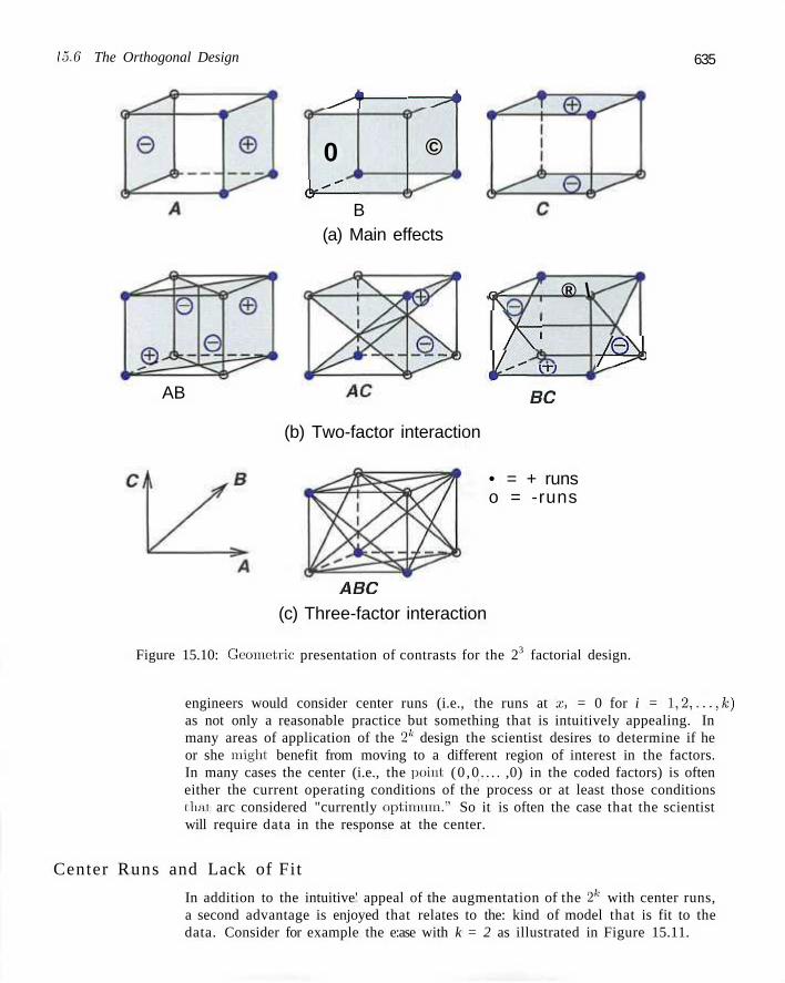
15.6 The Orthogonal Design 635
^ k \
0 ( ^ -
—-?*)
©
B (a) Main effects
AB
<\\ ® \
/v \("' ™
Pp, sc
(b) Two-factor interaction
• = + runs o = -runs
ABC (c) Three-factor interaction
Figure 15.10: Geometric presentation of contrasts for the 23 factorial design.
engineers would consider center runs (i.e., the runs at x, = 0 for i = l,2,...,k) as not only a reasonable practice but something that is intuitively appealing. In many areas of application of the 2k design the scientist desires to determine if he or she might, benefit from moving to a different region of interest in the factors. In many cases the center (i.e., the point (0 ,0 . . . . ,0) in the coded factors) is often either the current operating conditions of the process or at least those conditions that arc considered "currently optimum." So it is often the case that the scientist will require data in the response at the center.
Center Runs and Lack of Fit
In addition to the intuitive' appeal of the augmentation of the 2''' with center runs, a second advantage is enjoyed that relates to the: kind of model that is fit to the data. Consider for example the e:ase with k = 2 as illustrated in Figure 15.11.
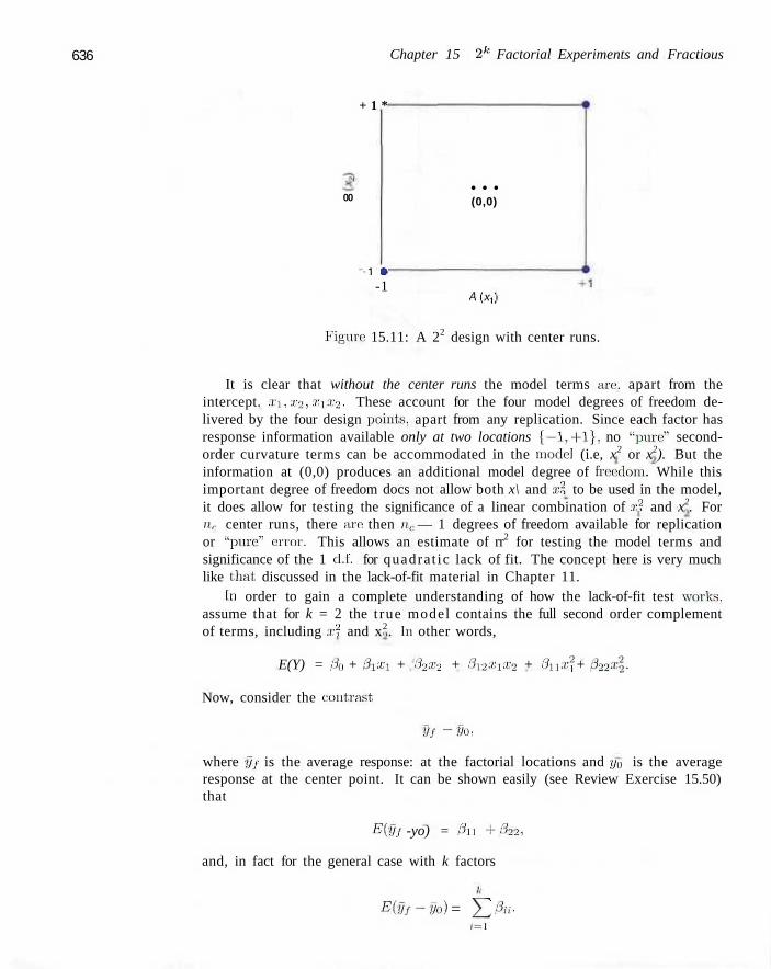
636 Chapter 15 2k Factorial Experiments and Fractious
+ 1 *
00
-1 »
• • • (0,0)
-1 A(X,:
Figure 15.11: A 22 design with center runs.
It is clear that without the center runs the model terms are. apart from the intercept. x\, x2, xix2 . These account for the four model degrees of freedom delivered by the four design points, apart from any replication. Since each factor has response information available only at two locations {—1,-1-1}, no "pure" second-order curvature terms can be accommodated in the model (i.e, x2 or x2). But the information at (0,0) produces an additional model degree of freedom. While this important degree of freedom docs not allow both x\ and x2, to be used in the model, it does allow for testing the significance of a linear combination of x2 and x2. For ii,. center runs, there are then nc — 1 degrees of freedom available for replication or "pure" error. This allows an estimate of rr2 for testing the model terms and significance of the 1 el.f. for quadrat ic lack of fit. The concept here is very much like that, discussed in the lack-of-fit material in Chapter 11.
In order to gain a complete understanding of how the lack-of-fit test works, assume that for k = 2 the t rue model contains the full second order complement of terms, including x2 and x2. In other words,
E(Y) = p\ + p\xx + >hx2 + Si%xxx2 + 3u.vf + p\2x\.
Now, consider the contrast
ill - f f t ) ,
where §f is the average response: at the factorial locations and yo is the average response at the center point. It can be shown easily (see Review Exercise 15.50) that
E(yj -yo) = Ai +#22,
and, in fact for the general case with k factors
E(5f-yo) = Y^$n-i=i
15.6 The Orthogonal Design 637
As a result the lack-of-fit test is a simple /-test (or F = t2) with
Vf - yo _ y~f -yo tnc-l
Tij-yu y/MSE{l/nf + l/nc)"
where nc is the number of factorial points and MSE is simply the sample variance of the response values at (0 ,0 . . . . , 0).
Example 15.7:1 An example is taken from Myers and Montgomery (2002). A chemical engineer is attempting to model the percent conversion in a process. There are two variables of interest, reaction time and reaction temperature. In an attempt to arrive at the appropriate model, a preliminary experiment is conducted in a 22 factorial using the current region of interest in reaction time and temperature. Single runs were made at each of the four factorial points and 5 runs were made at the design center in order that a lack-of-fit test for curvature could be conducted. Figure 15.12 shows the design region and the experimental runs on yield.
The time and temperature readings at the center are, of course, 35 minutes and 145°C. The estimates of the main effects and single interaction coefficient are computed through contrasts just as before. The center runs play no role in t h e compu ta t i on of b\, b2, and 612. This should be intuitively reasonable to the reader. The intercept is merely y for the entire experiment. This value is y = 40.4444. The standard errors are found through the use of diagonal elements of ( X ' X ) - 1 as discussed earlier. For this case
Xi x 2 Xi.X2
1 - 1 - 1 1 1 - 1 1 - 1 1 1 - 1 - 1 1 1 1 1
X = 1 0 0 0 1 0 0 0 1 0 0 0 1 0 0 0 1 0 0 0
After the computations we have
b0 = 40.4444, 61 = 0.7750, b2 = 0.3250, h2 = -0.0250,
Sbo = 0.06231, 86, = 0.09347, sb.2 = 0.09347, sbli = 0.09347,
tbo = 649.07 tbl = 8.29 tb2 = 3.48 tbl2 = 0.018, (P = 0.800).
The contrast yf - y0 = 40.425 - 40.46 = -0.035 and the t-statistic that tests for curvature is given by
t= / a - * * - 4 0 . 4 6 ^0.0430(1/4 + 1/5)
As a result, it appears as if the appropriate model should contain only first-order terms (apart from the intercept). J
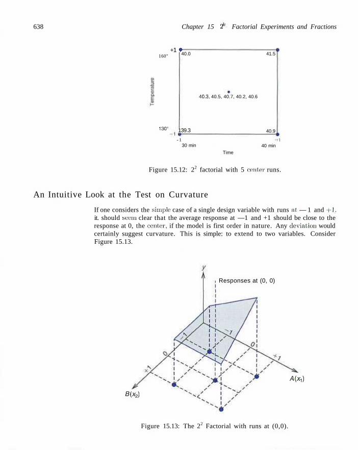
638 Chapter 15 2 Factorial Experiments and Fractions
+1 + 160"
130° 139.3
40.0 41.5
40.3, 40.5, 40.7, 40.2, 40.6
40.9
- 1 I I 30 min 40 min
Time
Figure 15.12: 22 factorial with 5 center runs.
An Intuitive Look at the Test on Curvature
If one considers the simple case of a single design variable with runs at — 1 and +1 . it. should seem clear that the average response at —1 and +1 should be close to the response at 0, the center, if the model is first order in nature. Any deviation would certainly suggest curvature. This is simple: to extend to two variables. Consider Figure 15.13.
Responses at (0, 0)
B(x2)
A(xi)
Figure 15.13: The 22 Factorial with runs at (0,0).
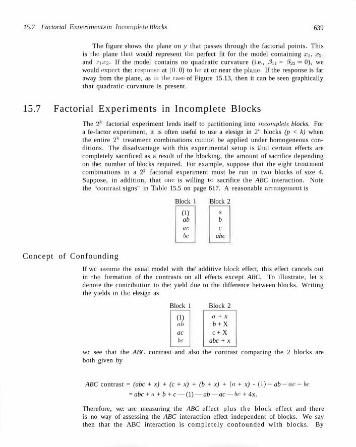
15.7 Factorial Experiments in Incomplete Blocks 639
The figure shows the plane on y that passes through the factorial points. This is the' plane that would represent the' perfect fit for the model containing xi , x2, and xix2 . If the model contains no quadratic curvature (i.e., 3n = 322 = 0), we would expect, the: response1 at (0. 0) to lie at or near the plane. If the response is far away from the plane, as in the case of Figure 15.13, then it can be seen graphically that quadratic curvature is present.
15.7 Factorial Experiments in Incomplete Blocks
The 2 factorial experiment lends itself to partitioning into incomplete blocks. For a fe-factor experiment, it is often useful to use a elesign in 2'' blocks (p < k) when the entire 2* treatment combinations cannot, be applied under homogeneous conditions. The disadvantage with this experimental setup is that certain effects are completely sacrificed as a result of the blocking, the amount of sacrifice depending on the: number of blocks required. For example, suppose that the eight treatment combinations in a 2 factorial experiment must be run in two blocks of size 4. Suppose, in addition, that one is willing tei sacrifice the ABC interaction. Note the "contrast signs" in Tabic 15.5 on page 617. A reasonable arrangement is
Block
(1) ab OC be
Block 2
a b c
abc
Concept of Confounding
If wc assume the usual model with the' additive bloc:k effect, this effect cancels out in the1 formation of the contrasts on all effects except ABC. To illustrate, let x denote the contribution to the: yield due to the difference between blocks. Writing the yields in the' elesign as
Block 1 Block 2
(1) 0.1)
ac be
a + x b + X c + X
abc + x
wc see that the ABC contrast and also the contrast comparing the 2 blocks are both given by
ABC contrast = (abc + x) + (c + x) + (b + x) + (a + x) - (I)
= abc + a + b + c — (1) — ab — ac — be + 4x.
ab be
Therefore, we: arc measuring the ABC effect plus t h e block effect and there is no way of assessing the ABC interaction effect independent of blocks. We say then that the ABC interaction is completely confounded wi th blocks. By
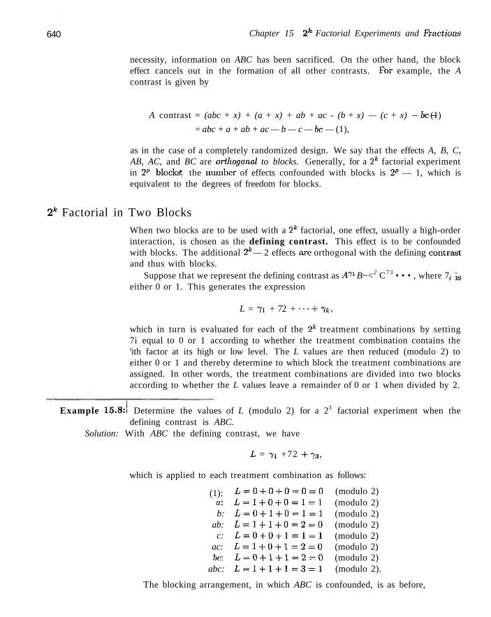
640 Chapter 15 2k Factorial Experiments and Fi-actions
necessity, information on ABC has been sacrificed. On the other hand, the block effect cancels out in the formation of all other contrasts. For example, the A contrast is given by
A contrast = (abc + x) + (a + x) + ab + ac - (b + x) — (c + x) -be- (1)
= abc + a + ab + ac — b — c — be — (1),
as in the case of a completely randomized design. We say that the effects A, B, C, AB, AC, and BC are orthogonal to blocks. Generally, for a 2k factorial experiment in 21' blocks*, the number of effects confounded with blocks is 2P — 1, which is equivalent to the degrees of freedom for blocks.
2k Factorial in Two Blocks
When two blocks are to be used with a 2k factorial, one effect, usually a high-order interaction, is chosen as the defining contrast. This effect is to be confounded with blocks. The additional 2k — 2 effects are orthogonal with the defining contrast and thus with blocks.
Suppose that we represent the defining contrast as A^'1 B~<2 C73 • • • , where 7 either 0 or 1. This generates the expression
is
L = 71 + 72 + 7ft,
which in turn is evaluated for each of the 2k treatment combinations by setting 7i equal to 0 or 1 according to whether the treatment combination contains the 'ith factor at its high or low level. The L values are then reduced (modulo 2) to either 0 or 1 and thereby determine to which block the treatment combinations are assigned. In other words, the treatment combinations are divided into two blocks according to whether the L values leave a remainder of 0 or 1 when divided by 2.
Example 15.8:1 Determine the values of L (modulo 2) for a 23 factorial experiment when the defining contrast is ABC.
Solution: With ABC the defining contrast, we have
L = 71 +72 +73 ,
which is applied to each treatment combination as follows:
(1): a: b:
ab: c:
ac: be:
abc:
L = 0 + 0 + 0 = 0 = 0 L=1+0+0=1=1 £ = 0 + 1 + 0 = 1 = 1 L=1+1+0=2=0 L = 0 + 0 + l = 1 = 1 L=1+0+1=2=0 L = 0 + 1 + 1 = 2 = 0 L=1+1+1=3=1
(modulo 2) (modulo 2) (modulo 2) (modulo 2) (modulo 2) (modulo 2) (modulo 2) (modulo 2).
The blocking arrangement, in which ABC is confounded, is as before,
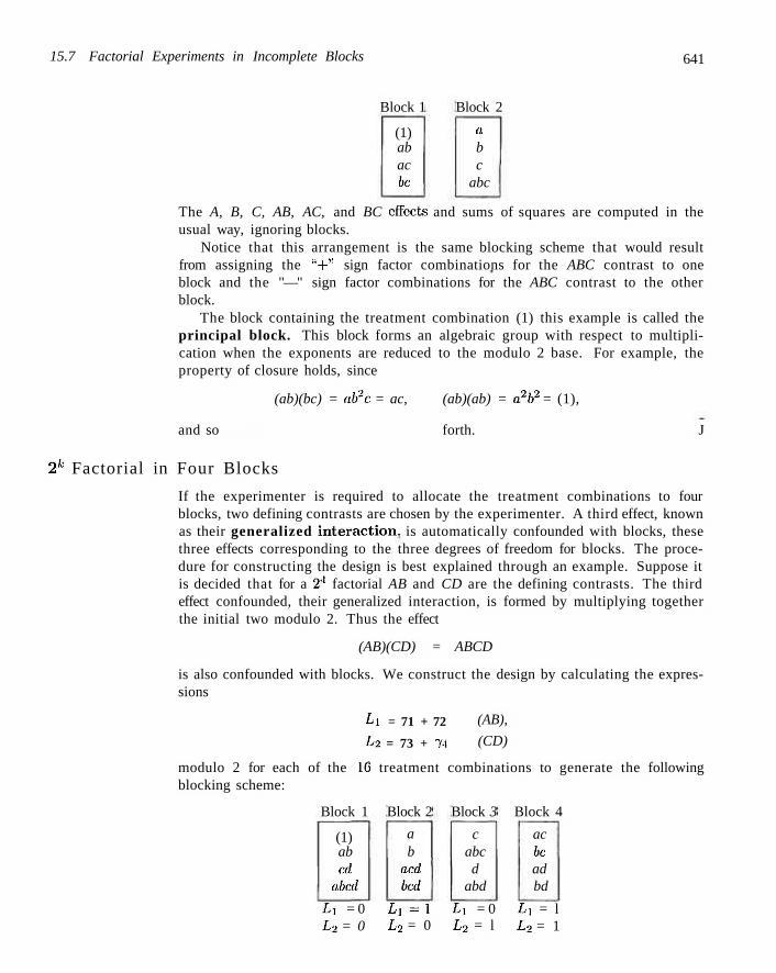
15.7 Factorial Experiments in Incomplete Blocks 641
Block 1
(1) ab ac be
Block 2
a b c
abc
The A, B, C, AB, AC, and BC effects and sums of squares are computed in the usual way, ignoring blocks.
Notice that this arrangement is the same blocking scheme that would result from assigning the ' ;+" sign factor combinations for the ABC contrast to one block and the "—" sign factor combinations for the ABC contrast to the other block.
The block containing the treatment combination (1) this example is called the principal block. This block forms an algebraic group with respect to multiplication when the exponents are reduced to the modulo 2 base. For example, the property of closure holds, since
(ab)(bc) = ab2c = ac, (ab)(ab) = a2b2 = (1),
and so forth. J
2k Factorial in Four Blocks
If the experimenter is required to allocate the treatment combinations to four blocks, two defining contrasts are chosen by the experimenter. A third effect, known as their generalized interaction, is automatically confounded with blocks, these three effects corresponding to the three degrees of freedom for blocks. The procedure for constructing the design is best explained through an example. Suppose it is decided that for a 24 factorial AB and CD are the defining contrasts. The third effect confounded, their generalized interaction, is formed by multiplying together the initial two modulo 2. Thus the effect
(AB)(CD) = ABCD
is also confounded with blocks. We construct the design by calculating the expressions
Lx = 71 + 72
E2 = 73 + 7i
(AB),
(CD)
modulo 2 for each of the 16 treatment combinations to generate the following blocking scheme:
Block 1
(1) ab cd
abed
Block 2
a b
acd bed
Block 3
c abc d
abd
Block 4
ac be ad bd
Lx = 0 L2 = 0
Li = l L2 = 0
Lx = 0 L2 = l
Li = l L2 = 1
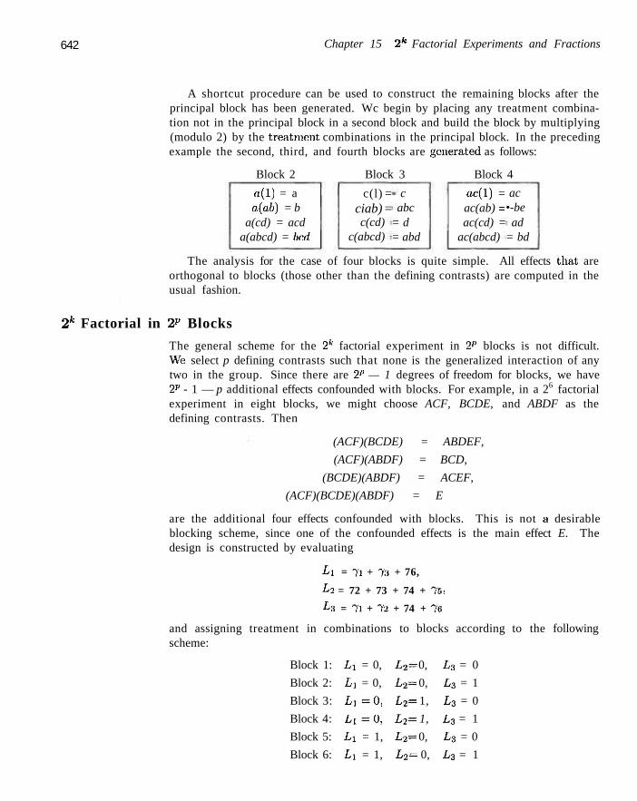
642 Chapter 15 2k Factorial Experiments and Fractions
A shortcut procedure can be used to construct the remaining blocks after the principal block has been generated. Wc begin by placing any treatment combination not in the principal block in a second block and build the block by multiplying (modulo 2) by the treatment combinations in the principal block. In the preceding example the second, third, and fourth blocks are generated as follows:
Block 2
a(l) = a o.(ab) = b
a(cd) = acd a(abcd) = bed
Block 3
c(l) = ciab) = c(cd)
c(abcd)
- c abc
= d = abd
Block 4
ac(l) = ac(ab) = ac(cd) =
ac(abcd)
ac •-be ad
= bd
The analysis for the case of four blocks is quite simple. All effects that are orthogonal to blocks (those other than the defining contrasts) are computed in the usual fashion.
2k Factorial in 2P Blocks
The general scheme for the 2k factorial experiment in 2P blocks is not difficult. We select p defining contrasts such that none is the generalized interaction of any two in the group. Since there are 2P — 1 degrees of freedom for blocks, we have 2P - 1 — p additional effects confounded with blocks. For example, in a 26 factorial experiment in eight blocks, we might choose ACF, BCDE, and ABDF as the defining contrasts. Then
(ACF)(BCDE) = ABDEF,
(ACF)(ABDF) = BCD,
(BCDE)(ABDF) = ACEF,
(ACF)(BCDE)(ABDF) = E
are the additional four effects confounded with blocks. This is not a desirable blocking scheme, since one of the confounded effects is the main effect E. The design is constructed by evaluating
Lx = 7i + 73 + 76,
L2 = 72 + 73 + 74 + 75)
£3 = 7i + 7a + 74 + 76
and assigning treatment in combinations to blocks according to the following scheme:
Block 1: Lx = 0, L2= 0, L3 = 0
Block 2: L] = 0, L2= 0, L3 = 1
Block 3: L i = 0 , L2= 1, L3 = 0
Block 4: L i = 0 , L2= 1, L3 = 1
Block 5: Lx = 1, L2= 0, L3 = 0
Block 6: Lx = 1, L 2= 0, L3 = 1
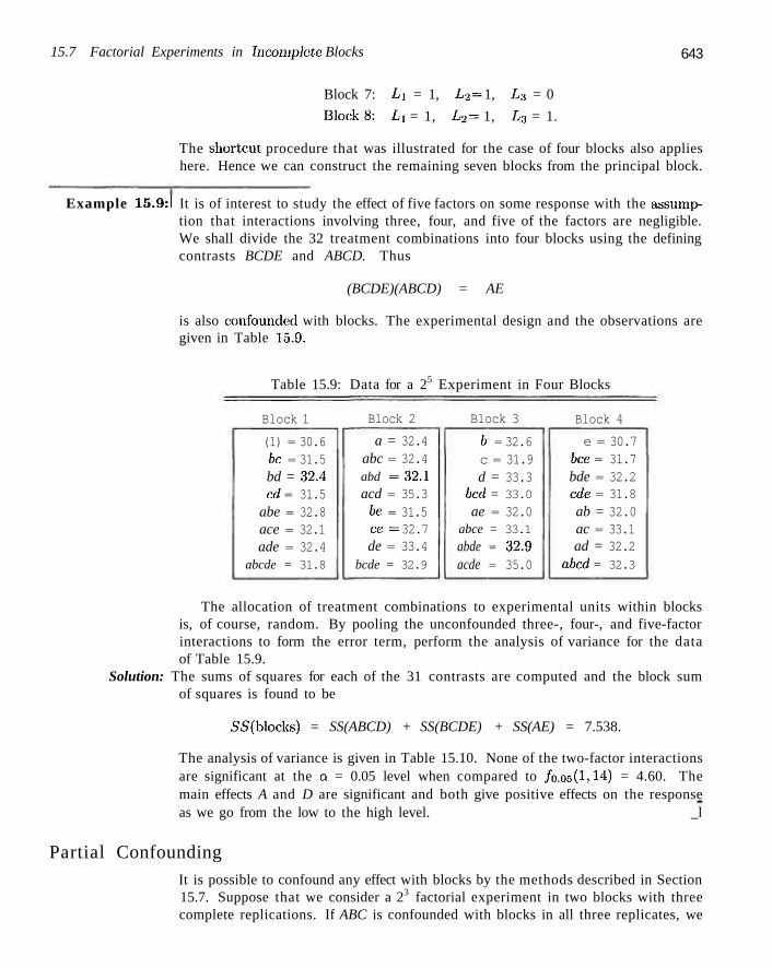
15.7 Factorial Experiments in Incomplete Blocks 643
Block 7: Lx = 1, L2= 1, Lj, = 0
BlockS: £i = 1, L 2 = 1, L3 = 1.
The shortcut procedure that was illustrated for the case of four blocks also applies here. Hence we can construct the remaining seven blocks from the principal block.
Example 15.9:1 It is of interest to study the effect of five factors on some response with the assumption that interactions involving three, four, and five of the factors are negligible. We shall divide the 32 treatment combinations into four blocks using the defining contrasts BCDE and ABCD. Thus
(BCDE)(ABCD) = AE
is also confoundeel with blocks. The experimental design and the observations are given in Table 15.9.
Table 15.9: Data for a 25 Experiment in Four Blocks
Block 1
(1) = 30.6 tbc = 31.5 bd = 32.4 cd = 31.5
abe = 32.8 ace = 32.1 ade = 32.4
abcde = 31.8
Block 2
a = 32.4 abc = 32.4 abd = 32.1 acd = 35.3 be = 31.5 ce = 32.7 de = 33.4
bcde = 32.9
Block 3
/; = 32.6 c = 31.9 d = 33.3
bed = 33.0 ae = 32.0
abce = 33.1 abde = 32.9 acde = 35.0
Block 4
e = 30.7 bee = 31.7 bde = 32.2 cde = 31.8 ab = 32.0 ac = 33.1 ad = 32.2
abed = 32.3
The allocation of treatment combinations to experimental units within blocks is, of course, random. By pooling the unconfounded three-, four-, and five-factor interactions to form the error term, perform the analysis of variance for the data of Table 15.9.
Solution: The sums of squares for each of the 31 contrasts are computed and the block sum of squares is found to be
SS(blocks) = SS(ABCD) + SS(BCDE) + SS(AE) = 7.538.
The analysis of variance is given in Table 15.10. None of the two-factor interactions are significant at the a = 0.05 level when compared to /o.05(1-14) = 4.60. The main effects A and D are significant and both give positive effects on the response as we go from the low to the high level. _l
Partial Confounding It is possible to confound any effect with blocks by the methods described in Section 15.7. Suppose that we consider a 23 factorial experiment in two blocks with three complete replications. If ABC is confounded with blocks in all three replicates, we
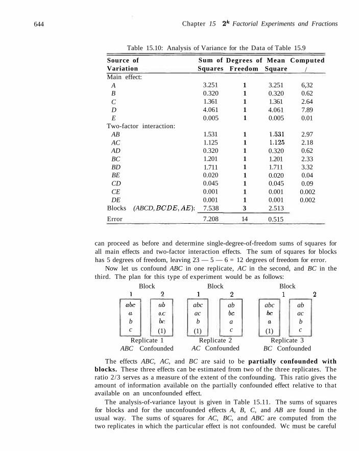
644 Chapter 15 2k Factorial Experiments and Fractions
Table 15.10: Analysis of Variance for the Data of Table 15.9
Source of Variation Main effect:
A B C D E
Two-factor interaction: AB AC AD BC BD BE CD CE DE
Blocks (ABCD,
Error
BCDE,AE):
Sum of Squares
3.251 0.320 1.361 4.061 0.005
1.531 1.125 0.320 1.201 1.711 0.020 0.045 0.001 0.001 7.538
7.208
Degrees of Freedom
1 1 1 1 1
1 1 1 1 1 1 1 1 1 3
14
Mean Square
3.251 0.320 1.361 4.061 0.005
1.531 1.125 0.320 1.201 1.711 0.020 0.045 0.001 0.001 2.513
0.515
Computed /
6,32 0.62 2.64 7.89 0.01
2.97 2.18 0.62 2.33 3.32 0.04 0.09 0.002 0.002
can proceed as before and determine single-degree-of-freedom sums of squares for all main effects and two-factor interaction effects. The sum of squares for blocks has 5 degrees of freedom, leaving 23 — 5 — 6 = 12 degrees of freedom for error.
Now let us confound ABC in one replicate, AC in the second, and BC in the third. The plan for this type of experiment would be as follows:
Block Block Block 1 2 1 2 1 2
abc a b c
ab 0.C
be
(1)
abc ac b
(1)
ab be a c
abc be a
(1)
ab ac b c
Replicate 1 ABC Confounded
Replicate 2 AC Confounded
Replicate 3 BC Confounded
The effects ABC, AC, and BC are said to be partially confounded with blocks. These three effects can be estimated from two of the three replicates. The ratio 2/3 serves as a measure of the extent of the confounding. This ratio gives the amount of information available on the partially confounded effect relative to that available on an unconfounded effect.
The analysis-of-variance layout is given in Table 15.11. The sums of squares for blocks and for the unconfounded effects A, B, C, and AB are found in the usual way. The sums of squares for AC, BC, and ABC are computed from the two replicates in which the particular effect is not confounded. Wc must be careful
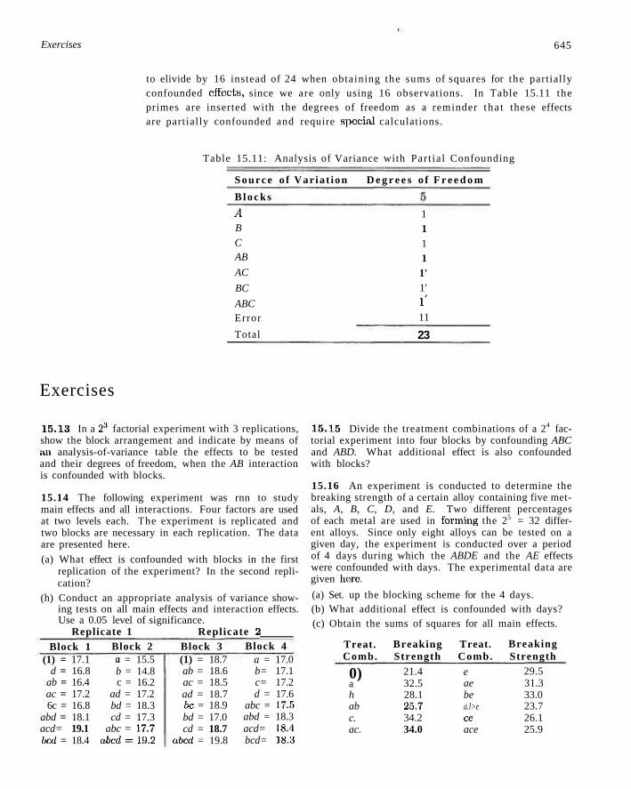
Exercises 645
to elivide by 16 instead of 24 when obtaining the sums of squares for the partially confounded effects, since we are only using 16 observations. In Table 15.11 the primes are inserted with the degrees of freedom as a reminder tha t these effects are partially confounded and require special calculations.
Table 15.11: Analysis of Variance with Part ia l Confounding
Source o f Var iat ion D e g r e e s o f F r e e d o m
B l o c k s
A B
C AB
AC
BC
ABC Error
Total
1 1 1 1 1' 1' l' 11
23
Exercises
15.13 In a 2'1 factorial experiment with 3 replications, show the block arrangement and indicate by means of tin analysis-of-variance table the effects to be tested and their degrees of freedom, when the AB interaction is confounded with blocks.
15.14 The following experiment was rnn to study main effects and all interactions. Four factors are used at two levels each. The experiment is replicated and two blocks are necessary in each replication. The data are presented here.
(a) What effect is confounded with blocks in the first replication of the experiment? In the second replication?
(h) Conduct an appropriate analysis of variance showing tests on all main effects and interaction effects. Use a 0.05 level of significance.
Replicate 1 Replicate 2 Block 1
(1) = 17.1 d = 16.8
ab = 16.4 ac = 17.2 6c = 16.8
abd = 18.1 acd= 19.1 bed = 18.4
Block 2 a = 15.5 b = 14.8 c = 16.2
ad = 17.2 bd = 18.3 cd = 17.3
abc = 17.7 abed =19.2
Block 3 (1) = 18.7 ab = 18.6 ac = 18.5 ad = 18.7 be = 18.9 bd = 17.0 cd = 18.7
abed = 19.8
Block 4 a = 17.0 b= 17.1 c= 17.2 d = 17.6
abc = 17.5 abd = 18.3 acd= 18.4 bcd= 18.3
15.15 Divide the treatment combinations of a 24 factorial experiment into four blocks by confounding ABC and ABD. What additional effect is also confounded with blocks?
15.16 An experiment is conducted to determine the breaking strength of a certain alloy containing five metals, A, B, C, D, and E. Two different percentages of each metal are used in forming the 25 = 32 different alloys. Since only eight alloys can be tested on a given day, the experiment is conducted over a period of 4 days during which the ABDE and the AE effects were confounded with days. The experimental data are given here.
(a) Set. up the blocking scheme for the 4 days. (b) What additional effect is confounded with days? (c) Obtain the sums of squares for all main effects.
Treat. Comb.
0) a h ab c. ac.
Breaking Strength
21.4 32.5 28.1 25.7 34.2 34.0
Treat. Comb.
e ae be a.l>e ce ace
Breaking Strength
29.5 31.3 33.0 23.7 26.1 25.9
646 Chapter 15 2k Factorial Experiments and Fractions
Treat. Comb.
be abc d ad bd abd cd acd bed abed
Breaking Strength
23.5 24.7 32,6 29.0 30.1 27.3 22.0 35.8 26.8 36.4
Treat. Comb. bee abce de ade bde abdc cde acde bede abede
Break ing S t r eng th
35.2 30.4 28.5 36.2 24.7 29.0 31.3 34.7 26.8 23.7
15.17 By confounding ABC in two replicates and AB in the third, show the block arrangement and the analysis-of-variance table for a 2'' factorial experiment with three replicates. What is the relative information on the confounded effects?
15.18 The following coded data represent the strength of a certain type of bread-wrapper stock produced under 16 different conditions, the latter representing two levels of each of four process variables. An operator effect was introduced into the model, since it was necessary to obtain half the experimental runs under operator 1 and half under operator 2. It. was felt that operators do have an effect, on the quality of the product.
(a) Assuming that all interactions are negligible, make significance tests for the factors A, B, C, and D. Use a 0.05 level of significance.
(b) What interaction is confounded with operators?
Operator 1
(1) = 18.8 ab = 16.5 ac = 17.8 be = 17.3 d = 1 3 . 5
abd= 17.6 acd = 18.5 bed = 17.6
Operator 2
a= 14.7 6=15 .1 c = 14.7
afcc = 19.0 ad = 16.9 bd= 17.5 cd = 18.2
abed =20.1
15.19 Consider a 25 experiment where the experimental runs are on 4 different machines. Use the machines as blocks, and assume that all main effects and two-factor interactions may be important.
(a) Which runs would be made on each of the 4 machines?
(b) Which effects are confounded with blocks?
15.20 An experiment is revealed in Myers and Montgomery (2002) in which optimum conditions are sought storing bovine semen to obtain maximum survival. The variables are percent sodium citrate, percent glyc
erol, and equilibration time in hours. The response is percent survival of the motile spermatozoa. The natural levels arc found in the above reference. Below are the data with coded levels for the factorial portion of the design and the center runs.
xi, Percent x2 X3 Sodium Percent Equilibration % Citrate Glycerol Time Survival
-1 1
-1 1
-1 1
-1 1 0 0
- 1 - 1
1 1
- 1 - 1
1 1 0 0
0 / 40 19 40 54 41 21 43 63 61
(a) Fit a linear regression model to the data and determine which linear and interaction terms are significant. Assume that the :cti2a;3 interaction is negligible.
(b) Test for quadratic lack of fit and comment.
15.21 Oil producers are interested in high strength-nickel alloys that are strong and corrosion resistant. An experiment conducted in which yield strengths were compared for nickel alloy tensile specimens charged in sulfuric acid solution saturated with carbon disulfide. Two alloys were combined; a 75% nickel composition and a 30% nickel composition. The alloys were tested under two different charging times, 25 and 50 days. A 23 factorial was conducted with the following factors
% sulfuric acid 4%, 6%: (xi)
charging time 25 days, 50 days: (#2)
nickel composition 30%, 75%: (2:3)
A specimen was prepared for each of the eight conditions. Since the engineers were not certain of the nature of the model (i.e., whether or not quadratic terms would be needed), a third level (middle level) was incorporated and four center runs were employed using four specimens at 5% sulfuric acid, 37.5 days, and 52.5% nickel composition. The following are the yield strengths in kilograms per square inch.
Charging Time 25 Days 50 Days
Nickel Sulfuric Acid Comp.
Sulfuric Acid 4% 6% 4% 6%
75% 30%
52.5 50.2
56.5 50.8
47.9 47.4
47.2 41.7
The center runs give the following strengths:
51.6, 51.4, 52.4, 52.9
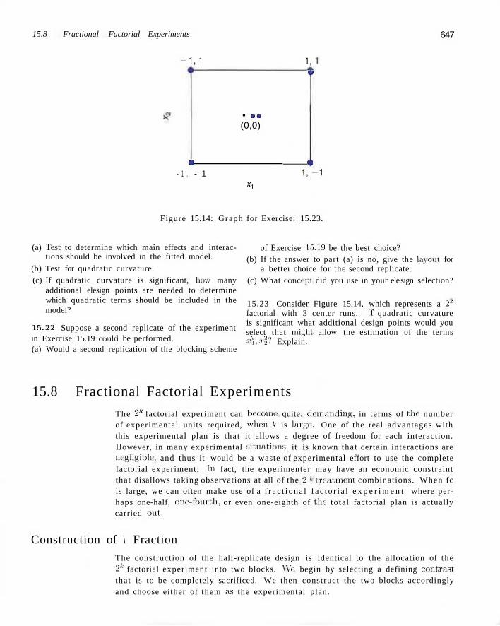
15.8 Fractional Factorial Experiments 647
1,1
• • • (0,0)
o
1, 11
<> - 1 , - 1
Xl
1 , - 1
Figure 15.14: Graph for Exercise: 15.23.
(a) Test to determine which main effects and interactions should be involved in the fitted model.
(b) Test for quadratic curvature. (c) If quadratic curvature is significant, how many
additional elesign points are needed to determine which quadratic terms should be included in the model?
15.22 Suppose a second replicate of the experiment in Exercise 15.19 e:e>tild be performed. (a) Would a second replication of the blocking scheme
of Exercise 15.19 be the best choice? (b) If the answer to part (a) is no, give the layout for
a better choice for the second replicate. (c) What concept did you use in your ele'sign selection?
15.23 Consider Figure 15.14, which represents a 2" factorial with 3 center runs. If quadratic curvature is significant what additional design points would you select that might allow the estimation of the terms a;?,arf? Explain.
15.8 Fractional Factorial Experiments
The 2k factorial experiment can become1 quite: demanding, in terms of the number of experimental units required, when k is large. One of the real advantages with this experimental plan is that it allows a degree of freedom for each interaction. However, in many experimental situations, it is known that certain interactions are negligible, and thus it would be a waste of experimental effort to use the complete factorial experiment. In fact, the experimenter may have an economic constraint that disallows taking observations at all of the 2 t reatment combinations. When fc is large, we can often make use of a f r a c t i o n a l f a c t o r i a l e x p e r i m e n t where perhaps one-half, one-fourth, or even one-eighth of the total factorial plan is actually carried out .
Construction of \ Fraction
The construction of the half-replicate design is identical to the allocation of the 2k factorial experiment into two blocks. We' begin by selecting a defining contrast tha t is to be completely sacrificed. We then construct the two blocks accordingly and choose either of them as the experimental plan.
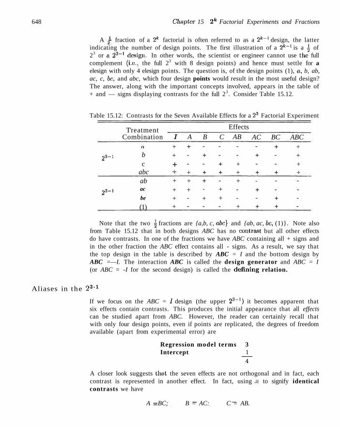
648 Chapter 15 2k Factorial Experiments and Fractions
A 1 fraction of a 2* factorial is often referred to as a 2k~l design, the latter indicating the number of design points. The first illustration of a 2k~l is a ^ of 23 or a 2 3 _ 1 design. In other words, the scientist or engineer cannot use the full complement (i.e.. the full 23 with 8 design points) and hence must settle for a elesign with only 4 elesign points. The question is, of the design points (1), a, b, ab, ac, c, be, and abc, which four design points would result in the most useful design? The answer, along with the important concepts involved, appears in the table of + and — signs displaying contrasts for the full 23. Consider Table 15.12.
Table 15.12: Contrasts for the Seven Available Effects for a 2:1 Factorial Experiment
23-1
2 3 - l
Treatment Combination
a
b c
abc ab ac
be
(1)
J
+ +
+ T
+ + + +
A
+ --+ + + --
B -+ -+ + -
+ -
C --+ + -+ + -
Effects
AB --+ + + --+
AC -+ -+ -
+ -+
BC + --+ --+ +
ABC + + + + ----
Aliases in the 2
Note that the two \ fractions are {a,b, c, abc} and {ab, ac, be, (1)}. Note also from Table 15.12 that in both designs ABC has no contrast but all other effects do have contrasts. In one of the fractions we have ABC containing all + signs and in the other fraction the ABC effect contains all - signs. As a result, we say that the top design in the table is described by ABC = I and the bottom design by ABC =—I. The interaction ABC is called the design generator and ABC = I (or ABC = -I for the second design) is called the denning relation.
3 - 1
If we focus on the ABC = / design (the upper 23_1) it becomes apparent that six effects contain contrasts. This produces the initial appearance that all effects can be studied apart from ABC. However, the reader can certainly recall that with only four design points, even if points are replicated, the degrees of freedom available (apart from experimental error) are
Regression model terms 3 Intercept 1
~4~
A closer look suggests that, the seven effects are not orthogonal and in fact, each contrast is represented in another effect. In fact, using = to signify identical contrasts we have
A s BC; B = AC: C = AB.
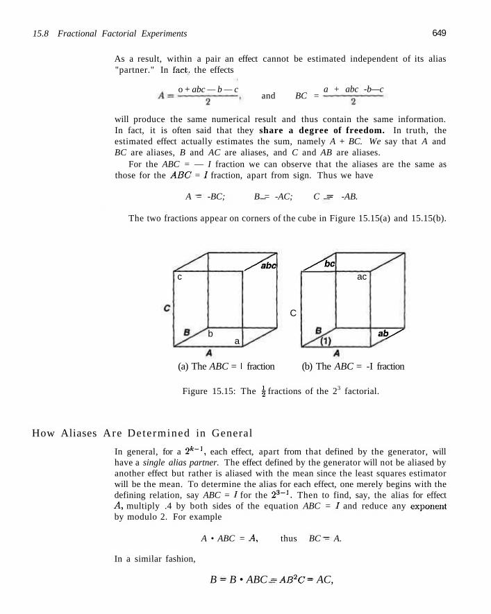
15.8 Fractional Factorial Experiments 649
As a result, within a pair an effect cannot be estimated independent of its alias "partner." In fact, the effects
o + abc — b — c and BC =
a + abc -b—c
will produce the same numerical result and thus contain the same information. In fact, it is often said that they share a degree of freedom. In truth, the estimated effect actually estimates the sum, namely A + BC. We say that A and BC are aliases, B and AC are aliases, and C and AB are aliases.
For the ABC = — I fraction we can observe that the aliases are the same as those for the ^4f?C = / fraction, apart from sign. Thus we have
A = -BC; B = -AC; C = -AB.
The two fractions appear on corners of the cube in Figure 15.15(a) and 15.15(b).
c
b a
S^abc
C
^ b c ac
ab/'
(a) The ABC = I fraction (b) The ABC = -I fraction
Figure 15.15: The \ fractions of the 23 factorial.
How Aliases Are Determined in General
In general, for a 2fc_1, each effect, apart from that defined by the generator, will have a single alias partner. The effect defined by the generator will not be aliased by another effect but rather is aliased with the mean since the least squares estimator will be the mean. To determine the alias for each effect, one merely begins with the defining relation, say ABC = / for the 2 3 _ 1 . Then to find, say, the alias for effect A, multiply .4 by both sides of the equation ABC = / and reduce any exponent by modulo 2. For example
A • ABC = A, thus BC = A.
In a similar fashion,
B = B • ABC = AB2C = AC,
650 Chapter 15 2k Factorial Experiments and Fractions
and. of course,
C = C- ABC = ABC2 = AB.
Now for the second fraction (i.e., defined by the relation ABC = —/),
A = -BC; B = -AC; C = -AB.
As a result, the numerical value of effect A is actually estimating A—BC. Similarly, the value of B estimates B — AC and the value for C estimates C — AB.
Formal Construction of the 2 k-l
A clear understanding of the concept of aliasing makes it very simple to understand the construction of the 2k_1. We begin with investigation of the 2 3 _ 1 . There are three factors and four design points required. The procedure begins with a full factorial in k - 1 = 2 factors A and B. Then a third factor is added according to the desired alias structures. For example, with ABC as the generator, clearly C = ± AB. Thus, C = AB or -AB is found to supplement the full factorial in A and B. Table 15.13 illustrates what is a very simple procedure.
Table 15.13: Construction of the Two 2 3 _ 1 Designs
Basic 22
A B
+ +
+ +
2:i
A
+ -+
-l.
B
—
+ j .
ABC C-
t I = AB
+
-+
2 3 - 1 ; . A B
+ -- + + +
ABC C =
= - J . : -AB
+ + -
Note that we saw earlier that ABC = I gives the design points a, b, c, and abc while ABC = —I gives (1), ac, be, and ab. Earlier we were able to construct the same designs using the table of contrasts in Table 15.12. However, as the design becomes more complicated with higher fractions, these contrast tables become more difficult to deal with.
Consider now a 2 4 - 1 (i.e., a ^ of a 24 factorial design) involving factors A, B, C, and D. As in the case of the 2 3 _ l , the highest-order interaction, in this case ABCD, is used as the generator. We must keep in mind that ABCD = / , the defining relation suggests that the information on ABCD is sacrificed. Here we begin with the full 23 in A, B, and C and form D = ± ABC to generate the two 2 4 _ 1 designs. Table 15.14 illustrates the construction of both designs.
Here, using the notations of a, b, c, and so on, we have the following designs:
ABCD = I, (1), ad, bd, ab, cd, ac, be, abed
ABCD = —/, d, a, b, abc, c, acd, bed, abc.
The aliases in the case of the 2'1_1 are found as illustrated earlier for the 2 3 _ 1 . Each effect has a single alias partner and is found by multiplication via the use of
15.8 Fractional Factorial Experiments 651
Table 15.14: Construction of the Two 2 4 _ 1 Designs
Basic 23
A B
+ -- + + + - -
+ -- + + +
C
— --
+ + + +
A
+ -+ -+ -
+
24-1.
B
—
+ + --
+ +
;ABCD
C
_ --
+ 4-
+ +
D =
= 1
= ABC
+ + -
+ --
+
A
+ -+ -+ -
+
2 4 - 1 ;
B
_
T
+ --+ +
ABCD =
C
— --j _
+ + +
D =
: -I
-ABC
+
-+ -+ + -
the defining relation. For example, the alias for .4 for the ABCD = / design is given by
A = A • ABCD = A2 BCD = BCD.
The alias for AB is given by
AB = AB • ABCD = A2B2CD = CD.
As we can observe easily, main effects are aliased with three factor interactions and two factor interactions are aliased with other two factor interactions. A complete listing is given by
A = BCD AB = CD
B = ACD AC = BD
C = ABD AD = BC
D = ABC.
Construction of the \ Fraction
In the case of the 4 fraction, two interactions are selected to be sacrificed rather than one, and the third results from finding the generalized interaction of the selected two. Note that this is very much like the construction of four blocks discussed in Section 15.7. The fraction used is simply one of the blocks. A simple example aids a great deal in seeing the connection to the construction of the 5 fraction. Consider the construction of \ of a 25 factorial (i.e., a 25~2), with factors A, B, C, D, and E. One procedure that avoids the confounding of two main effects is the choice of ABD and ACE as the interactions that correspond to the two generators, giving ABD = / and ACE = / as the defining relations. The third interaction sacrificed would then be (ABD)(ACE) = A2BCDE = BCDE. For the construction of the design, we begin with a 2 5 - 2 = 23 factorial in A, B, and C. We use the interactions ABD and ACE to supply the generators, so the 23 factorial in A, B, and C is supplemented by factor D = ± AB and E = ± AC.
652 Chapter 15 2k Factorial Experiments and Fractions
Thus one of the fractions is given by
A -
+ -
+ -+ -
+
B --
+ + --+ +
C ----
+ + + +
D = AB _i_
-—
+ + --
+
E = AC
+ -+ --
+ -+
de a be abd cd ace be abode
The other three fractions are found by using the generator {D = —AB, E = AC}, {D = AB.E = -AC}, and {D = -AB,E = -AC}. Consider an analysis of the above 25~2 design. It contains 8 design points to study five factors. The aliases for main effects are given by
A(ABD) = BD: A(ACE) = CE, A(BCDE) = ABCDE
B = AD = ABCE = CDE
C = ABCD =AE = BDE
D = AB = ACDE = BCE
E = ABDE =AC = BCD
Aliases for other effects can be found in the same fashion. The breakdown of degrees of freedom is given by (apart from replication)
Main effects Lack of fit Total
5 _2_ 7
(CD = BE, BC = DE)
We list interactions only through degree two in the lack of fit.
Consider now the case of a 2 6 - 2 , which allows 16 elesign points to study six factors. Once again two design generators are chosen. A pragmatic choice to supplement a 2G _ 2 = 24 full factorial in A, B, C, and D is to use E = ± ABC and F = ±BCD. The construction is given in Table 15.15.
Obviously, with 8 more design points than the 2 5 - 2 , the aliases for main effects will not present as difficult a problem. In fact, note that with defining relations ABCE = ± I, BCDF = ±1, and (ABCE)(BCDF) = ADEF = ± I, main effects will be aliased with interactions that are no less complex than those of third order. The alias structure for main effects is written
A= BCE = ABCDF = DEF,
B= ACE = CDF = ABDEF,
C= ABE = BDF = ACDEF.
D = ABCDE = BCF = AEF,
E = ABC = BCDEF = ADF,
F = ABCEF = BCD = ADE.
15.9 Analysis of Fractional Factorial Experiments 653
Table 15.15: A 2l'~2 Design
A — + -+ -+ -+ -+ -+ -+ -+
B — -+ + --+ + --+ + --+ +
C — ---+ + + + ----+ + + +
D — -------+ + + + + + j -
+
E = ABC — + + -+ --— -+ + -+ --+
F = BCD — -+ + + + --+ + ----+ +
Treatment Combination
(1) ae bef abf cef acf be abce df adef bde abd cde acd. bcdf abcdef
each with a single degree of freedom. For the two-factor interactions,
AB= CE - ACDF = BDEF, AF = BCEF = ABCD = DE,
AC= BE s ABDF = CDEF, BD = ACDE = CF = ABEF,
AD= BCDE = ABCF = EF, BF = ACEF = CD = ABDE,
AE= BC = ABCDEF = DF.
Here, of course, there is some aliasing among the two-factor interactions. The remaining 2 degrees of freedom are accounted for by the following groups:
ABD = CDE = ACF = BEF, ACD = BDE = ABF = CEF.
It becomes evident that we should always be aware of what the alias structure is for a fractional experiment before we finally recommend the experimental plan. Proper choice of defining contrasts is important, since it dictates the alias structure.
15.9 Analysis of Fractional Factorial Experiments
The difficulty of making formal significance tests using data from fractional factorial experiments lies in the determination of the proper error term. Unless there are data available from prior experiments, the error must come from a pooling of contrasts representing effects that are presumed to be negligible.
Sums of squares for individual effects are found by using essentially the same procedures given for the complete factorial. We can form a contrast in the treatment combinations by constructing the table of positive and negative signs. For
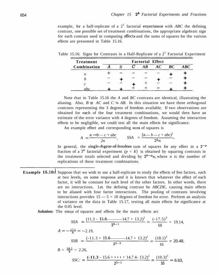
654 Chapter 15 2k Factorial Experiments and Fractions
example, for a half-replicate of a 23 factorial experiment with ABC the defining contrast, one possible set of treatment combinations, the appropriate algebraic sign for each contrast used in computing effects and the sums of squares for the various effects are presented in Table 15.16.
Table 15.16: Signs for Contrasts in a Half-Replicate of a 23 Factorial Experiment
Treatment Combination
Factorial Effect B AB AC BC ABC
a b c abc
+
+ +
+ +
+
+
+ + + +
Note that in Table 15.16 the A and BC contrasts are identical, illustrating the aliasing. Also, B — AC and C = AB. In this situation we have three orthogonal contrasts representing the 3 degrees of freedom available. If two observations are obtained for eae:h of the four treatment combinations, we would then have an estimate of the error variance with 4 degrees of freedom. Assuming the interaction effects to be negligible, we could test all the main effects for significance.
An example effect and corresponding sum of squares is
A = •b — c + abc
SSA = (a — b — c + abc)2
2n ' 22n In general, the single-degree-of-freedom sum of squares for any effect in a 2~v
fraction of a 2k factorial experiment (p < A:) is obtained by squaring contrasts in the treatment totals selected and dividing by 2k~''n, where n is the number of replications of these treatment combinations.
Example 15.10:1 Suppose that we wish to use a half-replicate to study the effects of five factors, each at two levels, on some response and it is known that whatever the effect of each factor, it will be constant for each level of the other factors. In other words, there are no interactions. Let. the defining contrast be ABCDE, causing main effects to be aliased with four factor interactions. The pooling of contrasts involving interactions provides 15 — 5 = 10 degrees of freedom for error. Perform an analysis of variance on the data in Table 15.17, testing all main effects for significance at the 0.05 level.
Solution: The sums of squares and effects for the main effects arc
SSA = (11.3 - 15.6 14.7 + 13.2)2 (-17.5)2
25-1 16 17.5
SSB
-2.19.
(-11.3 + 15.6 14.7 + 13.2)2 (18.1)2
0 5 - 1 16 B = ± | ! = 2.26,
SSC: (-11.3 - 15.6 + • • • + 14.7 4- 13.2)2 (10.3)2
2 5 - l 16
= 19.14,
= 20.48,
6.63,
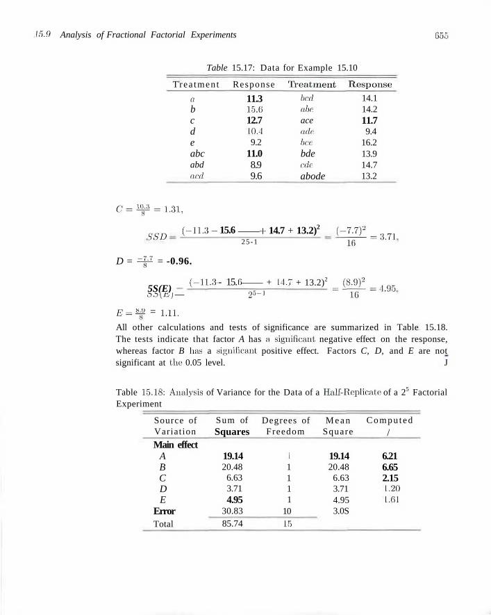
15.9 Analysis of Fractional Factorial Experiments &bl
Table 15.17: Data for Example 15.10
Trea tmen t Response Trea tmen t Response
a b c d e abc abd acd
C7=3$a = 1.31,
?<T ( " U ' 3 ~
D = =$Z = -0.96.
5S(E) ( _ 1 L 3
•5.5 -Cj —
E = M = l .ll.
15.6
- 15.
11.3 15.6 12.7 10.1 9.2
11.0 8.9 9.6
bed abc ace adc bee bde ale abode
+ 14.7 + 13.2)2
25-1
6 2 5 - l
+ 14.r • + 13.2)2
14.1 14.2 11.7 9.4
16.2 13.9 14.7 13.2
<-f=,n
- • 7 —
All other calculations and tests of significance are summarized in Table 15.18. The tests indicate that factor A has a significant, negative effect on the response, whereas factor B lias a significant, positive effect. Factors C, D, and E are not significant at the 0.05 level. J
Table 15.18: Analysis of Variance for the Data of a Half-Replicate of a 25 Factorial Experiment
Source of Variat ion
Main effect A B C D E
Error Total
Sum of Squares
19.14 20.48
6.63 3.71 4.95
30.83 85.74
Degrees of Freedom
1 1 1 1 1
10 15
M e a n Square
19.14 20.48
6.63 3.71 4.95 3.0S
C o m p u t e d /
6.21 6.65 2.15 1.20 1.61
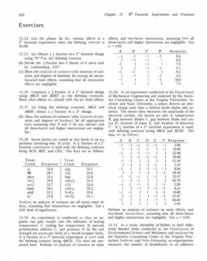
656
Exercises
Chapter 15 2k Factorial Experiments and Fractions
15.24 List the aliases for the: various effects in a 2 factorial experiment when the defining contrast is ACDE.
15.25 (a) Obtain a i fraction of a 21 factorial design using BCD as the defining contrast.
(b) Divide the \ fraction into 2 blocks of A units each by confounding ABC.
(c) Show the analysis-of-variance tabic (sources of variation and degrees of freedom) for testing all unconfounded main effects, assuming that all interaction effects are negligible.
15.26 Construct a \ fraction e>[ a 2° factorial elesign using ABCD and BDEF as the defining contrasts. Show what effects are: aliased with the six main effects.
15.27 (a) Using the defining contrasts ABCE and ABDF, obtain a j fraction of a 2° elesign.
(b) Show the analysis-of-variance! table (sources of variation and degrees of freedom) for all appropriate tests assuming that E and F do not interact and all three-factor and higher interactions are negligible.
15.28 Seven factors are' varied at, two levels in an experiment involving only 16 trials. A ;j fraction of a 2 factorial experiment is used with the defining contrasts being ACD, BEF, and CEG. The data are as follows:
Treat. C o m b .
(1 Ml abce cdef acef bade abdf hi
Response
31.6 28.7 33.1 33.6 33.7 34.2 32.5 27.8
Trea t . C o m b .
acg edg beg adefg efg abdeg bedfg abefg
Response 31.1 32.0 32.8 35.3 32.4 35.3 35.6 35.1
Perforin an analysis of variance em all seven main effects, assuming that interactions are negligible. Use a 0.05 level of significance.
15.29 An experiment is conducted sei that, an engineer can gain insight into the influence of sealing temperature A, cooling bar temperature B, percent polyethylene additive C, and pressure D on the seal strength (in grams per inch) of a. bread-wrapper Stock. A I fraction of a 2' factorial experiment is uscel with the defining contrast being ABCD. The data are: presented here. Perform an analysis of variance on main
effects, and two-factor interactions, assuming that all three-factor and higher interactions are negligible. Use a = 0.05.
A B C D Response
— 1
1 - 1
- 1 1
- I 1
- 1
- I 1
- 1 -1 1 1
- 1 1 1
- 1 1
- 1 - 1
1
6.6 6.9 7.9 (i.l 9.2 6.8
10.4 7.3 I
15.30 In an experiment conducted at the Department of Mechanical Engineering and analyzed by the Statistics Consulting Center at the Virginia Polytechnic Institute and State University, a sensor detects an electrical charge each time a turbine blade makes one; rotation. The sensor then measures the amplitude of the electrical current. Six factors arc rprn A, temperature B, gap between blades C, gap between blade and casing D, location of input E, and location of detection /•'. A j fraction of a 2° factorial experiment is used, with defining contrasts being ABCE and BCDF. The data are1 as follows:
A B - 1 - 1
1 - 1 - 1 1
1 1 - 1 - 1
1 - 1 - 1 1
1 1 - 1 - 1
1 - 1 - 1 L
1 1 - 1 - 1
1 - 1 - 1 1
I 1
C D - 1 - 1 - 1 - i - 1 - 1 - 1 - 1
1 - 1 1 - 1 1 - 1 1 - 1
- 1 1 - 1 1 - I 1
1 1 1 1 1 1 1 1 1 1
E - 1
1 1
- 1 1
- 1 - 1
1 - 1
1 1
- 1 1
- I - 1
1
F - 1 - 1
1 1 1 1 1
- 1 1 1
- 1 - 1 - 1 - 1
1 1
Response 3.89
10.46 25.98 39.88 61.88 3.22 8.94
20.29 32.07 50.76
2.80 8.15
16.80 25.47 44.44
2.45
Perform an analysis of variance on main effects, and two-factor interactions, assuming that all three-factor and higher interactions are negligible. Use a = 0.05.
15.31 In a study Durability of Rubber to Steel Adhesively Bonded Joints conducted at. the Department, of Environmental Science and Mechanics and analyzed by the Statistics Consulting Center at the Virginia Polytechnic Institute: and Stale University, an experimenter measures the number of breakdowns in an adhesive
15.10 Higher Fractions and Screening Designs 657
seal. It was postulated that concentration of seawafer A, temperature B, pH C, voltage D, and stress E influence the breakdown of an adhesive seal. A ^ fraction of a 2" factorial experiment is used, with the defining contrast being ABCDE. The data are as follows:
A - 1
1 - 1
1 - ]
1 - 1
1 - 1
1 - 1
1 - 1
1 -1
1
B -1 - 1
1 1
- 1 1 1 1
- 1 - 1
1 1
- 1 - 1
1 1
C - I
1 - 1 - 1
1 1 1 I
- 1 - 1 - 1 - 1
1 1 1 1
D 1
- 1 - 1 - 1 - I - 1 - 1 - 1
1 1 1 1 1 1 I 1
E
I - 1 - 1
1 - 1
1 1
- 1 - 1
1 1
- 1 1
- 1 - 1
1
Response 462 746 714
1070 474 832 764
1087 522 854 773
1068 572 831 819
1101
Perform an analysis of variance on main effects, and two-factor interactions, assuming that all three-factor and higher interactions are negligible. Use ev = 0.05.
15.32 Consider a 2r>_1 elesign with factors A, B, C, D, and E. Construct the design by beginning with a 2'1 and use E = ABCD as the generator. Show all aliases.
15.33 There arc six factors and only 8 elesign points can be used. Construct 23 and use D = AB, E
a 2 by beginning with a
generators.
15.34 Consider Exercise 15.33. Construct another 2''~'! that is different from the design chosen in Exercise 15.33.
15.35 for Exercise 15.33, give all aliases for the six main effects.
15.36 In Myers and Montgomery (2002), an application was discussed in which an engineer is concerned with the effects on the cracking of a fit antum alloy. The three factors are A, temperature, B, titanium content, and C, amount of grain refiner. The following gives a portion of the design and the response, crack length induced in the sample of the alloy.
A B C Response
I
I 0.5269 2.3380 4.0060 3.3640
AC and F = BC the
(a) What is the defining relation?
(b) Give aliases for all three main effects assuming that two factor interactions may be real,
(c) Assuming that interactions are' negligible, which main Factor is most important?
(d) For the factor named in (c), at. what level would you suggest, the factor be for final production, high or low?
(c) At what levels would you sugge:st the other factors be for final production?
(f) What hazards lie in the recommendations you made' in (d) and (e)? Be thorough in your answer.
15.10 Higher Fractions and Screening Designs
Some industrial situations require the analyst to determine which of a large number of controllable factors have an impact on some impor tant response. The factors may be qualitative eir class variables, regression variables, or a mixture of both . The analytical procedure may involve analysis of variance, regression, or both. Often the regression model used involves only linear main effects, although a fewr
interactions may be estimated. The situation calls for variable: screening and the resulting experimental designs are known as s c r e e n i n g d e s i g n s . Clearly, two-level orthogonal efosigns that are sa turated or nearly sa tura ted are viable candidates.
Design Resolution
Two-level orthogonal designs are often classified according to their r e s o l u t i o n , the latter determined through the following definition.
658 Chapter 15 2k Factorial Experiments and Fractions
Definition 15.1: The resolution of a two-level orthogonal elesign is the length of the smallest (least complex) interaction among the set of defining contrasts.
If the design is constructed as a full or fractional factorial [i.e., either a 2 or 2k~p (p = 1,2,..., A: - 1) design], the notion of design resolution is an aid in categorizing the impact of the aliasing. For example, a resolution II design would have little use since there would be at least one instance of aliasing of one main effee-t with another. A resolution III elesign will have all main effects (linear effects) orthogonal to each other. However, there will be some aliasing among linear effects and two-factor interactions. Clearly, then, if the analyst, is interested in studying main effects (linear effects in the case of regression) and there are no two-factor interactions, them a, elesign of resolution at least III is required.
15.11 Construction of Resolution III and IV Designs with 8, 16, and 32 Design Points
Useful designs of resolutions III and IV can be constructed for 2 to 7 variables with 8 design points. We merely begin with a 23 factorial that has been symbolically saturated with interactions.
Xl
- 1 1
-1 -1 1 1
-1 1
x2 - 1 -1 1
-1 1
-1 1 1
X3
-1 -1 -1 1
-1 1 1 1
xi-r2
1 -1 -1 1 1
-1 -1 1
X1X3 1
-1 1
-1 -1 1
-1 1
x2x3
1 1
-1 -1 -1 -1 1 1
XiX2
- 1 1 1 1
-1 - 1 -1 1
It is clear that a resolution III elesign can be constructed merely by replacing interaction columns by new main effects through 7 variables. For example, we may elefine
x4 = Xix2 (defining contrast ABD)
x-j = .('i.r.j (defining contrast ACE)
x$ = x2x3 (defining contrast BCF)
x- = 3:1X2X3 (defining contrast ABCG)
and obtain a 2 a fraction of a 2' factorial. The preceding expressions identify the chosen defining contrasts. Eleven additional defining contrasts result and all defining contrasts t:ontain at least three letters. Thus the design is a resolution III design. Clearly, if we begin with a. subset of the augmented columns and conclude with a design involving fewer than seven elesign variables, the result is a resolution III design in fewer than 7 variables.
A similar set of possible designs can be constructed for 16 elesign points by beginning with a 2'1 saturated with interactions. Definitions of variables that correspond to these interactions produce resolution III elesigns through 15 variables.
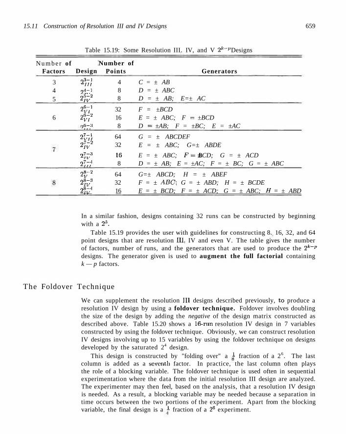
15.11 Construction of Resolution III and IV Designs 659
N u m b e r of Factors
3 4 5
6
Table 15.19: Some Resolution III. IV, and V 2k~v Designs
Design 2 3 - l '•III 2 , l - i 2 5 - 2 LIV 2 n- i r,(i-2 AVl 0 6- : i
Number of Points
4 8 8
32 16 8
Generators
C = ± AB D = ± ABC D = ± AB; E=± AC
F = ±BCD E = ± ABC; F = ±BCD D = ±AB; F = ±BC; E = ±AC
2 7 - l
07-2 LIV 27-. 'l
2 7 - l
64 32
16 8
G = ± ABCDEF E = ± ABC; G=± ABDE
E = ± ABC; F-± BCD; G = ± ACD D = ± AB; E = ±AC; F = ± BC; G = ± ABC
2 | r 2 64 G=± ABCD; H = ± ABEF 2°Z3 32 F = ± ABC; G = ± ABD; H = ± BCDE 2%* 16 E = ± BCD; F = ± ACD; G = ± ABC; H = ± ABD
In a similar fashion, designs containing 32 runs can be constructed by beginning with a 25.
Table 15.19 provides the user with guidelines for constructing 8. 16, 32, and 64 point designs that are resolution III, IV and even V. The table gives the number of factors, number of runs, and the generators that are used to produce the 2k~p
designs. The generator given is used to augment the full factorial containing k — p factors.
The Foldover Technique
We can supplement the resolution III designs described previously, to produce a resolution IV design by using a foldover technique. Foldover involves doubling the size of the design by adding the negative of the design matrix constructed as described above. Table 15.20 shows a 16-run resolution IV design in 7 variables constructed by using the foldover technique. Obviously, we can construct resolution IV designs involving up to 15 variables by using the foldover technique on designs developed by the saturated 24 design.
This design is constructed by "folding over" a 1 fraction of a 26. The last column is added as a seventh factor. In practice, the last column often plays the role of a blocking variable. The foldover technique is used often in sequential experimentation where the data from the initial resolution III design are analyzed. The experimenter may then feel, based on the analysis, that a resolution IV design is needed. As a result, a blocking variable may be needed because a separation in time occurs between the two portions of the experiment. Apart from the blocking variable, the final design is a 1 fraction of a 2e experiment.
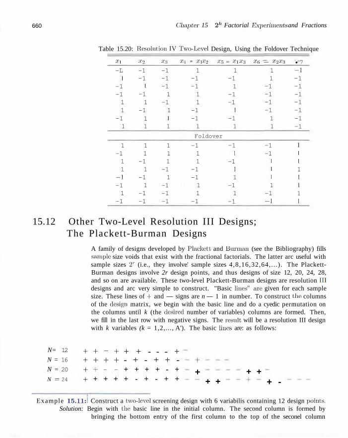
660 Chapter 15 2k Factorial Experiments and Fractions
Table 15.20: Resolution IV Two-Level Design, Using the Foldover Technique
Xl
-L 1
-1 -1 1 1
-1 1
x-> -1 -1 1
-1 1
-1 1 1
X;i
-1 -1 -1 1
-1 1 1 1
X4 = Xi
1 -1 -1 1 1
-1 -1 1
x2 Xs = X1X3
1 -1 1
-1 -1 1
-1 1
X6 — X2X3
1 1
-1 -1 -1 -1 1 1
•''7
-I -1 -1 -1 -1 -1 -1 -1
Foldover
1 -1 1 1
-1 -1 1
-1
1 1
-1 1
-1 1
-1 -1
1 1 1
-1 1
-1 -1 -1
-1 1 1
-1 -1 1 1
-1
-1 1
-1 1 1
-1 1
-1
-1 -1 1 1 1 1
-1 -1
1 1 1 1 I 1 1 1
15.12 Other Two-Level Resolution III Designs; The Plackett-Burman Designs
A family of designs developed by Plackctt and Burman (see the Bibliography) fills sample size voids that exist with the fractional factorials. The latter arc useful with sample sizes 2 r (i.e., they involve' sample sizes 4,8,16,32,64,. . . ) . The Plackett-Burman designs involve 2r design points, and thus designs of size 12, 20, 24, 28, and so on are available. These two-level Plackett-Burman designs are resolution III designs and arc very simple to construct. "Basic lines*' arc given for each sample size. These lines of -I- and — signs are n — 1 in number. To construct the columns of the elesign matrix, we begin with the basic line and do a cyedic permutation on the columns until k (the elesired number of variables) columns are formed. Then, we fill in the last row with negative signs. The result will be a resolution III design with k variables (k = 1,2,..., A'). The basic lines are: as follows:
N= 12
N = 16
N = 20
N = 24
+ + + +
+ - + + + + T — —
+ + +
+ + - - - + - + - + + -+ + + + - + + - + - + +
+ + + + + + -
Example 15.11:1 Construct a two-level screening design with 6 variabilis containing 12 design points. Solution: Begin with the basic line in the initial column. The second column is formed by
bringing the bottom entry of the first column to the top of the seconel column
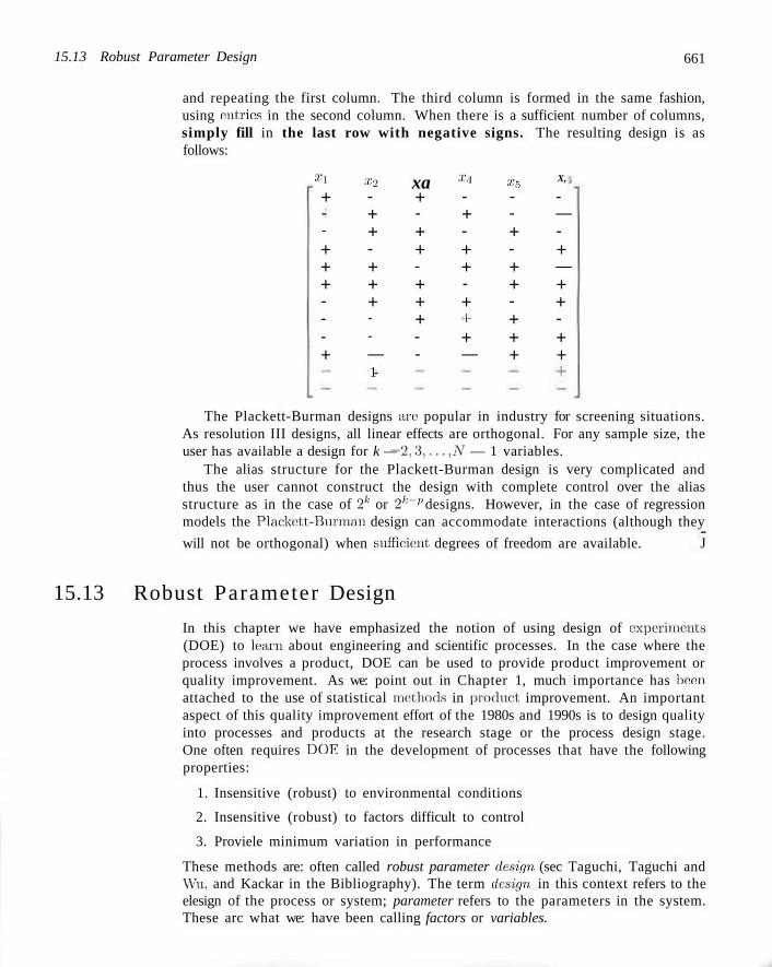
15.13 Robust Parameter Design 661
and repeating the first column. The third column is formed in the same fashion, using entries in the second column. When there is a sufficient number of columns, simply fill in the last row with negative signs. The resulting design is as follows:
Xl
+ --
+ + + ---+
x2 -+ + -+ + + --—
xa + -+ + -+ + + --
XA -+ -+ + -+ l-
+ —
x5 --+ -+ + -+ + +
X,
-— -+ — + + -+ +
1-
The Plackett-Burman designs arc popular in industry for screening situations. As resolution III designs, all linear effects are orthogonal. For any sample size, the user has available a design for k — 2 , 3 , . . . , Ar — 1 variables.
The alias structure for the Plackett-Burman design is very complicated and thus the user cannot construct the design with complete control over the alias structure as in the case of 2k or 2k~p designs. However, in the case of regression models the Plackett-Burman design can accommodate interactions (although they
will not be orthogonal) when sufficient, degrees of freedom are available. J
15.13 Robust Parameter Design
In this chapter we have emphasized the notion of using design of experiments (DOE) to learn about engineering and scientific processes. In the case where the process involves a product, DOE can be used to provide product improvement or quality improvement. As we: point out in Chapter 1, much importance has been attached to the use of statistical methods in product improvement. An important aspect of this quality improvement effort of the 1980s and 1990s is to design quality into processes and products at the research stage or the process design stage. One often requires DOE in the development of processes that have the following properties:
1. Insensitive (robust) to environmental conditions
2. Insensitive (robust) to factors difficult to control
3. Proviele minimum variation in performance
These methods are: often called robust parameter design (sec Taguchi, Taguchi and Wu, and Kackar in the Bibliography). The term design, in this context refers to the elesign of the process or system; parameter refers to the parameters in the system. These arc what we: have been calling factors or variables.
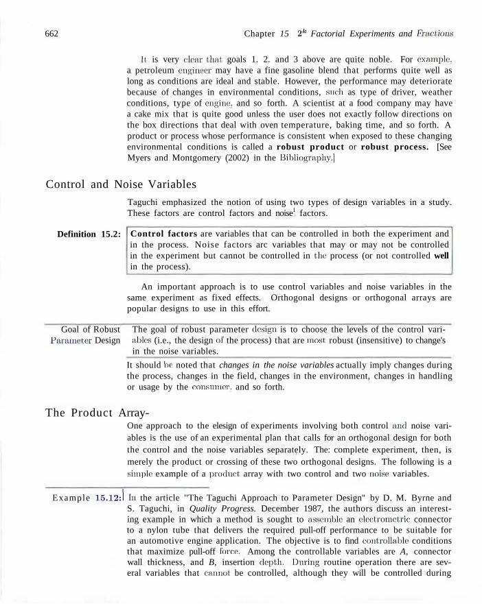
662 Chapter 15 2k Factorial Experiments and Fractious
It is very clear that, goals 1. 2. and 3 above are quite noble. For example, a petroleum engineer may have a fine gasoline blend that performs quite well as long as conditions are ideal and stable. However, the performance may deteriorate because of changes in environmental conditions, sue'h as type of driver, weather conditions, type of engine, and so forth. A scientist at a food company may have a cake mix that is quite good unless the user does not exactly follow directions on the box directions that deal with oven temperature, baking time, and so forth. A product or process whose performance is consistent when exposed to these changing environmental conditions is called a robust product or robust process. [See Myers and Montgomery (2002) in the Bibliography.]
Control and Noise Variables
Taguchi emphasized the notion of using two types of design variables in a study. These factors are control factors and noise1 factors.
Definition 15.2: Control factors are variables that can be controlled in both the experiment and in the process. Noise factors arc variables that may or may not be controlled in the experiment but cannot be controlled in the process (or not controlled well in the process).
An important approach is to use control variables and noise variables in the same experiment as fixed effects. Orthogonal designs or orthogonal arrays are popular designs to use in this effort.
Goal of Robust The goal of robust parameter efesign is to choose the levels of the control vari-Paraineter Design ables (i.e., the design e>f the process) that are most, robust (insensitive) to change's
in the noise variables.
It should be noted that changes in the noise variables actually imply changes during the process, changes in the field, changes in the environment, changes in handling or usage by the consumer, and so forth.
The Product Array-One approach to the elesign of experiments involving both control anel noise variables is the use of an experimental plan that calls for an orthogonal design for both the control and the noise variables separately. The: complete experiment, then, is merely the product or crossing of these two orthogonal designs. The following is a simple example of a product array with two control and two noise variables.
Example 15.12:1 In the article ''The Taguchi Approach to Parameter Design'' by D. M. Byrne and S. Taguchi, in Quality Progress. December 1987, the authors discuss an interesting example in which a method is sought to assemble an ele:ctrometi'ic connector to a nylon tube that delivers the required pull-off performance to be suitable for an automotive engine application. The objective is to find controllable conditions that maximize pull-off force Among the controllable variables are A, connector wall thickness, and B, insertion elepth. During routine operation there are several variables that cannot be controlled, although they will be controlled during
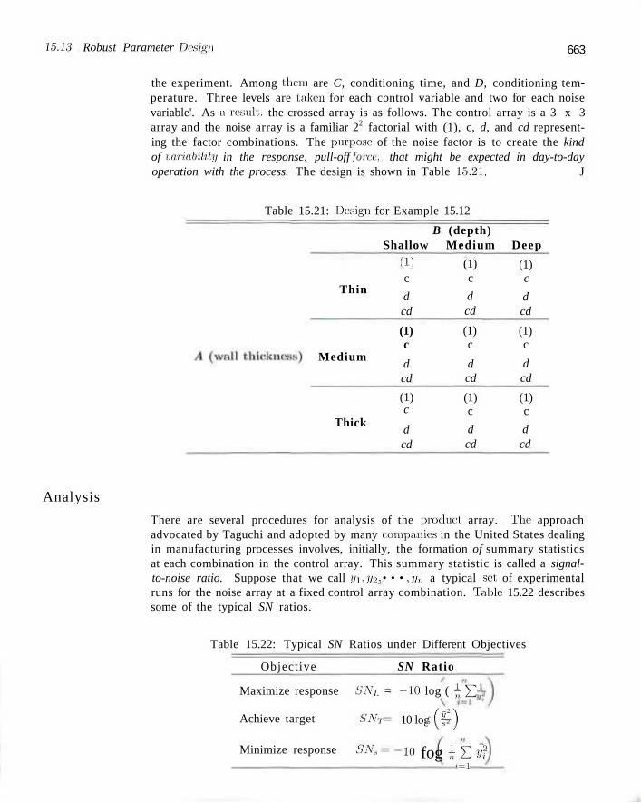
15.13 Robust Parameter Design 663
Analysis
the experiment. Among them are C, conditioning time, and D, conditioning temperature. Three levels are taken for each control variable and two for each noise variable'. As a result, the crossed array is as follows. The control array is a 3 x 3 array and the noise array is a familiar 22 factorial with (1), c, d, and cd representing the factor combinations. The purpose of the noise factor is to create the kind of variability in the response, pull-off force, that might be expected in day-to-day operation with the process. The design is shown in Table 15.21. J
Table 15.21: Design for Example 15.12
B (depth) Shallow Medium Deep
Thin
Medium
(D c
d cd
(1) c
d cd
(1) c
d cd
(1) c
d cd
(1) c
d cd
(1) c
d cd
Thick
(1) c
d cd
(1) (1) c c
d d cd cd
There are several procedures for analysis of the product array. The approach advocated by Taguchi and adopted by many companies in the United States dealing in manufacturing processes involves, initially, the formation of summary statistics at each combination in the control array. This summary statistic is called a signal-to-noise ratio. Suppose that we call yi,y>, • • • ,y„ a typical set of experimental runs for the noise array at a fixed control array combination. Table 15.22 describes some of the typical SN ratios.
Table 15.22: Typical SN Ratios under Different Objectives
Objective SN Ratio
Maximize response SNr, = —10 log ( ^ £
Achieve target SNT
Minimize response SN„
10 log < ( * )
io fog £ £ w t = l
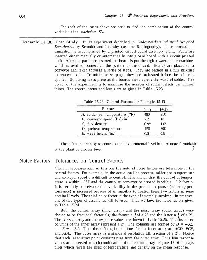
664 Chapter 15 2k Factorial Experiments and Fractions
For each of the cases above we seek to find the combination of the control variables that maximizes SN.
Example 15.13:1 Case Study In an experiment described in Understanding Industrial Designed Experiments by Schmidt and Launsby (see the Bibliography), solder process optimization is accomplished by a printed circuit-board assembly plant. Parts are inserted either manually or automatically into a bare board with a circuit printed on it. After the parts are inserted the board is put through a wave solder machine, which is used to connect all the parts into the circuit. Boards are placed on a conveyor and taken through a series of steps. They are bathed in a flux mixture to remove oxide. To minimize warpage, they are preheated before the solder is applied. Soldering takes place as the boards move across the wave of solder. The object of the experiment is to minimize the number of solder defects per million joints. The control factor and levels are as given in Table 15.23.
Table 15.23: Control Factors for Example 15.13
Factor A, solder pot temperature (°F) B, conveyor speed (ft/min) C, flux density D, preheat temperature E, wave height (in.)
( -1) 480 7.2 0.9° 150 0.5
(+1) 510 10 1.0° 200 0.6
These factors are easy to control at the experimental level but are more formidable
at the plant or process level. J
Noise Factors: Tolerances on Control Factors Often in processes such as this one the natural noise factors are tolerances in the control factors. For example, in the actual on-line process, solder pot temperature and conveyor speed are difficult to control. It is known that the control of temperature is within ±5°F and the control of conveyor belt speed is within ±0.2 ft/min. It is certainly conceivable that variability in the product response (soldering performance) is increased because of an inability to control these two factors at some nominal levels. The third noise factor is the type of assembly involved. In practice, one of two types of assemblies will be used. Thus we have the noise factors given in Table 15.24.
Both the control array (inner array) and the noise array (outer array) were chosen to be fractional factorials, the former a | of a 25 and the latter a ^ of a 23, The crossed array and the response values are shown in Table 15.25. The first three columns of the inner array represent a 23. The columns are formed by D = —AC and E = —BC. Thus the defining interactions for the inner array are ACD, BCE, and ADE. The outer array is a standard resolution III fraction of a 23. Notice that each inner array point contains runs from the outer array. Thus four response values are observed at each combination of the control array. Figure 15.16 displays plots which reveal the effect of temperature and density on the mean response.
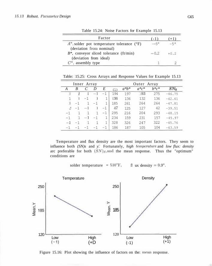
15.13 Robust. Parameter Design G65
Table 15.24: Noise Factors for Example 15.13
Factor ( -1) (+1) A*, solder pot temperature tolerance (°F)
(deviation from nominal) B*, conveyor sliced tolerance (ft/min)
(deviation from ideal) C*, assembly type
-5°
0.2
1
-5°
+0.2
2
Table: 15.25: Cross Arrays and Response Values for Example 15.13
Inner Array Ou te r Array A 1 1 1 J
-1 -1 -1 -1
B 1 1
-1 -1 1 1
-1 -1
C I
-1 1
-I 1
-1 1
-1
D -1 I
-1 1 1
-1 1
-1
E -1 1 1
-1 -1 1 1
-1
(1) 194 136 185 47 295 234 328 186
a*b* 197 136 261 125 216 159 326 187
a*c* 193 132 264 127 204 231 247 105
b*c* 275 136 264 42 293 157 322 104
SNS
-46.75
-42.61 -47.81
-39.51
-48.15
-45.97
-45.76
-43.59
Temperature and flux density are the most important factors. They seem to influence both (SN)s and y. Fortunately, high temperature and low flux: density arc preferable for both (SN)s- anel the mean response. Thus the "optimum" conditions are
solder temperature = 510°F, 11 ux density =0.9° .
250
>
120
Temperature
Low (-D
High (+D
250
I 185
120
Density
Low (-1)
High (+1)
Figure 15.16: Plot showing the influence of factors on the: mean response.
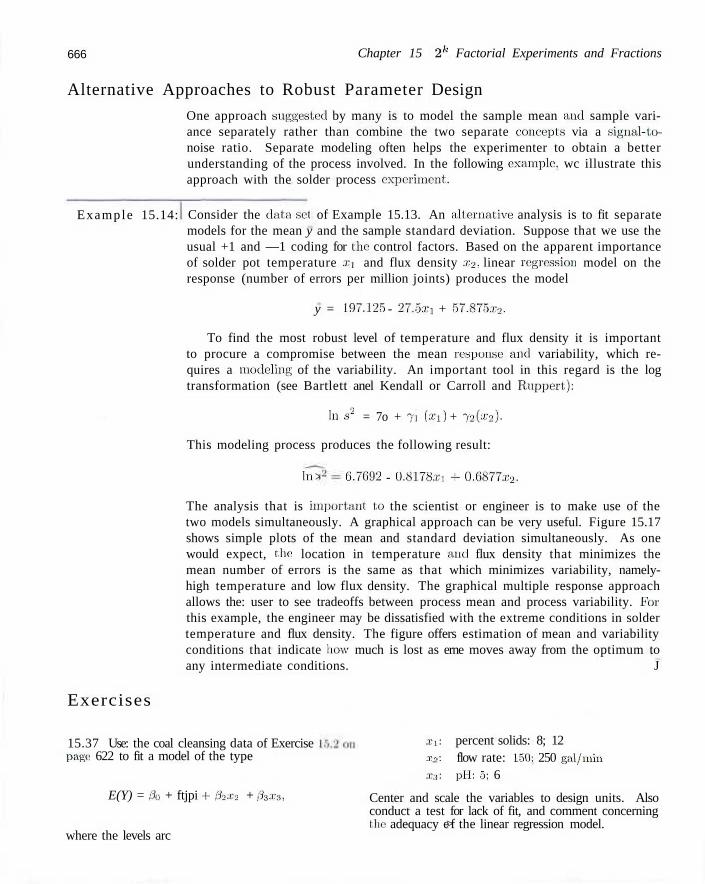
666 Chapter 15 2k Factorial Experiments and Fractions
Alternative Approaches to Robust Parameter Design
One approach suggested by many is to model the sample mean anel sample variance separately rather than combine the two separate concepts via a signal-to-noise ratio. Separate modeling often helps the experimenter to obtain a better understanding of the process involved. In the following example, wc illustrate this approach with the solder process experiment.
Example 15.14: Consider the data set of Example 15.13. An alternative analysis is to fit separate models for the mean y and the sample standard deviation. Suppose that we use the usual +1 and —1 coding for the control factors. Based on the apparent importance of solder pot temperature a?i and flux density x2, linear regression model on the response (number of errors per million joints) produces the model
y = 197.125 - 27.5a:i + 57.875.i.-2.
To find the most robust level of temperature and flux density it is important to procure a compromise between the mean response anel variability, which requires a modeling of the variability. An important tool in this regard is the log transformation (see Bartlett anel Kendall or Carroll and Ruppert):
In S3 = 7o + 71 (xi) + J2ix2).
This modeling process produces the following result:
I n > 6.7692 - 0.8178.7:, 4- 0.6877x2.
The analysis that is important, to the scientist or engineer is to make use of the two models simultaneously. A graphical approach can be very useful. Figure 15.17 shows simple plots of the mean and standard deviation simultaneously. As one would expect, the: location in temperature and flux density that minimizes the mean number of errors is the same as that which minimizes variability, namely-high temperature and low flux density. The graphical multiple response approach allows the: user to see tradeoffs between process mean and process variability. Feir this example, the engineer may be dissatisfied with the extreme conditions in solder temperature and flux density. The figure offers estimation of mean and variability conditions that indicate how much is lost as erne moves away from the optimum to any intermediate conditions. J
Exercises
15.37 Use: the coal cleansing data of Exercise page 622 to fit a model of the type
E(Y) = 0Q + ftjpi -t- 02X7 + P3X3,
where the levels arc
:z'i: percent solids: 8; 12 :ro: flow rate: 150: 250 gal/min :K3: pll: 5; 6
Center and scale the variables to design units. Also conduct a test for lack of fit, and comment concerning the adequacy e>f the linear regression model.
Review Exercises 667
in
a> Q
_3
-0.5
0.0
X), Temperature
1.0
Figure 15.17: Mean and s tandard deviation for Example 15.14.
15.38 A 2° factorial plan is used to build a regression model containing first-order coefficients and model terms for all two-factor interactions. Duplicate runs are made for each factor. Outline the analysis-of-variance table showing degrees of freedom for regression, lack of fit, and pure error.
Consider the -^ of the 27 factorial discussed in 15.39 Section 15.11. List the additional 11 defining contrasts.
15.40 Construct a Plackett-Burman design for 10 variables containing 24 experimental runs.
Review Exercises
15.41 A Plackett-Burman design is used for the purpose of studying the rheological properties of high-molecular-weight, copolymers. Two levels of each of six variables are fixed in the experiment. The viscosity of the polymer is the respemse. The data were analyzed by the Statistics Consulting Center at Virginia Polytechnic Institute and State University for personnel in the Chemical Engineering Department at the University. The variables are as follows: hard block chemistry xi, nitrogen flow rate X2, heat-up time x-z, percent compression x4, scans high and low £5, percent strain XQ. The data are presented here. Build a regression equation relating viscosity to the levels of the six variables. Conduct f-tests for all main effects. Recommend factors that should be retained for future studies and those that should not. Use the residual mean square (5 degrees of freedom) as a measure of experimental error.
Obs. x% X2 Xa x4 Xs Xe 1 1 - 1 1 2 1 1 - ' 3 - 1 1 ' 4 1 - 1 : 5 1 1 - : 6 1 1 1 7 - 1 1 1 8 - 1 - 1 : 9 - 1 - 1 -
10 1 - 1 -1 1 - 1 1 -12 - 1 - 1 -
1 - 1 - 1 - 1 I 1 - 1 - 1 I - 1 1 - 1 1 1 - 1 1 1 1 1 - 1 1 - 1 1 1 1 1 - 1 1 I 1 1 - 1 1 1 1 1 I - 1 1 1 1 - 1 - 1 1 1 - 1 - 1 - 1
194,700 588,400
7,533 514,100 277.300 493,500
8,969 18,340 6,793
160,400 7,008 3,637
15.42 A large petroleum company in the Southwest regularly conducts experiments to test additivess to drilling fluids. Plastic viscosity is a rheological measure reflecting the thickness of the fluid. Various polymers are added to the fluid to increase viscosity. The following is a data set in which two polymers are used at
668 Chapter 15 2k Factorial Experiments and Fractions
two levels each and the viscosity measured. The concentration of the polymers is indicated as "low" and "high." Conduct an analysis of the 22 factorial experiment. Test for effects for the two polymers and interaction.
Polymer 2 Low High
Polymer 1 Low High
3 3.5 11.7 12.0
11.3 12.0 21.7 22.4
15.43 A 22 factorial experiment is analyzed by the Statistics Consulting Center at Virginia Polytechnic Institute and State University. The client is a member of the Department of Housing, Interior Design, and Resource Management. The client is interested in comparing cold start versus preheating ovens in terms of total energy being delivered to the product. In addition, the conditions of convection are being compared to regular mode. Four experimental runs were made at each of the four factor combinations. Following are the data from the experiment:
Convection Mode Regular Mode
Preheat 618 619.3 629 611 581 585.7 581 595
Cold 575 573.7 574 572 558 562 562 566
Do an analysis of variance to study main effects and interaction. Draw conclusions.
15.44 Construct a design involving 12 runs where 2 factors are varied at 2 levels each. You are further restricted in that blocks of size 2 must be used, and you must be able to make significance tests on both main effects and the interaction effect.
15.45 In the study The Use of Regression Analysis for Correcting Matrix Effects in the X-Ray Fluorescence Analysis of Pyrotechnic Compositions, published in the Proceedings of the Tenth Conference on the Design of Experiments in Army Research Development and Testing, ARO-D Report 65-3 (1965), an experiment was conducted in which the concentrations of 4 components of a propellant mixture and the weights of fine and coarse particles in the slurry were each allowed to vary. Factors .4, B, C, and D, each at two levels, represent the concentrations of the 4 components and factors E and F, also at two levels, represent the weights of the fine and coarse particles present in the slurry. The goal of the analysis was to determine if the X-ray intensity ratios associated with component 1 of the propellant were significantly influenced by varying the concentrations of the various components and
the weights of the particle sizes in the mixture. A | fraction of a 26 factorial experiment was used with the defining contrasts being ADE, BCE, and ACF. The following data represent the total of a pair of intensity readings:
Treatment Intensity Batch Combination Ratio Total
1 2 3 4 5 6 7 8
abef cdef (1) ace bde abed adf bef
2.2480 1.8570 2.2428 2.3270 1.8830 1.8078 2.1424 1.9122
The pooled mean square error with 8 degrees of freedom is given by 0.02005. Analyze the data using a 0.05 level of significance to determine if the concentrations of the components and the weights of the fine and coarse particles present in the slurry have a significant influence on the intensity ratios associated with component 1. Assume that no interaction exists among the 6 factors.
15.46 Show the blocking scheme for a 27 factorial experiment in eight blocks of size 16 each, using ABCD, CDEFG, and BDF as defining contrasts. Indicate which interactions are completely sacrificed in the experiment.
15.47 Use Table 15.19 to construct a 16-run design with 8 factors that is resolution IV.
15.48 In your design of Review Exercise 15.47, verify that the design is indeed resolution IV.
15.49 Construct a design that contains nine design points, is orthogonal, contains 12 total runs, 3 degrees of freedom for replication error, and allows for a lack of fit test for pure quadratic curvature.
15.50 Consider a design which is a 23rj/ w4th 2 cen
ter runs. Consider y/ as the average response at the design parameter and j/o as the average response at the design center. Suppose the true regression model is
E(y) = 00+ 0lXl + 02X2 + 03x3
+ 0lix\ + 022X1+033X1.
(a) Give (and verify) E(yj — y0). (b) Explain what you have learned from the result in
(a).

15.14 Potential Misconceptions and Hazards; Relationship to Material in Other Chapters 669
15.14 Potential Misconceptions and Hazards; Relationship to Material in Other Chapters
In the use of fractional factorial experiments one: eif the most, important considerations that the analyst must be aware of is the design, resolution. A design of low resolution is smaller (and hence cheaper) than one of higher resolution. However, a price is paid for the cheaper design. The: elesign of lower resolution has heavier aliasing than one' of higher resolution. For example, if the researcher has expectation that two-factor interactions may be important, then resolution III should not be used. A resolution III elesign is strictly a main effects plan.
Chapter 16
Nonparametric Statistics
16.1 Nonparametric Tests
Most of the hypothesis-testing procedures discussed in previous chapters are based on the assumption that the random samples are selected from normal populations. Fortunately, most of these tests are still reliable when we expedience slight elepar-tures from normality, particularly when the sample size is large. Traditionally, these testing procedures have been referred to as pa ramet r i c me thods . In this chapter we consider a number of alternative test procedures, called nonparamet ric or distr ibution-free methods , that often assume no knowledge whatsoever about the distributions of the underlying populatiems, except perhaps that they are continuous.
Nonparametric or distribution-free procedures are used with increasing frequency by data, analysts. There: are many applications in science and engineering where the data are reported as values not on a continuum but rather on an ordinal scale such that it is quite natural to assign ranks to the data. In fact, the reader may notice quite early in this chapter that the distribution-free methods described here involve an analysis of ranks. Most analysts find the computations involved in nonparametric methods to be very appealing and intuitive.
For an example where a. nonparametric test is applicable, two judges might rank five brands of premium beer by assigning a rank of 1 to the brand believed to have the best overall quality, a rank of 2 to the second best, and so forth. A nonparametric te:st could then be used to determine whether there is any agreement be-tween the two judges.
We shoulel also point out that there are a number of disadvantages associated with nonparametric tests. Primarily, they do not utilize all the information provided by the sample, anel thus a nonparametric test will be less efficient than the corresponeUng parametric procedure when both methods are applicable. Consequently, to achieve the same power, a nonparametric test will require a larger sample size than will the corrcsponeliiig parametric test.
As we indicated earlier, slight departures from normality result in minor deviations from the ideal for the standard parametric tests. This is particularly true for the /-test and the F-test. In the case of the t-test and the F-test. the P-value
672 Chapter 16 Nonparametric Statistics
quoted may be slightly in error if there is a moderate violation of the normality assumption.
In summary, if a parametric and a nonparametric test are both applicable to the same set of data, we should carry out the more efficient parametric technique. However, we should recognize that, the assumptions of normality often cannot be justified and that we do not always have quantitative measurements. It is fortunate that statisticians have provided us with a number of useful nonparametric procedures. Armed with nonparametric techniques, the data analyst has more ammunition to accommodate a wider variety of experimental situations. It should be pointed out that even under the standard normal theory assumptions, the efficiencies of the nonparametric techniques are remarkably close to those of the corresponding parametric procedure. On the other hand, serious departures from normality will render the nonparametric method much more efficient than the parametric procedure.
Sign Test
The reader should recall that the procetiures discussed in Section 10.7 for testing the null hypothesis that p = po arc valid only if the population is approximately normal or if the sample is large. However, if n < 30 and the population is decidedly nonnormal, we must resort to a nonparametric test.
The sign test is used to test hypotheses on a population median. In the case of many of the nonparametric procedures, the mean is replaced by the median as the pertinent location paramete r under test. Recall that the sample median is defined in Section 1.4. The population counterpart, denoted by p has an analogous definition. Given a random variable X, p. is defined such that P(X > p.) < 0.5 and P(X < p) < 0.5. In the continuous case,
P(X > ft) = P(X < A) = 0.5.
Of course, if the distribution is symmetric, the population mean and median are equal. In testing the null hypothesis H0 that p — po against an appropriate alternative, on the basis of a random sample of size n, we replace each sample value exceeding po with a plus sign and each sample value less than po with a minus sign. If the null hypothesis is true and the population is symmetric, the sum of the plus signs should be approximately equal to the sum of the minus signs. When one sign appears more frequently than it should, based on chance alone, we reject the hypothesis that the population median p is equal to p0.
In theory the sign test is applicable only in situations where po cannot equal the value of any of the observations. Although there is a zero probability of obtaining a sample observation exactly equal to po when the population is continuous, nevertheless, in practice a sample value equal to po will often occur from a lack of precision in recording the data. When sample values equal to po are observed, they are excluded from the analysis and the sample size is correspondingly reduced.
The appropriate test statistic for the sign test is the binomial random variable X, representing the number of plus signs in our random sample. If the null hypothesis that p = po is true, the probability that a sample value results in either a plus or a minus sign is equal to 1/2. Therefore, to test the null hypothesis that p = po.
16.1 Nonparametric Tests 673
we are actually testing the null hypothesis that the number of plus signs is a value of a random variable having the binomial distribution with the parameter;; = 1/2. P-values for both one-sided and two-sided alternatives can then be calculated using this binomial distribution. For example, in testing
Ho- p = Po, Hi: ft. < po,
we shall reject Ho in favor of Hi only if the proportion of plus signs is sufficiently less than 1/2, that is, when the value x of our random variable is small. Hence, if the computed P-value
P = P(X < x when p = 1/2)
is less than or equal to some preselected significance level a, we reject Ha in favor of H\. For example, when n = 15 and x = 3, we find from Table A.l that
P = P(X < 3 when p = 1/2) = ^ S (x; 15, \ j = 0.0176,
so that the null hypothesis fi = po can certainly be rejected at the 0.05 level of significance but not at the 0.01 level.
To test the hypothesis
HQ: p = po,
Hi: p > po,
we reject Ho in favor of Hi only if the proportion of plus signs is sufficiently greater than 1/2, that is, when x is large. Hence, if the computed P-value
P = P(X > x when p = 1/2)
is less than cv, we reject Ho in favor of Hi. Finally, to test the hypothesis
Ho', p = Po,
Hi: pjt po,
we reject. Ho in favor of Hi when the proportion of plus signs is significantly less than or greater than 1/2. This, of course, is equivalent to x being sufficiently small or sufficiently large. Therefore, if x < n/2 and the computed P-value
P = 2P(X < x when p = 1/2)
is less than or equal to a, or if x > n/2 and the computed P-value
P = 2P(X > x when p = 1/2)
is less than or equal to a, we reject Ho in favor of Hi.
674 Chapter 16 Nonparametric Statistics
Whenever n > 10, binomial probabilities with p = 1/2 can be approximated from the normal curve, since np = nq > 5. Suppose, for example, that we wish to test the hypothesis
Ho'- p = po,
Hi: p < po,
at the a = 0.05 level of significance for a random sample of size n = 20 that yields x = 6 plus signs. Using the normal-curve approximation with
p = np= (20)(0.5) = 10
and
we find that
Therefore.
a = y/npq = v/(20)(0.5)(0.5) = 2.236,
6.5 - 10 ^ 2 3 6 " - - 1 - 5 ' -
P = P(X < 6) « P(Z < -1.57) = 0.0582,
which leads to the nonrejection of the null hypothesis.
Example 16.1:1 The following data represent the number of hours that a rechargeable hedge trimmer operates before a recharge is required:
1.5,2.2,0.9,1.3,2.0,1.6,1.8,1.5,2.0,1.2,1.7.
Use the sign test to test the hypothesis at the 0.05 level of significance that this particular trimmer operates with a median of 1.8 hours before requiring a recharge.
Solution: 1. Ho: p = 1.8.
2. Hi: j i / 1 . 8 .
3. a = 0.05.
4. Test statistic: Binomial variable X with p = 5.
5. Computations: Replacing each value by the symbol "+" if it exceeds 1.8, by the symbol "—': if it is less than 1.8, and discarding the one measurement that equals 1.8, we obtain the sequence
- + - - + - - +
for which n = 10, x = 3, and n /2 = 5. Therefore, from Table A.l the computed P-value is
1 3 1 P = 2P(X < 3 when p = -) = 2 ] T b(x; 10, -) = 0.3438 > 0.05.
x=0
16.1 Nonparametric Tests 675
6. Decision: Do not reject the null hypothesis anel conclude that the median operating time is not significantly different from .1.8 hours.
We can also use the sign test to test flic null hypothesis pi — fi2 = do for paired observations. Here we replace each difference, di, with a plus or minus sign depending on whether the adjustcel elifference, <7,- — e/n, is positive: or negative. Throughout this section we have assumed that the populations are symmetric. However, even if populations are skewed we can carry out the same test procedure, but the hypotheses refer to the population medians rather than the means.
Example 16.2:1 A taxi company is trying to decide whether the use of radial tires instead of regular belted tires improves fuel economy. Sixte-en cars are equipped with radial tires and driven over a prescribed test course. Without changing drivers, the same cars are then equipped with the regular belted tires and elrive'ii once again over the test course The gasoline consumption, in kilometers per liter, is given in Table 16.1.
Can wc conclude at the 0.05 level of significance that cars equipped with radial
Table 16.1: Data for Example 16.2
Car Radia l Tires Belted Tires
Car Radial Tires Belted Tires
1 4.2 1.1
9 7.4 6.9
2 4.7 4.9
10 4.9 4.9
3 6.6 6.2
1 1 G.J 6.0
4 7.0 6.9
12 5.2 4.9
5 6.7 6.8
13 5.7 5.3
6 4.5 4.4
14 6.9 6.5
7 5.7 5.7
15 6.8 7.1
8 6.0 5.8
16 4.9 4.8
tires obtain better fuel economy than those: equipped with regular belled tires? Solution: Let pi anel ft2 represent the median kilometers per liter for cars equipped with
radial and belted tires, respectively.
1. Ho: pi -fh = ()-
2. Hi: fn -fi2 > 0.
3. a = 0.05.
i. Test statistic: Binomial variable A' with p = 1/2.
5. Computations: After replacing each positive difference by a ''—v symbol and each negative difference by a "—" symbol, and then discarding the two zero differences, we obtain the sequence
+ - + + - + + + + + + + - +
for which n = 14 and x = 11. Using the normal-curve approximation, we find
1 0 - 8 - 7 , « z = = = 1.87.
v/(14)(().5)(0.5)
and then
P = P(X > 11) sa P(Z > 1.87) = 0.0307.
676 Chapter 16' Nonparametric Statistics
6. Decision: Reject Ho and conclude that, on the average, radial tires do improve fuel economy. J
Not. only is the sign test one of our simplest nonparametric procedures to apply, it has the additional advantage of being applicable to dichotomous data that. cannot be recorded em a numerical scale but can be represented by positive and negative response's. For example, the sign test is applicable in experiments where a qualitative response such as "hit" or "miss" is recorded, and in sensory-type experiments where a plus or minus sign is recorded depending on whether the taste tester correctly or incorrectly identifies the desired ingredient.
We shall attempt to make comparisons between many of the nonparametric procedures and the corresponding parametric tests. In the case of the sign test the competition is, of course, the t-test. If we arc sampling from a normal distribution, the use of the f-test will result in the larger power of the test. If the distribu-tion is merely symmetric, though not normal, the fr-test is preferred in terms of power unless the distribution has extremely "heavy tails" compared to the: normal distribution.
16.2 Signed-Rank Test
The reader should note that the sign test, utilizes only the: plus and minus signs of the differences between the observations and /Io hi the one-sample case, or the plus and minus signs of the differences between the pairs of observations in the paired-sample case, but it does not take into consideration the magnitudes of these differences. A test utilizing both direction and magnitude, proposed in 1945 by Frank Wilcoxon, is now commonly referred to as the Wilcoxon signed-rank test .
The analyst can extract more information from the data in a nonparametric fashion if it is reasonable to invoke an additional restriction on the distribution from which the data we're taken. The: Wilcoxon signed-rank test applies in the case of a symmet r i c continuous dis tr ibut ion. Under this condition we can test the null hypothesis fi. = /lo. We first subtract fio from each sample value, discarding all differences equal to zero. The remaining differences are then ranked without regard to sign. A rank of 1 is assigned to the: smallest absolute difference (i.e.. without sign), a rank of 2 to the next smallest, and so on. When the absolute value of two or more differences is the same, assign to each the average of the ranks that would have been assigned if the differences were: distinguishable. For example, if I he: fifth and sixth smallest differences arc equal in absolute value, each would be assigned a rank of 5.5. If the hypothesis p = po is true:, the total of the ranks corresponding to the positive differences should nearly equal the total of the1 ranks corresponding to the negative differences. Let us represent these totals by w+ and U/_, respectively. Wc designate the smaller of the M)+ and tfl_ by w.
In selecting repeated samples, we: would expect w+ and u;_, and therefore w, to vary. Thus we may think of w+, «.'_, and w as values of the corresponding random variables W+, W-, and W. The null hypothesis fi. = po can be rejected in favor of the alternative p < po, only if u.'+ is small and u>_ is large. Likewise, the alternative fi > po can be accepted only if w^ is large and W- is small. For a two-sided alternative we may reject. HQ in favor of Hi if either *<;_ or «;_ anel hence w is sufficiently small. Therefore, no matter what the alternative hypothesis
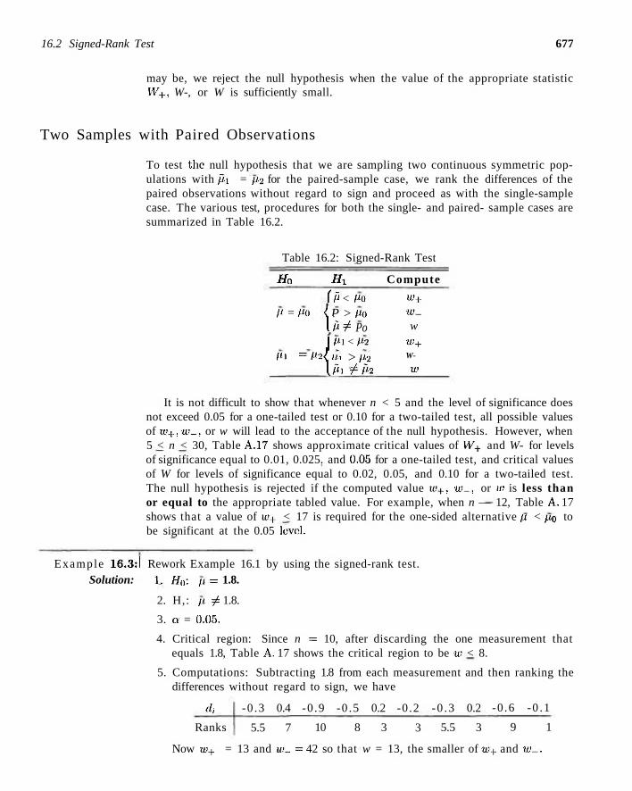
16.2 Signed-Rank Test 677
may be, we reject the null hypothesis when the value of the appropriate statistic W+, W-, or W is sufficiently small.
Two Samples with Paired Observations
To test the null hypothesis that we are sampling two continuous symmetric populations with fix = p2 for the paired-sample case, we rank the differences of the paired observations without regard to sign and proceed as with the single-sample case. The various test, procedures for both the single- and paired- sample cases are summarized in Table 16.2.
Table 16.2: Signed-Rank Test
Ho
/' = Po
Pi =Pi
Hx
(p < Po I P > Po IA 9s Po [Ml < P-2
I Pi > Pi U'i r^ih
Compute
w+ 10-
w w+ W-
w
It is not difficult to show that whenever n < 5 and the level of significance does not exceed 0.05 for a one-tailed test or 0.10 for a two-tailed test, all possible values of w+, «;_, or w will lead to the acceptance of the null hypothesis. However, when 5 < n < 30, Table A.17 shows approximate critical values of W+ and W- for levels of significance equal to 0.01, 0.025. and 0.05 for a one-tailed test, and critical values of W for levels of significance equal to 0.02, 0.05, and 0.10 for a two-tailed test. The null hypothesis is rejected if the computed value w+, W-, or w is less than or equal to the appropriate tabled value. For example, when n — 12, Table A. 17 shows that a value of w+ < 17 is required for the one-sided alternative p. < po to be significant at the 0.05 level.
Example 16.3:1 Rework Example 16.1 by using the signed-rank test. Solution: i. H0: p•= 1.8.
2. H,: p. ^ 1.8.
3. a = 0.05.
4. Critical region: Since n = 10, after discarding the one measurement that equals 1.8, Table A. 17 shows the critical region to be w < 8.
5. Computations: Subtracting 1.8 from each measurement and then ranking the differences without regard to sign, we have
d.
Ranks
-0 .3 0.4
5.5 7
-0 .9
10
-0 .5 0.2
8 3
-0 .2
3
-0 .3 0.2
5.5 3
-0 .6
9
-0 .1
1
Now iv-i- = 13 and w- = 42 so that w = 13, the smaller of w+ and iev_.
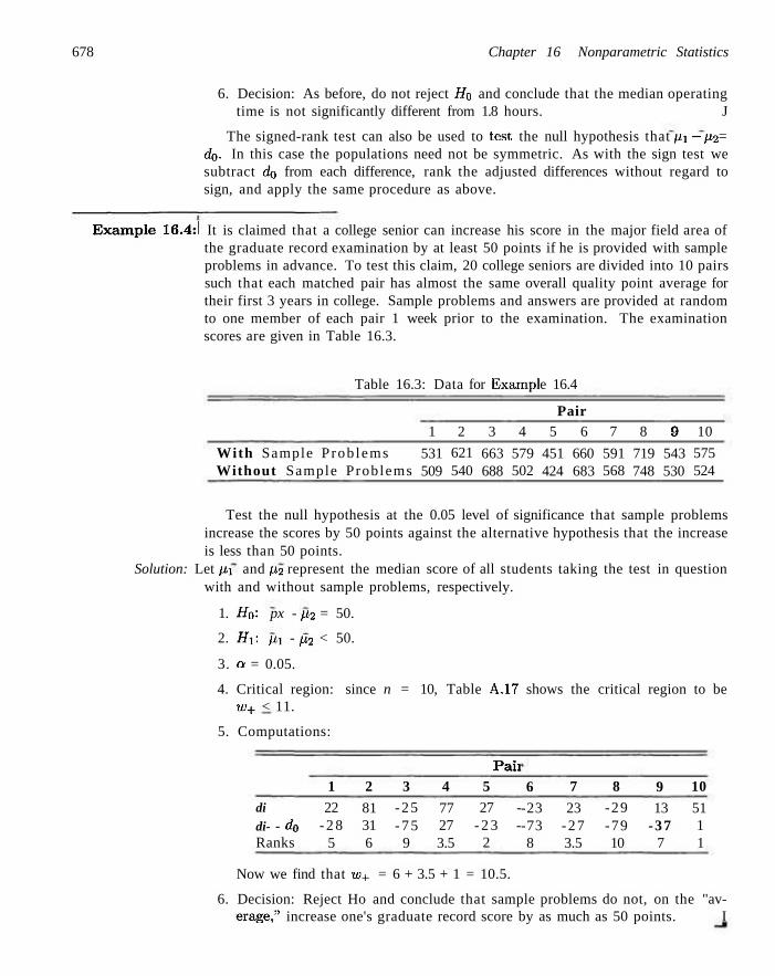
678 Chapter 16 Nonparametric Statistics
6. Decision: As before, do not reject Ho and conclude that the median operating time is not significantly different from 1.8 hours. J
The signed-rank test can also be used to test, the null hypothesis that pi—p2 = do- In this case the populations need not be symmetric. As with the sign test we subtract do from each difference, rank the adjusted differences without regard to sign, and apply the same procedure as above.
Example 16.4:1 It is claimed that a college senior can increase his score in the major field area of the graduate record examination by at least 50 points if he is provided with sample problems in advance. To test this claim, 20 college seniors are divided into 10 pairs such that each matched pair has almost the same overall quality point average for their first 3 years in college. Sample problems and answers are provided at random to one member of each pair 1 week prior to the examination. The examination scores are given in Table 16.3.
Table 16.3: Data for Exampl
With Sample Prob lems Without Sample Problems
1
531 509
2
621 540
3
663 688
4
579 502
e 16.4
Pair 5 6
451 660 424 683
7
591 568
8
719 748
9
543 530
10
575 524
Test the null hypothesis at the 0.05 level of significance that sample problems increase the scores by 50 points against the alternative hypothesis that the increase is less than 50 points.
Solution: Let px and p2 represent the median score of all students taking the test in question with and without sample problems, respectively.
1. H0: px - p2 = 50.
2. Hi: pi - p2 < 50.
3. a = 0.05.
4. Critical region: since n = 10, Table A.17 shows the critical region to be w+ < 11.
5. Computations:
di di- - d0
Ranks
1 22
- 2 8 5
2
81 31 6
3 -25 - 7 5
9
4
77 27 3.5
Paii 5 27 -
- 2 3 -2
6 -23 -73 8
7
23 -27 3.5
8 -29 -79 10
9 13
-37 7
10
51 1 1
Now we find that w+ = 6 + 3.5 + 1 = 10.5.
6. Decision: Reject Ho and conclude that sample problems do not, on the "average," increase one's graduate record score by as much as 50 points. I
Exercises 679
Normal Approximation for Large Samples
When n > 15, the sampling distribution of W+ (or VF_) approaches the normal distribution with mean
Pw+ n(n + 1)
and variance a^, = 2 n(n+ l ) (2n + l )
4 " v v + 24
Therefore, when n exceeds the largest, value in Table A. 17, the statistic
W+ - pw+ Z =
(*w+
can be used to determine the critical region for our test.
Exercises
16.1 The following data represent the time, in minutes, that a patient has to wait during 12 visits to a doctor's office before being seen by the doctor:
17 15 20 20 32 28 12 26 25 25 35 24
Use the sign test at the 0.05 level of significance to test. the doctor's claim that the median waiting time for her patients is not more than 20 minutes before being admitted to the examination room.
16.2 The following data represent, the number of hours of flight training received by 18 student pilots from a certain instructor prior to their first solo flight:
9 12 18 14 12 14 12 10 16 11 9 11 13 11 13 15 13 14
Using binomial probabilities from Table A.l, perform a sign test at the 0.02 level of significance to test the instructor's claim that the median time required before his students' solo is 12 hours of flight training.
16.3 A food inspector examines 16 jars of a certain brand of jam to determine the percent of foreign impurities. The following data were recorded:
2.4 2.3 3.1 2.2 2.3 1.2 1.0 2.4 1.7 1.1 4.2 1.9 1.7 3.6 1.6 2.3
Using the normal approximation to the binomial elis-tribution, perform a sign test at the 0.05 level of significance to test the null hypothesis that the median percent of impurities in this brand of jam is 2.5% against the alternative that the median percent of impurities is not 2.5%.
16.4 A paint supplier claims that a new additive will reduce the drying time of its acrylic paint. To test this claim, 12 panels of wood are painted, one-half of each panel with paint containing the regular additive and the other half with paint containing the new additive.
The drying times, in hours, were recorded as follows: Drying Time (hours)
Panel 1 2 3 4 5 6 7 8 9
lO-l l 12
N e w Addit ive 6.4 r>.8 7.4 5.5 6.3 7.8 8.6 8.2 7.0 4.9 5.9 6.5
Regular Addit ive 6.6 5.8 7.8 5.7 6.0 8.4 8.8 8.4 7.3 5.8 5.8 6.5
Use the sign test at the 0.05 level to test the null hypothesis that the new additive is no better than the regular additive in reducing the drying time of this kind of paint.
16.5 It is claimed that a new diet will reduce a person's weight by 4.5 kilograms, on average, in a period of 2 weeks. The weights of 10 women who followed this diet were recorded before and after a 2-week period yielding the following data:
Woman Weight Before Weight After 1 2 3 4 5 6 7 8 9
10
58.5 60.3 61.7 69.0 64.0 62.6 56.7 63.6 68.2 59.4
60.0 54.9 58.1 62,1 58.5 59.9 54.4 60.2 62.3 58.7
680 Chapter 16 Nonparametric Statistics
Use the sign test at the 0.05 level of significance to test the hypothesis that the diet reduces the median weight by 4.5 kilograms against the alternative hypothesis that the median difference in weight is less than 4.5 kilograms.
16.6 Two types of instruments for measuring the amount of sulfur monoxide in the atmosphere are beting compared in an air-pollution experiment. The following readings were recorded daily for a period of 2 weeks:
Sulfur Monox ide Day 1 2 3 4 5 6 7 8 9 10 11 12 13 14
Instrument A 0.96 0.82 0.75 0.61 0.89 0.64 0.81 0.68 0.65 0.84 0.59 0.94 0.91 0.77
Instrument B
0.87 0.74 0.63 0.55 0.76 0.70 0.69 0.57 0.53 0.88 0.51 0.79 0.84 0.63
Using the normal approximation to the binomial distribution, perform a sign test to determine whether the different instruments lead to different results. Use a 0.05 level of significance.
16.7 The following figures give the systolic blood pressure of 16 joggers before and after an 8-kilometer run:
Jogger Before After 1 2 3 4 5 6 7 8 9 10 11 12 13 14 15 16
158 149 160 155 164 138 163 159 165 145 150 161 132 155 146 159
164 158 163 160 172 147 167 169 173 147 156 164 133 161 154 170
Use the sign test at the 0.05 level of significance to test the null hypothesis that jogging 8 kilometers increases the median systolic blood pressure by 8 points against the alternative that the increase in the median is less than 8 points.
16.8 Analyze the data of Exercise 16.1 by using the signed-rank test.
16.9 Analyze the data of Exercise 16.2 by using the signed-rank test.
16.10 The weights of 5 people before they stopped smoking and 5 weeks after they stopped smoking, in kilograms, are as follows:
Individual
Before 66 80 69 52 75 After 71 82 68 56 73
Use the signed-rank test for paired observations to test the hypothesis, at the 0.05 level of significance, that giving up smoking has no effect on a person's weight against the alternative that one's weight increases if he or she quits smoking.
16.11 Rework Exercise 16.5 by using the signed-rank test.
16.12 The following are the numbers of prescriptions filled by two pharmacies over a 20-day period:
Day Pharmacy A Pharmacy B 1 2 3 4 5 6 7 8 9 10 11 12 13 14 15 16 17 18 19 20
19 21 15 17 24 12 19 14 20 18 23 21 17 12 16 15 20 18 14 22
17 15 12 12 16 15 11 13 14 21 19 15 11 10 20 12 13 17 16 18
Use the signed-rank test at the 0.01 level of significance to determine whether the two pharmacies, "on average," fill the same number of prescriptions against the alternative that pharmacy A fills more prescriptions than pharmacy B.
16.13 Rework Exercise 16.7 by using the signed-rank test,
16.14 Rework Exercise 16,6 by using the signed-rank test,
16.3 Wilcoxon Rank-Sum Test G81
16.3 Wilcoxon Rank-Sum Test
As we indicated earlier, the nonparametric procedure is generally an appropriate alternative to the normal theory test when the normality assumption eloes not hold. When we are interested in testing equality of means of two continuous distributions that are obviously nonnoriiial, and samples are independent (i.e., there is no pairing of observations), the Wilcoxon rank-sum tes t or Wilcoxon two-sample test is an appropriate- alternative to the two-sample fr-test described in Chapter 10.
Wc shall test the null hypothesis HQ that pi = p2 against some suitable alternative. First we select a random sample from each of the populations. Let n-i be the number of observations in the smaller sample, and n2 the number of observations in the larger sample'. When the- samples are- of equal size, y?i and -n2 may be randomly assigned. Arrange1 the nx + n2 observations of the combined samples in ascending order and substitute a rank of 1,2,. . . , n4 + n2 for each observation. In the case of ties (identical observations), we replace the observations by the mean of the ranks that the observations would have if they were distinguishable. For example', if the seventh anel eighth observations are identical, we would assign a rank of 7.5 to each of the two observations.
The sum of the ranks corresponding to the n i observations in the smaller sample is denoted by wi- Similarly, the value w2 represents the sum of the ?)•_> ranks corresponding to the larger sample. The- total til] +w2 depends only on the number of observations in the two samples anel is in no way affected by the results of the experiment. Hence, if rai = 3 and n2 = 4, then W\ + w2 = 1 + 2 + • • • + 7 = 28, regardless of the numerical values of the' observations. In general,
(m + n2){hi + n2 - 1) Wx + w-> = .
the- arithmetic sum of the integers 1,2 n-i + n2. Once we have determined Wi, it may be easier to find w2 by the- formula
(ll\ + Uo)(lli + u2 — 1) w2 = — tl.'i.
In choosing repeated samples of size' n-i and n2, we would expect -w\. and therefore w2. to vary. Thus we may think of wj and w2 as values of the random variables W\ and W2, respectively. The- null hypothesis ft\ = p2 will be rejected in favor of the alternative p\ < ft-2 only if Wi is small and w2 is large. Likewise, the alternative px > ft2 can be accepted only if u>x is large anel w2 is small. For a two-tailed test, wc may reject Hi in favor of Hi if «i is small and u:2 is large or if wj is large and w2 is small. In other words, the alternative' px < ft2 is accepted if ie:i is sufficiently small: the alternative //| > ft2 is accepted if w2 is sufficiently small; and the alternative: p.\ -£ ft2 is accepted if the minimum of «;i and w2 is sufficiently small. In actual practice we' usually base our decision em the value
n\(ii\ + 1) n2(n2 + 1) ux = ii'\ or u2 = w2
of the related statistic L,r] or U2 or on the value u of the statistic U, the minimum of I'i and U2- These statistics simplify the construction of table's of critical values,
682 Chapter 16 Nonparametric Statistics
since both U\ and U2 have symmetric sampling distributions and assume values in the interval from 0 to nin2, such that u-i +u2 = nin2.
From the formulas for m and u2 we see that ui will be small when K,'I is small and u2 will be small when w2 is small. Consequently, the null hypothesis will be rejected whenever the appropriate statistic U\, U2, or U assumes a value less than or equal to the desired critical value given in Table A. 18. The various test procedures are summarized in Table 16.4.
Table 16.4: Rank-Sum Test
Ho
Pi = P-2
Hi
(h <P2 < Mi > M-2
U<i ¥= fa
Compute
Ml
U2
U
Table A. 18 gives critical values of Ui and U2 for levels of significance equal to 0.001, 0.002, 0.01, 0.02, 0.025, and 0.05 for a one-tailed test, and critical values of U for levels of significance equal to 0.002, 0.02, 0.05, and 0.10 for a two-tailed test. If the observed value of t*j, u2, or u is less than or equal to the tabled critical value, the null hypothesis is rejected at the level of significance indicated by the table. Suppose, for example, that we wish to test the null hypothesis that px = p2
against the one-sideel alternative that pi < p2 at the 0.05 level of significance for random samples of size n\ = 3 and n2 = 5 that yield the value wx = 8. It follows that
U l = 8 - » = 2 .
Our one-tailed test is based on the statistic Ux- Using Table A.18, we reject the null hypothesis of equal means when ux < 1. Since ui = 2 does not fall in the rejection region, the null hypothesis cannot, be rejected.
Example 16.5:1 The nicotine content, of two brands of cigarettes, measured in milligrams, was found to be as follows:
Brand A
Brand B
2.1 4.0 6.3 5.4 4.8 3.7 6.1 3.3
4.1 0.6 3.1 2.5 4.0 6.2 1.6 2.2 1.9 5.4
Test the hypothesis, at the 0.05 level of significance, that the median nicotine contents of the two brands are equal against the alternative that they are unequal.
Solution: 1. H0: px = p2.
2. Hy. pi ^ p2.
3. a = 0.05.
4. Critical region: u < 17 (from Table A.18).
5. Computations: The observations are arranged in ascending order and ranks from 1 to 18 assigned.
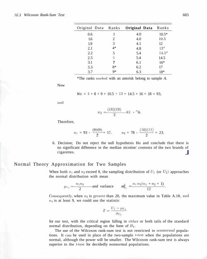
16.3 Wilcoxon Rank-Sum Test 683
Original Da ta
0.6 1.6 1.9 2.1 2.2 2.5 3.1 3.3 3.7
Ranks
1 2 3 4* 5 ii
7 8* 9*
Original Data
4.0 4.0 4.1 4.8 5.4 5.4 6.1 6.2 6.3
Ranks
10.5* 10.5 12 13* 14.5* 14.5 16* 17 18*
Now
anel
*The ranks marked with an asterisk belong to sample A.
Wx = 4 + 8 + 9 + 10.5 -J-13 + 14.5 + 16 + 18 = 93,
?i,'2 = 9 3 = lb.
Therefore,
(8)(9) (10)(11) u, = 93 - *-£-+ = 57, u2 = 78 - i—^—1 = 23.
2 2
6. Decision; Do not reject the null hypothesis Ho and conclude that there is no significant difference in the median nicotine' contents of the two brands of cigarettes.
Normal Theory Approximation for Two Samples
When both »i and n2 exceed 8, the sampling distribution of Ux (or U2) approaches the normal distribution with mean
mn2 . 2 vi-i ?!•>(«! + no + 1) ur. = and variance err, = .
2 12
Consequently, when n2 is greater than 20, the maximum value in Table A.18. and ni is at least 9, we could use the statistic
Z=U1^JH1±
for our test, with the critical region falling in either or both tails of the standard normal distribution, depending on the form of Hi .
The use of the Wilcoxon rank-sum test is not restricted to nonnormal populations. It can be used in place of the two-sample /-test when the populations are normal, although the power will be smaller. The Wilcoxon rank-sum test is always superior to the /-test for decidedly nonnormal populations.
684 Chapter 16' Nonparametric Statistics
16.4 Kruskal-Wallis Test
In Chapters 13, II. anel 15, the technique of analysis of variance is prominent as an analytical technique for testing equality of k > 2 population means. Again, however, the reader should recall that normality must be assumed in order that the F-test be theoretically correct. In this section we investigate a nonparametric alternative to analysis of variance.
The Kruskal-Wallis test, also called the Kruskal-Wallis H test , is a generalization of the: rank-sum test to the' case of k > 2 samples. It is used to test, the null hypothesis HQ that k independent samples are from identical populations. Introduced in 1952 by VV. H. Kruskal and W. A. Wallis, the test is a nonparametric procedure for testing the equality of means in the one-factor analysis of variance when the experimenter wishes to avoid the assumption that the samples were selected from normal populations.
Let. iii (i = l,2,....k) be the number of observations in the ith sample. First, we combine all fe samples anel arrange' the n = iii + n-2 + • • • + lit,- observations in ascending order, substituting the appropriate rank from 1,2,... ,n for each observation. In the case of ties (identical observations), we follow the usual procedure of replacing the observations by the means of the ranks that the observations would have: if they were distinguishable'. The' sum of the ranks corresponding to the n* observations in the ith sample is denoted by the random variable: R.j. Now let us consider the statistic
^rini;--3^1). n(n+ 1) £j m
which is approximated very well by a chi-squared distribution with k — 1 degrees of freedom when Ho is true anel if each sample consists of at least 5 observations. The fact that h. the assumed value of H, is large when the independent samples come: from populations that are not identical allows us to establish the following decision criterion for testing Ho:
Kruskal-Wallis To test the null hypothesis Hi that k independent samples are from ielentical Test populations, compute
fc= 12 £ * £ ( }
n(n +1) f-f m • ' i=i
where r,- is the assumed value of /?,-, for i = 1,2 k. If It falls in the critical region II > y- with v = k — 1 degrees of freedom, reject Hu at the a-level of significance; otherwise, fail to reject HQ.
Example 16.6:1 In an experiment to determine which of three different missile systems is preferable, the propellant burning rate is measured. The data, after coding, are given in Table 16.5. Use the Kruskal-Wallis test anel a significance level of a = 0.05 to test the hypothesis that the propellant burning rates are the same for the three missile systems.
16.4 Kruskal-Wallis Test 685
Table 16.5: Propellant Burning Rates
Missile System 2
24.0 19.8
16.7 18.9
22.8 23.2 17.6
19.8 20.2
18.1 17.8
18.4 17.3 18.8
19.1 19.7 19.3
17.3 18.9
Solution: 1. Ho: pi = p2 = p3-
2. Hi: The three means are not all equal.
3. a = 0.05.
4. Critical region: h > X0.05 = 5-991, for v = 2 degrees of freedom.
5. Computations: In Table 16.6 we convert the 19 observations to ranks and sum the ranks for each missile system.
Table 16.6: Ranks for Propellant Burning Rates
Missile System 1
19 1
17 14.5 9.5
n =61.0
r2
2
18 14.5
6 4
16 5
= 63.5
rs
3
7 11
2.5 2.5 13
9.5
8 12
= 65.5
Now, substituting m = 5, n2 = 6, n3 = 8, and n = 61.0, r2 = 63.5, and r3 = 65.5, our test statistic H assumes the value
h = 12
(19)(20)
61.02 63.52 65.5* \ + — r - + —^ 1 - (3)(20) = 1.66.
6. Decision: Since h = 1.66 does not fall in the critical region h > 5.991, we have insufficient evidence to reject the hypothesis that the propellant burning rates are the same for the three missile systems. J
686
Exercises
Chapter 16 Nonparametric Statistics
16.15 A cigarette manufacturer claims that the tar content of brand B cigarettes is lower than that of brand A. To test this claim, the following determinations of tar content, in milligrams, were recorded:
Brand A 1 12 9 13 11 M Brand B 10
Use the rank-sum test with a the claim is valid.
0.05 to test whether
16.16 To find out whether a new serum will arrest leukemia, 9 patients, who have all reached an advanced stage of the disease, are selected. Five patients receive the treatment and four do not. The survival times, in years, from the time the experiment; commenced are
Treatment 2.1 5.3 1,1 4.6 0.9 No treatment | 1.9 (To ±8 3.1
Use the rank-sum lest, at the 0.05 level o( significance, to determine if the: serum is effective.
16.17 The following data represent the number of hours that two different types of scientific pocket calculators operate before a recharge: is required.
Calculator A I 5.5 5.6 6.3 4.6 5.3 5.0 6.2 5.8 5.1 Calculator B \ 3.8 4.8 4.3 4.2 4.0 4.9 4.5 5.2 4.5
Use the rank-sum test with a = 0.01 to determine if calculator A operates longer than calculator B on a full battery charge.
16.18 A fishing line is being manufactured by two processes. To determine if there is a difference in the mean breaking strength of the lines. 10 pieces by each process are selected and then tested for breaking strength. The results are as follows:
Process 1
Process 2
10.4 9.6 8.7 <).r>
9.8 10.9 11.2 11.0
11.5 11.8 9.8 9.8
10.0 9.3
10.1 10.5
9.9 10.7 10.8 9.9
Use the rank-sum test with a = 0.1 to determine if there is a difference between the mean breaking strengths of the lines manufactured by the two processes.
16.19 From a mathematics class of 12 equally capable students using programmed materials, 5 are selected at random and given additional instruction by
the teacher. The results on the final examination were as follows:
Additional Instruction No Additional Instruction
87
75
69
88
G r a d e
78 91 80
01 82 93 79 67
Use the rank-sum test with a = 0.05 to determine if the additional instruction affects the average grade.
16.20 The following data represent the weights, in kilograms, of personal luggage carried on various flights by a member of a baseball team and a member of a basketball team.
Luggage Weight (ki lograms) Basebal l P layer 16.3 20.0 18.1 15.0 15.9 18.6 14.1 14.5 17.7 19.1 16.3 13.6 13.2 17.2
18.6 15.4 15.6 18.3 17.4 14.8 16.5
Basketbal l P l aye r 15.4 17.7 18.6 12.7 15.0 15.9
16.3 18.1 16.8 14.1 13.6 16.3
Use the rank-sum test with a = 0.05 to test the null hypothesis that the two athletes carry the same amount, of luggage on the average against the alternative hypothesis that the average weights of luggage for the two athletes are different.
16.21 The following data represent the operating time's in hours for three type's of scientific pocket calculators before a recharge is required:
Calculator
4.9 4.6
6.1 5.2
4.3 5.5 5.4 5.8 5.5
4.8
6.2 5.2
6.4 6.5
6.8 6.3
5.6 6.6
Use the Kruskal-Wallis test, at. the 0.01 level of significance, to test the hypothesis that the operating times for all three calculators are equal.
16.22 In Exercise 13.8 on page 523, use the Kruskal-Wallis test, at the 0.05 level e>f significance to determine if the organic chemical solvents differ significantly in sorption rate.
16.5 Runs Test 687
16.5 Runs Test
Definition 16.1:
Applying the many statistical concepts discussed throughout this book, it was always assumed that our sample data had been collected by some randomization procedure. The runs test, based on the order in wdiich the sample observations are obtained, is a useful technique for testing the null hypothesis Ho that the observations have indeed been drawn at random.
To illustrate the runs test, let us suppose that 12 people are polled to find out if they use a certain product. We would seriously question the assumed randomness of the sample if all 12 people were of the same sex. We shall designate a male and female by the symbols M and F, respectively, and record the outcomes according to their sex in the order in which they occur. A typical sequence for the experiment might be
M A/ F F F M F F M MM M,
where we have grouped subsequences of similar symbols. Such groupings are called runs.
A run is a subsequence of one or more identical symbols representing a common property of the data.
Regardless of whether our sample measurements represent qualitative or quantitative data, the runs test divides the data into two mutually exclusive categories: male or female; defective or nondefective; heads or tails: above or below the median: and so forth. Consequently, a sequence will always be limited to two distinct symbols. Let nx be the number of symbols associated with the category that occurs the least and n2 be the number of symbols that belong to the other category. Then the sample size n = ni + n2.
For the n = 12 symbols in our poll we have five runs, with the first containing two Ms, the second containing three Fs, and so on. If the number of runs is larger or smaller than what we would expect by chance, the hypothesis that the sample was drawn at random should be rejected. Certainly, a sample resulting in only two runs,
M M M M M M M F F F F F,
or the reverse, is most unlikely to occur from a random selection process. Such a result indicates that the first 7 people interviewed were all males followed by 5 females. Likewise, if the sample resulted in the maximum number of 12 runs, as in the alternating sequence
M F M F M F M F M F M F,
we would again be suspicious of the order in which the individuals were selected for the poll.
The runs test for randomness is based on the random variable V, the total number of runs that occur in the complete sequence of our experiment. In Table A.19, values of P(V < v * when Ho is true) are given for v* = 2 , 3 , . . . , 20 runs,
688 Chapter 16 Nonparametric Statistics
and values of m and n2 less than or equal to 10. The P-values for both one-tailed and two-tailed tests can be obtained using these tabled values.
In the poll taken previously we exhibit a total of 5 Fs and 7 Ms. Hence, with m = 5, n2 = 7, and v = 5, we note from Table A.19 for a two-tailed test that the P-value is
P = 2P(V < 5 when H0 is true) = 0.394 > 0.05.
That is, the value v = 5 is reasonable at the 0.05 level of significance when H0
is true, and therefore we have insufficient evidence to reject the hypothesis of randomness in our sample.
When the number of runs is large (for example if v = 11, while ni = 5 and n2 = 7), the P-value in a two-tailed test is
P = 2P(V > 11 when H0 is true) = 2[1 - P(V < 10 when H0 is true)]
2(1 - 0.992) = 0.016 < 0.05,
which leads us to reject the hypothesis that the sample values occurred at random. The runs test can also be used to detect departures in randomness of a sequence
of quantitative measurements over time, caused by trends or periodicities. Replacing each measurement in the order in wdiich they are collected by a plus symbol if it falls above the median, by a minus symbol if it falls below the median, and omitting all measurements that are exactly equal to the median, we generate a sequence of plus and minus symbols that are tested for randomness as illustrated in the following example.
Example 16.7:1 A machine is adjusted to dispense acrylic paint thinner into a container. Would you say that the amount of paint thinner being dispensed by this machine varies randomly if the contents of the next 15 containers are measured and found to be 3.6, 3.9, 4.1, 3.6, 3.8, 3.7, 3.4, 4.0, 3.8, 4.1, 3.9, 4.0. 3.8, 4.2, and 4.1 liters? Use a 0.1 level of significance.
Solution: 1. HQ: Sequence is random.
2. H]: Sequence is not random.
3. a = 0.1.
4. Test statistic: V, the total number of runs.
5. Computations: For the given sample we find x = 3.9. Replacing each measurement by the symbol "+" if it falls above 3.9, by the symbol " - " if it falls below 3.9, and omitting the two measurements that equal 3.9, we obtain the sequence
- + - - - - + - + + - + + for which nx = 6, n2 = 7, and v = 8. Therefore, from Table A.19. the computed P-value is
P = 2P(V > 8 when H0 is true) = 2(0.5) = 1.
6. Decision: Do not reject the hypothesis that the sequence of measurements varies randomly. -1
16.5 Runs Test 689
The runs test, although less powerful, can also be used as an alternative to the Wilcoxon two-sample test to test the claim that two random samples come from populations having the same distributions and therefore equal means. If the populations are symmetric, rejection of the claim of equal distributions is equivalent to accepting the alternative hypothesis that the means are not equal. In performing the test, we first combine the observations from both samples and arrange them in ascending order. Now assign the letter A to each observation taken from one of the populations and the letter B to each observation from the second population, thereby generating a sequence consisting of the symbols A and B. If observations from one population are tied with observations from the other population, the sequence of A and B symbols generated will not be unique and consequently the number of runs is unlikely to be unique. Procedures for breaking ties usually result in additional tedious computations, and for this reason we might prefer to apply the Wilcoxon rank-sum test whenever these situations occur.
To illustrate the use of runs in testing for equal means, consider the survival times of the leukemia patients of Exercise 16.16 on page 686 for which we have
0.5 B
0.9 A
1.4 A
1.9 B
2.1 A
2.8 B
3.1 B
4.6 A
5.3 A
resulting in v = 6 runs. If the two symmetric populations have equal means, the observations from the two samples will be intermingled, resulting in many runs. However, if the population means are significantly different, we would expect most of the observations for one of the two samples to be smaller than those for the other sample. In the extreme case where the populations do not overlap, we would obtain a sequence of the form
AAAAABBBB or BBBBAAAAA
and in either case there are only two runs. Consequently, the hypothesis of equal population means will be rejected at the a-level of significance only when v is small enough so that
P = P(V < v when H0 is true) < a,
implying a one-tailed test. Returning to the data of Exercise 16.16 on page 686 for which nx = 4, n2 = 5,
and v = 6, we find from Table A.19 that
P = P(V < 6 when H0 is true) = 0.786 > 0.05
and therefore fail to reject, the null hypothesis of equal means. Hence we conclude that the new serum does not prolong life by arresting leukemia.
WThen m and n2 increase in size, the sampling distribution of V approaches the normal distribution with mean
2nin2 , , , 2 2nin2(2nin2 - ni - n2) pv = 1-1 and variance ov = -. rx-, rr-
nx + n2 (nx + n2)2(nx + n2 - 1)
Consequently, when nx and n2 are both greater than 10, we could use the statistic
Z=V-^L
to establish the critical region for the runs test.
690 Chapter 16 Nonparametric Statistics
16.6 Tolerance Limits
Tolerance limits for a normal distribution of measurements are discussed in Chapter 9. In this section we consider a method for constructing tolerance intervals that are independent of the shape of the underlying distribution. As wc might suspect, for a reasonable degree of c:onfielence they will be substantially longer than those constructed assuming normality, and the sample size required is generally very large. Nonparametric tolerance limits are- stated in terms of the smallest and largest, observations in our sample.
Two-Sided Feir any distribution of measurements, two-sided tolerance limits arc indicated by-Tolerance Limits the smallest, and largest observations in a sample of size n, where n is determined
so that one e:an assert with 100( 1 —7)% confidence that at least the proportion 1 — 0. of the distribution is included between the sample extremes.
Table A.20 gives required sample sizes for selected values of 7 and 1 - a. For example, when 7 = 0.01 and 1 — a = 0.95, we must choose a random sample of size n = 130 in order to be 99% confident that at least 95% of the distribution of measurements is included between the sample extremes.
Instead of determining the sample size n such that a specified proportion of measurements are contained between the sample extremes, it is desirable in many industrial processes to determine the sample size such that a fixed proportion of the population falls below the largest (or above the smallest) observation in the sample. Such limits are called one-sided tolerance limits.
One-Sided For any distribution of measurements, a one-sided tolerance limit is determined Tolerance Limits by the smallest (largest) observation in a sample of size n. where n is determined
so that one can assert with 100(1 —7)% confidence that at least the proportion 1 - a of the distribution will exceed the smallest (be less than the largest) observation in the sample.
Table A.21 shows required sample sizes corresponding to selected values of 7 and 1 — Q. Hence, when 7 = 0.05 and l — ce = 0.70, wc must choose a sample of size n = 9 in order to be 95% confident that 70% of our distribution of measurements will exceed the smallest observation in the' sample.
16.7 Rank Correlation Coefficient
In Chapter 11 we use the sample correlation coefficient r to measure the linear relationship between two continuous variables X and Y. If ranks 1,2, . . . ,n are assigned to the x observations in order of magnitude and similarly to the y observations, and if these ranks are then substituted for the actual numerical values into the formula for the correlation coefficient in Chapter 11, we obtain the nonparametric counterpart of the conventional correlation coefficient. A correlation coefficient, calculated in this manner is known as the Spearman rank correlation coefficient and is denoted by rs. When there are no ties among either set of measurements, the formula for ra reduces to a much simpler expression involving the differences e7; between the ranks assigned to the n pairs of ,-r's and y's, which we now state.
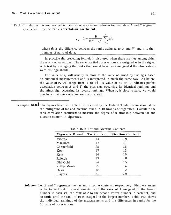
16.7 Rank Correlation Coefficient 691
Rank Correlation Coefficient
A nonparametric measure of association between two variables X and Y is given by the rank correlation coefficient
6 »\, = n(n2 -1) ^ '
where di is the difference between the ranks assigned to x, and iji, and n is the number of pairs of data.
In practice the preceding formula is also used when there are ties among either the rr or y observations. The ranks for tied observations are assigned as in the signed rank test by averaging the ranks that would have been assigned if the observations were distinguishable.
The value of re will usually be close to the value obtained by finding r based on numerical measurements and is interpreted in much the same way. As before, the value of ra will range from -1 to -1-1. A value of +1 or -1 indicates perfect association between X and Y, the plus sign occurring for identical rankings and the minus sign occurring for reverse rankings. When r s is close to zero, we would conclude that the variables are uncorrelated.
Example 16.8:1 The figures listed in Tabic 16.7, released by the Federal Trade Commission, show the milligrams of tar and nicotine found in 10 brands of cigarettes. Calculate the rank correlation coefficient to measure the degree of relationship between tar and nicotine content in cigarettes,
Table 16.7: Tar and Nicotine Contents
Cigarette Brand Tar Content Nicotine Content Viceroy Marlboro Chesterfield Kool Kent Raleigh Old Gold Philip Morris Oasis Plavers
14 17 28 17 16 13 24 25 18 31
0.9 1.1 1.6 1.3 1.0 0.8 1.5 1.4 1.2 2.0
Solution: Let X and Y represent the tar and nicotine contents, respectively. First we assign ranks to each set of measurements, with the rank of 1 assigned to the lowest number in each set, the rank of 2 to the second lowest number in each set. and so forth, until the rank of 10 is assigned to the largest number. Table 16.8 shows the individual rankings of the measurements and the differences in ranks for the 10 pairs of observations.
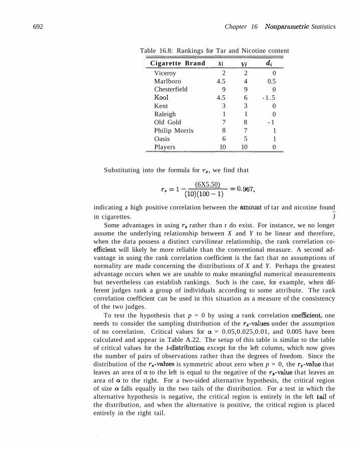
692 Chapter 16 Nonpai-ametric Statistics
Table 16.8: Rankings for Tar and Nicotine content
Cigarette Brand
Viceroy Marlboro Chesterfield Kool Kent Raleigh Old Gold Philip Morris Oasis Players
Xi
2 4.5
9 4.5
3 1 7 8 6
10
Vi 2 4 9 6 3 1 8 7 5
10
dt
0 0.5
0 -1 .5
0 0
- 1 1 1 0
Substituting into the formula for r3, we find that
(6X5.50) u~1 (io)(ioo-r) Jb7'
indicating a high positive correlation between the amount of tar and nicotine found in cigarettes. J
Some advantages in using rs rather than r do exist. For instance, we no longer assume the underlying relationship between X and Y to be linear and therefore, when the data possess a distinct curvilinear relationship, the rank correlation coefficient, will likely be more reliable than the conventional measure. A second advantage in using the rank correlation coefficient is the fact that no assumptions of normality are made concerning the distributions of X and Y. Perhaps the greatest advantage occurs when we are unable to make meaningful numerical measurements but nevertheless can establish rankings. Such is the case, for example, when different judges rank a group of individuals according to some attribute. The rank correlation coefficient can be used in this situation as a measure of the consistency of the two judges.
To test the hypothesis that p = 0 by using a rank correlation coefficient, one needs to consider the sampling distribution of the revalues under the assumption of no correlation. Critical values for a = 0.05,0.025,0.01, and 0.005 have been calculated and appear in Table A.22. The setup of this table is similar to the table of critical values for the t-distribution except for the left column, which now gives the number of pairs of observations rather than the degrees of freedom. Since the distribution of the revalues is symmetric about zero when p = 0, the revalue that leaves an area of a to the left is equal to the negative of the ?"s-value that leaves an area of a to the right. For a two-sided alternative hypothesis, the critical region of size a falls equally in the two tails of the distribution. For a test in which the alternative hypothesis is negative, the critical region is entirely in the left tail of the distribution, and when the alternative is positive, the critical region is placed entirely in the right tail.
Exercises 693
E x a m p l e 16.9:1 Refer to Example 16.8 and test the hypothesis that the correlation between the amount of ta r and nicotine found in cigarettes is zero against the alternative tha t it is greater than zero, Use a 0.01 love:] of significance.
Solution: 1. Ho: p = 0.
2. H , : p>0.
3. o = 0 . 0 1 .
4. Critical region: r s > 0.745 from Table A.22.
5. Computat ions: From Example 16.8, ra = 0.967.
6. Decision: Reject Ho and conclude tha t there is a significant correlation between the amount of tar and nicotine found in cigarettes.
Under the assumption of no correlation, it can be shown tha t the distr ibution of the r eva lue s approaches a normal distribution with a mean of 0 anel a s tandard deviation of l/\fn—1 as n increases. Consequently, when n exceeds the values given in Table A.22, one could test for a significant correlation by computing
r s - 0 , = ravn - 1 l/y/n - 1
and comparing with critical values of the s t andard normal distribution shown in Table A.3.
Exercises
16.23 A random sample of 15 adults living in a small town are selected to estimate the proportion of voters favoring a certain candidate for mayor. Each individual was also asked if he or she was a college graduate. By-letting Y and N designate the responses of "yes" and "no" to the education question, the following sequence was obtained:
A" N N N Y Y N Y Y N Y A" N N N
Use the runs test at the 0.1 level of significance to determine if the sequence supports the contention that the sample was selected at random.
16.24 A silver-plating process is being used to coat a certain type of serving tray. When the process is in control, the: thickness of the silver on the trays will vary randomly following a normal distribution with a mean of 0.02 millimeter and a standard deviation of 0.005 millimete'i'. Suppose that the next 12 trays examined show the following thicknesses of silver: 0.019, 0.021, 0.020, 0.019, 0.020, 0.018, 0.023, 0.021, 0.024, 0.022, 0.023, 0.022. Use the runs test to determine if the fluctuations in thickness from one tray to another are random. Let a = 0.05.
16.25 Use the runs test to test whether there is a difference in the average operating time for the two calculators of Exercise 16.17 on page 686.
16.26 In an industrial production line, items are inspected periodically for defectives. The following is a sequence of defective items, D, and nondefective items. N, produced by this production line:
D D N N N D N N D D N N N N
NDDDNNDNNNNDND
Use the large-sample theory for the runs test, with a significance level of 0.05, to determine whether the defectives are occurring at, random.
16.27 Assuming that the measurements of Exercise 1.14 on page 28 were recorded in successive rows from left, to right, as they were collected, use the runs test, with n = 0.05, to test the hypothesis that the data represent a random sequence.
16.28 How largo a sample is required to be 95% confident that, at least 85%. of the distribution of measurements is included between the sample extremes?
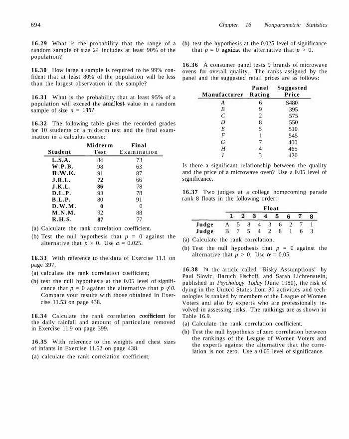
694 Chapter 16 Nonparametric Statistics
16.29 What is the probability that the range of a random sample of size 24 includes at least 90% of the population?
16.30 How large a sample is required to be 99% confident that at least 80% of the population will be less than the largest observation in the sample?
16.31 What is the probability that at least 95% of a population will exceed the smallest, value in a random sample of size n = 135?
16.32 The following table gives the recorded grades for 10 students on a midterm test and the final examination in a calculus course:
Student L.S.A. W.P .B . R.W.K. J.R.L. J.K.L. D.L.P. B.L.P. D . W . M . M.N.M. R.H.S.
Midterm Test
84 98 91 72 86 93 80
0 92 87
Final E x a m i n a t i o n
73 63 87 66 78 78 91
0 88 77
(a) Calculate the rank correlation coefficient. (b) Test the null hypothesis that p = 0 against the
alternative that p > 0. Use a = 0.025.
16.33 With reference to the data of Exercise 11.1 on page 397, (a) calculate the rank correlation coefficient; (b) test the null hypothesis at the 0.05 level of signifi
cance that p = 0 against the alternative that p ^ 0. Compare your results with those obtained in Exercise 11.53 on page 438.
16.34 Calculate the rank correlation coefficient for the daily rainfall and amount of particulate removed in Exercise 11.9 on page 399.
16.35 With reference to the weights and chest sizes of infants in Exercise 11.52 on page 438. (a) calculate the rank correlation coefficient;
(b) test the hypothesis at the 0.025 level of significance that p = 0 against the alternative that p > 0.
16.36 A consumer panel tests 9 brands of microwave ovens for overall quality. The ranks assigned by the panel and the suggested retail prices are as follows:
Panel Suggested Manufacturer Rating Price
A B C D E F G H I
6 9 2 8 5 1 7 4 3
S480 395 575 550 510 545 400 465 420
Is there a significant relationship between the quality and the price of a microwave oven? Use a 0.05 level of significance.
16.37 Two judges at a college homecoming parade rank 8 floats in the following order:
Float 6 8
Judge A 5 8 4 3 6 2 7 1 Judge B 7 5 4 2 8 1 6 3
(a) Calculate the rank correlation.
(b) Test the null hypothesis that p = 0 against the alternative that p > 0. Use a = 0.05.
16.38 In the article called "Risky Assumptions" by Paul Slovic, Baruch Fischoff, and Sarah Lichtenstein, published in Psychology Today (June 1980), the risk of dying in the United States from 30 activities and technologies is ranked by members of the League of Women Voters and also by experts who are professionally involved in assessing risks. The rankings are as shown in Table 16.9. (a) Calculate the rank correlation coefficient. (b) Test the null hypothesis of zero correlation between
the rankings of the League of Women Voters and the experts against the alternative that the correlation is not zero. Use a 0.05 level of significance.
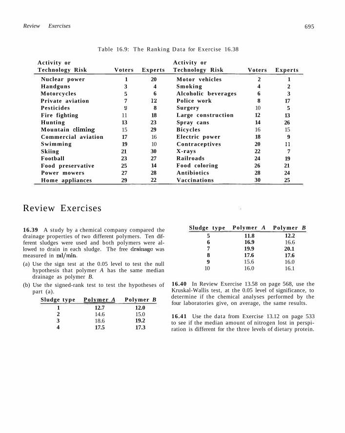
Review Exercises 695
Table 16.9: The Ranking Da ta for Exercise 16.38
Activity or Technology Risk
Nuclear power Handguns Motorcycles Private aviation Pesticides Fire fighting Hunting Mountain climing Commercial aviation Swimming Skiing Football Food preservative Power mowers Home appliances
Voters
1 3 5 7 9
11 13 15 17 19 21 23 25 27 29
Experts
20 4 6
12 8
18 23 29 16 10 30 27 14 28 22
Activity or Technology Risk
Motor vehicles Smoking Alcoholic beverages Police work Surgery Large construction Spray cans Bicycles Electric power Contraceptives X-rays Railroads Food coloring Antibiotics Vaccinations
Voters
2 4 6 8
10 12 14 16 18 20 22 24 26 28 30
Experts
1 2 3
17 5
13 26 15 9
11 7
19 21 24 25
Review Exercises
16.39 A study by a chemical company compared the drainage properties of two different polymers. Ten different sludges were used and both polymers were allowed to drain in each sludge. The free drainage was measured in ml/min.
(a) Use the sign test at the 0.05 level to test the null hypothesis that polymer A has the same median drainage as polymer B.
(b) Use the signed-rank test to test the hypotheses of part (a).
Sludge type Polymer A Polymer B 1 2 3 4
12.7 14.6 18.6 17.5
12.0 15.0 19.2 17.3
Sludge type 5 6 7 8 9
10
Polymer A 11.8 16.9 19.9 17.6 15.6 16.0
Polymer B 12.2 16.6 20.1 17.6 16.0 16.1
16.40 In Review Exercise 13.58 on page 568, use the Kruskal-Wallis test, at the 0.05 level of significance, to determine if the chemical analyses performed by the four laboratories give, on average, the same results.
16.41 Use the data from Exercise 13.12 on page 533 to see if the median amount of nitrogen lost in perspiration is different for the three levels of dietary protein.
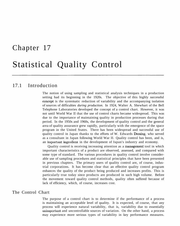
Chapter 17
Statistical Quality Control
17.1 Introduction The notion of using sampling and statistical analysis techniques in a production setting had its beginning in the 1920s. The objective of this highly successful concept is the systematic reduction of variability and the accompanying isolation of sources of difficulties during production. In 1924, Walter A. Shewhart of the Bell Telephone Laboratories developed the concept of a control chart. However, it was not until World War II that the use of control charts became widespread. This was due to the importance of maintaining quality in production processes during that period. In the 1950s and 1960s, the development of quality control and the general area of quality assurance grew rapidly, particularly with the emergence of the space program in the United States. There has been widespread and successful use of quality control in Japan thanks to the efforts of W. Edwards Deming, who served as a consultant in Japan following World War II. Quality control has been, and is, an important ingredient, in the development of Japan's industry and economy.
Quality control is receiving increasing attention as a management tool in which important characteristics of a product are observed, assessed, and compared with some type of standard. The various procedures in quality control involve considerable use of sampling procedures and statistical principles that have been presented in previous chapters. The primary users of quality control are, of course, industrial corporations. It has become clear that an effective quality control program enhances the quality of the product being produced and increases profits. This is particularly true today since products are produced in such high volume. Before the movement toward quality control methods, quality often suffered because of lack of efficiency, which, of course, increases cost.
The Control Chart
The purpose of a control chart is to determine if the performance of a process is maintaining an acceptable level of quality. It is expected, of course, that any process will experience natural variability, that is, variability due to essentially unimportant and uncontrollable sources of variation. On the other hand, a process may experience more serious types of variability in key performance measures.
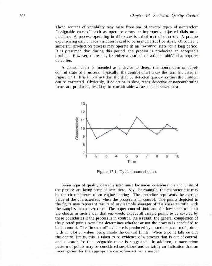
698 Chapter 17 Statistical Quality Control
These sources of variability may arise from one of several types of nonrandom "assignable causes," such as operator errors or improperly adjusted dials on a machine. A process operating in this state is called out of control. A process experiencing only chance variation is said to be in statist ical control. Of course, a successful production process may operate in an in-control state for a long period. It is presumed that during this period, the process is producing an acceptable product. However, there may be either a gradual or sudden "shift" that requires detection.
A control chart is intended as a device to detect the nonrandom or out-of-control state of a process. Typically, the control chart takes the form indicated in Figure 17.1. It is important that the shift be detected quickly so that the problem can be corrected. Obviously, if detection is slow, many defective or nonconforming items are produced, resulting in considerable waste and increased cost.
Figure 17.1: Typical control chart.
Some type of quality characteristic must be under consideration and units of the process are being sampled over time. Say, for example, the characteristic may be the circumference of an engine bearing. The centerline represents the average value of the characteristic when the process is in control. The points depicted in the figure may represent results of, say, sample averages of this characteristic, with the samples taken over time. The upper control limit and the lower control limit are chosen in such a way that one would expect all sample points to be covered by these boundaries if the process is in control. As a result, the general complexion of the plotted points over time determines whether or not the process is concluded to be in control. The "in control" evidence is produced by a random pattern of points, with all plotted values being inside the control limits. When a point falls outside the control limits, this is taken to be evidence of a process that is out of control, and a search for the assignable cause is suggested. In addition, a nonrandom pattern of points may be considered suspicious and certainly an indication that an investigation for the appropriate corrective action is needed.
17.2 Nature of the Control Limits 699
17.2 Nature of the Control Limits
The fundamental ideas on which control charts are based are similar in structure to hypothesis testing. Control limits are established to control the probability of making the error of concluding that the process is out. of control when in fact it is not. This corresponds to the probability of making a type I error if we were testing the null hypothesis that the process is in control. On the other hand, we must be attentive to the error of the second kind, namely, not. finding the process out of control when in fact it is (type II error). Thus the choice of control limits is similar to the choice of a critical region.
As in the case of hypothesis testing, the sample size at each point is important. The consideration of sample size depends to a large extent on the sensitivity or power of detection of the out-of-control state. In this application, the notion of power is very similar to that of the hypothesis-testing situation. Clearly, the larger the sample at each time period, the quicker the detection of an out-of-control process. In a sense, the control limits actually define what the user considers as being in control. In other words, the latitude given by the control limits obviously must depend in some sense on the process variability. As a result, the computation of the control limits will naturally depend on data taken from the process results. Thus any quality control must have its beginning with computation from a preliminary sample or set of samples which will establish both the centerline and the quality control limits.
17.3 Purposes of the Control Chart
One obvious purpose of the: control chart is mere surveillance of the process, that is, to determine if changes need to be made. In addition, the constant systematic gathering of data often allows management to assess process capability. Clearly, if a single performance characteristic is important, continual sampling anel estimation of the mean anel standard deviation of the performance characteristic offer updating of what the process can elo in terms of mean performance and random variation. This is valuable' even if the process stays in control for long periods. The systematic anel formal structure of the control chart can often prevent overreaction to changes that represent only random fluctuations. Obviously, in many situations, changes brought about by overreaction can create serious problems that are difficult to solve.
Quality characteristics of control charts fall generally into two categories, variables and a t t r ibu tes . As a result, types of control charts often take the same classifications. In the case of the variables type of chart, the characteristic is usually a measurement on a continuum, such as diameter, weight, and so on. For the attribute chart, the characteristic reflects whether the individual product conforms (defective or not). Applications for these two distinct situations are obvious.
In the case of the variables chart, control must be exerted on both central tendency and variability. A quality control analyst must be concerned about whether there has been a shift in values of performance characteristic on average. In addition, there will always be a concern about whether some change in process conditions results in a decrease: in precision (i.e., an increase in variability). Separate
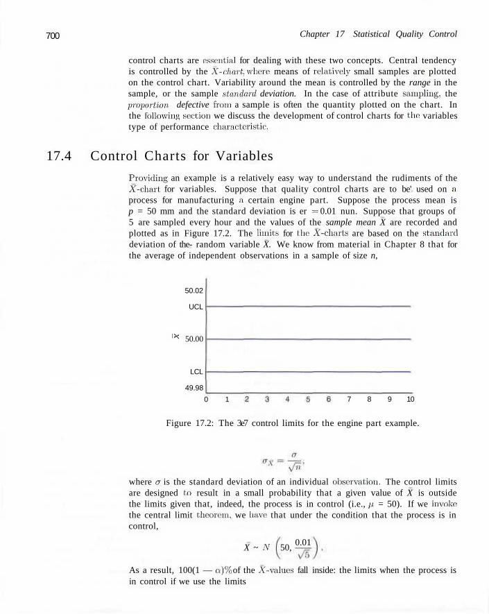
700 Chapter 17 Statistical Quality Control
control charts are essential for dealing with these two concepts. Central tendency is controlled by the X-chart, where means of relatively small samples are plotted on the control chart. Variability around the mean is controlled by the range in the sample, or the sample standard deviation. In the case of attribute sampling, the pro-portion defective from a sample is often the quantity plotted on the chart. In the following se;ction we discuss the development of control charts for the variables type of performance characteristic.
17.4 Control Charts for Variables
Provieling an example is a relatively easy way to understand the rudiments of the X-chart for variables. Suppose that quality control charts are to be' used on a process for manufacturing a certain engine part. Suppose the process mean is p = 50 mm and the standard deviation is er = 0.01 nun. Suppose that groups of 5 are sampled every hour and the values of the sample mean X are recorded and plotted as in Figure 17.2. The limits for the X-charts are based on the standard deviation of the- random variable X. We know from material in Chapter 8 that for the average of independent observations in a sample of size n,
50.02
UCL
' * 50.00
LCL
49.98
0 1 7 8 9 10
Figure 17.2: The 3e7 control limits for the engine part example.
where a is the standard deviation of an individual observation. The control limits are designed lei result in a small probability that a given value of X is outside the limits given that, indeed, the process is in control (i.e., p. = 50). If we invoke the central limit theorem, we have that under the condition that the process is in control,
X ~ Ar 50, 0.01
As a result, 100(1 — a)% of the X-values fall inside: the limits when the process is in control if we use the limits
17.4 Control Charts for Variables 701
LCL = p - za/2-^= = 50 - za/2(0.0045), UCL = p. + za/2-^= = 50 + 2 Q / 2 ( 0 . 0 0 4 5 ) . \/n >/n
Here LCL and UCL stand for lower control limit and upper control limit, respectively. Often the X-charts are based on limits that are referred to as "three-sigma" limits, referring, of course, to za/2 = 3 and limits that become
y/n
In our illustration the upper and lower limits become
LCL = 50 - 3(0.0045) = 49.9865, UCL = 50 + 3(0.0045) = 50.0135.
Thus, if we view the structure of the 3tr limits from the point of view of hypothesis testing, for a given sample point, the probability is 0.0026 that the X-value falls outside control limits, given that the process is in control. This is the probability of the analyst erroneously determining that the process is out of control (see Table A.3).
The example above not only illustrates the X-chart for variables, but also should provide the reader with an insight into the nature of control charts in general. The centerline generally reflects the ideal value of an important parameter. Control limits are established from knowledge of the sampling properties of the statistic that estimates the parameter in question. They very often involve a multiple of the standard deviation of the statistic. It has become general practice to use 3(7 limits. In the case of the X-chart provided here, the central limit theorem provides the user with a good approximation of the probability of falsely ruling that the process is out of control. In general, though, the user may not be able to rely on the normality of the statistic on the centerline. As a result, the exact probability of "type I error" may not be known. Despite this, it has become fairly standard to use the ka limits. While use of the 3<r limits is widespread, at times the user may wish to deviate from this approach. A smaller multiple of a may be appropriate when it is important to quickly detect an out-of-control situation. Because of economic considerations, it may prove costly to allow a process to continue to run out of control for even short periods, while the cost of the search and correction of assignable causes may be relatively small. Clearly, in this case, control limits that are tighter than 3o limits are appropriate.
Rational Subgroups
The sample values to be used in a quality control effort are divided into subgroups with a sample representing a subgroup. As we indicated earlier, time order of production is certainly a natural basis for selection of the subgroups. We may view the quality control effort very simply as (1) sampling, (2) detection of an out-of-control state, and (3) a search for assignable causes that may be occurring over time. The selection of the basis for these sample groups would appear to be straightforward. The choice of these subgroups of sampling information can have an important effect on the success of the quality control program. These subgroups
702 Chapter 17 Statistical Quality Control
are often called rational subgroups. Generally, if the analyst is interested in detecting a shift in location, it is felt that the subgroups should be chosen so that within-subgroup variability is small and that assignable causes, if they are present, can have the greatest chance of being detected. Thus we want to choose the subgroups in such a way as to maximize the between-subgroup variability. Choosing units in a subgroup that are produced close together in time, for example, is a reasonable approach. On the other hand, control charts are often used to control variability, in which case the performance statistic is variability within the sample. Thus it is more important to choose the rational subgroups to maximize the within-sample variability. In this case, the observations in the subgroups should behave more like a random sample and this variability within samples needs to be a depiction of the variability of the process.
It is important to note that control charts on variability should be established before the development of charts on center of location (say, X-charts). Any control chart on center of location will certainly depend on variability. For example, we have seen an illustration of the central tendency chart and it depends on a. In the sections that follow, an estimate of a from the data will be discussed.
X-Chart with Estimated Parameters
In the foregoing we have illustrated notions of the X-chart. that make use of the central limit theorem and employ known values of the process mean and standard deviation. As we indicated earlier, the control limits
LCL = p-za/2-=:, UCL = p + za/2 —= \jn \Jn
are used and an X-value falling outside these limits is viewed as evidence that the mean p has changed and thus the process may be out of control.
In many practical situations, it is unreasonable to assume that we know p and ex. As a result, estimates must be supplied from data taken when the process is in control. Typically, the estimates are determined during a period in which background information or start-up information is gathered. A basis for rational subgroups is chosen and data are gathered with samples of size n in each subgroup. The sample sizes are usually small, say, 4, 5, or 6, and k samples are taken, with k being at least 20. During this period in which it is assumed that the process is in control, the user establishes estimates of p and a, on which the control chart is based. The important information gathered during this period includes the sample means in the subgroup, the overall mean, and the sample range in each subgroup. In the following paragraphs we outline how this information is used to develop the control chart.
A portion of the sample information from these A: samples takes the form X j , X 2 , . . . , Xfc, where the random variable X{ is the average of the values in the zth sample. Obviously, the overall average is the random variable
This is the appropriate estimator of the process mean and, as a result, is the centerline in the X control chart. In quality control applications it is often convenient
17.4 Control Charts for Variables 703
to estimate a from the information related to the ranges in the samples rather than sample standard deviations. Let us define for the ith sample
H-i — ^ m n x , ! -™.| mm,?
as the range for the data in the ith sample. Here XmaX!, and Xm\a,i are the largest and smallest observation, respectively, in the sample. The appropriate estimate of er is a function of the average range
R=\±lk. h «=i
An estimate of o, say er, is obtained by
R d2
where d2 is a constant depending on the sample size. Values of d2 are shown in Table A.23.
Use of the range in producing an estimate of o has roots in quality-control-type applications, particularly since the range was so easy to compute in the era prior to the period in which time of computation is considered no difficulty. The assumption of normality of the individual observations is implicit in the X-chart. Of course, the existence of the central limit theorem is certainly helpful in this regard. Under the assumption of normality, we make use of a random variable called the relative range, given by
W=*. a
It turns out that the moments of W are simple functions of the sample size n (see the reference to Montgomery, 2000, in the Bibliography). The expected value of W is often referred to as d2. Thus by taking the expected value of W above,
a
As a result, the rationale for the estimate a = R/d2 is readily understood. It is well known that the range method produces an efficient estimator of a in relatively small samples. This makes the estimator particularly attractive in quality control applications since the sample sizes in the subgroups are generally small. Using the range method for estimation of a results in control charts with the following parameters:
UCL = X + - ^ = . centerline = X, LCL = X - 3
d2y/n.'' d2\/n
Defining the quantity
A2 = -r—=, d2y/n
704 Chapter 17 Statistical Quality Control
we have that
UCL = X + A2R, LCL = X - A2R.
To simplify the structure, the user of X-charts often finds values of A2 tabulated. Tabulations of values of A2 are given for various sample sizes in Table A.23.
fl-Charts to Control Variation
Up to this point all illustrations and details have dealt with the quality control analysts' attempt at detection of out-of-control conditions produced by a shift in the mean. The control limits are based on the distribution of the random variable X and depend on the assumption of normality on the individual observations. It is important for control to be applied to variability as well as center of location. In fact, many experts feel as if control of variability of the performance characteristic is more important and should be established before center of location should be considered. Process variability can be controlled through the use of plots of the sample range. A plot over time of the sample ranges is called an il-chart. The same general structure can be used as in the case of the X-chart, with R being the centerline and the control limits depending on an estimate of the standard deviation of the random variable R. Thus, as in the case of the X-chart, 3a- limits are established where "3cr" implies 3a R. The quantity an must be estimated from the data just as ox is estimated.
The estimate of on., the standard deviation, is also based on the distribution of the relative range
w.Z. a
The standard deviation of W is a known function of the sample size and is generally denoted by d3. As a result,
OR =crd3.
We can now replace a by a = R/d2, and thus the estimator of OR is
Rd3
Thus the quantities that define the i?-chart are
UCL = RD4, centerline = R, LCL = RD3,
where the constants D4 and D3 (depending only on n) are
D4 = l + 3 ^ , £>3 = l - 3 ^ . d2 d2
The constants D4 and D3 are tabulated in Table A.23.
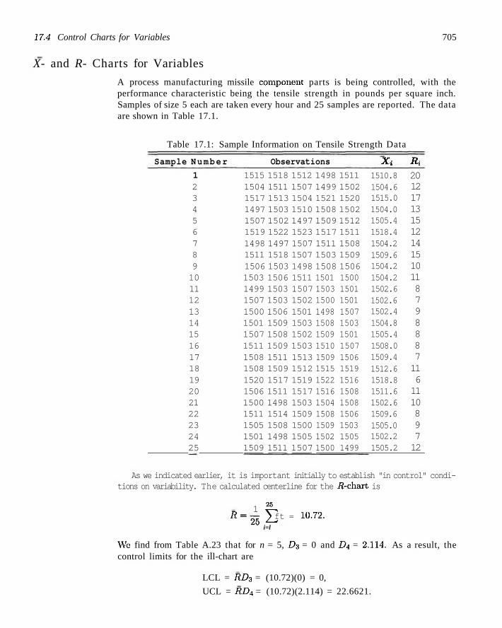
17.4 Control Charts for Variables 705
X- and R- Charts for Variables
A process manufacturing missile component parts is being controlled, with the performance characteristic being the tensile strength in pounds per square inch. Samples of size 5 each are taken every hour and 25 samples are reported. The data are shown in Table 17.1.
Table 17.1: Sample Information on Tensile Strength Data
Sample Number Observations Xi Ri
1 1515 1518 1512 1498 1511 2 1504 1511 1507 1499 1502 3 1517 1513 1504 1521 1520 4 1497 1503 1510 1508 1502 5 1507 1502 1497 1509 1512 6 1519 1522 1523 1517 1511 7 1498 1497 1507 1511 1508 8 1511 1518 1507 1503 1509 9 1506 1503 1498 1508 1506 10 1503 1506 1511 1501 1500 11 1499 1503 1507 1503 1501 12 1507 1503 1502 1500 1501 13 1500 1506 1501 1498 1507 14 1501 1509 1503 1508 1503 15 1507 1508 1502 1509 1501 16 1511 1509 1503 1510 1507 17 1508 1511 1513 1509 1506 18 1508 1509 1512 1515 1519 19 1520 1517 1519 1522 1516 20 1506 1511 1517 1516 1508 21 1500 1498 1503 1504 1508 22 1511 1514 1509 1508 1506 23 1505 1508 1500 1509 1503 24 1501 1498 1505 1502 1505 25 1509 1511 1507 1500 1499
As we indicated earlier, it is important initially to establish "in control" conditions on variability. The calculated centerline for the i?-chart is
1 25
* = 25 £ ft = 10-72. i=l
Wc find from Table A.23 that for n = 5, D3 = 0 and D4 = 2.114. As a result, the control limits for the ill-chart are
LCL = RD3 = (10.72)(0) = 0,
UCL = RD4 = (10.72)(2.114) = 22.6621.
1510.8 1504.6 1515.0 1504.0 1505.4 1518.4 1504.2 1509.6 1504.2 1504.2 1502.6 1502.6 1502.4 1504.8 1505.4 1508.0 1509.4 1512.6 1518.8 1511.6 1502.6 1509.6 1505.0 1502.2 1505.2
20 12 17 13 15 12 14 15 10 11 8 7 9 8 8 8 7 11 6 11 10 8 9 7 12
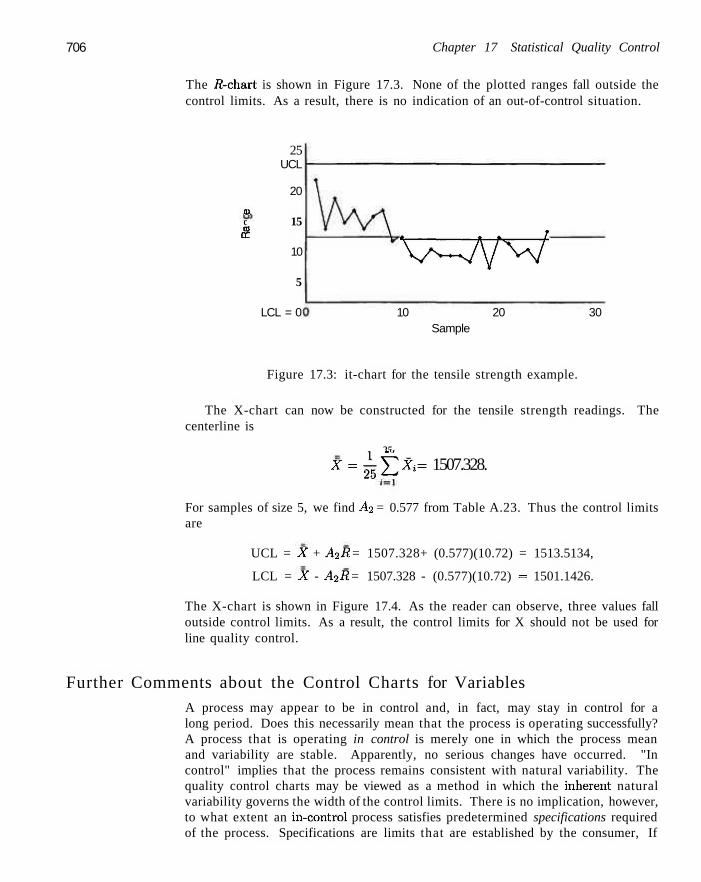
706 Chapter 17 Statistical Quality Control
The iZ-chart is shown in Figure 17.3. None of the plotted ranges fall outside the control limits. As a result, there is no indication of an out-of-control situation.
eu c to tr
25 UCL
20
15
10
5
LCL = 0
V^A/W 10 20
Sample 30
Figure 17.3: it-chart for the tensile strength example.
The X-chart can now be constructed for the tensile strength readings. The centerline is
25
X = ^ J T X = 1507.328.
For samples of size 5, we find A2 = 0.577 from Table A.23. Thus the control limits are
UCL = X + A2R = 1507.328+ (0.577)(10.72) = 1513.5134,
LCL = X - A2R = 1507.328 - (0.577)(10.72) = 1501.1426.
The X-chart is shown in Figure 17.4. As the reader can observe, three values fall outside control limits. As a result, the control limits for X should not be used for line quality control.
Further Comments about the Control Charts for Variables A process may appear to be in control and, in fact, may stay in control for a long period. Does this necessarily mean that the process is operating successfully? A process that is operating in control is merely one in which the process mean and variability are stable. Apparently, no serious changes have occurred. "In control" implies that the process remains consistent with natural variability. The quality control charts may be viewed as a method in which the inherent natural variability governs the width of the control limits. There is no implication, however, to what extent an in-control process satisfies predetermined specifications required of the process. Specifications are limits that are established by the consumer, If
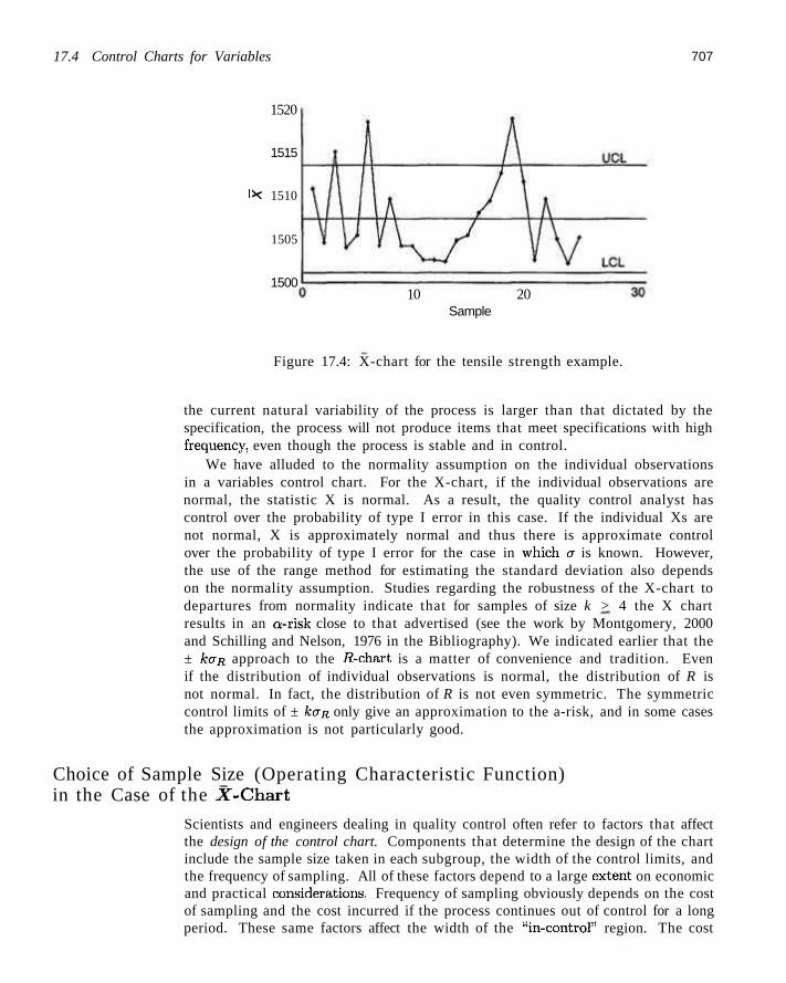
17.4 Control Charts for Variables 707
1520
1515
I* 1510
1505
1500 10 20
Sample
Figure 17.4: X-chart for the tensile strength example.
the current natural variability of the process is larger than that dictated by the specification, the process will not produce items that meet specifications with high frequency, even though the process is stable and in control.
We have alluded to the normality assumption on the individual observations in a variables control chart. For the X-chart, if the individual observations are normal, the statistic X is normal. As a result, the quality control analyst has control over the probability of type I error in this case. If the individual Xs are not normal, X is approximately normal and thus there is approximate control over the probability of type I error for the case in wdiich a is known. However, the use of the range method for estimating the standard deviation also depends on the normality assumption. Studies regarding the robustness of the X-chart to departures from normality indicate that for samples of size k > 4 the X chart results in an a-risk close to that advertised (see the work by Montgomery, 2000 and Schilling and Nelson, 1976 in the Bibliography). We indicated earlier that the ± kaR approach to the i?-chart is a matter of convenience and tradition. Even if the distribution of individual observations is normal, the distribution of R is not normal. In fact, the distribution of R is not even symmetric. The symmetric control limits of ± koR only give an approximation to the a-risk, and in some cases the approximation is not particularly good.
Choice of Sample Size (Operating Characteristic Function) in the Case of the X-Chart
Scientists and engineers dealing in quality control often refer to factors that affect the design of the control chart. Components that determine the design of the chart include the sample size taken in each subgroup, the width of the control limits, and the frequency of sampling. All of these factors depend to a large extent on economic and practical considerations. Frequency of sampling obviously depends on the cost of sampling and the cost incurred if the process continues out of control for a long period. These same factors affect the width of the "in-control" region. The cost
708 Chapter 17 Statistical Quality Control
that is associated with investigation and search for assignable causes has an impact on the width of the region and on frequency of sampling. A considerable amount of attention has been devoted to optimal design of control charts and extensive details will not be given here. The reader should refer to the work by Montgomery (2000) cited in the Bibliography for an excellent historical account of much of this research.
Choice of sample size and frequency of sampling involve balancing available resources to these two efforts. In many cases, the analyst may need to make changes in the strategy until the proper balance is achieved. The analyst should always be aware that if the cost of producing nonconforming items is great, a high sampling frequency with relatively small sample size is a proper strategy.
Many factors must be taken into consideration in the choice of a sample size. In the illustration and discussion we have emphasized the use of n = 4. 5, or 6. These values are considered relatively small for general problems in statistical inference but perhaps proper sample sizes for quality control. One justification, of course, is that the quality control is a continuing process and the results produced by one sample or set of units will be followed by results from many more. Thus the "effective" sample size of the entire quality control effort is many times larger than that used in a subgroup. It is generally considered to be more effective to sample frequently with a small sample size,
The analyst can make use of the notion of the power of a test to gain some insight into the effectiveness of the sample size chosen. This is particularly important since small sample sizes are usually used in each subgroup, Refer to Chapters 10 and 13 for a discussion of the power of formal tests on means and the analysis of variance. Although formal tests of hypotheses are not actually being conducted in quality control, one can treat the sampling information as if the strategy at each subgroup is to test a hypothesis, either on the population mean p or the standard deviation a. Of interest is the probability of detection of an out-of-control condition for a given sample, and perhaps more important, the expected number of runs required for detection. The probability of detection of a specified out-of-control condition corresponds to the power of a test. It is not our intention to show development of the power for all of the types of control charts presented here, but rather, to show the development for the X-chart and present power results for the i?-chart.
Consider the X-chart for a known. Suppose that the in-control state has p = Po- A study of the role of the subgroup sample size is tantamount to investigating the /3-risk, that is, the probability that an X-value remains inside the control limits, given that, indeed, a shift in the mean has occurred. Suppose that the form the shift takes is
p = po + ra.
Again, making use of the normality of X, we have
3 = P{LCL < X < UCL \p = po + ra}.
For the case of ka limits,
LCL = /io = , and UCL = po H—•=. s/n V n
17.4 Control Charts for Variables 709
As a result, if we denote by Z the standard normal random variable.
a = p\z<
-A pq + ka/y/n-p
Z <
o/^fn
Po + ka/sfn— (p + ra)
afy/n
= P(Z <k- rs/n~) - P(Z < -k - r\/h~).
H po - kajy/n - p
Z <
a/s/n
po -ko/sfn- (p + ra) o/s/n
Notice the role of n, r, and k in the expression for the /3-risk. The probability of not detecting a specific shift clearly increases with an increase in k, as expected. 3 decreases with an increase in r, the magnitude of the shift, and decreases with an increase in the sample size n.
It should be emphasized that the expression above results in the /3-risk (probability of type II error) for the case of a single sample. For example, suppose that in the case of a sample of size 4, a shift of a occurs in the mean. The probability of detecting the shift (power) in the first sample following the shift is (assume 3er limits)
1 - 5 = 1 - \P(Z < 1) - P(Z < -5)] = 0.1587.
On the other hand, the probability of detecting a shift of 2er is
1 - / 3 = 1 — [P(Z < - 1 ) - P(Z < -7)] = 0.8413.
The results above illustrate a fairly modest probability of detecting a shift of magnitude a and a fairly high probability of detecting a shift of magnitude 2a. The complete picture of how, say, 3<r control limits perform for the X-chart described here is depicted in Figure 17.5. Rather than plot power, a plot is given of 8 against r, where the shift in the mean is of magnitude rcr. Of course, the sample sizes of n = 4,5,6 result in a small probability of detecting a shift of l.Ocr or even 1.5<r on the first sample after the shift-
But if sampling is done frequently, the probability may not be as important as the average or expected number of runs required before detection of the shift. Quick detection is important and is certainly possible even though the probability of detection on the first sample is not high. It turns out that X-charts with these small samples will result in relatively rapid detection. If 3 is the probability of not detecting a shift on the first sample following the shift, then the probability of detecting the shift on the sth sample after the shift is (assuming independent samples)
Ps = (l-S)l3*-\
The reader should recognize this as an application of the geometric distribution. The average or expected value of the number of samples required for detection is
.1=1
710 Chapter 17 Statistical Quality Control
Figure 17.5: Operating characteristic curves for the X-chart with 3u limits. Here 3 is the type II probability error on the first sample after a shift in the mean of ra.
Thus the expected number of samples required to detect the shift in the mean is the reciprocal of the power (i.e., the probability of detection on the first sample following the shift).
Example 17.1:1 In a certain quality c:ontrol effort it is important for the quality control analyst to quickly detect shifts in the mean of ± a while using a 3(7 control chart with a sample size: n = 4. The expected number of samples that are required following the shift for the detection of the out-of-control state can be an aid in the assessment of the quality control procedure.
From Figure 17.5, for n = 4 and r = 1, it can be seen that 8 ~ 0.84. If wc allow 8 to denote: the number of samples required to detect, the shift, the mean of s is
E(s) = -1 1
dTfi = 6.25.
Thus, on the average, seven subgroups are required before detection of a shift of ± a. J
Choice of Sample Size for the i?-Chart
The OC curve for the it-chart is shown in Figure 17.6. Since the R-chart is used for control of the process standard deviation, the /3-risk is plotted as a function of
17.4 Control Charts for Variables 711
the in-control standard deviation, cry. and the standard deviation after the process goes out of control. The latter standard deviation will be denoted ax. Let
A-2 . . oa
For various sample sizes, 3 is plotter! against A.
oa
Figure 17.6: Operating characteristic curve for the jR-charts with 3c limits.
X- a n d S - C h a r t s for V a r i a b l e s
It is natural for the student, of statistics to anticipate use of the sample variance in the X-chart and in a chart to control variability. The range is efficient as an estimator for a, but this efficiency decreases as the sample size gets larger. For n as large as 10, the familiar statistic
JirhB*-*'2
should be used in the control chart for both the mean anel variability. The reader should recall from Chapter 9 that S2 is an unbiased estimator for o2 but. that 5 is not unbiased for n. It has become customary to correct S for bias in control chart, applications. Wc know, in general, that
E(S) f- a.
In the case in which the X, are independent, normally distributed with mean p and variance er2,
\ 1 / 2
E(S) = c4a, where c4 n - 1
T(n/2)
r[(n - l)/2
712 Chapter 17 Statistical Quality Control
and T(-) refers to the gamma function (see Chapter 6). For example, for n = 50, c4 = 3/8\/27r. In addition, the variance of the estimator S is
Var(S) = o-2(l-c2).
We have established the properties of S that will allow us to write control limits for both X and S. To build a proper structure, we begin by assuming that a is known. Later we discuss estimating a from a preliminary set of samples.
If the statistic S is plotted, the obvious control chart parameters are
UCL = c4a + 3a JI — c2, centerline = c4cr, LCL = c4o~ — 3o J1 — c2.
As usual, the control limits are defined more succinctly through use of tabulated constants. Let
B-, = c4 - 3 ^ 1 - e2, Bo = c4 + 3^/l-c2,
and thus we have
UCL = BQO, centerline = c4a, LCL = B$o.
The values of B& and Bo for variems sample sizes are tabulated in Table A.23. Now, of course, the control limits above serve as a basis for the development of
the quality control parameters for the situation that is most often seen in practice, namely, that in which a is unknown. We must once again assume that a set of base samples or preliminary samples is taken to produce an estimate of er during what is assumed to be an "in-control" period. Sample standard deviations Si, S2,..., Sm
are obtained from samples that are each of size n. An unbiased estimator of the type
is often used for a. Here, of course, S, the average value of the sample standard deviation in the preliminary sample, is the logical centerline in the control chart to control variability. The upper and lower control limits are unbiased estimators of the control limits that arc appropriate for the case where a is known. Since
c4J
the statistic S is an appropriate centerline (as an unbiased estimator of c4a) and the quantities
S-3—Jl-c2 and S + 3— c4 V c.|
are the appropriate lower and upper 3<r control limits, respectively. As a result, the centerline and limits for the 5-chart to control variability arc
LCL = B3S, centerline = S, UCL = B4S,
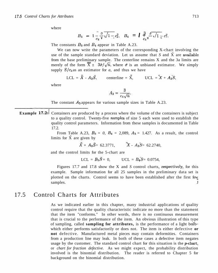
17.5 Control Charts for Attributes 713
where
B3 = \--Jl-c2, B4 = l + -Jl-c2. c4 V c4 V
The constants B3 and B4 appear in Table A.23. We can now write the parameters of the corresponding X-chart involving the
use of the sample standard deviation. Let us assume that S and X are available from the base preliminary sample. The centerline remains X and the 3a limits are merely of the form X ± 3&/\/v., where a is an unbiased estimator. We simply supply S/c4 as an estimator for a, and thus we have
LCL = X - A3S. centerline = X, UCL = X + A3S,
where
civ/n
The constant A3 appears for various sample sizes in Table A.23.
Example 17.2:1 Containers are produced by a process where the volume of the containers is subject to a quality control. Twenty-five samples of size 5 each were used to establish the quality control parameters. Information from these samples is documented in Table 17.2.
From Table A.23, B3 = 0, B4 = 2,089, A3 = 1.427. As a result, the control limits for X are given by
X + A3S = 62.3771, X - A3S = 62.2740,
and the control limits for the 5-chart are
LCL = B3S = 0, UCL = B4S = 0.0754,
Figures 17.7 and 17.8 show the X and S control charts, respectively, for this example. Sample information for all 25 samples in the preliminary data set is plotted on the charts. Control seems to have been established after the first few samples. J
17.5 Control Charts for Attributes
As we indicated earlier in this chapter, many industrial applications of quality control require that the quality characteristic indicate no more than the statement that the item "conforms." In other words, there is no continuous measurement that is crucial to the performance of the item. An obvious illustration of this type of sampling, called sampling for attributes, is the performance of a light bulb-which either performs satisfactorily or does not. The item is either defective or not defective. Manufactured metal pieces may contain deformities. Containers from a production line may leak. In both of these cases a defective item negates usage by the customer. The standard control chart for this situation is the p-chart, or chart for fraction defective. As we might expect, the probability distribution involved is the binomial distribution. The reader is referred to Chapter 5 for background on the binomial distribution.
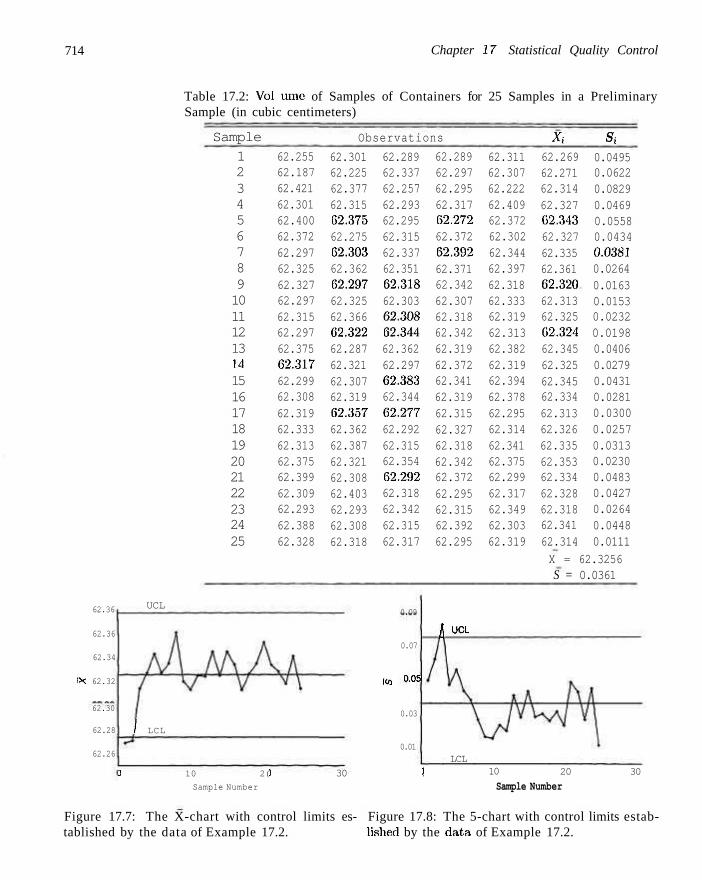
714 Chapter 17 Statistical Quality Control
Table 17.2: Vol tune of Samples of Containers for 25 Samples in a Preliminary Sample (in cubic centimeters)
62.36
62.36
62.34
IX 62.32
62.30
62.28
62.26
Sample
1 2 3 4 5 6 7 8 9 10 11 12 13 14 15 16 17 18 19 20 21 22 23 24 25
UCL
/ LCL
0 10 2(
Sample Number
62.255 62.187 62.421 62.301 62.400 62.372 62.297 62.325 62.327 62.297 62.315 62.297 62.375 62.317 62.299 62.308 62.319 62.333 62.313 62.375 62.399 62.309 62.293 62.388 62.328
i
Observations
62.301 62.225 62.377 62.315 62.375 62.275 62.303 62.362 62.297 62.325 62.366 62.322 62.287 62.321 62.307 62.319 62.357 62.362 62.387 62.321 62.308 62.403 62.293 62.308 62.318
30
62.289 62.337 62.257 62.293 62.295 62.315 62.337 62.351 62.318 62.303 62.308 62.344 62.362 62.297 62.383 62.344 62.277 62.292 62.315 62.354 62.292 62.318 62.342 62.315 62.317
0.09
0.07
ICO 0 0 5
0.03
0.01
(
62.289 62.297 62.295 62.317 62.272 62.372 62.392 62.371 62.342 62.307 62.318 62.342 62.319 62.372 62.341 62.319 62.315 62.327 62.318 62.342 62.372 62.295 62.315 62.392 62.295
h UCL
LCL 1
62.311 62.307 62.222 62.409 62.372 62.302 62.344 62.397 62.318 62.333 62.319 62.313 62.382 62.319 62.394 62.378 62.295 62.314 62.341 62.375 62.299 62.317 62.349 62.303 62.319
10
Xt 62.269 62.271 62.314 62.327 02.343 62.327 62.335 62.361 62.320 62.313 62.325 02.324 62.345 62.325 62.345 62.334 62.313 62.326 62.335 62.353 62.334 62.328 62.318 62.341 62.314
Si
0.0495 0.0622 0.0829 0.0469 0.0558 0.0434 0.0381 0.0264 0.0163 0.0153 0.0232 0.0198 0.0406 0.0279 0.0431 0.0281 0.0300 0.0257 0.0313 0.0230 0.0483 0.0427 0.0264 0.0448 0.0111
X = 62.3256 S = 0.0361
20
Sample Number 30
Figure 17.7: The X-chart with control limits es- Figure 17.8: The 5-chart with control limits estab-tablished by the data of Example 17.2. lished by the data, of Example 17.2.
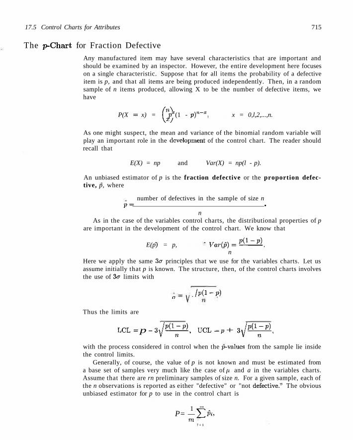
17.5 Control Charts for Attributes 715
The p-Chart for Fraction Defective
Any manufactured item may have several characteristics that are important and should be examined by an inspector. However, the entire development here focuses on a single characteristic. Suppose that for all items the probability of a defective item is p, and that all items are being produced independently. Then, in a random sample of n items produced, allowing X to be the number of defective items, we have
P(X = x) = Q px (1 - p)n-x, x = 0,l,2,...,n.
As one might suspect, the mean and variance of the binomial random variable will play an important role in the development of the control chart. The reader should recall that
E(X) = np and Var(X) = np(l - p).
An unbiased estimator of p is the fraction defective or the proportion defective, p, where
number of defectives in the sample of size n P = •
n As in the case of the variables control charts, the distributional properties of p
are important in the development of the control chart. We know that
E(p) = p, Var(p)='^—^. n
Here we apply the same 3er principles that we use for the variables charts. Let us assume initially that p is known. The structure, then, of the control charts involves the use of 3cr limits with
^ Jp(l-p)
Thus the limits are
LCL = p - 3 y ^ 4 UCL = P + 3t/^=4
with the process considered in control when the p-values from the sample lie inside the control limits.
Generally, of course, the value of p is not known and must be estimated from a base set of samples very much like the case of p and a in the variables charts. Assume that there are rn preliminary samples of size n. For a given sample, each of the n observations is reported as either "defective" or "not defective." The obvious unbiased estimator for p to use in the control chart is
1 '" P= — >JPt,
m 7 = 1
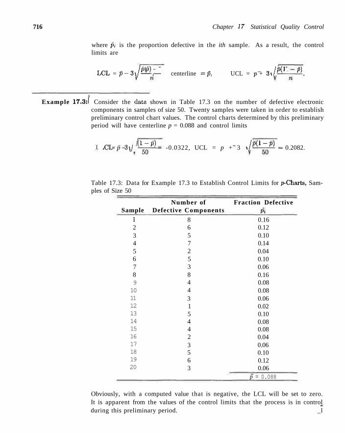
716 Chapter 17 Statistical Quality Control
where p, is the proportion defective in the ith sample. As a result, the control limits are
LCL = p-3\P^ p\ centerline =p, UCL = p + 3 i ' ^ ! p]
Example 17.3:1 Consider the data shown in Table 17.3 on the number of defective electronic components in samples of size 50. Twenty samples were taken in order to establish preliminary control chart values. The control charts determined by this preliminary period will have centerline p = 0.088 and control limits
I .CI. p :*V ( 15 0 ^ = -0.0322, UCL = p + 3 J 2 i L _ £ l = 0.2082.
Table 17.3: Data for Example 17.3 to Establish Control Limits for p-Charts, Samples of Size 50
Number of Fraction Defective Sample Defective Components pi
I 2 3 4 5 6 7 8 9 10 11 12 13 14 15 16 17 18 19 20
8 6 5 7 2 5 3 8 4 4 3 1 5 4 4 2 3 5 6 3
0.16 0.12 0.10 0.14 0.04 0.10 0.06 0.16 0.08 0.08 0.06 0.02 0.10 0.08 0.08 0.04 0.06 0.10 0.12 0.06
p = 0.088
Obviously, with a computed value that is negative, the LCL will be set to zero. It is apparent from the values of the control limits that the process is in control during this preliminary period. _l
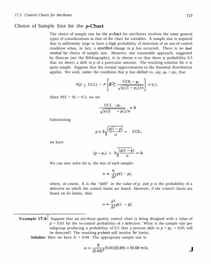
17.5 Control Charts for Attributes 717
Choice of Sample Size for the p-Chart
The choice of sample size for the p-chart for attributes involves the same general types of considerations as that of the chart for variables. A sample size is required that is sufficiently large to have a high probability of detection of an out-of-control condition when, in fact, a specified change in p has occurred. There is no best, method for choice of sample size. However, one reasonable approach, suggested by Duncan (sec the Bibliography), is to choose n so that there is probability 0.5 that we detect a shift in p of a particular amount. The resulting solution for n is quite simple. Suppose that the normal approximation to the binomial distribution applies. We wish, under the condition that p has shifted to, say, p t > po, that
P(p > UCL) = P
Since P(Z > 0) = 0.5, we set
z> UCL-pi
v / P i ( i - P i ) / r a 0.5.
UCL - Pi =Q
VVJi(l -pi)/n
Substituting
we have
P+JPJLZA = VCL,
(P-PO + S / ^ - O .
We can now solve for n, the size of each sample:
9 , » = £ a P ( 1 - P ) .
where, of course, A is the "shift" in the value of p, and p is the probability of a defective on which the control limits arc based. However, if the control charts are based on ko limits, then
u=-£2pil ~P)-
Example 17.4:1 Suppose that an attribute quality control chart is being designed with a value of p = 0.01 for the in-control probability of a defective. What is the sample size per subgroup producing a probability of 0.5 that a process shift to p = pi = 0.05 will be detected? The resulting p-chart will involve 3er limits.
Solution: Here we have A = 0.04. The appropriate sample size is
5(0.01)(0.99) = 55.68 « 56. I (0.04)
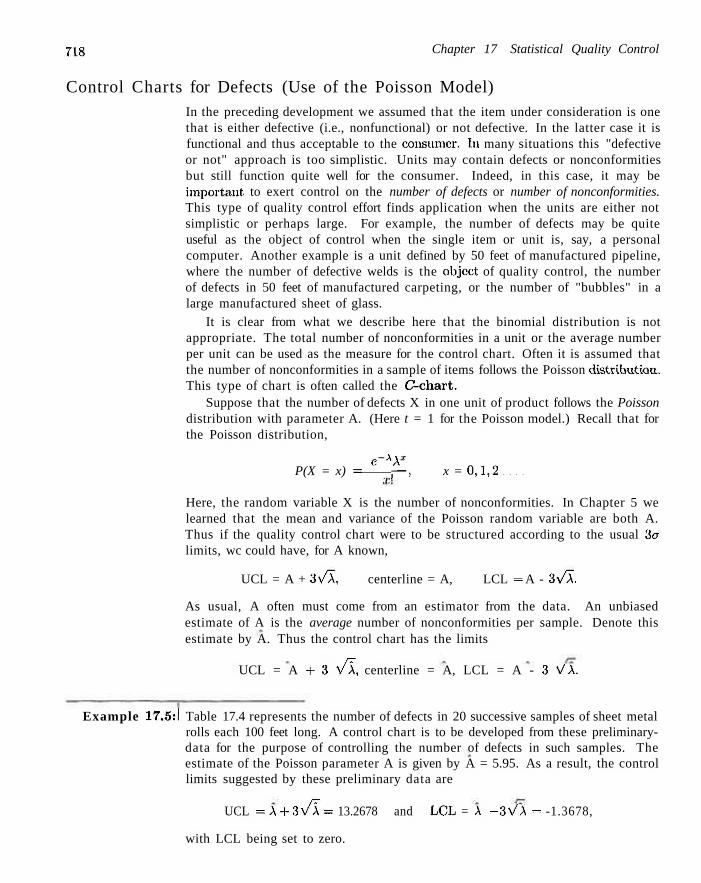
718 Chapter 17 Statistical Quality Control
Control Charts for Defects (Use of the Poisson Model) In the preceding development we assumed that the item under consideration is one that is either defective (i.e., nonfunctional) or not defective. In the latter case it is functional and thus acceptable to the consumer. In many situations this "defective or not" approach is too simplistic. Units may contain defects or nonconformities but still function quite well for the consumer. Indeed, in this case, it may be important, to exert control on the number of defects or number of nonconformities. This type of quality control effort finds application when the units are either not simplistic or perhaps large. For example, the number of defects may be quite useful as the object of control when the single item or unit is, say, a personal computer. Another example is a unit defined by 50 feet of manufactured pipeline, where the number of defective welds is the object of quality control, the number of defects in 50 feet of manufactured carpeting, or the number of "bubbles" in a large manufactured sheet of glass.
It is clear from what we describe here that the binomial distribution is not appropriate. The total number of nonconformities in a unit or the average number per unit can be used as the measure for the control chart. Often it is assumed that the number of nonconformities in a sample of items follows the Poisson distributioa. This type of chart is often called the C-chart.
Suppose that the number of defects X in one unit of product follows the Poisson distribution with parameter A. (Here t = 1 for the Poisson model.) Recall that for the Poisson distribution,
e-AA* P(X = x) = p - , x = 0,1,2
Here, the random variable X is the number of nonconformities. In Chapter 5 we learned that the mean and variance of the Poisson random variable are both A. Thus if the quality control chart were to be structured according to the usual 3u limits, wc could have, for A known,
UCL = A + 3\/A, centerline = A, LCL = A - 3\/A.
As usual, A often must come from an estimator from the data. An unbiased estimate of A is the average number of nonconformities per sample. Denote this estimate by A. Thus the control chart has the limits
UCL = A + 3 V l , centerline = A, LCL = A - 3 VX.
Example 17.5:1 Table 17.4 represents the number of defects in 20 successive samples of sheet metal rolls each 100 feet long. A control chart is to be developed from these preliminary-data for the purpose of controlling the number of defects in such samples. The estimate of the Poisson parameter A is given by A = 5.95. As a result, the control limits suggested by these preliminary data are
UCL = A + 3 \ / A ~ = 13.2678 and LCL = A - 3VA = -1.3678,
with LCL being set to zero.
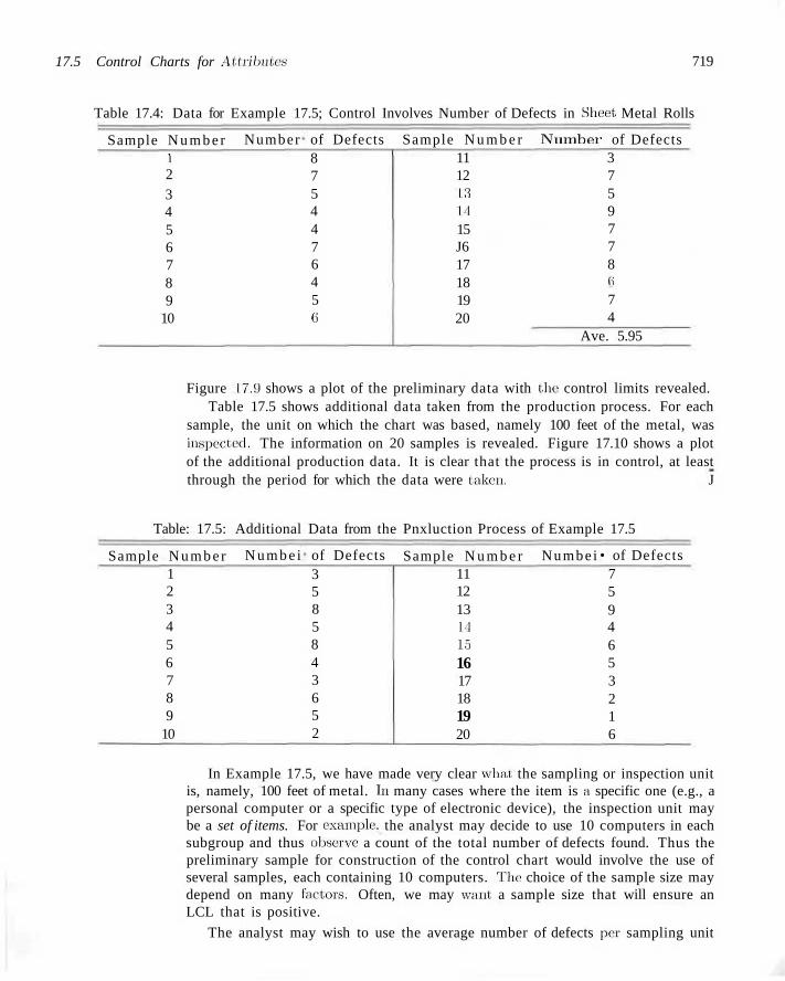
17.5 Control Charts for Attributes 719
Table 17.4: Data for Example 17.5; Control Involves Number of Defects in Sheet Metal Rolls
Sample N u m b e r 1 2 3 4 5 6 7 8 9
10
Number of Defects 8 7 5 4 4 7 6 4 5 6
Sample N u m b e r 11 12 13 14 15 J6 17 18 19 20
Numbei • of Defects 3 7 5 9 7 7 8 1!
7 4
Ave. 5.95
Figure 17.9 shows a plot of the preliminary data with the control limits revealed. Table 17.5 shows additional data taken from the production process. For each
sample, the unit on which the chart was based, namely 100 feet of the metal, was inspected. The information on 20 samples is revealed. Figure 17.10 shows a plot of the additional production data. It is clear that the process is in control, at least through the period for which the data were taken. J
Table: 17.5: Additional Data from the Pnxluction Process of Example 17.5
Sample N u m b e r 1 2 3 4 5 6 7 8 9
10
N u m b e i of Defects 3 5 8 5 8 4 3 6 5 2
Sample N u m b e r 11 12 13 14 15 16 17 18 19 20
Numbe i • of Defects 7 5 9 4 6 5 3 2 1 6
In Example 17.5, we have made very clear what the sampling or inspection unit is, namely, 100 feet of metal. In many cases where the item is a specific one (e.g., a personal computer or a specific type of electronic device), the inspection unit may be a set of items. For example, the analyst may decide to use 10 computers in each subgroup and thus observe a count of the total number of defects found. Thus the preliminary sample for construction of the control chart would involve the use of several samples, each containing 10 computers. The choice of the sample size may depend on many factors. Often, we may want a sample size that will ensure an LCL that is positive.
The analyst may wish to use the average number of defects per sampling unit
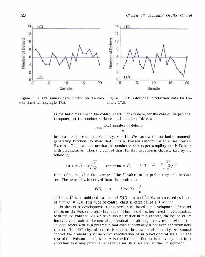
720 Chapter 17 Statistical Quality Control
Figure 17.9: Preliminary data plotted on the con- Figure 17.10: Additional production data for Ex-trol chart, for Example 17.5. ample 17.5.
as the basic measure in the control chart. For example, for the case of the personal computer, let the random variable total number of defects
U total number ile:fects
be measured for each sample of, say, n = 10. We can use the method of moment-generating functions to show that U is a, Poisson random variable (see Review Exercise 17.1) if we assume that the number t>f defects per sampling unit is Poisson with parameter A. Thus the control chart for this situation is characterized by the following:
<U UCL = U + 3\J —, centerline = U, LCL = U-3\!-.
Here, of course, U is the average of the [/-values in the preliminary or base data set. The term U/n is derived from the result that
E(U) = A. Vu.r(U) = -, n
and thus U is an unbiased estimate of E(U) = A and U/n is an unbiased estimate of Vo.r(U) = X/n. This type of control chart is often called a [/-chart.
In the entire development in this se:ction we based our development of control charts on the Poisson probability model. This model has been used in combination with the 3er concept. As we have implied earlier in this chapter, the notion of 3er limits has its roots in the normal approximation, although many users feel that the concept works well as a pragmatic tool even if normality is not even approximately correct. The difficulty, of course, is that in the absence of normality, we cannot control the probability of incorrect specification of an out-of-control state. In the case of the Poisson model, when A is small the distribution is cjuite asymmetric, a condition that may produce undesirable results if we hold to the 3er approach.
17.6 Cusum Control Charts 721
17.6 Cusum Control Charts
The disadvantage with Shewhart-type control charts, developed and illustrated in the preceding sections, lies in their inability to detect small changes in the mean. A quality control mechanism that has received considerable attention in the statistics literature and usage in industry is the cumulative sum (cusum) chart. The method for the cusum chart is simple and its appeal is intuitive. It should become obvious to the reader why it is more responsive to small changes in the mean. Consider a control chart for the mean with a reference level established at value W. Consider particular observations Xi , X2,..., Xr. The first r cusums are
Si = Xx~ W
52 = S! + (X2 - W)
53 = S2 + (X3 - W)
Sr = Sr-i+(X.,.-W).
It becomes clear that the cusum is merely the accumulation of differences from the reference level. That is,
Sk = £ ) ( X i - W), A: = 1,2,.
The cusum chart is, then, a plot of Sk against time. Suppose that we consider the reference level w to be an acceptable value of the
mean p.. Clearly, if there is no shift in p, the cusum chart should be approximately horizontal, with some minor fluctuations balanced around zero. Now, if there is only a moderate change in the mean, a relatively large change in the slope of the cusum chart should result, since each new observation has a chance of contributing a shift and the measure being plotted is accumulating these shifts. Of course, the signal that the mean has shifted lies in the nature of the slope of the cusum chart. The purpose of the chart is to detect changes that are moving away from the reference level. A nonzero slope (in either direction) represents a change away from the reference level. A positive slope indicates an increase in the mean above the reference level, while a negative slope signals a decrease.
Cusum charts are often devised with a defined acceptable quality level (AQL) and a rejectable quality level (RQL) preestablished by the user. Both represent values of the mean. These may be viewed as playing roles somewhat similar to those of the null and alternative mean of hypothesis testing. Consider a situation wdiere the analyst hopes to detect an increase in the value of the process mean. We shall use the notation po for AQL and pi for RQL and let pi > po. The reference level is now set at
2
The values of Sr (r = 1,2, ) will have a negative slope if the process mean is at Po and a positive slope if the process mean is at p i .
722 Chapter 17 Statistical Quality Control
Decision Rule for Cusum Char t s
As indicated earlier, the slope of the cusum chart provides the signal of action by the quality control analyst. The decision rule calls for action if, at the rth sampling period,
dr > h,
where h is a prespecified value called the length of the decision interval and
rf = Sr — min Si. 1 <!<!-1
In other words, action is taken if the data reveal that the current cusum value exceeds by a specified amount the previous smallest cusum value.
A modification in the mechanics described above allows for ease in employing the method. We have described a procedure that plots the cusums and computes differences. A simple modification involves plotting the differences directly and allows for checking against the decision interval. The general expression for dr is quite simple. For the cusum procedure wdrere we are detecting increases in the mean,
dr = max[0,eir_i + (Xr - W)\.
The choice of the value of h is, of course, very important. We do not choose in this book to provide the many details in the literature dealing with this choice. The reader is referred to Ewan and Kemp, 1960, and Montgomery, 2000, (see the Bibliography) for a thorough discussion. One important consideration is the expected run length. Ideally, the expected run length is quite large under p — po and quite small when p = p4.
Review Exercises
17.1 Consider X\, X2,. •., Xn independent Poisson Sample X R_ random variables with parameters pi,p2, • • • ,/J-n- Use the properties of moment-generating functions to show
n
that the random variable ]T) Xi is a Poisson random i = l
n n variable with mean Y Pi and variance Y P> •
i=i i = i
17.2 Consider the following data taken on subgroups of size 5. The data contain 20 averages and ranges on the diameter (in millimeters) of an important component part of an engine. Display X- and i?.-charts. Does the process appear to be in control?
Sample X R 1 2.3972 0.0052 2 2.4191 0.0117 3 2.4215 0.0062
4 5 e 7 8 9 10 11 12 13 14 15 16 17 18 19 20
2.3917 2.4151 2.4027 2.3921 2.4171 2.3951 2.4215 2.3887 2.4107 2.4009 2.3992 2.3889 2.4107 2.4109 2.3944 2.3951 2.4015
0.0089 0.0095 0.0101 0.0091 0.0059 0.0068 0.0048 0.0082 0.0032 0.0077 0.0107 0.0025 0.0138 0.0037 0.0052 0.0038 0.0017
Review Exercises 723
17.3 Suppose for Review Exercise 17.2 that the buyer has set specifications for the part. The specifications require that the diameter fall in the range covered by 2.40000 ± 0.0100 mm. What proportion of units produced by this process will not conform to specifications?
17.4 For the situation of Review Exercise 17.2, give numerical estimates of the mean and standard deviation of the diameter for the part being manufactured in the process.
17.5 Consider the data of Table 17.1. Suppose that additional samples of size 5 are taken and tensile strength recorded. The sampling produces the following results (in pounds per square inch).
Sample X R
Sample Si
1 2 3 4 5 6 7 8 9
10
1511 1508 1522 1488 1519 1524 1519 1504 1500 1519
22 14 11 18 6
11 8 7 8
14
(a) Plot the data, using the X- and /{-charts for the preliminary data of Table 17.1.
(b) Docs the process appear to be in control? If not, explain why.
17.6 Consider an in-control process with mean p = 25 and er = 1.0. Suppose that subgroups of size 5 are used with control limits, g+ 3o/\/n, and centerline at p. Suppose that a shift occurs in the mean, and thus the new mean is p = 26.5.
(a) What is the average number of samples required (following the shift) to detect the out-of-control situation?
(b) What is the standard deviation of the number of runs required?
17.7 Consider the situation of Example 17.2. The following data are taken on additional^samples of size 5. Plot the X- and S-values on the X- and S-charts that are produced by the data in the preliminary sample. Does the process appear to be in control? Explain why or why not.
Sample S i
1 2 3 4
62.280 62.319 62.297 62.318
0.062 0.049 0.077 0.042
5 6 7 8 9
10
62.315 62.389 62.401 62.315 62.298 62.337
0.038 0.052 0.059 0.042 0.036 0.068
17.8 Samples of size 50 are taken every hour from a process producing a certain type of item that is either considered defective or not defective. Twenty samples are taken.
Sample 1 2 3 4 5 0 7 8 9
10
Number of Defective
I tems 4 3 5 3 2 2 2 1 4 3
Sample 11 12 13 14 15 16 17 18 19 20
Number of Defective
I tems 2 4 1 2 3 1 1 2 3 1
(a) Construct a control chart for control of proportion defective.
(b) Does the process appear to be in control? Explain.
17.9 For the situation of Review Exercise 17.8, suppose that additional data are collected as follows:
Sample N u m b e r of Defective I tems
1 2 3 4 5 6 7 8 9
10
3 4 2 2 3 1 3 5 7 7
Does the process appear to be in control? Explain.
17.10 A quality control effort is being attempted for a process where large steel plates are being manufactured and surface defects are of concern. The goal is to set up a quality control chart for the number of defects per plate. The data are given next page. Set up the appropriate control chart, using this sample information. Does the process appear to be in control?

724 Chapter 17 Statistical Quality Control
Number of Number of Sample Defective Sample Defective
Plot Items Plot Items
Number of Number of Sample Defective Sample Defective
Plot Items Plot Items 1 2 3 4 5
4 2 1 3 0
11 12 13 14 15
1 2 2 3 1
6 7 8 9 10
4 5 3 2 2
16 17 18 19 20
4 3 2 1 3
Chapter 18
Bayesian Statistics (Optional)
18.1 Bayesian Concepts
The classical methods of estimation that we have studied so far are based solely on information provided by the random sample. These methods essentially interpret probabilities as relative frequencies. For example, in arriving at a 95% "confidence interval for p, we interpret the statement
P(-1 .96 < Z < 1.96) = 0.95
to mean that 95% of the time in repeated experiments Z will fall between -1.96 and 1.96. Since
o/s/n.
for a normal sample with known variance, the probability statement here means that 95% of the random intervals (X - 1.96a/\/n, X + l.96o/yrn) contain the true mean p. Another approach to statistical methods of estimation is called Bayesian methodology. The main idea of the method comes from the Bayes' rule described in Section 2.8. The key difference between the Bayesian approach and classical approach (i.e., the one we have discussed in this text thus far), is that in Bayesian concepts, the parameters are viewed as random variables.
Subjective Probability Subjective probability is the foundation of Bayesian concepts. In Chapter 2, we discussed two possible approaches of probability, namely, relative frequency and indifference approaches. The first one decides a probability as a consequence of repeated experiments. For instance, to decide the free-throw percentage of a basketball player, we can record the number of shots made and the total number of attempts this player has had so far. The probability of hitting a free-throw by this player can be calculated as the ratio of these two numbers. On the other hand, if we have no knowledge of any bias of a die, the probability that a 3 will appear in the next throw will be 1/6. Such an approach in probability interpretation is based on the indifference rule.
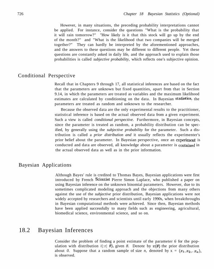
726 Chapter 18 Bayesian Statistics (Optional)
However, in many situations, the preceding probability interpretations cannot be applied. For instance, consider the questions "What is the probability that it will rain tomorrow?" "How likely is it that this stock will go up by the end of the month?" and "What is the likelihood that two companies will be merged together?" They can hardly be interpreted by the aforementioned approaches, and the answers to these questions may be different to different people. Yet these questions are constantly asked in daily life, and the approach used to explain those probabilities is called subjective probability, which reflects one's subjective opinion.
Conditional Perspective
Recall that in Chapters 9 through 17, all statistical inferences are based on the fact that the parameters are unknown but fixed quantities, apart from that in Section 9.14, in which the parameters are treated as variables and the maximum likelihood estimates are calculated by conditioning on the data. In Bayesian statistics, the parameters are treated as random and unknown to the researcher.
Because the observed data are the only experimental results to the practitioner, statistical inference is based on the actual observed data from a given experiment. Such a view is called conditional perspective. Furthermore, in Bayesian concepts, since the parameter is treated as random, a probability distribution can be specified, by generally using the subjective probability for the parameter. Such a distribution is called a prior distribution and it usually reflects the experimenter's prior belief about the parameter. In Bayesian perspective, once an experiment is conducted and data are observed, all knowledge about a parameter is contained in the actual observed data as well as in the prior information.
Bayesian Applications
Although Bayes' rule is credited to Thomas Bayes, Bayesian applications were first introduced by French Scientist Pierre Simon Laplace, who published a paper on using Bayesian inference on the unknown binomial parameters. However, due to its sometimes complicated modeling approach and the objections from many others against the use of the subjective prior distribution, Bayesian applications were not widely accepted by researchers and scientists until early 1990s, when breakthroughs in Bayesian computational methods were achieved. Since then, Bayesian methods have been applied successfully to many fields such as engineering, agricultural, biomedical science, environmental science, and so on.
18.2 Bayesian Inferences
Consider the problem of finding a point estimate of the parameter 6 for the population with distribution /(:r| 9), given 8. Denote by n(0) the prior distribution about 0. Suppose that a random sample of size n, denoted by x = (xx,x2,..., xn), is observed.
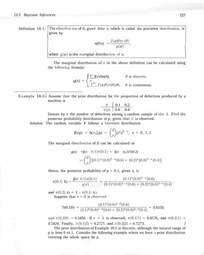
18-2 Bayesian Inferences 727
Definition 18.1: The e given
when
listril by
<iix)
ut ion of 0,
is the niai
give
•gina
n data x,
n(0\x) =
distribu
which is
f(X\0)7T
ion eif x.
called the
ie)
post erior disl ributioii. is
The marginal distribution of x in the above definition can be calculated using the following formula:
(J2 f(x\0)n(0), 0 is discrete. g(x) = { o
I (f° fix\0)rt(0) d.0, 0 is continuous.
Example 18.1:1 Assume that, the prior distribution for the proportion of defectives produced by a machine is
0.1 0.2 TT(P) 0.6 0.4
Denote by x the number of defectives among a random sample of size 2. Finel the posterior probability distribution of p, given that :/: is observed.
Solution: The random variable X follows a binomial distribution
f(x\p) = b(.r,2,p) = (2)p*q2-*, x = 0. 1.2.
The marginal distribution of X can be: calculated as
g(x) =f(x\ O.I)TT(O.I) + f(x\ ().2)7r(0.2)
2 |[(0.lHQ.9)2-s(0.6) + (0.2):n(0.8)2-''(0.4)].
Hence, the posterior probability of p = 0.1, given x, is
f(x\ O.l)Tr(O.l) ( O . l f t O J ) 2 - 3 5 ^ ) ?r(0.1| X) =
9ix) (0.1)"'(0.9)2^(0.6) + (0.2)*(0.8)2-'''-(0.4)'
anel TT(0.2| X) = 1 - TT(().1| X).
Suppose that x = 0 is observcel.
7r(0.1|0) = (0.1)°(0.9)2-°(0.6)
(0.1)°(0.9)2-°(0.6) + (0.2)(l(0.8)2-(l(0.4) = 0.6550.
and ~(0.2|0) = 0.3450. If a; = 1 is observed, TT(0.1|1) = 0.4576, anel jr(0.2jl) =
0.5424. Finally, ?r(0.112) = 0.2727, anel -(0.2|2) = 0.7273. J The prior distribution of Example 18.1 is discrete, although the natural range of
p is from 0 to 1. Consider the following example where we have a prior distribution covering the whole space for p.
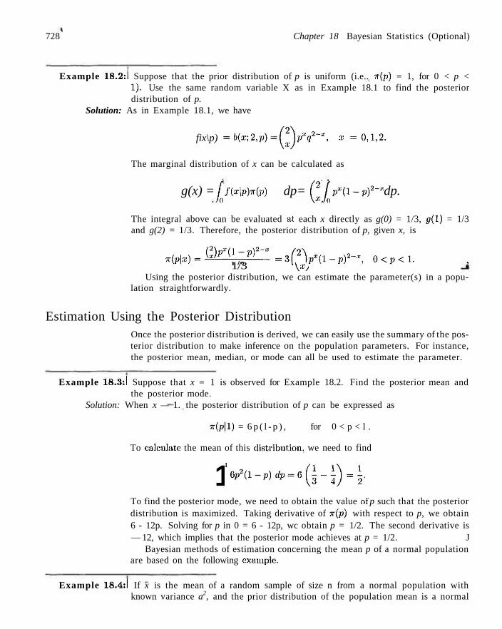
728 Chapter 18 Bayesian Statistics (Optional)
Example 18.2:1 Suppose that the prior distribution of p is uniform (i.e.. 7t(p) = 1, for 0 < p < I). Use the same random variable X as in Example 18.1 to find the posterior distribution of p.
Solution: As in Example 18.1, we have
fix\p) = b(x;2,p)= Q P V ~ * , as = 0,1,2.
The marginal distribution of x can be calculated as
g(x) = j f(x\p)rt(p) dp= Q J Pxi\-P)2-X dp.
The integral above can be evaluated at each x directly as g(0) = 1/3, #(1) = 1/3 and g(2) = 1/3. Therefore, the posterior distribution of p, given x, is
nip\x)={*)pX{]~P)2~* = 3 f 2 W - P ) 8 " . 0<p<l. , 1/3 \x;
Using the posterior distribution, we can estimate the parameter(s) in a population straightforwardly.
Estimation Using the Posterior Distribution Once the posterior distribution is derived, we can easily use the summary of the posterior distribution to make inference on the population parameters. For instance, the posterior mean, median, or mode can all be used to estimate the parameter.
Example 18.3:1 Suppose that x = 1 is observed for Example 18.2. Find the posterior mean and the posterior mode.
Solution: When x — 1. the posterior distribution of p can be expressed as
7r(p|l) = 6 p ( l - p ) , for 0 < p < l .
To calculate the mean of this distribution, we need to find
1 V(i-p)*>e(i-i)-l.
To find the posterior mode, we need to obtain the value of p such that the posterior distribution is maximized. Taking derivative of Tt(p) with respect to p, we obtain 6 - 12p. Solving for p in 0 = 6 - 12p, wc obtain p = 1/2. The second derivative is — 12, which implies that the posterior mode achieves at p = 1/2. J
Bayesian methods of estimation concerning the mean p of a normal population are based on the following example.
Example 18.4:1 If x is the mean of a random sample of size n from a normal population with known variance a2, and the prior distribution of the population mean is a normal
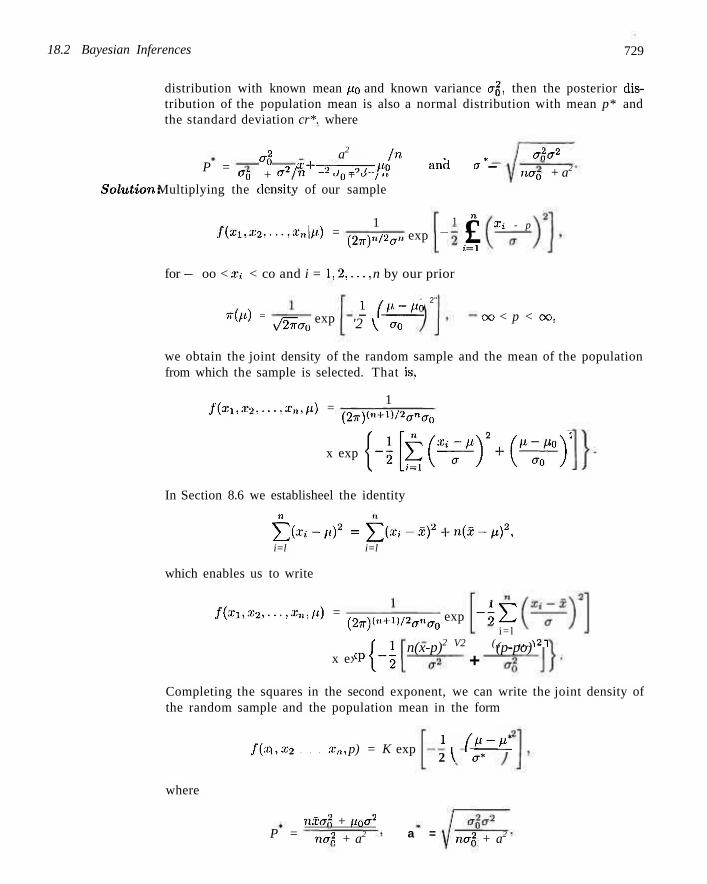
18.2 Bayesian Inferences 729
distribution with known mean p0 and known variance IT2,, then the posterior distribution of the population mean is also a normal distribution with mean p* and the standard deviation cr*. where
P = 4 °~o + °~2/n ao + a2/n
Solution: Multiplying the density of our sample
1
a2 jn , , x + ~^y~,—T~rl'<> a n c l a —
2^-2 <7ntT
no-Q + a2
f(xx,x2,...,x»\p) = (2TV)1'/'2O7> exp
1 n
- £ j = i
Xi - p
for — oo < Xi < co and i = 1.2,..,, n by our prior
2"
7r(/i) = v/27ri 7T(7o
exp 1 (P-Po
'2 \ ao oo < p < oo,
we obtain the joint density of the random sample and the mean of the population from which the sample is selected. That is.
f(xi,x2,...,xn,p) = 1
(27r)("+1)/2ej"CT0
{-i[t(^)2+(^y x exp
In Section 8.6 we establisheel the identity
J2ixi-p)2 = irix,-x)2+n(x-p)2, i=l i=l
which enables us to write
f(xi,x2,...,xn,p) = ( 2 ^ ) ( « + l ) / 2 0 - n ( 7 o
exp 1 -££
x exp •B i= l
V2 (,, _ ,,„\2-\ n(x-p)2 (p-po) +
Completing the squares in the second exponent, we can write the joint density of the random sample and the population mean in the form
fix i, x2 x„, p) = K exp 1 (ti-li* 2 I er*
where
P = nxa2, + poa2
na2. + a2 a = no2, + a2
730 Chapter 18 Bayesian Statistics (Optional)
and K is a function of the sample values and the known parameters. The marginal distribution of the sample is then
/
OO |
• oo V27TCT'
= K\Fhto*,
and the posterior distribution is f(xi,x2,...,xn,u)
exp 1 (p-p-2
dp
it(p\xi,x2,...,xn) = g(x,i,x2,...,xn)
1
v/27r< TtO* exp 2\ a* J — oo < p < oo,
which is identified as a normal distribution with mean p* and standard deviation
a*, where p* and a* are defined above. J The central limit theorem allows us to use Example 18.4 also when we select
random samples (n > 30 for many engineering experimental cases) from nonnormal populations (the distribution is not very far from symmetric), and when the prior distribution of the mean is approximately normal.
Several comments need to be made about Example 18.4. The posterior mean p* can also be written as
* _ °o - o-2jn I1 ~ ~2~~i 2~T~X "" 2~,—TT~U0:
which is the weighted average of the sample mean x and the prior mean p0- Since both coefficients are between 0 and 1 and sum to 1, the posterior mean p* is always between x and po- This means that the posterior estimation of the location of p is influenced by both x and po- Furthermore, the weight of x depends on the prior variance as well as the variance of the sample mean. For a large sample problem (n —> co), the posterior mean p* —> x. This means that the prior mean does not play any role in estimating the population mean p using the posterior distribution. This is very reasonable since it indicates that when the amount of data is substantial, information from the data will dominate the information of p provided by the prior. On the other hand, when the prior variance is large (er2 —• cc), the posterior mean p" also goes to x. Note that for a normal distribution the larger the variance, the flatter the density function. The flatness of the normal distribution in this case means that there is almost no subjective prior information available to the parameter p. Thus, it is reasonable that the posterior estimation p* only depends on the data value x.
Now consider the posterior standard deviation a*. This value can also be written as
a2a2/n
It is obvious that the value a* is smaller than both ao and a/^/n, the prior standard deviation and the standard deviation of x, respectively. This suggests that
18.2 Bayesian Inferences 731
the posterior estimation is more accurate than both the prior and the sample data. Hence, incorporating both the data and prior information results in better posterior information than using any of the data or prior alone. This is a common phenomenon in Bayesian inference. Furthermore, to compute p* and o* by the formulas in Example 18.4, we have assumed that er2 is known. Since this is generally not the case, we shall replace er2 by the sample variance s2 whenever n > 30.
Bayesian Interval Estimation
Similar to classical confidence interval, in Bayesian analysis, we can calculate a 100(1 - o)% Bayesian interval using the posterior distribution.
Definition 18.2: The interval a < 6 < b will be called a 100(1 — a)% Bayes interval for 9 if
/
a /.oo
TT(6\X) d.0= rr(9\x) d9 = ^ . -oo Jb 2 Recall that under the frequentist approach, probability of a confidence interval,
say 95%, is interpreted as a coverage probability, which means that if an experiment is repeated again and again (with considerable unobserved data), the probability that the calculated intervals according to the rule will cover the true parameter is 95%. However, in Bayesian interval interpretation, say for a 95% interval, we can simply phrase that the probability of the unknown parameter falling into the calculated interval (only depends on the observed data) is 95%.
Example 18.5:1 Suppose that X ~ b(x;n,p) with known n = 2, and the prior distribution of p is uniform ir(p) = 1, for 0 < p < 1, find a 95% Bayes interval for p.
Solution: As in Example 18.2, when x = 0, the posterior distribution is 7r(p|0) — 3(1 —p)2, for 0 < p < 1. Thus we need to solve for a and b using Definition 18.2, which yields the following:
0.025 ,-r ./o
3 ( l - p ) 2 d p = l - ( l - a ) 3
and
0.025 /V-P)2 Jb
dp=(l- bf
The solutions to the above equations result in a = 0.0084 and b = 0.7076. Therefore, the probability that p falls into (0.0084,0.7076) is 95%. J
For the normal (population) and normal (prior) case described in Example 18.4, the posterior mean p* is the Bayes estimate of the population mean p, and a 100(1 - Q ) % Bayesian interval for p can be constructed by computing the interval
P* ~ zn/2a* <p< p* + za/2a*,
which is centered at the posterior mean and contains 100(1 — a)% of the posterior probability.
732 Chapter 18 Bayesian Statistics (Optional)
Example 18.6:1 An electrical firm manufactures light, bulbs that have a length of life that is approximately normally distributed with a standard deviation eif 100 hours. Prior experience leads us to believe that p is a value of a normal random variable with a mean po = 800 hours and a standard deviation o~o — 10 hours. If a random sample of 25 bulbs has an average life of 780 hours, find a 95%. Bayesian interval for p.
Solution: Accortling to Example 18.4, the posterior distribution of the: mean is also a normal distribution with mean
_ (25)(780)(10)2+(800)(100)2 _ ' ' (25)(10)2 + (100)2
and standard eleviation
(10)2(100)5
80. y (25)(10)2+(100)2
The 95% Bayesian interval for p is then given by
796 - 1.96V§0 < p < 796 + 1.96\/80,
or
778.5 < p. < 813.5.
Hence, we arc 95% sure that p. will be between 778.5 and 813.5. On the other hand, ignoring the prior information about p, we could proceed
as in Section 9.4 and construct the classical 95% confidence: interval
780 - (1.96) (^=V\ < p < 780 + (1.96) ' 25
or 740.8 < p < 819.2, which is seen to be wider than the corresponding Bayesian
interval. J
18.3 Bayes Estimates Using Decision Theory Framework
Using Bayesian methodology, the posterior distribution of the parameter can be obtained. Bayes estimates can also be derived using the posterior distribution when a loss function is incurred. For instance, the most popular Bayes estimate used is under the squared-error loss function, which is similar to the least squares estimates were presented in Chapter 11 in our discussion of regression analysis.
Definition 18.3: The mean of the posterior distribution TT(9\X), denote by 0*, is called the Bayes estimate of 0, under the squared-error loss function.
Example 18.7:1 Find the Bayes estimates of p, for all the values of 3S3 for Example 18.1. Solution: When x = 0, p* = (0.1)(0.6550) + (0.2)(03450) = 0.1345.
When x - I, p* = (0.1)(0.4576) + (0.2)(0.5424) = 0.1542.
18.3 Bayes Estimates Using Decision Theory Framework 733
When x = 2, p* = (0.1)(0.2727) + (0.2)(0.7273) = 0.1727. Note that the classical estimate of p is p = x/n = 0, 1/2, and 1, respectively,
for the x values at 0, 1, anel 2. The'sc classical estimates are very different from the corresponding Bayes estimates. J
Example 18.8:1 Repeat Example 18.7 in the' situation of Example 18.2. Solution: Since the posterior distribution of p can be expressed as
. W - Q g a ^ - a Q p - d - a - , »<„<i,
the Bayes estimate of p is
• i
p* = E(P\.r.) = 3 Q j p' + >(l - p)2--': dp.
which yields p* = 1/4 for x = 0, p' = 1/2 for x = 1, and p* = 3/4 for x = 2, respectively. Notice that when x = 1 is observed, the Bayes estimate and the classical estimate p arc equivalent. J
For the normal situation as described in Example 18.4, the Bayes estimate of p under the squared-error loss will be' the posterior mean p*.
Example 18.9:1 Suppose that the sampling distribution of a random variable, X, is Poisson with parameter A. Assume that the prior distribution of A follows a gamma distribution with parameters (ov,/?). Finel the Bayes estimate of A under the squared-error loss function.
Solution: The density function of A" is
f(x\X) = e " A ^ - . for a; = 0,1 x\ '
anel the prior distribution of A is
^ = ^ r \ x ' x ~ X ( ~ X ! a ' for A>0-
Hence the posterior distribution of A can be expressed by
A ' * e, \x+e*-le-(l+l//9)A n(X\x) =
r-x y e -AA«- ' e -v- \ / A ~ /•a c 'Ax+o-l r-(l + l/,3)A dx 'll x\0«r(a) "A JO * T O )
1
(1 +i/0)-(*+a)r(x+ay
which follows another gamma distribution with parameters (x + a, (1 + l/3)~l). Using Theorem 6.3, we obtain the posterior mean
I + 1/0
734 Chapter 18 Bayesian Statistics (Optional)
Since the posterior mean is the Bayes estimate under the squared-error loss, A is
our Bayes estimate. J
Exercises
18.1 Estimate the proportion of defectives being produced by the machine! in Example 18.1 if the random sample of size 2 yields 2 defectives.
18.2 Let us assume that the prior distribution for the proportion y of drinks from a vending machine that overflow is
p w(p)
0.05 0.3
0.10 0.5
0.15 0.2
If 2 of the next 9 drinks from this machine overflow, find (a) the posterior distribution for the proportion p; (b) the Bayc:s estimate of p.
18.3 Repeat Exercise 18.2 when 1 of the: next 4 drinks overflows anel the uniform prior distribution is
jr(p) = 10, 0.05 < / > < 0.15.
18.4 The developer of a new condominium complex claims that 3 out of 5 buyers will prefer a two bedroom unit, while his banker claims that it. would be more correct to say that 7 out. of 10 buyers will prefer a two-bedroom unit. In previous predictions of this type, the banker has been twice as reliable as the developer. If 12 of the next 15 condominiums solel in this complex are: two-bedroom units, Bad
(a) the posterior probabilities associated with the claims of the developer anel banker:
(b) a point estimate: of the proportion of buyers who prefer a two-bedroom unit.
18.5 The burn time for the first stage of a rocket is a normal random variable with a standard deviation of 0.8 minute. Assume a normal prior distribution for p with a mean of 8 minutes and a standard deviation of 0.2 minute. If 10 of those rockets arc fired anel the first stage has an average burn time of 9 minutes, find a 95% Bayesian interval for p.
18.0 The daily profit, from a juice vending machine placed in an office building is a value of a normal random variable with unknown mean p and variance er". Of course, the mean will vary somewhat from building to building, and the distributor feels that these average
daily profits can be'st be described by a normal distribution with mean po = $30.00 and standard deviation rrn = SI.75. If one of these juice machines, placed in a certain building, showed an average daily profit o( X = $24.90 during the first 30 days with a standard deviation of s = $2.10, find
(a) a Bayes estimate of the true average daily profit for this building;
(b) a 95% Bayesian interval of p for this buileling; (c) the probability that the average daily preifit from
the machine in this buileling is between $24.00 anel $26.00.
18.7 The mathematics department, of a large university is designing a placement test, to be given to the incoming freshman classes. Members of the: department feel that the average grade for this test will vary from one freshman class to another. This variation of the average class grade is expressed subjectively by a normal distribution with mean po = 72 and variance: exo = 5.7G.
(a) What, prior probability eloes the department assign to the actual average grade being somewhere between 71.8 and 73.4 for next year's freshman class?
(b) If the test is tried on a random sample of 100 freshman students from the next, incoming freshman class resulting in an average grade of 70 with a variance of 64, construct a 95% Bayesian interval for /(.
(c) What posterior probability should the department assign to the event of part (a)'.'
18.8 Suppose that In Example 18.6 the electrical firm eloes not. have enough prior information regarding the population mean length of life to be able to assume a normal distribution for p. The firm believes, however, that p. is surely between 770 and 830 hours and it is fell that a more realistic Bayesian approach would be to assume the prior distribution
-( / ' ) = gg, 770 < p < 8;io.
If a random sample: of 25 bulbs gives an average life of 7K0 hours, follow the steps of the proof for Example
Exercise), 735
18.4 to find the posterior distribution
n(p\xi,X2,...,X2T,).
18.9 Suppose that the time to failure T of a certain hinge is an exponential random variable with probability density
f(t) = 0c.-et, t > 0.
From prior experience we are led to believe that. 0 is a value of an exponential random variable with probability density
T!(ff) = 2e"2 0 , 0 > 0.
If we have a sample of n observations on T, show that the posterior distribution of © is a gamma distribution with parameters
a = n + 1, and ,3 = [Y^ti + 2
18.10 Suppose that a sample consisting of 5, 6, 6, 7, 5, 6, 4, 9, 3, 6 and comes from a Poisson population with mean A. Assume that the parameter A follows a gamma distribution with parameters (3,2). Under the squared-error loss, find the Bayes estimate of A.
18.11 A random variable X follows a negative binomial distribution with parameters k = 5 and p (i.e., b*(x;5,p)). Furthermore, we know that p follows a uniform distribution in the interval (0,1). Find out the Bayes estimate of p under the squared-error loss. [Hint: You may find the density function in Exercise 6.50 useful. Also, the mean of the Beta distribution with parameters (a, 3) is a/(a + /?).]

Bibliography
(6
[7;
[9;
[10;
[11
[12
[13
[14
Bartlett, M. S. and Kendall, D. G. (1946). "The Statistical Analysis of Variance Heterogeneity and Logarithmic Transformation," Journal of the Royal Statistical Society, Ser. B. 8, 128-138.
Bowker, A. H. and Lieberman. G. J. (1972). Engineering Statistics, 2nd ed. Upper Saddle River, N.J.: Prentice Hall.
Box, G. E. P. (1988). "Signal to Noise Ratios, Performance Criteria and Transformations (with discussion)," Technometrics, 30, 1-17.
Box, G. E. P. Fung, C. A. (1986). "Studies in Quality Improvement: Minimizing Transmitted Variation by Parameter Design," Report 8. University of Wisconsin-Madison, Center for Quality and Productivity Improvement.
Box, G. E. P., Hunter, W. G. and Hunter, J. S. (1978). Statistics for Experimenters. New York: John Wiley & Sons.
Brownlee, K. A. (1984). Statistical Theory and Methodology: in Science and Engineering, 2nd ed. New York: John Wiles &: Sons.
Carroll, R. J. and Ruppert, D. (1988). Transformation and Weighting in Regression. New York: Chapman and Hall.
Chatterjee, S. Hadi, A. S. and Price, B. (1999). Regression Analysis by Example, 3rd ed. New York: John Wiles & Sons.
Cook, R. D. and Weisberg, S. (1982). Residuals and Influence in Regression. New York: Chapman and Hall.
Daniel, C. and Wood, F. S. (1999). Fitting Equations to Data: Computer Analysis of Multifactor Data, 2nd ed. New York: John Wiley & Sons.
Daniel, W. W. (1989). Applied Nonparametric Statistics, 2nd ed. Belmont, California: Wadsworth Publishing Company.
Devore, J. L. (2003). Probability and Statistics for Engineering and the Sciences, 6th ed. Belmont, Calif: Duxbury Press.
Dixon, W. J. (1983). Introduction to Statistical Analysis, 4th ed. New York: McGraw-Hill.
Draper, N. R. and Smith, H. (1998). Applied Regression analysis, 3rd ed. New York: John Wiley & Sons.
738 BIBLIOGRAPHY
[15] Duncan, A. (1986). Quality Control and Industrial Statistics, 5th ed. Homewood, Illinois: Irwin.
[16] Dyer, D. D. and Keating, J. P. (1980). "On the Determination of Critical Values for Bartlett's Test," J. Am. Stat. Assoc, 75, 313-319.
[17] Ewan, W. D. and Kemp, K. W. (1960). "Sampling Inspection of Continuous Processes with No Autocorrelation between Successive Results," Biometrika, Vol. 47, 363-380.
[18] Gunst, R. F. and Mason, R. L. (1980). Regression Analysis and Its Application: A Data-Oriented Approach. New York: Marcel Dckker.
[19] Guttman, I., Wilks, S. S. and Hunter, J. S. (1971). Introductory Engineering Statistics. New York: Wiley k Sons.
[20] Hicks, C. R. and Turner, K. V. (1999). Fundamental Concepts in the Design of Experiments, 5th ed. Oxford: Oxford University Press.
[21] Hoaglin, D. C, Mosteller, F. and Tukey, J. W. (1991). Fundamentals of Exploratory Analysis of Variance. New York: Wiley &; Sons.
[22] Hocking, R.R., (1976). "The Analysis and Selection of Variables in Linear Regression," Biometrics, 32, 1-49.
[23] Hoerl, A. E. and Wennard, R. W. (1970). "Ridge Regression: Applications to Nonorthogonal Problems," Technometrics, 12, 55-67.
[24] Hogg, R. V., Craig, A. and McKean, J. W. (2004). Introduction to Mathematical Statistics, 6th ed. Upper Saddle River, N.J.: Prentice Hall.
[25] Hogg, R. V. and Ledolter, J. (1992). Applied Statistics for Engineers and Physical Scientists, 2nd ed. Upper Saddle River: N.J.: Prentice Hall.
[26] Hollander, M. and Wolfe, D. (1999). Nonparametric Statistical Methods. New York: John Wiley & Sons.
[27] Johnson, N. L. and Leone, F. C. (1977). Statistics and E:vperimental Design: In Engineering and the Physical Sciences, Vols. I and II, 2nd ed, New York: John Wiley & Sons.
[28] Kackar, R. (1985). "Off-Line Quality Control, Parameter Design, and the Taguchi Methods," Journal of Quality Technology, 17, 176-188.
[29] Koopmans, L. H. (1987). An Introduction to Contemporary Statistics, 2nd ed. Boston: Duxbury Press.
[30] Larsen, R. J. and Morris, M. L. (2000). An Introduction to Mathematical Statistics and Its Applications, 3rd ed. Upper Saddle River, N.J.: Prentice Hall.
[31] Lehmann, E. L. and D'Abrera, H. J. M. (1998). Nonparametrics: Statistical Methods Based on Ranks, rev. ed. Upper Saddle River: N.J.: Prentice Hall,
[32] Lentner, M. and Bishop, T. (1986). Design and Analysis of Experiments, 2nd ed. Blacksburg, VA: Valley Book Co.
[33] Mallows, C. L. (1973). "Some comments of Cp," Technometrics, 15, 661-675.
BIBLIOGRAPHY 739
[34;
[35;
[3e;
[37
[38
[39
[40
[41
[42
[43;
[44
[45
[46;
[47;
[48
[49
[50;
[51
McClave, J. T., Dietrich, F. H. and Sincich, T. (1997). Statistics, 7th ed. Upper Saddle River, N.J.: Prentice Hall.
Montgomery, D. C. (2000). Introduction to Statistical Quality Control, 4th ed. New York: John Wiley & Sons.
Montgomery, D. C. (2001). Design and Analysis of Experiments, 5th ed. New York: John Wiley & Sons.
Mosteller, F. and Tukey, J. (1977). Data Analysis and Regression. Reading, MA: Addison-Wesley Publishing Co.
Myers. R. H. (1990). Classical and Modern Regression with Applications, 2nd ed. Boston: Duxbury Press.
Myers, R. H., Kliuri, A. I. and Vining, G. G. (1992). "Response Surface Alternatives to the Taguchi Robust Parameter Design Approach," The American Statistician, 46, 131-139.
Myers, R. H. and Montgomery, D. C. (2002). Response Surface Methodology: Process and Product Optimization Using Designed Experiments, 2nd ed. New York: John Wiley &i Sons.
Neter, J., Wassermann, W., and Kutner, M. H. (1989). Applied Linear Regression Models, 2nd ed. Burr Ridge, Illinois: Irwin.
Noether, G. E. (1976). Introduction to Statistics: A Nonparametric Approach, 2nd ed. Boston: Houghton Mifflin Company.
Olkin, I.. Gleser, L. J. and Dernian, C. (1994). Probability Models and Applications, 2nd Ed. New York: Prentice Hall.
Ott, R. L. and Longnecker, M. T. (2000). An Introduction to Statistical Methods and Data Analysis, 5th ed. Boston: Duxbury Press.
Plackett, R. L. and Burinan, J. P. (1946). "The Design of Multifactor Experiments," Biometrika, 33, 305-325.
Ross, S. M. (2002). Introduction to Applied Probability Models, 8th ed. New York: Academic Press, Inc.
Satterthwaite, F. E. (1946). "An approximate distribution of estimates of variance components," Biometrics, 2, 110-114.
Schilling, E. G. and Nelson, P. R. (1976). "The Effect, of Nonnormality on the Control Limits of X Charts," J. Quality Tech., 8, 347-373.
Schmidt, S. R. and Launsby, R. G. (1991). Understanding Industrial Designed Experiments. Colorado Springs, CO: Air Academy Press.
Shoemaker, A. C, Tsui, K.-L., and Wu, C. F. J. (1991). "Economical Experimentation Methods for Robust Parameter Design," Technometrics, 33, 415-428,
Snedecor, G. W. and Cochran, W. G. (1989). Statistical Methods, 8th ed. Allies, Iowa: The Iowa State University Press.

740 BIBLIOGRAPHY
[52] Steel, R. G. D., Torrie, J. H. and Dickey, D. A. (1996). Principles and Procedures of Statistics: A Biometrical Approach, 3rd ed. New York: McGraw-Hill.
[53] Taguchi, G. (1991). Introduction to Quality Engineering. White Plains, N.Y.: Unipub/Kraus International.
[54] Taguchi, G. and Wu, Y. (1985). Introduction to Off-Line Quality Control. Nagoya, Japan: Central Japan Quality Control Association.
[55] Thompson, W. O. and Cady, F. B. (1973). Proceedings of the University of Kentucky Conference on Regression with a Large Number of Predictor Variables. Lexington, Kentucky: University of Kentucjy press.
[56] Tukey, J. W. (1977). Exploratory Data Analysis. Reading, MA: Addison-Wesley Publishing Co.
[57] Vining, G. G. and Myers, R. H. (1990). "Combining Taguchi and Response Surface Philosophies: A Dual Response Approach." Journal of Quality Technology, 22, 38-45.
[58] Welch, W. J., Yu, T. K., Kang, S. M. and Sacks, J. (1990). "Computer Experiments for Quality Control by Parameter Design," Journal of Quality Technology, 22, 15-22.
[59] Winer, B. J. (1991). Statistical Principles In Experimental Design, 3rd ed. New York: McGraw-Hill.
Appendix A
Statistical Tables and Proofs
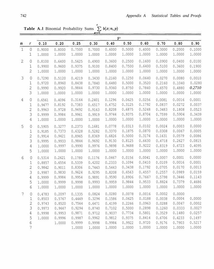
742 Appendix A Statistical Tables and Proofs
r Table A . l Binomial Probability Sums YI b(x;n,p)
x=0
n r 1 0
1
2 0 1 2
3 0 1 2 3
4 0 1 2 3 4
5 0 1 2 3 4 5
6 0 1 2 3 4 5 6
7 0 1 2 3 4 5 6 7
0.10
0.9000 1.0000
0.8100 0.9900 1.0000
0.7290 0.9720 0.9990 1.0000
0.6561 0.9477 0.9963 0.9999 1.0000
0.5905 0.9185 0.9914 0.9995 1.0000 1.0000
0.5314 0.8857 0.9842 0.9987 0.9999 1.0000 1.0000
0.4783 0.8503 0.9743 0.9973 0.9998 1.0000
0.20
0.8000 1.0000
0.6400 0.9600 1.0000
0.5120 0.8960 0.9920 1.0000
0.4096 0.8192 0.9728 0.9984 1.0000
0.3277 0.7373 0.9421 0.9933 0.9997 1.0000
0.2621 0.6554 0.9011 0.9830 0.9984 0.9999 1.0000
0.2097 0.5767 0.8520 0.9667 0.9953 0.9996 1.0000
0.25
0.7500 1.0000
0.5625 0.9375 1.0000
0.4219 0.8438 0.9844 1.0000
0.3164 0.7383 0.9492 0.9961 1.0000
0.2373 0.6328 0.8965 0.9844 0.9990 1.0000
0.1780 0.5339 0.8306 0.9624 0.9954 0.9998 1.0000
0.1335 0.4449 0.7564 0.9294 0.9871 0.9987 0.9999 1.0000
0.30
0.7000 1.0000
0.4900 0.9100 1.0000
0.3430 0.7840 0.9730 1.0000
0.2401 0.6517 0.9163 0.9919 1.0000
0.1681 0.5282 0.8369 0.9692 0.9976 1.0000
0.1176 0.4202 0.7443 0.9295 0.9891 0.9993 1.0000
0.0824 0.3294 0.6471 0.8740 0.9712 0.9962 0.9998 1.0000
I 0.40
0.6000 1.0000
0.3600 0.8400 1.0000
0.2160 0.6480 0.9360 1.0000
0.1296 0.4752 0.8208 0.9744 1.0000
0.0778 0.3370 0.6826 0.9130 0.9898 1.0000
0.0467 0.2333 0.5443 0.8208 0.9590 0.9959 1.0000
0.0280 0.1586 0.4199 0.7102 0.9037 0.9812 0.9984 1.0000
» 0.50
0.5000 1.0000
0.2500 0.7500 1.0000
0.1250 0.5000 0.8750 1.0000
0.0625 0.3125 0.6875 0.9375 1.0000
0.0313 0.1875 0.5000 0.8125 0.9688 1.0000
0.0156 0.1094 0.3438 0.6563 0.8906 0.9844 1.0000
0.0078 0.0625 0.2266 0.5000 0.7734 0.9375 0.9922 1.0000
0.60
0.4000 1.0000
0.1600 0.6400 1.0000
0.0640 0.3520 0.7840 1.0000
0.0256 0.1792 0.5248 0.8704 1.0000
0.0102 0.0870 0.3174 0.6630 0.9222 1.0000
0.0041 0.0410 0.1792 0.4557 0.7667 0.9533 1.0000
0.0016 0.0188 0.0963 0.2898 0.5801 0.8414 0.9720 1.0000
0.70
0.3000 1.0000
0.0900 0.5100 1.0000
0.0270 0.2160 0.6570 1.0000
0.0081 0.0837 0.3483 0.7599 1.0000
0.0024 0.0308 0.1631 0.4718 0.8319 1.0000
0.0007 0.0109 0.0705 0.2557 0.5798 0.8824 1.0000
0.0002 0.0038 0.0288 0.1260 0.3529 0.6706 0.9176 1.0000
0.80
0.2000 1.0000
0.0400 0.3600 1.0000
0.0080 0.1040 0.4880 1.0000
0.0016 0.0272 0.1808 0.5904 1.0000
0.0003 0.0067 0.0579 0.2627 0.6723 1.0000
0.0001 0.0016 0.0170 0.0989 0.3446 0.7379 1.0000
0.0000 0.0004 0.0047 0.0333 0.1480 0.4233 0.7903 1.0000
0.90
0.1000 1.0000
0.0100 0.1900 1.0000
0.0010 0.0280 0.2710 1.0000
0.0001 0.0037 0.0523 0.3439 1.0000
0.0000 0.0005 0.0086 0.0815 0.4095 1.0000
0.0000 0.0001 0.0013 0.0159 0.1143 0.4686 1.0000
0.0000 0.0002 0.0027 0.0257 0.1497 0.5217 1.0000
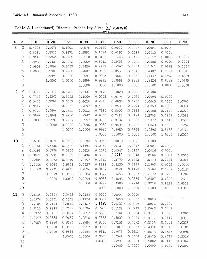
Table A.l Binomial Probability Table 743
r Table A . l (continued) Binomial Probability Sums J2 °ix'ini'P)
x=0
n r 8 0
1 2 3 4 5 6 7 8
9 0 1 2 3 4 5 6 7 8 9
10 0 1 2 3 4 5 6 7 8 9
10
11 0 1 2 3 4 5 6 7 8 9 10 11
0.10
0.4305
0.8131 0.9619
0.9950
0.9996 1.0000
0.3874
0.7748
0.9470
0.9917
0.9991 0.9999
1.0000
0.3487
0.7361
0.9298 0.9872
0.9984
0.9999 1.0000
0.3138
0.6974 0.9104 0.9815
0.9972
0.9997
1.0000
0.20
0.1678
0.5033
0.7969 0.9437
0.9896 0.9988
0.9999
1.0000
0.1342
0.4362
0.7382
0.9144 0.9804
0.9969 0.9997
1.0000
0.1074
0.3758
0.6778
0.8791 0.9672
0.9936
0.9991 0.9999
1.0000
0.0859
0.3221 0.6174
0.8389 0.9496 0.9883
0.9980
0.9998 1.0000
0.25
0.1001
0.3671 0.6785
0.8862
0.9727
0.9958
0.9996
1.0000
0.0751
0.3003
0.6007
0.8343
0.9511 0.9900
0.9987
0.9999
1.0000
0.0563
0.2440 0.5256
0.7759
0.9219
0.9803
0.9965
0.9996
1.0000
0.0422
0.1971 0.4552 0.7133
0.8854
0.9657 0.9924
0.9988 0.9999
1.0000
0.30
0.0576
0.2553
0.5518
0.8059
0.9420
0.9887 0.9987
0.9999
1.0000
0.0404
0.1960
0.4628 0.7297
0.9012
0.9747
0.9957
0.9996
1.0000
0.0282
0.1493
0.3828
0.6496
0.8497
0.9527
0.9894
0.9984
0.9999 1.0000
0.0198
0.1130 0.3127 0.5696
0.7897
0.9218
0.9784
0.9957 0.9994
1.0000
P 0.40
0.0168
0.1064
0.3154
0.5941
0.8263 0.9502
0.9915
0.9993
1.0000
0.0101
0.0705
0.2318
0.4826
0.7334
0.9006
0.9750
0.9962
0.9997
1.0000
0.0060
0.0464
0.1673
0.3823
0.6331
0.8338 0.9452
0.9877
0.9983 0.9999
1.0000
0.0036
0.0302 0.1189" 0.2963
0.5328
0.7535
0.9006
0.9707 0.9941
0.9993
1.0000
0.50
0.0039
0.0352
0.1445 0.3633
0.6367
0.8555
0.9648 0.9961
1.0000
0.0020
0.0195 0.0898
0.2539 0.5000
0.7461
0.9102
0.9805
0.9980
1.0000
0.0010
0.0107
0.0547
0.1719 0.3770
0.6230
0.8281
0.9453
0.9893
0.9990 1.0000
0.0005 0.0059 0.0327 •
0.1133 0.2744
0.5000
0.7256 0.8867 0.9673
0.9941
0.9995
1.0000
0.60
0.0007
0.0085
0.0498
0.1737 0.4059
0.6846
0.8936 0.9832
1.0000
0.0003
0.0038
0.0250 0.0994
0.2666
0.5174
0.7682
0.9295
0.9899
1.0000
0.0001
0.0017
0.0123
0.0548 0.1662
0.3669
0.6177 0.8327
0.9536
0.9940 1.0000
0.0000 0.0007
0.0059 0.0293 0.0994
0.2465 0.4672
0.7037 0.8811
0.9698 0.9964
1.0000
0.70
0.0001
0.0013
0.0113 0.0580 0.1941
0.4482
0.7447 0.9424
1.0000
0.0000
0.0004
0.0043 0.0253
0.0988
0.2703 0.5372
0.8040
0.9596
1.0000
0.0000
0.0001 0.0016
0.0106 0.0473
0.1503
0.3504
0.6172
0.8507
0.9718
1.0000
0.0000
0.0006 0.0043
0.0216
0.0782
0.2103 0.4304 0.6873
0.8870 0.9802 1.0000
0.80
0.0000
0.0001 0.0012
0.0104
0.0563 0.2031
0.4967 0.8322
1.0000
0.0000
0.0003 0.0031
0.0196
0.0856
0.2618
0.5638
0.8658
1.0000
0.0000 0.0001
0.0009 0.0064
0.0328
0.1209
0.3222
0.6242
0.8926 1.0000
0.0000 0.0002
0.0020
0.0117 0.0504
0.1611 0.3826
0.6779 0.9141
1.0000
0.90
0.0000
0.0004
0.0050 0.0381
0.1869
0.5695
1.0000
0.0000 0.0001
0.0009
0.0083
0.0530
0.2252
0.6126
1.0000
0.0000 0.0001
0.0016
0.0128 0.0702
0.2639
0.6513 1.0000
--.
0.0000
0.0003 0.0028 0.0185
0.0896 0.3026 0.6862
1.0000
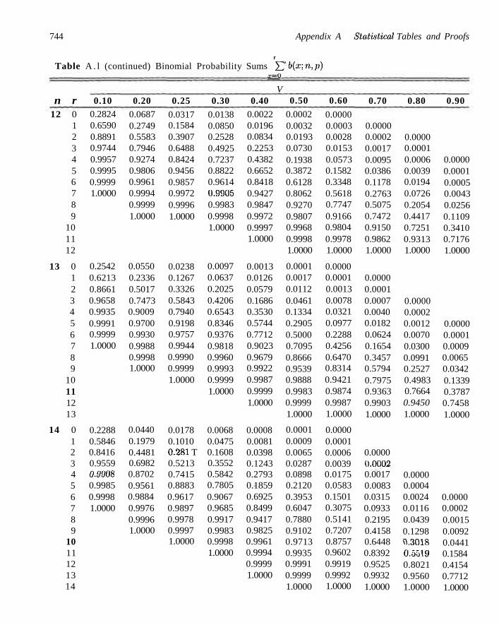
744 Appendix A Statistical Tables and Proofs
r
Table A . l (continued) Binomial Probability Sums YI 0ix:.n-.P) x=0
n r 12 0
1 2 3 4 5 6 7 8 9
10 11 12
13 0 1 2 3 4 5 6 7 8 9
10 11 12 13
14 0 1 2 3 4 5 6 7 8 9
10 11 12 13 14
0.10 0.2824 0.6590 0.8891 0.9744 0.9957 0.9995 0.9999 1.0000
0.2542 0.6213 0.8661 0.9658 0.9935 0.9991 0.9999 1.0000
0.2288 0.5846 0.8416 0.9559 0.9908 0.9985 0.9998 1.0000
0.20 0.0687 0.2749 0.5583 0.7946 0.9274 0.9806 0.9961 0.9994 0.9999 1.0000
0.0550 0.2336 0.5017 0.7473 0.9009 0.9700 0.9930 0.9988 0.9998 1.0000
0.0440 0.1979 0.4481 0.6982 0.8702 0.9561 0.9884 0.9976 0.9996 1.0000
0.25
0.0317 0.1584 0.3907 0.6488 0.8424 0.9456 0.9857 0.9972 0.9996 1.0000
0.0238 0.1267 0.3326 0.5843 0.7940 0.9198 0.9757 0.9944 0.9990 0.9999 1.0000
0.0178 0.1010 0.281 T 0.5213 0.7415 0.8883 0.9617 0.9897 0.9978 0.9997 1.0000
0.30
0.0138 0.0850 0.2528 0.4925 0.7237 0.8822 0.9614 0.9905 0.9983 0.9998 1.0000
0.0097 0.0637 0.2025 0.4206 0.6543 0.8346 0.9376 0.9818 0.9960 0.9993 0.9999 1.0000
0.0068 0.0475 0.1608 0.3552 0.5842 0.7805 0.9067 0.9685 0.9917 0.9983 0.9998 1.0000
V 0.40
0.0022 0.0196 0.0834 0.2253 0.4382 0.6652 0.8418 0.9427 0.9847 0.9972 0.9997 1.0000
0.0013 0.0126 0.0579 0.1686 0.3530 0.5744 0.7712 0.9023 0.9679 0.9922 0.9987 0.9999 1.0000
0.0008 0.0081 0.0398 0.1243 0.2793 0.1859 0.6925 0.8499 0.9417 0.9825 0.9961 0.9994 0.9999 1.0000
0.50
0.0002 0.0032 0.0193 0.0730 0.1938 0.3872 0.6128 0.8062 0.9270 0.9807 0.9968 0.9998 1.0000
0.0001 0.0017 0.0112 0.0461 0.1334 0.2905 0.5000 0.7095 0.8666 0.9539 0.9888 0.9983 0.9999 1.0000
0.0001 0.0009 0.0065 0.0287 0.0898 0.2120 0.3953 0.6047 0.7880 0.9102 0.9713 0.9935 0.9991 0.9999 1.0000
0.60
0.0000 0.0003 0.0028 0.0153 0.0573 0.1582 0.3348 0.5618 0.7747 0.9166 0.9804 0.9978 1.0000
0.0000 0.0001 0.0013 0.0078 0.0321 0.0977 0.2288 0.4256 0.6470 0.8314 0.9421 0.9874 0.9987 1.0000
0.0000 0.0001 0.0006 0.0039 0.0175 0.0583 0.1501 0.3075 0.5141 0.7207 0.8757 0.9602 0.9919 0.9992 1.0000
0.70
0.0000 0.0002 0.0017 0.0095 0.0386 0.1178 0.2763 0.5075 0.7472 0.9150 0.9862 1.0000
0.0000 0.0001 0.0007 0.0040 0.0182 0.0624 0.1654 0.3457 0.5794 0.7975 0.9363 0.9903 1.0000
0.0000 0.0002 0.0017 0.0083 0.0315 0.0933 0.2195 0.4158 0.6448 0.8392 0.9525 0.9932 1.0000
0.80
0.0000 0.0001 0.0006 0.0039 0.0194 0.0726 0.2054 0.4417 0.7251 0.9313 1.0000
0.0000 0.0002 0.0012 0.0070 0.0300 0.0991 0.2527 0.4983 0.7664 0.9450 1.0000
0.0000 0.0004 0.0024 0.0116 0.0439 0.1298 u.3018 0.5519 0.8021 0.9560 1.0000
0.90
0.0000 0.0001 0.0005 0.0043 0.0256 0.1109 0.3410 0.7176 1.0000
0.0000 0.0001 0.0009 0.0065 0.0342 0.1339 0.3787 0.7458 1.0000
0.0000 0.0002 0.0015 0.0092 0.0441 0.1584 0.4154 0.7712 1.0000
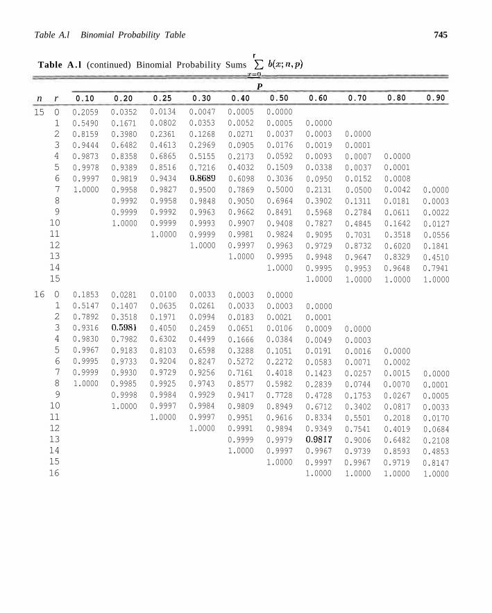
Table A.l Binomial Probability Table 745
r Table A . l (continued) Binomial Probability Sums Y2 Kxin>P)
x=a
n r 15 0
1 2 3 4 5 6 7 8 9 10 11 12 13 14 15
16 0 1 2 3 4 5 6 7 8 9 10 11 12 13 14 15 16
0.10
0.2059 0.5490 0.8159 0.9444 0.9873 0.9978 0.9997 1.0000
0.1853 0.5147 0.7892 0.9316 0.9830 0.9967 0.9995 0.9999 1.0000
0.20
0.0352 0.1671 0.3980 0.6482 0.8358 0.9389 0.9819 0.9958 0.9992 0.9999 1.0000
0.0281 0.1407 0.3518 0.5981 0.7982 0.9183 0.9733 0.9930 0.9985 0.9998 1.0000
0.25
0.0134 0.0802 0.2361 0.4613 0.6865 0.8516 0.9434 0.9827 0.9958 0.9992 0.9999 1.0000
0.0100 0.0635 0.1971 0.4050 0.6302 0.8103 0.9204 0.9729 0.9925 0.9984 0.9997 1.0000
0.30
0.0047 0.0353 0.1268 0.2969 0.5155 0.7216 0.8089 0.9500 0.9848 0.9963 0.9993 0.9999 1.0000
0.0033 0.0261 0.0994 0.2459 0.4499 0.6598 0.8247 0.9256 0.9743 0.9929 0.9984 0.9997 1.0000
P 0.40
0.0005 0.0052 0.0271 0.0905 0.2173 0.4032 0.6098 0.7869 0.9050 0.9662 0.9907 0.9981 0.9997 1.0000
0.0003 0.0033 0.0183 0.0651 0.1666 0.3288 0.5272 0.7161 0.8577 0.9417 0.9809 0.9951 0.9991 0.9999 1.0000
0.50
0.0000 0.0005 0.0037 0.0176 0.0592 0.1509 0.3036 0.5000 0.6964 0.8491 0.9408 0.9824 0.9963 0.9995 1.0000
0.0000 0.0003 0.0021 0.0106 0.0384 0.1051 0.2272 0.4018 0.5982 0.7728 0.8949 0.9616 0.9894 0.9979 0.9997 1.0000
0.60
0.0000 0.0003 0.0019 0.0093 0.0338 0.0950 0.2131 0.3902 0.5968 0.7827 0.9095 0.9729 0.9948 0.9995 1.0000
0.0000 0.0001 0.0009 0.0049 0.0191 0.0583 0.1423 0.2839 0.4728 0.6712 0.8334 0.9349 0.9817 0.9967 0.9997 1.0000
0.70
0.0000 0.0001 0.0007 0.0037 0.0152 0.0500 0.1311 0.2784 0.4845 0.7031 0.8732 0.9647 0.9953 1.0000
0.0000 0.0003 0.0016 0.0071 0.0257 0.0744 0.1753 0.3402 0.5501 0.7541 0.9006 0.9739 0.9967 1.0000
0.80
0.0000 0.0001 0.0008 0.0042 0.0181 0.0611 0.1642 0.3518 0.6020 0.8329 0.9648 1.0000
0.0000 0.0002 0.0015 0.0070 0.0267 0.0817 0.2018 0.4019 0.6482 0.8593 0.9719 1.0000
0.90
0.0000 0.0003 0.0022 0.0127 0.0556 0.1841 0.4510 0.7941 1.0000
0.0000 0.0001 0.0005 0.0033 0.0170 0.0684 0.2108 0.4853 0.8147 1.0000
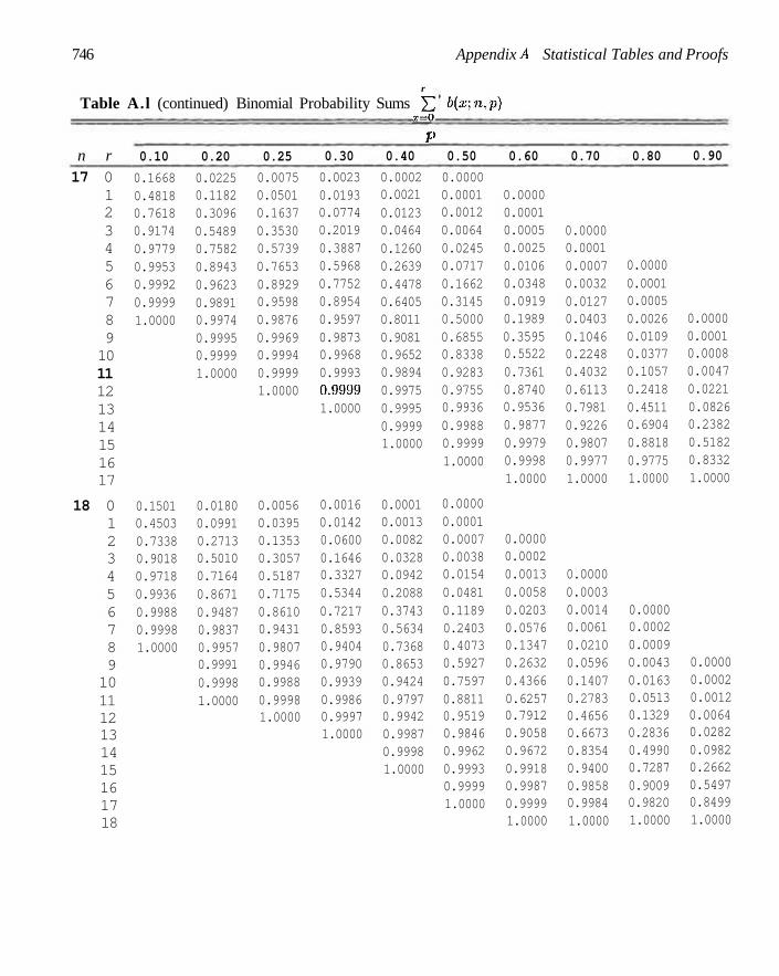
746 Appendix A Statistical Tables and Proofs
r
Table A.l (continued) Binomial Probability Sums YL °ix-n^p) x=Q
n r 17 0
1 2 3 4 5 6 7 8 9 10 11 12 13 14 15 16 17
18 0 1 2 3 4 5 6 7 8 9 10 11 12 13 14 15 16 17 18
0.10
0.1668 0.4818 0.7618 0.9174 0.9779 0.9953 0.9992 0.9999 1.0000
0.1501 0.4503 0.7338 0.9018 0.9718 0.9936 0.9988 0.9998 1.0000
0.20
0.0225 0.1182 0.3096 0.5489 0.7582 0.8943 0.9623 0.9891 0.9974 0.9995 0.9999 1.0000
0.0180 0.0991 0.2713 0.5010 0.7164 0.8671 0.9487 0.9837 0.9957 0.9991 0.9998 1.0000
0.25
0.0075 0.0501 0.1637 0.3530 0.5739 0.7653 0.8929 0.9598 0.9876 0.9969 0.9994 0.9999 1.0000
0.0056 0.0395 0.1353 0.3057 0.5187 0.7175 0.8610 0.9431 0.9807 0.9946 0.9988 0.9998 1.0000
0.30
0.0023 0.0193 0.0774 0.2019 0.3887 0.5968 0.7752 0.8954 0.9597 0.9873 0.9968 0.9993 0.9999 1.0000
0.0016 0.0142 0.0600 0.1646 0.3327 0.5344 0.7217 0.8593 0.9404 0.9790 0.9939 0.9986 0.9997 1.0000
I 0.40
0.0002 0.0021 0.0123 0.0464 0.1260 0.2639 0.4478 0.6405 0.8011 0.9081 0.9652 0.9894 0.9975 0.9995 0.9999 1.0000
0.0001 0.0013 0.0082 0.0328 0.0942 0.2088 0.3743 0.5634 0.7368 0.8653 0.9424 0.9797 0.9942 0.9987 0.9998 1.0000
i
0.50
0.0000 0.0001 0.0012 0.0064 0.0245 0.0717 0.1662 0.3145 0.5000 0.6855 0.8338 0.9283 0.9755 0.9936 0.9988 0.9999 1.0000
0.0000 0.0001 0.0007 0.0038 0.0154 0.0481 0.1189 0.2403 0.4073 0.5927 0.7597 0.8811 0.9519 0.9846 0.9962 0.9993 0.9999 1.0000
0.60
0.0000 0.0001 0.0005 0.0025 0.0106 0.0348 0.0919 0.1989 0.3595 0.5522 0.7361 0.8740 0.9536 0.9877 0.9979 0.9998 1.0000
0.0000 0.0002 0.0013 0.0058 0.0203 0.0576 0.1347 0.2632 0.4366 0.6257 0.7912 0.9058 0.9672 0.9918 0.9987 0.9999 1.0000
0.70
0.0000 0.0001 0.0007 0.0032 0.0127 0.0403 0.1046 0.2248 0.4032 0.6113 0.7981 0.9226 0.9807 0.9977 1.0000
0.0000 0.0003 0.0014 0.0061 0.0210 0.0596 0.1407 0.2783 0.4656 0.6673 0.8354 0.9400 0.9858 0.9984 1.0000
0.80
0.0000 0.0001 0.0005 0.0026 0.0109 0.0377 0.1057 0.2418 0.4511 0.6904 0.8818 0.9775 1.0000
0.0000 0.0002 0.0009 0.0043 0.0163 0.0513 0.1329 0.2836 0.4990 0.7287 0.9009 0.9820 1.0000
0.90
0.0000 0.0001 0.0008 0.0047 0.0221 0.0826 0.2382 0.5182 0.8332 1.0000
0.0000 0.0002 0.0012 0.0064 0.0282 0.0982 0.2662 0.5497 0.8499 1.0000
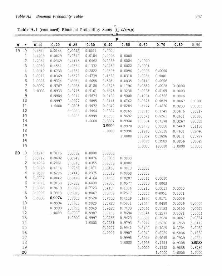
Table A.l Binomial Probability Table 747
r
Table A . l (continued) Binomial Probability Sums YI b(x;n,p) x=a
n r 19 0
1 2 3 4 5 6 7 8 9 10 11 12 13 14 15 16 17 18 19
20 0 1 2 3 4 5 6 7 8 9 10 11 12 13 14 15 16 17 18 19 20
0.10
0.1351 0.4203 0.7054 0.8850 0.9648 0.9914 0.9983 0.9997 1.0000
0.1216 0.3917 0.6769 0.8670 0.9568 0.9887 0.9976 0.9996 0.9999 1.0000
0.20
0.0144 0.0829 0.2369 0.4551 0.6733 0.8369 0.9324 0.9767 0.9933 0.9984 0.9997 1.0000
0.0115 0.0692 0.2061 0.4114 0.6296 0.8042 0.9133 0.9679 0.9900 0.9974 0.9994 0.9999 1.0000
0.25
0.0042 0.0310 0.1113 0.2631 0.4654 0.6678 0.8251 0.9225 0.9713 0.9911 0.9977 0.9995 0.9999 1.0000
0.0032 0.0243 0.0913 0.2252 0.4148 0.6172 0.7858 0.8982 0.9591 0.9861 0.9961 0.9991 0.9998 1.0000
0.30
0.0011 0.0104 0.0462 0.1332 0.2822 0.4739 0.6655 0.8180 0.9161 0.9674 0.9895 0.9972 0.9994 0.9999 1.0000
0.0008 0.0076 0.0355 0.1071 0.2375 0.4164 0.6080 0.7723 0.8867 0.9520 0.9829 0.9949 0.9987 0.9997 1.0000
P 0.40
0.0001 0.0008 0.0055 0.0230 0.0696 0.1629 0.3081 0.4878 0.6675 0.8139 0.9115 0.9648 0.9884 0.9969 0.9994 0.9999 1.0000
0.0000 0.0005 0.0036 0.0160 0.0510 0.1256 0.2500 0.4159 0.5956 0.7553 0.8725 0.9435 0.9790 0.9935 0.9984 0.9997 1.0000
0.50
0.0000 0.0004 0.0022 0.0096 0.0318 0.0835 0.1796 0.3238 0.5000 0.6762 0.8204 0.9165 0.9682 0.9904 0.9978 0.9996 1.0000
0.0000 0.0002 0.0013 0.0059 0.0207 0.0577 0.1316 0.2517 0.4119 0.5881 0.7483 0.8684 0.9423 0.9793 0.9941 0.9987 0.9998 1.0000
0.60
0.0000 0.0001 0.0006 0.0031 0.0116 0.0352 0.0885 0.1861 0.3325 0.5122 0.6919 0.8371 0.9304 0.9770 0.9945 0.9992 0.9999 1.0000
0.0000 0.0003 0.0016 0.0065 0.0210 0.0565 0.1275 0.2447 0.4044 0.5841 0.7500 0.8744 0.9490 0.9840 0.9964 0.9995 1.0000
0.70
0.0000 0.0001 0.0006 0.0028 0.0105 0.0326 0.0839 0.1820 0.3345 0.5261 0.7178 0.8668 0.9538 0.9896 0.9989 1.0000
0.0000 0.0003 0.0013 0.0051 0.0171 0.0480 0.1133 0.2277 0.3920 0.5836 0.7625 0.8929 0.9645 0.9924 0.9992 1.0000
0.80
0.0000 0.0003 0.0016 0.0067 0.0233 0.0676 0.1631 0.3267 0.5449 0.7631 0.9171 0.9856 1.0000
0.0000 0.0001 0.0006 0.0026 0.0100 0.0321 0.0867 0.1958 0.3704 0.5886 0.7939 0.9308 0.9885 1.0000
0.90
0.0000 0.0003 0.0017 0.0086 0.0352 0.1150 0.2946 0.5797 0.8649 1.0000
0.0000 0.0001 0.0004 0.0024 0.0113 0.0432 0.1330 0.3231 0,6083 0.8784 1.0000
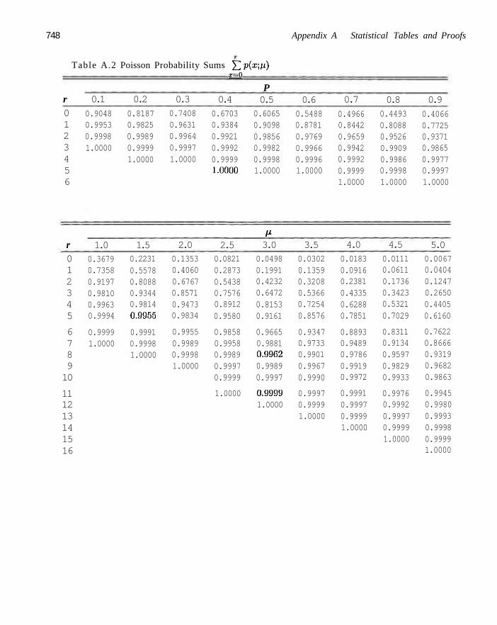
748 Appendix A Statistical Tables and Proofs
Table A.2 Poisson Probability Sums YI Pix\ M) x=0
r 0 1 2 3 4 5 6
0.1
0.9048 0.9953 0.9998 1.0000
0.2
0.8187 0.9825 0.9989 0.9999 1.0000
0.3
0.7408 0.9631 0.9964 0.9997 1.0000
0.4
0.6703 0.9384 0.9921 0.9992 0.9999 1.0000
P 0.5
0.6065 0.9098 0.9856 0.9982 0.9998 1.0000
0.6
0.5488 0.8781 0.9769 0.9966 0.9996 1.0000
0.7
0.4966 0.8442 0.9659 0.9942 0.9992 0.9999 1.0000
0.8
0.4493 0.8088 0.9526 0.9909 0.9986 0.9998 1.0000
0.9
0.4066 0.7725 0.9371 0.9865 0.9977 0.9997 1.0000
r 0 1 2 3 4 5
6 7 8 9 10
11 12 13 14 15 16
1.0 0.3679 0.7358 0.9197 0.9810 0.9963 0.9994
0.9999 1.0000
1.5 0.2231 0.5578 0.8088 0.9344 0.9814 0.9955
0.9991 0.9998 1.0000
2.0 0.1353 0.4060 0.6767 0.8571 0.9473 0.9834
0.9955 0.9989 0.9998 1.0000
2.5 0.0821 0.2873 0.5438 0.7576 0.8912 0.9580
0.9858 0.9958 0.9989 0.9997 0.9999
1.0000
M 3.0
0.0498 0.1991 0.4232 0.6472 0.8153 0.9161
0.9665 0.9881 0.9962 0.9989 0.9997
0.9999 1.0000
3.5 0.0302 0.1359 0.3208 0.5366 0.7254 0.8576
0.9347 0.9733 0.9901 0.9967 0.9990
0.9997 0.9999 1.0000
4.0
0.0183 0.0916 0.2381 0.4335 0.6288 0.7851
0.8893 0.9489 0.9786 0.9919 0.9972
0.9991 0.9997 0.9999 1.0000
4.5
0.0111 0.0611 0.1736 0.3423 0.5321 0.7029
0.8311 0.9134 0.9597 0.9829 0.9933
0.9976 0.9992 0.9997 0.9999 1.0000
5.0 0.0067 0.0404 0.1247 0.2650 0.4405 0.6160
0.7622 0.8666 0.9319 0.9682 0.9863
0.9945 0.9980 0.9993 0.9998 0.9999 1.0000
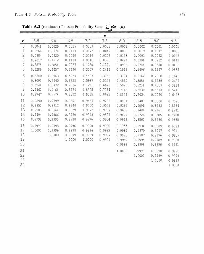
Table A.2 Poisson Probability Table 749
Table A.2 (continued) Poisson Probability Sums YL Pix'-> u) x=0
r
0 1 2 3 4 5
6 7 8 9 10
11 12 13 14 15
16 17 18 19 20
21 22 23 24
5.5 0.0041 0.0266 0.0884 0.2017 0.3575 0.5289
0.6860 0.8095 0.8944 0.9462 0.9747
0.9890 0.9955 0.9983 0.9994 0.9998
0.9999 1.0000
6.0 0.0025 0.0174 0.0620 0.1512 0.2851 0.4457
0.6063 0.7440 0.8472 0.9161 0.9574
0.9799 0.9912 0.9964 0.9986 0.9995
0.9998 0.9999 1.0000
6.5 0.0015 0.0113 0.0430 0.1118 0.2237 0.3690
0.5265 0.6728 0.7916 0.8774 0.9332
0.9661 0.9840 0.9929 0.9970 0.9988
0.9996 0.9998 0.9999 1.0000
7.0 0.0009 0.0073 0.0296 0.0818 0.1730 0.3007
0.4497 0.5987 0.7291 0.8305 0.9015
0.9467 0.9730 0.9872 0.9943 0.9976
0.9990 0.9996 0.9999 1.0000
/* 7.5
0.0006 0.0047 0.0203 0.0591 0.1321 0.2414
0.3782 0.5246 0.6620 0.7764 0.8622
0.9208 0.9573 0.9784 0.9897 0.9954
0.9980 0.9992 0.9997 0.9999
8.0
0.0003 0.0030 0.0138 0.0424 0.0996 0.1912
0.3134 0.4530 0.5925 0.7166 0.8159
0.8881 0.9362 0.9658 0.9827 0.9918
0.9963 0.9984 0.9993 0.9997 0.9999
1.0000
8.5 0.0002 0.0019 0.0093 0.0301 0.0744 0.1496
0.2562 0.3856 0.5231 0.6530 0.7634
0.8487 0.9091 0.9486 0.9726 0.9862
0.9934 0.9970 0.9987 0.9995 0.9998
0.9999 1.0000
9.0
0.0001 0.0012 0.0062 0.0212 0.0550 0.1157
0.2068 0.3239 0.4557 0.5874 0.7060
0.8030 0.8758 0.9261 0.9585 0.9780
0.9889 0.9947 0.9976 0.9989 0.9996
0.9998 0.9999 1.0000
9.5
0.0001 0.0008 0.0042 0.0149 0.0403 0.0885
0.1649 0.2687 0.3918 0.5218 0.6453
0.7520 0.8364 0.8981 0.9400 0.9665
0.9823 0.9911 0.9957 0.9980 0.9991
0.9996 0.9999 0.9999 1.0000
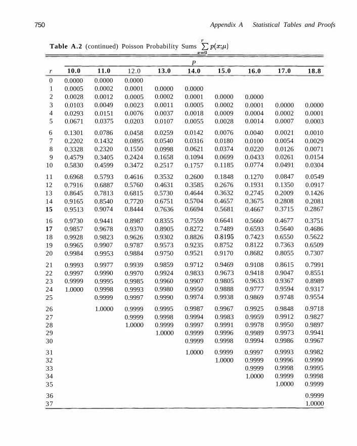
750 Appendix A Statistical Tables and Proofs
Table A.2 (continued) Poisson Probability Sums YI Pixi ll) x=0
r
0 1 2 3 4 5
6 7 8 9
10
11 12 13 14 15
16 17 18 19 20
21 22 23 24 25
26 27 28 29 30
31 32 33 34 35
36 37
10.0
0.0000 0.0005 0.0028 0.0103 0.0293 0.0671
0.1301 0.2202 0.3328 0.4579 0.5830
0.6968 0.7916 0.8645 0.9165 0.9513
0.9730 0.9857 0.9928 0.9965 0.9984
0.9993 0.9997 0.9999 1.0000
11.0 0.0000 0.0002 0.0012 0.0049 0.0151 0.0375
0.0786 0.1432 0.2320 0.3405 0.4599
0.5793 0.6887 0.7813 0.8540 0.9074
0.9441 0.9678 0.9823 0.9907 0.9953
0.9977 0.9990 0.9995 0.9998 0.9999
1.0000
12.0
0.0000 0.0001 0.0005 0.0023 0.0076 0.0203
0.0458 0.0895 0.1550 0.2424 0.3472
0.4616 0.5760 0.6815 0.7720 0.8444
0.8987 0.9370 0.9626 0.9787 0.9884
0.9939 0.9970 0.9985 0.9993 0.9997
0.9999 0.9999 1.0000
13.0
0.0000 0.0002 0.0011 0.0037 0.0107
0.0259 0.0540 0.0998 0.1658 0.2517
0.3532 0.4631 0.5730 0.6751 0.7636
0.8355 0.8905 0.9302 0.9573 0.9750
0.9859 0.9924 0.9960 0.9980 0.9990
0.9995 0.9998 0.9999 1.0000
P 14.0
0.0000 0.0001 0.0005 0.0018 0.0055
0.0142 0.0316 0.0621 0.1094 0.1757
0.2600 0.3585 0.4644 0.5704 0.6694
0.7559 0.8272 0.8826 0.9235 0.9521
0.9712 0.9833 0.9907 0.9950 0.9974
0.9987 0.9994 0.9997 0.9999 0.9999
1.0000
15.0
0.0000 0.0002 0.0009 0.0028
0.0076 0.0180 0.0374 0.0699 0.1185
0.1848 0.2676 0.3632 0.4657 0.5681
0.6641 0.7489 0.8195 0.8752 0.9170
0.9469 0.9673 0.9805 0.9888 0.9938
0.9967 0.9983 0.9991 0.9996 0.9998
0.9999 1.0000
16.0
0.0000 0.0001 0.0004 0.0014
0.0040 0.0100 0.0220 0.0433 0.0774
0.1270 0.1931 0.2745 0.3675 0.4667
0.5660 0.6593 0.7423 0.8122 0.8682
0.9108 0.9418 0.9633 0.9777 0.9869
0.9925 0.9959 0.9978 0.9989 0.9994
0.9997 0.9999 0.9999 1.0000
17.0
0.0000 0.0002 0.0007
0.0021 0.0054 0.0126 0.0261 0.0491
0.0847 0.1350 0.2009 0.2808 0.3715
0.4677 0.5640 0.6550 0.7363 0.8055
0.8615 0.9047 0.9367 0.9594 0.9748
0.9848 0.9912 0.9950 0.9973 0.9986
0.9993 0.9996 0.9998 0.9999 1.0000
18.8
0.0000 0.0001 0.0003
0.0010 0.0029 0.0071 0.0154 0.0304
0.0549 0.0917 0.1426 0.2081 0.2867
0.3751 0.4686 0.5622 0.6509 0.7307
0.7991 0.8551 0.8989 0.9317 0.9554
0.9718 0.9827 0.9897 0.9941 0.9967
0.9982 0.9990 0.9995 0.9998 0.9999
0.9999 1.0000
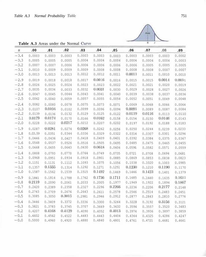
Table A.3 Normal Probability Table 751
Table A.3 Areas under the Normal Curve
.00 .01 .02 .03 .04 .05 .06 .07 .08 .09 3.4 3.3 3.2 3.1 3.0
2.9 2.8 2.7 2.6 2.5
2.4 2.3 2.2 2.1 2.0
1.9 1.8 1.7 1.6 1.5
1.4 1.3 1.2 1.1 1.0
0.9 0.8 0.7 0.6 0.5
0.4 0.3 0.2 0.1 0.0
0.0003
0.0005
0.0007
0.0010
0.0013
0.0019
0.0026
0.0035
0.0047 0.0062
0.0082
0.0107 0.0139
0.0179
0.0228
0.0287
0.03.59
0.0446 0.0548
0.0668
0.0808 0.0968
0.1151
0.1357 0.1587
0.1841 0.2119
0.2420
0.2743 0.3085
0.3446
0.3821
0.4207
0.4602 0.5000
0.0003
0.0005
0.0007
0.0009
0.0013
0.0018
0.0025 0.0034
0.0045
0.0060
0.0080 0.0104
0.0136 0.0171
0.0222
0.0281
0.0351
0.0436 0.0537
0.0655
0.0793
0.0951
0.1131
0.1335
0.1562
0.1814
0.2090
0.2389
0.2709 0.3050
0.3409
0.3783
0.4168 0.4562
0.4960
0.0003
0.0005
0.0006
0.0009
0.0013
0.0018
0.0024
0.0033 0.0044
0.0059
0.0078
0.0102 0.0132
0.0170
0.0217
0.0274
0.0344
0.0427 0.0526 0.0643
0.077S
0.0934
0.1112
0.1314 0.1539
0.1788 0.2061
0.2358
0.2676 0.3015
0.3372
0.3745 0.4 L29
0.4522 0.4920
0.0003
0.0004
0.0006
0.0009 0.0012
0.0017
0.0023
0.0032
0.0043
0.0057
0.0075 0.0099
0.0129
0.0166 0.0212
0.0208
0.0336
0.0418
0.0516 0.0630
0.0764
0.0918
0.1093 0.1292
0.1515
0.1762
0.2033
0.2327
0.2643
0.2981
0.3336
0.3707
0.4090
0.4483 0.4880
0.0003
0.0004
0.0006
0.0008 0.0012
0.00 IG
0.0023
0.(1031 0.0041
0.0055
0.0073
0.0096 0.0125
0.0162
0.0207
0.0262
0.0329
0.0409
0.0505
0.0018
0.0749
0.0901
0.1075
0.1271
0.1192
0.1736
0.2005
0.2296
0.2611 0.2946
0.3300
0.3669
0.4052
0.4443 0.4840
0.0003 0.0004
0.0006 0.0008
0.0011
0.0016
0.0022
0.0030 0.0040
0.0054
0.0071 0.0094
0.0122
0.0158 0.0202
0.0256 0.0322
0.0401
0.0495 0.0606
0.0735
0.0885
0.1056 0.1251
0.1469
0.1711
0.1977
0.2206
0.2578 0.2912
0.3264
0.3632
0.4013 0.4404
0.4801
0.0003
0.0004
0.0006 0.0008
0.0011
0.0015
0.0021 0.0029
0.0039
0.0052
0.0069
0.0091
0.0119
0.0154
0.0197
0.0250
0.0314
0.0392
0.0485
0.0591
0.0721
0.0869
0.1038
11.1230
0.1446
0.1685
0.1949
0.2236
0.2546 0.2877
0.3228
0.3594
0.3974
0.4364
0.4761
0.0003
0.0004
0.0005
0.0008
0.0011
0.0015
0.0021
0.0028 0.0038
0.0051
0.0068
0.0089
0.0110
0.0150 0.0192
0.0244
0.0307
0.0384
0.0475
0.0582
0.0708 0.0853
0.1020
0.1210
0.1423
0.1660 0.1922
0.2206
0.2514
0.2843
0.3192
0.3557 0.3936
0.4325 0.4721
0.0003
0.0004
0.0005
0.0007
0.0010
0.0(114
0.0020
0.0027
0.0037
0.0049
0.0066
0.0087
0.0113
0.0146
0.0188
0.0239 0.0301
0.0375
0.0465 0.0571
0.0694
0.0838
0.1003 0.1190
0.1401
0.1635 0.1894
0.2177
0.2483 0.2810
0.3156
0.3520
0.3897
0.4286
0.4681
0.0002
0.0003
0.0005
0.0007
0.0010
0.001 1
0.0019
0.0026 0.0036
0.0048
0.0064 0.0084
0.0110
0.0143
0.0183
0.0233
0.0294
0.0367
0.0455
0.0559
0.0681 0.0823
0.0985
0.1170
0.1379
0.1611
0.1807
0.2148
0.2451 0.2776
0.3121 0.3483
0.3859
0.4247 0.4641
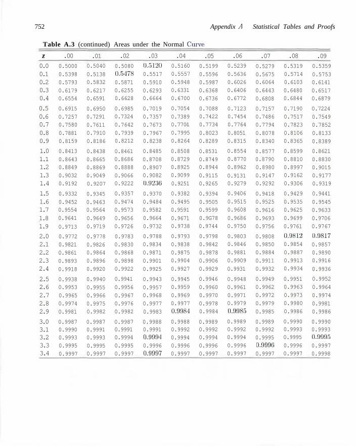
752 Appendix A Statistical Tables and Proofs
Table A.3 (continued) Areas under the Normal Curve:
z 0.0 0.1 0.2 0.3 0.4
0.5 0.6 0.7 0.8 0.9
1.0 1.1 1.2 1.3 1.4
1.5 1.6 1.7 1.8 1.9
2.0 2.1 2.2 2.3 2.4
2.5 2.6 2.7 2.8 2.9
3.0 3.1 3.2 3.3 3.4
.00
0.5000
0.5398
0.5793
0.6179 0.6554
0.6915
0.7257 0.7580
0.7881
0.8159
0.8413
0.8643 0.8849
0.9032
0.9192
0.9332
0.9452 0.9554
0.9641
0.9713
0.9772
0.9821
0.9861
0.9893
0.9918
0.9938 0.9953
0.9965
0.9974
0.9981
0.9987 0.9990 0.9993
0.9995
0.9997
.01
0.5040
0.5138 0.5832
0.6217 0.6591
0.6950 0.7291
0.7611
0.7910
0.8186
0.8438
0.8665
0.8869
0.9049
0.9207
0.9345
0.9463 0.9564
0.9649
0.9719
0.9778
0.9826 0.9864
0.9896
0.9920
0.9940
0.9955
0.9966
0.9975 0.9982
0.9987 0.9991 0.9993
0.9995 0.9997
.02
0.5080
0.5478
0.5871
0.6255 0.6628
0.6985 0.7324
0.7642
0.7939 0.8212
0.8461 0.8686
0.8888
0.9066 0.9222
0.9357
0.9474
0.9573
0.9656
0.9726
0.9783
0.9830
0.9868
0.9898
0.9922
0.9941
0.9956
0.9967
0.9976
0.9982
0.9987 0.9991 0.9994
0.9995
0.9997
.03
0.5120
0.5517
0.5910
0.6293 0.6664
0.7019
0.7357
0.7673
0.7967 0.8238
0.8485
0.8708
0.8907 0.9082
0.1)236
0.9370
0.9484
0.9582
0.9664
0.9732
0.9788
0.9834
0.9871
0.9901
0.9925
0.9943
0.9957 0.9968
0.9977
0.9983
0.9988 0.9991 0.0994
0.9996
0.9097
.04
0.5160
0.5557
0.5948
0.6331
0.6700
0.7054
0.7389 0.7701
0.7995
0.8264
0.8508
0.8729 0.8925
0.9099
0.9251
0.9382
0.9495
0.9591
0.9671 0.9738
0.9793
0.9838
0.9875 0.9904
0.9927
0.9945 0.9959
0.9969
0.9977
0.9984
0.9988 0.9992
0.9994
0.9996
0.9997
.05
0.5199
0.5596
0.5987
0.6368
0.6736
0.7088 0.7422
0.7734
0.8023
0.8289
0.8531
0.8749 0.8944
0.9115
0.9265
0.9394
0.9505 0.9599
0.9G78
0.9744
0.9798
0.9842
0.9878
0.9906
0.9929
0.9946
0.9960
0.9970
0.9978 0.9984
0.9989 0.9992 0.9994
0.9996
0.9997
.06
0.5239
0.5636
0.6026
0.6406
0.6772
0.7123 0.7454
0.7764
0.8051
0.8315
0.8554
0.8770
0.8962
0.9131 0.9279
0.9406
0.9515
0.9608
0.9686
0.9750
0.9803 0.9846
0.9881
0.9909
0.9931
0.9948
0.9961
0.9971 0.9979
0.9985
0.9989 0.9992 0.9994
0.9996
0.9997
.07
0.5279
0.5675 0.6064
0.6443
0.6808
0.7157 0.7486
0.7794
0.8078
0.8340
0.8577 0.8790
0.8980
0.9147 0.9292
0.9418
0.9525
0.9616
0.9693
0.9756
0.9808 0.9850
0.9884
0.9911
0.9932
0.9949
0.9962
0.9972
0.9979
0.9985
0.9989 0.9992
0.9995
0.9996
0.9997
.08
0.5319
0.5714
0.6103
0.6480 0.6844
0.7190
0.7517
0.7823
0.8106
0.8365
0.8599
0.8810
0.8997 0.9162
0.9306
0.9429
0.9535
0.9625
0.9699
0.9761
0.9812
0.9854
0.9887
0.9913
0.9934
0.9951 0.9963
0.9973
0.9980
0.9986
0.9990 0.9993 0.9995
0.9996
0.9997
.09
0.5359
0.5753 0.6141
0.6517 0.6879
0.7224
0.7549
0.7852
0.8133
0.8389
0.8621
0.8830
0.9015
0.9177
0.9319
0.9441
0.9545
0.9633
0.9706
0.9767
0.9817
0.9857
0.9890 0.9916
0.9936
0.9952
0.9964
0.9974
0.9981
0.9986
0.9990 0.9993 0.9995
0.9997
0.9998
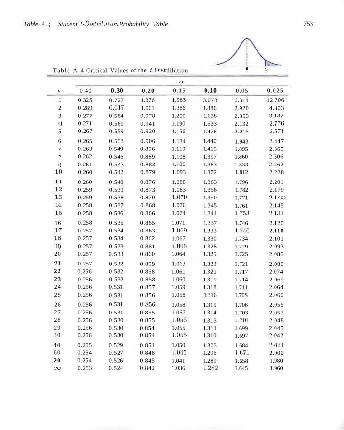
Table A.4 Student t-Distribtiiion Probability Table 753
T a b l e A . 4 Critical Values
v
1 2 3 1
5
6 7 8
i) 10
11 12 13 11 15
16 17 IS 1!) 20
21 22 23 24 25
26 27 28 29 30
40 60
120 CO
0.40
0.325 0.289 0.277 0.271 0.267
0.265 0.263 0.262 0.261 0.260
0.260 0.259 0.259 0.258 0.258
0.258 0.257 0.257 0.257 0.257
0.257 0.256 0.256 0.256 0.256
0.256 0.256 0.256 0.256 0.256
0.255 0.254 0.254 0.253
0.30
0.727 0.617 0.584 0.569 0.559
0.553 0.549 0.546 0.543 0.542
0.540 0.539 0.538 0.537 0.536
0.535 0.534 0.534 0.533 0.533
0.532 0.532 0.532 0.531
0.531
0.531
0.531 0.530 0.530 0.530
0.529 0.527 0.526 0.524
of the f-Dist;
0.20
1.376 1.061 0.978 0.941 0.920
0.906 0.896 0.889 0.883 0.879
0.876 0.873 0.870 0.868 0.866
0.865 0.863 0.862 0.861 0.860
0.859 0.858 0.858 0.857 0.856
0.850 0.855 0.855 0.854 0.854
0.851 0.848 0.845 0.842
dilution
Q
0.15
1.963 1.386 1.250 1.190 1.156
1.134 1.119 1.108 1.100 1.093
1.088 1.083 1.079 1.076 1.074
1.071 1.069 1.067 1.1)66 1.064
1.063 1.061 1.060 1.059 1.058
1.058 1.057 1.056 1.055 1.055
1.050 1.015 1.041 1.036
0.10
3.078 1.886 1.638 1.533 1.476
1.440 1.415 1.397 1.383 1.372
1.363 1.356 1.350 1.345 1.341
1.337 1.333 1.330 1.328 1.325
1.323 1.321 1.319 1.318 1.316
1.315 1.314
1.313 1.311 1.310
1.303 1.296 1.289 1.282
0
0.05
6.314 2.920 2.353 2.132 2.015
1.943 1.895 1.860 1.833 1.812
1.796 1.782 1.771 1.761 1,753
1.746 1.740 1.734 1.729 1.725
1.721 1.717 1.714 1.711 1.70S
1.706 1.703 1.701 1.699 1.697
1.684 1.671 1.658 1.645
;,
0 .025
12.706 4.303 3.182 2.770 2.571
2.447 2.365 2.306 2.262 2.228
2.201 2.179 2.1 GO 2.145 2.131
2.120 2.110 2.101 2.093 2.086
2.080 2.074 2.069 2.064 2.060
2.056 2.052 2.048 2.045 2.042
2.021 2.000 1.980 1.960
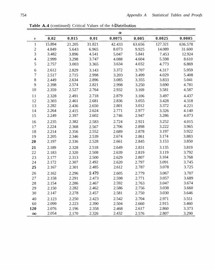
754 Appendix A Statistical Tables and Proofs
Table A.4 (continued) Critical Values of the f-Distribution
V
1 2 3 4 5
6 7 8 9
10
11 12 13 14 15
16 17 18 19 20
21 22 23 24 25
26 27 28 29 30
40 60
120 CO
0.02 15.894 4.849 3.482 2.999 2.757
2.612 2.517 2.449 2.398 2.359
2.328 2.303 2.282 2.264 2.249
2.235 2.224 2.214 2.205 2.197
2.189 2.183 2.177 2.172 2.167
2.162 2.158 2.154 2.150 2.147
2.123 2.099 2.076 2.054
0.015
21.205 5.643 3.896 3.298 3.003
2.829 2.715 2.634 2.574 2.527
2.491 2.461 2.436 2.415 2.397
2.382 2.368 2.356 2.346 2.336
2.328 2.320 2.313 2.307 2.301
2.296 2.291 2.286 2.282 2.278
2.250 2.223 2.196 2.170
0.01 31.821 6.965 4.541 3.747 3.365
3.143 2.998 2.896 2.821 2.764
2.718 2.681 2.650 2.624 2.602
2.583 2.567 2.552 2.539 2.528
2.518 2.508 2.500 2.492 2.485
2.479 2.473 2.467 2.462 2.457
2.423 2.390 2.358 2.326
a 0.0075
42.433 8.073 5.047 4.088 3.634
3.372 3.203 3.085 2.998 2.932
2.879 2.836 2.801 2.771 2.746
2.724 2.706 2.689 2.674 2.661
2.649 2.639 2.629 2.620 2.612
2.605 2.598 2.592 2.586 2.581
2.542 2.504 2.468 2.432
0.005 63.656 9.925 5.841 4.604 4.032
3.707 3.499 3.355 3.250 3.169
3.106 3.055 3.012 2.977 2.947
2.921 2.898 2.878 2.861 2.845
2.831 2.819 2.807 2.797 2.787
2.779 2.771 2.763 2.756 2.750
2.704 2.660 2.617 2.576
0.0025 127.321
14.089 7.453 5.598 4.773
4.317 4.029 3.833 3.690 3.581
3.497 3.428 3.372 3.326 3.286
3.252 3.222 3.197 3.174 3.153
3.135 3.119 3.104 3.091 3.078
3.067 3.057 3.047 3.038 3.030
2.971 2.915 2.860 2.807
0.0005
636.578 31.600 12.924 8.610 6.869
5.959 5.408 5.041 4.781 4.587
4.437 4.318 4.221 4.140 4.073
4.015 3.965 3.922 3.883 3.850
3.819 3.792 3.768 3.745 3.725
3.707 3.689 3.674 3.660 3.646
3.551 3.460 3.373 3.290
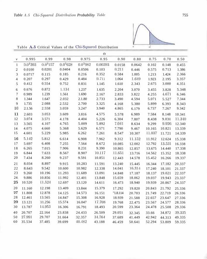
Table A.5 Chi-Squ-ared Distribution. Probability Tabic 755
T a b l e A . 5 Critical Values of the Chi-Squared Distribution 0 A
a
v 0 .995 0.99 0 .98 0 .975 0 .95 0 .90 0 .80 0 .75 0 .70 0 .50
1 2 3 4 5
6 7 8 9
10
11 12 13 14 15
16 17 18 19 20
21 22 23 24 25
20 27 28 29 30
40 50 60
0.04393 0.0100 0.0717 0.207 0.412
0.676 0.989 1.344 1.735 2.1.56
2.603 3.074 3.565 4.075 4.601
5.142 5.697 6.265 6.844 7.434
8.034 8.643 9.260 9.886
10.520
11.160 11.808 12.461 13.121 13.787
20.707 27.991 35.534
().()3157 0.0201
0.115 0.297 0.554
0.872 1.239 1.647 2.088 2.558
3.053 3.571 4.107 4.660 5.229
5.812 6.408 7.015 7.633 8.260
8.897 9.542
10.196 10.856 11.524
12.198 12.878 13.565 11.256 14.953
22.164 29.707 37.485
0.03628 0.0404 0.185 0.429 0.752
1.134 1.561 2.032 2.532 3.059
3.609 4.178 4.765 5.368 5.985
6.614 7.255 7.906 8.567 9.237
9.915 10.600 11.293 11.992 12.697
13.409 14.125 14.847 15.574 16.306
23.838 31.664 39.699
0.03982 0.0506 0.216 0.484 0.831
1.237 1.690 2.1.80 2.700 3.247
3.816 4.404 5.009 5.629 6.262
6.908 7.564 8.231 8.907 9.591
10.283 10.982 11.689 12.401 13.120
13.844 14.573 15.308 16.047 16.791
24.433 32.357 40,182
0.00393 0.103 0.352 11.71 1 1.145
1.635 2.167 2.733 3.325 3.940
4.575
5.226 5.892 6.571 7.261
7.962 8.672 9.390
10.117 10.851
11.591 12.338 13.091 13.848 14.611
15.379 16.151 16.928 17.708 18.493
26.509 34.764 43.188
0.0158 0.211 0.584 1.064 1.610
2.204 2.833 3.490 4.168 4.865
5.578 6.304 7.041 7.790 8.547
9.312 10.085 10.865 11.651 12.443
13.240 14.041 14.848 15.659 16.473
17.292 "1.8.114 18.939 19.768 20.599
29.051 37.689 46.459
0.0642 0.446 1.005 1.649 2.343
3.070 3.822 4.594 5.380 6.179
6.989
7.807 8.634 9.467
10.307
11.152 12.002 12.857 13.716 14.578
15.445 16.311 17.187 18.062 18.940
19.820 20.703 21.588 22.475 23.364
32.345 41.449 50.641
0.102 0.575 1.213 1.923 2.675
3.455 4.255 5.071 5.899 6.737
7.584 8.438 9.299
10.165 11.037
11.912 12.792 13.675 14.562 15.452
16.344 17.240 18.137 19.037 19.939
20.843 21.749 22.657 23.567 24.478
33.66 42.942 52.294
0.148 0.713 1.424 2.195 3.000
3.828 4.671 5.527 6.393 7.267
8.148 9.031 9.926
10.821 11.721
12.624 13.531 14.440 15.352 16.266
17.182 18.101 19.021 19.943 20.867
21.792 22.719 23.647 24.577 25.508
34.872 44.313 53.809
0.455 1.386 2.366 3.357 4.351
5.348 6.346 7.344 8.343 9.342
10.341 11.340 12.340 13.339 14.339
15.338 16.338 17.338 18.338 19.337
20.337 21.337 22.337 23.337 24.337
25.336 26.336 27.336 28.336 29.336
39.335 49.335 59.335
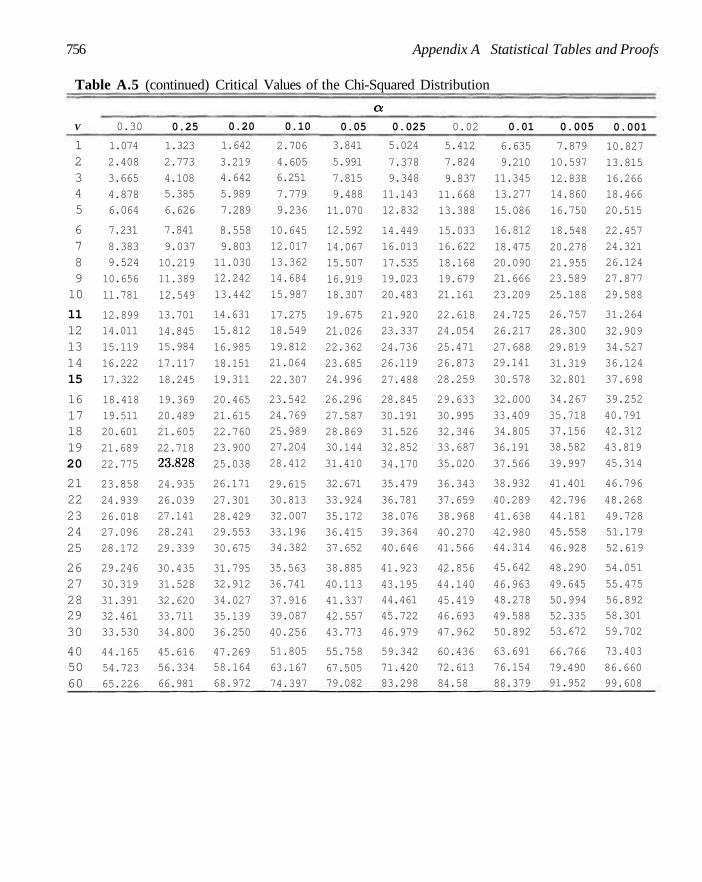
756 Appendix A Statistical Tables and Proofs
Table A.5 (continued) Critical Values of the Chi-Squared Distribution
V
1 2 3 4 5
6 7 8 9 10
11 12 13 14 15
16 17 18 19 20
21 22 23 24 25
26 27 28 29 30
40 50 60
0.30
1.074
2.408
3.665
4.878 6.064
7.231
8.383
9.524
10.656
11.781
12.899 14.011
15.119
16.222
17.322
18.418
19.511
20.601
21.689
22.775
23.858
24.939
26.018 27.096
28.172
29.246
30.319
31.391 32.461
33.530
44.165
54.723
65.226
0.25
1.323
2.773
4.108 5.385
6.626
7.841
9.037
10.219
11.389
12.549
13.701
14.845 15.984
17.117
18.245
19.369
20.489
21.605
22.718
23-828
24.935
26.039 27.141
28.241
29.339
30.435
31.528
32.620 33.711
34.800
45.616 56.334
66.981
0.20
1.642
3.219 4.642
5.989
7.289
8.558
9.803
11.030 12.242
13.442
14.631
15.812
16.985
18.151
19.311
20.465
21.615
22.760
23.900
25.038
26.171
27.301
28.429 29.553
30.675
31.795 32.912
34.027
35.139
36.250
47.269 58.164
68.972
0.10
2.706
4.605 6.251
7.779
9.236
10.645
12.017
13.362
14.684
15.987
17.275 18.549
19.812
21.064
22.307
23.542
24.769
25.989 27.204
28.412
29.615
30.813
32.007
33.196 34.382
35.563
36.741
37.916 39.087
40.256
51.805
63.167
74.397
0.05
3.841
5.991
7.815
9.488
11.070
12.592
14.067
15.507
16.919 18.307
19.675
21.026
22.362
23.685
24.996
26.296
27.587
28.869 30.144
31.410
32.671
33.924
35.172
36.415 37.652
38.885
40.113
41.337 42.557
43.773
55.758
67.505 79.082
a 0.025
5.024
7.378
9.348
11.143
12.832
14.449
16.013
17.535
19.023
20.483
21.920
23.337
24.736
26.119
27.488
28.845
30.191
31.526 32.852
34.170
35.479
36.781
38.076 39.364
40.646
41.923
43.195 44.461
45.722
46.979
59.342
71.420 83.298
0.02
5.412
7.824
9.837
11.668
13.388
15.033
16.622
18.168
19.679
21.161
22.618
24.054
25.471
26.873
28.259
29.633
30.995
32.346 33.687
35.020
36.343
37.659
38.968
40.270 41.566
42.856
44.140
45.419 46.693
47.962
60.436
72.613 84.58
0.01
6.635
9.210
11.345
13.277
15.086
16.812
18.475
20.090 21.666
23.209
24.725
26.217
27.688 29.141
30.578
32.000
33.409
34.805
36.191
37.566
38.932
40.289
41.638
42.980 44.314
45.642
46.963 48.278
49.588
50.892
63.691
76.154
88.379
0.005
7.879
10.597
12.838 14.860
16.750
18.548
20.278
21.955 23.589
25.188
26.757
28.300
29.819
31.319
32.801
34.267
35.718 37.156
38.582
39.997
41.401
42.796
44.181
45.558
46.928
48.290
49.645
50.994
52.335 53.672
66.766
79.490 91.952
0.001
10.827
13.815
16.266 18.466
20.515
22.457
24.321
26.124
27.877
29.588
31.264
32.909
34.527
36.124
37.698
39.252
40.791 42.312
43.819
45.314
46.796
48.268
49.728
51.179
52.619
54.051
55.475
56.892 58.301
59.702
73.403
86.660 99.608
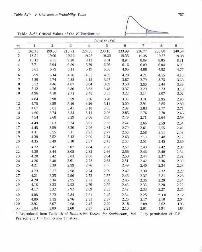
Table A.(> F-Distribution Probability Table
Table A.6* Critical Values of the F-Distribution
757
fo.or,ici,i>2) Vi
1 161.45 199.50 2 18.51 19.00 3 10.13 9.55 4 7.71 6.94 5 6.61 5.79
6 5.99 5.14 7 5.59 4.74 8 5.32 4.46 9 5.12 4.26
10 4.96 4.10
11 4.84 3.98 12 4.75 3.89 13 4.67 3.81 14 4.60 3.74 15 4.54 3.68
16 4.49 3.63 17 4.45 3.59 18 1.41 3.55 19 4.38 3.52 20 4.35 3.49
21 4.32 3.47 22 4.30 3.44 23 4.28 3.42 24 4.26 3.40 25 4.21 3.39
26 4.23 3.37 27 4.21 3.35 28 4.20 3.34 29 4.18 3.33 30 4.17 3.32
40 4.08 3.23 60 4.00 3.15
120 3.92 3.07 oc. 3.84 3.00
* Reproduced from Table
215.71 19.16 9.28 6.59 5,11
4.76 4.35 4.07 3.86 3.71
3.59 3.49 3.41 3.34 3.29
3.24 3.20 3.16 3.13 3.10
3.07 3.05 3.03 3.01 2.99
2.98 2.96 2.95 2.93 2.92
2.84 2.76 2.68 2.60
18 of Biomt Pearson and the Biometrika Trustees.
224.58 19.25 9.12 6.39 5.19
4.53 4.12 3.84 3.63 3.48
3.36 3.26 3.18 3.11 3.06
3.01 2.96 2.93 2.90 2.87
2.84 2.82 2.80 2.78 2.76
2.74 2.73 2.71 2.70 2.69
2.61 2.53 2.45 2.37
trika Table
230.16 233.99 19.30 19.33 9.0J 8.94 6.26 6.16 5.05 4.95
4.39 4.28 3.97 3.87 3.69 3.58 3.48 3.37 3.33 3.22
3.20 3.09 3.11 3.00 3.03 2.92 2.96 2.85 2.90 2.79
2.85 2.74 2.81 2.70 2.77 2.66 2.74 2.63 2.71 2.60
2.68 2,57 2.66 2,55 2.64 2,53 2.62 2,51 2.GO 2.49
2,59 2.47 2,57 2.46 2.56 2.45 2.55 2.43 2,53 2.42
2.45 2.34 2.37 2.25 2.29 2.18 2.21 2.10
> for Statisticians, Vo
236.77 19.35 8.89 6.09 4.88
4.21 3.79 3.50 3.29 3.14
3.01 2.91 2.83 2.76 2.71
2.66 2,61 2.58 2.5-1 2.51
2.49 2.46 2.44 2.42 2.40
2.39 2.37 2.36 2.35 2.33
2.25 2.17 2.09 2.01
. I. by
238.88 19.37 8.85 6.04 4.82
4.15 3.73 3.44 3.23 3.07
2.95 2.85 2.77 2.70 2.64
2,59 2,55 2,51 2.48 2.45
2.42 2.40 2.37 2.36 2.34
2.32 2,31 2.29 2.28 2.27
2. J 8 2.10 2.02 1.94
permission
240.54 19.38 8.81 6.00 4.77
4.10 3.68 3.39 3.18 3.02
2.90 2.80 2.71 2.65 2,59
2,54 2.49 2.46 2,12 2.39
2.37 2.34 2.32 2.30 2.28
2.27 2.25 2.24 2.22 2.21
2.12 2.04 1.96 1.88
of E S .
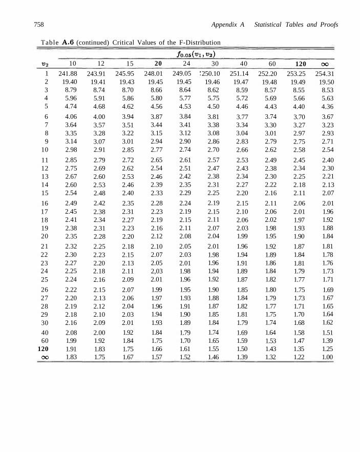
758 Appendix A Statistical Tables and Proofs
Table A.6 (continued) Critical Values of the F-Distribution
v2
1 2 3 4 5
6 7 8 9
10
11 12 13 14 15
16 17 18 19 20
21 22 23 24 25
26 27 28 29 30
40 60
120 CO
10
241.88 19.40 8.79 5.96 4.74
4.06 3.64 3.35 3.14 2.98
2.85 2.75 2.67 2.60 2.54
2.49 2.45 2.41 2.38 2.35
2.32 2.30 2.27 2.25 2.24
2.22 2.20 2.19 2.18 2.16
2.08 1.99 1.91 1.83
12
243.91 19.41 8.74 5.91 4.68
4.00 3.57 3.28 3.07 2.91
2.79 2.69 2.60 2.53 2.48
2.42 2.38 2.34 2.31 2.28
2.25 2.23 2.20 2.18 2.16
2.15 2.13 2.12 2.10 2.09
2.00 1.92 1.83 1.75
15
245.95 19.43 8.70 5.86 4.62
3.94 3.51 3.22 3.01 2.85
2.72 2.62 2.53 2.46 2.40
2.35 2.31 2.27 2.23 2.20
2.18 2.15 2.13 2.11 2.09
2.07 2.06 2.04 2.03 2.01
1.92 1.84 1.75 1.67
20
248.01 19.45 8.66 5.80 4.56
3.87 3.44 3.15 2.94 2.77
2.65 2.54 2.46 2.39 2.33
2.28 2.23 2.19 2.16 2.12
2.10 2.07 2.05 2,03 2.01
1.99 1.97 1.96 1.94 1.93
1.84 1.75 1.66 1.57
/ o . 0 5 ( ^ 1
24
249.05 1 19.45 8.64 5.77 4.53
3.84 3.41 3.12 2.90 2.74
2.61 2.51 2.42 2.35 2.29
2.24 2.19 2.15 2.11 2.08
2.05 2.03 2.01 1.98 1.96
1.95 1.93 1.91 1.90 1.89
1.79 1.70 1.61 1.52
, « 2 )
30
250.10 19.46 8.62 5.75 4.50
3.81 3.38 3.08 2.86 2.70
2.57 2.47 2.38 2.31 2.25
2.19 2.15 2.11 2.07 2.04
2.01 1.98 1.96 1.94 1.92
1.90 1.88 1.87 1.85 1.84
1.74 1.65 1.55 1.46
40
251.14 19.47 8.59 5.72 4.46
3.77 3.34 3.04 2.83 2.66
2.53 2.43 2.34 2.27 2.20
2.15 2.10 2.06 2.03 1.99
1.96 1.94 1.91 1.89 1.87
1.85 1.84 1.82 1.81 1.79
1.69 1.59 1.50 1.39
60
252.20 19.48 8.57 5.69 4.43
3.74 3.30 3.01 2.79 2.62
2.49 2.38 2.30 2.22 2.16
2.11 2.06 2.02 1.98 1.95
1.92 1.89 1.86 1.84 1.82
1.80 1.79 1.77 1.75 1.74
1.64 1.53 1.43 1.32
120 253.25
19.49 8.55 5.66 4.40
3.70 3.27 2.97 2.75 2.58
2.45 2.34 2.25 2.18 2.11
2.06 2.01 1.97 1.93 1.90
1.87 1.84 1.81 1.79 1.77
1.75 1.73 1.71 1.70 1.68
1.58 1.47 1.35 1.22
CO
254.31 19.50 8.53 5.63 4.36
3.67 3.23 2.93 2.71 2.54
2.40 2.30 2.21 2.13 2.07
2.01 1.96 1.92 1.88 1.84
1.81 1.78 1.76 1.73 1.71
1.69 1.67 1.65 1.64 1.62
1.51 1.39 1.25 1.00
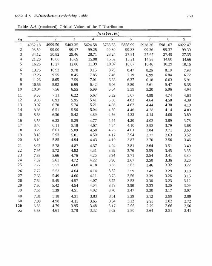
Table A.6 F-Distribution Probability Table 759
Table A.6 (continued) Critical Values of the F-Distribution
v2
1 2 3 4 5
6 7 8 9
10
11 12 13 14 15
16 17 18 19 20
21 22 23 24 25
26 27 28 29 30
40 60
120 CO
1
4052.18 98.50 34.12 21.20 16.26
13.75 12.25 11.26 10.56 10.04
9.65 9.33 9.07 8.86 8.68
8.53 8.40 8.29 8.18 8.10
8.02 7.95 7.88 7.82 7.77
7.72 7.68 7.64 7.60 7.56
7.31 7.08 6.85 6.63
2
4999.50 99.00 30.82 18.00 13.27
10.92 9.55 8.65 8.02 7.56
7.21 6.93 6.70 6.51 6.36
6.23 6.11 6.01 5.93 5.85
5.78 5.72 5.66 5.61 5.57
5.53 5.49 5.45 5.42 5.39
5.18 4.98 4.79 4.61
3
5403.35 99.17 29.46 16.69 12.06
9.78 8.45 7.59 6.99 6.55
6.22 5.95 5.74 5.56 5.42
5.29 5.18 5.09 5.01 4.94
4.87 4.82 4.76 4.72 4.68
4.64 4.60 4.57 4.54 4.51
4.31 4.13 3.95 3.78
fo.oiivi,v2) 4
5624.58 99.25 28.71 15.98 11.39
9.15 7.85 7.01 6.42 5.99
5.67 5.41 5.21 5.04 4.89
4.77 4.67 4.58 4.50 4.43
4.37 4.31 4.26 4.22 4.18
4.14 4.11 4.07 4.04 4.02
3.83 3.65 3.48 3.32
5
5763.65 99.30 28.24 15.52 10.97
8.75 7.46 6.63 6.06 5.64
5.32 5.06 4.86 4.69 4.56
4.44 4.34 4.25 4.17 4.10
4.04 3.99 3.94 3.90 3.85
3.82 3.78 3.75 3.73 3.70
3.51 3.34 3.17 3.02
6
5858.99 99.33 27.91 15.21 10.67
8.47 7.19 6.37 5.80 5.39
5.07 4.82 4.62 4.46 4.32
4.20 4.10 4.01 3.94 3.87
3.81 3.76 3.71 3.67 3.63
3.59 3,56 3.53 3.50 3.47
3.29 3.12 2.96 2.80
7
5928.36 99.36 27.67 14.98 10.46
8.26 6.99 6.18 5.61 5.20
4.89 4.64 4.44 4.28 4.14
4.03 3.93 3.84 3.77 3.70
3.64 3.59 3.54 3.50 3.46
3.42 3.39 3.36 3.33 3.30
3.12 2.95 2.79 2.64
8
5981.07 99.37 27.49 14.80 10.29
8.10 6.84 6.03 5.47 5.06
4.74 4.50 4.30 4.14 4.00
3.89 3.79 3.71 3.63 3.56
3.51 3.45 3.41 3.36 3.32
3.29 3.26 3.23 3.20 3.17
2.99 2.82 2.66 2.51
9
6022.47 99.39 27.35 14.66 10.16
7.98 6.72 5.91 5.35 4.94
4.63 4.39 4.19 4.03 3.89
3.78 3.68 3.60 3.52 3.46
3.40 3.35 3.30 3.26 3.22
3.18 3.15 3.12 3.09 3.07
2.89 2.72 2,56 2.41
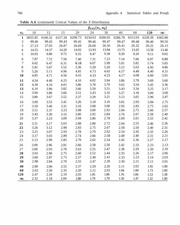
760 Appendix A Statistical Tables and Proofs
Table A.6 (continued) Critical Values of the F-Distribution
v2
1 2 3 4 5
6 7 8 9
10
11 12 13 14 15
16 17 18 19 20
21 22 23 24 25
26 27 28 29 30
40 60
120 CO
10
6055.85 99.40 27.23 14.55 10.05
7.87 6.62 5.81 5.26 4.85
4.54 4.30 4.10 3.94 3.80
3.69 3.59 3.51 3.43 3.37
3.31 3.26 3.21 3.17 3.13
3.09 3.06 3.03 3.00 2.98
2.80 2.63 2.47 2.32
12
6106.32 99.42 27.05 14.37 9.89
7.72 6.47 5.67 5.11 4.71
4.40 4.16 3.96 3.80 3.67
3.55 3.46 3.37 3.30 3.23
3.17 3.12 3.07 3.03 2.99
2.96 2.93 2.90 2.87 2.84
2.66 2.50 2.34 2.18
15
6157.28 99.43 26.87 14.20 9.72
7.56 6.31 5.52 4.96 4.56
4.25 4.01 3.82 3.66 3.52
3.41 3.31 3.23 3.15 3.09
3.03 2.98 2.93 2.89 2.85
2.81 2.78 2.75 2.73 2.70
2.52 2.35 2.19 2.04
20
6208.73 99.45 26.69 14.02 9.55
7.40 6.16 5.36 4.81 4.41
4.10 3.86 3.66 3.51 3.37
3.26 3.16 3.08 3.00 2.94
2.88 2.83 2.78 2.74 2.70
2.66 2.63 2.60 2.57 2.55
2.37 2.20 2.03 1.88
/0.0lC"l! 24
,v2) 30
6234.63 6260.65 99.46 26.60 13.93 9.47
7.31 6.07 5.28 4.73 4.33
4.02 3.78 3.59 3.43 3.29
3.18 3.08 3.00 2.92 2.86
2.80 2.75 2.70 2.66 2.62
2.58 2.55 2.52 2.49 2.47
2.29 2.12 1.95 1.79
99.47 26.50 13.84 9.38
7.23 5.99 5.20 4.65 4.25
3.94 3.70 3.51 3.35 3.21
3.10 3.00 2.92 2.84 2.78
2.72 2.67 2.62 2.58 2.54
2.50 2.47 2.44 2.41 2.39
2.20 2.03 1.86 1.70
40
6286.78 99.47 26.41 13.75 9.29
7.14 5.91 5.12 4.57 4.17
3.86 3.62 3.43 3.27 3.13
3.02 2.92 2.84 2.76 2.69
2.64 2.58 2.54 2.49 2.45
2.42 2.38 2.35 2.33 2.30
2.11 1.94 1.76 1.59
60
6313.03 99.48 26.32 13.65 9.20
7.06 5.82 5.03 4.48 4.08
3.78 3.54 3.34 3.18 3.05
2.93 2.83 2.75 2.67 2.61
2.55 2.50 2.45 2.40 2.36
2.33 2.29 2.26 2.23 2.21
2.02 1.84 1.66 1.47
120 6339.39
99.49 26.22 13.56 9.11
6.97 5.74 4.95 4.40 4.00
3.69 3.45 3.25 3.09 2.96
2.84 2.75 2.66 2.58 2.52
2.46 2.40 2.35 2.31 2.27
2.23 2.20 2.17 2.14 2.11
1.92 1.73 1.53 1.32
CO
6365.86 99.50 26.13 13.46 9.02
6.88 5.65 4.86 4.31 3.91
3.60 3.36 3.17 3.00 2.87
2.75 2.65 2.57 2.49 2.42
2.36 2.31 2.26 2.21 2.17
2.13 2.10 2.06 2.03 2.01
1.80 1.60 1.38 1.00
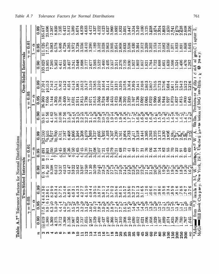
Table A. 7 Tolerance Factors for Normal Distributions 761
e*-
f-
0 0 « 0 0 » . X i O M O O C N S O O N O C N O O N M
T - i r ^ C 5 0 i o - * " t r c o ' c o CO <-*
a i . o o e N r H e s t - H o o o o s N M e N o i o N ' ^ t c o o N N N i H T t N W H a f f l T ' o ^ i N C l O O O S O r H O O T l ' ^ f f l N N a N S D O l f l H N l N r t l O O l f l N e O c l O O f f l e O f f i l N f f l N O O o o ) P 3 M ^ o o - * c i o o o N O i o i . o f * r t M c i H c e B a o O ( » N t ~ t o f f l © e c i n ' * - ! i i c N
^ M C N i H c i e N ' * « H C N N e j j i o O ' * ' ^ O i H i n i » ^ i , L O r J o o c o S i c c o o ' * r - c c i e N a 3 o o - * ' ! ? e ' * w * o o i i : - * K 5 o o « i O H N ( n ( 3 ! i c c f f i i ' O J O O f f l n c c e ) r - N ' * t N i N q o q N c e O M H O i o q s o i n i n ^ ^ n c o c i ^ c o a o q e o o o N N N e o f f l L o i n i o n ^ © ^ o i o ^ ^ ^ c o c o ' c o c o c o c o c o c o c o c o c o c o c o e ^ M c - ^ CO i - l
O O l f M X O N H H L l f f l H m O ^ e o n n S C N C N C I M U C l O l i j T l i t - C N O C l O o o x t < o c o o o c o i - H r - i c o i ^ ' - H < o c M o o i o ( ^ O i O C v i c o c > i c ^ c o c N i a ) c o ^ i , e N i > - c O T - - i C T r N O H e N N ^ - c O ! » N o e o i o - * T f T f « M M - ; H q q c a o ) f f l q M ( » o q o c f f l c c > r ^ t c ^ c o c o c o c o c s c ^ e N C ^ C ' - i e N c < ) M < ^ e > i o i c N C ^
0 e j L 0 f f i O C l . ' 5 0 0 O l . ' 5 N H O O © n O N ' * d « t - M e R ( D - * C 0 0 1 O T f e N N L 0 « - 0 C i O H H ^ c N i O T f « N i N H H q q q f f l q o ) i K N N q o q c o i o o i . O ' * ^ - < ' ' * N 6 6 - ^ C O n c i M c i l N c i N M c i « N N H - i - i - H - H H r t i - ! r t r t H - i - i ^ r H i - l r ^
t ^ ^ i > - c ; i o t ^ e > i r o - ^ c ^ c o c ^ r ~ c ^ c o t ^ o c ^ e N i - H i : - ^ c ^ o i o c i o ^ ^ c o O i - i C 5 ( » o c c o i - ^ o ^ c » c o c o i - H ^ o o i > - c N c o t ^ c o c v i c ^ c o i £ > c n c o o ^ c o ^ e x ) c ^ c o l ^ ( C Q < » i o ^ i , l v c o c e > i O O O n o i W f o o n O Q O O ^ ' n c i ^ o O l M W O ^ ' r t c l - H H o m a c n a o ^ f f l r a t n m I H m r\l rv~i h— r—, \r\ \r, .r-t -Hi -rr -rr¥ -rr* -TM -r* -TM rr\ ro ,—. rt-i rvi r^ n-, r»-t
C C N c l O O m ^ N C O C I N . . • - - • - ~ -~ _ . . . . . . . . . p p C5 00 C» r-; p O O CO
L ^ i N ( » N d i o i . O L O ^ ^ ^ ^ ^ ^ ^ m c i " r i e o r ? c i c o « M c i c i t N c i c i o o c i —
K N e N C M M
« M S L T * « C O n N ( N I N I N N ( N l M ( N c l l N N I N ( N . O rH
a r-*
o
SS g
•3 g,
^ S
CJ M -W w
«> o '•SCO e
c ^ J—
3(5
O l S S O H N X O o i o c i o o - - -CO O lO <M CO
N a o o - ^ o o a n N i o i M M N O H ^ c o H o o ^ i o c i o r j o 1
o o c o o o o t ^ C ) c o o c n c i o c o c o c c O ' - H i - i - g < o o i 3 j e c - i t - - c o i i - H ^ o s i o c o c ; o o t s - e o ^ t , c o c o e c < i ^ - i o j l v c o i o ^ ! < c o c > i e r > i T - H i - i :
CO CO rH o o o o o c c i o o r a N
- . -. -.. ,, ... -.. - v — ~ . . ~ , - . . „ . . , „....-_ . p p p 00 00 p Moi-^bod^co^oiJO^o^'^^^^^^-^-^cocococococo^cocococoi^ t CM rH rH <N
H H O i O L 1 » S O i n W O N « ) S H i 0 C S H 0 0 C N H X N H f f l O , * ' * C > I U 3 O M r - C S O O O l i ; i i : ^ 0 0 « l . ' 3 e D H N N O O N ' * N C N I O N H r ( t - ^ l > O l . O H » l l 5 N N O O O rtrt^coM-HffioeNqMNqiO'rjnciciHtsoosffl(DifflO'*-*««iNciHHCs
r f T " M c o « M c i c i « « c o c i l ^ ( ^ i ? i i ^ ( > i c : c i c . i c i l > i c i ^ ( ^ N _ ; -tf T? r-J ' 06 c i H t-1 o ui -* C O M H
. . C l l - O O O i n ( M » e < 5 « O T / O C N O C I « O B C S N O L O Q O O . - - ^ ' T f C l X O i n t O I N t N O L O C L ' j e S W C ' H O f f l O e O C l O N C O C O C l T ) "
t o « O H o o i o n N - o a o o » N N ! O H n f ; ( M c s H H O o o » o i » o o x o
M O X C l N M N C N C I S O O O l O C T - . M 3 ! - « H r J i c l » O i n ! t O N t —1 O " . . _ -b c » r o c D O ^ ^ C O C O C O C O C O C O C N C > J c ^ < M t N C N C N C ^ CO rH
O H a T t l O O O H H ? 5 N O - * I . O M C N T f l N f f l l O N O t M n i n t C e D ^ ( D a ) T f O ) i C O O N O M o a n N ^ f o w M N w ^ L i N H i n o i C H i o i n N H e o c i o N w i n B i O H x e N ^ ( O C i a D N C N W q ^ C l H q q X O O N N i S t O - t ' n t N t N H H O O f f l O O l X M N N L O O O C S C O C O I O I O ^ ^ ^ ^ ^ - ^ C O C O C O C O C O C O C O C O C O C O C O C ^ Tf rH
r J B O O ' V N « r i a O N H C l , * ( < ) X C ) H N H O O l . O M C B M 0 5 e N H M l O M H < 0 0 I- i N N H O n c j N l O O X H l C O l U i - X i n n H / C B I ' O N n C S N k O C O N T j I N O ® c q e o q ^ q h L O M i N H q q a q x M N N O B ^ H ^ r t c o N i N N C i H H H H q i - ^ a : o i o ^ r ^ c ^ - o c o r o c o - o c o c ^ o i c N i c < i c N < - ^ o i c ^ CO
c s c o w e M 3 : ( o t - < s t - i . o N O S N c c o N o x o o e M H i o x o : s c a - * u : x o N o H X I O S H B P J f f l r t r t l . O X M X W C I O r t - ' C ^ a W M O l . l C N O X l - C l O O O S - * o s n n t - M H - s M N o m i n i T j r f e i j n w M H o c o c i f f l c s o x M X N S N o CM OC IO "H/ CO CO
:CO C I C ^ O I CM CM C^(NCMCMeMCMeMC^(MCM<C<ICM — r H r H r — r H rH H H H
n n i ' i o o N x o o H M n i r i o t e N f f i K o i o o u o i o o o o c o o o o o o o H H H H H H H H H H N f l « M 1 ' ^ I O ( 0 N a 0 ( 5 O l S O W O 0
H H N N M
X J * " ^
<3 rS
<
£ Ti r, ce
73
s 0 a
1 ^ i
•i-3 £
T I a> X
LJ
i>^-aS -*
r5 •
^ 4-=
<tf P3 a;
w 0
£ & 0
>; S CS P. a 0
O
0
SCO
II # «=5
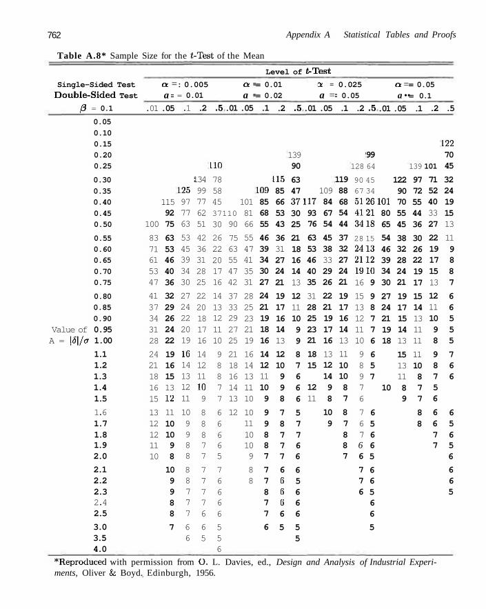
762 Appendix A Statistical Tables and Proofs
Table A.8* Sample Size for the t-Test of the Mean
Single-Sided Test
Double-Sided Test
/3 = 0.1
0.05
0.10
0.15
0.20
0.25
0.30
0.35
0.40
0.45
0.50
0.55
0.60
0.65
0.70
0.75
0.80
0.85
0.90
Value of 0.95 A = \5\/a 1.00
1.1 1.2 1.3 1.4 1.5
1.6 1.7 1.8 1.9 2.0
2.1 2.2 2.3 2.4 2.5
3.0 3.5 4.0
.01
100
83 71 61 53 47
41 37 34 31 28
24 21 18 16 15
13 12 12 11 10
a = a = .05
115 92 75
63 53 46 40 36
32 29 26 24 22
19 16 15 13 12
11 10 10 9 8
10 9 9 8 8
7
: 0.005 = 0.01
.1
: 125 97 77 63
53 45 39 34 30
27 24 22 20 19
10 14 13 12 11
10 9 9 8 8
8 8 7 7 7
6 6
.2
134 99 77 62 51
42 36 31 28 25
22 20 18 17 16
14 12 11 10 9
8 8 8 7 7
7 7 7 7 6
6 5
.5
110
78 58 45
.01
37110
30
26 22 20 17 16
14 13 12 11 10
9 8 8 7 7
6 6 6 6 5
7 6 6 6 6
5 5 6
90
75 63 55 47 42
37 33 29 27 25
21 18 16 14 13
12
a -a -.05
101 81 66
55 47 41 35 31
28 25 23 21 19
16 14 13 11 10
10 11 10 10 9
8 8
Level of t-Test
= 0.01
= 0.02
.1
: 109 85 68 55
46 39 34 30 27
24 21 19 18 16
14 12 11 10 9
9 9 8 8 7
7 7 8 7 7
6
.2
115 85 66 53 43
36 31 27 24 21
19 17 16 14 13
12 10 9 9 8
7 8 7 7 7
6 6 6 6 6
5
.5
139 90
63 47
e
.01
37117
30 25
21 18 16 14 13
12 11 10 9 9
8 7 6 6 6
5 7 7 6 6
6 5 6 6 6
5 5
93 76
63 53 46 40 35
31 28 25 23 21
18 15
12 11
y =
a = .05
109 84 67 54
45 38 33 29 26
22 21 19 17 16
13 12 14 9 8
10 9
0.025
= 0.05
.1
119 88 68 54 44
37 32 27 24 21
19 17 16 14 13
11 10 10 8 7
8 7 8 8 7
.2
i
.5
99 128 64
90 45 67 34
.01
5126101
4121
3418
28 15 2413
2112
1910
16
15 13 12 11 10
9 8 9 7 6
7 6 7 6 6
7 7 6
9
9 8 7 7 6
6 5 7
6 5 6 6 5
6 6 5 6 6
5
80 65
54 46 39 34 30
27 24 21 19 18
10
a = a ••
.05
122 90 70 55 45
38 32 28 24 21
19 17 15 14 13
15 13 11 8 9
= 0.05
= 0.1
.1 .2
139 101
97 72 55 44 36
30 26 22 19 17
15 14 13 11 11
11 10 8 7 7
8 8
71 52 40 33 27
22 19 17 15 13
12 11 10 9 8
9 8 7 5 6
6 6 7 7
.5
122 70 45
32 24 19 15 13
11 9 8 8 7
6 6 5 5 5
7 6 6
6 5 6 5 6
6 6 5
*Reproduced with permission from O. L. Davies, ed., Design and Analysis of Industrial Experiments, Oliver & Boyd. Edinburgh, 1956.
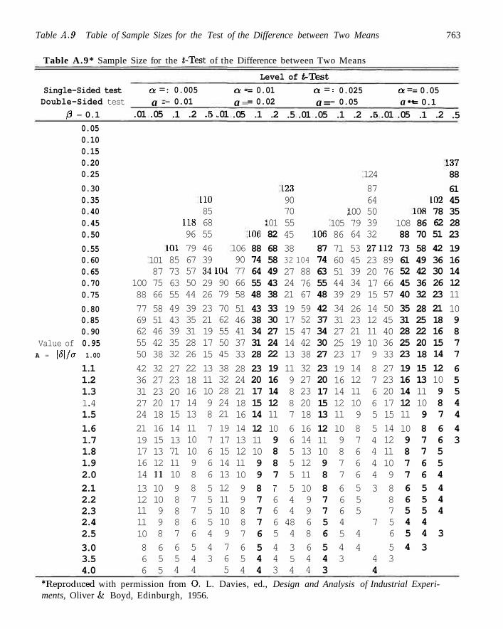
Table A.9 Table of Sample Sizes for the Test of the Difference between Two Means 763
Table A.9* Sample Size for the £-Test of the Difference between Two Means
Single-Sided test Double-Sided test
/3 = 0.1
0.05 0.10 0.15 0.20 0.25
0.30 0.35 0.40 0.45 0.50
0.55 0.60 0.65 0.70 0.75
0.80 0.85 0.90
Value of 0.95 A = |<5|/CT 1.00
1.1 1.2 1.3 1.4 1.5
1.6 1.7 1.8 1.9 2.0 2.1 2.2 2.3 2.4 2.5
3.0 3.5 4.0
.01
100 88
77 69 62 55 50
42 36 31 27 24
21 19 17 16 14
13 12 11 11 10
8 6 6
a = a -.05
101 87 75 66
58 51 46 42 38
32 27 23 20 18
16 15 13 12 11
10 10 9 9 8
6 5 5
: 0.005 = 0.01
.1
:
101 85 73 63 55
49 43 39 35 32
27 23 20 17 15
14 13 71 11 10
9 8 8 8 7
6 5 4
.2
118 96
79 67 57 50 44
39 35 31 28 26
22 18 16 14 13
11 10 10 9 8 8 7 7 6 6
5 4 4
.5,
110 85 68 55
46 39
.01
34104 29 26
23 21 19 17 15
13 11 10 9 8
7 7 6 6 6
5 5 5 5 4 4 3
90 79
70 62 55 50 45
38 32 28 24 21
19 17 15 14 13 12 11 10 10 9
7 6 5
a -a = .05
106 90 77 66 58
51 46 41 37 33
28 24 21 18 16
14 13 12 11 10 9 9 8 8 7 6 5 4
Level of t-Test
= 0.01 = 0.02
.1
: 106
88 74 64 55 48
43 38 34 31 28
23 20 17 15 14
12 11 10 9 9 8 7 7 7 6
5 4 4
.2
101 82
68 58 49 43 38
33 30 27 24 22
19 16 14 12 11
10 9 8 8 7 -7 1
6 6 6 5
4 4 3
.5
123 90 70 55 45
38
.01
32 104 27 24 21
19 17 15 14 13
11 9 8 8 7
6 6 5 5 5 5 4 4 48 4
3 5 4
88 76 67
59 52 47 42 38
32 27 23 20 18
16 14 13 12 11 10 9 9 6 8
6 4 4
a = a = .05
106
87 74 63 55 48
42 37 34 30 27
23 20 17 15 13
12 11 10 9 8 8 7 7 5 6
5 4 3
: 0.025 = 0.05
.1
; 105 86
71 60 51 44 39
34 31 27 25 23
19 16 14 12 11
10 9 8 7 7 6 6 6 4 5 4 3
.2
100 79 64
53 45 39 34 29
26 23 21 19 17
14 12 11 10 9
8 7 6 6 6 5 5 5
4
4
.5
124
87 64 50 39 32
.01
27112 23 20 17 15
14 12 11 10 9
8 7 6 6 5
5 4 4 4 4 3
7
4 4
89 76 66 57
50 45 40 36 33
27 23 20 17 15
14 12 11 10 9 8 8 7 5 6
5 3
a = a •• .05
108 88
73 61 52 45 40
35 31 28 25 23
19 16 14 12 11
10 9 8 7 7 6 6 5 4 5 4
= 0.05 = 0.1
.1
: 108 86 70
58 49 42 36 32
28 25 22 20 18
15 13 11 10 9
8 7 7 6 6 5 5 5 4 4
3
.2
102 78 62 51
42 36 30 26 23
21 18 16 15 14
12 10 9 8 7
6 6 5 5 4 4 4 4
3
.5
137 88
61 45 35 28 23
19 16 14 12 11
10 9 8 7 7
6 5 5 4 4
4 3
^Reproduced with permission from O. L. Davies, ed., Design and Analysis of Industrial Experiments, Oliver &: Boyd, Edinburgh, 1956.
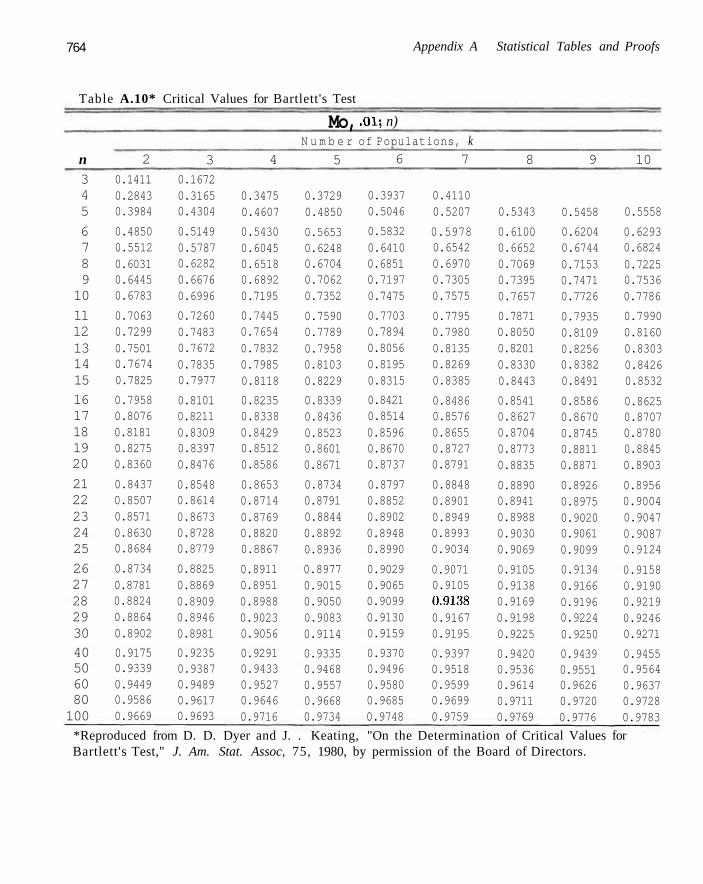
764 Appendix A Statistical Tables and Proofs
Table A.10* Critical Values for Bartlett's Test
n 3 4 5
6 7 8 9 10
11 12 13 14 15
16 17 18 19 20
21 22 23 24 25
26 27 28 29 30 40 50 60 80 100
2
0.1411 0.2843 0.3984
0.4850 0.5512 0.6031 0.6445 0.6783
0.7063 0.7299 0.7501 0.7674 0.7825
0.7958 0.8076 0.8181 0.8275 0.8360
0.8437 0.8507 0.8571 0.8630 0.8684
0.8734 0.8781 0.8824 0.8864 0.8902
0.9175 0.9339 0.9449 0.9586 0.9669
3 0.1672 0.3165 0.4304
0.5149 0.5787 0.6282 0.6676 0.6996
0.7260 0.7483 0.7672 0.7835 0.7977
0.8101 0.8211 0.8309 0.8397 0.8476
0.8548 0.8614 0.8673 0.8728 0.8779
0.8825 0.8869 0.8909 0.8946 0.8981
0.9235 0.9387 0.9489 0.9617 0.9693
4
0.3475 0.4607
0.5430 0.6045 0.6518 0.6892 0.7195
0.7445 0.7654 0.7832 0.7985 0.8118
0.8235 0.8338 0.8429 0.8512 0.8586
0.8653 0.8714 0.8769 0.8820 0.8867
0.8911 0.8951 0.8988 0.9023 0.9056
0.9291 0.9433 0.9527 0.9646 0.9716
Mo, .01; n) N u m b e r of Populations, k
5
0.3729 0.4850
0.5653 0.6248 0.6704 0.7062 0.7352
0.7590 0.7789 0.7958 0.8103 0.8229
0.8339 0.8436 0.8523 0.8601 0.8671
0.8734 0.8791 0.8844 0.8892 0.8936
0.8977 0.9015 0.9050 0.9083 0.9114
0.9335 0.9468 0.9557 0.9668 0.9734
6
0.3937 0.5046
0.5832 0.6410 0.6851 0.7197 0.7475
0.7703 0.7894 0.8056 0.8195 0.8315
0.8421 0.8514 0.8596 0.8670 0.8737
0.8797 0.8852 0.8902 0.8948 0.8990
0.9029 0.9065 0.9099 0.9130 0.9159
0.9370 0.9496 0.9580 0.9685 0.9748
7
0.4110 0.5207
0.5978 0.6542 0.6970 0.7305 0.7575
0.7795 0.7980 0.8135 0.8269 0.8385
0.8486 0.8576 0.8655 0.8727 0.8791
0.8848 0.8901 0.8949 0.8993 0.9034
0.9071 0.9105 0.9138 0.9167 0.9195
0.9397 0.9518 0.9599 0.9699 0.9759
8
0.5343
0.6100 0.6652 0.7069 0.7395 0.7657
0.7871 0.8050 0.8201 0.8330 0.8443
0.8541 0.8627 0.8704 0.8773 0.8835
0.8890 0.8941 0.8988 0.9030 0.9069
0.9105 0.9138 0.9169 0.9198 0.9225
0.9420 0.9536 0.9614 0.9711 0.9769
9
0.5458
0.6204 0.6744 0.7153 0.7471 0.7726
0.7935 0.8109 0.8256 0.8382 0.8491
0.8586 0.8670 0.8745 0.8811 0.8871
0.8926 0.8975 0.9020 0.9061 0.9099
0.9134 0.9166 0.9196 0.9224 0.9250
0.9439 0.9551 0.9626 0.9720 0.9776
10
0.5558
0.6293 0.6824 0.7225 0.7536 0.7786
0.7990 0.8160 0.8303 0.8426 0.8532
0.8625 0.8707 0.8780 0.8845 0.8903
0.8956 0.9004 0.9047 0.9087 0.9124
0.9158 0.9190 0.9219 0.9246 0.9271
0.9455 0.9564 0.9637 0.9728 0.9783
*Reproduced from D. D. Dyer and J. . Keating, "On the Determination of Critical Values for Bartlett's Test," J. Am. Stat. Assoc, 75, 1980, by permission of the Board of Directors.
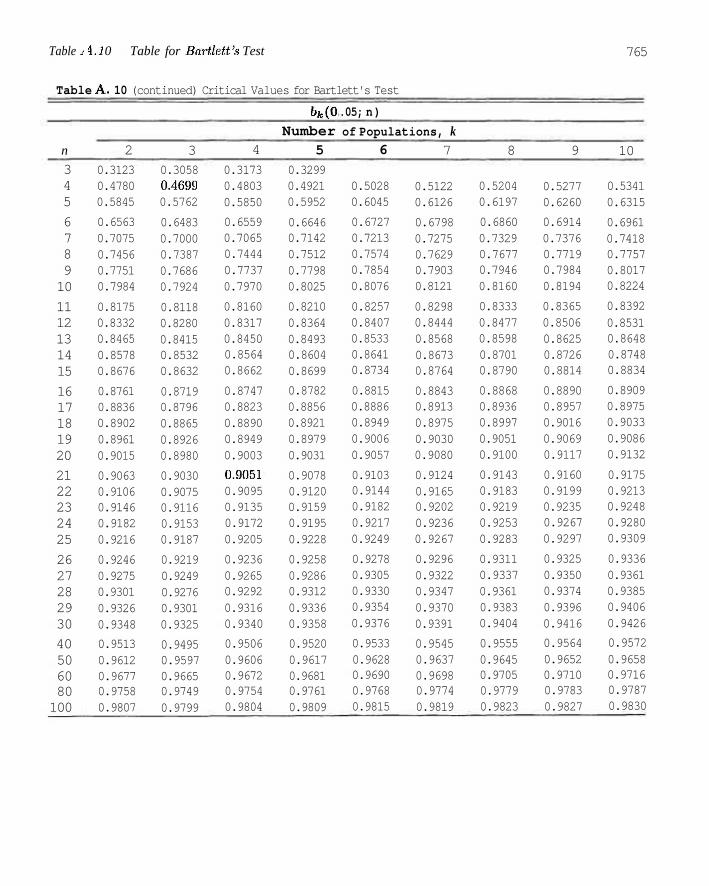
Table J IJ 0 Table for Bartlett's Test
Table A. 10 (continued) Critical Values for Bartlett's Test
n
3 4 5
6 7 8 9 10
11 12 13 14 15
16 17 18 19 20
21 22 23 24 25
26 27 28 29 30
40 50 60 80 100
2
0.3123 0.4780 0.5845
0.6563 0.7075 0.7456 0.7751 0.7984
0.8175 0.8332 0.8465 0.8578 0.8676
0.8761 0.8836 0.8902 0.8961 0.9015
0.9063 0.9106 0.9146 0.9182 0.9216
0.9246 0.9275 0.9301 0.9326 0.9348
0.9513 0.9612 0.9677 0.9758 0.9807
3 0.3058 0.4699 0.5762
0.6483 0.7000 0.7387 0.7686 0.7924
0.8118 0.8280 0.8415 0.8532 0.8632
0.8719 0.8796 0.8865 0.8926 0.8980
0.9030 0.9075 0.9116 0.9153 0.9187
0.9219 0.9249 0.9276 0.9301 0.9325
0.9495 0.9597 0.9665 0.9749 0.9799
4
0.3173 0.4803 0.5850
0.6559 0.7065 0.7444 0.7737 0.7970
0.8160 0.8317 0.8450 0.8564 0.8662
0.8747 0.8823 0.8890 0.8949 0.9003
0.9051 0.9095 0.9135 0.9172 0.9205
0.9236 0.9265 0.9292 0.9316 0.9340
0.9506 0.9606 0.9672 0.9754 0.9804
Mo Number
5
0.3299 0.4921 0.5952
0.6646 0.7142 0.7512 0.7798 0.8025
0.8210 0.8364 0.8493 0.8604 0.8699
0.8782 0.8856 0.8921 0.8979 0.9031
0.9078 0.9120 0.9159 0.9195 0.9228
0.9258 0.9286 0.9312 0.9336 0.9358
0.9520 0.9617 0.9681 0.9761 0.9809
.05; n)
of Populations, k 6
0.5028 0.6045
0.6727 0.7213 0.7574 0.7854 0.8076
0.8257 0.8407 0.8533 0.8641 0.8734
0.8815 0.8886 0.8949 0.9006 0.9057
0.9103 0.9144 0.9182 0.9217 0.9249
0.9278 0.9305 0.9330 0.9354 0.9376
0.9533 0.9628 0.9690 0.9768 0.9815
7
0.5122 0.6126
0.6798 0.7275 0.7629 0.7903 0.8121
0.8298 0.8444 0.8568 0.8673 0.8764
0.8843 0.8913 0.8975 0.9030 0.9080
0.9124 0.9165 0.9202 0.9236 0.9267
0.9296 0.9322 0.9347 0.9370 0.9391
0.9545 0.9637 0.9698 0.9774 0.9819
8
0.5204 0.6197
0.6860 0.7329 0.7677 0.7946 0.8160
0.8333 0.8477 0.8598 0.8701 0.8790
0.8868 0.8936 0.8997 0.9051 0.9100
0.9143 0.9183 0.9219 0.9253 0.9283
0.9311 0.9337 0.9361 0.9383 0.9404
0.9555 0.9645 0.9705 0.9779 0.9823
9
0.5277 0.6260
0.6914 0.7376 0.7719 0.7984 0.8194
0.8365 0.8506 0.8625 0.8726 0.8814
0.8890 0.8957 0.9016 0.9069 0.9117
0.9160 0.9199 0.9235 0.9267 0.9297
0.9325 0.9350 0.9374 0.9396 0.9416
0.9564 0.9652 0.9710 0.9783 0.9827
765
10
0.5341 0.6315
0.6961 0.7418 0.7757 0.8017 0.8224
0.8392 0.8531 0.8648 0.8748 0.8834
0.8909 0.8975 0.9033 0.9086 0.9132
0.9175 0.9213 0.9248 0.9280 0.9309
0.9336 0.9361 0.9385 0.9406 0.9426
0.9572 0.9658 0.9716 0.9787 0.9830
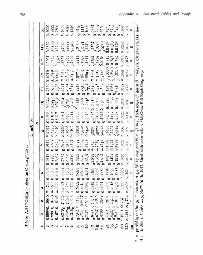
766 Appendix A Statistical Tables and Proofs
+ 3 CD
o H cc
"a a £ c j
o O o
14*4
CO CD 3
J« > , 1
s o '4H
O * i H rH
^ V
3 IB
H
rH O
d II a
e
8
w •^ r-l
t> n
t -rH
rH rH
O H
(35
CM
t-
(0
IO
rr
M
(N
^
O CO O 3 h O l O O CO O O CO CM I O O CO Ui O C ^ CM LO CO CM CM r H r H —
H o to t - o i - n o r H O C O C D O H « O r H O OC CO L.O r r CO CM H ^ c o c o o o o cr;
o o o o o c o o o o o o o o o
CM O r H CO CO I O O CN CM CO r r CO
•* o o rr CM CM CO CM O l CM CM r H
O r H O CM
t-- to
CO r - r? s i ui co o H (B N rH O O
O O O O O O O O O O O O
b - CO t v c© LO l O O r H O N l O t
r H 0 0 Tj< a U5 O! CO 3 0 r r CO CM CM
CM CM
CM C I
O0
LO rH O CO I O CO LO CM O l
O O O C O O O O O O O
t o O CO O l 0 0 CO LO r r CO o o o o d d O 0 0 CO r H LO O 0 0 CO LO
c o o o d d
ci ci rr TJ- LO 0 0 O l O 0 0 h - CO r r
o d d O l CO CO CO - * CO LO t v O 0 0 CO t o
r T O ! LO O l CM O 0 LO r H rr CO CO
d d d t~ rT CO 0 1 0 0 I— CO O CO -rl< r H CO
O ! -<H 1 ^ i - I-H o i I V LO CM CM CM CM
o d d X O H r r LO O CN O N CO CM CM
r H CM 0 0 0 rH r r 0 1 CD CM
O N X CO CO CO O OC CO
r H .—* r H - H O O
d d d o d d O OO r H CM r - O CO O l LO CN H H
CO 0 0 LO
-Hi CO
0 0
o o o o c o o o o o o o o o o o rr CM CM t*- rH O CO Ol t-00 CO LO
•* Ol rH LO CM to X CI N -H Tf M
CO 1-— CO cc — O 00
O O O o o o
CO h- t-CM O Ol 00 -H 00 CO S O
t^ — —I CO O —I O rr Ol LO -iH CO
CO CO CM
o d d CN S LO CM O "rH LO CM Ol CO CO CM
CO CN N rH O CO rr O L O CM CM rH
ci ci ci LO rr CO o lO i—i CM CM
00 O CO CO O to CO —' 00 —i — c o d d CC IV X c to Ol rf rH 00 rH f—i O
O O O O O C O O C O O O O O O
00 LO O l 0 0 CO CM 0 1 CO — 0 0 N CO
Ol 00 LO o o
o o o o o CM CC O I V O r H T— CO r r © t v CD
r H CO CO CO LO 0 0 LO n<
r f
d
rT CO r r
0C cc I V o CO - H CO CO
O 0 0 0 0 0 0 CM r r CC CN N CM CM rH
I O CN N C l CO LO H CN O l - H —i O
O O O O O O O O O
(N CN CO CO O l o O l LO CO CO CO CO
o o o o c c c o o CO CO r H t ^ CO CO CO C l t v O l t ~ CO
l O LO O l t v Ol LO 0 0 r H CO LO LO - *
CO O CM CN N N CM 0 0 LO r r CO CO
- CO N O 0 0 N 0 0 CO oc CM CM H
d d d 0 1 CO 00 Ol Ol r r o LO o CO CM CM
CC CO o
O l r j i LO LO LO CO t v r T r H
o o o o o o o o o o o o o o o
CC LO CM OO CO rH LO CO CM CI OO N
Ol LO o CM CO 00 CO o c cc to LO
tv — rr CM LO CO O CN O rr rr CO
00 CM 00 CM 00 00 rr 00 CM CO CM CM
L O i—I CO 00 CO CM
o o o o o o c o o o o o o o o rr — rr CI CO rH IV OO 00 Ol 00 IV
d d d
IV 0C LO LC Ol CM
LO 00 CO
CD CO LO
o d d LO 00 rr 00 rH rr 00 CM CC r-; I-- p
o d d o d d
O l C Ol O i—I cc CM 00 rr LO rf rr
Ol t-- rr rH LO
oi co co " CM rO CO
LO CO 00 Ol rH O CM Oi LO CM rH rH
o o o o o o o o o
0 CO CO LO CM rr 01 rf CO Ol Ol oc
CM l-~ LO CM LO
r- co
oo r-i oi r-LO CO Ol
cc
d to d
tv rT
rH CM LO N- T—I rH CO H C5 CM CM —I
o o o c o o O: CO CO Ol CO t-Ol Ol CO Ol Ol o
Ol OC CO N CN N CM 00 CO (51 00 00
LO r t rr rr © LO IV IV
O C O O O O O O O O O O O O C
0 0 CM LO CO lO
N C N O rr CO rr CN CC © rr CO CM
C N M r r i f i CO N C O O eN w o i-H rH (N
rH O O CM CO r f
CO — «
.0167
.0083
o c
0245
0125
o o
0344
0178
o o
.0461
0242
o o
,0567
0302
o o
.0594
0316
o o
.0625
0334
o o .0668
.0357
o o
.0722
.0387
o o
.0796
0429
o o
,0902
0489
o o
1069
0585
o o — O l I V LO CO t— r H O
d d r H VO LO CM r H CM CM i-H
d d
s§
o
o
o
c
o
o
o
—,
o
o
o
o
o
o
8
I o
rf. O
s>
X 58
— a
C3 C
C/2
O
:3
0 0 r H r r t-5 A
s
CO ! < _
£ o -5 a < •=
cc a) CO K
Ol
•J" M H '-< a a
£ gf i a | o ^ s i o 0. .*-• c-i*w j - ;
-o o § 0 .3 -* TJ O
o o a « D r-<
* rC
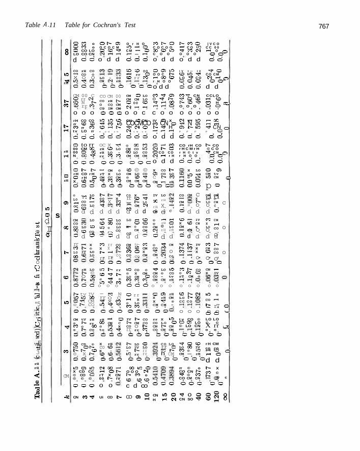
Table A. 11 Table for Cochran's Test 767
*J CO
CD
F cc
33 JH
T3 o o t-
c «+5
•s: CD 3
L™ > "5 CJ +^
'C o TT o
.5 •5 3 o rH rH
<i _cy
3 S
to o d II a
s
8
in •>* rH
t-£0
b-r-<
rH
H
O rH
£35
CO
t-
CO
to
•
M
CM
•«
O CO o O CO o O CO LO LO CO CN
d
O t ^ © O r H O C 0 I V O S « O | V C O O C O C M L O - H O C O C O O r H C O L O C C 0 0 O C C r T C M —. O O O O L O r r c O C M i-H O <--, C M r H r H r- l — r H C O O O O O O O
d o o d d d o c o d d o d d d o
CO rH CO rH CO © x o o LO r? CO
LO — 00 CN CM rH
CO CO 00 rH rr O CO rr CO
O O O C O O o o o
CM 00 C O rr CM O N h CO rr CO
CO CM 00 CO rH t-O CO CM CO IN CM
CM O LO CM CM LO O 00 CO N H H
0 © L O I V t — I V r T O O O C N C D L O r J i C O C M r H O O C D L O r r C O C M r H r - , r H O O O O O O O
o d d o d d d d C O r T © n r f CN CCLO o rr t- r r o c e I-H o r T r H O O I V C C r T C<5 H r , r H r H O O O O O O ^
o o o o o o o o c c o o o o o o o rH CO CO rr CO cc CO rr CO t v LO rr
o d d O to rr 00 CM 0C 00 O X N CC r »
L O L O C O CN C CN IV © X C M r H L O rH 3C •H CO IO COCMCO W CN O r« N O rHrH O r H t v r T C M O N ' t H Cl N m rr CN o n c o C N C N C M C N — ; • • " ! • " } P P P P P
o d d o d d o d d d o c d o OC X rT rH O LO rH LO — rr CO CO
© X CO CM CO LO X LO CO CM CM CM
o o o o o o o o o
O r H C O CO rH CO t - CO C N t - O r H C M r H © C O O C O C O r H © t v r r C N r-, <N I-H r H r H O O O O
o d d d o c c d O t - t -rH CD r H O r H O X CO LO
— CM © rT X LO CM CC CM rT CO CO
cc © © CM LO CO © CC rT CM CM CM
X CO h-© CO LO C Iv CO CM r- rH
X LO
LO rT ©
O O O C O O O O O O o c O O C
O © CM tv IO CN 0
p ° d d ©
LO .—1 OC
o CM CO CO 00
== rr CO LO
X
,-o CO CO CO d
LO
CO
d
IV IV CO
LO t-
LO
d LO
o CO Ui = X © LO LO
IV 00 CO rr d rr CO LO
rt
— CO X 1—
rr
X
d O X ©
CO
=' rr X r-t
rr
rT X CO CO
d LO CO LO CO
d CO <N
co
CO rr .—> CO d LO
X
CO d CM O CO CO
X CO
CM
d r-i O © CM
d tree O co
rr LO r-i
d CO CO CO CM
— CO CM X CM
IV
X rH
CM d © © CM CM
= © CO rT CM
LO
rH
X rH d r-, rH © rH
d it CM
CM
C
r-i O LO rH
d CM
o CO rH
CO
CM i — i
<== CO X CM
='
CO
CM
H
d
CO
o d
CO
c X t-o d IV CN X o d IV X X
o
CM LO LO o d CO X LO o d CO CM O
o
CM © CM C
=> CM i-H
CO
o d t^ CO CO
o
c
o
o
rH LO r- © o x t— lO
o o o LO t^ rr
CC rT t-c rr © LO rr CO
o o o o o o o o LO CO © © X CM LO CN C CO CO CO
rT LO LO CM © CO CO — tv CM CN rH
^ N CO © CO CO rT CM ©
CN r-X IV
o o c o o o o o o o o o o o o o o
t- tv IV IO 1.1 CO O rn CM © t~- CO
- n N rr o c rr x CO LO rT rT
O rr r-l X © LO CO CO
O © rH X rH CM X HC" © CM CM —
CO t-LO t-CC CO
lO ©
CO rH
£- rT c O O w o o o c o o o o o o o o o o o o
CM tV rH © t- rr CO © X © f- CO
rH —I O X CM C © CO X to LO rT
IV tv CO rr
t- CO CM CO o t-rr CO
rr X LO CO LO O CN I— CN CO CN CM
t v CO © O © LO © LO CN
LO LO © © X rr 0 o o ' - '
O O O C O O O O C o o o c o o o o
O CD © l.O O h-t- t- o © X t—
X rH co co X — CO CO
t— LO LO IV — tv LO rr
O LO rr rr
CO LO rr o CO t-n CM
rT O CO LO OO IV CO © to CM — rH
C O O O O O C O O O O O O O C
r H CM co co
IH O
d d
CO o
L O C 1 L O C M X r H X l O O X CD CC .-H O ' © CO O rT X CN © © © 00 t— IV
N O O O I N t ^ CO o
o o o o o
CN M r j Ui CO I v
<£) p P c d co
rr © o CO CN t— r r © CO CO CM CN
h - X CO © t— © c
o c o O O C c c
CO OS S CN tO O H H N
rf o O CN SO TP § * 8
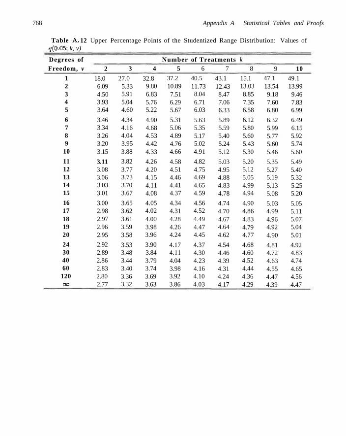
768 Appendix A Statistical Tables and Proofs
Table A. 12 Upper Percentage Points of the Studentized Range Distribution: Values of </(0.05; k, v)
Degrees of Freedom, v
1 2 3 4 5
6 7 8 9
10
11 12 13 14 15
16 17 18 19 20
24 30 40 60
120 oo
2
18.0 6.09 4.50 3.93 3.64
3.46 3.34 3.26 3.20 3.15
3.11 3.08 3.06 3.03 3.01
3.00 2.98 2.97 2.96 2.95
2.92 2.89 2.86 2.83 2.80 2.77
3
27.0 5.33 5.91 5.04 4.60
4.34 4.16 4.04 3.95 3.88
3.82 3.77 3.73 3.70 3.67
3.65 3.62 3.61 3.59 3.58
3.53 3.48 3.44 3.40 3.36 3.32
4
32.8 9.80 6.83 5.76 5.22
4.90 4.68 4.53 4.42 4.33
4.26 4.20 4.15 4.11 4.08
4.05 4.02 4.00 3.98 3.96
3.90 3.84 3.79 3.74 3.69 3.63
Number of Treatments k 5
37.2 10.89 7.51 6.29 5.67
5.31 5.06 4.89 4.76 4.66
4.58 4.51 4.46 4.41 4.37
4.34 4.31 4.28 4.26 4.24
4.17 4.11 4.04 3.98 3.92 3.86
6
40.5 11.73 8.04 6.71 6.03
5.63 5.35 5.17 5.02 4.91
4.82 4.75 4.69 4.65 4.59
4.56 4.52 4.49 4.47 4.45
4.37 4.30 4.23 4.16 4.10 4.03
7
43.1 12.43 8.47 7.06 6.33
5.89 5.59 5.40 5.24 5.12
5.03 4.95 4.88 4.83 4.78
4.74 4.70 4.67 4.64 4.62
4.54 4.46 4.39 4.31 4.24 4.17
8
15.1 13.03 8.85 7.35 6.58
6.12 5.80 5.60 5.43 5.30
5.20 5.12 5.05 4.99 4.94
4.90 4.86 4.83 4.79 4.77
4.68 4.60 4.52 4.44 4.36 4.29
9
47.1 13.54 9.18 7.60 6.80
6.32 5.99 5.77 5.60 5.46
5.35 5.27 5.19 5.13 5.08
5.03 4.99 4.96 4.92 4.90
4.81 4.72 4.63 4.55 4.47 4.39
10
49.1 13.99 9.46 7.83 6.99
6.49 6.15 5.92 5.74 5.60
5.49 5.40 5.32 5.25 5.20
5.05 5.11 5.07 5.04 5.01
4.92 4.83 4.74 4.65 4.56 4.47
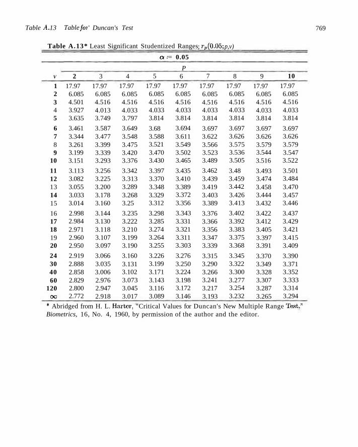
Table A. 13 Table foi
Table A.13*
V
1 2 3 4 5
6 7 8 9
10
11 12 13 14 15
16 17 18 19 20
24 30 40 60
120 oo
2
17.97 6.085 4.501 3.927 3.635
3.461 3.344 3.261 3.199 3.151
3.113 3.082 3.055 3.033 3.014
2.998 2.984 2.971 2.960 2.950
2.919 2.888 2.858 2.829 2.800 2.772
' Duncan's Test
Least Significant Studentized Ranges
3
17.97 6.085 4.516 4.013 3.749
3.587 3.477 3.399 3.339 3.293
3.256 3.225 3.200 3.178 3.160
3.144 3.130 3.118 3.107 3.097
3.066 3.035 3.006 2.976 2.947 2.918
4
17.97 6.085 4.516 4.033 3.797
3.649 3.548 3.475 3.420 3.376
3.342 3.313 3.289 3.268 3.25
3.235 3.222 3.210 3.199 3.190
3.160 3.131 3.102 3.073 3.045 3.017
a •
5
17.97 6.085 4.516 4.033 3.814
3.68 3.588 3.521 3.470 3.430
3.397 3.370 3.348 3.329 3.312
3.298 3.285 3.274 3.264 3.255
3.226 3.199 3.171 3.143 3.116 3.089
= 0.05
P 6
17.97 6.085 4.516 4.033 3.814
3.694 3.611 3.549 3.502 3.465
3.435 3.410 3.389 3.372 3.356
3.343 3.331 3.321 3.311 3.303
3.276 3.250 3.224 3.198 3.172 3.146
; rp(0.05;
7
17.97 6.085 4.516 4.033 3.814
3.697 3.622 3.566 3.523 3.489
3.462 3.439 3.419 3.403 3.389
3.376 3.366 3.356 3.347 3.339
3.315 3.290 3.266 3.241 3.217 3.193
p,v)
8
17.97 6.085 4.516 4.033 3.814
3.697 3.626 3.575 3.536 3.505
3.48 3.459 3.442 3.426 3.413
3.402 3.392 3.383 3.375 3.368
3.345 3.322 3.300 3.277 3.254 3.232
9
17.97 6.085 4.516 4.033 3.814
3.697 3.626 3.579 3.544 3.516
3.493 3.474 3.458 3.444 3.432
3.422 3.412 3.405 3.397 3.391
3.370 3.349 3.328 3.307 3.287 3.265
10
17.97 6.085 4.516 4.033 3.814
3.697 3.626 3.579 3.547 3.522
3.501 3.484 3.470 3.457 3.446
3.437 3.429 3.421 3.415 3.409
3.390 3.371 3.352 3.333 3.314 3.294
769
* Abridged from H. L. Harter, "Critical Values for Duncan's New Multiple Range Test." Biometrics, 16, No. 4, 1960, by permission of the author and the editor.
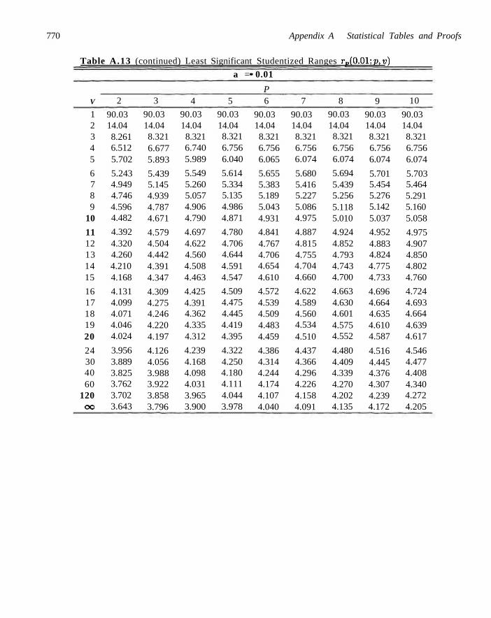
770 Appendix A Statistical Tables and Proofs
Table A.13 (continued) Least Significant Studentized Ranges rp(0.01'.p,v)
V
1 2 3 4 5
6 7 8 9
10
11 12 13 14 15
16 17 18 19 20
24 30 40 60
120 oo
2
90.03 14.04 8.261 6.512 5.702
5.243 4.949 4.746 4.596 4.482
4.392 4.320 4.260 4.210 4.168
4.131 4.099 4.071 4.046 4.024
3.956 3.889 3.825 3.762 3.702 3.643
3
90.03 14.04 8.321 6.677 5.893
5.439 5.145 4.939 4.787 4.671
4.579 4.504 4.442 4.391 4.347
4.309 4.275 4.246 4.220 4.197
4.126 4.056 3.988 3.922 3.858 3.796
4
90.03 14.04 8.321 6.740 5.989
5.549 5.260 5.057 4.906 4.790
4.697 4.622 4.560 4.508 4.463
4.425 4.391 4.362 4.335 4.312
4.239 4.168 4.098 4.031 3.965 3.900
a =
5
90.03 14.04 8.321 6.756 6.040
5.614 5.334 5.135 4.986 4.871
4.780 4.706 4.644 4.591 4.547
4.509 4.475 4.445 4.419 4.395
4.322 4.250 4.180 4.111 4.044 3.978
•• 0.01
P 6
90.03 14.04 8.321 6.756 6.065
5.655 5.383 5.189 5.043 4.931
4.841 4.767 4.706 4.654 4.610
4.572 4.539 4.509 4.483 4.459
4.386 4.314 4.244 4.174 4.107 4.040
7
90.03 14.04 8.321 6.756 6.074
5.680 5.416 5.227 5.086 4.975
4.887 4.815 4.755 4.704 4.660
4.622 4.589 4.560 4.534 4.510
4.437 4.366 4.296 4.226 4.158 4.091
8
90.03 14.04 8.321 6.756 6.074
5.694 5.439 5.256 5.118 5.010
4.924 4.852 4.793 4.743 4.700
4.663 4.630 4.601 4.575 4.552
4.480 4.409 4.339 4.270 4.202 4.135
9
90.03 14.04 8.321 6.756 6.074
5.701 5.454 5.276 5.142 5.037
4.952 4.883 4.824 4.775 4.733
4.696 4.664 4.635 4.610 4.587
4.516 4.445 4.376 4.307 4.239 4.172
10
90.03 14.04 8.321 6.756 6.074
5.703 5.464 5.291 5.160 5.058
4.975 4.907 4.850 4.802 4.760
4.724 4.693 4.664 4.639 4.617
4.546 4.477 4.408 4.340 4.272 4.205
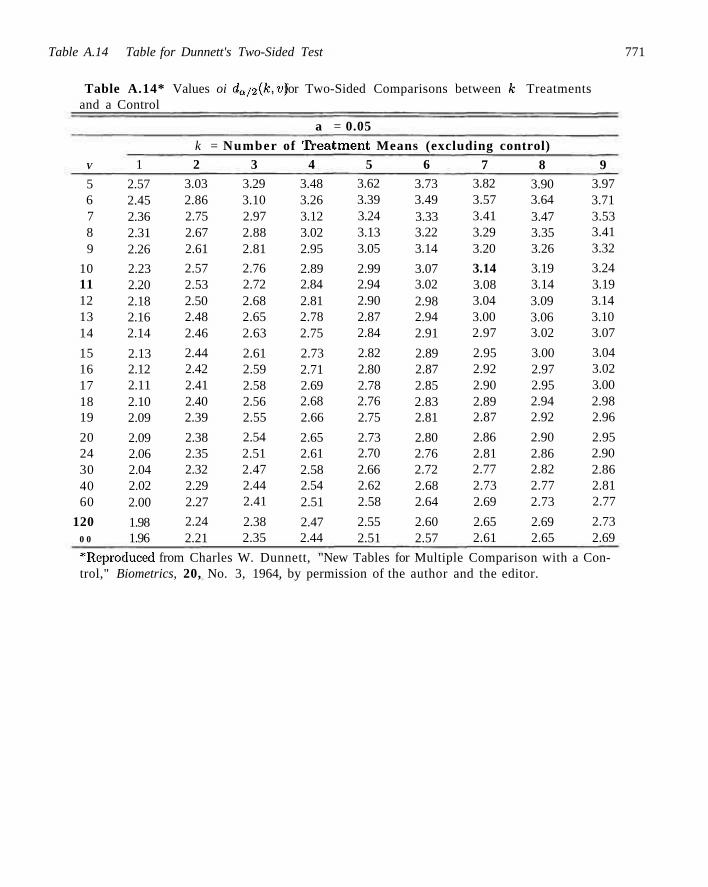
Table A.14 Table for Dunnett's Two-Sided Test 771
Table A.14* Values oi daj2(k,v) for Two-Sided Comparisons between A: Treatments and a Control
V
5 6 7 8 9
10 11 12 13 14
15 16 17 18 19
20 24 30 40 60
120 0 0
1
2.57 2.45 2.36 2.31 2.26
2.23 2.20 2.18 2.16 2.14
2.13 2.12 2.11 2.10 2.09
2.09 2.06 2.04 2.02 2.00
1.98 1.96
k =
2 3.03 2.86 2.75 2.67 2.61
2.57 2.53 2.50 2.48 2.46
2.44 2.42 2.41 2.40 2.39
2.38 2.35 2.32 2.29 2.27
2.24 2.21
a = 0.05
Number of Treatment Means (excluding control) 3
3.29 3.10 2.97 2.88 2.81
2.76 2.72 2.68 2.65 2.63
2.61 2.59 2.58 2.56 2.55
2.54 2.51 2.47 2.44 2.41
2.38 2.35
4 3.48 3.26 3.12 3.02 2.95
2.89 2.84 2.81 2.78 2.75
2.73 2.71 2.69 2.68 2.66
2.65 2.61 2.58 2.54 2.51
2.47 2.44
5 3.62 3.39 3.24 3.13 3.05
2.99 2.94 2.90 2.87 2.84
2.82 2.80 2.78 2.76 2.75
2.73 2.70 2.66 2.62 2.58
2.55 2.51
6 3.73 3.49 3.33 3.22 3.14
3.07 3.02 2.98 2.94 2.91
2.89 2.87 2.85 2.83 2.81
2.80 2.76 2.72 2.68 2.64
2.60 2.57
7 3.82 3.57 3.41 3.29 3.20
3.14 3.08 3.04 3.00 2.97
2.95 2.92 2.90 2.89 2.87
2.86 2.81 2.77 2.73 2.69
2.65 2.61
8 3.90 3.64 3.47 3.35 3.26
3.19 3.14 3.09 3.06 3.02
3.00 2.97 2.95 2.94 2.92
2.90 2.86 2.82 2.77 2.73
2.69 2.65
9 3.97 3.71 3.53 3.41 3.32
3.24 3.19 3.14 3.10 3.07
3.04 3.02 3.00 2.98 2.96
2.95 2.90 2.86 2.81 2.77
2.73 2.69
^Reproduced from Charles W. Dunnett, "New Tables for Multiple Comparison with a Control," Biometrics, 20, No. 3, 1964, by permission of the author and the editor.
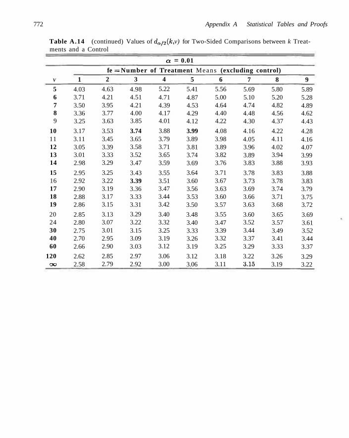
772 Appendix A Statistical Tables and Proofs
Table A.14 (continued) Values of dQ/2(k, v) for Two-Sided Comparisons between k Treatments and a Control
V
5 6 7 8 9
10 11 12 13 14
15 16 17 18 19
20 24 30 40 60
120 oo
1
4.03 3.71 3.50 3.36 3.25
3.17 3.11 3.05 3.01 2.98
2.95 2.92 2.90 2.88 2.86
2.85 2.80 2.75 2.70 2.66
2.62 2.58
fe = 2
4.63 4.21 3.95 3.77 3.63
3.53 3.45 3.39 3.33 3.29
3.25 3.22 3.19 3.17 3.15
3.13 3.07 3.01 2.95 2.90
2.85 2.79
a = 0.01
Number of Treatment Means (excluding control) 3
4.98 4.51 4.21 4.00 3.85
3.74 3.65 3.58 3.52 3.47
3.43 3.39 3.36 3.33 3.31
3.29 3.22 3.15 3.09 3.03
2.97 2.92
4
5.22 4.71 4.39 4.17 4.01
3.88 3.79 3.71 3.65 3.59
3.55 3.51 3.47 3.44 3.42
3.40 3.32 3.25 3.19 3.12
3.06 3.00
5
5.41 4.87 4.53 4.29 4.12
3.99 3.89 3.81 3.74 3.69
3.64 3.60 3.56 3.53 3.50
3.48 3.40 3.33 3.26 3.19
3.12 3.06
6
5.56 5.00 4.64 4.40 4.22
4.08 3.98 3.89 3.82 3.76
3.71 3.67 3.63 3.60 3.57
3.55 3.47 3.39 3.32 3.25
3.18 3.11
7
5.69 5.10 4.74 4.48 4.30
4.16 4.05 3.96 3.89 3.83
3.78 3.73 3.69 3.66 3.63
3.60 3.52 3.44 3.37 3.29
3.22 3,15
8
5.80 5.20 4.82 4.56 4.37
4.22 4.11 4.02 3.94 3.88
3.83 3.78 3.74 3.71 3.68
3.65 3.57 3.49 3.41 3.33
3.26 3.19
9
5.89 5.28 4.89 4.62 4.43
4.28 4.16 4.07 3.99 3.93
3.88 3.83 3.79 3.75 3.72
3.69 3.61 3.52 3.44 3.37
3.29 3.22
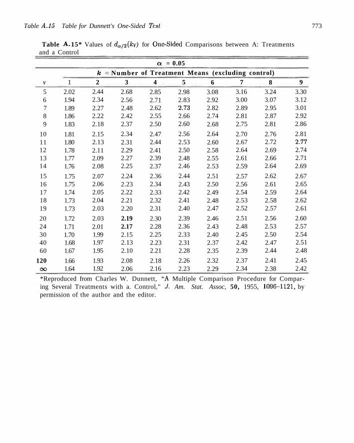
Table A.15 Table for Dunnett's One-Sided Test 773
Table A. 15* Values of da/2(k, v) for One-Sided Comparisons between A: Treatments and a Control
V
5 6 7 8 9
10 11 12 13 14
15 16 17 18 19
20 24 30 40 60
120 CO
1
2.02 1.94 1.89 1.86 1.83
1.81 1.80 1.78 1.77 1.76
1.75 1.75 1.74 1.73 1.73
1.72 1.71 1.70 1.68 1.67
1.66 1.64
k = 2
2.44 2.34 2.27 2.22 2.18
2.15 2.13 2.11 2.09 2.08
2.07 2.06 2.05 2.04 2.03
2.03 2.01 1.99 1.97 1.95
1.93 1.92
Number 3
2.68 2.56 2.48 2.42 2.37
2.34 2.31 2.29 2.27 2.25
2.24 2.23 2.22 2.21 2.20
2.19 2.17 2.15 2.13 2.10
2.08 2.06
a = 0.05 of Treatment Means (excluding control)
4
2.85 2.71 2.62 2.55 2.50
2.47 2.44 2.41 2.39 2.37
2.36 2.34 2.33 2.32 2.31
2.30 2.28 2.25 2.23 2.21
2.18 2.16
5
2.98 2.83 2,73 2.66 2.60
2.56 2.53 2.50 2.48 2.46
2.44 2.43 2.42 2.41 2.40
2.39 2.36 2.33 2.31 2.28
2.26 2.23
6 3.08 2.92 2.82 2.74 2.68
2.64 2.60 2.58 2.55 2.53
2.51 2.50 2.49 2.48 2.47
2.46 2.43 2.40 2.37 2.35
2.32 2.29
7 3.16 3.00 2.89 2.81 2.75
2.70 2.67 2.64 2.61 2.59
2.57 2.56 2.54 2.53 2.52
2.51 2.48 2.45 2.42 2.39
2.37 2.34
8 3.24 3.07 2.95 2.87 2.81
2.76 2.72 2.69 2.66 2.64
2.62 2.61 2.59 2.58 2.57
2.56 2.53 2.50 2.47 2.44
2.41 2.38
9 3.30 3.12 3.01 2.92 2.86
2.81 2,77 2.74 2.71 2.69
2.67 2.65 2.64 2.62 2.61
2.60 2.57 2.54 2.51 2.48
2.45 2.42
*Reproduced from Charles W. Dunnett, "A Multiple Comparison Procedure for Comparing Several Treatments with a. Control." J. Am. Stat. Assoc, 50, 1955, 1096-1121, by permission of the author and the editor.
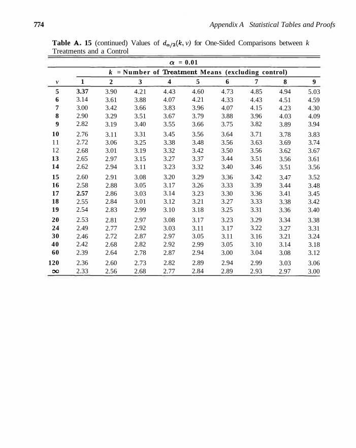
774 Appendix A Statistical Tables and Proofs
Table A. 15 (continued) Values of da/2(k, v) for One-Sided Comparisons between k Treatments and a Control
V
5 6 7 8 9
10 11 12 13 14
15 16 17 18 19
20 24 30 40 60
120 CO
1 3.37 3.14 3.00 2.90 2.82
2.76 2.72 2.68 2.65 2.62
2.60 2.58 2.57 2.55 2.54
2.53 2.49 2.46 2.42 2.39
2.36 2.33
k = 2
3.90 3.61 3.42 3.29 3.19
3.11 3.06 3.01 2.97 2.94
2.91 2.88 2.86 2.84 2.83
2.81 2.77 2.72 2.68 2.64
2.60 2.56
a = 0.01 Number of Treatment Means (excluding control)
3 4.21 3.88 3.66 3.51 3.40
3.31 3.25 3.19 3.15 3.11
3.08 3.05 3.03 3.01 2.99
2.97 2.92 2.87 2.82 2.78
2.73 2.68
4
4.43 4.07 3.83 3.67 3.55
3.45 3.38 3.32 3.27 3.23
3.20 3.17 3.14 3.12 3.10
3.08 3.03 2.97 2.92 2.87
2.82 2.77
5
4.60 4.21 3.96 3.79 3.66
3.56 3.48 3.42 3.37 3.32
3.29 3.26 3.23 3.21 3.18
3.17 3.11 3.05 2.99 2.94
2.89 2.84
6
4.73 4.33 4.07 3.88 3.75
3.64 3.56 3.50 3.44 3.40
3.36 3.33 3.30 3.27 3.25
3.23 3.17 3.11 3.05 3.00
2.94 2.89
7
4.85 4.43 4.15 3.96 3.82
3.71 3.63 3.56 3.51 3.46
3.42 3.39 3.36 3.33 3.31
3.29 3.22 3.16 3.10 3.04
2.99 2.93
8 4.94 4.51 4.23 4.03 3.89
3.78 3.69 3.62 3.56 3.51
3.47 3.44 3.41 3.38 3.36
3.34 3.27 3.21 3.14 3.08
3.03 2.97
9
5.03 4.59 4.30 4.09 3.94
3.83 3.74 3.67 3.61 3.56
3.52 3.48 3.45 3.42 3.40
3.38 3.31 3.24 3.18 3.12
3.06 3.00
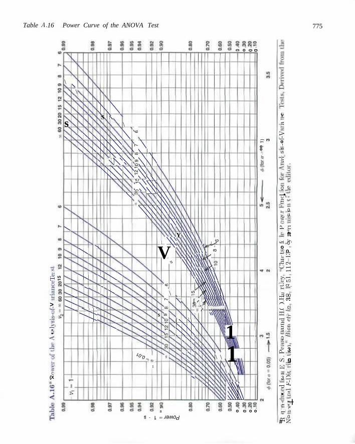
Table A. 16 Power Curve of the ANOVA Test 775
o o o o
CO
5 2
>
CO
--
C (X
\
s \
\
s \
^
1 k
vx\ \ \ \
\ X
V v U
"
S>:
\ \ S A.
\ \ ^ s \ \ \
i^S
N V
J ss.
s .
\
\
\ \
*>
t\X \
k\W \ \ ^
^
f\ \ \
k ^
io'o* 1
^ YV
s 1 ^ V
V
' IO
*
\ r--
S °>
H
Y \N\\
si i
i n
N [
\ \
^ s V^NN
\. x^
< sN
^
\ L j / to
ULl i °°
vfSiJl''
VV Nff\Y
i\\0\w\\
« \ 1 <'«SB!IN
/ v\ \ \ \ \ \ \ \ \ \V\YVVC\V
\ :o
\ \
1 1 \ \
1 i\
1 1
' — CO
o o
'
c; V
si
> o
1 CO
HI
> 71
95 a o o o o
fl - I = JOMOd
o —• o p
-.' r*
0, jL
— . [ 1
o H J
b r ^
> i
s , | " 0 /J
p •-• ft >-> 0
o TO r H
-M r H i—1
r-* CU L O
4 ^
a w r**>
•v_
T3 r H
S
o Gn
£ zn a _, 3
T^
•
:: T
~ n #
cr..
00 CO
ci
"!"* r -
W
e o
3 r ^
g
*-» / " N
Ci X
—| -. ; H
0 <4
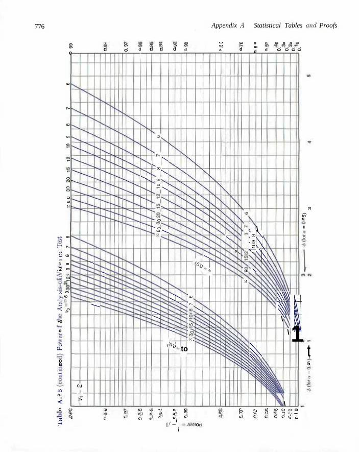
776 Appendix A Statistical Tables and Proofs
s e
ID
N
CO
<T>
a
r "
1 "
3 O CO
o ID
K
+3 to CO
i -4 r-Cj O CO H 3 en .2 o
« s CO o >.CO
"3 8 < v «
+3
o cu
£
o a
'-§
CO rH
< C c
[5
e i
a Cl
3
J
.
*«s
T
OO
d
^
0 c c
3 I 1
cn d
0 c
j i
d
I
Cl
c c
^
en rj> d d
3
J i
u a e
to
en d
L J X
CD
O
x
^
5 a % o 00 "sv
^
1 *; i a i c
•sj*1*
T ^ %
r j 1
c a c
1-
• N .
J 1
i
i
o
d
to
c a c
S CD
1 h-
' m 1 o
-S s
i
^ *b
\
Ori
°*i 7
O CO
a
c a c
K,
> 1
s
O
d
s
o (D d
CO
i co X
a
c h c
> i
\
> s \
L
c 6 C
> 1 1
o o o o o
d © o d d
\
$
c u c
SA 1 \
) c
1 c
> c r f > c
\
\ ) c ) c j c
1 1
1 o J T -
j d
en
in" q
II
o
\
t i 5
l:
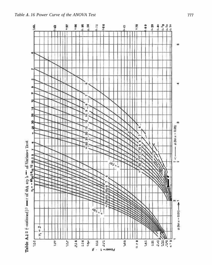
Table A. 16 Power Curve of the ANOVA Test 777
3 CD CJ
O
i CO
>> cc3
< CB
I CL
"g
O y
co rH
I—I
3
g c
r-
co
Ol
o
CM
U5 T -
c?
s 8
CO
1-
co
0)
CM
T -O CM
ID 8
II
0 a c
P
1 1 !
5
.
g d
0 0 c
3 D 3
d
c a c
> i
d
<i e e
3 1 3
01 01 d d
u 0 c
l>
s > .
v, 1 o> . ^
**CM
1 CO^v^
< o - — „
^ 8
3 * n 0 3 C
.
t
i
CM 0 1
d
'Oc
c c e
n 3
O o> d
u
c c e
S < 0
^coj
" 8 .
3 n 9
l°c
$3 JJ
i>
g d
c 0 c
3 3 3
v s \
d o IO
d
\ 1 CO
> >is
, . C M
. ° "vP
8
o h. d
X,
c I c
\
^
3 3 3
o o o o o irj ^ co CM T -
d d d d d
\
*
\
V
C\ 1 \ v
c t
c
3 C 3 * 3 C
^ i w
y
I 3 C f C 3 C
\ l l
i 3 C
-> C
i tt\
3 O 4 r-3 d
V CO CM
& - 1= J3M0J
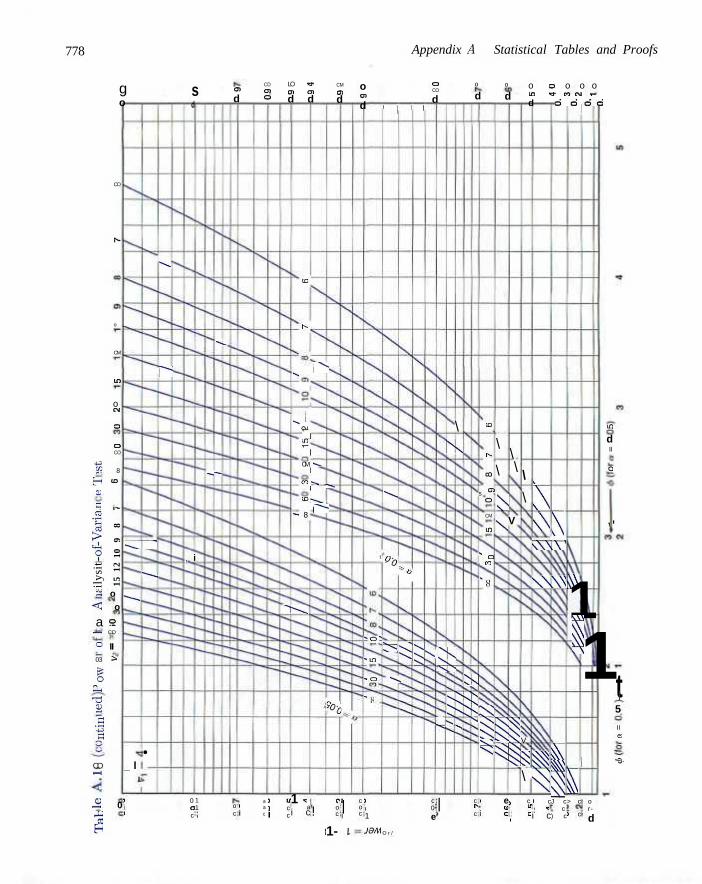
778 Appendix A Statistical Tables and Proofs
g o
CD
N
o
CM
i n
o CM
O
O CO
43 ?t 8
H <o CO
9 r-
-of-
Var
ia
10
9 8
ilys
it
15 1
2
S o <! o
a 9 — CD
o II 03 >
1 CH
T3 2
1 CO r H
JS 0
1
^
|*"-
- ^ "
~-— ~~
_ l »
3 j 1
•
s d
, i
0 o c
1 1 1
^
^
~~-
O)
d
o c
1 i
CD O l O
a a c
i i i
LO *J en a i d d
CO
N
s 1 ^
„ 1 CM
' " l LT1
"l CM s J
1 CO ;~.
1 ^
C O ^ ^
„ 1 ^ 8
^ * * ^ s ^
u c c
1 ••: i a i c
1
!
1
CM
en d
%>c
p o c
1-
o Ol
d
o CO
d 1 1 1 1
1 | i
I
c o c
t
i o :
- U I
s ^
%
JV
- o " ^
' 8 .
1 i 1
J3M
**
^ ^
O r /
\
c 0 e
\ \
r
**»
1 |
o
d
^N
S ^ V s
V
c r-c
<D
r-
co
s m
O
CM
IQ
s O - CO
*8
o
d
\
\
;> s
\ \
V
o o o o o LO T « CM -r-d d o d o
\
\
|
^
1
i
g =$
e CI c
^ §
> 1 1
V
^ \
c ir c
V
\ \ \
1
\ voiV
\N\\
^
^ 1 c 1 * i c
^ s J c
c ) c
\\\ 1 1 1 1
^ > c
> c
o r-
d
en
d II
o
I '
t 1 5
II e
H »
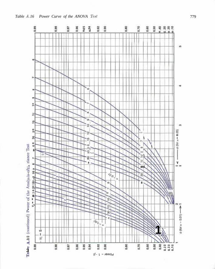
Table A. 16 Power Curve of the ANOVA Test 779
en 01 d d o o o o
t en S
r"
9 PL,
CO rH
< CP
3
CO
CO
O l
o
CM
i n
o CM
O
o ID
8
r-
cn
(N
o
o CO
o 8 II S?
u 1
CD
5
.
^
i
__ J~~~
CO
""N
CD
V. | > N '
1
~-o CM — ^ ,
1 " - O
m • 1
t o " - - ^ .
*• 8 ^ ^
-
v ^
>°c
k o
s j °° J
O
*«.
m.
co-
" 8 -
\ \ l
•o
]> "~-~
\
.
••jN\
- C O
\
CO
03
o
CM
\
mi
8
\ \
\
\ \ \ \
^ 1 Ti^
1 ^
\J
k\
\ \ \
8
i
o II B
v CO CM
o o o CO CM r-_
o d d
0 - I = JOMOd
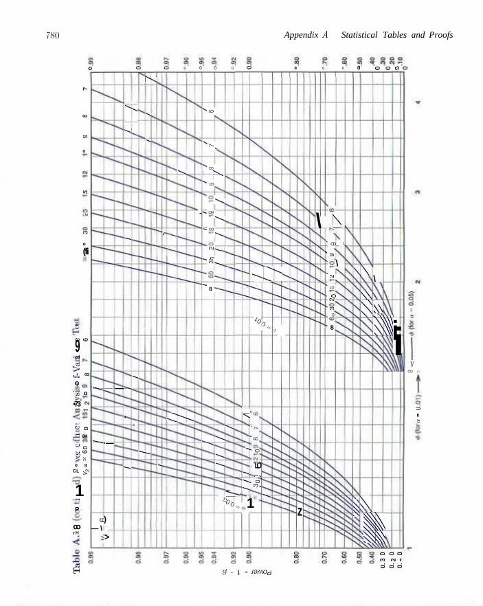
780 Appendix A Statistical Tables and Proofs
o
r-
co
c>
o
i n
CM
CO
o
(fi
-
<y io
9 cd
r5 cj, » o x o
•73 N
CC T -
2 0 -cr, CM
, J o Ui CO
E 8 0 II
CL jCM
1 H
P
co r H
«**
»—
IS.
— \
J - -
•
)
>
O
J \
"*
>J
•~~
— *«
'
__
*-
-
""'
_^_
~
O
' ~-
0
"•
0 0
"
•^J"~-^^
sco
"" ^
S CO 1 r** ^ 0 1
•» CM
1 CO
^
"^
^
0 O
CM.*. 1
•~ O t o ^ l
"" 8
__J --
^
J
" s ^
^
k
-\h
~<0
' rv
" CO
^ O
**L
,,
^
1
• LO •"«
- O CO.
0^
-««
'J
a
z
0 0
\ N * CD \
s 03
" C.J
* LO
» O
m . 0
* 8
\
0 0 0 0 0
Sl\
§
\ \ ^
\
\
a SI
11
i i V
CO r -
o II B
0 O O O P) N r o d d
$f - I = JOAAOd
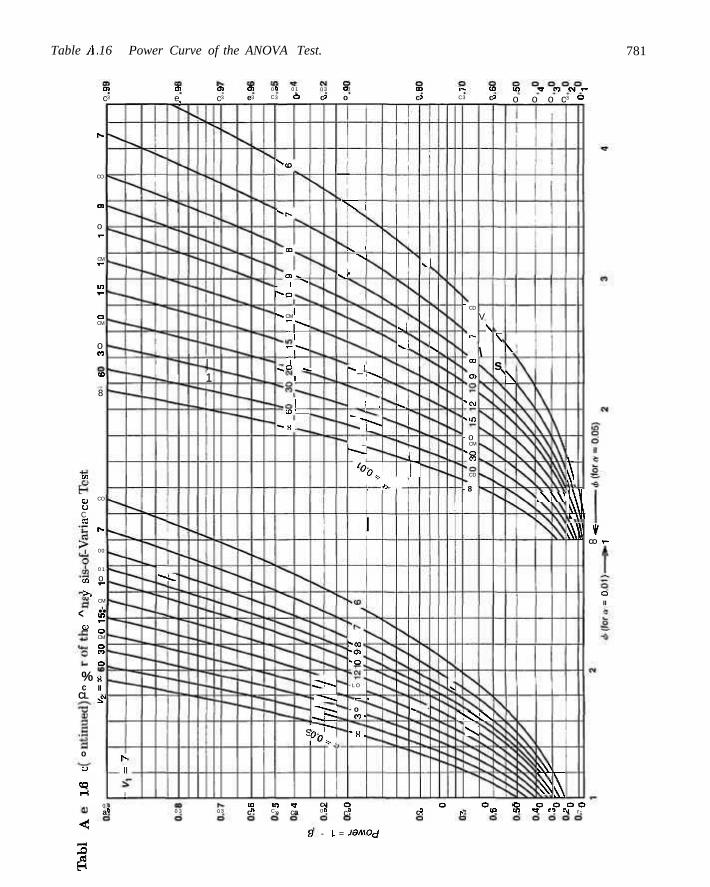
Table A. 16 Power Curve of the ANOVA Test. 781
CO
o u C cl
CO
>>
< o
% c
CL
o
CJ
CO T-l
<
I
UI
c
f -
CO
O l
o ""
CM T *
U3 r "
O CM
o CO
IO
8
CO
f-
00
0 1
o T -
CM
•'• IO T -
O CM
O CO
O
H II
i f
0 a
3
r* II
. 1
O l
e
1
^ _
)
1
| 1
0 )
c 3
i 0 3 0 3
O l
e 3
0
C
3 0 1
3 O
^ C D
•""•r-
m
(31 . .
. 1 ""' ^•o
1 • v . CM
' ~ | " * , v ,
I
"P" ,. 1 CD ^
1
1 CO' ,
""- K .
s
0
c 3
3
^^*^^ ^ 1
^ *. •^^ 1***"
vr
co in Tt c c 3 C » c a 0
0 3
o
—
> v i
y ^ 1
"V,
. s j
~> 1 T^N,
^ 1 ' T"-
-• 1
«V
CO
c
s 1
s j
•v.
1 r ; «
|
""•OO ^ O )
* o
- L O
T- •» - o
co-
" K -
3
„J
s
V 1 *
r -
C
^
3
" CD
r -
CO
O l
N C M
**.LO
- o CM
~ o CO
CD
- 8
CO
c
V \
\
^sCsOs • \
3
\
s s
g o o o o 3 c 1 c 3 r- Cl 3
U3 » f ) N r
o o o c 1
\
\
c t i
A A V
t ^
\ I
3 O
I
\ \\ \ ' t m
\ 3 O O O O 3 >! T C 3 C J r-
y CO «-
O II
£, - l = JOMOd
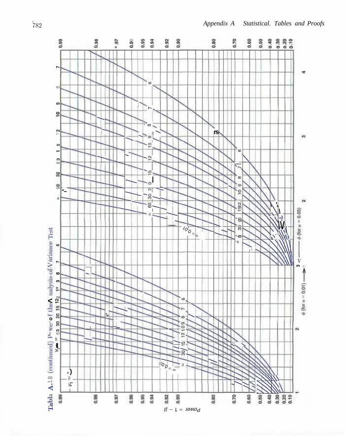
rs2 Appendix A Statistical. Tables and Proofs
| o
CD C l
O O O O O
E5
>
< s
o B
c OH
CO —I
< CD
0
t ^
CO
o i
o
CM 1—
i n
*-o CM
O
CD
8
CO
r~
CO
O l
o
CM
O
O CO
CO CD
S
|| -CM
..
a
1
)
i"
.J
T Y*
~_c
i • L
_____
.
j
P"
"*• " - * * c ,
*
•— ^
—•~- ^ :~~-]
^ ^ i
^•^^
__
CO
N ^
" CO
p* -S .O
s^CSI
^ m
| CN ""*•—.
"*-o cn^—.
C D — ^ .
1
^***»v
.
j ^ ______
i I J *
?"*
*°K
"co
r" * - C M ,
"**•«« J"_-"' r*--• 8 - ^
rs
__.
•Vj
8 - ^ .
Kt
rs.
^ > "-^s^l
^ ^
to
\ -
co
x o
£• stO
»o CM
CO
•o CO
" 8
sJ \
\
I s
^ N \ s.
\ \ N s \
\\N
\ \ \
\ v i >
\V w w
i
\ \ Nv.\
\ \ \ \ \ \ \ \ \ \ \ \ \
Hi
Vl
i
V CO r -
( 1 - 1 = J9M0d
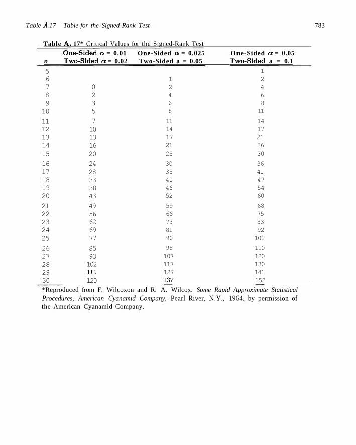
Table A. 17 Table for the Signed-Rank Test 783
Table A. 17* Critical Values for the Signed-Rank Test
One-Sided a = 0.01 One-Sided a = 0.025 One-Sided a = 0.05 n Two-Sided a = 0.02 Two-Sided a = 0.05 Two-Sided a = 0.1
1 1 2 2 4 4 6 6 8 8 11
11 14 14 17 17 21 21 26 25 30
30 36 35 41 40 47 46 54 52 60
59 68 66 75 73 83 81 92 90 101
98 110 107 120 117 130 127 141 137 152
*Reproduced from F. Wilcoxon and R. A. Wilcox. Some Rapid Approximate Statistical Procedures, American Cyanamid Company, Pearl River, N.Y., 1964. by permission of the American Cyanamid Company.
5 6 7 8 9 10
11 12 13 14 15
16 17 18 19 20
21 22 23 24 25
26 27 28 29 30
0 2 3 5
7 10 13 16 20
24 28 33 38 43
49 56 62 69 77
85 93 102 111 120
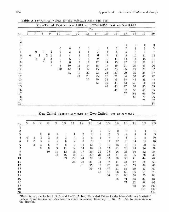
784 Appendix A Statistical Tables and Proofs
Table A . 1 8 * Critical Values for the Wilcoxon Rank-Sum Test
One-Tai led Test at a = 0 .001 or T w o - T a i l e d Test at a = 0 .002 n2
m 6 7 8 9 10 11 12 13 14 15 16 17 18 19 20
1 2 3 4 5 0 0 6 0 1 2 7 8 9
10 11 12 13 14 15 16 17 18 19 20
2 3 5
1 2 3 5 7
0 1 3 5 6 8
10
0 2 4 6 8
10 12 15
0 2 4 7 9
12 14 17 20
1 3 5 8
11 14 17 20 23 26
1 3 0 9
12 15 19 22 25 29 32
1 4 7
10 14 17 21 24 28 32 36 40
2 5 8
11 15 19 23 27 31 35 39 43 48
0 2 5 9
13 17 21 25 29 34 38 43 47 52 57
0 3 6
10 14 18 23 27 32 37 42 46 51 56 61 66
0 3 7
11 15 20 25 29 34 40 45 50 55 60 66 71 77
0 3 7
12 16 21 26 32 37 42 48 54 59 65 70 76 82 88
One-Tailed Test at a = 0.01 or Two-Tailed Test at a = 0.02
n2
nx 5 6 7 8 9 10 11 12 13 14 15 16 17 18 19 20 1 2 3 4 0 5 1 6 7 8 9
10 11 12 13 14 15 16 17 18 19 20
0 1 1 2 3 3 4
6
0 2 4 6 8
10
1 3 5 7 9
11 14
1 3 6 8
11 13 16 19
I 4 7 9
12 15 18 22 25
2 5 8
11 14 17 21 24 28 31
0 2 5 9
12 16 20 23 27 31 35 39
0 2 6
10 13 17 22 26 30 34 38 43 47
0 3 7
11 15 19 24 28 33 37 42 47 51 56
0 3 7
12 16 21 26 31 36 41 46 51 56 61 66
0 4 8
13 18 23 28 33 38 44 49 55 60 66 71 77
0 4 9
14 19 24 30 36 41 47 53 59 65 70 76 82 88
1 4 9
15 20 26 32 38 44 50 56 63 69 75 82 88 94
101
1 5
10 16 22 28 34 40 47 53 60 67 73 80 87 93
100 107 114
*Based in part on Tables 1, 3, 5. and 7 of D. Auble, "Extended Tables for the Mann-Whitney Statistic," Bulletin of the Institute of Educational Research ai Indiana University, 1, No. 2, 1953, by permission of the director.
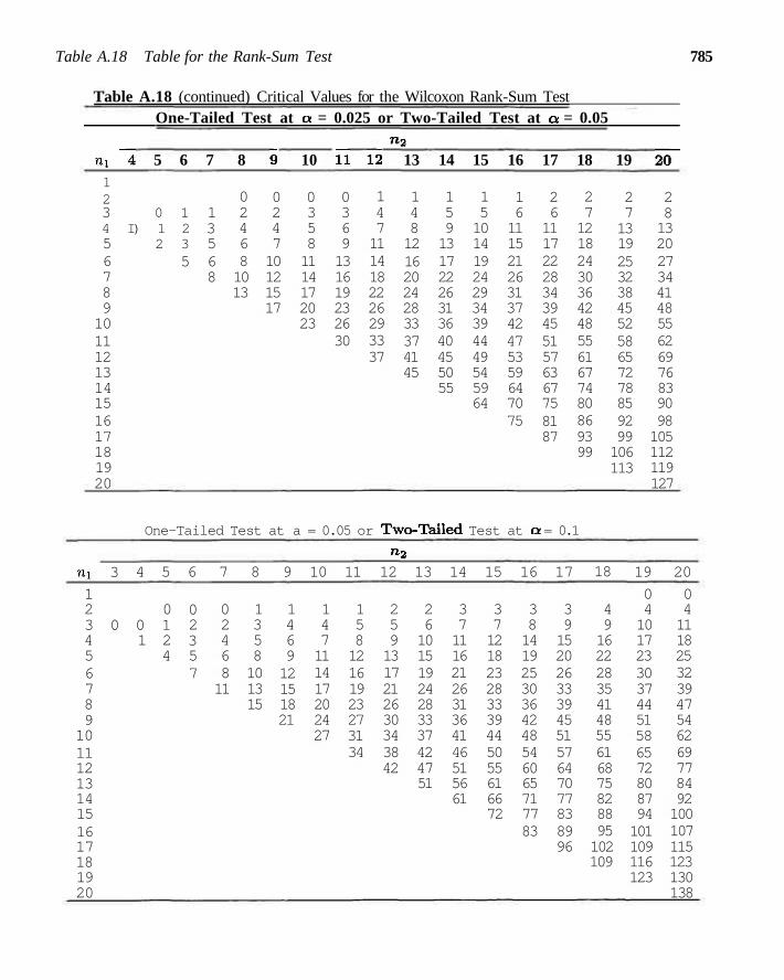
Table A.18 Table for the Rank-Sum Test 785
Table A.18 (continued) Critical Values for the Wilcoxon Rank-Sum Test One-Tailed Test at a = 0.025 or Two-Tailed Test at a = 0.05
n2
nx ~4 5 6 7 8 9" 10 i i 12" 13 14 15 16 17 18 19 20~ 1 2 3 4 I 5 6 7 8 9 10 11 12 13 14 15 16 17 18 19 20
0 1 ) 1 2
2 3 5
1 3 5 6 8
0 2 4 6 8 10 13
0 2 4 7 10 12 15 17
0 3 5 8 11 14 17 20 23
0 3 6 9 13 16 19 23 26 30
1 4 7 11 14 18 22 26 29 33 37
1 4 8 12 16 20 24 28 33 37 41 45
1 5 9 13 17 22 26 31 36 40 45 50 55
1 5 10 14 19 24 29 34 39 44 49 54 59 64
1 6 11 15 21 26 31 37 42 47 53 59 64 70 75
2 6 11 17 22 28 34 39 45 51 57 63 67 75 81 87
2 7 12 18 24 30 36 42 48 55 61 67 74 80 86 93 99
2 7 13 19 25 32 38 45 52 58 65 72 78 85 92 99 106 113
2 8 13 20 27 34 41 48 55 62 69 76 83 90 98 105 112 119 127
One-Tailed Test at a = 0.05 or Two-Tailed Test at a = 0.1
n_ 3 n2
4 5 6 7 8 9 10 11 12 13 14 15 16 17 18 19 20
1 2 0 3 0 0 1 4 5 6 7 8 9 10 11 12 13 14 15 16 17 18 19 20
1 2 4
0 2 3 5 7
0 2 4 6 8 11
1 3 5 8 10 13 15
1 4 6 9 12 15 18 21
1 4 7 11 14 17 20 24 27
1 5 8 12 16 19 23 27 31 34
2 5 9 13 17 21 26 30 34 38 42
2 6 10 15 19 24 28 33 37 42 47 51
3 7 11 16 21 26 31 36 41 46 51 56 61
3 7 12 18 23 28 33 39 44 50 55 61 66 72
3 8 14 19 25 30 36 42 48 54 60 65 71 77 83
3 9 15 20 26 33 39 45 51 57 64 70 77 83 89 96
4 9 16 22 28 35 41 48 55 61 68 75 82 88 95 102 109
0 4 10 17 23 30 37 44 51 58 65 72 80 87 94 101 109 116 123
0 4 11 18 25 32 39 47 54 62 69 77 84 92 100 107 115 123 130 138
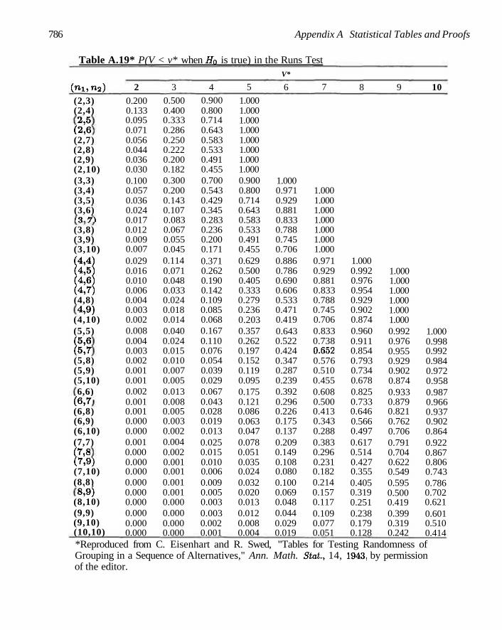
786 Appendix A Statistical Tables and Proofs
Table A.19* P(V < v* when H0 is true) in the Runs Test
(nx,n2) (2,3) (2,4) 2,5
(2,6 (2,7) (2,8) (2,9) (2,10) (3,3) (3,4) (3,5) (3,6) t'i 7 i (3,8) (3,9) (3,10) m m (4,8) 4,9)
(4,10) (5,5) (5,6 (5,7 (5,8) (5,9) (5,10) 6,6)
(6,7 (6,8) (6,9) (6,10) (7,7) (7,8 (7,9) (7,10) (8,8) 8,9)
(8,10) (9,9) (9,10) (10,10)
2 0.200 0.133 0.095 0.071 0.056 0.044 0.036 0.030 0.100 0.057 0.036 0.024 0.017 0.012 0.009 0.007 0.029 0.016 0.010 0.006 0.004 0.003 0.002 0.008 0.004 0.003 0.002 0.001 0.001 0.002 0.001 0.001 0.000 0.000 0.001 0.000 0.000 0.000 0.000 0.000 0.000 0.000 0.000 0.000
3
0.500 0.400 0.333 0.286 0.250 0.222 0.200 0.182 0.300 0.200 0.143 0.107 0.083 0.067 0.055 0.045 0.114 0.071 0.048 0.033 0.024 0.018 0.014 0.040 0.024 0.015 0.010 0.007 0.005 0.013 0.008 0.005 0.003 0.002 0.004 0.002 0.001 0.001 0.001 0.001 0.000 0.000 0.000 0.000
4 0.900 0.800 0.714 0.643 0.583 0.533 0.491 0.455 0.700 0.543 0.429 0.345 0.283 0.236 0.200 0.171 0.371 0.262 0.190 0.142 0.109 0.085 0.068 0.167 0.110 0.076 0.054 0.039 0.029 0.067 0.043 0.028 0.019 0.013 0.025 0.015 0.010 0.006 0.009 0.005 0.003 0.003 0.002 0.001
5
1.000 1.000 1.000 1.000 1.000 1.000 1.000 1.000 0.900 0.800 0.714 0.643 0.583 0.533 0.491 0.455 0.629 0.500 0.405 0.333 0.279 0.236 0.203 0.357 0.262 0.197 0.152 0.119 0.095 0.175 0.121 0.086 0.063 0.047 0.078 0.051 0.035 0.024 0.032 0.020 0.013 0.012 0.008 0.004
V*
6
1.000 0.971 0.929 0.881 0.833 0.788 0.745 0.706 0.886 0.786 0.690 0.606 0.533 0.471 0.419 0.643 0.522 0.424 0.347 0.287 0.239 0.392 0.296 0.226 0.175 0.137 0.209 0.149 0.108 0.080 0.100 0.069 0.048 0.044 0.029 0.019
7
1.000 1.000 1.000 1.000 1.000 1.000 1.000 0.971 0.929 0.881 0.833 0.788 0.745 0.706 0.833 0.738 0-652 0.576 0.510 0.455 0.608 0.500 0.413 0.343 0.288 0.383 0.296 0.231 0.182 0.214 0.157 0.117 0.109 0.077 0.051
8
1.000 0.992 0.976 0.954 0.929 0.902 0.874 0.960 0.911 0.854 0.793 0.734 0.678 0.825 0.733 0.646 0.566 0.497 0.617 0.514 0.427 0.355 0.405 0.319 0.251 0.238 0.179 0.128
9
1.000 1.000 1.000 1.000 1.000 1.000 0.992 0.976 0.955 0.929 0.902 0.874 0.933 0.879 0.821 0.762 0.706 0.791 0.704 0.622 0.549 0.595 0.500 0.419 0.399 0.319 0.242
10
1.000 0.998 0.992 0.984 0.972 0.958 0.987 0.966 0.937 0.902 0.864 0.922 0.867 0.806 0.743 0.786 0.702 0.621 0.601 0.510 0.414
*Reproduced from C. Eisenhart and R. Swed, "Tables for Testing Randomness of Grouping in a Sequence of Alternatives," Ann. Math. Stat., 14, 1943, by permission of the editor.
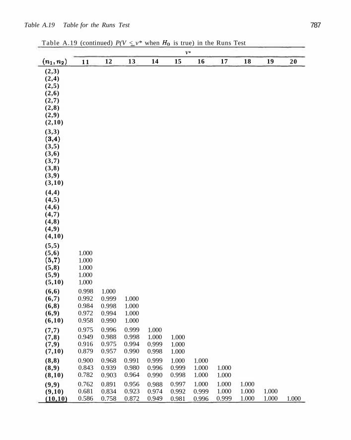
Table A.19 Table for the Runs Test 787
Table A.19 (conti nued) P(V < v* when Ho is true) in the Runs Test
V*
( n i , n 2 ) 11 12 13 14 15 16 17 18 19 20
(2,3) (2,4) (2,5) (2,6) (2,7) (2,8) (2,9) (2,10) (3,3) (3,4) (3,5) (3,6) (3,7) (3,8) (3,9) (3,10)
(4,4) (4,5) (4,6) (4,7) (4,8) (4,9) (4,10) (5,5) (5,6) (5,7) (5,8) (5,9) (5,10) (6,6) (6,7) (6,8) (6,9) (6,10)
(7,7) (7,8) (7,9) (7,10) (8,8) (8,9) (8,10) (9,9) (9,10) (10,10)
1.000 1.000 1.000 1.000 1.000 0.998 0.992 0.984 0.972 0.958
0.975 0.949 0.916 0.879
0.900 0.843 0.782
0.762 0.681 0.586
1.000 0.999 0.998 0.994 0.990 0.996 0.988 0.975 0.957
0.968 0.939 0.903 0.891 0.834 0.758
1.000 1.000 1.000 1.000 0.999 0.998 0.994 0.990
0.991 0.980 0.964
0.956 0.923 0.872
1.000 1.000 0.999 0.998 0.999 0.996 0.990
0.988 0.974 0.949
1.000 1.000 1.000 1.000 0.999 0.998 0.997 0.992 0.981
1.000 1.000 1.000 1.000 0.999 0.996
1.000 1.000 1.000 1.000 0.999
1.000 1.000 1.000
1.000 1.000 1.000
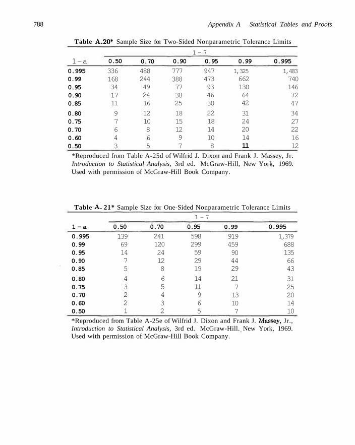
788 Appendix A Statistical Tables and Proofs
Table A.20* Sample Size for Two-Sided Nonparametric Tolerance Limits
1-a 0.995 0.99 0.95 0.90 0.85
0.80 0.75 0.70 0.60 0.50
0.50
336 168 34 17 11
9 7 6 4 3
0.70
488 244 49 24 16
12 10 8 6 5
0.90
777 388 77 38 25
18 15 12 9 7
1 - 7 0.95
947 473 93 46 30
22 18 14 10 8
0.99
1,325 662 130 64 42
31 24 20 14 11
0.995
1,483 740 146 72 47
34 27 22 16 12
*Reproduced from Table A-25d of Wilfrid J. Dixon and Frank J. Massey, Jr. Introduction to Statistical Analysis, 3rd ed. McGraw-Hill, New York, 1969. Used with permission of McGraw-Hill Book Company.
Table A. 21* Sample Size for One-Sided Nonparametric Tolerance Limits
1 - a
0.995 0.99 0.95 0.90 0.85
0.80 0.75 0.70 0.60 0.50
0.50
139 69 14 7 5
4 3 2 2 1
0.70
241 120 24 12 8
6 5 4 3 2
1 - 7
0.95
598 299 59 29 19
14 11 9 6 5
0.99
919 459 90 44 29
21 7 13 10 7
0.995
1.379 688 135 66 43
31 25 20 14 10
*Reproduced from Table A-25e of Wilfrid J. Dixon and Frank J. Massey. Jr., Introduction to Statistical Analysis, 3rd ed. McGraw-Hill. New York, 1969. Used with permission of McGraw-Hill Book Company.
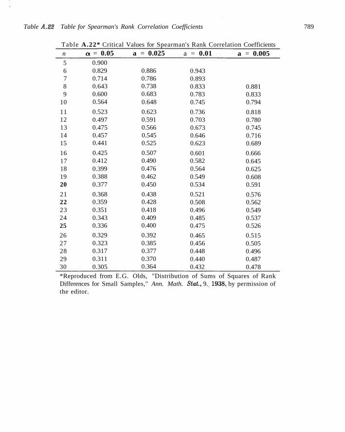
Table A.22 Table for Spearman's Rank Correlation Coefficients 789
Table A.22* Critical Values for Spearman's Rank Correlation Coefficients n
5 6 7 8 9
10
11 12 13 14 15
16 17 18 19 20
21 22 23 24 25
26 27 28 29 30
a = 0.05 0.900 0.829 0.714 0.643 0.600 0.564
0.523 0.497 0.475 0.457 0.441
0.425 0.412 0.399 0.388 0.377
0.368 0.359 0.351 0.343 0.336
0.329 0.323 0.317 0.311 0.305
a = 0.025
0.886 0.786 0.738 0.683 0.648
0.623 0.591 0.566 0.545 0.525
0.507 0.490 0.476 0.462 0.450
0.438 0.428 0.418 0.409 0.400
0.392 0.385 0.377 0.370 0.364
a = 0.01
0.943 0.893 0.833 0.783 0.745
0.736 0.703 0.673 0.646 0.623
0.601 0.582 0.564 0.549 0.534
0.521 0.508 0.496 0.485 0.475
0.465 0.456 0.448 0.440 0.432
a = 0.005
0.881 0.833 0.794
0.818 0.780 0.745 0.716 0.689
0.666 0.645 0.625 0.608 0.591
0.576 0.562 0.549 0.537 0.526
0.515 0.505 0.496 0.487 0.478
*Reproduced from E.G. Olds, "Distribution of Sums of Squares of Rank Differences for Small Samples," Ann. Math. Stat., 9. 1938, by permission of the editor.
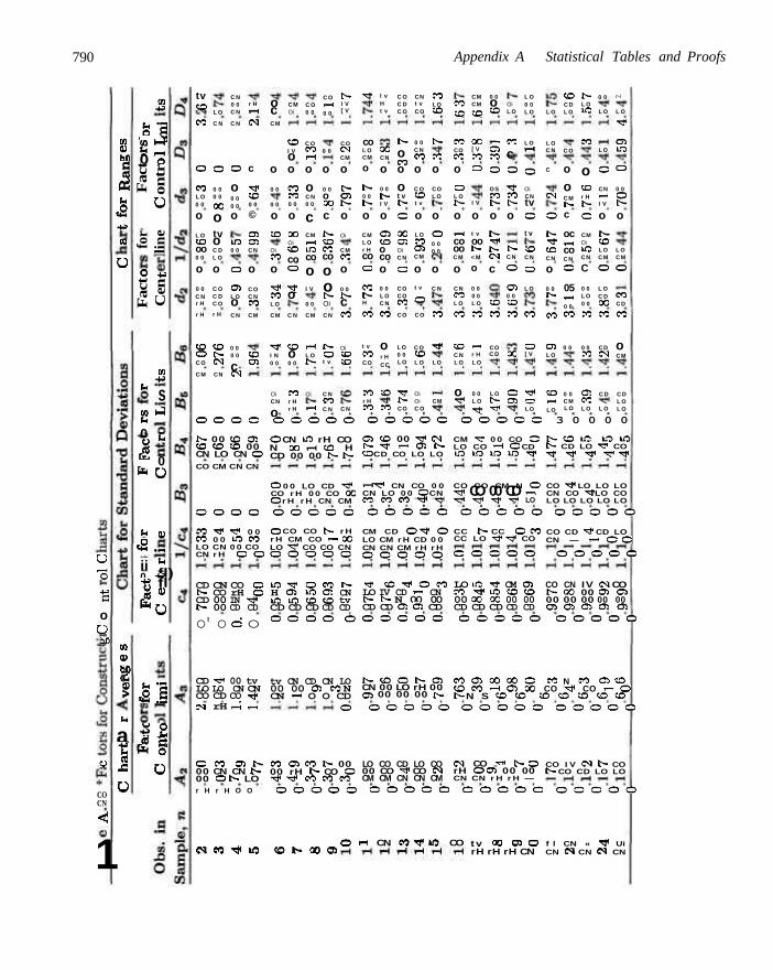
790 Appendix A Statistical Tables and Proofs
O "3
t o
O 00
o
* CO CN
<
1
$ M
1 I L O
<tH
H->
CM
U
en - W
Is S ^ 0 o
Fac
t on
tr
O
for
lin
e
O + j
Fac
t C
en
I L
2 0
l I-H
U
£ ii 0
1
en H J
s I - )
L i
0 U
en « H
(H
fl) 4 J
fl I I I
u
en eu
a1
1 L i
a I u
I's
ti rSg o
tv co C O
O
C O L O 0 0
o
L O C D oo 0 0
o
0 0 C N r H
r H
C O O C O
C M
L O
C N
o
0 0 0 0
oo o tv o C D L O
o
C O C D C O
r H
C O t v C N
CN
C N 0 0 C N
C N
O
o 0 0 0 0
o
l O 0 0
o
C l L O o C N
0 0 0 0
c CN:
r H r-t
< N
c
N < C O 0 0
©
Oi Oi C N
o
C O C N C O
CM
C O O l
o c CM
o
0 0
0 0
o
C O
Oi C O
o
•>cf C O L O
CM
N < I N 0 0
Oi CN
o
CM Oi
C O I V o o
C O C O 0 0
o
0 0 Oi C O
co o
_* o C N
C O o 0 0
C O r H r H
C O 0 0
C O C O r ^
o
o C N 0 0
c CM r-^ l O co o I V
0 0
CM
r-i L O t -
Oi
r-l
C O r-< 0 0
0 0
o
0 0 o oo c
1 - -cc C O co
o o I V Oi
C N
I V o t v
C N C O C N
t v I V [ V
C O c N CM
o
1--o t -
o
Oi
CM C O
o
0 0 1 - -c C O
Oi C O C O
C N
N "
co L O CM
o
t v 0 0 t v
o
CM L O r H co o
C O I V H
C O
t v
C O C O
C O r H C O
l v H t v
oc CN
o
0 0 t v I V
o
o C O o co o
0 0 L O C N
C O
o r H CC
C O
C O
C O C D C O
I V
o C O o
o t v I V
o
oc Oi Oi C N
o
C O C O C O
C O
L O 0 0 L O
r -I V C O
CN t v C O
0 0 C N C O
o
C O C O t v
o
L O C O O l CM
o t v
o C O
C O C O L O
Oi Oi C O
C O L O C O
I V
CO
o
C O L O
o
o 0 0 0 0
o
C N
C O
N "
L O
CM
C O
cc
C O CO CO
o
o L O I V
o r ^ co oo C M
o
C N C O L O
C O
C O C N L O
o Tt<
CM CM
cc
oc [ V CO
o
I V
o t v
oo t v
< M
o
0 0 0 0 L O
C O
r-f r H L O
0 0 L O
N-
0 0 o CO
ci C O
o
O S CO I V
o t v i H t v ( M
c
C O
CO
CO C D
L O t v ^ H
Oi L O
C O
c o
_8f C O ( V
o
iv C N
O
Oi 0 0 C O
C O
0 C
o C 5
L O 0 0 L O
L O r-1
o Oi CN tv o t v
co C N
o
L O
C O
o [ V
*Cf r H LO
L O
L O C N
C
C N
o
1 ^ "* C O C N
o
0 0 I V
co
O l L O
C O r-H L O
C O C D L O
C O
o
o C M f -
c
oc r H co C N
CO
05 i—i 0 0
C O
0 0
0 0 C M L O
I V L O I O
CO
o C O r H I V
c
CM Oi l O C N
C
0 0 L O 0 0
CO
0 0 CO
C D C O L O
0 0
L O
L O
o CN —1 I V
o
1 -C D L O C M
O
L O C D O C
C O
C D CN
C D
L O
r-i
L O
r1
C D L O
O
0 0
1 ^
o
L O CM
O
C O C D
C O
o CM
C D L O L O
O O O O O O O O O O O O O O O O O O C 3 0 0 0 0
Is- 00 CO CD CO CO CO 00 CN LO CN O
O CN IO rH CO N » H C O H CD 00 00 Is- t -
CD CO 00 n< CN I V - r t r n O i t v O CD CO LO LO
CM T T 0 0 CO O LO CO —I O CD LO LO LO LO ^ r
N O I O L O U ) t— CD LO •n? CO ^ i ^ * ^ f ^ ^ i
CO CM CN CN
O 0 0 LO CD ^P CO r H 0 0 CO X O r H r H CN CM
H Ti l CN CO 0 0 CN LO 0 0 O CN CO CO CO M 1 M 1
CO CO CM N O •** CO 00 CD rn •*cH "*Ct* ^cfl TH LO
CO • * LO LO LO CN CO ^ LO CO LO LO LO LO LO
O O O O O O O O O O O O O O O O O O O O O O O O
M T f TJ I 0 0 CO 0 0 LO CO LO CN 0 0 CO CN r H O O
O CO CO t V r H r H CM CO r r 0 0 LO -_P CO CO CN O O O O O
CM CD O T * O LO CM r H CD 0 0 CN CN CM r H r H O O O O O
CC N CC O M CC LO T * -D" CO
CO CD - * CD LO CN — r - O O
O O O O O O O O O O
CD CN CO O t- CO rH O CD 00 IN rti IV 00 CD CD
o' o d o
CD -* 00 tv LO LO CN CN CO CD CO -* M rH r-i r-<
LO -tr O CO IV H Ol LO Ol CN LO LO CO CO tv CD CD CD CD CD O O O O O
tv CN CD CN LO 00 00 O) M N CN -H O O CD
•* C O N O C O LO IV CD rH CN t- S N 00 00 CD CD Ol Oi CD
LO LC Tf CM Ol CO '* LO CO CO 00 X- 00 00 00 CD CD CD CD CD
CO CN IV (N CO b- 00 00 Ol Ol 00 00 00 00 00 Oi Ol CD Ol Ol
O O O O O O O O O O O O O O O
N C O O N O CN 00 LO rH 00 Ol 00 00 00 t v
C O O O O O O O M N CO O CO C O C O r H O O O CO M1 CO r- O S N S CO CO CO CO CO <o CO
O O O O O O O O O O O O O O O O
O W O I N 00 CN CN t -00 O t v LO
CO Ol CO t v 00 00 rH IV CO O ™tf —Cf CO CO CO
LO CO CD LO CO 00 CO - * CO (M CM CM CN CN CM
CNI CO -H N O rH O Ol 00 00 CN CN r H r H —
CO I V CN ( V CO t - CO CD LO LO
r H r H O O O O O O O O O O O O O O O O O O O O O O
N W J I O e b - t o s O tH CN M r f W CO t v 00 O O
rH rH rH CN f l CN « rj< Ui CN ( N CN CN CN
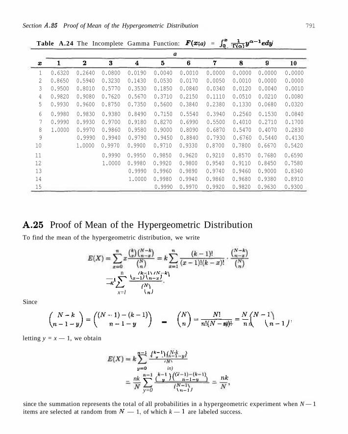
Section A.25 Proof of Mean of the Hypergeometric Distribution 791
Table A.24 The Incomplete Gamma Function: F(x; a) = /<_f rh?,ya~le~y dy
a
X 1 2 3 4 5 6 7 8 9 10 1 0.6320 0.2640 0.0800 0.0190 0.0040 0.0010 0.0000 0.0000 0.0000 0.0000 2 0.8650 0.5940 0.3230 0.1430 0.0530 0.0170 0.0050 0.0010 0.0000 0.0000 3 0.9500 0.8010 0.5770 0.3530 0.1850 0.0840 0.0340 0.0120 0.0040 0.0010 4 0.9820 0.9080 0.7620 0.5670 0.3710 0.2150 0.1110 0.0510 0.0210 0.0080 5 0.9930 0.9600 0.8750 0.7350 0.5600 0.3840 0.2380 0.1330 0.0680 0.0320
6 0.9980 0.9830 0.9380 0.8490 0.7150 0.5540 0.3940 0.2560 0.1530 0.0840 7 0.9990 0.9930 0.9700 0.9180 0.8270 0.6990 0.5500 0.4010 0.2710 0.1700 8 1.0000 0.9970 0.9860 0.9580 0.9000 0.8090 0.6870 0.5470 0.4070 0.2830 9 0.9990 0.9940 0.9790 0.9450 0.8840 0.7930 0.6760 0.5440 0.4130
10 1.0000 0.9970 0.9900 0.9710 0.9330 0.8700 0.7800 0.6670 0.5420
11 0.9990 0.9950 0.9850 0.9620 0.9210 0.8570 0.7680 0.6590 12 1.0000 0.9980 0.9920 0.9800 0.9540 0.9110 0.8450 0.7580 13 0.9990 0.9960 0.9890 0.9740 0.9460 0.9000 0.8340 14 1.0000 0.9980 0.9940 0.9860 0.9680 0.9380 0.8910 15 0.9990 0.9970 0.9920 0.9820 0.9630 0.9300
A.25 Proof of Mean of the Hypergeometric Distribution To find the mean of the hypergeometric distribution, we write
n (k-l\(J\'-k\ — I S~* Vx-lKn-x/ - K 2L, (N\
x=l \n)
Since
(„^\)=C;1-,1-r
)) - ©-ao^-H-N/N-l n)\~ n \n-l)'
letting y = x — 1, we obtain
n-l (k-l\( N-k \
j/=0 in)
_ nk Y > ( y )j' n-i-y ) _ nk
y=0 \n-XJ
since the summation represents the total of all probabilities in a hypergeometric experiment when N — 1 items are selected at random from AT — 1. of which k — 1 are labeled success.
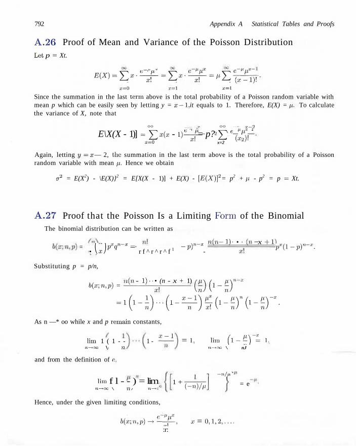
792 Appendix A Statistical Tables and Proofs
A.26 Proof of Mean and Variance of the Poisson Distribution Lot p = Xt.
e-^p* w-E-TF-E-Tf-rS^ni
1 = 0 1 = 1 1 = 1
e~''px-
3T-"i)i
Since the summation in the last term above is the total probability of a Poisson random variable with mean p which can be easily seen by letting y = x—l, it equals to 1. Therefore, E(X) = p.. To calculate the variance of X, note that
OO _ _ , . a, O O _ , , . y . _ 0
e V _ j r n C t'px * E\X(X - 1)] = 5>(:t: - lf-£- = p? Y, x=0 x=2 («2)«
Again, letting j / = I — 2, the summation in the last term above is the total probability of a Poisson random variable with mean p. Hence we obtain
cr2 = E(X2) - \E(X)}2 = E[X(X - 1)] + E(X) - [E(X)\2 = p2 + p. - p2 = p = Xt.
A.27 Proof that the Poisson Is a Limiting Form of the Binomial The binomial distribution can be written as
• • U " K « — r f ^ r ^ r ^ f 1 - ' 5 " -
njn - 1 ) - • • (n - x +1) x px(l-p)n-*.
Substituting p = p/n,
b(x;n,p) = i(n - ! ) • • • (n - x + 1) /p
($(»-£) -KhO-^so-i.H-r-
As n —* oo while x and p remain constants,
lim 1 ( 1 - -n—»oo \ 71
and from the definition of e.
1 -. X ' - l
= 1, lim {l-'-YX = l. n—»oc \ nJ
lim f l - - ) = lim TI—.oc \ n ' n—»c
-i -n/n'
1 + ( - " ) / r
= e
Hence, under the given limiting conditions,
bix;n,p)->~f-, 1 = 0,1,2,.... :r:
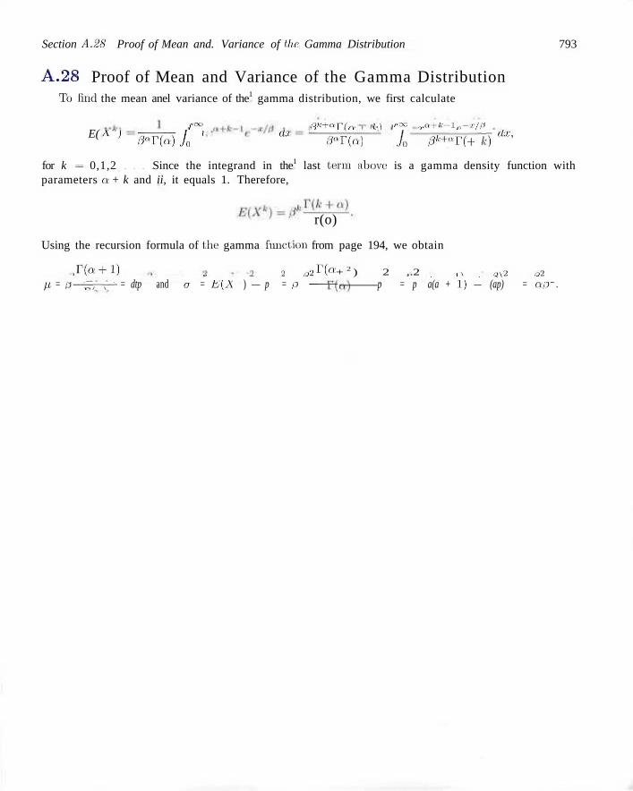
Section A.28 Proof of Mean and. Variance of the Gamma Distribution 793
A.28 Proof of Mean and Variance of the Gamma Distribution Tei find the mean anel variance of the1 gamma distribution, we first calculate
E( /•oo ,«rivr/n, I i.] roc va+k-l„-x/p
A ) d»r(a)j0 ' CU ll»T(a) ./,-, P^r(a + k)aj"
for k = 0,1,2 Since the integrand in the1 last term above- is a gamma density function with parameters a + k and ii, it equals 1. Therefore,
r(o)
Using the recursion formula of the gamma function from page 194, we obtain
T(a'T-l) __ , 2 , j 2 r ( f v + 2 ) 2 ,.2 . , \ . ,o\2 ,o2 // = / j — — — — = dtp and a = £/(A ) — p = ,o ——— p = p a(a + I) — (ap) = ap.
Appendix B
Answers to Odd-Numbered Non-Review Exercises
Chapter 1
1.1 (a) Sample size = 15
(b) Sample mean = 3.787
(c) Sample median = 3.6
(e) *tr(20) = 3- ( i 7 8
1.3 (b) Yes, aging process reduced the tensile strength.
(c) xAglng = 209.90. xKo _.gjns = 222.10
(d) XAging = 210.00, KNO aging = 221.50. The means ane] medians are similar for e:ach group.
1.5 (b) Control: x = 5.60, x = 5.00, :i; t l. ( lu) = 5.13. Treatment: if: = 7.60, z = 4.50, s ti(l0) =
5.63.
(c) The extreme value of 37 in the treatment group plays a strong leverage role for the mean calculation.
1.7 Sample variance = 0.943 Sample standard deviation = 0.971
1.9 No aging: sample variance = 23.62, sample standard deviation = 4.86. Aging: sample variance = 42.12, sample standard deviation = 0.49.
1.11 Control: sample variance = 69.38, sample standard deviation = 8.33. Treatment: sample variance = 128.04. sample standard deviation = 11.32.
1.13 (a) Mean = 124.3, median = 120;
(b) 175 is an extreme observation.
1.15 Yes, P-value = 0.03125; probability of obtaining HHHHII with a fair coin.
1.17 Nonsmokers (a) 30.32, (b) 7.13; Smokers (a.) 43.70, (b) 16.93. (d) Smokers appear to take longer time to fall asleep. For smokers the time to fall asleep is more: variable.
1.19
1.21
Stem.
0
2 3 4 5 6
Leaf 22233457 023558 035 03 057 0569 0005
Frequency 8 6 3 2 3 4 4
(b) Class Class Re l . In te rva l Midpo in t Fi-eq. Freq. 0.0-0.9 1.0-1.9 2.0-2.9 3.0-3.9 4.0-4.9 5.0-5.0 0.0-6.9
0.45 1.45 2.45 3.45 4.45 5.45 6.45
8 6 3 2 3 4 4
0.267 0.200 0.100 0.067 0.100 0.133 0.133
(c) Sample mean = 2.7967 Sample range = 6.3 Sample! standard deviation 2.2273
(a) Sample mean = 1.7743 Sample median = 1.77
(b) Sample standard deviation = 0.3905.
796 Appendix B Answers to Odd-Numbered Non-Review Exercises
1.23 (b) xi99o = 160.15, a-1980 = 395.10.
(c) The mean emissions dropped between 1980 and 1990, the variability also decreased because there were no longer extremely large emissions.
1.25 (a) Sample mean = 33.31
(b) Sample median = 26.35
(d) x t r ( 1 0 ) = 30.97
Chapter 2
2.1 (a) 5= {8,16,24,32,40,48}
(b) S = { - 5 , 1 }
(c) S = {T, UT, HHT, HHH}
(d) S = {Africa, Antarctica. Asia, Australia, Europe, North America, South America}
(e) S = <p
2.3 A = C
2.5 S ={1HH. \HT, ITH, ITT, 2H, 2T, 'AHH, 3HT, 3777, 3TT. 4H. AT, bHH. 5HT, 5TH, oTT, &H, 6T}
2.7 Sx ={MMMM,MMMF,MMFM.MFMM, FMMM. MMFF. MFMF. MFFM. FMFM, FFMM, FMMF, MFFF. FMFF, FFMF, FFFM,FFFF}; S2 ={0 ,1 ,2 ,3 ,4}
2.9 (a) A = {1HH, 1HT, ITH, ITT. 2H, 2T}
(b) B = { i rT ,3TT ,5TT}
(c) A ={3HH,3HT.3TH.3TT,4H,4T, hHH, hHT, 5TH, oTT, 6H, 6T}
(d) A n B = {3TT, 5TT}
(e) AUB={1HH. IHT,1TH, ITT.2H.2T, 3TT, 5TT}
2.11 (a) S={MxM2.MiFx,MxF2,M2Mx,M2Fx, M2 F2, F, Mx, Fi M2 ,FxF2, F2 Mv, F2 M2, F2Fx)
(b) A = {M\Mo,MyFi,MiF2,M2Mx,M2F], M2F2]
(c) B = {MxF1,MiF2,M2FJ.M2F2.F\Mi. FxM2,F2Mi,F2M2)
(d) C={FxF2,F2Fi}
(e) A O B = {MiFi,MxF2, M2Fi,M2F2}
(f) A U C={MiM2, MxFi, 1V/1F2, M2Mx, M2FuM2F2,FxF2,F2Fx}
2.15 (a) {nitrogen, potassium, uranium, oxygen}
(b) {copper, sodium, zinc, oxygen}
(c) {copper, sodium, nitrogen, potassium, uranium, zinc}
(d) {copper, uranium, zinc}
(e) $
(f) {oxygen}
2.19 (a) The family will experience mechanical problems but will receive no ticket for traffic violation and will not arrive at a campsite that has no vacancies.
(b) The family will receive a traffic ticket and arrive at a campsite that has no vacancies but will not experience mechanical problems.
(c) The family will experience mechanical problems and will arrive at a campsite that has no vacancies.
(d) The family will receive a traffic ticket but will not arrive at a campsite that has no vacancies.
(e) The family will not experience mechanical problems.
2.2]
2.23
2.25
2.27
2.29
2.31
2.33
2.35
2.37
2.39
2.41
2.43
2.45
2.47
2.49
18
156
20
48
210
(a) 1024;
72
362,880
2,880
(b) 243
(a) 40,320; (b) 336
360
24
3,360
7,920
56
Chapter 3 797
2.51 (a) Sum of the probabilities exceeds 1.
(b) Sum of the probabilities is less than 1.
(c) A negative probability.
(d) Probability of both a heart and a black card is zero.
2.53 S = {$10, $25, $100}: P(10) = ^ ; P(25) = fjj,
Pim = Tab 5u 2.55 (a) 0.3; (b) 0.2
2.57 (a) 5/26; (b) 9/26; (c) 19/26
2.59 10/117
2.61 95/663
2.63 (a) 94/54,145; (b) 143/39,984
2.65 (a) 22/25; (b) 3/25; (c) 17/50
2.67 (a) 0.32; (b) 0.68; (c) office or den
2.69 (a) 0.8; (b) 0.45; (c) 0.55
2.71 (a) 0.31; (b) 0.93; (c) 0.31
2.73 (a) 0.009; (b) 0.999: (c) 0.01
2.75 (a) 0.048; (b) $50,000; (c) 812,500
2.77 (a) The probability that a convict who pushed dope also committed armed robbery.
(b) The probability that a convict who committed armed robbery did not push dope.
(c) The probability that a convict who did not push dope also did not commit armed robbery.
2.79 (a) 14/39; (b) 95/112
2.81 (a) 5/34; (b) 3/8
2.83 (a) 0.018; (b) 0.614; (c) 0.166; (d) 0.479
2.85 (a) 0.35; (b) 0.875; (c) 0.55
2.87 (a) 9/28; (b) 3/4; (c) 0.91
2.89 0.27
2.91 5/8
2.93 (a) 0.0016; (b) 0.9984.
2.95 (a) 1/5; (b) 4/15; (c) 3/5.
2.97 (a) 91/323; (b) 91/323.
2.99 (a) 0.75112 (b) 0.2045.
2.101 0.0960
2.103 0.40625
2.105 0.1124
2.107 (a) 0.045; (b) 0.564; (c) 0.630; (d) 0.1064
Chapter 3
3.1 Discrete; continuous; continuous; discrete; discrete; continuous.
3 3 Sample Space
HHH HHT HTH THH HTT THT TTH TTT
3
—1 - 1 - 1 - 3
3.5 (a) 1/30; (b) 1/10
3.7 (a) 0.68; (b) 0.375
3.9 (b) 19/80
3.11
3.13
fix) 0
F(x) = <
(0, f o r x < 0 , 0.41, for 0 < x< 1 0.78, for 1 < a: < 2 0.94, for 2 < x < 3 0.99, for 3 < x < 4, 1, for x > 4
3.15 0. 2 7> 6 7> 1,
for x < 0, for 0 < :r < 1, for 1 < a: < 2, for x > 2
Fix) = i
(a) 4/7; (b) 5/7
3.17 (b) 1/4; (c) 0.3
3.19 F(x) = (x- l ) /2 , for 0 < x < 3; 1/4
3.21 (a) 3/2; (b) F(x) = xAl2, for 0 < x < 1; 0.3004
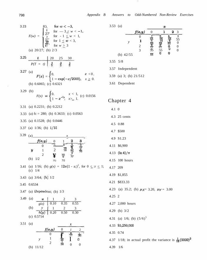
798 Appendix B Answers to Odd-Numbered Non-Review Exercises
3.23
F(w) = .
3.25
fO, f o r u i < - 3 , for — 3 < w < —1, for - 1 < w < 1, for 1 < in < 3,
_1, for w > 3 (a) 20/27; (b) 2/3
20 25 30
3.53 (a) l
27' 7
37 ' 19 27'
3.27
P(T = t)
(a) F(x) =
i
0,
3 1
a: < 0 .
1 -exp(-a- /2000) , x > 0. (b) 0.6065; (c) 0.6321
3.29 (b) F(x)
0,
3.31
3.33
3.35
3.37
3.39
1 - x ~ a
(a) 0.2231; (b) 0.2212
x < 1, x> 1.
(c) 0.0156
(a) fc = 280; (b) 0.3633: (c) 0.0563
(a) 0.1528; (b) 0.0446
(a) 1/36; (b) 1/15
(a) x
ffay) 0 1 2
(b) 1/2
0 1 "Ti 3 _
2 I
¥ ¥ 7TJ 70
^_J_~
1 f 70"
7_r~
7l>
3.41 (a) 1/16; (b) g(x) = 12.x-(l - a;)2, for 0 < :r < 1; (c) 1/4
3.43 (a) 3/64; (b,
3.45 0.6534
3.47 (a) Depende
3.49 (a) x
gix) (b) y
h(y) (c) 0.5714
3.51 (a)
1/2
nt; (b)
1 0.10
1 0.20
ffay)
y
(b) 11/12
0 1 2
1/3
2 0.35
2 0.50
0
f 315
3 0.55
3 0.30
X
1 2 H 1 "
I o 0 0
/(«>0>> 0
y i 2 3
(b) 42/55
3.55 5/8
3.57 Independent
3.59 (a) 3; (b) 21/512
3.61 Dependent
Chapter 4
4.1 0
4.3 25 cents
4.5 0.88
4.7 $500
4.9 S1.23
4.11 $6,900
4.13 (ln4)/7r
4.15 100 hours
4.17 209
4.19 $1,855
4.21 $833.33
4.23 (a) 35.2; (b) px =
4.25 2
4.27 2,000 hours
4.29 (b) 3/2
4.31 (a) 1/6; (b) (5/6)5
4.33 $5,250,000
4.35 0.74
0 1 2 1 6 6
¥ I f I f f ? 55 55 u
55 0 0
3.20, pY = 3.00
4.37 1/18; in actual profit the variance is
4.39 1/6
3 1
55 0 0 0
TS(5000)2
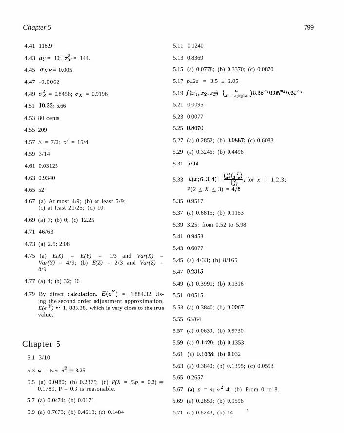
Chapter 5 799
4.41 118.9
4.43 pY = 10; oY = 144.
4.45 aXY = 0.005
4.47 -0.0062
4,49 o2x = 0.8456; <x.v = 0.9196
4.51 10.33: 6.66
4.53 80 cents
4.55 209
4.57 //. = 7/2; o2 = 15/4
4.59 3/14
4.61 0.03125
4.63 0.9340
4.65 52
4.67 (a) At most 4/9; (b) at least 5/9; (c) at least 21/25; (d) 10.
4.69 (a) 7; (b) 0; (c) 12.25
4.71 46/63
4.73 (a) 2.5: 2.08
4.75 (a) E(X) = E(Y) = 1/3 and Var(X) = Var(Y) = 4/9; (b) E(Z) = 2/3 and Var(Z) = 8/9
4.77 (a) 4; (b) 32; 16
4.79 By direct calculation, ^(e*") = 1,884.32 Using the second order adjustment approximation, E(e ) % 1. 883.38. which is very close to the true value.
Chapter 5
5.1 3/10
5.3 p. = 5.5; a 8.25
5.5 (a) 0.0480; (b) 0.2375; (c) P(X = 5\p = 0.3) 0.1789, P = 0.3 is reasonable.
5.7 (a) 0.0474: (b) 0.0171
5.9 (a) 0.7073; (b) 0.4613; (c) 0.1484
5.11 0.1240
5.13 0.8369
5.15 (a) 0.0778; (b) 0.3370; (c) 0.0870
5.17 p±2a = 3.5 ± 2.05
5.19 f(xux2,x-j) = (x. _* _i:.i)0.35X!0.05:l'20.60T:)
5.21 0.0095
5.23 0.0077
5.25 0.8070
5.27 (a) 0.2852; (b) 0.9887: (c) 0.6083
5.29 (a) 0.3246; (b) 0.4496
5.31 5/14
5.33 h(x;6,3.4) = ^ k " , for x = 1,2,3;
P(2 < X < 3) = 4J/5
5.35 0.9517
5.37 (a) 0.6815; (b) 0.1153
5.39 3.25: from 0.52 to 5.98
5.41 0.9453
5.43 0.6077
5.45 (a) 4/33; (b) 8/165
5.47 0.2315
5.49 (a) 0.3991; (b) 0.1316
5.51 0.0515
5.53 (a) 0.3840; (b) 0.0067
5.55 63/64
5.57 (a) 0.0630; (b) 0.9730
5.59 (a) 0.1429; (b) 0.1353
5.61 (a) 0.1638; (b) 0.032
5.63 (a) 0.3840; (b) 0.1395; (c) 0.0553
5.65 0.2657
5.67 (a) p = 4;a2= 4; (b) From 0 to 8.
5.69 (a) 0.2650; (b) 0.9596
5.71 (a) 0.8243; (b) 14
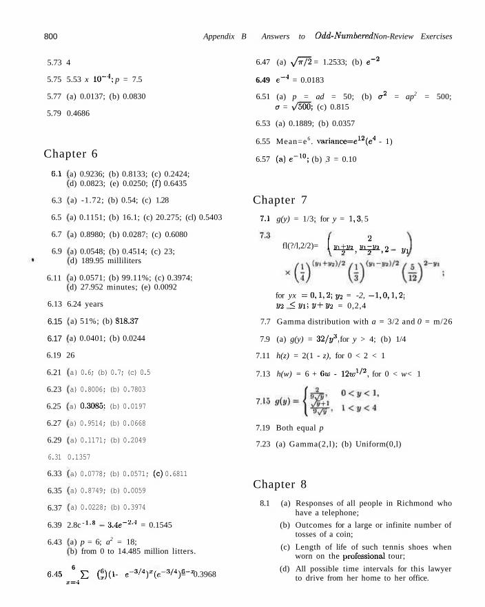
800
5.73 4
5.75 5.53 x 1 0 - 4 ; p = 7.5
5.77 (a) 0.0137; (b) 0.0830
5.79 0.4686
Chapter 6
6.1
Appendix B Answers to Odd-Numbered Non-Review Exercises
6.47 (a) yfiT/2 = 1.2533; (b) e - 2
6.49 e~4 = 0.0183
6.51 (a) p = ad = 50; (b) er2 = ap2 = 500; a = v/500; (c) 0.815
6.53 (a) 0.1889; (b) 0.0357
6.55 Mean=e6 . variance=e12(e4 - 1)
6.57 ( a ) e - 1 0 ; (b) 3 = 0.10
6.3
6.5
6.7
6.9
6.11
6.13 6.24 years
6.15
6.17
6.19 26
6.21
6.23
6.25
6.27
6.29
6.33
6.35
6.37
6.39 2.8c
6.43
a) 0.9236; (b) 0.8133; (c) 0.2424; d) 0.0823; (e) 0.0250; (f) 0.6435
a) -1.72; (b) 0.54; (c) 1.28
a) 0.1151; (b) 16.1; (c) 20.275; (cl) 0.5403
a) 0.8980; (b) 0.0287: (c) 0.6080
a) 0.0548; (b) 0.4514; (c) 23; d) 189.95 milliliters
a) 0.0571: (b) 99.11%; (c) 0.3974: d) 27.952 minutes; (e) 0.0092
a) 51%; (b) 818.37
a) 0.0401; (b) 0.0244
a) 0.6; (b) 0.7; (c) 0.5
a) 0.8006: (b) 0.7803
a) 0.3085: (b) 0.0197
a) 0.9514; (b) 0.0668
a) 0.1171; (b) 0.2049
6.31 0.1357
a) 0.0778; (b) 0.0571; (c) 0.6811
a) 0.8749; (b) 0.0059
a) 0.0228; (b) 0.3974
- 1 . 8 3.4e~2-4 = 0.1545
a) p = 6; a2 = 18; b) from 0 to 14.485 million litters.
6
Chapter 7
7.1 g(y) = 1/3; for y = 1,3, 5
fl(?/l,2/2)= Ln+«i,n-V2t2 yi
for yx = 0 , 1 , 2 ; y2 = -2, - 1 , 0 , 1 , 2 ; V2 <yi',Vl +2/2 = 0,2,4
7.7 Gamma distribution with a = 3/2 and 0 = m/26
7.9 (a) g(y) = 32/y3, for y > 4; (b) 1/4
7.11 h(z) = 2(1 - z), for 0 < 2 < 1
7.13 h(w) = 6 + 6ui - 12w1 / 2 , for 0 < w< 1
7.
6-45 £ 0(1 - e-^4)x(er''i'4)G-x = 0.3968 x=4
7.19 Both equal p
7.23 (a) Gamma(2,l); (b) Uniform(0,l)
Chapter 8
8.1 (a) Responses of all people in Richmond who have a telephone;
(b) Outcomes for a large or infinite number of tosses of a coin;
(c) Length of life of such tennis shoes when worn on the professional tour;
(d) All possible time intervals for this lawyer to drive from her home to her office.
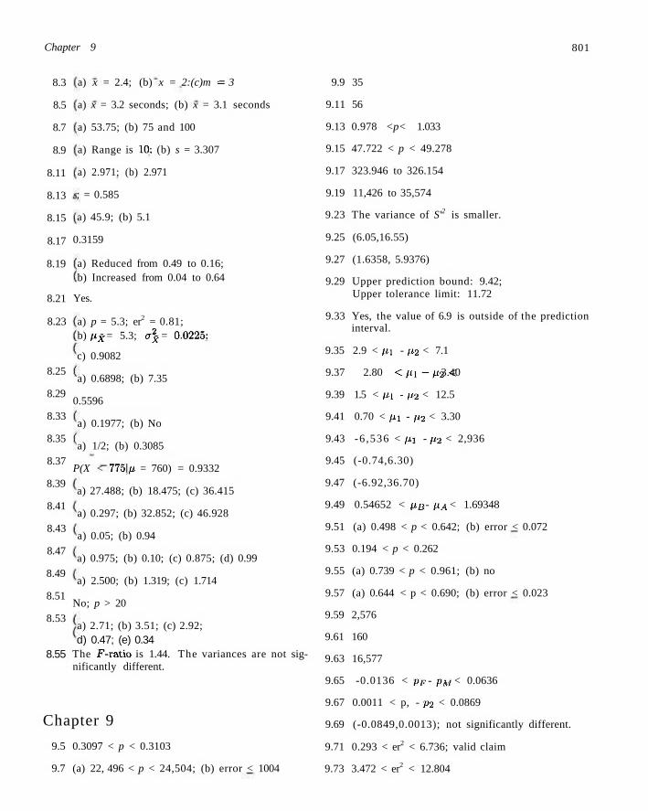
Chapter 9 801
8.3
8.5
8.7
8.9
8.11
8.13
8.15
8.17
8.19
8.21
8.23
8.25
8.29
8.33
8.35
8.37
8.39
8.41
8.43
8.47
8.49
8.51
8.53
8.55
a) x = 2.4; (b) x = 2:(c)m = 3
a) x = 3.2 seconds; (b) x = 3.1 seconds
a) 53.75; (b) 75 and 100
a) Range is 10: (b) s = 3.307
a) 2.971; (b) 2.971
; = 0.585
a) 45.9; (b) 5.1
0.3159
a) Reduced from 0.49 to 0.16; b) Increased from 0.04 to 0.64
Yes.
a) p = 5.3; er2 = 0.81; b) px = 5.3; o\ = 0.0225:
c) 0.9082
a) 0.6898; (b) 7.35
0.5596
a) 0.1977; (b) No
a) 1/2; (b) 0.3085
P(X < 7751// = 760) = 0.9332
a) 27.488; (b) 18.475; (c) 36.415
a) 0.297; (b) 32.852; (c) 46.928
a) 0.05; (b) 0.94
a) 0.975; (b) 0.10; (c) 0.875; (d) 0.99
a) 2.500; (b) 1.319; (c) 1.714
No; p > 20
a) 2.71; (b) 3.51; (c) 2.92; d) 0.47; (e) 0.34
The .F-ratio is 1.44. The variances are not significantly different.
Chapter 9
9.5 0.3097 < p < 0.3103
9.7 (a) 22, 496 < p < 24,504; (b) error < 1004
9.9 35
9.11 56
9.13 0.978 <p< 1.033
9.15 47.722 < p < 49.278
9.17 323.946 to 326.154
9.19 11,426 to 35,574
9.23 The variance of S'2 is smaller.
9.25 (6.05,16.55)
9.27 (1.6358, 5.9376)
9.29 Upper prediction bound: 9.42; Upper tolerance limit: 11.72
9.33 Yes, the value of 6.9 is outside of the prediction interval.
9.35 2.9 < px - p2 < 7.1
9.37 2.80 <pi-p2< 3.40
9.39 1.5 < pi - p2 < 12.5
9.41 0.70 < pi - p2 < 3.30
9.43 -6 ,536 < px - p2 < 2,936
9.45 (-0.74,6.30)
9.47 (-6.92,36.70)
9.49 0.54652 < pB - pA < 1.69348
9.51 (a) 0.498 < p < 0.642; (b) error < 0.072
9.53 0.194 < p < 0.262
9.55 (a) 0.739 < p < 0.961; (b) no
9.57 (a) 0.644 < p < 0.690; (b) error < 0.023
9.59 2,576
9.61 160
9.63 16,577
9.65 -0.0136 < pF - pM < 0.0636
9.67 0.0011 < p, - p 2 < 0.0869
9.69 (-0.0849,0.0013); not significantly different.
9.71 0.293 < er2 < 6.736; valid claim
9.73 3.472 < er2 < 12.804
802 Appendix B Answers to Odd-Numbered Non-Review Exercises
9.75 9.27 < a < 34.16
9.77 0.549 < <TI/(T2 < 2.690
9.79 0.016 < a\/a\ < 0.454; no
9.81 1 fl xt j = i
9.83 (a) L(x\,x2 .r„) =
(2
(b) p=-\ E In a',:
i A i / i \ / £ ( l n , , - " ) ' / J * '
; = i
- 2 _ 1 ^ 1=1
h\xi- -\ £ hi-Tj
9.85 a:lnp-|- (1 — s)lii(l - p ) . Set the derivative with respect to p = 0; p = x = 1.0
Chapter 10
10.1 (a) Conclude that fewer than 30% of the public are allergic to some cheese products when, in fact, 30% or more are allergic.
(b) Conclude that at least 30% of the public are allergic to some cheese products when, in fact, fewer than 30% are allergic.
10.3 (a) The firm is not guilty;
(b) the firm is guilty.
10.5 (a) 0.1286;
(b) 3 = 0.0901; 3 = 0.0708.
(c) The probability of a type I error is somewhat, large.
10.7 (a) 0.0559;
(b) 0 = 0.0017; 3 = 0.00968; 3 = 0.5557
10.9 (a) a = 0.0032; (b) 3 = 0.0062
10.11 (a) a = 0.1357; (b) 3 = 0.2578
10.13 a = 0.0094; ,3 = 0.0122
10.15 (a) Q = 0.0718; (b) 3 = 0.1151
10.17 (a) Q = 0.0384; (b) 3 = 0.5; 3 = 0.2776
10.19 z= -1.64; P-valuc=0.10
10.21 2 = -2.76; yes, p < 40 months; P-value=0.0029
10.23 z = 8.97; yes, //. > 20,000 kilometers; P-value< 0.001
10.25 t = 0.77; fail to reject Ho-
10.27 t = 12.72; P-value < 0.0005; reject H0.
10.29 t = -1.98; Reject //(.; P-value = 0.0312
10.31 z = —2.60; conclude p/, — PQ < 12 kilograms.
10.33 t = 1.50; no sufficient evidence to conclude that the increase in substrate concentration would cause an increase in the mean velocity by more than 0.5 micromolc per 30 minutes.
10.35 t = 0.70; no sufficient evidence to support that the serum is effective.
10.37 t = 2.55; reject HQ: p\ — u2 > 4 kilometers.
10.39 t = 0.22; fail to reject HQ.
10.41 t = 2.76; reject H0-
10.43 t = 2.48; P-value < 0.02; reject Ho
ld.45 t = —2.53; reject Ho', the claim is valid.
10.47 n = 6
10.49 78.28 « 79 due to round up.
10.51 5
10.53 (a) H0: M h o t - .V/COM = 0, Hi: 1 1 / ^ - itfcoui 9* 0;
(b) paired t, t = 0.99; P-value > 0.30; fail to reject Ho.
10.55 P-value = 0.4044 (with a one-tailed test); the claim is not refuted.
10.57 P-value = 0.0207; yes, the coin is not balanced.
10.59 z = —5.06 and P-value RS 0; conclude that le ss than 1/5 of the homes are heated by oil.
10.61 z = 1.44; fail to reject Ha.
10.63 z = 2.36 with P-value = 0.0182; yes, the difference is significant.
10.65 z = 1.10 with P-valuc = 0.1357; we do not have sufficient evidence to conclude that breast cancer is more prevalent in the urban community.
Chapter 11 803
10.67 x 2 = 18-13 with P-value = 0.0676 (from com- 11.7 (b) y = 343.706 + 3.221a;; puter output): do not reject HQ: a2 = 0.03. (c) y = $ 4 5 6 a t advertising casts being $35
10.69 x 2 = 63.75 with P-value = 0.8998 (from com- 11.9 (a) y = 153.175 - 6.324a;; puter output); do not reject H0. ( b ) - = m ^ x = 4g u n j t s
10.71 x2 = 42-37 with P-value = 0.0117 (from com- 1 U 1 (b) y = -1847.633 + 3.653a: puter output); machine is out of control.
11.13 (b) y = 31.709 + 0.353a; 10.73 / = 1.33 with P-value = 0.3095 (from computer
output); fail to reject H0: ax = a2. 11.17 (a) s2 = 176.4;
10.75 / = 0.086 with P-value = 0.0328 (from com- (b) ' = 2 '04= f a i l t o r c J e c t H»' $ = °-puter output); reject HQ: ax = o2 at level greater n , a < \ 2 _ n An
than 0.0328. i l - i J W S ~ U 4 U ;
(b) 4.324 < Q < 8.503; 10.77 / = 19.67 with P-valuc = 0.0008 (from com- , , o 446 < 3 < 3 172
puter output); reject Ho'. a\ = a2. , 11.21 (a) s2 = 6.626:
10.79 x = 4-47; there is no sufficient evidence to claim that the coin is unbalanced. (b) 2.684 < a < 8.968;
10.81 x - 1 0-1 4 ; reJect H0, the ratio is not 5:2:2:1. (c) 0.498 < 0 < 0.637
11.23 t = -2.24; reject H0: 0 < 6 10.83 x2 = 2-33; do not reject H0: binomial distribu
tion. 11.25 (a) 24.438 < pY\24.5 < 27.106;
10.85 x2 = 3.125; do not reject H0: geometric distri- (b) 2 1 ' 8 8 < W> < 2 9 ' 6 6
b u t i o n ' 11.27 7.81 < /lyiLo < 10.81
10.89 x2 = 5.19; do not reject HQ: normal distribution. . . 9„ , , . , . „ . „
10.91 x = 5.47; do not reject Ho. (b) no, (the 95% confidence interval on mean mpg is (27.95,29.60));
10.93 x — 124.59; yes, occurrence of these tvpes of . . ., .,, crime is dependent on the city district. " ^ m , , e s P e r S a l l o n wl11 l l k e l>" e x c e e d 1 8
10.95 x 2 = 31.17 with P-value < 0.0001; attitudes are 1 1 3 3 ^ * = 3Al56x
not homogeneous. *
10.97 x 2 = 5-92 with P-value = 0.4332: do not reject 1 L 3 5 (a) b = '"«, j '•• HQ. , 5 X '
10.99 x = 1'84: do not reject HQ.
Chapter 11
(b) ?) = 2.003a:
J2 (^li-S'l)3'2i 11.37 E(B)=0 + ~p-=h
11.39 (a) a = 10.812, b = -0.3437;
11.1 (a) a = 64.529, b = 0.561; (b) t = 0 .43 ; the regression is linear.
(b) 0 = 81.4
11.3 (a) j / = 6.4136 + 1.8091a:;
11.41 / = 1.12; the regression is linear.
11.43 / = 1.71 and P-value = 0.2517; the regression is (b) y = 9.580 at temperature 1.75 linear.
11.5 (a) 0 = 5.8254 +0.5676a;; 11.45 (a) P = -11 .3251 - 0.0449X;
(c) y = 34.205 at 50° C (b) yes;
804 Appendix B Answers to Odd-Numbered Non-Review Exercises
(c) R2 = 0.9355;
(d) yes
11.47 (b) N = -175.9025 + 0.0902V; R2 = 0.3322.
11.49 r = 0.240
11.53 (a) r = 0.392;
(b) t = 2.04; fail to reject HQ: p = 0; however, the P-value = 0.053 is marginal.
Chapter 12
12.1 (a) y = 27.547 -1- 0.922a;. + 0.284x2;
(b) y = 84 at x_ = 64 and x2 = 4.
12.3 y = 0.5800 + 2.7122z. + 2.0497x2.
12.5 (a) y = 56.4633 + 0.1525.x- 0.00008a:2;
(b) y = 86.7% when temperature is at 225°C.
12.7 y = 141.6118 - 0.2819a; + 0.0003a:2.
12.9 (a) y = -102.7132 + 0.6054x. + 8.9236.r2 + 1.4374a;3 + 0.0136.T4:
(b) t} = 287.6.
12.11 0 = 3.3205 + 0.4210a:. - 0.2958x2 + 0.0164x3 + 0.1247x4.
12.13 0 = -6.5122 + 1.9994x1 - 3.6751x2 + 2.5245x3 + 5.1581x4 + 14.4012x5.
12.15 (a) 0 = 350.9943 - 1.2720x. - 0.1539x2:
(b) 0 = 140.9
12.17 0.1651
12.19 242.72
12.21 (a) a%3 = 28.0955; (b) aB, B 2 = -0.0096
12.23 29.93 < PY\XQ.& < 31.97
12.25 t = 2.86; reject H0 and in favor of 32 > 0.
12.27 t = 3.524 with P-value = 0.01; reject HQ and in favor of 0i > 2.
12.29 (a) t = -1.09 with P-value = 0.3562;
(b) t = -1.72 with P-value = 0.1841:
(c) Yes; no sufficient evidence to show that xi and x2 are significant.
12.31 R2 = 0.9997
12.33 / = 5.106 with P-value = 0.0303; the regression is not significant at level 0.01.
12.35
12.37
12.39
12.41
12.43
12.45
12.47
12.49
12.51
12.53
/ = 34.90 with P-value = 0.0002; reject HQ and conclude 0\ > 0.
/ = 10.18 with P-value < 0.01; xi and x2 are significant in the presence of 13 and X4.
The two-variable model is better.
First model: R2^ = 92.7%, CV = 9.0385;
Second model: R2^ = 98.1%, CV = 4.6287; The partial /—test shows P-value = 0.0002; model 2 is better.
Using x2 alone is not much different from using xi and x2 together since the R^yS are 0.7696 versus 0.7591.
(a) mpg = 5.9593 - 0.00003773 odometer + 0.3374 octane - 12.6266«i - 12.9846^;
(b) sedan;
(c) they are not significantly different.
(b) 0 = 4.690 seconds;
(c) 4.450 < /iy|{i80,260} < 4.930
0 = 2.1833 + 0.9576x2 + 3.3253x3
(a) 0 = -587.211 + 428.433x;
(b) 0 = 1180 - 191.691x + 35.20945x2;
(c) quadratic model
a2Bl = 20,588; &2
Bll = 62.6502; o-B,,B„ = -1103.5
12.55 (a) Intercept model is the best.
12.57 (a) 0 = 3.1368 + 0.6444xi - 0.0104x2 + 0.5046x3 - 0.1197x4 - 2.4618x5 + 1.5044x6;
(b) 0 = 4.6563 + 0.5133x3 - 0.1242x4;
(d) 0 = 4.6563+ 0.5133x3-0.1242x4;
(e) two observations have large .R-student values and should be checked.
12.59 (a) 0 = 125.8655 + 7.7586xi + 0.0943x2 -0.0092xix2;
(b) the model with x 2 alone is the best.
Chapter 13 805
Chapter 13
13.3 / = 0.31; no sufficient evidence to support that there are differences among the 6 machines.
13.5 / = 14.52: yes, the difference is significant
13.7 / = 2.25; no sufficient evidence to support that the different concentrations of MgNH4P04 significantly affect the attained height of chrysanthemums.
13.9 / = 8.38; the average specific activities differ significantly.
13.11 (a) / = 14.28; reject H0;
(b) / = 23.23; reject HQ:
(c) / = 2.48; fail to reject H0.
13.13 (a) / = 13.50; treatment means differ;
(b) / ( l vs. 2)=29.35: significant; / ( 3 vs. 4)=3.59; not significant
13.15 X3 Xi x 4 •1:2
56.52 59.66 61.12 61.96
13.17 (a) / = 9.01; yes, significant;
(b) Substrate Modified Removal
Depletion Hess Kicknet Surber Kicknet
13.35 / = 0.58; not significant
13.39 / = 5.03; grades are affected by different professors.
13.41 p < 0.0001; / = 122.37; the amount of dye has an effect on the color of the fabric.
13.43 (a) / = 14.9; operators differ significantly;
(b) er2 = 28.91; .s2 = 8.32.
13.45 (a) / = 3.33; no significant difference; however, the P-value = 0.0564 is marginal;
(b) a'i = 1.08; s2 = 2.25.
13.49 9.
13.51 (a) yij = p. + a . + £__,-, a . ~ n(x; 0, a a ) ;
(b) d 2 = 0 (the estimated variance component is -0.00027); a2 = 0.0206.
13.53 (a) y^ =p + aj +cy, a. ~ n{x;0,aa);
(b) yes; / = 5.63 with P-value = 0.0121;
(c) there is a significant loom variance component.
13.19 Comparing the Control to 1 and 2: significant; Comparing the Control to 3 and 4: insignificant
13.21 The mean absorption for aggregate 4 is significantly lower than the other aggregate.
13.23 / = 70.27 with P-value < 0.0001; reject HQ.
XO X2.=. X100 £ 7 5 X50 55.167 60.167 64.167 70.500 72.833
Temperature is important; Both 75 and 50°(C) yielded batteries with significantly longest activated life.
13.27 (a) /(fertilizer)=6.11; significant;
(b) / = 17.37; significant; / = 0.96; not significant
13.29 / = 5.99; percent of foreign additives is not the same for all three brands of jam; Brand A.
13.31 /(station)=26.14; significant
13.33 /(diet)=11.86; significant
Chapter 14
14.1 (a) / = 8.13; significant;
(b) / = 5.18; significant;
(c) / = 1.63; insignificant
14.3 (a) / = 14.81; significant;
(b) / = 9.04; significant;
(v.) f = 0.61; insignificant;
14.5 (a) / = 34.40; significant;
(b) / = 26.95; significant;
(c) / = 20.30; significant;
14.7 Test for effect of amount of catalyst: / = 46.63 with P-value = 0.0001; Test for effect of temperature: / = 10.85 with P-value = 0.0002; Test for effect of interaction: / = 2.06 with P-value = 0.074.
806 Appendix B Answers to Odd-Numbered Non-Review Exercises
14.9 (a) Source of Variation
Sum of Mean df Squares Squares /
cutting speed 1 12.000 12.000 1.32 0.2836 tool geometry 1 675.000 675.000 74.31 < 0.0001 interaction 1 192.000 192.000 21.14 0.0018 Error 8 72.667 9.083
Total 11 951.667
(b) The interaction effect masks the effect of cutting speed;
(c) /tool geomctrv=l = 16.51 and P-value = 0.0036; /tool geomctrv=2 = 5.94 and P-value = 0.0407.
14.11 (a) Source of Variation df
Sum of Mean Squares Squares /
Method 1 0.00010414 0.00010414 6.57 0.0226 Laboratory 6 0.00805843 0.00134307 84.70 < 0.0001 interaction 6 0.00019786 0.00003298 2.08 0.1215 Error 14 0.000222 0.00001586
Total 27 0.00858243
(b) The interaction is not significant;
(c) Both main effects are significant;
(e) /iaboratory=i = 0.01576 and P-value = 0.9019; no significant difference of the methods in laboratory 1; /tool j_eomDtr.v=2 = 9.081 and P-value = 0.0093.
14.13 (b) Source of Variation df
Sum of Squares
Mean Squares
Method Laboratory interaction 1 0.00000833 0.00000833 Error 8 0.00306667 0.00038333
1 0.06020833 0.06020833 157.07 < 0.0001 1 0.06020833 0.06020833 157.07 < 0.0001
0.02 0.8864
Total 11 0.12349167 (c) Both time and treatment influence the
magnesium uptake significantly, although there is no significant interaction between them.
(d) y = p + 3TT\me+3zZ + 0TZT\mc*Z + e, where Z = 1 when treatment=l and Z = 0 when treatment=2:
(c) / = 0.02 with P-value = 0.8864; the interaction in the model is insignificant
14.15 (a) AB AC BC ABC
f = 3.83; significant; / = 3.79; significant; / = 1.31; not significant; : / = 1.63: not significant;
(b) A : f = 0.54; not significant; B : f = 6.85: significant; C : f = 2.15; not significant;
(c) The presence of AC interaction masks the main effect C.
14.17 (a) S t r e s s / = 45.96 with P-value < 0.0001; coating / = 0.05 with P-value = 0.8299; humidity / = 2.13 with P-value = 0.1257; coating x humidity / = 3.41 with P-value = 0.0385; coating x stress / = 0.08 with P-value = 0.9277; humidity x stress / = 3.15 with P-value = 0.0192; coating x humidity x stress / = 1.93 with P-value = 0.1138.
(b) The best combination appears to be uncoated, medium humidity, and a stress level of 20.
14.19 E f f e c t / P
14.21
14.23
Temperature Surface HRC T x S T x H R C SxHRC T x S x H R C
14.122 6.70 1.67 5.50 2.69 5.41 3.02
< 0.0001 0.0020 0.1954 0.0006 0.0369 0.0007 0.0051
(a) yes: brand x type; brand x temperature;
(b) yes;
(c) brand Y, powdered detergent, high temperature.
(a)
Effect f P
Time Temp Solvent Time x Temp Time x Solvent Temp x Solvent Time x Temp x Solvent 6.22
543.53 209.79
4.97 2.66 2.04 0.03
< 0.0001 < 0.0001
0.0457 0.1103 0.1723 0.8558 0.0140
Although three two-way interactions are shown insignificant, they may be masked by the significant three-way interaction.
14.25 (a) / = 1.49; no significant interaction;
(b) /(operators)=12.45; significant; /(filters)=8.39; significant;
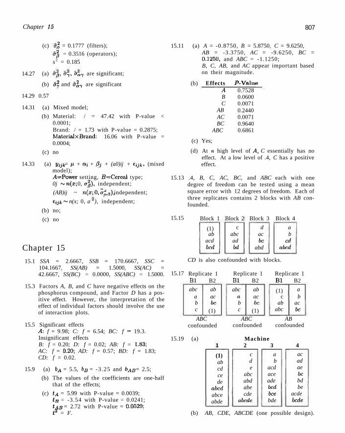
Chapter 15 807
14.27
(c) a2 = 0.1777 (filters); o2p = 0.3516 (operators); s2 = 0.185
(a) era, i77, oa~j are significant;
(b) a2 and tr -,, are significant
14.29 0.57
14.31 (a) Mixed model;
(b) Material: / = 47.42 with P-value < 0.0001; Brand: / = 1.73 with P-value = 0.2875; MaterialxBrand: 16.06 with P-value = 0.0004;
(c) no
14.33 (a) yijk = p. + a . + #,- + (a0)ij + eyfe, (mixed model); A=Power setting, B=Cereal type; 0j ~ n(x; 0, txg), independent;
(AB)ij ~ n(x;0,aag), independent; eijk ~ n(x; 0, a ), independent;
(b) no;
(c) no
Chapter 15
15.1 SSA = 2.6667, SSB = 170.6667, SSC = 104.1667. SS(AB) = 1.5000, SS(AC) = 42.6667, SS(BC) = 0.0000, SS(ABC) = 1.5000.
15.3 Factors A, B, and C have negative effects on the phosphorus compound, and Factor D has a positive effect. However, the interpretation of the effect of individual factors should involve the use of interaction plots.
15.5 Significant effects A: f = 9.98; C: f = 6.54; BC: f = 19.3. Insignificant effects B: f = 0.20; D: f = 0.02; AB: f = 1.83; AC: f = 0.20: AD: f = 0.57; BD: f = 1.83; CD: f = 0.02.
15.9 (a) bA = 5.5, bB = -3.25 and bAD = 2.5;
(b) The values of the coefficients are one-half that of the effects;
(c) tA = 5.99 with P-value = 0.0039; tB = -3.54 with P-value = 0.0241; tAB = 2.72 with P-value = 0.0529: t2 = F.
15.11 (a) A = -0.8750, B = 5.8750. C = 9.6250, AB = -3.3750, AC = -9.6250, BC = 0.1250, and ABC = -1.1250; B, C, AB, and AC appear important based on their magnitude.
(b) Effects A B C
AB AC BC
ABC
P-Value 0.7528 0.0600 0.0071 0.2440 0.0071 0.9640 0.6861
(c) Yes;
(d) At a high level of A, C essentially has no effect. At a low level of .4, C has a positive effect.
15.13 .4, B, C, AC, BC, and ABC each with one degree of freedom can be tested using a mean square error with 12 degrees of freedom. Each of three replicates contains 2 blocks with AB confounded.
15.15 Block 1
(1) ab
acd bed
Block 2
c abc ad bd
Block 3
d ac be
abd
Block 4
a b
cd abed
CD is also confounded with blocks.
15.17 Replicate 1 BI B2
Replicate 1 Replicate 1 BI B2 BI B2
abc a b c
ab ac be
(1)
abc a b c
ab ac be
(1)
(1) c
ab abc
a b
ac be
ABC confounded
ABC AB
15.19 (a)
confounded confounded
Machine 2 3 4
(1) ab cd ce de
abed abce abde
c d e
abc abd abe cde
abede
a b
acd ace ade bed bee bde
ac ad ae be bd be
acde bede
(b) AB, CDE, ABCDE (one possible design).
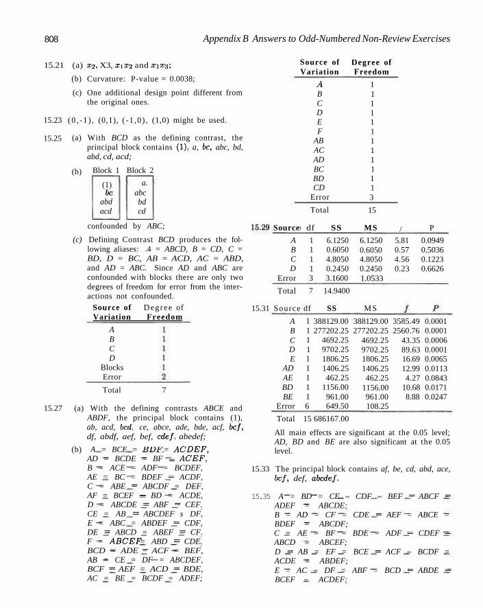
808 Appendix B Answers to Odd-Numbered Non-Review Exercises
15.21 (a) x2 , X3, X|X2 and X1X3;
(b) Curvature: P-value = 0.0038;
(c) One additional design point different from the original ones.
15.23 (0 , -1 ) , (0,1), ( -1 ,0) , (1,0) might be used.
15.25 (a) With BCD as the defining contrast, the principal block contains (1), a, be, abc, bd, abd, cd, acd;
(b) Block 1
(1) be
abd acd
Block 2
a. abc bd cd
confounded by ABC;
(c) Defining Contrast BCD produces the following aliases: .4 = ABCD, B = CD, C = BD, D = BC, AB = ACD, AC = ABD, and AD = ABC. Since AD and ABC are confounded with blocks there are only two degrees of freedom for error from the interactions not confounded.
Source of Degree of Variation Freedom
A B C D
Blocks Error
Source
A B C D
Error
Source of Variation
A B C D E F
AB AC AD BC BD CD
Error
Total
df SS
1 6.1250 1 0.6050 1 4.8050 1 0.2450 3 3.1600
Degree of Freedom
1 1 1 1 1 1 1 1 1 1 1 1 3
15
MS
6.1250 0.6050 4.8050 0.2450 1.0533
/ 5.81 0.57 4.56 0.23
P
0.0949 0.5036 0.1223 0.6626
Total 7 14.9400
15.31 Source df SS MS
Total 7
15.27 (a) With the defining contrasts ABCE and ABDF, the principal block contains (1), ab, acd, bed, ce, abce, ade, bde, acf, bef, df, abdf, aef, bef, cdef, abedef;
(b) A = BCE = BDF = ACDEF, AD = BCDE = BF = ACEF, B = ACE = ADF = BCDEF, AE = BC = BDEF = ACDF, C = ABE = ABCDF = DEF, AF = BCEF = BD = ACDE, D = ABCDE = ABF = CEF. CE = AB = ABCDEF s DF, E = ABC = ABDEF = CDF, DE = ABCD = ABEF = CF. F = ABCEF = ABD = CDE. BCD = ADE = ACF = BEF, AB = CE = DF = ABCDEF, BCF = AEF = ACD = BDE, AC = BE = BCDF = ADEF;
A B C D E
AD AE BD BE
Error
1 1 1 1 1 1 1 1 1 6
388129.00 388129.00 3585.49 0.0001 277202.25
4692.25 9702.25 1806.25 1406.25 462.25
1156.00 961.00 649.50
277202.25 4692.25 9702.25 1806.25 1406.25 462.25
1156.00 961.00 108.25
2560.76 0.0001 43.35 0.0006 89.63 0.0001 16.69 0.0065 12.99 0.0113 4.27 0.0843
10.68 0.0171 8.88 0.0247
Total 15 686167.00
All main effects are significant at the 0.05 level; AD, BD and BE are also significant at the 0.05 level.
15.33 The principal block contains af, be, cd, abd, ace, bef, def, abedef.
15.35 A = BD = CE = CDF = BEF = ABCF = ADEF = ABCDE: B = AD = CF = CDE = AEF = ABCE = BDEF = ABCDF; C = AE = BF = BDE = ADF = CDEF ~ ABCD = ABCEF; D = AB = EF = BCE = ACF = BCDF = ACDE = ABDEF; E = AC = DF = ABF = BCD = ABDE = BCEF = ACDEF:
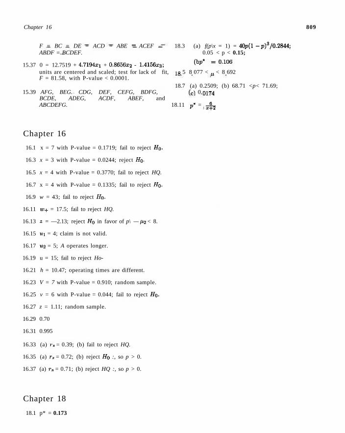
Chapter 16 809
F = BC = DE = ACD = ABE = ACEF = 18.3 (a) f(p\x = 1) = 40p(l -p) 3 /0 .2844; ABDF = BCDEF. 0.05 < p < 0.15;
15.37 0 = 12.7519 + 4.7194xi + 0.8656x2 - 1.4156x3; ^ p* = 0 1 0 6
units are centered and scaled; test for lack of fit, 18 5 8 077 < u < 8 692 F = 81.58, with P-value < 0.0001.
18.7 (a) 0.2509; (b) 68.71 <p< 71.69; 15.39 AFG, BEG. CDG, DEF, CEFG, BDFG, c) 0 0174
BCDE, ADEG, ACDF, ABEF, and ABCDEFG. 18.11 p* = - ^
Chapter 16
16.1 x = 7 with P-value = 0.1719; fail to reject H0.
16.3 x = 3 with P-value = 0.0244; reject H0.
16.5 x = 4 with P-value = 0.3770; fail to reject HQ.
16.7 x = 4 with P-value = 0.1335; fail to reject H0.
16.9 w = 43; fail to reject H0.
16.11 «,+ = 17.5; fail to reject HQ.
16.13 2 = —2.13; reject HQ in favor of p\ — p2 < 8.
16.15 «i = 4; claim is not valid.
16.17 u2 = 5; A operates longer.
16.19 u = 15; fail to reject Ho-
16.21 h = 10.47; operating times are different.
16.23 V = 7 with P-value = 0.910; random sample.
16.25 v = 6 with P-value = 0.044; fail to reject H0.
16.27 z = 1.11; random sample.
16.29 0.70
16.31 0.995
16.33 (a) rs = 0.39; (b) fail to reject HQ.
16.35 (a) rs = 0.72; (b) reject Ho :, so p > 0.
16.37 (a) r s = 0.71; (b) reject HQ :, so p > 0.
Chapter 18
18.1 p* = 0.173

Index
2k factorial experiment, 611 aliases, 649 center runs, 634 confounding, 639 defining contrast, 640 defining relation, 648 design generator, 648 diagnostic plotting, 618 factor screening, 612 foldover, 659 fractional factorial, 647 incomplete blocks, 639 orthogonal design, 631 partial confounding. 644 Plackett-Burman designs, 660 principal block, 641 regression setting, 625 resolution, 658
Cp statistic, 493, 494 F-distribution, 261-264 R2, 407, 408 X-chart, 702
operating characteristic function, 707 /-distribution, 257-259, 261 P-value, 4, 334, 336 AVchart, 704 S-chart, 711
Acceptable quality level, 721 Acceptance sampling, 153 Additive rule, 52 Adjusted R2, 466, 467 Analysis of variance, 264, 511 ANOVA table, 416 Approximation
binomial to hypergeometric, 155 normal to binomial, 187. 188 Poisson to binomial, 163
Average, 107 811
Backward elimination, 482 Bar chart, 82 Bartlett's test, 519 Bayes estimate. 732 Bayes' rule, 68, 70, 71 Bayesian
inference, 726 interval, 731 methodology, 269. 725 perspective, 726
Bernoulli process. 143 trial, 143, 144
Beta distribution, 206 Bias, 231 Binomial distribution, 144
mean of, 147 variance of, 147
Blocks, 513 Box plot, 3, 236
Categorical variable, 474 Central limit theorem, 245 Chebyshev's theorem, 131-133 Chi-squared distribution, 200, 201 Cochran's test, 521 Coefficient of determination, 407, 435
adjusted, 467 Coefficient of multiple determination, 465 Coefficient of variation, 474 Combination, 46 Completely randomized design. 513 Conditional distribution. 95
joint, 99 Conditional perspective. 726 Conditional probability, 58-61, 64, 70-72 Confidence
coefficient, 273 degree of, 273
812 INDEX
limits, 273, 275 Confidence interval, 273, 274, 285
for difference of two means, 288, 289, 291, 293 for difference of two proportions, 303 for paired observations, 296 for ratio of standard deviations, 309 for ratio of variances, 308 for single mean, 274-279 for single proportion, 300 for single variance, 307 for standard deviation, 307 interpretation of, 292 of large sample, 280
Contingency table, 374 marginal frequency, 374
Continuity correction, 190 Continuous distribution
exponential, 196 gamma, 195 lognormal, 201 normal, 172 uniform, 171 Weibull, 203, 204
Control chart X-chart, 702 tf-chart, 704 S-chart, 711 (7-chart, 720 p-chart, 713 Cusum chart, 721 for attributes, 713 for variable, 700
Correlation coefficient, 121, 432 Pearson product-moment, 434 population, 434 sample, 434
Covariance, 115, 119 Cross validation, 490 Cumulative distribution function, 81, 86
Data display, 236 Degrees of freedom, 15, 16, 255, 256 Descriptive statistics, 3 Design of experiment
i factorial, 648 blocking, 535 completely randomized design, 536 concept of confounding, 639
contrast, 613 control factor, 662 defining contrast, 640 defining relation, 648 foldover, 659 fractional factorial, 625, 647 incomplete block design, 604 interaction, 574 Latin square, 549 main effects, 574 noise factor, 662 orthogonal design, 631 randomized block design, 537 resolution, 658 robust parameter design, 661
Design of experiments fractional factorial, 612
Deviation, 116 Discrete distribution
binomial, 143, 144 geometric, 158, 160 hypergeometric, 152, 153 multinomial, 143, 149 negative binomial, 158, 159 Poisson, 161, 162 uniform, 141, 142
Distribution, 19. 23 t-, 257, 258 beta, 206 binomial, 143, 144, 188 bivariate normal, 433 chi-squared, 200 discrete uniform, 142 empirical, 236 Erlang, 206 exponential, 194, 196 gamma, 194, 195 geometric, 158, 160 hypergeometric, 152-154 lognormal. 201 multinomial, 143, 149 multivariate hypergeometric, 156 negative binomial, 158-160 normal, 19, 172, 173, 188 Poisson, 161, 162 posterior, 727 prior, 726
INDEX 813
skewed, 23 symmetric, 23 variance ratio, 263 Weibull, 202, 203
Distribution-free methods, 671 Dot plot. 3, 8, 29 Duncan's multiple-range test, 530
Erlang distribution, 206 Error
in estimating mean, 276 in estimating the mean, 277 type I, 324 type II, 325
Estimate, 12 Estimation, 270
difference of two sample means, 288 maximum likelihood, 310, 311, 315 of single variance, 306 of the ratio of variances, 308 paird observations, 294 proportion, 299 two proportions, 302
Estimator, 270 efficient, 271 maximum likelihood, 311, 313 method of moments, 317 unbiased. 270, 271
Event, 34 Expectation
mathematical, 107, 108, 111 Expected mean squares
ANOVA model, 556 Expected value, 108-111 Experiment-wise error rate, 529 Experimental unit, 289, 295, 574 Exponential distribution, 194, 196
mean of, 196 memoryless property, 198 relationship to Poisson process, 196 variance of. 196
Factor, 26 Factorial experiment, 573
in blocks, 594 masking effects, 575 mixed model, 602 model II, 600
model III, 602 pooling mean squares, 594 three-factor ANOVA, 590 two-factor ANOVA, 577
Fixed effects experiment, 555 Forward selection, 482
Gamma distribution, 194, 195 mean of, 196 relationship to Poisson process, 196 variance of, 196
Gamma function, 194 Geometric distribution, 158, 160
mean of, 161 variance of, 161
Goodness-of-fit test, 240, 371, 372
Historical data, 27 Hypergeometric distribution, 152, 154
mean of, 154 variance of, 154
Hypothesis, 322 alternative, 322 null, 322 statistical, 321 testing, 322, 323
Independence, 60-62, 64 statistical, 97-99
Indicator variable, 474 Interaction, 25 Interquartile range, 236, 237 Interval estimate, 272, 273
Bayesian, 731
Lack of fit, 419 Latin squares, 549 Least squares method, 394, 395 Level of significance, 324, 325 Likelihood function, 310 Linear predictor, 501 Linear regression
ANOVA, 415 categorical variable, 474, 475 coefficient of determination, 407 correlation, 432 data transformation, 426 dependent variable, 389
814 INDEX
empirical model, 391 error sum of squares, 415 fitted regression, 392 fitted value, 417 independent variable, 389 lack of fit, 419 least squares, 394 mean response, 394, 409 model selection, 479, 490 multiple, 390, 445 normal equation, 396 overfitting, 408 prediction, 409 prediction interval, 410, 411 pure experimental error, 419, 420 random error, 391 regression coefficient, 392 regression sum of squares, 464 regressor, 389 residual, 394 simple, 389, 390 statistical model, 391 test of linearity, 417 through the origin, 413 total sum of squares, 415
Logistic regression, 500 effective dose, 502 odds ratio, 503
Lognormal distribution, 201 mean of, 202 variance of, 202
Marginal distribution, 93, 94, 98, 99 joint, 99
Masking effect, 575 Maximum likelihood estimation, 310 Mean, 19, 107, 108, 110, 111
sample, 232 Mean squared error, 287 Mean squares, 416 Mode, 728 Model I experiment, 555 Model II experiment, 555 Model selection, 479
Cp statistic, 493, 494 backward elimination, 482 forward selection, 482 PRESS, 490
sequential methods, 479 stepwise regression, 483
Moment-generating function, 219, 220 Moments
about the origin, 220 Multicollinearity, 479 Multinomial distribution, 149 Multiple comparison test, 527
Duncan's test, 530 Dunnett's test, 531 experiment-wise error rate, 529 Tukey's test, 529
Multiple linear regression, 445 i?-student residuals, 486 adjusted R2, 466 ANOVA, 457 coefficient of multiple determination, 465 error sum of squares, 462 inference, 458 multicollinearity, 479 normal equations, 447 orthogonal variables, 470 outlier, 486 polynomial, 448 regression sum of squares, 463 studentized residuals, 486 variable screening, 461 variance-covariance matrix, 456
Multiple regression HAT matrix, 485
Multiplication rule, 40 Multiplicative rules, 61 Multivariate hypergeometric distribution, 156
Negative binomial distribution, 158, 159 Negative exponential distribution, 196 Noncentral F-distribution, 560 Noncentrality parameter, 560 Nonlinear regression, 499
binary response, 499 count data, 500 logistic, 500
Nonparametric methods, 671 Kruskall-Wallis test, 684 runs test, 687 sign test, 672 signed-rank test, 676 tolerance limits, 690
INDEX 815
Wilcoxon rank-sum test, 681 Normal distribution. 172, 173
mean of, 175 normal curve, 172. 173. 175 standard, 177 variance of, 175
Normal probability plot, 236 Normal quantile-quantile plot, 240, 241
Observational study. 3, 26 OC curve, 338 One sided confidence bound, 277 One-way ANOVA, 513
contrast, 524 contrast sum of squares, 525 grand mean, 514 single-degrce-of-frecdom contrast, 523 treatment, 513 treatment effect, 514
Orthogonal contrasts, 525 Orthogonal variables, 470 Outlier, 236, 486
Paired observations, 294 estimation of, 294
Permutation, 43 circular. 44
Plot box, 236 normal quantile-quantile, 240, 241 quantile, 239
Point estimate, 270, 272 standard error, 280
Poisson distribution. 161, 162 mean of. 163 variance of, 163
Poisson process, 161 relationship to gamma distribution, 196
Polynomial regression, 445, 448 Pooled estimate of variance, 290 Population, 2, 4, 229, 230
mean of. 230 variance of, 230
Posterior distribution, 727 Power chart
ANOVA model, 561 Power of a test, 331
ANOVA model, 559
Prediction interval, 281, 282, 285 for a future observation. 282
Prior distribution, 726 Probability, 31, 48, 49
coverage, 731 Probability density function, 84, 86
joint, 92, 93 Probability distribution, 80
continuous. 84 discrete, 80 joint. 91, 98 mean of, 107 variance of, 116
Probability function, 80 Probability mass function, 80
joint, 92
Quality control, 697 control chart, 697, 698 control limits, 699 in control, 698 out of control, 698
Quantile, 239 Quantile plot, 236, 238, 239
Random sample, 231
Random effects experiment variance components, 557
Random effects model, 555 Random sample, 231
simple. 7 Random sampling. 229 Random variable, 77
continuous, 80 discrete, 79 mean of, 107, 110 variance of, 116, 118
Randomized complete block design, 537 Rank correlation coefficient, 691
Spearman, 690 Regression, 20 Rejectable quality level, 721 Relative frequency, 22, 23, 28, 29, 107 Reliability
failure rate, 204 Residual, 394, 429 Response surface methodology, 452
816 INDEX
Retrospective study, 27 Rule of elimination, 68, 70
Sample, 1, 229, 230 mean, 3, 11-13, 19, 28, 29, 229, 232 median, 3, 11-13, 28, 29, 232 mode, 232 random, 231 range, 15, 28, 29 standard deviation, 3, 15, 16, 28. 29, 234 variance, 15, 16, 28, 229, 232, 233
Sample size, 7 in estimating a mean, 277 in estimating a proportion, 301 in hypothesis testing, 352
Sample space, 31 continuous, 79 discrete, 79 partition, 53
Sampling distribution, 243, 244 of mean, 244
Significant level, 334 Single proportion test, 361 Squared-error loss, 732 Standard deviation, 116, 118, 131 Standard error of mean, 280 Standard normal distribution, 177 Statistic, 232 Statistical inference, 269 Stem-and-leaf plot, 3, 21, 22, 28, 29 Stepwise regression, 481 Subjective probability, 725 Sum of squares
of error, 415 of regression, 415 total, 407
Test goodness-of-fit, 240, 371
Test statistic, 324 Tests for the equality of variances, 519
Bartlett's test, 519 Cochran's test, 521
Tests of hypotheses, 19, 270, 321 P-value, 334, 336 choice of sample size, 350, 353 critical region, 324 critical value, 324
goodness-of-fit, 372 important properties, 331 on two means, 345 one-tailed, 332 paired observations, 347 single proportion, 361 single sample, variance known, 338 single sample, variance unknown, 342 single variance, 367 size of test, 325 test for homogeneity, 377 test for independence, 374 test for several proportions, 378 test statistics, 328 two means with unknown and unequal vari
ances, 347 two means with unknown but equal variances,
346 two variances, 367 two-tailed, 332
Tolerance interval, 284, 285 limits, 283, 284
Total probability, 68 Treatment
negative effect, 575 positive effect, 575
TYimmed mean, 12, 13
Unbiased estimator, 271 Uniform distribution. 141, 142, 171
discrete, 141, 142
Variability, 8, 9, 14-16, 116, 131, 232, 261, 263, 264
between samples, 264 within samples, 264
Variable transformation discrete, 212
Variance, 115, 116, 118 sample, 233
Variance ratio distribution, 263 Venn diagram, 36
Weibull distribution, 202, 203 mean of, 203 variance of, 203


![(2) Essential MATLAB for Engineers and Scientists [www matlabtrainings blogfa com]](https://img.dokumen.tips/doc/110x75/634dc13c92e70b3087020bdf/2-essential-matlab-for-engineers-and-scientists-www-matlabtrainings-blogfa-com.jpg)


