Probabilistic Frechet Means and Statistics on Vineyards

Elizabeth Munch∗, Paul Bendich†, Katharine Turner‡,Sayan Mukherjee§, Jonathan Mattingly¶, and John Harer‖.

July 25, 2013

Abstract

In order to use persistence diagrams as a true statistical tool, it would be very useful to have agood notion of mean and variance for a set of diagrams. In [20], Mileyko and his collaborators madethe first study of the properties of the Frechet mean in (Dp,Wp), the space of persistence diagramsequipped with the p-th Wasserstein metric. In particular, they showed that the Frechet mean of afinite set of diagrams always exists, but is not necessarily unique. As an unfortunate consequence, onesees that the means of a continuously-varying set of diagrams do not themselves vary continuously,which presents obvious problems when trying to extend the Frechet mean definition to the realm ofvineyards.

We fix this problem by altering the original definition of Frechet mean so that it now becomes aprobability measure on the set of persistence diagrams; in a nutshell, the mean of a set of diagramswill be a weighted sum of atomic measures, where each atom is itself the (Frechet mean) persistencediagram of a perturbation of the input diagrams. We show that this new definition defines a (Holder)continuous map, for each k, from (Dp)k → P (Dp), and we present several examples to show how itmay become a useful statistic on vineyards.

1 Introduction

The field of topological data analysis (TDA) was first introduced [14] in 2000, and has rapidly beenapplied to many different areas: for example, in the study of protein structure [1, 2, 19], plant rootstructure [17], speech patterns [4], image compression and segmentation [6, 16], neuroscience [11], or-thodontia [18], gene expression [13], and signal analysis [24].

A key tool in TDA is the persistence diagram [7, 14]. Given a set of points χ in some possiblyhigh-dimensional metric space, the persistence diagram d(χ) is a computable summary of the datawhich provides a compact two-dimensional representation of the multi-scale topological informationcarried by the point cloud; see Figure 1 for an example of such a diagram and Section 2 for a morerigorous description. If the point cloud varies continuously over time (or some other parameter) thenthe persistence diagrams vary continuously over time [9]; the diagrams stacked on top of each otherthen form what is called a vineyard [10].

A key part of data analysis is to model variation in data. To address this there has been a recenteffort to study the mean and variance of a set of persistence diagrams [3, 5, 20, 26], as well a veryrecent paper that gives nice convergence rates for persistence diagrams of larger and larger point cloudssampled from a compactly-supported measure [8]. There are a variety of reasons to want to characterizestatistical properties of diagrams. For example, given a massive point cloud χ, there is a computational

∗Department of Mathematics, Duke University and Institute for Mathematics and its Applications, University of Min-nesota†Department of Mathematics, Duke University‡Department of Mathematics, University of Chicago§Departments of Statistical Science, Computer Science, Mathematics, and Institute for Genome Sciences & Policy, Duke

University¶Department of Mathematics, Duke University‖Departments of Mathematics, Computer Science, and Electrical and Computer Engineering, Duke University

1

arX

iv:1

307.

6530

v1 [

mat

h.PR

] 2

4 Ju

l 201

3

and statistical advantage to subsampling the data to produce smaller point clouds χ1, . . . , χn, andcomputing the mean and variance of the set of persistence diagrams obtained from the n subsampleddata sets. In statistical terminology, this example consists of computing a bootstrap estimate [?] ofpersistence diagram of the data. This procedure requires a good definition for the mean (and variance)of a set of persistence diagrams.

The papers [20,26] make careful study of the geometric and analytic properties of the space (Dp,Wp)of persistence diagrams equipped with the Wasserstein metric, which enables a definition or mean andvariance in the former paper, and an algorithm for their computation in the latter. There is, however,an unfortunate problem with the definition in [20]: namely, the mean of a set of diagrams can itself bea set of diagrams, rather than a single unique diagram. This results in means that do not continuouslyvary as the input set of diagrams vary.

In this paper, we provide an alternative definition for the mean of a set of diagrams. The key idea isthat our mean is not itself a diagram, but is rather a probabilistic mixture of diagrams, thus an elementof P(Dp), the space of probability distributions over persistence diagrams. Uniqueness of this new meanwill be obvious from the definition we propose. More crucially, we prove (Theorem 13) continuity ofthe map (Dp)

k → P(Dp) taking a set of k persistence diagrams to its mean; in fact, we show that thismap is Holder with exponent 1

2 . Finally, we give examples of this mean computed on diagrams drawnfrom samples of various point clouds, and introduce a useful way to visualize them.

Outline Section 2 contains definitions for persistence diagrams and vineyards, as well as a discussionof the space (Dp,Wp). The contributions of [20] and [26] are reviewed more fully in Section 3, and thenon-uniqueness issue is also discussed in that section. We give our new definition in Section 4, andprove its desirable theoretical properties in Section 5, although some technical details are confined tothe Appendix. Examples, implementation details, and a discussion of visualization, all come in Section6, and the paper concludes with some discussion in Section 7.

2 Diagrams and Vineyards

Here we give the basic definitions for persistence diagrams and vineyards, and then move on to adescription of the metric space (Dp,Wp). For more details on persistence, see [15]. We assume thereader is familiar with homology; [23] is a good reference. For the expert, we note that all homologygroups in this paper need to be computed with field coefficients.

2.1 Persistent Homology

To define persistent homology, we start with a nested sequence of topological spaces,

∅ = X0 ⊆ X1 ⊆ X2 ⊆ · · · ⊆ Xn = X. (1)

Often this sequence arises from the sublevel sets of a continuous function, f : X → R, where Xi =f−1((−∞, ai]) with a0 ≤ a1 ≤ · · · ≤ an. For many applications, this function is the distance function

dχ(x) = infv∈χ‖x− v‖

from a point cloud χ such as in the example of Figure 1a. In this case, a sublevel can be visualized asa union of balls around the points in χ.

The sequence of inclusion maps from Equation (1) induces maps on homology for any dimension r,

0 // Hr(X1) // Hr(X2) // · · · // Hr(Xn). (2)

In order to understand the changing space, we look at where homology classes appear and disappear inthis sequence.

Let ϕji : Hr(Xi) −→ Hr(Xj) be the composition of necessary maps from Equation (2). The homologyclass γ ∈ Hr(Xi) is said to be born at Xi if it is not in the image of ϕii−1. This same class is said to die

2

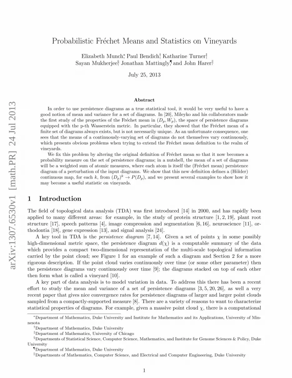
(a) Point cloud sampled from an annulus.(b) Persistence diagram encoding informationabout the point cloud.

Figure 1: A point cloud, shown at left, is sampled from an annulus. In order to summarize thetopological data, we look at the level sets of the distance function from the set of points, then constructthe persistence diagram, shown at right. The points near the diagonal are considered noise, while thesingle point far from the diagonal gives information about the hole in the annulus.

at Xj if its image in Hr(Xj−1) is not in the image of ϕj−1i−1 , but its image in Hr(Xj) is in the image of

ϕji−1. In the case that the spaces arose from the level sets of a function f as defined above, we definethe persistence of a class γ which is born at Xi = f−1((−∞, ai]) and dies at Xj = f−1((−∞, aj ] to bepers(γ) = aj − ai.

Notice that this equivalence can also be seen from working with persistence modules [7], an abstrac-tion of the definition presented here where persistence is defined at the algebraic level. In fact, givenany set of maps between vector spaces,

V1// V2

// · · · // Vn,

we can analogously define the birth and death of classes in the vector spaces.In order to visualize the changing homology, we draw a persistence diagram dr for each dimension

r. A persistence diagram is a set of points with multiplicity in the upper half plane (b, d) ∈ R2 | d ≥ balong with countably many copies of the points on the diagonal ∆ = (x, x) ∈ R2. For each class γwhich is born at Xi and dies at Xj , we draw a point at (ai, aj). A point in the persistence diagramwhich is close to the diagonal represents a class which was born and died very quickly. A point whichis far from the diagonal had a longer life. Depending on the context, this may mean the class is moreimportant, or more telling of the inherent topology of the space. See Figure 1b for an example.

2.2 The Space (Dp,Wp)

In order to define a framework for statistics, we will ignore the connection to topological spaces or mapsbetween vector spaces and instead focus on the space of persistence diagrams abstractly.

Definition 1. An abstract persistence diagram is a countable multiset of points along with the diagonal,∆ = (x, x) ∈ R2 | x ∈ R, with points in ∆ having countably infinite multiplicity.

The distance between these abstract diagrams is the pth Wasserstein distance.

3

Definition 2. The pth Wasserstein distance between two persistence diagrams X and Y is given by

Wp[σ](X,Y ) := infϕ:X→Y

[∑x∈X

σ(x, ϕ(x))p

]1/p

where 1 ≤ p ≤ ∞, σ is a metric on the plane, and ϕ ranges over bijections between X and Y .

We often use σ = Lq. Notice that for p =∞,

W∞[Lq](X,Y ) := infϕ:X→Y

supx∈X‖x− ϕ(x)‖q.

W∞[L∞] is often referred to as the bottleneck distance. For the remainder of this paper, we will beusing Wp[L2], which we refer to as Wp for brevity.

The persistence pers(u) of a point u = (x, y) in a diagram is defined to be y − x, and the pth

total persistence of a diagram d is defined to be the sum of the pth-powers of the persistences of theoff-diagonal points in d.

Definition 3. The space of persistence diagrams is

Dp = d |Wp(d, d∅) <∞ = d | Persp(d) <∞

along with the pth-Wasserstein metric, Wp = Wp[L2], from Definition 2.

The authors in [20] show that (Dp,Wp) is a Polish (complete and separable) space, and they alsodescribe all of the compact sets in this space. In [26], it is shown that Dp is a geodesic space, and thusthat every pair of diagrams has a minimal geodesic between them. This geodesic can be defined usinga bijection between the diagrams which minimizes Wasserstein distance.

2.3 Vineyards

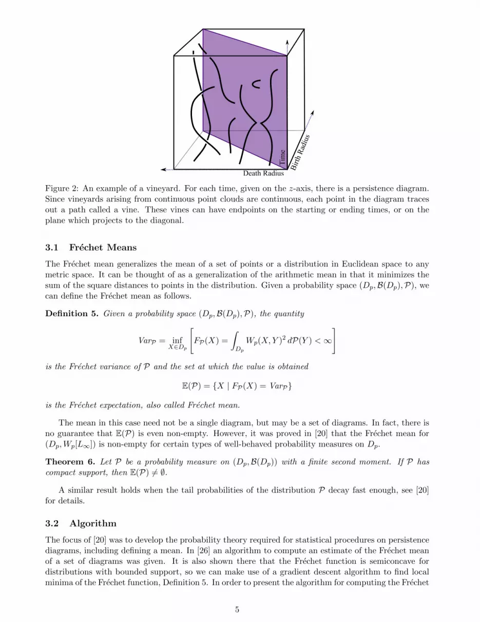
The first definitions of vineyards [10,21] were used in the well-behaved case of a homotopy between twofunctions. In this case, each off-diagonal point of a diagram varies continuously in time, D(X(t)), and iscalled a vine. Vines can start and end at off diagonal points at times 0 or 1, or have starting or endingpoints on the diagonal for any t, see Figure 2.

As we do with persistence diagrams, let us consider the space of abstract vineyards to be the spaceof paths in persistence diagram space.

Definition 4. The space of abstract vineyards is

V = v : [0, 1]→ Dp

the space of maps from the unit interval to Dp where v is continuous with respect to Wp.

3 Frechet Means of Diagrams

This section reviews previous definitions of the mean of a set of diagrams [20] and an algorithm tocompute the mean [26]. We will define the mean of a diagram as the Frechet mean, give the algorithmfor the computation of this mean, and finally present the non-uniqueness problem.

4

Death Radius

Bir

th R

adiu

s

Tim

e

Figure 2: An example of a vineyard. For each time, given on the z-axis, there is a persistence diagram.Since vineyards arising from continuous point clouds are continuous, each point in the diagram tracesout a path called a vine. These vines can have endpoints on the starting or ending times, or on theplane which projects to the diagonal.

3.1 Frechet Means

The Frechet mean generalizes the mean of a set of points or a distribution in Euclidean space to anymetric space. It can be thought of as a generalization of the arithmetic mean in that it minimizes thesum of the square distances to points in the distribution. Given a probability space (Dp,B(Dp),P), wecan define the Frechet mean as follows.

Definition 5. Given a probability space (Dp,B(Dp),P), the quantity

VarP = infX∈Dp

[FP(X) =

∫Dp

Wp(X,Y )2 dP(Y ) <∞

]

is the Frechet variance of P and the set at which the value is obtained

E(P) = X | FP(X) = VarP

is the Frechet expectation, also called Frechet mean.

The mean in this case need not be a single diagram, but may be a set of diagrams. In fact, there isno guarantee that E(P) is even non-empty. However, it was proved in [20] that the Frechet mean for(Dp,Wp[L∞]) is non-empty for certain types of well-behaved probability measures on Dp.

Theorem 6. Let P be a probability measure on (Dp,B(Dp)) with a finite second moment. If P hascompact support, then E(P) 6= ∅.

A similar result holds when the tail probabilities of the distribution P decay fast enough, see [20]for details.

3.2 Algorithm

The focus of [20] was to develop the probability theory required for statistical procedures on persistencediagrams, including defining a mean. In [26] an algorithm to compute an estimate of the Frechet meanof a set of diagrams was given. It is also shown there that the Frechet function is semiconcave fordistributions with bounded support, so we can make use of a gradient descent algorithm to find localminima of the Frechet function, Definition 5. In order to present the algorithm for computing the Frechet

5

a

b

c

x

y

z

d

(a)

a

b

c

d

x

y

z

(b)

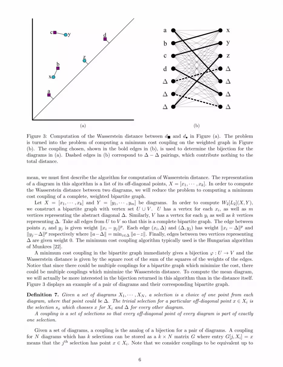
Figure 3: Computation of the Wasserstein distance between d and d• in Figure (a). The problemis turned into the problem of computing a minimum cost coupling on the weighted graph in Figure(b). The coupling chosen, shown in the bold edges in (b), is used to determine the bijection for thediagrams in (a). Dashed edges in (b) correspond to ∆ − ∆ pairings, which contribute nothing to thetotal distance.

mean, we must first describe the algorithm for computation of Wasserstein distance. The representationof a diagram in this algorithm is a list of its off-diagonal points, X = [x1, · · · , xk]. In order to computethe Wasserstein distance between two diagrams, we will reduce the problem to computing a minimumcost coupling of a complete, weighted bipartite graph.

Let X = [x1, · · · , xk] and Y = [y1, · · · , ym] be diagrams. In order to compute W2[L2](X,Y ),we construct a bipartite graph with vertex set U ∪ V . U has a vertex for each xi, as well as mvertices representing the abstract diagonal ∆. Similarly, V has a vertex for each yi as well as k verticesrepresenting ∆. Take all edges from U to V so that this is a complete bipartite graph. The edge betweenpoints xi and yj is given weight ‖xi − yj‖p. Each edge (xi,∆) and (∆, yj) has weight ‖xi − ∆‖p and‖yj−∆‖p respectively where ‖a−∆‖ = minz∈∆ ‖a−z‖. Finally, edges between two vertices representing∆ are given weight 0. The minimum cost coupling algorithm typically used is the Hungarian algorithmof Munkres [22].

A minimum cost coupling in the bipartite graph immediately gives a bijection ϕ : U → V and theWasserstein distance is given by the square root of the sum of the squares of the weights of the edges.Notice that since there could be multiple couplings for a bipartite graph which minimize the cost, therecould be multiple couplings which minimize the Wasserstein distance. To compute the mean diagram,we will actually be more interested in the bijection returned in this algorithm than in the distance itself.Figure 3 displays an example of a pair of diagrams and their corresponding bipartite graph.

Definition 7. Given a set of diagrams X1, · · · , XN , a selection is a choice of one point from eachdiagram, where that point could be ∆. The trivial selection for a particular off-diagonal point x ∈ Xi isthe selection sx which chooses x for Xi and ∆ for every other diagram.

A coupling is a set of selections so that every off-diagonal point of every diagram is part of exactlyone selection.

Given a set of diagrams, a coupling is the analog of a bijection for a pair of diagrams. A couplingfor N diagrams which has k selections can be stored as a k × N matrix G where entry G[j,Xi] = xmeans that the jth selection has point x ∈ Xi. Note that we consider couplings to be equivalent up to

6

a

b cf

g

x

y

z

h

(a) (b)

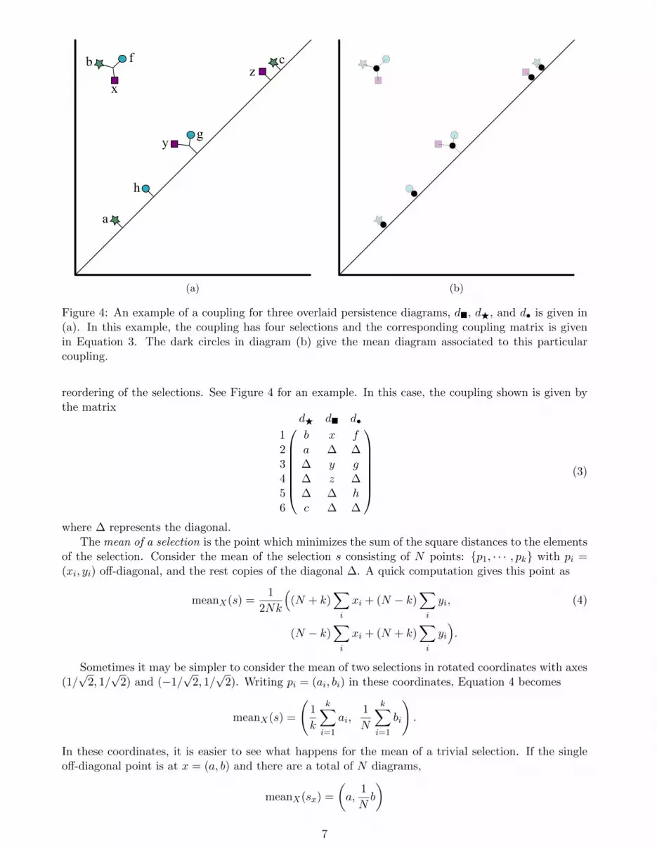
Figure 4: An example of a coupling for three overlaid persistence diagrams, d, dF, and d• is given in(a). In this example, the coupling has four selections and the corresponding coupling matrix is givenin Equation 3. The dark circles in diagram (b) give the mean diagram associated to this particularcoupling.

reordering of the selections. See Figure 4 for an example. In this case, the coupling shown is given bythe matrix

dF d d•

1 b x f2 a ∆ ∆3 ∆ y g4 ∆ z ∆5 ∆ ∆ h6 c ∆ ∆

(3)

where ∆ represents the diagonal.The mean of a selection is the point which minimizes the sum of the square distances to the elements

of the selection. Consider the mean of the selection s consisting of N points: p1, · · · , pk with pi =(xi, yi) off-diagonal, and the rest copies of the diagonal ∆. A quick computation gives this point as

meanX(s) =1

2Nk

((N + k)

∑i

xi + (N − k)∑i

yi, (4)

(N − k)∑i

xi + (N + k)∑i

yi

).

Sometimes it may be simpler to consider the mean of two selections in rotated coordinates with axes(1/√

2, 1/√

2) and (−1/√

2, 1/√

2). Writing pi = (ai, bi) in these coordinates, Equation 4 becomes

meanX(s) =

(1

k

k∑i=1

ai,1

N

k∑i=1

bi

).

In these coordinates, it is easier to see what happens for the mean of a trivial selection. If the singleoff-diagonal point is at x = (a, b) and there are a total of N diagrams,

meanX(sx) =

(a,

1

Nb

)7

so the point is placed at distance 1N ‖x−∆‖ from the diagonal.

The mean of a coupling, mean(G), is a diagram in Dp with a point at the mean of each selection.When it is unclear as to the set of diagrams from which this mean arose, we will denote it as meanX(G).Note that the mean of the selection yields a point while the mean of a coupling yields a diagram.

Now we are ready to give the algorithm for the Frechet mean of a set of diagrams. Given a finiteset of diagrams X1, · · · , XN, start with a candidate for the mean, Y , and compute the bijection forW2[L2](Y,Xi). We denote this as WassersteinPairing(Y,Xi). From this, we have a coupling G whereG[yj , Xi] gives the point in Xi which was paired to point yj ∈ Y . Set Y ′ = mean(G). This new diagramis now the candidate for the mean and the process is repeated. The algorithm terminates when theWasserstein pairing does not change. [26] uses the structure of (D2,W2[L2]) to prove that this algorithmterminates at a local minimum of the Frechet function. See Algorithm 1 for the pseudocode.

Algorithm 1 Algorithm for computing the Frechet Mean of a finite set of diagrams

Input: Persistence diagrams X1, · · · , XN

Output: Y , a persistence diagram giving a local min of the Frechet functionChoose one of the Xi randomly, set Y = Xi

Initialize matching G . G[yj , Xi] = the xk ∈ Xi matched. with the point yj ∈ Y

stop = False

while stop == False do

for each diagram Xi do . Determine the best GP =WassersteinPairing(Y,Xi)for each pair (yj , xk) ∈ P do

Set G[yj , Xi] = xkend for

end for

Initialize empty diagram Y ′ . Move each point to thefor each point yj ∈ Y do . barycenter of its selection.

y′j = meanG[yj , X1], · · · , G[yj , XN ] . Y ′ = meanX(G)Add y′j to Y ′

end for

if WassersteinPairing(Y,Xi) = WassersteinPairing(Y ′, Xi) ∀i thenstop = True

end ifY = Y ′

end whilereturn Y

3.3 Issues with extensions to Vineyards

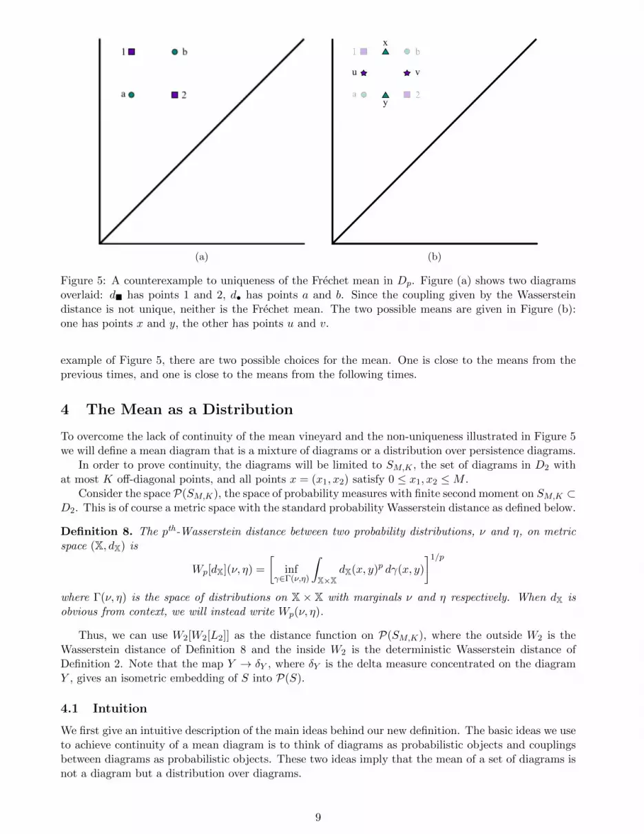
Consider the example of Figure 5. Here we have two persistence diagrams overlaid: d has square points1 and 2, d• has circle points a and b. Since the four points lie exactly on a square, the pairing to givethe Wasserstein distance could either be (a, 1), (b, 2) or (a, 2), (b, 1). Thus there are two diagramswhich give a minimum of the Frechet function: the diagram with u and v, or the diagram with x and y.

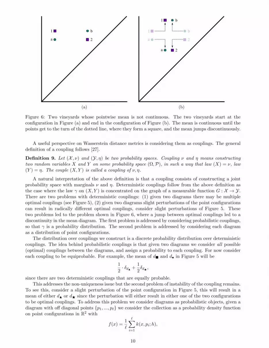
If two vineyards pass through this configuration, the mean of the vineyards constructed by findingthe mean at each time will not be continuous. Consider for example two vineyards of two points each whostart in the elongated configuration of Figure 6a and move along the dotted lines to the configurationin Figure 6b. At the bend of the dotted line, the points are at the corners of a square, so as in the

8

(a)

x

a

1

2

b

y

u v

(b)

Figure 5: A counterexample to uniqueness of the Frechet mean in Dp. Figure (a) shows two diagramsoverlaid: d has points 1 and 2, d• has points a and b. Since the coupling given by the Wassersteindistance is not unique, neither is the Frechet mean. The two possible means are given in Figure (b):one has points x and y, the other has points u and v.

example of Figure 5, there are two possible choices for the mean. One is close to the means from theprevious times, and one is close to the means from the following times.

4 The Mean as a Distribution

To overcome the lack of continuity of the mean vineyard and the non-uniqueness illustrated in Figure 5we will define a mean diagram that is a mixture of diagrams or a distribution over persistence diagrams.

In order to prove continuity, the diagrams will be limited to SM,K , the set of diagrams in D2 withat most K off-diagonal points, and all points x = (x1, x2) satisfy 0 ≤ x1, x2 ≤M .

Consider the space P(SM,K), the space of probability measures with finite second moment on SM,K ⊂D2. This is of course a metric space with the standard probability Wasserstein distance as defined below.

Definition 8. The pth-Wasserstein distance between two probability distributions, ν and η, on metricspace (X, dX) is

Wp[dX](ν, η) =

[inf

γ∈Γ(ν,η)

∫X×X

dX(x, y)p dγ(x, y)

]1/p

where Γ(ν, η) is the space of distributions on X × X with marginals ν and η respectively. When dX isobvious from context, we will instead write Wp(ν, η).

Thus, we can use W2[W2[L2]] as the distance function on P(SM,K), where the outside W2 is theWasserstein distance of Definition 8 and the inside W2 is the deterministic Wasserstein distance ofDefinition 2. Note that the map Y → δY , where δY is the delta measure concentrated on the diagramY , gives an isometric embedding of S into P(S).

4.1 Intuition

We first give an intuitive description of the main ideas behind our new definition. The basic ideas we useto achieve continuity of a mean diagram is to think of diagrams as probabilistic objects and couplingsbetween diagrams as probabilistic objects. These two ideas imply that the mean of a set of diagrams isnot a diagram but a distribution over diagrams.

9

a 2

1 b

(a)

a 2

1 b

a

1

2

b

(b)

Figure 6: Two vineyards whose pointwise mean is not continuous. The two vineyards start at theconfiguration in Figure (a) and end in the configuration of Figure (b). The mean is continuous until thepoints get to the turn of the dotted line, where they form a square, and the mean jumps discontinuously.

A useful perspective on Wasserstein distance metrics is considering them as couplings. The generaldefinition of a coupling follows [27].

Definition 9. Let (X , ν) and (Y, η) be two probability spaces. Coupling ν and η means constructingtwo random variables X and Y on some probability space (Ω,P), in such a way that law (X) = ν, law(Y ) = η. The couple (X,Y ) is called a coupling of ν, η.

A natural interpretation of the above definition is that a coupling consists of constructing a jointprobability space with marginals ν and η. Deterministic couplings follow from the above definition asthe case where the law γ on (X,Y ) is concentrated on the graph of a measurable function G : X → Y.There are two problems with deterministic couplings: (1) given two diagrams there may be multipleoptimal couplings (see Figure 5), (2) given two diagrams slight perturbations of the point configurationscan result in radically different optimal couplings, consider slight perturbations of Figure 5. Thesetwo problems led to the problem shown in Figure 6, where a jump between optimal couplings led to adiscontinuity in the mean diagram. The first problem is addressed by considering probabilistic couplings,so that γ is a probability distribution. The second problem is addressed by considering each diagramas a distribution of point configurations.

The distribution over couplings we construct is a discrete probability distribution over deterministiccouplings. The idea behind probabilistic couplings is that given two diagrams we consider all possible(optimal) couplings between the diagrams, and assign a probability to each coupling. For now considereach coupling to be equiprobable. For example, the mean of d and d• in Figure 5 will be

1

2· δdN +

1

2δdF ,

since there are two deterministic couplings that are equally probable.This addresses the non-uniqueness issue but the second problem of instability of the coupling remains.

To see this, consider a slight perturbation of the point configuration in Figure 5, this will result in amean of either dN or dF since the perturbation will either result in either one of the two configurationsto be optimal couplings. To address this problem we consider diagrams as probabilistic objects, given adiagram with off diagonal points p1, ..., p` we consider the collection as a probability density functionon point configurations in R2 with

f(x) =1

`

∑i=1

k(x, pi;h),

10

where k(x, pi;h) is a density function centered at pi and localized to a region h in R2. In this case,slightly perturbing the points in Figure 5 will result in a mean diagram of

pN · δdN + pFδdF ,

where pN = 1 − pF ≈ .5 since the probability of the two optimal matches of the localized probabilitydistributions around the points in Figure 5 is about equal, whether the points are slightly perturbed ornot.

In general, if X = X1, · · · , XN is a set of diagrams from SM,K , we define its mean to be thefollowing distribution on SM,NK :

Definition 10.µX =

∑G

P(H = G) · δmeanX(G)

Here the sum is taken over all possible couplings G on the set of diagrams, and meanX(G) ∈ S isthe mean diagram for the specific coupling G. Note that the mean meanX(G) of a set of N diagrams,each with at most K points, can itself have at most NK points, so that µX , as defined, is indeed anelement of P(SM,NK). The weights P(H = G) are derived from a random variable H which can bethought of either as a probabilistic coupling where each point in the input diagram is replaced with alocalized distribution centered on the point or as the probability that a stochastic perturbation of theinput diagrams would lead to G being the optimal matching. We now explain this in more detail.

4.2 The Definition of H

We are given a set X = X1, · · · , XN of diagrams from SM,K . Sometimes, where appropriate, we willalso use X =

⋃iXi to represent the set of off-diagonal points in all the Xi. We now define H, a coupling

valued random variable.First, we fix an α > 0 and a probability distribution η on R2 which is absolutely continuous with

respect to Lebesgue measure λ. This means that η has a Radon-Nikodym derivative; there exists ameasureable non-negative function f on R2 such that the equation η(A) =

∫A fdλ holds for every

measurable set A. We further require that f is bounded with support of a ball of radius α, B(0, α),and is radially symmetric. Examples of distributions satisfying these requirements are the uniformdistribution U(Bα(0)) or the truncated normal distribution N (0, σ2, α) which is just the portion of thestandard normal distribution N (0, σ2) contained inside of Bα(0) and normalized to have total mass 1.For each x ∈ R2, let ηx be the translation of η centered around x.

We will often be considering the measure of a ball of a radius smaller than α centered around x, sowe use the following notation

η(r) = ηx(Br(x)).

By construction we know that η(r) ≤ πr2f(0) where f is the probability density function correspondingto the density η.

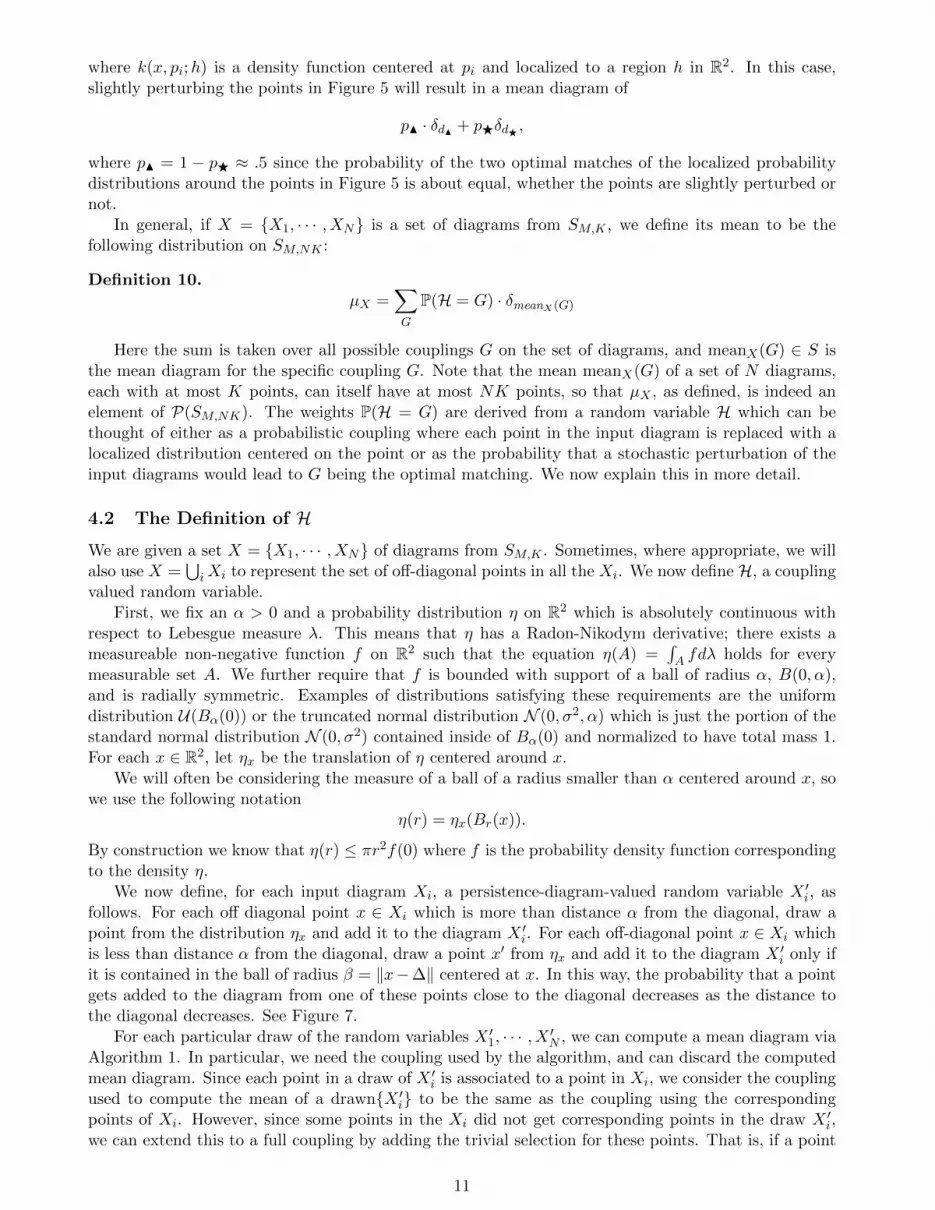
We now define, for each input diagram Xi, a persistence-diagram-valued random variable X ′i, asfollows. For each off diagonal point x ∈ Xi which is more than distance α from the diagonal, draw apoint from the distribution ηx and add it to the diagram X ′i. For each off-diagonal point x ∈ Xi whichis less than distance α from the diagonal, draw a point x′ from ηx and add it to the diagram X ′i only ifit is contained in the ball of radius β = ‖x−∆‖ centered at x. In this way, the probability that a pointgets added to the diagram from one of these points close to the diagonal decreases as the distance tothe diagonal decreases. See Figure 7.

For each particular draw of the random variables X ′1, · · · , X ′N , we can compute a mean diagram viaAlgorithm 1. In particular, we need the coupling used by the algorithm, and can discard the computedmean diagram. Since each point in a draw of X ′i is associated to a point in Xi, we consider the couplingused to compute the mean of a drawnX ′i to be the same as the coupling using the correspondingpoints of Xi. However, since some points in the Xi did not get corresponding points in the draw X ′i,we can extend this to a full coupling by adding the trivial selection for these points. That is, if a point

11

Figure 7: The method for drawing points. For a point x ∈ Xi which is more than distance α from thediagonal as at right, a point is drawn from the distribution ηx, which has mean α and is contained inthe ball of radius α centered at x. This point is then added to the diagram X ′i. For a point x ∈ Xi

which is less than distance α from the diagonal as at left, a point is still drawn from the distributionηx, however the point is only added to X ′i if it is inside the ball of radius β = ‖x−∆‖ centered at x.

x ∈ Xi did not lead to a drawn point in X ′i, we add the selection which chooses x for Xi and ∆ forevery other diagram. This completes the definition of the random variable H: as desribed above, eachdraw of X ′1, · · · , X ′N leads to the draw H = G, where G is the coupling on X described above.

4.3 Example

Here is an example to make the discussion above a little more clear. Consider the three overlaid diagramsin Figure 8a. Points are drawn in the ball of radius α centered at each point. Since a, c, h, g, y, and zare near the diagonal there is a chance that no point is drawn for them. In this particular draw, givenin Figure 8b, no point is drawn for a or c.

When computing the mean of the diagrams in Figure 8b, the coupling used is

d′F d′ d′©

1 b′ x′ f ′

2 ∆ y′ g′

3 ∆ ∆ h′

4 ∆ z′ ∆

. (5)

So, to find the corresponding coupling for the original diagrams, we replace each point with its corre-sponding point, and add in the trivial selection for the points that were not chosen:

dF d d©

1 b x f2 ∆ y g3 ∆ ∆ h4 ∆ z ∆5 a ∆ ∆6 c ∆ ∆

. (6)

5 Continuity

In this section, we prove our main theorem: that the mean distribution varies continuously when facedwith a continuously varying set of input diagrams. We start by developing some more detailed theoryabout the measures ηx, as well as fixing some notation which will be needed in the proof.

12

a

b cf

g

x

y

z

h

(a)

z'

h'

b'

f '

g'

x'

y'

(b)

Figure 8: An example of corresponding couplings for a given draw. The original diagrams are dF, dand d© in Figure (a). A point is drawn near each point away from the diagonal, and points are drawnfor some points near the diagonal to construct d′F, d′ and d′© in Figure (b). The coupling for the meanof these three diagrams is computed using Algorithm 1 and the associated coupling is given in Equation5. Then the coupling is converted to a coupling for dF, d and d© in Equation 6 and drawn in Figure(a).

5.1 Product Measures

For each point x ∈ R2, recall that we have the probability distribution ηx, with support contained inthe ball Bα(x). We use this to define a new distribution η′x, given by the formula:

η′x =1

ηx(B‖x−∆‖(x))ηx

∣∣∣B‖x−∆‖(x)

(7)

Note that η′x = ηx iff x is more than α away from the diagonal.As before, we start with a set X = Xi of input diagrams, and we let X =

⋃iXi be the set of all

off-diagonal points in all the Xi. Recall that, for each draw of the set of random variables X ′i, someof the points in each Xi created a drawn point in X ′i and some did not. To formalize this, we definethe subset-valued random variable Ω ⊂ X to be the set of points in X which do indeed lead to a drawnpoint; note that each draw of Ω will always contain the points in X which are more than α away fromthe diagonal, but it may contain more points as well.

For each subset ω ⊂ X, consider the space (R2)|ω|, where we have associated a copy of R2 to eachpoint in ω. For each coupling G on X, we define Uω,G ⊂ (R2)|ω| to be the set of points which lead tothis coupling. Notice that this set is completely independent of the locations of the points from theoriginal diagrams; it relies only on the combinatorial structure of G.

Let η′ω =∏x∈ω η

′x be the product measure on (R2)|ω|. Then the probability that G is the coupling

used assuming ω is chosen isP(H = G | Ω = ω) = η′ω(Uω,G).

For example, say X consists of two diagrams, X1 and X2, where X1 has a single off-diagonal pointx1, and X2 has a single off diagonal point x2. Then there are exactly two possible couplings:

G1 =

(X1 X2

1 x1 ∆2 ∆ x2

), G2 =

(X1 X2

1 x1 x2

).

13

If ω = x1, x2, then the space we are interested in is (R2)2. So Uω,G1 is the set of points which wouldrather be paired with the diagonal than with each other, thus

Uω,G1 = (a, b) ∈ (R2)2 | ‖a−∆‖2 + ‖b−∆‖2 ≤ ‖a− b‖2.

Likewise, Uω,G2 is the set of points where being paired to each other is better, so

Uω,G2 = (a, b) ∈ (R2)2 | ‖a− b‖2 ≤ ‖a−∆‖2 + ‖b−∆‖2.

For the purposes of determining the probability of G1, we must take the locations of x1 and x2 intoaccount. Now we are only interested in the (a, b) ∈ Uω,G1 for which a is in the support of η′x1

and b isin the support of η′x2

. So, the probability that G1 is chosen assuming both points are picked is

P(H = G1 | Ω = ω) = η′ω(Uω,G1) = (η′x1× η′x2

)(Uω,G1).

Likewise, the probability that G2 is chosen assuming both points are picked is

P(H = G2 | Ω = ω) = η′ω(Uω,G2) = (η′x1× η′x2

)(Uω,G2).

This construction is particularly useful since we can consider the same coupling for two sets ofdiagrams which are close. Since Uω,G is independent of the actual diagrams, the only thing varying isthe measure.

5.2 The Proof

We will prove Holder continuity for the map that takes a set of persistence diagrams to its meandistribution. First we give a lemma which bounds the distance between the measures associated tonearby points in the plane. The proof, which is purely analytical, can be found in the Appendix.

Lemma 11. Let fx and fy be the Radon-Nikodym derivatives of ηx|B(x,‖x−∆‖) and ηy|B(y,‖y−∆‖) respec-tively. Then ∫

|fx − fy| dλ ≤ 4πα‖x− y‖f(0)

where f is the Radon-Nikodym derivative of η.

Next we prove a result which relates the mean of a set of diagrams to the mean of a new set whichis obtained by simply moving one of the points in one of the diagrams to a new location.

Proposition 12. Let Z = Z1, Z2, . . . , ZN ∈ (SM,K)N with mean µ ∈ P(SM,NK). Let Z1 be the samediagram as Z1 except that one of the off-diagonal points, x, has been moved to the new location y (whilestill maintaining Z1 ∈ SM,K). Let µ be the mean of Z = Z1, Z2, Z3, . . . ZN. Then

W2(µ, µ)2 ≤ 8παf(0)‖x− y‖M2+ ‖x− y‖2.

Here M is the maximal distance between diagrams in SM,NK and f is the Radon-Nikodym derivative ofη.

Proof. Let G be the set of couplings on the set of diagrams Z = Z1, Z2, . . . , ZN and G the set ofcouplings on the set of diagrams Z = Z1, Z2, . . . ZN. The bijection ϕ : Z1 → Z1, which sends x to yand fixes every other point, induces a bijection between G and G which we will also denote by ϕ.

In order to understand the bound we will put on W2(µ, µ), it is best to use the earth mover analogyfor Wasserstein distance. Each distribution is thought of as dirt piles, and the cost of moving a dirt pileis the amount of dirt times the distance it must be moved.

In this analogy, since µ =∑

P(H = G)δmean(G), mean(G) is the location of the dirt piles andP(H = G) is the quantity of dirt in that location. Then we will pair the couplings in G with couplings inG via ϕ. This pairs up the piles in a way that the amount of dirt in the matched piles are approximately

14

the same. Then we can argue that we move most of the dirt a short distance, and the amount of leftoverdirt is small enough to move it anywhere without too much penalty.

Note that minP(HZ = G),P(HZ = ϕ(G)) for G ∈ G is the maximum amount of dirt that can bemoved from meanZ(G) to meanZ(G). This fact, combined with the argument in the paragraph above,gives the inequality

W2(µ, µ)2 ≤∑G∈G

minP(HZ = G),P(HZ = ϕ(G)) ·W2(meanZ(G),meanZ(ϕ(G)))2

+∑G∈G|P(HZ = G)− P(HZ = ϕ(G))| ·M2

(8)

where M is the maximum distance between any two diagrams in SM,NK .First, we will bound W2(meanZ(G),meanZ(ϕ(G))). For selections m in Z which do not contain x

the corresponding selection, ϕ(m), in Z is the same set of points and hence meanZ(m) = meanZ(ϕ(m)).

If m is a selection of Z with points x, z2, · · · , zN then the corresponding selection ϕ(m) in Z isϕ(x), z2, · · · , zN . Consider the means of the selections m and ϕ(m) in rotated coordinates with axes(1/√

2, 1/√

2) and (−1/√

2, 1/√

2). Without loss of generality, let x, z2, · · · , zk be the off-diagonal points,which leaves N − k copies of the diagonal. Writing zi = (ui, vi), x = (a, b) and ϕ(x) = (a, b) in thesecoordinates, we have

meanZ(m) =

(1k (a+

k∑i=2

ui),1N (b+

k∑i=2

vi)

),

meanZ(ϕ(m)) =

(1k (a+

k∑i=2

ui),1N (b+

k∑i=2

vi)

),

.

Thus ‖meanZ(m) − meanZ(ϕ(m))‖2 =(a−ak

)2+(b−bN

)2≤ (a − a)2 + (b − b)2 = ‖x − ϕ(x)‖2.

Given a coupling G exactly one selection will involve x and hence for every coupling G ∈ G we haveW2(meanZ(G),meanZ(ϕ(G)))2 ≤ ‖x− ϕ(x)‖2 and hence∑

G∈GminP(HZ = G),P(HZ = ϕ(G)) ·W2(meanZ(G),meanZ(ϕ(G)))2 ≤ ‖x− ϕ(x)‖2. (9)

Let Ω and Ω be random variables giving the subsets of Z and Z, respetively, which do indeed leadto a drawn point.

We now wish to bound∑

G∈G |P(HZ = G) − P(HZ = ϕ(G))|. Let us fix a subset ω ⊂ Z such thatx ∈ ω. For z ∈ R2 let fz be the Radon-Nikodym derivative for the measure ηz|B(z,‖z−∆‖). Let Fω and

Fϕ(ω) be functions over z = (z1, z2, . . . , z|ω|) ∈ (R2)|ω| of the form Fω(z) = fx(z1)∏zi∈ω,zi 6=x fzi(zi) and

Fϕ(ω)(z) = fy(z1)∏xi∈ω,xi 6=x fxi(zi).

Since G and ϕ(G) have the same combinatorial structure, Uω,G = Uϕ(ω),ϕ(G). Also observe that theset of points for which multiple couplings minimize the Wasserstein distance has Lebesgue measure zeroand thus the distinct UG,ω are disjoint except for a set of measure zero. Therefore for each ω containingx: ∑

G∈G|P(HZ = G and Ω = ω)− P(HZ = ϕ(G) and Ω = ϕ(ω))|

≤∑G∈G

∫UG,ω

|Fω − Fϕ(ω)| dΛ

≤∫

(R2)|ω||Fω − Fϕ(ω)| dλ

≤ P(Ω = ω)

P(x ∈ Ω)

∫R2

|fx − fϕ(x)| dλ

15

From Lemma 14 we have∫R2 |fx − fϕ(x)| dλ ≤ 4παf(0)‖x− ϕ(x)‖.

We also know that P(x ∈ Ω) =∑ω:x∈ω P(Ω = ω) because if x is chosen in Ω then exactly one of

the events Ω = ω with ω ∈ ω : x ∈ ω occurs and the events Ω = ω with ω ∈ ω : x ∈ ω are disjoint.Therefore, ∑

ω:x∈ω

∑G∈GX

|P(HZ = G and Ω = ω)− P(HZ = ϕ(G) and Ω = ϕ(ω))|

≤∑ω:x∈ω

P(Ω = ω)

P(x ∈ Ω)4παf(0)‖x− ϕ(x)‖

= 4παf(0)‖x− ϕ(x)‖

(10)

Now consider the subsets ω such that x /∈ ω. Here

P(HZ = G and Ω = ω)

P(x /∈ Ω)=

P(HZ = ϕ(G) and Ω = ϕ(ω))

P(ϕ(x) /∈ Ω)

and hence

|P(HZ = G and Ω = ω)− P(HZ = ϕ(G) and Ω = ϕ(ω))| = P(HZ = G and Ω = ω)

∣∣∣∣∣1− P(ϕ(x) /∈ Ω)

P(x /∈ Ω)

∣∣∣∣∣ .Taking the sum over ω not containing x and all G ∈ G we have∑

ω:x/∈ω

∑G∈G|P(HZ = G and Ω = ω)− P(HZ = ϕ(G) and Ω = ϕ(ω))|

= P(x /∈ Ω)

∣∣∣∣1− P(ϕ(x) /∈ Ω)

P(x /∈ Ω)

∣∣∣∣= |P(x /∈ Ω)− P(ϕ(x) /∈ Ω)|

= |(1− P(x ∈ Ω))− (1− P(ϕ(x) ∈ Ω))|

= |P(x ∈ Ω)− P(ϕ(x) ∈ Ω)|

This is bounded by

|P(x ∈ Ω)− P(ϕ(x) ∈ Ω)| ≤ |∫fx dλ−

∫fϕ(x) dλ| ≤

∫|fx − fϕ(x)| dλ ≤ 4παf(0)‖x− ϕ(x)‖,

which implies

|P(HZ = G and Ω = ω)− P(HZ = ϕ(G) and Ω = ϕ(ω))| ≤ 4παf(0)‖x− ϕ(x)‖. (11)

Thus considering both (10) and (11), we have∑G∈G|P(HZ = G)− P(HZ = ϕ(G))|

≤∑ω

∑G∈G|P(HZ = G and Ω = ω)− P(HZ = ϕ(G) and Ω = ϕ(ω))|

=∑ω:x∈ω

∑G∈G|P(HZ = G and Ω = ω)− P(HZ = ϕ(G) and Ω = ϕ(ω))|

+∑ω:x/∈ω

∑G∈G|P(HZ = G and Ω = ω)− P(HZ = ϕ(G) and Ω = ϕ(ω))|

≤ 8παf(0)‖x− ϕ(x)‖

(12)

Combining inequalities (9) and (12) provides the final bound

W2(µ, µ)2 ≤ ‖x− ϕ(x)‖2 + 8παf(0)‖x− ϕ(x)‖M2.

16

With these last two steps in hand, we can finally prove our main theorem.

Theorem 13. Let

Φ : (SM,K)N −→ P(SM,NK)(X1, · · · , XN ) 7−→ µX

be the map which sends a set of diagrams to its mean as defined above. Then Φ is Holder continuouswith exponent 1/2. That is ,there exists a constant C such that

W2(µX , µY ) ≤ C√W2(X,Y )

for all X,Y ∈ (SM,K)N .

The main idea of the proof is, given two close sets of diagrams (X1, · · · , XN ) and (Y1, · · · , YN ), tocreate a bijection from most of the couplings of the Xi to most of the couplings of the Yi in such a waythat the probability of getting the corresponding couplings is similar and the associated mean diagramsare close. This allows for a transportation plan which moves most of the mass a short way, and we canthen argue that although the rest of the mass could be moved a long distance, its weight is negligible.Equations 14 and 8 each encode this information for different transportation plans.

Proof. Let X = (X1, · · · , XN ) and Y = (Y1, · · · , YN ) denote sets of diagrams in (SM,K)N with corre-sponding means µX and µY . We wish to find a constant C such that W2(µX , µY ) ≤ C

√W2(X,Y ).

For the moment assume that W2(X,Y ) ≤ 1.For each i, let ϕi be an optimal bijection given by W2(Xi, Yi). Let Xi be the diagram consisting of

points x in Xi such that ϕi(x) 6= ∆. Likewise, let Yi be the diagram consisting of points y ∈ Yi suchthat ϕ−1

i (y) 6= ∆.Let GX be the set of all couplings for the diagrams X1, · · · , XN , and let G

Xbe the set of all couplings

for the diagrams X1, · · · , XN . GY and GY

are defined similarly. Note that since all diagrams are inSM,K , they have finitely many off-diagonal points, and therefore finitely many couplings.

There is an injection iX

: GX→ GX which takes a coupling G ∈ G

Xand maps it to the coupling

G′ ∈ GX which has all the same selections along with the trivial selection for each unused point x ∈Xi \ Xi. Likewise, there is an injection i

Y: G

Y→ GY .

We will bound W2(µX , µY ) using the triangle inequality:

W2(µX , µY ) ≤W2(µX , µX) +W2(µX, µ

Y) +W2(µ

Y, µY ). (13)

This will be done in two parts; first we will bound W2(µX , µX) and W2(µY , µY ), then we will boundW2(µ

X, µ

Y).

Part 1: In order to understand the bound we will put on W2(µX , µX), it is best to use the earthmover analogy for Wasserstein distance. Each distribution is thought of as dirt piles, and the cost ofmoving a dirt pile is the amount of dirt times the distance it must be moved.

In this analogy, since µX =∑

P(H = G)δmean(G), mean(G) is the location of the dirt piles andP(H = G) is the quantity of dirt in that location. Then we will pair up most of the couplings in GXwith couplings in G

Xin such a way that the dirt piles are approximately the same. Then we can argue

that we move most of the dirt a short distance, and the amount of leftover dirt is small enough to moveit anywhere without too much penalty.

The pairing comes from the map iX

: GX→ GX . Note that minP(HX = i

X(G),P(H

X= G) for

G ∈ GX

is the maximum amount of dirt that can be moved from meanX(iX

(G)) to meanX

(G). The

17

above argument gives the inequality

W2(µX , µX)2 ≤∑G∈G

X

minP(HX = iX

(G),P(HX

= G) ·W2(meanX(iX

(G)),meanX

(G))2

+∑G∈G

X

|P(HX = iX

(G))− P(HX

= G)| ·M2

+∑G∈GX

G6∈Im (iX

)

|P(HX = G)| ·M2

(14)

where M is the maximum distance between any two diagrams in SM,NK . In this equation, the first termcorresponds to moving as much dirt as possible from meanX(i

X(G)) to mean

X(G), the second term

accounts for the leftover dirt from this motion, and the last term is the amount of dirt from couplingswhich have no pair.

In order to bound W2(meanX

(G),meanX(iX

(G)))2, observe that every off diagonal point that ap-pears in mean

X(G) also appears in meanX(i

X(G)) and that the additional points in meanX(i

X(G))

correspond to the trivial selections mx for all x ∈ X \ X. Each of these additional points are at distance‖x − ∆‖/N to the diagonal. Thus, using the bijection sending each of these additional points to thediagonal,

W2(meanX(iX

(G)),meanX

(G))2 ≤∑

x∈X\X

‖x−∆‖2

N2.

Therefore,∑G∈G

X

minP(HX = iX

(G)),P(HX

= G) ·W2(meanX(iX

(G)),meanX

(G))2 ≤∑

x∈X\X

‖x−∆‖2

N2 (15)

Let Ω and Ω be random variables defined on subsets of X and X respectively which gives the set ofpoints which do indeed lead to a drawn point. Note that

P(HX = iX

(G)) = P(HX = iX

(G) and Ω ⊂ X) + P(HX = iX

(G) and Ω 6⊂ X)

andP(H

X= G) = P(H

X= G and Ω ⊂ X).

Hence, ∑G∈G

X

|P(HX = iX

(G))− P(HX

= G)|

≤∑G∈G

X

|P(HX = iX

(G) and Ω ⊂ X)− P(HX

= G and Ω ⊂ X)|

+∑G∈G

X

P(HX = iX

(G) and Ω 6⊂ X).

(16)

Note that for any subset ω ⊂ X and coupling G ∈ GX

,

P(HX = iX

(G) and Ω = ω) =P(HX = iX

(G) | Ω = ω) · P(Ω = ω)

=η′ω(UiX

(G),ω)∏x∈ω

P(x ∈ Ω)∏x∈Xx 6∈ω

P(x /∈ Ω)

and likewise

P(HX

= G and Ω = ω) =P(HX

= G | Ω = ω) · P(Ω = ω)

=η′ω(UG,ω)∏x∈ω

P(x ∈ Ω)∏x∈Xx6∈ω

P(x /∈ Ω).

18

Comparing these two equations gives

P(HX = iX

(G) and Ω = ω) = P(HX

= G and Ω = ω) ·∏

x∈X\X

P(x /∈ Ω).

This equation with the triangle inequality gives∑G∈G

X

|P(HX = iX

(G) and Ω ⊂ X)− P(HX

= G and Ω ⊂ X)|

≤∑ω⊂X

∑G∈G

X

|P(HX

= G and Ω = ω)− P(HX

= G and Ω = ω)|

≤∑ω⊂X

∑G∈G

X

P(HX

= G and Ω = ω) ·

1−∏

x∈X\X

P(x /∈ Ω)

≤∑ω⊂X

∑G∈G

X

P(HX

= G and Ω = ω) ·∑

x∈X\X

P(x ∈ Ω),

(17)

where the final inequality follows from the union bound. From our method of drawing points P(x ∈Ω) = η(‖x−∆‖) ≤ f(0)‖x−∆‖2. Thus we can further continue equation (17) as follows.∑

G∈GX

|P(HX = iX

(G) and Ω ⊂ X)− P(HX

= G and Ω ⊂ X)|

≤ P(Ω ⊂ X)∑

x∈X\X

f(0)‖x−∆‖2

≤∑

x∈X\X

f(0)π‖x−∆‖2

(18)

This bounds the first piece of Equation 16, and thus all that remains to be bounded from Equation14 is the leftover from Equation 16 and the leftover from Equation 14,∑

G∈GX

P(HX = iX

(G) and Ω 6⊂ X) +∑G∈GX

G6∈Im (iX

)

|P(HX = G)|.

Note that for any G ∈ GX \ Im (iX

), it is impossible to form the coupling G without at least one point

outside of X, soP(HX = G) = P(HX = G and Ω 6⊂ X).

Therefore, ∑G∈G

X

P(HX = iX

(G) and Ω 6⊂ X) +∑G∈GX

G 6∈Im (iX

)

|P(HX = G)|

=∑G∈GX

P(HX = G and Ω 6⊂ X)

= P(Ω 6⊂ X)

≤∑

x∈X\X

η(‖x−∆‖)

≤∑

x∈X\X

f(0)π‖x−∆‖2

(19)

So combining Equation 14 with Equations 15, 16, 18, and 19, we have

W2(µX , µX)2 ≤ (2πf(0)M2

+ 1/N2)∑

x∈X\X

‖x−∆‖2 ≤ (2πf(0)M2

+ 1/N2)W2(X,Y )2.

19

Note that the argument for Y is similar, so we also have

W2(µY , µY )2 ≤ (2πf(0)M2

+ 1/N2)W2(X,Y )2.

Together these imply that

W2(µX , µX) +W2(µY , µY ) ≤ 2

√2πf(0)M

2+ 1/N2W2(X,Y ) (20)

Part 2: We now wish to bound W2(µX, µ

Y). To do this we will use the triangle inequality alongside

Proposition 12.Consider an arbitrary ordering of the points in X and order the points in Y accordingly via ϕ. For

each j, we create a set of diagrams Xj by taking the first j points to be from Y and the remainingpoints from X. Note that X0 = X and Xm = Y , where m is the total number of off-diagonal pointscontained in the diagrams in X, and therefore the triangle inequality gives:

W2(µX, µ

Y) ≤

m−1∑j=0

W2(µXj , µXj+1).

If x is the point in Xj which is moved to ϕ(x) in Xj+1 then Proposition 12 shows that W2(µXj , µXj+1)2 ≤8πf(0)α‖x−ϕ(x)‖M2

+‖x−ϕ(x)‖2. Using the stipulation that W2(X,Y ) ≤ 1 we know that ‖x−ϕ(x)‖ ≤1 for every x ∈ X and hence

W2(µXj , µXj+1) ≤√

(8πf(0)αM2

+ 1)‖x− ϕ(x)‖.

This implies that

W2(µX, µ

Y) ≤

√8πf(0)αM

2+ 1

∑x∈X

√‖x− ϕ(x)‖.

Now ‖x− ϕ(x)‖ ≤W2(X,Y ) for all x ∈ X. Since there are at most NK points in X we know

W2(µX, µ

Y) ≤ NK

√W2(X,Y )

√8πf(0)αM

2+ 1. (21)

We finally can say, assuming W2(X,Y ) ≤ 1, that

W2(µX , µY ) ≤W2(µX , µX) +W2(µX, µ

Y) +W2(µ

Y, µY )

≤ 2W2(X,Y )

√2πf(0)M

2+ 1/N2 +NK

√W2(X,Y )

√8πf(0)αM

2+ 1

≤ (2

√2πf(0)M

2+ 1/N2 +NK

√8πf(0)αM

2+ 1)

√W2(X,Y ).

(22)

Set

C := max(2√

2πf(0)M2

+ 1/N2 +NK

√8πf(0)αM

2+ 1),M.

If W2(X,Y ) ≤ 1 then equation (22) implies that W2(µX , µY ) ≤ C√W2(X,Y ). If W2(X,Y ) > 1 we also

know W2(µX , µY ) ≤ C√W2(X,Y ) as M satisfies W2(µX , µY ) ≤M ≤ C.

6 Examples

We now give some examples of the probabilistic Frechet mean of a set of diagrams, introducing a usefulway to visualize them along the way. Recall that the mean distribution of a set of diagrams is a weightedsum of delta-measures, each one concentrated on the mean of one of the possible matchings among thediagrams, with the weights given by the probability that a pertrubation of the diagrams would producethat matching.

20

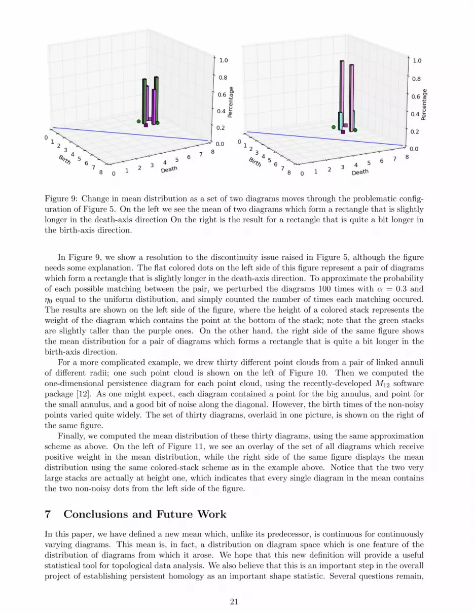
Figure 9: Change in mean distribution as a set of two diagrams moves through the problematic config-uration of Figure 5. On the left we see the mean of two diagrams which form a rectangle that is slightlylonger in the death-axis direction On the right is the result for a rectangle that is quite a bit longer inthe birth-axis direction.

In Figure 9, we show a resolution to the discontinuity issue raised in Figure 5, although the figureneeds some explanation. The flat colored dots on the left side of this figure represent a pair of diagramswhich form a rectangle that is slightly longer in the death-axis direction. To approximate the probabilityof each possible matching between the pair, we perturbed the diagrams 100 times with α = 0.3 andη0 equal to the uniform distibution, and simply counted the number of times each matching occured.The results are shown on the left side of the figure, where the height of a colored stack represents theweight of the diagram which contains the point at the bottom of the stack; note that the green stacksare slightly taller than the purple ones. On the other hand, the right side of the same figure showsthe mean distribution for a pair of diagrams which forms a rectangle that is quite a bit longer in thebirth-axis direction.

For a more complicated example, we drew thirty different point clouds from a pair of linked annuliof different radii; one such point cloud is shown on the left of Figure 10. Then we computed theone-dimensional persistence diagram for each point cloud, using the recently-developed M12 softwarepackage [12]. As one might expect, each diagram contained a point for the big annulus, and point forthe small annulus, and a good bit of noise along the diagonal. However, the birth times of the non-noisypoints varied quite widely. The set of thirty diagrams, overlaid in one picture, is shown on the right ofthe same figure.

Finally, we computed the mean distribution of these thirty diagrams, using the same approximationscheme as above. On the left of Figure 11, we see an overlay of the set of all diagrams which receivepositive weight in the mean distribution, while the right side of the same figure displays the meandistribution using the same colored-stack scheme as in the example above. Notice that the two verylarge stacks are actually at height one, which indicates that every single diagram in the mean containsthe two non-noisy dots from the left side of the figure.

7 Conclusions and Future Work

In this paper, we have defined a new mean which, unlike its predecessor, is continuous for continuouslyvarying diagrams. This mean is, in fact, a distribution on diagram space which is one feature of thedistribution of diagrams from which it arose. We hope that this new definition will provide a usefulstatistical tool for topological data analysis. We also believe that this is an important step in the overallproject of establishing persistent homology as an important shape statistic. Several questions remain,

21

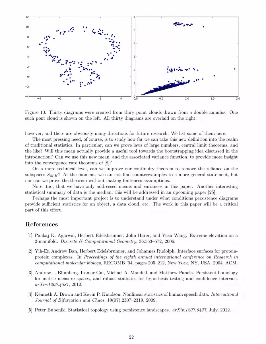
Figure 10: Thirty diagrams were created from thiry point clouds drawn from a double annulus. Onesuch pont cloud is shown on the left. All thirty diagrams are overlaid on the right.

however, and there are obviously many directions for future research. We list some of them here.The most pressing need, of course, is to study how far we can take this new definition into the realm

of traditional statistics. In particular, can we prove laws of large numbers, central limit theorems, andthe like? Will this mean actually provide a useful tool towards the bootstrapping idea discussed in theintroduction? Can we use this new mean, and the associated variance function, to provide more insightinto the convergence rate theorems of [8]?

On a more technical level, can we improve our continuity theorem to remove the reliance on thesubspaces SM,K? At the moment, we can not find counterexamples to a more general statement, butnor can we prove the theorem without making finiteness assumptions.

Note, too, that we have only addressed means and variances in this paper. Another interestingstatistical summary of data is the median; this will be addressed in an upcoming paper [25].

Perhaps the most important project is to understand under what conditions persistence diagramsprovide sufficient statistics for an object, a data cloud, etc. The work in this paper will be a criticalpart of this effort.

References

[1] Pankaj K. Agarwal, Herbert Edelsbrunner, John Harer, and Yusu Wang. Extreme elevation on a2-manifold. Discrete & Computational Geometry, 36:553–572, 2006.

[2] Yih-En Andrew Ban, Herbert Edelsbrunner, and Johannes Rudolph. Interface surfaces for protein-protein complexes. In Proceedings of the eighth annual international conference on Resaerch incomputational molecular biology, RECOMB ’04, pages 205–212, New York, NY, USA, 2004. ACM.

[3] Andrew J. Blumberg, Itamar Gal, Michael A. Mandell, and Matthew Pancia. Persistent homologyfor metric measure spaces, and robust statistics for hypothesis testing and confidence intervals.arXiv:1206.4581, 2012.

[4] Kenneth A. Brown and Kevin P. Knudson. Nonlinear statistics of human speech data. InternationalJournal of Bifurcation and Chaos, 19(07):2307–2319, 2009.

[5] Peter Bubenik. Statistical topology using persistence landscapes. arXiv:1207.6437, July, 2012.

22

Figure 11: The mean distribution for a set of thirty diagrams sampled from a double annulus. The leftside shows all positive-weight diagrams in the mean overlaid in one figure, while the right side indicatesthe weights in a three-dimensional plot.

[6] Gunnar Carlsson, Tigran Ishkhanov, Vin de Silva, and Afra Zomorodian. On the local behavior ofspaces of natural images. International Journal of Computer Vision, 76:1–12, 2008. 10.1007/s11263-007-0056-x.

[7] Frederic Chazal, David Cohen-Steiner, Marc Glisse, Leonidas J. Guibas, and Steve Y. Oudot.Proximity of persistence modules and their diagrams. In Proceedings of the 25th annual symposiumon Computational geometry, SCG ’09, pages 237–246, New York, NY, USA, 2009. ACM.

[8] Frederic Chazal, Marc Glisse, Catharine Labruere, and Bertrand Michel. Optimal rates of conver-gence for persistence diagrams in topological data analysis. arXiv:1305.6239, 2013.

[9] David Cohen-Steiner, Herbert Edelsbrunner, and John Harer. Stability of persistence diagrams.Discrete Comput. Geom., 37(1):103–120, January 2007.

[10] David Cohen-Steiner, Herbert Edelsbrunner, and Dmitriy Morozov. Vines and vineyards by up-dating persistence in linear time. Proceedings of the twenty-second annual symposium on Compu-tational geometry - SCG ’06, page 119, 2006.

[11] Y Dabaghian, F Memoli, L Frank, and G Carlsson. A topological paradigm for hippocampal spatialmap formation using persistent homology. PLoS Comput Biol, 8(8):e1002581, 08 2012.

[12] Anastasia Deckard, Jose’ A. Perea, John Harer, and Steve Haase. Sw1pers: Sliding windows and1-persistence scoring; discovering periodicity in gene expression time series data. To appear, 2013.

[13] Mary-Lee Dequeant, Sebastian Ahnert, Herbert Edelsbrunner, Thomas M. A. Fink, Earl F. Glynn,Gaye Hattem, Andrzej Kudlicki, Yuriy Mileyko, Jason Morton, Arcady R. Mushegian, Lior Pachter,Maga Rowicka, Anne Shiu, Bernd Sturmfels, and Olivier Pourquie. Comparison of pattern detectionmethods in microarray time series of the segmentation clock. PLoS ONE, 3(8):e2856, 2008.

[14] H. Edelsbrunner, D. Letscher, and A. Zomorodian. Topological persistence and simplification. InFoundations of Computer Science, 2000. Proceedings. 41st Annual Symposium on, pages 454 –463,2000.

[15] Herbert Edelsbrunner and John Harer. Persistent homology — a survey, chapter Surveys on Dis-crete and Computational Geometry: Twenty Years Later, pages 257–282. American MathematicalSociety, Providence, RI, 2008.

23

[16] Herbert Edelsbrunner, John Harer, Vijay Natarajan, and Valerio Pascucci. Morse-smale complexesfor piecewise linear 3-manifolds. In Proceedings of the nineteenth annual symposium on Computa-tional geometry, SCG ’03, pages 361–370, New York, NY, USA, 2003. ACM.

[17] T. Galkovskyi, Y. Mileyko, A. Bucksch, B. Moore, O. Symonova, C. A. Price, C. N. Topp, A. S.Iyer-Pascuzzi, P. R. Zurek, S. Fang, J. Harer, P. N. Benfey, and J. S. Weitz. Gia roots: Softwarefor high throughput analysis of plant root system architecture. BMC Plant Biology, 12(116), 2012.

[18] Jennifer Gamble and Giseon Heo. Exploring uses of persistent homology for statistical analysis oflandmark-based shape data. Journal of Multivariate Analysis, 101(9):2184 – 2199, 2010.

[19] Jeffrey J. Headd, Y. E. Andrew Ban, Paul Brown, Herbert Edelsbrunner, Madhuwanti Vaidya, andJohannes Rudolph. Protein-protein interfaces: properties, preferences, and projections. Journal ofProteome Research, 6(7):2576–2586, 2007. PMID: 17542628.

[20] Yuriy Mileyko, Sayan Mukherjee, and John Harer. Probability measures on the space of persistencediagrams. Inverse Problems, 27(12):124007, 2011.

[21] Dmitriy Morozov. Homological Illusions of Persistence and Stability. PhD thesis, Duke University,2008.

[22] James Munkres. Algorithms for the assignment and transportation problems. Journal of the Societyfor Industrial and Applied Mathematics, 5(1):32–38, 1957.

[23] James R. Munkres. Elements of Algebraic Topology. Addison Wesley, 1993.

[24] Jose A. Perea and John Harer. Sliding windows and persistence: An application of topologicalmethods to signal analysis. To appear, 2013.

[25] Katharine Turner. Medians and means for sets of persistence diagrams. In preparation, 2013.

[26] Katharine Turner, Yuriy Mileyko, Sayan Mukherjee, and John Harer. Frechet means for distribu-tions of persistence diagrams. ArXiV, page arXiv:1206.2790, 2011.

[27] Cedric Villani. Optimal Transport: Old and New. Springer, 2009.

A Appendix

Lemma 14. Let fx and fy be the Radon-Nikodym derivatives of ηx|B(x,‖x−∆‖) and ηy|B(y,‖y−∆‖) respec-tively. Then ∫

|fx − fy| dλ ≤ 4πα‖x− y‖f(0)

where f is the Radon-Nikodym derivative of η.

Proof. Without loss of generality we may assume that ‖x−∆‖ ≥ ‖y −∆‖.The Radon-Nikodym derivative f is the limit of functions of the form

∑i ai1B(0,ri) where 1S is the

indicator function over the set S and the ai are positive. By taking limits it is sufficient to prove theresult for functions f of the form

∑i ai1B(0,ri). If f =

∑i ai1B(0,ri) then

fy =∑

i:ri≤‖y−∆‖

ai1B(y,ri) +∑

i:ri>‖y−∆‖

ai1B(y,‖y−∆‖)

24

and

fx =∑

i:ri≤‖x−∆‖

ai1B(x,ri) +∑

i:ri>‖x−∆‖

ai1B(x,‖x−∆‖)

=∑

i:ri≤‖y−∆‖

ai1B(x,ri) +∑

i:‖y−∆‖<ri≤‖x−∆‖

ai(1B(x,‖y−∆‖) + 1A(x,[‖y−∆‖,ri]))

+∑

i:ri>‖x−∆‖

ai(1B(x,‖y−∆‖) + 1A(x,[‖y−∆‖,‖x−∆‖])).

where A(x, [a, b]) denotes the annulus centered at x with inner radius a and outer radius b. From theselast two equations, we compute:∫|fx − fy| dλ ≤

∑i:ri≤‖y−∆‖

ai

∫|1B(x,ri) − 1B(y,ri)| dλ+

∑i:ri>‖y−∆‖

ai

∫|1B(x,‖y−∆‖) − 1B(y,‖y−∆‖)| dλ

+∑

i:‖y−∆‖<ri≤‖x−∆‖

ai

∫|1A(x,[‖y−∆‖,ri]))| dλ+

∑i:ri>‖x−∆‖

ai

∫|1A(x,[‖y−∆‖,‖x−∆‖])| dλ.

For each i, if ‖x− y‖ < ri, then a ball of diameter 2ri − ‖x− y‖ fits in the intersection of B(x, ri) andB(y, ri). Thus, recalling that the absolute value of the difference between the indicator functions of twosets is just the indicator function of their symmetric difference, we compute:∫

|1B(x,ri) − 1B(y,ri)| dλ ≤ 2πr2i − 2π(ri − ‖x− y‖/2)2 ≤ 2πri‖x− y‖ ≤ 2πα‖x− y‖. (23)

The bound in (23) also holds if ‖x− y‖ ≥ ri as then the integral is 2πr2i .

For each r with α ≥ ‖x−∆‖ ≥ r ≥ ‖y −∆‖∫|1A(x,[‖y−∆‖,r])| dλ = πr2 − π‖y −∆‖2

≤ π‖x−∆‖2 − π‖y −∆‖2

≤ π‖x−∆‖2 − π(‖x−∆‖ − ‖x− y‖)2

≤ 2π‖x−∆‖‖x− y‖≤ 2απ‖x− y‖

Similarly if ‖x−∆‖ > α ≥ r ≥ ‖y −∆‖ then∫|1A(x,[‖y−∆‖,r])| dλ ≤ 2απ‖x− y‖ also.

Together these imply that ∫|fx − fy| dλ ≤ 4απ‖x− y‖

∑i

ai

Observing that∑

i ai is the value of f at 0 completes the proof.

25