Embed Size (px)
Citation preview


iii
Preparation of this document
This study is an update of an earlier project led by the Aquatic Resource Management for Local Community Development Programme (ALCOM) entitled the “Southern African Development Community Water Resource Database” (SADC-WRD).
Compared with the earlier study, made for SADC, this one is considerably more refined and sophisticated. Perhaps the most significant advances are the vast amount of spatial data and the provision of simplified and advanced custom-made data management and analytical tool-sets that have been integrated within a single geographic information system (GIS) interface.
The publication is presented into two parts to inform readers of various levels of familiarity with the benefits of spatial analyses for aquatic resources management.
Part 1 is divided into two main sections:• The first section is aimed at administrators and managers with only a
passing knowledge of spatial analyses but who would be interested to know the capabilities of the African Water Resource Database (AWRD) to assist with their decision-making. They may be department or division heads in government, non-governmental organizations (NGOs) and international organizations. Thus, a few examples of decision-making at this level based on spatial analyses from AWRD are described.
• The second section is addressed to professionals in technical fields who may actually or potentially employ the results of spatial analyses in their work. They may be in international organizations, government, universities or in the commercial sector. The case studies best serve to inform them of AWRD capabilities.
Part 2 is also divided into two main sections:• The first section is written for spatial analysts in government, international
organizations or the private sector.• The second is for university teachers and students who may wish to use
AWRD for educational purposes. This section includes a workbook with exercises, offering educational possibilities of AWRD.
iv
Foreword
The “Status and Development of the African Water Resources Database (AWRD)” was presented at the twelfth session of the Committee for Inland Fisheries of Africa (CIFA) held in Yaoundé, Cameroon, from 2 to 5 December 2002. The Committee acknowledged that such GIS-based products are “powerful tools for fishery and aquaculture management, planning and development.” The Committee also noted that there were still outstanding issues to be resolved before such tools could practically and effectively be used by Member countries. The present report represents the follow-up activities based on CIFA’s recommendations.
Inland aquatic resources in developing regions around the world are immensely significant for food security as well as economic growth and poverty alleviation. However, the rational and sustainable use of essential resources is critical. The multi-purpose nature of inland water use patterns creates distinct sets of challenges for implementation of responsible development and management measures, and hence to the promotion of water, food and environmental security.
Geospatial information is increasingly being used for better understanding development issues and improving decision-making. The Millennium Development Goals (MDG) and their 2015 targets for halving the proportion of people living with hunger and poverty, and improving living conditions in the sector of education, gender, health and sanitation have heightened this awareness.
This report is one of a series of GIS-based publications under production by FAO’s Aquaculture Management and Conservation Service (FIMA) to update an earlier project led by the Aquatic Resource Management for Local Community Development Programme (ALCOM) entitled the “Southern African Development Community Water Resource Database” (SADC-WRD). The body of work presented represents both an expansion to the data and an enhancement of the original SADC-WRD analytic interface. Extended to cover the entire African continent, the new WRD has been entitled the “African Water Resources Database” and it is aimed at facilitating responsible inland aquatic resource management. It thus provides a valuable instrument to promote food security.
The AWRD allows for the integration of different types of information, e.g. fishery statistics, into a cohesive program that, because of its visual nature, is easy to understand and interpret. Systems such as the AWRD are excellent means to attract and direct investments in aquaculture and fisheries development.
I am confident that further explorations and applications of the AWRD data will deepen our understanding of inland aquatic resource management and will demonstrate the usefulness of the AWRD tool, whilst being immediately applicable to assist in a wide variety of recent issues addressed at CIFA such as: improving the reporting on status and trends in inland fisheries and aquaculture; co-management of shared inland fisheries resources; transboundary movements of aquatic species; and increased participation of stakeholders in the decision-making process about watershed area uses.
Alfred Yeboa TeteboCIFA ChairmanDirector of Fisheries Ministry of Fisheries Ghana
v
Abstract
This report represents a follow-up activity based on the recommendations by the Committee for Inland Fisheries of Africa (CIFA). The report is an update of an earlier project led by the Aquatic Resource Management for Local Community Development Programme (ALCOM) entitled the “Southern African Development Community Water Resource Database” (SADC-WRD). The body of work presented in this publication represents both an expansion to the earlier data and an enhancement of the original SADC-WRD analytic interface. Extended to cover the entire African continent, the new set of data and tools has been entitled the “African Water Resource Database” (AWRD). The overall aim of the AWRD is to facilitate responsible inland aquatic resource management. It thus provides a valuable instrument to promote food security.
The AWRD data archive includes 28 thematic data layers drawn from over 25 data sources, resulting in 156 unique datasets. The core data layers include: various depictions of surface waterbodies; multiple watershed models; aquatic species; rivers; political boundaries; population density; soils; satellite imagery; and many other physiographic and climatological data types. The AWRD archival data have been specifically formatted to allow their direct utilization within any geographic information system (GIS) software package conforming to Open-GIS standards. To display and analyse the AWRD archive, the AWRD also contains a large assortment of new custom applications and tools programmed to run under version 3 of the ArcView GIS software environment (ArcView 3.x). There are six analytical modules within the AWRD interface: 1) the Data and Metadata Module; 2) the Surface Waterbodies Module; 3) the Watershed Module; 4); the Aquatic Species Module; 5) the Statistical Analysis Module; and lastly, 6) the Additional Tools and Customization Module. Many of these tools come with simple and advanced options and allow the user to perform analyses on their own data.
The case studies presented in this publication illustrate how the AWRD archive and tools can be used to address key inland aquatic resource management issues such as the status of fishery resources and transboundary movements of aquatic species. This publication by no means cover all the issues that could be resolved using the AWRD, but they do provide a solid reference base for inland aquatic resource management in Africa. Based on a review and recommendations by CIFA, a number of opportunities to implement the AWRD tools and data in Africa have already been identified. Likewise, a number of future developments for the AWRD have been proposed, including AWRD-like frameworks for Latin America and Asia.
This publication is organized in two parts to inform readers who may be at varying levels of familiarity with GIS and with the benefits of the AWRD. The first part describes the AWRD and is divided into two main sections. The first presents a general overview and is addressed to administrators and managers while the second is written for professionals in technical fields. The second part is a “how to” supplement and includes a technical manual for spatial analysts and a workbook for university students and teachers.
vi
The primary AWRD interface, tool-sets and data integral to the function of the AWRD are distributed in two DVD’s accompanying part 2 of this publication and are also available for download on the Internet in FAO’s GeoNetwork and GISFish GIS portals. A more limited distribution of the above primary database/interface, but divided among ten separate CD-ROM disks, is available upon request to FAO’s Aquaculture Management and Conservation Service. Also, high resolution elevation datasets and images amounting to 38 gigabytes are available upon request for those who need them.
Jenness, J.; Dooley, J.; Aguilar-Manjarrez, J.; Riva, C. African Water Resource Database. GIS-based tools for inland aquatic resource
management. 2. Technical manual and workbook. CIFA Technical Paper. No. 33, Part 2. Rome, FAO. 2007. 308 p.
vii
Acknowledgements
This report was funded by regular programme funding of the Aquaculture Management and Conservation Service (FIMA) of the FAO. Special thanks goes to Dr J.M. Kapetsky for his valuable advice, contributions to the organization of this publication, review of part 1, suggestions of applications examples for the GIS interface and writing the case study on “Inventory of fisheries habitats and fisheries productivities”.
Appreciation goes to John Moehl for his general advice; Luigi Maiorano, for his contributions to the technical edits of part 2 of the present publication; and John Jorgensen for his review of part 1 and for suggesting references to the introduction of this publication.
Patrizia Monteduro prepared the AWRD archive datasets for their publication on the Internet in FAO’s GeoNetwork GIS portal, and Roberto Giaccio wrote the script to convert the metadata documentation from the AWRD archive into an XML format for display in GeoNetwork.
Emily Garding made a final quality check on the AWRD tools and tested the exercises presented in the workbook of part 2 of this publication.
The authors benefited from the data provided by Jippe Hoogeveen on the “Atlas of Water Resources and Irrigation in Africa” and by John Latham on “Africover” databases.
The following persons are recognized for their support, in alphabetical order: Devin Bartley, Gertjan de Graaf, Ashley Halls, Matthias Halwart, Eric Reynolds, Doris Soto, and Ashley Steel.
Some of the locational referencing tools for the AWRD were adapted from original tools developed for the McLennan Co. 9-1-1 Emergency Assistance District in Waco, Texas, the United States of America, and are presented here with their permission. Several general purpose tools, including the Select by Theme tool, the Query Builder tool, the Summarize tool and the statistics Histogram window, are adapted from original tools developed for the Saguaro project (University of Arizona; Tucson, Arizona, the United States of America, and are also presented here with their permission. We gratefully acknowledge the generosity of both organizations for sharing these resources with us.
We thank all the organizations which created the datasets and made them available for our use.
Chrissi Smith, Françoise Schatto-Terrible and Tina Farmer proofed the document and supervised its publication. The document layout specialist was Nadia Pellicciotta.
viii
Contents
Preparation of this documentForewordAbstractAcknowledgementsAcronyms and abbreviations
1. TECHNICAL MANUAL
1.1 Introduction GIS training Installation of software Installation of AWRD extension Installation of AWRD data archive Loading AWRD Tools into ArcView AWRD archive
Overview of AWRD interface, menus, and additional view tables and functionsAWRD interfaceAWRD Modules menuAWRD Tools menuAdditional AWRD tools
1.2 Data and Metadata Module Metadata tools Metadata viewer tool Metadata editor tool Loading AWRD datasets
1.3 Surface Waterbodies Module Manage surface waterbody themes Surface waterbody viewer Export Data Report GeoStats for surface waterbodies polygon themes Predict potential fish yield
1.4 Watersheds Module Watersheds maintenance tools Registering new custom watershed models or other polygonal themes Watershed selection and analysis tools Watershed selection tool Watershed visualization tools Select by Relationships with Another Theme tool Watershed statistic viewer
iiiivv
viixvii
1
1123367
1111121314
1516161729
323436383839
4547556869748487
ix
1.5 Aquatic Species Module Aquatic Species Viewer View image of species Add to map, clear and link to FishBase Identifying all species in a particular area of interest Multipoint functions Incorporating aquatic species data from non-AWRD sources
1.6 Statistical Analysis Module Summary statistics on a Theme Probability Distribution Calculator Summarize Theme Tool Classification and ranking tool Classification and weighting strategies Simple linear regression tool Regression options Output options Example of performing analysis on different subsets of data
1.7 Additional tools and Customization Module Locational referencing tools Find locations by Theme Enter Coordinates and Zoom to Location tool Coordinates Converter tool Report coordinates based on screen inputs Zoom to Gazeteer Locations tool Select by Theme tool Query Builder tool Add base map to a view Tools for calculating and reporting Geostatistics River identification tool Image Export and Base Mapping tool Loading and unloading the Image Export and Base Mapping
Extension Tools common between Views and Layouts Tools only available while working with layouts Tools only available while working with views Load Theme Database Adjusting polygon borders and patterns
1.8 Add-on extensions and additional AWRD Table and View functions Adding additional extensions to your project Add-on AWRD additional extensions Add-on ESRI additional extensions Additional extensions from the Internet Additional AWRD table tools Table editing tools (“Edit”menu) Table information tools (“Table”and “Field” menus) Additional AWRD View tools
919194959799
100
104105109112115120125125125130
134135135138139140142147149153154157158
159160169171173175
178178179179180181182184189
x
1.9 SIFRA Compendium Review of SIFRA data by clicking on a country Review of SIFRA data Compendium data selecting from list
2. WORKBOOK Exercise 1. Inventory of fisheries habitats and productivities Exercise 2. Surface waterbodies inventory Exercise 3. Predicting potential fish yield Exercise 4. Preliminary hydrological reporting Exercise 5. Invasive and introduced aquatic species Exercise 6. Production of simple map graphical outputs and base mapping
3. GLOSSARYReferences
APPENDIXA1. Index of Buttons for AWRD interface, AWRD modules, AWRD tools and AWRD table and view functions.A2. Schematic diagram of AWRD interface and modulesA3. Schematic diagram of AWRD menus and additional buttons
190191192
195196203212219231245
271283
285307308
xi
Tables
1.1 List of AWRD data layers 1.2 AWRD interface description 1.3 Additional AWRD tools 1.4 Data and Metadata Module buttons and menu items 1.5 Metadata editor tool buttons 1.6 General (1) reference dialog 1.7 General (2) reference dialog 1.8 Projection reference dialog 1.9 Data Maintenance reference dialog 1.10 Data Quality reference dialog 1.11 Metadata reference dialog 1.12 Contact reference dialog 1.13 Distribution reference dialog 1.14 Spatial reference dialog 1.15 Data Registration reference dialog 1.16 Surface Waterbodies Module buttons and menu items 1.17 Data on selected waterbodies module 1.18 Original data for 14 sample waterbodies 1.19 Watersheds Module buttons and menu items 1.20 Watersheds maintenance tools buttons 1.21 Watershed selection and analysis tools buttons 1.22 Watershed zooming tools buttons 1.23 Watershed flashing tools buttons 1.24 Other watershed visualization tools buttons 1.25 Select by relationship with another theme tool buttons 1.26 Aquatic Species Module buttons and menu items 1.27 Aquatic Species Viewer buttons and menu items 1.28 Statistical Analysis Module buttons and menu items 1.29 Water Requirement Submodel 1.30 Additional Tools and Customization Module buttons and menu items 1.31 Image Export and Base Mapping tool 1.32 Estimating the output pixel sizes based on pre-set DPIs 1.33 Add on Extensions buttons and menu items 1.34 SIFRA Compendium buttons and menu items 2.1 Summary of AWRD buttons and menu items 2.2 Summary and purpose of data used for comparison of surface waterbody counts
and areas 2.3 Counts and surface areas of surface waterbodies from three sources with
non-fisheries habitats removed 2.4 Summary and purpose of data used for comparison of surface waterbodies counts
and areas 2.5 Surface areas of WCMC inland fisheries habitats of Africa 2.6 Summary and purpose of data used for comparison of surface waterbodies counts
and areas 2.7 Counts of fishery habitats for the African continent from the GNS dataset 2.8 Summary of AWRD buttons and menu items 2.9 Summary and purpose of data used for Tanzanian analysis 2.10 Summary and purpose of data used for Zimbabwean analysis 2.11 Sample excel table for the Republic of Zimbabwe watersheds 2.12 Summary of AWRD buttons and menu items
71214151818192021222324262829333443454768777879859192
104119134159167178190196
196
197
199199
200200203204207209212
xii
2.13 Summary and purpose of data used for researching existing estimates of potential yield
2.14 Lake Tanganyika potential annual fish yield 2.15 Summary and purpose of data used for estimating potential yield from historical
data 2.16 Summary statistics for historic catch: Nokoue Lagoon 2.17 Summary and purpose of data used for estimating potential yield from statistical
models 2.18 Potential yield for Lake Sagara, the United Republic of Tanzania, and Lake
Kabamba, the Democratic Republic of the Congo 2.19 Summary of AWRD buttons and menu items 2.20 Summary and purpose of data used to generate statistics on the Volta River
megabasin 2.21 Statistics on Lake Volta megabasin 2.22 Summary and purpose of data used to generate statistics for the Republic of
Ghana and Burkina Faso 2.23 Statistics on the Republic of Ghana and Burkina Faso 2.24 Summary and purpose of data used to generate statistics on the Volta River
megabasin 2.25 Regression analysis on Lake Volta megabasin 2.26 Summary and purpose of data used to generate statistics on the Volta River
megabasin 2.27 Lake Volta area values from multiple sources 2.28 Summary of AWRD buttons and menu items 2.29 Summary and purpose of data used 2.30 Summary and purpose of data used 2.31 Summary and purpose of data used 2.32 Summary of AWRD menu and button items 2.33 Summary and purpose of data used 2.34 Summary and purpose of data used 2.35 Summary and purpose of data used 2.36 Summary and purpose of data used 2.37 Summary and purpose of data used 2.38 Summary and purpose of data used A1 AWRD interface description A2 Additional AWRD tools A3 Data and Metadata Module buttons and menu items A4 Surface Waterbodies Module buttons and menu items A5 Surface waterbodies viewer buttons and menu items A6 Watersheds Module buttons and menu items A7 Watersheds maintenance tools buttons A8 Watershed selection and analysis tools buttons A9 Watershed zooming tools buttons A10 Watershed flashing tools buttons A11 Other watershed visualization tools buttons A12 Select by relationship with another theme tool buttons A13 Aquatic Species Module buttons and menu items A14 Aquatic Species Viewer buttons and menu items A15 Statistical Analysis Module buttons and menu items A16 Additional Tools and Customization Module buttons A17 Add on Extensions buttons and menu items A18 SIFRA Compendium buttons and menu items
213213
214214
216
216219
220221
223224
226226
228229231232235237245246250255260264268286288289290291292293294295296297299299300302303304305
xiii
Figures
1.1 The AWRD data structure 1.2 The AWRD Interface 1.3 The AWRD Modules menu 1.4 The AWRD Tools menu 1.5 Data and Metadata Module 1.6 Link to AWRD Metadata Web page for the active theme 1.7 Recording metadata for the active theme 1.8 Metadata General (1) reference dialog 1.9 General (2) reference dialog 1.10 Projection reference dialog 1.11 Data Maintenance reference dialog 1.12 Data Quality reference dialog 1.13 Metadata reference dialog 1.14 Contact reference dialog 1.15 Adding new contacts 1.16 Distribution reference dialog 1.17 Restrictions reference dialog 1.18 Spatial reference dialog 1.19 Data Registration reference dialog 1.20a Metadata for hydrological basins of Africa 1.20b Loading data from the AWRD data archive 1.21 Surface Waterbodies Module 1.22 The surface waterbodies viewer dialog 1.23 Opening the “Manage Surface Waterbody Themes” 1.24 Surface waterbody attribute report associated with the selected waterbody (e.g.
Lake Tanganyika) 1.25 Saving the new Export Table in an ArcView Project 1.26 Potential fish yield prediction for Lake Tanganyika using the general Potential Fish
Yield Calculator 1.27 Potential fish yield prediction for Lake Tanganyika using the “Potential Fish Yield for
Selected SWB” in the Surface Waterbodies Module dialog (Model 2) 1.28 Starting the Watersheds Module 1.29 The watershed maintenance tools 1.30 Saving the information regarding the selected watershed as a text file on the hard
drive and viewing the report produced by the Report button on the screen 1.31 Saving the new dataset to a new dBASE table and viewing the dBASE table in the
ArcView Project 1.32 Selection of the data layers 1.33 Viewing watershed statistics source data (e.g. mean annual air temperature)
without Spatial Analyst (on the left) and with Spatial Analyst (on the right) 1.34 Changing data for calculating statistics on the selected watersheds 1.35 Changing the watershed model to analyse 1.36 Registering new custom watershed model (simple version) 1.37 Calculation of area in the originally defined measurement units 1.38 Generating new data from grid themes 1.39 Selecting and adding the grids of interest to the view from the AWRD Modules
menu option or by clicking the View Data button on the Watersheds Module 1.40 Combining the four grids into a single grid 1.41 Viewing the new grid “Summer Precipitation”
41113131516171819202122232425262727283031323335
3738
41
424546
48
4950
515254555758
596060
xiv
1.42 Adding the new grid (Summer Precipitation) into the AWRD 1.43 Specifying the projection of the new grid 1.44 Registering the new grid 1.45 Visualization of the new registered grid 1.46 Calculation of summary data for the new grid 1.47 Selecting the watershed model to remove 1.48 Selecting the grid theme to remove 1.49 Deleting specific data tables 1.50 Watershed selection and analysis tools 1.51 Upstream drainage basin s for Lake Tanganyika 1.52 Upstream drainage basin s for Lake Tanganyika and drainage basins for Lake
Victoria 1.53 Upstream and downstream drainage basins for Lake Tanganyika 1.54 Entire Congo-Zaire megabasin 1.55a Selection of the portion lying upstream of the confluence of the Kasai and Sankuru
rivers, in the Congo-Zaire megabasin 1.55b Entire Congo-Zaire megabasin except the portion lying upstream of the confluence
of the Kasai and Sankuru rivers 1.56 Identifying all upstream , downstream and megabasin watersheds by clicking on
any watershed in the theme 1.57 The megabasin functions 1.58 Watershed zooming tools 1.59 Using the watershed zooming tools in the Niger megabasin 1.60 The watershed flashing tools 1.61 Other watershed visualization tools 1.62 Visualization of the watersheds directly upstream with the “Move Upstream” tool 1.63 The custom legend tool 1.64 Applying a semi-transparent green colour to the unassociated watershed 1.65 Saving graphics and themes of a flow regime 1.66 Various spatial relationships available with the Select by Relationship with Another
Theme Tool 1.67a Selection of the Republic of Botswana and selection of the correct parameters to
identify its entire drainage basin 1.67b Entire drainage area for the Republic of Botswana 1.67c Areas which drain out of the Republic of Botswana 1.68 Attribute data of watersheds 1.69 Statistics on the combined set of selected watersheds 1.70 The Aquatic Species Module 1.71 Aquatic Species Viewer 1.72 The four base themes available for the Aquatic Species Module 1.73 Full-size image of southern mouthbrooder (Pseudocrenilabrus philander) available
in the Aquatic Species Module 1.74 The Add to Map button displaying the geographic distribution of common carp 1.75 Automatic link to FishBase Web site 1.76 Identifying the extent of a specific sub-national or national area on the view 1.77 Identifying all the species located in the selected Area of Interest (megabasin) 1.78 Identifying all the species located in the selected area of interest (sub-national
boundaries) 1.79 Converting Multipoints to Points (Clarias gariepinus) locations 1.80 Importing an Excel table into ArcView through the Aquatic Species Module 1.81 Importing data from FishBase into AWRD 1.82 The Statistical Analysis Module 1.83a The statistics report (Simple output) for the FAO watershed model 1.83b The statistics report (Advanced output) for the FAO watershed model 1.84 Summary Statistics Calculator on a Field in a Table
61626364646566676870
717272
73
74
75767677787980818283
84
8686878889919293
9495969798
99100101103104106107108
xv
1.85 Probability Distribution Calculator 1.86 Table Probability Distribution Calculator 1.87a Using the Summarize Theme tool to divide the data into subsets based on the
District values 1.87b Calculating the surface waterbodies average by Districts 1.87c Saving the combined features into a new theme 1.88a Application of the classification and ranking tool (Simple version) 1.88b Setting different output options with the simple classification and ranking tool 1.89 Application of the classification and ranking tool (Advanced option) 1.90 Application of the advanced classification and ranking tool to determine potential
fish farming areas for common carp 1.91 Saving list of ranking criteria (“Save” button) 1.92 Loading saved selection criteria sets (“Load” button) 1.93 Multiple Output Options for saving selection criteria sets 1.94 Generating a Summary Report about the classification criteria 1.95 Creating the new table illustrating how each score was established 1.96 The Summary Statistic Calculator 1.97a Regression report of rainfall and elevation for all watersheds in Africa 1.97b The scatterplot 1.97c The new “regression ” theme attribute table 1.98 Regression analysis of rainfall and elevation for the Nile River megabasin 1.99 Regression analysis of rainfall and elevation for the Niger megabasin 1.100 The Manage Data Sources 1.101 The Additional Tools and Customization Module 1.102 Selecting the Theme, the field and the term to search and viewing the results of
the Find Location by Theme tool 1.103 Looking at the attributes to screen duplicate or closely matching named results 1.104 Entering coordinates in the preferred format and finding location based on a
coordinate reference 1.105 Coordinates Conversion tool 1.106 Getting X/Y Coordinates by clicking on the screen (the Republic of Madagascar) 1.107 Constraining a search with the Zoom to Gazetteer Locations tool 1.108 Reviewing all the attribute data associated with the selected feature 1.109 Searching by gazetteer locations 1.110 Find location based on both a zoom-to-location and a gazetteer search 1.111 Using the Select by Theme tool to select all the rivers intersecting a particular
watershed 1.112 Setting new Theme Definitions to the Terrestrial Watershed and Large Marine
Ecosystem dataset 1.113 Selecting features from a theme trough the query builder tool 1.114 Background images available in the AWRD 1.115 Reporting GeoStatistics for the selected features 1.116 Identifying the projection before reporting Geostatistics 1.117 Specifying geostatistics calculation parameters and viewing the results in the theme
attribute table 1.118 Renaming the selected river segments 1.119 The IEBM tools for views (top) and for layouts (bottom) 1.120 Choosing the image type 1.121 Checking for other image format translation 1.122 Selecting the name and directory location for the image 1.123 Output reports from the export of Views 1.124 Prompts and output reports from the Image Export tool in Layout mode 1.125 Sample Report for a successful output with accompanying WorldFile 1.126 The Report View/Layout Details tools 1.127 The Resize Window Dimensions tool
110111
113114115117118120
121122122123124124126127129130131132133134
136137
139140141143144145147
149
151152153155155
156158160161161162163164165166168
xvi
1.128 The Make a copy of a View/Layout tools 1.129 The Create LO/ViewFrame-Page tool 1.130 The Resize LO/ViewFrame-Pixels tool 1.131 The Toggle View TOC On/Off tool 1.132a The Create Fitted Map and Polygonal Mask Theme tool 1.132b Basic layout resulting from the Create Fitted Map tool 1.133a Importing a precompiled theme database by database component or for base
mapping 1.133b Object Database Import failure due to missing dependency 1.134a Comparison of a polygon theme with and without polygon borders 1.134b Comparison of a polygon theme with and without polygon transparency 1.134c Adjust polygon border and pattern tool 1.135 The Add-on Extensions 1.136 Selecting additional AWRD Extensions 1.137 Opening the list of ESRI Extensions 1.138 Link to ESRI Arcscripts Web site 1.139a Table information and editing tools (under “Edit”, “Table” and “Field” menus) 1.139b The attribute table to edit 1.139c Adding record numbers 1.140 Identifying table source 1.141 Identifying field types 1.142 Showing field information 1.143a Opening the table in Excel and selecting the data to import 1.143b Importing the data into an ArcView table 1.144 Exporting data into an Excel spreadsheet 1.145 The SIFRA Compendium 1.146 Opening the SIFRA Compendium introduction 1.147 Reviewing the SIFRA Compendium data by clicking on a country 1.148 Reviewing the SIFRA Compendium data by selecting from list through the AWRD
Interface or through the AWRD Tools menuA1 The AWRD InterfaceA2 The AWRD Modules menuA3 The AWRD Tools menuA4 Data and Metadata ModuleA5 Surface Waterbodies ModuleA6 The surface waterbodies viewer dialogA7 Starting the Watersheds ModuleA8 The watershed maintenance toolsA9 Watershed selection and analysis toolsA10 Watershed zooming toolsA11 The watershed flashing toolsA12 Other watershed visualization toolsA13 Various spatial relationships available with the select by Relationship with Another
Theme ToolA14 The Aquatic Species ModuleA15 Aquatic Species ViewerA16 The Statistical Analysis ModuleA17 The Additional Tools and Customization ModuleA18 The Add-on ExtensionsA19 The SIFRA Compendium
169170170171172173
174175176176177178179180181182183184185186186187187188190191192
193285287287288289290292293294295296297
298299300301302304305

xvii
Acronyms and abbreviations
ADM Administrative data layerAFDS African Data SamplerAGLW Agriculture, Land and Water Division AIMG Ancillary Image and Map GraphicALCOM Aquatic Resource Management for Local Community
Development ProgrammeANNO AnnotationANOVA Analysis of VarianceAOI Area Of InterestAQSP Aquatic SpeciesARAS Ancillary RasterASCII American Standard Code for Information InterchangeAVEC Ancillary VectorAWRD African Water Resources DatabaseAWRIA FAO-AGLW’s African Water Resources and Irrigation in
AfricaBADC Belgian Administration for Development CooperationBIL Band Interleaved by Line raster data formatBIP Band Interleaved by Pixels image file formatBMP Bitmap BNA Early ASCII mapping format for Atlas-Graphics thematic
mapping package BSQ Band Sequential image fileCCRF FAO Code of Conduct for Responsible FisheriesCD Compact DiskCGM Computer Graphics Metafile CIA US Central Intelligence AgencyCIFA Committee for Inland Fisheries of AfricaCRES Centre for Resource and Environmental StudiesCRU Climate Research UnitDAF Digital Atlas of AfricadBASE DatabaseDBC Database ComponentDCW Digital Chart of the World DD Decimal Degrees DEM Digital Elevation ModelDMA The former U.S. Defense Mapping Agency, which is now entitled
the U.S. National Imagery and Mapping Agency (NIMA)DN/DNNET DCW Drainage Network layerDPI Dots-Per-InchDTED NIMA’s Digital Terrain Elevation Data at various raster
postingsEC European CommissionECW Earth Resource Mapping’s “Enhanced Compression Wavelet”
format for raster imageryEDC United States Geological Survey Earth Resources Observation
Systems (EROS) Data Center
xviii
EMF Enhanced Metafile FormatEPS Encapsulated Postscript (file extension)EROS Earth Resources Observation SystemsESAD NASA’s Earth Science Applications DirectorateESRI Environmental Systems Research Institute, Redlands,
CaliforniaETM+ Landsat Enhanced Thematic Mapper DataETOPO2 A 2 minute Elevation Topographic DEM including bathymetryETOPO5 An early global 5 minute DEMEU European UnionFAO Food and Agricultural Organization of the United NationsFIMA Aquaculture Management and Conservation ServiceGARP Genetic Algorithm for Rule-Set ProductionGeoCover-LC Land Cover based on Ortho-Rectified LandSat ImageryGeoNet Gazetteer Name ServerGeoNetwork FAO’s Spatial Data and Information PortalGIEWS FAO’s Global Information and Early Warning SystemGIF Graphic Interchange Format (file extension)GIS Geographic Information Systems and software platforms GIWA Global International Water AssessmentGLOBE NOAA distributed release of GTopo30GNS/GeoNet NIMA’s Geographic Names Server Gazetteer of Named
LocationsGSDI Global Spatial Data Infrastructure clearing-house for SDIGSM Golden Software Map, a proprietary GIS formatGT30/GTopo30 Global Topographic 30 arc second DEM database, nominal 1km
postingsGT30BATH Combined GTopo30 and Scripps/Smith and Sandwell
BathymetryGUI Graphical User InterfaceGZTR Gazetteer/Named LocationH1k/HYDRO1k Global Hydrological 1 kilometre database HTML Hyper Text Markup Language HYD Hydrological feature subset of the LC/LCPOLY (DCW Land
Cover layer)ID Identifier, usually denoting a unique numerical or alphanumeric
codeIEBM Image Export and Base Mapping tool-set of the AWRDIHO Standards for Maritime Waterbodies based on the International
Hydrographic Bureau of the International Hydrographic Organization
ISCGM International Steering Committee for Global MappingISO International Organization for StandardizationIW VMap0 Inland Water layerJPG/JPEG Graphics file type/extension (lossy compressed 24 bit color
image storage format developed by the Joint Photographic Experts Group)
JPL NASA’s Jet Propulsion LaboratoryJRC Joint Research Centre of the European CommissionLAEA Lambert Azimuthal Equal Area projection systemLC/LCPOLY DCW Land Cover layerLCL Lower Confidence LimitLME Large Marine Ecosystems

xix
LO LayoutLOE Level of EffortLWDD FAO’s Land and Water Development DivisionMADE Multipurpose land cover databasesMGLD MSSL Global Lakes DatabaseMM The secondary maritime encoding parameter pertaining to the
proposed FAO hydrological encoding standard MODIS Moderate resolution imaging spectroradiometer sensor on Terra
satelliteMrSID LizardTech’s commercial compression format for spatial
imageryMSSL Mullard Space Science LaboratoryNASA U.S. National Aeronautical and Space AdministrationNGA National Geospatial-Intelligence Agency (new name for
NIMA)NGDC NOAA’s National Geo-Physical Data CenterNGO Non-Governmental Organization
NIMA U.S. National Imagery and Mapping Agency, formerly the U.S. Defense Mapping Agency (DMA)
NOAA U.S. National Oceanographic and Atmospheric AdministrationODB Object DatabaseONC Operational Navigation ChartsORNL U.S. Oak Ridge National LaboratoryOrtho/ORTH Orthographically-rectified, i.e. flattened or adjusted for elevation
changesOrthoTM Ortho-rectified or flattened imagery OS Operating SystemOVRVW A virtual Overview mapPAIA FAO’s Priority Areas for Interdisciplinary ActionPDF Portable Document Format (Adobe Acrobat)PNG Portable Network Graphics (graphic file standard/extension)PS PostScript (file name extension)PTES or Pfaf Pfafstetter Topological Encoding Scheme, a 5 to potentially 22
long numeric digit or encoding string for encoding spatially based continental hydrographic data.
PY Potential YieldPYPUA Potential Yield per Unit of AreaRAID Redundant Array of Inexpensive Disks RDBMS Relational Database Management SystemsRGB 3 band spatial imagery forced into the Red:Green:Blue
spectrumRIV Rivers and Drainage/FlowRRSU The SADC Regional Remote Sensing Unit located in Harare
ZimbabweSADC The Southern African Development CommunitySAIAB South African Institute for Aquatic Biodiversity (formerly
known as JLB Institute of Ichthyology)SARPO The Southern African Regional Programme Office of WWF
located in Harare ZimbabweSDE see Manual (subsect. Excel Import and Export Tools)SDI Spatial Data InfrastructureSHD Shaded Relief
xx
SIFRA Source Book for the Inland Fisheries Resources of AfricaSRTM Shuttle Radar Topography MissionSSN-TF FAO’s Spatial Standards and Norm Task ForceSWB Surface WaterbodyTIF/TIFF Tagged Image File Format (graphics/image file format)TM Landsat Thematic Mapper.TOC Table Of ContentsTOR Terms of ReferenceU.S. The United StatesUCL Upper Confidence LimitUFI Unique/Universal Feature IdentifierUN United NationsUN-CS United Nations Cartographic SectionUNEP United Nations Environment ProgrammeUN-GD The UN-CS 1:10-1:5 million Global GIS Database UNGIWG United Nations Geographic Information Services Working
GroupUNL University of Nebraska at Lincoln, USAURI University of Rhode Islands, USAURL Universal Resource Locator for the identification of specific
locations or web-sites on the WWWUSAID The U.S. Agency for International DevelopmentUSFS The U.S. Forestry ServiceUSGS The United States Geological SurveyUTM Universal Transverse MercatorVMAP NIMA’s Vector Smart Map standard for various scales of vector
dataVMAP0 Vector Map for Level 0VPF NIMA’s Vector Product Format for the encoding of VMAP
data librariesVRTL A seamless 1:750 000 Virtual basemapWC Water Course layer of VMAP0WCMC World Conservation Monitoring CentreWDBII CIA’s 1:3 - 1:5m scale World Database IIWGS World Geodetic Standard, 1984 standard datum and spheroidWMF Windows Metafile (file name extension)WRD The original SADC Water Resource Database produced by
ALCOMWRI World Resources InstituteWS WatershedsWTLND WetlandsWVS World Vector ShorelineWWF World Wide Fund for Nature (known as World Wildlife Fund
in the U.S.)WWW World Wide Web
Sect
ion
1.1
1. Technical Manual
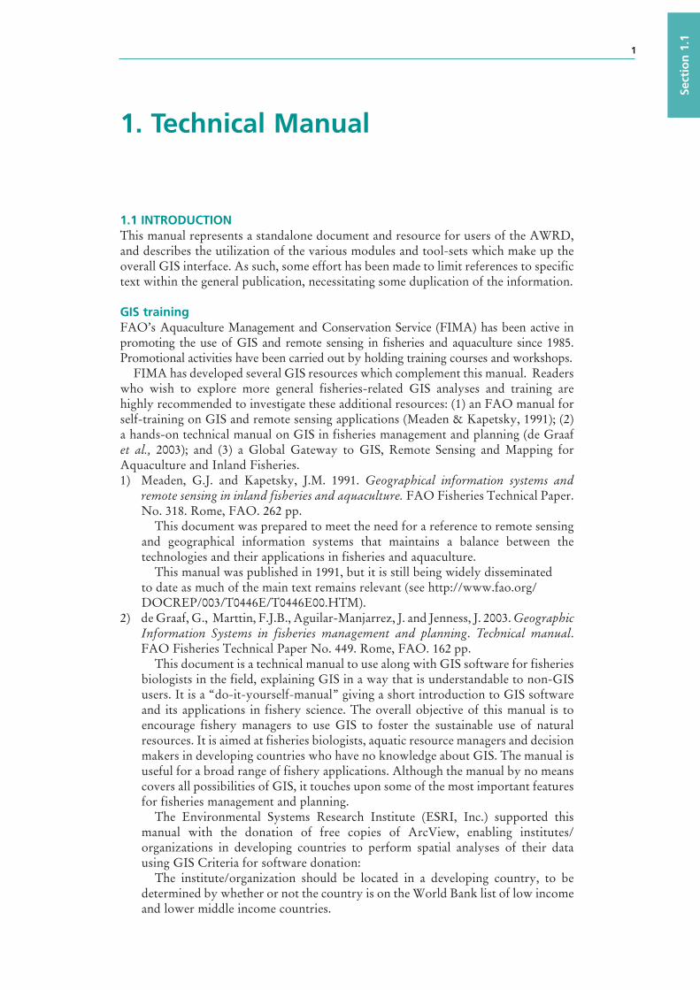
1.1 INTRODUCTIONThis manual represents a standalone document and resource for users of the AWRD, and describes the utilization of the various modules and tool-sets which make up the overall GIS interface. As such, some effort has been made to limit references to specific text within the general publication, necessitating some duplication of the information.
GIS trainingFAO’s Aquaculture Management and Conservation Service (FIMA) has been active in promoting the use of GIS and remote sensing in fisheries and aquaculture since 1985. Promotional activities have been carried out by holding training courses and workshops.
FIMA has developed several GIS resources which complement this manual. Readers who wish to explore more general fisheries-related GIS analyses and training are highly recommended to investigate these additional resources: (1) an FAO manual for self-training on GIS and remote sensing applications (Meaden & Kapetsky, 1991); (2) a hands-on technical manual on GIS in fisheries management and planning (de Graaf et al., 2003); and (3) a Global Gateway to GIS, Remote Sensing and Mapping for Aquaculture and Inland Fisheries.1) Meaden, G.J. and Kapetsky, J.M. 1991. Geographical information systems and
remote sensing in inland fisheries and aquaculture. FAO Fisheries Technical Paper. No. 318. Rome, FAO. 262 pp.
This document was prepared to meet the need for a reference to remote sensing and geographical information systems that maintains a balance between the technologies and their applications in fisheries and aquaculture.
This manual was published in 1991, but it is still being widely disseminated to date as much of the main text remains relevant (see http://www.fao.org/DOCREP/003/T0446E/T0446E00.HTM).
2) de Graaf, G., Marttin, F.J.B., Aguilar-Manjarrez , J. and Jenness , J. 2003. Geographic Information Systems in fisheries management and planning. Technical manual. FAO Fisheries Technical Paper No. 449. Rome, FAO. 162 pp.
This document is a technical manual to use along with GIS software for fisheries biologists in the field, explaining GIS in a way that is understandable to non-GIS users. It is a “do-it-yourself-manual” giving a short introduction to GIS software and its applications in fishery science. The overall objective of this manual is to encourage fishery managers to use GIS to foster the sustainable use of natural resources. It is aimed at fisheries biologists, aquatic resource managers and decision makers in developing countries who have no knowledge about GIS. The manual is useful for a broad range of fishery applications. Although the manual by no means covers all possibilities of GIS, it touches upon some of the most important features for fisheries management and planning.
The Environmental Systems Research Institute (ESRI, Inc.) supported this manual with the donation of free copies of ArcView, enabling institutes/organizations in developing countries to perform spatial analyses of their data using GIS Criteria for software donation:
The institute/organization should be located in a developing country, to be determined by whether or not the country is on the World Bank list of low income and lower middle income countries.
1
African Water Resource Database – Technical manual and workbook2
(http://www.worldbank.org/data/countryclass/classgroups.htm#Low_income); involved in research or education in inland fisheries biology/management/planning; a non-profit organization; recognized nationally or regionally by the government(s) involved; in need of support in respect with software; and endorsed by the FAO’s Regional Aquaculture/Fisheries Officer (Bangkok, Thailand; Accra, Ghana; Santiago de Chile, Chile).
3) The “GISFish” Global Gateway to GIS, Remote Sensing and Mapping for Aquaculture and Inland Fisheries.
There are many opportunities to use GIS and remote sensing to improve the sustainability of aquaculture and inland fisheries, and fundamental issues in aquaculture and inland fisheries can be resolved with the help of GIS and remote sensing. However, overall, our research has concluded that the aquaculture and inland fisheries GIS user base is low. Therefore, the objectives of this Gateway are to: (1) improve the sustainability of aquaculture and inland fisheries by promoting the use of GIS, remote sensing and mapping; (2) facilitate the use of GIS, remote sensing, and mapping through easy access to comprehensive information on applications and training opportunities; and (3) provide a “one stop” site from which to obtain the depth and breadth of the global experience on GIS, remote sensing and mapping in aquaculture and inland fisheries.
The Gateway is being designed for a very broad range of users. The beneficiaries will mainly consist of people working with global and regional analysis on aquaculture and inland fisheries management and planning, including researchers and project managers in national and international organizations and scientific institutes. Other beneficiaries are the commercial sector and planners and managers in fields apart from aquaculture and inland fisheries, specifically those involved with coastal area management and river and lake basin management.
The Gateway is available at http://www.fao.org/fi/gisfish.
Installation of softwareThis manual includes 2 DVD’s containing the AWRD spatial data archive. To use this manual you need to have ArcView3.x installed. ESRI’s Spatial Analyst extension is not required for the AWRD, but it would be very useful for those who want to work with raster data. The system requirements for ArcView 3.3 using Microsoft Windows are:
• Computer: Industry-standard personal computer with at least a Pentium or higher Intel-based microprocessor and a hard disk
• Memory: The minimum requirements recommended by ESRI are 24 MB RAM (32 MB recommended, and performance will increase as RAM increases). However, some functions within the AWRD are very memory-intensive and may require considerably more memory in order to run efficiently, and users are encouraged to install the maximum amount of RAM possible.
• Operating System: Windows 98/98SE, Windows Me, Windows NT 4.0, Windows 2000, and Windows XP--Home Edition and Professional. ArcView 3.x is not expected to run under Windows Vista.
(For additional details see: http://www.esri.com/software/arcview /arcview3x.html)
ArcView Spatial Analyst 2 requires ArcView 3.2 or higher and is supported on:• Microsoft Windows: Windows XP (Home Edition and Professional), Windows
2000, Windows NT 4.0 and Windows 95/98. (For additional details see: http://www.esri.com/software/arcview/extensions/spatialanalyst/index.html)
Technical manual 3
Sect
ion
1.1
Note The AWRD data archive and extensions are available on the DVDs that accompany the present publication. Additionally, this material and future updates and/or enhancements will also be made available in the Internet in a Web site dedicated to the AWRD.
To install ArcView and the Spatial Analyst extension: put the ArcView installation CD-ROM in your PC and follow the instructions on your screen. After the installation of ArcView is complete you might be asked if you want to install Seagate Crystal reporting. This will take a lot of space on your hard disk, and for the exercises in the manual you do not need it, so press NO unless you plan to use Crystal Reports for other purposes. After you have installed ArcView, you may install the optional Spatial Analyst extension if it is available: put the installation CD-ROM of the Spatial Analyst extension in your PC and follow the instructions on your screen.
Installation of AWRD extensionInstallation of this AWRD extension is similar to that of most ArcView 3.x extensions, in that it requires only that you place a single file into the ArcView extensions folder. To install the AWRD:
1. Open Windows Explorer and locate the file “awrd_tools.avx” in DVD1. It should be at the top level in DVD1, so you do not need to search through any of the folders.
2. Copy that file by selecting it and clicking the “Edit” menu, then “Copy”, or by simply clicking [Control]-C.
3. Using Windows Explorer, open the ArcView extensions folder on your hard drive. This folder is named “ext32” and is located inside the “ArcView” folder. In almost all cases, the full pathname for the Extensions folder is: “C:\esri\av_gis30\arcview \ext32”.
4. Paste the “awrd_tools.avx” file into the “ext32” folder by clicking the “Edit” menu, then “Paste”, or by simply clicking [Control]-V.
5. The AWRD extension requires the AWRD data archive in order to function properly, so install the data archive before trying to use the AWRD extension in ArcView.
Installation of AWRD data archiveThe AWRD data archive is quite large (approximately 5.5 GB in this general release). The AWRD will function best with all the data installed on the hard drive and available to the extension. However, the authors of the AWRD recognize that in some cases users will not have the hard drive capacity to install the entire archive. Therefore we present 3 installation options for users with differing levels of available space.
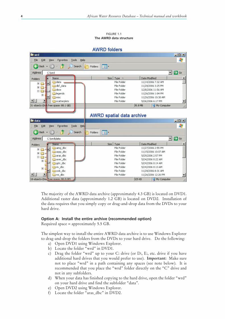
In all cases, the AWRD data archive must be organized correctly. The AWRD tools expect to find specific datasets in specific folders, so the tools may crash if the datasets are not in the correct location. As seen in Figure 1.1, the general AWRD folder must contain several subfolders named “data”, “dbf_data”, “docs”, “legends”, “misc” and “scatterplots”. The “Data” subfolder contains the actual data archive, and is divided up into a number of database components containing different types of data. The additional folders “dbf_data”, “docs”, “legends”, “misc” and “scatterplots” contain additional tools, documents and tables that are used by the AWRD extension.
African Water Resource Database – Technical manual and workbook4
FIGURE 1.1The AWRD data structure
The majority of the AWRD data archive (approximately 4.3 GB) is located on DVD1. Additional raster data (approximately 1.2 GB) is located on DVD2. Installation of the data requires that you simply copy or drag-and-drop data from the DVDs to your hard drive.
Option A: Install the entire archive (recommended option)Required space = approximately 5.5 GB.
The simplest way to install the entire AWRD data archive is to use Windows Explorer to drag-and-drop the folders from the DVDs to your hard drive. Do the following:
a) Open DVD1 using Windows Explorer.b) Locate the folder “wrd” in DVD1.c) Drag the folder “wrd” up to your C: drive (or D:, E:, etc. drive if you have
additional hard drives that you would prefer to use). Important: Make sure not to place “wrd” in a path containing any spaces (see note below). It is recommended that you place the “wrd” folder directly on the “C” drive and not in any subfolders.
d) When your data has finished copying to the hard drive, open the folder “wrd” on your hard drive and find the subfolder “data”.
e) Open DVD2 using Windows Explorer.f) Locate the folder “aras_dbc” in DVD2.
Technical manual 5
Sect
ion
1.1
g) Drag the folder “aras_dbc” into the “wrd\data” folder on your hard drive.h) After all desired files have been copied, remember to set the file attributes so
they are not “read-only” or “archive” (see note below).
Option B: Install a subset of the AWRD archiveRequired space = 935 MB to 5.5 GB.
If you have limited space, you may install a subset of the data archive. The AWRD tools will have reduced functionality in this case, but most functions will still work. Important: This installation option is slightly more complicated than Option 1 and requires that you take care to install data in the correct folder. Do the following:a) Decide which hard drive you plan to install the AWRD data to. This example will
assume you are installing to the C: drive.b) Open the C:\ drive using Windows Explorer.c) Add a new folder named “wrd”. Important: Make sure not to place “wrd” in a
path containing any spaces (see note below). It is recommended that you place the “wrd” folder directly on the “C” drive and not in any subfolders.
d) Open DVD1 using Windows Explorer.e) Open the folder “wrd” in DVD1.
Required Files:a) Locate the folders “dbf_data”, “docs”, “legends”, “misc” and “scatterplots” in the
“wrd” folder in DVD1 and drag them into the “wrd” folder on your hard drive. These necessary files require approximately 290 MB.
b) Locate the folder “wrd” on your hard drive and add a new subfolder named “data”.
c) Return to DVD1 and open the folder “wrd\data”.d) Find the subfolders “aqsp_dbc”, “swb_dbc” and “ws_dbc” in the “wrd\data”
folder and drag them into your “wrd\data” folder on your hard drive. These necessary files require approximately 645 MB.
Optional Files:All of these are important to various AWRD functions, but the AWRD should function in a diminished capacity without them. These datasets are described in detail in Section 2.2 of part 1.a) Background Imagery: Find the folder “aimg_dbc” from the “wrd\data” folder
on DVD1, and drag it into your “wrd\data” folder on your hard drive. All the background imagery files require 630 MB.
b) Ancillary Vector Data: Find the folder “avec_dbc” from the “wrd\data” folder on DVD1, and drag it into your “wrd\data” folder on your hard drive. All the ancillary vector files require approximately 2.15 GB.
c) Gazetteer Data: Find the folder “gztr_dbc” from the “wrd\data” folder on DVD1, and drag it into your “wrd\data” folder on your hard drive. All the gazetteer files require approximately 528 MB.
d) Rivers: Find the folder “riv_dbc” from the “wrd\data” folder on DVD1, and drag it into your “wrd\data” folder on your hard drive. All the river data files require approximately 112 MB.
e) Ancillary Raster Data: Insert DVD2 and find the folder “aimg_dbc”. Drag this folder into your “wrd\data” folder on your hard drive. All the ancillary raster data files require approximately 1.15 GB.
After all desired files have been copied, remember to set the file attributes so they are not “read-only” or “archive” (see note below).
African Water Resource Database – Technical manual and workbook6
Notes: • You are recommended to copy the data contained on the DVDs onto your hard drive
into a single folder (for instance: C:\wrd), making sure that the entire path contains no spaces or long names, as ArcView has problems with these types of paths. For example, do not copy the data into your ‘My Documents’ folder, because the name of this folder contains a space between the words “My” and “Documents.” In some cases, this space will cause ArcView to be unable to find documents that are stored in this folder, causing ArcView to crash at unexpected times.
• If you have installed data using either Option 1 or Option 2, pay special attention to the fact that when you copy files from any CD or DVD onto your hard disk, these files will likely be designated as “Archive” and “Read Only”. To be able to work with the files, you will need to change the properties of the files you use: open the Windows Explorer, right-click on the file(s) you copied and are going use, click properties, and look in the General tab under Attributes (at the bottom). All tick boxes need to be empty. If one of the boxes is ticked, untick it, so that the files can be edited. You are encouraged to do this for all files that you copy from the DVDs, and you can do this quickly by right-clicking on your single folder containing all folders and files (i.e. “C:\wrd\”), unticking the tick boxes as described above, and clicking “OK”. Windows will likely ask you whether you wish to apply this change to just the single folder to all folders, subfolders and files, so chose the “all folders, subfolders and files” option and click “OK”.
• Because the data are available uncompressed on the DVDs, you may at any time copy individual datasets to your hard drive. You may want to do this if, for example, you accidentally delete or corrupt one of the AWRD original datasets on the hard drive. If you wish to copy individual datasets from the DVD to the hard drive, you are recommended to use the standard “Manage Data Sources” function available in ArcView. This function will make sure that all necessary spatial files are copied over:
1. Open a view 2. Click the “File” menu, then “Manage Data Sources…” 3. Use the “Source Manager” dialog to copy data from the DVDs to your hard
drive. Important: If you are replacing archive data, make sure that you copy the DVD
data to the original location of the data that you are replacing. If you place it in the incorrect folder, the AWRD tools will not be able to find it.
Option C: Read data from the DVD (least recommended)The worst-case scenario would be that you do not have space to install even the minimum required AWRD data. In this case you may be able to run certain functions directly from DVD1. Operation may be very slow and some functions will not work, and a few functions may actually crash ArcView if you attempt them. However, you should be able to perform some of the more important tasks. If you do choose this option, and you encounter a crash, please let the authors of the AWRD know what the circumstances of the crash were so we can revise the AWRD extension to prevent the crash. If you choose this option, you will not be able to access any of the ancillary raster data. To use this option, you only need to place DVD1 in your DVD player. When you load the AWRD tools into ArcView, you will be asked to specify the DVD drive name.
Loading AWRD Tools into ArcViewAfter installing the AWRD extension and the AWRD data archive, you may now start ArcView and load the AWRD extension into your project by clicking on the “File” menu, then “Extensions…”, scrolling down through the list of available extensions, and then clicking on the checkbox next to the extension named “African Water Resource Database”.
Technical manual 7
Sect
ion
1.1
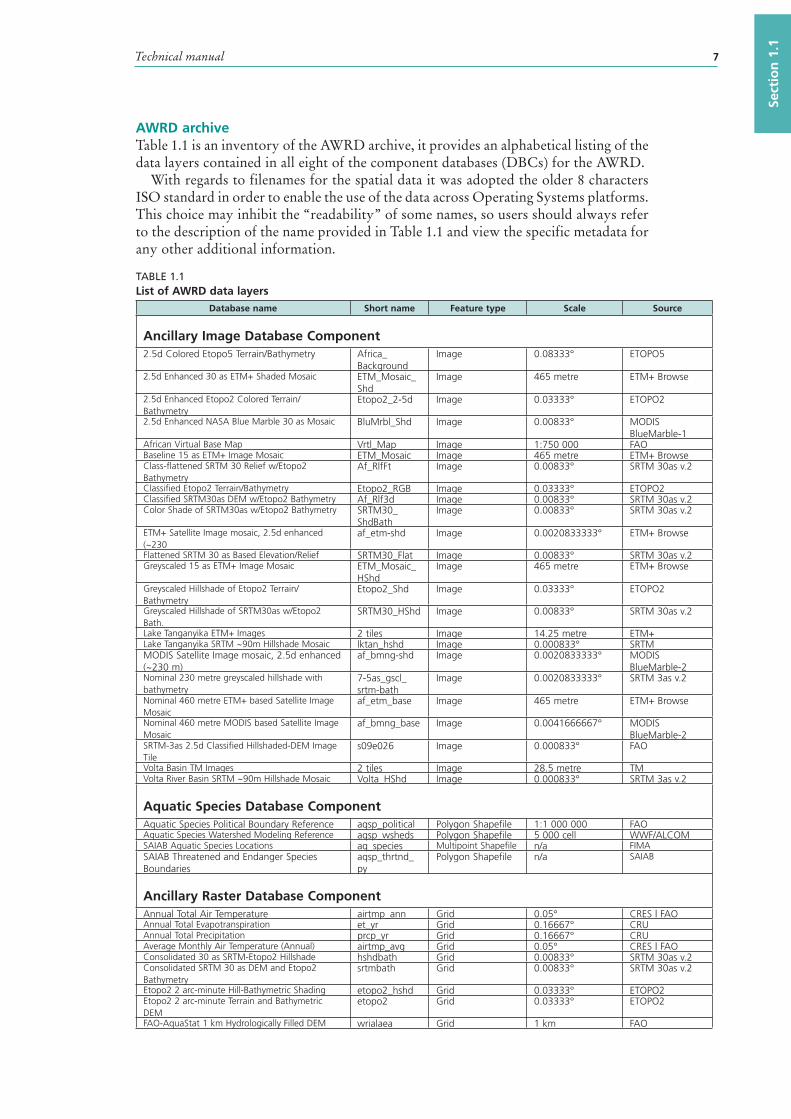
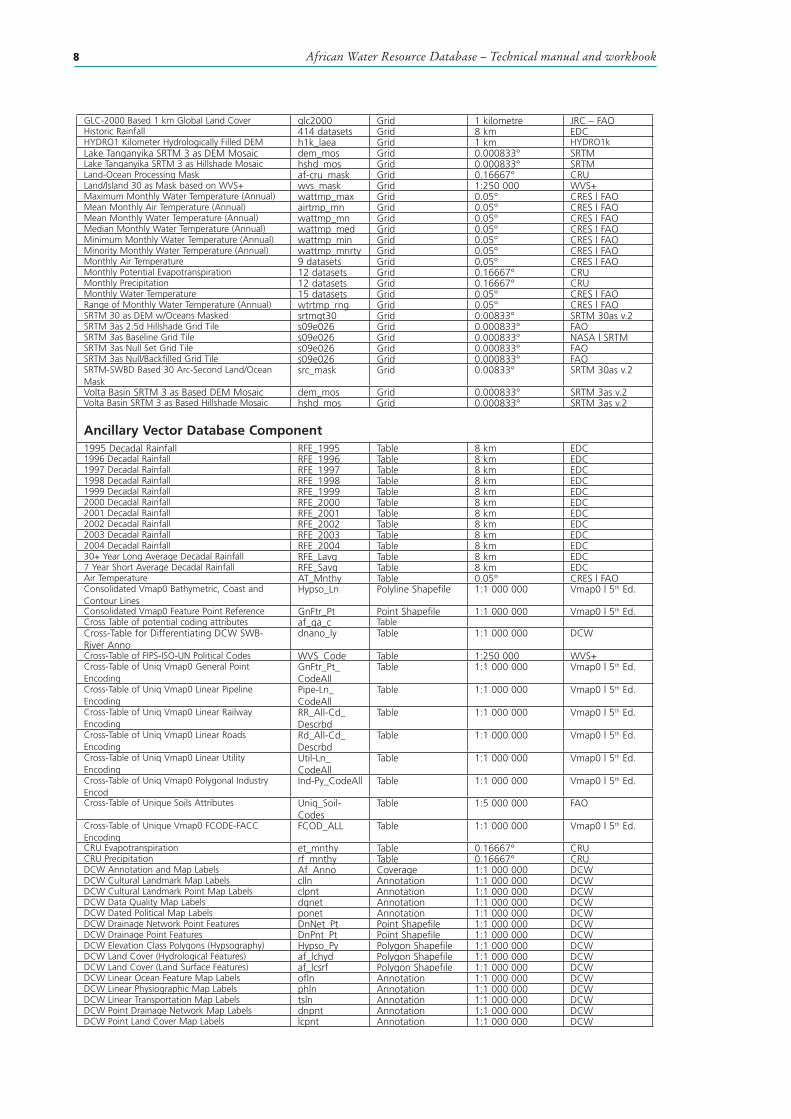
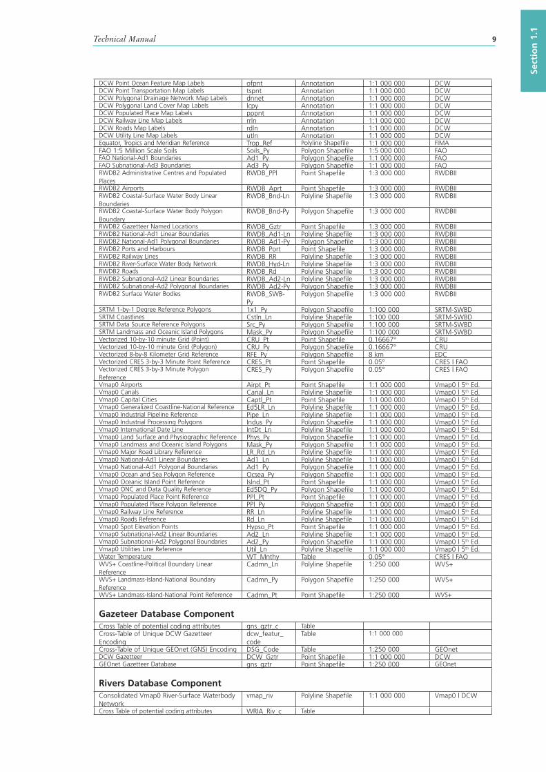
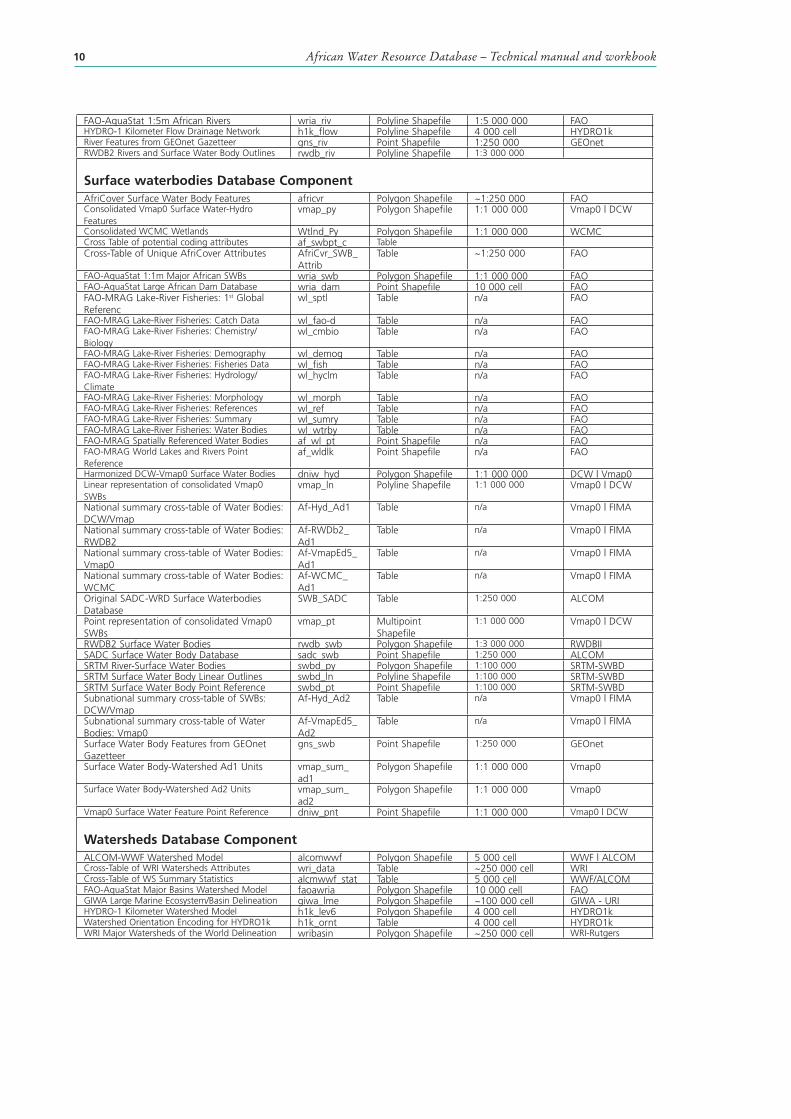
AWRD archiveTable 1.1 is an inventory of the AWRD archive, it provides an alphabetical listing of the data layers contained in all eight of the component databases (DBCs) for the AWRD.
With regards to filenames for the spatial data it was adopted the older 8 characters ISO standard in order to enable the use of the data across Operating Systems platforms. This choice may inhibit the “readability” of some names, so users should always refer to the description of the name provided in Table 1.1 and view the specific metadata for any other additional information.
TABLE 1.1List of AWRD data layers
Database name Short name Feature type Scale Source
Ancillary Image Database Component2.5d Colored Etopo5 Terrain/Bathymetry Africa_
BackgroundImage 0.08333° ETOPO5
2.5d Enhanced 30 as ETM+ Shaded Mosaic ETM_Mosaic_Shd
Image 465 metre ETM+ Browse
2.5d Enhanced Etopo2 Colored Terrain/Bathymetry
Etopo2_2-5d Image 0.03333° ETOPO2
2.5d Enhanced NASA Blue Marble 30 as Mosaic BluMrbl_Shd Image 0.00833° MODIS BlueMarble-1
African Virtual Base Map Vrtl_Map Image 1:750 000 FAOBaseline 15 as ETM+ Image Mosaic ETM_Mosaic Image 465 metre ETM+ BrowseClass-flattened SRTM 30 Relief w/Etopo2 Bathymetry
Af_RlfFt Image 0.00833° SRTM 30as v.2
Classified Etopo2 Terrain/Bathymetry Etopo2_RGB Image 0.03333° ETOPO2Classified SRTM30as DEM w/Etopo2 Bathymetry Af_Rlf3d Image 0.00833° SRTM 30as v.2Color Shade of SRTM30as w/Etopo2 Bathymetry SRTM30_
ShdBathImage 0.00833° SRTM 30as v.2
ETM+ Satellite Image mosaic, 2.5d enhanced (~230
af_etm-shd Image 0.0020833333° ETM+ Browse
Flattened SRTM 30 as Based Elevation/Relief SRTM30_Flat Image 0.00833° SRTM 30as v.2Greyscaled 15 as ETM+ Image Mosaic ETM_Mosaic_
HShdImage 465 metre ETM+ Browse
Greyscaled Hillshade of Etopo2 Terrain/Bathymetry
Etopo2_Shd Image 0.03333° ETOPO2
Greyscaled Hillshade of SRTM30as w/Etopo2 Bath.
SRTM30_HShd Image 0.00833° SRTM 30as v.2
Lake Tanganyika ETM+ Images 2 tiles Image 14.25 metre ETM+Lake Tanganyika SRTM ~90m Hillshade Mosaic lktan_hshd Image 0.000833° SRTMMODIS Satellite Image mosaic, 2.5d enhanced (~230 m)
af_bmng-shd Image 0.0020833333° MODIS BlueMarble-2
Nominal 230 metre greyscaled hillshade with bathymetry
7-5as_gscl_srtm-bath
Image 0.0020833333° SRTM 3as v.2
Nominal 460 metre ETM+ based Satellite Image Mosaic
af_etm_base Image 465 metre ETM+ Browse
Nominal 460 metre MODIS based Satellite Image Mosaic
af_bmng_base Image 0.0041666667° MODIS BlueMarble-2
SRTM-3as 2.5d Classified Hillshaded-DEM Image Tile
s09e026 Image 0.000833° FAO
Volta Basin TM Images 2 tiles Image 28.5 metre TMVolta River Basin SRTM ~90m Hillshade Mosaic Volta_HShd Image 0.000833° SRTM 3as v.2
Aquatic Species Database ComponentAquatic Species Political Boundary Reference aqsp_political Polygon Shapefile 1:1 000 000 FAOAquatic Species Watershed Modeling Reference aqsp_wsheds Polygon Shapefile 5 000 cell WWF/ALCOMSAIAB Aquatic Species Locations aq_species Multipoint Shapefile n/a FIMASAIAB Threatened and Endanger Species Boundaries
aqsp_thrtnd_py
Polygon Shapefile n/a SAIAB
Ancillary Raster Database ComponentAnnual Total Air Temperature airtmp_ann Grid 0.05° CRES | FAOAnnual Total Evapotranspiration et_yr Grid 0.16667° CRUAnnual Total Precipitation prcp_yr Grid 0.16667° CRUAverage Monthly Air Temperature (Annual) airtmp_avg Grid 0.05° CRES | FAOConsolidated 30 as SRTM-Etopo2 Hillshade hshdbath Grid 0.00833° SRTM 30as v.2Consolidated SRTM 30 as DEM and Etopo2 Bathymetry
srtmbath Grid 0.00833° SRTM 30as v.2
Etopo2 2 arc-minute Hill-Bathymetric Shading etopo2_hshd Grid 0.03333° ETOPO2Etopo2 2 arc-minute Terrain and Bathymetric DEM
etopo2 Grid 0.03333° ETOPO2
FAO-AquaStat 1 km Hydrologically Filled DEM wrialaea Grid 1 km FAO
African Water Resource Database – Technical manual and workbook8
GLC-2000 Based 1 km Global Land Cover glc2000 Grid 1 kilometre JRC – FAOHistoric Rainfall 414 datasets Grid 8 km EDCHYDRO1 Kilometer Hydrologically Filled DEM h1k_laea Grid 1 km HYDRO1kLake Tanganyika SRTM 3 as DEM Mosaic dem_mos Grid 0.000833° SRTMLake Tanganyika SRTM 3 as Hillshade Mosaic hshd_mos Grid 0.000833° SRTMLand-Ocean Processing Mask af-cru_mask Grid 0.16667° CRULand/Island 30 as Mask based on WVS+ wvs_mask Grid 1:250 000 WVS+Maximum Monthly Water Temperature (Annual) wattmp_max Grid 0.05° CRES | FAOMean Monthly Air Temperature (Annual) airtmp_mn Grid 0.05° CRES | FAOMean Monthly Water Temperature (Annual) wattmp_mn Grid 0.05° CRES | FAOMedian Monthly Water Temperature (Annual) wattmp_med Grid 0.05° CRES | FAOMinimum Monthly Water Temperature (Annual) wattmp_min Grid 0.05° CRES | FAOMinority Monthly Water Temperature (Annual) wattmp_mnrty Grid 0.05° CRES | FAOMonthly Air Temperature 9 datasets Grid 0.05° CRES | FAOMonthly Potential Evapotranspiration 12 datasets Grid 0.16667° CRUMonthly Precipitation 12 datasets Grid 0.16667° CRUMonthly Water Temperature 15 datasets Grid 0.05° CRES | FAORange of Monthly Water Temperature (Annual) wtrtmp_rng Grid 0.05° CRES | FAOSRTM 30 as DEM w/Oceans Masked srtmgt30 Grid 0.00833° SRTM 30as v.2SRTM 3as 2.5d Hillshade Grid Tile s09e026 Grid 0.000833° FAOSRTM 3as Baseline Grid Tile s09e026 Grid 0.000833° NASA | SRTMSRTM 3as Null Set Grid Tile s09e026 Grid 0.000833° FAOSRTM 3as Null/Backfilled Grid Tile s09e026 Grid 0.000833° FAOSRTM-SWBD Based 30 Arc-Second Land/Ocean Mask
src_mask Grid 0.00833° SRTM 30as v.2
Volta Basin SRTM 3 as Based DEM Mosaic dem_mos Grid 0.000833° SRTM 3as v.2Volta Basin SRTM 3 as Based Hillshade Mosaic hshd_mos Grid 0.000833° SRTM 3as v.2
Ancillary Vector Database Component1995 Decadal Rainfall RFE_1995 Table 8 km EDC1996 Decadal Rainfall RFE_1996 Table 8 km EDC1997 Decadal Rainfall RFE_1997 Table 8 km EDC1998 Decadal Rainfall RFE_1998 Table 8 km EDC1999 Decadal Rainfall RFE_1999 Table 8 km EDC2000 Decadal Rainfall RFE_2000 Table 8 km EDC2001 Decadal Rainfall RFE_2001 Table 8 km EDC2002 Decadal Rainfall RFE_2002 Table 8 km EDC2003 Decadal Rainfall RFE_2003 Table 8 km EDC2004 Decadal Rainfall RFE_2004 Table 8 km EDC30+ Year Long Average Decadal Rainfall RFE_Lavg Table 8 km EDC7 Year Short Average Decadal Rainfall RFE_Savg Table 8 km EDCAir Temperature AT_Mnthy Table 0.05° CRES | FAOConsolidated Vmap0 Bathymetric, Coast and Contour Lines
Hypso_Ln Polyline Shapefile 1:1 000 000 Vmap0 | 5th Ed.
Consolidated Vmap0 Feature Point Reference GnFtr_Pt Point Shapefile 1:1 000 000 Vmap0 | 5th Ed.Cross Table of potential coding attributes af_ga_c TableCross-Table for Differentiating DCW SWB-River Anno
dnano_ly Table 1:1 000 000 DCW
Cross-Table of FIPS-ISO-UN Political Codes WVS_Code Table 1:250 000 WVS+Cross-Table of Uniq Vmap0 General Point Encoding
GnFtr_Pt_CodeAll
Table 1:1 000 000 Vmap0 | 5th Ed.
Cross-Table of Uniq Vmap0 Linear Pipeline Encoding
Pipe-Ln_CodeAll
Table 1:1 000 000 Vmap0 | 5th Ed.
Cross-Table of Uniq Vmap0 Linear Railway Encoding
RR_All-Cd_Descrbd
Table 1:1 000 000 Vmap0 | 5th Ed.
Cross-Table of Uniq Vmap0 Linear Roads Encoding
Rd_All-Cd_Descrbd
Table 1:1 000 000 Vmap0 | 5th Ed.
Cross-Table of Uniq Vmap0 Linear Utility Encoding
Util-Ln_CodeAll
Table 1:1 000 000 Vmap0 | 5th Ed.
Cross-Table of Uniq Vmap0 Polygonal Industry Encod
Ind-Py_CodeAll Table 1:1 000 000 Vmap0 | 5th Ed.
Cross-Table of Unique Soils Attributes Uniq_Soil-Codes
Table 1:5 000 000 FAO
Cross-Table of Unique Vmap0 FCODE-FACC Encoding
FCOD_ALL Table 1:1 000 000 Vmap0 | 5th Ed.
CRU Evapotranspiration et_mnthy Table 0.16667° CRUCRU Precipitation rf_mnthy Table 0.16667° CRUDCW Annotation and Map Labels Af_Anno Coverage 1:1 000 000 DCWDCW Cultural Landmark Map Labels clln Annotation 1:1 000 000 DCWDCW Cultural Landmark Point Map Labels clpnt Annotation 1:1 000 000 DCWDCW Data Quality Map Labels dqnet Annotation 1:1 000 000 DCWDCW Dated Political Map Labels ponet Annotation 1:1 000 000 DCWDCW Drainage Network Point Features DnNet_Pt Point Shapefile 1:1 000 000 DCWDCW Drainage Point Features DnPnt_Pt Point Shapefile 1:1 000 000 DCWDCW Elevation Class Polygons (Hypsography) Hypso_Py Polygon Shapefile 1:1 000 000 DCWDCW Land Cover (Hydrological Features) af_lchyd Polygon Shapefile 1:1 000 000 DCWDCW Land Cover (Land Surface Features) af_lcsrf Polygon Shapefile 1:1 000 000 DCWDCW Linear Ocean Feature Map Labels ofln Annotation 1:1 000 000 DCWDCW Linear Physiographic Map Labels phln Annotation 1:1 000 000 DCWDCW Linear Transportation Map Labels tsln Annotation 1:1 000 000 DCWDCW Point Drainage Network Map Labels dnpnt Annotation 1:1 000 000 DCWDCW Point Land Cover Map Labels lcpnt Annotation 1:1 000 000 DCW
8
Sect
ion
1.1
DCW Point Ocean Feature Map Labels ofpnt Annotation 1:1 000 000 DCWDCW Point Transportation Map Labels tspnt Annotation 1:1 000 000 DCWDCW Polygonal Drainage Network Map Labels dnnet Annotation 1:1 000 000 DCWDCW Polygonal Land Cover Map Labels lcpy Annotation 1:1 000 000 DCWDCW Populated Place Map Labels pppnt Annotation 1:1 000 000 DCWDCW Railway Line Map Labels rrln Annotation 1:1 000 000 DCWDCW Roads Map Labels rdln Annotation 1:1 000 000 DCWDCW Utility Line Map Labels utln Annotation 1:1 000 000 DCWEquator, Tropics and Meridian Reference Trop_Ref Polyline Shapefile 1:1 000 000 FIMAFAO 1:5 Million Scale Soils Soils_Py Polygon Shapefile 1:5 000 000 FAOFAO National-Ad1 Boundaries Ad1_Py Polygon Shapefile 1:1 000 000 FAOFAO Subnational-Ad3 Boundaries Ad3_Py Polygon Shapefile 1:1 000 000 FAORWDB2 Administrative Centres and Populated Places
RWDB_PPl Point Shapefile 1:3 000 000 RWDBII
RWDB2 Airports RWDB_Aprt Point Shapefile 1:3 000 000 RWDBIIRWDB2 Coastal-Surface Water Body Linear Boundaries
RWDB_Bnd-Ln Polyline Shapefile 1:3 000 000 RWDBII
RWDB2 Coastal-Surface Water Body Polygon Boundary
RWDB_Bnd-Py Polygon Shapefile 1:3 000 000 RWDBII
RWDB2 Gazetteer Named Locations RWDB_Gztr Point Shapefile 1:3 000 000 RWDBIIRWDB2 National-Ad1 Linear Boundaries RWDB_Ad1-Ln Polyline Shapefile 1:3 000 000 RWDBIIRWDB2 National-Ad1 Polygonal Boundaries RWDB_Ad1-Py Polygon Shapefile 1:3 000 000 RWDBIIRWDB2 Ports and Harbours RWDB_Port Point Shapefile 1:3 000 000 RWDBIIRWDB2 Railway Lines RWDB_RR Polyline Shapefile 1:3 000 000 RWDBIIRWDB2 River-Surface Water Body Network RWDB_Hyd-Ln Polyline Shapefile 1:3 000 000 RWDBIIRWDB2 Roads RWDB_Rd Polyline Shapefile 1:3 000 000 RWDBIIRWDB2 Subnational-Ad2 Linear Boundaries RWDB_Ad2-Ln Polyline Shapefile 1:3 000 000 RWDBIIRWDB2 Subnational-Ad2 Polygonal Boundaries RWDB_Ad2-Py Polygon Shapefile 1:3 000 000 RWDBIIRWDB2 Surface Water Bodies RWDB_SWB-
PyPolygon Shapefile 1:3 000 000 RWDBII
SRTM 1-by-1 Degree Reference Polygons 1x1_Py Polygon Shapefile 1:100 000 SRTM-SWBDSRTM Coastlines Cstln_Ln Polyline Shapefile 1:100 000 SRTM-SWBDSRTM Data Source Reference Polygons Src_Py Polygon Shapefile 1:100 000 SRTM-SWBDSRTM Landmass and Oceanic Island Polygons Mask_Py Polygon Shapefile 1:100 000 SRTM-SWBDVectorized 10-by-10 minute Grid (Point) CRU_Pt Point Shapefile 0.16667° CRUVectorized 10-by-10 minute Grid (Polygon) CRU_Py Polygon Shapefile 0.16667° CRUVectorized 8-by-8 Kilometer Grid Reference RFE_Py Polygon Shapefile 8 km EDCVectorized CRES 3-by-3 Minute Point Reference CRES_Pt Point Shapefile 0.05° CRES | FAOVectorized CRES 3-by-3 Minute Polygon Reference
CRES_Py Polygon Shapefile 0.05° CRES | FAO
Vmap0 Airports Airpt_Pt Point Shapefile 1:1 000 000 Vmap0 | 5th Ed.Vmap0 Canals Canal_Ln Polyline Shapefile 1:1 000 000 Vmap0 | 5th Ed.Vmap0 Capital Cities Captl_Pt Point Shapefile 1:1 000 000 Vmap0 | 5th Ed.Vmap0 Generalized Coastline-National Reference Ed5LR_Ln Polyline Shapefile 1:1 000 000 Vmap0 | 5th Ed.Vmap0 Industrial Pipeline Reference Pipe_Ln Polyline Shapefile 1:1 000 000 Vmap0 | 5th Ed.Vmap0 Industrial Processing Polygons Indus_Py Polygon Shapefile 1:1 000 000 Vmap0 | 5th Ed.Vmap0 International Date Line IntDt_Ln Polyline Shapefile 1:1 000 000 Vmap0 | 5th Ed.Vmap0 Land Surface and Physiographic Reference Phys_Py Polygon Shapefile 1:1 000 000 Vmap0 | 5th Ed.Vmap0 Landmass and Oceanic Island Polygons Mask_Py Polygon Shapefile 1:1 000 000 Vmap0 | 5th Ed.Vmap0 Major Road Library Reference LR_Rd_Ln Polyline Shapefile 1:1 000 000 Vmap0 | 5th Ed.Vmap0 National-Ad1 Linear Boundaries Ad1_Ln Polyline Shapefile 1:1 000 000 Vmap0 | 5th Ed.Vmap0 National-Ad1 Polygonal Boundaries Ad1_Py Polygon Shapefile 1:1 000 000 Vmap0 | 5th Ed.Vmap0 Ocean and Sea Polygon Reference Ocsea_Py Polygon Shapefile 1:1 000 000 Vmap0 | 5th Ed.Vmap0 Oceanic Island Point Reference Islnd_Pt Point Shapefile 1:1 000 000 Vmap0 | 5th Ed.Vmap0 ONC and Data Quality Reference Ed5DQ_Py Polygon Shapefile 1:1 000 000 Vmap0 | 5th Ed.Vmap0 Populated Place Point Reference PPl_Pt Point Shapefile 1:1 000 000 Vmap0 | 5th Ed.Vmap0 Populated Place Polygon Reference PPl_Py Polygon Shapefile 1:1 000 000 Vmap0 | 5th Ed.Vmap0 Railway Line Reference RR_Ln Polyline Shapefile 1:1 000 000 Vmap0 | 5th Ed.Vmap0 Roads Reference Rd_Ln Polyline Shapefile 1:1 000 000 Vmap0 | 5th Ed.Vmap0 Spot Elevation Points Hypso_Pt Point Shapefile 1:1 000 000 Vmap0 | 5th Ed.Vmap0 Subnational-Ad2 Linear Boundaries Ad2_Ln Polyline Shapefile 1:1 000 000 Vmap0 | 5th Ed.Vmap0 Subnational-Ad2 Polygonal Boundaries Ad2_Py Polygon Shapefile 1:1 000 000 Vmap0 | 5th Ed.Vmap0 Utilities Line Reference Util_Ln Polyline Shapefile 1:1 000 000 Vmap0 | 5th Ed.Water Temperature WT_Mnthy Table 0.05° CRES | FAOWVS+ Coastline-Political Boundary Linear Reference
Cadmn_Ln Polyline Shapefile 1:250 000 WVS+
WVS+ Landmass-Island-National Boundary Reference
Cadmn_Py Polygon Shapefile 1:250 000 WVS+
WVS+ Landmass-Island-National Point Reference Cadmn_Pt Point Shapefile 1:250 000 WVS+
Gazeteer Database ComponentCross Table of potential coding attributes gns_gztr_c TableCross-Table of Unique DCW Gazetteer Encoding
dcw_featur_code
Table 1:1 000 000
Cross-Table of Unique GEOnet (GNS) Encoding DSG_Code Table 1:250 000 GEOnetDCW Gazetteer DCW_Gztr Point Shapefile 1:1 000 000 DCWGEOnet Gazetteer Database gns_gztr Point Shapefile 1:250 000 GEOnet
Rivers Database ComponentConsolidated Vmap0 River-Surface Waterbody Network
vmap_riv Polyline Shapefile 1:1 000 000 Vmap0 | DCW
Cross Table of potential coding attributes WRIA_Riv_c Table
Technical Manual 9
African Water Resource Database – Technical manual and workbook10
FAO-AquaStat 1:5m African Rivers wria_riv Polyline Shapefile 1:5 000 000 FAOHYDRO-1 Kilometer Flow Drainage Network h1k_flow Polyline Shapefile 4 000 cell HYDRO1kRiver Features from GEOnet Gazetteer gns_riv Point Shapefile 1:250 000 GEOnetRWDB2 Rivers and Surface Water Body Outlines rwdb_riv Polyline Shapefile 1:3 000 000
Surface waterbodies Database ComponentAfriCover Surface Water Body Features africvr Polygon Shapefile ~1:250 000 FAOConsolidated Vmap0 Surface Water-Hydro Features
vmap_py Polygon Shapefile 1:1 000 000 Vmap0 | DCW
Consolidated WCMC Wetlands Wtlnd_Py Polygon Shapefile 1:1 000 000 WCMCCross Table of potential coding attributes af_swbpt_c TableCross-Table of Unique AfriCover Attributes AfriCvr_SWB_
AttribTable ~1:250 000 FAO
FAO-AquaStat 1:1m Major African SWBs wria_swb Polygon Shapefile 1:1 000 000 FAOFAO-AquaStat Large African Dam Database wria_dam Point Shapefile 10 000 cell FAOFAO-MRAG Lake-River Fisheries: 1st Global Referenc
wl_sptl Table n/a FAO
FAO-MRAG Lake-River Fisheries: Catch Data wl_fao-d Table n/a FAOFAO-MRAG Lake-River Fisheries: Chemistry/Biology
wl_cmbio Table n/a FAO
FAO-MRAG Lake-River Fisheries: Demography wl_demog Table n/a FAOFAO-MRAG Lake-River Fisheries: Fisheries Data wl_fish Table n/a FAOFAO-MRAG Lake-River Fisheries: Hydrology/Climate
wl_hyclm Table n/a FAO
FAO-MRAG Lake-River Fisheries: Morphology wl_morph Table n/a FAOFAO-MRAG Lake-River Fisheries: References wl_ref Table n/a FAOFAO-MRAG Lake-River Fisheries: Summary wl_sumry Table n/a FAOFAO-MRAG Lake-River Fisheries: Water Bodies wl_wtrby Table n/a FAOFAO-MRAG Spatially Referenced Water Bodies af_wl_pt Point Shapefile n/a FAOFAO-MRAG World Lakes and Rivers Point Reference
af_wldlk Point Shapefile n/a FAO
Harmonized DCW-Vmap0 Surface Water Bodies dniw_hyd Polygon Shapefile 1:1 000 000 DCW | Vmap0Linear representation of consolidated Vmap0 SWBs
vmap_ln Polyline Shapefile 1:1 000 000 Vmap0 | DCW
National summary cross-table of Water Bodies: DCW/Vmap
Af-Hyd_Ad1 Table n/a Vmap0 | FIMA
National summary cross-table of Water Bodies: RWDB2
Af-RWDb2_Ad1
Table n/a Vmap0 | FIMA
National summary cross-table of Water Bodies: Vmap0
Af-VmapEd5_Ad1
Table n/a Vmap0 | FIMA
National summary cross-table of Water Bodies: WCMC
Af-WCMC_Ad1
Table n/a Vmap0 | FIMA
Original SADC-WRD Surface Waterbodies Database
SWB_SADC Table 1:250 000 ALCOM
Point representation of consolidated Vmap0 SWBs
vmap_pt Multipoint Shapefile
1:1 000 000 Vmap0 | DCW
RWDB2 Surface Water Bodies rwdb_swb Polygon Shapefile 1:3 000 000 RWDBIISADC Surface Water Body Database sadc_swb Point Shapefile 1:250 000 ALCOMSRTM River-Surface Water Bodies swbd_py Polygon Shapefile 1:100 000 SRTM-SWBDSRTM Surface Water Body Linear Outlines swbd_ln Polyline Shapefile 1:100 000 SRTM-SWBDSRTM Surface Water Body Point Reference swbd_pt Point Shapefile 1:100 000 SRTM-SWBDSubnational summary cross-table of SWBs:DCW/Vmap
Af-Hyd_Ad2 Table n/a Vmap0 | FIMA
Subnational summary cross-table of Water Bodies: Vmap0
Af-VmapEd5_Ad2
Table n/a Vmap0 | FIMA
Surface Water Body Features from GEOnet Gazetteer
gns_swb Point Shapefile 1:250 000 GEOnet
Surface Water Body-Watershed Ad1 Units vmap_sum_ad1
Polygon Shapefile 1:1 000 000 Vmap0
Surface Water Body-Watershed Ad2 Units vmap_sum_ad2
Polygon Shapefile 1:1 000 000 Vmap0
Vmap0 Surface Water Feature Point Reference dniw_pnt Point Shapefile 1:1 000 000 Vmap0 | DCW
Watersheds Database ComponentALCOM-WWF Watershed Model alcomwwf Polygon Shapefile 5 000 cell WWF | ALCOMCross-Table of WRI Watersheds Attributes wri_data Table ~250 000 cell WRICross-Table of WS Summary Statistics alcmwwf_stat Table 5 000 cell WWF/ALCOMFAO-AquaStat Major Basins Watershed Model faoawria Polygon Shapefile 10 000 cell FAOGIWA Large Marine Ecosystem/Basin Delineation giwa_lme Polygon Shapefile ~100 000 cell GIWA - URIHYDRO-1 Kilometer Watershed Model h1k_lev6 Polygon Shapefile 4 000 cell HYDRO1kWatershed Orientation Encoding for HYDRO1k h1k_ornt Table 4 000 cell HYDRO1kWRI Major Watersheds of the World Delineation wribasin Polygon Shapefile ~250 000 cell WRI-Rutgers
Technical manual 11
Sect
ion
1.1
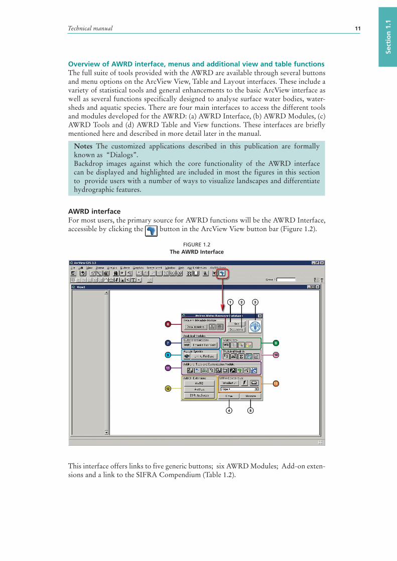
Overview of AWRD interface, menus and additional view and table functionsThe full suite of tools provided with the AWRD are available through several buttons and menu options on the ArcView View, Table and Layout interfaces. These include a variety of statistical tools and general enhancements to the basic ArcView interface as well as several functions specifically designed to analyse surface water bod ies, water-sheds and aquatic species . There are four main interfaces to access the different tools and modules developed for the AWRD: (a) AWRD Interface, (b) AWRD Modules, (c) AWRD Tools and (d) AWRD Table and View functions. These interfaces are briefly mentioned here and described in more detail later in the manual.
Notes The customized applications described in this publication are formally known as “Dialogs”.Backdrop images against which the core functionality of the AWRD interface can be displayed and highlighted are included in most the figures in this section to provide users with a number of ways to visualize landscapes and differentiate hydrographic features.
AWRD interfaceFor most users, the primary source for AWRD functions will be the AWRD Interface, accessible by clicking the button in the ArcView View button bar (Figure 1.2).
FIGURE 1.2The AWRD Interface
This interface offers links to five generic buttons; six AWRD Modules; Add-on exten-sions and a link to the SIFRA Compendium (Table 1.2).
African Water Resource Database – Technical manual and workbook12
TABLE 1.2AWRD interface description
Label
(Fig. 1.2)AWRD Generic buttons Description
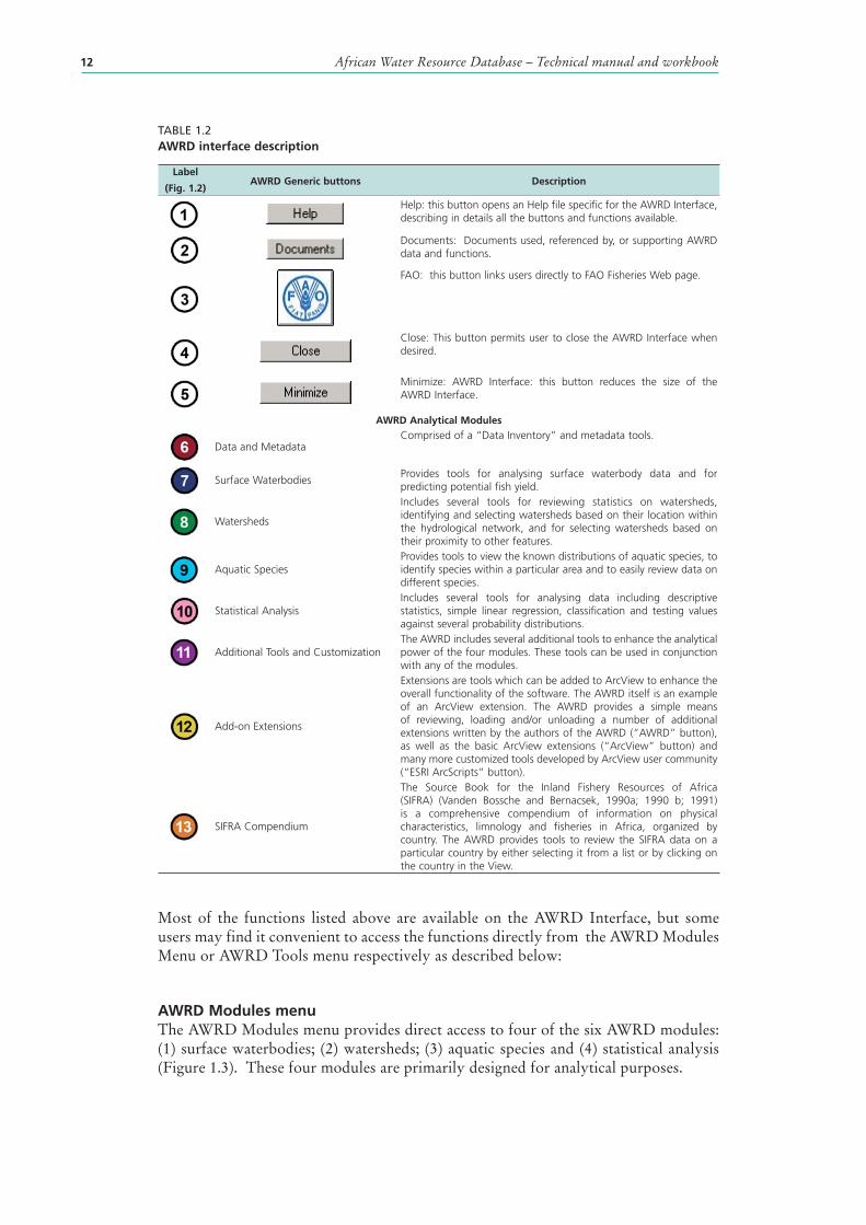
Help: this button opens an Help file specific for the AWRD Interface, describing in details all the buttons and functions available.
Documents : Documents used, referenced by, or supporting AWRD data and functions.
FAO: this button links users directly to FAO Fisheries Web page.
Close: This button permits user to close the AWRD Interface when desired.
Minimize: AWRD Interface: this button reduces the size of the AWRD Interface.
AWRD Analytical Modules
Data and Metadata Comprised of a “Data Inventory” and metadata tools.
Surface Waterbodies Provides tools for analysing surface waterbod y data and for predicting potential fish yield.
Watersheds
Includes several tools for reviewing statistics on watersheds, identifying and selecting watersheds based on their location within the hydrological network, and for selecting watersheds based on their proximity to other features.
Aquatic Species Provides tools to view the known distributions of aquatic species , to identify species within a particular area and to easily review data on different species.
Statistical Analysis Includes several tools for analysing data including descriptive statistics , simple linear regression , classification and testing values against several probability distributions.
Additional Tools and Customization The AWRD includes several additional tools to enhance the analytical power of the four modules. These tools can be used in conjunction with any of the modules.
Add-on Extensions
Extensions are tools which can be added to ArcView to enhance the overall functionality of the software. The AWRD itself is an example of an ArcView extension. The AWRD provides a simple means of reviewing, loading and/or unloading a number of additional extensions written by the authors of the AWRD (“AWRD” button), as well as the basic ArcView extensions (“ArcView” button) and many more customized tools developed by ArcView user community (“ESRI ArcScripts” button).
SIFRA Compendium
The Source Book for the Inland Fishery Resources of Africa (SIFRA) (Vanden Bossche and Bernacsek, 1990a; 1990 b; 1991) is a comprehensive compendium of information on physical characteristics, limnology and fisheries in Africa, organized by country. The AWRD provides tools to review the SIFRA data on a particular country by either selecting it from a list or by clicking on the country in the View.
Most of the functions listed above are available on the AWRD Interface, but some users may find it convenient to access the functions directly from the AWRD Modules Menu or AWRD Tools menu respectively as described below:
AWRD Modules menuThe AWRD Modules menu provides direct access to four of the six AWRD modules: (1) surface waterbodies; (2) watersheds; (3) aquatic species and (4) statistical analysis (Figure 1.3). These four modules are primarily designed for analytical purposes.
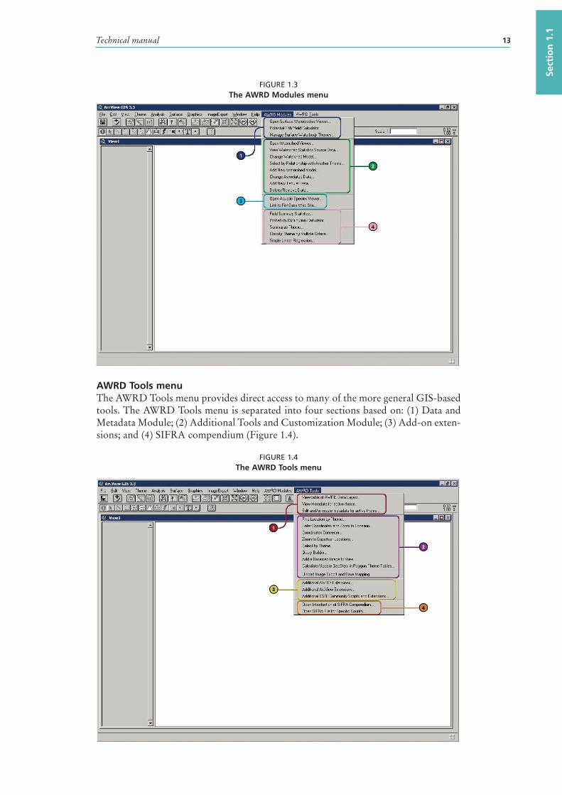
Technical manual 13
Sect
ion
1.1
FIGURE 1.3The AWRD Modules menu
AWRD Tools menu The AWRD Tools menu provides direct access to many of the more general GIS-based tools. The AWRD Tools menu is separated into four sections based on: (1) Data and Metadata Module; (2) Additional Tools and Customization Module; (3) Add-on exten-sions; and (4) SIFRA compendium (Figure 1.4).
FIGURE 1.4The AWRD Tools menu
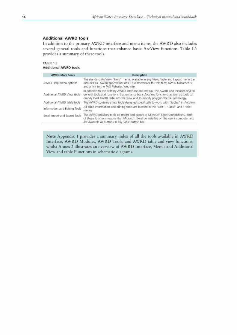
African Water Resource Database – Technical manual and workbook14
Additional AWRD toolsIn addition to the primary AWRD interface and menu items, the AWRD also includes several general tools and functions that enhance basic ArcView functions. Table 1.3 provides a summary of these tools.
TABLE 1.3Additional AWRD tools
AWRD More tools Description
AWRD Help menu optionsThe standard ArcView “Help” menu, available in any View, Table and Layout menu bar includes six AWRD specific options: Four references to Help files; AWRD Documents; and a link to the FAO Fisheries Web site.
Additional AWRD View toolsIn addition to the primary AWRD Interface and menus, the AWRD also includes several general tools and functions that enhance basic ArcView functions, as well as tools to quickly load AWRD data into the view and to modify polygon theme symbology.
Additional AWRD table tools The AWRD contains a few tools designed specifically to work with “tables” in ArcView.
Information and Editing ToolsAll table information and editing tools are located in the “Edit”, “Table” and “Field ” menus
Excel Import and Export Tools The AWRD provides tools to import and export to Microsoft Excel spreadsheets. Both of these functions require that Microsoft Excel be installed on the user’s computer and are available as buttons in any Table button bar.
Note Appendix 1 provides a summary index of all the tools available in AWRD Interface, AWRD Modules, AWRD Tools; and AWRD table and view functions; whilst Annex 2 illustrates an overview of AWRD Interface, Menus and Additional View and table Functions in schematic diagrams.
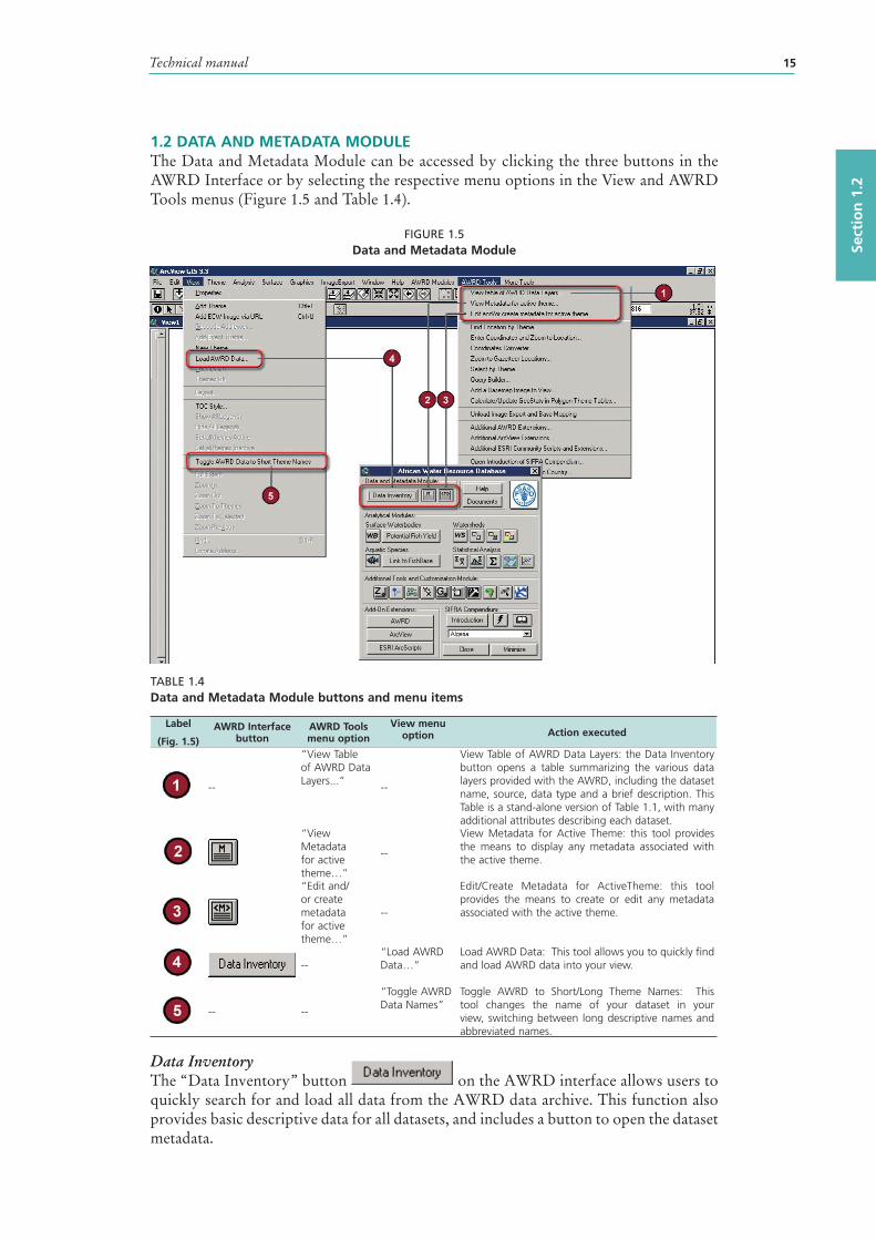
Technical manual 15
Sect
ion
1.2
1.2 DATA AND METADATA MODULEThe Data and Metadata Module can be accessed by clicking the three buttons in the AWRD Interface or by selecting the respective menu options in the View and AWRD Tools menus (Figure 1.5 and Table 1.4).
FIGURE 1.5Data and Metadata Module
TABLE 1.4Data and Metadata Module buttons and menu items
Label
(Fig. 1.5)AWRD Interface
buttonAWRD Tools menu option
View menu option Action executed
--
“View Table of AWRD Data Layers...”
--
View Table of AWRD Data Layers: the Data Inventory button opens a table summarizing the various data layers provided with the AWRD, including the dataset name, source, data type and a brief description. This Table is a stand-alone version of Table 1.1, with many additional attributes describing each dataset.
“View Metadata for active theme…”
--
View Metadata for Active Theme : this tool provides the means to display any metadata associated with the active theme.
“Edit and/or create metadata for active theme…”
--
Edit/Create Metadata for ActiveTheme: this tool provides the means to create or edit any metadata associated with the active theme.
--“Load AWRD Data…”
Load AWRD Data: This tool allows you to quickly find and load AWRD data into your view.
-- --
“Toggle AWRD Data Names”
Toggle AWRD to Short/Long Theme Names: This tool changes the name of your dataset in your view, switching between long descriptive names and abbreviated names.
Data InventoryThe “Data Inventory” button on the AWRD interface allows users to quickly search for and load all data from the AWRD data archive. This function also provides basic descriptive data for all datasets, and includes a button to open the dataset metadata.
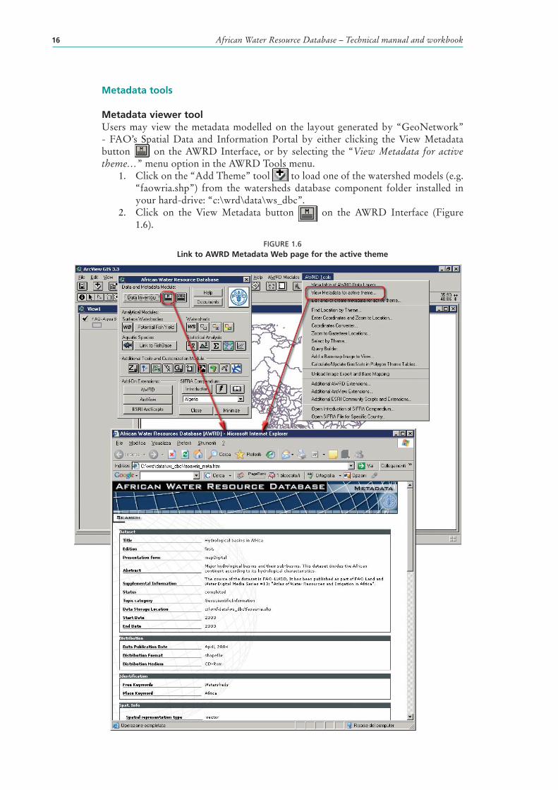
African Water Resource Database – Technical manual and workbook16
Metadata tools
Metadata viewer toolUsers may view the metadata modelled on the layout generated by “GeoNetwork” - FAO’s Spatial Data and Information Portal by either clicking the View Metadata button on the AWRD Interface, or by selecting the “View Metadata for active theme…” menu option in the AWRD Tools menu.
1. Click on the “Add Theme” tool to load one of the watershed models (e.g. “faowria.shp”) from the watersheds database component folder installed in your hard-drive: “c:\wrd\data\ws_dbc”.
2. Click on the View Metadata button on the AWRD Interface (Figure 1.6).
FIGURE 1.6Link to AWRD Metadata Web page for the active theme
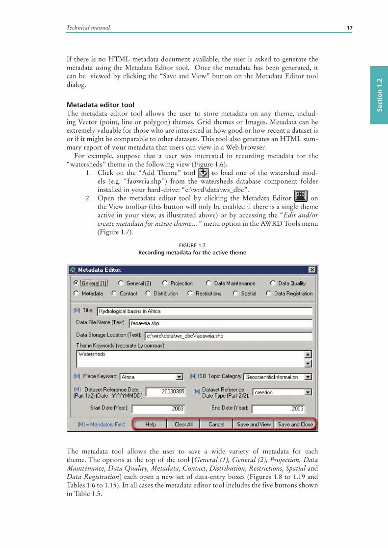
Technical manual 17
Sect
ion
1.2
If there is no HTML metadata document available, the user is asked to generate the metadata using the Metadata Editor tool. Once the metadata has been generated, it can be viewed by clicking the “Save and View” button on the Metadata Editor tool dialog.
Metadata editor toolThe metadata editor tool allows the user to store metadata on any theme , includ-ing Vector (point, line or polygon) themes, Grid themes or Images. Metadata can be extremely valuable for those who are interested in how good or how recent a dataset is or if it might be comparable to other datasets. This tool also generates an HTML sum-mary report of your metadata that users can view in a Web browser.
For example, suppose that a user was interested in recording metadata for the “watersheds” theme in the following view (Figure 1.6).
1. Click on the “Add Theme” tool to load one of the watershed mod-els (e.g. “faowria.shp”) from the watersheds database component folder installed in your hard-drive: “c:\wrd\data\ws_dbc”.
2. Open the metadata editor tool by clicking the Metadata Editor on the View toolbar (this button will only be enabled if there is a single theme active in your view, as illustrated above) or by accessing the “Edit and/or create metadata for active theme…” menu option in the AWRD Tools menu (Figure 1.7).
FIGURE 1.7Recording metadata for the active theme
The metadata tool allows the user to save a wide variety of metadata for each theme . The options at the top of the tool [General (1), General (2), Projection, Data Maintenance, Data Quality, Metadata, Contact, Distribution, Restrictions, Spatial and Data Registration] each open a new set of data-entry boxes (Figures 1.8 to 1.19 and Tables 1.6 to 1.15). In all cases the metadata editor tool includes the five buttons shown in Table 1.5.
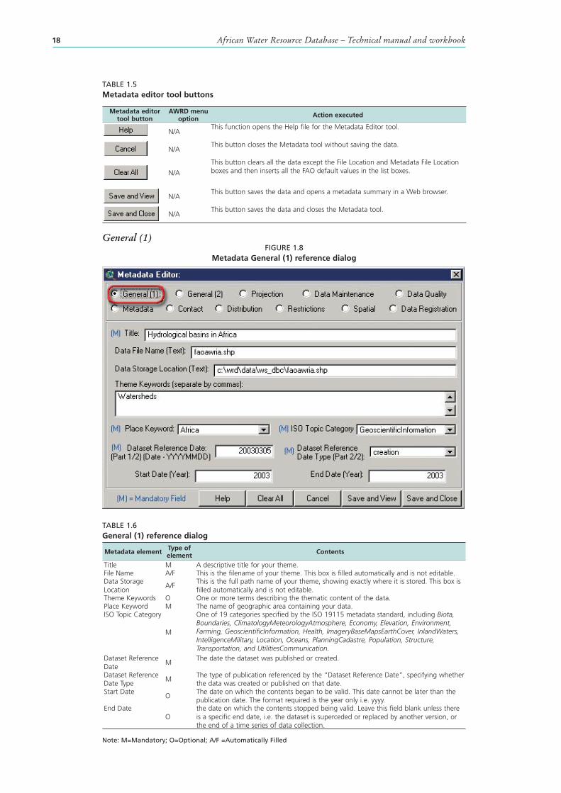
African Water Resource Database – Technical manual and workbook18
TABLE 1.5Metadata editor tool buttons
Metadata editor tool button
AWRD menu option Action executed
N/AThis function opens the Help file for the Metadata Editor tool.
N/AThis button closes the Metadata tool without saving the data.
N/A
This button clears all the data except the File Location and Metadata File Location boxes and then inserts all the FAO default values in the list boxes.
N/AThis button saves the data and opens a metadata summary in a Web browser.
N/AThis button saves the data and closes the Metadata tool.
General (1)FIGURE 1.8
Metadata General (1) reference dialog
TABLE 1.6General (1) reference dialog
Metadata element Type of element Contents
Title M A descriptive title for your theme. File Name A/F This is the filename of your theme. This box is filled automatically and is not editable.Data Storage Location
A/FThis is the full path name of your theme, showing exactly where it is stored. This box is filled automatically and is not editable.
Theme Keywords O One or more terms describing the thematic content of the data.Place Keyword M The name of geographic area containing your data.ISO Topic Category
M
One of 19 categories specified by the ISO 19115 metadata standard, including Biota, Boundaries, ClimatologyMeteorologyAtmosphere, Economy, Elevation, Environment, Farming, GeoscientificInformation, Health, ImageryBaseMapsEarthCover, InlandWaters, IntelligenceMilitary, Location, Oceans, PlanningCadastre, Population, Structure, Transportation, and UtilitiesCommunication.
Dataset Reference Date
MThe date the dataset was published or created.
Dataset Reference Date Type
MThe type of publication referenced by the “Dataset Reference Date”, specifying whether the data was created or published on that date.
Start DateO
The date on which the contents began to be valid. This date cannot be later than the publication date. The format required is the year only i.e. yyyy.
End DateO
the date on which the contents stopped being valid. Leave this field blank unless there is a specific end date, i.e. the dataset is superceded or replaced by another version, or the end of a time series of data collection.
Note: M=Mandatory; O=Optional; A/F =Automatically Filled
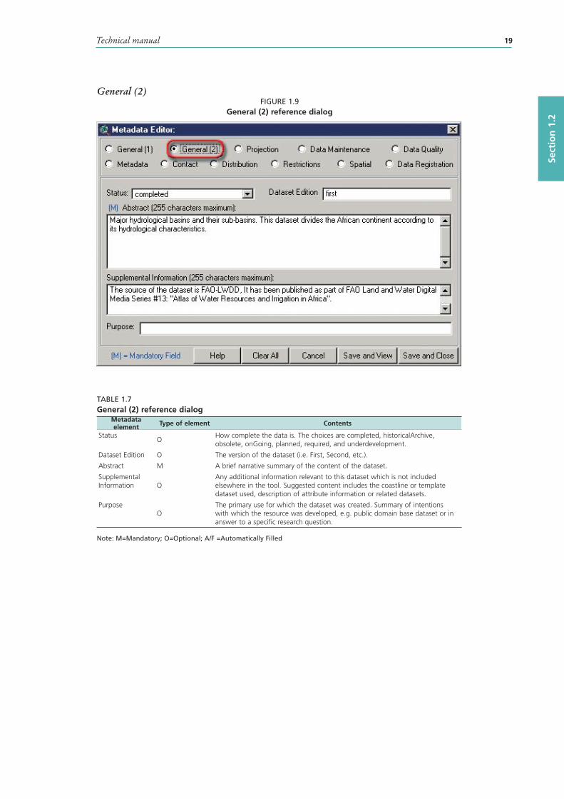
Technical manual 19
Sect
ion
1.2
General (2)FIGURE 1.9
General (2) reference dialog
TABLE 1.7General (2) reference dialog
Metadata element Type of element Contents
StatusO
How complete the data is. The choices are completed, historicalArchive, obsolete, onGoing, planned, required, and underdevelopment.
Dataset Edition O The version of the dataset (i.e. First, Second, etc.).
Abstract M A brief narrative summary of the content of the dataset.
Supplemental Information O
Any additional information relevant to this dataset which is not included elsewhere in the tool. Suggested content includes the coastline or template dataset used, description of attribute information or related datasets.
PurposeO
The primary use for which the dataset was created. Summary of intentions with which the resource was developed, e.g. public domain base dataset or in answer to a specific research question.
Note: M=Mandatory; O=Optional; A/F =Automatically Filled
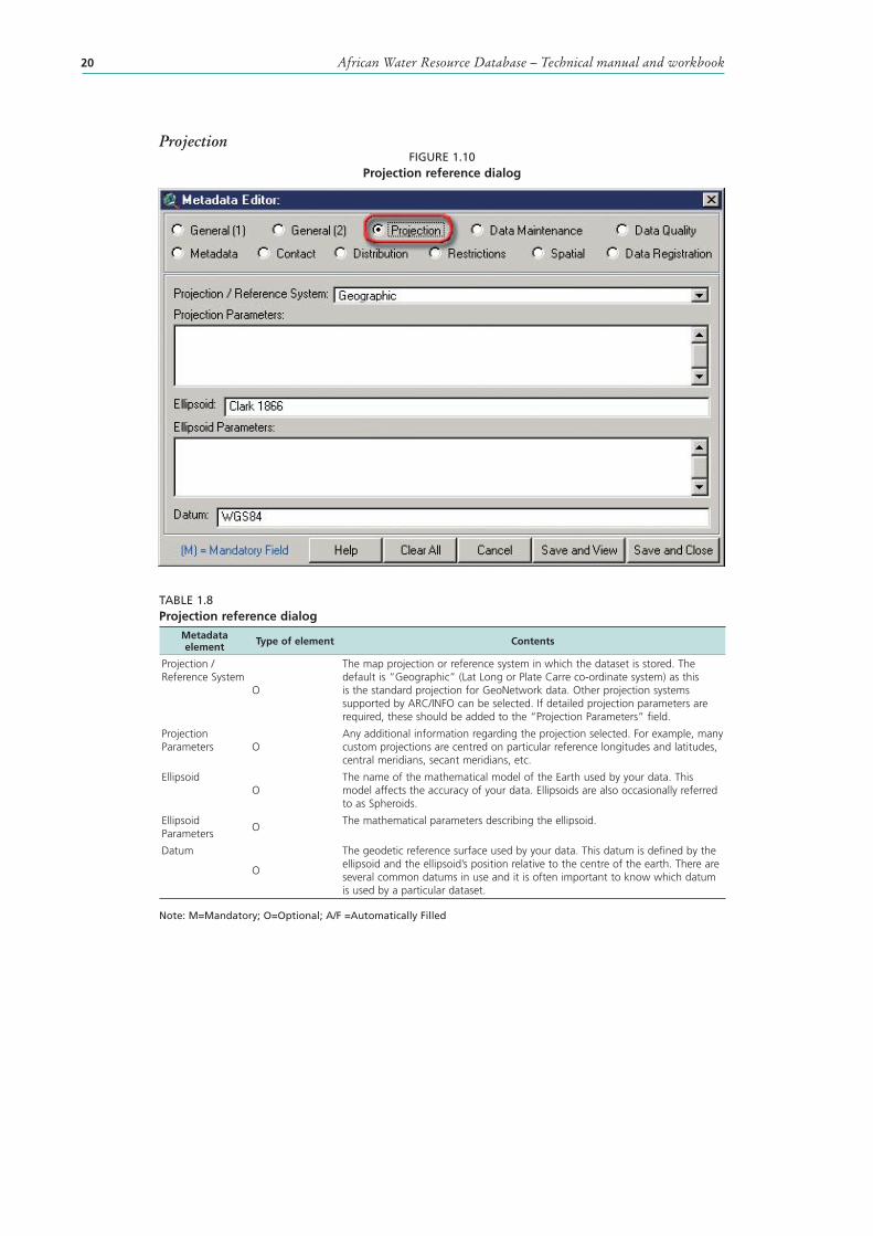
African Water Resource Database – Technical manual and workbook20
ProjectionFIGURE 1.10
Projection reference dialog
TABLE 1.8Projection reference dialog
Metadata element Type of element Contents
Projection / Reference System
O
The map projection or reference system in which the dataset is stored. The default is “Geographic” (Lat Long or Plate Carre co-ordinate system) as this is the standard projection for GeoNetwork data. Other projection systems supported by ARC/INFO can be selected. If detailed projection parameters are required, these should be added to the “Projection Parameters” field.
Projection Parameters O
Any additional information regarding the projection selected. For example, many custom projections are centred on particular reference longitudes and latitudes, central meridians, secant meridians, etc.
EllipsoidO
The name of the mathematical model of the Earth used by your data. This model affects the accuracy of your data. Ellipsoids are also occasionally referred to as Spheroids.
Ellipsoid Parameters
OThe mathematical parameters describing the ellipsoid.
Datum
O
The geodetic reference surface used by your data. This datum is defined by the ellipsoid and the ellipsoid’s position relative to the centre of the earth. There are several common datums in use and it is often important to know which datum is used by a particular dataset.
Note: M=Mandatory; O=Optional; A/F =Automatically Filled
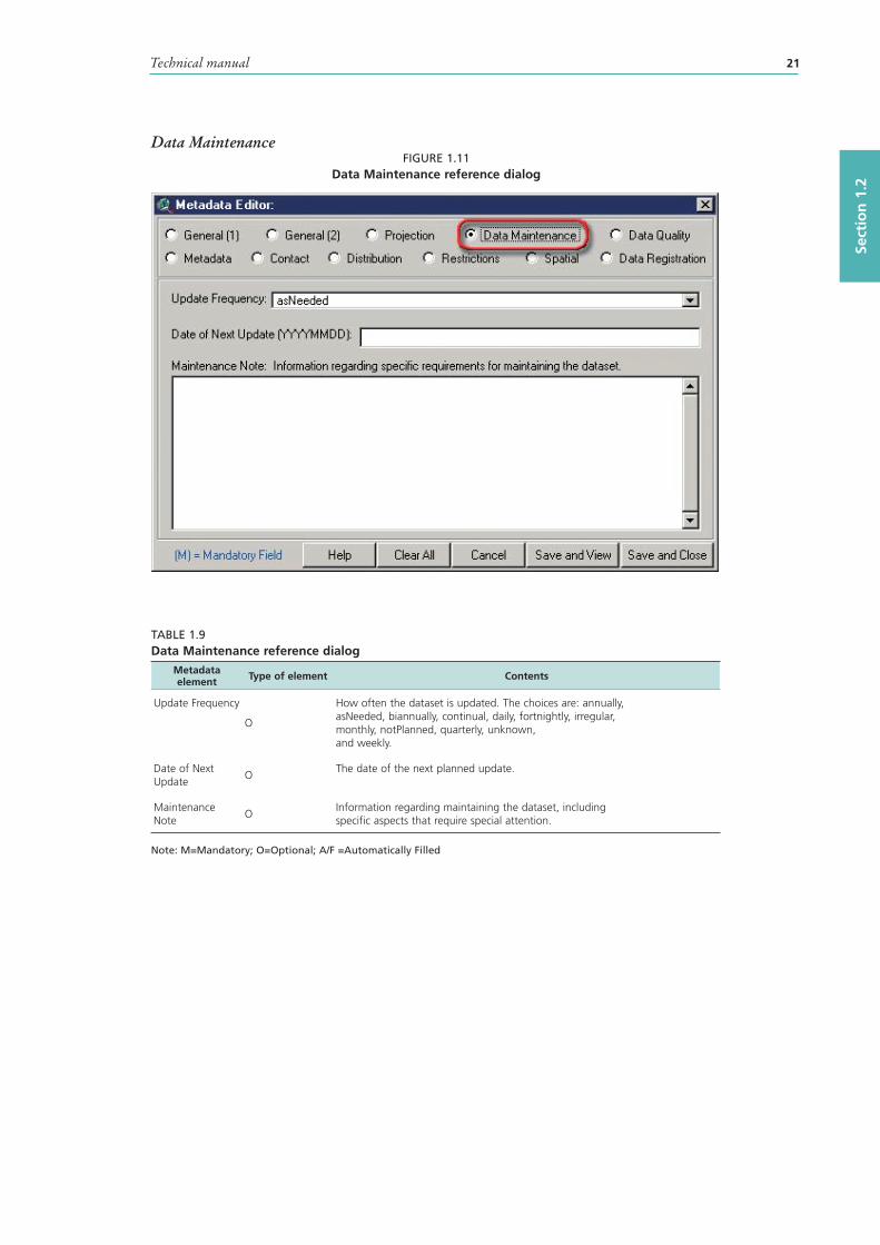
Technical manual 21
Sect
ion
1.2
Data MaintenanceFIGURE 1.11
Data Maintenance reference dialog
TABLE 1.9Data Maintenance reference dialog
Metadata element Type of element Contents
Update Frequency
O
How often the dataset is updated. The choices are: annually, asNeeded, biannually, continual, daily, fortnightly, irregular, monthly, notPlanned, quarterly, unknown, and weekly.
Date of Next Update
OThe date of the next planned update.
Maintenance Note
OInformation regarding maintaining the dataset, including specific aspects that require special attention.
Note: M=Mandatory; O=Optional; A/F =Automatically Filled
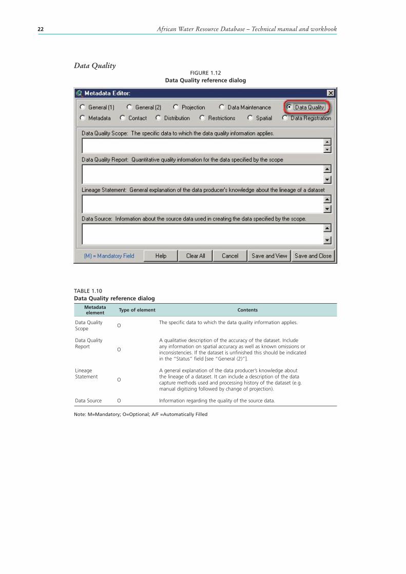
African Water Resource Database – Technical manual and workbook22
Data QualityFIGURE 1.12
Data Quality reference dialog
TABLE 1.10Data Quality reference dialog
Metadata element Type of element Contents
Data Quality Scope
OThe specific data to which the data quality information applies.
Data Quality Report
O
A qualitative description of the accuracy of the dataset. Include any information on spatial accuracy as well as known omissions or inconsistencies. If the dataset is unfinished this should be indicated in the “Status” field [see “General (2)”].
Lineage Statement
O
A general explanation of the data producer’s knowledge about the lineage of a dataset. It can include a description of the data capture methods used and processing history of the dataset (e.g. manual digitizing followed by change of projection) .
Data Source O Information regarding the quality of the source data.
Note: M=Mandatory; O=Optional; A/F =Automatically Filled
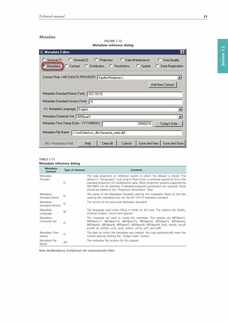
Technical manual 23
Sect
ion
1.2
MetadataFIGURE 1.13
Metadata reference dialog
TABLE 1.11Metadata reference dialog
Metadata element Type of element Contents
Metadata Provider
O
The map projection or reference system in which the dataset is stored. The default is “Geographic” (Lat Long or Plate Carre co-ordinate system) as this is the standard projection for GeoNetwork data. Other projection systems supported by ARC/INFO can be selected. If detailed projection parameters are required, these should be added to the “Projection Parameters” field.
Metadata Standard Name
OThe name of the Metadata Standard used by this metadata. Many of the lists used by this metadata tool use the ISO 19115 metadata standard.
Metadata Standard Version
OThe version of this particular Metadata Standard.
Metadata Language
MThe language used when filling in fields on this tool. The options are Arabic, Chinese, English, French and Spanish.
Metadata Character Set
O
The character set used to create the metadata. The options are 8859part1, 8859part11, 8859part14, 8859part15, 8859part2, 8859part3, 8859part4, 8859part5, 8859part6, 8859part7, 8859part8, 8859part9, big5, ebcdic, eucJP, eucKR, jis, shiftJIS, ucs2, ucs4, usAscii, utf16, utf7, and utf8.
Metadata Time Stamp
OThe date on which the metadata was created. You may automatically insert the current date by clicking the “Today’s Date” button.
Metadata File Name
A/FThe metadata file location for this dataset.
Note: M=Mandatory; O=Optional; A/F =Automatically Filled
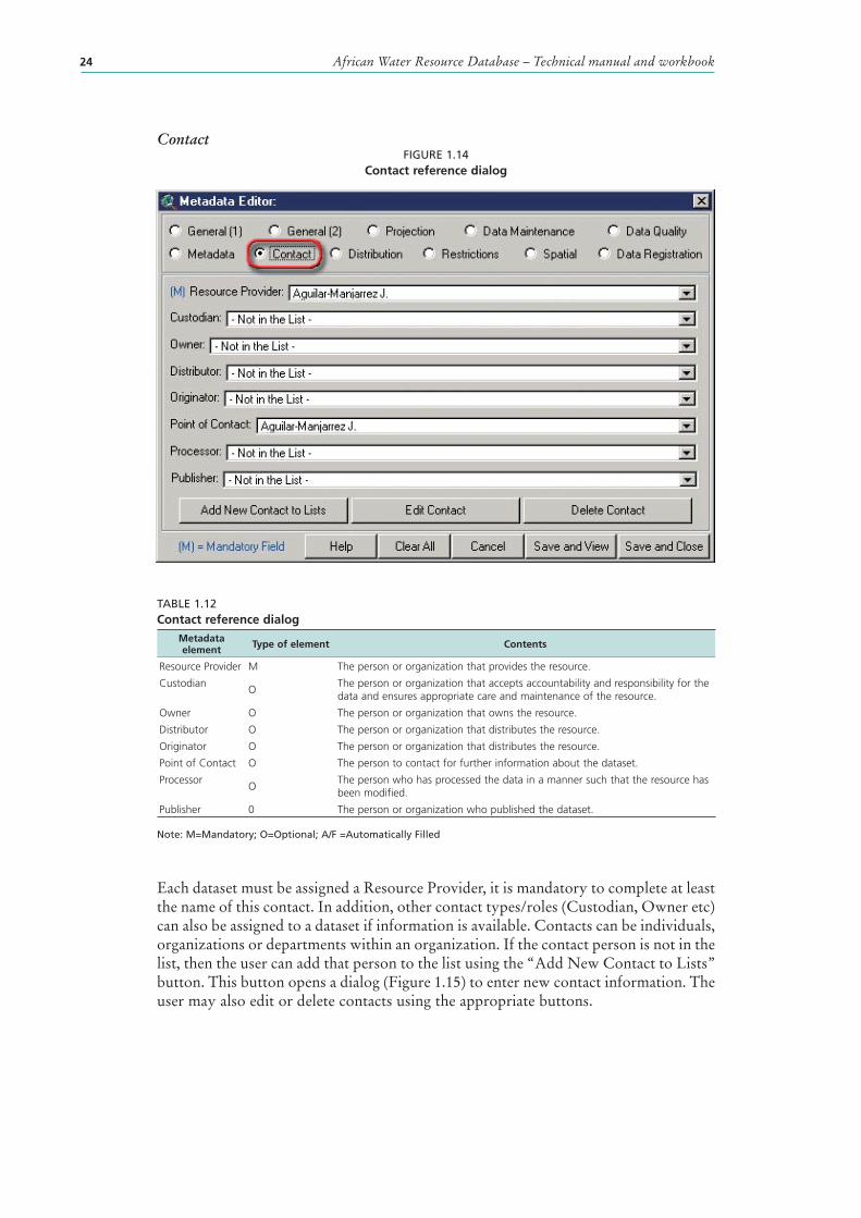
African Water Resource Database – Technical manual and workbook24
ContactFIGURE 1.14
Contact reference dialog
TABLE 1.12Contact reference dialog
Metadata element Type of element Contents
Resource Provider M The person or organization that provides the resource.
CustodianO
The person or organization that accepts accountability and responsibility for the data and ensures appropriate care and maintenance of the resource.
Owner O The person or organization that owns the resource.
Distributor O The person or organization that distributes the resource.
Originator O The person or organization that distributes the resource.
Point of Contact O The person to contact for further information about the dataset.
ProcessorO
The person who has processed the data in a manner such that the resource has been modified.
Publisher 0 The person or organization who published the dataset.
Note: M=Mandatory; O=Optional; A/F =Automatically Filled
Each dataset must be assigned a Resource Provider, it is mandatory to complete at least the name of this contact. In addition, other contact types/roles (Custodian, Owner etc) can also be assigned to a dataset if information is available. Contacts can be individuals, organizations or departments within an organization. If the contact person is not in the list, then the user can add that person to the list using the “Add New Contact to Lists” button. This button opens a dialog (Figure 1.15) to enter new contact information. The user may also edit or delete contacts using the appropriate buttons.
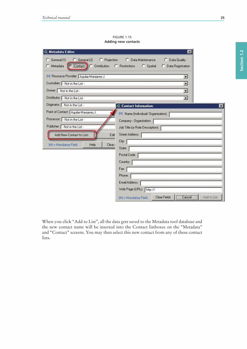
Technical manual 25
Sect
ion
1.2
FIGURE 1.15Adding new contacts
When you click “Add to List”, all the data gets saved to the Metadata tool database and the new contact name will be inserted into the Contact listboxes on the “Metadata” and “Contact” screens. You may then select this new contact from any of these contact lists.
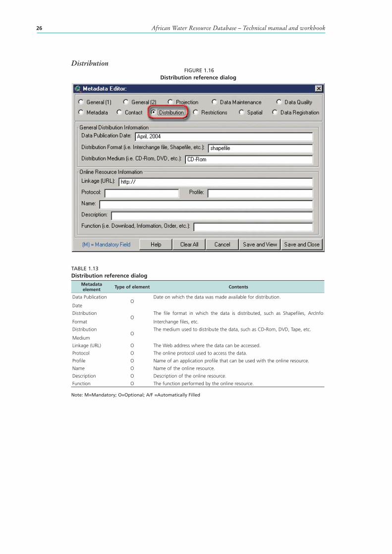
African Water Resource Database – Technical manual and workbook26
Distribution FIGURE 1.16
Distribution reference dialog
TABLE 1.13Distribution reference dialog
Metadata element Type of element Contents
Data Publication
DateO
Date on which the data was made available for distribution.
Distribution
FormatO
The file format in which the data is distributed, such as Shapefiles, ArcInfo
Interchange files, etc.
Distribution
MediumO
The medium used to distribute the data, such as CD-Rom, DVD, Tape, etc.
Linkage (URL) O The Web address where the data can be accessed.
Protocol O The online protocol used to access the data.
Profile O Name of an application profile that can be used with the online resource.
Name O Name of the online resource.
Description O Description of the online resource.
Function O The function performed by the online resource.
Note: M=Mandatory; O=Optional; A/F =Automatically Filled
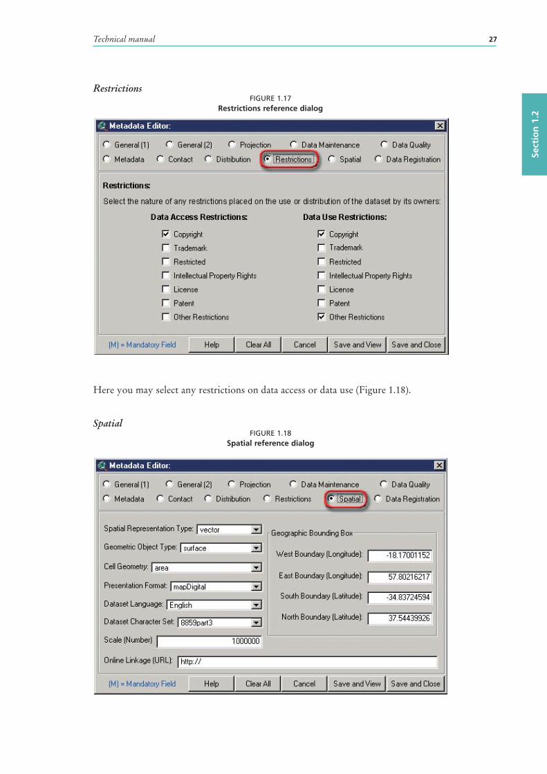
Technical manual 27
Sect
ion
1.2
RestrictionsFIGURE 1.17
Restrictions reference dialog
Here you may select any restrictions on data access or data use (Figure 1.18).
SpatialFIGURE 1.18
Spatial reference dialog
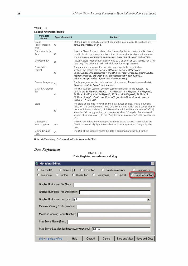
African Water Resource Database – Technical manual and workbook28
TABLE 1.14Spatial reference dialog
Metadata element Type of element Contents
Spatial Representation Type
OMethod used to spatially represent geographic information. The options are textTable, vector, or grid.
Geometric Object Type O
(Feature Class - for vector data only). Name of point and vector spatial objects used to locate zero-, one- and two-dimensional spatial locations in the dataset. The options are complexes, composites, curve, point, solid, and surface.
Cell GeometryO
(Raster Object Type) Identification of grid data as point or cell. Needed for raster data only. The default is “cell” which is true for image datasets.
Presentation Format
O
The presentation format for the data, e.g. map, table or vertical cross section. The options are documentDigital, documentHardcopy, imageDigital, imageHardcopy, mapDigital, mapHardcopy, modelDigital, modelHardcopy, profileDigital, profileHardcopy, tableDigital, tableHardcopy, videoDigital, and videoHardcopy.
Dataset LanguageO
The language of any text information in the dataset. The options are Arabic, Chinese, English, French and Spanish.
Dataset Character Set
O
The character set used for any text based information in the dataset. The options are 8859part1, 8859part11, 8859part14, 8859part15, 8859part2, 8859part3, 8859part4, 8859part5, 8859part6, 8859part7, 8859part8, 8859part9, big5, ebcdic, eucJP, eucKR, jis, shiftJIS, ucs2, ucs4, usAscii, utf16, utf7, and utf8.
Scale
O
The scale of the map from which the dataset was derived. This is a numeric field, for 1: 1 000 000 enter 1 000 000. For datasets which are a compilation of maps at different scales (e.g. Sub National Administrative Boundaries of Africa) leave this field empty and add a comment (such as “Compiled from national sources at various scales”) to the “Supplemental Information” field [see General (2)].
Geographic Bounding Box A/F
These values reflect the geographic extremes of the dataset. These values are filled in automatically by the Metadata tool, but they can be changed by the user.
Online Linkage (URL)
OThe URL of the Website where the data is published or described further.
Note: M=Mandatory; O=Optional; A/F =Automatically Filled
Data RegistrationFIGURE 1.19
Data Registration reference dialog
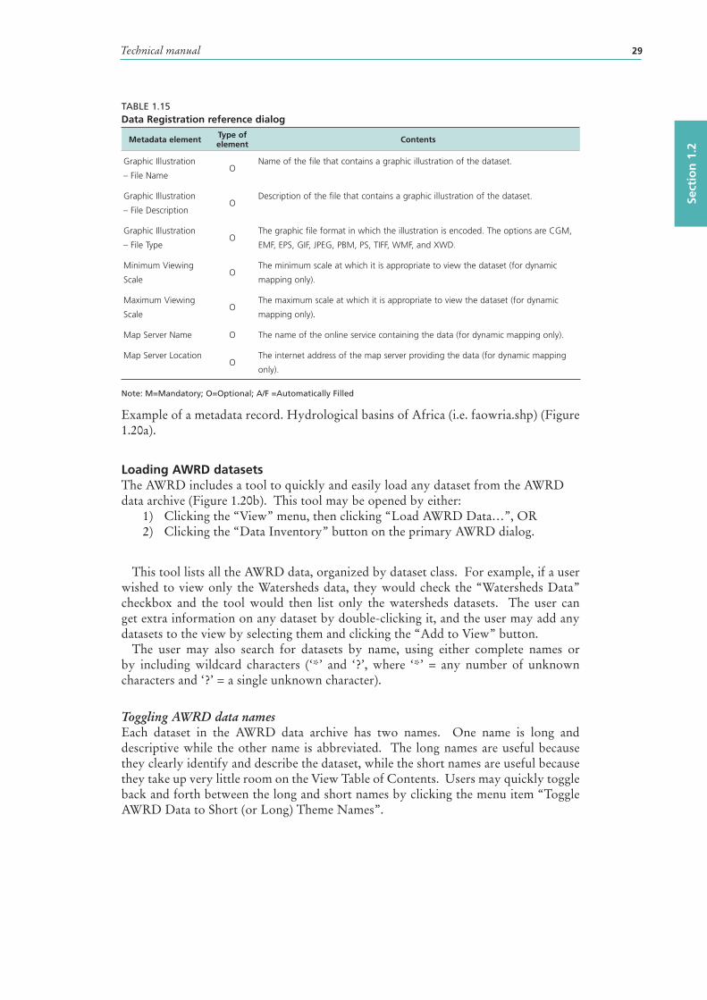
Technical manual 29
Sect
ion
1.2
TABLE 1.15Data Registration reference dialog
Metadata element Type of element Contents
Graphic Illustration
– File NameO
Name of the file that contains a graphic illustration of the dataset.
Graphic Illustration
– File DescriptionO
Description of the file that contains a graphic illustration of the dataset.
Graphic Illustration
– File TypeO
The graphic file format in which the illustration is encoded. The options are CGM,
EMF, EPS, GIF, JPEG, PBM, PS, TIFF, WMF, and XWD.
Minimum Viewing
ScaleO
The minimum scale at which it is appropriate to view the dataset (for dynamic
mapping only).
Maximum Viewing
ScaleO
The maximum scale at which it is appropriate to view the dataset (for dynamic
mapping only).
Map Server Name O The name of the online service containing the data (for dynamic mapping only).
Map Server LocationO
The internet address of the map server providing the data (for dynamic mapping
only).
Note: M=Mandatory; O=Optional; A/F =Automatically Filled
Example of a metadata record. Hydrological basins of Africa (i.e. faowria.shp) (Figure 1.20a).
Loading AWRD datasetsThe AWRD includes a tool to quickly and easily load any dataset from the AWRD data archive (Figure 1.20b). This tool may be opened by either:
1) Clicking the “View” menu, then clicking “Load AWRD Data…”, OR2) Clicking the “Data Inventory” button on the primary AWRD dialog.
This tool lists all the AWRD data, organized by dataset class. For example, if a user wished to view only the Watersheds data, they would check the “Watersheds Data” checkbox and the tool would then list only the watersheds datasets. The user can get extra information on any dataset by double-clicking it, and the user may add any datasets to the view by selecting them and clicking the “Add to View” button.
The user may also search for datasets by name, using either complete names or by including wildcard characters (‘*’ and ‘?’, where ‘*’ = any number of unknown characters and ‘?’ = a single unknown character).
Toggling AWRD data namesEach dataset in the AWRD data archive has two names. One name is long and descriptive while the other name is abbreviated. The long names are useful because they clearly identify and describe the dataset, while the short names are useful because they take up very little room on the View Table of Contents. Users may quickly toggle back and forth between the long and short names by clicking the menu item “Toggle AWRD Data to Short (or Long) Theme Names”.
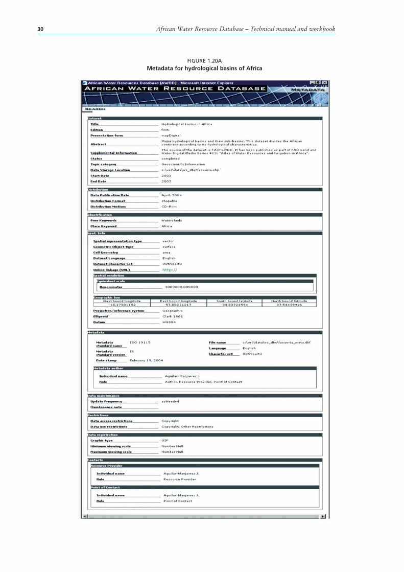
African Water Resource Database – Technical manual and workbook30
FIGURE 1.20AMetadata for hydrological basins of Africa
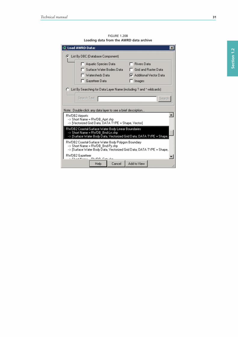
Technical manual 31
Sect
ion
1.2
FIGURE 1.20BLoading data from the AWRD data archive

African Water Resource Database – Technical manual and workbook32
1.3 SURFACE WATERBODIES MODULEThe Surface Waterbodies (SWB ) Module is designed to provide users of the AWRD with quick and easy access to data on the surface waterbod ies of Africa, as well as providing users with a method to predict potential SWB yields based on two possible models. The module is designed to work with a variety of surface waterbody datasets, including seven of the surface waterbody (SWB) layers resident within the SWB portion of the AWRD.
Open the Surface Waterbodies Viewer by clicking on the button in the AWRD Interface, or by clicking the “Open Surface Waterbodies Viewer…” menu option in the AWRD Modules menu (Figure 1.21)
FIGURE 1.21Surface Waterbodies Module
Table 1.16 provides a summary of the buttons available in the Surface Waterbod ies Module.
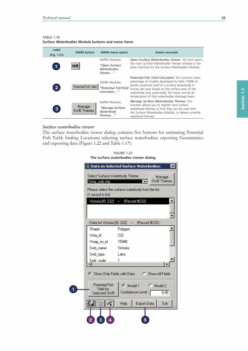
Technical manual 33
Sect
ion
1.3
TABLE 1.16Surface Waterbodies Module buttons and menu items
Label
(Fig. 1.21)AWRD button AWRD menu option Action executed
AWRD Modules
“Open Surface Waterbodies Viewer…”
Open Surface Waterbodies Viewer: this tool opens the main Surface Waterbodies Viewer window is the basic interface for the Surface Waterbodies Module.
AWRD Modules
“Potential FishYield Calculator…”
Potential Fish Yield Calculator : this function takes advantage of models developed by Halls (1999) to predict potential yield of a surface waterbody in tonnes per year based on the surface area of the waterbody and, potentially, the mean annual air temperature of that waterbodies drainage basin.
AWRD Modules
“Manage Surface Waterbody Themes…”
Manage Surface Waterbodies Themes: this function allows you to register new surface waterbod y themes so that they can be used with the Surface Waterbodies Module, or delete currently registered themes.
Surface waterbodies viewer The surface waterbodies viewer dialog contains five buttons for estimating Potential Fish Yield ; finding Locations; selecting surface waterbodies; reporting Geostatistics and exporting data (Figure 1.22 and Table 1.17).
FIGURE 1.22The surface waterbodies viewer dialog
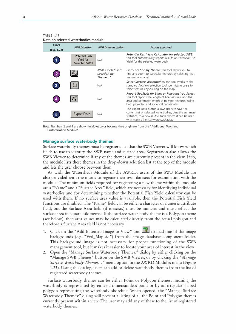
African Water Resource Database – Technical manual and workbook34
TABLE 1.17Data on selected waterbodies module
Label
(Fig. 1.22)AWRD button AWRD menu option Action executed
N/A
Potential Fish Yield Calculator for selected SWB: this tool automatically reports results on Potential Fish Yield for the selected waterbody.
AWRD Tools “Find Location by Theme...”
Find Location by Theme: this tool allows you to find and zoom to particular features by selecting that feature from a list.
N/ASelect Surface Waterbodies: this tool works as the standard ArcView selection tool, permitting users to select features by clicking on the map.
N/A
Report GeoStats for Lines or Polygons You Select: this tool reports the length of line features, and the area and perimeter length of polygon features, using both projected and spherical coordinates.
N/A
The Export Data button allows users to save the current set of selected waterbodies, plus the summary statistics, to a new dBASE table where it can be used with many other software packages.
Note: Numbers 2 and 4 are shown in violet color because they originate from the “Additional Tools and Customization Module”.
Manage surface waterbody themesSurface waterbody themes must be registered so that the SWB Viewer will know which fields to use to identify the SWB name and surface area. Registration also allows the SWB Viewer to determine if any of the themes are currently present in the view. If so, the module lists these themes in the drop-down selection list at the top of the module and lets the user choose between them.
As with the Watersheds Module of the AWRD, users of the SWB Module are also provided with the means to register their own datasets for examination with the module. The minimum fields required for registering a new theme within the module are a “Name” and a “Surface Area” field, which are necessary for identifying individual waterbodies and for determining whether the Potential Fish Yield calculator can be used with them. If no surface area value is available, then the Potential Fish Yield functions are disabled. The “Name” field can be either a character or numeric attribute field, but the Surface Area field (if it exists) must be numeric and must reflect the surface area in square kilometres. If the surface water bod y theme is a Polygon theme (see below), then area values may be calculated directly from the actual polygon and therefore a Surface Area field is not necessary.
1. Click on the “Add Basemap Image to View” tool to load one of the image backgrounds (e.g. “Vrtl_Map.sid”) from the image database component folder. This background image is not necessary for proper functioning of the SWB management tool, but it makes it easier to locate your area of interest in the view.
2. Open the “Manage Surface Waterbody Themes:” dialog by either clicking on the “Manage SWB Themes” button on the SWB Viewer, or by clicking the “Manage Surface Waterbody Themes…” menu option in the AWRD Modules menu (Figure 1.23). Using this dialog, users can add or delete waterbody themes from the list of registered waterbody themes.
Surface waterbody themes can be either Point or Polygon themes, meaning the waterbody is represented by either a dimensionless point or by an irregular-shaped polygon representing the waterbody shoreline. When opened, the “Manage Surface Waterbody Themes:” dialog will present a listing of all the Point and Polygon themes currently present within a view. The user may add any of these to the list of registered waterbody themes.
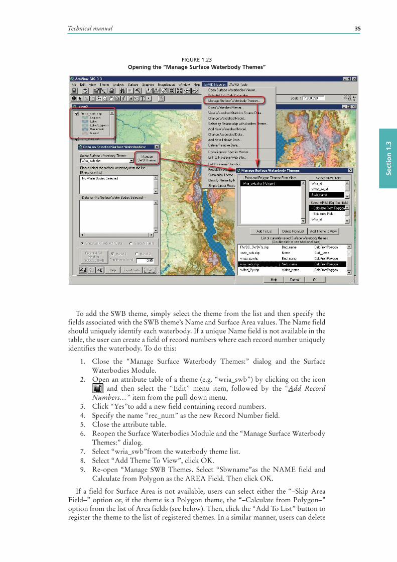
Technical manual 35
Sect
ion
1.3
FIGURE 1.23Opening the “Manage Surface Waterbody Themes”
To add the SWB theme , simply select the theme from the list and then specify the fields associated with the SWB theme’s Name and Surface Area values. The Name field should uniquely identify each waterbody. If a unique Name field is not available in the table, the user can create a field of record numbers where each record number uniquely identifies the waterbody. To do this:
1. Close the “Manage Surface Waterbody Themes:” dialog and the Surface Waterbodies Module.
2. Open an attribute table of a theme (e.g. “wria_swb”) by clicking on the icon and then select the “Edit” menu item, followed by the “Add Record
Numbers…” item from the pull-down menu. 3. Click “Yes”to add a new field containing record numbers.4. Specify the name “rec_num” as the new Record Number field.5. Close the attribute table.6. Reopen the Surface Waterbodies Module and the “Manage Surface Waterbody
Themes:” dialog.7. Select “wria_swb”from the waterbody theme list.8. Select “Add Theme To View”, click OK.9. Re-open “Manage SWB Themes. Select “Sbwname”as the NAME field and
Calculate from Polygon as the AREA Field. Then click OK.
If a field for Surface Area is not available, users can select either the “–Skip Area Field–” option or, if the theme is a Polygon theme, the “–Calculate from Polygon–” option from the list of Area fields (see below). Then, click the “Add To List” button to register the theme to the list of registered themes. In a similar manner, users can delete
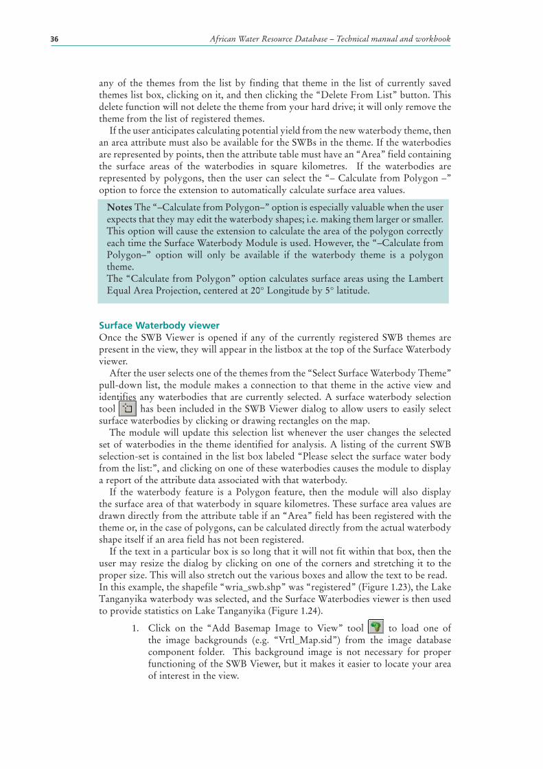
African Water Resource Database – Technical manual and workbook36
any of the themes from the list by finding that theme in the list of currently saved themes list box, clicking on it, and then clicking the “Delete From List” button. This delete function will not delete the theme from your hard drive; it will only remove the theme from the list of registered themes.
If the user anticipates calculating potential yield from the new waterbody theme , then an area attribute must also be available for the SWBs in the theme. If the waterbodies are represented by points, then the attribute table must have an “Area” field containing the surface areas of the waterbodies in square kilometres. If the waterbodies are represented by polygons, then the user can select the “– Calculate from Polygon –” option to force the extension to automatically calculate surface area values.
Notes The “–Calculate from Polygon–” option is especially valuable when the user expects that they may edit the waterbody shapes; i.e. making them larger or smaller. This option will cause the extension to calculate the area of the polygon correctly each time the Surface Waterbody Module is used. However, the “–Calculate from Polygon–” option will only be available if the waterbody theme is a polygon theme. The “Calculate from Polygon” option calculates surface areas using the Lambert Equal Area Projection, centered at 20° Longitude by 5° latitude.
Surface Waterbody viewerOnce the SWB Viewer is opened if any of the currently registered SWB themes are present in the view, they will appear in the listbox at the top of the Surface Waterbody viewer.
After the user selects one of the themes from the “Select Surface Waterbody Theme” pull-down list, the module makes a connection to that theme in the active view and identifies any waterbodies that are currently selected. A surface waterbody selection tool has been included in the SWB Viewer dialog to allow users to easily select surface waterbodies by clicking or drawing rectangles on the map.
The module will update this selection list whenever the user changes the selected set of waterbodies in the theme identified for analysis. A listing of the current SWB selection-set is contained in the list box labeled “Please select the surface water bod y from the list:”, and clicking on one of these waterbodies causes the module to display a report of the attribute data associated with that waterbody.
If the waterbody feature is a Polygon feature, then the module will also display the surface area of that waterbody in square kilometres. These surface area values are drawn directly from the attribute table if an “Area” field has been registered with the theme or, in the case of polygons, can be calculated directly from the actual waterbody shape itself if an area field has not been registered.
If the text in a particular box is so long that it will not fit within that box, then the user may resize the dialog by clicking on one of the corners and stretching it to the proper size. This will also stretch out the various boxes and allow the text to be read. In this example, the shapefile “wria_swb.shp” was “registered” (Figure 1.23), the Lake Tanganyika waterbody was selected, and the Surface Waterbodies viewer is then used to provide statistics on Lake Tanganyika (Figure 1.24).
1. Click on the “Add Basemap Image to View” tool to load one of the image backgrounds (e.g. “Vrtl_Map.sid”) from the image database component folder. This background image is not necessary for proper functioning of the SWB Viewer, but it makes it easier to locate your area of interest in the view.
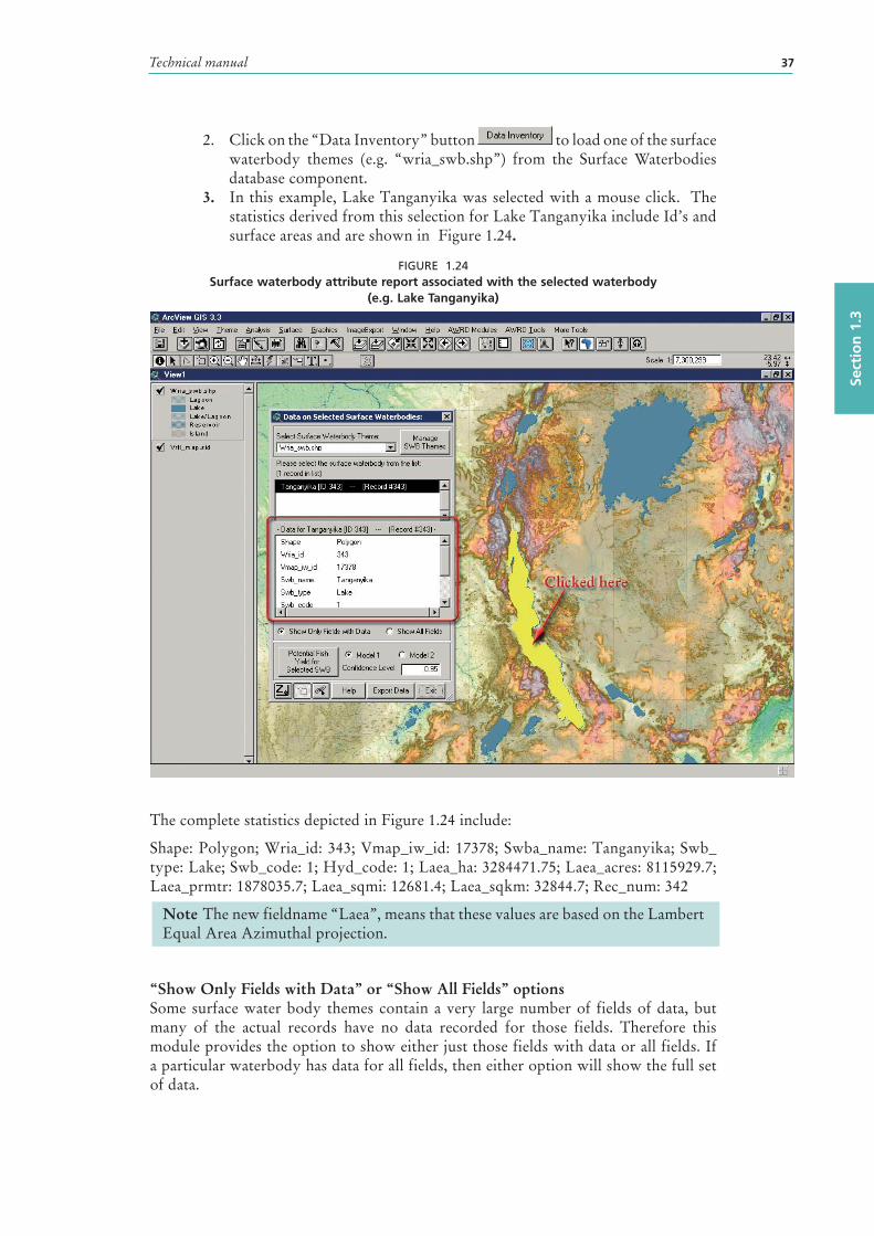
Technical manual 37
Sect
ion
1.3
2. Click on the “Data Inventory” button to load one of the surface waterbody themes (e.g. “wria_swb.shp”) from the Surface Waterbodies database component.
3. In this example, Lake Tanganyika was selected with a mouse click. The statistics derived from this selection for Lake Tanganyika include Id’s and surface areas and are shown in Figure 1.24.
FIGURE 1.24Surface waterbody attribute report associated with the selected waterbody
(e.g. Lake Tanganyika)
The complete statistics depicted in Figure 1.24 include:
Shape: Polygon; Wria_id: 343; Vmap_iw_id: 17378; Swba_name: Tanganyika; Swb_type: Lake; Swb_code: 1; Hyd_code: 1; Laea_ha: 3284471.75; Laea_acres: 8115929.7; Laea_prmtr: 1878035.7; Laea_sqmi: 12681.4; Laea_sqkm: 32844.7; Rec_num: 342
Note The new fieldname “Laea”, means that these values are based on the Lambert Equal Area Azimuthal projection.
“Show Only Fields with Data” or “Show All Fields” options Some surface water bod y themes contain a very large number of fields of data, but many of the actual records have no data recorded for those fields. Therefore this module provides the option to show either just those fields with data or all fields. If a particular waterbody has data for all fields, then either option will show the full set of data.
African Water Resource Database – Technical manual and workbook38
Export Data If one or more surface water bod ies are currently selected, then a user may export those records to a new table by clicking on the “Export Data” button . During any export, the user will be prompted to specify where to save the data and the module will then generate a new table based on only those selected waterbodies. If the selected SWBs are polygon features, then the module will also generate surface area values (in square kilometres) for each of the waterbodies.
1. With at least one surface waterbody selected, click the “Export Data” button on the SWB Viewer dialog.
2. Type a name for file you are exporting and then select a location to store it in your hard drive. Click “OK”. After any data have been exported to a new table, that new table will automatically be added to the ArcView project (Figure 1.25).
FIGURE 1.25Saving the new Export Table in an ArcView Project
Report GeoStats for surface waterbodies polygon themesDue to the tight integration of tool-sets between the modules of the AWRD, users can also access tools which may have applications outside of a particular module. One such tool is the Report GeoStats tool , which reports geostatistics for any active SWB Polygon theme in a view, when the user clicks on any SWB polygon on the map.
Users can calculate or update the area values for any polygon theme using also the “Calculate/Update GeoStats in Polygon Themes Tables…” option in the AWRD
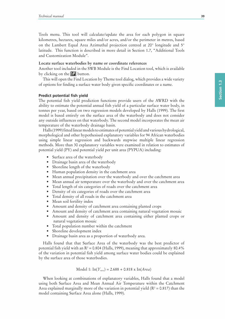
Technical manual 39
Sect
ion
1.3
Tools menu. This tool will calculate/update the area for each polygon in square kilometres, hectares, square miles and/or acres, and/or the perimeter in metres, based on the Lambert Equal Area Azimuthal projection centred at 20° longitude and 5° latitude. This function is described in more detail in Section 1.7, “Additional Tools and Customization Module”.
Locate surface waterbodies by name or coordinate references Another tool included in the SWB Module is the Find Location tool, which is available by clicking on the button.
This will open the Find Location by Theme tool dialog, which provides a wide variety of options for finding a surface water bod y given specific coordinates or a name.
Predict potential fish yieldThe potential fish yield prediction functions provide users of the AWRD with the ability to estimate the potential annual fish yield of a particular surface water bod y , in tonnes per year, based on two regression models developed by Halls (1999). The first model is based entirely on the surface area of the waterbody and does not consider any outside influences on that waterbody. The second model incorporates the mean air temperature of the waterbody drainage basin .
Halls (1999) fitted linear models to estimates of potential yield and various hydrological, morphological and other hypothesised explanatory variables for 94 African waterbodies using simple linear regression and backwards stepwise multiple linear regression methods. More than 30 explanatory variables were examined in relation to estimates of potential yield (PY) and potential yield per unit area (PYPUA) including:
• Surface area of the waterbody• Drainage basin area of the waterbody• Shoreline length of the waterbody• Human population density in the catchment area• Mean annual precipitation over the waterbody and over the catchment area• Mean annual air temperature over the waterbody and over the catchment area• Total length of six categories of roads over the catchment area• Density of six categories of roads over the catchment area• Total density of all roads in the catchment area• Mean soil fertility index• Amount and density of catchment area containing planted crops• Amount and density of catchment area containing natural vegetation mosaic• Amount and density of catchment area containing either planted crops or
natural vegetation mosaic• Total population number within the catchment• Shoreline development index• Drainage basin area as a proportion of waterbody area.
Halls found that that Surface Area of the waterbody was the best predictor of potential fish yield with an R2 = 0.804 (Halls, 1999), meaning that approximately 80.4% of the variation in potential fish yield among surface water bod ies could be explained by the surface area of those waterbodies.
Model 1: In(Ynew) = 2.688 + 0.818 x In(Area)
When looking at combinations of explanatory variables, Halls found that a model using both Surface Area and Mean Annual Air Temperature within the Catchment Area explained marginally more of the variation in potential yield (R2 = 0.817) than the model containing Surface Area alone (Halls, 1999).
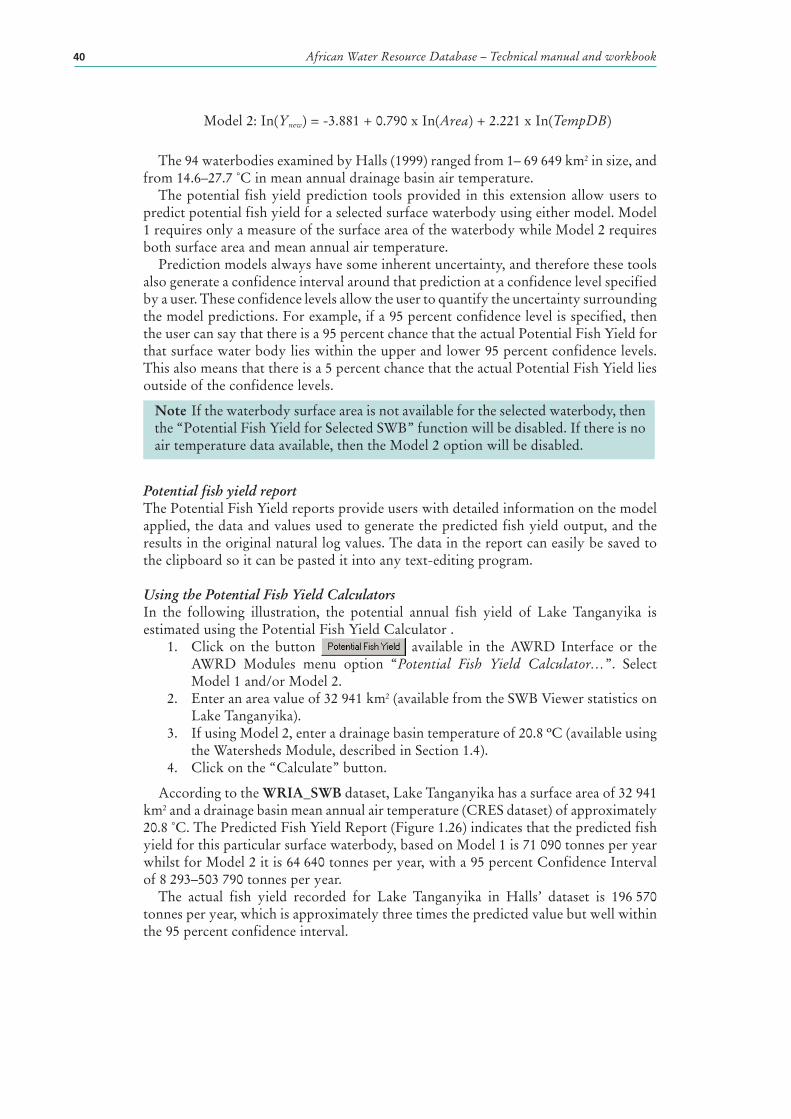
African Water Resource Database – Technical manual and workbook40
Model 2: In(Ynew) = -3.881 + 0.790 x In(Area) + 2.221 x In(TempDB)
The 94 waterbodies examined by Halls (1999) ranged from 1– 69 649 km2 in size, and from 14.6–27.7 ˚C in mean annual drainage basin air temperature .
The potential fish yield prediction tools provided in this extension allow users to predict potential fish yield for a selected surface waterbod y using either model . Model 1 requires only a measure of the surface area of the waterbody while Model 2 requires both surface area and mean annual air temperature .
Prediction models always have some inherent uncertainty, and therefore these tools also generate a confidence interval around that prediction at a confidence level specified by a user. These confidence levels allow the user to quantify the uncertainty surrounding the model predictions. For example, if a 95 percent confidence level is specified, then the user can say that there is a 95 percent chance that the actual Potential Fish Yield for that surface water bod y lies within the upper and lower 95 percent confidence levels. This also means that there is a 5 percent chance that the actual Potential Fish Yield lies outside of the confidence levels.
Note If the waterbody surface area is not available for the selected waterbody, then the “Potential Fish Yield for Selected SWB” function will be disabled. If there is no air temperature data available, then the Model 2 option will be disabled.
Potential fish yield report The Potential Fish Yield reports provide users with detailed information on the model applied, the data and values used to generate the predicted fish yield output, and the results in the original natural log values. The data in the report can easily be saved to the clipboard so it can be pasted it into any text-editing program.
Using the Potential Fish Yield CalculatorsIn the following illustration, the potential annual fish yield of Lake Tanganyika is estimated using the Potential Fish Yield Calculator .
1. Click on the button available in the AWRD Interface or the AWRD Modules menu option “Potential Fish Yield Calculator…”. Select Model 1 and/or Model 2.
2. Enter an area value of 32 941 km2 (available from the SWB Viewer statistics on Lake Tanganyika).
3. If using Model 2, enter a drainage basin temperature of 20.8 ºC (available using the Watersheds Module, described in Section 1.4).
4. Click on the “Calculate” button.
According to the WRIA_SWB dataset, Lake Tanganyika has a surface area of 32 941 km2 and a drainage basin mean annual air temperature (CRES dataset) of approximately 20.8 ˚C. The Predicted Fish Yield Report (Figure 1.26) indicates that the predicted fish yield for this particular surface waterbod y , based on Model 1 is 71 090 tonnes per year whilst for Model 2 it is 64 640 tonnes per year, with a 95 percent Confidence Interval of 8 293–503 790 tonnes per year.
The actual fish yield recorded for Lake Tanganyika in Halls ’ dataset is 196 570 tonnes per year, which is approximately three times the predicted value but well within the 95 percent confidence interval .
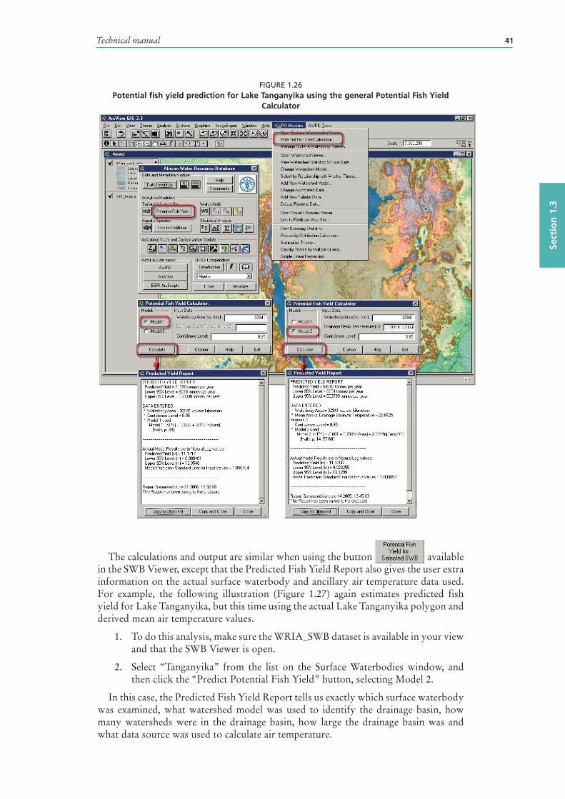
Technical manual 41
Sect
ion
1.3
FIGURE 1.26Potential fish yield prediction for Lake Tanganyika using the general Potential Fish Yield
Calculator
The calculations and output are similar when using the button available in the SWB Viewer, except that the Predicted Fish Yield Report also gives the user extra information on the actual surface waterbod y and ancillary air temperature data used. For example, the following illustration (Figure 1.27) again estimates predicted fish yield for Lake Tanganyika , but this time using the actual Lake Tanganyika polygon and derived mean air temperature values.
1. To do this analysis, make sure the WRIA_SWB dataset is available in your view and that the SWB Viewer is open.
2. Select “Tanganyika” from the list on the Surface Waterbodies window, and then click the “Predict Potential Fish Yield” button, selecting Model 2.
In this case, the Predicted Fish Yield Report tells us exactly which surface waterbod y was examined, what watershed model was used to identify the drainage basin , how many watersheds were in the drainage basin , how large the drainage basin was and what data source was used to calculate air temperature .
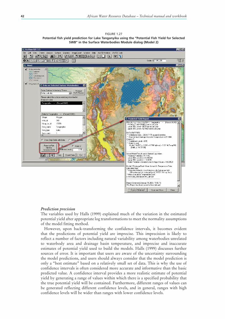
African Water Resource Database – Technical manual and workbook42
FIGURE 1.27Potential fish yield prediction for Lake Tanganyika using the “Potential Fish Yield for Selected
SWB” in the Surface Waterbodies Module dialog (Model 2)
Prediction precisionThe variables used by Halls (1999) explained much of the variation in the estimated potential yield after appropriate log transformations to meet the normality assumptions of the model fitting method.
However, upon back-transforming the confidence interval s, it becomes evident that the predictions of potential yield are imprecise. This imprecision is likely to reflect a number of factors including natural variability among waterbodies unrelated to waterbody area and drainage basin temperature , and imprecise and inaccurate estimates of potential yield used to build the models. Halls (1999) discusses further sources of error. It is important that users are aware of the uncertainty surrounding the model predictions, and users should always consider that the model prediction is only a “best estimate” based on a relatively small set of data. This is why the use of confidence interval s is often considered more accurate and informative than the basic predicted value. A confidence interval provides a more realistic estimate of potential yield by generating a range of values within which there is a specified probability that the true potential yield will be contained. Furthermore, different ranges of values can be generated reflecting different confidence level s, and in general, ranges with high confidence levels will be wider than ranges with lower confidence levels.
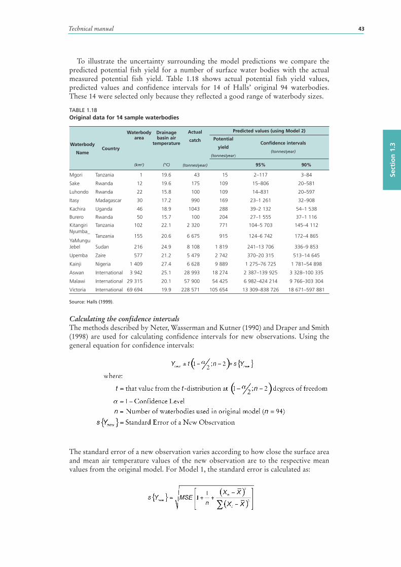
Technical manual 43
Sect
ion
1.3
To illustrate the uncertainty surrounding the model predictions we compare the predicted potential fish yield for a number of surface water bod ies with the actual measured potential fish yield. Table 1.18 shows actual potential fish yield values, predicted values and confidence interval s for 14 of Halls’ original 94 waterbodies. These 14 were selected only because they reflected a good range of waterbody sizes.
TABLE 1.18Original data for 14 sample waterbodies
Waterbody
NameCountry
Waterbody area
(km2)
Drainage basin air
temperature
(°C)
Actual
catch
(tonnes/year)
Predicted values (using Model 2)
Potential
yield
(tonnes/year)
Confidence intervals
(tonnes/year)
95% 90%
Mgori Tanzania 1 19.6 43 15 2–117 3–84
Sake Rwanda 12 19.6 175 109 15–806 20–581
Luhondo Rwanda 22 15.8 100 109 14–831 20–597
Itasy Madagascar 30 17.2 990 169 23–1 261 32–908
Kachira Uganda 46 18.9 1043 288 39–2 132 54–1 538
Burero Rwanda 50 15.7 100 204 27–1 555 37–1 116
Kitangiri Tanzania 102 22.1 2 320 771 104–5 703 145–4 112Nyumba_
YaMunguTanzania 155 20.6 6 675 915 124–6 742 172–4 865
Jebel Sudan 216 24.9 8 108 1 819 241–13 706 336–9 853
Upemba Zaire 577 21.2 5 479 2 742 370–20 315 513–14 645
Kainji Nigeria 1 409 27.4 6 628 9 889 1 275–76 725 1 781–54 898
Aswan International 3 942 25.1 28 993 18 274 2 387–139 925 3 328–100 335
Malawi International 29 315 20.1 57 900 54 425 6 982–424 214 9 766–303 304
Victoria International 69 694 19.9 228 571 105 654 13 309–838 726 18 671–597 881
Source: Halls (1999).
Calculating the confidence intervalsThe methods described by Neter, Wasserman and Kutner (1990) and Draper and Smith (1998) are used for calculating confidence interval s for new observations. Using the general equation for confidence intervals:
The standard error of a new observation varies according to how close the surface area and mean air temperature values of the new observation are to the respective mean values from the original model . For Model 1, the standard error is calculated as:
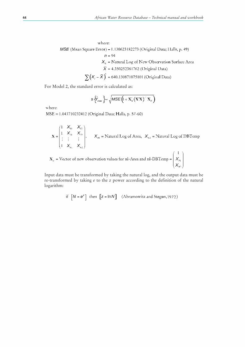
African Water Resource Database – Technical manual and workbook44
For Model 2, the standard error is calculated as:
Input data must be transformed by taking the natural log, and the output data must be re-transformed by taking e to the z power according to the definition of the natural logarithm:
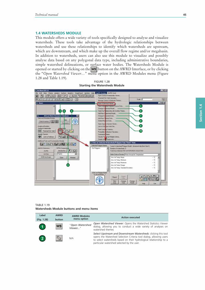
Technical manual 45
Sect
ion
1.4
1.4 WATERSHEDS MODULEThis module offers a wide variety of tools specifically designed to analyse and visualize watersheds. These tools take advantage of the hydrologic relationships between watersheds and use these relationships to identify which watersheds are upstream , which are downstream , and which make up the overall flow regime and/or megabasin . In addition to watersheds, users can also use this module to visualize and possibly analyse data based on any polygonal data type, including administrative boundaries, simple watershed delineations, or surface water bod ies. The Watersheds Module is opened or started by clicking on the button on the AWRD Interface, or by clicking the “Open Watershed Viewer…” menu option in the AWRD Modules menu (Figure 1.28 and Table 1.19).
FIGURE 1.28Starting the Watersheds Module
TABLE 1.19Watersheds Module buttons and menu items
Label
(Fig. 1.28)
AWRD
buttonAWRD Modules
menu option Action executed
“Open Watershed Viewer...”
Open Watershed Viewer: Opens the Watershed Statistics Viewer dialog, allowing you to conduct a wide variety of analyses on watershed themes
N/A
Select Upstream and Downstream Watersheds: clicking this tool opens the Watershed Selection Criteria tool dialog, allowing users to select watersheds based on their hydrological relationship to a particular watershed selected by the user.
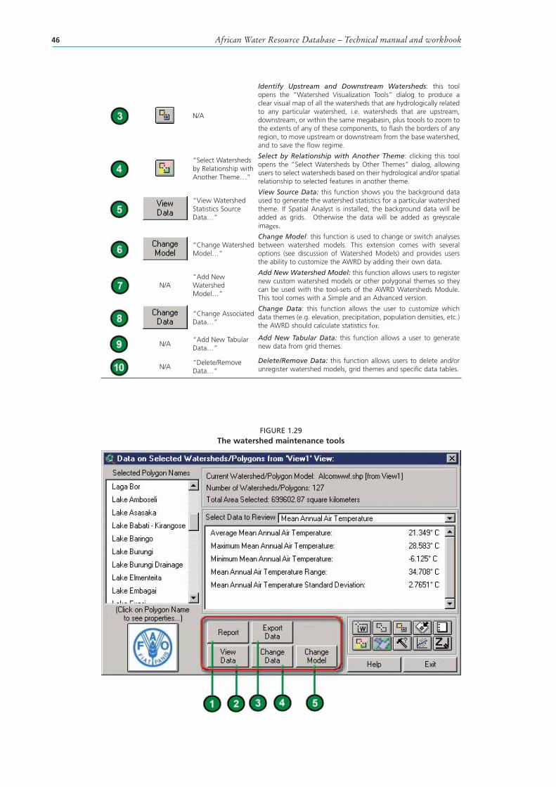
African Water Resource Database – Technical manual and workbook46
N/A
Identify Upstream and Downstream Watersheds: this tool opens the “Watershed Visualization Tools” dialog to produce a clear visual map of all the watersheds that are hydrologically related to any particular watershed , i.e. watersheds that are upstream, downstream, or within the same megabasin, plus toools to zoom to the extents of any of these components, to flash the borders of any region, to move upstream or downstream from the base watershed, and to save the flow regime.
“Select Watersheds by Relationship with Another Theme…”
Select by Relationship with Another Theme: clicking this tool opens the “Select Watersheds by Other Themes” dialog, allowing users to select watersheds based on their hydrological and/or spatial relationship to selected features in another theme.
“View Watershed Statistics Source Data…”
View Source Data: this function shows you the background data used to generate the watershed statistics for a particular watershed theme. If Spatial Analyst is installed, the background data will be added as grids. Otherwise the data will be added as greyscale images.
“Change Watershed Model…”
Change Model: this function is used to change or switch analyses between watershed models. This extension comes with several options (see discussion of Watershed Models) and provides users the ability to customize the AWRD by adding their own data.
N/A“Add New Watershed Model…”
Add New Watershed Model: this function allows users to register new custom watershed models or other polygonal themes so they can be used with the tool-sets of the AWRD Watersheds Module. This tool comes with a Simple and an Advanced version.
“Change Associated Data…”
Change Data: this function allows the user to customize which data themes (e.g. elevation, precipitation, population densities, etc.) the AWRD should calculate statistics for.
N/A“Add New Tabular Data…”
Add New Tabular Data: this function allows a user to generate new data from grid themes.
N/A“Delete/Remove Data…”
Delete/Remove Data: this function allows users to delete and/or unregister watershed models, grid themes and specific data tables.
FIGURE 1.29The watershed maintenance tools
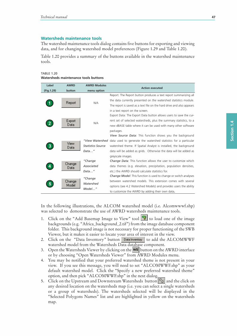
Technical manual 47
Sect
ion
1.4
Watersheds maintenance toolsThe watershed maintenance tools dialog contains five buttons for exporting and viewing data, and for changing watershed model preferences (Figure 1.29 and Table 1.20).
Table 1.20 provides a summary of the buttons available in the watershed maintenance tools.
TABLE 1.20Watersheds maintenance tools buttons
Label
(Fig.1.29)
AWRD
button
AWRD Modules
menu optionAction executed
N/A
Report: The Report button produces a text report summarizing all
the data currently presented on the watershed statistics module.
The report is saved as a text file on the hard drive and also appears
in a text report on the screen.
N/A
Export Data: The Export Data button allows users to save the cur-
rent set of selected watersheds, plus the summary statistics, to a
new dBASE table where it can be used with many other software
packages.
“View Watershed
Statistics Source
Data…”
View Source Data: This function shows you the background
data used to generate the watershed statistics for a particular
watershed theme. If Spatial Analyst is installed, the background
data will be added as grids. Otherwise the data will be added as
greyscale images.
“Change
Associated
Data…”
Change Data: This function allows the user to customize which
data themes (e.g. elevation, precipitation, population densities,
etc.) the AWRD should calculate statistics for.
“Change
Watershed
Model…”
Change Model: This function is used to change or switch analyses
between watershed models. This extension comes with several
options (see 4.2 Watershed Models) and provides users the ability
to customize the AWRD by adding their own data.
In the following illustrations, the ALCOM watershed model (i.e. Alcomwwwf.shp) was selected to demonstrate the use of AWRD watersheds maintenance tools.
1. Click on the “Add Basemap Image to View” tool to load one of the image backgrounds (e.g. “Africa_background_2.tif”) from the image database component folder. This background image is not necessary for proper functioning of the SWB Viewer, but it makes it easier to locate your area of interest in the view.
2. Click on the “Data Inventory” button to add the ALCOMWWF watershed model from the Watersheds Data database component.
3. Open the Watersheds Viewer by clicking on the button on the AWRD interface or by choosing “Open Watersheds Viewer” from AWRD Modules menu.
4. You may be notified that your preferred watershed theme is not present in your view. If you see this message, you will need to set “ALCOMWWF.shp” as your default watershed model. Click the “Specify a new preferred watershed theme” option, and then pick “ALCOMWWF.shp” in the next dialog.
5. Click on the Upstream and Downstream Watersheds button and the click on any desired location on the watersheds map (i.e. you can select a single watersheds or a group of watersheds). The watersheds selected will be displayed in the “Selected Polygons Names” list and are highlighted in yellow on the watersheds map.
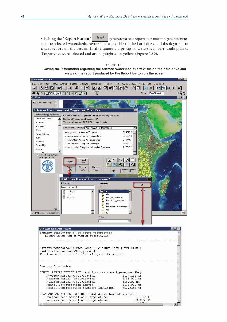
African Water Resource Database – Technical manual and workbook48
Clicking the “Report Button” generates a text report summarizing the statistics for the selected watersheds, saving it as a text file on the hard drive and displaying it in a text report on the screen. In this example a group of watersheds surrounding Lake Tanganyika were selected and are highlighted in yellow (Figure 1.30).
FIGURE 1.30Saving the information regarding the selected watershed as a text file on the hard drive and
viewing the report produced by the Report button on the screen
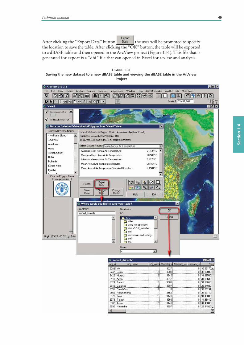
Technical manual 49
Sect
ion
1.4
After clicking the “Export Data” button the user will be prompted to specify the location to save the table. After clicking the “OK” button, the table will be exported to a dBASE table and then opened in the ArcView project (Figure 1.31). This file that is generated for export is a “dbf” file that can opened in Excel for review and analysis.
FIGURE 1.31Saving the new dataset to a new dBASE table and viewing the dBASE table in the ArcView
Project
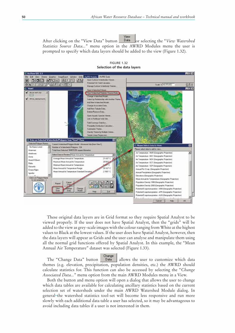
African Water Resource Database – Technical manual and workbook50
After clicking on the “View Data” button or selecting the “View Watershed Statistics Source Data...” menu option in the AWRD Modules menu the user is prompted to specify which data layers should be added to the view (Figure 1.32).
FIGURE 1.32Selection of the data layers
These original data layers are in Grid format so they require Spatial Analyst to be viewed properly. If the user does not have Spatial Analyst, then the “grids” will be added to the view as grey-scale images with the colour ranging from White at the highest values to Black at the lowest values. If the user does have Spatial Analyst, however, then the data layers will appear as Grids and the user can analyse and manipulate them using all the normal grid functions offered by Spatial Analyst. In this example, the “Mean Annual Air Temperature” dataset was selected (Figure 1.33).
The “Change Data” button allows the user to customize which data themes (e.g. elevation , precipitation , population densities, etc.) the AWRD should calculate statistics for. This function can also be accessed by selecting the “Change Associated Data...” menu option from the main AWRD Modules menu in a View.
Both the button and menu option will open a dialog that allows the user to change which data tables are available for calculating ancillary statistics based on the current selection set of watersheds under the main AWRD Watershed Module dialog. In general the watershed statistics tool-set will become less responsive and run more slowly with each additional data table a user has selected, so it may be advantageous to avoid including data tables if a user is not interested in them.
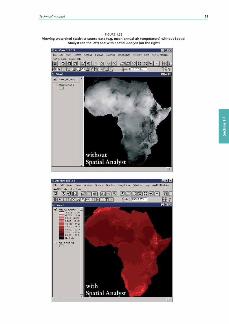
Technical manual 51
Sect
ion
1.4
FIGURE 1.33Viewing watershed statistics source data (e.g. mean annual air temperature) without Spatial
Analyst (on the left) and with Spatial Analyst (on the right)
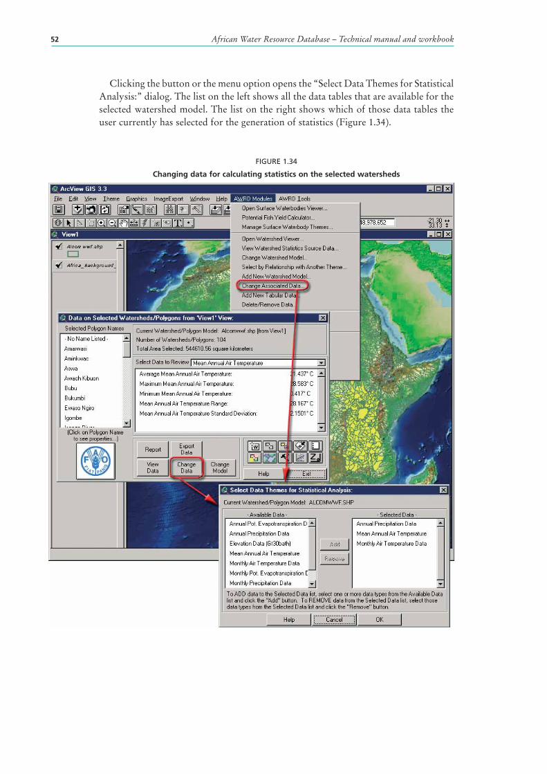
African Water Resource Database – Technical manual and workbook52
Clicking the button or the menu option opens the “Select Data Themes for Statistical Analysis:” dialog. The list on the left shows all the data tables that are available for the selected watershed model . The list on the right shows which of those data tables the user currently has selected for the generation of statistics (Figure 1.34).
FIGURE 1.34
Changing data for calculating statistics on the selected watersheds
Technical manual 53
Sect
ion
1.4
The user may add to the data tables selected by clicking on any or all of the items in the “–Available Data–” list and clicking the “Add” button. These items will immediately appear in the “–Selected Data–” list.
Similarly, a user may remove any selected data tables by selecting any or all of them from the “–Selected Data–” list and clicking the “Remove” button. Hitting the “Remove” button here does not delete the data, but rather simply tells the Watershed Statistics Module not to calculate statistics for those data. If the user wants to truly delete any of these data, then the “Delete/Remove Data…” menu option must be used. The user must hit the “OK” button to apply any changes.
The “Change Model” button allows the user to change or switch analyses between watershed models. The AWRD currently has three complex watershed models and two simple watershed delineations “registered” with the interface. This extension comes with several options and provides users the ability to customize the AWRD by adding their own data.
The custom menus and dialogs associated with the Change WS Model function provide the means whereby watershed or other data layers can be “registered” for analysis using the AWRD. Many of the watershed and data analysis tools available in the AWRD are designed to function only if a properly encoded WS model is available. Three such models are provided with the AWRD, along with a default set of core elevation and sample climatological data layers so that the base statistical functions are enabled. However, only one WS model may be analysed at a time, and these Watershed Model Maintenance Tools provide users with the means to change the default WS model, add new watershed models, add new data layers, change processing preferences and modify which analytical layers are examined, and lastly, to remove data from consideration.
The statistical data for the watersheds (e.g. elevation , precipitation , air temperature , water temperature and population densities) are derived from Grid datasets. In order for a particular grid of data to be useful for a particular watershed model , we must conduct statistical analyses on the grid to determine the relevant statistics for each watershed in the model. These statistics are then saved to a table, and this table is joined to the watershed model when the Watershed Statistics Viewer is opened. The Watershed Statistics Viewer works by checking the current selection of watersheds and then looking up the associated statistical data from the data tables, then calculating overall statistics based on the data for each watershed and the sizes of those watersheds.
This extension is designed to enable users to switch among a variety of watershed models or to add additional watershed models and then generate statistical data. Because the statistical data are drawn from Grid themes, users must have ESRI’s Spatial Analyst extension in order to revise or generate new statistical data. However, because the relevant summary tables have already been generated from the GTopo30 baseline elevation layer and the sample climatological data layers for each of the three WS models currently registered in the AWRD, even users lacking access to Spatial Analyst will be able to fully utilize the AWRD tool-sets.
This function can be also accessed selecting the “Change Watershed Model…” menu option from the main AWRD Modules menu, which opens the “Select Desired Watershed/Polygon Model and Data:” dialog (Figure 1.35).
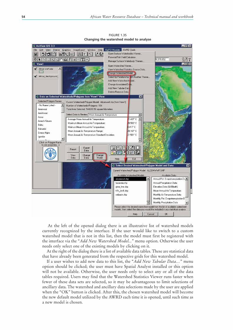
African Water Resource Database – Technical manual and workbook54
FIGURE 1.35Changing the watershed model to analyse
At the left of the opened dialog there is an illustrative list of watershed models currently recognized by the interface. If the user would like to switch to a custom watershed model that is not in this list, then the model must first be registered with the interface via the “Add New Watershed Model...” menu option. Otherwise the user needs only select one of the existing models by clicking on it.
At the right of the dialog there is a list of available data tables. These are statistical data that have already been generated from the respective grids for this watershed model .
If a user wishes to add new data to this list, the “Add New Tabular Data…” menu option should be clicked; the user must have Spatial Analyst installed or this option will not be available. Otherwise, the user needs only to select any or all of the data tables required. Users may find that the Watershed Statistics Viewer runs faster when fewer of these data sets are selected, so it may be advantageous to limit selections of ancillary data. The watershed and ancillary data selections made by the user are applied when the “OK” button is clicked. After this, the chosen watershed model will become the new default model utilized by the AWRD each time it is opened, until such time as a new model is chosen.
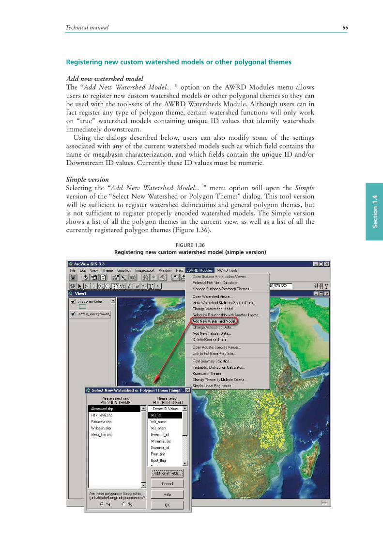
Technical manual 55
Sect
ion
1.4
Registering new custom watershed models or other polygonal themes
Add new watershed model The “Add New Watershed Model... ” option on the AWRD Modules menu allows users to register new custom watershed models or other polygonal themes so they can be used with the tool-sets of the AWRD Watersheds Module. Although users can in fact register any type of polygon theme , certain watershed functions will only work on “true” watershed models containing unique ID values that identify watersheds immediately downstream .
Using the dialogs described below, users can also modify some of the settings associated with any of the current watershed models such as which field contains the name or megabasin characterization, and which fields contain the unique ID and/or Downstream ID values. Currently these ID values must be numeric.
Simple versionSelecting the “Add New Watershed Model... ” menu option will open the Simple version of the “Select New Watershed or Polygon Theme:” dialog. This tool version will be sufficient to register watershed delineations and general polygon themes, but is not sufficient to register properly encoded watershed models. The Simple version shows a list of all the polygon themes in the current view, as well as a list of all the currently registered polygon themes (Figure 1.36).
FIGURE 1.36Registering new custom watershed model (simple version)
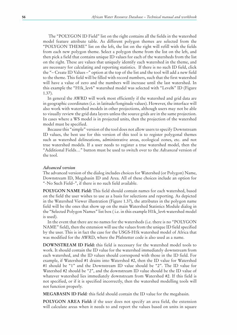
African Water Resource Database – Technical manual and workbook56
The “POLYGON ID Field” list on the right contains all the fields in the watershed model feature attribute table. As different polygon themes are selected from the “POLYGON THEME” list on the left, the list on the right will refill with the fields from each new polygon theme . Select a polygon theme from the list on the left, and then pick a field that contains unique ID values for each of the watersheds from the list on the right. These are values that uniquely identify each watershed in the theme, and are necessary for calculating and reporting statistics. If there is no such ID field, click the “– Create ID Values –” option at the top of the list and the tool will add a new field to the theme. This field will be filled with record numbers, such that the first watershed will have a value of zero and the numbers will increase until the last watershed. In this example the “H1k_lev6” watershed model was selected with “Level6” ID (Figure 1.37).
In general the AWRD will work most efficiently if the watershed and grid data are in geographic coordinates (i.e. in latitude/longitude values). However, the interface will also work with watershed models in other projections, although users may not be able to visually review the grid data layers unless the source grids are in the same projection . In cases where a WS model is in projected units, then the projection of the watershed model must be specified.
Because this “simple” version of the tool does not allow users to specify Downstream ID values, the best use for this version of this tool is to register polygonal themes such as watershed delineations, administrative areas, ecological zones, etc. and not true watershed models. If a user needs to register a true watershed model , then the “Additional Fields…” button must be used to switch over to the Advanced version of the tool.
Advanced version The advanced version of the dialog includes choices for Watershed (or Polygon) Name, Downstream ID, Megabasin ID and Area. All of these choices include an option for “-No Such Field–”, if there is no such field available.
POLYGON NAME Field: This field should contain names for each watershed , based on the field the user wishes to use as a basis for selections and reporting. As depicted in the Watershed Viewer illustration (Figure 1.37), the attributes in the polygon name field will be the ones that show up on the main Watershed Statistics Module dialog in the “Selected Polygon Names” list box ( i.e. in this example H1k_lev6 watershed model is used).
In the event that there are no names for the watersheds (i.e. there is no “POLYGON NAME” field) , then the extension will use the values from the unique ID field specified by the user. This is in fact the case for the USGS-H1k watershed model of Africa that was modified for the AWRD, where the Pfafstetter code is also used as a name.
DOWNSTREAM ID Field: this field is necessary for the watershed model tools to work. It should contain the ID value for the watershed immediately downstream from each watershed, and the ID values should correspond with those in the ID field. For example, if Watershed #1 drains into Watershed #2, then the ID value for Watershed #1 should be “1” and the Downstream ID value should be “2”. The ID value for Watershed #2 should be “2”, and the downstream ID value should be the ID value of whatever watershed lies immediately downstream from Watershed #2. If this field is not specified, or if it is specified incorrectly, then the watershed modelling tools will not function properly.
MEGABASIN ID Field: this field should contain the ID value for the megabasin.
POLYGON AREA Field: if the user does not specify an area field, the extension will calculate areas when it needs to and report the values based on units in square
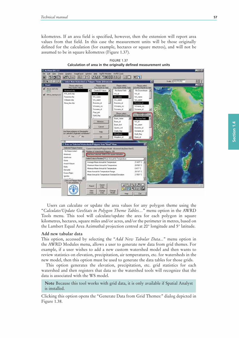
Technical manual 57
Sect
ion
1.4
kilometres. If an area field is specified, however, then the extension will report area values from that field. In this case the measurement units will be those originally defined for the calculation (for example, hectares or square metres), and will not be assumed to be in square kilometres (Figure 1.37).
FIGURE 1.37Calculation of area in the originally defined measurement units
Users can calculate or update the area values for any polygon theme using the “Calculate/Update GeoStats in Polygon Theme Tables…” menu option in the AWRD Tools menu. This tool will calculate/update the area for each polygon in square kilometres, hectares, square miles and/or acres, and/or the perimeter in metres, based on the Lambert Equal Area Azimuthal projection centred at 20° longitude and 5° latitude.
Add new tabular dataThis option, accessed by selecting the “Add New Tabular Data...” menu option in the AWRD Modules menu, allows a user to generate new data from grid themes. For example, if a user wishes to add a new custom watershed model and then wants to review statistics on elevation , precipitation , air temperatures, etc. for watersheds in the new model, then this option must be used to generate the data tables for those grids.
This option generates the elevation, precipitation, etc. grid statistics for each watershed and then registers that data so the watershed tools will recognize that the data is associated with the WS model.
Note Because this tool works with grid data, it is only available if Spatial Analyst is installed.
Clicking this option opens the “Generate Data from Grid Themes:” dialog depicted in Figure 1.38.
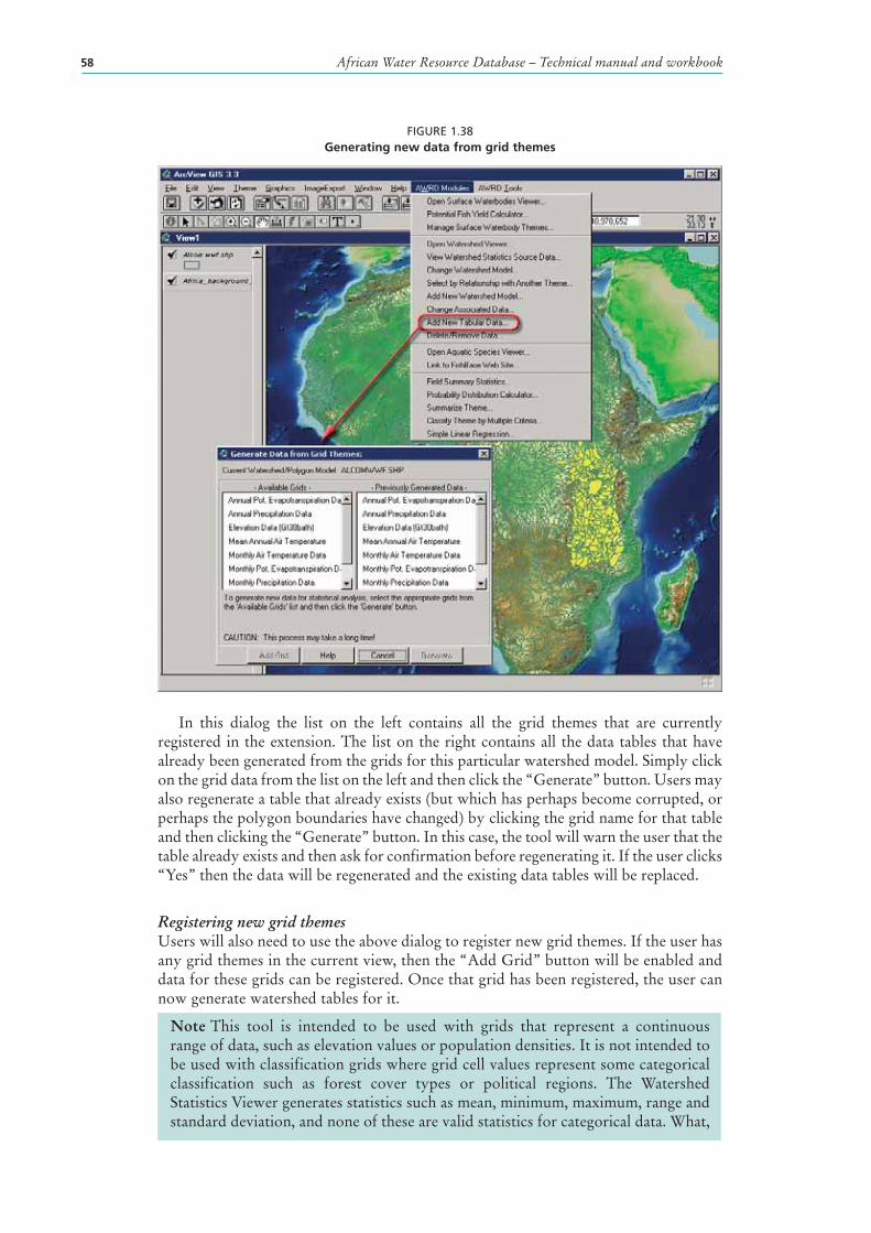
African Water Resource Database – Technical manual and workbook58
FIGURE 1.38Generating new data from grid themes
In this dialog the list on the left contains all the grid themes that are currently registered in the extension. The list on the right contains all the data tables that have already been generated from the grids for this particular watershed model . Simply click on the grid data from the list on the left and then click the “Generate” button. Users may also regenerate a table that already exists (but which has perhaps become corrupted, or perhaps the polygon boundaries have changed) by clicking the grid name for that table and then clicking the “Generate” button. In this case, the tool will warn the user that the table already exists and then ask for confirmation before regenerating it. If the user clicks “Yes” then the data will be regenerated and the existing data tables will be replaced.
Registering new grid themesUsers will also need to use the above dialog to register new grid themes. If the user has any grid themes in the current view, then the “Add Grid” button will be enabled and data for these grids can be registered. Once that grid has been registered, the user can now generate watershed tables for it.
Note This tool is intended to be used with grids that represent a continuous range of data, such as elevation values or population densities. It is not intended to be used with classification grids where grid cell values represent some categoricalclassification such as forest cover types or political regions. The Watershed Statistics Viewer generates statistics such as mean , minimum , maximum , range and standard deviation, and none of these are valid statistics for categorical data. What,
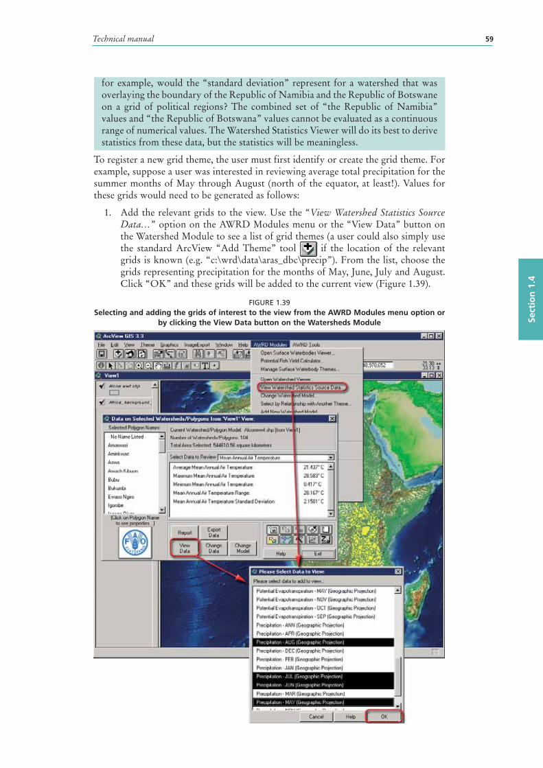
Technical manual 59
Sect
ion
1.4
for example, would the “standard deviation” represent for a watershed that was overlaying the boundary of the Republic of Namibia and the Republic of Botswane on a grid of political regions? The combined set of “the Republic of Namibia” values and “the Republic of Botswana” values cannot be evaluated as a continuous range of numerical values. The Watershed Statistics Viewer will do its best to derive statistics from these data, but the statistics will be meaningless.
To register a new grid theme , the user must first identify or create the grid theme. For example, suppose a user was interested in reviewing average total precipitation for the summer months of May through August (north of the equator, at least!). Values for these grids would need to be generated as follows:
1. Add the relevant grids to the view. Use the “View Watershed Statistics Source Data…” option on the AWRD Modules menu or the “View Data” button on the Watershed Module to see a list of grid themes (a user could also simply use the standard ArcView “Add Theme” tool if the location of the relevant grids is known (e.g. “c:\wrd\data\aras_dbc\precip”). From the list, choose the grids representing precipitation for the months of May, June, July and August. Click “OK” and these grids will be added to the current view (Figure 1.39).
FIGURE 1.39Selecting and adding the grids of interest to the view from the AWRD Modules menu option or
by clicking the View Data button on the Watersheds Module
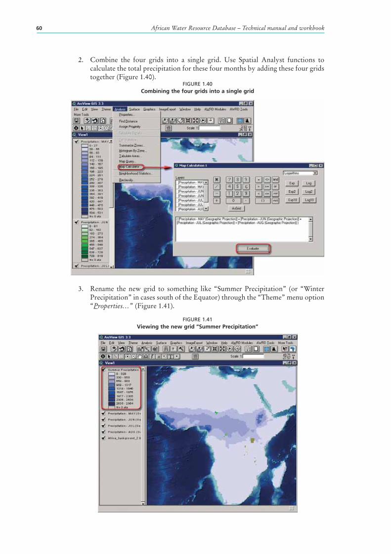
African Water Resource Database – Technical manual and workbook60
2. Combine the four grids into a single grid . Use Spatial Analyst functions to calculate the total precipitation for these four months by adding these four grids together (Figure 1.40).
FIGURE 1.40Combining the four grids into a single grid
3. Rename the new grid to something like “Summer Precipitation ” (or “Winter Precipitation” in cases south of the Equator) through the “Theme” menu option “Properties…” (Figure 1.41).
FIGURE 1.41Viewing the new grid “Summer Precipitation”
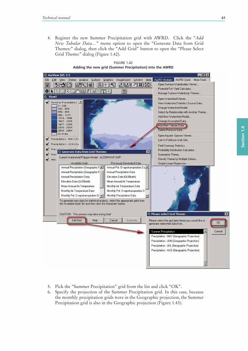
Technical manual 61
Sect
ion
1.4
4. Register the new Summer Precipitation grid with AWRD. Click the “Add New Tabular Data…” menu option to open the “Generate Data from Grid Themes:” dialog, then click the “Add Grid” button to open the “Please Select Grid Theme:” dialog (Figure 1.42).
FIGURE 1.42Adding the new grid (Summer Precipitation) into the AWRD
5. Pick the “Summer Precipitation” grid from the list and click “OK”.6. Specify the projection of the Summer Precipitation grid . In this case, because
the monthly precipitation grids were in the Geographic projection, the Summer Precipitation grid is also in the Geographic projection (Figure 1.43).
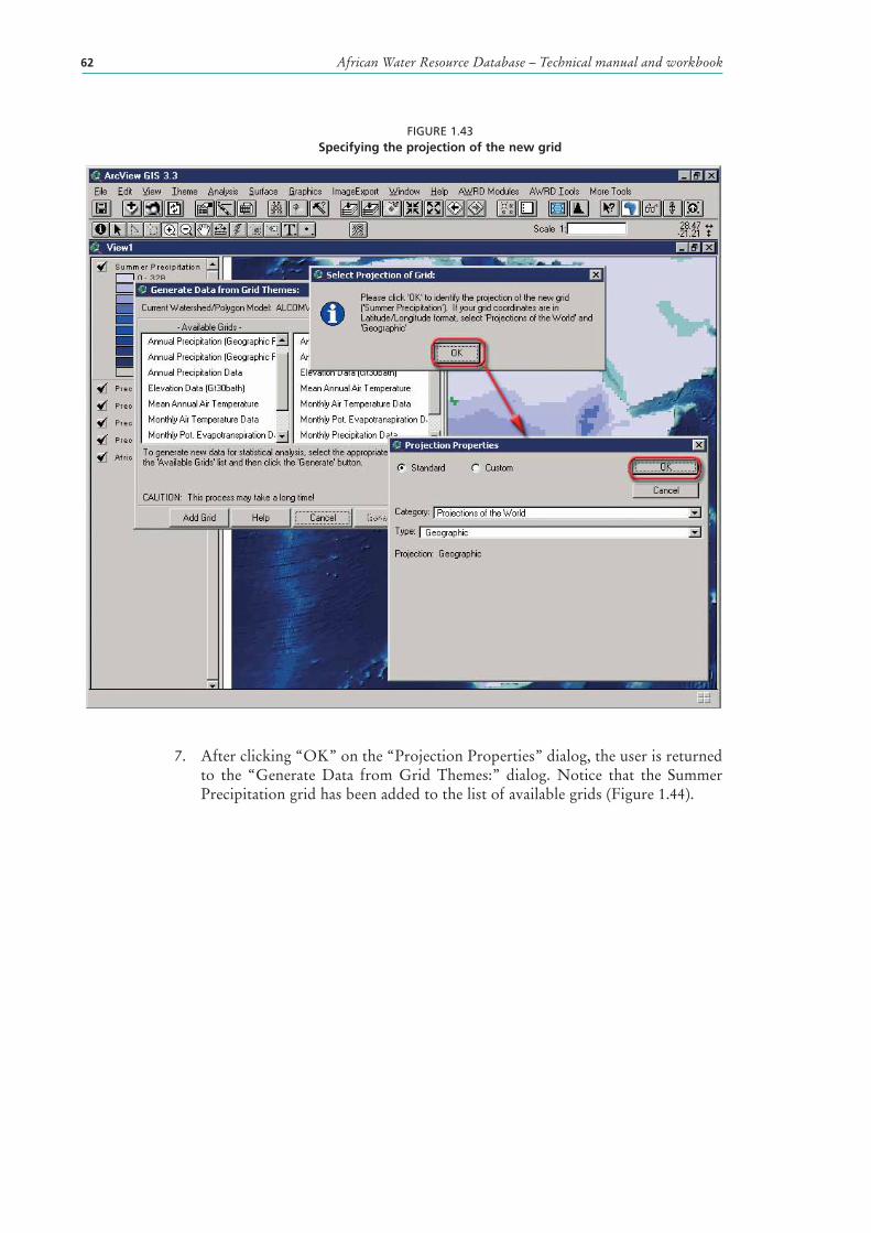
African Water Resource Database – Technical manual and workbook62
FIGURE 1.43Specifying the projection of the new grid
7. After clicking “OK” on the “Projection Properties” dialog, the user is returned to the “Generate Data from Grid Themes:” dialog. Notice that the Summer Precipitation grid has been added to the list of available grids (Figure 1.44).
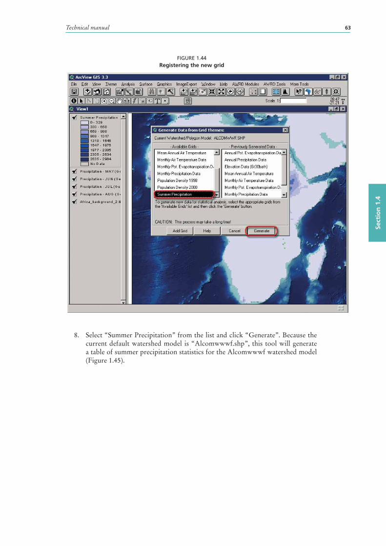
Technical manual 63
Sect
ion
1.4
FIGURE 1.44Registering the new grid
8. Select “Summer Precipitation” from the list and click “Generate”. Because the current default watershed model is “Alcomwwwf.shp”, this tool will generate a table of summer precipitation statistics for the Alcomwwwf watershed model (Figure 1.45).
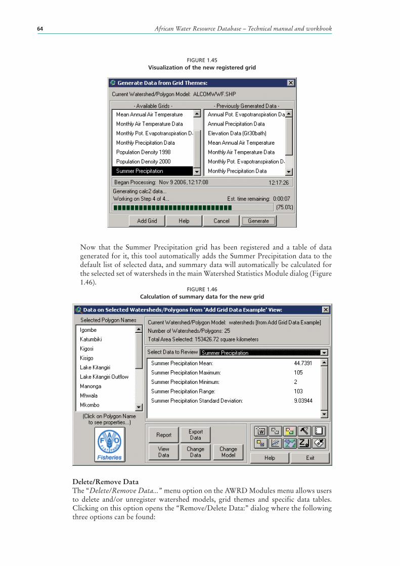
African Water Resource Database – Technical manual and workbook64
FIGURE 1.45Visualization of the new registered grid
Now that the Summer Precipitation grid has been registered and a table of data generated for it, this tool automatically adds the Summer Precipitation data to the default list of selected data, and summary data will automatically be calculated for the selected set of watersheds in the main Watershed Statistics Module dialog (Figure 1.46).
FIGURE 1.46Calculation of summary data for the new grid
Delete/Remove DataThe “Delete/Remove Data...” menu option on the AWRD Modules menu allows users to delete and/or unregister watershed models, grid themes and specific data tables. Clicking on this option opens the “Remove/Delete Data:” dialog where the following three options can be found:
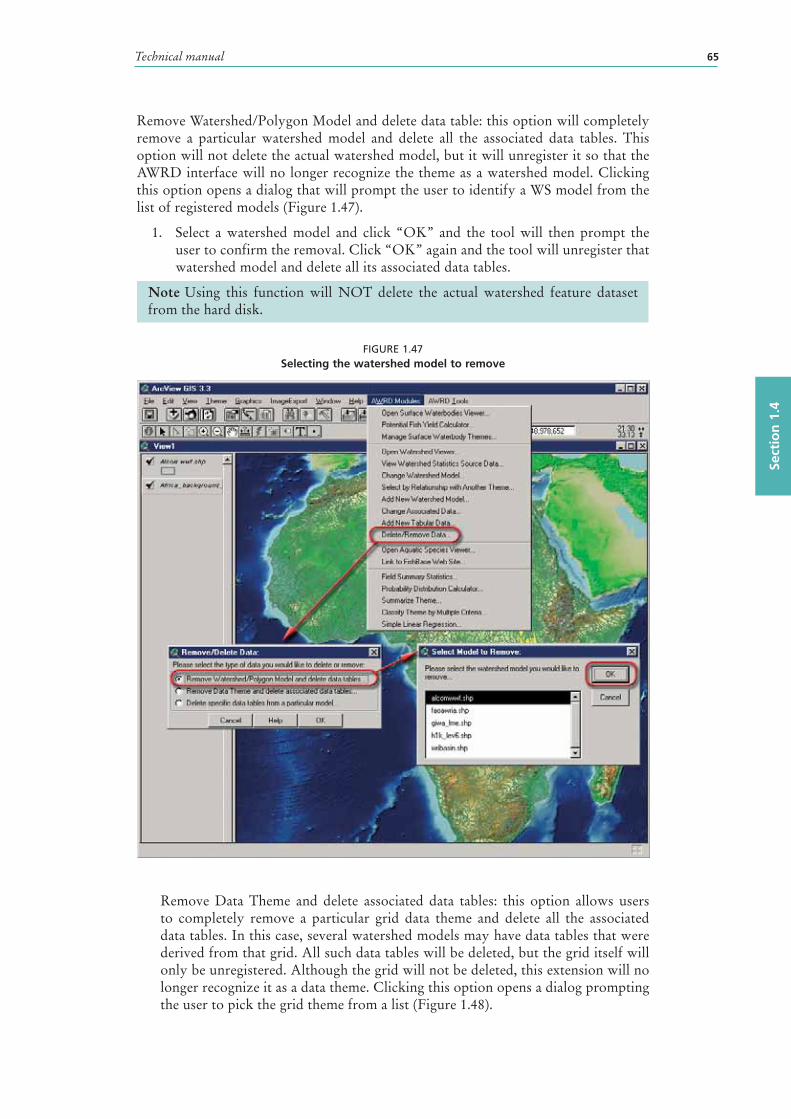
Technical manual 65
Sect
ion
1.4
Remove Watershed/Polygon Model and delete data table: this option will completely remove a particular watershed model and delete all the associated data tables. This option will not delete the actual watershed model, but it will unregister it so that the AWRD interface will no longer recognize the theme as a watershed model. Clicking this option opens a dialog that will prompt the user to identify a WS model from the list of registered models (Figure 1.47).
1. Select a watershed model and click “OK” and the tool will then prompt the user to confirm the removal. Click “OK” again and the tool will unregister that watershed model and delete all its associated data tables.
Note Using this function will NOT delete the actual watershed feature dataset from the hard disk.
FIGURE 1.47Selecting the watershed model to remove
Remove Data Theme and delete associated data tables: this option allows users to completely remove a particular grid data theme and delete all the associated data tables. In this case, several watershed models may have data tables that were derived from that grid. All such data tables will be deleted, but the grid itself will only be unregistered. Although the grid will not be deleted, this extension will no longer recognize it as a data theme. Clicking this option opens a dialog prompting the user to pick the grid theme from a list (Figure 1.48).
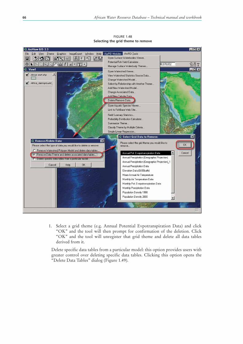
African Water Resource Database – Technical manual and workbook66
FIGURE 1.48Selecting the grid theme to remove
1. Select a grid theme (e.g. Annual Potential Evpotranspiration Data) and click “OK” and the tool will then prompt for confirmation of the deletion. Click “OK” and the tool will unregister that grid theme and delete all data tables derived from it.
Delete specific data tables from a particular model : this option provides users with greater control over deleting specific data tables. Clicking this option opens the “Delete Data Tables” dialog (Figure 1.49).
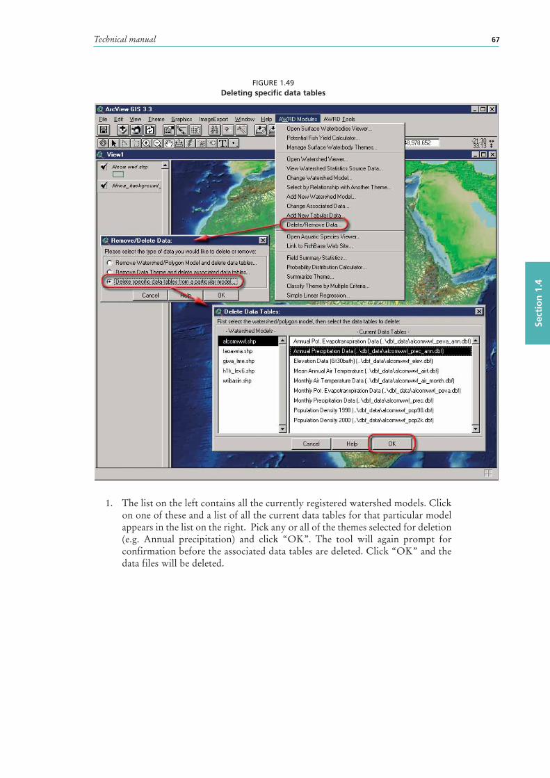
Technical manual 67
Sect
ion
1.4
FIGURE 1.49Deleting specific data tables
1. The list on the left contains all the currently registered watershed models. Click on one of these and a list of all the current data tables for that particular model appears in the list on the right. Pick any or all of the themes selected for deletion (e.g. Annual precipitation) and click “OK”. The tool will again prompt for confirmation before the associated data tables are deleted. Click “OK” and the data files will be deleted.
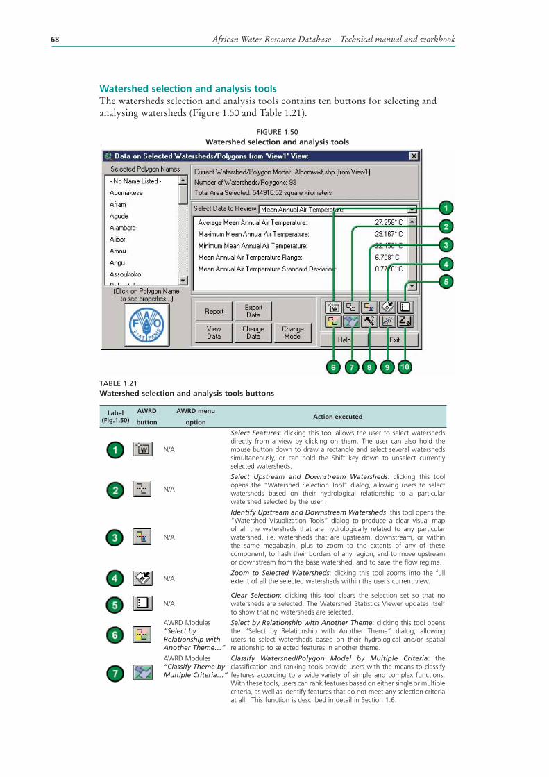
African Water Resource Database – Technical manual and workbook68
Watershed selection and analysis tools The watersheds selection and analysis tools contains ten buttons for selecting and analysing watersheds (Figure 1.50 and Table 1.21).
FIGURE 1.50Watershed selection and analysis tools
TABLE 1.21Watershed selection and analysis tools buttons
Label (Fig.1.50)
AWRD
button
AWRD menu
optionAction executed
N/A
Select Features: clicking this tool allows the user to select watersheds directly from a view by clicking on them. The user can also hold the mouse button down to draw a rectangle and select several watersheds simultaneously, or can hold the Shift key down to unselect currently selected watersheds.
N/A
Select Upstream and Downstream Watersheds: clicking this tool opens the “Watershed Selection Tool” dialog, allowing users to select watersheds based on their hydrological relationship to a particular watershed selected by the user.
N/A
Identify Upstream and Downstream Watersheds: this tool opens the “Watershed Visualization Tools” dialog to produce a clear visual map of all the watersheds that are hydrologically related to any particular watershed , i.e. watersheds that are upstream, downstream, or within the same megabasin, plus to zoom to the extents of any of these component, to flash their borders of any region, and to move upstream or downstream from the base watershed, and to save the flow regime.
N/AZoom to Selected Watersheds: clicking this tool zooms into the full extent of all the selected watersheds within the user’s current view.
N/AClear Selection: clicking this tool clears the selection set so that no watersheds are selected. The Watershed Statistics Viewer updates itself to show that no watersheds are selected.
AWRD Modules “Select by Relationship with Another Theme…”
Select by Relationship with Another Theme: clicking this tool opens the “Select by Relationship with Another Theme” dialog, allowing users to select watersheds based on their hydrological and/or spatial relationship to selected features in another theme.
AWRD Modules “Classify Theme by Multiple Criteria…”
Classify Watershed/Polygon Model by Multiple Criteria: the classification and ranking tools provide users with the means to classify features according to a wide variety of simple and complex functions. With these tools, users can rank features based on either single or multiple criteria, as well as identify features that do not meet any selection criteria at all. This function is described in detail in Section 1.6.
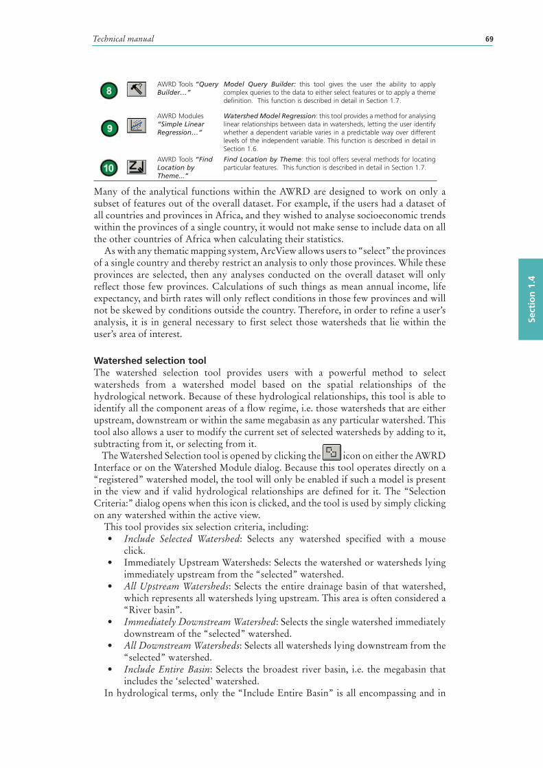
Technical manual 69
Sect
ion
1.4
AWRD Tools “Query Builder…”
Model Query Builder: this tool gives the user the ability to apply complex queries to the data to either select features or to apply a theme definition. This function is described in detail in Section 1.7.
AWRD Modules “Simple Linear Regression…”
Watershed Model Regression: this tool provides a method for analysing linear relationships between data in watersheds, letting the user identify whether a dependent variable varies in a predictable way over different levels of the independent variable. This function is described in detail in Section 1.6.
AWRD Tools “Find Location by Theme...”
Find Location by Theme: this tool offers several methods for locating particular features. This function is described in detail in Section 1.7.
Many of the analytical functions within the AWRD are designed to work on only a subset of features out of the overall dataset. For example, if the users had a dataset of all countries and provinces in Africa, and they wished to analyse socioeconomic trends within the provinces of a single country, it would not make sense to include data on all the other countries of Africa when calculating their statistics.
As with any thematic mapping system, ArcView allows users to “select” the provinces of a single country and thereby restrict an analysis to only those provinces. While these provinces are selected, then any analyses conducted on the overall dataset will only reflect those few provinces. Calculations of such things as mean annual income, life expectancy, and birth rates will only reflect conditions in those few provinces and will not be skewed by conditions outside the country. Therefore, in order to refine a user’s analysis, it is in general necessary to first select those watersheds that lie within the user’s area of interest.
Watershed selection toolThe watershed selection tool provides users with a powerful method to select watersheds from a watershed model based on the spatial relationships of the hydrological network. Because of these hydrological relationships, this tool is able to identify all the component areas of a flow regime, i.e. those watersheds that are either upstream , downstream or within the same megabasin as any particular watershed. This tool also allows a user to modify the current set of selected watersheds by adding to it, subtracting from it, or selecting from it.
The Watershed Selection tool is opened by clicking the icon on either the AWRD Interface or on the Watershed Module dialog. Because this tool operates directly on a “registered” watershed model , the tool will only be enabled if such a model is present in the view and if valid hydrological relationships are defined for it. The “Selection Criteria:” dialog opens when this icon is clicked, and the tool is used by simply clicking on any watershed within the active view.
This tool provides six selection criteria, including:• Include Selected Watershed: Selects any watershed specified with a mouse
click.• Immediately Upstream Watersheds: Selects the watershed or watersheds lying
immediately upstream from the “selected” watershed.• All Upstream Watersheds: Selects the entire drainage basin of that watershed ,
which represents all watersheds lying upstream . This area is often considered a “River basin”.
• Immediately Downstream Watershed: Selects the single watershed immediately downstream of the “selected” watershed.
• All Downstream Watersheds: Selects all watersheds lying downstream from the “selected” watershed .
• Include Entire Basin: Selects the broadest river basin , i.e. the megabasin that includes the ‘selected’ watershed .
In hydrological terms, only the “Include Entire Basin” is all encompassing and in
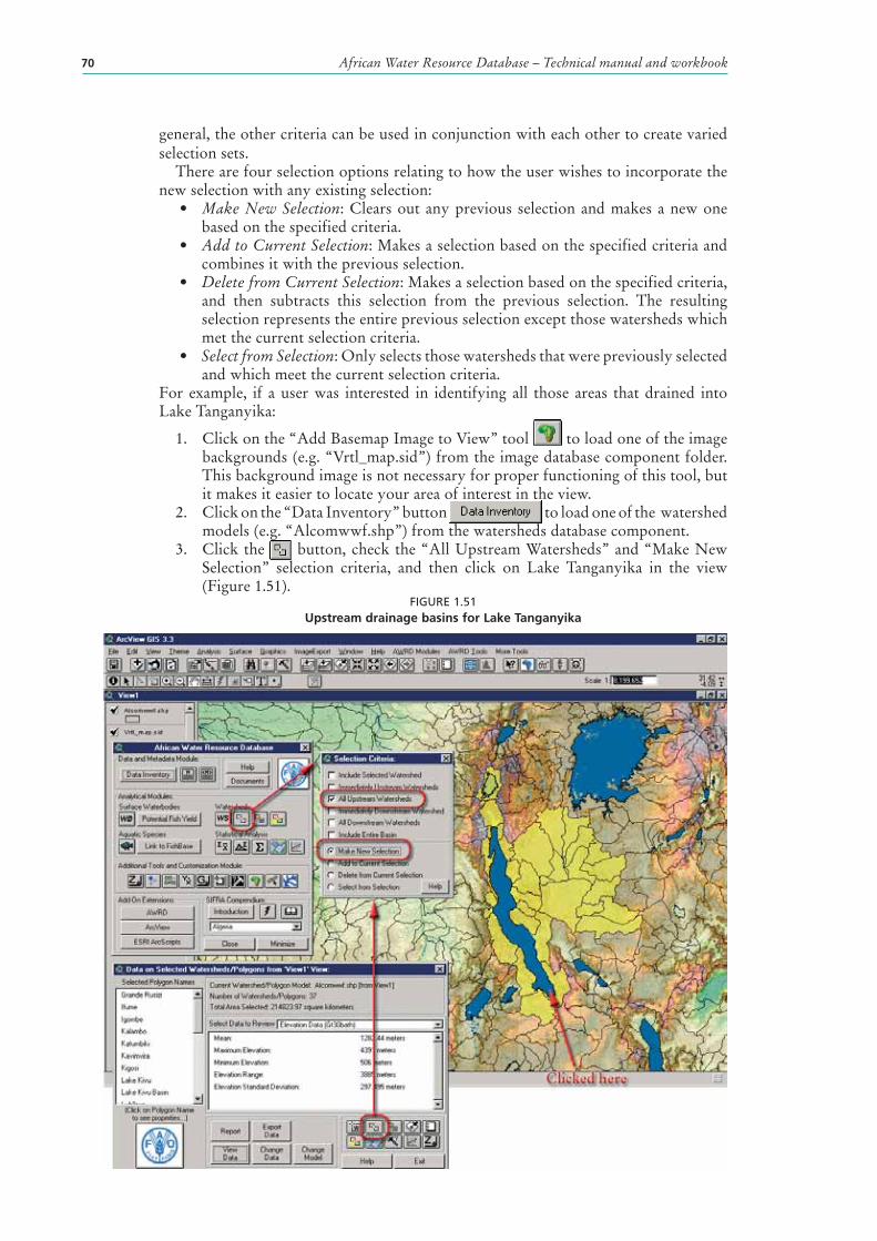
African Water Resource Database – Technical manual and workbook70
general, the other criteria can be used in conjunction with each other to create varied selection sets.
There are four selection options relating to how the user wishes to incorporate the new selection with any existing selection:
• Make New Selection: Clears out any previous selection and makes a new one based on the specified criteria.
• Add to Current Selection: Makes a selection based on the specified criteria and combines it with the previous selection.
• Delete from Current Selection: Makes a selection based on the specified criteria, and then subtracts this selection from the previous selection. The resulting selection represents the entire previous selection except those watersheds which met the current selection criteria.
• Select from Selection: Only selects those watersheds that were previously selected and which meet the current selection criteria.
For example, if a user was interested in identifying all those areas that drained into Lake Tanganyika :
1. Click on the “Add Basemap Image to View” tool to load one of the image backgrounds (e.g. “Vrtl_map.sid”) from the image database component folder. This background image is not necessary for proper functioning of this tool, but it makes it easier to locate your area of interest in the view.
2. Click on the “Data Inventory” button to load one of the watershed models (e.g. “Alcomwwf.shp”) from the watersheds database component.
3. Click the button, check the “All Upstream Watersheds” and “Make New Selection” selection criteria, and then click on Lake Tanganyika in the view (Figure 1.51).
FIGURE 1.51Upstream drainage basin s for Lake Tanganyika
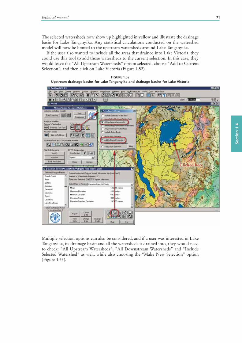
Technical manual 71
Sect
ion
1.4
The selected watersheds now show up highlighted in yellow and illustrate the drainage basin for Lake Tanganyika . Any statistical calculations conducted on the watershed model will now be limited to the upstream watersheds around Lake Tanganyika.
If the user also wanted to include all the areas that drained into Lake Victoria , they could use this tool to add those watersheds to the current selection . In this case, they would leave the “All Upstream Watersheds” option selected, choose “Add to Current Selection”, and then click on Lake Victoria (Figure 1.52).
FIGURE 1.52Upstream drainage basin s for Lake Tanganyika and drainage basins for Lake Victoria
Multiple selection options can also be considered, and if a user was interested in Lake Tanganyika , its drainage basin and all the watersheds it drained into, they would need to check: “All Upstream Watersheds”; “All Downstream Watersheds” and “Include Selected Watershed” as well, while also choosing the “Make New Selection” option (Figure 1.53).
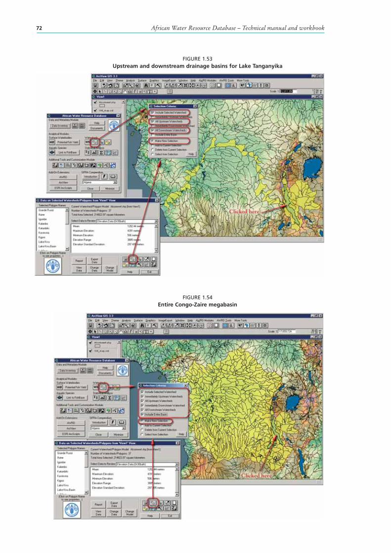
African Water Resource Database – Technical manual and workbook72
FIGURE 1.53Upstream and downstream drainage basin s for Lake Tanganyika
FIGURE 1.54Entire Congo-Zaire megabasin
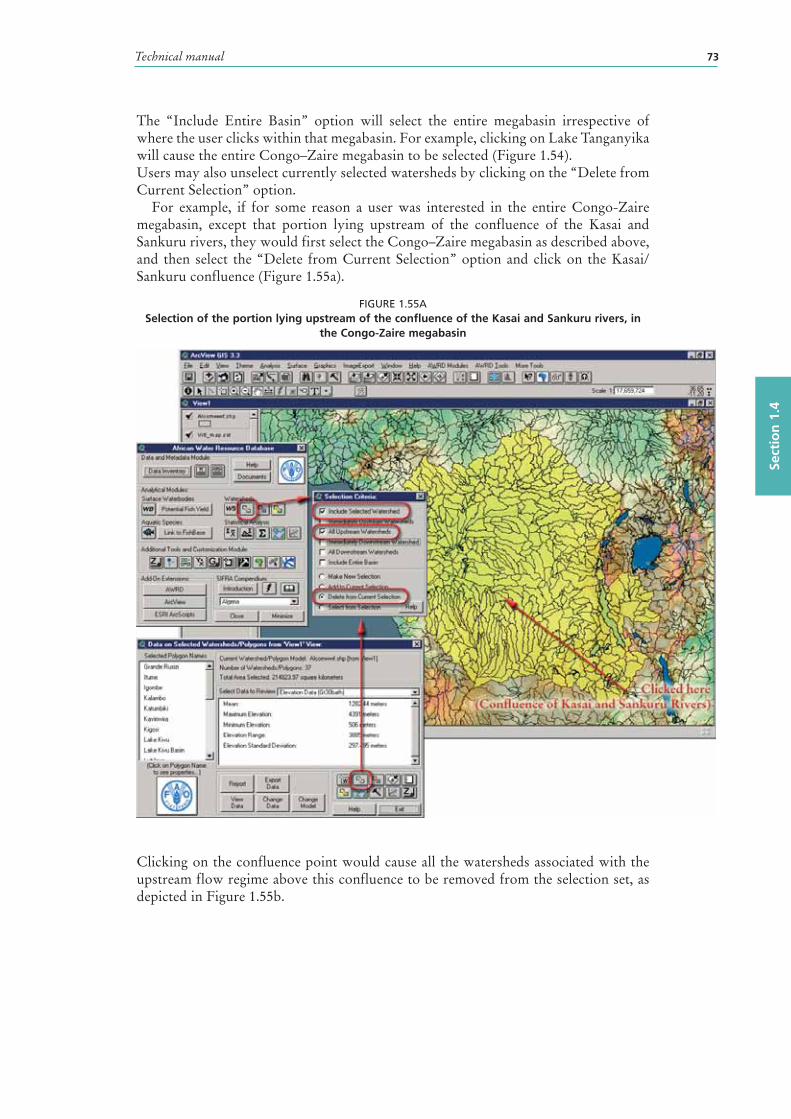
Technical manual 73
Sect
ion
1.4
The “Include Entire Basin” option will select the entire megabasin irrespective of where the user clicks within that megabasin. For example, clicking on Lake Tanganyika will cause the entire Congo–Zaire megabasin to be selected (Figure 1.54).Users may also unselect currently selected watersheds by clicking on the “Delete from Current Selection” option.
For example, if for some reason a user was interested in the entire Congo-Zaire megabasin , except that portion lying upstream of the confluence of the Kasai and Sankuru rivers, they would first select the Congo–Zaire megabasin as described above, and then select the “Delete from Current Selection” option and click on the Kasai/Sankuru confluence (Figure 1.55a).
FIGURE 1.55ASelection of the portion lying upstream of the confluence of the Kasai and Sankuru rivers, in
the Congo-Zaire megabasin
Clicking on the confluence point would cause all the watersheds associated with the upstream flow regime above this confluence to be removed from the selection set, as depicted in Figure 1.55b.
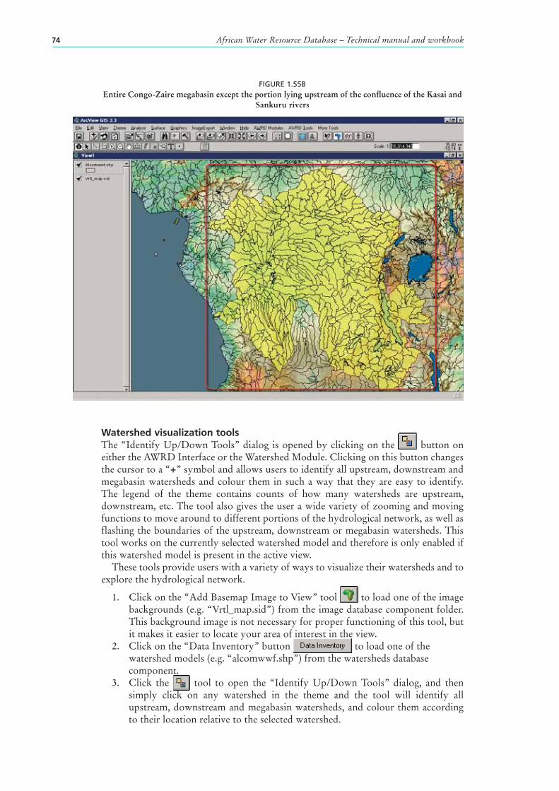
African Water Resource Database – Technical manual and workbook74
FIGURE 1.55BEntire Congo-Zaire megabasin except the portion lying upstream of the confluence of the Kasai and
Sankuru rivers
Watershed visualization tools The “Identify Up/Down Tools” dialog is opened by clicking on the button on either the AWRD Interface or the Watershed Module. Clicking on this button changes the cursor to a “+” symbol and allows users to identify all upstream , downstream and megabasin watersheds and colour them in such a way that they are easy to identify. The legend of the theme contains counts of how many watersheds are upstream, downstream, etc. The tool also gives the user a wide variety of zooming and moving functions to move around to different portions of the hydrological network, as well as flashing the boundaries of the upstream, downstream or megabasin watersheds. This tool works on the currently selected watershed model and therefore is only enabled if this watershed model is present in the active view.
These tools provide users with a variety of ways to visualize their watersheds and to explore the hydrological network.
1. Click on the “Add Basemap Image to View” tool to load one of the image backgrounds (e.g. “Vrtl_map.sid”) from the image database component folder. This background image is not necessary for proper functioning of this tool, but it makes it easier to locate your area of interest in the view.
2. Click on the “Data Inventory” button to load one of the watershed models (e.g. “alcomwwf.shp”) from the watersheds database component.
3. Click the tool to open the “Identify Up/Down Tools” dialog, and then simply click on any watershed in the theme and the tool will identify all upstream , downstream and megabasin watersheds, and colour them according to their location relative to the selected watershed.
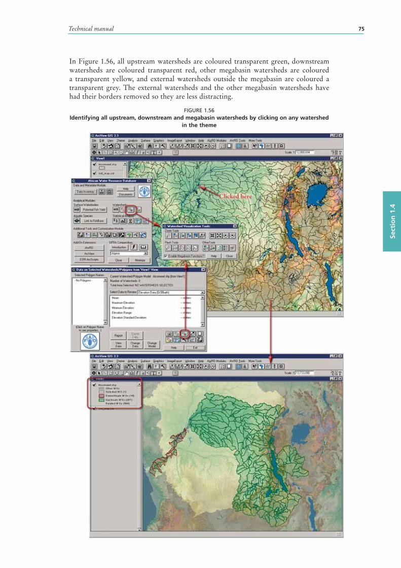
Technical manual 75
Sect
ion
1.4
In Figure 1.56, all upstream watersheds are coloured transparent green, downstream watersheds are coloured transparent red, other megabasin watersheds are coloured a transparent yellow, and external watersheds outside the megabasin are coloured a transparent grey. The external watersheds and the other megabasin watersheds have had their borders removed so they are less distracting.
FIGURE 1.56Identifying all upstream , downstream and megabasin watersheds by clicking on any watershed
in the theme
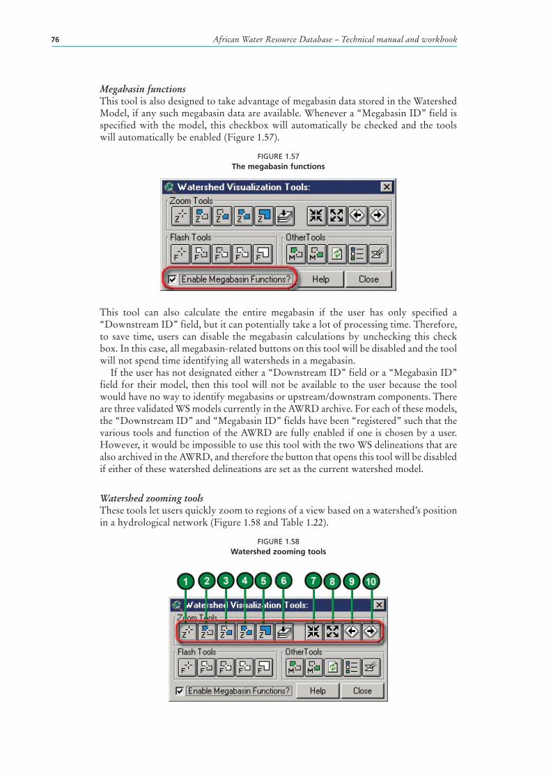
African Water Resource Database – Technical manual and workbook76
Megabasin functionsThis tool is also designed to take advantage of megabasin data stored in the Watershed Model, if any such megabasin data are available. Whenever a “Megabasin ID” field is specified with the model , this checkbox will automatically be checked and the tools will automatically be enabled (Figure 1.57).
FIGURE 1.57The megabasin functions
This tool can also calculate the entire megabasin if the user has only specified a “Downstream ID” field, but it can potentially take a lot of processing time. Therefore, to save time, users can disable the megabasin calculations by unchecking this check box. In this case, all megabasin-related buttons on this tool will be disabled and the tool will not spend time identifying all watersheds in a megabasin.
If the user has not designated either a “Downstream ID” field or a “Megabasin ID” field for their model , then this tool will not be available to the user because the tool would have no way to identify megabasins or upstream /downstram components. There are three validated WS models currently in the AWRD archive. For each of these models, the “Downstream ID” and “Megabasin ID” fields have been “registered” such that the various tools and function of the AWRD are fully enabled if one is chosen by a user. However, it would be impossible to use this tool with the two WS delineations that are also archived in the AWRD, and therefore the button that opens this tool will be disabled if either of these watershed delineations are set as the current watershed model.
Watershed zooming toolsThese tools let users quickly zoom to regions of a view based on a watershed ’s position in a hydrological network (Figure 1.58 and Table 1.22).
FIGURE 1.58Watershed zooming tools
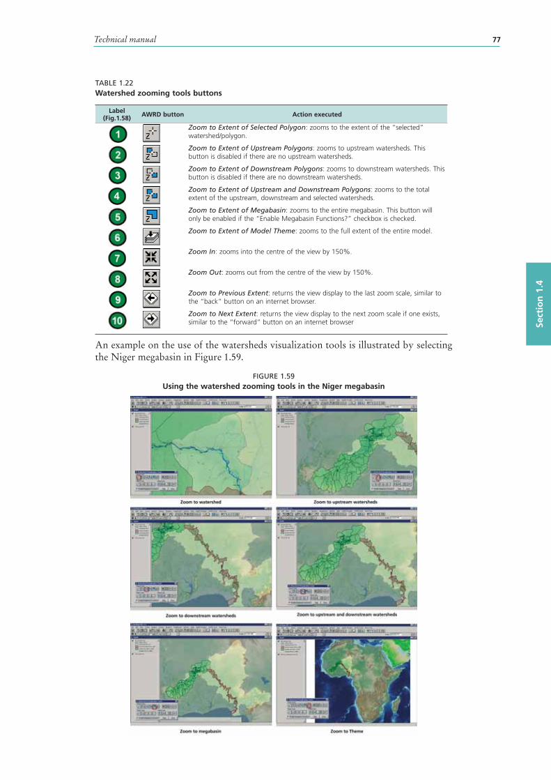
Technical manual 77
Sect
ion
1.4
TABLE 1.22Watershed zooming tools buttons
Label (Fig.1.58) AWRD button Action executed
Zoom to Extent of Selected Polygon: zooms to the extent of the “selected” watershed/ polygon.
Zoom to Extent of Upstream Polygons: zooms to upstream watersheds. This button is disabled if there are no upstream watersheds.
Zoom to Extent of Downstream Polygons: zooms to downstream watersheds. This button is disabled if there are no downstream watersheds.
Zoom to Extent of Upstream and Downstream Polygons: zooms to the total extent of the upstream, downstream and selected watersheds.
Zoom to Extent of Megabasin: zooms to the entire megabasin. This button will only be enabled if the “Enable Megabasin Functions?” checkbox is checked.
Zoom to Extent of Model Theme: zooms to the full extent of the entire model.
Zoom In: zooms into the centre of the view by 150%.
Zoom Out: zooms out from the centre of the view by 150%.
Zoom to Previous Extent: returns the view display to the last zoom scale, similar to the “back” button on an internet browser.
Zoom to Next Extent: returns the view display to the next zoom scale if one exists, similar to the “forward” button on an internet browser
An example on the use of the watersheds visualization tools is illustrated by selecting the Niger megabasin in Figure 1.59.
FIGURE 1.59Using the watershed zooming tools in the Niger megabasin
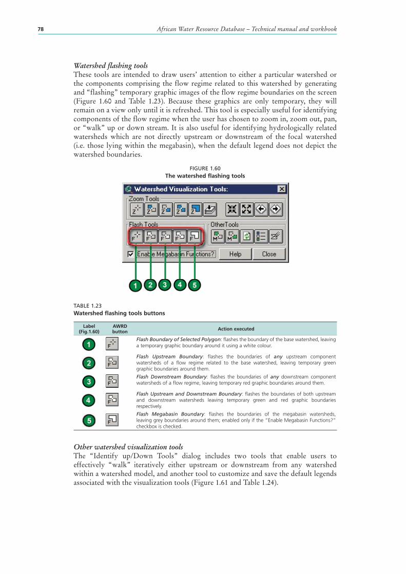
African Water Resource Database – Technical manual and workbook78
Watershed flashing toolsThese tools are intended to draw users’ attention to either a particular watershed or the components comprising the flow regime related to this watershed by generating and “flashing” temporary graphic images of the flow regime boundaries on the screen (Figure 1.60 and Table 1.23). Because these graphics are only temporary, they will remain on a view only until it is refreshed. This tool is especially useful for identifying components of the flow regime when the user has chosen to zoom in, zoom out, pan, or “walk” up or down stream. It is also useful for identifying hydrologically related watersheds which are not directly upstream or downstream of the focal watershed (i.e. those lying within the megabasin ), when the default legend does not depict the watershed boundaries.
FIGURE 1.60The watershed flashing tools
TABLE 1.23Watershed flashing tools buttons
Label (Fig.1.60)
AWRD button Action executed
Flash Boundary of Selected Polygon: flashes the boundary of the base watershed, leaving a temporary graphic boundary around it using a white colour.
Flash Upstream Boundary: flashes the boundaries of any upstream component watersheds of a flow regime related to the base watershed, leaving temporary green graphic boundaries around them.
Flash Downstream Boundary: flashes the boundaries of any downstream component watersheds of a flow regime, leaving temporary red graphic boundaries around them.
Flash Upstream and Downstream Boundary: flashes the boundaries of both upstream and downstream watersheds leaving temporary green and red graphic boundaries respectively.
Flash Megabasin Boundary: flashes the boundaries of the megabasin watersheds, leaving grey boundaries around them; enabled only if the “Enable Megabasin Functions?” checkbox is checked.
Other watershed visualization toolsThe “Identify up/Down Tools” dialog includes two tools that enable users to effectively “walk” iteratively either upstream or downstream from any watershed within a watershed model , and another tool to customize and save the default legends associated with the visualization tools (Figure 1.61 and Table 1.24).
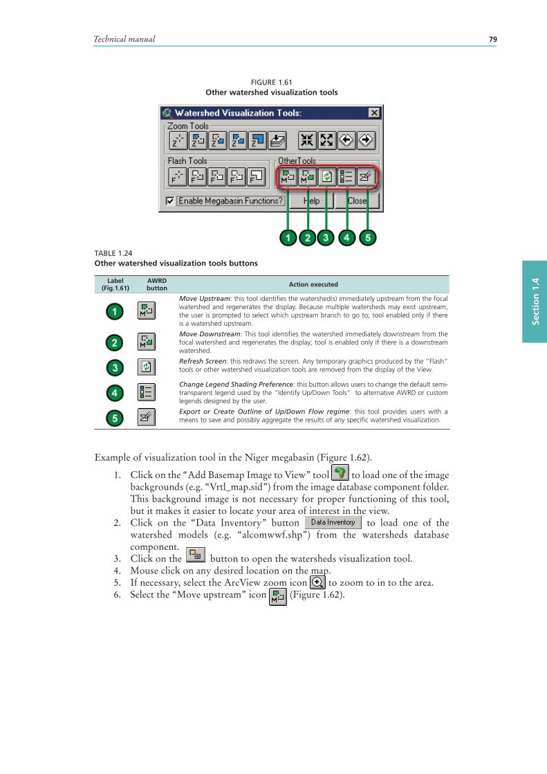
Technical manual 79
Sect
ion
1.4
FIGURE 1.61Other watershed visualization tools
TABLE 1.24Other watershed visualization tools buttons
Label (Fig.1.61)
AWRD button Action executed
Move Upstream: this tool identifies the watershed( s) immediately upstream from the focal watershed and regenerates the display. Because multiple watersheds may exist upstream, the user is prompted to select which upstream branch to go to; tool enabled only if there is a watershed upstream.
Move Downstream: This tool identifies the watershed immediately downstream from the focal watershed and regenerates the display; tool is enabled only if there is a downstream watershed.
Refresh Screen: this redraws the screen. Any temporary graphics produced by the “Flash” tools or other watershed visualization tools are removed from the display of the View.
Change Legend Shading Preference: this button allows users to change the default semi-transparent legend used by the “Identify Up/Down Tools” to alternative AWRD or custom legends designed by the user.
Export or Create Outline of Up/Down Flow regime: this tool provides users with a means to save and possibly aggregate the results of any specific watershed visualization.
Example of visualization tool in the Niger megabasin (Figure 1.62).
1. Click on the “Add Basemap Image to View” tool to load one of the image backgrounds (e.g. “Vrtl_map.sid”) from the image database component folder. This background image is not necessary for proper functioning of this tool, but it makes it easier to locate your area of interest in the view.
2. Click on the “Data Inventory” button to load one of the watershed models (e.g. “alcomwwf.shp”) from the watersheds database component.
3. Click on the button to open the watersheds visualization tool.4. Mouse click on any desired location on the map.5. If necessary, select the ArcView zoom icon to zoom to in to the area.6. Select the “Move upstream” icon (Figure 1.62).
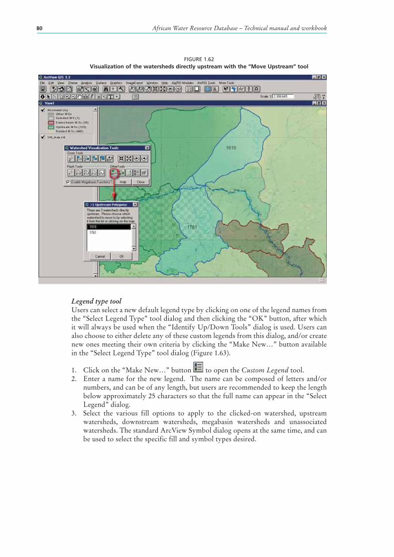
African Water Resource Database – Technical manual and workbook80
FIGURE 1.62Visualization of the watersheds directly upstream with the “Move Upstream” tool
Legend type toolUsers can select a new default legend type by clicking on one of the legend names from the “Select Legend Type” tool dialog and then clicking the “OK” button, after which it will always be used when the “Identify Up/Down Tools” dialog is used. Users can also choose to either delete any of these custom legends from this dialog, and/or create new ones meeting their own criteria by clicking the “Make New…” button available in the “Select Legend Type” tool dialog (Figure 1.63).
1. Click on the “Make New…” button to open the Custom Legend tool.2. Enter a name for the new legend. The name can be composed of letters and/or
numbers, and can be of any length, but users are recommended to keep the length below approximately 25 characters so that the full name can appear in the “Select Legend” dialog.
3. Select the various fill options to apply to the clicked-on watershed , upstream watersheds, downstream watersheds, megabasin watersheds and unassociated watersheds. The standard ArcView Symbol dialog opens at the same time, and can be used to select the specific fill and symbol types desired.
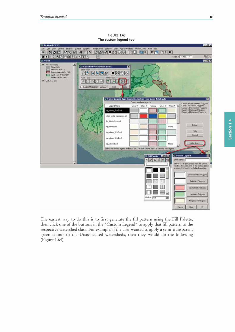
Technical manual 81
Sect
ion
1.4
FIGURE 1.63The custom legend tool
The easiest way to do this is to first generate the fill pattern using the Fill Palette, then click one of the buttons in the “Custom Legend” to apply that fill pattern to the respective watershed class. For example, if the user wanted to apply a semi-transparent green colour to the Unassociated watersheds, then they would do the following (Figure 1.64).
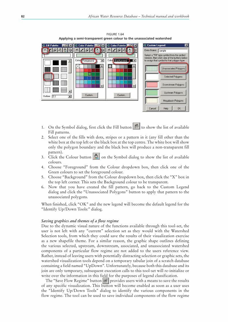
African Water Resource Database – Technical manual and workbook82
FIGURE 1.64Applying a semi-transparent green colour to the unassociated watershed
1. On the Symbol dialog, first click the Fill button to show the list of available Fill patterns.
2. Select one of the fills with dots, stripes or a pattern in it (any fill other than the white box at the top left or the black box at the top centre. The white box will show only the polygon boundary and the black box will produce a non-transparent fill pattern).
3. Click the Colour button on the Symbol dialog to show the list of available colours.
4. Choose “Foreground” from the Colour dropdown box, then click one of the Green colours to set the foreground colour.
5. Choose “Background” from the Colour dropdown box, then click the “X” box in the top left corner. This sets the Background colour to be transparent.
6. Now that you have created the fill pattern, go back to the Custom Legend dialog and click the “Unassociated Polygons” button to apply that pattern to the unassociated polygons.
When finished, click “OK” and the new legend will become the default legend for the “Identify Up/Down Tools:” dialog.
Saving graphics and themes of a flow regimeDue to the dynamic visual nature of the functions available through this tool-set, the user is not left with any “current” selection set as they would with the Watershed Selection tools, from which they could save the results of their visualization exercise as a new shapefile theme . For a similar reason, the graphic shape outlines defining the various selected, upstream , downstream , associated, and unassociated watershed components of a particular flow regime are not added to the users reference view. Rather, instead of leaving users with potentially distracting selection or graphic sets, the watershed visualization tools depend on a temporary tabular join of a scratch database containing a field named “UpDown”. Unfortunately, because both this database and its join are only temporary, subsequent execution calls to this tool-set will re-initialize or write over the information in this field for the purposes of legend classification .
The “Save Flow Regime” button provides users with a means to save the results of any specific visualization. This button will become enabled as soon as a user uses the “Identify Up/Down Tools” dialog to identify the various components in the flow regime. The tool can be used to save individual components of the flow regime
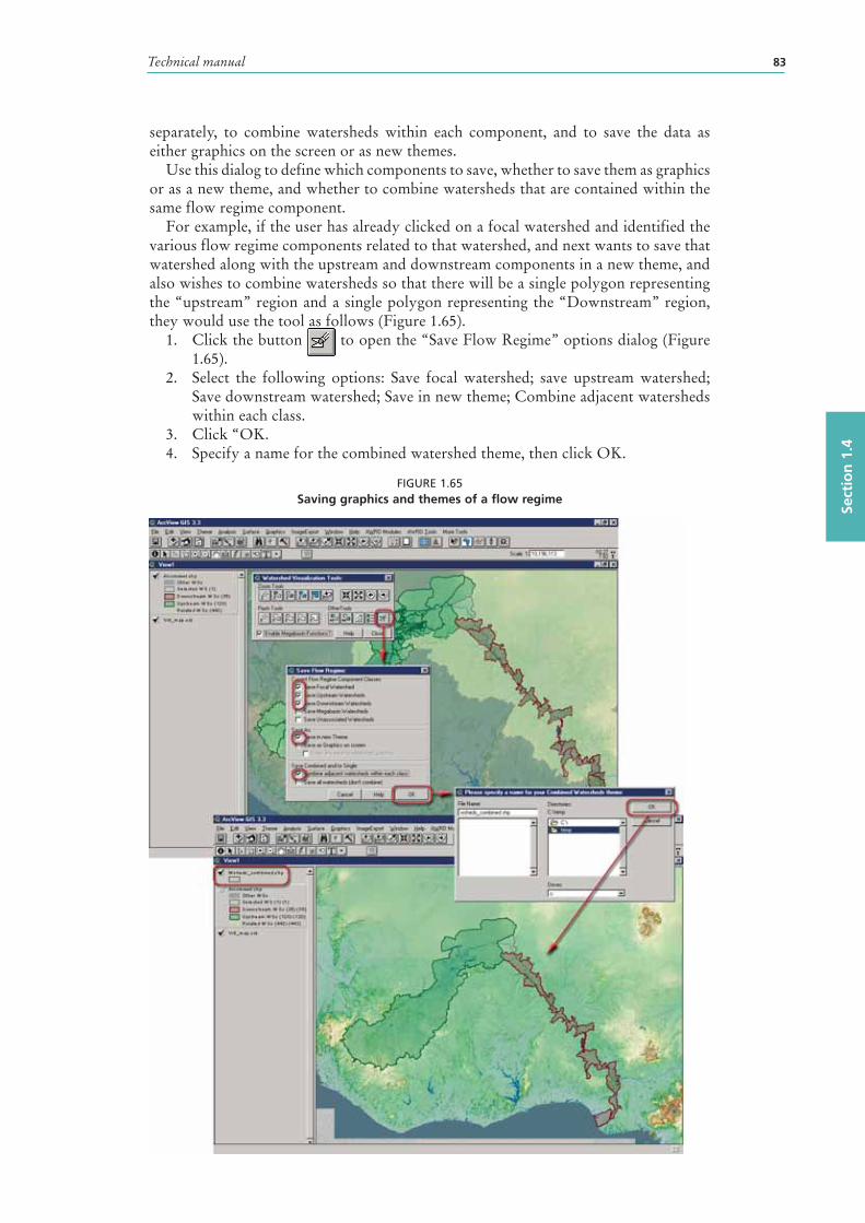
Technical manual 83
Sect
ion
1.4
separately, to combine watersheds within each component, and to save the data as either graphics on the screen or as new themes.
Use this dialog to define which components to save, whether to save them as graphics or as a new theme , and whether to combine watersheds that are contained within the same flow regime component.
For example, if the user has already clicked on a focal watershed and identified the various flow regime components related to that watershed, and next wants to save that watershed along with the upstream and downstream components in a new theme, and also wishes to combine watersheds so that there will be a single polygon representing the “upstream” region and a single polygon representing the “Downstream” region, they would use the tool as follows (Figure 1.65).
1. Click the button to open the “Save Flow Regime” options dialog (Figure 1.65).
2. Select the following options: Save focal watershed; save upstream watershed; Save downstream watershed; Save in new theme; Combine adjacent watersheds within each class.
3. Click “OK.4. Specify a name for the combined watershed theme, then click OK.
FIGURE 1.65Saving graphics and themes of a flow regime
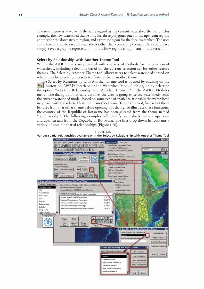
African Water Resource Database – Technical manual and workbook84
The new theme is saved with the same legend as the current watershed theme. In this example, the new watershed theme only has three polygons; one for the upstream region, another for the downstream region, and a third polygon for the focal watershed. The user could have chosen to save all watersheds rather than combining them, or they could have simply saved a graphic representation of the flow regime components on the screen.
Select by Relationship with Another Theme ToolWithin the AWRD, users are provided with a variety of methods for the selection of watersheds, including selections based on the current selection set for other feature themes. The Select by Another Theme tool allows users to select watersheds based on where they lie in relation to selected features from another theme .
The Select by Relationship with Another Theme tool is opened by clicking on the button on AWRD Interface or the Watershed Module dialog, or by selecting
the option “Select by Relationship with Another Theme…” in the AWRD Modules menu. The dialog automatically assumes the user is going to select watersheds from the current watershed model , based on some type of spatial relationship the watersheds may have with the selected features in another theme . To use this tool, first select those features from that other theme before opening this dialog. To illustrate these functions, the country of the Republic of Botswana has been selected from the theme named “countries.shp”. The following examples will identify watersheds that are upstream and downstream from the Republic of Botswana. The first drop down list contains a variety of possible spatial relationships (Figure 1.66).
FIGURE 1.66Various spatial relationships available with the Select by Relationship with Another Theme Tool
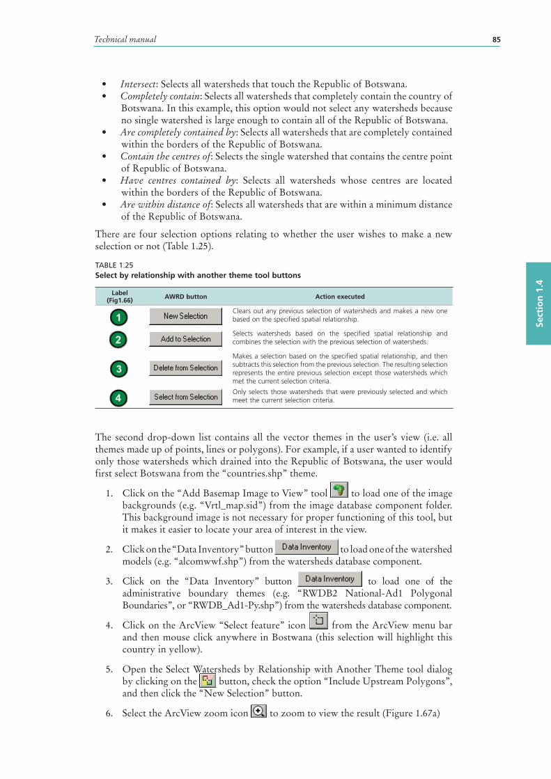
Technical manual 85
Sect
ion
1.4
• Intersect: Selects all watersheds that touch the Republic of Botswana .• Completely contain: Selects all watersheds that completely contain the country of
Botswana . In this example, this option would not select any watersheds because no single watershed is large enough to contain all of the Republic of Botswana.
• Are completely contained by: Selects all watersheds that are completely contained within the borders of the Republic of Botswana .
• Contain the centres of: Selects the single watershed that contains the centre point of Republic of Botswana .
• Have centres contained by: Selects all watersheds whose centres are located within the borders of the Republic of Botswana .
• Are within distance of: Selects all watersheds that are within a minimum distance of the Republic of Botswana .
There are four selection options relating to whether the user wishes to make a new selection or not (Table 1.25).
TABLE 1.25Select by relationship with another theme tool buttons
Label (Fig1.66) AWRD button Action executed
Clears out any previous selection of watersheds and makes a new one based on the specified spatial relationship.
Selects watersheds based on the specified spatial relationship and combines the selection with the previous selection of watersheds.
Makes a selection based on the specified spatial relationship, and then subtracts this selection from the previous selection. The resulting selection represents the entire previous selection except those watersheds which met the current selection criteria.
Only selects those watersheds that were previously selected and which meet the current selection criteria.
The second drop-down list contains all the vector themes in the user’s view (i.e. all themes made up of points, lines or polygons). For example, if a user wanted to identify only those watersheds which drained into the Republic of Botswana , the user would first select Botswana from the “countries.shp” theme .
1. Click on the “Add Basemap Image to View” tool to load one of the image backgrounds (e.g. “Vrtl_map.sid”) from the image database component folder. This background image is not necessary for proper functioning of this tool, but it makes it easier to locate your area of interest in the view.
2. Click on the “Data Inventory” button to load one of the watershed models (e.g. “alcomwwf.shp”) from the watersheds database component.
3. Click on the “Data Inventory” button to load one of the administrative boundary themes (e.g. “RWDB2 National-Ad1 Polygonal Boundaries”, or “RWDB_Ad1-Py.shp”) from the watersheds database component.
4. Click on the ArcView “Select feature” icon from the ArcView menu bar and then mouse click anywhere in Bostwana (this selection will highlight this country in yellow).
5. Open the Select Watersheds by Relationship with Another Theme tool dialog by clicking on the button, check the option “Include Upstream Polygons”, and then click the “New Selection” button.
6. Select the ArcView zoom icon to zoom to view the result (Figure 1.67a)
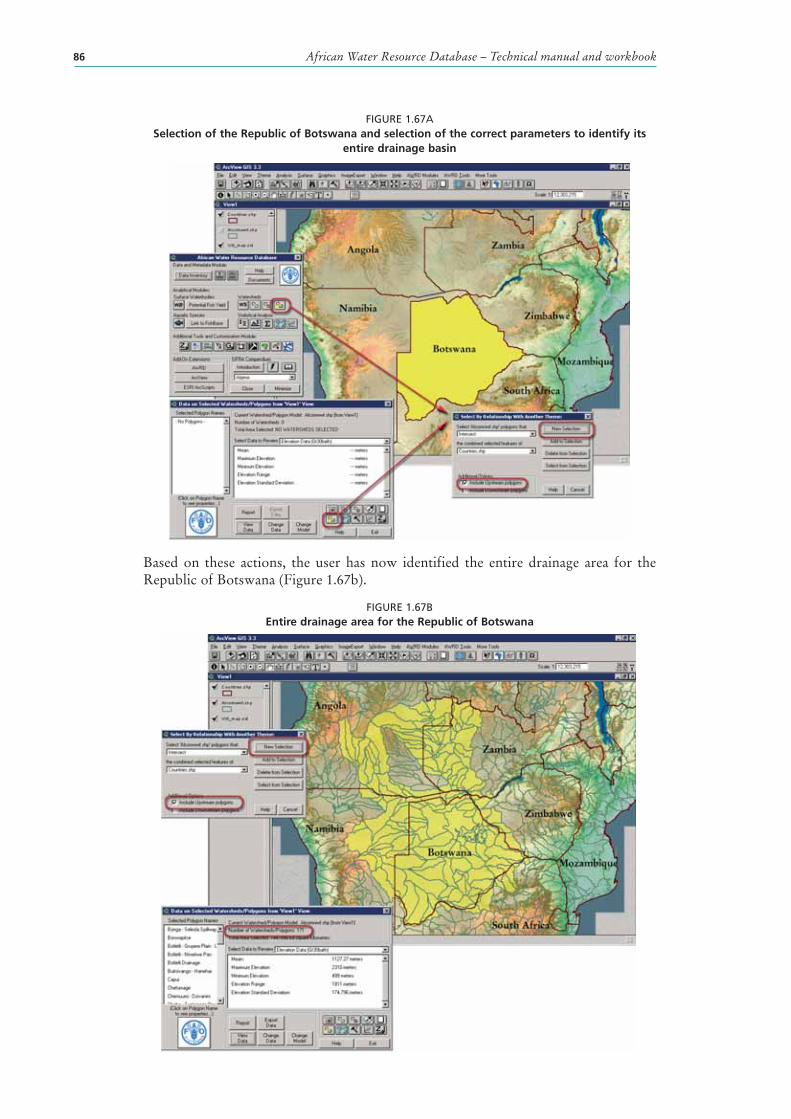
African Water Resource Database – Technical manual and workbook86
FIGURE 1.67ASelection of the Republic of Botswana and selection of the correct parameters to identify its
entire drainage basin
Based on these actions, the user has now identified the entire drainage area for the Republic of Botswana (Figure 1.67b).
FIGURE 1.67BEntire drainage area for the Republic of Botswana
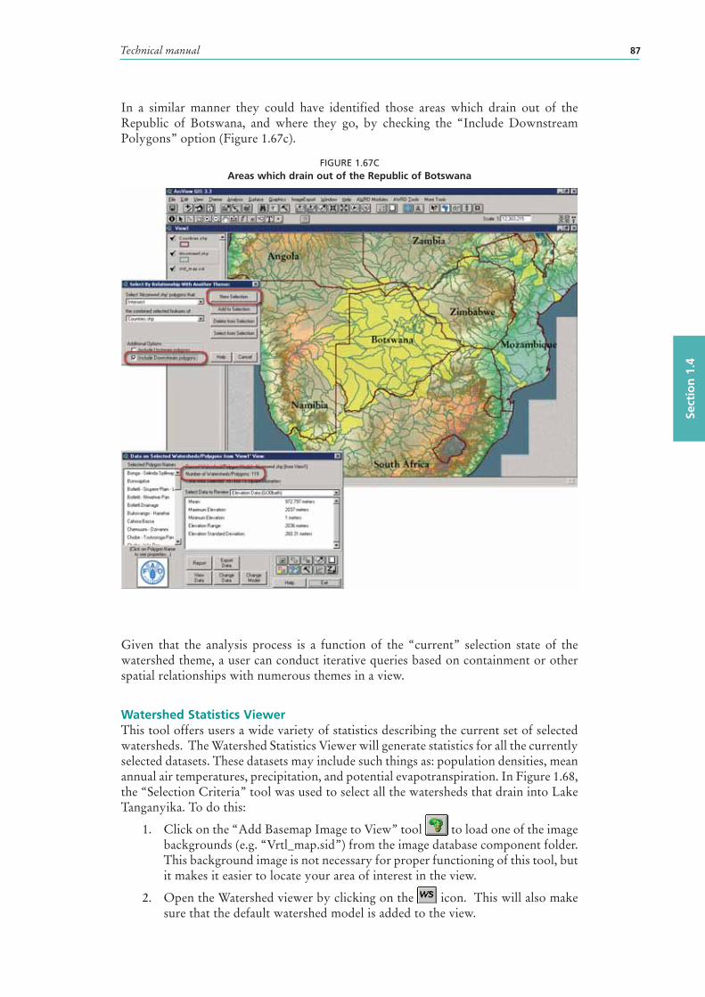
Technical manual 87
Sect
ion
1.4
In a similar manner they could have identified those areas which drain out of the Republic of Botswana , and where they go, by checking the “Include Downstream Polygons” option (Figure 1.67c).
FIGURE 1.67CAreas which drain out of the Republic of Botswana
Given that the analysis process is a function of the “current” selection state of the watershed theme , a user can conduct iterative queries based on containment or other spatial relationships with numerous themes in a view.
Watershed Statistics ViewerThis tool offers users a wide variety of statistics describing the current set of selected watersheds. The Watershed Statistics Viewer will generate statistics for all the currently selected datasets. These datasets may include such things as: population densities, mean annual air temperatures, precipitation , and potential evapotranspiration . In Figure 1.68, the “Selection Criteria” tool was used to select all the watersheds that drain into Lake Tanganyika. To do this:
1. Click on the “Add Basemap Image to View” tool to load one of the image backgrounds (e.g. “Vrtl_map.sid”) from the image database component folder. This background image is not necessary for proper functioning of this tool, but it makes it easier to locate your area of interest in the view.
2. Open the Watershed viewer by clicking on the icon. This will also make sure that the default watershed model is added to the view.
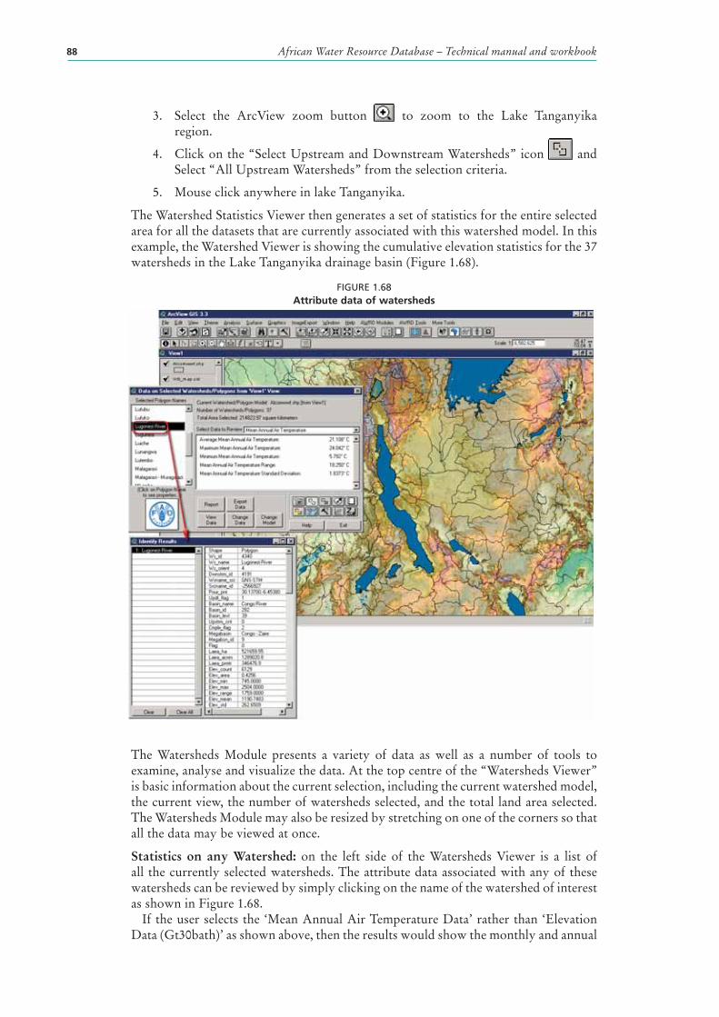
African Water Resource Database – Technical manual and workbook88
3. Select the ArcView zoom button to zoom to the Lake Tanganyika region.
4. Click on the “Select Upstream and Downstream Watersheds” icon and Select “All Upstream Watersheds” from the selection criteria.
5. Mouse click anywhere in lake Tanganyika.
The Watershed Statistics Viewer then generates a set of statistics for the entire selected area for all the datasets that are currently associated with this watershed model. In this example, the Watershed Viewer is showing the cumulative elevation statistics for the 37 watersheds in the Lake Tanganyika drainage basin (Figure 1.68).
FIGURE 1.68Attribute data of watersheds
The Watersheds Module presents a variety of data as well as a number of tools to examine, analyse and visualize the data. At the top centre of the “Watersheds Viewer” is basic information about the current selection , including the current watershed model , the current view, the number of watersheds selected, and the total land area selected. The Watersheds Module may also be resized by stretching on one of the corners so that all the data may be viewed at once.
Statistics on any Watershed: on the left side of the Watersheds Viewer is a list of all the currently selected watersheds. The attribute data associated with any of these watersheds can be reviewed by simply clicking on the name of the watershed of interest as shown in Figure 1.68.
If the user selects the ‘Mean Annual Air Temperature Data’ rather than ‘Elevation Data (Gt30bath)’ as shown above, then the results would show the monthly and annual
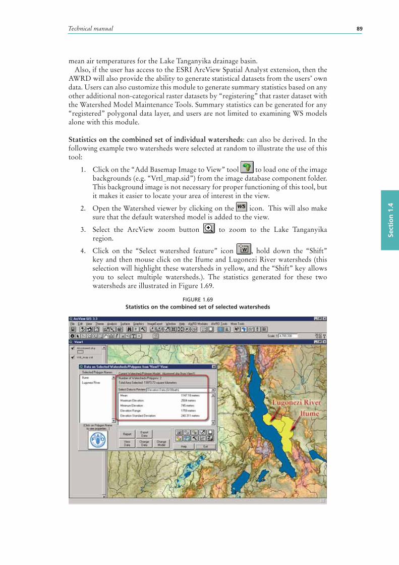
Technical manual 89
Sect
ion
1.4
mean air temperatures for the Lake Tanganyika drainage basin .Also, if the user has access to the ESRI ArcView Spatial Analyst extension, then the
AWRD will also provide the ability to generate statistical datasets from the users’ own data. Users can also customize this module to generate summary statistics based on any other additional non-categorical raster datasets by “registering ” that raster dataset with the Watershed Model Maintenance Tools. Summary statistics can be generated for any “registered” polygonal data layer, and users are not limited to examining WS models alone with this module.
Statistics on the combined set of individual watersheds: can also be derived. In the following example two watersheds were selected at random to illustrate the use of this tool:
1. Click on the “Add Basemap Image to View” tool to load one of the image backgrounds (e.g. “Vrtl_map.sid”) from the image database component folder. This background image is not necessary for proper functioning of this tool, but it makes it easier to locate your area of interest in the view.
2. Open the Watershed viewer by clicking on the icon. This will also make sure that the default watershed model is added to the view.
3. Select the ArcView zoom button to zoom to the Lake Tanganyika region.
4. Click on the “Select watershed feature” icon , hold down the “Shift” key and then mouse click on the Ifume and Lugonezi River watersheds (this selection will highlight these watersheds in yellow, and the “Shift” key allows you to select multiple watersheds.). The statistics generated for these two watersheds are illustrated in Figure 1.69.
FIGURE 1.69 Statistics on the combined set of selected watersheds
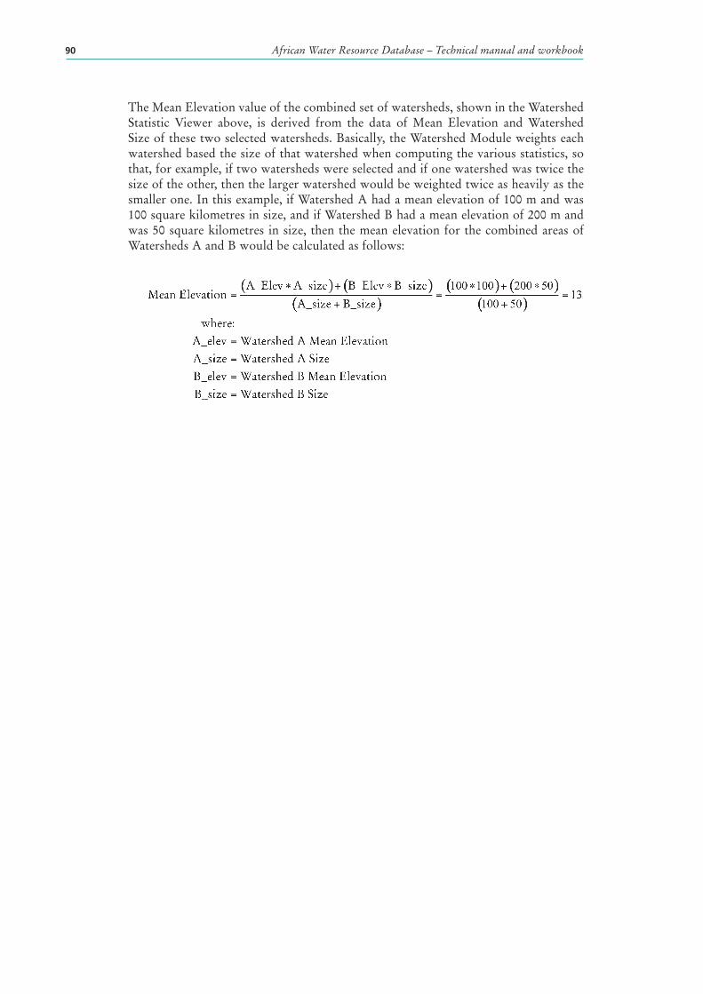
African Water Resource Database – Technical manual and workbook90
The Mean Elevation value of the combined set of watersheds, shown in the Watershed Statistic Viewer above, is derived from the data of Mean Elevation and Watershed Size of these two selected watersheds. Basically, the Watershed Module weights each watershed based the size of that watershed when computing the various statistics, so that, for example, if two watersheds were selected and if one watershed was twice the size of the other, then the larger watershed would be weighted twice as heavily as the smaller one. In this example, if Watershed A had a mean elevation of 100 m and was 100 square kilometres in size, and if Watershed B had a mean elevation of 200 m and was 50 square kilometres in size, then the mean elevation for the combined areas of Watersheds A and B would be calculated as follows:
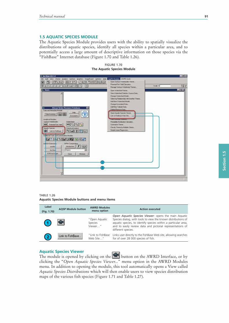
Technical manual 91
Sect
ion
1.5
1.5 AQUATIC SPECIES MODULE The Aquatic Species Module provides users with the ability to spatially visualize the distributions of aquatic species , identify all species within a particular area, and to potentially access a large amount of descriptive information on those species via the “FishBase” Internet database (Figure 1.70 and Table 1.26).
FIGURE 1.70The Aquatic Species Module
TABLE 1.26Aquatic Species Module buttons and menu items
Label
(Fig. 1.70)AQSP Module button AWRD Modules
menu option Action executed
“Open Aquatic Species Viewer…”
Open Aquatic Species Viewer: opens the main Aquatic Species dialog, with tools to view the known distributions of aquatic species, to identify species within a particular area, and to easily review data and pictorial representations of different species.
“Link to FishBase Web Site…”
Links user directly to the FishBase Web site, allowing searches for of over 28 000 species of fish.
Aquatic Species ViewerThe module is opened by clicking on the button on the AWRD Interface, or by clicking the “Open Aquatic Species Viewer...” menu option in the AWRD Modules menu. In addition to opening the module, this tool automatically opens a View called Aquatic Species Distributions which will then enable users to view species distribution maps of the various fish species (Figure 1.71 and Table 1.27).
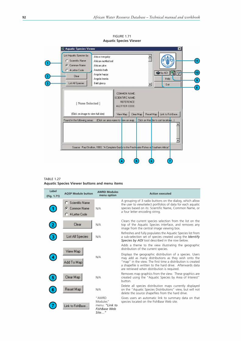
African Water Resource Database – Technical manual and workbook92
FIGURE 1.71Aquatic Species Viewer
TABLE 1.27Aquatic Species Viewer buttons and menu items
Label
(Fig. 1.71)AQSP Module button AWRD Modules
menu option Action executed
N/A
A grouping of 3 radio buttons on the dialog, which allow the user to view/select portfolios of data for each aquatic species based on its: Scientific Name, Common Name, or a four letter encoding string.
N/AClears the current species selection from the list on the top of the Aquatic Species interface, and removes any image from the central image viewing box.
N/ARefreshes and fully populates the Aquatic Species list from a sub-selection set of species created using the Identify Species by AOI tool described in the row below.
orN/A
Adds a theme to the view illustrating the geographic distribution of the current species.
Displays the geographic distribution of a species. Users may add as many distributions as they wish onto the “map” in the view. The first time a distribution is created a shapefile is written to the hard drive. Afterwards data are retrieved when distribution is required.
N/ARemoves map graphics from the view. These graphics are created using the “Aquatic Species by Area of Interest” button.
N/ADelete all species distribution maps currently displayed on the “Aquatic Species Distributions” view, but will not delete the source shapefiles from the hard drive.
“AWRD Modules” menu: “Link to FishBase Web Site…”
Gives users an automatic link to summary data on that species located on the FishBase Web site.
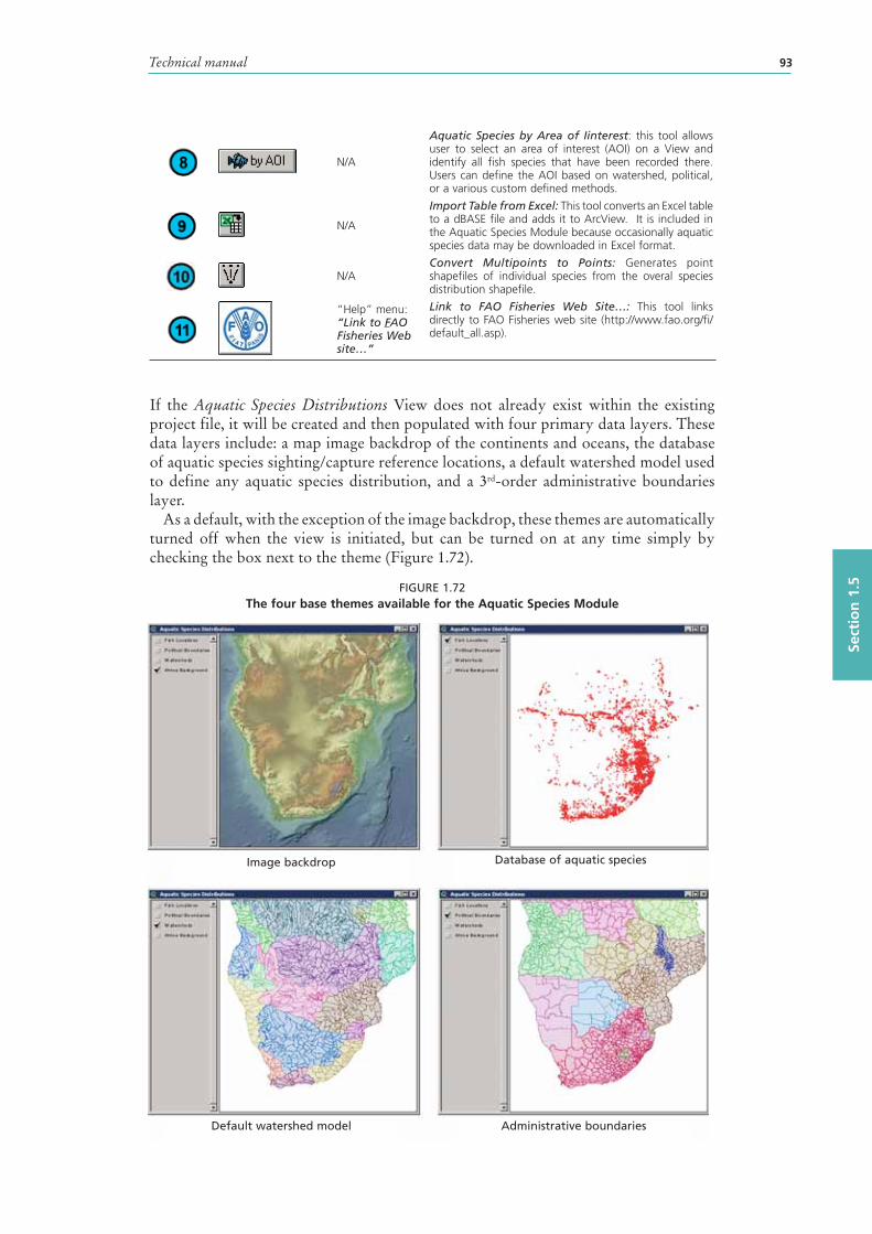
Technical manual 93
Sect
ion
1.5
N/A
Aquatic Species by Area of Iinterest: this tool allows user to select an area of interest (AOI) on a View and identify all fish species that have been recorded there. Users can define the AOI based on watershed , political, or a various custom defined methods.
N/A
Import Table from Excel: This tool converts an Excel table to a dBASE file and adds it to ArcView. It is included in the Aquatic Species Module because occasionally aquatic species data may be downloaded in Excel format.
N/AConvert Multipoints to Points: Generates point shapefiles of individual species from the overal species distribution shapefile.
“Help” menu: “Link to FAO Fisheries Web site…”
Link to FAO Fisheries Web Site…: This tool links directly to FAO Fisheries web site (http://www.fao.org/fi/default_all.asp).
If the Aquatic Species Distributions View does not already exist within the existing project file, it will be created and then populated with four primary data layers. These data layers include: a map image backdrop of the continents and oceans, the database of aquatic species sighting/capture reference locations, a default watershed model used to define any aquatic species distribution , and a 3rd-order administrative boundaries layer.
As a default, with the exception of the image backdrop, these themes are automatically turned off when the view is initiated, but can be turned on at any time simply by checking the box next to the theme (Figure 1.72).
FIGURE 1.72The four base themes available for the Aquatic Species Module
Image backdrop Database of aquatic species
Default watershed model Administrative boundaries
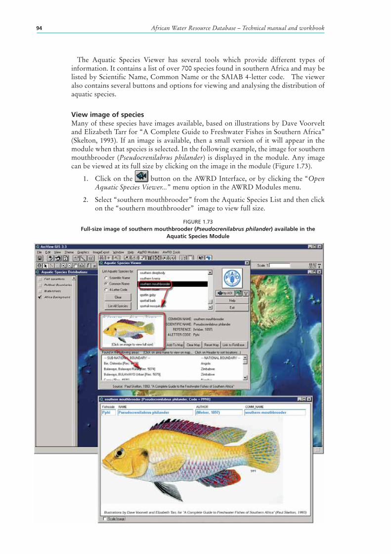
African Water Resource Database – Technical manual and workbook94
The Aquatic Species Viewer has several tools which provide different types of information. It contains a list of over 700 species found in southern Africa and may be listed by Scientific Name, Common Name or the SAIAB 4-letter code. The viewer also contains several buttons and options for viewing and analysing the distribution of aquatic species .
View image of speciesMany of these species have images available, based on illustrations by Dave Voorvelt and Elizabeth Tarr for “A Complete Guide to Freshwater Fishes in Southern Africa” (Skelton , 1993). If an image is available, then a small version of it will appear in the module when that species is selected. In the following example, the image for southern mouthbrooder (Pseudocrenilabrus philander) is displayed in the module. Any image can be viewed at its full size by clicking on the image in the module (Figure 1.73).
1. Click on the button on the AWRD Interface, or by clicking the “Open Aquatic Species Viewer...” menu option in the AWRD Modules menu.
2. Select “southern mouthbrooder” from the Aquatic Species List and then click on the “southern mouthbrooder” image to view full size.
FIGURE 1.73Full-size image of southern mouthbrooder (Pseudocrenilabrus philander) available in the
Aquatic Species Module
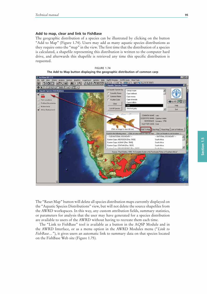
Technical manual 95
Sect
ion
1.5
Add to map, clear and link to FishBaseThe geographic distribution of a species can be illustrated by clicking on the button “Add to Map” (Figure 1.74). Users may add as many aquatic species distributions as they require onto the “map” in the view. The first time that the distribution of a species is calculated, a shapefile representing this distribution is written to the computer hard drive, and afterwards this shapefile is retrieved any time this specific distribution is requested.
FIGURE 1.74The Add to Map button displaying the geographic distribution of common carp
The “Reset Map” button will delete all species distribution maps currently displayed on the “Aquatic Species Distributions” view, but will not delete the source shapefiles from the AWRD workspaces. In this way, any custom attribution fields, summary statistics , or parameters for analysis that the user may have generated for a species distribution are available to users of the AWRD without having to recreate them each time.
The “Link to FishBase” tool is available as a button in the AQSP Module and in the AWRD Interface, or as a menu option in the AWRD Modules menu (“Link to FishBase…”), it gives users an automatic link to summary data on that species located on the FishBase Web site (Figure 1.75).
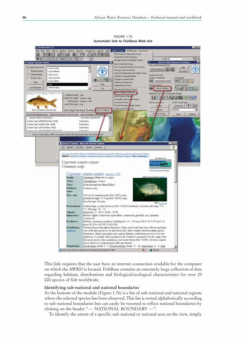
African Water Resource Database – Technical manual and workbook96
FIGURE 1.75Automatic link to FishBase Web site
This link requires that the user have an internet connection available for the computer on which the AWRD is located. FishBase contains an extremely large collection of data regarding habitats, distributions and biological/ecological characteristics for over 29 000 species of fish worldwide.
Identifying sub-national and national boundariesAt the bottom of the module (Figure 1.76) is a list of sub-national and national regions where the selected species has been observed. This list is sorted alphabetically according to sub-national boundaries but can easily be resorted to reflect national boundaries by clicking on the header “--- NATIONAL BOUNDARY ---”.
To identify the extent of a specific sub-national or national area on the view, simply
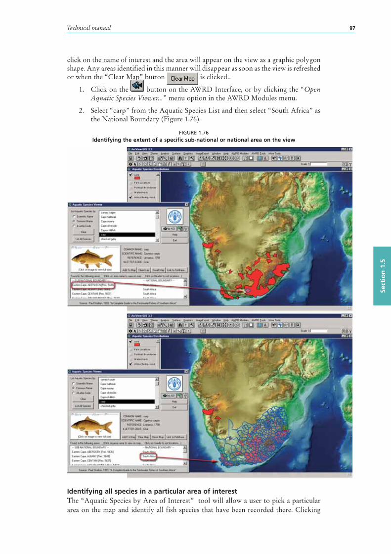
Technical manual 97
Sect
ion
1.5
click on the name of interest and the area will appear on the view as a graphic polygon shape. Any areas identified in this manner will disappear as soon as the view is refreshed or when the “Clear Map” button is clicked..
1. Click on the button on the AWRD Interface, or by clicking the “Open Aquatic Species Viewer...” menu option in the AWRD Modules menu.
2. Select “carp” from the Aquatic Species List and then select “South Africa” as the National Boundary (Figure 1.76).
FIGURE 1.76Identifying the extent of a specific sub-national or national area on the view
Identifying all species in a particular area of interestThe “Aquatic Species by Area of Interest” tool will allow a user to pick a particular area on the map and identify all fish species that have been recorded there. Clicking
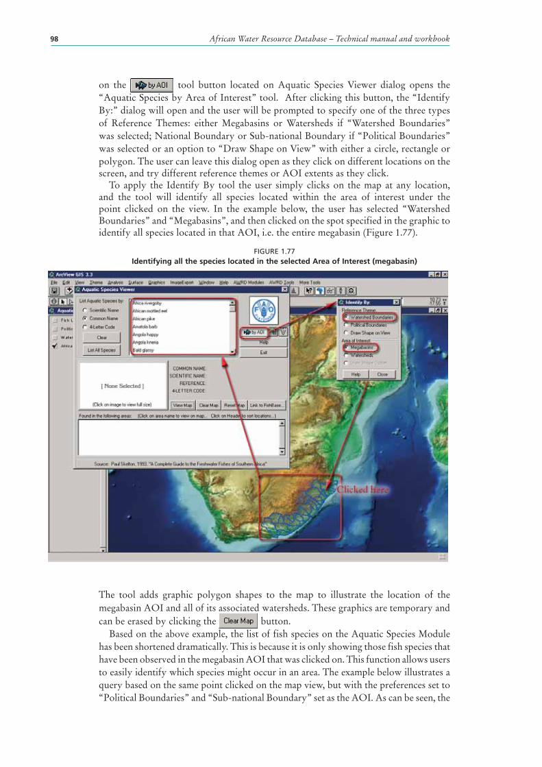
African Water Resource Database – Technical manual and workbook98
on the tool button located on Aquatic Species Viewer dialog opens the “Aquatic Species by Area of Interest” tool. After clicking this button, the “Identify By:” dialog will open and the user will be prompted to specify one of the three types of Reference Themes: either Megabasins or Watersheds if “Watershed Boundaries” was selected; National Boundary or Sub-national Boundary if “Political Boundaries” was selected or an option to “Draw Shape on View” with either a circle, rectangle or polygon. The user can leave this dialog open as they click on different locations on the screen, and try different reference themes or AOI extents as they click.
To apply the Identify By tool the user simply clicks on the map at any location, and the tool will identify all species located within the area of interest under the point clicked on the view. In the example below, the user has selected “Watershed Boundaries” and “Megabasins”, and then clicked on the spot specified in the graphic to identify all species located in that AOI, i.e. the entire megabasin (Figure 1.77).
FIGURE 1.77Identifying all the species located in the selected Area of Interest (megabasin)
The tool adds graphic polygon shapes to the map to illustrate the location of the megabasin AOI and all of its associated watersheds. These graphics are temporary and can be erased by clicking the button.
Based on the above example, the list of fish species on the Aquatic Species Module has been shortened dramatically. This is because it is only showing those fish species that have been observed in the megabasin AOI that was clicked on. This function allows users to easily identify which species might occur in an area. The example below illustrates a query based on the same point clicked on the map view, but with the preferences set to “Political Boundaries” and “Sub-national Boundary” set as the AOI. As can be seen, the
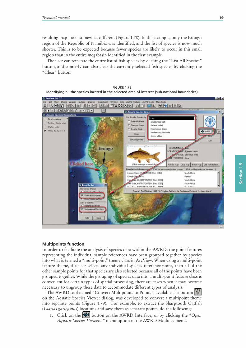
Technical manual 99
Sect
ion
1.5
resulting map looks somewhat different (Figure 1.78). In this example, only the Erongo region of the Republic of Namibia was identified, and the list of species is now much shorter. This is to be expected because fewer species are likely to occur in this small region than in the entire megabasin identified in the first example.
The user can reinstate the entire list of fish species by clicking the “List All Species” button, and similarly can also clear the currently selected fish species by clicking the “Clear” button.
FIGURE 1.78Identifying all the species located in the selected area of interest (sub-national boundaries)
Multipoints functionIn order to facilitate the analysis of species data within the AWRD, the point features representing the individual sample references have been grouped together by species into what is termed a “multi-point” theme class in ArcView. When using a multi-point feature theme, if a user selects any individual species reference point, then all of the other sample points for that species are also selected because all of the points have been grouped together. While the grouping of species data into a multi-point feature class is convenient for certain types of spatial processing, there are cases when it may become necessary to ungroup these data to accommodate different types of analysis.
The AWRD tool named “Convert Multipoints to Points”, available as a button on the Aquatic Species Viewer dialog, was developed to convert a multipoint theme into separate points (Figure 1.79). For example, to extract the Sharptooth Catfish (Clarias gariepinus) locations and save them as separate points, do the following:
1. Click on the button on the AWRD Interface, or by clicking the “Open Aquatic Species Viewer...” menu option in the AWRD Modules menu.
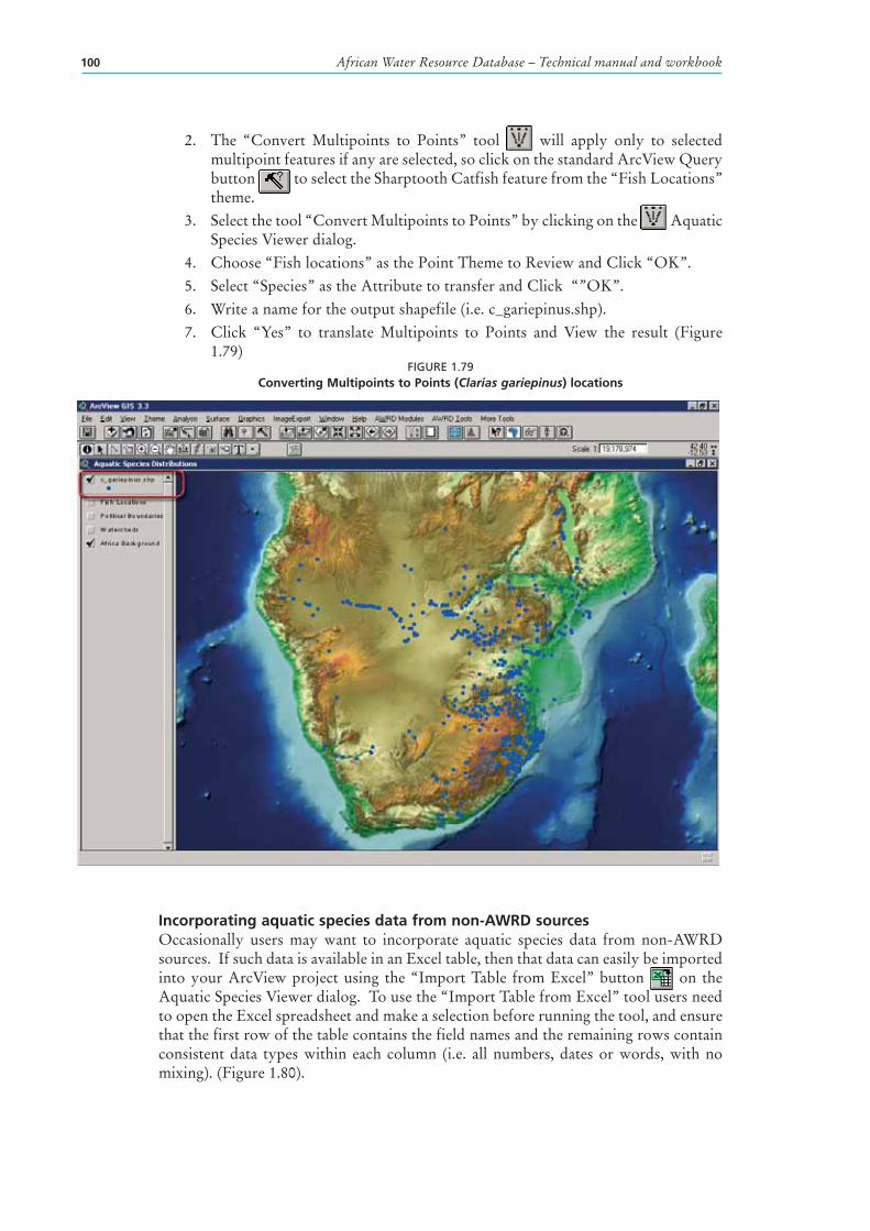
African Water Resource Database – Technical manual and workbook100
2. The “Convert Multipoints to Points” tool will apply only to selected multipoint features if any are selected, so click on the standard ArcView Query button to select the Sharptooth Catfish feature from the “Fish Locations” theme.
3. Select the tool “Convert Multipoints to Points” by clicking on the Aquatic Species Viewer dialog.
4. Choose “Fish locations” as the Point Theme to Review and Click “OK”.5. Select “Species” as the Attribute to transfer and Click “”OK”.6. Write a name for the output shapefile (i.e. c_gariepinus.shp).7. Click “Yes” to translate Multipoints to Points and View the result (Figure
1.79)FIGURE 1.79
Converting Multipoints to Points (Clarias gariepinus) locations
Incorporating aquatic species data from non-AWRD sourcesOccasionally users may want to incorporate aquatic species data from non-AWRD sources. If such data is available in an Excel table, then that data can easily be imported into your ArcView project using the “Import Table from Excel” button on the Aquatic Species Viewer dialog. To use the “Import Table from Excel” tool users need to open the Excel spreadsheet and make a selection before running the tool, and ensure that the first row of the table contains the field names and the remaining rows contain consistent data types within each column (i.e. all numbers, dates or words, with no mixing). (Figure 1.80).
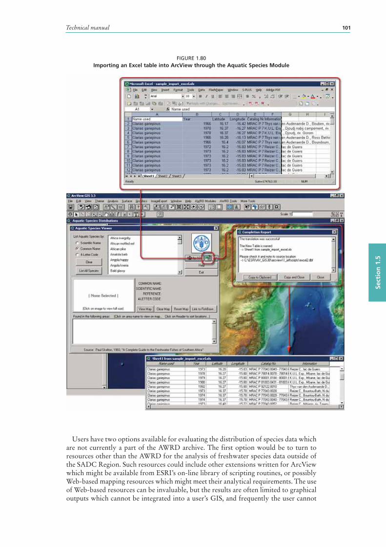
Technical manual 101
Sect
ion
1.5
FIGURE 1.80Importing an Excel table into ArcView through the Aquatic Species Module
Users have two options available for evaluating the distribution of species data which are not currently a part of the AWRD archive. The first option would be to turn to resources other than the AWRD for the analysis of freshwater species data outside of the SADC Region. Such resources could include other extensions written for ArcView which might be available from ESRI’s on-line library of scripting routines, or possibly Web-based mapping resources which might meet their analytical requirements. The use of Web-based resources can be invaluable, but the results are often limited to graphical outputs which cannot be integrated into a user’s GIS, and frequently the user cannot
African Water Resource Database – Technical manual and workbook102
refine the parameters used during any analysis. Such resources hold great promise and may offer cost-effective mechanisms for expanding the analysis of species data via the AWRD to taxa other than freshwater fish species.
The second method available for users of the AWRD would be to directly access and import data from other data sources. For freshwater fisheries data, one highly recommended data source for users to consider is FishBase, (www.fishbase.org). Based on the direct link to FishBase available in the AQSP Module dialog, users can not only access and download a wealth of species specific information, but can also directly access the species sampling records made available from a wide variety of organizations, museums and researchers.
The importation and evaluation of FishBase species data into the AWRD is a relatively simple procedure requiring six basic steps (see also Figure 1.81):
1. Click on the button on the AWRD Interface or the “Open Aquatic Species Viewer...” menu option in the AWRD Modules menu to open your Aquatic Species Viewer.
2. Select an aquatic species on the dialog (e.g. Nile tilapia) and then click on the “Link to FishBase...” button.
3. After the Fishbase browser window opens and FishBase has processed the request for the proper genus and species of fish, select the “Biogeographic modelling” link under the Tools list at the bottom of the page.
4. Soon a page will open with a list of location coordinates. Use the “Select All” button above the right list box to select all the coordinates, then move the mouse over the selected records and copy these coordinates by clicking the right mouse button and selecting “copy”.
5. Go back into ArcView and open a new script window from the main ArcView
project dialog , and then paste the point location data into the empty script using the “Edit” menu “Paste” command.
6. Click the button in the Script button bar to convert these locations to a point shapefile, and optionally add that shapefile to a view.
7. After you have created your new shapefile, you may delete the script if you wish.
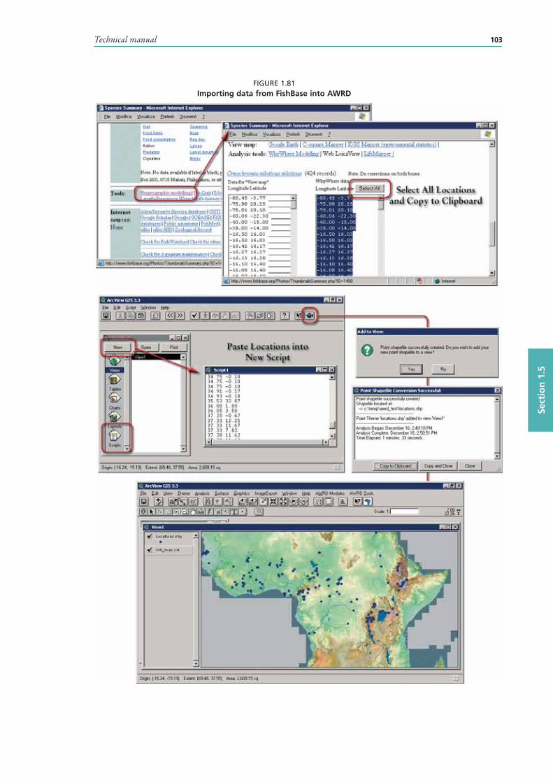
Technical manual 103
Sect
ion
1.5
FIGURE 1.81Importing data from FishBase into AWRD
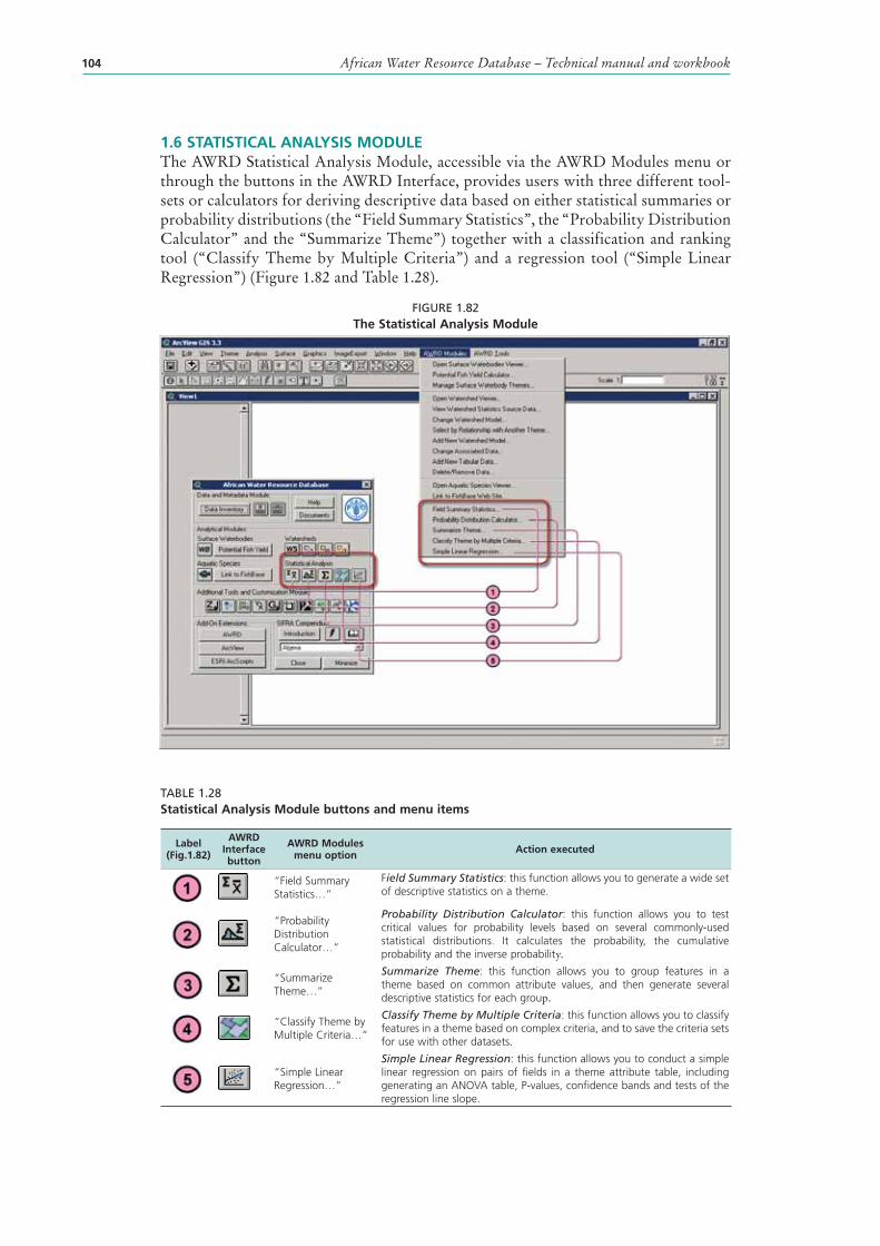
African Water Resource Database – Technical manual and workbook104
1.6 STATISTICAL ANALYSIS MODULEThe AWRD Statistical Analysis Module, accessible via the AWRD Modules menu or through the buttons in the AWRD Interface, provides users with three different tool-sets or calculators for deriving descriptive data based on either statistical summaries or probability distributions (the “Field Summary Statistics”, the “Probability Distribution Calculator” and the “Summarize Theme”) together with a classification and ranking tool (“Classify Theme by Multiple Criteria”) and a regression tool (“Simple Linear Regression”) (Figure 1.82 and Table 1.28).
FIGURE 1.82The Statistical Analysis Module
TABLE 1.28Statistical Analysis Module buttons and menu items
Label (Fig.1.82)
AWRD Interface button
AWRD Modules menu option Action executed
“Field Summary Statistics…”
Field Summary Statistics: this function allows you to generate a wide set of descriptive statistics on a theme.
“Probability Distribution Calculator…”
Probability Distribution Calculator: this function allows you to test critical values for probability levels based on several commonly-used statistical distributions. It calculates the probability, the cumulative probability and the inverse probability.
“Summarize Theme…”
Summarize Theme: this function allows you to group features in a theme based on common attribute values, and then generate several descriptive statistics for each group.
“Classify Theme by Multiple Criteria…”
Classify Theme by Multiple Criteria: this function allows you to classify features in a theme based on complex criteria, and to save the criteria sets for use with other datasets.
“Simple Linear Regression…”
Simple Linear Regression: this function allows you to conduct a simple linear regression on pairs of fields in a theme attribute table, including generating an ANOVA table, P-values, confidence bands and tests of the regression line slope.
Technical manual 105
Sect
ion
1.6
Statistics and probability toolsThe statistics and probability tools contained within the AWRD (Figure 1.82) provide users the ability to classify data, calculate a wide range of summary statistical data from themes and tables, and to easily generate both probability values and critical values from several statistical distributions.
Field summary statisticsThis tool provides functions similar to those available in the basic ArcView “Statistics…” options under the standard “Field” menu in the Table menu bar, with the exception that there are both more options and statistics are reported with a higher level of precision. The tool may be used to generate statistics on either a theme in a view or a field in a table.
Summary Statistics on a Theme
The button in the Statistical Analysis Module section of the AWRD Interface will only be enabled if the user has a View open and active. When the user clicks the button, they will be prompted to identify the theme and fields they wish to calculate statistics on. If the button does not respond, click on a view to enable the button. This statistics tool is also available as a menu option in the AWRD Modules menu (i.e. “Field Summary Statistics…”), or as a button in the Select by Theme tool dialog and Query Builder tool dialog .
The user can also choose to calculate statistics on either all the features in the theme or only the selected features. If no features are selected, then this tool will use all the features regardless of which option is chosen. The user can also choose to calculate statistics on multiple fields at one time.
The user can also specify certain values that they do not want included in the analysis. For example, it is common practice to designate some number to mean “No Data”, or to identify values that should not be involved in any analysis. Researchers often use -9999 or -99999 for this purpose, especially with datasets in which such a value would be impossible (i.e. elevation , population , area, etc.). The user can designate as many of these values as they want by entering them into the “Ignore Values” section and checking the “Ignore” box. The user can also choose between either the Simple or Advanced output.
The Simple output includes the Sum, Number of Features, Mean, Minimum and Maximum, and is reported in a text box.
1. Click on the “Add Basemap Image to View” tool to load one of the image backgrounds (e.g. “Etopo2_2-5d.jp2”) from the image database component folder. This background image is not necessary for proper functioning of these tools, but it makes it easier to locate your area of interest in the view.
2. Click on the “Data Inventory” button to load one of the watershed model themes (e.g. “alcomwwf.shp”) from the Watersheds database component.
3. Click on the button on the AWRD Interface, or the “Field Summary Statistics...” menu option in the AWRD Modules menu.
4. Select hectares (Laea_ha) and perimeter (Laea_prmtr) from the list by holding down the [SHIFT] key in the keyboard and click “OK” (Figure 1.83a).
Note The fieldname prefix “Laea”, means that these values are based on the Lambert Equal Area Azimuthal projection.
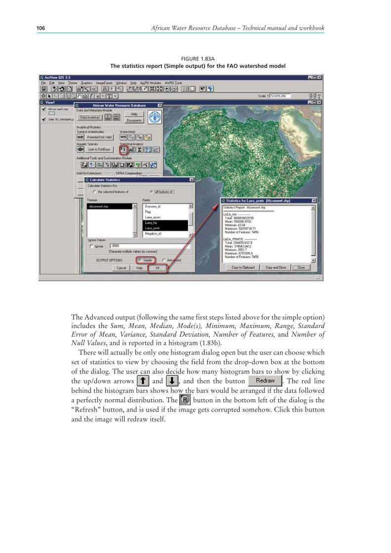
African Water Resource Database – Technical manual and workbook106
FIGURE 1.83AThe statistics report (Simple output) for the FAO watershed model
The Advanced output (following the same first steps listed above for the simple option) includes the Sum, Mean, Median, Mode(s), Minimum, Maximum, Range, Standard Error of Mean, Variance, Standard Deviation, Number of Features, and Number of Null Values, and is reported in a histogram (1.83b).
There will actually be only one histogram dialog open but the user can choose which set of statistics to view by choosing the field from the drop-down box at the bottom of the dialog. The user can also decide how many histogram bars to show by clicking the up/down arrows and , and then the button . The red line behind the histogram bars shows how the bars would be arranged if the data followed a perfectly normal distribution . The button in the bottom left of the dialog is the “Refresh” button, and is used if the image gets corrupted somehow. Click this button and the image will redraw itself.
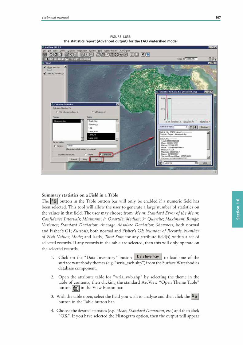
Technical manual 107
Sect
ion
1.6
FIGURE 1.83BThe statistics report (Advanced output) for the FAO watershed model
Summary statistics on a Field in a TableThe button in the Table button bar will only be enabled if a numeric field has been selected. This tool will allow the user to generate a large number of statistics on the values in that field. The user may choose from: Mean; Standard Error of the Mean; Confidence Intervals; Minimum; 1st Quartile; Median; 3rd Quartile; Maximum; Range; Variance; Standard Deviation; Average Absolute Deviation; Skewness, both normal and Fisher’s G1; Kurtosis, both normal and Fisher’s G2; Number of Records; Number
of Null Values; Mode; and lastly, Total Sum for any attribute field(s) within a set of selected records. If any records in the table are selected, then this will only operate on the selected records.
1. Click on the “Data Inventory” button to load one of the surface waterbody themes (e.g. “wria_swb.shp”) from the Surface Waterbodies database component.
2. Open the attribute table for “wria_swb.shp” by selecting the theme in the table of contents, then clicking the standard ArcView “Open Theme Table” button in the View button bar.
3. With the table open, select the field you wish to analyse and then click the button in the Table button bar.
4. Choose the desired statistics (e.g. Mean, Standard Deviation, etc.) and then click “OK”. If you have selected the Histogram option, then the output will appear
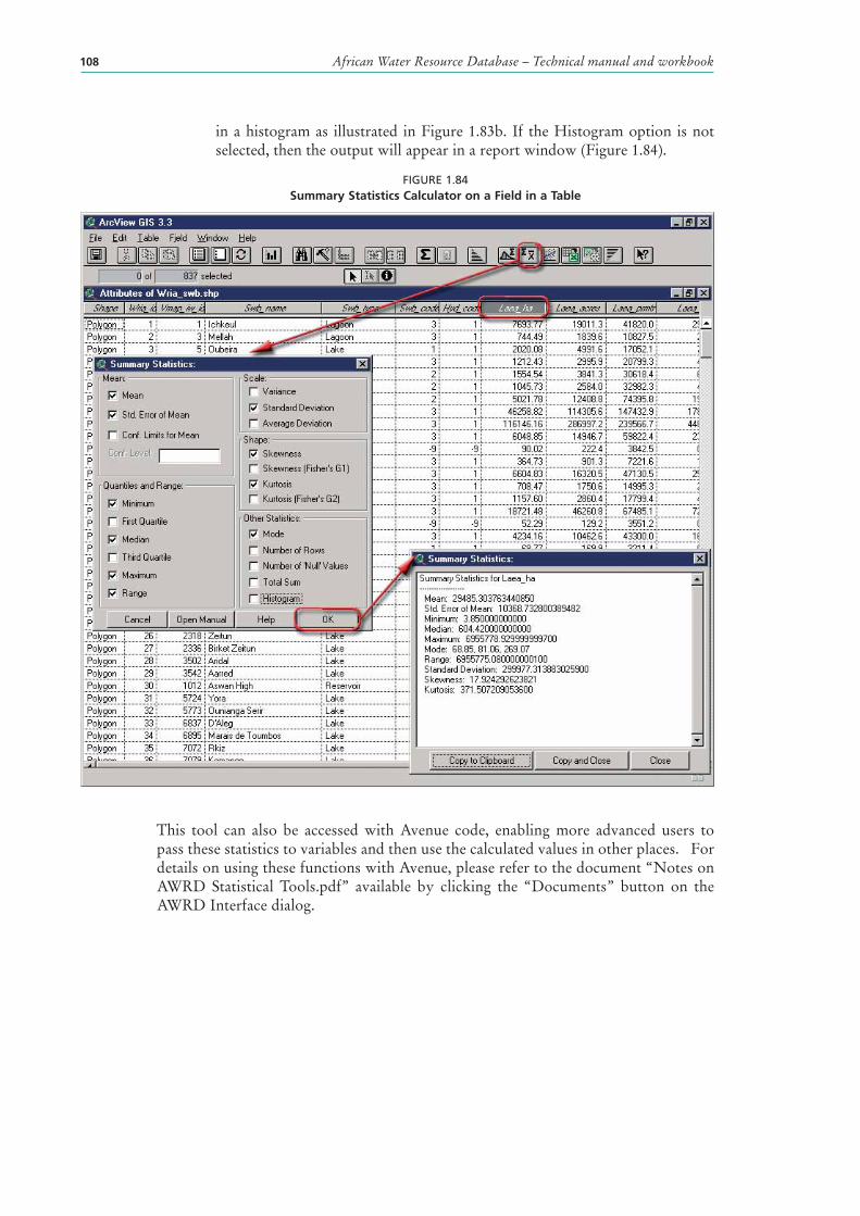
African Water Resource Database – Technical manual and workbook108
in a histogram as illustrated in Figure 1.83b. If the Histogram option is not selected, then the output will appear in a report window (Figure 1.84).
FIGURE 1.84Summary Statistics Calculator on a Field in a Table
This tool can also be accessed with Avenue code, enabling more advanced users to pass these statistics to variables and then use the calculated values in other places. For details on using these functions with Avenue, please refer to the document “Notes on AWRD Statistical Tools.pdf” available by clicking the “Documents” button on the AWRD Interface dialog.
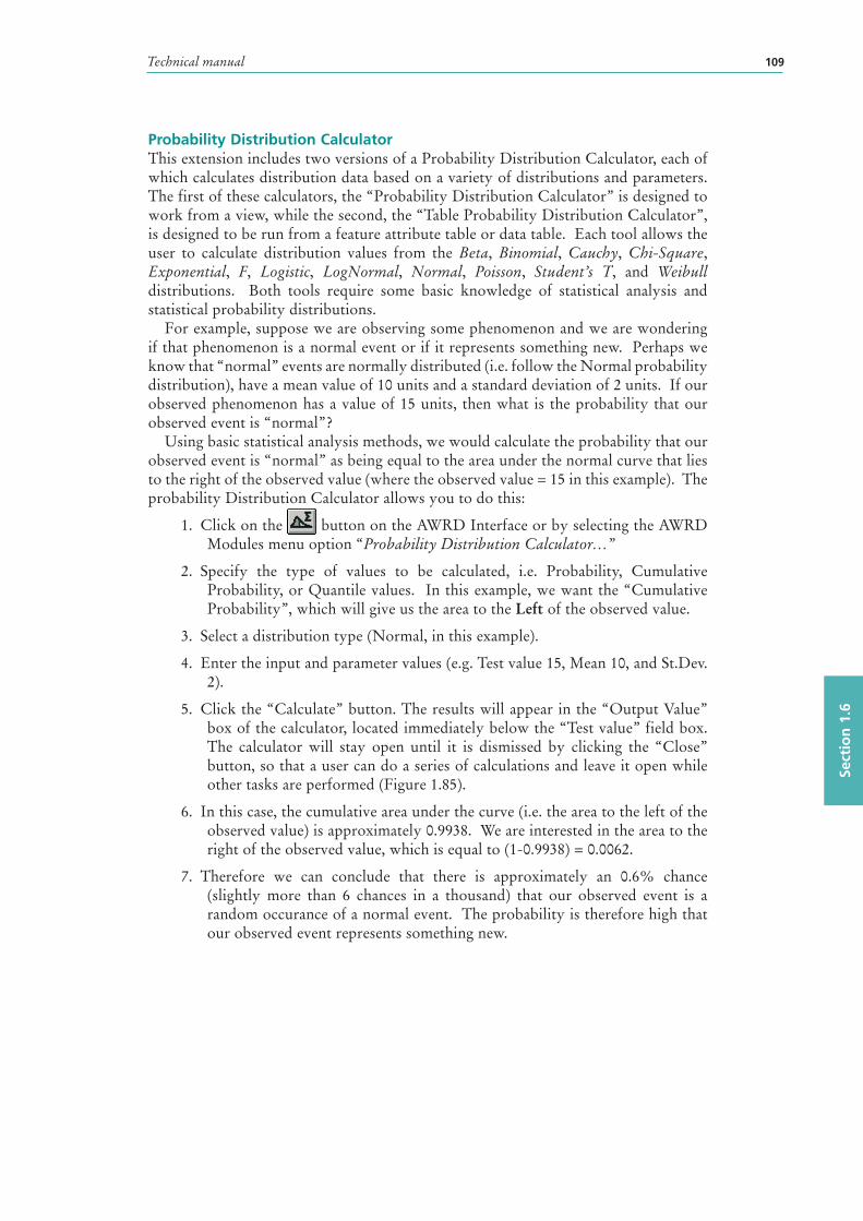
Technical manual 109
Sect
ion
1.6
Probability Distribution CalculatorThis extension includes two versions of a Probability Distribution Calculator, each of which calculates distribution data based on a variety of distributions and parameters. The first of these calculators, the “Probability Distribution Calculator” is designed to work from a view, while the second, the “Table Probability Distribution Calculator”, is designed to be run from a feature attribute table or data table. Each tool allows the user to calculate distribution values from the Beta , Binomial , Cauchy , Chi-Square , Exponential , F, Logistic , LogNormal , Normal , Poisson , Student’s T, and Weibull distributions. Both tools require some basic knowledge of statistical analysis and statistical probability distributions.
For example, suppose we are observing some phenomenon and we are wondering if that phenomenon is a normal event or if it represents something new. Perhaps we know that “normal” events are normally distributed (i.e. follow the Normal probability distribution), have a mean value of 10 units and a standard deviation of 2 units. If our observed phenomenon has a value of 15 units, then what is the probability that our observed event is “normal”?
Using basic statistical analysis methods, we would calculate the probability that our observed event is “normal” as being equal to the area under the normal curve that lies to the right of the observed value (where the observed value = 15 in this example). The probability Distribution Calculator allows you to do this:
1. Click on the button on the AWRD Interface or by selecting the AWRD Modules menu option “Probability Distribution Calculator…”
2. Specify the type of values to be calculated, i.e. Probability, Cumulative Probability, or Quantile values. In this example, we want the “Cumulative Probability”, which will give us the area to the Left of the observed value.
3. Select a distribution type (Normal, in this example).
4. Enter the input and parameter values (e.g. Test value 15, Mean 10, and St.Dev. 2).
5. Click the “Calculate” button. The results will appear in the “Output Value” box of the calculator , located immediately below the “Test value” field box. The calculator will stay open until it is dismissed by clicking the “Close” button, so that a user can do a series of calculations and leave it open while other tasks are performed (Figure 1.85).
6. In this case, the cumulative area under the curve (i.e. the area to the left of the observed value) is approximately 0.9938. We are interested in the area to the right of the observed value, which is equal to (1-0.9938) = 0.0062.
7. Therefore we can conclude that there is approximately an 0.6% chance (slightly more than 6 chances in a thousand) that our observed event is a random occurance of a normal event. The probability is therefore high that our observed event represents something new.
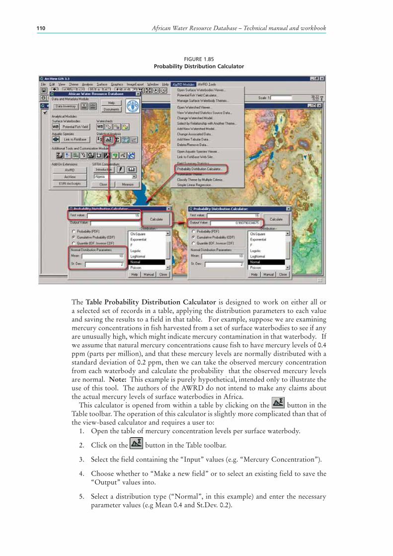
African Water Resource Database – Technical manual and workbook110
FIGURE 1.85Probability Distribution Calculator
The Table Probability Distribution Calculator is designed to work on either all or a selected set of records in a table, applying the distribution parameters to each value and saving the results to a field in that table. For example, suppose we are examining mercury concentrations in fish harvested from a set of surface waterbodies to see if any are unusually high, which might indicate mercury contamination in that waterbody. If we assume that natural mercury concentrations cause fish to have mercury levels of 0.4 ppm (parts per million), and that these mercury levels are normally distributed with a standard deviation of 0.2 ppm, then we can take the observed mercury concentration from each waterbody and calculate the probability that the observed mercury levels are normal. Note: This example is purely hypothetical, intended only to illustrate the use of this tool. The authors of the AWRD do not intend to make any claims about the actual mercury levels of surface waterbodies in Africa.
This calculator is opened from within a table by clicking on the button in the Table toolbar. The operation of this calculator is slightly more complicated than that of the view-based calculator and requires a user to:
1. Open the table of mercury concentration levels per surface waterbody.
2. Click on the button in the Table toolbar.
3. Select the field containing the “Input” values (e.g. “Mercury Concentration”).
4. Choose whether to “Make a new field” or to select an existing field to save the “Output” values into.
5. Select a distribution type (“Normal”, in this example) and enter the necessary parameter values (e.g Mean 0.4 and St.Dev. 0.2).
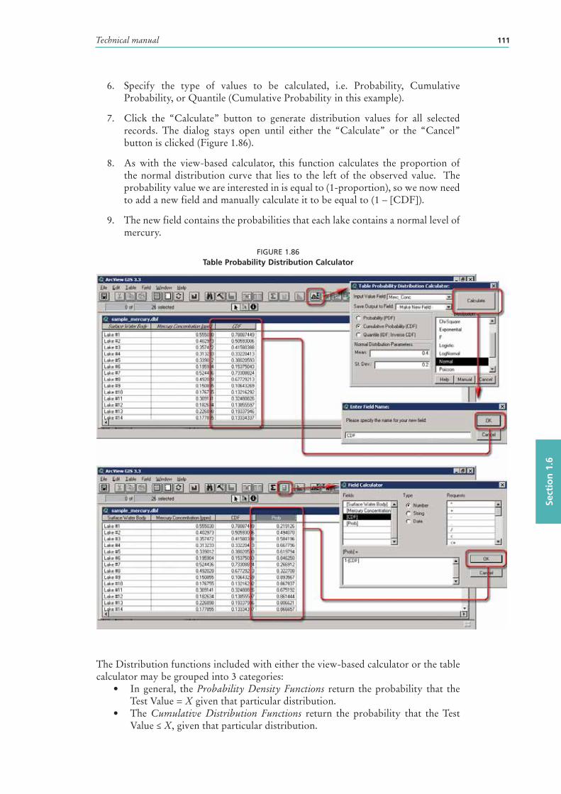
Technical manual 111
Sect
ion
1.6
6. Specify the type of values to be calculated, i.e. Probability, Cumulative Probability, or Quantile (Cumulative Probability in this example).
7. Click the “Calculate” button to generate distribution values for all selected records. The dialog stays open until either the “Calculate” or the “Cancel” button is clicked (Figure 1.86).
8. As with the view-based calculator, this function calculates the proportion of the normal distribution curve that lies to the left of the observed value. The probability value we are interested in is equal to (1-proportion), so we now need to add a new field and manually calculate it to be equal to (1 – [CDF]).
9. The new field contains the probabilities that each lake contains a normal level of mercury.
FIGURE 1.86Table Probability Distribution Calculator
The Distribution functions included with either the view-based calculator or the table calculator may be grouped into 3 categories:
• In general, the Probability Density Functions return the probability that the Test Value = X given that particular distribution .
• The Cumulative Distribution Functions return the probability that the Test Value ≤ X, given that particular distribution .
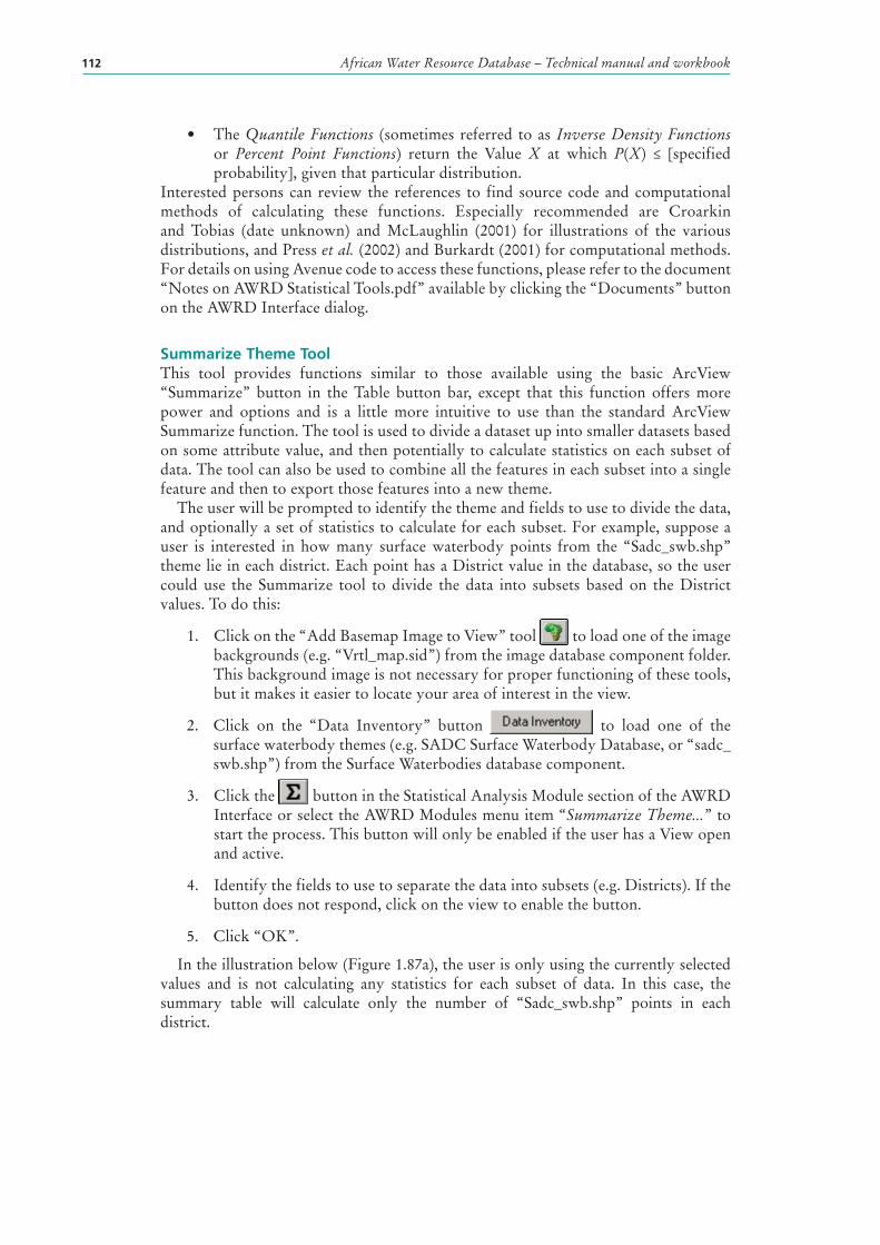
African Water Resource Database – Technical manual and workbook112
• The Quantile Functions (sometimes referred to as Inverse Density Functions or Percent Point Functions) return the Value X at which P(X) ≤ [specified probability ], given that particular distribution .
Interested persons can review the references to find source code and computational methods of calculating these functions. Especially recommended are Croarkin and Tobias (date unknown) and McLaughlin (2001) for illustrations of the various distributions, and Press et al. (2002) and Burkardt (2001) for computational methods. For details on using Avenue code to access these functions, please refer to the document “Notes on AWRD Statistical Tools.pdf” available by clicking the “Documents” button on the AWRD Interface dialog.
Summarize Theme ToolThis tool provides functions similar to those available using the basic ArcView “Summarize” button in the Table button bar, except that this function offers more power and options and is a little more intuitive to use than the standard ArcView Summarize function. The tool is used to divide a dataset up into smaller datasets based on some attribute value, and then potentially to calculate statistics on each subset of data. The tool can also be used to combine all the features in each subset into a single feature and then to export those features into a new theme .
The user will be prompted to identify the theme and fields to use to divide the data, and optionally a set of statistics to calculate for each subset. For example, suppose a user is interested in how many surface waterbod y points from the “Sadc_swb.shp” theme lie in each district. Each point has a District value in the database, so the user could use the Summarize tool to divide the data into subsets based on the District values. To do this:
1. Click on the “Add Basemap Image to View” tool to load one of the image backgrounds (e.g. “Vrtl_map.sid”) from the image database component folder. This background image is not necessary for proper functioning of these tools, but it makes it easier to locate your area of interest in the view.
2. Click on the “Data Inventory” button to load one of the surface waterbody themes (e.g. SADC Surface Waterbody Database, or “sadc_swb.shp”) from the Surface Waterbodies database component.
3. Click the button in the Statistical Analysis Module section of the AWRD Interface or select the AWRD Modules menu item “Summarize Theme...” to start the process. This button will only be enabled if the user has a View open and active.
4. Identify the fields to use to separate the data into subsets (e.g. Districts). If the button does not respond, click on the view to enable the button.
5. Click “OK”.
In the illustration below (Figure 1.87a), the user is only using the currently selected values and is not calculating any statistics for each subset of data. In this case, the summary table will calculate only the number of “Sadc_swb.shp” points in each district.
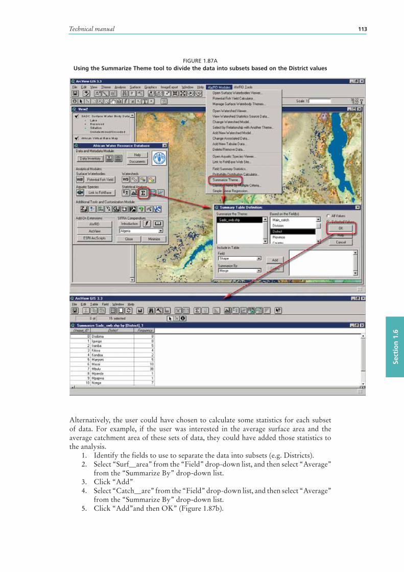
Technical manual 113
Sect
ion
1.6
FIGURE 1.87AUsing the Summarize Theme tool to divide the data into subsets based on the District values
Alternatively, the user could have chosen to calculate some statistics for each subset of data. For example, if the user was interested in the average surface area and the average catchment area of these sets of data, they could have added those statistics to the analysis.
1. Identify the fields to use to separate the data into subsets (e.g. Districts).2. Select “Surf__area” from the “Field” drop-down list, and then select “Average”
from the “Summarize By” drop-down list.3. Click “Add”4. Select “Catch__are” from the “Field” drop-down list, and then select “Average”
from the “Summarize By” drop-down list.5. Click “Add”and then OK” (Figure 1.87b).
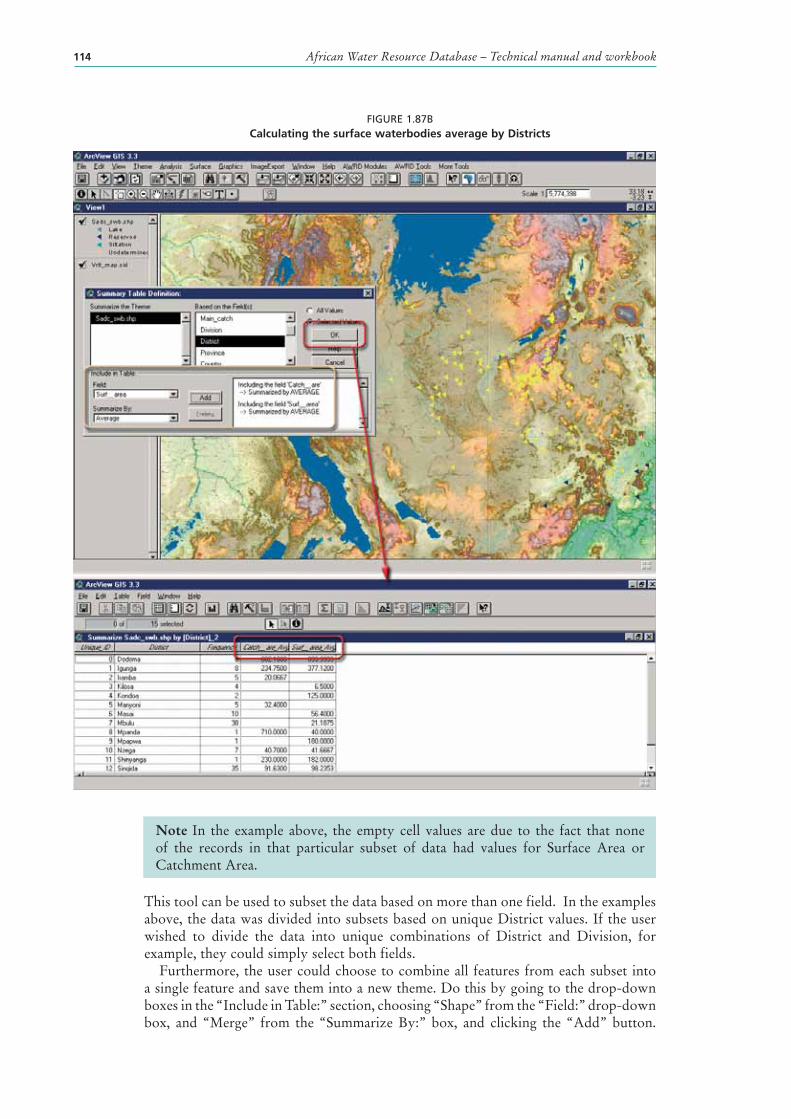
African Water Resource Database – Technical manual and workbook114
FIGURE 1.87BCalculating the surface waterbodies average by Districts
Note In the example above, the empty cell values are due to the fact that none of the records in that particular subset of data had values for Surface Area or Catchment Area.
This tool can be used to subset the data based on more than one field. In the examples above, the data was divided into subsets based on unique District values. If the user wished to divide the data into unique combinations of District and Division, for example, they could simply select both fields.
Furthermore, the user could choose to combine all features from each subset into a single feature and save them into a new theme . Do this by going to the drop-down boxes in the “Include in Table:” section, choosing “Shape” from the “Field:” drop-down box, and “Merge” from the “Summarize By:” box, and clicking the “Add” button.
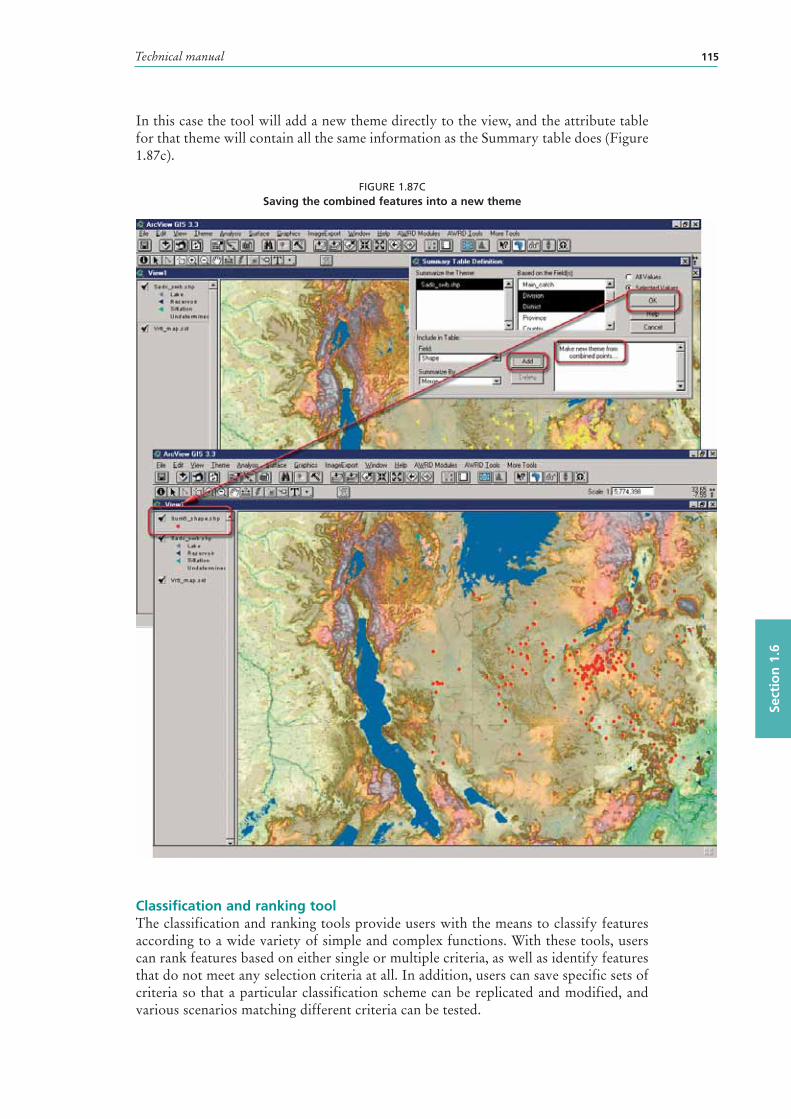
Technical manual 115
Sect
ion
1.6
In this case the tool will add a new theme directly to the view, and the attribute table for that theme will contain all the same information as the Summary table does (Figure 1.87c).
FIGURE 1.87CSaving the combined features into a new theme
Classification and ranking toolThe classification and ranking tools provide users with the means to classify features according to a wide variety of simple and complex functions. With these tools, users can rank features based on either single or multiple criteria, as well as identify features that do not meet any selection criteria at all. In addition, users can save specific sets of criteria so that a particular classification scheme can be replicated and modified, and various scenarios matching different criteria can be tested.
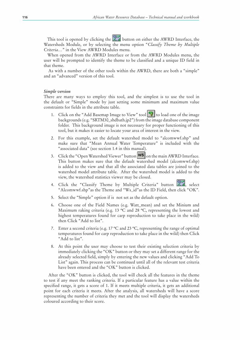
African Water Resource Database – Technical manual and workbook116
This tool is opened by clicking the button on either the AWRD Interface, the Watersheds Module, or by selecting the menu option “Classify Theme by Multiple Criteria…” in the View AWRD Modules menu.
When opened from the AWRD Interface or from the AWRD Modules menu, the user will be prompted to identify the theme to be classified and a unique ID field in that theme.
As with a number of the other tools within the AWRD, there are both a “simple” and an “advanced” version of this tool.
Simple versionThere are many ways to employ this tool, and the simplest is to use the tool in the default or “Simple” mode by just setting some minimum and maximum value constraints for fields in the attribute table.
1. Click on the “Add Basemap Image to View” tool to load one of the image backgrounds (e.g. “SRTM30_shdbath.jp2”) from the image database component folder. This background image is not necessary for proper functioning of this tool, but it makes it easier to locate your area of interest in the view.
2. For this example, set the default watershed model to “alcomwwf.shp” and make sure that “Mean Annual Water Temperature” is included with the “associated data” (see section 1.4 in this manual).
3. Click the “Open Watershed Viewer” button on the main AWRD Interface. This button makes sure that the default watershed model (alcomwwf.shp) is added to the view and that all the associated data tables are joined to the watershed model attribute table. After the watershed model is added to the view, the watershed statistics viewer may be closed.
4. Click the “Classify Theme by Multiple Criteria” button , select “Alcomwwf.shp”as the Theme and “Ws_id”as the ID Field, then click “OK”.
5. Select the “Simple” option if is not set as the default option.
6. Choose one of the Field Names (e.g. Watt_mean) and set the Minium and Maximum raking criteria (e.g. 13 ºC and 28 ºC, representing the lowest and highest temperatures found for carp reproduction to take place in the wild) then Click “Add to list”.
7. Enter a second criteria (e.g. 17 ºC and 23 ºC, representing the range of optimal temperatures found for carp reproduction to take place in the wild) then Click “Add to list”.
8. At this point the user may choose to test their existing selection criteria by immediately clicking the “OK” button or they may set a different range for the already selected field, simply by entering the new values and clicking “Add To List” again. This process can be continued until all of the relevant test criteria have been entered and the “OK” button is clicked.
After the “OK” button is clicked, the tool will check all the features in the theme to test if any meet the ranking criteria . If a particular feature has a value within the specified range , it gets a score of 1. If it meets multiple criteria, it gets an additional point for each criteria it meets. After the analysis, all watersheds will have a score representing the number of criteria they met and the tool will display the watersheds coloured according to their score.
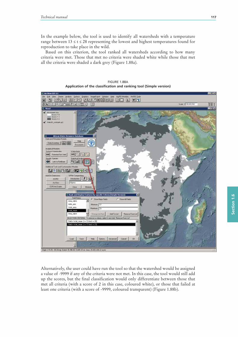
Technical manual 117
Sect
ion
1.6
In the example below, the tool is used to identify all watersheds with a temperature range between 13 ≤ t ≤ 28 representing the lowest and highest temperatures found for reproduction to take place in the wild.
Based on this criterion, the tool ranked all watersheds according to how many criteria were met. Those that met no criteria were shaded white while those that met all the criteria were shaded a dark grey (Figure 1.88a).
FIGURE 1.88AApplication of the classification and ranking tool (Simple version)
Alternatively, the user could have run the tool so that the watershed would be assigned a value of -9999 if any of the criteria were not met. In this case, the tool would still add up the scores, but the final classification would only differentiate between those that met all criteria (with a score of 2 in this case, coloured white), or those that failed at least one criteria (with a score of -9999, coloured transparent) (Figure 1.88b).
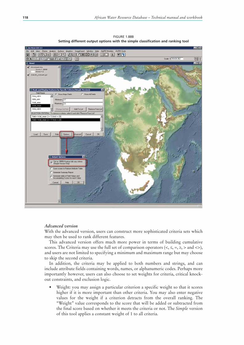
African Water Resource Database – Technical manual and workbook118
FIGURE 1.88BSetting different output options with the simple classification and ranking tool
Advanced versionWith the advanced version, users can construct more sophisticated criteria sets which may then be used to rank different features.
This advanced version offers much more power in terms of building cumulative scores. The Criteria may use the full set of comparison operators (<, ≤, =, ≥, > and <>), and users are not limited to specifying a minimum and maximum range but may choose to skip the second criteria.
In addition, the criteria may be applied to both numbers and strings, and can include attribute fields containing words, names, or alphanumeric codes. Perhaps more importantly however, users can also choose to set weights for criteria, critical knock-out constraints, and exclusion logic.
• Weight: you may assign a particular criterion a specific weight so that it scores higher if it is more important than other criteria. You may also enter negative values for the weight if a criterion detracts from the overall ranking . The “Weight” value corresponds to the score that will be added or subtracted from the final score based on whether it meets the criteria or not. The Simple version of this tool applies a constant weight of 1 to all criteria.
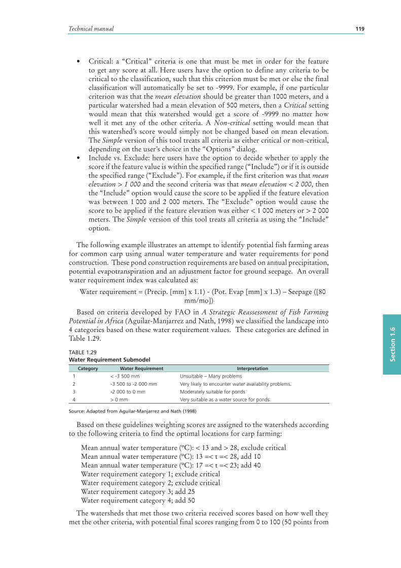
Technical manual 119
Sect
ion
1.6
• Critical: a “Critical” criteria is one that must be met in order for the feature to get any score at all. Here users have the option to define any criteria to be critical to the classification , such that this criterion must be met or else the final classification will automatically be set to -9999. For example, if one particular criterion was that the mean elevation should be greater than 1000 meters, and a particular watershed had a mean elevation of 500 meters, then a Critical setting would mean that this watershed would get a score of -9999 no matter how well it met any of the other criteria. A Non-critical setting would mean that this watershed’s score would simply not be changed based on mean elevation. The Simple version of this tool treats all criteria as either critical or non-critical, depending on the user’s choice in the “Options” dialog.
• Include vs. Exclude: here users have the option to decide whether to apply the score if the feature value is within the specified range (“Include”) or if it is outside the specified range (“Exclude”). For example, if the first criterion was that mean elevation > 1 000 and the second criteria was that mean elevation < 2 000, then the “Include” option would cause the score to be applied if the feature elevation was between 1 000 and 2 000 meters. The “Exclude” option would cause the score to be applied if the feature elevation was either < 1 000 meters or > 2 000 meters. The Simple version of this tool treats all criteria as using the “Include” option.
The following example illustrates an attempt to identify potential fish farming areas for common carp using annual water temperature and water requirements for pond construction. These pond construction requirements are based on annual precipitation, potential evapotranspiration and an adjustment factor for ground seepage. An overall water requirement index was calculated as:
Water requirement = (Precip. [mm] x 1.1) - (Pot. Evap [mm] x 1.3) – Seepage ([80 mm/mo])
Based on criteria developed by FAO in A Strategic Reassessment of Fish Farming Potential in Africa (Aguilar-Manjarrez and Nath, 1998) we classified the landscape into 4 categories based on these water requirement values. These categories are defined in Table 1.29.
TABLE 1.29Water Requirement Submodel
Category Water Requirement Interpretation
1 < -3 500 mm Unsuitable – Many problems
2 -3 500 to -2 000 mm Very likely to encounter water availability problems.
3 -2 000 to 0 mm Moderately suitable for ponds
4 > 0 mm Very suitable as a water source for ponds.
Source: Adapted from Aguilar-Manjarrez and Nath (1998)
Based on these guidelines weighting scores are assigned to the watersheds according to the following criteria to find the optimal locations for carp farming:
Mean annual water temperature (ºC): < 13 and > 28, exclude criticalMean annual water temperature (ºC): 13 =< t =< 28, add 10Mean annual water temperature (ºC): 17 =< t =< 23; add 40Water requirement category 1; exclude criticalWater requirement category 2; exclude criticalWater requirement category 3; add 25 Water requirement category 4; add 50
The watersheds that met those two criteria received scores based on how well they met the other criteria, with potential final scores ranging from 0 to 100 (50 points from
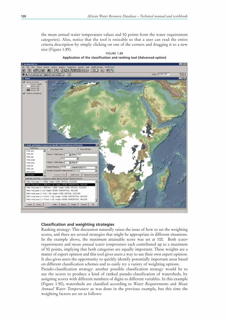
African Water Resource Database – Technical manual and workbook120
the mean annual water temperature values and 50 points from the water requirement categories). Also, notice that the tool is resizable so that a user can read the entire criteria description by simply clicking on one of the corners and dragging it to a new size (Figure 1.89).
FIGURE 1.89Application of the classification and ranking tool (Advanced option)
Classification and weighting strategiesRanking strategy: This discussion naturally raises the issue of how to set the weighting scores, and there are several strategies that might be appropriate in different situations. In the example above, the maximum attainable score was set at 100. Both water requirements and mean annual water temperature each contributed up to a maximum of 50 points, implying that both categories are equally important. These weights are a matter of expert opinion and this tool gives users a way to use their own expert opinion. It also gives users the opportunity to quickly identify potentially important areas based on different classification schemes and to easily try a variety of weighting options.Pseudo-classification strategy: another possible classification strategy would be to use the scores to produce a kind of ranked pseudo-classification of watersheds, by assigning scores with different numbers of digits to different variables. In this example (Figure 1.90), watersheds are classified according to Water Requirements and Mean Annual Water Temperature as was done in the previous example, but this time the weighting factors are set as follows:
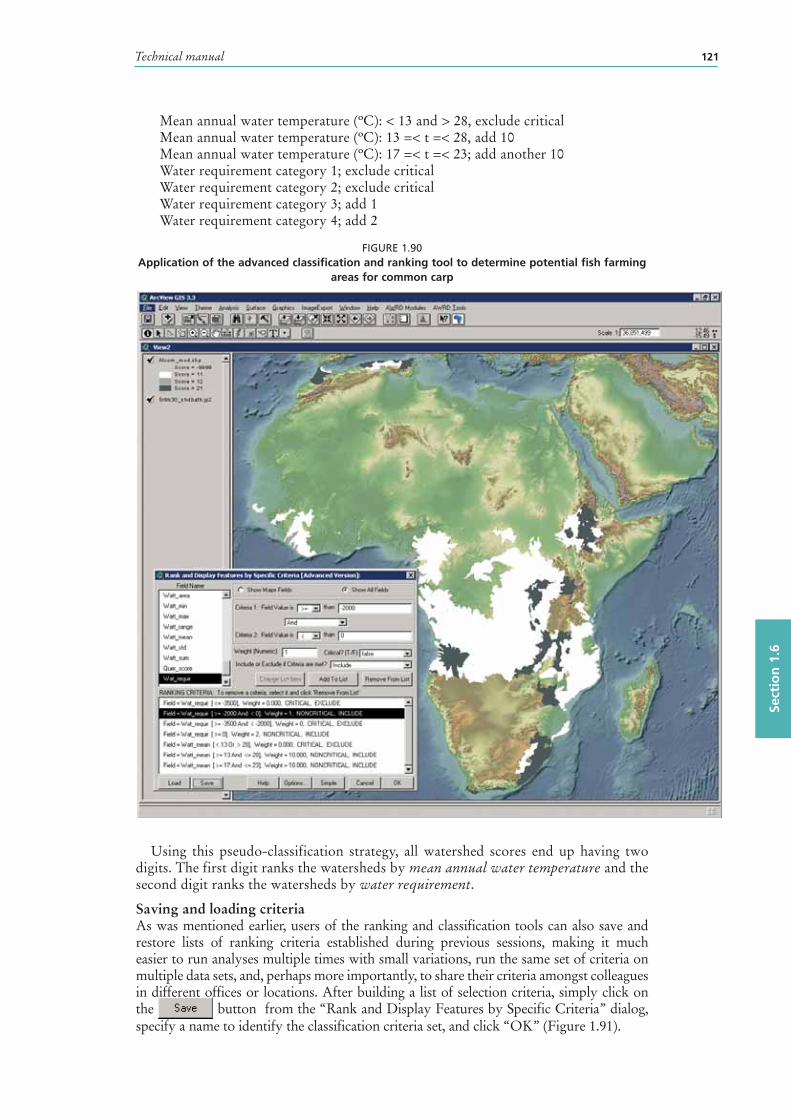
Technical manual 121
Sect
ion
1.6
Mean annual water temperature (ºC): < 13 and > 28, exclude criticalMean annual water temperature (ºC): 13 =< t =< 28, add 10Mean annual water temperature (ºC): 17 =< t =< 23; add another 10Water requirement category 1; exclude criticalWater requirement category 2; exclude criticalWater requirement category 3; add 1Water requirement category 4; add 2
FIGURE 1.90Application of the advanced classification and ranking tool to determine potential fish farming
areas for common carp
Using this pseudo-classification strategy, all watershed scores end up having two digits. The first digit ranks the watersheds by mean annual water temperature and the second digit ranks the watersheds by water requirement.
Saving and loading criteriaAs was mentioned earlier, users of the ranking and classification tools can also save and restore lists of ranking criteria established during previous sessions, making it much easier to run analyses multiple times with small variations, run the same set of criteria on multiple data sets, and, perhaps more importantly, to share their criteria amongst colleagues in different offices or locations. After building a list of selection criteria, simply click on the button from the “Rank and Display Features by Specific Criteria” dialog, specify a name to identify the classification criteria set, and click “OK” (Figure 1.91).
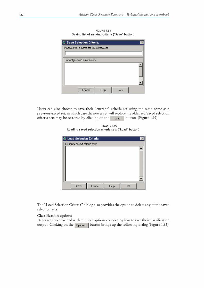
African Water Resource Database – Technical manual and workbook122
FIGURE 1.91Saving list of ranking criteria (“Save” button)
Users can also choose to save their “current” criteria set using the same name as a previous-saved set, in which case the newer set will replace the older set. Saved selection criteria sets may be restored by clicking on the button (Figure 1.92).
FIGURE 1.92Loading saved selection criteria sets (“Load” button)
The “Load Selection Criteria” dialog also provides the option to delete any of the saved selection sets.
Classification optionsUsers are also provided with multiple options concerning how to save their classification output. Clicking on the button brings up the following dialog (Figure 1.93).
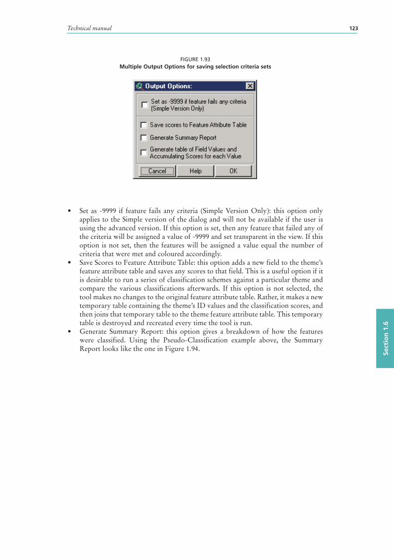
Technical manual 123
Sect
ion
1.6
FIGURE 1.93Multiple Output Options for saving selection criteria sets
• Set as -9999 if feature fails any criteria (Simple Version Only): this option only applies to the Simple version of the dialog and will not be available if the user is using the advanced version. If this option is set, then any feature that failed any of the criteria will be assigned a value of -9999 and set transparent in the view. If this option is not set, then the features will be assigned a value equal the number of criteria that were met and coloured accordingly.
• Save Scores to Feature Attribute Table: this option adds a new field to the theme ’s feature attribute table and saves any scores to that field. This is a useful option if it is desirable to run a series of classification schemes against a particular theme and compare the various classifications afterwards. If this option is not selected, the tool makes no changes to the original feature attribute table. Rather, it makes a new temporary table containing the theme’s ID values and the classification scores, and then joins that temporary table to the theme feature attribute table. This temporary table is destroyed and recreated every time the tool is run.
• Generate Summary Report: this option gives a breakdown of how the features were classified. Using the Pseudo-Classification example above, the Summary Report looks like the one in Figure 1.94.
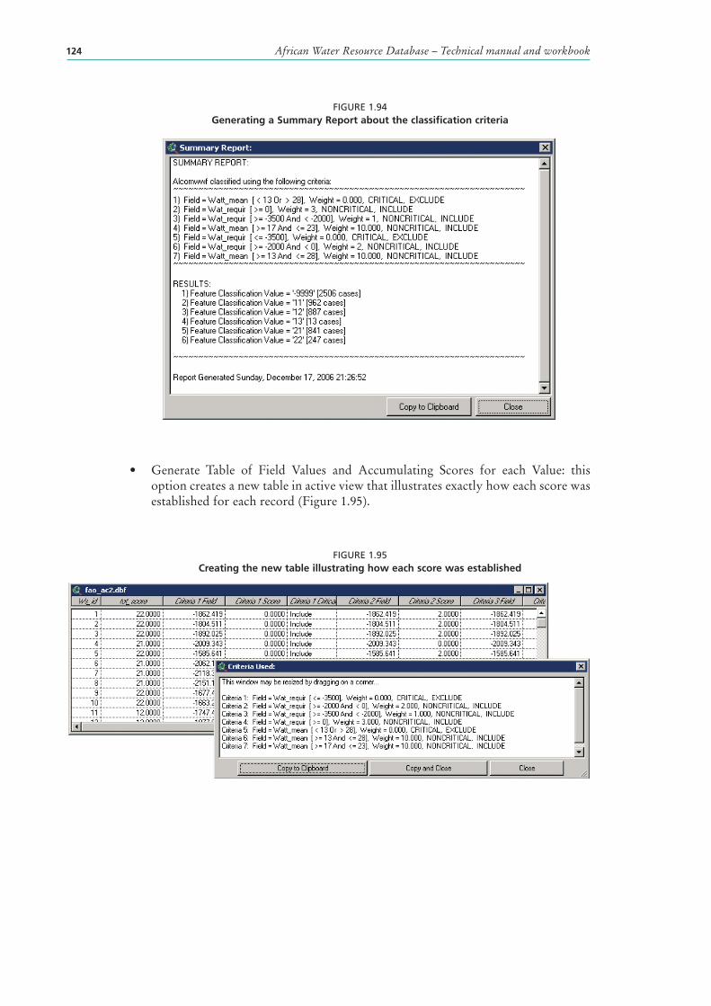
African Water Resource Database – Technical manual and workbook124
FIGURE 1.94Generating a Summary Report about the classification criteria
• Generate Table of Field Values and Accumulating Scores for each Value: this option creates a new table in active view that illustrates exactly how each score was established for each record (Figure 1.95).
FIGURE 1.95Creating the new table illustrating how each score was established
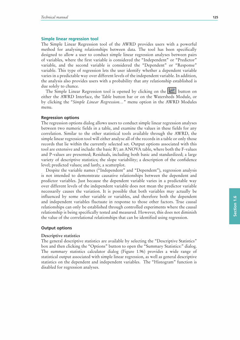
Technical manual 125
Sect
ion
1.6
Simple linear regression toolThe Simple Linear Regression tool of the AWRD provides users with a powerful method for analysing relationships between data. The tool has been specifically designed to allow a user to conduct simple linear regression analyses between pairs of variables, where the first variable is considered the “Independent” or “Predictor” variable, and the second variable is considered the “Dependent” or “Response” variable. This type of regression lets the user identify whether a dependent variable varies in a predictable way over different levels of the independent variable. In addition, the analysis also provides users with a probability that any relationship established is due solely to chance.
The Simple Linear Regression tool is opened by clicking on the button on either the AWRD Interface, the Table button bar or on the Watersheds Module, or by clicking the “Simple Linear Regression…” menu option in the AWRD Modules menu.
Regression options The regression options dialog allows users to conduct simple linear regression analyses between two numeric fields in a table, and examine the values in these fields for any correlation . Similar to the other statistical tools available through the AWRD, the simple linear regression tool will either analyse all of the records in a table or only those records that lie within the currently selected set. Output options associated with this tool are extensive and include: the basic R2; an ANOVA table, where both the F-values and P-values are presented; Residuals, including both basic and standardized; a large variety of descriptive statistics ; the slope variability; a description of the confidence level ; predicted values ; and lastly, a scatterplot .
Despite the variable names (“Independent” and “Dependent”), regression analysis is not intended to demonstrate causative relationships between the dependent and predictor variables. Just because the dependent variable varies in a predictable way over different levels of the independent variable does not mean the predictor variable necessarily causes the variation. It is possible that both variables may actually be influenced by some other variable or variables, and therefore both the dependent and independent variables fluctuate in response to those other factors. True causal relationships can only be established through controlled experiments where the causal relationship is being specifically tested and measured. However, this does not diminish the value of the correlational relationships that can be identified using regression.
Output options
Descriptive statisticsThe general descriptive statistics are available by selecting the “Descriptive Statistics” box and then clicking the “Options” button to open the “Summary Statistics:” dialog. The summary statistics calculator dialog (Figure 1.96) provides a wide range of statistical output associated with simple linear regression , as well as general descriptive statistics on the dependent and independent variables. The “Histogram” function is disabled for regression analyses.
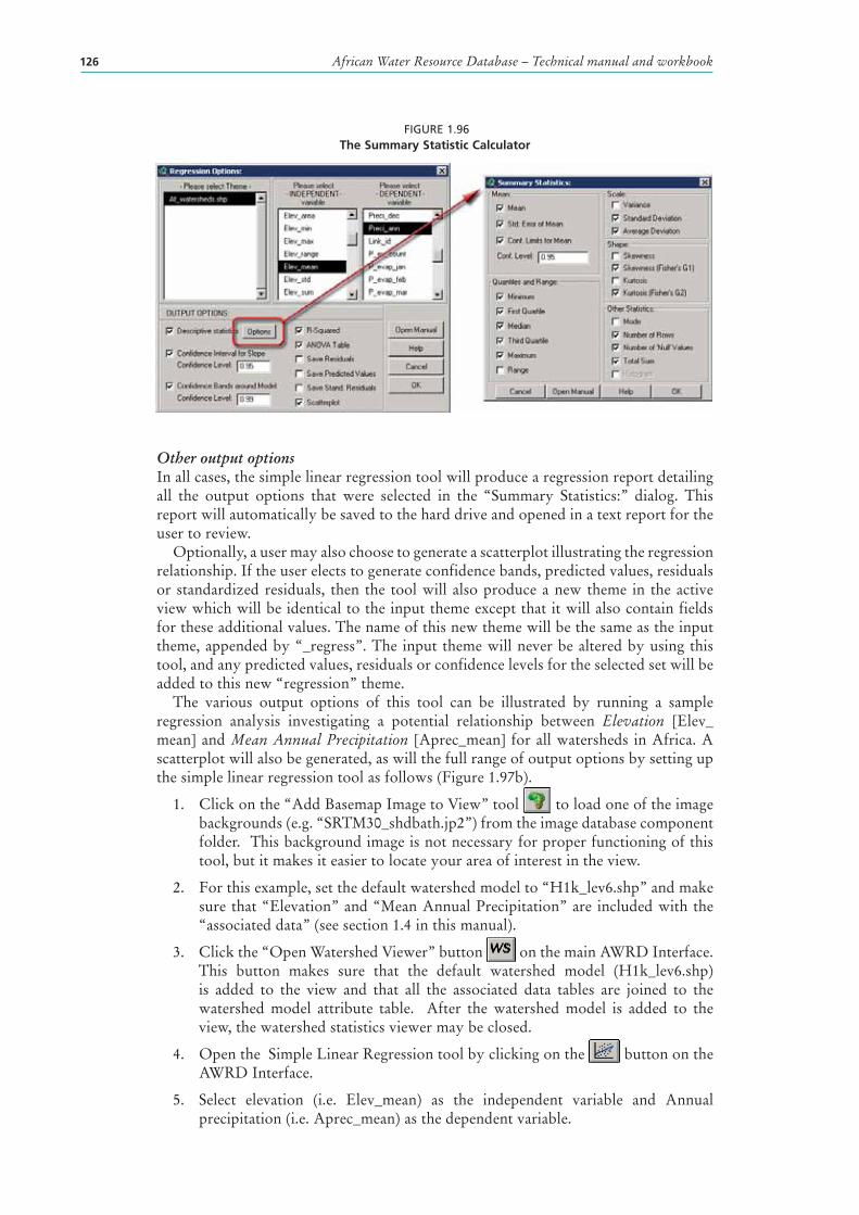
African Water Resource Database – Technical manual and workbook126
FIGURE 1.96The Summary Statistic Calculator
Other output optionsIn all cases, the simple linear regression tool will produce a regression report detailing all the output options that were selected in the “Summary Statistics:” dialog. This report will automatically be saved to the hard drive and opened in a text report for the user to review.
Optionally, a user may also choose to generate a scatterplot illustrating the regression relationship. If the user elects to generate confidence bands , predicted values , residuals or standardized residuals , then the tool will also produce a new theme in the active view which will be identical to the input theme except that it will also contain fields for these additional values. The name of this new theme will be the same as the input theme, appended by “_regress”. The input theme will never be altered by using this tool, and any predicted values, residuals or confidence level s for the selected set will be added to this new “regression” theme.
The various output options of this tool can be illustrated by running a sample regression analysis investigating a potential relationship between Elevation [Elev_mean ] and Mean Annual Precipitation [Aprec_mean] for all watersheds in Africa. A scatterplot will also be generated, as will the full range of output options by setting up the simple linear regression tool as follows (Figure 1.97b).
1. Click on the “Add Basemap Image to View” tool to load one of the image backgrounds (e.g. “SRTM30_shdbath.jp2”) from the image database component folder. This background image is not necessary for proper functioning of this tool, but it makes it easier to locate your area of interest in the view.
2. For this example, set the default watershed model to “H1k_lev6.shp” and make sure that “Elevation” and “Mean Annual Precipitation” are included with the “associated data” (see section 1.4 in this manual).
3. Click the “Open Watershed Viewer” button on the main AWRD Interface. This button makes sure that the default watershed model (H1k_lev6.shp) is added to the view and that all the associated data tables are joined to the watershed model attribute table. After the watershed model is added to the view, the watershed statistics viewer may be closed.
4. Open the Simple Linear Regression tool by clicking on the button on the AWRD Interface.
5. Select elevation (i.e. Elev_mean) as the independent variable and Annual precipitation (i.e. Aprec_mean) as the dependent variable.
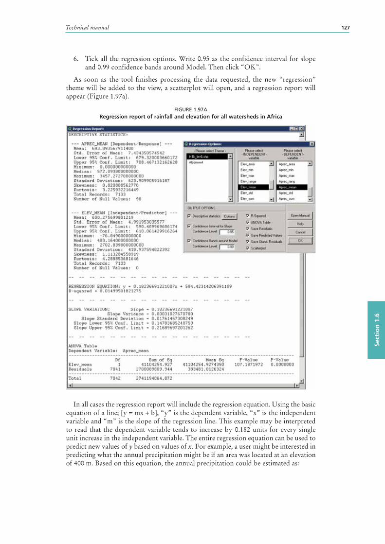
Technical manual 127
Sect
ion
1.6
6. Tick all the regression options. Write 0.95 as the confidence interval for slope and 0.99 confidence bands around Model. Then click “OK”.
As soon as the tool finishes processing the data requested, the new “regression ” theme will be added to the view, a scatterplot will open, and a regression report will appear (Figure 1.97a).
FIGURE 1.97ARegression report of rainfall and elevation for all watersheds in Africa
In all cases the regression report will include the regression equation. Using the basic equation of a line; [y = mx + b], “y” is the dependent variable, “x” is the independent variable and “m” is the slope of the regression line. This example may be interpreted to read that the dependent variable tends to increase by 0.182 units for every single unit increase in the independent variable. The entire regression equation can be used to predict new values of y based on values of x. For example, a user might be interested in predicting what the annual precipitation might be if an area was located at an elevation of 400 m. Based on this equation, the annual precipitation could be estimated as:
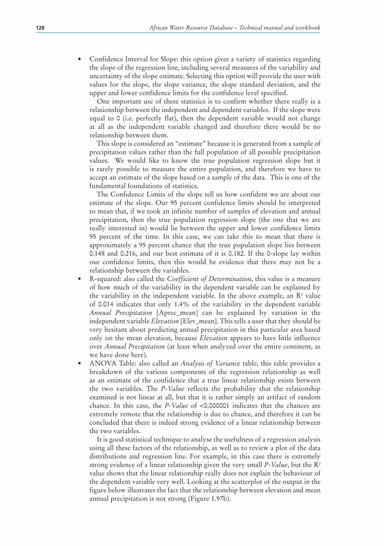
African Water Resource Database – Technical manual and workbook128
• Confidence Interval for Slope: this option gives a variety of statistics regarding the slope of the regression line, including several measures of the variability and uncertainty of the slope estimate. Selecting this option will provide the user with values for the slope, the slope variance, the slope standard deviation, and the upper and lower confidence limits for the confidence level specified.
One important use of these statistics is to confirm whether there really is a relationship between the independent and dependent variables. If the slope were equal to 0 (i.e. perfectly flat), then the dependent variable would not change at all as the independent variable changed and therefore there would be no relationship between them.
This slope is considered an “estimate” because it is generated from a sample of precipitation values rather than the full population of all possible precipitation values. We would like to know the true population regression slope but it is rarely possible to measure the entire population, and therefore we have to accept an estimate of the slope based on a sample of the data. This is one of the fundamental foundations of statistics.
The Confidence Limits of the slope tell us how confident we are about our estimate of the slope. Our 95 percent confidence limits should be interpreted to mean that, if we took an infinite number of samples of elevation and annual precipitation , then the true population regression slope (the one that we are really interested in) would lie between the upper and lower confidence limits 95 percent of the time. In this case, we can take this to mean that there is approximately a 95 percent chance that the true population slope lies between 0.148 and 0.216, and our best estimate of it is 0.182. If the 0-slope lay within our confidence limits, then this would be evidence that there may not be a relationship between the variables.
• R-squared: also called the Coefficient of Determination, this value is a measure of how much of the variability in the dependent variable can be explained by the variability in the independent variable. In the above example, an R2 value of 0.014 indicates that only 1.4% of the variability in the dependent variable Annual Precipitation [Aprec_mean ] can be explained by variation in the independent variable Elevation [Elev_mean]. This tells a user that they should be very hesitant about predicting annual precipitation in this particular area based only on the mean elevation , because Elevation appears to have little influence over Annual Precipitation (at least when analyzed over the entire continent, as we have done here).
• ANOVA Table: also called an Analysis of Variance table, this table provides a breakdown of the various components of the regression relationship as well as an estimate of the confidence that a true linear relationship exists between the two variables. The P-Value reflects the probability that the relationship examined is not linear at all, but that it is rather simply an artifact of random chance. In this case, the P-Value of <0.000001 indicates that the chances are extremely remote that the relationship is due to chance, and therefore it can be concluded that there is indeed strong evidence of a linear relationship between the two variables.
It is good statistical technique to analyse the usefulness of a regression analysis using all these factors of the relationship, as well as to review a plot of the data distributions and regression line. For example, in this case there is extremely strong evidence of a linear relationship given the very small P-Value, but the R2 value shows that the linear relationship really does not explain the behaviour of the dependent variable very well. Looking at the scatterplot of the output in the figure below illustrates the fact that the relationship between elevation and mean annual precipitation is not strong (Figure 1.97b).
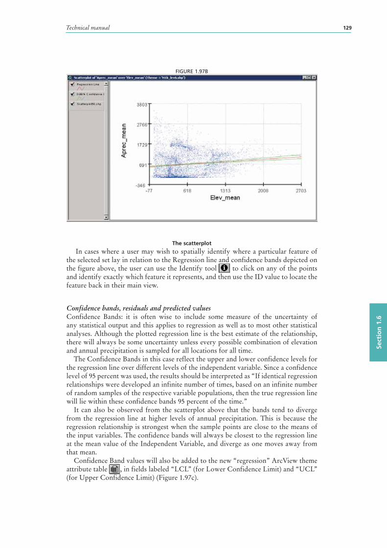
Technical manual 129
Sect
ion
1.6
FIGURE 1.97B
The scatterplot
In cases where a user may wish to spatially identify where a particular feature of the selected set lay in relation to the Regression line and confidence bands depicted on the figure above, the user can use the Identify tool to click on any of the points and identify exactly which feature it represents, and then use the ID value to locate the feature back in their main view.
Confidence bands, residuals and predicted valuesConfidence Bands: it is often wise to include some measure of the uncertainty of any statistical output and this applies to regression as well as to most other statistical analyses. Although the plotted regression line is the best estimate of the relationship, there will always be some uncertainty unless every possible combination of elevation and annual precipitation is sampled for all locations for all time.
The Confidence Bands in this case reflect the upper and lower confidence level s for the regression line over different levels of the independent variable. Since a confidence level of 95 percent was used, the results should be interpreted as “If identical regression relationships were developed an infinite number of times, based on an infinite number of random samples of the respective variable populations, then the true regression line will lie within these confidence bands 95 percent of the time.”
It can also be observed from the scatterplot above that the bands tend to diverge from the regression line at higher levels of annual precipitation . This is because the regression relationship is strongest when the sample points are close to the means of the input variables. The confidence bands will always be closest to the regression line at the mean value of the Independent Variable, and diverge as one moves away from that mean.
Confidence Band values will also be added to the new “regression ” ArcView theme attribute table , in fields labeled “LCL” (for Lower Confidence Limit) and “UCL” (for Upper Confidence Limit) (Figure 1.97c).
African Water Resource Database – Technical manual and workbook130
FIGURE 1.97CThe new “regression ” theme attribute table
Residuals and Predicted Values: along with confidence bands , the new “regression ” theme attribute table also contains fields for the predicted values , residuals and standardized residuals . The “model ” field holds values for the predicted value of Mean Annual Precipitation based on the regression equation and that record’s value for Mean Elevation. The Residuals field [resids] holds values reflecting how much the measured Mean Annual Precipitation deviated from the predicted model value. The Standardized Residuals field [res_stand] standardizes these residuals values by converting them to Z-scores, making it easy to identify extreme outliers.
Example of performing analyses on different subsets of dataOne of the strong points of the Simple Linear Regression tool is that a user can restrict the analysis to a subset of features by selecting those features prior to analysis. If any features are selected, then the tool will only operate on those selected features. If no features are selected, then the tool will operate on all features in the theme .
If, for example, a user was really only interested in phenomena occurring within the Nile River megabasin:
1. Using the HYDRO-1K watershed model from the previous example, click the Select Upstream and Downstream Watersheds” tool of the Watersheds Module. Choose the “Include Entire Basin” option and then click anywhere in Lake Victoria. This will select all watersheds in the Nile River megabasin.
2. Open the Simple Linear Regression tool by clicking on the button on the AWRD Interface.
3. Select elevation (i.e. Elev_mean) as the independent variable and Annual precipitation (i.e. Aprec_mean) as the dependent variable.
4. Tick all the regression options. 5. Write 0.95 as the confidence level for slope, and 0.99 as the confidence level for
the model. Then click “OK”.
The regression report and scatterplot are illustrated in Figure 1.98.
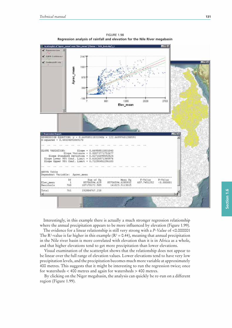
Technical manual 131
Sect
ion
1.6
FIGURE 1.98Regression analysis of rainfall and elevation for the Nile River megabasin
Interestingly, in this example there is actually a much stronger regression relationship where the annual precipitation appears to be more influenced by elevation (Figure 1.99).
The evidence for a linear relationship is still very strong with a P-Value of <0.000001 The R2-value is far higher in this example (R2 = 0.44), meaning that annual precipitation in the Nile river basin is more correlated with elevation than it is in Africa as a whole, and that higher elevations tend to get more precipitation than lower elevations.
Visual examination of the scatterplot shows that the relationship does not appear to be linear over the full range of elevation values. Lower elevations tend to have very low precipitation levels, and the precipitation becomes much more variable at approximately 400 metres. This suggests that it might be interesting to run the regression twice; once for watersheds < 400 metres and again for watersheds > 400 metres.
By clicking on the Niger megabasin , the analysis can quickly be re-run on a different region (Figure 1.99).

African Water Resource Database – Technical manual and workbook132
FIGURE 1.99Regression analysis of rainfall and elevation for the Niger megabasin
The results of this analysis are also very interesting in that they differ from the relationship established for the continent as a whole. The evidence for a linear relationship is still very strong with a P-Value of 0.0000110, but the R2-value is very low at 0.08, meaning that elevation has little influence on annual precipitation in this region. Interestingly, the regression relationship assumes a different direction than was seen in the Nile megabasin , in that here the mean annual precipitation decreases as elevation increases.
There are several excellent texts available that discuss regression in exhaustive detail. For those who are interested, we recommend. Draper and Smith (1998) and Neter et al. (1996).
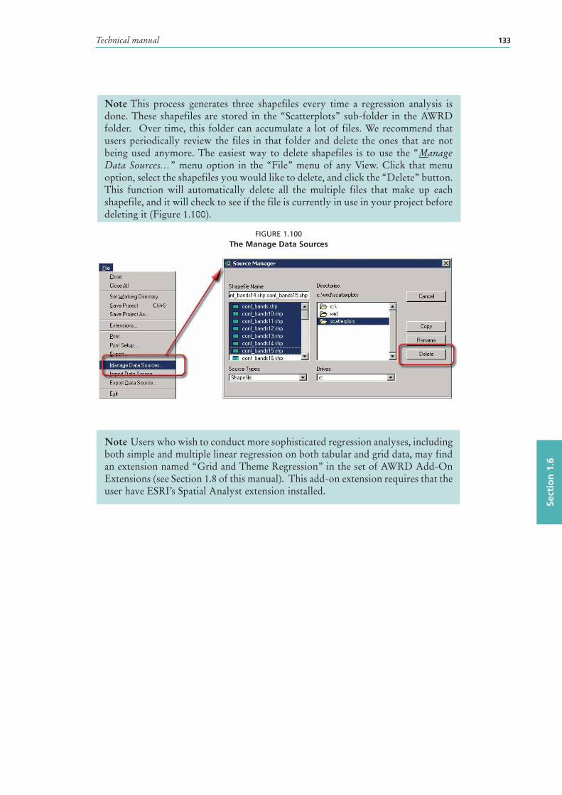
Technical manual 133
Sect
ion
1.6
Note This process generates three shapefiles every time a regression analysis is done. These shapefiles are stored in the “Scatterplots” sub-folder in the AWRD folder. Over time, this folder can accumulate a lot of files. We recommend that users periodically review the files in that folder and delete the ones that are not being used anymore. The easiest way to delete shapefiles is to use the “Manage Data Sources…” menu option in the “File” menu of any View. Click that menu option, select the shapefiles you would like to delete, and click the “Delete” button. This function will automatically delete all the multiple files that make up each shapefile, and it will check to see if the file is currently in use in your project before deleting it (Figure 1.100).
FIGURE 1.100The Manage Data Sources
Note Users who wish to conduct more sophisticated regression analyses, including both simple and multiple linear regression on both tabular and grid data, may find an extension named “Grid and Theme Regression” in the set of AWRD Add-On Extensions (see Section 1.8 of this manual). This add-on extension requires that the user have ESRI’s Spatial Analyst extension installed.
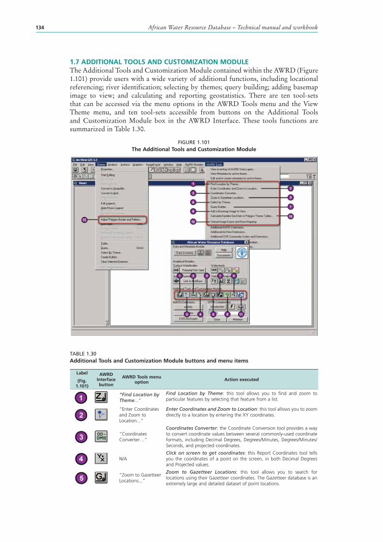
African Water Resource Database – Technical manual and workbook134
1.7 ADDITIONAL TOOLS AND CUSTOMIZATION MODULEThe Additional Tools and Customization Module contained within the AWRD (Figure 1.101) provide users with a wide variety of additional functions, including locational referencing; river identification; selecting by themes; query building; adding basemap image to view; and calculating and reporting geostatistics. There are ten tool-sets that can be accessed via the menu options in the AWRD Tools menu and the View Theme menu, and ten tool-sets accessible from buttons on the Additional Tools and Customization Module box in the AWRD Interface. These tools functions are summarized in Table 1.30.
FIGURE 1.101The Additional Tools and Customization Module
TABLE 1.30Additional Tools and Customization Module buttons and menu items
Label
(Fig. 1.101)
AWRD Interface button
AWRD Tools menu option Action executed
“Find Location by Theme...”
Find Location by Theme: this tool allows you to find and zoom to particular features by selecting that feature from a list.
“Enter Coordinates and Zoom to Location...”
Enter Coordinates and Zoom to Location: this tool allows you to zoom directly to a location by entering the XY coordinates.
“Coordinates Converter…”
Coordinates Converter: the Coordinate Conversion tool provides a way to convert coordinate values between several commonly-used coordinate formats, including Decimal Degrees, Degrees/Minutes, Degrees/Minutes/Seconds, and projected coordinates.
N/AClick on screen to get coordinates: this Report Coordinates tool tells you the coordinates of a point on the screen, in both Decimal Degrees and Projected values.
“Zoom to Gazetteer Locations...”
Zoom to Gazetteer Locations: this tool allows you to search for locations using their Gazetteer coordinates. The Gazetteer database is an extremely large and detailed dataset of point locations.
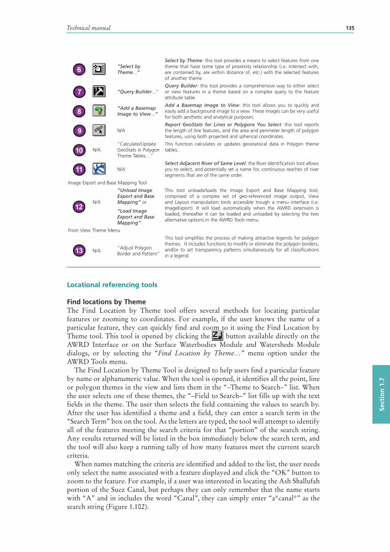
Technical manual 135
Sect
ion
1.7
“Select by Theme...”
Select by Theme: this tool provides a means to select features from one theme that have some type of proximity relationship (i.e. intersect with, are contained by, are within distance of, etc.) with the selected features of another theme.
“Query Builder...”Query Builder: this tool provides a comprehensive way to either select or view features in a theme based on a complex query to the feature attribute table.
“Add a Basemap Image to View...”
Add a Basemap Image to View: this tool allows you to quickly and easily add a background image to a view. These images can be very useful for both aesthetic and analytical purposes.
N/A Report GeoStats for Lines or Polygons You Select: this tool reports the length of line features, and the area and perimeter length of polygon features, using both projected and spherical coordinates.
N/A“Calculate/Update GeoStats in Polygon Theme Tables…”
This function calculates or updates geostatiscal data in Polygon theme tables.
N/ASelect Adjacent River of Same Level: the River Identification tool allows you to select, and potentially set a name for, continuous reaches of river segments that are of the same order.
Image Export and Base Mapping Tool
N/A
“Unload Image Export and Base Mapping” or
“Load Image Export and Base Mapping”
This tool unloads/loads the Image Export and Base Mapping tool, comprised of a complex set of geo-referenced image output, View and Layout manipulation tools accessible trough a menu interface (i.e. ImageExport). It will load automatically when the AWRD extension is loaded; thereafter it can be loaded and unloaded by selecting the two alternative options in the AWRD Tools menu.
From View Theme Menu
N/A“Adjust Polygon Border and Pattern”
This tool simplifies the process of making attractive legends for polygon themes. It includes functions to modify or eliminate the polygon borders, and/or to set transparency patterns simultaneously for all classifications in a legend.
Locational referencing tools
Find locations by ThemeThe Find Location by Theme tool offers several methods for locating particular features or zooming to coordinates. For example, if the user knows the name of a particular feature, they can quickly find and zoom to it using the Find Location by Theme tool. This tool is opened by clicking the button available directly on the AWRD Interface or on the Surface Waterbodies Module and Watersheds Module dialogs, or by selecting the “Find Location by Theme…” menu option under the AWRD Tools menu.
The Find Location by Theme Tool is designed to help users find a particular feature by name or alphanumeric value. When the tool is opened, it identifies all the point, line or polygon themes in the view and lists them in the “–Theme to Search–” list. When the user selects one of these themes, the “–Field to Search–” list fills up with the text fields in the theme . The user then selects the field containing the values to search by. After the user has identified a theme and a field, they can enter a search term in the “Search Term” box on the tool. As the letters are typed, the tool will attempt to identify all of the features meeting the search criteria for that “portion” of the search string. Any results returned will be listed in the box immediately below the search term, and the tool will also keep a running tally of how many features meet the current search criteria.
When names matching the criteria are identified and added to the list, the user needs only select the name associated with a feature displayed and click the “OK” button to zoom to the feature. For example, if a user was interested in locating the Ash Shallufah portion of the Suez Canal, but perhaps they can only remember that the name starts with “A” and in includes the word “Canal”, they can simply enter “a*canal*” as the search string (Figure 1.102).
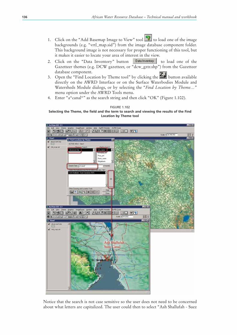
African Water Resource Database – Technical manual and workbook136
1. Click on the “Add Basemap Image to View” tool to load one of the image backgrounds (e.g. “vrtl_map.sid”) from the image database component folder. This background image is not necessary for proper functioning of this tool, but it makes it easier to locate your area of interest in the view.
2. Click on the “Data Inventory” button to load one of the Gazetteer themes (e.g. DCW gazetteer, or “dcw_gztr.shp”) from the Gazetteer database component.
3. Open the “Find Location by Theme tool” by clicking the button available directly on the AWRD Interface or on the Surface Waterbodies Module and Watersheds Module dialogs, or by selecting the “Find Location by Theme…” menu option under the AWRD Tools menu.
4. Enter “a*canal*” as the search string and then click “OK” (Figure 1.102).
FIGURE 1.102Selecting the Theme, the field and the term to search and viewing the results of the Find
Location by Theme tool
Notice that the search is not case sensitive so the user does not need to be concerned about what letters are capitalized. The user could then to select “Ash Shallufah - Suez
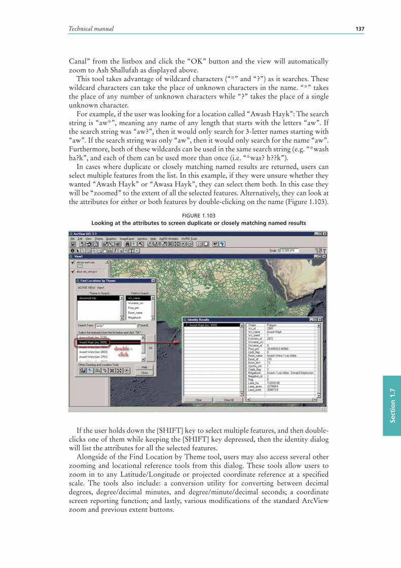
Technical manual 137
Sect
ion
1.7
Canal” from the listbox and click the “OK” button and the view will automatically zoom to Ash Shallufah as displayed above.
This tool takes advantage of wildcard characters (“*” and “?”) as it searches. These wildcard characters can take the place of unknown characters in the name. “*” takes the place of any number of unknown characters while “?” takes the place of a single unknown character.
For example, if the user was looking for a location called “Awash Hayk”: The search string is “aw*”, meaning any name of any length that starts with the letters “aw”. If the search string was “aw?”, then it would only search for 3-letter names starting with “aw”. If the search string was only “aw”, then it would only search for the name “aw”. Furthermore, both of these wildcards can be used in the same search string (e.g. “*wash ha?k”, and each of them can be used more than once (i.e. “*was? h??k”).
In cases where duplicate or closely matching named results are returned, users can select multiple features from the list. In this example, if they were unsure whether they wanted “Awash Hayk” or “Awasa Hayk”, they can select them both. In this case they will be “zoomed” to the extent of all the selected features. Alternatively, they can look at the attributes for either or both features by double-clicking on the name (Figure 1.103).
FIGURE 1.103Looking at the attributes to screen duplicate or closely matching named results
If the user holds down the [SHIFT] key to select multiple features, and then double-clicks one of them while keeping the [SHIFT] key depressed, then the identity dialog will list the attributes for all the selected features.
Alongside of the Find Location by Theme tool, users may also access several other zooming and locational reference tools from this dialog. These tools allow users to zoom in to any Latitude/Longitude or projected coordinate reference at a specified scale. The tools also include: a conversion utility for converting between decimal degrees, degree/decimal minutes, and degree/minute/decimal seconds; a coordinate screen reporting function; and lastly, various modifications of the standard ArcView zoom and previous extent buttons.
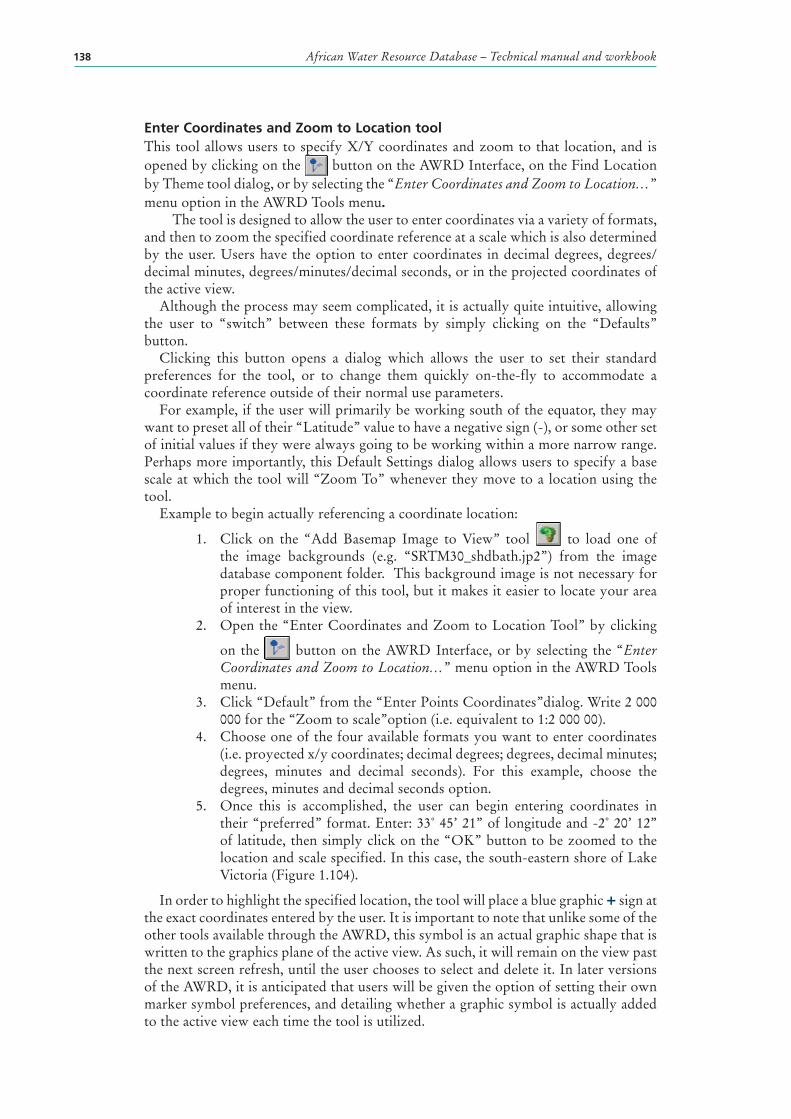
African Water Resource Database – Technical manual and workbook138
Enter Coordinates and Zoom to Location tool This tool allows users to specify X/Y coordinates and zoom to that location, and is opened by clicking on the button on the AWRD Interface, on the Find Location by Theme tool dialog, or by selecting the “Enter Coordinates and Zoom to Location …” menu option in the AWRD Tools menu.
The tool is designed to allow the user to enter coordinates via a variety of formats, and then to zoom the specified coordinate reference at a scale which is also determined by the user. Users have the option to enter coordinates in decimal degrees, degrees/decimal minutes, degrees/minutes/decimal seconds, or in the projected coordinates of the active view.
Although the process may seem complicated, it is actually quite intuitive, allowing the user to “switch” between these formats by simply clicking on the “Defaults” button.
Clicking this button opens a dialog which allows the user to set their standard preferences for the tool, or to change them quickly on-the-fly to accommodate a coordinate reference outside of their normal use parameters.
For example, if the user will primarily be working south of the equator, they may want to preset all of their “Latitude” value to have a negative sign (-), or some other set of initial values if they were always going to be working within a more narrow range . Perhaps more importantly, this Default Settings dialog allows users to specify a base scale at which the tool will “Zoom To” whenever they move to a location using the tool.
Example to begin actually referencing a coordinate location:
1. Click on the “Add Basemap Image to View” tool to load one of the image backgrounds (e.g. “SRTM30_shdbath.jp2”) from the image database component folder. This background image is not necessary for proper functioning of this tool, but it makes it easier to locate your area of interest in the view.
2. Open the “Enter Coordinates and Zoom to Location Tool” by clicking
on the button on the AWRD Interface, or by selecting the “Enter Coordinates and Zoom to Location …” menu option in the AWRD Tools menu.
3. Click “Default” from the “Enter Points Coordinates”dialog. Write 2 000 000 for the “Zoom to scale”option (i.e. equivalent to 1:2 000 00).
4. Choose one of the four available formats you want to enter coordinates (i.e. proyected x/y coordinates; decimal degrees; degrees, decimal minutes; degrees, minutes and decimal seconds). For this example, choose the degrees, minutes and decimal seconds option.
5. Once this is accomplished, the user can begin entering coordinates in their “preferred” format. Enter: 33˚ 45’ 21’’ of longitude and -2˚ 20’ 12’’ of latitude, then simply click on the “OK” button to be zoomed to the location and scale specified. In this case, the south-eastern shore of Lake Victoria (Figure 1.104).
In order to highlight the specified location, the tool will place a blue graphic + sign at the exact coordinates entered by the user. It is important to note that unlike some of the other tools available through the AWRD, this symbol is an actual graphic shape that is written to the graphics plane of the active view. As such, it will remain on the view past the next screen refresh, until the user chooses to select and delete it. In later versions of the AWRD, it is anticipated that users will be given the option of setting their own marker symbol preferences, and detailing whether a graphic symbol is actually added to the active view each time the tool is utilized.
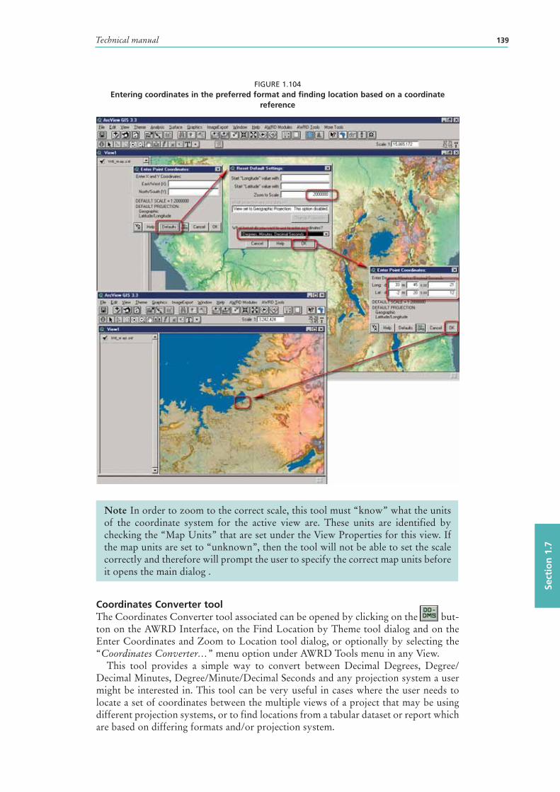
Technical manual 139
Sect
ion
1.7
FIGURE 1.104Entering coordinates in the preferred format and finding location based on a coordinate
reference
Note In order to zoom to the correct scale, this tool must “know” what the units of the coordinate system for the active view are. These units are identified by checking the “Map Units” that are set under the View Properties for this view. If the map units are set to “unknown”, then the tool will not be able to set the scale correctly and therefore will prompt the user to specify the correct map units before it opens the main dialog .
Coordinates Converter toolThe Coordinates Converter tool associated can be opened by clicking on the but-ton on the AWRD Interface, on the Find Location by Theme tool dialog and on the Enter Coordinates and Zoom to Location tool dialog, or optionally by selecting the “Coordinates Converter…” menu option under AWRD Tools menu in any View.
This tool provides a simple way to convert between Decimal Degrees, Degree/Decimal Minutes, Degree/Minute/Decimal Seconds and any projection system a user might be interested in. This tool can be very useful in cases where the user needs to locate a set of coordinates between the multiple views of a project that may be using different projection systems, or to find locations from a tabular dataset or report which are based on differing formats and/or projection system.
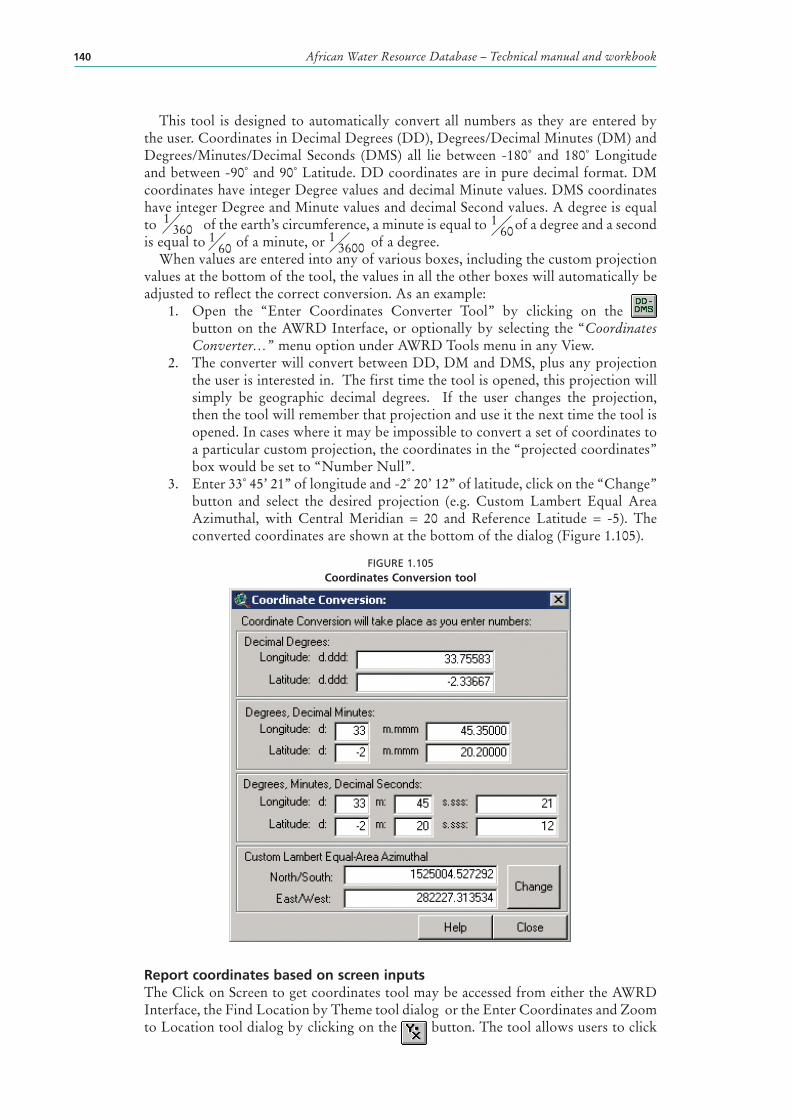
African Water Resource Database – Technical manual and workbook140
This tool is designed to automatically convert all numbers as they are entered by the user. Coordinates in Decimal Degrees (DD ), Degrees/Decimal Minutes (DM ) and Degrees/Minutes/Decimal Seconds (DMS ) all lie between -180˚ and 180˚ Longitude and between -90˚ and 90˚ Latitude. DD coordinates are in pure decimal format. DM coordinates have integer Degree values and decimal Minute values. DMS coordinates have integer Degree and Minute values and decimal Second values. A degree is equal to of the earth’s circumference, a minute is equal to of a degree and a second is equal to of a minute, or of a degree.
When values are entered into any of various boxes, including the custom projection values at the bottom of the tool, the values in all the other boxes will automatically be adjusted to reflect the correct conversion. As an example:
1. Open the “Enter Coordinates Converter Tool” by clicking on the button on the AWRD Interface, or optionally by selecting the “Coordinates Converter…” menu option under AWRD Tools menu in any View.
2. The converter will convert between DD, DM and DMS, plus any projection the user is interested in. The first time the tool is opened, this projection will simply be geographic decimal degrees. If the user changes the projection, then the tool will remember that projection and use it the next time the tool is opened. In cases where it may be impossible to convert a set of coordinates to a particular custom projection, the coordinates in the “projected coordinates” box would be set to “Number Null”.
3. Enter 33˚ 45’ 21’’ of longitude and -2˚ 20’ 12’’ of latitude, click on the “Change” button and select the desired projection (e.g. Custom Lambert Equal Area Azimuthal, with Central Meridian = 20 and Reference Latitude = -5). The converted coordinates are shown at the bottom of the dialog (Figure 1.105).
FIGURE 1.105Coordinates Conversion tool
Report coordinates based on screen inputsThe Click on Screen to get coordinates tool may be accessed from either the AWRD Interface, the Find Location by Theme tool dialog or the Enter Coordinates and Zoom to Location tool dialog by clicking on the button. The tool allows users to click
1 360 1 3600
1 60 1 60
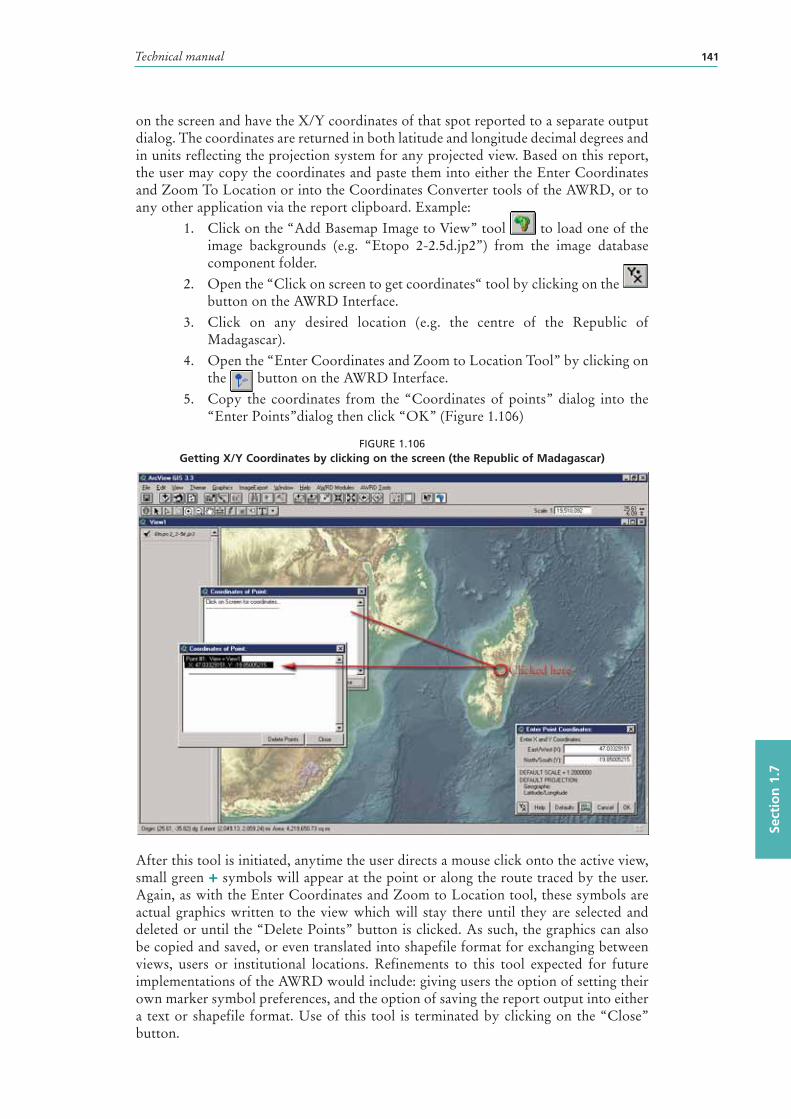
Technical manual 141
Sect
ion
1.7
on the screen and have the X/Y coordinates of that spot reported to a separate output dialog. The coordinates are returned in both latitude and longitude decimal degrees and in units reflecting the projection system for any projected view. Based on this report , the user may copy the coordinates and paste them into either the Enter Coordinates and Zoom To Location or into the Coordinates Converter tools of the AWRD, or to any other application via the report clipboard. Example:
1. Click on the “Add Basemap Image to View” tool to load one of the image backgrounds (e.g. “Etopo 2-2.5d.jp2”) from the image database component folder.
2. Open the “Click on screen to get coordinates“ tool by clicking on the button on the AWRD Interface.
3. Click on any desired location (e.g. the centre of the Republic of Madagascar).
4. Open the “Enter Coordinates and Zoom to Location Tool” by clicking on the button on the AWRD Interface.
5. Copy the coordinates from the “Coordinates of points” dialog into the “Enter Points”dialog then click “OK” (Figure 1.106)
FIGURE 1.106Getting X/Y Coordinates by clicking on the screen (the Republic of Madagascar)
After this tool is initiated, anytime the user directs a mouse click onto the active view, small green + symbols will appear at the point or along the route traced by the user. Again, as with the Enter Coordinates and Zoom to Location tool, these symbols are actual graphics written to the view which will stay there until they are selected and deleted or until the “Delete Points” button is clicked. As such, the graphics can also be copied and saved, or even translated into shapefile format for exchanging between views, users or institutional locations. Refinements to this tool expected for future implementations of the AWRD would include: giving users the option of setting their own marker symbol preferences, and the option of saving the report output into either a text or shapefile format. Use of this tool is terminated by clicking on the “Close” button.
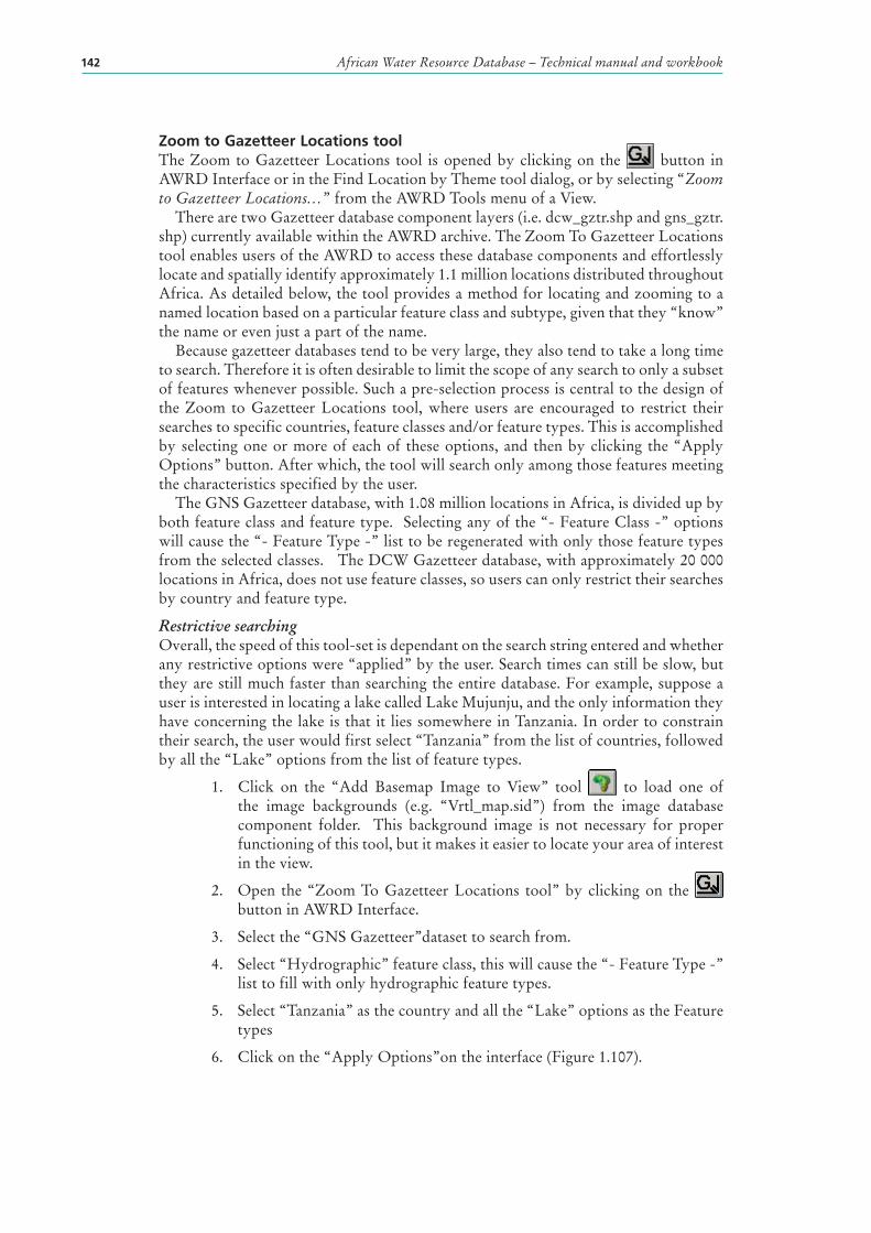
African Water Resource Database – Technical manual and workbook142
Zoom to Gazetteer Locations toolThe Zoom to Gazetteer Locations tool is opened by clicking on the button in AWRD Interface or in the Find Location by Theme tool dialog, or by selecting “Zoom to Gazetteer Locations…” from the AWRD Tools menu of a View.
There are two Gazetteer database component layers (i.e. dcw_gztr.shp and gns_gztr.shp) currently available within the AWRD archive. The Zoom To Gazetteer Locations tool enables users of the AWRD to access these database components and effortlessly locate and spatially identify approximately 1.1 million locations distributed throughout Africa. As detailed below, the tool provides a method for locating and zooming to a named location based on a particular feature class and subtype, given that they “know” the name or even just a part of the name.
Because gazetteer databases tend to be very large, they also tend to take a long time to search. Therefore it is often desirable to limit the scope of any search to only a subset of features whenever possible. Such a pre-selection process is central to the design of the Zoom to Gazetteer Locations tool, where users are encouraged to restrict their searches to specific countries, feature classes and/or feature types. This is accomplished by selecting one or more of each of these options, and then by clicking the “Apply Options” button. After which, the tool will search only among those features meeting the characteristics specified by the user.
The GNS Gazetteer database, with 1.08 million locations in Africa, is divided up by both feature class and feature type. Selecting any of the “- Feature Class -” options will cause the “- Feature Type -” list to be regenerated with only those feature types from the selected classes. The DCW Gazetteer database, with approximately 20 000 locations in Africa, does not use feature classes, so users can only restrict their searches by country and feature type.
Restrictive searchingOverall, the speed of this tool-set is dependant on the search string entered and whether any restrictive options were “applied” by the user. Search times can still be slow, but they are still much faster than searching the entire database. For example, suppose a user is interested in locating a lake called Lake Mujunju, and the only information they have concerning the lake is that it lies somewhere in Tanzania. In order to constrain their search, the user would first select “Tanzania” from the list of countries, followed by all the “Lake” options from the list of feature types.
1. Click on the “Add Basemap Image to View” tool to load one of the image backgrounds (e.g. “Vrtl_map.sid”) from the image database component folder. This background image is not necessary for proper functioning of this tool, but it makes it easier to locate your area of interest in the view.
2. Open the “Zoom To Gazetteer Locations tool” by clicking on the button in AWRD Interface.
3. Select the “GNS Gazetteer”dataset to search from.
4. Select “Hydrographic” feature class, this will cause the “- Feature Type -” list to fill with only hydrographic feature types.
5. Select “Tanzania” as the country and all the “Lake” options as the Feature types
6. Click on the “Apply Options”on the interface (Figure 1.107).
Technical manual 143
Sect
ion
1.7
FIGURE 1.107Constraining a search with the Zoom to Gazetteer Locations tool
In the example above, the total number of records available for query has dropped from 1 083 354 to 131, and the user has not yet begun entering their search string!
As with the Find Location by Theme tool, search strings are not case-sensitive so the user need not worry about capitalization. Also, the user can again use the “*” and “?” wildcard characters in their search. The “*” symbol specifies that any number of characters may be substituted for it. For example, since the user is not sure of the spelling of Lake Mujunju, but is confident that the name contains “Muj”, then they may enter “*muj*” to identify all names that include the characters “muj”.
The use of the “*” at the front also frees the user from specifying “Lake” in front of the name. This is useful in cases where a potentially matching name in the Gazetteer might include “Mujunju Pools” or “Mujunju Dam” rather than “Lake Munjunju”.
Note Users may choose between two different gazetteers upon which to base queries, both of which are based on NIMA’s Geographic Name Server (GNS) database. The GNS Gazetteer database is a point shapefile with over 1 083 000 points in Africa and takes a little bit longer to search than the worldwide DCW Gazetteer shapefile with over 151 000 points (of which approximately 20 000 are in Africa). For more information concerning these gazetteers and the specific feature classes or types available please review the metadata associated with each data layer and/or alternatively visit http://earth-info.nima.mil/gns/html/index.html. This Web site can also be reached by clicking the “GNS Web Site” button on the top right of the Gazetteer dialog.
The user may choose the “?” symbol, in cases where they wish only one character to be substituted in their search criteria, or when they may be unsure of a single letter. For example, if the user again wanted to find the feature named “Lake Mujunju”, but was not quite sure of the spelling, they could enter a search string similar to “Lake Muj?nju” or “Lake M?j?nju”.
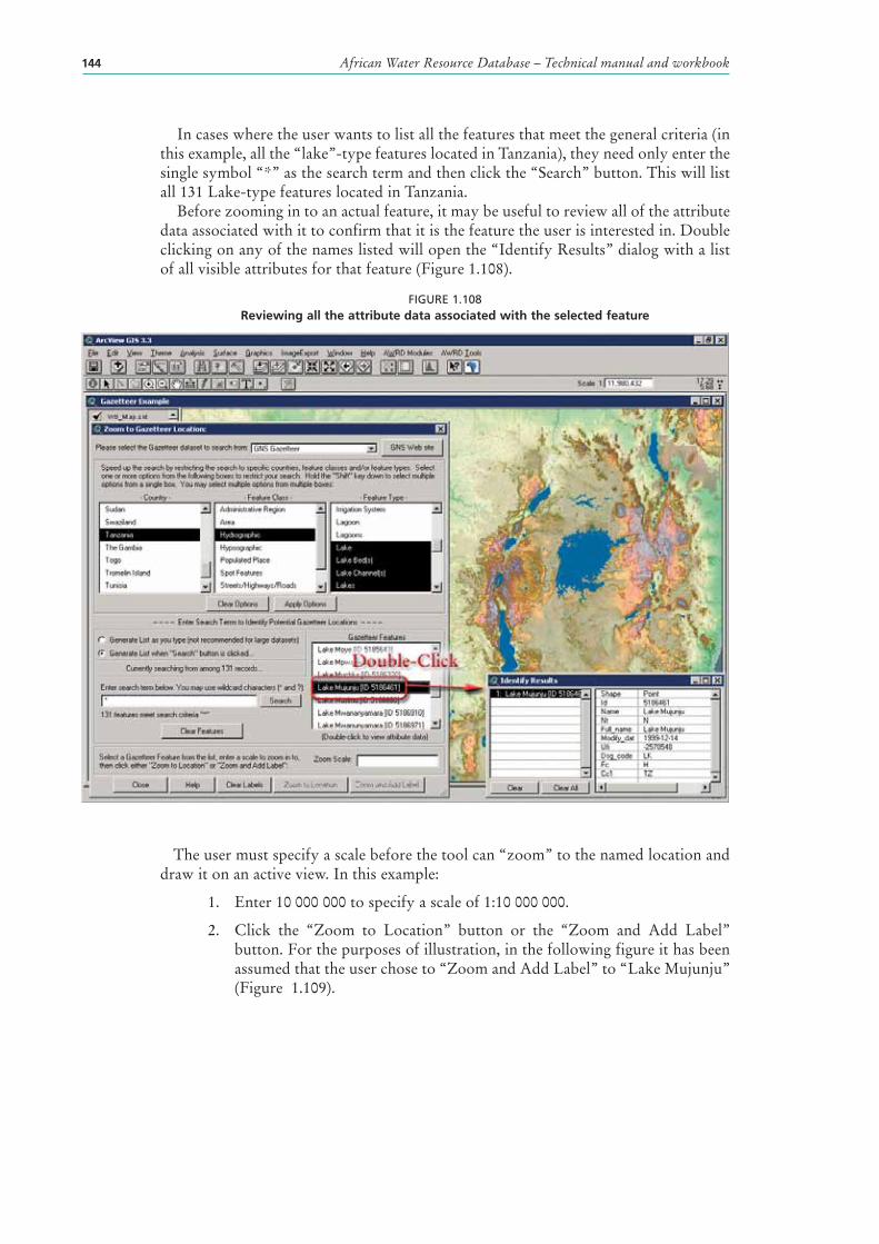
African Water Resource Database – Technical manual and workbook144
In cases where the user wants to list all the features that meet the general criteria (in this example, all the “lake”-type features located in Tanzania), they need only enter the single symbol “*” as the search term and then click the “Search” button. This will list all 131 Lake-type features located in Tanzania.
Before zooming in to an actual feature, it may be useful to review all of the attribute data associated with it to confirm that it is the feature the user is interested in. Double clicking on any of the names listed will open the “Identify Results” dialog with a list of all visible attributes for that feature (Figure 1.108).
FIGURE 1.108Reviewing all the attribute data associated with the selected feature
The user must specify a scale before the tool can “zoom ” to the named location and draw it on an active view. In this example:
1. Enter 10 000 000 to specify a scale of 1:10 000 000.
2. Click the “Zoom to Location” button or the “Zoom and Add Label” button. For the purposes of illustration, in the following figure it has been assumed that the user chose to “Zoom and Add Label” to “Lake Mujunju” (Figure 1.109).
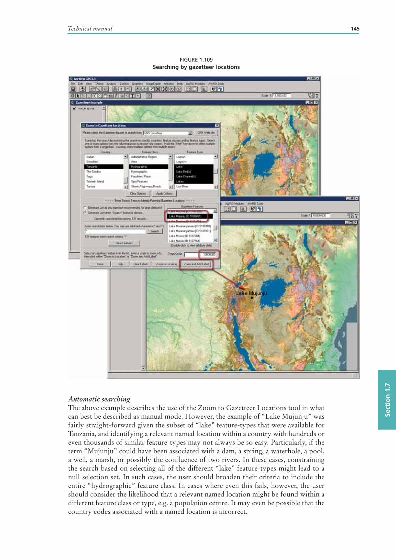
Technical manual 145
Sect
ion
1.7
FIGURE 1.109Searching by gazetteer locations
Automatic searching The above example describes the use of the Zoom to Gazetteer Locations tool in what can best be described as manual mode. However, the example of “Lake Mujunju” was fairly straight-forward given the subset of “lake” feature-types that were available for Tanzania, and identifying a relevant named location within a country with hundreds or even thousands of similar feature-types may not always be so easy. Particularly, if the term “Mujunju” could have been associated with a dam, a spring, a waterhole, a pool, a well, a marsh, or possibly the confluence of two rivers. In these cases, constraining the search based on selecting all of the different “lake” feature-types might lead to a null selection set. In such cases, the user should broaden their criteria to include the entire “hydrographic” feature class. In cases where even this fails, however, the user should consider the likelihood that a relevant named location might be found within a different feature class or type, e.g. a population centre. It may even be possible that the country codes associated with a named location is incorrect.
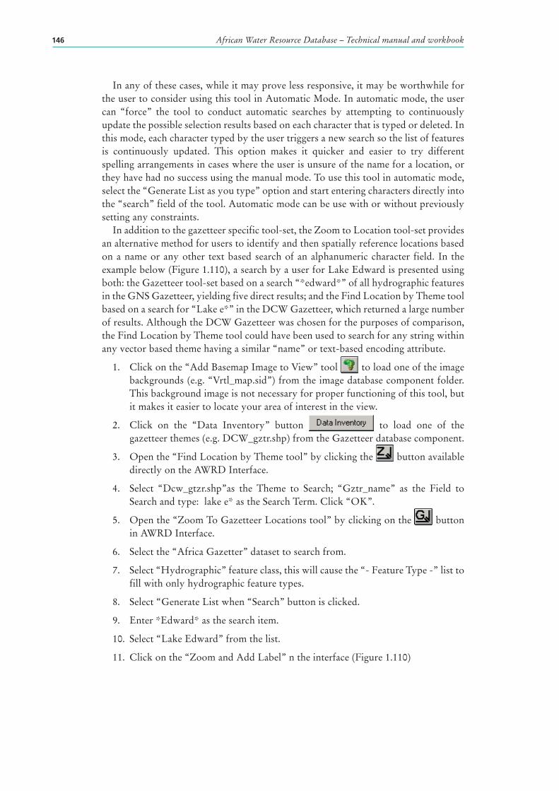
African Water Resource Database – Technical manual and workbook146
In any of these cases, while it may prove less responsive, it may be worthwhile for the user to consider using this tool in Automatic Mode. In automatic mode, the user can “force” the tool to conduct automatic searches by attempting to continuously update the possible selection results based on each character that is typed or deleted. In this mode, each character typed by the user triggers a new search so the list of features is continuously updated. This option makes it quicker and easier to try different spelling arrangements in cases where the user is unsure of the name for a location, or they have had no success using the manual mode. To use this tool in automatic mode, select the “Generate List as you type” option and start entering characters directly into the “search” field of the tool. Automatic mode can be use with or without previously setting any constraints.
In addition to the gazetteer specific tool-set, the Zoom to Location tool-set provides an alternative method for users to identify and then spatially reference locations based on a name or any other text based search of an alphanumeric character field. In the example below (Figure 1.110), a search by a user for Lake Edward is presented using both: the Gazetteer tool-set based on a search “*edward*” of all hydrographic features in the GNS Gazetteer, yielding five direct results; and the Find Location by Theme tool based on a search for “Lake e*” in the DCW Gazetteer, which returned a large number of results. Although the DCW Gazetteer was chosen for the purposes of comparison, the Find Location by Theme tool could have been used to search for any string within any vector based theme having a similar “name” or text-based encoding attribute.
1. Click on the “Add Basemap Image to View” tool to load one of the image backgrounds (e.g. “Vrtl_map.sid”) from the image database component folder. This background image is not necessary for proper functioning of this tool, but it makes it easier to locate your area of interest in the view.
2. Click on the “Data Inventory” button to load one of the gazetteer themes (e.g. DCW_gztr.shp) from the Gazetteer database component.
3. Open the “Find Location by Theme tool” by clicking the button available directly on the AWRD Interface.
4. Select “Dcw_gtzr.shp”as the Theme to Search; “Gztr_name” as the Field to Search and type: lake e* as the Search Term. Click “OK”.
5. Open the “Zoom To Gazetteer Locations tool” by clicking on the button in AWRD Interface.
6. Select the “Africa Gazetter” dataset to search from.
7. Select “Hydrographic” feature class, this will cause the “- Feature Type -” list to fill with only hydrographic feature types.
8. Select “Generate List when “Search” button is clicked.
9. Enter *Edward* as the search item.
10. Select “Lake Edward” from the list.
11. Click on the “Zoom and Add Label” n the interface (Figure 1.110)
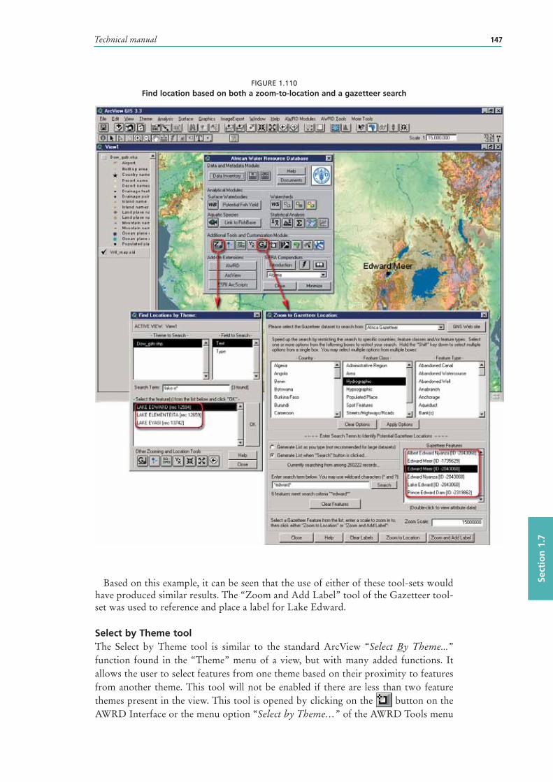
Technical manual 147
Sect
ion
1.7
FIGURE 1.110Find location based on both a zoom-to-location and a gazetteer search
Based on this example, it can be seen that the use of either of these tool-sets would have produced similar results. The “Zoom and Add Label” tool of the Gazetteer tool-set was used to reference and place a label for Lake Edward.
Select by Theme tool The Select by Theme tool is similar to the standard ArcView “Select By Theme...” function found in the “Theme” menu of a view, but with many added functions. It allows the user to select features from one theme based on their proximity to features from another theme. This tool will not be enabled if there are less than two feature themes present in the view. This tool is opened by clicking on the button on the AWRD Interface or the menu option “Select by Theme…” of the AWRD Tools menu
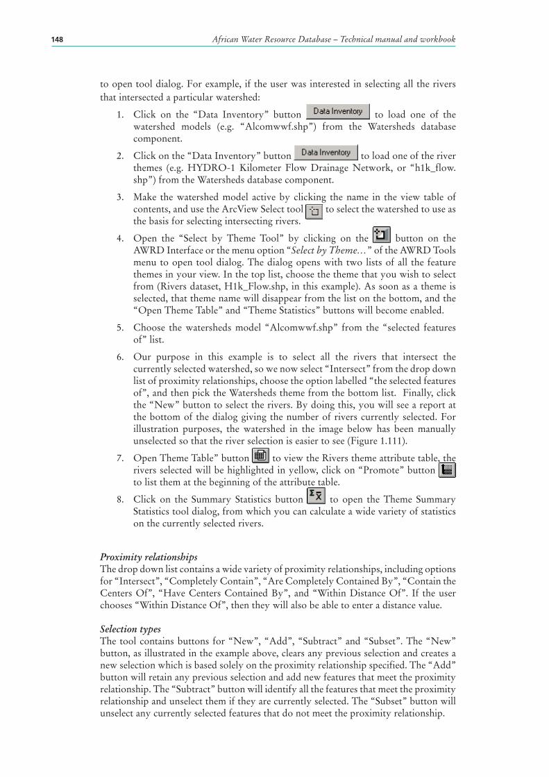
African Water Resource Database – Technical manual and workbook148
to open tool dialog. For example, if the user was interested in selecting all the rivers that intersected a particular watershed :
1. Click on the “Data Inventory” button to load one of the watershed models (e.g. “Alcomwwf.shp”) from the Watersheds database component.
2. Click on the “Data Inventory” button to load one of the river themes (e.g. HYDRO-1 Kilometer Flow Drainage Network, or “h1k_flow.shp”) from the Watersheds database component.
3. Make the watershed model active by clicking the name in the view table of contents, and use the ArcView Select tool to select the watershed to use as the basis for selecting intersecting rivers.
4. Open the “Select by Theme Tool” by clicking on the button on the AWRD Interface or the menu option “Select by Theme…” of the AWRD Tools menu to open tool dialog. The dialog opens with two lists of all the feature themes in your view. In the top list, choose the theme that you wish to select from (Rivers dataset, H1k_Flow.shp, in this example). As soon as a theme is selected, that theme name will disappear from the list on the bottom, and the “Open Theme Table” and “Theme Statistics” buttons will become enabled.
5. Choose the watersheds model “Alcomwwf.shp” from the “selected features of” list.
6. Our purpose in this example is to select all the rivers that intersect the currently selected watershed , so we now select “Intersect” from the drop down list of proximity relationships, choose the option labelled “the selected features of”, and then pick the Watersheds theme from the bottom list. Finally, click the “New” button to select the rivers. By doing this, you will see a report at the bottom of the dialog giving the number of rivers currently selected. For illustration purposes, the watershed in the image below has been manually unselected so that the river selection is easier to see (Figure 1.111).
7. Open Theme Table” button to view the Rivers theme attribute table, the rivers selected will be highlighted in yellow, click on “Promote” button to list them at the beginning of the attribute table.
8. Click on the Summary Statistics button to open the Theme Summary Statistics tool dialog, from which you can calculate a wide variety of statistics on the currently selected rivers.
Proximity relationshipsThe drop down list contains a wide variety of proximity relationships, including options for “Intersect”, “Completely Contain”, “Are Completely Contained By”, “Contain the Centers Of”, “Have Centers Contained By”, and “Within Distance Of”. If the user chooses “Within Distance Of”, then they will also be able to enter a distance value.
Selection typesThe tool contains buttons for “New”, “Add”, “Subtract” and “Subset”. The “New” button, as illustrated in the example above, clears any previous selection and creates a new selection which is based solely on the proximity relationship specified. The “Add” button will retain any previous selection and add new features that meet the proximity relationship. The “Subtract” button will identify all the features that meet the proximity relationship and unselect them if they are currently selected. The “Subset” button will unselect any currently selected features that do not meet the proximity relationship.
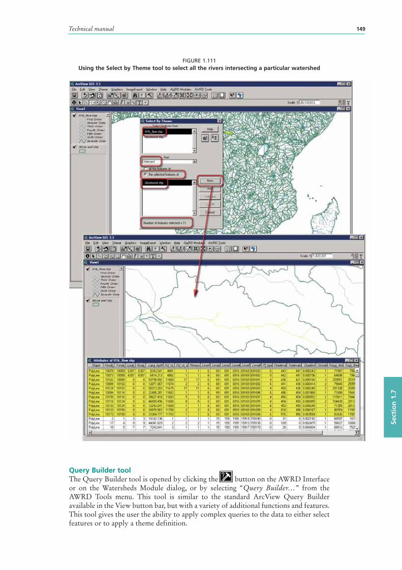
Technical manual 149
Sect
ion
1.7
FIGURE 1.111Using the Select by Theme tool to select all the rivers intersecting a particular watershed
Query Builder toolThe Query Builder tool is opened by clicking the button on the AWRD Interface or on the Watersheds Module dialog, or by selecting “Query Builder…” from the AWRD Tools menu. This tool is similar to the standard ArcView Query Builder available in the View button bar, but with a variety of additional functions and features. This tool gives the user the ability to apply complex queries to the data to either select features or to apply a theme definition.
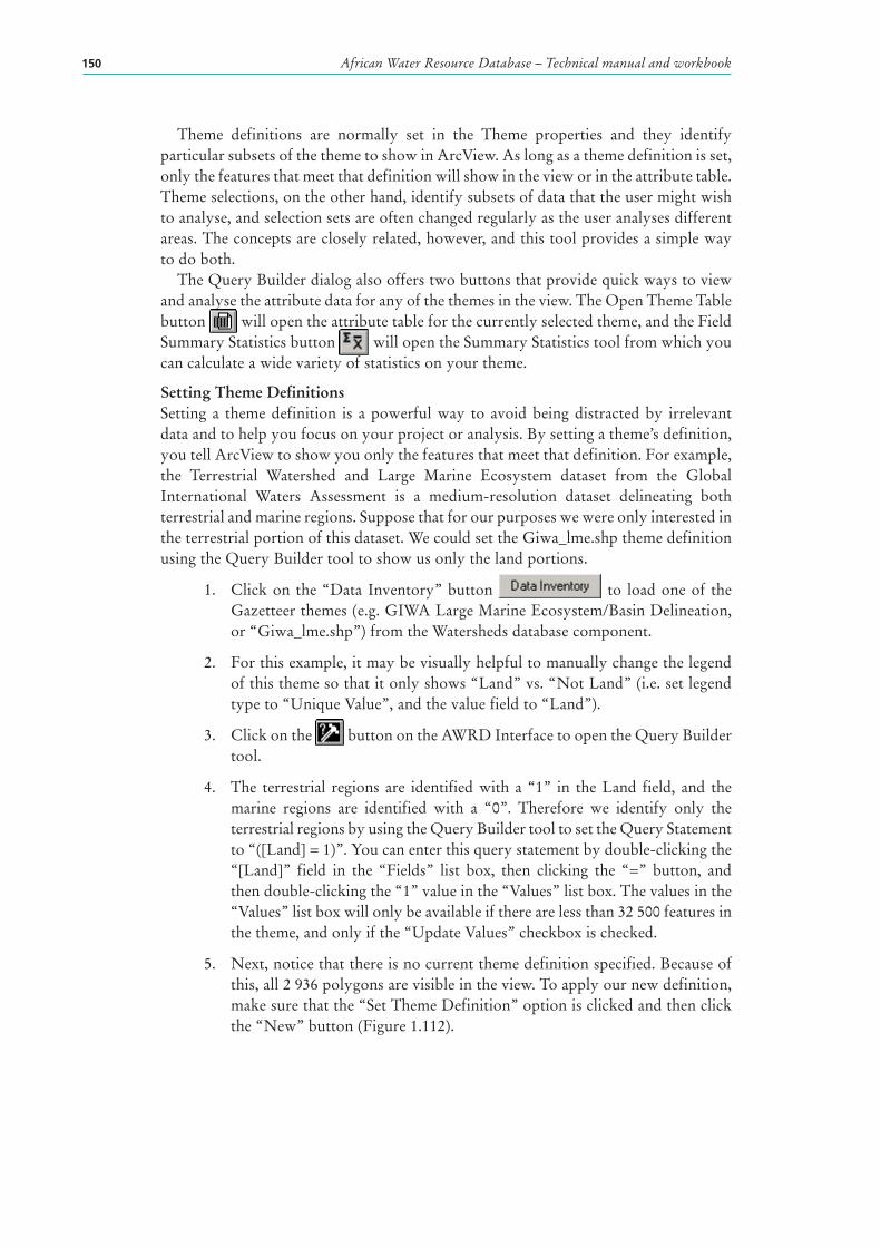
African Water Resource Database – Technical manual and workbook150
Theme definitions are normally set in the Theme properties and they identify particular subsets of the theme to show in ArcView. As long as a theme definition is set, only the features that meet that definition will show in the view or in the attribute table. Theme selections, on the other hand, identify subsets of data that the user might wish to analyse, and selection sets are often changed regularly as the user analyses different areas. The concepts are closely related, however, and this tool provides a simple way to do both.
The Query Builder dialog also offers two buttons that provide quick ways to view and analyse the attribute data for any of the themes in the view. The Open Theme Table button will open the attribute table for the currently selected theme , and the Field Summary Statistics button will open the Summary Statistics tool from which you can calculate a wide variety of statistics on your theme.
Setting Theme DefinitionsSetting a theme definition is a powerful way to avoid being distracted by irrelevant data and to help you focus on your project or analysis. By setting a theme’s definition, you tell ArcView to show you only the features that meet that definition. For example, the Terrestrial Watershed and Large Marine Ecosystem dataset from the Global International Waters Assessment is a medium-resolution dataset delineating both terrestrial and marine regions. Suppose that for our purposes we were only interested in the terrestrial portion of this dataset. We could set the Giwa_lme.shp theme definition using the Query Builder tool to show us only the land portions.
1. Click on the “Data Inventory” button to load one of the Gazetteer themes (e.g. GIWA Large Marine Ecosystem/Basin Delineation, or “Giwa_lme.shp”) from the Watersheds database component.
2. For this example, it may be visually helpful to manually change the legend of this theme so that it only shows “Land” vs. “Not Land” (i.e. set legend type to “Unique Value”, and the value field to “Land”).
3. Click on the button on the AWRD Interface to open the Query Builder tool.
4. The terrestrial regions are identified with a “1” in the Land field, and the marine regions are identified with a “0”. Therefore we identify only the terrestrial regions by using the Query Builder tool to set the Query Statement to “([Land] = 1)”. You can enter this query statement by double-clicking the “[Land]” field in the “Fields” list box, then clicking the “=” button, and then double-clicking the “1” value in the “Values” list box. The values in the “Values” list box will only be available if there are less than 32 500 features in the theme , and only if the “Update Values” checkbox is checked.
5. Next, notice that there is no current theme definition specified. Because of this, all 2 936 polygons are visible in the view. To apply our new definition, make sure that the “Set Theme Definition” option is clicked and then click the “New” button (Figure 1.112).
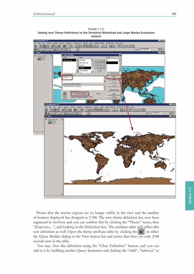
Technical manual 151
Sect
ion
1.7
FIGURE 1.112Setting new Theme Definitions to the Terrestrial Watershed and Large Marine Ecosystem
dataset
Notice that the marine regions are no longer visible in the view and the number of features displayed has dropped to 2 788. The new theme definition has now been registered in ArcView and you can confirm this by clicking the “Theme” menu, then “Properties…”, and looking in the Definition box. The attribute table will reflect this new definition as well. Open the theme attribute table by clicking the on either the Query Builder dialog or the View button bar and notice that there are only 2788 records now in the table.
You may clear this definition using the “Clear Definition” button, and you can add to it by building another Query Statement and clicking the “Add”, “Subtract” or
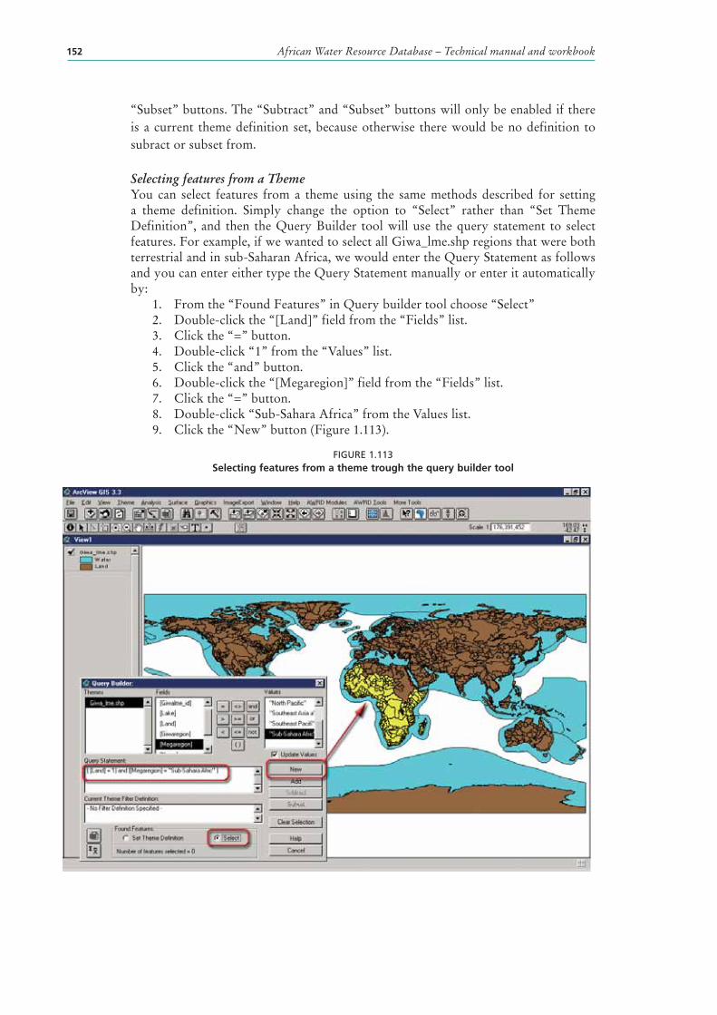
African Water Resource Database – Technical manual and workbook152
“Subset” buttons. The “Subtract” and “Subset” buttons will only be enabled if there is a current theme definition set, because otherwise there would be no definition to subract or subset from.
Selecting features from a ThemeYou can select features from a theme using the same methods described for setting a theme definition. Simply change the option to “Select” rather than “Set Theme Definition”, and then the Query Builder tool will use the query statement to select features. For example, if we wanted to select all Giwa_lme.shp regions that were both terrestrial and in sub-Saharan Africa, we would enter the Query Statement as follows and you can enter either type the Query Statement manually or enter it automatically by:
1. From the “Found Features” in Query builder tool choose “Select” 2. Double-click the “[Land]” field from the “Fields” list.3. Click the “=” button.4. Double-click “1” from the “Values” list.5. Click the “and” button.6. Double-click the “[Megaregion]” field from the “Fields” list.7. Click the “=” button.8. Double-click “Sub-Sahara Africa” from the Values list.9. Click the “New” button (Figure 1.113).
FIGURE 1.113Selecting features from a theme trough the query builder tool
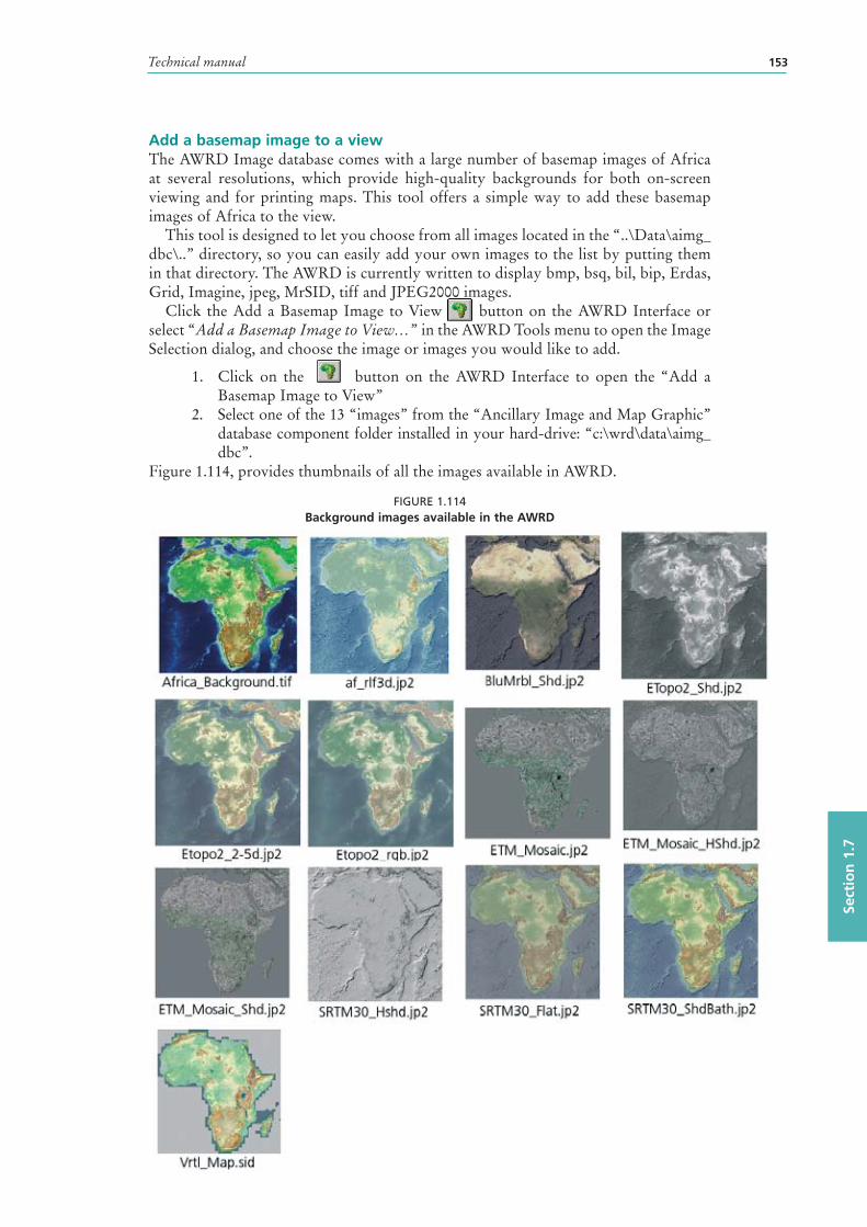
Technical manual 153
Sect
ion
1.7
Add a basemap image to a view The AWRD Image database comes with a large number of basemap images of Africa at several resolutions, which provide high-quality backgrounds for both on-screen viewing and for printing maps. This tool offers a simple way to add these basemap images of Africa to the view.
This tool is designed to let you choose from all images located in the “..\Data\aimg_dbc\..” directory, so you can easily add your own images to the list by putting them in that directory. The AWRD is currently written to display bmp, bsq, bil, bip, Erdas, Grid, Imagine, jpeg, MrSID, tiff and JPEG2000 images.
Click the Add a Basemap Image to View button on the AWRD Interface or select “Add a Basemap Image to View…” in the AWRD Tools menu to open the Image Selection dialog, and choose the image or images you would like to add.
1. Click on the button on the AWRD Interface to open the “Add a Basemap Image to View”
2. Select one of the 13 “images” from the “Ancillary Image and Map Graphic” database component folder installed in your hard-drive: “c:\wrd\data\aimg_dbc”.
Figure 1.114, provides thumbnails of all the images available in AWRD.
FIGURE 1.114Background images available in the AWRD
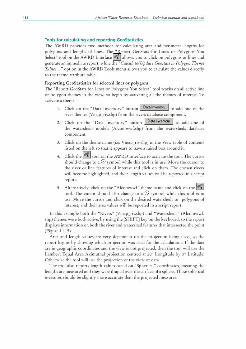
African Water Resource Database – Technical manual and workbook154
Tools for calculating and reporting GeoStatisticsThe AWRD provides two methods for calculating area and perimeter lengths for polygons and lengths of lines. The “Report GeoStats for Lines or Polygons You Select” tool on the AWRD Interface allows you to click on polygons or lines and generate an immediate report , while the “Calculate/Update Geostats in Polygon Theme
Tables…” option in the AWRD Tools menu allows you to calculate the values directly to the theme attribute table.
Reporting GeoStatistics for selected lines or polygons The “Report GeoStats for Lines or Polygons You Select” tool works on all active line or polygon themes in the view, so begin by activating all the themes of interest. To activate a theme :
1. Click on the “Data Inventory” button to add one of the river themes (Vmap_riv.shp) from the rivers database component.
2. Click on the “Data Inventory” button to add one of the watersheds models (Alcomwwf.shp) from the watersheds database component.
3. Click on the theme name (i.e. Vmap_riv.shp) in the View table of contents listed on the left so that it appears to have a raised box around it.
4. Click the tool on the AWRD Interface to activate the tool. The cursor should change to a symbol while this tool is in use. Move the cursor to the river or line features of interest and click on them. The chosen rivers will become highlighted, and their length values will be reported in a script report.
5. Alternatively, click on the “Alcomwwf” theme name and click on the tool. The cursor should also change to a symbol while this tool is in use. Move the cursor and click on the desired watersheds or polygons of interest, and their area values will be reported in a script report.
In this example both the “Rivers” (Vmap_riv.shp) and “Watersheds” (Alcomwwf.shp) themes were both active, by using the [SHIFT] key on the keyboard, so the report displays information on both the river and watershed features that intersected the point (Figure 1.115).
Area and length values are very dependent on the projection being used, so the report begins by showing which projection was used for the calculations. If the data are in geographic coordinates and the view is not projected, then the tool will use the Lambert Equal Area Azimuthal projection centred at 20° Longitude by 5° Latitude. Otherwise the tool will use the projection of the view or data.
The tool also reports length values based on “Spherical” coordinates, meaning the lengths are measured as if they were draped over the surface of a sphere. These spherical measures should be slightly more accurate than the projected measures.
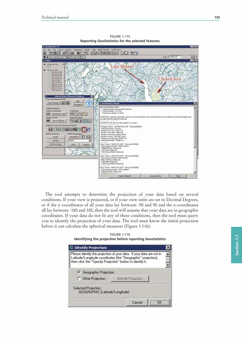
Technical manual 155
Sect
ion
1.7
FIGURE 1.115Reporting GeoStatistics for the selected features
The tool attempts to determine the projection of your data based on several conditions. If your view is projected, or if your view units are set to Decimal Degrees, or if the y-coordinates of all your data lay between -90 and 90 and the x-coordinates all lay between -180 and 180, then the tool will assume that your data are in geographic coordinates. If your data do not fit any of these conditions, then the tool must query you to identify the projection of your data. The tool must know the initial projection before it can calculate the spherical measures (Figure 1.116).
FIGURE 1.116Identifying the projection before reporting Geostatistics
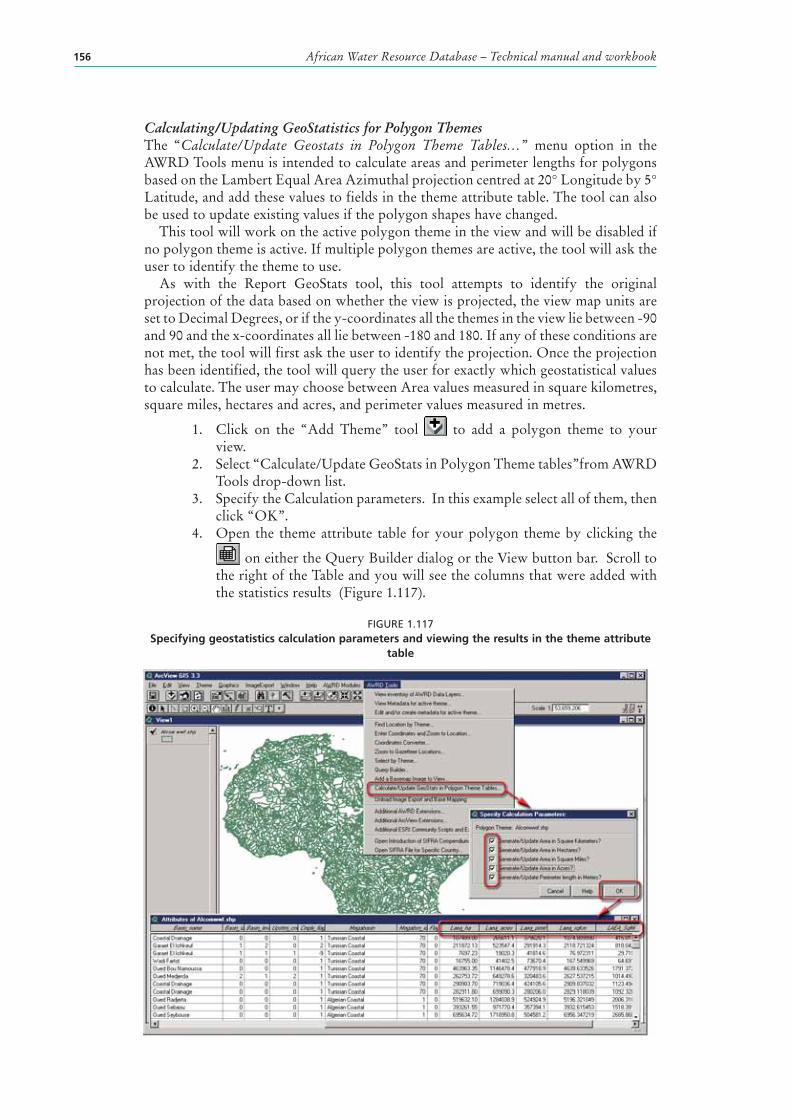
African Water Resource Database – Technical manual and workbook156
Calculating/Updating GeoStatistics for Polygon ThemesThe “Calculate/Update Geostats in Polygon Theme Tables…” menu option in the AWRD Tools menu is intended to calculate areas and perimeter lengths for polygons based on the Lambert Equal Area Azimuthal projection centred at 20° Longitude by 5° Latitude, and add these values to fields in the theme attribute table. The tool can also be used to update existing values if the polygon shapes have changed.
This tool will work on the active polygon theme in the view and will be disabled if no polygon theme is active. If multiple polygon themes are active, the tool will ask the user to identify the theme to use.
As with the Report GeoStats tool, this tool attempts to identify the original projection of the data based on whether the view is projected, the view map units are set to Decimal Degrees, or if the y-coordinates all the themes in the view lie between -90 and 90 and the x-coordinates all lie between -180 and 180. If any of these conditions are not met, the tool will first ask the user to identify the projection. Once the projection has been identified, the tool will query the user for exactly which geostatistical values to calculate. The user may choose between Area values measured in square kilometres, square miles, hectares and acres, and perimeter values measured in metres.
1. Click on the “Add Theme” tool to add a polygon theme to your view.
2. Select “Calculate/Update GeoStats in Polygon Theme tables”from AWRD Tools drop-down list.
3. Specify the Calculation parameters. In this example select all of them, then click “OK”.
4. Open the theme attribute table for your polygon theme by clicking the
on either the Query Builder dialog or the View button bar. Scroll to the right of the Table and you will see the columns that were added with the statistics results (Figure 1.117) .
FIGURE 1.117Specifying geostatistics calculation parameters and viewing the results in the theme attribute
table
Technical manual 157
Sect
ion
1.7
River Identification toolThe River Identification tool is designed to allow the user to identify continuous sections of river which are at the same order level. This assumes that the river theme being examined has river segments ranked according to the standard river order system, such that smaller tributaries have lower values than larger tributaries. For example, the theme Wria_riv.shp contains river order values for each river segment in the “Rank” field.
The River Identification tool will give you an easy way to select, and potentially rename, all attached river segments of a particular order. “Select Adjacent Rivers of Same Level” button on the AWRD Interface to start the process. This button will only be enabled if the user has a single river theme active in their view. The user will first be prompted to identify the Rank and Name fields for the river theme, and then the River Identification tool will stay open for as long as the user wishes to keep it open. When the River Identification tool has been opened, the cursor will turn into a
symbol. Use this symbol to click on a river segment of interest.In this example, the smallest tributaries are identified with “1” values, and when two
Level-1 tributaries come together they form a Level-2 river. Two Level-2 rivers merge to form a Level-3 river, etc.
1. Click on the “Data Inventory” button to load one of the rivers datasets (e.g. Wria_riv.shp) from the Rivers database component.
2. Click on “Select Adjacent Rivers of Same Level” button on the AWRD Interface. Select “Rank”as the River Level Field and “Wria_id”as the River Name Field. Click “OK”.
3. The cursor will turn into a symbol, use this symbol to click on a river segment of interest. Doing this will open the “Select River”dialog presenting the ID of the river selected. The text box labelled “River Name” tells us the name of the first selected segment, and the names of the other river segments. If we wished to, we could rename all three of these segments by clicking the “Rename” button and entering a new name.
4. Select “Theme” from ArcView Table of Contents (top menu bar) then select “Auto-label” use “Wria_id” as the Label Field (Figure 1.118).
If the user wished to select additional river segments along with the three that are currently selected, or if they wish to deselect one of the currently selected segments, then they could hold down the [SHIFT] key as they clicked on the rivers. Holding down the Shift key causes the tool to select or deselect individual segments without considering any adjacent segments.
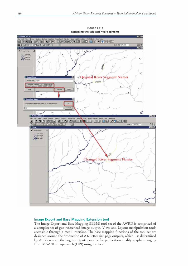
African Water Resource Database – Technical manual and workbook158
FIGURE 1.118Renaming the selected river segments
Image Export and Base Mapping Extension toolThe Image Export and Base Mapping (IEBM) tool-set of the AWRD is comprised of a complex set of geo-referenced image output, View, and Layout manipulation tools accessible through a menu interface. The base mapping functions of the tool-set are designed around the production of A4/Letter size page outputs, which – as determined by ArcView – are the largest outputs possible for publication quality graphics ranging from 300–600 dots-per-inch (DPI) using the tool.
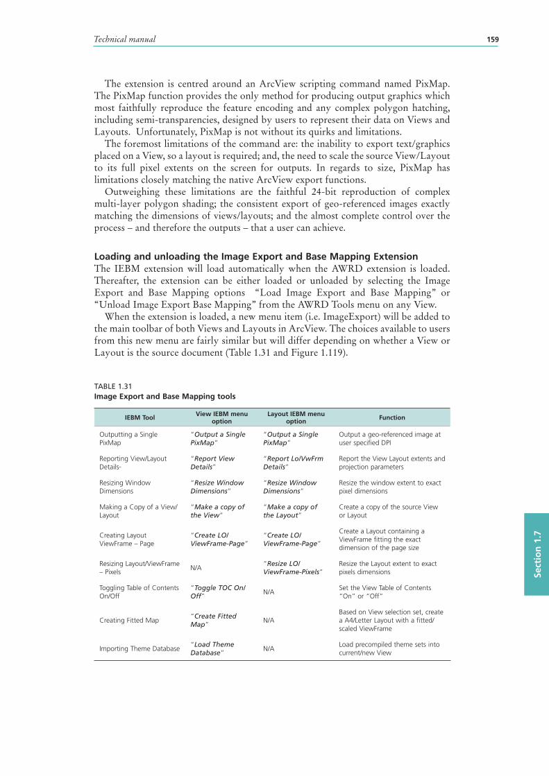
Technical manual 159
Sect
ion
1.7
The extension is centred around an ArcView scripting command named PixMap. The PixMap function provides the only method for producing output graphics which most faithfully reproduce the feature encoding and any complex polygon hatching, including semi-transparencies, designed by users to represent their data on Views and Layouts. Unfortunately, PixMap is not without its quirks and limitations.
The foremost limitations of the command are: the inability to export text/graphics placed on a View, so a layout is required; and, the need to scale the source View/Layout to its full pixel extents on the screen for outputs. In regards to size, PixMap has limitations closely matching the native ArcView export functions.
Outweighing these limitations are the faithful 24-bit reproduction of complex multi-layer polygon shading; the consistent export of geo-referenced images exactly matching the dimensions of views/layouts; and the almost complete control over the process – and therefore the outputs – that a user can achieve.
Loading and unloading the Image Export and Base Mapping ExtensionThe IEBM extension will load automatically when the AWRD extension is loaded. Thereafter, the extension can be either loaded or unloaded by selecting the Image Export and Base Mapping options “Load Image Export and Base Mapping” or “Unload Image Export Base Mapping” from the AWRD Tools menu on any View.
When the extension is loaded, a new menu item (i.e. ImageExport) will be added to the main toolbar of both Views and Layouts in ArcView. The choices available to users from this new menu are fairly similar but will differ depending on whether a View or Layout is the source document (Table 1.31 and Figure 1.119).
TABLE 1.31Image Export and Base Mapping tools
IEBM Tool View IEBM menu option
Layout IEBM menu option Function
Outputting a Single PixMap
“Output a Single PixMap”
“Output a Single PixMap”
Output a geo-referenced image at user specified DPI
Reporting View/Layout Details
“Report View Details”
“Report Lo/VwFrm Details”
Report the View Layout extents and projection parameters
Resizing Window Dimensions
“Resize Window Dimensions”
“Resize Window Dimensions”
Resize the window extent to exact pixel dimensions
Making a Copy of a View/Layout
“Make a copy of the View”
“Make a copy of the Layout”
Create a copy of the source View or Layout
Creating Layout ViewFrame – Page
“Create LO/ViewFrame-Page”
“Create LO/ViewFrame-Page”
Create a Layout containing a ViewFrame fitting the exact dimension of the page size
Resizing Layout/ViewFrame – Pixels
N/A“Resize LO/ViewFrame-Pixels”
Resize the Layout extent to exact pixels dimensions
Toggling Table of Contents On/Off
“Toggle TOC On/Off”
N/ASet the View Table of Contents “On” or “Off”
Creating Fitted Map“Create Fitted Map”
N/ABased on View selection set, create a A4/Letter Layout with a fitted/scaled ViewFrame
Importing Theme Database “Load Theme Database”
N/ALoad precompiled theme sets into current/new View
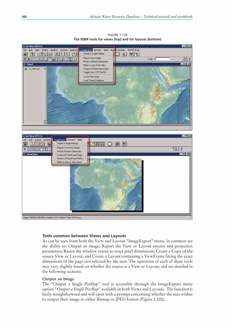
African Water Resource Database – Technical manual and workbook160
FIGURE 1.119The IEBM tools for views (top) and for layouts (bottom)
Tools common between Views and LayoutsAs can be seen from both the View and Layout “ImageExport” menu, in common are the ability to: Output an image ; Report the View or Layout extents and projection parameters; Resize the window extent to exact pixel dimensions; Create a Copy of the source View or Layout; and Create a Layout containing a ViewFrame fitting the exact dimensions of the page size selected by the user. The operation of each of these tools may vary slightly based on whether the source is a View or Layout, and are detailed in the following sections.
Output an image The “Output a Single PixMap” tool is accessible through the ImageExport menu option “Output a Single PixMap” available in both Views and Layouts. The function is fairly straightforward and will open with a prompt concerning whether the user wishes to output their image to either Bitmap or JPEG format (Figure 1.120).
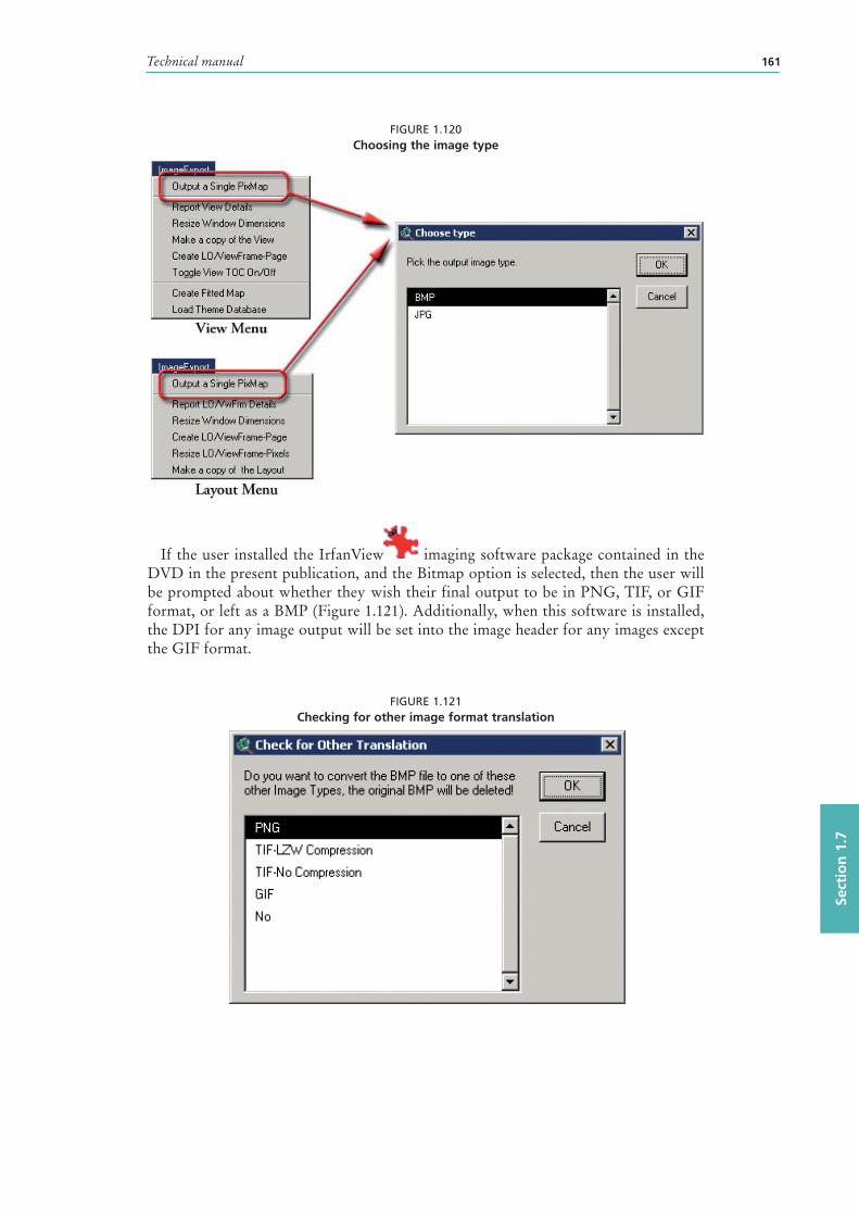
Technical manual 161
Sect
ion
1.7
FIGURE 1.120Choosing the image type
If the user installed the IrfanView imaging software package contained in the DVD in the present publication , and the Bitmap option is selected, then the user will be prompted about whether they wish their final output to be in PNG, TIF, or GIF format, or left as a BMP (Figure 1.121). Additionally, when this software is installed, the DPI for any image output will be set into the image header for any images except the GIF format.
FIGURE 1.121Checking for other image format translation
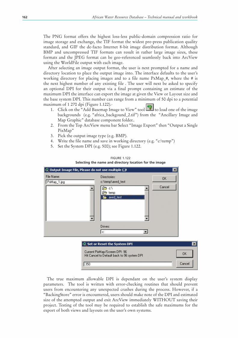
African Water Resource Database – Technical manual and workbook162
The PNG format offers the highest loss-less public-domain compression ratio for image storage and exchange, the TIF format the widest pre-press publication quality standard, and GIF the de-facto Internet 8-bit image distribution format. Although BMP and uncompressed TIF formats can result in rather large image sizes, these formats and the JPEG format can be geo-referenced seamlessly back into ArcView using the WorldFile output with each image.
After selecting an image output format, the user is next prompted for a name and directory location to place the output image into. The interface defaults to the user’s working directory for placing images and to a file name PxMap_#, where the # is the next highest number of any existing file . The user will next be asked to specify an optional DPI for their output via a final prompt containing an estimate of the maximum DPI the interface can export the image at given the View or Layout size and the base system DPI. This number can range from a minimum of 50 dpi to a potential maximum of 1 270 dpi (Figure 1.122).
1. Click on the “Add Basemap Image to View” tool to load one of the image backgrounds (e.g. “africa_backgound_2.tif”) from the “Ancillary Image and Map Graphic” database component folder..
2. From the Top ArcView menu bar Select “Image Export” then “Output a Single PixMap”
3. Pick the output image type (e.g. BMP).4. Write the file name and save in working directory (e.g. “c:\temp”)5. Set the System DPI (e.g. 500); see Figure 1.122.
FIGURE 1.122Selecting the name and directory location for the image
The true maximum allowable DPI is dependant on the user’s system display parameters. The tool is written with error-checking routines that should prevent users from encountering any unexpected crashes during the process. However, if a “BackingStore” error is encountered, users should make note of the DPI and estimated size of the attempted output and exit ArcView immediately WITHOUT saving their project. Testing of the tool may be required to establish the safe maximums for the export of both views and layouts on the user’s own systems.
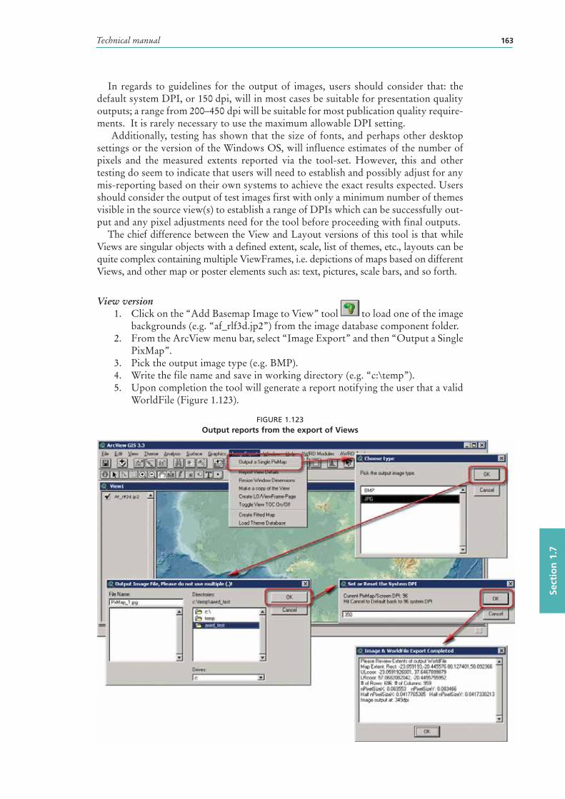
Technical manual 163
Sect
ion
1.7
In regards to guidelines for the output of images, users should consider that: the default system DPI, or 150 dpi, will in most cases be suitable for presentation quality outputs; a range from 200–450 dpi will be suitable for most publication quality require-ments. It is rarely necessary to use the maximum allowable DPI setting.
Additionally, testing has shown that the size of fonts, and perhaps other desktop settings or the version of the Windows OS, will influence estimates of the number of pixels and the measured extents reported via the tool-set. However, this and other testing do seem to indicate that users will need to establish and possibly adjust for any mis-reporting based on their own systems to achieve the exact results expected. Users should consider the output of test images first with only a minimum number of themes visible in the source view(s) to establish a range of DPIs which can be successfully out-put and any pixel adjustments need for the tool before proceeding with final outputs.
The chief difference between the View and Layout versions of this tool is that while Views are singular objects with a defined extent, scale, list of themes, etc., layouts can be quite complex containing multiple ViewFrames, i.e. depictions of maps based on different Views, and other map or poster elements such as: text, pictures, scale bars, and so forth.
View version1. Click on the “Add Basemap Image to View” tool to load one of the image
backgrounds (e.g. “af_rlf3d.jp2”) from the image database component folder.2. From the ArcView menu bar, select “Image Export” and then “Output a Single
PixMap”.3. Pick the output image type (e.g. BMP).4. Write the file name and save in working directory (e.g. “c:\temp”).5. Upon completion the tool will generate a report notifying the user that a valid
WorldFile (Figure 1.123).
FIGURE 1.123Output reports from the export of Views
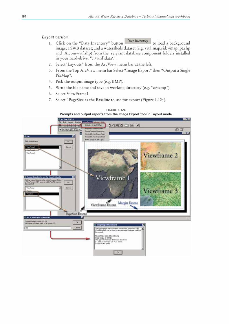
African Water Resource Database – Technical manual and workbook164
Layout version1. Click on the “Data Inventory” button to load a background
image; a SWB dataset; and a watersheds dataset (e.g. vrtl_map.sid; vmap_pt.shp and Alcomwwf.shp) from the relevant database component folders installed in your hard-drive: “c:\wrd\data\”.
2. Select”Layouts” from the ArcView menu bar at the left.3. From the Top ArcView menu bar Select “Image Export” then “Output a Single
PixMap”.4. Pick the output image type (e.g. BMP).5. Write the file name and save in working directory (e.g. “c:\temp”).6. Select ViewFrame1.7. Select “PageSize as the Baseline to use for export (Figure 1.124).
FIGURE 1.124Prompts and output reports from the Image Export tool in Layout mode
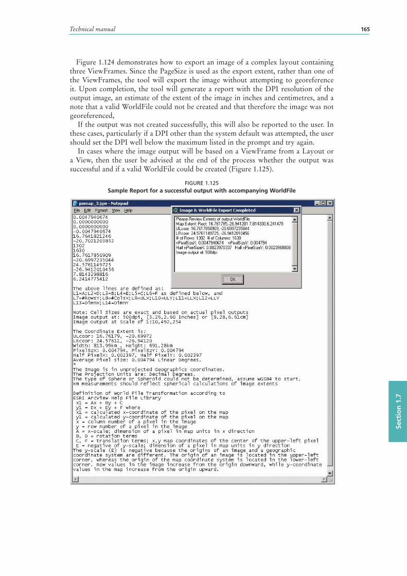
Technical manual 165
Sect
ion
1.7
Figure 1.124 demonstrates how to export an image of a complex layout containing three ViewFrames. Since the PageSize is used as the export extent, rather than one of the ViewFrames, the tool will export the image without attempting to georeference it. Upon completion, the tool will generate a report with the DPI resolution of the output image, an estimate of the extent of the image in inches and centimetres, and a note that a valid WorldFile could not be created and that therefore the image was not georeferenced,
If the output was not created successfully, this will also be reported to the user. In these cases, particularly if a DPI other than the system default was attempted, the user should set the DPI well below the maximum listed in the prompt and try again.
In cases where the image output will be based on a ViewFrame from a Layout or a View, then the user be advised at the end of the process whether the output was successful and if a valid WorldFile could be created (Figure 1.125).
FIGURE 1.125Sample Report for a successful output with accompanying WorldFile
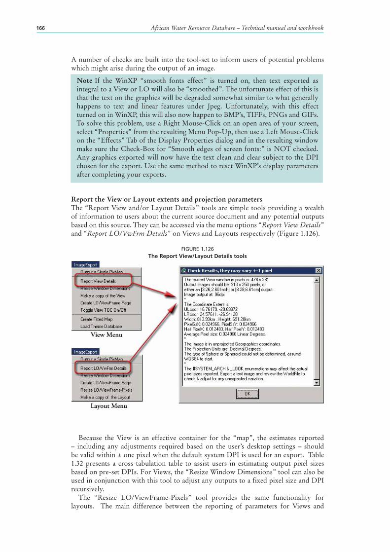
African Water Resource Database – Technical manual and workbook166
A number of checks are built into the tool-set to inform users of potential problems which might arise during the output of an image.
Note If the WinXP “smooth fonts effect” is turned on, then text exported as integral to a View or LO will also be “smoothed”. The unfortunate effect of this is that the text on the graphics will be degraded somewhat similar to what generally happens to text and linear features under Jpeg. Unfortunately, with this effect turned on in WinXP, this will also now happen to BMP’s, TIFFs, PNGs and GIFs. To solve this problem, use a Right Mouse-Click on an open area of your screen, select “Properties” from the resulting Menu Pop-Up, then use a Left Mouse-Click on the “Effects” Tab of the Display Properties dialog and in the resulting window make sure the Check-Box for “Smooth edges of screen fonts:” is NOT checked. Any graphics exported will now have the text clean and clear subject to the DPI chosen for the export. Use the same method to reset WinXP’s display parameters after completing your exports.
Report the View or Layout extents and projection parametersThe “Report View and/or Layout Details” tools are simple tools providing a wealth of information to users about the current source document and any potential outputs based on this source. They can be accessed via the menu options “Report View Details” and “Report LO/VwFrm Details” on Views and Layouts respectively (Figure 1.126).
FIGURE 1.126The Report View/Layout Details tools
Because the View is an effective container for the “map”, the estimates reported – including any adjustments required based on the user’s desktop settings – should be valid within ± one pixel when the default system DPI is used for an export . Table 1.32 presents a cross-tabulation table to assist users in estimating output pixel sizes based on pre-set DPIs. For Views, the “Resize Window Dimensions” tool can also be used in conjunction with this tool to adjust any outputs to a fixed pixel size and DPI recursively.
The “Resize LO/ViewFrame-Pixels” tool provides the same functionality for layouts. The main difference between the reporting of parameters for Views and
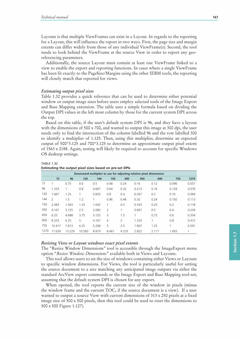
Technical manual 167
Sect
ion
1.7
Layouts is that multiple ViewFrames can exist in a Layout. In regards to the reporting for a Layout, this will influence the report in two ways. First, the page size and margin extents can differ widely from those of any individual ViewFrame(s). Second, the tool needs to look behind the ViewFrame at the source View in order to report any geo-referencing parameters.
Additionally, the source Layout must contain at least one ViewFrame linked to a view to enable the export and reporting functions. In cases where a single ViewFrame has been fit exactly to the PageSize/Margins using the other IEBM tools, the reporting will closely match that reported for views.
Estimating output pixel sizesTable 1.32 provides a quick reference that can be used to determine either potential window or output image sizes before users employ selected tools of the Image Export and Base Mapping extension. The table uses a simple formula based on dividing the Output DPI values in the left most column by those for the current system DPI across the top.
Based on this table, if the user’s default system DPI is 96, and they have a layout with the dimensions of 500 x 700, and wanted to output this image at 300 dpi, the user needs only to find the intersection of the column labelled 96 and the row labelled 300 to identify a multiplier of 1.125. Then, using this multiplier, determine an expected output of 500*3.125 and 700*3.125 to determine an approximate output pixel extent of 1563 x 2188. Again, testing will likely be required to account for specific Windows OS desktop settings.
TABLE 1.32Estimating the output pixel sizes based on pre-set DPIs
Downward multiplier to use for adjusting relative pixel dimensions
72 96 120 144 150 300 450 600 750 1270
72 1 0.75 0.6 0.5 0.48 0.24 0.16 0.12 0.096 0.057
96 1.333 1 0.8 0.667 0.64 0.32 0.213 0.16 0.128 0.076
120 1.667 1.25 1 0.833 0.8 0.4 0.267 0.2 0.16 0.094
144 2 1.5 1.2 1 0.96 0.48 0.32 0.24 0.192 0.113
150 2.083 1.563 1.25 1.042 1 0.5 0.333 0.25 0.2 0.118
300 4.167 3.125 2.5 2.083 2 1 0.667 0.5 0.4 0.236
450 6.25 4.688 3.75 3.125 3 1.5 1 0.75 0.6 0.354
600 8.333 6.25 5 4.167 4 2 1.333 1 0.8 0.472
750 10.417 7.813 6.25 5.208 5 2.5 1.667 1.25 1 0.591
1270 17.639 13.229 10.583 8.819 8.467 4.233 2.822 2.117 1.693 1
Resizing View or Layout windows exact pixel extentsThe “Resize Window Dimensions” tool is accessible through the ImageExport menu option “Resize Window Dimensions” available both in Views and Layouts.
This tool allows users to set the size of windows containing either Views or Layouts to specific window dimensions. For Views, the tool is particularly useful for setting the source document to a size matching any anticipated image outputs via either the standard ArcView export commands or the Image Export and Base Mapping tool-set; assuming that the default system DPI is chosen for any export.
When opened, the tool reports the current size of the window in pixels (minus the window frame and the current TOC, if the source document is a view). If a user wanted to output a source View with current dimensions of 313 x 250 pixels at a fixed image size of 500 x 500 pixels, then this tool could be used to reset the dimensions to 500 x 500 Figure 1.127).
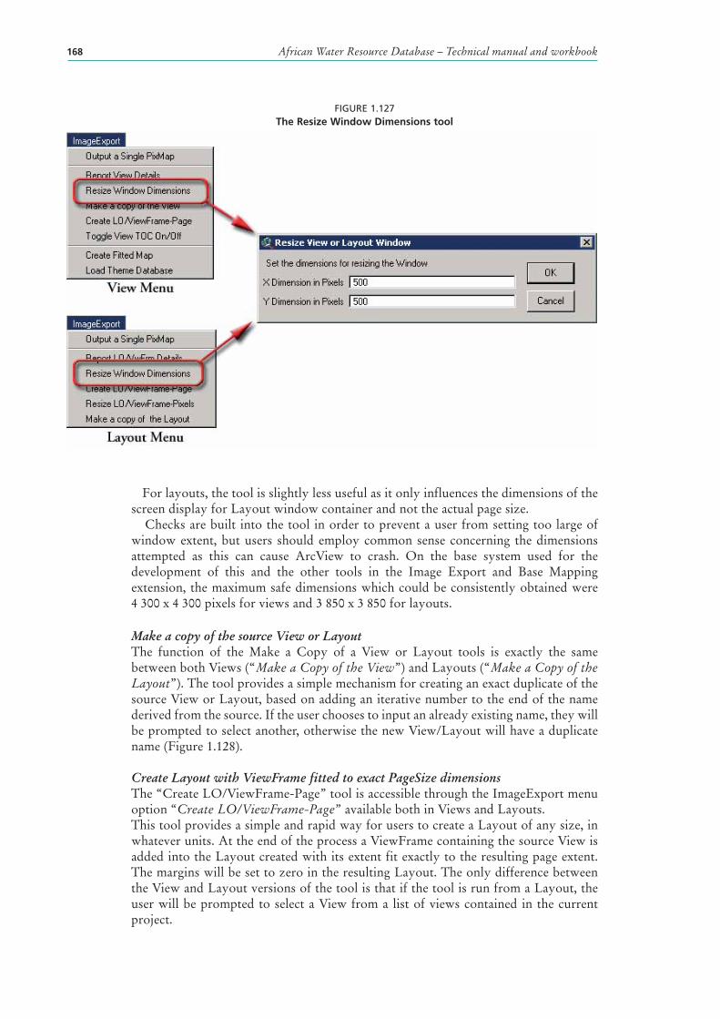
African Water Resource Database – Technical manual and workbook168
FIGURE 1.127The Resize Window Dimensions tool
For layouts, the tool is slightly less useful as it only influences the dimensions of the screen display for Layout window container and not the actual page size.
Checks are built into the tool in order to prevent a user from setting too large of window extent, but users should employ common sense concerning the dimensions attempted as this can cause ArcView to crash. On the base system used for the development of this and the other tools in the Image Export and Base Mapping extension, the maximum safe dimensions which could be consistently obtained were 4 300 x 4 300 pixels for views and 3 850 x 3 850 for layouts.
Make a copy of the source View or LayoutThe function of the Make a Copy of a View or Layout tools is exactly the same between both Views (“Make a Copy of the View”) and Layouts (“Make a Copy of the Layout”). The tool provides a simple mechanism for creating an exact duplicate of the source View or Layout, based on adding an iterative number to the end of the name derived from the source. If the user chooses to input an already existing name, they will be prompted to select another, otherwise the new View/Layout will have a duplicate name (Figure 1.128).
Create Layout with ViewFrame fitted to exact PageSize dimensionsThe “Create LO/ViewFrame-Page” tool is accessible through the ImageExport menu option “Create LO/ViewFrame-Page” available both in Views and Layouts.This tool provides a simple and rapid way for users to create a Layout of any size, in whatever units. At the end of the process a ViewFrame containing the source View is added into the Layout created with its extent fit exactly to the resulting page extent. The margins will be set to zero in the resulting Layout. The only difference between the View and Layout versions of the tool is that if the tool is run from a Layout, the user will be prompted to select a View from a list of views contained in the current project.
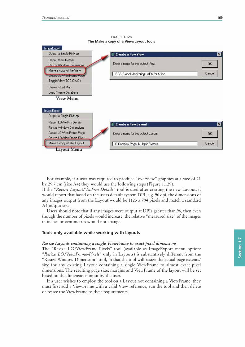
Technical manual 169
Sect
ion
1.7
FIGURE 1.128The Make a copy of a View/Layout tools
For example, if a user was required to produce “overview” graphics at a size of 21 by 29.7 cm (size A4) they would use the following steps (Figure 1.129).If the “Report Layout/VwFrm Details” tool is used after creating the new Layout, it would report that based on the users default system DPI, e.g. 96 dpi, the dimensions of any images output from the Layout would be 1123 x 794 pixels and match a standard A4 output size.
Users should note that if any images were output at DPIs greater than 96, then even though the number of pixels would increase, the relative “measured size” of the images in inches or centimetres would not change.
Tools only available while working with layouts
Resize Layouts containing a single ViewFrame to exact pixel dimensions The “Resize LO/ViewFrame-Pixels” tool (available as ImageExport menu option: “Resize LO/ViewFrame-Pixels” only in Layouts) is substantively different from the “Resize Window Dimension” tool, in that the tool will resize the actual page extents/size for any existing Layout containing a single ViewFrame to almost exact pixel dimensions. The resulting page size, margins and ViewFrame of the layout will be set based on the dimensions input by the user.
If a user wishes to employ the tool on a Layout not containing a ViewFrame, they must first add a ViewFrame with a valid View reference, run the tool and then delete or resize the ViewFrame to their requirements.
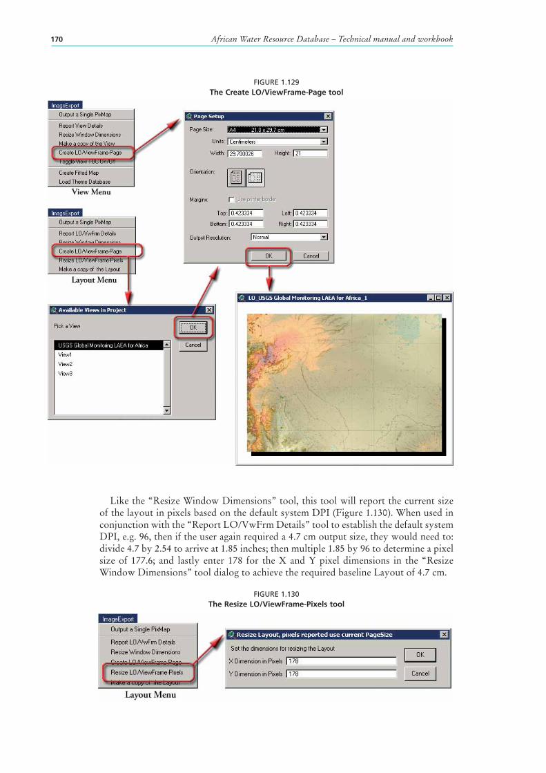
African Water Resource Database – Technical manual and workbook170
FIGURE 1.129The Create LO/ViewFrame-Page tool
Like the “Resize Window Dimensions” tool, this tool will report the current size of the layout in pixels based on the default system DPI (Figure 1.130). When used in conjunction with the “Report LO/VwFrm Details” tool to establish the default system DPI, e.g. 96, then if the user again required a 4.7 cm output size, they would need to: divide 4.7 by 2.54 to arrive at 1.85 inches; then multiple 1.85 by 96 to determine a pixel size of 177.6; and lastly enter 178 for the X and Y pixel dimensions in the “Resize Window Dimensions” tool dialog to achieve the required baseline Layout of 4.7 cm.
FIGURE 1.130The Resize LO/ViewFrame-Pixels tool
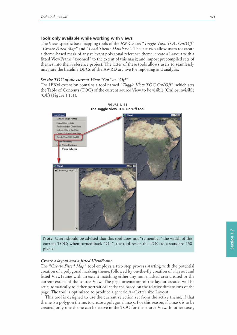
Technical manual 171
Sect
ion
1.7
Tools only available while working with viewsThe View-specific base mapping tools of the AWRD are: “Toggle View TOC On/Off” “Create Fitted Map” and “Load Theme Database”. The last two allow users to: create a theme -based mask of any relevant polygonal reference theme; create a Layout with a fitted ViewFrame “zoomed” to the extent of this mask; and import precompiled sets of themes into their reference project. The latter of these tools allows users to seamlessly integrate the baseline DBCs of the AWRD archive for reporting and analysis.
Set the TOC of the current View “On” or “Off”The IEBM extension contains a tool named “Toggle View TOC On/Off”, which sets the Table of Contents (TOC) of the current source View to be visible (On) or invisible (Off) (Figure 1.131).
FIGURE 1.131The Toggle View TOC On/Off tool
Note Users should be advised that this tool does not “remember” the width of the current TOC; when turned back “On”, the tool resets the TOC to a standard 150 pixels.
Create a layout and a fitted ViewFrameThe “Create Fitted Map” tool employs a two step process starting with the potential creation of a polygonal masking theme , followed by on-the-fly creation of a layout and fitted ViewFrame with an extent matching either any non-masked area created or the current extent of the source View. The page orientation of the layout created will be set automatically to either portrait or landscape based on the relative dimensions of the page. The tool is optimized to produce a generic A4/Letter size Layout.
This tool is designed to use the current selection set from the active theme , if that theme is a polygon theme, to create a polygonal mask. For this reason, if a mask is to be created, only one theme can be active in the TOC for the source View. In other cases,
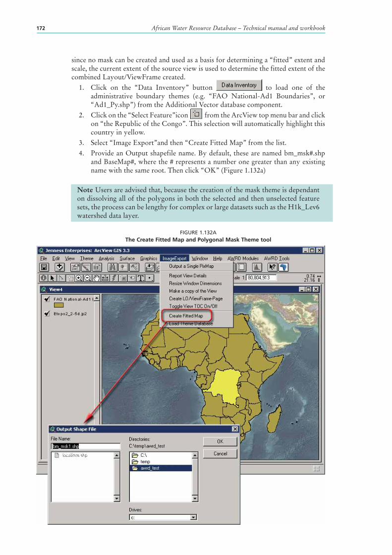
African Water Resource Database – Technical manual and workbook172
since no mask can be created and used as a basis for determining a “fitted” extent and scale, the current extent of the source view is used to determine the fitted extent of the combined Layout/ViewFrame created.
1. Click on the “Data Inventory” button to load one of the administrative boundary themes (e.g. “FAO National-Ad1 Boundaries”, or “Ad1_Py.shp”) from the Additional Vector database component.
2. Click on the “Select Feature”icon from the ArcView top menu bar and click on “the Republic of the Congo”. This selection will automatically highlight this country in yellow.
3. Select “Image Export”and then “Create Fitted Map” from the list.4. Provide an Output shapefile name. By default, these are named bm_msk#.shp
and BaseMap#, where the # represents a number one greater than any existing name with the same root. Then click “OK” (Figure 1.132a)
Note Users are advised that, because the creation of the mask theme is dependant on dissolving all of the polygons in both the selected and then unselected feature sets, the process can be lengthy for complex or large datasets such as the H1k_Lev6 watershed data layer.
FIGURE 1.132AThe Create Fitted Map and Polygonal Mask Theme tool
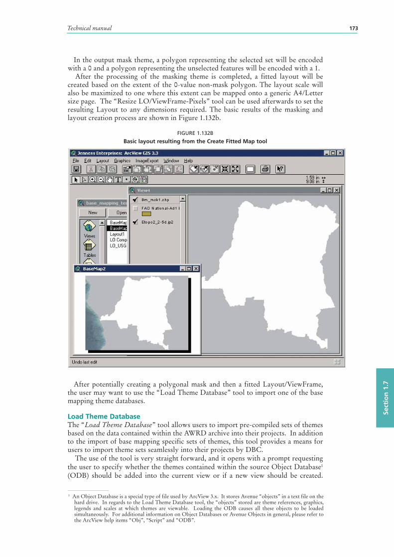
Technical manual 173
Sect
ion
1.7
In the output mask theme , a polygon representing the selected set will be encoded with a 0 and a polygon representing the unselected features will be encoded with a 1.
After the processing of the masking theme is completed, a fitted layout will be created based on the extent of the 0-value non-mask polygon. The layout scale will also be maximized to one where this extent can be mapped onto a generic A4/Letter size page. The “Resize LO/ViewFrame-Pixels” tool can be used afterwards to set the resulting Layout to any dimensions required. The basic results of the masking and layout creation process are shown in Figure 1.132b.
FIGURE 1.132B
Basic layout resulting from the Create Fitted Map tool
After potentially creating a polygonal mask and then a fitted Layout/ViewFrame, the user may want to use the “Load Theme Database” tool to import one of the base mapping theme databases.
Load Theme DatabaseThe “Load Theme Database” tool allows users to import pre-compiled sets of themes based on the data contained within the AWRD archive into their projects. In addition to the import of base mapping specific sets of themes, this tool provides a means for users to import theme sets seamlessly into their projects by DBC.
The use of the tool is very straight forward, and it opens with a prompt requesting the user to specify whether the themes contained within the source Object Database1 (ODB) should be added into the current view or if a new view should be created.
1 An Object Database is a special type of file used by ArcView 3.x. It stores Avenue “objects” in a text file on the hard drive. In regards to the Load Theme Database tool, the “objects” stored are theme references, graphics, legends and scales at which themes are viewable. Loading the ODB causes all these objects to be loaded simultaneously. For additional information on Object Databases or Avenue Objects in general, please refer to the ArcView help items “Obj”, “Script” and “ODB”.
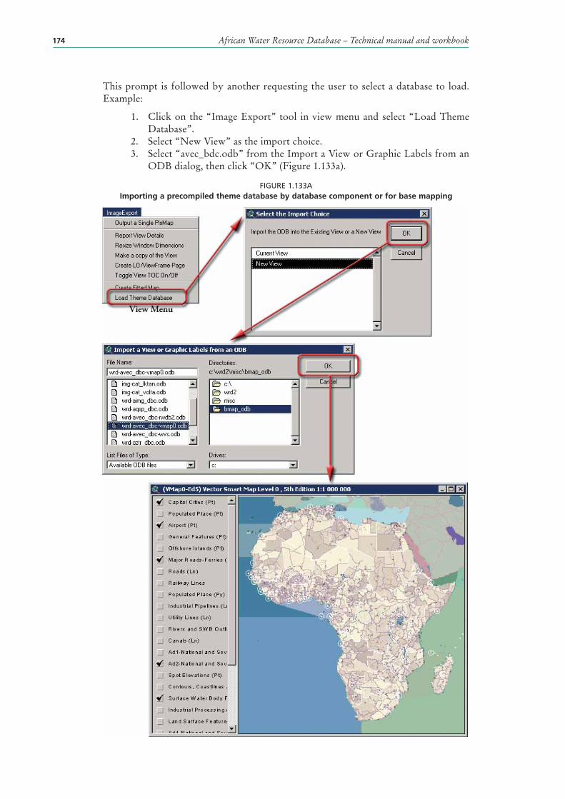
African Water Resource Database – Technical manual and workbook174
This prompt is followed by another requesting the user to select a database to load. Example:
1. Click on the “Image Export” tool in view menu and select “Load Theme Database”.
2. Select “New View” as the import choice.3. Select “avec_bdc.odb” from the Import a View or Graphic Labels from an
ODB dialog, then click “OK” (Figure 1.133a).
FIGURE 1.133AImporting a precompiled theme database by database component or for base mapping
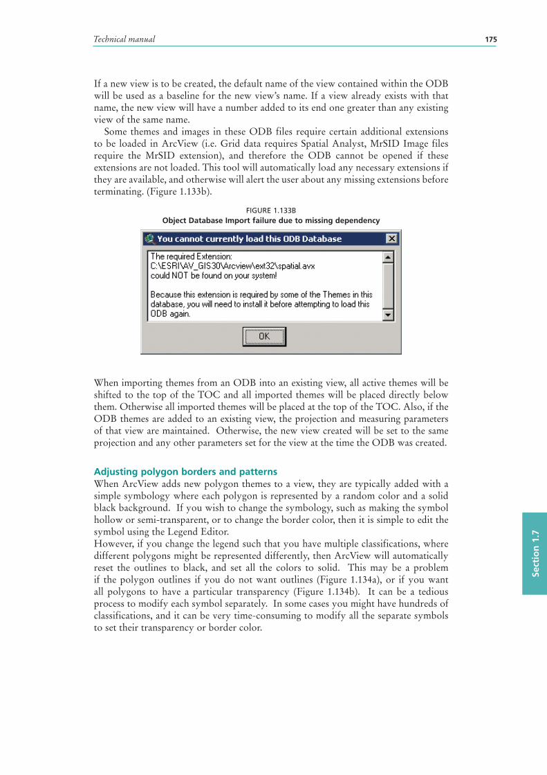
Technical manual 175
Sect
ion
1.7
If a new view is to be created, the default name of the view contained within the ODB will be used as a baseline for the new view’s name. If a view already exists with that name, the new view will have a number added to its end one greater than any existing view of the same name.
Some themes and images in these ODB files require certain additional extensions to be loaded in ArcView (i.e. Grid data requires Spatial Analyst, MrSID Image files require the MrSID extension), and therefore the ODB cannot be opened if these extensions are not loaded. This tool will automatically load any necessary extensions if they are available, and otherwise will alert the user about any missing extensions before terminating. (Figure 1.133b).
FIGURE 1.133BObject Database Import failure due to missing dependency
When importing themes from an ODB into an existing view, all active themes will be shifted to the top of the TOC and all imported themes will be placed directly below them. Otherwise all imported themes will be placed at the top of the TOC. Also, if the ODB themes are added to an existing view, the projection and measuring parameters of that view are maintained. Otherwise, the new view created will be set to the same projection and any other parameters set for the view at the time the ODB was created.
Adjusting polygon borders and patternsWhen ArcView adds new polygon themes to a view, they are typically added with a simple symbology where each polygon is represented by a random color and a solid black background. If you wish to change the symbology, such as making the symbol hollow or semi-transparent, or to change the border color, then it is simple to edit the symbol using the Legend Editor.However, if you change the legend such that you have multiple classifications, where different polygons might be represented differently, then ArcView will automatically reset the outlines to black, and set all the colors to solid. This may be a problem if the polygon outlines if you do not want outlines (Figure 1.134a), or if you want all polygons to have a particular transparency (Figure 1.134b). It can be a tedious process to modify each symbol separately. In some cases you might have hundreds of classifications, and it can be very time-consuming to modify all the separate symbols to set their transparency or border color.
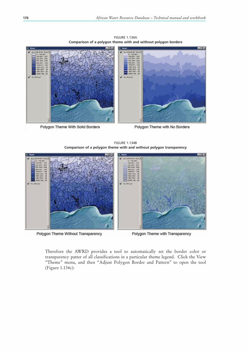
African Water Resource Database – Technical manual and workbook176
FIGURE 1.134AComparison of a polygon theme with and without polygon borders
FIGURE 1.134BComparison of a polygon theme with and without polygon transparency
Therefore the AWRD provides a tool to automatically set the border color or transparency patter of all classifications in a particular theme legend. Click the View “Theme” menu, and then “Adjust Polygon Border and Pattern” to open the tool (Figure 1.134c):
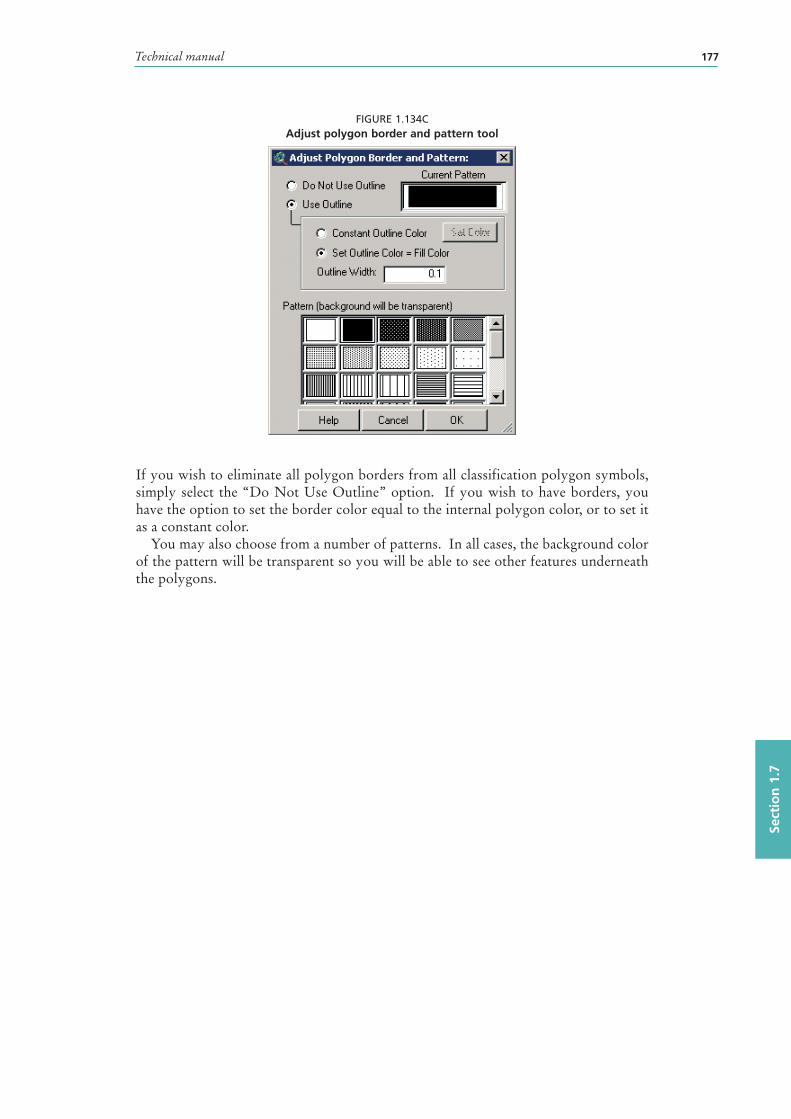
Technical manual 177
Sect
ion
1.7
FIGURE 1.134CAdjust polygon border and pattern tool
If you wish to eliminate all polygon borders from all classification polygon symbols, simply select the “Do Not Use Outline” option. If you wish to have borders, you have the option to set the border color equal to the internal polygon color, or to set it as a constant color.
You may also choose from a number of patterns. In all cases, the background color of the pattern will be transparent so you will be able to see other features underneath the polygons.
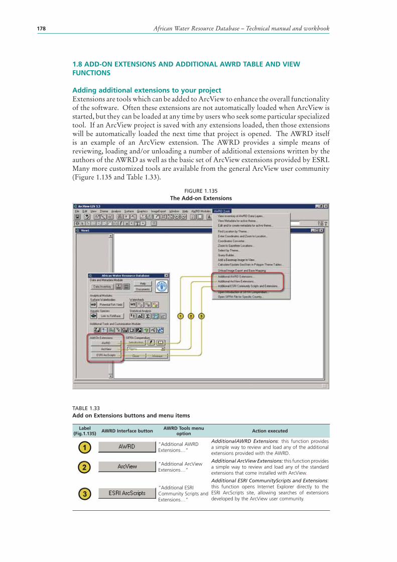
African Water Resource Database – Technical manual and workbook178
1.8 ADD-ON EXTENSIONS AND ADDITIONAL AWRD TABLE AND VIEW FUNCTIONS
Adding additional extensions to your projectExtensions are tools which can be added to ArcView to enhance the overall functionality of the software. Often these extensions are not automatically loaded when ArcView is started, but they can be loaded at any time by users who seek some particular specialized tool. If an ArcView project is saved with any extensions loaded, then those extensions will be automatically loaded the next time that project is opened. The AWRD itself is an example of an ArcView extension. The AWRD provides a simple means of reviewing, loading and/or unloading a number of additional extensions written by the authors of the AWRD as well as the basic set of ArcView extensions provided by ESRI. Many more customized tools are available from the general ArcView user community (Figure 1.135 and Table 1.33).
FIGURE 1.135The Add-on Extensions
TABLE 1.33Add on Extensions buttons and menu items
Label (Fig.1.135) AWRD Interface button AWRD Tools menu
option Action executed
“Additional AWRD Extensions…”
AdditionalAWRD Extensions: this function provides a simple way to review and load any of the additional extensions provided with the AWRD.
“Additional ArcView Extensions…”
Additional ArcView Extensions: this function provides a simple way to review and load any of the standard extensions that come installed with ArcView.
“Additional ESRI Community Scripts and Extensions…”
Additional ESRI CommunityScripts and Extensions: this function opens Internet Explorer directly to the ESRI ArcScripts site, allowing searches of extensions developed by the ArcView user community.
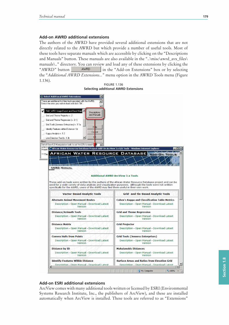
Technical manual 179
Sect
ion
1.8
Add-on AWRD additional extensionsThe authors of the AWRD have provided several additional extensions that are not directly related to the AWRD but which provide a number of useful tools. Most of these tools have separate manuals which are accessible by clicking on the “Descriptions and Manuals” button. These manuals are also available in the “..\misc\awrd_avx_files\manuals\..” directory. You can review and load any of these extensions by clicking the “AWRD” button in the “Add-on Extensions” box or by selecting the “Additional AWRD Extensions...” menu option in the AWRD Tools menu (Figure 1.136).
FIGURE 1.136Selecting additional AWRD Extensions
Add-on ESRI additional extensionsArcView comes with many additional tools written or licensed by ESRI (Environmental Systems Research Institute, Inc., the publishers of ArcView), and these are installed automatically when ArcView is installed. These tools are referred to as “Extensions”
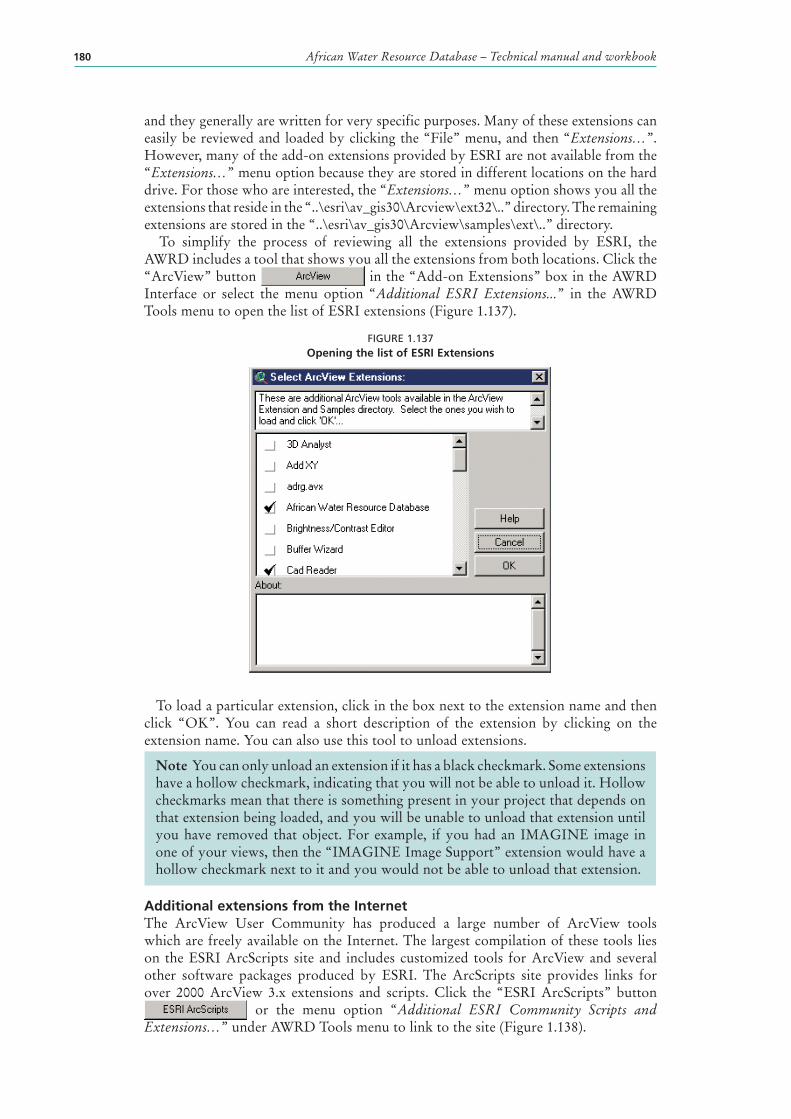
African Water Resource Database – Technical manual and workbook180
and they generally are written for very specific purposes. Many of these extensions can easily be reviewed and loaded by clicking the “File” menu, and then “Extensions…”. However, many of the add-on extensions provided by ESRI are not available from the “Extensions…” menu option because they are stored in different locations on the hard drive. For those who are interested, the “Extensions…” menu option shows you all the extensions that reside in the “..\esri\av_gis30\Arcview\ext32\..” directory. The remaining extensions are stored in the “..\esri\av_gis30\Arcview\samples\ext\..” directory.
To simplify the process of reviewing all the extensions provided by ESRI, the AWRD includes a tool that shows you all the extensions from both locations. Click the “ArcView” button in the “Add-on Extensions” box in the AWRD Interface or select the menu option “Additional ESRI Extensions...” in the AWRD Tools menu to open the list of ESRI extensions (Figure 1.137).
FIGURE 1.137Opening the list of ESRI Extensions
To load a particular extension, click in the box next to the extension name and then click “OK”. You can read a short description of the extension by clicking on the extension name. You can also use this tool to unload extensions.
Note You can only unload an extension if it has a black checkmark. Some extensions have a hollow checkmark, indicating that you will not be able to unload it. Hollow checkmarks mean that there is something present in your project that depends on that extension being loaded, and you will be unable to unload that extension until you have removed that object. For example, if you had an IMAGINE image in one of your views, then the “IMAGINE Image Support” extension would have a hollow checkmark next to it and you would not be able to unload that extension.
Additional extensions from the InternetThe ArcView User Community has produced a large number of ArcView tools which are freely available on the Internet. The largest compilation of these tools lies on the ESRI ArcScripts site and includes customized tools for ArcView and several other software packages produced by ESRI. The ArcScripts site provides links for over 2000 ArcView 3.x extensions and scripts. Click the “ESRI ArcScripts” button
or the menu option “Additional ESRI Community Scripts and Extensions…” under AWRD Tools menu to link to the site (Figure 1.138).
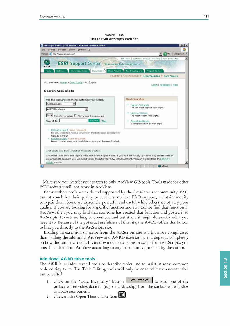
Technical manual 181
Sect
ion
1.8
FIGURE 1.138Link to ESRI Arcscripts Web site
Make sure you restrict your search to only ArcView GIS tools. Tools made for other ESRI software will not work in ArcView.
Because these tools are made and supported by the ArcView user community, FAO cannot vouch for their quality or accuracy, nor can FAO support, maintain, modify or repair them. Some are extremely powerful and useful while others are of very poor quality. If you are looking for a specific function and you cannot find that function in ArcView, then you may find that someone has created that function and posted it to ArcScripts. It costs nothing to download and test it and it might do exactly what you need it to. Because of the potential usefulness of this site, the AWRD offers this button to link you directly to the ArcScripts site.
Loading an extension or script from the ArcScripts site is a bit more complicated than loading the additional ArcView and AWRD extensions, and depends completely on how the author wrote it. If you download extensions or scrips from ArcScripts, you must load them into ArcView according to any instructions provided by the author.
Additional AWRD table toolsThe AWRD includes several tools to describe tables and to assist in some common table-editing tasks. The Table Editing tools will only be enabled if the current table can be edited.
1. Click on the “Data Inventory” button to load one of the surface waterbodies datasets (e.g. sadc_sbw.shp) from the surface waterbodies database component.
2. Click on the Open Theme table icon .
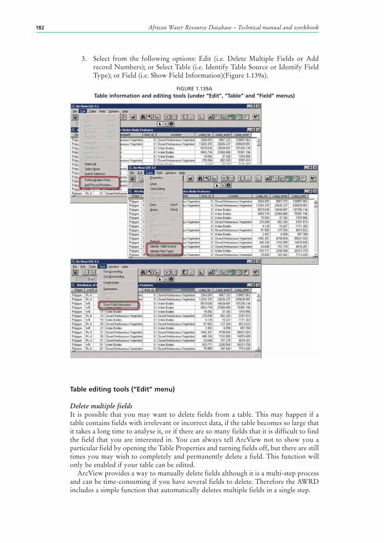
African Water Resource Database – Technical manual and workbook182
3. Select from the following options: Edit (i.e. Delete Multiple Fields or Add record Numbers); or Select Table (i.e. Identify Table Source or Identify Field Type); or Field (i.e. Show Field Information)(Figure 1.139a).
FIGURE 1.139ATable information and editing tools (under “Edit”, “Table” and “Field” menus)
Table editing tools (“Edit” menu)
Delete multiple fieldsIt is possible that you may want to delete fields from a table. This may happen if a table contains fields with irrelevant or incorrect data, if the table becomes so large that it takes a long time to analyse it, or if there are so many fields that it is difficult to find the field that you are interested in. You can always tell ArcView not to show you a particular field by opening the Table Properties and turning fields off, but there are still times you may wish to completely and permanently delete a field. This function will only be enabled if your table can be edited.
ArcView provides a way to manually delete fields although it is a multi-step process and can be time-consuming if you have several fields to delete. Therefore the AWRD includes a simple function that automatically deletes multiple fields in a single step.
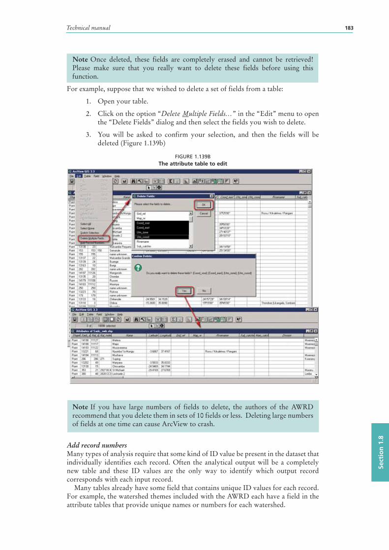
Technical manual 183
Sect
ion
1.8
Note Once deleted, these fields are completely erased and cannot be retrieved! Please make sure that you really want to delete these fields before using this function.
For example, suppose that we wished to delete a set of fields from a table:
1. Open your table.
2. Click on the option “Delete Multiple Fields…” in the “Edit” menu to open the “Delete Fields” dialog and then select the fields you wish to delete.
3. You will be asked to confirm your selection , and then the fields will be deleted (Figure 1.139b)
FIGURE 1.139BThe attribute table to edit
Note If you have large numbers of fields to delete, the authors of the AWRD recommend that you delete them in sets of 10 fields or less. Deleting large numbers of fields at one time can cause ArcView to crash.
Add record numbersMany types of analysis require that some kind of ID value be present in the dataset that individually identifies each record. Often the analytical output will be a completely new table and these ID values are the only way to identify which output record corresponds with each input record.
Many tables already have some field that contains unique ID values for each record. For example, the watershed themes included with the AWRD each have a field in the attribute tables that provide unique names or numbers for each watershed.
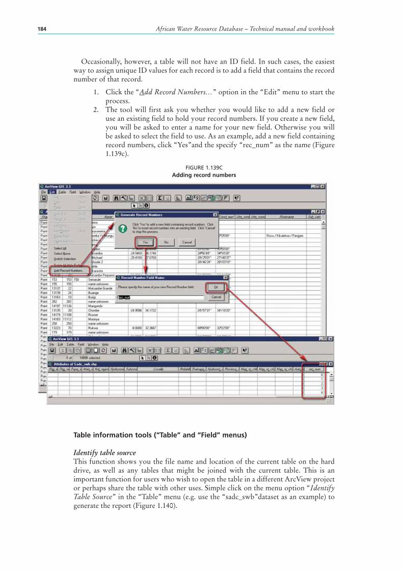
African Water Resource Database – Technical manual and workbook184
Occasionally, however, a table will not have an ID field. In such cases, the easiest way to assign unique ID values for each record is to add a field that contains the record number of that record.
1. Click the “Add Record Numbers…” option in the “Edit” menu to start the process.
2. The tool will first ask you whether you would like to add a new field or use an existing field to hold your record numbers. If you create a new field, you will be asked to enter a name for your new field. Otherwise you will be asked to select the field to use. As an example, add a new field containing record numbers, click “Yes”and the specify “rec_num” as the name (Figure 1.139c).
FIGURE 1.139CAdding record numbers
Table information tools (“Table” and “Field” menus)
Identify table sourceThis function shows you the file name and location of the current table on the hard drive, as well as any tables that might be joined with the current table. This is an important function for users who wish to open the table in a different ArcView project or perhaps share the table with other uses. Simple click on the menu option “Identify Table Source” in the “Table” menu (e.g. use the “sadc_swb”dataset as an example) to generate the report (Figure 1.140).
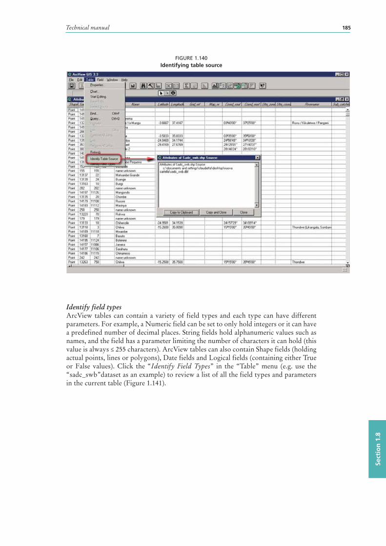
Technical manual 185
Sect
ion
1.8
FIGURE 1.140Identifying table source
Identify field typesArcView tables can contain a variety of field types and each type can have different parameters. For example, a Numeric field can be set to only hold integers or it can have a predefined number of decimal places. String fields hold alphanumeric values such as names, and the field has a parameter limiting the number of characters it can hold (this value is always ≤ 255 characters). ArcView tables can also contain Shape fields (holding actual points, lines or polygons), Date fields and Logical fields (containing either True or False values). Click the “Identify Field Types” in the “Table” menu (e.g. use the “sadc_swb”dataset as an example) to review a list of all the field types and parameters in the current table (Figure 1.141).
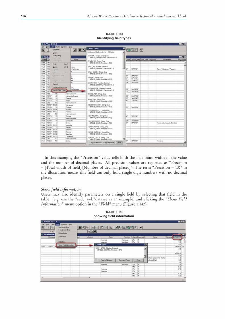
African Water Resource Database – Technical manual and workbook186
FIGURE 1.141Identifying field types
In this example, the “Precision” value tells both the maximum width of the value and the number of decimal places. All precision values are reported as “Precision = [Total width of field].[Number of decimal places]”. The term “Precision = 1.0” in the illustration means this field can only hold single digit numbers with no decimal places.
Show field informationUsers may also identify parameters on a single field by selecting that field in the table (e.g. use the “sadc_swb”dataset as an example) and clicking the “Show Field Information” menu option in the “Field” menu (Figure 1.142).
FIGURE 1.142Showing field information
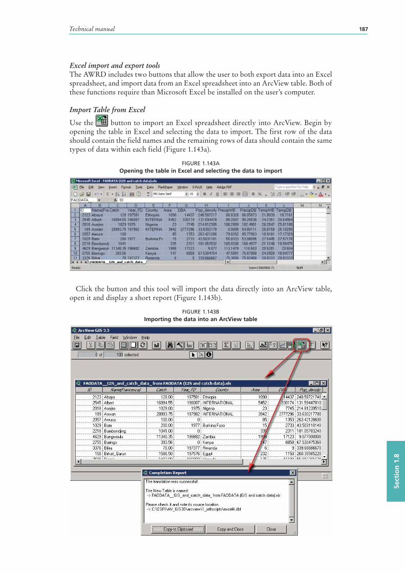
Technical manual 187
Sect
ion
1.8
Excel import and export toolsThe AWRD includes two buttons that allow the user to both export data into an Excel spreadsheet, and import data from an Excel spreadsheet into an ArcView table. Both of these functions require than Microsoft Excel be installed on the user’s computer.
Import Table from Excel
Use the button to import an Excel spreadsheet directly into ArcView. Begin by opening the table in Excel and selecting the data to import. The first row of the data should contain the field names and the remaining rows of data should contain the same types of data within each field (Figure 1.143a).
FIGURE 1.143AOpening the table in Excel and selecting the data to import
Click the button and this tool will import the data directly into an ArcView table, open it and display a short report (Figure 1.143b).
FIGURE 1.143BImporting the data into an ArcView table
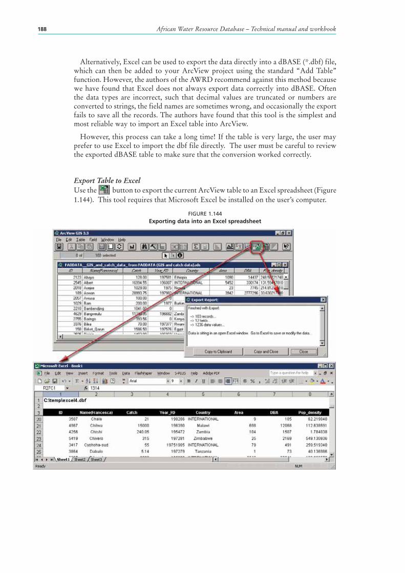
African Water Resource Database – Technical manual and workbook188
Alternatively, Excel can be used to export the data directly into a dBASE (*.dbf) file, which can then be added to your ArcView project using the standard “Add Table” function. However, the authors of the AWRD recommend against this method because we have found that Excel does not always export data correctly into dBASE. Often the data types are incorrect, such that decimal values are truncated or numbers are converted to strings, the field names are sometimes wrong, and occasionally the export fails to save all the records. The authors have found that this tool is the simplest and most reliable way to import an Excel table into ArcView.
However, this process can take a long time! If the table is very large, the user may prefer to use Excel to import the dbf file directly. The user must be careful to review the exported dBASE table to make sure that the conversion worked correctly.
Export Table to ExcelUse the button to export the current ArcView table to an Excel spreadsheet (Figure 1.144). This tool requires that Microsoft Excel be installed on the user’s computer.
FIGURE 1.144Exporting data into an Excel spreadsheet
Technical manual 189
Sect
ion
1.8
Additional AWRD View toolsThese tools do not work specifically with any AWRD datasets or functions, but rather serve as general enhancements to other basic ArcView functions.
Zoom to Next Extent
The Zoom to Next Extent button in the View button bar works in conjunction with the standard ArcView Zoom to Previous Extent button . When the user zooms in or out to different extents, ArcView remembers a list of the last several extents. When the Zoom to Previous Extent button is clicked, the view returns to the last extent in the list, similar to the manner in which the “Back” button in an internet browser works. The Zoom to Next Extent button allows the user to go forward through the list, much like clicking the “Forward” button in an internet browser. The list is cleared as soon as the user selects a new extent by using one of the basic zooming or panning tools, and the Zoom to Next Extent button is then disabled until the user clicks the Zoom to Previous Extent button again.
Additional View functions (“View” menu)The AWRD Extension adds four menu options to the “View” menu in the View Interface, allowing you to expand or collapse the legends for all the themes in the view and to select or deselect all the themes in the view.
Showing and Hiding LegendsThe theme legend shows the symbols that ArcView uses to display the theme in the view. These symbols are generally coloured boxes, lines or dots, and they are occasionally graduated by size or colour. In some cases, the theme legends may be so large that they fill the entire visible Table of Contents, and therefore users may wish to collapse the legends so that they can see the full list of themes. ArcView allows you to collapse or expand individual theme legends (i.e. “Theme” menu option: “Hide/Show Legend”). The “Show All Legends” and “Hide All Legends” options of the “View” menu, included with the AWRD, automatically expand or collapse the legends of all the themes in the view.
Selecting and deselecting ThemesArcView allows you to select themes for various reasons, including identifying themes the user wishes to delete from the view or possibly identifying themes the user wishes to analyse. The standard method to select a theme is simply to click on the theme name in the Table of Contents. A “selected” theme is referred to as an “Active” theme, and visually it appears to have a raised box surrounding its name in the Table of Contents. Users can set multiple themes as Active by holding the Shift key down as they click on them.
Occasionally users may wish to set all themes active. This is especially likely if they wish to delete all the themes from the view. The AWRD menu options “Set all themes Active” and “Set all themes Inactive” in the “View” menu provide an easy way to automatically select or deselect all themes in the view.
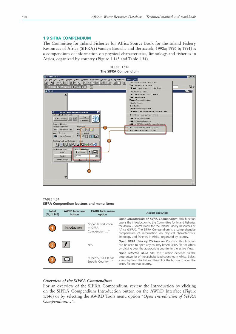
African Water Resource Database – Technical manual and workbook190
1.9 SIFRA COMPENDIUM The Committee for Inland Fisheries for Africa Source Book for the Inland Fishery Resources of Africa (SIFRA) (Vanden Bossche and Bernacsek, 1990a; 1990 b; 1991) is a compendium of information on physical characteristics, limnology and fisheries in Africa, organized by country (Figure 1.145 and Table 1.34).
FIGURE 1.145The SIFRA Compendium
TABLE 1.34SIFRA Compendium buttons and menu items
Label (Fig.1.145)
AWRD Interface button
AWRD Tools menu option Action executed
“Open Introduction of SIFRA Compendium…”
Open Introduction of SIFRA Compendium: this function opens the introduction to the Committee for Inland Fisheries for Africa - Source Book for the Inland Fishery Resources of Africa (SIFRA). The SIFRA Compendium is a comprehensive compendium of information on physical characteristics, limnology and fisheries in Africa, organized by country.
N/AOpen SIFRA data by Clicking on Country: this function can be used to open any country based SIFRA file for Africa by clicking over the appropriate country in the active View.
“Open SIFRA File for Specific Country…”
Open Selected SIFRA File: this function depends on the drop-down list of the alphabetized countries in Africa. Select a country from the list and then click the button to open the SIFRA file on that country.
Overview of the SIFRA CompendiumFor an overview of the SIFRA Compendium, review the Introduction by clicking on the SIFRA Compendium Introduction button on the AWRD Interface (Figure 1.146) or by selecting the AWRD Tools menu option “Open Introduction of SIFRA Compendium…”.
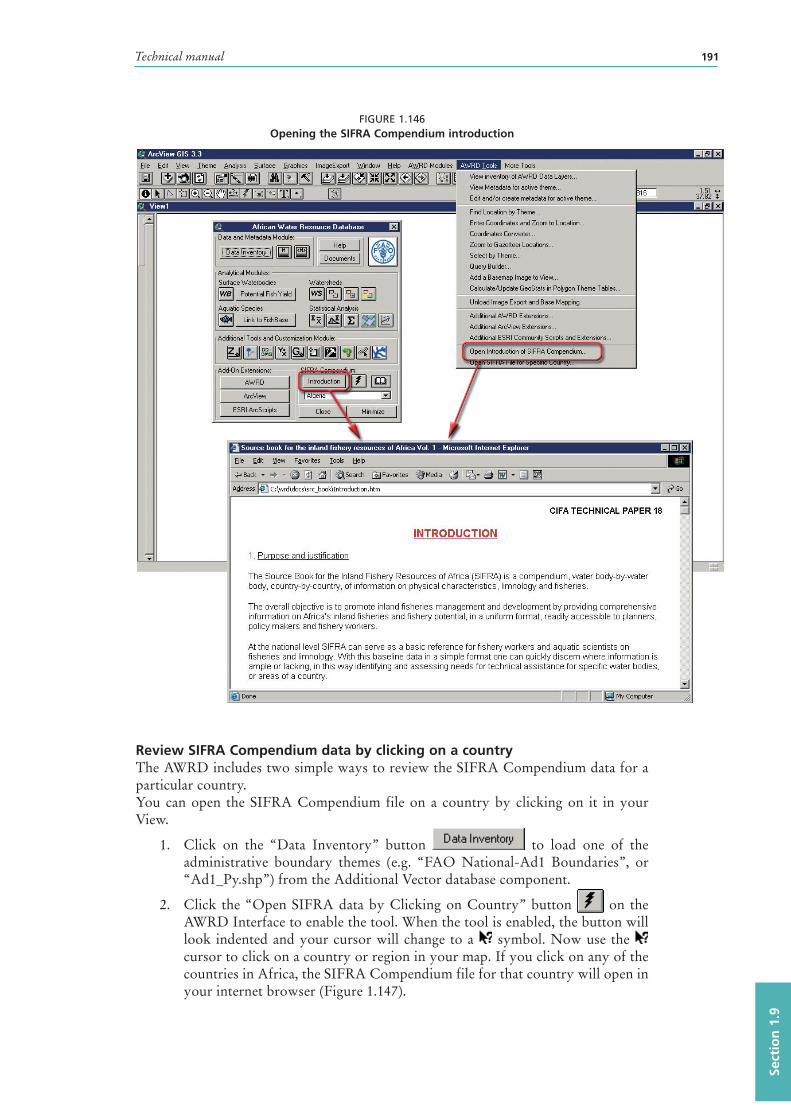
Technical manual 191
Sect
ion
1.9
FIGURE 1.146Opening the SIFRA Compendium introduction
Review SIFRA Compendium data by clicking on a countryThe AWRD includes two simple ways to review the SIFRA Compendium data for a particular country.You can open the SIFRA Compendium file on a country by clicking on it in your View.
1. Click on the “Data Inventory” button to load one of the administrative boundary themes (e.g. “FAO National-Ad1 Boundaries”, or “Ad1_Py.shp”) from the Additional Vector database component.
2. Click the “Open SIFRA data by Clicking on Country” button on the AWRD Interface to enable the tool. When the tool is enabled, the button will look indented and your cursor will change to a symbol. Now use the cursor to click on a country or region in your map. If you click on any of the countries in Africa, the SIFRA Compendium file for that country will open in your internet browser (Figure 1.147).
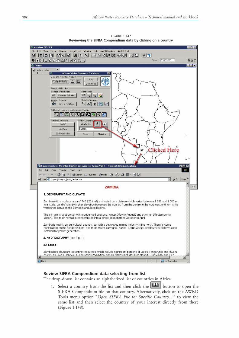
African Water Resource Database – Technical manual and workbook192
FIGURE 1.147Reviewing the SIFRA Compendium data by clicking on a country
Review SIFRA Compendium data selecting from listThe drop-down list contains an alphabetized list of countries in Africa.
1. Select a country from the list and then click the button to open the SIFRA Compendium file on that country. Alternatively, click on the AWRD Tools menu option “Open SIFRA File for Specific Country…” to view the same list and then select the country of your interest directly from there (Figure 1.148).
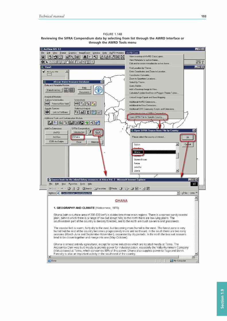
Technical manual 193
Sect
ion
1.9
FIGURE 1.148Reviewing the SIFRA Compendium data by selecting from list through the AWRD Interface or
through the AWRD Tools menu

195
2. Workbook
The exercises in this workbook assume that users will have a basic understanding of GIS concepts and methods. Readers with no previous experience in GIS are suggested to read publications by Meaden and Kapetsky (1991) for an understanding of the basic concepts and de Graaf et al. (2003) for a first hands-on experience with GIS data and tools. It is also assumed that users have read part 1 of this publication and have tested the main tools described in section 2.3 in part 1 and then described in detail in section 1 in part 2 of this publication prior to completing the exercises of this workbook.
In addition, exercise procedures have been written with respect to the ArcView 3.x software only. However, an attempt has been made to sufficiently explain each step such that translations to other software might be possible.
The exercises are based on the case studies presented in part 1 of this publication. Thus, they address some of the key issues in inland aquatic resource management. The readers are advised to read the relevant case study in part 1 before they begin its corresponding exercise.
Given that one of the most basic components of fisheries management is the inventory of resources, the first two exercises address concerns for local and regional resource inventory and analysis. Exercise 1 corresponds to the second case study (Inventory of fisheries habitats and fisheries productivities) and demonstrates a method to inventory fisheries habitats and fisheries productivities of African inland waters. Exercise 2 examines the creation of a surface waterbodies inventory using the United Republic of Tanzania and the Republic of Zimbabwe, and corresponds with the first case study (Surface waterbodies inventory). The order of these first two case studies are reversed because the analysis presented in Exercise 2 is difficult to replicate in a workbook exercise. The user must make a large number of decisions and judgment calls in Exercise 2, and in some cases there is no way to know what the correct answers are, so this workbook exercise is presented as an optional secondary exercise to illustrate a general methodological approach to identify unnamed features.
Exercise 3 explores estimates of potential fish yield as a critical value for fisheries managers by integrating relevant models in a GIS environment. Exercise 4 illustrates how users may create hydrological reports by summarizing statistical information across a range of human, environmental, and climatological factors using the Volta River megabasin as an example.
Exercise 5 is focused on the analysis of invasive and introduced aquatic species and illustrates how the AWRD provides a robust approach to the analysis of aquatic taxa. The last exercise provides users with guidelines and suggestions for the creation of base or reference maps which can be integrated to support reporting or for presentation purposes.
The exercises will reacquaint the user with the AWRD archive and technical manual and will help illustrate the usefulness of the AWRD. It should become clear that with the use of GIS (thus the AWRD) there is a surprisingly wide range of questions that can be answered using easily obtained information.
By completing the exercises in this workbook the reader should be able to re-create the results presented in the case studies presented in part 1 of this publication, while having the opportunity to explore the various AWRD datasets and tools. Time estimates were based on the amount of time a GIS expert took to complete the exercises.
Tick boxes are provided alongside each step of a given exercise to help the user keep track of where he/she left of.
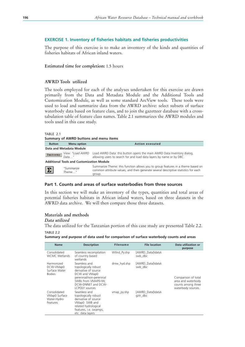
African Water Resource Database – Technical manual and workbook196
EXERCISE 1. Inventory of fisheries habitats and fisheries productivities
The purpose of this exercise is to make an inventory of the kinds and quantities of fisheries habitats of African inland waters.
Estimated time for completion: 1.5 hours
AWRD Tools utilized
The tools employed for each of the analyses undertaken for this exercise are drawn primarily from the Data and Metadata Module and the Additional Tools and Customization Module, as well as some standard ArcView tools. These tools were used to load and summarize data from the AWRD archive: select subsets of surface waterbody data based on feature class, and to join the gazetteer database with a cross-tabulation table of feature class names. Table 2.1 summarizes the AWRD modules and tools used in this case study.
TABLE 2.1Summary of AWRD buttons and menu items
Button Menu option Action executed
Data and Metadata Module
View: “Load AWRD Data…”
Load AWRD Data: this button opens the main AWRD Data Inventory dialog, allowing users to search for and load data layers by name or by DBC.
Additional Tools and Customization Module
“Summarize Theme…”
Summarize Theme: this function allows you to group features in a theme based on common attribute values, and then generate several descriptive statistics for each group.
Part 1. Counts and areas of surface waterbodies from three sources
In this section we will make an inventory of the types, quantities and total areas of potential fisheries habitats in African inland waters, based on three datasets in the AWRD data archive. We will then compare those three datasets.
Materials and methods Data utilizedThe data utilized for the Tanzanian portion of this case study are presented Table 2.2.TABLE 2.2Summary and purpose of data used for comparison of surface waterbody counts and areas
Name Description Filename File location Data utilization or purpose
Consolidated WCMC Wetlands
Seamless recompilation of country based wetlands
Wtlnd_Py.shp [AWRD_Data]\data\swb_dbc
Comparison of total area and waterbody counts among three waterbody sources.
Harmonized DCW-VMap0 Surface Water Bodies
Seamless and topologically robust derivative of source DCW and VMap0 perennial/non-perennial SWBs from VMAP0-IW, DCW-DNNET and DCW-LCPOLY sources
dniw_hyd.shp [AWRD_Data]\data\swb_dbc
Consolidated VMap0 Surface Water-Hydro Features
Seamless and topologically robust derivative of source VMap0 SWB and related hydrological features, i.e. swamps, etc. data layers
vmap_py.shp [AWRD_Data]\data\gztr_dbc
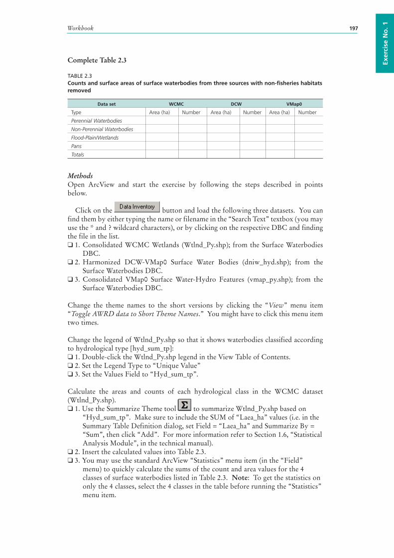
Workbook 197
Exer
cise
No
. 1
Complete Table 2.3
TABLE 2.3Counts and surface areas of surface waterbodies from three sources with non-fisheries habitats removed
Data set WCMC DCW VMap0
Type Area (ha) Number Area (ha) Number Area (ha) Number
Perennial Waterbodies
Non-Perennial Waterbodies
Flood-Plain/Wetlands
Pans
Totals
MethodsOpen ArcView and start the exercise by following the steps described in points below.
Click on the button and load the following three datasets. You can find them by either typing the name or filename in the “Search Text” textbox (you may use the * and ? wildcard characters), or by clicking on the respective DBC and finding the file in the list.❑ 1. Consolidated WCMC Wetlands (Wtlnd_Py.shp); from the Surface Waterbodies
DBC.❑ 2. Harmonized DCW-VMap0 Surface Water Bodies (dniw_hyd.shp); from the
Surface Waterbodies DBC.❑ 3. Consolidated VMap0 Surface Water-Hydro Features (vmap_py.shp); from the
Surface Waterbodies DBC.
Change the theme names to the short versions by clicking the “View” menu item “Toggle AWRD data to Short Theme Names.” You might have to click this menu item two times.
Change the legend of Wtlnd_Py.shp so that it shows waterbodies classified according to hydrological type [hyd_sum_tp]:❑ 1. Double-click the Wtlnd_Py.shp legend in the View Table of Contents.❑ 2. Set the Legend Type to “Unique Value”❑ 3. Set the Values Field to “Hyd_sum_tp”.
Calculate the areas and counts of each hydrological class in the WCMC dataset (Wtlnd_Py.shp).❑ 1. Use the Summarize Theme tool to summarize Wtlnd_Py.shp based on
“Hyd_sum_tp”. Make sure to include the SUM of “Laea_ha” values (i.e. in the Summary Table Definition dialog, set Field = “Laea_ha” and Summarize By = “Sum”, then click “Add”. For more information refer to Section 1.6, “Statistical Analysis Module”, in the technical manual).
❑ 2. Insert the calculated values into Table 2.3.❑ 3. You may use the standard ArcView “Statistics” menu item (in the “Field”
menu) to quickly calculate the sums of the count and area values for the 4 classes of surface waterbodies listed in Table 2.3. Note: To get the statistics on only the 4 classes, select the 4 classes in the table before running the “Statistics” menu item.
African Water Resource Database – Technical manual and workbook198
Calculate the areas and counts of each hydrological class in the DCW dataset (dniw_hyd.shp).❑ 1. Use the Summarize Theme tool to summarize dniw_hyd.shp based on
“Hyd_code”. Make sure to include the SUM of “Laea_ha” values.❑ 2. The class “Perennial Water Bodies” corresponds with [Hyd_code] = 1. Enter the
count and area values for [Hyd_code] = 1 into the “Perennial Water Bodies” row in Table 2.3.
❑ 3. The class “Non-Perennial Water Bodies” corresponds with [Hyd_code] = 1. Enter the count and area values for [Hyd_code] = 2 into the “Non-Perennial Water Bodies” row in Table 2.3.
❑ 4. The class “Flood-Plain/Wetlands” corresponds with [Hyd_code] = 14 and [Hyd_code] = 15. Enter the count and area values for [Hyd_code] = (14 and 15) into the “Flood-Plain/Wetlands” row in Table 2.3.
❑ 5. The class “Pans” corresponds with [Hyd_code] = 3 and [Hyd_code] = 5. Enter the count and area values for [Hyd_code] = (3 and 5) into the “Pans” row in Table 2.3.
Calculate the areas and counts of each hydrological class in the VMap0 dataset (vmap_py.shp).❑ 1. Use the Summarize Theme tool to summarize vmap_py.shp based on “Bnd_
code”. Make sure to include the SUM of “Laea_ha” values.❑ 2. The class “Perennial Water Bodies” corresponds with [Bnd_code] = 1. Enter the
count and area values for [Bnd_code] = 1 into the “Perennial Water Bodies” row in Table 2.3.
❑ 3. The class “Non-Perennial Water Bodies” corresponds with [Bnd_code] = 1. Enter the count and area values for [Bnd_code] = 2 into the “Non-Perennial Water Bodies” row in Table 2.3.
❑ 4. The class “Flood-Plain/Wetlands” corresponds with [Bnd_code] = 14, [Bnd_code] = 16, and [Bnd_code] = 17. Enter the count and area values for [Bnd_code] = (14, 16 and 17) into the “Flood-Plain/Wetlands” row in Table 2.3.
❑ 5. The class “Pans” corresponds with [Bnd_code] = 3 and [Bnd_code] = 5. Enter the count and area values for [Bnd_code] = (3 and 5) into the “Pans” row in Table 2.3.
Notice the differences between data sources: WCMC and DCW contain approximately the same total area of waterbodies, while VMap0 contains considerably less. This suggests that WCMC and DCW may include waterbodies that are missed by VMap0.
However, VMap0 and DCW both contain similar total numbers of waterbodies, while WCMC has a considerably smaller number. This suggests that multiple waterbodies may be aggregated into single units in the WCMC data, while being maintained as separate entities in the DCW and VMap0 data.
There may be a variety of reasons why datasets in general differ. In this case, the metadata for the three datasets show that both the DCW and VMap0 were originally derived from VMap0 sources, and have since been postprocessed using different methods. The WCMC data comes from a different source entirely.
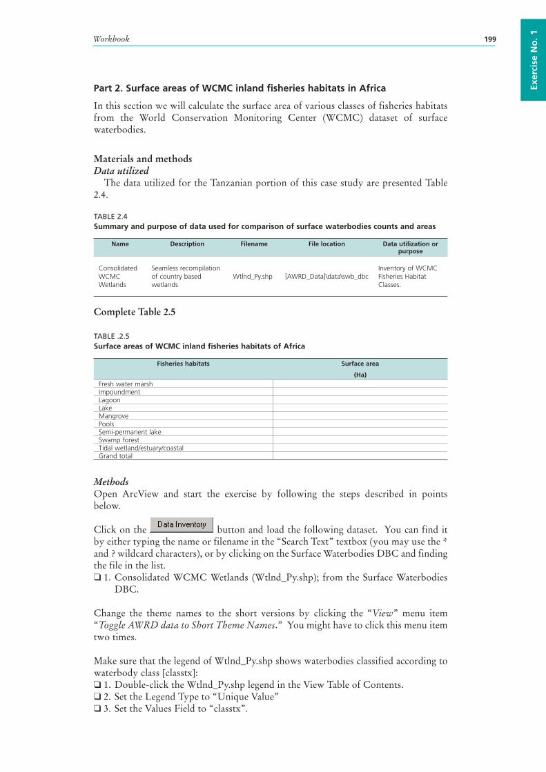
Workbook 199
Exer
cise
No
. 1
Part 2. Surface areas of WCMC inland fisheries habitats in Africa
In this section we will calculate the surface area of various classes of fisheries habitats from the World Conservation Monitoring Center (WCMC) dataset of surface waterbodies.
Materials and methods Data utilized
The data utilized for the Tanzanian portion of this case study are presented Table 2.4.
TABLE 2.4Summary and purpose of data used for comparison of surface waterbodies counts and areas
Name Description Filename File location Data utilization or purpose
Consolidated WCMC Wetlands
Seamless recompilation of country based wetlands
Wtlnd_Py.shp [AWRD_Data]\data\swb_dbcInventory of WCMC Fisheries Habitat Classes.
Complete Table 2.5
TABLE .2.5Surface areas of WCMC inland fisheries habitats of Africa
Fisheries habitats Surface area
(Ha)Fresh water marshImpoundmentLagoonLakeMangrovePoolsSemi-permanent lakeSwamp forestTidal wetland/estuary/coastalGrand total
MethodsOpen ArcView and start the exercise by following the steps described in points below.
Click on the button and load the following dataset. You can find it by either typing the name or filename in the “Search Text” textbox (you may use the * and ? wildcard characters), or by clicking on the Surface Waterbodies DBC and finding the file in the list.❑ 1. Consolidated WCMC Wetlands (Wtlnd_Py.shp); from the Surface Waterbodies
DBC.
Change the theme names to the short versions by clicking the “View” menu item “Toggle AWRD data to Short Theme Names.” You might have to click this menu item two times.
Make sure that the legend of Wtlnd_Py.shp shows waterbodies classified according to waterbody class [classtx]:❑ 1. Double-click the Wtlnd_Py.shp legend in the View Table of Contents.❑ 2. Set the Legend Type to “Unique Value”❑ 3. Set the Values Field to “classtx”.
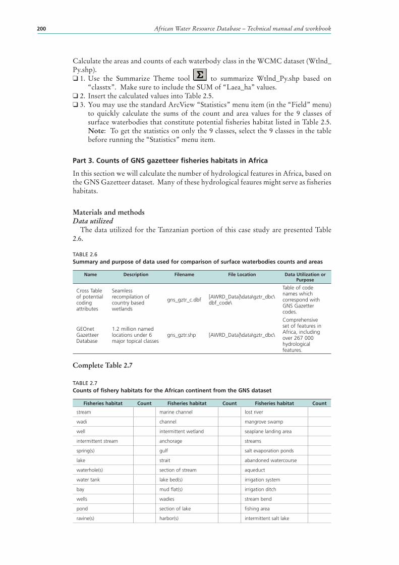
African Water Resource Database – Technical manual and workbook200
Calculate the areas and counts of each waterbody class in the WCMC dataset (Wtlnd_Py.shp).❑ 1. Use the Summarize Theme tool to summarize Wtlnd_Py.shp based on
“classtx”. Make sure to include the SUM of “Laea_ha” values.❑ 2. Insert the calculated values into Table 2.5.❑ 3. You may use the standard ArcView “Statistics” menu item (in the “Field” menu)
to quickly calculate the sums of the count and area values for the 9 classes of surface waterbodies that constitute potential fisheries habitat listed in Table 2.5. Note: To get the statistics on only the 9 classes, select the 9 classes in the table before running the “Statistics” menu item.
Part 3. Counts of GNS gazetteer fisheries habitats in Africa
In this section we will calculate the number of hydrological features in Africa, based on the GNS Gazetteer dataset. Many of these hydrological feaures might serve as fisheries habitats.
Materials and methods Data utilized
The data utilized for the Tanzanian portion of this case study are presented Table 2.6.
TABLE 2.6Summary and purpose of data used for comparison of surface waterbodies counts and areas
Name Description Filename File Location Data Utilization or Purpose
Cross Table of potential coding attributes
Seamless recompilation of country based wetlands
gns_gztr_c.dbf [AWRD_Data]\data\gztr_dbc\dbf_code\
Table of code names which correspond with GNS Gazetter codes.
GEOnet Gazetteer Database
1.2 million named locations under 6 major topical classes
gns_gztr.shp [AWRD_Data]\data\gztr_dbc\
Comprehensive set of features in Africa, including over 267 000 hydrological features.
Complete Table 2.7
TABLE 2.7 Counts of fishery habitats for the African continent from the GNS dataset
Fisheries habitat Count Fisheries habitat Count Fisheries habitat Count
stream marine channel lost river
wadi channel mangrove swamp
well intermittent wetland seaplane landing area
intermittent stream anchorage streams
spring(s) gulf salt evaporation ponds
lake strait abandoned watercourse
waterhole(s) section of stream aqueduct
water tank lake bed(s) irrigation system
bay mud flat(s) irrigation ditch
wells wadies stream bend
pond section of lake fishing area
ravine(s) harbor(s) intermittent salt lake
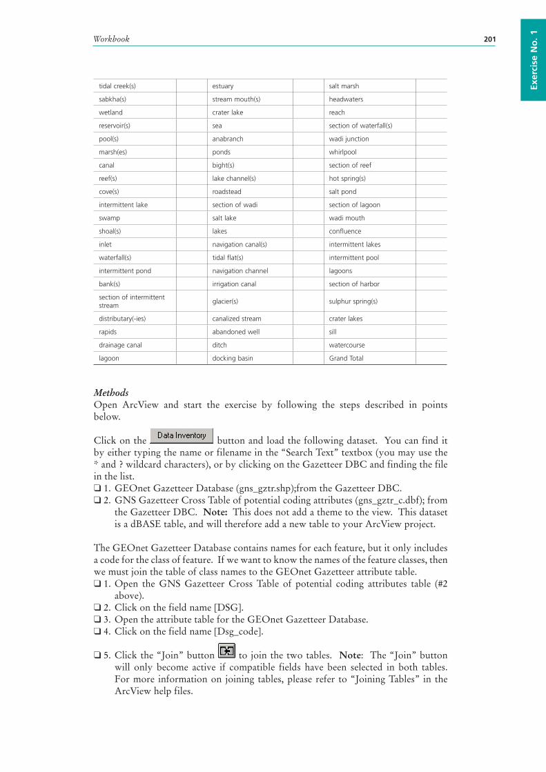
Workbook 201
Exer
cise
No
. 1
tidal creek(s) estuary salt marsh
sabkha(s) stream mouth(s) headwaters
wetland crater lake reach
reservoir(s) sea section of waterfall(s)
pool(s) anabranch wadi junction
marsh(es) ponds whirlpool
canal bight(s) section of reef
reef(s) lake channel(s) hot spring(s)
cove(s) roadstead salt pond
intermittent lake section of wadi section of lagoon
swamp salt lake wadi mouth
shoal(s) lakes confluence
inlet navigation canal(s) intermittent lakes
waterfall(s) tidal flat(s) intermittent pool
intermittent pond navigation channel lagoons
bank(s) irrigation canal section of harbor
section of intermittent stream
glacier(s) sulphur spring(s)
distributary(-ies) canalized stream crater lakes
rapids abandoned well sill
drainage canal ditch watercourse
lagoon docking basin Grand Total
MethodsOpen ArcView and start the exercise by following the steps described in points below.
Click on the button and load the following dataset. You can find it by either typing the name or filename in the “Search Text” textbox (you may use the * and ? wildcard characters), or by clicking on the Gazetteer DBC and finding the file in the list.❑ 1. GEOnet Gazetteer Database (gns_gztr.shp);from the Gazetteer DBC.❑ 2. GNS Gazetteer Cross Table of potential coding attributes (gns_gztr_c.dbf); from
the Gazetteer DBC. Note: This does not add a theme to the view. This dataset is a dBASE table, and will therefore add a new table to your ArcView project.
The GEOnet Gazetteer Database contains names for each feature, but it only includes a code for the class of feature. If we want to know the names of the feature classes, then we must join the table of class names to the GEOnet Gazetteer attribute table.❑ 1. Open the GNS Gazetteer Cross Table of potential coding attributes table (#2
above).❑ 2. Click on the field name [DSG].❑ 3. Open the attribute table for the GEOnet Gazetteer Database.❑ 4. Click on the field name [Dsg_code].
❑ 5. Click the “Join” button to join the two tables. Note: The “Join” button will only become active if compatible fields have been selected in both tables. For more information on joining tables, please refer to “Joining Tables” in the ArcView help files.
African Water Resource Database – Technical manual and workbook202
The GEOnet Gazetteer database contains types of features. We are only interested in the hydrological features in this example. Hydrological features are designated with a value of “H” in the [FC] field.❑ 1. While the GEOnet Gazetteer atribute table is open, select the hydrological features
by clicking the Query button and using the following query string:
( [Fc] = “H” )❑ 2. You should have 267 039 hydrological features selected for Africa. Summarize
these by [Code_type] using the button, and enter the values into Table 2.7.
Exercise SummaryThis exercise demonstrated how to generate inventories of potential fisheries habitats, including counts and areas, extracted from four data sources in the AWRD archive. These inventories describe fisheries habitats across all of Africa, however, the methodology describe in this exercise could be easily adapted to analyzing habitat availability in any region of interest.
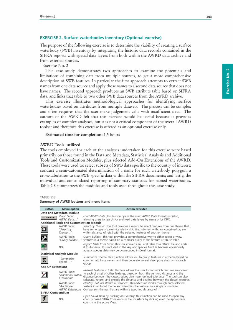
Workbook 203
Exer
cise
No
. 2
EXERCISE 2. Surface waterbodies inventory (Optional exercise)
The purpose of the following exercise is to determine the viability of creating a surface waterbody (SWB) inventory by integrating the historic data records contained in the SIFRA reports with spatial data layers from both within the AWRD data archive and from external sources. Exercise No. 2
This case study demonstrates two approaches to examine the potentials and limitations of combining data from multiple sources, to get a more comprehensive description of SWB features. In particular the first approach attempts to extract SWB names from one data source and apply those names to a second data source that does not have names. The second approach produces an SWB attribute table based on SIFRA data, and links that table to two other SWB data sources from the AWRD archive.
This exercise illustrates methodological approaches for identifying surface waterbodies based on attributes from multiple datasets. The process can be complex and often requires that the user make judgement calls with insufficient data. The authors of the AWRD felt that this exercise would be useful because it provides examples of complex analyses, but it is not a critical component of the overall AWRD toolset and therefore this exercise is offered as an optional exercise only.
Estimated time for completion: 1.5 hours
AWRD Tools utilizedThe tools employed for each of the analyses undertaken for this exercise were based primarily on those found in the Data and Metadata, Statistical Analysis and Additional Tools and Customization Modules, plus selected Add-On Extensions of the AWRD. These tools were used to: select subsets of SWB data specific to the country of interest; conduct a semi-automated determination of a name for each waterbody polygon; a cross-tabulation to the SWB specific data within the SIFRA documents; and lastly, the individual and consolidated reporting of summary statistics for named waterbodies. Table 2.8 summarizes the modules and tools used throughout this case study.
TABLE 2.8Summary of AWRD buttons and menu items
Button Menu option Action executedData and Metadata Module
View: “Load AWRD Data…”
Load AWRD Data: this button opens the main AWRD Data Inventory dialog, allowing users to search for and load data layers by name or by DBC.
Additional Tools and Customization ModuleAWRD Tools: “Select by Theme…”
Select by Theme: this tool provides a means to select features from one theme that have some type of proximity relationship (i.e. intersect with, are contained by, are within distance of, etc.) with the selected features of another theme.
AWRD Tools: “Query Builder…”
Query Builder: this tool provides a comprehensive way to either select or view features in a theme based on a complex query to the feature attribute table.
N/AImport Table from Excel: This tool converts an Excel table to a dBASE file and adds it to ArcView. It is included in the Aquatic Species Module because occasionally aquatic species data may be downloaded in Excel format.
Statistical Analysis Module
“Summarize Theme…”
Summarize Theme: this function allows you to group features in a theme based on common attribute values, and then generate several descriptive statistics for each group.
Add-On Extensions
AWRD Tools: “Additional AWRD Extensions”
Nearest Features v. 3.8a: this tool allows the user to find which features are closest to each of a set of other features, based on both the centroid distance and the distance between the closest edges given user defined tolerance. The tool can also calculate, return, and encode the distance and bearing between the closest features.
AWRD Tools: “Additional AWRD Extensions
Identify Features Within a Distance: This extension works through each selected feature in an Input theme and identifies the features in a single or multiple Comparison themes that are within a specified distance of it.
SIFRA Compendium
N/AOpen SIFRA Data by Clicking on Country: this function can be used to open any country based SIFRA Compendium file for Africa by clicking over the appropriate country in the active View.
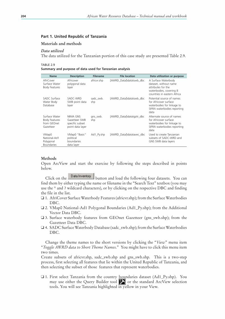
African Water Resource Database – Technical manual and workbook204
Part 1. United Republic of Tanzania
Materials and methods
Data utilizedThe data utilized for the Tanzanian portion of this case study are presented Table 2.9.
TABLE 2.9Summary and purpose of data used for Tanzanian analysis
Name Description Filename File location Data utilization or purpose
AfriCover Surface Water Body Features
Africover polygonal data layer
africvr.shp [AWRD_Data]\data\swb_dbc A Surface Waterbody dataset, without name attributes for the waterbodies, covering 8 countries in eastern Africa
SADC Surface Water Body Database
SADC-WRD SWB point data layer
sadc_swb.shp
[AWRD_Data]\data\swb_dbc Potential source of names for Africover surface waterbodies for linkage to SIFRA waterbodies reporting data
Surface Water Body Features from GEOnet Gazetteer
NIMA GNS Gazetteer SWB specific subset point data layer
gns_swb.shp
[AWRD_Data]\data\gztr_dbc Alternate source of names for Africover surface waterbodies for linkage to SIFRA waterbodies reporting data
VMap0 National-Ad1 Polygonal Boundaries
VMap0 “Basic” political boundaries data layer
Ad1_Py.shp [AWRD_Data]\data\avec_dbc Used to create Tanzanian subsets of SADC-WRD and GNS SWB data layers
MethodsOpen ArcView and start the exercise by following the steps described in points below.
Click on the button and load the following four datasets. You can find them by either typing the name or filename in the “Search Text” textbox (you may use the * and ? wildcard characters), or by clicking on the respective DBC and finding the file in the list.❑ 1. AfriCover Surface Waterbody Features (africvr.shp); from the Surface Waterbodies
DBC.❑ 2. VMap0 National-Ad1 Polygonal Boundaries (Ad1_Py.shp); from the Additional
Vector Data DBC.❑ 3. Surface waterbody features from GEOnet Gazetteer (gns_swb.shp); from the
Gazetteer Data DBC.❑ 4. SADC Surface Waterbody Database (sadc_swb.shp); from the Surface Waterbodies
DBC.
Change the theme names to the short versions by clicking the “View” menu item “Toggle AWRD data to Short Theme Names.” You might have to click this menu item two times.Create subsets of africvr.shp, sadc_swb.shp and gns_swb.shp. This is a two-step process, first selecting all features that lie within the United Republic of Tanzania, and then selecting the subset of those features that represent waterbodies.
❑ 1. First select Tanzania from the country boundaries dataset (Ad1_Py.shp). You may use either the Query Builder tool or the standard ArcView selection tools. You will see Tanzania highlighted in yellow in your View.
Workbook 205
Exer
cise
No
. 2
❑ 2. Zoom in to the extent of Tanzania by clicking the standard ArcView “Zoom to Selection” button.
❑ 3. Select the sadc_swb.shp surface waterbody points that intersect with Tanzania. Do this by clicking on the sadc_swb.shp theme to make it active, then clicking the “Select By Theme” tool . Select features from the active theme (i.e. Sadc_swb.shp) that “Intersect” the selected features of “Ad1_Py.shp” (i.e. Tanzania). Click the “New” button and you will see all sadc_swb features highlighted in yellow for Tanzania. At the bottom of the dialog, you should see that approximately 328 points are selected.
❑ 4. Refine the selection to include only features that are known to be waterbodies. Click on the Query Builder tool , make sure that the “Select” option is chosen (not “Set Theme Definition”), and enter the following query string (this query string is basically identifying all points that are not of type “Unknown”):
( [Type] <> “U” )❑ 5. Click the Subset button to select the subset of waterbody
points. At the bottom of the dialog, you should see that approximately 127 points are now selected.
❑ 6. The next step is to convert this subset of features into a new independent shapefile. Click “Convert to shapefile...” from the “Theme” menu and then choose a name (e.g. Tz_sadc_wb.shp) and the location in your hard drive where you wish to store this new theme.
❑ 7. Now repeat steps 3 – 6 using the “gns_swb.shp” and “africvr.shp” datasets. The Query Builder Search strings are as follows:
a. Gns_swb.shp: ( [Fc] = “H” ) b. Africvr.shp: ( [Lcid] = “WB” )
Once you have created the new subset shapefiles of africvr.shp (i.e. Tz_afcvr_wb.shp), sadc_swb.shp (i.e. Tz_sadc_wb.shp), and Gns_swb.shp (i.e. Tz_Gns_wb.shp) you can now run the extensions “Identify Features Within Distance” and “Nearest Features” to find which Tz_sadc_wb points are closest to each Tz_afcvr_wb polygon. The Tz_sadc_wb points will provide the first estimate of the name that should be associated with each Tz_afcvr_wb polygon. Important: This method will only provide a rough estimate of the correct names of the Africover waterbody polygons! The logic assumes that intersecting or nearby SADC or Gazetteer points will be referring to the same waterbody as the Africover polygon, and that therefore we can identify the Africover polygon name using these intersecting points, but this assumption may not be valid in many cases. Furthermore, some Africover polygons may intersect multiple SADC or Gazetteer points, and in such cases there is no simple method to determine which point is the correct one to use to get the Africover waterbody name. This process will require the user to examine the outputs closely and make judgment calls about the correct names to apply.
❑ 1. First add a new String field to Tz_afcvr_wb to hold the new waterbody names. Make sure that you select “string” from the drop-down list of field types, and that it is of sufficient length to hold any potential names (50 characters should be enough). For help on adding new fields to ArcView tables, please refer to “Adding and deleting fields in a table” in the ArcView help files.
❑ 2. Click “Additional AWRD Extensions” from the AWRD interface and then load “Identify Features Within Distance” by checking the box on the left of the extension name. This will add the button to your View button bar.
African Water Resource Database – Technical manual and workbook206
❑ 3. Click the “AWRD” button under the “Add-On Extensions” section of the AWRD interface, and then load “Nearest Features” by checking the box on the left of the extension name. This will add the button to your View button bar.
❑ 4. First identify which Tz_afcvr_wb polygons intersect with multiple Tz_sadc_wb points. In these cases, there will be multiple potential names to assign to the Tz_afcvr_wb polygons, and therefore these polygons will need to be examined individually. Make sure that no Tz_afcvr_wb polygons or Tz_sadc_wb points are selected before beginning this analysis.
❑ 5. Click the button and select Tz_afcvr_wb as the input theme, with “Auto ID” as the input theme ID field. Click ‘OK’.
❑ 6. In the next dialog, select Tz_sadc_wb as the comparison theme and “Name” as the comparison theme ID field. Click ‘Add’ to add to the list of comparison themes, and then click ‘OK’ to move to the next dialog.
❑ 7. In the “Select Analysis Type” dialog, select the 4th option down (Identify Features if any part of the shape is less than ____ map units), and enter a value of 0.0001 as the number of map units. Click ‘OK’.
❑ 8. In the “Select OUTPUT Data:” dialog, make sure that the first output table option is selected (“Identify each INPUT feature, along with the number of Comparison Features within the specified distance”). Also make sure that the options “Distance to Closest Edge”, “Input Feature ID” and “Comparison Feature ID” are selected. At the bottom of the dialog, select the option “Join Tables”. Click ‘OK’.
❑ 9. Simply click ‘OK’ for the next two dialogs, and the extension will go to work. Upon completion, the extension will create a table listing exactly how many Tz_sadc_wb points are less than 0.0001 degrees of each Tz_afcvr_wb polygon, and automatically join that table with the Tz_afcvr_wb attribute table.
❑ 10. Identify all Tz_afcvr_wb polygons that intersect with multiple Tz_sadc_wb points using the Query Builder tool . Select the theme Tz_afcvr_wb and use the following query string:
( [Count of Features] > 1 )❑ 11. Based on this query, we see that 10 Tz_afcvr_wb polygons intersect multiple
Tz_sadc_wb points. Examine each of these Tz_afcvr_wb polygons separately and estimate which Tz_sadc_wb point is the most likely to have the correct name. Set the attribute table to “Editable” and type this name into the new “Name” field. Save your edits after you have entered the names.
❑ 12. For the remaining 384 Tz_afcvr_wb polygons, we will try using the nearest single Tz_sadc_wb point as our best guess for the name of the waterbody. We will limit our search distance to 25 km from each Tz_afcvr_wb polygon.
❑ 13. Click the View Properties menu item and make sure that the View Distance Units are set to Kilometers.
❑ 14. Select the remaining 384 unnamed Tz_afcvr_wb polygons.❑ 15. Click the to start the Nearest Features tool. Select Tz_afcvr_wb as the input
theme, with “Auto ID” as the input theme ID field. Click ‘OK’.❑ 16. In the next dialog, select Tz_sadc_wb as the comparison theme and “Name” as
the comparison theme ID field. Click ‘Add’ to add to the list of comparison themes, and then click ‘OK’ to move to the next dialog.
❑ 17. Enter “1” for the “Number of Closest Comparison Features per Input Feature:”, and select the option “Comparison Feature ID”.
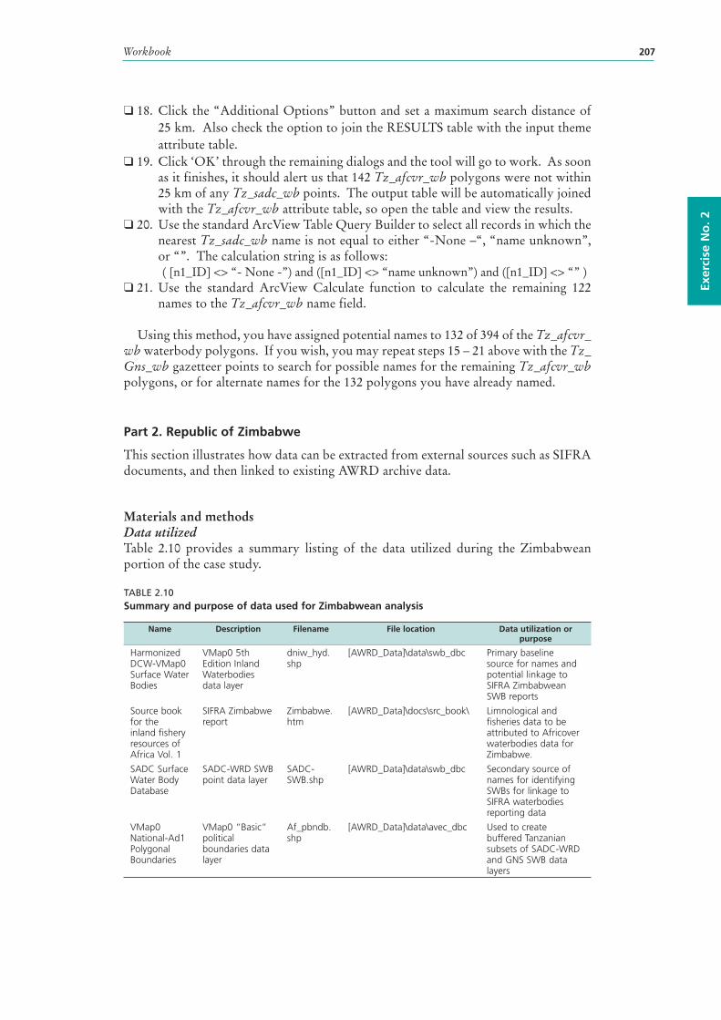
Workbook 207
Exer
cise
No
. 2
❑ 18. Click the “Additional Options” button and set a maximum search distance of 25 km. Also check the option to join the RESULTS table with the input theme attribute table.
❑ 19. Click ‘OK’ through the remaining dialogs and the tool will go to work. As soon as it finishes, it should alert us that 142 Tz_afcvr_wb polygons were not within 25 km of any Tz_sadc_wb points. The output table will be automatically joined with the Tz_afcvr_wb attribute table, so open the table and view the results.
❑ 20. Use the standard ArcView Table Query Builder to select all records in which the nearest Tz_sadc_wb name is not equal to either “-None –“, “name unknown”, or “”. The calculation string is as follows:
( [n1_ID] <> “- None -”) and ([n1_ID] <> “name unknown”) and ([n1_ID] <> “” )❑ 21. Use the standard ArcView Calculate function to calculate the remaining 122
names to the Tz_afcvr_wb name field.
Using this method, you have assigned potential names to 132 of 394 of the Tz_afcvr_wb waterbody polygons. If you wish, you may repeat steps 15 – 21 above with the Tz_Gns_wb gazetteer points to search for possible names for the remaining Tz_afcvr_wb polygons, or for alternate names for the 132 polygons you have already named.
Part 2. Republic of Zimbabwe
This section illustrates how data can be extracted from external sources such as SIFRA documents, and then linked to existing AWRD archive data.
Materials and methodsData utilizedTable 2.10 provides a summary listing of the data utilized during the Zimbabwean portion of the case study.
TABLE 2.10Summary and purpose of data used for Zimbabwean analysis
Name Description Filename File location Data utilization or purpose
Harmonized DCW-VMap0 Surface Water Bodies
VMap0 5th Edition Inland Waterbodies data layer
dniw_hyd.shp
[AWRD_Data]\data\swb_dbc Primary baseline source for names and potential linkage to SIFRA Zimbabwean SWB reports
Source book for the inland fishery resources of Africa Vol. 1
SIFRA Zimbabwe report
Zimbabwe.htm
[AWRD_Data]\docs\src_book\ Limnological and fisheries data to be attributed to Africover waterbodies data for Zimbabwe.
SADC Surface Water Body Database
SADC-WRD SWB point data layer
SADC-SWB.shp
[AWRD_Data]\data\swb_dbc Secondary source of names for identifying SWBs for linkage to SIFRA waterbodies reporting data
VMap0 National-Ad1 Polygonal Boundaries
VMap0 “Basic” political boundaries data layer
Af_pbndb.shp
[AWRD_Data]\data\avec_dbc Used to create buffered Tanzanian subsets of SADC-WRD and GNS SWB data layers
African Water Resource Database – Technical manual and workbook208
MethodsOpen ArcView and start the exercise by following the steps described in points below.
Click on the button and load the following three datasets. You can find them by either typing the name or filename in the “Search Text” textbox (you may use the * and ? wildcard characters), or by clicking on the respective DBC and finding the file in the list.❑ 1. VMap0 National-Ad1 Polygonal Boundaries (Ad1_Py.shp); from the Additional
Vector Data DBC.❑ 2. Harmonized DCW-VMap0 Surface Waterbodies (dniw_hyd.shp); from the
Surface Waterbodies DBC.❑ 3. SADC Surface Waterbody Database (sadc_swb.shp); from the Surface Waterbodies
DBC.
Change the theme names to the short versions by clicking the “View” menu item “Toggle AWRD data to Short Theme Names.” You might have to click this menu item two times.
Create subsets of dniw_hyd.shp and sadc_swb.shp. This is a two-step process, first selecting all features that lie within the Republic of Zimbabwe, and then selecting the subset of those features that represent waterbodies.
❑ 1. Set your View Map Units to Decimal Degrees, and Distance Units to Kilometers by clicking the View menu, then Properties.
❑ 2. First select Zimbabwe from the country boundaries dataset (Ad1_Py.shp). You may use either the Query Builder tool or the standard ArcView selection tools. You will see Zimbabwe highlighted in yellow in your View.
❑ 3. Zoom in to the extent of Zimbabwe by clicking the standard ArcView “Zoom to Selection” button.
❑ 4. Select the sadc_swb.shp surface waterbody points that intersect with Zimbabwe. Do this by clicking on the sadc_swb.shp theme to make it active, then clicking the “Select By Theme” tool . Select features from the active theme (i.e. Sadc_swb.shp) that “Are Within Distance Of” the selected features of “Ad1_Py.shp” (i.e. Zimbabwe). Set a distance value of 1 km. Click the “New” button and you will see all sadc_swb features highlighted in yellow for Zimbabwe. At the bottom of the dialog, you should see that approximately 9 938 points are selected.
❑ 5. Refine the selection to include only features that are known to be waterbodies. Click on the Query Builder tool , make sure that the “Select” option is chosen (not “Set Theme Definition”), and enter the following query string (this query string is basically identifying all points that are not of type “Unknown”):
( [Type] <> “U” )❑ 6. Click the Subset button to select the subset of waterbody points.
At the bottom of the dialog, you should see that the number of selected points (9 938) has not changed, indicating that all SADC SWB points within 1 km of Zimbabwe are known to be actual surface waterbodies.
❑ 7. The next step is to convert this subset of features into a new independent shapefile. Click “Convert to shapefile...” from the “Theme” menu and then choose a name (e.g. Zi_sadc_swb.shp) and the location in your hard drive where you wish to store this new theme.
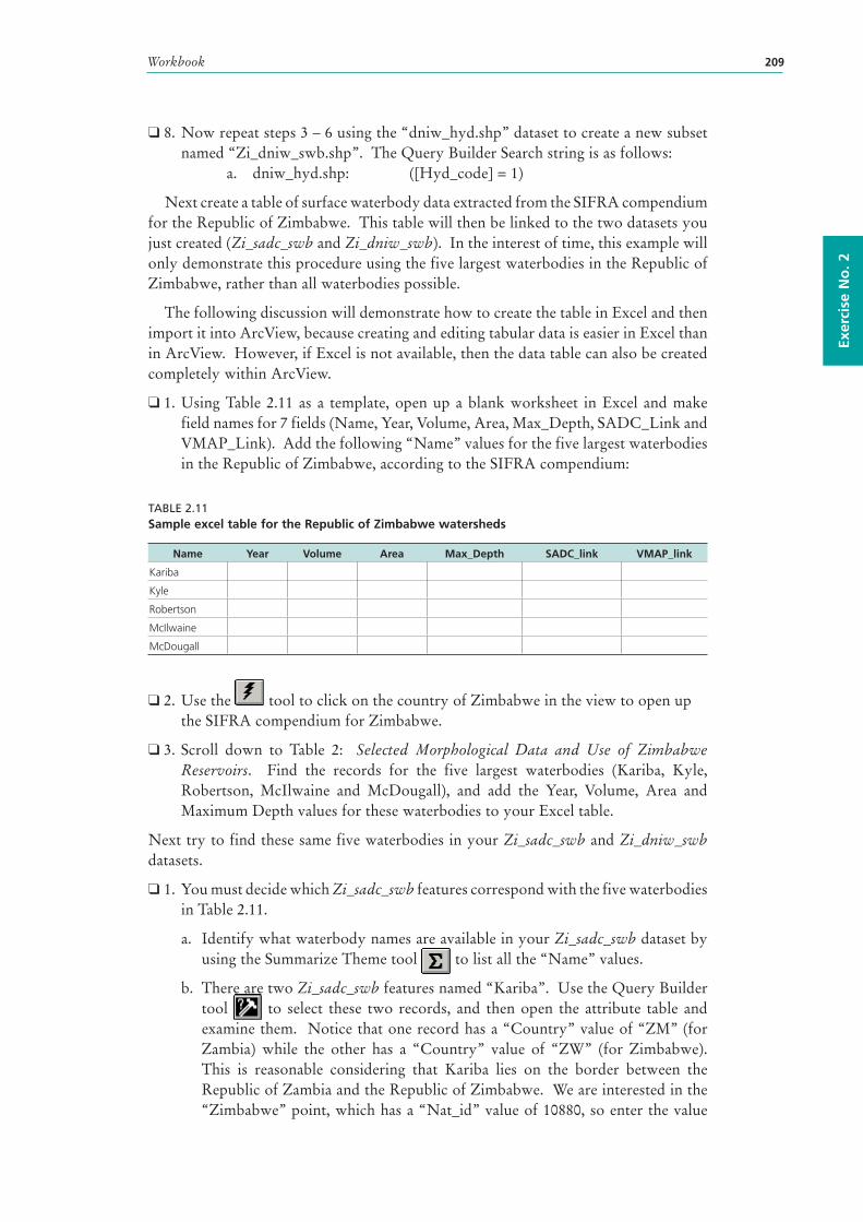
Workbook 209
Exer
cise
No
. 2
❑ 8. Now repeat steps 3 – 6 using the “dniw_hyd.shp” dataset to create a new subset named “Zi_dniw_swb.shp”. The Query Builder Search string is as follows:
a. dniw_hyd.shp: ([Hyd_code] = 1)
Next create a table of surface waterbody data extracted from the SIFRA compendium for the Republic of Zimbabwe. This table will then be linked to the two datasets you just created (Zi_sadc_swb and Zi_dniw_swb). In the interest of time, this example will only demonstrate this procedure using the five largest waterbodies in the Republic of Zimbabwe, rather than all waterbodies possible.
The following discussion will demonstrate how to create the table in Excel and then import it into ArcView, because creating and editing tabular data is easier in Excel than in ArcView. However, if Excel is not available, then the data table can also be created completely within ArcView.
❑ 1. Using Table 2.11 as a template, open up a blank worksheet in Excel and make field names for 7 fields (Name, Year, Volume, Area, Max_Depth, SADC_Link and VMAP_Link). Add the following “Name” values for the five largest waterbodies in the Republic of Zimbabwe, according to the SIFRA compendium:
TABLE 2.11Sample excel table for the Republic of Zimbabwe watersheds
Name Year Volume Area Max_Depth SADC_link VMAP_link
Kariba
Kyle
Robertson
McIlwaine
McDougall
❑ 2. Use the tool to click on the country of Zimbabwe in the view to open up the SIFRA compendium for Zimbabwe.
❑ 3. Scroll down to Table 2: Selected Morphological Data and Use of Zimbabwe
Reservoirs. Find the records for the five largest waterbodies (Kariba, Kyle, Robertson, McIlwaine and McDougall), and add the Year, Volume, Area and Maximum Depth values for these waterbodies to your Excel table.
Next try to find these same five waterbodies in your Zi_sadc_swb and Zi_dniw_swb datasets.
❑ 1. You must decide which Zi_sadc_swb features correspond with the five waterbodies in Table 2.11.
a. Identify what waterbody names are available in your Zi_sadc_swb dataset by using the Summarize Theme tool to list all the “Name” values.
b. There are two Zi_sadc_swb features named “Kariba”. Use the Query Builder tool to select these two records, and then open the attribute table and examine them. Notice that one record has a “Country” value of “ZM” (for Zambia) while the other has a “Country” value of “ZW” (for Zimbabwe). This is reasonable considering that Kariba lies on the border between the Republic of Zambia and the Republic of Zimbabwe. We are interested in the “Zimbabwe” point, which has a “Nat_id” value of 10880, so enter the value
African Water Resource Database – Technical manual and workbook210
“10880” into the “SADC_Link” field for the waterbody “Kariba” in your Excel table
c. There are no Zi_sadc_swb features with the word “Kyle” anywhere in the name. However, with a bit of searching we can find that there is a Zi_sadc_swb feature very close to the Zi_dniw_swb polygon named “Lake Kyle”, which has a “Surf__area” value of 9 105 ha and a “Capacity” value of 1 425 000 000 m2, both of which correspond to our SIFRA data for Kyle. This Zi_sadc_swb feature has a “Nat_id” value of 6183, so enter the value “6183” into the “SADC_Link” field for the waterbody “Kyle” in your Excel table.
d. There are no Zi_sadc_swb features with the word “Robertson” anywhere in the name. However, with a bit of searching we can find that there is a Zi_sadc_swb feature very close to the Zi_dniw_swb polygon named “Lake Manyame”, which has a “Comments” value of “Also known as Robertson (=Darwendale)”. This Zi_sadc_swb feature has a “Nat_id” value of 2599, so enter the value “2599” into the “SADC_Link” field for the waterbody “Robertson” in your Excel table.
e. There are no Zi_sadc_swb features with the word “McIlwaine” anywhere in the name. However, there is one Zi_sadc_swb feature with the word “McIllwaine”, which you can find using the Query Builder tool with the following search string:
( [Name].Contains(“waine”) )
This Zi_sadc_swb feature has a “Nat_id” value of 9793, so enter the value “9793” into the “SADC_Link” field for the waterbody “McIlwaine” in your Excel table.
f. There are no Zi_sadc_swb features with the word “McDougall” anywhere in the name. However, with a bit of searching we can find that there is a Zi_sadc_swb feature very close to the Zi_dniw_swb polygon named “Lake MacDougall”, which has a “Surf__area” value of 2 023 ha and a “Capacity” value of 285 000 000 m2, both of which correspond to our SIFRA data for McDougall. This Zi_sadc_swb feature has a “Nat_id” value of 6303, so enter the value “6303” into the “SADC_Link” field for the waterbody “McDougall” in your Excel table.
❑ 2. You must decide which Zi_dniw_swb features correspond with the five waterbodies in Table 2.11.
a. Identify what waterbody names are available in your Zi_dniw_swb dataset by using the Summarize Theme tool to list all the “Hyd_name” values.
b. There is one Zi_dniw_swb feature with the name “Kariba” in the name (Hyd_name = “Lake Kariba:Sanyati:Sebungwe:Sengwa”). This Zi_dniw_swb feature has a “Uniq_id” value of 17274, so enter the value “17274” into the “VMAP_Link” field for the waterbody “Kariba” in your Excel table.
c. There is one Zi_dniw_swb feature with the name “Kyle” in the name (Hyd_name = “Lake Kyle”). This Zi_dniw_swb feature has a “Uniq_id” value of 18135, so enter the value “18135” into the “VMAP_Link” field for the waterbody “Kyle” in your Excel table.
d. There are no Zi_dniw_swb features with the word “Robertson” anywhere
Workbook 211
Exer
cise
No
. 2
in the name. However, with a bit of searching we can find that there is a Zi_dniw_swb feature named “Lake Manyame” which is very close to the Zi_sadc_swb point named “Manyame”, and this Zi_sadc_swb point has a “Comments” value of “Also known as Robertson (=Darwendale)”. Therefore the polygon “Lake Manyame” is very likely the same feature as “Robertson. This Zi_dniw_swb feature has a “Uniq_id” value of 17608, so enter the value “17608” into the “VMAP_Link” field for the waterbody “Robertson” in your Excel table.
e. There is one Zi_dniw_swb feature with the name “McIlwaine” in the name (Hyd_name = “Lake Mcilwaine”). This Zi_dniw_swb feature has a “Uniq_id” value of 17639, so enter the value “17639” into the “VMAP_Link” field for the waterbody “McIlwaine” in your Excel table.
f. There are no Zi_dniw_swb features with the word “McDougall” anywhere in the name. However, there is one Zi_dniw_swb feature with the word “MacDougall” (Hyd_name = “Lake Macdougall”), which you can find using the Query Builder tool with the following search string:
( [Hyd_name].Contains(“dougall”) )
This Zi_dniw_swb feature has a “Uniq_id” value of 18167, so enter the value “18167” into the “VMAP_Link” field for the waterbody “McDougall” in your Excel table.
❑ 3. Next import your Excel table into your ArcView project and link it to your Zi_dniw_swb and Zi_sadc_swb attribute tables.
a. Select your data in the Excel table, then use the Import From Excel tool (located in your ArcView Table button bar) to import that data into a new ArcView table.
b. In your new imported table, click the field name “SADC_link”.
c. Open your Zi_sadc_swb attribute table and click on the field name “Nat_id”.
d. Click back on your new imported table to make it the active document, and then click the field name “SADC_link”.
e. Click the Join Tables button to join your SADC attributes to your table.
f. Open your Zi_dniw_swb attribute table and click on the field name “Uniq_id”.
g. Click back on your new imported table to make it the active document, and then click the field name “VMAP_link”.
h. Click the Join Tables button to join your VMAP attributes to your table.
i. Save your joined table as a single dBASE table using the “Export” menu item in the Table “File” menu.
Exercise SummaryThis exercise has demonstrated two potential methods for identifying attributes of waterbodies. The first method illustrates how attributes can be extracted from nearby or intersecting features from separate datasets, and the second method shows how attribute data may be found in reports such as the SIFRA documents. The methods illustrated in this case study may be adapted to identify attributes of other features of interest, in cases where you have access to multiple datasets describing the same spatial phenomena.
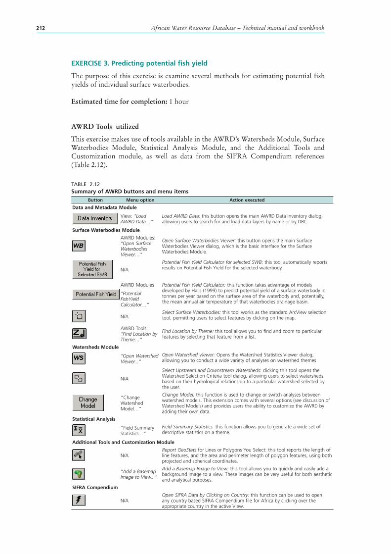
African Water Resource Database – Technical manual and workbook212
EXERCISE 3. Predicting potential fish yield
The purpose of this exercise is examine several methods for estimating potential fish yields of individual surface waterbodies.
Estimated time for completion: 1 hour
AWRD Tools utilized
This exercise makes use of tools available in the AWRD’s Watersheds Module, Surface Waterbodies Module, Statistical Analysis Module, and the Additional Tools and Customization module, as well as data from the SIFRA Compendium references (Table 2.12).
TABLE 2.12Summary of AWRD buttons and menu items
Button Menu option Action executed
Data and Metadata Module
View: “Load AWRD Data…”
Load AWRD Data: this button opens the main AWRD Data Inventory dialog, allowing users to search for and load data layers by name or by DBC.
Surface Waterbodies Module
AWRD Modules: “Open Surface Waterbodies Viewer…”
Open Surface Waterbodies Viewer: this button opens the main Surface Waterbodies Viewer dialog, which is the basic interface for the Surface Waterbodies Module.
N/A
Potential Fish Yield Calculator for selected SWB: this tool automatically reports results on Potential Fish Yield for the selected waterbody.
AWRD Modules
“Potential FishYield Calculator…”
Potential Fish Yield Calculator : this function takes advantage of models developed by Halls (1999) to predict potential yield of a surface waterbody in tonnes per year based on the surface area of the waterbody and, potentially, the mean annual air temperature of that waterbodies drainage basin.
N/ASelect Surface Waterbodies: this tool works as the standard ArcView selection tool, permitting users to select features by clicking on the map.
AWRD Tools: “Find Location by Theme…”
Find Location by Theme: this tool allows you to find and zoom to particular features by selecting that feature from a list.
Watersheds Module
“Open Watershed Viewer...”
Open Watershed Viewer: Opens the Watershed Statistics Viewer dialog, allowing you to conduct a wide variety of analyses on watershed themes
N/A
Select Upstream and Downstream Watersheds: clicking this tool opens the Watershed Selection Criteria tool dialog, allowing users to select watersheds based on their hydrological relationship to a particular watershed selected by the user.
“Change Watershed Model…”
Change Model: this function is used to change or switch analyses between watershed models. This extension comes with several options (see discussion of Watershed Models) and provides users the ability to customize the AWRD by adding their own data.
Statistical Analysis
“Field Summary Statistics…”
Field Summary Statistics: this function allows you to generate a wide set of descriptive statistics on a theme.
Additional Tools and Customization Module
N/AReport GeoStats for Lines or Polygons You Select: this tool reports the length of line features, and the area and perimeter length of polygon features, using both projected and spherical coordinates.
“Add a Basemap Image to View...”
Add a Basemap Image to View: this tool allows you to quickly and easily add a background image to a view. These images can be very useful for both aesthetic and analytical purposes.
SIFRA Compendium
N/AOpen SIFRA Data by Clicking on Country: this function can be used to open any country based SIFRA Compendium file for Africa by clicking over the appropriate country in the active View.
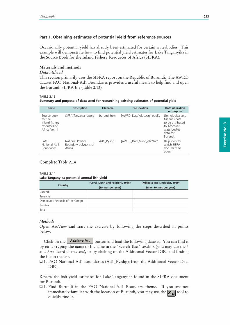
Workbook 213
Exer
cise
No
. 3
Part 1. Obtaining estimates of potential yield from reference sources
Occasionally potential yield has already been estimated for certain waterbodies. This example will demonstrate how to find potential yield estimates for Lake Tanganyika in the Source Book for the Inland Fishery Resources of Africa (SIFRA).
Materials and methods Data utilizedThis section primarily uses the SIFRA report on the Republic of Burundi. The AWRD dataset FAO National-Ad1 Boundaries provides a useful means to help find and open the Burundi SIFRA file (Table 2.13).
TABLE 2.13Summary and purpose of data used for researching existing estimates of potential yield
Name Description Filename File location Data utilization or purpose
Source book for the inland fishery resources of Africa Vol. 1
SIFRA Tanzania report burundi.htm [AWRD_Data]\docs\src_book\ Limnological and fisheries data to be attributed to Africover waterbodies data for Burundi.
FAO National-Ad1 Boundaries
National Political Boundary polygons of Africa
Ad1_Py.shp [AWRD_Data]\avec_dbc\fao\ Help identify which SIFRA document to open.
Complete Table 2.14
TABLE 2.14Lake Tanganyika potential annual fish yield
Country(Corsi, Dunn and Felicioni, 1986)
(tonnes per year)
(Mikkola and Lindquist, 1989)
(max. tonnes per year)
Burundi
Tanzania
Democratic Republic of the Congo
Zambia
Total
MethodsOpen ArcView and start the exercise by following the steps described in points below.
Click on the button and load the following dataset. You can find it by either typing the name or filename in the “Search Text” textbox (you may use the * and ? wildcard characters), or by clicking on the Additional Vector DBC and finding the file in the list.❑ 1. FAO National-Ad1 Boundaries (Ad1_Py.shp); from the Additional Vector Data
DBC.
Review the fish yield estimates for Lake Tanganyika found in the SIFRA document for Burundi.❑ 1. Find Burundi in the FAO National-Ad1 Boundary theme. If you are not
immediately familiar with the location of Burundi, you may use the tool to quickly find it.
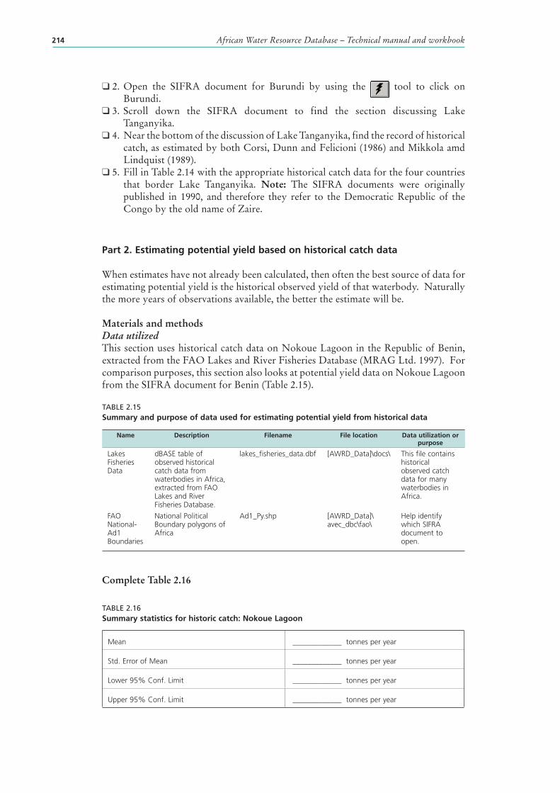
African Water Resource Database – Technical manual and workbook214
❑ 2. Open the SIFRA document for Burundi by using the tool to click on Burundi.
❑ 3. Scroll down the SIFRA document to find the section discussing Lake Tanganyika.
❑ 4. Near the bottom of the discussion of Lake Tanganyika, find the record of historical catch, as estimated by both Corsi, Dunn and Felicioni (1986) and Mikkola amd Lindquist (1989).
❑ 5. Fill in Table 2.14 with the appropriate historical catch data for the four countries that border Lake Tanganyika. Note: The SIFRA documents were originally published in 1990, and therefore they refer to the Democratic Republic of the Congo by the old name of Zaire.
Part 2. Estimating potential yield based on historical catch data
When estimates have not already been calculated, then often the best source of data for estimating potential yield is the historical observed yield of that waterbody. Naturally the more years of observations available, the better the estimate will be.
Materials and methods Data utilizedThis section uses historical catch data on Nokoue Lagoon in the Republic of Benin, extracted from the FAO Lakes and River Fisheries Database (MRAG Ltd. 1997). For comparison purposes, this section also looks at potential yield data on Nokoue Lagoon from the SIFRA document for Benin (Table 2.15).
TABLE 2.15Summary and purpose of data used for estimating potential yield from historical data
Name Description Filename File location Data utilization or purpose
Lakes Fisheries Data
dBASE table of observed historical catch data from waterbodies in Africa, extracted from FAO Lakes and River Fisheries Database.
lakes_fisheries_data.dbf [AWRD_Data]\docs\ This file contains historical observed catch data for many waterbodies in Africa.
FAO National-Ad1 Boundaries
National Political Boundary polygons of Africa
Ad1_Py.shp [AWRD_Data]\avec_dbc\fao\
Help identify which SIFRA document to open.
Complete Table 2.16
TABLE 2.16Summary statistics for historic catch: Nokoue Lagoon
Mean _____________ tonnes per year
Std. Error of Mean _____________ tonnes per year
Lower 95% Conf. Limit _____________ tonnes per year
Upper 95% Conf. Limit _____________ tonnes per year
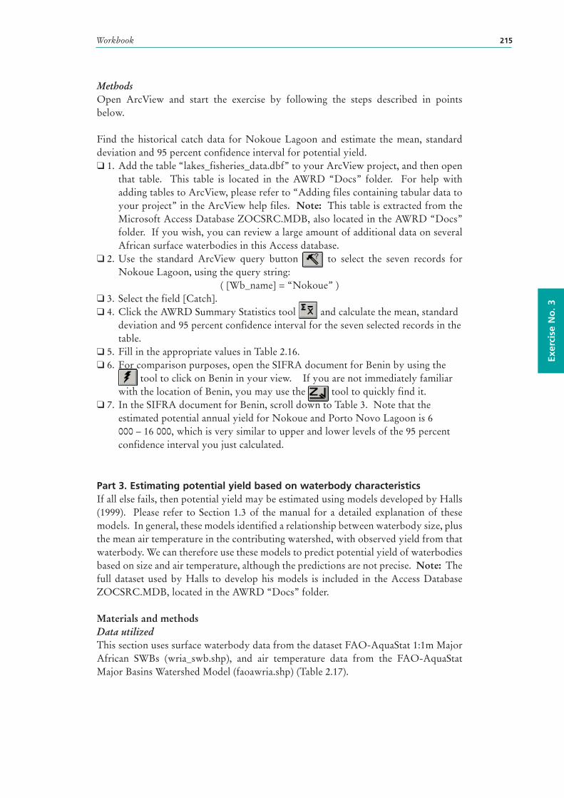
Workbook 215
Exer
cise
No
. 3
MethodsOpen ArcView and start the exercise by following the steps described in points below.
Find the historical catch data for Nokoue Lagoon and estimate the mean, standard deviation and 95 percent confidence interval for potential yield.❑ 1. Add the table “lakes_fisheries_data.dbf” to your ArcView project, and then open
that table. This table is located in the AWRD “Docs” folder. For help with adding tables to ArcView, please refer to “Adding files containing tabular data to your project” in the ArcView help files. Note: This table is extracted from the Microsoft Access Database ZOCSRC.MDB, also located in the AWRD “Docs” folder. If you wish, you can review a large amount of additional data on several African surface waterbodies in this Access database.
❑ 2. Use the standard ArcView query button to select the seven records for Nokoue Lagoon, using the query string:
( [Wb_name] = “Nokoue” )❑ 3. Select the field [Catch].❑ 4. Click the AWRD Summary Statistics tool and calculate the mean, standard
deviation and 95 percent confidence interval for the seven selected records in the table.
❑ 5. Fill in the appropriate values in Table 2.16.❑ 6. For comparison purposes, open the SIFRA document for Benin by using the
tool to click on Benin in your view. If you are not immediately familiar with the location of Benin, you may use the tool to quickly find it.
❑ 7. In the SIFRA document for Benin, scroll down to Table 3. Note that the estimated potential annual yield for Nokoue and Porto Novo Lagoon is 6 000 – 16 000, which is very similar to upper and lower levels of the 95 percent confidence interval you just calculated.
Part 3. Estimating potential yield based on waterbody characteristicsIf all else fails, then potential yield may be estimated using models developed by Halls (1999). Please refer to Section 1.3 of the manual for a detailed explanation of these models. In general, these models identified a relationship between waterbody size, plus the mean air temperature in the contributing watershed, with observed yield from that waterbody. We can therefore use these models to predict potential yield of waterbodies based on size and air temperature, although the predictions are not precise. Note: The full dataset used by Halls to develop his models is included in the Access Database ZOCSRC.MDB, located in the AWRD “Docs” folder.
Materials and methods Data utilizedThis section uses surface waterbody data from the dataset FAO-AquaStat 1:1m Major African SWBs (wria_swb.shp), and air temperature data from the FAO-AquaStat Major Basins Watershed Model (faoawria.shp) (Table 2.17).
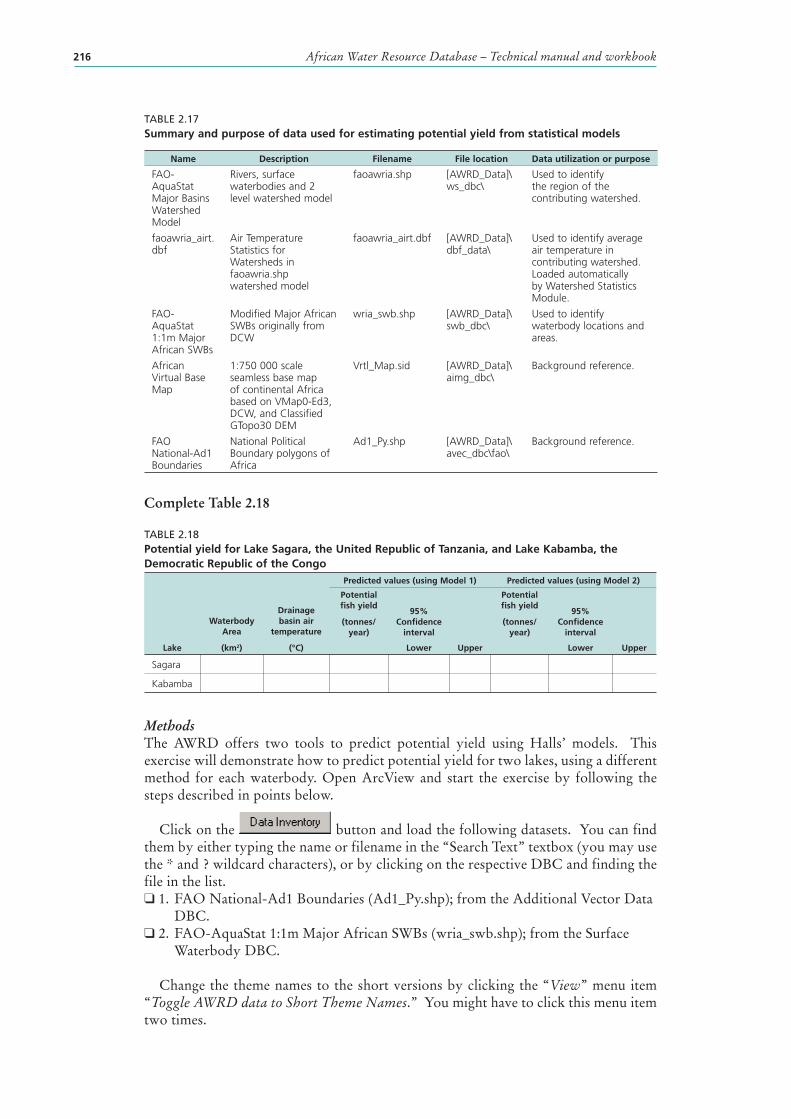
African Water Resource Database – Technical manual and workbook216
TABLE 2.17Summary and purpose of data used for estimating potential yield from statistical models
Name Description Filename File location Data utilization or purpose
FAO-AquaStat Major Basins Watershed Model
Rivers, surface waterbodies and 2 level watershed model
faoawria.shp [AWRD_Data]\ws_dbc\
Used to identify the region of the contributing watershed.
faoawria_airt.dbf
Air Temperature Statistics for Watersheds in faoawria.shp watershed model
faoawria_airt.dbf [AWRD_Data]\dbf_data\
Used to identify average air temperature in contributing watershed. Loaded automatically by Watershed Statistics Module.
FAO-AquaStat 1:1m Major African SWBs
Modified Major African SWBs originally from DCW
wria_swb.shp [AWRD_Data]\swb_dbc\
Used to identify waterbody locations and areas.
African Virtual Base Map
1:750 000 scale seamless base map of continental Africa based on VMap0-Ed3, DCW, and Classified GTopo30 DEM
Vrtl_Map.sid [AWRD_Data]\aimg_dbc\
Background reference.
FAO National-Ad1 Boundaries
National Political Boundary polygons of Africa
Ad1_Py.shp [AWRD_Data]\avec_dbc\fao\
Background reference.
Complete Table 2.18
TABLE 2.18Potential yield for Lake Sagara, the United Republic of Tanzania, and Lake Kabamba, the Democratic Republic of the Congo
Lake
Waterbody Area
(km2)
Drainage basin air
temperature
(°C)
Predicted values (using Model 1) Predicted values (using Model 2)
Potential fish yield
(tonnes/year)
95% Confidence
interval
Potential fish yield
(tonnes/year)
95% Confidence
interval
Lower Upper Lower Upper
Sagara
Kabamba
MethodsThe AWRD offers two tools to predict potential yield using Halls’ models. This exercise will demonstrate how to predict potential yield for two lakes, using a different method for each waterbody. Open ArcView and start the exercise by following the steps described in points below.
Click on the button and load the following datasets. You can find them by either typing the name or filename in the “Search Text” textbox (you may use the * and ? wildcard characters), or by clicking on the respective DBC and finding the file in the list.❑ 1. FAO National-Ad1 Boundaries (Ad1_Py.shp); from the Additional Vector Data
DBC.❑ 2. FAO-AquaStat 1:1m Major African SWBs (wria_swb.shp); from the Surface
Waterbody DBC.
Change the theme names to the short versions by clicking the “View” menu item “Toggle AWRD data to Short Theme Names.” You might have to click this menu item two times.
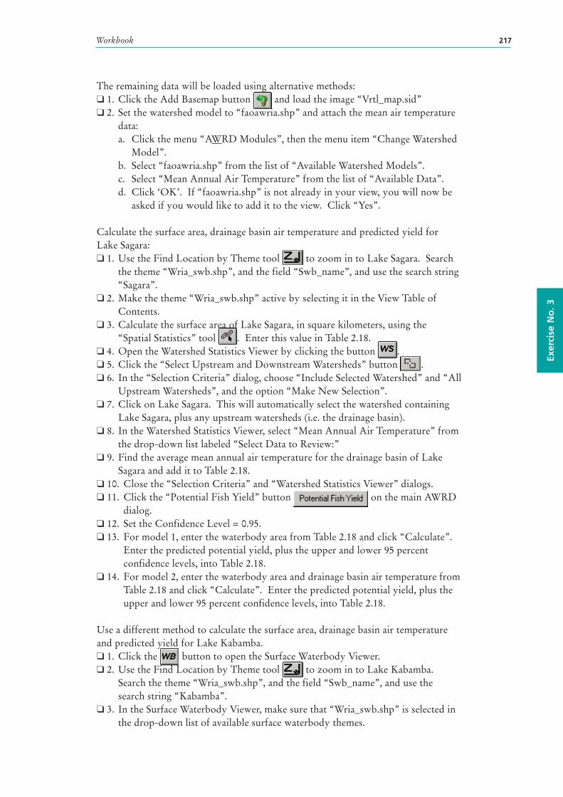
Workbook 217
Exer
cise
No
. 3
The remaining data will be loaded using alternative methods:❑ 1. Click the Add Basemap button and load the image “Vrtl_map.sid”❑ 2. Set the watershed model to “faoawria.shp” and attach the mean air temperature
data:a. Click the menu “AWRD Modules”, then the menu item “Change Watershed
Model”.b. Select “faoawria.shp” from the list of “Available Watershed Models”.c. Select “Mean Annual Air Temperature” from the list of “Available Data”.d. Click ‘OK’. If “faoawria.shp” is not already in your view, you will now be
asked if you would like to add it to the view. Click “Yes”.
Calculate the surface area, drainage basin air temperature and predicted yield for Lake Sagara:❑ 1. Use the Find Location by Theme tool to zoom in to Lake Sagara. Search
the theme “Wria_swb.shp”, and the field “Swb_name”, and use the search string “Sagara”.
❑ 2. Make the theme “Wria_swb.shp” active by selecting it in the View Table of Contents.
❑ 3. Calculate the surface area of Lake Sagara, in square kilometers, using the “Spatial Statistics” tool . Enter this value in Table 2.18.
❑ 4. Open the Watershed Statistics Viewer by clicking the button .❑ 5. Click the “Select Upstream and Downstream Watersheds” button .❑ 6. In the “Selection Criteria” dialog, choose “Include Selected Watershed” and “All
Upstream Watersheds”, and the option “Make New Selection”.❑ 7. Click on Lake Sagara. This will automatically select the watershed containing
Lake Sagara, plus any upstream watersheds (i.e. the drainage basin).❑ 8. In the Watershed Statistics Viewer, select “Mean Annual Air Temperature” from
the drop-down list labeled “Select Data to Review:”❑ 9. Find the average mean annual air temperature for the drainage basin of Lake
Sagara and add it to Table 2.18.❑ 10. Close the “Selection Criteria” and “Watershed Statistics Viewer” dialogs.❑ 11. Click the “Potential Fish Yield” button on the main AWRD
dialog.❑ 12. Set the Confidence Level = 0.95.❑ 13. For model 1, enter the waterbody area from Table 2.18 and click “Calculate”.
Enter the predicted potential yield, plus the upper and lower 95 percent confidence levels, into Table 2.18.
❑ 14. For model 2, enter the waterbody area and drainage basin air temperature from Table 2.18 and click “Calculate”. Enter the predicted potential yield, plus the upper and lower 95 percent confidence levels, into Table 2.18.
Use a different method to calculate the surface area, drainage basin air temperature and predicted yield for Lake Kabamba.❑ 1. Click the button to open the Surface Waterbody Viewer.❑ 2. Use the Find Location by Theme tool to zoom in to Lake Kabamba.
Search the theme “Wria_swb.shp”, and the field “Swb_name”, and use the search string “Kabamba”.
❑ 3. In the Surface Waterbody Viewer, make sure that “Wria_swb.shp” is selected in the drop-down list of available surface waterbody themes.
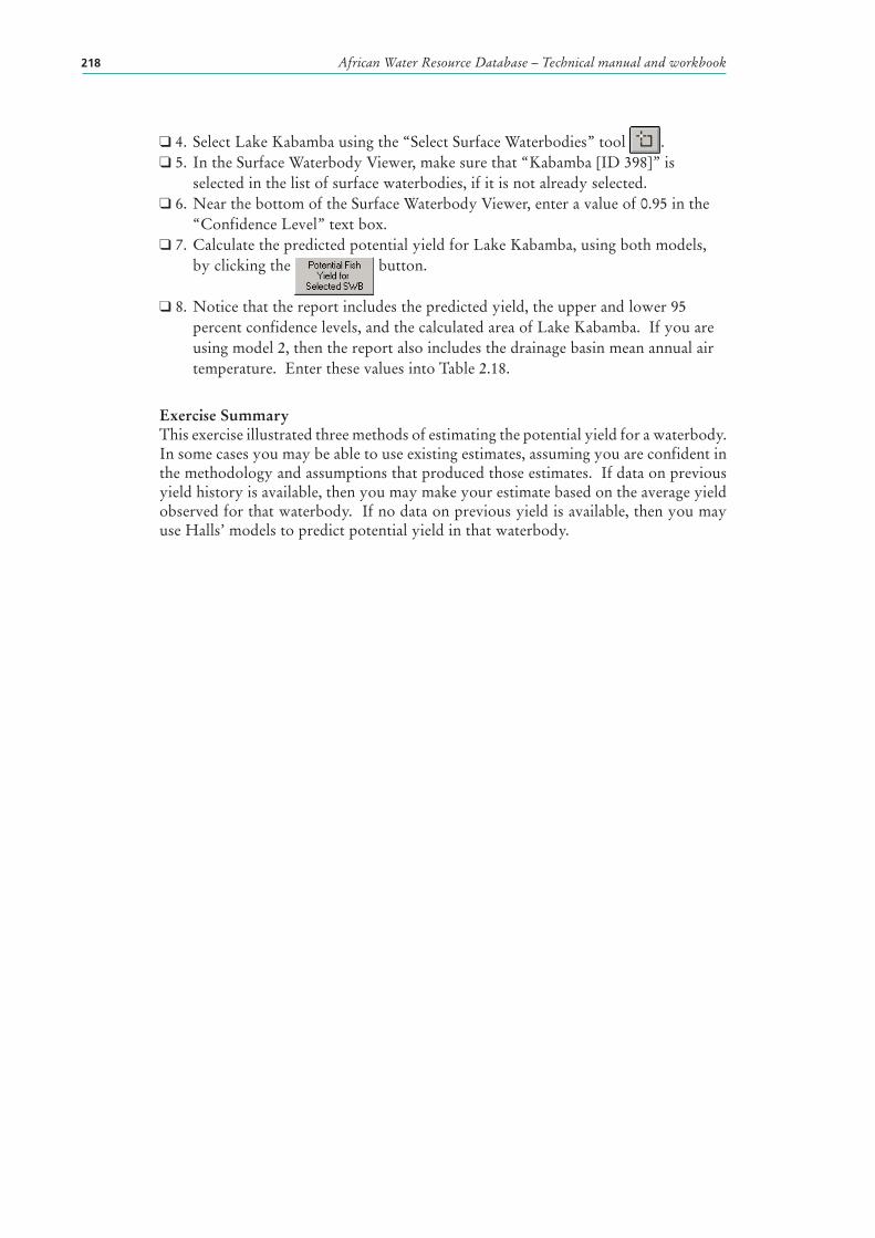
African Water Resource Database – Technical manual and workbook218
❑ 4. Select Lake Kabamba using the “Select Surface Waterbodies” tool .❑ 5. In the Surface Waterbody Viewer, make sure that “Kabamba [ID 398]” is
selected in the list of surface waterbodies, if it is not already selected.❑ 6. Near the bottom of the Surface Waterbody Viewer, enter a value of 0.95 in the
“Confidence Level” text box.❑ 7. Calculate the predicted potential yield for Lake Kabamba, using both models,
by clicking the button.
❑ 8. Notice that the report includes the predicted yield, the upper and lower 95 percent confidence levels, and the calculated area of Lake Kabamba. If you are using model 2, then the report also includes the drainage basin mean annual air temperature. Enter these values into Table 2.18.
Exercise SummaryThis exercise illustrated three methods of estimating the potential yield for a waterbody. In some cases you may be able to use existing estimates, assuming you are confident in the methodology and assumptions that produced those estimates. If data on previous yield history is available, then you may make your estimate based on the average yield observed for that waterbody. If no data on previous yield is available, then you may use Halls’ models to predict potential yield in that waterbody.
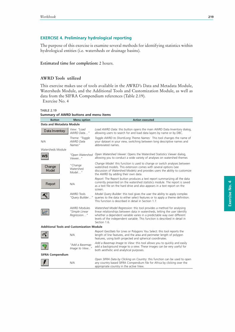
Workbook 219
Exer
cise
No
. 4
EXERCISE 4. Preliminary hydrological reporting
The purpose of this exercise is examine several methods for identifying statistics within hydrological entities (i.e. watersheds or drainage basins).
Estimated time for completion: 2 hours.
AWRD Tools utilized
This exercise makes use of tools available in the AWRD’s Data and Metadata Module, Watersheds Module, and the Additional Tools and Customization Module, as well as data from the SIFRA Compendium references (Table 2.19). Exercise No. 4
TABLE 2.19Summary of AWRD buttons and menu items
Button Menu option Action executed
Data and Metadata Module
View: “Load AWRD Data…”
Load AWRD Data: this button opens the main AWRD Data Inventory dialog, allowing users to search for and load data layers by name or by DBC.
N/ATheme: “Toggle AWRD Data Names”
Toggle AWRD to Short/Long Theme Names: This tool changes the name of your dataset in your view, switching between long descriptive names and abbreviated names.
Watersheds Module
“Open Watershed Viewer...”
Open Watershed Viewer: Opens the Watershed Statistics Viewer dialog, allowing you to conduct a wide variety of analyses on watershed themes
“Change Watershed Model…”
Change Model: this function is used to change or switch analyses between watershed models. This extension comes with several options (see discussion of Watershed Models) and provides users the ability to customize the AWRD by adding their own data.
N/A
Report: The Report button produces a text report summarizing all the data currently presented on the watershed statistics module. The report is saved as a text file on the hard drive and also appears in a text report on the screen.
AWRD Tools “Query Builder…”
Model Query Builder: this tool gives the user the ability to apply complex queries to the data to either select features or to apply a theme definition. This function is described in detail in Section 1.7.
AWRD Modules “Simple Linear Regression…”
Watershed Model Regression: this tool provides a method for analysing linear relationships between data in watersheds, letting the user identify whether a dependent variable varies in a predictable way over different levels of the independent variable. This function is described in detail in Section 1.6.
Additional Tools and Customization Module
N/AReport GeoStats for Lines or Polygons You Select: this tool reports the length of line features, and the area and perimeter length of polygon features, using both projected and spherical coordinates.
“Add a Basemap Image to View...”
Add a Basemap Image to View: this tool allows you to quickly and easily add a background image to a view. These images can be very useful for both aesthetic and analytical purposes.
SIFRA Compendium
N/AOpen SIFRA Data by Clicking on Country: this function can be used to open any country based SIFRA Compendium file for Africa by clicking over the appropriate country in the active View.
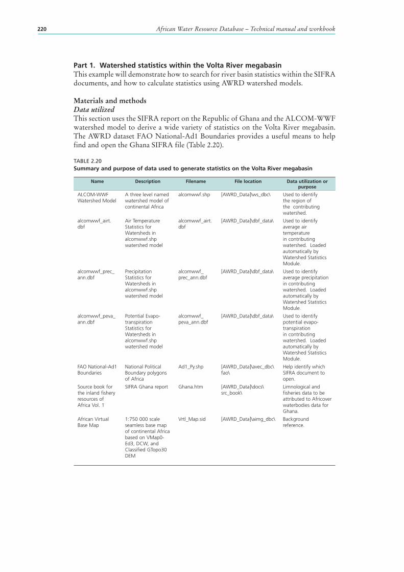
African Water Resource Database – Technical manual and workbook220
Part 1. Watershed statistics within the Volta River megabasinThis example will demonstrate how to search for river basin statistics within the SIFRA documents, and how to calculate statistics using AWRD watershed models.
Materials and methods Data utilizedThis section uses the SIFRA report on the Republic of Ghana and the ALCOM-WWF watershed model to derive a wide variety of statistics on the Volta River megabasin. The AWRD dataset FAO National-Ad1 Boundaries provides a useful means to help find and open the Ghana SIFRA file (Table 2.20).
TABLE 2.20Summary and purpose of data used to generate statistics on the Volta River megabasin
Name Description Filename File location Data utilization or purpose
ALCOM-WWF Watershed Model
A three level named watershed model of continental Africa
alcomwwf.shp [AWRD_Data]\ws_dbc\ Used to identify the region of the contributing watershed.
alcomwwf_airt.dbf
Air Temperature Statistics for Watersheds in alcomwwf.shp watershed model
alcomwwf_airt.dbf
[AWRD_Data]\dbf_data\ Used to identify average air temperature in contributing watershed. Loaded automatically by Watershed Statistics Module.
alcomwwf_prec_ann.dbf
Precipitation Statistics for Watersheds in alcomwwf.shp watershed model
alcomwwf_prec_ann.dbf
[AWRD_Data]\dbf_data\ Used to identify average precipitation in contributing watershed. Loaded automatically by Watershed Statistics Module.
alcomwwf_peva_ann.dbf
Potential Evapo-transpiration Statistics for Watersheds in alcomwwf.shp watershed model
alcomwwf_peva_ann.dbf
[AWRD_Data]\dbf_data\ Used to identify potential evapo-transpiration in contributing watershed. Loaded automatically by Watershed Statistics Module.
FAO National-Ad1 Boundaries
National Political Boundary polygons of Africa
Ad1_Py.shp [AWRD_Data]\avec_dbc\fao\
Help identify which SIFRA document to open.
Source book for the inland fishery resources of Africa Vol. 1
SIFRA Ghana report Ghana.htm [AWRD_Data]\docs\src_book\
Limnological and fisheries data to be attributed to Africover waterbodies data for Ghana.
African Virtual Base Map
1:750 000 scale seamless base map of continental Africa based on VMap0-Ed3, DCW, and Classified GTopo30 DEM
Vrtl_Map.sid [AWRD_Data]\aimg_dbc\ Background reference.
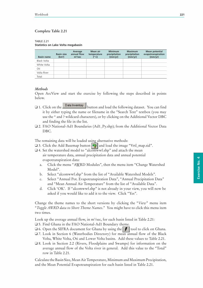
Workbook 221
Exer
cise
No
. 4
Complete Table 2.21
TABLE 2.21Statistics on Lake Volta megabasin
Basin nameBasin size
(km2)
Average annual flow
m3/sec
Mean air temperature
(º C)
Minimum precipitation
(mm/yr)
Maximum precipitation
(mm/yr)
Mean potential evapotranspiration
(mm/yr)
Black Volta
White Volta
Oti
Volta River
Total
MethodsOpen ArcView and start the exercise by following the steps described in points below.
❑ 1. Click on the button and load the following dataset. You can find it by either typing the name or filename in the “Search Text” textbox (you may use the * and ? wildcard characters), or by clicking on the Additional Vector DBC and finding the file in the list.
❑ 2. FAO National-Ad1 Boundaries (Ad1_Py.shp); from the Additional Vector Data DBC.
The remaining data will be loaded using alternative methods:❑ 3. Click the Add Basemap button and load the image “Vrtl_map.sid”.❑ 4. Set the watershed model to “alcomwwf.shp” and attach the mean
air temperature data, annual precipitation data and annual potential evapotranspiration data:
a. Click the menu “AWRD Modules”, then the menu item “Change Watershed Model”.
b. Select “alcomwwf.shp” from the list of “Available Watershed Models”.c. Select “Annual Pot. Evapotranspiration Data”, “Annual Precipitation Data”
and “Mean Annual Air Temperature” from the list of “Available Data”.d. Click ‘OK’. If “alcomwwf.shp” is not already in your view, you will now be
asked if you would like to add it to the view. Click “Yes”.
Change the theme names to the short versions by clicking the “View” menu item “Toggle AWRD data to Short Theme Names.” You might have to click this menu item two times.
Look up the average annual flow, in m3/sec, for each basin listed in Table 2.21:❑ 5. Find Ghana in the FAO National-Ad1 Boundary theme.❑ 6. Open the SIFRA document for Ghana by using the tool to click on Ghana.❑ 7. Look in Section 6 (Waterbodies Directory) for mean annual flow of the Black
Volta, White Volta, Oti and Lower Volta basins. Add these values to Table 2.21.❑ 8. Look in Section 2.2 (Rivers, Floodplains and Swamps) for information on the
average annual flow of the Volta river in general. Add this value to the “Total” row in Table 2.21.
Calculate the Basin Size, Mean Air Temperature, Minimum and Maximum Precipitation, and the Mean Potential Evapotranspiration for each basin listed in Table 2.21.
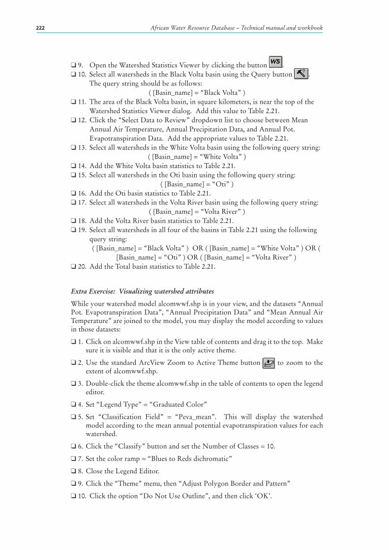
African Water Resource Database – Technical manual and workbook222
❑ 9. Open the Watershed Statistics Viewer by clicking the button .❑ 10. Select all watersheds in the Black Volta basin using the Query button .
The query string should be as follows:( [Basin_name] = “Black Volta” )
❑ 11. The area of the Black Volta basin, in square kilometers, is near the top of the Watershed Statistics Viewer dialog. Add this value to Table 2.21.
❑ 12. Click the “Select Data to Review” dropdown list to choose between Mean Annual Air Temperature, Annual Precipitation Data, and Annual Pot. Evapotranspiration Data. Add the appropriate values to Table 2.21.
❑ 13. Select all watersheds in the White Volta basin using the following query string:( [Basin_name] = “White Volta” )
❑ 14. Add the White Volta basin statistics to Table 2.21.❑ 15. Select all watersheds in the Oti basin using the following query string:
( [Basin_name] = “Oti” )❑ 16. Add the Oti basin statistics to Table 2.21. ❑ 17. Select all watersheds in the Volta River basin using the following query string:
( [Basin_name] = “Volta River” )❑ 18. Add the Volta River basin statistics to Table 2.21. ❑ 19. Select all watersheds in all four of the basins in Table 2.21 using the following
query string: ( [Basin_name] = “Black Volta” ) OR ( [Basin_name] = “White Volta” ) OR (
[Basin_name] = “Oti” ) OR ( [Basin_name] = “Volta River” )❑ 20. Add the Total basin statistics to Table 2.21.
Extra Exercise: Visualizing watershed attributes
While your watershed model alcomwwf.shp is in your view, and the datasets “Annual Pot. Evapotranspiration Data”, “Annual Precipitation Data” and “Mean Annual Air Temperature” are joined to the model, you may display the model according to values in those datasets:
❑ 1. Click on alcomwwf.shp in the View table of contents and drag it to the top. Make sure it is visible and that it is the only active theme.
❑ 2. Use the standard ArcView Zoom to Active Theme button to zoom to the extent of alcomwwf.shp.
❑ 3. Double-click the theme alcomwwf.shp in the table of contents to open the legend editor.
❑ 4. Set “Legend Type” = “Graduated Color”
❑ 5. Set “Classification Field” = “Peva_mean”. This will display the watershed model according to the mean annual potential evapotranspiration values for each watershed.
❑ 6. Click the “Classify” button and set the Number of Classes = 10.
❑ 7. Set the color ramp = “Blues to Reds dichromatic”
❑ 8. Close the Legend Editor.
❑ 9. Click the “Theme” menu, then “Adjust Polygon Border and Pattern”
❑ 10. Click the option “Do Not Use Outline”, and then click ‘OK’.
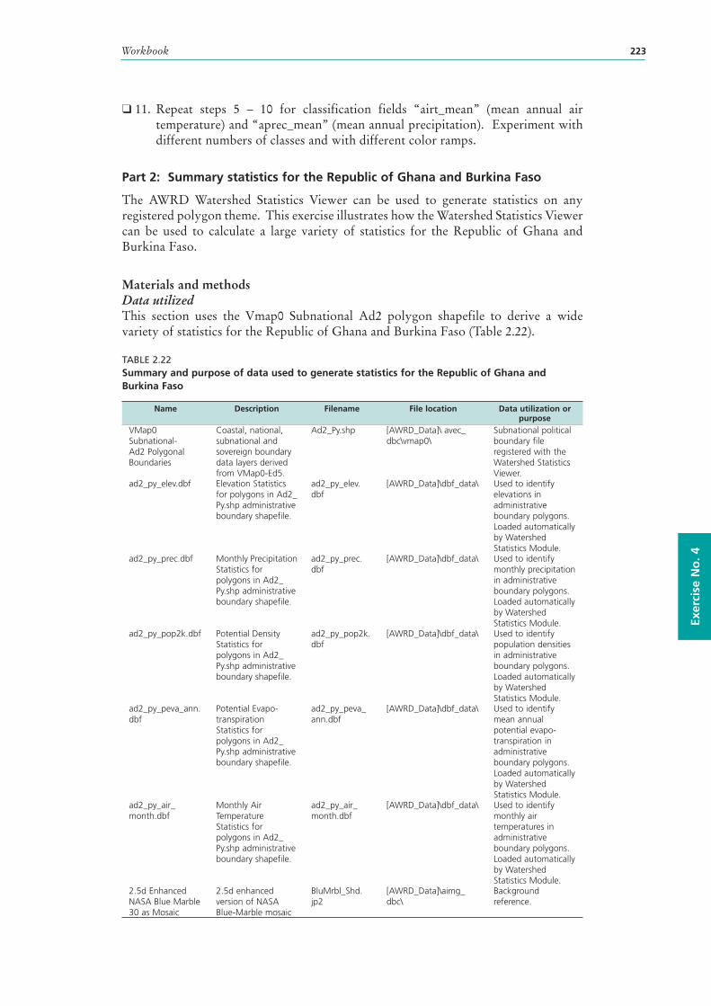
Workbook 223
Exer
cise
No
. 4
❑ 11. Repeat steps 5 – 10 for classification fields “airt_mean” (mean annual air temperature) and “aprec_mean” (mean annual precipitation). Experiment with different numbers of classes and with different color ramps.
Part 2: Summary statistics for the Republic of Ghana and Burkina Faso
The AWRD Watershed Statistics Viewer can be used to generate statistics on any registered polygon theme. This exercise illustrates how the Watershed Statistics Viewer can be used to calculate a large variety of statistics for the Republic of Ghana and Burkina Faso.
Materials and methods Data utilizedThis section uses the Vmap0 Subnational Ad2 polygon shapefile to derive a wide variety of statistics for the Republic of Ghana and Burkina Faso (Table 2.22).
TABLE 2.22Summary and purpose of data used to generate statistics for the Republic of Ghana and Burkina Faso
Name Description Filename File location Data utilization or purpose
VMap0 Subnational-Ad2 Polygonal Boundaries
Coastal, national, subnational and sovereign boundary data layers derived from VMap0-Ed5.
Ad2_Py.shp [AWRD_Data]\ avec_dbc\vmap0\
Subnational political boundary file registered with the Watershed Statistics Viewer.
ad2_py_elev.dbf Elevation Statistics for polygons in Ad2_Py.shp administrative boundary shapefile.
ad2_py_elev.dbf
[AWRD_Data]\dbf_data\ Used to identify elevations in administrative boundary polygons. Loaded automatically by Watershed Statistics Module.
ad2_py_prec.dbf Monthly Precipitation Statistics for polygons in Ad2_Py.shp administrative boundary shapefile.
ad2_py_prec.dbf
[AWRD_Data]\dbf_data\ Used to identify monthly precipitation in administrative boundary polygons. Loaded automatically by Watershed Statistics Module.
ad2_py_pop2k.dbf Potential Density Statistics for polygons in Ad2_Py.shp administrative boundary shapefile.
ad2_py_pop2k.dbf
[AWRD_Data]\dbf_data\ Used to identify population densities in administrative boundary polygons. Loaded automatically by Watershed Statistics Module.
ad2_py_peva_ann.dbf
Potential Evapo-transpiration Statistics for polygons in Ad2_Py.shp administrative boundary shapefile.
ad2_py_peva_ann.dbf
[AWRD_Data]\dbf_data\ Used to identify mean annual potential evapo-transpiration in administrative boundary polygons. Loaded automatically by Watershed Statistics Module.
ad2_py_air_month.dbf
Monthly Air Temperature Statistics for polygons in Ad2_Py.shp administrative boundary shapefile.
ad2_py_air_month.dbf
[AWRD_Data]\dbf_data\ Used to identify monthly air temperatures in administrative boundary polygons. Loaded automatically by Watershed Statistics Module.
2.5d Enhanced NASA Blue Marble 30 as Mosaic
2.5d enhanced version of NASA Blue-Marble mosaic
BluMrbl_Shd.jp2
[AWRD_Data]\aimg_dbc\
Background reference.
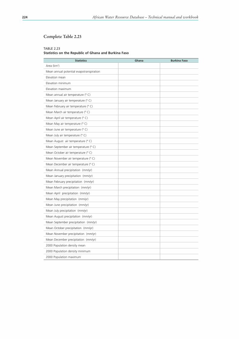
African Water Resource Database – Technical manual and workbook224
Complete Table 2.23
TABLE 2.23Statistics on the Republic of Ghana and Burkina Faso
Statistics Ghana Burkina Faso
Area (km2)
Mean annual potential evapotranspiration
Elevation mean
Elevation minimum
Elevation maximum
Mean annual air temperature (º C)
Mean January air temperature (º C)
Mean February air temperature (º C)
Mean March air temperature (º C)
Mean April air temperature (º C)
Mean May air temperature (º C)
Mean June air temperature (º C)
Mean July air temperature (º C)
Mean August air temperature (º C)
Mean September air temperature (º C)
Mean October air temperature (º C)
Mean November air temperature (º C)
Mean December air temperature (º C)
Mean Annual precipitation (mm/yr)
Mean January precipitation (mm/yr)
Mean February precipitation (mm/yr)
Mean March precipitation (mm/yr)
Mean April precipitation (mm/yr)
Mean May precipitation (mm/yr)
Mean June precipitation (mm/yr)
Mean July precipitation (mm/yr)
Mean August precipitation (mm/yr)
Mean September precipitation (mm/yr)
Mean October precipitation (mm/yr)
Mean November precipitation (mm/yr)
Mean December precipitation (mm/yr)
2000 Population density mean
2000 Population density minimum
2000 Population maximum
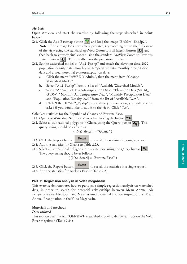
Workbook 225
Exer
cise
No
. 4
MethodsOpen ArcView and start the exercise by following the steps described in points below.❑ 1. Click the Add Basemap button and load the image “BluMrbl_Shd.jp2”.
Note: If this image looks extremely pixilated, try zooming out to the full extent of the view using the standard ArcView Zoom to Full Extent button , and then back to your original extent using the standard ArcView Zoom to Previous Extent button . This usually fixes the pixilation problem.
❑ 2. Set the watershed model to “Ad2_Py.shp” and attach the elevation data, 2000 population density data, monthly air temperature data, monthly precipitation data and annual potential evapotranspiration data:a. Click the menu “AWRD Modules”, then the menu item “Change
Watershed Model”.b. Select “Ad2_Py.shp” from the list of “Available Watershed Models”.c. Select “Annual Pot. Evapotranspiration Data”, “Elevation Data (SRTM_
GT30)”, “Monthly Air Temperature Data”, “Monthly Precipitation Data” and “Population Density 2000” from the list of “Available Data”.
d. Click ‘OK’. If “Ad2_Py.shp” is not already in your view, you will now be asked if you would like to add it to the view. Click “Yes”.
Calculate statistics for the Republic of Ghana and Burkina Faso.❑ 1. Open the Watershed Statistics Viewer by clicking the button .❑ 2. Select all subnational polygons in Ghana using the Query button . The
query string should be as follows:( [Na2_descri] = “Ghana” )
❑ 3. Click the Report button to see all the statistics in a single report.❑ 4. Add the statistics for Ghana to Table 2.23.❑ 5. Select all subnational polygons in Burkina Faso using the Query button .
The query string should be as follows:( [Na2_descri] = “Burkina Faso” )
❑ 6. Click the Report button to see all the statistics in a single report.❑ 7. Add the statistics for Burkina Faso to Table 2.23.
Part 3: Regression analysis in Volta megabasinThis exercise demonstrates how to perform a simple regression analysis on watershed data, in order to search for potential relationships between Mean Annual Air Temperature vs. Elevation, and Mean Annual Potential Evapotranspiration vs. Mean Annual Precipitation in the Volta Megabasin.
Materials and methods Data utilizedThis section uses the ALCOM-WWF watershed model to derive statistics on the Volta River megabasin (Table 2.24).
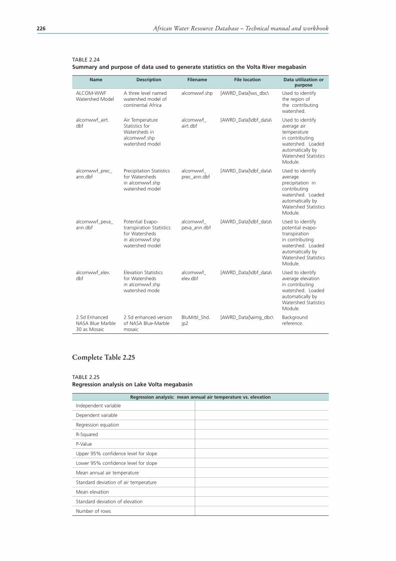
African Water Resource Database – Technical manual and workbook226
TABLE 2.24Summary and purpose of data used to generate statistics on the Volta River megabasin
Name Description Filename File location Data utilization or purpose
ALCOM-WWF Watershed Model
A three level named watershed model of continental Africa
alcomwwf.shp [AWRD_Data]\ws_dbc\ Used to identify the region of the contributing watershed.
alcomwwf_airt.dbf
Air Temperature Statistics for Watersheds in alcomwwf.shp watershed model
alcomwwf_airt.dbf
[AWRD_Data]\dbf_data\ Used to identify average air temperature in contributing watershed. Loaded automatically by Watershed Statistics Module.
alcomwwf_prec_ann.dbf
Precipitation Statistics for Watersheds in alcomwwf.shp watershed model
alcomwwf_prec_ann.dbf
[AWRD_Data]\dbf_data\ Used to identify average precipitation in contributing watershed. Loaded automatically by Watershed Statistics Module.
alcomwwf_peva_ann.dbf
Potential Evapo-transpiration Statistics for Watersheds in alcomwwf.shp watershed model
alcomwwf_peva_ann.dbf
[AWRD_Data]\dbf_data\ Used to identify potential evapo-transpiration in contributing watershed. Loaded automatically by Watershed Statistics Module.
alcomwwf_elev.dbf
Elevation Statistics for Watersheds in alcomwwf.shp watershed mode
alcomwwf_elev.dbf
[AWRD_Data]\dbf_data\ Used to identify average elevation in contributing watershed. Loaded automatically by Watershed Statistics Module.
2.5d Enhanced NASA Blue Marble 30 as Mosaic
2.5d enhanced version of NASA Blue-Marble mosaic
BluMrbl_Shd.jp2
[AWRD_Data]\aimg_dbc\ Background reference.
Complete Table 2.25
TABLE 2.25Regression analysis on Lake Volta megabasin
Regression analysis: mean annual air temperature vs. elevation
Independent variable
Dependent variable
Regression equation
R-Squared
P-Value
Upper 95% confidence level for slope
Lower 95% confidence level for slope
Mean annual air temperature
Standard deviation of air temperature
Mean elevation
Standard deviation of elevation
Number of rows
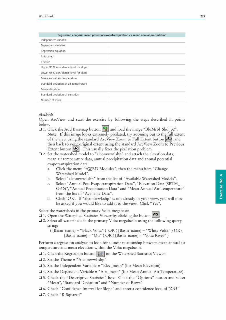
Workbook 227
Exer
cise
No
. 4
Regression analysis: mean potential evapotranspiration vs. mean annual precipitation
Independent variable
Dependent variable
Regression equation
R-Squared
P-Value
Upper 95% confidence level for slope
Lower 95% confidence level for slope
Mean annual air temperature
Standard deviation of air temperature
Mean elevation
Standard deviation of elevation
Number of rows
MethodsOpen ArcView and start the exercise by following the steps described in points below.❑ 1. Click the Add Basemap button and load the image “BluMrbl_Shd.jp2”.
Note: If this image looks extremely pixilated, try zooming out to the full extent of the view using the standard ArcView Zoom to Full Extent button , and then back to your original extent using the standard ArcView Zoom to Previous Extent button . This usually fixes the pixilation problem.
❑ 2. Set the watershed model to “alcomwwf.shp” and attach the elevation data, mean air temperature data, annual precipitation data and annual potential evapotranspiration data:a. Click the menu “AWRD Modules”, then the menu item “Change
Watershed Model”.b. Select “alcomwwf.shp” from the list of “Available Watershed Models”.c. Select “Annual Pot. Evapotranspiration Data”, “Elevation Data (SRTM_
Gt30)”, “Annual Precipitation Data” and “Mean Annual Air Temperature” from the list of “Available Data”.
d. Click ‘OK’. If “alcomwwf.shp” is not already in your view, you will now be asked if you would like to add it to the view. Click “Yes”.
Select the watersheds in the primary Volta megabasin.❑ 1. Open the Watershed Statistics Viewer by clicking the button .❑ 2. Select all watersheds in the primary Volta megabasin using the following query
string: ( [Basin_name] = “Black Volta” ) OR ( [Basin_name] = “White Volta” ) OR (
[Basin_name] = “Oti” ) OR ( [Basin_name] = “Volta River” )
Perform a regression analysis to look for a linear relationship between mean annual air temperature and mean elevation within the Volta megabasin.❑ 1. Click the Regression button on the Watershed Statistics Viewer.❑ 2. Set the Theme = “Alcomwwf.shp”❑ 3. Set the Independent Variable = “Elev_mean” (for Mean Elevation)❑ 4. Set the Dependent Variable = “Airt_mean” (for Mean Annual Air Temperature)❑ 5. Check the “Descriptive Statistics” box. Click the “Options” button and select
“Mean”, “Standard Deviation” and “Number of Rows”❑ 6. Check “Confidence Interval for Slope” and enter a confidence level of “0.95”❑ 7. Check “R-Squared”
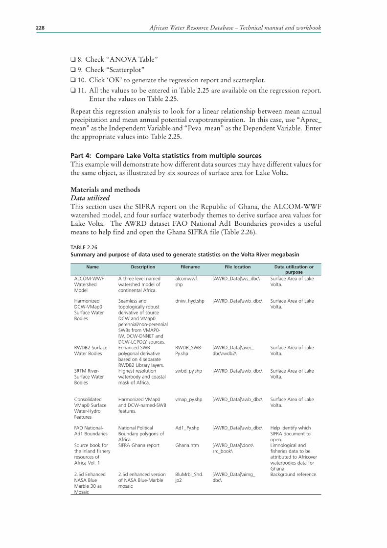
African Water Resource Database – Technical manual and workbook228
❑ 8. Check “ANOVA Table”❑ 9. Check “Scatterplot”❑ 10. Click ‘OK’ to generate the regression report and scatterplot.❑ 11. All the values to be entered in Table 2.25 are available on the regression report.
Enter the values on Table 2.25.
Repeat this regression analysis to look for a linear relationship between mean annual precipitation and mean annual potential evapotranspiration. In this case, use “Aprec_mean” as the Independent Variable and “Peva_mean” as the Dependent Variable. Enter the appropriate values into Table 2.25.
Part 4: Compare Lake Volta statistics from multiple sourcesThis example will demonstrate how different data sources may have different values for the same object, as illustrated by six sources of surface area for Lake Volta.
Materials and methods Data utilizedThis section uses the SIFRA report on the Republic of Ghana, the ALCOM-WWF watershed model, and four surface waterbody themes to derive surface area values for Lake Volta. The AWRD dataset FAO National-Ad1 Boundaries provides a useful means to help find and open the Ghana SIFRA file (Table 2.26).
TABLE 2.26Summary and purpose of data used to generate statistics on the Volta River megabasin
Name Description Filename File location Data utilization or purpose
ALCOM-WWF Watershed Model
A three level named watershed model of continental Africa.
alcomwwf.shp
[AWRD_Data]\ws_dbc\ Surface Area of Lake Volta.
Harmonized DCW-VMap0 Surface Water Bodies
Seamless and topologically robust derivative of source DCW and VMap0 perennial/non-perennial SWBs from VMAP0-IW, DCW-DNNET and DCW-LCPOLY sources.
dniw_hyd.shp [AWRD_Data]\swb_dbc\ Surface Area of Lake Volta.
RWDB2 Surface Water Bodies
Enhanced SWB polygonal derivative based on 4 separate RWDB2 Library layers.
RWDB_SWB-Py.shp
[AWRD_Data]\avec_dbc\rwdb2\
Surface Area of Lake Volta.
SRTM River-Surface Water Bodies
Highest resolution waterbody and coastal mask of Africa.
swbd_py.shp [AWRD_Data]\swb_dbc\ Surface Area of Lake Volta.
Consolidated VMap0 Surface Water-Hydro Features
Harmonized VMap0 and DCW-named-SWB features.
vmap_py.shp [AWRD_Data]\swb_dbc\ Surface Area of Lake Volta.
FAO National-Ad1 Boundaries
National Political Boundary polygons of Africa
Ad1_Py.shp [AWRD_Data]\swb_dbc\ Help identify which SIFRA document to open.
Source book for the inland fishery resources of Africa Vol. 1
SIFRA Ghana report Ghana.htm [AWRD_Data]\docs\src_book\
Limnological and fisheries data to be attributed to Africover waterbodies data for Ghana.
2.5d Enhanced NASA Blue Marble 30 as Mosaic
2.5d enhanced version of NASA Blue-Marble mosaic
BluMrbl_Shd.jp2
[AWRD_Data]\aimg_dbc\
Background reference.
Workbook 229
Exer
cise
No
. 4
Complete Table 2.27
TABLE 2.27Lake Volta area values from multiple sources
Source Area of Lake Volta (km2)
alcomwwf.shp
SIFRA Document for Ghana
rwdb_swb-py.shp
swbd_py.shp
dniw_hyd.shp
vmap_py.shp1
1Note that Lake Volta from vmap_py.shp includes three polygons.
MethodsOpen ArcView and start the exercise by following the steps described in points below.
Click on the button and load the following datasets. You can find them by either typing the name or filename in the “Search Text” textbox (you may use the * and ? wildcard characters), or by clicking on the respective DBC and finding the file in the list.❑ 1. FAO National-Ad1 Boundaries (Ad1_Py.shp); from the Additional Vector Data
DBC.❑ 2. ALCOM-WWF Watershed Model (alcomwwf.shp); from the Watersheds DBC.❑ 3. RWDB2 Surface Water Bodies (RWDB_SWB-Py.shp); from the Surface Waterbody
DBC.❑ 4. SRTM River-Surface Water Bodies (swbd_py.shp); from the Surface Waterbody
DBC.❑ 5. Harmonized DCW-VMap0 Surface Water Bodies (dniw_hyd.shp); from the
Surface Waterbody DBC. ❑ 6. Consolidated VMap0 Surface Water-Hydro Features (vmap_py.shp); from the
Surface Waterbody DBC.
The remaining data will be loaded using an alternative method:❑ 1. Click the Add Basemap button and load the image “BluMrbl_Shd.jp2”.
Note: If this image looks extremely pixilated, try zooming out to the full extent of the view using the standard ArcView Zoom to Full Extent button , and then back to your original extent using the standard ArcView Zoom to Previous Extent button . This usually fixes the pixilation problem.
Change the theme names to the short versions by clicking the “View” menu item “Toggle AWRD data to Short Theme Names.” You might have to click this menu item two times.
Open the SIFRA document for Ghana and look up the area, in km2, for Lake Volta:❑ 1. Find Ghana in the FAO National-Ad1 Boundary theme.❑ 2. Open the SIFRA document for Ghana by using the tool to click on Ghana.❑ 3. Look in Table 2 (Morphological Data for Major Lakes, Reservoirs and Lagoons)
for the area of Lake Volta. Add this value to Table 2.27.
Calculate the area, in km2, for Lake Volta using the remaining five data sources.
❑ 1. Make alcomwwf.shp active by clicking on it in the View Table of Contents.

African Water Resource Database – Technical manual and workbook230
❑ 2. Calculate the area in km2 for Lake Volta by clicking on it with the Report Descriptive Spatial Statistics tool . Add this value to the alcomwwf.shp row in Table 2.27.
❑ 3. Make dniw_hyd.shp active by clicking on it in the View Table of Contents.
❑ 4. Calculate the area in km2 for Lake Volta by clicking on it with the Report Descriptive Spatial Statistics tool . Add this value to the dniw_hyd.shp row in Table 2.27.
❑ 5. Make rwdb_swb-py.shp active by clicking on it in the View Table of Contents.
❑ 6. Calculate the area in km2 for Lake Volta by clicking on it with the Report Descriptive Spatial Statistics tool . Add this value to the rwdb_swb-py.shp row in Table 2.27.
❑ 7. Make swbd_py.shp active by clicking on it in the View Table of Contents.
❑ 8. Calculate the area in km2 for Lake Volta by clicking on it with the Report Descriptive Spatial Statistics tool . Note: This action may take longer with this theme than with the previous themes because this dataset has a very high-resolution border for Lake Volta. Add this area value to the swbd_py.shp row in Table 2.27.
❑ 9. Make vmap_py.shp active by clicking on it in the View Table of Contents.
❑ 10. Vmap_py.shp does not include the entire area of Lake Volta in a single polygon. This dataset breaks Lake Volta up into three separate regions. These regions are easier to distinguish if you add polygon borders to the theme:
a. Click the “Theme” menu, then “Adjust Polygon Border and Pattern”
b. Click the option “Use Outline”.
c. Click the option “Constant Outline Color”.
d. Click the “Set Color” button and choose a dark color.
e. Set the “Outline Width” = 0.1
f. Click ‘OK’.
g. Zoom into the southern portion of Lake Volta to see the three separate regions.
❑ 11. Identify the three polygons that make up Lake Volta and use the Report Descriptive Spatial Statistics tool to calculate the area in km2 for each of them. Add up the three area values and enter the total to the vmap_py.shp row in Table 2.27.
Exercise SummaryThis exercise illustrates several ways to generate statistics on watersheds, waterbodies and other polygons using tools from the AWRD toolset. In particular, Part 4 of the exercise illustrates the fact that different data sources can lead to different statistical results on the same feature. In a case like this, it is often a good idea to look at the metadata for the data source, to determine the age of the data and the scale at which it was digitized or created.
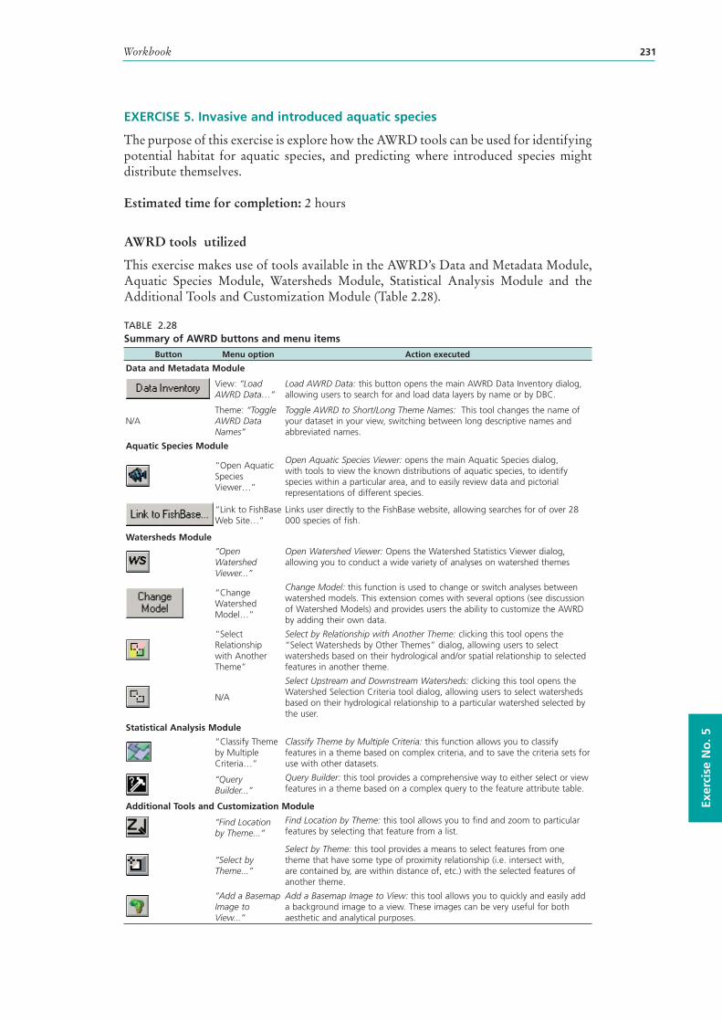
Workbook 231
Exer
cise
No
. 5
EXERCISE 5. Invasive and introduced aquatic species
The purpose of this exercise is explore how the AWRD tools can be used for identifying potential habitat for aquatic species, and predicting where introduced species might distribute themselves.
Estimated time for completion: 2 hours
AWRD tools utilized
This exercise makes use of tools available in the AWRD’s Data and Metadata Module, Aquatic Species Module, Watersheds Module, Statistical Analysis Module and the Additional Tools and Customization Module (Table 2.28).
TABLE 2.28Summary of AWRD buttons and menu items
Button Menu option Action executed
Data and Metadata Module
View: “Load AWRD Data…”
Load AWRD Data: this button opens the main AWRD Data Inventory dialog, allowing users to search for and load data layers by name or by DBC.
N/ATheme: “Toggle AWRD Data Names”
Toggle AWRD to Short/Long Theme Names: This tool changes the name of your dataset in your view, switching between long descriptive names and abbreviated names.
Aquatic Species Module
“Open Aquatic Species Viewer…”
Open Aquatic Species Viewer: opens the main Aquatic Species dialog, with tools to view the known distributions of aquatic species, to identify species within a particular area, and to easily review data and pictorial representations of different species.
“Link to FishBase Web Site…”
Links user directly to the FishBase website, allowing searches for of over 28 000 species of fish.
Watersheds Module
“Open Watershed Viewer...”
Open Watershed Viewer: Opens the Watershed Statistics Viewer dialog, allowing you to conduct a wide variety of analyses on watershed themes
“Change Watershed Model…”
Change Model: this function is used to change or switch analyses between watershed models. This extension comes with several options (see discussion of Watershed Models) and provides users the ability to customize the AWRD by adding their own data.
“Select Relationship with Another Theme”
Select by Relationship with Another Theme: clicking this tool opens the “Select Watersheds by Other Themes” dialog, allowing users to select watersheds based on their hydrological and/or spatial relationship to selected features in another theme.
N/A
Select Upstream and Downstream Watersheds: clicking this tool opens the Watershed Selection Criteria tool dialog, allowing users to select watersheds based on their hydrological relationship to a particular watershed selected by the user.
Statistical Analysis Module
“Classify Theme by Multiple Criteria…”
Classify Theme by Multiple Criteria: this function allows you to classify features in a theme based on complex criteria, and to save the criteria sets for use with other datasets.
“Query Builder...”
Query Builder: this tool provides a comprehensive way to either select or view features in a theme based on a complex query to the feature attribute table.
Additional Tools and Customization Module
“Find Location by Theme...”
Find Location by Theme: this tool allows you to find and zoom to particular features by selecting that feature from a list.
“Select by Theme...”
Select by Theme: this tool provides a means to select features from one theme that have some type of proximity relationship (i.e. intersect with, are contained by, are within distance of, etc.) with the selected features of another theme.
“Add a Basemap Image to View...”
Add a Basemap Image to View: this tool allows you to quickly and easily add a background image to a view. These images can be very useful for both aesthetic and analytical purposes.

African Water Resource Database – Technical manual and workbook232
Part 1: Potential distribution of North African Catfish, based on FishBase locations and alcomwwf.shp watershedsThis exercise will illustrate how to import data from FishBase and analyze potential habitat using those locations in conjunction with a watershed model. This exercise does not include a table in the workbook to fill out. Rather, the exercise is to generate a point shapefile of catfish locations, and then generate shapefiles of catfish distributions and potential distributions.
Materials and methods Data utilizedThis section uses the ALCOM-WWF watershed model in conjunction with downloaded sharptooth catfish locations to identify the potential distribution of this species. The background image SRTM30_ShdBath.jp2 provides a spatial reference (Table 2.29).
TABLE 2.29Summary and purpose of data used
Name Description Filename File location Data utilization or purpose
ALCOM-WWF Watershed Model
A three level named watershed model of continental Africa
alcomwwf.shp
[AWRD_Data]\ws_dbc\ Used to identify the region of the contributing watershed.
Sharptooth Catfish Locations
Set of coordinates for observed sharptooth catfish locations, downloaded from FishBase
N/A http://www.fishbase.org/Summary/SpeciesSummary.php?id=1934
Used to identify watersheds in which sharptooth catfish have been observed.
Color Shade of SRTM30as w/ETopo2 Bathymetry
2.5d enhanced RGB image of SRTM-30 terrestrial elevation and ETopo2 bathymetric data
SRTM30_ShdBath.jp2
[AWRD_Data]\aimg_dbc\ Background reference.
MethodsOpen ArcView and start the exercise by following the steps below.
Click the Aquatic Species Viewer button to open up the Aquatic Species Distribution view and the associated Aquatic Species Viewer dialog.
Download locations for Sharptooth Catfish from FishBase:❑ 1. In the Aquatic Species Viewer, choose the option to list aquatic species by
Common Name, and then find and select “Sharptooth Catfish” in the list of species.
❑ 2. With “Sharptooth Catfish” selected, click the button “Link to FishBase” .
❑ 3. While at the FishBase Web site for Sharptooth Catfish, scroll down to the section titled “Tools” near the bottom and click the link to “Biogeographic Modelling”.
❑ 4. You should see two list boxes at the bottom of the “Biogeographic Modelling Tools” page. The one on the right has a button named “Select All” above it. Click that button to select all the sharptooth catfish coordinates in the listbox.
❑ 5. Click [CONTROL]-C to copy that list to the computer memory.❑ 6. Return to ArcView and open a blank script.
Workbook 233
Exer
cise
No
. 5
❑ 7. Either click the standard ArcView “Paste” button , or simply click [CONTROL]-V, to paste the list into your blank script window.
❑ 8. Click the “Convert Text to Point Shapefile” button in the Script Button Bar (Note: This button has the same picture as the “Open Aquatic Species Viewer” button on the main AWRD dialog, but it is not the same button).
❑ 9. You will be asked what to name your new point shapefile (this example will assume the name “catfish.shp”), and whether you would like to add it to a view. Choose the option to “Make New View”.
❑ 10. Close your script window containing the list of location coordinates. You may delete this script document if you like.
Add additional data:❑ 1. Set the watershed model to “alcomwwf.shp”:
a. Click the menu “AWRD Modules”, then the menu item “Change Watershed Model”.
b. Select “alcomwwf.shp” from the list of “Available Watershed Models”.c. This exercise does not require any additional data. You may select any of
the additional datasets if you wish, or none of them.d. Click ‘OK’. If “alcomwwf.shp” is not already in your view, you will now
be asked if you would like to add it to the view. Click “Yes”.❑ 2. Click the Add Basemap button and load the image “SRTM30_ShdBath.
jp2”. Note: If this image looks extremely pixilated, try zooming out to the full extent of the view using the standard ArcView Zoom to Full Extent button , and then back to your original extent using the standard ArcView Zoom to Previous Extent button . This usually fixes the pixilation problem.
Change the theme names to the short versions by clicking the “View” menu item “Toggle AWRD data to Short Theme Names.” You might have to click this menu item two times.
Identify watersheds that contain observed FishBase catfish locations:❑ 1. Select all of your catfish locations by opening the catfish.shp attribute table with
the button, then clearing any current selection with the button, and finally selecting all locations with the Switch Selection button .
❑ 2. Click back on your view to make it active.❑ 3. Click the “Select by Relationship with Another Theme” button to open
the watershed theme selection dialog.❑ 4. Use the dialog to selection the alcomwwf.shp polygons that intersect with the
combined features of your selected catfish.shp locations.❑ 5. Save this subset of selected alcomwwf.shp watershed polygons to a new
shapefile:a. Click on the alcomwwf.shp theme in the View Table of Contents to make
it the active theme.b. Click the “Convert to Shapefile” menu item in the “Theme” menuc. When asked, say “Yes” to add the new theme to your view.d. If you wish to clear the black polygon borders surrounding each watershed
polygon, click the “Theme” menu, then “Adjust Polygon Border and Pattern”, then choose the option “Do Not Use Outline”, and then click ‘OK’.
African Water Resource Database – Technical manual and workbook234
❑ 6. Your new shapefile represents the observed distribution of sharptooth catfish, based on observed locations from FishBase.
Optional Exercise: Identify watersheds that either intersect or lie up or downstream of the observed FishBase catfish locations: Warning: This optional exercise is not difficult, but it will take the computer much longer to process the steps. Plan for 10-20 minutes of computer processing time to complete this exercise.❑ 1. Select all of your catfish.shp locations by opening the catfish attribute table with
the button, then clearing any current selection with the button, and finally selecting all locations with the Switch Selection button .
❑ 2. Click the “Select by Relationship with Another Theme” button to open the watershed theme selection dialog.
❑ 3. Use the dialog to selection the alcomwwf.shp polygons that intersect with the combined features of your selected catfish.shp locations. Choose both of the options “Include Upstream polygons” and “Include Downstream Polygons”. This query will take much longer to process than the last query because it has to search through the hydrological network to identify all watersheds that are upstream and downstream of all the catfish locations.
❑ 4. Save this subset of selected alcomwwf.shp watershed polygons to a new shapefile:a. Click on the alcomwwf.shp theme in the View Table of Contents to make
it the active theme.b. Click the “Convert to Shapefile” menu item in the “Theme” menuc. When asked, say “Yes” to add the new theme to your view.d. If you wish to clear the black polygon borders surrounding each watershed
polygon, click the “Theme” menu, then “Adjust Polygon Border and Pattern”, then choose the option “Do Not Use Outline”, and then click ‘OK’.
❑ 5. Your new shapefile represents the potential distribution of sharptooth catfish, based on observed locations from FishBase.
Part 2: Potential distribution of common carp in SADC region, based on aquatic species locations and alcomwwf.shp watershedsThe ICES Code of Practice on the Introductions and Transfers of Marine Organisms (ICES, 2004) and the FAO Code of Conduct for Responsible Fisheries (FAO 1995) call upon agencies to notify responsible authorities in states that may be impacted by introductions of non-native species. This exercise will demonstrate how to identify areas that might be affected by introduction of an invasive species.
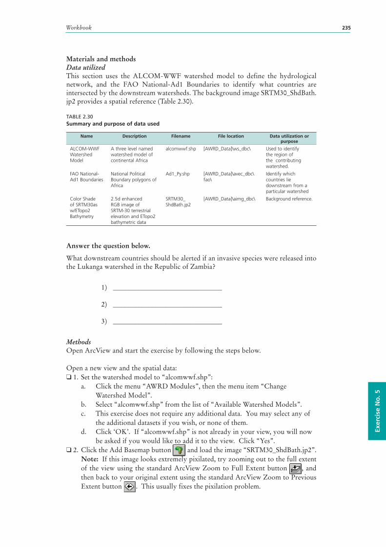
Workbook 235
Exer
cise
No
. 5
Materials and methods Data utilizedThis section uses the ALCOM-WWF watershed model to define the hydrological network, and the FAO National-Ad1 Boundaries to identify what countries are intersected by the downstream watersheds. The background image SRTM30_ShdBath.jp2 provides a spatial reference (Table 2.30).
TABLE 2.30Summary and purpose of data used
Name Description Filename File location Data utilization or purpose
ALCOM-WWF Watershed Model
A three level named watershed model of continental Africa
alcomwwf.shp [AWRD_Data]\ws_dbc\ Used to identify the region of the contributing watershed.
FAO National-Ad1 Boundaries
National Political Boundary polygons of Africa
Ad1_Py.shp [AWRD_Data]\avec_dbc\fao\
Identify which countries lie downstream from a particular watershed
Color Shade of SRTM30as w/ETopo2 Bathymetry
2.5d enhanced RGB image of SRTM-30 terrestrial elevation and ETopo2 bathymetric data
SRTM30_ShdBath.jp2
[AWRD_Data]\aimg_dbc\ Background reference.
Answer the question below.
What downstream countries should be alerted if an invasive species were released into the Lukanga watershed in the Republic of Zambia?
1) ________________________________
2) ________________________________
3) ________________________________
MethodsOpen ArcView and start the exercise by following the steps below.
Open a new view and the spatial data:❑ 1. Set the watershed model to “alcomwwf.shp”:
a. Click the menu “AWRD Modules”, then the menu item “Change Watershed Model”.
b. Select “alcomwwf.shp” from the list of “Available Watershed Models”.c. This exercise does not require any additional data. You may select any of
the additional datasets if you wish, or none of them.d. Click ‘OK’. If “alcomwwf.shp” is not already in your view, you will now
be asked if you would like to add it to the view. Click “Yes”.❑ 2. Click the Add Basemap button and load the image “SRTM30_ShdBath.jp2”.
Note: If this image looks extremely pixilated, try zooming out to the full extent of the view using the standard ArcView Zoom to Full Extent button , and then back to your original extent using the standard ArcView Zoom to Previous Extent button . This usually fixes the pixilation problem.
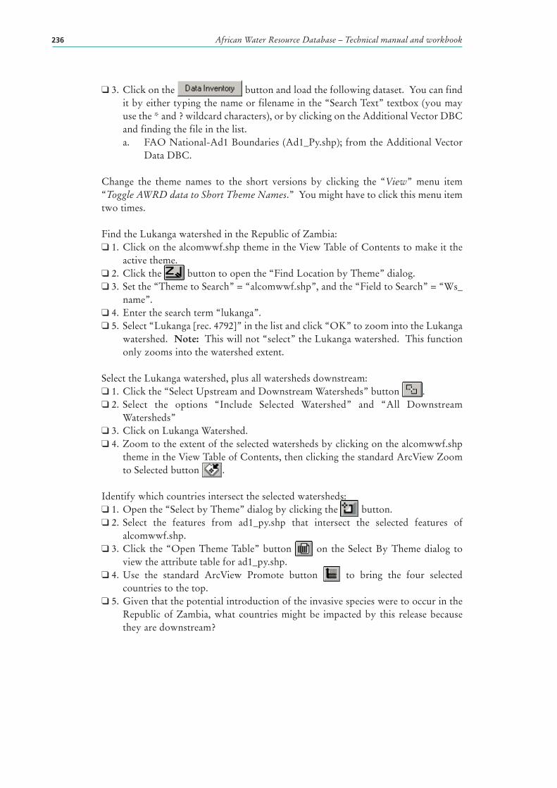
African Water Resource Database – Technical manual and workbook236
❑ 3. Click on the button and load the following dataset. You can find it by either typing the name or filename in the “Search Text” textbox (you may use the * and ? wildcard characters), or by clicking on the Additional Vector DBC and finding the file in the list.a. FAO National-Ad1 Boundaries (Ad1_Py.shp); from the Additional Vector
Data DBC.
Change the theme names to the short versions by clicking the “View” menu item “Toggle AWRD data to Short Theme Names.” You might have to click this menu item two times.
Find the Lukanga watershed in the Republic of Zambia:❑ 1. Click on the alcomwwf.shp theme in the View Table of Contents to make it the
active theme.❑ 2. Click the button to open the “Find Location by Theme” dialog.❑ 3. Set the “Theme to Search” = “alcomwwf.shp”, and the “Field to Search” = “Ws_
name”.❑ 4. Enter the search term “lukanga”.❑ 5. Select “Lukanga [rec. 4792]” in the list and click “OK” to zoom into the Lukanga
watershed. Note: This will not “select” the Lukanga watershed. This function only zooms into the watershed extent.
Select the Lukanga watershed, plus all watersheds downstream:❑ 1. Click the “Select Upstream and Downstream Watersheds” button .❑ 2. Select the options “Include Selected Watershed” and “All Downstream
Watersheds”❑ 3. Click on Lukanga Watershed.❑ 4. Zoom to the extent of the selected watersheds by clicking on the alcomwwf.shp
theme in the View Table of Contents, then clicking the standard ArcView Zoom to Selected button .
Identify which countries intersect the selected watersheds:❑ 1. Open the “Select by Theme” dialog by clicking the button.❑ 2. Select the features from ad1_py.shp that intersect the selected features of
alcomwwf.shp.❑ 3. Click the “Open Theme Table” button on the Select By Theme dialog to
view the attribute table for ad1_py.shp.❑ 4. Use the standard ArcView Promote button to bring the four selected
countries to the top.❑ 5. Given that the potential introduction of the invasive species were to occur in the
Republic of Zambia, what countries might be impacted by this release because they are downstream?
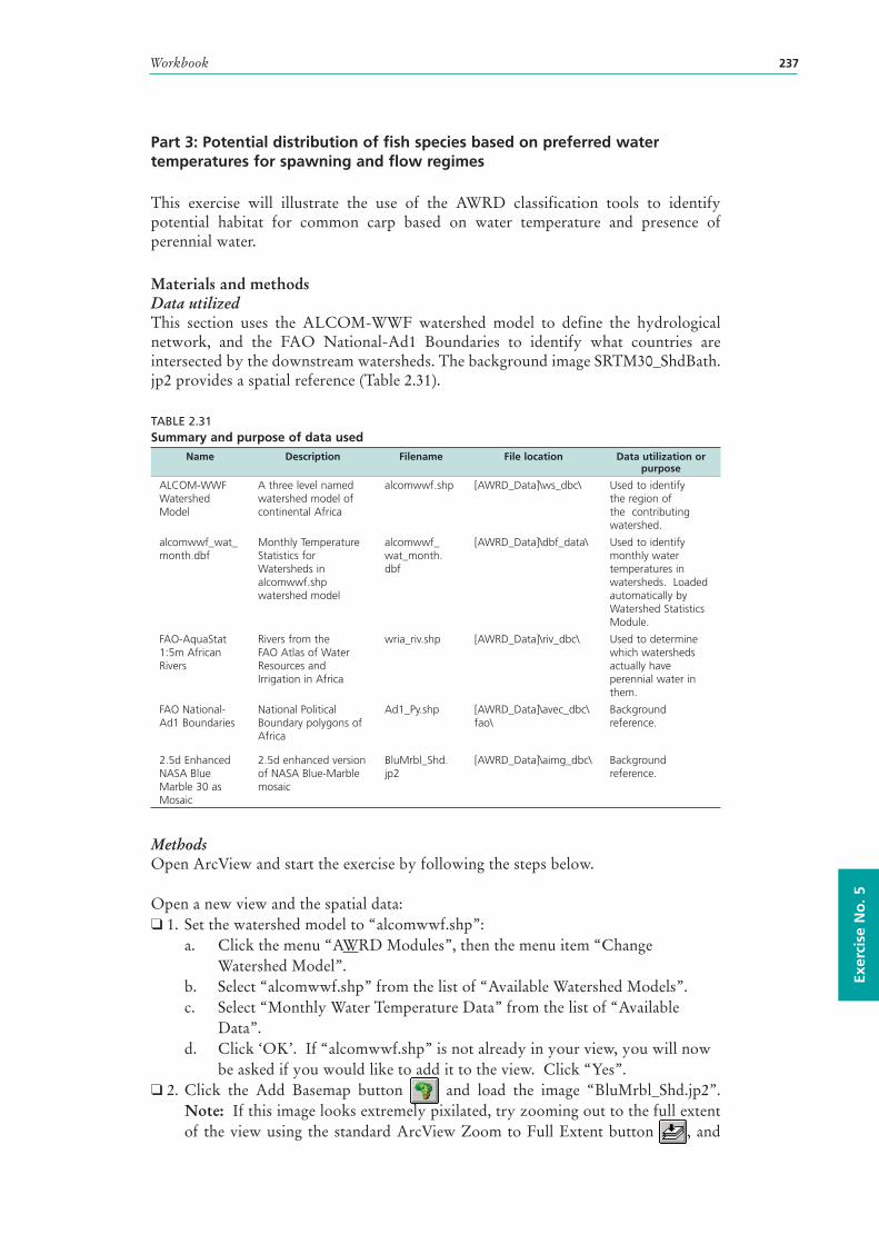
Workbook 237
Exer
cise
No
. 5
Part 3: Potential distribution of fish species based on preferred water temperatures for spawning and flow regimes
This exercise will illustrate the use of the AWRD classification tools to identify potential habitat for common carp based on water temperature and presence of perennial water.
Materials and methods Data utilizedThis section uses the ALCOM-WWF watershed model to define the hydrological network, and the FAO National-Ad1 Boundaries to identify what countries are intersected by the downstream watersheds. The background image SRTM30_ShdBath.jp2 provides a spatial reference (Table 2.31).
TABLE 2.31Summary and purpose of data used
Name Description Filename File location Data utilization or purpose
ALCOM-WWF Watershed Model
A three level named watershed model of continental Africa
alcomwwf.shp [AWRD_Data]\ws_dbc\ Used to identify the region of the contributing watershed.
alcomwwf_wat_month.dbf
Monthly Temperature Statistics for Watersheds in alcomwwf.shp watershed model
alcomwwf_wat_month.dbf
[AWRD_Data]\dbf_data\ Used to identify monthly water temperatures in watersheds. Loaded automatically by Watershed Statistics Module.
FAO-AquaStat 1:5m African Rivers
Rivers from the FAO Atlas of Water Resources and Irrigation in Africa
wria_riv.shp [AWRD_Data]\riv_dbc\ Used to determine which watersheds actually have perennial water in them.
FAO National-Ad1 Boundaries
National Political Boundary polygons of Africa
Ad1_Py.shp [AWRD_Data]\avec_dbc\fao\
Background reference.
2.5d Enhanced NASA Blue Marble 30 as Mosaic
2.5d enhanced version of NASA Blue-Marble mosaic
BluMrbl_Shd.jp2
[AWRD_Data]\aimg_dbc\ Background reference.
MethodsOpen ArcView and start the exercise by following the steps below.
Open a new view and the spatial data:❑ 1. Set the watershed model to “alcomwwf.shp”:
a. Click the menu “AWRD Modules”, then the menu item “Change Watershed Model”.
b. Select “alcomwwf.shp” from the list of “Available Watershed Models”.c. Select “Monthly Water Temperature Data” from the list of “Available
Data”.d. Click ‘OK’. If “alcomwwf.shp” is not already in your view, you will now
be asked if you would like to add it to the view. Click “Yes”.❑ 2. Click the Add Basemap button and load the image “BluMrbl_Shd.jp2”.
Note: If this image looks extremely pixilated, try zooming out to the full extent of the view using the standard ArcView Zoom to Full Extent button , and
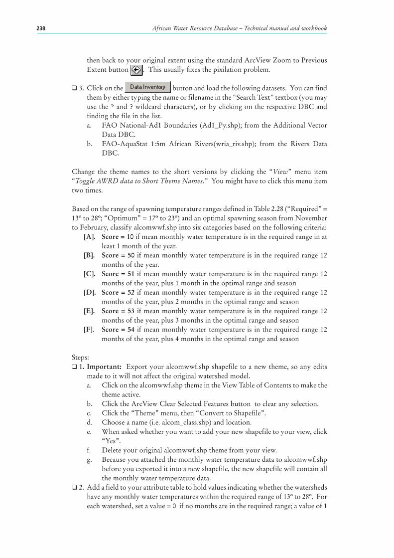
African Water Resource Database – Technical manual and workbook238
then back to your original extent using the standard ArcView Zoom to Previous Extent button . This usually fixes the pixilation problem.
❑ 3. Click on the button and load the following datasets. You can find them by either typing the name or filename in the “Search Text” textbox (you may use the * and ? wildcard characters), or by clicking on the respective DBC and finding the file in the list.a. FAO National-Ad1 Boundaries (Ad1_Py.shp); from the Additional Vector
Data DBC.b. FAO-AquaStat 1:5m African Rivers(wria_riv.shp); from the Rivers Data
DBC.
Change the theme names to the short versions by clicking the “View” menu item “Toggle AWRD data to Short Theme Names.” You might have to click this menu item two times.
Based on the range of spawning temperature ranges defined in Table 2.28 (“Required” = 13º to 28º; “Optimum” = 17º to 23º) and an optimal spawning season from November to February, classify alcomwwf.shp into six categories based on the following criteria:
[A]. Score = 10 if mean monthly water temperature is in the required range in at least 1 month of the year.
[B]. Score = 50 if mean monthly water temperature is in the required range 12 months of the year.
[C]. Score = 51 if mean monthly water temperature is in the required range 12 months of the year, plus 1 month in the optimal range and season
[D]. Score = 52 if mean monthly water temperature is in the required range 12 months of the year, plus 2 months in the optimal range and season
[E]. Score = 53 if mean monthly water temperature is in the required range 12 months of the year, plus 3 months in the optimal range and season
[F]. Score = 54 if mean monthly water temperature is in the required range 12 months of the year, plus 4 months in the optimal range and season
Steps:❑ 1. Important: Export your alcomwwf.shp shapefile to a new theme, so any edits
made to it will not affect the original watershed model.a. Click on the alcomwwf.shp theme in the View Table of Contents to make the
theme active.b. Click the ArcView Clear Selected Features button to clear any selection.c. Click the “Theme” menu, then “Convert to Shapefile”.d. Choose a name (i.e. alcom_class.shp) and location.e. When asked whether you want to add your new shapefile to your view, click
“Yes”.f. Delete your original alcomwwf.shp theme from your view.g. Because you attached the monthly water temperature data to alcomwwf.shp
before you exported it into a new shapefile, the new shapefile will contain all the monthly water temperature data.
❑ 2. Add a field to your attribute table to hold values indicating whether the watersheds have any monthly water temperatures within the required range of 13º to 28º. For each watershed, set a value = 0 if no months are in the required range; a value of 1
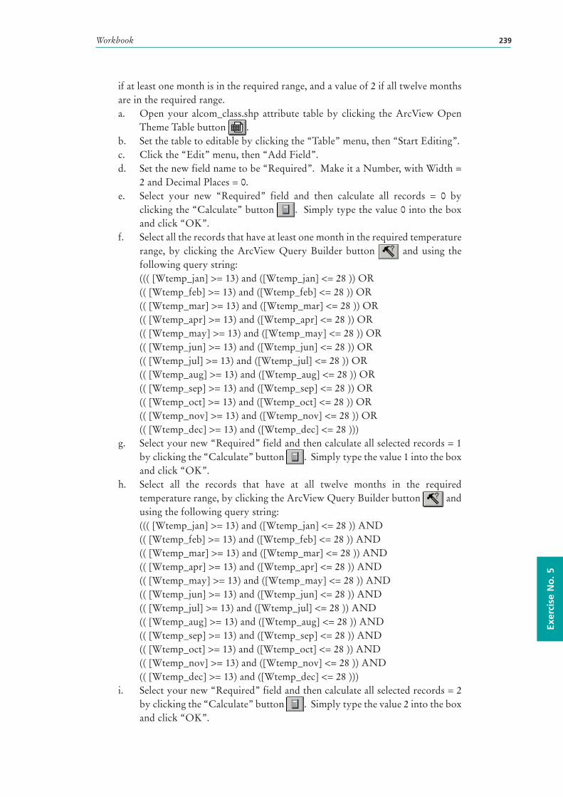
Workbook 239
Exer
cise
No
. 5
if at least one month is in the required range, and a value of 2 if all twelve months are in the required range.a. Open your alcom_class.shp attribute table by clicking the ArcView Open
Theme Table button .b. Set the table to editable by clicking the “Table” menu, then “Start Editing”.c. Click the “Edit” menu, then “Add Field”.d. Set the new field name to be “Required”. Make it a Number, with Width =
2 and Decimal Places = 0.e. Select your new “Required” field and then calculate all records = 0 by
clicking the “Calculate” button . Simply type the value 0 into the box and click “OK”.
f. Select all the records that have at least one month in the required temperature range, by clicking the ArcView Query Builder button and using the following query string:((( [Wtemp_jan] >= 13) and ([Wtemp_jan] <= 28 )) OR(( [Wtemp_feb] >= 13) and ([Wtemp_feb] <= 28 )) OR(( [Wtemp_mar] >= 13) and ([Wtemp_mar] <= 28 )) OR(( [Wtemp_apr] >= 13) and ([Wtemp_apr] <= 28 )) OR(( [Wtemp_may] >= 13) and ([Wtemp_may] <= 28 )) OR(( [Wtemp_jun] >= 13) and ([Wtemp_jun] <= 28 )) OR(( [Wtemp_jul] >= 13) and ([Wtemp_jul] <= 28 )) OR(( [Wtemp_aug] >= 13) and ([Wtemp_aug] <= 28 )) OR(( [Wtemp_sep] >= 13) and ([Wtemp_sep] <= 28 )) OR(( [Wtemp_oct] >= 13) and ([Wtemp_oct] <= 28 )) OR(( [Wtemp_nov] >= 13) and ([Wtemp_nov] <= 28 )) OR(( [Wtemp_dec] >= 13) and ([Wtemp_dec] <= 28 )))
g. Select your new “Required” field and then calculate all selected records = 1 by clicking the “Calculate” button . Simply type the value 1 into the box and click “OK”.
h. Select all the records that have at all twelve months in the required temperature range, by clicking the ArcView Query Builder button and using the following query string:((( [Wtemp_jan] >= 13) and ([Wtemp_jan] <= 28 )) AND(( [Wtemp_feb] >= 13) and ([Wtemp_feb] <= 28 )) AND(( [Wtemp_mar] >= 13) and ([Wtemp_mar] <= 28 )) AND(( [Wtemp_apr] >= 13) and ([Wtemp_apr] <= 28 )) AND(( [Wtemp_may] >= 13) and ([Wtemp_may] <= 28 )) AND(( [Wtemp_jun] >= 13) and ([Wtemp_jun] <= 28 )) AND(( [Wtemp_jul] >= 13) and ([Wtemp_jul] <= 28 )) AND(( [Wtemp_aug] >= 13) and ([Wtemp_aug] <= 28 )) AND(( [Wtemp_sep] >= 13) and ([Wtemp_sep] <= 28 )) AND(( [Wtemp_oct] >= 13) and ([Wtemp_oct] <= 28 )) AND(( [Wtemp_nov] >= 13) and ([Wtemp_nov] <= 28 )) AND(( [Wtemp_dec] >= 13) and ([Wtemp_dec] <= 28 )))
i. Select your new “Required” field and then calculate all selected records = 2 by clicking the “Calculate” button . Simply type the value 2 into the box and click “OK”.
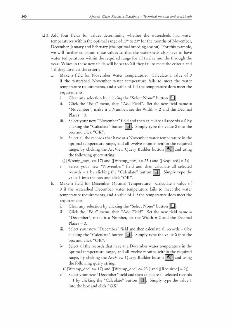
African Water Resource Database – Technical manual and workbook240
❑ 3. Add four fields for values determining whether the watersheds had water temperatures within the optimal range of 17º to 23º for the months of November, December, January and February (the optimal breeding season). For this example, we will further constrain these values so that the watersheds also have to have water temperatures within the required range for all twelve months through the year. Values in these new fields will be set to 0 if they fail to meet the criteria and 1 if they do meet the criteria.a. Make a field for November Water Temperature. Calculate a value of 0
if the watershed November water temperature fails to meet the water temperature requirements, and a value of 1 if the temperature does meet the requirements.i. Clear any selection by clicking the “Select None” button .ii. Click the “Edit” menu, then “Add Field”. Set the new field name =
“November”, make it a Number, set the Width = 2 and the Decimal Places = 0.
iii. Select your new “November” field and then calculate all records = 0 by clicking the “Calculate” button . Simply type the value 0 into the box and click “OK”.
iv. Select all the records that have at a November water temperature in the optimal temperature range, and all twelve months within the required range, by clicking the ArcView Query Builder button and using the following query string:
(( [Wtemp_nov] >= 17) and ([Wtemp_nov] <= 23 ) and ([Required] = 2))v. Select your new “November” field and then calculate all selected
records = 1 by clicking the “Calculate” button . Simply type the value 1 into the box and click “OK”.
b. Make a field for December Optimal Temperature. Calculate a value of 0 if the watershed December water temperature fails to meet the water temperature requirements, and a value of 1 if the temperature does meet the requirements.i. Clear any selection by clicking the “Select None” button .ii. Click the “Edit” menu, then “Add Field”. Set the new field name =
“December”, make it a Number, set the Width = 2 and the Decimal Places = 0.
iii. Select your new “December” field and then calculate all records = 0 by clicking the “Calculate” button . Simply type the value 0 into the box and click “OK”.
iv. Select all the records that have at a December water temperature in the optimal temperature range, and all twelve months within the required range, by clicking the ArcView Query Builder button and using the following query string:
(( [Wtemp_dec] >= 17) and ([Wtemp_dec] <= 23 ) and ([Required] = 2))v. Select your new “December” field and then calculate all selected records
= 1 by clicking the “Calculate” button . Simply type the value 1 into the box and click “OK”.
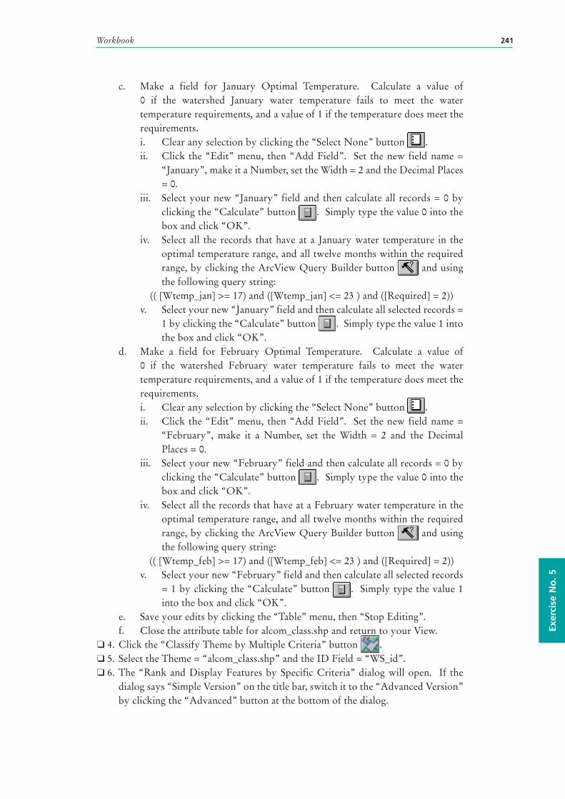
Workbook 241
Exer
cise
No
. 5
c. Make a field for January Optimal Temperature. Calculate a value of 0 if the watershed January water temperature fails to meet the water temperature requirements, and a value of 1 if the temperature does meet the requirements.i. Clear any selection by clicking the “Select None” button .ii. Click the “Edit” menu, then “Add Field”. Set the new field name =
“January”, make it a Number, set the Width = 2 and the Decimal Places = 0.
iii. Select your new “January” field and then calculate all records = 0 by clicking the “Calculate” button . Simply type the value 0 into the box and click “OK”.
iv. Select all the records that have at a January water temperature in the optimal temperature range, and all twelve months within the required range, by clicking the ArcView Query Builder button and using the following query string:
(( [Wtemp_jan] >= 17) and ([Wtemp_jan] <= 23 ) and ([Required] = 2))v. Select your new “January” field and then calculate all selected records =
1 by clicking the “Calculate” button . Simply type the value 1 into the box and click “OK”.
d. Make a field for February Optimal Temperature. Calculate a value of 0 if the watershed February water temperature fails to meet the water temperature requirements, and a value of 1 if the temperature does meet the requirements.i. Clear any selection by clicking the “Select None” button .ii. Click the “Edit” menu, then “Add Field”. Set the new field name =
“February”, make it a Number, set the Width = 2 and the Decimal Places = 0.
iii. Select your new “February” field and then calculate all records = 0 by clicking the “Calculate” button . Simply type the value 0 into the box and click “OK”.
iv. Select all the records that have at a February water temperature in the optimal temperature range, and all twelve months within the required range, by clicking the ArcView Query Builder button and using the following query string:
(( [Wtemp_feb] >= 17) and ([Wtemp_feb] <= 23 ) and ([Required] = 2))v. Select your new “February” field and then calculate all selected records
= 1 by clicking the “Calculate” button . Simply type the value 1 into the box and click “OK”.
e. Save your edits by clicking the “Table” menu, then “Stop Editing”.f. Close the attribute table for alcom_class.shp and return to your View.
❑ 4. Click the “Classify Theme by Multiple Criteria” button .❑ 5. Select the Theme = “alcom_class.shp” and the ID Field = “WS_id”.❑ 6. The “Rank and Display Features by Specific Criteria” dialog will open. If the
dialog says “Simple Version” on the title bar, switch it to the “Advanced Version” by clicking the “Advanced” button at the bottom of the dialog.
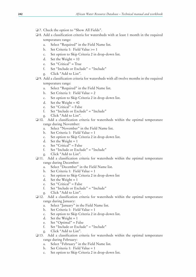
African Water Resource Database – Technical manual and workbook242
❑ 7. Check the option to “Show All Fields”.❑ 8. Add a classification criteria for watersheds with at least 1 month in the required
temperature range:a. Select “Required” in the Field Name list.b. Set Criteria 1: Field Value >= 1c. Set option to Skip Criteria 2 in drop-down list.d. Set the Weight = 10e. Set “Critical” = Truef. Set “Include or Exclude” = “Include”g. Click “Add to List”.
❑ 9. Add a classification criteria for watersheds with all twelve months in the required temperature range:a. Select “Required” in the Field Name list.b. Set Criteria 1: Field Value = 2c. Set option to Skip Criteria 2 in drop-down list.d. Set the Weight = 40e. Set “Critical” = Falsef. Set “Include or Exclude” = “Include”g. Click “Add to List”.
❑ 10. Add a classification criteria for watersheds within the optimal temperature range during November:a. Select “November” in the Field Name list.b. Set Criteria 1: Field Value = 1c. Set option to Skip Criteria 2 in drop-down list.d. Set the Weight = 1e. Set “Critical” = Falsef. Set “Include or Exclude” = “Include”g. Click “Add to List”.
❑ 11. Add a classification criteria for watersheds within the optimal temperature range during December:a. Select “December” in the Field Name list.b. Set Criteria 1: Field Value = 1c. Set option to Skip Criteria 2 in drop-down listd. Set the Weight = 1e. Set “Critical” = Falsef. Set “Include or Exclude” = “Include”g. Click “Add to List”.
❑ 12. Add a classification criteria for watersheds within the optimal temperature range during January:a. Select “January” in the Field Name list.b. Set Criteria 1: Field Value = 1c. Set option to Skip Criteria 2 in drop-down list.d. Set the Weight = 1e. Set “Optimal” = Falsef. Set “Include or Exclude” = “Include”g. Click “Add to List”.
❑ 13. Add a classification criteria for watersheds within the optimal temperature range during February:a. Select “February” in the Field Name list.b. Set Criteria 1: Field Value = 1c. Set option to Skip Criteria 2 in drop-down list.
Workbook 243
Exer
cise
No
. 5
d. Set the Weight = 1e. Set “Critical” = Falsef. Set “Include or Exclude” = “Include”g. Click “Add to List”.
❑ 14. Save your classification criteria. This will save time when you do the next part of the exercise.
❑ 15. Click “OK” to classify alcom_class.shp according to your classification criteria.
Now you have classified the continent of Africa according to required and optimal carp spawning temperatures, and therefore you have identified regions that range from poor-to-excellent potential for maintaining carp populations. However, many of these watersheds are in dry climates without perennial water sources, and which are therefore unlikely to support carp populations. The next step of this exercise is to restrict the analysis to only those watersheds that actually have water in them.❑ 1. Open your alcom_class.shp attribute table by clicking the ArcView Open Theme
Table button .❑ 2. Set the table to Editable by clicking the “Table” menu, then “Start Editing”.❑ 3. Click the “Edit” menu, then “Add Field”.❑ 4. Set the new field name to be “Perennial”. Make it a Number, with Width = 2 and
Decimal Places = 0.❑ 5. Select your new “Perennial” field and then calculate all records = 0 by clicking the
“Calculate” button . Simply type the value 0 into the box and click “OK”.❑ 6. Save your edits by clicking the “Table” menu, then “Stop Editing”. ❑ 7. Return to your View.❑ 8. Use the AWRD Query Builder tool to select the perennial rivers from
wria_riv.shp. Use the following query string:( [Regime] = 1 )
❑ 9. Use the AWRD Select by Theme tool to select the watersheds from alcom_class.shp which intersect these selected perennial rivers.
❑ 10. Open the alcom_class.shp attribute table using the ArcView Open Theme Table button .
❑ 11. Set the table to Editable by clicking the “Table” menu, then “Start Editing”.❑ 12. Select your new Perennial field and calculate all selected records = 1 by clicking
the “Calculate” button . Simply type the value 1 into the box and click “OK”.
❑ 13. Save your edits by clicking the “Table” menu, then “Stop Editing”.❑ 14. Return to your View.❑ 15. Click the “Classify Theme by Multiple Criteria” button .❑ 16. Select the Theme = “alcom_class.shp” and the ID Field = “WS_id”.❑ 17. When your “Rank and Display Features by Specific Criteria” dialog opens, click
the “Load” button and load the criteria set you saved in the previous part of this exercise. If you did not save your criteria from the previous exercise, they you will need to recreate them following the steps above.
❑ 18. Add a new criteria to filter out the watersheds that do not have perennial water:
a. Select “Perennial” in the Field Name list.b. Set Criteria 1: Field Value = 1c. Set option to Skip Criteria 2.d. Set the Weight = 0
African Water Resource Database – Technical manual and workbook244
e. Set “Critical” = Truef. Set “Include or Exclude” = “Include”g. Click “Add to List”.
❑ 19. Save your revised classification criteria if you wish. ❑ 20. Click “OK” to classify alcom_class.shp according to your classification
criteria.
Exercise SummaryThis exercise has demonstrated how to generate observed and potential distributions of aquatic species, using both downloaded data from FishBase as well as data from the AWRD archive. Tools and data from the watershed module were used to identify watersheds that were downstream from a potential introduction point, providing an example of how to identify areas along the hydrological network that might be impacted by management actions. Finally, this exercise demonstrated the use of the classification tools to rank watersheds in accordance with their suitability for carp spawning.
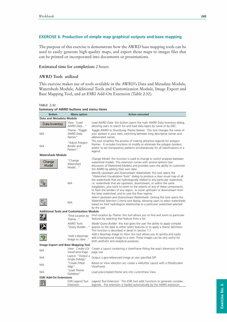
Workbook 245
Exer
cise
No
. 6
EXERCISE 6. Production of simple map graphical outputs and base mapping
The purpose of this exercise is demonstrate how the AWRD base mapping tools can be used to easily generate high-quality maps, and export those maps to images files that can be printed or incorporated into documents or presentations.
Estimated time for completion: 2 hours
AWRD Tools utilized
This exercise makes use of tools available in the AWRD’s Data and Metadata Module, Watersheds Module, Additional Tools and Customization Module, Image Export and Base Mapping Tool, and an ESRI Add-On Extension (Table 2.32).
TABLE 2.32Summary of AWRD buttons and menu items
Button Menu option Action executed
Data and Metadata ModuleView: “Load AWRD Data…”
Load AWRD Data: this button opens the main AWRD Data Inventory dialog, allowing users to search for and load data layers by name or by DBC.
N/ATheme: “Toggle AWRD Data Names”
Toggle AWRD to Short/Long Theme Names: This tool changes the name of your dataset in your view, switching between long descriptive names and abbreviated names.
N/A“Adjust Polygon Border and Pattern”
This tool simplifies the process of making attractive legends for polygon themes. It includes functions to modify or eliminate the polygon borders, and/or to set transparency patterns simultaneously for all classifications in a legend.
Watersheds Module
“Change Watershed Model…”
Change Model: this function is used to change or switch analyses between watershed models. This extension comes with several options (see discussion of Watershed Models) and provides users the ability to customize the AWRD by adding their own data.
N/A
Identify Upstream and Downstream Watersheds: this tool opens the “Watershed Visualization Tools” dialog to produce a clear visual map of all the watersheds that are hydrologically related to any particular watershed , i.e. watersheds that are upstream, downstream, or within the same megabasin, plus tools to zoom to the extents of any of these components, to flash the borders of any region, to move upstream or downstream from the base watershed, and to save the flow regime.
N/A
Select Upstream and Downstream Watersheds: clicking this tool opens the Watershed Selection Criteria tool dialog, allowing users to select watersheds based on their hydrological relationship to a particular watershed selected by the user.
Additional Tools and Customization Module
“Find Location by Theme...”
Find Location by Theme: this tool allows you to find and zoom to particular features by selecting that feature from a list.
AWRD Tools “Query Builder…”
Model Query Builder: this tool gives the user the ability to apply complex queries to the data to either select features or to apply a theme definition. This function is described in detail in Section 1.7.
“Add a Basemap Image to View...”
Add a Basemap Image to View: this tool allows you to quickly and easily add a background image to a view. These images can be very useful for both aesthetic and analytical purposes.
Image Export and Base Mapping Tool
N/AView: Create LO/ViewFrame-Page
Create a Layout containing a ViewFrame fitting the exact dimension of the page size
N/ALayout: “Output a Single PixMap”
Output a geo-referenced image at user specified DPI
N/A“Create Fitted Map”
Based on View selection set, create a A4/Letter Layout with a fitted/scaled ViewFrame
N/A“Load Theme Database”
Load precompiled theme sets into current/new View
ESRI Add-On ExtensionsESRI Legend Tool Extension
Legend Tool Extension: This ESRI tool adds functions to generate complex legends. The extension is loaded automatically by the AWRD extension.
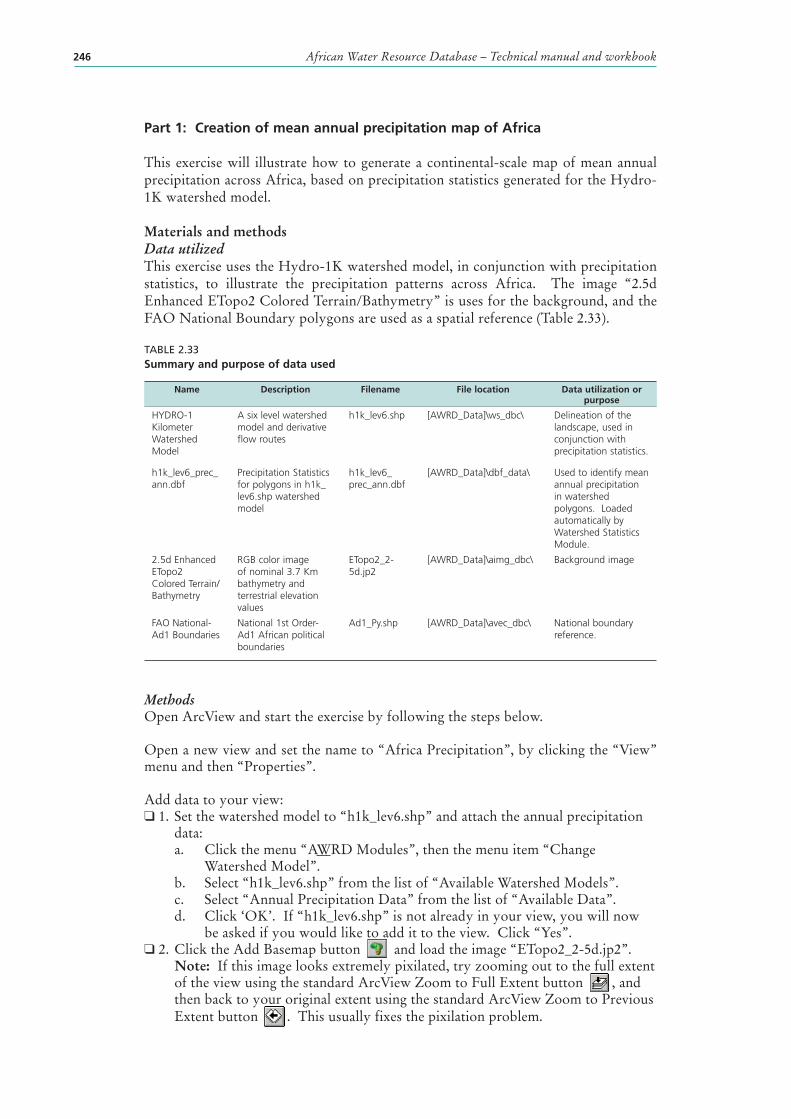
African Water Resource Database – Technical manual and workbook246
Part 1: Creation of mean annual precipitation map of Africa
This exercise will illustrate how to generate a continental-scale map of mean annual precipitation across Africa, based on precipitation statistics generated for the Hydro-1K watershed model.
Materials and methods Data utilizedThis exercise uses the Hydro-1K watershed model, in conjunction with precipitation statistics, to illustrate the precipitation patterns across Africa. The image “2.5d Enhanced ETopo2 Colored Terrain/Bathymetry” is uses for the background, and the FAO National Boundary polygons are used as a spatial reference (Table 2.33).
TABLE 2.33Summary and purpose of data used
Name Description Filename File location Data utilization or purpose
HYDRO-1 Kilometer Watershed Model
A six level watershed model and derivative flow routes
h1k_lev6.shp [AWRD_Data]\ws_dbc\ Delineation of the landscape, used in conjunction with precipitation statistics.
h1k_lev6_prec_ann.dbf
Precipitation Statistics for polygons in h1k_lev6.shp watershed model
h1k_lev6_prec_ann.dbf
[AWRD_Data]\dbf_data\ Used to identify mean annual precipitation in watershed polygons. Loaded automatically by Watershed Statistics Module.
2.5d Enhanced ETopo2 Colored Terrain/Bathymetry
RGB color image of nominal 3.7 Km bathymetry and terrestrial elevation values
ETopo2_2-5d.jp2
[AWRD_Data]\aimg_dbc\ Background image
FAO National-Ad1 Boundaries
National 1st Order-Ad1 African political boundaries
Ad1_Py.shp [AWRD_Data]\avec_dbc\ National boundary reference.
MethodsOpen ArcView and start the exercise by following the steps below.
Open a new view and set the name to “Africa Precipitation”, by clicking the “View” menu and then “Properties”.
Add data to your view:❑ 1. Set the watershed model to “h1k_lev6.shp” and attach the annual precipitation
data:a. Click the menu “AWRD Modules”, then the menu item “Change
Watershed Model”.b. Select “h1k_lev6.shp” from the list of “Available Watershed Models”.c. Select “Annual Precipitation Data” from the list of “Available Data”.d. Click ‘OK’. If “h1k_lev6.shp” is not already in your view, you will now
be asked if you would like to add it to the view. Click “Yes”.❑ 2. Click the Add Basemap button and load the image “ETopo2_2-5d.jp2”.
Note: If this image looks extremely pixilated, try zooming out to the full extent of the view using the standard ArcView Zoom to Full Extent button , and then back to your original extent using the standard ArcView Zoom to Previous Extent button . This usually fixes the pixilation problem.
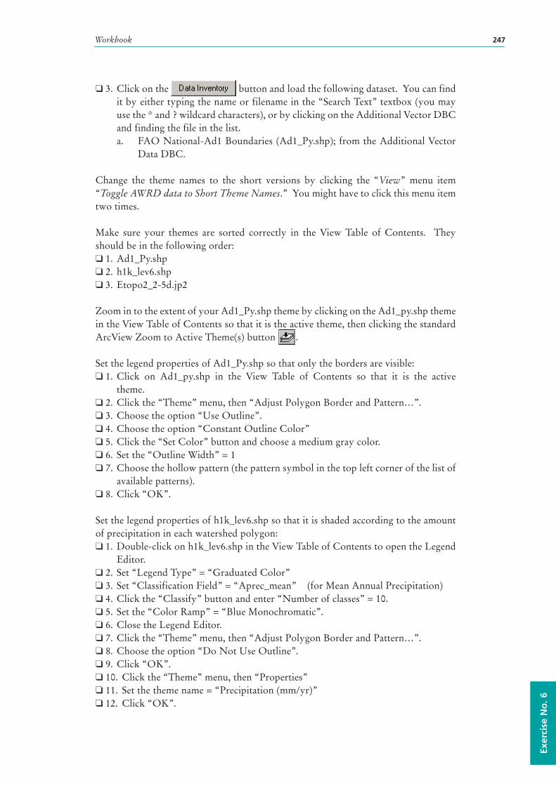
Workbook 247
Exer
cise
No
. 6
❑ 3. Click on the button and load the following dataset. You can find it by either typing the name or filename in the “Search Text” textbox (you may use the * and ? wildcard characters), or by clicking on the Additional Vector DBC and finding the file in the list.a. FAO National-Ad1 Boundaries (Ad1_Py.shp); from the Additional Vector
Data DBC.
Change the theme names to the short versions by clicking the “View” menu item “Toggle AWRD data to Short Theme Names.” You might have to click this menu item two times.
Make sure your themes are sorted correctly in the View Table of Contents. They should be in the following order:❑ 1. Ad1_Py.shp❑ 2. h1k_lev6.shp❑ 3. Etopo2_2-5d.jp2
Zoom in to the extent of your Ad1_Py.shp theme by clicking on the Ad1_py.shp theme in the View Table of Contents so that it is the active theme, then clicking the standard ArcView Zoom to Active Theme(s) button .
Set the legend properties of Ad1_Py.shp so that only the borders are visible:❑ 1. Click on Ad1_py.shp in the View Table of Contents so that it is the active
theme.❑ 2. Click the “Theme” menu, then “Adjust Polygon Border and Pattern…”.❑ 3. Choose the option “Use Outline”.❑ 4. Choose the option “Constant Outline Color”❑ 5. Click the “Set Color” button and choose a medium gray color.❑ 6. Set the “Outline Width” = 1❑ 7. Choose the hollow pattern (the pattern symbol in the top left corner of the list of
available patterns).❑ 8. Click “OK”.
Set the legend properties of h1k_lev6.shp so that it is shaded according to the amount of precipitation in each watershed polygon:❑ 1. Double-click on h1k_lev6.shp in the View Table of Contents to open the Legend
Editor.❑ 2. Set “Legend Type” = “Graduated Color”❑ 3. Set “Classification Field” = “Aprec_mean” (for Mean Annual Precipitation)❑ 4. Click the “Classify” button and enter “Number of classes” = 10.❑ 5. Set the “Color Ramp” = “Blue Monochromatic”.❑ 6. Close the Legend Editor.❑ 7. Click the “Theme” menu, then “Adjust Polygon Border and Pattern…”.❑ 8. Choose the option “Do Not Use Outline”.❑ 9. Click “OK”.❑ 10. Click the “Theme” menu, then “Properties”❑ 11. Set the theme name = “Precipitation (mm/yr)”❑ 12. Click “OK”.
African Water Resource Database – Technical manual and workbook248
Convert the view to a 15 cm x 15 cm layout:❑ 1. Click the “ImageExport” menu, then “Create LO/ViewFrame-Page”❑ 2. Set the Page Setup “Units” = “Centimeters”❑ 3. Set the “Width” = 15❑ 4. Set the “Height” = 15❑ 5. The layout will appear, and the only thing you will see on the layout will be the
view frame containing the view. ❑ 6. Double-click on the view frame to open the View Frame Properties dialog.❑ 7. Set the “Scale” – “User Specified Scale”❑ 8. Set the scale value = 70000000 (70 million)❑ 9. Click “OK”.
Note that the layout is linked to the view. If you move or add anything to the view, it will also appear in the layout. You may wish to try panning the view using the ArcView Pan tool and observing the effects on the layout. You will often need to pan the view a bit to get the image in the layout positioned correctly, especially after adding features like legends to the layout.
Add a legend to your layout, explaining the colors that correspond with each precipitation level.
❑ 1. Click the Custom Legend Tool in your Layout tool bar.❑ 2. Click in your layout somewhere, to open the “Custom Legend” dialog.❑ 3. Read the introductory text, then click “Next” to go to Step 1 of the Custom
Legend Tool.❑ 4. While in Step 1 of the Custom Legend tool:
a. Set the View = “Africa Precipitation”b. Select the theme “Precipitation (mm/yr)” to show in your custom legend.c. For the “number of label and symbol columns”, select “One per theme”.d. Click “Next” to go to Step 2.
❑ 5. While in Step 2 of the Custom Legend Tool:a. Set the “Optional Title” = “Precipitation (mm/yr)”b. Set the “Title Font” = “Arial”c. Set the “Title Size (pts)” = 18d. Set the “Title Style” = “Normal”e. On the “Title Positioning Options, choose the option that is centered
directly above the image.f. Click “Next” to go to Step 3.
❑ 6. While in Step 3 of the Custom Legend Tool:a. Select the top border style (a single line).b. Set the “Border Width” = 1.5c. Set the “Border Color” = “Black”d. Set the “Background Color” = “Light Gray”e. Click “Next” to go to Step 4.
❑ 7. While in Step 4 of the Custom Legend Tool:a. Select the option to show area symbols as Rectangles.b. The option for line symbols does not apply here, as there are no polyline
themes being symbolized in this legend.c. Click “Next” to go to Step 5.
❑ 8. While in Step 5 of the Custom Legend Tool:a. Leave the default values as they are.b. Click the “Preview” button to see how the legend looks.
Workbook 249
Exer
cise
No
. 6
c. It will probably be to large, but that can be fixed later. Decide if you like the text and colors of the legend. If it is acceptable, click “Finish” to close the Custom Legend Tool.
❑ 9. The legend will probably need to be moved and resized:a. Use the ArcView Pointer tool to select your new legend.b. Drag the legend down to the lower left corner of the layout.c. Because the legend is selected, it will have small squares on the sides and at
the corners of the legend. These squares are called “handles”. If you wish to resize the legend, click on one of the corner handles and drag it to change the dimensions.
d. Position and size the legend so that it looks good to you.e. If you wish, you can decompose the legend into separate elements by
clicking the ArcView Ungroup button . You may need to click it several times before you get all the subgroups split up. Then you can select each individual element and modify it using the Symbol Window. For example, you could set the some of the text to be a different font or a larger font size. It would be a good idea to regroup the legend elements when you finish (select them all, then click the ArcView Group button ), so that the entire legend can easily be resized or repositioned.
Export the image to a *.bmp file:❑ 1. Click the “ImageExport” menu, then “Output a Single Pixmap”.❑ 2. For Output Image Type, select “BMP”.❑ 3. You may be asked if you wish to convert the BMP to another image type. This
option is only available if you have installed IrfanView. For this example, we will choose “No” if we are offered this option.
❑ 4. Select a name and location to create your image file.❑ 5. Select a resolution = 200 for the image file. Note: Often the default resolution
value will produce a very high-resolution image, and you can usually reduce the default value to keep down the image size.
❑ 6. The layout will change size while the function is working. Upon completion, you will see a report of some statistical information on the pixel size. Note: If possible, this function will also create a “World File” that allows the image to be used in a GIS system. The report also gives details on the data included in the world file.
❑ 7. Click “OK” to close the report, and your layout will return to the proper size.
Now the image file can be treated like any other image file, added to documents or presentations or emailed. It can also be further edited in any image processing software you may use. If it has a world file, it can even be imported into a GIS and treated like any other image-based spatial data layer.
Try opening a program that accepts images, such as Microsoft Word or Powerpoint (or even ArcView), and importing your new image.
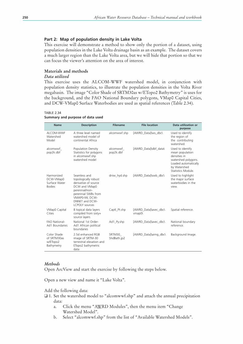
African Water Resource Database – Technical manual and workbook250
Part 2: Map of population density in Lake VoltaThis exercise will demonstrate a method to show only the portion of a dataset, using population densities in the Lake Volta drainage basin as an example. The dataset covers a much larger region than the Lake Volta area, but we will hide that portion so that we can focus the viewer’s attention on the area of interest.
Materials and methods Data utilizedThis exercise uses the ALCOM-WWF watershed model, in conjunction with population density statistics, to illustrate the population densities in the Volta River megabasin. The image “Color Shade of SRTM30as w/ETopo2 Bathymetry” is uses for the background, and the FAO National Boundary polygons, VMap0 Capital Cities, and DCW-VMap0 Surface Waterbodies are used as spatial references (Table 2.34).
TABLE 2.34Summary and purpose of data used
Name Description Filename File location Data utilization or purpose
ALCOM-WWF Watershed Model
A three level named watershed model of continental Africa
alcomwwf.shp [AWRD_Data]\ws_dbc\ Used to identify the region of the contributing watershed.
alcomwwf_pop2k.dbf
Population Density Statistics for polygons in alcomwwf.shp watershed model
alcomwwf_pop2k.dbf
[AWRD_Data]\dbf_data\ Used to identify mean population densities in watershed polygons. Loaded automatically by Watershed Statistics Module.
Harmonized DCW-VMap0 Surface Water Bodies
Seamless and topologically robust derivative of source DCW and VMap0 perennial/non-perennial SWBs from VMAP0-IW, DCW-DNNET and DCW-LCPOLY sources
dniw_hyd.shp [AWRD_Data]\swb_dbc\ Used to highlight the major surface waterbodies in the view.
VMap0 Capital Cities
8 topical data layers compiled from sixty+ source layers
Captl_Pt.shp [AWRD_Data]\avec_dbc\vmap0\
Spatial reference.
FAO National-Ad1 Boundaries
National 1st Order-Ad1 African political boundaries
Ad1_Py.shp [AWRD_Data]\avec_dbc\ National boundary reference.
Color Shade of SRTM30as w/ETopo2 Bathymetry
2.5d enhanced RGB image of SRTM-30 terrestrial elevation and ETopo2 bathymetric data
SRTM30_ShdBath.jp2
[AWRD_Data]\aimg_dbc\ Background Image.
MethodsOpen ArcView and start the exercise by following the steps below.
Open a new view and name it “Lake Volta”.
Add the following data:❑ 1. Set the watershed model to “alcomwwf.shp” and attach the annual precipitation
data:a. Click the menu “AWRD Modules”, then the menu item “Change
Watershed Model”.b. Select “alcomwwf.shp” from the list of “Available Watershed Models”.
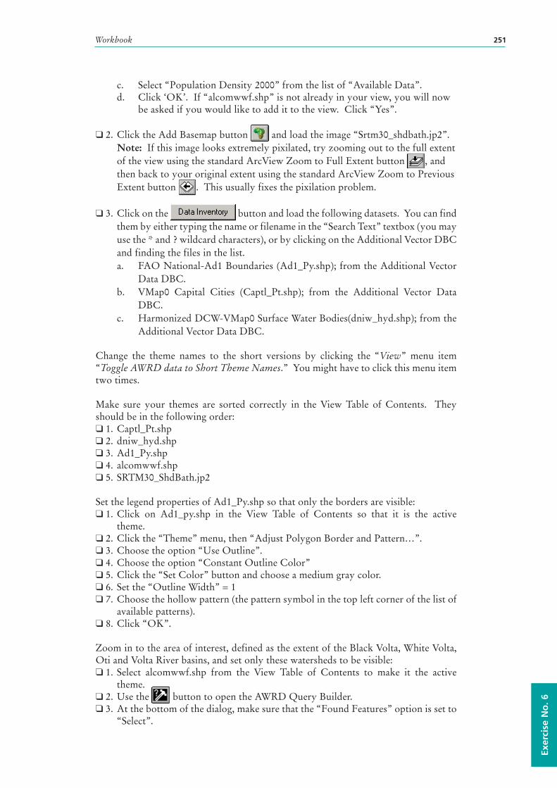
Workbook 251
Exer
cise
No
. 6
c. Select “Population Density 2000” from the list of “Available Data”.d. Click ‘OK’. If “alcomwwf.shp” is not already in your view, you will now
be asked if you would like to add it to the view. Click “Yes”.
❑ 2. Click the Add Basemap button and load the image “Srtm30_shdbath.jp2”. Note: If this image looks extremely pixilated, try zooming out to the full extent of the view using the standard ArcView Zoom to Full Extent button , and then back to your original extent using the standard ArcView Zoom to Previous Extent button . This usually fixes the pixilation problem.
❑ 3. Click on the button and load the following datasets. You can find them by either typing the name or filename in the “Search Text” textbox (you may use the * and ? wildcard characters), or by clicking on the Additional Vector DBC and finding the files in the list.a. FAO National-Ad1 Boundaries (Ad1_Py.shp); from the Additional Vector
Data DBC.b. VMap0 Capital Cities (Captl_Pt.shp); from the Additional Vector Data
DBC.c. Harmonized DCW-VMap0 Surface Water Bodies(dniw_hyd.shp); from the
Additional Vector Data DBC.
Change the theme names to the short versions by clicking the “View” menu item “Toggle AWRD data to Short Theme Names.” You might have to click this menu item two times.
Make sure your themes are sorted correctly in the View Table of Contents. They should be in the following order:❑ 1. Captl_Pt.shp❑ 2. dniw_hyd.shp❑ 3. Ad1_Py.shp❑ 4. alcomwwf.shp❑ 5. SRTM30_ShdBath.jp2
Set the legend properties of Ad1_Py.shp so that only the borders are visible:❑ 1. Click on Ad1_py.shp in the View Table of Contents so that it is the active
theme.❑ 2. Click the “Theme” menu, then “Adjust Polygon Border and Pattern…”.❑ 3. Choose the option “Use Outline”.❑ 4. Choose the option “Constant Outline Color”❑ 5. Click the “Set Color” button and choose a medium gray color.❑ 6. Set the “Outline Width” = 1❑ 7. Choose the hollow pattern (the pattern symbol in the top left corner of the list of
available patterns).❑ 8. Click “OK”.
Zoom in to the area of interest, defined as the extent of the Black Volta, White Volta, Oti and Volta River basins, and set only these watersheds to be visible:❑ 1. Select alcomwwf.shp from the View Table of Contents to make it the active
theme.❑ 2. Use the button to open the AWRD Query Builder.❑ 3. At the bottom of the dialog, make sure that the “Found Features” option is set to
“Select”.
African Water Resource Database – Technical manual and workbook252
❑ 4. Select the watersheds in the Black Volta, White Volta, Oti and Volta River Basins using the following query string:
( [Basin_name] = “Black Volta” ) OR ( [Basin_name] = “White Volta” ) OR ( [Basin_name] = “Oti” ) OR ( [Basin_name] = “Volta River” )
❑ 5. Leave the Query Builder dialog open, and click the ArcView “Zoom to Selected Features” button to zoom into the selected area.
❑ 6. We are only interested in these selected watersheds, and we set all other watersheds to be invisible. We can do this by setting the theme definition, using the AWRD Query Builder dialog:a. Near the bottom of the Query Builder Dialog, set the “Found Features”
option to “Set Theme Definition”.b. Set the following definition string (which is the same string used above):
( [Basin_name] = “Black Volta” ) OR ( [Basin_name] = “White Volta” ) OR ( [Basin_name] = “Oti” ) OR ( [Basin_name] = “Volta River” )
c. Click “New” to set the definition.d. Close the Query Builder dialog.
❑ 7. Clear the selection on alcomwwf.shp by clicking the ArcView Clear Selection button .
Set the legend properties of alcomwwf.shp so that it is shaded according to the population density in each watershed polygon:❑ 1. Double-click on alcomwwf.shp in the View Table of Contents to open the Legend
Editor.❑ 2. Set “Legend Type” = “Graduated Color”❑ 3. Set “Classification Field” = “P2k_mean” (for 2000 Mean Population Density)❑ 4. Click the “Classify” button and enter “Number of classes” = 10.❑ 5. Set the “Color Ramp” = “Red Monochromatic”.❑ 6. Ramp the colors using the Ramp button .❑ 7. Close the Legend Editor.❑ 8. Click the “Theme” menu, then “Adjust Polygon Border and Pattern…”.❑ 9. Choose the option “Do Not Use Outline”.❑ 10. Click “OK”.❑ 11. Click the “Theme” menu, then “Properties”❑ 12. Set the theme name = “Volta Population”❑ 13. Click “OK”.
Add labels to your view, providing names for countries and capitals:❑ 1. Open your ArcView symbol window by either clicking [CONTROL]-P, or
clicking the “Window” menu and then “Show Symbol Window…”.❑ 2. Add the Country Name labels:
a. In the Symbol Window, set the default text to be Times New Roman, with “Size” = 24 and “Style” = “Bold”.
b. Click the theme Ad1_Py.shp in your View Table of Contents to make it the active theme.
c. Open the Auto-Label dialog by either clicking [CONTROL]-L, or by clicking the “Theme” menu and then “Auto-Label…”.
d. Set the Label Field = “Country_na”e. Choose the option “Find Best Label Placementf. Choose the option “Remove Duplicates”g. Choose the option “Scale Labels”
Workbook 253
Exer
cise
No
. 6
h. Click “OK”. i. If you wish to add additional country name labels manually, use the ArcView
Label tool to click on the view wherever you wish to place a new label.❑ 3. Add the Capital City Name labels:
a. In the Symbol Window, set the default text to be Arial, with “Size” = 18 and “Style” = “Italic”.
b. Click the theme Captl_Pt.shp in your View Table of Contents to make it the active theme.
c. Open the Auto-Label dialog by either clicking [CONTROL]-L, or by clicking the “Theme” menu and then “Auto-Label…”.
d. Set the Label Field = “Name_propr”e. Choose the option “Find Best Label Placementf. Choose the option “Remove Duplicates”g. Choose the option “Scale Labels”h. Click “OK”.
❑ 4. Close the Symbol Window.❑ 5. If necessary, you can move any of these labels by selecting it with the tool,
and dragging it to a new location.
Convert the view to a 16 cm x 20 cm layout:❑ 1. Click the “ImageExport” menu, then “Create LO/ViewFrame-Page”❑ 2. Set the Page Setup “Units” = “Centimeters”❑ 3. Set the “Width” = 16❑ 4. Set the “Height” = 20❑ 5. The layout will appear, and the only thing you will see on the layout will be the
view frame containing the view. ❑ 6. Double-click on the view frame to open the View Frame Properties dialog.❑ 7. Set the “Scale” – “User Specified Scale”❑ 8. Set the scale value = 6500000 (6.5 million)❑ 9. Click “OK”.
Note that the layout view frame is linked to the view. If you move or add anything to the view, it will also appear in the layout view frame. You may wish to try panning the view using the ArcView Pan tool and observing the effects on the layout. You will often need to pan the view a bit to get the image in the layout positioned correctly, especially after adding features like legends to the layout. If you wish, you can unlink the layout view frame by double clicking on the view frame to open the “View Frame Properties” dialog, and then unchecking the “Live Link” checkbox.
Add a legend to your layout, explaining the colors that correspond with each population density level.❑ 1. Click the Custom Legend Tool in your Layout tool bar.❑ 2. Click in your layout somewhere, to open the “Custom Legend” dialog.❑ 3. Read the introductory text, then click “Next” to go to Step 1 of the Custom
Legend Tool.❑ 4. While in Step 1 of the Custom Legend tool:
a. Set the View = “Lake Volta”b. Select the theme “Volta Population” to show in your custom legend.c. For the “number of label and symbol columns”, select “One per theme”.d. Click “Next” to go to Step 2.
African Water Resource Database – Technical manual and workbook254
❑ 5. While in Step 2 of the Custom Legend Tool:a. Set the “Optional Title” = “Population Density (pp/km2)”b. Set the “Title Font” = “Arial”c. Set the “Title Size (pts)” = 18d. Set the “Title Style” = “Normal”e. On the “Title Positioning Options, choose the option that is centered
directly above the image.f. Click “Next” to go to Step 3.
❑ 6. While in Step 3 of the Custom Legend Tool:a. Select the top border style (a single line).b. Set the “Border Width” = 1.5c. Set the “Border Color” = “Black”d. Set the “Background Color” = “White”e. Click “Next” to go to Step 4.
❑ 7. While in Step 4 of the Custom Legend Tool:a. Select the option to show area symbols as Rectangles.b. The option for line symbols does not apply here, as there are no polyline
themes being symbolized in this legend.c. Click “Next” to go to Step 5.
❑ 8. While in Step 5 of the Custom Legend Tool:a. Leave the default values as they are.b. Click the “Preview” button to see how the legend looks.c. It will probably be to large, but that can be fixed later. Decide if you like the
text and colors of the legend. If it is acceptable, click “Finish” to close the Custom Legend Tool.
❑ 9. The legend will probably need to be moved and resized:a. Use the ArcView Pointer tool to select your new legend.b. Drag the legend down to the lower left corner of the layout.c. If you wish to resize the legend, click on one of the corner handles and drag
it to change the dimensions. d. Position and size the legend so that it looks good to you.e. If you wish, you can decompose the legend into separate elements by
clicking the ArcView Ungroup button . You may need to click it several times before you get all the subgroups split up. Then you can select each individual element and modify it using the Symbol Window. For example, you could set the some of the text to be a different font or a larger font size. It would be a good idea to regroup the legend elements when you finish (select them all, then click the ArcView Group button ), so that the entire legend can easily be resized or repositioned.
Export the layout to a *.jpg image:❑ 1. Click the “ImageExport” menu, then “Output a Single Pixmap”.❑ 2. For Output Image Type, select “JPG”.❑ 3. Select a name and location to create your image file.❑ 4. Select a resolution = 200 for the image file. Note: Often the default resolution
value will produce a very high-resolution image, and you can usually reduce the default value to keep down the image size.
❑ 5. The layout will change size while the function is working. Upon completion, you will see a report of some statistical information on the pixel size. Note: If possible, this function will also create a “World File” that allows the image to be
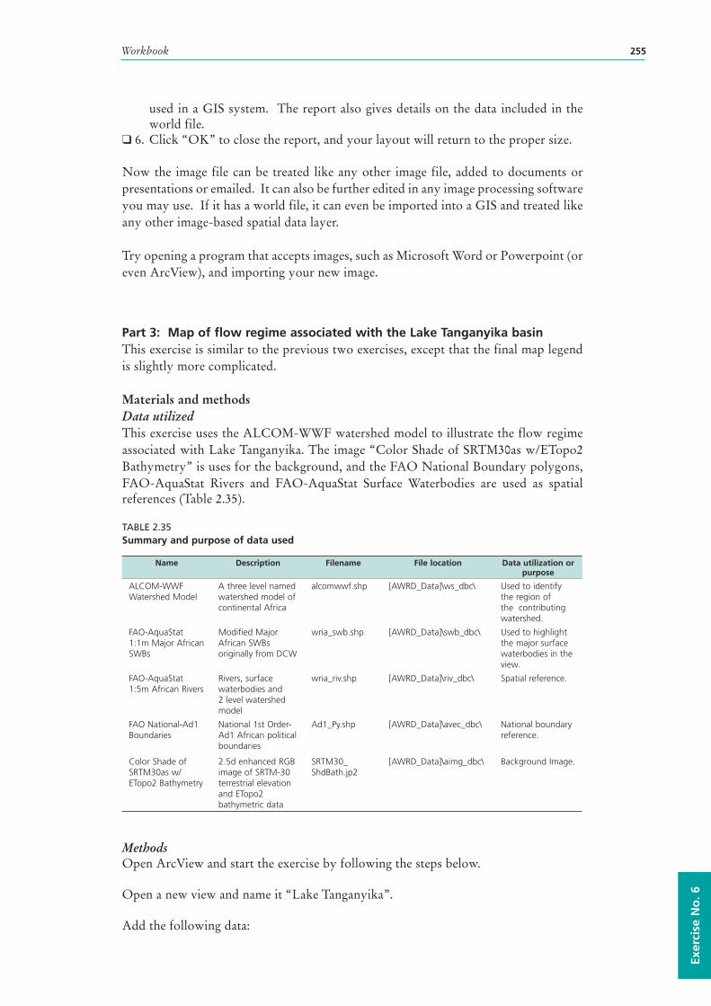
Workbook 255
Exer
cise
No
. 6
used in a GIS system. The report also gives details on the data included in the world file.
❑ 6. Click “OK” to close the report, and your layout will return to the proper size.
Now the image file can be treated like any other image file, added to documents or presentations or emailed. It can also be further edited in any image processing software you may use. If it has a world file, it can even be imported into a GIS and treated like any other image-based spatial data layer.
Try opening a program that accepts images, such as Microsoft Word or Powerpoint (or even ArcView), and importing your new image.
Part 3: Map of flow regime associated with the Lake Tanganyika basinThis exercise is similar to the previous two exercises, except that the final map legend is slightly more complicated.
Materials and methods Data utilizedThis exercise uses the ALCOM-WWF watershed model to illustrate the flow regime associated with Lake Tanganyika. The image “Color Shade of SRTM30as w/ETopo2 Bathymetry” is uses for the background, and the FAO National Boundary polygons, FAO-AquaStat Rivers and FAO-AquaStat Surface Waterbodies are used as spatial references (Table 2.35).
TABLE 2.35Summary and purpose of data used
Name Description Filename File location Data utilization or purpose
ALCOM-WWF Watershed Model
A three level named watershed model of continental Africa
alcomwwf.shp [AWRD_Data]\ws_dbc\ Used to identify the region of the contributing watershed.
FAO-AquaStat 1:1m Major African SWBs
Modified Major African SWBs originally from DCW
wria_swb.shp [AWRD_Data]\swb_dbc\ Used to highlight the major surface waterbodies in the view.
FAO-AquaStat 1:5m African Rivers
Rivers, surface waterbodies and 2 level watershed model
wria_riv.shp [AWRD_Data]\riv_dbc\ Spatial reference.
FAO National-Ad1 Boundaries
National 1st Order-Ad1 African political boundaries
Ad1_Py.shp [AWRD_Data]\avec_dbc\ National boundary reference.
Color Shade of SRTM30as w/ETopo2 Bathymetry
2.5d enhanced RGB image of SRTM-30 terrestrial elevation and ETopo2 bathymetric data
SRTM30_ShdBath.jp2
[AWRD_Data]\aimg_dbc\ Background Image.
MethodsOpen ArcView and start the exercise by following the steps below.
Open a new view and name it “Lake Tanganyika”.
Add the following data:
African Water Resource Database – Technical manual and workbook256
❑ 1. Set the watershed model to “alcomwwf.shp” and attach the annual precipitation data:a. Click the menu “AWRD Modules”, then the menu item “Change
Watershed Model”.b. Select “alcomwwf.shp” from the list of “Available Watershed Models”.c. This exercise does not require any additional data. You may select any
datasets you wish or none at all.d. Click ‘OK’. If “alcomwwf.shp” is not already in your view, you will now
be asked if you would like to add it to the view. Click “Yes”.
❑ 2. Click the Add Basemap button and load the image “Srtm30_shdbath.jp2”. Note: If this image looks extremely pixilated, try zooming out to the full extent of the view using the standard ArcView Zoom to Full Extent button , and then back to your original extent using the standard ArcView Zoom to Previous Extent button . This usually fixes the pixilation problem.
❑ 3. Click on the button and load the following datasets. You can find them by either typing the name or filename in the “Search Text” textbox (you may use the * and ? wildcard characters), or by clicking on the respective DBC and finding the file in the list.a. FAO National-Ad1 Boundaries (Ad1_Py.shp); from the Additional Vector
Data DBC.b. FAO-AquaStat 1:1m Major African SWBs (wria_swb.shp); from the Surface
Waterbody DBC.c. FAO-AquaStat 1:5m African Rivers (wria_riv.shp); from the Surface
Waterbody DBC.
Change the theme names to the short versions by clicking the “View” menu item “Toggle AWRD data to Short Theme Names.” You might have to click this menu item two times.
Make sure your themes are sorted correctly in the View Table of Contents. They should be in the following order:❑ 1. Ad1_Py.shp ❑ 2. alcomwwf.shp❑ 3. wria_swb.shp❑ 4. wria_riv.shp❑ 5. SRTM30_ShdBath.jp2
Set the legend properties of Ad1_Py.shp so that only the borders are visible:❑ 1. Click on Ad1_py.shp in the View Table of Contents so that it is the active
theme.❑ 2. Click the “Theme” menu, then “Adjust Polygon Border and Pattern…”.❑ 3. Choose the option “Use Outline”.❑ 4. Choose the option “Constant Outline Color”❑ 5. Click the “Set Color” button and choose a light gray color.❑ 6. Set the “Outline Width” = 1.5❑ 7. Choose the hollow pattern (the pattern symbol in the top left corner of the list of
available patterns).❑ 8. Click “OK”.
Workbook 257
Exer
cise
No
. 6
Find and zoom in to Lake Tanganyika:❑ 1. Click on the wria_swb.shp theme in the View Table of Contents to make it the
active theme.❑ 2. Click the button to open the “Find Location by Theme” dialog.❑ 3. Set the “Theme to Search” = “wria_swb.shp”, and the “Field to Search” = “Swb_
name”.❑ 4. Enter the search term “tanganyika”.❑ 5. Select “Tanganyika [rec. 342]” in the list and click “OK” to zoom in to Lake
Tanganyika.
Display and zoom in to the hydrological network associated with Lake Tanganyika:❑ 1. Use the “Identify Upstream and Downstream Watersheds” tool to click on
Lake Tanganyika.❑ 2. Click the “Zoom to Extent of Upstream and Downstream Polygons” button
to see the full drainage system associated with Lake Tanganyika.❑ 3. Change the legend symbols associated with the watershed model by clicking the
button. Choose the legend named “just_primary.avl”.
Change the theme names back to the long versions by clicking the “View” menu item “Toggle AWRD data to Long Theme Names.”
Change the name of the theme “ALCOM-WWF Watershed Model” to “Lake Tanganyika Flow Regime”.❑ 1. Select the theme “ALCOM-WWF Watershed Model in the View Table of
Contents to make it active.❑ 2. Click the “Theme” menu, then “Properties”, to open the “Theme Properties”
dialog.❑ 3. Enter the new theme name “Lake Tanganyika Flow Regime” into the “Theme
Name” text box.
Add Country Name labels to your view:❑ 1. Open your ArcView symbol window by either clicking [CONTROL]-P, or
clicking the “Window” menu and then “Show Symbol Window…”.❑ 2. In the Symbol Window, set the default text to be Times New Roman, with “Size”
= 14 and “Style” = “Bold”.❑ 3. Click the theme “FAO National-Ad1 Boundaries” in your View Table of
Contents to make it the active theme.❑ 4. Open the Auto-Label dialog by either clicking [CONTROL]-L, or by clicking
the “Theme” menu and then “Auto-Label…”.❑ 5. Set the Label Field = “Country_na”❑ 6. Choose the option “Find Best Label Placement❑ 7. Choose the option “Remove Duplicates”❑ 8. Choose the option “Scale Labels”❑ 9. Click “OK”. ❑ 10. You will probably need to adjust some of the names, either moving them or
changing the text. To change the text, double-click on the label with the tool and then type in the correct text.
❑ 11. If you wish to add country name labels manually, use the ArcView Label tool to click on the view wherever you wish to place a new label.
African Water Resource Database – Technical manual and workbook258
Convert the view to a 20 cm x 16 cm layout:❑ 1. Click the “ImageExport” menu, then “Create LO/ViewFrame-Page”❑ 2. Set the Page Setup “Units” = “Centimeters”❑ 3. Set the “Width” = 20❑ 4. Set the “Height” = 16❑ 5. The layout will appear, and the only thing you will see on the layout will be the
view frame containing the view. ❑ 6. Double-click on the view frame to open the View Frame Properties dialog.❑ 7. Set the “Scale” – “User Specified Scale”❑ 8. Set the scale value = 14000000 (14 million)❑ 9. Click “OK”.
Note that the layout is linked to the view. If you move or add anything to the view, it will also appear in the layout. You may wish to try panning the view using the ArcView Pan tool and observing the effects on the layout. You will often need to pan the view a bit to get the image in the layout positioned correctly, especially after adding features like legends to the layout.
Add a legend to your layout, explaining the colors that correspond with each population density level:❑ 1. Click the Custom Legend Tool in your Layout tool bar.❑ 2. Click in your layout somewhere, to open the “Custom Legend” dialog.❑ 3. Read the introductory text, then click “Next” to go to Step 1 of the Custom
Legend Tool.❑ 4. While in Step 1 of the Custom Legend tool:
a. Set the View = “Lake Tanganyika”b. Select the theme “Lake Tanganyika Flow Regime” to show in your custom
legend.c. Select the theme “FAO-AquaStat 1:5m African Rivers” to show in your
custom legend tool.d. For the “number of label and symbol columns”, select “2”.e. Click “Next” to go to Step 2.
❑ 5. While in Step 2 of the Custom Legend Tool:a. Delete the text in the “Optional Title” textbox. This will automatically
disable the remaining options.b. Click “Next” to go to Step 3.
❑ 6. While in Step 3 of the Custom Legend Tool:a. Select the top border style (a single line).b. Set the “Border Width” = 1.5c. Set the “Border Color” = “Black”d. Set the “Background Color” = “White”e. Select the option “Round corners”f. Click “Next” to go to Step 4.
❑ 7. While in Step 4 of the Custom Legend Tool:a. Select the option to show area symbols as Rectangles.b. Select the option to show line symbols as horizontal lines.c. Click “Next” to go to Step 5.
❑ 8. While in Step 5 of the Custom Legend Tool:a. Leave the default values as they are.b. Click the “Preview” button to see how the legend looks.
Workbook 259
Exer
cise
No
. 6
c. It will probably be to large, but that can be fixed later. Decide if you like the text and colors of the legend. If it is acceptable, click “Finish” to close the Custom Legend Tool.
❑ 9. The legend will probably need to be moved and resized:a. Use the ArcView Pointer tool to select your new legend.b. Drag the legend down to the lower left corner of the layout.c. If you wish to resize the legend, click on one of the corner handles and drag
it to change the dimensions. d. Position and size the legend so that it looks good to you.e. If you wish, you can decompose the legend into separate elements by
clicking the ArcView Ungroup button . You may need to click it several times before you get all the subgroups split up. Then you can select each individual element and modify it using the Symbol Window. For example, you could set the some of the text to be a different font or a larger font size. It would be a good idea to regroup the legend elements when you finish (select them all, then click the ArcView Group button ), so that the entire legend can easily be resized or repositioned.
Export the layout to a *.jpg image:❑ 1. Click the “ImageExport” menu, then “Output a Single Pixmap”.❑ 2. For Output Image Type, select “JPG”.❑ 3. Select a name and location to create your image file.❑ 4. Select a resolution = 200 for the image file. Note: Often the default resolution
value will produce a very high-resolution image, and you can usually reduce the default value to keep down the image size.
❑ 5. The layout will change size while the function is working. Upon completion, you will see a report of some statistical information on the pixel size. Note: If possible, this function will also create a “World File” that allows the image to be used in a GIS system. The report also gives details on the data included in the world file.
❑ 6. Click “OK” to close the report, and your layout will return to the proper size.
Part 4: Map of Nile megabasin wetlandsThis exercise will generate a simple map with no background to distract from the main image, introducing the concept of a mask. This exercise will also introduce some common map elements such as a title, scale bar and north arrow.
Materials and methods Data utilizedThis exercise uses the ALCOM-WWF watershed model to identify the region of the Nile River Megabasin. The WCMC Wetlands are then displayed within the Nile River Megabasin (Table 2.36).
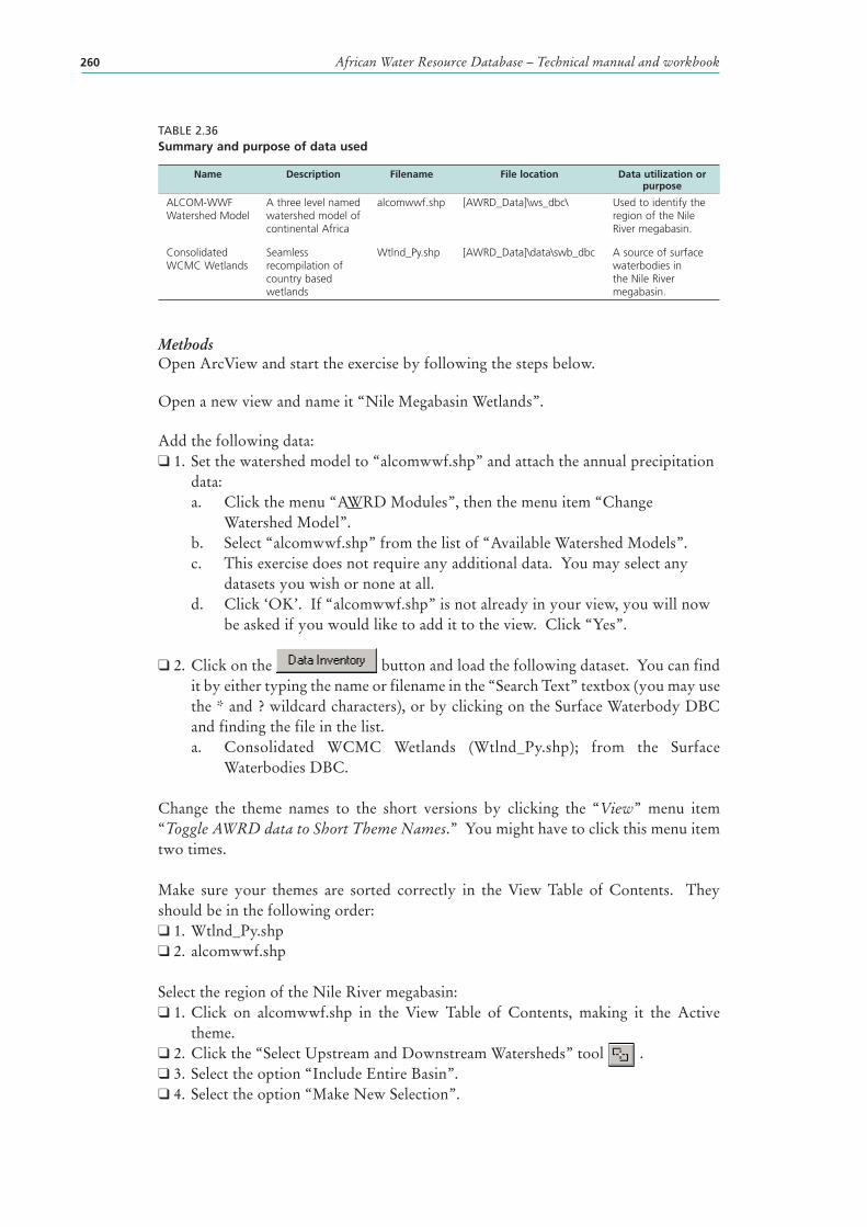
African Water Resource Database – Technical manual and workbook260
TABLE 2.36Summary and purpose of data used
Name Description Filename File location Data utilization or purpose
ALCOM-WWF Watershed Model
A three level named watershed model of continental Africa
alcomwwf.shp [AWRD_Data]\ws_dbc\ Used to identify the region of the Nile River megabasin.
Consolidated WCMC Wetlands
Seamless recompilation of country based wetlands
Wtlnd_Py.shp [AWRD_Data]\data\swb_dbc A source of surface waterbodies in the Nile River megabasin.
MethodsOpen ArcView and start the exercise by following the steps below.
Open a new view and name it “Nile Megabasin Wetlands”.
Add the following data:❑ 1. Set the watershed model to “alcomwwf.shp” and attach the annual precipitation
data:a. Click the menu “AWRD Modules”, then the menu item “Change
Watershed Model”.b. Select “alcomwwf.shp” from the list of “Available Watershed Models”.c. This exercise does not require any additional data. You may select any
datasets you wish or none at all.d. Click ‘OK’. If “alcomwwf.shp” is not already in your view, you will now
be asked if you would like to add it to the view. Click “Yes”.
❑ 2. Click on the button and load the following dataset. You can find it by either typing the name or filename in the “Search Text” textbox (you may use the * and ? wildcard characters), or by clicking on the Surface Waterbody DBC and finding the file in the list.a. Consolidated WCMC Wetlands (Wtlnd_Py.shp); from the Surface
Waterbodies DBC.
Change the theme names to the short versions by clicking the “View” menu item “Toggle AWRD data to Short Theme Names.” You might have to click this menu item two times.
Make sure your themes are sorted correctly in the View Table of Contents. They should be in the following order:❑ 1. Wtlnd_Py.shp ❑ 2. alcomwwf.shp
Select the region of the Nile River megabasin:❑ 1. Click on alcomwwf.shp in the View Table of Contents, making it the Active
theme.❑ 2. Click the “Select Upstream and Downstream Watersheds” tool .❑ 3. Select the option “Include Entire Basin”.❑ 4. Select the option “Make New Selection”.
Workbook 261
Exer
cise
No
. 6
❑ 5. Click anywhere in the Nile River megabasin to select the entire megabasin. Hint: Lake Victoria is in the Nile River megabasin, and is an easy feature to find.
Create a mask and zoom in to the Nile River megabasin:❑ 1. While the Nile River megabasin is selected, click the ImageExport menu, and then
“Create Fitted Map”. This function will create a new shapefile which will act as a mask for the selected area.
❑ 2. Specify the name and location for your mask shapefile. This exercise will use the name “nile_mask.shp”.
❑ 3. It may take a few minutes to make the mask shapefile, so be patient. When it finishes, it will add the mask shapefile to your view and zoom in to the selected area. It will also make a layout which is linked to the view.
Adjust the mask legend properties:❑ 1. Double-click on nile_mask.shp in the Theme Table of Contents to open up the
Legend Editor.❑ 2. Double-click on the symbol for Mask Value = 0 to open up the Symbol Window.
This are a represents the interior of the Nile River megabasin.❑ 3. Set a hollow symbol (in the upper left corner of the list of symbols), with an
outline width of 2.❑ 4. Close the Symbol Window and click “Apply” on the Legend Editor window.❑ 5. Double-click on the symbol for Mask Value = 1 to open the Symbol Window.
This area represents the exterior of the Nile River megabasin, and will be masked out in the final map.
❑ 6. Select a solid symbol (in the middle of the top row of the list of symbols), with an outline width of “None”. Set the Foreground Color = white.
Change the theme names to the long versions by clicking the “View” menu item “Toggle AWRD data to Long Theme Names.”
If you wish, you may adjust your WCMC legend properties, by either changing the color of any wetland types to make them more distinctive, or by deleting any types that you do not wish to include in the map. All these functions are done in the Legend Editor.
Open your layout that was created when you made the mask. Note that the layout is linked to the view. If you move or add anything to the view, it will also appear in the layout. You may wish to try panning the view using the ArcView Pan tool and observing the effects on the layout. You will often need to pan the view a bit to get the image in the layout positioned correctly, especially after adding features like legends to the layout.❑ 1. Double-click on the view frame to open the View Frame Properties dialog.❑ 2. Set the “Scale” – “User Specified Scale”❑ 3. Set the scale value = 17000000 (17 million)❑ 4. Click “OK”.
Add a legend to your layout, explaining the colors that correspond with each wetland type:
❑ 1. Click the Custom Legend Tool in your Layout tool bar.❑ 2. Click in your layout somewhere, to open the “Custom Legend” dialog.❑ 3. Read the introductory text, then click “Next” to go to Step 1 of the Custom
Legend Tool.
African Water Resource Database – Technical manual and workbook262
❑ 4. While in Step 1 of the Custom Legend tool:a. Set the View = “Nile Megabasin Wetlands”b. Select the theme “Consolidated WCMC Wetlands” to show in your custom
legend.c. For the “number of label and symbol columns”, select “One per theme”.d. Click “Next” to go to Step 2.
❑ 5. While in Step 2 of the Custom Legend Tool:a. Set the “Optional Title” = “Legend”b. Set the “Title Font” = “Arial”c. Set the “Title Size (pts)” = 18d. Set the “Title Style” = “Normal”e. On the “Title Positioning Options, choose the option that is centered
directly above the image.f. Click “Next” to go to Step 3.
❑ 6. While in Step 3 of the Custom Legend Tool:a. Select the top border style (a single line).b. Set the “Border Width” = 1.5c. Set the “Border Color” = “Black”d. Set the “Background Color” = “White”e. Select the option “Round corners”f. Click “Next” to go to Step 4.
❑ 7. While in Step 4 of the Custom Legend Tool:a. Select the option to show area symbols as Rectangles.b. The option for line symbols does not apply here, as there are no polyline
themes being symbolized in this legend.c. Click “Next” to go to Step 5.
❑ 8. While in Step 5 of the Custom Legend Tool:a. Leave the default values as they are.b. Click the “Preview” button to see how the legend looks.c. It will probably be to large, but that can be fixed later. Decide if you like the
text and colors of the legend. If it is acceptable, click “Finish” to close the Custom Legend Tool.
❑ 9. The legend will probably need to be moved and resized:a. Use the ArcView Pointer tool to select your new legend.b. Drag the legend down to the lower left corner of the layout.c. If you wish to resize the legend, click on one of the corner handles and drag
it to change the dimensions. d. Position and size the legend so that it looks good to you.e. If you wish, you can decompose the legend into separate elements by
clicking the ArcView Ungroup button . You may need to click it several times before you get all the subgroups split up. Then you can select each individual element and modify it using the Symbol Window. For example, you could set the some of the text to be a different font or a larger font size. It would be a good idea to regroup the legend elements when you finish (select them all, then click the ArcView Group button ), so that the entire legend can easily be resized or repositioned.
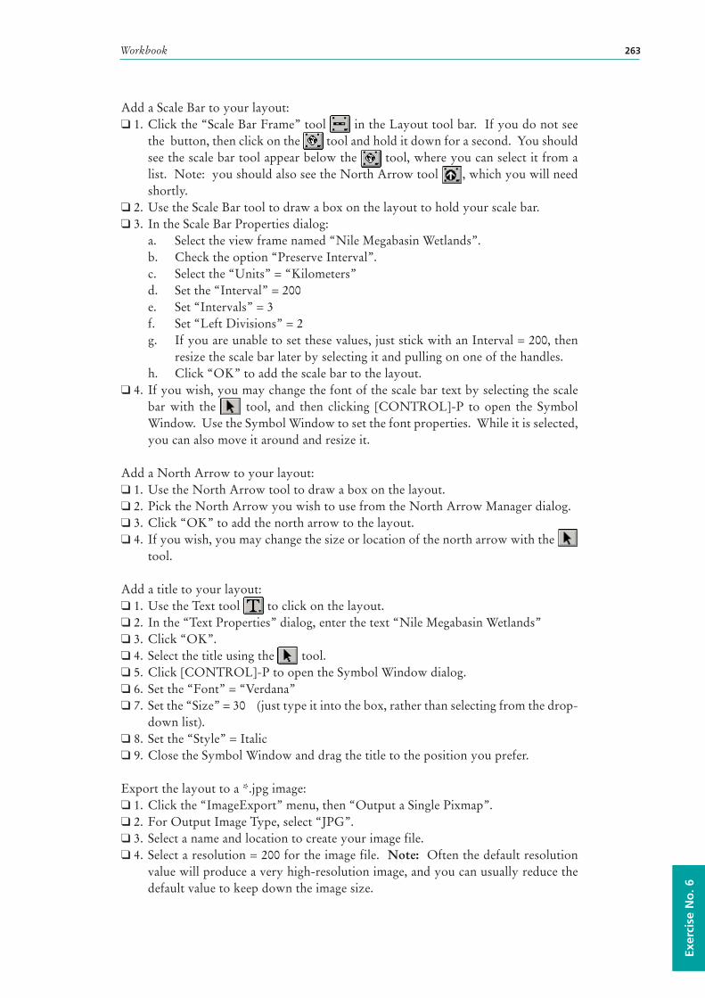
Workbook 263
Exer
cise
No
. 6
Add a Scale Bar to your layout:❑ 1. Click the “Scale Bar Frame” tool in the Layout tool bar. If you do not see
the button, then click on the tool and hold it down for a second. You should see the scale bar tool appear below the tool, where you can select it from a list. Note: you should also see the North Arrow tool , which you will need shortly.
❑ 2. Use the Scale Bar tool to draw a box on the layout to hold your scale bar.❑ 3. In the Scale Bar Properties dialog:
a. Select the view frame named “Nile Megabasin Wetlands”.b. Check the option “Preserve Interval”.c. Select the “Units” = “Kilometers”d. Set the “Interval” = 200e. Set “Intervals” = 3f. Set “Left Divisions” = 2g. If you are unable to set these values, just stick with an Interval = 200, then
resize the scale bar later by selecting it and pulling on one of the handles.h. Click “OK” to add the scale bar to the layout.
❑ 4. If you wish, you may change the font of the scale bar text by selecting the scale bar with the tool, and then clicking [CONTROL]-P to open the Symbol Window. Use the Symbol Window to set the font properties. While it is selected, you can also move it around and resize it.
Add a North Arrow to your layout:❑ 1. Use the North Arrow tool to draw a box on the layout.❑ 2. Pick the North Arrow you wish to use from the North Arrow Manager dialog.❑ 3. Click “OK” to add the north arrow to the layout.❑ 4. If you wish, you may change the size or location of the north arrow with the
tool.
Add a title to your layout:❑ 1. Use the Text tool to click on the layout.❑ 2. In the “Text Properties” dialog, enter the text “Nile Megabasin Wetlands”❑ 3. Click “OK”.❑ 4. Select the title using the tool.❑ 5. Click [CONTROL]-P to open the Symbol Window dialog.❑ 6. Set the “Font” = “Verdana”❑ 7. Set the “Size” = 30 (just type it into the box, rather than selecting from the drop-
down list).❑ 8. Set the “Style” = Italic❑ 9. Close the Symbol Window and drag the title to the position you prefer.
Export the layout to a *.jpg image:❑ 1. Click the “ImageExport” menu, then “Output a Single Pixmap”.❑ 2. For Output Image Type, select “JPG”.❑ 3. Select a name and location to create your image file.❑ 4. Select a resolution = 200 for the image file. Note: Often the default resolution
value will produce a very high-resolution image, and you can usually reduce the default value to keep down the image size.
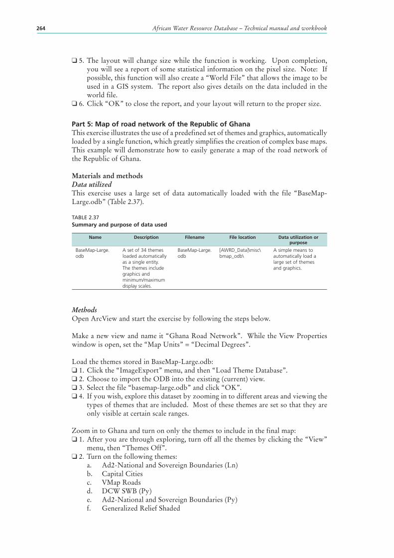
African Water Resource Database – Technical manual and workbook264
❑ 5. The layout will change size while the function is working. Upon completion, you will see a report of some statistical information on the pixel size. Note: If possible, this function will also create a “World File” that allows the image to be used in a GIS system. The report also gives details on the data included in the world file.
❑ 6. Click “OK” to close the report, and your layout will return to the proper size.
Part 5: Map of road network of the Republic of GhanaThis exercise illustrates the use of a predefined set of themes and graphics, automatically loaded by a single function, which greatly simplifies the creation of complex base maps. This example will demonstrate how to easily generate a map of the road network of the Republic of Ghana.
Materials and methods Data utilizedThis exercise uses a large set of data automatically loaded with the file “BaseMap-Large.odb” (Table 2.37).
TABLE 2.37Summary and purpose of data used
Name Description Filename File location Data utilization or purpose
BaseMap-Large.odb
A set of 34 themes loaded automatically as a single entity. The themes include graphics and minimum/maximum display scales.
BaseMap-Large.odb
[AWRD_Data]\misc\bmap_odb\
A simple means to automatically load a large set of themes and graphics.
MethodsOpen ArcView and start the exercise by following the steps below.
Make a new view and name it “Ghana Road Network”. While the View Properties window is open, set the “Map Units” = “Decimal Degrees”.
Load the themes stored in BaseMap-Large.odb:❑ 1. Click the “ImageExport” menu, and then “Load Theme Database”.❑ 2. Choose to import the ODB into the existing (current) view.❑ 3. Select the file “basemap-large.odb” and click “OK”.❑ 4. If you wish, explore this dataset by zooming in to different areas and viewing the
types of themes that are included. Most of these themes are set so that they are only visible at certain scale ranges.
Zoom in to Ghana and turn on only the themes to include in the final map:❑ 1. After you are through exploring, turn off all the themes by clicking the “View”
menu, then “Themes Off”.❑ 2. Turn on the following themes:
a. Ad2-National and Sovereign Boundaries (Ln)b. Capital Citiesc. VMap Roadsd. DCW SWB (Py)e. Ad2-National and Sovereign Boundaries (Py)f. Generalized Relief Shaded
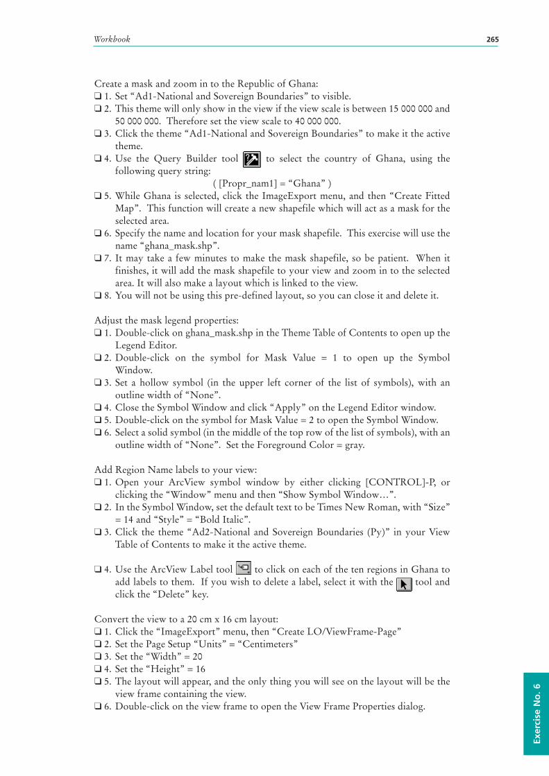
Workbook 265
Exer
cise
No
. 6
Create a mask and zoom in to the Republic of Ghana:❑ 1. Set “Ad1-National and Sovereign Boundaries” to visible.❑ 2. This theme will only show in the view if the view scale is between 15 000 000 and
50 000 000. Therefore set the view scale to 40 000 000.❑ 3. Click the theme “Ad1-National and Sovereign Boundaries” to make it the active
theme. ❑ 4. Use the Query Builder tool to select the country of Ghana, using the
following query string:( [Propr_nam1] = “Ghana” )
❑ 5. While Ghana is selected, click the ImageExport menu, and then “Create Fitted Map”. This function will create a new shapefile which will act as a mask for the selected area.
❑ 6. Specify the name and location for your mask shapefile. This exercise will use the name “ghana_mask.shp”.
❑ 7. It may take a few minutes to make the mask shapefile, so be patient. When it finishes, it will add the mask shapefile to your view and zoom in to the selected area. It will also make a layout which is linked to the view.
❑ 8. You will not be using this pre-defined layout, so you can close it and delete it.
Adjust the mask legend properties:❑ 1. Double-click on ghana_mask.shp in the Theme Table of Contents to open up the
Legend Editor.❑ 2. Double-click on the symbol for Mask Value = 1 to open up the Symbol
Window.❑ 3. Set a hollow symbol (in the upper left corner of the list of symbols), with an
outline width of “None”.❑ 4. Close the Symbol Window and click “Apply” on the Legend Editor window.❑ 5. Double-click on the symbol for Mask Value = 2 to open the Symbol Window.❑ 6. Select a solid symbol (in the middle of the top row of the list of symbols), with an
outline width of “None”. Set the Foreground Color = gray.
Add Region Name labels to your view:❑ 1. Open your ArcView symbol window by either clicking [CONTROL]-P, or
clicking the “Window” menu and then “Show Symbol Window…”.❑ 2. In the Symbol Window, set the default text to be Times New Roman, with “Size”
= 14 and “Style” = “Bold Italic”.❑ 3. Click the theme “Ad2-National and Sovereign Boundaries (Py)” in your View
Table of Contents to make it the active theme.
❑ 4. Use the ArcView Label tool to click on each of the ten regions in Ghana to add labels to them. If you wish to delete a label, select it with the tool and click the “Delete” key.
Convert the view to a 20 cm x 16 cm layout:❑ 1. Click the “ImageExport” menu, then “Create LO/ViewFrame-Page”❑ 2. Set the Page Setup “Units” = “Centimeters”❑ 3. Set the “Width” = 20❑ 4. Set the “Height” = 16❑ 5. The layout will appear, and the only thing you will see on the layout will be the
view frame containing the view. ❑ 6. Double-click on the view frame to open the View Frame Properties dialog.
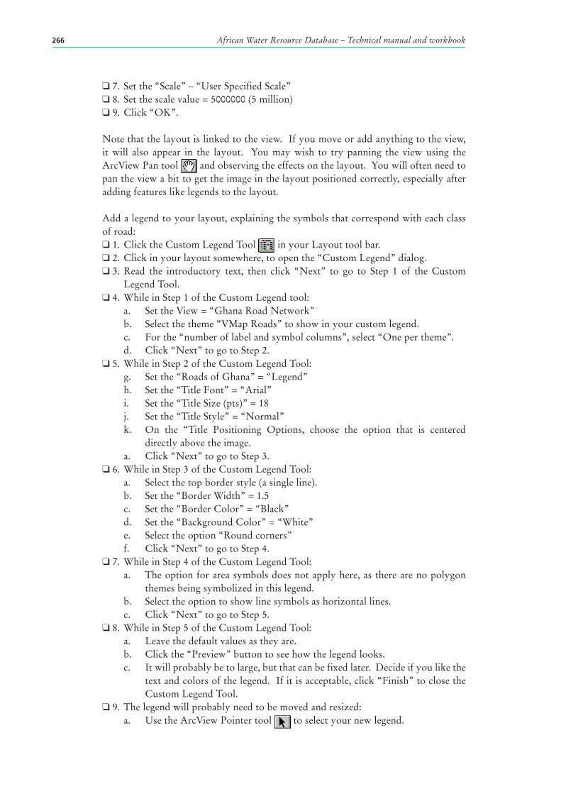
African Water Resource Database – Technical manual and workbook266
❑ 7. Set the “Scale” – “User Specified Scale”❑ 8. Set the scale value = 5000000 (5 million)❑ 9. Click “OK”.
Note that the layout is linked to the view. If you move or add anything to the view, it will also appear in the layout. You may wish to try panning the view using the ArcView Pan tool and observing the effects on the layout. You will often need to pan the view a bit to get the image in the layout positioned correctly, especially after adding features like legends to the layout.
Add a legend to your layout, explaining the symbols that correspond with each class of road:❑ 1. Click the Custom Legend Tool in your Layout tool bar.❑ 2. Click in your layout somewhere, to open the “Custom Legend” dialog.❑ 3. Read the introductory text, then click “Next” to go to Step 1 of the Custom
Legend Tool.❑ 4. While in Step 1 of the Custom Legend tool:
a. Set the View = “Ghana Road Network”b. Select the theme “VMap Roads” to show in your custom legend.c. For the “number of label and symbol columns”, select “One per theme”.d. Click “Next” to go to Step 2.
❑ 5. While in Step 2 of the Custom Legend Tool:g. Set the “Roads of Ghana” = “Legend”h. Set the “Title Font” = “Arial”i. Set the “Title Size (pts)” = 18j. Set the “Title Style” = “Normal”k. On the “Title Positioning Options, choose the option that is centered
directly above the image.a. Click “Next” to go to Step 3.
❑ 6. While in Step 3 of the Custom Legend Tool:a. Select the top border style (a single line).b. Set the “Border Width” = 1.5c. Set the “Border Color” = “Black”d. Set the “Background Color” = “White”e. Select the option “Round corners”f. Click “Next” to go to Step 4.
❑ 7. While in Step 4 of the Custom Legend Tool:a. The option for area symbols does not apply here, as there are no polygon
themes being symbolized in this legend.b. Select the option to show line symbols as horizontal lines.c. Click “Next” to go to Step 5.
❑ 8. While in Step 5 of the Custom Legend Tool:a. Leave the default values as they are.b. Click the “Preview” button to see how the legend looks.c. It will probably be to large, but that can be fixed later. Decide if you like the
text and colors of the legend. If it is acceptable, click “Finish” to close the Custom Legend Tool.
❑ 9. The legend will probably need to be moved and resized:a. Use the ArcView Pointer tool to select your new legend.
Workbook 267
Exer
cise
No
. 6
b. Drag the legend down to the lower left corner of the layout.c. If you wish to resize the legend, click on one of the corner handles and drag
it to change the dimensions. d. Position and size the legend so that it looks good to you.e. If you wish, you can decompose the legend into separate elements by
clicking the ArcView Ungroup button . You may need to click it several times before you get all the subgroups split up. Then you can select each individual element and modify it using the Symbol Window. For example, you could set the some of the text to be a different font or a larger font size. It would be a good idea to regroup the legend elements when you finish (select them all, then click the ArcView Group button ), so that the entire legend can easily be resized or repositioned.
Add a Scale Bar to your layout:❑ 1. Click the “Scale Bar Frame” tool in the Layout tool bar. If you do not see
the button, then click on the tool and hold it down for a second. You should see the scale bar tool appear below the tool, where you can select it from a list. Note: you should also see the North Arrow tool , which you will need shortly.
❑ 2. Use the Scale Bar tool to draw a box on the layout to hold your scale bar.❑ 3. In the Scale Bar Properties dialog:
a. Select the view frame named “Ghana Road Network”.b. Check the option “Preserve Interval”.c. Select the “Units” = “Kilometers”d. Set the “Interval” = 50e. Set “Intervals” = 3f. Set “Left Divisions” = 2g. If you are unable to set these values, just stick with an Interval = 50, then
resize the scale bar later by selecting it and pulling on one of the handles.h. Click “OK” to add the scale bar to the layout.
❑ 4. If you wish, you may change the font of the scale bar text by selecting the scale bar with the tool, and then clicking [CONTROL]-P to open the Symbol Window. Use the Symbol Window to set the font properties. While it is selected, you can also move it around and resize it.
Add a North Arrow to your layout:❑ 1. Use the North Arrow tool to draw a box on the layout.❑ 2. Pick the North Arrow you wish to use from the North Arrow Manager dialog.❑ 3. Click “OK” to add the north arrow to the layout.❑ 4. If you wish, you may change the size or location of the north arrow with the
tool.
Add a title to your layout:❑ 1. Use the Text tool to click on the layout.❑ 2. In the “Text Properties” dialog, enter the text “Ghana”❑ 3. Click “OK”.❑ 4. Select the title using the tool.❑ 5. Click [CONTROL]-P to open the Symbol Window dialog.❑ 6. Set the “Font” = “Verdana”
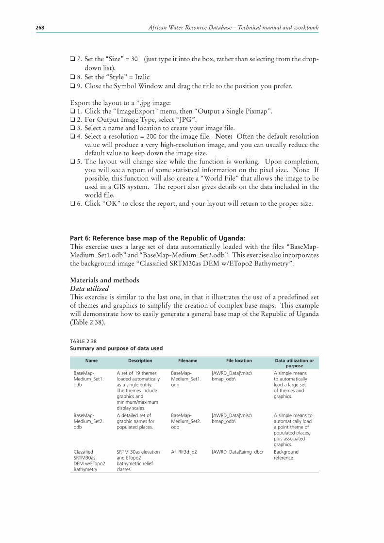
African Water Resource Database – Technical manual and workbook268
❑ 7. Set the “Size” = 30 (just type it into the box, rather than selecting from the drop-down list).
❑ 8. Set the “Style” = Italic❑ 9. Close the Symbol Window and drag the title to the position you prefer.
Export the layout to a *.jpg image:❑ 1. Click the “ImageExport” menu, then “Output a Single Pixmap”.❑ 2. For Output Image Type, select “JPG”.❑ 3. Select a name and location to create your image file.❑ 4. Select a resolution = 200 for the image file. Note: Often the default resolution
value will produce a very high-resolution image, and you can usually reduce the default value to keep down the image size.
❑ 5. The layout will change size while the function is working. Upon completion, you will see a report of some statistical information on the pixel size. Note: If possible, this function will also create a “World File” that allows the image to be used in a GIS system. The report also gives details on the data included in the world file.
❑ 6. Click “OK” to close the report, and your layout will return to the proper size.
Part 6: Reference base map of the Republic of Uganda:This exercise uses a large set of data automatically loaded with the files “BaseMap-Medium_Set1.odb” and “BaseMap-Medium_Set2.odb”. This exercise also incorporates the background image “Classified SRTM30as DEM w/ETopo2 Bathymetry”.
Materials and methods Data utilizedThis exercise is similar to the last one, in that it illustrates the use of a predefined set of themes and graphics to simplify the creation of complex base maps. This example will demonstrate how to easily generate a general base map of the Republic of Uganda (Table 2.38).
TABLE 2.38Summary and purpose of data used
Name Description Filename File location Data utilization or purpose
BaseMap-Medium_Set1.odb
A set of 19 themes loaded automatically as a single entity. The themes include graphics and minimum/maximum display scales.
BaseMap-Medium_Set1.odb
[AWRD_Data]\misc\bmap_odb\
A simple means to automatically load a large set of themes and graphics.
BaseMap-Medium_Set2.odb
A detailed set of graphic names for populated places.
BaseMap-Medium_Set2.odb
[AWRD_Data]\misc\bmap_odb\
A simple means to automatically load a point theme of populated places, plus associated graphics.
Classified SRTM30as DEM w/ETopo2 Bathymetry
SRTM 30as elevation and ETopo2 bathymetric relief classes
Af_Rlf3d.jp2 [AWRD_Data]\aimg_dbc\ Background reference.
Workbook 269
Exer
cise
No
. 6
MethodsOpen ArcView and start the exercise by following the steps below.
Make a new view and name it “Uganda”. While the View Properties window is open, set the “Map Units” = “Decimal Degrees”.
Load the themes stored in BaseMap-Medium_Set1.odb and BaseMap-Medium_Set2.odb:❑ 1. Click the “ImageExport” menu, and then “Load Theme Database”.❑ 2. Choose to import the ODB into the existing (current) view.❑ 3. Select the file “basemap-medium_set1.odb” and click “OK”.❑ 4. Click the “ImageExport” menu, and then “Load Theme Database”.❑ 5. Choose to import the ODB into the existing (current) view.❑ 6. Select the file “basemap-medium_set2.odb” and click “OK”.❑ 7. If you wish, explore these datasets by zooming in to different areas and viewing
the types of themes that are included. Most of these themes are set so that they are only visible at certain scale ranges.
Reset the basemap background image:❑ 1. Turn off the visibility of “Srtm30_flat.jp2”.❑ 2. Turn off the visibility of “Etopo_2_2-5d.jp2❑ 3. Click the Add Basemap button and load the image “Af_Rlf3d.jp2”. Note: If
this image looks extremely pixilated, try zooming out to the full extent of the view using the standard ArcView Zoom to Full Extent button , and then back to your original extent using the standard ArcView Zoom to Previous Extent button
. This usually fixes the pixilation problem.
Zoom in to Uganda:❑ 1. Click the theme “Ad1-National and Sovereign Boundaries” to make it the active
theme. ❑ 2. Use the Query Builder tool to select the country of Ghana, using the
following query string:( [Ad1_name] = “Uganda” )
❑ 3. Zoom in to Uganda using the ArcView Zoom to Selected button .
Add Country Name labels to your view:❑ 1. Open your ArcView symbol window by either clicking [CONTROL]-P, or
clicking the “Window” menu and then “Show Symbol Window…”.❑ 2. In the Symbol Window, set the default text to be Times New Roman, with “Size”
= 24 and “Style” = “Bold Italic”. Set the text color = dark gray.❑ 3. Click the theme “Ad1-National and Sovereign Boundaries (Py)” in your View
Table of Contents to make it the active theme.❑ 4. Drag “Ad1-National and Sovereign Boundaries (Py)” to the bottom of the table
of contents, so that it is underneath all the other themes.❑ 5. Open the Theme Properties for “Ad1-National and Sovereign Boundaries (Py)”
by clicking the “Theme” Menu, then “Properties”.❑ 6. Scroll down to the “Display” icon on the left side of the “Properties” dialog.❑ 7. Click the “Display” icon, and delete both the Minimum and Maximum scale.❑ 8. Use the ArcView Label tool to click on each of the countries in the view to
add labels to them. If you wish to delete a label, select it with the tool and
click the “Delete” key. If you wish to edit the label, double-click on it with the tool and enter the new text in the “Text Properties” dialog.
Convert the view to a 20 cm x 16 cm layout:❑ 1. Click the “ImageExport” menu, then “Create LO/ViewFrame-Page”❑ 2. Set the Page Setup “Units” = “Centimeters”❑ 3. Set the “Width” = 20❑ 4. Set the “Height” = 16❑ 5. The layout will appear, and the only thing you will see on the layout will be the
view frame containing the view. ❑ 6. Double-click on the view frame to open the View Frame Properties dialog.❑ 7. Set the “Scale” – “User Specified Scale”❑ 8. Set the scale value = 5000000 (5 million)❑ 9. Click “OK”.
Note that the layout is linked to the view. If you move or add anything to the view, it will also appear in the layout. You may wish to try panning the view using the ArcView Pan tool and observing the effects on the layout. You will often need to pan the view a bit to get the image in the layout positioned correctly, especially after adding features like legends to the layout.
Export the layout to a *.jpg image:❑ 1. Click the “ImageExport” menu, then “Output a Single Pixmap”.❑ 2. For Output Image Type, select “JPG”.❑ 3. Select a name and location to create your image file.❑ 4. Select a resolution = 200 for the image file. Note: Often the default resolution
value will produce a very high-resolution image, and you can usually reduce the default value to keep down the image size.
❑ 5. The layout will change size while the function is working. Upon completion, you will see a report of some statistical information on the pixel size. Note: If possible, this function will also create a “World File” that allows the image to be used in a GIS system. The report also gives details on the data included in the world file.
❑ 6. Click “OK” to close the report, and your layout will return to the proper size.
Exercise SummaryThis exercise has demonstrated how to create high-quality, high-resolution base map images for use in publications and presentations. The image-export functions provided with the AWRD far exceed the standard layout export tools included with ArcView, and provide a valuable resource for land managers and researchers who wish to create effective, clear and readable maps.
African Water Resource Database - (en rule) Technical manual and workbook270
271
3. Glossary
Active Theme. In an ArcView view, the Active Theme (or Themes) are the themes that are selected so that they appear to have a raised box drawn around them in the view Table of Contents. Some types of tools and buttons only work on active themes, so the theme must be set to active before the tool or button will become available.
Add-On. See Extension.
Ancillary Data. Any data which is accessory or related to the main topic and not of remote sensing origin.
ArcView Project. In ArcView 3, a file for creating and storing documents for GIS work. All activity in ArcView 3 takes place within project files, which use five types of documents to organize information: views, tables, charts, layouts, and Avenue scripts. A project file organizes its documents and stores their unique settings in an ASCII format file with the extension .apr.
ArcScript. See Script.
ASCII (American Standard Code for Information Interchange). The de facto standard for the format of text files in computers and on the Internet that assigns a 7-bit binary number to each alphanumeric or special character. ASCII defines 128 possible characters.
Attribute Table. The attribute table of a spatial dataset is the table containing all the descriptive data that is associated with each spatial feature. ESRI Shapefiles are actually composed of multiple files, one of which contains the attribute table in a dBASE database file.
Basin. In the context of hydrology and related subjects this includes a drainage area of a stream, river or lake.
Basemap. A map depicting background reference information such as landforms, roads, landmarks, and political boundaries, onto which other, thematic information is placed. A basemap is used for locational reference and often includes a geodetic control network as part of its structure.
Blue Marble. A NASA project to present a true-color image of the land surface, without cloud cover, of the entire planet. The final composite image is based on satellite images taken between June and September, 2001. Efforts are currently underway to generate a new generation of Blue Marble images depicting the earth at monthly intervals (see http://earthobservatory.nasa.gov/Newsroom/BlueMarble/).
Bitmap. An image format in which one or more bits represent each pixel on the screen. The number of bits per pixel determines the shades of gray or number of colors that a bitmap can represent. Bitmap files generally have the extension .bmp.
Catchment. See watersheds.
African Water Resource Database – Technical manual and workbook272
Cell. Element of a data grid or data matrix. Each cell corresponds to a portion of the ground surface. The value associated to each cell represents either a thematic attribute or the average value of a parameter, associated to the corresponding surface.
Confidence Band. In regression analysis, the width of the confidence interval for a given confidence level changes in size over the range of the predictor variable. The region defined within the confidence levels is referred to as a confidence band. The confidence band is narrowest at the mean predictor value, and expands as you move away from the mean.
Confidence Interval. A statistical measure reflecting an interval between two numbers with an associated probability value. Statistical analyses generally produce numerical values which predict or explain something about a statistical population, such as the predicted potential fish yield from a waterbody. However, due to the nature of statistics, these predictions always have some level of uncertainty about them. Confidence intervals show the amount of uncertainty. For example, we may be able to predict that a waterbody may have a predicted potential yield of 1 000 tonnes per year, but this value does not tell us anything about the variation or uncertainty about that prediction. A confidence interval might say that we are 95 percent certain that the true potential yield is between 800 and 1 200 tonnes per year, which gives us much more information about the true potential yield of that waterbody, and will let us plan management strategies accordingly.
Confidence Level. The probability value associated with a confidence interval. A confidence interval with a confidence level of 0.90 should be interpreted to mean that, if an infinite number of samples were drawn from a particular population, and 90 percent confidence intervals were calculated for each sample, then the true population statistic would lie within the confidence interval 90 percent of the time.
Cross Table. A table in the AWRD archive which contains attribute values that correspond with codes in other AWRD datasets. For example, the AWRD Surface Waterbody dataset “africvr.shp” contains LCID codes for each waterbody, and the “Cross Table of Unique AfriCover Attributes” table contains descriptions for those LCID codes.
Database. One or more structured sets of persistent data, managed and stored as a unit and generally associated with software to update and query the data. A simple database might be a single file with many records, each of which references the same set of fields. A GIS database includes data about the spatial locations and shapes of geographic features recorded as points, lines, areas, pixels, grid cells, or TINs, as well as their attributes.
dBASE. A simple database format which is used by ArcView 3.x. Shapefiles use dBASE tables to store attributes.
Decimal Degrees. A method of defining locations on the surface of the earth using degrees, which are angular measurements where the vertex of the angle is located at the center of the earth. Locations are defined by Latitude on the Y-coordinate (ranging from -90º at the south pole to 90º at the north pole), and Longitude on the X-coordinate (ranging from -180º to 180º, where 0º is located at Greenwich, England). See also DMS (Degrees Minutes Seconds).
Glossary 273
DEM (Digital Elevation Model). Represents a topographic surface using a continuous array of elevation values, referenced to a common datum. DEMs are used typically to represent terrain relief.
DCW (Digital Chart of the World ). Worldwide dataset produced from data by the U.S. Defense Mapping Agency along with data from Australia, Canada and the United Kingdom.
Dialog. The customized applications described in the present publication.
DMS (Degrees Minutes Seconds). A method of defining locations on the earth using degrees (see Decimal Degrees). In this case, latitude and longitude values are each expressed using 3 numbers; Degrees, Minutes and Seconds. Degrees are integer values and represent 1/360 of the length of the ellipse defined by the line of latitude or longitude. Minutes are integer values equal to 1/60 of a degree, and seconds are decimal values equal to 1/3 600 of a degree.
Drainage basin. See watersheds.
Ellipsoid. The Earth surface is approximately described by an ellipsoid, a closed surface all planar sections of which are ellipses. In general, an ellipsoid has three independent axes, and is usually specified by the length of the three semi-axes. If the lengths of two axes are the same, the ellipsoid is called “ellipsoid of revolution” or spheroid. Due to the rotation around its axis, the Earth has the shape of a spheroid. Several spheroids are used to model the Earth surface and project it onto a two-dimensional map; the choice of the reference spheroid depends on the region of the Earth to be represented and the required precision. The spheroids quoted in this work are Clarke 1866, WGS72 and WGS84. Clarke 1866 is used to map the North America and the Philippines. The World Geodetic System (WGS) spheroids have been developed to be used for global mapping; the number indicates the year of calculation. WGS84 is the most recent version, and is also used by the Global Positioning System.
ENVISAT (Environment Satellite). ENVISAT satellite is an Earth-observing satellite built by the European Space Agency. It was launched on March 1, 2002 aboard an Ariane 5 into a Sun synchronous polar orbit at a height of 790 km (+/− 10 km). It orbits the Earth in about 101 minutes with a repeat cycle of 35 days.
ESRI (Environmental Systems Research Institute). The largest GIS software company, and the maker of ArcView 3.x, ArcINFO and ArcGIS.
Extension. In ArcView 3.x, an extension is a separate add-on tool that can be loaded into your ArcView project. Extension are composed of scripts, dialogs, menus, buttons and/or tools, and generally provide additional functionality to the standard ArcView tools. The AWRD is an example of an ArcView extension.
Feature Attribute Table. See Attribute Table.
FishBase. An extensive online database of over 28 500 worldwide species of fish, intended for researchers, fisheries managers, zoologists and anyone who is interested in fish. This database may be viewed at http://www.fishbase.org/home.htm.
African Water Resource Database – Technical manual and workbook274
Fuzzy classification. Any method for classifying data that allows attributes to apply to objects by membership values, so that an object may be considered a partial member of a class. Class membership is usually defined on a continuous scale from zero to one, where zero is nonmembership and one is full membership. Fuzzy classification may also be applied to geographic objects themselves, so that an object’s boundary is treated as a gradated area rather than an exact line. In GIS, fuzzy classification has been used in the analysis of soil, vegetation, and other phenomena that tend to change gradually in their physical composition and for which attributes are often partly qualitative in nature.
Gazetteer. A list of geographic place names and their coordinates. Entries may include other information as well, such as area, population, or cultural statistics. Atlases often include gazetteers, which are used as indexes to their maps. Well-known digital gazetteers include the U.S. Geological Survey Geographic Names Information System (GNIS) and the Alexandria Digital Library Gazetteer.
Geocoding. Procedures applied to a satellite image to generate a new image with the projection and scale properties of a map. In particular, map coordinates are associated to the center point of each element (pixel) of the resulting image.
Geodatabase. A collection of geographic datasets for use by ArcGIS. There are various types of geographic datasets, including feature classes, attribute tables, raster datasets, network datasets, topologies, and many others.
GIS (Geographic Information Systems). A computer system for capturing, storing, checking, integrating, manipulating, analysing and displaying data related to positions on the Earth’s surface. Typically, a Geographical Information System (or Spatial Information System) is used for handling maps of one kind or another. These might be represented as several different layers where each layer holds data about a particular kind of feature. Each feature is linked to a position on the graphical image of a map. In aquaculture, it has been used to assess the suitability of geographical sectors, and also to investigate the suitability of a species to an area.
Geostatistics. A class of statistics used to analyze and predict the values associated with spatial or spatio-temporal phenomena. Geostatistics provides a means of exploring spatial data and generating continuous surfaces from selected sampled data points.
GeoTIFF. See TIFF.
GIF (Graphics Interchange Format). A type of image file usually used for charts or graphs. It uses a lossless compression format which works well with images with few colors, but poorly with photographs (see JPEG, JPEG2000, MrSID, PNG and TIFF for image formats usually used with high-color photographs). GIF files generally have the extension .gif.
GPS (Global Positioning System). A constellation of twenty-four satellites, developed by the U.S. Department of Defense, that orbits the Earth at an altitude of 20 200 km. These satellites transmit signals that allow a GPS receiver anywhere on Earth to calculate its own location. The Global Positioning System is used in navigation, mapping, surveying, and other applications where precise positioning is necessary.
Glossary 275
GTOPO30 (Global 30 Arc Second Elevation Data). A global digital elevation model (DEM) with a horizontal grid spacing of 30 arc seconds (approximately 1 kilometer). GTOPO30 was derived from several raster and vector sources of topographic information. GTOPO30, completed in late 1996, was developed over a three year period through a collaborative effort led by staff at the U.S. Geological Survey’s Center for Earth Resources Observation and Science (EROS).
Grid. In cartography, any network of parallel and perpendicular lines superimposed on a map and used for reference. These grids are usually referred to by the map projection or coordinate system they represent, such as universal transverse Mercator grid. Grid also refers to a specific type of ESRI dataset, defined as a raster layer in which data values are arrayed across the landscape in square grid cells (analogous to pixels in a raster image).
HYDRO1k (Global Hydrological 1 kilometre database). Geographic database developed to provide comprehensive and consistent global coverage of topographically derived data sets, including streams, drainage basins and ancillary layers derived from the USGS’ 30 arc-second digital elevation model of the world (GTOPO30). HYDRO1k provides a suite of geo-referenced data sets, both raster and vector, which will be of value for all users who need to organize, evaluate, or process hydrologic information on a continental scale. Developed at the U.S. Geological Survey’s Center for Earth Resources Observation and Science (EROS), the HYDRO1k project’s goal is to provide to users, on a continent by continent basis, hydrologically correct DEMs along with ancillary data sets for use in continental and regional scale modeling and analyses.
Image. A representation or description of a scene, typically produced by an optical or electronic device, such as a camera or a scanning radiometer. Common examples include remotely sensed data (for example, satellite data), scanned data, and photographs.
JPEG (Joint Photographic Experts Group). A type of image file best suited for full color images such as photographs. It is a highly compressed format, which makes it useful for data storage and transmission, but it is uses a “lossy” compression method (meaning that some data is lost when it is compressed), which limits its use for GIS purposes. JPEG image files typically have the extension .jpg or .jpeg.
JPEG2000 (Joint Photographic Experts Group). An updated version of JPEG which offers more efficient compression of images and can use both lossless and lossy compression algorithms. The lossless compression method makes JPEG2000 images very useful in GIS applications. This is a new format, however, and therefore ArcView 3.x requires an add-on extension to view them. This add-on extension is automatically loaded by the AWRD. JPEG2000 image files typically have the extension .jp2 or .j2c.
KML (Keyhole Markup Language). Grammar and file format for modeling and storing geographic features such as points, lines, images, polygons, and models for display in Google Earth. A KML file is processed by Google Earth in a similar way that HTML and XML files are processed by web browsers. Like HTML, KML has a tag-based structure with names and attributes used for specific display purposes. Thus, Google Earth acts as a browser of KML files.
African Water Resource Database – Technical manual and workbook276
Landsat. The U.S. Landsat satellites are the first series of Earth Observation satellites providing global, repeated coverage of the Earth surface. The sensors onboard these satellites operate in the visible up to middle infrared wavelengths, and in the thermal infrared. The first satellite of the mission, ERTS-1 (later renamed Landsat-1) was launched in 1972. The current Landsat-7 mission hosts the Enhanced Thematic Mapper sensor; of its nine channels, seven acquire data in the visible up to middle infrared, at 30 m resolution. More information on the Landsat-7 mission can be found in the USGS Web pages (http://landsat7.usgs.gov/index.php) and in the NASA Web pages (http://landsat.gsfc.nasa.gov/).
Layout. In ArcView 3.x, one of the five types of documents that can be contained within a project file. The layout is where users create maps for export or printing, and usually include legends, titles and north arrows.
Legend. A theme legend shows the symbols that ArcView uses to display the theme in the view. These symbols are generally coloured boxes, lines or dots, and they are occasionally graduated by size or colour. Legends are shown in the view Table of Contents and often included on printed maps.
Line. On a map, a shape defined by a connected series of unique x,y coordinate pairs. A line may be straight or curved.
Maps. Graphic representation of the physical features (natural, artificial, or both) of a part or the whole of the Earth’s surface, by means of signs and symbols or photographic imagery, at an established scale, on a specified projection, and with the means of orientation indicated.
Megabasin. The largest delineation of watershed, representing the entire landscape that contributes water to the final outlet (i.e. either the ocean or an internal basin). Landscape features that separate megabasins are sometimes referred to as continental divides.
MERIS (Medium Resolution Imaging Spectrometer). MERIS is a programmable, medium-spectral resolution, imaging spectrometer operating in the solar reflective spectral range. Fifteen spectral bands can be selected by ground command, each of which has a programmable width and a programmable location in the 390 nm to 1 040 nm spectral range. The instrument scans the Earth’s surface by the so called “push-broom” method. Linear CCD arrays provide spatial sampling in the across-track direction, while the satellite’s motion provides scanning in the along-track direction. MERIS is designed so that it can acquire data over the Earth whenever illumination conditions are suitable. The instrument’s 68.5° field of view around nadir covers a swath width of 1 150 km. This wide field of view is shared between five identical optical modules arranged in a fan shape configuration.
Metadata. Information that describes the content, quality, condition, origin, and other characteristics of data or other pieces of information. Metadata for spatial data may describe and document its subject matter; how, when, where, and by whom the data was collected; availability and distribution information; its projection, scale, resolution, and accuracy; and its reliability with regard to some standard. Metadata consists of properties and documentation. Properties are derived from the data source (for example, the coordinate system and projection of the data), while documentation is entered by a person (for example, keywords used to describe the data).
Glossary 277
MODIS (Moderate Resolution Imaging Spectroradiometer). is a key instrument aboard the Terra (EOS AM) and Aqua (EOS PM) satellites. Terra’s orbit around the Earth is timed so that it passes from north to south across the equator in the morning, while Aqua passes south to north over the equator in the afternoon. Terra MODIS and Aqua MODIS are viewing the entire Earth’s surface every 1 to 2 days, acquiring data in 36 spectral bands, or groups of wavelengths. These data will improve our understanding of global dynamics and processes occurring on the land, in the oceans, and in the lower atmosphere. MODIS is playing a vital role in the development of validated, global, interactive Earth system models able to predict global change accurately enough to assist policy makers in making sound decisions concerning the protection of our environment.
MrSID (Multiresolution Seamless Image Database). An image format very similar to JPEG2000, in which full color photographic images can be compressed using a lossless compression format and then displayed in a GIS. One image dataset in the AWRD archive is provided in MrSID format. MrSID image files generally have the extension .sid.
Multipoint. A geometric element defined by a set of points. The entire set is treated as a single object, and there are generally several multipoint objects in a single multipoint shapefile.
ODB (Object Database). A special type of file used by ArcView 3.x, storing Avenue “objects” in a text file on the hard drive. In regards to the AWRD Load Theme Database tool, the “objects” stored are theme references, graphics, legends and scales at which themes are viewable. Loading the ODB causes all these objects to be loaded simultaneously.
ONC. NOAA’s 1:1 000 000 Operational Navigation Charts, these charts are the cartographic baseline for both the original DCW and any subsequent updates of the VMAP0 spatial data libraries
OrthoTM. Ortho-rectified or flattened imagery based on the Universal Transverse Mercator (UTM) projection system using the WGS84 standard datum and spheroid, Thematic Mapper LandSat satellite sensor
Pixels. (Picture elements). Cells of an image matrix. The ground surface corresponding to the pixel is determined by the instantaneous field of view (IFOV) of the sensor system, e.g. the solid angle extending from a detector to the area on the ground it measures at any instant. The digital values of the pixels are the measures of the radiant flux of electromagnetic energy emitted or reflected by the imaged Earth surface in each sensor channel.
Pixmap. An internal ArcView object that defines what is shown on the monitor screen. The AWRD Image Export and Base Mapping tools use the Pixmap object to export high-quality image files of maps and layouts.
Point. A geometric element defined by a pair of x,y coordinates.
Polygon. In a GIS framework, a polygon is a closed line (or a closed set of lines) representing a surface. The surface is generally homogeneous with respect to some criteria; for example, land use or type, administrative units, etc. Map coordinates (easting, northing and height) are associated to the vertices of the polygon.
African Water Resource Database – Technical manual and workbook278
Polyline. In a GIS framework, a polyline is a set of straight line segments (connected or not) representing a linear geographic feature, such as a road or a railway. The polyline may also connect points homogeneous with respect to some criteria, such as a contour line. Map coordinates (easting, northing and height) are associated to the vertices of the segments.
PNG (Portable Network Graphics). A type of image format using a high-efficiency lossless compression algorithm. PNG files can be much larger than JPEG files, but have the advantage of not losing any data in the compression. PNG files generally have the extension .png.
Projection. A method by which the curved surface of the earth is portrayed on a flat surface. This generally requires a systematic mathematical transformation of the earth’s graticule of lines of longitude and latitude onto a plane. Some projections can be visualized as a transparent globe with a light bulb at its center (though not all projections emanate from the globe’s center) casting lines of latitude and longitude onto a sheet of paper. Generally, the paper is either flat and placed tangent to the globe (a planar or azimuthal projection) or formed into a cone or cylinder and placed over the globe (cylindrical and conical projections). Every map projection distorts distance, area, shape, direction, or some combination thereof.
R2 (or R-Squared). A statistical measured referred to as the “coefficient of determination”, and which reflects the proportion of variability in one variable that can be explained by the corresponding variability in another variable.
RADARSAT. Canada’s series of remote sensing satellites. RADARSAT-1 was launched on November, 1995; RADARSAT-2 will be presumably launched on 2005. RADARSAT-1 hosts a Synthetic Aperture Radar (SAR), an active sensor operating in the microwave portion of the electromagnetic spectrum at C-band in HH polarization. The SAR operates in seven different acquisition modes, with spatial resolution ranging from 6.25 to 100 m. RADARSAT-2 will carry an enhanced version of the same sensor. More details on RADARSAT-1 and -2 are available in the Canadian Space Agency Web pages (http://www.space.gc.ca/asc/eng/csa_sectors/earth/radarsat1/radarsat1.asp and .../radarsat2/radarsat2.asp).
Raster. A spatial data model that defines space as an array of equally sized cells arranged in rows and columns, and comprised of single or multiple bands. Each cell contains an attribute value and location coordinates. Unlike a vector structure, which stores coordinates explicitly, raster coordinates are contained in the ordering of the matrix. Groups of cells that share the same value represent the same type of geographic feature.
Regression. See Simple Linear Regression (SLR).
Remote Sensing. The gathering and analysis of data from the study area or organism that is physically removed from the sensing equipment, e.g. sub-water surface detection instruments, aircraft or satellite.
Residual. In regression analysis, the difference between the observed response value and the predicted response value from the regression equation.
Resolution. The area of the ground surface corresponding to a pixel in a satellite image.
Glossary 279
Revised/Relational World Databank II. A collection of vector representations of land outlines, rivers and political boundaries, originally compiled by the U.S. Government in the 1980’s and regularly updated.
River basin. Total land area drained by a river and its tributaries.
River Order. See Stream Order.
RWDBSII. See Revised/Relational World Databank II.
RWDBS2. See Revised/Relational World Databank II.
SAR (Synthetic Aperture Radar). An imaging radar is an active instrument that transmits microwave pulses toward the Earth surface and measures the magnitude of the signal scattered back towards it. The return signals from different portions of the ground surface are combined to form an image. A Synthetic Aperture Radar (SAR) is a special type of imaging radar. It is a complex system that measures both the amplitude and phase of the return signals; their analysis exploits the Doppler effect created by the motion of the spacecraft with respect to the imaged surface to achieve high ground resolution. As the source of the electromagnetic radiation used to sense the Earth surface is the system itself, it can be operated during day and night. The atmospheric transmittance in the microwave interval used by remote sensing SAR systems (2 to 30 GHz) is higher than 90 percent, also in presence of ice and rain droplets (except under heavy tropical thunderstorms); thus, SAR can acquire data in all weather conditions.
Scale. The ratio between a distance or area on a map and the corresponding distance or area on the ground.
Scatterplot. A statistical plot illustrating the relationship between two variables as measured on a set of sampling points. In regression analysis, each sample is plotted on the scatterplot such that the X-value is equal to the value of the Predictor variable and the Y-value is equal to the value of the Response variable. Regression scatterplots often include a regression line illustrating the best-fitting line that goes through the data.
Script. In ArcView 3.x, one of the five types of documents that can be contained within a project file. An ArcView 3.x script contains Avenue code, which can be used to automate tasks, add new capabilities, and build complete applications.
Selection. ArcView 3.x and the AWRD both offer extensive analytical functions which can be applied to your spatial data. By selecting certain features before the analysis, you can restrict the analysis to only the data you are interested in. Often determining the correct feature selection set is one of the more complicated parts of the analysis, and the AWRD offers extensive tools to select by query or by selecting on the screen, as well as modifying the current selection set by adding, subtracting or subsetting from it.
Shapefile. A vector file format for storing the location, shape, and attributes of geographic features.
SIFRA (Source Book for the Inland Fishery Resources of Africa). A compendium of information on the physical characteristics, limnology and fisheries in Africa, organized by Country. SIFRA was originally compiled in 1990 by Vanden Bossche and Bernacsek, and published by FAO as CIFA Technical Paper No. 18.1. It can be viewed online at http://www.fao.org/docrep/005/T0473E/T0473E00.htm.

African Water Resource Database – Technical manual and workbook280
Simple Linear Regression (SLR). A statistical technique to estimate the relationship between a predictor variable and a response variable. The relationship is defined using the equation of a line, Y = a + bX, where a is the Y-intercept and b is the slope of the line. Using this relationship, you may estimate what the response variable would be given any particular value of the predictor variable. The accuracy of any predictions depends on the strength of the linear relationship, and predictions should generally include confidence intervals.
Spatial Resolution. The area of the ground surface corresponding to a pixel in a satellite image.
SRTM (Shuttle Radar Topography Mission). is a joint project between the National Geospatial-Intelligence Agency (NGA) and the National Aeronautics and Space Administration (NASA). The objective of this project is to produce digital topographic data for 80 percent of the Earth’s land surface (all land areas between 60° north and 56° south latitude), with data points located every 1-arc second (approximately 30 meters) on a latitude/longitude grid. The absolute vertical accuracy of the elevation data will be 16 meters (at 90 percent confidence). The SRTM obtained elevation data on a near-global scale to generate the most complete high-resolution digital topographic database of Earth. SRTM consisted of a specially modified radar system that flew onboard the Space Shuttle Endeavour during an 11-day mission in February of 2000.
SPOT (Système Pour l’Observation de la Terre). French Earth Observation satellites operating in the optical wavelengths. The first satellite, SPOT-1 was launched in 1986; the most recent satellite, SPOT-5, was launched in 2000. Among its instruments, the HRG acquires data in five channels useful to study land cover: a panchromatic channel (spatial resolution 2.5 or 5 m), three channels in the visible and near infrared wavelengths (spatial resolution 10 m) and one channel in the short-wave infrared (spatial resolution 20 m). More information on the SPOT satellites can be found at the SPOT Image Web site (http://www.spotimage.com) and at the CNES Web site (http://www.cnes.fr).
Stream Order. A method of ranking stream segments according to their location in the hydrological network. Stream segments that form the starting points of the hydrological network are assigned a stream order value of 1. When two stream segments with the same stream order value converge, they form a new segment with an incrementally higher value (i.e. two level-1 segments converge to form a level-2 segment, and two converging level-2 segments form a level-3 segment.). If stream segments with different order values converge, then the resulting segment has the same value as the higher of the two converging segments.
UTM (Universal Transverse Mercator). A commonly used projected coordinate system that divides the globe into 60 zones, starting at -180° longitude. Each zone extends north-south from 84° North to 80° South, spans 6° of longitude, and has its own central meridian.
TOC (Table of Contents). In ArcView 3.x, this is the list of themes available in a View. The TOC is located on the left side of a view. Themes in the view may be set to visible or invisible by checking boxes in the TOC.
Theme. In ArcView 3.x, a theme is a spatial dataset that has been loaded into a view, and is displayed with a customizable legend. Themes are analogous to Layers in ArcInfo or ArcGIS, and may be created from any type of spatial data.
Glossary 281
TIFF (Tagged Image File Format). An image format commonly used for high-color digital photographs. TIFF images with embedded spatial information are referred to as “GeoTIFF” files, and are useful in GIS systems because they can contain a large amount of data. TIFF files tend to be large, however, and therefore are poor for data storage or transmission. TIFF files generally have the extension .tif or .tiff.
Vector. A data structure used to represent geographic features. Features are represented by points, lines or polygons. A line is made up of connected points (vertices), and a polygon of connected lines. Map coordinates (easting, northing and height) are associated to each point (or vertex) in a vector feature. Attributes are also associated with each feature (as opposed to the raster data structure, which associates attributes with grid cells).
Vector Map. A vector-based data product in vector product format (VPF) at several scales divided into groups, referred to as levels. For example, VMap Level 1 includes vector maps at a scale of 1:250 000 and VMap Level 2 includes vector maps at a scale of 1:50 000.
View. In ArcView 3.x, one of the five types of documents that can be contained within a project file. An ArcView View contains the actual map and themes, and is where spatial analysis usually takes place.
View Frame. The object in an ArcView Layout which displays the image from a View. View frames generally have live links to their respective view, such that changes in the view automatically are reflected in the layout.
Watershed. The area which supplies water by surface and subsurface flow from rain to any given point in the drainage system, and are most often delineated for distinctive points such as populations centers, lakes or river intersections. Watersheds provide a useful way to divide the landscape up into smaller hydrologically-related regions, which can then be analyzed in terms of in-flow and out-flow of moisture, energy and other parameters, such as nutrients and pollutants. Watersheds are also defined as the total land surface from which an aquifer or river system receives its water, and the term is synonymous with drainage basins, river basins or catchments. Watershed management. (river basin management) Planned used of watersheds (river basins) in accordance with predetermined objectives.
Watershed model. A special type of vector dataset, in which the landscape is divided into watershed polygons and each polygon has attributes that identify its place in the overall hydrological network.
World File. A file associated with an image, defining the spatial attributes of that image. An image with a world file can be loaded into a GIS along with all other forms of spatial data. World files typically define the projection, coordinate system, ellipsoid and datum of the image, the spatial coordinates of one of the corners of the image, and the real-world size of the image pixels. The AWRD includes tools to export maps into a variety of image formats, and to create world files for these maps.
XML (Extensible Markup Language). A type of document format in which objects can be stored in a text file.
African Water Resource Database – Technical manual and workbook282
Glossary compiled from the following sources:
Anonymous. 1998. AQUALEX. Multilingual glossary of aquaculture terms/ Glossaire multilingue relatif aux termes utilisés en aquaculture. CD-ROM, John Wiley & Sons Ltd. & Praxis Publ., UK.
Art, H.W. 1993. The dictionary of ecology and environmental science. 115 West 18th Street, New York, NY 10011: Henry Holt and Company, Inc.; 632 pp.
Association for Geographic Information (AGI) GIS Dictionary (http://www.geo.ed.ac.uk/agidict/welcome.html)
Barnabé, G. (ed.) 1990 Aquaculture. Chichester, UK, Ellis Horwood. Vol.1, 528p. Vol.2, 584 pp. Transl. by L.M. Laird.
Center for Spatially Integrated Social Science (CSISS): http://www.csiss.org/cookbook/glossary.php
Choudury, K. and Jansen, L.J.M. 1999. Terminology for integrated resources planning and management. Rome, FAO. 69 pp.
Chrisman, N. Glossary for Exploring GIS, by: http://www.wiley.com/college/chrisman/glossary.html
Earth Sciences Sector of Natural Resources Canada. Canada Center for Remote Sensing (CCRS). Glossary of remote sensing terms (http://ccrs.nrcan.gc.ca/glossary/index_e.php).
ESRI. 2001. The ESRI Press dictionary of GIS terminology. Environmental Systems Research Institute, Inc. Redlands, California, USA (available at:
http://www.esri.com/library/glossary/a_d.html).FAO 2006. Glossary of Aquaculture. http://www.fao.org/fi/glossary/aquaculture/FAO Fisheries Department. 2003 World Fisheries and Aquaculture Atlas. CD-ROM.
Rome, FAO. 2nd ed. FAO/IPTRID/ICID/ODA. 2001. Irrigation guidelines, land and water digital media
series No 12. FAO, handbook on pressurized irrigation techniques. Helms, J. A. 1998. The dictionary of forestry. 5400 Grosvenor Lane, Bethesda, MD
20814- 2198: Society of American Foresters. 210 pp. Hoehn, P., and Lynette, M. Dictionary of abbreviations and acronyms in geographic
information systems, cartography and remote sensing. (available at http://www.lib.berkeley.edu/EART/abbrev.html).
Perry-Castañeda Library Map Collection. Glossary of Cartographic Terms online at http://www.lib.utexas.edu/maps/glossary.html. The University of Texas.
Voser, S.A. Glossary of glossaries (available at http://www.geocities.com/CapeCanaveral/1224/terms/terms_txt.html)
UNESCO/WMO. 1992. International glossary of hydrology, 2d editionUnited Nations (1997): Glossary of Environment Statistics. Studies in Methods,
Series F, No. 67.Wenger, K.F. Forestry Handbook. 2 ed. New York: John Wiley & Sons; 1984. 1 335
pp. Wikipedia On-line encyclopedia (available at http://en.wikipedia.org/wiki/Main_
Page)
References
Aguilar-Manjarrez, J. & Nath, S.S. 1998. A strategic reassessment of fish farming potential in Africa. CIFA Technical Paper. No. 32. Rome, FAO. 170 pp. (also available at http://www.fao.org/docrep/w8522e/w8522e00.htm).
Burkardt, J. 2001. PROB - probability density functions. Sample Fortran code for calculating density functions. [Web Page]. (available at: http://www.psc.edu/~burkardt/src/prob/prob.htm).
Corsi, F., Dunn, I. & Felicioni, E. 1986. Etude sous-sectorielle: Le pêches et la pisci-culture au Burundi. Rapport de la mission Novembre–Decembre 1985. Projet PNUD/FAO BDI/85/U71 Mars 1986.
Croarkin, C. & Tobias, P. (no date). Engineering and statistics handbook [Web Page]. (available at: http://www.itl.nist.gov/div898/handbook/).
de Graaf, G., Marttin, F.J.B., Aguilar-Manjarrez , J. & Jenness , J. 2003. Geographic Information Systems in fisheries management and planning. Technical manual. FAO Fisheries Technical Paper No. 449. Rome, FAO. 162 pp.
Draper, N.R. & Smith, H. 1998. Applied Regression Analysis. 3rd ed. New York, John Wiley & Sons, Inc. 706 pp. (Wiley Series in Probability and Statistics).
FAO. 1995. Code of conduct of responsible fisheries. Rome, FAO. (available at http://www.fao.org/DOCREP/005/v9878e/v9878e00.htm#PRE).
Halls, A.S. 1999. Spatial models for the evaluation and management of inland fisheries, final report. 47 Prince’s Gate, South Kensington, London SW7 2QA: MRAG Ltd.; FIR 1998 Plansys 23220 01 20. 90 pp.
ICES. 2004. ICES Code of Practice on the Introductions and Transfers of Marine Organisms 2004. Copenhagen, Denmark. 29 pp. (available at: http://www.ices.dk/reports/general/2004/ICESCOP2004.pdf).
Meaden, G.J. & Kapetsky, J.M. 1991. Geographical information systems and remote sensing in inland fisheries and aquaculture. FAO Fisheries Technical Paper. No. 318. Rome, FAO. 262 pp.
McLaughlin, M.P. 2001. Regress+, appendix A. A compendium of common probabil-ity distributions (version 2.3) [Web Page]. (available at: http://www.causaScientia.org/math_stat/Dists/Compendium.pdf).
Mikkola, H. & Lindquist, O.V. 1989. Report on a Project Mobilization Mission. Preparatory Phase: Lake Tanganyika Regional Fisheries Research Project, GCP/RAF/229/FIN, Rome, FAO.
MRAG Ltd. 1997. Technical Database Specification Document for the FAO Lakes and River Fisheries Database. Available in AWRD Docs folder.
Neter, J., Wasserman, W. & Kutner, M.H. 1990. Applied linear statistical models: regression, analysis of variance and experimental designs. 3rd ed. Burr Ridge, Illinois: Irwin; 1 181 pp.
Neter , J., Wasserman , W., Nachtschiem, C.J. & Kutner , M.H. 1996. Applied lin-ear statistical models: regression , analysis of variance and experimental design. 4th ed. Burr Ridge, Illinois, McGraw-Hill/Irwin. 1 408 pp.
283
African Water Resource Database – Technical manual and workbook284
Press, W.H., Teukolsky, S.A., Vetterling, W.T. & Flannery, B.P. 2002. Numerical recipies in C: the art of scientific computing. 2nd ed. Cambridge: Cambridge University Press; 994 pp.
Skelton, P.H. 1993. A complete guide to the freshwater fishes of Southern Africa. Voorvelt, Dave and Tarr, Elizabeth, Illustrators. Halfway House, South Africa: Southern Book Publishers; 390 pp.
Vanden Bossche, J.-P. & Bernacsek, G.M. 1990a. Source book for the inland fishery resources of Africa: 1. CIFA Technical Paper. No. 18.1. Rome, FAO. 240 pp. (also available at http://www.fao.org/docrep/005/T0473E/T0473E00.htm).
Vanden Bossche, J.-P. & Bernacsek, G.M. 1990b. Source book for the inland fishery resources of Africa: 2. CIFA Technical Paper. No. 18.2. Rome, FAO. 411 pp. (also available at http://www.fao.org/docrep/005/T0360E/T0360E00.htm).
Vanden Bossche, J.-P. & Bernacsek, G.M. 1991. Source book for the inland fishery resources of Africa: 3. CIFA Technical Paper, No. 18.3. Rome, FAO. 219 pp. (also available at http://www.fao.org/docrep/005/T0361E/T0361E00.htm).
RECOMMENDED FURTHER READING
(Relevant papers not cited in the main document)
Abramowitz, M. & Stegun, I.A. 1972. Handbook of mathematical functions with formulas, graphs and mathematical tables. NewYork, Dover Publications, Inc., 1 046 pp.
Golub, G.H. & Van Loan, C.F. 1996. Matrix computations. 3rd ed. Baltimore: The Johns Hopkins Univerisity Press; 694 pp. (Johns Hopkins Studies in the Mathematical Sciences).
Jeffrey, A. 2000. Handbook of mathematical formulas and integrals. 2nd ed. San Diego Academic Press. 433 pp.
Isaaks, E.H. & Srivastava, R.M. 1989. An introduction to applied geostatistics. Oxford University Press. 561 pp.
Ott, R.L. 1993. An introduction to statistical methods and data analysis. 4th ed. Belmont, California, Duxbury Press. 1 051 pp.
Rogerson, P.A. 2001. Statistical methods for geography. Sage Publications, Ltd. 236 pp.
Stewart, J. 1998. Calculus concepts and contexts. Pacific Grove: Brooks/Cole Publishing Company; 991 pp.
Zar, J.H. 1999. Biostatistical analysis, 4th Ed. Prentice-Hall, Inc. 929 pp.
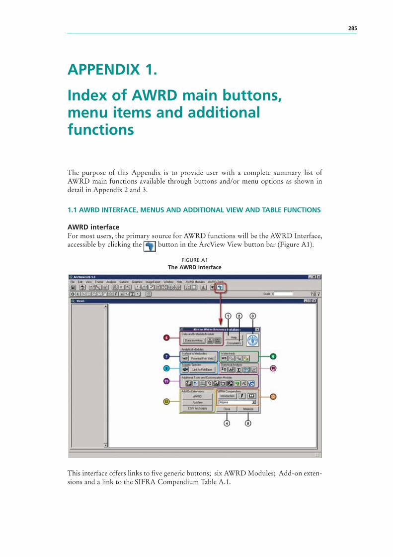
APPENDIX 1.
Index of AWRD main buttons, menu items and additional functions
The purpose of this Appendix is to provide user with a complete summary list of AWRD main functions available through buttons and/or menu options as shown in detail in Appendix 2 and 3.
1.1 AWRD INTERFACE, MENUS AND ADDITIONAL VIEW AND TABLE FUNCTIONS
AWRD interfaceFor most users, the primary source for AWRD functions will be the AWRD Interface, accessible by clicking the button in the ArcView View button bar (Figure A1).
FIGURE A1The AWRD Interface
This interface offers links to five generic buttons; six AWRD Modules; Add-on exten-sions and a link to the SIFRA Compendium Table A.1.
285
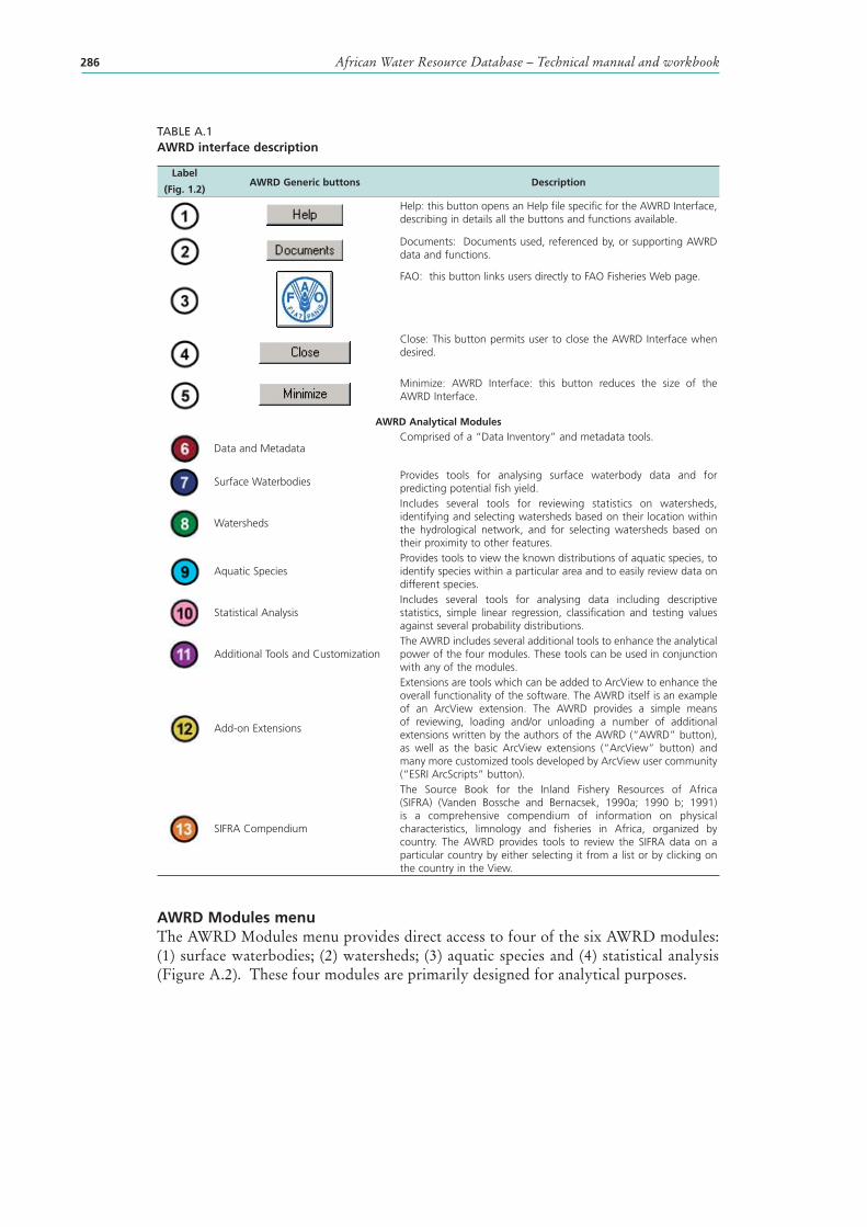
African Water Resource Database – Technical manual and workbook286
TABLE A.1AWRD interface description
Label
(Fig. 1.2)AWRD Generic buttons Description
Help: this button opens an Help file specific for the AWRD Interface, describing in details all the buttons and functions available.
Documents : Documents used, referenced by, or supporting AWRD data and functions.
FAO: this button links users directly to FAO Fisheries Web page.
Close: This button permits user to close the AWRD Interface when desired.
Minimize: AWRD Interface: this button reduces the size of the AWRD Interface.
AWRD Analytical Modules
Data and Metadata Comprised of a “Data Inventory” and metadata tools.
Surface Waterbodies Provides tools for analysing surface waterbod y data and for predicting potential fish yield.
Watersheds
Includes several tools for reviewing statistics on watersheds, identifying and selecting watersheds based on their location within the hydrological network, and for selecting watersheds based on their proximity to other features.
Aquatic Species Provides tools to view the known distributions of aquatic species , to identify species within a particular area and to easily review data on different species.
Statistical Analysis Includes several tools for analysing data including descriptive statistics , simple linear regression , classification and testing values against several probability distributions.
Additional Tools and Customization The AWRD includes several additional tools to enhance the analytical power of the four modules. These tools can be used in conjunction with any of the modules.
Add-on Extensions
Extensions are tools which can be added to ArcView to enhance the overall functionality of the software. The AWRD itself is an example of an ArcView extension. The AWRD provides a simple means of reviewing, loading and/or unloading a number of additional extensions written by the authors of the AWRD (“AWRD” button), as well as the basic ArcView extensions (“ArcView” button) and many more customized tools developed by ArcView user community (“ESRI ArcScripts” button).
SIFRA Compendium
The Source Book for the Inland Fishery Resources of Africa (SIFRA) (Vanden Bossche and Bernacsek, 1990a; 1990 b; 1991) is a comprehensive compendium of information on physical characteristics, limnology and fisheries in Africa, organized by country. The AWRD provides tools to review the SIFRA data on a particular country by either selecting it from a list or by clicking on the country in the View.
AWRD Modules menuThe AWRD Modules menu provides direct access to four of the six AWRD modules: (1) surface waterbodies; (2) watersheds; (3) aquatic species and (4) statistical analysis (Figure A.2). These four modules are primarily designed for analytical purposes.
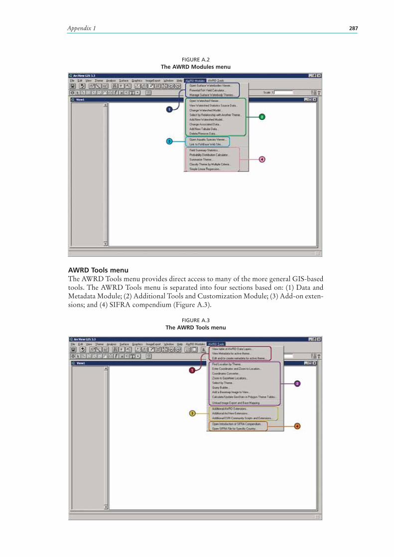
Appendix 1 287
FIGURE A.2The AWRD Modules menu
AWRD Tools menu The AWRD Tools menu provides direct access to many of the more general GIS-based tools. The AWRD Tools menu is separated into four sections based on: (1) Data and Metadata Module; (2) Additional Tools and Customization Module; (3) Add-on exten-sions; and (4) SIFRA compendium (Figure A.3).
FIGURE A.3The AWRD Tools menu
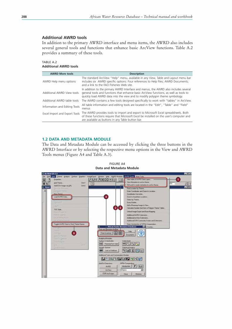
African Water Resource Database – Technical manual and workbook288
Additional AWRD toolsIn addition to the primary AWRD interface and menu items, the AWRD also includes several general tools and functions that enhance basic ArcView functions. Table A.2 provides a summary of these tools.
TABLE A.2Additional AWRD tools
AWRD More tools Description
AWRD Help menu optionsThe standard ArcView “Help” menu, available in any View, Table and Layout menu bar includes six AWRD specific options: Four references to Help files; AWRD Documents; and a link to the FAO Fisheries Web site.
Additional AWRD View toolsIn addition to the primary AWRD Interface and menus, the AWRD also includes several general tools and functions that enhance basic ArcView functions, as well as tools to quickly load AWRD data into the view and to modify polygon theme symbology.
Additional AWRD table tools The AWRD contains a few tools designed specifically to work with “tables” in ArcView.
Information and Editing ToolsAll table information and editing tools are located in the “Edit”, “Table” and “Field ” menus
Excel Import and Export Tools The AWRD provides tools to import and export to Microsoft Excel spreadsheets. Both of these functions require that Microsoft Excel be installed on the user’s computer and are available as buttons in any Table button bar.
1.2 DATA AND METADATA MODULEThe Data and Metadata Module can be accessed by clicking the three buttons in the AWRD Interface or by selecting the respective menu options in the View and AWRD Tools menus (Figure A4 and Table A.3).
FIGURE A4Data and Metadata Module
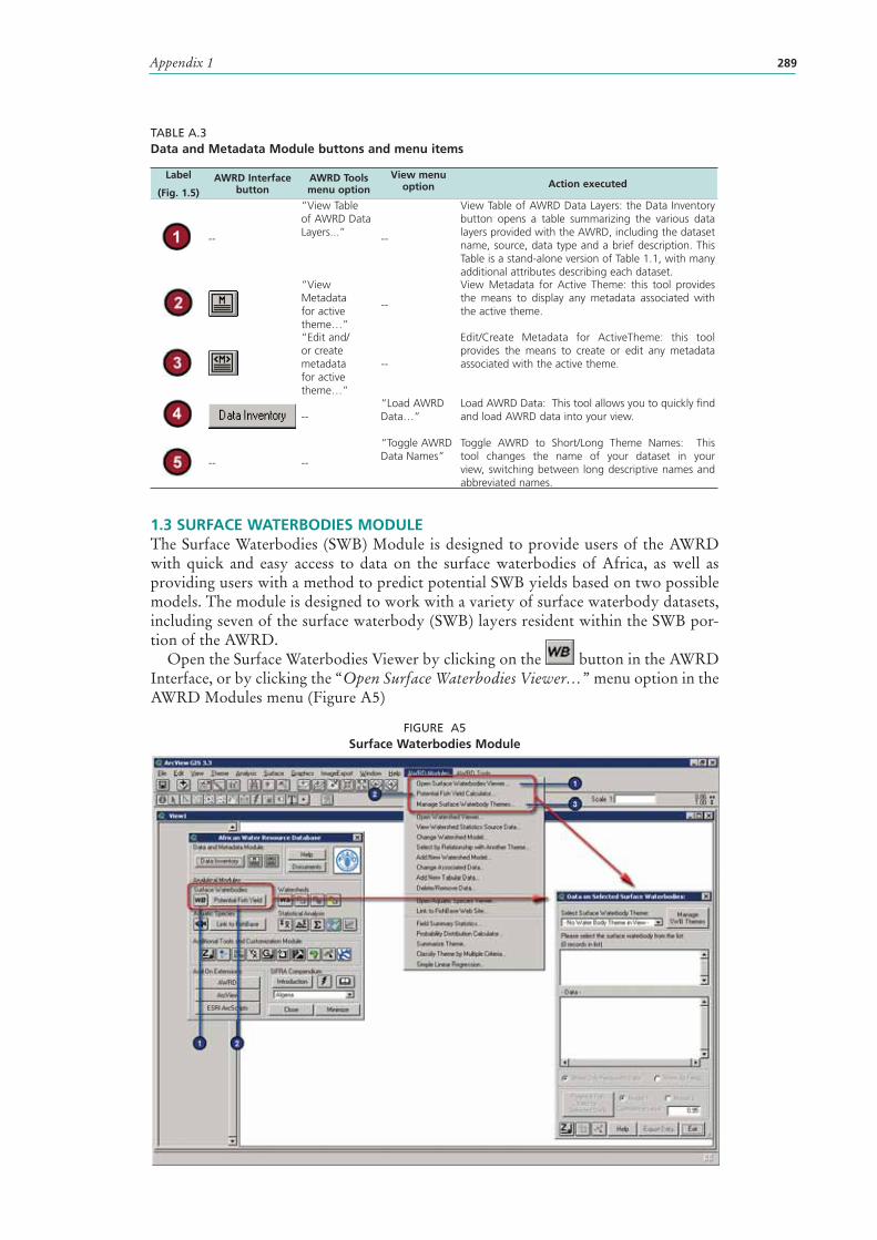
Appendix 1 289
TABLE A.3Data and Metadata Module buttons and menu items
Label
(Fig. 1.5)AWRD Interface
buttonAWRD Tools menu option
View menu option Action executed
--
“View Table of AWRD Data Layers...”
--
View Table of AWRD Data Layers: the Data Inventory button opens a table summarizing the various data layers provided with the AWRD, including the dataset name, source, data type and a brief description. This Table is a stand-alone version of Table 1.1, with many additional attributes describing each dataset.
“View Metadata for active theme…”
--
View Metadata for Active Theme : this tool provides the means to display any metadata associated with the active theme.
“Edit and/or create metadata for active theme…”
--
Edit/Create Metadata for ActiveTheme: this tool provides the means to create or edit any metadata associated with the active theme.
--“Load AWRD Data…”
Load AWRD Data: This tool allows you to quickly find and load AWRD data into your view.
-- --
“Toggle AWRD Data Names”
Toggle AWRD to Short/Long Theme Names: This tool changes the name of your dataset in your view, switching between long descriptive names and abbreviated names.
1.3 SURFACE WATERBODIES MODULEThe Surface Waterbodies (SWB ) Module is designed to provide users of the AWRD with quick and easy access to data on the surface waterbod ies of Africa, as well as providing users with a method to predict potential SWB yields based on two possible models. The module is designed to work with a variety of surface waterbody datasets, including seven of the surface waterbody (SWB) layers resident within the SWB por-tion of the AWRD.
Open the Surface Waterbodies Viewer by clicking on the button in the AWRD Interface, or by clicking the “Open Surface Waterbodies Viewer…” menu option in the AWRD Modules menu (Figure A5)
FIGURE A5Surface Waterbodies Module
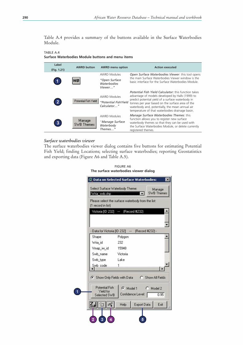
African Water Resource Database – Technical manual and workbook290
Table A.4 provides a summary of the buttons available in the Surface Waterbod ies Module.
TABLE A.4Surface Waterbodies Module buttons and menu items
Label
(Fig. 1.21)AWRD button AWRD menu option Action executed
AWRD Modules
“Open Surface Waterbodies Viewer…”
Open Surface Waterbodies Viewer: this tool opens the main Surface Waterbodies Viewer window is the basic interface for the Surface Waterbodies Module.
AWRD Modules
“Potential FishYield Calculator…”
Potential Fish Yield Calculator : this function takes advantage of models developed by Halls (1999) to predict potential yield of a surface waterbody in tonnes per year based on the surface area of the waterbody and, potentially, the mean annual air temperature of that waterbodies drainage basin.
AWRD Modules
“Manage Surface Waterbody Themes…”
Manage Surface Waterbodies Themes: this function allows you to register new surface waterbod y themes so that they can be used with the Surface Waterbodies Module, or delete currently registered themes.
Surface waterbodies viewer The surface waterbodies viewer dialog contains five buttons for estimating Potential Fish Yield ; finding Locations; selecting surface waterbodies; reporting Geostatistics and exporting data (Figure A6 and Table A.5).
FIGURE A6The surface waterbodies viewer dialog
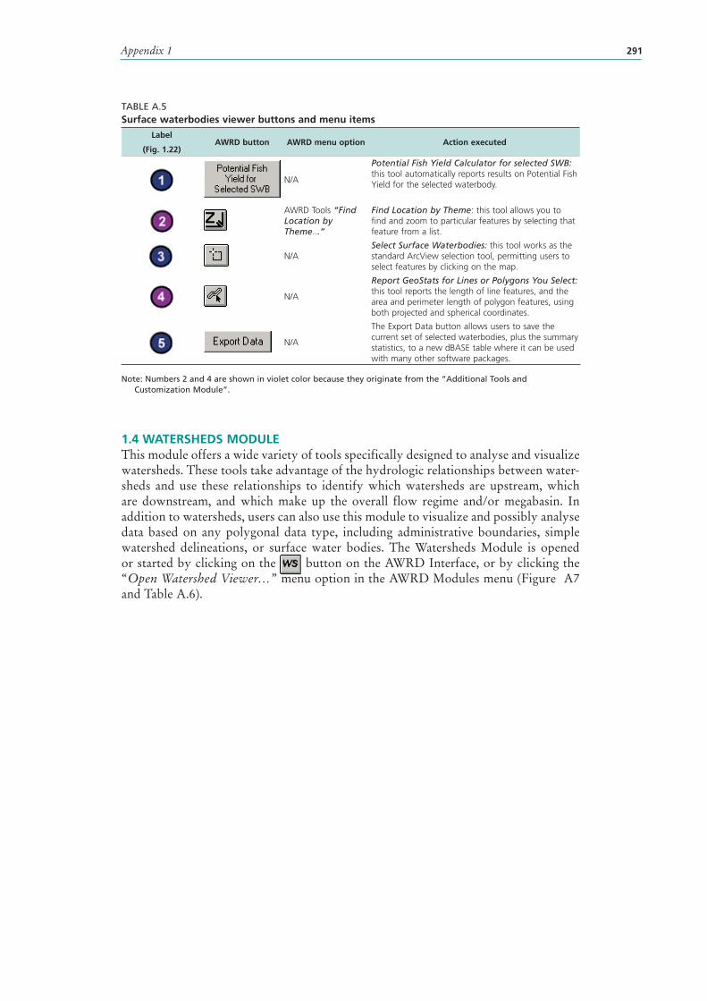
Appendix 1 291
TABLE A.5Surface waterbodies viewer buttons and menu items
Label
(Fig. 1.22)AWRD button AWRD menu option Action executed
N/A
Potential Fish Yield Calculator for selected SWB: this tool automatically reports results on Potential Fish Yield for the selected waterbody.
AWRD Tools “Find Location by Theme...”
Find Location by Theme: this tool allows you to find and zoom to particular features by selecting that feature from a list.
N/ASelect Surface Waterbodies: this tool works as the standard ArcView selection tool, permitting users to select features by clicking on the map.
N/A
Report GeoStats for Lines or Polygons You Select: this tool reports the length of line features, and the area and perimeter length of polygon features, using both projected and spherical coordinates.
N/A
The Export Data button allows users to save the current set of selected waterbodies, plus the summary statistics, to a new dBASE table where it can be used with many other software packages.
Note: Numbers 2 and 4 are shown in violet color because they originate from the “Additional Tools and Customization Module”.
1.4 WATERSHEDS MODULEThis module offers a wide variety of tools specifically designed to analyse and visualize watersheds. These tools take advantage of the hydrologic relationships between water-sheds and use these relationships to identify which watersheds are upstream , which are downstream , and which make up the overall flow regime and/or megabasin . In addition to watersheds, users can also use this module to visualize and possibly analyse data based on any polygonal data type, including administrative boundaries, simple watershed delineations, or surface water bod ies. The Watersheds Module is opened or started by clicking on the button on the AWRD Interface, or by clicking the “Open Watershed Viewer…” menu option in the AWRD Modules menu (Figure A7 and Table A.6).
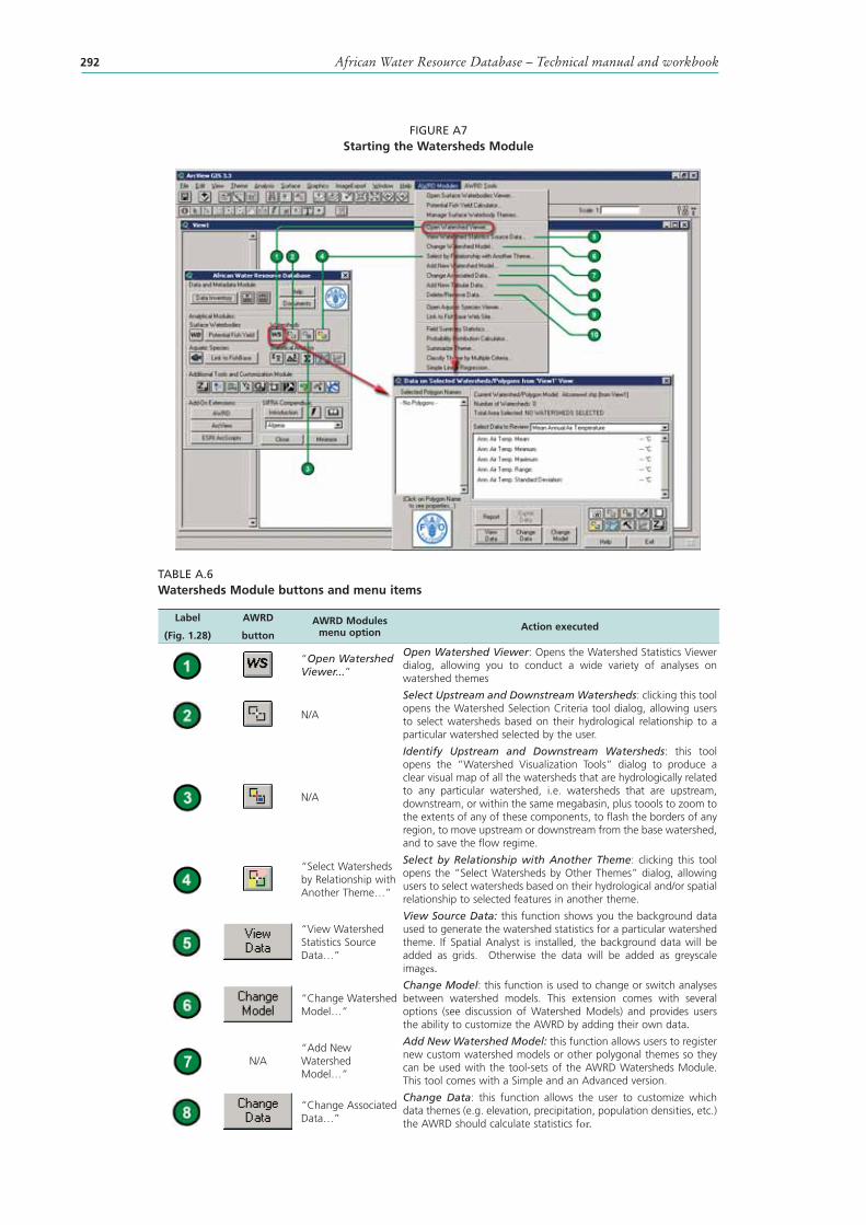
African Water Resource Database – Technical manual and workbook292
FIGURE A7Starting the Watersheds Module
TABLE A.6Watersheds Module buttons and menu items
Label
(Fig. 1.28)
AWRD
buttonAWRD Modules
menu option Action executed
“Open Watershed Viewer...”
Open Watershed Viewer: Opens the Watershed Statistics Viewer dialog, allowing you to conduct a wide variety of analyses on watershed themes
N/A
Select Upstream and Downstream Watersheds: clicking this tool opens the Watershed Selection Criteria tool dialog, allowing users to select watersheds based on their hydrological relationship to a particular watershed selected by the user.
N/A
Identify Upstream and Downstream Watersheds: this tool opens the “Watershed Visualization Tools” dialog to produce a clear visual map of all the watersheds that are hydrologically related to any particular watershed , i.e. watersheds that are upstream, downstream, or within the same megabasin, plus toools to zoom to the extents of any of these components, to flash the borders of any region, to move upstream or downstream from the base watershed, and to save the flow regime.
“Select Watersheds by Relationship with Another Theme…”
Select by Relationship with Another Theme: clicking this tool opens the “Select Watersheds by Other Themes” dialog, allowing users to select watersheds based on their hydrological and/or spatial relationship to selected features in another theme.
“View Watershed Statistics Source Data…”
View Source Data: this function shows you the background data used to generate the watershed statistics for a particular watershed theme. If Spatial Analyst is installed, the background data will be added as grids. Otherwise the data will be added as greyscale images.
“Change Watershed Model…”
Change Model: this function is used to change or switch analyses between watershed models. This extension comes with several options (see discussion of Watershed Models) and provides users the ability to customize the AWRD by adding their own data.
N/A“Add New Watershed Model…”
Add New Watershed Model: this function allows users to register new custom watershed models or other polygonal themes so they can be used with the tool-sets of the AWRD Watersheds Module. This tool comes with a Simple and an Advanced version.
“Change Associated Data…”
Change Data: this function allows the user to customize which data themes (e.g. elevation, precipitation, population densities, etc.) the AWRD should calculate statistics for.
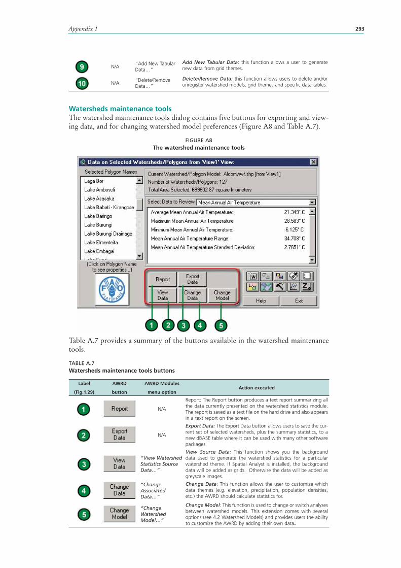
Appendix 1 293
N/A“Add New Tabular Data…”
Add New Tabular Data: this function allows a user to generate new data from grid themes.
N/A“Delete/Remove Data…”
Delete/Remove Data: this function allows users to delete and/or unregister watershed models, grid themes and specific data tables.
Watersheds maintenance toolsThe watershed maintenance tools dialog contains five buttons for exporting and view-ing data, and for changing watershed model preferences (Figure A8 and Table A.7).
FIGURE A8The watershed maintenance tools
Table A.7 provides a summary of the buttons available in the watershed maintenance tools.
TABLE A.7Watersheds maintenance tools buttons
Label
(Fig.1.29)
AWRD
button
AWRD Modules
menu optionAction executed
N/A
Report: The Report button produces a text report summarizing all the data currently presented on the watershed statistics module. The report is saved as a text file on the hard drive and also appears in a text report on the screen.
N/A
Export Data: The Export Data button allows users to save the cur-rent set of selected watersheds, plus the summary statistics, to a new dBASE table where it can be used with many other software packages.
“View Watershed Statistics Source Data…”
View Source Data: This function shows you the background data used to generate the watershed statistics for a particular watershed theme. If Spatial Analyst is installed, the background data will be added as grids. Otherwise the data will be added as greyscale images.
“Change Associated Data…”
Change Data: This function allows the user to customize which data themes (e.g. elevation, precipitation, population densities, etc.) the AWRD should calculate statistics for.
“Change Watershed Model…”
Change Model: This function is used to change or switch analyses between watershed models. This extension comes with several options (see 4.2 Watershed Models) and provides users the ability to customize the AWRD by adding their own data.
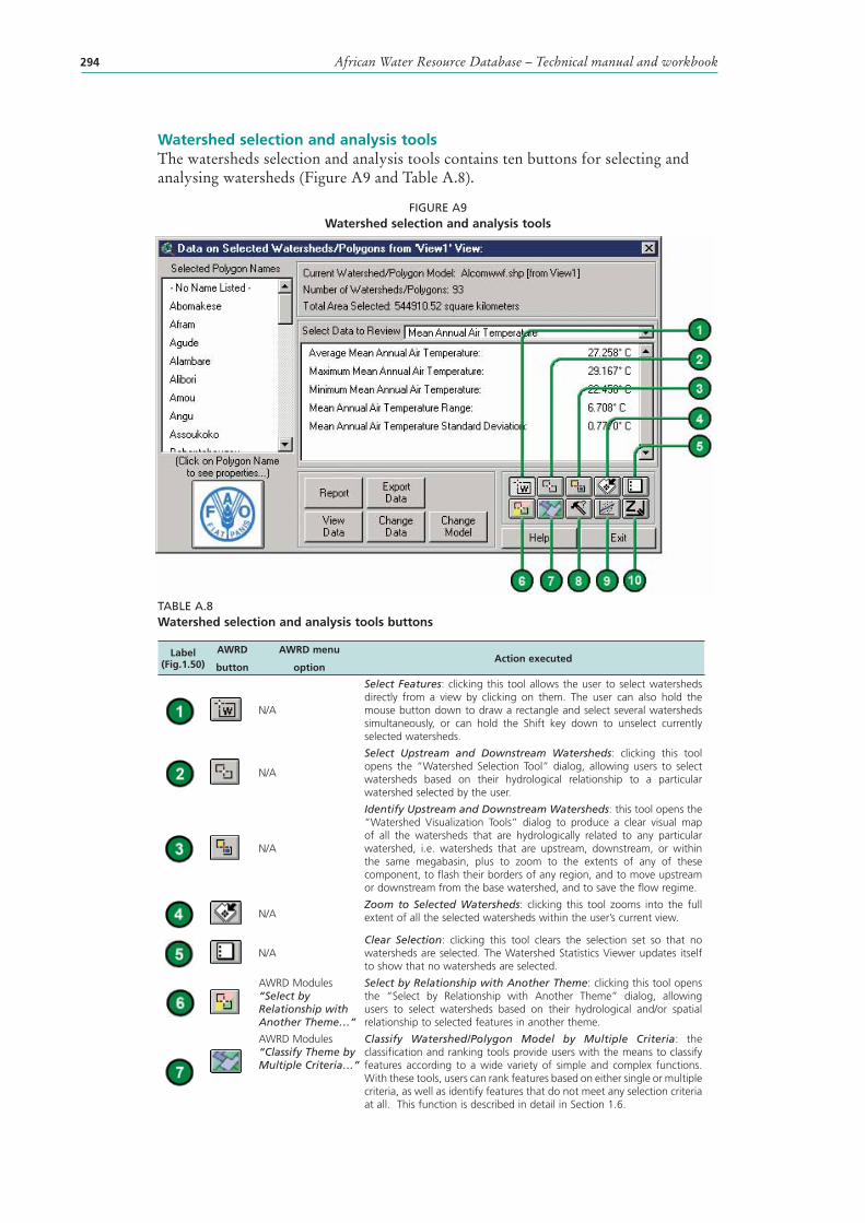
African Water Resource Database – Technical manual and workbook294
Watershed selection and analysis tools The watersheds selection and analysis tools contains ten buttons for selecting and analysing watersheds (Figure A9 and Table A.8).
FIGURE A9Watershed selection and analysis tools
TABLE A.8Watershed selection and analysis tools buttons
Label (Fig.1.50)
AWRD
button
AWRD menu
optionAction executed
N/A
Select Features: clicking this tool allows the user to select watersheds directly from a view by clicking on them. The user can also hold the mouse button down to draw a rectangle and select several watersheds simultaneously, or can hold the Shift key down to unselect currently selected watersheds.
N/A
Select Upstream and Downstream Watersheds: clicking this tool opens the “Watershed Selection Tool” dialog, allowing users to select watersheds based on their hydrological relationship to a particular watershed selected by the user.
N/A
Identify Upstream and Downstream Watersheds: this tool opens the “Watershed Visualization Tools” dialog to produce a clear visual map of all the watersheds that are hydrologically related to any particular watershed , i.e. watersheds that are upstream, downstream, or within the same megabasin, plus to zoom to the extents of any of these component, to flash their borders of any region, and to move upstream or downstream from the base watershed, and to save the flow regime.
N/AZoom to Selected Watersheds: clicking this tool zooms into the full extent of all the selected watersheds within the user’s current view.
N/AClear Selection: clicking this tool clears the selection set so that no watersheds are selected. The Watershed Statistics Viewer updates itself to show that no watersheds are selected.
AWRD Modules “Select by Relationship with Another Theme…”
Select by Relationship with Another Theme: clicking this tool opens the “Select by Relationship with Another Theme” dialog, allowing users to select watersheds based on their hydrological and/or spatial relationship to selected features in another theme.
AWRD Modules “Classify Theme by Multiple Criteria…”
Classify Watershed/Polygon Model by Multiple Criteria: the classification and ranking tools provide users with the means to classify features according to a wide variety of simple and complex functions. With these tools, users can rank features based on either single or multiple criteria, as well as identify features that do not meet any selection criteria at all. This function is described in detail in Section 1.6.
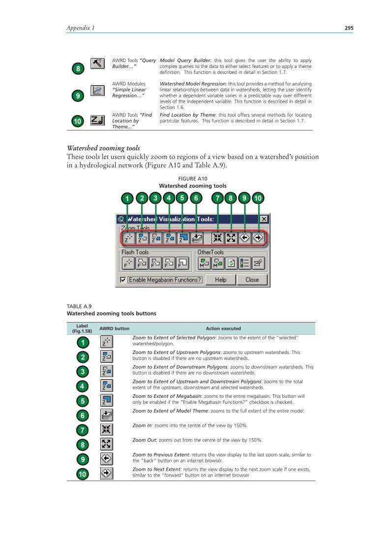
Appendix 1 295
AWRD Tools “Query Builder…”
Model Query Builder: this tool gives the user the ability to apply complex queries to the data to either select features or to apply a theme definition. This function is described in detail in Section 1.7.
AWRD Modules “Simple Linear Regression…”
Watershed Model Regression: this tool provides a method for analysing linear relationships between data in watersheds, letting the user identify whether a dependent variable varies in a predictable way over different levels of the independent variable. This function is described in detail in Section 1.6.
AWRD Tools “Find Location by Theme...”
Find Location by Theme: this tool offers several methods for locating particular features. This function is described in detail in Section 1.7.
Watershed zooming toolsThese tools let users quickly zoom to regions of a view based on a watershed ’s position in a hydrological network (Figure A10 and Table A.9).
FIGURE A10Watershed zooming tools
TABLE A.9Watershed zooming tools buttons
Label (Fig.1.58) AWRD button Action executed
Zoom to Extent of Selected Polygon: zooms to the extent of the “selected” watershed/ polygon.
Zoom to Extent of Upstream Polygons: zooms to upstream watersheds. This button is disabled if there are no upstream watersheds.
Zoom to Extent of Downstream Polygons: zooms to downstream watersheds. This button is disabled if there are no downstream watersheds.
Zoom to Extent of Upstream and Downstream Polygons: zooms to the total extent of the upstream, downstream and selected watersheds.
Zoom to Extent of Megabasin: zooms to the entire megabasin. This button will only be enabled if the “Enable Megabasin Functions?” checkbox is checked.
Zoom to Extent of Model Theme: zooms to the full extent of the entire model.
Zoom In: zooms into the centre of the view by 150%.
Zoom Out: zooms out from the centre of the view by 150%.
Zoom to Previous Extent: returns the view display to the last zoom scale, similar to the “back” button on an internet browser.
Zoom to Next Extent: returns the view display to the next zoom scale if one exists, similar to the “forward” button on an internet browser
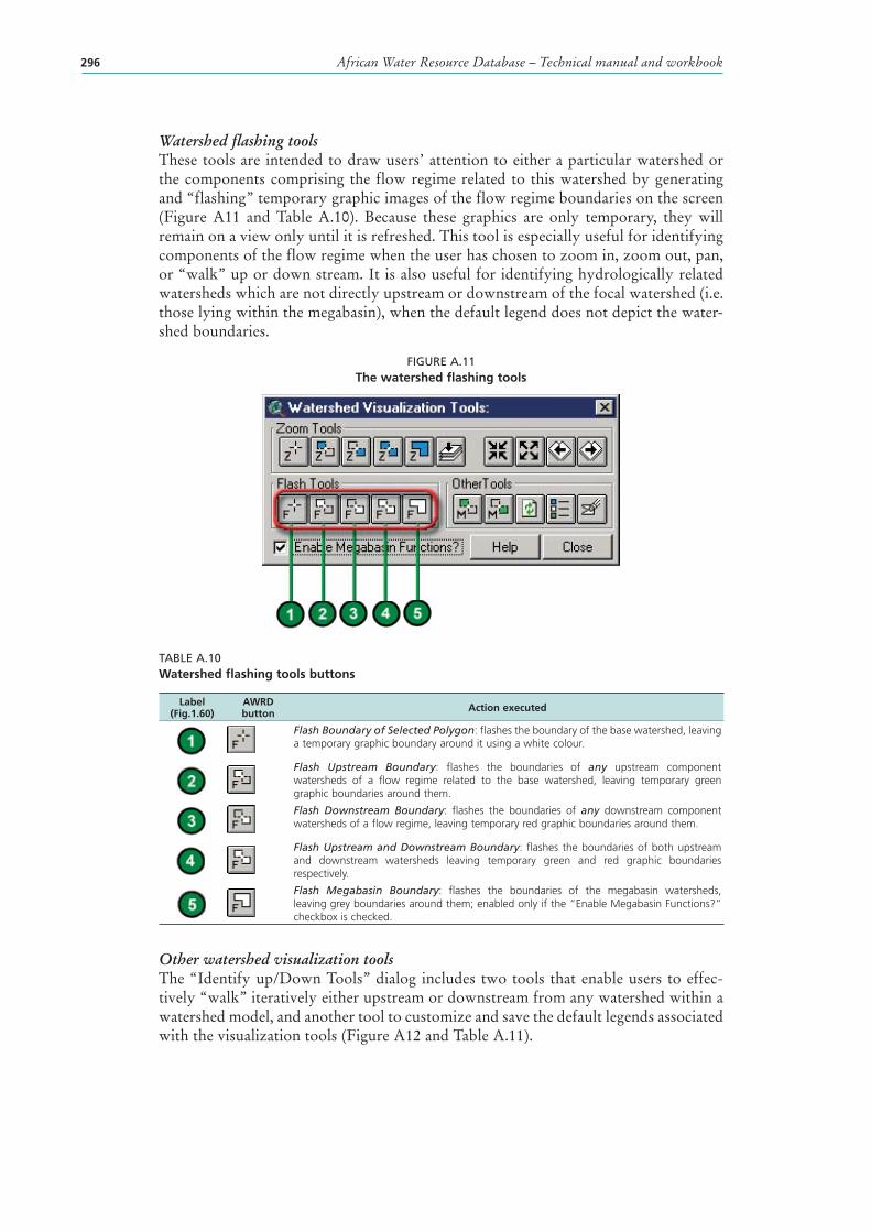
African Water Resource Database – Technical manual and workbook296
Watershed flashing toolsThese tools are intended to draw users’ attention to either a particular watershed or the components comprising the flow regime related to this watershed by generating and “flashing” temporary graphic images of the flow regime boundaries on the screen (Figure A11 and Table A.10). Because these graphics are only temporary, they will remain on a view only until it is refreshed. This tool is especially useful for identifying components of the flow regime when the user has chosen to zoom in, zoom out, pan, or “walk” up or down stream. It is also useful for identifying hydrologically related watersheds which are not directly upstream or downstream of the focal watershed (i.e. those lying within the megabasin ), when the default legend does not depict the water-shed boundaries.
FIGURE A.11The watershed flashing tools
TABLE A.10Watershed flashing tools buttons
Label (Fig.1.60)
AWRD button Action executed
Flash Boundary of Selected Polygon: flashes the boundary of the base watershed, leaving a temporary graphic boundary around it using a white colour.
Flash Upstream Boundary: flashes the boundaries of any upstream component watersheds of a flow regime related to the base watershed, leaving temporary green graphic boundaries around them.
Flash Downstream Boundary: flashes the boundaries of any downstream component watersheds of a flow regime, leaving temporary red graphic boundaries around them.
Flash Upstream and Downstream Boundary: flashes the boundaries of both upstream and downstream watersheds leaving temporary green and red graphic boundaries respectively.
Flash Megabasin Boundary: flashes the boundaries of the megabasin watersheds, leaving grey boundaries around them; enabled only if the “Enable Megabasin Functions?” checkbox is checked.
Other watershed visualization toolsThe “Identify up/Down Tools” dialog includes two tools that enable users to effec-tively “walk” iteratively either upstream or downstream from any watershed within a watershed model , and another tool to customize and save the default legends associated with the visualization tools (Figure A12 and Table A.11).
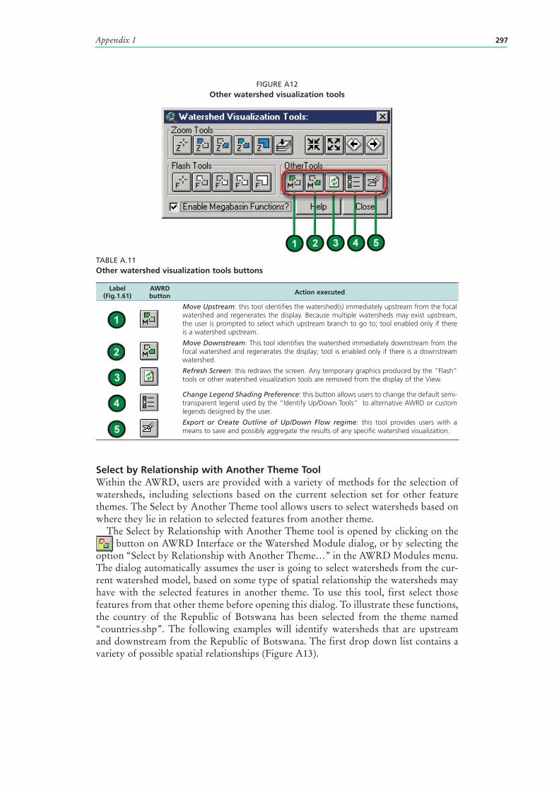
Appendix 1 297
FIGURE A12Other watershed visualization tools
TABLE A.11Other watershed visualization tools buttons
Label (Fig.1.61)
AWRD button Action executed
Move Upstream: this tool identifies the watershed( s) immediately upstream from the focal watershed and regenerates the display. Because multiple watersheds may exist upstream, the user is prompted to select which upstream branch to go to; tool enabled only if there is a watershed upstream.
Move Downstream: This tool identifies the watershed immediately downstream from the focal watershed and regenerates the display; tool is enabled only if there is a downstream watershed.
Refresh Screen: this redraws the screen. Any temporary graphics produced by the “Flash” tools or other watershed visualization tools are removed from the display of the View.
Change Legend Shading Preference: this button allows users to change the default semi-transparent legend used by the “Identify Up/Down Tools” to alternative AWRD or custom legends designed by the user.
Export or Create Outline of Up/Down Flow regime: this tool provides users with a means to save and possibly aggregate the results of any specific watershed visualization.
Select by Relationship with Another Theme ToolWithin the AWRD, users are provided with a variety of methods for the selection of watersheds, including selections based on the current selection set for other feature themes. The Select by Another Theme tool allows users to select watersheds based on where they lie in relation to selected features from another theme .
The Select by Relationship with Another Theme tool is opened by clicking on the button on AWRD Interface or the Watershed Module dialog, or by selecting the
option “Select by Relationship with Another Theme…” in the AWRD Modules menu. The dialog automatically assumes the user is going to select watersheds from the cur-rent watershed model , based on some type of spatial relationship the watersheds may have with the selected features in another theme . To use this tool, first select those features from that other theme before opening this dialog. To illustrate these functions, the country of the Republic of Botswana has been selected from the theme named “countries.shp”. The following examples will identify watersheds that are upstream and downstream from the Republic of Botswana. The first drop down list contains a variety of possible spatial relationships (Figure A13).
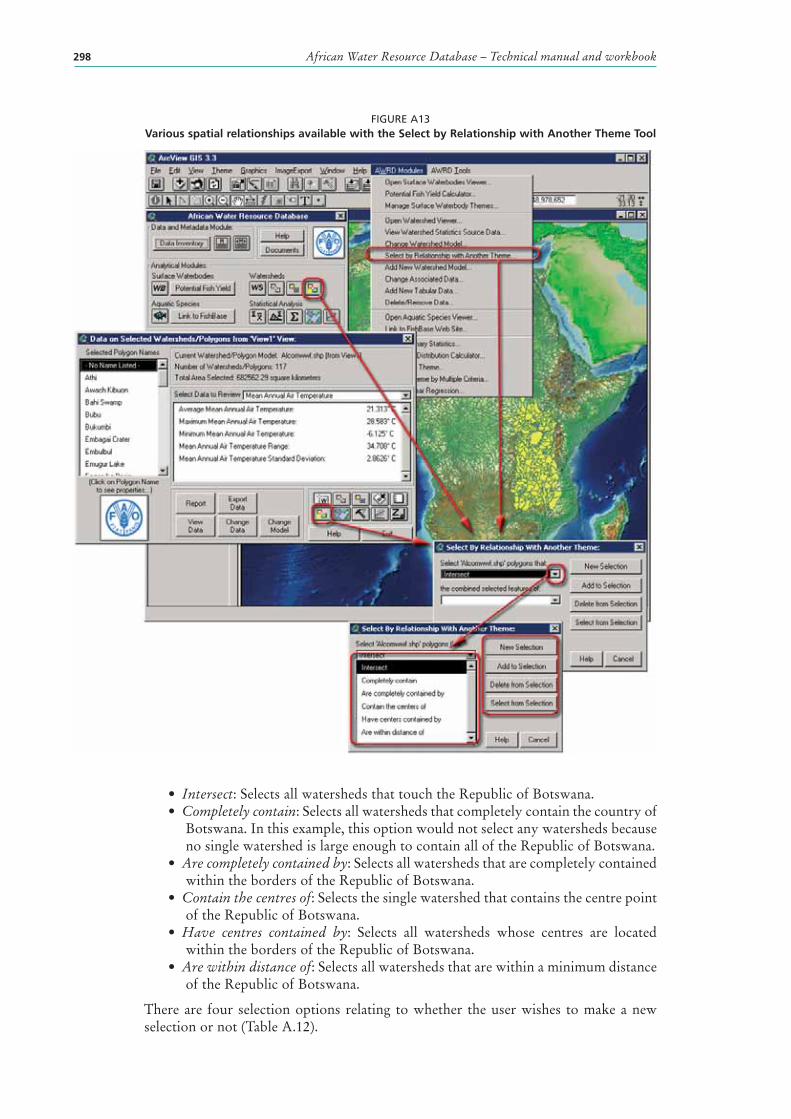
African Water Resource Database – Technical manual and workbook298
FIGURE A13Various spatial relationships available with the Select by Relationship with Another Theme Tool
• Intersect: Selects all watersheds that touch the Republic of Botswana .• Completely contain: Selects all watersheds that completely contain the country of
Botswana . In this example, this option would not select any watersheds because no single watershed is large enough to contain all of the Republic of Botswana.
• Are completely contained by: Selects all watersheds that are completely contained within the borders of the Republic of Botswana .
• Contain the centres of: Selects the single watershed that contains the centre point of the Republic of Botswana .
• Have centres contained by: Selects all watersheds whose centres are located within the borders of the Republic of Botswana .
• Are within distance of: Selects all watersheds that are within a minimum distance of the Republic of Botswana .
There are four selection options relating to whether the user wishes to make a new selection or not (Table A.12).
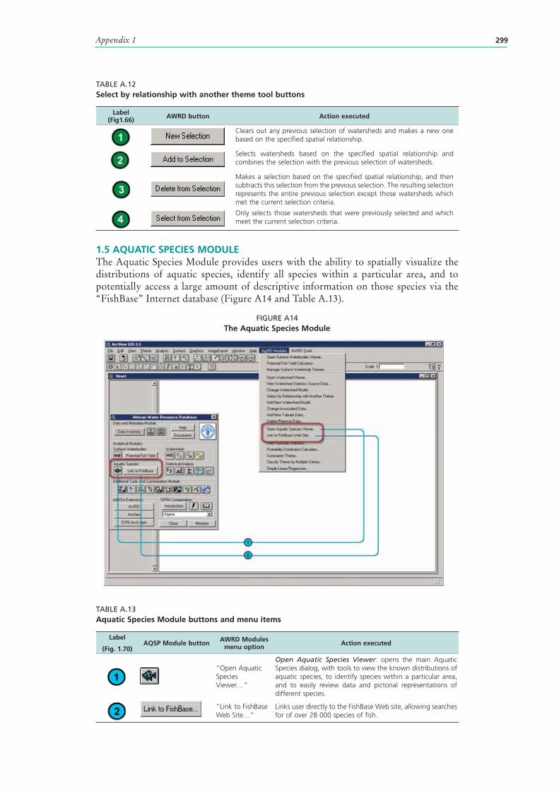
Appendix 1 299
TABLE A.12Select by relationship with another theme tool buttons
Label (Fig1.66) AWRD button Action executed
Clears out any previous selection of watersheds and makes a new one based on the specified spatial relationship.
Selects watersheds based on the specified spatial relationship and combines the selection with the previous selection of watersheds.
Makes a selection based on the specified spatial relationship, and then subtracts this selection from the previous selection. The resulting selection represents the entire previous selection except those watersheds which met the current selection criteria.
Only selects those watersheds that were previously selected and which meet the current selection criteria.
1.5 AQUATIC SPECIES MODULE The Aquatic Species Module provides users with the ability to spatially visualize the distributions of aquatic species , identify all species within a particular area, and to potentially access a large amount of descriptive information on those species via the “FishBase” Internet database (Figure A14 and Table A.13).
FIGURE A14The Aquatic Species Module
TABLE A.13Aquatic Species Module buttons and menu items
Label
(Fig. 1.70)AQSP Module button AWRD Modules
menu option Action executed
“Open Aquatic Species Viewer…”
Open Aquatic Species Viewer: opens the main Aquatic Species dialog, with tools to view the known distributions of aquatic species, to identify species within a particular area, and to easily review data and pictorial representations of different species.
“Link to FishBase Web Site…”
Links user directly to the FishBase Web site, allowing searches for of over 28 000 species of fish.
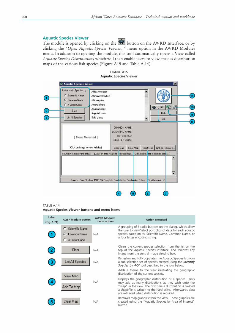
African Water Resource Database – Technical manual and workbook300
Aquatic Species ViewerThe module is opened by clicking on the button on the AWRD Interface, or by clicking the “Open Aquatic Species Viewer...” menu option in the AWRD Modules menu. In addition to opening the module, this tool automatically opens a View called Aquatic Species Distributions which will then enable users to view species distribution maps of the various fish species (Figure A15 and Table A.14).
FIGURE A15Aquatic Species Viewer
TABLE A.14Aquatic Species Viewer buttons and menu items
Label
(Fig. 1.71)AQSP Module button AWRD Modules
menu option Action executed
N/A
A grouping of 3 radio buttons on the dialog, which allow the user to view/select portfolios of data for each aquatic species based on its: Scientific Name, Common Name, or a four letter encoding string.
N/AClears the current species selection from the list on the top of the Aquatic Species interface, and removes any image from the central image viewing box.
N/ARefreshes and fully populates the Aquatic Species list from a sub-selection set of species created using the Identify Species by AOI tool described in the row below.
orN/A
Adds a theme to the view illustrating the geographic distribution of the current species.
Displays the geographic distribution of a species. Users may add as many distributions as they wish onto the “map” in the view. The first time a distribution is created a shapefile is written to the hard drive. Afterwards data are retrieved when distribution is required.
N/ARemoves map graphics from the view. These graphics are created using the “Aquatic Species by Area of Interest” button.
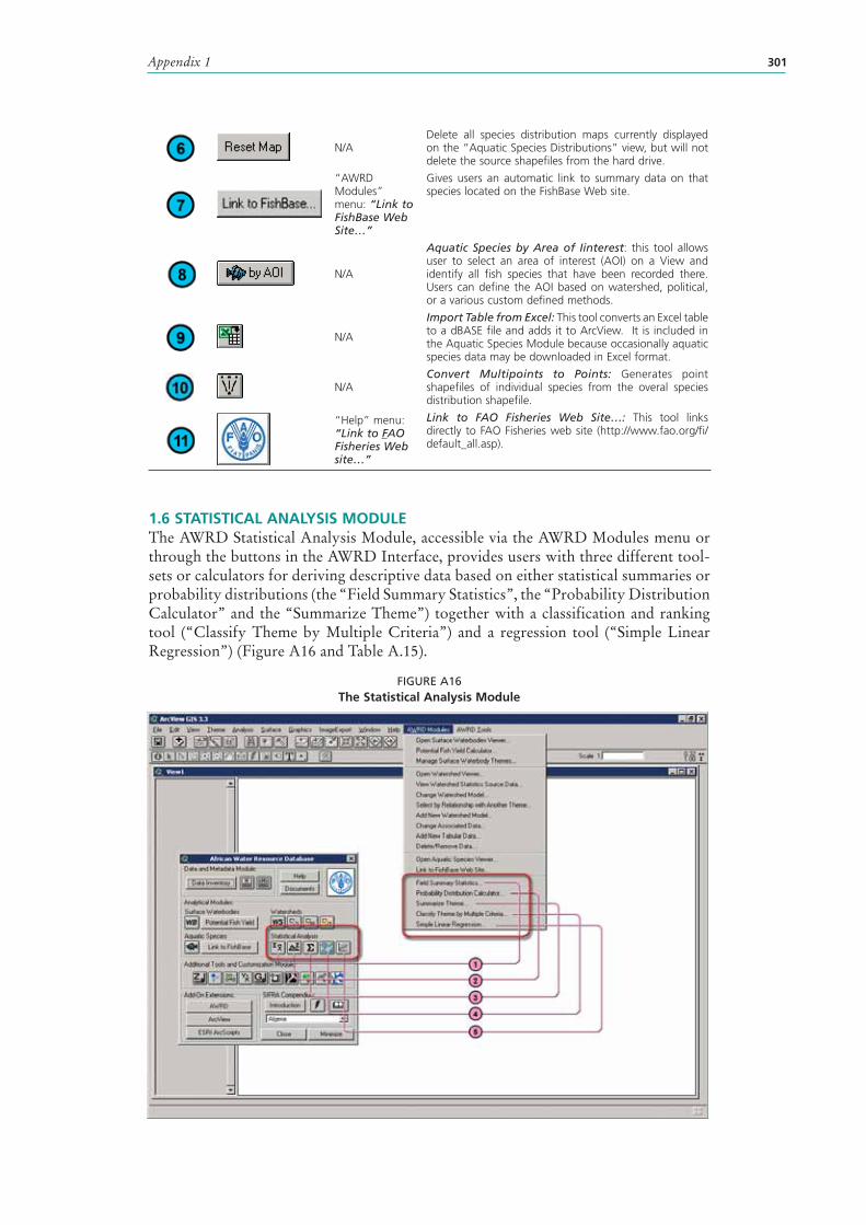
Appendix 1 301
N/ADelete all species distribution maps currently displayed on the “Aquatic Species Distributions” view, but will not delete the source shapefiles from the hard drive.
“AWRD Modules” menu: “Link to FishBase Web Site…”
Gives users an automatic link to summary data on that species located on the FishBase Web site.
N/A
Aquatic Species by Area of Iinterest: this tool allows user to select an area of interest (AOI) on a View and identify all fish species that have been recorded there. Users can define the AOI based on watershed , political, or a various custom defined methods.
N/A
Import Table from Excel: This tool converts an Excel table to a dBASE file and adds it to ArcView. It is included in the Aquatic Species Module because occasionally aquatic species data may be downloaded in Excel format.
N/AConvert Multipoints to Points: Generates point shapefiles of individual species from the overal species distribution shapefile.
“Help” menu: “Link to FAO Fisheries Web site…”
Link to FAO Fisheries Web Site…: This tool links directly to FAO Fisheries web site (http://www.fao.org/fi/default_all.asp).
1.6 STATISTICAL ANALYSIS MODULEThe AWRD Statistical Analysis Module, accessible via the AWRD Modules menu or through the buttons in the AWRD Interface, provides users with three different tool-sets or calculators for deriving descriptive data based on either statistical summaries or probability distributions (the “Field Summary Statistics”, the “Probability Distribution Calculator” and the “Summarize Theme”) together with a classification and ranking tool (“Classify Theme by Multiple Criteria”) and a regression tool (“Simple Linear Regression”) (Figure A16 and Table A.15).
FIGURE A16The Statistical Analysis Module
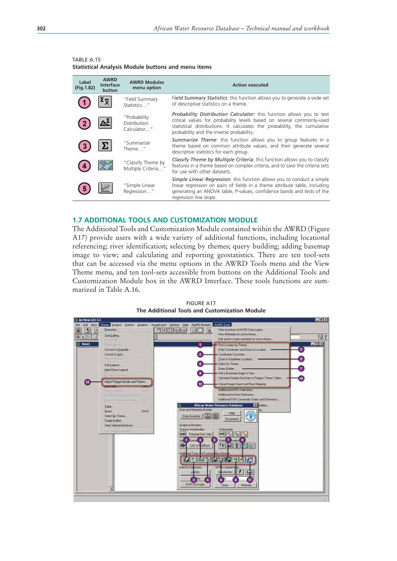
African Water Resource Database – Technical manual and workbook302
TABLE A.15Statistical Analysis Module buttons and menu items
Label (Fig.1.82)
AWRD Interface button
AWRD Modules menu option Action executed
“Field Summary Statistics…”
Field Summary Statistics: this function allows you to generate a wide set of descriptive statistics on a theme.
“Probability Distribution Calculator…”
Probability Distribution Calculator: this function allows you to test critical values for probability levels based on several commonly-used statistical distributions. It calculates the probability, the cumulative probability and the inverse probability.
“Summarize Theme…”
Summarize Theme: this function allows you to group features in a theme based on common attribute values, and then generate several descriptive statistics for each group.
“Classify Theme by Multiple Criteria…”
Classify Theme by Multiple Criteria: this function allows you to classify features in a theme based on complex criteria, and to save the criteria sets for use with other datasets.
“Simple Linear Regression…”
Simple Linear Regression: this function allows you to conduct a simple linear regression on pairs of fields in a theme attribute table, including generating an ANOVA table, P-values, confidence bands and tests of the regression line slope.
1.7 ADDITIONAL TOOLS AND CUSTOMIZATION MODULEThe Additional Tools and Customization Module contained within the AWRD (Figure A17) provide users with a wide variety of additional functions, including locational referencing; river identification; selecting by themes; query building; adding basemap image to view; and calculating and reporting geostatistics. There are ten tool-sets that can be accessed via the menu options in the AWRD Tools menu and the View Theme menu, and ten tool-sets accessible from buttons on the Additional Tools and Customization Module box in the AWRD Interface. These tools functions are sum-marized in Table A.16.
FIGURE A17The Additional Tools and Customization Module
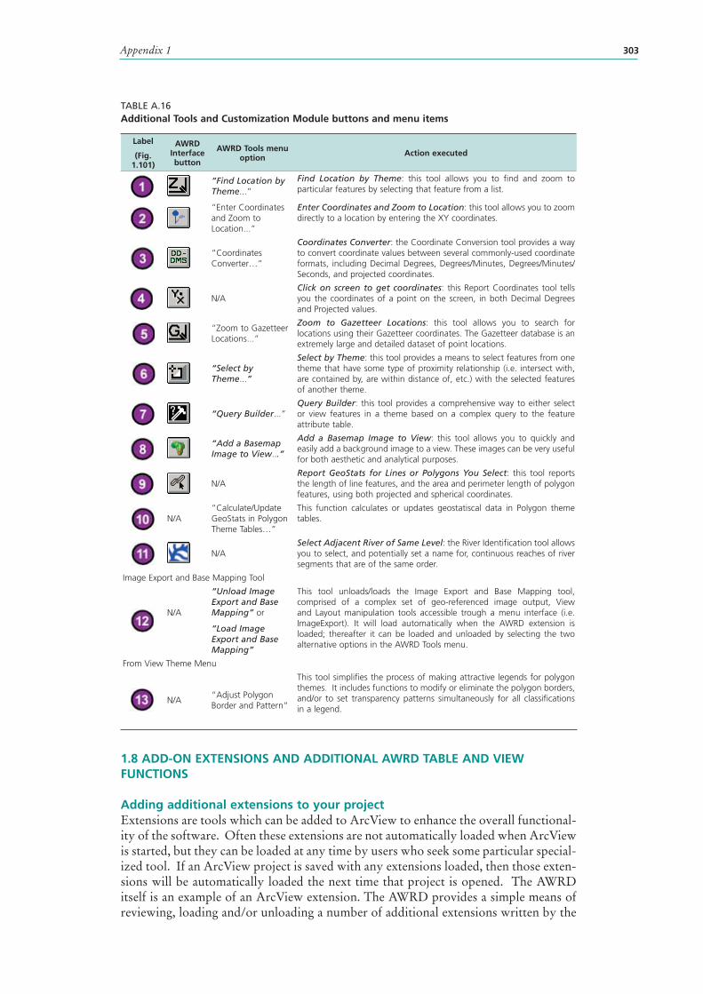
Appendix 1 303
TABLE A.16Additional Tools and Customization Module buttons and menu items
Label
(Fig. 1.101)
AWRD Interface button
AWRD Tools menu option Action executed
“Find Location by Theme...”
Find Location by Theme: this tool allows you to find and zoom to particular features by selecting that feature from a list.
“Enter Coordinates and Zoom to Location...”
Enter Coordinates and Zoom to Location: this tool allows you to zoom directly to a location by entering the XY coordinates.
“Coordinates Converter…”
Coordinates Converter: the Coordinate Conversion tool provides a way to convert coordinate values between several commonly-used coordinate formats, including Decimal Degrees, Degrees/Minutes, Degrees/Minutes/Seconds, and projected coordinates.
N/AClick on screen to get coordinates: this Report Coordinates tool tells you the coordinates of a point on the screen, in both Decimal Degrees and Projected values.
“Zoom to Gazetteer Locations...”
Zoom to Gazetteer Locations: this tool allows you to search for locations using their Gazetteer coordinates. The Gazetteer database is an extremely large and detailed dataset of point locations.
“Select by Theme...”
Select by Theme: this tool provides a means to select features from one theme that have some type of proximity relationship (i.e. intersect with, are contained by, are within distance of, etc.) with the selected features of another theme.
“Query Builder...”Query Builder: this tool provides a comprehensive way to either select or view features in a theme based on a complex query to the feature attribute table.
“Add a Basemap Image to View...”
Add a Basemap Image to View: this tool allows you to quickly and easily add a background image to a view. These images can be very useful for both aesthetic and analytical purposes.
N/A Report GeoStats for Lines or Polygons You Select: this tool reports the length of line features, and the area and perimeter length of polygon features, using both projected and spherical coordinates.
N/A“Calculate/Update GeoStats in Polygon Theme Tables…”
This function calculates or updates geostatiscal data in Polygon theme tables.
N/ASelect Adjacent River of Same Level: the River Identification tool allows you to select, and potentially set a name for, continuous reaches of river segments that are of the same order.
Image Export and Base Mapping Tool
N/A
“Unload Image Export and Base Mapping” or
“Load Image Export and Base Mapping”
This tool unloads/loads the Image Export and Base Mapping tool, comprised of a complex set of geo-referenced image output, View and Layout manipulation tools accessible trough a menu interface (i.e. ImageExport). It will load automatically when the AWRD extension is loaded; thereafter it can be loaded and unloaded by selecting the two alternative options in the AWRD Tools menu.
From View Theme Menu
N/A“Adjust Polygon Border and Pattern”
This tool simplifies the process of making attractive legends for polygon themes. It includes functions to modify or eliminate the polygon borders, and/or to set transparency patterns simultaneously for all classifications in a legend.
1.8 ADD-ON EXTENSIONS AND ADDITIONAL AWRD TABLE AND VIEW FUNCTIONS
Adding additional extensions to your projectExtensions are tools which can be added to ArcView to enhance the overall functional-ity of the software. Often these extensions are not automatically loaded when ArcView is started, but they can be loaded at any time by users who seek some particular special-ized tool. If an ArcView project is saved with any extensions loaded, then those exten-sions will be automatically loaded the next time that project is opened. The AWRD itself is an example of an ArcView extension. The AWRD provides a simple means of reviewing, loading and/or unloading a number of additional extensions written by the
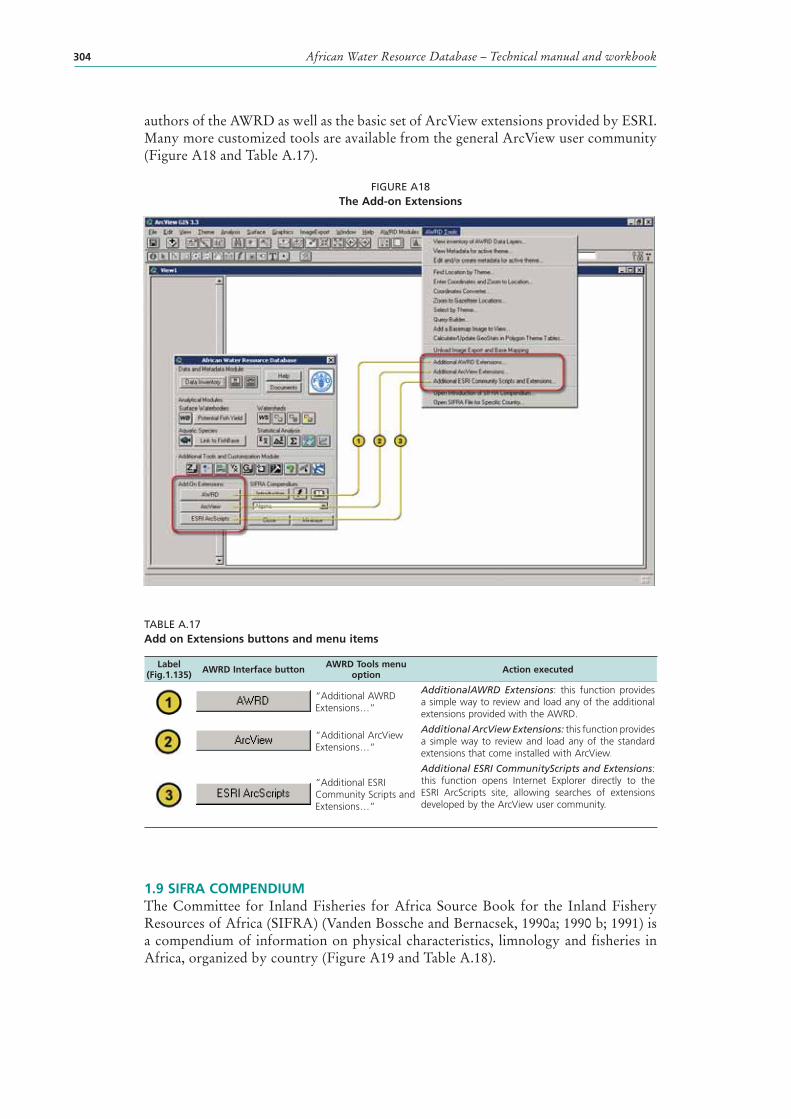
African Water Resource Database – Technical manual and workbook304
authors of the AWRD as well as the basic set of ArcView extensions provided by ESRI. Many more customized tools are available from the general ArcView user community (Figure A18 and Table A.17).
FIGURE A18The Add-on Extensions
TABLE A.17Add on Extensions buttons and menu items
Label (Fig.1.135) AWRD Interface button AWRD Tools menu
option Action executed
“Additional AWRD Extensions…”
AdditionalAWRD Extensions: this function provides a simple way to review and load any of the additional extensions provided with the AWRD.
“Additional ArcView Extensions…”
Additional ArcView Extensions: this function provides a simple way to review and load any of the standard extensions that come installed with ArcView.
“Additional ESRI Community Scripts and Extensions…”
Additional ESRI CommunityScripts and Extensions: this function opens Internet Explorer directly to the ESRI ArcScripts site, allowing searches of extensions developed by the ArcView user community.
1.9 SIFRA COMPENDIUM The Committee for Inland Fisheries for Africa Source Book for the Inland Fishery Resources of Africa (SIFRA) (Vanden Bossche and Bernacsek, 1990a; 1990 b; 1991) is a compendium of information on physical characteristics, limnology and fisheries in Africa, organized by country (Figure A19 and Table A.18).
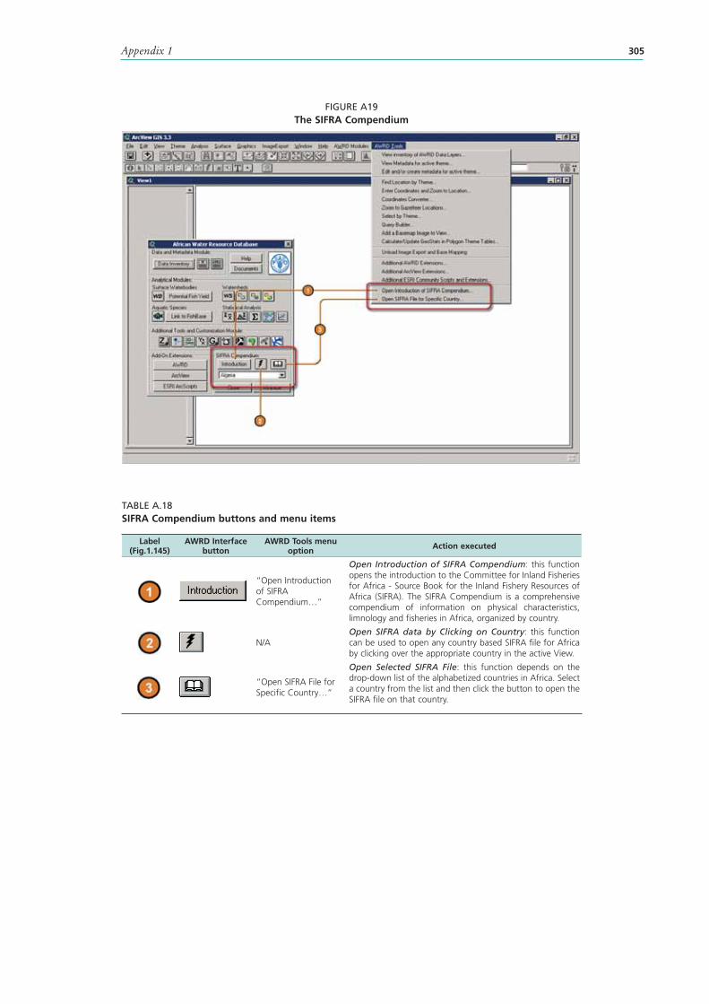
Appendix 1 305
FIGURE A19The SIFRA Compendium
TABLE A.18SIFRA Compendium buttons and menu items
Label (Fig.1.145)
AWRD Interface button
AWRD Tools menu option Action executed
“Open Introduction of SIFRA Compendium…”
Open Introduction of SIFRA Compendium: this function opens the introduction to the Committee for Inland Fisheries for Africa - Source Book for the Inland Fishery Resources of Africa (SIFRA). The SIFRA Compendium is a comprehensive compendium of information on physical characteristics, limnology and fisheries in Africa, organized by country.
N/AOpen SIFRA data by Clicking on Country: this function can be used to open any country based SIFRA file for Africa by clicking over the appropriate country in the active View.
“Open SIFRA File for Specific Country…”
Open Selected SIFRA File: this function depends on the drop-down list of the alphabetized countries in Africa. Select a country from the list and then click the button to open the SIFRA file on that country.
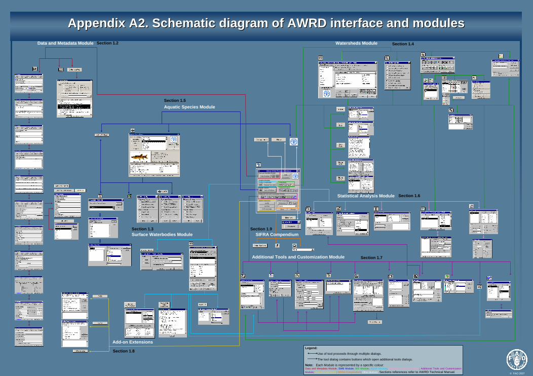
Appendix A2. Schematic diagram of AWRD interface and modulesAppendix A2. Schematic diagram of AWRD interface and modules
© FAO 2007
Data and Metadata Module
Aquatic Species Module
Watersheds Module
Additional Tools and Customization Module
Add-on Extensions
Surface Waterbodies Module
Statistical Analysis Module
SIFRA Compendium
Section 1.2
Section 1.5
Section 1.3
Section 1.8
Section 1.7
Section 1.6
Section 1.4
Section 1.9
Legend:
Use of tool proceeds through multiple dialogs.
The tool dialog contains buttons which open additional tools dialogs.
Note: Each Module is represented by a specific colour:Data and Metadata Module; SWB Module; WS Module; AQSP Module; Statistical Analysis Module; Additional Tools and Customization Module; Add-on Extensions; SIFRA Compendium; Other Buttons. Sections references refer to AWRD Technical Manual.
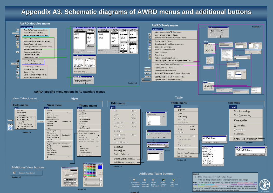
Appendix A3. Schematic diagrams of AWRD menus and additional butAppendix A3. Schematic diagrams of AWRD menus and additional buttonstons
© FAO 2007
AWRD Modules menu
View
Layout
AWRD Tools menu
Help menu
AWRD- specific menu options in AV standard menus
View
View menu
Additional View buttons
Zoom to Next Extent
View, Table, Layout
Section 1.4
Section 1.7
Section 1.1
Section 1.7
Table
Edit menu Table menu Field menu
Section 1.7
Section 1.7
Section 1.7
Additional Table buttons
Probability Distribution Calculator
Field Summary Statistics
Simple Linear Regression
Export Table to Excel
Import Table from Excel
Section 1.7
Section 1.7
Legend:
Use of tool proceeds through multiple dialogs.
The tool dialog contains buttons which open additional tools dialogs.
Note: Each Module is represented by a specific colour (Data and Metadata Module; SWB Module; WS Module; AQSP Module; Statistical Analysis Module; Additional Tools and Customization Module; Add-on Extensions; SIFRA Compendium; Other Buttons). Dotted arrows and boundary refer to functions from no-AWRD extension, but automatically loaded when the AWRD extensionis loaded. Sections references refer to AWRD Technical Manual.
Theme menu
Section 1.2
Section 1.2
Section 1.7