Cost-Based Predictive Spatiotemporal Join

IEEE TRANSACTIONS OF KNOWLEDGE AND DATA ENGINEERING, VOL. X, NO. X, XXXXX 200X 1

Cost-Based Predictive Spatio-Temporal JoinWook-Shin Han, Jaehwa Kim, Byung Suk Lee, Yufei Tao, Ralf Rantzau, Volker Markl

Abstract—A predictive spatio-temporal join finds all pairs of moving objects satisfying a join condition on future time and space. Inthis paper we present CoPST, the first and foremost algorithm for such a join using two spatio-temporal indexes. In a predictive spatio-temporal join, the bounding boxes of the outer index are used to perform window searches on the inner index, and these boundingboxes enclose objects with increasing laxity over time. CoPST constructs globally tightened bounding boxes “on the fly” to performwindow searches during join processing, thus significantly minimizing overlap and improving the join performance. CoPST adaptsgracefully to large scale databases, by dynamically switching between main-memory buffering and disk-based buffering, through anovel probabilistic cost model. Our extensive experiments validate the cost model and show its accuracy for realistic data sets. We alsoshowcase the superiority of CoPST over algorithms adapted from state of the art spatial join algorithms, by a speedup of up to an orderof magnitude.

Index Terms—H.2.4.k spatial databases, H.2.4.m temporal databases

F

1 INTRODUCTION

MOVING object database systems managing spatio-temporal objects have been an area of active

research, and have applications in areas like telemat-ics, location-based services, air traffic control systems,etc. Particularly in a wireless environment, techniquesfor managing a large number of moving objects effec-tively and efficiently are becoming increasingly impor-tant. Spatio-temporal queries used in a moving objectdatabase system can be classified into historical queries[1], [2], [3], which handle past information, and predictivequeries [4], [5], which extrapolate the past informationinto the future. Each type of queries has its own appli-cation areas and pertinent research issues.

In this paper we consider predictive queries with afocus on spatio-temporal join operations. A predictivespatio-temporal join is a key query operation in a mov-ing object database system. The formal definition of thepredictive spatio-temporal join is as follows:

Definition 1: [6] Given two sets R and S of spatio-temporal objects, a future timestamp tq , and a distancethreshold d, a predictive spatio-temporal join finds allpairs of objects < o1, o2 > such that o1 ∈ R, o2 ∈ S, and

• W.-S. Han and J Kim is with the Department of Computer Engineering,Kyungpook National University, 1370 Sankyuk-dong, Book-gu, Daegu702-701, Korea.E-mail: {wshan,jhkim}@{knu.ac.kr,www-db.knu.ac.kr}

• B. S. Lee is with the Department of Computer Science, University ofVermont, Burlington, Vermont 05405, U.S.A.E-mail: [email protected]

• Y. Tao is with the Department of Computer Science and Engineering,Chinese University of Hong Kong, Sha Tin, New Territories, Hong Kong.E-mail: [email protected]

• R. Rantzau is with the IBM Silicon Valley Laboratory, 555 Bailey Ave,San Jose, CA 95141, U.S.A.E-mail: [email protected]

• V. Markl is with the Technische Universitat Berlin, Einsteinufer 17, 10587Berlin, Germany.E-mail: [email protected]

Manuscript received XXXX XX, 200X; revised XXXX XX, 200X.

the distance between the objects o1 and o2 at tq is shorterthan d.

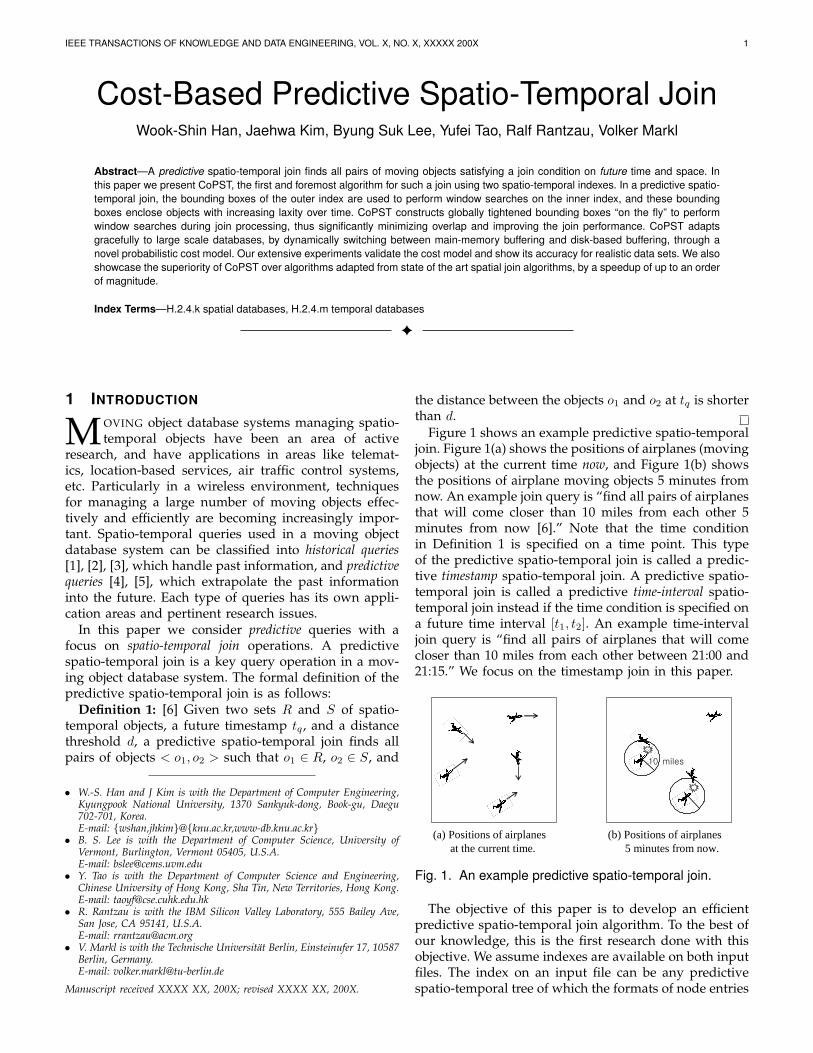
Figure 1 shows an example predictive spatio-temporaljoin. Figure 1(a) shows the positions of airplanes (movingobjects) at the current time now, and Figure 1(b) showsthe positions of airplane moving objects 5 minutes fromnow. An example join query is “find all pairs of airplanesthat will come closer than 10 miles from each other 5minutes from now [6].” Note that the time conditionin Definition 1 is specified on a time point. This typeof the predictive spatio-temporal join is called a predic-tive timestamp spatio-temporal join. A predictive spatio-temporal join is called a predictive time-interval spatio-temporal join instead if the time condition is specified ona future time interval [t1, t2]. An example time-intervaljoin query is “find all pairs of airplanes that will comecloser than 10 miles from each other between 21:00 and21:15.” We focus on the timestamp join in this paper.

(a) Positions of airplanes at the current time.

(b) Positions of airplanes 5 minutes from now.

10 miles

Fig. 1. An example predictive spatio-temporal join.

The objective of this paper is to develop an efficientpredictive spatio-temporal join algorithm. To the best ofour knowledge, this is the first research done with thisobjective. We assume indexes are available on both inputfiles. The index on an input file can be any predictivespatio-temporal tree of which the formats of node entries


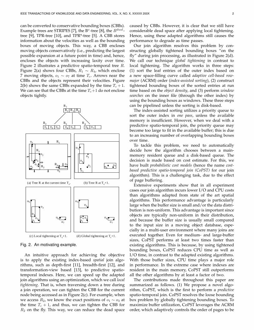
can be converted to conservative bounding boxes (CBBs).Example trees are STRIPES [7], the Bx-tree [8], the Bdual-tree [9], TPR-tree [10], and TPR*-tree [5]. A CBB storesinformation about the velocities as well as the boundingboxes of moving objects. This way, a CBB enclosesmoving objects conservatively (i.e., predicting the largestpossible expansion at a future point in time) and, hence,encloses the objects with increasing laxity over time.Figure 2 illustrates a predictive spatio-temporal tree R.Figure 2(a) shows four CBBs, R1 ∼ R4, which enclose7 moving objects, o1 ∼ o7 at time Tc. Arrows near theCBBs and the objects represent their velocities. Figure2(b) shows the same CBBs expanded by the time Tc + 1.We can see that the CBBs at the time Tc+1 do not encloseobjects tightly.

(b) Tree R at Tc+1.(a) Tree R at the current time Tc.

o1o2

o4

o3

o6

o7

o5

o2

o4

o3

o6o7

o1

R2 R3 R4

o1 o2 o3

R1

R3

R2R4

o4 o5 o6 o7

R1

R2 R3 R4

(c) Local tightening at Tc+1.

o2

o3

o6

o7o1

o5

o4

o5

(d) Global tightening at Tc+1.

o2

o3

o6

o7o1

o4

o5

Fig. 2. An motivating example.

An intuitive approach for achieving the objectiveis to apply the existing index-based spatial join algo-rithms, such as depth-first [11], breadth-first [12], andtransformation-view based [13], to predictive spatio-temporal indexes. Here, we can speed up the adaptedjoin algorithms using an optimization, which we call localtightening. That is, when traversing down a tree duringa join operation, we can tighten the CBB for the currentnode being accessed as in Figure 2(c). For example, whenwe access R2, we know the exact positions of o1 ∼ o3 atthe time Tc + 1, and thus, we can tighten the CBB forR2 on the fly. This way, we can reduce the dead space

caused by CBBs. However, it is clear that we still haveconsiderable dead space after applying local tightening.Hence, using these adapted algorithms still causes theperformance to degrade as time passes.

Our join algorithm resolves this problem by con-structing globally tightened bounding boxes “on thefly” during join processing, as illustrated in Figure 2(d).We call our technique global tightening in contrast tolocal tightening. The algorithm works in three steps:(1) sort the leaf entries of the outer index based ona new space-filling curve called adaptive cell-based row-major (ACRM) order (index-assisted sorting), (2) constructtightened bounding boxes of the sorted entries at runtime based on the object density, and (3) perform windowsearches on the inner file (through the other index) byusing the bounding boxes as windows. These three stepscan be pipelined unless the sorting is disk-based.

The index-assisted sorting utilizes a priority queue tosort the outer index in one pass, unless the availablememory is insufficient. However, when we deal with apredictive spatio-temporal join, the priority queue maybecome too large to fit in the available buffer; this is dueto an increasing number of overlapping bounding boxesover time.

To tackle this problem, we need to automaticallydecide how the algorithm chooses between a main-memory resident queue and a disk-based queue. Thedecision is made based on cost estimate. For this, wehave built probabilistic cost models (hence the name cost-based predictive spatio-temporal join (CoPST) for our joinalgorithm). This is a challenging task, due to the effectof page buffering.

Extensive experiments show that in all experimentcases our join algorithm incurs lower I/O and CPU coststhan algorithms adapted from state of the art spatialalgorithms. This performance advantage is particularlylarge when the buffer size is small and/or the data distri-bution is non-uniform. This advantage is important sinceobjects are typically non-uniform in their distribution,and because the buffer size is usually small comparedto the input size in a moving object database, espe-cially in a multi-user environment where many joins areexecuted together. Even for medium- and large-buffersizes, CoPST performs at least two times faster thanexisting algorithms. This is because, by using tightenedbounding boxes, CoPST reduces CPU time as well asI/O time, in contrast to the adapted existing algorithms.With those buffer sizes, CPU time plays a major rolein performance. In the extreme case where indexes areresident in the main memory, CoPST still outperformsall the other algorithms by at least a factor of two.

The contributions made throughout this paper aresummarized as follows. (1) We propose a novel algo-rithm, CoPST, which is the first to perform a predictivespatio-temporal join. CoPST resolves the loose boundingbox problem by globally tightening bounding boxes. Tomaximize buffer utilization, CoPST leverages the ACRMorder, which adaptively controls the order of pages to be


joined depending on the available buffer size. Note thatthe ACRM order is “conscious” of the buffer size, unlikethe well-known Z order [14] and Hilbert order [15]. (2)We develop a probabilistic cost model which our join al-gorithm uses to decide whether to store its intermediatedata structure (i.e., a priority queue) in main memoryor disk. By incorporating the effect of page bufferinginto the cost, our model can accurately estimate the costfor a varying buffer size. Furthermore, by exploitinghistograms, our model can support non-uniform datawithout losing accuracy. (3) Through extensive exper-iments we demonstrate the performance advantage ofour algorithm over the algorithms adapted from currentstate of the art spatial join algorithms.

The remainder of this paper is organized as follows.Section 2 describes the basic CoPST algorithm for amemory-resident priority queue, and Section 3 presentsa probabilistic cost model of the algorithm. Section 4enhances the basic algorithm to handle a disk-basedpriority queue. Section 5 presents the performance eval-uations. Section 6 reviews related work, and Section 7concludes the paper.

2 BASIC COPST ALGORITHM

2.1 Basic concepts

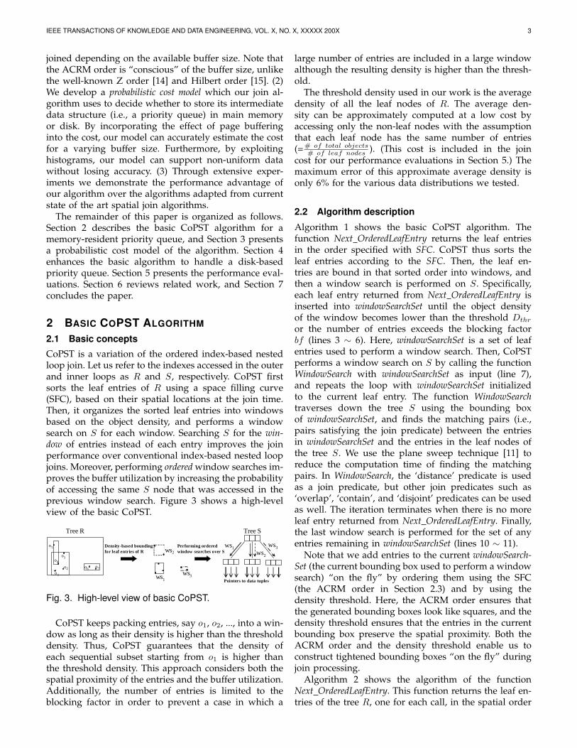
CoPST is a variation of the ordered index-based nestedloop join. Let us refer to the indexes accessed in the outerand inner loops as R and S, respectively. CoPST firstsorts the leaf entries of R using a space filling curve(SFC), based on their spatial locations at the join time.Then, it organizes the sorted leaf entries into windowsbased on the object density, and performs a windowsearch on S for each window. Searching S for the win-dow of entries instead of each entry improves the joinperformance over conventional index-based nested loopjoins. Moreover, performing ordered window searches im-proves the buffer utilization by increasing the probabilityof accessing the same S node that was accessed in theprevious window search. Figure 3 shows a high-levelview of the basic CoPST.

Density-based boundingfor leaf entries of R

Tree S

Performing ordered window searches over S

Pointers to data tuples

ws1ws2

ws3

Tree R

ws1

ws2

ws3

o2

o4

o3

o6 o7

o1

o5

Fig. 3. High-level view of basic CoPST.

CoPST keeps packing entries, say o1, o2, ..., into a win-dow as long as their density is higher than the thresholddensity. Thus, CoPST guarantees that the density ofeach sequential subset starting from o1 is higher thanthe threshold density. This approach considers both thespatial proximity of the entries and the buffer utilization.Additionally, the number of entries is limited to theblocking factor in order to prevent a case in which a

large number of entries are included in a large windowalthough the resulting density is higher than the thresh-old.

The threshold density used in our work is the averagedensity of all the leaf nodes of R. The average den-sity can be approximately computed at a low cost byaccessing only the non-leaf nodes with the assumptionthat each leaf node has the same number of entries(=# of total objects

# of leaf nodes ). (This cost is included in the joincost for our performance evaluations in Section 5.) Themaximum error of this approximate average density isonly 6% for the various data distributions we tested.

2.2 Algorithm description

Algorithm 1 shows the basic CoPST algorithm. Thefunction Next OrderedLeafEntry returns the leaf entriesin the order specified with SFC. CoPST thus sorts theleaf entries according to the SFC. Then, the leaf en-tries are bound in that sorted order into windows, andthen a window search is performed on S. Specifically,each leaf entry returned from Next OrderedLeafEntry isinserted into windowSearchSet until the object densityof the window becomes lower than the threshold Dthr

or the number of entries exceeds the blocking factorbf (lines 3 ∼ 6). Here, windowSearchSet is a set of leafentries used to perform a window search. Then, CoPSTperforms a window search on S by calling the functionWindowSearch with windowSearchSet as input (line 7),and repeats the loop with windowSearchSet initializedto the current leaf entry. The function WindowSearchtraverses down the tree S using the bounding boxof windowSearchSet, and finds the matching pairs (i.e.,pairs satisfying the join predicate) between the entriesin windowSearchSet and the entries in the leaf nodes ofthe tree S. We use the plane sweep technique [11] toreduce the computation time of finding the matchingpairs. In WindowSearch, the ‘distance’ predicate is usedas a join predicate, but other join predicates such as‘overlap’, ‘contain’, and ‘disjoint’ predicates can be usedas well. The iteration terminates when there is no moreleaf entry returned from Next OrderedLeafEntry. Finally,the last window search is performed for the set of anyentries remaining in windowSearchSet (lines 10 ∼ 11).

Note that we add entries to the current windowSearch-Set (the current bounding box used to perform a windowsearch) “on the fly” by ordering them using the SFC(the ACRM order in Section 2.3) and by using thedensity threshold. Here, the ACRM order ensures thatthe generated bounding boxes look like squares, and thedensity threshold ensures that the entries in the currentbounding box preserve the spatial proximity. Both theACRM order and the density threshold enable us toconstruct tightened bounding boxes “on the fly” duringjoin processing.

Algorithm 2 shows the algorithm of the functionNext OrderedLeafEntry. This function returns the leaf en-tries of the tree R, one for each call, in the spatial order


Algorithm 1 Basic CoPST(rootR, rootS, t, SFC, Dthr, bf)Require: rootR: root node of tree R, rootS: root node of tree S,

t: join timestamp, SFC: space filling curve,Dthr : density threshold, bf : blocking factor

Ensure: The join result returned by the function WindowSearch.1: initialize windowSearchSet to an empty set ∅.2: for each leaf entry e returned from

Next OrderedLeafEntry(rootR, rootS, t, SFC) do3: if (Density(windowSearchSet ∪ {e}) ≥ Dthr) and

(Cardinality(windowSearchSet ∪ {e}) ≤ bf) then4: insert e into windowSearchSet5: continue {skip the rest of this for loop.}6: end if7: WindowSearch(windowSearchSet, rootS, t)8: initialize windowSearchSet to the current leaf entry e9: end for

10: if windowSearchSet is not empty then11: WindowSearch(windowSearchSet, rootS, t)12: end if

specified by SFC. It maintains a priority queue for thispurpose. The priority queue is initialized with the rootnode of R (lines 1 ∼ 5). If the current entry e, removedfrom the priority queue, is a leaf entry, then the entry isreturned (lines 8 ∼ 9). Otherwise, from all the entries inthe node the current entry is pointing to, those whoseregions match the region of the root of S are foundand inserted into the priority queue (lines 10 ∼ 15).Here, the function CBB(node) obtains a CBB of node; thefunction MBB(CBB,t) constructs a minimum boundingbox of CBB at timestamp t. Note that the algorithmeliminates unnecessary page accesses by not insertingentries that do not match the region of the root of S(line 12).

Algorithm 2 Next OrderedLeafEntry(rootR, rootS, t, SFC)Require: rootR: root node of tree R, rootS: root node of tree S,

t: a join timestamp, SFC: a space filling curveEnsure: The next entry of R, matching the region of S, ordered

according to SFC.Variable: priorityQueue: a global data structure whose elements

are maintained in an order sorted by SFC1: if priorityQueue has not been initialized then2: rootEntry.CBB = CBB(rootR)3: rootEntry.ref = rootR4: Enqueue(priorityQueue, rootEntry, t, SFC)5: end if6: while priorityQueue is not empty do7: e = Dequeue(priorityQueue, t, SFC)8: if e is a leaf entry then {e points to an object}9: return e

10: else {e points to a node}11: for each entry e′ in the node pointed to by e.ref do12: if JoinPredicate(MBB(e′.CBB, t), MBB(CBB(rootS), t))

then13: Enqueue(priorityQueue, e′, t, SFC)14: end if15: end for16: end if17: end while

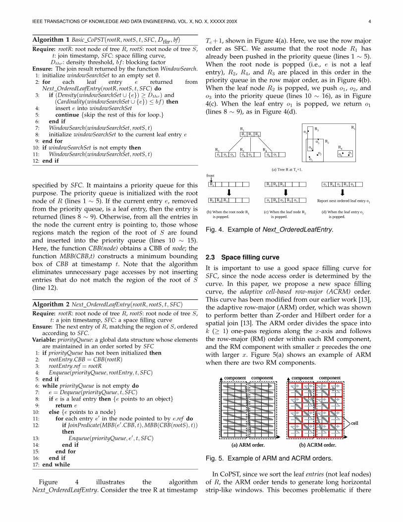
Figure 4 illustrates the algorithmNext OrderedLeafEntry. Consider the tree R at timestamp

Tc +1, shown in Figure 4(a). Here, we use the row majororder as SFC. We assume that the root node R1 hasalready been pushed in the priority queue (lines 1 ∼ 5).When the root node is popped (i.e., e is not a leafentry), R2, R4, and R3 are placed in this order in thepriority queue in the row major order, as in Figure 4(b).When the leaf node R2 is popped, we push o1, o2, ando3 into the priority queue (lines 10 ∼ 16), as in Figure4(c). When the leaf entry o1 is popped, we return o1

(lines 8 ∼ 9), as in Figure 4(d).

(a) Tree R at Tc+1.

R1

R2 R4 R3 o1 R4 o2 R3 o3

(b) When the root node R1is popped.

R2 R4 R3

(c) When the leaf node R2is popped.

front

o1 R4 o2 R3 o3

(d) When the leaf entry o1is popped.

Report next ordered leaf entry o1

R2 R3 R4

o1 o2 o3 o4 o5 o6 o7

R1

R2 R3 R4 o2

o4

o3

o6o7

o1

o5

R1R3

R2

R4

Fig. 4. Example of Next OrderedLeafEntry.

2.3 Space filling curve

It is important to use a good space filling curve forSFC, since the node access order is determined by thecurve. In this paper, we propose a new space fillingcurve, the adaptive cell-based row-major (ACRM) order.This curve has been modified from our earlier work [13],the adaptive row-major (ARM) order, which was shownto perform better than Z-order and Hilbert order for aspatial join [13]. The ARM order divides the space intok (≥ 1) one-pass regions along the x-axis and followsthe row-major (RM) order within each RM component,and the RM component with smaller x precedes the onewith larger x. Figure 5(a) shows an example of ARMwhen there are two RM components.

component component component component

cell

(a) ARM order. (b) ACRM order.

component component component component

cell

(a) ARM order. (b) ACRM order.

Fig. 5. Example of ARM and ACRM orders.

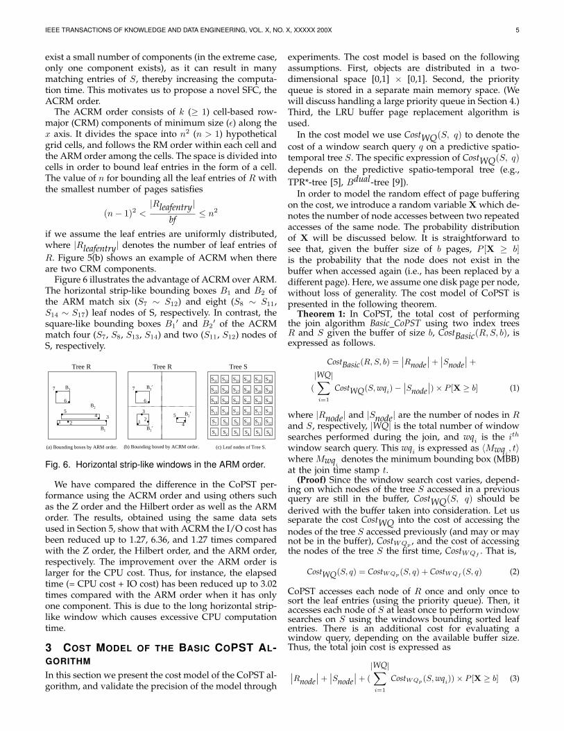
In CoPST, since we sort the leaf entries (not leaf nodes)of R, the ARM order tends to generate long horizontalstrip-like windows. This becomes problematic if there


exist a small number of components (in the extreme case,only one component exists), as it can result in manymatching entries of S, thereby increasing the computa-tion time. This motivates us to propose a novel SFC, theACRM order.

The ACRM order consists of k (≥ 1) cell-based row-major (CRM) components of minimum size (ε) along thex axis. It divides the space into n2 (n > 1) hypotheticalgrid cells, and follows the RM order within each cell andthe ARM order among the cells. The space is divided intocells in order to bound leaf entries in the form of a cell.The value of n for bounding all the leaf entries of R withthe smallest number of pages satisfies

(n− 1)2 <|Rleafentry|

bf≤ n2

if we assume the leaf entries are uniformly distributed,where |Rleafentry| denotes the number of leaf entries ofR. Figure 5(b) shows an example of ACRM when thereare two CRM components.

Figure 6 illustrates the advantage of ACRM over ARM.The horizontal strip-like bounding boxes B1 and B2 ofthe ARM match six (S7 ∼ S12) and eight (S8 ∼ S11,S14 ∼ S17) leaf nodes of S, respectively. In contrast, thesquare-like bounding boxes B1

′ and B2′ of the ACRM

match four (S7, S8, S13, S14) and two (S11, S12) nodes ofS, respectively.

(c) Leaf nodes of Tree S.(b) Bounding boxed by ACRM order.(a) Bounding boxes by ARM order.

6

5

4

7

21

3

6

4 3

7

21

5

S1 S2 S3

B1’

B2’

B3’

B1

B3

B2

S4 S5

S7 S8 S9 S10 S11

S25 S26 S27 S28 S29

S19 S20 S21 S22 S23

S13 S14 S15 S16 S17

S6

S12

S30

S24

S18

S31 S32 S33 S34 S35 S36

Tree RTree R Tree S

Fig. 6. Horizontal strip-like windows in the ARM order.

We have compared the difference in the CoPST per-formance using the ACRM order and using others suchas the Z order and the Hilbert order as well as the ARMorder. The results, obtained using the same data setsused in Section 5, show that with ACRM the I/O cost hasbeen reduced up to 1.27, 6.36, and 1.27 times comparedwith the Z order, the Hilbert order, and the ARM order,respectively. The improvement over the ARM order islarger for the CPU cost. Thus, for instance, the elapsedtime (= CPU cost + IO cost) has been reduced up to 3.02times compared with the ARM order when it has onlyone component. This is due to the long horizontal strip-like window which causes excessive CPU computationtime.

3 COST MODEL OF THE BASIC COPST AL-GORITHMIn this section we present the cost model of the CoPST al-gorithm, and validate the precision of the model through

experiments. The cost model is based on the followingassumptions. First, objects are distributed in a two-dimensional space [0,1] × [0,1]. Second, the priorityqueue is stored in a separate main memory space. (Wewill discuss handling a large priority queue in Section 4.)Third, the LRU buffer page replacement algorithm isused.

In the cost model we use CostWQ(S, q) to denote thecost of a window search query q on a predictive spatio-temporal tree S. The specific expression of CostWQ(S, q)depends on the predictive spatio-temporal tree (e.g.,TPR*-tree [5], Bdual-tree [9]).

In order to model the random effect of page bufferingon the cost, we introduce a random variable X which de-notes the number of node accesses between two repeatedaccesses of the same node. The probability distributionof X will be discussed below. It is straightforward tosee that, given the buffer size of b pages, P [X ≥ b]is the probability that the node does not exist in thebuffer when accessed again (i.e., has been replaced by adifferent page). Here, we assume one disk page per node,without loss of generality. The cost model of CoPST ispresented in the following theorem.

Theorem 1: In CoPST, the total cost of performingthe join algorithm Basic CoPST using two index treesR and S given the buffer of size b, CostBasic(R, S, b), isexpressed as follows.

CostBasic(R, S, b) =∣∣Rnode

∣∣ +∣∣Snode

∣∣ +

(

|WQ|∑i=1

CostWQ(S, wqi)−∣∣Snode

∣∣)× P [X ≥ b] (1)

where |Rnode| and |Snode| are the number of nodes in Rand S, respectively, |WQ| is the total number of windowsearches performed during the join, and wqi is the ith

window search query. This wqi is expressed as 〈Mwqi, t〉

where Mwqi

denotes the minimum bounding box (MBB)at the join time stamp t.

(Proof) Since the window search cost varies, depend-ing on which nodes of the tree S accessed in a previousquery are still in the buffer, CostWQ(S, q) should bederived with the buffer taken into consideration. Let usseparate the cost CostWQ into the cost of accessing thenodes of the tree S accessed previously (and may or maynot be in the buffer), CostWQp , and the cost of accessingthe nodes of the tree S the first time, CostWQf

. That is,

CostWQ(S, q) = CostWQp(S, q) + CostWQf (S, q) (2)

CoPST accesses each node of R once and only once tosort the leaf entries (using the priority queue). Then, itaccesses each node of S at least once to perform windowsearches on S using the windows bounding sorted leafentries. There is an additional cost for evaluating awindow query, depending on the available buffer size.Thus, the total join cost is expressed as

∣∣Rnode∣∣ +

∣∣Snode∣∣ + (

|WQ|∑i=1

CostWQp(S, wqi))× P [X ≥ b] (3)


This can be rewritten as follows using Equation 2.

=∣∣Rnode

∣∣ +∣∣Snode

∣∣ + (

|WQ|∑i=1

CostWQ(S, wqi)−

|WQ|∑i=1

CostWQf (S, wqi))× P [X ≥ b] (4)

Here,∑|WQ|

i=1 CostWQf(S, wqi), the summation of the

costs of accessing the nodes of S the first time, is thesame as the number of nodes in S,

∣∣Snode∣∣. Hence,

Equation 4 can be rewritten as Equation 1.Now, let us discuss the probability distribution of the

random variable X. We can regard X values as inter-arrival times. Here, following common practice [16], [17],we measure time intervals in terms of the number ofpage accesses between two repeated accesses of the samepage in the page reference string. Consider a stochastic

process {St =t∑

i=1

Xi|t = 1, 2, ...}, where Xi is i.i.d. drawn

from F (X), and St is the time to the t-th event. Addi-tionally, consider N(t) defined as the number of eventsoccurring in (0, t]. Due to the ordered window searches,CoPST shows high locality of page accesses so that theprobability of Xt being greater than a certain time periodl decreases dramatically with increasing l. This, alongwith the iid property of Xt, indicates that N(t) is aPoisson process, and thus, X follows the exponentialdistribution. The probability density function f(X) isthus expressed as:

f(x; λ) =

{λe−λx if x ≥ 00 if x < 0

(5)

where λ > 0 and the parameter λ is equal to the inverseof the mean µ of X. P [X ≥ b] is expressed as follows.

P [X ≥ b] = 1−∫ b

0

f(X) = 1− (1− e−λb) = e−λb

Similar approaches are used to estimate the probabilitydistribution for the depth-first spatial join [18], [19].

To model X as an exponential random variable indi-cates that most of X values are less than µ × c (c ≥ 1),where c is a constant. When c = 2, P [X ≥ µ× c] = e−2 '0.14; when c = 3, P [X ≥ µ×c] = e−3 ' 0.05. In CoPST, 1)a page fault rate decreases significantly in case the buffersize is larger than the number of pages accessed duringa window search, and 2) between any two consecutivewindow searches WQ1 and WQ2, a set of pages accessedby WQ1 significantly overlap with a set of pages accessedby WQ2. Thus, we estimate µ as the average number ofnodes accessed during each window search on the treeS. That is,

µ =

(∑|WQ|i=1 CostWQ(S, wqi)

)

|WQ| (6)

Then, P [X ≥ b] is expressed as follows.

P [X ≥ b] = e

−

∣∣WQ∣∣

∑∣∣WQ∣∣

i=1CostWQ(S,wq

i)

×b

(7)

Now we estimate |WQ| and∑|WQ|

i=1 CostWQ(S, wqi).To do so, we construct a two-dimensional histogram,where each bucket corresponds to a cell in the ACRMorder. To calculate the number of objects in the buckets,we first obtain a set of CBBs, leafCBBs, of leaf nodesof R by only accessing the parent non-leaf nodes of theleaf nodes. Second, for each CBB in leafCBBs, we findbuckets which overlap the CBB, and evenly distributethe number of objects in the CBB to the overlappingbuckets. Here, we assume that each leaf node has thesame number of entries, as in Section 2.1. After these twosteps, if there is a histogram bucket whose size is largerthan the blocking factor, we partition the histogrambucket along the y-axis to simulate the ACRM orderso that the size of each partitioned bucket is less thanthe blocking factor. After constructing the histogram, wecan estimate |WQ| as the number of buckets in the his-

togram. To estimate∑|WQ|

i=1 CostWQ(S, wqi), we performwindow searches using the buckets on the tree S. Inthese window searches, we only need to access non-leafnodes of S. Note that all these estimation costs, whichare included in the join cost throughout all experiments,constitute less than 1% of the total performance cost.

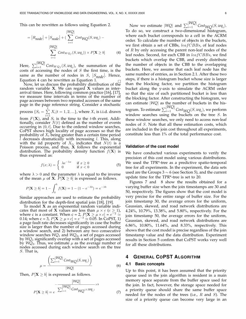
Validation of the cost model

We have conducted various experiments to verify theprecision of this cost model using various distributions.We used the TPR*-tree as a predictive spatio-temporaltree for all experiments. In the experiment, the data setsused are the Groups 3 ∼ 6 (see Section 5), and the currentupdate time for the TPR*-tree is set to 20.

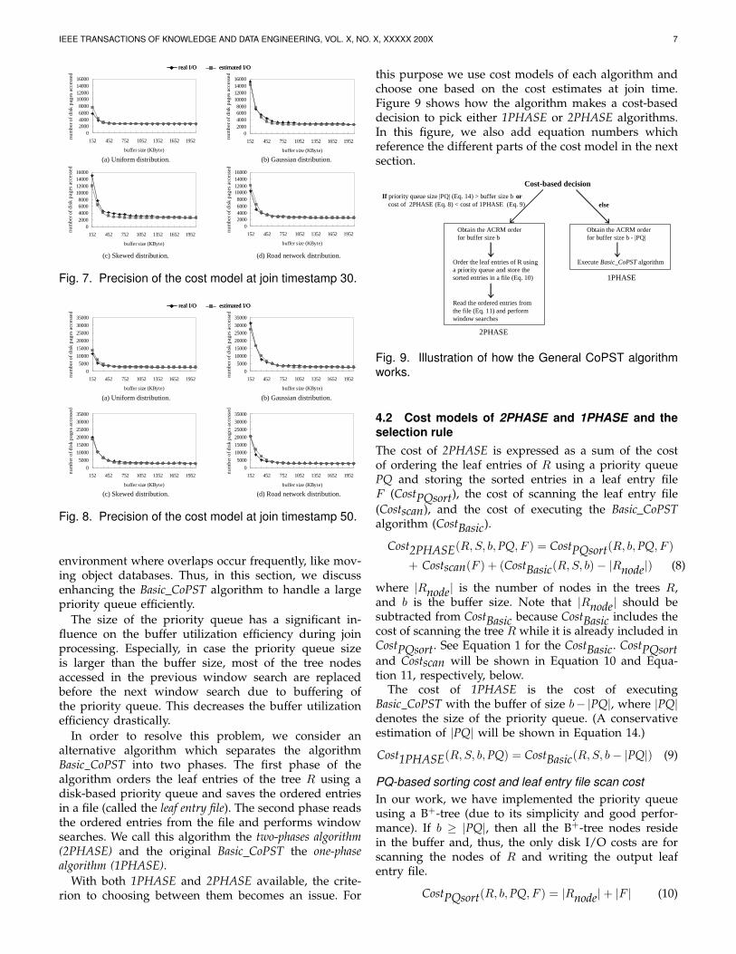
Figures 7 and 8 show the results obtained for avarying buffer size when the join timestamps are 30 and50, respectively. The figures show that the cost model isvery precise for the entire range of buffer size. For thejoin timestamp 30, the average errors for the uniform,Gaussian, skewed, and road network distributions are4.24%, 10.79%, 13.38%, and 5.80%, respectively. For thejoin timestamp 50, the average errors for the uniform,Gaussian, skewed, and road network distributions are6.86%, 10.80%, 11.64%, and 8.33%, respectively. Thisshows that the cost model is precise regardless of the jointimestamp value and the data distribution. Experimentresults in Section 5 confirm that CoPST works very wellfor all these distributions.

4 GENERAL COPST ALGORITHM

4.1 Basic concepts

Up to this point, it has been assumed that the priorityqueue used in the join algorithm is resident in a mainmemory space separate from the buffer space used forthe join. In fact, however, the storage space needed fora priority queue should share the same buffer spaceneeded for the nodes of the trees (i.e., R and S). Thesize of a priority queue can become very large in an


02000400060008000

10000120001400016000

152 452 752 1052 1352 1652 1952

buffer size (KByte)

num

ber o

f dis

k pa

ges

acce

ssed

02000400060008000

10000120001400016000

152 452 752 1052 1352 1652 1952

buffer size (KByte)

num

ber o

f dis

k pa

ges

acce

ssed

02000400060008000

10000120001400016000

152 452 752 1052 1352 1652 1952

buffer size (KByte)

num

ber o

f dis

k pa

ges

acce

ssed

02000400060008000

10000120001400016000

152 452 752 1052 1352 1652 1952

buffer size (KByte)

num

ber o

f dis

k pa

ges

acce

ssed

(a) Uniform distribution. (b) Gaussian distribution.

(c) Skewed distribution. (d) Road network distribution.

real I/O estimated I/Oreal I/O estimated I/O

Fig. 7. Precision of the cost model at join timestamp 30.

0

5000

10000

15000

20000

25000

30000

35000

152 452 752 1052 1352 1652 1952

buffer size (KByte)

num

ber o

f dis

k pa

ges

acce

ssed

0

5000

10000

15000

20000

25000

30000

35000

152 452 752 1052 1352 1652 1952

buffer size (KByte)

num

ber o

f dis

k pa

ges

acce

ssed

0

5000

10000

15000

20000

25000

30000

35000

152 452 752 1052 1352 1652 1952

buffer size (KByte)

num

ber o

f dis

k pa

ges

acce

ssed

0

5000

10000

15000

20000

25000

30000

35000

152 452 752 1052 1352 1652 1952

buffer size (KByte)

num

ber o

f dis

k pa

ges

acce

ssed



real I/O estimated I/Oreal I/O estimated I/O

Fig. 8. Precision of the cost model at join timestamp 50.

environment where overlaps occur frequently, like mov-ing object databases. Thus, in this section, we discussenhancing the Basic CoPST algorithm to handle a largepriority queue efficiently.

The size of the priority queue has a significant in-fluence on the buffer utilization efficiency during joinprocessing. Especially, in case the priority queue sizeis larger than the buffer size, most of the tree nodesaccessed in the previous window search are replacedbefore the next window search due to buffering ofthe priority queue. This decreases the buffer utilizationefficiency drastically.

In order to resolve this problem, we consider analternative algorithm which separates the algorithmBasic CoPST into two phases. The first phase of thealgorithm orders the leaf entries of the tree R using adisk-based priority queue and saves the ordered entriesin a file (called the leaf entry file). The second phase readsthe ordered entries from the file and performs windowsearches. We call this algorithm the two-phases algorithm(2PHASE) and the original Basic CoPST the one-phasealgorithm (1PHASE).

With both 1PHASE and 2PHASE available, the crite-rion to choosing between them becomes an issue. For

this purpose we use cost models of each algorithm andchoose one based on the cost estimates at join time.Figure 9 shows how the algorithm makes a cost-baseddecision to pick either 1PHASE or 2PHASE algorithms.In this figure, we also add equation numbers whichreference the different parts of the cost model in the nextsection.

Cost-based decision

If priority queue size |PQ| (Eq. 14) > buffer size b orcost of 2PHASE (Eq. 8) < cost of 1PHASE (Eq. 9) else

Order the leaf entries of R usinga priority queue and store thesorted entries in a file (Eq. 10)

Read the ordered entries fromthe file (Eq. 11) and perform window searches

Execute Basic_CoPST algorithm

Obtain the ACRM orderfor buffer size b

Obtain the ACRM orderfor buffer size b - |PQ|

2PHASE

1PHASE

Fig. 9. Illustration of how the General CoPST algorithmworks.

4.2 Cost models of 2PHASE and 1PHASE and theselection ruleThe cost of 2PHASE is expressed as a sum of the costof ordering the leaf entries of R using a priority queuePQ and storing the sorted entries in a leaf entry fileF (CostPQsort), the cost of scanning the leaf entry file(Costscan), and the cost of executing the Basic CoPSTalgorithm (CostBasic).

Cost2PHASE(R, S, b, PQ, F ) = CostPQsort(R, b, PQ, F )

+ Costscan(F ) + (CostBasic(R, S, b)− |Rnode|) (8)

where |Rnode| is the number of nodes in the trees R,and b is the buffer size. Note that |Rnode| should besubtracted from CostBasic because CostBasic includes thecost of scanning the tree R while it is already included inCostPQsort. See Equation 1 for the CostBasic. CostPQsortand Costscan will be shown in Equation 10 and Equa-tion 11, respectively, below.

The cost of 1PHASE is the cost of executingBasic CoPST with the buffer of size b− |PQ|, where |PQ|denotes the size of the priority queue. (A conservativeestimation of |PQ| will be shown in Equation 14.)

Cost1PHASE(R,S, b, PQ) = CostBasic(R,S, b− |PQ|) (9)

PQ-based sorting cost and leaf entry file scan costIn our work, we have implemented the priority queueusing a B+-tree (due to its simplicity and good perfor-mance). If b ≥ |PQ|, then all the B+-tree nodes residein the buffer and, thus, the only disk I/O costs are forscanning the nodes of R and writing the output leafentry file.

CostPQsort(R, b, PQ, F ) = |Rnode|+ |F | (10)


where f is the average fill factor of a node, and |F | isthe size of the leaf entry file.

Here, |F | equals the number of pages required to storeall the leaf entries, that is, equals |Rleafentry|/bf , where|Rleafentry| is the number of leaf entries in R and bf is theblocking factor of a page. Thus, Equation 10 is rewrittenas

CostPQsort(R, b, PQ, F ) = |Rnode|+ |Rleafentry|/bf

= |Rnode|+ |Rleafnode| × f

The leaf entry file scanning cost is expressed as:

Costscan(F ) = |Rleafnode| × f (11)

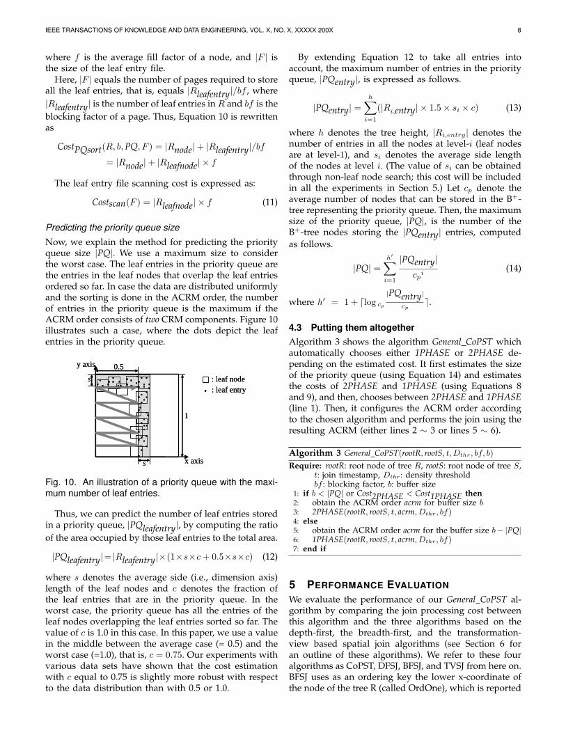
Predicting the priority queue size

Now, we explain the method for predicting the priorityqueue size |PQ|. We use a maximum size to considerthe worst case. The leaf entries in the priority queue arethe entries in the leaf nodes that overlap the leaf entriesordered so far. In case the data are distributed uniformlyand the sorting is done in the ACRM order, the numberof entries in the priority queue is the maximum if theACRM order consists of two CRM components. Figure 10illustrates such a case, where the dots depict the leafentries in the priority queue.

x axis

y axis

s

s

0.5

: leaf node: leaf entry

1

x axis

y axis

s

s

0.5

: leaf node: leaf entry

1

Fig. 10. An illustration of a priority queue with the maxi-mum number of leaf entries.

Thus, we can predict the number of leaf entries storedin a priority queue, |PQleafentry|, by computing the ratioof the area occupied by those leaf entries to the total area.

|PQleafentry|= |Rleafentry|×(1×s×c + 0.5×s×c) (12)

where s denotes the average side (i.e., dimension axis)length of the leaf nodes and c denotes the fraction ofthe leaf entries that are in the priority queue. In theworst case, the priority queue has all the entries of theleaf nodes overlapping the leaf entries sorted so far. Thevalue of c is 1.0 in this case. In this paper, we use a valuein the middle between the average case (= 0.5) and theworst case (=1.0), that is, c = 0.75. Our experiments withvarious data sets have shown that the cost estimationwith c equal to 0.75 is slightly more robust with respectto the data distribution than with 0.5 or 1.0.

By extending Equation 12 to take all entries intoaccount, the maximum number of entries in the priorityqueue, |PQentry|, is expressed as follows.

|PQentry| =h∑

i=1

(|Ri,entry| × 1.5× si × c) (13)

where h denotes the tree height, |Ri,entry| denotes thenumber of entries in all the nodes at level-i (leaf nodesare at level-1), and si denotes the average side lengthof the nodes at level i. (The value of si can be obtainedthrough non-leaf node search; this cost will be includedin all the experiments in Section 5.) Let cp denote theaverage number of nodes that can be stored in the B+-tree representing the priority queue. Then, the maximumsize of the priority queue, |PQ|, is the number of theB+-tree nodes storing the |PQentry| entries, computedas follows.

|PQ| =h′∑

i=1

|PQentry|cp

i(14)

where h′ = 1 + dlog cp

|PQentry|cp

e.

4.3 Putting them altogetherAlgorithm 3 shows the algorithm General CoPST whichautomatically chooses either 1PHASE or 2PHASE de-pending on the estimated cost. It first estimates the sizeof the priority queue (using Equation 14) and estimatesthe costs of 2PHASE and 1PHASE (using Equations 8and 9), and then, chooses between 2PHASE and 1PHASE(line 1). Then, it configures the ACRM order accordingto the chosen algorithm and performs the join using theresulting ACRM (either lines 2 ∼ 3 or lines 5 ∼ 6).

Algorithm 3 General CoPST(rootR, rootS, t, Dthr, bf, b)

Require: rootR: root node of tree R, rootS: root node of tree S,t: join timestamp, Dthr : density thresholdbf : blocking factor, b: buffer size

1: if b < |PQ| or Cost2PHASE < Cost1PHASE then2: obtain the ACRM order acrm for buffer size b3: 2PHASE(rootR, rootS, t, acrm, Dthr, bf)4: else5: obtain the ACRM order acrm for the buffer size b− |PQ|6: 1PHASE(rootR, rootS, t, acrm, Dthr, bf)7: end if

5 PERFORMANCE EVALUATION

We evaluate the performance of our General CoPST al-gorithm by comparing the join processing cost betweenthis algorithm and the three algorithms based on thedepth-first, the breadth-first, and the transformation-view based spatial join algorithms (see Section 6 foran outline of these algorithms). We refer to these fouralgorithms as CoPST, DFSJ, BFSJ, and TVSJ from here on.BFSJ uses as an ordering key the lower x-coordinate ofthe node of the tree R (called OrdOne), which is reported


the best ordering choice in BFSJ [12]. The main objectiveof the experiments is to compare the join processing costof CoPST against DFSJ, BFSJ, and TVSJ and evaluate theeffect of the cost-based switch-over between 1PHASEand 2PHASE in CoPST for a varying buffer size. InSection 5.1 we describe the setup for the experiments,and in Section 5.2 we present the experiments conductedand their results.

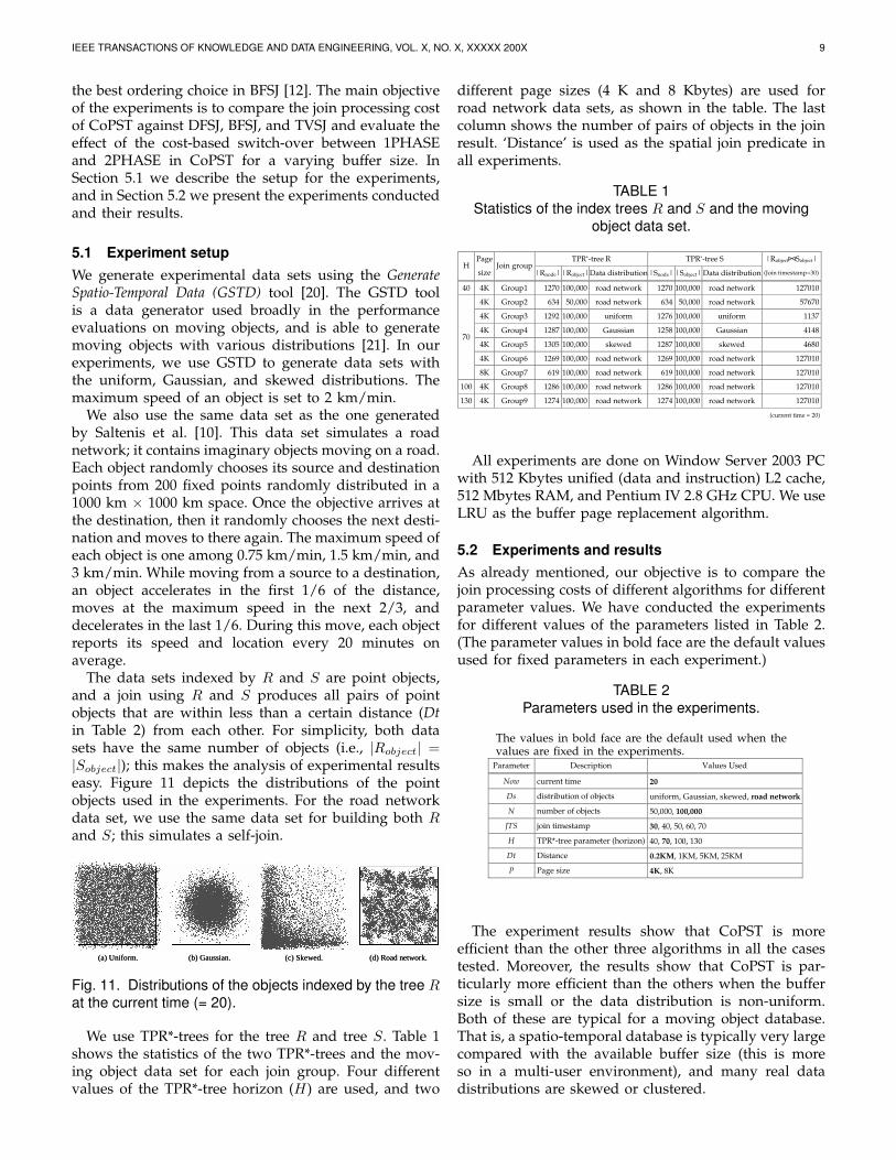
5.1 Experiment setupWe generate experimental data sets using the GenerateSpatio-Temporal Data (GSTD) tool [20]. The GSTD toolis a data generator used broadly in the performanceevaluations on moving objects, and is able to generatemoving objects with various distributions [21]. In ourexperiments, we use GSTD to generate data sets withthe uniform, Gaussian, and skewed distributions. Themaximum speed of an object is set to 2 km/min.

We also use the same data set as the one generatedby Saltenis et al. [10]. This data set simulates a roadnetwork; it contains imaginary objects moving on a road.Each object randomly chooses its source and destinationpoints from 200 fixed points randomly distributed in a1000 km × 1000 km space. Once the objective arrives atthe destination, then it randomly chooses the next desti-nation and moves to there again. The maximum speed ofeach object is one among 0.75 km/min, 1.5 km/min, and3 km/min. While moving from a source to a destination,an object accelerates in the first 1/6 of the distance,moves at the maximum speed in the next 2/3, anddecelerates in the last 1/6. During this move, each objectreports its speed and location every 20 minutes onaverage.

The data sets indexed by R and S are point objects,and a join using R and S produces all pairs of pointobjects that are within less than a certain distance (Dtin Table 2) from each other. For simplicity, both datasets have the same number of objects (i.e., |Robject| =|Sobject|); this makes the analysis of experimental resultseasy. Figure 11 depicts the distributions of the pointobjects used in the experiments. For the road networkdata set, we use the same data set for building both Rand S; this simulates a self-join.

(a) Uniform. (b) Gaussian. (c) Skewed. (d) Road network.(a) Uniform. (b) Gaussian. (c) Skewed. (d) Road network.

Fig. 11. Distributions of the objects indexed by the tree Rat the current time (= 20).

We use TPR*-trees for the tree R and tree S. Table 1shows the statistics of the two TPR*-trees and the mov-ing object data set for each join group. Four differentvalues of the TPR*-tree horizon (H) are used, and two

different page sizes (4 K and 8 Kbytes) are used forroad network data sets, as shown in the table. The lastcolumn shows the number of pairs of objects in the joinresult. ‘Distance’ is used as the spatial join predicate inall experiments.

TABLE 1Statistics of the index trees R and S and the moving

object data set.

TPR*-tree R TPR*-tree S H

Page

size Join group

|Rnode| |Robject| Data distribution |Snode| |Sobject| Data distribution

|Robject Sobject|

(Join timestamp=30)

40 4K Group1 1270 100,000 road network 1270 100,000 road network 127010

4K Group2 634 50,000 road network 634 50,000 road network 57670

4K Group3 1292 100,000 uniform 1276 100,000 uniform 1137

4K Group4 1287 100,000 Gaussian 1258 100,000 Gaussian 4148

4K Group5 1305 100,000 skewed 1287 100,000 skewed 4680


70




(current time = 20)

All experiments are done on Window Server 2003 PCwith 512 Kbytes unified (data and instruction) L2 cache,512 Mbytes RAM, and Pentium IV 2.8 GHz CPU. We useLRU as the buffer page replacement algorithm.

5.2 Experiments and resultsAs already mentioned, our objective is to compare thejoin processing costs of different algorithms for differentparameter values. We have conducted the experimentsfor different values of the parameters listed in Table 2.(The parameter values in bold face are the default valuesused for fixed parameters in each experiment.)

TABLE 2Parameters used in the experiments.

The values in bold face are the default used when thevalues are fixed in the experiments.

Parameter Description Values Used

Now current time 20

Ds distribution of objects uniform, Gaussian, skewed, road network

N number of objects 50,000, 100,000

JTS join timestamp 30, 40, 50, 60, 70

H TPR*-tree parameter (horizon) 40, 70, 100, 130

Dt Distance 0.2KM, 1KM, 5KM, 25KM

P Page size 4K, 8K The experiment results show that CoPST is more

efficient than the other three algorithms in all the casestested. Moreover, the results show that CoPST is par-ticularly more efficient than the others when the buffersize is small or the data distribution is non-uniform.Both of these are typical for a moving object database.That is, a spatio-temporal database is typically very largecompared with the available buffer size (this is moreso in a multi-user environment), and many real datadistributions are skewed or clustered.


For applications that require quick responses, it maybe desirable to have both indexes resident in the mainmemory. In this case, the CPU cache, with its limitedsize, amounts to the buffer of a disk-based environment.The Pentium IV CPU uses a “pseudo LRU” (a variantof LRU) as the cache entry replacement policy [22]. Ourexperiment shows that CoPST consistently outperformsthe other methods even in a main-memory environment.

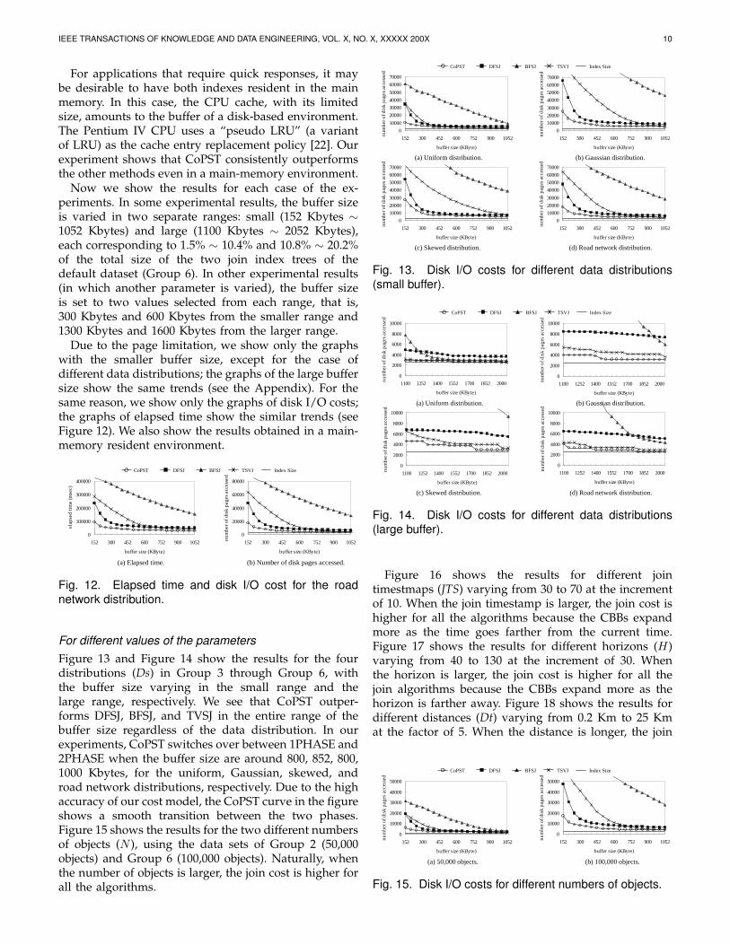
Now we show the results for each case of the ex-periments. In some experimental results, the buffer sizeis varied in two separate ranges: small (152 Kbytes ∼1052 Kbytes) and large (1100 Kbytes ∼ 2052 Kbytes),each corresponding to 1.5% ∼ 10.4% and 10.8% ∼ 20.2%of the total size of the two join index trees of thedefault dataset (Group 6). In other experimental results(in which another parameter is varied), the buffer sizeis set to two values selected from each range, that is,300 Kbytes and 600 Kbytes from the smaller range and1300 Kbytes and 1600 Kbytes from the larger range.

Due to the page limitation, we show only the graphswith the smaller buffer size, except for the case ofdifferent data distributions; the graphs of the large buffersize show the same trends (see the Appendix). For thesame reason, we show only the graphs of disk I/O costs;the graphs of elapsed time show the similar trends (seeFigure 12). We also show the results obtained in a main-memory resident environment.

0

100000

200000

300000

400000

152 300 452 600 752 900 1052

buffer size (KByte)

elap

sed

tim

e (m

sec)

0

20000

40000

60000

80000

152 300 452 600 752 900 1052

buffer size (KByte)

num

ber o

f dis

k pa

ges

acce

ssed

(a) Elapsed time. (b) Number of disk pages accessed.

CoPST DFSJ BFSJ TSVJ Index Size

Fig. 12. Elapsed time and disk I/O cost for the roadnetwork distribution.

For different values of the parametersFigure 13 and Figure 14 show the results for the fourdistributions (Ds) in Group 3 through Group 6, withthe buffer size varying in the small range and thelarge range, respectively. We see that CoPST outper-forms DFSJ, BFSJ, and TVSJ in the entire range of thebuffer size regardless of the data distribution. In ourexperiments, CoPST switches over between 1PHASE and2PHASE when the buffer size are around 800, 852, 800,1000 Kbytes, for the uniform, Gaussian, skewed, androad network distributions, respectively. Due to the highaccuracy of our cost model, the CoPST curve in the figureshows a smooth transition between the two phases.Figure 15 shows the results for the two different numbersof objects (N ), using the data sets of Group 2 (50,000objects) and Group 6 (100,000 objects). Naturally, whenthe number of objects is larger, the join cost is higher forall the algorithms.

0

10000

20000

30000

40000

50000

60000

70000

152 300 452 600 752 900 1052

buffer size (KByte)

num

ber o

f dis

k pa

ges

acce

ssed

0

10000

20000

30000

40000

50000

60000

70000

152 300 452 600 752 900 1052

buffer size (KByte)

num

ber o

f dis

k pa

ges

acce

ssed

0

10000

20000

30000

40000

50000

60000

70000

152 300 452 600 752 900 1052

buffer size (KByte)

num

ber o

f dis

k pa

ges

acce

ssed

0

10000

20000

30000

40000

50000

60000

70000

152 300 452 600 752 900 1052

buffer size (KByte)

num

ber o

f dis

k pa

ges

acce

ssed




Fig. 13. Disk I/O costs for different data distributions(small buffer).

0

2000

4000

6000

8000

10000

1100 1252 1400 1552 1700 1852 2000

buffer size (KByte)

num

ber o

f dis

k pa

ges

acce

ssed

0

2000

4000

6000

8000

10000

1100 1252 1400 1552 1700 1852 2000

buffer size (KByte)

num

ber o

f dis

k pa

ges

acce

ssed

0

2000

4000

6000

8000

10000

1100 1252 1400 1552 1700 1852 2000

buffer size (KByte)

num

ber o

f dis

k pa

ges

acce

ssed

0

2000

4000

6000

8000

10000

1100 1252 1400 1552 1700 1852 2000

buffer size (KByte)

num

ber o

f dis

k pa

ges

acce

ssed




Fig. 14. Disk I/O costs for different data distributions(large buffer).

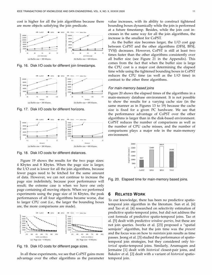
Figure 16 shows the results for different jointimestmaps (JTS) varying from 30 to 70 at the incrementof 10. When the join timestamp is larger, the join cost ishigher for all the algorithms because the CBBs expandmore as the time goes farther from the current time.Figure 17 shows the results for different horizons (H)varying from 40 to 130 at the increment of 30. Whenthe horizon is larger, the join cost is higher for all thejoin algorithms because the CBBs expand more as thehorizon is farther away. Figure 18 shows the results fordifferent distances (Dt) varying from 0.2 Km to 25 Kmat the factor of 5. When the distance is longer, the join

0

10000

20000

30000

40000

50000

152 300 452 600 752 900 1052

buffer size (KByte)

num

ber o

f dis

k pa

ges

acce

ssed

0

10000

20000

30000

40000

50000

152 300 452 600 752 900 1052

buffer size (KByte)

num

ber o

f dis

k pa

ges

acce

ssed

(a) 50,000 objects. (b) 100,000 objects.


Fig. 15. Disk I/O costs for different numbers of objects.


cost is higher for all the join algorithms because thereare more objects satisfying the join predicate.

0

20000

40000

60000

80000

100000

120000

140000

30 40 50 60 70

join timestamp

num

ber o

f dis

k pa

ges

acce

ssed

0

20000

40000

60000

80000

100000

30 40 50 60 70

join timestamp

num

ber o

f dis

k pa

ges

acce

ssed

(a) Buffer size = 300 Kbytes. (b) Buffer size = 600 Kbytes.


Fig. 16. Disk I/O costs for different join timestamps.

0

20000

40000

60000

80000

100000

40 70 100 130

horizon

num

ber o

f dis

k pa

ges

acce

ssed

0

10000

20000

30000

40000

50000

60000

40 70 100 130

horizon

num

ber o

f dis

k pa

ges

acce

ssed



Fig. 17. Disk I/O costs for different horizons.

0

20000

40000

60000

80000

100000

0.2 1 5 25

distance

num

ber o

f dis

k pa

ges

acce

ssed

0

10000

20000

30000

40000

50000

60000

70000

0.2 1 5 25

distance

num

ber o

f dis

k pa

ges

acce

ssed



Fig. 18. Disk I/O costs for different distances.

Figure 19 shows the results for the two page sizes:4 Kbytes and 8 Kbytes. When the page size is larger,the I/O cost is lower for all the join algorithms, becausefewer pages need to be fetched for the same amountof data. However, we can not continue to increase thepage size indefinitely, because poor performance willresult; the extreme case is when we have one onlypage containing all moving objects. When we performedexperiments using the page size of 16 Kbytes, the peakperformances of all four algorithms became worse, dueto larger CPU cost (i.e., the larger the bounding boxesare, the more comparisons are made).

0

10000

20000

30000

40000

50000

60000

70000

152 300 452 600 752 900 1052

buffer size (KByte)

num

ber o

f dis

k pa

ges

acce

ssed

0

10000

20000

30000

40000

50000

60000

70000

152 300 452 600 752 900 1052

buffer size (KByte)

num

ber o

f dis

k pa

ges

acce

ssed

(b) Page size = 8 Kbytes.(a) Page size = 4 Kbytes.


Fig. 19. Disk I/O costs for different page sizes.

In all these experiments, we see that CoPST gains moreadvantage over the other algorithms as the parameter

value increases, with its ability to construct tightenedbounding boxes dynamically while the join is performedat a future timestamp. Besides, while the join cost in-creases in the same way for all the join algorithms, theincrease is the smallest for CoPST.

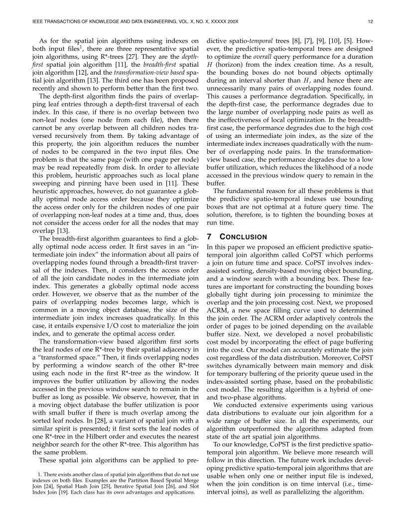
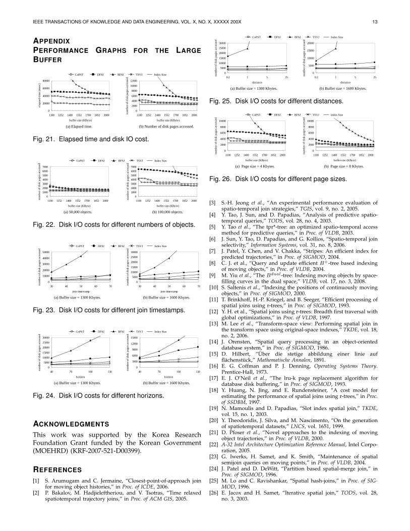
As the buffer size becomes larger, the I/O cost gapbetween CoPST and the other algorithms (DFSJ, BFSJ,TVSJ) decreases. However, CoPST is still at least twotimes faster than the other algorithms consistently overall buffer size (see Figure 21 in the Appendix). Thiscomes from the fact that when the buffer size is largethe CPU cost is a major cost determining the elapsedtime while using the tightened bounding boxes in CoPSTreduces the CPU time (as well as the I/O time) incontrast to the other three algorithms.

For main-memory based joinsFigure 20 shows the elapsed times of the algorithms in amain-memory database environment. It is not possibleto show the results for a varying cache size (in thesame manner as in Figures 13 to 19) because the cachesize is fixed for a given PC hardware. We see thatthe performance advantage of CoPST over the otheralgorithms is larger than in the disk-based environment.CoPST reduces the number of comparisons as well asthe number of CPU cache misses, and the number ofcomparisons plays a major role in the main-memoryenvironment.

9437

22469

26610

20188

0

5000

10000

15000

20000

25000

30000

CoPST DFSJ BFSJ TSVJ

elap

sed

tim

e (m

sec)

Fig. 20. Elapsed time for main-memory based joins.

6 RELATED WORK

To our knowledge, there has been no predictive spatio-temporal join algorithm in the literature. Sun et al. [6]and Tao et al. [4] researched on selectivity estimation ofpredictive spatio-temporal joins, but did not address thecost formula of predictive spatio-temporal joins. Tao etal. [5] dealt with predictive window queries, but these arenot join queries. Iwerks et al. [23] proposed a “spatialsemijoin” algorithm, but the join time was the presentand the focus was on how to maintain join results as timepasses. Jeong et al. [3] studied the performance of spatio-temporal join strategies, but they considered only his-torical spatio-temporal joins. Similarly, Arumugam andJermaine [1] dealt with historical closest-pair joins, andBakalov et al. [2] dealt with a variant of historical spatio-temporal join.


As for the spatial join algorithms using indexes onboth input files1, there are three representative spatialjoin algorithms, using R*-trees [27]. They are the depth-first spatial join algorithm [11], the breadth-first spatialjoin algorithm [12], and the transformation-view based spa-tial join algorithm [13]. The third one has been proposedrecently and shown to perform better than the first two.

The depth-first algorithm finds the pairs of overlap-ping leaf entries through a depth-first traversal of eachindex. In this case, if there is no overlap between twonon-leaf nodes (one node from each file), then therecannot be any overlap between all children nodes tra-versed recursively from them. By taking advantage ofthis property, the join algorithm reduces the numberof nodes to be compared in the two input files. Oneproblem is that the same page (with one page per node)may be read repeatedly from disk. In order to alleviatethis problem, heuristic approaches such as local planesweeping and pinning have been used in [11]. Theseheuristic approaches, however, do not guarantee a glob-ally optimal node access order because they optimizethe access order only for the children nodes of one pairof overlapping non-leaf nodes at a time and, thus, doesnot consider the access order for all the nodes that mayoverlap [13].

The breadth-first algorithm guarantees to find a glob-ally optimal node access order. It first saves in an “in-termediate join index” the information about all pairs ofoverlapping nodes found through a breadth-first traver-sal of the indexes. Then, it considers the access orderof all the join candidate nodes in the intermediate joinindex. This generates a globally optimal node accessorder. However, we observe that as the number of thepairs of overlapping nodes becomes large, which iscommon in a moving object database, the size of theintermediate join index increases quadratically. In thiscase, it entails expensive I/O cost to materialize the joinindex, and to generate the optimal access order.

The transformation-view based algorithm first sortsthe leaf nodes of one R*-tree by their spatial adjacency ina “transformed space.” Then, it finds overlapping nodesby performing a window search of the other R*-treeusing each node in the first R*-tree as the window. Itimproves the buffer utilization by allowing the nodesaccessed in the previous window search to remain in thebuffer as long as possible. We observe, however, that ina moving object database the buffer utilization is poorwith small buffer if there is much overlap among thesorted leaf nodes. In [28], a variant of spatial join with asimilar spirit is presented; it first sorts the leaf nodes ofone R*-tree in the Hilbert order and executes the nearestneighbor search for the other R*-tree. This algorithm hasthe same problem.

These spatial join algorithms can be applied to pre-

1. There exists another class of spatial join algorithms that do not useindexes on both files. Examples are the Partition Based Spatial MergeJoin [24], Spatial Hash Join [25], Iterative Spatial Join [26], and SlotIndex Join [19]. Each class has its own advantages and applications.

dictive spatio-temporal trees [8], [7], [9], [10], [5]. How-ever, the predictive spatio-temporal trees are designedto optimize the overall query performance for a durationH (horizon) from the index creation time. As a result,the bounding boxes do not bound objects optimallyduring an interval shorter than H , and hence there areunnecessarily many pairs of overlapping nodes found.This causes a performance degradation. Specifically, inthe depth-first case, the performance degrades due tothe large number of overlapping node pairs as well asthe ineffectiveness of local optimization. In the breadth-first case, the performance degrades due to the high costof using an intermediate join index, as the size of theintermediate index increases quadratically with the num-ber of overlapping node pairs. In the transformation-view based case, the performance degrades due to a lowbuffer utilization, which reduces the likelihood of a nodeaccessed in the previous window query to remain in thebuffer.

The fundamental reason for all these problems is thatthe predictive spatio-temporal indexes use boundingboxes that are not optimal at a future query time. Thesolution, therefore, is to tighten the bounding boxes atrun time.

7 CONCLUSIONIn this paper we proposed an efficient predictive spatio-temporal join algorithm called CoPST which performsa join on future time and space. CoPST involves index-assisted sorting, density-based moving object bounding,and a window search with a bounding box. These fea-tures are important for constructing the bounding boxesglobally tight during join processing to minimize theoverlap and the join processing cost. Next, we proposedACRM, a new space filling curve used to determinedthe join order. The ACRM order adaptively controls theorder of pages to be joined depending on the availablebuffer size. Next, we developed a novel probabilisticcost model by incorporating the effect of page bufferinginto the cost. Our model can accurately estimate the joincost regardless of the data distribution. Moreover, CoPSTswitches dynamically between main memory and diskfor temporary buffering of the priority queue used in theindex-assisted sorting phase, based on the probabilisticcost model. The resulting algorithm is a hybrid of one-and two-phase algorithms.

We conducted extensive experiments using variousdata distributions to evaluate our join algorithm for awide range of buffer size. In all the experiments, ouralgorithm outperformed the algorithms adapted fromstate of the art spatial join algorithms.

To our knowledge, CoPST is the first predictive spatio-temporal join algorithm. We believe more research willfollow in this direction. The future work includes devel-oping predictive spatio-temporal join algorithms that areusable when only one or neither input file is indexed,when the join condition is on time interval (i.e., time-interval joins), as well as parallelizing the algorithm.


APPENDIXPERFORMANCE GRAPHS FOR THE LARGEBUFFER

0

20000

40000

60000

80000

1100 1252 1400 1552 1700 1852 2000

buffer size (KByte)

elap

sed

tim

e (m

sec)

0

2000

4000

6000

8000

10000

12000

1100 1252 1400 1552 1700 1852 2000

buffer size (KByte)

num

ber o

f dis

k pa

ges

acce

ssed

(a) Elapsed time. (b) Number of disk pages accessed.


Fig. 21. Elapsed time and disk IO cost.

0

1000

2000

3000

4000

5000

6000

7000

1100 1252 1400 1552 1700 1852 2000

buffer size (KByte)

num

ber o

f dis

k pa

ges

acce

ssed

0

1000

2000

3000

4000

5000

6000

7000

1100 1252 1400 1552 1700 1852 2000

buffer size (KByte)

num

ber o

f dis

k pa

ges

acce

ssed

(a) 50,000 objects. (b) 100,000 objects.


Fig. 22. Disk I/O costs for different numbers of objects.

0

10000

20000

30000

40000

50000

30 40 50 60 70

join timestamp

num

ber o

f dis

k pa

ges

acce

ssed

0

5000

10000

15000

20000

25000

30000

30 40 50 60 70

join timestamp

num

ber o

f dis

k pa

ges

acce

ssed



Fig. 23. Disk I/O costs for different join timestamps.

0

5000

10000

15000

20000

25000

30000

40 70 100 130

horizon

num

ber o

f dis

k pa

ges

acce

ssed

0

3000

6000

9000

12000

15000

40 70 100 130

horizon

num

ber o

f dis

k pa

ges

acce

ssed



Fig. 24. Disk I/O costs for different horizons.

ACKNOWLEDGMENTS

This work was supported by the Korea ResearchFoundation Grant funded by the Korean Government(MOEHRD) (KRF-2007-521-D00399).

REFERENCES

[1] S. Arumugam and C. Jermaine, “Closest-point-of-approach joinfor moving object histories,” in Proc. of ICDE, 2006.

[2] P. Bakalov, M. Hadjieleftheriou, and V. Tsotras, “Time relaxedspatiotemporal trajectory joins,” in Proc. of ACM GIS, 2005.

0

5000

10000

15000

20000

25000

30000

0.2 1 5 25

distance

num

ber o

f dis

k pa

ges

acce

ssed

0

5000

10000

15000

20000

0.2 1 5 25

distance

num

ber o

f dis

k pa

ges

acce

ssed



Fig. 25. Disk I/O costs for different distances.

0

2000

4000

6000

8000

10000

1100 1252 1400 1552 1700 1852 2000

buffer size (KByte)

num

ber o

f dis

k pa

ges

acce

ssed

0

2000

4000

6000

8000

10000

1100 1252 1400 1552 1700 1852 2000

buffer size (KByte)

num

ber o

f dis

k pa

ges

acce

ssed


(b) Page size = 8 Kbytes.(a) Page size = 4 Kbytes.

Fig. 26. Disk I/O costs for different page sizes.

[3] S.-H. Jeong et al., “An experimental performance evaluation ofspatio-temporal join strategies,” TGIS, vol. 9, no. 2, 2005.

[4] Y. Tao, J. Sun, and D. Papadias, “Analysis of predictive spatio-temporal queries,” TODS, vol. 28, no. 4, 2003.

[5] Y. Tao et al., “The tpr*-tree: an optimized spatio-temporal accessmethod for predictive queries,” in Proc. of VLDB, 2003.

[6] J. Sun, Y. Tao, D. Papadias, and G. Kollios, “Spatio-temporal joinselectivity,” Information Systems, vol. 31, no. 8, 2006.

[7] J. Patel, Y. Chen, and V. Chakka, “Stripes: An efficient index forpredicted trajectories,” in Proc. of SIGMOD, 2004.

[8] C. J. et al., “Query and update efficient B+-tree based indexingof moving objects,” in Proc. of VLDB, 2004.

[9] M. Yiu et al., “The Bdual-tree: Indexing moving objects by space-filling curves in the dual space,” VLDB, vol. 17, no. 3, 2008.

[10] S. Saltenis et al., “Indexing the positions of continuously movingobjects,” in Proc. of SIGMOD, 2000.

[11] T. Brinkhoff, H.-P. Kriegel, and B. Seeger, “Efficient processing ofspatial joins using r-trees,” in Proc. of SIGMOD, 1993.

[12] Y. H. et al., “Spatial joins using r-trees: Breadth first traversal withglobal optimizations,” in Proc. of VLDB, 1997.

[13] M. Lee et al., “Transform-space view: Performing spatial join inthe transform space using original-space indexes,” TKDE, vol. 18,no. 2, 2006.

[14] J. Orensten, “Spatial query processing in an object-orienteddatabase system,” in Proc. of SIGMOD, 1986.

[15] D. Hilbert, “Uber die stetige abbildung einer linie aufflachenstuck,” Mathematische Annalen, 1891.

[16] E. G. Coffman and P. J. Denning, Operating Systems Theory.Prentice-Hall, 1973.

[17] E. J. O’Neil et al., “The lru-k page replacement algorithm fordatabase disk buffering,” in Proc. of SIGMOD, 1993.

[18] Y. Huang, N. Jing, and E. Rundensteiner, “A cost model forestimating the performance of spatial joins using r-trees,” in Proc.of SSDBM, 1997.

[19] N. Mamoulis and D. Papadias, “Slot index spatial join,” TKDE,vol. 15, no. 1, 2003.

[20] Y. Theodoridis, J. Silva, and M. Nascimento, “On the generationof spatiotemporal datasets,” LNCS, vol. 1651, 1999.

[21] D. Pfoser et al., “Novel approaches to the indexing of movingobject trajectories,” in Proc. of VLDB, 2000.

[22] A-32 Intel Architecture Optimization Reference Manual, Intel Corpo-ration, 2005.

[23] G. Iwerks, H. Samet, and K. Smith, “Maintenance of spatialsemijoin queries on moving points,” in Proc. of VLDB, 2004.

[24] J. Patel and D. DeWitt, “Partition based spatial-merge join,” inProc. of SIGMOD, 1996.

[25] M. Lo and C. Ravishankar, “Spatial hash-joins,” in Proc. of SIG-MOD, 1996.

[26] E. Jacox and H. Samet, “Iterative spatial join,” TODS, vol. 28,no. 3, 2003.


[27] N. Beckmann, H.-P. Kriegel, R. Schneider, and B. Seeger, “Ther*-tree: An efficient and robust access method for points andrectangles,” in Proc. of SIGMOD, 1990.

[28] J. Zhang et al., “All-nearest-neighbors queries in spatialdatabases,” in Proc. of SSDBM, 2004.

Wook-Shin Han received the B.S. degree inComputer Engineering from Kyungpook Na-tional University in 1994, and the M.S. andPh.D. degrees in Computer Science from KoreaAdvanced Institute of Science and Technology(KAIST), in 1996 and 2001, respectively. He iscurrently an assistant professor in the Depart-ment of Computer Engineering at KyungpookNational University . In the past, he has workedas a post-doctoral researcher at IBM AlmadenResearch Center working on parallel progres-

sive optimization. His research interests include query processing andoptimization, simiarity search, XML databases, object-oriented/object-relational databases, and information retrieval. He is the workshop chairof CIKM 2009. He is an editorial board member of several internationaljournals.

Jaehwa Kim is a member of the database labled by Professor Han in Department of Com-puter Engineering at Kyungpook National Uni-versity. He is interested in join processing andsimilarity search.

Byung Suk Lee is Associate Professor of Com-puter Science at the University of Vermont. Hismain research interests are database systems,data management, and query processing. Heheld several positions in industry and academia:previously at Gold Star Electric, Bell Commu-nications Research, Datacom Global Communi-cations, and University of St. Thomas, and cur-rently at the University of Vermont. He was alsoa visiting professor at Dartmouth College and aparticipating guest at Lawrence Livermore Na-

tional Laboratory. He served on international conferences as a programcommittee member, a publicity chair, a special session organizer, and aworkshop organizer, and also on the review panels of US federal fundingagencies. He holds a B.S. degree from Seoul National University, M.S.from KAIST, and Ph.D. from Stanford University.

Yufei Tao is engaged in research of databasesystems. He is particularly interested in indexstructures and query algorithms on multidimen-sional data, and has published primarily on tem-poral databases, spatial databases, and privacypreservation. He received the Hong Kong youngscientist award in 2002. He has served the pro-gram committees of most prestigious databaseconferences such as SIGMOD, VLDB, ICDE,and is currently an associate editor of ACMTransactions on Database Systems (TODS). He

joined the Chinese University of Hong Kong in September 2006. Beforethat, he held positions at the Carnegie Mellon University and the CityUniversity of Hong Kong. He is a member of the ACM.

Ralf Rantzau is a researcher as well as se-nior software engineer at IBM. Ralf received hisPhD degree at Universitat Stuttgart. He currentlyworks on business intelligence, data integration,and RFID data management at IBM Silicon Val-ley Laboratory. Prior, Ralf worked in the Intelli-gent Information Systems research group at IBMAlmaden Research Center on privacy technol-ogy for information systems as well as context-based search problems. He has published over20 scientific papers, submitted several invention

disclosures, and won the Best Paper Award at ICDE in 2006.

Volker Markl is a full professor at Technis-che Universitat Berlin, leading the DatabaseSystems and Information Management Group.Volker Markl received his PhD degree at Tech-nische Universitat Munchen. Prior, Dr. Markllead a research group at FORWISS, the Bavar-ian Research Center for Knowledge-Based Sys-tems and worked as a research staff memberand project leader at IBM’s Almaden ResearchCenter. His research areas include indexing,query processing and optimization, information

extraction, information integration, and cloud computing. Volker Marklhas given more than 100 invited talks at industry, conference anduniversities, has published more than 50 papers at world-class scientificvenues, and has submitted more than 20 invention disclosures. VolkerMarkl earned numerous prestigious awards, including the InformationSociety and Technology Price 2001 awarded by the European Union,an IBM Outstanding Technological Achievement Award, and the PatGoldberg Best Paper Award.

Documents

Cost-Based Predictive Spatiotemporal Join