Electronic copy available at: http://ssrn.com/abstract=1917062

1

Predictability of Implied Volatility: Evidence from the Over-the-counter Currency Option Markets

Alfred Huah-Syn Wonga* 

Richard Heaneyb Amalia Di Iorio c

Abstract

This paper provides an empirical study on the predictability of implied volatility using dataset collected from the London over-the-counter currency option market. The present work is motivated by the lack of empirical studies that address implied volatility characteristics across various maturities. We applied both in and out-of-sample tests that include the nonparametric variance ratio and interval forecasts methodologies. Contrary to the weak-form market efficiency theory, this study provides evidence of non-random movement in the implied volatility series and indicates predictability of implied volatility series. The result suggests that there is a need to account for the differences in data characteristics that exist across the volatility term structure.

JEL classification: G10, G12, G13, G14, G17

Keywords: Implied volatility, Currency option, Over-the-counter, Market Efficiency

Alfred Wong acknowledges financial support from Centre for Research and Graduate Training, Charles Sturt University, Australia. The work presented in this study reflects the opinions of the authors alone and does not necessarily reflect the views of the British Bankers’ Association.  *  Correspondence author, School of Business, Charles Sturt University, Panorama Avenue, Bathurst 2795, Australia. Tel: (612) 6338 4619, Fax: (612) 6338 4769. e-mail: awong@csu.edu.au a School of Business, Charles Sturt University, Bathurst, New South Wales, Australia. b UWA Business School, University of Western Australia, Perth, Western Australia, Australia c Graduate School of Business and Law, RMIT University, Melbourne, Victoria, Australia.

 

Electronic copy available at: http://ssrn.com/abstract=1917062

2

1. Introduction

The study of foreign exchange volatility has attracted considerable interest in the literature due to its vital role in the financial markets, including for instance, pricing in the currency option market, risk forecasting, portfolio diversification, multinational investment activities and the implementation of foreign exchange policies by the central banks. Indeed, since the early 1980s, the study of volatility modelling in the foreign exchange market has become an important part of the finance literature.

Although the volatility of asset returns is considered elusive, some stylized facts are well documented: mean-reversion, pronounced persistence and an “asymmetric pattern” induced by market innovations. Such attributes are discussed in Poon and Granger (2005) and Engle and Patton (2001). While the existing literature is dominated by volatility forecasting using time series techniques1, studies into the dynamics of option-implied volatility have received little attention. This examination is necessary as it has important implications for the implementation of relatively recent option-pricing frameworks and time series models that treat foreign exchange volatility as an unobservable component. These approaches often assume a random walk process in the estimation of the underlying foreign exchange volatility. Studies on currency option pricing that assume volatility follows a random walk process include for example, Chesney and Scott (1989), Heston (1993), Melino and Turnbull (1995), Bates (1996), Duffie, Pan and Singleton (2000). These are largely motivated by the work of Hull and White (1987). Time series modelling techniques used by Harvey, Ruiz and Shephard (1994) and Chowdhury and Sarno (2004) also assume a random walk component in the modelling of foreign exchange volatility. Nelson (1991) suggests that the logarithm of the conditional variance takes on the characteristic of a random walk process.

Modelling foreign exchange volatility as a random walk process is largely motivated by the skewness and kurtosis effects observed in empirical data. However, such models ignore the ‘term structure’ effect reported in the currency option market, asset returns and volatility changes are generally assumed to be independent. Gessner and Poncet (1997) argue that modelling of asset price volatility as a random walk process contradicts empirical findings and market convention. Traders often argue that the market data exhibits a mean reverting pattern rather than a random walk process. In line with this view, Sabanis (2003) extended the work of Hull and White (1987) by allowing the volatility of the underlying asset to follow a mean reverting process. More recently, Bali and Demirtas (2008) present evidence of mean reversion in asset price volatility using data from the index futures market.

                                                            1 A comprehensive literature survey by Poon and Granger (2003) reports a total of 93 studies on asset volatility prediction have been studied in various market contexts.

Electronic copy available at: http://ssrn.com/abstract=1917062

3

A number of authors have shown that foreign exchange volatility is not well described by a random process. A study by Scott (1987) shows that only marginal improvement is made to the option pricing model when volatility of the underlying asset is assumed to vary randomly over time. Chesney and Scott (1989) compared the performance of the random variance option-pricing model with the Garman-Kohlhagen (1983) model; the random variance model takes on the assumption that the log of volatility follows a random walk process over time while a constant volatility parameter is used in the Garman-Kohlhagen (1983) model. The results indicate a mean squared error of 1.431 for the former while the latter has a value of 0.056 against the observed price2. This suggests that option pricing models that assume a random walk in the volatility process do not provide a better fit to market prices than a constant variance model. Instead, Chesney and Scott (1989) suggest that allowing the volatility of the U.S. dollar/Swiss franc exchange rate to follow a mean-reverting process generates a lower pricing error for the calls and puts compared with the constant volatility model. Xu and Taylor (1994) examine the term structure of implied volatility using currency option data from the Philadelphia Stock Exchange. Their joint test for a random walk process over the implied volatility spread (between the short and long-term volatility) and long-term volatility is rejected. However, the same hypothesis for the long-term implied volatility series is not rejected at the five percent significance level.

This article examines the dynamics of the implied volatility series by performing various in-sample and out-of-sample tests on quoted implied volatility of four major currencies. It focuses on the over-the-counter European currency options of different maturities. Since implied volatility are actively traded in this market, daily quoted implied volatility can be observed and this provides a reliable data source for empirical examination. Tests are performed for the implied volatility series with maturities of one-week, one-month, three-month, six-month, one-year and two-year.

While former studies test for random walk property in asset prices, empirical tests based on implied volatility data have yet to be undertaken. This study provides an extension to the existing literature on the random walk hypothesis using option-implied volatility estimates. It further adds to a growing interest in the option-implied volatility literature driven by a greater appreciation of the information content of option prices.

In this analysis, both conventional and nonparametric variance ratio methodologies are employed. These include the distribution-free variance ratio test of Wright (2000) in order to avoid the potential sensitivity of the test results induced by non-normality, heteroscedasticity and excess kurtosis frequently observed in volatility data. To confirm the robustness of the variance ratio test results, the Sidack-adjusted p-values are also calculated for all maturities and currency pairs. This controls for possible biases due to sample size distortions. For completeness, the standard unit root tests are also reported

                                                            2 See Table 3 on pp.276 of Chesney and Scott (1989).

4

in this study. Finally, out-of-sample tests are performed using various forecasting models to check robustness of the variance ratio test results. The paper is structured as follows. Section 2 provides a brief literature on implied volatility and the behaviour of foreign exchange volatility. Section 3 introduces the implied volatility data and describes the nature of the datasets. In Section 4, the variance ratio methods and in-sample test results are presented. Model comparison tests are conducted in Section 5 and the out-of-sample test results are reported. The conclusion of this study is provided in Section 6.

2. Literature Review 2.1 Implied volatility Estimation

Early research into option-implied volatility by Latane and Rendleman (1976), Schmalensee and Trippi (1978), and Beckers (1981) suggests that implied volatility is a better estimate of realised volatility than historical data based estimates. In essence, the estimation of implied volatility involves solving the level of volatility that equates the observed option price with the theoretical price according to the Black-Scholes (1973) model. The application of this procedure suffers from various measurement error problems due to market frictions (Hentschel, 2003). This raises doubt about the precision of implied volatility estimated in the traditional way. Dunis and Keller (1995) propose the use of quoted implied volatility traded in the over-the-counter currency option market to mitigate such measurement errors. Another study by Covig and Low (2003) also uses implied volatility data from the over-the-counter currency option market to eliminate data biases induced by maturity effects, the nonsynchronisation problem and moneyness effects commonly found in empirical studies.

Another possible concern for the estimation of implied volatility relates to the liquidity of the option market. Indeed, empirical work by Brenner, Eldor and Hauser (2001) suggests that market liquidity is important for the pricing of option contracts. Their study shows that illiquid currency options are priced 21% less than liquid options. A recent industry survey conducted by the Bank for International Settlements suggests that most currency options are traded in the over-the-counter market3. The over-the-counter currency option market is quite liquid thus allowing a more accurate estimate of implied volatility and this further alleviates measurement error problems that arise from various market frictions.

                                                            3 See BIS Quarterly Review, March 2009, Table 19 and Table 23A.

5

2.2 Random Walk and Foreign Exchange Volatility

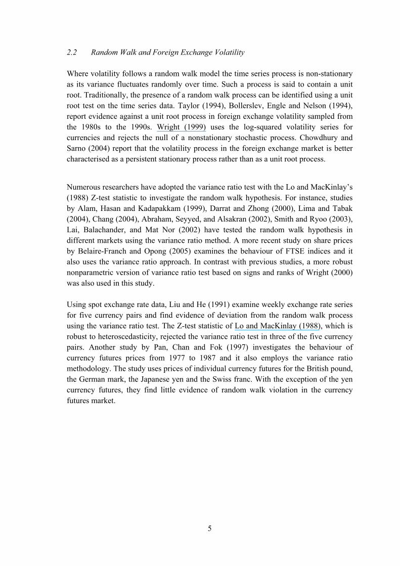
Where volatility follows a random walk model the time series process is non-stationary as its variance fluctuates randomly over time. Such a process is said to contain a unit root. Traditionally, the presence of a random walk process can be identified using a unit root test on the time series data. Taylor (1994), Bollerslev, Engle and Nelson (1994), report evidence against a unit root process in foreign exchange volatility sampled from the 1980s to the 1990s. Wright (1999) uses the log-squared volatility series for currencies and rejects the null of a nonstationary stochastic process. Chowdhury and Sarno (2004) report that the volatility process in the foreign exchange market is better characterised as a persistent stationary process rather than as a unit root process.

Numerous researchers have adopted the variance ratio test with the Lo and MacKinlay’s (1988) Z-test statistic to investigate the random walk hypothesis. For instance, studies by Alam, Hasan and Kadapakkam (1999), Darrat and Zhong (2000), Lima and Tabak (2004), Chang (2004), Abraham, Seyyed, and Alsakran (2002), Smith and Ryoo (2003), Lai, Balachander, and Mat Nor (2002) have tested the random walk hypothesis in different markets using the variance ratio method. A more recent study on share prices by Belaire-Franch and Opong (2005) examines the behaviour of FTSE indices and it also uses the variance ratio approach. In contrast with previous studies, a more robust nonparametric version of variance ratio test based on signs and ranks of Wright (2000) was also used in this study. Using spot exchange rate data, Liu and He (1991) examine weekly exchange rate series for five currency pairs and find evidence of deviation from the random walk process using the variance ratio test. The Z-test statistic of Lo and MacKinlay (1988), which is robust to heteroscedasticity, rejected the variance ratio test in three of the five currency pairs. Another study by Pan, Chan and Fok (1997) investigates the behaviour of currency futures prices from 1977 to 1987 and it also employs the variance ratio methodology. The study uses prices of individual currency futures for the British pound, the German mark, the Japanese yen and the Swiss franc. With the exception of the yen currency futures, they find little evidence of random walk violation in the currency futures market.

6

3. Data  

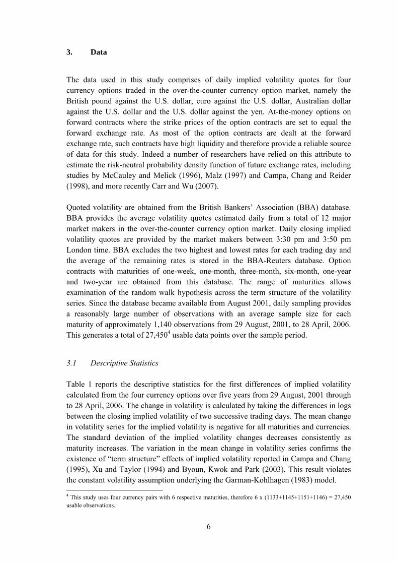
The data used in this study comprises of daily implied volatility quotes for four currency options traded in the over-the-counter currency option market, namely the British pound against the U.S. dollar, euro against the U.S. dollar, Australian dollar against the U.S. dollar and the U.S. dollar against the yen. At-the-money options on forward contracts where the strike prices of the option contracts are set to equal the forward exchange rate. As most of the option contracts are dealt at the forward exchange rate, such contracts have high liquidity and therefore provide a reliable source of data for this study. Indeed a number of researchers have relied on this attribute to estimate the risk-neutral probability density function of future exchange rates, including studies by McCauley and Melick (1996), Malz (1997) and Campa, Chang and Reider (1998), and more recently Carr and Wu (2007). Quoted volatility are obtained from the British Bankers’ Association (BBA) database. BBA provides the average volatility quotes estimated daily from a total of 12 major market makers in the over-the-counter currency option market. Daily closing implied volatility quotes are provided by the market makers between 3:30 pm and 3:50 pm London time. BBA excludes the two highest and lowest rates for each trading day and the average of the remaining rates is stored in the BBA-Reuters database. Option contracts with maturities of one-week, one-month, three-month, six-month, one-year and two-year are obtained from this database. The range of maturities allows examination of the random walk hypothesis across the term structure of the volatility series. Since the database became available from August 2001, daily sampling provides a reasonably large number of observations with an average sample size for each maturity of approximately 1,140 observations from 29 August, 2001, to 28 April, 2006. This generates a total of 27,4504 usable data points over the sample period.

3.1 Descriptive Statistics

Table 1 reports the descriptive statistics for the first differences of implied volatility calculated from the four currency options over five years from 29 August, 2001 through to 28 April, 2006. The change in volatility is calculated by taking the differences in logs between the closing implied volatility of two successive trading days. The mean change in volatility series for the implied volatility is negative for all maturities and currencies. The standard deviation of the implied volatility changes decreases consistently as maturity increases. The variation in the mean change in volatility series confirms the existence of “term structure” effects of implied volatility reported in Campa and Chang (1995), Xu and Taylor (1994) and Byoun, Kwok and Park (2003). This result violates the constant volatility assumption underlying the Garman-Kohlhagen (1983) model.                                                             4 This study uses four currency pairs with 6 respective maturities, therefore 6 x (1133+1145+1151+1146) = 27,450 usable observations.

7

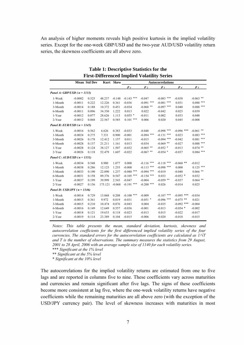
An analysis of higher moments reveals high positive kurtosis in the implied volatility series. Except for the one-week GBP/USD and the two-year AUD/USD volatility return series, the skewness coefficients are all above zero.

Table 1: Descriptive Statistics for the First-Differenced Implied Volatility Series

Mean Std Dev Kurt Skewρ 1 ρ 2 ρ 3 ρ 4 ρ 5

Panel A: GBP/USD ( n = 1133)

1-Week -0.0002 0.525 48.237 -0.148 -0.143 *** -0.047 -0.083 *** -0.038 -0.063 **

1-Month -0.0011 0.222 12.226 0.361 -0.036 -0.091 *** -0.081 *** 0.031 0.088 ***

3-Month -0.0014 0.188 10.372 0.451 -0.034 -0.068 ** -0.097 *** 0.040 0.088 ***

6-Month -0.0011 0.096 34.350 1.222 0.013 0.022 -0.042 0.025 0.0391-Year -0.0012 0.077 28.626 1.113 0.055 * -0.011 0.002 0.033 0.0482-Year -0.0012 0.068 22.567 0.585 0.101 *** 0.006 0.020 0.045 -0.008

Panel B: EUR/USD ( n = 1145)

1-Week -0.0016 0.562 6.626 0.383 -0.033 -0.048 -0.098 *** -0.096 *** -0.061 **

1-Month -0.0024 0.275 7.331 0.900 -0.001 -0.094 *** -0.131 *** 0.023 0.083 ***

3-Month -0.0026 0.178 12.412 1.157 0.011 -0.015 -0.094 *** -0.042 0.081 ***

6-Month -0.0028 0.137 21.211 1.161 0.013 -0.034 -0.069 ** -0.027 0.088 ***

1-Year -0.0028 0.124 38.127 1.507 -0.032 -0.065 ** -0.052 * -0.013 0.074 **

2-Year -0.0026 0.118 52.479 1.607 -0.022 -0.067 ** -0.054 * -0.037 0.084 ***

Panel C: AUD/USD ( n = 1151)

1-Week -0.0034 0.548 8.980 1.077 0.008 -0.116 *** -0.118 *** -0.060 ** -0.0121-Month -0.0038 0.286 12.125 1.255 -0.008 -0.113 *** -0.098 *** 0.000 0.125 ***

3-Month -0.0033 0.190 22.090 1.237 -0.080 *** -0.094 *** -0.019 -0.040 0.066 **

6-Month -0.0031 0.158 89.376 0.547 -0.105 *** -0.154 *** 0.033 -0.052 * 0.0321-Year -0.0037 0.199 39.999 2.543 -0.047 -0.004 -0.059 ** -0.037 0.064 **

2-Year -0.0027 0.156 175.121 -0.068 -0.191 *** -0.200 *** 0.026 -0.014 0.025

Panel D: USD/JPY ( n = 1146)

1-Week -0.0014 0.729 13.068 0.208 -0.100 *** -0.009 -0.107 *** -0.095 *** -0.0341-Month -0.0015 0.361 9.972 0.819 -0.031 -0.051 * -0.096 *** -0.075 ** 0.0213-Month -0.0015 0.210 10.474 0.876 -0.043 0.004 -0.035 -0.092 *** -0.0046-Month -0.0016 0.149 12.649 0.557 -0.036 -0.001 -0.013 -0.054 * -0.0021-Year -0.0018 0.121 19.633 0.118 -0.023 -0.013 0.015 -0.022 -0.0172-Year -0.0019 0.114 23.389 0.104 -0.015 -0.006 0.020 -0.018 -0.015

Autocorrelations

Notes: This table presents the mean, standard deviation, kurtosis, skewness and autocorrelation coefficients for the first differenced implied volatility series of the four currencies. The standard errors for the autocorrelation coefficients are calculated as 1/√T and T is the number of observations. The summary measures the statistics from 29 August, 2001 to 28 April, 2006 with an average sample size of 1140 for each volatility series. *** Significant at the 1% level ** Significant at the 5% level * Significant at the 10% level

The autocorrelations for the implied volatility returns are estimated from one to five lags and are reported in columns five to nine. These coefficients vary across maturities and currencies and remain significant after five lags. The signs of these coefficients become more consistent at lag five, where the one-week volatility returns have negative coefficients while the remaining maturities are all above zero (with the exception of the USD/JPY currency pair). The level of skewness increases with maturities in most

8

instances. These findings are consistent with the “fat tail” effect, indicating that the distributions of the volatility series significantly depart from the normality assumption.

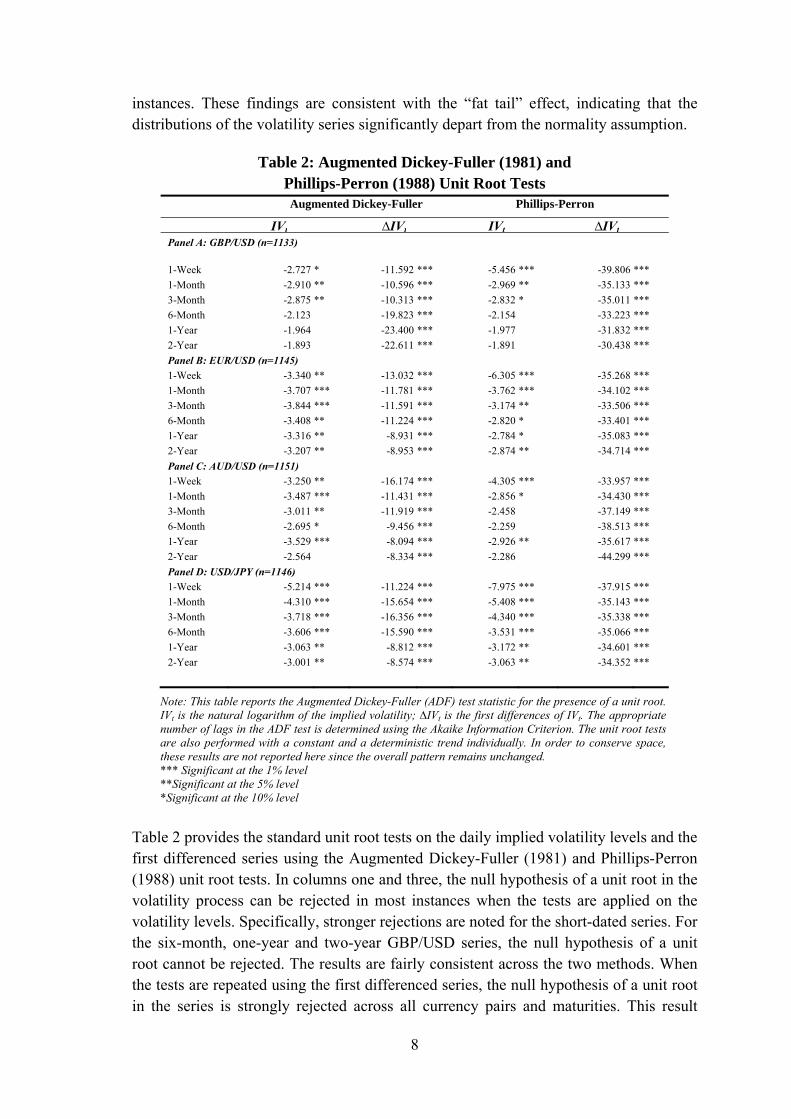
Table 2: Augmented Dickey-Fuller (1981) and

Phillips-Perron (1988) Unit Root Tests

Augmented Dickey-Fuller Phillips-Perron

IVt ∆IVt IVt ∆IVt Panel A: GBP/USD (n=1133)

1-Week -2.727 * -11.592 *** -5.456 *** -39.806 ***

1-Month -2.910 ** -10.596 *** -2.969 ** -35.133 ***

3-Month -2.875 ** -10.313 *** -2.832 * -35.011 ***

6-Month -2.123 -19.823 *** -2.154 -33.223 ***

1-Year -1.964 -23.400 *** -1.977 -31.832 ***

2-Year -1.893 -22.611 *** -1.891 -30.438 ***

Panel B: EUR/USD (n=1145)

1-Week -3.340 ** -13.032 *** -6.305 *** -35.268 ***

1-Month -3.707 *** -11.781 *** -3.762 *** -34.102 ***

3-Month -3.844 *** -11.591 *** -3.174 ** -33.506 ***

6-Month -3.408 ** -11.224 *** -2.820 * -33.401 ***

1-Year -3.316 ** -8.931 *** -2.784 * -35.083 ***

2-Year -3.207 ** -8.953 *** -2.874 ** -34.714 ***

Panel C: AUD/USD (n=1151)

1-Week -3.250 ** -16.174 *** -4.305 *** -33.957 ***

1-Month -3.487 *** -11.431 *** -2.856 * -34.430 ***

3-Month -3.011 ** -11.919 *** -2.458 -37.149 ***

6-Month -2.695 * -9.456 *** -2.259 -38.513 ***

1-Year -3.529 *** -8.094 *** -2.926 ** -35.617 ***

2-Year -2.564 -8.334 *** -2.286 -44.299 ***

Panel D: USD/JPY (n=1146)

1-Week -5.214 *** -11.224 *** -7.975 *** -37.915 ***

1-Month -4.310 *** -15.654 *** -5.408 *** -35.143 ***

3-Month -3.718 *** -16.356 *** -4.340 *** -35.338 ***

6-Month -3.606 *** -15.590 *** -3.531 *** -35.066 ***

1-Year -3.063 ** -8.812 *** -3.172 ** -34.601 ***

2-Year -3.001 ** -8.574 *** -3.063 ** -34.352 ***

Note: This table reports the Augmented Dickey-Fuller (ADF) test statistic for the presence of a unit root. IVt is the natural logarithm of the implied volatility; ∆IVt is the first differences of IVt. The appropriate number of lags in the ADF test is determined using the Akaike Information Criterion. The unit root tests are also performed with a constant and a deterministic trend individually. In order to conserve space, these results are not reported here since the overall pattern remains unchanged. *** Significant at the 1% level **Significant at the 5% level *Significant at the 10% level

Table 2 provides the standard unit root tests on the daily implied volatility levels and the first differenced series using the Augmented Dickey-Fuller (1981) and Phillips-Perron (1988) unit root tests. In columns one and three, the null hypothesis of a unit root in the volatility process can be rejected in most instances when the tests are applied on the volatility levels. Specifically, stronger rejections are noted for the short-dated series. For the six-month, one-year and two-year GBP/USD series, the null hypothesis of a unit root cannot be rejected. The results are fairly consistent across the two methods. When the tests are repeated using the first differenced series, the null hypothesis of a unit root in the series is strongly rejected across all currency pairs and maturities. This result

9

holds under both methods. Thus, the Augmented Dickey-Fuller (1981) and Phillips-Perron (1988) unit root tests provide evidence of stationary in first differences of the volatility series while the volatility levels are strictly stationary.

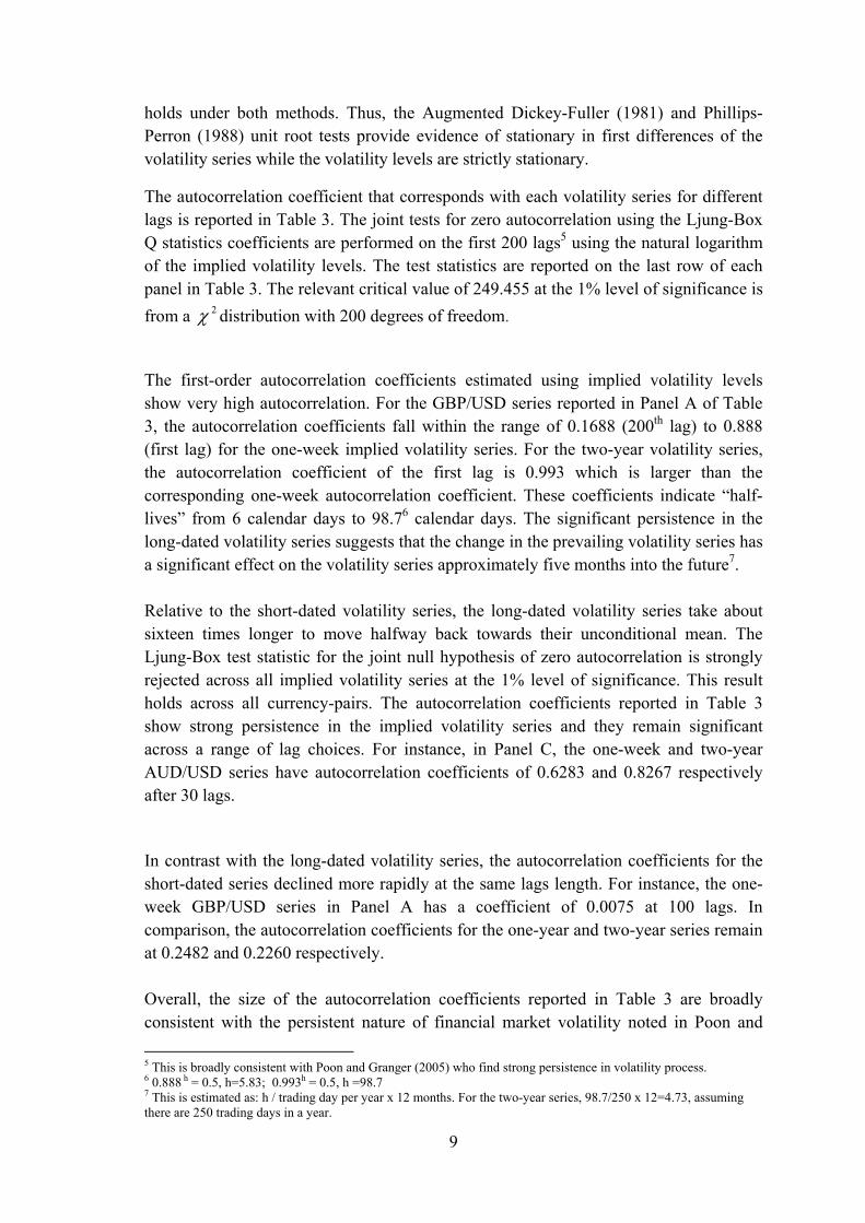
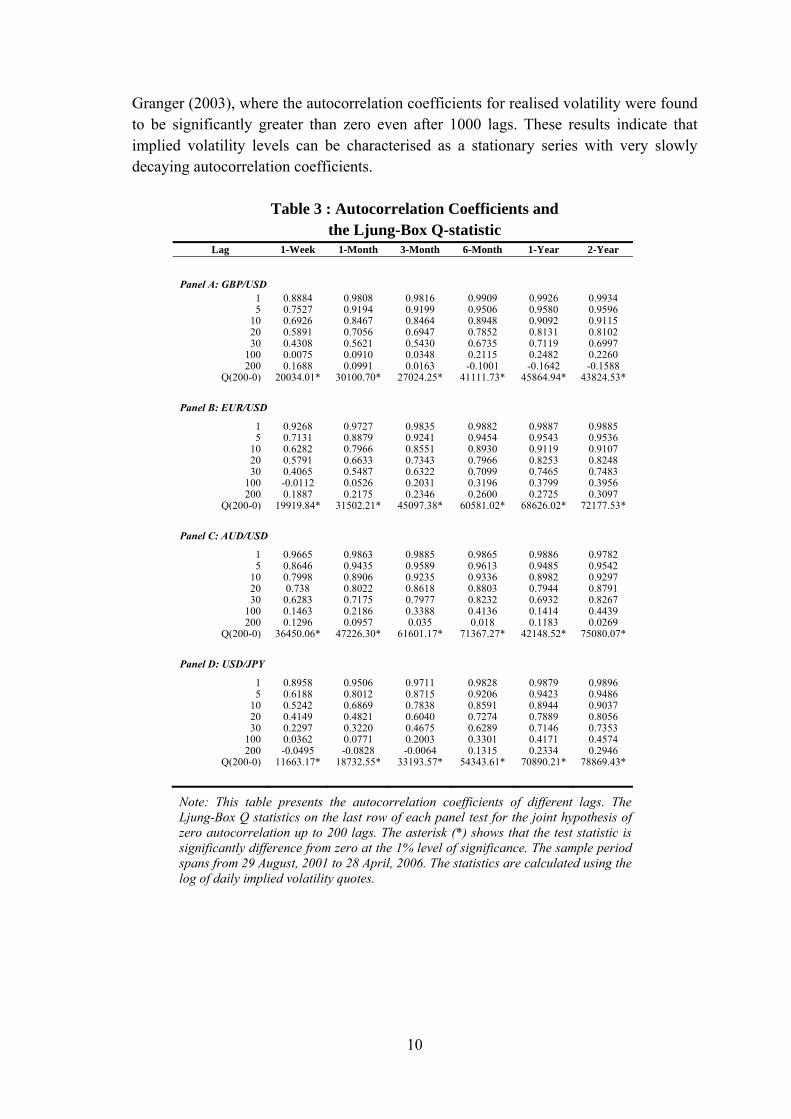
The autocorrelation coefficient that corresponds with each volatility series for different lags is reported in Table 3. The joint tests for zero autocorrelation using the Ljung-Box Q statistics coefficients are performed on the first 200 lags5 using the natural logarithm of the implied volatility levels. The test statistics are reported on the last row of each panel in Table 3. The relevant critical value of 249.455 at the 1% level of significance is

from a 2 distribution with 200 degrees of freedom.

The first-order autocorrelation coefficients estimated using implied volatility levels show very high autocorrelation. For the GBP/USD series reported in Panel A of Table 3, the autocorrelation coefficients fall within the range of 0.1688 (200th lag) to 0.888 (first lag) for the one-week implied volatility series. For the two-year volatility series, the autocorrelation coefficient of the first lag is 0.993 which is larger than the corresponding one-week autocorrelation coefficient. These coefficients indicate “half-lives” from 6 calendar days to 98.76 calendar days. The significant persistence in the long-dated volatility series suggests that the change in the prevailing volatility series has a significant effect on the volatility series approximately five months into the future7.

Relative to the short-dated volatility series, the long-dated volatility series take about sixteen times longer to move halfway back towards their unconditional mean. The Ljung-Box test statistic for the joint null hypothesis of zero autocorrelation is strongly rejected across all implied volatility series at the 1% level of significance. This result holds across all currency-pairs. The autocorrelation coefficients reported in Table 3 show strong persistence in the implied volatility series and they remain significant across a range of lag choices. For instance, in Panel C, the one-week and two-year AUD/USD series have autocorrelation coefficients of 0.6283 and 0.8267 respectively after 30 lags.

In contrast with the long-dated volatility series, the autocorrelation coefficients for the short-dated series declined more rapidly at the same lags length. For instance, the one-week GBP/USD series in Panel A has a coefficient of 0.0075 at 100 lags. In comparison, the autocorrelation coefficients for the one-year and two-year series remain at 0.2482 and 0.2260 respectively.

Overall, the size of the autocorrelation coefficients reported in Table 3 are broadly consistent with the persistent nature of financial market volatility noted in Poon and

                                                            5 This is broadly consistent with Poon and Granger (2005) who find strong persistence in volatility process. 6 0.888 h = 0.5, h=5.83; 0.993h = 0.5, h =98.7 7 This is estimated as: h / trading day per year x 12 months. For the two-year series, 98.7/250 x 12=4.73, assuming there are 250 trading days in a year.

10

Granger (2003), where the autocorrelation coefficients for realised volatility were found to be significantly greater than zero even after 1000 lags. These results indicate that implied volatility levels can be characterised as a stationary series with very slowly decaying autocorrelation coefficients.

Table 3 : Autocorrelation Coefficients and

the Ljung-Box Q-statistic Lag 1-Week 1-Month 3-Month 6-Month 1-Year 2-Year

Panel A: GBP/USD

1 0.8884 0.9808 0.9816 0.9909 0.9926 0.9934 5 0.7527 0.9194 0.9199 0.9506 0.9580 0.9596

10 0.6926 0.8467 0.8464 0.8948 0.9092 0.9115 20 0.5891 0.7056 0.6947 0.7852 0.8131 0.8102 30 0.4308 0.5621 0.5430 0.6735 0.7119 0.6997

100 0.0075 0.0910 0.0348 0.2115 0.2482 0.2260 200 0.1688 0.0991 0.0163 -0.1001 -0.1642 -0.1588

Q(200-0) 20034.01* 30100.70* 27024.25* 41111.73* 45864.94* 43824.53*

Panel B: EUR/USD

1 0.9268 0.9727 0.9835 0.9882 0.9887 0.9885 5 0.7131 0.8879 0.9241 0.9454 0.9543 0.9536

10 0.6282 0.7966 0.8551 0.8930 0.9119 0.9107 20 0.5791 0.6633 0.7343 0.7966 0.8253 0.8248 30 0.4065 0.5487 0.6322 0.7099 0.7465 0.7483

100 -0.0112 0.0526 0.2031 0.3196 0.3799 0.3956 200 0.1887 0.2175 0.2346 0.2600 0.2725 0.3097

Q(200-0) 19919.84* 31502.21* 45097.38* 60581.02* 68626.02* 72177.53*

Panel C: AUD/USD

1 0.9665 0.9863 0.9885 0.9865 0.9886 0.9782 5 0.8646 0.9435 0.9589 0.9613 0.9485 0.9542

10 0.7998 0.8906 0.9235 0.9336 0.8982 0.9297 20 0.738 0.8022 0.8618 0.8803 0.7944 0.8791 30 0.6283 0.7175 0.7977 0.8232 0.6932 0.8267

100 0.1463 0.2186 0.3388 0.4136 0.1414 0.4439 200 0.1296 0.0957 0.035 0.018 0.1183 0.0269

Q(200-0) 36450.06* 47226.30* 61601.17* 71367.27* 42148.52* 75080.07*

Panel D: USD/JPY

1 0.8958 0.9506 0.9711 0.9828 0.9879 0.9896 5 0.6188 0.8012 0.8715 0.9206 0.9423 0.9486

10 0.5242 0.6869 0.7838 0.8591 0.8944 0.9037 20 0.4149 0.4821 0.6040 0.7274 0.7889 0.8056 30 0.2297 0.3220 0.4675 0.6289 0.7146 0.7353

100 0.0362 0.0771 0.2003 0.3301 0.4171 0.4574 200 -0.0495 -0.0828 -0.0064 0.1315 0.2334 0.2946

Q(200-0) 11663.17* 18732.55* 33193.57* 54343.61* 70890.21* 78869.43*

Note: This table presents the autocorrelation coefficients of different lags. The Ljung-Box Q statistics on the last row of each panel test for the joint hypothesis of zero autocorrelation up to 200 lags. The asterisk (*) shows that the test statistic is significantly difference from zero at the 1% level of significance. The sample period spans from 29 August, 2001 to 28 April, 2006. The statistics are calculated using the log of daily implied volatility quotes.

11

4. Methodology

4.1 The Conventional Variance Ratio Test

The preceding analyses suggest that the null hypothesis of a unit root in the volatility data can be rejected across all currencies and maturities. Since both a unit root and uncorrelated increments are required for the random walk process to hold (Liu and He, 1991), variance ratio tests are employed in the following section to investigate the violation of the uncorrelated increments requirement.

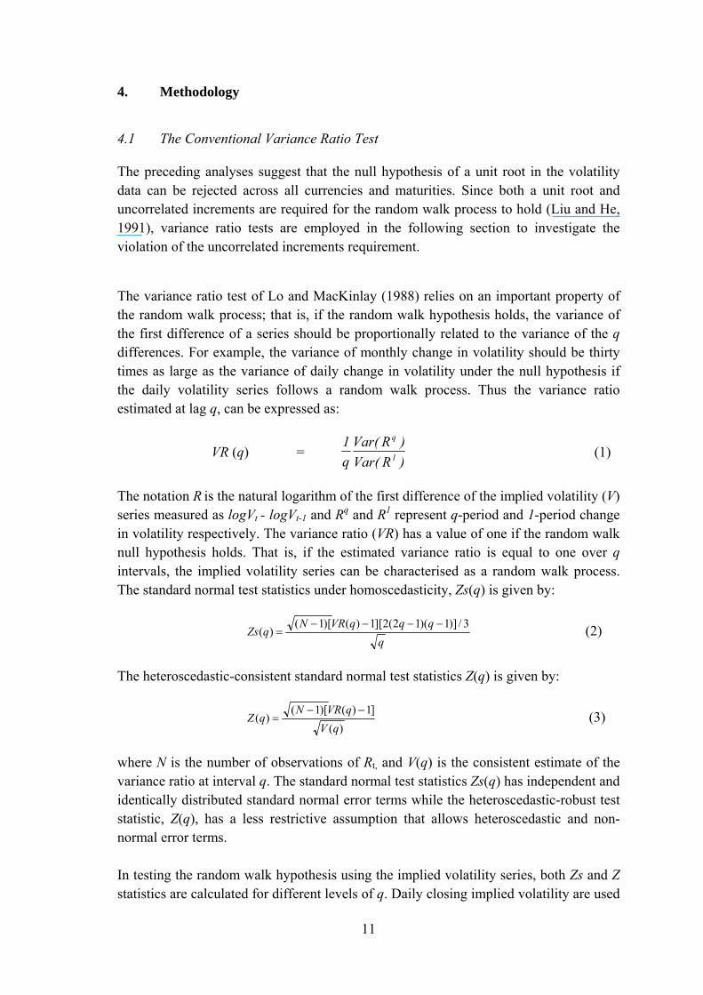
The variance ratio test of Lo and MacKinlay (1988) relies on an important property of the random walk process; that is, if the random walk hypothesis holds, the variance of the first difference of a series should be proportionally related to the variance of the q differences. For example, the variance of monthly change in volatility should be thirty times as large as the variance of daily change in volatility under the null hypothesis if the daily volatility series follows a random walk process. Thus the variance ratio estimated at lag q, can be expressed as:

VR (q) = )R(Var

)R(Var

q

11

q

(1)

The notation R is the natural logarithm of the first difference of the implied volatility (V) series measured as logVt - logVt-1 and Rq and R1 represent q-period and 1-period change in volatility respectively. The variance ratio (VR) has a value of one if the random walk null hypothesis holds. That is, if the estimated variance ratio is equal to one over q intervals, the implied volatility series can be characterised as a random walk process. The standard normal test statistics under homoscedasticity, Zs(q) is given by:

q

qqqVRNqZs

3/)]1)(12(2][1)()[1()(

(2)

The heteroscedastic-consistent standard normal test statistics Z(q) is given by:

)(

]1)()[1()(

qV

qVRNqZ

(3)

where N is the number of observations of Rt, and V(q) is the consistent estimate of the variance ratio at interval q. The standard normal test statistics Zs(q) has independent and identically distributed standard normal error terms while the heteroscedastic-robust test statistic, Z(q), has a less restrictive assumption that allows heteroscedastic and non-normal error terms. In testing the random walk hypothesis using the implied volatility series, both Zs and Z statistics are calculated for different levels of q. Daily closing implied volatility are used

12

as the base observation interval. The Zs and Z statistics are calculated for each q by comparing the variance of the base interval with the variance for two-day, five-day, ten-day, twenty-day and thirty-day periods. The VR for each level of q is calculated for the volatility series with maturities of one-week, one-month, three-month, six-month, one-year and two-year. Since both Zs(q) and Z(q) statistics are asymptotic normal, the usual critical values are used for hypothesis testing. For completeness, the variance ratio test is also performed using volatility levels for the selected currency pairs.

4.2 The Nonparametric Variance Ratio Test

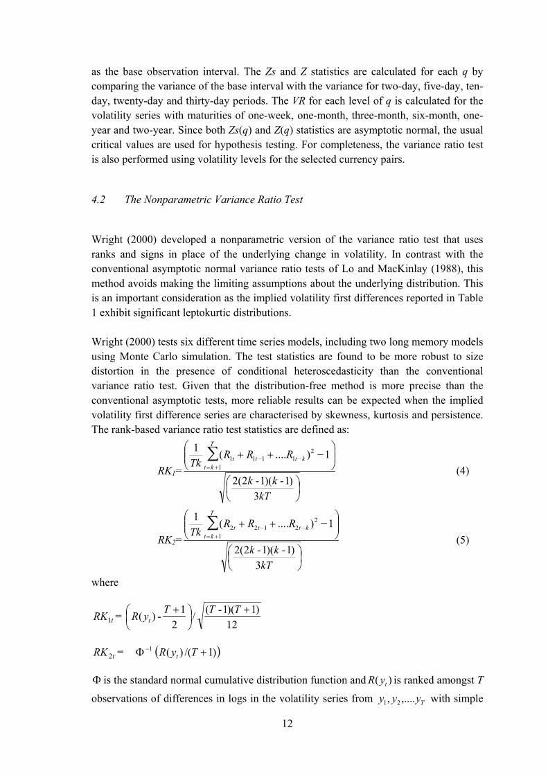
Wright (2000) developed a nonparametric version of the variance ratio test that uses ranks and signs in place of the underlying change in volatility. In contrast with the conventional asymptotic normal variance ratio tests of Lo and MacKinlay (1988), this method avoids making the limiting assumptions about the underlying distribution. This is an important consideration as the implied volatility first differences reported in Table 1 exhibit significant leptokurtic distributions.

Wright (2000) tests six different time series models, including two long memory models using Monte Carlo simulation. The test statistics are found to be more robust to size distortion in the presence of conditional heteroscedasticity than the conventional variance ratio test. Given that the distribution-free method is more precise than the conventional asymptotic tests, more reliable results can be expected when the implied volatility first difference series are characterised by skewness, kurtosis and persistence. The rank-based variance ratio test statistics are defined as:

RK1=

kT

kk

RRRTk kt

T

kttt

3

)1-)(1-2(2

1)....(1 2

11

111∑ (4)

RK2=

kT

kk

RRRTk kt

T

kttt

3

)1-)(1-2(2

1)....(1 2

21

122∑ (5)

where

tRK1 = 12

)1)(1-(/

2

1-)(

TTT

yR t

tRK2 = 1 )1/()( TyR t

is the standard normal cumulative distribution function and )( tyR is ranked amongst T

observations of differences in logs in the volatility series from Tyyy ,...., 21 with simple

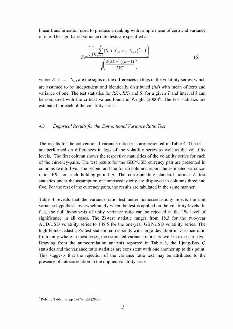
13

linear transformation used to produce a ranking with sample mean of zero and variance of one. The sign-based variance ratio tests are specified as:

S1=

kT

kk

SSSTk kt

T

kttt

3

)1)(12(2

1)....(1 2

11

(6)

where ktt SS ..... are the signs of the differences in logs in the volatility series, which

are assumed to be independent and identically distributed (iid) with mean of zero and variance of one. The test statistics for RK1, RK2 and S1 for a given T and interval k can be compared with the critical values found in Wright (2000)8. The test statistics are estimated for each of the volatility series.

4.3 Empirical Results for the Conventional Variance Ratio Test

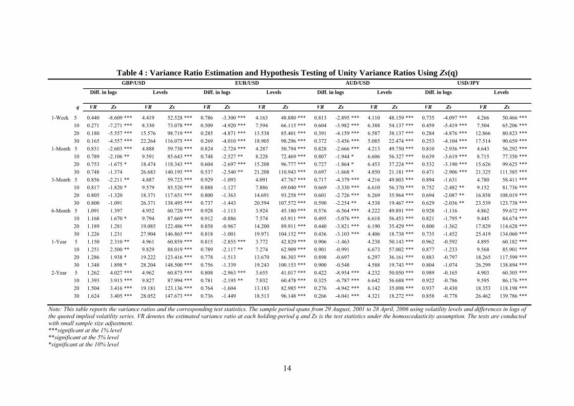
The results for the conventional variance ratio tests are presented in Table 4. The tests are performed on differences in logs of the volatility series as well as the volatility levels. The first column shows the respective maturities of the volatility series for each of the currency-pairs. The test results for the GBP/USD currency pair are presented in columns two to five. The second and the fourth columns report the estimated variance-ratio, VR, for each holding-period q. The corresponding standard normal Zs-test statistics under the assumption of homoscedasticity are displayed in columns three and five. For the rest of the currency pairs, the results are tabulated in the same manner.

Table 4 reveals that the variance ratio test under homoscedasticity rejects the unit variance hypothesis overwhelmingly when the test is applied on the volatility levels. In fact, the null hypothesis of unity variance ratio can be rejected at the 1% level of significance in all cases. The Zs-test statistic ranges from 18.3 for the two-year AUD/USD volatility series to 148.5 for the one-year GBP/USD volatility series. The high homoscedastic Zs-test statistic corresponds with large deviation in variance ratio from unity where in most cases, the estimated variance ratios are well in excess of five. Drawing from the autocorrelation analysis reported in Table 3, the Ljung-Box Q statistics and the variance ratio statistics are consistent with one another up to this point. This suggests that the rejection of the variance ratio test may be attributed to the presence of autocorrelation in the implied volatility series.

                                                            8 Refer to Table 1 on pp.3 of Wright (2000).

 

14

Table 4 : Variance Ratio Estimation and Hypothesis Testing of Unity Variance Ratios Using Zs(q) GBP/USD EUR/USD AUD/USD USD/JPY

Diff. in logs Levels Diff. in logs Levels Diff. in logs Levels Diff. in logs Levels

q VR Zs VR Zs VR Zs VR Zs VR Zs VR Zs VR Zs VR Zs

1-Week 5 0.440 -8.609 *** 4.419 52.528 *** 0.786 -3.300 *** 4.163 48.880 *** 0.813 -2.895 *** 4.110 48.159 *** 0.735 -4.097 *** 4.266 50.466 ***

10 0.271 -7.271 *** 8.330 73.078 *** 0.509 -4.920 *** 7.594 66.115 *** 0.604 -3.982 *** 6.388 54.137 *** 0.459 -5.419 *** 7.504 65.206 ***

20 0.180 -5.557 *** 15.576 98.719 *** 0.285 -4.871 *** 13.538 85.401 *** 0.391 -4.159 *** 6.587 38.137 *** 0.284 -4.876 *** 12.866 80.823 ***

30 0.165 -4.557 *** 22.264 116.075 *** 0.269 -4.010 *** 18.905 98.296 *** 0.372 -3.456 *** 5.085 22.474 *** 0.253 -4.104 *** 17.514 90.659 ***

1-Month 5 0.831 -2.603 *** 4.888 59.730 *** 0.824 -2.724 *** 4.287 50.794 *** 0.828 -2.666 *** 4.213 49.750 *** 0.810 -2.936 *** 4.643 56.292 ***

10 0.789 -2.106 ** 9.591 85.643 *** 0.748 -2.527 ** 8.228 72.469 *** 0.807 -1.944 * 6.606 56.327 *** 0.639 -3.619 *** 8.715 77.350 ***

20 0.753 -1.675 * 18.474 118.343 *** 0.604 -2.697 *** 15.208 96.777 *** 0.727 -1.864 * 6.453 37.224 *** 0.532 -3.190 *** 15.626 99.625 ***

30 0.748 -1.374 26.683 140.195 *** 0.537 -2.540 ** 21.208 110.943 *** 0.697 -1.668 * 4.850 21.181 *** 0.471 -2.906 *** 21.325 111.585 ***

3-Month 5 0.856 -2.211 ** 4.887 59.723 *** 0.929 -1.093 4.091 47.767 *** 0.717 -4.379 *** 4.216 49.803 *** 0.894 -1.631 4.780 58.411 ***

10 0.817 -1.820 * 9.579 85.520 *** 0.888 -1.127 7.886 69.040 *** 0.669 -3.330 *** 6.610 56.370 *** 0.752 -2.482 ** 9.152 81.736 ***

20 0.805 -1.320 18.371 117.651 *** 0.800 -1.363 14.691 93.258 *** 0.601 -2.726 *** 6.269 35.964 *** 0.694 -2.087 ** 16.858 108.019 ***

30 0.800 -1.091 26.371 138.495 *** 0.737 -1.443 20.594 107.572 *** 0.590 -2.254 ** 4.538 19.467 *** 0.629 -2.036 ** 23.539 123.738 ***

6-Month 5 1.091 1.397 4.952 60.720 *** 0.928 -1.113 3.924 45.180 *** 0.576 -6.564 *** 4.222 49.891 *** 0.928 -1.116 4.862 59.672 ***

10 1.168 1.670 * 9.794 87.669 *** 0.912 -0.886 7.574 65.911 *** 0.495 -5.076 *** 6.618 56.453 *** 0.821 -1.795 * 9.445 84.674 ***

20 1.189 1.281 19.085 122.486 *** 0.858 -0.967 14.200 89.911 *** 0.440 -3.821 *** 6.190 35.429 *** 0.800 -1.362 17.829 114.628 ***

30 1.226 1.231 27.904 146.865 *** 0.818 -1.001 19.971 104.152 *** 0.436 -3.103 *** 4.406 18.738 *** 0.735 -1.452 25.419 134.060 ***

1-Year 5 1.150 2.310 ** 4.961 60.859 *** 0.815 -2.855 *** 3.772 42.829 *** 0.906 -1.463 4.238 50.143 *** 0.962 -0.592 4.895 60.182 ***

10 1.251 2.500 ** 9.829 88.019 *** 0.789 -2.117 ** 7.274 62.909 *** 0.901 -0.991 6.673 57.002 *** 0.877 -1.233 9.568 85.901 ***

20 1.286 1.938 * 19.222 123.416 *** 0.778 -1.513 13.670 86.303 *** 0.898 -0.697 6.297 36.161 *** 0.883 -0.797 18.265 117.599 ***

30 1.348 1.898 * 28.204 148.500 *** 0.756 -1.339 19.243 100.153 *** 0.900 -0.548 4.588 19.743 *** 0.804 -1.074 26.299 138.894 ***

2-Year 5 1.262 4.027 *** 4.962 60.875 *** 0.808 -2.963 *** 3.655 41.017 *** 0.422 -8.954 *** 4.232 50.050 *** 0.989 -0.165 4.903 60.305 ***

10 1.393 3.915 *** 9.827 87.994 *** 0.781 -2.195 ** 7.032 60.478 *** 0.325 -6.787 *** 6.642 56.688 *** 0.922 -0.786 9.595 86.176 ***

20 1.504 3.416 *** 19.181 123.136 *** 0.764 -1.604 13.183 82.985 *** 0.276 -4.942 *** 6.142 35.098 *** 0.937 -0.430 18.353 118.198 ***

30 1.624 3.405 *** 28.052 147.673 *** 0.736 -1.449 18.513 96.148 *** 0.266 -4.041 *** 4.321 18.272 *** 0.858 -0.778 26.462 139.786 ***

Note: This table reports the variance ratios and the corresponding test statistics. The sample period spans from 29 August, 2001 to 28 April, 2006 using volatility levels and differences in logs of the quoted implied volatility series. VR denotes the estimated variance ratio at each holding-period q and Zs is the test statistics under the homoscedasticity assumption. The tests are conducted with small sample size adjustment. ***significant at the 1% level **significant at the 5% level *significant at the 10% level

 

15

In sharp contrast, rejections of the null hypothesis are most evident for short-dated series when the test is repeated using first differences of the implied volatility series. For these series, the Zs-test statistics are above 1.96 suggesting the random walk hypothesis can be comfortably rejected at the 5% level of significance (two-tailed test). Notably, the one- week and one-month series are consistently rejected across all four currency-pairs. For the USD/JPY currency-pair, rejections of the null hypothesis at 1% level of significance can be found for the one-week and one-month series at various holding-periods (q). However for the AUD/USD and the GBP/USD currency pairs, rejections of the null hypothesis are more widespread and can be found across all maturities. Consistent with this pattern, the variance ratios estimated using first differences are also closer to unity compared with those estimated with volatility levels. This can be seen across all currency-pairs.

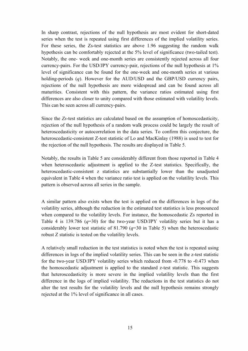
Since the Zs-test statistics are calculated based on the assumption of homoscedasticity, rejection of the null hypothesis of a random walk process could be largely the result of heteroscedasticity or autocorrelation in the data series. To confirm this conjecture, the heteroscedastic-consistent Z-test statistic of Lo and MacKinlay (1988) is used to test for the rejection of the null hypothesis. The results are displayed in Table 5. Notably, the results in Table 5 are considerably different from those reported in Table 4 when heteroscedastic adjustment is applied to the Z-test statistics. Specifically, the heteroscedastic-consistent z statistics are substantially lower than the unadjusted equivalent in Table 4 when the variance ratio test is applied on the volatility levels. This pattern is observed across all series in the sample.

A similar pattern also exists when the test is applied on the differences in logs of the volatility series, although the reduction in the estimated test statistics is less pronounced when compared to the volatility levels. For instance, the homoscedastic Zs reported in Table 4 is 139.786 (q=30) for the two-year USD/JPY volatility series but it has a considerably lower test statistic of 81.790 (q=30 in Table 5) when the heteroscedastic robust Z statistic is tested on the volatility levels. A relatively small reduction in the test statistics is noted when the test is repeated using differences in logs of the implied volatility series. This can be seen in the z-test statistic for the two-year USD/JPY volatility series which reduced from -0.778 to -0.473 when the homoscedastic adjustment is applied to the standard z-test statistic. This suggests that heteroscedasticity is more severe in the implied volatility levels than the first difference in the logs of implied volatility. The reductions in the test statistics do not alter the test results for the volatility levels and the null hypothesis remains strongly rejected at the 1% level of significance in all cases.

 

16

Table 5 : Variance Ratio Estimation and Hypothesis Testing of Unity Variance Ratios Using Z(q) GBP/USD EUR/USD AUD/USD USD/JPY

Diff. in logs Levels Diff. in logs Levels Diff. in logs Levels Diff. in logs Levels

q VR Z VR Z VR Z VR Z VR Z VR Z VR Z VR Z

1-Week 5 0.440 -1.588 4.419 30.390 *** 0.786 -3.019 *** 4.163 33.880 *** 0.813 -2.519 ** 4.110 6.784 *** 0.735 -3.376 *** 4.266 34.086 ***

10 0.271 -2.245 ** 8.330 43.122 *** 0.509 -4.453 *** 7.594 47.938 *** 0.604 -3.540 *** 6.388 8.150 *** 0.459 -4.488 *** 7.504 46.867 ***

20 0.180 -2.446 ** 15.576 59.498 *** 0.285 -4.496 *** 13.538 63.504 *** 0.391 -3.847 *** 6.587 6.286 *** 0.284 -4.111 *** 12.866 62.116 ***

30 0.165 -2.311 ** 22.264 70.923 *** 0.269 -3.750 *** 18.905 74.249 *** 0.372 -3.253 *** 5.085 4.056 *** 0.253 -3.525 *** 17.514 72.751 ***

1-Month 5 0.831 -1.864 * 4.888 29.552 *** 0.824 -2.328 ** 4.287 32.883 *** 0.828 -2.238 ** 4.213 6.931 *** 0.810 -2.037 ** 4.643 38.461 ***

10 0.789 -1.852 * 9.591 42.697 *** 0.748 -2.170 ** 8.228 49.159 *** 0.807 -1.704 * 6.606 8.225 *** 0.639 -2.638 *** 8.715 54.828 ***

20 0.753 -1.657 * 18.474 59.867 *** 0.604 -2.380 ** 15.208 67.572 *** 0.727 -1.722 * 6.453 5.939 *** 0.532 -2.475 ** 15.626 73.796 ***

30 0.748 -1.465 26.683 71.954 *** 0.537 -2.285 ** 21.208 78.122 *** 0.697 -1.575 4.850 3.720 *** 0.471 -2.346 ** 21.325 85.711 ***

3-Month 5 0.856 -1.800 * 4.887 30.853 *** 0.929 -0.778 4.091 29.878 *** 0.717 -1.697 * 4.216 6.824 *** 0.894 -1.072 4.780 39.237 ***

10 0.817 -1.738 * 9.579 44.519 *** 0.888 -0.824 7.886 45.488 *** 0.669 -1.548 6.610 8.074 *** 0.752 -1.761 * 9.152 56.278 ***

20 0.805 -1.426 18.371 62.105 *** 0.800 -1.056 14.691 62.604 *** 0.601 -1.414 6.269 5.629 *** 0.694 -1.598 16.858 77.395 ***

30 0.800 -1.225 26.371 74.132 *** 0.737 -1.156 20.594 72.471 *** 0.590 -1.215 4.538 3.358 *** 0.629 -1.619 23.539 92.037 ***

6-Month 5 1.091 0.144 4.952 33.339 *** 0.928 -0.522 3.924 26.312 *** 0.576 -1.289 4.222 6.784 *** 0.928 -0.638 4.862 36.491 ***

10 1.168 0.304 9.794 48.444 *** 0.912 -0.459 7.574 40.589 *** 0.495 -1.248 6.618 8.016 *** 0.821 -1.162 9.445 52.702 ***

20 1.189 0.291 19.085 68.639 *** 0.858 -0.546 14.200 56.413 *** 0.440 -1.087 6.190 5.498 *** 0.800 -0.969 17.829 73.789 ***

30 1.226 0.386 27.904 83.524 *** 0.818 -0.592 19.971 65.741 *** 0.436 -0.927 4.406 3.207 *** 0.735 -1.079 25.419 89.170 ***

1-Year 5 1.150 0.507 4.961 36.169 *** 0.815 -0.984 3.772 24.003 *** 0.906 -0.860 4.238 6.856 *** 0.962 -0.283 4.895 33.777 ***

10 1.251 0.740 9.829 52.647 *** 0.789 -0.849 7.274 37.601 *** 0.901 -0.617 6.673 8.127 *** 0.877 -0.697 9.568 48.918 ***

20 1.286 0.711 19.222 74.877 *** 0.778 -0.676 13.670 52.816 *** 0.898 -0.460 6.297 5.635 *** 0.883 -0.504 18.265 68.945 ***

30 1.348 0.846 28.204 91.471 *** 0.756 -0.625 19.243 61.750 *** 0.900 -0.371 4.588 3.395 *** 0.804 -0.709 26.299 83.760 ***

2-Year 5 1.262 1.153 4.962 37.057 *** 0.808 -0.872 3.655 23.035 *** 0.422 -1.379 4.232 6.761 *** 0.989 -0.074 4.903 33.001 ***

10 1.393 1.379 9.827 53.886 *** 0.781 -0.766 7.032 36.167 *** 0.325 -1.325 6.642 7.983 *** 0.922 -0.425 9.595 47.785 ***

20 1.504 1.499 19.181 76.422 *** 0.764 -0.629 13.183 50.602 *** 0.276 -1.125 6.142 5.403 *** 0.937 -0.261 18.353 67.335 ***

30 1.624 1.742 * 28.052 93.027 *** 0.736 -0.593 18.513 58.909 *** 0.266 -0.968 4.321 3.104 *** 0.858 -0.493 26.462 81.790 ***

Note: This table reports variance ratios with the corresponding test statistics. The sample period spans from 29 August, 2001 to 28 April, 2006 using volatility levels and differences in logs of the quoted implied volatility series. VR denotes the estimated variance ratio at each holding-period q and Z is the Lo and MacKinlay (1988) test statistics robust to heteroscedasticity. The tests are conducted with small sample size adjustment. ***significant at the 1% level **significant at the 5% level *significant at the 10% level

 

17

Together, the results presented in Tables 4 and 5 suggest that most of the rejections of the null hypothesis under homoscedasticity are not robust to heteroscedasticity when the variance ratio test is performed on the difference in log volatility series. In particular, the long-dated series of six-month, one-year and two-year are no longer rejected under the heteroscedastic-consistent Z statistic. Therefore it is clear that the variance ratios of these series are significantly different from one due to the presence of heteroscedasticity in the volatility process. More importantly, this is consistent with the findings of Diebold and Nerlove (1989) who find strong ARCH effects in the volatility patterns of spot exchange rates. In contrast, short-dated implied volatility series of one-week and one-month remain significant in Table 5 with the heteroscedastic adjusted z-test statistic. The only exception is the two-year GBP/USD series which is marginally rejected with a Z-test statistic of 1.742 over an interval of 30 days.

The rejection of the null hypothesis is particularly strong for the Japanese yen. For example, the heteroscedastic-consistent z-statistics associated with time interval, q of 5, 10, 20 and 30, are -3.376, -4.488, -4.111, -3.525 for the one-week USD/JPY series. Clearly, the null hypothesis is strongly rejected at the 1% level of significance. For the three-month series, rejections of the unity variance ratio assumption are also reported for time intervals of 10 and 20 days. For the EUR/USD and AUD/USD currency pairs, rejections of the null are also reported for the one-week and one-month series. These short-dated series results are robust to heteroscedasticity and thus the rejections of the variance ratio test appear to be related to autocorrelation rather than heteroscedasticity.

4.4 Empirical Results for the Nonparametric Variance Ratio Test

Although the preceding test results reported in Table 5 are robust to heteroscedasticity, the conventional variance ratio assumes the sampling distribution of the variance ratio test statistic is normally distributed. As the quoted volatility series are far from normally distributed, violation of the underlying assumption in the variance ratio test statistics can produce erroneous test results.

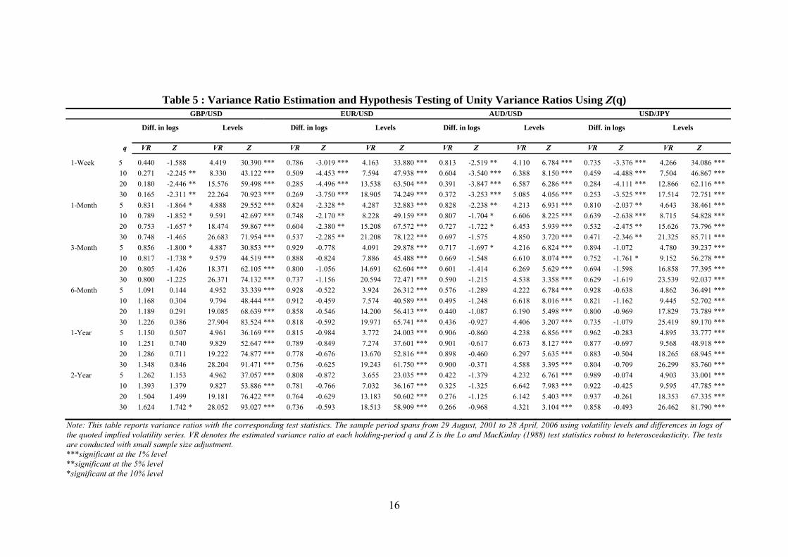
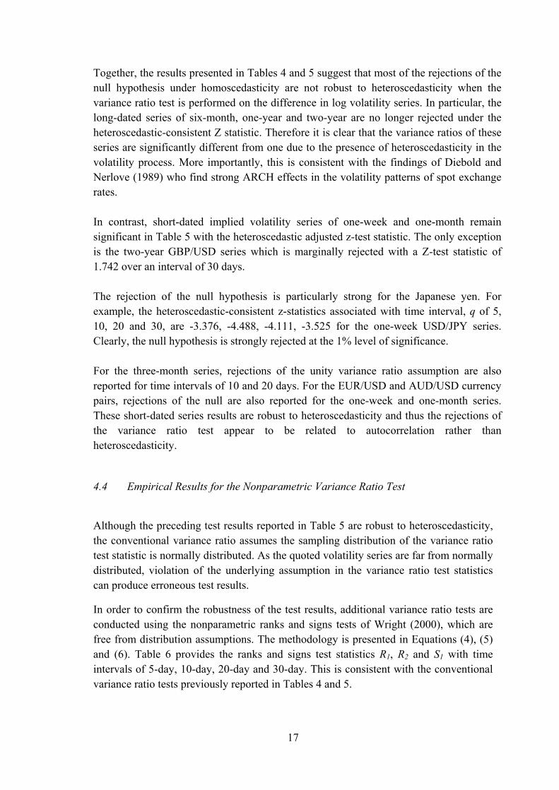
In order to confirm the robustness of the test results, additional variance ratio tests are conducted using the nonparametric ranks and signs tests of Wright (2000), which are free from distribution assumptions. The methodology is presented in Equations (4), (5) and (6). Table 6 provides the ranks and signs test statistics R1, R2 and S1 with time intervals of 5-day, 10-day, 20-day and 30-day. This is consistent with the conventional variance ratio tests previously reported in Tables 4 and 5.

 

18

Table 6 : Hypothesis Testing of Unity Variance Ratios Using Ranks and Signs GBP/USD EUR/USD AUD/USD USD/JPY

K RK1 RK2 S1 RK1 RK2 S1 RK1 RK2 S1 RK1 RK2 S1

1-Week 5 -2.702 *** -3.031 *** -2.360 ** -3.140 *** -3.302 *** -2.844 *** -2.354 ** -2.746 *** -0.939 -4.229 *** -4.447 *** -3.030 ***

10 -3.963 *** -4.554 *** -3.177 *** -4.319 *** -4.803 *** -3.322 *** -3.481 *** -4.016 *** -1.572 -5.220 *** -5.638 *** -3.524 ***

20 -3.735 *** -4.216 *** -2.914 *** -3.925 *** -4.595 *** -2.840 *** -3.347 *** -4.101 *** -1.498 -4.645 *** -5.020 *** -3.390 ***

30 -3.102 *** -3.475 *** -2.548 ** -3.167 *** -3.751 *** -2.231 ** -2.544 ** -3.305 *** -1.107 -3.872 *** -4.189 *** -3.099 ***

1-Month 5 -2.494 ** -2.773 *** -1.425 -3.103 *** -2.926 *** -2.594 *** -3.042 *** -2.917 *** -3.655 *** -3.439 *** -3.271 *** -2.714 ***

10 -1.678 * -2.240 ** -0.579 -2.925 *** -2.899 *** -2.386 ** -2.405 ** -2.278 ** -2.763 *** -3.944 *** -4.038 *** -2.870 ***

20 -1.396 -1.941 * 0.147 -2.610 *** -2.799 *** -2.129 ** -2.001 ** -2.088 ** -1.993 ** -3.362 *** -3.544 *** -2.720 ***

30 -1.046 -1.582 0.516 -2.394 ** -2.578 *** -1.935 * -1.807 * -1.871 * -1.574 -3.021 *** -3.172 *** -2.701 ***

3-Month 5 -1.797 * -2.034 ** 0.003 -0.991 -1.103 -0.436 -1.117 -1.466 0.228 -0.867 -1.045 -0.679

10 -1.316 -1.731 * 0.761 -0.845 -1.044 -0.654 -0.885 -1.218 -0.042 -2.185 ** -2.394 ** -1.868 *

20 -1.075 -1.406 1.081 -0.725 -1.244 -0.341 -1.017 -1.394 -0.043 -2.190 ** -2.276 ** -1.977 **

30 -0.698 -1.102 1.381 -0.775 -1.374 -0.344 -0.839 -1.237 0.392 -1.922 * -2.089 ** -1.679 *

6-Month 5 3.586 *** 3.328 *** 1.079 1.877 * 1.186 1.248 1.926 * 1.475 1.826 * 0.790 0.497 1.270

10 3.359 *** 3.076 *** 1.045 1.319 0.905 0.535 1.723 * 1.372 1.630 -0.809 -1.014 0.124

20 2.692 *** 2.263 ** 0.439 0.426 0.143 -0.388 0.999 0.790 0.996 -0.904 -1.020 -0.175

30 2.903 *** 2.335 ** 0.600 0.183 -0.143 -0.446 0.895 0.697 0.927 -0.749 -1.004 -0.340

1-Year 5 3.662 *** 3.961 *** 1.576 1.475 0.951 1.053 -0.065 -0.670 0.005 2.542 ** 2.310 ** 2.710 ***

10 3.321 *** 3.646 *** 1.716 * 1.251 1.022 0.570 0.701 0.038 0.587 0.867 0.647 1.429

20 2.706 *** 2.772 *** 1.441 0.824 0.783 -0.052 0.967 0.474 0.565 0.487 0.374 0.515

30 2.837 *** 2.768 *** 1.289 0.635 0.543 -0.217 0.762 0.400 0.327 0.165 -0.011 0.018

2-Year 5 4.115 *** 4.912 *** 2.671 *** 2.611 *** 2.192 ** 1.797 * 1.292 1.206 -0.713 3.010 *** 2.995 *** 1.815 *

10 3.667 *** 4.434 *** 2.446 ** 2.227 ** 2.010 ** 1.393 2.151 ** 2.268 ** -0.197 1.455 1.369 0.343

20 2.957 *** 3.617 *** 1.989 ** 1.552 1.416 1.058 1.609 2.024 ** -0.779 0.889 0.946 -0.483

30 3.028 *** 3.646 *** 1.900 * 1.155 0.961 0.717 1.478 1.949 * -0.939 0.343 0.369 -0.833

Note: The table reports nonparametric variance ratio test of Wright (2000) with a null hypothesis of one. The sample period spans from 29 August, 2001 to 28 April, 2006 using differences in logs of implied volatility quotes. The rank tests statistics are denoted as RK1 and RK2 while S1 denotes the results for the sign tests. ***significant at the 1% level **significant at the 5% level *significant at the 10% level

 

19

As indicated in Table 6, the nonparametric ranks and signs statistics show that there is sufficient evidence to reject the null hypothesis of unity variance ratio across all currency pairs. Notably, the three-month contracts have the lowest rejection rate among the various maturities. For maturities of one month or less, there is strong rejection of the random walk hypothesis across all currency pairs at various values of k. The rejections are stronger with the rank-based tests RK1 and RK2. These test statistics are mostly significant at the 5% level and constitute convincing evidence against the random walk hypothesis across all currency pairs. The test statistics are larger for short-dated volatility. These results are fairly consistent with the heteroscedasticity adjusted conventional variance ratio tests reported in Table 5 for the EUR/USD and USD/JPY currency pairs.

In contrast with the rank-based test results, the sign-based tests provide some evidence of rejection of the null of unity variance ratio for the one-year and two-year volatility series. However, as demonstrated by Wright (2000), the sign-based test statistics are normally less robust than the rank-based tests but they can still be more powerful than the conventional variance ratio tests. Following a paper by Belaire-Franch and Opong (2005), Sidack-adjusted p-values9 are used to control for possible test-size distortions in the ranks and signs tests. The adjusted p-value is estimated as:

)1(1~ji

Sji Pp (7)

where Number of k values

jiP = p-value computed for nonparametric variance ratio test j for a given value k,

i = 1,2,…. To perform this adjustment, the p-value of each variance ratio test that corresponds to the ranks and signs tests are estimated for each currency pair. Since the tests are performed over four different intervals, the number of k values used to estimate the corrected p-values is set to four. Thus, for each currency pair, the p-values are estimated for every maturity using intervals of 5, 10, 20 and 30 days, resulting in a total of 72 adjusted p-values for the entire sample.

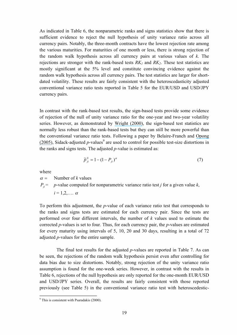
The final test results for the adjusted p-values are reported in Table 7. As can

be seen, the rejections of the random walk hypothesis persist even after controlling for data bias due to size distortions. Notably, strong rejection of the unity variance ratio assumption is found for the one-week series. However, in contrast with the results in Table 6, rejections of the null hypothesis are only reported for the one-month EUR/USD and USD/JPY series. Overall, the results are fairly consistent with those reported previously (see Table 5) in the conventional variance ratio test with heteroscedestic-

                                                            9 This is consistent with Psaradakis (2000).

 

20

robust test statistics. With the exception of the GBP/USD currency pair, no rejection of unity variance ratio is reported for series with maturity of three month and above. It is interesting to note that for the GBP/USD currency pair, the six-month, one-year and two-year volatility series still reject the ranks tests using RK1 and RK2 although only marginal rejection was reported for the two-year volatility in Table 5.

Table 7 : Sidack-adjusted SjiP

~-values for Ranks and Signs

1-Week 1-Month 3-Month 6-Month 1-Year 2-Year

Panel A: GBP/USD

RK1 0.011 ** 0.431 0.662 0.014 ** 0.015 ** 0.007 ***

RK2 0.004 *** 0.183 0.441 0.051 * 0.014 ** 0.001 ***

S1 0.041 ** 0.897 0.794 0.750 0.368 0.120

Panel B: EUR/USD

RK1 0.004 *** 0.029 ** 0.867 0.688 0.694 0.306

RK2 0.002 *** 0.022 ** 0.659 0.868 0.837 0.385

S1 0.040 ** 0.107 0.984 0.884 0.880 0.561

Panel C: AUD/USD

RK1 0.030 ** 0.124 0.796 0.531 0.909 0.380

RK2 0.007 *** 0.116 0.557 0.701 0.978 0.271

S1 0.590 0.146 0.998 0.552 0.981 0.910

Panel D: USD/JPY

RK1 0.000 *** 0.003 *** 0.305 0.880 0.717 0.579

RK2 0.000 *** 0.003 *** 0.256 0.826 0.750 0.581

S1 0.005 *** 0.022 ** 0.401 0.909 0.627 0.768

Notes: This table presents the final test results using the Sidack-corrected p-values. The adjusted p-values are calculated from individual p-value that corresponds to the variance ratio test with four values of k (5,10,20,30). ***significant at the 1% level **significant at the 5% level *significant at the 10% level

4.5 Mean Reversion

The variance ratio statistics is strictly unity when a stationary series is uncorrelated over time. Campbell, Lo and MacKinlay (1997) show that the ratio of the variance of a q-period variable and q times the variance of a one-period variable can be reduced to (1+ρ1), where ρ1 is the first-order autocorrelation coefficient of the variable. Under this rationale, the calculated variance ratio is simply one plus the zero autocorrelation (that is ρ1 = 0) for an uncorrelated return series, and hence this gives rise to the notion of variance ratio is unity. However, if positive first-order autocorrelation is present in the return series, then the sum of one plus the first-order autocorrelation will be larger than one. Conversely, the presence of negative first-order autocorrelations will reduce (1+ρ1) to below a value of one.

 

21

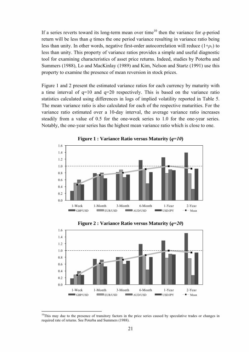
If a series reverts toward its long-term mean over time10 then the variance for q-period return will be less than q times the one period variance resulting in variance ratio being less than unity. In other words, negative first-order autocorrelation will reduce (1+ρ1) to less than unity. This property of variance ratios provides a simple and useful diagnostic tool for examining characteristics of asset price returns. Indeed, studies by Poterba and Summers (1988), Lo and MacKinlay (1989) and Kim, Nelson and Startz (1991) use this property to examine the presence of mean reversion in stock prices.

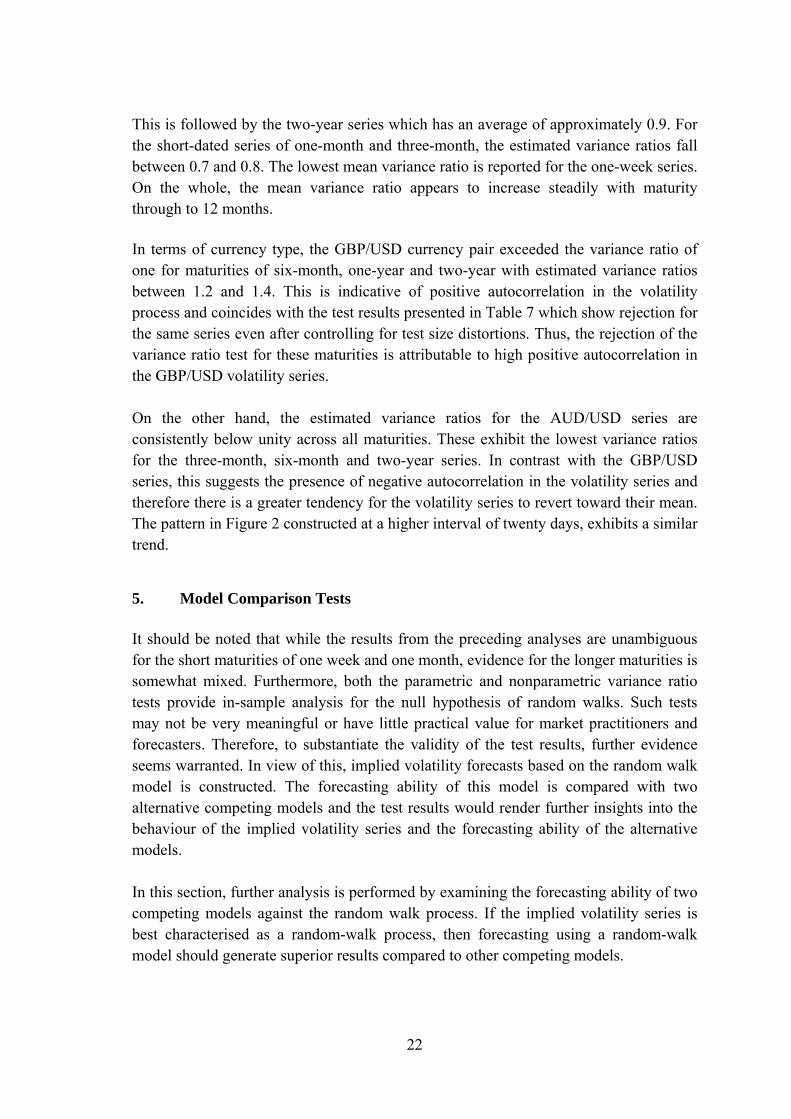
Figure 1 and 2 present the estimated variance ratios for each currency by maturity with a time interval of q=10 and q=20 respectively. This is based on the variance ratio statistics calculated using differences in logs of implied volatility reported in Table 5. The mean variance ratio is also calculated for each of the respective maturities. For the variance ratio estimated over a 10-day interval, the average variance ratio increases steadily from a value of 0.5 for the one-week series to 1.0 for the one-year series. Notably, the one-year series has the highest mean variance ratio which is close to one.

Figure 1 : Variance Ratio versus Maturity (q=10)

0.0

0.2

0.4

0.6

0.8

1.0

1.2

1.4

1.6

1-Week 1-Month 3-Month 6-Month 1-Year 2-YearGBP/USD EUR/USD AUD/USD USD/JPY Mean

Figure 2 : Variance Ratio versus Maturity (q=20)

0.0

0.2

0.4

0.6

0.8

1.0

1.2

1.4

1.6

1-Week 1-Month 3-Month 6-Month 1-Year 2-YearGBP/USD EUR/USD AUD/USD USD/JPY Mean

                                                            10This may due to the presence of transitory factors in the price series caused by speculative trades or changes in required rate of returns. See Poterba and Summers (1988).

 

22

This is followed by the two-year series which has an average of approximately 0.9. For the short-dated series of one-month and three-month, the estimated variance ratios fall between 0.7 and 0.8. The lowest mean variance ratio is reported for the one-week series. On the whole, the mean variance ratio appears to increase steadily with maturity through to 12 months.

In terms of currency type, the GBP/USD currency pair exceeded the variance ratio of one for maturities of six-month, one-year and two-year with estimated variance ratios between 1.2 and 1.4. This is indicative of positive autocorrelation in the volatility process and coincides with the test results presented in Table 7 which show rejection for the same series even after controlling for test size distortions. Thus, the rejection of the variance ratio test for these maturities is attributable to high positive autocorrelation in the GBP/USD volatility series.

On the other hand, the estimated variance ratios for the AUD/USD series are consistently below unity across all maturities. These exhibit the lowest variance ratios for the three-month, six-month and two-year series. In contrast with the GBP/USD series, this suggests the presence of negative autocorrelation in the volatility series and therefore there is a greater tendency for the volatility series to revert toward their mean. The pattern in Figure 2 constructed at a higher interval of twenty days, exhibits a similar trend.

5. Model Comparison Tests

It should be noted that while the results from the preceding analyses are unambiguous for the short maturities of one week and one month, evidence for the longer maturities is somewhat mixed. Furthermore, both the parametric and nonparametric variance ratio tests provide in-sample analysis for the null hypothesis of random walks. Such tests may not be very meaningful or have little practical value for market practitioners and forecasters. Therefore, to substantiate the validity of the test results, further evidence seems warranted. In view of this, implied volatility forecasts based on the random walk model is constructed. The forecasting ability of this model is compared with two alternative competing models and the test results would render further insights into the behaviour of the implied volatility series and the forecasting ability of the alternative models.

In this section, further analysis is performed by examining the forecasting ability of two competing models against the random walk process. If the implied volatility series is best characterised as a random-walk process, then forecasting using a random-walk model should generate superior results compared to other competing models.

 

23

Three different time series forecasting models are constructed including a driftless random walk model, an autoregressive integrated moving average (ARIMA) model and an artificial neural networks (ANNs) model. These models are used to generate one-day ahead out-of-sample forecasts of implied volatility changes for each of the six maturities examined in the previous section. The out-of-sample prediction is adopted as a means of avoiding data mining issues associated with in-sample inference.

The implied volatility data is divided into two subsamples. The first subsample consists of 900 observations of daily log implied volatility changes from 29 August 2001 to 29

April 2005 and is used for modelling. For out-of-sample forecasting evaluations, the second subsample is used. This consists of 250 daily observations from 30 August 2005 to 28 April 2006. The modelling and forecasting tests are performed using first-differences in the implied volatility series. This specification is motivated by the lack of stationarity in the volatility levels according to the unit root results reported in Table 2, particularly for the longer maturities. For the competing models, the well-established univariate autoregressive integrated moving average (ARIMA) model is used as the linear forecasting model, while the more flexible artificial neural networks (ANNs) model is chosen to capture possible nonlinear structure in the volatility series.

5.1 The Random Walk Model

Empirical evidence suggests that foreign exchange volatility is persistent with a root close to unity; for example, the studies by Engle and Bollerslev (1986) and Engle and Gonzalez-Rivera (1991). It appears reasonable to expect that the random walk is used as the first forecasting model. The persistent nature of implied volatility also suggests that an I(1) process provides a better characterisation of the volatility series for the purpose of forecasting. Thus, the first specification considered is a driftless random walk model:

tM

t μIV =Δ (8)

where,

MtIVΔ = The first-difference of the implied volatility series for a given

maturity M for period t, tμ     = a white noise process.   

5.2 The ARIMA(p,1,q) Model

This is a general univariate linear model to account for higher-order autoregressive processes combined with a moving-average processes to capture time series variation in

 

24

the data. It allows the series, tIV , to depend linearly on its own past values plus a

combination of current and previous values of a white noise error term:

jt

q

jj

p

it

Miti

Mt IVIV

11

(9)

where,

jt = a white noise process,

p = order of autoregressive component, q = order of moving-average component, The parameters p and q are non-negative integers and the autoregressive and moving

average-parameters are defined as 10,10 , 0≠ so that the series tIV is

stationary.

The Schwarz’s Bayesian information criterion (SBIC) is relied upon to determine the appropriate values for p and q (Brooks, 2002). The model is estimated for all six maturities that correspond to each of the four currency pairs. In most instances, the information criterion selects either an ARIMA(2,1,1) or an ARIMA(2,1,2) process for the short-dated series of one-week and one-month. For the three-month, six-month, one-year and two-year series, the SBIC criterion results in selection of an ARIMA(1,1,0) process.

5.3 Artificial Neural Networks Model

The artificial neural networks (ANNs) model is a nonparametric technique that is not new in the finance literature. For instance, Trippi and DeSieno (1992) and Altman, Marco and Varetto (1994) have previously examined the usefulness of this method in the trading of equity index futures and the prediction of corporate distress respectively. Ferland and Lalancette (2006) also adopt the ANNs model to estimate volatility in the EuroDollar futures market. Due to the flexibility of this approach, it can be used to approximate any nonlinear behaviour in the data series (Campbell, Lo and MacKinlay, 1997). The estimation procedure uses a feedforward neural network11 model with two hidden layers.

tl

s

i

Mitil

k

ll

Mt IVgIV

0

110 (10)

where M

tIV = system output or the estimated change in the IV series for maturity M estimated at period t,

                                                            11 Further exposition on ANNs is provided in Campbell, Lo, and MacKinlay (1997).

 

25

s = number of inputs or lagged first difference of the implied volatility series,

0α = intercept coefficient of the model,

l = network weighting estimated from l =1,…to k,

ilψ = the weights from the input i layer to the hidden unit,

lψ0 = bias weights of the hidden unit l,

tε = error term of the model.

The inputs are connected to multiple nodes; weighting is applied at each node and (.)g

determines the connections between the nodes and is used as the activation function to enhance the nonlinearity of the model.

5.4 The Forecast Performance Test

The out-of-sample forecasting accuracy of the models is carried out using three different evaluation measures. The first measure is the root-mean-squared error (RMSE) while the mean-error (ME) and mean-absolute-error (MAE) are also reported in the test

results. Out-of-sample forecasts of the series MtIV are calculated using each of the

models defined in the previous section and these one-day ahead forecasts are estimated using data from the second subsample (30 August 2005 to 28 April 2006). For a given maturity M at period t, the RMSE is defined as:

N

t

Mt

Mt IVIV

NRMSE

1

2)(1 (11)

where MtIV

represents the forecast values for options with maturity M at period t,

MtIV is the actual value for maturity M at period t and N is the forecast horizon which is

one day. The second forecast performance test provides a relative measure of forecasting error for the rival models. A ratio, RMSECM/RMSERW, is calculated for the various models relative to a random walk process where RMSECM denotes the root-mean-squared error for the competing models, while RMSERW is the root-mean-squared error for the benchmark random walk model. A ratio of 1.0 suggests that the competing model is as good as the random walk benchmark model. A ratio less than 1.0 indicates that the benchmark model is out-predicted by the competing model. No gain is achieved from using the competing models if the ratio is greater than 1.0. Inferences are based on the null hypothesis of zero difference in the forecast accuracy measured using RMSE, that is the competing models relative to the driftless random walk model.

 

26

In the third appraisal, the Diebold-Mariano statistics (Diebold and Mariano, 1995) are employed to examine the statistical significance of the forecast errors between the random walk and the competing model. The null hypothesis of zero difference in forecast error between the random walk and the competing model is assumed in this approach. Specifically, the loss differential is measured as the difference between the squared forecast error of the competing models and that of the benchmark random walk model. The test statistic is useful for comparing forecast accuracy as it allows the forecast errors to be “non-Gaussian, non-zero mean, serially correlated, and contemporaneously correlated” (pp.253, Diebold and Mariano, 1995). The Diebold-Mariano statistic is specified as:

)(ˆ dV

dDM (12)

where the loss function differential, td )(-)( |,|, httCMhttRW egeg with h-step ahead

forecast error, and

)(ˆ dV = the estimated standard error for the sample mean loss differential, d ,

eRW = the forecast error for the random walk model estimated as2

|,

httRWt IVIV

eCM = the forecast error for the competing model estimated as 2

|,

httCMt IVIV

5.5 Forecast Results

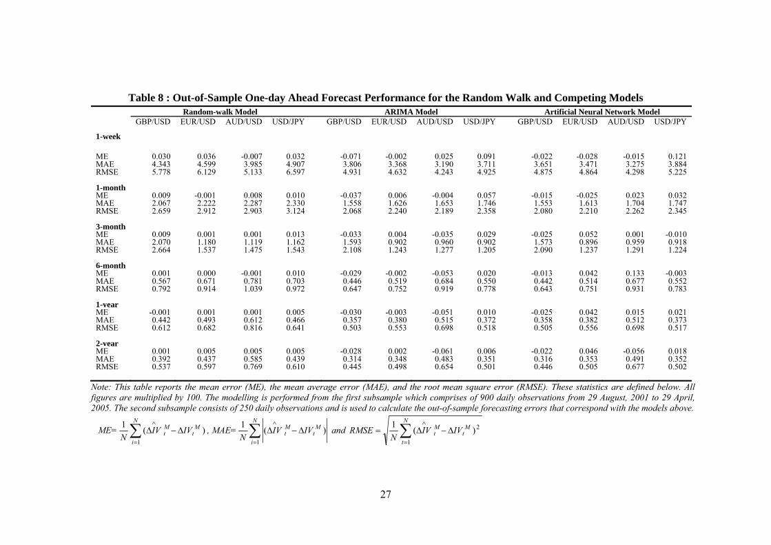
Table 8 provides the out-of-sample RMSE statistics associated with the driftless random walk, ARIMA and the ANNs model for one-day ahead forecasts. The RMSE statistics unambiguously favour the competing models over the random walk. Notably, in all cases the RMSE for the competing models is consistently lower than those reported for the benchmark model. For example, the one-week GBP/USD has a RMSE of 5.78 using the random walk model, while the ARIMA and ANNs have RMSEs of 4.93 and 4.88 respectively.

For the two-year series of the same currency, the RMSE reported for the random walk model is 0.54 while the ARIMA and ANNs models both have lower RMSE (0.45). This pattern is reported across all maturities and currency pairs. This suggests that the competing models have higher forecasting accuracy than the random walk model. Thus the random walk specification does not receive support against the two alternative models when using the RMSE criterion. This further validates the preceding random walk violations when using conventional and nonparametric variance ratio tests.

The predictive accuracy of the ARIMA and ANNs models is not distinctly different from each other although the ARIMA model has marginally lower RMSEs, particularly for the shorter maturities of one-week and one-month. For these maturities, the mean

 

27

Table 8 : Out-of-Sample One-day Ahead Forecast Performance for the Random Walk and Competing Models Random-walk Model ARIMA Model Artificial Neural Network Model

GBP/USD EUR/USD AUD/USD USD/JPY GBP/USD EUR/USD AUD/USD USD/JPY GBP/USD EUR/USD AUD/USD USD/JPY

1-week

ME 0.030 0.036 -0.007 0.032 -0.071 -0.002 0.025 0.091 -0.022 -0.028 -0.015 0.121 MAE 4.343 4.599 3.985 4.907 3.806 3.368 3.190 3.711 3.651 3.471 3.275 3.884 RMSE 5.778 6.129 5.133 6.597 4.931 4.632 4.243 4.925 4.875 4.864 4.298 5.225 1-month ME 0.009 -0.001 0.008 0.010 -0.037 0.006 -0.004 0.057 -0.015 -0.025 0.023 0.032 MAE 2.067 2.222 2.287 2.330 1.558 1.626 1.653 1.746 1.553 1.613 1.704 1.747 RMSE 2.659 2.912 2.903 3.124 2.068 2.240 2.189 2.358 2.080 2.210 2.262 2.345 3-month ME 0.009 0.001 0.001 0.013 -0.033 0.004 -0.035 0.029 -0.025 0.052 0.001 -0.010 MAE 2.070 1.180 1.119 1.162 1.593 0.902 0.960 0.902 1.573 0.896 0.959 0.918 RMSE 2.664 1.537 1.475 1.543 2.108 1.243 1.277 1.205 2.090 1.237 1.291 1.224 6-month ME 0.001 0.000 -0.001 0.010 -0.029 -0.002 -0.053 0.020 -0.013 0.042 0.133 -0.003 MAE 0.567 0.671 0.781 0.703 0.446 0.519 0.684 0.550 0.442 0.514 0.677 0.552 RMSE 0.792 0.914 1.039 0.972 0.647 0.752 0.919 0.778 0.643 0.751 0.931 0.783 1-year ME -0.001 0.001 0.001 0.005 -0.030 -0.003 -0.051 0.010 -0.025 0.042 0.015 0.021 MAE 0.442 0.493 0.612 0.466 0.357 0.380 0.515 0.372 0.358 0.382 0.512 0.373 RMSE 0.612 0.682 0.816 0.641 0.503 0.553 0.698 0.518 0.505 0.556 0.698 0.517 2-year ME 0.001 0.005 0.005 0.005 -0.028 0.002 -0.061 0.006 -0.022 0.046 -0.056 0.018 MAE 0.392 0.437 0.585 0.439 0.314 0.348 0.483 0.351 0.316 0.353 0.491 0.352 RMSE 0.537 0.597 0.769 0.610 0.445 0.498 0.654 0.501 0.446 0.505 0.677 0.502

Note: This table reports the mean error (ME), the mean average error (MAE), and the root mean square error (RMSE). These statistics are defined below. All figures are multiplied by 100. The modelling is performed from the first subsample which comprises of 900 daily observations from 29 August, 2001 to 29 April, 2005. The second subsample consists of 250 daily observations and is used to calculate the out-of-sample forecasting errors that correspond with the models above.

ME=

N

i

Mt

Mt IVIV

N1

)(1

, MAE=

N

i

Mt

Mt IVIV

N1

)(1

and

N

t

Mt

Mt IVIV

NRMSE

1

2)(1

 

28

RMSE difference (mean RMSE for ARIMA less mean RMSE for ANNs) is -0.14 and -0.005 respectively, while differences for the three-month to two-year series fall between -0.003 and -0.013. In comparison, the mean RMSE gap between the random walk and the competing models is much larger, for instance forecasting using the random walk model results in a mean RMSE of 5.91 for the one-week volatility series while the ANN model gives a corresponding value of 4.82. The differences in RMSEs decrease steadily as maturity increases.

A consistent result across all three models is that the lowest RMSE is reported for the one-week AUD/USD volatility series while the GBP/USD recorded the lowest RMSEs for the one-month, six-month, one-year and two-year series. This tends to suggest that although improvement in predictive accuracy can be achieved using the ARIMA and ANN models, these models performed equally well for the AUD/USD and GBP/USD series. However, the performance for the three-month volatility series appears mixed across all currency pairs. Specifically, in that while the lowest RMSE is reported for the AUD/USD currency pair under the random walk model, both the ARIMA and ANN models have the lowest RMSEs for the USD/JPY volatility series. By maturity, the forecasting performance for the two-year series has the lowest mean RMSEs while the one-month series has the highest RMSEs. Overall, a regular pattern of RMSEs across maturities can be noted – that is, the root-mean-squared errors decrease proportionately with maturity.

Results from the RMSE ratios in Table 9 paint a very similar picture. For each currency pair, the ratio for each maturity is estimated. In all instances, the RMSE ratios, which is measured as the ratio of RMSE from the competing model divided by the RMSE from the random walk model, is less than 1.0. This is suggestive of lower forecasting error when using the competing models. Such a pattern is observed consistently across maturities and currencies.

For short-dated maturities of one-week and one-month, the mean RMSE ratios for the ARIMA model are 0.796 and 0.764. These values are lower than the results for the one-year and the two-year series of 0.824 and 0.833 respectively. A similar observation can be made when the ratios are calculated using the ANNs model. Thus, forecasting using the ARIMA model can achieve an improvement of 17% to 24%12 compared with the random walk model. On the whole, as maturity increases, the mean RMSE ratios move closer to 1.0, indicating that the choice of forecasting model becomes less important for the long-dated volatility series. The same result is reported when using the ANNs model.

                                                            12 Using mean RMSE ratio for the one-month series, this is estimated as 1-0.7638 = 23.62%

 

29

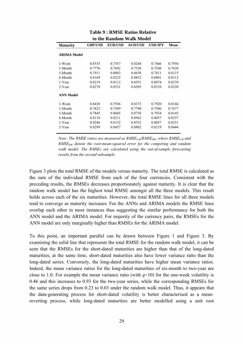
Table 9 : RMSE Ratios Relative to the Random Walk Model

Maturity GBP/USD EUR/USD AUD/USD USD/JPY Mean

ARIMA Model

1-Week 0.8535 0.7557 0.8268 0.7466 0.7956 1-Month 0.7776 0.7692 0.7538 0.7548 0.7638 3-Month 0.7911 0.8083 0.8658 0.7811 0.8115 6-Month 0.8169 0.8225 0.8852 0.8001 0.8312 1-Year 0.8219 0.8112 0.8551 0.8074 0.8239 2-Year 0.8278 0.8331 0.8505 0.8210 0.8328 ANN Model

1-Week 0.8438 0.7936 0.8373 0.7920 0.8166 1-Month 0.7823 0.7589 0.7790 0.7506 0.7677 3-Month 0.7845 0.8045 0.8758 0.7934 0.8145 6-Month 0.8118 0.8211 0.8962 0.8057 0.8337 1-Year 0.8246 0.8152 0.8552 0.8057 0.8251 2-Year 0.8299 0.8457 0.8802 0.8219 0.8444

Note: The RMSE ratios are measured as RMSECM/RMSERW, where RMSECM and RMSERW denote the root-mean-squared error for the competing and random walk model. The RMSEs are calculated using the out-of-sample forecasting results from the second subsample.

Figure 3 plots the total RMSE of the models versus maturity. The total RMSE is calculated as the sum of the individual RMSE from each of the four currencies. Consistent with the preceding results, the RMSEs decreases proportionately against maturity. It is clear that the random walk model has the highest total RMSE amongst all the three models. This result holds across each of the six maturities. However, the total RMSE lines for all three models tend to converge as maturity increases. For the ANNs and ARIMA models the RMSE lines overlap each other in most instances thus suggesting the similar performance for both the ANN model and the ARIMA model. For majority of the currency pairs, the RMSEs for the ANN model are only marginally higher than RMSEs for the ARIMA model.

To this point, an important parallel can be drawn between Figure 1 and Figure 3. By examining the solid line that represents the total RMSE for the random walk model, it can be seen that the RMSEs for the short-dated maturities are higher than that of the long-dated maturities; at the same time, short-dated maturities also have lower variance ratio than the long-dated series. Conversely, the long-dated maturities have higher mean variance ratios. Indeed, the mean variance ratios for the long-dated maturities of six-month to two-year are close to 1.0. For example the mean variance ratio (with q=10) for the one-week volatility is 0.46 and this increases to 0.93 for the two-year series, while the corresponding RMSEs for the same series drops from 0.23 to 0.03 under the random walk model. Thus, it appears that the data-generating process for short-dated volatility is better characterised as a mean-reverting process, while long-dated maturities are better modelled using a unit root

 

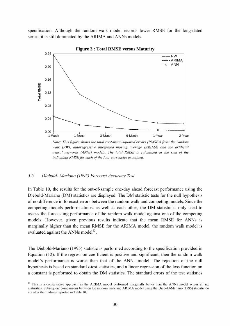
30

specification. Although the random walk model records lower RMSE for the long-dated series, it is still dominated by the ARIMA and ANNs models.

Figure 3 : Total RMSE versus Maturity

0.00

0.04

0.08

0.12

0.16

0.20

0.24

1-Week 1-Month 3-Month 6-Month 1-Year 2-Year

RWARIMAANN

To

tal R

MS

E

Note: This figure shows the total root-mean-squared errors (RMSEs) from the random walk (RW), autoregressive integrated moving average (ARIMA) and the artificial neural networks (ANNs) models. The total RMSE is calculated as the sum of the individual RMSE for each of the four currencies examined.

5.6 Diebold- Mariano (1995) Forecast Accuracy Test

In Table 10, the results for the out-of-sample one-day ahead forecast performance using the Diebold-Mariano (DM) statistics are displayed. The DM statistic tests for the null hypothesis of no difference in forecast errors between the random walk and competing models. Since the competing models perform almost as well as each other, the DM statistic is only used to assess the forecasting performance of the random walk model against one of the competing models. However, given previous results indicate that the mean RMSE for ANNs is marginally higher than the mean RMSE for the ARIMA model, the random walk model is evaluated against the ANNs model13.

The Diebold-Mariano (1995) statistic is performed according to the specification provided in Equation (12). If the regression coefficient is positive and significant, then the random walk model’s performance is worse than that of the ANNs model. The rejection of the null hypothesis is based on standard t-test statistics, and a linear regression of the loss function on a constant is performed to obtain the DM statistics. The standard errors of the test statistics

                                                            13 This is a conservative approach as the ARIMA model performed marginally better than the ANNs model across all six maturities. Subsequent comparisons between the random walk and ARIMA model using the Diebold-Mariano (1995) statistic do not alter the findings reported in Table 10.

 

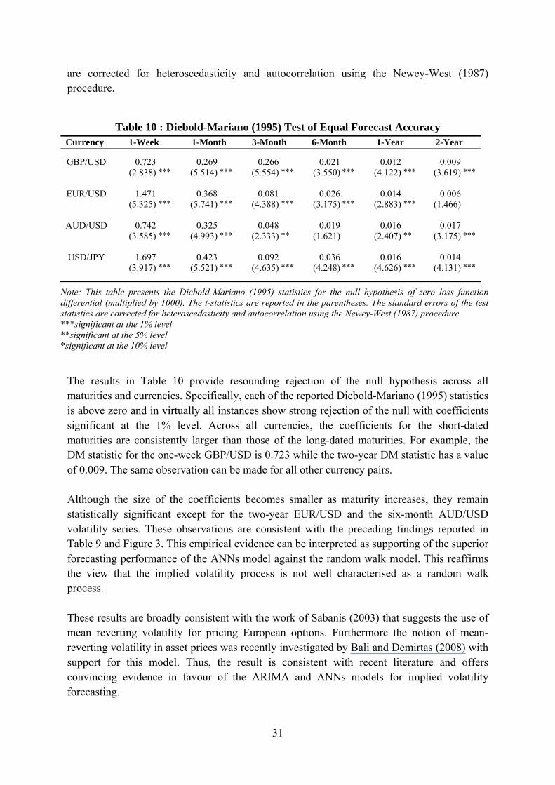
31

are corrected for heteroscedasticity and autocorrelation using the Newey-West (1987) procedure.

Table 10 : Diebold-Mariano (1995) Test of Equal Forecast Accuracy Currency 1-Week 1-Month 3-Month 6-Month 1-Year 2-Year

GBP/USD 0.723 0.269 0.266 0.021 0.012 0.009 (2.838) *** (5.514) *** (5.554) *** (3.550) *** (4.122) *** (3.619) ***

EUR/USD 1.471 0.368 0.081 0.026 0.014 0.006 (5.325) *** (5.741) *** (4.388) *** (3.175) *** (2.883) *** (1.466) AUD/USD 0.742 0.325 0.048 0.019 0.016 0.017 (3.585) *** (4.993) *** (2.333) ** (1.621) (2.407) ** (3.175) ***

USD/JPY 1.697 0.423 0.092 0.036 0.016 0.014 (3.917) *** (5.521) *** (4.635) *** (4.248) *** (4.626) *** (4.131) ***

Note: This table presents the Diebold-Mariano (1995) statistics for the null hypothesis of zero loss function differential (multiplied by 1000). The t-statistics are reported in the parentheses. The standard errors of the test statistics are corrected for heteroscedasticity and autocorrelation using the Newey-West (1987) procedure. ***significant at the 1% level **significant at the 5% level *significant at the 10% level

The results in Table 10 provide resounding rejection of the null hypothesis across all maturities and currencies. Specifically, each of the reported Diebold-Mariano (1995) statistics is above zero and in virtually all instances show strong rejection of the null with coefficients significant at the 1% level. Across all currencies, the coefficients for the short-dated maturities are consistently larger than those of the long-dated maturities. For example, the DM statistic for the one-week GBP/USD is 0.723 while the two-year DM statistic has a value of 0.009. The same observation can be made for all other currency pairs.

Although the size of the coefficients becomes smaller as maturity increases, they remain statistically significant except for the two-year EUR/USD and the six-month AUD/USD volatility series. These observations are consistent with the preceding findings reported in Table 9 and Figure 3. This empirical evidence can be interpreted as supporting of the superior forecasting performance of the ANNs model against the random walk model. This reaffirms the view that the implied volatility process is not well characterised as a random walk process.

These results are broadly consistent with the work of Sabanis (2003) that suggests the use of mean reverting volatility for pricing European options. Furthermore the notion of mean-reverting volatility in asset prices was recently investigated by Bali and Demirtas (2008) with support for this model. Thus, the result is consistent with recent literature and offers convincing evidence in favour of the ARIMA and ANNs models for implied volatility forecasting.

 

32

6. Conclusion

Previous studies have tested the random walk hypothesis for securities traded on stock exchanges. This paper examines the random walk hypothesis using traded implied volatility data collected from the over-the-counter currency option market using various in-sample and out-of-sample tests, in addition to standard unit root tests. The test statistics are applied to the implied volatility levels and the differences in logs for the volatility series for four major currencies. Both parametric and nonparametric variance ratio tests are applied in analysis of the data. The null hypothesis of a random walk process in the implied volatility series is consistently rejected across all currency pairs examined. Specifically, for the one-week and one-month series, violations of the random walk persist even after controlling for data bias and test size distortions. These results are confirmed in out-of-sample forecasting tests.

The main empirical finding from the variance ratio tests appear to suggest that there is potential for variation with respect to the appropriateness of the random walk process for modelling quoted volatility process across various maturities and currencies. Thus time series in foreign exchange implied volatility is not well characterised by a random walk process. This implies that option pricing and volatility models that assume a random walk in volatility across all maturities is not consistent with empirical findings reported in this paper. It further suggests that while it may be useful to model foreign exchange volatility as a random walk process, the volatility patterns that exist within the term structure need to be recognised. In particular, short-dated volatility series of one-week and one-month are better characterised as a mean reverting process. This proposition is supported by the out-of-sample test results.

The out-of-sample forecasting accuracy tests demonstrate the usefulness of alternative volatility modelling methods, namely the ARIMA and ANNs. In particular, autoregressive integrated moving average (ARIMA) process and artificial neural networks (ANNs) models produce superior volatility forecasts compared with the random walk model. This underscores the merit of such modelling techniques in capturing the nonlinear behaviour of volatility.

 

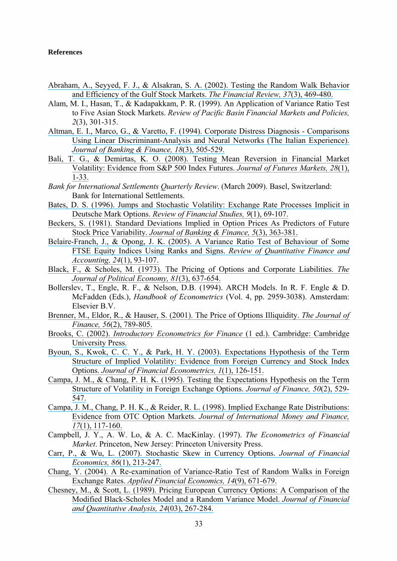
33

References

Abraham, A., Seyyed, F. J., & Alsakran, S. A. (2002). Testing the Random Walk Behavior and Efficiency of the Gulf Stock Markets. The Financial Review, 37(3), 469-480.

Alam, M. I., Hasan, T., & Kadapakkam, P. R. (1999). An Application of Variance Ratio Test to Five Asian Stock Markets. Review of Pacific Basin Financial Markets and Policies, 2(3), 301-315.

Altman, E. I., Marco, G., & Varetto, F. (1994). Corporate Distress Diagnosis - Comparisons Using Linear Discriminant-Analysis and Neural Networks (The Italian Experience). Journal of Banking & Finance, 18(3), 505-529.

Bali, T. G., & Demirtas, K. O. (2008). Testing Mean Reversion in Financial Market Volatility: Evidence from S&P 500 Index Futures. Journal of Futures Markets, 28(1), 1-33.

Bank for International Settlements Quarterly Review. (March 2009). Basel, Switzerland: Bank for International Settlements.

Bates, D. S. (1996). Jumps and Stochastic Volatility: Exchange Rate Processes Implicit in Deutsche Mark Options. Review of Financial Studies, 9(1), 69-107.

Beckers, S. (1981). Standard Deviations Implied in Option Prices As Predictors of Future Stock Price Variability. Journal of Banking & Finance, 5(3), 363-381.

Belaire-Franch, J., & Opong, J. K. (2005). A Variance Ratio Test of Behaviour of Some FTSE Equity Indices Using Ranks and Signs. Review of Quantitative Finance and Accounting, 24(1), 93-107.

Black, F., & Scholes, M. (1973). The Pricing of Options and Corporate Liabilities. The Journal of Political Economy, 81(3), 637-654.

Bollerslev, T., Engle, R. F., & Nelson, D.B. (1994). ARCH Models. In R. F. Engle & D. McFadden (Eds.), Handbook of Econometrics (Vol. 4, pp. 2959-3038). Amsterdam: Elsevier B.V.

Brenner, M., Eldor, R., & Hauser, S. (2001). The Price of Options Illiquidity. The Journal of Finance, 56(2), 789-805.

Brooks, C. (2002). Introductory Econometrics for Finance (1 ed.). Cambridge: Cambridge University Press.

Byoun, S., Kwok, C. C. Y., & Park, H. Y. (2003). Expectations Hypothesis of the Term Structure of Implied Volatility: Evidence from Foreign Currency and Stock Index Options. Journal of Financial Econometrics, 1(1), 126-151.

Campa, J. M., & Chang, P. H. K. (1995). Testing the Expectations Hypothesis on the Term Structure of Volatility in Foreign Exchange Options. Journal of Finance, 50(2), 529-547.

Campa, J. M., Chang, P. H. K., & Reider, R. L. (1998). Implied Exchange Rate Distributions: Evidence from OTC Option Markets. Journal of International Money and Finance, 17(1), 117-160.

Campbell, J. Y., A. W. Lo, & A. C. MacKinlay. (1997). The Econometrics of Financial Market. Princeton, New Jersey: Princeton University Press.

Carr, P., & Wu, L. (2007). Stochastic Skew in Currency Options. Journal of Financial Economics, 86(1), 213-247.

Chang, Y. (2004). A Re-examination of Variance-Ratio Test of Random Walks in Foreign Exchange Rates. Applied Financial Economics, 14(9), 671-679.

Chesney, M., & Scott, L. (1989). Pricing European Currency Options: A Comparison of the Modified Black-Scholes Model and a Random Variance Model. Journal of Financial and Quantitative Analysis, 24(03), 267-284.

 

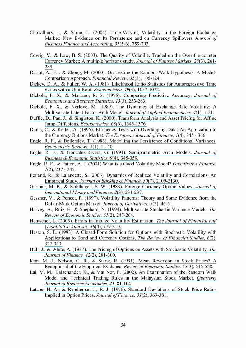
34

Chowdhury, I., & Sarno, L. (2004). Time-Varying Volatility in the Foreign Exchange Market: New Evidence on Its Persistence and on Currency Spillovers Journal of Business Finance and Accounting, 31(5-6), 759-793.

Covrig, V., & Low, B. S. (2003). The Quality of Volatility Traded on the Over-the-counter

Currency Market: A multiple horizons study. Journal of Futures Markets, 23(3), 261-285.

Darrat, A., F. , & Zhong, M. (2000). On Testing the Random-Walk Hypothesis: A Model-Comparison Approach. Financial Review, 35(3), 105-124.

Dickey, D. A., & Fuller, W. A. (1981). Likelihood Ratio Statistics for Autoregressive Time Series with a Unit Root. Econometrica, 49(4), 1057-1072.

Diebold, F. X., & Mariano, R. S. (1995). Comparing Predictive Accuracy. Journal of Economics and Business Statistics, 13(3), 253-263.

Diebold, F. X., & Nerlove, M. (1989). The Dynamics of Exchange Rate Volatility: A Multivariate Latent Factor Arch Model. Journal of Applied Econometrics, 4(1), 1-21.

Duffie, D., Pan, J., & Singleton, K. (2000). Transform Analysis and Asset Pricing for Affine Jump-Diffusions. Econometrica, 68(6), 1343-1376.

Dunis, C., & Keller, A. (1995). Efficiency Tests with Overlapping Data: An Application to the Currency Options Market. The European Journal of Finance, 1(4), 345 - 366.

Engle, R. F., & Bollerslev, T. (1986). Modelling the Persistence of Conditional Variances. Econometric Reviews, 5(1), 1 - 50.

Engle, R. F., & Gonzalez-Rivera, G. (1991). Semiparametric Arch Models. Journal of Business & Economic Statistics, 9(4), 345-359.

Engle, R. F., & Patton, A. J. (2001).What is a Good Volatility Model? Quantitative Finance, 1(2), 237 - 245.

Ferland, R., & Lalancette, S. (2006). Dynamics of Realized Volatility and Correlations: An Empirical Study. Journal of Banking & Finance, 30(7), 2109-2130.

Garman, M. B., & Kohlhagen, S. W. (1983). Foreign Currency Option Values. Journal of International Money and Finance, 2(3), 231-237.

Gessner, V., & Poncet, P. (1997). Volatility Patterns: Theory and Some Evidence from the Dollar-Mark Option Market. Journal of Derivatives, 5(2), 46-61.

Harvey, A., Ruiz, E., & Shephard, N. (1994). Multivariate Stochastic Variance Models. The Review of Economic Studies, 61(2), 247-264.

Hentschel, L. (2003). Errors in Implied Volatility Estimation. The Journal of Financial and Quantitative Analysis, 38(4), 779-810.

Heston, S. L. (1993). A Closed-Form Solution for Options with Stochastic Volatility with Applications to Bond and Currency Options. The Review of Financial Studies, 6(2), 327-343.

Hull, J., & White, A. (1987). The Pricing of Options on Assets with Stochastic Volatility. The Journal of Finance, 42(2), 281-300.

Kim, M. J., Nelson, C. R., & Startz, R. (1991). Mean Reversion in Stock Prices? A Reappraisal of the Empirical Evidence. Review of Economic Studies, 58(3), 515-528.

Lai, M. M., Balachander, K., & Mat Nor, F. (2002). An Examination of the Random Walk Model and Technical Trading Rules in the Malaysian Stock Market. Quarterly Journal of Business Economics, 41, 81-104.

Latane, H. A., & Rendleman Jr, R. J. (1976). Standard Deviations of Stock Price Ratios Implied in Option Prices. Journal of Finance, 31(2), 369-381.

 

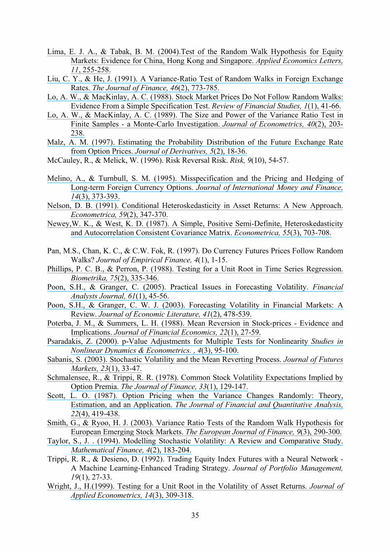
35

Lima, E. J. A., & Tabak, B. M. (2004).Test of the Random Walk Hypothesis for Equity Markets: Evidence for China, Hong Kong and Singapore. Applied Economics Letters, 11, 255-258.

Liu, C. Y., & He, J. (1991). A Variance-Ratio Test of Random Walks in Foreign Exchange Rates. The Journal of Finance, 46(2), 773-785.

Lo, A. W., & MacKinlay, A. C. (1988). Stock Market Prices Do Not Follow Random Walks: Evidence From a Simple Specification Test. Review of Financial Studies, 1(1), 41-66.

Lo, A. W., & MacKinlay, A. C. (1989). The Size and Power of the Variance Ratio Test in Finite Samples - a Monte-Carlo Investigation. Journal of Econometrics, 40(2), 203-238.

Malz, A. M. (1997). Estimating the Probability Distribution of the Future Exchange Rate from Option Prices. Journal of Derivatives, 5(2), 18-36.

McCauley, R., & Melick, W. (1996). Risk Reversal Risk. Risk, 9(10), 54-57. Melino, A., & Turnbull, S. M. (1995). Misspecification and the Pricing and Hedging of

Long-term Foreign Currency Options. Journal of International Money and Finance, 14(3), 373-393.

Nelson, D. B. (1991). Conditional Heteroskedasticity in Asset Returns: A New Approach. Econometrica, 59(2), 347-370.

Newey,W. K., & West, K. D. (1987). A Simple, Positive Semi-Definite, Heteroskedasticity and Autocorrelation Consistent Covariance Matrix. Econometrica, 55(3), 703-708.

Pan, M.S., Chan, K. C., & C.W. Fok, R. (1997). Do Currency Futures Prices Follow Random

Walks? Journal of Empirical Finance, 4(1), 1-15. Phillips, P. C. B., & Perron, P. (1988). Testing for a Unit Root in Time Series Regression.

Biometrika, 75(2), 335-346. Poon, S.H., & Granger, C. (2005). Practical Issues in Forecasting Volatility. Financial

Analysts Journal, 61(1), 45-56. Poon, S.H., & Granger, C. W. J. (2003). Forecasting Volatility in Financial Markets: A

Review. Journal of Economic Literature, 41(2), 478-539. Poterba, J. M., & Summers, L. H. (1988). Mean Reversion in Stock-prices - Evidence and

Implications. Journal of Financial Economics, 22(1), 27-59. Psaradakis, Z. (2000). p-Value Adjustments for Multiple Tests for Nonlinearity Studies in

Nonlinear Dynamics & Econometrics. , 4(3), 95-100. Sabanis, S. (2003). Stochastic Volatility and the Mean Reverting Process. Journal of Futures

Markets, 23(1), 33-47. Schmalensee, R., & Trippi, R. R. (1978). Common Stock Volatility Expectations Implied by

Option Premia. The Journal of Finance, 33(1), 129-147. Scott, L. O. (1987). Option Pricing when the Variance Changes Randomly: Theory,

Estimation, and an Application. The Journal of Financial and Quantitative Analysis, 22(4), 419-438.

Smith, G., & Ryoo, H. J. (2003). Variance Ratio Tests of the Random Walk Hypothesis for European Emerging Stock Markets. The European Journal of Finance, 9(3), 290-300.

Taylor, S., J. . (1994). Modelling Stochastic Volatility: A Review and Comparative Study. Mathematical Finance, 4(2), 183-204.

Trippi, R. R., & Desieno, D. (1992). Trading Equity Index Futures with a Neural Network - A Machine Learning-Enhanced Trading Strategy. Journal of Portfolio Management, 19(1), 27-33.

Wright, J., H.(1999). Testing for a Unit Root in the Volatility of Asset Returns. Journal of Applied Econometrics, 14(3), 309-318.

 

36

Wright, J. H. (2000). Alternative Variance-Ratio Tests Using Ranks and Signs. Journal of Business & Economic Statistics, 18(1), 1-9.

Xu, X., & Taylor, S. J. (1994). The Term Structure of Volatility Implied by Foreign Exchange Options. Journal of Financial and Quantitative Analysis, 29(1), 57-74.