Embed Size (px)
Citation preview
Reconciling the Return PredictabilityEvidence
Martin LettauColumbia University, New York University, CEPR, NBER
Stijn Van NieuwerburghNew York University and NBER
Evidence of stock-return predictability by financial ratios is still controversial, as docu-mented by inconsistent results for in-sample and out-of-sample regressions and by substan-tial parameter instability. This article shows that these seemingly incompatible results canbe reconciled if the assumption of a fixed steady state mean of the economy is relaxed. Wefind strong empirical evidence in support of shifts in the steady state and propose simplemethods to adjust financial ratios for such shifts. The in-sample forecasting relationship ofadjusted price ratios and future returns is statistically significant and stable over time. Inreal time, however, changes in the steady state make the in-sample return forecastabilityhard to exploit out-of-sample. The uncertainty of estimating the size of steady-state shiftsrather than the estimation of their dates is responsible for the difficulty of forecasting stockreturns in real time. Our conclusions hold for a variety of financial ratios and are robust tochanges in the econometric technique used to estimate shifts in the steady state. (JEL 12,14)
1. Introduction
The question of whether stock returns are predictable has received an enormousamount of attention. This is not surprising because the existence of returnpredictability is not only of interest to practitioners but also has importantimplications for financial models of risk and return. One branch of the literatureasserts that expected returns contain a time-varying component that impliespredictability of future returns. Due to its persistence, the predictive componentis stronger over longer horizons than over short horizons. Classic predictivevariables are financial ratios, such as the dividend-price ratio, the earnings-price ratio, and the book-to-market ratio (Rozeff, 1984; Fama and French,1988; Campbell and Shiller, 1988; Cochrane, 1991; Goetzmann and Jorion,1993; Hodrick, 1992; Lewellen, 2004, and others), but other variables have alsobeen found to be powerful predictors of long-horizon returns (e.g., Lettau and
We thank an anonymous referee, Matt Spiegel (the editor), Yakov Amihud, John Campbell, Kenneth French,Sydney Ludvigson, Eli Ofek, Matthew Richardson, Ivo Welch, Robert Whitelaw, and the seminar participantsat Duke, McGill, NYU, UNC, and Wharton for comments. Address correspondence to M. Lettau, Departmentof Economics, Columbia University, International Affairs Building, 420 W. 118th Street, New York 10027;telephone: (212) 998-0378; or e-mail: [email protected].
C© The Author 2007. Published by Oxford University Press on behalf of The Society for Financial Studies. Allrights reserved. For Permissions, please email: [email protected]:10.1093/rfs/hhm074 Advance Access publication December 10, 2007
The Review of Financial Studies / v 21 n 4 2008
Ludvigson, 2001; Lustig and Van Nieuwerburgh, 2005a; Menzly, Santos, andVeronesi, 2004; Piazzesi, Schneider, and Tuzel, 2006). Moreover, these studiesconclude that growth rates of fundamentals, such as dividends or earnings, aremuch less forecastable than returns, suggesting that most of the variation offinancial ratios is due to variations in expected returns.
These conclusions are controversial because the forecasting relationship offinancial ratios and future stock returns exhibits a number of disconcertingfeatures. First, correct inference is problematic because financial ratios areextremely persistent; in fact, standard tests leave the possibility of unit rootsopen. Nelson and Kim (1993); Stambaugh (1999); Ang and Bekaert (2006);Ferson, Sarkissian, and Simin (2003); and Valkanov (2003) conclude that thestatistical evidence of forecastability is weaker once tests are adjusted forhigh persistence. Second, financial ratios have poor out-of-sample forecastingpower, as shown in Bossaerts and Hillion (1999) and Goyal and Welch (2003,2004), but see Campbell and Thompson (2007) for a different interpretationof the out-of-sample evidence.1 Third, and related to the poor out-of-sampleevidence, the forecasting relationship of returns and financial ratios exhibitssignificant instability over time. For example, in rolling 30-year regressions ofannual log CRSP value-weighted returns on lagged log dividend-price ratios,the ordinary least squares (OLS) regression coefficient varies between zero and0.5 and the associated R2 ranges from close to zero to 30%, depending on thesubsample. Not surprisingly, the hypothesis of a constant regression coefficientis routinely rejected (Viceira, 1996; Paye and Timmermann, 2005).
In addition to concerns that return forecastability might be spurious, thebenchmark model of time-varying expected returns faces additional challenges.The extreme persistence of price ratios implies that expected returns have tobe extremely persistent as well. However, if shocks to expected returns havea half-life of many years or even decades, as implied by the high persistenceof financial ratios, they are unlikely to be linked to many plausible economicrisk factors, such as those linked to business cycles. Instead, researchers haveto identify slow-moving factors that are primary determinants of equity risk.In addition, the extraordinary valuation ratios in the late 1990s represent asignificant challenge for the benchmark model. Given the historical recordof returns, fundamentals, and prices, it is exceedingly unlikely that persistentstationary shocks to expected returns are capable of explaining price multipleslike those seen in 1999 or 2000.
In summary, the return predictability literature has yet to provide convincinganswers to the following four questions: What is the source of parameter insta-bility? Why is the out-of-sample evidence so much weaker than the in-sampleevidence? Why has even the in-sample evidence disappeared in the late 1990s?
1 There is some ambiguity about the use of the term “forecast” in this literature. Most papers use “forecast” torefer to in-sample regressions using the entire sample. In contrast, predictions using only currently available dataare referred to as “out-of-sample forecasts.” We follow this convention.
1608
Reconciling the Return Predictability Evidence
Why are price ratios extremely persistent? In this paper, we show that these puz-zling empirical patterns can be explained if the steady-state mean of financialratios has changed over the course of the sample period. Such changes couldbe due to changes in the steady-state growth rate of economic fundamentalsresulting from permanent technological innovations and/or changes in the ex-pected return of equity caused by, for example, improved risk sharing, changesin stock market participation, changes in the tax code, or lower macroeconomicvolatility.
Using standard econometric techniques, we show that the hypothesis of per-manent changes in the mean of various price ratios is supported by the data.We then ask how such changes affect the forecasting relationship of returnsand lagged price ratios. Standard econometric techniques that assume that theregressor is stationary will lead to biased estimates and incorrect inference.However, since deviations of price ratios from their steady-state values are sta-tionary, it is straightforward to correct for the nonstationarity if the timing andmagnitudes of shifts in steady states can be estimated. We conduct tests thatincorporate such adjustments from the perspective of an econometrician withaccess to the entire historical sample (in-sample tests), as well as from the per-spective of an investor who forecasts returns in real time (out-of-sample tests).
Our in-sample results conclude that “adjusted” price ratios have favorableproperties compared to unadjusted price ratios. In the full sample, the slopecoefficient in regressions of annual log returns on the lagged log dividend-price ratio increases from 0.094 for the unadjusted ratio to 0.235 and 0.455for the adjusted ratio with one and two steady-state shifts, respectively. Whilethe statistical significance of the coefficient on the unadjusted dividend-priceratio is marginal, coefficients on the adjusted dividend-price ratios are stronglysignificant. Finally, the regression coefficients using adjusted price ratios asregressors are more stable over time. We find similar differences for other priceratios, such as the earnings-price ratio and the book-to-market ratio.
In real time, however, the changes in the steady state are not only difficultto detect but also estimated with significant uncertainty, making the in-samplereturn forecastability hard to exploit. Results for out-of-sample forecastingtests reflect this difficulty. While adjusted price ratios have superior out-of-sample forecasting power relative to their unadjusted counterparts, they donot outperform the benchmark random walk model. Why does the real-timeprediction fail to beat the random walk model? In real time an investor facestwo challenges. First, she has to estimate the timing of a break. Second, ifshe detects a new break, she has to estimate the new mean after the breakoccurs. If the new break occurred toward the end of the sample that the investorhas access to, the new mean has to be estimated using a small number ofobservations and is subject to significant uncertainty. We perform additionaltests to evaluate the relative difficulty of estimating the break dates versusestimating the means relative to the pure out-of-sample forecasts and the ex postadjusted dividend-price ratio. We find that (i) the estimation of the break dates
1609
The Review of Financial Studies / v 21 n 4 2008
in real time is not crucial and the resulting prediction errors are smaller thanfor the random walk model, and (ii) that the estimation of the magnitude of thebreak in the mean dividend-price ratio entails substantial uncertainty, and isultimately responsible for the failure of the real-time out-of-sample predictionsto beat the random walk. These findings can explain the lack of out-of-samplepredictability documented by Goyal and Welch (2004).
Several papers have explored the impact of structural breaks on return pre-dictability. For example, Viceira (1996) and Paye and Timmermann (2005)reported evidence in favor of breaks in the OLS coefficient in the forecastingregression of returns on the lagged dividend-price ratio. Our focus is insteadon shifts in the mean of financial ratios, which, in turn, render the forecastingrelationship unstable if such shifts are not taken into account. In other words,in contrast to Viceira (1996) and Paye and Timmermann (2005), we focus onthe behavior of the mean of price ratios instead of the behavior of the slope co-efficient. Pastor and Stambaugh (2001) use a Bayesian framework to estimatebreaks in the equity premium. They find several shifts in the equity premiumsince 1834 and identify the sharpest drop in the 1990s, which is consistent withthe timing of the shift in price ratios identified in this paper. This paper is alsorelated to the recent literature on inference in forecasting regressions with per-sistent regressors (e.g., Amihud and Hurwich, 2004; Ang and Bekaert, 2006;Campbell and Yogo, 2002; Lewellen, 2004; Torous, Volkanov, and Yan, 2004;Eliasz, 2005). In these papers, asymptotic distributions for OLS regressions arederived under the assumption that the forecasting variable is a close-to unit, yetstationary, root process. In contrast, we allow for the presence of a small butstatistically important nonstationary component in forecasting variables.
The rest of the paper is organized as follows. In Section 2, we establish thatthe standard dividend-price ratio does not significantly forecast stock returnsor dividend growth. We find much stronger evidence for return predictabilityin various subsamples. The slope coefficient in the return equation is muchsmaller in the full sample than in any of the constituent subsamples, whichconfirms the instability of the forecasting relationship over time. In Sections3 and 4, we show how changes in the steady-state affect the dividend-priceratio and other price ratios. For the log dividend-price ratio, we find evidencefor either one break in the early 1990s or two breaks around 1954 and 1994.Other valuation ratios, such as the earnings-price ratio and the book-to-marketvalue ratio, exhibit similar breaks. We show that filtering out this nonstationarycomponent yields adjusted price ratios that have strong and stable in-samplereturn predictability. In Section 5, we study out-of-sample predictability. We usea recursive Perron procedure that estimates both the break dates and the meansof the regimes in real time. We show that using the break-adjusted dividend-price series produces superior one-step-ahead return forecasts compared tousing the unadjusted dividend-price series, but does slightly worse than thenaive random walk model. Using a Hamilton (1989) regime-switching model,we show that if the investor did not have to estimate regime means in real
1610
Reconciling the Return Predictability Evidence
time, but only the regime-switching dates, her out-of-sample forecast wouldimprove substantially, and beat the random walk. The Hamilton procedure leadsto slightly later break dates but predictability results that are virtually as goodas those when the (ex post) break dates were known and used. In sum, thehardest part of real-time out-of-sample prediction in the presence of regimes isthe estimation uncertainty about the mean of the new regime. In Section 6, weconsider a vector error correction model that includes the return and dividendgrowth predictability equations and imposes a joint present value restrictionon the slope parameters from both equations. We find that this restrictionis satisfied when we use the adjusted dividend-price ratio as an independentvariable, but not when we use the unadjusted series. We use this framework toestimate long-horizon regressions. Finally, in Section 7, we find that our simplemodel serves as a plausible data generating process. It is able to replicate boththe findings of no predictability when the unadjusted dividend-price ratio isused and the findings of in-sample and out-of-sample predictability when theadjusted series is used.
2. Instability of Forecasting Relationships
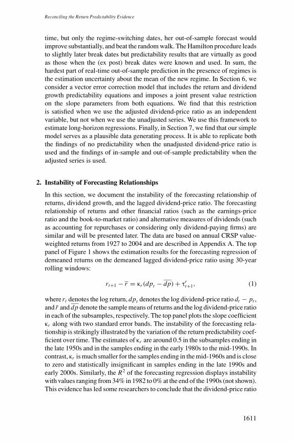
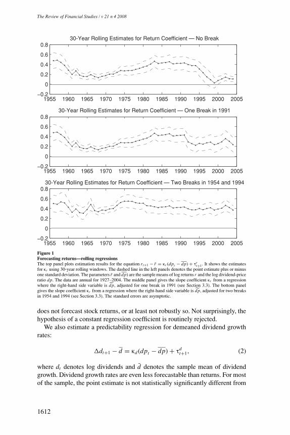
In this section, we document the instability of the forecasting relationship ofreturns, dividend growth, and the lagged dividend-price ratio. The forecastingrelationship of returns and other financial ratios (such as the earnings-priceratio and the book-to-market ratio) and alternative measures of dividends (suchas accounting for repurchases or considering only dividend-paying firms) aresimilar and will be presented later. The data are based on annual CRSP value-weighted returns from 1927 to 2004 and are described in Appendix A. The toppanel of Figure 1 shows the estimation results for the forecasting regression ofdemeaned returns on the demeaned lagged dividend-price ratio using 30-yearrolling windows:
rt+1 − r = κr (dpt − dp) + τrt+1, (1)
where rt denotes the log return, dpt denotes the log dividend-price ratio dt − pt ,and r and dp denote the sample means of returns and the log dividend-price ratioin each of the subsamples, respectively. The top panel plots the slope coefficientκr along with two standard error bands. The instability of the forecasting rela-tionship is strikingly illustrated by the variation of the return predictability coef-ficient over time. The estimates of κr are around 0.5 in the subsamples ending inthe late 1950s and in the samples ending in the early 1980s to the mid-1990s. Incontrast, κr is much smaller for the samples ending in the mid-1960s and is closeto zero and statistically insignificant in samples ending in the late 1990s andearly 2000s. Similarly, the R2 of the forecasting regression displays instabilitywith values ranging from 34% in 1982 to 0% at the end of the 1990s (not shown).This evidence has led some researchers to conclude that the dividend-price ratio
1611
The Review of Financial Studies / v 21 n 4 2008
1955 1960 1965 1970 1975 1980 1985 1990 1995 2000 2005−0.2
0
0.2
0.4
0.6
0.830-Year Rolling Estimates for Return Coefficient — No Break
1955 1960 1965 1970 1975 1980 1985 1990 1995 2000 2005−0.2
0
0.2
0.4
0.6
0.830-Year Rolling Estimates for Return Coefficient — One Break in 1991
1955 1960 1965 1970 1975 1980 1985 1990 1995 2000 2005−0.2
0
0.2
0.4
0.6
0.830-Year Rolling Estimates for Return Coefficient — Two Breaks in 1954 and 1994
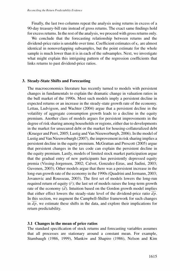
Figure 1Forecasting returns—rolling regressionsThe top panel plots estimation results for the equation rt+1 − r = κr (dpt − dp) + τr
t+1. It shows the estimatesfor κr using 30-year rolling windows. The dashed line in the left panels denotes the point estimate plus or minusone standard deviation. The parameters r and dp) are the sample means of log returns r and the log dividend-priceratio dp. The data are annual for 1927–2004. The middle panel gives the slope coefficient κr from a regressionwhere the right-hand side variable is dp, adjusted for one break in 1991 (see Section 3.3). The bottom panelgives the slope coefficient κr from a regression where the right-hand side variable is dp, adjusted for two breaksin 1954 and 1994 (see Section 3.3). The standard errors are asymptotic.
does not forecast stock returns, or at least not robustly so. Not surprisingly, thehypothesis of a constant regression coefficient is routinely rejected.
We also estimate a predictability regression for demeaned dividend growthrates:
�dt+1 − d = κd (dpt − dp) + τdt+1, (2)
where dt denotes log dividends and d denotes the sample mean of dividendgrowth. Dividend growth rates are even less forecastable than returns. For mostof the sample, the point estimate is not statistically significantly different from
1612
Reconciling the Return Predictability Evidence
zero, and the regression R2 never exceeds 16% (not shown). Interestingly, thedividend-price ratio at the end of the 1990s seems to forecast neither stockreturns nor dividend growth. This is a conundrum from the perspective of anypresent value model (see Section 3.1), as also pointed out by Cochrane (2007)and Bainsbergen and Koijen (2007).
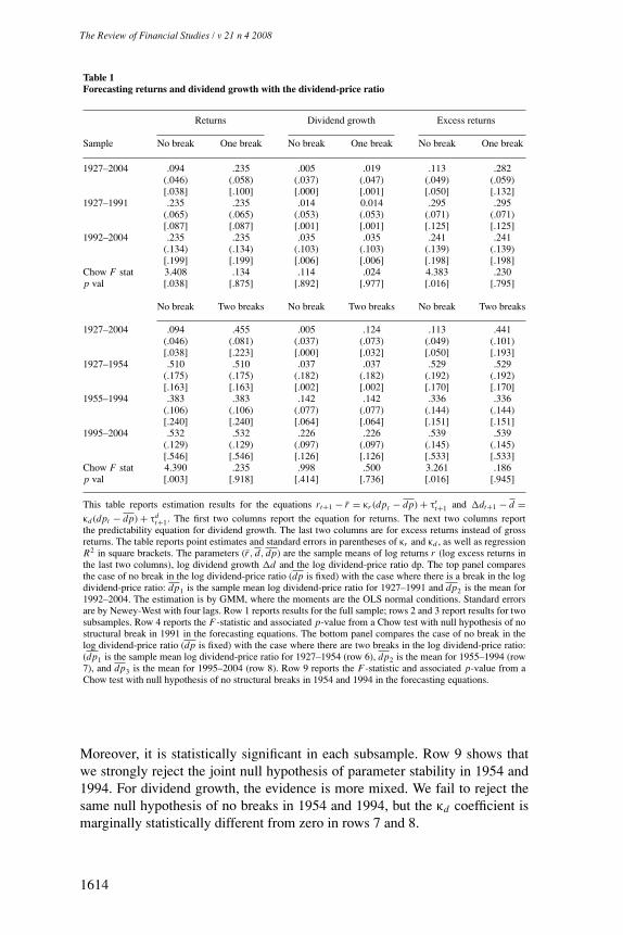
The left two columns of Table 1, denoted “No Break,” report the coefficientsκr and κd from equations (1) and (2) and their asymptotic standard errorsfor the entire 1927–2004 sample, as well as for various subsamples. The firstrow shows that the dividend-price ratio marginally predicts stock returns (firstcolumn); the coefficient is significant at the 5% level if asymptotic standarderrors are used for inference. However, small-sample standard errors computedfrom a Bootstrap simulation suggest that the coefficient κr is not statisticallydifferent from zero for the entire sample.2 The dividend-price ratio does notforecast dividend growth at conventional significance levels (third column).Thus, we cannot reject the hypothesis that the dividend-price ratio forecastsneither dividend growth nor returns.
Rows 2 and 3 report the results for two nonoverlapping samples that span theentire period: 1927–1991 and 1992–2004. We will justify this particular choiceof subsamples in Section 3. The estimates of κr display a remarkable patternacross subsamples: in both subsamples, κr is much larger than its estimate in thewhole sample. In fact, the estimates are almost identical in the two subsamples:.2353 in the 1927–1991 subsample compared to .2351 in the later 1992–2004subsample. Yet, when we join the two subsamples, the point estimate drops to.094. In addition, κr is strongly statistically significant in both subsamples butonly marginally significant in the whole sample. Confirming the instability ofκr estimates, row 4 reports the results of a Chow test, which rejects the nullhypothesis of no structural break in 1991 at the 4% level. Finally, the dividendgrowth forecasting relationship displays less instability, and the coefficientremains insignificant in both subsamples.
The pattern of κr is not unique to the specific subsamples chosen. We obtainvery similar results when we use three nonoverlapping subsamples: 1927–1954,1955–1994, and 1995–2004 (bottom half of Table 1). Again, we find that thereturn predictability coefficient κr is estimated to be much higher in each ofthe three subsamples than in the entire subsample. In row 5, the predictabilitycoefficient is .09, whereas it is .51, .38, and .53 in rows 6–8, respectively.
2 Asymptotic standard errors may be a poor indicator of the estimation uncertainty in small samples, and the pvalues for the null of no predictability may be inaccurate. The asymptotic corrections advocated by Hansen andHodrick (1980) have poor small-sample properties. Ang and Bekaert (2006) find that use of those standard errorsleads to overrejection of the no-predictability null. The Bootstrap exercise imposes the null of no predictabilityand asks how likely it is to observe the estimated κr coefficients reported in the first column of Table 1. Wefind that the small-sample p value for κr is 6.8% compared to an asymptotic p value of 4.1%. We also conducta second Bootstrap exercise to find the small-sample bias in the return coefficient. Consistent with Stambaugh(1999), we find an upward bias. If the true value is .094, the Bootstrap exercise estimates a coefficient of.115. Detailed results are available upon request. The empirical size of tests-based asymptotic and bootstrappedstandard errors tends to be larger than their nominal size if the regressor is highly persistent (e.g., Amihud,Hurvich, and Wang, 2005). Alternative tests with better size properties weaken the evidence for forecastabilitywith the dividend-price ratio further.
1613
The Review of Financial Studies / v 21 n 4 2008
Table 1Forecasting returns and dividend growth with the dividend-price ratio
Returns Dividend growth Excess returns
Sample No break One break No break One break No break One break
1927–2004 .094 .235 .005 .019 .113 .282(.046) (.058) (.037) (.047) (.049) (.059)[.038] [.100] [.000] [.001] [.050] [.132]
1927–1991 .235 .235 .014 0.014 .295 .295(.065) (.065) (.053) (.053) (.071) (.071)[.087] [.087] [.001] [.001] [.125] [.125]
1992–2004 .235 .235 .035 .035 .241 .241(.134) (.134) (.103) (.103) (.139) (.139)[.199] [.199] [.006] [.006] [.198] [.198]
Chow F stat 3.408 .134 .114 .024 4.383 .230p val [.038] [.875] [.892] [.977] [.016] [.795]
No break Two breaks No break Two breaks No break Two breaks
1927–2004 .094 .455 .005 .124 .113 .441(.046) (.081) (.037) (.073) (.049) (.101)[.038] [.223] [.000] [.032] [.050] [.193]
1927–1954 .510 .510 .037 .037 .529 .529(.175) (.175) (.182) (.182) (.192) (.192)[.163] [.163] [.002] [.002] [.170] [.170]
1955–1994 .383 .383 .142 .142 .336 .336(.106) (.106) (.077) (.077) (.144) (.144)[.240] [.240] [.064] [.064] [.151] [.151]
1995–2004 .532 .532 .226 .226 .539 .539(.129) (.129) (.097) (.097) (.145) (.145)[.546] [.546] [.126] [.126] [.533] [.533]
Chow F stat 4.390 .235 .998 .500 3.261 .186p val [.003] [.918] [.414] [.736] [.016] [.945]
This table reports estimation results for the equations rt+1 − r = κr (dpt − dp) + τrt+1 and �dt+1 − d =
κd (dpt − dp) + τdt+1. The first two columns report the equation for returns. The next two columns report
the predictability equation for dividend growth. The last two columns are for excess returns instead of grossreturns. The table reports point estimates and standard errors in parentheses of κr and κd , as well as regressionR2 in square brackets. The parameters (r , d, dp) are the sample means of log returns r (log excess returns inthe last two columns), log dividend growth �d and the log dividend-price ratio dp. The top panel comparesthe case of no break in the log dividend-price ratio (dp is fixed) with the case where there is a break in the logdividend-price ratio: dp1 is the sample mean log dividend-price ratio for 1927–1991 and dp2 is the mean for1992–2004. The estimation is by GMM, where the moments are the OLS normal conditions. Standard errorsare by Newey-West with four lags. Row 1 reports results for the full sample; rows 2 and 3 report results for twosubsamples. Row 4 reports the F-statistic and associated p-value from a Chow test with null hypothesis of nostructural break in 1991 in the forecasting equations. The bottom panel compares the case of no break in thelog dividend-price ratio (dp is fixed) with the case where there are two breaks in the log dividend-price ratio:(dp1 is the sample mean log dividend-price ratio for 1927–1954 (row 6), dp2 is the mean for 1955–1994 (row7), and dp3 is the mean for 1995–2004 (row 8). Row 9 reports the F-statistic and associated p-value from aChow test with null hypothesis of no structural breaks in 1954 and 1994 in the forecasting equations.
Moreover, it is statistically significant in each subsample. Row 9 shows thatwe strongly reject the joint null hypothesis of parameter stability in 1954 and1994. For dividend growth, the evidence is more mixed. We fail to reject thesame null hypothesis of no breaks in 1954 and 1994, but the κd coefficient ismarginally statistically different from zero in rows 7 and 8.
1614
Reconciling the Return Predictability Evidence
Finally, the last two columns repeat the analysis using returns in excess of a90-day treasury-bill rate instead of gross returns. The exact same findings holdfor excess returns. In the rest of the analysis, we proceed with gross returns only.
We conclude that the forecasting relationship between returns and thedividend-price ratio is unstable over time. Coefficient estimates of κr are almostidentical in nonoverlapping subsamples, but the point estimate for the wholesample is much lower than it is in each of the subsamples. Next, we investigatewhat might explain this intriguing pattern of the regression coefficients thatlinks returns to past dividend-price ratios.
3. Steady-State Shifts and Forecasting
The macroeconomics literature has recently turned to models with persistentchanges in fundamentals to explain the dramatic change in valuation ratios inthe bull market of the 1990s. Most such models imply a persistent decline inexpected returns or an increase in the steady-state growth rate of the economy.Lettau, Ludvigson, and Wachter (2004) argue that a persistent decline in thevolatility of aggregate consumption growth leads to a decline in the equitypremium. Another class of models argues for persistent improvements in thedegree of risk sharing among households or regions, either due to developmentsin the market for unsecured debt or the market for housing-collateralized debt(Krueger and Perri, 2005; Lustig and Van Nieuwerburgh, 2006). In the model ofLustig and Van Nieuwerburgh (2007), the improvement in risk sharing implies apersistent decline in the equity premium. McGrattan and Prescott (2005) arguethat persistent changes in the tax code can explain the persistent decline inthe equity premium. Lastly, models of limited stock market participation arguethat the gradual entry of new participants has persistently depressed equitypremia (Vissing-Jorgensen, 2002; Calvet, Gonzalez-Eiras, and Sadini, 2003;Guvenen, 2003). Other models argue that there was a persistent increase in thelong-run growth rate of the economy in the 1990s (Quadrini and Jermann, 2003;Jovanovic and Rousseau, 2003). The first set of models lowers the long-runrequired return of equity (r ); the last set of models raises the long-term growthrate of the economy (d). Intuition based on the Gordon growth model impliesthat either effect lowers the steady-state level of the dividend-price ratio dp.In this section, we augment the Campbell-Shiller framework for such changesin dp, we estimate these shifts in the data, and explore their implications forreturn predictability.
3.1 Changes in the mean of price ratiosThe standard specification of stock returns and forecasting variables assumesthat all processes are stationary around a constant mean. For example,Stambaugh (1986, 1999), Mankiw and Shapiro (1986), Nelson and Kim
1615
The Review of Financial Studies / v 21 n 4 2008
(1993), and Lewellen (1999) considered the following model:
rt+1 = r + κr yt + τrt+1 (3)
yt = y + vt (4)
The mean of the forecasting variable yt , y, is constant and the stochasticcomponent vt is assumed to be stationary, often specified as an AR(1) process.Means of financial ratios are determined by properties of the steady state of theeconomy. For example, the mean of the log dividend-price ratio dp is a functionof the growth rate d of log dividends and expected log return r in steady state
dp = log(exp(r ) − exp(d)) − d, (5)
whereas the stochastic component depends on expected future deviations ofreturns and dividend growth from their steady-state values (Campbell andShiller, 1988):
dpt = dp + Et
∞∑j=1
ρ j−1[(rt+ j − r ) − (�dt+ j − d)], (6)
where ρ = (1 + exp(dp))−1 is a constant. Similar equations can be derived forother financial ratios (e.g., Vuolteenaho, 2000). Berk, Green, and Naik (1999)show how stock returns and book-to-market ratios are related in a generalequilibrium model.
A crucial assumption is that the steady state of the economy is constant overtime: The average long-run growth rate of the economy as well as the averagelong-run return of equity are fixed and not allowed to change. However, ifeither the steady-state growth rate or expected return were to change, theeffects on financial ratios and their stochastic relationships with returns wouldbe profound. Even relatively small changes in long-run growth and/or expectedreturn have large effects on the mean of the dividend-price ratio, as can be seenfrom Equation (5). The effects of steady-state shifts on other valuation ratios,such as the earnings-price ratio and the book-to-market ratio, are similar. Inthis paper, we entertain the possibility that the steady state of the US economyhas indeed changed since 1926, and we study the effect of these changes on theforecasting relationship of returns and price ratios.
A steady state is characterized by long-run growth and expected return.Any short-term deviation from steady state is expected to be only temporaryand the economy is expected to return to its steady state eventually. Thus,steady-state growth and expected return must be constant in expectations, butthe steady state might shift unexpectedly. Correspondingly, we assume thatEtr t+ j = r t , Et dt+ j = dt , Et dpt+ j = dpt .
3
3 Although the log dividend-price ratio is a nonlinear function of steady-state returns and growth, we assume thatthe steady-state log dividend-price ratio is also (approximately) a martingale: Et dpt+ j = dpt . This assumption
1616
Reconciling the Return Predictability Evidence
The log linear framework introduced earlier illustrates the effect of time-varying steady states, though none of our results depend on the accuracy of theapproximation. Just as in the case with constant steady state, the log dividend-price ratio is the sum of the steady-state dividend-price ratio and the discountedsum of expected returns minus expected dividend growth in excess of steady-state growth and returns4
dpt = dpt + Et
∞∑j=1
ρj−1t [(rt+ j − r t ) − (�dt+ j − dt )], (7)
where ρt = (1 + exp(dpt ))−1. The important difference of Equation (7) com-
pared to Equation (6) is that the mean of the log dividend-price ratio is nolonger constant. In fact, it not only varies over time but it is nonstationary. If,for example, the steady-state growth rate increases permanently, the steady-state dividend-price ratio decreases and the current log dividend-price ratiodeclines permanently. While the log dividend-price ratio contains a nonstation-ary component, it is important to note that deviations of dpt from steady statesare stationary as long as deviations of dividend growth and returns from theirrespective steady states are stationary, an assumption we maintain through-out the paper.5 In other words, the dividend-price ratio dpt itself contains anonstationary component dpt but the appropriately demeaned dividend-priceratio dpt − dpt is stationary. The implications for forecasting regressions withthe dividend-price ratio are immediate. First, in the presence of steady-stateshifts, a nonstationary dividend-price ratio is not a well-defined predictor andthis nonstationarity could cause the empirical patterns described in the previ-ous section. Second, the dividend-price ratio must be adjusted to remove thenonstationary component dpt to render a stationary process.
While we emphasized the effect of steady-state shifts on the dividend-priceratio, the intuition carries through to other financial ratios. Changes in the steadystate have similar effects on the earnings-price ratio and the book-to-marketratio. However, other permanent changes in the economy, such as changes in
is justified for the specific processes for steady-state returns and growth that we will consider next. Appendix Cspells out a simple asset pricing model where the price-dividend ratio in levels follows a (bounded) martingale.It shows that dp and d are approximate (bounded) martingales.
4 Appendix B presents a detailed derivation. Under our assumption, the log approximation in a model with time-varying steady states is as accurate as the approximation for the corresponding model with constant steady state.In fact, the ex ante expressions of the approximate log dividend-price ratio (6) and (7) are exactly the same. Onlytheir ex post values are different in periods when the steady state shifts.
5 Of course, in a finite sample, it is impossible to conclusively distinguish a truly permanent change from anextremely persistent one. Thus, our insistence of nonstationarity might seem misguided. However, the importantinsight is that the dividend-price ratio is not only a function of (less) persistent changes in expected growthrates and expected returns that could potentially have cyclical sources but is also affected by either extremelypersistent or permanent structural changes in the economy. This distinction turns out to be very useful, as wewill show in the remainder of the article. In this sense, our assumption of true nonstationarity can be regardedto include “extremely persistent but stationary.” In a finite sample, the conclusions will be the same in eithersetting. The distinction of “permanent” versus “extremely persistent” is important, however, for structural assetpricing models because permanent shocks might have a much larger impact on prices than very persistent ones.
1617
The Review of Financial Studies / v 21 n 4 2008
payout policies, could affect different ratios differently. In the following section,we provide evidence that steady-state shifts have occurred in our sample andpropose simple methods to adjust financial ratios for such shifts.
3.2 Steady-state shifts in the dividend-price ratioHas the steady-state relationship of growth rates and expected returns shiftedsince the beginning of our sample in 1926? If so, have these shifts affectedthe stochastic relationship between returns and price ratios? In this section, weuse econometric techniques that exploit the entire sample to detect changesin the steady state. In Section 5, we study how investors in real time mighthave assessed the possibility of shifts in the steady states without the benefit ofknowing the whole sample. In both cases, there is strong empirical evidencein favor of changes in the steady state and we find that such changes havedramatic effects on the forecasting relationship of returns and price ratios.We suggest a simple adjustment to the dividend-price ratio and revisit theforecasting equations from Section 2. We first study shifts in the dividend-priceratios in detail and consider alternative ratios in Section 4.
Our econometric specification is directly motivated by the framework thatallows for changes in the steady state laid out in the previous section. Equa-tion (7) implies that the log dividend-price ratio is the sum of a nonstationarycomponent and a stationary component. In this section, we model the nonsta-tionary component as a constant that is subject to rare structural breaks as inBai and Perron (1998).6
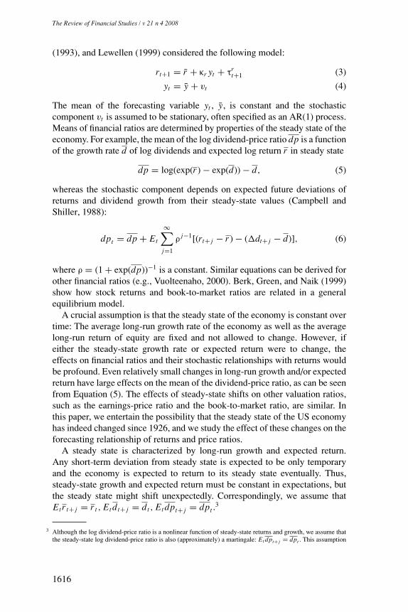
The full line in each of the panels of Figure 2 shows the log dividend-price ra-tio from 1927 to 2004. Visually, the series displays evidence of nonstationarity.In particular, the bull market of the 1990s is hard to reconcile with a stationarymodel. The dividend-price ratio has risen since, but at the end of our sample in2004, prices would have to fall an additional 46% for the dividend-price ratioto return to its historical mean. One possible explanation is that the bull marketof the 1990s represents a sequence of extreme realizations from a stationarydistribution.
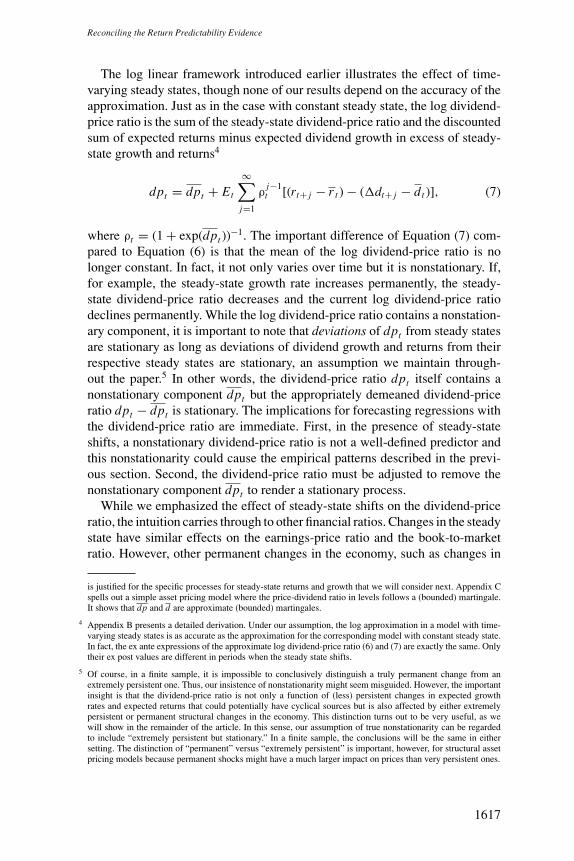
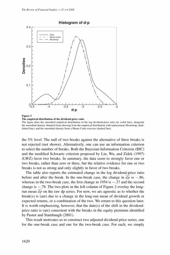
The solid line in Figure 3 shows the smoothed empirical distribution of thelog dividend-price ratio dpt . This distribution has a fat left tail, mainly due tothe observations in the last 15 years. To investigate whether this is a typical plotfrom a stationary distribution, we conduct two exercises. Following Campbell,Lo, and MacKinlay (1997); Stambaugh (1999); Campbell and Yogo (2002);Ang and Bekaert (2006); and many others we estimate an AR(1) process forthe log dividend-price ratio. First, in a Bootstrap exercise, we draw from theempirical distribution with replacement. The smoothed Bootstrap distributionis the dash-dotted line in the figure. Second, we compute the density of dptusing Monte Carlo simulations from an estimated AR(1) model with normal
6 As an alternative, we have also studied in-sample predictability in a Hamilton regime-switching model. Becausethe estimated regimes are so persistent, the predictability coefficients are very close to the ones we report here.In Section 5, we revisit the Hamilton model in the context of out-of-sample predictability.
1618
Reconciling the Return Predictability Evidence
1940 1960 1980 2000−4.5
−4
−3.5
−3
−2.5One Break in 1991
1940 1960 1980 2000−4.5
−4
−3.5
−3
−2.5One Break in 1991
undajusted d−padjusted d−p 1 break
1940 1960 1980 2000−4.5
−4
−3.5
−3
−2.5Two Breaks in 1954 and 1994
1940 1960 1980 2000−4.5
−4
−3.5
−3
−2.5Two Breaks in 1954 and 1994
undajusted d−padjusted d−p 2 breaks
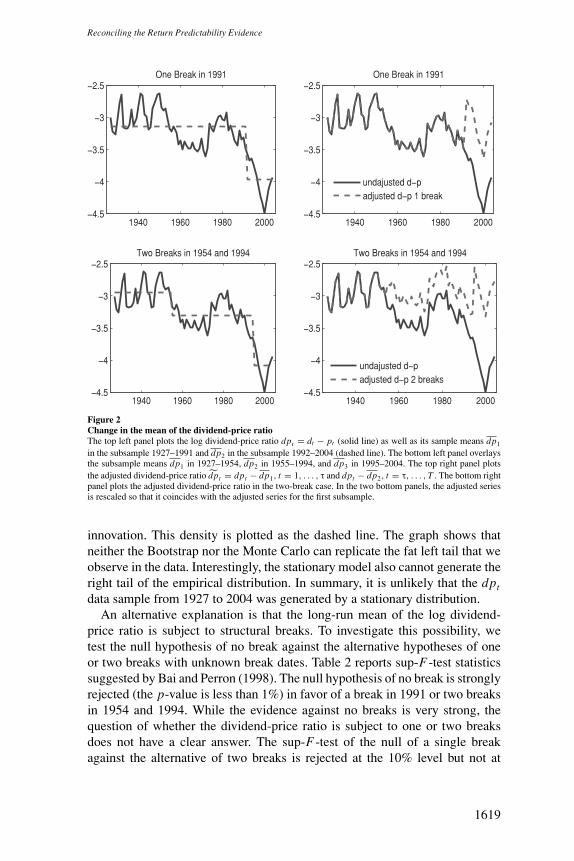
Figure 2Change in the mean of the dividend-price ratioThe top left panel plots the log dividend-price ratio dpt = dt − pt (solid line) as well as its sample means dp1
in the subsample 1927–1991 and dp2 in the subsample 1992–2004 (dashed line). The bottom left panel overlaysthe subsample means dp1 in 1927–1954, dp2 in 1955–1994, and dp3 in 1995–2004. The top right panel plotsthe adjusted dividend-price ratio dpt = dpt − dp1, t = 1, . . . , τ and dpt − dp2, t = τ, . . . , T . The bottom rightpanel plots the adjusted dividend-price ratio in the two-break case. In the two bottom panels, the adjusted seriesis rescaled so that it coincides with the adjusted series for the first subsample.
innovation. This density is plotted as the dashed line. The graph shows thatneither the Bootstrap nor the Monte Carlo can replicate the fat left tail that weobserve in the data. Interestingly, the stationary model also cannot generate theright tail of the empirical distribution. In summary, it is unlikely that the dptdata sample from 1927 to 2004 was generated by a stationary distribution.
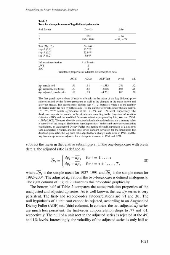
An alternative explanation is that the long-run mean of the log dividend-price ratio is subject to structural breaks. To investigate this possibility, wetest the null hypothesis of no break against the alternative hypotheses of oneor two breaks with unknown break dates. Table 2 reports sup-F-test statisticssuggested by Bai and Perron (1998). The null hypothesis of no break is stronglyrejected (the p-value is less than 1%) in favor of a break in 1991 or two breaksin 1954 and 1994. While the evidence against no breaks is very strong, thequestion of whether the dividend-price ratio is subject to one or two breaksdoes not have a clear answer. The sup-F-test of the null of a single breakagainst the alternative of two breaks is rejected at the 10% level but not at
1619
The Review of Financial Studies / v 21 n 4 2008
d-p
Den
siti
es
-4.5 -4 -3.5 -3 -2.5 -20
0.1
0.2
0.3
0.4
DataMonte CarloBootstrap
Histogram of d-p
Figure 3The empirical distribution of the dividend-price ratioThe figure plots the smoothed empirical distribution of the log dividend-price ratio dp (solid line), alongsidethe smoothed density obtained from drawing from the empirical distribution with replacement (Bootstrap, dash-dotted line), and the smoothed density from a Monte Carlo exercise (dashed line).
the 5% level. The null of two breaks against the alternative of three breaks isnot rejected (not shown). Alternatively, one can use an information criterionto select the number of breaks. Both the Bayesian Information Criterion (BIC)and the modified Schwartz criterion proposed by Liu, Wu, and Zidek (1997)(LWZ) favor two breaks. In summary, the data seem to strongly favor one ortwo breaks, rather than zero or three, but the relative evidence for one or twobreaks is not as strong and only slightly in favor of two breaks.
The table also reports the estimated change in the log dividend-price ratiobefore and after the break. In the one-break case, the change in dp is −.86,whereas in the two-break case, the first change in 1954 is −.37 and the secondchange is −.78. The two plots in the left column of Figure 2 overlay the long-run mean dp on the raw dp series. For now, we are agnostic as to whether thebreak(s) is (are) due to a change in the long-run mean of dividend growth orexpected returns, or a combination of the two. We return to this question later.It is worth emphasizing, however, that the date(s) of the shift in the dividend-price ratio is (are) consistent with the breaks in the equity premium identifiedby Pastor and Stambaugh (2001).
This result motivates us to construct two adjusted dividend-price series, onefor the one-break case and one for the two-break case. For each, we simply
1620
Reconciling the Return Predictability Evidence
Table 2Tests for change in mean of log dividend-price ratio
# of Breaks Date(s) �dp
1 1991 −.862 1954, 1994 −.37, −.78
Test (H0, H1) Statisticsup-F (0,1) 13.7***sup-F (0,2) 23.9***sup-F (1,2) 9.64*
Information criterion # of BreaksLWZ 2BIC 2
Persistence properties of adjusted dividend-price ratio
AC(1) AC(2) ADF Test p val s.d.
dp, unadjusted .91 .81 −1.383 .586 .42dp, adjusted, one break .77 .55 −3.016 .038 .26dp, adjusted, two breaks .61 .23 −4.731 .010 .20
The first panel reports dates of structural breaks in the mean of the log dividend-priceratio estimated by the Perron procedure as well as the changes in the mean before andafter the breaks. The second panel reports sup-F(i, j) statistics where i is the numberof breaks under the null hypothesis and j is the number of breaks under the alternative.‘*’, ‘**’, ‘***’ denote significance at the 1%, 5%, and 10% level, respectively. Thethird panel reports the number of breaks chosen according to the Bayesian InformationCriterion (BIC) and the modified Schwartz criterion proposed by Liu, Wu, and Zidek(1997) (LWZ). The tests allow for autocorrelation in the residuals and the trimming valueis set to 5% of the sample. The bottom panel reports first- and second-order autocorrelationcoefficients, an Augmented Dickey-Fuller test, testing the null hypothesis of a unit root(and associated p-value), and the time-series standard deviation for the unadjusted logdividend-price ratio, the log price ratio adjusted for a change in its mean in 1991, and thelog dividend-price ratio adjusted for a change in its mean in 1954 and 1994.
subtract the mean in the relative subsample(s). In the one-break case with breakdate τ, the adjusted ratio is defined as
dpt ={
dpt − dp1 for t = 1, . . . , τ
dpt − dp2 for t = τ + 1, . . . , T ,(8)
where dp1 is the sample mean for 1927–1991 and dp2 is the sample mean for1992–2004. The adjusted dp ratio in the two-break case is defined analogously.The right column of Figure 2 illustrates this procedure graphically.
The bottom half of Table 2 compares the autocorrelation properties of theunadjusted and adjusted dp series. As is well known, the raw dp series is verypersistent. The first- and second-order autocorrelations are .91 and .81. Thenull hypothesis of a unit root cannot be rejected, according to an AugmentedDickey Fuller (ADF) test (third column). In contrast, the two adjusted dp seriesare much less persistent; the first-order autocorrelation drops to .77 and .61,respectively. The null of a unit root in the adjusted series is rejected at the 4%and 1% levels. Interestingly, the volatility of the adjusted series is only half as
1621
The Review of Financial Studies / v 21 n 4 2008
large as for the adjusted series (last column). This substantially alleviates theburden on standard asset pricing models to match the volatility of the price-dividend ratio, once the nonstationary nature of the mean dp ratio has beentaken into account.
3.3 Forecasting with the adjusted dividend-price ratioWe now revisit the return and dividend growth predictability Equations (1)and (2), but use the adjusted dividend-price ratios instead of the raw seriesas predictor variable. The second and fourth columns of Table 1 show theestimation results of the return and dividend growth predictability regressionsusing dp, respectively. Rows 1–4 are for the one-break case; rows 5–9 are for thetwo-break case. Starting with the one-break case because the adjusted dividend-price ratio is the same as the raw series with each subsample, the results in rows 2and 3 are unchanged. But now in row 1, we find that the adjusted dividend-priceratio significantly predicts stock returns. The coefficient for the entire sampleis .235, which is almost identical to the estimates in the two subsamples. Thus,the low point estimate for κr in the first column was due to averaging acrossregimes. Not taking the nonstationarity of the dp ratio into account severelybiases the point estimate for κr downward. Furthermore, row 4 shows thatthe evidence for a break in the forecasting relationship between returns and thedividend-price ratio has disappeared. The null hypothesis of parameter stabilitycan no longer be rejected when using dp. The full-sample regression R2 is 10%,more than twice the value of the first column. The results for dividend growthpredictability remain largely unchanged. This is not surprising given that wedid not detect much instability in the relationship between �dt+1 and dpt tobegin with.
The rolling window estimates confirm this result.7 The middle panel ofFigure 1 shows that the coefficient κr is much more stable in the one-break casethan in the no-break case (top panel). In particular, its value in the 1990s hoversaround .3, compared to zero without the adjustment. Likewise, the regressionR2 is also more stable and does not drop off in the 1990s. The same exerciseshows that the dividend growth relationship is stable and that κd never movesfar from zero (not shown). The evidence for dividend growth predictability isweak at best.8
The bottom panel of Table 1 uses dp, adjusted for breaks in 1954 and 1994.The full-sample estimate for κr is now .455 (row 5) and highly significant.9
7 In the rolling window estimation, we assume that the break in dp is caused by a break in mean expected returns r .The alternative assumption that the break is in the long-run growth rate of the economy g gives identical results.
8 The lack of predictive power of the dividend-price ratio for dividend growth does not imply that dividend growthis not forecastable, because any correlated movement in expected returns and expected dividend growth cancelsin d − p, as shown in Lettau and Ludvigson (2005).
9 A Bootstrap analysis confirms that the small-sample p-value (asymptotic p-value) is 1.11% (0.00%) in the one-break case and 0.00% (0.00%) in the two-break case. A second Bootstrap exercise shows that the small-samplebias in the coefficients is small relative to their magnitude. In the one-break case, the bias is .019 (we estimate
1622
Reconciling the Return Predictability Evidence
The full-sample regression R2 is 22%. In contrast, dividend growth is notpredictable. The bottom panel of Figure 1 shows that the rolling estimatesfor κr are very stable when we use dp adjusted for two breaks. The pointestimate hovers around .4 and the return regression R2 goes up as high as 40%.Moreover, the Chow test in row 9 finds no evidence for instability in eitherforecasting equation.
We conclude that taking changes in the long-run mean of the dividend-priceratio into account is crucial for forecasts of stock returns. Forecasting with theunadjusted dividend-price ratio series results in coefficient instability in theforecasting regression and unreliable inference (insignificance in small sam-ples, and results depending on the subsample). These disconcerting propertiesare due to a nonstationary component that shifts the mean of the dividend-priceratio. In Section 3.1, we extend the model to allow for such nonstationarity indp. In this section, we examined a simple form of nonstationarity, a structuralbreak. Appropriately adjusting the dividend-price ratio for the structural breakstrengthens the evidence for return predictability, but not dividend growth pre-dictability. The predictability coefficient is stable over time and least-squarescoefficient estimates are highly significant. Finally, the in-sample return pre-dictability evidence stands up to the usual problem of persistent regressor bias(Nelson and Kim, 1993; Stambaugh, 1999; Ang and Bekaert, 2006; Valkanov,2003) because the adjusted dividend-price ratio is much less persistent.
4. Other Financial Ratios
While the dividend-price ratio has been the classic prediction variable, it isuseful to investigate to what extent our results are robust to a different measureof payouts. Lamont (1998) finds that the log earnings-price ratio ep forecastsreturns. We find very much the same patterns for the earnings-price ratio asfor the dividend-price ratio. The earnings data start in 1946 and are describedin Appendix A. The book-to-market ratio is computed from the same earningsand dividend data using the clean-surplus method (Vuolteenaho, 2000).
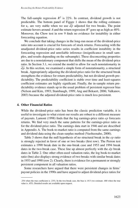
Table 3 shows that the null hypothesis of no structural break in the ep ratiois strongly rejected in favor of one or two breaks (first row). The Perron testestimates a 1990 break date in the one-break case and 1953 and 1994 breakdates in the two-break case. These line up almost perfectly with the dp breakdates in Table 2. One other often-used valuation ratio, the log book-to-marketratio (bm) also displays strong evidence of two breaks with similar break datesin 1953 and 1990 (row 2). Clearly, there is evidence for a permanent or stronglypersistent component in all valuation ratios.
Some researchers have argued that there were persistent changes in firms’payout policies in the 1990s and have argued to adjust dividend-price ratios for
.254 when the true coefficient is .235). In the two-break case, the bias is .013 (we estimate .468 when the truevalue is .455). Detailed results are available upon request.
1623
The Review of Financial Studies / v 21 n 4 2008
Table 3Tests for change in mean of financial ratios
Structural break tests
H0 H1 sup-F-test p-value Date(s) � mean
ep zero break one break 15.5 < 1% 1990 −.67zero break two breaks 18.0 < 1% 1953, 1994 −.50, −.62
bm zero break one break 9.3 < 10% 1953 −.80zero break two breaks 17.9 < 1% 1953, 1990 −.71, −.33
de zero break one break 5.6 > 10% 1993 −.24zero break two breaks 5.3 > 10% 1990, 1993 +.27, −.46
dpnas zero break one break 10.2 < 5% 1992 −.75zero break two breaks 18.1 < 1% 1954, 1995 −.35, −.70
dprep zero break one break 3.7 > 10% 1990 −.43zero break two breaks 4.5 > 10% 1954, 1991 −.23, −.34zero break three breaks 20.1 < 1% 1957, 1973, 1990 −.46, +.50, −.57
The top half of the table reports sup-F Perron tests of the null hypothesis of no break against the alternativehypothesis of one (first row) or two (second row) breaks with unknown break date. It reports the p-value of thetest statistic, as well as the resulting break date. The last column reports the estimated change in means beforeand after the break(s). These tests are performed for the log earnings-price ratio ep = e − p, the log bookto-market value of equity ratio bm = b − m, the log dividend-earnings ratio de = d − e, the log dividend-priceratio adjusted for repurchases dprep, and the log dividend-price ratio of the universe of CRSP firms that excludesthe NASDAQ firms dpnas.
repurchases (Fama and French, 2001; Grullon and Michaely, 2002; Boudoukhet al., 2004). First, we find no evidence for a break in the payout ratio de = d − eat the 10% level (row 3 of Table 2). This is consistent with the view that bothdp and ep contain structural breaks. Second, even if there was a break in thede ratio and we took the point estimate for de in the subsamples, we wouldfind that more than three-fourths of the change in the mean dividend-price ratiocomes from a change in the mean earnings-price ratio and less than one-fourthfrom a change in de (dp = ep + de). In particular, for our S&P 500 samplefrom 1946 to 2004 with a 1991 break date, we find a change in dp of −.81, achange in ep of −.63, and a change in de of −.18.
To further investigate the role of repurchases and the role of a changingcomposition in CRSP, we consider two additional valuation ratios. First, weconsider the CRSP universe without NASDAQ stocks. Arguably, removingNASDAQ stocks goes a long way toward eliminating new economy and non–dividend-aying companies that became more prevalent in the 1990s.10 Wecompute the dividend-price ratio, dpnas, and the dividend growth for this group.This time series has properties very similar to those of the series with theNASDAQ. The Perron tests in row 5 of Table 3 show a break of −75% in 1992,close to the −86% change in the full-sample series in 1991. For the two-break
10 Fama and French (2001) document that the fraction of nonfinancial, nonutility firms that paid dividends declinedby almost 45% between 1978 and 1999. However, most of that decline is attributable to new firms and to smallfirms. They write: “The characteristics of dividend payers (large profitable firms) do not change much after1978.” We take this group to be the value-weighted CRSP index without NASDAQ stocks. This series starts todeviate from the full-sample series in 1973. We verified that the dividend growth rate of this set of firms did notchange in the 1990s. Average dividend growth from 1927 to 1991 was 5.45%. Average dividend growth from1992 to 2004 was 5.46%.
1624
Reconciling the Return Predictability Evidence
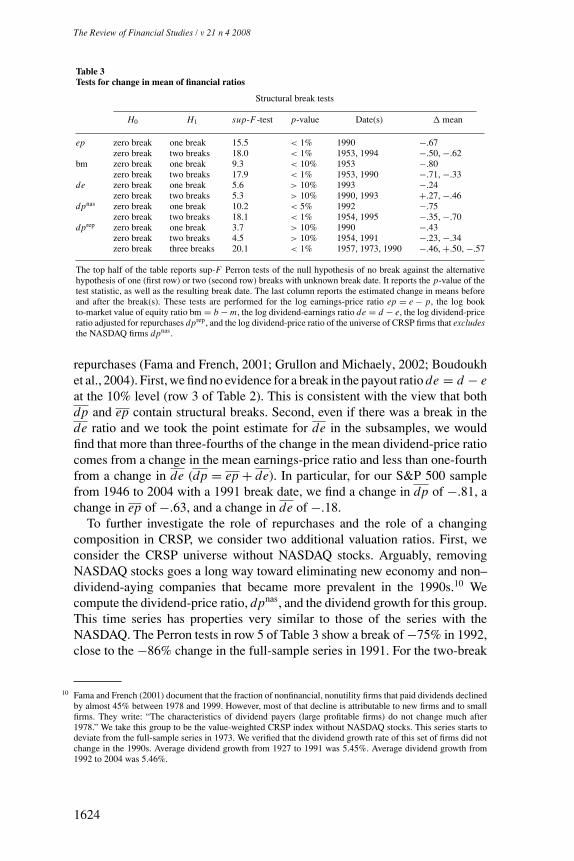
Table 4Forecasting returns with other financial ratios
Predictor y No break One break Two breaks Three breaks
ep .119 .214 .216(.030) (.039) (.045)[.104] [.190] [.185]
bm .070 .255 .308(.036) (.063) (.064)[.030] [.154] [.188]
dpnas .110 .250 .417(.048) (.056) (.090)[.043] [.105] [.182]
dprep .191 .282 .361 .576(.054) (.065) (.084) (.097)[.079] [.126] [.161] [.250]
This table reports estimation results for the equation rt+1 − r = κr (yt −y) + τr
t+1, where y is the log earnings-price ratio ep = e − p in the firstrow, the log book-to-market value ratio bm = b − m in the second row, thelog dividend-price ratio without the NASDAQ firms dpnas in the third row,and the repurchase adjusted log dividend-price ratio dprep in the fourthrow. The table reports point estimates and standard errors in parenthesesof κr , and the regression R2 in brackets. The regressor is the unadjustedvaluation ratio in the first column, the one-break adjusted valuation ratioin the second column, and the two-break adjusted valuation ratio in thethird column. For the predictor dprep, we report the three-break case aswell. The break dates for all regressors are reported in Table 3. The sampleis 1946–2004 in row 1, and 1927–2004 in all other rows.
case, the break dates and magnitudes are also very similar: 1954 and 1995 and−35% and −70%.
Second, we use the Boudoukh et al. (2004) repurchase yield data, availablefrom 1971 onward, and construct a corrected dividend-price ratio and dividendgrowth rate series. We label this repurchase-adjusted dividend price seriesdprep.11 The case favored by the data is a three-break case with break dates in1957, 1973, and 1990 (see last row of Table 3). We show next that these twoadjustments do not materially affect our predictability results with the standarddividend-price ratio presented earlier. This leads us to conclude that structuralchanges in payout policies and/or the composition of firms in the 1990s canonly explain a small part of the change in the dividend-price ratio.
We first turn to the forecasting regressions with the earnings-price ratio.When we use the earnings-price ratio as a return predictor, we obtain similarresults to what we reported for the dividend-price ratio in Table 1. The firstrow of Table 4 shows that when the unadjusted earnings-price ratio is theindependent variable, the slope coefficient is .119. Just as in the dividend-price ratio regressions, this coefficient displays parameter instability amongsubsamples: the full-sample point estimate is lower than the estimates in allsubsamples, and the Chow test of no break has a p-value of only .15 (notshown). The next two columns show that this bias is due to averaging over
11 We note that this is just one possible adjustment. The correct adjustment depends on the investor under consider-ation. Here, an investor’s cash flows are adjusted for aggregate repurchases, but not for seasoned equity offeringsnor initial public offerings.
1625
The Review of Financial Studies / v 21 n 4 2008
subsamples. Once we use the adjusted ep ratio, the instability disappears andthe full-sample point estimate increases to .215 in both the one-break and two-break cases. These coefficients are twice the size of the ones obtained withthe unadjusted ep ratio and are measured precisely. The regression R2 almostdoubles. The slope coefficient is very similar to the one we found in the firstpanel of Table 1: κr = .235. One difference from the results in Table 1 is thatthe adjusted earnings-price ratio also significantly forecasts earnings growth,with a negative sign (not shown).
For the unadjusted lagged log book-to-market ratio bm = b − m, we findthat the predictability coefficient κr is only marginally significant. The pointestimate is .07, lower than the point estimates in the subsamples 1927–1952(.26), 1953–1990 (.44), and 1991–2004 (.72), all of which are strongly sig-nificant. Again, this downward bias is due to averaging over the break(s).The full-sample point estimate increases to .255 with the one-break adjustedbm series as regressor and to .308 with the two-break adjusted bm series. Theregression R2 increases from 3% in the first column to 19% in the third column.
The return predictability findings for dpnas and dprep are also similar tothe benchmark dp results. First, using dpnas without break adjustment, wefind a point estimate for κr of .11. This point estimate is lower than in eithersubsample (.24 in 1927–1992 and .30 in 1993–2004). Once we use the break-adjusted series, the point estimate more than doubles to .250. Just as for thestandard dp ratio, the downward bias comes from averaging over the break.The break-adjusted point estimate is close to the .235 we found for the samplethat includes the NASDAQ. We obtain further increases in the point estimateand the R2 in the two-break case. Second, using dprep, the full-sample returnpredictability coefficient is .19, higher than the .09 for the standard dp series, butagain lower than in either subsample (.25 in 1927–1990 and .53 in 1991–2004).Clearly, adjusting for repurchases improves the forecasting power of the dpratio. However, adjusting for the breaks is important and further strengthens thecase for predictability. In the preferred case of three breaks, the predictabilitycoefficient is .58, three times its unadjusted value. The regression R2 is alsothree times higher.
We conclude that the other financial ratios indicate a predictability patternsimilar to that of the dividend-price ratio. Without an adjustment for the changein their long-run mean, the relationship between 1-year ahead returns and finan-cial ratios is unstable over time. However, once we filter out the nonstationarycomponent, we find a stable forecasting relationship and a large predictabilitycoefficient. The fact that the results are so similar for earnings and dividenddata suggests that an explanation that exclusively rests on changing payoutpolicies misses the most important structural changes in the economy: changesin long-run growth rate or long-run expected returns.
1626
Reconciling the Return Predictability Evidence
5. Out-of-Sample Predictability
The in-sample predictability results presented so far used a break adjustmentconstructed using the entire data sample. In this section, we investigate how aninvestor who forms an adjusted dividend-price ratio in real time fares in predict-ing out-of-sample returns. We compare the out-of-sample forecasting propertiesof adjusted dividend-price ratios to the unadjusted series and a random walkmodel. We find that a real-time dividend-price ratio adjustment yields uni-formly smaller prediction errors compared to the unadjusted series but slightlylarger forecast errors than the random walk model.
Why does real-time prediction fail to beat the random walk model? In realtime, an investor faces two challenges. First, she has to estimate the timingof a break. Second, if she detects a new break, she has to estimate the newmean after the break occurs. If the new break occurred toward the end of thesample that the investor has access to, the new mean can only be estimatedusing a small number of observations and is subject to significant estimationuncertainty. To investigate which issue is responsible for the deterioration ofthe out-of-sample forecasting power, we consider two additional exercises. Inthe first exercise, the investor predicts out-of-sample using the ex post adjusteddividend-price ratio series considered in Section 3.1. In other words, we endowthe investor with information about estimated break dates and means from theentire sample—thus, this case is not a pure out-of-sample test. However, it setsan informative benchmark for the analysis of the pure out-of-sample forecasts.In a second exercise, we consider a Hamilton (1989) regime-switching modelfor the mean of the dividend-price ratio. In this model, the regime meansare estimated using data from the entire data sample. The Hamilton modelcomputes two estimates for the break dates (regime-switching probabilities):(i) “unsmoothed” probabilities estimated using only currently available data,and (ii) “smoothed” probabilities based on the entire sample. While this caseis not a pure out-of-sample forecast, it allows us to study the relative difficultyof estimating the break dates versus estimating the means relative to the pureout-of-sample forecasts and the ex post adjusted dividend-price ratio.
The conclusions from these two exercises are that (i) the estimation ofthe break dates in real time is not crucial and the resulting prediction errorsare smaller than for the random walk model, and (ii) the estimation of themagnitude of the break in the mean dividend-price ratio entails substantialuncertainty, and is ultimately responsible for the failure of the real-time out-of-sample predictions to beat the random walk. These findings can explain thelack of out-of-sample predictability documented by Goyal and Welch (2004).
5.1 Real-time dividend price adjustmentsBefore presenting the estimation results, we confirm our earlier conclusion(based on ex post data; see Figure 3) that it is extremely unlikely that thedividend-price ratio sample is drawn from a stationary distribution, based on
1627
The Review of Financial Studies / v 21 n 4 2008
Year
d-p
1950 1955 1960 1965 1970 1975 1980 1985 1990 1995 2000-2
-1.5
-1
-0.5
0
0.5
1
1.5
2Data2.5%5%95%97.5%
Recursive Bootstrapped Quantiles of d-p
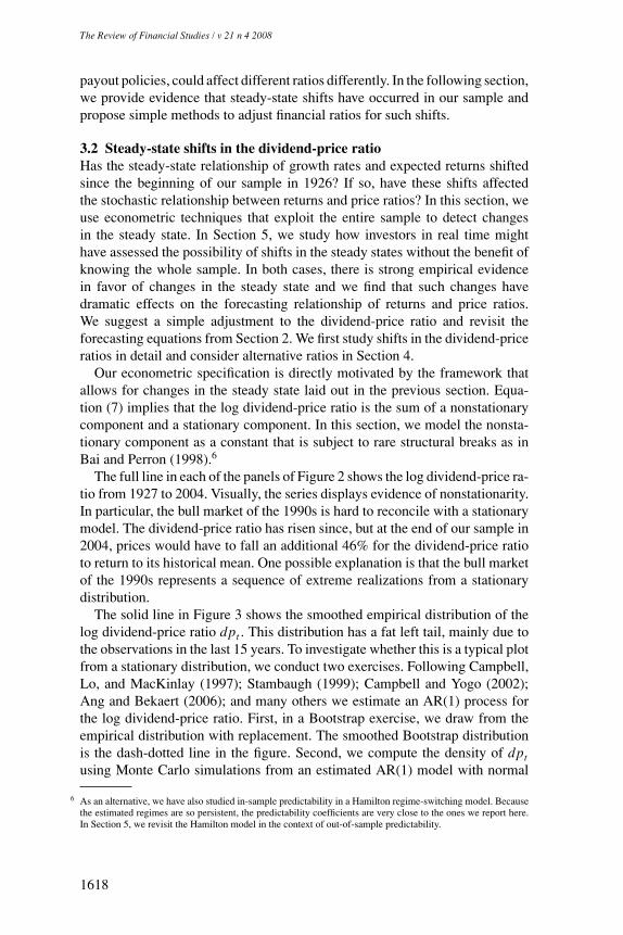
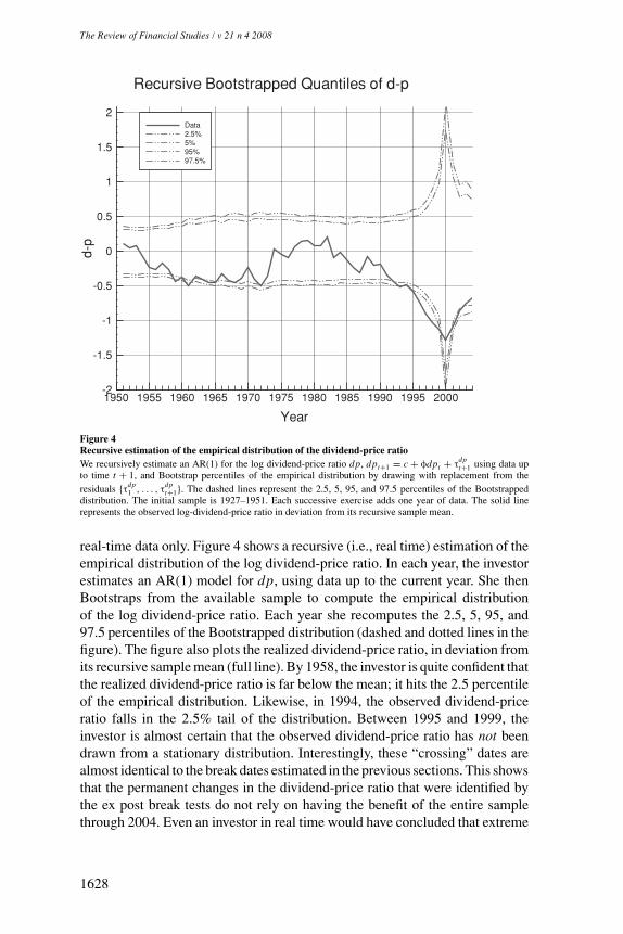
Figure 4Recursive estimation of the empirical distribution of the dividend-price ratioWe recursively estimate an AR(1) for the log dividend-price ratio dp, dpt+1 = c + φdpt + τ
dpt+1 using data up
to time t + 1, and Bootstrap percentiles of the empirical distribution by drawing with replacement from theresiduals {τdp
1 , . . . , τdpt+1}. The dashed lines represent the 2.5, 5, 95, and 97.5 percentiles of the Bootstrapped
distribution. The initial sample is 1927–1951. Each successive exercise adds one year of data. The solid linerepresents the observed log-dividend-price ratio in deviation from its recursive sample mean.
real-time data only. Figure 4 shows a recursive (i.e., real time) estimation of theempirical distribution of the log dividend-price ratio. In each year, the investorestimates an AR(1) model for dp, using data up to the current year. She thenBootstraps from the available sample to compute the empirical distributionof the log dividend-price ratio. Each year she recomputes the 2.5, 5, 95, and97.5 percentiles of the Bootstrapped distribution (dashed and dotted lines in thefigure). The figure also plots the realized dividend-price ratio, in deviation fromits recursive sample mean (full line). By 1958, the investor is quite confident thatthe realized dividend-price ratio is far below the mean; it hits the 2.5 percentileof the empirical distribution. Likewise, in 1994, the observed dividend-priceratio falls in the 2.5% tail of the distribution. Between 1995 and 1999, theinvestor is almost certain that the observed dividend-price ratio has not beendrawn from a stationary distribution. Interestingly, these “crossing” dates arealmost identical to the break dates estimated in the previous sections. This showsthat the permanent changes in the dividend-price ratio that were identified bythe ex post break tests do not rely on having the benefit of the entire samplethrough 2004. Even an investor in real time would have concluded that extreme
1628
Reconciling the Return Predictability Evidence
observations of dividend-price ratios are unlikely to be generated by a stationaryprocess with constant parameters.
Next we construct a real-time adjustment of the dividend-price ratio that canbe used in out-of-sample forecasting tests. In each year T ′ ≤ T , the investorestimates the Perron structural break test using data available up to year T ′ usingone of the three tests: the sequential sup-F-test with a 10% critical value, theBIC criterion, and the LWZ criterion. Given the break dates and correspondingmeans, the real-time adjustment of the dividend-price ratio is analogous tothe adjustment using the entire sample in Equation (8), with the exceptionthat only data up to date T ′ instead of T are used in the estimation. Denotethis corrected ratio dp
Pt,T ′ , t = 1, . . . , T ′. The out-of-sample return forecast for
period T ′ + 1 is then computed from a regression of returns rt+1 on dpPt,T ′
for t = 1, . . . , T ′ − 1 and the currently observed adjusted dividend-price ratiodp
Pt,T ′ .12
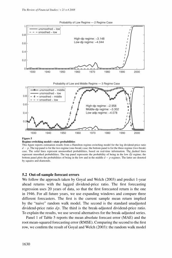
To gauge the relative difficulties of estimating the timing of a break versusthe estimation of the means, we also use a “pseudo” real-time adjustment basedon a Hamilton (1989) regime-switching model in real time. The dividend-priceratio is assumed to follow an AR(1) with different means in either two regimes(one-break case) or three regimes (two-break case). The top panel of Figure5 shows the smoothed (based on the entire sample) and unsmoothed (real-time) estimates of the probability that the dividend-price ratio is drawn fromthe low regime, when two regimes are considered. Using real-time data, theinvestor puts nonzero probability on a shift to the low d − p regime startingin early 1990. By 1995, she is more than 50% certain that the shift occurred.The difference between smoothed probabilities and unsmoothed probabilitiesis that the investor is assigning a higher likelihood to the new, low dividend-price regime earlier because she has access to the entire data set. Note that thedp estimates for the two regimes coincide with our ex post estimates becausethey use the entire data sample. When she considers three regimes instead, theinvestor increases the real-time probability of a switch from the high to themiddle dp regime in 1954. By 1960, she is more than 50% certain that the firstshift occurred (see middle panel of Figure 5). In 1990, she starts to attributeprobability mass to the low-p regime, and by 1996, she is more than 50%confident that the economy left the middle-dp regime for the low-dp regime.As in the two-regime case, the smoothed probabilities indicate that knowingthe entire sample yields a faster transition to the new regime.
Not surprisingly, the regimes in the Hamilton model are estimated to be verypersistent. The probability of remaining in the current regime is above 0.9 inall cases. In other words, the regimes identified by the Hamilton estimation areclose to permanent structural breaks as specified in the Perron model.
12 This procedure implies that there are no breaks between T ′ and T ′ + 1, consistent with our assumption that thebreak is unpredictable.
1629
The Review of Financial Studies / v 21 n 4 2008
1930 1940 1950 1960 1970 1980 1990 20000
0.2
0.4
0.6
0.8
1
Probability of Low Regime — 2 Regime Case
1930 1940 1950 1960 1970 1980 1990 20000
0.2
0.4
0.6
0.8
1
Probability of Low and Middle Regime — 3 Regime Case
unsmoothed − lowsmoothed − low
unsmoothed − middleunsmoothed − lowsmoothed − middlesmoothed − low
High-dp regime: −3.148Low-dp regime: −4.044
High-dp regime: −2.958Middle-dp regime: −3.302Low-adp regime: −4.078
Figure 5Regime-switching model—state probabilitiesThis figure reports estimation results from a Hamilton regime-switching model for the log dividend-price ratiod − p. The top panel is for the two-regime (one-break) case; the bottom panel is for the three-regime (two-break)case. The solid lines represent unsmoothed probabilities, based on real-time information. The dashed linesrepresent smoothed probabilities. The top panel represents the probability of being in the low dp regime; thebottom panel plots the probabilities of being in the low and in the middle d − p regimes. The latter are denotedby squares and diamonds.
5.2 Out-of-sample forecast errorsWe follow the approach taken by Goyal and Welch (2003) and predict 1-yearahead returns with the lagged dividend-price ratio. The first forecastingregression uses 20 years of data, so that the first forecasted return is the onein 1946. For all future years, we use expanding windows and compare threedifferent forecasters. The first is the current sample mean return impliedby the “naive” random walk model. The second is the standard unadjusteddividend-price ratio dp. The third is the break-adjusted dividend-price ratio.To explain the results, we use several alternatives for the break-adjusted series.
Panel 1 of Table 5 reports the mean absolute forecast error (MAE) and theroot mean-squared forecasting error (RMSE). Comparing the second to the firstrow, we confirm the result of Goyal and Welch (2003): the random walk model
1630
Reconciling the Return Predictability Evidence
Table 5Out-of-sample predictability
Mean absolute error Root mean-squared error
Panel 1: Data
BenchmarksRandom walk .1338 .1605Unadjusted dp .1411 .1685
Pure OOSdpP —Perron sequential sup-F .1350 .1661dpP —Perron LWZ criterion .1391 .1680dpP —Perron BIC criterion .1370 .1646
Pseudo OOSdp—Perron, ex post, one break .1309 .1558dp—Perron, ex post, two breaks .1158 .1421dpH —Hamilton, one break, smoothed .1286 .1543dpH —Hamilton, two breaks, smoothed .1100 .1340dpH —Hamilton, one break, unsmoothed .1330 .1590dpH —Hamilton, two breaks, unsmoothed .1243 .1512
Panel 2: Monte Carlo—one break
Random walk .1212 .1525Unadjusted dp .1210 .1555dp—ex post, one break .1058 .1334
Panel 3: Monte Carlo—two breaks
Random walk .1222 .1533Unadjusted dp .1203 .1516dp—ex post, one break .1165 .1493dp—ex post, two breaks .1064 .1336
The table reports one-period ahead return forecast errors based on the Random Walk model (row 1)and based on the forecasting equation rt+1 − r = κr (dpt − dp) + τr
t+1 with fixed dp (row 2). Rows
3 through 5 use the real-time Perron procedure to estimate dpP
. We report results for three differentmethods of selecting the number of break: the sequential sup-F-test with 10% critical value, andthe LWZ and BIC information criteria. Rows 6 and 7 use the ex post break-adjusted dividend priceratios with a change in dp in 1991 (row 6), and two changes in the mean dp in 1954 and 1994
(row 7). Rows 8–11 use the Hamilton approach to construct adjusted dividend-price ratios dpH
.We consider the cases of two regimes and three regimes. All numbers denote returns per annum.The second and third panels report results from a Monte Carlo exercise. We simulate the structuralmodel under the null hypothesis that the data generating process has one break in 1991 (panel 2) orhas two breaks in 1954 and 1994 (panel 3). We compare the same three out-of-sample forecastingexercises as in the data (panel 1). Except in the last panel, we also look at the forecast errors whenwe only correct for the second break and not the first one. The structural parameters in panels 2and 3 are the same and were obtained from the Vector Error Correction Model (VECM) parametersestimated under the assumption of two breaks in 1954 and 1994 for the period 1947–2004, the sameforecasting period as in panel 1.
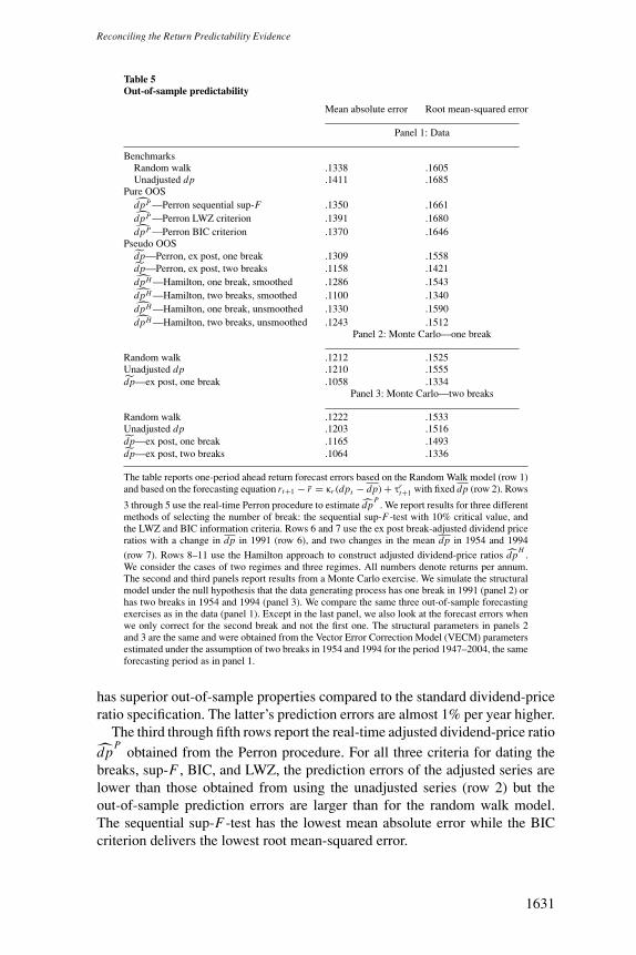
has superior out-of-sample properties compared to the standard dividend-priceratio specification. The latter’s prediction errors are almost 1% per year higher.
The third through fifth rows report the real-time adjusted dividend-price ratiodp
Pobtained from the Perron procedure. For all three criteria for dating the
breaks, sup-F , BIC, and LWZ, the prediction errors of the adjusted series arelower than those obtained from using the unadjusted series (row 2) but theout-of-sample prediction errors are larger than for the random walk model.The sequential sup-F-test has the lowest mean absolute error while the BICcriterion delivers the lowest root mean-squared error.
1631
The Review of Financial Studies / v 21 n 4 2008
1930 1940 1950 1960 1970 1980 1990 2000−4.5
−4
−3.5
−3
−2.5Probability-weighted mean-dp estimates — 2 regime Case
1930 1940 1950 1960 1970 1980 1990 2000−4.5
−4
−3.5
−3
−2.5Probability-weighted mean-dp estimates — 3 Regime Case
unsmoothedsmoothedex post
unsmoothedsmoothedex post
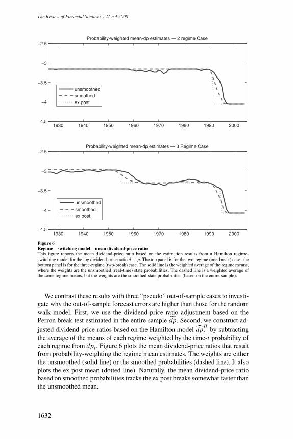
Figure 6Regime—switching model—mean dividend-price ratioThis figure reports the mean dividend-price ratio based on the estimation results from a Hamilton regime-switching model for the log dividend-price ratio d − p. The top panel is for the two-regime (one-break) case; thebottom panel is for the three-regime (two-break) case. The solid line is the weighted average of the regime means,where the weights are the unsmoothed (real-time) state probabilities. The dashed line is a weighted average ofthe same regime means, but the weights are the smoothed state probabilities (based on the entire sample).
We contrast these results with three “pseudo” out-of-sample cases to investi-gate why the out-of-sample forecast errors are higher than those for the randomwalk model. First, we use the dividend-price ratio adjustment based on thePerron break test estimated in the entire sample dp. Second, we construct ad-justed dividend-price ratios based on the Hamilton model dp
Ht by subtracting
the average of the means of each regime weighted by the time-t probability ofeach regime from dpt . Figure 6 plots the mean dividend-price ratios that resultfrom probability-weighting the regime mean estimates. The weights are eitherthe unsmoothed (solid line) or the smoothed probabilities (dashed line). It alsoplots the ex post mean (dotted line). Naturally, the mean dividend-price ratiobased on smoothed probabilities tracks the ex post breaks somewhat faster thanthe unsmoothed mean.
1632
Reconciling the Return Predictability Evidence
Rows 6 and 7 in Panel 1 of Table 5 show that the use of the ex post adjusteddividend-price ratios dp substantially reduces the forecasting error. The MAEand RMSE of the dividend-price ratio adjusted for a single break in 1991 arelower than those for the random walk model. The out-of-sample forecastingpower of the dividend-price ratio adjusted for two breaks in 1954 and 1994is dramatically improved compared to the unadjusted ratio and to the randomwalk model. The RMSE and MAE are reduced by 12–15% compared to therandom walk model.
The pseudo out-of-sample forecast errors based on the Hamilton correctionwith smoothed probabilities are similar but slightly lower than those in theex post Perron correction. Since both cases use the entire sample to estimatethe regime means and probabilities, it is not surprising that the out-of-sampleresults are comparable. The Hamilton model allows for a smoother adjustmentto a new regime compared to the Perron model, which might account for thelower forecast error.
For the Hamilton regime-switching model, we also compute pseudo out-of-sample forecast errors based on unsmoothed probabilities. Recall that theseprobabilities are estimated using only currently available information, but es-timates of regime means are based on information of the entire sample. Thus,this case enables us to assess the relative difficulty of real-time estimation ofthe timing of breaks versus real-time estimation of the level of regimes. In-terestingly, the out-of-sample prediction errors of the case with unsmoothedprobabilities are only slightly higher than those with ex post Perron adjust-ment and smoothed probabilities. In the one-break example, the RMSE for theunsmoothed Hamilton adjustment is 15.90% compared to 15.58% for the expost Perron adjustment and 15.43% for the smoothed Hamilton adjustment.In contrast, the forecast errors for the pure OOS adjustments are significantlyhigher; between 16.46 and 16.80%, depending on the selection criterion.
Where does the difference in forecast errors come from? In the Hamiltonadjustment with unsmoothed probabilities, the investor estimates the proba-bility of each regime in real time but has access to the entire time series toestimate the mean dp ratio in the different regimes.13 In the ex post Perron andsmoothed Hamilton procedures, the investor estimates not only break dates inreal time, but also the long-run mean in the current regime. Our results suggestthat the poor real-time out-of-sample forecasts are to a larger extent due touncertainty about the magnitudes of breaks rather than uncertainty about theexact timing of a break. Estimating a new long-run mean based on a few datapoints incurs a lot of measurement error. For example, if the Perron investor in2001 detects a break in 1995, she has only six data points to estimate the new
13 A satisfactory resolution that avoids any look-ahead bias in the Hamilton model would be to conduct a fullBayesian analysis in which the investor estimates the number of regimes, the regime-switching dates, and theirassociated long-run means based on real-time available data and prior information. Pettenuzzo and Timmermann(2005) have worked out such an estimation in the context of an asset allocation problem.
1633
The Review of Financial Studies / v 21 n 4 2008
dpP
. The difficulty in estimating this mean is what accounts for the increase inprediction errors.
6. Long-Horizon Predictability
An important component of the empirical work on return predictability useslong-horizon regressions. In this section we provide a framework for analyzinglong-horizon predictability. We use the ex post dividend-price ratio as thepredictor and derive theoretical restrictions that link return and dividend growthto lagged dividend-price ratios at different horizons. Rather than estimatingregressions for various horizons separately, the advantage of this approach isthat fewer parameters have to be estimated. Moreover, the restrictions guaranteethat the estimates across horizons are consistent with each other.
Recall the return and dividend growth predictability Equations (1) and (2)
rt+1 = κr dpt + τrt+1, (9)
�dt+1 = κd dpt + τdt+1, (10)
where variables with a tilde are appropriately demeaned and stationary. Sub-tracting Equation (10) from Equation (9) and using the log linear approximationfor log returns rt+1 = dpt − ρdpt+1 + �dt+1 yields the implied AR(1) processfor the dividend-price ratio in (11):
dpt+1 = φdpt + τdpt+1 , where (11)
1 − ρφ = κr − κd (12)
where the innovations are linked by ρτdpt+1 = τd
t+1 − τrt+1. The model imposes a
nonlinear present value restriction (12) on the predictability coefficients κr andκd . Because ρ < 1 and stationarity implies |φ| < 1, κr − κd must be positive.This is another way of saying that either returns (κr �= 0) or dividend growth(κd �= 0) have to be forecastable (or both). Most researchers work with Equa-tions (9) and (11); we work with (9) and (10) instead because long-horizonrestrictions are more easily derived in this case. Iterating forward on Equations(9) and (10), we obtain the (annualized) H -period dividend growth and returnforecasting equations
1
H
H∑j=1
rt+ j = κr (H ) dpt + τrt,t+H , (13)
1
H
H∑j=1
�dt+ j = κd (H ) dpt + τdt,t+H , (14)
1634
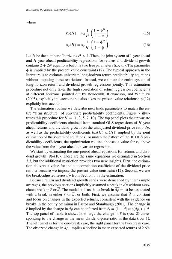
Reconciling the Return Predictability Evidence
where
κd (H ) = κd1
H
(1 − φH
1 − φ
)(15)
κr (H ) = κr1
H
(1 − φH
1 − φ
). (16)
Let N be the number of horizons H > 1. Then, the joint system of 1-year aheadand H -year ahead predictability regressions for returns and dividend growthcontains 2 + 2N equations but only two free parameters (κd , κr ). The parameterφ is implied by the present value constraint (12). The typical approach in theliterature is to estimate univariate long-horizon return predictability equationswithout imposing these restrictions. Instead, we estimate the entire system oflong-horizon return and dividend growth regressions jointly. This estimationprocedure not only takes the high correlation of return regression coefficientsat different horizons, pointed out by Boudoukh, Richardson, and Whitelaw(2005), explicitly into account but also takes the present value relationship (12)explicitly into account.
The estimation routine we describe next finds parameters to match the en-tire “term structure” of univariate predictability coefficients. Figure 7 illus-trates this procedure for H = {1, 3, 5, 7, 10}. The top panel plots the univariatepredictability coefficients obtained from standard OLS regressions of H -yearahead returns and dividend growth on the unadjusted dividend-price ratio dp,as well as the predictability coefficients (κd (H ), κr (H )) implied by the jointestimation of the system of equations. To match the pattern of the 10 OLS pre-dictability coefficients, the optimization routine chooses a value for κr abovethe value from the 1-year ahead univariate regression.
We start by estimating the one-period ahead equations for returns and divi-dend growth (9)–(10). These are the same equations we estimated in Section3.3, but the additional restriction provides two new insights. First, the estima-tion delivers a value for the autocorrelation coefficient of the dividend-priceratio φ because we impose the present value constraint (12). Second, we usethe break-adjusted series dp from Section 3 in the estimation.
Because return and dividend growth series were demeaned by their sampleaverages, the previous sections implicitly assumed a break in dp without asso-ciated break in r or d . The model tells us that a break in dp must be associatedwith a break in either r or d , or both. First, we assume that d is constantand focus on changes in the expected returns, consistent with the evidence onbreaks in the equity premium in Pastor and Stambaugh (2001). The change inr implied by the change in dp can be inferred from rt = (1 + d) exp(dpt ) + d.The top panel of Table 6 shows how large the change in r is (row 2) corre-sponding to the change in the mean dividend-price ratio in the data (row 1).The left panel is for the one-break case, the right panel for the two-break case.The observed change in dpt implies a decline in mean expected returns of 2.6%
1635
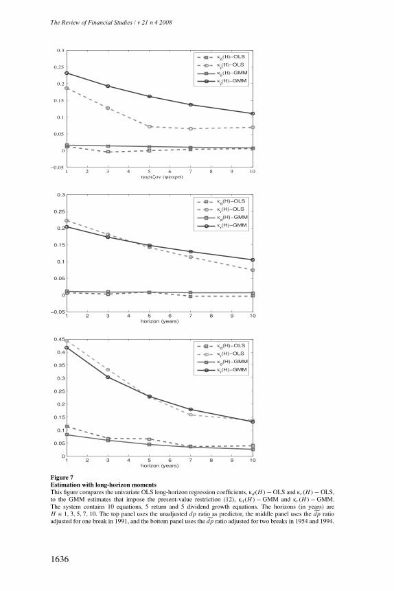
The Review of Financial Studies / v 21 n 4 2008
1 2 3 4 5 6 7 8 9 10−0.05
0
0.05
0.1
0.15
0.2
0.25
0.3
ηοριζον (ψεαρσ)
κδ(Η)−OLS
κρ(Η)−OLS
κδ(Η)−GMM
κρ(Η)−GMM
1 2 3 4 5 6 7 8 9 10−0.05
0
0.05
0.1
0.15
0.2
0.25
0.3
horizon (years)
κd(H)−OLS
κr(H)−OLS
κd(H)−GMM
κr(H)−GMM
1 2 3 4 5 6 7 8 9 100
0.05
0.1
0.15
0.2
0.25
0.3
0.35
0.4
0.45
horizon (years)
κd(H)−OLS
κr(H)−OLS
κd(H)−GMM
κr(H)−GMM
Figure 7Estimation with long-horizon momentsThis figure compares the univariate OLS long-horizon regression coefficients, κd (H ) − OLS and κr (H ) − OLS,to the GMM estimates that impose the present-value restriction (12), κd (H ) − GMM and κr (H ) − GMM.The system contains 10 equations, 5 return and 5 dividend growth equations. The horizons (in years) areH ∈ 1, 3, 5, 7, 10. The top panel uses the unadjusted dp ratio as predictor, the middle panel uses the dp ratioadjusted for one break in 1991, and the bottom panel uses the dp ratio adjusted for two breaks in 1954 and 1994.
1636
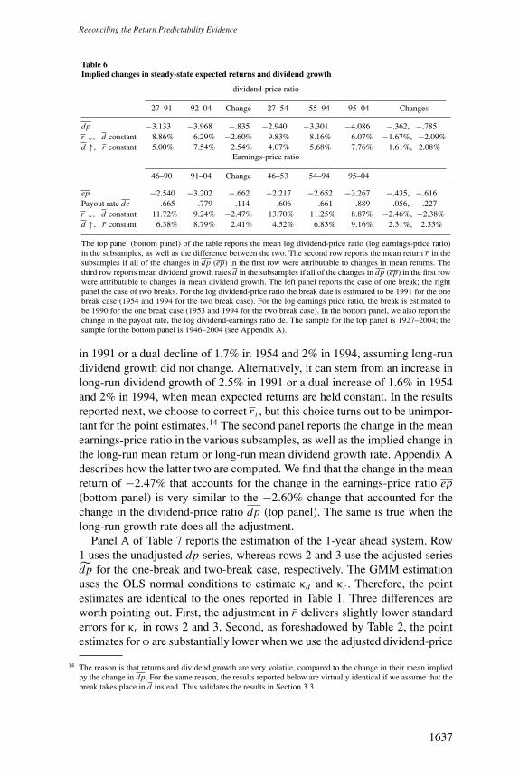
Reconciling the Return Predictability Evidence
Table 6Implied changes in steady-state expected returns and dividend growth
dividend-price ratio
27–91 92–04 Change 27–54 55–94 95–04 Changes
dp −3.133 −3.968 −.835 −2.940 −3.301 −4.086 −.362, −.785r ↓, d constant 8.86% 6.29% −2.60% 9.83% 8.16% 6.07% −1.67%, −2.09%d ↑, r constant 5.00% 7.54% 2.54% 4.07% 5.68% 7.76% 1.61%, 2.08%
Earnings-price ratio
46–90 91–04 Change 46–53 54–94 95–04
ep −2.540 −3.202 −.662 −2.217 −2.652 −3.267 −.435, −.616Payout rate de −.665 −.779 −.114 −.606 −.661 −.889 −.056, −.227r ↓, d constant 11.72% 9.24% −2.47% 13.70% 11.25% 8.87% −2.46%, −2.38%d ↑, r constant 6.38% 8.79% 2.41% 4.52% 6.83% 9.16% 2.31%, 2.33%
The top panel (bottom panel) of the table reports the mean log dividend-price ratio (log earnings-price ratio)in the subsamples, as well as the difference between the two. The second row reports the mean return r in thesubsamples if all of the changes in dp (ep) in the first row were attributable to changes in mean returns. Thethird row reports mean dividend growth rates d in the subsamples if all of the changes in dp (ep) in the first rowwere attributable to changes in mean dividend growth. The left panel reports the case of one break; the rightpanel the case of two breaks. For the log dividend-price ratio the break date is estimated to be 1991 for the onebreak case (1954 and 1994 for the two break case). For the log earnings price ratio, the break is estimated tobe 1990 for the one break case (1953 and 1994 for the two break case). In the bottom panel, we also report thechange in the payout rate, the log dividend-earnings ratio de. The sample for the top panel is 1927–2004; thesample for the bottom panel is 1946–2004 (see Appendix A).
in 1991 or a dual decline of 1.7% in 1954 and 2% in 1994, assuming long-rundividend growth did not change. Alternatively, it can stem from an increase inlong-run dividend growth of 2.5% in 1991 or a dual increase of 1.6% in 1954and 2% in 1994, when mean expected returns are held constant. In the resultsreported next, we choose to correct r t , but this choice turns out to be unimpor-tant for the point estimates.14 The second panel reports the change in the meanearnings-price ratio in the various subsamples, as well as the implied change inthe long-run mean return or long-run mean dividend growth rate. Appendix Adescribes how the latter two are computed. We find that the change in the meanreturn of −2.47% that accounts for the change in the earnings-price ratio ep(bottom panel) is very similar to the −2.60% change that accounted for thechange in the dividend-price ratio dp (top panel). The same is true when thelong-run growth rate does all the adjustment.
Panel A of Table 7 reports the estimation of the 1-year ahead system. Row1 uses the unadjusted dp series, whereas rows 2 and 3 use the adjusted seriesdp for the one-break and two-break case, respectively. The GMM estimationuses the OLS normal conditions to estimate κd and κr . Therefore, the pointestimates are identical to the ones reported in Table 1. Three differences areworth pointing out. First, the adjustment in r delivers slightly lower standarderrors for κr in rows 2 and 3. Second, as foreshadowed by Table 2, the pointestimates for φ are substantially lower when we use the adjusted dividend-price
14 The reason is that returns and dividend growth are very volatile, compared to the change in their mean impliedby the change in dp. For the same reason, the results reported below are virtually identical if we assume that thebreak takes place in d instead. This validates the results in Section 3.3.
1637
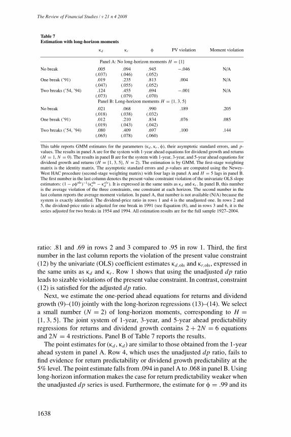
The Review of Financial Studies / v 21 n 4 2008
Table 7Estimation with long-horizon moments
κd κr φ PV violation Moment violation
Panel A: No long-horizon moments H = {1}No break .005 .094 .945 −.046 N/A
(.037) (.046) (.052)One break (’91) .019 .235 .813 .004 N/A
(.047) (.055) (.052)Two breaks (’54, ’94) .124 .455 .694 −.001 N/A
(.073) (.079) (.070)Panel B: Long-horizon moments H = {1, 3, 5}
No break .021 .068 .990 .189 .205(.018) (.038) (.032)
One break (’91) .012 .210 .834 .076 .085(.019) (.043) (.042)
Two breaks (’54, ’94) .080 .409 .697 .100 .144(.065) (.078) (.060)
This table reports GMM estimates for the parameters (κd , κr , φ), their asymptotic standard errors, and p-values. The results in panel A are for the system with 1-year ahead equations for dividend growth and returns(H = 1, N = 0). The results in panel B are for the system with 1-year, 3-year, and 5-year ahead equations fordividend growth and returns (H = {1, 3, 5}, N = 2). The estimation is by GMM. The first-stage weightingmatrix is the identity matrix. The asymptotic standard errors and p-values are computed using the Newey-West HAC procedure (second-stage weighting matrix) with four lags in panel A and H = 5 lags in panel B.The first number in the last column denotes the present-value constraint violation of the univariate OLS slopeestimators: (1 − ρφols)−1(κols
r − κolsd ). It is expressed in the same units as κd and κr . In panel B, this number
is the average violation of the three constraints, one constraint at each horizon. The second number in thelast column reports the average moment violation. In panel A, that number is not available (N/A) because thesystem is exactly identified. The dividend-price ratio in rows 1 and 4 is the unadjusted one. In rows 2 and5, the dividend-price ratio is adjusted for one break in 1991 (see Equation (8), and in rows 3 and 6, it is theseries adjusted for two breaks in 1954 and 1994. All estimation results are for the full sample 1927–2004.
ratio: .81 and .69 in rows 2 and 3 compared to .95 in row 1. Third, the firstnumber in the last column reports the violation of the present value constraint(12) by the univariate (OLS) coefficient estimates κd,ols and κr,ols, expressed inthe same units as κd and κr . Row 1 shows that using the unadjusted dp ratioleads to sizable violations of the present value constraint. In contrast, constraint(12) is satisfied for the adjusted dp ratio.
Next, we estimate the one-period ahead equations for returns and dividendgrowth (9)–(10) jointly with the long-horizon regressions (13)–(14). We selecta small number (N = 2) of long-horizon moments, corresponding to H ={1, 3, 5}. The joint system of 1-year, 3-year, and 5-year ahead predictabilityregressions for returns and dividend growth contains 2 + 2N = 6 equationsand 2N = 4 restrictions. Panel B of Table 7 reports the results.
The point estimates for (κd , κd ) are similar to those obtained from the 1-yearahead system in panel A. Row 4, which uses the unadjusted dp ratio, fails tofind evidence for return predictability or dividend growth predictability at the5% level. The point estimate falls from .094 in panel A to .068 in panel B. Usinglong-horizon information makes the case for return predictability weaker whenthe unadjusted dp series is used. Furthermore, the estimate for φ = .99 and its
1638
Reconciling the Return Predictability Evidence
standard error indicate that we cannot reject the null hypothesis of a unit rootin the dividend-price ratio.15
Results using adjusted series reported in rows 5 and 6 are quite different.Once we use the adjusted ratio dp, we find strong evidence for return pre-dictability. The point estimates remain large: .210 in the one-break case and.409 in the two-break case. Moreover, the asymptotic standard errors on κr
are reduced. The reason is that we use restrictions of the term structure of pre-dictability coefficients that cannot be uncovered by estimating the long-horizonmoments in isolation; imposing these constraints improves the inference on κr
and κd . Put differently, the univariate OLS long-horizon coefficients violate thepresent value constraint. The first number in the last column reports the averageviolation across the three constraints (the RMSE); it is 19% in row 1. This vi-olation is lower in rows 5 and 6. The second number in the last column reportsthe average moment violation (RMSE) and measures the degree to which theimposed restrictions are satisfied. In row 5, the average moment violation isonly 8.5%, less than half as big as in row 4.
The middle and bottom panels of Figure 7 graphically illustrate the long-horizon estimation results with the adjusted dividend-price ratio for the larger{1, 3, 5, 7, 10}-year system. First, the one-period coefficients are very similar tothe ones we reported for the {1, 3, 5}-year system. Second, the two panels showthat when the adjusted dividend-price ratio is used, the pattern of GMM long-horizon regression slopes generated by our model lines up almost perfectly withthe univariate OLS regression slopes. Put differently, the normal conditionsfor the long-horizon moments are satisfied at the model-implied long-horizonpredictability coefficients. This contrasts with the first panel, which is for theunadjusted dp ratio. There, the OLS coefficients are quite different from theGMM estimates. The correction supports both our specification and our mainargument.
The results for the {1, 3, 5}-year and {1, 3, 5, 10}-year systems are represen-tative of the results we found for different numbers of long-horizon momentsand choices of horizons. Imposing long-horizon information confirms the re-sults of the earlier sections: returns are predictable by the dividend-price ratio,once its nonstationary component is removed.
7. Monte Carlo Simulations
In this section, we provide further evidence that the model in Equations (9)–(11)captures the moments of the data well. We use a Monte Carlo exercise to show(i) that this model replicates the failures that are found in the in-sample andout-of-sample predictability literature using the unadjusted dp ratio, and (ii)that it matches the moments once the dividend-price ratio is properly adjustedfor and after taking into account small-sample inference issues.
15 The standard error of φ is implied by the estimates for κd and κr through Equation (12) and computed using thedelta method.
1639
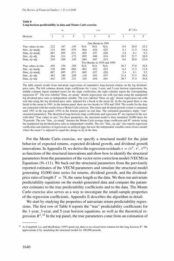
The Review of Financial Studies / v 21 n 4 2008
Table 8Long-horizon predictability in data and Monte Carlo exercise
κr s.e. R2 (%)
Horizon 1 3 5 1 3 5 1 3 5
One Break in 1991True values in sim. .222 .187 .159 N/A N/A N/A 8.9 20.0 25.2Sim., dp unadj. .115 .092 .075 .064 .034 .025 5.1 11.5 14.6Data, dp unadj. .087 .095 .071 .065 .037 .026 2.4 8.1 9.2Sim., dp adj. .264 .214 .175 .093 .048 .034 10.5 22.7 28.0Data, dp adj. .220 .200 .150 .084 .047 .033 8.6 20.0 22.0
Two Breaks in 1954 and 1994True values in sim. .456 .330 .249 N/A N/A N/A 20.7 37.0 38.8Sim., dp unadj. .128 .089 .064 .063 .032 .023 6.2 11.5 12.8Data, dp unadj. .087 .095 .071 .065 .037 .026 2.4 8.1 9.2Sim., dp adj. .483 .340 .249 .110 .052 .037 21.4 37.5 38.6Data, dp adj. .442 .355 .231 .102 .054 .041 20.7 37.4 30.8
The table reports results from univariate regressions of cumulative long-horizon returns on the log dividend-price ratio. The left columns denote slope coefficients for 1-year, 3-year, and 5-year horizon regressions; themiddle columns report standard errors for the slope coefficients; the right columns report the correspondingregression R2. The rows labeled “Data, dp unadj.” denote regressions run with real data using the unadjustedlog dividend-price ratio as independent variable. The rows labeled “Data, dp adj.” denote regressions run withreal data using the log dividend-price ratio, adjusted for a break in the mean dp. In the top panel there is onebreak in this mean in 1991; in the bottom panel, there are two breaks in 1954 and 1994. The results for the dataare contrasted with the results from a Monte Carlo exercise. The return and dividend growth system is estimateduntil 1991 in the top panel (1954 in the bottom panel) on real data. The estimated parameters imply “true”structural parameters. The theoretical long-horizon slope coefficients and regression R2 are reported in the rowwith label “True values in sim.” For these parameters, the structural model is then simulated 10,000 times for78 periods. The row “Sim., dp unadj.” denotes the Monte Carlo average slope coefficient and R2 statistic usingthe unadjusted log dividend-price ratio as independent variable. The row “Sim., dp adj.” also reports regressioncoefficients and statistics of regressions on artificial data, but now the independent variable comes from a modelwhere the mean r is adjusted to equal the change in dp in the data.
For the Monte Carlo exercise, we specify a structural model for the jointbehavior of expected returns, expected dividend growth, and dividend growthinnovations. In Appendix D, we derive the regression residuals τ = (τd , τr , τdp)as functions of the structural innovations and show how to identify the structuralparameters from the parameters of the vector error correction model (VECM) inEquations (9)–(11). We back out the structural parameters from the previouslyreported estimates of the VECM parameters and simulate the structural modelgenerating 10,000 time series for returns, dividend growth, and the dividend-price ratio of length T = 78, the same length as the data. We then run univariatepredictability equations on the model-generated data and compare the param-eter estimates to the true predictability coefficients and to the data. The MonteCarlo exercise also serves as a way to investigate the small-sample propertiesof the regression coefficients. Appendix E describes the algorithm in detail.
We start by studying the properties of univariate return predictability regres-sions. The first row of Table 8 reports the “true” predictability coefficients forthe 1-year, 3-year, and 5-year horizon equations, as well as the theoretical re-gression R2.16 In the top panel, the true parameters come from an estimation of
16 As Campbell, Lo, and MacKinlay (1997) point out, there is no closed-form solution for the long-horizon R2. Weapproximate it by simulating the structural model for 100,000 periods.
1640
Reconciling the Return Predictability Evidence
the VECM that assumes a break in dp in 1991; in the bottom panel we specifytwo breaks, in 1954 and 1994.
The second and fourth rows report the same coefficients and R2 estimateson simulated data. This simulation ignores the presence of the break(s). Row 2uses the unadjusted dp ratio, and row 4 the adjusted dp to predict returns. Thesecond row shows that the model with the unadjusted dp ratio fails to detect thereturn predictability that is present in the data. The simulation-based estimateof κr and the regression R2 are too small. The regression R2 does not increaseenough with the horizon. The 1-year ahead coefficient is not significant whenwe use the small-sample standard error (fourth column). Moreover, this failureof the model matches the failure in the data. Row 3 shows the results of thesame univariate regressions in the data using the unadjusted dp ratio. The slopecoefficients, standard errors, and R2 line up closely with the results from theMonte Carlo simulation without break adjustment.
In row 4, we adjust each Monte Carlo series for a break in 1991 (top panel)or two breaks in 1954 and 1994 (bottom panel). The predictability coefficientsat all horizons now line up closely with their true values. The model withadjusted dp ratio recovers the true predictability pattern of row 1. Moreover,the predictability coefficients, their standard errors, and the regression R2 fromthe model in row 4 match the ones from regressions of observed returns onobserved adjusted dividend-price ratios (row 5). Results for dividend growthregressions are not reported but the simulations recover the lack of predictabilityin the true κd coefficients implied by the VECM.
Comparing row 4 to row 1, we notice that there is some small-sample bias.In line with the findings of Stambaugh (1999), the estimate for κr is upwardbiased. In the first panel, the true value of the slope coefficient in the 1-yearahead return regression is .222 versus .264 in simulation, a bias of .042. Atthe 5-year horizon, the upward bias is only .016. Likewise, the R2 of theregression is slightly upward biased in the simulation: 10.5% versus 8.9% at1-year horizon and 28% versus 25% at the 5-year horizon. In the two-break casereported in the second panel, the bias is smaller. The 1-year ahead coefficientestimate is .483 versus the true value of .456. The upward bias disappears atthe 5-year horizon. Overall, the bias is small relative to the magnitude of thecoefficients, and therefore does not affect our conclusions. Finally, the small-sample standard errors, averaged across Monte Carlo simulations of the samelength of the data, are very similar to the asymptotic standard errors from thedata (middle columns).
Panels 2 and 3 of Table 5 report the out-of-sample prediction errors from asecond Monte Carlo exercise. We simulate the structural model under the nullhypothesis that the data generating process has one break in 1991 (panel 2) orhas two breaks in 1954 and 1994 (panel 3). We compare the same three out-of-sample forecasting exercises as in the data (panel 1). In addition, we look at theforecast errors when we only correct for the second break and not the first one.The “true” parameters in panels 2 and 3 are the same and were obtained from
1641
The Review of Financial Studies / v 21 n 4 2008
the VECM parameters estimated under the assumption of two breaks in 1954and 1994 for the period 1947–2004, the same forecasting period as in panel 1.The details are shown in Appendix E. The Monte Carlo exercise regeneratesthe pattern we found in the data. When the unadjusted dividend-price ratio isused as a forecasting variable, the out-of-sample prediction errors are large andclose to the random walk errors. On the other hand, when we implement theone-break or two-break adjustment in the model, the simulated data generatesubstantially lower prediction errors, mimicking the improvement in the data.
The simple model (9)–(11) replicates the patterns of univariate 1-year aheadand long-horizon regression results in-sample as well as 1-year ahead out-of-sample prediction errors found in the data. In particular, it regenerates (i) thefailures of using the unadjusted dp ratio as a predictor, and (ii) the successesof using the adjusted dp ratio.
8. Conclusion
The macroeconomics literature has recently turned to models with persistentchanges in fundamentals to explain the dramatic change in valuation ratios inthe bull market of the 1990s. Most such models imply a persistent decline inexpected returns or a persistent increase in the dividend growth rate. In thispaper, we argue that either of such changes leads to a persistent decline in themean of financial ratios. Such changes in the mean of valuation ratios haveimportant effects on estimation and inference of return forecasting regressions.We consider various econometric techniques to detect shifts in the mean of priceratios and suggest a simple procedure to extract their stationary component.The adjusted price ratios robustly forecast returns in sample. At the sametime, we show that shifts in the steady-state expected returns and growth rateof fundamentals are responsible for the instability of the return forecastingrelation. Out-of-sample return predictions based on the adjusted price ratiosimprove relative to those based on the unadjusted ratios. However, estimationuncertainty about the magnitude of the break, rather than the break date, isultimately what prevents a real-time investor to profit.
Appendix
A. Data descriptionWe use annual end-of-year data from 1926 to 2004 from CRSP on the value-weighted market return (NASDAQ, NYSE, AMEX), with and without dividendcapitalization. Net return including dividends are denoted Rt and returns ex-cluding dividends are Rex. The dividend yield Dt+1/Pt is the difference ofcapitalized and uncapitalized series; the dividend level is the product of thedividend yield Dt+1/Pt and the price Pt of a portfolio that does not rein-vest dividends. The dividend-price ratio is defined as Dt+1/Pt+1 and dividend
1642

Reconciling the Return Predictability Evidence
growth as the change in the dividend level (Dt+1 − Dt )/Dt . We then definelog returns rt+1 = log(1 + Rt+1), log dividend growth �dt+1 = log(Dt+1/Dt ),and the log dividend-price ratio dpt ≡ dt − pt = log(Dt/Pt ).
Data used in Section 4 are derived from monthly S&P 500 dividend-price andprice-earnings ratios and end-of-month composite price index data from Haver.The data are from January 1946 to December 2004. Book-to-market ratios arefrom Vuolteenaho (2000) for 1927–1999. The observations for 1999–2004 areconstructed using the clean-surplus ratio method with earnings and dividenddata from Haver.
The second panel of Table 6 reports the subsample and full-sample meansof the log earnings-price ratio (ep), dividend-earnings ratio (payout rate), andthe implied mean changes in long-run expected returns r or expected dividendgrowth d. The implied change in r , holding d = 0.0709 fixed, is computedas r = d + (1 + d)(D/E)(E/P). Likewise, the implied change in d, holdingr = .1098 fixed, is computed as d = (r − (D/E)(E/P))/(1 + (D/E)(E/P)).
B. A modified log-approximationIn this section, we extend the Campbell-Shiller log linear approximation toallow for time-varying steady-state growth rates and returns. This frameworkis a useful organizing principle for the empirical analysis in the main text, butmost of our specifications do not impose the approximation. Our results donot depend on the accuracy of the approximation, but the framework helps tounderstand the intuition and implications.
The gross return of an asset is defined as
Rt+1 ≡ Pt+1 + Dt+1
Pt= Dt+1
Dt
1 + Pt+1/Dt+1
Pt/Dt. (B1)
As of period t , the steady-state (gross) growth rate of dividends is Dt andsteady-state expected (gross) returns are Rt , implying a steady state for theprice-dividend ratio in levels (PDt ) and logs (pdt )
PDt = Dt
Rt − Dt=⇒ pdt = dt − log(exp(r t ) − exp(dt )). (B2)
Instead of presuming that the steady-state growth rates and expected returnsare constant, we allow for the possibility that the steady state may change overtime. The only requirement that we impose on the steady state log returns andlog growth rates is that they are martingales; Et [r t+ j ] = r t , Et [dt+ j ] = dt . Inother words, the steady state is constant in expectation only. We also assumethat the steady-state log P/D ratio is a martingale; Et [pdt+ j ] = pdt . Although,in general, these assumptions can be inconsistent with each other since thelog P/D ratio is a nonlinear function of r t and dt , we show in Appendix Cthat the martingale assumptions are satisfied to a very good approximation forreasonable break processes. Log linearizing (B1) around the steady state in
1643
The Review of Financial Studies / v 21 n 4 2008
t + 1 and expressing the variables in deviations from steady state yields
pdt − pdt = (�dt+1 − dt ) − (rt+1 − r t ) + ρt+1(pdt+1 − pdt+1)
+�pdt+1 + �r t+1 − �dt+1, (B3)
where pdt = pt − dt and ρt+1 = exp(pdt+1)
1+exp(pdt+1). The last two assumptions state that
ρt is a martingale, and that deviations from the mean price-dividend ratio areuncorrelated with ρ; Et [ρt+ j ] = ρt and Et [ρt+ j (pdt+ j − pdt )] = 0. Given ourassumptions, we can take conditional expectations and solve the expectationaldifference equation for pdt :
pdt − pdt = Et [�dt+1 − dt ] − Et [rt+1 − r t ] + ρt Et [pdt+1 − pdt+1]. (B4)
=∞∑j=1
ρj−1t Et [�dt+ j − dt ] − Et [rt+ j − r t ]. (B5)
The log price-dividend ratio is the sum of the steady-state price-dividend ratioand the discounted sum of expected dividend growth minus expected returnsin excess of steady-state growth and returns
pdt = pdt +∞∑j=1
ρj−1t Et [�dt+ j ] − Et [rt+ j ], (B6)
where �dt+ j = �dt+ j − dt and rt+ j = rt+ j − r t . The expression in the maintext for dpt follows from (B6) and dpt = −pdt .
C. An asset pricing model with steady-state shifts
This appendix solves a fully specified asset pricing model where the steady-statelog dividend-price ratio follows an approximate, bounded martingale. Breaksin the steady-state dividend-price ratio originate in breaks in the steady-statemean dividend growth rate. Evidence for such breaks in US data is provided inTimmermann (2001).
Log dividend growth is �dt+1 = g + qt + εt+1. The unconditional averageconsumption growth rate is g, qt is the stochastic component of the long-runmean, and εt+1 is a temporary consumption growth shock, εt+1 ∼ N (0, σ2
ε ).Let Qt = (1 − A exp(qt ))−1 for a constant A given next. We assume that Qt isa martingale and show below that this implies that log dividend growth is alsoa martingale.
Qt+1 = Qt + ηt+1
1644
Reconciling the Return Predictability Evidence
The innovation to the random walk is independent from εt+1 and has thefollowing distribution:
ηt+1 ={
0, w.p. π
wt+1, w.p. 1 − π and wt+1 ∼ N(0, σ2
w,t+1
).
With probability π, the innovation wt+1 is 0, where π is close to 1 to capturethat a break is a rare occurrence. With the complementary probability 1 − π,there is a break with normally distributed break size. The innovation standarddeviation of wt+1 is time varying. It takes on the following form:
σw,t+1 = σw(1 − exp(κ(1 − Qt ))). (C1)
This implies that for Qt � 1, σw,t+1 ≈ σw and as Qt → 1, σw,t+1 → 0. Theparameter κ governs how fast the standard deviation of w shrinks as Qt ap-proaches 1 from above. This specification guarantees that Qt > 1 (at least incontinuous time). In other words, Qt is a bounded martingale.
If investors are risk neutral with a time discount factor of β, asset returnshave to satisfy the Euler equation
1 = Et
[β
Dt+1
Dt
1 + Pt+1
Dt+1
PtDt
].
Conjecture that the price-dividend ratio takes the following form:
Pt
Dt= Qt − 1.
Using this conjecture, the Euler equation becomes
1 = Et
[βeg+εt+1 A−1 Qt+1
Qt
].
Because the innovation to Qt+1 is independent from the innovation εt+1, theconjecture is verified for
A = βeg+σ2ε /2 Et
[Qt+1
Qt
]= βeg+σ2
ε /2,
because Qt is a martingale. The log dividend-price ratio is also an (approximate)martingale. Consider a Taylor approximation of dt+1 − pt+1 around Qt :
dt+1 − pt+1 = dt − pt + 1
1 − Qt(Qt+1 − Qt ) + Ot+1.
Because Qt is a martingale, Et [dt+1 − pt+1] = dt − pt + Et [Ot+1]. As long asthe conditional mean of the higher order terms Ot+1 is small, the log dividend-price ratio is approximately a martingale. For reasonable break processes the
1645
The Review of Financial Studies / v 21 n 4 2008
higher order terms turn out to be negligible. For example, if π = .99, σw = 5,and κ =, the conditional mean of the higher-order terms is 0.00006 for a price-dividend ratio level of 40, 0.00017 for a price-dividend ratio level of 20, and0.00048 for a price-dividend ratio of 2, which is tiny compared to the value ofd − p, which is −3.10 on average in a simulation with the same parameters.By the same token, Et [qt+1] ≈ qt . The difference between the conditionalexpectation of qt+1 and qt is −0.000005 for a price-dividend ratio level of 40,−0.0000068 for P/D = 20, and −0.0003114 for a price-dividend ratio of 2.Again, this is small relative to the simulation average for q of −0.0094.
The aforementioned specification imposes that Qt > 1, or equivalently qt >
−∞. It would be easy to impose tighter restrictions on the steady-state logdividend growth rate process qt , based on an priori “reasonable range” forlog dividend growth by modifying (C1). For example, one could impose thatthe long-run dividend growth rate should not be smaller than −5% per year.This amounts to price-dividend ratios in excess of 11.5 (Q > 12.5). The samebounded martingale approach would work with such a restriction.
D. Structural model
We propose a model for log dividend growth �d and log returns r , whereexpected dividend growth z and expected returns x follow an AR(1) withautoregressive coefficient φ
�dt+1 − d = zt + εt+1 zt+1 = φzt + ζt+1 (D1)
rt+1 − r = xt + ηt+1 xt+1 = φxt + ξt+1, (D2)
where d is the long-run mean log dividend growth and r is the long-run meanreturn. The model has three fundamental shocks: a dividend innovation εt+1,an innovation in expected dividends ζt+1, and an innovation in expected returnsξt+1. The return decomposition in Campbell (1991) implies that
ηt+1 = − ρ
1 − ρφξt+1 + ρ
1 − ρφζt+1 + εt+1. (D3)
We assume that all three errors are serially uncorrelated and have zerocross covariance at all leads and lags: Cov(εt+1, ζt+ j ) = 0, ∀ j �= 1, andCov(εt+1, ξt+ j ) = 0, ∀ j �= 1, except Cov(ζt , ξt ) = χ and Cov(ζt , εt ) = λ.
In steady-state, the log dividend-price ratio is dp = log( r−d1+d
), hence dp ≈r−d1+d
and ρ ≈ 1+d1+r . The log dividend-price ratio can be written as
dpt = dt − pt = dp + xt − zt
1 − ρφ. (D4)
This equation clearly shows that the demeaned dividend-price ratio is an im-perfect forecaster of returns. Returns are predicted by xt (D2), which con-
1646
Reconciling the Return Predictability Evidence
tains not only the demeaned dp ratio, but also expected dividend growth zt :xt = (1 − ρφ)(dpt − dp) + zt .
This structural model implies a reduced form model that recovers the twopredictability equations from Section 2:
(�dt+1 − d) = κd (dpt − dp) + τdt+1 (D5)
(rt+1 − r ) = κr (dpt − dp) + τrt+1 (D6)
(dpt+1 − dp) = φ(dpt − dp) + τdpt+1. (D7)
The third equation of this Vector Error Correction Model is an AR(1) processfor the dividend-price ratio. Because of Equation (6), the dividend-price ratio isthe difference of two AR(1) processes with the same root φ, which is again anAR(1) process. We also considered a model where expected dividend growthhas a different autoregressive coefficient ψ �= φ: zt+1 = ψzt + ζt+1. In thatcase the dividend-price ratio is an ARMA(1,1) with roots φ + ψ and −φψ.Since the dp ratio is well described by an AR(1) model in the data, we setφ = ψ.
The slope coefficients are related to the structural parameters
κd = Cov(�dt+1, dt − pt )
Var(dt − pt )= −(1 − ρφ)
(σ2
ζ − χ)
σ2ξ + σ2
ζ − 2χ. (D8)
κr = Cov(rt+1, dt − pt )
Var(dt − pt )= (1 − ρφ)
(σ2
ξ − χ)
σ2ξ + σ2
ζ − 2χ. (D9)
The innovations to the VECM, τ = (τd , τr , τdp), are given by
τdt+1 = εt+1 + xt
( −κd
1 − ρφ
)+ zt
(κr
1 − ρφ
)(D10)
τrt+1 = εt+1 + xt
( −κd
1 − ρφ
)+ zt
(κr
1 − ρφ
)− ρ
ξt+1 − ζt+1
1 − ρφ(D11)
τdpt+1 = ξt+1 − ζt+1
1 − ρφ. (D12)
The structural model imposes a restriction on the innovation vector: ρτdpt+1 =
(τdt+1 − τr
t+1). Another way to write this restriction is as a restriction on aweighted sum of κr and κd :
κr − κd = 1 − ρφ.
We call this restriction the present value constraint.Leaving aside the mean parameters (d, r , dp), which play no role in the
demeaned system, the structural parameter vector is � = (φ, σζ, σξ, σε,χ,λ).The variance σ2
η is implied by (D3). The vector of parameters from the re-
1647
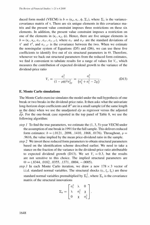
The Review of Financial Studies / v 21 n 4 2008
duced form model (VECM) is b = (κd , κr ,φ, �τ), where �τ is the variance-covariance matrix of τ. There are six unique elements in this covariance ma-trix and the present value constraint imposes three restrictions on these sixelements. In addition, the present value constraint imposes a restriction onone of the elements in (κr , κd ,φ). Hence, there are five unique elements inb = (κr , κd , στr , στd , στr ,τd ), where στr and στd are the standard deviations ofτr and τd , and στr ,τd is the covariance between the two. When we estimatethe nonsingular system of Equations (D5) and (D6), we can use these fivecoefficients to identify five out of six structural parameters in �. Therefore,whenever we back out structural parameters from the reduced form estimates,we find it convenient to tabulate results for a range of values for Vz , whichmeasures the contribution of expected dividend growth to the variance of thedividend-price ratio
Vz = σ2z
(1 − ρφ)2σ2dp
= σ2ζ(
σ2ξ + σ2
ζ − 2χ) . (D13)
E. Monte Carlo simulations
The Monte Carlo exercise simulates the model under the null hypothesis of onebreak or two breaks in the dividend-price ratio. It then asks what the univariatelong-horizon slope coefficients and R2 are in a small sample (of the same lengthas the data) when we use the unadjusted dp as regressor versus the adjusteddp. For the one-break case reported in the top panel of Table 8, we use thefollowing algorithm:
step 1 To find the true parameters, we estimate the (1, 3, 5)-year VECM underthe assumption of one break in 1991 for the full sample. This delivers reducedform estimates: b = (.0121, .2098, .1410, .1868, .0176). Throughout, ρ =.9616, the value implied by the mean price-dividend ratio in the sample.
step 2 We invert these reduced form parameters to obtain structural parametersbased on the identification scheme described earlier. We need to take astance on the fraction of the variance in the dividend-price ratio attributableto expected dividend growth (D13). We set Vz = 0.3, but the resultsare not sensitive to this choice. The implied structural parameters are� = (.8344, .0182, .0355, .1371, .0004,−.0005).
step 3 In each Monte Carlo iteration, we draw a new 178 × 3 vector ofi.i.d. standard normal variables. The structural shocks (εt , ζt , ξt ) are these
standard normal variables premultiplied by �12u , where �u is the covariance
matrix of the structural innovations
�u =
⎡⎢⎣
σ2ε λ 0
λ σ2ζ χ
0 χ σ2ξ
⎤⎥⎦ .
1648

Reconciling the Return Predictability Evidence
step 4 We recursively build up time series for x , r − r , z, and �d − daccording to (D1) and (D2). We form a time series for the demeaneddividend-price ratio from (D4).
step 5a Under the null hypothesis of one break in 1991, the break-adjustedseries for returns, dividend growth, and dividend-price ratio are obtained byadding constant long-run means r , d , and dp to the demeaned series. i.e.,the adjusted dp series is the demeaned series plus the mean over the entiresample 1927–2004, which is dp = −3.272. Likewise, the adjusted dividendgrowth series �d is formed by adding to the demeaned series �d − dthe sample mean d = .0432. We then back out r = d + (1 + d) exp(dp) =.0827, and form the adjusted return series as the demeaned series plus this r .
step 5b On the other hand, the unadjusted series still displays a break in1991. To obtain the unadjusted series, we need to add in a different meanbefore and after 1991. As before, we assume d did not change, so that thechange in dp entirely comes from a change in r . The unadjusted dp seriesis obtained by adding in the 1927–1991 mean (−3.133) before 1991 andthe 1992–2004 mean (−3.968) after 1991. Likewise, for returns, we addin .0886 before 1991 and .0629 after 1991. These are the subsample meansdp and r that were reported in lines 1 and 2 of Table 6 (left panel).
step 6 We form annualized, cumulative long-horizon returns and dividendgrowth rates 1
H
∑Hj=1 �rt+ j and 1
H
∑Hj=1 �dt+ j in the same way. There is
one set of unadjusted series and one set of adjusted series, correspondingto each horizon H .
step 7 After the formation, we discard the first 100 observations (burn-in), andare left with the same number of observations as in the data: 78− longesthorizon +1. For the 1-, 3-, and 5-year system we report on, the longesthorizon is 5, so all statistics are computed with 74 observations.
step 8 We then run univariate 1-, 3-, and 5-year ahead predictability regressionsof adjusted returns and dividend growth on both unadjusted and adjusteddividend-price ratios. We keep track of the predictability coefficients andregression R2.
step 9 We repeat this procedure 10,000 times and report the averagepredictability coefficients and R2 across Monte Carlo iterations.
The Monte Carlo exercise in the two-break case is exactly analogous(bottom panel of Table 8). In step 1, we estimate the 1-, 3-, and 5-year aheadVECM system under the null of two breaks in 1954 and 1994. The VECM co-efficient vector is b = (0.0795, 0.4089, 0.1391, 0.1743, 0.0157). The impliedstructural parameter vector for Vz = 0.3 is � = (0.6974, 0.0293, 0.0635,
0.1339, 0.0014,−0.0012). To construct the unadjusted dp and return serieswe use the means reported in the right panel of Table 6.
We conduct a separate Monte Carlo exercise for the out-of-sample pre-dictability (panels 2 and 3 in Table 5). We simulate the model under the nullhypothesis of two breaks in 1954 and 1994. For simplicity, we use the same true
1649
The Review of Financial Studies / v 21 n 4 2008
parameters in both panels 2 and 3. They are obtained from estimating the 1-yearahead VECM under the assumption of two breaks in 1954 and 1994, but for theperiod 1947–2004, which is the same sample period as we use in the data (panel1 of Table 5). We then construct adjusted and unadjusted dp ratios as in theprevious algorithm, and run the same out-of-sample predictions as in the data.
ReferencesAmihud, Y., and C. M. Hurwich. 2004. Predictive Regressions: A Reduced-Bias Estimation Method. Financialand Quantitative Analysis 39:813–41.
Amihud, Y., C. M. Hurvich, and Y. Wang. 2005. Hypothesis Testing in Predictive Regressions. UnpublishedPaper.
Ang, A., and G. Bekaert. 2006. Stock Return Predictability: Is It There? Review of Financial Studies, forthcoming.
Bai, J., and P. Perron. 1998. Estimating and Testing Linear Models with Multiple Structural Changes. Econo-metrica 66:47–78.
Bainsbergen, J. van, and R. Koijen. 2007. Predictive Regressions: A Present-Value Approach. UnpulishedManuscript.
Bai, J., and P. Perron. 1998. Estimating and Testing Linear Models with Multiple Structural Changes. Econo-metrica 66:47–78.
Berk, J. B., R. C. Green, and V. Naik. 1999. Optimal Investment, Growth Options, and Security Returns. Journalof Finance 54:1153–607.
Bossaerts, P., and P. Hillion. 1999. Implementing Statistical Criteria to Select Return Forecasting Models: WhatDo We Learn? Review of Financial Studies 12:405–28.
Boudoukh, J., R. Michaely, M. Richardson, and M. Roberts. 2004. On the Importance of Measuring PayoutYield: Implications for Empirical Asset Pricing. Working Paper 10651, NBER.
Boudoukh, J., M. Richardson, and R. F. Whitelaw. 2005. The Myth of Long-Horizon Predictability. WorkingPaper, New York University.
Calvet, L., M. Gonzalez-Eiras, and P. Sadini. 2003. Financial Innovation, Market Participation, and Asset Prices.Working Paper 9840, NBER.
Campbell, J. Y. 1991. A Variance Decomposition for Stock Returns. Economic Journal 101:157–79.
Campbell, J. Y., A. W. Lo, and C. MacKinlay. 1997. The Econometrics of Financial Markets. Princeton, NJ:Princeton University Press.
Campbell, J. Y., and R. J. Shiller. 1988. The dividend-price Ratio and Expectations of Future Dividends andDiscount Factors. Review of Financial Studies 1:195–227.
Campbell, J. Y., and S. Thompson. 2007. Predicting the Equity Premium out of Sample: Can Anything Beat theHistorical Average? Working Paper 11468, NBER.
Campbell, J. Y., and M. Yogo. 2002. Efficient Tests of Stock Return Predictability. Unpublished Paper, HarvardUniversity.
Cochrane, J. H. 1991. Explaining the Variance of Price-Dividend Ratios. Review of Financial Studies 5:243–80.
Cochrane, J. H. 2007. The Dog That Did Not Bark: A Defense of Return Predictability. Unpublished Paper,University of Chicago Graduate School of Business.
Eliasz, P. 2005. Optimal Median Unbiased Estimation of Coefficients on Highly Persistent Regressors. Unpub-lished Paper, Department of Economcis, Princeton University.
1650
Reconciling the Return Predictability Evidence
Fama, E. F., and K. R. French. 1988. Dividend Yields and Expected Stock Returns. Journal of FinancialEconomics 22:3–27.
Fama, E. F., and K. R. French. 2001. Disappearing Dividends: Changing Firm Characteristics or Lower Propensityto Pay. Journal of Financial Economics 60:3–43.
Ferson, W. E., S. Sarkissian, and T. T. Simin. 2003. Spurious Regressions in Financial Economics? Journal ofFinance 58:1393–1413.
Goetzmann, W. N., and P. Jorion. 1993. Testing the Predictive Power of Dividend Yields. Journal of Finance48:663–79.
Goyal, A., and I. Welch. 2003. Predicting the Equity Premium with Dividend Ratios. Management Science 49:639–54.
Goyal, A., and I. Welch. 2004. A Comprehensive Look at the Empirical Performance of the Equity PremiumPrediction. Working Paper, Brown University.
Grullon, G., and R. Michaely. 2002. Dividends, Share Repurchases, and the Substitution Hypothesis. Journal ofFinance 57:1649–84.
Guvenen, M. F. 2003. A Parsimonious Macroeconomic Model for Asset Pricing: Habit Formation or Cross-Sectional Heterogeneity? Working Paper 499, Rochester Center for Economic Research.
Hamilton, J. D. 1989. A New Approach to the Analysis of Nonstationary Returns and the Business Cycle.Econometrica 57:357–84.
Hansen, L. P., and R. J. Hodrick. 1980. Forward Exchange Rates as Optimal Predictors of Future Spot Rates: AnEconometric Analysis. Journal of Political Economy 88:829–53.
Hodrick, R. 1992. Dividend Yields and Expected Stock Returns: Alternative Procedures for Inference andMeasurement. Review of Financial Studies 5:357–86.
Jovanovic, B., and P. L. Rousseau. 2003. Specific Capital and the Division of Rents. Unpublished Paper, NewYork University.
Krueger, D., and F. Perri. 2005. Does Income Inequality Lead to Consumption Inequality? Some EmpiricalFindings and a Theoretical Explanation. Review of Economic Studies, forthcoming.
Lamont, O. 1998. Earnings and Expected Returns. Journal of Finance 53:1563–87.
Lettau, M., and S. C. Ludvigson. 2001. Consumption, Aggregate Wealth, and Expected Stock Returns. Journalof Finance 56:815–49.
Lettau, M., and S. C. Ludvigson. 2005. Expected Returns and Expected Dividend Growth. Journal of FinancialEconomics 76:583–626.
Lettau, M., S. C. Ludvigson, and J. A. Wachter. 2004. The Declining Equity Premium: What Role DoesMacroeconomic Risk Play? Forthcoming, Review of Financial Studies.
Lewellen, J. W. 1999. The Time Series Relations Among Expected Return, Risk, and Book-to-Market. Journalof Financial Economics 54:5–53.
Lewellen, J. W. 2004. Predicting Returns with Financial Ratios. Journal of Financial Economics 74:209–235.
Liu, J., S. Wu, and J. Zidek. 1997. On Segmented Multivariate Regressions. Statistica Sinica 7:497–525.
Lustig, H., and S. Van Nieuwerburgh. 2005a. Housing Collateral, Consumption Insurance, and Risk Premia: AnEmpirical Perspective. Journal of Finance 60:1167–219.
Lustig, H., and S. Van Nieuwerburgh. 2006. How Much Does Household Collateral Constrain Regional RiskSharing? Unpublished Manuscript, University of California at Los Angeles and New York University.
Lustig, H., and S. Van Nieuwerburgh. 2007. Can Housing Collateral Explain Long-Run Swings in Asset Returns?.Unpublished Manuscript, University of California at Los Angeles and New York University.
1651
The Review of Financial Studies / v 21 n 4 2008
Mankiw, N. G., and M. Shapiro. 1986. Risk and Return: Consumption Beta versus Market Beta. Review ofEconomics and Statistics 68:452–59.
McGrattan, E. R., and E. C. Prescott. 2005. Taxes, Regulations, and the Value of U.S. and U.K. Corporations.Review of Economic Studies 72.
Menzly, L., T. Santos, and P. Veronesi. 2004. Understanding Predictability. Journal of Political Economy 112:1–47.
Nelson, C. C., and M. J. Kim. 1993. Predictable Stock Returns: The Role of Small Sample Bias. Journal ofFinance 43:641–61.
Pastor, L., and R. F. Stambaugh. 2001. The Equity Premium and Structural Breaks. Journal of Finance 56:1207–39.
Paye, B. S., and A. Timmermann. 2005. Instability of Return Prediction Models. Journal of Empirical Finance,forthcoming.
Pettenuzzo, D., and A. Timmermann. 2005. Predictability of Stock Returns and Asset Allocation under StructuralBreaks. Unpublished Paper, Bocconi University and University of California at San Diego.
Piazzesi, M., M. Schneider, and S. Tuzel. 2006. Housing, Consumption, and Asset Pricing. Journal of FinancialEconomics, forthcoming.
Quadrini, V., and U. Jermann. 2003. Stock Market Boom and the Productivity Gains of the 1990s. UnpublishedPaper, University of Southern California.
Rozeff, M. S. 1984. Dividend Yields A Equity Risk Premia. Journal of Portfolio Managment 49:141–60.
Stambaugh, R. F. 1986. Bias in Regressions with Lagged Stochastic Regressors. Working Paper, University ofChicago.
Stambaugh, R. F. 1999. Predictive Regressions. Journal of Financial Economics 54:375–421.
Timmermann, A. 2001. Structural Breaks, Incomplete Information, and Stock Prices. Journal of Business andEconomic Statistics 19:299–314.
Torous, W., R. Volkanov, and S. Yan. 2004. On Predicting Returns with Nearly Integrated Explanatory Variables.Journal of Business 77:937–66.
Valkanov, R. 2003. Long-Horizon Regressions: Theoretical Results and Applications. Journal of FinancialEconomics 68:201–32.
Viceira, L. 1996. Testing for Structural Change in the Predictability of Asset Returns. Unpublished Manuscript,Harvard University.
Vissing-Jorgensen, A. 2002. Limited Asset Market Participation and Intertemporal Substitution. Journal ofPolitical Economy 110:825–53.
Vuolteenaho, T. 2000. Understanding the Aggregate Book-Market Ratio and Its Implications to Current Equity-Premium Expectations. Unpublished Paper, Harvard University.
1652