Conditional Currency Hedging

MELK C. BUCHER∗

This version: November 2015

ABSTRACT

This research proposes Conditional Currency Hedging based on FX risk factors as a way to improve

the risk/ return trade-off of given stock, bond or commodity portfolios. In our employed sample, a

conditional currency hedging framework based on Volatility, Carry Trade and Dollar Risks results

in lower variance as well as higher average return of a global equity portfolio than achieved by either

no, full or unconditional mean-variance hedging. This suggests that conditioning the hedging policy

upon the state of risk factors could significantly enhance the performance for investors globally.

Further analysis with bond and commodity performance data will follow.

JEL Classification: F31, G11, G15

Keywords: FX risk factors, Currency Hedging, Mean-variance analysis

∗s/bf-HSG, University of St.Gallen. Author contact: melk.bucher@unisg.ch. Bucher would like to thank PaulSoderlind and Angelo Ranaldo for their guidance and feedback. All the views expressed in the paper are of the authoralone.

I. Introduction to the topic

In their long-range study on Global Currency Hedging, Cambpell et al. (2010) find that over-

and under-hedging in certain currencies can lead to risk reductions of global equity portfolios,

relative both to no and to full hedging. Using a mean-variance framework, they form optimal

(zero net-investment) FX portfolios for given stock or bond portfolios. Thereby they rely on equity

(bond) market betas of currencies as a measure of risk.

This paper sets out to extend the analysis by conditioning the analysis on the state of underlying

FX risk factors. The question is whether the optimal exposure to different currencies is a function

of (current and lagged) underlying FX risks. If so, we would expect a superior risk/ return trade-off

of conditional FX hedging relative to no, full as well as unconditional hedging.

A. Risk factors and Pricing in the FX market

The FX risk pricing factors to be employed for conditioning the mean-variance analysis above are

derived from a recent literature stream, which tries to account for the Carry Trade and Momentum

Puzzles in a similar way as Asset Pricing theories in the Equity markets do. The proposed FX

pricing factors focus on different potential explanations. One can distinguish conventional risk

factors, FX returns-based risk factors as well as alternative (non-risk-based) explanations to account

for the profitability of carry and momentum strategies (e.g. Burnside, 2011 & Burnside et al., 2011).

The traditional risk factors employed usually come from the equities realm where literature has

long used them in models to price payoffs in that market. These models encompass the traditional

CAPM (market excess return as sole factor), the three-factor model of Fama and French (1993),

which additionally uses the value and size premia as factors, or more fundamental models employing

industrial production or consumption growth data as factors.

More recently, factors have been derived from currency returns themselves, partially due to

the acknowledgment that FX is a different investment class with different market participants,

and should thus be priced by different risk factors than equities (e.g. Burnside, 2012). One set of

pricing factors are derived from currencies sorted by their forward discount. For instance Lustig et

al. (2011) form two risk factors: the level factor DOL (Dollar Factor) captures the average excess

return of all foreign currency against the dollar; the slope factor HML (Carry Trade Risk Factor) is

the return differential between the highest and lowest discount portfolios and captures carry trade

risk. The authors can relate the latter to global equity market volatility. Menkhoff et al. (2012a)

on the other hand form a direct FX Volatility risk factor (VOL) and are able to account for the

excess returns of the carry trade therewith.

Mancini et al. (2013) have proposed a Liquidity risk factor, and have documented that high-

(low-) yielding currencies offer exposure to (protection from) this risk. In their high-frequency

sample from 2007-2009 the tradable liquidity risk factor IML (illiquid minus liquid) strongly predicts

carry trade performance. Other proposed risk factors include Currency Skewness (e.g. Rafferty,

2011) as well as Correlation Risk (COR (e.g. Mueller et al., 2012). The motivation behind the

2

Skewness factor is the idea that investment currencies of carry trades often crash in tandem as

liquidity dries up. Mueller et al. (2012) provide evidence that high (low) interest rate currencies

have high (low) correlation risk exposure, that is they fare relatively worse (better) during times of

increased exchange rate correlation. Finally, Burnside (2012) argues that the profitability of carry

trade and momentum could be due to the possibility of rare disasters or Peso Problems. When

these rare disasters do not occur in sample, the model cannot be calibrated properly and thus

produces unaccounted-for excess returns.

Another argument states that risk factors alone cannot explain the whole outperformance of

carry trade and momentum (Barroso et al., 2013). Barroso et al. (2013) for instance explain

the outperformance with non-profit-maximizing market participants (such as Central Banks), a

Scarcity of Profit-seeking Capital and abundance of capital pursuing goals unrelated to profitability.

Other potential factors cited in the literature are Microstructure-based explanations –such as price

pressure (e.g. Burnside, Eichenbaum & Rebelo, 2011) or adverse selection (Burnside, Eichenbaum

& Rebelo, 2009)–, Behavioral explanations (e.g. Burnside, Han, Hirshleifer & Wang, 2011) or Limits

to arbitrage (e.g. Menkhoff et al., 2012b).

B. Conditional approaches in Asset Pricing

Apart from incorporating novel risk factors, recent international finance literature has also often

employed conditional approaches and models.

Christiansen, Ranaldo and Soderlind (2011) for instance capture time-varying systematic risk

of carry trade strategies in the form of a logistic smooth transition regression model. They ap-

ply regime-changing constants and coefficients to risk factors, based on FX volatility and liquidity

regime variables. Thereby, they find a strong negative effect of volatility on carry trade performance

by the direct effect of the changing constant as well as the increased correlation with traditional

risk factors in high-volatility periods. This pattern is also reflected in individual currencies with

investment (funding) currencies exhibiting increased positive (negative) correlation with stock re-

turns and increased negative (positive) correlation with bond returns in times of higher volatility;

this in-line with relatively constant safe haven versus investment characteristics of currencies. The

conditional (regime-dependent) risk exposure thereby drastically increases the cross-sectional model

fit of the asset pricing model.

Lettau, Maggiori and Weber (2014) have recently proposed a downside risk capital asset pricing

model (DR-CAPM). Apart from the unconditional CAPM market beta, they additionally posit a

(conditional) downside beta, defined by an exogenous threshold for the market return. The central

finding thereby is that the currency carry trade, as well as other cross-sectional strategies, is more

highly correlated with aggregate market returns conditional on low aggregate returns than it is

conditional on high aggregate market returns (p. 10). The DR-CAPM can jointly explain the

cross-sectional fit across different asset classes, such as currencies, equities, equity index options,

sovereign bonds and commodities. Like Christiansen et al. (2011), they also employ a form of

contemporaneous conditionality.

3

C. Proposed Research

C.1. Research Gap

How is the conditional correlation between equities, bonds and commodities with FX impacted

by FX risk factors? While Campbell et al. (2010) condition upon interest differentials and find no

significant difference between their baseline unconditional and conditional models, we can perform

a similar analysis with the recently proposed FX risk factors as conditioning information: These

encompass Carry Trade, Dollar and Momentum Performance, as well as Volatility, Liquidity and

Correlation Risks. This results in a more fundamental analysis in the sense of identifying the

nature of the underlying risk impacting the equity-FX correlation, rather than taking the equity

market-beta of currencies as both risk measure as well as input to the mean-variance analysis. If the

underlying premise of time-varying correlation according to the FX risk state is true, this implies

lower-than-anticipated diversification benefits through static (unconditional) FX hedging as well as

an outperformance of conditional relative to unconditional FX hedging.

C.2. Research Question

How do FX risk factors impact the dependence between FX and equities, bonds and commodities

markets, and thus the mean-variance hedging rationale of investors in these asset classes?

C.3. Research Goal

The main research goal is to find out if and in what way the optimal hedging rationale for global

equity, bond and commodities investors is impacted by changing FX risks. The underlying premise

is that the optimal (variance-minimizing) FX portfolio weights are not static, but a function of

the current risk state of financial markets. Thus, the basic hypothesis to be tested is whether risk

factors have an impact on the mean-variance FX hedging strategy of international equity, bond

and commodity portfolios through time.

The proposed paper leads to several contributions: For one, it applies the findings of recent

research with regards to FX pricing factors in the context of portfolio risk management. This

leads to a more fundamental understanding of the channel of various risks on the co-movement and

relationship between different asset classes under different conditions. For two, concrete recom-

mendations will be derived in terms of optimal (risk-dependent) hedging for investor in different

asset classes.

II. Research Design

The proposed research is an empirical panel study on optimal hedging of international invest-

ment portfolios with changing FX positions depending on risk factors. As far as possible, the

research design follows Campbell et al. (2010)’s analysis in order to ensure comparability of results

as well as consistency in analysis.

4

A. Risk/ pricing factors

Given that the focus of analysis is not upon a particular risk factor, but rather on the effect of

broader FX risks on the co-dependency between currencies with equities, bonds and commodities,

the paper deliberately considers a variety of factors. Thereby we start with the two most established

FX-based risk factors: The Dollar and Carry Trade Risk factors, as defined in Lustig et al. (2011)

(or in Verdelhan, 2013). As mentioned in section 1.2 the Dollar Factor effectively measures the

average excess return on all foreign currency portfolios against the dollar, while the carry trade risk

factor is similar to a zero-cost strategy long in the highest forward-discount currencies and short in

the lowest forward-discount currencies. As Verdelhan (2013) finds, Carry and Dollar factors reflect

two distinct kinds of global shocks.

We then add Momentum and FX-Volatility risk factors, as defined in Menkhoff et al. (2012b).

As Menkhoff et al. (2012b) as well as Burnside, Eichenbaum and Rebelo (2011) find, the momen-

tum strategy has different risk-return characteristics than the carry trade and likely thus capture

different fundamental risk factors. The FX volatility factor might be strongly related to the carry

factor defined above, given that Lustig et al. (2011) have found the latter to be related to Equity

volatility. Lastly, we add Illiquidity (Mancini et al., 2013) as well as Correlation (Mueller et al.,

2014) risk factors.

In staying close to the Asset Pricing literature, we measure all risk factors on a global, instead

of on a currency-specific level. This has the advantage that we measure the sensitivity of currencies

with respect to global shocks, rather than idiosyncratic phenomena. On the other hand, we thereby

imply (much as in a CAPM framework) relatively constant sensitivity of individual currencies to

these risk factors over time.

More specifically, we employ the following measurements for the conditioning variables:

1. Dollar factor (DOL): Equally-weighted excess return of all (foreign) currencies against the

dollar (Lustig et al., 2011)

2. Carry Trade factor (HML): Excess return of highest forward discount minus lowest forward

discount currency portfolios (in USD) (Lustig et al., 2011)

3. Volatility (VOL) pricing factor: Average absolute log return of all available currencies in a

given time interval (Menkhoff et al., 2012a)

4. Momentum factor (MOM ): Excess return of best-performing minus lowest-performing (over

a past holding period) currency portfolios (Menkhoff et al., 2012b)

5. Illiquidity factor (IML): Measure based on average price impact and return reversal, trading

cost and price dispersion of all available currencies in a given time interval (Mancini et al.,

2013)

6. Correlation factor (COR): Average of realized correlations of all available currencies in a given

time interval (Mueller et al., 2012)

5

B. Baseline analysis

The empirical analysis is based on the estimation of risk-minimizing currency positions for

exogenously given stock, bond and commodity portfolios. Risk is thereby defined as the standard

deviation of the portfolio. Campbell et al. (2010) show that unconditional mean-variance analysis

amounts to regressing the hedged portfolio excess returns in domestic currency on a constant and

the vector of currency excess returns, and switching the sign of the slopes.

To incorporate conditionality, they interact the regressors (the currency excess returns) with the

conditional information –in their case the deviation of interest rate differentials from their time-

series mean. In other words, they “consider a conditional model for risk management currency

demand that depends linearly on interested differentials (p.111)”. We can proceed similarly in our

case and regress hedged excess portfolio returns on a constant, the vector of currency excess returns

as well as additionally the vectors of currency excess returns interacted with the six risk factors.

Following Verdelhan (2013), we break down the carry factor into an unconditional one (HML) as

well as a conditional one (HML multiplied by the interest differential of the currencies). This leads

to a conditionality in conditionality.

B.1. Formal conditional mean-variance estimation procedure

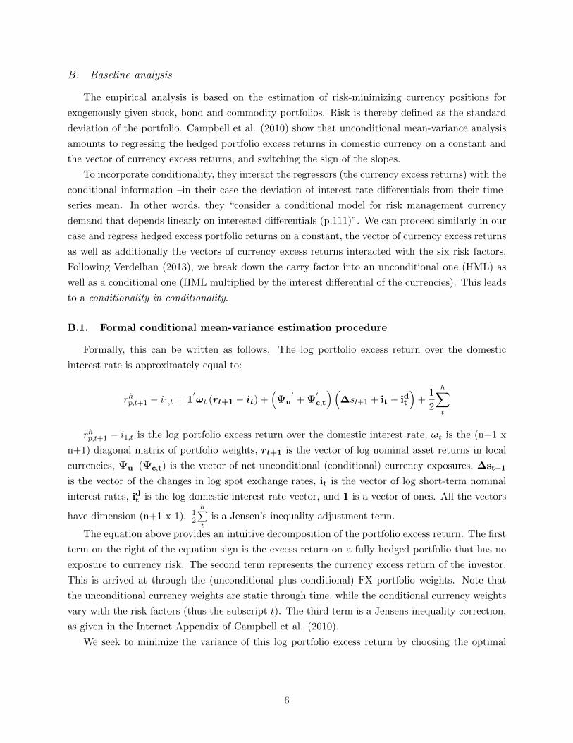
Formally, this can be written as follows. The log portfolio excess return over the domestic

interest rate is approximately equal to:

rhp,t+1 − i1,t = 1′ωt (rt+1 − it) +

(Ψu

′+ Ψ

′c,t

)(∆st+1 + it − idt

)+

1

2

h∑t

rhp,t+1 − i1,t is the log portfolio excess return over the domestic interest rate, ωt is the (n+1 x

n+1) diagonal matrix of portfolio weights, rt+1 is the vector of log nominal asset returns in local

currencies, Ψu (Ψc,t) is the vector of net unconditional (conditional) currency exposures, ∆st+1

is the vector of the changes in log spot exchange rates, it is the vector of log short-term nominal

interest rates, idt is the log domestic interest rate vector, and 1 is a vector of ones. All the vectors

have dimension (n+1 x 1). 12

h∑t

is a Jensen’s inequality adjustment term.

The equation above provides an intuitive decomposition of the portfolio excess return. The first

term on the right of the equation sign is the excess return on a fully hedged portfolio that has no

exposure to currency risk. The second term represents the currency excess return of the investor.

This is arrived at through the (unconditional plus conditional) FX portfolio weights. Note that

the unconditional currency weights are static through time, while the conditional currency weights

vary with the risk factors (thus the subscript t). The third term is a Jensens inequality correction,

as given in the Internet Appendix of Campbell et al. (2010).

We seek to minimize the variance of this log portfolio excess return by choosing the optimal

6

unconditional and conditional currency weights:

argmin(σ2p,t+1)

Ψu,Ψc,t

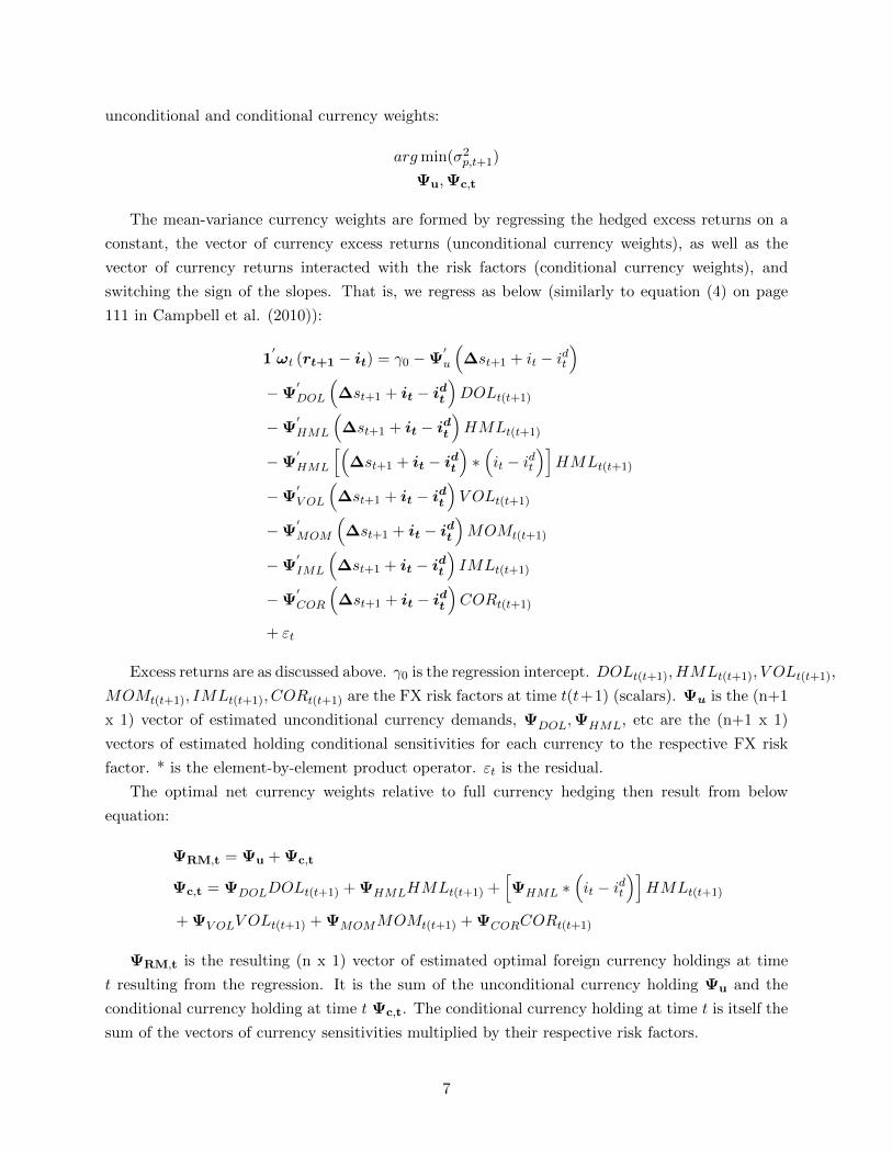
The mean-variance currency weights are formed by regressing the hedged excess returns on a

constant, the vector of currency excess returns (unconditional currency weights), as well as the

vector of currency returns interacted with the risk factors (conditional currency weights), and

switching the sign of the slopes. That is, we regress as below (similarly to equation (4) on page

111 in Campbell et al. (2010)):

1′ωt (rt+1 − it) = γ0 − Ψ

′u

(∆st+1 + it − idt

)− Ψ

′DOL

(∆st+1 + it − idt

)DOLt(t+1)

− Ψ′HML

(∆st+1 + it − idt

)HMLt(t+1)

− Ψ′HML

[(∆st+1 + it − idt

)∗(it − idt

)]HMLt(t+1)

− Ψ′V OL

(∆st+1 + it − idt

)V OLt(t+1)

− Ψ′MOM

(∆st+1 + it − idt

)MOMt(t+1)

− Ψ′IML

(∆st+1 + it − idt

)IMLt(t+1)

− Ψ′COR

(∆st+1 + it − idt

)CORt(t+1)

+ εt

Excess returns are as discussed above. γ0 is the regression intercept. DOLt(t+1), HMLt(t+1), V OLt(t+1),

MOMt(t+1), IMLt(t+1), CORt(t+1) are the FX risk factors at time t(t+1) (scalars). Ψu is the (n+1

x 1) vector of estimated unconditional currency demands, ΨDOL,ΨHML, etc are the (n+1 x 1)

vectors of estimated holding conditional sensitivities for each currency to the respective FX risk

factor. * is the element-by-element product operator. εt is the residual.

The optimal net currency weights relative to full currency hedging then result from below

equation:

ΨRM,t = Ψu + Ψc,t

Ψc,t = ΨDOLDOLt(t+1) + ΨHMLHMLt(t+1) +[ΨHML ∗

(it − idt

)]HMLt(t+1)

+ ΨV OLV OLt(t+1) + ΨMOMMOMt(t+1) + ΨCORCORt(t+1)

ΨRM,t is the resulting (n x 1) vector of estimated optimal foreign currency holdings at time

t resulting from the regression. It is the sum of the unconditional currency holding Ψu and the

conditional currency holding at time t Ψc,t. The conditional currency holding at time t is itself the

sum of the vectors of currency sensitivities multiplied by their respective risk factors.

7

As in Campbell et al. (2010), we are primarily interested in estimating the vector of the slopes

ΨDOL,ΨHML, etc. and testing whether they are different from zero. If they are zero (null hypothe-

sis), we reover the purely unconditional risk management demands. If they are different from zero,

the conditional risk factors do impact the optimal hedging rationale vis-a-vis unconditional hedging

demands.

We can then analyze the standard deviation, mean returns, the Sharpe ratio and other risk/

return characteristics of the unhedged, hedged, unconditional mean-variance as well as conditional

mean-variance portfolios. The working hypothesis is for the conditional mean-variance portfolio

to have the lowest standard deviation of all portfolios. If it is statistically different (lower) than

the unconditional standard deviation, it would be an indication that optimal risk management

demands are impacted by conditioning on risk factors at a given time.

C. Data

C.1. Variables and sources

The data collection effort is similar as in Campbell et al. (2010). The empirical analysis

is based on stock return data from Morgan Stanley Capital International (MSCI), whereby total

return country indices in local currencies are used. Data on spot exchange rates, short-term interest

rates, and long-term bond yields are mainly from the International Financial Statistics database

(IFS) of the International Monetary Fund (IMF). Whenever such data is not available, we resort

to OECD data1. Excess returns of all bilateral exchange rates (e.g./ CAD-EUR) are implied by

the relative excess returns of the involved currencies to the USD.

The main data sample is as in Campbell et al. (2010), encompassing the Eurozone, Australia,

Canada, Japan, Switzerland, the United Kingdom and the United States. These are the 7 countries

where data on all of above go back longest (July 1975). The Eurozone is proxied by Germany (in

terms of exchange rate, stock market as well as interest rate data) before introduction of the Euro

in January 1999. A broader sample with FX, interest rates and stock data on more countries,

but in a smaller timeframe (given availability) may be added to that subsequently to see whether

the findings can be generalized to other countries, including Emerging Economies. Additionally

to Campbell et al. (2010), we will also add various commodity index return data to analyze the

hedging regime for Commodity investors.

To construct our conditional risk factors, we obtain FX data of the same set of 48 currencies

as in Menkhoff et al. (2012). We directly get the DOL, HML and VOL risk factor data from the

authors Menkhoff et al. (2012), underlying their article on Currency Momentum Strategies. The

data thereby ranges from March 1976 to January 2010. After that, we construct the risk factors

by the same recipe as Lustig et al. (2011) (DOL, HML) and Menkhoff et al. (2012) (VOL, MOM),

respectively. We will double-check that our calculated risk factor values are historically the same

as the ones we obtain directly. The IML and COR risk factors will be constructed as described by

1For Switzerland, in the time span from 1976:3 to 1979:12, we use OECD data given unavailable IMF data.

8

Mancini et al. (2013) and Mueller et al. (2012), respectively, based on our sample of 48 currencies.

Data are monthly. The sample period starts in March 1976, the earliest date for which we have

data for all variables (including Risk Factors), and ends in October 2014.

C.2. Data transformation

For the baseline analysis, data are transformed as in Campbell et al. (2010) (see pages 91-95).

This we do to ensure comparability of our results with our enlarged sample with the findings of

Campbell et al. (2010). First we take logs of returns, as this allows for the additive portfolio return

decomposition outlined in II.B before. We then form 3-month-overlapping (log) returns for stock,

bond and FX excess returns. We correct for the inherent autocorrelation by forming Newey-West

(HAC) standard errors with automatic lag detection.

Additionally, as a robustness test, we will form 1- and 3- month non-overlapping returns, and

see how our results are affected. This will presumably have the benefit of removing or reducing the

inherent autocorrelation, and possibly lead to more exact coefficient estimates (optimal currency

weights).

III. Preliminary analysis and results

Our preliminary analysis is based on stock and FX excess returns as well as risk factor data

(DOL, HML, VOL) from March 1976 to January 2010. This time span is employed, as the data

set on risk factors obtained from Menkhoff et al. (2010) ends in January 2010. The data are

transformed as discussed above.

A. Summary statistics

To get an intuition of the underlying data, we first run some descriptive statistics. It is instruc-

tive to compare these to the values in Campbell et al. (2010), whose sample ends in 2005, and see

in what way they are different in our enlarged dataset including the years of the financial crisis.

This is worthwile, as it impacts subsequent unconditional and conditional analysis results.

Interest rates are generally lower in all 7 countries compared to Campbell et al. (2010). This is

not surprising as the added data from 2006 until 2010 falls in a timespan of extremely low interest

rates, as monetary authorities worldwide grappled with the aftermath of the Financial Crisis and

subsequent Recession. However, especially Euroland has much lower rates than in the sample of

our baseline paper this is due to our different definition of Euroland, featuring only Germany

as the Eurozone ante-1999. Campbell et al. (2010), on the other hand, construct Euroland as a

stock market value-weighted index of Germany, France, Italy and the Netherlands. This different

definition of Euroland before 1999 also impacts the other variables (lower excess stock returns,

higher log exchange rate changes).

Excess stock returns are consistently lower than in Campbell et al. (2010)’s sample, given that

2006-2010 featured heavy stock market losses. In terms of log exchange rate changes, the data look

9

rather similar to Campbells sample, with somewhat higher values for Euroland (as explained) and

Switzerland, as the Swiss Franc appreciated strongly during the Crisis period. Excess currency

returns are quite similar.

B. Unconditional FX hedging

In this section we proceed along the unconditional analysis in Campbell et al. (2010) to see

whether and to what extent the findings can be replicated in our enlarged dataset. This forms the

base model on top of which the conditional risk factors will then be introduced in the next section.

Formally, as discussed in II.B before, the unconditional analysis regresses an exogenously given

stock portfolio (hedged excess returns in local currencies) on an intercept and a vector of currency

excess returns (against the domestic currency of the investor) in order to find the unconditional

optimal currency demands relative to full hedging currency demands. This is shown below:

1′ωt (rt+1 − it) = γ0 − Ψ

′u

(∆st+1 + it − idt

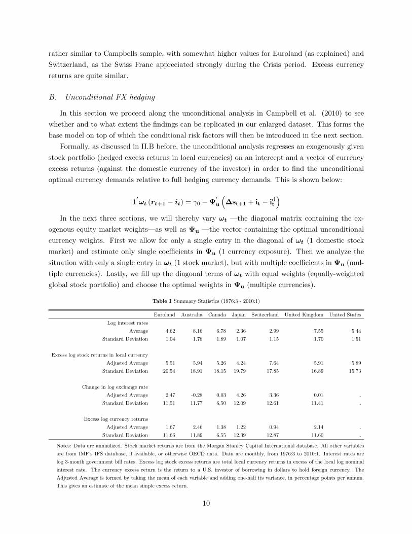
)In the next three sections, we will thereby vary ωt —the diagonal matrix containing the ex-

ogenous equity market weights—as well as Ψu —the vector containing the optimal unconditional

currency weights. First we allow for only a single entry in the diagonal of ωt (1 domestic stock

market) and estimate only single coefficients in Ψu (1 currency exposure). Then we analyze the

situation with only a single entry in ωt (1 stock market), but with multiple coefficients in Ψu (mul-

tiple currencies). Lastly, we fill up the diagonal terms of ωt with equal weights (equally-weighted

global stock portfolio) and choose the optimal weights in Ψu (multiple currencies).

Table I Summary Statistics (1976:3 - 2010:1)

Euroland Australia Canada Japan Switzerland United Kingdom United States

Log interest rates

Average 4.62 8.16 6.78 2.36 2.99 7.55 5.44

Standard Deviation 1.04 1.78 1.89 1.07 1.15 1.70 1.51

Excess log stock returns in local currency

Adjusted Average 5.51 5.94 5.26 4.24 7.64 5.91 5.89

Standard Deviation 20.54 18.91 18.15 19.79 17.85 16.89 15.73

Change in log exchange rate

Adjusted Average 2.47 -0.28 0.03 4.26 3.36 0.01 .

Standard Deviation 11.51 11.77 6.50 12.09 12.61 11.41 .

Excess log currency returns

Adjusted Average 1.67 2.46 1.38 1.22 0.94 2.14 .

Standard Deviation 11.66 11.89 6.55 12.39 12.87 11.60 .

Notes: Data are annualized. Stock market returns are from the Morgan Stanley Capital International database. All other variables

are from IMF’s IFS database, if available, or otherwise OECD data. Data are monthly, from 1976:3 to 2010:1. Interest rates are

log 3-month government bill rates. Excess log stock excess returns are total local currency returns in excess of the local log nominal

interest rate. The currency excess return is the return to a U.S. investor of borrowing in dollars to hold foreign currency. The

Adjusted Average is formed by taking the mean of each variable and adding one-half its variance, in percentage points per annum.

This gives an estimate of the mean simple excess return.

10

B.1. Single Country Stock Portfolios with Single Currency Exposure

The empirical analysis first examines the case of an investor who is fully invested in a specific

country stock market and is considering whether exposure to other currencies could help reduce

the volatility of his quarterly portfolio return.

Table II below shows the case of an investor holding an exogenous stock portfolio from a single

country, and can use just one foreign currency to manage risk. The cells of Table II indicate the

unconditionally optimal amount of U.S. dollars invested long (if positive) or short (if negative) in

the respective currency (in columns), given a certain base country stock index (and currency) (in

rows). We report Newey-West heteroskedasticity and autocorrelation consistent standard errors

in parentheses below each optimal currency exposure, and indicate with one, two, or three stars

coefficients for which we reject the null of zero at 10%, 5%, and 1% significance level, respectively.

In other words, we consider an investor who is deciding how much to hedge of the currency

exposure implicit in an investment in a specific stock market, in isolation of other investments the

investor might hold. For instance, the first non-empty entry in the first column corresponds to the

Australian stock market and the euro, and has a value of 0.45 (significant at 1%). This means

that a risk-minimizing Euroland investor with an exogenous Australian stock market portfolio and

with access to The Australian dollar and the euro should buy a portfolio of euro-denominated bills

worth 1.45 euros per euro invested in the Australian stock market, financing this long position

by borrowing in Australian dollars. That is, he should overhedge the Australian dollar exposure

incurred through his stock market holdings, and a hold a net 45% exposure to the EUR/AUD

exchange rate.

11

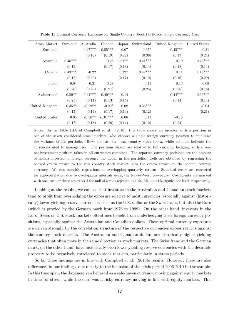
Table II Optimal Currency Exposure for Single-Country Stock Portfolios: Single Currency Case

Stock Market Euroland Australia Canada Japan Switzerland United Kingdom United States

Euroland -0.47*** -0.55*** 0.07 0.65* -0.45*** -0.31

(0.16) (0.19) (0.22) (0.36) (0.17) (0.24)

Australia 0.45*** 0.25 0.31** 0.41*** 0.19 0.43***

(0.15) (0.17) (0.13) (0.14) (0.18) (0.14)

Canada 0.43*** -0.22 0.32* 0.42*** 0.11 1.18***

(0.12) (0.20) (0.17) (0.12) (0.16) (0.29)

Japan 0.04 -0.31 -0.28 0.15 -0.13 -0.09

(0.28) (0.20) (0.21) (0.25) (0.26) (0.18)

Switzerland -0.59** -0.44*** -0.49*** -0.14 -0.44*** -0.39***

(0.25) (0.11) (0.13) (0.15) (0.14) (0.14)

United Kingdom 0.35** -0.29** -0.29* 0.08 0.36*** -0.04

(0.15) (0.14) (0.17) (0.14) (0.12) (0.21)

United States 0.05 -0.36** -1.01*** 0.06 0.13 -0.15

(0.17) (0.18) (0.26) (0.14) (0.12) (0.24)

Notes: As in Table IIIA of Campbell et al. (2010), this table shows an investor with a position in

one of the seven considered stock markets, who chooses a single foreign currency position to minimize

the variance of his portfolio. Rows indicate the base country stock index, while columns indicate the

currencies used to manage risk. The positions shown are relative to full currency hedging, with a zero

net-investment position taken in all currencies combined. The reported currency positions are the amount

of dollars invested in foreign currency per dollar in the portfolio. Cells are obtained by regressing the

hedged excess return to the row country stock market onto the excess return on the column country

currency. We run monthly regressions on overlapping quarterly returns. Standard errors are corrected

for autocorrelation due to overlapping intervals using the Newey-West procedure. Coefficients are marked

with one, two, or three asterisks if the null of zero is rejected at 10%, 5%, and 1% signficance level, respectively.

Looking at the results, we can see that investors in the Australian and Canadian stock markets

tend to profit from overhedging the exposure relative to most currencies, especially against (histori-

cally) lower-yielding reserve currencies, such as the U.S. dollar or the Swiss franc, but also the Euro

(which is proxied by the German mark from 1976 to 1999). On the other hand, investors in the

Euro, Swiss or U.S. stock markets oftentimes benefit from underhedging their foreign currency po-

sitions, especially against the Australian and Canadian dollars. These optimal currency exposures

are driven strongly by the correlation structure of the respective currencies excess returns against

the country stock markets. The Australian and Canadian dollars are historically higher-yielding

currencies that often move in the same direction as stock markets. The Swiss franc and the German

mark, on the other hand, have historically been lower-yielding reserve currencies with the desirable

property to be negatively correlated to stock markets, particularly in stress periods.

So far these findings are in line with Campbell et al. (2010)s results. However, there are also

differences in our findings, due mostly to the inclusion of the crisis period 2006-2010 in the sample.

In this time span, the Japanese yen behaved as a safe-haven currency, moving against equity markets

in times of stress, while the euro was a risky currency moving in-line with equity markets. This

12

impacts our results with regards to investors in the Japan and Euroland stock markets: While

Euro, Swiss and British investors in the Japanese stock market should have overhedged their yen

exposure in Campbell et al. (2010)s sample, this is no longer the case. Generally, the yen should

be about fully hedged by investors domiciled in the other six currencies. Also, investments into the

Euroland stock market should generally be less strongly underhedged than in Campbells sample,

where all but Swiss investors should have underhedged their euro exposure.

B.2. Single Country Stock Portfolios with Multiple Currencies Exposure

Table III depicts the situation for investors in the respective row stock markets that now have

not one, but all of the discussed currencies at their disposal to optimally hedge their 3-month stock

returns. Note that the investor basically overlays an optimal zero-net investment strategy on top of

his inherent currency exposure through the stock market investment. Thus, the currency exposures

in each row must add up to zero, with the diagonal term (stock market base currency) being the

opposite of the sum of the other cells in the same row.

Some stylized facts emerge: Most strikingly, the Canadian dollar seems to be positively corre-

lated to all country-stock markets and thus a short position in the Canadian dollar is optimal for

investors in all seven stock markets. Less strong are the short positions in the Australian dollar

and the British pound. These currency short positions are then invested in positive positions in

the U.S. dollar and/ or the Swiss franc. Positions in the Japanese yen are generally near zero (fully

hedged).

Compared to Campbell et al. (2010), in our analysis the optimal euro exposure is lower, usually

only slightly (statistically insignificantly) above zero. On the other hand, the optimal yen exposure

is only slightly negative, much closer to zero, than in Campbell et al. (2010)’s sample until 2005.

This is most likely due to the aforementioned depreciation (appreciation) of the euro (yen) in the

Financial crisis.

13

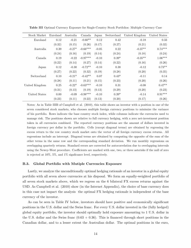
Table III Optimal Currency Exposure for Single-Country Stock Portfolios: Multiple Currency Case

Stock Market Euroland Australia Canada Japan Switzerland United Kingdom United States

Euroland 0.12 -0.21 -0.60** 0.12 0.42 -0.18 0.33

(0.32) (0.15) (0.26) (0.17) (0.27) (0.21) (0.32)

Australia 0.39 -0.27* -0.66*** -0.05 0.22 -0.37** 0.74***

(0.24) (0.16) (0.19) (0.14) (0.24) (0.18) (0.24)

Canada 0.19 -0.22 -0.97*** -0.10 0.39* -0.35** 1.06***

(0.22) (0.14) (0.27) (0.14) (0.22) (0.16) (0.26)

Japan 0.12 -0.30 -0.72** -0.10 0.38 -0.12 0.73**

(0.27) (0.22) (0.32) (0.19) (0.28) (0.20) (0.35)

Switzerland 0.10 -0.21* -0.42** 0.07 0.43* -0.11 0.14

(0.28) (0.11) (0.21) (0.15) (0.23) (0.20) (0.26)

United Kingdom 0.25 -0.22* -0.63*** -0.10 0.31 -0.08 0.47**

(0.31) (0.13) (0.19) (0.13) (0.29) (0.20) (0.23)

United States 0.00 -0.09 -0.98*** -0.10 0.39* -0.14 0.91***

(0.23) (0.11) (0.22) (0.13) (0.20) (0.17) (0.26)

Notes: As in Table IIIB of Campbell et al. (2010), this table shows an investor with a position in one of the

seven considered stock markets, who chooses multiple foreign currency positions to minimize the variance

of his portfolio. Rows indicate the base country stock index, while columns indicate the currencies used to

manage risk. The positions shown are relative to full currency hedging, with a zero net-investment position

taken in all currencies combined. The reported currency positions are the amount of dollars invested in

foreign currency per dollar in the portfolio. Cells (except diagonal terms) are obtained by regressing the

excess return to the row country stock market onto the vector of all foreign currency excess returns. All

regressions include an intercept. Diagonal terms are obtained by computing the opposite of the sum of the

other terms in the same row and the corresponding standard deviation. We run monthly regressions on

overlapping quarterly returns. Standard errors are corrected for autocorrelation due to overlapping intervals

using the Newey-West procedure. Coefficients are marked with one, two, or three asterisks if the null of zero

is rejected at 10%, 5%, and 1% signficance level, respectively.

B.3. Global Portfolio with Mutiple Currencies Exposure

Lastly, we analyze the unconditionally optimal hedging rationale of an investor in a global equity

portfolio with all seven above currencies at his disposal. We form an equally-weighted portfolio of

all seven stock markets above, which we regress on the 6 bilateral FX excess returns against the

USD. As Campbell et al. (2010) show (in the Internet Appendix), the choice of base currency does

in this case not impact the analysis the optimal FX hedging rationale is independent of the base

currency of the investor.

As can be seen in Table IV below, investors should have positive and economically significant

positions in the U.S. dollar and the Swiss franc. For every U.S. dollar invested in the (fully hedged)

global equity portfolio, the investor should optimally hold exposure amounting to 1 U.S. dollar in

the U.S. dollar and the Swiss franc (0.63 + 0.36). This is financed through short positions in the

Canadian dollar, and to a lesser extent the Australian dollar. The optimal positions in the euro,

14

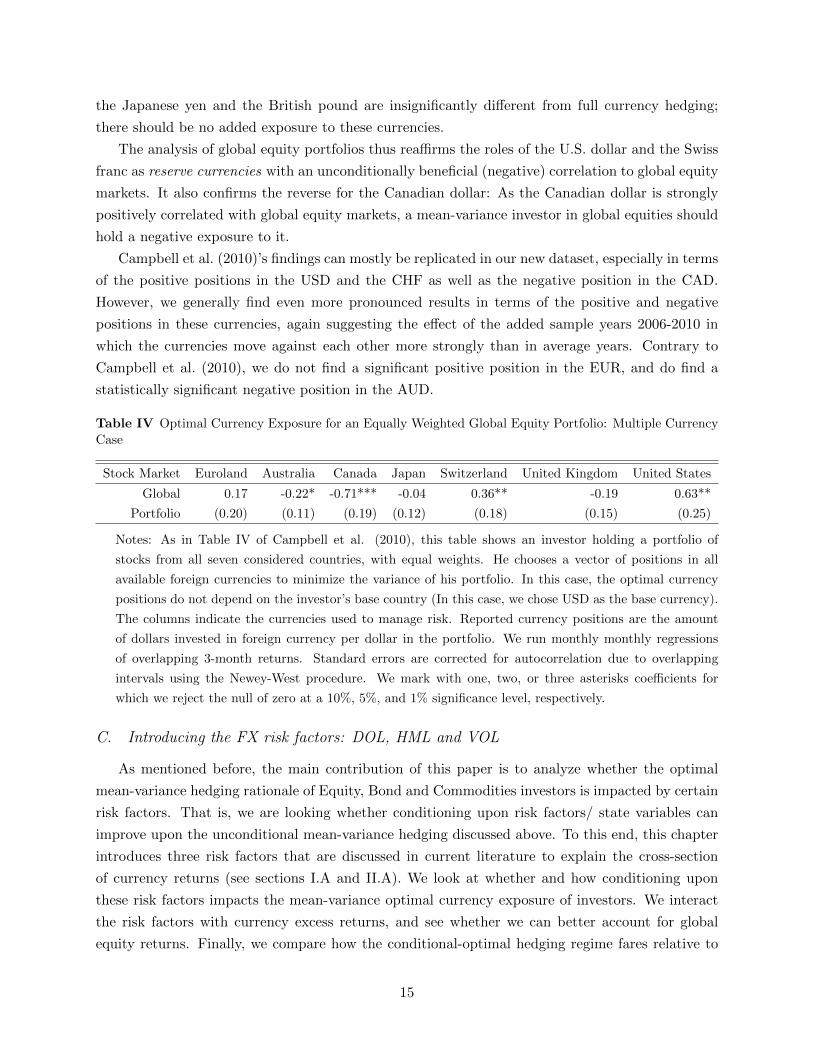
the Japanese yen and the British pound are insignificantly different from full currency hedging;

there should be no added exposure to these currencies.

The analysis of global equity portfolios thus reaffirms the roles of the U.S. dollar and the Swiss

franc as reserve currencies with an unconditionally beneficial (negative) correlation to global equity

markets. It also confirms the reverse for the Canadian dollar: As the Canadian dollar is strongly

positively correlated with global equity markets, a mean-variance investor in global equities should

hold a negative exposure to it.

Campbell et al. (2010)’s findings can mostly be replicated in our new dataset, especially in terms

of the positive positions in the USD and the CHF as well as the negative position in the CAD.

However, we generally find even more pronounced results in terms of the positive and negative

positions in these currencies, again suggesting the effect of the added sample years 2006-2010 in

which the currencies move against each other more strongly than in average years. Contrary to

Campbell et al. (2010), we do not find a significant positive position in the EUR, and do find a

statistically significant negative position in the AUD.

Table IV Optimal Currency Exposure for an Equally Weighted Global Equity Portfolio: Multiple CurrencyCase

Stock Market Euroland Australia Canada Japan Switzerland United Kingdom United States

Global 0.17 -0.22* -0.71*** -0.04 0.36** -0.19 0.63**

Portfolio (0.20) (0.11) (0.19) (0.12) (0.18) (0.15) (0.25)

Notes: As in Table IV of Campbell et al. (2010), this table shows an investor holding a portfolio of

stocks from all seven considered countries, with equal weights. He chooses a vector of positions in all

available foreign currencies to minimize the variance of his portfolio. In this case, the optimal currency

positions do not depend on the investor’s base country (In this case, we chose USD as the base currency).

The columns indicate the currencies used to manage risk. Reported currency positions are the amount

of dollars invested in foreign currency per dollar in the portfolio. We run monthly monthly regressions

of overlapping 3-month returns. Standard errors are corrected for autocorrelation due to overlapping

intervals using the Newey-West procedure. We mark with one, two, or three asterisks coefficients for

which we reject the null of zero at a 10%, 5%, and 1% significance level, respectively.

C. Introducing the FX risk factors: DOL, HML and VOL

As mentioned before, the main contribution of this paper is to analyze whether the optimal

mean-variance hedging rationale of Equity, Bond and Commodities investors is impacted by certain

risk factors. That is, we are looking whether conditioning upon risk factors/ state variables can

improve upon the unconditional mean-variance hedging discussed above. To this end, this chapter

introduces three risk factors that are discussed in current literature to explain the cross-section

of currency returns (see sections I.A and II.A). We look at whether and how conditioning upon

these risk factors impacts the mean-variance optimal currency exposure of investors. We interact

the risk factors with currency excess returns, and see whether we can better account for global

equity returns. Finally, we compare how the conditional-optimal hedging regime fares relative to

15

unconditional-optimal and full hedging in terms of the risk of the overall investor portfolios.

We use three risk factors as conditioning state variables in our analysis: The Dollar (DOL),

High-Minus-Low (HML) and Volatility (VOL) risk factors. As discussed, the DOL and HML are

based on Lustig et al. (2011)’s paper on Common Risk Factors in Currency Markets. DOL is

defined as the average excess return of all foreign currency against the dollar, while HML is the

difference in returns between the highest and lowest discount portfolios, and is a proxy for carry

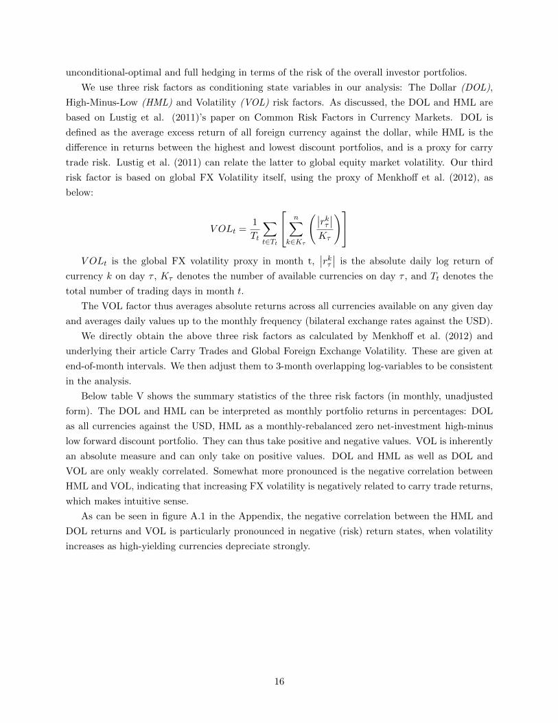
trade risk. Lustig et al. (2011) can relate the latter to global equity market volatility. Our third

risk factor is based on global FX Volatility itself, using the proxy of Menkhoff et al. (2012), as

below:

V OLt =1

Tt

∑t∈Tt

n∑k∈Kτ

(∣∣rkτ ∣∣Kτ

)V OLt is the global FX volatility proxy in month t,

∣∣rkτ ∣∣ is the absolute daily log return of

currency k on day τ , Kτ denotes the number of available currencies on day τ , and Tt denotes the

total number of trading days in month t.

The VOL factor thus averages absolute returns across all currencies available on any given day

and averages daily values up to the monthly frequency (bilateral exchange rates against the USD).

We directly obtain the above three risk factors as calculated by Menkhoff et al. (2012) and

underlying their article Carry Trades and Global Foreign Exchange Volatility. These are given at

end-of-month intervals. We then adjust them to 3-month overlapping log-variables to be consistent

in the analysis.

Below table V shows the summary statistics of the three risk factors (in monthly, unadjusted

form). The DOL and HML can be interpreted as monthly portfolio returns in percentages: DOL

as all currencies against the USD, HML as a monthly-rebalanced zero net-investment high-minus

low forward discount portfolio. They can thus take positive and negative values. VOL is inherently

an absolute measure and can only take on positive values. DOL and HML as well as DOL and

VOL are only weakly correlated. Somewhat more pronounced is the negative correlation between

HML and VOL, indicating that increasing FX volatility is negatively related to carry trade returns,

which makes intuitive sense.

As can be seen in figure A.1 in the Appendix, the negative correlation between the HML and

DOL returns and VOL is particularly pronounced in negative (risk) return states, when volatility

increases as high-yielding currencies depreciate strongly.

16

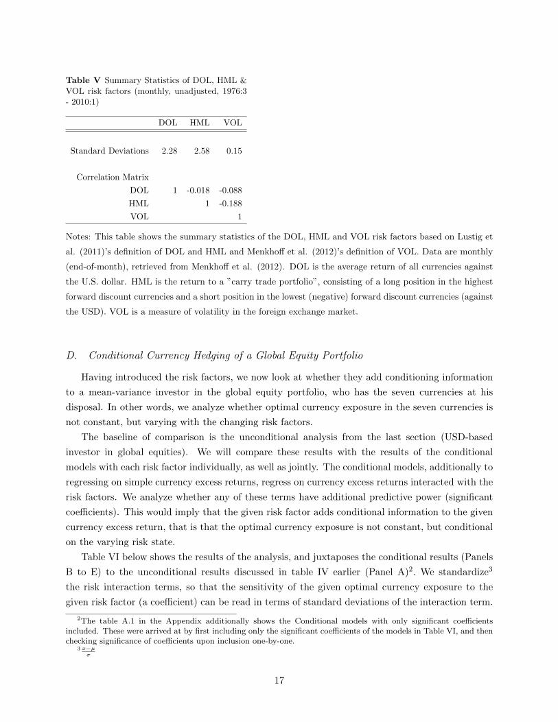
Table V Summary Statistics of DOL, HML &VOL risk factors (monthly, unadjusted, 1976:3- 2010:1)

DOL HML VOL

Standard Deviations 2.28 2.58 0.15

Correlation Matrix

DOL 1 -0.018 -0.088

HML 1 -0.188

VOL 1

Notes: This table shows the summary statistics of the DOL, HML and VOL risk factors based on Lustig et

al. (2011)’s definition of DOL and HML and Menkhoff et al. (2012)’s definition of VOL. Data are monthly

(end-of-month), retrieved from Menkhoff et al. (2012). DOL is the average return of all currencies against

the U.S. dollar. HML is the return to a ”carry trade portfolio”, consisting of a long position in the highest

forward discount currencies and a short position in the lowest (negative) forward discount currencies (against

the USD). VOL is a measure of volatility in the foreign exchange market.

D. Conditional Currency Hedging of a Global Equity Portfolio

Having introduced the risk factors, we now look at whether they add conditioning information

to a mean-variance investor in the global equity portfolio, who has the seven currencies at his

disposal. In other words, we analyze whether optimal currency exposure in the seven currencies is

not constant, but varying with the changing risk factors.

The baseline of comparison is the unconditional analysis from the last section (USD-based

investor in global equities). We will compare these results with the results of the conditional

models with each risk factor individually, as well as jointly. The conditional models, additionally to

regressing on simple currency excess returns, regress on currency excess returns interacted with the

risk factors. We analyze whether any of these terms have additional predictive power (significant

coefficients). This would imply that the given risk factor adds conditional information to the given

currency excess return, that is that the optimal currency exposure is not constant, but conditional

on the varying risk state.

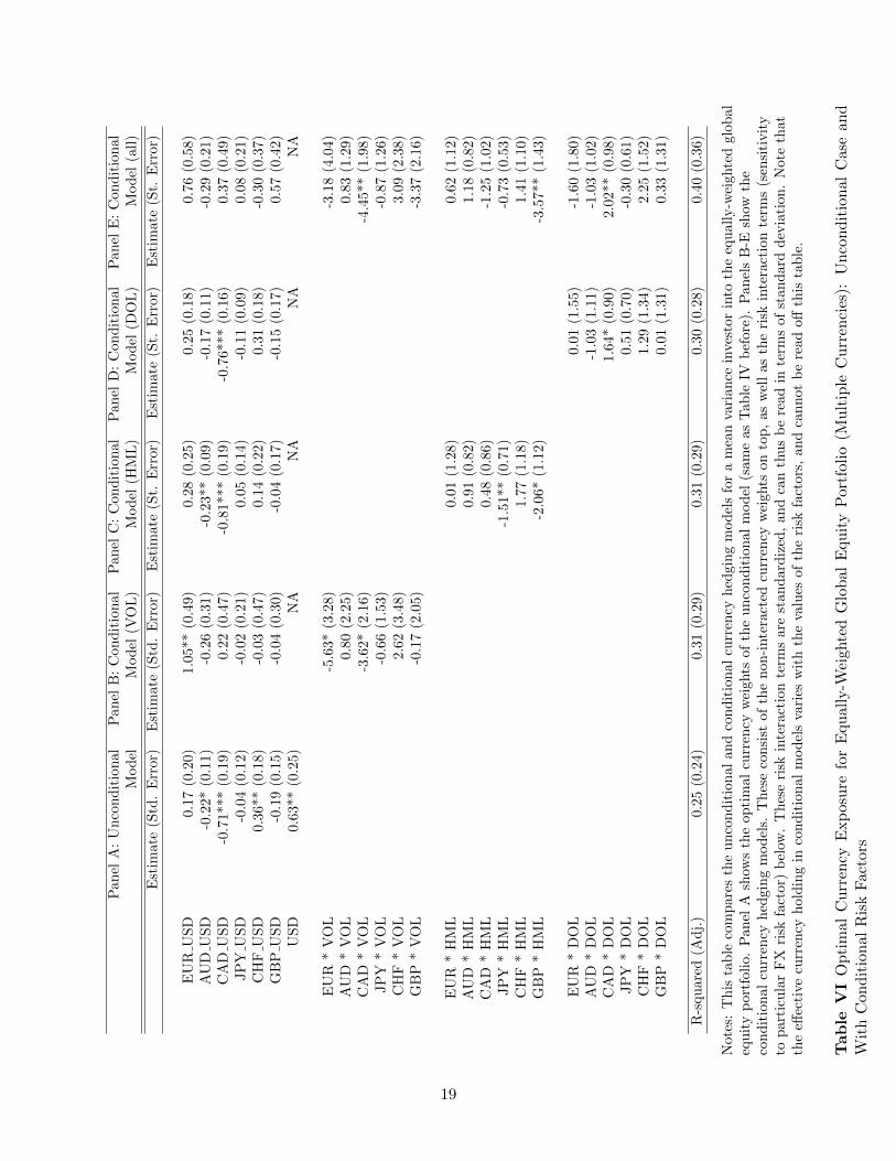
Table VI below shows the results of the analysis, and juxtaposes the conditional results (Panels

B to E) to the unconditional results discussed in table IV earlier (Panel A)2. We standardize3

the risk interaction terms, so that the sensitivity of the given optimal currency exposure to the

given risk factor (a coefficient) can be read in terms of standard deviations of the interaction term.

2The table A.1 in the Appendix additionally shows the Conditional models with only significant coefficientsincluded. These were arrived at by first including only the significant coefficients of the models in Table VI, and thenchecking significance of coefficients upon inclusion one-by-one.

3 x−µσ

17

This should ease interpretation. Other than in the unconditional case, the conditional analysis is

dependent on the home currency of the investor4. We analyze in terms of a USD-domiciled investor

who can hedge with all six bilateral exchange rates against the USD. Thereby, we cannot, as in the

unconditional case, calculate the home currency position (USD) as a static residual position (the

sum of the opposite of the regression coefficients), as it varies with the risk factors.

Lastly, we note that the table VI helps us understand the sensitivity of optimal exposure to

the various currencies, as risk factors change. It does not, however, give us a good intuition about

what that means in terms of actual net currency exposure on average or in different states. This

intuition will helped by Table VII further down in this section.

Formally, we now add to the prior analysis (unconditional mean variance investor with an

equally-weighted portfolio and multiple currencies) the three conditional interaction terms in below

formula:

1′ωt (rt+1 − it) = γ0 − Ψ

′u

(∆st+1 + it − idt

)− Ψ

′DOL

(∆st+1 + it − idt

)DOLt+1

− Ψ′HML

(∆st+1 + it − idt

)HMLt+1

− Ψ′V OL

(∆st+1 + it − idt

)V OLt+1

As we already discussed, ωt is the (n+1 x n+1) diagonal matrix of stock market weights and

Ψu is the (n+1 x 1) vector of unconditional currency weights. ΨDOL,ΨHML and ΨV OL are the

(n+1 x 1) vectors of optimal currency weight sensitivity to the global (scalar) DOLt, HMLt and

V OLt risk factors.

4This has yet to be proven or shown

18

Pan

elA

:U

nco

nd

itio

nal

Pan

elB

:C

on

dit

ion

al

Pan

elC

:C

on

dit

ion

al

Pan

elD

:C

ond

itio

nal

Pan

elE

:C

on

dit

ion

al

Mod

elM

od

el(V

OL

)M

od

el(H

ML

)M

od

el(D

OL

)M

od

el(a

ll)

Est

imat

e(S

td.

Err

or)

Est

imate

(Std

.E

rror)

Est

imate

(St.

Err

or)

Est

imate

(St.

Err

or)

Est

imate

(St.

Err

or)

EU

RU

SD

0.17

(0.2

0)1.0

5**

(0.4

9)

0.2

8(0

.25)

0.2

5(0

.18)

0.7

6(0

.58)

AU

DU

SD

-0.2

2*(0

.11)

-0.2

6(0

.31)

-0.2

3**

(0.0

9)

-0.1

7(0

.11)

-0.2

9(0

.21)

CA

DU

SD

-0.7

1***

(0.1

9)0.2

2(0

.47)

-0.8

1***

(0.1

9)

-0.7

6**

*(0

.16)

0.3

7(0

.49)

JP

YU

SD

-0.0

4(0

.12)

-0.0

2(0

.21)

0.0

5(0

.14)

-0.1

1(0

.09)

0.0

8(0

.21)

CH

FU

SD

0.36

**(0

.18)

-0.0

3(0

.47)

0.1

4(0

.22)

0.3

1(0

.18)

-0.3

0(0

.37)

GB

PU

SD

-0.1

9(0

.15)

-0.0

4(0

.30)

-0.0

4(0

.17)

-0.1

5(0

.17)

0.5

7(0

.42)

US

D0.

63**

(0.2

5)N

AN

AN

AN

A

EU

R*

VO

L-5

.63*

(3.2

8)

-3.1

8(4

.04)

AU

D*

VO

L0.8

0(2

.25)

0.8

3(1

.29)

CA

D*

VO

L-3

.62*

(2.1

6)

-4.4

5**

(1.9

8)

JP

Y*

VO

L-0

.66

(1.5

3)

-0.8

7(1

.26)

CH

F*

VO

L2.6

2(3

.48)

3.0

9(2

.38)

GB

P*

VO

L-0

.17

(2.0

5)

-3.3

7(2

.16)

EU

R*

HM

L0.0

1(1

.28)

0.6

2(1

.12)

AU

D*

HM

L0.9

1(0

.82)

1.1

8(0

.82)

CA

D*

HM

L0.4

8(0

.86)

-1.2

5(1

.02)

JP

Y*

HM

L-1

.51**

(0.7

1)

-0.7

3(0

.53)

CH

F*

HM

L1.7

7(1

.18)

1.4

1(1

.10)

GB

P*

HM

L-2

.06*

(1.1

2)

-3.5

7**

(1.4

3)

EU

R*

DO

L0.0

1(1

.55)

-1.6

0(1

.80)

AU

D*

DO

L-1

.03

(1.1

1)

-1.0

3(1

.02)

CA

D*

DO

L1.6

4*

(0.9

0)

2.0

2**

(0.9

8)

JP

Y*

DO

L0.5

1(0

.70)

-0.3

0(0

.61)

CH

F*

DO

L1.2

9(1

.34)

2.2

5(1

.52)

GB

P*

DO

L0.0

1(1

.31)

0.3

3(1

.31)

R-s

qu

ared

(Ad

j.)

0.25

(0.2

4)0.3

1(0

.29)

0.3

1(0

.29)

0.3

0(0

.28)

0.4

0(0

.36)

Not

es:

Th

ista

ble

com

par

esth

eu

nco

nd

itio

nal

and

con

dit

ion

al

curr

ency

hed

gin

gm

od

els

for

am

ean

vari

ance

inves

tor

into

the

equ

all

y-w

eighte

dglo

bal

equ

ity

por

tfol

io.

Pan

elA

show

sth

eop

tim

alcu

rren

cyw

eights

of

the

un

con

dit

ion

al

mod

el(s

am

eas

Tab

leIV

bef

ore

).P

an

els

B-E

show

the

con

dit

ion

alcu

rren

cyhed

gin

gm

od

els.

Th

ese

consi

stof

the

non

-inte

ract

edcu

rren

cyw

eights

on

top

,as

wel

las

the

risk

inte

ract

ion

term

s(s

ensi

tivit

yto

par

ticu

lar

FX

risk

fact

or)

bel

ow.

Th

ese

risk

inte

ract

ion

term

sare

stan

dard

ized

,an

dca

nth

us

be

read

inte

rms

of

stan

dard

dev

iati

on

.N

ote

that

the

effec

tive

curr

ency

hol

din

gin

con

dit

ion

alm

od

els

vari

esw

ith

the

valu

esof

the

risk

fact

ors

,an

dca

nn

ot

be

read

off

this

tab

le.

Tab

leV

IO

pti

mal

Cu

rren

cyE

xp

osu

refo

rE

qu

ally

-Wei

ghte

dG

lob

alE

qu

ity

Por

tfol

io(M

ult

iple

Cu

rren

cies

):U

nco

nd

itio

nal

Case

an

dW

ith

Con

dit

ion

alR

isk

Fac

tors

19

D.1. Conditional vs Unconditional Models

First thing to note is that indeed the (adjusted) R-squared of all conditional models are higher

than in the unconditional case. This can be seen as a first potential indication that all the con-

ditional risk factors add to the explanatory power of the model, and thus potentially to the FX

hedging strategy of the equity investor5.

Secondly, we note that by including the risk factors and interaction terms, the unconditional

coefficients of many currency excess returns (such as CAD/USD or CHF/USD) vanish. This is

strong indication that many of the negative and positive coefficients in the unconditional analysis

(Panel A) are due to correlation between various currency and equity returns that are ultimately

driven by the now included risk factors.

Thirdly we note the high (Newey-West) standard errors in the conditional models. The Newey-

West standard errors are quite high relative to the conditional coefficient estimates. On top of

that, particularly the introduction of the VOL risk factor additionally increases the standard errors

on the unconditional coefficient estimates. These could be arising due to a variety of potential

reasons: For one, we estimate a high number of cofficients, which could be multicollinear to some

degree. For two, the DOL, HML and VOL time series might display inherent autocorrelation (they

are arguably not random, but come in cycles of risk). For three, the correlation structure might

be different in different states of the world or in different times. For four, there might in fact be

a reasonable amount of randomness or noise in the coefficients. The standard errors in any case

should make us wary of the danger of overfitting and thus beget additional robustness tests.

D.2. Individual risk factor-based models

We turn the attention first to the conditional models incorporating a single-risk factor, depicted

in Panels B to D.

The VOL risk factor seems to drive a lot of the correlation structure (positive, negative) between

currency excess returns and global equity returns. When including VOL as a risk factor, all of the

significant (FX excess return) coefficients in the unconditional model vanish. On the other hand,

we obtain a significant positive coefficient on the unconditional EUR/USD excess return, while

obtaining negative coefficients on the EUR/USD * VOL as well as CAD/USD * VOL interaction

terms. This is strong indication that a lot of the detected positive and negative unconditional

hedging demands in currencies are ultimately due to currencies different sensitivity to the volatility

risk factor. It also implies that by conditioning on Volatility alone, investors could potentially hedge

better and simpler than unconditionally. The VOL conditional model reaches a higher R-squared

than the unconditional model, and only relies on two currency positions in the EUR/USD and

CAD/USD, as these react particularly negatively to volatility innovations (5.6 and 3.6 factors of

standard deviation).

5The R-squared are obtained by the underlying regression model (regressing global equity returns on unconditionaland conditional factors) before switching the sign of the unconditional and conditional slopes to arrive at mean-variance FX coefficients.

20

The HML model, other than the VOL model, leaves a lot of the unconditional partial corre-

lation structure of the currency excess returns with equity returns intact, so that the coefficients

on AUD/USD and CAD/USD stay significantly negative, even slightly amplified. It also has sig-

nificantly negative JPY/USD * HML and GBP/USD * HML interaction terms, meaning that the

higher the (absolute) products of these two currencies with HML excess returns, the more negative

should be the position in these two currencies. Interestingly, these are two currencies whose uncon-

ditional exposure does not impact performance. Only in interaction with Carry Trade risk (HML)

does the mean variance investor add exposure to these currencies.

The DOL conditional model, as the HML model, leaves some of the unconditional correla-

tion structure of the currency excess returns with equity returns intact. The CAD/USD and the

CHF/USD coefficients remain close to their unconditional values, although the CHF/USD coef-

ficient narrowly misses significance at the 10% level. Additionally, there is a strongly positive

CAD/USD * DOL term. The DOL model is quite simple. It relies mainly on one bilateral ex-

change rate: the CAD/USD. The higher the DOL (meaning that the Dollar depreciates relative

to broad currency basket), the more positive should be the position in the CAD as a high-yielding

currency strongly positively correlated with equities. Vice versa, as DOL tanks (in risk states)

and the USD appreciates, the conditional mean variance investor should take a strongly negative

position in the CAD/USD.

The HML and DOL risk interaction terms are somewhat less intuitive than the VOL one, as

they are the product of two variables which can both be negative or positive (FX excess returns

and risk factors).

D.3. Joint conditional model with all risk factors

What happens when we form a conditional model with all three risk factors combined? Are the

risk factors complementary, or are the risk factors essentially proxies for the same underlying risk?

The (adjusted) R-squared of the joint model is significantly higher than of the single-risk factor

models. This is a first indication that the three risk factors are proxies for different underlying

sources of risk, and all add different and useful conditioning information.

Also, all of the risk factors have at least one significant interaction term with excess returns.

Fourthly, of the interaction terms, the CAD/USD * DOL has positive (negatively correlated with

equities) and the JPY/USD * HML, the GBP/USD * HML and CAD/USD * VOL negative (pos-

itively correlated with equities) hedging properties, meaning that the conditional mean variance

investor into the global equity portfolio should take positive (negative) exposure to these terms.

The positive CAD/USD * DOL is at first surprising, as the CAD/USD has a strongly negative

coefficient in the unconditional model. However, interpretation is not easy, especially as the inter-

action terms are factors of two terms. It might arise primarily due to negative correlation with

equities in states where both CAD/USD and DOL are negative or where both are positive. The

negative JPY/USD * HML and GBP/USD * HML terms indicate that the higher the absolute

JPY/USD, GBP/USD and HML returns become, the lower the exposure of the conditional mean-

21

variance investor in the JPY and GBP currencies. Particularly large is the negative coefficient of

the CAD/USD * VOL term, indicating that the higher the FX market volatility the more negative

the position should be in the CAD/USD of the conditional investor. This makes intuitive sense,

as the CAD/USD (as a risky currency against the USD) is moving down with equities in times of

increased stress and volatility.

D.4. Economic significance of the risk factors on optimal currency hedging

While we have previously seen (in Table VI) that the optimal currency exposure in the 7

currencies have differing sensitivities to the risk factors (through the coefficients of the interaction

terms), the table is not intuitive to interpret, as it does not show us the net optimal currency

exposure in different risk states.

To get a better intuition of what the estimated models mean for effective currency exposure of a

conditional mean-variance investor in global equities, we analyze the FX holdings of the estimated

conditional models (Panels B to E in Table VII below) at the 5%, 50% and 95% percentiles of the

risk factors and juxtapose these to the unconditional optimal currency demands of the unconditional

model (Panel A in Table VII). Table A.2 in the Appendix additionally shows the 90% confidence

intervals of the currency positions. This way we get a better feeling of the sensitivity of the optimal

currency exposure in a currency to the changing risk factors, as well as how far it deviates from

its unconditional value. The DOL and HML risk factors are thereby sorted from low to high, and

the VOL risk factor in opposite direction. Low negative values of DOL and HML are indicative

of risk states (stress), such as during unwinding of carry trades in the markets; the same goes for

high values of VOL.

First thing to note is that some currency exposures generally seem more sensitive than others to

the various risk factors. The CAD/USD exposure reacts particularly sensitively to the changing risk

factors, varying drastically between different risk regimes. The different risk factors also each seem

to be affect different currency pairs: while Volatility has a strong impact on the optimal EUR/USD,

CAD/USD and USD exposures, the HML risk factor particularly influences the JPY/USD and

CHF/USD exposures, for instance.

As discussed above, the EUR/USD exchange rate exposure is particularly affected by volatility:

Optimal exposure decreases with increasing volatility, being significantly positive in calm periods,

and slightly negative in high volatility periods. It is not as much affected by the HML and DOL

risk factors. Relative to other currencies, the AUD/USD exposure does not vary very strongly,

and is mostly at a negative value close to zero. The CAD/USD exchange rate on the other hand

varies most strongly of all bilateral exchange rates with the risk factors. In bad states, it is very

negative across all risk factors, and stays negative even in good states (however, much less negative;

strong increase in net exposure). It is extremely strongly related to the DOL and VOL factors.

The JPY/USD exchange rate is most strongly related to the HML risk factor. In times of low

HML, optimal exposure is positive and in times of low HML, it is negative. This pattern might be

expected of a safe, low-yielding currency.

22

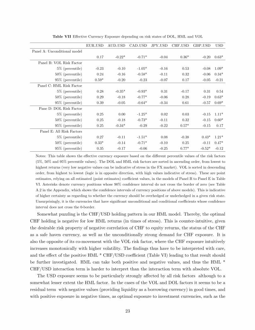
Table VII Effective Currency Exposure depending on risk states of DOL, HML and VOL

EUR USD AUD USD CAD USD JPY USD CHF USD GBP USD USD

Panel A: Unconditional model

0.17 -0.22* -0.71* -0.04 0.36* -0.20 0.63*

Panel B: VOL Risk Factor

5% (percentile) -0.23 -0.10 -1.05* -0.16 0.53 -0.08 1.09*

50% (percentile) 0.24 -0.16 -0.58* -0.11 0.32 -0.06 0.34*

95% (percentile) 0.59* -0.20 -0.23 -0.07 0.17 -0.05 -0.21

Panel C: HML Risk Factor

5% (percentile) 0.28 -0.35* -0.93* 0.31 -0.17 0.31 0.54

50% (percentile) 0.29 -0.18 -0.77* -0.06 0.28 -0.19 0.63*

95% (percentile) 0.39 -0.05 -0.64* -0.34 0.61 -0.57 0.69*

Pane D: DOL Risk Factor

5% (percentile) 0.25 0.00 -1.25* 0.02 0.03 -0.15 1.11*

50% (percentile) 0.25 -0.18 -0.73* -0.11 0.32 -0.15 0.60*

95% (percentile) 0.25 -0.34* -0.29 -0.22 0.57* -0.15 0.17

Panel E: All Risk Factors

5% (percentile) 0.27 -0.11 -1.51* 0.08 -0.38 0.43* 1.21*

50% (percentile) 0.33* -0.14 -0.71* -0.10 0.25 -0.11 0.47*

95% (percentile) 0.35 -0.17 -0.06 -0.25 0.77* -0.52* -0.12

Notes: This table shows the effective currency exposure based on the different percentile values of the risk factors

(5%, 50% and 95% percentile values). The DOL and HML risk factors are sorted in ascending order, from lowest to

highest returns (very low negative values can be indicative of stress in the FX market). VOL is sorted in descending

order, from highest to lowest (logic is in opposite direction, with high values indicative of stress). These are point

estimates, relying on all estimated (point estimates) coefficient values, in the models of Panel B to Panel E in Table

VI. Asterisks denote currency positions whose 90% confidence interval do not cross the border of zero (see Table

A.2 in the Appendix, which shows the confidence intervals of currency positions of above models). This is indicative

of higher certainty as regarding to whether the currency should be overhedged or underhedged in a given risk state.

Unsurprisingly, it is the currencies that have significant unconditional and conditional coefficients whose confidence

interval does not cross the 0-border.

Somewhat puzzling is the CHF/USD holding pattern in our HML model. Thereby, the optimal

CHF holding is negative for low HML returns (in times of stress). This is counter-intuitive, given

the desirable risk property of negative correlation of CHF to equity returns, the status of the CHF

as a safe haven currency, as well as the unconditionally strong demand for CHF exposure. It is

also the opposite of its co-movement with the VOL risk factor, where the CHF exposure intuitively

increases monotonically with higher volatility. The findings thus have to be interpreted with care,

and the effect of the positive HML * CHF/USD coefficient (Table VI) leading to that result should

be further investigated. HML can take both positive and negative values, and thus the HML *

CHF/USD interaction term is harder to interpret than the interaction term with absolute VOL.

The USD exposure seems to be particularly strongly affected by all risk factors although to a

somewhat lesser extent the HML factor. In the cases of the VOL and DOL factors it seems to be a

residual term with negative values (providing liquidity as a borrowing currency) in good times, and

with positive exposure in negative times, as optimal exposure to investment currencies, such as the

23

CAD, is negative. The interpretation of the DOL factor here has to be handled with care, however:

it basically is just the opposite of the performance of the DOL against all other currencies. That

the USD exposure should be positively related to USD performance is clear, and does not allow

the interpretation as a risk factor.

E. Conditional vs Unconditional FX hedging: Portfolio Performance

Having discussed the risk factor-based conditional models of a global equity investor, we now

turn to comparing the performance of these models to complete and unconditional hedging. Camp-

bell et al. (2010) in their study find a statistically significantly decreased standard deviation of

unconditional hedging relative to full hedging. On the other hand, their conditional model based

on differences to time-series averages of the forward discounts/ interest rates between countries

does not decrease standard deviation significantly.

We undertake a similar performance comparison with different conditional information –our

FX risk factors –, and in an enlarged dataset –adding the 2006-2010 crisis and post-crisis years.

Additionally to Standard deviation, we also consider the Mean returns and the Sharpe ratio of

returns under the different hedging regimes. This gives us additional insights as to what the

costs are (in terms of foregone mean return) for these potential reductions in standard deviation.

The Sharpe ratio as the ratio between average performance and volatility of that performance is

an arguably better-suited performance measure for the different hedging regimes. With a higher

Sharpe ratio-Portfolio, one can replicate any level of standard deviation of a lower Sharpe ratio-

Portfolio with a higher return by simply choosing the appropriate leverage ratio.

E.1. Standard deviation, Mean and Sharpe ratios of Complete, Unconditional and

Conditional hedging

As discussed in section the portfolio log excess return can be decomposed into the sum of the

fully hedged asset excess returns, the currency excess returns, as well as a Jensens inequality term.

Here, we approximate the portfolio log excess returns as the sum of the equity and FX excess

returns, not yet incorporating the Jensens inequality term . We annualize both standard deviation

and mean returns. In case of the mean return, we add one-half of the variance of returns to form the

adjusted average (to approximate simple returns). The Sharpe ratio is then the ratio of annualized

mean return to annualized standard devation.

rhp,t+1 − i1,t = 1′ωt (rt+1 − it) +

(Ψu

′+ Ψ

′c,t

)(∆st+1 + it − idt

)+

1

2

h∑t

Table VIII below shows us these three measures for the equally-weighted global equity portfolio

under full hedging, unconditional hedging, and conditional hedging. We perform a horserace of

the unconditional and conditional models with all currencies and interaction terms, as well as with

only the significant coefficients.

24

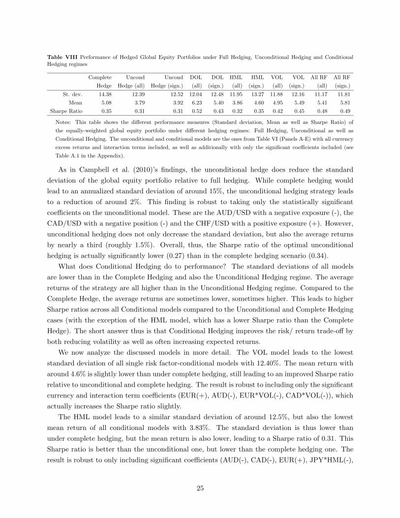
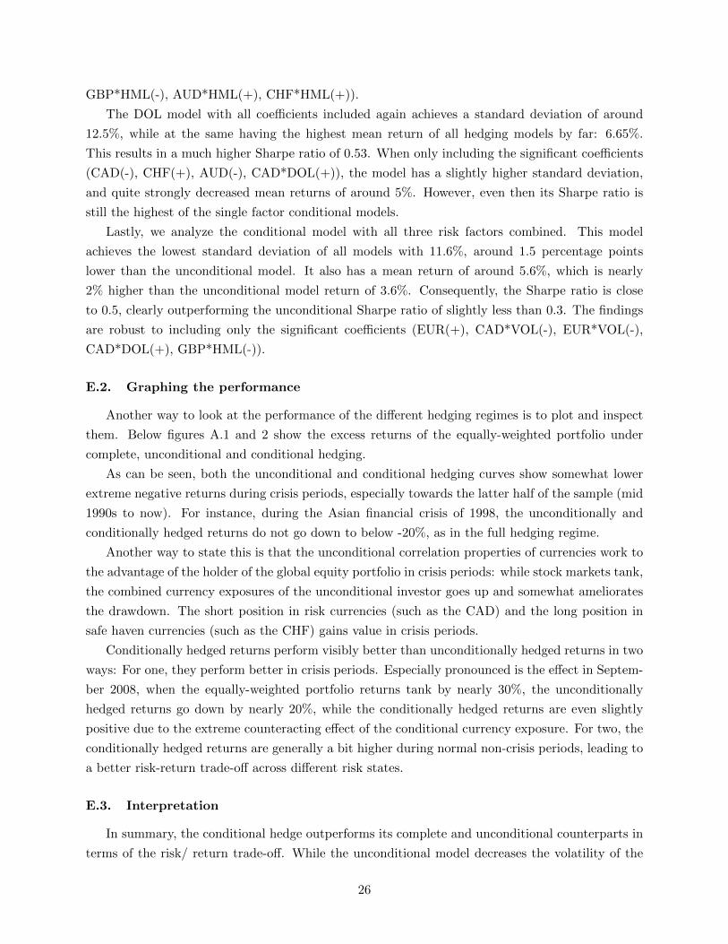
Table VIII Performance of Hedged Global Equity Portfolios under Full Hedging, Unconditional Hedging and ConditionalHedging regimes

Complete Uncond Uncond DOL DOL HML HML VOL VOL All RF All RF

Hedge Hedge (all) Hedge (sign.) (all) (sign.) (all) (sign.) (all) (sign.) (all) (sign.)

St. dev. 14.38 12.39 12.52 12.04 12.48 11.95 13.27 11.88 12.16 11.17 11.81

Mean 5.08 3.79 3.92 6.23 5.40 3.86 4.60 4.95 5.49 5.41 5.81

Sharpe Ratio 0.35 0.31 0.31 0.52 0.43 0.32 0.35 0.42 0.45 0.48 0.49

Notes: This table shows the different performance measures (Standard deviation, Mean as well as Sharpe Ratio) of

the equally-weighted global equity portfolio under different hedging regimes: Full Hedging, Unconditional as well as

Conditional Hedging. The unconditional and conditional models are the ones from Table VI (Panels A-E) with all currency

excess returns and interaction terms included, as well as additionally with only the significant coefficients included (see

Table A.1 in the Appendix).

As in Campbell et al. (2010)’s findings, the unconditional hedge does reduce the standard

deviation of the global equity portfolio relative to full hedging. While complete hedging would

lead to an annualized standard deviation of around 15%, the unconditional hedging strategy leads

to a reduction of around 2%. This finding is robust to taking only the statistically significant

coefficients on the unconditional model. These are the AUD/USD with a negative exposure (-), the

CAD/USD with a negative position (-) and the CHF/USD with a positive exposure (+). However,

unconditional hedging does not only decrease the standard deviation, but also the average returns

by nearly a third (roughly 1.5%). Overall, thus, the Sharpe ratio of the optimal unconditional

hedging is actually significantly lower (0.27) than in the complete hedging scenario (0.34).

What does Conditional Hedging do to performance? The standard deviations of all models

are lower than in the Complete Hedging and also the Unconditional Hedging regime. The average

returns of the strategy are all higher than in the Unconditional Hedging regime. Compared to the

Complete Hedge, the average returns are sometimes lower, sometimes higher. This leads to higher

Sharpe ratios across all Conditional models compared to the Unconditional and Complete Hedging

cases (with the exception of the HML model, which has a lower Sharpe ratio than the Complete

Hedge). The short answer thus is that Conditional Hedging improves the risk/ return trade-off by

both reducing volatility as well as often increasing expected returns.

We now analyze the discussed models in more detail. The VOL model leads to the lowest

standard deviation of all single risk factor-conditional models with 12.40%. The mean return with

around 4.6% is slightly lower than under complete hedging, still leading to an improved Sharpe ratio

relative to unconditional and complete hedging. The result is robust to including only the significant

currency and interaction term coefficients (EUR(+), AUD(-), EUR*VOL(-), CAD*VOL(-)), which

actually increases the Sharpe ratio slightly.

The HML model leads to a similar standard deviation of around 12.5%, but also the lowest

mean return of all conditional models with 3.83%. The standard deviation is thus lower than

under complete hedging, but the mean return is also lower, leading to a Sharpe ratio of 0.31. This

Sharpe ratio is better than the unconditional one, but lower than the complete hedging one. The

result is robust to only including significant coefficients (AUD(-), CAD(-), EUR(+), JPY*HML(-),

25

GBP*HML(-), AUD*HML(+), CHF*HML(+)).

The DOL model with all coefficients included again achieves a standard deviation of around

12.5%, while at the same having the highest mean return of all hedging models by far: 6.65%.

This results in a much higher Sharpe ratio of 0.53. When only including the significant coefficients

(CAD(-), CHF(+), AUD(-), CAD*DOL(+)), the model has a slightly higher standard deviation,

and quite strongly decreased mean returns of around 5%. However, even then its Sharpe ratio is

still the highest of the single factor conditional models.

Lastly, we analyze the conditional model with all three risk factors combined. This model

achieves the lowest standard deviation of all models with 11.6%, around 1.5 percentage points

lower than the unconditional model. It also has a mean return of around 5.6%, which is nearly

2% higher than the unconditional model return of 3.6%. Consequently, the Sharpe ratio is close

to 0.5, clearly outperforming the unconditional Sharpe ratio of slightly less than 0.3. The findings

are robust to including only the significant coefficients (EUR(+), CAD*VOL(-), EUR*VOL(-),

CAD*DOL(+), GBP*HML(-)).

E.2. Graphing the performance

Another way to look at the performance of the different hedging regimes is to plot and inspect

them. Below figures A.1 and 2 show the excess returns of the equally-weighted portfolio under

complete, unconditional and conditional hedging.

As can be seen, both the unconditional and conditional hedging curves show somewhat lower

extreme negative returns during crisis periods, especially towards the latter half of the sample (mid

1990s to now). For instance, during the Asian financial crisis of 1998, the unconditionally and

conditionally hedged returns do not go down to below -20%, as in the full hedging regime.

Another way to state this is that the unconditional correlation properties of currencies work to

the advantage of the holder of the global equity portfolio in crisis periods: while stock markets tank,

the combined currency exposures of the unconditional investor goes up and somewhat ameliorates

the drawdown. The short position in risk currencies (such as the CAD) and the long position in

safe haven currencies (such as the CHF) gains value in crisis periods.

Conditionally hedged returns perform visibly better than unconditionally hedged returns in two

ways: For one, they perform better in crisis periods. Especially pronounced is the effect in Septem-

ber 2008, when the equally-weighted portfolio returns tank by nearly 30%, the unconditionally

hedged returns go down by nearly 20%, while the conditionally hedged returns are even slightly

positive due to the extreme counteracting effect of the conditional currency exposure. For two, the

conditionally hedged returns are generally a bit higher during normal non-crisis periods, leading to

a better risk-return trade-off across different risk states.

E.3. Interpretation

In summary, the conditional hedge outperforms its complete and unconditional counterparts in

terms of the risk/ return trade-off. While the unconditional model decreases the volatility of the

26

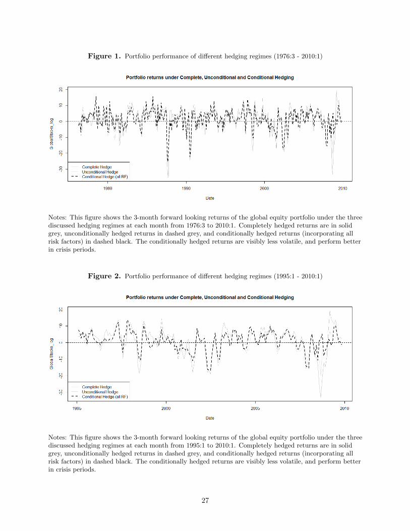
Figure 1. Portfolio performance of different hedging regimes (1976:3 - 2010:1)

Notes: This figure shows the 3-month forward looking returns of the global equity portfolio under the threediscussed hedging regimes at each month from 1976:3 to 2010:1. Completely hedged returns are in solidgrey, unconditionally hedged returns in dashed grey, and conditionally hedged returns (incorporating allrisk factors) in dashed black. The conditionally hedged returns are visibly less volatile, and perform betterin crisis periods.

Figure 2. Portfolio performance of different hedging regimes (1995:1 - 2010:1)

Notes: This figure shows the 3-month forward looking returns of the global equity portfolio under the threediscussed hedging regimes at each month from 1995:1 to 2010:1. Completely hedged returns are in solidgrey, unconditionally hedged returns in dashed grey, and conditionally hedged returns (incorporating allrisk factors) in dashed black. The conditionally hedged returns are visibly less volatile, and perform betterin crisis periods.

27

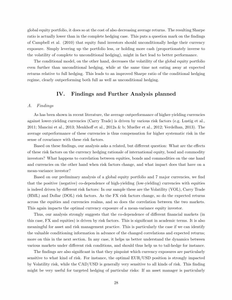
global equity portfolio, it does so at the cost of also decreasing average returns. The resulting Sharpe

ratio is actually lower than in the complete hedging case. This puts a question mark on the findings

of Campbell et al. (2010) that equity fund investors should unconditionally hedge their currency

exposure. Simply levering up the portfolio less, or holding more cash (proportionately inverse to

the volatility of complete to unconditional hedging), might in fact lead to better performance.

The conditional model, on the other hand, decreases the volatility of the global equity portfolio

even further than unconditional hedging, while at the same time not eating away at expected

returns relative to full hedging. This leads to an improved Sharpe ratio of the conditional hedging

regime, clearly outperforming both full as well as unconditional hedging.

IV. Findings and Further Analysis planned

A. Findings

As has been shown in recent literature, the average outperformance of higher-yielding currencies

against lower-yielding currencies (Carry Trade) is driven by various risk factors (e.g. Lustig et al.,

2011; Mancini et al., 2013; Menkhoff et al., 2012a & b; Mueller et al., 2012; Verdelhan, 2013). The

average outperformance of these currencies is thus compensation for higher systematic risk in the

sense of covariance with these risk factors.

Based on these findings, our analysis asks a related, but different question: What are the effects

of these risk factors on the currency hedging rationale of international equity, bond and commodity

investors? What happens to correlation between equities, bonds and commodities on the one hand

and currencies on the other hand when risk factors change, and what impact does that have on a

mean-variance investor?

Based on our preliminary analysis of a global equity portfolio and 7 major currencies, we find

that the positive (negative) co-dependence of high-yielding (low-yielding) currencies with equities

is indeed driven by different risk factors: In our sample these are the Volatility (VOL), Carry Trade

(HML) and Dollar (DOL) risk factors. As the FX risk factors change, so do the expected returns

across the equities and currencies realms, and so does the correlation between the two markets.

This again impacts the optimal currency exposure of a mean-variance equity investor.

Thus, our analysis strongly suggests that the co-dependence of different financial markets (in

this case, FX and equities) is driven by risk factors. This is significant in academic terms. It is also

meaningful for asset and risk management practice. This is particularly the case if we can identify

the valuable conditioning information in advance of the changed correlations and expected returns;

more on this in the next section. In any case, it helps us better understand the dynamics between

various markets under different risk conditions, and should thus help us to tail-hedge for instance.

The findings are also significant in that they pinpoint which currency exposures are particularly

sensitive to what kind of risk. For instance, the optimal EUR/USD position is strongly impacted

by Volatility risk, while the CAD/USD is generally very sensitive to all kinds of risk. This finding

might be very useful for targeted hedging of particular risks: If an asset manager is particularly

28

concerned about increasing volatility, he should drastically decrease his net EUR/USD position (or

even go short) for instance. This is even more significant, as the conditional models are quite sparse,

and beat the unconditional hedging performance with at most two or three currency weights. This

is tantamount to ease of implementation.

A.1. Qualification of Findings

Two major qualifications have to be made regarding the findings of our preliminary analysis.

For one, there are very large (Newey-West) standard errors of the coefficients with regards to

unconditional and conditional currency exposure (Table VI). The size of the standard errors makes

inference for some currency-risk factor combinations difficult; namely for those, for which the 90%

confidence interval passes the 0-threshold in terms of effective currency exposure (see Table A.2 in

the Appendix) for both the unconditional and conditional models. As a robustness test, we have

thus tested how performance is affected when we only include statistically significant coefficients in

both the unconditional and the conditional hedging models (Table VIII shows the performance of

the models in Table A.1 in the Appendix –which generally holds up well.

The standard errors have multiple reasons to come about: For one, there is large autocorrelation

in the overlapping 3-month returns we have used for our analysis so far by design. We have used

these to ensure comparability with Campbell et al. (2010) who do this for their analysis. As an

easy fix, we will look at how the analysis changes when we use non-overlapping returns (see next

section).

But another, in a sense more fundamental reason for the large standard errors could be due

to currencies changing their inherent risk characteristics in terms of unconditional and conditional

correlation properties with the equities markets over time. As a case in point, the yen (euro) was

an overhedged (underhedged) currency in Campbell et al. (2010)’s sample, indicating negative

(positive) correlation properties for global equity investors from 1975-2005. In the sample period

added from 2006-2010, the picture reversed: then yen as a safe-haven currency gained strongly

against both the euro and the equities markets in the crisis. As much as risk characteristics of

currencies change through time, the coefficients of our analysis will change too. This implies

potentially fruitful research into country-specific risk factors (such as fiscal or monetary data of a

country) added to or interacted with our global FX-market risk factors.

The second major qualification is how far the conditional models can actually be implemented

by investors. Our conditional hedging models indicate what the optimal currency weights would be

in different risk states. However, the conditionality built-in into these models is contemporaneous

to the equity and FX excess returns. It is thus an open question to what extent investors can make

use of the conditional risk factors. In terms of downside risk management, it is valuable in itself

to know how the systematic currency risk characteristics change as the risk factors change. This is

a question of risk preferences. However, to what extent one can actually approximate the returns

of the optimal conditional models throughout the risk states (as in Table VIII) is a question that

should be further examined. It strongly depends on the persistence as well as the ability to forecast

29

the risk factors through time. It is a stylized fact that both Volatility as well as the performance

of the Carry Trade comes in cycles, whereby periods of relatively stable Volatility / Carry Trade

Performance drastically change to very different levels.

B. Further Analysis Planned

Further to our above analysis, our findings should be both corroborated as well as added to.

In terms of validating and corroborating our above results, we will firstly look at non-overlapping

returns at various different frequencies (as opposed to the current 3-month overlapping returns, as

in Campbell et al., 2010), and will see whether and in what way our results are affected. Newey-

West standard errors might decrease, as autocorrelation decreases, improving the inference. We

will use a different definition of the euro, not relying on the German mark before 1999, but value-

weighting it with different European currencies ante-1999 (similarly to Campbell et al., 2010).

We will transform the risk factors to log-likelihoods in order to simplify interpretation of the risk

factors themselves as well as the interaction terms with currency excess returns. We will enlarge

the sample to include the most recent 4 years 2011-2014. We will perform further robustness tests,

such as looking at subsamples, and performing pseudo-out of sample forecasting to see how valuable

a model calibrated in one time period really is in the next.

Importantly, we also want to extend our analysis. Further to equities, we will additionally look

at how bond and commodity investors and their hedging rationales are affected by changing risk

factors. We will introduce further risk factors –the Momentum, Illiquidity and Correlation factors

discussed in sections I.A and II.A. We will analyze other performance measures, such as downstate

standard deviations and maximum drawdowns, and will particularly focus on the risk properties of

the different hedging regimes in crisis periods. Potential considerations, rather for future research,

are the introduction of country-specific risk factors to account for the changing risk properties of

currencies through time and of transaction costs to analyze the net effects of portfolio re-balancing

following the changing risk factors.

Importantly, we will focus on the tradability of the discussed conditional models. In the current

models, the investor at time t forms currency weights based on (equity, currency, etc.) excess

returns as well as risk factors in t+ 1. The insights would be even more enticing, if they could be

traded in real-time, based on data available at time t when the portfolio weights are chosen. To

this end, we will condition upon contemporaneous and lagged risk factors at time t, rather than

t+ 1.

30

REFERENCES

Acharya, Viral, Yakov Amihud, and Sreedhar Bharath, 2012, Liquidity Risk of Corporate Bond

Returns: A Conditional Approach, Working Paper .

Barroso, Pedro, and Pedro Santa-clara, 2013, Beyond the Carry Trade : Optimal Currency Port-

folios, Working Paper 1–34.

Burnside, C., M. Eichenbaum, I. Kleshchelski, and S. Rebelo, 2011a, Do Peso Problems Explain

the Returns to the Carry Trade?, Review of Financial Studies 24, 853–891.

Burnside, Craig, 2011, Carry Trades And Risk, NBER Working Paper Series .

Burnside, Craig, 2012, Understanding the Profitability of Currency-Trading Strategies.

Burnside, Craig, Martin Eichenbaum, and Sergio Rebelo, 2011b, Carry Trade and Momentum in

Currency Markets, Annual Review of Financial Economics 3, 511–535.

Campbell, John Y, Karine Serfaty-de Medeiros, and Luis M Viceira, 2010, Global Currency Hedg-

ing, The Journal of Finance 65, 87–122.

Christiansen, Charlotte, Angelo Ranaldo, and Paul Soderlind, 2011, The Time-Varying Systematic

Risk of Carry Trade Strategies, Journal of Financial and Quantitative Analysis 46, 1107–1125.

De Santis, Giorgio, and Bruno Gerard, 2014, International Asset Pricing and Portfolio Diversifica-

tion with Time-Varying Risk, The Journal of Finance 52, 1881–1912.

Frazzini, Andrea, Ronen Israel, and Tobias J. Moskowitz, 2012, Trading Costs of Asset Pricing

Anomalies, Working Paper .

Gabaix, Xavier, and Matteo Maggiori, 2014, International Liquidity and Exchange Rate Dynamics,

NBER Working Paper Series .

Lettau, Martin, Matteo Maggiori, and Michael Weber, 2014, Conditional risk premia in currency

markets and other asset classes, Journal of Financial Economics (forthcoming) .

Lustig, H., N. Roussanov, and a. Verdelhan, 2011, Common Risk Factors in Currency Markets,

Review of Financial Studies 24, 3731–3777.

31

Mancini, Loriano, Angelo Ranaldo, and Jan Wrampelmeyer, 2013, Liquidity in the Foreign Ex-

change Market: Measurement, Commonality, and Risk Premiums, The Journal of Finance 68,

1805–1841.

Menkhoff, Lukas, Lucio Sarno, Maik Schmeling, and Andreas Schrimpf, 2012a, Carry Trades and

Global Foreign Exchange Volatility, The Journal of Finance 67, 681–718.

Menkhoff, Lukas, Lucio Sarno, Maik Schmeling, and Andreas Schrimpf, 2012b, Currency momen-

tum strategies, Journal of Financial Economics 106, 660–684.

Mueller, Philippe, Andreas Stathopoulos, and Andrea Vedolin, 2012, International Correlation

Risk, Working Paper .

Rafferty, Barry, 2011, Currency Returns , Skewness and Crash Risk, Working Paper .

Ross, Steve, 2014, The Recovery Theorem, The Journal of Finance .

Verdelhan, Adrien, 2013, The Share of Systematic Variation in Bilateral Exchange Rates, Working

Paper .

32

Appendix A. Further Graphs and Tables

33

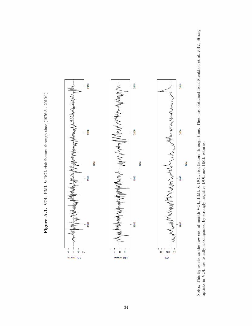
Fig

ure

A.1

.V

OL

,H

ML

&D

OL

risk

fact

ors

thro

ugh

tim

e(1

976:3

-2010:1

)

Not

es:

Th

isfi

gure

show

sth

era

wen

d-o

f-m

onth

VO

L,

HM

L&

DO

Lri

skfa

ctors

thro

ugh

tim

e.T

hes

eare

ob

tain

edfr

om

Men

kh

off

etal.

,2012.

Str

on

gu

pti

cks

inV

OL

are

usu

ally

acco

mp

anie

dby

stro

ngly

neg

ati

veD

OL

an

dH

ML

retu

rns.

34

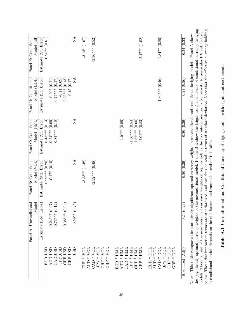
Pan

elA

:U

nco

nd

itio

nal

Pan

elB

:C

on

dit

ion

al

Pan

elC

:C

on

dit

ion

al

Pan

elD

:C

ond

itio

nal

Pan

elE

:C

on

dit

ion

al

Mod

elM

od

el(V

OL

)M

od

el(H

ML

)M

od

el(D

OL

)M

od

el(a

ll)

Est

imat

e(S

td.

Err

or)

Est

imate

(Std

.E

rror)

Est

imate

(St.

Err

or)

Est

imate

(St.

Err

or)

Est

imate

(St.

Err

or)

EU

RU

SD

0.9

9***

(0.2

0)

0.4

3***

(0.1

4)

0.9

5**

(0.6

1)

AU

DU

SD

-0.2

4***

(0.0

7)-0

.17*

(0.1

0)

-0.2

4***

(0.0

9)

-0.2

0*

(0.1

1)

CA

DU

SD

-0.7

3***

(0.1

2)-0

.81***

(0.1

8)

-0.7

4**

*(0

.17)

JP

YU

SD

-0.1

1(0

.09)

CH

FU

SD

0.38

***

(0.0

5)0.3

8**

*(0

.13)

GB

PU

SD

-0.1

5(0

.17)

US

D0.

59**

(0.2

5)N

AN

AN

AN

A

EU

R*

VO

L-3

.53**

(1.4

8)

-3.1

3*

(1.6

7)

AU

D*

VO

LC

AD

*V

OL

-2.9

2***

(0.4

8)

-3.9

6***

(0.5

2)

JP

Y*

VO

LC

HF

*V

OL

GB

P*

VO

L

EU

R*

HM

LA

UD

*H

ML

1.4

0**

(0.5

5)

CA

D*

HM

LJP

Y*

HM

L-1

.56***

(0.5

4)

CH

F*

HM

L1.8

7***

(0.6

0)

GB

P*

HM

L-2

.01**

(0.8

3)

-2.4

7**

(1.0

2)

EU

R*

DO

LA

UD

*D

OL

CA

D*

DO

L1.3

0***

(0.4

6)

1.8

4**

(0.8

0)

JP

Y*

DO

LC

HF

*D

OL

GB

P*

DO

L

R-s

qu

ared

(Ad

j.)

0.24

(0.2

4)0.3

0(0

.29)

0.3

0(0

.29)

0.2

7(0

.26)

0.3

4(0

.33)

Not

es:

This

tab

leco

mp

ares

the

stat

isti

call

ysi

gnifi

cant

op

tim

al

curr

ency

wei

ghts

inu

nco

nd

itio

nal

an

dco

nd

itio

nal

hed

gin

gm

od

els.

Pan

elA

show

sth

e(s

ign

ifica

nt)

opti

mal

curr

ency

wei

ghts

ofth

eu

nco

nd

itio

nal

mod

el.

Pan

els

B-E

show

the

(sig

nifi

cant)

coeffi

cien

tsof

con

dit

ion

al

curr

ency

hed

gin

gm

od

els.

Th

ese

con

sist

ofth

en

on-i

nte

ract

edcu

rren

cyw

eights

on

top

,as

wel

las

the

risk

inte

ract

ion

term

s(s

ensi

tivit

yto

part

icu

lar

FX

risk

fact

or)

bel

ow.

Th

ese

risk

inte

ract

ion

term

sar

est

and

ard

ized

,an

dca

nth

us

be

read

inte

rms

of

stan

dard

dev

iati

on

.N

ote

that

the

effec

tive

curr

ency

hold

ing

inco

nd

itio

nal

mod

els

dep

end

son

the

risk

fact

ors,

an

dca

nn

ot

be

read

off

this

tab

le.

Tab

leA

.1U

nco

nd

itio

nal

and

Con

dit

ion

alC

urr

ency

Hed

gin

gm

od

els

wit

hsi

gnifi

cant

coeffi

cien

ts

35

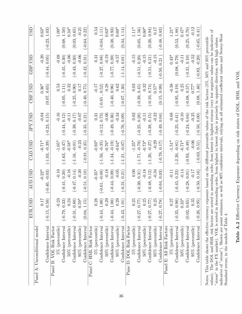
EU

RU

SD

AU

DU

SD

CA

DU

SD

JP

YU

SD

CH

FU

SD

GB

PU

SD

US

D

Pan

elA

:U

nco

nd

itio

nal

mod

el0.

17-0

.22*

-0.7

1*-0

.04

0.3

6*

-0.2

00.6

3*

Con

fid

ence

Inte

rval

(-0.

15,

0.50

)(-

0.40

,-0

.03)

(-1.

03,

-0.3

9)(-

0.23

,0.

15)

(0.0

7,0.6

5)

(-0.4

4,

0.0

5)

(-0.2

3,

1.0

3)

Pan

elB

:V

OL

Ris

kF

acto

r5%

(per

centi

le)

-0.2

3-0

.10

-1.0

5*-0

.16

0.5

3-0

.08

1.0

9*

Con

fid

ence

Inte

rval

(-0.

79,

0.33

)(-

0.41

,0.

20)

(-1.

63,

-0.4

7)(-

0.44

,0.

12)

(-0.

05,

1.1

1)

(-0.4

5,

0.3

0)

(0.6

8,

1.5

0)

50%

(per

centi

le)

0.24

-0.1

6-0

.58*

-0.1

10.3

2-0

.06

0.3

4*

Con

fid

ence

Inte

rval

(-0.

31,

0.80

)(-

0.47

,0.

14)

(-1.

16,

-0.0

1)(-

0.39

,0.

17)

(-0.

25,

0.9

0)

(-0.4

3,

0.3

0)

(0.0

3,

0.6

5)

95%

(per

centi

le)

0.59

*-0

.20

-0.2

3-0

.07

0.1

7-0

.06

-0.2

1C

onfi

den

ceIn

terv

al(0

.04,

1.15

)(-

0.51

,0.

10)

(-0.

81,

0.35

)(-

0.35

,0.

21)

(-0.

40,

0.7

5)

(-0.4

2,

0.3

1)

(-0.6

4,

0.2

2)

Pan

elC

:H

ML

Ris

kF

acto

r5%

(per

centi

le)

0.28

-0.3

5*-0

.93*

0.31

-0.1

70.3

10.5

4C

onfi

den

ceIn

terv

al(-

0.44

,1.

00)

(-0.

61,

-0.0

8)(-

1.50

,-0

.35)

(-0.

12,

0.73

)(-

0.85

,0.5

2)

(-0.2

7,

0.8

8)

(-0.0

4,

1.1

1)

50%

(per

centi

le)

0.29

-0.1

8-0

.76*

-0.0

60.2

8-0

.19

0.6

3*

Con

fid

ence

Inte

rval

(-0.

44,

1.00

)(-

0.44

,0.

09)

(-1.

34,

-0.1

9)(-

0.49

,0.

36)

(-0.

40,

0.9

6)

(-0.7

7,

0.3

9)

(0.3

8,

0.9

3)

95%

(per

centi

le)

0.29

-0.0

5-0

.64*

-0.3

40.6

2-0

.57

0.6

9*

Con

fid

ence

Inte

rval

(-0.

43,

1.01

)(-

0.31

,0.

21)

(-1.

21,

-0.0

7)(-

0.76

,0.

09)

(-0.

07,

1.3

0)

(-1.1

4,

0.0

1)

(0.3

4,

1.1

4)

Pan

eD

:D

OL

Ris

kF

acto

r5%

(per

centi

le)

0.25

0.00

-1.2

5*0.

020.0

3-0

.15

1.1

1*

Con

fid

ence

Inte

rval

(-0.

27,

0.77

)(-

0.30

,0.

31)

(-1.

71,

-0.7

9)(-

0.25

,0.

28)

(-0.

39,

0.4

5)

(-0.5

1,

0.2

0)

(0.6

5,

1.5

6)

50%

(per

centi

le)

0.25

-0.1

8-0

.73*

-0.1

10.3

2-0

.15

0.6

0*

Con

fid

ence

Inte

rval

(-0.

27,

0.77

)(-

0.48

,0.

12)

(-1.

20,

-0.2

7)(-

0.38

,0.

15)

(-0.

10,

0.7

4)

(-0.5

1,

0.2

1)

(0.2

6,

0.9

4)

95%

(per

centi

le)

0.25

-0.3

4-0

.29

-0.2

20.5

7*

-0.1

50.1

7C

onfi

den

ceIn

terv

al(-

0.27

,0.

78)

(-0.

64,

0.03

)(-

0.76

,0.

17)

(-0.

49,

0.04

)(0

.15,

0.9

9)

(-0.5

0,

0.2

1)

(-0.4

8,

0.8

3)

Pan

elE

:A

llR

isk

Fac

tors

5%(p

erce

nti

le)

0.27

-0.1

1-1

.51*

0.08

-0.3

80.4

3*

1.2

1*

Con

fid

ence

Inte

rval

(-0.

35,

0.90

)(-

0.45

,0.

23)

(-2.

20,

-0.8

1)(-

0.25

,0.

41)

(-0.

95,

0.1

9)

(0.0

8,

0.7

9)

(0.5

3,

1.8

8)

50%

(per

centi

le)

0.33

*-0

.14

-0.7

1*-0

.10

0.2

5-0

.11

0.4

7*

Con

fid

ence

Inte

rval

(0.0

2,0.

65)

(-0.

28,

0.01

)(-

0.93

,-0

.49)

(-0.

24,

0.04

)(-

0.08

,0.5

7)

(-0.3

1,

0.1

0)

(0.2

5,

0.7

0)

95%

(per

centi

le)

0.35

-0.1

7-0

.06

-0.2

50.7

7*

-0.5

2-0

.12

Con

fid

ence

Inte

rval

(-0.

26,

0.95

)(-

0.50

,0.

16)

(-0.

63,

0.51

)(-

0.50

,0.

00)

(0.0

8,1.4

6)

(-0.8

3,

-0.2

0)

(-0.6

5,

0.4

1)

Not

es:

This

tab

lesh

ows

the

effec

tive

curr

ency

exp

osu

reb

ase

don

the

diff

eren

tp

erce

nti

leva

lues

of

the

risk

fact

ors

(5%

,50%

an

d95%

per

centi

leva

lues

).T

he

DO

Lan

dH

ML

risk

fact

ors

are

sort

edin

asc

end

ing

ord

er,

from

low

est

toh

igh

est

retu

rns

(ver

ylo

wneg

ati

veva

lues

can

be

ind

icati

veof

”str

ess”

inth

eF

Xm

arket

).V

OL

isso

rted

ind

esce

nd

ing

ord

er,

from

hig

hes

tto

low

est

(logic

isp

reci

sely

inop

posi

ted

irec

tion

,w

ith

hig

hva

lues

ind

icat

ive

of”s

tres

s”).

Sh

own

are

poi

nt

esti

mat

es,

as

wel

las

90%

con

fid

ence

inte

rvals

,re

lyin

gon

all

esti

mate

dco

effici

ent

valu

esan

dN

ewey

-Wes

tS

tan

dar

der

rors

,in

the

mod

els

ofT

able

4.

Tab

leA

.2E

ffec

tive

Cu

rren

cyE

xp

osu

red

epen

din

gon

risk

stat

esof

DO

L,

HM

Lan

dV

OL

36