NBER WORKING PAPER SERIES

HEDGING MACROECONOMIC AND FINANCIAL UNCERTAINTY AND VOLATILITY

Ian Dew-BeckerStefano GiglioBryan T. Kelly

Working Paper 26323http://www.nber.org/papers/w26323

NATIONAL BUREAU OF ECONOMIC RESEARCH1050 Massachusetts Avenue

Cambridge, MA 02138September 2019

We appreciate helpful comments from Dmitry Muravyev, Federico Gavazzoni, Nina Boyarchenko, Ivan Shaliastovich, Emil Siriwardane, and seminar participants at Kellogg, CITE, Syracuse, Yale, the University of Illinois, the Federal Reserve Board, UT Austin, LBS, LSE, Columbia, Queen Mary, FIRS, WFA, INSEAD, SITE, the NBER, UIUC, the MFA, Temple, the AEA, UBC, the CBOE, and the Federal Reserve Bank of Chicago. The views expressed herein are those of the authors and do not necessarily reflect the views of the National Bureau of Economic Research.

At least one co-author has disclosed a financial relationship of potential relevance for this research. Further information is available online at http://www.nber.org/papers/w26323.ack

NBER working papers are circulated for discussion and comment purposes. They have not been peer-reviewed or been subject to the review by the NBER Board of Directors that accompanies official NBER publications.

© 2019 by Ian Dew-Becker, Stefano Giglio, and Bryan T. Kelly. All rights reserved. Short sections of text, not to exceed two paragraphs, may be quoted without explicit permission provided that full credit, including © notice, is given to the source.

Hedging Macroeconomic and Financial Uncertainty and VolatilityIan Dew-Becker, Stefano Giglio, and Bryan T. KellyNBER Working Paper No. 26323September 2019JEL No. E32,G12,G13

ABSTRACT

We study the pricing of uncertainty shocks using a wide-ranging set of options that reveal premia for macroeconomic risks. Portfolios hedging macro uncertainty have historically earned zero or even significantly positive returns, while those exposed to the realization of large shocks have earned negative premia. The results are consistent with an important role for "good uncertainty". Options for nonfinancials are particularly important for spanning macro risks and good uncertainty. The results dictate the role of uncertainty and volatility in structural models and we show they are consistent with a simple extension of the long-run risk model.

Ian Dew-BeckerKellogg School of ManagementNorthwestern University2001 Sheridan RoadEvanston, IL 60208and NBERian.dewbecker@gmail.com

Stefano GiglioYale School of Management165 Whitney AvenueNew Haven, CT 06520and NBERstefano.giglio@yale.edu

Bryan T. KellyYale School of Management165 Whitney Ave.New Haven, CT 06511and NBERbryan.kelly@yale.edu

1 Introduction

Background

A major concern among policymakers and economists is whether uncertainty shocks have

negative effects on the economy. There are numerous theories that explore the relationship

between uncertainty and real activity. Some models focus on contractionary effects of un-

certainty, such as models with wait-and-see effects in investment, while others argue that

uncertainty can be high in periods of high growth, like the late 1990’s, due to learning effects

(Pastor and Veronesi (2009)). The effect of uncertainty shocks on the economy is thus an

empirical question.1

The finance literature has recently developed a set of models that can simultaneously

accommodate both types of mechanisms.2 Sometimes there is uncertainty about how good

a new technology will be, as perhaps happened in the late 1990’s, while in others one may

be uncertain about exactly how destructive an event, like the financial crisis, will be: there

are both good and bad types of uncertainty. The average uncertainty shock may therefore

be good, bad, or neutral, depending on their relative volatilities.

The empirical literature studying the real effects of uncertainty has focused almost en-

tirely on analyzing raw correlations or using vector autoregressions (VARs) with varying

identifying assumptions. That work thus far has not resolved the question of whether un-

certainty is on average contractionary or expansionary in either the short- or long-run.3

Methods

This paper develops a novel empirical approach using insights from finance to evaluate

the effects of uncertainty shocks on the economy. Instead of studying a VAR, with all of

the associated identification challenges and opacity, we use financial markets to provide a

window on how investors perceive uncertainty shocks. We construct portfolios that directly

hedge innovations in uncertainty and then measure their average returns. If investors accept

negative average returns on those hedging portfolios, as they would on an insurance contract,

that implies that they view uncertainty as being bad on average, in the sense that it rises

in high marginal utility states. On the other hand, if the hedging portfolios have positive

1See Caballero (1999) and Bloom (2009) for wait-and-see type models. Gilchrist and Williams (2005) andBloom et al. (2017) extensively discuss the potentially expansionary effects of uncertainty shocks in suchmodels.

2See Bekaert, Engstrom, and Ermolov (2015), Segal, Shaliastovich, and Yaron (2015), Patton and Shep-pard (2015), and Barunık, Kocenda and Vacha (2016).

3For contractionary effects see Bloom (2009), Alexopoulos and Cohen (2009), Leduc and Liu (2016), andCaldara et al. (2016). Papers finding little or no effect include Bachmann and Bayer (2013) and Berger,Dew-Becker, and Giglio (2018)). For reverse causation, see Bachmann and Moscarini (2012), Ludvigson,Ma, and Ng (2015), and Creal and Wu (2017).

2

average returns, then investors view uncertainty as typically rising in low marginal utility or

good states. Rather than running sophisticated regressions of output on uncertainty, we let

investors speak to the question.

While there is a large literature that estimates the risk premia for uncertainty based

on the pricing of S&P 500 options,4 recent evidence shows that aggregate uncertainty has

multiple dimensions (Ludvigson, Ma, and Ng (2015); Baker, Bloom, and Davis (2015)).

S&P 500 uncertainty is related to conditions in the financial sector, but there is good reason

to think that the driving force in the economy could be uncertainty about other features of

the macroeconomy, such as interest rates, inflation, or the availability of inputs to production,

like crude oil.5 This paper contributes to the literature by estimating risk premia associated

with uncertainty in 19 different markets covering a range of different features of the economy,

including financial conditions, inflation, and the prices of real assets. We find that there are

important differences between the financial uncertainty that has been studied in the past

and uncertainty about the real economy, which is novel to this paper.

We also study uncertainty indexes from Jurado, Ludvigson, and Ng (JLN; 2015) and the

economic policy uncertainty (EPU) index of Baker, Bloom, and Davis (2015). Fitting those

indexes actually requires using more than just the S&P 500 – the results show that in order

to span uncertainty about the real economy, it is important to have implied volatilities for

real assets, like energies and metals, underscoring the value of the breadth of our dataset.

So far we have discussed economic uncertainty – the dispersion of agents’ conditional

distribution for future outcomes – but much of the literature also studies volatility – the

magnitude of realized shocks to fundamentals. Whereas uncertainty in theoretical models

is a forward-looking conditional variance, volatility is a backward-looking sample variance.

That is, for some shock ε, with vart (εt+1) = σ2t , uncertainty is σ2

t , while volatility is ε2t . The

distinction is crucial from the theoretical point of view: models in which forward-looking

uncertainty matters for the economy have predictions about σ2t but not about ε2

t . Our

analysis of returns on options yields hedging portfolios for both uncertainty and volatility,

σ2 and ε2, taking advantage of the fact that options of different maturities have different

exposures to σ2 and ε2.

Results

The empirical analysis yields two key findings. First, across 19 individual option markets,

4See Egloff, Leippold, and Wu (2010), Dew-Becker et al. (2017), Van Binsbergen and Koijen (2017),Andries et al. (2015), and Ait-Sahalia, Karaman, and Mancini (2015).

5See, for example, Bretscher, Schmid, and Vedolin (2018) for a study of the real effects of interestrate uncertainty, Elder and Serletis (2010) for oil price uncertainty, Darby et al. (1999) for exchange rateuncertainty, and Huizinga (1993) and Elder (2004) for inflation uncertainty.

3

portfolios that directly hedge uncertainty shocks have historically earned returns that are

in the majority of cases positive. For nonfinancial underlyings and the JLN macro and

inflation uncertainty indexes – which we show hedge uncertainty about the real economy –

the premia are statistically and economically significantly positive, with Sharpe ratios near

0.5. The results imply that investors in these markets view periods of high uncertainty about

the real economy as being good on average – good uncertainty is relatively more important

than bad.

For the financial sector (that includes the S&P 500) and the JLN financial uncertainty

and EPU index (which we show is tightly linked to financial markets), the premium on

uncertainty is not distinguishable from zero, implying that good and bad uncertainty are

roughly balanced over time. So financial uncertainty in some episodes is associated with how

good the future will be, while in others the uncertainty is about how bad things will be, with

the two channels equally important.

The second empirical result runs in the opposite direction: consistently across both the

financial and real sectors of the economy, portfolios that hedge realized volatility – large

realized futures returns, positive or negative – earn statistically and economically significantly

negative returns. Investors on average therefore view periods in which shocks to fundamentals

themselves are large as being bad. This result contributes to the growing literature studying

skewness risk in the economy: if shocks to the economy are skewed to the left, then large

shocks tend to be bad.6 An explanation for the pricing of realized volatility is then simply

that hedging realized volatility helps hedge downward jumps and disasters.

The two key results of the paper – that uncertainty carries a nonnegative premium

across almost all of our 19 option markets while realized volatility caries a statistically and

economically significant negative premium – have at least two important implications for

policymakers. First, since good uncertainty tends to dominate bad uncertainty in the broad

cross-section on average – particularly for the macroeconomy – policymakers and economists

should not reflexively view uncertainty as signaling trouble for the economy. At least as

often, it is actually associated with positive events. Second, because the negative variance

risk premium that has been observed in the past for the S&P 500 holds robustly across many

markets, jumps – which drive surprises in realized volatility – tend to be robustly viewed

as bad events by investors, regardless of where they occur. According to asset prices, what

policymakers should focus on, rather than uncertainty about the future (the possibility that

something extreme might happen), is the realization of extreme (typically negative) events.

For investors, the results imply that it is jump risk that is primarily priced in options

6See Barro (2006), Bloom, Guvenen, and Salgado (2016), and Seo and Wachter (2018a,b)

4

markets, rather than variation in implied volatility. In option-pricing language, investors are

compensated for selling gamma, not vega. If anything, vega has historically earned a positive

premium. So the mean-variance efficient portfolio among the assets we study is short gamma

– jump risk – and either neutral to or long vega (exposure to implied volatility).7

Our last contribution is to show that the two empirical results are consistent with a simple

consumption-based asset pricing model. We take the standard long-run risk model and enrich

it to include both good and bad volatility shocks. In addition to its well known ability to

match the equity premium, this extension also allows it to match the premia on implied and

realized volatility, while generating novel facts for consumption skewness. Furthermore, it

shows how the premia we study sharply identify the quantitative importance of good and

bad uncertainty shocks, and clarifies exactly what makes “good” uncertainty good.

Relationship with past work

The paper is related to two main strands of literature. The first studies the relation-

ship between uncertainty and the macroeconomy. Numerous channels have been proposed

through which uncertainty about various aspects of the aggregate economy may have real

effects, but the models do not generate a uniform prediction that uncertainty shocks are nec-

essarily contractionary.8 While there are contractionary forces, such as wait-and see effects

and Keynesian demand channels, there are also forces through which uncertainty can be

expansionary, including learning, precautionary saving, and the Oi–Hartman–Abel effect.9

Our results are consistent with an important role for expansionary forces – good uncertainty

shocks.

The related empirical literature tries to measure whether uncertainty does in fact have

contractionary effects.10 This paper builds on work that has typically focused on VAR

evidence by providing measures of risk premia that indicate how investors perceive the effects

of aggregate uncertainty shocks. It also builds on the finance literature estimating the

pricing of uncertainty and volatility (ε2) risk. While the past literature has primarily studied

S&P 500 implied volatility,11 an important contribution of this paper is to examine a much

7See Ait-Sahalia, Karaman, and Mancini (2015) for evidence on the S&P 500. This paper shows that thesame result holds for options on a much broader range of underlyings, which helps increase diversification,and that that range of underlyings is important for spanning the whole range of shocks that hit the economy.

8See Basu and Bundick (2017), Bloom (2009), Bloom et al. (2017), Leduc and Liu (2015), and Gourio(2013).

9Oi (1961), Hartman (1972), and Abel (1983). See analysis in Gilchrist and Williams (2005) and Bloomet al. (2017)

10Recent examples include Berger, Dew-Becker, and Giglio (2017), Jurado, Ludvigson, and Ng (2015),Ludvigson, Ma, and Ng (2015), Baker, Bloom, and Davis (2015), Bachmann and Bayer (2013), and Alex-opoulos and Cohen (2009).

11In macroeconomics, see Bloom (2009), and Basu and Bundick (2017), among many others. In finance,see, for example, Carr and Wu (2009), Bollerslev and Todorov (2011), Ait-Sahalia, Karaman, and Mancini

5

broader range of asset classes, showing that they have a better link to uncertainty about

macroeconomic outcomes. Furthermore, this paper isolates the premium on implied volatility

as opposed to just the realized variance risk premium studied in past work in finance –

the distinction between the two is crucial because it is only implied volatility, not realized

volatility, that captures the forward-looking concept of uncertainty on which the theoretical

models are based.

In the literature on good and bad uncertainty, some papers have used option prices to

specifically identify the good and bad components (e.g. Kilic and Shaliastovich (2019)).

That method requires using a full range of strikes, and thus is most appropriate in very deep

option markets, such as that for the S&P 500. Here, since we use a wide range of underlyings,

we focus on at-the-money options, which are most liquid, to give the most accurate data.

However, we show analytically that even with the returns on just at-the-money options, we

can still uncover the relative importance of good and bad shocks. Identifying good and bad

volatility separately also requires making assumptions about exactly how they affect asset

prices – for example, the common assumption that good volatility affects only the right-

hand side of the distribution of returns. Since we do not claim to separately identify the

components, we can avoid those added restrictions.

Finally, it is important to distinguish between aggregate uncertainty – uncertainty about

the state of the aggregate economy – and idiosyncratic uncertainty, or uncertainty about

shocks at, say, the household or firm level. Our results apply to sector-level uncertainty,

since we price uncertainty shocks in areas like the stock market, interest rates, and the price

of oil and other goods. The concept of uncertainty thus lies somewhere between aggregate and

purely idiosyncratic. Our results do not address models based on purely firm- or household-

level shocks, e.g. Christiano, Motto, and Rostagno (2014).

The remainder of the paper is organized as follows. Section 1.1 describes in more detail

the paper’s key distinction between realized and implied volatility and discusses how they

are distinguished conceptually and empirically. Section 2 describes the data and its basic

characteristics. Section 3 discusses the construction of portfolios that hedge realized volatility

and uncertainty. Section 4 reports the cost of hedging volatility and uncertainty in our

data and section 5 presents robustness results. Finally, section 6 briefly presents a simple

consumption-based model consistent with the results and section 7 concludes.

(2015), and Dew-Becker et al. (2015). There are a few papers that have studied specific markets, such asindividual equities (e.g. Bakshi, Kapadia, and Madan (2003)) or Treasury bonds (Mueller, Vedolin, and Yen(2017)). Prokopczuk et al. (2017) examine the variance risk premium across many of the same markets thatwe study (see also Trolle and Schwartz (2010)).

6

1.1 The distinction between implied and realized volatility

In models of time-varying uncertainty, both structural and reduced form, there is typically

a shock, say, εt, that has a time-varying conditional variance, vart−1 (εt) = σ2t−1. Given

that structure, realized volatility measures the volatility of the realized shock in period t,

ε2t . Uncertainty, on the other hand, is the forward-looking conditional variance, σ2

t , which

can also be viewed as the expectation of future realized volatility (σ2t = Et[ε

2t+1]). Realized

volatility therefore measures the magnitude of the shock that occurred in the present period,

while uncertainty measures the expected future magnitude of shocks.

Current realized volatility and the expectation of future volatility (uncertainty) are em-

pirically related. So a natural question is whether it makes theoretical and practical sense

to distinguish between implied and realized volatility. Since we are studying asset prices,

when uncertainty rises, current asset prices typically fall; in turn, this means that the square

of the price change (realized volatility) rises. This intuition seems to imply that implied

and realized volatility are mechanically connected, and cannot logically or empirically be

distinguished.

That intuition has a flaw. It is true that when uncertainty rises, prices fall and realized

volatility increase. But it is also true that when uncertainty falls, prices rise and realized

volatility still increases: realized volatility is a quadratic function of price movements, so

both uncertainty increases and decreases induce an increase in realized volatility. To a good

approximation, uncertainty shocks will actually have no average effect on – and hence no

mechanical correlation with – realized volatility.

We show below that the correlation between implied and realized volatility shocks in

the markets we study is far from 1 – in fact it averages only 0.2 (see table 3 and section

3.2) – showing that there is independent variation that can be used to distinguish investors

attitudes to them.12

2 Measures of uncertainty and realized volatility

This section describes our main data sources and then examines various measures of uncer-

tainty and realized volatility.

12This implies volatility is not driven by a pure GARCH model (Engle (1982); Bollerslev (1986)): impliedvolatility is not a deterministic function of past realized volatility.

7

2.1 Data

2.1.1 Options and futures

We obtain data on prices of financial and commodity futures and options from the end-of-day

database from the CME Group, which reports closing settlement prices, volume, and open

interest for markets covering financial, energy, metals, and agricultural underlyings over the

period 1983–2015. Each market includes both futures and options, with the options written

on the futures. The futures may be cash- or physically settled, while the options settle into

futures. As an example, a crude oil call option gives its holder the right to buy a crude oil

future at the strike price. The underlying crude oil future is itself physically settled – if held

to maturity, the buyer must take delivery of oil.13

To be included in the analysis, contracts are required to have least 15 years of data and

maturities for options extending to at least six months, which leaves 14 commodity and 5

financial underlyings. The final contracts included in the data set have 18 to 31 years of

data. A number of standard filters are applied to the data to reduce noise and eliminate

outliers. Those filters are described in appendix A.1.

We calculate implied volatility for all of the options using the Black–Scholes (1973) model

(technically, the Black (1976) model for the case of futures).14 Unless otherwise specified,

implied volatility is calculated at the three-month maturity.

In addition to depending on uncertainty, implied volatilities also contain a risk premium,

which can potentially vary over time. However, even in the presence of that risk premium

implied volatilities appear to provide good summaries of the available information in the

data for forecasting future volatility, driving out other standard uncertainty measures from

forecasting regressions. Appendix A.2 compares implied volatilities to regression-based fore-

casts of future volatilities and shows that they are all over 90 percent correlated (with an

average correlation of 97 percent), indicating that option-implied volatility is a good, if not

perfect, proxy for true (physical) uncertainty. For that reason, in what follows we will often

refer to implied volatility and uncertainty interchangeably, with the understanding that de-

viations due to time-varying risk premia are quantitatively small at the monthly frequencies

we focus on.15

13The underlying futures in general expire in the same month as the option. Crude oil options, for example,currently expire three business days before the underlying future.

14The majority of the options that we study have American exercise, while the Black model technicallyrefers to European options. We examine IVs calculated assuming both exercise styles (we calculate AmericanIVs using a binomial tree) and obtain nearly identical results. Since there are no dividends on futurescontracts, early exercise is only rarely optimal for the options studied here.

15See also Bekaert, Hoerova, and Lo Duca (2013) for an analysis of the variation in risk premia in impliedvolatilities.

8

2.1.2 Alternative uncertainty measures

In addition to implied volatilities, we also examine two other measures which are not based on

asset prices and are constructed to measure uncertainty about the macroeconomy. The first

uncertainty index is developed in a pair of papers by Jurado, Ludvigson, and Ng (JLN; 2015)

and Ludvigson, Ma, and Ng (2017). We follow their construction methodology and further

extend it to yield measures of uncertainty that pertain to financial markets, real activity,

and goods prices, with the latter two also being combined into an overall macroeconomy

group.16 The goal of the JLN framework is to estimate uncertainty on each date, σ2t . The

method can also be extended to create a realized volatility index.17

The second uncertainty index is the Economic Policy Uncertainty (EPU) index of Baker,

Bloom, and Davis (2015). The EPU index is constructed based on media discussion of un-

certainty, the number of federal tax provisions changing in the near future, and forecaster

disagreement. Unlike the JLN framework, there is no distinction in this case between volatil-

ity and uncertainty, so we treat the EPU index as measuring only uncertainty.

Unlike option implied volatilities, these indexes do not measure uncertainty implied by

asset prices. So while they certainly have measurement error of their own, it is not due to

a time-varying volatility risk premium. In that sense, they have a separate source of error

from the option implied volatilities and thus give a useful alternative perspective.

2.2 The time series of implied volatility

Figure 1 plots option implied volatility for three major futures: the S&P 500, crude oil, and

US Treasury bonds. The implied volatilities clearly share common variation; for example, all

rise around 1991, 2001, and 2008. On the other hand, they also have substantial independent

variation. Their overall correlations (also reported in the figure) are only in the range 0.5–0.6.

Table 1 reports pairwise correlations of implied volatility across the 19 underlyings. The

largest correlations in implied volatility are among similar underlyings – crude and heating

16The construction involves two basic steps. First, realized squared forecast errors are constructed for280 macroeconomic and financial time series. 134 macro series are from McCracken and Ng (2016), whilethe remaining financial indicators are from Ludvigson and Ng (2007). Our analysis uses code from thereplication files of JLN. The macro price series are defined as those referring to price indexes, and the realseries are the remainder of the macro time series. Denoting the error for series i as εi,t, there is a varianceprocess, σ2

i,t = E[ε2i,t]. So ε2i,t constitutes a noisy signal about σ2

i,t. JLN then estimate σ2i,t from the history

of ε2i,t using a two-sided smoother and create an uncertainty index as the first principal component of the

estimated σ2i,t. For the component indexes, we take the first principal component of the σ2

i,t correspondingto the relevant group of indicators.

17This is done by taking the first principal component from the cross-section of the ε2i,t in a given month,

instead of the σ2i,t.

9

oil, the agricultural products, gold and silver, and the British Pound and Swiss Franc.

Correlations outside those groups are notably smaller, in many cases close to zero.

The largest eigenvalue of the correlation matrix explains 43 percent of the total variation.

The remaining eigenvalues are much smaller, though – even the second largest only explains

15 percent of the total variation. Eight eigenvalues are required to explain 90 percent of

the total variation in the IVs, which is perhaps a reasonable estimate of the number of

independent components in the data.

The common variation in the implied volatilities is much larger than the common varia-

tion in the underlying futures returns. The largest principal component for the futures re-

turns explains less than half as much variation – 18 percent versus 43. In other words, while

the individual futures prices may be driven by idiosyncratic shocks, or their correlations with

each other might change over time, masking common variation, investor uncertainty about

futures returns has a substantial degree of commonality across markets (similar to Herskovic

et al. (2016)), showing that we are not studying uncertainty that is purely idiosyncratic and

isolated to individual futures markets. The table below formalizes that result, reporting the

variation explained by the first eigenvalue for implied volatility, realized volatility (discussed

below), and the underlying futures returns, along with bootstrapped 95-percent confidence

bands.

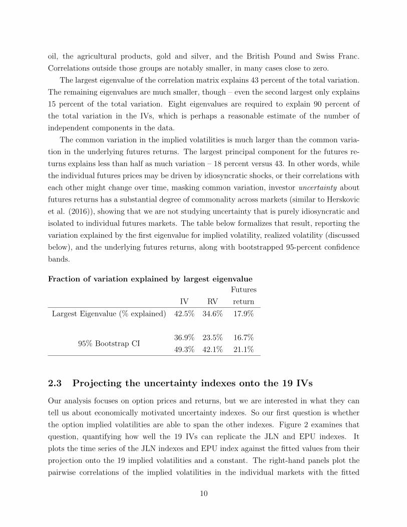
Fraction of variation explained by largest eigenvalue

Futures

IV RV return

Largest Eigenvalue (% explained) 42.5% 34.6% 17.9%

95% Bootstrap CI36.9% 23.5% 16.7%

49.3% 42.1% 21.1%

2.3 Projecting the uncertainty indexes onto the 19 IVs

Our analysis focuses on option prices and returns, but we are interested in what they can

tell us about economically motivated uncertainty indexes. So our first question is whether

the option implied volatilities are able to span the other indexes. Figure 2 examines that

question, quantifying how well the 19 IVs can replicate the JLN and EPU indexes. It

plots the time series of the JLN indexes and EPU index against the fitted values from their

projection onto the 19 implied volatilities and a constant. The right-hand panels plot the

pairwise correlations of the implied volatilities in the individual markets with the fitted

10

uncertainty. For financials, the correlation with S&P 500 implied volatility is 95 percent.

The next highest correlation is only 62 percent, for Treasury bonds. So figure 2 shows that

fitted financial uncertainty is very nearly equivalent to S&P 500 implied volatility.18

The second row plots fitted uncertainty for real variables. In this case, gold, copper, crude

oil, and heating oil are the most important contributors. The implied volatilities capture

well the lower-frequency variation, though they may miss some of the more high-frequency

variation.

The results for the price component of JLN uncertainty are reported in the third row.

The highest correlations are again for heating oil, crude oil, natural gas, gold, and copper.

These results show that uncertainty about the real economy and inflation are driven by

similar factors, and that those factors are notably distinct from financial uncertainty. They

also show why having a broad range of IVs, and looking at markets beyond the S&P 500, is

important, emphasizing the paper’s contribution.

The bottom panels plot results for the EPU index. The highest pairwise correlations

are with financial IVs, Treasuries, gold, the S&P 500, and currencies. So the fit of the IVs

to the EPU index comes mostly from the financial rather than the nonfinancial options.

That implies that the EPU index measures a similar type of uncertainty as other financial

uncertainty measures, perhaps because news coverage often focuses on financial markets.19

Appendix A.3.1 shows that even though the options do not perfectly replicate the uncer-

tainty indexes, the capture the economically relevant part. In particular, the spanned part

is related to economic outcomes, while the unspanned part is not.

Finally, appendix A.3.2 examines similar regressions for realized volatility, instead of

uncertainty, and comes to similar conclusions.

3 Constructing option portfolios to hedge uncertainty

Implied volatility and the uncertainty indexes are not directly tradable – only the options

themselves are. This section shows how to construct option portfolios that hedge shocks to

implied and realized volatility in each of the 19 markets and also the JLN and EPU indexes.

In principle, the uncertainty indexes could be hedged with other assets, not just options.

We focus on option returns because they depend directly on volatility and uncertainty – which

18The strong fit the S&P 500 implied volatility is not simply due to the fact that S&P 500 returns areincluded in the JLN construction. The results are similar when all variables involving the S&P 500 index(returns, dividends, etc.) are dropped.

19To account for possible overfitting due to the fact that we have 19 explanatory variables, we experimentedwith lasso and variable selection based on information criteria. The results were highly similar in all cases.

11

is why they are used to construct implied volatility measures – whereas for other assets, like

equities, the connection is less clear and stable. Adding more assets also increases estimation

error and overfitting.

We report results for two approaches to hedging shocks. The first uses the Black–Scholes

model to give analytic approximations for portfolio loadings. The second, in section 5.4,

simply estimates a standard linear factor model – thus estimating the loadings empirically.

The first requires more assumptions but is statistically more powerful, while the second is

more robust but generates somewhat wider confidence bands. The results from both are

economically highly similar.

3.1 Straddle portfolios

We study two-week returns on straddles with maturities between one and six months.20

A straddle is a portfolio holding a put and a call with the same maturity and strike; we

specifically study zero-delta straddles, that is, straddles with the strike set so that the Black–

Scholes delta of the portfolio – the derivative of its price with respect to the value of the

underlying – is zero. The final payoff of a zero-delta straddle depends on the absolute value

of the return on the underlying, meaning that they have symmetrical exposures to positive

and negative returns, and no local directional exposure to the underlying. For the remainder

of the paper, we refer to zero-delta straddles simply as straddles (that is, we only work with

zero-delta straddles).

Straddles give investors exposure both to realized and implied volatility. They are ex-

posed to realized volatility because the final payoff of the portfolio is a function of the

absolute value of the underlying futures return. But when a straddle is sold before maturity,

the sale price will also depend on expected future volatility, meaning that straddles can give

exposure to uncertainty shocks.

The exposures of straddles can be approximated theoretically using the Black–Scholes

model, as in Coval and Shumway (2001), Bakshi and Kapadia (2003), and Cremers, Halling,

20Past work on option returns and volatility risk premia has examined returns at frequencies of anywherefrom a day (e.g. Andries et al. (2017)), to holding to maturity (Bakshi and Kapadia (2003)). The precisionof estimates of the riskiness of the straddles is, all else equal, expected to be higher with shorter windows.On the other hand, shorter windows cause any measurement error in option prices to have larger effects.

Some of the existing literature, beginning with Bakshi and Kapadia (2003), examines delta-hedged returns.Even with delta hedging, the higher-order risk exposures of the straddles change substantially as the priceof the underlying changes over time.

Another alternative is to examine returns on synthetic variance swaps. Synthetic variance swap prices areconstructed using the full range of strikes, so they require much more data than straddles. The markets westudy do not all have liquid options at extreme strikes and multiple maturities, so we focus on straddles,which just require liquidity near the money.

12

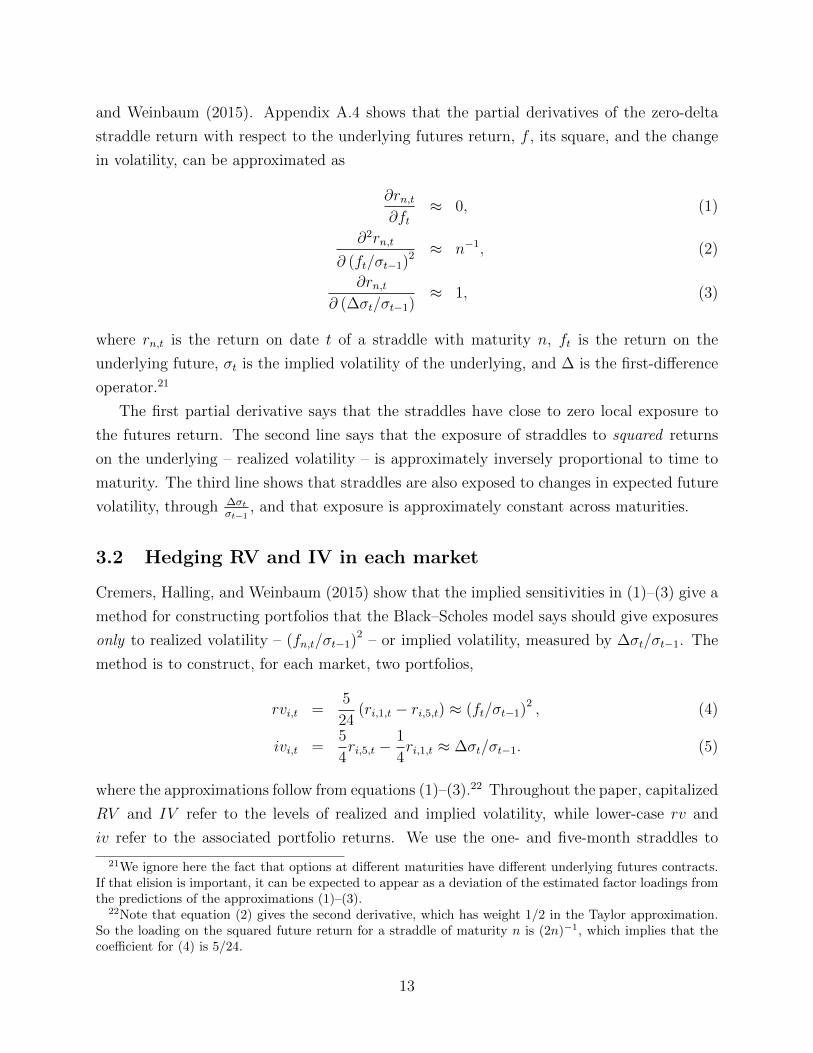
and Weinbaum (2015). Appendix A.4 shows that the partial derivatives of the zero-delta

straddle return with respect to the underlying futures return, f , its square, and the change

in volatility, can be approximated as

∂rn,t∂ft

≈ 0, (1)

∂2rn,t

∂ (ft/σt−1)2 ≈ n−1, (2)

∂rn,t∂ (∆σt/σt−1)

≈ 1, (3)

where rn,t is the return on date t of a straddle with maturity n, ft is the return on the

underlying future, σt is the implied volatility of the underlying, and ∆ is the first-difference

operator.21

The first partial derivative says that the straddles have close to zero local exposure to

the futures return. The second line says that the exposure of straddles to squared returns

on the underlying – realized volatility – is approximately inversely proportional to time to

maturity. The third line shows that straddles are also exposed to changes in expected future

volatility, through ∆σtσt−1

, and that exposure is approximately constant across maturities.

3.2 Hedging RV and IV in each market

Cremers, Halling, and Weinbaum (2015) show that the implied sensitivities in (1)–(3) give a

method for constructing portfolios that the Black–Scholes model says should give exposures

only to realized volatility – (fn,t/σt−1)2 – or implied volatility, measured by ∆σt/σt−1. The

method is to construct, for each market, two portfolios,

rvi,t =5

24(ri,1,t − ri,5,t) ≈ (ft/σt−1)2 , (4)

ivi,t =5

4ri,5,t −

1

4ri,1,t ≈ ∆σt/σt−1. (5)

where the approximations follow from equations (1)–(3).22 Throughout the paper, capitalized

RV and IV refer to the levels of realized and implied volatility, while lower-case rv and

iv refer to the associated portfolio returns. We use the one- and five-month straddles to

21We ignore here the fact that options at different maturities have different underlying futures contracts.If that elision is important, it can be expected to appear as a deviation of the estimated factor loadings fromthe predictions of the approximations (1)–(3).

22Note that equation (2) gives the second derivative, which has weight 1/2 in the Taylor approximation.So the loading on the squared future return for a straddle of maturity n is (2n)−1, which implies that thecoefficient for (4) is 5/24.

13

construct the portfolios as those are the shortest and longest maturities that we consistently

observe in the data.

The purpose of constructing these portfolios is to give a simple and direct method of

measuring the premia associated with realized and implied volatility that does not require

any complicated estimation or data transformation. One might worry that they do not obtain

the desired exposures in practice. Figure A.2 and table A.1 in the appendix show that the

theoretical predictions for the loadings are fairly accurate (though not perfect) empirically.

Appendix A.4 also examines the accuracy of the Black–Scholes approximation for returns in

a simulated setting.

Even though the rv and iv portfolios theoretically load on separate risk factors, they

need not be uncorrelated. It is well known from the GARCH literature (e.g. Engle (1982)

and Bollerslev (1986)) that in many markets, innovations to realized volatility are correlated

with innovations to implied volatility. Table 3 reports the correlations between the rv and iv

returns in the 19 markets. GARCH effects appear most strongly for the financial underlyings

and precious metals, where the average correlation is 0.44. For the other nonfinancial un-

derlyings, the effects are much smaller, and the correlation between the rv and iv returns is

only 0.03 on average (it is 0.09 on average across all nonfinancials). So for the nonfinancials,

innovations to realized and implied volatility returns are essentially independent on average.

These weak correlations are valuable for the identification, since they show that surprises in

realized and implied volatility are far from the same and can be hedged separately.

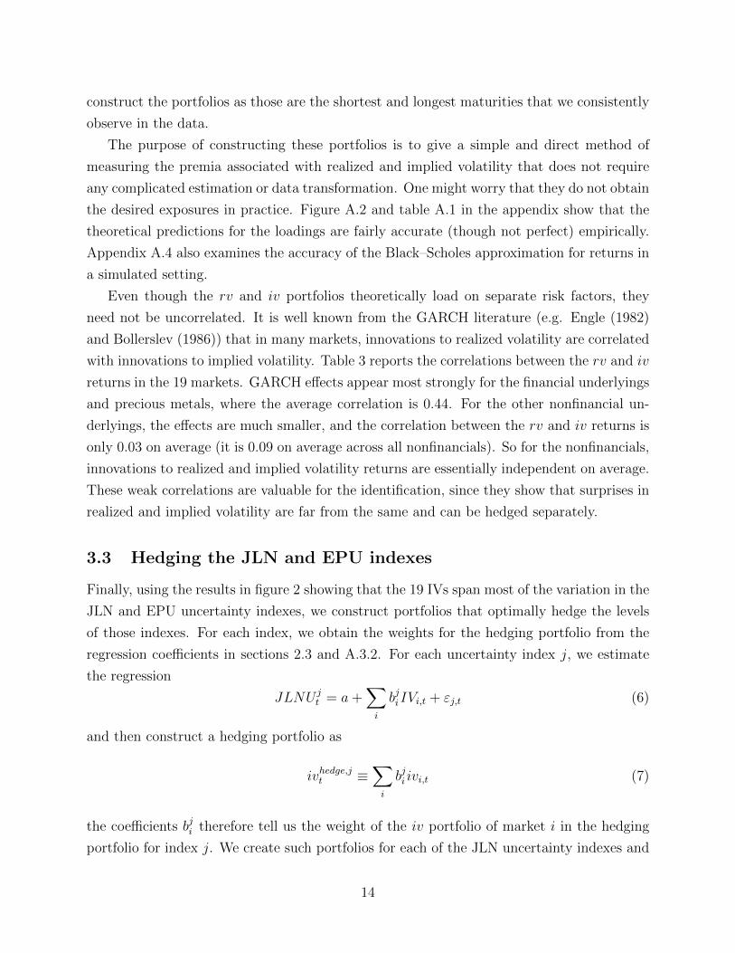
3.3 Hedging the JLN and EPU indexes

Finally, using the results in figure 2 showing that the 19 IVs span most of the variation in the

JLN and EPU uncertainty indexes, we construct portfolios that optimally hedge the levels

of those indexes. For each index, we obtain the weights for the hedging portfolio from the

regression coefficients in sections 2.3 and A.3.2. For each uncertainty index j, we estimate

the regression

JLNU jt = a+

∑i

bjiIVi,t + εj,t (6)

and then construct a hedging portfolio as

ivhedge,jt ≡∑i

bji ivi,t (7)

the coefficients bji therefore tell us the weight of the iv portfolio of market i in the hedging

portfolio for index j. We create such portfolios for each of the JLN uncertainty indexes and

14

the EPU index. We also construct similarly a hedge portfolio for the JLN realized volatility

series (JLNRV ) from the regression

JLNRV jt = a+

∑i

bRV,ji RVi,t + εRV,j,t (8)

rvhedge,jt ≡∑i

bjirvi,t (9)

For the main results, the hedging weights, bji , are estimated using the full-sample re-

gression. Section 4.2 reports results using hedging weights estimated on a rolling basis, bji,t,

where bji,t is estimated with a regression using data up to date t− 1.23

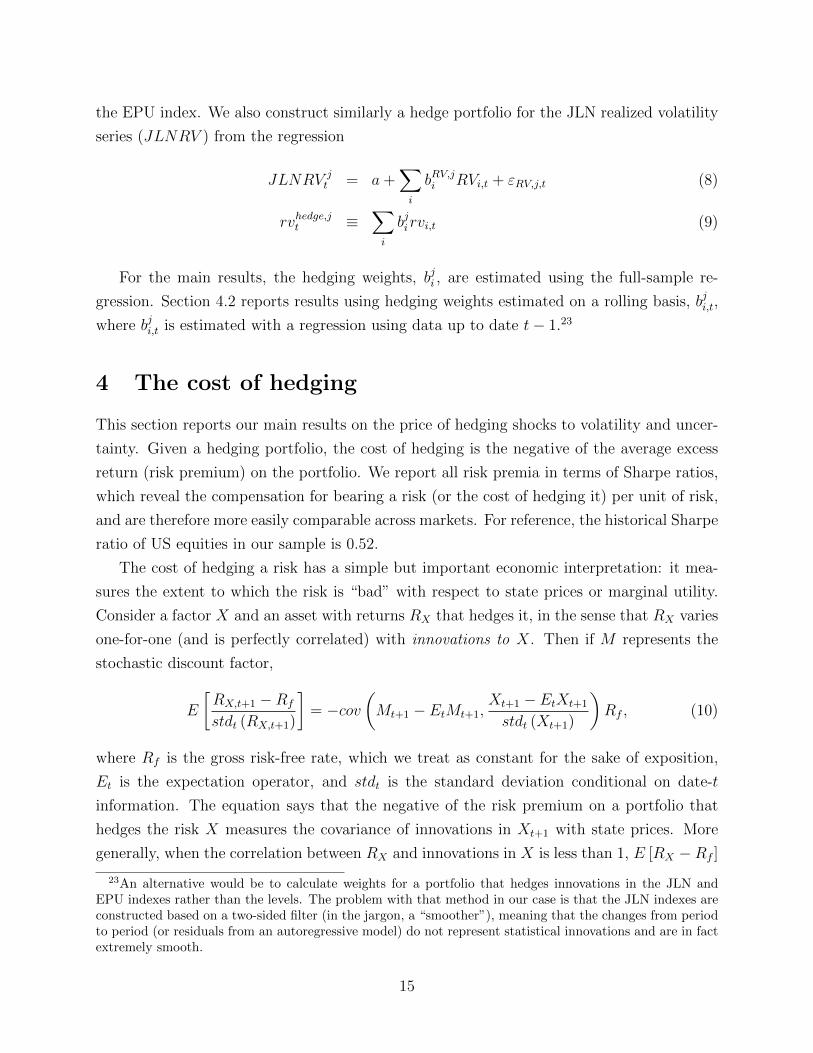
4 The cost of hedging

This section reports our main results on the price of hedging shocks to volatility and uncer-

tainty. Given a hedging portfolio, the cost of hedging is the negative of the average excess

return (risk premium) on the portfolio. We report all risk premia in terms of Sharpe ratios,

which reveal the compensation for bearing a risk (or the cost of hedging it) per unit of risk,

and are therefore more easily comparable across markets. For reference, the historical Sharpe

ratio of US equities in our sample is 0.52.

The cost of hedging a risk has a simple but important economic interpretation: it mea-

sures the extent to which the risk is “bad” with respect to state prices or marginal utility.

Consider a factor X and an asset with returns RX that hedges it, in the sense that RX varies

one-for-one (and is perfectly correlated) with innovations to X. Then if M represents the

stochastic discount factor,

E

[RX,t+1 −Rf

stdt (RX,t+1)

]= −cov

(Mt+1 − EtMt+1,

Xt+1 − EtXt+1

stdt (Xt+1)

)Rf , (10)

where Rf is the gross risk-free rate, which we treat as constant for the sake of exposition,

Et is the expectation operator, and stdt is the standard deviation conditional on date-t

information. The equation says that the negative of the risk premium on a portfolio that

hedges the risk X measures the covariance of innovations in Xt+1 with state prices. More

generally, when the correlation between RX and innovations in X is less than 1, E [RX −Rf ]

23An alternative would be to calculate weights for a portfolio that hedges innovations in the JLN andEPU indexes rather than the levels. The problem with that method in our case is that the JLN indexes areconstructed based on a two-sided filter (in the jargon, a “smoother”), meaning that the changes from periodto period (or residuals from an autoregressive model) do not represent statistical innovations and are in factextremely smooth.

15

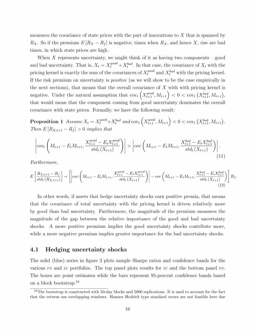
measures the covariance of state prices with the part of innovations to X that is spanned by

RX . So if the premium E [RX −Rf ] is negative, times when RX , and hence X, rise are bad

times, in which state prices are high.

When X represents uncertainty, we might think of it as having two components – good

and bad uncertainty. That is, Xt = Xgoodt +Xbad

t . In that case, the covariance of Xt with the

pricing kernel is exactly the sum of the covariances of Xgoodt and Xbad

t with the pricing kernel.

If the risk premium on uncertainty is positive (as we will show to be the case empirically in

the next sections), that means that the overall covariance of X with with pricing kernel is

negative. Under the natural assumption that covt

(Xgoodt+1 ,Mt+1

)< 0 < covt

(Xbadt+1,Mt+1

),

that would mean that the component coming from good uncertainty dominates the overall

covariance with state prices. Formally, we have the following result:

Proposition 1 Assume Xt = Xgoodt +Xbad

t and covt

(Xgoodt+1 ,Mt+1

)< 0 < covt

(Xbadt+1,Mt+1

).

Then E [RX,t+1 −Rf ] > 0 implies that∣∣∣∣∣covt(Mt+1 − EtMt+1,

Xgoodt+1 − EtX

goodt+1

stdt (Xt+1)

)∣∣∣∣∣ >∣∣∣∣cov(Mt+1 − EtMt+1,

Xbadt+1 − EtXbad

t+1

stdt (Xt+1)

)∣∣∣∣ .(11)

Furthermore,

E

[RX,t+1 −Rf

stdt (RX,t+1)

]=

[∣∣∣∣∣cov(Mt+1 − EtMt+1,

Xgoodt+1 − EtX

goodt+1

stdt (Xt+1)

)∣∣∣∣∣− cov(Mt+1 − EtMt+1,

Xbadt+1 − EtX

badt+1

stdt (Xt+1)

)]Rf .

(12)

In other words, if assets that hedge uncertainty shocks earn positive premia, that means

that the covariance of total uncertainty with the pricing kernel is driven relatively more

by good than bad uncertainty. Furthermore, the magnitude of the premium measures the

magnitude of the gap between the relative importance of the good and bad uncertainty

shocks. A more positive premium implies the good uncertainty shocks contribute more,

while a more negative premium implies greater importance for the bad uncertainty shocks.

4.1 Hedging uncertainty shocks

The solid (blue) series in figure 3 plots sample Sharpe ratios and confidence bands for the

various rv and iv portfolios. The top panel plots results for iv and the bottom panel rv.

The boxes are point estimates while the bars represent 95-percent confidence bands based

on a block bootstrap.24

24The bootstrap is constructed with 50-day blocks and 5000 replications. It is used to account for the factthat the returns use overlapping windows. Hansen–Hodrick type standard errors are not feasible here due

16

Across the top panel, the iv portfolios tend to earn zero or even positive returns. For

financials, the average Sharpe ratios tend to be near zero or weakly negative (the S&P,

in particular, yields a Sharpe ratio of -0.23, which is just 1 standard error from zero and

therefore statistically not significant). For the nonfinancials, all 14 sample Sharpe ratios are

actually positive. Overall, for only one out of 19 contracts (British pound) do we find a

significantly negative Sharpe ratio.

To formally estimate the average Sharpe ratios across contracts, we use a random effects

model, which yields an estimate of the population mean Sharpe ratio while simultaneously

accounting for the fact that each of the sample Sharpe ratios is estimated with error, and

that the errors are potentially correlated across contracts (see appendix A.5).

For both nonfinancials and all markets overall, the estimated population mean Sharpe

ratio is statistically and economically significantly positive, while for financials it is close to

zero. The group-level means have the advantage of being much more precisely estimated

than the Sharpe ratios for the markets individually. They show that on average, instead of

there being a cost to hedging uncertainty shocks, uncertainty-hedging portfolios actually earn

positive returns. For nonfinancials, the average Sharpe ratio is 0.37, and the lower end of

the 95-percent confidence interval is 0.14. For the overall mean, the corresponding numbers

are 0.26 and 0.5, so the average Sharpe ratios are significantly positive in both cases.

The right-hand section of figure 3 reports the Sharpe ratios for the portfolios hedging

the EPU and JLN indexes. Since those hedging portfolios are constructed combining the

individual iv portfolios, it is not surprising that they reflect the Sharpe ratios of those port-

folios. The hedging portfolios for JLN financial uncertainty and the EPU index both place

relatively more weight on the financials, which have Sharpe ratios that are weakly negative

and indistinguishable from zero. The portfolios hedging macro and price uncertainty, on

the contrary, have Sharpe ratios that are positive and in one case marginally statistically

significant.

The top panel of figure 3 contains our key results on the cost of hedging different types of

uncertainty shocks. It shows that across the board, risk premia for uncertainty are indistin-

guishable from zero or, if anything, somewhat positive. The results allow us to quantify the

relative importance of good and bad uncertainty across the various markets. For financial

underlyings, including the S&P 500, the zero or very weakly negative risk premium implies

that there is close to an equal split between good and bad uncertainty. For the nonfinancial

underlyings, which are closely linked to the JLN real and price uncertainty series, the results

imply that the majority of the variation in uncertainty is of the good type. So overall, across

to the fact that observations in the data are not equally spaced in time. The block bootstrap additionallyaccounts for other sources of serial correlation in the returns, such as time-varying risk premia.

17

a wide range of underlying economic risks, good uncertainty seems to equal or even dominate

bad uncertainty.

4.2 Hedging realized volatility shocks

The bottom panel of figure 3 reports analogous results for the cost of hedging realized

volatility shocks. The numbers are drastically different. Whereas the iv portfolios have

historically earned weakly positive returns, the rv portfolios have almost all historically

earned strongly negative returns. For the S&P 500, this result is well known and is referred

to as the variance risk premium. The S&P 500 rv portfolio has the most negative Sharpe

ratio, at -1.19 – the premium for selling insurance against shocks to realized volatility is more

than twice as large as the premium on the stock market over the same period. Treasuries also

have a significantly negative return, but the other financials in our sample – all currencies

– have Sharpe ratios close to zero. For the nonfinancials, 11 of 14 estimated Sharpe ratios

are negative. So whereas the cost of hedging uncertainty shocks with the iv portfolios is

consistently negative in the top panel, the cost of hedging realized volatility shocks using

the rv portfolios is positive in the bottom panel.

Looking at the category means, in this case all three estimates – financials, nonfinancials,

and all assets – are negative. The values are statistically significant for the nonfinancials

and the overall mean. The point estimate for the overall mean Sharpe ratio is -0.28 and the

upper end of the 95-percent confidence interval is -0.04. Those values are almost the same

as what we obtain for the iv portfolios, but with the opposite sign.

Finally, the right-hand section of the bottom panel of figure 3 reports the returns from

the JLN rv hedging portfolios – those that hedge the realized volatility of the JLN macro

series.25 Again, consistent with the fact that the rv portfolios themselves consistently earn

negative returns, hedging the JLN indexes for realized volatility historically has a positive

cost. For all three subindexes, the hedging portfolios earn extremely negative returns, with

the Sharpe ratios for financial, real, and price volatility at -1.18, -0.94, and -0.96.

In sum, in stark contrast to the results for hedging uncertainty, the bottom panel of figure

3 shows that there has historically been an extremely large cost to hedge realized volatility.

Contracts that, rather than loading on changes in implied volatility, load on actual realized

squared returns – which the analysis above shows directly hedge extreme events in the

macroeconomy – earn negative Sharpe ratios with magnitudes up to twice as large as that

for the overall stock market. So while uncertainty shocks in the economy appear to be a mix

25There is no realized volatility equivalent of the EPU index, so here we only look at the JLN ones, forwhich both the uncertainty and the realized volatility versions can be constructed, as discussed above.

18

of good and bad (with close to equal importance for financials, and tilted towards good for

nonfinancials), volatility – the realization of large shocks – is viewed as mostly bad, for both

financials and nonfinancials.

But how can that be? Doesn’t uncertainty lead to higher volatility? The answer is that

what we are pricing is innovations. When there is a surprise in volatility – ε2t is larger than

expected – that is typically bad. On the other hand, when there is a shock to uncertainty

– σ2t unexpectedly rises, that is apparently sometimes associated with good news (a new

invention) and sometimes bad. Section 6 formalizes that idea, describing a simple extension

of the standard long-run risk model of Bansal and Yaron (2004) that is consistent with our

results.

4.3 Combined portfolios

An alternative way to hedge aggregate uncertainty is simply to buy all the iv or rv portfolios

simultaneously. Since tables 1 and 2 show that realized and implied volatility are imperfectly

correlated across markets, even larger Sharpe ratios can be earned by holding portfolios that

diversify across the various underlyings. Table 4 reports results of various implementations

of such a strategy. Looking first at the top panel, the first row reports results for portfolios

that put equal weight on every available underlying in each period, the second row uses only

nonfinancial underlyings, and the third row only financial underlyings. The columns report

Sharpe ratios for various combinations of the rv and iv portfolios. The first two columns

report Sharpe ratios for strategies that hold only the rv or only the iv portfolios, the third

column uses a strategy that is short rv and long iv portfolios in equal weights, while the final

column is short rv and long iv, but with weights inversely proportional to their variances

(i.e. a simple risk parity strategy).

The Sharpe ratios reported in table 4 are generally larger than those in figure 3. The

portfolios that are short rv and long iv are able to attain Sharpe ratios above 1. The largest

Sharpe ratios come in the portfolios that combine rv and iv, which follows from the fact that

they are positively correlated, so going short rv and long iv leads to internal hedging. All of

that said, these Sharpe ratios remain generally plausible. Values near 1 are observed in other

contexts (e.g. Broadie, Chernov, and Johannes (2009) for put option returns, Asness and

Moskowitz (2013) for global value and momentum strategies, and Dew-Becker et al. (2017)

for variance swaps).

The portfolios that take advantage of all underlyings simultaneously seem to perform

best, presumably because they are the most diversified. While holding exposure to implied

volatility among the financials earns effectively a zero risk premium, it is still generally

19

worthwhile to include financials for the sake of hedging.

Finally, the bottom panel of table 4 reports the skewness of the various strategies from

above. One might think that the negative returns on the rv portfolio are driven by its

positive skewness, but the iv portfolio also is positively skewed and has positive average

returns. So the degree of skewness does not seem to explain differences in average returns

in this setting.

5 Robustness

This section examines some potential concerns about the robustness of the results.

5.1 One-week holding period returns

Our main analysis is based on two-week holding period returns for straddles, which strike

a balance between having more precise estimates of risk premia and reducing the impact of

measurement error in prices. We have repeated all of our analysis using one-week holding

period returns, and find very similar results. Appendix figure A.5 is the analog of figure

3, but constructed using one-week returns. The results are qualitatively and quantitatively

very similar to the baseline.

5.2 Split sample and rolling window results

To address the concern that the results could be driven by outliers (though note that there

would need to be outliers in all 19 markets), figures A.6 and A.7 replicate the main results in

figure 3, but splitting the sample in half (before and after June 2000). The confidence bands

are naturally wider, and the point estimates vary more from market to market in the two

figures. Nevertheless, the qualitative results are the same as in the full-sample case, showing

that realized volatility earns a negative premium while the premium on implied volatility is

positive.

To further evaluate the possibility that the results are driven by a small number of

observations, figure A.8 plots Sharpe ratios for the rv and iv portfolios in five-year rolling

windows for each of the 19 markets, as well as for the equal-weighted portfolios of all 19

markets. The sample Sharpe ratios are reasonably stable over time. In no case do the

results appear to be driven by a single outlying period or episode. Note that these results

are not informative about variation in the conditional risk premium; with a five-year window,

the standard error for the Sharpe ratios is 0.45, so even if the true conditional Sharpe ratios

20

are constant, the five-year rolling estimates should display large amounts of variation over

time.

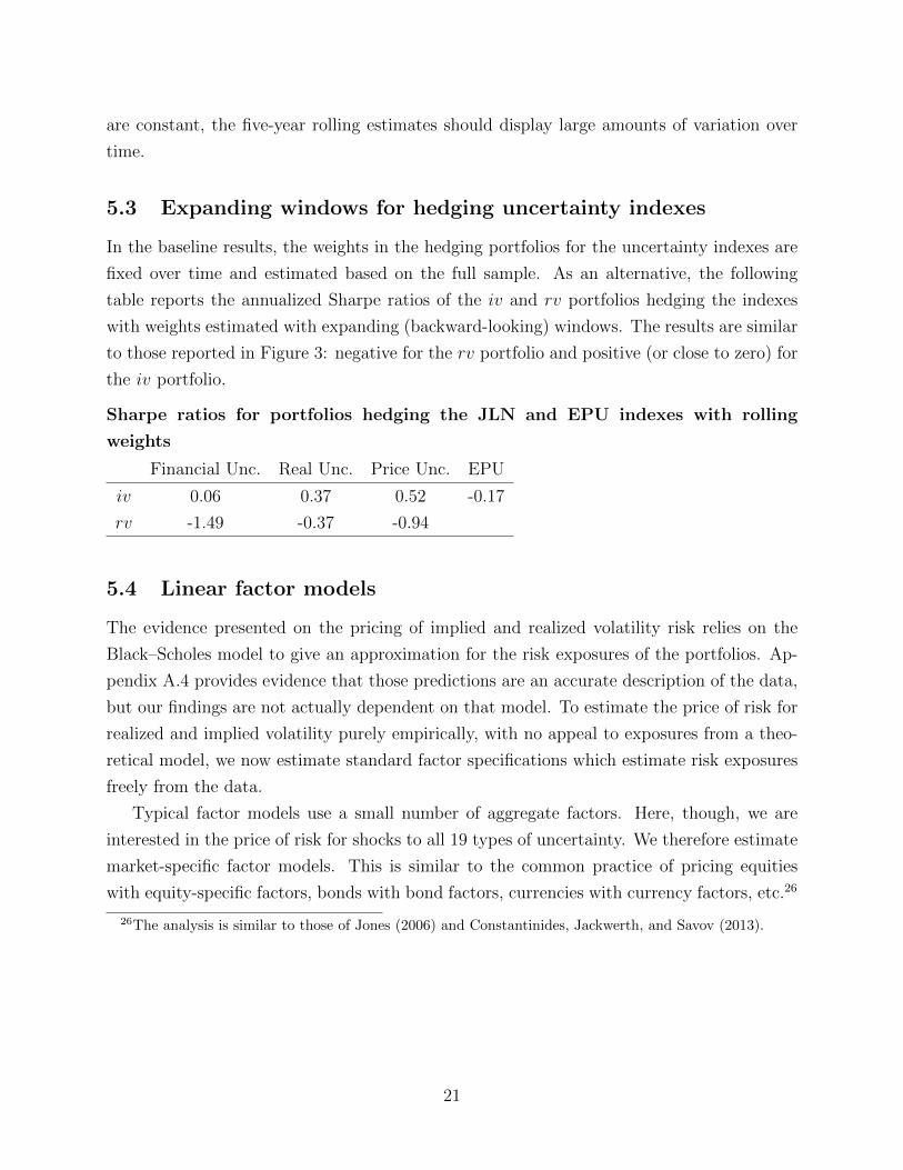
5.3 Expanding windows for hedging uncertainty indexes

In the baseline results, the weights in the hedging portfolios for the uncertainty indexes are

fixed over time and estimated based on the full sample. As an alternative, the following

table reports the annualized Sharpe ratios of the iv and rv portfolios hedging the indexes

with weights estimated with expanding (backward-looking) windows. The results are similar

to those reported in Figure 3: negative for the rv portfolio and positive (or close to zero) for

the iv portfolio.

Sharpe ratios for portfolios hedging the JLN and EPU indexes with rolling

weights

Financial Unc. Real Unc. Price Unc. EPU

iv 0.06 0.37 0.52 -0.17

rv -1.49 -0.37 -0.94

5.4 Linear factor models

The evidence presented on the pricing of implied and realized volatility risk relies on the

Black–Scholes model to give an approximation for the risk exposures of the portfolios. Ap-

pendix A.4 provides evidence that those predictions are an accurate description of the data,

but our findings are not actually dependent on that model. To estimate the price of risk for

realized and implied volatility purely empirically, with no appeal to exposures from a theo-

retical model, we now estimate standard factor specifications which estimate risk exposures

freely from the data.

Typical factor models use a small number of aggregate factors. Here, though, we are

interested in the price of risk for shocks to all 19 types of uncertainty. We therefore estimate

market-specific factor models. This is similar to the common practice of pricing equities

with equity-specific factors, bonds with bond factors, currencies with currency factors, etc.26

26The analysis is similar to those of Jones (2006) and Constantinides, Jackwerth, and Savov (2013).

21

5.4.1 Specification

For each market we estimate a time-series model of the form

ri,n,t = ai,n + βfi,nfi,t

IVi,t−1

+ βf2

i,n

1

2

(fi,t

IVi,t−1

)2

+ β∆IVi,n

∆IVi,tIVi,t−1

+ εi,n,t, (13)

where fi,t is the futures return for underlying i and ∆IVi,t is the change in the five-month

at-the-money implied volatility for underlying i. The underlying futures return controls for

any exposure of the straddles to the underlying, though the Black–Scholes model predicts

that effect to be small.

Much more important is the fact that straddles have a nonlinear exposure to the fu-

tures return. (fi,t/IVi,t−1)2 captures that nonlinearity. Consistent with the construction and

interpretation of the rv portfolio, βf2

i,n will be interpreted as the exposure of the straddles

to realized volatility.27 Finally, the third factor is the change in the at-the-money implied

volatility for the specific market at the five-month maturity.28

We estimate a standard linear specification for the risk premia,

E [ri,n,t] = γfi βfi,nStd

(fi,t

IVi,t−1

)+ γf

2

i βf2

i,nStd

((fi,t

IVi,t−1

)2)

+ γ∆IVi β∆IV

i,n Std

(∆IVi,tIVi,t−1

)+ αi,n,(14)

E [fi,t/IVi,t−1] = γfi Std(fi,t/IVi,t−1). (15)

where αi,n is a fitting error. The γ coefficients represent the risk premia that are earned

by investments that provide direct exposure to the factors. Due to the scaling by standard

deviations, the γ’s are estimates of what the Sharpe ratios on the factors would be if it were

possible to invest in them directly (neither f 2i,t nor ∆IVi,t is an asset return that one can

directly purchase in our data; fi,t itself is tradable, though, which is why we impose the second

equality). The difference between the method here and the rv and iv portfolios discussed

above is that the factor model does not require assumptions about the risk exposures of the

straddles – instead estimating them from (13) – whereas the rv and iv portfolios rely on the

Black–Scholes model. So the results using the factor models should be more robust, but also

have more estimation error.

27The results are similar when the second factor is the absolute value of the futures return or when it ismeasured as the sum of squared daily returns over the return period.

28Since the IVs may be measured with error, we construct this factor by regressing available impliedvolatilities on maturity for each underlying and date and then taking the fitted value from that regressionat the five-month maturity.

22

5.4.2 Results

The dashed (red) series in figure 3 plots the estimated risk premia across the various markets

along with 95-percent confidence bands. The top panel plots γ∆IVi , while the bottom panel

plots γf2

i . Simple inspection shows that the results are extremely close to those for the iv

and rv portfolios. The γ∆IVi estimates are almost all positive, while the γf

2

i are almost all

negative. As before, we produce a random effects estimate of the mean of the risk premia

in various groups. The random effects estimates of the means in the various groups are also

similar, both in magnitude and statistical significance, to the main results in the solid series.

The main difference between the two series is that the confidence bands are wider for the

factor model estimates, which is consistent with the fact that the factor model estimates

impose less structure and must estimate the factor loadings of the individual straddles.

5.5 Pricing the independent parts of RV and IV

The main results above report returns associated with assets that hedge innovations to

realized and implied volatility. Table 3 shows that those returns are positively correlated:

months with increases in realized volatility also tend to have increases in implied volatility.

A natural question is what would happen if we were to construct a portfolio that loaded on

the independent part of those returns, e.g. an increase in implied volatility holding realized

volatility fixed. Section A.8 in the appendix reports an SDF-based analysis that prices the

independent components and shows that the results are similar to the main specification

(see figure A.9).

5.6 Liquidity

If the options used here are highly illiquid, the analysis will be substantially complicated for

three reasons. First, to the extent that illiquidity represents a real cost faced by investors

– e.g. a bid/ask spread – then returns calculated from settlement prices do not represent

returns earned by investors. Second, illiquidity itself could carry a risk premium that the

options might be exposed to. Third, bid/ask spreads represent an added layer of noise

in prices. The identification of the premia for realized volatility and uncertainty depends

on differences in returns on options across maturities, so what is most important for our

purposes is how liquidity varies across maturities. This section shows that the liquidity of

the straddles studied here is generally highly similar to that of the widely studied S&P 500

contracts traded on the CBOE, and the liquidity does not appear to substantially deteriorate

across maturities.

23

We measure liquidity using two methods. First, since our data set does not include

posted bid/ask spreads, we estimate the standard Roll (1984) effective spread using the

daily returns.29 The top panel of appendix figure A.10 plots the effective bid/ask spreads

for straddles at maturities of 1, 3, and 5 months. The average posted bid/ask spreads for

CBOE S&P 500 straddles, for which we have data since 1996, are also reported in the figure.

At the one-month maturity, the effective spreads are approximately 6 percent on average,

which is similar to the 6.6-percent average posted spreads for one-month CBOE S&P 500

straddles. More importantly, the spreads actually decline at longer maturities indicating

that there is less observed negative autocovariance in returns for options at those maturities.

For the three- and five-month options, the spreads are smaller by about half, averaging 2 to

3 percent. This is again consistent with posted spreads for CBOE S&P 500 contracts, which

decline to 4.0 percent on average at six months.30

As a second measure of liquidity, we obtained posted bid/ask spreads for the options

closest to the money on Friday, 8/4/2017 for our 19 contracts plus the CBOE S&P 500

options at maturities of 1, 4, and 7 months. Those spreads are plotted in the bottom

panel of figure A.10. For the majority of the options, the spreads are less than 3 percent,

consistent with the 4.1-percent bid/ask spread for one-month S&P 500 options at the CBOE.

Across nearly all the contracts, the posted spreads again decline with maturity, and for 10

of the 19 contracts the one-month posted spreads are nearly indistinguishable from that for

the S&P 500, which is typically viewed as a highly liquid market and where incorporating

bid-ask spreads generally has minimal effects on return calculations (Bondarenko (2014)).

Figure A.10 yields two important results. First, it shows that the liquidity of the straddles

is reasonably high, in the sense that effective and posted spreads are both relatively narrow

in absolute terms for most of the contracts and that they compare favorably with spreads

for the more widely studied S&P 500 options traded at the CBOE. Second, liquidity does

not appear to deteriorate as the maturity of the options grows, and in fact in many cases

there are improvements with increasing maturities, again consistent with CBOE data.

Section A.4.3 in the appendix reports statistics for volume across maturities, showing

that the markets are generally fairly similar. Section A.4.4 reports an additional robustness

test that measures returns using a method that is robust to certain types of measurement

errors in prices, showing that the main results are essentially identical.

29The Roll model assumes that there is an unobservable mid-quote that follows a random walk in logs andthat observed prices have equal probability of being from a buy or sell order. Bid-ask bounce then inducesnegative autocorrelation in returns, from which the spread can be inferred (when the autocorrelation ispositive, we set the spread to zero).

30Even though postead spreads growth in absolute terms with maturity, straddle prices grow by more(approximately with the square root of maturity), causing the percentage spreads to decline.

24

Finally, it is useful to note that while the liquidity of option markets changed significantly

in the last 30 years, the patterns in risk premia for the rv and iv portfolios appear stable

over time (see, for example, the rolling Sharpe ratios of figure A.8), suggesting that liquidity

is not the main driver of our results.

Even though the liquidity is similar across many of the markets, one might still ask how

trading costs affect the returns we have been studying. Any trading cost will lower the return

of a portfolio, regardless of whether an investor is long or short. By studying returns based

on quoted prices, we are essentially looking at the return averaged across what the buyer

and seller receive. For example, if the return on a portfolio based on quoted prices is 10

percent and there are total trading costs to each side of 1 percent, then the buyer earns a

return of 9 percent while the seller has a loss of 11 percent. Looking at quotes is therefore

natural for illustrating the return that the average investor sees.

6 Model

To help provide some context for the empirical results and fit them into a standard frame-

work, this section describes results from a simple extension of the standard long-run risk

model of Bansal and Yaron (2004). The analysis is primarily in appendix A.10 and here we

report the specification and key results.

Agents have Epstein–Zin preferences over consumption , Ct, with a unit elasticity of

substitution, where the lifetime utility function, vt, satisfies

vt = (1− β) logCt +β

1− αlogEt exp ((1− α) vt+1) (16)

where α is the coefficient of relative risk aversion. Consumption growth follows the process

∆ct = xt−1 +√σ2B,t−1 + σ2

G,t−1εt + Jbt (17)

xt = φxxt−1 + ωxηx,t + ωx,Gησ,G,t − ωx,Bησ,B,t (18)

σ2j,t = (1− φσ) σ2

j + φσσ2j,t−1 + ωjησ,j,t, for j ∈ {B,G} (19)

where εt and the η·,t are independent standard normal random variables. xt represents the

consumption trend. We have two deviations from the usual setup. First, we include jump

shocks, Jbt, where bt is a Poisson distributed random variable with intensity λ and J is the

magnitude of the jump. This addition allows for random variation in realized volatility and

is drawn from Drechsler and Yaron (2011). Second, there are two components to volatility,

which we refer to as bad and good. Bad volatility, σ2B, is associated with low future con-

25

sumption growth, while good volatility, σ2G, is associated with high future growth (where all

of the ω· coefficients are nonnegative).

Define realized volatility to be the realized quadratic variation in consumption growth,

while implied volatility is the conditional variance of consumption growth (these are formal-

ized in the appendix).

Proposition 2 The average excess returns on forward claims to realized and implied volatil-

ity for consumption growth in this model are,

E [RVt+1 − PRV,t] = J2λ (1− exp (−αJ)) (20)

E [IVt+1 − PIV,t] = (α− 1)(vY,x (ωx,GωG − ωx,BωB) + vY,σ

(ω2G + ω2

B

))(21)

where Px,t is the forward price for x. E [IVt+1 − PIV,t] > 0 for ωx,G sufficiently larger than

ωx,B. Furthermore, the sign of E [RVt+1 − PRV,t] is the same as the sign of J and of the

conditional skewness of consumption growth (i.e. the skewness of ∆ct+1 conditional on date-

t information).

Proposition 2 contains our key analytic results. We analyze premia for realized and

implied volatility on consumption – real activity – consistent with the focus in the empirical

analysis on macro volatility and uncertainty. The negative premium on realized volatility

is driven by downward jumps, similar to the literature on the volatility risk premium in

equities (Drechsler and Yaron (2011), Wachter (2013)). The sign of the premium on implied

volatility depends on the contribution of good versus bad volatility. When good volatility

shocks, where high volatility is associated with high future growth (e.g. due to learning

about new technologies), are relatively larger than bad volatility shocks (ωx,GωG > ωx,BωB)

the premium on implied volatility can be positive.

The appendix provides a numerical calibration of the model using values close to those in

Bansal and Yaron’s (2004) original choices. It shows that the model generates quantitatively

realistic Sharpe ratios for implied and realized volatility in addition to a reasonable equity

premium.

The key economic mechanism for the positive pricing of uncertainty shocks is that high

volatility is sometimes associated with higher long-term growth. Intuitively, that mechanism

contributes positive skewness to consumption growth, while the jumps contribute negative

skewness. The appendix provides novel evidence on the skewness of consumption growth

consistent with the model. In particular, conditional skewness in the model, which depends

only on the jumps, is more negative than the skewness of expected consumption growth,

26

which depends on the relationship of volatility and long-run growth (x). We show that

consumption growth displays exactly the same pattern in US data.

So a simple version of the long-run risk model with good and bad volatility shocks and

jumps in consumption can match our key empirical facts. Furthermore, the empirical results

are sharp, in the sense that the sign of the premium on implied volatility identifies the

relative importance of the bad and good volatility shocks, while the sign of the premium on

realized volatility identifies the sign of consumption jumps.

7 Conclusion

This paper studies the pricing of uncertainty and realized volatility across a broad array of

options on financial and commodity futures. Uncertainty is proxied by implied volatility

– which theoretically measures investors’ conditional variances for future returns – and a

number of uncertainty indexes developed in the literature. Realized volatility, on the other

hand, measures how large realized shocks have been. In modeling terms, if εt+1 ∼ N (0, σ2t ),

uncertainty is σ2t , while volatility is the realization of ε2

t .

A large literature in macroeconomics and finance has focused on the effects of uncertainty

on the economy. This paper explores empirically how investors perceive uncertainty shocks.

If uncertainty shocks have major contractionary effects so that they are associated with high

marginal utility for the average investor, then assets that hedge uncertainty should earn

negative average returns. On the other hand, the finance literature has recently argued that

in many cases uncertainty can be good. For example, during the late 1990’s, it may have

been the case that investors were not sure about how good new technologies would turn out

to be.

The contribution of this paper is to construct hedging portfolios for a range of types

of macro uncertainty, including interest rates, energy prices, and uncertainty indexes. The

cost of hedging uncertainty shocks reveals the relative importance of good and bad types of

uncertainty. Furthermore, using a wide range of options is important for capturing uncer-

tainty about the real economy and inflation, as opposed to just about financial markets. The

empirical results imply that uncertainty shocks, no matter what type of uncertainty we look

at, are not viewed as being negative by investors, or at least not sufficiently negative that it

is costly to hedge them. Financial uncertainty appears to be roughly equally split between

the good and bad types, while nonfinancial uncertainty is relatively more strongly driven by

good uncertainty – the cost of hedging nonfinancial uncertainty shocks is negative.

What is highly costly to hedge is realized volatility. Portfolios that hedge extreme returns

27

in futures markets – and hence large innovations in macroeconomic time series – earn strongly

negative returns, with premia that are in many cases one to two times as large as the premium

on the aggregate stock market over the same period. So what is consistently high in bad

times is not uncertainty, but realized volatility. Periods in which futures markets and the

macroeconomy are highly volatile and display large movements appear to be periods of high

marginal utility, in the sense that their associated state prices are high. This is consistent

with (and complementary to) the findings in Berger, Dew-Becker, and Giglio (2019), who

provide VAR evidence that shocks to volatility predict declines in real activity in the future,

while shocks to uncertainty do not.

Berger, Dew-Becker, and Giglio (2019) show that the VAR evidence and pricing results

for realized volatility are consistent with the view that it is downward jumps in the economy

that investors are most averse to. They show that a simple model in which fundamental

shocks are both stochastically volatile and negatively skewed can quantitatively match the

pricing of uncertainty and realized volatility, along with the VAR evidence. Similarly, Seo

and Wachter (2018a,b) show that negative skewness can explain the pricing of credit default

swaps and put options. This paper thus also contributes to the growing literature studying

the effects of skewness. In a world where fundamental shocks are negatively skewed, the

most extreme shocks – those that generate realized volatility – tend to be negative, which

can explain why realized volatility would be so costly to hedge.

References

Abel, Andrew B., “Optimal Investment Under Uncertainty,” American Economic Review, 1983,73 (1), 228–233.

Ait-Sahalia, Yacine, Mustafa Karaman, and Loriano Mancini, “The Term Structure ofVariance Swaps, Risk Premia and the Expectations Hypothesis,” 2015. Working paper.

Alexopoulos, Michelle and Jon Cohen, “Uncertain Times, Uncertain Measures,” 2009. Work-ing paper.

Andries, Marianne, Thomas M Eisenbach, Martin C Schmalz, and Yichuan Wang,“The term structure of the price of variance risk,” 2015.

Asness, Clifford S, Tobias J Moskowitz, and Lasse Heje Pedersen, “Value and momentumeverywhere,” The Journal of Finance, 2013, 68 (3), 929–985.

Bachmann, Rudiger and Christian Bayer, ““Wait-and-See” business cycles?,” Journal ofMonetary Economics, 2013, 60 (6), 704–719.

and Giuseppe Moscarini, “Business Cycles and Endogenous Uncertainty,” 2012. Workingpaper.

28

Baker, Scott R, Nicholas Bloom, and Steven J Davis, “Measuring economic policy uncer-tainty,” The Quarterly Journal of Economics, 2016, 131 (4), 1593–1636.

Bakshi, Gurdip and Nikunj Kapadia, “Delta-Hedge Gains and the Negative Market VolatilityRisk Premium,” The Review of Financial Studies, 2003, 16(2), 527–566.

, , and Dilip Madan, “Stock Return Characteristics, Skew Laws, and the DifferentialPricing of Individual Equity Options,” Review of Financial Studies, 2003, 16 (1), 101–143.

Barro, Robert J., “Rare Disasters and Asset Markets in the Twentieth Century,” QuarterlyJournal of Economics, 2006, 121(3), 823–866.

Barunık, Jozef, Evzen Kocenda, and Lukas Vacha, “Asymmetric connectedness on the U.S.stock market: Bad and good volatility spillovers,” Journal of Financial Markets, 2016, 27, 55– 78.

Basu, Susanto and Brent Bundick, “Uncertainty Shocks in a Model of Effective Demand,”2015. Working paper.

Bekaert, Geert, Eric Engstrom, and Andrey Ermolov, “Bad environments, good environ-ments: A non-Gaussian asymmetric volatility model,” Journal of Econometrics, 2015, 186 (1),258–275.

, Marie Hoerova, and Marco Lo Duca, “Risk, uncertainty and monetary policy,” Journalof Monetary Economics, 2013, 60 (7), 771–788.

Berger, David, Ian Dew-Becker, and Stefano Giglio, “Uncertainty shocks as second-momentnews shocks,” 2017. Working paper.

Binsbergen, Jules H. Van and Ralph S.J. Koijen, “The Term Structure of Returns: Factsand Theory,” Journal of Financial Economics, 2017, 124 (1), 1–21.

Black, Fischer, “The pricing of commodity contracts,” Journal of Financial Economics, 1976, 3(1-2), 167–179.

and Myron Scholes, “The Pricing of Options and Corporate Liabilities,” The Journal ofPolitical Economy, 1973, 81 (3), 637–654.

Bloom, Nicholas, “The Impact of Uncertainty Shocks,” Econometrica, 2009, 77(3), 623–685.

, Max Floetotto, Nir Jaimovich, Itay Saporta-Eksten, and Stephen J. Terry, “ReallyUncertain Business Cycles,” 2014. Working paper.

Bollerslev, Tim, “Generalized autoregressive conditional heteroskedasticity,” Journal of econo-metrics, 1986, 31 (3), 307–327.

and Viktor Todorov, “Tails, fears, and risk premia,” Journal of Finance, 2011, 66(6),2165–2211.

Bondarenko, Oleg, “Why Are Put Options So Expensive?,” Quarterly Journal of Finance, 2014,04 (03), 1450015.

29

Bretscher, Lorenzo, Lukas Schmid, and Andrea Vedolin, “Interest rate risk managementin uncertain times,” The Review of Financial Studies, 2018, 31 (8), 3019–3060.

Broadie, Mark, Mikhail Chernov, and Michael Johannes, “Understanding Index OptionReturns,” The Review of Financial Studies, 2009, 22(11), 4493–4529.

Caballero, Ricardo J, “Aggregate investment,” Handbook of macroeconomics, 1999, 1, 813–862.

Caldara, Dario, Cristina Fuentes-Albero, Simon Gilchrist, and Egon Zakrajsek, “Themacroeconomic impact of financial and uncertainty shocks,” European Economic Review, 2016.

Choi, Hoyong, Philippe Mueller, and Andrea Vedolin, “Bond Variance Risk Premiums,”Review of Finance, 2017, 21 (3), 987–1022.

Christiano, Lawrence J., Roberto Motto, and Massimio Rostagno, “Risk Shocks,” Amer-ican Economic Review, 2014, 104(1), 27–65.

Constantinides, George M, Jens Carsten Jackwerth, and Alexi Savov, “The puzzle ofindex option returns,” Review of Asset Pricing Studies, 2013, 3 (2), 229–257.

Creal, Drew D and Jing Cynthia Wu, “Monetary policy uncertainty and economic fluctua-tions,” International Economic Review, 2017, 58 (4), 1317–1354.

Cremers, Martijn, Michael Halling, and David Weinbaum, “Aggregate Jump and VolatilityRisk in the Cross-Section of Stock Returns,” The Journal of Finance, 2015, 70 (2), 577–614.

Darby, Julia, Andrew Hughes Hallett, Jonathan Ireland, and Laura Piscitelli, “Theimpact of exchange rate uncertainty on the level of investment,” The Economic Journal, 1999,109 (454), 55–67.

Dew-Becker, Ian, Stefano Giglio, Anh Le, and Marius Rodriguez, “The price of variancerisk,” Journal of Financial Economics, 2017, 123 (2), 225 – 250.

Drechsler, Itamar and Amir Yaron, “What’s Vol Got to Do with it?,” The Review of FinancialStudies, 2011, 24(1), 1–45.

Egloff, Daniel, Markus Leippold, and Liuren Wu, “The Term Structure of Variance SwapRates and Optimal Variance Swap Investments,” Journal of Financial and Quantitative Anal-ysis, 2010, 45(5), 1279–1310.

Elder, John, “Another perspective on the effects of inflation uncertainty,” Journal of Money,Credit, and Banking, 2004, 36 (5), 911–928.

and Apostolos Serletis, “Oil price uncertainty,” Journal of Money, Credit and Banking,2010, 42 (6), 1137–1159.

Engle, Robert F, “Autoregressive conditional heteroscedasticity with estimates of the variance ofUnited Kingdom inflation,” Econometrica: Journal of the Econometric Society, 1982, pp. 987–1007.

Gilchrist, Simon and John C Williams, “Investment, capacity, and uncertainty: a putty–clayapproach,” Review of Economic Dynamics, 2005, 8 (1), 1–27.

30

Gourio, Francois, “Credit Risk and Disaster Risk,” American Economic Journal: Macroeco-nomics, 2013, 5(3), 1–34. Working paper.

Hartman, Richard, “The effects of price and cost uncertainty on Investment,” Journal of Eco-nomic Theory, 1972, 5 (2), 258–266.

Herskovic, Bernard, Bryan Kelly, Hanno Lustig, and Stijn Van Nieuwerburgh, “Thecommon factor in idiosyncratic volatility: Quantitative asset pricing implications,” Journal ofFinancial Economics, 2016, 119 (2), 249–283.

Huizinga, John, “Inflation uncertainty, relative price uncertainty, and investment in US manu-facturing,” Journal of Money, Credit and Banking, 1993, 25 (3), 521–549.

Jones, Christopher S, “A nonlinear factor analysis of S&P 500 index option returns,” TheJournal of Finance, 2006, 61 (5), 2325–2363.

Jurado, Kyle, Sydney Ludvigson, and Serena Ng, “Measuring Uncertainty,” American Eco-nomic Review, 2015, 105 (3), 1177–1216.

Kilic, Mete and Ivan Shaliastovich, “Good and bad variance premia and expected returns,”Management Science, 2019, 65 (6), 2522–2544.

Leduc, Sylvain and Zheng Liu, “Uncertainty shocks are aggregate demand shocks,” Journal ofMonetary Economics, 2016, 82, 20–35.

Ludvigson, Sydney C, Sai Ma, and Serena Ng, “Uncertainty and Business Cycles: ExogenousImpulse or Endogenous Response?,” Technical Report, National Bureau of Economic Research2015.

McCracken, Michael W and Serena Ng, “FRED-MD: A monthly database for macroeconomicresearch,” Journal of Business & Economic Statistics, 2016, 34 (4), 574–589.

Oi, Walter, “The Desirability of Price Instability Under Perfect Competition,” Econometrica,1961, 29 (1), 58–64.

Pastor, L’ubos and Pietro Veronesi, “Technological Revolutions and Stock Prices,” The Amer-ican Economic Review, 2009, pp. 1451–1483.

Patton, Andrew J and Kevin Sheppard, “Good volatility, bad volatility: Signed jumps andthe persistence of volatility,” Review of Economics and Statistics, 2015, 97 (3), 683–697.

Prokopczuk, Marcel, Lazaros Symeonidis, and Chardin Wese Simen, “Variance risk incommodity markets,” Journal of Banking & Finance, 2017, 81, 136–149.

Salgado, Sergio, Fatih Guvenen, and Nicholas Bloom, “Skewed Business Cycles,” 2016.Working paper.

Segal, Gill, Ivan Shaliastovich, and Amir Yaron, “Good and bad uncertainty: Macroeco-nomic and financial market implications,” Journal of Financial Economics, 2015, 117 (2),369–397.

Seo, Sang Byung and Jessica A. Wacheter, “Do Rare Events Explain CDX Tranche Spreads?,”The Journal of Finance, 0 (ja).

31

and Jessica A Wachter, “Option prices in a model with stochastic disaster risk,” Manage-ment Science, 2018.

Trolle, Anders B and Eduardo S Schwartz, “Variance risk premia in energy commodities,”The Journal of Derivatives, 2010, 17 (3), 15–32.

Wachter, Jessica A., “Can time-varying risk of rare disasters explain aggregate stock marketvolatility?,” Journal of Finance, 2013, 68(3), 987–1035.

32

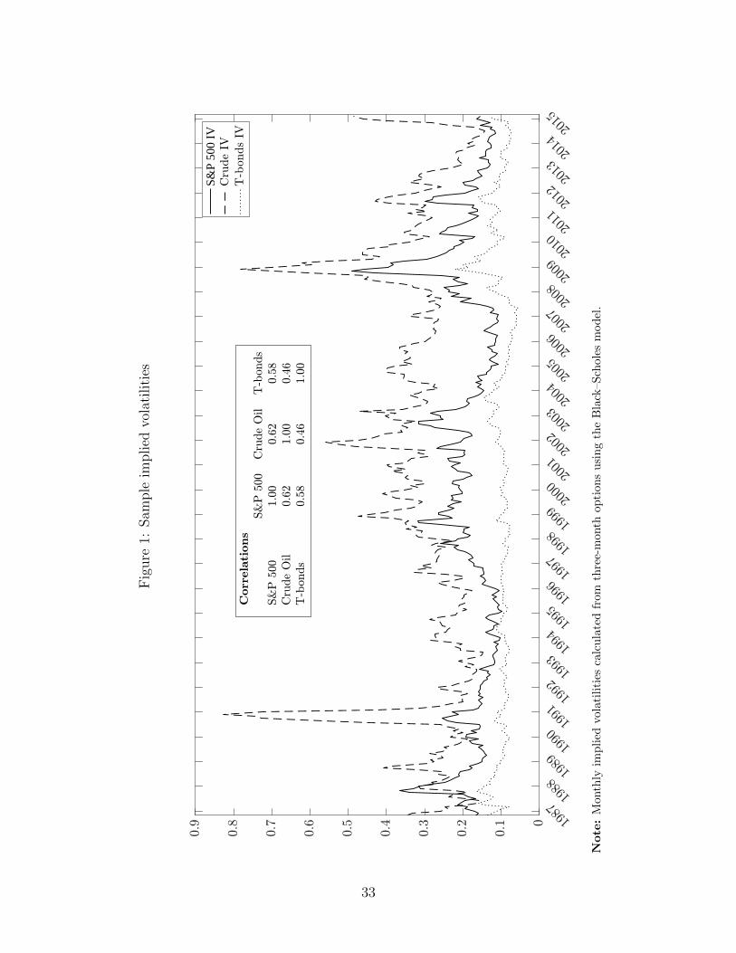
Fig

ure

1:Sam

ple

implied

vola

tiliti

es

S&P

500

IV

Note

:M

onth

lyim

pli

edvo

lati

liti

esca

lcu

late

dfr

omth

ree-

mon

thop

tion

su

sin

gth

eB

lack

–Sch

oles

mod

el.

33

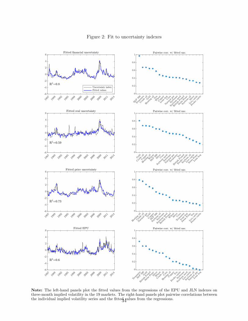
Figure 2: Fit to uncertainty indexes

Note: The left-hand panels plot the fitted values from the regressions of the EPU and JLN indexes onthree-month implied volatility in the 19 markets. The right-hand panels plot pairwise correlations betweenthe individual implied volatility series and the fitted values from the regressions.34

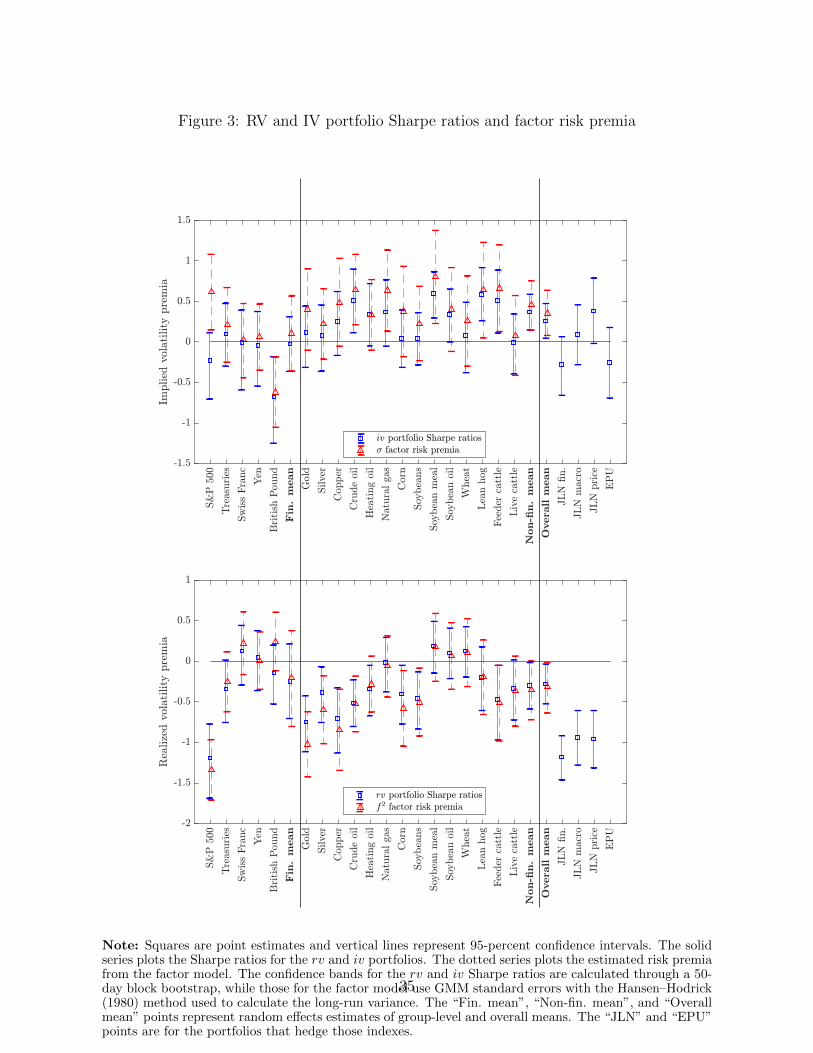
Figure 3: RV and IV portfolio Sharpe ratios and factor risk premia

Note: Squares are point estimates and vertical lines represent 95-percent confidence intervals. The solidseries plots the Sharpe ratios for the rv and iv portfolios. The dotted series plots the estimated risk premiafrom the factor model. The confidence bands for the rv and iv Sharpe ratios are calculated through a 50-day block bootstrap, while those for the factor model use GMM standard errors with the Hansen–Hodrick(1980) method used to calculate the long-run variance. The “Fin. mean”, “Non-fin. mean”, and “Overallmean” points represent random effects estimates of group-level and overall means. The “JLN” and “EPU”points are for the portfolios that hedge those indexes.

35

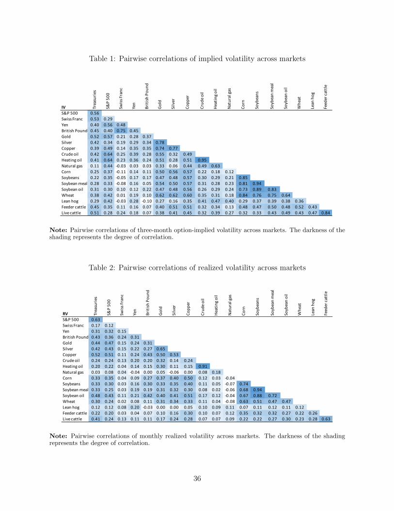
Table 1: Pairwise correlations of implied volatility across markets

IV Trea

surie

s

S&P

500

Swiss

Fran

c

Yen

Briti

sh P

ound

Gol

d

Silv

er

Copp

er

Crud

e oil

Hea

ting o

il

Nat

ural

gas

Corn

Soyb

eans

Soyb

ean

mea

l

Soyb

ean

oil

Whe

at

Lean

hog

Feed

er ca

ttle

S&P 500 0.56Swiss Franc 0.53 0.29Yen 0.40 0.56 0.48British Pound 0.45 0.40 0.75 0.45Gold 0.52 0.57 0.21 0.28 0.37Silver 0.42 0.34 0.19 0.29 0.34 0.78Copper 0.39 0.49 0.14 0.35 0.35 0.74 0.77Crude oil 0.42 0.64 0.25 0.39 0.28 0.55 0.32 0.49Heating oil 0.41 0.64 0.23 0.36 0.24 0.51 0.28 0.51 0.95Natural gas 0.11 0.44 -0.03 0.03 0.03 0.33 0.06 0.44 0.49 0.63Corn 0.25 0.37 -0.11 0.14 0.11 0.50 0.56 0.57 0.22 0.18 0.12Soybeans 0.22 0.35 -0.05 0.17 0.17 0.47 0.48 0.57 0.30 0.29 0.21 0.85Soybean meal 0.28 0.33 -0.08 0.16 0.05 0.54 0.50 0.57 0.31 0.28 0.23 0.81 0.94Soybean oil 0.31 0.30 0.10 0.12 0.22 0.47 0.48 0.56 0.26 0.29 0.24 0.73 0.89 0.83Wheat 0.38 0.42 0.01 0.19 0.10 0.62 0.62 0.60 0.35 0.31 0.18 0.84 0.76 0.75 0.64Lean hog 0.29 0.42 -0.03 0.28 -0.10 0.27 0.16 0.35 0.41 0.47 0.40 0.29 0.37 0.39 0.38 0.36Feeder cattle 0.45 0.35 0.11 0.16 0.07 0.40 0.51 0.51 0.32 0.34 0.13 0.48 0.47 0.50 0.48 0.52 0.43Live cattle 0.51 0.28 0.24 0.18 0.07 0.38 0.41 0.45 0.32 0.39 0.27 0.32 0.33 0.43 0.49 0.43 0.47 0.84

Note: Pairwise correlations of three-month option-implied volatility across markets. The darkness of theshading represents the degree of correlation.

Table 2: Pairwise correlations of realized volatility across markets

RV Trea

suri

es

S&P

500

Swis

s Fra

nc

Yen

Brit

ish

Poun

d

Gol

d

Silv

er

Copp

er

Crud

e oi

l

Hea

ting

oil

Nat

ural

gas

Corn

Soyb

eans

Soyb

ean

mea

l

Soyb

ean

oil

Whe

at

Lean

hog

Feed

er c

attl

eS&P 500 0.63Swiss Franc 0.17 0.12Yen 0.31 0.32 0.15British Pound 0.43 0.36 0.24 0.31Gold 0.44 0.47 0.15 0.24 0.31Silver 0.42 0.43 0.15 0.22 0.27 0.65Copper 0.52 0.51 0.11 0.24 0.43 0.50 0.53Crude oil 0.24 0.24 0.13 0.20 0.20 0.32 0.14 0.24Heating oil 0.20 0.22 0.04 0.14 0.15 0.30 0.11 0.15 0.91Natural gas 0.03 0.08 0.04 -0.04 0.00 0.05 -0.06 0.00 0.08 0.18Corn 0.33 0.35 0.04 0.09 0.27 0.37 0.40 0.50 0.12 0.03 -0.04Soybeans 0.33 0.30 0.03 0.16 0.30 0.33 0.35 0.40 0.11 0.05 -0.07 0.74Soybean meal 0.33 0.25 0.03 0.19 0.19 0.31 0.32 0.30 0.08 0.02 -0.06 0.68 0.94Soybean oil 0.48 0.43 0.11 0.21 0.42 0.40 0.41 0.51 0.17 0.12 -0.04 0.67 0.88 0.72Wheat 0.30 0.24 0.02 0.08 0.11 0.31 0.34 0.33 0.11 0.04 -0.08 0.63 0.51 0.47 0.47Lean hog 0.12 0.12 0.08 0.20 -0.03 0.00 0.00 0.05 0.10 0.09 0.11 0.07 0.11 0.12 0.11 0.12Feeder cattle 0.22 0.20 0.03 0.04 0.07 0.10 0.16 0.30 0.10 0.07 0.12 0.35 0.32 0.32 0.27 0.22 0.26Live cattle 0.41 0.24 0.13 0.11 0.11 0.17 0.24 0.28 0.07 0.07 0.09 0.22 0.22 0.27 0.30 0.23 0.28 0.63

Note: Pairwise correlations of monthly realized volatility across markets. The darkness of the shadingrepresents the degree of correlation.

36

Table 3: Correlations between rv and iv portfolio returns in each market

Std(rv) Std(iv) Corr(rv,iv)S&P 500 0.03 0.08 0.48T-bonds 0.03 0.08 0.01CHF 0.04 0.08 0.63JPY 0.04 0.08 0.61GBP 0.04 0.07 0.41Gold 0.04 0.12 0.48Silver 0.04 0.08 0.45Copper 0.03 0.10 0.03Crude Oil 0.04 0.09 0.05Heating oil 0.04 0.08 0.01Natural gas 0.04 0.08 -0.17Corn 0.04 0.08 0.06Soybeans 0.04 0.09 0.17Soybean meal 0.04 0.11 0.20Soybean oil 0.04 0.09 0.21Wheat 0.04 0.08 0.08Lean hog 0.05 0.10 -0.24Feeder cattle 0.05 0.10 0.03Live cattle 0.04 0.08 -0.12

Note: The table reports, for each underlying, the standard deviation of the two-week returns to the rvand iv portfolios, and their correlation.

Table 4: Portfolios of rv and iv across markets

Panel A: Sharpe ratiosrv iv Equal weight Risk-parity

All underlyings -0.75 *** 0.54 ** 1.09 *** 0.96 ***Nonfinancials -0.65 *** 0.68 *** 0.96 *** 0.97 ***Financials -0.37 ** -0.04 0.42 *** 0.13

Panel B: Skewnessrv iv Equal weight Risk-parity

All underlyings 1.21 *** 1.81 *** -0.73 *** 1.02 ***Nonfinancials 1.63 *** 1.52 *** -1.31 *** 0.84 ***Financials 2.02 *** 2.94 *** -1.40 *** 2.20 ***

rv+iv

rv+iv

Note: Sharpe ratios and skewness of portfolios combining rv and iv portfolios across markets. For eachpanel, the first row reports a portfolio constructed using straddles from all available markets on each date,the second row using only nonfinancial underlyings, the third row only financial underlyings. Each columncorresponds to a different portfolio. The first column is an equal-weighted RV portfolio, the second is anequal-weighted IV portfolio, the third is an equal-weighted long-short IV minus RV portfolio, and the lastis the same long/short portfolio but weighted by the inverse of the variance (risk-parity). *** indicatessignificance at the 1-percent level, ** the 5-percent level, and * the 10-percent level.

37

A.1 Data filters and transformations

The observed option prices very often appear to have nontrivial measurement errors. Thissection describes the various filters we use and then proceeds to provide more informationabout the specifics of the data transformations we apply. Code is available on request.

First, we note that the price formats for futures and strike prices for many of the com-modities change over time. That is, they will move between, say, 1/8ths, 1/16ths, andpennies. We make the prices into a consistent decimal time series for each commodity byinspecting the prices directly and then coding by hand the change dates.

We then remove all options with the following properties

1. Strikes greater than 5 times the futures price

2. Options with open interest below the 5th percentile across all contracts in the sample

3. Price less then 5 ticks above zero

4. Maturity less than 9 days

5. Maturity greater than 8 months.

6. Options with prices below their intrinsic value (the value if exercised immediately)

Note that in our baseline results, we do not remove options for which we have no volumeinformation, or for which volume is zero. However, we have reproduced our main analysis(figure 3) including that filter and find, if anything, stronger results. We report them inAppendix figure A.4.

We then calculate implied volatilities using the Black–Scholes formula, treating the op-tions as though they are European. We have also replicated the analysis using Americanimplied volatilities and find nearly identical results (the reason is that in most cases weultimately end up converting the IVs back into prices, meaning that any errors in the pric-ing formula are largely irrelevant – it is just a temporary data transformation, rather thanactually representing a volatility calculation).

The data are then further filtered based on the IVs:

1. Eliminate all zero or negative IVs

2. All options with IV more than 50 percent (in proportional terms) different from theaverage for the same underlying, date, and maturity

3. We then filter outliers along all three dimensions, strike, date, and maturity, removingthe following:

(a) If the IV changes for a contract by 15 percent or more on a given day thenmoves by 15 percent or more in the opposite direction in a single day within thenext week, and if it moves by less than 3 percent on average over that window,for options with maturity greater than 90 days (this eliminates temporary largechanges in IVs that are reversed that tend to be observed early in the life of theoptions).

A.1

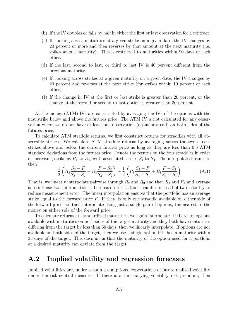
(b) If the IV doubles or falls by half in either the first or last observation for a contract

(c) If, looking across maturities at a given strike on a given date, the IV changes by20 percent or more and then reverses by that amount at the next maturity (i.e.spikes at one maturity). This is restricted to maturities within 90 days of eachother.

(d) If the last, second to last, or third to last IV is 40 percent different from theprevious maturity.

(e) If, looking across strikes at a given maturity on a given date, the IV changes by20 percent and reverses at the next strike (for strikes within 10 percent of eachother).

(f) If the change in IV at the first or last strike is greater than 20 percent, or thechange at the second or second to last option is greater than 30 percent.

At-the-money (ATM) IVs are constructed by averaging the IVs of the options with thefirst strike below and above the futures price. The ATM IV is not calculated for any obser-vation where we do not have at least one observation (a put or a call) on both sides of thefutures price.

To calculate ATM straddle returns, we first construct returns for straddles with all ob-servable strikes. We calculate ATM straddle returns by averaging across the two closeststrikes above and below the current futures price as long as they are less than 0.5 ATMstandard deviations from the futures price. Denote the returns on the four straddles in orderof increasing strike as R1 to R4, with associated strikes S1 to S4. The interpolated return isthen

1

2

(R2

S3 − FS3 − S2

+R3F − S2

S3 − S2

)+

1

2

(R1

S4 − FS4 − S1

+R1F − S1

S4 − S1

)(A.1)

That is, we linearly interpolate pairwise through R2 and R3 and then R1 and R4 and averageacross those two interpolations. The reason to use four straddles instead of two is to try toreduce measurement error. The linear interpolation ensures that the portfolio has an averagestrike equal to the forward price F . If there is only one straddle available on either side ofthe forward price, we then interpolate using just a single pair of options, the nearest to themoney on either side of the forward price.

To calculate returns at standardized maturities, we again interpolate. If there are optionsavailable with maturities on both sides of the target maturity and they both have maturitiesdiffering from the target by less than 60 days, then we linearly interpolate. If options are notavailable on both sides of the target, then we use a single option if it has a maturity within35 days of the target. This does mean that the maturity of the option used for a portfolioat a desired maturity can deviate from the target.

A.2 Implied volatility and regression forecasts

Implied volatilities are, under certain assumptions, expectations of future realized volatilityunder the risk-neutral measure. If there is a time-varying volatility risk premium, then

A.2

implied volatilities will be imperfectly correlated with physical expectations of future realizedvolatility, which constitutes actual uncertainty. This section compares implied volatilities toregression-based forecasts of future volatility to evaluate the quantitative magnitude of thatdeviation.

For each market, we estimate the regression

RVi,t = ai + bi (L)RVi,t−1 + ciIVi,t−1 + εi,t (A.2)

where bi (L) is a polynomial in the lag operator, L, and ai and ci are coefficients. RVi,t isrealized volatility in month t for market i – the sum of squared daily futures returns duringthe month. IVi,t is the (at-the-money) implied volatility at the end of month t in market i.

The table below reports the correlation between the fitted values from that regres-sion – which represent physical uncertainty – and implied volatility. That is, it reportscorr (bi (L)RVi,t−1 + ciIVi,t−1, IVi,t−1). Ideally, we would like that correlation to be 1, sothat implied volatility is perfectly correlated with physical uncertainty, and hedging impliedvolatility hedges uncertainty. Note that this does not require that risk premia are constant.If bi (L) = 0 but ci 6= 1, risk premia are time-varying, but the physical uncertainty is stillperfectly correlated with implied volatility. It is only deviations of bi (L) from zero thatreduce the correlation. To the extent that the implied volatility summarizes all availableinformation, we would expect bi = 0.

Correlations of implied volatility with fitted uncertainty

S&P 500 0.966 Crude oil 0.998 Silver 0.984Treasuries 0.940 Feeder cattle 0.951 Soybeans 0.970British Pound 0.987 Gold 0.994 Soybean meal 0.974Swiss Franc 0.994 Heating oil 0.992 Soybean oil 0.946Yen 0.976 Lean hogs 0.937 Wheat 0.998Copper 0.963 Live cattle 0.919Corn 0.994 Natural gas 0.949

The table shows that across the various markets, the correlations are all high, with aminimum of 91.1 percent and a mean of 97.0 percent. So while implied volatility is notliterally the same as physical uncertainty, it appears to be fairly close. In the baselineresults, we allow for two lags in the polynomial b, but we have experimented with alternativespecifications and obtain similar results.

A.3 Further results on spanning the uncertainty in-

dexes with options

A.3.1 The economic content of the spanned uncertainty indexes

This section examines the relationship of the spanned and unspanned parts of the uncertaintyindexes with the macroeconomy. Denote the fitted value from the regression of the JLNU

A.3

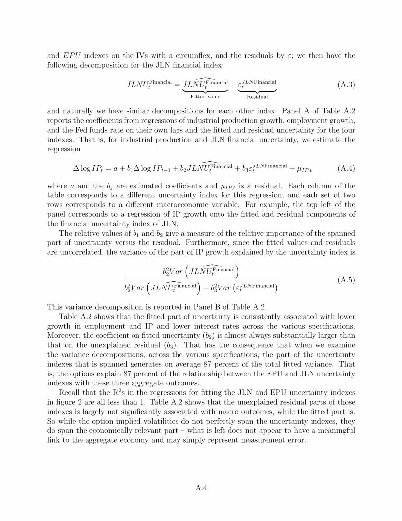
and EPU indexes on the IVs with a circumflex, and the residuals by ε; we then have thefollowing decomposition for the JLN financial index:

JLNUFinancialt = JLNUFinancial

t︸ ︷︷ ︸Fitted value

+ εJLNFinancialt︸ ︷︷ ︸

Residual

(A.3)

and naturally we have similar decompositions for each other index. Panel A of Table A.2reports the coefficients from regressions of industrial production growth, employment growth,and the Fed funds rate on their own lags and the fitted and residual uncertainty for the fourindexes. That is, for industrial production and JLN financial uncertainty, we estimate theregression

∆ log IPt = a+ b1∆ log IPt−1 + b2JLNUFinancial

t + b3εJLNFinancialt + µIP,t (A.4)

where a and the bj are estimated coefficients and µIP,t is a residual. Each column of thetable corresponds to a different uncertainty index for this regression, and each set of tworows corresponds to a different macroeconomic variable. For example, the top left of thepanel corresponds to a regression of IP growth onto the fitted and residual components ofthe financial uncertainty index of JLN.

The relative values of b1 and b2 give a measure of the relative importance of the spannedpart of uncertainty versus the residual. Furthermore, since the fitted values and residualsare uncorrelated, the variance of the part of IP growth explained by the uncertainty index is

b22V ar

(JLNUFinancial

t

)b2

2V ar(

JLNUFinancialt

)+ b2

3V ar(εJLNFinancialt

) (A.5)

This variance decomposition is reported in Panel B of Table A.2.Table A.2 shows that the fitted part of uncertainty is consistently associated with lower

growth in employment and IP and lower interest rates across the various specifications.Moreover, the coefficient on fitted uncertainty (b2) is almost always substantially larger thanthat on the unexplained residual (b3). That has the consequence that when we examinethe variance decompositions, across the various specifications, the part of the uncertaintyindexes that is spanned generates on average 87 percent of the total fitted variance. Thatis, the options explain 87 percent of the relationship between the EPU and JLN uncertaintyindexes with these three aggregate outcomes.

Recall that the R2s in the regressions for fitting the JLN and EPU uncertainty indexesin figure 2 are all less than 1. Table A.2 shows that the unexplained residual parts of thoseindexes is largely not significantly associated with macro outcomes, while the fitted part is.So while the option-implied volatilities do not perfectly span the uncertainty indexes, theydo span the economically relevant part – what is left does not appear to have a meaningfullink to the aggregate economy and may simply represent measurement error.

A.4

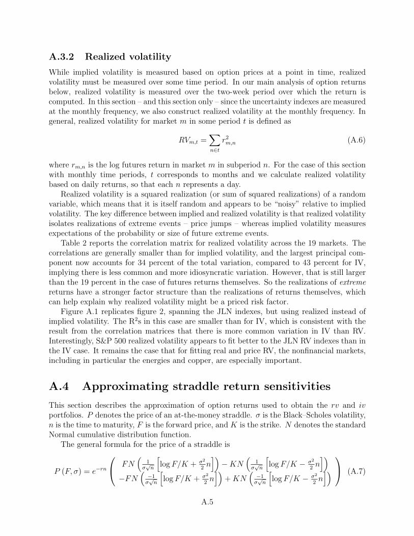
A.3.2 Realized volatility

While implied volatility is measured based on option prices at a point in time, realizedvolatility must be measured over some time period. In our main analysis of option returnsbelow, realized volatility is measured over the two-week period over which the return iscomputed. In this section – and this section only – since the uncertainty indexes are measuredat the monthly frequency, we also construct realized volatility at the monthly frequency. Ingeneral, realized volatility for market m in some period t is defined as

RVm,t =∑n∈t

r2m,n (A.6)

where rm,n is the log futures return in market m in subperiod n. For the case of this sectionwith monthly time periods, t corresponds to months and we calculate realized volatilitybased on daily returns, so that each n represents a day.

Realized volatility is a squared realization (or sum of squared realizations) of a randomvariable, which means that it is itself random and appears to be “noisy” relative to impliedvolatility. The key difference between implied and realized volatility is that realized volatilityisolates realizations of extreme events – price jumps – whereas implied volatility measuresexpectations of the probability or size of future extreme events.

Table 2 reports the correlation matrix for realized volatility across the 19 markets. Thecorrelations are generally smaller than for implied volatility, and the largest principal com-ponent now accounts for 34 percent of the total variation, compared to 43 percent for IV,implying there is less common and more idiosyncratic variation. However, that is still largerthan the 19 percent in the case of futures returns themselves. So the realizations of extremereturns have a stronger factor structure than the realizations of returns themselves, whichcan help explain why realized volatility might be a priced risk factor.

Figure A.1 replicates figure 2, spanning the JLN indexes, but using realized instead ofimplied volatility. The R2s in this case are smaller than for IV, which is consistent with theresult from the correlation matrices that there is more common variation in IV than RV.Interestingly, S&P 500 realized volatility appears to fit better to the JLN RV indexes than inthe IV case. It remains the case that for fitting real and price RV, the nonfinancial markets,including in particular the energies and copper, are especially important.

A.4 Approximating straddle return sensitivities

This section describes the approximation of option returns used to obtain the rv and ivportfolios. P denotes the price of an at-the-money straddle. σ is the Black–Scholes volatility,n is the time to maturity, F is the forward price, and K is the strike. N denotes the standardNormal cumulative distribution function.

The general formula for the price of a straddle is

P (F, σ) = e−rn

FN(

1σ√n

[logF/K + σ2

2n])−KN

(1

σ√n

[logF/K − σ2

2n])

−FN(−1σ√n

[logF/K + σ2

2n])

+KN(−1σ√n

[logF/K − σ2

2n]) (A.7)

A.5

We calculate the straddles at the strike such that d1 = 0, which is

K = F exp

(σ2

2n

)(A.8)

The price is then

P = e−rnF exp

(σ2

2n

)(−N

(−σ√n)

+N(σ√n))

(A.9)

The derivative of the price with respect to the underlying at that point is zero. The secondderivative of the straddle’s price is

PFF (Ft, σt) = 2e−rnN ′ (0)

Ftσt√n

(A.10)

The sensitivity to volatility is

Pσ (Ft, σt) = 2e−rnFtN′ (0)√n (A.11)

The local approximation for returns that we use is

∂rt+1

∂xt+1

=∂

∂xt+1

P (Ft+1, σt+1)

P (Ft, σt)(A.12)

and we evaluate the derivatives at the point Ft+1 = Ft, σt+1 = σt.We have

∂2rt+1

∂F 2t+1

=PFFP

(A.13)

= 2e−rnN ′ (0)

Ftσt√n

1

e−rnF exp(σ2

2n)

(−N (−σ√n) +N (σ

√n))

(A.14)

We then use the approximation

N(σ√n)−N

(−σ√n)≈ 2N ′ (0)σt

√n (A.15)

and use exp(σ2

2n)≈ 1, yielding

∂2rt+1

∂F 2t+1

≈ 1

F 2t σ

2t n

(A.16)

Since ∂F 2t+1/F

2t σ

2t = ∂ (ft+1/σt)

2, where ft is the log futures return, we have

∂2rt+1

∂ (ft+1/σt)2 ≈

1

n(A.17)

A.6

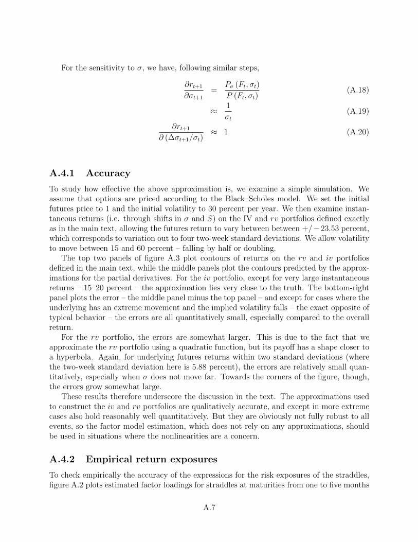
For the sensitivity to σ, we have, following similar steps,

∂rt+1

∂σt+1

=Pσ (Ft, σt)

P (Ft, σt)(A.18)

≈ 1

σt(A.19)

∂rt+1

∂ (∆σt+1/σt)≈ 1 (A.20)

A.4.1 Accuracy

To study how effective the above approximation is, we examine a simple simulation. Weassume that options are priced according to the Black–Scholes model. We set the initialfutures price to 1 and the initial volatility to 30 percent per year. We then examine instan-taneous returns (i.e. through shifts in σ and S) on the IV and rv portfolios defined exactlyas in the main text, allowing the futures return to vary between between +/−23.53 percent,which corresponds to variation out to four two-week standard deviations. We allow volatilityto move between 15 and 60 percent – falling by half or doubling.

The top two panels of figure A.3 plot contours of returns on the rv and iv portfoliosdefined in the main text, while the middle panels plot the contours predicted by the approx-imations for the partial derivatives. For the iv portfolio, except for very large instantaneousreturns – 15–20 percent – the approximation lies very close to the truth. The bottom-rightpanel plots the error – the middle panel minus the top panel – and except for cases where theunderlying has an extreme movement and the implied volatility falls – the exact opposite oftypical behavior – the errors are all quantitatively small, especially compared to the overallreturn.

For the rv portfolio, the errors are somewhat larger. This is due to the fact that weapproximate the rv portfolio using a quadratic function, but its payoff has a shape closer toa hyperbola. Again, for underlying futures returns within two standard deviations (wherethe two-week standard deviation here is 5.88 percent), the errors are relatively small quan-titatively, especially when σ does not move far. Towards the corners of the figure, though,the errors grow somewhat large.

These results therefore underscore the discussion in the text. The approximations usedto construct the iv and rv portfolios are qualitatively accurate, and except in more extremecases also hold reasonably well quantitatively. But they are obviously not fully robust to allevents, so the factor model estimation, which does not rely on any approximations, shouldbe used in situations where the nonlinearities are a concern.

A.4.2 Empirical return exposures

To check empirically the accuracy of the expressions for the risk exposures of the straddles,figure A.2 plots estimated factor loadings for straddles at maturities from one to five months

A.7

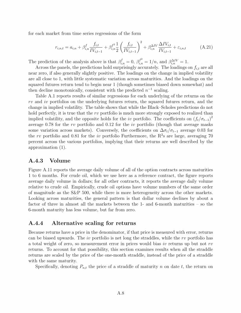
for each market from time series regressions of the form

ri,n,t = ai,n + βfi,nfi,t

IVi,t−1

+ βf2

i,n

1

2

(fi,t

IVi,t−1

)2

+ β∆IVi,n

∆IVi,tIVi,t−1

+ εi,n,t (A.21)

The prediction of the analysis above is that βfi,n = 0, βf2

i,n = 1/n, and β∆IVi,n = 1.

Across the panels, the predictions hold surprisingly accurately. The loadings on fi,t are allnear zero, if also generally slightly positive. The loadings on the change in implied volatilityare all close to 1, with little systematic variation across maturities. And the loadings on thesquared futures return tend to begin near 1 (though sometimes biased down somewhat) andthen decline monotonically, consistent with the predicted n−1 scaling.

Table A.1 reports results of similar regressions for each underlying of the returns on therv and iv portfolios on the underlying futures return, the squared futures return, and thechange in implied volatility. The table shows that while the Black–Scholes predictions do nothold perfectly, it is true that the rv portfolio is much more strongly exposed to realized thanimplied volatility, and the opposite holds for the iv portfolio. The coefficients on (ft/σt−1)2

average 0.78 for the rv portfolio and 0.12 for the iv portfolio (though that average maskssome variation across markets). Conversely, the coefficients on ∆σt/σt−1 average 0.03 forthe rv portfolio and 0.81 for the iv portfolio Furthermore, the R2s are large, averaging 70percent across the various portfolios, implying that their returns are well described by theapproximation (1).

A.4.3 Volume

Figure A.11 reports the average daily volume of all of the option contracts across maturities1 to 6 months. For crude oil, which we use here as a reference contract, the figure reportsaverage daily volume in dollars; for all other contracts, it reports the average daily volumerelative to crude oil. Empirically, crude oil options have volume numbers of the same orderof magnitude as the S&P 500, while there is more heterogeneity across the other markets.Looking across maturities, the general pattern is that dollar volume declines by about afactor of three in almost all the markets between the 1- and 6-month maturities – so the6-month maturity has less volume, but far from zero.

A.4.4 Alternative scaling for returns

Because returns have a price in the denominator, if that price is measured with error, returnscan be biased upwards. The iv portfolio is net long the straddles, while the rv portfolio hasa total weight of zero, so measurement error in prices would bias iv returns up but not rvreturns. To account for that possibility, this section examines results when all the straddlereturns are scaled by the price of the one-month straddle, instead of the price of a straddlewith the same maturity.

Specifically, denoting Pn,t the price of a straddle of maturity n on date t, the return on

A.8

an n-month straddle used in the main results is

Rn,t =Pn−1,t+1 − Pn,t

Pn,t(A.22)

We consider returns on a portfolio that puts weight Pn,t

P1,ton the n-month straddle and weight

1− Pn,t

P1,ton the risk-free asset (which is a tradable portfolio), which is

rrescaledn,t+1 =Pn−1,t+1 − Pn,t

Pn,t

Pn,tP1,t

+

(1− Pn,t

P1,t

)rf,t (A.23)

=Pn−1,t+1 − Pn,t

P1,t

+

(1− Pn,t

P1,t

)rf,t (A.24)

This portfolio is useful for two reasons. First, the one-month maturity has the highest volumein most markets we study, and it is typically considered to be the most accurate. Second, thiseliminates differences in bias across maturities since in this specification, the denominator isthe same for all n.

For rrescaledn,t+1 , similar calculations to those above yield the results that

∂2rrescaledn,t+1

∂ (ft+1/σt)2 ≈ 1√

n(A.25)

∂rrescaledn,t+1

∂ (∆σt+1/σt)≈√n (A.26)

We then calculate alternative rv and iv portfolios as

ivrescaledt =3√12

(√5/12rrescaled5,t −

√1/12rrescaled1,t

)(A.27)

rvrescaledt =5/48√

12

(√12rrescaled1,t −

√12/5rrescaled5,t

)(A.28)

Figure A.12 replicates figure 3 with the rescaled returns. The results are nearly identicalto the baseline for both the Sharpe ratios on the iv and rv portfolios and the estimatedfactor risk premia. These results show that when we correct for the potential bias inducedby low liquidity and measurement error at longer maturities, the estimates are essentiallyunchanged.

A.5 Random effects models

Denote the vector of true Sharpe ratios for the straddles in market i as sri. Our goal isto estimate the distribution of sri across the various underlyings. A natural benchmark

A.9

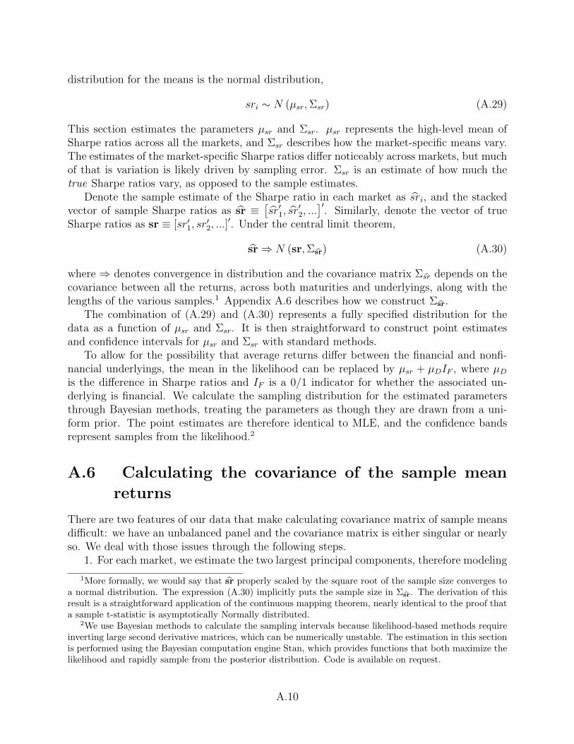
distribution for the means is the normal distribution,

sri ∼ N (µsr,Σsr) (A.29)

This section estimates the parameters µsr and Σsr. µsr represents the high-level mean ofSharpe ratios across all the markets, and Σsr describes how the market-specific means vary.The estimates of the market-specific Sharpe ratios differ noticeably across markets, but muchof that is variation is likely driven by sampling error. Σsr is an estimate of how much thetrue Sharpe ratios vary, as opposed to the sample estimates.

Denote the sample estimate of the Sharpe ratio in each market as sri, and the stackedvector of sample Sharpe ratios as sr ≡

[sr′1, sr

′2, ...

]′. Similarly, denote the vector of true

Sharpe ratios as sr ≡ [sr′1, sr′2, ...]

′. Under the central limit theorem,

sr⇒ N (sr,Σsr) (A.30)

where ⇒ denotes convergence in distribution and the covariance matrix Σsr depends on thecovariance between all the returns, across both maturities and underlyings, along with thelengths of the various samples.1 Appendix A.6 describes how we construct Σsr.

The combination of (A.29) and (A.30) represents a fully specified distribution for thedata as a function of µsr and Σsr. It is then straightforward to construct point estimatesand confidence intervals for µsr and Σsr with standard methods.

To allow for the possibility that average returns differ between the financial and nonfi-nancial underlyings, the mean in the likelihood can be replaced by µsr + µDIF , where µDis the difference in Sharpe ratios and IF is a 0/1 indicator for whether the associated un-derlying is financial. We calculate the sampling distribution for the estimated parametersthrough Bayesian methods, treating the parameters as though they are drawn from a uni-form prior. The point estimates are therefore identical to MLE, and the confidence bandsrepresent samples from the likelihood.2

A.6 Calculating the covariance of the sample mean

returns

There are two features of our data that make calculating covariance matrix of sample meansdifficult: we have an unbalanced panel and the covariance matrix is either singular or nearlyso. We deal with those issues through the following steps.

1. For each market, we estimate the two largest principal components, therefore modeling

1More formally, we would say that sr properly scaled by the square root of the sample size converges toa normal distribution. The expression (A.30) implicitly puts the sample size in Σsr. The derivation of thisresult is a straightforward application of the continuous mapping theorem, nearly identical to the proof thata sample t-statistic is asymptotically Normally distributed.

2We use Bayesian methods to calculate the sampling intervals because likelihood-based methods requireinverting large second derivative matrices, which can be numerically unstable. The estimation in this sectionis performed using the Bayesian computation engine Stan, which provides functions that both maximize thelikelihood and rapidly sample from the posterior distribution. Code is available on request.

A.10

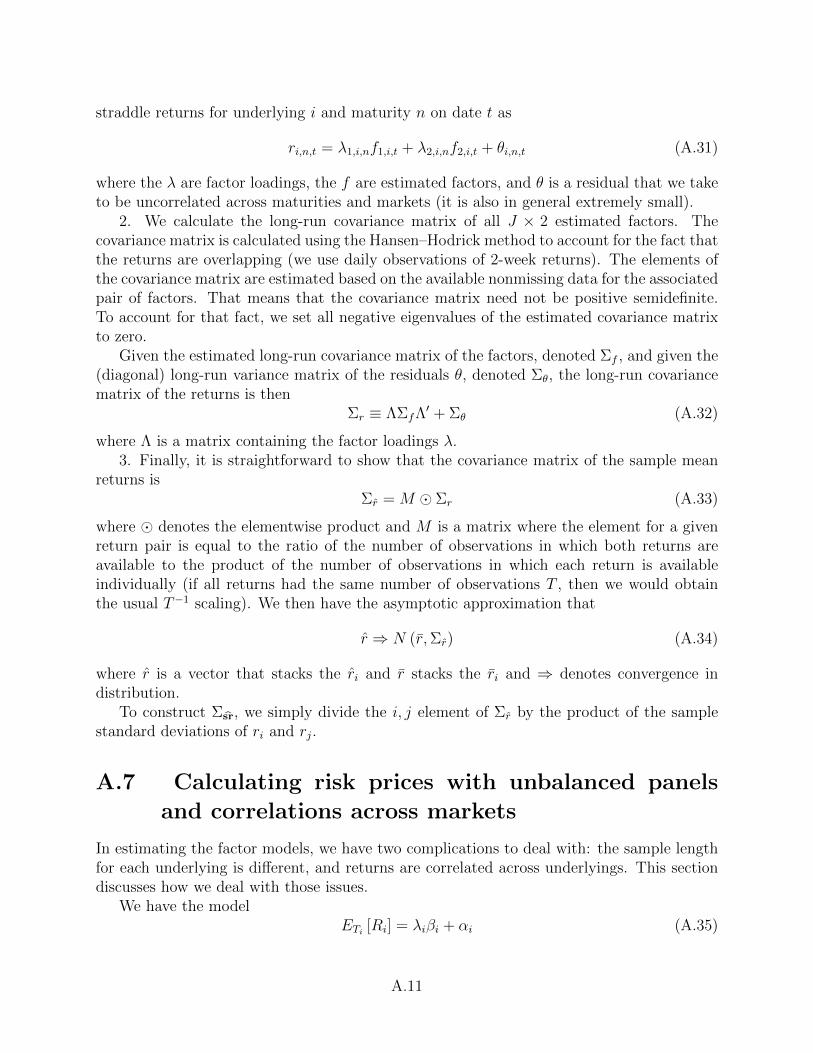
straddle returns for underlying i and maturity n on date t as

ri,n,t = λ1,i,nf1,i,t + λ2,i,nf2,i,t + θi,n,t (A.31)

where the λ are factor loadings, the f are estimated factors, and θ is a residual that we taketo be uncorrelated across maturities and markets (it is also in general extremely small).

2. We calculate the long-run covariance matrix of all J × 2 estimated factors. Thecovariance matrix is calculated using the Hansen–Hodrick method to account for the fact thatthe returns are overlapping (we use daily observations of 2-week returns). The elements ofthe covariance matrix are estimated based on the available nonmissing data for the associatedpair of factors. That means that the covariance matrix need not be positive semidefinite.To account for that fact, we set all negative eigenvalues of the estimated covariance matrixto zero.

Given the estimated long-run covariance matrix of the factors, denoted Σf , and given the(diagonal) long-run variance matrix of the residuals θ, denoted Σθ, the long-run covariancematrix of the returns is then

Σr ≡ ΛΣfΛ′ + Σθ (A.32)

where Λ is a matrix containing the factor loadings λ.3. Finally, it is straightforward to show that the covariance matrix of the sample mean

returns isΣr = M � Σr (A.33)

where � denotes the elementwise product and M is a matrix where the element for a givenreturn pair is equal to the ratio of the number of observations in which both returns areavailable to the product of the number of observations in which each return is availableindividually (if all returns had the same number of observations T , then we would obtainthe usual T−1 scaling). We then have the asymptotic approximation that

r ⇒ N (r,Σr) (A.34)

where r is a vector that stacks the ri and r stacks the ri and ⇒ denotes convergence indistribution.

To construct Σsr, we simply divide the i, j element of Σr by the product of the samplestandard deviations of ri and rj.

A.7 Calculating risk prices with unbalanced panels

and correlations across markets

In estimating the factor models, we have two complications to deal with: the sample lengthfor each underlying is different, and returns are correlated across underlyings. This sectiondiscusses how we deal with those issues.

We have the modelETi [Ri] = λiβi + αi (A.35)

A.11

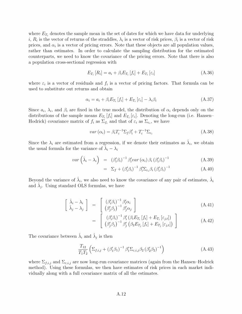
where ETi denotes the sample mean in the set of dates for which we have data for underlyingi, Ri is the vector of returns of the straddles, λi is a vector of risk prices, βi is a vector of riskprices, and αi is a vector of pricing errors. Note that these objects are all population values,rather than estimates. In order to calculate the sampling distribution for the estimatedcounterparts, we need to know the covariance of the pricing errors. Note that there is alsoa population cross-sectional regression with

ETi [Ri] = ai + βiETi [fi] + ETi [εi] (A.36)

where εi is a vector of residuals and fi is a vector of pricing factors. That formula can beused to substitute out returns and obtain

αi = ai + βiETi [fi] + ETi [εi]− λiβi (A.37)

Since ai, λi, and βi are fixed in the true model, the distribution of αi depends only on thedistributions of the sample means ETi [fi] and ETi [εi]. Denoting the long-run (i.e. Hansen–Hodrick) covariance matrix of fi as Σfi and that of εi as Σεi , we have

var (αi) = βiT−1i Σfβ

′i + T−1

i Σεi (A.38)

Since the λi are estimated from a regression, if we denote their estimates as λi, we obtainthe usual formula for the variance of λi − λi

var(λi − λi

)= (β′iβi)

−1β′ivar (αi) βi (β

′iβi)

−1(A.39)

= Σf + (β′iβi)−1β′iΣεiβi (β

′iβi)

−1(A.40)

Beyond the variance of λi, we also need to know the covariance of any pair of estimates, λiand λj. Using standard OLS formulas, we have

[λi − λiλj − λj

]=

[(β′iβi)

−1 β′iαi(β′jβj

)−1β′jαj

](A.41)

=

[(β′iβi)

−1 β′i (βiETi [ft] + ETi [εj,t])(β′jβj

)−1β′j(β2ETj [ft] + ETj [εj,t]

) ] (A.42)

The covariance between λi and λj is then

T12

T1T2

(Σf,i,j + (β′1β1)

−1β′1Σε,i,jβ2 (β′2β2)

−1)

(A.43)

where Σf,i,j and Σε,i,j are now long-run covariance matrices (again from the Hansen–Hodrickmethod). Using these formulas, we then have estimates of risk prices in each market indi-vidually along with a full covariance matrix of all the estimates.

A.12

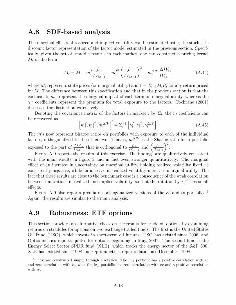
A.8 SDF-based analysis

The marginal effects of realized and implied volatility can be estimated using the stochasticdiscount factor representation of the factor model estimated in the previous section. Specif-ically, given the set of straddle returns in each market, one can construct a pricing kernelMt of the form

Mt = M −mfi

fi,tIVi,t−1

−mf2

i

(fi,t

IVi,t−1

)2

−m∆IVi

∆IVi,tIVi,t−1

(A.44)

where Mt represents state prices (or marginal utility) and 1 = Et−1MtRt for any return pricedby M . The difference between this specification and that in the previous section is that thecoefficients m... represent the marginal impact of each term on marginal utility, whereas theγ... coefficients represent the premium for total exposure to the factors. Cochrane (2001)discusses the distinction extensively.

Denoting the covariance matrix of the factors in market i by Σi, the m coefficients canbe recovered as [

mfi ,m

f2

i ,m∆IVi

]′= Σ−1

i

[γfi , γ

f2

i , γ∆IVi

]′(A.45)

The m’s now represent Sharpe ratios on portfolios with exposure to each of the individualfactors, orthogonalized to the other two. That is, m∆IV

i is the Sharpe ratio for a portfolio

exposed to the part of∆IVi,tIVi,t−1

that is orthogonal tofi,t

IVi,t−1and

(fi,t

IVi,t−1

)2

.

Figure A.9 reports the results of this exercise. The findings are qualitatively consistentwith the main results in figure 3 and in fact even stronger quantitatively. The marginaleffect of an increase in uncertainty on marginal utility, holding realized volatility fixed, isconsistently negative, while an increase in realized volatility increases marginal utility. Thefact that these results are close to the benchmark case is a consequence of the weak correlationbetween innovations in realized and implied volatility, so that the rotation by Σ−1

i has smalleffects.

Figure A.9 also reports premia on orthogonalized versions of the rv and iv portfolios.3

Again, the results are similar to the main analysis.

A.9 Robustness: ETF options

This section provides an alternative check on the results for crude oil options by examiningreturns on straddles for options on two exchange traded funds. The first is the United StatesOil Fund (USO), which invests in short-term oil futures. USO has existed since 2006, andOptionmetrics reports quotes for options beginning in May, 2007. The second fund is theEnergy Select Sector SPDR fund (XLE), which tracks the energy sector of the S&P 500.XLE has existed since 1998 and Optionmetrics reports data since December, 1998.

3These are constructed simply through a rotation. The rv⊥ portfolio has a positive correlation with rvand zero correlation with iv, whie the iv⊥ portfolio has zero correlation with rv and a positive correlationwith iv.

A.13

We eliminate observations using the following filters:1. Volume less than 10 contracts2. Time to maturity less than 15 days3. Bid-ask spread greater than 20 percent of bid/ask midpoint4. Initial log moneyness – log strike divided by the futures price – greater than 0.75

implied volatility units in absolute value (where implied volatility is scaled by he square rootof time to maturity).

We then calculate straddle returns as in the main text over two-week periods and averageacross the two straddles nearest to the money for each maturity, weighting them by theinverse of their absolute moneyness.

The top section of table A.9.1 reports the number of (potentially overlapping) two-weekstraddle return observations across maturities for USO, XLE, and the CME Group futuresoptions used in the main analysis. Since the CME data goes back to 1983, there are far moreobservations for that series than the other two. More interestingly, though, the numberof observations only declines by about 10 percent between the 1- and 6-month maturities,while it falls by more than 2/3 for the XLE and USO samples. The CME data therefore hassuperior coverage at longer horizons, which justifies its use in our main analysis.

The bottom section of table A.9.1 reports the correlations of the USO and XLE straddlereturns with those for the CME on the days where they overlap. The correlations areapproximately 90 percent at all maturities for USO and 50 percent for XLE. The 90-percentcorrelations for USO and the CME sample provide a general confirmation of the accuracy ofthe CME straddle returns, since we would expect the USO and CME options to be highlysimilar as USO literally holds futures. The lower correlation for XLE is not surprising giventhat it holds energy sector stocks rather than crude oil futures.

Table A.9.1.Maturity: 1 2 3 4 5 6

# obs. USO 1640 1616 1721 1679 1118 525XLE 2612 2545 2454 1928 1134 369CME 6762 6645 6817 6801 6606 5998

Corr. w/ USO 0.93 0.96 0.95 0.92 0.89 0.83CME XLE 0.43 0.48 0.50 0.49 0.50 0.53

In the main text, the RV and IV portfolio returns are calculated using 5- and 1-monthstraddles. Since the number of observations drops off substantially between 4 and 5 monthsfor both XLE and USO, though, here we examine returns on RV and IV portfolios usingboth 5- and 4-month straddles for the long-maturity side.

Figure A.13 plots estimated annualized Sharpe ratios along with 95-percent confidencebands for the RV and IV portfolios using 4- and 5-month straddles for the three sets ofoptions. In all four cases, the three confidence intervals always overlap substantially. Thefact that the sample for the CME options is far larger is evident in its confidence bandsbeing much narrower than those for the other two sources. For the IV portfolios, USO hasreturns that are close to zero, but its confidence bands range from -1 to greater than 0.5,indicating that it is not particularly informative about the Sharpe ratio.

Table A.9.2 reports confidence bands for the difference between the IV and RV averagereturns constructed with the CME data and the same portfolios constructed using USO

A.14

and XLE. The top panel shows that the differences for the IV portfolios are negative forUSO and positive for XLE, but only the difference for USO constructed with the 4-monthstraddle is statistically significant. The bottom panel similarly shows mixed results for thepoint estimates for the differences for the RV portfolios, with none of the differences beingstatistically significant.

Table A.9.2. Differences between CME and USO, XLE mean returns

USO - CME, 4mo. USO - CME, 5mo. XLE - CME, 4mo. XLE - CME, 5mo.IV return -2.2 -2.2 -0.8 -1.4

[-3.9,-0.2] [-4.8,0.4] [-2.5,4.1] [-4.1,6.3]RV return 0.43 0.47 -0.27 0.67

[-0.6,1.4] [-0.6,1.4] [-1.8,1.3] [-1.5,2.6]

Notes: the table reports percentage (two-week) returns on USO and XLE minus returns on

CME RV and IV portfolios. 95-percent confidence intervals are reported in brackets.

The fact that the USO and CME straddle returns are highly correlated does not neces-sarily mean that the CME data is accurate for the mean return on the straddles. To checkwhether the difference in the means observed in the USO and XLE data would affect outmain results, we ask how the Sharpe ratios of the RV and IV portfolios in the CME datawould change if we shifted their means by the average differences reported in table A.9.2.The bars labeled “CME, USO adj.” and CME, XLE adj.” show how the confidence bandswould change if we shifted them by exactly the point estimates from table A.9.2. Note thatthis is not the same as shifting the Sharpe ratio for the CME data to match that for theXLE or USO data. The reason is that the difference in table A.9.2 is calculated only for thereturns on matching dates, whereas the Sharpe ratio calculated in figure A.13 is calculatedusing the full sample for the CME data. So the two adjusted bands take the full-sampleband and then shift it by the mean difference calculated on the dates that overlap betweenthe CME data and XLE or USO.

Figure A.13 shows that the economic conclusions drawn for the crude oil straddles are notchanged if the mean returns are shifted by the differences observed in table A.9.1. The RVportfolio returns remain statistically significantly negative in all four cases, the changes inthe point estimates are well inside the original confidence intervals. The top panel shows thatthe IV returns using 5-month straddles are similarly unaffected. For the 4-month straddles,the only difference is that with the USO options, the estimated Sharpe ratio falls by abouthalf and is no longer statistically significantly greater than zero. So, again, out of eight cases– IV and RV with 4- and 5-month straddles – in only one is there a nontrivial change in theconclusions, and even there the Sharpe ratio on the IV portfolio does not become negative,it is simply less positive.

Overall, the period in which the USO and XLE options are traded is too short to usethem for our main analysis. This section shows that the USO straddle returns are highlycorrelated with the CME returns. The mean returns on the XLE and CME straddles arehighly similar, while they differ somewhat more for CME and USO. However, shifting themeans used for the CME options in the main analysis by the observed difference betweenthe CME and USO options does not substantially change any of the conclusions.

A.15

A.10 Model

A.10.1 Dynamics

Consumption growth follows

∆ct = xt−1 +√σ2B,t−1 + σ2

G,t−1εt + Jbt (A.46)

xt = φxxt−1 + ωxηx,t + ωx,Gησ,G,t − ωx,Bησ,B,t (A.47)

σ2j,t = (1− φσ) σ2

j + φσσ2j,t−1 + ωjησ,j,t (A.48)

for j ∈ {G,B}. The shocks ε, ηx, ηG, ηB are independent and Gaussian with unit variances.The ω coefficients are all assumed to be positive. bt is a Poisson random variable withintensity λ.

The dynamics can also be written as

[xt

σ2t − σ2

]=

[φx 00 φσ

] [xt−1

σ2t−1 − σ2

]+

[ωx ωx,G 00 ωG ωB

] ηx,tηG,tηB,t

(A.49)

∆ct = xt−1 + σ2t−1εt + Jbt (A.50)

Yt = FYt−1 +Gηt (A.51)

where Yt = [xt, σ2t − σ2]

′, etc. The fact that the model can be rewritten with only a single

variance process follows from the linearity of the two processes, the fact that they have thesame rate of mean reversion, and the fact that they appear additively. We can then writeconsumption and dividend growth as

∆ct = c′Y Yt−1 +√σ2 + g′Y Yt−1εt + Jbt (A.52)

∆dt = γ(c′Y Yt−1 +

√σ2 + g′Y Yt−1εt + Jbt

)+ ωdεd,t (A.53)

for vectors cY and gY . ∆dt is log dividend growth, which we will use for modeling equities.It satisfies ∆dt = γ∆ct +ωdεd,t (εd,t ∼ N (0, 1)), where γ determines the leverage of equities.

A.10.2 Preferences

We assume agents have Epstein–Zin preferences with a unit IES,

vt = (1− β) ct +β

1− αlogEt exp ((1− α) vt+1) (A.54)

vct =β

1− αlogEt exp ((1− α) (vct+1 + ∆ct+1)) (A.55)

where vct is the log utility/consumption ratio, vct = vt − ct. We look for a solution to themodel of the form

vct = v + v′Y Yt (A.56)

A.16

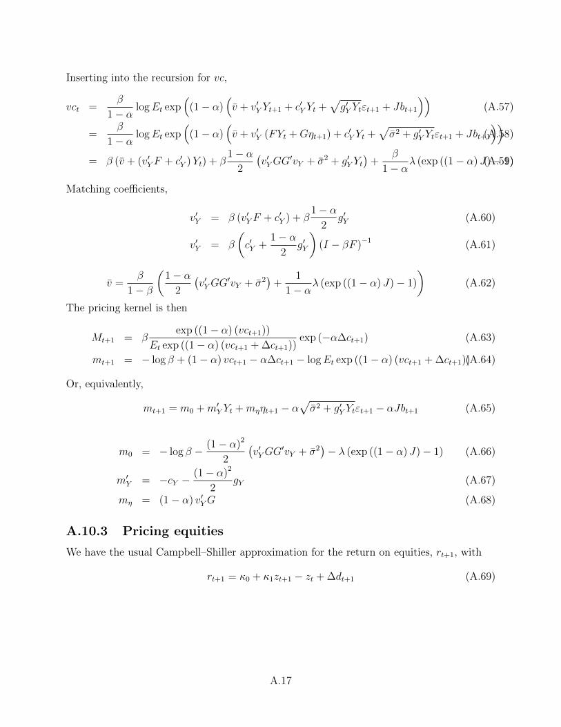
Inserting into the recursion for vc,

vct =β

1− αlogEt exp

((1− α)

(v + v′Y Yt+1 + c′Y Yt +

√g′Y Ytεt+1 + Jbt+1

))(A.57)

=β

1− αlogEt exp

((1− α)

(v + v′Y (FYt +Gηt+1) + c′Y Yt +

√σ2 + g′Y Ytεt+1 + Jbt+1

))(A.58)

= β (v + (v′Y F + c′Y )Yt) + β1− α

2

(v′YGG

′vY + σ2 + g′Y Yt)

+β

1− αλ (exp ((1− α) J)− 1)(A.59)

Matching coefficients,

v′Y = β (v′Y F + c′Y ) + β1− α

2g′Y (A.60)

v′Y = β

(c′Y +

1− α2

g′Y

)(I − βF )−1 (A.61)

v =β

1− β

(1− α

2

(v′YGG

′vY + σ2)

+1

1− αλ (exp ((1− α) J)− 1)

)(A.62)

The pricing kernel is then

Mt+1 = βexp ((1− α) (vct+1))

Et exp ((1− α) (vct+1 + ∆ct+1))exp (−α∆ct+1) (A.63)

mt+1 = − log β + (1− α) vct+1 − α∆ct+1 − logEt exp ((1− α) (vct+1 + ∆ct+1))(A.64)

Or, equivalently,

mt+1 = m0 +m′Y Yt +mηηt+1 − α√σ2 + g′Y Ytεt+1 − αJbt+1 (A.65)

m0 = − log β − (1− α)2

2

(v′YGG

′vY + σ2)− λ (exp ((1− α) J)− 1) (A.66)

m′Y = −cY −(1− α)2

2gY (A.67)

mη = (1− α) v′YG (A.68)

A.10.3 Pricing equities

We have the usual Campbell–Shiller approximation for the return on equities, rt+1, with

rt+1 = κ0 + κ1zt+1 − zt + ∆dt+1 (A.69)

A.17

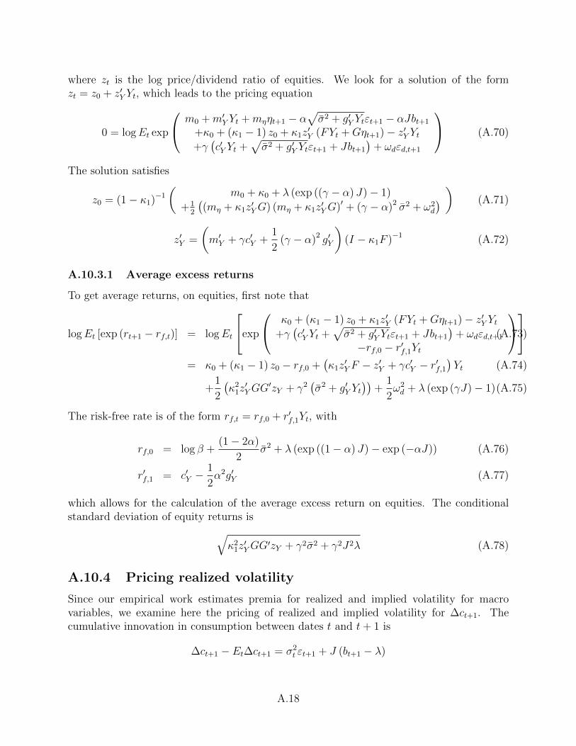
where zt is the log price/dividend ratio of equities. We look for a solution of the formzt = z0 + z′Y Yt, which leads to the pricing equation

0 = logEt exp

m0 +m′Y Yt +mηηt+1 − α√σ2 + g′Y Ytεt+1 − αJbt+1

+κ0 + (κ1 − 1) z0 + κ1z′Y (FYt +Gηt+1)− z′Y Yt

+γ(c′Y Yt +

√σ2 + g′Y Ytεt+1 + Jbt+1

)+ ωdεd,t+1

(A.70)

The solution satisfies

z0 = (1− κ1)−1

(m0 + κ0 + λ (exp ((γ − α) J)− 1)

+12

((mη + κ1z

′YG) (mη + κ1z

′YG)′ + (γ − α)2 σ2 + ω2

d

) ) (A.71)

z′Y =

(m′Y + γc′Y +

1

2(γ − α)2 g′Y

)(I − κ1F )−1 (A.72)

A.10.3.1 Average excess returns

To get average returns, on equities, first note that

logEt [exp (rt+1 − rf,t)] = logEt

exp

κ0 + (κ1 − 1) z0 + κ1z′Y (FYt +Gηt+1)− z′Y Yt

+γ(c′Y Yt +

√σ2 + g′Y Ytεt+1 + Jbt+1

)+ ωdεd,t+1

−rf,0 − r′f,1Yt

(A.73)

= κ0 + (κ1 − 1) z0 − rf,0 +(κ1z

′Y F − z′Y + γc′Y − r′f,1

)Yt (A.74)

+1

2

(κ2

1z′YGG

′zY + γ2(σ2 + g′Y Yt

))+

1

2ω2d + λ (exp (γJ)− 1)(A.75)

The risk-free rate is of the form rf,t = rf,0 + r′f,1Yt, with

rf,0 = log β +(1− 2α)

2σ2 + λ (exp ((1− α) J)− exp (−αJ)) (A.76)

r′f,1 = c′Y −1

2α2g′Y (A.77)

which allows for the calculation of the average excess return on equities. The conditionalstandard deviation of equity returns is√

κ21z′YGG

′zY + γ2σ2 + γ2J2λ (A.78)

A.10.4 Pricing realized volatility

Since our empirical work estimates premia for realized and implied volatility for macrovariables, we examine here the pricing of realized and implied volatility for ∆ct+1. Thecumulative innovation in consumption between dates t and t+ 1 is

∆ct+1 − Et∆ct+1 = σ2t εt+1 + J (bt+1 − λ)

A.18

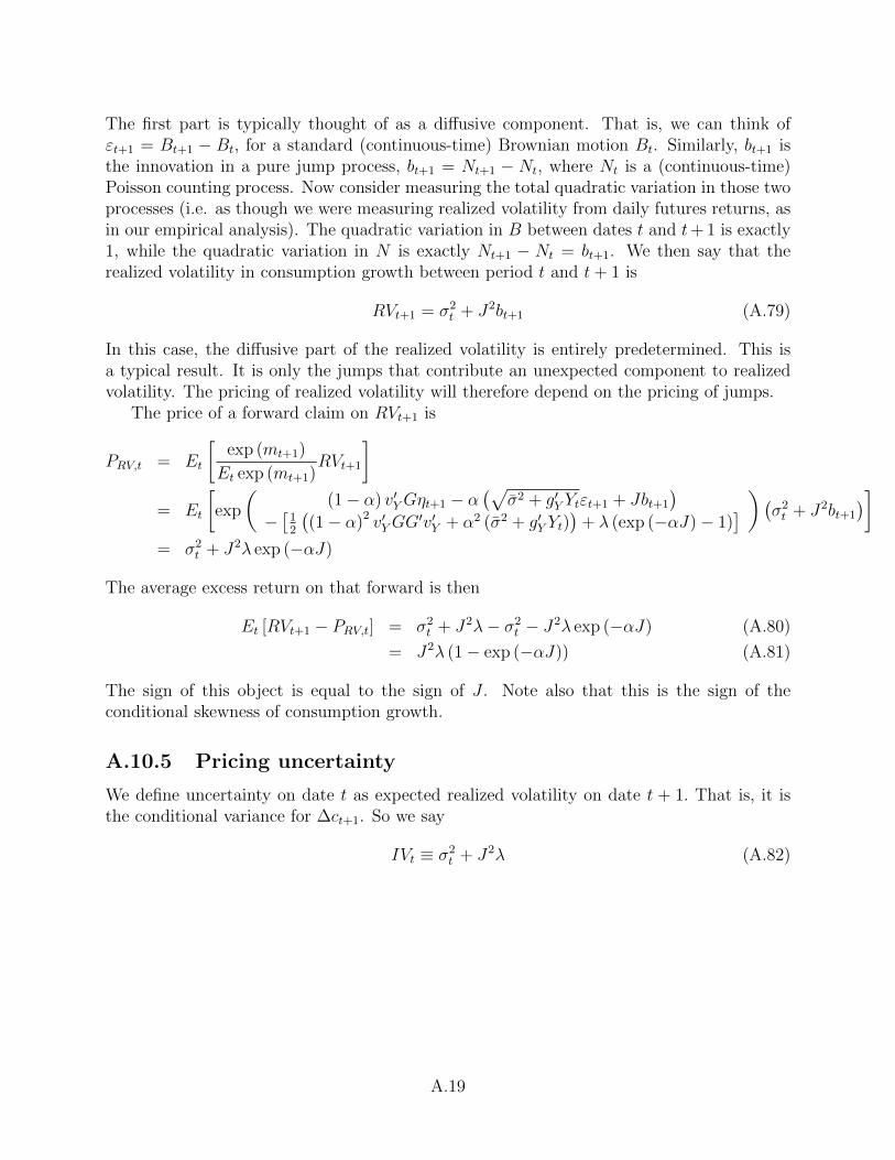
The first part is typically thought of as a diffusive component. That is, we can think ofεt+1 = Bt+1 − Bt, for a standard (continuous-time) Brownian motion Bt. Similarly, bt+1 isthe innovation in a pure jump process, bt+1 = Nt+1 − Nt, where Nt is a (continuous-time)Poisson counting process. Now consider measuring the total quadratic variation in those twoprocesses (i.e. as though we were measuring realized volatility from daily futures returns, asin our empirical analysis). The quadratic variation in B between dates t and t+ 1 is exactly1, while the quadratic variation in N is exactly Nt+1 − Nt = bt+1. We then say that therealized volatility in consumption growth between period t and t+ 1 is

RVt+1 = σ2t + J2bt+1 (A.79)

In this case, the diffusive part of the realized volatility is entirely predetermined. This isa typical result. It is only the jumps that contribute an unexpected component to realizedvolatility. The pricing of realized volatility will therefore depend on the pricing of jumps.

The price of a forward claim on RVt+1 is

PRV,t = Et

[exp (mt+1)

Et exp (mt+1)RVt+1

]= Et

[exp

((1− α) v′YGηt+1 − α

(√σ2 + g′Y Ytεt+1 + Jbt+1

)−[

12

((1− α)2 v′YGG

′v′Y + α2 (σ2 + g′Y Yt))

+ λ (exp (−αJ)− 1)] ) (σ2

t + J2bt+1

)]= σ2

t + J2λ exp (−αJ)

The average excess return on that forward is then

Et [RVt+1 − PRV,t] = σ2t + J2λ− σ2

t − J2λ exp (−αJ) (A.80)

= J2λ (1− exp (−αJ)) (A.81)

The sign of this object is equal to the sign of J . Note also that this is the sign of theconditional skewness of consumption growth.

A.10.5 Pricing uncertainty

We define uncertainty on date t as expected realized volatility on date t + 1. That is, it isthe conditional variance for ∆ct+1. So we say

IVt ≡ σ2t + J2λ (A.82)

A.19

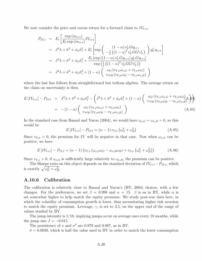
We now consider the price and excess return for a forward claim to IVt+1.

PIV,t = Et

[exp (mt+1)

Et exp (mt+1)IVt+1

]= J2λ+ σ2 + φσσ

2t + Et

[exp

((1− α) v′YGηt+1

−12

((1− α)2 v′YGG

′v′Y) ) g′Y ηt+1

]= J2λ+ σ2 + φσσ

2t +

Et [exp ((1− α) v′YGηt+1) g′YGηt+1]

exp(

12

((1− α)2 v′YGG

′v′Y))

= J2λ+ σ2 + φσσ2t + (1− α)

(ωG (vY,xωx,G + vY,σωG)

+ωB (vY,σωB − vY,xωx,B)

)where the last line follows from straightforward but tedious algebra. The average return onthe claim on uncertainty is then

E [IVt+1]− PIV,t = J2λ+ σ2 + φσσ2t −

(J2λ+ σ2 + φσσ

2t + (1− α)

(ωG (vY,xωx,G + vY,σωG)

+ωB (vY,σωB − vY,xωx,B)

))(A.83)

= − (1− α)

(ωG (vY,xωx,G + vY,σωG)

+ωB (vY,σωB − vY,xωx,B)

)(A.84)

In the standard case from Bansal and Yaron (2004), we would have ωx,G = ωx,B = 0, so thiswould be

E [IVt+1]− PIV,t = (α− 1) vY,σ(ω2G + ω2

B

)(A.85)

Since vY,σ < 0, the premium for IV will be negative in that case. Now when ωx,G can bepositive, we have

E [IVt+1]− PIV,t = (α− 1)(vY,x (ωx,GωG − ωx,BωB) + vY,σ

(ω2G + ω2

B

))(A.86)

Since vY,x > 0, if ωx,G is sufficiently large relatively to ωx,B, the premium can be positive.The Sharpe ratio on this object depends on the standard deviation of IVt+1−PIV,t, which

is exactly√ω2G + ω2

B.

A.10.6 Calibration

The calibration is relatively close to Bansal and Yaron’s (BY; 2004) choices, with a fewchanges. For the preferences, we set β = 0.998 and α = 15. β is as in BY, while α isset somewhat higher to help match the equity premium. We study post-war data here, inwhich the volatility of consumption growth is lower, thus necessitating higher risk aversionto match the equity premium. Leverage, γ, is set to 3.5, on the upper end of the range ofvalues studied by BY.

The jump intensity is 1/18, implying jumps occur on average once every 18 months, whilethe jump size J = −0.015.

The persistence of x and σ2 are 0.979 and 0.987, as in BY.σ = 0.0039, which is half the value used in BY in order to match the lower consumption

A.20

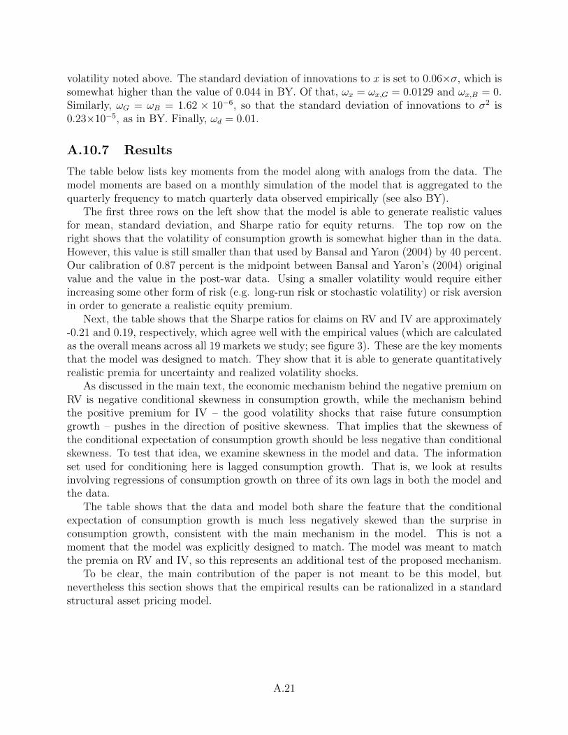
volatility noted above. The standard deviation of innovations to x is set to 0.06×σ, which issomewhat higher than the value of 0.044 in BY. Of that, ωx = ωx,G = 0.0129 and ωx,B = 0.Similarly, ωG = ωB = 1.62 × 10−6, so that the standard deviation of innovations to σ2 is0.23×10−5, as in BY. Finally, ωd = 0.01.

A.10.7 Results

The table below lists key moments from the model along with analogs from the data. Themodel moments are based on a monthly simulation of the model that is aggregated to thequarterly frequency to match quarterly data observed empirically (see also BY).

The first three rows on the left show that the model is able to generate realistic valuesfor mean, standard deviation, and Sharpe ratio for equity returns. The top row on theright shows that the volatility of consumption growth is somewhat higher than in the data.However, this value is still smaller than that used by Bansal and Yaron (2004) by 40 percent.Our calibration of 0.87 percent is the midpoint between Bansal and Yaron’s (2004) originalvalue and the value in the post-war data. Using a smaller volatility would require eitherincreasing some other form of risk (e.g. long-run risk or stochastic volatility) or risk aversionin order to generate a realistic equity premium.

Next, the table shows that the Sharpe ratios for claims on RV and IV are approximately-0.21 and 0.19, respectively, which agree well with the empirical values (which are calculatedas the overall means across all 19 markets we study; see figure 3). These are the key momentsthat the model was designed to match. They show that it is able to generate quantitativelyrealistic premia for uncertainty and realized volatility shocks.

As discussed in the main text, the economic mechanism behind the negative premium onRV is negative conditional skewness in consumption growth, while the mechanism behindthe positive premium for IV – the good volatility shocks that raise future consumptiongrowth – pushes in the direction of positive skewness. That implies that the skewness ofthe conditional expectation of consumption growth should be less negative than conditionalskewness. To test that idea, we examine skewness in the model and data. The informationset used for conditioning here is lagged consumption growth. That is, we look at resultsinvolving regressions of consumption growth on three of its own lags in both the model andthe data.

The table shows that the data and model both share the feature that the conditionalexpectation of consumption growth is much less negatively skewed than the surprise inconsumption growth, consistent with the main mechanism in the model. This is not amoment that the model was explicitly designed to match. The model was meant to matchthe premia on RV and IV, so this represents an additional test of the proposed mechanism.

To be clear, the main contribution of the paper is not meant to be this model, butnevertheless this section shows that the empirical results can be rationalized in a standardstructural asset pricing model.

A.21

Summary statistics from the model and empirical data, 1947–2018Model Data Model Data

E [rm − rf ] 0.077 0.056 std (∆c) 0.0087 0.0052std (rm − rf ) 0.14 0.11 skewt (∆ct+1) -0.32 -0.15E[rm−rf ]std(rm−rf)

0.53 0.52 skew (Et∆ct+1) -0.10 -0.07

E[RVt+1−PRV,t]std[RVt+1−PRV,t]

-0.21 -0.32

E[RVt+1−PRV,t]std[RVt+1−PRV,t]

0.19 0.26

A.22

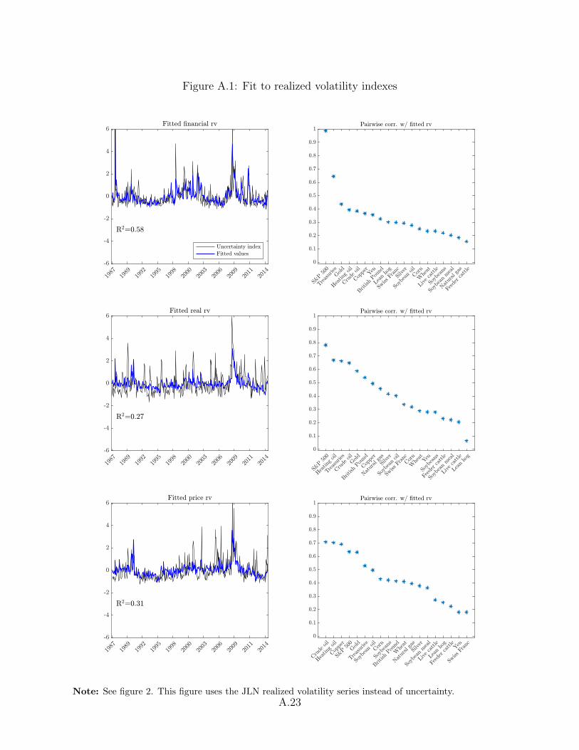
Figure A.1: Fit to realized volatility indexes

Note: See figure 2. This figure uses the JLN realized volatility series instead of uncertainty.A.23

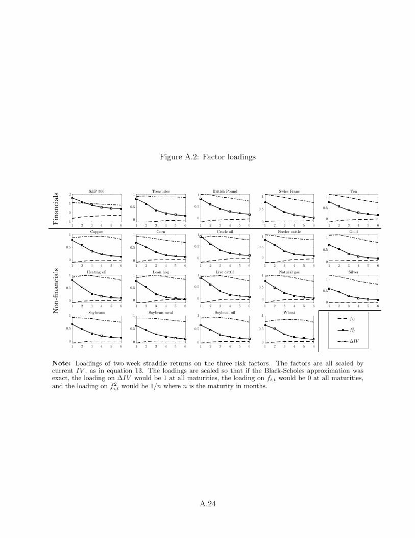
Figure A.2: Factor loadings

Note: Loadings of two-week straddle returns on the three risk factors. The factors are all scaled bycurrent IV , as in equation 13. The loadings are scaled so that if the Black-Scholes approximation wasexact, the loading on ∆IV would be 1 at all maturities, the loading on fi,t would be 0 at all maturities,and the loading on f2i,t would be 1/n where n is the maturity in months.

A.24

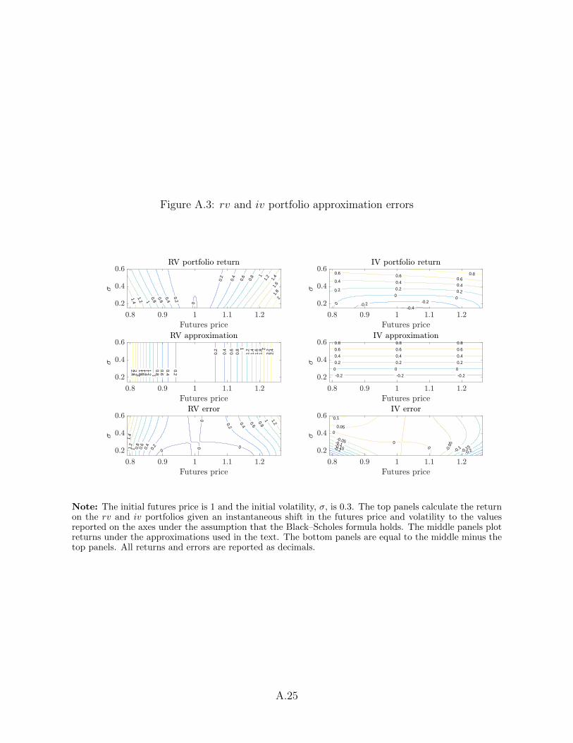
Figure A.3: rv and iv portfolio approximation errors

RV portfolio return

0

0.2

0.2

0.4

0.4

0.6

0.6

0.8

0.8

1

1

1.2

1.2

1.4

1.4

1.6

1.8

2

0.8 0.9 1 1.1 1.2

Futures price

0.2

0.4

0.6

<

IV portfolio return

-0.4

-0.2-0.2

00

0

0.20.20.2

0.40.40.4

0.60.6

0.6 0.8

0.8 0.9 1 1.1 1.2

Futures price

0.2

0.4

0.6

<

RV approximation

0.2

0.2

0.4

0.4

0.6

0.6

0.8

0.8

1

1

1.2

1.2

1.4

1.4

1.6

1.6

1.8

1.8

2

2

2.2

2.2

2.4

2.4

0.8 0.9 1 1.1 1.2

Futures price

0.2

0.4

0.6

<

IV approximation

-0.2-0.2-0.2

000

0.20.20.2

0.40.40.4

0.60.60.6

0.80.80.8

0.8 0.9 1 1.1 1.2

Futures price

0.2

0.4

0.6

<

RV error

0

00

0

0.2

0.2

0.4

0.4

0.6

0.6

0.8

0.8

1

1

1.2

1.2

1.4

0.8 0.9 1 1.1 1.2

Futures price

0.2

0.4

0.6

<

IV error

-0.2-0.2

-0.15-0.15

-0.1

-0.1

-0.05-0

.050

0

0

0.05

0.1

0.8 0.9 1 1.1 1.2

Futures price

0.2

0.4

0.6

<

Note: The initial futures price is 1 and the initial volatility, σ, is 0.3. The top panels calculate the returnon the rv and iv portfolios given an instantaneous shift in the futures price and volatility to the valuesreported on the axes under the assumption that the Black–Scholes formula holds. The middle panels plotreturns under the approximations used in the text. The bottom panels are equal to the middle minus thetop panels. All returns and errors are reported as decimals.

A.25

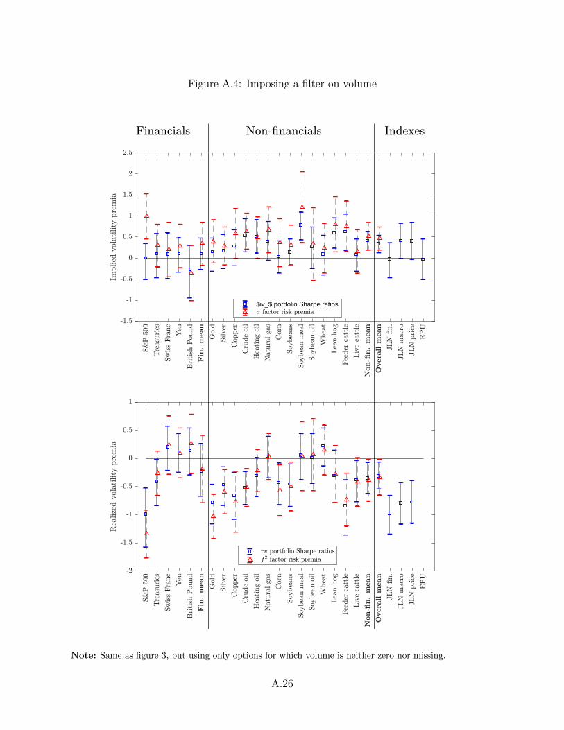
Figure A.4: Imposing a filter on volume

$iv_$ portfolio Sharpe ratios

Note: Same as figure 3, but using only options for which volume is neither zero nor missing.

A.26

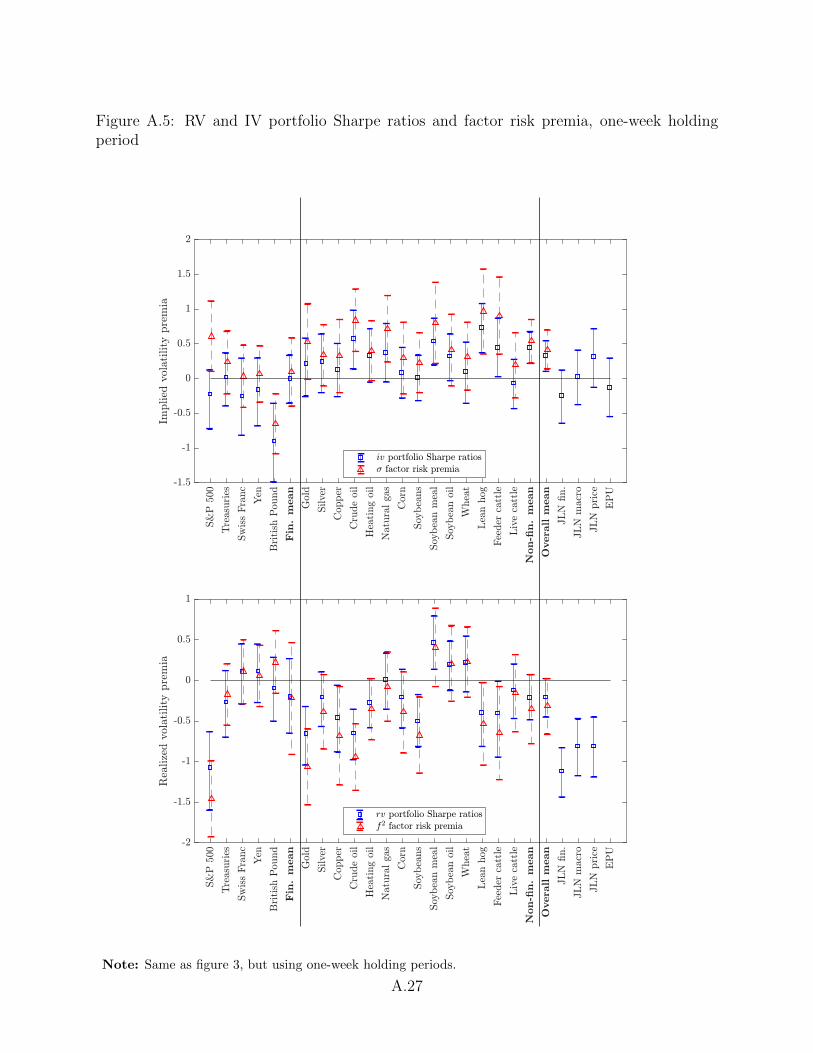
Figure A.5: RV and IV portfolio Sharpe ratios and factor risk premia, one-week holdingperiod

Note: Same as figure 3, but using one-week holding periods.

A.27

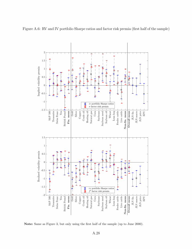
Figure A.6: RV and IV portfolio Sharpe ratios and factor risk premia (first half of the sample)

Note: Same as Figure 3, but only using the first half of the sample (up to June 2000).

A.28

Figure A.7: RV and IV portfolio Sharpe ratios and factor risk premia (second half of thesample)

Note: Same as Figure 3, but only using the second half of the sample (after June 2000).

A.29

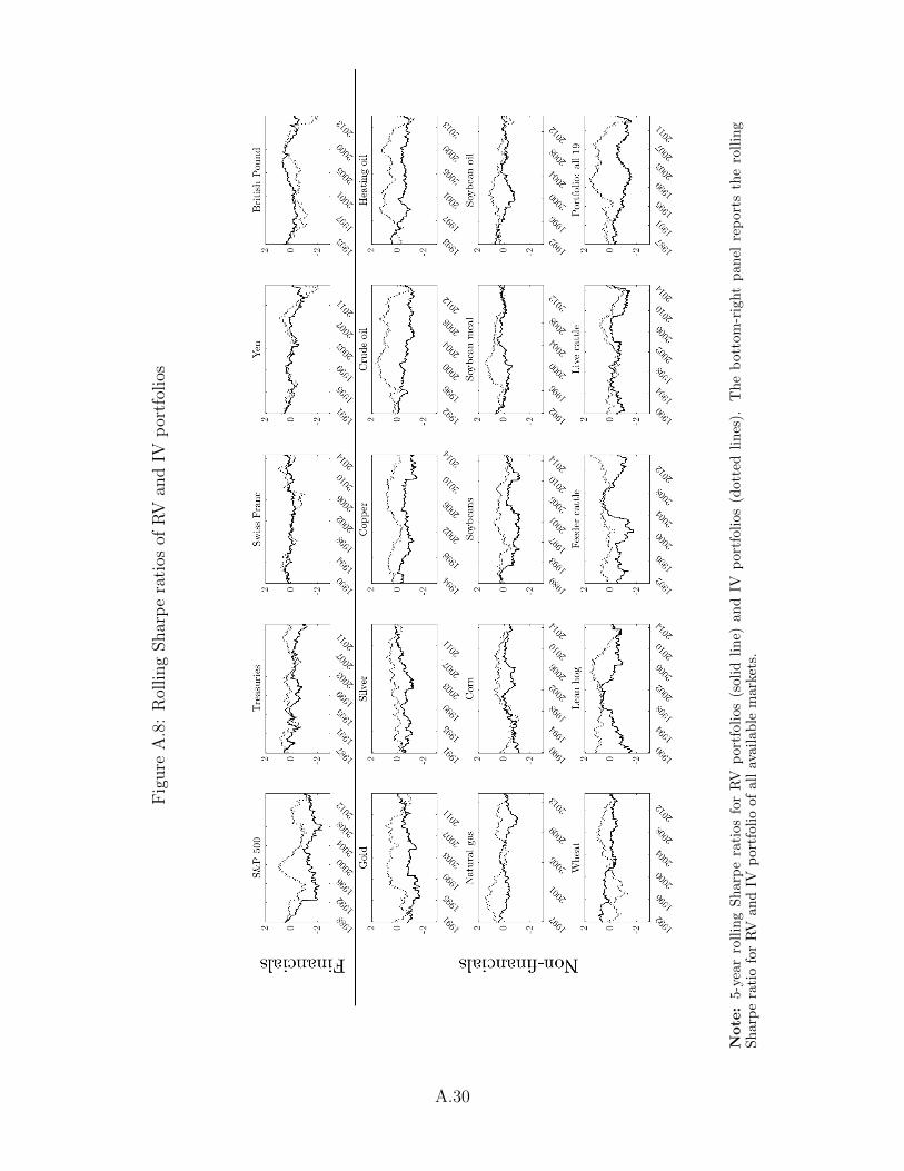
Fig

ure

A.8

:R

olling

Shar

pe

rati

osof

RV

and

IVp

ortf

olio

s

Note

:5-

year

roll

ing

Sh

arp

era

tios

for

RV

por

tfol

ios

(sol

idli

ne)

and

IVp

ortf

olio

s(d

otte

dli

nes

).T

he

bot

tom

-rig

ht

pan

elre

por

tsth

ero

llin

gS

har

pe

rati

ofo

rR

Van

dIV

port

foli

oof

all

avai

lab

lem

arke

ts.

A.30

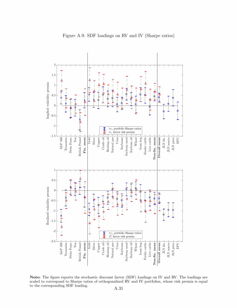
Figure A.9: SDF loadings on RV and IV (Sharpe ratios)

Note: The figure reports the stochastic discount factor (SDF) loadings on IV and RV. The loadings arescaled to correspond to Sharpe ratios of orthogonalized RV and IV portfolios, whose risk premia is equalto the corresponding SDF loading.

A.31

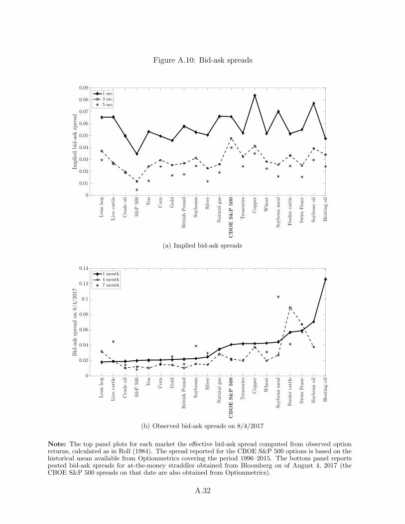
Figure A.10: Bid-ask spreads

(a) Implied bid-ask spreads

(b) Observed bid-ask spreads on 8/4/2017

Note: The top panel plots for each market the effective bid-ask spread computed from observed optionreturns, calculated as in Roll (1984). The spread reported for the CBOE S&P 500 options is based on thehistorical mean available from Optionmetrics covering the period 1996–2015. The bottom panel reportsposted bid-ask spreads for at-the-money straddles obtained from Bloomberg on of August 4, 2017 (theCBOE S&P 500 spreads on that date are also obtained from Optionmetrics).

A.32

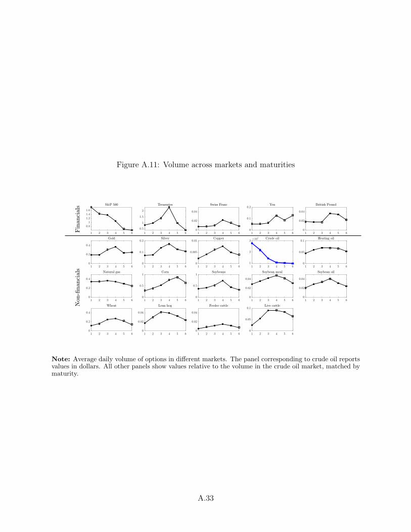
Figure A.11: Volume across markets and maturities

Note: Average daily volume of options in different markets. The panel corresponding to crude oil reportsvalues in dollars. All other panels show values relative to the volume in the crude oil market, matched bymaturity.

A.33

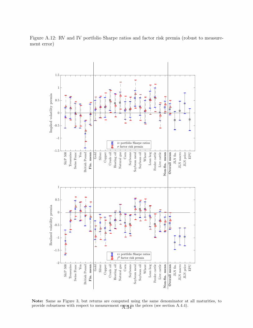
Figure A.12: RV and IV portfolio Sharpe ratios and factor risk premia (robust to measure-ment error)

Note: Same as Figure 3, but returns are computed using the same denominator at all maturities, toprovide robustness with respect to measurement error in the prices (see section A.4.4).A.34

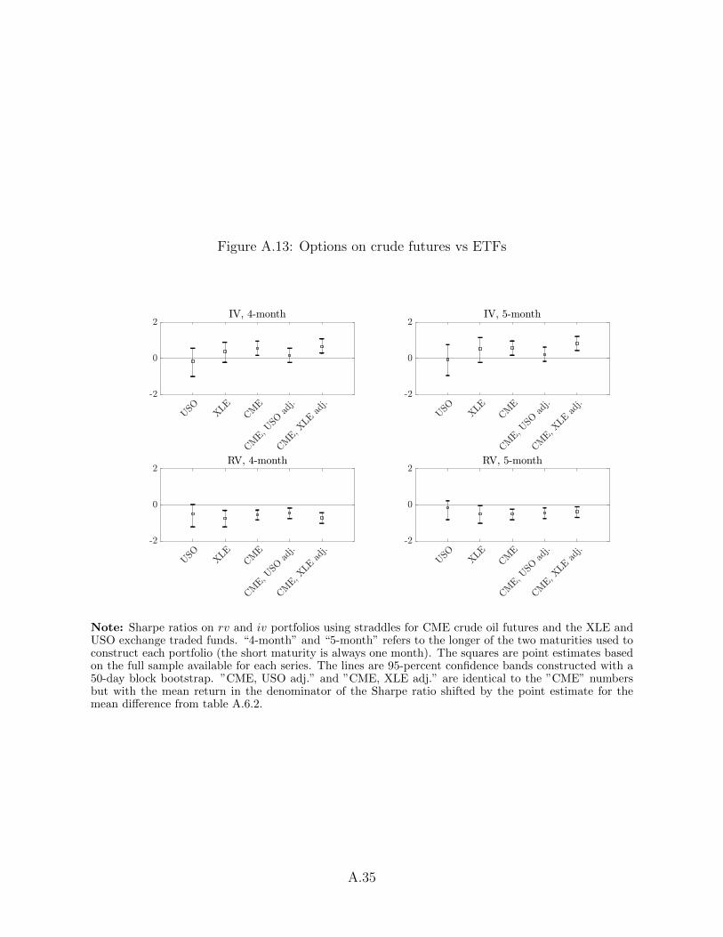
Figure A.13: Options on crude futures vs ETFs

Note: Sharpe ratios on rv and iv portfolios using straddles for CME crude oil futures and the XLE andUSO exchange traded funds. “4-month” and “5-month” refers to the longer of the two maturities used toconstruct each portfolio (the short maturity is always one month). The squares are point estimates basedon the full sample available for each series. The lines are 95-percent confidence bands constructed with a50-day block bootstrap. ”CME, USO adj.” and ”CME, XLE adj.” are identical to the ”CME” numbersbut with the mean return in the denominator of the Sharpe ratio shifted by the point estimate for themean difference from table A.6.2.

A.35

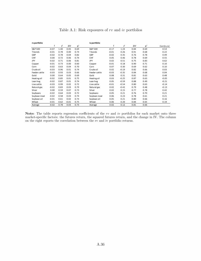
Table A.1: Risk exposures of rv and iv portfolios

rv portfolio iv portfoliof f2 ΔIV R2 f f2 ΔIV R2 Corr(rv,iv)

S&P 500 -0.07 1.40 0.05 0.69 S&P 500 -0.17 1.24 0.84 0.69 0.53T-bonds -0.01 0.78 0.00 0.74 T-bonds -0.01 0.26 0.91 0.68 0.22GBP -0.02 0.78 0.04 0.82 GBP -0.02 0.35 0.76 0.78 0.49CHF 0.00 0.72 0.06 0.74 CHF 0.05 0.46 0.78 0.69 0.55JPY -0.02 0.71 0.06 0.81 JPY 0.02 0.51 0.75 0.83 0.62Copper -0.01 0.73 0.00 0.60 Copper -0.01 0.18 0.90 0.71 0.10Corn -0.02 0.63 0.04 0.70 Corn 0.07 0.30 0.69 0.62 0.10Crude oil -0.03 0.96 0.01 0.74 Crude oil 0.02 -0.19 0.82 0.66 0.03Feeder cattle -0.03 0.93 0.03 0.66 Feeder cattle -0.03 -0.35 0.84 0.68 0.04Gold 0.00 0.64 0.05 0.69 Gold 0.08 0.31 0.81 0.63 0.48Heating oil -0.02 0.85 0.01 0.75 Heating oil 0.03 -0.25 0.87 0.63 -0.05Lean hog -0.02 0.87 0.01 0.74 Lean hog 0.05 -0.59 0.88 0.49 -0.21Live cattle -0.03 0.99 0.02 0.72 Live cattle -0.01 -0.54 0.80 0.63 -0.14Natural gas -0.02 0.83 0.03 0.79 Natural gas 0.02 -0.42 0.79 0.48 -0.13Silver 0.00 0.59 0.07 0.73 Silver 0.02 0.15 0.77 0.78 0.42Soybeans -0.02 0.64 0.03 0.72 Soybeans 0.05 0.21 0.76 0.70 0.21Soybean meal -0.02 0.58 0.03 0.74 Soybean meal 0.06 0.23 0.78 0.61 0.21Soybean oil -0.01 0.61 0.02 0.73 Soybean oil 0.05 0.21 0.80 0.66 0.16Wheat -0.01 0.62 -0.01 0.75 Wheat 0.06 0.20 0.84 0.65 0.19Average -0.02 0.78 0.03 0.73 Average 0.02 0.12 0.81 0.66

Note: The table reports regression coefficients of the rv and iv portfolios for each market onto threemarket-specific factors: the futures return, the squared futures return, and the change in IV. The columnon the right reports the correlation between the rv and iv portfolio returns.

A.36

Table A.2: Economic activity and option-fitted uncertainty indexes

Panel A: regression coefficientsUncertainty measure:

Fitted -0.206 *** -0.317 *** -0.276 *** -0.129 **Residual -0.092 -0.065 -0.191 *** -0.037Fitted -0.020 *** -0.023 *** -0.012 * -0.023 ***Residual -0.015 -0.010 -0.019 * -0.021 ***Fitted -0.319 *** -0.455 *** -0.442 *** -0.268 **Residual 0.080 0.023 -0.262 ** 0.039

Panel B: variance decompositionUncertainty measure: Financial Real Price EPU

Fitted 0.953 0.972 0.853 0.949Residual 0.047 0.028 0.147 0.051Fitted 0.877 0.879 0.525 0.641Residual 0.123 0.121 0.475 0.359Fitted 0.985 0.998 0.887 0.986Residual 0.015 0.002 0.113 0.014

Financial Real Price EPU

Empl

.FF

RIP

Empl

.FF

RIP

Note: Panel A reports the coefficients from regressions of industrial production growth, employmentgrowth, and the Fed funds rate on their own lags and the fitted and residual uncertainty for the fourindexes. * indicates significance at the 10-percent level, ** 5-percent, and *** 1-percent. Fitted uncertaintyis obtained by projecting each uncertainty index on the 19 IVs. Panel B reports the corresponding variancedecomposition.

A.37

Table A.3: Economic activity and option-fitted realized volatility indexes

Panel A: regression coefficientsUncertainty measure:

Fitted -0.179 *** -0.432 *** -0.394 ***Residual -0.076 -0.010 -0.108 ***Fitted -0.027 *** -0.040 *** -0.026 ***Residual -0.006 -0.003 0.000Fitted -0.267 ** -0.598 *** -0.608 ***Residual 0.019 0.000 -0.157

Panel B: variance decompositionUncertainty measure: Financial Real Price

Fitted 0.882 0.999 0.858Residual 0.118 0.001 0.142Fitted 0.968 0.989 0.999Residual 0.032 0.011 0.001Fitted 0.996 1.000 0.873Residual 0.004 0.000 0.127

Financial Real Price

Empl

.FF

RIP

Empl

.FF

RIP

Note: Same as table A.2, but using realized volatilities.

A.38