Particle Accelerators, 1996, Vol. 55, pp. [247-256] /1-10

Reprints available directly from the publisher

Photocopying pennitted by license only

© 1996 OPA (Overseas Publishers Association)

Amsterdam B.V. Published in The Netherlands under

license by Gordon and Breach Science Publishers SA

Printed in Malaysia

PRECISE MEASUREMENT OF THEBETATRON TUNE

R. BARTOLINI,l M. GIOVANNOZZI,l W. SCANDALE,lA. BAZZANI2 and E. TODESC02

lCERN, CH-1211 Geneva 23, Switzerland

2INFN, Sezione di Bologna, Via Imerio 46, 1-40126 Bologna, Italy

(Received 5 January 1996; infinalform 5 January 1996)

In circular accelerators, sophisticated algorithms for frequency analysis can provide very preciseestimates of the betatron tune from a relatively short sequence of tum-by-tum measurements ofthe beam position. They rely either on analytical interpolations of the Fast Fourier Transform,or on the numerical estimate of the Continuous Fourier Transform.

In this paper we review these methods, and the analytical estimates of the frequency error asa function of the sample size. Furthermore, we evaluate numerically the influence of noise in thedetermination of the tune. Finally, we present experimental applications to the LEP machine: theyprovide an accurate estimate of the detuning with amplitude due to the chromaticity sextupoles.

Keywords: Tune measurement.

1 INTRODUCTION

In circular accelerators, the tune can be measured by sampling the transverseposition ofthe beam for N turns and by performing the Fast FourierTransform(FFT) of the stored data. This approach has an intrinsic error proportionalto 1/N. In routine situations, N is chosen of the order of a thousand, asto reduce the tune error below 10-3. However, there are special cases whereeither a better resolution or a faster measurement is desired. For instance, it isimportant to estimate the precise dependence of the tune with the oscillationamplitude or the precise distance of the working point from some harmfulresonance, whenever strong non-linear magnetic fields perturb the regular

*Work partially supported by EC Human Capital and Mobility contract Nr. ERBCHRXCT­940480.

[247]/1

[248]/2 R. BARTOLINI et al.

motion of the particles. Furthermore one could try to measure the tune using avery limited number of turns, whenever the initial beam deflection is smearedout too quickly, either by filamentation or by head-tailor radiation· damping.

In these and other situations, it is of paramount importance to make useof more efficient algorithms, as those suggested by E. Asseol

-3 and by

J. Laskar.4- 6 The first one is based on the analytical interpolation of the FFT,while the second one relies on the search of the maximum of the ContinuousFourier Transform. Both of them provide tune estimates more accurate thanthose of a plain FFT, as discussed in Ref. 7.

Another issue is the effect of the finite resolution of the instrumentationused to measure the beam position. In computer simulations, this is obviouslynegligible. In real measurements, instead, the finite resolution of the beamposition monitor introduces a noise, that modifies the frequency response ofthe beam.8,g

In the absence of noise, the outlined algorithms for tune determinationhave an intrinsic error proportional to 1/N 2 . The error becomes proportionalto 1/N 4

, when the raw data are treated with a Hanning filter. In presence ofnoise, the determination of the tune is less precise. We checked numericallythat the error is still smaller than that of a plain FFT, i.e. smaller than 1/N,at least for a signal to noise ratio varying in the range between 1 and 10-3•

As an experimental application, we discuss the measurement of thedetuning with the amplitude in LEP, under condition of strong damping (theinitial oscillations of the beam disappear in about 150 turns).

The plan of the paper is the following. In Section 2 we recall the methodsto compute the tune and the estimate of the algorithmic error as a functionof N. In Section 3 we discuss the effect of noise. In Section 4 we discuss themeasurement of the detuning with the amplitude in LEP at 20 GeV.

2 TUNE DETERMINATION AND ERROR ESTIMATE

A standard way to measure the tune consists in displacing transversally theparticles by a fast kicker, in observing the beam position over N turns, andin Fourier analyzing the stored data. The tune is in general deduced byinspecting the power spectrum computed by an FFT and by choosing thevalue corresponding to the maximum frequency response. There are twobasic methods to improve the resolution of the spectral analysis. Both ofthem rely on the assumption that the spectrum of the transverse oscillations

PRECISE DETERMINATION OF THE BETATRON TUNE [249]/3

of the beam contains a limited number of peaks. They correspond to theeigenfrequencies of the motion or to combinations of them driven by eitherlinear or non-linear coupling, or by the interplay of synchrotron and betatronmotion. In general, the harmonics of these peaks decrease very rapidly, andtherefore can be neglected.

2.1 Fourier Series (FS)

The Fourier Series (FS) algorithm allows to compute the tune, using Nconsecutive values of the orbit. The time series {z (1), z(2), ... , z(N)} ofone of the orbit coordinates, can be expanded as a linear combination ofN orthonormal functions:

N

zen) = L ¢(Vj) exp(2ninvj)j=l

jVj =-;

N(1)

the coefficients ¢ (Vj ), representing the amplitude spectrum, are given by theinverse formula

1 N</J(Vj) = N Lz(n)exp(-2JTinvj).

n=l

(2)

One assumes that the N samples zen) are in fact extended in a periodicsampled signal of period N.

2.1.1 Fast Fourier Transform (FFT) In principle, the computation of theFS for a signal of N samples requires N 2 operations; indeed, if N is a powerof two, one can define an algorithm that computes the FS by using onlyN log N operations: this method is called Fast Fourier Transform (FFT).

The error associated with the FFT is due to the discreteness of thefrequencies Vj, and is given by

CFFTIE PFT I :::: --;;- where

1CFPT = -.

2(3)

The FFT provides a very fast estimate of the complete Fourier spectrum,however, the evaluation ofthe main frequency is made with a poor precision.

[250]/4 R. BARTOLINI et al.

2.1.2 Interpolated FFT Since the error in the FFT estimate is due tothe discreteness of the spectrum, one can try to obtain better results by

interpolating it around the main peale The tune is then the abscissa of the

maximum of the interpolating function. Following the approach outlined byAsseo,1-3 we use as interpolating function the spectrum of a pure sinusoidal

signal with unknown frequency v Pint:

(4)

(5)

For large N, the accuracy is given by

CPintIE Pint l::s N2 .

This estimate holds, provided that the distance in frequency between the mainpeak and the closest one is larger than liN (for more details see Ref. 7).

2.1.3 Interpolated FFTwith Data Windowing A standard approach usedin signal processing theory to improve the Fourier analysis is based onfiltering the data z(n) using weight functions X (n) (see Ref. 10). In thiscase, the FS of the orbit reads

1 n4>(Vj) = N Lz(n)x(n)exp(-2Jrinvj).

n=l

If we consider a Hanning filter

x(n) = 28in2 c;;) ;

(6)

(7)

then, the spectrum of a pure sinusoidal signal of frequency VQ is given by

The effect of the filter is to increase the width of the main peak centered atVQ and to decrease the amplitude of the sidelobes. In fact their height as afunction of N is reduced to 11N 3 while without filter it is liN.

PRECISE DETERMINATION OF THE BETATRON TUNE [251]/5

By applying the same reasoning used for the case of the interpolated FFT,it is possible to show that the expression (8) can be used as interpolatingfunction: in this case vo represents the unknown interpolating frequency. Inthis case the error scales as:

CFHanIE Fint I ::s ~.

The details can be found in Ref. 7.

2.2 Fourier Transform Methods

(9)

2.2.1 Fourier Transform (FT) Another very effective approach for spectralanalysis which has been extensively used in the literature4- 6,11 is based on theFourier Transform (FT). Let us consider a continuous function f(t), wheret E R. Then, it can be expanded as a linear combination of an infinite numberof orthonormal functions:

+00

f(t) = f ¢(v) exp(2nivt)dv.

-00

(10)

The function 4J(v) is the FT of f(t), and is given by the inverse formula

N

¢(v) = ~ f f(t)exp(-2nivt)dt.

o

(11)

In our case we have a discrete system, whose orbit z(n) is defined only forinteger times. Therefore one has to replace the integral (11) with a discretesum:

1 N¢(v) = N L zen) exp(-2nivn).

n=O(12)

Contrary to the case of the interpolated FFT, no analytical formulas areavailable; indeed, the maximum can be computed using v FFT as a first guess,an by applying standard numerical tools such as the bisection method or theNewton method.

[252]16 R. BARTOLINI et al.

(13)

The scaling laws are the same as in the case of the interpolated FFT. Forlarge N, provided that the distance ~v between the main frequency and the

closest one is greater than 1/N, one has

CFTlEFT l::s N2 ·

Otherwise the error is independent of N.

2.2.2 FT and Data Windowing As already mentioned, data windowingconsiderably improves the precision of the method: one defines an FT as

1 N¢(v) = N Lz(n)x(n) exp(-2nivn)

n=Q

(14)

where x(n) is a window function. In the case of a Hanning window [seeEquation (7)] one obtains an error estimate which scales like N-4 :

CPTHanIE FTHan l::s N4

This result is proven in Ref. 7.

3 EFFECT OF NOISE

(15)

There are several perturbing, effects that reduce the precision associated tothe measure of the transverse beam position. In general, one can assumethat the main source of uncertainty is related to the granularity of theAnalog-to-Digital-Converter (ADC), used to digitize the position signal. Thismeans that all the other perturbations such as the non-linear response ofthe pick-up, its finite resolution, the electronic noise, the distortion due tothe cable transmission, and so on, are negligible compared to the step ofthe ADC. The least significant bit (LSB) of the ADC is equal to zero orone, randomly. In the frequency domain, the random variation of the LSBintroduces a white noise whose r.m.s. amplitude is 1/2 LSB. The effect onthe tune precision can be investigated using a simple numerical model thatcontains a main sinusoidal wave offrequency VQ (with its harmonics), togetherwith a secondary sinusoidal wave of frequency VI (with its harmonics). Theamplitude of the harmonics is assumed to decrease rapidly. We thereforeconsider

PRECISE DETERMINATION OF THE BETATRON TUNE [253]/7

0

-2

-4

:::=.- -6Z'-"~ -8eJJQ

-10~

-12

-14

-16

1

--No noise

----<>- S/N=1 000

- - -S/N=100

- -6 - S/N=10

- - S/N=1

2 3

Log(N)

4 5

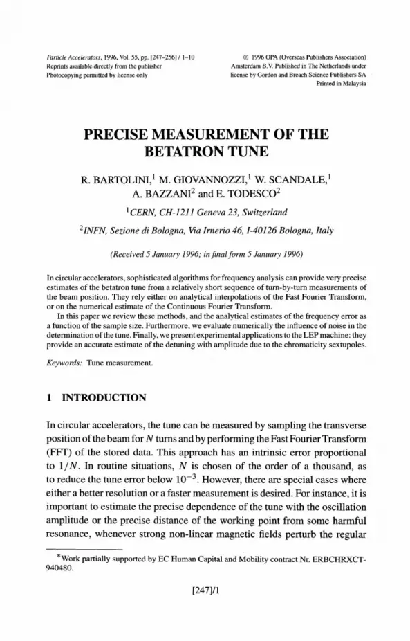
FIGURE 1 Tune error E (N) versus N for different values of the signal over noise power ratios / n. The signal is generated by two sine waves plus harmonics. The tune is computed using theinterpolation of the FFT plus Hanning filtering. Five cases, referring to different signal to noiseratio, are shown.

0

-2

-4

~ -6Z'-"W -8eJJ --No noiseQ

-10 - - - S/N=1 000~

---6-S/N=100-12 - - - - S/N=10

-14 -S/N=1

-16

1 2 3 4 5

Log (N)

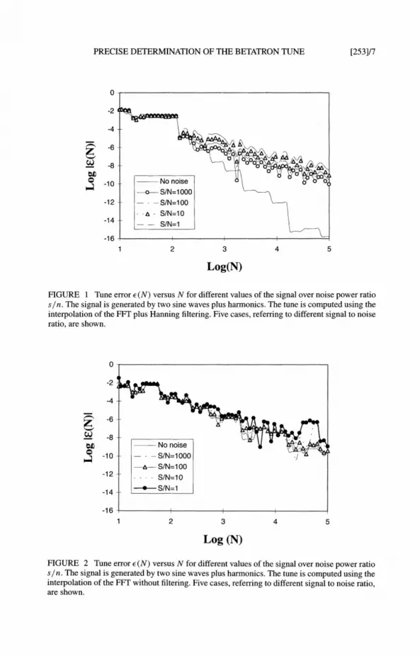
FIGURE 2 Tune error E (N) versus N for different values of the signal over noise power ratios / n. The signal is generated by two sine waves plus harmonics. The tune is computed using theinterpolation of the FFT without filtering. Five cases, referring to different signal to noise ratio,are shown.

[254]18

0.3

0.28

0.26

0.24

~0.22

= 0.2=~0.18

0.16

0.14

0.12

0.1

2000

R. BARTOLINI et al.

--tuney- - - - tune x

2200 2400 2600 2800 3000 3200 3400 3600 3800

Amplitude y

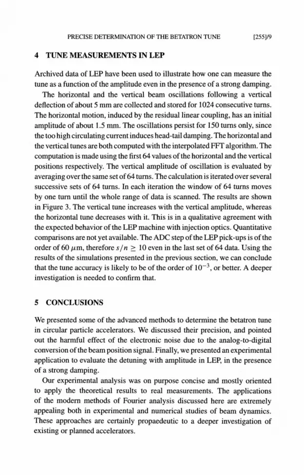
FIGURE 3 Horizontal and vertical tune as a function of vertical amplitude. The tune iscomputed using a moving window of 64 turns. The vertical amplitude, averaged over the 64 tumwindow, is in j.Lm. The method used is the interpolation of the FFT without filtering.

zen) = e2n:ivon + Lak e2n:ivokn +bae2n:iv1n + Lbk e2n:iv1kn +r(n) LSB ,k k

(16)

where lakl, Ibkl < 1, n E N, and r(n) is a random variable equal to 0 or 1.In our simulations we chose Va = 0.28 and VI = 0.31 to simulate the

working point of the LHC. We consider five harmonics of Va and VI, andwe assume that their amplitudes decrease exponentially with their order. Themain tune Va is found using the interpolated FFT algorithm. The referencecase, without noise, is compared to several cases,where the signal to noisepower ratio (s / n) vary over a large range. Due to the noise, the precisionassociated to the tune is reduced, as shown in Figures 1 and 2. In particular,the beneficial effect of the Hanning filter is completely lost, even if the noiseis small (s / n = 1000). On the other hand, the effect of the noise has a weakdependence on the s / n ratio. In addition, the tune error scales always betterthan 1/N, even in the extreme case when the noise and the signal powers areequal.

PRECISE DETERMINATION OF THE BETATRON TUNE

4 TUNE MEASUREMENTS IN LEP

[255]/9

Archived data of LEP have been used to illustrate how one can measure thetune as a function of the amplitude even in the presence of a strong damping.

The horizontal and the vertical beam oscillations following a verticaldeflection of about 5 mm are collected and stored for 1024 consecutive turns.The horizontal motion, induced by the residual linear coupling, has an initialamplitude of about 1.5 mm. The oscillations persist for 150 turns only, sincethe too high circulating current induces head-tail damping. The horizontal andthe vertical tunes are both computed with the interpolated FFT algorithm. Thecomputation is made using the first 64 values of the horizontal and the verticalpositions respectively. The vertical amplitude of oscillation is evaluated byaveraging over the same set of64 turns. The calculation is iterated over severalsuccessive sets of 64 turns. In each iteration the window of 64 turns movesby one tum until the whole range of data is scanned. The results are shownin Figure 3. The vertical tune increases with the vertical amplitude, whereasthe horizontal tune decreases with it. This is in a qualitative agreement withthe expected behavior of the LEP machine with injection optics. Quantitativecomparisons are not yet available. The ADC step of the LEP pick-ups is of theorder of 60 /-Lm, therefore s/ n 2: 10 even in the last set of 64 data. Using theresults of the simulations presented in the previous section, we can concludethat the tune accuracy is likely to be of the order of 10-3, or better. A deeperinvestigation is needed to confirm that.

5 CONCLUSIONS

We presented some of the advanced methods to determine the betatron tunein circular particle accelerators. We discussed their precision, and pointedout the harmful effect of the electronic noise due to the analog-to-digitalconversion ofthe beam position signal. Finally, we presented an experimentalapplication to evaluate the detuning with .amplitude in LEP, in the presenceof a strong damping.

Our experimental analysis was on purpose concise and mostly orientedto apply the theoretical results to real measurements. The applicationsof the modem methods of Fourier analysis discussed here are extremelyappealing both in experimental and numerical studies of beam dynamics.These approaches are certainly propaedeutic to a deeper investigation ofexisting or planned accelerators.

[256]/10

References

R. BARTOLINI et at.

[1] E. Asseo, J. Bengtsson and M. Chanel, in Fourth European Signal Processing Conference,edited by J.L. Lacoume, et al. (North Holland, Amsterdam, 1988) pp. 1317-1320.

[2] E. Asseo, CERN PS Note (LEA) 85-3 (1985).[3] E. Asseo, CERN PS Note (LEA) 87-1 (1987).[4] J. Laskar, Icarus, 88, 266-291 (1990).[5] J. Laskar, Physica D, 67, 257-281 (1993).[6] H.S. Dumas and J. Laskar, Phys. Rev. Lett., 70, 2975-2979 (1993).[7] R. Bartolini, A. Bazzani, M. Giovannozzi, W. Scandale and E. Todesco, CERN SL 95-84

(AP) (1995).[8] H. Jakob, et aI., CERN SL 95-68 (BI) (1995).[9] H,J. Schmickler, CERN LEP Note (BI) 87-10 (1987).

[10] F.J. Harris, Proceedings of the IEEE, 66, 51-83 (1978).[11] P. Tran, et aI., Submitted to the PAC Conference, Dallas (1995).