Embed Size (px)
Citation preview
Aachener Beiträge zur Technischen Akustik
λογος
Dirk Schroder
Physically Based Real-Time Auralizationof Interactive Virtual Environments

PHYSICALLY BASED REAL-TIME AURALIZATION OF
INTERACTIVE VIRTUAL ENVIRONMENTS
Von der Fakultät für Elektrotechnik und Informationstechnik derRheinisch-Westfälischen Technischen Hochschule Aachen
zur Erlangung des akademischen Grades einesDoktors der Ingenieurwissenschaften
genehmigte Dissertation
vorgelegt von
Diplom-IngenieurDirk Schröder
aus Köln
Berichter: Univ.-Prof. Dr. rer. nat. Michael VorländerProf. U. Peter Svensson, Ph.D., NTNU Trondheim
Tag der mündlichen Prüfung: 04. Februar 2011
Diese Dissertation ist auf den Internetseiten der Hochschulbibliothek online verfügbar.

ii
Dirk Schroder
Physically Based Real-Time Auralizationof Interactive Virtual Environments
Logos Verlag Berlin GmbH
λογος

Aachener Beitrage zur Technischen AkustikEditor:Prof. Dr. rer. nat. Michael VorlanderInstitute of Technical AcousticsRWTH Aachen University52056 Aachenwww.akustik.rwth-aachen.de
Bibliographic information published by the Deutsche Nationalbibliothek
The Deutsche Nationalbibliothek lists this publication in the Deutsche Nationalbibliografie;detailed bibliographic data are available in the Internet at http://dnb.d-nb.de .
D 82 (Diss. RWTH Aachen University, 2011)
c© Copyright Logos Verlag Berlin GmbH 2011
All rights reserved.
ISBN 978-3-8325-3031-0
ISSN 1866-3052
Vol. 11
Logos Verlag Berlin GmbHComeniushof, Gubener Str. 47,D-10243 Berlin
Tel.: +49 (0)30 / 42 85 10 90Fax: +49 (0)30 / 42 85 10 92http://www.logos-verlag.de

∼ To my beloved parents, Ursula and Friedhelm Schröder ∼
iii

iv
Abstract
Over the last decades, Virtual Reality (VR) technology has emerged to be a power-ful tool for a wide variety of applications covering conventional use, e.g., in science,design, medicine and engineering, as well as in more visionary applications such asthe creation of virtual spaces that aim to act real. However, the high capabilitiesof today’s VR-systems are mostly limited to first-class visual rendering. In orderto boost the range of applications, state-of-the-art systems aim to reproduce virtualenvironments as realistically as possible for the purpose of maximizing the user’s feel-ing of immersion, presence and acceptance. Such immersive systems deliver multiplesensory stimuli and provide an opportunity to act interactively, as reality is neithermono-modal nor static.
Analogous to visualization, the auralization of virtual environments describes thesimulation of sound propagation inside enclosures where methods of GeometricalAcoustics are mostly applied for a high-quality synthesis of aural stimuli that goalong with a certain realistic behavior. Here, best results are achieved by combiningdeterministic methods for the computation of early specular sound reflections withstochastic approaches for the computation of the reverberant sound field. By adapt-ing acceleration algorithms from Computer Graphics, current implementations canmanage the computational load of moving sound sources around a moving receiver inreal-time – even for complex but static architectural scenarios.
In the course of this thesis, the design and implementation of the real-time roomacoustics simulation software RAVEN will be described, which is a vital part of theimplemented 3D sound-rendering system of RWTH Aachen University’s immersiveVR-system. RAVEN relies on present-day knowledge of room acoustical simulationtechniques and enables a physically accurate auralization of sound propagation incomplex environments including important wave effects such as sound scattering,airborne sound insulation between rooms and sound diffraction. Despite this realisticsound field rendering, not only spatially distributed and freely movable sound sourcesand receivers are supported at runtime but also modifications and manipulationsof the environment itself. All major features are evaluated by investigating both theoverall accuracy of the room acoustics simulation and the performance of implementedalgorithms, and possibilities for further simulation optimizations are identified byassessing empirical studies of subjects operating in immersive environments.
v

vi
ZusammenfassungIn den letzten Jahrzehnten hat sich die Virtual Reality (VR) Technologie zu einemleistungsfähigen Werkzeug entwickelt, das in einer Vielzahl von herkömmlichen An-wendungen Einzug gehalten hat. Hierzu gehören Bereiche aus Forschung, De-sign, Medizin und Entwicklung, in denen neue Wege über die Verwendung von VReingeschlagen werden, wie z.B. die Erstellung virtueller Umgebungen, in denen ver-sucht wird ein möglichst plausibles Abbild der Wirklichkeit zu schaffen. Die theo-retisch hohe Leistungsfähigkeit heutiger VR-Systeme ist allerdings meist beschränktauf eine qualitativ hochwertige visuelle Darstellung, obwohl deren Anwendungsbereichsignifikant erweitert werden kann durch den Einsatz multi-modaler Systeme. Multi-modale Systeme können mehrere Sinnesreize gleichzeitig stimulieren und bieten demBenutzer die Möglichkeit mit der virtuellen Welt direkt zu interagieren – denn in denmeisten Fällen sind reale Situationen weder mono-modal noch statisch. Diese soge-nannten immersiven Systeme sind dafür konzipiert ein virtuelles Abbild einer Umge-bung so realistisch wie möglich wiederzugeben, um so beim Benutzer das Gefühl derImmersion, Präsenz und Akzeptanz zu verstärken.
In Analogie zur Visualisierung beschreibt die Auralisierung von virtuellen Umge-bungen die Simulation von Schallausbreitung innerhalb von Räumen oder anderenbegrenzten Gebieten. Methoden der Geometrischen Akustik kommen hier meistenszum Einsatz, da sie eine qualitativ hochwertige und physikalisch basierte Schallfeld-Synthese ermöglichen. Die besten Ergebnisse werden hierbei mit Hilfe von hy-briden Verfahren erreicht, die deterministischen Methoden für die Berechnung vonfrühen spiegelnden Schallreflexionen mit stochastischen Simulationsverfahren für eineadäquate Nachbildung des Nachhalls in Räumen kombinieren. Durch die Adaptionvon Beschleunigungs-Algorithmen aus der Computergrafik sind aktuelle Implemen-tierungen in der Lage bewegte Schallquellen und Empfänger in komplexen, aber statis-chen architektonischen Szenarien in Echtzeit zu simulieren.
Im Zuge dieser Arbeit wird das Konzept und die Umsetzung der echtzeitfähi-gen Raumakustik-Simulationssoftware RAVEN beschrieben, die ein wesentlicher Be-standteil des immersiven VR-Systems an der RWTH Aachen ist. RAVEN basiert aufdem heutigen Wissen von raumakustischen Simulationsverfahren und ermöglicht einephysikalisch korrekte Simulation der Schallausbreitung in komplexen Umgebungen,einschließlich wichtiger Welleneffekte wie Schallstreuung, Luftschalldämmung zwis-chen Räumen und Schallbeugung. Die angewandten Simulationsverfahren werdenhinsichtlich ihrer Genauigkeit und Grenzen ihrer Echtzeitfähigkeit untersucht, wobeigezeigt werden wird, dass RAVEN trotz der realistischen Klangfeldsynthese nicht nurdie Echtzeit-Simulation von räumlich verteilten und frei beweglichen Schallquellenund Empfängern ermöglicht, sondern auch die direkte Änderung und Manipulationder virtuellen Umgebung selbst. Des weiteren werden Möglichkeiten für die weitereOptimierung der Simulationsparametrierung aufgezeigt, die durch die Beurteilungempirischer Studien von Versuchspersonen identifiziert werden konnten.
vii

viii
Preface
"Whereas film is used to show reality to an audience, cyberspace is usedto give a virtual body, and a role, to everyone in the audience. Print andradio tell; stage and film show; cyberspace embodies. [...]. A spacemakersets up a world for an audience to act directly within, and not just so theaudience can imagine they are experiencing an interesting reality, but sothey can experience it directly. [...]. The filmmaker says, ‘Look. I’ll showyou’. The spacemaker says, ‘Here, I’ll help you discover’."
(Elements of a Cyberspace Playhouse, Randal Walser)
I remember that I had my first contact with the term "Virtual Reality" at theage of 17, that was in 1992, when I saw the movie "The Lawnmower Man" directedby Brett Leonard. In this movie, Pierce Brosnan plays Dr. Lawrence Angelo, avisionary computer scientist who was dreaming of the possibility to excite, trainand even improve a subject’s brain/mind capabilities by using sophisticated VirtualReality technology. Angelo was convinced that "Virtual Reality holds a key to theevolution of the human mind". According to his theory, a ground-breaking man-machine interconnection could be established by completely immersing subjects tocyberspace – a term that was coined in the 80s by William F. Gibson who describedin his debut novel "Neuromancer" cyberspace as a
"[...] representation of data abstracted from banks of every computer in the humansystem. Unthinkable complexity. Lines of light ranged in the non-space of the mind,clusters and constellations of data. Like city lights, receding.".
By using such an interface, Angelo hoped to enable a direct link to the humanconsciousness for altering both the perception and reception. His first subject washis lawnmower man, Jobe Smith, who was retarded. Angelo successfully improvedhis intelligence by sending him to cyberspace, but major side-effects evolved sinceSmith got addicted to information. To keep it short: After developing supernaturalpsychic power that went along with a God psychosis, Smith left his physical body anduploaded his mind to cyberspace making him virtually immortal. He became "CyberChrist".
Although I hope that "The Lawnmower Man" is not Brett Leonard’s masterpiece,the core idea of this movie has fascinated me until today. It was even my mainmotivation to study communication and information technology at RWTH AachenUniversity. I wanted to face immersive technology from a professional side and seehow close we really are to the claim of Simulism. Simulism postulates that realitycan be simulated (for example by computers) to a degree indistinguishable from the"true" ontic reality and can contain conscious minds who are not aware whether theyare living inside a simulation.
ix
Today, technologically-achieved Virtual Reality does not entirely satisfy the ex-perience of actuality, i.e., participants are not yet in doubt about the nature of whatthey experience. However, computing power and simulation techniques have improveddrastically during the last 20 years and first prototypes of real-time immersive en-vironments have already been built. Quite limited in their capabilities though, butgood effort is made in improving such systems. Is it then too far-fetched to raise thequestion if Virtual Reality technology is perhaps only some steps away from fulfillingmankind’s dream to make us become God-like creators of our own reality? A sim-ulated reality, generated by a human-machine interface that makes the transcendingmedium disappear and enables an imagination beyond belief. Heim even went a stepfurther and claimed that Virtual Reality is not necessarily bound to what we knowfrom our own experiences of reality with all of its anchoring elements of stability suchas time and space. In his book "The Metaphysics of Virtual Reality" he argued that
"[...] The ultimate Virtual Reality is a philosophical experience, probably an experi-ence of the sublime or awesome. The sublime, as Kant defined it, is the spine-tinglingchill that comes from the realization of how small our finite perceptions are in the faceof the infinity of possible, virtual worlds we may settle into and inhabit. The finalpoint of a virtual world is to dissolve the constraints of the anchored world so thatwe can lift anchor – not to drift aimlessly without point, but to explore anchorage inever-new places and, perhaps, find our way back to experience the most primitive andpowerful alternative embedded in the question posed by Leibniz: Why is there anythingat all rather than nothing?".
What does "reality" then mean? If we were able to fake it through mediatedhallucinations, is our subjective reality just a manipulable cognitive process of thehuman brain? This is still a highly controversial question in epistemology until to-day. According to Coyne there are basically two schools of thought on how reality issubjectively perceived and how it should be represented to create its virtual counter-part. Here, the data-oriented view regards reality as a matter of data input statingthat only a greater quantity of data and a higher quality of detail effects a sense ofthe real since the human body is considered to be just an elaborate input device. Onthe contrary, the constructivist view claims that
"We rely on simple cues and clues from the environment. We can be immersed inany environment. Depending on our state of mind, our interest, what we have beentaught to experience, our personal and collective expectations, and our familiarity withthe medium."1
The probably most uncompromising constructivist view – that I like the most – iscalled Radical Constructivism, which was mainly advocated by Von Glasersfeld anddescribes reality as
"[...] the world we experience; from it alone we deduce, in our own ways, ideasand things as well as the concepts of the relations with which we create links andbuild up theories that allow us to formulate more or less viable explanations andpredictions in our life world.",
1Richard Coyne, Heidegger and Virtual Reality: The Implications of Heidegger’s Thinking forComputer Representations.
x
and further
"We never use all existing signals2 but select a relatively small number and, ifneeded, complement this selection with perceptions recalled (which are not producedspontaneously by the senses). The need is established by the context of the action inwhich we find ourselves; and this context never requires us seeing the ‘environment’as it is ‘in reality’ [...]. From the perspective of acting it is irrelevant whether one’sidea of the environment is a ‘true’ picture of ontic reality.".
In other words, the Radical Constructivism postulates that our reality is con-structed from individual sensory performance and limited memory capacity. An ob-jective perception and complete knowledge of the ontic reality is therefore impossibleand, thus, reality is reduced to a subjective experience of our ‘true’ world. Moreover,we can learn to accept any immersive virtual reality system as real without the need ofa complete representation of ontic reality in its entire complexity. Thus, ignoring thisconstructed nature of perception, as it is done in data-oriented approaches, impliesthat a Virtual Reality system for a fly does not differ much to that for a human. Butis this really feasible? From my point of view, it is definitely not.
For the next roughly two hundred pages, I will describe the concept and implemen-tation details of a software framework for the human-centered real-time auralizationof dynamic and interactive virtual environments. RAVEN, as I entitled this frame-work, was born during my master thesis at the Institute of Technical Acoustics (ITA),RWTH Aachen University, and became quite mature during my Ph.D. studies. Todayit offers features that I could not even think of on the day when RAVEN was born.I wish I could claim the credits for this work all by myself, but I truly had immensesupport and would like to take the opportunity to thank some very special people fortheir trust, effort, collaboration and friendship during my doctoral studies.
I want to start with Michael Vorländer who not only served as my doctoral advisorbut also encouraged and guided me throughout my entire time as Ph.D. student. Ifeel tremendously lucky that Michael gave me the chance to carry out my researchat his institute with almost unlimited support in every perspective. Tobias Lentzdefinitely drew me to the research area of Virtual Acoustics by supervising my masterthesis and later working with me side by side. Together with Ingo Assenmacher, whowas working at the Virtual Reality Group (VRG) at the Center for Computing andCommunication of RWTH Aachen University, I had the honor to be part of a workgroup of professional and reliable experts who always poured their heart and soul intoour mutual goal of building a cutting-edge Virtual Reality system. The work groupwas gradually enforced through the Ph.D. students Frank Wefers (ITA) and DominikRausch (VRG), who both turned out to be valuable team members working out theirhearts to make the impossible possible. It was an exciting time for all of us – so fullof frustration, but also so full of joy and glory. Special thanks to Torsten Kuhlen,head of the VRG at RWTH Aachen University, who supported and encouraged ourwork throughout the years.
Apart from this work group, I am grateful for having had so many helping hands.Doubtlessly, two important names are hereby Alexander Pohl and Sönke Pelzer whohave always accompanied me during my entire Ph.D. time, either as student work-ers, master students, colleagues or friends. Even when their own time schedule was
2Stimuli of the ontic reality.
xi
extremely tight, they were always working through illness to help me meet publica-tion deadlines. You have my deepest gratitude. Furthermore, I would like to thankmy former student workers Lukas Aspöck, Jochen Giese and Martin Landt – reli-able persons who were always doing their assigned work in a very passionate way.Thanks also to Philipp Dross, Stefan Reuter, Alexander Ryba, Marc Schlütter, BjörnStarke, Moritz Fricke, Philipp Schmidt, Stephan Gsell, Umberto Palmieri, ElzbietaNowicka, David Kolf and Lukas Jauer for their exceptional work either in the scopeof their Master thesis and/or student research project. I would also like to thank UweStephenson for his many valuable advices on the secrets of stochastic models for thesimulation of edge diffraction. Paula Niemietz was the charming voice in my demon-stration videos and I’m very grateful for her time, commitment and great personality.I also want to express my deepest gratitude to the German Research foundation whohave supported my research over the last three years. Their scholarship doubtlesslygave me the freedom to think more broadly about my graduate work.
Special thanks to all my colleagues at ITA for the interesting, often funny andnever-ending discussions during our legendary coffee breaks. Especially GottfriedBehler, Andreas Franck, Rainer Thaden, Rolf Kaldenbach, Ingo Witew, MichaelMakarski, Anselm Goertz, Janina Fels, Pascal Dietrich, Markus Müller-Trapet, RenzoVitale, Jan Köhler, Bruno Sanches Masiero, João Henrique Diniz Guimarães, Mar-tin Pollow, Matthias Lievens, Sebastian Fingerhuth, Marc Aretz, Martin Guski andElena Shabalina had always a sympathetic ear and solutions for my problems. Theywere an unfailing source of encouragement during my ITA time and I can think ofno finer individuals to work with. Special thanks to Uwe Schlömer and the membersof the mechanical workshop for their time and expertise to help design and assembleseveral prototypes with unbelievable accuracy. I had a great time with my ITA familyand I will miss all of you.
During my Ph.D. studies, I was also tremendously lucky to spend some months inTrondheim, Norway, at NTNU’s Centre for Quantifiable Quality of Service in Com-munication Systems (Q2S) under the supervision of Peter Svensson. Peter instilledin me a love for simulating edge diffraction of sound and I’m very grateful for hispatient advice. He also agreed on becoming my second mentor of my graduate workand I truly can think of no one better. Nima Darabi and Jordi Puig were definitely asource of inspiration for me with their infectious enthusiasm and outlook on life thatresurrected my almost forgotten passion for art and philosophy. It was an amazingtime at office E-228 in any perspective.
Finally, I would like to thank my parents, Ursula and Friedhelm Schröder. Wordscan hardly express my deepest gratitude for their everlasting love, sacrifice, guidanceand encouragement. This dissertation is dedicated to them.
xii

Contents
Abstract v
Zusammenfassung vii
Preface ix
Acronyms xvii
I Introduction 1
1 Introduction 31.1 Virtual Environments . . . . . . . . . . . . . . . . . . . . . . . . . . . 31.2 Related Work . . . . . . . . . . . . . . . . . . . . . . . . . . . . . . . 51.3 Interactive Virtual Environments at RWTH Aachen University . . . . 61.4 Aim of this Work . . . . . . . . . . . . . . . . . . . . . . . . . . . . . 8
II Concept 11
2 Sound Propagation in Rooms 132.1 Acoustical Point Sources . . . . . . . . . . . . . . . . . . . . . . . . . 132.2 Sound Absorption . . . . . . . . . . . . . . . . . . . . . . . . . . . . . 152.3 Sound Scattering . . . . . . . . . . . . . . . . . . . . . . . . . . . . . 162.4 Sound Transmission . . . . . . . . . . . . . . . . . . . . . . . . . . . . 172.5 Sound Diffraction . . . . . . . . . . . . . . . . . . . . . . . . . . . . . 182.6 (Binaural) Room Impulse Response . . . . . . . . . . . . . . . . . . . 202.7 Principle of Auralization . . . . . . . . . . . . . . . . . . . . . . . . . 22
3 Multimodal Representation of Airborne Sound Sources 253.1 Directional Pattern of Sound Sources . . . . . . . . . . . . . . . . . . 273.2 Motion Capturing of Sound Sources . . . . . . . . . . . . . . . . . . . 313.3 Audiovisual Avatars . . . . . . . . . . . . . . . . . . . . . . . . . . . . 33
4 Modeling and Handling of Complex Environments 354.1 Polygonal Scene Model . . . . . . . . . . . . . . . . . . . . . . . . . . 354.2 Spatial Data Structures . . . . . . . . . . . . . . . . . . . . . . . . . . 37
4.2.1 General . . . . . . . . . . . . . . . . . . . . . . . . . . . . . . 374.2.2 Binary Space Partitioning (BSP) . . . . . . . . . . . . . . . . 38
xiii
4.2.3 Spatial Hashing . . . . . . . . . . . . . . . . . . . . . . . . . . 434.3 Dynamic Coupling of Rooms . . . . . . . . . . . . . . . . . . . . . . . 45
5 Room Acoustics Simulation 475.1 General . . . . . . . . . . . . . . . . . . . . . . . . . . . . . . . . . . 475.2 Deterministic Image Source Method . . . . . . . . . . . . . . . . . . . 52
5.2.1 General . . . . . . . . . . . . . . . . . . . . . . . . . . . . . . 525.2.2 Construction of the Room Impulse Response (IS) . . . . . . . 545.2.3 Diffraction . . . . . . . . . . . . . . . . . . . . . . . . . . . . . 55
5.3 Stochastic Ray Tracing . . . . . . . . . . . . . . . . . . . . . . . . . . 595.3.1 General . . . . . . . . . . . . . . . . . . . . . . . . . . . . . . 595.3.2 Diffuse Rain . . . . . . . . . . . . . . . . . . . . . . . . . . . . 615.3.3 Diffracted Rain . . . . . . . . . . . . . . . . . . . . . . . . . . 665.3.4 Construction of the Room Impulse Response (RT) . . . . . . . 70
5.4 Hybrid Room Acoustics Simulation . . . . . . . . . . . . . . . . . . . 745.5 Simulation of Sound Propagation between Rooms . . . . . . . . . . . 76
5.5.1 Sound Transmission Model . . . . . . . . . . . . . . . . . . . . 765.5.2 Rendering Filter Networks . . . . . . . . . . . . . . . . . . . . 79
5.6 Limits of Geometrical Acoustics . . . . . . . . . . . . . . . . . . . . . 81
6 Dynamically Changing Virtual Environments 836.1 Real-time Constraints . . . . . . . . . . . . . . . . . . . . . . . . . . 846.2 Process Analysis of Interaction Events . . . . . . . . . . . . . . . . . 86
6.2.1 Rotational and Translational Movements of Sound Sources andthe User . . . . . . . . . . . . . . . . . . . . . . . . . . . . . . 87
6.2.2 Creation, Modification and Destruction of Dynamic Geometry 916.2.3 Interaction with Portals . . . . . . . . . . . . . . . . . . . . . 93
6.3 Parallel Computing . . . . . . . . . . . . . . . . . . . . . . . . . . . . 94
III Real-time Implementation 97
7 Acceleration ofGeometric Operations 997.1 Point-In-Polygon Test . . . . . . . . . . . . . . . . . . . . . . . . . . 997.2 Ray-Polygon Intersection Search . . . . . . . . . . . . . . . . . . . . . 101
7.2.1 Binary Space Partitioning . . . . . . . . . . . . . . . . . . . . 1017.2.2 Spatial Hashing . . . . . . . . . . . . . . . . . . . . . . . . . . 103
7.3 Collision Tests . . . . . . . . . . . . . . . . . . . . . . . . . . . . . . . 105
8 Efficient Handling of Complex Dynamic Sceneries 1098.1 Tracking of Sound Paths . . . . . . . . . . . . . . . . . . . . . . . . . 1098.2 The Path Propagation Tree . . . . . . . . . . . . . . . . . . . . . . . 113
9 Real-time Implementation of Room Acoustics Simulation Methods1159.1 Real-time Implementation of the Image Source Method . . . . . . . . 115
9.1.1 Plane-Polygon Map . . . . . . . . . . . . . . . . . . . . . . . . 1169.1.2 Image Source Tree . . . . . . . . . . . . . . . . . . . . . . . . 117
xiv
9.1.3 Tracking of Edge Diffraction Paths . . . . . . . . . . . . . . . 1209.1.4 Powersets of Image Sources . . . . . . . . . . . . . . . . . . . 122
9.2 Real-time Implementation of Ray Tracing . . . . . . . . . . . . . . . 123
IV Evaluation 127
10 Analytical Validation 12910.1 Hybrid Simulation Model . . . . . . . . . . . . . . . . . . . . . . . . . 12910.2 Sound Transmission . . . . . . . . . . . . . . . . . . . . . . . . . . . . 13210.3 Sound Diffraction . . . . . . . . . . . . . . . . . . . . . . . . . . . . . 134
11 Performance 14111.1 Test Models . . . . . . . . . . . . . . . . . . . . . . . . . . . . . . . . 14111.2 Performance of the Image Source Method . . . . . . . . . . . . . . . . 143
11.2.1 Binary Space Partitioning . . . . . . . . . . . . . . . . . . . . 14311.2.2 Spatial Hashing . . . . . . . . . . . . . . . . . . . . . . . . . . 14611.2.3 Handling of Dynamic Objects . . . . . . . . . . . . . . . . . . 149
11.3 Performance of Ray Tracing . . . . . . . . . . . . . . . . . . . . . . . 153
12 Optimization of Input Parameters 15712.1 Listening Tests . . . . . . . . . . . . . . . . . . . . . . . . . . . . . . 15712.2 Example Evaluation of Listening Tests . . . . . . . . . . . . . . . . . 159
V Summary & Outlook 163
13 Summary and Discussion 165
14 Outlook 171
VI Appendix 175
A Room Models 177
B RAVEN 183
Bibliography 195
Curriculum vitae 207
xv

xvi
Acronyms
AABB Axis-Aligned Bounding BoxAFC Alternative Forced ChoiceASG Acoustic Scene GraphACG Audio Communication GroupBEM Boundary Element MethodBCI Brain Computer InterfaceBF Brute ForceBRIR Binaural Room Impulse ResponseBRTF Binaural Room Transfer FunctionBSP Binary Space PartitioningBTME Biot-Tolstoy-Medwin ExpressionBVH Bounding Volume HierarchyCAVE Cave Automatic Virtual EnvironmentCG Computer GraphicsCTC Cross-Talk CancellationDAPDF Deflection Angle Probability Density FunctionDC Deflection CylinderDG Directivity GroupDIS Diffraction Image SourceDS Diffraction SourceFEM Finite Element MethodGA Geometrical AcousticsGPU Graphics Processing UnitGUI Graphical User InterfaceHRIR Head Related Impulse ResponseHRTF Head Related Transfer FunctionILD Interaural Level DifferenceIS Image SourceIST Image Source TreeITA Institute of Technical Acoustics, RWTH Aachen UniversityITD Interaural Time DifferenceJND Just Noticeable DifferenceLIFO Last-In-First-OutLTI Linear Time-InvariantMPI Message Passing InterfaceNTNU Norges Teknisk-Naturvitenskapelige UniversitetOpenDAFF Open Directional Audio File FormatOpenMP Open Multi-Processing
xvii

PPM Plane-Polygon MapPST Path Search TreePT Parameter ThresholdPPG Propagation Path GraphPS Primary SourceRAVEN Room Acoustics for Virtual EnvironmentsRIR Room Impulse ResponseRT Ray TracingRTF Room Transfer FunctionRWTH Rheinisch-Westfälische Technische HochschuleSEA Statistical Energy AnalysisSH Spatial HashingSS Secondary SourceUTD Uniform Theory of DiffractionVA Virtual AcousticsVC Voxel CandidatesViSTA Virtual Reality for Scientific Technical ApplicationsVT Voxel TracingVR Virtual RealityVRG Virtual Reality Group, RWTH Aachen University
xviii

Part I
Introduction

2
Chapter 1
Introduction
"Our argument is that experiencing presence in a remote operationstask or in a virtual environment (VE) requires the ability to focus onone meaningfully coherent set of stimuli (in the VE) to the exclusion ofunrelated stimuli (in the physical location). To the extent that the stimuliin the physical location fit in with the VE stimuli, they may be integratedto form a meaningful whole."
(Measuring Presence in Virtual Environments: A Presence Questionaire,Bob G. Witmer and Michael J. Singer, American scientists)
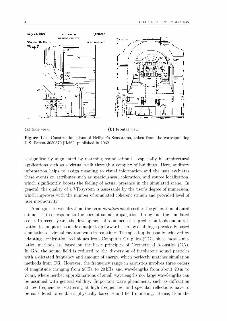
1.1 Virtual EnvironmentsIn 1956, Morton L. Heilig started with the development of a one-person theater,which he later called the Sensorama. The Sensorama combined projected film, audio,vibration, wind, and odors, in order to create a plausible set of stimuli that made theuser rather feel the presented scenery, such as a motorcycle ride through New York,instead of just observing it as on television (see Fig. 1.1). As the age of computerswas still about to begin at that time, the entire experience was prerecorded andplayed back on demand. Nonetheless, Heilig’s machine can be regarded today as thefirst multi-modal immersive virtual experience – at least in the modern interpretationof Virtual Reality (VR)-systems, as the idea of creating the ultimate medium thatperfectly matches reality has always fascinated mankind since the dawn of time. Eversince Heilig’s pioneering work, considerable effort has been put into the developmentof improved VR-systems, where the term VR refers from a technical point of view tothe representation and simultaneous perception of reality and its physical attributesin an interactive computer-generated virtual environment. Today, VR-technology isused in numerous applications, for instance, engineering, science, design, medicine, artand architecture. The focus of these applications lies usually on the visual componentof the virtual environment, and other modalities, if present at all, are often added justas an effect without any plausible reference to the physical aspects of the presentedscenery. However, VR-systems that aim at enabling immersive applications shouldaddress at least the hearing, too, since it is a well-known fact that the visual perception
4 CHAPTER 1. INTRODUCTION
(a) Side view. (b) Frontal view.
Figure 1.1: Construction plans of Heiliger’s Sensorama, taken from the correspondingU.S. Patent 3050870 [Hei62] published in 1962.
is significantly augmented by matching sound stimuli – especially in architecturalapplications such as a virtual walk through a complex of buildings. Here, auditoryinformation helps to assign meaning to visual information and the user evaluatesthese events on attributes such as spaciousness, coloration, and source localization,which significantly boosts the feeling of actual presence in the simulated scene. Ingeneral, the quality of a VR-system is assessable by the user’s degree of immersion,which improves with the number of simulated coherent stimuli and provided level ofuser interactivity.
Analogous to visualization, the term auralization describes the generation of auralstimuli that correspond to the current sound propagation throughout the simulatedscene. In recent years, the development of room acoustics prediction tools and aural-ization techniques has made a major leap forward, thereby enabling a physically basedsimulation of virtual environments in real-time. The speed-up is usually achieved byadapting acceleration techniques from Computer Graphics (CG), since most simu-lation methods are based on the basic principles of Geometrical Acoustics (GA).In GA, the sound field is reduced to the dispersion of incoherent sound particleswith a dictated frequency and amount of energy, which perfectly matches simulationmethods from CG. However, the frequency range in acoustics involves three ordersof magnitude (ranging from 20Hz to 20 kHz and wavelengths from about 20m to2 cm), where neither approximations of small wavelengths nor large wavelengths canbe assumed with general validity. Important wave phenomena, such as diffractionat low frequencies, scattering at high frequencies, and specular reflections have tobe considered to enable a physically based sound field modeling. Hence, from the
1.2. RELATED WORK 5
physical point of view (not to mention the challenge of implementation), the questionof modeling and simulation of an exact virtual sound is by orders of magnitude moredifficult than the task of creating visual images, which might be the reason for thedelayed implementation of physically based 3D audio rendering engines for virtualenvironments.
Whereas low-reflective outdoor scenarios can be simulated rather fast and accu-rately today, the determination of the spatial sound field in enclosures is still a difficulttask, especially under real-time constraints. In indoor scenarios, even rather simplesituations require quite complex acoustic models, and the more the user is allowedto interact with the scenery, the more this complexity increases. Flexible simulationmodels are therefore required that describe directional patterns of sound-emittingsources and the receiver, as well as the wave phenomena of sound diffraction, soundscattering and sound transmission, without leading to an explosion of computationtime. Especially complete dynamic environments become quite challenging, wherethe user is not only allowed to move freely in all three dimensions and interact withsound sources in any order, but also to modify the scene geometry itself and directlyperceive the impact on the sound field in real-time. Unfortunately, a change of thescene geometry significantly affects the whole auralization chain and, therefore, mak-ing a number of approximations is inevitable to keep the computational workloadin such demanding situations within the given real-time constraints. However, theresulting sound is not intended to be physically absolutely correct, but perceptivelyplausible, whereby knowledge of the human sound perception and the field of psy-choacoustics are essential to find the optimal balance between simulation accuracyand available computation power.
1.2 Related WorkReal-time auralization systems have been investigated by many groups. Notable hereis the pioneering work by Lauri Savioja et al. at the TKK Helsinki University, Finland,who presented the first audio-visual virtual environment called Experimental VirtualEnvironment (EVE) that featured a physically based auralization engine known asDigital Interactive Virtual Acoustics (DIVA) [Sav99, SHLV99]. Some years later,Thomas Funkhouser et al. introduced a very fast simulation method that first enabledthe real-time simulation of sound propagation paths in complex architectural scenariosby means of so-called beam trees that encode specular reflection paths of a staticsound source in a very efficient manner [FTC+04]. At the same time, Nicolas Tsingoset al. introduced a concept for the perceptual audio rendering of complex virtualenvironments [TGD04] in connection with the ’REVES’ research project at INRIA,France. Lately, quite advanced simulation frameworks were presented such as thework by Christian Lauterbach et al. [CLT+08] at the University of North Carolina,USA as well as the Open Source projects ’UNI-VERSE’ [Lun08] and the auralizationframework by Noisternig et al. [NKSS08].
The aim of the VR activities at Rheinisch-Westfälische Technische Hochschule
6 CHAPTER 1. INTRODUCTION
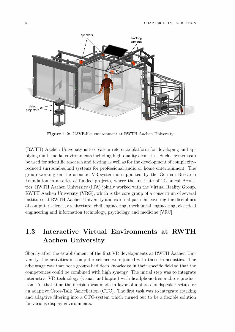
Figure 1.2: CAVE-like environment at RWTH Aachen University.
(RWTH) Aachen University is to create a reference platform for developing and ap-plying multi-modal environments including high-quality acoustics. Such a system canbe used for scientific research and testing as well as for the development of complexity-reduced surround-sound systems for professional audio or home entertainment. Thegroup working on the acoustic VR-system is supported by the German ResearchFoundation in a series of funded projects, where the Institute of Technical Acous-tics, RWTH Aachen University (ITA) jointly worked with the Virtual Reality Group,RWTH Aachen University (VRG), which is the core group of a consortium of severalinstitutes at RWTH Aachen University and external partners covering the disciplinesof computer science, architecture, civil engineering, mechanical engineering, electricalengineering and information technology, psychology and medicine [VRC].
1.3 Interactive Virtual Environments at RWTHAachen University
Shortly after the establishment of the first VR developments at RWTH Aachen Uni-versity, the activities in computer science were joined with those in acoustics. Theadvantage was that both groups had deep knowledge in their specific field so that thecompetences could be combined with high synergy. The initial step was to integrateinteractive VR technology (visual and haptic) with headphone-free audio reproduc-tion. At that time the decision was made in favor of a stereo loudspeaker setup foran adaptive Cross-Talk Cancellation (CTC). The first task was to integrate trackingand adaptive filtering into a CTC-system which turned out to be a flexible solutionfor various display environments.
1.3. INTERACTIVE VIRTUAL ENVIRONMENTS AT RWTH AACHEN UNIVERSITY 7
(a) Virtual exploration of a concert hall. (b) Object manipulation.
(c) Sound source manipulation. (d) Virtual exploration of a sound source.
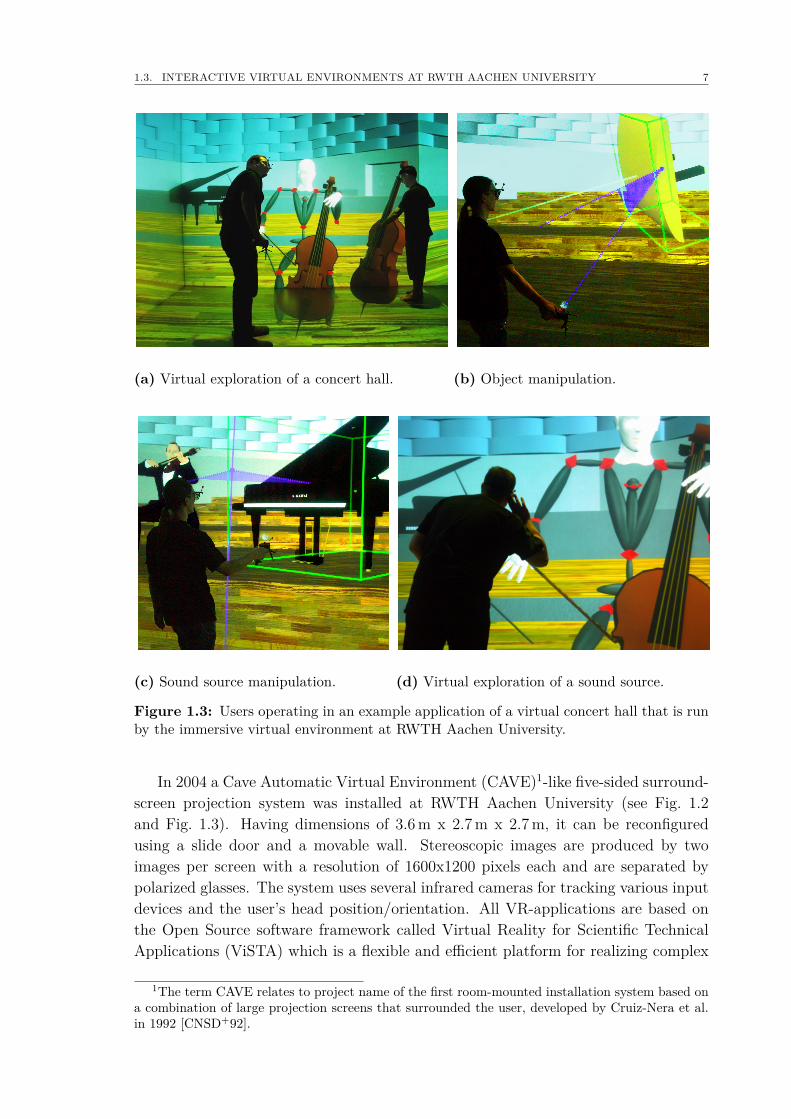
Figure 1.3: Users operating in an example application of a virtual concert hall that is runby the immersive virtual environment at RWTH Aachen University.
In 2004 a Cave Automatic Virtual Environment (CAVE)1-like five-sided surround-screen projection system was installed at RWTH Aachen University (see Fig. 1.2and Fig. 1.3). Having dimensions of 3.6m x 2.7m x 2.7m, it can be reconfiguredusing a slide door and a movable wall. Stereoscopic images are produced by twoimages per screen with a resolution of 1600x1200 pixels each and are separated bypolarized glasses. The system uses several infrared cameras for tracking various inputdevices and the user’s head position/orientation. All VR-applications are based onthe Open Source software framework called Virtual Reality for Scientific TechnicalApplications (ViSTA) which is a flexible and efficient platform for realizing complex
1The term CAVE relates to project name of the first room-mounted installation system based ona combination of large projection screens that surrounded the user, developed by Cruiz-Nera et al.in 1992 [CNSD+92].
8 CHAPTER 1. INTRODUCTION
scientific and industrial applications [AK08]. One of ViSTA’s key feature comprisesfunctionality for creating multi-modal interaction metaphors including visual, hapticand acoustic stimuli. For such elaborate multi-modal interfaces, flexible sharing ofdifferent types of data with low latency access is needed while maintaining a commontemporal context. Therefore, ViSTA has an inherent high-performance device driverarchitecture. It provides a novel approach for history recording of input data by meansof a ring buffer concept that guarantees both a low latency and a consistent temporalaccess to device samples at the same time [Ass09]. Furthermore, a compensationscheme for tracking data is integrated in ViSTA that, based on current trackingsamples, can predict the state of the human head position and orientation for thetime of application.
For reproducing acoustic signals, the dynamic CTC-system has been upgradedto four loudspeakers that are installed at the top of the CAVE (see Fig. 1.2). Thissetup was chosen over a simple stereo system in order to achieve a good binauralreproduction that is independent of the user’s orientation, where the best currentspeaker configuration is determined by minimizing the overall compensation energy[Len07]. Audio streaming is conducted using Steinberg’s ASIO professional audioarchitecture at a sampling rate of 44.1 kHz and a streaming buffer size (block length)of 512 samples, whereby a dedicated low-latency convolution engine is applied thatimplements a parallelized and highly optimized non-uniformly partitioned convolutionin the frequency domain. Here, a smooth filter transition is realized by cross-fadingin the time domain. This engine manages to convolve 88200 filter coefficients, whichrelates to a filter length of 2 s at 44.1 kHz sampling rate, with signals of more than 50sound sources in real-time [Wef07, WB10].
1.4 Aim of this WorkAnother vital part of the VR-system at RWTH Aachen University yields thehybrid real-time room acoustics simulation software Room Acoustics for VirtualEnvironments (RAVEN), where the concept and implementation will be completelydescribed in the course of this thesis. After only 6 years of intensive development,today RAVEN provides an open and flexible real-time simulation framework that isfully integrated in the exisiting ViSTA framework as a network service and which isunique in the large number of simulation features (a brief overview is given in Appx.B). RAVEN relies on present-day knowledge of room acoustical simulation techniquesbased on GA and enables a physically accurate auralization of sound propagation incomplex environments in real-time, including important wave effects such as soundscattering, airborne sound insulation between rooms and sound diffraction. Despitethis realistic sound field rendering, not only are spatially distributed and freely mov-able sound sources and receivers supported at runtime but also modifications andmanipulations of the environment itself.
All major features will be evaluated by investigating both the overall accuracy ofthe room acoustics simulation and the performance of implemented algorithms, where

1.4. AIM OF THIS WORK 9
it will be shown that RAVEN is able to handle simulation events at interactive rateswith an overall simulation accuracy that can compete with state-of-the-art (commer-cial) software solutions. In addition, possibilities for further simulation optimizationsare identified by assessing empirical studies of subjects operating in immersive envi-ronments.

10 CHAPTER 1. INTRODUCTION

Part II
Concept

12
Chapter 2
Sound Propagation in Rooms
"Darkness is to space what silence is to sound, i.e., the interval."
Marshall McLuhan, Canadian media theorist
To auralize the acoustical characteristics of an architectural virtual scenario,proper physical models are required that capture the complex process of sound prop-agation within enclosures, i.e., rooms. The reverberation caused by sound reflectionsis an essential acoustical attribute of a room, as it gives the room its very individualsound. In this chapter, models for the description of a sound source, sound ab-sorption, sound scattering, sound transmission, and sound diffraction will be brieflyintroduced, which allow the computation of the alteration of sound intensity at acertain position for a certain time. They are the basis for almost any room acous-tical simulation methods and, thus, an integral part of the auralization chain thatdescribes the sound propagation from a sound source to a receiver inside of rooms.More details on acoustical simulation methods are given in Chap. 5.
2.1 Acoustical Point SourcesWhen a sound source radiates sound, energy of wave motion is propagated outwardfrom the sound source’s center, whereby the corresponding sound-carrying air parti-cles move backward and forward, parallel to the wave motion’s direction. This leadsto an alternating increase and decrease of air pressure. The most important terms forsound wave propagation in air are the sound pressure p, which describes the position-and time-dependent fluctuation of the wave’s air pressure, and the vectorial soundparticle velocity ~ν, which is a term for the oscillation velocity of the medium’s parti-cles around their resting position. These two terms are associated with each other bythe following equations,
−grad p = ρ0∂~ν
∂tand − div ~ν = 1
ρ0c2∂p
∂t, (2.1)
where ρ0 is the static density of air and c is the speed of sound in air. One caneliminate the sound particle velocity ~ν by simply inserting the latter equation into
14 CHAPTER 2. SOUND PROPAGATION IN ROOMS
the other, which results in the so-called wave equation:
∆p = 1c2∂2p
∂t2. (2.2)
In theory, any wave type can be theoretically derived from this equation, butin practice, most solutions have to be approximated due to the analytic complex-ity. However, a simple solution of the wave equation is a spherical wave due to itssymmetry, with
p(r, t) = ρ0
4πr∂Q
∂t
(t− r
c
), (2.3)
where r is the distance to the sound source and Q is the volume velocity, whichis a function that describes the propagation of a pressure distortion evenly into alldirections with the velocity c, starting from a point source S (r=0). Thus, the equationdescribes a spherical wave with a force proportional to r−1.
A basic quantity for describing the mean energy flow of a sound wave through anreference area is called sound intensity ~I, which describes the energy that is trans-ported per second through an area A, with
~I = p·~ν = 1T
·∫ T
0p·~ν dt. (2.4)
The sound power P then follows accordingly to P =∫A~Id ~A, which solves for spherical
waves to
P = ρ0ω2Q2
8πc and I = |~I| = P
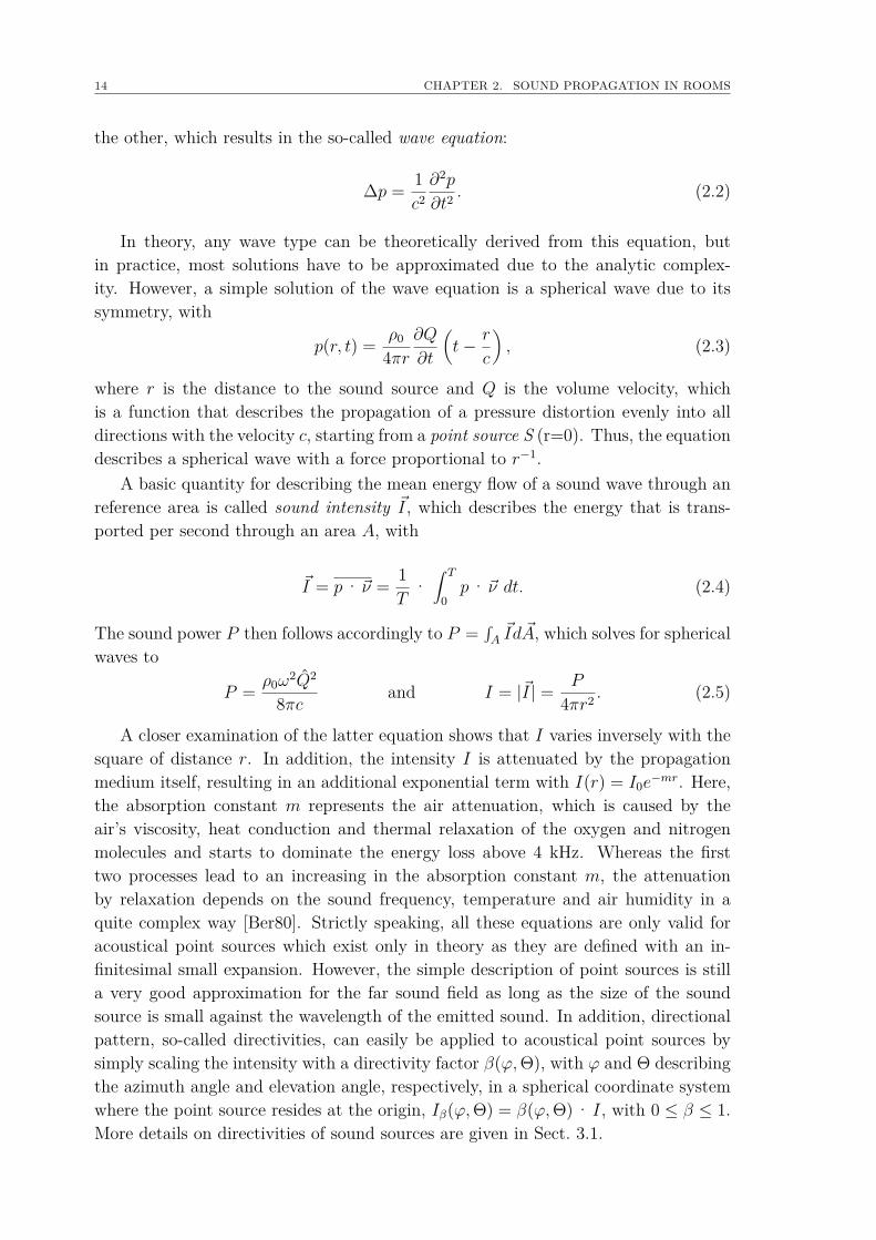
4πr2 . (2.5)
A closer examination of the latter equation shows that I varies inversely with thesquare of distance r. In addition, the intensity I is attenuated by the propagationmedium itself, resulting in an additional exponential term with I(r) = I0e
−mr. Here,the absorption constant m represents the air attenuation, which is caused by theair’s viscosity, heat conduction and thermal relaxation of the oxygen and nitrogenmolecules and starts to dominate the energy loss above 4 kHz. Whereas the firsttwo processes lead to an increasing in the absorption constant m, the attenuationby relaxation depends on the sound frequency, temperature and air humidity in aquite complex way [Ber80]. Strictly speaking, all these equations are only valid foracoustical point sources which exist only in theory as they are defined with an in-finitesimal small expansion. However, the simple description of point sources is stilla very good approximation for the far sound field as long as the size of the soundsource is small against the wavelength of the emitted sound. In addition, directionalpattern, so-called directivities, can easily be applied to acoustical point sources bysimply scaling the intensity with a directivity factor β(ϕ,Θ), with ϕ and Θ describingthe azimuth angle and elevation angle, respectively, in a spherical coordinate systemwhere the point source resides at the origin, Iβ(ϕ,Θ) = β(ϕ,Θ) · I, with 0 ≤ β ≤ 1.More details on directivities of sound sources are given in Sect. 3.1.
2.2. SOUND ABSORPTION 15
2.2 Sound AbsorptionIf a plane sound wave hits1 an infinitely large and smooth medium, it will be reflectedon the surface according to Snell’s law2, which means that the wave’s angle of inci-dence is equal with the reflection angle. A reflection is the abrupt direction changeof the wave front at an interface between two dissimilar media, most likely with achange of both amplitude and phase. In the case of a specular reflection, the incidentand the reflected wave front can be written as
pi(x, y, t) = pej(ωt−kxcos(Θ)−kysin(Θ)) and
pr(x, y, t) = pRej(ωt+kxcos(Θ)−kysin(Θ)),
(2.6)
where Θ is the angle of incidence and reflection, k is the wave number, and R is thereflection factor following
R =pr
pi
= Zcos(Θ)− Z0
Zcos(Θ) + Z0, (2.7)
with Z0 = ρ0c denoting the characteristic air impedance and Z representing thesurface impedance, which is the ratio between the total sound pressure and the surfacenormal component of the total sound particle velocity, both at the point of incident.
For a local reacting surface, which means that the surface impedance is indepen-dent of the angle of incidence, the remaining intensity Ir of the reflected wave relatesto the incidence intensity Ir multiplied by the absolute value of the squared reflec-tion factor, i.e., |R|2 of the surface. Hence, the absorbed energy relates to the factor1 − |R|2, called absorption factor α, which is defined as the ratio between the lostenergy portion and the impacting sound energy, with
α = |pi|2 − |pr|2
|pi|2
= 1− |R|2
= 4Re(ς)cos(Θ)1 + 2Re(ς)cos(Θ) + |ς|2cos2(Θ) , ς = Z/Z0.
(2.8)
By means of this absorption coefficient, the intensity of the reflected sound wavecan be expressed by the simple equation Ir = (1−α)Ii. However, the absorption factordepends on the angle Θ meaning that α has to be averaged over all possible anglesof incidence. Since this would be quite impractical in general, absorption coefficientsare usually measured in a reverberation chamber according to DIN EN ISO standard354 [ISO03].
1The sound wave of an acoustical point sources can usually be assumed to be plane in the far-field.2Willebrord Snellius, Dutch astronomer and mathematician, 1580 - 1626.
16 CHAPTER 2. SOUND PROPAGATION IN ROOMS
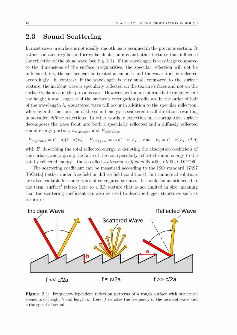
2.3 Sound ScatteringIn most cases, a surface is not ideally smooth, as is assumed in the previous section. Itrather contains regular and irregular dents, bumps and other textures that influencethe reflection of the plane wave (see Fig. 2.1). If the wavelength is very large comparedto the dimensions of the surface irregularities, the specular reflection will not beinfluenced, i.e., the surface can be treated as smooth and the wave front is reflectedaccordingly. In contrast, if the wavelength is very small compared to the surfacetexture, the incident wave is specularly reflected on the texture’s faces and not on thesurface’s plane as in the previous case. However, within an intermediate range, wherethe height h and length a of the surface’s corrugation profile are in the order of halfof the wavelength λ, a scattered wave will occur in addition to the specular reflection,whereby a distinct portion of the sound energy is scattered in all directions resultingin so-called diffuse reflections. In other words, a reflection on a corrugation surfacedecomposes the wave front into both a specularly reflected and a diffusely reflectedsound energy portion, Er,specular and Er,diffuse,
Er,specular = (1−s)(1−α)Ei, Er,diffuse = (s)(1−α)Ei, and Er = (1−α)Ei, (2.9)
with Er describing the total reflected energy, α denoting the absorption coefficient ofthe surface, and s giving the ratio of the non-specularly reflected sound energy to thetotally reflected energy – the so-called scattering coefficient [Kut00, VM00, CDD+06].
The scattering coefficient can be measured according to the ISO standard 17497[ISO04a] (either under free-field or diffuse field conditions), but numerical solutionsare also available for some types of corrugated surfaces. It should be mentioned thatthe term ‘surface’ relates here to a 3D texture that is not limited in size, meaningthat the scattering coefficient can also be used to describe bigger structures such asfurniture.
f << c/2a f ≈ c/2a f >> c/2a
ah
Incident Wave Reflected Wave
Scattered Wave
Figure 2.1: Frequency-dependent reflection patterns of a rough surface with structuralelements of height h and length a. Here, f denotes the frequency of the incident wave andc the speed of sound.
2.4. SOUND TRANSMISSION 17
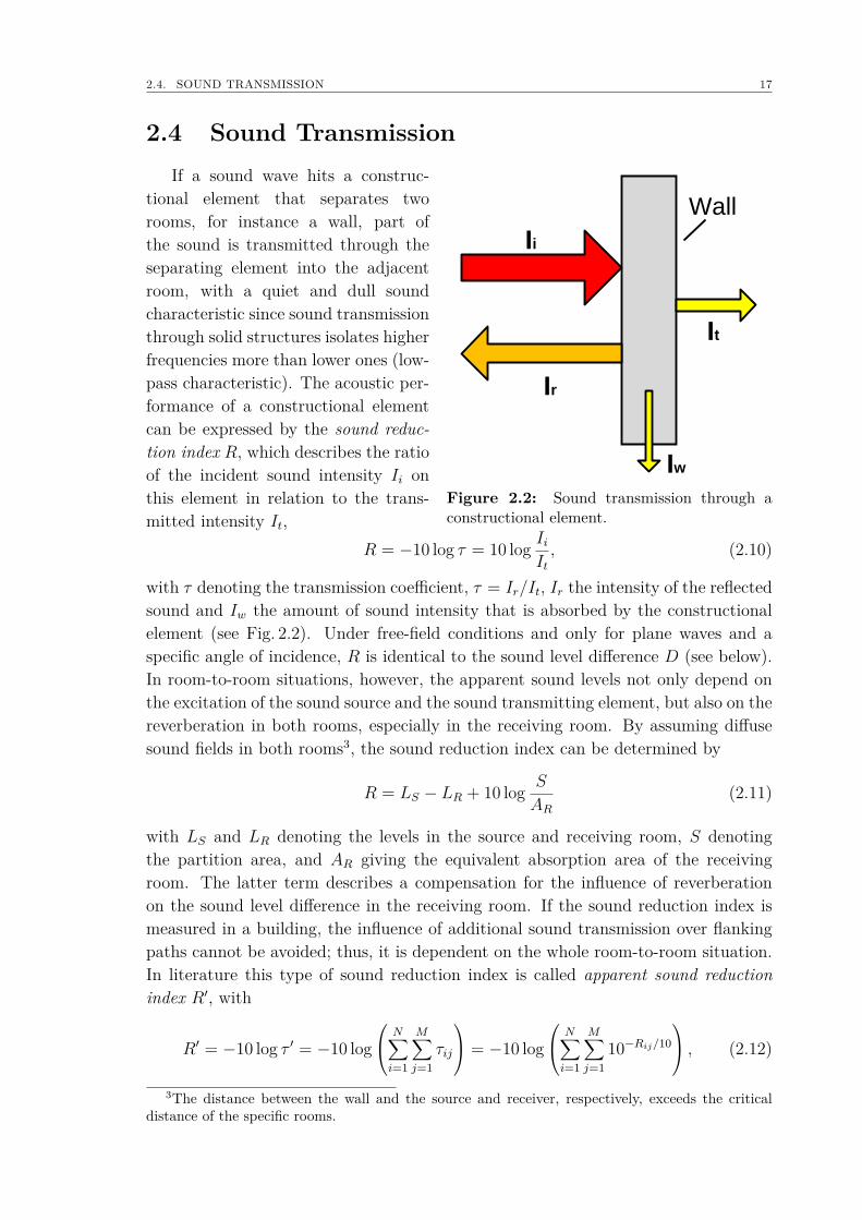
2.4 Sound TransmissionIf a sound wave hits a construc-
Wall
Ii
Ir
It
Iw
Figure 2.2: Sound transmission through aconstructional element.
tional element that separates tworooms, for instance a wall, part ofthe sound is transmitted through theseparating element into the adjacentroom, with a quiet and dull soundcharacteristic since sound transmissionthrough solid structures isolates higherfrequencies more than lower ones (low-pass characteristic). The acoustic per-formance of a constructional elementcan be expressed by the sound reduc-tion index R, which describes the ratioof the incident sound intensity Ii onthis element in relation to the trans-mitted intensity It,
R = −10 log τ = 10 log IiIt, (2.10)
with τ denoting the transmission coefficient, τ = Ir/It, Ir the intensity of the reflectedsound and Iw the amount of sound intensity that is absorbed by the constructionalelement (see Fig. 2.2). Under free-field conditions and only for plane waves and aspecific angle of incidence, R is identical to the sound level difference D (see below).In room-to-room situations, however, the apparent sound levels not only depend onthe excitation of the sound source and the sound transmitting element, but also on thereverberation in both rooms, especially in the receiving room. By assuming diffusesound fields in both rooms3, the sound reduction index can be determined by
R = LS − LR + 10 log S
AR(2.11)
with LS and LR denoting the levels in the source and receiving room, S denotingthe partition area, and AR giving the equivalent absorption area of the receivingroom. The latter term describes a compensation for the influence of reverberationon the sound level difference in the receiving room. If the sound reduction index ismeasured in a building, the influence of additional sound transmission over flankingpaths cannot be avoided; thus, it is dependent on the whole room-to-room situation.In literature this type of sound reduction index is called apparent sound reductionindex R′, with
R′ = −10 log τ ′ = −10 log N∑i=1
M∑j=1
τij
= −10 log N∑i=1
M∑j=1
10−Rij/10
, (2.12)
3The distance between the wall and the source and receiver, respectively, exceeds the criticaldistance of the specific rooms.
18 CHAPTER 2. SOUND PROPAGATION IN ROOMS
where N andM relate to the number of transmission paths from the source room intothe receiving room via flanking elements. As mentioned above, the level differenceD is the second important quantity for classifying of the insulation characteristics ofa structural element, which is independent of the area of the partition and includesthe whole room-to-room situation. There are two versions of D which differ in thedescription of the sound field in the receiving room,
Dn = LS − LR − 10 log A
10m2 and DnT = LS − LR + 10 log T
0.5s. (2.13)
Here, the normalized level difference Dn refers to an equivalent absorption area of10m2, whereas the standardized level difference DnT refers to a reverberation time of0.5s in the receiving room. Measuring specifications for both parameters, R and D,are given in the standard DIN EN ISO 140-3 [ISO04b].
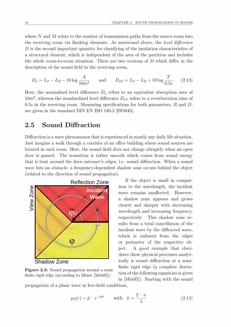
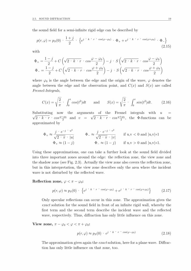
2.5 Sound DiffractionDiffraction is a wave phenomenon that is experienced in mostly any daily life situation.Just imagine a walk through a corridor of an office building where sound sources arelocated in each room. Here, the sound field does not change abruptly when an opendoor is passed. The transition is rather smooth which comes from sound energythat is bent around the door entrance’s edges, i.e. sound diffraction. When a soundwave hits an obstacle, a frequency-dependent shadow zone occurs behind the object(related to the direction of sound propagation).
If the object is small in compar-Reflection Zone
Vie
w Z
on
e
Shadow Zone
Incident
Wave
j0
j
Figure 2.3: Sound propagation around a semi-finite rigid edge (according to Möser [Mös05]).
ison to the wavelength, the incidentwave remains unaffected. However,a shadow zone appears and growsclearer and sharper with decreasingwavelength and increasing frequency,respectively. This shadow zone re-sults from a total cancellation of theincident wave by the diffracted wave,which is radiated from the edgesor perimeter of the respective ob-ject. A good example that eluci-dates these physical processes analyt-ically is sound diffraction at a semi-finite rigid edge (a complete deriva-tion of the following equations is givenin [Mös95]). Starting with the sound
propagation of a plane wave in free-field conditions,
pS(r) = p· e−jkr with k = 2 · π
λ(2.14)
2.5. SOUND DIFFRACTION 19
the sound field for a semi-infinite rigid edge can be described by
p(r, ϕ) = pS(0) · 1 + j
2 ·ej· k· r· cos(ϕ−ϕ0) · Φ+ + ej· k· r· cos(ϕ+ϕ0) · Φ−
(2.15)
with
Φ+ = 1− j2 + C
(√2 · k· r· cos
ϕ− ϕ0
2
)− j·S
(√2 · k· r· cos
ϕ− ϕ0
2
)Φ− = 1− j
2 + C(√
2 · k· r· cosϕ+ ϕ0
2
)− j·S
(√2 · k· r· cos
ϕ+ ϕ0
2
)where ϕ0 is the angle between the edge and the origin of the wave, ϕ denotes theangle between the edge and the observation point, and C(x) and S(x) are calledFresnel-Integrals,
C(x) =√
2π
·∫ x
0cos(t2)dt and S(x) =
√2π
·∫ x
0sin(t2)dt. (2.16)
Substituting now the arguments of the Fresnel integrals with u =√2 · k· r· cosϕ−ϕ0
2 and v =√
2 · k· r· cosϕ+ϕ02 , the Φ-functions can be
approximated by
Φ+ ≈j· e−j·u2
√2 ·π· |u|
Φ− ≈j· e−j· v2
√2 ·π· |v|
if u,v < 0 and |u,v|»1
Φ+ ≈ (1− j) Φ− ≈ (1− j) if u,v > 0 and |u,v|»1.
Using these approximations, one can take a further look at the sound field dividedinto three important zones around the edge: the reflection zone, the view zone andthe shadow zone (see Fig. 2.3). Actually the view zone also covers the reflection zone,but in this interpretation, the view zone describes only the area where the incidentwave is not disturbed by the reflected wave.
Reflection zone, ϕ < π − ϕ0:
p(r, ϕ) ≈ pS(0) ·ej· k· r· cos(ϕ−ϕ0) + ej· k· r· cos(ϕ+ϕ0)
(2.17)
Only specular reflections can occur in this zone. The approximation gives theexact solution for the sound field in front of an infinite rigid wall, whereby thefirst term and the second term describe the incident wave and the reflectedwave, respectively. Thus, diffraction has only little influence on this zone.
View zone, π − ϕ0 < ϕ < π + ϕ0:
p(r, ϕ) ≈ pS(0) · ej· k· r· cos(ϕ−ϕ0) (2.18)
The approximation gives again the exact solution, here for a plane wave. Diffrac-tion has only little influence on that zone, too.
20 CHAPTER 2. SOUND PROPAGATION IN ROOMS
Shadow Zone, ϕ > π + ϕ0:
p(r, ϕ) ≈ pQ(0) · j − 12 ·√
2 · π
e−j· k· r
√2 · k· r
1∥∥∥cos (ϕ−ϕ0)2
∥∥∥+∥∥∥cos (ϕ+ϕ0)
2
∥∥∥ (2.19)
This equation describes the sound pressure at an arbitrary point within theshadow zone. As one can see from the equation, diffraction has a significantinfluence on that zone that cannot be neglected.
A plot of the sound pressure distribution using the equations given above is de-picted in Fig. 2.3. It shows the typical behavior of a reflected and diffracted waveat an edge - here with a very smooth transition from the view zone into the shadowzone.
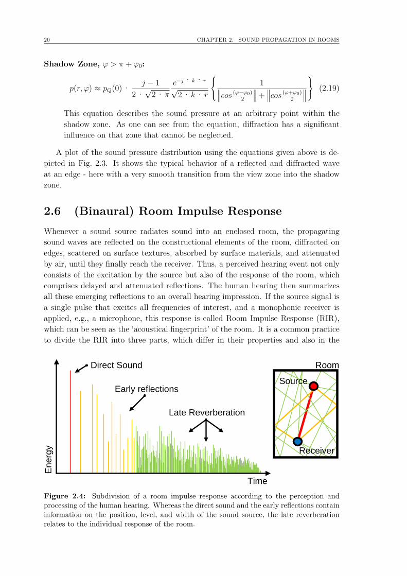
2.6 (Binaural) Room Impulse ResponseWhenever a sound source radiates sound into an enclosed room, the propagatingsound waves are reflected on the constructional elements of the room, diffracted onedges, scattered on surface textures, absorbed by surface materials, and attenuatedby air, until they finally reach the receiver. Thus, a perceived hearing event not onlyconsists of the excitation by the source but also of the response of the room, whichcomprises delayed and attenuated reflections. The human hearing then summarizesall these emerging reflections to an overall hearing impression. If the source signal isa single pulse that excites all frequencies of interest, and a monophonic receiver isapplied, e.g., a microphone, this response is called Room Impulse Response (RIR),which can be seen as the ‘acoustical fingerprint’ of the room. It is a common practiceto divide the RIR into three parts, which differ in their properties and also in the
En
erg
y
Late Reverberation
Early reflections
Time
Direct Sound
Source
Receiver
Room
Figure 2.4: Subdivision of a room impulse response according to the perception andprocessing of the human hearing. Whereas the direct sound and the early reflections containinformation on the position, level, and width of the sound source, the late reverberationrelates to the individual response of the room.
2.6. (BINAURAL) ROOM IMPULSE RESPONSE 21
perception and processing by the human hearing, called (1) the direct sound, (2) theearly reflections and (3) the late reverberation (see Fig. 2.4).
Direct Sound This first and strongest arriving impulse is evaluated by the humanhearing for localizing the sound source, also known as precedence effect [Bla96].The direct sound is delayed by the distance d between source and receiver andattenuated only by air.
Early Reflections The first reflections from the surrounding constructional ele-ments or other obstacles in the room arrive at the listener. These (low-order)reflections are added to the initial direct sound by the human hearing meaningthat they cannot be perceived separately, even if their level is up to 10dB higher(Haas effect [Bla96]). Information about the sound source such as position, dis-tance, source width, and loudness, are mostly related to these first reflections(direct sound and early reflections).
Late Reverberation Typically with a delay of 50-80ms to the direct sound, thenumber of reflections increases gradually and the human hearing cannot per-ceive them as single events anymore. This diffuse-like sound field forms a late re-verberation which is nearly independent of the listener’s position, as the humanhearing starts to perform a quite rough energetic integration over a certain timeslot and angle field [Bla96]. Reverberation is a very important and probably themost conspicuous acoustical attribute of a room, since certain characteristics,such as room volume and room shape, are directly associated with it, therebygiving the room its very individual sound.
Most room acoustical parameters, such as reverberation time, clarity and gain, aredirectly derivable from the RIR [Vor08]. Yet an auralization (see next section) wouldlack a proper spatial representation of the sound source, since a very important pieceof information is missing in the response, i.e., the influence of the human head andthe torso, which reflect, diffract and retard the arriving sound waves significantly.
For instance, a sound wave propagating from a source located on one side ofthe head travels a longer time to the contralateral ear than to the lateral ear, calledInteraural Time Difference (ITD), and the signals at both eardrums vary in their level,called Interaural Level Difference (ILD). The Just Noticeable Differences (JNDs)4 ofILD and ITD depend on the direction of sound incidence and also on the charac-teristics of the presented signals; e.g., the source localization only works for signalswith frequency components above 200Hz. The smallest JND-values are found in thehorizontal plane of the head-related coordinate system, where both, ILD and ITDare very high. Here, the localization is accurate to 1 for frontal sources, whereas theprecision decreases to 10 for sources from the left or right side, and to about 5 for
4The JND is the smallest detectable difference between a starting and secondary level of a par-ticular sensory stimulus (Weber’s Law of Just Noticeable Difference).
22 CHAPTER 2. SOUND PROPAGATION IN ROOMS
backward sound incidence. For sound sources directly above or below the head, thelocalization is worst with an inaccuracy of about 20 [Bla96].
In general, the spatial hearing of the
Figure 2.5: Artifical dummy head (ITA).
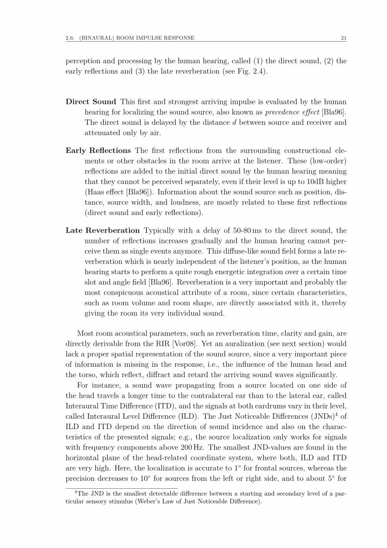
human auditory system is performed byanalyzing both, monaural signals whichare identical for both ears and binauralsignals that differ for the two eardrumsin terms of arrival time, phase andlevel. For a proper spatial representa-tion of the sound source, these effectshave to be taken into account eitherby measuring the RIR with an artifi-cial dummy head (see Fig. 2.5) as binau-ral measurement microphone, or by us-ing a set of angle-dependent filters thatdescribe the linear sound distortion ofthe head and torso in acoustical sim-ulations, called Head Related ImpulseResponses (HRIRs) and Head RelatedTransfer Functions (HRTFs) in the time domain and frequency domain, respectively.A Binaural Room Impulse Response (BRIR) is therefore a two-channel RIR whereeach channel additionally contains the head-related auditory cues for the correspond-ing ear. More information on spatial perception and evaluation by the human auditorycortex are given in [Bla96].
2.7 Principle of AuralizationAlmost any medium, whether it is solid, liquid or gaseous, can transmit vibrationsand thus sound waves. In most cases, a sound transmitting system of coupled mediacan be assumed to be linear and time-invariant, or in other words, it is assumed thatthe system is at rest during the time of inspection. By definition, the propagationof a signal through such an Linear Time-Invariant (LTI)- system is unambiguouslydescribable by the corresponding impulse response. Thus, an LTI-system with knownimpulse response h(t) and input signal s(t) will yield an output signal g(t) with
g(t) =∫ ∞−∞
s(τ)h(t− τ)dτ = s(t) ∗ h(t) (2.20)
or in the frequency domain with
G(f) = S(f) ·H(f), (2.21)
where H(f) is called the transfer function. Here, the description in the frequencydomain is usually preferred, since it avoids the more complex convolution operator.Upon now considering a room with a sound source and a listener, as such a system in
2.7. PRINCIPLE OF AURALIZATION 23
HD
HE
HHead
HAir
HD
HE
HHead
HAir
HD
HHead
HAir
HD
HE
HHead
HAir
BRIR
Reflections
HE
HE
HE
HE
Source
Description
Room
Response
Receiver
Description
Right Ear
BRIR Left Ear
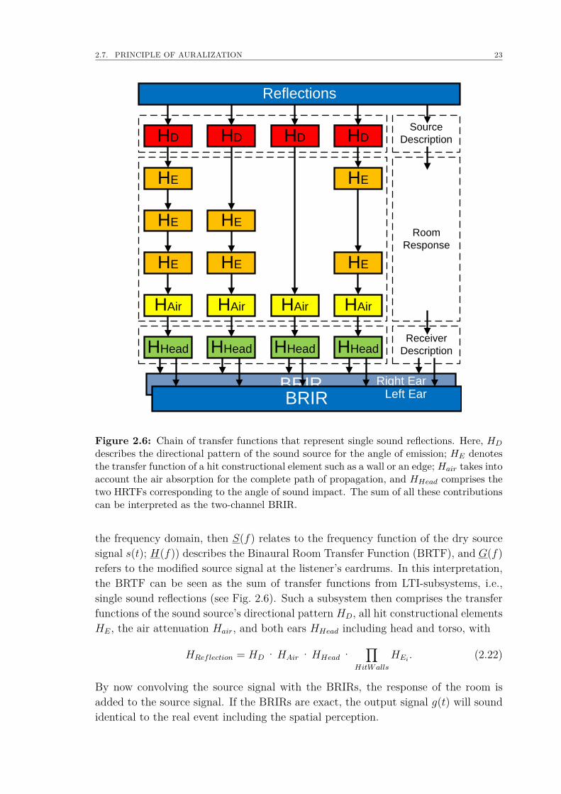
Figure 2.6: Chain of transfer functions that represent single sound reflections. Here, HD
describes the directional pattern of the sound source for the angle of emission; HE denotesthe transfer function of a hit constructional element such as a wall or an edge; Hair takes intoaccount the air absorption for the complete path of propagation, and HHead comprises thetwo HRTFs corresponding to the angle of sound impact. The sum of all these contributionscan be interpreted as the two-channel BRIR.
the frequency domain, then S(f) relates to the frequency function of the dry sourcesignal s(t); H(f)) describes the Binaural Room Transfer Function (BRTF), and G(f)refers to the modified source signal at the listener’s eardrums. In this interpretation,the BRTF can be seen as the sum of transfer functions from LTI-subsystems, i.e.,single sound reflections (see Fig. 2.6). Such a subsystem then comprises the transferfunctions of the sound source’s directional pattern HD, all hit constructional elementsHE, the air attenuation Hair, and both ears HHead including head and torso, with
HReflection = HD ·HAir ·HHead ·∏
HitWalls
HEi. (2.22)
By now convolving the source signal with the BRIRs, the response of the room isadded to the source signal. If the BRIRs are exact, the output signal g(t) will soundidentical to the real event including the spatial perception.

24 CHAPTER 2. SOUND PROPAGATION IN ROOMS
Chapter 3
Multimodal Representation ofAirborne Sound Sources
"He is not seeing real people, of course. This is all a part of the mov-ing illustration drawn by his computer according to specifications com-ing down the fiber-optic cable. The people are pieces of software calledavatars. They are the audiovisual bodies that people use to communicatewith each other in the Metaverse."
(Snow Crash, Neal Stephenson, American writer)
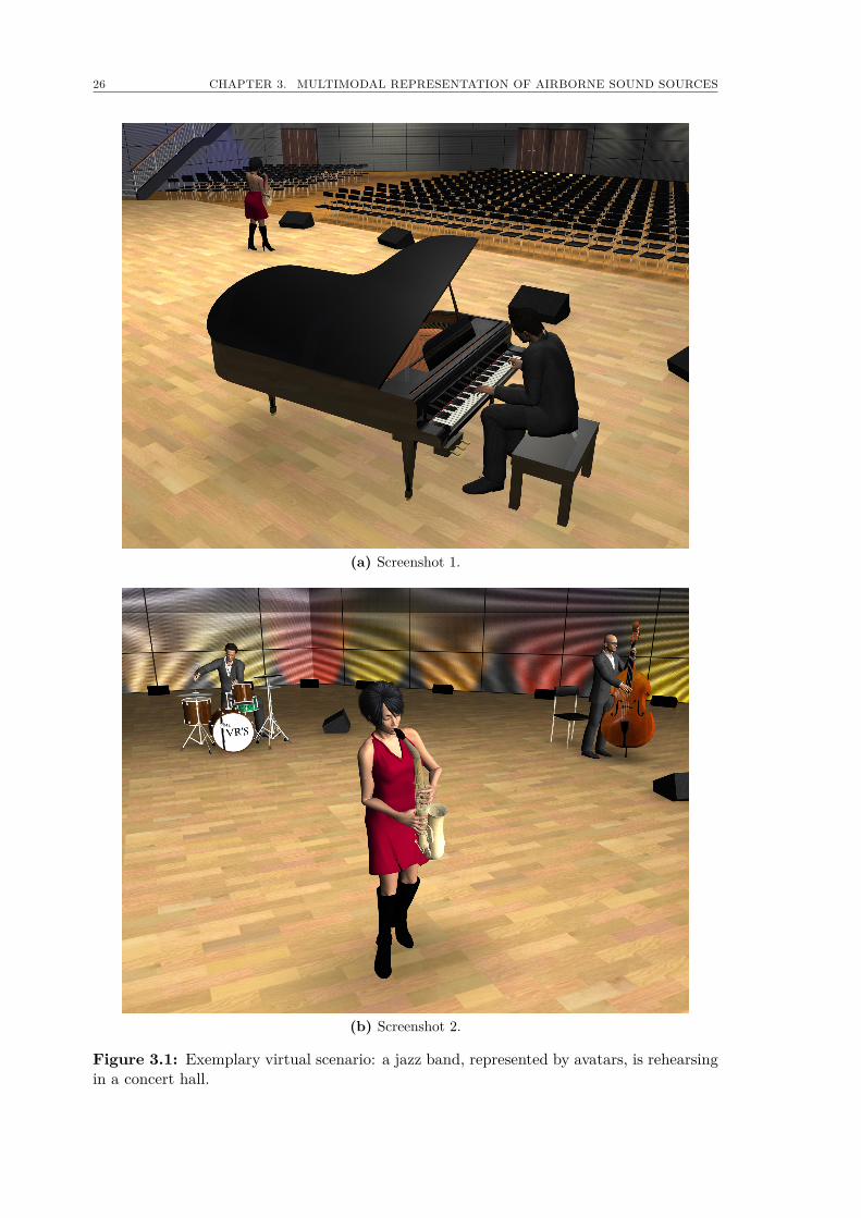
In order to gain a certain user acceptance of virtual scenarios where natural air-borne sound sources are involved, a realistic representation of these sources is required,since the user will always intuitively assign directional patterns and motions to objectsproducing sound, in compliance with individual everyday experiences. Therefore, themultimodal representation of virtual sound sources, called avatars in the following,not only demands a good visualization and high-quality input audio data, but also theinclusion of directional patterns of the source’s sound radiation and the sound source’snatural movements - at least in more complicated cases such as a human speaker ora musician. Just imagine avatars of a jazz band performing in a virtual concert hall(see Fig. 3.1). Rather than static people, one would expect a more lifelike situationwhere the musicians are performing with a certain passion leading to characteristicmovements of the players and their instruments. Most likely, these movements wouldresult in a change of the coloration and level of the produced sound depending on theuser’s position and orientation. Obviously, the lack of such authenticity diminishesthe overall acceptance of the presented scenery which means that the user will stopbehaving naturally at a certain point, even if other senses are stimulated adequately[Mor05, JNW06].
In connection with the representation of natural sound sources, numerous inves-tigations have been carried out concerning either the determination of directionalpatterns of sound sources or the description and reproduction of corresponding an-imated avatars. However, they have rarely been conducted in a cross-disciplinaryway. Consequently, there are only very few resources available that provide such
26 CHAPTER 3. MULTIMODAL REPRESENTATION OF AIRBORNE SOUND SOURCES
(a) Screenshot 1.
(b) Screenshot 2.
Figure 3.1: Exemplary virtual scenario: a jazz band, represented by avatars, is rehearsingin a concert hall.
3.1. DIRECTIONAL PATTERN OF SOUND SOURCES 27
(a) Musician performing inside the measurementsetup.
(b) Close up of a microphone housing building acorner of the pentakis dodecahedron.
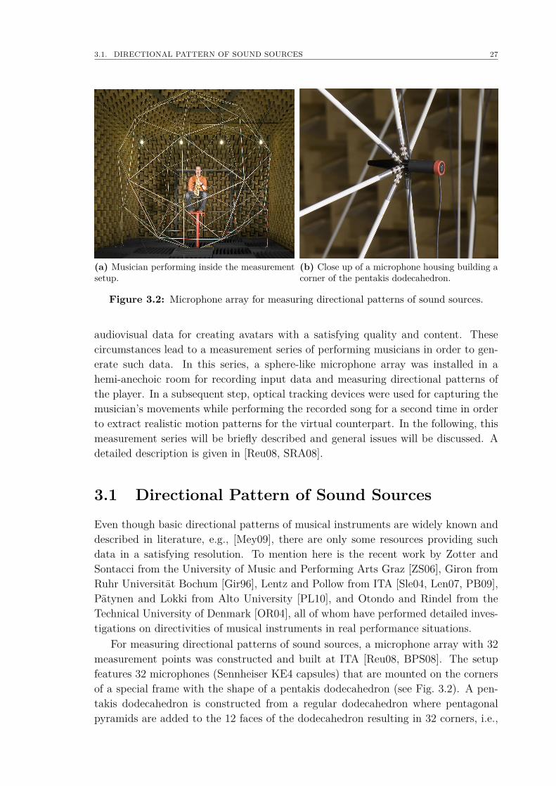
Figure 3.2: Microphone array for measuring directional patterns of sound sources.
audiovisual data for creating avatars with a satisfying quality and content. Thesecircumstances lead to a measurement series of performing musicians in order to gen-erate such data. In this series, a sphere-like microphone array was installed in ahemi-anechoic room for recording input data and measuring directional patterns ofthe player. In a subsequent step, optical tracking devices were used for capturing themusician’s movements while performing the recorded song for a second time in orderto extract realistic motion patterns for the virtual counterpart. In the following, thismeasurement series will be briefly described and general issues will be discussed. Adetailed description is given in [Reu08, SRA08].
3.1 Directional Pattern of Sound Sources
Even though basic directional patterns of musical instruments are widely known anddescribed in literature, e.g., [Mey09], there are only some resources providing suchdata in a satisfying resolution. To mention here is the recent work by Zotter andSontacci from the University of Music and Performing Arts Graz [ZS06], Giron fromRuhr Universität Bochum [Gir96], Lentz and Pollow from ITA [Sle04, Len07, PB09],Pätynen and Lokki from Alto University [PL10], and Otondo and Rindel from theTechnical University of Denmark [OR04], all of whom have performed detailed inves-tigations on directivities of musical instruments in real performance situations.
For measuring directional patterns of sound sources, a microphone array with 32measurement points was constructed and built at ITA [Reu08, BPS08]. The setupfeatures 32 microphones (Sennheiser KE4 capsules) that are mounted on the cornersof a special frame with the shape of a pentakis dodecahedron (see Fig. 3.2). A pen-takis dodecahedron is constructed from a regular dodecahedron where pentagonalpyramids are added to the 12 faces of the dodecahedron resulting in 32 corners, i.e.,
28 CHAPTER 3. MULTIMODAL REPRESENTATION OF AIRBORNE SOUND SOURCES
Input Data
Ch01
Ch02
Ch31
Ch32
...
1/3-Octave
Bandpass
Filtering and
Averaging1/3-
Octave
Band
Database
Time Interval
Spherical
Harmonics
Transformation
1/3-Octave
Band
Averaging
Input
Analysis and Interpolation
Graphical
Interpolation
Storage
1
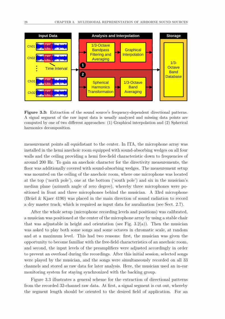
2
Figure 3.3: Extraction of the sound source’s frequency-dependent directional patterns.A signal segment of the raw input data is usually analyzed and missing data points arecomputed by one of two different approaches: (1) Graphical interpolation and (2) Sphericalharmonics decomposition.
measurement points all equidistant to the center. In ITA, the microphone array wasinstalled in the hemi anechoic room equipped with sound-absorbing wedges on all fourwalls and the ceiling providing a hemi free-field characteristic down to frequencies ofaround 200 Hz. To gain an anechoic character for the directivity measurements, thefloor was additionally covered with sound-absorbing wedges. The measurement setupwas mounted on the ceiling of the anechoic room, where one microphone was locatedat the top (‘north pole’), one at the bottom (‘south pole’) and six in the musician’smedian plane (azimuth angle of zero degree), whereby three microphones were po-sitioned in front and three microphones behind the musician. A 33rd microphone(Brüel & Kjaer 4190) was placed in the main direction of sound radiation to recorda dry master track, which is required as input data for auralization (see Sect. 2.7).
After the whole setup (microphone recording levels and positions) was calibrated,a musician was positioned at the center of the microphone array by using a stable chairthat was adjustable in height and orientation (see Fig. 3.2(a)). Then the musicianwas asked to play both some songs and some octaves in chromatic scale, at randomand at a maximum level. This had two reasons: first, the musician was given theopportunity to become familiar with the free-field characteristics of an anechoic room,and second, the input levels of the preamplifiers were adjusted accordingly in orderto prevent an overload during the recordings. After this initial session, selected songswere played by the musician, and the songs were simultaneously recorded on all 33channels and stored as raw data for later analysis. Here, the musician used an in-earmonitoring system for staying synchronized with the backing group.
Figure 3.3 illustrates a general scheme for the extraction of directional patternsfrom the recorded 32-channel raw data. At first, a signal segment is cut out, wherebythe segment length should be oriented to the desired field of application. For an
3.1. DIRECTIONAL PATTERN OF SOUND SOURCES 29
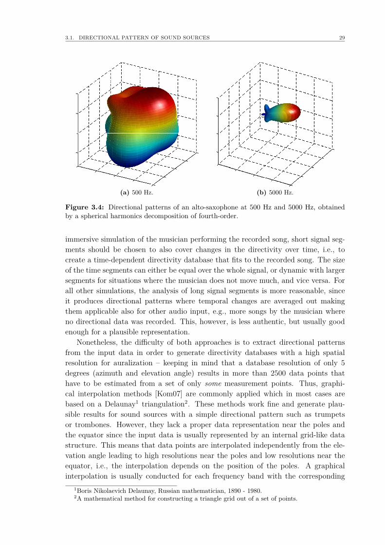
(a) 500 Hz. (b) 5000 Hz.
Figure 3.4: Directional patterns of an alto-saxophone at 500 Hz and 5000 Hz, obtainedby a spherical harmonics decomposition of fourth-order.
immersive simulation of the musician performing the recorded song, short signal seg-ments should be chosen to also cover changes in the directivity over time, i.e., tocreate a time-dependent directivity database that fits to the recorded song. The sizeof the time segments can either be equal over the whole signal, or dynamic with largersegments for situations where the musician does not move much, and vice versa. Forall other simulations, the analysis of long signal segments is more reasonable, sinceit produces directional patterns where temporal changes are averaged out makingthem applicable also for other audio input, e.g., more songs by the musician whereno directional data was recorded. This, however, is less authentic, but usually goodenough for a plausible representation.
Nonetheless, the difficulty of both approaches is to extract directional patternsfrom the input data in order to generate directivity databases with a high spatialresolution for auralization – keeping in mind that a database resolution of only 5degrees (azimuth and elevation angle) results in more than 2500 data points thathave to be estimated from a set of only some measurement points. Thus, graphi-cal interpolation methods [Kom07] are commonly applied which in most cases arebased on a Delaunay1 triangulation2. These methods work fine and generate plau-sible results for sound sources with a simple directional pattern such as trumpetsor trombones. However, they lack a proper data representation near the poles andthe equator since the input data is usually represented by an internal grid-like datastructure. This means that data points are interpolated independently from the ele-vation angle leading to high resolutions near the poles and low resolutions near theequator, i.e., the interpolation depends on the position of the poles. A graphicalinterpolation is usually conducted for each frequency band with the corresponding
1Boris Nikolaevich Delaunay, Russian mathematician, 1890 - 1980.2A mathematical method for constructing a triangle grid out of a set of points.
30 CHAPTER 3. MULTIMODAL REPRESENTATION OF AIRBORNE SOUND SOURCES
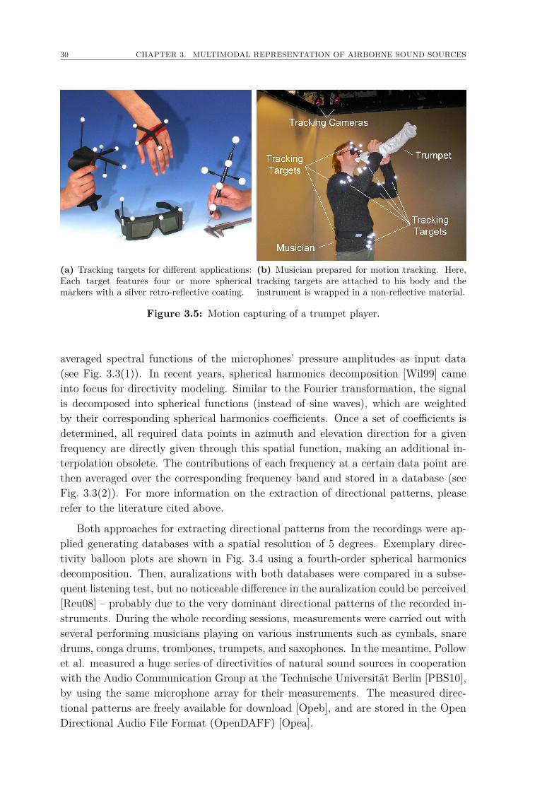
(a) Tracking targets for different applications:Each target features four or more sphericalmarkers with a silver retro-reflective coating.
(b) Musician prepared for motion tracking. Here,tracking targets are attached to his body and theinstrument is wrapped in a non-reflective material.
Figure 3.5: Motion capturing of a trumpet player.
averaged spectral functions of the microphones’ pressure amplitudes as input data(see Fig. 3.3(1)). In recent years, spherical harmonics decomposition [Wil99] cameinto focus for directivity modeling. Similar to the Fourier transformation, the signalis decomposed into spherical functions (instead of sine waves), which are weightedby their corresponding spherical harmonics coefficients. Once a set of coefficients isdetermined, all required data points in azimuth and elevation direction for a givenfrequency are directly given through this spatial function, making an additional in-terpolation obsolete. The contributions of each frequency at a certain data point arethen averaged over the corresponding frequency band and stored in a database (seeFig. 3.3(2)). For more information on the extraction of directional patterns, pleaserefer to the literature cited above.
Both approaches for extracting directional patterns from the recordings were ap-plied generating databases with a spatial resolution of 5 degrees. Exemplary direc-tivity balloon plots are shown in Fig. 3.4 using a fourth-order spherical harmonicsdecomposition. Then, auralizations with both databases were compared in a subse-quent listening test, but no noticeable difference in the auralization could be perceived[Reu08] – probably due to the very dominant directional patterns of the recorded in-struments. During the whole recording sessions, measurements were carried out withseveral performing musicians playing on various instruments such as cymbals, snaredrums, conga drums, trombones, trumpets, and saxophones. In the meantime, Pollowet al. measured a huge series of directivities of natural sound sources in cooperationwith the Audio Communication Group at the Technische Universität Berlin [PBS10],by using the same microphone array for their measurements. The measured direc-tional patterns are freely available for download [Opeb], and are stored in the OpenDirectional Audio File Format (OpenDAFF) [Opea].
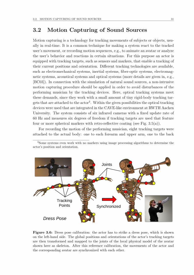
3.2. MOTION CAPTURING OF SOUND SOURCES 31
3.2 Motion Capturing of Sound Sources
Motion capturing is a technology for tracking movements of subjects or objects, usu-ally in real-time. It is a common technique for making a system react to the trackeduser’s movement, or recording motion sequences, e.g., to animate an avatar or analyzethe user’s behavior and reactions in certain situations. For this purpose an actor isequipped with tracking targets, such as sensors and markers, that enable a tracking oftheir current positions and orientation. Different tracking technologies are available,such as electromechanical systems, inertial systems, fiber-optic systems, electromag-netic systems, acoustical systems and optical systems (more details are given in, e.g.,[BC03]). In connection with the simulation of natural sound sources, a non-intrusivemotion capturing procedure should be applied in order to avoid disturbances of theperforming musician by the tracking devices. Here, optical tracking systems meetthese demands, since they work with a small amount of tiny rigid-body tracking tar-gets that are attached to the actor3. Within the given possibilities the optical trackingdevices were used that are integrated in the CAVE-like environment at RWTH AachenUniversity. The system consists of six infrared cameras with a fixed update rate of60 Hz and measures six degrees of freedom if tracking targets are used that featurefour or more spherical markers with retro-reflective coating (see Fig. 3.5(a)).
For recording the motion of the performing musician, eight tracking targets wereattached to the actual body: one to each forearm and upper arm, one to the back
3Some systems even work with no markers using image processing algorithms to determine theactor’s position and orientation.
Tracking
Points
Joints
Synchronized
Dress Pose
Figure 3.6: Dress pose calibration: the actor has to strike a dress pose, which is shownon the left-hand side. The global positions and orientations of the actor’s tracking targetsare then transformed and mapped to the joints of the local physical model of the avatarshown here as skeleton. After this reference calibration, the movements of the actor andthe corresponding avatar are synchronized with each other.
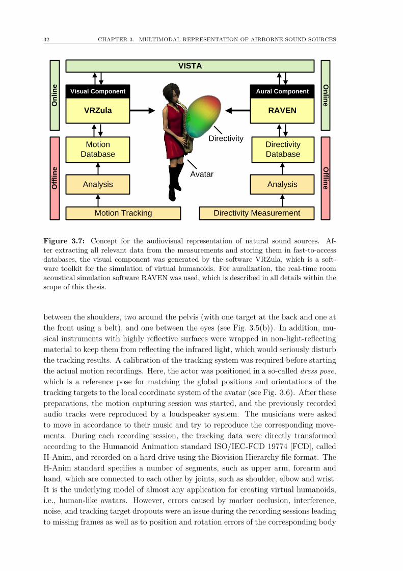
32 CHAPTER 3. MULTIMODAL REPRESENTATION OF AIRBORNE SOUND SOURCES
VRZula
Visual Component
Motion
Database
RAVEN
Aural Component
Directivity
Database
VISTA
Analysis Analysis
Motion Tracking Directivity Measurement
Directivity
Avatar
Off
lin
eO
nlin
e
Offlin
eO
nlin
e
Figure 3.7: Concept for the audiovisual representation of natural sound sources. Af-ter extracting all relevant data from the measurements and storing them in fast-to-accessdatabases, the visual component was generated by the software VRZula, which is a soft-ware toolkit for the simulation of virtual humanoids. For auralization, the real-time roomacoustical simulation software RAVEN was used, which is described in all details within thescope of this thesis.
between the shoulders, two around the pelvis (with one target at the back and one atthe front using a belt), and one between the eyes (see Fig. 3.5(b)). In addition, mu-sical instruments with highly reflective surfaces were wrapped in non-light-reflectingmaterial to keep them from reflecting the infrared light, which would seriously disturbthe tracking results. A calibration of the tracking system was required before startingthe actual motion recordings. Here, the actor was positioned in a so-called dress pose,which is a reference pose for matching the global positions and orientations of thetracking targets to the local coordinate system of the avatar (see Fig. 3.6). After thesepreparations, the motion capturing session was started, and the previously recordedaudio tracks were reproduced by a loudspeaker system. The musicians were askedto move in accordance to their music and try to reproduce the corresponding move-ments. During each recording session, the tracking data were directly transformedaccording to the Humanoid Animation standard ISO/IEC-FCD 19774 [FCD], calledH-Anim, and recorded on a hard drive using the Biovision Hierarchy file format. TheH-Anim standard specifies a number of segments, such as upper arm, forearm andhand, which are connected to each other by joints, such as shoulder, elbow and wrist.It is the underlying model of almost any application for creating virtual humanoids,i.e., human-like avatars. However, errors caused by marker occlusion, interference,noise, and tracking target dropouts were an issue during the recording sessions leadingto missing frames as well as to position and rotation errors of the corresponding body
3.3. AUDIOVISUAL AVATARS 33
parts. Therefore, a post-processing of the data was applied in order to amend shortocclusion errors and achieve smooth, synchronized and plausible movement patternsof the virtual musician.
3.3 Audiovisual AvatarsWith the processed input data, synchronized audiovisual representations of naturalsound sources were created and applied to immersive simulations to further improvetheir authenticity, whereby the overall concept is summarized in Fig. 3.7. The visualcomponent of the avatars was generated by the software VRZula [Val07], which is partof the real-time software platform for VR-applications at RWTH Aachen University,called ViSTA [AK08]. VRZula is a software toolkit for the simulation of virtual hu-manoids and is based on a layer model according to the human anatomy. Usingthis toolkit, avatars were created and animated at runtime by directly applying therecorded motion data to the underlying avatar’s physical model at interactive ratesresulting in quite natural movements of the avatar. For the aural component, direc-tional patterns of the sound sources that corresponded to the current time intervalof the song were taken into account by simply importing the generated databases inRAVEN and adding the radiation characteristics to the point source description ofthe acoustical simulation (see Chap. 5).

34 CHAPTER 3. MULTIMODAL REPRESENTATION OF AIRBORNE SOUND SOURCES
Chapter 4
Modeling and Handling ofComplex Environments
"There is something new: A globe about the size of a grapefruit, aperfectly detailed rendition of Planet Earth, hanging in space at arm’slength in front of his eyes. Hiro has heard about this but never seen it.It is a piece of CIC software called, simply, Earth. It is the user interfacethat CIC uses to keep track of every bit of spatial information that it owns- all the maps, weather data, architectural plans, and satellite surveillancestuff."
(Snow Crash, Neal Stephenson, American writer)
In contrast to trivial outdoor situations, the real-time auralization of especiallyindoor scenarios, which come along with a more reverberant sound field characteris-tic, requires for a physical-based room acoustical simulation in order to generate anatural sounding and adequate aural stimulus for the current situation (see Chap.5). Regarding real-time constraints, an efficient concept of modeling and handlingcomplex geometric environments is needed to overcome the complexity of such simu-lations and keep computation times at a low level. In this chapter, the transformationof real-world scene data into a computer simulation representation is described andmodel limitations are briefly discussed. This also includes the basics of spatial sub-division, which significantly speeds up the processing time of geometric operations.The most common space-partitioning strategies are introduced, whereby two of them,Binary Space Partitioning and Spatial Hashing, are discussed in detail, since they areapplied in RAVEN. This chapter closes with introducing a concept for processingmultiple dynamically-linked geometric subspaces, which will be the basis for the en-tire auralization concept of complex virtual environments (see Sect. 5.5).
4.1 Polygonal Scene ModelA suitable model that represents all necessary physical aspects of the real-world sceneis required to simulate room acoustics with the computer. Not only does such a model
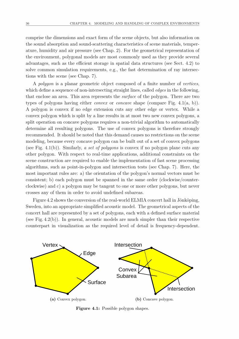
36 CHAPTER 4. MODELING AND HANDLING OF COMPLEX ENVIRONMENTS
comprise the dimensions and exact form of the scene objects, but also information onthe sound absorption and sound-scattering characteristics of scene materials, temper-ature, humidity and air pressure (see Chap. 2). For the geometrical representation ofthe environment, polygonal models are most commonly used as they provide severaladvantages, such as the efficient storage in spatial data structures (see Sect. 4.2) tosolve common simulation requirements, e.g., the fast determination of ray intersec-tions with the scene (see Chap. 7).
A polygon is a planar geometric object composed of a finite number of vertices,which define a sequence of non-intersecting straight lines, called edges in the following,that enclose an area. This area represents the surface of the polygon. There are twotypes of polygons having either convex or concave shape (compare Fig. 4.1(a, b)).A polygon is convex if no edge extension cuts any other edge or vertex. While aconvex polygon which is split by a line results in at most two new convex polygons, asplit operation on concave polygons requires a non-trivial algorithm to automaticallydetermine all resulting polygons. The use of convex polygons is therefore stronglyrecommended. It should be noted that this demand causes no restrictions on the scenemodeling, because every concave polygon can be built out of a set of convex polygons(see Fig. 4.1(b)). Similarly, a set of polygons is convex if no polygon plane cuts anyother polygon. With respect to real-time applications, additional constraints on thescene construction are required to enable the implementation of fast scene processingalgorithms, such as point-in-polygon and intersection tests (see Chap. 7). Here, themost important rules are: a) the orientation of the polygon’s normal vectors must beconsistent; b) each polygon must be spanned in the same order (clockwise/counter-clockwise) and c) a polygon may be tangent to one or more other polygons, but nevercrosses any of them in order to avoid undefined subareas.
Figure 4.2 shows the conversion of the real-world ELMIA concert hall in Jönköping,Sweden, into an appropriate simplified acoustic model. The geometrical aspects of theconcert hall are represented by a set of polygons, each with a defined surface material(see Fig. 4.2(b)). In general, acoustic models are much simpler than their respectivecounterpart in visualization as the required level of detail is frequency-dependent.
Vertex
Edge
Surface
(a) Convex polygon.
Convex
Subarea
Intersection
Intersection
(b) Concave polygon.
Figure 4.1: Possible polygon shapes.
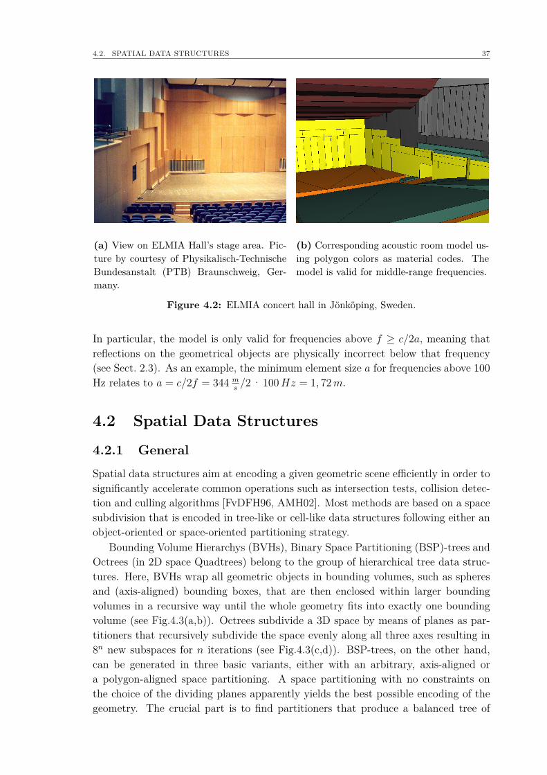
4.2. SPATIAL DATA STRUCTURES 37
(a) View on ELMIA Hall’s stage area. Pic-ture by courtesy of Physikalisch-TechnischeBundesanstalt (PTB) Braunschweig, Ger-many.
(b) Corresponding acoustic room model us-ing polygon colors as material codes. Themodel is valid for middle-range frequencies.
Figure 4.2: ELMIA concert hall in Jönköping, Sweden.
In particular, the model is only valid for frequencies above f ≥ c/2a, meaning thatreflections on the geometrical objects are physically incorrect below that frequency(see Sect. 2.3). As an example, the minimum element size a for frequencies above 100Hz relates to a = c/2f = 344 m
s/2 · 100Hz = 1, 72m.
4.2 Spatial Data Structures
4.2.1 General
Spatial data structures aim at encoding a given geometric scene efficiently in order tosignificantly accelerate common operations such as intersection tests, collision detec-tion and culling algorithms [FvDFH96, AMH02]. Most methods are based on a spacesubdivision that is encoded in tree-like or cell-like data structures following either anobject-oriented or space-oriented partitioning strategy.
Bounding Volume Hierarchys (BVHs), Binary Space Partitioning (BSP)-trees andOctrees (in 2D space Quadtrees) belong to the group of hierarchical tree data struc-tures. Here, BVHs wrap all geometric objects in bounding volumes, such as spheresand (axis-aligned) bounding boxes, that are then enclosed within larger boundingvolumes in a recursive way until the whole geometry fits into exactly one boundingvolume (see Fig.4.3(a,b)). Octrees subdivide a 3D space by means of planes as par-titioners that recursively subdivide the space evenly along all three axes resulting in8n new subspaces for n iterations (see Fig.4.3(c,d)). BSP-trees, on the other hand,can be generated in three basic variants, either with an arbitrary, axis-aligned ora polygon-aligned space partitioning. A space partitioning with no constraints onthe choice of the dividing planes apparently yields the best possible encoding of thegeometry. The crucial part is to find partitioners that produce a balanced tree of
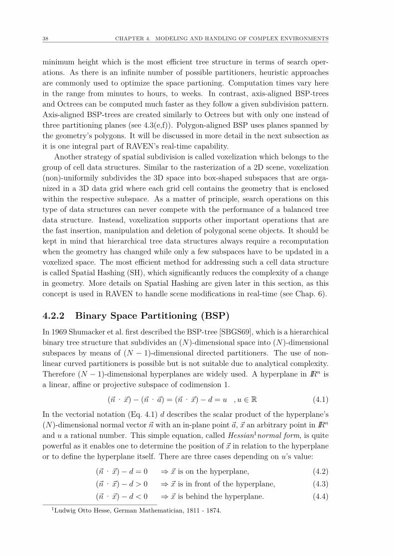
38 CHAPTER 4. MODELING AND HANDLING OF COMPLEX ENVIRONMENTS
minimum height which is the most efficient tree structure in terms of search oper-ations. As there is an infinite number of possible partitioners, heuristic approachesare commonly used to optimize the space partioning. Computation times vary herein the range from minutes to hours, to weeks. In contrast, axis-aligned BSP-treesand Octrees can be computed much faster as they follow a given subdivision pattern.Axis-aligned BSP-trees are created similarly to Octrees but with only one instead ofthree partitioning planes (see 4.3(e,f)). Polygon-aligned BSP uses planes spanned bythe geometry’s polygons. It will be discussed in more detail in the next subsection asit is one integral part of RAVEN’s real-time capability.
Another strategy of spatial subdivision is called voxelization which belongs to thegroup of cell data structures. Similar to the rasterization of a 2D scene, voxelization(non)-uniformily subdivides the 3D space into box-shaped subspaces that are orga-nized in a 3D data grid where each grid cell contains the geometry that is enclosedwithin the respective subspace. As a matter of principle, search operations on thistype of data structures can never compete with the performance of a balanced treedata structure. Instead, voxelization supports other important operations that arethe fast insertion, manipulation and deletion of polygonal scene objects. It should bekept in mind that hierarchical tree data structures always require a recomputationwhen the geometry has changed while only a few subspaces have to be updated in avoxelized space. The most efficient method for addressing such a cell data structureis called Spatial Hashing (SH), which significantly reduces the complexity of a changein geometry. More details on Spatial Hashing are given later in this section, as thisconcept is used in RAVEN to handle scene modifications in real-time (see Chap. 6).
4.2.2 Binary Space Partitioning (BSP)In 1969 Shumacker et al. first described the BSP-tree [SBGS69], which is a hierarchicalbinary tree structure that subdivides an (N)-dimensional space into (N)-dimensionalsubspaces by means of (N − 1)-dimensional directed partitioners. The use of non-linear curved partitioners is possible but is not suitable due to analytical complexity.Therefore (N − 1)-dimensional hyperplanes are widely used. A hyperplane in IRn isa linear, affine or projective subspace of codimension 1.
(~n· ~x)− (~n·~a) = (~n· ~x)− d = u , u ∈ R (4.1)
In the vectorial notation (Eq. 4.1) d describes the scalar product of the hyperplane’s(N)-dimensional normal vector ~n with an in-plane point ~a, ~x an arbitrary point in IRn
and u a rational number. This simple equation, called Hessian1normal form, is quitepowerful as it enables one to determine the position of ~x in relation to the hyperplaneor to define the hyperplane itself. There are three cases depending on u’s value:
(~n· ~x)− d = 0 ⇒ ~x is on the hyperplane, (4.2)(~n· ~x)− d > 0 ⇒ ~x is in front of the hyperplane, (4.3)(~n· ~x)− d < 0 ⇒ ~x is behind the hyperplane. (4.4)
1Ludwig Otto Hesse, German Mathematician, 1811 - 1874.
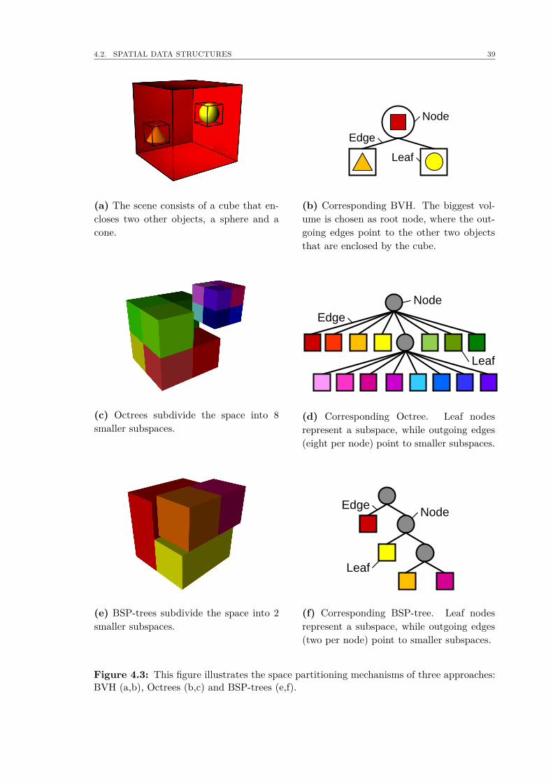
4.2. SPATIAL DATA STRUCTURES 39
(a) The scene consists of a cube that en-closes two other objects, a sphere and acone.
Node
Edge
Leaf
(b) Corresponding BVH. The biggest vol-ume is chosen as root node, where the out-going edges point to the other two objectsthat are enclosed by the cube.
(c) Octrees subdivide the space into 8smaller subspaces.
Node
Leaf
Edge
(d) Corresponding Octree. Leaf nodesrepresent a subspace, while outgoing edges(eight per node) point to smaller subspaces.
(e) BSP-trees subdivide the space into 2smaller subspaces.
Node
Leaf
Edge
(f) Corresponding BSP-tree. Leaf nodesrepresent a subspace, while outgoing edges(two per node) point to smaller subspaces.
Figure 4.3: This figure illustrates the space partitioning mechanisms of three approaches:BVH (a,b), Octrees (b,c) and BSP-trees (e,f).
40 CHAPTER 4. MODELING AND HANDLING OF COMPLEX ENVIRONMENTS
The classification depends on the direction of the hyperplanes’s normal vector. Apoint ~x lies in front of the hyperplane, which means that it is on the same side as thenormal vector ~n points to, if u is greater than zero (Eq. 4.3). The opposite case, i.e.the point ~x lies behind the hyperplane, leads to Equation 4.4. A hyperplane itself isrepresented by a set of all points ~x that fulfill Equation 4.2, which also can be usedto test if a point ~x lies on the hyperplane.
In the case of IR3, the hyperplane’s equation (~n· ~x) − d = 0 defines a two-dimensional plane. An arbitrary plane could be chosen as partitioner, but, as men-tioned before, it would unreasonably decelerate the BSP-tree creation. Therefore, itis suitable to use planes spanned by the scene polygons as partitioners, since it makesthe BSP-tree creation faster and more transparent. Each tree node contains one par-titioner that divides the current subspace into two smaller subspaces (see 4.3(e,f)).The point in question can have three possible relative locations: 1) on, 2) in-front-ofand 3) behind the partitioner. In the first case, the query can be stopped. To pursuethe latter two cases, the test is continued by branching to the respective son of thenode, left for ‘behind’, right for ‘in-front’. The tree’s root node therefore refers to thewhole space, while a leaf node refers to a subspace which cannot be further subdividedreasonably, i.e., the remaining partition is a convex set of polygons (see Sect.4.1).
Contrary to the naive approach to test the position of a point against all planes,the tree structure allows one to determine this position by testing only a subsetof planes, which significantly speeds up operations such as intersection tests. Thissubset is defined by the path in the tree. By using a balanced tree, i.e., a tree ofminimum height, the number of tests can also be minimized, which drops the searchcomplexity from O(N) to O(logN), where N is the number of polygons. Here, thecrucial part is to choose an appropriate partitioner from the polygon set where twofactors are important: the resulting sets of polygons for the two subspaces should benearly equal in size to obtain a balanced tree. On the other hand, polygons whichcross the partitioner need to be split and the resulting polygons must be assigned tothe respective sets. Since this operation increases the overall polygon count, thesecuts should be kept to a minimum. A criterion which reflects these two aspects hasbeen proposed in [RE01]. It measures the ratio r(p), 0 ≤ r(p) ≤ 1, between a set ofpolygons P on both sides of a possible partitioner p ∈ P and the number of polygonss(p) that must be split when choosing p as a partitioner.
r(p) := minp∈P
∑p′ 6=p δin front(p′, p)∑p′ 6=p δbehind(p′, p) ,
∑p′ 6=p δbehind(p′, p)∑p′ 6=p δin front(p′, p)
(4.5)
s(p) :=∑p′ 6=p
δcrosses(p′, p) (4.6)
Here, δ counts the number of occurrences for polygonal spatial relationships and p′
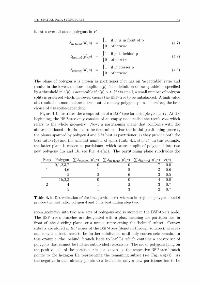
4.2. SPATIAL DATA STRUCTURES 41
iterates over all other polygons in P .
δin front(p′, p) =1 if p′ is in front of p
0 otherwise(4.7)
δbehind(p′, p) =1 if p′ is behind p
0 otherwise(4.8)
δcrosses(p′, p) =1 if p′ crosses p
0 otherwise(4.9)
The plane of polygon p is chosen as partitioner if it has an ‘acceptable’ ratio andresults in the lowest number of splits s(p). The definition of ‘acceptable’ is specifiedby a threshold t: r(p) is acceptable if r(p) > t. If t is small, a small number of polygonsplits is preferred which, however, causes the BSP-tree to be unbalanced. A high valueof t results in a more balanced tree, but also many polygon splits. Therefore, the bestchoice of t is scene-dependent.
Figure 4.4 illustrates the computation of a BSP-tree for a simple geometry. At thebeginning, the BSP-tree only consists of an empty node called the tree’s root whichrefers to the whole geometry. Now, a partitioning plane that conforms with theabove-mentioned criteria has to be determined. For the initial partitioning process,the planes spanned by polygon 4 and 6 fit best as partitioner, as they provide both thebest ratio r(p) and the smallest number of splits (Tab. 4.1, step 1). In this example,the latter plane is chosen as partitioner, which causes a split of polygon 1 into twonew polygons (1a and 1b, see Fig. 4.4(a)). The partitioning plane subdivides the
Step Polygon ∑δcrosses(p′, p)
∑δin front(p′, p)
∑δbehind(p′, p) r(p)
0,1,2,3,7 0 0 7 0.01 4,6 1 5 3 0.6
5 2 6 3 0.51b,2,3 0 0 4 0.0
2 4 1 2 3 0.75 1 3 2 0.7
Table 4.1: Determination of the best partitioners: whereas in step one polygon 4 and 6provide the best ratio, polygon 4 and 5 fits best during step two.
room geometry into two new sets of polygons and is stored in the BSP-tree’s node.The BSP-tree’s branches are designated with a plus, meaning the partition lies ‘infront of’ the dividing plane, or a minus, representing the ‘behind’ subset. Convexsubsets are stored in leaf nodes of the BSP-trees (denoted through squares), whereasnon-convex subsets have to be further subdivided until only convex sets remain. Inthis example, the ‘behind’ branch leads to leaf L1 which contains a convex set ofpolygons that cannot be further subdivided reasonably. The set of polygons lying onthe positive side of the partitioner is not convex, so the respective BSP-tree branchpoints to the hexagon H1 representing the remaining subset (see Fig. 4.4(a)). Asthe negative branch already points to a leaf node, only a new partitioner has to be
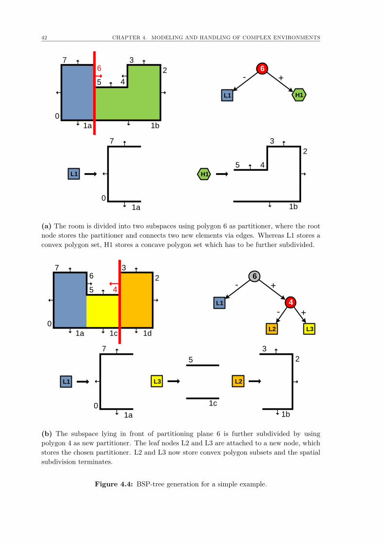
42 CHAPTER 4. MODELING AND HANDLING OF COMPLEX ENVIRONMENTS
6
+-
L1
76
0
1a
5 4
3
2
1b
H1
L1
0
7
1a
3
2
1b
H1
45
(a) The room is divided into two subspaces using polygon 6 as partitioner, where the rootnode stores the partitioner and connects two new elements via edges. Whereas L1 stores aconvex polygon set, H1 stores a concave polygon set which has to be further subdivided.
6
+-
L1
76
0
1a 1c
5 4
3
2
1d
L1
0
7
1a
3
2
1b
4
+-
L2 L3
L2L3
1c
5
(b) The subspace lying in front of partitioning plane 6 is further subdivided by usingpolygon 4 as new partitioner. The leaf nodes L2 and L3 are attached to a new node, whichstores the chosen partitioner. L2 and L3 now store convex polygon subsets and the spatialsubdivision terminates.
Figure 4.4: BSP-tree generation for a simple example.
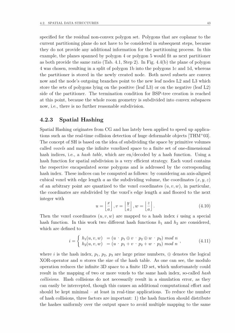
4.2. SPATIAL DATA STRUCTURES 43
specified for the residual non-convex polygon set. Polygons that are coplanar to thecurrent partitioning plane do not have to be considered in subsequent steps, becausethey do not provide any additional information for the partitioning process. In thisexample, the planes spanned by polygon 4 or polygon 5 would fit as next partitioneras both provide the same ratio (Tab. 4.1, Step 2). In Fig. 4.4(b) the plane of polygon4 was chosen, resulting in a split of polygon 1b into the polygons 1c and 1d, whereasthe partitioner is stored in the newly created node. Both novel subsets are convexnow and the node’s outgoing branches point to the new leaf nodes L2 and L3 whichstore the sets of polygons lying on the positive (leaf L3) or on the negative (leaf L2)side of the partitioner. The termination condition for BSP-tree creation is reachedat this point, because the whole room geometry is subdivided into convex subspacesnow, i.e., there is no further reasonable subdivision.
4.2.3 Spatial HashingSpatial Hashing originates from CG and has lately been applied to speed up applica-tions such as the real-time collision detection of huge deformable objects [THM+03].The concept of SH is based on the idea of subdividing the space by primitive volumescalled voxels and map the infinite voxelized space to a finite set of one-dimensionalhash indices, i.e., a hash table, which are en/decoded by a hash function. Using ahash function for spatial subdivision is a very efficient strategy. Each voxel containsthe respective encapsulated scene polygons and is addressed by the correspondinghash index. These indices can be computed as follows: by considering an axis-alignedcubical voxel with edge length a as the subdividing volume, the coordinates (x, y, z)of an arbitrary point are quantized to the voxel coordinates (u, v, w), in particular,the coordinates are subdivided by the voxel’s edge length a and floored to the nextinteger with
u =⌊x
a
⌋, v =
⌊y
a
⌋, w =
⌊z
a
⌋. (4.10)
Then the voxel coordinates (u, v, w) are mapped to a hash index i using a specialhash function. In this work two different hash functions h1 and h2 are considered,which are defined to
i =h1(u, v, w) = (u· p1 ⊕ v· p2 ⊕ w· p3) mod nh2(u, v, w) = (u· p1 + v· p2 + w· p3) mod n , (4.11)
where i is the hash index, p1, p2, p3 are large prime numbers, ⊕ denotes the logicalXOR-operator and n stores the size of the hash table. As one can see, the modulooperation reduces the infinite 3D space to a finite 1D set, which unfortunately couldresult in the mapping of two or more voxels to the same hash index, so-called hashcollisions. Hash collisions do not necessarily result in a simulation error, as theycan easily be intercepted, though this causes an additional computational effort andshould be kept minimal – at least in real-time applications. To reduce the numberof hash collisions, three factors are important: 1) the hash function should distributethe hashes uniformly over the output space to avoid multiple mapping to the same
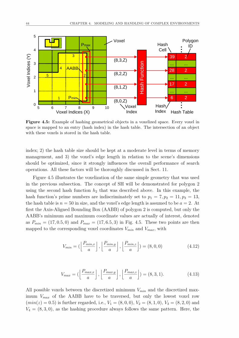
44 CHAPTER 4. MODELING AND HANDLING OF COMPLEX ENVIRONMENTS
2
1
5
4
3
2
Voxel
AABB
Pmin
5 6 7 8 9 100
1
2
3
4
5
Voxel Indices (X)
Vo
xe
l In
dic
es (
Y)
(8,0,Z)
(8,1,Z)
(8,2,Z)
(8,3,Z)
...
...
Hash Table
Ha
sh
Fu
nctio
n
Voxel
Index
Hash
Index
39
...
2
...
...
28
...
17
...
6
2
...
2
Polygon
IDPmax Hash
Cell
Figure 4.5: Example of hashing geometrical objects in a voxelized space. Every voxel inspace is mapped to an entry (hash index) in the hash table. The intersection of an objectwith these voxels is stored in the hash table.
index; 2) the hash table size should be kept at a moderate level in terms of memorymanagement, and 3) the voxel’s edge length in relation to the scene’s dimensionsshould be optimized, since it strongly influences the overall performance of searchoperations. All these factors will be thoroughly discussed in Sect. 11.
Figure 4.5 illustrates the voxelization of the same simple geometry that was usedin the previous subsection. The concept of SH will be demonstrated for polygon 2using the second hash function h2 that was described above. In this example, thehash function’s prime numbers are indiscriminately set to p1 = 7, p2 = 11, p3 = 13,the hash table is n = 50 in size, and the voxel’s edge length is assumed to be a = 2. Atfirst the Axis-Aligned Bounding Box (AABB) of polygon 2 is computed, but only theAABB’s minimum and maximum coordinate values are actually of interest, denotedas Pmin = (17, 0.5, 0) and Pmax = (17, 6.5, 3) in Fig. 4.5. These two points are thenmapped to the corresponding voxel coordinates Vmin and Vmax, with
Vmin = (⌊Pmin,xa
⌋,⌊Pmin,ya
⌋,⌊Pmin,za
⌋) = (8, 0, 0) (4.12)
Vmax = (⌊Pmax,xa
⌋,⌊Pmax,ya
⌋,⌊Pmax,za
⌋) = (8, 3, 1). (4.13)
All possible voxels between the discretized minimum Vmin and the discretized max-imum Vmax of the AABB have to be traversed, but only the lowest voxel row(min(z) = 0.5) is further regarded, i.e., V1 = (8, 0, 0), V2 = (8, 1, 0), V3 = (8, 2, 0) andV4 = (8, 3, 0), as the hashing procedure always follows the same pattern. Here, the
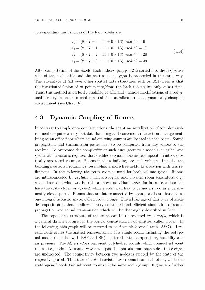
4.3. DYNAMIC COUPLING OF ROOMS 45
corresponding hash indices of the four voxels are:
i1 = (8 · 7 + 0 · 11 + 0 · 13) mod 50 = 6i2 = (8 · 7 + 1 · 11 + 0 · 13) mod 50 = 17i3 = (8 · 7 + 2 · 11 + 0 · 13) mod 50 = 28i4 = (8 · 7 + 3 · 11 + 0 · 13) mod 50 = 39
(4.14)
After computation of the voxels’ hash indices, polygon 2 is sorted into the respectivecells of the hash table and the next scene polygon is proceeded in the same way.The advantage of SH over other spatial data structures such as BSP-trees is thatthe insertion/deletion of m points into/from the hash table takes only O(m) time.Thus, this method is perfectly qualified to efficiently handle modifications of a polyg-onal scenery in order to enable a real-time auralization of a dynamically-changingenvironment (see Chap. 6).
4.3 Dynamic Coupling of RoomsIn contrast to simple one-room situations, the real-time auralization of complex envi-ronments requires a very fast data handling and convenient interaction management.Imagine an office floor where sound emitting sources are located in each room. Soundpropagation and transmission paths have to be computed from any source to thereceiver. To overcome the complexity of such huge geometric models, a logical andspatial subdivision is required that enables a dynamic scene decomposition into acous-tically separated volumes. Rooms inside a building are such volumes, but also thebuilding’s outer surroundings, resembling a more free-field-like situation with less re-flections. In the following the term room is used for both volume types. Roomsare interconnected by portals, which are logical and physical room separators, e.g.,walls, doors and windows. Portals can have individual states, for instance, a door canhave the state closed or opened, while a solid wall has to be understood as a perma-nently closed portal. Rooms that are interconnected by open portals are handled asone integral acoustic space, called room groups. The advantage of this type of scenedecomposition is that it allows a very controlled and efficient simulation of soundpropagation and sound transmission which will be thoroughly described in Sect. 5.5.
The topological structure of the scene can be represented by a graph, which isa general data structure for the logical concatenation of entities, called nodes. Inthe following, this graph will be referred to as Acoustic Scene Graph (ASG). Here,each node stores the spatial representation of a single room, including the polygo-nal model (encoded with BSP and SH), material data, temperature, humidity andair pressure. The ASG’s edges represent polyhedral portals which connect adjacentrooms, i.e., nodes. As sound waves will pass the portals from both sides, these edgesare undirected. The connectivity between two nodes is steered by the state of therespective portal. The state closed dissociates two rooms from each other, while thestate opened pools two adjacent rooms in the same room group. Figure 4.6 further
46 CHAPTER 4. MODELING AND HANDLING OF COMPLEX ENVIRONMENTS
Ro
om
Gro
up
2
R1
R3
R5 R8
R2
R4
R6
R7
Room Group 1
R2R4R6
R5 R1R3
R8 R7
Figure 4.6: Logical and spatial subdivision of a complex scene by the example of a typicaloffice floor plan. The scene consists of eight rooms that are interconnected by doors. Here,gray doors are opened, while red doors are closed. The corresponding ASG describes thetopological structure of the acoustical scene. Portals are represented by the graph’s edges,whereby gray and red edges relate to the state opened and closed, respectively. With thegiven portal configuration, the rooms can be pooled in two room groups representing twoseparated acoustic spaces.
illustrates the concept of ASG by the example of an office floor. The floor plan isgiven on the left-hand side. The scene contains eight rooms that are interconnectedby ten doors, which are defined as portals. All this information is encoded in theASG, which perfectly matches the auralization concept of coupled rooms that is fur-ther described in Sect. 5.5. An example is shown in Fig. 4.6, where – according to thegiven portal configuration – the scene is divided into two room groups representingthe currently coupled acoustic spaces.
Chapter 5
Room Acoustics Simulation
"In the silence of dead monitors, the hardcopy hums into trays, signalafter signal from the chaos, the various voices are collected, and after thefinal signal, one can listen and wait for the encoded call of the void."
(Frank Drake, American astrophysicist)
Today, artificial methods, such as reverberation generators, are applied in manyVR-systems for auralizing virtual indoor environments, since they are easy and fastto implement and provide reasonable results at the first listening. However, while thismight be sufficient in gaming or other applications where no accurate representationof the virtual scene is necessary, these methods are absolutely inappropriate for animmersive representation of real-word scenarios, as they are totally unable to coverthe whole complexity of room acoustics. Thus, a physical-based simulation of soundpropagation is obligatory in order to gain an auditory representation of the scenewith a certain realistic behavior. This chapter describes – after a brief overview onroom acoustics simulation in general – all physical simulation models that are im-plemented in RAVEN. A hybrid simulation model is introduced that combines bothroom acoustics and building acoustics and that generates BRIR with a quality thatcan truly compete with commercial state-of-the-art off-line solutions1, while main-taining a highly flexible handling for the real-time application (the latter is describedin more detail in the next chapter).
5.1 GeneralThe era of computer-based room acoustics simulation began in the 1960’s, wherescientists started to realize the big advantages that came with the development ofcomputers, as they offered a much faster calculation of numerical problems thanever before2. Then, in 1968, Asbjørn Krokstad, Svein Strøm and Svein Sørsdal atthe Norges Teknisk-Naturvitenskapelige Universitet (NTNU) in Trondheim, Norway,
1Demonstration videos and sound files are available for download under www.ravenaudio.de.2And one should not forget that computers at that time had a memory capacity of a few kilobyte
and a processing power of a today’s off-the-shelf washing machine.
48 CHAPTER 5. ROOM ACOUSTICS SIMULATION
published the first paper about the computer-based calculation of an acoustical roomresponse by means of a Ray Tracing (RT)-technique [KSS68], inspired by a vision-ary presentation by Manfred Schroeder at the International Congress on Acousticsin 1962 [SAB62]. With increasing processing power of successive computer genera-tions, extensive effort was put into the development of improved and more complexsimulation methods, but still, after 40 years of development, none of the existing ap-proaches holds as the ultimate method, even though state-of-the-art implementationscan compete with the established and reliable scale models [Vor08]. As mentionedearlier, sound propagation in a certain medium is described by the wave equation,which is a second-order linear partial differential equation of waves. This equationhas to be solved in order to determine the RIR (see Sect. 2.6), but usually no analyticsolutions exist apart from simple case studies. Thus, they must be approximated,which is usually done by means of basically two different approaches: wave-basedmethods and methods of GA (or combinations of both).
Numerical wave-based methods, for instance the Finite Element Method (FEM)and the Boundary Element Method (BEM), provide most accurate simulations ofacoustical wave propagation in air, fluids and solids by discretizing the room intoa finite number of subspaces and solving the corresponding partial and constraineddifferential wave equations [Zie00, vE00, Mec02]. The great disadvantages of thesenumerical approaches are their computational costs, where computation times rangefrom minutes to hours, days, and weeks. Whereas the propagation of low frequencysound waves in small room geometries can be calculated rather fast [KDS93, Pie88],the computation time explodes for room acoustical simulation involving the wholefrequency band and for room geometries of higher complexity. Therefore, wave-basedmethods are usually applied for simulating low-frequency RIRs that represent theroom’s modal structure up to Schroeder frequency. Above that frequency, room modesare statistically overlapping and the faster methods of GA can be applied. In GA, thesound field description is reduced to the dispersion of incoherent sound particles witha dictated frequency and amount of energy, similar to the wave-particle dualism inphysics3. Each sound particle represents a spherical wave with infinitely small openingangle and decreasing intensity according to the basic 1/r2 distance law. Consideringthe division of the RIR into three parts – the direct sound, the early reflections, andthe late reverberation – it was shown that each part has its individual requirements,mostly dependent on the human’s perception of room acoustics (see Sect. 2.6). Insummary, the direct sound and the early reflections have to be as precise as possiblein aspects of timing and spectral information, because small deviations directly affectthe localization of sound sources. By contrast, the late part of the RIR is evaluatedby the hearing with a much lower temporal resolution, where the total reverberantenergy is integrated over certain time slots and angle fields. Late reverberation isusually dominated by scattered reflections and can be interpreted as a diffuse sound
3In this interpretation, delay line models and radiosity methods are considered to be basically ge-ometric as well, since wave propagation is reduced to the time-domain approach of energy transitionfrom wall to wall.
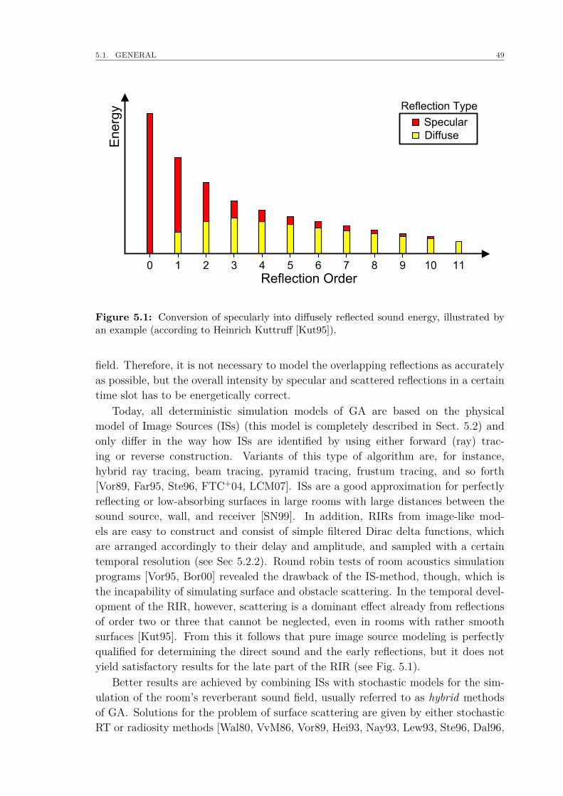
5.1. GENERAL 49
Reflection Order
En
erg
y
0 1 2 3 4 5 6 7 8 9 10 11
Specular
Diffuse
Reflection Type
Figure 5.1: Conversion of specularly into diffusely reflected sound energy, illustrated byan example (according to Heinrich Kuttruff [Kut95]).
field. Therefore, it is not necessary to model the overlapping reflections as accuratelyas possible, but the overall intensity by specular and scattered reflections in a certaintime slot has to be energetically correct.
Today, all deterministic simulation models of GA are based on the physicalmodel of Image Sources (ISs) (this model is completely described in Sect. 5.2) andonly differ in the way how ISs are identified by using either forward (ray) trac-ing or reverse construction. Variants of this type of algorithm are, for instance,hybrid ray tracing, beam tracing, pyramid tracing, frustum tracing, and so forth[Vor89, Far95, Ste96, FTC+04, LCM07]. ISs are a good approximation for perfectlyreflecting or low-absorbing surfaces in large rooms with large distances between thesound source, wall, and receiver [SN99]. In addition, RIRs from image-like mod-els are easy to construct and consist of simple filtered Dirac delta functions, whichare arranged accordingly to their delay and amplitude, and sampled with a certaintemporal resolution (see Sec 5.2.2). Round robin tests of room acoustics simulationprograms [Vor95, Bor00] revealed the drawback of the IS-method, though, which isthe incapability of simulating surface and obstacle scattering. In the temporal devel-opment of the RIR, however, scattering is a dominant effect already from reflectionsof order two or three that cannot be neglected, even in rooms with rather smoothsurfaces [Kut95]. From this it follows that pure image source modeling is perfectlyqualified for determining the direct sound and the early reflections, but it does notyield satisfactory results for the late part of the RIR (see Fig. 5.1).
Better results are achieved by combining ISs with stochastic models for the sim-ulation of the room’s reverberant sound field, usually referred to as hybrid methodsof GA. Solutions for the problem of surface scattering are given by either stochasticRT or radiosity methods [Wal80, VvM86, Vor89, Hei93, Nay93, Lew93, Ste96, Dal96,
50 CHAPTER 5. ROOM ACOUSTICS SIMULATION
Lam96, CR05]. The fast radiosity methods are based on the irradiation and reradi-ation of sound energy among surface elements in order to calculate the total energydensity at a receiving point via direct and reverberant paths [Kut00]. Here, idealdiffuse reflections are assumed meaning that the directional pattern of arriving soundis equally distributed over all directions and the energy decreases exponentially withtime. This assumption is, however, too rough if the room geometry is extremely longor flat and if it contains objects such as columns or privacy screens. Room acousti-cal effects such as (flutter) echoes or curved decays could therefore stay undetected[Rin04]. In addition, and with regard to auralization, the level, direction of arrival,and temporal distribution of late arriving reflections have a strong influence on thelistener’s spatial impression and should therefore not be randomized [BS95]. Fortu-nately, all these limitations do not apply for stochastic RT, which is a Monte Carlomethod for computing the quantized energy envelope of the RIR. This envelopecomes in a time- and frequency-dependent energy histogram, where the size of bothtime slots and frequency bands is orientated to the human hearing, i.e., time slots areused with the size of a few milliseconds, and the overall frequency range is separatedin (1/3-) octave bands (a complete description is given in Sect. 5.3).
As a matter of principle, basic methods of GA do not cover the important wavephenomenon of sound diffraction (see Sect. 2.5), and fail to correctly simulate soundpropagation from hidden sound sources to a receiver where the direct line of sightis blocked by other objects. However, there are several approaches for incorporatingdiffraction into deterministic and stochastic GA simulation methods. A very simplesolution has been described by Maekawa [Mae68]. Additionally to the length c of thedirect sound path from a sound source to a receiver, the effective path length aroundthe obstacles a + b is calculated. The detour d = a + b − c is then used as inputparameter for calculating a wavelength-dependent sound insulation. Unfortunately,this simple approach is too much of an approximation for auralization, but it isaccurate enough in cases where rough estimations do suffice, e.g., during the planningstage of a noise barrier. Another approach is to model edge diffraction following theprinciple of Huygens4-Fresnel5, which states that any point on a primary wavefrontcan be thought of as secondary sources that produce a new wavefront in the directionof propagation and that interfere with each other. The space between the sourceand the receiver is subdivided into concentric ellipsoids, so-called Fresnel ellipsoids[BW99]. Here, diffraction is modeled as a loss of sound energy where the energy ofeach Fresnel zone is summed up and scaled by a visibility factor to determine theamount of energy at the receiver position [KJM05]. An alternative approach, whichis based on the Geometrical Theory of Diffraction [Kel62], is the Uniform Theory ofDiffraction (UTD) [KP74]. The UTD is a high-frequency approximation and modelsan infinite edge as a secondary source of diffracted waves that can be reflected anddiffracted again on their way to the receiver. For a given source and receiver position,the energy attenuation caused by edge diffraction is described by complex valued
4Christiaan Huygens, Dutch mathematician and physicist, 1629 - 1695.5Augustin-Jean Fresnel, French physicist, 1788 - 1827.
5.1. GENERAL 51
diffraction coefficients that are computed by means of geometrical information aboutthe shortest paths through the respective edge sequences to the receiver (followingFermat’s6 principle). A very accurate approach which makes no assumption about thefrequency and (w)edge shape is the formulation for finite edges of the Biot-Tolstoy-Medwin Expression (BTME) for diffraction [BT57, Med81], which uses the conceptof secondary sources. It gives an exact solution for diffraction from a rigid wedge.However, this method is inappropriate for the use in real-time applications due to itscomputational complexity. Fortunately, Svensson et al. derived a fast and quite exactmethod for the computation of edge diffraction impulse responses [SFV99] from thisformulation. Here, directivity functions for these secondary sources are computeddirectly from geometrical information such as the wedge’s open angle, edge length,and the source- and receiver position. Another diffraction model was developed byStephenson where energy particles are bent around an obstacle following a deflectionangle probability density function which is derived from Heisenberg’s uncertaintyprinciple7 [Ste04]. This diffraction model fits perfectly to algorithms that model soundpropagation as the dispersion of energy particles, such as stochastic RT. Comparisonsbetween Svensson’s and Stephenson’s model have shown that both methods providesimilar results [SS07], although they are based on totally different assumptions.
In multi-room situations, another aspect of sound propagation has to be takeninto account: the wave phenomenon of sound transmission (see Sect. 2.4). Predictionmodels are well established such as the Statistical Energy Analysis (SEA) and themethod applied in the European Standard EN 12354. In SEA, sound transmissionin a stationary building is described by the power flow between subsystems whichrepresent resonant systems with high modal density [LM62, CP69, CP70]. Eachsubsystem describes one part of the whole building structure and oscillates ratherindependently of other parts in the building, whereby different wave types, suchas bending, longitudinal and transverse waves, are handled separately. Now, uponfeeding power into one of these subsystems, part of the energy dissipates, while theremaining energy is further distributed to adjacent subsystems. A good allegoryfor SEA is the comparison with water containers that are interconnected via a tubesystem. The energy of sound sources can be seen as water that is pumped intoone or many water containers and then further distributed among other connectedcontainers. While losses from damping and radiation can be interpreted here as waterleaks of the respective containers, coupling refers to the cross-section and capacity ofthe connecting tube [Vor08]. Although never explicitly referred to SEA, the predictionmodel which is used in the European Standard EN 12354 [EN97] is actually equivalentto first-order SEA, i.e., direct paths and flanking paths via one junction are takeninto account for sound transmission calculations. It is mainly based on the workby Gerretsen, who developed a fundamental equation system for describing soundinsulation in buildings [Ger79, Ger86] by means of fitting transmission coefficients(more details are given in Sect. 5.5).
6Pierre de Fermat, French lawyer and mathematician, 1601 - 1665.7Werner Heisenberg, German physicist, 1901 - 1976.
52 CHAPTER 5. ROOM ACOUSTICS SIMULATION
In summary, state-of-the-art of room acoustics simulation methods are wave-basedmethods for frequencies below the Schroeder frequency, and hybrid methods of GAfor simulations above that frequency. Hybrid methods account for both specularand diffuse reflections, and also for the wave phenomenon of sound diffraction ifadequate model extensions are used. For calculating the sound transmission betweencoupled rooms, reliable SEA prediction models are available. Samuel Siltanen etal. recently introduced an interesting concept that aims at generalizing all thesesimulation methods in one integral room acoustic rendering equation [SLKS07]. Sofar, an acoustic radiance transfer method of GA is derived from this equation thathandles specular and diffuse reflections, but a model upgrading to sound diffractionand sound transmission is planned for the future.
In real-time applications, however, a separate handling of the specular and diffusepart of the BRIR is advantageous to gain filter update rates that correspond to humanperception (more details are given in the next chapter). In the following, RAVEN’sfundamental prediction models for room acoustics simulation will be further discussed.In detail, they are:
• A hybrid simulation method of GA combining ISs with stochastic RT, whereboth methods can handle sound diffraction adapting the prediction models bySvensson and Stephenson (see Sect. 5.2 and 5.3).
• A secondary source model for sound transmission that utilizes room acousti-cal simulations and filter functions from interpolated spectra of transmissioncoefficients for rendering auralization filter networks (see Sect. 5.5).
5.2 Deterministic Image Source Method
5.2.1 GeneralThe IS-method by Allen and Berkley [AB79] (and in its extended version by Borish[Bor84]) is a procedure for constructing specular reflections between two points, e.g.,a point-like Primary Source (PS) S and a point receiver R, located inside an arbitrarypolyhedral compound, e.g., a room (see Sect. 4.1). The deterministic method becamevery popular not only in acoustics but also in radiowave physics and in CG, because itis relatively simple. It is based upon the determination of virtual secondary sources,i.e., ISs, that can be considered to cause specular reflections (see Fig. 5.2(a)). TheseISs are generated by mirroring primary/secondary point sources on the room’s faces,which is a basic and simple geometrical operation and further illustrated in Fig. 5.2(b).Here, ~S represents the point source that is supposed to be mirrored on the plane, ~n thenormalized plane’s normal vector, ~P a point that lies on the plane, ~r the connectionvector between ~S and ~P , and α the angle between ~n and ~r. A directed vector, whichis perpendicular to the plane and ends at the point source ~S, is required to determinethe mirrored secondary point source ~I. Obviously, this vector is the product of ~nwith the source’s distance to the plane, i.e., ~n· |~r|cos(α). The mirrored source ~I is
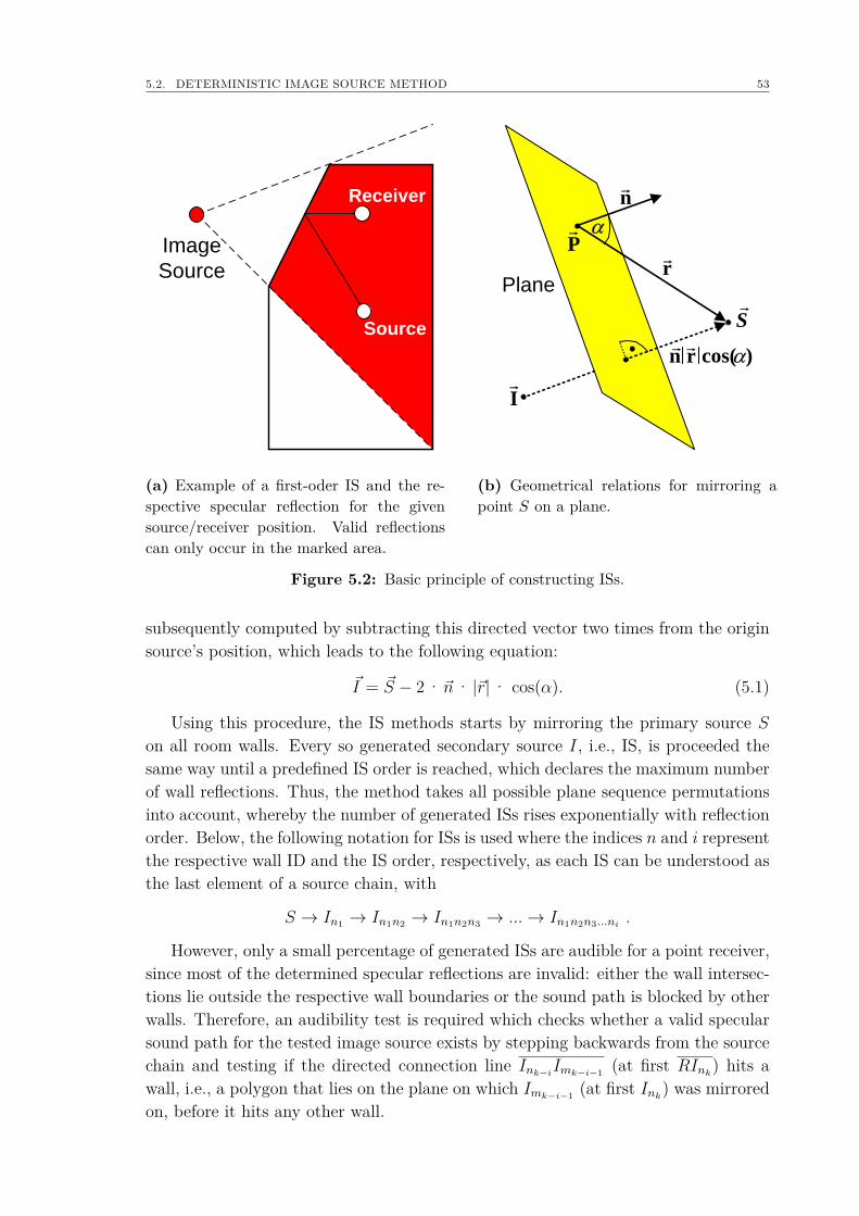
5.2. DETERMINISTIC IMAGE SOURCE METHOD 53
Source
Receiver
Image
Source
(a) Example of a first-oder IS and the re-spective specular reflection for the givensource/receiver position. Valid reflectionscan only occur in the marked area.
S
r
n
P
n
Plane
I
r
)cos(
(b) Geometrical relations for mirroring apoint S on a plane.
Figure 5.2: Basic principle of constructing ISs.
subsequently computed by subtracting this directed vector two times from the originsource’s position, which leads to the following equation:
~I = ~S − 2 ·~n· |~r|· cos(α). (5.1)
Using this procedure, the IS methods starts by mirroring the primary source Son all room walls. Every so generated secondary source I, i.e., IS, is proceeded thesame way until a predefined IS order is reached, which declares the maximum numberof wall reflections. Thus, the method takes all possible plane sequence permutationsinto account, whereby the number of generated ISs rises exponentially with reflectionorder. Below, the following notation for ISs is used where the indices n and i representthe respective wall ID and the IS order, respectively, as each IS can be understood asthe last element of a source chain, with
S → In1 → In1n2 → In1n2n3 → ...→ In1n2n3...ni.
However, only a small percentage of generated ISs are audible for a point receiver,since most of the determined specular reflections are invalid: either the wall intersec-tions lie outside the respective wall boundaries or the sound path is blocked by otherwalls. Therefore, an audibility test is required which checks whether a valid specularsound path for the tested image source exists by stepping backwards from the sourcechain and testing if the directed connection line Ink−i
Imk−i−1 (at first RInk) hits a
wall, i.e., a polygon that lies on the plane on which Imk−i−1 (at first Ink) was mirrored
on, before it hits any other wall.
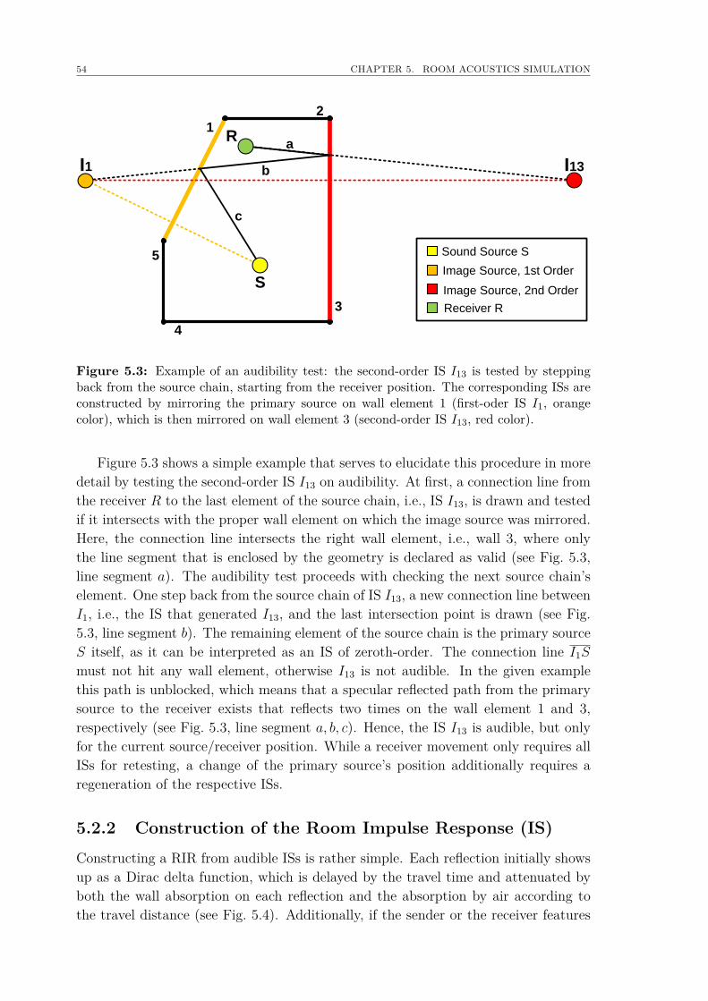
54 CHAPTER 5. ROOM ACOUSTICS SIMULATION
S
R
I1
1
2
3
4
5
I13
a
b
c
Sound Source S
Image Source, 1st Order
Image Source, 2nd Order
Receiver R
Figure 5.3: Example of an audibility test: the second-order IS I13 is tested by steppingback from the source chain, starting from the receiver position. The corresponding ISs areconstructed by mirroring the primary source on wall element 1 (first-oder IS I1, orangecolor), which is then mirrored on wall element 3 (second-order IS I13, red color).
Figure 5.3 shows a simple example that serves to elucidate this procedure in moredetail by testing the second-order IS I13 on audibility. At first, a connection line fromthe receiver R to the last element of the source chain, i.e., IS I13, is drawn and testedif it intersects with the proper wall element on which the image source was mirrored.Here, the connection line intersects the right wall element, i.e., wall 3, where onlythe line segment that is enclosed by the geometry is declared as valid (see Fig. 5.3,line segment a). The audibility test proceeds with checking the next source chain’selement. One step back from the source chain of IS I13, a new connection line betweenI1, i.e., the IS that generated I13, and the last intersection point is drawn (see Fig.5.3, line segment b). The remaining element of the source chain is the primary sourceS itself, as it can be interpreted as an IS of zeroth-order. The connection line I1S
must not hit any wall element, otherwise I13 is not audible. In the given examplethis path is unblocked, which means that a specular reflected path from the primarysource to the receiver exists that reflects two times on the wall element 1 and 3,respectively (see Fig. 5.3, line segment a, b, c). Hence, the IS I13 is audible, but onlyfor the current source/receiver position. While a receiver movement only requires allISs for retesting, a change of the primary source’s position additionally requires aregeneration of the respective ISs.
5.2.2 Construction of the Room Impulse Response (IS)
Constructing a RIR from audible ISs is rather simple. Each reflection initially showsup as a Dirac delta function, which is delayed by the travel time and attenuated byboth the wall absorption on each reflection and the absorption by air according tothe travel distance (see Fig. 5.4). Additionally, if the sender or the receiver features
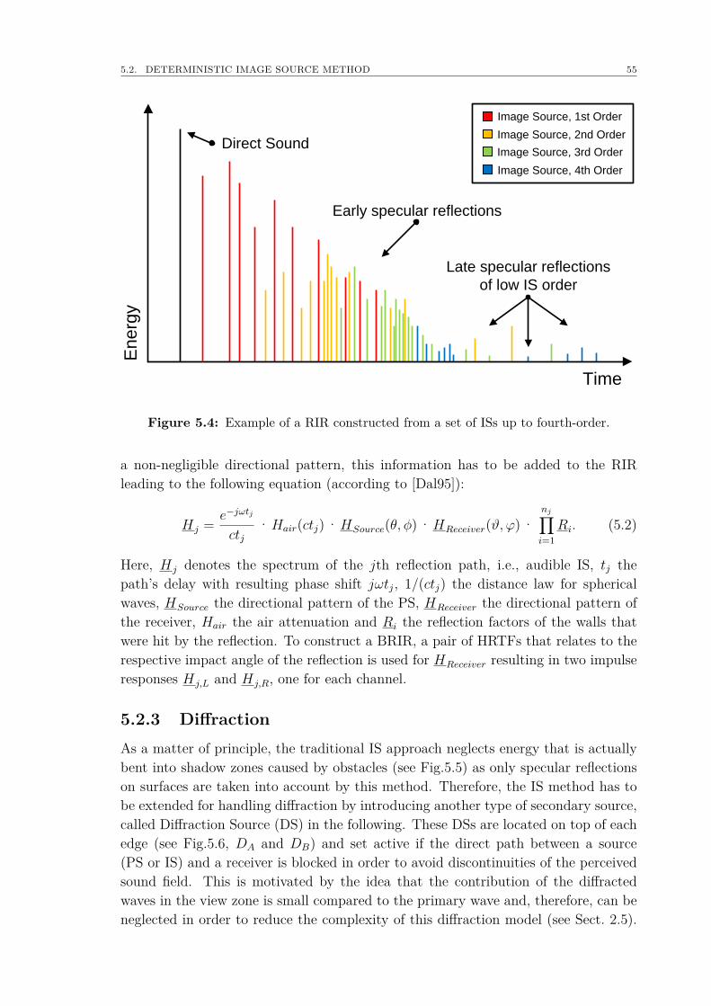
5.2. DETERMINISTIC IMAGE SOURCE METHOD 55
En
erg
y
Late specular reflections
of low IS order
Early specular reflections
Direct Sound
Time
Image Source, 1st Order
Image Source, 2nd Order
Image Source, 3rd Order
Image Source, 4th Order
Figure 5.4: Example of a RIR constructed from a set of ISs up to fourth-order.
a non-negligible directional pattern, this information has to be added to the RIRleading to the following equation (according to [Dal95]):
Hj = e−jωtj
ctj·Hair(ctj) ·HSource(θ, φ) ·HReceiver(ϑ, ϕ) ·
nj∏i=1
Ri. (5.2)
Here, Hj denotes the spectrum of the jth reflection path, i.e., audible IS, tj thepath’s delay with resulting phase shift jωtj, 1/(ctj) the distance law for sphericalwaves, HSource the directional pattern of the PS, HReceiver the directional pattern ofthe receiver, Hair the air attenuation and Ri the reflection factors of the walls thatwere hit by the reflection. To construct a BRIR, a pair of HRTFs that relates to therespective impact angle of the reflection is used for HReceiver resulting in two impulseresponses Hj,L and Hj,R, one for each channel.
5.2.3 DiffractionAs a matter of principle, the traditional IS approach neglects energy that is actuallybent into shadow zones caused by obstacles (see Fig.5.5) as only specular reflectionson surfaces are taken into account by this method. Therefore, the IS method has tobe extended for handling diffraction by introducing another type of secondary source,called Diffraction Source (DS) in the following. These DSs are located on top of eachedge (see Fig.5.6, DA and DB) and set active if the direct path between a source(PS or IS) and a receiver is blocked in order to avoid discontinuities of the perceivedsound field. This is motivated by the idea that the contribution of the diffractedwaves in the view zone is small compared to the primary wave and, therefore, can beneglected in order to reduce the complexity of this diffraction model (see Sect. 2.5).
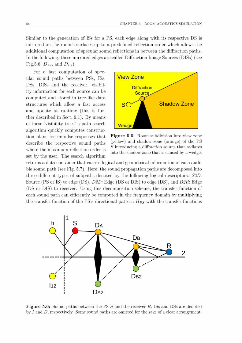
56 CHAPTER 5. ROOM ACOUSTICS SIMULATION
Similar to the generation of ISs for a PS, each edge along with its respective DS ismirrored on the room’s surfaces up to a predefined reflection order which allows theadditional computation of specular sound reflections in between the diffraction paths.In the following, these mirrored edges are called Diffraction Image Sources (DISs) (seeFig.5.6, DA2, and DB2).
For a fast computation of spec-
Shadow Zone
View Zone
S
Wedge
DiffractionSource
Figure 5.5: Room subdivision into view zone(yellow) and shadow zone (orange) of the PSS introducing a diffraction source that radiatesinto the shadow zone that is caused by a wedge.
ular sound paths between PSs, ISs,DSs, DISs and the receiver, visibil-ity information for each source can becomputed and stored in tree-like datastructures which allow a fast accessand update at runtime (this is fur-ther described in Sect. 9.1). By meansof these ‘visibility trees’ a path searchalgorithm quickly computes construc-tion plans for impulse responses thatdescribe the respective sound pathswhere the maximum reflection order isset by the user. The search algorithmreturns a data container that carries logical and geometrical information of each audi-ble sound path (see Fig. 5.7). Here, the sound propagation paths are decomposed intothree different types of subpaths denoted by the following logical descriptors: S2D:Source (PS or IS) to edge (DS), D2D: Edge (DS or DIS) to edge (DS), and D2R: Edge(DS or DIS) to receiver. Using this decomposition scheme, the transfer function ofeach sound path can efficiently be computed in the frequency domain by multiplyingthe transfer function of the PS’s directional pattern HPS with the transfer functions
SI1
I12
DA
DA2
DB
DB2
R
1
2
Figure 5.6: Sound paths between the PS S and the receiver R. ISs and DSs are denotedby I and D, respectively. Some sound paths are omitted for the sake of a clear arrangement.
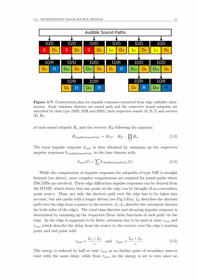
5.2. DETERMINISTIC IMAGE SOURCE METHOD 57
S2D
S DA
D2R
DA R
D2D
DA2 DB
D2R
DB R
D2D
DA2 DB
D2R
DB2 R
D2R
DA R
D2D
DA2 DB
D2R
DB R
S2D
S DA
S2D
S DA
S2D
I12 DA
S2D
I12 DA
D2D
DA2 DB
DB2 R
S2D
I12 DA
D2R
Audible Sound Paths
Figure 5.7: Construction plan for impulse responses extracted from edge visibility infor-mation. Each container denotes one sound path and the respective sound subpaths aredescribed by their type (S2D, D2R and D2D), their respective sender (S, D, I) and receiver(D, R).
of each sound subpath Hn and the receiver HR following the equation
HAudibleSoundPathi= HPS ·HR ·
∏n
Hn. (5.3)
The total impulse response hsum is then obtained by summing up the respectiveimpulse responses hAudibleSoundPathi
in the time domain with
hsum(t) =∑i
hAudibleSoundPathi(t). (5.4)
While the computation of impulse responses for subpaths of type S2R is straightforward (see above), more complex computations are required for sound paths whereDSs/DISs are involved. These edge diffraction impulse responses can be derived fromthe BTME, which states that any point on the edge can be thought of as a secondarypoint source. Thus, not only the shortest path over the edge has to be taken intoaccount, but also paths with a longer detour (see Fig.5.8(a), L0 describes the shortestpath over the edge from a source to the receiver, L1-L4 describe the outermost detoursfor both sides of the edge). The total time-discrete and decaying impulse response isdetermined by summing up the respective Dirac delta functions of each path via theedge. As the edge is supposed to be finite, attention has to be paid at time τmin andτmax which describe the delay from the source to the receiver over the edge’s startingpoint and end point with
τmin = L1 + L2
cand τmax = L3 + L4
c. (5.5)
The energy is reduced by half at time τmin as no further pairs of secondary sourcesexist with the same delay, while from τmax on the energy is set to zero since no
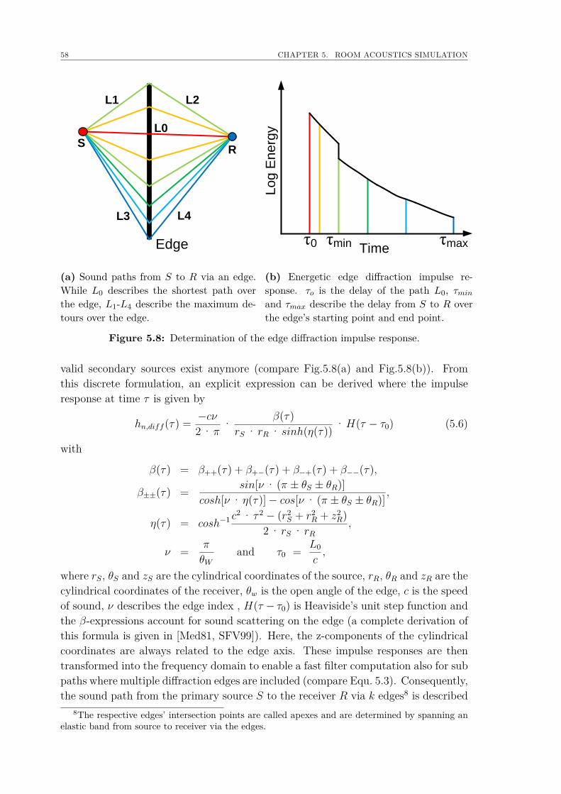
58 CHAPTER 5. ROOM ACOUSTICS SIMULATION
SR
L1 L2
L3 L4
L0
Edge
(a) Sound paths from S to R via an edge.While L0 describes the shortest path overthe edge, L1-L4 describe the maximum de-tours over the edge.
Time
Lo
g E
ne
rgy
τ0 τmin τmax
(b) Energetic edge diffraction impulse re-sponse. τo is the delay of the path L0, τminand τmax describe the delay from S to R overthe edge’s starting point and end point.
Figure 5.8: Determination of the edge diffraction impulse response.
valid secondary sources exist anymore (compare Fig.5.8(a) and Fig.5.8(b)). Fromthis discrete formulation, an explicit expression can be derived where the impulseresponse at time τ is given by
hn,diff (τ) = −cν2 ·π
· β(τ)rS · rR · sinh(η(τ)) ·H(τ − τ0) (5.6)
with
β(τ) = β++(τ) + β+−(τ) + β−+(τ) + β−−(τ),
β±±(τ) = sin[ν · (π ± θS ± θR)]cosh[ν · η(τ)]− cos[ν · (π ± θS ± θR)] ,
η(τ) = cosh−1 c2 · τ 2 − (r2
S + r2R + z2
R)2 · rS · rR
,
ν = π
θWand τ0 = L0
c,
where rS, θS and zS are the cylindrical coordinates of the source, rR, θR and zR are thecylindrical coordinates of the receiver, θw is the open angle of the edge, c is the speedof sound, ν describes the edge index , H(τ − τ0) is Heaviside’s unit step function andthe β-expressions account for sound scattering on the edge (a complete derivation ofthis formula is given in [Med81, SFV99]). Here, the z-components of the cylindricalcoordinates are always related to the edge axis. These impulse responses are thentransformed into the frequency domain to enable a fast filter computation also for subpaths where multiple diffraction edges are included (compare Equ. 5.3). Consequently,the sound path from the primary source S to the receiver R via k edges8 is described
8The respective edges’ intersection points are called apexes and are determined by spanning anelastic band from source to receiver via the edges.
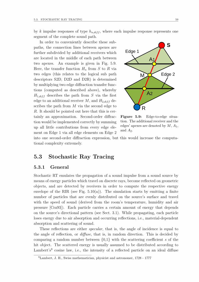
5.3. STOCHASTIC RAY TRACING 59
by k impulse responses of type hn,diff , where each impulse response represents onesegment of the complete sound path.
In order to conveniently describe these sub-S
R
A1
A2
M
Edge 1
Edge 2
Figure 5.9: Edge-to-edge situa-tion. The additional receiver and theedges’ apexes are denoted byM , A1,and A2.
paths, the connection lines between apexes arefurther subdivided by additional receivers whichare located in the middle of each path betweentwo apexes. An example is given in Fig. 5.9.Here, the transfer function Hn from S to R viatwo edges (this relates to the logical sub pathdescriptors S2D, D2D and D2R) is determinedby multiplying two edge diffraction transfer func-tions (computed as described above), wherebyH1,diff describes the path from S via the firstedge to an additional receiver M , and H2,diff de-scribes the path from M via the second edge toR. It should be pointed out here that this is cer-tainly an approximation. Second-order diffrac-tion would be implemented correctly by summingup all little contributions from every edge ele-ment on Edge 1 via all edge elements on Edge 2into one second-order diffraction expression, but this would increase the computa-tional complexity extremely.
5.3 Stochastic Ray Tracing
5.3.1 GeneralStochastic RT emulates the propagation of a sound impulse from a sound source bymeans of energy particles which travel on discrete rays, become reflected on geometricobjects, and are detected by receivers in order to compute the respective energyenvelope of the RIR (see Fig. 5.10(a)). The simulation starts by emitting a finitenumber of particles that are evenly distributed on the source’s surface and travelwith the speed of sound (derived from the room’s temperature, humidity and airpressure [Cra93]). Each particle carries a certain amount of energy that dependson the source’s directional pattern (see Sect. 3.1). While propagating, each particleloses energy due to air absorption and occurring reflections, i.e., material-dependentabsorption and scattering of sound.
These reflections are either specular, that is, the angle of incidence is equal tothe angle of reflection, or diffuse, that is, in random direction. This is decided bycomparing a random number between 0,1 with the scattering coefficient s of thehit object. The scattered energy is usually assumed to be distributed according toLambert’s9 cosine law, i.e., the intensity of a reflected particle on an ideal diffuse
9Lambert, J. H., Swiss mathematician, physicist and astronomer, 1728 - 1777
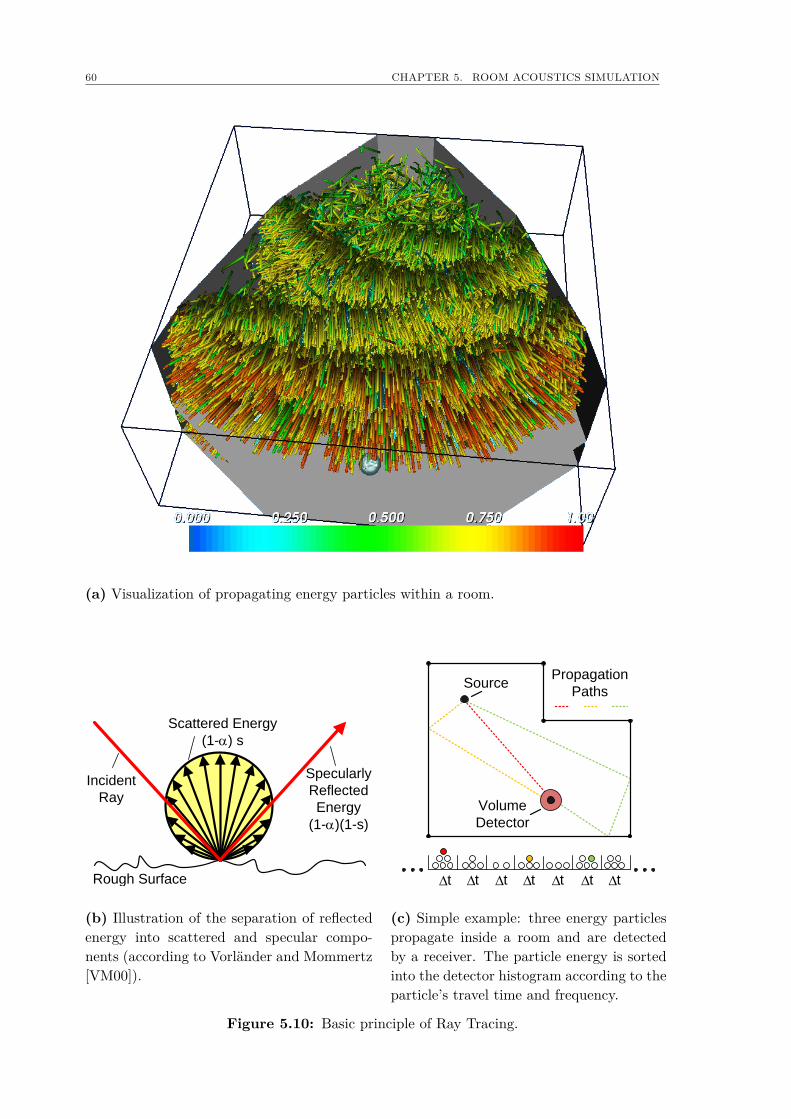
60 CHAPTER 5. ROOM ACOUSTICS SIMULATION
(a) Visualization of propagating energy particles within a room.
Incident
Ray
Scattered Energy
(1-a) s
Specularly
Reflected
Energy
(1-a)(1-s)
Rough Surface
(b) Illustration of the separation of reflectedenergy into scattered and specular compo-nents (according to Vorländer and Mommertz[VM00]).
Source
Volume
Detector
t t t t t t t
Propagation
Paths
(c) Simple example: three energy particlespropagate inside a room and are detectedby a receiver. The particle energy is sortedinto the detector histogram according to theparticle’s travel time and frequency.
Figure 5.10: Basic principle of Ray Tracing.
5.3. STOCHASTIC RAY TRACING 61
scattering wall is independent of the angle of incidence but proportional to the cosineof the angle of reflection [Kut00]. However, angle-dependent energy distributions arealso applicable and should be used to describe special types of geometries that scatterin a preferred direction [CDD+06]. As it follows from the definition of the scatteringcoefficient (see Sect. 2.3), the factor s has to be taken into account for the energyattenuation of each particle in addition to the absorption coefficient α (see Sect. 2.2).Therefore, the particle’s energy is weighted with s if the reflection was diffuse andwith (1 − s) if the reflection was specular (see Fig. 5.10(b)). Each particle is traceduntil a predefined termination condition is fulfilled, e.g., exceeded simulation lengthor under-run of a minimum particle’s energy threshold.
In contrast to the IS method, receivers are represented by detectors that haveeither a volume or a surface, as the probability for hitting a point-like receiver ina 3D space with a finite number of particles is equal to zero. Whenever a particlehits a detector, the current particle’s energy, angle of incidence, and running timeis logged and stored in the respective entry of the detector’s particle histogram (seeFig. 5.10(c)). The histogram is organized as a clustered container of time slots ∆t,where the size of ∆t should be orientated to the time resolution of human hearingand the desired relative energy variance. Hence, ∆t should be selected in the rangeof a few milliseconds, whereby the detection resolution can be reduced over time al-lowing greater ∆t for the late part of the impulse response and vice versa. Sincematerial data (absorption- and scattering coefficients), directional patterns of emit-ting sources, and the energy attenuation by air are strongly frequency-dependent,RT can only be performed for a certain frequency. Thus, a complete RT comprisesnot only one but several cycles where the center frequencies of either octave bandsor one-third octave band are usually chosen as simulation frequencies resulting in 10and 31 cycles, respectively, for the audible frequency range. From this one receivesa three dimensional histogram from the ray tracing simulation, with k time slotsof length ∆t on the abscissa, the n frequency bands on the ordinate and the time-and frequency-dependent energies E(k, n) on the applicate. These values can eitherbe seen as temporal energy distribution En(k) for a certain frequency band or asshort-time spectral energy density Ek(n) for a time slot ∆t. In the following, theterm histogram will refer to this type of data structure and can be regarded as thetemporal envelope of the energetic spatial impulse response.
5.3.2 Diffuse Rain
In Monte Carlo methods, such as RT, stochastic fluctuations occur in the simulationresults, which are mostly dependent on the number of energy particles, the meanreflection rate of the room, and the detector size (more details are given in [Vor08]).Diffuse rain now offers a concept to lower the number of necessary particles withoutincreasing these errors [Hei94, SDV07, PSV11]. Similar to radiosity, each diffusereflection causes a secondary radiation starting from the respective particle’s pointof intersection in direction to the detector. The additional energy obtained by the
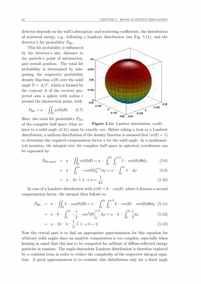
62 CHAPTER 5. ROOM ACOUSTICS SIMULATION
detector depends on the wall’s absorption- and scattering coefficients, the distributionof scattered energy, e.g., following a Lambert distribution (see Fig. 5.11), and thedetector’s hit probability PHit.
This hit probability is influenced
Figure 5.11: Lambert distribution, cos(θ).
by the detector’s size, distance tothe particle’s point of intersection,and overall position. The total hitprobability is determined by inte-grating the respective probabilitydensity function w(θ) over the solidangle Ω = A/r2, which is formed bythe contour A of the receiver pro-jected onto a sphere with radius raround the intersection point, with
PHit = a·∫∫
Ωw(θ)dΩ. (5.7)
Here, the total hit probability PHitof the complete half space (that re-lates to a solid angle of 2π) must be exactly one. Before taking a look at a Lambertdistribution, a uniform distribution of the density function is assumed first (w(θ) = 1)to determine the required compensation factor a for the solid angle. In a mathemat-ical notation, the integral over the complete half space in spherical coordinates canbe expressed by:
PHit,equal = a·∫∫
Ωw(θ)dΩ = a·
∫ 2π
0
∫ π/2
01 · sin(θ)dθdϕ (5.8)
= a·∫ 2π
0−cos(θ)|π/20 dϕ = a·
∫ 2π
01 · dϕ (5.9)
= a· 2π != 1→ a = 12π . (5.10)
In case of a Lambert distribution with w(θ) = b· cos(θ), where b denotes a secondcompensation factor, the integral then follows to
PHit = a·∫∫
Ωb· cos(θ)dΩ = a·
∫ 2π
0
∫ π/2
0b· cos(θ) · sin(θ)dθdϕ (5.11)
= a· b·∫ 2π
0−1
2 · cos2(θ)∣∣∣∣π/20
dϕ = a· b·∫ 2π
0
12dϕ (5.12)
= a· 2π· b· 12
!= 1→ b = 2. (5.13)
Now the crucial part is to find an appropriate approximation for this equation forarbitrary solid angles since an analytic computation is too complex, especially whenkeeping in mind that this has to be computed for millions of diffuse-reflected energyparticles at runtime. The angle-dependent Lambert distribution is therefore replacedby a constant term in order to reduce the complexity of the respective integral equa-tion. A good approximation is to evaluate this distribution only for a fixed angle
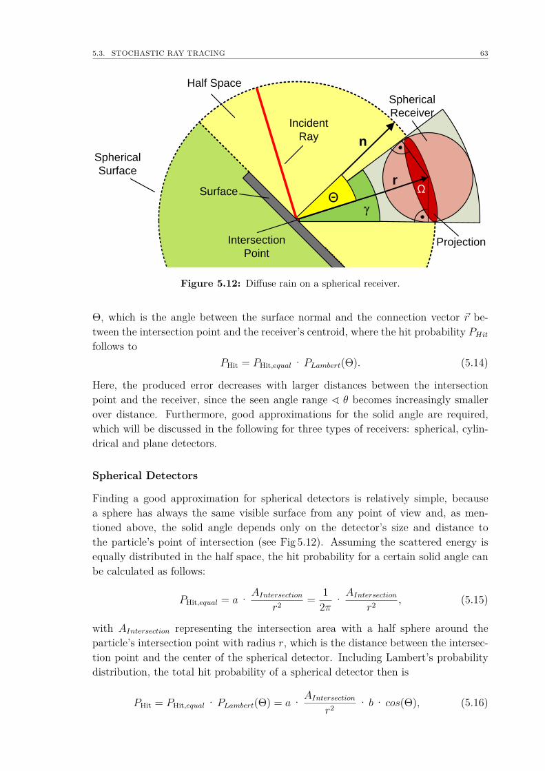
5.3. STOCHASTIC RAY TRACING 63
Ωr
Spherical
Surface
Spherical
ReceiverIncident
Ray
Θg
ProjectionIntersection
Point
Surface
Half Space
n
Figure 5.12: Diffuse rain on a spherical receiver.
Θ, which is the angle between the surface normal and the connection vector ~r be-tween the intersection point and the receiver’s centroid, where the hit probability PHitfollows to
PHit = PHit,equal ·PLambert(Θ). (5.14)
Here, the produced error decreases with larger distances between the intersectionpoint and the receiver, since the seen angle range ^ θ becomes increasingly smallerover distance. Furthermore, good approximations for the solid angle are required,which will be discussed in the following for three types of receivers: spherical, cylin-drical and plane detectors.
Spherical Detectors
Finding a good approximation for spherical detectors is relatively simple, becausea sphere has always the same visible surface from any point of view and, as men-tioned above, the solid angle depends only on the detector’s size and distance tothe particle’s point of intersection (see Fig 5.12). Assuming the scattered energy isequally distributed in the half space, the hit probability for a certain solid angle canbe calculated as follows:
PHit,equal = a· AIntersectionr2 = 1
2π · AIntersectionr2 , (5.15)
with AIntersection representing the intersection area with a half sphere around theparticle’s intersection point with radius r, which is the distance between the intersec-tion point and the center of the spherical detector. Including Lambert’s probabilitydistribution, the total hit probability of a spherical detector then is
PHit = PHit,equal ·PLambert(Θ) = a· AIntersectionr2 · b· cos(Θ), (5.16)
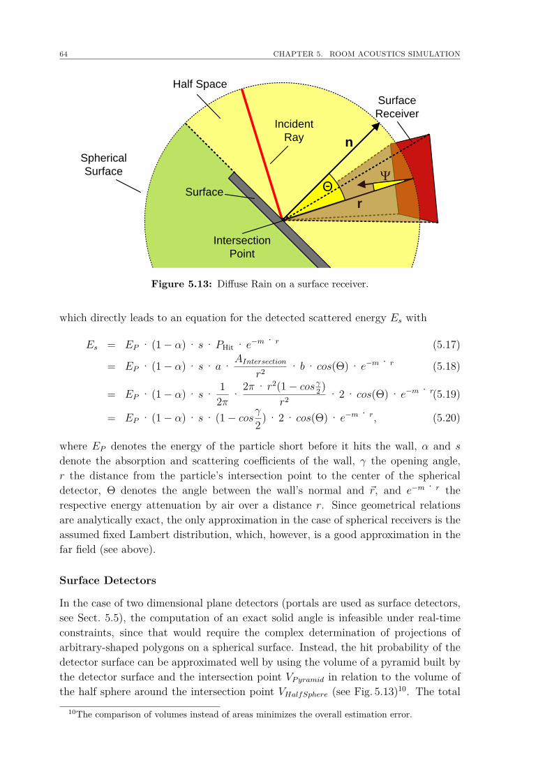
64 CHAPTER 5. ROOM ACOUSTICS SIMULATION
r
Spherical
Surface
Surface
ReceiverIncident
Ray
Y
Intersection
Point
Surface
Half Space
Θ
n
Figure 5.13: Diffuse Rain on a surface receiver.
which directly leads to an equation for the detected scattered energy Es with
Es = EP · (1− α) · s·PHit · e−m· r (5.17)
= EP · (1− α) · s· a· AIntersectionr2 · b· cos(Θ) · e−m· r (5.18)
= EP · (1− α) · s· 12π ·
2π· r2(1− cosγ2 )r2 · 2 · cos(Θ) · e−m· r(5.19)
= EP · (1− α) · s· (1− cosγ2 ) · 2 · cos(Θ) · e−m· r, (5.20)
where EP denotes the energy of the particle short before it hits the wall, α and s
denote the absorption and scattering coefficients of the wall, γ the opening angle,r the distance from the particle’s intersection point to the center of the sphericaldetector, Θ denotes the angle between the wall’s normal and ~r, and e−m· r therespective energy attenuation by air over a distance r. Since geometrical relationsare analytically exact, the only approximation in the case of spherical receivers is theassumed fixed Lambert distribution, which, however, is a good approximation in thefar field (see above).
Surface Detectors
In the case of two dimensional plane detectors (portals are used as surface detectors,see Sect. 5.5), the computation of an exact solid angle is infeasible under real-timeconstraints, since that would require the complex determination of projections ofarbitrary-shaped polygons on a spherical surface. Instead, the hit probability of thedetector surface can be approximated well by using the volume of a pyramid built bythe detector surface and the intersection point VPyramid in relation to the volume ofthe half sphere around the intersection point VHalfSphere (see Fig. 5.13)10. The total
10The comparison of volumes instead of areas minimizes the overall estimation error.
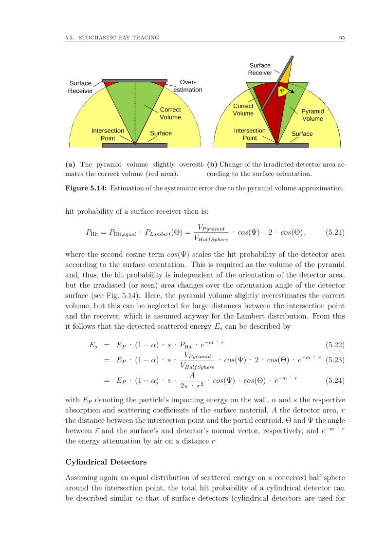
5.3. STOCHASTIC RAY TRACING 65
Intersection
Point
Surface
Receiver
Over-
estimation
Correct
Volume
Surface
(a) The pyramid volume slightly overesti-mates the correct volume (red area).
Intersection
Point
Surface
Receiver
Correct
Volume Pyramid
Volume
Surface
Y
(b) Change of the irradiated detector area ac-cording to the surface orientation.
Figure 5.14: Estimation of the systematic error due to the pyramid volume approximation.
hit probability of a surface receiver then is:
PHit = PHit,equal ·PLambert(Θ) = VPyramidVHalfSphere
· cos(Ψ) · 2 · cos(Θ), (5.21)
where the second cosine term cos(Ψ) scales the hit probability of the detector areaaccording to the surface orientation. This is required as the volume of the pyramidand, thus, the hit probability is independent of the orientation of the detector area,but the irradiated (or seen) area changes over the orientation angle of the detectorsurface (see Fig. 5.14). Here, the pyramid volume slightly overestimates the correctvolume, but this can be neglected for large distances between the intersection pointand the receiver, which is assumed anyway for the Lambert distribution. From thisit follows that the detected scattered energy Es can be described by
Es = EP · (1− α) · s·PHit · e−m· r (5.22)
= EP · (1− α) · s· VPyramidVHalfSphere
· cos(Ψ) · 2 · cos(Θ) · e−m· r (5.23)
= EP · (1− α) · s· A
2π· r2 · cos(Ψ) · cos(Θ) · e−m· r (5.24)
with EP denoting the particle’s impacting energy on the wall, α and s the respectiveabsorption and scattering coefficients of the surface material, A the detector area, rthe distance between the intersection point and the portal centroid, Θ and Ψ the anglebetween ~r and the surface’s and detector’s normal vector, respectively, and e−m· r
the energy attenuation by air on a distance r.
Cylindrical Detectors
Assuming again an equal distribution of scattered energy on a conceived half spherearound the intersection point, the total hit probability of a cylindrical detector canbe described similar to that of surface detectors (cylindrical detectors are used for
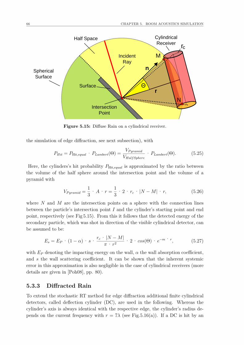
66 CHAPTER 5. ROOM ACOUSTICS SIMULATION
Spherical
Surface
Cylindrical
Receiver
Incident
Ray
Intersection
Point
Surface
Half Space
Θ
M
N
rc
r
n
Figure 5.15: Diffuse Rain on a cylindrical receiver.
the simulation of edge diffraction, see next subsection), with
PHit = PHit,equal ·PLambert(Θ) = VPyramidVHalfSphere
·PLambert(Θ). (5.25)
Here, the cylinders’s hit probability PHit,equal is approximated by the ratio betweenthe volume of the half sphere around the intersection point and the volume of apyramid with
VPyramid = 13 ·A· r = 1
3 · 2 · rc · |N −M |· r, (5.26)
where N and M are the intersection points on a sphere with the connection linesbetween the particle’s intersection point I and the cylinder’s starting point and endpoint, respectively (see Fig 5.15). From this it follows that the detected energy of thesecondary particle, which was shot in direction of the visible cylindrical detector, canbe assumed to be:
Es = EP · (1− α) · s· rc · |N −M |π· r2 · 2 · cos(Θ) · e−m· r, (5.27)
with EP denoting the impacting energy on the wall, α the wall absorption coefficient,and s the wall scattering coefficient. It can be shown that the inherent systemicerror in this approximation is also negligible in the case of cylindrical receivers (moredetails are given in [Poh08], pp. 80).
5.3.3 Diffracted RainTo extend the stochastic RT method for edge diffraction additional finite cylindricaldetectors, called deflection cylinder (DC), are used in the following. Whereas thecylinder’s axis is always identical with the respective edge, the cylinder’s radius de-pends on the current frequency with r = 7λ (see Fig.5.16(a)). If a DC is hit by an
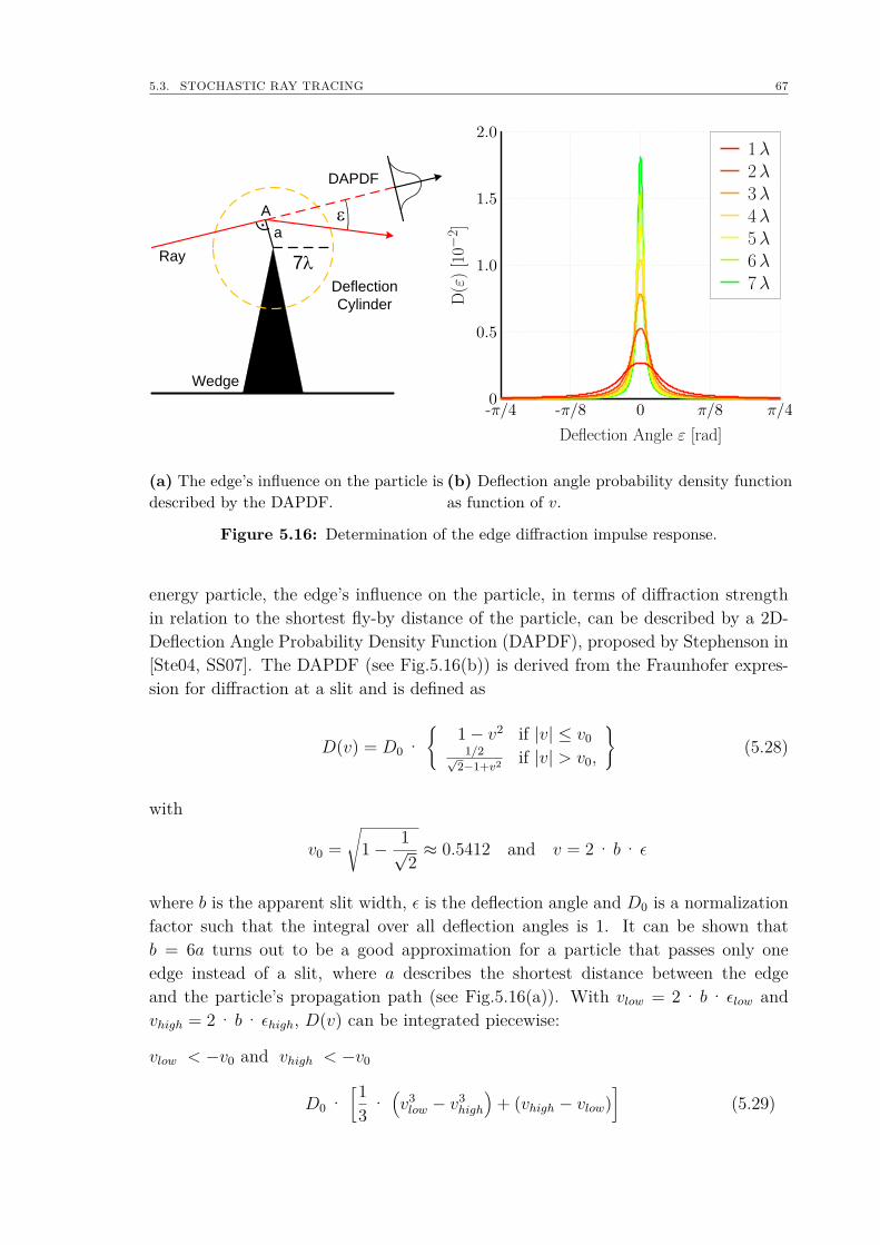
5.3. STOCHASTIC RAY TRACING 67
e
Wedge
Ray
Deflection
Cylinder
a
DAPDF
7l
A
(a) The edge’s influence on the particle isdescribed by the DAPDF.
D(ε
)[1
0−2 ]
Deflection Angle ε [rad]
1λ2λ3λ4λ5λ6λ7λ
(b) Deflection angle probability density functionas function of v.
Figure 5.16: Determination of the edge diffraction impulse response.
energy particle, the edge’s influence on the particle, in terms of diffraction strengthin relation to the shortest fly-by distance of the particle, can be described by a 2D-Deflection Angle Probability Density Function (DAPDF), proposed by Stephenson in[Ste04, SS07]. The DAPDF (see Fig.5.16(b)) is derived from the Fraunhofer expres-sion for diffraction at a slit and is defined as
D(v) = D0 ·
1− v2 if |v| ≤ v01/2√
2−1+v2 if |v| > v0,
(5.28)
with
v0 =√
1− 1√2≈ 0.5412 and v = 2 · b· ε
where b is the apparent slit width, ε is the deflection angle and D0 is a normalizationfactor such that the integral over all deflection angles is 1. It can be shown thatb = 6a turns out to be a good approximation for a particle that passes only oneedge instead of a slit, where a describes the shortest distance between the edgeand the particle’s propagation path (see Fig.5.16(a)). With vlow = 2 · b· εlow andvhigh = 2 · b· εhigh, D(v) can be integrated piecewise:
vlow < −v0 and vhigh < −v0
D0 ·[13 ·
(v3low − v3
high
)+ (vhigh − vlow)
](5.29)
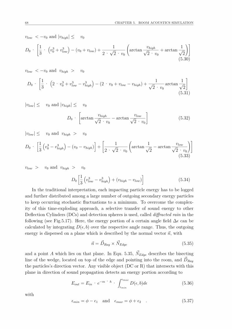
68 CHAPTER 5. ROOM ACOUSTICS SIMULATION
vlow < −v0 and |vhigh| ≤ v0
D0 ·[
13 ·
(v3
0 + v3low
)− (v0 + vlow) + 1
2 ·√
2 · v0
(arctan vhigh√
2 · v0+ arctan 1√
2
)](5.30)
vlow < −v0 and vhigh > v0
D0 ·[
13 ·
(2 · v3
0 + v3low − v3
high
)− (2 · v0 + vlow − vhigh) + 1√
2 · v0arctan 1√
2
](5.31)
|vlow| ≤ v0 and |vhigh| ≤ v0
D0 ·[arctan vhigh√
2 · v0− arctan vlow√
2 · v0
](5.32)
|vlow| ≤ v0 and vhigh > v0
D0 ·[13(v3
0 − v3high
)− (v0 − vhigh)
]+[
12 ·√
2 · v0
(arctan 1√
2− arctan vlow√
2 · v0
)](5.33)
vlow > v0 and vhigh > v0
D0
[13(v3low − v3
high
)+ (vhigh − vlow)
](5.34)
In the traditional interpretation, each impacting particle energy has to be loggedand further distributed among a large number of outgoing secondary energy particlesto keep occurring stochastic fluctuations to a minimum. To overcome the complex-ity of this time-exploding approach, a selective transfer of sound energy to otherDeflection Cylinders (DCs) and detection spheres is used, called diffracted rain in thefollowing (see Fig.5.17). Here, the energy portion of a certain angle field ∆ε can becalculated by integrating D(ε, b) over the respective angle range. Thus, the outgoingenergy is dispersed on a plane which is described by the normal vector ~n, with
~n = ~DRay × ~NEdge (5.35)
and a point A which lies on that plane. In Equ. 5.35, ~NEdge describes the bisectingline of the wedge, located on top of the edge and pointing into the room, and ~DRay
the particles’s direction vector. Any visible object (DC or R) that intersects with thisplane in direction of sound propagation detects an energy portion according to
Eout = Ein · e−m·h ·∫ εmax
εmin
D(ε, b)dε (5.36)
withεmin = φ− ε1 and εmax = φ+ ε2 . (5.37)
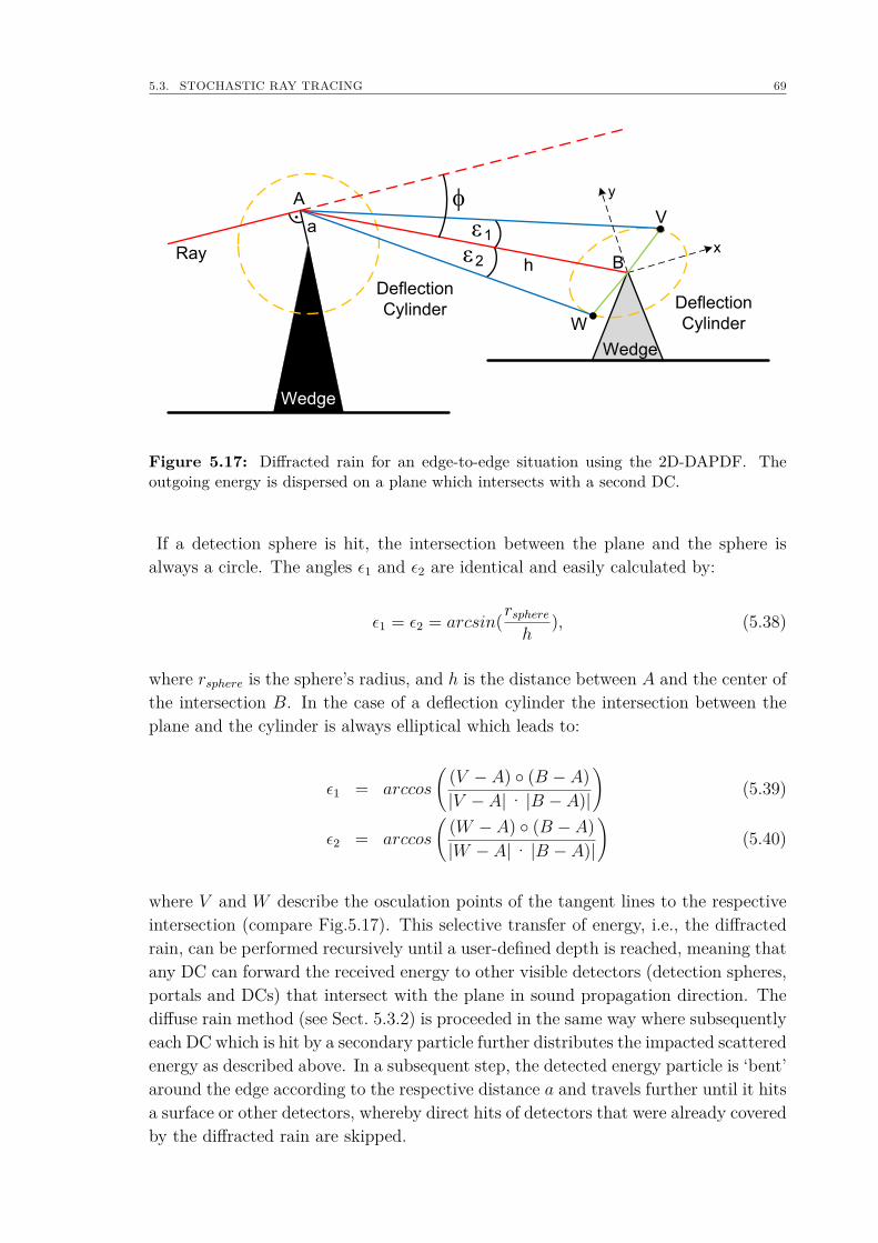
5.3. STOCHASTIC RAY TRACING 69
1
2
Wedge
Ray
Deflection Cylinder
a
Wedge
Deflection Cylinder
V
x
y
W
A
Bh
Figure 5.17: Diffracted rain for an edge-to-edge situation using the 2D-DAPDF. Theoutgoing energy is dispersed on a plane which intersects with a second DC.
If a detection sphere is hit, the intersection between the plane and the sphere isalways a circle. The angles ε1 and ε2 are identical and easily calculated by:
ε1 = ε2 = arcsin(rsphereh
), (5.38)
where rsphere is the sphere’s radius, and h is the distance between A and the center ofthe intersection B. In the case of a deflection cylinder the intersection between theplane and the cylinder is always elliptical which leads to:
ε1 = arccos
((V − A) (B − A)|V − A|· |B − A)|
)(5.39)
ε2 = arccos
((W − A) (B − A)|W − A|· |B − A)|
)(5.40)
where V and W describe the osculation points of the tangent lines to the respectiveintersection (compare Fig.5.17). This selective transfer of energy, i.e., the diffractedrain, can be performed recursively until a user-defined depth is reached, meaning thatany DC can forward the received energy to other visible detectors (detection spheres,portals and DCs) that intersect with the plane in sound propagation direction. Thediffuse rain method (see Sect. 5.3.2) is proceeded in the same way where subsequentlyeach DC which is hit by a secondary particle further distributes the impacted scatteredenergy as described above. In a subsequent step, the detected energy particle is ‘bent’around the edge according to the respective distance a and travels further until it hitsa surface or other detectors, whereby direct hits of detectors that were already coveredby the diffracted rain are skipped.
70 CHAPTER 5. ROOM ACOUSTICS SIMULATION
5.3.4 Construction of the Room Impulse Response (RT)As mentioned above, a detector’s energy histogram represents only the energy enve-lope of the RIR. While many room acoustical parameters, e.g., reverberation timeand clarity, can be easily calculated from such histograms, they cannot be applieddirectly to auralization due to the lack of an appropriate temporal resolution. How-ever, the RIR’s temporal fine structure can be synthesized well by means of a Pois-son11-distributed noise process [Hei94]. By assuming a sound reflection as event, theprobability wn(∆t) of the occurrence of n events in a time interval ∆t is given by
wn(∆t) = (µ∆t)nn! e−µ∆t n = 0, 1, 2, ..., µ > 0, ∆t ≥ 0, (5.41)
where µ denotes the mean event occurrence. On the other hand, a time interval ∆At
of two consecutive events of a temporal Poisson process is exponentially distributedand the associated density distribution w(∆tA) follows [Ros70]
w(∆tA)d∆tA = µe−µ∆tAd∆tA. (5.42)
Using this equation, the interval size ∆tA can be derived as a function of a uniformlydistributed random number z, leading to
∆tA(z) = 1µln(1z
)0 < z ≤ 1, (5.43)
where the mean event occurrence µ relates to the mean reflection density of the roomwith
µ = 4πc3t2
V. (5.44)
Based on this equation, the noise process can be synthesized by using Dirac deltafunctions with constant magnitude as random events. Starting at a time
t0 = 3
√2V ln 24πc3 ≈ 0, 0014 3
√V , (5.45)
which describes the minimum time between t + ∆tA, the sequence of Dirac deltas isconsecutively generated using Equ. 5.43 until a maximum length is reached [Dro06,Pel07]. In order to adapt to the sampling frequency of the RIR, the Dirac deltas areoptionally signed counting Dirac deltas positive and negative in the temporal firstand second half of a sample, respectively, and restricting the number of Dirac deltasper sample to one (see Fig. 5.18(a)). Furthermore, µ can be kept at a maximumof µ = 10, 000 s−1 without generating acoustical artifacts such as rattling [Hei94].In the following, these sequences of Dirac deltas are the basis for constructing bothmonaural and binaural RIRs.
Monaural Room Impulse Response
With regard to real-time auralization, the monaural RIR can efficiently be constructedby preprocessing bandpass-filtered Dirac delta sequences that are weighted online with
11Poisson, S.-D., French mathematician, geometer, and physicist, 1781-1840
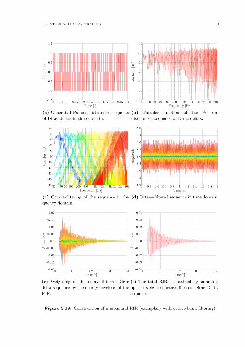
5.3. STOCHASTIC RAY TRACING 71
Amplitude
Time [s]
(a) Generated Poisson-distributed sequenceof Dirac deltas in time domain.
Modulus[dB]
Frequency [Hz]
(b) Transfer function of the Poisson-distributed sequence of Dirac deltas.
Modulus[dB]
Frequency [Hz]
(c) Octave-filtering of the sequence in fre-quency domain.
Amplitude
Time [s]
(d) Octave-filtered sequence in time domain.
Amplitude
Time [s]
(e) Weighting of the octave-filtered Diracdelta sequence by the energy envelope of theRIR.
Amplitude
Time [s]
(f) The total RIR is obtained by summingup the weighted octave-filtered Dirac Deltasequence.
Figure 5.18: Construction of a monaural RIR (exemplary with octave-band filtering).
72 CHAPTER 5. ROOM ACOUSTICS SIMULATION
the simulated energy envelope of the RIR. Consequently, the Dirac delta sequence hd(see Fig. 5.18(a)) is transformed to frequency domain (see Fig. 5.18(b)) and filteredby an asymmetrical high/low-pass-combination with differing slope and shape of aRaised Cosine Filter RCF (n) with
RCF (n) =
0 if f < flow12
(1 + cos
(2πffn
))if flow ≤ f < fn
12
(1− cos
(2πffn+1
))if fn ≤ f < fhigh
0 if f ≥ fhigh,
(5.46)
where fn denotes the center frequency of the nth frequency band, and flow and fhigh de-scribe the lower and upper limit of the frequency band, respectively (see Fig. 5.18(c)).Then the filtered spectrum is transformed back to the time domain resulting in n
bandpass-filtered Dirac delta sequences hd(n) (see Fig. 5.18(d)). As long as the vol-ume of the room does not change drastically, these sequences have to be computedonly once, which can be accomplished during a preprocessing step of the simulation.The monaural RIR s(i) can then be quickly constructed online by weighting hd(n)sample-wise with
si = vi ·√√√√ En(k)∑g(k)
i=g(k−1)+1 v2i
·√
BWfs/2
(5.47)
with g(k) = bk· fs · ∆tc,
where ∆t denotes the length of the histogram’s time slot, vi the value of the ith sampleof hd(n), fs the sampling frequency, BW the width of the regarded frequency bandn, and En(k) the energy of the histogram’s kth time slot that relates to the ith sample(see Fig. 5.18(e)). In a final step, summing up all weighted noise sequences in thetime domain leads to the overall monaural RIR(see Fig. 5.18(f)).
Binaural Room Impulse Response
Constructing a BRIR from a detector’s energy histogram is somewhat more complexcompared to the monaural case. For a human receiver, HRIRs that relate to thedirections of incoming sound reflections have to be additionally taken into account.Instead of assuming an ideal diffuse sound field where the direction of arriving soundreflections is totally randomized, binaural detectors can be used in order to gathertemporal and spectral information on impacting energy particles in a more realisticway. RAVEN’s binaural detector is modeled as a sphere with head-related coordinatesystem, where the sphere’s surface is subdivided into m discrete Directivity Groups(DGs) with a certain resolution in azimuth- and elevation direction. Energy particlesare assigned to these groups depending on their angle of impact and resulting in menergy histograms, one for each directivity group (see Fig. 5.19(1)).
From this data, a hit probability for each DG can be calculated by averaging andcomparing slot-wise the respective histograms’ short time spectra Ek(n), wherebyhigh energy leads to high probability and vice versa (see Fig. 5.19(2)). During the
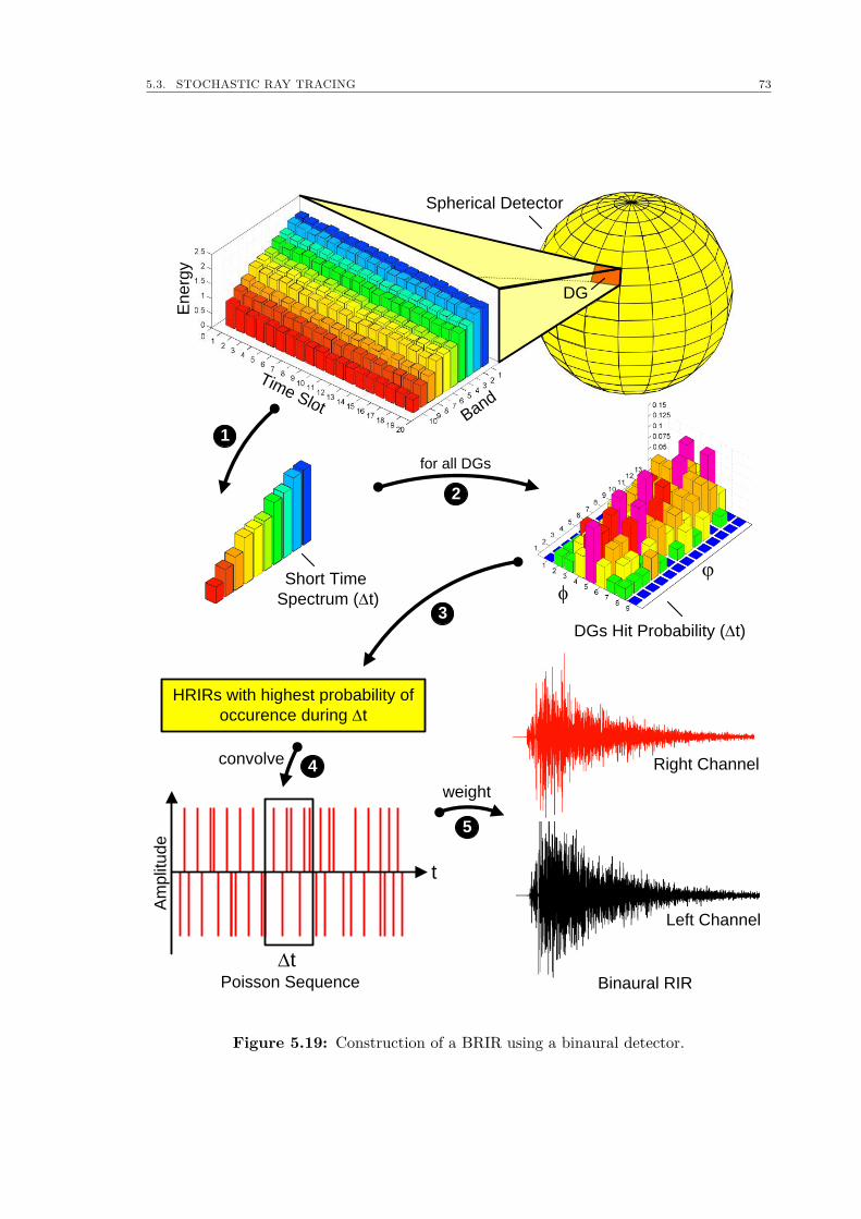
5.3. STOCHASTIC RAY TRACING 73
Time SlotBand
En
erg
y
Spherical Detector
Phit(Dt)
j
f
HRIRs with highest probability of
occurence during Dt
Am
plit
ud
e
t
Dt
Short Time
Spectrum (Dt)
DGs Hit Probability (Dt)
Poisson Sequence
for all DGs
1
2
3
4convolve
5
weight
DG
Binaural RIR
Right Channel
Left Channel
Figure 5.19: Construction of a BRIR using a binaural detector.
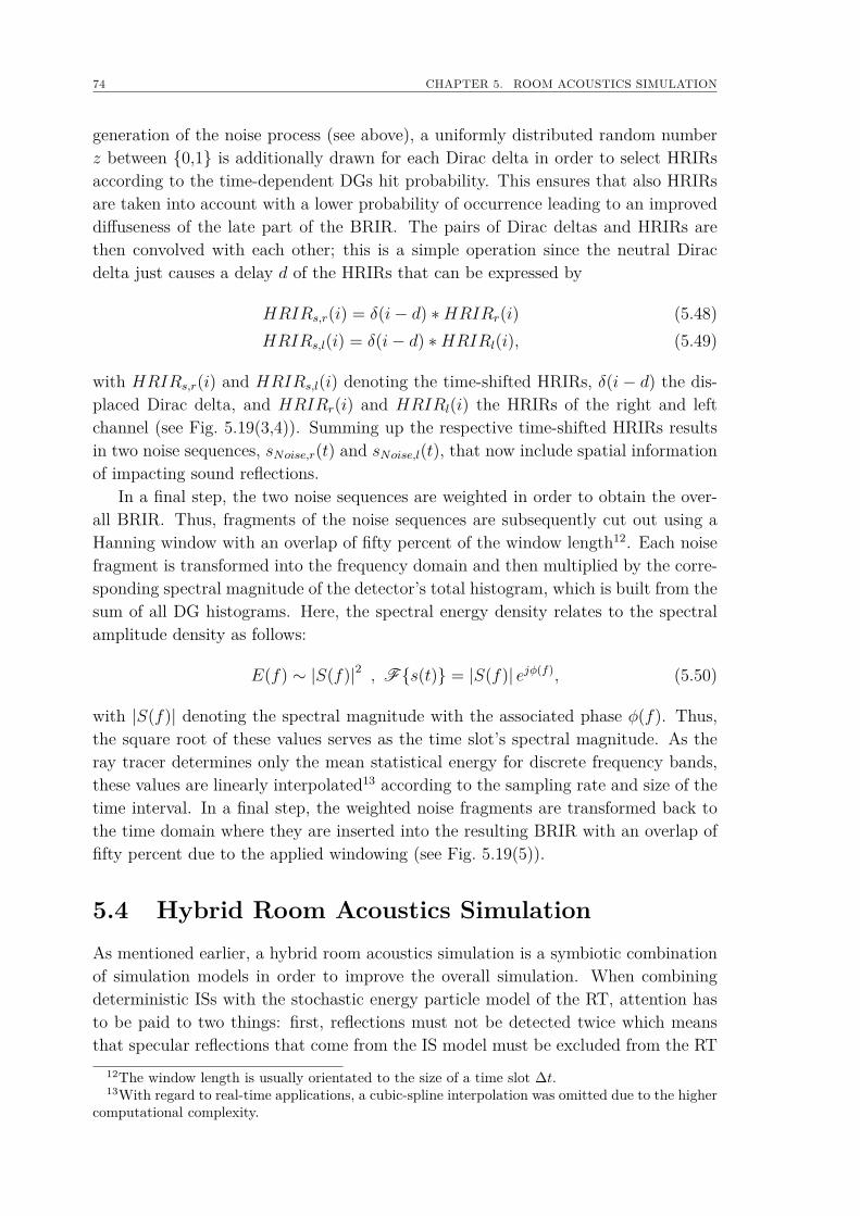
74 CHAPTER 5. ROOM ACOUSTICS SIMULATION
generation of the noise process (see above), a uniformly distributed random numberz between 0,1 is additionally drawn for each Dirac delta in order to select HRIRsaccording to the time-dependent DGs hit probability. This ensures that also HRIRsare taken into account with a lower probability of occurrence leading to an improveddiffuseness of the late part of the BRIR. The pairs of Dirac deltas and HRIRs arethen convolved with each other; this is a simple operation since the neutral Diracdelta just causes a delay d of the HRIRs that can be expressed by
HRIRs,r(i) = δ(i− d) ∗HRIRr(i) (5.48)HRIRs,l(i) = δ(i− d) ∗HRIRl(i), (5.49)
with HRIRs,r(i) and HRIRs,l(i) denoting the time-shifted HRIRs, δ(i− d) the dis-placed Dirac delta, and HRIRr(i) and HRIRl(i) the HRIRs of the right and leftchannel (see Fig. 5.19(3,4)). Summing up the respective time-shifted HRIRs resultsin two noise sequences, sNoise,r(t) and sNoise,l(t), that now include spatial informationof impacting sound reflections.
In a final step, the two noise sequences are weighted in order to obtain the over-all BRIR. Thus, fragments of the noise sequences are subsequently cut out using aHanning window with an overlap of fifty percent of the window length12. Each noisefragment is transformed into the frequency domain and then multiplied by the corre-sponding spectral magnitude of the detector’s total histogram, which is built from thesum of all DG histograms. Here, the spectral energy density relates to the spectralamplitude density as follows:
E(f) ∼ |S(f)|2 , Fs(t) = |S(f)| ejφ(f), (5.50)
with |S(f)| denoting the spectral magnitude with the associated phase φ(f). Thus,the square root of these values serves as the time slot’s spectral magnitude. As theray tracer determines only the mean statistical energy for discrete frequency bands,these values are linearly interpolated13 according to the sampling rate and size of thetime interval. In a final step, the weighted noise fragments are transformed back tothe time domain where they are inserted into the resulting BRIR with an overlap offifty percent due to the applied windowing (see Fig. 5.19(5)).
5.4 Hybrid Room Acoustics SimulationAs mentioned earlier, a hybrid room acoustics simulation is a symbiotic combinationof simulation models in order to improve the overall simulation. When combiningdeterministic ISs with the stochastic energy particle model of the RT, attention hasto be paid to two things: first, reflections must not be detected twice which meansthat specular reflections that come from the IS model must be excluded from the RT
12The window length is usually orientated to the size of a time slot ∆t.13With regard to real-time applications, a cubic-spline interpolation was omitted due to the higher
computational complexity.
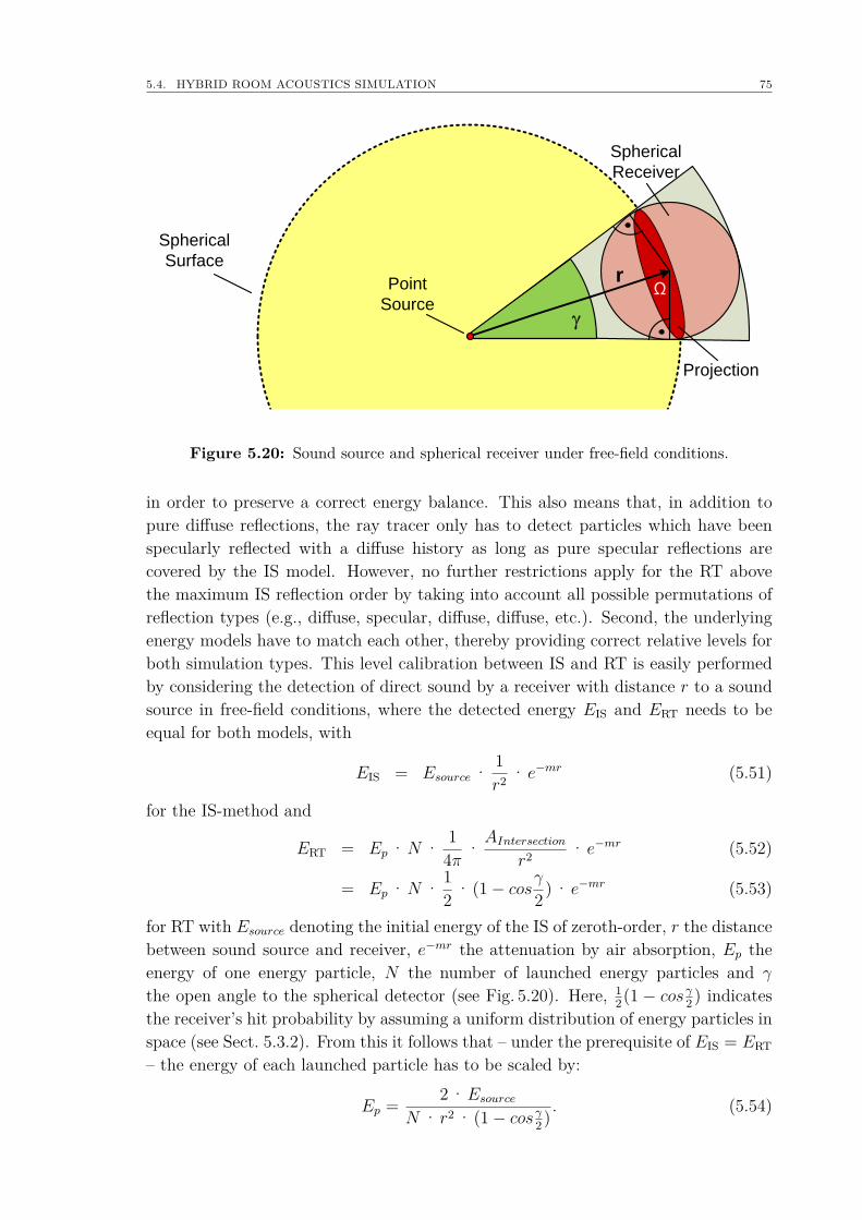
5.4. HYBRID ROOM ACOUSTICS SIMULATION 75
Ωr
Spherical
Surface
Spherical
Receiver
g
Projection
Point
Source
Figure 5.20: Sound source and spherical receiver under free-field conditions.
in order to preserve a correct energy balance. This also means that, in addition topure diffuse reflections, the ray tracer only has to detect particles which have beenspecularly reflected with a diffuse history as long as pure specular reflections arecovered by the IS model. However, no further restrictions apply for the RT abovethe maximum IS reflection order by taking into account all possible permutations ofreflection types (e.g., diffuse, specular, diffuse, diffuse, etc.). Second, the underlyingenergy models have to match each other, thereby providing correct relative levels forboth simulation types. This level calibration between IS and RT is easily performedby considering the detection of direct sound by a receiver with distance r to a soundsource in free-field conditions, where the detected energy EIS and ERT needs to beequal for both models, with
EIS = Esource · 1r2 · e−mr (5.51)
for the IS-method and
ERT = Ep ·N · 14π · AIntersection
r2 · e−mr (5.52)
= Ep ·N · 12 · (1− cosγ2 ) · e−mr (5.53)
for RT with Esource denoting the initial energy of the IS of zeroth-order, r the distancebetween sound source and receiver, e−mr the attenuation by air absorption, Ep theenergy of one energy particle, N the number of launched energy particles and γ
the open angle to the spherical detector (see Fig. 5.20). Here, 12(1 − cosγ2 ) indicates
the receiver’s hit probability by assuming a uniform distribution of energy particles inspace (see Sect. 5.3.2). From this it follows that – under the prerequisite of EIS = ERT
– the energy of each launched particle has to be scaled by:
Ep = 2 ·EsourceN · r2 · (1− cosγ2 ) . (5.54)
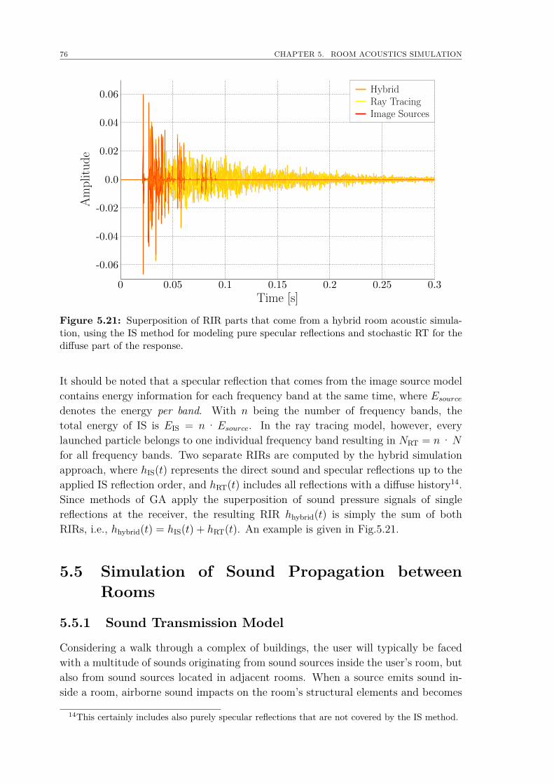
76 CHAPTER 5. ROOM ACOUSTICS SIMULATION
Amplitude
Time [s]
HybridRay TracingImage Sources
Figure 5.21: Superposition of RIR parts that come from a hybrid room acoustic simula-tion, using the IS method for modeling pure specular reflections and stochastic RT for thediffuse part of the response.
It should be noted that a specular reflection that comes from the image source modelcontains energy information for each frequency band at the same time, where Esourcedenotes the energy per band. With n being the number of frequency bands, thetotal energy of IS is EIS = n·Esource. In the ray tracing model, however, everylaunched particle belongs to one individual frequency band resulting in NRT = n·N
for all frequency bands. Two separate RIRs are computed by the hybrid simulationapproach, where hIS(t) represents the direct sound and specular reflections up to theapplied IS reflection order, and hRT(t) includes all reflections with a diffuse history14.Since methods of GA apply the superposition of sound pressure signals of singlereflections at the receiver, the resulting RIR hhybrid(t) is simply the sum of bothRIRs, i.e., hhybrid(t) = hIS(t) + hRT(t). An example is given in Fig.5.21.
5.5 Simulation of Sound Propagation betweenRooms
5.5.1 Sound Transmission Model
Considering a walk through a complex of buildings, the user will typically be facedwith a multitude of sounds originating from sound sources inside the user’s room, butalso from sound sources located in adjacent rooms. When a source emits sound in-side a room, airborne sound impacts on the room’s structural elements and becomes
14This certainly includes also purely specular reflections that are not covered by the IS method.
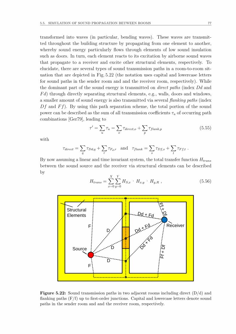
5.5. SIMULATION OF SOUND PROPAGATION BETWEEN ROOMS 77
transformed into waves (in particular, bending waves). These waves are transmit-ted throughout the building structure by propagating from one element to another,whereby sound energy particularly flows through elements of low sound insulationsuch as doors. In turn, each element reacts to its excitation by airborne sound wavesthat propagate to a receiver and excite other structural elements, respectively. Toelucidate, there are several types of sound transmission paths in a room-to-room sit-uation that are depicted in Fig. 5.22 (the notation uses capital and lowercase lettersfor sound paths in the sender room and and the receiver room, respectively). Whilethe dominant part of the sound energy is transmitted on direct paths (index Dd andFd) through directly separating structural elements, e.g., walls, doors and windows,a smaller amount of sound energy is also transmitted via several flanking paths (indexDf and Ff). By using this path separation scheme, the total portion of the soundpower can be described as the sum of all transmission coefficients τu of occurring pathcombinations [Ger79], leading to
τ ′ =∑u
τu =∑o
τdirect,o +∑p
τflank,p (5.55)
with
τdirect =∑q
τDd,q +∑r
τFd,r and τflank =∑s
τDf,s +∑t
τFf,t .
By now assuming a linear and time invariant system, the total transfer function Htrans
between the sound source and the receiver via structural elements can be describedby
Htrans =X∑x=0
Y∑y=0
HS,x ·Hx,y ·Hy,R , (5.56)
Dd + Fd
Ff +
Df
Ff +
Df
D
D
D
F
F
Source
Receiver
Structural
Elements Dd + Fd
Dd
+ Fd
Figure 5.22: Sound transmission paths in two adjacent rooms including direct (D/d) andflanking paths (F/f) up to first-order junctions. Capital and lowercase letters denote soundpaths in the sender room and and the receiver room, respectively.
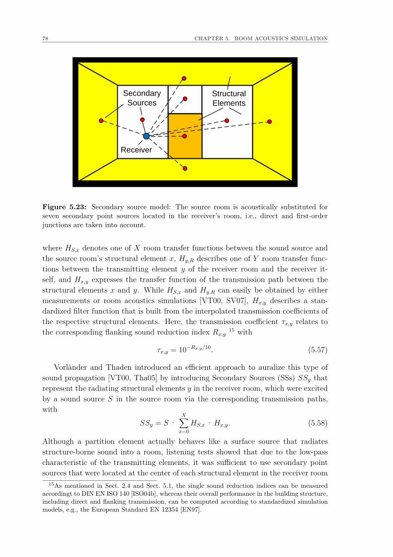
78 CHAPTER 5. ROOM ACOUSTICS SIMULATION
Receiver
Secondary
SourcesStructural
Elements
Figure 5.23: Secondary source model: The source room is acoustically substituted forseven secondary point sources located in the receiver’s room, i.e., direct and first-orderjunctions are taken into account.
where HS,x denotes one of X room transfer functions between the sound source andthe source room’s structural element x, Hy,R describes one of Y room transfer func-tions between the transmitting element y of the receiver room and the receiver it-self, and Hx,y expresses the transfer function of the transmission path between thestructural elements x and y. While HS,x and Hy,R can easily be obtained by eithermeasurements or room acoustics simulations [VT00, SV07], Hx,y describes a stan-dardized filter function that is built from the interpolated transmission coefficients ofthe respective structural elements. Here, the transmission coefficient τx,y relates tothe corresponding flanking sound reduction index Rx,y
15 with
τx,y = 10−Rx,y/10. (5.57)
Vorländer and Thaden introduced an efficient approach to auralize this type ofsound propagation [VT00, Tha05] by introducing Secondary Sources (SSs) SSy thatrepresent the radiating structural elements y in the receiver room, which were excitedby a sound source S in the source room via the corresponding transmission paths,with
SSy = S·X∑x=0
HS,x ·Hx,y. (5.58)
Although a partition element actually behaves like a surface source that radiatesstructure-borne sound into a room, listening tests showed that due to the low-passcharacteristic of the transmitting elements, it was sufficient to use secondary pointsources that were located at the center of each structural element in the receiver room
15As mentioned in Sect. 2.4 and Sect. 5.1, the single sound reduction indices can be measuredaccordingt to DIN EN ISO 140 [ISO04b], whereas their overall performance in the building structure,including direct and flanking transmission, can be computed according to standardized simulationmodels, e.g., the European Standard EN 12354 [EN97].
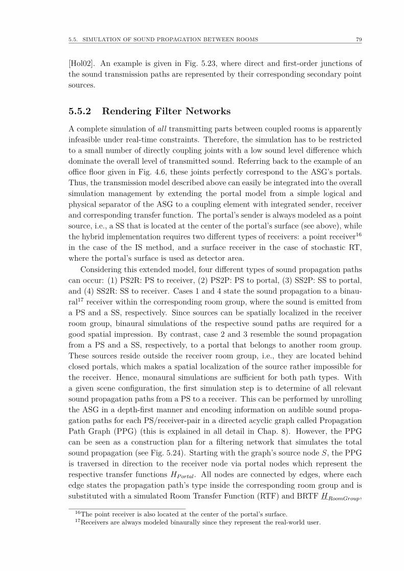
5.5. SIMULATION OF SOUND PROPAGATION BETWEEN ROOMS 79
[Hol02]. An example is given in Fig. 5.23, where direct and first-order junctions ofthe sound transmission paths are represented by their corresponding secondary pointsources.
5.5.2 Rendering Filter Networks
A complete simulation of all transmitting parts between coupled rooms is apparentlyinfeasible under real-time constraints. Therefore, the simulation has to be restrictedto a small number of directly coupling joints with a low sound level difference whichdominate the overall level of transmitted sound. Referring back to the example of anoffice floor given in Fig. 4.6, these joints perfectly correspond to the ASG’s portals.Thus, the transmission model described above can easily be integrated into the overallsimulation management by extending the portal model from a simple logical andphysical separator of the ASG to a coupling element with integrated sender, receiverand corresponding transfer function. The portal’s sender is always modeled as a pointsource, i.e., a SS that is located at the center of the portal’s surface (see above), whilethe hybrid implementation requires two different types of receivers: a point receiver16
in the case of the IS method, and a surface receiver in the case of stochastic RT,where the portal’s surface is used as detector area.
Considering this extended model, four different types of sound propagation pathscan occur: (1) PS2R: PS to receiver, (2) PS2P: PS to portal, (3) SS2P: SS to portal,and (4) SS2R: SS to receiver. Cases 1 and 4 state the sound propagation to a binau-ral17 receiver within the corresponding room group, where the sound is emitted froma PS and a SS, respectively. Since sources can be spatially localized in the receiverroom group, binaural simulations of the respective sound paths are required for agood spatial impression. By contrast, case 2 and 3 resemble the sound propagationfrom a PS and a SS, respectively, to a portal that belongs to another room group.These sources reside outside the receiver room group, i.e., they are located behindclosed portals, which makes a spatial localization of the source rather impossible forthe receiver. Hence, monaural simulations are sufficient for both path types. Witha given scene configuration, the first simulation step is to determine of all relevantsound propagation paths from a PS to a receiver. This can be performed by unrollingthe ASG in a depth-first manner and encoding information on audible sound propa-gation paths for each PS/receiver-pair in a directed acyclic graph called PropagationPath Graph (PPG) (this is explained in all detail in Chap. 8). However, the PPGcan be seen as a construction plan for a filtering network that simulates the totalsound propagation (see Fig. 5.24). Starting with the graph’s source node S, the PPGis traversed in direction to the receiver node via portal nodes which represent therespective transfer functions HPortal. All nodes are connected by edges, where eachedge states the propagation path’s type inside the corresponding room group and issubstituted with a simulated Room Transfer Function (RTF) and BRTF HRoomGroup,
16The point receiver is also located at the center of the portal’s surface.17Receivers are always modeled binaurally since they represent the real-world user.
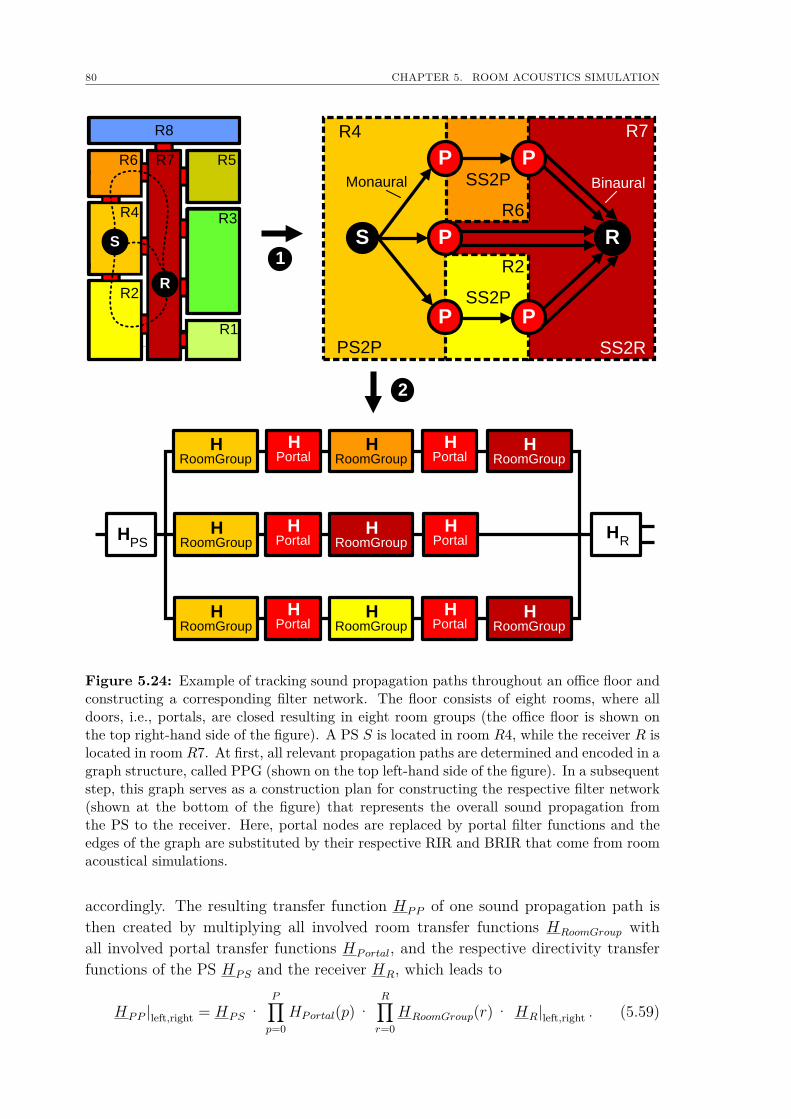
80 CHAPTER 5. ROOM ACOUSTICS SIMULATION
R2
R4
R6 R5
R1
R3
R7
R8
R
S R
P
S
PP
R7
R6
R4
R2
PS2P SS2R
SS2P
SS2P
P
P
BinauralMonaural
1
2
HRoomGroup
HRoomGroup
HRoomGroup
HPortal
HRoomGroup
HRoomGroup
HRoomGroup
HRoomGroup
HRoomGroup
HPS
HPortal
HPortal
HR
HPortal
HPortal
HPortal
Figure 5.24: Example of tracking sound propagation paths throughout an office floor andconstructing a corresponding filter network. The floor consists of eight rooms, where alldoors, i.e., portals, are closed resulting in eight room groups (the office floor is shown onthe top right-hand side of the figure). A PS S is located in room R4, while the receiver R islocated in room R7. At first, all relevant propagation paths are determined and encoded in agraph structure, called PPG (shown on the top left-hand side of the figure). In a subsequentstep, this graph serves as a construction plan for constructing the respective filter network(shown at the bottom of the figure) that represents the overall sound propagation fromthe PS to the receiver. Here, portal nodes are replaced by portal filter functions and theedges of the graph are substituted by their respective RIR and BRIR that come from roomacoustical simulations.
accordingly. The resulting transfer function HPP of one sound propagation path isthen created by multiplying all involved room transfer functions HRoomGroup withall involved portal transfer functions HPortal, and the respective directivity transferfunctions of the PS HPS and the receiver HR, which leads to
HPP |left,right = HPS ·P∏p=0
HPortal(p) ·R∏r=0
HRoomGroup(r) · HR|left,right . (5.59)
5.6. LIMITS OF GEOMETRICAL ACOUSTICS 81
The scene’s total transmission characteristics for a PS/receiver-pair is then easilydetermined by summing up the contributions of each propagation path that can beconducted either in the time domain or in the frequency domain. The simulation ofsound propagation between rooms obviously requires a large number of simulationsteps that cannot be handled on a single machine anymore, since each involved roomgroup calls for a hybrid room acoustical simulation. Especially with regard to real-time auralization of dynamically changing scenes, a computing cluster of distributedsystems should be employed in order to handle this significant rise in computationaleffort. This is further explained in the next chapter.
5.6 Limits of Geometrical AcousticsAlthough state-of-the-art methods of GA usually provide good simulation resultsin practice, one should not forget that this approach of sound wave decompositioninherently has some important limitations, meaning that methods of GA can onlyapproximate real-world sound propagation with a particular uncertainty.
Large rooms The most important constraint of GA is the restriction to large rooms.The IS-model as well as stochastic RT deal with geometric reflections of soundwaves which postulates small wavelengths compared to the room geometry.Acoustic phase effects such as room modes, which significantly influence thelow-frequency range, are not modeled by geometrical approaches.
Broadband source signals Broadband signals are required for auralization, asthey conceal phase effects which would occur with single tone source signals.
CAD room models Important for good simulation results are appropriate roommodels. In this context, an appropriate model does not necessarily refer to ahigh level of detail, but to an accurate reproduction of the reflection character-istics of objects and room boundaries using adequate absorption and scatteringcoefficients as surface descriptors.
Low absorption coefficients The IS-model is only exact for reflection coefficientsof R = 1 and R = −1, respectively, with |R| =
√1− α, but it is still a good
approximation for low absorption coefficients. However, the assumed planewave field for the moment of reflection is well suited only if a spherical waveis considered with a large distance between the wall and the sound source andthe receiver, and a constant angle of incidence, where the latter is only a validapproximation for angles of up to 60 between the impacting reflection and thesurface normal.

82 CHAPTER 5. ROOM ACOUSTICS SIMULATION
Chapter 6
Dynamically Changing VirtualEnvironments
"Experience is not what happens to you. It is what you do with whathappens to you."
(The Highest State of Consciousness, Aldous Huxley, English writer)
A prerequisite for any immersive simulation is the creation of a dynamic rep-resentation of the virtual scene, because real-world scenarios are usually not static.While the real-time visualization of dynamic scenes is a rather fast operation inCG, a small change in the scene configuration affects the whole auralization chain- this includes rather simple operations such as the motion of sound source anduser, i.e., the listener, but also the more complex modification of scene geometry,either of geometrical scene objects or of scene portals. By recalling the scene graphrepresentation of the virtual scene (see Sect. 4.3 and Sect. 5.5), the number of soundpaths that have to be taken into account for the simulation increases drasticallywith the number of nodes and portals. Unfortunately, room acoustical simulationsare the most complex operation among all other system tasks that must respond touser interactions at interactive rates. To overcome the simulation complexity, severalapproximations are necessary; they will be described in this chapter. Upper limitsfor the computation time of simulation events are identified that yield a smoothand plausible auralization with best possible simulation quality within the giventime constraints. Furthermore, filter update strategies are introduced that aim atkeeping computation costs low by updating only relevant parts of the BRIR using avery fast data handling and convenient interaction management. Finally, a conceptfor parallel computing is described. Here, simulation processes are distributed ona computing cluster of multi-core shared-memory machines in order to handle thesimulation workload at interactive rates even in complex scenarios.
84 CHAPTER 6. DYNAMICALLY CHANGING VIRTUAL ENVIRONMENTS
6.1 Real-time ConstraintsBy considering the situation in a virtual environment, the complex calculation ofBRIRs (see previous chapter) is just one small fragment in the input-output aural-ization chain. Other system components such as motion tracking, audio hardware,signal convolution, and audio reproduction already produce latency which limits themaximum permissible computation time for room acoustics simulations. This meansthat the overall quality of auralization is scaled by the available computation power,whereby the system’s minimum quality must not under-run the constraints given byhuman perception. For the total delay between the user’s action and the system’sreaction, a lag of about 50ms can be regarded as generally acceptable and the continu-ous audio stream should be updated with 60Hz [Vor08]. Obviously, this is practicallyimpossible, since hardware itself already causes a lag of more than 50% of the totalprocessing time (50ms) – at least today. Fortunately, when taking a closer look atthe situation in a virtual environment, one will see that these rules do not necessarilyapply for all elements of the auralization chain. It was shown in psycho-acoustical ex-periments that the visual and auditory sensory perceptions are allowed to be slightlyshifted to each other, whereby a good perceived coincidence of the visual and auralstimuli was still found for an additional delay up to 35ms [KvdPvEJ06, vdPK00].This is important for the synchronization of audiovisual stimuli such as avatars (seeChap. 3). Furthermore, Brungart et al. found that a lag of 70ms between the trackingevent and the system’s auditory response remains unnoticed by the user [BSM+04].Besides psycho-acoustical studies, behavior patterns of users in specific simulationsituations1 are also relevant for assessing simulation constraints, but theoretical andempirical investigations on typical movements of users operating in virtual environ-ments are still a subject of research (e.g., [AB95, WO95, CHV02, LJ03]). In general,user movements in CAVE-like environments can be classified into three categories:
Inspection The user is inspecting a static object by moving up and down and fromone side to the other in order to gather more detailed information. User in-teraction such as the creation, manipulation and destruction of objects can beseen as part of that category, too.
Observation The user is standing at a fixed spot and uses both head and bodyrotations to watch at different display surfaces of the CAVE-like environment.
Exploration The user is exploring the virtual environment by simultaneously walk-ing2 and looking at the scenery.
Consequently, Lentz et al. carried out user studies to gather more detailed informationon typical behavior patterns for each classification type by tracking head movementsof users who were interactively inspecting, observing and exploring an architecturalscenario of a virtual concert hall [Len07]. In all cases, head rotations were identified
1Here, user task and simulation environment have to be regarded in particular.2Mostly indirect via the control interface.
6.1. REAL-TIME CONSTRAINTS 85
as fastest and most abrupt movements with peak values of about 45 per second,while translational position changes were rather smooth, mostly in the range of 30-50 cm/s. Rotational head movements thus require very fast updates, since this typeof behavior results in a drastic change of the auditory event. Here, processing timesshould not exceed the tracking constraint of 70ms (see above) to maintain a synchro-nized audiovisual simulation. In the current configuration of RWTH’s VR-system,about 35ms lag is produced by other system components, which means that only35ms remain for the complete auralization event. As long as the positions of bothsound sources and user are rather fixed, most simulation data stays unchanged andonly changing directional patterns of sound sources and user have to be updated3. Incontrast, translational movements of sound sources and user require at least a partialresimulation of the BRIRs as sound propagation paths (may) have changed. Investi-gations by Witew et al. showed that the overall sound impression in a room does notchange dramatically in the immediate vicinity of the listener [Wit04, WD07]. Thismeans that low update rates of the room acoustics simulation can be seen as sufficientfor translational movements. By assuming 25 cm4 and 1m as thresholds for triggeringthe recalculation of the specular and diffuse part of the BRIR, respectively, and tak-ing into account the results from the user studies, maximum permissible computationtimes for the room acoustics simulation can be identified [Len07]:
• To catch 70% of the translational movements greater than 25 cm, a recalculationhas to be performed approximately every 750ms.
• Correct early specular reflections in about 90% of translational movementsgreater than 25 cm require an update every 550ms.
From this it follows that computation times for ISs (specular part of the BRIR)should not exceed 550ms, while 2 s5 is set as maximum computation time for process-ing the computationally demanding ray tracing, since the late reverberant sound fieldwill hardly change within one meter. Thus, BRIRs are updated gradually accordingto the position changes of sound sources and user.
A more demanding interaction event is user modification of the scene geometryeither by creating, manipulating or destroying geometrical objects. In such situations,the sound field might change drastically, e.g., by inserting a reflector panel to thevirtual scene (see Fig. 6.1). Most likely the user will inspect and observe the dynamicobject in a very concentrated way, where rotational and translational head movementsoccur at a high and low level, respectively, while less information is extracted from theaural stimuli due to the change of concentration focus. A first update of the wholeBRIR within 35ms6 after the modification event would be ideal, but a completeroom acoustical simulation of a geometrically changed environment including bothspecular and diffuse part of the BRIR comprises too many algorithmic operations to
3This is a very fast operation with processing times far below 35ms.425 cm relate to the half width of a common concert hall seat.5This relates to a maximum velocity of sound sources and receiver of 0.5m/s.670ms - 35ms system lag = 35ms, see above.
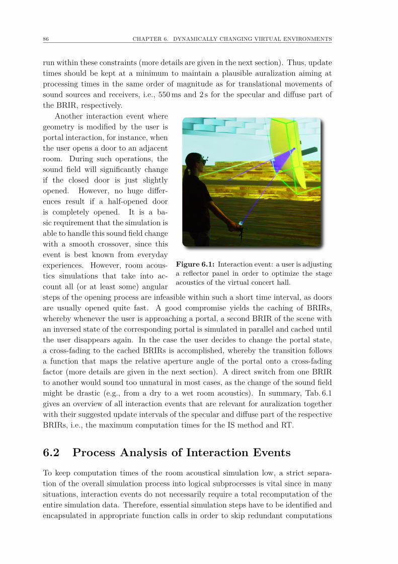
86 CHAPTER 6. DYNAMICALLY CHANGING VIRTUAL ENVIRONMENTS
run within these constraints (more details are given in the next section). Thus, updatetimes should be kept at a minimum to maintain a plausible auralization aiming atprocessing times in the same order of magnitude as for translational movements ofsound sources and receivers, i.e., 550ms and 2 s for the specular and diffuse part ofthe BRIR, respectively.
Another interaction event where
Figure 6.1: Interaction event: a user is adjustinga reflector panel in order to optimize the stageacoustics of the virtual concert hall.
geometry is modified by the user isportal interaction, for instance, whenthe user opens a door to an adjacentroom. During such operations, thesound field will significantly changeif the closed door is just slightlyopened. However, no huge differ-ences result if a half-opened dooris completely opened. It is a ba-sic requirement that the simulation isable to handle this sound field changewith a smooth crossover, since thisevent is best known from everydayexperiences. However, room acous-tics simulations that take into ac-count all (or at least some) angularsteps of the opening process are infeasible within such a short time interval, as doorsare usually opened quite fast. A good compromise yields the caching of BRIRs,whereby whenever the user is approaching a portal, a second BRIR of the scene withan inversed state of the corresponding portal is simulated in parallel and cached untilthe user disappears again. In the case the user decides to change the portal state,a cross-fading to the cached BRIRs is accomplished, whereby the transition followsa function that maps the relative aperture angle of the portal onto a cross-fadingfactor (more details are given in the next section). A direct switch from one BRIRto another would sound too unnatural in most cases, as the change of the sound fieldmight be drastic (e.g., from a dry to a wet room acoustics). In summary, Tab. 6.1gives an overview of all interaction events that are relevant for auralization togetherwith their suggested update intervals of the specular and diffuse part of the respectiveBRIRs, i.e., the maximum computation times for the IS method and RT.
6.2 Process Analysis of Interaction EventsTo keep computation times of the room acoustical simulation low, a strict separa-tion of the overall simulation process into logical subprocesses is vital since in manysituations, interaction events do not necessarily require a total recomputation of theentire simulation data. Therefore, essential simulation steps have to be identified andencapsulated in appropriate function calls in order to skip redundant computations
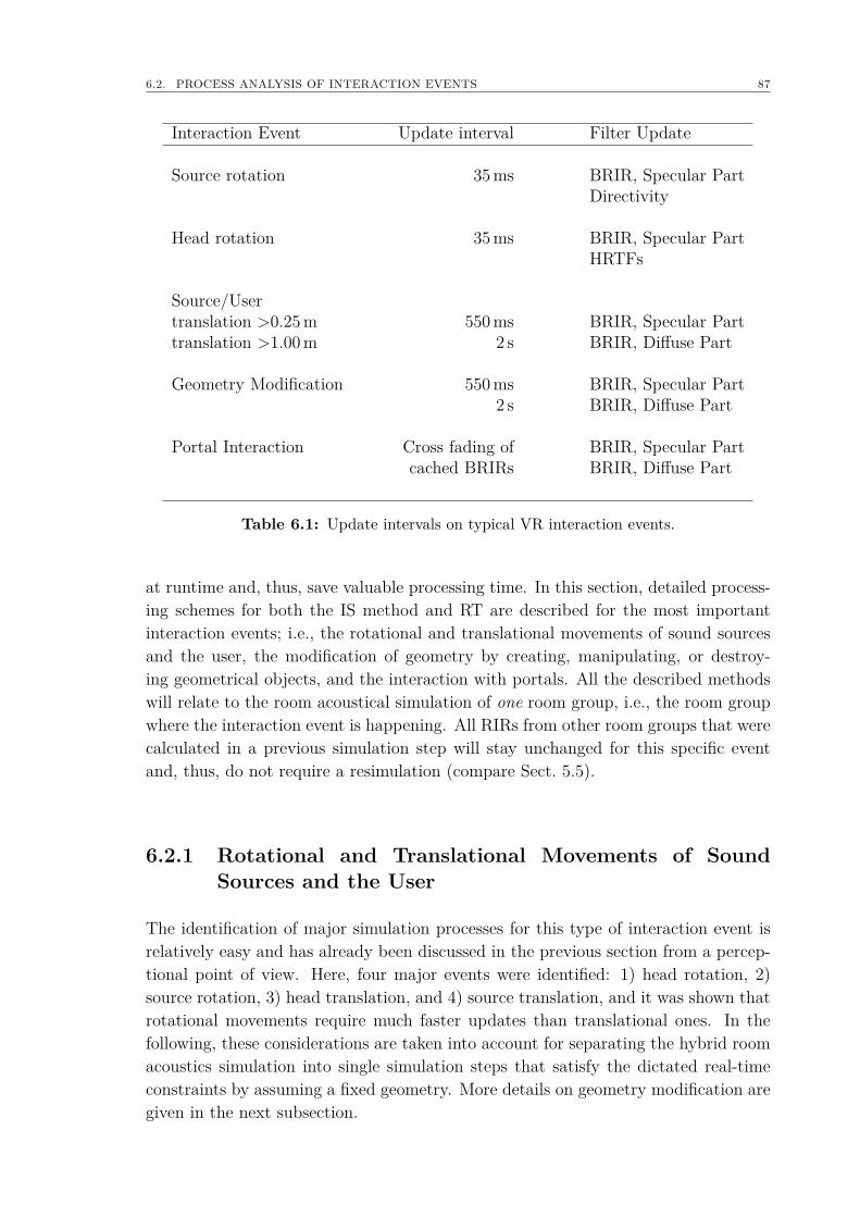
6.2. PROCESS ANALYSIS OF INTERACTION EVENTS 87
Interaction Event Update interval Filter Update
Source rotation 35ms BRIR, Specular PartDirectivity
Head rotation 35ms BRIR, Specular PartHRTFs
Source/Usertranslation >0.25m 550ms BRIR, Specular Parttranslation >1.00m 2 s BRIR, Diffuse Part
Geometry Modification 550ms BRIR, Specular Part2 s BRIR, Diffuse Part
Portal Interaction Cross fading of BRIR, Specular Partcached BRIRs BRIR, Diffuse Part
Table 6.1: Update intervals on typical VR interaction events.
at runtime and, thus, save valuable processing time. In this section, detailed process-ing schemes for both the IS method and RT are described for the most importantinteraction events; i.e., the rotational and translational movements of sound sourcesand the user, the modification of geometry by creating, manipulating, or destroy-ing geometrical objects, and the interaction with portals. All the described methodswill relate to the room acoustical simulation of one room group, i.e., the room groupwhere the interaction event is happening. All RIRs from other room groups that werecalculated in a previous simulation step will stay unchanged for this specific eventand, thus, do not require a resimulation (compare Sect. 5.5).
6.2.1 Rotational and Translational Movements of SoundSources and the User
The identification of major simulation processes for this type of interaction event isrelatively easy and has already been discussed in the previous section from a percep-tional point of view. Here, four major events were identified: 1) head rotation, 2)source rotation, 3) head translation, and 4) source translation, and it was shown thatrotational movements require much faster updates than translational ones. In thefollowing, these considerations are taken into account for separating the hybrid roomacoustics simulation into single simulation steps that satisfy the dictated real-timeconstraints by assuming a fixed geometry. More details on geometry modification aregiven in the next subsection.
88 CHAPTER 6. DYNAMICALLY CHANGING VIRTUAL ENVIRONMENTS
Image Source Method
Before starting the online simulation of the virtual environment, all ISs of primaryand secondary sound sources are preprocessed up to a specific reflection order andstored in data containers that are associated with the respective sound sources oredges (implementation details are given in Chap. 9). Since ISs are related to theroom’s geometry, the overall cloud of ISs does not change as long as the respectivesound source is not moved and – as assumed – no geometrical modifications of theroom are carried out. To handle the identified four major interaction events efficiently,it is reasonable to separate the IS method into three fundamental simulation steps:
IS Translation If the primary sound source is moved (all secondary sound sourcesare static for a fixed geometry), the corresponding position update also involvesthe associated ISs. To obtain the new positions of the ISs, displacement vectorsare simply added to the current positions of the ISs. These vectors have tobe computed individually for each IS and are the product of the displacementvector of the sound source multiplied by an IS-dependent translation matrix(more details are given in Chap. 9).
IS Audibility Test As described before, this test identifies all audible ISs for pri-mary and secondary sources, and their properties with regard to sound sourceand user (angles of emission and impact, length of sound propagation path andthe user’s position) using several acceleration techniques which are described indetail in Chap. 7 and 9. These audible ISs are then stored in a separate datacontainer that is associated with the respective (primary oder secondary) soundsource.
IS Filter Construction For each audible IS, the filter construction consists of amultiplication of surface/edge-specific transfer functions, the sound source’sdirectivity, and the HRTFs in the frequency domain. The resulting transferfunction is transformed back into the time domain and shifted by the computeddelay of the respective IS. The BRIR is then obtained by simply summing upthe contributions of all ISs (see Sect. 5.2).
By using this separation scheme, three entry points into the IS simulation canbe identified that handle the major four interaction events efficiently (see Fig. 6.2).The spin of both sound source and user’s head is the most frequently occurringinteraction event during a simulation and, fortunately, also the least time-consumingsimulation step (entry point 3). Rotational movements only require a reconstructionof the binaural filter, since the set of currently audible ISs stays unchanged. Duringthis reconstruction, HRTFs and/or the directivity of the sound source are simplyexchanged by transfer functions that match the changed orientation resulting in arecomputed BRIR which adapts the new situation. More simulation steps are requiredfor translational head movements (entry point 2). Here, the audibility of ISs may havechanged, as for the new position some specular reflections may become blocked by
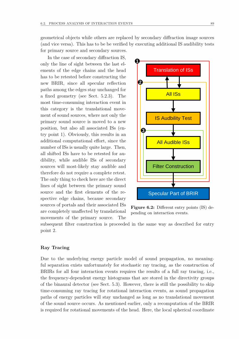
6.2. PROCESS ANALYSIS OF INTERACTION EVENTS 89
geometrical objects while others are replaced by secondary diffraction image sources(and vice versa). This has to be be verified by executing additional IS audibility testsfor primary source and secondary sources.
In the case of secondary diffraction IS,
Translation of ISs
All ISs
IS Audbility Test
All Audible ISs
Filter Construction
Specular Part of BRIR
1
2
3
Figure 6.2: Different entry points (IS) de-pending on interaction events.
only the line of sight between the last el-ements of the edge chains and the headhas to be retested before constructing thenew BRIR, since all specular reflectionpaths among the edges stay unchanged fora fixed geometry (see Sect. 5.2.3). Themost time-consuming interaction event inthis category is the translational move-ment of sound sources, where not only theprimary sound source is moved to a newposition, but also all associated ISs (en-try point 1). Obviously, this results in anadditional computational effort, since thenumber of ISs is usually quite large. Then,all shifted ISs have to be retested for au-dibility, while audible ISs of secondarysources will most-likely stay audible andtherefore do not require a complete retest.The only thing to check here are the directlines of sight between the primary soundsource and the first elements of the re-spective edge chains, because secondarysources of portals and their associated ISsare completely unaffected by translationalmovements of the primary source. Thesubsequent filter construction is proceeded in the same way as described for entrypoint 2.
Ray Tracing
Due to the underlying energy particle model of sound propagation, no meaning-ful separation exists unfortunately for stochastic ray tracing, as the construction ofBRIRs for all four interaction events requires the results of a full ray tracing, i.e.,the frequency-dependent energy histograms that are stored in the directivity groupsof the binaural detector (see Sect. 5.3). However, there is still the possibility to skiptime-consuming ray tracing for rotational interaction events, as sound propagationpaths of energy particles will stay unchanged as long as no translational movementof the sound source occurs. As mentioned earlier, only a recomputation of the BRIRis required for rotational movements of the head. Here, the local spherical coordinate
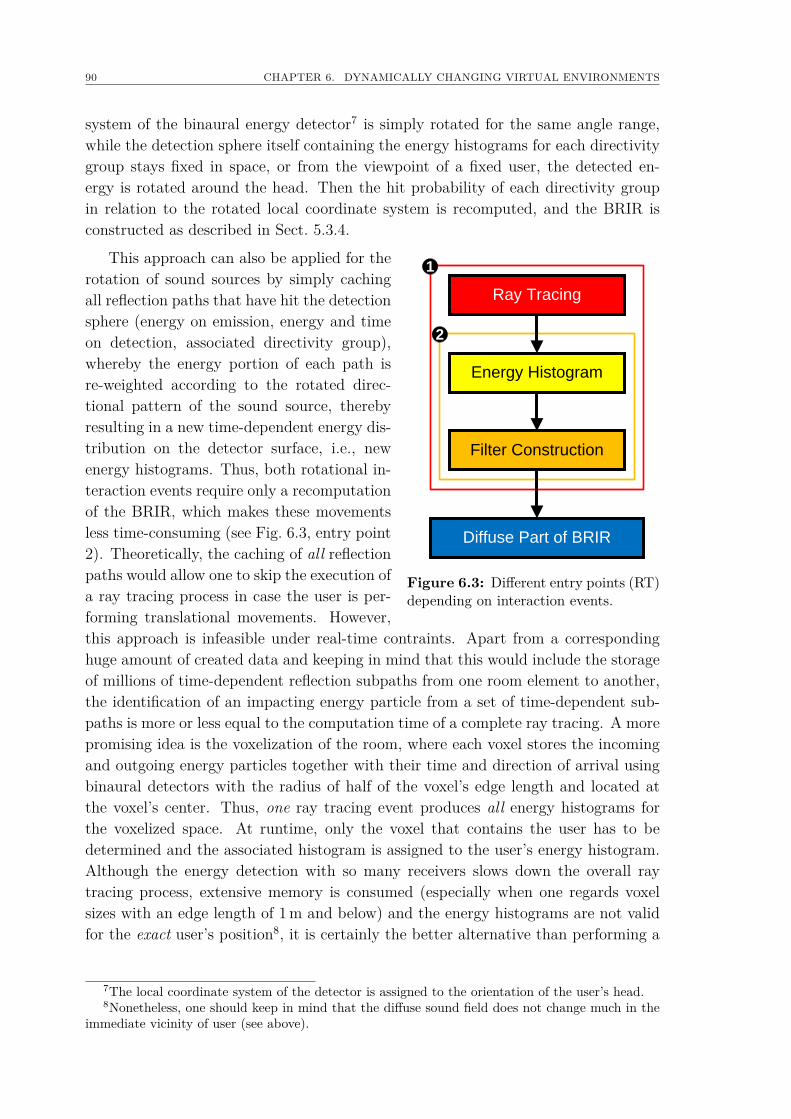
90 CHAPTER 6. DYNAMICALLY CHANGING VIRTUAL ENVIRONMENTS
system of the binaural energy detector7 is simply rotated for the same angle range,while the detection sphere itself containing the energy histograms for each directivitygroup stays fixed in space, or from the viewpoint of a fixed user, the detected en-ergy is rotated around the head. Then the hit probability of each directivity groupin relation to the rotated local coordinate system is recomputed, and the BRIR isconstructed as described in Sect. 5.3.4.
This approach can also be applied for the
Ray Tracing
Energy Histogram
Filter Construction
Diffuse Part of BRIR
3
2
1
Figure 6.3: Different entry points (RT)depending on interaction events.
rotation of sound sources by simply cachingall reflection paths that have hit the detectionsphere (energy on emission, energy and timeon detection, associated directivity group),whereby the energy portion of each path isre-weighted according to the rotated direc-tional pattern of the sound source, therebyresulting in a new time-dependent energy dis-tribution on the detector surface, i.e., newenergy histograms. Thus, both rotational in-teraction events require only a recomputationof the BRIR, which makes these movementsless time-consuming (see Fig. 6.3, entry point2). Theoretically, the caching of all reflectionpaths would allow one to skip the execution ofa ray tracing process in case the user is per-forming translational movements. However,this approach is infeasible under real-time contraints. Apart from a correspondinghuge amount of created data and keeping in mind that this would include the storageof millions of time-dependent reflection subpaths from one room element to another,the identification of an impacting energy particle from a set of time-dependent sub-paths is more or less equal to the computation time of a complete ray tracing. A morepromising idea is the voxelization of the room, where each voxel stores the incomingand outgoing energy particles together with their time and direction of arrival usingbinaural detectors with the radius of half of the voxel’s edge length and located atthe voxel’s center. Thus, one ray tracing event produces all energy histograms forthe voxelized space. At runtime, only the voxel that contains the user has to bedetermined and the associated histogram is assigned to the user’s energy histogram.Although the energy detection with so many receivers slows down the overall raytracing process, extensive memory is consumed (especially when one regards voxelsizes with an edge length of 1m and below) and the energy histograms are not validfor the exact user’s position8, it is certainly the better alternative than performing a
7The local coordinate system of the detector is assigned to the orientation of the user’s head.8Nonetheless, one should keep in mind that the diffuse sound field does not change much in the
immediate vicinity of user (see above).
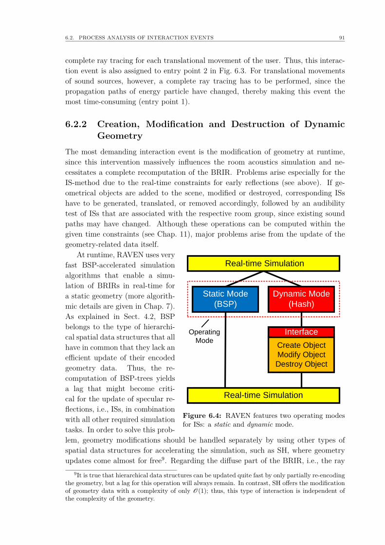
6.2. PROCESS ANALYSIS OF INTERACTION EVENTS 91
complete ray tracing for each translational movement of the user. Thus, this interac-tion event is also assigned to entry point 2 in Fig. 6.3. For translational movementsof sound sources, however, a complete ray tracing has to be performed, since thepropagation paths of energy particle have changed, thereby making this event themost time-consuming (entry point 1).
6.2.2 Creation, Modification and Destruction of DynamicGeometry
The most demanding interaction event is the modification of geometry at runtime,since this intervention massively influences the room acoustics simulation and ne-cessitates a complete recomputation of the BRIR. Problems arise especially for theIS-method due to the real-time constraints for early reflections (see above). If ge-ometrical objects are added to the scene, modified or destroyed, corresponding ISshave to be generated, translated, or removed accordingly, followed by an audibilitytest of ISs that are associated with the respective room group, since existing soundpaths may have changed. Although these operations can be computed within thegiven time constraints (see Chap. 11), major problems arise from the update of thegeometry-related data itself.
At runtime, RAVEN uses very Real-time Simulation
Static Mode
(BSP)
Dynamic Mode
(Hash)
Real-time Simulation
Interface
Create Object
Modify Object
Destroy Object
Operating
Mode
Figure 6.4: RAVEN features two operating modesfor ISs: a static and dynamic mode.
fast BSP-accelerated simulationalgorithms that enable a simu-lation of BRIRs in real-time fora static geometry (more algorith-mic details are given in Chap. 7).As explained in Sect. 4.2, BSPbelongs to the type of hierarchi-cal spatial data structures that allhave in common that they lack anefficient update of their encodedgeometry data. Thus, the re-computation of BSP-trees yieldsa lag that might become criti-cal for the update of specular re-flections, i.e., ISs, in combinationwith all other required simulationtasks. In order to solve this prob-lem, geometry modifications should be handled separately by using other types ofspatial data structures for accelerating the simulation, such as SH, where geometryupdates come almost for free9. Regarding the diffuse part of the BRIR, i.e., the ray
9It is true that hierarchical data structures can be updated quite fast by only partially re-encodingthe geometry, but a lag for this operation will always remain. In contrast, SH offers the modificationof geometry data with a complexity of only O(1); thus, this type of interaction is independent ofthe complexity of the geometry.

92 CHAPTER 6. DYNAMICALLY CHANGING VIRTUAL ENVIRONMENTS
All Image Sources of Room Group
Image Sources
Static Geometry
Image Sources
Dynamic Geometry
Initially
Audible
Initally
Not Audible
Still AudibleBlocked by
Dynamic ObjectAudible Not audible
fewsome
many
Figure 6.5: Logical differentation of ISs that enables an efficient handling of geometry-related modification events. Here, ISs that are associated with the initial static geometryand with dynamic objects are handled individually.
tracing simulations, it is sufficient to update the BSP-tree first and then perform a raytracing, because BSP-accelerated intersection tests will always outperform SH (seeChap. 11). Here, the lag produced by the update of the hierarchical tree structurewill be compensated multiple times, because ray tracing requires millions of inter-section tests more than the IS-method. Therefore, only the special handling of ISsduring modification events will be further described, since ray tracing is always han-dled just straight forward. During a preprocessing step, a static geometrical scene isselected from a database, necessary parameters for the IS-method are defined and therespective ISs are generated. For a convenient handling of ISs during all interactionevents, RAVEN uses hierarchical tree data structures, where all possible IS reflectionpermutations are encoded in that tree (more details are given in Chap. 9). Then,in order to handle the different types of user interaction at runtime, the simulationcan be switched into two operating modes, either in static or dynamic mode (see Fig.6.4). In the default static mode, RAVEN uses fast BSP-accelerated simulation meth-ods that handle all interaction events with a fixed geometry (see previous section).As soon as a geometry-related modification event happens, RAVEN is switched intodynamic mode, where all dynamic geometrical objects are handled separately fromthe static scene. Using the concepts of SH for a fast re-encoding of spatial data, sixbasic operations on dynamic objects are considered in this operating mode: creation,destruction, and manipulation, which includes the translation, the rotation, and thescaling of the object as well as the change of surface materials. It is reasonable todifferentiate between ISs, which were generated in static and dynamic mode, as someinteraction events allow an a priori exclusion of ISs (see Fig. 6.5, orange and lightgreen box). While translational movements of sound sources or user always require anaudibility test on all ISs of the room group, i.e., static and dynamic ISs, a categoriza-tion of ISs into four logical groups yields various advantages if the positions of sound
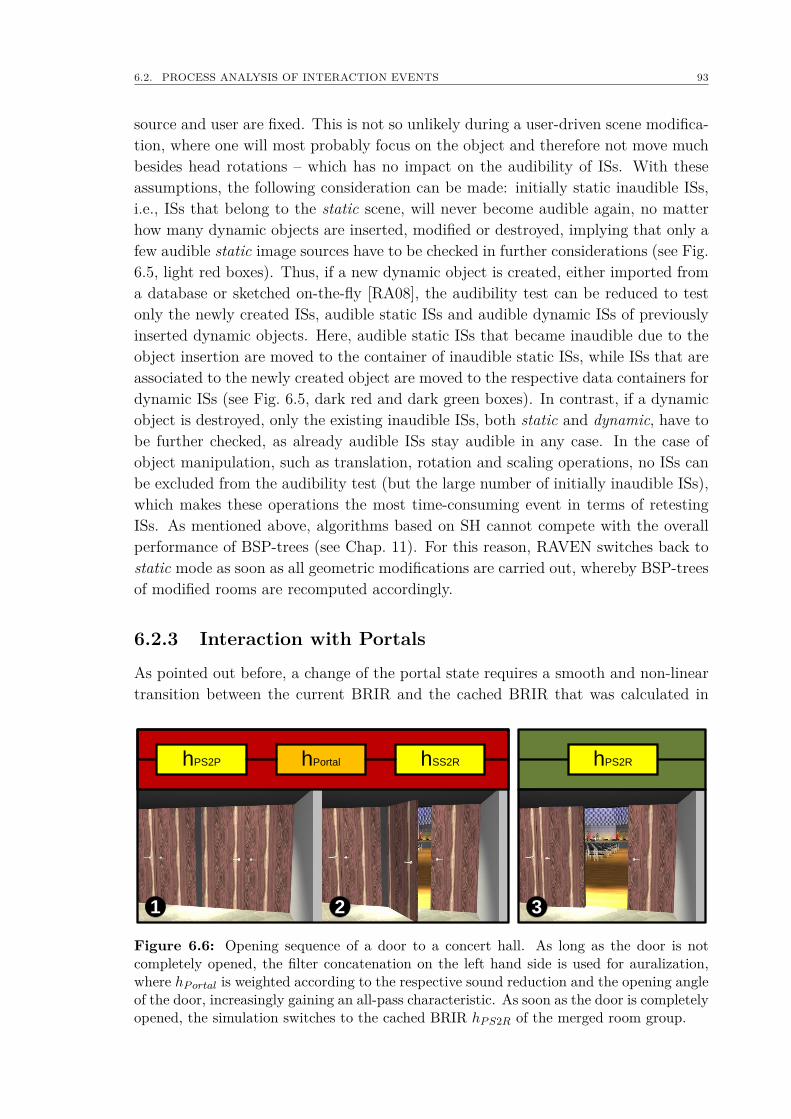
6.2. PROCESS ANALYSIS OF INTERACTION EVENTS 93
source and user are fixed. This is not so unlikely during a user-driven scene modifica-tion, where one will most probably focus on the object and therefore not move muchbesides head rotations – which has no impact on the audibility of ISs. With theseassumptions, the following consideration can be made: initially static inaudible ISs,i.e., ISs that belong to the static scene, will never become audible again, no matterhow many dynamic objects are inserted, modified or destroyed, implying that only afew audible static image sources have to be checked in further considerations (see Fig.6.5, light red boxes). Thus, if a new dynamic object is created, either imported froma database or sketched on-the-fly [RA08], the audibility test can be reduced to testonly the newly created ISs, audible static ISs and audible dynamic ISs of previouslyinserted dynamic objects. Here, audible static ISs that became inaudible due to theobject insertion are moved to the container of inaudible static ISs, while ISs that areassociated to the newly created object are moved to the respective data containers fordynamic ISs (see Fig. 6.5, dark red and dark green boxes). In contrast, if a dynamicobject is destroyed, only the existing inaudible ISs, both static and dynamic, have tobe further checked, as already audible ISs stay audible in any case. In the case ofobject manipulation, such as translation, rotation and scaling operations, no ISs canbe excluded from the audibility test (but the large number of initially inaudible ISs),which makes these operations the most time-consuming event in terms of retestingISs. As mentioned above, algorithms based on SH cannot compete with the overallperformance of BSP-trees (see Chap. 11). For this reason, RAVEN switches back tostatic mode as soon as all geometric modifications are carried out, whereby BSP-treesof modified rooms are recomputed accordingly.
6.2.3 Interaction with Portals
As pointed out before, a change of the portal state requires a smooth and non-lineartransition between the current BRIR and the cached BRIR that was calculated in
hSS2RhPortalhPS2P hPS2R
1 2 3
Figure 6.6: Opening sequence of a door to a concert hall. As long as the door is notcompletely opened, the filter concatenation on the left hand side is used for auralization,where hPortal is weighted according to the respective sound reduction and the opening angleof the door, increasingly gaining an all-pass characteristic. As soon as the door is completelyopened, the simulation switches to the cached BRIR hPS2R of the merged room group.
94 CHAPTER 6. DYNAMICALLY CHANGING VIRTUAL ENVIRONMENTS
parallel for the inversed portal state while the user was approaching the portal. Itwas also shown in Sect. 5.5 that the sound propagation from a primary sound sourceto a receiver, i.e., the user, via a portal can be expressed by a convolution of the RIRhPS2P of the source room with the portal filter hPortal and the BRIR hSS2R of thereceiver room. By contrast, if the portal is opened, the sound propagation from theprimary sound sound source to the receiver is described by the BRIR hPS2R of themerged room groups only. The crucial part now is to crossfade from one BRIR toanother that matches the opening and closing sequence in a natural way, especiallyin cases that are best known from real-world experiences, such as the opening andclosing of a door or a window. Plausible results can be achieved by using n-th rootfunctions, i.e., y(x) = n
√x with x ∈ [0, 1], for weighting the portal’s sound reduction
indices according to the relative aperture angle of the portal. By using this function,the portal’s sound reduction is continuously lowered during an opening sequenceuntil hPortal has gained an all-pass filter characteristic (portal completely opened).However in the opposite case, the sound reduction indices are increased again untilthey have reached their original values (portal completely closed). Figure 6.6 furtherillustrates this approach by the example of an opening sequence of a door. Here,as long as the door is not completely opened, the overall BRIR is described by theconcatenation of three filters, hPS2P , hPortal, and hSS2R, where hPortal is modified asdescribed above (see Fig. 6.6, (1) and (2)). Then, as soon as hPortal has gained the all-pass characteristic, the auralization will sound very similar to the direct convolutionwith hS2R of the merged room group (see Fig. 6.6, (3)) allowing a hard switch to thecached BRIR without any adverse effects [Pel07]. Demonstration videos are availablefor download under www.ravenaudio.de.
6.3 Parallel ComputingThe real-time room acoustical simulation of a dynamic virtual environment that con-tains various rooms and sound sources by far exceeds the computational power ofone CPU-Core. Thus, a parallel computation of single simulation processes has to becarried out in order to meet real-time constraints also for complex situations. Con-cepts for parallel computing are typically divided in two main categories according totheir underlying memory architecture, i.e., either shared or distributed memory. Oneof the main solutions for parallel computing on distributed memory, such as comput-ing clusters, is the Message Passing Interface (MPI) which is a platform-independentcommunication protocol for the data transfer between single processes by passingexplicit messages, e.g., via a high-speed ethernet connection, from one or many com-puters to other computers [MPI08]. The respective counterpart for shared memorymachines, e.g., multi-core PCs, is called Open Multi-Processing (OpenMP). OpenMPallows master threads to open parallel sub-threads following a fork-join strategy forthe parallel execution of computation tasks in order to speed up the processing timeof the overall operation [Ope08]. The idea itself suggests combining both approachesby using a computing cluster with multi-core worker clients that are connected via
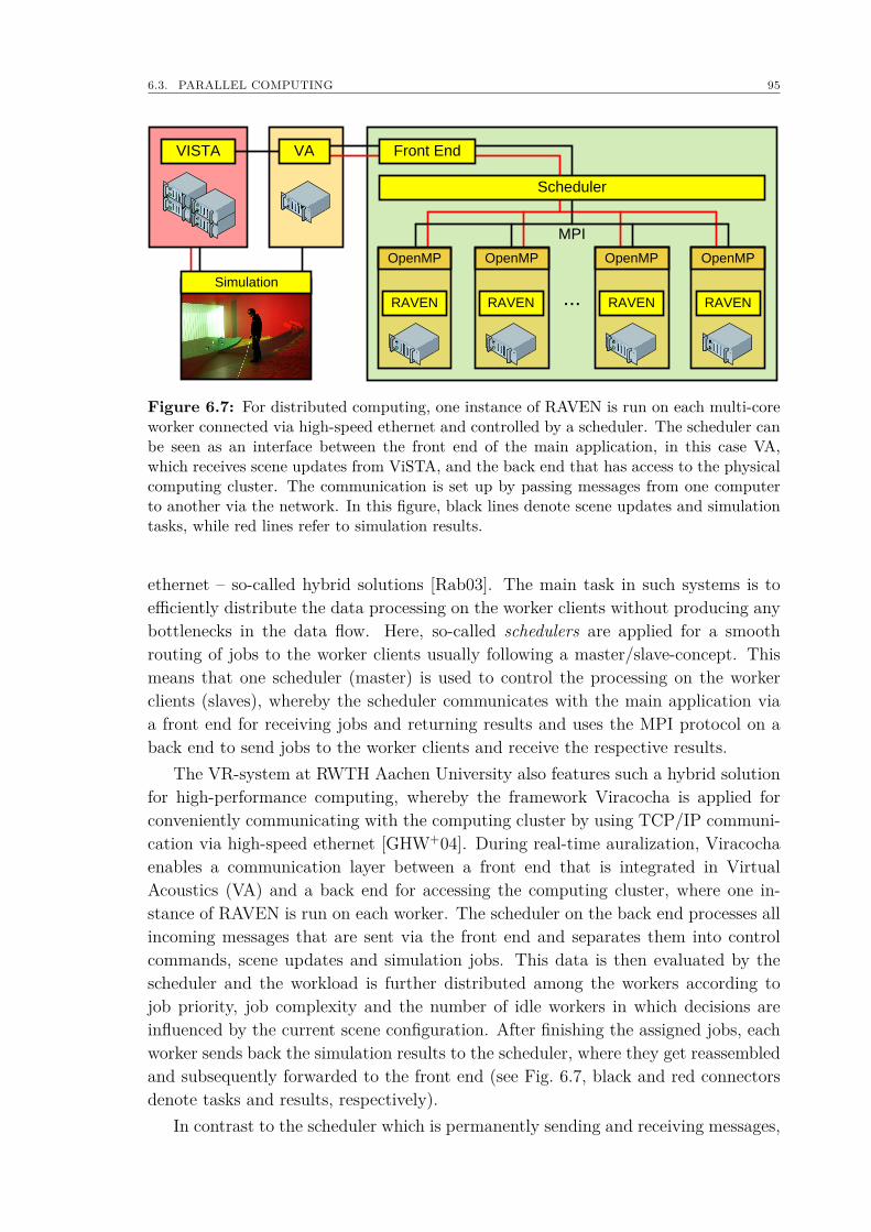
6.3. PARALLEL COMPUTING 95
RAVEN RAVEN RAVEN RAVEN
OpenMP OpenMP OpenMP OpenMP
VISTA
Scheduler
Front EndVA
...
MPI
Simulation
Figure 6.7: For distributed computing, one instance of RAVEN is run on each multi-coreworker connected via high-speed ethernet and controlled by a scheduler. The scheduler canbe seen as an interface between the front end of the main application, in this case VA,which receives scene updates from ViSTA, and the back end that has access to the physicalcomputing cluster. The communication is set up by passing messages from one computerto another via the network. In this figure, black lines denote scene updates and simulationtasks, while red lines refer to simulation results.
ethernet – so-called hybrid solutions [Rab03]. The main task in such systems is toefficiently distribute the data processing on the worker clients without producing anybottlenecks in the data flow. Here, so-called schedulers are applied for a smoothrouting of jobs to the worker clients usually following a master/slave-concept. Thismeans that one scheduler (master) is used to control the processing on the workerclients (slaves), whereby the scheduler communicates with the main application viaa front end for receiving jobs and returning results and uses the MPI protocol on aback end to send jobs to the worker clients and receive the respective results.
The VR-system at RWTH Aachen University also features such a hybrid solutionfor high-performance computing, whereby the framework Viracocha is applied forconveniently communicating with the computing cluster by using TCP/IP communi-cation via high-speed ethernet [GHW+04]. During real-time auralization, Viracochaenables a communication layer between a front end that is integrated in VirtualAcoustics (VA) and a back end for accessing the computing cluster, where one in-stance of RAVEN is run on each worker. The scheduler on the back end processes allincoming messages that are sent via the front end and separates them into controlcommands, scene updates and simulation jobs. This data is then evaluated by thescheduler and the workload is further distributed among the workers according tojob priority, job complexity and the number of idle workers in which decisions areinfluenced by the current scene configuration. After finishing the assigned jobs, eachworker sends back the simulation results to the scheduler, where they get reassembledand subsequently forwarded to the front end (see Fig. 6.7, black and red connectorsdenote tasks and results, respectively).
In contrast to the scheduler which is permanently sending and receiving messages,
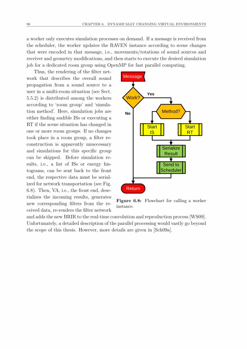
96 CHAPTER 6. DYNAMICALLY CHANGING VIRTUAL ENVIRONMENTS
a worker only executes simulation processes on demand. If a message is received fromthe scheduler, the worker updates the RAVEN instance according to scene changesthat were encoded in that message, i.e., movements/rotations of sound sources andreceiver and geometry modifications, and then starts to execute the desired simulationjob for a dedicated room group using OpenMP for fast parallel computing.
Thus, the rendering of the filter net-
Work?
Start
RT
Send to
Scheduler
Serialize
Result
Start
IS
Return
Message
Method?
Yes
No
Figure 6.8: Flowchart for calling a workerinstance.
work that describes the overall soundpropagation from a sound source to auser in a multi-room situation (see Sect.5.5.2) is distributed among the workersaccording to ‘room group’ and ‘simula-tion method’. Here, simulation jobs areeither finding audible ISs or executing aRT if the scene situation has changed inone or more room groups. If no changestook place in a room group, a filter re-construction is apparently unnecessaryand simulations for this specific groupcan be skipped. Before simulation re-sults, i.e., a list of ISs or energy his-tograms, can be sent back to the frontend, the respective data must be serial-ized for network transportation (see Fig.6.8). Then, VA, i.e., the front end, dese-rializes the incoming results, generatesnew corresponding filters from the re-ceived data, re-renders the filter networkand adds the new BRIR to the real-time convolution and reproduction process [WS09].Unfortunately, a detailed description of the parallel processing would vastly go beyondthe scope of this thesis. However, more details are given in [Sch09a].
Part III
Real-time Implementation

98
Chapter 7
Acceleration ofGeometric Operations
"The first ten million years were the worst, said Marvin, and the secondten million years, they were the worst, too. The third ten million years Ididn’t enjoy at all. After that I went into a bit of a decline."
(The Hitchhiker’s Guide to the Galaxy, Douglas Adams, British writer)
A prerequisite for real-time implementations is the profiling of function calls atruntime in order to identify bottlenecks in the overall simulation process. In methodsof GA, these bottlenecks are usually two basic functions that are called extremelyoften during a room-acoustics simulation: 1) point-in-polygon test and 2) intersectiontests of rays with scene objects, i.e., polygons and detectors. In the following, bothfunction types will be elucidated and concepts for the implementation will be given,while their overall performance is thoroughly discussed in Chap. 11.
7.1 Point-In-Polygon TestEven though there is a wide variety of approaches for an efficient point-in-polygon-test, no approach is the best in all application areas. Whereas some strategies arevery fast, yet only work with a certain type of polygon, others can handle differentkinds of polygons but operate poorly in terms of computing time. In addition, someapproaches use preprocessing information to speed up the algorithms, but use morememory. Others, however, exclusively perform the test during runtime. The mostcommonly known and for general polygons speediest point-in-polygon test is the so-called crossing test [Shi62] which is based on Jordan’s Curve Theorem1. Here, allpolygon’s vertices and the test point P are projected onto one of the xy-, xz-, oryz-planes (see Fig. 7.1(a)), where it is suitable to choose the plane which maximizesthe area of the projected polygon to avoid numerical issues [Gla89]. Then, a ray isshot from the test point’s projection P ′ into an arbitrary direction and the numberof intersections with the projected polygon edges is counted, whereby, as stated by
1Marie Ennemond Camille Jordan, French mathematician, 1838 - 1922.
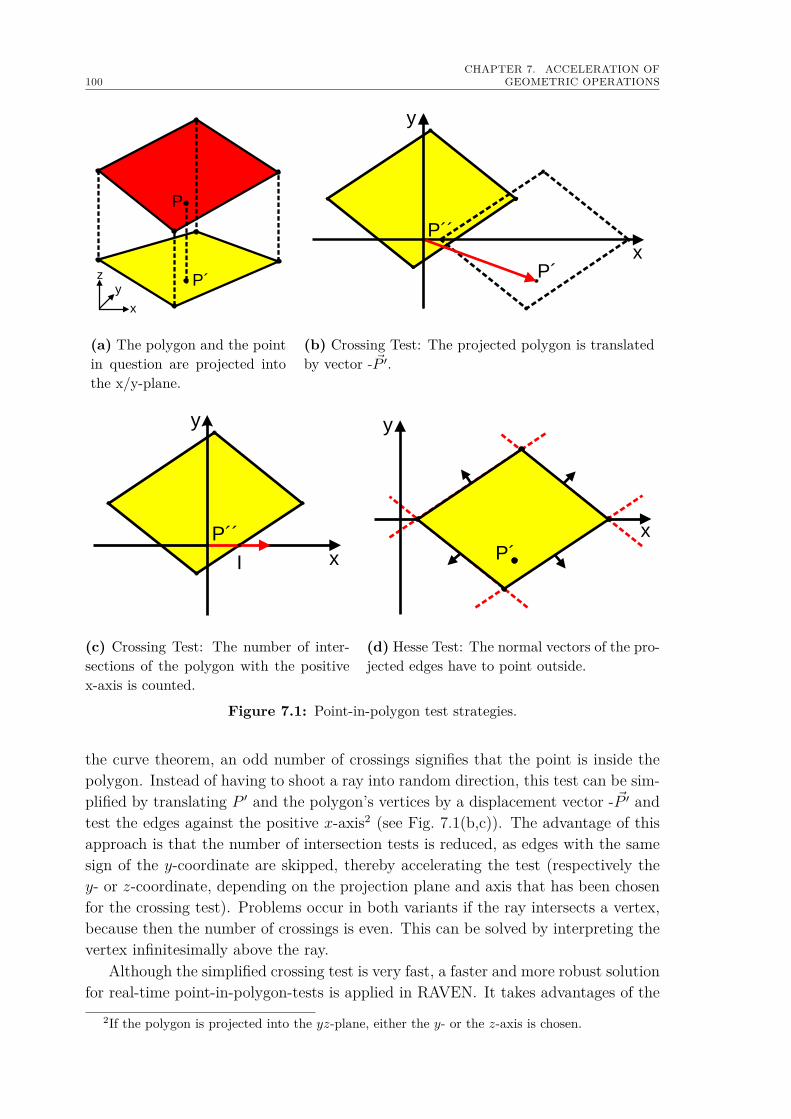
100CHAPTER 7. ACCELERATION OF
GEOMETRIC OPERATIONS
x
yz
P
P´
(a) The polygon and the pointin question are projected intothe x/y-plane.
x
y
P´
P´´
(b) Crossing Test: The projected polygon is translatedby vector - ~P ′.
y
I
P´´
x
(c) Crossing Test: The number of inter-sections of the polygon with the positivex-axis is counted.
x
y
P´
(d) Hesse Test: The normal vectors of the pro-jected edges have to point outside.
Figure 7.1: Point-in-polygon test strategies.
the curve theorem, an odd number of crossings signifies that the point is inside thepolygon. Instead of having to shoot a ray into random direction, this test can be sim-plified by translating P ′ and the polygon’s vertices by a displacement vector - ~P ′ andtest the edges against the positive x-axis2 (see Fig. 7.1(b,c)). The advantage of thisapproach is that the number of intersection tests is reduced, as edges with the samesign of the y-coordinate are skipped, thereby accelerating the test (respectively they- or z-coordinate, depending on the projection plane and axis that has been chosenfor the crossing test). Problems occur in both variants if the ray intersects a vertex,because then the number of crossings is even. This can be solved by interpreting thevertex infinitesimally above the ray.
Although the simplified crossing test is very fast, a faster and more robust solutionfor real-time point-in-polygon-tests is applied in RAVEN. It takes advantages of the
2If the polygon is projected into the yz-plane, either the y- or the z-axis is chosen.
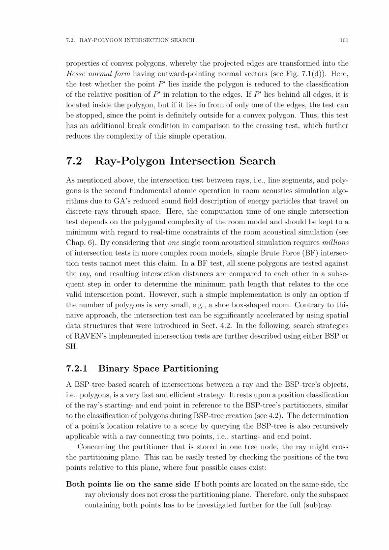
7.2. RAY-POLYGON INTERSECTION SEARCH 101
properties of convex polygons, whereby the projected edges are transformed into theHesse normal form having outward-pointing normal vectors (see Fig. 7.1(d)). Here,the test whether the point P ′ lies inside the polygon is reduced to the classificationof the relative position of P ′ in relation to the edges. If P ′ lies behind all edges, it islocated inside the polygon, but if it lies in front of only one of the edges, the test canbe stopped, since the point is definitely outside for a convex polygon. Thus, this testhas an additional break condition in comparison to the crossing test, which furtherreduces the complexity of this simple operation.
7.2 Ray-Polygon Intersection SearchAs mentioned above, the intersection test between rays, i.e., line segments, and poly-gons is the second fundamental atomic operation in room acoustics simulation algo-rithms due to GA’s reduced sound field description of energy particles that travel ondiscrete rays through space. Here, the computation time of one single intersectiontest depends on the polygonal complexity of the room model and should be kept to aminimum with regard to real-time constraints of the room acoustical simulation (seeChap. 6). By considering that one single room acoustical simulation requires millionsof intersection tests in more complex room models, simple Brute Force (BF) intersec-tion tests cannot meet this claim. In a BF test, all scene polygons are tested againstthe ray, and resulting intersection distances are compared to each other in a subse-quent step in order to determine the minimum path length that relates to the onevalid intersection point. However, such a simple implementation is only an option ifthe number of polygons is very small, e.g., a shoe box-shaped room. Contrary to thisnaive approach, the intersection test can be significantly accelerated by using spatialdata structures that were introduced in Sect. 4.2. In the following, search strategiesof RAVEN’s implemented intersection tests are further described using either BSP orSH.
7.2.1 Binary Space PartitioningA BSP-tree based search of intersections between a ray and the BSP-tree’s objects,i.e., polygons, is a very fast and efficient strategy. It rests upon a position classificationof the ray’s starting- and end point in reference to the BSP-tree’s partitioners, similarto the classification of polygons during BSP-tree creation (see 4.2). The determinationof a point’s location relative to a scene by querying the BSP-tree is also recursivelyapplicable with a ray connecting two points, i.e., starting- and end point.
Concerning the partitioner that is stored in one tree node, the ray might crossthe partitioning plane. This can be easily tested by checking the positions of the twopoints relative to this plane, where four possible cases exist:
Both points lie on the same side If both points are located on the same side, theray obviously does not cross the partitioning plane. Therefore, only the subspacecontaining both points has to be investigated further for the full (sub)ray.
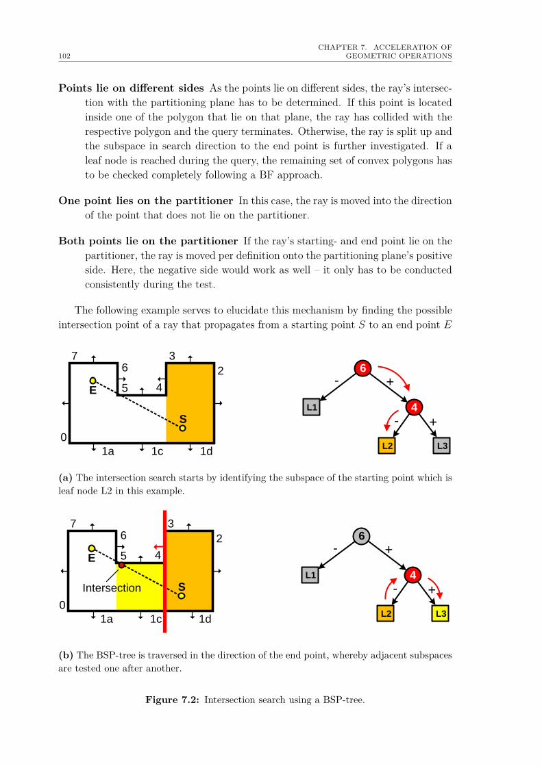
102CHAPTER 7. ACCELERATION OF
GEOMETRIC OPERATIONS
Points lie on different sides As the points lie on different sides, the ray’s intersec-tion with the partitioning plane has to be determined. If this point is locatedinside one of the polygon that lie on that plane, the ray has collided with therespective polygon and the query terminates. Otherwise, the ray is split up andthe subspace in search direction to the end point is further investigated. If aleaf node is reached during the query, the remaining set of convex polygons hasto be checked completely following a BF approach.
One point lies on the partitioner In this case, the ray is moved into the directionof the point that does not lie on the partitioner.
Both points lie on the partitioner If the ray’s starting- and end point lie on thepartitioner, the ray is moved per definition onto the partitioning plane’s positiveside. Here, the negative side would work as well – it only has to be conductedconsistently during the test.
The following example serves to elucidate this mechanism by finding the possibleintersection point of a ray that propagates from a starting point S to an end point E
6
+
+
-
-L1
L2 L3
4
76
0
1a 1c
5 4
3
2
1d
S
E
(a) The intersection search starts by identifying the subspace of the starting point which isleaf node L2 in this example.
6
+
+
-
-L1
L2 L3
4
76
0
1a 1c
5 4
3
2
1d
S
E
Intersection
(b) The BSP-tree is traversed in the direction of the end point, whereby adjacent subspacesare tested one after another.
Figure 7.2: Intersection search using a BSP-tree.
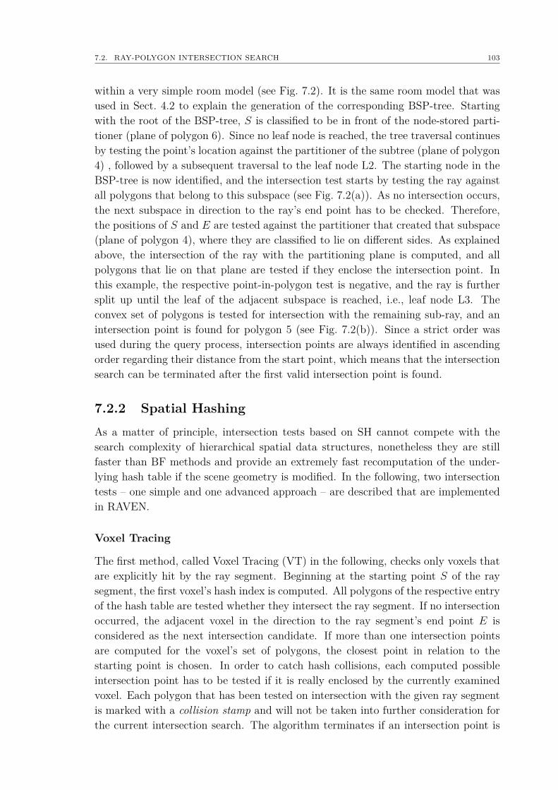
7.2. RAY-POLYGON INTERSECTION SEARCH 103
within a very simple room model (see Fig. 7.2). It is the same room model that wasused in Sect. 4.2 to explain the generation of the corresponding BSP-tree. Startingwith the root of the BSP-tree, S is classified to be in front of the node-stored parti-tioner (plane of polygon 6). Since no leaf node is reached, the tree traversal continuesby testing the point’s location against the partitioner of the subtree (plane of polygon4) , followed by a subsequent traversal to the leaf node L2. The starting node in theBSP-tree is now identified, and the intersection test starts by testing the ray againstall polygons that belong to this subspace (see Fig. 7.2(a)). As no intersection occurs,the next subspace in direction to the ray’s end point has to be checked. Therefore,the positions of S and E are tested against the partitioner that created that subspace(plane of polygon 4), where they are classified to lie on different sides. As explainedabove, the intersection of the ray with the partitioning plane is computed, and allpolygons that lie on that plane are tested if they enclose the intersection point. Inthis example, the respective point-in-polygon test is negative, and the ray is furthersplit up until the leaf of the adjacent subspace is reached, i.e., leaf node L3. Theconvex set of polygons is tested for intersection with the remaining sub-ray, and anintersection point is found for polygon 5 (see Fig. 7.2(b)). Since a strict order wasused during the query process, intersection points are always identified in ascendingorder regarding their distance from the start point, which means that the intersectionsearch can be terminated after the first valid intersection point is found.
7.2.2 Spatial HashingAs a matter of principle, intersection tests based on SH cannot compete with thesearch complexity of hierarchical spatial data structures, nonetheless they are stillfaster than BF methods and provide an extremely fast recomputation of the under-lying hash table if the scene geometry is modified. In the following, two intersectiontests – one simple and one advanced approach – are described that are implementedin RAVEN.
Voxel Tracing
The first method, called Voxel Tracing (VT) in the following, checks only voxels thatare explicitly hit by the ray segment. Beginning at the starting point S of the raysegment, the first voxel’s hash index is computed. All polygons of the respective entryof the hash table are tested whether they intersect the ray segment. If no intersectionoccurred, the adjacent voxel in the direction to the ray segment’s end point E isconsidered as the next intersection candidate. If more than one intersection pointsare computed for the voxel’s set of polygons, the closest point in relation to thestarting point is chosen. In order to catch hash collisions, each computed possibleintersection point has to be tested if it is really enclosed by the currently examinedvoxel. Each polygon that has been tested on intersection with the given ray segmentis marked with a collision stamp and will not be taken into further consideration forthe current intersection search. The algorithm terminates if an intersection point is
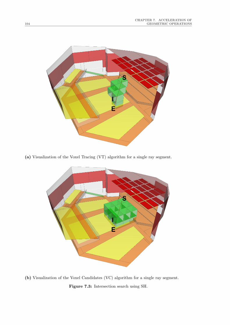
104CHAPTER 7. ACCELERATION OF
GEOMETRIC OPERATIONS
(a) Visualization of the Voxel Tracing (VT) algorithm for a single ray segment.
(b) Visualization of the Voxel Candidates (VC) algorithm for a single ray segment.
Figure 7.3: Intersection search using SH.
7.3. COLLISION TESTS 105
found or the end point of the ray segment is reached. The concept is illustrated inFig. 7.3(a).
Voxel Candidates
The second applied method, the so-called Voxel Candidates (VC), uses no smarttraversal of single voxels. Instead, all voxels that are enclosed by or intersect with theray segment’s AABB are regarded as possible intersection candidates. In a next step,an intersection test with all candidates, i.e., polygons that are stored in the respectivevoxels, is carried out and returns the intersection point with the closest distance tothe ray segment’s starting point (see Fig. 7.3(b)). Similar to VT, each tested polygonacquires a collision stamp to avoid multiple testing of the same candidate. A polygonis usually stored in more than one voxel, whereby the total number depends on thevoxel size. The advantage of this approach is that hash collisions can be neglected.It is sufficient to check in a final test if the identified intersection point is enclosed bythe ray segment’s AABB, which is a fast and simple operation. On the other hand,the identification of intersection candidates is quite rough and probably leads to ahigher number of intersection tests.
7.3 Collision TestsFor further considerations, it should be noted that in the current implementation thedetailed geometry of spherical and cylindrical detectors is not added to the geometricalscene but is handled separately for three reasons:
Virtual Objects Logically, the shape of volume detectors does not belong to thephysical scene, since they refer only to points (receiver positions) or line seg-ments (edges).
Accuracy Intersection tests on detectors with curved surfaces would be too rough,since their geometrical scene representation must be heavily approximated toavoid an explosion of the overall polygon count.
Re-computations A separate handling avoids re-computations of the rooms’ un-derlying spatial data structures each time a detector is moved.
This also means that intersection tests between rays and the scene geometry that areexecuted at any case during the RT simulation, do not return whether one or moredetectors were hit. Thus, this has to be investigated in an additional step. Fortu-nately, only a qualitative intersection test is required in many algorithmic situationsthat relate to detectors, whereby it is sufficient to determine whether the ray col-lides with the detector without the need of detailed knowledge about the intersectionpoints’ positions (e.g., to decide whether the diffuse rain has to be triggered for adetector). In addition, these tests can be efficiently reduced by adding information
106CHAPTER 7. ACCELERATION OF
GEOMETRIC OPERATIONS
about essential detector points, such as corner points and centroids, to the under-lying spatial data structures and, thus, checking only detectors that lie within thesubspaces between the ray’s starting and end point3. In the following, only quickcollision tests for spherical and cylindrical detectors will be further described, sincethis information comes directly from the ray intersection test with the geometricalscene for plane detectors, i.e., portals. More information regarding efficiently com-puting relations between geometrical objects can be found in series such as AndrewGlassner’s Graphics Gems series [Gla93, Arv91, Kir92, Hec94, Pae95].
Spherical Detectors
The test whether a ray collides with a spherical detector can be reduced to a 2Dproblem by spanning a plane that is defined through the direction vector ~b of theray and the connection vector ~a between the ray’s starting point S and the sphere’scentroid C. The intersection area of a sphere with a plane that goes through thecentroid is always a circle with the same radius r as the sphere, which is depictedin Fig. 7.4(a). The closest point P on the ray segment between the starting point Sand the end point E to the centroid C is along a perpendicular ~d from C to the ray’sdirection vector ~b, which can be described by
P = ~S + u·~b with ~b ~d = 0, ~b = E − S and ~d = C − P. (7.1)
The shifting factor u is easy to compute by substituting one equation into the other,which results in
u = ~a ~b~b ~b
, (7.2)
where ~a is the connection vector between C and S. The last step of this test is tocompare the length d of ~d against the radius of the sphere: if r is smaller than d, acollision of the ray with the sphere is impossible. An additional testing if the pointP lies in between S and E (0 ≤ u ≤ 1) can be omitted, since rays travel from surfaceto surface and detectors will always be located in between.
Cylindrical Detectors
In the case of cylindrical detectors, the collision test can also be expressed by verysimple geometrical operations. In the following, the same vector notation is used asin the previous test with SE, whereby ~sE and ~e additionally denote the cylinder’sstarting point, the connection vector between S and SE, and the direction vector ofthe cylinder’s axis , i.e., the edge (see Fig. 7.4(b)). At first, the normalized normalvector ~n of a plane that is spanned by ~e and ~b is computed with
~n = ~e×~b with ~n = ~n
|~n|. (7.3)
3In this case, the term ray is literally incorrect, as it has no end point per definition. In indoorscenarios, however, a ray is always reduced to a line segment.
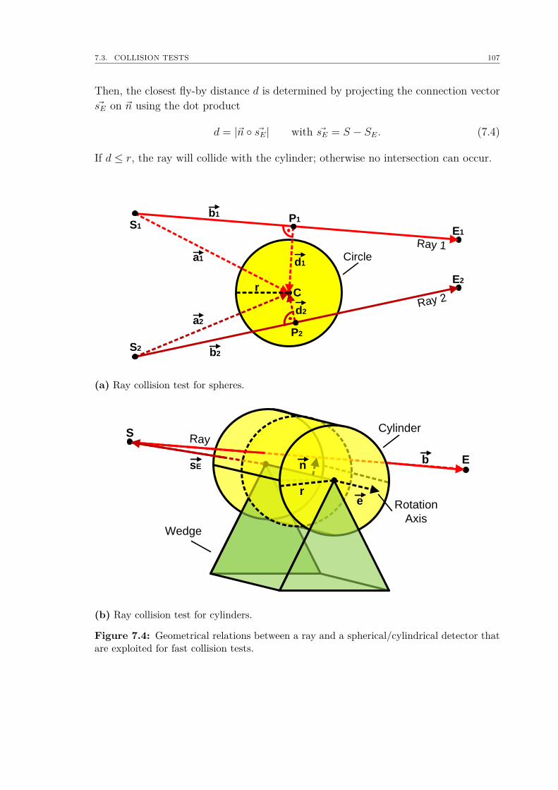
7.3. COLLISION TESTS 107
Then, the closest fly-by distance d is determined by projecting the connection vector~sE on ~n using the dot product
d = |~n ~sE| with ~sE = S − SE. (7.4)
If d ≤ r, the ray will collide with the cylinder; otherwise no intersection can occur.
Ray 1
Ray 2
d1
d2
a1
a2
S1
S2
C
E1
E2
P1
P2
Circle
r
b1
b2
(a) Ray collision test for spheres.
RayS
E
Cylinder
re
bnsE
Wedge
Rotation
Axis
(b) Ray collision test for cylinders.
Figure 7.4: Geometrical relations between a ray and a spherical/cylindrical detector thatare exploited for fast collision tests.

108CHAPTER 7. ACCELERATION OF
GEOMETRIC OPERATIONS
Chapter 8
Efficient Handling of ComplexDynamic Sceneries
"A set is a Many that allows itself to be thought of as a One."
(Infinity and the Mind, Rudolf von Bitter Rucker, American writer)
In multi-room environments, user interaction with portals will always result ina change of connected room groups. Therefore, concepts for a fast handling of suchstate changes are required, whereby the underlying simulation model has already beendescribed in Sect. 4.3. Here, a major prerequisite is to keep computation times to aminimum by avoiding simulations of redundant and unnecessary sound propagationpaths from a sound source to a receiver across the changed scene. In the following,implementation details will be given that offer a smart processing of such simulationsby taking into account physical attributes of the scene during the determination ofup-to-date propagation paths.
8.1 Tracking of Sound PathsAs already introduced in Sect. 4.3 and Sect. 5.5, the Acoustic Scene Graph (ASG) isthe groundwork for an efficient handling of the room acoustics simulation in multi-room scenarios. In summary, each room is represented by one scene node whichis interconnected to other nodes via bidirectional edges, called portals since theyrepresent not only a logical concatenation but also a physical surface between twoadjacent rooms such as doors or windows. An ASG can be implemented fairly easyby using basically two classes representing either a scene node or a portal. All scenenodes store instances of their respective portals, where the number of portals perscene node may be theoretically unlimited. Each portal saves two room IDs: (1)the room ID where it originates from, and (2) the room ID where it connects to. Inaddition, each portal also saves a pointer to the corresponding counter-portal of theadjacent room which connects the same scene nodes in the opposite direction. Thisyields the possibility to freely traverse this connected graph and, thus, use a multitudeof search algorithms to find propagation paths across the scenery in the case that the
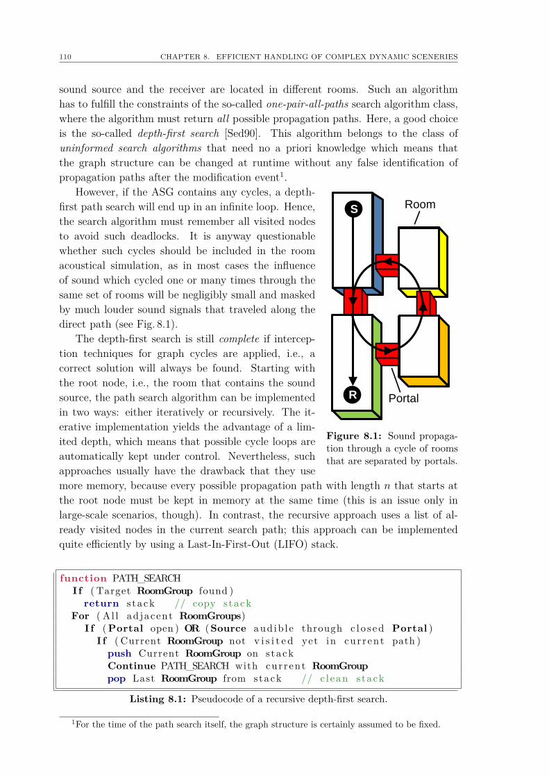
110 CHAPTER 8. EFFICIENT HANDLING OF COMPLEX DYNAMIC SCENERIES
sound source and the receiver are located in different rooms. Such an algorithmhas to fulfill the constraints of the so-called one-pair-all-paths search algorithm class,where the algorithm must return all possible propagation paths. Here, a good choiceis the so-called depth-first search [Sed90]. This algorithm belongs to the class ofuninformed search algorithms that need no a priori knowledge which means thatthe graph structure can be changed at runtime without any false identification ofpropagation paths after the modification event1.
However, if the ASG contains any cycles, a depth-
S
R
Room
Portal
Figure 8.1: Sound propaga-tion through a cycle of roomsthat are separated by portals.
first path search will end up in an infinite loop. Hence,the search algorithm must remember all visited nodesto avoid such deadlocks. It is anyway questionablewhether such cycles should be included in the roomacoustical simulation, as in most cases the influenceof sound which cycled one or many times through thesame set of rooms will be negligibly small and maskedby much louder sound signals that traveled along thedirect path (see Fig. 8.1).
The depth-first search is still complete if intercep-tion techniques for graph cycles are applied, i.e., acorrect solution will always be found. Starting withthe root node, i.e., the room that contains the soundsource, the path search algorithm can be implementedin two ways: either iteratively or recursively. The it-erative implementation yields the advantage of a lim-ited depth, which means that possible cycle loops areautomatically kept under control. Nevertheless, suchapproaches usually have the drawback that they usemore memory, because every possible propagation path with length n that starts atthe root node must be kept in memory at the same time (this is an issue only inlarge-scale scenarios, though). In contrast, the recursive approach uses a list of al-ready visited nodes in the current search path; this approach can be implementedquite efficiently by using a Last-In-First-Out (LIFO) stack.
function PATH_SEARCHI f ( Target RoomGroup found )
return s tack // copy stackFor ( Al l ad jacent RoomGroups)
I f (Portal open ) OR (Source aud ib l e through c l o s ed Portal )I f ( Current RoomGroup not v i s i t e d yet in cur rent path )
push Current RoomGroup on stackContinue PATH_SEARCH with cur rent RoomGrouppop Last RoomGroup from stack // c l ean stack
Listing 8.1: Pseudocode of a recursive depth-first search.
1For the time of the path search itself, the graph structure is certainly assumed to be fixed.
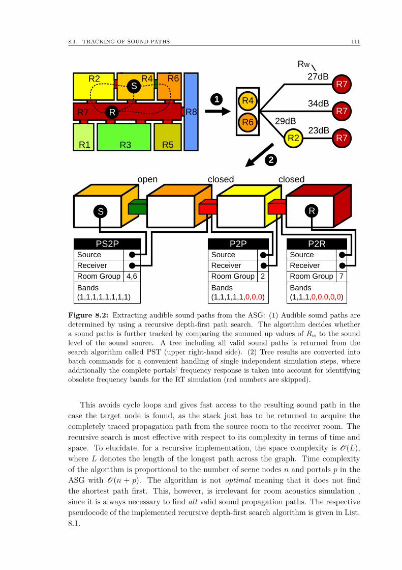
8.1. TRACKING OF SOUND PATHS 111
R2 R4 R6
R5R1 R3
S
R7 R R8
R4
R6 29dB
34dB
27dB
23dBR2
R7
R7
R7
Rw
1
2
PS2P P2P P2R
R
open closed closed
Bands
(1,1,1,1,1,0,0,0)
Room Group
Receiver
Source
2
Bands
(1,1,1,1,1,1,1,1)
Room Group
Receiver
Source
4,6
Bands
(1,1,1,0,0,0,0,0)
Room Group
Receiver
Source
7
S
Figure 8.2: Extracting audible sound paths from the ASG: (1) Audible sound paths aredetermined by using a recursive depth-first path search. The algorithm decides whethera sound paths is further tracked by comparing the summed up values of Rw to the soundlevel of the sound source. A tree including all valid sound paths is returned from thesearch algorithm called PST (upper right-hand side). (2) Tree results are converted intobatch commands for a convenient handling of single independent simulation steps, whereadditionally the complete portals’ frequency response is taken into account for identifyingobsolete frequency bands for the RT simulation (red numbers are skipped).
This avoids cycle loops and gives fast access to the resulting sound path in thecase the target node is found, as the stack just has to be returned to acquire thecompletely traced propagation path from the source room to the receiver room. Therecursive search is most effective with respect to its complexity in terms of time andspace. To elucidate, for a recursive implementation, the space complexity is O(L),where L denotes the length of the longest path across the graph. Time complexityof the algorithm is proportional to the number of scene nodes n and portals p in theASG with O(n + p). The algorithm is not optimal meaning that it does not findthe shortest path first. This, however, is irrelevant for room acoustics simulation ,since it is always necessary to find all valid sound propagation paths. The respectivepseudocode of the implemented recursive depth-first search algorithm is given in List.8.1.
112 CHAPTER 8. EFFICIENT HANDLING OF COMPLEX DYNAMIC SCENERIES
The depth-first search always results in a hierarchical Path Search Tree (PST)which is depicted in Fig. 8.2 (step 1) for the same scene example that was given inSect. 5.5, except that the portal between room R4 and R6 is now opened. The root ofthe PST relates to the room group which contains the sound source, while leaf nodesrefer to the receiver’s room group and child nodes are assigned to the traversed roomgroups in between the source and receiver. All nodes, except the root node, mayappear multiple times in the PST, since sound can travel on various paths throughthe same room group via different portals. As one can see from the pseudocode above,the path search is already tweaked by checking the audibility of the current soundsource. For this test, the sound reduction index Rw of the corresponding portals istaken into account in order to terminate path searches for branches where the summedup total insulation exceeds the sound level of the sound source (shown values in Fig.8.2 are only exemplary). For RT, this concept of source elimination is further refinedby additionally regarding the detailed frequency response of the portal, i.e., of thecorresponding constructional element. In many cases, such elements feature a low-pass characteristic, meaning that higher frequencies will probably be inaudible after asingle element is passed, while lower frequencies will most-likely cross several of them.Not only does the refined path search exclude inaudible sources but it also excludesfrequency bands of audible sources. Hence, the RT simulation of sound sources thatare not located in the receiver room group can be reduced to the simulation of onlysome frequency bands; this obviously reduces the computational effort significantly.This is further illustrated in Fig. 8.2 (step 2) for the propagation path that includestwo portals. Here, only the three remaining frequency bands have to be simulated,since all other bands are completely damped by the portals that are included in thecorresponding propagation path. From this it follows that the path search resultscan be seen as a specification for triggering the room acoustics simulations, wherebyidentical subpaths are skipped. Therefore, an appropriate and handy-to-use datastructure for describing each single simulation step has to be defined, which goesalong with the extracted data from the path search:struct simStep
int type ; // type o f sub pathvoid∗ source , r e c e i v e r ; // po in t e r to source / r e c e i v e rl i s t <SceneNode∗> roomGroup ; // l i s t o f invo lved scene nodesl i s t <int> frequencyBands ; // l i s t o f invo lved f requency bands
Using this data structure, a complete propagation path consists of a list of suchsimulation steps, whereby each entry contains the type of simulation (PS2R: PS toReceiver, PS2P: PS to Portal, SS2R: SS to Receiver, SS2P: SS to Portal, see Sect.5.5), pointers to the sender (PS orSS) and receiver (listener or portal), pointers tothe room group’s scene nodes, and a list of all involved frequency band IDs, withstruct soundPath
l i s t <simStep> subPaths ; // l i s t o f invo lved s imu la t i on s t ep s
whereby each simulation step is independent from the others. This infers that thesimulation scheduler does not have to follow a certain order of path propagation.

8.2. THE PATH PROPAGATION TREE 113
R4
R6
R2
R7
R7
R7 R
P
S
R7R4, R6
R2
PS2P SS2RSS2P
P
BinauralMonauralP
P
Figure 8.3: Transformation of the PST, resulting from the recursive depth-first search,into a directed acyclic PPG.
8.2 The Path Propagation TreeAfter all simulations are carried out, the PST is further processed in order to extracta blueprint for a filtering network that simulates the sound propagation from the PSto the listener: the so-called Path Propagation Tree (PPG) as was already introducedin Sect. 5.5. The computation of this directed acyclic graph from a PST is fairly easy,because the PPG already contains all necessary data that are needed for constructingthe corresponding filter network. This conversion is conducted in four steps: First,the PST’s root node is replaced by a source node S which represents the PS. Second,all edges of the PST are replaced by nodes that represent their respective portalfilters. Third, all nodes of the PST are substituted by edges that represent the soundpropagation between two points, i.e., the simulated RIRs. And fourth, all leaf nodesof the PST are merged to a single summation point R, representing the receiver (anexample is given in Fig. 8.3). Although the PPG is actually just a twisted version ofthe PST, it offers a more transparent description of the filter concatenation, whichis of major importance for the real-time convolution of the complete filter network[WS09, WSPV09].

114 CHAPTER 8. EFFICIENT HANDLING OF COMPLEX DYNAMIC SCENERIES
Chapter 9
Real-time Implementation of RoomAcoustics Simulation Methods
"Of course I’m sane, when trees start talking to me, I don’t talk back."
(The Light Fantastic, Terry Pratchet, British writer)
Properly identifying simulation events and their respective input data is a basicrequirement in almost any real-time application in order to avoid unnecessary compu-tational overheads. This includes not only a logical separation of simulations eventsinto single processes (see Chap. 5 and Chap. 6), but also an optimized storage andhandling of data in terms of accessibility, demand, efficiency, and transparency. How-ever, a complete description of all implementation details and tweaks that are appliedin RAVEN is infeasible within the scope of this thesis, especially when keeping in mindthat today, RAVEN has grown to roughly 70000 thousand lines of code. Therefore,only the most important details for both the IS method and RT will be further re-garded that have the biggest impact on the overall implementation concept. Nonethe-less, detailed descriptions can be found in [Sle04, Dro06, Pel07, Poh08, Ryb09].
9.1 Real-time Implementation of the ImageSource Method
In this section, several implementation concepts for the use with ISs are describedthat offer three fundamental advantages: first, a significant reduction in the overallnumber of ISs is gained for the processing of a single simulation step. Second, aconvenient handling of relationships between ISs is acquired by organizing all ISsin so-called Image Source Trees (ISTs) that support a fast expansion, update anddestruction of tree nodes, i.e., ISs, which is basic necessity during modification eventsof the geometry. And third, concepts for the determination whether specific sceneobjects are visible from a certain position are introduced by the example of a tree-likedata structure. This tree describes the visibility of edges among each other in orderto further exclude scene elements from the simulation.
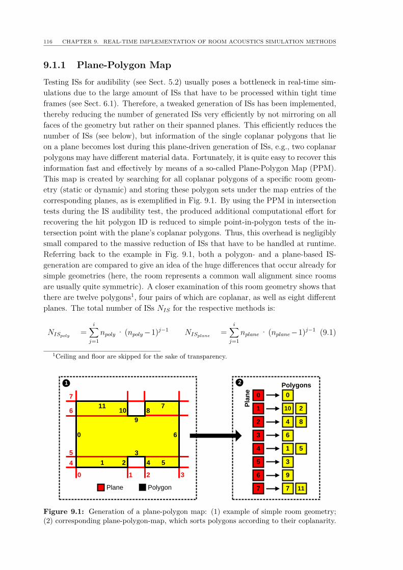
116 CHAPTER 9. REAL-TIME IMPLEMENTATION OF ROOM ACOUSTICS SIMULATION METHODS
9.1.1 Plane-Polygon MapTesting ISs for audibility (see Sect. 5.2) usually poses a bottleneck in real-time sim-ulations due to the large amount of ISs that have to be processed within tight timeframes (see Sect. 6.1). Therefore, a tweaked generation of ISs has been implemented,thereby reducing the number of generated ISs very efficiently by not mirroring on allfaces of the geometry but rather on their spanned planes. This efficiently reduces thenumber of ISs (see below), but information of the single coplanar polygons that lieon a plane becomes lost during this plane-driven generation of ISs, e.g., two coplanarpolygons may have different material data. Fortunately, it is quite easy to recover thisinformation fast and effectively by means of a so-called Plane-Polygon Map (PPM).This map is created by searching for all coplanar polygons of a specific room geom-etry (static or dynamic) and storing these polygon sets under the map entries of thecorresponding planes, as is exemplified in Fig. 9.1. By using the PPM in intersectiontests during the IS audibility test, the produced additional computational effort forrecovering the hit polygon ID is reduced to simple point-in-polygon tests of the in-tersection point with the plane’s coplanar polygons. Thus, this overhead is negligiblysmall compared to the massive reduction of ISs that have to be handled at runtime.Referring back to the example in Fig. 9.1, both a polygon- and a plane-based IS-generation are compared to give an idea of the huge differences that occur already forsimple geometries (here, the room represents a common wall alignment since roomsare usually quite symmetric). A closer examination of this room geometry shows thatthere are twelve polygons1, four pairs of which are coplanar, as well as eight differentplanes. The total number of ISs NIS for the respective methods is:
NISpoly=
i∑j=1
npoly · (npoly−1)j−1 NISplane=
i∑j=1
nplane · (nplane−1)j−1 (9.1)
1Ceiling and floor are skipped for the sake of transparency.
Plane Polygon
30 1 2
4
5
6
7
1110
9
87
6
54
3
21
0
0 0
1
2 4
3 6
4 1
5 3
6 9
7 7
210
8
5
11
Pla
ne
Polygons1 2
Figure 9.1: Generation of a plane-polygon map: (1) example of simple room geometry;(2) corresponding plane-polygon-map, which sorts polygons according to their coplanarity.
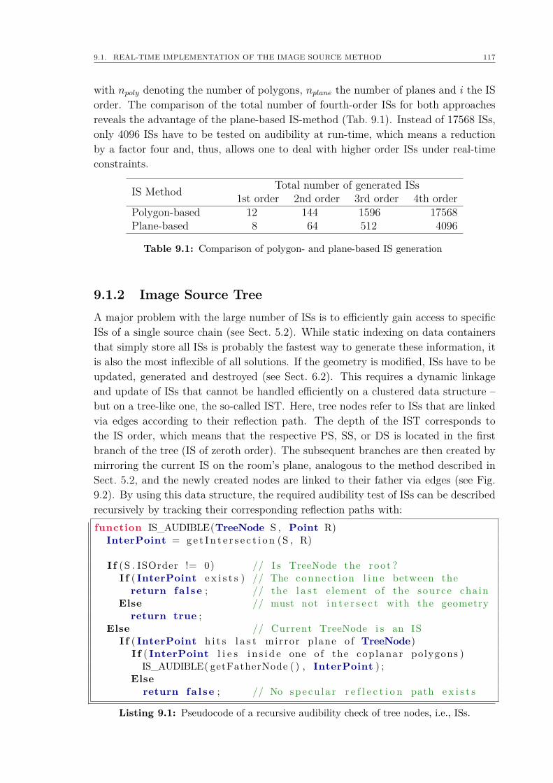
9.1. REAL-TIME IMPLEMENTATION OF THE IMAGE SOURCE METHOD 117
with npoly denoting the number of polygons, nplane the number of planes and i the ISorder. The comparison of the total number of fourth-order ISs for both approachesreveals the advantage of the plane-based IS-method (Tab. 9.1). Instead of 17568 ISs,only 4096 ISs have to be tested on audibility at run-time, which means a reductionby a factor four and, thus, allows one to deal with higher order ISs under real-timeconstraints.
IS Method Total number of generated ISs1st order 2nd order 3rd order 4th order
Polygon-based 12 144 1596 17568Plane-based 8 64 512 4096
Table 9.1: Comparison of polygon- and plane-based IS generation
9.1.2 Image Source TreeA major problem with the large number of ISs is to efficiently gain access to specificISs of a single source chain (see Sect. 5.2). While static indexing on data containersthat simply store all ISs is probably the fastest way to generate these information, itis also the most inflexible of all solutions. If the geometry is modified, ISs have to beupdated, generated and destroyed (see Sect. 6.2). This requires a dynamic linkageand update of ISs that cannot be handled efficiently on a clustered data structure –but on a tree-like one, the so-called IST. Here, tree nodes refer to ISs that are linkedvia edges according to their reflection path. The depth of the IST corresponds tothe IS order, which means that the respective PS, SS, or DS is located in the firstbranch of the tree (IS of zeroth order). The subsequent branches are then created bymirroring the current IS on the room’s plane, analogous to the method described inSect. 5.2, and the newly created nodes are linked to their father via edges (see Fig.9.2). By using this data structure, the required audibility test of ISs can be describedrecursively by tracking their corresponding reflection paths with:function IS_AUDIBLE(TreeNode S , Point R)
InterPoint = ge t I n t e r s e c t i o n (S , R)
I f (S . ISOrder != 0) // I s TreeNode the root ?I f ( InterPoint e x i s t s ) // The connect ion l i n e between the
return fa l se ; // the l a s t element o f the source chainElse // must not i n t e r s e c t with the geometry
return true ;Else // Current TreeNode i s an IS
I f ( InterPoint h i t s l a s t mirror plane o f TreeNode)I f ( InterPoint l i e s i n s i d e one o f the coplanar polygons )
IS_AUDIBLE( getFatherNode ( ) , InterPoint ) ;Else
return fa l se ; // No specu l a r r e f l e c t i o n path e x i s t s
Listing 9.1: Pseudocode of a recursive audibility check of tree nodes, i.e., ISs.
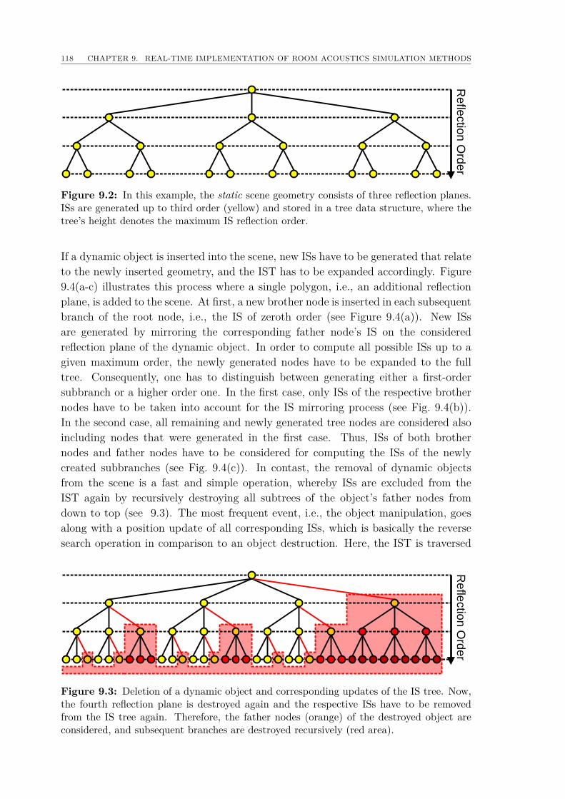
118 CHAPTER 9. REAL-TIME IMPLEMENTATION OF ROOM ACOUSTICS SIMULATION METHODS
Re
flectio
n O
rde
r
Figure 9.2: In this example, the static scene geometry consists of three reflection planes.ISs are generated up to third order (yellow) and stored in a tree data structure, where thetree’s height denotes the maximum IS reflection order.
If a dynamic object is inserted into the scene, new ISs have to be generated that relateto the newly inserted geometry, and the IST has to be expanded accordingly. Figure9.4(a-c) illustrates this process where a single polygon, i.e., an additional reflectionplane, is added to the scene. At first, a new brother node is inserted in each subsequentbranch of the root node, i.e., the IS of zeroth order (see Figure 9.4(a)). New ISsare generated by mirroring the corresponding father node’s IS on the consideredreflection plane of the dynamic object. In order to compute all possible ISs up to agiven maximum order, the newly generated nodes have to be expanded to the fulltree. Consequently, one has to distinguish between generating either a first-ordersubbranch or a higher order one. In the first case, only ISs of the respective brothernodes have to be taken into account for the IS mirroring process (see Fig. 9.4(b)).In the second case, all remaining and newly generated tree nodes are considered alsoincluding nodes that were generated in the first case. Thus, ISs of both brothernodes and father nodes have to be considered for computing the ISs of the newlycreated subbranches (see Fig. 9.4(c)). In contast, the removal of dynamic objectsfrom the scene is a fast and simple operation, whereby ISs are excluded from theIST again by recursively destroying all subtrees of the object’s father nodes fromdown to top (see 9.3). The most frequent event, i.e., the object manipulation, goesalong with a position update of all corresponding ISs, which is basically the reversesearch operation in comparison to an object destruction. Here, the IST is traversed
Re
flectio
n O
rde
r
Figure 9.3: Deletion of a dynamic object and corresponding updates of the IS tree. Now,the fourth reflection plane is destroyed again and the respective ISs have to be removedfrom the IS tree again. Therefore, the father nodes (orange) of the destroyed object areconsidered, and subsequent branches are destroyed recursively (red area).
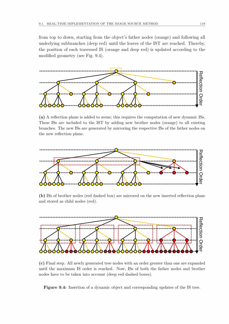
9.1. REAL-TIME IMPLEMENTATION OF THE IMAGE SOURCE METHOD 119
from top to down, starting from the object’s father nodes (orange) and following allunderlying subbranches (deep red) until the leaves of the IST are reached. Thereby,the position of each traversed IS (orange and deep red) is updated according to themodified geometry (see Fig. 9.4).
Re
flectio
n O
rde
r
(a) A reflection plane is added to scene; this requires the computation of new dynamic ISs.These ISs are included to the IST by adding new brother nodes (orange) to all existingbranches. The new ISs are generated by mirroring the respective ISs of the father nodes onthe new reflection plane.
Re
flectio
n O
rde
r
(b) ISs of brother nodes (red dashed box) are mirrored on the new inserted reflection planeand stored as child nodes (red).
Re
flectio
n O
rde
r
(c) Final step. All newly generated tree nodes with an order greater than one are expandeduntil the maximum IS order is reached. Now, ISs of both the father nodes and brothernodes have to be taken into account (deep red dashed boxes).
Figure 9.4: Insertion of a dynamic object and corresponding updates of the IS tree.
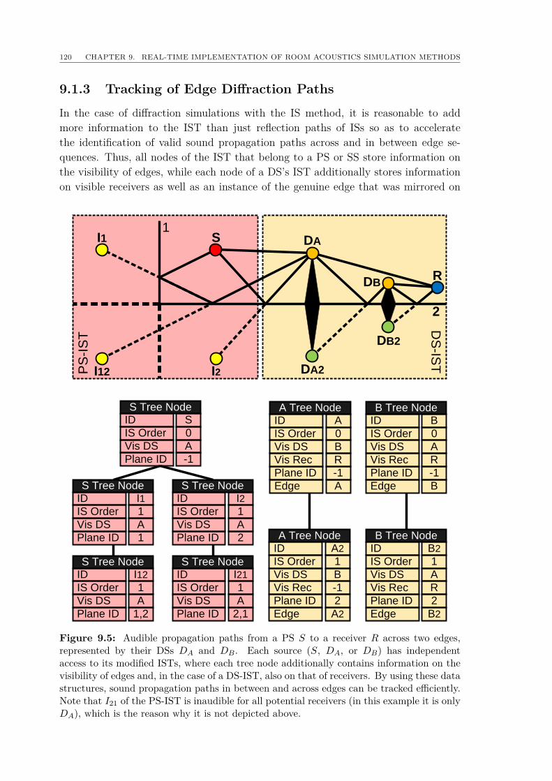
120 CHAPTER 9. REAL-TIME IMPLEMENTATION OF ROOM ACOUSTICS SIMULATION METHODS
9.1.3 Tracking of Edge Diffraction Paths
In the case of diffraction simulations with the IS method, it is reasonable to addmore information to the IST than just reflection paths of ISs so as to acceleratethe identification of valid sound propagation paths across and in between edge se-quences. Thus, all nodes of the IST that belong to a PS or SS store information onthe visibility of edges, while each node of a DS’s IST additionally stores informationon visible receivers as well as an instance of the genuine edge that was mirrored on
SI1
I12
R
1
2
I2
DS
-IST
PS
-IS
T
S Tree NodeID
IS Order
Vis DS
S
0
A
Plane ID -1
S Tree NodeID
IS Order
Vis DS
I1
1
A
Plane ID 1
S Tree NodeID
IS Order
Vis DS
I2
1
A
Plane ID 2
S Tree NodeID
IS Order
Vis DS
I12
1
A
Plane ID 1,2
A Tree NodeID
IS Order
Vis DS
A
0
B
Plane ID
R
Edge
Vis Rec
-1
A
A Tree NodeID
IS Order
Vis DS
A2
1
B
Plane ID
-1
Edge
Vis Rec
2
A2
B Tree NodeID
IS Order
Vis DS
B
0
A
Plane ID
R
Edge
Vis Rec
-1
B
B Tree NodeID
IS Order
Vis DS
B2
1
A
Plane ID
R
Edge
Vis Rec
2
B2
DB
DB2
DA
DA2
S Tree NodeID
IS Order
Vis DS
I21
1
A
Plane ID 2,1
Figure 9.5: Audible propagation paths from a PS S to a receiver R across two edges,represented by their DSs DA and DB. Each source (S, DA, or DB) has independentaccess to its modified ISTs, where each tree node additionally contains information on thevisibility of edges and, in the case of a DS-IST, also on that of receivers. By using these datastructures, sound propagation paths in between and across edges can be tracked efficiently.Note that I21 of the PS-IST is inaudible for all potential receivers (in this example it is onlyDA), which is the reason why it is not depicted above.
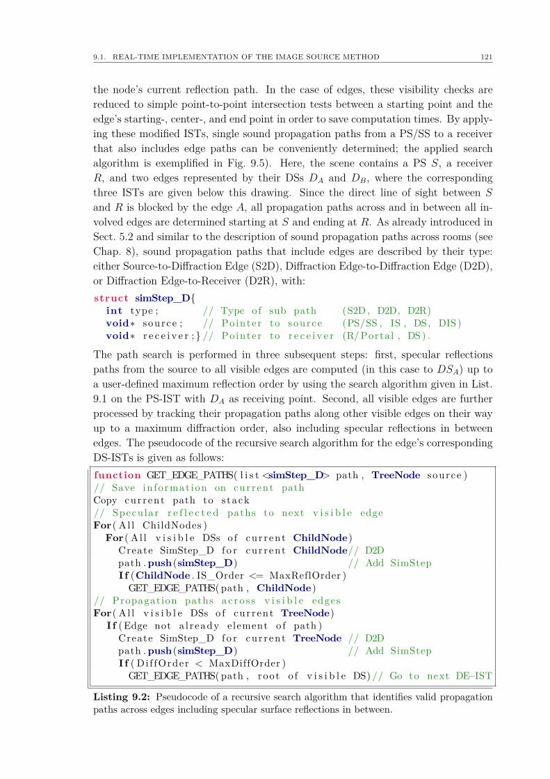
9.1. REAL-TIME IMPLEMENTATION OF THE IMAGE SOURCE METHOD 121
the node’s current reflection path. In the case of edges, these visibility checks arereduced to simple point-to-point intersection tests between a starting point and theedge’s starting-, center-, and end point in order to save computation times. By apply-ing these modified ISTs, single sound propagation paths from a PS/SS to a receiverthat also includes edge paths can be conveniently determined; the applied searchalgorithm is exemplified in Fig. 9.5). Here, the scene contains a PS S, a receiverR, and two edges represented by their DSs DA and DB, where the correspondingthree ISTs are given below this drawing. Since the direct line of sight between S
and R is blocked by the edge A, all propagation paths across and in between all in-volved edges are determined starting at S and ending at R. As already introduced inSect. 5.2 and similar to the description of sound propagation paths across rooms (seeChap. 8), sound propagation paths that include edges are described by their type:either Source-to-Diffraction Edge (S2D), Diffraction Edge-to-Diffraction Edge (D2D),or Diffraction Edge-to-Receiver (D2R), with:struct simStep_D
int type ; // Type o f sub path (S2D , D2D, D2R)void∗ source ; // Pointer to source (PS/SS , IS , DS, DIS)void∗ r e c e i v e r ; // Pointer to r e c e i v e r (R/Portal , DS) .
The path search is performed in three subsequent steps: first, specular reflectionspaths from the source to all visible edges are computed (in this case to DSA) up toa user-defined maximum reflection order by using the search algorithm given in List.9.1 on the PS-IST with DA as receiving point. Second, all visible edges are furtherprocessed by tracking their propagation paths along other visible edges on their wayup to a maximum diffraction order, also including specular reflections in betweenedges. The pseudocode of the recursive search algorithm for the edge’s correspondingDS-ISTs is given as follows:function GET_EDGE_PATHS( l i s t <simStep_D> path , TreeNode source )// Save in fo rmat ion on cur rent pathCopy cur rent path to s tack// Specu lar r e f l e c t e d paths to next v i s i b l e edgeFor( Al l ChildNodes )
For( Al l v i s i b l e DSs o f cur rent ChildNode)Create SimStep_D f o r cur rent ChildNode// D2Dpath .push(simStep_D) // Add SimStepI f (ChildNode . IS_Order <= MaxReflOrder )GET_EDGE_PATHS( path , ChildNode)
// Propagation paths a c r o s s v i s i b l e edgesFor( Al l v i s i b l e DSs o f cur rent TreeNode)
I f (Edge not a l r eady element o f path )Create SimStep_D f o r cur rent TreeNode // D2Dpath .push(simStep_D) // Add SimStepI f ( Di f fOrder < MaxDiffOrder )GET_EDGE_PATHS( path , root o f v i s i b l e DS) // Go to next DE−IST
Listing 9.2: Pseudocode of a recursive search algorithm that identifies valid propagationpaths across edges including specular surface reflections in between.
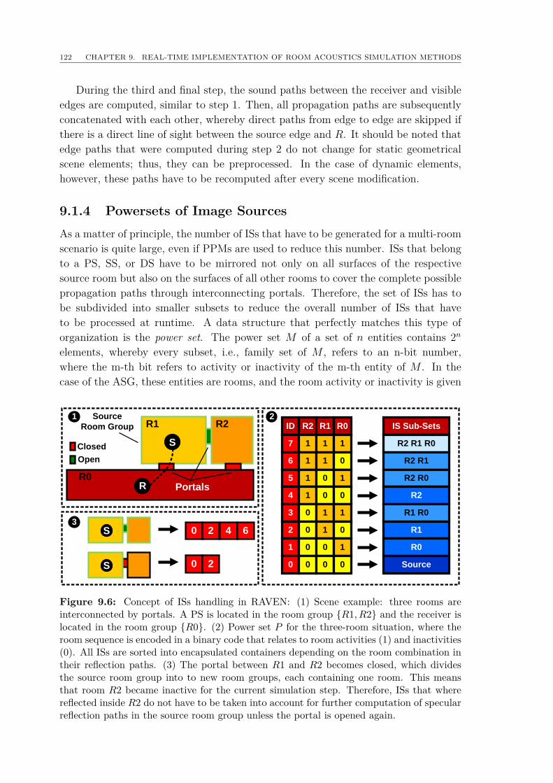
122 CHAPTER 9. REAL-TIME IMPLEMENTATION OF ROOM ACOUSTICS SIMULATION METHODS
During the third and final step, the sound paths between the receiver and visibleedges are computed, similar to step 1. Then, all propagation paths are subsequentlyconcatenated with each other, whereby direct paths from edge to edge are skipped ifthere is a direct line of sight between the source edge and R. It should be noted thatedge paths that were computed during step 2 do not change for static geometricalscene elements; thus, they can be preprocessed. In the case of dynamic elements,however, these paths have to be recomputed after every scene modification.
9.1.4 Powersets of Image SourcesAs a matter of principle, the number of ISs that have to be generated for a multi-roomscenario is quite large, even if PPMs are used to reduce this number. ISs that belongto a PS, SS, or DS have to be mirrored not only on all surfaces of the respectivesource room but also on the surfaces of all other rooms to cover the complete possiblepropagation paths through interconnecting portals. Therefore, the set of ISs has tobe subdivided into smaller subsets to reduce the overall number of ISs that haveto be processed at runtime. A data structure that perfectly matches this type oforganization is the power set. The power set M of a set of n entities contains 2nelements, whereby every subset, i.e., family set of M , refers to an n-bit number,where the m-th bit refers to activity or inactivity of the m-th entity of M . In thecase of the ASG, these entities are rooms, and the room activity or inactivity is given
R1 R2
R0R
S
1 2
3S
S 0 2
4 60 2
ID R2 R1 R0
7 1 1 1
6 1 1 0
5 1 0 1
4 1 0 0
3 0 1 1
2 0 1 0
1 0 0 1
0 0 0 0
IS Sub-Sets
R2 R1 R0
R2 R1
R2 R0
R2
R1 R0
R1
R0
Source
Source
Room Group
Portals
Closed
Open
Figure 9.6: Concept of ISs handling in RAVEN: (1) Scene example: three rooms areinterconnected by portals. A PS is located in the room group R1, R2 and the receiver islocated in the room group R0. (2) Power set P for the three-room situation, where theroom sequence is encoded in a binary code that relates to room activities (1) and inactivities(0). All ISs are sorted into encapsulated containers depending on the room combination intheir reflection paths. (3) The portal between R1 and R2 becomes closed, which dividesthe source room group into to new room groups, each containing one room. This meansthat room R2 became inactive for the current simulation step. Therefore, ISs that wherereflected inside R2 do not have to be taken into account for further computation of specularreflection paths in the source room group unless the portal is opened again.
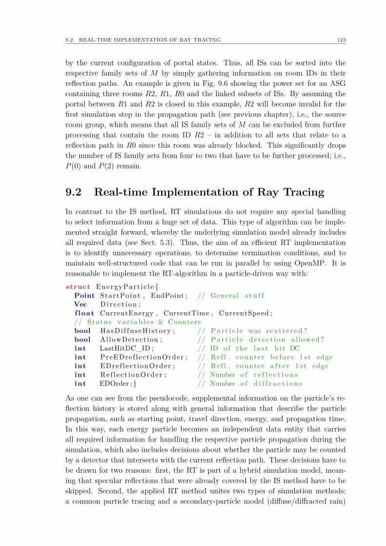
9.2. REAL-TIME IMPLEMENTATION OF RAY TRACING 123
by the current configuration of portal states. Thus, all ISs can be sorted into therespective family sets of M by simply gathering information on room IDs in theirreflection paths. An example is given in Fig. 9.6 showing the power set for an ASGcontaining three rooms R2, R1, R0 and the linked subsets of ISs. By assuming theportal between R1 and R2 is closed in this example, R2 will become invalid for thefirst simulation step in the propagation path (see previous chapter), i.e., the sourceroom group, which means that all IS family sets of M can be excluded from furtherprocessing that contain the room ID R2 – in addition to all sets that relate to areflection path in R0 since this room was already blocked. This significantly dropsthe number of IS family sets from four to two that have to be further processed; i.e.,P (0) and P (2) remain.
9.2 Real-time Implementation of Ray TracingIn contrast to the IS method, RT simulations do not require any special handlingto select information from a huge set of data. This type of algorithm can be imple-mented straight forward, whereby the underlying simulation model already includesall required data (see Sect. 5.3). Thus, the aim of an efficient RT implementationis to identify unnecessary operations, to determine termination conditions, and tomaintain well-structured code that can be run in parallel by using OpenMP. It isreasonable to implement the RT-algorithm in a particle-driven way with:struct EnergyPart i c l e
Point StartPoint , EndPoint ; // General s t u f fVec Dir e c t i on ;f loat CurrentEnergy , CurrentTime , CurrentSpeed ;// Status v a r i a b l e s & Countersbool HasDi f fu seHi s tory ; // Pa r t i c l e was s c a t t e r ed ?bool AllowDetect ion ; // Pa r t i c l e d e t e c t i on al lowed ?int LastHitDC_ID ; // ID o f the l a s t h i t DCint PreEDref lect ionOrder ; // Re f l . counter be f o r e 1 s t edgeint EDref l ect ionOrder ; // Re f l . counter a f t e r 1 s t edgeint Ref l e c t i onOrder ; // Number o f r e f l e c t i o n sint EDOrder ; // Number o f d i f f r a c t i o n s
As one can see from the pseudocode, supplemental information on the particle’s re-flection history is stored along with general information that describe the particlepropagation, such as starting point, travel direction, energy, and propagation time.In this way, each energy particle becomes an independent data entity that carriesall required information for handling the respective particle propagation during thesimulation, which also includes decisions about whether the particle may be countedby a detector that intersects with the current reflection path. These decisions have tobe drawn for two reasons: first, the RT is part of a hybrid simulation model, mean-ing that specular reflections that were already covered by the IS method have to beskipped. Second, the applied RT method unites two types of simulation methods:a common particle tracing and a secondary-particle model (diffuse/diffracted rain)

124 CHAPTER 9. REAL-TIME IMPLEMENTATION OF ROOM ACOUSTICS SIMULATION METHODS
that can be interpreted as a first-order radiosity dialect (see Sect. 5.3). Here, directhits of a scattered or diffracted energy particle with detectors that cross the currentpropagation path ought not be counted, as this energy portion was already coveredby diffuse rain and diffracted rain, respectively. The easiest way to control all sta-tus variables and reflection counters is to implement three basic functions that areexecuted each time the respective event occurs:function REFLECTED()
a l l owDetec t i on = true ; // Allow de t e c t i onlastHitDC_ID = −1; // Set to dummy ID
Ref l e c t i onOrder++; // Counter incrementI f (EDOrder == 0) PreEDref lect ionOrder++;Else EDref l ect ionOrder++;
function SCATTERED()HasDi f fu seHi s tory = true ; // D i f f u s e h i s t o r ya l l owDetec t i on = fa l se ; // Forbid de t e c t i onlastHitDC_ID = −1; // Set to dummy ID
Ref l e c t i onOrder++; // Counter incrementI f (EDOrder == 0) PreEDref lect ionOrder++;Else EDref l ect ionOrder++;
function DIFFRACTED( int cy l inder ID )EDOrder++; // Increment D i f f r a c t i o n Ordera l l owDetec t i on = fa l se ; // Forbid de t e c t i onlastHitDC_ID = cy l inder ID ; // Set to c y l i nd e r ID
Listing 9.3: Pseudocode of energy particle functions that set status variables and countersaccording to the occurred event.
The final decision whether the particle is allowed to be detected is then made by alogical comparison of all relevant counters and states, with// Check i f cur r ent path i s a l r eady covered by the IS methodfunction DETECTION_ALLOWED_HYBRID
I f (EDOrder !=0)return (
HasDi f fuseHi s tory | |( PreEDref lect ionOrder > MaxPreEDISOrder ) | |( EDre f l ect ionOrder > MaxEDISOrder ) | |(EDOrder > MaxEDOrder ) ) ;
Elsereturn ( r e f l e c t i o nOrd e r > MaxISOrder ) ;
// Check i f d i f f u s e / d i f f r a c t e d ra in was a l r eady detec tedfunction DETECTION_ALLOWED_PARTICLE( )
return a l l owDetec t i on ;
Listing 9.4: Pseudocode of logical functions that evaluate the particle’s states and countersin order to return whether the particle is currently valid for detection.
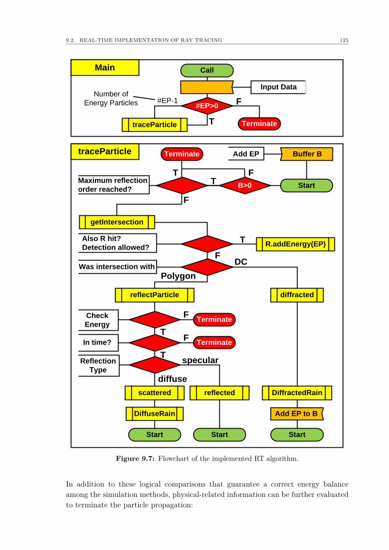
9.2. REAL-TIME IMPLEMENTATION OF RAY TRACING 125
Main
traceParticle
Call
traceParticle
#EP>0
Input Data
#EP-1Number of
Energy Particles
T
F
Buffer B
B>0
getIntersection
R.addEnergy(EP)
reflectedscattered
diffractedreflectParticle
In time?
Was intersection with
DiffuseRain
DiffractedRain
Add EP to B
Start
Start StartStart
Check
Energy
Terminate
Reflection
Type
Terminate
Terminate
Terminate
DC
Polygon
Also R hit?
Detection allowed?
Maximum reflection
order reached?
Add EP
F
F
F
F
specular
diffuse
TT
T
T
T
F
Figure 9.7: Flowchart of the implemented RT algorithm.
In addition to these logical comparisons that guarantee a correct energy balanceamong the simulation methods, physical-related information can be further evaluatedto terminate the particle propagation:

126 CHAPTER 9. REAL-TIME IMPLEMENTATION OF ROOM ACOUSTICS SIMULATION METHODS
Particle Energy If the particle’s energy underruns a user-defined energy threshold,it is terminated.
Propagation Time If the particle’s propagation time exceeds the histogram lengthor the particle cannot reach a detector within the given maximum propagationtime, it is terminated.
Reflection Order If the particle’s reflection order is greater than a user-definedmaximum, it is terminated in order to kill algorithmic deadlocks, as particlesmay become trapped between polygons2. However, this break condition oughtnot interfere with the RT model, which means that a number in the magnitudeof thousands should be set to avoid errors in the late part of the RIR.
The current implementation features a particle buffer where energy particles thathit a DC are temporarily stored until they are further traced. This avoids recursivecalls of the RT’s main routine and enables a clear and transparent implementation,whereby a flowchart is given in Fig. 9.7.
2This can happen for two reasons: (1) floating point imprecision on the dedicated working ma-chine, and (2) inaccurate modeling of the room geometry.

Part IV
Evaluation

128
Chapter 10
Analytical Validation
"The logic of validation allows us to move between the two limits ofdogmatism and skepticism."
(Paul Ricœr, French philosopher)
This chapter serves to investigate both the accuracy of the presented simulationconcept and the quality of the corresponding implementation, whereby three crucialparts can be identified: first, the hybrid simulation model itself that takes into ac-count specular and diffuse reflections; second, the simulation of sound transmissionthrough structural elements into adjacent rooms; and third, the computation of soundpropagation into shadow zones of edges. All three parts are assessed simply and trans-parently in order to reduce the number of simulation uncertainties that usually comefrom imprecise input data. Thus, the focus of this chapter lies more in validating theoverall simulation concept than in showing that simulation results match real-wordmeasurements of some specific setups. However, the latter has already been shownin various publications, where, for instance, a car interior [ANVS09, Jau10, AJ10] ora recording studio [AM10] were chosen as test scenario. In addition, more compar-isons either with reference simulations or real-world measurements can be found in[Dro06, SDV07, VS09a, VS09b, PS].
10.1 Hybrid Simulation Model
An appropriate and simple test for validating the hybrid simulation model is theanalysis of the room’s reverberation time in comparison with the scattering coeffi-cients of the applied surface materials. A complete diffuse sound field relates to ascattering coefficient of 1, whereby the simulated reverberation time has to match
130 CHAPTER 10. ANALYTICAL VALIDATION
calculations according to Sabine1 and Eyring2, respectively. In addition, it is also awell-known fact that the reverberation time increases in less diffuse environments andreaches a maximum for a scattering coefficient of 0, i.e., purely specular IS-modeling.In between these two extremes, the reverberation time falls exponentially with anincreasing diffuseness of the sound field, i.e., increasing scattering coefficients [Vor08].Thus, investigating reverberation times with variable scattering coefficients ought toreveal if the two energy models of deterministic ISs and stochastic RT are combinedcorrectly with one another.
Test Model & Simulation Parameterization
A simple shoebox-shaped room with a volume of 1344 m3 was chosen as test modelfeaturing a calculated reverberation time of 0.43 s and 0.58 s according to Eyring andSabine, respectively. Here, the equation according to Eyring is more accurate, sinceit is not based on the assumption of low-absorbing surfaces as in Sabine’s approach.The room’s side walls were modeled with an absorption factor of 0.05, while a factorof 0.8 was assigned to both the floor and the ceiling. In contrast, the same scat-tering coefficient was used for both materials and varied in steps of 0.05 during thesimulations. A sound source was positioned in one half of the room, and 36 in-planereceivers were evenly distributed outside the source’s critical distance in the oppositehalf of the room (see Fig. 10.1(a)). Room acoustical simulations were carried outby taking into account ISs of up to order 4, performing RT simulations with 25000particles per frequency bands (octave band resolution), and averaging the results ofall 36 receivers (more details are given in Fig. 10.1(b)).
Reverberation Time vs Scattering Coefficient
Figure 10.1(c) shows a comparison of the simulation results, whereby reverberationtimes (T30) were either calculated according to DIN EN ISO 3382 [ISO07], i.e., for thecenter frequencies 500Hz and 1 kHz (red line), or by evaluating all center frequenciesbetween 30Hz and 16 kHz (orange line). In addition, the values of reverberation timesare given that were calculated according to Sabine (green line) and Eyring (blue line).
Taking a closer look, one can see that the simulated reverberation times showthe typical exponentially decreasing behavior with increasing diffuseness of the soundfield, where simulated reverberation times start to match the prediction of Sabine forscattering coefficients of greater than 0.6. For a scattering coefficient of exactly one,the simulations according to DIN EN ISO 3382 exactly match the reverberation timeaccording to Eyring, whereas the value derived from all 10 octave-band just missedthat point by a very narrow margin. From this it follows that the transition frompure specular reflections to a diffuse sound field is covered correctly by the appliedhybrid simulation.
1Wallace C. Sabine, American physicist, 1868 - 1919.2Carl F. Eyring, Mexican physicist, 1889 - 1951.
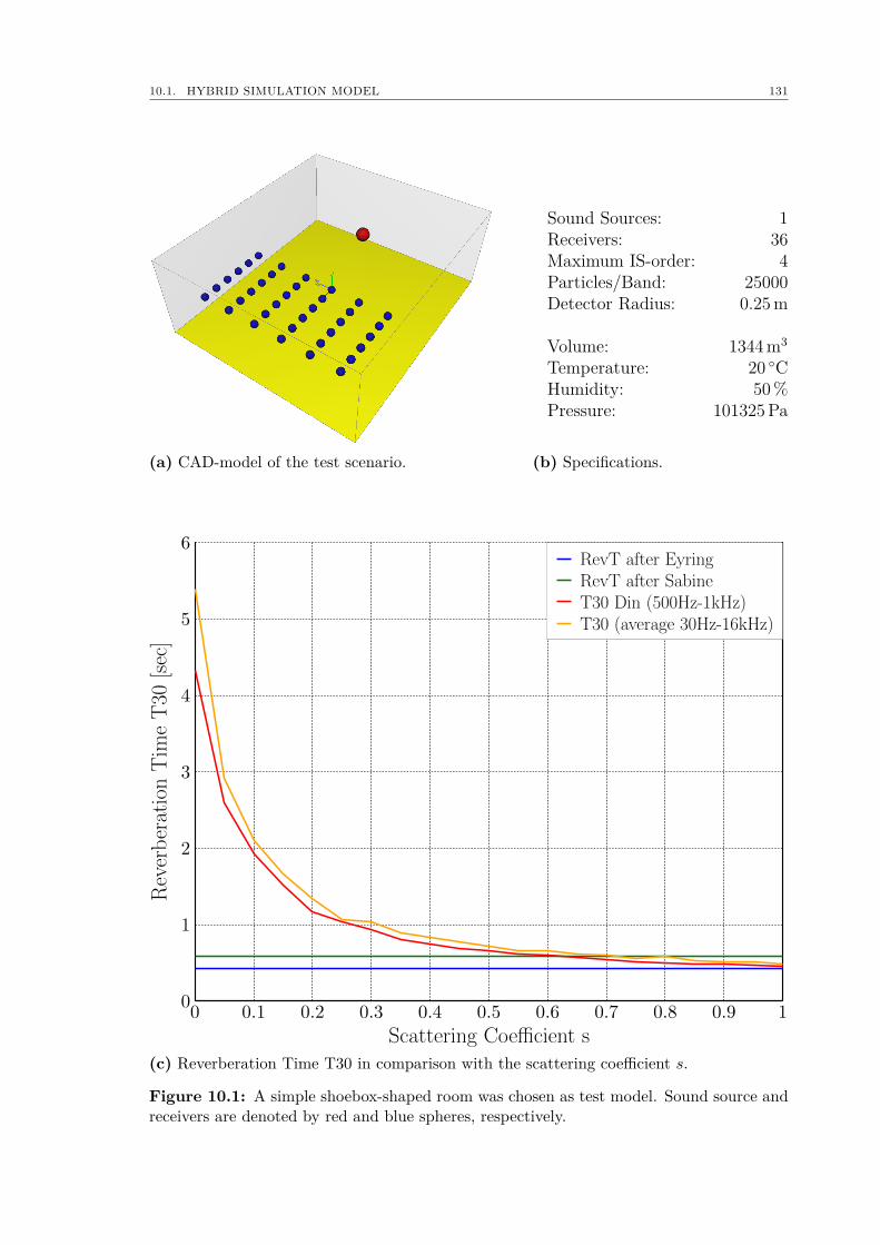
10.1. HYBRID SIMULATION MODEL 131
(a) CAD-model of the test scenario.
Sound Sources: 1Receivers: 36Maximum IS-order: 4Particles/Band: 25000Detector Radius: 0.25m
Volume: 1344 m3
Temperature: 20 CHumidity: 50%Pressure: 101325Pa
(b) Specifications.
Rev
erb
erat
ion
Tim
eT
30[s
ec]
Scattering Coefficient s
RevT after EyringRevT after SabineT30 Din (500Hz-1kHz)T30 (average 30Hz-16kHz)
(c) Reverberation Time T30 in comparison with the scattering coefficient s.
Figure 10.1: A simple shoebox-shaped room was chosen as test model. Sound source andreceivers are denoted by red and blue spheres, respectively.
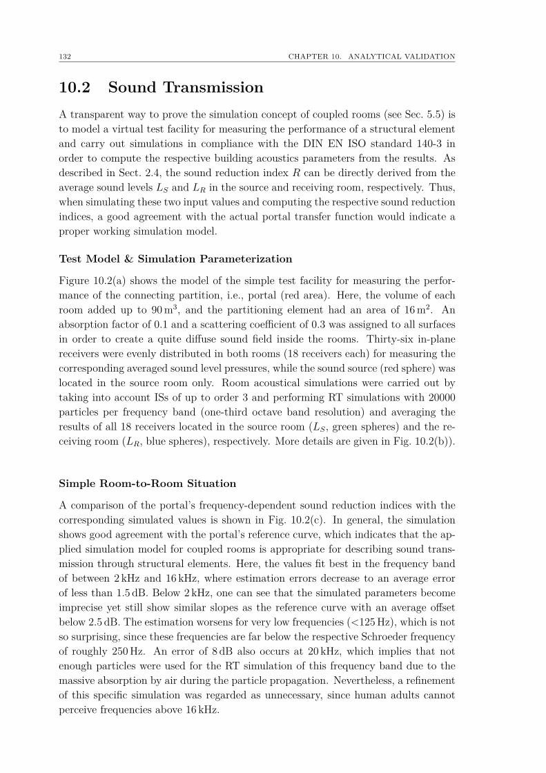
132 CHAPTER 10. ANALYTICAL VALIDATION
10.2 Sound TransmissionA transparent way to prove the simulation concept of coupled rooms (see Sec. 5.5) isto model a virtual test facility for measuring the performance of a structural elementand carry out simulations in compliance with the DIN EN ISO standard 140-3 inorder to compute the respective building acoustics parameters from the results. Asdescribed in Sect. 2.4, the sound reduction index R can be directly derived from theaverage sound levels LS and LR in the source and receiving room, respectively. Thus,when simulating these two input values and computing the respective sound reductionindices, a good agreement with the actual portal transfer function would indicate aproper working simulation model.
Test Model & Simulation Parameterization
Figure 10.2(a) shows the model of the simple test facility for measuring the perfor-mance of the connecting partition, i.e., portal (red area). Here, the volume of eachroom added up to 90 m3, and the partitioning element had an area of 16 m2. Anabsorption factor of 0.1 and a scattering coefficient of 0.3 was assigned to all surfacesin order to create a quite diffuse sound field inside the rooms. Thirty-six in-planereceivers were evenly distributed in both rooms (18 receivers each) for measuring thecorresponding averaged sound level pressures, while the sound source (red sphere) waslocated in the source room only. Room acoustical simulations were carried out bytaking into account ISs of up to order 3 and performing RT simulations with 20000particles per frequency band (one-third octave band resolution) and averaging theresults of all 18 receivers located in the source room (LS, green spheres) and the re-ceiving room (LR, blue spheres), respectively. More details are given in Fig. 10.2(b)).
Simple Room-to-Room Situation
A comparison of the portal’s frequency-dependent sound reduction indices with thecorresponding simulated values is shown in Fig. 10.2(c). In general, the simulationshows good agreement with the portal’s reference curve, which indicates that the ap-plied simulation model for coupled rooms is appropriate for describing sound trans-mission through structural elements. Here, the values fit best in the frequency bandof between 2 kHz and 16 kHz, where estimation errors decrease to an average errorof less than 1.5 dB. Below 2 kHz, one can see that the simulated parameters becomeimprecise yet still show similar slopes as the reference curve with an average offsetbelow 2.5 dB. The estimation worsens for very low frequencies (<125Hz), which is notso surprising, since these frequencies are far below the respective Schroeder frequencyof roughly 250Hz. An error of 8 dB also occurs at 20 kHz, which implies that notenough particles were used for the RT simulation of this frequency band due to themassive absorption by air during the particle propagation. Nevertheless, a refinementof this specific simulation was regarded as unnecessary, since human adults cannotperceive frequencies above 16 kHz.
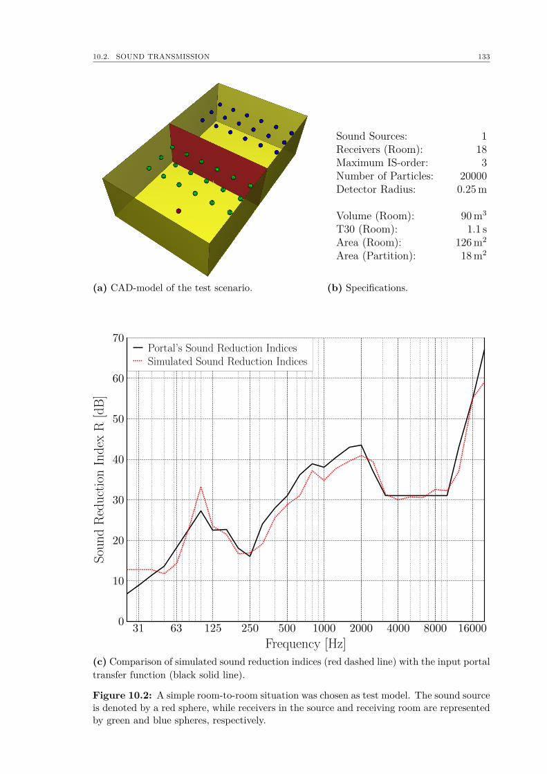
10.2. SOUND TRANSMISSION 133
(a) CAD-model of the test scenario.
Sound Sources: 1Receivers (Room): 18Maximum IS-order: 3Number of Particles: 20000Detector Radius: 0.25m
Volume (Room): 90 m3
T30 (Room): 1.1 sArea (Room): 126 m2
Area (Partition): 18 m2
(b) Specifications.
SoundReductionIndex
R[dB]
Frequency [Hz]
Portal’s Sound Reduction IndicesSimulated Sound Reduction Indices
(c) Comparison of simulated sound reduction indices (red dashed line) with the input portaltransfer function (black solid line).
Figure 10.2: A simple room-to-room situation was chosen as test model. The sound sourceis denoted by a red sphere, while receivers in the source and receiving room are representedby green and blue spheres, respectively.
134 CHAPTER 10. ANALYTICAL VALIDATION
10.3 Sound DiffractionAs described earlier, the implemented hybrid approach for simulating edge diffractionfrom finite edges is based on Stephenson’s DAPDF (stochastic RT, see Sect. 5.3.3)and Svensson’s secondary source model (IS-model, see Sect. 5.2.3), where in variouscomparisons both approaches proved to work very well in either 2D (Stephenson)[SS07, Ste10a] or 3D (Svensson) [SW00, SSV10, SE10]. Here, especially the latter isappropriate as a reference model, since it is today one of the most accurate simulationmethods utilizing GA for computing edge diffraction from finite edges. However, theimplemented extension of Stephenson’s stochastic model to 3D still has to be verified.
It was shown in Sect. 2.5 that the sound phenomenon of edge diffraction is a quitecomplex process already in the theoretical case of sound diffraction from a semi-infinite edge. Since infinite edges do not exist in reality, a simple test scenario of asingle, but finite wedge was chosen, where the analytical solution is still well known.In the following, the test setup is described in all detail, and simulation results arecompared and discussed that were obtained either by RAVEN’s simulation methodsof edge diffraction (IS-model and RT) or Svensson’s Open Source Edge DiffractionMATLAB toolbox [Sve10].
Test Model & Simulation Parameterization
Similar to the test scenario presented in [Ste10a], Fig. 10.3 shows the investigatedmodel of a single wedge with an inner angle of 10 – though this time completely in 3Dand with fix receiver positions3. The edge length was set at 100m to prevent an earlycut-off of the edge diffraction impulse responses (see Fig. 5.8) to better investigatethe accuracy of their overall decay. As in the original test case, all surfaces weremodeled as fully absorbent to suppress any sound reflections but the direct sound,all material parameters were set accordingly. The sound source (red sphere) and allreceivers (blue spheres) were positioned in-plane on a circle having a radius of 10mand with center on the edge, whereby the sound source was exactly located at theheight of the diffracting edge. Meanwhile, receivers were distributed around the edgein increments of 12 (seen from the edge), i.e., at −84 , −72 , ... , +72 , +84 . Thisresulted in a total number of 15 receivers with the same distance of 10m to the edgeas the sound source, where a positive and negative angle corresponded to receivers inthe view and shadow zone, respectively.
As only the direct sound path over the edge was investigated in the original testseries, room acoustical simulations had to be carried out separately, since the directsound is covered solely by the accurate IS-model in the case of hybrid simulations (seeSect. 5.4). Consequently, the first simulation series was carried out with ISs of up toorder 0 (direct sound) and no RT, whereas in the second series RT simulations wereperformed with 100000 particles per frequency band (one-third octave band resolu-tion), a detection sphere radius of roughly 1m, and no ISs (all important simulation
3In the original test scenarios, the receivers were positioned at multiples of the regarded wave-lengths in a 2D scenario.
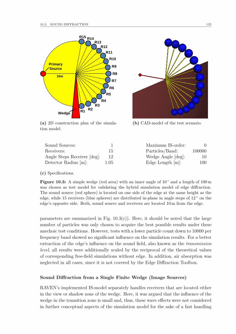
10.3. SOUND DIFFRACTION 135
Primary
Source
R1R2
R3
R4
R5
R6
R7
R8
R9
R10
R11
R12
R13R14R15
Wedge
10m
(a) 2D construction plan of the simula-tion model.
(b) CAD-model of the test scenario.
Sound Sources: 1 Maximum IS-order: 0Receivers: 15 Particles/Band: 100000Angle Steps Receiver [deg]: 12 Wedge Angle [deg]: 10Detector Radius [m]: 1.05 Edge Length [m]: 100
(c) Specifications.
Figure 10.3: A simple wedge (red area) with an inner angle of 10 and a length of 100mwas chosen as test model for validating the hybrid simulation model of edge diffraction.The sound source (red sphere) is located on one side of the edge at the same height as theedge, while 15 receivers (blue spheres) are distributed in-plane in angle steps of 12 on theedge’s opposite side. Both, sound source and receivers are located 10m from the edge.
parameters are summarized in Fig. 10.3(c)). Here, it should be noted that the largenumber of particles was only chosen to acquire the best possible results under theseanechoic test conditions. However, tests with a lower particle count down to 10000 perfrequency band showed no significant influence on the simulation results. For a betterextraction of the edge’s influence on the sound field, also known as the transmissionlevel, all results were additionally scaled by the reciprocal of the theoretical valuesof corresponding free-field simulations without edge. In addition, air absorption wasneglected in all cases, since it is not covered by the Edge Diffraction Toolbox.
Sound Diffraction from a Single Finite Wedge (Image Sources)
RAVEN’s implemented IS-model separately handles receivers that are located eitherin the view or shadow zone of the wedge. Here, it was argued that the influence of thewedge in the transition zone is small and, thus, these wave effects were not consideredin further conceptual aspects of the simulation model for the sake of a fast handling
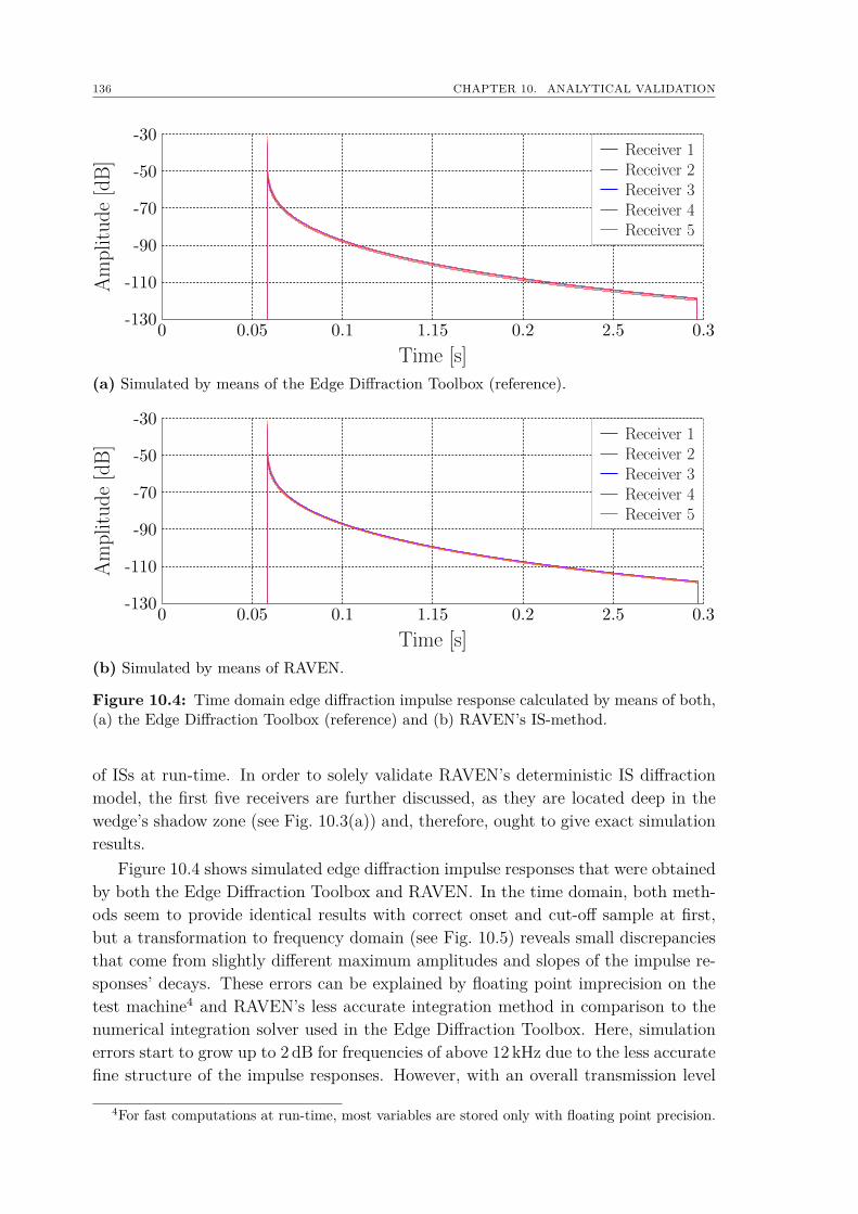
136 CHAPTER 10. ANALYTICAL VALIDATIONAmplitude[dB]
Time [s]
Receiver 1Receiver 2Receiver 3Receiver 4Receiver 5
(a) Simulated by means of the Edge Diffraction Toolbox (reference).
Amplitude[dB]
Time [s]
Receiver 1Receiver 2Receiver 3Receiver 4Receiver 5
(b) Simulated by means of RAVEN.
Figure 10.4: Time domain edge diffraction impulse response calculated by means of both,(a) the Edge Diffraction Toolbox (reference) and (b) RAVEN’s IS-method.
of ISs at run-time. In order to solely validate RAVEN’s deterministic IS diffractionmodel, the first five receivers are further discussed, as they are located deep in thewedge’s shadow zone (see Fig. 10.3(a)) and, therefore, ought to give exact simulationresults.
Figure 10.4 shows simulated edge diffraction impulse responses that were obtainedby both the Edge Diffraction Toolbox and RAVEN. In the time domain, both meth-ods seem to provide identical results with correct onset and cut-off sample at first,but a transformation to frequency domain (see Fig. 10.5) reveals small discrepanciesthat come from slightly different maximum amplitudes and slopes of the impulse re-sponses’ decays. These errors can be explained by floating point imprecision on thetest machine4 and RAVEN’s less accurate integration method in comparison to thenumerical integration solver used in the Edge Diffraction Toolbox. Here, simulationerrors start to grow up to 2 dB for frequencies of above 12 kHz due to the less accuratefine structure of the impulse responses. However, with an overall transmission level
4For fast computations at run-time, most variables are stored only with floating point precision.
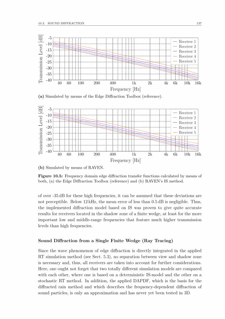
10.3. SOUND DIFFRACTION 137
Transm
ission
Level[dB]
Frequency [Hz]
Receiver 1Receiver 2Receiver 3Receiver 4Receiver 5
(a) Simulated by means of the Edge Diffraction Toolbox (reference).
Transm
ission
Level[dB]
Frequency [Hz]
Receiver 1Receiver 2Receiver 3Receiver 4Receiver 5
(b) Simulated by means of RAVEN.
Figure 10.5: Frequency domain edge diffraction transfer functions calculated by means ofboth, (a) the Edge Diffraction Toolbox (reference) and (b) RAVEN’s IS method.
of over -35 dB for these high frequencies, it can be assumed that these deviations arenot perceptible. Below 12 kHz, the mean error of less than 0.5 dB is negligible. Thus,the implemented diffraction model based on IS was proven to give quite accurateresults for receivers located in the shadow zone of a finite wedge, at least for the moreimportant low and middle-range frequencies that feature much higher transmissionlevels than high frequencies.
Sound Diffraction from a Single Finite Wedge (Ray Tracing)
Since the wave phenomenon of edge diffraction is directly integrated in the appliedRT simulation method (see Sect. 5.3), no separation between view and shadow zoneis necessary and, thus, all receivers are taken into account for further considerations.Here, one ought not forget that two totally different simulation models are comparedwith each other, where one is based on a deterministic IS-model and the other on astochastic RT method. In addition, the applied DAPDF, which is the basis for thediffracted rain method and which describes the frequency-dependent diffraction ofsound particles, is only an approximation and has never yet been tested in 3D.
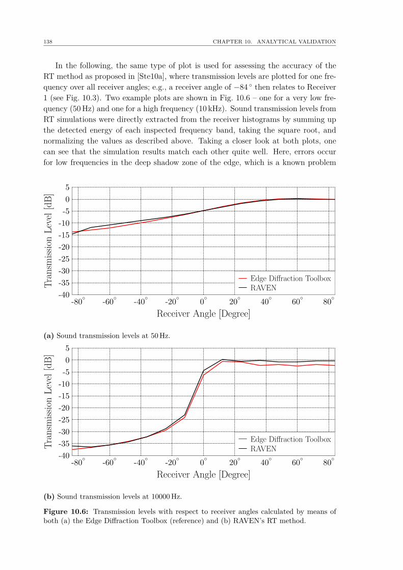
138 CHAPTER 10. ANALYTICAL VALIDATION
In the following, the same type of plot is used for assessing the accuracy of theRT method as proposed in [Ste10a], where transmission levels are plotted for one fre-quency over all receiver angles; e.g., a receiver angle of −84 then relates to Receiver1 (see Fig. 10.3). Two example plots are shown in Fig. 10.6 – one for a very low fre-quency (50Hz) and one for a high frequency (10 kHz). Sound transmission levels fromRT simulations were directly extracted from the receiver histograms by summing upthe detected energy of each inspected frequency band, taking the square root, andnormalizing the values as described above. Taking a closer look at both plots, onecan see that the simulation results match each other quite well. Here, errors occurfor low frequencies in the deep shadow zone of the edge, which is a known problem
Tra
nsm
issi
onL
evel
[dB
]
Receiver Angle [Degree]
Edge Diffraction ToolboxRAVEN
(a) Sound transmission levels at 50Hz.
Tra
nsm
issi
onL
evel
[dB
]
Receiver Angle [Degree]
Edge Diffraction ToolboxRAVEN
(b) Sound transmission levels at 10000Hz.
Figure 10.6: Transmission levels with respect to receiver angles calculated by means ofboth (a) the Edge Diffraction Toolbox (reference) and (b) RAVEN’s RT method.

10.3. SOUND DIFFRACTION 139
of the DAPDF, especially if the distance from the source to the edge is smaller thana few wavelengths [Ste10a]. Besides Receiver 1 at −84 (deepest shadow zone), thesimulation at 10 kHz matches very well the results of the Edge Diffraction toolbox inthe wedge’s shadow zone, but other errors of about 2 dB occur in the view zone thatare attributed to wave effects not covered by the simplified simulation method basedon RT. Nonetheless, the overall good agreement shows that the 2D-DAPDF has beensuccessfully ported to 3D by using the diffracted rain method.

140 CHAPTER 10. ANALYTICAL VALIDATION
Chapter 11
Performance
"You may delay, but time will not, and lost time is never found again."
(Benjamin Franklin, American politician and scientist)
This chapter investigates the performance of RAVEN’s core simulation conceptswith respect to real-time capability, since a complete analysis of all involved algo-rithms would go far beyond the scope of this thesis. It was proven in various publica-tions that the entire simulation concept is able to work within the dictated real-timeconstraints given in Chap. 6, where detailed performance analyses of single algorithmscan be found in [SL06, SDV07, Pel07, LSVA07, Poh08, Ryb09, Sch09a]. Therefore,the focus of this chapter is rather the overall speed-up that can be gained by utilizingspatial data structures in room acoustics simulation.
After introducing five room models that were used as input data throughout thetests, the performance of both BSP- and SH-based search algorithms is analyzed withrespect to the two main simulation functions – the IS method and RT. Afterwards,computation times caused by operations on dynamic geometric objects are furtherdiscussed in order to reveal issues of both types of data structures and prove theoverall concept of handling dynamic scene modifications (see Chap. 6).
All results are compared to that of BF approaches, which helps to better ratethe gained speed-ups by the use of spatial data structures. It should be noted thatthe simulation of edge diffraction was omitted in all tests for three reasons: first,no additional information on the performance of spatial data structures is gainedfrom including diffraction to the simulation algorithms. Second, the exclusion of edgediffraction leads to simple and comprehensive test scenarios. And third, a detailedperformance analysis of edge diffraction simulations is already given in [Poh08].
11.1 Test ModelsFive different geometrical scenes of different complexity and size were considered foranalyzing the performance of simulation algorithms. All models were constructed
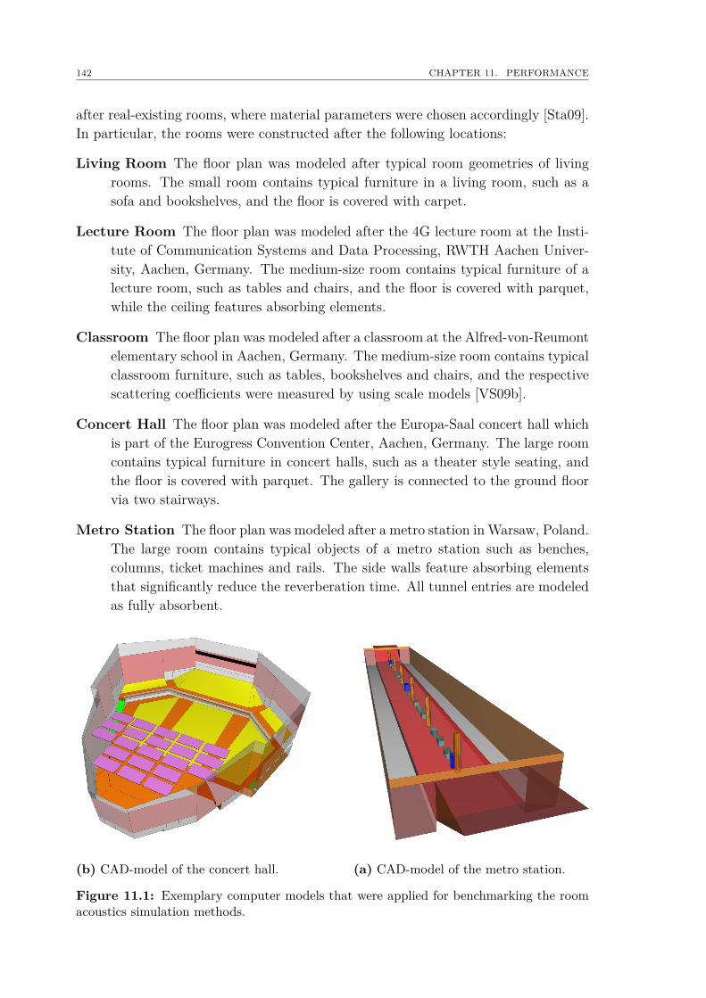
142 CHAPTER 11. PERFORMANCE
after real-existing rooms, where material parameters were chosen accordingly [Sta09].In particular, the rooms were constructed after the following locations:
Living Room The floor plan was modeled after typical room geometries of livingrooms. The small room contains typical furniture in a living room, such as asofa and bookshelves, and the floor is covered with carpet.
Lecture Room The floor plan was modeled after the 4G lecture room at the Insti-tute of Communication Systems and Data Processing, RWTH Aachen Univer-sity, Aachen, Germany. The medium-size room contains typical furniture of alecture room, such as tables and chairs, and the floor is covered with parquet,while the ceiling features absorbing elements.
Classroom The floor plan was modeled after a classroom at the Alfred-von-Reumontelementary school in Aachen, Germany. The medium-size room contains typicalclassroom furniture, such as tables, bookshelves and chairs, and the respectivescattering coefficients were measured by using scale models [VS09b].
Concert Hall The floor plan was modeled after the Europa-Saal concert hall whichis part of the Eurogress Convention Center, Aachen, Germany. The large roomcontains typical furniture in concert halls, such as a theater style seating, andthe floor is covered with parquet. The gallery is connected to the ground floorvia two stairways.
Metro Station The floor plan was modeled after a metro station in Warsaw, Poland.The large room contains typical objects of a metro station such as benches,columns, ticket machines and rails. The side walls feature absorbing elementsthat significantly reduce the reverberation time. All tunnel entries are modeledas fully absorbent.
(b) CAD-model of the concert hall. (a) CAD-model of the metro station.
Figure 11.1: Exemplary computer models that were applied for benchmarking the roomacoustics simulation methods.
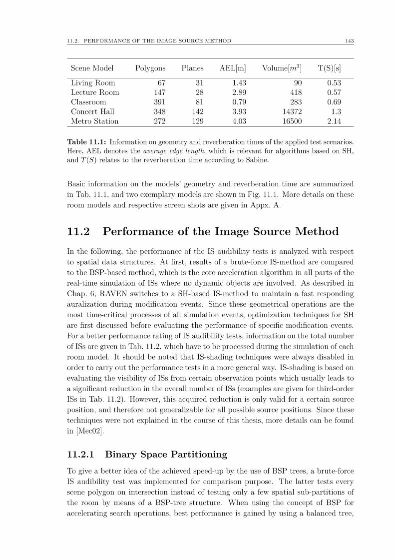
11.2. PERFORMANCE OF THE IMAGE SOURCE METHOD 143
Scene Model Polygons Planes AEL[m] Volume[m3] T(S)[s]
Living Room 67 31 1.43 90 0.53Lecture Room 147 28 2.89 418 0.57Classroom 391 81 0.79 283 0.69Concert Hall 348 142 3.93 14372 1.3Metro Station 272 129 4.03 16500 2.14
Table 11.1: Information on geometry and reverberation times of the applied test scenarios.Here, AEL denotes the average edge length, which is relevant for algorithms based on SH,and T (S) relates to the reverberation time according to Sabine.
Basic information on the models’ geometry and reverberation time are summarizedin Tab. 11.1, and two exemplary models are shown in Fig. 11.1. More details on theseroom models and respective screen shots are given in Appx. A.
11.2 Performance of the Image Source MethodIn the following, the performance of the IS audibility tests is analyzed with respectto spatial data structures. At first, results of a brute-force IS-method are comparedto the BSP-based method, which is the core acceleration algorithm in all parts of thereal-time simulation of ISs where no dynamic objects are involved. As described inChap. 6, RAVEN switches to a SH-based IS-method to maintain a fast respondingauralization during modification events. Since these geometrical operations are themost time-critical processes of all simulation events, optimization techniques for SHare first discussed before evaluating the performance of specific modification events.For a better performance rating of IS audibility tests, information on the total numberof ISs are given in Tab. 11.2, which have to be processed during the simulation of eachroom model. It should be noted that IS-shading techniques were always disabled inorder to carry out the performance tests in a more general way. IS-shading is based onevaluating the visibility of ISs from certain observation points which usually leads toa significant reduction in the overall number of ISs (examples are given for third-orderISs in Tab. 11.2). However, this acquired reduction is only valid for a certain sourceposition, and therefore not generalizable for all possible source positions. Since thesetechniques were not explained in the course of this thesis, more details can be foundin [Mec02].
11.2.1 Binary Space PartitioningTo give a better idea of the achieved speed-up by the use of BSP trees, a brute-forceIS audibility test was implemented for comparison purpose. The latter tests everyscene polygon on intersection instead of testing only a few spatial sub-partitions ofthe room by means of a BSP-tree structure. When using the concept of BSP foraccelerating search operations, best performance is gained by using a balanced tree,
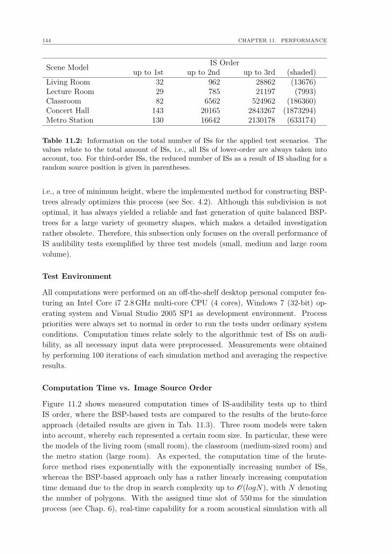
144 CHAPTER 11. PERFORMANCE
Scene Model IS Orderup to 1st up to 2nd up to 3rd (shaded)
Living Room 32 962 28862 (13676)Lecture Room 29 785 21197 (7993)Classroom 82 6562 524962 (186360)Concert Hall 143 20165 2843267 (1873294)Metro Station 130 16642 2130178 (633174)
Table 11.2: Information on the total number of ISs for the applied test scenarios. Thevalues relate to the total amount of ISs, i.e., all ISs of lower-order are always taken intoaccount, too. For third-order ISs, the reduced number of ISs as a result of IS shading for arandom source position is given in parentheses.
i.e., a tree of minimum height, where the implemented method for constructing BSP-trees already optimizes this process (see Sec. 4.2). Although this subdivision is notoptimal, it has always yielded a reliable and fast generation of quite balanced BSP-trees for a large variety of geometry shapes, which makes a detailed investigationrather obsolete. Therefore, this subsection only focuses on the overall performance ofIS audibility tests exemplified by three test models (small, medium and large roomvolume).
Test Environment
All computations were performed on an off-the-shelf desktop personal computer fea-turing an Intel Core i7 2.8GHz multi-core CPU (4 cores), Windows 7 (32-bit) op-erating system and Visual Studio 2005 SP1 as development environment. Processpriorities were always set to normal in order to run the tests under ordinary systemconditions. Computation times relate solely to the algorithmic test of ISs on audi-bility, as all necessary input data were preprocessed. Measurements were obtainedby performing 100 iterations of each simulation method and averaging the respectiveresults.
Computation Time vs. Image Source Order
Figure 11.2 shows measured computation times of IS-audibility tests up to thirdIS order, where the BSP-based tests are compared to the results of the brute-forceapproach (detailed results are given in Tab. 11.3). Three room models were takeninto account, whereby each represented a certain room size. In particular, these werethe models of the living room (small room), the classroom (medium-sized room) andthe metro station (large room). As expected, the computation time of the brute-force method rises exponentially with the exponentially increasing number of ISs,whereas the BSP-based approach only has a rather linearly increasing computationtime demand due to the drop in search complexity up to O(logN), with N denotingthe number of polygons. With the assigned time slot of 550ms for the simulationprocess (see Chap. 6), real-time capability for a room acoustical simulation with all
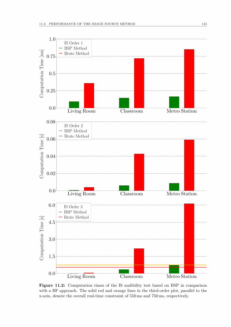
11.2. PERFORMANCE OF THE IMAGE SOURCE METHOD 145
Com
putation
Tim
e[m
s]IS Order 1BSP MethodBrute Method
Com
putation
Tim
e[s]
IS Order 2BSP MethodBrute Method
Com
putation
Tim
e[s]
IS Order 3BSP MethodBrute Method
Figure 11.2: Computation times of the IS audibility test based on BSP in comparisonwith a BF approach. The solid red and orange lines in the third-order plot, parallel to thex-axis, denote the overall real-time constraint of 550ms and 750ms, respectively.
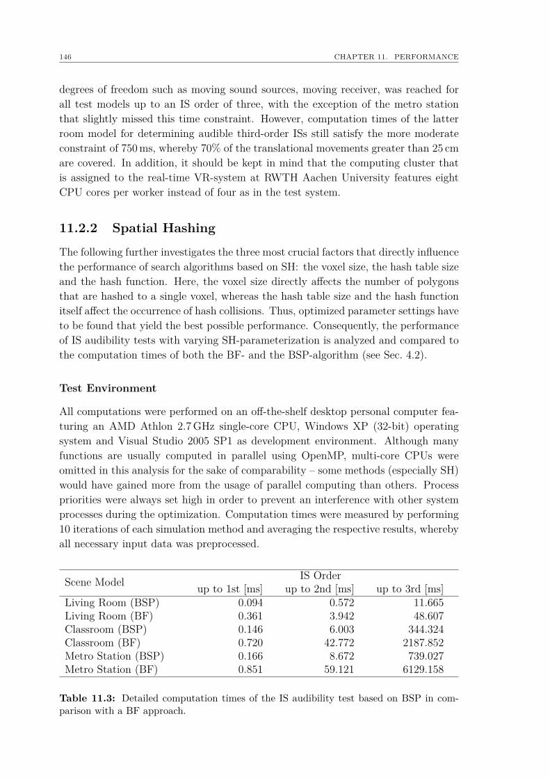
146 CHAPTER 11. PERFORMANCE
degrees of freedom such as moving sound sources, moving receiver, was reached forall test models up to an IS order of three, with the exception of the metro stationthat slightly missed this time constraint. However, computation times of the latterroom model for determining audible third-order ISs still satisfy the more moderateconstraint of 750ms, whereby 70% of the translational movements greater than 25 cmare covered. In addition, it should be kept in mind that the computing cluster thatis assigned to the real-time VR-system at RWTH Aachen University features eightCPU cores per worker instead of four as in the test system.
11.2.2 Spatial Hashing
The following further investigates the three most crucial factors that directly influencethe performance of search algorithms based on SH: the voxel size, the hash table sizeand the hash function. Here, the voxel size directly affects the number of polygonsthat are hashed to a single voxel, whereas the hash table size and the hash functionitself affect the occurrence of hash collisions. Thus, optimized parameter settings haveto be found that yield the best possible performance. Consequently, the performanceof IS audibility tests with varying SH-parameterization is analyzed and compared tothe computation times of both the BF- and the BSP-algorithm (see Sec. 4.2).
Test Environment
All computations were performed on an off-the-shelf desktop personal computer fea-turing an AMD Athlon 2.7GHz single-core CPU, Windows XP (32-bit) operatingsystem and Visual Studio 2005 SP1 as development environment. Although manyfunctions are usually computed in parallel using OpenMP, multi-core CPUs wereomitted in this analysis for the sake of comparability – some methods (especially SH)would have gained more from the usage of parallel computing than others. Processpriorities were always set high in order to prevent an interference with other systemprocesses during the optimization. Computation times were measured by performing10 iterations of each simulation method and averaging the respective results, wherebyall necessary input data was preprocessed.
Scene Model IS Orderup to 1st [ms] up to 2nd [ms] up to 3rd [ms]
Living Room (BSP) 0.094 0.572 11.665Living Room (BF) 0.361 3.942 48.607Classroom (BSP) 0.146 6.003 344.324Classroom (BF) 0.720 42.772 2187.852Metro Station (BSP) 0.166 8.672 739.027Metro Station (BF) 0.851 59.121 6129.158
Table 11.3: Detailed computation times of the IS audibility test based on BSP in com-parison with a BF approach.
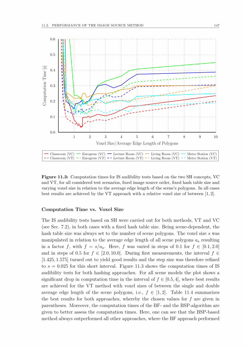
11.2. PERFORMANCE OF THE IMAGE SOURCE METHOD 147
Com
putation
Tim
e[s]
Voxel Size/Average Edge Length of Polygons
Classroom (VC)Classroom (VT)
Eurogress (VC)Eurogress (VT)
Lecture Room (VC)Lecture Room (VT)
Living Room (VC)Living Room (VT)
Metro Station (VC)Metro Station (VT)
Figure 11.3: Computation times for IS audibility tests based on the two SH concepts, VCand VT, for all considered test scenarios, fixed image source order, fixed hash table size andvarying voxel size in relation to the average edge length of the scene’s polygons. In all casesbest results are achieved by the VT approach with a relative voxel size of between [1, 2].
Computation Time vs. Voxel Size
The IS audibility tests based on SH were carried out for both methods, VT and VC(see Sec. 7.2), in both cases with a fixed hash table size. Being scene-dependent, thehash table size was always set to the number of scene polygons. The voxel size s wasmanipulated in relation to the average edge length of all scene polygons aa resultingin a factor f , with f = s/aa. Here, f was varied in steps of 0.1 for f ∈ [0.1, 2.0]and in steps of 0.5 for f ∈ [2.0, 10.0]. During first measurements, the interval f ∈[1.425, 1.575] turned out to yield good results and the step size was therefore refinedto s = 0.025 for this short interval. Figure 11.3 shows the computation times of ISaudibility tests for both hashing approaches. For all scene models the plot shows asignificant drop in computation time in the interval of f ∈ [0.5, 4], where best resultsare achieved for the VT method with voxel sizes of between the single and doubleaverage edge length of the scene polygons, i.e., f ∈ [1, 2]. Table 11.4 summarizesthe best results for both approaches, whereby the chosen values for f are given inparentheses. Moreover, the computation times of the BF- and the BSP-algorithm aregiven to better assess the computation times. Here, one can see that the BSP-basedmethod always outperformed all other approaches, where the BF approach performed
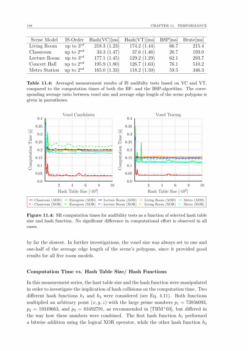
148 CHAPTER 11. PERFORMANCE
Scene Model IS-Order Hash(VC)[ms] Hash(VT)[ms] BSP[ms] Brute[ms]Living Room up to 3rd 218.3 (1.23) 174.2 (1.44) 66.7 215.4Classroom up to 2nd 33.3 (1.47) 37.6 (1.46) 26.7 193.0Lecture Room up to 3rd 177.1 (1.45) 129.2 (1.29) 62.1 293.7Concert Hall up to 2nd 195.9 (1.80) 126.7 (1.63) 76.1 510.2Metro Station up to 2nd 165.0 (1.33) 118.2 (1.50) 59.5 346.3
Table 11.4: Averaged measurement results of IS audibilty tests based on VC and VT,compared to the computation times of both the BF- and the BSP-algorithm. The corre-sponding average ratio between voxel size and average edge length of the scene polygons isgiven in parentheses.
Com
putation
Tim
e[s]
Hash Table Size [·103]
Voxel Candidates
Classroom (ADD)Classroom (XOR)
Eurogress (ADD)Eurogress (XOR)
Lecture Room (ADD)Lecture Room (XOR)
Living Room (ADD)Living Room (XOR)
Metro (ADD)Metro (XOR)
Com
putation
Tim
e[s]
Hash Table Size [·103]
Voxel Tracing
Figure 11.4: SH computation times for audibility tests as a function of selected hash tablesize and hash function. No significant difference in computational effort is observed in allcases.
by far the slowest. In further investigations, the voxel size was always set to one andone-half of the average edge length of the scene’s polygons, since it provided goodresults for all five room models.
Computation Time vs. Hash Table Size/ Hash Functions
In this measurement series, the hast table size and the hash function were manipulatedin order to investigate the implication of hash collisions on the computation time. Twodifferent hash functions h1 and h2 were considered (see Eq. 4.11). Both functionsmultiplied an arbitrary point (x, y, z) with the large prime numbers p1 = 73856093,p2 = 19349663, and p3 = 83492791, as recommended in [THM+03], but differed inthe way how these numbers were combined. The first hash function h1 performeda bitwise addition using the logical XOR operator, while the other hash function h2
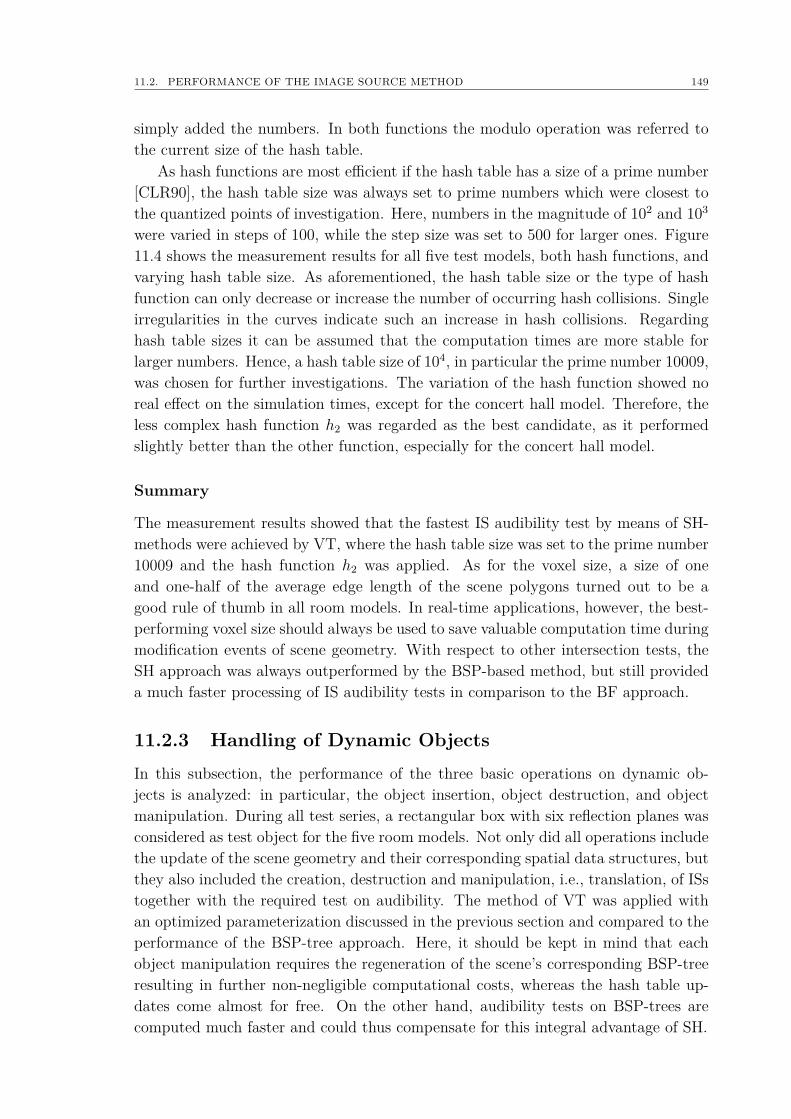
11.2. PERFORMANCE OF THE IMAGE SOURCE METHOD 149
simply added the numbers. In both functions the modulo operation was referred tothe current size of the hash table.
As hash functions are most efficient if the hash table has a size of a prime number[CLR90], the hash table size was always set to prime numbers which were closest tothe quantized points of investigation. Here, numbers in the magnitude of 102 and 103
were varied in steps of 100, while the step size was set to 500 for larger ones. Figure11.4 shows the measurement results for all five test models, both hash functions, andvarying hash table size. As aforementioned, the hash table size or the type of hashfunction can only decrease or increase the number of occurring hash collisions. Singleirregularities in the curves indicate such an increase in hash collisions. Regardinghash table sizes it can be assumed that the computation times are more stable forlarger numbers. Hence, a hash table size of 104, in particular the prime number 10009,was chosen for further investigations. The variation of the hash function showed noreal effect on the simulation times, except for the concert hall model. Therefore, theless complex hash function h2 was regarded as the best candidate, as it performedslightly better than the other function, especially for the concert hall model.
Summary
The measurement results showed that the fastest IS audibility test by means of SH-methods were achieved by VT, where the hash table size was set to the prime number10009 and the hash function h2 was applied. As for the voxel size, a size of oneand one-half of the average edge length of the scene polygons turned out to be agood rule of thumb in all room models. In real-time applications, however, the best-performing voxel size should always be used to save valuable computation time duringmodification events of scene geometry. With respect to other intersection tests, theSH approach was always outperformed by the BSP-based method, but still provideda much faster processing of IS audibility tests in comparison to the BF approach.
11.2.3 Handling of Dynamic ObjectsIn this subsection, the performance of the three basic operations on dynamic ob-jects is analyzed: in particular, the object insertion, object destruction, and objectmanipulation. During all test series, a rectangular box with six reflection planes wasconsidered as test object for the five room models. Not only did all operations includethe update of the scene geometry and their corresponding spatial data structures, butthey also included the creation, destruction and manipulation, i.e., translation, of ISstogether with the required test on audibility. The method of VT was applied withan optimized parameterization discussed in the previous section and compared to theperformance of the BSP-tree approach. Here, it should be kept in mind that eachobject manipulation requires the regeneration of the scene’s corresponding BSP-treeresulting in further non-negligible computational costs, whereas the hash table up-dates come almost for free. On the other hand, audibility tests on BSP-trees arecomputed much faster and could thus compensate for this integral advantage of SH.
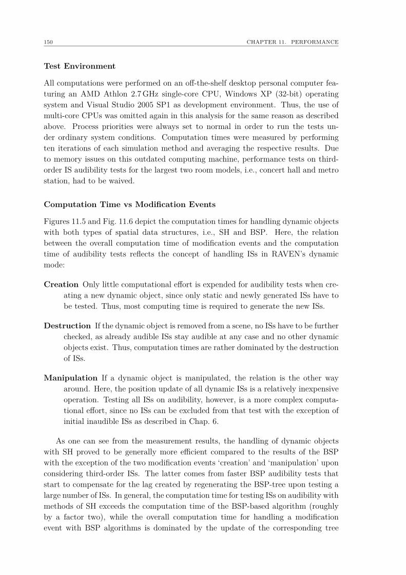
150 CHAPTER 11. PERFORMANCE
Test Environment
All computations were performed on an off-the-shelf desktop personal computer fea-turing an AMD Athlon 2.7GHz single-core CPU, Windows XP (32-bit) operatingsystem and Visual Studio 2005 SP1 as development environment. Thus, the use ofmulti-core CPUs was omitted again in this analysis for the same reason as describedabove. Process priorities were always set to normal in order to run the tests un-der ordinary system conditions. Computation times were measured by performingten iterations of each simulation method and averaging the respective results. Dueto memory issues on this outdated computing machine, performance tests on third-order IS audibility tests for the largest two room models, i.e., concert hall and metrostation, had to be waived.
Computation Time vs Modification Events
Figures 11.5 and Fig. 11.6 depict the computation times for handling dynamic objectswith both types of spatial data structures, i.e., SH and BSP. Here, the relationbetween the overall computation time of modification events and the computationtime of audibility tests reflects the concept of handling ISs in RAVEN’s dynamicmode:
Creation Only little computational effort is expended for audibility tests when cre-ating a new dynamic object, since only static and newly generated ISs have tobe tested. Thus, most computing time is required to generate the new ISs.
Destruction If the dynamic object is removed from a scene, no ISs have to be furtherchecked, as already audible ISs stay audible at any case and no other dynamicobjects exist. Thus, computation times are rather dominated by the destructionof ISs.
Manipulation If a dynamic object is manipulated, the relation is the other wayaround. Here, the position update of all dynamic ISs is a relatively inexpensiveoperation. Testing all ISs on audibility, however, is a more complex computa-tional effort, since no ISs can be excluded from that test with the exception ofinitial inaudible ISs as described in Chap. 6.
As one can see from the measurement results, the handling of dynamic objectswith SH proved to be generally more efficient compared to the results of the BSPwith the exception of the two modification events ‘creation’ and ‘manipulation’ uponconsidering third-order ISs. The latter comes from faster BSP audibility tests thatstart to compensate for the lag created by regenerating the BSP-tree upon testing alarge number of ISs. In general, the computation time for testing ISs on audibility withmethods of SH exceeds the computation time of the BSP-based algorithm (roughlyby a factor two), while the overall computation time for handling a modificationevent with BSP algorithms is dominated by the update of the corresponding tree
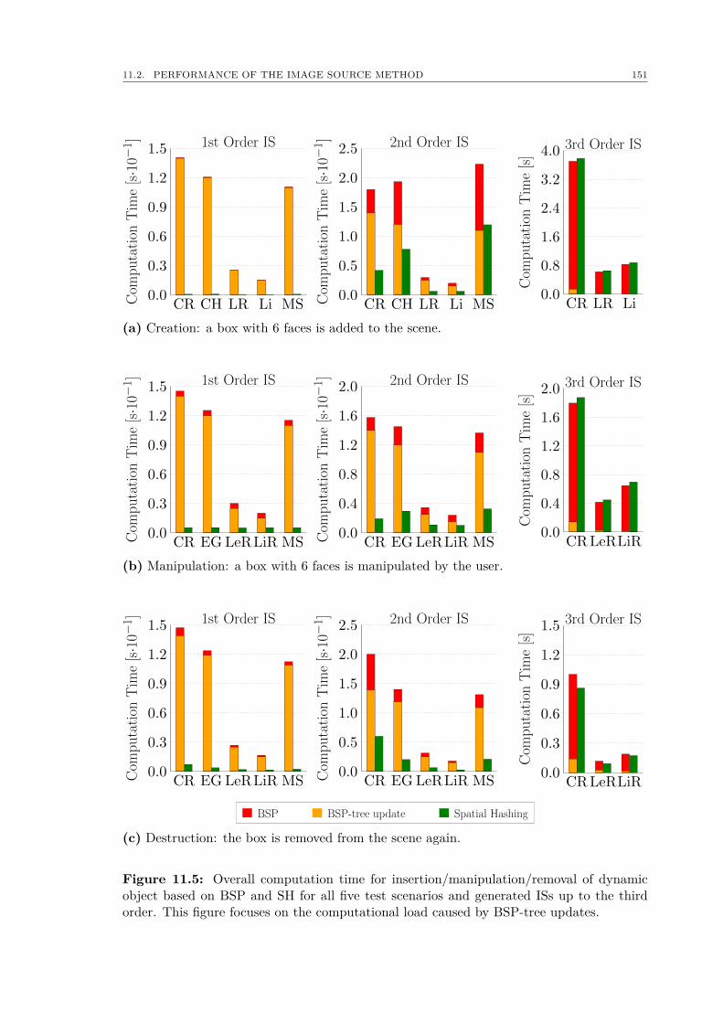
11.2. PERFORMANCE OF THE IMAGE SOURCE METHOD 151
Com
putation
Tim
e[s·10
−1 ] 1st Order IS
Com
putation
Tim
e[s·10
−1 ] 2nd Order IS
Com
putation
Tim
e[s]
3rd Order IS
(a) Creation: a box with 6 faces is added to the scene.
Com
putation
Tim
e[s·10
−1 ] 1st Order IS
Com
putation
Tim
e[s·10
−1 ] 2nd Order IS
Com
putation
Tim
e[s]
3rd Order IS
(b) Manipulation: a box with 6 faces is manipulated by the user.
Com
putation
Tim
e[s·10
−1 ] 1st Order IS
Com
putation
Tim
e[s·10
−1 ] 2nd Order IS
Com
putation
Tim
e[s]
3rd Order IS
BSP BSP-tree update Spatial Hashing
(c) Destruction: the box is removed from the scene again.
Figure 11.5: Overall computation time for insertion/manipulation/removal of dynamicobject based on BSP and SH for all five test scenarios and generated ISs up to the thirdorder. This figure focuses on the computational load caused by BSP-tree updates.
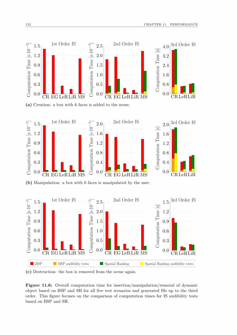
152 CHAPTER 11. PERFORMANCECom
putation
Tim
e[s·10
−1 ] 1st Order IS
Com
putation
Tim
e[s·10
−1 ] 2nd Order IS
Com
putation
Tim
e[s]
3rd Order IS
(a) Creation: a box with 6 faces is added to the scene.
Com
putation
Tim
e[s·10
−1 ] 1st Order IS
Com
putation
Tim
e[s·10
−1 ] 2nd Order IS
Com
putation
Tim
e[s]
3rd Order IS
(b) Manipulation: a box with 6 faces is manipulated by the user.
Com
putation
Tim
e[s·10
−1 ] 1st Order IS
Com
putation
Tim
e[s·10
−1 ] 2nd Order IS
Com
putation
Tim
e[s]
3rd Order IS
BSP BSP audibility tests Spatial Hashing Spatial Hashing audibility tests
(c) Destruction: the box is removed from the scene again.
Figure 11.6: Overall computation time for insertion/manipulation/removal of dynamicobject based on BSP and SH for all five test scenarios and generated ISs up to the thirdorder. This figure focuses on the comparison of computation times for IS audibility testsbased on BSP and SH.
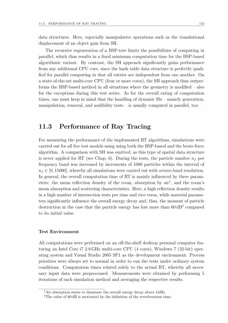
11.3. PERFORMANCE OF RAY TRACING 153
data structures. Here, especially manipulative operations such as the translationaldisplacement of an object gain from SH.
The recursive regeneration of a BSP-tree limits the possibilities of computing inparallel, which thus results in a fixed minimum computation time for the BSP-basedalgorithmic variant. By contrast, the SH approach significantly gains performancefrom any additional CPU core, since the hash table data structure is perfectly quali-fied for parallel computing in that all entries are independent from one another. Ona state-of-the-art multi-core CPU (four or more cores), the SH approach thus outper-forms the BSP-based method in all situations where the geometry is modified – alsofor the exceptions during this test series. As for the overall rating of computationtimes, one must keep in mind that the handling of dynamic ISs – namely generation,manipulation, removal, and audibility tests – is usually computed in parallel, too.
11.3 Performance of Ray Tracing
For measuring the performance of the implemented RT algorithms, simulations werecarried out for all five test models using using both the BSP-based and the brute-forcealgorithm. A comparison with SH was omitted, as this type of spatial data structureis never applied for RT (see Chap. 6). During the tests, the particle number nf perfrequency band was increased by increments of 1000 particles within the interval ofnf ∈ [0, 15000], whereby all simulations were carried out with octave-band resolution.In general, the overall computation time of RT is mainly influenced by three param-eters: the mean reflection density of the room, absorption by air1, and the room’smean absorption and scattering characteristics. Here, a high reflection density resultsin a high number of intersection tests per time and vice versa, while material parame-ters significantly influence the overall energy decay and, thus, the moment of particledestruction in the case that the particle energy has lost more than 60 dB2 comparedto its initial value.
Test Environment
All computations were performed on an off-the-shelf desktop personal computer fea-turing an Intel Core i7 2.8GHz multi-core CPU (4 cores), Windows 7 (32-bit) oper-ating system and Visual Studio 2005 SP1 as the development environment. Processpriorities were always set to normal in order to run the tests under ordinary systemconditions. Computation times related solely to the actual RT, whereby all neces-sary input data were preprocessed. Measurements were obtained by performing 5iterations of each simulation method and averaging the respective results.
1Air absorption starts to dominate the overall energy decay above 4 kHz.2The value of 60 dB is motivated by the definition of the reverberation time.
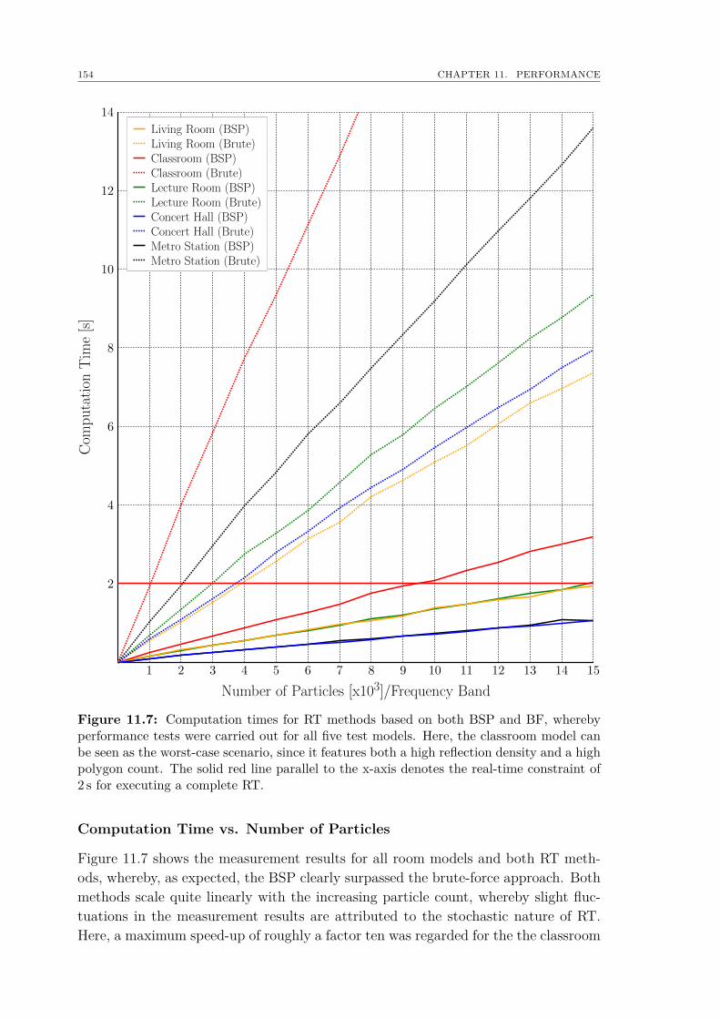
154 CHAPTER 11. PERFORMANCECom
putation
Tim
e[s]
Number of Particles [x103]/Frequency Band
Living Room (BSP)Living Room (Brute)Classroom (BSP)Classroom (Brute)Lecture Room (BSP)Lecture Room (Brute)Concert Hall (BSP)Concert Hall (Brute)Metro Station (BSP)Metro Station (Brute)
Figure 11.7: Computation times for RT methods based on both BSP and BF, wherebyperformance tests were carried out for all five test models. Here, the classroom model canbe seen as the worst-case scenario, since it features both a high reflection density and a highpolygon count. The solid red line parallel to the x-axis denotes the real-time constraint of2 s for executing a complete RT.
Computation Time vs. Number of Particles
Figure 11.7 shows the measurement results for all room models and both RT meth-ods, whereby, as expected, the BSP clearly surpassed the brute-force approach. Bothmethods scale quite linearly with the increasing particle count, whereby slight fluc-tuations in the measurement results are attributed to the stochastic nature of RT.Here, a maximum speed-up of roughly a factor ten was regarded for the the classroom
11.3. PERFORMANCE OF RAY TRACING 155
model, which can be seen as an algorithmic worst-case scenario , since this medium-sized room combines two aspects: a quite high reflection density and a high polygoncount.
When taking a closer look at the plots’ respective slopes, one can see that theactual order of curves from top to down varies for both methods, which reveals moreinformation on the overall behavior of RT. Whereas computation times for the brute-force approach are dominated by the models’ respective polygon count, no significantinfluence of this model parameter can be observed in the case of the BSP-basedmethod due to the decrease in search complexity to O(logN). In the latter case,computation times mostly depend on the room’s mean reflection density, as one cansee in Fig. 11.7 when comparing the results for the metro station, the concert hall andthe classroom. Although these models have roughly the same number of polygons,the first two models scale best, whereas the classroom scales worst due to the muchhigher reflection density.
With the assigned time slot of 2 s for RT simulation (see Chap. 6), all models can besimulated in real-time, especially when using small numbers of rays at first to generatea low-resolution histogram. If the listener stays at one place for a longer period oftime, the ray tracer can update the corresponding histogram with more rays to acquirea higher resolution and determine a longer impulse response, respectively. Apart fromthis, listening tests have shown that the required number of energy particles can begenerally kept at a quite low level (usually in the range of 5000 (small room) and15000 particles (large room) per frequency band), which will be further described inthe next chapter.

156 CHAPTER 11. PERFORMANCE
Chapter 12
Optimization of Input Parameters
"Everybody experiences far more than he understands. Yet it is expe-rience, rather than understanding, that influences behavior."
(Marshall McLuhan, Canadian media theorist)
It was mentioned earlier that the quality of a VR-system is assessable by theuser’s degree of immersion that improves with the number of simulated coherentstimuli and the level of both the plausibility and interactivity. At any rate, immersiveenvironments should thus aim at simulating opto-acoustical scenes in a plausible way,since it is a well-known fact that the visual perception is significantly augmentedby matching sound stimuli. Auditory information helps to assign meaning to visualinformation and vice versa.
As shown in the previous two sections, methods of GA can provide quite accurateresults at interactive rates. However, computational costs should always be kept to aminimum to enable complex simulations also on less powerful computing machines.Such a lowering of processing power is typically achieved by reducing the order of ISsand/or the number of traced energy particles, as these parameters strongly influencethe computational costs. Nonetheless, they also influence the perceptual quality ofthe auralization. Fortunately, a degradation of simulation accuracy is not necessarilyaudible, where a Parameter Threshold (PT) can be seen as a measure for an opti-mum parameterization in that no perceptible improvement can be achieved above thisthreshold. Consequently, several series of listening tests were performed described inthe following. Here, a criterion-free 3-Alternative Forced Choice (AFC)-paradigmwith two different assessment methods is applied in order to experimentally deter-mine the respective PTs for different room types, where a 3x2-design revealed theinteraction of relevant technical and perceptual conditions.
12.1 Listening TestsFive series of listening tests were carried out for the same five room scenarios (liv-
ing room, classroom, lecture room, concert hall and metro station) that were already
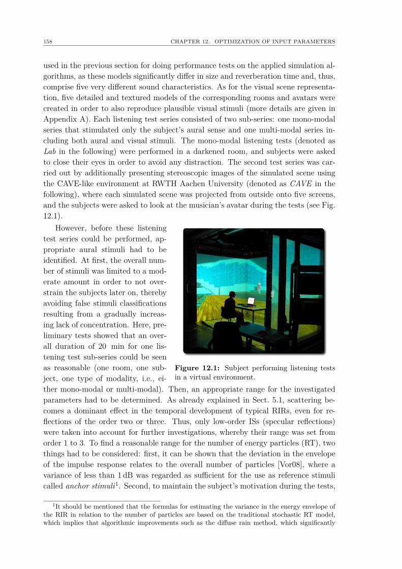
158 CHAPTER 12. OPTIMIZATION OF INPUT PARAMETERS
used in the previous section for doing performance tests on the applied simulation al-gorithms, as these models significantly differ in size and reverberation time and, thus,comprise five very different sound characteristics. As for the visual scene representa-tion, five detailed and textured models of the corresponding rooms and avatars werecreated in order to also reproduce plausible visual stimuli (more details are given inAppendix A). Each listening test series consisted of two sub-series: one mono-modalseries that stimulated only the subject’s aural sense and one multi-modal series in-cluding both aural and visual stimuli. The mono-modal listening tests (denoted asLab in the following) were performed in a darkened room, and subjects were askedto close their eyes in order to avoid any distraction. The second test series was car-ried out by additionally presenting stereoscopic images of the simulated scene usingthe CAVE-like environment at RWTH Aachen University (denoted as CAVE in thefollowing), where each simulated scene was projected from outside onto five screens,and the subjects were asked to look at the musician’s avatar during the tests (see Fig.12.1).
However, before these listening
Figure 12.1: Subject performing listening testsin a virtual environment.
test series could be performed, ap-propriate aural stimuli had to beidentified. At first, the overall num-ber of stimuli was limited to a mod-erate amount in order to not over-strain the subjects later on, therebyavoiding false stimuli classificationsresulting from a gradually increas-ing lack of concentration. Here, pre-liminary tests showed that an over-all duration of 20 min for one lis-tening test sub-series could be seenas reasonable (one room, one sub-ject, one type of modality, i.e., ei-ther mono-modal or multi-modal). Then, an appropriate range for the investigatedparameters had to be determined. As already explained in Sect. 5.1, scattering be-comes a dominant effect in the temporal development of typical RIRs, even for re-flections of the order two or three. Thus, only low-order ISs (specular reflections)were taken into account for further investigations, whereby their range was set fromorder 1 to 3. To find a reasonable range for the number of energy particles (RT), twothings had to be considered: first, it can be shown that the deviation in the envelopeof the impulse response relates to the overall number of particles [Vor08], where avariance of less than 1 dB was regarded as sufficient for the use as reference stimulicalled anchor stimuli1. Second, to maintain the subject’s motivation during the tests,
1It should be mentioned that the formulas for estimating the variance in the energy envelope ofthe RIR in relation to the number of particles are based on the traditional stochastic RT model,which implies that algorithmic improvements such as the diffuse rain method, which significantly
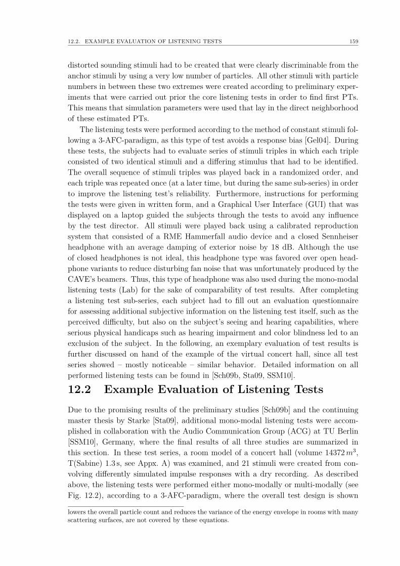
12.2. EXAMPLE EVALUATION OF LISTENING TESTS 159
distorted sounding stimuli had to be created that were clearly discriminable from theanchor stimuli by using a very low number of particles. All other stimuli with particlenumbers in between these two extremes were created according to preliminary exper-iments that were carried out prior the core listening tests in order to find first PTs.This means that simulation parameters were used that lay in the direct neighborhoodof these estimated PTs.
The listening tests were performed according to the method of constant stimuli fol-lowing a 3-AFC-paradigm, as this type of test avoids a response bias [Gel04]. Duringthese tests, the subjects had to evaluate series of stimuli triples in which each tripleconsisted of two identical stimuli and a differing stimulus that had to be identified.The overall sequence of stimuli triples was played back in a randomized order, andeach triple was repeated once (at a later time, but during the same sub-series) in orderto improve the listening test’s reliability. Furthermore, instructions for performingthe tests were given in written form, and a Graphical User Interface (GUI) that wasdisplayed on a laptop guided the subjects through the tests to avoid any influenceby the test director. All stimuli were played back using a calibrated reproductionsystem that consisted of a RME Hammerfall audio device and a closed Sennheiserheadphone with an average damping of exterior noise by 18 dB. Although the useof closed headphones is not ideal, this headphone type was favored over open head-phone variants to reduce disturbing fan noise that was unfortunately produced by theCAVE’s beamers. Thus, this type of headphone was also used during the mono-modallistening tests (Lab) for the sake of comparability of test results. After completinga listening test sub-series, each subject had to fill out an evaluation questionnairefor assessing additional subjective information on the listening test itself, such as theperceived difficulty, but also on the subject’s seeing and hearing capabilities, whereserious physical handicaps such as hearing impairment and color blindness led to anexclusion of the subject. In the following, an exemplary evaluation of test results isfurther discussed on hand of the example of the virtual concert hall, since all testseries showed – mostly noticeable – similar behavior. Detailed information on allperformed listening tests can be found in [Sch09b, Sta09, SSM10].
12.2 Example Evaluation of Listening TestsDue to the promising results of the preliminary studies [Sch09b] and the continuingmaster thesis by Starke [Sta09], additional mono-modal listening tests were accom-plished in collaboration with the Audio Communication Group (ACG) at TU Berlin[SSM10], Germany, where the final results of all three studies are summarized inthis section. In these test series, a room model of a concert hall (volume 14372m3,T(Sabine) 1.3 s, see Appx. A) was examined, and 21 stimuli were created from con-volving differently simulated impulse responses with a dry recording. As describedabove, the listening tests were performed either mono-modally or multi-modally (seeFig. 12.2), according to a 3-AFC-paradigm, where the overall test design is shown
lowers the overall particle count and reduces the variance of the energy envelope in rooms with manyscattering surfaces, are not covered by these equations.
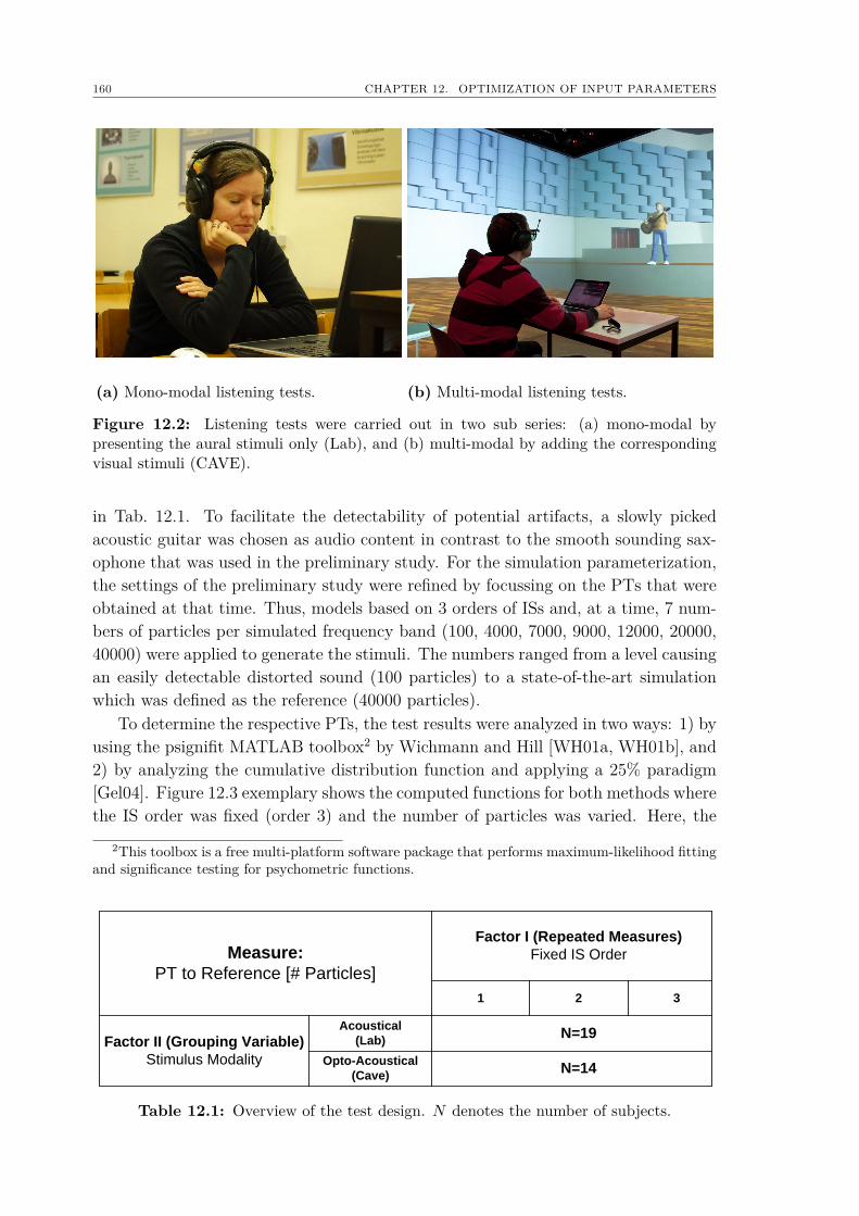
160 CHAPTER 12. OPTIMIZATION OF INPUT PARAMETERS
(a) Mono-modal listening tests. (b) Multi-modal listening tests.
Figure 12.2: Listening tests were carried out in two sub series: (a) mono-modal bypresenting the aural stimuli only (Lab), and (b) multi-modal by adding the correspondingvisual stimuli (CAVE).
in Tab. 12.1. To facilitate the detectability of potential artifacts, a slowly pickedacoustic guitar was chosen as audio content in contrast to the smooth sounding sax-ophone that was used in the preliminary study. For the simulation parameterization,the settings of the preliminary study were refined by focussing on the PTs that wereobtained at that time. Thus, models based on 3 orders of ISs and, at a time, 7 num-bers of particles per simulated frequency band (100, 4000, 7000, 9000, 12000, 20000,40000) were applied to generate the stimuli. The numbers ranged from a level causingan easily detectable distorted sound (100 particles) to a state-of-the-art simulationwhich was defined as the reference (40000 particles).
To determine the respective PTs, the test results were analyzed in two ways: 1) byusing the psignifit MATLAB toolbox2 by Wichmann and Hill [WH01a, WH01b], and2) by analyzing the cumulative distribution function and applying a 25% paradigm[Gel04]. Figure 12.3 exemplary shows the computed functions for both methods wherethe IS order was fixed (order 3) and the number of particles was varied. Here, the
2This toolbox is a free multi-platform software package that performs maximum-likelihood fittingand significance testing for psychometric functions.
Measure:
PT to Reference [# Particles]
Factor II (Grouping Variable)
Stimulus Modality
Acoustical
(Lab)
Opto-Acoustical
(Cave)
N=19
N=14
Factor I (Repeated Measures)
Fixed IS Order
1 2 3
Table 12.1: Overview of the test design. N denotes the number of subjects.
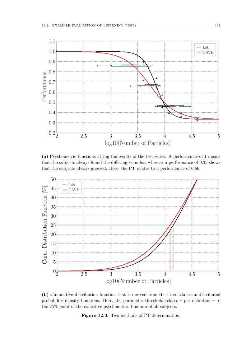
12.2. EXAMPLE EVALUATION OF LISTENING TESTS 161
Perform
ance
log10(Number of Particles)
LabCAVE
(a) Psychometric functions fitting the results of the test series. A performance of 1 meansthat the subjects always found the differing stimulus, whereas a performance of 0.33 showsthat the subjects always guessed. Here, the PT relates to a performance of 0.66.
Cum.Distribution
Function[%
]
log10(Number of Particles)
LabCAVE
(b) Cumulative distribution function that is derived from the fitted Gaussian-distributedprobability density functions. Here, the parameter threshold relates – per definition – tothe 25% point of the collective psychometric function of all subjects.
Figure 12.3: Two methods of PT determination.
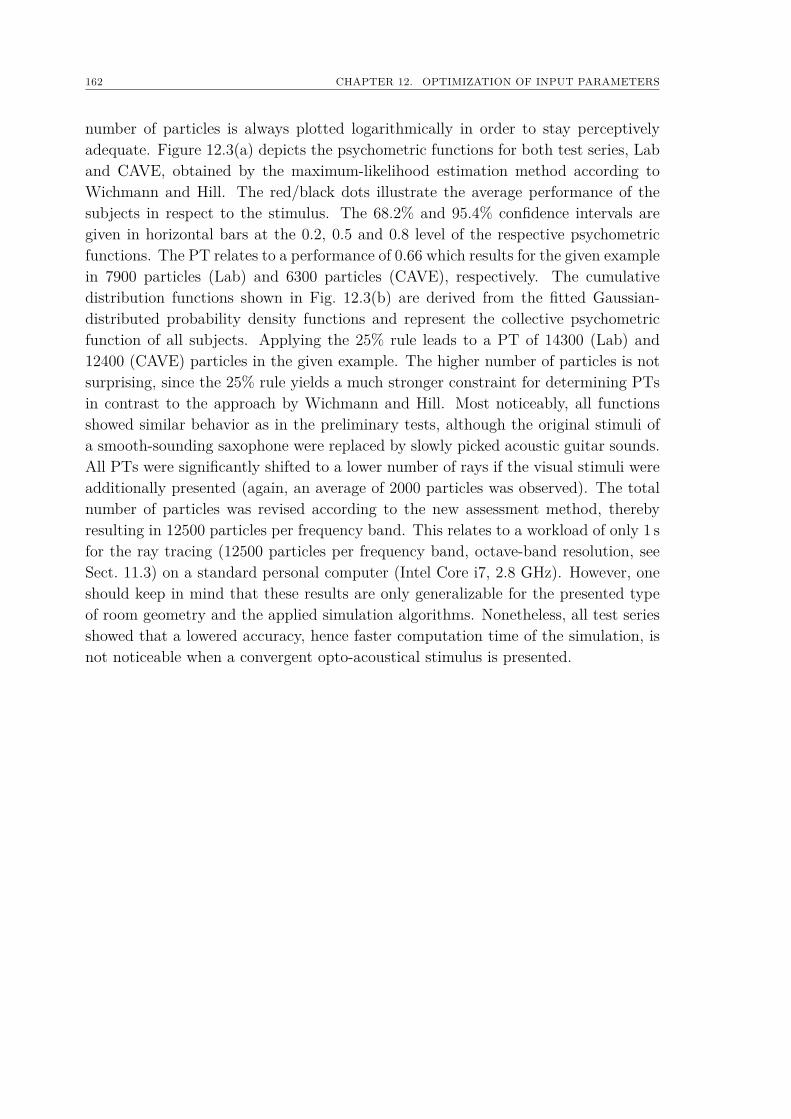
162 CHAPTER 12. OPTIMIZATION OF INPUT PARAMETERS
number of particles is always plotted logarithmically in order to stay perceptivelyadequate. Figure 12.3(a) depicts the psychometric functions for both test series, Laband CAVE, obtained by the maximum-likelihood estimation method according toWichmann and Hill. The red/black dots illustrate the average performance of thesubjects in respect to the stimulus. The 68.2% and 95.4% confidence intervals aregiven in horizontal bars at the 0.2, 0.5 and 0.8 level of the respective psychometricfunctions. The PT relates to a performance of 0.66 which results for the given examplein 7900 particles (Lab) and 6300 particles (CAVE), respectively. The cumulativedistribution functions shown in Fig. 12.3(b) are derived from the fitted Gaussian-distributed probability density functions and represent the collective psychometricfunction of all subjects. Applying the 25% rule leads to a PT of 14300 (Lab) and12400 (CAVE) particles in the given example. The higher number of particles is notsurprising, since the 25% rule yields a much stronger constraint for determining PTsin contrast to the approach by Wichmann and Hill. Most noticeably, all functionsshowed similar behavior as in the preliminary tests, although the original stimuli ofa smooth-sounding saxophone were replaced by slowly picked acoustic guitar sounds.All PTs were significantly shifted to a lower number of rays if the visual stimuli wereadditionally presented (again, an average of 2000 particles was observed). The totalnumber of particles was revised according to the new assessment method, therebyresulting in 12500 particles per frequency band. This relates to a workload of only 1 sfor the ray tracing (12500 particles per frequency band, octave-band resolution, seeSect. 11.3) on a standard personal computer (Intel Core i7, 2.8 GHz). However, oneshould keep in mind that these results are only generalizable for the presented typeof room geometry and the applied simulation algorithms. Nonetheless, all test seriesshowed that a lowered accuracy, hence faster computation time of the simulation, isnot noticeable when a convergent opto-acoustical stimulus is presented.

Part V
Summary & Outlook

164
Chapter 13
Summary and Discussion
"Master Control Program: End of Line."
(Tron, Steven Lisberger, American filmmaker)
This thesis described the concept and the implementation of the real-time room acous-tics simulation framework RAVEN which is today a vital part of the interactive 3Dsound rendering system of RWTH Aachen University’s immersive VR-environment.After a brief excursus about the fundamentals of acoustics and the description ofa concept for the multi-modal representation of natural sound sources, a physicallybased hybrid simulation method was introduced that took into account all importantsound phenomena, i.e, sound transmission, sound diffraction, and sound scattering.Here, a deterministic IS-model for the exact computation of early specular soundreflections was combined with a stochastic ray tracer that was able to model latereverberation with a correct energy distribution over time (diffuse and late specularreflections). The real-time performance was achieved by introducing a flexible simu-lation framework that enabled real-time modifications of sound sources, receivers andthe scene geometry. Consequently, the concept of scene graphs was adapted for adynamic linkage of autonomously operating room groups, i.e., rooms that were con-nected through open portals and encoded in optimized spatial data structures for fastgeometrical operations. Particular features of RAVEN were the following:
Hybrid Simulation Model The hybrid simulation model was not based on anyassumption of ideal diffuse sound fields but on a full room acoustics simula-tion. In this way the simulation framework was able to process any kind ofroom shape and volume except small rooms at low frequencies. Specular andscattered components of the impulse response were treated separately, wherebythe decision with regard to the amount of specular and diffuse reflections wasexclusively room-dependent and purely based on physical sound field aspects.Novel concepts for simulating sound diffraction were incorporated into the sim-ulation framework: as for the IS-model, an efficient method for handling sounddiffraction across an edge sequence was described, whereby Svensson’s deter-ministic secondary source model of edge diffraction from a finite wedge was uti-lized for computing time-domain edge diffraction impulse responses of reflection
166 CHAPTER 13. SUMMARY AND DISCUSSION
paths via edges. Furthermore, Stephenson’s frequency-dependent 2D-diffractionmodel of energy particles passing an edge was ported to 3D resulting in a newRT-method for distributing diffracted scattered energy among receivers, called‘diffracted rain’. This name was chosen in analogy to the ‘diffuse rain’ methodby Heinz, which allows a significant lowering of the number of necessary parti-cles without producing errors in the energy envelope of the RIR (an improvedversion was also featured by the applied ray tracer). Methods for construct-ing both monaural and binaural RIRs were described with special focus on thebinaural synthesis. Here, spatial cues were not only added to the direct soundand early reflections, but also to the late reverberation by introducing a spatialdetector that selected appropriate HRTFs with respect to the energy distribu-tion on the detector’s surface over time. In this way, spatial cues were addedin a more plausible way to BRIRs, since the common assumption of randomimpacting energy for later times of the impulse response holds only in an idealdiffuse sound field1.
Coupled Rooms Regarding the simulation of complex virtual indoor scenarios, anefficient approach for the auralization of sound transmission from adjacent andindirectly-connected room groups was developed on the basis of standardizedbuilding acoustics quantities and room acoustics simulations. This included anappropriate data structure for the scene representation and an analysis of soundtransmission paths in typical room-to-room situations. For the exclusion ofinaudible sound sources and frequency ranges, respectively, a search algorithm ofvalid sound paths was designed that took into account the current states (openedor closed) and sound insulation values of all involved portals. In addition, acommand structure was implemented that converted audible sound transmissionpaths into single simulation steps that directly controlled the application flowof the subsequent filter synthesis (monaural and binaural).
Scene Representation The simulation framework required only CAD room modelsas input data, where several data formats of commercial 3D modeling tools couldbe imported. However, some constraints regarding the scene modeling were re-quired for the sake of an efficient processing of geometry at runtime, e.g., the useof convex polygons for fast point-in-polygon tests. Surface properties were setsolely according to standardized material parameters, i.e., frequency-dependentabsorption-, scattering- and sound reduction coefficients/indices. The frame-work then adjusted all relevant runtime parameters automatically and inher-ently, such as the division of the RIR into specular and scattered components.The topological structure of the scene was represented by a graph-structurecalled ASG. Here, each node stored the spatial representation of a single room,including the polyhedral model (encoded as both the BSP-tree and spatial hashtable for accelerating geometry-related operations), material data, temperature,humidity and air pressure. The ASG’s edges represented polygonal portals that
1Example auralizations are available for download under www.ravenaudio.de.
167
connected adjacent rooms, i.e., nodes. The connectivity between nodes wassteered by the state of the respective portals, whereby the state ’closed’ and’opened’ dissociated and pooled two room groups, respectively.
Interactive Environments Another important design aspect for enabling an inter-active room acoustics simulation was the creation of highly flexible interactioninterfaces that provided a maximum degree of freedom in terms of supporteduser modification events. While code adjustments for operations such as theexchange of material parameters and the manipulation of portal states wererelatively easy to implement, the requirements of a modifiable geometry turnedout to be quite an algorithmic challenge. After first test implementations, itbecame clear that RAVEN’s acceleration algorithms based on hierarchical BSPdid not meet the criteria of dynamically manipulable geometry, since any mod-ification called for a time-consuming recalculation of at least large parts of thecorresponding BSP-trees. It was therefore decided to introduce two differentmodi operandi for geometrical scene objects: static and dynamic. Whereasstatic objects were not modifiable during the simulation and therefore process-able in a quick and efficient way, the size, shape, position, and orientation ofdynamic objects were manipulable by the user at runtime. This unconditionedmodification of dynamic objects was enabled by switching from BSP-trees to aslower, but more flexible approach of spatial subdivision – that of SH. SpatialHashing (SH) is based on the idea of subdividing the 3D space by primitivevolumes called voxels and mapping the infinitely voxelized subspaces to a fi-nite set of one-dimensional hash indices. Whereas the concept of SH was easilyembeddable to the applied ray tracing algorithm, a dynamic handling of ISsturned out to be more complicated as ISs had to be generated, destroyed andupdated (audibility and position) at runtime. Consequently, a hierarchical treedata structure was introduced that efficiently organized ISs for a convenient andfast processing.
Parallel Computing Since the top-level interface of RAVEN was unified, the un-derlying computation hardware was transparent and could be either a singlecomputer or a computation cluster of varying size. The latter was driven bya master scheduler that distributed simulation events by passing messages vianetwork to dedicated (multi-core) worker clients using the concepts of OpenMPand MPI for parallel processing. This made the approach very scalable so thatthe hardware could be chosen to match the complexity of the scenery.
The accuracy of the presented room acoustics simulation model was evaluated bymeans of three simple test scenarios, each testing one specific simulation event. Inparticular, these investigations encompassed the hybrid model itself, the simulationof sound transmission between two coupled rooms, and the computation of sounddiffraction from a single wedge, where simulation results were compared to analyticalsolutions. In all cases, RAVEN provided quite accurate results and, thus, showed thehigh capabilities of the underlying simulation framework.
168 CHAPTER 13. SUMMARY AND DISCUSSION
Furthermore, several test series were carried out, where RAVEN had to prove itsreal-time performance in a large variety of application events. Five different scenarioswere chosen for further investigation, whereby the corresponding room models differedstrongly with respect to room volume and polygonal complexity ranging from a smallliving room to a large metro station. In the case of static geometry, computation timesshowed that RAVEN’s BSP-based simulation acceleration enabled a quite plausibleauralization of all room types within the given real-time constraints of 550ms and 2 sfor the IS-method and RT, respectively2. In more detail, ISs of up to order three andRT with a sufficient number of energy particles that related to a standard deviationof less than 1 dB in the energy envelope of the corresponding impulse responses, werecomputable on an off-the-shelf multi-core PC for almost any room type in real-time.
In addition, investigations were carried out on a single-core standard PC regardingthe real-time modification of dynamic geometrical objects when applying accelerationmethods based on BSP and SH to the IS-method. Before the actual test serieswere begun, intersection tests based on SH were analyzed, thus revealing a strongdependency of the achieved performance on the chosen voxel size. Here, good resultswere obtained for all scene models by setting the voxel size to one and one-half of theaverage edge length of the corresponding scene polygons. In general, the performancetests showed that BSP-accelerated intersection tests were much more efficient than thetwo introduced methods based on SH. Yet they also showed the strong disadvantageof hierarchical spatial data structures, because each object manipulation requiredan update of the corresponding BSP-tree, resulting in additional computation timethat – in combination with the IS audibility test – was unable to compete with theperformance of SH during modification events such as the creation, manipulation,and destruction of dynamic geometrical objects. However, in cases of more complexroom geometries and ISs of up to order three, a large number of audibility tests hadto be performed, where the combination of BSP-tree regeneration and fast BSP-basedintersection tests could keep up with the performance of the SH approach.
In a subsequent series of listening tests, room acoustical simulations were regardedfrom a perceptual point of view in order to further optimize their parameterization foraudio-visual applications. Here, listening tests were carried out by using a criterion-free 3-AFC-paradigm with two different assessment methods and with the partici-pation of expert listeners. The subsequent evaluation of test results showed that alowered accuracy, hence faster computation time of the simulation, was not noticeableas long as a convergent opto-acoustical stimulus was presented.
In conclusion, a unique auralization framework was presented that relied onpresent-day knowledge of room acoustical simulation techniques and enabled a phys-ically accurate auralization of sound propagation in complex environments, includingthe important wave effects of sound scattering, sound transmission and sound diffrac-tion. Despite this realistic sound field rendering, not only were spatially distributed
2The decision regarding the update rate and depth of impulse response simulation was based onthe interaction and speed of movement of the user when operating in the immersive environment atRWTH Aachen University.

169
and freely movable sound sources and receivers supported at runtime, but also real-time modifications and manipulations of the geometrical environment itself were madepossible.

170 CHAPTER 13. SUMMARY AND DISCUSSION
Chapter 14
Outlook
"Look, I want you to know what we’re talking about here. This isn’tlike TV only better. This is life. It’s a piece of somebody’s life. Pure anduncut, straight from the cerebral cortex. You’re there. You’re doing it,seeing it, hearing it ... feeling it."
(Strange Days, James Cameron, American filmmaker)
Despite the good performance of the whole simulation framework, there are certainlymany aspects that still have to be investigated. This includes improvements in theapplied room acoustics simulation model as well as new simulation strategies andalgorithmic concepts that further reduce the overall computation time. Outlinedhere are some important ideas for future changes that will further enhance the rangeof RAVEN applications:
Numerical Simulations The frequencies below the Schroeder frequency could besimulated by combining wave-based and ray-based simulation methods in or-der to obtain realistic broadband RIRs, at least for small rooms. Here, severalcase studies were already carried out by Aretz et al., whereby RAVEN was com-bined with a fast finite element method FEM-solver [Fra08] for computing roomimpulse responses of small rooms [ANVS09, AJ10, AM10]. Although compu-tation times of the FEM-solver by far exceeded the given real-time constraints,the combination of both methods significantly enhanced the overall quality ofthe auralization and should therefore be added to RAVEN’s simulation frame-work in the future, but then in a real-time capable version. Until then, low-frequency RIRs could be preprocessed by the FEM-solver and combined withRAVEN’s on-line simulation results. Although physically not absolutely cor-rect, this combination would still result in a quite plausible auralization also oflow-frequencies.
Diffracted Rain Recent investigations by Stephenson revealed several issues regard-ing the DAPDF [Ste10b]. It was shown that the basic reciprocity-principle wasnot fulfilled when applying the DAPDF. This infers that simulation resultsdiffered if the positions of source and receiver were simply exchanged, which in
172 CHAPTER 14. OUTLOOK
the worst case could lead to deviations in the transmission level of up to severaldecibels. Here, Stephenson proposed introducing a new term to the mathemat-ical description of the DAPDF that compensated for this error, but then otherissues occurred. However, these problems do not directly affect the simulationmodel of the ‘diffracted rain’ RT-method, since values of the DAPDF are readin from a database with a resolution of one degree. Thus, the only thing to dois to regenerate this DAPDF-database as soon as an improved description ofthe DAPDF exists.
Time- and Frequency-Dependent Room Models An interesting idea for en-hancing the quality and speed of room acoustics simulations at the same timewas introduced by Pelzer who has already added this concept to RAVEN’s sim-ulation framework in a first stage [PV10]. The approach uses a set of roommodels with graduated level of detail of the same scene geometry, where everysingle room model is optimized for a certain frequency range, i.e., low detailsfor low frequencies and vice versa. Moreover, the level of detail is also decreasedwith increasing sound propagation time during the simulation, since accuratereflection patterns are not so important in the late part of the RIR, where manysound reflections from different directions overlap at the same time. Thus, atotal simulation speed-up of a factor of six can be achieved when combined withthe speed-up due to frequency-matched geometries.
Improved Sound Transmission Simulation The introduced approach for theauralization of sound transmission is certainly more a rough approximationthan a physically correct simulation in aspects of building acoustics. However,regarding the continuously increasing computation power, future versions willbe able to account for more and more sound transmission paths until the real-time simulation finally reaches and maybe outstrips the simulation quality ofcommercial off-line building acoustics software. These tools are usually basedon the same concepts as applied in RAVEN and typically simulate the soundtransmission up to first-order junctions. Although RAVEN’s auralization con-cept of sound transmission proved to work quite well, a validation includingsystematic listening tests should be performed to gather more information onthe importance of sound transmission paths and the positioning of secondarysources.
Perceptual Culling By considering the perceived sound of a source located in aneighboring room and damped by a closed portal, the sound impression is mostlyinfluenced by the portal’s transfer function and the impulse response of the roomwhere the user is located in. Especially two sound sources at different positionsin the separated sender room will have very similar impulse responses for thetotal sound propagation to the receiver. Hence, it is actually unnecessary torender two individual impulse responses, as they would sound nearly the same.In addition, Tsingos et al. introduced a technique called Perceptual Culling,
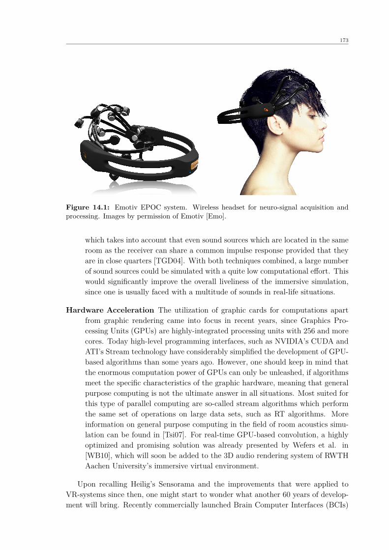
173
Figure 14.1: Emotiv EPOC system. Wireless headset for neuro-signal acquisition andprocessing. Images by permission of Emotiv [Emo].
which takes into account that even sound sources which are located in the sameroom as the receiver can share a common impulse response provided that theyare in close quarters [TGD04]. With both techniques combined, a large numberof sound sources could be simulated with a quite low computational effort. Thiswould significantly improve the overall liveliness of the immersive simulation,since one is usually faced with a multitude of sounds in real-life situations.
Hardware Acceleration The utilization of graphic cards for computations apartfrom graphic rendering came into focus in recent years, since Graphics Pro-cessing Units (GPUs) are highly-integrated processing units with 256 and morecores. Today high-level programming interfaces, such as NVIDIA’s CUDA andATI’s Stream technology have considerably simplified the development of GPU-based algorithms than some years ago. However, one should keep in mind thatthe enormous computation power of GPUs can only be unleashed, if algorithmsmeet the specific characteristics of the graphic hardware, meaning that generalpurpose computing is not the ultimate answer in all situations. Most suited forthis type of parallel computing are so-called stream algorithms which performthe same set of operations on large data sets, such as RT algorithms. Moreinformation on general purpose computing in the field of room acoustics simu-lation can be found in [Tsi07]. For real-time GPU-based convolution, a highlyoptimized and promising solution was already presented by Wefers et al. in[WB10], which will soon be added to the 3D audio rendering system of RWTHAachen University’s immersive virtual environment.
Upon recalling Heilig’s Sensorama and the improvements that were applied toVR-systems since then, one might start to wonder what another 60 years of develop-ment will bring. Recently commercially launched Brain Computer Interfaces (BCIs)

174 CHAPTER 14. OUTLOOK
aim at detecting user thoughts, feelings and expressions by using a set of sensorsto tune into electric signals produced by the brain (see Fig. 14.1). Maybe oneday, such a system can also work in a reverse way by inducing multi-modal stimulidirectly to the cerebral cortex, either for augmenting or totally cutting-off real-world perception – a state of mind where frontiers will fade between realism andsimulism, i.e., the birth of the ultimate medium. Certainly it is going to be a longand difficult road until that day and improvements are only gained in tiny little steps.
Perhaps this thesis has been one of them.

Part VI
Appendix

176
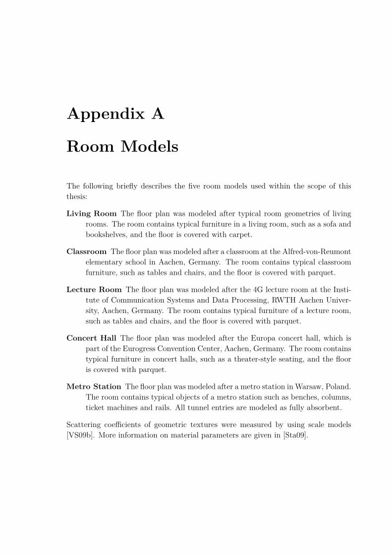
Appendix A
Room Models
The following briefly describes the five room models used within the scope of thisthesis:
Living Room The floor plan was modeled after typical room geometries of livingrooms. The room contains typical furniture in a living room, such as a sofa andbookshelves, and the floor is covered with carpet.
Classroom The floor plan was modeled after a classroom at the Alfred-von-Reumontelementary school in Aachen, Germany. The room contains typical classroomfurniture, such as tables and chairs, and the floor is covered with parquet.
Lecture Room The floor plan was modeled after the 4G lecture room at the Insti-tute of Communication Systems and Data Processing, RWTH Aachen Univer-sity, Aachen, Germany. The room contains typical furniture of a lecture room,such as tables and chairs, and the floor is covered with parquet.
Concert Hall The floor plan was modeled after the Europa concert hall, which ispart of the Eurogress Convention Center, Aachen, Germany. The room containstypical furniture in concert halls, such as a theater-style seating, and the flooris covered with parquet.
Metro Station The floor plan was modeled after a metro station in Warsaw, Poland.The room contains typical objects of a metro station such as benches, columns,ticket machines and rails. All tunnel entries are modeled as fully absorbent.
Scattering coefficients of geometric textures were measured by using scale models[VS09b]. More information on material parameters are given in [Sta09].
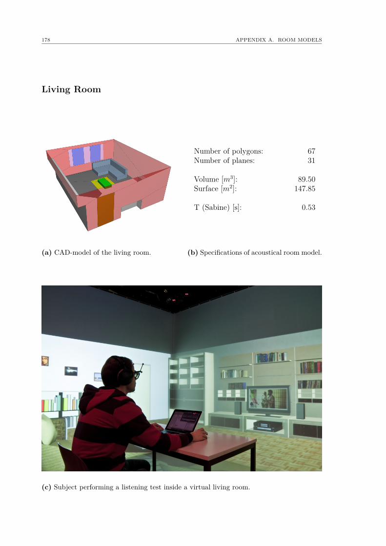
178 APPENDIX A. ROOM MODELS
Living Room
(a) CAD-model of the living room.
Number of polygons: 67Number of planes: 31
Volume [m3]: 89.50Surface [m2]: 147.85
T (Sabine) [s]: 0.53
(b) Specifications of acoustical room model.
(c) Subject performing a listening test inside a virtual living room.
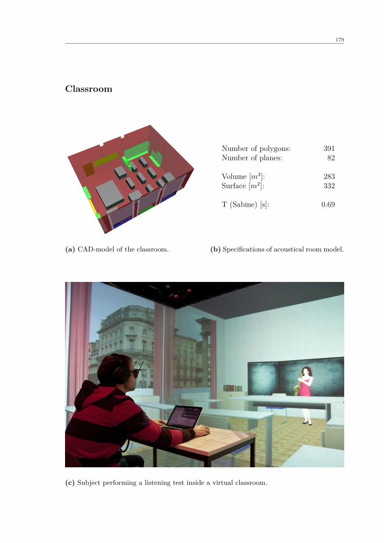
179
Classroom
(a) CAD-model of the classroom.
Number of polygons: 391Number of planes: 82
Volume [m3]: 283Surface [m2]: 332
T (Sabine) [s]: 0.69
(b) Specifications of acoustical room model.
(c) Subject performing a listening test inside a virtual classroom.
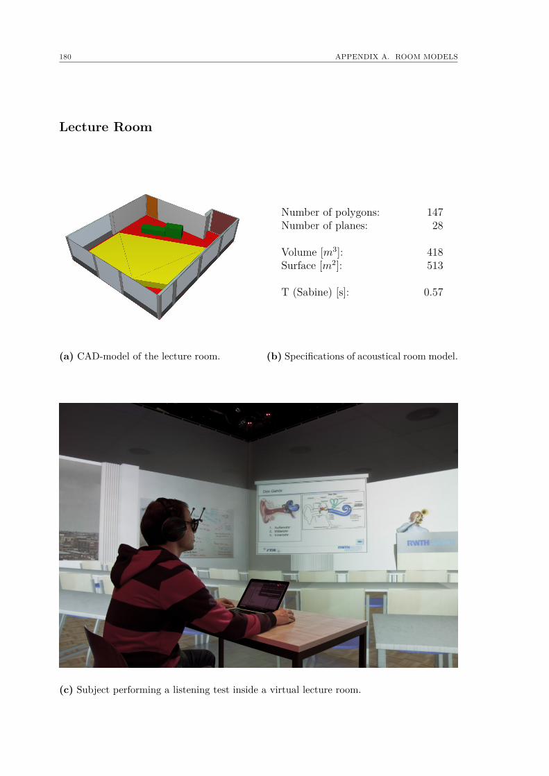
180 APPENDIX A. ROOM MODELS
Lecture Room
(a) CAD-model of the lecture room.
Number of polygons: 147Number of planes: 28
Volume [m3]: 418Surface [m2]: 513
T (Sabine) [s]: 0.57
(b) Specifications of acoustical room model.
(c) Subject performing a listening test inside a virtual lecture room.
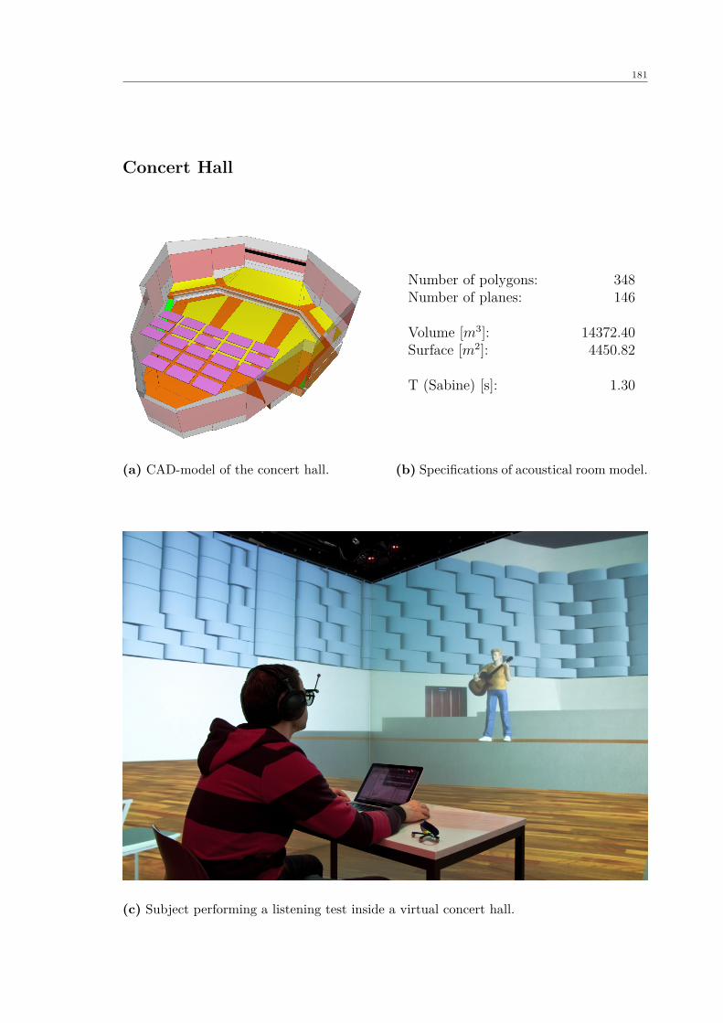
181
Concert Hall
(a) CAD-model of the concert hall.
Number of polygons: 348Number of planes: 146
Volume [m3]: 14372.40Surface [m2]: 4450.82
T (Sabine) [s]: 1.30
(b) Specifications of acoustical room model.
(c) Subject performing a listening test inside a virtual concert hall.
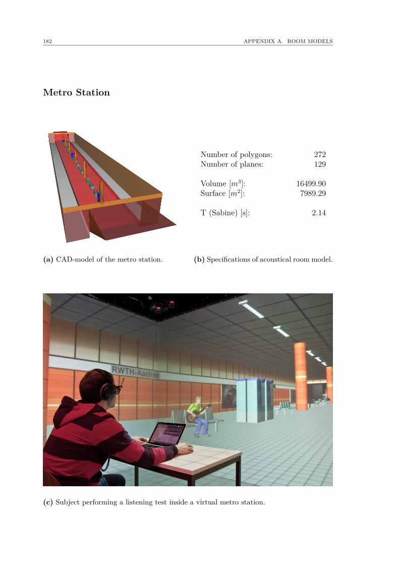
182 APPENDIX A. ROOM MODELS
Metro Station
(a) CAD-model of the metro station.
Number of polygons: 272Number of planes: 129
Volume [m3]: 16499.90Surface [m2]: 7989.29
T (Sabine) [s]: 2.14
(b) Specifications of acoustical room model.
(c) Subject performing a listening test inside a virtual metro station.
Appendix B
RAVEN
As described in the course of this thesis, RAVEN relies on present-day knowledgeof room acoustical simulation techniques and enables a physically quite accurateauralization of sound propagation in complex environments supporting spatiallydistributed and freely movable sound sources and receivers, as well as modificationsand manipulations of the geometrical environment at runtime.
Particular features of RAVEN are:
• Only standardized input data required.
• Hybrid simulation model that combines deterministic ISs with stochastic RT fora complete physically based simulation of room acoustics including importantwave effects such as sound scattering, airborne sound insulation between roomsand sound diffraction.
• Real-time room- and building acoustics auralization of dynamically-coupledrooms.
• Real-time modification of sound sources, receivers, and geometrical objects.
• Support of parallel computing on both, distributed- and shared-memory ma-chines.
• Powerful GUI and visualization toolbox for off-line use (see below).
• Special batch mode for the use with other applications such as MATLAB.
• More specific software details along with demonstration videos and sound filescan be found here: www.ravenaudio.de
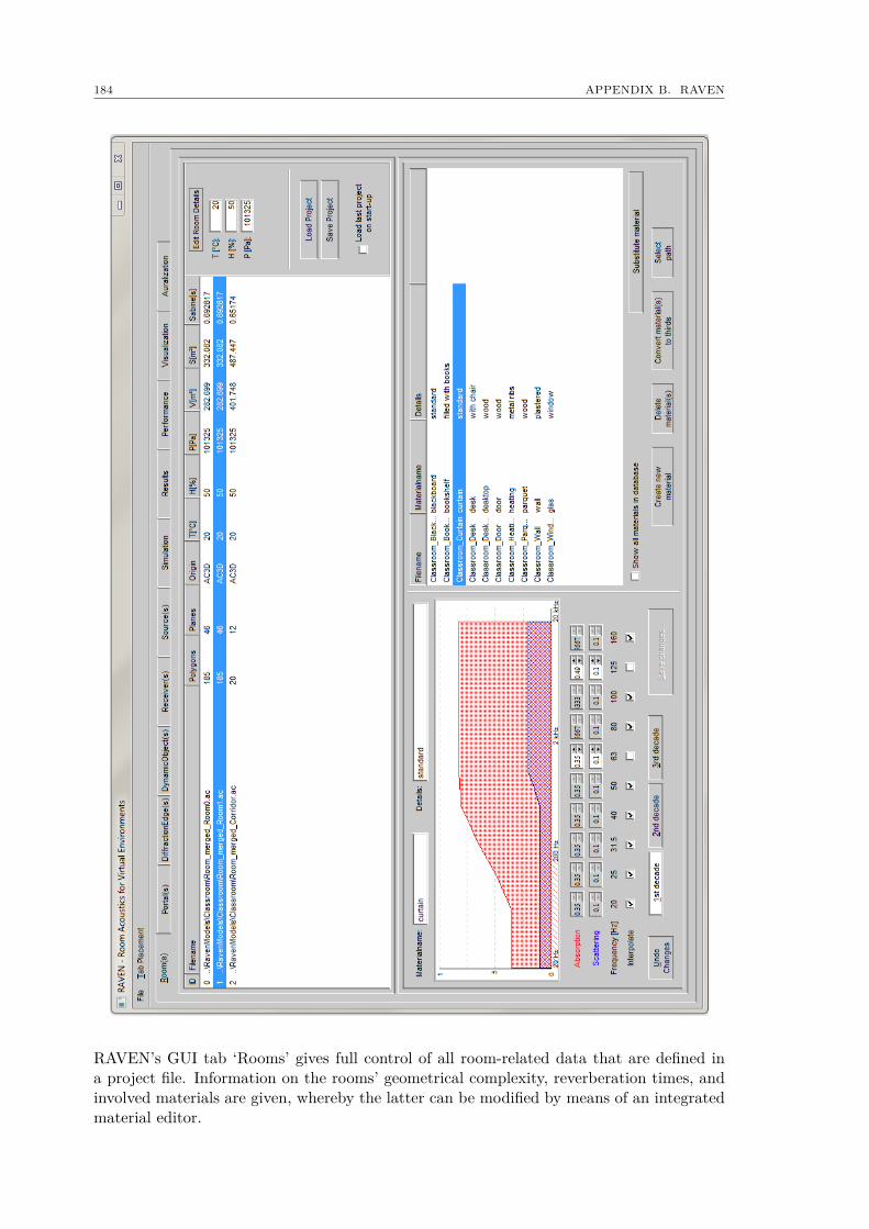
184 APPENDIX B. RAVEN
RAVEN’s GUI tab ‘Rooms’ gives full control of all room-related data that are defined ina project file. Information on the rooms’ geometrical complexity, reverberation times, andinvolved materials are given, whereby the latter can be modified by means of an integratedmaterial editor.
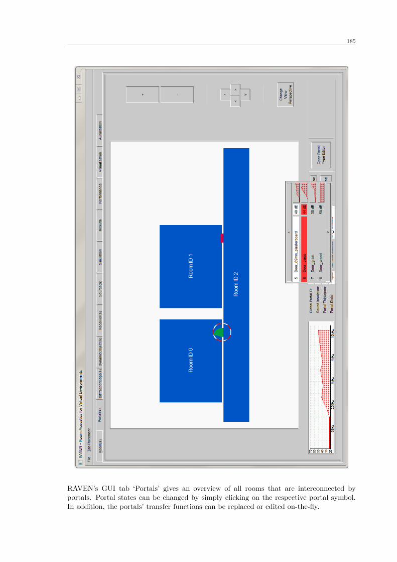
185
RAVEN’s GUI tab ‘Portals’ gives an overview of all rooms that are interconnected byportals. Portal states can be changed by simply clicking on the respective portal symbol.In addition, the portals’ transfer functions can be replaced or edited on-the-fly.
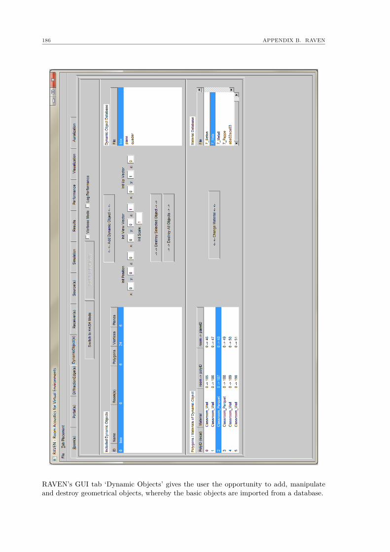
186 APPENDIX B. RAVEN
RAVEN’s GUI tab ‘Dynamic Objects’ gives the user the opportunity to add, manipulateand destroy geometrical objects, whereby the basic objects are imported from a database.
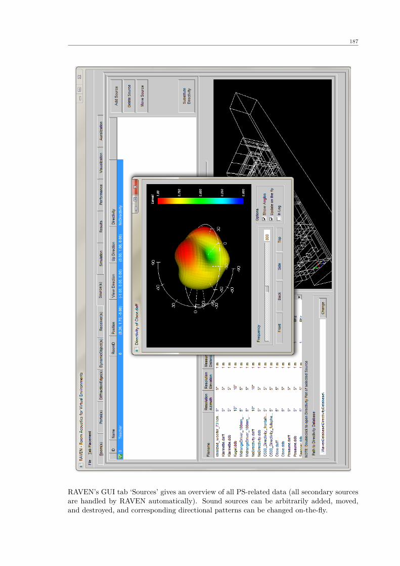
187
RAVEN’s GUI tab ‘Sources’ gives an overview of all PS-related data (all secondary sourcesare handled by RAVEN automatically). Sound sources can be arbitrarily added, moved,and destroyed, and corresponding directional patterns can be changed on-the-fly.
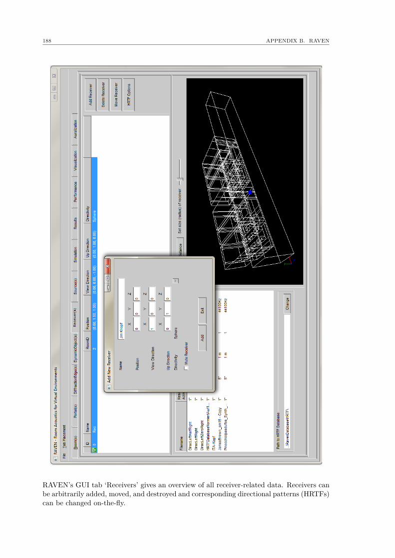
188 APPENDIX B. RAVEN
RAVEN’s GUI tab ‘Receivers’ gives an overview of all receiver-related data. Receivers canbe arbitrarily added, moved, and destroyed and corresponding directional patterns (HRTFs)can be changed on-the-fly.
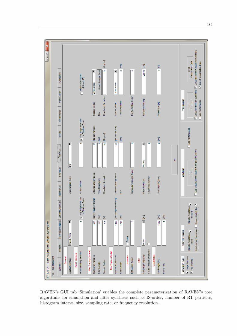
189
RAVEN’s GUI tab ‘Simulation’ enables the complete parameterization of RAVEN’s corealgorithms for simulation and filter synthesis such as IS-order, number of RT particles,histogram interval size, sampling rate, or frequency resolution.

190 APPENDIX B. RAVEN
RAVEN’s GUI tab ‘Results’ offers a convenient view of project-wise sorted simulation re-sults such as RIRs and BRIRs (specular and diffuse parts plus their hybrid combinations),Schroeder plots, energy histograms, and room acoustical quantities.
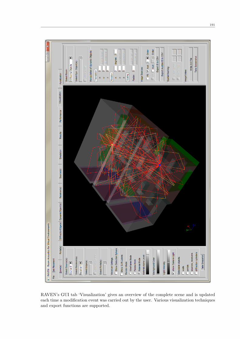
191
RAVEN’s GUI tab ‘Visualization’ gives an overview of the complete scene and is updatedeach time a modification event was carried out by the user. Various visualization techniquesand export functions are supported.
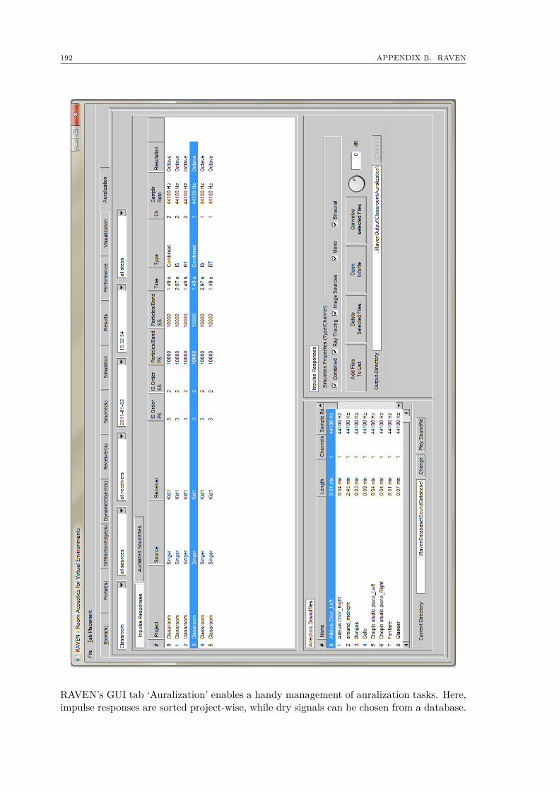
192 APPENDIX B. RAVEN
RAVEN’s GUI tab ‘Auralization’ enables a handy management of auralization tasks. Here,impulse responses are sorted project-wise, while dry signals can be chosen from a database.
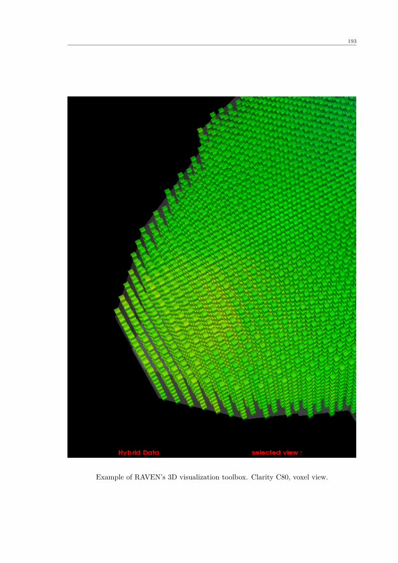
193
Example of RAVEN’s 3D visualization toolbox. Clarity C80, voxel view.
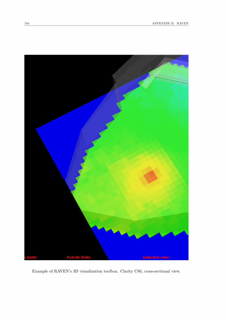
194 APPENDIX B. RAVEN
Example of RAVEN’s 3D visualization toolbox. Clarity C80, cross-sectional view.
Bibliography
[AB79] J. B. Allen and D. A. Berkley. Image Method for Efficiently SimulatingSmall-Room Acoustics. Journal of the Acoustical Society of America,65:943, 1979.
[AB95] R. Azuma and G. Bishop. A frequency-domain analysis of head-motionprediction. In Proceedings of the 22nd annual conference on ComputerGraphics and Interactive Techniques, New York, NY, USA, 1995.
[AJ10] M. Aretz and L. Jauer. Perceptual comparison of measured and simu-lated sound fields in small rooms. In Proceedings of the DAGA, Berlin,Germany, 2010.
[AK08] I. Assenmacher and T. Kuhlen. The VISTA Virtual Reality Toolkit.In Proceedings of the IEEE VR SEARIS, Reno, USA, 2008.
[AM10] A. Aretz and P. Maier. Simulation based Auralization of the Acousticsin a Studio Room using a combined Wave and Ray based Approach.In Proceedings of the 26th Tonmeistertagung, Leipzig, Germany, 2010.
[AMH02] T. Akenine-Möller and E. Haines. Real-Time Rendering, 2nd edition.A.K. Peters, 2002.
[ANVS09] M. Aretz, R. Nöthen, M. Vorländer, and D. Schröder. Combined broad-band impulse responses using fem and hybrid ray-based methods. InProceedings of the EAA Auralization Symposium, Espoo, Finland, 2009.
[Arv91] J. Arvo, editor. Graphics Gems II. Academic Press, 1991.
[Ass09] I. Assenmacher. Low latency technology for interactive virtual environ-ments. PhD thesis, RWTH Aachen University, 2009.
[BC03] G. C. Burdea and P. Coiffet. Virtual Reality Technology, 2nd edition.John Wiley & Sons, 2003.
[Ber80] B. Bernfeld. Absorption of Sound by Air: A Personal Calculator Pro-gram. In Proceedings of the 66th AES Convention, Los Angeles, USA,1980.
[Bla96] J. Blauert. Spatial Hearing – The Psychophysics of Human SoundLocalization, revised edition. MIT Press, 1996.
[Bor84] J. Borish. Extension of the Image Model to Arbitrary Polyhedra. Jour-nal of the Acoustical Society of America, 75:1827, 1984.
196 BIBLIOGRAPHY
[Bor00] I. Bork. A comparison of room simulation software – the 2nd RoundRobin on room acoustical computer simulation. Acta Acustica Unitedwith Acustica, 86:943, 2000.
[BPS08] G. K. Behler, M. Pollow, and D. Schröder. Messung und Simulation vonRaumimpulsantworten für eine realistische Auralisation. In Proceedingsof the 25th Tonmeistertagung, Leipzig, Germany, 2008.
[BS95] J.S. Bradley and G.A. Soulodre. The influence of late arriving energyon spatial impression. Journal of the Acoustical Society of America,97:2263, 1995.
[BSM+04] D. S. Brungart, D. D. Simpson, R. L. McKinley, A. J. Kordik, R. C.Dallman, and D. A. Ovenshire. The interaction between head-trackerlatency, source duration, and response time in the localization of vir-tual sound sources. In Proceedings of ICAD 04 - 10th Meeting of theInternational Conference on Auditory Display, Sydney, Australia, 2004.
[BT57] M. A. Biot and I. Tolstoy. Formulation of wave propagation in infinitemedia by normal coordinates with an application to diffraction. Journalof the Acoustical Society of America, 29:381, 1957.
[BW99] M. Born and E. Wolf. Principles of Optics, 7th Edition. PergamonPress, 1999.
[CDD+06] T. J. Cox, B.-I. L. Dalenbäck, P. D’Antonio, J. J. Embrechts, J. Y.Jeon, E. Mommertz, and M. Vorländer. A Tutorial on Scattering andDiffusion Coeffcients for Room Acoustic Surfaces. Acta Acustica Unitedwith Acustica, 92:1, 2006.
[CHV02] L. Chai, W.A. Hoff, and T. Vincent. Three-dimensional motion andstructure estimation using inertial sensors and computer vision for aug-mented reality. Presence: Teleoperators and Virtual Environments,11:474, 2002.
[CLR90] T. Cormen, C. Leiserson, and R. Rivest. Introduction to Algorithms.MIT Press, 1990.
[CLT+08] A. Chandak, C. Lauterbach, M. Taylor, Z. Ren, and D. Manocha.AD-Frustum: Adaptive Frustum Tracing for Interactive Sound Propa-gation. IEEE Transactions on Visualization and Computer Graphics,14:1707, 2008.
[CNSD+92] C. Cruz-Neira, D. Sandin, T. DeFanti, R. Kenyon, and J. Hart. Thecave: Audio visual experience automatic virtual environment. Com-munications of the ACM, 35:64, 1992.
[CP69] M. J. Crocker and A. J. Price. Sound Transmission using StatisticalEnergy Analysis. Jounal of Sound and Vibration, 9:460, 1969.
BIBLIOGRAPHY 197
[CP70] M. J. Crocker and A. J. Price. Sound transmission through double pan-els using statistical energy analysis. Journal of the Acoustical Societyof America, 47:683, 1970.
[CR05] C. L. Christensen and J. H. Rindel. A new scattering method thatcombines roughness and diffraction effects. In Proceedings of the ForumAcousticum, Budapest, Hungary, 2005.
[Cra93] O. Cramer. The variation of the specific heat ratio and the speed ofsound in air with temperature, pressure, humidity, and CO2 concen-tration. Journal of the Acoustical Society of America, 93:2510, 1993.
[Dal95] B.-I. L. Dalenbäck. A New Model for Room Acoustic Prediction andAuralization. PhD thesis, Chalmers University if Technology, Gothen-burg, Sweden, 1995.
[Dal96] B.-I. L. Dalenbäck. Room acoustic prediction based on a unified treat-ment of diffuse and specular reflection. Journal of the Acoustical Societyof America, 100:899, 1996.
[Dro06] P. Dross. Real-time capable reverberation estimator for virtual environ-ments. Master’s thesis, RWTH Aachen University, Aachen, Germany,2006.
[Emo] Emotiv. www.emotiv.com.
[EN97] European Standard EN. 12354: Building acoustics - estimation ofacoustic performance of buildings from the performance of products,1997.
[Far95] A. Farina. RAMSETE - a new Pyramid Tracer for medium and largescale acoustic problems. In Proceedings of the Euronoise, Lyon, France,1995.
[FCD] ISO/IEC FCD. 19774:200x: Information technology - Computer graph-ics and image processing - Humanoid animation (H-Anim), www.hanim.org/.
[Fra08] A. Franck. Finite-Elemente-Methoden, Lösungsalgorithmen undWerkzeuge für die akustische Simulationstechnik. PhD thesis, Instituteof Technical Acoustics, RWTH Aachen University, Aachen, Germany,2008.
[FTC+04] T. A. Funkhouser, N. Tsingos, I. Carlbom, G. Elko, M. Sondhi, J. E.West, G. Pingal, P. Min, and A. Ngan. A beam tracing method forinteractive architectural acoustics. Journal of the Acoustical Society ofAmerica, 115:739, 2004.
[FvDFH96] J. D. Foley, A. van Dam, S. K. Feiner, and J. F. Hughes. ComputerGraphics, Principles and Practice, 2nd edition. Addison-Wesley, 1996.
198 BIBLIOGRAPHY
[Gel04] S. A. Gelfand. Hearing. An Introduction to psychological and physio-logical acoustics, 4th edition. Dekker, 2004.
[Ger79] E. Gerretsen. Calculation of sound transmission between dwellings bypartitions and flanking structures. Applied Acoustics, 12:413, 1979.
[Ger86] E. Gerretsen. Calculation of airborne and impact sound insulationbetween dwellings. Applied Acoustics, 19:245, 1986.
[GHW+04] A. Gerndt, B. Hentschel, M. Wolter, T. Kuhlen, and C. H. Bischof.VIRACOCHA: An Efficient Parallelization Framework for Large-ScaleCFD Post-Processing in Virtual Environments. IEEE Computer Soci-ety, page 50, 2004.
[Gir96] F. Giron. Investigations about the directivity of sound sources. PhDthesis, Ruhr Universität, Bochum, Germany, 1996.
[Gla89] A. Glassner. An Introduction to Ray Tracing. Academic Press, 1989.
[Gla93] A. Glassner, editor. Graphics Gems. Academic Press, 1993.
[Hec94] P. Heckbert, editor. Graphics Gems IV. Morgan Kaufmann, 1994.
[Hei62] Morton L. Heilig. Sensorama simulator, August 1962.
[Hei93] R. Heinz. Binaural room simulation based on an image source modelwith addition of statistical methods to include the diffuse sound scat-tering of walls and to predict the reverberant tail. Applied Acoustics,38:145, 1993.
[Hei94] R. Heinz. Entwicklung und Beurteilung von computergestützten Meth-oden zur binauralen Raumsimulation. PhD thesis, RWTH Aachen Uni-versity, Aachen, Germany, 1994.
[Hol02] J. Holländer. Improvements on an algorithm for insulation of airbornesound insulation. Institute of Technical Acoustics, RWTH Aachen Uni-versity, Aachen, Germany, 2002.
[ISO03] DIN EN ISO. 354: Acoustics – Measurement of sound absorption in areverberation room, 2003.
[ISO04a] ISO. 17497: Acoustics – Measurement of sound scattering of surfaces,2004.
[ISO04b] DIN EN ISO. 140: Acoustics – Measurement of sound insulation inbuildings and of building elements, 2004.
[ISO07] DIN EN ISO. 3382-2: Acoustics – Measurement of room acoustic pa-rameters – Part 2: Reverberation time in ordinary rooms, 2007.
[Jau10] L. Jauer. Schallfeld Simulation im Fahrzeuginnenraum mittels kom-binierter wellen- und strahlenbasierter Simulationsverfahren. Master’sthesis, RWTH Aachen University, Aachen, Germany, 2010.
BIBLIOGRAPHY 199
[JNW06] D. Jackèl, S. Neunreither, and F. Wagner. Methoden der Computeran-imation. Springer, 2006.
[KDS93] M. Kleiner, B. I. Dalenbäck, and U. P. Svensson. Auralization - AnOverview. Journal of the Audio Engineering Society, 41:861, 1993.
[Kel62] J. B. Keller. Geometrical theory of diffraction. Journal of the OpticalSociety of America, 52:116, 1962.
[Kir92] D. Kirk, editor. Graphics Gems III. Morgan Kaufmann, 1992.
[KJM05] B. Kapralos, M. Jenkin, and E. Milios. Acoustical diffraction model-ing utilizing the huygens-fresnel principle. In Proceedings of the IEEEInternational Workshop, Ontario, Canada, 2005.
[Kom07] L. Komzsik. Approximation Techniques for Engineers. CRC PRess,2007.
[KP74] R. G. Kouyoumijan and P. H. Pathak. A uniform geometrical theoryof diffraction for an edge in a perfectly conducting surface. Proceedingsof the IEEE, 62:1448, 1974.
[KSS68] A. Krokstad, S. Strøm, and S. Sørsdal. Calculating the acoustical roomresponse by the use of a ray tracing technique. Journal on Sound andVibration, 8:118, 1968.
[Kut95] H. Kuttruff. A simple iteration scheme for the computation of decayconstants in enclosures with diffusely reflecting boundaries. Journal ofthe Acoustical Society of America,, 98:288, 1995.
[Kut00] H. Kuttruff. Room Acoustics, 4th edition. Elsevier, 2000.
[KvdPvEJ06] A.G. Kohlrausch, S. L. J. D. E. van de Par, R. L. J. van Eijk, andJ. F. Juola. Human performance in detecting audio-visual asynchrony.Journal of the Acoustical Society of America, 120:3084–3085, 2006.
[Lam96] Y.W. Lam. A comparison of three reflection modelling methods usedin room acoustics computer models. Journal of the Acoustical Societyof America, 100:2181, 1996.
[LCM07] C. Lauterbach, A. Chandak, and D. Manocha. Interactive Sound Ren-dering in Complex and Dynamic Scenes using Frustum Tracing. IEEETransactions on Visualization and Computer Graphics, 13:1672, 2007.
[Len07] T. Lentz. Binaural Technology for Virtual Reality. PhD thesis, RWTHAachen University, Aachen, Germany, 2007.
[Lew93] P. Lewers. A combined bream tracing and radiant exchange computermodel of room acoustics. Applied Acoustics, 38:161, 1993.
200 BIBLIOGRAPHY
[LJ03] J. J. LaViola Jr. A testbed for studying and choosing predictive track-ing algorithms in virtual environments. In Proceedings of the 7th Inter-national Immersive Projection Technologies Workshop, 9th Eurograph-ics Workshop on Virtual Environments, Zurich, Switzerland, 2003.
[LM62] R. H. Lyon and G. Maidanik. Power flow between linearly coupledoscillators. Journal of the Acoustical Society of America, 40:7, 1962.
[LSVA07] T. Lentz, D. Schröder, M. Vorländer, and I. Assenmacher. Virtualreality system with integrated sound field simulation and reproduction.EURASIP Journal on Advances in Signal Processing, 2007:19, 2007.
[Lun08] P. Lundén. Uni-verse acoustic simulation system: interactive realtimeroom acoustic simulation in dynamic 3D environments. Journal of theAcoustical Society of America, 123:3937, 2008.
[Mae68] Z. Maekawa. Noise reduction by screens. Applied Acoustics, 1:157,1968.
[Mec02] F. P. Mechel. Formulas of Acoustics. Springer, 2002.
[Med81] H. Medwin. Shadowing by finite noise barriers. Journal of the Acous-tical Society of America, 69:1060, 1981.
[Mey09] J. Meyer. Acoustics and the Performance of Music, 5th edition.Springer, 2009.
[Mor05] M. Mori. Views on the uncanny valley. In Proceedings of the IEEE-RASHumanoids Workshop, Tsukuba, Japan, 2005.
[MPI08] MPI. A Message-Passing Interface Standard Version 2.1, www.mcs.anl.gov/research/projects/mpi, 2008.
[Mös95] M. Möser. Die Wirkung von zylindrischen Aufsätzen an Schallschirmen.Acustica, 81:565, 1995.
[Mös05] M. Möser. Technische Akustik, 6th edition. Springer, 2005.
[Nay93] G. M. Naylor. ODEON - another hybrid room acoustical model. AppliedAcoustics, 38:131, 1993.
[NKSS08] M. Noisternig, B. Katz, S. Siltanen, and L. Savioja. Framework for real-time auralization in architectural acoustics. Journal of the AcousticalSociety of America, 94:1000, 2008.
[Opea] OpenDaff. www.opendaff.org.
[Opeb] OpenMeasurements. www.openmeasurements.net.
[Ope08] OpenMP. Application Program Interface Version 3.0, www.openmp.org,2008.
BIBLIOGRAPHY 201
[OR04] F. Otondo and J. H Rindel. The influence of the directivity of musicalinstruments in a room. Acta Acustica United with Acustica, 90:1178,2004.
[Pae95] A. Paeth, editor. Graphics Gems V. Morgan Kaufmann, 1995.
[PB09] M. Pollow and G. Behler. Variable Directivity for Platonic SoundSources Based on Spherical Harmonics Optimization. Acta AcusticaUnited with Acustica, 95:1082, 2009.
[PBS10] M. Pollow, G.K. Behler, and F. Schultz. Musical instrument recordingfor building a directivity database. In Proceedings of the DAGA, Berlin,Germany, 2010.
[Pel07] S. Pelzer. Real-time auralization of complex dynamic virtual environ-ments. Master’s thesis, RWTH Aachen University, Aachen, Germany,2007.
[Pie88] A. Pietrzyk. Computer modeling of the sound field in small rooms. InProceedings of the 15th AES International Conference on Audio Acous-tics and Small Spaces, Copenhagen, Denmark, 1988.
[PL10] J. Pätynen and T. Lokki. Directivities of symphony orchestra instru-ments. Acta Acustica United with Acustica, 96:138, 2010.
[Poh08] A. Pohl. Beugungsalgorithmen für die Echtzeit-Raumakustiksimulation. Master’s thesis, RWTH Aachen University,Aachen, Germany, 2008.
[PS] A. Pohl and D. Schröder.
[PSV11] S. Pelzer, D. Schröder, and M. Vorländer. The number of necessaryrays in simulations based on geometrical acoustics using the diffuse raintechnique. In Proceedings of the DAGA, Düsseldorf, Germany, 2011.
[PV10] S. Pelzer and M. Vorländer. Frequency- and time-dependent geome-try for real-time auralization. In Proceedings of the 20th InternationalCongress on Acoustics (ICA), Syndey, Australia, 2010.
[RA08] D. Rausch and I. Assenmacher. A sketch-based interface for architec-tural modification in virtual environments. In Proceedings of the 5thVR/AR Workshop, Magdeburg, Germany, 2008.
[Rab03] R. Rabenseifner. Hybrid parallel programming: Performance problemsand chances. In Proceedings of the 45th Cray User Group Conference,Columbus, OH, USA, 2003.
[RE01] S. Ranta-Eskola. Binary Space Partitioning Trees and Polygon Re-moval in Real Time 3D Rendering. Master’s thesis, Uppsala University,Uppsala, Sweden, 2001.
202 BIBLIOGRAPHY
[Reu08] S. Reuter. Simulation of natural sound sources in immersive virtual en-vironments. Master’s thesis, RWTH Aachen University, Aachen, Ger-many, 2008.
[Rin04] J. H. Rindel. Evaluation of room acoustic qualities and defects by useof auralization,. In Proceedings of the 148th Meeting of the AcousticalSociety of America, San Diego, CA, USA, 2004.
[Ros70] S. M. Ross. Applied probability models with optimization applications.Holden-Day, 1970.
[Ryb09] A. Ryba. Real-time auralization of modifiable rooms. Master’s thesis,RWTH Aachen University, Aachen, Germany, 2009.
[SAB62] M. R. Schroeder, B. S. Atal, and C. Bird. Digital computers in roomacoustics. In Proceedings of the 4th International Congress on Acous-tics, Copenhagen, Denmark, 1962.
[Sav99] L. Savioja. Modeling Techniques for Virtual Acoustics. PhD thesis,Helsinki University of Technology, Helsinki, Finland, 1999.
[SBGS69] R. Shumacker, R. Brand, M. Gilliland, and W. Sharp. Study for Apply-ing Computer-Generated Images to Visual Simulations, AFHRL-TR-69-14. Technical report, U.S. Air Force Human Resources Laboratory,1969.
[Sch09a] M. Schlütter. Parallelisierung von Algorithmen für die Echtzeit-Raumakustiksimulation. Master’s thesis, RWTH Aachen University,Aachen, Germany, 2009.
[Sch09b] D. Schröder. Optimization of input parameters for real-time roomacoustics simulations. In Proceedings of the International Conferenceon Acoustics NAG/DAGA, pages 1456–1458, Rotterdam, The Nether-lands, 2009.
[SDV07] D. Schröder, P. Dross, and M. Vorländer. A fast reverberation estima-tor for virtual environments. In Proceedings of the 30th AES Interna-tional Conference, Saariselkä, Finland, 2007.
[SE10] U. P. Svensson and H. El-Bann Zidan. Early energy conditions insmall rooms and in convolutions of small-room impulse responses. InProceedings of the 129th AES Convention, San Francisco, USA, 2010.
[Sed90] R. Sedgewick. Algorithms in C. Addison-Wesley, 1990.
[SFV99] U. P. Svensson, R. I. Fred, and J. Vanderkooy. An analytic secondarysource model of edge diffraction impulse responses. Journal of theAcoustical Society of America, 106:2331, 1999.
[Shi62] M. Shimrat. Algorithm 112: Position of point relative to polygon.Communications of the ACM, 5:434, 1962.
BIBLIOGRAPHY 203
[SHLV99] L. Savioja, J. Huopaniemi, T. Lokki, and R. Väänänen. Creating inter-active virtual acoustic environments. Journal of the Audio EngineeringSociety, 47:675, 1999.
[SL06] D. Schröder and T. Lentz. Real-time processing of image sources usingbinary space partitioning. Journal of the Audio Engineering Society,54(7/8):604–619, 2006.
[Sle04] K. Slenczka. Simulations of natural sound sources for binaural synthe-sis. PhD thesis, RWTH Aachen University, Aachen, Germany, 2004.
[SLKS07] S. Siltanen, T. Lokki, S. Kiminki, and L. Savioja. The room acous-tic rendering equation. Journal of the Acoustical Society of America,122:1624, 2007.
[SN99] J. S. Suh and P. A. Nelson. Measurement of transient response ofrooms and comparison with geometrical acoustic models. Journal ofthe Acoustical Society of America, 105:2304, 1999.
[SRA08] D. Schröder, S. Reuter, and I. Assemnacher. Multimodale Darstellungnatürlicher Schallquellen in virtuellen Umgebungen. In Proceedings ofthe DAGA, Dresden, Germany, 2008.
[SS07] U. M. Stephenson and U. P. Svensson. An improved energetic approachto diffraction based on the uncertainty principle. In Proceedings of the19th International Congress on Acoustics, Madrid, Spain, 2007.
[SSM10] D. Schröder, B. Starke, and H.-J. Maempel. Optimization of inputparameters for the real-time simulation of room acoustics - revisited.In Proceedings of the DAGA, Berlin, Germany, 2010.
[SSV10] D. Schröder, U. P. Svensson, and M. Vorländer. Open measurementsof edge diffraction from a noise barrier scale model. In Proceedings ofthe International Symposium on Room Acoustics (ISRA), Melbourne,Australia, 2010.
[Sta09] B. Starke. Investigation of the influence of acoustical simulation pa-rameters on the perception in virtual environments. Master’s thesis,RWTH Aachen University, Aachen, Germany, 2009.
[Ste96] U. M. Stephenson. Quantized Pryamidal Beam Tracing - a New Al-gorithm for Room Acoustics and Noise Immission Prognosis. ACTAACUSTICA united with ACUSTICA, 82:517, 1996.
[Ste04] U. M. Stephenson. Beugungssimulation ohne Rechenzeitexplosion:die Methode der quantisierten Pyramidenstrahlen; ein neues Berech-nungsverfahren für Raumakustik und Lärmimmissionsprognose; Ver-gleiche, Ansätze, Lösungen. PhD thesis, RWTH Aachen University,Aachen, Germany, 2004.
[Ste10a] U. M. Stephenson. Simulation of diffraction within ray tracing. ActaAcustica United with Acustica, 96:516, 2010.
204 BIBLIOGRAPHY
[Ste10b] U. M. Stephenson. Some further experiments with the beam diffractionmodel based on the uncer tainty relation - is it valid also with doublediffraction? In Proceedings of the DAGA, Berlin, Germany, 2010.
[SV07] D. Schröder and M. Vorländer. Hybrid method for room acoustic sim-ulation in real-time. In Proceedings of the 20th International Congresson Acoustics (ICA), Madrid, Spain, 2007.
[Sve10] Edge Diffraction Matlab Toolbox by U. Peter Svensson. www.iet.ntnu.no/~svensson/software/index.html, 2010.
[SW00] U. P. Svensson and K. Wendlandt. The influence of a loudspeakercabinet’s shape on the radiated power. In Proceedings of Baltic Acoustic2000, Vilnius, Lithuania, 2000.
[TGD04] N. Tsingos, E. Gallo, and G. Drettakis. Perceptual audio rendering ofcomplex virtual environments. ACM Transactions on Graphics (SIG-GRAPH Conference Proceedings), 3, 2004.
[Tha05] R. Thaden. Auralisation in Building Acoustics. PhD thesis, RWTHAachen University, Aachen, Germany, 2005.
[THM+03] M. Teschner, B. Heidelberger, M. Müller, D. Pomeranets, andM. Gross. Optimized Spatial Hashing for Collision Detection of De-formable Objects. In Proceedings of the VMV, Munich, Germany, 2003.
[Tsi07] N. Tsingos. Using programmable graphics hard-ware for auralization.In Proceedings of the EAA Auralization Symposium, Espoo, Finland,2007.
[Val07] J. T. Valvoda. Virtual Humanoids and Presence in Virtual Environ-ments. PhD thesis, RWTH Aachen University, Aachen, Germany, 2007.
[vdPK00] S. van de Par and A. Kohlrausch. Sensitivity to Auditory-Visual Asyn-chrony and to Jitter in Auditory-Visual Timing. In Proceedings of theHuman Vision and Electronic Imaging V, San Jose, USA, 2000.
[vE00] O. von Estorff. Boundary Elements in Acoustics: Advances and Appli-cations. WIT Press, 2000.
[VM00] M. Vorländer and E. Mommertz. Definition and measurement ofrandom-incidence scattering coeffcients. Applied Acoustics, 60:187,2000.
[Vor89] M. Vorländer. Simulation of the transient and steady-state sound prop-agation in rooms using a new combined ray-tracing/image-source algo-rithm. Journal of the Acoustical Society of America, 86:172, 1989.
[Vor95] M. Vorländer. International Round Robin on room acoustical com-puter simulations. In Proceedings of the 15th International Congresson Acoustics, Trondheim, Norway, 1995.
BIBLIOGRAPHY 205
[Vor08] M. Vorländer. Auralization - Fundamentals of Acoustics, Modelling,Simulation, Algorithms and Acoustic Virtual Reality. Springer, 2008.
[VRC] VRCA. www.vrca.rwth-aachen.de.
[VS09a] R. Vitale and D. Schröder. Investigation of scattering coefficient ofeveryday furniture. In Proceedings of the International Conference onAcoustics NAG/DAGA, Rotterdam, The Netherlands, 2009.
[VS09b] R. Vitale and D. Schröder. Measurements of scattering coefficientsfor classroom acoustics computer simulation. In Proceedings of theEURONOISE, Edinburgh, UK, 2009.
[VT00] M. Vorländer and R. Thaden. Auralisation of airborne sound insulationin buildings. Acustica united with Acta Acustica, 86:70, 2000.
[VvM86] J. Vian and D. van Maercke. Calculation of the room impulse responseusing a ray-tracing method. In Proceedings of the ICA Symposium onAcoustics and Theatre Planning for the Performing Arts, Vancouver,Canada, 1986.
[Wal80] J. P. Walsh. The design of Godot: A system for computer-aided roomacoustics modeling and simulation. In Proceedings of the 10th Interna-tional Conference on Acoustics, Sydney, Australia, 1980.
[WB10] F. Wefers and J. Berg. High-performance real-time FIR-filtering usingfast convolution on graphics hardware. In Proceedings of the DAFX,Graz, Austria, 2010.
[WD07] I. Witew and P. Dietrich. Assessment of the Uncertainty in RoomAcoustical Measurements. In Proceedings of the 19th InternationalCongress on Acoustics, Madrid, Spain, 2007.
[Wef07] F. Wefers. Optimizing segmented realtime convolution. Master’s thesis,RWTH Aachen University, Aachen, Germany, 2007.
[WH01a] F. A. Wichmann and N. J. Hill. The psychometric function: I. fitting,sampling and goodness-of-fit. Perception and Psychophysics, 63:1293,2001.
[WH01b] F. A. Wichmann and N. J. Hill. The psychometric function: Ii.bootstrap-based confidence intervals and sampling. Perception andPsychophysics, 63:1314, 2001.
[Wil99] E.G. Williams. Fourier Acoustics: Sound Radiation and NearfieldAcoustical Holography. Academic Press, 1999.
[Wit04] I. Witew. Spatial variation of lateral measures in different concert halls.In Proceedings of the 18th International Congress on Acoustics, Kyoto,Japan, 2004.
206 BIBLIOGRAPHY
[WO95] J. R. Wu and M. Ouhyoung. A 3D tracking experiment on latencyand its compensation methods in virtual environments. In Proceed-ings of the 8th annual ACM symposium on User interface and softwaretechnology, New York, NY, USA, 1995.
[WS09] F. Wefers and D. Schröder. Real-time auralization of coupled rooms.In Proceedings of the EAA Auralization Symposium, Espoo, Finland,2009.
[WSPV09] F. Wefers, D. Schröder, S. Pelzer, and M. Vorländer. Real-time filter-ing for interactive virtual acoustic prototyping. In Proceedings of theEURONOISE, Edinburgh, UK, 2009.
[Zie00] O.C. Zienkiewicz. Finite Element Method Volume 1 - The Basis, 5thedition. Elsevier, 2000.
[ZS06] F. Zotter and A. Sontacci. Virtual Game-Lan Graz, IEM Report 35/06.Technical report, Institute of Electronic Music and Acoustic, Universityof Music and Performing Arts, Graz, Austria, 2006.

Curriculum vitae
Personal Data
Date of Birth: 22th of June, 1974Place of Birth: Cologne, GermanyFiliation: Ursula and Friedhelm Schröder
Education
01/2005–02/2011 Ph.D. Studies at the Institute of Technical AcousticsRWTH Aachen University, GermanyConcentration: Virtual Acoustics/Immersive Audio
10/1997–10/2004 Master Degree in Electrical Engineering (Dipl.-Ing.)RWTH Aachen University, GermanyConcentration: Communication- and Information Technology
Professional Experience
05/2011–today Research Fellow (ERCIM Scholar)Centre for Quantifiable Quality of Service in CommunicationSystems, Centre of Excellence, NTNU Trondheim, Norway
01/2005–03/2011 Research/Teaching AssistantInstitute of Technical Acoustics, RWTH Aachen University,Germany
08/2009–12/2009 Research/Teaching AssistantCentre for Quantifiable Quality of Service in CommunicationSystems, Centre of Excellence, NTNU Trondheim, Norway
10/2003–02/2004 InternshipPhilips Research, Aachen, Germany
06/2003–08/2003 InternshipIntelligent Systems and Control (ISAC) Research Group,Belfast, United Kingdom

λογος
Logos Verlag BerlinISBN 978-3-8325-3031-0
ISSN 1866-3052
Analogous to visualization, the auralization of virtual environments descri-bes the simulation of sound propagation inside enclosures where methodsof Geometrical Acoustics are mostly applied for a high-quality synthesis ofaural stimuli that go along with a certain realistic behavior. In the courseof this thesis, the design and implementation of the real-time room acou-stics simulation software RAVEN will be described, which is a vital part ofthe implemented 3D sound-rendering system of RWTH Aachen University’simmersive Virtual Reality system.
RAVEN relies on present-day knowledge of room acoustical simulation tech-niques and enables a physically accurate auralization of sound propagationin complex environments including important wave effects such as soundscattering, airborne sound insulation between rooms and sound diffraction.Despite this realistic sound field rendering, not only spatially distributed andfreely movable sound sources and receivers are supported at runtime butalso modifications and manipulations of the environment itself.
All major features are evaluated by investigating both the overall accuracyof the room acoustics simulation and the performance of implemented al-gorithms, and possibilities for further simulation optimizations are identifiedby assessing empirical studies of subjects operating in immersive environ-ments.