arX

iv:c

ond-

mat

/030

4048

v1 [

cond

-mat

.sof

t] 2

Apr

200

3

Phase separation kinetics in compressible

polymer solutions: Computer simulation of the

early stages

Peter Virnau1, Marcus Muller1, Luis Gonzalez MacDowell2,

and Kurt Binder1

1Institut fur Physik, Johannes Gutenberg–Universitat Mainz,

Staudinger Weg 7, 55099 Mainz, Germany2Dpto. de Quimica Fisica, Facultad de Cc. Qumicas,

Universidad Complutense, 28040 Madrid, Spain

February 2, 2008

Abstract

A coarse-grained model for solutions of polymers in supercritical flu-

ids is introduced and applied to the system of hexadecane and carbon

dioxide as a representative example. Fitting parameters of the model to

the gas-liquid critical point properties of the pure systems, and allow-

ing for a suitably chosen parameter that describes the deviation from the

Lorentz-Berthelot mixing rule, we model the liquid-gas and fluid-fluid un-

mixing transitions of this system over a wide range of temperatures and

pressures in reasonable agreement with experiment. Interfaces between

the polymer-rich phase and the gas can be studied both at temperatures

above and below the end point of the triple line where liquid and vapor

carbon dioxide and the polymer rich phase coexist. In the first case in-

terfacial adsorption of fluid carbon dioxide can be demonstrated. Our

model can also be used to simulate quenches from the one-phase to the

two-phase region. A short animation and a series of snapshots help to

visualize the early stages of bubble nucleation and spinodal decomposi-

tion. Furthermore we discuss deviations from classical nucleation theory

for small nuclei.

PACS: 64.60.Qb, 82.20.Wt, 05.70.Fh, 61.41.+e

1

1 Introduction

The phase behavior of polymer-solvent systems has important application in theindustry for the production and processing of many kinds of plastic materials [1,2, 3, 4, 5, 6]. An example is the formation of solid polystyrene foams [3, 4, 5, 6].In addition, both the understanding of the equilibrium phase diagram of thesesystems and the kinetic mechanism of phase separation are challenging problemsof statistical mechanics. On the one hand, variation of the molecular weight ofthe polymer (i.e. the “chain length” of the flexible linear macromolecule, N)offers a control parameter that leaves intermolecular forces invariant, and henceallows a more stringent test of the theory than would be possible for smallmolecule systems. On the other hand, it is crucial to take the compressibilityof the system fully into account, since for practical reasons one normally wishesto use supercritical fluids (e.g., CO2) as a solvent [1, 2, 3, 4, 5, 6]. Then smallchanges of the pressure result in a large variation of the solvent density, andthis fact obviously facilitates applications. While for an incompressible polymersolution (as it is modelled, for instance, by the well-known Flory-Huggins latticetheory [7, 8, 9, 10]) the early stages of phase separation can only be studied if onerealizes a rapid temperature quench from a state in the one phase region into themiscibility gap (cf. Fig. 1a), for compressible polymer solutions it is possible toinduce phase separation by an (experimentally much more convenient) pressurejump (cf. Fig. 1b). Of course, in Fig. 1 we have made the tacit assumptionthat including the pressure does not change the qualitative form of the phasediagram, i.e., the point (Tc, xc) in (T, x, p)-space becomes a line (Tc(p), xc(p))or, expressed in the appropriate inverse functions, (pc(T ), xc(T )), respectively(Fig. 1b). In reality, the situation is more complicated, since one must treatboth the densities of CO2 and hexadecane as two coupled order parameters,which both play a crucial role in the possible phase transitions (remember thatfor the pure solvent at its critical point gas-liquid phase separation starts). As aresult, it can happen that both gas-liquid and liquid-liquid phase separation arepresent in the phase diagram, leading to the occurrence of a triple line (Fig. 2)[11]. As will be discussed below, the presence of the triple line has a profoundinfluence on the interface properties and hence the nucleation behavior in thesystem.

The present paper is devoted to a study of the early stages of phase separa-tion kinetics in such systems by computer simulation. We use a coarse-grainedmodel for mixtures of hexadecane and carbondioxide as an archetypical exam-ple. The reason for the choice of this particular system is the fact that recentlyextensive experiments on nucleation in this system have been performed [12]. InSec. 2, we shall briefly describe the model and the simulation techniques. Sec. 3presents the relevant static equilibrium properties, in particular, the phase dia-gram and the properties of planar interfaces separating coexisting phases. Sec. 4describes simulations of quenching experiments under different conditions, thatlead either to nucleation and growth or spinodal decomposition. Sec. 5 summa-rizes our conclusions.

2

2 Model and Simulation Techniques

A fully atomistic simulation of mixtures of hexadecane (C16 H34) and carbon-dioxide (CO2), which aims at both establishing phase diagrams as a function ofthe three variables T, p and x, and the study of phase transition kinetics undervarious conditions, would be an extremely formidable problem. The potentialsfor the length of the covalent bonds in these molecules (as well as the potentialsfor bond angles) are very stiff. Hence, an extremely short time step (of theorder of about 1 fs) would be required in a Molecular Dynamics (MD) simula-tion. In a corresponding Monte Carlo (MC) simulation only very small randomdisplacements of atoms would be admissible. Thus, for liquid alkanes it is aquite common and well-established practice to integrate CH2-groups (as well asthe CH3 end groups) into “united atoms” [13], and also to work with a fixedC-C bond length. These simplifications already reduce the necessary computertime by a factor of 100. However, we have estimated that even for such a sim-plified model computer resources as they are available today still are not yetsufficient. Thus it was chosen to simplify the model even further, representingCO2 by a single pseudo-atom, and representing C16 H34 by a flexible chain of 5subsequent effective segments, each of which then contains roughly 3 successiveC-C bonds. All such effective monomeric units interact with a truncated andshifted Lennard Jones (LJ) potential,

VLJ (r) = 4εhh[(σhh

r)12 − (

σhh

r)6 +

127

16384], r ≤ rc = 2 · 21/6σ , (1)

while VLJ(r > rc) = 0. Subsequent effective monomers along a chain are inaddition exposed to a finitely extensible nonlinear elastic (FENE) potential [14]

VFENE(r) = −33.75ǫhh ln[1 − (r

1.5σhh

)2] (2)

The constants in this potential are chosen such that the most favorable distancebetween bonded neighbors is 0.96 σhh, while the preferred distance between non-bonded effective monomers is 21/6 σhh ≈ 1.12 σhh. This mismatch is desirableto prevent crystallization at high densities [15], which is appropriate for glass-forming polymers [3, 4, 5, 6].

The parameters σhh, εhh set the scales for energy and length of our hexade-cane model. Since we wish that our model fits the thermodynamic propertiesof this material in the fluid phase as faithfully as possible, we have adjustedthem such that the critical temperature Tc = 723 K and the critical densityρc = 0.21 g/cm3 of hexadecane are correctly reproduced. In simulations, acritical point can be computed by a finite size scaling study of the liquid-gastransition along the lines of the techniques proposed by Wilding et al. [16]. Acomparison of critical temperature and density in Lennard-Jones units with theexperimental values yields εhh = 5.787 · 10−21 J, σhh = 4.523 · 10−10m [17, 18].

Since the description of hexadecane is thus already reduced to a crudelycoarse-grained model, it would not make sense to keep all atomistic detail for

3

carbon dioxide. Thus the CO2 molecule is also coarse-grained into a point par-ticle, and we require an interaction potential between CO2 molecules of exactlythe same LJ form as in Eq. (1), but with parameters εcc, σcc. Requiring oncemore that the critical temperature and density of real CO2 are correctly re-produced we obtained [17] εcc = 4.201 · 10−21 J, and σcc = 3.693 · 10−10 m.It is clear that this procedure ignores some physical effects, e.g., the fact thatthe CO2 molecules carry electrical multipole moments is completely neglected.Nevertheless our model not only describes the gas-liquid coexistence curve ofhexadecane and CO2 over a reasonable temperature range [17], but also otherdata (like the critical pressure, or the temperature dependence of the surfacetension near Tc [18]).

Of course, the choice of interaction parameters between CO2 and hexadecaneis more subtle. We model the interaction between the pseudoatoms representingCO2 and the pseudoatoms representing three subsequent CH2 groups again bya LJ potential of the form Eq. (1), but now with parameters εhc, σhc. It thenremains to find an optimal choice for these parameters. The simplest choicewould be the well-known Lorentz-Berthelot mixing rule [19]

εhc =√

εhh εcc , σhc = (σhh + σcc)/2 . (3)

However, when one tries the choice Eq. (3) the resulting phase diagram of ourmodel system would be of type I in the classification scheme of Van Konynen-burg and Scott [20, 21] (i.e., the critical points of pure hexadecane and CO2 areconnected by a critical line of the mixture system. Liquid-liquid phase seper-ation does not exist and thus there is no three phase coexistence). However,experimentally it is known [22] that alkane – CO2 mixtures exhibit a type I –phase behavior only for very short alkanes, while for hexadecane – CO2 mix-tures the phase diagram is of type III. Instead of a connecting line we ratherobserve a topology as shown in Fig. 3 [17, 23]. In the (p,T) projection of thephase diagram, a critical line emerges from the critical point of hexadecane anddoes not end at the critical point of CO2. In addition we observe liquid-liquidimmisciblity and a three-phase line. When we want to obtain this behavior fromour coarse-grained model we must allow for a deviation from the first equationof Eq. (3), assuming rather

εhc = ξ√

εhh, εcc , ξ < 1 . (4)

It turns out that a suitable choice for the parameter ξ which characterizes thedeviation from the Lorentz-Berthelot mixing rule is [17, 18, 23] ξ = 0.886.Eq. (4) with this choice of ξ was in fact used to compute the phase diagramshown in Fig. 3. However, experimental measurements of the critical line varyconsiderably and a small modification in ξ rises or lowers the critical line. Detailsabout how such phase diagrams are in fact estimated from the simulation aregiven elsewhere [18].

For a study of the phase diagram (Fig. 3) as well as for a study of theinterfacial free energy between coexisting gas and liquid phases [17, 18] thegrandcanonical ensemble is used, where volume V , temperature T , and the

4

chemical potentials µc, µh are fixed. Both the particle numbers Nc and Nh

of CO2 and hexadecane and the pressure p are then (fluctuating) observables“measured” in the simulation [18]. Fig. 4 shows an isothermal slice through thephase diagram at T = 486 K. This temperature is higher than the temperatureof the critical end point where the critical line ending at the critical point ofCO2 and the line of triple points (ptrip(T )) in the (p, T ) phase diagram (Fig. 3)meet. Therefore unlike Fig. 2 there is no triple point in the phase diagram, andthe qualitative features are the same as in Fig. 1b. At this temperature we shallexamine the kinetics of the phase separation in Sec.4.

In order to observe the kinetics of bubble nucleation in the vicinity of thebinodal we control the undersaturation of the system by fixing the chemical po-tential of both species. As a starting configuration we use a homogeneous stateequilibrated at a higher temperature. This situation corresponds to a simulationcell in contact with a much larger reservoir which is held at constant undersat-uration. As the number of particles in the simulation cell is not conserved, andthe particles do not move according to a realistic dynamics, we do not obtaininformation about the time scale of bubble nucleation. The kinetics of phaseseparation in the vicinity of the binodal is, however, chiefly determined by thefree energy barrier the system encounters on its path towards the equilibriumstate. Hence, we expect the relaxation path to be similar to a simulation withrealistic dynamics. The most natural choice would be to apply Molecular Dy-namics methods [24, 25]. However, if the number of particles was conserved wewould need prohibitively large simulation cells for the undersaturation not todecrease substantially even in the very early stages of nucleation. The simula-tion of spinodal decomposition took place in the canonical ensemble. Again, ahomogeneous starting configuration was equilibrated at a higher temperatureand quenched to a state below a critical point of the mixture system. We onlyallowed for local Monte Carlo displacements which should yield kinetics compa-rable to those obtained in Molecular Dynamics.

3 Static equilibrium properties

First we return to the phase diagrams in Figs. 3, 4 and discuss their propertiesmore closely. Note that at the temperature chosen in Fig. 4 (T = 486 K) weare very far below the critical point of pure hexadecane (which is Tc = 723 K).Therefore the hexadecane melt (with some dissolved carbon dioxide) coexistswith almost pure CO2 the composition of which gradually changes from gas- toliquid-like with increasing pressure. In both cases there is almost no hexadecanepresent. This is reflected in the coexistence curve which rapidly approaches theCO2 molar fraction x = 1.

We have also included the results of an analytical approximation for thephase diagram of our model, obtained from a thermodynamic perturbation the-ory [23] called TPT1, developed along the lines of Wertheim et al. [27]. It is seenthat this theory describes the coexistence curve in Fig.4 at pressures that aremuch smaller than the critical pressure pcrit(T ) almost quantitatively, while the

5

critical pressure itself is clearly overestimated. Of course, such an overestima-tion of the critical parameters pcrit(T ), xcrit(T ) is quite typical for all theoriesthat invoke a mean field description of the critical behavior, as TPT1 does. Asimilar analytical study for more alcane-CO2 systems has been performed re-cently [28]. Note also that the TPT1 theory readily yields a spinodal curve,which has the standard meaning of separating “metastable states” from “unsta-ble states” in the phase diagram [29, 30, 31]. The naive (mean-field) descriptionimplies that in the metastable region of the phase diagram the initial stages ofphase separation kinetics are described by nucleation and growth [29, 30], whilein the unstable region the decay mechanism is spinodal decomposition [30, 31].In systems with short range forces there is no well-defined sharp spinodal line,the actual transition between both decay mechanisms occurs rather graduallyin a broad transition region, and this region is not centered around the meanfield spindodal but occurs close to the coexistence curve [31]. However, forthe quenching experiment performed at T = 486 K and x = 0.60, where thefinal state corresponds to a pressure of about p ≈130 bar, we are so close tothe coexistence curve and so far from the mean field spinodal, that classicalnucleation-type behavior [29, 30] should be observable. In order to demonstratethe mechanism of spinodal decomposition, we quenched into the unstable regionas defined by the mean-field spinodal (compare with Fig. 4).

Classical nucleation theory assumes (in our case) the formation of spher-ical gas bubbles of essentially pure CO2 within a hexadecane matrix . Fora quantitative understanding of the free energy barrier against homogeneousnucleation, clearly the understanding of the interface between macroscopic co-existing phases is a prerequisite. As discussed elsewhere [17, 18], such interfacesare most conveniently studied in the grandcanonical ensemble in conjunctionwith a multicanonical preweighting scheme that generates mixed-phase config-urations. Choosing a simulation box of rectangular shape L × L × cL witha constant c = 2 or larger and periodic boundary conditions, one generatessystem configurations where the two coexisting phases are separated by twoparallel L × L interfaces (compare with Fig. 5a). “Measuring” the canonicalprobability of these two-phase configurations relative to the probability of thepure phases is a standard method for the estimation of interfacial free energies[16, 17, 18, 32, 33, 34, 35, 36, 37]. The results for T=486 K are shown in the in-let of Fig. 4. In addition, this method can be used to generate well-equilibratedconfigurations of interfaces allowing a study of the interfacial structure. Fig. 5shows, as an example, two snapshot pictures of such states containing inter-faces, one at T=486 K and the other at T=243 K. The size of the particles isenlarged (radii shown are σcc, σhh rather than σcc/2, σhh/2), for the sake ofa clearer view. The temperature T=243 K is slightly lower than the tempera-ture of the critical point of pure CO2, and thus the system possesses a triplepoint where a polymer-rich phase coexists with two CO2-rich phases, one beingliquid CO2 and the other the gas. Consequently, when we study the interfacebetween the polymer-rich phase and gaseous CO2, a layer of the third phase(liquid CO2) intrudes at this interface. The thickness of this layer is expectedto diverge when the pressure approaches the value of the triple point pressure.

6

For higher pressures, we then have a coexistence between the polymer rich-phase and the liquid-like dense CO2, similar to the situation that occurs at thehigher temperature (Fig. 5a). At low enough temperatures, where a triple pointoccurs, one expects a strong decrease of the interfacial tension already whenthe triple point pressure is approached [11]: the interfacial tension between thepolymer-rich phase and liquid-like CO2 is much smaller than the interfacialtension between the polymer-rich phase and the gas. The barrier against nu-cleation also decreases when one approaches the spinodal from the metastableregion. This fact facilitates nucleation of relatively large droplets observable onthe time-scales of our Monte Carlo simulation.

4 Monte Carlo simulation of bubble nucleation

The animation in Fig. 6 visualizes how phase separation in polymer solutionsproceeds via nucleation. In the beginning the system fluctuates around a meta-stable free energy minimum. One observes the “birth and death” of small den-sity fluctuations in the hexadecane matrix (displayed as red spheres) whichbecome visible whenever the blue background shines through the slice. Theseirregular voids are too small, however, to lead to an immediate decay of theinitial metastable state. Usually the voids also contain a few CO2 molecules(displayed as small yellow spheres). Only after some time lag a void managesto grow to critical size and overcome the free energy barrier which seperates themetastable from the homogeneous equilibrium state. From now on the bubblewill grow until it fills the whole simulation box. As expected, the critical voidgets also filled with CO2 molecules, thus decreasing the supersaturation of theremaining polymer-rich phase. Remarkably, this filling of the bubble does notoccur homogeneously: at the interface between the gas and the polymer, i.e.,at the surface of the bubble, the CO2 density is clearly higher than it is in thecenter of the bubble. This surface enrichment effect may be interpreted as aprecursor to interfacial wetting of the fluid CO2 predicted when one approachesthe triple point [11]. A quantitative analysis of this phenomena is in preparation[40].

Of course, the observation of a nucleation event displayed in Fig. 6 is by nomeans the first observation of nucleation phenomena by computer simulations:e.g., already Ref. [29] contains a series of snapshot pictures illustrating nucle-ation in the two-dimensional lattice gas model. Since then many more elaboratestudies have appeared. However, the present work deals with nucleation in asystem of industrial relevance, namely bubble nucleation in metastable poly-mer melts supersaturated with supercritical CO2. In addition, the nucleationmechanism here is quite nontrivial, since the “critical bubble” (which just hasthe size to be at the nucleation barrier, where there is a 50% chance of growthor decay) is characterized by two variables, its size and the number of CO2

molecules it contains. Similarly the interface is described by nontrivial profilesof two variables, the total density and the relative concentration of CO2. Sucha nontrivial coupling between two order parameters has also been predicted by

7

recent self-consistent field calculations based on a qualitatively similar model[11]. Since these mean field descriptions do not take into account the effects offluctuations, a check by computer simulation methods is clearly warranted.

When we quench to a position below the critical point (Fig. 7), the be-havior is rather different: fluctuations in the relative concentration of CO2 getgradually more pronounced everywhere. These fluctuations are not localized,however, in the form of identifiable bubbles, but rather form an irregular perco-lating network. This is the hallmark of spinodal decomposition [30, 31]. Sincethe linear theory of spinodal decomposition only holds for systems with longrange forces in the very early stages [31], we do not attempt a more quantita-tive analysis of this data. Note also that the build-up of these concentrationfluctuations is relatively faster than the nucleation of bubbles. Hence the sep-aration of time scales between the structural relaxation and the rate constantof spinodal decomposition is less well established. In the intermediate stagesof spinodal decomposition, we also expect hydrodynamic mechanisms to prevail[30, 31], which are not captured by Monte Carlo moves.

Returning now to the simulation of nucleation phenomena, we ask how onecan quantify these observations. A straightforward but tedious method wouldbe to repeat dynamic simulations as shown in Fig. 6 many times in order toextract an estimate of the nucleation rate from the average time it takes toform a bubble or a droplet. Of course, since the nucleation rate is expected todecrease dramatically if the quench depth is decreased slightly, such a directmethod works hardly in practice. An indirect method to obtain informationon the surface free energy of clusters as a function of cluster size simply usesthe final equilibrium states of simulations. An estimate for the free energy as afunction of density can be obtained directly from the probability distribution. Inthis context special care has to be taken of finite-size effects to identify regions ofdensities which correspond to a single cluster [41, 42]. If we assume that bubbles(or droplets) are spherical, filled with gas and surrounded by a homogeneousliquid of coexistence density (or vice versa), we can assign a radius to eachdensity and hence a free energy estimate to each radius. Fig. 8 indicates thatthe surface free energy obtained this way is somewhat smaller than expectedfrom the so-called “capillarity approximation”. A simple estimate of the freeenergy is Fs = 4πR2γint, where R is the radius of the cluster and γint theinterfacial tension of flat interfaces as shown in Fig. 5 and derived in Fig. 4.As a consequence, the nucleation barrier is lower than the classical theory ofhomogeneous nucleation [29, 30] would predict. Differences in γint also decreasewith increasing cluster size and distance to the critical point of the mixture. Atthis point, however, the findings are still somewhat preliminary, and more workwill be necessary to obtain sufficiently accurate results [43].

5 Concluding Remarks

In summary, we have presented a simple model and computational tools whichallow us to examine equilibrium properties and kinetics of phase separation

8

in systems of industrial relevance. We were able to produce a two-componentmixture phase diagram with a complete critical line which is in qualitative agree-ment with experiments. For a system at T=486 K we determined the isothermand interfacial tension of a flat surface as a function of pressure. In a small ani-mations and a series of snapshots we visualized bubble nucleation and spinodaldecomposition for this specific system. For the first case we found a precursorof interfacial wetting which was also observed on a flat surface in the vicinityof the three-phase coexistence line. Finally, we found evidence that for smallbubbles the interfacial tension is smaller than expected by classical theory ofhomogeneous nucleation.

6 Acknowledgements

Financial support from the BASF AG (P.V.) and from the Deutsche Forschungs-gemeinschaft (DFG) via a Heisenberg fellowship (M.M.) and by grant No BT314/17-3 (L.G.M) is gratefully acknowledged. LGM would like to thank Min-isterio de Ciencia y Tecnologia (MCYT) and Universidad Complutense (UCM)for the award of a Ramon y Cajal fellowship and for financial support undercontract BFM-2001-1420-C02-01. We are grateful to E. Hadicke, B. Rathke, R.Strey, and D.W. Heermann for stimulating discussions, and to NIC Julich, HLRStuttgart, and ZDV Mainz for generous grants of computer time.

9

0 0.2 0.4 0.6 0.8 1molar fraction x

tem

pera

ture

[a.u

.]

one-phase region

p=const

coexistence curvespinodal curvecritical point

temperature quench(x

c,T

c)

two-phase region

metastable-> nucleation

unstable-> spinodal decomposition

0 0.2 0.4 0.6 0.8 1molar fraction x

pres

sure

[a.u

.]

one-phase region

T=const

coexistence curvespinodal curvecritical point

pressure jump(x

c,p

c)

two-phase region

metastable-> nucleation

unstable-> spinodal decomposition

Figure 1: a) Schematic phase diagram of an incompressible polymer solution.Temperature T and molar fraction x of the solvent are variables, pressure p isconstant. The position of the critical point is shown by •. We indicate how asudden decrease of temperature from a state in the one phase region to a state inthe two-phase region is carried out. Note that the molar fraction xc of the criticalpoint tends to unity when the chain length N of the macromolecule gets large.b) Schematic isothermal slice of a phase diagram of a compressible polymersolution, using pressure p and molar fraction x of the solvent as variables. Weindicate how a pressure jump experiment could be performed. In both casesa) and b) it is assumed that the state after the jump is in the unstable regionof the phase diagram, i.e., underneath the spinodal curve. If the quench endsin between the spinodal curve and the coexistence curve, phase seperation willstart by homogeneous nucleation.

Figure 2: Isotherms of a simple model-system obtained from self-consistentfield calculations [11]. At T=343.7 K the phase diagram is like the schematicdiagram in Fig. 1b. However, at temperatures close to the critical point of pureCO2 we observe liquid-liquid immiscibility for a type III system. A three phaseline and a second critical point occur.

200 300 400 500 600 700 800 900temperature [K]

0

100

200

300

400pr

essu

re [b

ar]

ξ=0.886 (sim)ξ=0.886 (TPT1)

gl coex. (sim) experiment experiment (2)

Figure 3: Projection of the hexadecane-CO2 phase diagram (p,T,x) onto thepressure-temperature plane. Black lines, + and •: simulations (for ξ = 0.886),red lines: analytic calculations from a thermodynamic pertubation theory(TPT1) based on the same model [23], blue lines: experimental data. Gas-liquidcoexistence lines are from [44, 45], the two critical lines are taken from [39] and[22, 46] (dashed blue) and differ considerably. Experiments are in qualitativeagreement with both simulations and analytic calculations. Three features canbe identified: Gas-liquid coexistence lines (+) of pure CO2 and hexadecane bothend at the corresponding critical point (at T=304 K and T=723 K respectively).A line of critical points (•) emerges from the critical point of pure hexadecaneand gradually changes its composition from gas-liquid hexadecane to liquid CO2

- liquid hexadecane. The red dotted three-phase line (TPT1) lies slightly belowthe corresponding CO2 coexistence curve, but only above the critical point ofCO2 it is distinguished in this plot. The critical point of CO2 and the the endpoint of the three-phase line are connected by another short critical line whichcannot be distinguished, too.

0 50 100 150 200 250 300p [bar]

0

5

10

15

γ [m

N/m

]

0 0.2 0.4 0.6 0.8 1molar fraction x

0

100

200

300

400

pres

sure

[bar

]

nucleation

spinodal decomposition

Figure 4: Isothermal slice through the phase diagram in Fig. 3 at temperatureT=486 K. Black curve with circles shows the simulated coexistence curve. Redcurves are corresponding predictions from TPT1 theory [23] for coexistence(full) and the spinodal curve (dotted), respectively. The position of the criticalpoints are denoted by •. ⋄ indicate phase diagram positions of nucleation andspinodal decomposition movies in Fig. 6 and Fig. 7. (Inset): surface tension asa function of pressure.

Figure 5: Snapshot pictures of systems in the center of the two-phase coexis-tence region for T=243 K and T=486 K. Snapshots show a 2σhh slice througha box with dimensions Lx × Ly × Lz =18 σhh × 18 σhh × 54 σhh. Positionsof particles are projected into the xz plane. CO2 particles are shown as yellowcircles of radius σcc, while effective monomers of hexadecane are shown as redcircles of radius σhh (we choose σhh = 1 as our unit of length, which then impliesσcc = 0.816), the background is blue. For T=243 K interfacial wetting can beobserved.

Figure 6: (Remark: The final version (submitted to New Journal of Physics)will contain a short animation. Here, only snap-shot pictures are shown.) Ashort animation showing the time evolution of a quenching experiment into themetastable region (T=486 K, x=0.60 and (final) pressure p ≈ 130 bar - comparewith Fig.4). Phase separation occurs via nucleation. The linear dimension of thesimulation box is 22.5 σhh. The movie is generated from subsequent snapshotpictures of a grandcanonical Monte Carlo simulation. For clarity, not the wholesimulation but only a slice of thickness 2 σhh is shown. The color coding is thesame as in Fig. 5.

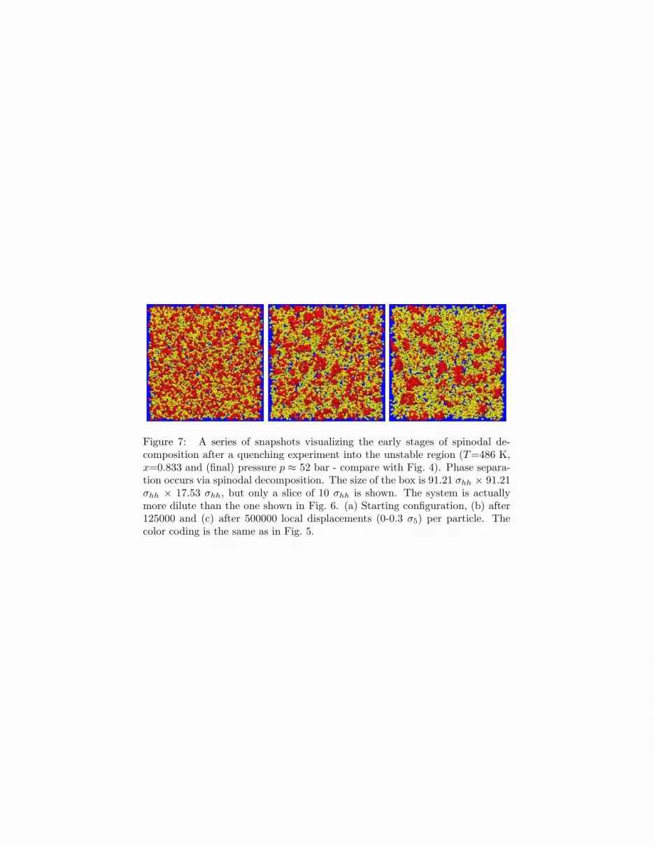
Figure 7: A series of snapshots visualizing the early stages of spinodal de-composition after a quenching experiment into the unstable region (T=486 K,x=0.833 and (final) pressure p ≈ 52 bar - compare with Fig. 4). Phase separa-tion occurs via spinodal decomposition. The size of the box is 91.21 σhh × 91.21σhh × 17.53 σhh, but only a slice of 10 σhh is shown. The system is actuallymore dilute than the one shown in Fig. 6. (a) Starting configuration, (b) after125000 and (c) after 500000 local displacements (0-0.3 σ5) per particle. Thecolor coding is the same as in Fig. 5.

0 5 10 15 20 25radius [10

-10m]

0

50

100

∆F/k

T

4πR2γ/kT

simulation

p=pcoex

(C16

H34

) p=0.5*pcrit

L=6.74 σhh

L= 9 σhh

L=11.3 σhh

Figure 8: Free energy as a function of droplet size for T=486 K and p = 0.5 pcrit

and p≈0 (coexistence pressure of pure hexadecane - compare with Fig. 3 andFig. 4). Indigo line: A simple estimate for the free energy: ∆F = 4πγR2,surface tension γ is taken from Fig. 4 (inlet) (flat surface). Black: resultsfrom simulations of different system sizes. Only the envelope of the curves isrelevant. Other parts of the curves belong to regions of the distribution whereno nucleation is expected. For small droplets the free energy is smaller thanexpected. Differences decrease with increasing radius and decreasing distancefrom the critical point of the isotherm.

References

[1] L. A. Kleintjens, In Supercritical Fluids. Kiran, E., Levelt-Sengers, J. M.H., Eds (Kluwer, Dordrecht, 1994)

[2] Kiran,E., and Brennecke, Eds. Supercritical Fluid Engineering Science ACSSymposium Series 514 (American Chem. Soc., Washington D. C., 1993)

[3] J.H. Han and C.D. Han, J. Polym. Sci., Part B: Polym. Phys. 28, 711(1990)

[4] S.K. Goel and E.J. Beckman, Poly. Eng. Sci. 34, 1137 (1994); 34, 1148(1994)

[5] C.M. Stafford, T.P. Russell, and T.J. McCarthy, Macromolecules 32, 7610(1999)

[6] B. Krause, H.-J. P. Sijbesma, P. Munuklu, N.F.A. van der Vegt, andW. Wessling, Macromolecules 34, 8792 (2001); B. Krause, R. Mettinkhof,N.F.A van der Vegt, and M. Wessling, ibid, 34, 874 (2001)

[7] P.J. Flory, Principles of Polymer Chemistry (Cornell University Press,Ithaca, 1953)

[8] P.J. Flory, J. Chem. 9, 660 (1941); M.L. Huggins, ibid, 9, 440 (1941)

[9] K. Binder, J. Chem. Phys. 79, 6387 (1983); Adv. Polymer Sci. 112, 181(1994)

[10] B. Widom, Physica A194, 532 (1993)

[11] M. Muller, L.G. MacDowell, P. Virnau, and K. Binder, J. Chem. Phys.117, 5480 (2002)

[12] E. Hadicke, H. Schuch, W. Huttenschmidt, P. Virnau, M. Muller, L.G.MacDowell, K. Binder, B. Rathke, E. Strey, and D.W. Heermann, in prepa-ration.

[13] W. Paul, G.D. Smith, D.Y. Yoon, B. Farago, S. Rathgeber, A. Zirkel, L.Willner, and D. Richter, Phys. Rev. Lett. 80, 2346 (1998); W. Paul, AIPConf. Proc. 469, 575 (1999)

[14] K. Kremer and G.S. Grest, J. Chem. Phys. 92, 5057 (1990)

[15] C. Bennemann, W. Paul, K. Binder and B. Dunweg, Phys. Rev. E57, 843(1998)

[16] N.B. Wilding, in Annual Reviews of Computational Physics IV. (ed. byD. Stauffer) p.37 (World Scientific, Singapore, 1996); N.B. Wilding, M.Muller, and K. Binder, J. Chem. Phys. 105, 802 (1996); N.B. Wilding, F.Schmid, and P. Nielaba, Phys. Rev. E58, 2201 (1998)

[17] P. Virnau, M. Muller, L. Gonzalez MacDowell and K. Binder, Comp. Phys.Commun. 147, 978 (2002)

[18] P. Virnau, M. Muller, L. Gonzalez MacDowell, and K. Binder, to be pub-lished.

[19] G.C. Maitland, M. Rigby, E.B. Smith and W.A. Wakeham, Intermolecular

Forces (Clarendon, Oxford, 1981)

[20] P. Van Konynenburg and R. L. Scott, Philos. Trans. R. Soc. London SeriesA298, 495 (1980)

[21] J.S. Rowlinson and F.L. Swinton, Liquids and Liquid Mixtures (Butter-worth, London 1982)

[22] G.M. Schneider, Adv. Chem. Phys. 27, 1 (1970)

[23] L.G. MacDowell, P. Virnau, M. Muller, and K. Binder, J. Chem. Phys.117, 6360 (2002)

[24] K. Binder and G. Cicotti (eds) Monte Carlo and Molecular Dynamics of

Condensed Matter Systems (Societa Italiana di Fisica, Bologna, 1996)

[25] K. Binder (ed.) Monte Carlo and Molecular Dynamics Simulaltions in Poly-

mer Science (Oxford, University Press, New York, 1995).

[26] F. Varnik and K. Binder, J. Chem. Phys. 117, 6336 (2002)

[27] M.S. Wertheim, J. Stat. Phys. 35, 19, 35 (1984); ibid, 42, 459, 477 (1986);J. Chem. Phys. 85, 2929 (1986); ibid, 87, 7323 (1987); W.G. Chapman, G.Jackson, and K.E. Gubbins, Mol. Phys. 65, 1057 (1988)

[28] A. Galindo and F. J. Blas, JPC-B, 106, 4503 (2002)

[29] K. Binder and D. Stauffer, Adv. Phys. 25, 343 (1976)

[30] J.D. Gunton, M. San Miguel, and P.S. Sahni, in Phase Transitions and

Critical Phenomena, Vol 8 (edited by C. Domb and J.L. Lebowitz), p. 267(Academic Press, London, 1983)

[31] K. Binder and P. Fratzl, in Phase Transformations of Materials (ed. by G.Kostorz) p. 409 (Wiley-VCH, Weinheim, 2001)

[32] K. Binder, Phys. Rev. A25, 1699 (1982)

[33] B.A. Berg, V. Hansmann, and T. Neuhaus, Phys. Rev. B47, 497 (1993); Z.Phys. B90, 229 (1993)

[34] M. Muller, K. Binder, and W. Oed, J. Chem. Soc., Faraday Trans. 91, 2369(1995)

[35] J.E. Hunter, III, and W.P. Reinhardt, J. Chem. Phys. 103, 8627 (1995)

[36] J.J Potoff and A.Z. Panagiotopoulos, J. Chem. Phys. 112, 6411 (2000)

[37] T.S. Jain and J.J. de Pablo, preprint

[38] K. Binder and M.H. Kalos, J. Stat, Phys. 22, 363 (1980); K. Binder, Phys-ica A, in press (2002)

[39] T.Charoensombut-Amon, R.J. Martin, and R.Kobayashi, Fluid PhaseEquilibria. 38, 89 (1986)

[40] Y. Lin, M. Muller, and K. Binder, to be published.

[41] L. Gonzalez MacDowell, P. Virnau, M. Muller, and K. Binder, to be pub-lished

[42] P. Virnau, L. Gonzalez MacDowell, M. Muller, and K. Binder,cond-mat/0303642

[43] P. Virnau, M. Muller, L. Gonzalez MacDowell, and K. Binder, to be pub-lished

[44] R. Span and W. Wagner, JPCRD 25, 1509 (1996)

[45] B. D. Smith and R. Srivastava, Elsevier, Amsterdam (1986)

[46] G. Schneider, Z. Alwani, W. Heim, E. Horvath, and E.U. Franck, Chem.Ingr. Tech., 39, 649 (1967)