Embed Size (px)
Citation preview

Performance Management Paper F5 Course Notes ACF5CN07(D)

l

(i)
BPP provides revision courses, question days, mock days and specific material to assist you in this important phase of your studies.
F5 Performance Management Study Programme Page Introduction to the paper and the course............................................................................................................... (ii) 1 Costing ........................................................................................................................................................ 1.1 2a Activity based costing................................................................................................................................ 2a.1 2b Target costing............................................................................................................................................ 2b.1 2c Life cycle costing ........................................................................................................................................2c.1 2d Backflush accounting................................................................................................................................. 2d.1 2e Throughput accounting.............................................................................................................................. 2e.1
End of Day 1 – refer to Course Companion for Home Study Progress test 1
3 Limiting factor analysis ................................................................................................................................ 3.1 4 Pricing decisions ......................................................................................................................................... 4.1 5 Short term decisions.................................................................................................................................... 5.1 6 Risk and uncertainty .................................................................................................................................... 6.1
End of Day 2 – refer to Course Companion for Home Study Progress test 2
Course exam 1
7 Objectives of budgetary control ................................................................................................................... 7.1 8 Budgetary systems...................................................................................................................................... 8.1 9a Quantitative analysis in budgeting............................................................................................................. 9a.1 9b Learning curves......................................................................................................................................... 9b.1 10 Budgeting and standard costing ................................................................................................................ 10.1 11a Variance analysis .................................................................................................................................... 11a.1
End of Day 3 – refer to Course Companion for Home Study Progress test 3
11b Further variance analysis ........................................................................................................................ 11b.1 12 Behavioural aspects of standard costing................................................................................................... 12.1 13 Performance management ........................................................................................................................ 13.1 14 Divisional performance measures ............................................................................................................. 14.1 15 Further performance management............................................................................................................ 15.1
End of Day 4 – refer to Course Companion for Home Study Progress test 4
Course exam 2
16 Answers to lecture examples..................................................................................................................... 16.1 17 Question and Answer bank ....................................................................................................................... 17.1 18 Appendix A: Pilot Paper questions ........................................................................................................... 18.1 19 Appendix B: Relevant articles.................................................................................................................... 19.1 20 Appendix C: Mathematical formulae.......................................................................................................... 20.1
Don’t forget to plan your revision phase!
• Revision of syllabus • Testing of knowledge • Question practice • Exam technique practice

INTRODUCTION
(ii)
Introduction to Paper F5 Performance Management Overall aim of the syllabus To develop knowledge and skills in the application of management accounting techniques to quantitative and qualitative information for planning, decision-making, performance evaluation, and control.
The syllabus The broad syllabus headings are:
A Specialist cost and management accounting techniques B Decision making techniques C Budgeting D Standard costing and variance analysis E Performance Measurement and control
Main capabilities On successful completion of this paper, candidates should be able to:
• Explain, apply, and evaluate cost accounting techniques
• Select and appropriately apply decision-making techniques to evaluate business choices and promote efficient and effective use of scarce business resources, appreciating the risks and uncertainty inherent in business and controlling those risks
• Apply budgeting techniques and evaluate alternative methods of budgeting, planning and control
• Use standard costing systems to measure and control business performance and to identify remedial action
• Assess the performance of a business from both a financial and non-financial viewpoint, appreciating the problems of controlling divisionalised businesses and the importance of allowing for external aspects.
Links with other papers
Advanced Performance
Management (P5)
Performance Management (F5)
Management Accounting (F2)

INTRODUCTION
(iii)
F5 is the middle paper in the management accounting section of the qualification structure. It builds upon F2 which covers techniques and feeds into P5 which requires you to think strategically and consider environmental factors.
F5 requires you to be able to apply techniques and think about their impact on the organisation. It seeks to examine candidates’ understanding of how to manage the performance of a business.
Assessment methods and format of the exam Examiner: Geoff Cordwell
The examination is a three hour paper with 15 minutes' reading time.
Format of the Exam
4 compulsory 25-mark questions
Questions on each paper will be drawn from as many of the five syllabus areas as possible. It is likely that they will be based on simple, realistic scenarios. The paper will be approximately 50% calculation, 50% discussion, but it is unlikely that a fully written question will be set. Wherever possible students will first be asked to analyse / interpret given numbers and then prepare calculations of their own.

INTRODUCTION
(iv)
Course Aims Achieving ACCA's Study Guide Outcomes Amended to reflect presentation in main body
A Specialist cost and management accounting techniques
A1 Activity based costing Chapter 2a A2 Target costing Chapter 2b A3 Life cycle costing Chapter 2c A4 Backflush accounting Chapter 2d A5 Throughput accounting Chapter 2e
B Decision-making techniques
B1 Multi-limiting factors and the use of linear programming and shadow pricing Chapter 3 B2 Pricing decisions Chapter 4 B3 Make-or-buy and other short-term decisions Chapter 5 B4 Dealing with risk and uncertainty in decision-making Chapter 6
C Budgeting
C1 Objectives Chapter 7 C2 Budgetary systems Chapters 7 & 8 C3 Types of budget Chapter 8 C4 Quantitative analysis in budgeting Chapters 9a & b C5 Behavioural aspects of budgeting Chapter 7
D Standard costing and variance analysis
D1 Budgeting and standard costing Chapter 10 D2 Basic variances and operating statements Chapter 11a D3 Material mix and yield variances Chapter 11b D4 Planning and operational variances Chapter 11b D5 Behavioural aspects of standard costing Chapter 12
E Performance measurement and control
E1 The scope of performance measurement Chapter 13 E2 Divisional performance and transfer pricing Chapter 14 E3 Performance analysis in not-for-profit organisations and the public sector Chapter 15 E4 External considerations and behavioural aspects Chapter 15

INTRODUCTION
(v)
Classroom tuition and Home study Your studies for BPP consist of two elements, classroom tuition and home study.
Classroom tuition In class we aim to cover the key areas of the syllabus. To ensure examination success you will to spend private study time reinforcing your classroom course with question practice and reviewing areas of the Course Notes and Study Text.
Home study To support you with your private study BPP provides you with a Course Companion which helps you to work at home and aims to ensure your private study time is effectively used. The Course Companion includes a Home Study section which breaks down your home study by days, one to be covered at the end of each day of the course. You will find clear guidance as to the time to spend on various activities and their importance.
You are also provided with progress tests and two course exams which should be submitted for marking as they become due.
These may include questions on topics covered in class and home study.
BPP Learn Online Come and visit the BPP Learn Online free at www.bpp.com/acca/learnonline for exam tips, FAQs and syllabus health check.
ACCA Forum We have thriving ACCA bulletin boards at www.bpp.com/accaforum. Register and discuss your studies with tutors and students.
Helpline If you have any queries during your private study simply contact your class tutor on the telephone number or e-mail address that they will supply. Alternatively, call +44 (0)20 8740 2222 (or your local training centre if outside the London area) and ask for a tutor for this paper to speak to you or to call you back within 24 hours.
Feedback The success of BPP’s courses has been built on what you, the students tell us. At the end of the course for each subject, you will be given a feedback form to complete and return.
If you have any issues or ideas before you are given the form to complete, please raise them with the course tutor or relevant head of centre.
If this is not possible, please email [email protected].

INTRODUCTION
(vi)
Key to Icons
Exam alert This is an area that commonly gets examined so you should make sure you are comfortable with
this section.
Formula to learn This formula will not be provided in the exam so you need to learn it.
Question practice from the Course Companion Question practice is key to passing the exam. Please refer to your Course Companion
Skills test standard A area which has frequently been tested in skills tests
Course Companion reference Further reading is needed in this area to consolidate your knowledge

1.1
Syllabus Guide Detailed Outcomes Having studied this chapter you will be able to:
• Gain a broader background knowledge of areas covered in paper F2. These topics will be built upon throughout F5
Exam Context These topics will not be examined in their own right. However, this knowledge could be examined as part of other topics such as ABC, pricing, etc.
Qualification Context You will have studied these areas in F2 and will continue to build on them in your management accounting studies.
Business Context Absorption costing is a method of apportioning all the production costs to a unit. Historically, this was a very common costing method in the manufacturing industry.
Costing

1: COSTING
1.2
Overview
Costing
Absorption Costing
Contribution
Marginal Costing
Reconciliation of profit Under / Over Absorption
OAR

1: COSTING
1.3
1 Principles of absorption costing 1.1 A method whereby all production costs are included in the costing of a cost unit, ie. direct
materials, direct labour, variable production overheads and fixed production overheads. IAS2 requires an element of fixed production overhead to be ‘absorbed’ into product cost for inventory valuation purposes. All production costs are charged to units of production.
Example of a standard cost card for a cost unit 1.2
$/unit Direct costs: Direct materials (5kg @ $3/kg) 15.00 Direct labour (3 hrs @ $6/hr) 18.00 33.00 Indirect costs: Variable overheads 2.00 Fixed overheads 3.00 Full product cost 38.00
2 Calculating the cost per unit 2.1

1: COSTING
1.4
Revision Example: CD Factory Cost Card
$ Direct materials: Blank CD 0.50 Box 0.50 Direct labour 3.00 Direct expense: Royalties 1.00 PRIME (direct) COST 5.00 Indirect production costs ?
TOTAL PRODUCTION COST ?
Indirect Production costs/ overheads Costs such as rent, supervisor’s salary, electricity etc are also incurred during production but they cannot be directly related to each CD. How should these costs be allocated to a CD? Three Step Process: (1) Allocate/apportion overheads to cost centres (2) Re-apportion service centre costs to production cost
centres (3) Absorb into production
For example: Total overheads are $20,000
Pressing
Packing
Canteen
(1) Allocate: Pressing & packing supervisors and a chef.
$5,000 $3,000 $2,000
Apportion: Rent based on floor space 500m2 300m2 200m2 $10,000 across 1,000m2 $5,000 $3,000 $2,000 (2) Re-apportion:
Direct method : no inter-service cost centre work Step Method : recognise significant inter-service cost centre work Reciprocal : recognise all inter-service cost centre work
Eg. Direct method Total Pressing Packing Canteen $ $ $ $ Total production overheads 20,000 10,000 6,000 4,000 Split canteen based on no. employees
(80% pressing, 20% packing) 3,200 800 (4,000) 20,000 13,200 6,800 Nil
(3) Absorb into production
Labour ½ hr @ $6/hr
Box 50c
CD 50c
Overheads ???
Royalties $1

1: COSTING
1.5
3 Overhead absorption rates 3.1 O.A.R =
levelactivity (normal) Expectedcosts overhead Estimated
Example CD Factory continued. (Step 3) Absorb into production –
Produce 20,000 CDs Pressing = $13,200/20,000 CDs = $0.66 Packing = $6,800/20,000 CDs = $0.34 $1.00 → add to cost card
Absorption Costing Summary 3.2
PRODUCTION COSTS
DIRECT COSTS INDIRECT COST $5.00 per unit 1 Allocate + apportion: Pressing Packing Canteen $10,000 $6,000 $4,000 2 Re-allocate service CCs: Pressing Packing $13,200 $6,800 2 Absorb into production Pressing Packing $0.66 $0.34
COST CARD $ Direct materials 1.00 Direct labour 3.00 Direct expenses 1.00 PRIME COST 5.00 Fixed overheads absorbed 1.00 TOTAL PRODUCTION COST 6.00

1: COSTING
1.6
4 Absorption into units of production
Bases 4.1 (a) Per unit
(b) Per direct labour hour Most frequently used in exams (c) Per machine hour (d) Percentage of direct materials cost (e) Percentage of direct labour cost (f) Percentage of prime cost
4.2 The basis level is always determined by the normal level of activity (IAS2) and the basis chosen should bear some reasonable relationship to the product.
Example CD Factory continued. If the factory produces CDs and DVDs, it cannot absorb $1 per unit across both.
Labour hours are as follows:
Pressing Packing Produce 10,000 DVDs 10,000 labour hours 2,500 labour hours Produce 10,000 CDs 5,000 labour hours 2,500 labour hours 15,000 labour hours 5,000 labour hours
OAR Pressing = $13,200 / 15,000 labour hours = $0.88/hr Packing = $6,800 / 5,000 labour hours = $1.36/hr
∴ DVD OAR: $ Pressing (1hr x $0.88) 0.88 Packing (¼ hr x $1.36) 0.34 1.22
∴ CD OAR: Pressing (1/2 hr x $0.88) 0.44 Packing (¼ hr x $1.36) 0.34 0.78
Pressing Packing DVD 1 hr ¼ hr CD ½ hr ¼ hr

1: COSTING
1.7
5 Under / Over Absorption 5.1
$ Actual overhead expenditure X Amount of overhead absorbed (X) Under/(over) absorption X/(X)
5.2 Reasons for under/over absorption:
Expenditure variance – Actual overhead expenditure differed from budgeted overhead expenditure.
Volume variance – Actual production activity differed from expected (normal) activity level.
Lecture example 1 Preparation question
Selling price per unit $10 Variable costs per unit direct materials $2 direct labour $3 production overhead $1 selling and distribution $1 Fixed costs: Production: budgeted $8,000 actual $8,500 Selling and distribution: (budgeted and actual) $2,000 Activity levels: Year 1 Units Budgeted production 4,000 Actual sales 4,200 Actual production 4,400 There is no opening inventory in Year 1. Required Prepare an income statement under absorption costing.

1: COSTING
1.8
Solution
Year 1 $ $ Sales Cost of sales: opening inventory Production: variable costs fixed costs closing inventory (Over)/under absorption Gross profit Variable selling & distribution Fixed selling & distribution Net profit Workings:

1: COSTING
1.9
6 Advantages and disadvantages of absorption costing 6.1 Advantages of absorption costing.
(a) It recognises that selling prices must cover all costs. (b) It complies with IAS 2 on accounting for inventory, whereby the value of inventory
must include an appropriate amount of fixed production overhead.
6.2 Disadvantages of absorption costing. (a) Profits can be manipulated by simply changing production levels. This is because
overheads will be carried forward in closing inventory. (b) It is based on the assumption that overheads are volume related. In the next chapter
we will see that ABC assumes that many overheads are complexity and diversity related, not merely volume related.
7 Principles of marginal costing (variable costing) 7.1 (a) A principle whereby variable production costs only are charged to cost units and
the fixed costs attributable to the relevant period are written off in full against the contribution for the period.
(b) Inventory is valued at variable cost of production.
8 Contribution 8.1 Contribution towards fixed costs is represented by:
(a) Selling price per unit less all variable costs per unit (whether production admin. or selling etc).
(b) Fixed costs + profit.

1: COSTING
1.10
Lecture example 2 Preparation question
There is no opening inventory in Year 1.
Required Complete the income statement under marginal costing principles.
Solution
$ $ Sales Variable production costs: opening inventory production closing inventory Variable selling & distribution CONTRIBUTION Fixed costs: production selling & distribution PROFIT
Selling price per unit $10 Variable costs per unit direct materials $2 direct labour $3 production overhead $1 selling and distribution $1 Fixed costs: Production: budgeted $8,000 actual $8,500 Selling and distribution: (budgeted and actual) $2,000 Activity levels: Units Budgeted production 4,000 Actual sales 4,200 Actual production 4,400

1: COSTING
1.11
Workings:
9 Advantages and disadvantages of marginal costing
Advantages 9.1 (a) Most appropriate for decision making as it highlights contribution. (It is useful for
short-term pricing decisions or decisions on one-off or ad-hoc contracts.) (b) Fixed costs are treated in accordance with their nature, ie as period costs. (c) Profit depends on sales and efficiency not on production levels. (d) Slightly simpler variance analysis.
Disadvantages 9.2 (a) There is a danger that products will be sold on an ongoing basis at a marginal
contribution which fails to cover fixed costs. (b) Does not comply with IAS 2, thus necessitating year end adjustments for the
preparation of published accounts. (c) Necessitates analysis of mixed costs between fixed and variable. (d) Seasonal variations in a year can cause unnecessary profit variances.

1: COSTING
1.12
10 Effect of inventory valuation on profit 10.1 (a) Production = sales (so inventory is constant)
AC profit = MC profit (b) Production < sales (so inventory is falling)
AC profit < MC profit (c) Production > sales (so inventory is climbing)
AC profit > MC profit
10.2 If there is a difference between the two profit figures the difference between the figures will effectively be the OAR/unit x movement in inventory.
10.3 You can remember which profit will be highest using SIAM S – Stock (Inventories) I – Increase A – Absorption profit M – More
Lecture example 3 Preparation question
Reconcile the profit figures calculated in lecture examples 1 and 2.
Solution

1: COSTING
1.13
Lecture example 4 Preparation question Required
When opening inventories were 8,500 litres and closing inventories 6,750 litres, a firm had a profit of $62,100 using marginal costing. Assuming that the fixed overhead absorption rate was $3 per litre, what would be the profit using absorption costing? A $41,850 B $56,850 C $67,350 D $82,250
Solution
11 Chapter summary • Absorption costing includes the absorption of overheads when calculating a cost per
unit
• The absorption happens over a three-step process 1 Allocate & apportion 2 Reapportion
3 Absorb levelactivity (normal) Expected
costs overhead Estimated
• Marginal costing doesn’t include overheads in unit costs instead charging them to the income statement in full
• Contribution (selling price less variable costs) is a key tool for decision making

1: COSTING
1.14
Additional Notes It is important that you can remember the basics covered in this chapter. Complete the following examples for the Year 2 data. (Year 1 completed earlier in the chapter.)
Lecture example 5 Preparation question
Selling price per unit $10 Variable costs per unit direct materials $2 direct labour $3 production overhead $1 selling and distribution $1 Fixed costs: Production: budgeted $8,000 actual $8,500 Selling and distribution: (budgeted and actual) $2,000 Activity levels: Year 1 Year 2 Units Units Budgeted production 4,000 4,000 Actual sales 4,200 4,000 Actual production 4,400 3,800 There is no opening inventory in Year 1. Required Prepare an income statement under absorption costing for Year 2.
Solution
each year

1: COSTING
1.15
Lecture example 6 Preparation question
There is no opening inventory in Year 1. Required Complete the Year 2 income statement under marginal costing principles.
Selling price per unit $10 Variable costs per unit direct materials $2 direct labour $3 production overhead $1 selling and distribution $1 Fixed costs: Production: budgeted $8,000 actual $8,500 Selling and distribution: (budgeted and actual) $2,000 Activity levels: Year 1 Year 2 Units Units Budgeted production 4,000 4,000 Actual sales 4,200 4,000 Actual production 4,400 3,800
each year

1: COSTING
1.16
Solution
Lecture example 7 Preparation question
Reconcile the profit figures calculated in lecture examples 5 and 6.
Solution
END OF CHAPTER

2a.1
Syllabus Guide Detailed Outcomes Having studied this chapter you will be able to:
• Identify appropriate cost drivers under ABC
• Calculate costs per driver and per unit using ABC
• Compare ABC and traditional methods of overhead absorption based on production units, labour hours or machine hours
• Explain the implications of switching to ABC for pricing, sales strategy, performance management and decision-making
Exam Context ABC appeared on the pilot paper for 25 marks. You should expect both calculations and interpretation.
Qualification Context Assessment of modern management accounting methods in a rapidly changing business environment will be assessed in the Professional level paper Advanced Performance Management (APM) P5.
Business Context The concepts of ABC were developed in the manufacturing sector of the US during the 1970s and 1980s. Absorption costing has become outdated for many businesses due to the diversity of product ranges and high level of overheads. As such ABC is becoming a much more appropriate tool for businesses to use when costing their products.
Activity based costing

2a: ACTIVITY BASED COSTING
2a.2
Overview
Activity based costing
Cost pools Cost drivers
Benefits Criticisms
Implications
Calculation of cost/unit Comparison with AbsorptionCosting
Implications of ABC

2a: ACTIVITY BASED COSTING
2a.3
1 Activity based costing (ABC)
Introduction 1.1 In this chapter we will be looking at an alternative method of cost accumulation, ABC. ABC
is a modern alternative to absorption costing which attempts to overcome the problems of costing in a modern manufacturing environment.
Traditional absorption costing 1.2 Traditional absorption costing uses a single basis for absorbing all overheads into cost
units for a particular production department cost centre. A business will choose the basis that best reflects the way in which overheads are being incurred, eg in an automated business much of the overhead cost will be related to maintenance and repair of the machinery. It is likely that this will vary to some extent with machine hours worked so we would have used a machine hour absorption rate.
PRODUCTION SET-UP COSTS
MACHINE OIL
SUPERVISOR SALARY
MACHINE REPAIRS
Activity based costing 1.3 Production overheads are by no means all volume-related and hence a single basis for
absorption, eg labour hours, would not adequately reflect the complexity of producing certain products/cost units as opposed to others.
1.4 ABC is an extension of absorption costing specifically considering what causes each type of overhead category to occur, ie what the cost drivers are. Each type of overhead is absorbed using a different basis depending on the cost driver.
Activities Cost drivers
PRODUCTION SET UP COSTS
NUMBER OF PRODUCTION SET UPS
MACHINE OIL AND MACHINE REPAIRS
TOTAL MACHINE HOURS
SUPERVISOR SALARY
TOTAL LABOUR HOURS
PRODUCTION DEPARTMENT
A
OAR = MACHINE HOURS
Reasons fordevelopment

2a: ACTIVITY BASED COSTING
2a.4
Steps in ABC 1.5 (1) Group overheads into activities, according to how they are driven. These are known
as cost pools. (2) Identify the cost drivers for each activity, ie what causes the activity cost to be
incurred. (3) Calculate a cost per unit of cost driver. (4) Absorb activity costs into production based on usage of cost drivers.
Cost driver analysis 1.6 Today's complex business environment means that costs are incurred because cost drivers
occur at different levels.
1.7 There are four key categories for activities and their related costs.
Categories Type of cost Cost driver Unit Direct Units produced Batch Set ups
Inspection Batches produced
Product R&D Marketing
Products produced
Facility sustaining Depreciation Rent
None
The difference between unit costs under absorption costing and ABC depends upon the proportion of overhead in each category. If most overheads are unit level or facility sustaining the costs will be similar. If overheads are batch or product sustaining costs, the resulting unit costs will be very different.
2 Absorption costing vs Activity based costing Overhead absorption rates using ABC should be more closely linked to the causes of overhead costs. The modern business environment has much wider product ranges than seen before, complex production process and decreasing product lifecycles. ABC recognises these factors by using multiple cost drivers when absorbing overheads.

2a: ACTIVITY BASED COSTING
2a.5
Lecture example 1 Technique Demonstration Dodo Ltd manufactures three products, A, B and C. Data for the period just ended is as follows:
A B COutput (units) 20,000 25,000 2,000 $/unit $/unit $/unitSales price 20 20 20Direct material cost 5 10 10Labour hours/unit 2 1 1Wages paid at $5/hr Total production overheads for Dodo Ltd amount to $190,000. Required (a) Calculate the profit per unit obtained on each product if production overheads are absorbed
on the basis of labour hours (Traditional Absorption Costing).
Solution

2a: ACTIVITY BASED COSTING
2a.6
The following data is now also available: $ Machining 55,000 Quality control and set-up costs 90,000 Receiving 30,000 Packing 15,000 190,000 Cost driver data A B C Labour hours/unit 2 1 1 Machine hours/unit 2 2 2 No. of production runs 10 13 2 No. of component receipts 10 10 2 No. of customer orders 20 20 20 Required (b) Using ABC, show the cost and gross profit per unit for each product during the period and
contrast this with the profit calculated using absorption costing. (c) What factors should be considered when comparing the results?
Solution
These are known as cost pools

2a: ACTIVITY BASED COSTING
2a.7
3 Implications of ABC
When ABC should be used 3.1 (a) When production overheads are high relative to prime costs (eg service sector)
(b) When there is a whole diversity of product range (c) When there are considerable differences in the use of resources by products (d) Where consumption of resources is not driven by volume
Benefits of ABC 3.2 The use of ABC provides opportunities for
(a) Cost control and reduction by the efficient management of cost drivers (b) Better costing information used to assist pricing decisions (c) Reanalysis of production and output/product mix decisions (d) Profitability analysis (by customer, product line etc) (e) A more realistic estimate of costs and profits which can be used in performance
appraisal
Criticisms of ABC 3.3 (a) It is time consuming and expensive
(b) Will be of limited benefit if overhead costs are primarily volume related (c) Reduced benefit if the company is producing only one product or a range of products
with similar costs (d) Complex situations may have multiple cost drivers (e) Some arbitrary apportionment may still exist
Merits &criticisms of ABC

2a: ACTIVITY BASED COSTING
2a.8
Implications 3.4 Before considering a switch to ABC it is important to consider whether the benefits outweigh
the costs and to ensure that the appropriate cost drivers can be identified as such a switch will have implications on: • Pricing • Sales strategy • Performance management • Decision making
Lecture example 2 Exam standard for 8 marks Discuss what the implications of moving to ABC are for each of the above four categories.
Solution
4 Chapter summary • Activity Based Costing groups overheads into activities. These are referred to as
cost pools
• The item that causes the costs to be incurred is the cost driver
• Overheads are absorbed into products using the cost drivers
• ABC results in a more meaningful product cost when overheads are high and there is a wide diversity of product range
Implications ofswitching to ABC
END OF CHAPTER
Q1 Abkaber

2b.1
Syllabus Guide Detailed Outcomes Having studied this chapter you will be able to:
• Derive a target cost in manufacturing and service industries
• Explain the difficulties of using target costing in service industries
• Explain the implications of using target costing on pricing, cost control and performance management
• Suggest how a target cost gap might be closed
Exam Context Target costing may form all or part of a question. You should be prepared to not only calculate a target cost but also to discuss the difficulties and implications of using target costing.
Qualification Context Assessment of modern management accounting methods in a rapidly changing business environment will be assessed in the Professional level paper Advanced Performance Management (APM) P5.
Business Context Target costing was developed in Japan in response to the problems of controlling and reducing costs over a product’s lifecycle.
Target costing

2b: TARGET COSTING
2b.2
Overview
Target costing
Deriving a target cost
Closing a target cost gap
Implications Target costing in service industries

2b: TARGET COSTING
2b.3
1 Target costing
Introduction 1.1 In a modern environment with shortening product lifecycles, organisations have to
continually redesign their products. It is essential that they try to achieve a target cost during the product’s development.
Cost plus pricing 1.2 Under traditional approaches to pricing, businesses calculate the cost of manufacturing and
selling a product, and then add mark up, to give the profit element. These methods are known as "cost plus pricing".
1.3 A major criticism of cost plus pricing techniques is that they do not consider any external factors (eg demand for product; no. of competitors, etc). They are therefore unlikely to maximise the profits that a business will generate.
Target costing 1.4 As product life cycles have become much shorter, the planning, development and design
stage of a product is critical to an organisation's cost management process. Cost reduction must be considered at this stage of a product’s life cycle, rather than during the production process.
1.5 Target costing involves setting a selling price for your product by reference to the market. From this your desired profit margin is deducted leaving you with a target cost.

2b: TARGET COSTING
2b.4
2 Deriving a target cost
Implementing target costing 2.1 (a) Define product specification and estimate anticipated sales volume.
(b) Set a target selling price at which the company will be able to achieve the desired market share.
(c) Required profit is estimated based on profit margins or return on investment. (d) Target cost is calculated as:
$ Target selling price X Less: target profit (X) Target cost X
(e) The estimated cost of the product is calculated based on the product specification and current cost levels.
(f) Estimated Product Cost – Target Cost = Cost Gap (g) Efforts are made to close the cost gap. Aim to "design out" costs before production
starts. (h) Negotiate with customer on price before deciding whether the project will go ahead.
Target Costing:
target cost (3rd)
mark-up (2nd)
selling price (1st)
Traditionally:
Cost (1st)
mark-up (2nd)
selling price (3rd)
Case Study 1Mercedes Benz
and target costing

2b: TARGET COSTING
2b.5
Lecture example 1 Preparation question Dinnae Ltd, a sports goods manufacturer is about to launch a new model of tennis racquet on which it requires a pretax ROI (return on initial investment) of 30%. Buildings and equipment needed for production are to cost £5,000,000. Expected sales levels are 40,000 racquets pa. at a selling price of $67.50 per racquet. Required What is the target cost for annual production?
Solution
3 Implications 3.1 Target costing turns the traditional cost plus approach to pricing on its head, meaning
pricing is the first consideration. Cost control is considered right up front as part of the development of the product not merely as an activity which happens alongside production.
3.2 Performance management will therefore focus on ensuring sales targets are met: ie have we set the right price and ways of improving processes / development to drive down costs to at least the level of the target cost.

2b: TARGET COSTING
2b.6
4 Closing a target cost gap
Lecture example 2 Idea Generation Suggest possible ways to close a target cost gap.
Solution
5 Implications of target costing in service industries 5.1 The target costing approach is a sensible basis for estimating / driving down costs
regardless of the type of business. However, due to the nature of service industries this process is more difficult in these businesses.
5.2 Unlike manufacturing, service industries have the following characteristics which make cost and performance measurement more difficult: Simultaneity – created at time consumed Heterogeneity – quality / consistency varies Intangibility – of what is provided Perishability – cannot make in advance and store up.
5.3 In addition to these problems, service organisations will require more qualitative information to arrive at a price and evaluate performance eg • Quality of service • Repeat customers etc

2b: TARGET COSTING
2b.7
6 Chapter summary • Target costing is an approach that sets the selling price of a product or service with
reference to the market place
• Selling price less desired margin = target cost
• Any cost gap should be closed via the design and development of the product
• Target costing can be applied to service industries but the measurement of cost is more difficult

2b: TARGET COSTING
2b.8
END OF CHAPTER

2c.1
Syllabus Guide Detailed Outcomes Having studied this chapter you will be able to:
• Identify the costs involved at different stages of the life cycle
• Explain the implications of lifecycle costing on pricing, performance management and decision-making
Exam Context Life cycle costing is likely to be examined via a discussion question. You should be aware of not only the stages of the product life cycle but also the implications of the life cycle on pricing.
Qualification Context Assessment of modern management accounting methods in a rapidly changing business environment will be assessed in the Professional level paper Advanced Performance Management (APM) P5.
Business Context Product life cycles are becoming shorter and shorter. Organisations increasingly reassess product lifecycle costs and revenues as the time available to sell the product and recover the investment shrinks. Increasingly, companies are attempting to optimise life cycle revenues and profits through the consideration of product warranties, spare parts and the ability to upgrade existing products. The concept of life cycle stages has a significant impact upon business strategy and performance.
Life cycle costing

2c: LIFE CYCLE COSTING
2c.2
Overview
Life cycle costing
Product life cycle Implications of Life cycle costing

2c: LIFE CYCLE COSTING
2c.3
1 Life cycle costing
Introduction 1.1 Life cycle costing aims to cost a product, service, customer or project over its entire lifecycle
with the aim of maximising the return over the total life while minimising costs.
1.2 Traditionally the costs and revenues of a product are assessed on a financial year or period by period basis.
1.3 Product life cycle costing considers all the costs that will be incurred from design to abandonment of a new product and compares these to the revenues that can be generated from selling this product at different target prices throughout the product's life.
2 Product life cycle 2.1 The product life cycle (PLC) can be divided into five stages.

2c: LIFE CYCLE COSTING
2c.4
2.2 Characteristics of the PLC
Stage Sales Volume Costs Development None Research & development Introduction Very low levels Very high fixed costs (eg Fixed
(non-current) assets, advertising) Growth Rapid increase Increase in variable costs
Some fixed costs increase (eg. Increase number of fixed (non-current) assets)
Maturity Stable High volume
Primarily variable costs
Decline Falling demand Primarily variable costs (now decreasing) Some fixed costs (eg decommissioning costs)
Impact of PLC in the modern environment 2.3 (a) Shorter product life cycles.
(b) Clearer strategic planning required. (c) 90% of costs to be incurred throughout its life cycle will have been determined before
a product reaches the market.
Maximising return over the product lifecycle 2.4 There are a number of ways that return can be increased over the life cycle.
(a) Design costs out of products Approximately 70% – 90% of a product's lifecycle costs are determined by decisions made early in the lifecycle at the design and development stage. Thus design and production teams must work together to ensure costs are minimised.
(b) Minimise the time to market This is the time from the conception of the product to its launch. If a company can get a product to the market place very quickly, it will give the product as long a span as possible without competitors' rival products in the market place. This should mean that market share is increased in the long run.
(c) Minimise breakeven time Pricing strategies will affect both contribution and volumes generated. A short breakeven time is very important for liquidity purposes.
(d) Extend the length of the life cycle itself For example, product development, finding other uses for a product or staggering the launch of the product in different markets.

2c: LIFE CYCLE COSTING
2c.5
2.5 Collected data are compared with budgeted costs to check whether expected savings have been realised.
3 Implications 3.1 Given that there will be different levels of demand for a product over its expected life, it
would not be appropriate to set one price for the product's entire life.
3.2 An understanding of the stages a product goes through enables you to price accordingly to either manipulate demand (low price, demand will rise and the intro stage is shortened) or to maximise profit.
3.3 All costs relating to a product including R&D are associated with the product. This enables true assessment of a products profitability.
3.4 Having looked at a product’s PLC it is clear that initially the product will make a loss. Viewing profitability on a periodic basis can put unnecessary pressure on management due to the visibility of the loss and could lead to wrong decisions being taken.
Advantages 3.5 (a) Considers external factors throughout a products expected life.
(b) Considers all costs incurred on a product, and therefore leads to cost reduction. (c) Very useful in the modern competitive environment, in which products often have a
short life cycle and when a large portion of costs will be committed prior to production commencing.
Lecture example 1 Exam standard for 6 marks Why might Target costing and Product life cycle be useful in providing management information for a manufacturer of mobile phones?
Solution

2c: LIFE CYCLE COSTING
2c.6
4 Chapter summary • Life cycle costing considers all costs and revenues of a product throughout its life
rather than on a periodic basis
• Understanding the product life cycle enables you to price accordingly to either manipulate demand or maximise profit
END OF CHPATEREND OF CHAPTER
Q2Cost Management
Techniques

2d.1
Syllabus Guide Detailed Outcomes Having studied this chapter you will be able to:
• Describe the process of backflush accounting and contrast with traditional cost accounting
• Explain the implications of backflush accounting on performance management and the control of a manufacturing process
• Identify the benefits of introducing backflush accounting
• Evaluate the decision to switch to backflush accounting from traditional process control
Exam Context This topic could feature in part or all of a question but you will not have to prepare T accounts. Techniques such as backflush accounting are often compared with the traditional techniques you will have seen in F2.
Qualification Context This topic is only likely to be examined at this paper.
Business Context Backflush accounting is best suited to companies that maintain low or no inventory.
Backflush accounting

2d: BACKFLUSH ACCOUNTING
2d.2
Overview
Backflush accounting
Backflush accounting Traditional Cost accounting
Implications of Backflush accounting
Suitability Advantages
Disadvantages

2d: BACKFLUSH ACCOUNTING
2d.3
1 Backflush accounting
Overview of traditional cost accounting systems 1.1
Work-in-progress Finished goods B/f X FG X B/f X C of S X Mat X C/f X WIP X C/f X Lab X O/H X X X X X
Direct labour Bank X WIP X
Production Overhead
control Cred X WIP X
1.2 Traditional costing systems use sequential tracking to track costs as units pass from raw materials throughout the production process to their eventual sale.
1.3 In an effort to eliminate non-value adding activities a complex costing system may be replaced by a simplified system focusing on output.
Backflush accounting 1.4 Backflush accounting is a simplified standard costing system which focuses on the output of
an organisations manufacturing process and then using standard costs works backwards to attribute costs to inventory and sales (i.e. 'flush' out manufacturing costs).
1.5 Cost accounts are simplified to reduce the amount of data handling. In backflush, there are no process accounts. When a sale is made, the following is recorded: Dr Cost of sales Cr Materials Cr Conversion costs All at standard cost. Labour is treated as an indirect cost. Production is dependent on demand and so labour is paid regardless of activity.
Raw materials B/f X WIP X Cred X C/F X X X
To cost of sales

2d: BACKFLUSH ACCOUNTING
2d.4
1.6 Trigger points determine when entries are made in the accounting system, for example: • Purchase of materials • Sale of goods
Materials Cost of sales C of S X Materials X To I/S X Conversion X X X
Conversion costs
C of S X
Please note: double entry will not be required in the exam.
2 Implications of backflush accounting
Suitability of backflush accounting 2.1 It is particularly applicable under the following circumstances:
(a) In a JIT environment, (see Ch 12) or a situation where the overall process time is short, there should be very little inventory of raw materials, WIP and even finished goods, so the bulk of manufacturing costs should be the costs of sale.
(b) In a TQM environment, (see Ch 12) where there are strong relationships with suppliers, costs should be known with a high degree of certainty. Hence there will be minimal variances arising during production.

2d: BACKFLUSH ACCOUNTING
2d.5
Lecture example 1 Preparation question A company operates a backflush costing system. The standard cost of product X is: $ Materials 8 Conversion 13 21 Details of transactions in the month were: $ Raw materials b/f 100 Purchases 8,000 Conversion 13,000 Cost of good sold at standard cost 18,500 Required
What is the closing balance on raw materials account?
Solution

2d: BACKFLUSH ACCOUNTING
2d.6
Advantages of backflush accounting 2.2 (a) Simpler than traditional costing systems, no separate account for WIP
(b) Fewer entries therefore saving in the time and cost of operating a complex cost accounting system
(c) It discourages managers from producing for inventory as inventory does not add value until it is sold
(d) The accounting function can be refocused to add value in the strategic and tactical planning aspects of the business
Disadvantages of backflush accounting 2.3 (a) Backflush will not suit all companies. It cannot successfully operate in situations
where inventory levels are significant and tend to fluctuate (b) The production process needs to be relatively short with accurate standard production
costs (c) The absence of detailed financial information may make the task of management
control more difficult. Adequate production controls are therefore vital (d) Reconciliation of cost accounts to financial accounts could be more difficult
Lecture example 2 Idea Generation How might you evaluate the decision to switch to backflush accounting from traditional cost accounting?
Solution

2d: BACKFLUSH ACCOUNTING
2d.7
3 Chapter summary • Backflush costing is a simplified accounting system
• The actual sale of the goods is the trigger for the accounting entries
• Entries are made at standard cost
• It is appropriate within JIT & TQM environments, ie when there is little or no inventory and little price variation

2d: BACKFLUSH ACCOUNTING
2d.8
END OF CHAPTER

2e.1
Syllabus Guide Detailed Outcomes Having studied this chapter you will be able to:
• Calculate and interpret a throughput accounting ratio (TPAR)
• Suggest how a TPAR could be improved
• Apply throughput accounting to a multi-product decision-making problem
Exam Context This topic could be the focus of an entire question. Be prepared to perform calculations and to discuss the results.
Qualification Context Assessment of modern management accounting methods in a rapidly changing business environment will be assessed in the Professional level paper Advanced Performance Management (APM) P5.
Business Context Throughput accounting is an accounting system based on the theory of constraints, (TOC). TOC was developed by Eliyahu Goldratt in 1986. Throughput accounting is now being successfully adopted by many factories wishing to improve their performance.
Throughput accounting

2e: THROUGHPUT ACCOUNTING
2e.2
Overview
Throughput accounting
Throughput accounting and decision making
Throughput accounting ratios
Theory of constraints Throughput accounting
Return/hour Cost/hour
TPAR
Products Divisions
Limiting factor scenarios
Goldratt’s 5 steps

2e: THROUGHPUT ACCOUNTING
2e.3
1 Throughput accounting (TA) and Theory of constraints (TOC)
Theory of constraints (TOC) 1.1 The theory of constraints is a production system where the key financial concept is the
maximisation of throughput while keeping conversion and investment costs to a minimum.
1.2 Throughput = Sales revenue – Material cost
1.3 TOC focuses on bottlenecks in the production process which act as a barrier to throughput maximisation.
Bottlenecks
100 units 50 units 100 units per hour per hour per hour
One process will inevitably act as a bottleneck, known as a binding constraint.
1.4 Goldratt’s five steps for dealing with a bottleneck activity were:
Step 1 – Identify the binding constraint
Step 2 – Exploit. The highest possible output must be achieved from the binding constraint. This output must never be delayed and as such a buffer inventory should be held immediately before the constraint
Step 3 – Subordinate. Operations prior to the binding constraint should operate at the same speed as it so that WIP does not build up
Step 4 – Elevate the systems bottleneck. Steps should be taken to increase resources or improve its efficiency
Step 5 – Return to step 1. The removal of one bottleneck will create another elsewhere in the system
Throughput accounting (TA) 1.5 TA is an accounting system based on the theory of constraints. It is very similar to marginal
costing but can be used for longer-term decision making about production capacity. It is an alternative system of cost and management accounting in a JIT environment.
Raw Materials
Materials Preparation
Component Preparation
Final Assembly Sales

2e: THROUGHPUT ACCOUNTING
2e.4
1.6 TA emphasises throughput, inventory minimisation and cost control. Three concepts: (a) All factory costs are fixed in the short run, with the exception of material cost. (b) In a JIT environment, producing for inventory is bad. Ideally inventory would be zero.
Products should not be made unless there is a customer for them. This means accepting some idle time in non-bottleneck operations. WIP should be valued at material cost only, so that no value is added to profit until a sale is made.
(c) Profit is determined by the rate at which throughput can be generated, ie how quickly raw materials can be turned into sales to generate cash. Producing just to increase inventory creates no profit and so should not be encouraged.
Traditional Costing Throughput accounting Labour costs and variable overheads are treated as variable costs.
All costs other than materials are seen as fixed in the short term.
Inventory is valued at total production cost.
Inventory is valued at material cost only.
Value is added when an item is produced.
Value is added when an item is sold.
Product profitability can be determined by deducting a product cost from selling price.
Profitability is determined by the rate at which money is earned.
2 Ratios 2.1 (a) Total Factory Costs (TFC) = Fixed production costs, including labour
(b) Return per factory hour = resource key on Time
purchases materialrevenue Sales −
(c) Cost per factory hour = resource key on Time
costs factory Total
(d) TPA ratio = hour factory perCost hour factory per Return
2e: THROUGHPUT ACCOUNTING
2e.5
Lecture example 1 Exam standard for 5 marks MN Ltd manufactures automated industrial trolleys, known as TRLs. Each TRL sells for $2,000 and the material cost per unit is $600. Labour and variable overhead are $5,500 and $8,000 per week respectively. Fixed production costs are $450,000 per annum and marketing and administrative costs are $265,000 per annum. The trolleys are made on three different machines. Machine X makes the four frame panels required for each TRL. Its maximum output is 180 frame panels per week. Machine X is old and unreliable and it breaks down from time to time. It is estimated that, on average, between 15 and 20 hours of production are lost per month. Machine Y can manufacture parts for 52 TRLs per week and machine Z, which is old but reasonably reliable, can process and assemble 30 TRLs per week. The company has recently introduced a just-in-time (JIT) system and it is company policy to hold little work-in-progress and no finished goods inventory from week to week. The company operates a 40-hour week, 48 weeks a year. Required
Calculate the throughput accounting ratio for the key resource for an average hour.
Solution

2e: THROUGHPUT ACCOUNTING
2e.6
Lecture example 2 Exam standard for 4 marks What actions could you take to improve a throughput accounting ratio?
Solution
3 Throughput accounting and decision making
Ranking production 3.1 Products/divisions are ranked by TPA ratio.
3.2 If two or more products are made in the same factory, they can be ranked on return per factory hour, not TPA ratio, since their costs will be identical.
Target for decision making 3.3 The TPA ratio should be greater than one if a product is to be viable. Return/hour enables
businesses to make short-term decisions when there is a scarce resource. Priority must be given to products generating the best ratios.
Use in performance management 3.4 A division of a company is not discouraged from inventory building if reported profit is used
as a principal performance measure.
3.5 This is at odds with the JIT philosophy where purchase and production costs should only be incurred if there is to be an immediate return generated. Use of TPAR instead of (or in addition to) profit should resolve this problem.
Is it good or bad?

2e: THROUGHPUT ACCOUNTING
2e.7
3
Lecture example 3 Preparation question – Inventory minimisation Will and Grace operate separate divisions making and selling products with identical cost structures.
Sales price per unit $50 Direct materials per unit $12 Direct labour per unit $8 Fixed production overheads of $200,000 per month are absorbed across the normal production level of 10,000 units per month. In each division assume a bottleneck capacity of 20,000 hours. In April, Will makes and sells exactly 10,000 units whilst Grace makes 12,000 units and sells only 9,500. Neither Will nor Grace has any opening or closing inventory of raw materials or components. Required Show which manager would benefit if bonuses were given on (a) Profit (b) Throughput accounting ratios
Solution

2e: THROUGHPUT ACCOUNTING
2e.8
Limiting factors 3.6 You will have seen earlier in your studies how to deal with a limiting factor. 3.7 The approach is to maximise contribution / unit of limiting factor. In a throughput
environment the approach is the same except that we maximise return / unit of limiting factor
Lecture example 4 Exam standard for 10 marks PH plc produces three different products and has adopted throughput accounting for its short-term decisions. The employees are guaranteed a weekly salary that is equivalent to their normal working hours paid at their normal hourly rate of $7 per hour. The units are produced in batches of 100 units. Costs and selling prices per batch are as follows: Unit Adam James Luke $/batch $/batch $/batch Selling price 340 450 270 Material K ($5/kg) 150 120 90 Material L ($10/kg) 70 90 40 Material M ($15/kg) 30 75 45 Labour ($7/hour) 21 28 42 Factory costs absorbed 20 80 40

2e: THROUGHPUT ACCOUNTING
2e.9
PH plc is preparing its production plans and has estimated the maximum demand from its customers to be as follows: Batches Adam 500 James 400 Luke 350
However, these demand maximums do not include a contract for the delivery of 50 batches of each product to an important customer. If this minimum contract is not satisfied then PH plc will have to pay a substantial financial penalty for non-delivery. Material L is in short supply and the maximum amount available is 7,000 kg. Required Prepare calculations to determine the production mix that will maximise the profit of PH plc.
Solution

2e: THROUGHPUT ACCOUNTING
2e.10
4 Chapter summary • Throughput accounting focuses on maximising throughput
• Throughput = sales – materials
• All labour and variable overheads are seen as fixed in the short term
• Decisions are made with reference to the TPAR
• Limiting factor decisions are based upon return per limiting factor
END OF CHAPTER
Q3HYC

3.1
Syllabus Guide Detailed Outcomes Having studied this chapter you will be able to:
• Select an appropriate technique in a scarce resource situation
• Formulate and solve a multiple scarce resource problem both graphically and using simultaneous equations as appropriate
• Explain and calculate shadow prices (dual prices) and discuss their implications on decision-making and performance management
• Calculate slack and explain the implications of the existence of slack for decision-making and performance management
Exam Context Linear programming is likely to be examined as a mixture of calculations and discussion
Qualification Context Single limiting factors are assumed knowledge as these are covered in F2. Linear programming was also seen in F2.
Business Context Linear programming is a mathematical model developed during the second World War. Post war many industries used it in daily planning. Linear programming is heavily used in business management to maximise income or minimise costs of a production scheme. Businesses may not be able to determine their principal budget factor with certainty. Linear programming allows the question “What limits us?” to be posed and the solutions found.
Limiting factor analysis

3: LIMITING FACTOR ANALYSIS
3.2
Overview
Shadow prices Limiting factor analysis
Single limiting factors Multiple limiting factors
Slack / Surplus
Linear programming • Graphical • Simultaneous equations

3: LIMITING FACTOR ANALYSIS
3.3
1 Introduction
Brought forward knowledge 1.1 The production and sales plans of a business may be limited by a limiting factor/scarce
resource (the 'principal budget factor'). This could be: • demand • materials • labour • machine hours • money The plans of the business must be built around this factor.
2 Single constraint 2.1 If the business makes more than one product, it will want to find the product mix which will
maximise profit given the limiting factor by ranking products in terms of greatest contribution per unit of limiting factor.
Lecture example 1 Preparation question Jam & Sponge has just changed its cake mix and is struggling to cope with increased demand for its cakes. Machine time available is 300 hours per week.
Fairy Butterfly Pixie Information per batch: $ $ $ Sales price 150 120 100 Variable cost 100 80 70 Fixed cost 20 20 20 Profit 30 20 10 Machine time per batch 5hrs 2hrs 1hr Demand per week 50 50 50
Required What is the optimal production plan?
Solution

3: LIMITING FACTOR ANALYSIS
3.4
3 Shadow prices 3.1 A shadow price or (dual price) is
• the additional contribution generated from one additional unit of limiting factor. • the opportunity cost of not having the use of one extra unit. • the maximum extra amount that should be paid for one additional unit of scarce
resource.

3: LIMITING FACTOR ANALYSIS
3.5
Lecture example 2 Preparation question Jam & Sponge has just changed its cake mix and is struggling to cope with increased demand for its cakes. Machine time available is 300 hours per week.
Fairy Butterfly Pixie Information per batch: $ $ $ Sales price 150 120 100 Variable cost 100 80 70 Fixed cost 20 20 20 Profit 30 20 10 Machine time per batch 5hrs 2hrs 1hr Demand per week 50 50 50 Required (a) What would happen if five extra machine hours were made available? (b) What is the shadow price of one machine hour?
Solution

3: LIMITING FACTOR ANALYSIS
3.6
4 More than one constraint – graphical linear programming
4.1 When there is more than one limiting factor, the above method cannot be used. Instead linear programming using graphical analysis and simultaneous equations needs to be used.
Steps 4.2 Formulating the model
(a) Define variables
(b) Establish constraints – generally in the form: amount of resource used ≤ amount available
(c) Formulate objective function Solving the problem using graphs (only if two variables): (d) Plot constraints on a graph (e) Identify the feasible region ie. those combinations of variables which are possible
within the resource constraints (f) Plot the slope of the objective function (iso-contribution / profit line) and slide to
optimal point (away from the origin for a maximum, towards the origin for a minimum) (g) Calculate the value of the objective function at the optimal point.
Lecture example 3 Exam standard for 16 marks
KG Ltd makes two products, the Purse and the Handbag. Each purse earns $5 contribution and each handbag earns $6. Inputs are as follows: Purse Handbag Leather 1½ m2 2m2 Skilled labour 45 min 30 min There are six skilled labourers each working a 35 hour week and delivery contracts limit the amount of leather available to 600m2 each week. KG Ltd has an EU quota ruling whereby it has to produce at least as many handbags as it does purses. Leather costs $8 per m2, wages are paid at $4.20 per hour. Required Determine the optimal production plan for KG Ltd and calculation the contribution that can be achieved.

3: LIMITING FACTOR ANALYSIS
3.7
Solution (a) Identify variables
(b) Formulate objective function
(c) State constraints as linear relationships

3: LIMITING FACTOR ANALYSIS
3.8
(d) Plot a graph
(e) Determine optimal point (f) Calculate value of objective function at optimal point

3: LIMITING FACTOR ANALYSIS
3.9
5 Using simultaneous equations Instead of sliding out the iso-contribution line, simultaneous equations can be used to solve the problem
Lecture example 4 Exam standard for 5 marks Solve the problem in lecture example 3 using simultaneous equations
Solution
Note: You may find using simultaneous equations quicker but it is not recommended until you have graphically shown the constraints. If the question requires the graphical method, you must draw a graph
Slack / Surplus 5.1 Slack occurs when the maximum availability of a resource is not used 5.2 Surplus occurs when more output has been made than the minimum requirement
3: LIMITING FACTOR ANALYSIS
3.10
6 Using linear programming 6.1 Assumptions made in linear programming techniques include:
(a) fixed costs are unchanged by decision (b) unit variable cost is constant (c) estimates of demand and resource requirements are known with certainty (d) units of output are divisible (e) total amount of each scarce resource is known with certainty (f) no interdependence between demand for products
6.2 Linear programming can be useful in the following situations: (a) Budgeting (b) Calculation of relevant costs (c) Production decisions (d) Payment for scarce resources (e) Control (f) Capital budgeting
7 Chapter summary • Single limiting factor problems can be solved by maximising contribution / limiting
factor
• Multiple limiting factor problems are solved via linear programming. First formulate the model. Secondly solve the problem using graphs or simultaneous equations
• A shadow price is the additional contribution generated from one more unit of limiting factor
• Slack occurs when not all of a resource has been used.
• Surplus occurs when additional output has been made.

3: LIMITING FACTOR ANALYSIS
3.11
Additional Notes
8 More than one constraint – computer based linear programming
8.1 The computer based method must be used when there are 3 or more variables. It involves: • deciding on the objective • formulating the constraints (including slack variables) • interpretation of computer output
Computer input 8.2 The inputs into the linear programming package, based on the information in example 3, will
be as follows: Let P = number of purses made and sold per week Let H = number of handbags made and sold per week Let S1 = surplus of leather Let S2 = surplus of labour Let S3 = excess of handbags made over quota Maximise Z = 5P + 6H Subject to: (Leather) 1.5P + 2H + S1 = 600 (Labour) 0.75P + 0.5H + S2 = 210 (Quota) P – H + S3 = 0 (Non-negativity) P, H ≥ 0
Computer output 8.3 The computer output will vary according to linear programming package used. However, all
packages will incorporate similar information.

3: LIMITING FACTOR ANALYSIS
3.12
Lecture example 5 Exam standard for 9 marks
The output from 2 computers utilised to solve the problem highlighted in example 3 is as follows:
Objective function value: 1,880.000 Variable Value Relative loss P 160.000 0 H 180.000 0 Constraint Slack/Surplus Shadow price/worth S1 0.000 2.667 S2 0.000 1.333 S3 20.000 0.000
P H S1 S2 S3 Soln
P 1 160.000 H 1 180.000 S3 1 20.000 Z 0 0 2.667 1.333 0 1880.000
Required (a) Interpret the computer output of the linear programming packages. (b) Should KG Ltd accept an offer from Edwards Ltd for supplying of leather at $10.50/m2?
Solution
END OF CHPATEREND OF CHAPTER

4.1
Syllabus Guide Detailed Outcomes Having studied this chapter you will be able to:
• Explain the factors that influence the pricing of a product or service
• Explain the price elasticity of demand
• Derive and manipulate a straight line demand equation. Derive an equation for the total cost function (including volume-based discounts)
• Evaluate a decision to increase production and sales levels, considering incremental costs, incremental revenues and other factors
• Explain different pricing strategies
• Calculate a price from a given strategy using cost-plus pricing and relevant costing
Exam Context Questions on pricing are likely to include calculation, discussion and practical application of pricing strategies.
Qualification Context Pricing methods will also be evaluated in the Professional level paper Advanced Performance Management paper (P5).
Business Context There are many strategies which can be adopted when pricing a product. Given today’s competitive industries with short-lived products and service industries, pricing decisions are vital.
Pricing decisions

4: PRICING DECISIONS
4.2
Overview
Pricing decisions
Price elasticity
P%Q%
ΔΔ
Total cost functionY = a + bx
Pricing strategies • Cost plus
o Full cost o Marginal cost o Relevant cost o Standard cost
• Market penetration • Market skimming • Premium pricing • Price discrimination • Product bundling • Psychological pricing • Product line pricing • Complementary
products • Loss leaders • Controlled pricing • Volume discounting
Demand function P = a – bQ
Demand
4: PRICING DECISIONS
4.3
1 Introduction 1.1 Historically the cost of a product would have had a large influence on the selling price set for
that product. Today there are many factors that will influence that price.
Lecture example 1 Idea Generation Discuss the factors that will influence price.
Solution
2 Demand 2.1 Economic theory is that the higher the price charged the less demand there will be for
normal goods.
Price elasticity 2.2 Price elasticity of demand (PED) is a measure of the responsiveness of demand to changes
in price. Some products are more responsive than others.
2.3 PED is calculated P%Q%
ΔΔ =
Pinchange%Qinchange%
When PED > 1: The product is described as having elastic demand. This means that a small change in price will cause a proportionately greater change in quantity demanded. When PED < 1: The opposite applies. The product has inelastic demand and prices can be changed greatly without creating large changes in demand.

4: PRICING DECISIONS
4.4
2.4 An awareness of the PED of a product will assist companies when setting price.
2.5 Where demand is inelastic prices can be raised.
2.6 If demand is elastic the company needs to weigh up whether an increase in price generates more or less revenue as quantity demanded will fall.
2.7 Factors determining elasticity of demand include: • availability of substitutes • complementary products • disposable income • tastes and fashions • necessities
Lecture example 2 Exam standard for 2 marks A football club charges $12 per ticket for home games. Average attendance at these regular games is 16,000. When prices were increased by $1 per ticket, attendance fell by 2,500. Required
Determine the PED if ticket price increases from $12 to $13.
Solution
Demand and theindividual firm
4: PRICING DECISIONS
4.5
Demand function 2.8 Price will affect the quantity demanded for a product. Output considerations will alter the
price to be charged. If the demand function is known, and the desired output has been calculated, the appropriate price can be determined for the product.
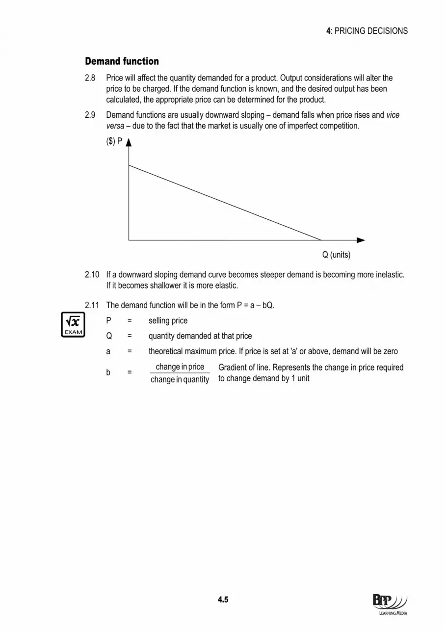
2.9 Demand functions are usually downward sloping – demand falls when price rises and vice versa – due to the fact that the market is usually one of imperfect competition. ($) P
Q (units)
2.10 If a downward sloping demand curve becomes steeper demand is becoming more inelastic. If it becomes shallower it is more elastic.
2.11 The demand function will be in the form P = a – bQ. P = selling price Q = quantity demanded at that price a = theoretical maximum price. If price is set at 'a' or above, demand will be zero
b = quantity in change
price in change Gradient of line. Represents the change in price required to change demand by 1 unit

4: PRICING DECISIONS
4.6
Lecture example 3 Exam standard for 5 marks
A football club charges $12 per ticket for home games. Average attendance at these regular games is 16,000. When prices were increased by $1 per ticket, attendance fell by 2,500. Required
Assuming attendance to be purely price dependent, what should be the ticket price to ensure a full house with capacity being 25,000?
Solution
3 Total cost function 3.1 When determining price and output levels we need to bear in mind the cost and revenue
behaviours. These can be expressed as equations and graphed (as you will have seen in your earlier studies on cost behaviours).
3.2 Most simply the costs of producing an item are expressed as y = a + bx y = total cost a = fixed cost b = variable cost / unit x = output

4: PRICING DECISIONS
4.7
3.3 However this assumes fixed costs remain unchanged and variable costs per unit are constant. However, this will not always be the case.
3.4 In the short term we may be able to assume that fixed costs stay the same but variable costs could change due to economies of scale or bulk buying.
Lecture example 4 Technique Demonstration A volume based discount (for bulk buying) is available as follows: $10 a unit for the first 10,000 units $7 a unit for 10,001 – 15,000 units $5 a unit for 15,001 units and above Fixed costs are $50,000 Required
Express the cost equations and illustrate using a graph.
Solution

4: PRICING DECISIONS
4.8
3.5 You may be required to evaluate a decision to increase production and sales. If so you need to bear in mind the incremental costs and revenues associated with that decision.
3.6 Note: incremental costs will not just be variable costs. Any cost change that occurs as a result of that decision is incremental.
4 Pricing strategies
Cost plus 4.1 The price of the product is calculated by adding an appropriate profit mark up to the
product's cost. This cost could be: • absorption/full cost (including ABC) • marginal cost • relevant cost – (Chapter 5) • standard cost
Advantages 4.2 (a) Readily understood/easy to apply.
(b) Readily determined. (c) Doesn't require/assume a linear and stable price/quantity relationship.
Disadvantages 4.3 (a) Because it ignores the impact that the price will have on quantity demanded, it will not
maximise profit. (b) If the basis of absorbing overheads changes, the price of the product will change.
Thus absorption costing methods require accurate overhead and activity levels. (c) Price may need to be adjusted to reflect market conditions.
Market penetration 4.4 A policy of low prices when the product is first launched to obtain sales volume and market
share.
4.5 Useful if: (a) the firm wants to discourage new entrants into the market (b) the firm wishes to shorten the initial period of the product's life cycle (c) there are significant economies of scale to be achieved.
Market skimming 4.6 Involves charging high prices when a product is first launched and spending heavily on
advertising and sales promotion to obtain sales. As the product moves into the later stages of its life cycle (growth, maturity and decline) progressively lower prices will be charged. The aim of market skimming is to gain high unit profits early in the product's life.
Cost plus pricingexamples in
Section 4

4: PRICING DECISIONS
4.9
4.7 Useful if: (a) the product is new and different, so that customers are prepared to pay high prices to
be 'one up' on people who do not own it, (b) the product has a short life cycle and needs to recover development costs and make
a profit quickly.
Premium pricing 4.8 Making a product appear 'different' so as to justify a premium price. The product may be
different in terms of quality, reliability, durability, after-sales service or extended warranties. Heavy advertising can establish brand loyalty which can help to sustain a premium.
Price discrimination 4.9 When a company can sell into two or more separate markets, it might be able to charge a
different price in each market. To be successful the company must prevent the transfer of goods from the cheap market to the more expensive one.
Product bundling 4.10 Selling a number of products or services as a package at a price lower than the aggregate
of their individual prices.
Psychological pricing 4.11 Psychological pricing strategies include pricing a product at £19.99 instead of £20.
4.12 Another example would be withdrawing an unsuccessful product from the market and then relaunching it at a higher price, the customer having equated the lower price with lower quality (which was not the seller's intention).
Product – line pricing 4.13 Most organisations sell not just one product but a range of products. Focus is placed on the
profit from the whole range rather than the profit on each single product.
Complementary product pricing 4.14 These products are sold separately but are used together. One product would tend to be
priced competitively which attracts demand for the complementary product.
Loss leaders 4.15 Particularly useful in retailing, a very low price is charged for one product, which is intended
to make consumers buy additional products in the range that carry higher profit margins.
Controlled pricing 4.16 Monopolies have the potential power to charge very high prices for their goods/services as
demand is inelastic. Frequently monopolies are regulated to ensure customers receive value for money.
Case Study 2New laws to stop
British Internetprice rip-offs

4: PRICING DECISIONS
4.10
Volume discounts 4.17 These are given in order to increase sales volume without reducing prices permanently.
They also allow differentiation between customers ie wholesale v retail.
5 Other considerations 5.1 Bear in mind decisions should not just be based on financial factors. Non financial
considerations should also be made. These might include: • Company objectives – profit, sales, revenue, market share, long term or short term • Competition and markets – competing products and reaction of competitors • Production capacity – demand may exceed supply • Product lifecycle – introduction, growth, maturity, decline • Superior innovation, technology or quality – may set higher prices • Customer's buying power • Other products in range – displacing or supplementary • Availability of resources • Impact on staff • Impact on customers • Competitors' reactions • Opportunity costs • Impact on other products
Lecture example 5 Exam standard for 10 marks Recently company X has developed a new portable DVD recorder and wonders what price it should charge for a product which is at the leading edge of technology. Required Explain the relevance of the product life cycle when considering which pricing policies could be adopted.
Solution

4: PRICING DECISIONS
4.11
6 Chapter summary • PED measures the responsiveness of demand to a change in price. PED >1 = elastic
demand. PED <1 = inelastic demand
• Price can be determined using the demand function – P= a – bQ
• The pricing strategy should be chosen bearing in mind both financial and non-financial factors.

4: PRICING DECISIONS
4.12
END OF CHPATEREND OF CHAPTER

5.1
Syllabus Guide Detailed Outcomes Having studied this chapter you will be able to:
• Explain the issues surrounding make vs. buy and outsourcing decisions
• Calculate and compare “make” costs with “buy-in” costs
• Compare in-house costs and outsource costs of completing tasks and consider other issues surrounding this decision
• Apply relevant costing principles in situations involving shut down, one-off contracts and the further processing of joint products
Exam Context Questions on this chapter are likely to involve calculations but also discussion of factors that should be taken into account when making decisions.
Qualification Context This chapter builds upon the knowledge of relevant costing seen in Management Accounting (F2). This concept is hugely important for decision making and will be used within Financial Management (F9) when looking at investment appraisal using techniques such as NPV.
Business Context Relevant costing is a hugely important tool for businesses when making decisions.
Short-term decisions

5: SHORT-TERM DECISIONS
5.2
Overview
Short-term decisions
Relevant costs • Future • Cashflow • Specific to decision • Opportunity costs
Decisions • Accept or reject • Make or buy • Outsourcing • Shut down • Minimum price • Further processing

5: SHORT-TERM DECISIONS
5.3
1 Decision making scenarios 1.1 (a) Accept or reject
(b) Make or buy (c) Outsource (d) Shutdown (e) Minimum price of an order/job/contract (f) Further processing decisions
2 Relevant costs The relevant cost concept is fundamental in decision-making.
2.1 In order for a cost to be a relevant cost it must be (i) future (ii) cash flow (iii) incremental
2.2 Relevant costs may also be: (a) Opportunity costs – the value of a benefit sacrificed when one course of action is
chosen in preference to an alternative. The opportunity cost is represented by the potential benefit forgone
(b) Avoidable costs – the specific costs of an activity or sector of a business which would be avoided if that activity or sector did not exist. Avoidable costs are usually associated with shutdown decisions. Fixed costs may be avoided if they are specific to a department or product. Allocated fixed costs are unlikely to change.
2.3 The following are not relevant costs. Sunk costs – costs that have already been incurred. Committed costs – these might include the cost of materials under a long term-contract.

5: SHORT-TERM DECISIONS
5.4
Relevant cost of materials 2.4
In inventory
If take from inventory can’t
replace it
If take from inventory won’t
be replaced
If take from inventory will be
replaced
Lecture example 1 Technique Demonstration
A contract requires 400 kg of X and 200 kg of Y. The following data is available In stock Historic
cost Current
purchase price
Scrap value
X 300 kg $2/kg $3/kg $2.20 Y 300 kg 50c/kg $2/kg $1.50
X is no longer used by the company; Y is regularly used for other products/purposes within the business. Required What is the relevant cost of X and Y to be included in the contract cost?

5: SHORT-TERM DECISIONS
5.5
Solution

5: SHORT-TERM DECISIONS
5.6
Relevant cost of labour 1.5
Lecture example 2 Technique Demonstration
A plc is deciding whether to undertake a new contract. 15 hours of labour are required for the contract. Labour is currently at full capacity producing X.
Cost card for X $/unit Direct materials (10 kg @ $2) 20 Direct labour (5 hrs @ $6) 30 Variable overheads (60% of direct labour) 18 68 Selling price 90 Contribution 22 Required What is the cost of using 15 hours of labour for the contract?

5: SHORT-TERM DECISIONS
5.7
Solution
3 Accept or reject decisions
Lecture example 3 Exam standard question for 10 marks Proposal received: To manufacture 12,000 units of T over 12 months at a selling price of $3 per unit. The following statement has been prepared: $ $ $ Sales revenue 36,000 Costs: Material X at historical cost 5,000 Material Z at contract price 9,000 Manufacturing labour 10,000 Depreciation of machine 4,000 Variable overheads @ 30c per unit 3,600 Fixed overheads (absorbed @ 80% of manufacturing labour) 8,000 (39,600) (3,600)

5: SHORT-TERM DECISIONS
5.8
Further information 1 Material X cannot be used or sold for any other product. It would cost $200 to dispose of the
existing inventories. 2 Each unit of new production uses two kilos of material Z. The company has entered into a
long-term contract to buy 24,000 kilos at an average price of 37.5c per kilo. The current price is 17.5c per kilo. This material is regularly used in the manufacture of the company's other products.
3 The machine which would be used to manufacture T was bought new three years ago for $22,000. It had an estimated life of five years with a scrap value of $2,000. If the new product is not manufactured the machine could be sold immediately for $7,000. If it is used for one year it is estimated that it could then be sold for $4,000.
4 The new product requires the use of skilled labour, which is scarce. If product T were not made this labour could be used on other activities, which would yield a contribution of $1,000.
Required Prepare a statement of relevant costs and revenues and determine whether or not the proposal should be accepted.
Solution

5: SHORT-TERM DECISIONS
5.9
4 Make or buy decisions
Lecture example 4 Technique Demonstration Product A can be bought for $23. Alternatively it can be made in two labour hours requiring $10 per unit of raw materials. Currently labour is at full capacity making product B which makes a contribution of $9 in three labour hours, labour being paid at the rate of $5 per hour. Fixed overheads are absorbed at the rate of $2.00 per labour hour. Required Advise the company whether to make or buy product A.

5: SHORT-TERM DECISIONS
5.10
Solution
4.1 Remember decisions should not be purely based on financial factors.
4.2 Making the product gives the company more control whereas buying the product gives them access to an organisation with specific expertise.
4.3 They will also need to consider what the impact will be on: (i) the workforce (ii) customers (iii) competitors.

5: SHORT-TERM DECISIONS
5.11
Lecture example 5 Exam standard for 10 marks Dolphin make three components. Details for the following year are as follows: A J H Production (units) 5,000 4,000 3,000 $ $ $ Direct material / unit 15 6 18 Direct labour / unit 15 20 22 Variable prodn overheads / unit 5 4 4 Directly attributable fixed costs 2,000 3,000 6,000 Other fixed costs are $20,000 A subcontractor has quoted a price per unit of 30 39 50 Required
Should Dolphin make or buy the components and what considerations should they take into account when making their decision?
Solution

5: SHORT-TERM DECISIONS
5.12
5 Outsourcing decisions
Lecture example 6 Exam standard for 10 marks Agency currently produces high gloss marketing brochures once a month for distribution to clients. Currently one of the junior members of the team spends one day at the end of each month overseeing the printing and mailing of these brochures. Her manager is concerned that this may not be the best use of her time. She is currently paid an annual salary of $19,500. Other costs incurred in this process are the lease of a specialist colour printer and copier. This is leased at $500 per month with another six months remaining on the contract. The cost of the high quality, glossy paper and ink is $300 each month. The distribution costs $50 per month. The agency have received a quote of $325 per month from a printing company who would produce and mail the brochures. Required
Should the agency outsource the brochure print and distribution (consideration should be given to both financial and non-financial factors)?
Solution
Outsourcing

5: SHORT-TERM DECISIONS
5.13
6 Shutdown decisions 6.1 These decisions may involve the closure of
(a) a division (b) a product (c) a department of a business that appears to be loss making.
6.2 Shutdown decisions should not be made on the basis of profitability under absorption costing as this fails to consider the relevance of fixed overheads.
6.3 Shutdown decisions should focus on (a) Variable costs (b) Avoidable costs (what constitutes an avoidable cost may be different depending upon
the timing of the decision) (c) Directly attributable costs (and revenues) if the closure is made (d) Timing
Lecture example 7 Exam standard for 8 marks Lewis Ltd manufactures three products, the Keir, the Lucy and the Gareth. Forecasted income statements for next year are as follows: K L G Total $'000 $'000 $'000 $'000 Sales 600 300 200 1,100 Cost of production Materials 200 60 30 290 Labour 95 20 10 125 Variable overhead 75 10 5 90 Fixed overhead 200 50 80 330 Gross margin 30 160 75 265 Selling costs 40 20 15 75 Net margin (10) 140 60 190 The directors are considering the closure of the Keir product line, due to the losses incurred. You obtain the following information: (1) Fixed production overheads consist of an apportionment of general factory overheads,
based on 80% of direct materials cost. The remaining overheads are specific to the product concerned.
(2) Selling costs are based on commission paid to sales staff. Required
(a) Determine if the Keir product line should be closed down. (b) Suggest other factors that should be considered prior to a final decision.

5: SHORT-TERM DECISIONS
5.14
Solution

5: SHORT-TERM DECISIONS
5.15
7 Minimum price
Lecture example 8 Exam standard for 10 marks LB Ltd has been approached by a customer to manufacture a specialised machine. This would be a one-off order which LB Ltd would have to undertake in addition to its normal budgeted production. The assistant accountant has prepared the following quotation:
Note $ Direct materials: Aluminium plating (20m2 @ $10per m2) 1 200
Rivets (100 @ $1 each) 2 100 Direct labour: Skilled (50 hrs @ $16 per hour) 3 800 Semi-skilled (20 hrs @ $10 per hour) 4 200 Overheads 5 100 1,400 Administration overhead @ 10% of production cost 6 140 1,540 Profit 20% of total cost 7 308 Selling price £1,848 Notes 1 The aluminium plating is regularly used on other work within the business. It has an
inventory value of $10 per m2 although the current purchase price has recently risen to $12 per m2.
2 Rivets are currently held in inventory and cost $1 each although the company has no further use for them. They could be sold to a scrap merchant for $0.50 each.
3 Skilled labourers are paid $16 per hour and are currently fully utilised on other work. If the job was undertaken it would be necessary to either work a maximum of 40 hours of overtime (paid at time and an half) and/or reduce the production of another product which earns contribution of $20 per hour.
4 There is currently 100 hours of idle semi-skilled labour time available. 5 Overheads represent an apportionment to cover factory fixed costs. 6 It is policy to add 10% to the production cost of each job to cover the administration cost of
orders accepted. 7 Profit of 20% of total cost is added to each job as part of standard pricing policy.
5: SHORT-TERM DECISIONS
5.16
Required Prepare, on a relevant cost basis, the minimum price which should be quoted for the job.
Solution

5: SHORT-TERM DECISIONS
5.17
8 Qualitative factors
Assumptions in relevant costing 8.1 (a) Cost behaviour patterns are known with certainty
(b) Costs, prices and volumes are known with certainty (c) Objective is to maximise profit/contribution (d) Information is complete and reliable
8.2 Note: state all assumptions made in relevant costing questions
Other factors to consider 8.3 Exam questions may require a discussion of other factors, aside from the financial
calculation, that should be taken into account in making any decision.
8.4 Timescale can also be relevant. Many fixed costs can be varied, but only in the long-term.
Lecture example 9 Exam standard for 5 marks Required Provide examples of other factors that should be considered prior to LB Ltd's final decision in lecture example 8.
Solution

5: SHORT-TERM DECISIONS
5.18
9 Joint costs and products
Processes 9.1 In certain circumstances more than one product may be produced from a single process.
These products may sell in their current state or may need further, separate processing before they can be sold.
Joint costs 9.2 The costs of the process will need to be apportioned between the products created by the
process in order to (a) value inventory (b) prepare financial accounts
9.3 These costs are not relevant when deciding whether to process any product further because they are (a) sunk (b) arbitrarily apportioned
9.4 The total joint cost may be relevant for decisions regarding the viability of the process as a whole.
9.5 Joint costs can be apportioned between products based on (a) physical quantity (b) relative sales value (c) net realisable value
Joint productsSection 4

5: SHORT-TERM DECISIONS
5.19
Lecture example 10 Preparation question Selling price at
separation Selling price
after separation
Post separation
costs
Output
X 3 5 10,000 2,500 Y 5 10 8,000 1,500 Z 8 15 12,000 2,000 Joint processing costs are 20,000 Required
Which products should be processed further?
Solution
10 Chapter summary • Decisions should be made on the basis of relevant costs
• Relevant costs must be future, cashflows and specific to the decision. They may also be opportunity costs
• Non financial considerations should also be taken into account before making a final decision

5: SHORT-TERM DECISIONS
5.20
END OF CHAPTEREND OF CHAPTER

6.1
Syllabus Guide Detailed Outcomes Having studied this chapter you will be able to:
• Suggest research techniques to reduce uncertainty e.g. focus groups, market research
• Explain the use of simulation, expected values and sensitivity
• Apply expected values and sensitivity to decision-making problems
• Apply the techniques of maximax, maximin, and minimax regret to decision-making problems including the production of profit tables
Exam Context The examiner will expect students to understand risk and apply methods to help resolve the risks in decision making.
Qualification Context The areas covered in this chapter build upon the use of expected values to deal with risk and uncertainty seen in Management Accounting (F2). This will be also be developed further in the Professional level paper Advanced Performance Management (P5) which evaluates the role that risk and uncertainty play in strategic planning.
Business Context Risk and uncertainty are a factor of real-life decisions. Techniques that can quantify the range of possible results are very important.
The airport industry is known to use simulation to predict the usage of its shops and services. This allows airport design to be considered at the planning stage rather than the construction stage.
Risk and uncertainty

6: RISK AND UNCERTAINTY
6.2
Overview
Risk and uncertainty
Risk attitude • Risk seeker • Risk averse • Risk neutral
Risk vs Uncertainty
• Sensitivity analysis
• Simulation
Expected values ×∑p
Techniques
• Data tables • Joint probabilities
Decision methods • Maximax • Maximin • Minimax regret

6: RISK AND UNCERTAINTY
6.3
1 Introduction 1.1 Decision making involves making decisions now which will affect future outcomes and it is
unlikely that future cash flows will be known with certainty.
Risk 1.2 Risk exists where a decision maker has knowledge that several possible future outcomes
are possible, usually due to past experience. This past experience enables a decision maker to estimate the probability of the likely occurrence of each potential future outcome.
Uncertainty 1.3 Uncertainty exists when the future is unknown and the decision maker has no past
experience on which to base predictions. Techniques can be adopted to reduce uncertainty. These might include: • market research • focus groups
2 Risk preference 2.1 (a) Risk seeker – An optimist. A decision maker who is interested in the best outcomes
no matter how small a chance that they may occur. (b) Risk neutral – A decision maker who is concerned with the most likely outcome. (c) Risk averse – A pessimist. A decision maker who acts on the assumption that the
worst outcome might occur.
Lecture example 1 Idea Generation
Investment A B Expected NPV $10,000 $10,000 Highest possible $25,000 $11,000 Lowest possible $(10,000) $9,000 Required
Which investment would be chosen by a decision maker who is: (a) Risk seeking? (b) Risk neutral? (c) Risk averse?
Allowing foruncertainty.
Section 2

6: RISK AND UNCERTAINTY
6.4
3 Data tables 3.1 If there is one decision and one uncertain variable it is often easiest to display all options on
a data table, which may be generated easily by a spreadsheet.
Lecture example 2 Technique Demonstration John must decide how best to use a monthly factory capacity of 1,200 units for a special contract to sell units @ $9 each. His demand from regular customers is uncertain and as follows: Monthly demand (units) Probability 400 0.2 500 0.3 700 0.4 900 0.1 1.0
All units cost $6 to make. Selling price to regular customers is $11 per unit. The company can vary production levels during the month to match demand (up to the maximum 1,200 units). For the special contract the company must enter a binding agreement now at a level of either 800, 700, 500 or 300 units. Required Display all possible profits in a profit data table.
Solution

6: RISK AND UNCERTAINTY
6.5
4 Expected values
Definition 4.1 Where there is uncertainty and a range of possible future outcomes has been quantified (for
example, best, worst and most likely) probabilities can be assigned to these outcomes and a weighted average (expected value) of those outcomes calculated.
EV = Σpx where p is the probability of the outcome occurring and x is the value of the outcome (profit or cost).
4.2 When faced with a number of alternative decisions, the one with the highest EV should be chosen.
Lecture example 3 Technique Demonstration Required Suppose we assume that in lecture example 2 John wants to maximise profits over the long term. Find the optimal level of special contract to commit to every month, using expected values.
Solution

6: RISK AND UNCERTAINTY
6.6
Limitations of expected values 4.3 (a) EV is a long-term average, so that the EV will not be reached in the short term and
is therefore not suitable for one-off decisions. (b) The results are dependent on the accuracy of the probability distribution. In particular,
it uses discrete variables rather than continuous variables (i.e variables are point estimates rather than a continuous range). This may not accurately model the real situation.
(c) EV takes no account of the risk associated with a decision. (d) The EV itself may not represent a single possible outcome.
5 Decision methods
Maximin decisions 5.1 Maximise the minimum return of each decision.
Risk averse decision-maker.
Lecture example 4 Preparation question Risk averse Required
Assuming a totally risk averse attitude, what would be taken using the data table in lecture example 2?
Solution
5.2 Criticisms of maximin • Ignores the probability of each outcome occurring • Is conservative (doesn’t try to maximise profit)

6: RISK AND UNCERTAINTY
6.7
Maximax decisions 5.3 Aim for the best possible return.
Risk seeking decision maker.
Lecture example 5 Preparation question Risk seeking Required
Assuming a risk seeking attitude, what decision would be taken using the data table in lecture example 2?
Solution
5.4 Criticisms of maximax • Ignores the probability of each outcome occurring • Is overly optimistic
Minimax regret decision rule 5.5 'Regret' means opportunity cost from making the wrong decision.
The decision rule chooses the option which minimises the maximum opportunity cost from making the wrong decision.

6: RISK AND UNCERTAINTY
6.8
Lecture example 6 Preparation question Required
Using the minimax regret rule, what decision would be taken using the data table in lecture example 2?
Solution
6 Two way data table
Purpose 6.1 If there are two variables about which a company is concerned when planning, a two way
data table can be prepared (using a spreadsheet model) which will display all possible outcomes.
Analysis 6.2 Analysis could take the form of expected values or the data table could be used only to give
management an overview of the decision it is facing.

6: RISK AND UNCERTAINTY
6.9
Lecture example 7 Exam standard for 15 marks Browns Ltd manufactures and sells a single product in a competitive market. The unit cost is $19 but sales price and demand are both uncertain. Brown Ltd believes that the following circumstances could occur:
Price Prob Demand Prob $ Units
28 0.2 30,000 0.4 29 0.35 35,000 0.5 30 0.45 40,000 0.1
Brown Ltd has fixed costs of $320,000. Required (a) Construct a two-way data table for contribution generated.
Demand (units) 30,000 35,000 40,000 Prob
28 Price ($)
29
30 (b) Calculate the expected value of Brown Ltd's contribution.
Joint probability table Demand ('000 units) 30 35 40 Prob 0.4 0.5 0.1
28 0.2 Price ($) 29 0.35
30 0.45
Expected value Demand ('000 units) 30 35 40
28 Price ($) 29
30

6: RISK AND UNCERTAINTY
6.10
(c) What is the probability of Brown Ltd at least breaking even?
7 Sensitivity analysis 7.1 Assessing probabilities of a range of variables may be difficult with certainty. Sensitivity
analysis permits an alternative way of assessing risk. Decisions are assessed for their response to a change in a variable.
7.2 Approaches to sensitivity analysis are: (a) calculating the maximum percentage change in a variable before the decision would
change. (b) assessing if the decision would change if a variable changed by x% of estimate. (c) estimating by how much costs / revenues would need to change before the decision
maker would be indifferent between two options
7.3 Limitations of sensitivity analysis • Only one variable can be tested at a time • There is no decision rule • It does not quantify the probability of the variable changing
Lecture example 8 Technique Demonstration Company P is considering the launch of a new product. Details are as follows: Sales 10,000 units @ $10 100,000 Material costs $2 per unit 20,000 Labour cost $3 per unit 30,000 (50,000) Fixed Overheads (30,000) Profit 20,000
Q4Stow Health
Centre

6: RISK AND UNCERTAINTY
6.11
Required Assess the sensitivity of the product to a change in (a) material cost (b) units sold
Solution
8 Simulation 8.1 Simulation models can be used to deal with decisions where there are a number of
uncertain variables.
8.2 Simulation models can be created using computers and random numbers. These numbers are linked to probability distributions so that the number chosen occurs with the same probability that the real life event would occur.
8.3 Simulation can be used for estimating queues in shops as this depends on two uncertainties; arrival of customers at the shop and service time. Two sets of probabilities and random numbers will be required.
Simulationmodels

6: RISK AND UNCERTAINTY
6.12
9 Chapter summary • Risk is where a decision-maker has past experience. With uncertainty there is no
past experience
• There are three types of risk preference (a) Risk seeker – optimist (b) Risk verse – pessimist (c) Risk neutral – uses expected values
• Expected values are calculated as ∑px
• Two-way data tables can be used to display all possible outcomes from a decision.
END OF CHAPTER

7.1
Syllabus Guide Detailed Outcomes Having studied this chapter you will be able to:
• Outline the objectives of a budgetary control system
• Explain how corporate and divisional objectives may differ and can be reconciled
• Identify and resolve conflicting objectives and explain implications
• Explain how budgetary systems fit within the performance hierarchy
• Identify the factors which influence behaviour
• Discuss the issues surrounding setting the difficulty level for a budget
• Explain the benefits and difficulties of the participation of employees in the negotiation of targets
Exam Context The topics covered in this chapter will be examined via discussion questions.
Qualification Context Topics in this chapter will be developed further in the Professional level paper Advanced Performance Management paper (P5) as the role of corporate planning and strategic objectives is discussed.
Business Context Budgeting continues to be a hugely important tool for businesses today.
Objectives of budgetary control

7: OBJECTIVES OF BUDGETARY CONTROL
7.2
Overview
Objectives of budgetary control
Planning and control cycle
Controllable vs uncontrollable exptFeedback & feedforward control
General Motivation
Participation
Budgetary control Behavioural aspects

7: OBJECTIVES OF BUDGETARY CONTROL
7.3
1 Introduction 1.1 Long-term strategic plans are broken down into short-term plans and targets. This is
generally done in the form of a budget or forecast. A budget is a financial and/or quantitative plan of operations for a forthcoming period.
2 Planning and control 2.1 Budgeting is part of the overall process of planning and control. A budget is a plan which will
assist in achieving objectives.
Objectives 2.2 Objectives are set to help the organisation control performance.
The system of objectives ranges from high level general objectives to lower level goals for particular individuals in a clear structure.
2.3 The lower level objectives are set once the corporate objectives have been made.
Considerations in setting objectives 2.4 Objectives must take into account the attitudes of stakeholders and of the conflicts that
may arise between stakeholder groups ie people with an interest in what the organisation does.
MISSION
Corporate Objectives
Business Objectives
Operational Objectives
Individual Objectives
Horizontal consistency
Vertical consistency
Planning &control in theperformance
hierarchy
Corporate vs unitobjectives

7: OBJECTIVES OF BUDGETARY CONTROL
7.4
2.5 Any resulting conflicts may be resolved via: • Prioritisation • Compromise • Negotiation • Satisficing
2.6 The cycle of planning and control:
2.7 Purpose of budgetary control: P – Planning R – Responsibility I – Integration and co-ordination M – Motivation E – Evaluation and control
3 Budgetary control 3.1 A system must be controlled to keep it steady or enable it to change safely.
Control is required because unpredictable disturbances arise and enter the system, so that actual results/(outputs) deviate from expected results. Examples of disturbances from the environment which would impact on a business system would be as follows: • Rise in the cost of raw materials • Changes in demand levels • Price war A control system must ensure that the business is capable of surviving the disturbances.
3.2 The components of a controlled system are: • a meaningful target or standard • a method of gathering information from a system (sensor) • a method of comparing information to a standard (comparator) • the means to initiate control action (effector)
The planning andcontrol cycle

7: OBJECTIVES OF BUDGETARY CONTROL
7.5
3.3
Controllable vs uncontrollable costs 3.4 A controllable cost is a cost which can be influenced by the budget holder.
There may well be costs which cannot be changed by the budget holder or by management within a given time period. These are uncontrollable costs. Responsibility accounting associates costs and revenues with the managers that can control them. It therefore distinguishes between controllable and uncontrollable costs.
Feedback control 3.5 A feedback system operates by comparing actual (historical) results against a standard or
plan, and taking control action where differences between actual and plan have occurred. Events in the past are used to take corrective action for the future. Positive feedback indicates that results were better than planned. Control action may be taken to encourage the deviation from what was originally expected. Negative feedback indicates worse results than planned. Control action aims to get back to the original plan.

7: OBJECTIVES OF BUDGETARY CONTROL
7.6
Feedforward control 3.6 A feedforward system operates by comparing planned results against a current (revised)
forecast of what results will be (unless corrective measures are taken). Control action is triggered by differences between anticipated and planned results.
4 Behavioural aspects of budgeting
General considerations 4.1 Accountants must consider the impact of their budgeting systems on human behaviour.
(a) Budget pressure unites employees against management (b) Pressure may lead to negative results (c) Workers form into protective groups (d) Accounting personnel equate success with finding fault in workers (e) Workers feel victimised – loss of confidence and motivation results (f) Supervisors use budgets as an expression of their position of superiority A good system of control must influence employees in the direction of the company’s best interests.
Motivation and budget setting 4.2 Best performance is usually achieved when a budget is perceived as challenging but
achievable. Hofstede's analysis suggested targets should be set at 'almost achievable' levels for maximum motivation and performance.
4.3 It is vital that the goals of management are in line with the goals of the organisation as a whole. This is known as goal congruence. Management accountants should therefore try to ensure that management and employees have positive attitudes towards setting and implementing budgets, and feedback of results.
Current date
£
Planned results
Control action
Forecast
Poor attitudeswhen setting
budgets

7: OBJECTIVES OF BUDGETARY CONTROL
7.7
Participation in budgeting 4.4 In a top-down system, budgets are imposed on individuals by their managers.
In a bottom-up system, the budget holder is invited to have input at the budget setting stage. In between these two extremes is negotiated budgeting. Regardless of the initial approach taken the final budget is likely to be arrived at after much negotiation between senior and junior management and so in reality budgeting is actually a bargaining process.
4.5 Advantages of top-down (imposed) budgeting systems include: (a) Likely to be quicker (b) Avoid budgetary slack and budget bias (c) Utilise senior management awareness of total resource availability
4.6 Advantages of bottom-up budgeting systems include: (a) More detailed information used in budget setting processes – after top-down
advantages (b) Morale and motivation is improved (c) Increased likelihood of achievement
5 Chapter summary • Budgeting is part of the planning and control process
• Managers should only be assessed on those items within their control
• Control can be feedback or feedforward – comparison of past results or forecast results to plan
• The budget set and the participation in the process can have a large impact on motivation

7: OBJECTIVES OF BUDGETARY CONTROL
7.8
END OF CHAPTER

8.1
Syllabus Guide Detailed Outcomes Having studied this chapter you will be able to:
• Explain how budgetary systems fit within the performance hierarchy
• Select and explain appropriate budgetary systems for an organisation, including top-down, bottom-up, rolling, zero-base, activity-based incremental and feed-forward control
• Describe the information used in budget systems and the sources of the information needed
• Explain the difficulties of changing a budgetary system
• Explain how budget systems can deal with uncertainty in the environment
• Indicate the usefulness and problems with different budget types (zero-base, activity- based, incremental, master, functional and flexible)
• Explain the difficulties of changing the type of budget used
• Prepare a flexed budget and comment on its usefulness
• Explain the importance of flexing budgets in performance management
• Apply expected values and explain the problems and benefits
• Explain the benefits and dangers inherent in using spreadsheets in budgeting
Exam Context The topics covered in this chapter will be predominantly examined via discussion questions. You need to understand the different techniques, the problems inherent in budgeting and suggest ways to overcome them.
Qualification Context Some budgeting approaches were seen in Management Accounting (F2). These are built upon in F5 and will be developed further in the Professional level paper Advanced Performance Management paper (P5).
Business Context Increasingly businesses will use alternative budgets not just one fixed budget to assist with planning or control. Increasingly the need for key non-financial indicators is as important as the budget itself.
The beyond budgeting model was developed by Hope and Fraser in the late 1990s who led the beyond budgeting round table. This was a consortium of advanced manufacturing organisations.
Budgetary systems

8: BUDGETARY SYSTEMS
8.2
Overview
Budgetary systems
Activity based Rolling Beyond budgeting
Fixed Flexible Flexed
Incremental
Zero based
Changing budgetary systems
Budgeting and uncertainty

8: BUDGETARY SYSTEMS
8.3
1 Budget hierarchy 1.1 Master budget
Operating Financial budgets budgets (Income Statement) (Balance sheet)
Sales budget Fixed (non-current) assets budget Production budget Working capital budget Direct material usage Cash budgets Direct material purchases Direct labour budget Factory overhead budget Selling & distribution budget Admin. exp. budget
1.2 Problems in constructing budgets • Forecasting availability of resources, prices, sales • Expected inflation should be included in calculations. This can be difficult, due to
different price inflation for materials, labour, expenses, etc • Tendency by management to overstate expected costs, to allow themselves some
slack (particularly if budgets are seen as a punitive cost exercise) • Interdepartmental rivalries can result in dysfunctional behaviour (or sub-optimisation) • Employees may resist budgets which they feel are too onerous or are ill conceived
2 Alternative budget systems
Fixed budgets 2.1 A fixed budget is one that is not adjusted regardless of the level of activity attained in a
period. The fixed budget is the master budget prepared before the beginning of the budget period. It is based on budgeted volumes and costs/revenues and as such are often unrealistic as the actual level of activity will be almost certainly different from the level of activity originally planned.
Flexible budgets 2.2 The flexible budget is a budget which is designed to change as volume of activity changes.
This can be done by recognising the behaviour of different costs (fixed, variable, semi-variable etc).
Traditionalbudgetary
systems Section 1.1

8: BUDGETARY SYSTEMS
8.4
Useful at the planning stage to show different results from various possible activity levels allowing better planning for uncertainty in the future.
Flexed budgets 2.3 Used at the control stage budgets need to be flexed to reflect the actual activity level
achieved in a given period before the budget can meaningfully be compared with actual results and variance analysis performed.
Purpose of flexible / flexed budgets 2.4 (a) Designed to cope with different activity levels to keep the budget meaningful and
hence preserve the relevance of variances for effective control. (b) Useful at planning stage to show different results from possible activity levels. (c) Necessary as control device because we can meaningfully compare actual results
with relevant flexible budget, ie budgetary control.
Lecture example 1 Technique Demonstration Chateau Larnaque has a bottling plant for its wine and has prepared flexible budgets:
Flexible Budgets Bottles: 10,000 12,000 14,000 Production costs: $ $ $ Materials 30,000 36,000 42,000 Labour 27,000 31,000 35,000 Overhead 20,000 20,000 20,000
Required If actual production was 12,350 bottles and the production costs incurred totalled $90,000, what is the meaningful total variance for performance evaluation purposes?

8: BUDGETARY SYSTEMS
8.5
Solution
Lecture example 2 Exam standard for 15 marks C operates a system of quarterly budgets. Budgets for the next three quarters have been prepared. The figures below reflect the likely cost behaviour of each element of cost. Quarter 4 is being developed based on these budgets and other information available. Budget for Quarters 1 to 3 Q1 Q2 Q3 (000) (000) (000) Activity Sales (units) 18 34 30 Production (units) 20 40 30 Costs $'000 $'000 $'000 Direct materials 50 100 75 Production labour 180 280 230 Factory overheads (excluding indirect labour) 170 200 185 Administration 30 30 30 Selling and distribution 29 37 35

8: BUDGETARY SYSTEMS
8.6
In the current planning stage for quarter four, flexible budgets are to be developed for low, most likely and high sales volumes (38,000, 44,000 and 50,000 units respectively). The company wishes to have a closing inventory (end of Quarter 4) equal to the opening inventory for Quarter 1. Management will therefore adjust the production levels to fall in line with this policy. Cost structures as for Quarters 1 to 3 will apply to quarter four except for the following.
• Raw material prices are expected to rise by 10%.
• Production labour rates will increase by 2½%. Management have declared that all labour rate increases must be matched by increased efficiency, however, so that labour costs (both total fixed and variable per unit) are unaltered.
• A quarterly bonus payment of 50% of the variable labour cost per unit will apply for all production above 40,000 units.
• Fixed factory overheads and fixed selling and distribution expenses will rise by 5%. The expected selling price per unit is $18. Inventory is valued at full factory cost of $13 per unit. This has been established using absorption principles and based on long-run cost and capacity predictions. Small fluctuations in cost prices or volumes will not cause this unit cost to be amended. Required
(a) Summarise the variable cost per unit and the total fixed cost for each cost heading that will apply to Quarter 4, for production below 40,000 units.
(b) Prepare flexible separate budget profit statements for the three levels of sales.
Solution

8: BUDGETARY SYSTEMS
8.7
Incremental budgeting 2.5 Incremental budgeting is where the budget is based on the current year’s budget (or results)
plus an extra amount for estimated growth or inflation.
2.6 Incremental budgeting may be appropriate for certain costs. For example in a stable environment it may be sufficient to budget salary costs by taking current year plus wage inflation. However, if the headcount was larger than necessary this approach would keep building in unnecessary cost which would never get stripped out.
2.7 Traditionally this type of budgeting would have been very evident in the public sector. This would often result in departments becoming locked in to public expenditure. Advantage (a) Easy Disadvantages (a) Unnecessary spending (b) Budgeting slack (c) No business scrutiny
Case Study 3Stop overfeedingour greedy baby

8: BUDGETARY SYSTEMS
8.8
Zero base budgeting (ZBB) 2.8 ZBB is a technique used to allocate resources more efficiently thus reducing waste and
increasing efficiency.
2.9 The process of ZBB starts from the basic premise that next year's budget is zero; every process or item of expenditure, or intended activity (referred to as a ‘decision package’), must be justified in its entirety before it can be included in the budget.
2.10 ZBB is not particularly suitable for direct manufacturing costs but lends itself very well to support expenses or discretionary costs.
2.11 ZBB is particularly useful in public sector organisations where funding (income) is set and the best possible service for the available budget needs to be achieved.
Advantages of ZBB 2.12 (a) Can identify and remove inefficient or obsolete operations
(b) Necessitates close examination of organisation’s operations (c) Results in a more efficient allocation of resources
Disadvantages of ZBB 2.13 (a) May emphasise short-term benefits to detriment of longer-term goals
(b) May need skills not available in organisation (c) Resistance from employees (d) Time and effort required (e) Ranking activities is very difficult
Rolling budgets 2.14 Rolling budgets are also called continuous budgets. They are particularly useful when an
organisation is facing a period of uncertainty making it difficult to prepare accurate forecasts. For example, it may be difficult to estimate the level of inflation for the forthcoming period.
2.15 Rolling budgets are an attempt to prepare targets and plans which are more realistic and certain, particularly with a regard to price levels, by shortening the period between preparing budgets.
2.16 Instead of preparing a periodic budget annually for the full budget period, budgets would be prepared, say, every one, two or three months (four, six, or even twelve budgets each year). Each of these budgets would plan for the next twelve months so that the current budget is extended by an extra period as the current period ends: hence the name rolling budgets. Cash budgets are usually prepared on a rolling basis.
2.17 Advantages of rolling budgets (a) They reduce the element of uncertainty (b) Managers have to regularly reassess the budget (c) Planning and control will be based on a more recent plan (d) The budget always extends for some time into the future
ImplementingZBB
Case Study 4What a waste

8: BUDGETARY SYSTEMS
8.9
2.18 Disadvantages of rolling budgets (a) Effort and expense required to continuously update the budget (b) May demotivate managers
Activity-based budgeting (ABB) 2.19 Activity-based budgeting involves defining the activities that underlie the financial figures in
each function and using the level of activity to decide how much resource should be allocated, how well it is being managed and to explain variances from budget.
2.20 ABB recognises that: (a) activities drive costs (b) the causes (drivers) of cost should be controlled rather than the cost themselves (c) not all activities are value-adding (d) demand and decisions beyond the control of a department's manager drive many
departmental activities (e) traditional financial measures of performance are unable to fulfil the objective of
continuous improvement
2.21 Advantages of ABB (a) Focuses on whole of activity therefore more likely to be right (b) Critical success factors are identified – allows performance measurement (c) Takes company strategy into account
Beyond budgeting 2.22 Traditional budgeting has been much criticised in recent years. It is argued that budgets
(a) are time consuming to produce and add little value to the business (b) have insufficient external focus (c) are often the results of internal bargaining (d) are too rigid and prevent fast response (e) protect rather than reduce cost (f) stifle innovation (g) fail to focus on shareholder values Since the late 1990s some companies are abandoning the traditional budgetary cycle in favour of 'beyond budgeting'. Examples include Volvo, Ikea and Bulmers.
2.23 Two concepts underlie the beyond budgeting approach: (a) Adaptive management processes instead of rigid budgeting (b) Decentralised management with employee empowerment Adaptive management process involves: (a) Planning on a rolling basis (b) Focus on cash forecasts not cost control (c) KPIs referenced to external benchmarks such as competitors
8: BUDGETARY SYSTEMS
8.10
Decentralised management involves: (a) Managers empowered to make decisions. This speeds up response times and
enables opportunities to be exploited (b) Teams are motivated as have responsibility. Rewards are team-based (c) Customer-orientated teams are established.
Lecture example 3 Exam standard for 4 marks Orchard designs and sells mobile phones. Traditionally they have prepared detailed budgets each year. The MD is now considering changing its budgeting approach to a 'Beyond Budget' approach. Required Advise the management whether a beyond budgeting approach should be adopted.
Solution
3 Changing budgetary systems 3.1 Whilst the business environment may dictate that a change in budgetary system is
necessary, the change is not without its problems. The following need to be borne in mind. • Employee resistance • Cost of change • Learning curve • Loss of control • Training • Lack of accounting systems

8: BUDGETARY SYSTEMS
8.11
4 Budgeting and uncertainty 4.1 Preparing a budget involves forecasting which is open to risk and uncertainty
Some of the tools we have seen (in Chapters 4 & 8) will help to deal with this. Examples include. • Flexible budgeting • Rolling budgets • Probabilistic budgeting (Section 4.2) • Sensitivity analysis
Expected values 4.2 You have already come across expected values when dealing with risk and uncertainty.
Budgets are subject to risk and uncertainty and as such expected values may be incorporated into the budget. This process is known as probabilistic budgeting
Lecture example 4 Preparation question Orchard has made the following predictions for the profitability of its product the Russet for the upcoming financial year. Profit / (loss) Probability $’000 Best 400 0.3 Most likely 200 0.5 Worst (150) 0.2
Required
Calculate the expected value that would be included in the budget.
Solution

8: BUDGETARY SYSTEMS
8.12
Obviously the problems discussed earlier about expected values still hold ie (a) The results are dependent on the accuracy of the probability distribution. (b) EV takes no account of the risk associated with a decision. (c) The EV itself may not represent a single possible outcome.
5 Chapter summary • Flexible budgets are ideal for planning
• Flexed budgets are the best budget for control as they allow you to compare like for like
• Incremental budgets tend to build in slack and inefficiency
• ZBB results in efficient resource allocation and is suitable for discretionary spend
• Rolling budgets are useful in times of uncertainty
• ABB ensures the causes of cost are managed
• Beyond budgeting focuses on cashflow forecasting and external KPI's. This is particularly suitable in rapidly changing business environments
• Probabilistic budgeting incorporates expected values.
Spreadsheets andwhat if analysis

8: BUDGETARY SYSTEMS
8.13
6 Additional Information 6.1 The proforma for the operating budgets is detailed below. These will give you an idea of the
information required to complete the budgets. You will not be asked to prepare an operating budget but may need to interpret or talk about the information required to prepare them. Production Budget Sales X Add: closing inventory X Less: opening inventory (X) Production X Materials Usage Budget Production X @ kg / unit Materials usage X Materials Purchases Budget
Usage X Add: closing inventory X Less: opening inventory (X) Purchases in kg X @ £/unit Purchases in£ X Labour Budget Production X @ hrs / unit Labour hours X @ £/unit Labour in£ X
6.2 Information required to complete these budgets may include: Sales Consider • Trends • Economic environment • Competition • Change in tastes • Change in pricing Production Raw material needed • Change in processes • Quality of materials • Wastage

8: BUDGETARY SYSTEMS
8.14
Cost of raw material • Economic environment • Quality needed • Inflation • Competition for supplies Labour • Wage increases • Overtime • Idle time • Absenteeism • Productivity rates
END OF CHAPTER

9a.1
Syllabus Guide Detailed Outcomes Having studied this chapter you will be able to:
• Analyse fixed and variable cost elements from total cost data using high/low and regression methods
• Explain the use of forecasting techniques, including time series, simple average growth models and estimates based on judgement and experience. Predict a future value from provided time series analysis data using both additive and proportional data
Exam Context These techniques are likely to form a calculation element of a question, but as always be prepared to comment on the calculations. You will not be required to prepare a time series analysis from the raw data but you do need to be able to explain the approach.
Qualification Context Use of regression analysis and the correlation co-efficient featured in Management Accounting (F2).
Business Context Business will use a variety of models and techniques to help them forecast the performance of their business.
The earliest form of linear regression was the method of least squares which was published in 1805 by Legendre and by Gauss in 1809. They both applied the method to the problem of determining the orbits of bodies around the sun.
Quantitative analysis in budgeting

9a: QUANTITATIVE ANALYSIS IN BUDGETING
9a.2
Overview
Quantitative analysis in budgeting
High-low method Time series analysis
Linear regression Simple average growth model

9a: QUANTITATIVE ANALYSIS IN BUDGETING
9a.3
1 Introduction 1.1 In order to prepare budgets, forecasts of costs and revenues will need to be undertaken.
You will have seen in your earlier studies the use of the high-low method and linear regression to analyse total costs into their fixed and variable elements.
2 High-low method Refer to the additional notes at the end of the chapter if you need to refresh your memory.
3 Linear regression Regression analysis attempts to find the factors that bring about the change in results. For example, what is the relationship between advertising expenditure and sales volume?
Variables 3.1 The dependent variable ("y") is influenced by the independent variable ("x"). A linear
relationship y = a + bx will be established with "a" being the value of "y" when "x" is equal to 0. (eg what would sales be with no advertising expenditure?) and "b" the increase/(decrease) in "y" brought about by a change in x by 1 unit (eg how much extra sales revenue would $1 of advertising expenditure generate?).
Example 3.2
Quarter 1 2 3 4 5 6 7 8 Advertising expt ($’000) 22 15 7 44 29 18 10 37 Sales (‘000 units) 11 12 7 20 14 11 11 22
Scattergraph 3.3 This can be used to identify the general relationship (if one exists).
Sales level 25 –
(‘000’s units) × 20 – × 15 – × × 10 – × × × × 5 – × 5 10 15 20 25 30 35 40
Advertising expenditure ($000’s)
Scatter diagrams

9a: QUANTITATIVE ANALYSIS IN BUDGETING
9a.4
3.4 Regression analysis (also known as "method of least squares") finds the straight line which minimises the squares of the vertical distances from the original data to the regression line, ie the 'line of best-fit'.
3.5 To calculate the values of a and b for the straight line expression y = a + bx, the following formulae are used:
b = 2x) - (2xn
yxxy - n
∑∑
∑∑∑
a = ny∑
nxb∑−
where n is number of pairs of observations.
Lecture example 1 Preparation question The advertising and sales data could be represented as x and y as follows:
X Y XY X2 Y2 ('000s) ('000s)
22 11 242 484 121 15 12 180 225 144 7 7 49 49 49 44 20 880 1,936 400 29 14 406 841 196 18 11 198 324 121 10 11 110 100 121
37 22 814 1,369 484 182 108 2,879 5,328 1,636
Required (a) Calculate b and a, and the expression for sales. (b) Forecast the level of sales if advertising is $20,000.
Solution

9a: QUANTITATIVE ANALYSIS IN BUDGETING
9a.5
Limitations of using linear regression 3.6 (a) Assumes a straight-line relationship (can be tested by calculating "r").
(b) Forecasts are only reliable within the range of the data used in the initial calculation (interpolation). Forecasting usually involves extrapolation outside the given range of observations, where working conditions and therefore cost patterns may change.
(c) The observations used may be untypical. (d) Historic data is used and patterns may change in the future.
4 Forecasting techniques As we have seen linear regression can be used as a forecasting tool, other methods include time series analysis, average growth models and estimations using judgement and experience
Time series analysis 4.1 An analysis of past patterns of demand or sales which will be used to construct expected
patterns in the future.
Components of a time series 4.2 (a) Trend (T): the underlying increase or decrease in demand.
For example, a steady decline in the average sales of a national daily newspaper or a steady increase in sales of Sony PlayStations.

9a: QUANTITATIVE ANALYSIS IN BUDGETING
9a.6
(b) Seasonal variations (SV): short-term repeated fluctuations from the trend. For example, sales of tabloid newspapers being higher on Mondays and Saturdays than other days due to the extra sports coverage, or sales of ice cream being higher in summer than in winter.
(c) Cyclical variations: recurring patterns over a longer period of time, not generally of a fixed nature. For example, changes in unemployment, movement from recession to economic growth.
(d) Random variations: these will be included in past data but could not be included in future estimates. For example, high sales of a tabloid newspaper due to exclusive photographs of a member of the royals in a compromising position.
The additive model and the multiplicative (proportional)model 4.3 In the additive model the components are assumed to add together to give the time series
(TS). TS = T + SV The multiplicative model multiplies the components together. TS = T x SV The multiplicative model is better when the trend is increasing or decreasing over time.
Trend and seasonal variation 4.4 The trend can be found using moving averages.
If seasonal variations repeat after four periods, say, we can smooth out these variations, and calculate the underlying trend, by looking at averages for each quarter’s figures. Then each average can be compared to an actual value and the seasonal variation found: Additive model: SV = TS – T
Multiplicative model: SV = T
TS
Seasonally adjusted/deseasonalised data 4.5 Seasonal variation factors can be used to smooth actual data.
Additive model : Deseasonalised sales = Actual sales – Seasonal variation
Multiplicative model : Deseasonalised sales = variation Seasonalsales Actual
Note: Your examiner has stated that you will not need to carry out time series analysis from raw data. However, you do need to be able to explain the approach.

9a: QUANTITATIVE ANALYSIS IN BUDGETING
9a.7
Lecture example 2 Preparation question The following represents Trisaris Ltd's sales figures and trend figures over the last three years.
Time Period Time Series (sales) Yr 1 Q1 18 Q2 60 Q3 90 Q4 102 Yr 2 Q1 30 Q2 72 Q3 99 Q4 120 Yr 3 Q1 36 Q2 90 Q3 114 Q4 135 Required Use the multiplicative model to forecast quarterly sales in Year 4.
Solution
Year Period Time series (TS)
Moving average
Centred moving
average (T)
Seasonal variation
(SV)

9a: QUANTITATIVE ANALYSIS IN BUDGETING
9a.8
Lecture example 3 Preparation question The management accountant at Ran Bay Sunglasses has determined the trend equation of sales against time is y = 1,000,000 + 80,000 x where x denotes the quarter (x increases by one for each new quarter) and y is unit sales. The average seasonal variations in demand are shown below: Q1 Q2 Q3 Q4 Average S.V. -15% +10% +15% -10% Required Forecast sales for quarters 17 to 20, assuming the same pattern of seasonal variations to apply.
Solution

9a: QUANTITATIVE ANALYSIS IN BUDGETING
9a.9
Advantages of time series forecasts 4.6 (a) Reflects the underlying pattern
(b) Simple and cheap method of forecasting (c) Can be developed to a more complex model
Disadvantages of time series forecasts 4.7 (a) Assumes all changes are time related, eg what other causal factors could be used in
the above analysis? (b) Equal weight is given to all figures regardless of how old they are (c) How reliable is the past data?
5 Simple average growth models 5.1 Growth rates can be calculated using past data and then used to forecast future periods.
Lecture example 4 Preparation question Year Sales $ 2004 200,000 2005 220,000 2006 245,000 2007 260,000 Required
Calculate the average growth rate.
Solution
Forecastingproblems

9a: QUANTITATIVE ANALYSIS IN BUDGETING
9a.10
6 Chapter summary • Linear regression can be used to determine the relationship between two variables
and then to forecast other levels of costs / sales
• Time series analysis can also be used to forecast. It looks at underlying trends, seasonal, cyclical and random variations
• If a trend is increasing or decreasing over time the multiplicative model should be used.
TS = T x SV
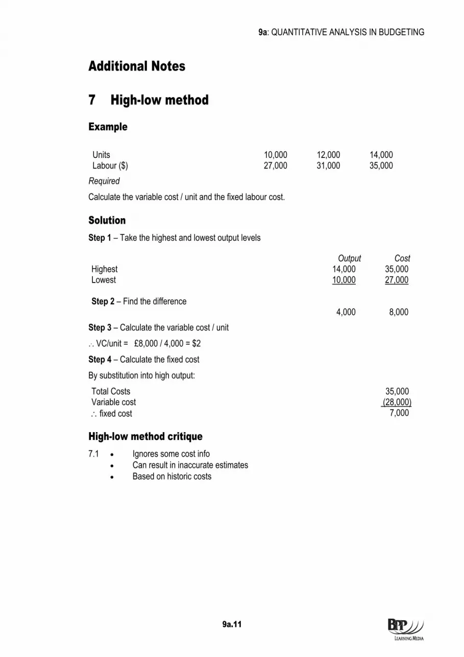
9a: QUANTITATIVE ANALYSIS IN BUDGETING
9a.11
Additional Notes
7 High-low method
Example Units 10,000 12,000 14,000 Labour ($) 27,000 31,000 35,000
Required Calculate the variable cost / unit and the fixed labour cost.
Solution Step 1 – Take the highest and lowest output levels
Output Cost Highest 14,000 35,000 Lowest 10,000 27,000 Step 2 – Find the difference 4,000 8,000
Step 3 – Calculate the variable cost / unit ... VC/unit = £8,000 / 4,000 = $2 Step 4 – Calculate the fixed cost By substitution into high output: Total Costs 35,000 Variable cost (28,000) ∴fixed cost 7,000
High-low method critique 7.1 • Ignores some cost info
• Can result in inaccurate estimates • Based on historic costs

9a: QUANTITATIVE ANALYSIS IN BUDGETING
9a.12
END OF CHPATEREND OF CHAPTER

9b.1
Syllabus Guide Detailed Outcomes Having studied this chapter you will be able to:
• Estimate the learning effect and apply the learning curve to a budgetary problem, including calculations on the steady state
• Discuss the reservations with the learning curve
Exam Context Learning curves appeared on the pilot paper. You should expect both calculations and discussion.
Qualification Context Learning curves are another tool that can be used in forecasting in addition to the other tools seen here in Chapter 9a.
Business Context The learning relationship was first quantified in 1936 at an air force base in the US. They found that as aircraft production doubled labour time fell by 10-15%.
Businesses are able to reduce costs and therefore the price they charge to the customer as they benefit from the learning curve.
Learning curves

9b: LEARNING CURVES
9b.2
Overview
Theory As cumulative output doubles the average time to produce a
unit falls by a given rate Formula Y = axb
Learning curves
Experience effect Conditions Steady state

9b: LEARNING CURVES
9b.3
1 Managing future costs 1.1 Calculating costs of established products and services made using established methods is
relatively straightforward. Standards and budgets can be set.
1.2 Costing new products and services is inherently uncertain. Modern business environments tend to: • be highly automated • have short production runs • involve short product life cycles • hold lower levels of inventory
1.3 New costing techniques will be required.
2 Learning curve theory
Introduction 2.1 When new working practices or products are introduced, the theory is that as a workforce
gains experience in a task, it will come to perform that task quicker. This means that labour costs and variable overheads (if labour hour driven) will be lower in later periods of production than when the new product or production technique is introduced.
Theory 2.2 The theory of learning curves will only hold if the following conditions apply:
(a) There is a significant manual element in the task being considered. (b) The task must be repetitive. (c) Production must be at an early stage so that there is room for improvement. (d) There must be consistency in the workforce. (e) There must not be extensive breaks in production, or workers will 'forget' the skill. (f) Workforce is motivated.
Rule 2.3 As cumulative output doubles, the cumulative average time per unit falls to a given
percentage of the previous cumulative average time per unit. Cumulative average time is the average time for all units produced so far.

9b: LEARNING CURVES
9b.4
Lecture example 1 Technique Demonstration A firm's workforce experiences a 75% learning rate.
Output Total time Cumulative average time (batches) (hours) (hours) 1 2 4 8 Required If the budgeted time for the first batch is 100 hours, calculate the time to produce eight batches in total.
Solution
Cumulative average time per unit
Cumulative output
Learning effect
Steady state
Y = axb

9b: LEARNING CURVES
9b.5
Formula 2.4 Y= aXb
where Y is the cumulative average time per unit taken to produce X units a is the time taken to produce the first unit X is the cumulative number of units b is the index of learning (calculated as 2log
rlog where r is the learning rate)
Lecture example 2 Technique Demonstration (With the formula) A firm's workforce experiences a 75% learning rate. The budgeted time for the first batch is 100 hours. Required Using the formula Y= aXb , calculate the time to produce: (a) the first 10 batches in total (b) the 10th batch only.
Solution

9b: LEARNING CURVES
9b.6
2.5 You may be given the formula relating to cost not time ie: Y= aXb where Y is the cumulative average cost per unit taken to produce X units
a is the cost to produce the first unit X is the cumulative number of units b is the index of learning (calculated as 2log
rlog where r is the learning rate)
Exactly the same process applies.
Lecture example 3 Preparation question A firm's workforce experiences a 75% learning rate. The budgeted cost for the first batch is $200 Required Using the formula Y= aXb , calculate the cost of producing: (a) the first 10 batches in total (b) the 10th batch only.
Solution

9b: LEARNING CURVES
9b.7
Steady state 2.6 Eventually, the time per unit will reach a steady state where no further improvement can be
made.
Cessation of learning effect 2.7 Practical reasons for the learning effect to cease are:
(a) when machine efficiency restricts any further improvement. (b) the workforce reach their physical limits. (c) there is a ‘go-slow’ agreement among the workforce.
Lecture example 4 Exam standard for 8 marks Flogel Ltd has just produced the first full batch of a new product taking 200 hours. Flogel has a learning curve effect of 85%. Required
(a) How long will it take to produce the next 15 batches? (b) Flogel expects that after the 30th batch has been produced, the learning effect will cease. From the 31st batch onwards, each batch will take the same time as the 30th batch. What time per batch should be budgeted?
Solution

9b: LEARNING CURVES
9b.8
Uses of learning curve theory 2.8 The learning curve theory can be used in the business for:
• forecasting labour hours required • cash forecasting • standard setting • cost calculation • price setting
Problems with learning curve theory 2.9 Although it seems a useful and easy to apply technique learning curve theory is not without
problems: • How do we calculate the rate? • How do we know when the production will reach steady state? • Is the rate really constant?
3 Experience effect 3.1 The 'learning curve' is a term usually applied to the time taken by the skilled labour element
in production.
3.2 The 'experience curve' covers all costs that may reduce due to technological and managerial learning effects, following an increase in production volumes: • Material costs may decrease with quantity discounts • Variable overheads follow the pattern of direct labour • Fixed overheads per unit will decrease as production volumes rise.
3.3 The experience curve is exploited through • growth • market share • mass production
4 Chapter summary • The amount of time needed for production may reduce when the product is new,
repetitive and has a significant manual element
• Learning curve theory states that as cumulative output doubles, the cumulative average time per unit falls to a given percentage of the previous cumulative average time per unit
• The time / cost for production of units can be calculated if the rate of learning is known using the formula Y= aXb
• Eventually a consistent time to produce a unit will be reached from which it is not possible to improve any further. This is known as steady state.
Q5 Dench
END OF CHAPTER

10.1
Syllabus Guide Detailed Outcomes Having studied this chapter you will be able to:
• Explain the use of standard costs
• Outline the methods used to derive standard costs and discuss the different types of cost possible
• Prepare budgets and standards that allow for waste and idle time
• Explain and apply the principle of controllability in the performance management system
Exam Context These topics are likely to be examined alongside the variances which will be covered in the next few chapters.
Qualification Context This chapter takes the standard costing seen in Management Accounting (F2) further.
Business Context Standard cost systems are still widely used throughout UK industry. For example, Whitbread restaurants track performance of their weekly food margins against the standard food margin percentage.
Budgeting and standard costing

10: BUDGETING AND STANDARD COSTING
10.2
Overview
Budgeting and standard costing
Standards and budgets Waste and idle time Controllability
Purpose of standards Calculation of standards Bases of standard

10: BUDGETING AND STANDARD COSTING
10.3
1 Standards 1.1 A standard is prepared by management in advance, and details their expectations of the
future.
1.2 Standards are not just for items of production in manufacturing businesses. They exist in many different spheres. Standard times for repairing cars, standard punctualities for train companies and standard response times for ambulances are just some of the many examples encountered.
1.3 A standard cost is an estimated unit cost.
1.4 You will have come across standard costs before as part of costing. When trying to establish a cost of a unit be it under absorption or marginal costing the cost card was derived using standard costs As a reminder:
Example of a standard cost card for a cost unit 1.5
$/unit Direct costs: Direct materials (5kg @ $3/kg) 15.00 Direct labour (3 hrs @ $6/hr) 18.00 33.00 Indirect costs: Variable
overheads 2.00
Fixed overheads 3.00 Full product cost 38.00 The costs in the cost card are built up using for example, the expected amount of material at the expected price of the material.
2 Purposes of standards 2.1 The uses of standard costing are as follows:
(a) Prediction of costs and times for decision making, eg for allocating resources. (b) Standard costing is used in setting budgets – an accurate standard will increase the
accuracy of the budget. (c) Variance analysis is a control technique which compares actual with standard costs
and revenues. (d) Performance evaluation systems make use of standards as motivators and also as
a basis for assessment. (e) Inventory valuation – this is often less time consuming than alternative valuations
methods such as FIFO or weighted average.

10: BUDGETING AND STANDARD COSTING
10.4
3 Bases 3.1 (a) Ideal standard – assumes an optimum level of efficiency.
(b) Attainable standard – makes an allowance for normal inefficiencies but also includes hoped-for improvements.
(c) Current standard – based on current efficiency levels and achievements. (d) Basic standard/historic standard – not updated regularly, used to show changes
over the long term.
Lecture example 1 Idea Generation How do you think each of the bases of standard would impact an employee's motivation?
Solution
4 Deriving standards 4.1 The standard cost of materials will be estimated by the purchasing department
Lecture example 2 Idea Generation What considerations will (a) the purchasing department take into account when trying to establish the standard cost of
material? (b) the production department take into account when trying to establish the quantity of material
needed per unit?

10: BUDGETING AND STANDARD COSTING
10.5
Solution
Lecture example 3 Idea Generation If inflation is significant, would a standard be relevant?
Solution
4.2 Setting standards for other elements on the cost card will undergo a similar process.
Setting standardsfor overheads

10: BUDGETING AND STANDARD COSTING
10.6
5 Standards and budgets 5.1 Similarities:
• Are very similar in terms of their motivation impacts on employees • Standards generally form the basis for the budget • Both used for control
5.2 Differences:
Standards Budgets By Unit In total For areas of repetition All areas Financial & non-financial targets Financial targets
6 Waste and idle time 6.1 We have seen that one of the items to take into account when preparing standards is
wastage. This may be due to: • spillage • poor skills of labour force • natural wastage / evaporation
6.2 If wastage is not built into the standards they will not be achievable. Attainable standards would therefore have allowances for wastage built in.
6.3 If wastage occurs before production then allowance should be made within the purchases budget.
6.4 If it occurs during production then the allowance should be within the production budget
Lecture example 4 Technique Demonstration Each unit of X uses 6 kg of material. Budgeted sales in month 1 are 18,000 units. During the production process 10% of production is usually scrapped as being faulty. Opening inventories of finished units are15,000 and closing inventories are11,400 Required
What is the amount of raw material required for Month 1?
Budgets andstandardscompared

10: BUDGETING AND STANDARD COSTING
10.7
Solution
6.5 A similar process needs to be considered with labour.
6.6 The labour force may not be able to work 100% of the time. This could be due to late delivery of materials, machine breakdowns or not enough work.
6.7 When this happens this is known as idle time. To set an attainable standard some allowance for idle time should be built in to the labour efficiency targets.
7 Chapter summary • Standard costs have many uses in performance management
• Standards should be set at an attainable level to drive the best performance
• Allowance for idle time / wastage should be built in to standards
• Managers should only be held accountable for the items within their control
Q6McDreamy

10: BUDGETING AND STANDARD COSTING
10.8
END OF CHAPTER

11a.1
Syllabus Guide Detailed Outcomes Having studied this chapter you will be able to:
• Calculate, identify the cause of and interpret basic variances
• Explain the effect on labour variances where the learning curve has been used in the budget process
• Produce full operating statements in both a marginal cost and full absorption costing environment, reconciling actual profit to budgeted profit
• Calculate the effect of idle time and waste on variances including where idle time has been budgeted for
• Explain the possible causes of idle time and waste and suggest methods of control
• Calculate, using a simple situation, ABC-based variances
• Explain the different methods available for deciding whether or not too investigate a variance cause
Exam Context Calculation of variances in this paper is likely to focus more heavily on those not examined at F2. However, you must also be prepared to discuss and interpret all variances.
Qualification Context This chapter revises and builds upon the variance analysis performed at F2.
Business Context Variance calculations are universally performed to enable management to understand which areas of the business are/are not performing well.
Variance analysis

11a: VARIANCE ANALYSIS
11a.2
Overview
Variance analysis
Basic variances Waste and idle time
Interpretation When to investigate Variance investigation methods
Variances and the learning curve
ABC and variance analysis

11a: VARIANCE ANALYSIS
11a.3
1 Calculation basic of variances 1.1 Variance analysis reconciles actual to budgeted costs, revenue or profit. It is a way of
explaining the difference between actual and budgeted results. They can either be favourable (F), ie better than expected or adverse (A), worse than expected.
1.2 Each variance is calculated separately.
Budgeted outcome X Actual outcome X Variance X
1.3 Material variances $ Price – based on actual purchases What should they have cost? X What did they cost? (X) X Kgs Usage – based on actual production What should it have used? X What did it use? (X) Difference valued at standard cost X $X
1.4 Labour variances $ Rate – based on hours paid What should they have cost? X What did they cost? (X) X Idle time – Hrs Hours worked X Hours paid (X) Difference valued at standard rate per hour $X Efficiency – based on actual production Hrs How long should it have taken? X How long did it take? (X) Difference valued at standard rate per hour X $X

11a: VARIANCE ANALYSIS
11a.4
1.5 Variable overhead variances $ Expenditure – based on actual hours worked What should they have cost? X What did they cost? (X) X Efficiency – based on actual production Hrs How long should it have taken? X How long did it take? (X) Difference valued at standard rate per hour X $X NB: This assumes variable overheads are incurred per labour hour.
1.6 Fixed overhead variances Under marginal costing, the fixed overhead variance is just the difference between budgeted and actual fixed overhead costs, ie fixed overhead expenditure variance. Under absorption costing, the fixed overhead variance can be further subdivided as follows:
Total variance (over/under absorption)
Expenditure variance Volume variance
$ Units Budget expenditure X Budgeted units X Actual expenditure (X) Actual units (X) X X Difference value at OAR
per unit
$X
Efficiency Capacity
Hours Hours How long should it have taken? X Budgeted hours worked X How long did it take? (X) Actual hours worked (X) X Difference valued at OAR rate per hr
$X Difference value at OAR rate per hour
X $X

11a: VARIANCE ANALYSIS
11a.5
1.7 Sales variances Price – based on actual units sold $ What should they sell for? X What did they sell for? (X) X Volume – based on actual units sold Units Budgeted sales X Actual sales (X) X Difference valued at standard contribution/unit $X Under absorption costing this variance will be valued at standard profit/unit.
Lecture example 1 Preparation question Brenda and Eddie run The Italian Restaurant selling a variety of pasta dishes each using similar ingredients and taking the same amount of time to prepare. To try to control costs they instigate a standard costing system, deriving the following standard cost per meal. $/meal Ingredients (average value) 400g @ $1.50/kg = 0.60 Labour 30 mins @ $4/hour = 2.00 Variable overheads 30 mins @ $1/hour = 0.50 Fixed overheads 30 mins @ $2.50/hour = 1.25 4.35 Standard profit 2.60 Selling price 6.95 The overheads are absorbed on the assumption that Brenda and Eddie normally sell 100 pasta meals per day over the year during which they are open for 300 days. During one six day week, the following results are obtained: Meals sold 630 total revenue = $4,500 Ingredients bought: 260 kg for $380 used: 240 kg Hours paid: 300 hrs costing $1,350 Time lost due to late delivery of ingredients = 10 hours Variable overheads $325 Fixed overheads $750
Required Reconcile the budgeted contribution to the actual profit (for one week) using marginal costing and suggest possible causes for the variances identified.

11a: VARIANCE ANALYSIS
11a.6
Solution
Operating Statement (under marginal costing)
$ Budgeted contribution Sales volume contribution variance Sales price variance Cost variances: $(F) $(A) Materials Price Usage Labour Rate Idle Efficiency Variable o/h Expenditure Efficiency Actual contribution Fixed overheads Budgeted Expenditure variance Actual Actual profit
Workings:

11a: VARIANCE ANALYSIS
11a.7

11a: VARIANCE ANALYSIS
11a.8
Differences between absorption costing and marginal costing 1.8 Variances calculated using absorption costing are the same as under marginal costing
except: (a) Fixed overheads – see Section 1.6 (b) Sales volume profit variance:
variance in units valued at standard profit/unit, not contribution/unit (c) Operating statement will usually reconcile budgeted profit to actual profit.
Lecture example 2 Preparation question Required Using the information in lecture example 1, analyse the fixed overhead variances in detail and prepare an operating statement using absorption costing principles.
Solution
Operating Statement (under absorption costing)
Workings:
$ Budgeted profit Sales volume profit variance Sales price variance Cost variances: $(F) $(A) Materials Price Usage Labour Rate Idle Efficiency Variable o/h Expenditure Efficiency Fixed o/h Expenditure Efficiency Capacity Actual profit

11a: VARIANCE ANALYSIS
11a.9
2 Idle time and wastage 2.1 The calculations we have seen so far for idle time assume that no allowance was initially
made in the budget for idle time. As you have seen a company may budget for idle time. If this is the case the idle time variance is the difference between the standard idle time allowed and the actual idle time that occurred.
Lecture example 3 Technique Demonstration James’ budget allows for idle time of 5%. His budgeted hours for the month were 10,000. Actual hours were 9,500 of which 550 were idle hours. Budgeted rates of pay were $7 per hour. Required
Calculate the idle time variance.
Solution

11a: VARIANCE ANALYSIS
11a.10
2.2 In the same way that idle time can be included in the budgets so might wastage. Calculation of wastage above and beyond the expected wastage should also be made.
Lecture example 4 Idea Generation What methods of control would you recommend to improve idle time and wastage?
Solution
3 Variances and the learning curve 3.1 If budgets are put together whilst still experiencing the learning curve. Variances should be
favourable as we continue to improve and become more efficient.
3.2 Standards should be revised once the particular product moves to its steady state.
4 ABC and variance analysis 4.1 All overheads within an ABC system are treated as variable overheads. No fixed overhead
variances are calculated. $ Expenditure – based on actual activity level What should it have cost? X What did it cost? (X) X Efficiency – based on actual production activity How much should it have taken? X How much did it take? (X) Difference valued at standard rate per activity X $X

11a: VARIANCE ANALYSIS
11a.11
Lecture example 5 Technique Demonstration Extracts from V Co's records for June are as follows.
Budget Actual Production 1,000 units 1,200 units Cost of orders $1,500 $2,275 Activity - Orders 500 540 Required:
Calculate the overhead expenditure and efficiency variances relating to orders.
Solution
5 Interpretation of variances
Causes of variances 5.1 Obviously the cause of the variance must be determined before appropriate action can be
taken. An employee should only be judged on what they have control over. (a) Different controllable expenditure (b) Different uncontrollable expenditure (c) Inaccurate standard due to
• poor planning • use of unrealistic standard
(d) Inaccurate measurement

11a: VARIANCE ANALYSIS
11a.12
Interdependence of variances 5.2 In order to interpret variances effectively any interdependence between variances must be
identified, i.e. it is not always possible to look at individual variances in isolation.
5.3 For example, a decision to purchase better quality, higher price materials may result in an adverse price variance but a favourable usage variance.
5.4 The following table may help you to think about some of the operational causes of variances.
Variance Favourable Adverse Material price Unforeseen discounts received
Greater care in purchasing Change in material standard
Price increase Careless purchasing Change in material standard
Material usage
Material used of higher quality than standard More efficient use of material Errors in allocating material to jobs
Defective material Excessive waste or theft Stricter quality control Errors in allocating material to jobs
Labour rate Use of workers at a rate of pay lower than standard
Wage rate increase
Idle time The idle time variance is always adverse
Machine breakdown Illness or injury to worker
Labour efficiency
Output produced more quickly than expected because of worker motivation, better quality materials etc Errors in allocating time to jobs
Lost time in excess of standard Output lower than standard set because of lack of training, sub-standard materials etc Errors in allocating time to jobs
Fixed overhead expenditure
Savings in costs incurred Increase in cost of services used
Overhead expenditure variances ought to be traced to the individual cost centres where the variances occurred. Fixed overhead volume
Production or level of activity greater than budgeted
Production or level of activity less than budgeted
Efficiency Reasons for this tie in exactly to labour efficiency
Reasons for this tie in exactly to labour efficiency
Capacity Labour worked for more hours than budgeted. Maybe due to more production than expected
Maybe a result of lower production volumes or higher absenteeism eg holidays / sickness

11a: VARIANCE ANALYSIS
11a.13
Variance Favourable Adverse Sales price Unplanned price increase
Fewer discounts given than expected
Anticipated increase in selling price did not happen More discounts allowed than expected
Sales volume Additional demand experienced Fall in demand Lower output
Lecture example 6 Idea Generation Required Discuss instances when a favourable variance may not be good news and when adverse variances may be good for a business.
Solution

11a: VARIANCE ANALYSIS
11a.14
6 Investigating variances
When to investigate 6.1 Once variances have been calculated, which variances need investigating must be decided.
General factors for consideration would be: (a) Size of variance (b) Controllability of variance (c) Cost of investigation (d) Interrelationships with other variances (e) Level of standard (f) Trend emerging In order to help your understanding of the significance of size of variances, a percentage variance chart may be prepared.
Lecture example 7 Exam standard for 5 marks Standard cost of material is $12/kg and standard usage for one unit is 10 kg. Output Usage Cost Price variance Usage
variance units kg $ $ $ January 20 200 2,900 500 A - February 30 320 4,500 660 A 240 A March 40 450 6,000 600 A 600 A Required Prepare a percentage variance chart of the following data.
Solution

11a: VARIANCE ANALYSIS
11a.15
Variance investigation models These models are:
6.2 Rule of thumb model This involves setting acceptable limits for variances. Only if the variances are outside these limits should they be investigated.
6.3 Statistical control charts Here variances and control limits are marked on a chart. Not only will variances outside the control limits be investigated but any worsening in trends can be spotted and investigated.
6.4 Statistical significance model Historical data is used to calculate an expected deviation around the variance. Any variances outside of this deviation will be investigated. A 95% or 0.05 significance rule would state that variances should be investigated if they exceed 1.96 standard deviations from the standard. A 99% or 0.01 significance rule would state that variances should be investigated if they exceed 2. 58 standard deviations from the standard.
Varianceinvestigation
modelsSection 7.2

11a: VARIANCE ANALYSIS
11a.16
Lecture example 8 Exam standard for 3 marks Analysis of past data reveals that costs per month are $50,000 with a standard deviation of $3,000. A 0.01 significance rule is in use. Actual travel expenses are $55,000. Required
Should the resulting variance be investigated?
Solution
7 Chapter summary • Variance analysis is a performance evaluation tool that is often used especially as a
part of cost control
• Interpretation of variances is as important as the calculations themselves
• Where idle time is budgeted, the resulting variance compares the idle time allowed with actual idle time
• Before deciding to investigate a variance factors such as size, trend and controllability should be considered
• There are three variance investigation models: Rule of thumb, statistical control charts and the statistical significance model
END OF CHPATEREND OF CHAPTER

11b.1
Syllabus Guide Detailed Outcomes Having studied this chapter you will be able to:
• Calculate, identify the cause of and explain mix and yield variances
• Explain the wider issues involved in changing mix e.g. cost, quality and performance measurement issues
• Identify and explain the interrelationship between price, mix and yield
• Suggest and justify alternative methods of controlling production processes
• Calculate a revised budget
• Identify and explain those factors that could and could not be allowed to revise an original budget
• Calculate planning and operational variances for sales, including market size and market share, materials and labour
• Explain the manipulation issues in revising budgets
Exam Context Expect to have to both calculate and discuss the variances in this chapter. Mix and yield variances were the subject of one of the questions on the pilot paper.
Qualification Context This chapter builds upon the variance analysis performed at F2.
Business Context Variance calculations are universally performed to enable management to understand which areas of the business are/are not performing well.
Further variance analysis

11b: FURTHER VARIANCE ANALYSIS
11b.2
Overview
Further variance analysis
Mix and yield variances Alternative production control methods
Planning and operational variances

11b: FURTHER VARIANCE ANALYSIS
11b.3
1 Mix variances
Materials and labour inputs 1.1 Where inputs can be substituted for one another, the efficiency/usage variance can be
subdivided. The materials and labour variances can both be split into mix and yield (or output) components.
1.2 The mix variance represents the financial impact of using a different proportion of raw materials.
1.3 The yield variance represents the financial impact of the input yielding a different level of output to the standard.
1.4 The same principle can be applied to labour if different grades of labour are needed for one product.
Lecture example 1 Exam standard for 6 marks Brenda and Eddie are analysing the main ingredients to their basic pasta sauce. The standard ingredients for one batch of tomato pasta sauce are: $ Onions 5kg @ $2/kg 10 Tomatoes 5kg @ $4/kg 20 30 Over the last month, 100 batches of sauce were prepared, using the following ingredients: Onions 600 kg Tomatoes 900 kg Required
Calculate the materials mix and yield variances and comment on their meaning.

11b: FURTHER VARIANCE ANALYSIS
11b.4
Solution

11b: FURTHER VARIANCE ANALYSIS
11b.5
Lecture example 2 Idea Generation What are the implications of a change in mix?
Solution
1.5 Mix and yield with losses
Lecture example 3 Exam standard for 6 marks A company has a process in which three inputs are mixed together to produce Product Pip. The standard mix of inputs to produce 90 kg of Product Pip is shown below: $ 50 kg of ingredient A at $80 per kg 4,000 30 kg of ingredient J at $100 per kg 3,000 20 kg of ingredient H at $120 per kg 2,400 9,400 During March 2,000 kg of ingredients were used to produce 1,900 kg of Product Pip. Inputs were as follows: $ 1,040 kg of ingredient A at $75 per kg 78,000 560 kg of ingredient J at $105 per kg 58,800 400 kg of ingredient H at $125 per kg 50,000 186,800 Required
Calculate the materials mix and yield variance for June.
Issues involved inchanging the mix.
Section 8.5

11b: FURTHER VARIANCE ANALYSIS
11b.6
Solution
1.6 The sales volume variance can also be analysed further but this is known as a mix and quantity variance.
2 Alternative production control methods 2.1 Looking at mix and yield variances in isolation may not be sufficient in a modern business
environment where as much focus is placed on quality as cost.
2.2 Other methods to be used could include: • Quality control measures • Customer satisfaction scores • Wastage rates • Number of late deliveries
Q7 ACCA-Chem

11b: FURTHER VARIANCE ANALYSIS
11b.7
3 Planning and operational variances 3.1 The variance analysis you have studied so far has compared actual results with a budget
which was set at the beginning of the year. Is this sensible?
Approach to planning and operational variances 3.2
3.3 The traditional variances we have seen so far can be investigated further to look at the elements driven by a wrong standard (Planning variances) and the elements that were within the manager’s control (Operational variances).

11b: FURTHER VARIANCE ANALYSIS
11b.8
Lecture example 4 Exam standard for 8 marks The following data relate to product AJ and its material content for the month of June. Budget Actual Output – 15,000 units of AJ Output – 14,000 units of AJ Materials – 4kg per unit @ $9 per kg Materials – 54,000 kg @ $9.50 It has now been agreed that the standard price for the raw material purchased in June should have been $9.30 per kg and the standard kg / unit should have been 3.8 kg. Required Calculate the total and planning and operational variances for materials price and usage.
Solution

11b: FURTHER VARIANCE ANALYSIS
11b.9
Lecture example 5 Exam standard for 10 marks Chianti Limited manufactures and sells a single product. The company uses a standard costing system, and the standard cost per unit is as follows:
$ Materials: 1 litre at $1 per litre 1.00 Direct labour – 2 hours at $2.50 per hour 5.00 Variable overhead 1.40 Standard cost 7.40 Standard contribution 8.60 Budgeted sales price 16.00 Budgeted production and sales for 20X8 were 5,000 units. The budgeted fixed overhead was $20,000. Actual production in 20X8 was 5,200 units, and 5,100 units were sold for $81,000. Production costs were:
Materials: purchased and used: 5,150 litres costing $ 5,120 Labour: 10,200 hours were paid for and cost $27,400 Variable overheads $ 7,000 Fixed overheads $19,500 You have also found the following: (a) Material usage should have been 1.2 litres per unit, at a price of $0.95 per litre. (b) Labour rate should have been $2.60 per hour. (c) Industry sales of Chiantis were 10% lower than forecast Required
Calculate meaningful variances.
Solution

11b: FURTHER VARIANCE ANALYSIS
11b.10

11b: FURTHER VARIANCE ANALYSIS
11b.11
Advantages of revising the budget 3.4 (a) Highlights those variances which are controllable and those which aren’t
(b) Ensures that operational performance is appraised by reference to realistic targets. (c) Should ensure that future budgets are more realistic.
Disadvantages of revising the budget 3.5 (a) Determination of revised budget
• may be biased • may need external information
(b) Use of revised budget may undermine original budget as a target and as a motivator. (c) Employees may use this system to their advantage by excusing operating problems
as poor planning if this method is used.
4 Chapter summary • A mix variance is the result of a different mix of materials to the standard being used
• A yield variance occurs when a different quantity from standard is input in order to achieve the desired output
• Planning variances represent the difference between the original and revised budget
• Operational variances are those items which were within a manger’s control. They are the difference between the revised budget and the actual

11b: FURTHER VARIANCE ANALYSIS
11b.12
END OF CHAPTER

12.1
Syllabus Guide Detailed Outcomes Having studied this chapter you will be able to:
• Describe the dysfunctional nature of some variances in the modern environments of JIT and TQM
• Discuss the behavioural problems resulting from using standard costs in rapidly changing environments
• Discuss the effect that variances have on staff motivation and action
Exam Context Topics in this chapter are most likely to appear as discussion elements within a standard costing or variance question.
Qualification Context Topics such as Total Quality Management (TQM) and Just in time (JIT) will be developed in the Professional level paper Advanced Performance Management paper (P5).
Business Context Many businesses still use standard costing despite operating in service industries or rapidly changing markets.
Home Study Chapter - Behavioural aspects of standard costing

12: BEHAVIOURAL ASPECTS OF STANDARD COSTING
12.2
Overview
Behavioural aspects of Standard Costing
Standard costing in service industries
Behavioural impacts of standard costing in the modern environment
Modern business environment • WCM • TQM • JIT
Criticisms of standard costing

12: BEHAVIOURAL ASPECTS OF STANDARD COSTING
12.3
1 The modern business environment and world class manufacturing
1.1 Traditional production methods have centred around high volume, low unit cost outputs. However, in recent years many changes have taken place in the nature of the world economy, technology, market demand and manufacturing practices.
Lecture example 1 Idea Generation Required What are some features of the environment that businesses now have to operate in?
Solution
World class manufacturing 1.2 Features of WCM
(a) Quality improvement (b) JIT based production (c) Managing people (d) Flexible approach to customer requirements
1.3 Main benefits (a) Improved quality and a reduced cost to the customer (b) Dramatic improvements in production efficiency (c) Improved motivation and greater loyalty from key employees (d) Improvements in customer satisfaction and the development of genuine goodwill (e) The achievement of competitive advantage (f) Increase in medium to long-term profitability

12: BEHAVIOURAL ASPECTS OF STANDARD COSTING
12.4
2 Total quality management TQM is a business philosophy aimed at improving quality.
Get it right, first time 2.1 The cost of preventing mistakes is less than the cost of correcting them if they occur.
Continuous improvement 2.2 Never be satisfied with current achievement. It is always possible to improve performance.
Goals of TQM 2.3 (a) To gain competitive advantage via continuously improved quality
(b) To continuously reduce the cost of providing enhanced quality (c) Innovation (d) Provide first class customer service (e) To involve all employees
Design for quality 2.4 Design quality into an organisation's products and operations from the outset.
(a) Reduce the number of parts in a product (b) Use components common to other products in the organisation (c) Improve physical characteristics to meet customers’ needs
Performance measurement 2.5 Traditional variance analysis is not appropriate in a TQM environment, due to the focus on
• continuous improvement • quality as opposed to cost
2.6 Alternative measures of performance, therefore, include: (a) measuring incoming supplies (b) monitoring work as it proceeds (c) measuring customer satisfaction
Can standardcosting and TQM
co-exist?

12: BEHAVIOURAL ASPECTS OF STANDARD COSTING
12.5
3 Just-in-time 3.1 JIT is a system whose objective is to produce or buy units as they are required rather than
for inventory. It is a demand 'pull' system.
3.2 Aims to restructure the manufacturing process to bring about more flexible, rapid and cost effective production. This will include the elimination of non-value adding activities.
3.3 There are two aspects of JIT: • JIT production: production is customer demand driven • JIT purchasing: purchase components/materials to meet production requirements
JIT purchasing 3.4 Objective:
(a) Buy in raw materials as you need them (b) Zero inventory of raw materials (c) Usage of raw materials matched with delivery from supplier
3.5 Elements: (a) Frequent deliveries (b) Control over delivery timing (c) Close working relations with fewer suppliers (d) Long-term contracts (e) Quality assurance
Lecture example 2 Preparation question Required
What are the advantages and disadvantages of JIT purchasing?
Solution

12: BEHAVIOURAL ASPECTS OF STANDARD COSTING
12.6
JIT production 3.6 Objective:
(a) Obtain low cost, high quality, on-time production to order (b) By minimising inventory levels between successive processes and therefore (c) Minimising idle equipment, facilities and workers
3.7 Elements: (a) WIP and finished goods reductions (b) Decreased lead and set-up times (c) Zero defects and continuous improvement (see TQM) (d) Flexible workforce (e) Quality control as part of the production process (f) Producing to order (g) Detection of production problems as they occur
Innovation and improvement 3.8 JIT philosophy is to cause failures, since the failure is an opportunity to improve the process.
The problem might be due to machine failure, a set-up or quality problem etc.
3.9 This approach of continual trouble-shooting leads to: (a) A series of small, low-cost improvements (b) A culture of constant analysis and improvement
Performance measurement 3.10 Traditional variance analysis is not appropriate in a JIT environment as supplier quality and
reliability is more important than cost
4 Criticisms of standard costing 4.1 Standard costing has some disadvantages and, arguably, is less relevant in the modern
environment than previously. (a) Standard costing works best in a stable environment; the modern business
environment is very fast changing (b) Regular revisions to the standard are required. This process is expensive and time
consuming (c) Meeting the standard should not necessarily be accepted as satisfactory if further
improvements could be made (d) Techniques associated with standard costing (such as variance analysis) are less
useful in a modern environment of customised products
Standard costingand new
philosophy
The role inmodern businessof standards and
variances

12: BEHAVIOURAL ASPECTS OF STANDARD COSTING
12.7
Revision of standards 4.2 Standards should be reviewed regularly, and revised when there is a change in the basis
upon which they were set. This ensures that they remain useful as a performance measure.
5 Setting standards in service industries 5.1 The application of standard costing in service industries does have its problems.
(a) Difficult to establish a measurable cost unit for some services. (b) In some service organisations every cost unit will be different or heterogeneous. (c) Since the human influence is so great in many services it can be difficult to predict
and control the quality of the output and the resources used in its production.
5.2 To overcome these problems and enable the application of standard costing for planning and control in service industries it is therefore necessary to do the following. (a) Establish a measurable cost unit. For example, cost per passenger-mile or a tonne-
mile, or for hotels, such as a guest-night. (b) Attempt to reduce the heterogeneity of services. If every service provided to the
customer is the same as the last, then it will be possible to set a standard cost for the service and use this to maximise efficiency and reduce waste.
(c) Reduce the element of human influence. By swapping machines for humans wherever possible.

12: BEHAVIOURAL ASPECTS OF STANDARD COSTING
12.8
6 Behavioural impacts of standard costing in the modern environment
6.1 As seen in Chapter 10 standard costing is often perceived as being at odds with the modern business environment.
Traditional manufacturing
Modern environment Impacts of standard costing
High labour cost, low overhead
Low labour cost, high overhead
Overhead variances do not have enough detail to aid performance measurement
Stable environment / products
Rapidly changing environment / products
Regular revision of standards can be demotivating for employees as the goal post keep moving
Standard product Customised product Differences between products make developing a standard difficult. Resulting variances may not be meaningful and certain employees may be unfairly penalised
Focus on cost Focus on quality Variance analysis encourages cost control. Desired quality may drive adverse price variances
Raw material and finished goods inventory is important
JIT philosophy Inventory may be built up in an effort to improve efficiency variances
6.2 Despite the criticisms and impacts, many businesses still operate with standard costing as it does aid planning and control. Other non-financial measures should be used alongside it such as on time deliveries, customer satisfaction measures and so on.
7 Chapter summary • The changes occurring in today’s business environment result in standard costing
being criticised
• Standard costing is often still used as it still aids planning, control and decision making
• Care must be taken when using it for control as modern business philosophies such as TQM and JIT will often drive adverse price or efficiency variances
• Other mechanisms reflecting today’s key indicators must be used in performance management
END OF CHAPTER

13.1
Syllabus Guide Detailed Outcomes Having studied this chapter you will be able to:
• Describe, calculate and interpret financial performance indicators for profitability, liquidity and risk in both manufacturing and service businesses. Suggest methods to improve these measures
• Describe, calculate and interpret non-financial performance indicators (NFPIs) and suggest method to improve the performance indicated
• Explain the causes and problems created by short-termism and financial manipulation of results and suggest methods to encourage a long-term view
• Explain and interpret the Balanced Scorecard, and the Building Block model proposed by Fitzgerald and Moon
• Discuss the difficulties of target setting in qualitative areas
Exam Context Financial and non-financial control appeared on the pilot paper for 25 marks. You should expect to calculate, explain and apply the knowledge from this chapter. The examiner is passionate about the use of non-financial indicators and believes they often give a better indication of a company’s prospects.
Qualification Context Topics in this chapter will be developed in the Professional level Advanced Performance Management paper (P5). In P5 you will be asked to discuss the appropriateness of various performance ratios as well as evaluating the use of the balanced scorecard and building blocks. The ratios in this chapter also feature in F7.
Business Context In 1992, Robert S Kaplan and David Norton introduced the balanced scorecard, a concept measuring a company's activities in terms of its vision and strategies. It provides managers with a comprehensive view of the performance of a business.
Performance management

13: PERFORMANCE MANAGEMENT
13.2
Overview
Short termism Balanced scorecard Performance measurement in service businesses
Performance management
Financial performance indicators
• Profitability • Liquidity • Gearing
Non financial performance indicators
Building block model

13: PERFORMANCE MANAGEMENT
13.3
1 Performance measurement
Financial performance indicators 1.1 Analysis and interpretation of a company's accounts will give an indication of the company's
performance. The aims would be to: • assess the company’s performance and financial position (in comparison with other
companies in the same industry) • try to assess the potential future performance or identify weakness
Company performance assessment 1.2 This would usually involve:
(a) ratio analysis (b) review of the A/c’s to highlight issues not disclosed by ratio analysis (e.g.: contingent
liabilities) (c) review of the benefits / wealth from the point of view of the other stakeholders (d) analysis of other financial and non-financial information from external sources
Areas for analysis 1.3 (a) Profitability – how well a company performs, given its asset base
(b) Liquidity – short-term financial position (c) Gearing – measure of risk These areas can all be assessed using ratios but when presented with a set of accounts, you should start by looking at obvious trends or changes in figures (you will normally be given figures with some sort of comparative data).
Basis for comparison 1.4 (a) Over time
(b) With other companies (c) With industry averages (d) With other performance measures

13: PERFORMANCE MANAGEMENT
13.4
2 Profitability ratios 2.1 ROCE = %
employed Capitaltax andinterest beforeProfit
(total assets less current liabilities)
ROCE = PBIT × Sales Sales Capital Employed Net Profit Asset Margin Turnover ROCE states profit as a percentage of capital employed and shows how well the business utilises the funds invested in it. There are three comparisons that can be made: (i) The change in ROCE from year to year (ii) Comparison to other similar businesses (iii) Comparison to the market borrowing rate Note: ROCE should be increasing. If it is static or reducing it is important to determine whether this is due to a reduced profit margin or asset turnover. If both profit margin and asset turnover are deteriorating then the company has a profitability problem.
2.2 Net profit margin
% 100 Sales
profitNet×
A high profit margin indicates that either sales prices are high or total costs are being kept well under control.
2.3 Gross profit margin
% 100 Sales
COS)(Sales×
−
A high gross profit margin indicates that either sales prices are high or production costs are being kept well under control.
2.4 Asset turnover The ratio of sales turnover to the amount of capital employed
CL)-CA+(FASales
This shows the turnover that is generated from each $1 worth of assets employed.

13: PERFORMANCE MANAGEMENT
13.5
3 Liquidity/working capital ratios 3.1 The current ratio can be calculated by dividing the most liquid assets in the business
(receivables, inventories and cash) by the business' payables.
Current ratio = sliabilitieCurrent
assetsCurrent
3.2 The current ratio can be amended by excluding the inventory from the current assets. This gives the quick ratio or acid test.
Quick ratio = sliabilitieCurrent
sinventorie assetsCurrent −
1 Receivables period salesCredit
sreceivable Average × 365 = days
2 Inventory period
sales ofCost goods finished Average × 365 = days
3 Payables period
purchasesCredit payables Average = × 365 = days
3.3 Improving the ratios Inventory (a) Reducing the raw material inventory holding period
• Introduce JIT (Just-in-Time) inventory management systems • Reducing the variety of parts and components used and, consequently, the
variety of inventory to hold (b) Reducing the production time
• Redesign of the factory layout to facilitate a smoother flow through the production process
• Introduction of TQM (Total Quality Management) philosophy. This should reduce or eliminate the level of rejects and costly rectification work
• Provide relevant staff training and development focused on continuously seeking improvements in performance and efficient practices
• Invest in the on going review of product and process design to ensure only value adding activities are undertaken in the manufacturing or service processes
• Introduction of automated processes where appropriate.
Liquidity andworking capitalratios question

13: PERFORMANCE MANAGEMENT
13.6
(c) Reduce finished goods inventory holding periods • If possible, operate a JIT philosophy of only manufacturing to order thus
reducing finished goods inventory levels to zero • Regular review of inventory turnover by finished inventory item with a view to
eliminating slow or obsolete inventory line.
Lecture example 1 Idea Generation What measures could be undertaken to improve the receivables ratio?
Solution
Lecture example 2 Idea Generation What measures could be undertaken to improve the payables ratio? Discuss whether it is wise to take them.
Solution

13: PERFORMANCE MANAGEMENT
13.7
4 Gearing ratios 4.1 Gearing ratio =
funds) ers'(sharehold equity debt term Longdebt term-Long
+
Gearing measures the financial risk of a company.
Business risk 4.2 Business risk refers to the variability in earnings which is due to the business activities of the
organisation. This can result from the organisation’s products, customers, suppliers or cost structure.
Quantification of business risk – operating gearing 4.3 Operating gearing is a ratio which is calculated to quantify business risk. It looks specifically
at the operating cost structure of the organisation.
(PBIT) tax andinterest beforeProfit onContributi
4.4 If operating gearing is high this indicates that a large proportion of the organisation’s operating costs are fixed. Fixed costs make profit more volatile as PBIT becomes more vulnerable to downturns in business volume.
Lecture example 3 Preparation question ARH has the following results for the last two years of trading. ARH INCOME STATEMENT FOR THE YEAR ENDED 31.12.X4 31.12.X5 $'000 $'000 Sales 14,400 17,000 Less cost of sales 11,800 12,600 Gross profit 2,600 4,400 Less expenses 1,000 2,000 Less interest 200 – Net profit for the year 1,400 2,400 Dividends paid 520 780
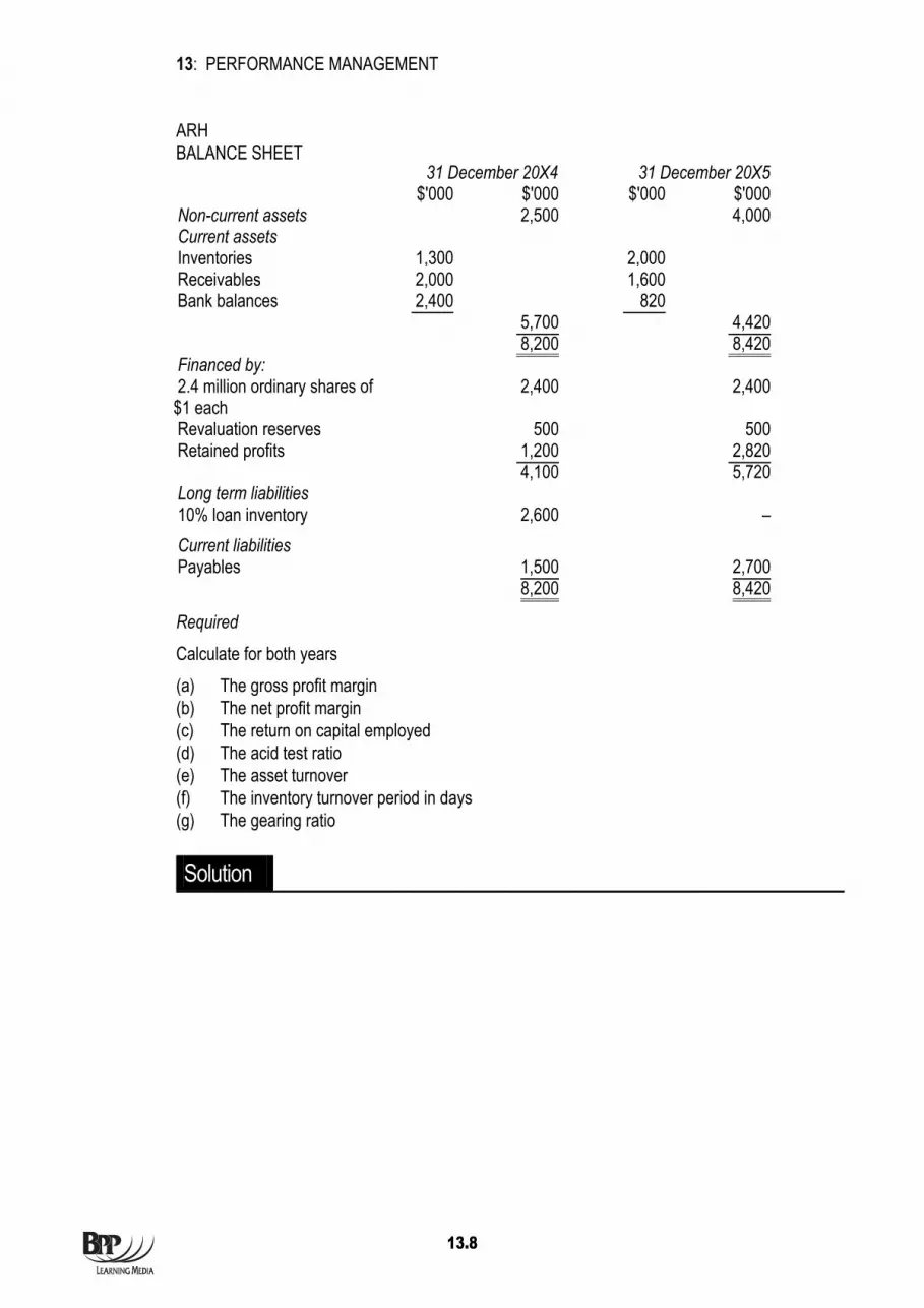
13: PERFORMANCE MANAGEMENT
13.8
ARH BALANCE SHEET
31 December 20X4 31 December 20X5 $'000 $'000 $'000 $'000 Non-current assets 2,500 4,000 Current assets Inventories 1,300 2,000 Receivables 2,000 1,600 Bank balances 2,400 820 5,700 4,420 8,200 8,420 Financed by: 2.4 million ordinary shares of $1 each
2,400 2,400
Revaluation reserves 500 500 Retained profits 1,200 2,820 4,100 5,720 Long term liabilities 10% loan inventory 2,600 – Current liabilities Payables 1,500 2,700 8,200 8,420 Required
Calculate for both years (a) The gross profit margin (b) The net profit margin (c) The return on capital employed (d) The acid test ratio (e) The asset turnover (f) The inventory turnover period in days (g) The gearing ratio
Solution

13: PERFORMANCE MANAGEMENT
13.9
5 Limitations and strengths of ratios 5.1 Limitations:
(a) Not useful on their own – need to be compared to yardstick. (b) Must be carefully defined. (c) Inflation needs to be adjusted for – often forgotten. (d) Different basis of calculating between companies. (e) Based on historical costs – accurate reflection of future?
5.2 Strengths: (a) Easier to understand than absolute measures. (b) Easier to look at changes over time. (c) Puts performance into context. (d) Can be used as targets. (e) Summarise results.
Other problems with financial performance indicators 5.3 (a) Focus only on variables which can be expressed in monetary terms ignoring other
important variable which cannot be expressed in monetary terms (b) Focus on past (c) Do not convey the full picture of a company's performance in a modern business
environment eg. quality, customer satisfaction (d) Focus on the short term

13: PERFORMANCE MANAGEMENT
13.10
6 Non-financial performance indicators (NFPIs)
Definition 6.1 NFPI's are measures of performance based on non-financial information which may
originate in and be used by operating departments to monitor and control their activities without any accounting input.
Examples 6.2 Examples of non-financial performance indicators are summarised in the table below.
Area assessed Performance measures Service quality Number of complaints
Proportion of repeat bookings On-time deliveries Customer waiting time
Production performance Set up times Number of suppliers Days' inventory in hand Output per employee Materials yield percentage Production schedule adherence Output requiring reworking Manufacturing lead times
Marketing effectiveness Trends in market share Sales volume growth Customer visits per salesperson Client contact hours per salesperson Customer survey response information
Personnel Number of complaints received Staff turnover Days lost through absenteeism Days lost through accidents/sickness Training time per employee
Different industries will place a different weighting on each area depending on those most critical to their success.
Value of NFPIs 6.3 (a) Information can be provided quickly for managers (eg. per shift, daily or hourly) unlike
traditional financial performance reports. (b) Anything can be measured/compared if it is meaningful to do so. (c) Easy to calculate and easier for non-financial managers to understand and use
effectively.

13: PERFORMANCE MANAGEMENT
13.11
(d) Less likely to be manipulated than traditional profit related measures (counteract short termism).
(e) Can be quantitative or qualitative. (f) Provide better information about key areas such as quality, customer satisfaction,
employees. (g) Better indicator of future prospects than financial indicators which focus on the short
term
Problems with NFPI's 6.4 (a) Too many measures can lead to information overload for managers, providing
information which is not truly useful. (b) May lead managers to pursue detailed operational goals at the expense of overall
corporate strategy. (c) Need to be developed and refined over time to ensure remain relevant. (d) Need to be linked with financial measures.
Lecture example 4 Idea Generation Required
In the role of a well known chain coffee shop manager, state a number of non-financial measures (both quantitative and qualitative) that you may wish to develop for your business when the objective you have been set is to “delight the customer with every cup!”.
Solution
13: PERFORMANCE MANAGEMENT
13.12
7 Short-termism 7.1 Short-termism – is when managers focus on their performance in the short term often at
the expense of long-term performance.
7.2 If manager's performance is measured on a short-term basis or a company is under pressure to report positive growth short-termism may occur.
Lecture example 5 Idea Generation List some of the short-term decisions managers may take and the potential consequences of them.
Solution
7.3 Other actions which may occur if managers are measured on a short-term basis is the manipulation of results.

13: PERFORMANCE MANAGEMENT
13.13
Lecture example 6 Idea Generation What could be done to encourage managers to take decisions in the long-term interests of the company?
Solution
8 The balanced scorecard 8.1 A popular approach in current management thinking to performance measurement (for
service and non-service organisations) is the use of what is called a "balanced scorecard", consisting of a variety of indicators both financial and non-financial.
8.2 The balanced scorecard focuses on four different perspectives and aims to establish goals for each together with measures which can be used to evaluate whether these goals have been achieved.
Case Study 5Analog Devices

13: PERFORMANCE MANAGEMENT
13.14
How do we create value for our shareholders? Financial perspective
Goals Measures
How do
customers see us?
What must we excel at?
Customer perspective
Internal business perspective
Goals Measures Goals Measures
Innovation and
learning perspective
Goals Measures
Can we continue to improve and create value?

13: PERFORMANCE MANAGEMENT
13.15
Perspective Question Customer What do existing and new customers value from us? This
perspective gives rise to targets that matter to customers: cost, quality and so on
Internal What processes must we excel at to achieve our financial and customer objectives? This perspective aims to improve internal processes and decision-making
Innovation and learning
Can we continue to improve and create future value? This perspective considers the business's capacity to maintain its competitive position by acquiring new skills and developing new products
Financial How do we create value for our shareholders? This perspective covers traditional measures, such as growth, profitability and shareholder value, but these are set by talking to the shareholder or shareholders direct
Features 8.3 (a) Traditional measures are mainly inward looking and narrow in focus with over
emphasis on financial measures and short term goals. (b) The Balanced Scorecard focuses on both internal and external factors and links
performance measures to key elements of a company's strategy. (c) It requires a balanced consideration of both financial and non-financial measures and
goals to prevent improvements being made in one area at the expense of another. (d) It attempts to identify the needs and concerns of customers to identify new products
and markets and focuses on comparison with competitors to establish best practice.
Lecture example 7 Idea Generation Required
Recommend one performance measure for each of the four perspectives of the balanced scorecard for a restaurant. State the reason for your choice of measure.
Solution

13: PERFORMANCE MANAGEMENT
13.16
9 Performance measurement in service businesses 9.1 In Chapter 2b the characteristics which make cost and performance measurement difficult in
service industries were discussed.
9.2 Current thinking is that if something is difficult to measure it is because it has not been defined clearly enough.
Fitzgerald and Moon's building blocks 9.3 Fitzgerald and Moon (1996) focused on performance measurement in service businesses.
The diagram below shows their building blocks for dimensions, standards and rewards. This framework is also known as the results and determinants framework.

13: PERFORMANCE MANAGEMENT
13.17
9.4 Performance of the organisation is viewed over six dimensions, the first two listed on the diagram – Profit and Competitiveness being the results of the other four determinants: (a) Quality – being reliability courtesy, competence and availability (b) Flexibility – the ability to deliver at the right time, response to customer requirements
and changes in demand (c) Resource utilisation – best use of inputs to create outputs. This is usually
measured in terms of productivity (d) Innovation – ability to develop new products or services, move into new markets and
continuous improvement
9.5 Underlying the achievement of results via the determinants are the standards: Ownership – Employees need to participate in the creation of standards to take
ownership of them but this can sometimes lead to the inclusion of some budgetary slack
Achievement – The standards set must be challenging but achievable Equity – Each division or department must have appropriate standards set for
it in order to ensure fairness in measurement
9.6 And the rewards: Clarity – The objectives of the organisation need to be clearly understood Motivation – Individuals need to be motivated to achieve the objectives Controllability – Managers should not be held responsible for costs over which they
have no control
10 Chapter summary • Performance of a business can be evaluated by financial indicators
• Financial indicators focus on the past and are short-term measures as such non-financial indicators also need to be used. A balance is needed between both
• Performance indicators need to be devised to ensure that they do not encourage mangers to focus on the short term
• Tools such as the balanced scorecard help to evaluate a business by looking at all key areas using a variety of financial and non-financial indicators
• The building blocks model focuses on performance measurement in service businesses.
Competitivenessand resource
utilisationquestion
Section 6.3.3

13: PERFORMANCE MANAGEMENT
13.18
END OF CHAPTER

14.1
Syllabus Guide Detailed Outcomes Having studied this chapter you will be able to:
• Explain the basis for setting a transfer price using variable cost, full cost and the principles behind allowing for intermediate markets
• Explain how transfer prices can distort the performance assessment of divisions and decisions made
• Explain the meaning of, and calculate, Return on Investment (ROI) and Residual Income (RI), and discuss their shortcomings
• Compare divisional performance and recognise the problems of doing so
Exam Context You should be prepared to discuss the difficulty in assessing performance in a divisionalised business. You will not need to calculate a transfer price but must be able to explain how and why they are used along with any implications.
Qualification Context The concepts in this chapter will all be developed in the Professional level paper Advanced Performance Management paper (P5). P5 requires a discussion on the need for and evaluation of transfer prices and evaluation of performance measure such as ROI and RI.
Business Context ROI or ROCE is a key tool many businesses use when assessing how a new investment will impact a division’s performance.
Many companies will set prices for goods transferred between divisions to enable performance evaluation to take place. This price is known as a transfer price.
Divisional performance measures

14: DIVISIONAL PERFORMANCE MEASURES
14.2
Overview
Divisional performance measures
Responsibility accounting Investment centre performance appraisal
methods
Transfer pricing
ROI RI
Approaches • Market based • Cost based • Opportunity cost
Aims

14: DIVISIONAL PERFORMANCE MEASURES
14.3
1 Introduction 1.1 Generally a company with several divisions will be a decentralised organisation. In such
organisations divisional managers tend be responsible for making their own decisions concerning the operation of their division.
1.2 Advantages of decentralisation include: (a) Decisions taken more quickly (b) Increase motivation of management (c) Increase quality of decisions due to local knowledge (d) Reduce head office bureaucracy (e) Provide better training for all levels of management
1.3 Disadvantages of decentralisation (a) Potential for dysfunctional decision-making (b) Duplication amongst divisions leading to greater cost (c) Senior management loss of control Appropriate performance evaluation methods are therefore needed.
Conditions for a good performance measure 1.4 A good performance measure should:
(a) Provide incentive to the divisional manager to make decisions which are in the best interests of the overall company (goal congruence)
(b) Only include factors for which the manager (division) can be held accountable (c) Recognise the long-term objectives as well as short-term objectives of the
organisation.
Responsibility accounting 1.6 Responsibility accounting is the term used to measure performance of decentralised units.
1.7 Responsibility structure
Manager's area of responsibility
Typical financial performance measure
Cost centre Decisions over costs Standard costing variances Revenue centre Revenues only Revenues Profit centre Decisions over costs and
revenues Controllable profit
Investment centre Decisions over costs, revenues, and assets
Return on investment and residual income
So far we have seen many of the performance measures dealing with the first three of these responsibility centres.

14: DIVISIONAL PERFORMANCE MEASURES
14.4
2 Investment centres 2.1 Within an investment centre, managers also have responsibility over investments and
assets. To measure their performance purely on say profit would be only focussing on part of the picture. To overcome this we use two methods which measure the assets and the profit they generate.
Return on investment (ROI)
2.2 ROI = Investment Divisional
Profit Divisional x 100
2.3 Profit should be before interest and tax (PBIT). It may also be helpful in measuring performance to calculate ROI based on controllable profit. For the investment use year end values of total assets less current liabilities. Alternatively an average book value may be used.
2.4 ROI enables performance in different divisions to be compared. Similarly, new investments can also be appraised using ROI.
2.5 Decision rule Only projects which increase the existing ROI should be undertaken.
2.6 Problems with ROI • Dysfunctional behaviour – only projects which increase ROI will be accepted, this
could be at the expense of growth in corporate profits. • The ratio will be distorted by the age of the assets • Profit can be manipulated
Lecture example 1 Technique Demonstration Brenda and Eddie have two franchises in different parts of town and want to monitor the performance of the two managers who have full control over investments. Forecast results for the year are: Vittorio’s Dugaldo’s $ $ Profits 90,000 135,000 Investment 500,000 750,000 Vittorio is considering investing in a labour-saving piece of equipment which will cost $8,000. This will generate an increase in net profit of $1,200 each year for 10 years, after which time the equipment is expected to have no resale value. Vittorio uses straight-line depreciation. Dugaldo has been offered a replacement oven for one of his existing ones. The existing one is written down in the books to a zero NBV but is very inefficient and costs $5,000 p.a. in maintenance, with an additional $20,000 p.a. opportunity cost due to it being idle.

14: DIVISIONAL PERFORMANCE MEASURES
14.5
The replacement will cost $75,000, will have no downtime and negligible maintenance costs in its early years. Depreciation will be 20% p.a. straight-line. Each oven is estimated to generate $60,000 p.a. before these costs are considered. Required (a) Would profit or ROI be more equitable for comparing Vittorio's and Dugaldo's forecast
performance? (b) Show why, in each case, ROI (based on opening book values) will lead to dysfunctional
decisions. Brenda and Eddie’s group ROCE is 12%.
Solution
Residual income 2.7 Traditionally the main alternative to ROI. It provides a hurdle figure for profit based on the
company’s minimum required percentage return from a division. $ PBIT(or controllable profit) X less: "imputed interest" (= Divisional Investment × Cost of Capital) (X) Residual income X The result is an absolute figure.

14: DIVISIONAL PERFORMANCE MEASURES
14.6
Lecture example 2 Technique Demonstration Required Re-assess the decisions in lecture example 1 using residual income.
Solution
Advantages of residual income 2.8 • Avoids dysfunctional behaviour
• Different costs of capital can be used to reflect risk
ROI vs RI 2.9 In practice, however, ROI is used more frequently than RI, for the following reasons:
(a) Dysfunctional behaviour is not material (b) ROI is consistent with corporate assessment (ROCE) (c) Percentages are more easily understood (d) RI requires a cost of capital

14: DIVISIONAL PERFORMANCE MEASURES
14.7
Lecture example 3 Exam standard for 6 marks Required Discuss the strengths and weaknesses of ROI and RI as methods of assessing the performance of divisions.
Solution

14: DIVISIONAL PERFORMANCE MEASURES
14.8
3 Transfer pricing 3.1 Within a decentralised organisation there may be a division which makes units that are then
transferred to another division. It will usually be necessary to charge the receiving division for the goods that it has received in order for performance to be measured equitably. A transfer price is the price at which goods are transferred internally.
3.2 It is vital that the transfer price is carefully selected to ensure all parties act in the best interest of the company.
3.3 The goals of a transfer pricing system are: (a) Goal congruence (b) Equitable performance measurement (c) Retain divisional autonomy (d) Motivate divisional managers (e) Optimum resource allocation
4 Transfer pricing in practice
Market based approaches 4.1 If an external market exists for transferred goods (and there is unsatisfied demand
externally), the transfer price can be set as the external market price.
4.2 The selling division will earn at least the same profit on internal sales as external sales, the receiving division will pay a commercial price and both divisions will have their profit measured in an equitable way. The managers of both divisions will behave in a goal congruent way.
4.3 If savings are made by selling internally then this may be reflected in the transfer price, eg by offering a discount equivalent to saved transport costs.
Case Study 6GSK settles
largest taxdispute in history

14: DIVISIONAL PERFORMANCE MEASURES
14.9
Lecture example 4 Exam standard for 6 marks What are the advantages and disadvantages of a market-based approach?
Solution
Cost based approaches 4.4 The idea behind these approaches are similar to those involved in manufacturing accounts,
that is to say the supplying division has its costs of manufacturing refunded and is also given a profit margin to encourage the transfer.
Actual cost vs standard cost 4.5 Use of actual costs would result in
(a) all inefficiencies passed on to buying division (b) no encouragement for cost control in selling division (c) buying division does not know in advance what price it will be paying (d) performance measurement is therefore difficult Using standard costs overcomes all these problems.

14: DIVISIONAL PERFORMANCE MEASURES
14.10
Standard full cost plus percentage 4.6 Advantages
(a) Covers all costs of selling division. (b) Selling division always encouraged to make the transfer. Disadvantage (a) May lead to dysfunctional behaviour.
Lecture example 5 Preparation question Goods are transferred from Division S to Division R at cost + 10%. $ Division S Variable costs 20.00 Fixed overhead 8.00 28.00 Standard profit @ 10% 2.80 Transfer price 30.80 Division R, the receiving division, can buy externally @ $26. Required (a) Discuss the likely outcome of setting the transfer price at $30.80. (b) Recommend a transfer price.
Solution
Standard variable cost 4.7 Advantage
(a) Receiving division always encouraged to take the transfer. Disadvantages (a) Supplying division does not cover fixed costs. (b) May lead to dysfunctional behaviour.

14: DIVISIONAL PERFORMANCE MEASURES
14.11
Opportunity cost based approach to transfer pricing 4.8 Minimum transfer price = marginal cost to selling division + opportunity cost to selling
division Maximum transfer price = external purchase price (i) If external market for intermediate product, opportunity cost = contribution foregone (ii) If no external market, the opportunity cost is likely to be nil. (Beware of situations
when the company is at full capacity on another task.) 4.9 Opportunity cost-based approaches should always result in goal congruent behaviour.
Lecture example 6 Preparation question A company operates two divisions, Able and Baker. Able manufactures two products, X and Y. Product X is sold to external customers for $42 per unit. The only outlet for product Y is Baker. Baker supplies an external market and can obtain its semi-finished supplies (product Y) from either Able or an external source. Baker currently has the opportunity to purchase product Y from an external supplier for $38 per unit. The capacity of division Able is measured in units of output, irrespective of whether product X, Y or combination of both are being manufactured. The associated product costs are as follows. X Y Variable costs per unit 32 35 Fixed overheads per unit 5 5 Total unit costs 37 40 Required
Using the above information, provide advice on the determination of an appropriate transfer price for the sale of product Y from division Able to division Baker under the following conditions. (a) When division Able has spare capacity and limited external demand for product X (b) When division Able is operating at full capacity with unsatisfied external demand for product X
Solution

14: DIVISIONAL PERFORMANCE MEASURES
14.12
Head office intervention 4.10 In practice, companies tend to employ a system whereby, broadly, the production plan is
imposed by head office and transfers are made using cost information from within the company ie transfers are made at cost plus a profit element.
4.11 Advantage of head office imposed plan: (a) No problems need arise re goal congruence.
4.12 Disadvantages of head office imposed plan: (a) Loss of autonomous divisional decision-making power (b) De-motivating
Imperfect market 4.13 When units costs and revenues are not constant but vary with output careful analysis will
need to be undertaken to establish the output that will maximise profit for the group and then the transfer price that will maximise profit in both divisions.

14: DIVISIONAL PERFORMANCE MEASURES
14.13
Lecture example 7 Exam standard for 10 marks Furniture Co is a large company that manufactures and sells furniture. It has three divisions: Division A purchases logs and produces finished planks. Approximately 2/3 of its output is sold to Division B, with the remainder sold externally. Division B manufactures furniture. The policy of Furniture Co is that the Division B must buy all its timber from Division A and sell all its output to Division C. Division C sells furniture to outlets. It only sells items purchased from Div B. Currently return on investment (ROI) is used to assess divisional performance. Each division adopts a cost-plus pricing policy for all external and internal sales. The senior management of Furniture Co has stated that the divisions should consider themselves to be independent businesses as far as possible. Required
(a) For each division suggest, with reasons, the behavioural consequences that might arise as a result of the current performance evaluation methods.
(b) Suggest with reasons, an appropriate transfer pricing policy that could be used for transfers from Division B to Division C, indicating any problems that may arise as a consequence of the policy you suggest.
Solution

14: DIVISIONAL PERFORMANCE MEASURES
14.14
Lecture example 8 Exam standard for 8 marks AJH plc has two divisions. Division 1 manufactures a component called the Woody which it sells on the external market as well as transferring to Division 2. Division 2 then sells the Woody after further processing as the Woody Deluxe. The following information is available: Division 1 Division 2 Market price Woody 150 Market price Woody Deluxe 300 Production costs 60 80 Non-production overheads 150,000 150,000 External demand 5,000 3,000 75% of the production cost per component is variable. Division 1 sets a transfer price of marginal cost plus 40%. Required Calculate the profit generated by each division.
Solution

14: DIVISIONAL PERFORMANCE MEASURES
14.15
5 Chapter summary • A good performance measure should be one that drives goal congruence, measures
mangers only on those items that they can control and recognises long-term as well as short-term objectives
• ROI is the most commonly used measure within a decentralised business but can result in dysfunctional behaviour
• Using RI will ensure all decisions result in goal congruent behaviour
• Within a decentralised business it may be necessary to set transfer prices when goods are transferred between divisions
• Transfer prices can be set on the basis of cost, market price or opportunity cost
• Cost based transfer prices are most likely to result in dysfunctional behaviour
Q8Divisional
PerformanceMeasures

14: DIVISIONAL PERFORMANCE MEASURES
14.16
END OF CHAPTER

15.1
Syllabus Guide Detailed Outcomes Having studied this chapter you will be able to:
• Comment on the problems of having non-quantifiable objectives in performance management
• Explain how performance could be measured in this sector (NFPOs and the public sector)
• Comment on the problems of having multiple objectives in this sector
• Outline Value for Money (VFM) as a public sector objective
• Explain the need to allow for external considerations in performance management, including stakeholders, market conditions and allowance for competitors
• Suggest ways in which external considerations could be allowed for in performance management
• Interpret performance in the light of external considerations
• Identify and explain the behaviour aspects of performance management
Exam Context Questions from this section of the syllabus are likely to be discussion questions. Ensure you apply your answer to the scenario given ie public sector or not-for profit organisation.
Qualification Context This chapter will be developed further in the Professional level paper Advanced Performance Management (P5) under the strategic performance measurement section.
Business Context The issues contained within this chapter are those encountered daily in not for profit organisations (NFPO’s).
Further performance management

15: FURTHER PERFORMANCE MANAGEMENT
15.2
Overview
Objectives Evaluation of performance
Further performance management
External factors Behavioural aspects

15: FURTHER PERFORMANCE MANAGEMENT
15.3
1 Objectives 1.1 Profit seeking organisations
Primary objective: • maximise the wealth of the owners of the business – (equity) Secondary objectives might be: • ensure survival • provide a quality product/service (customer satisfaction) • be a good corporate citizen (health and safety/environment) • create wealth/benefits for management/employees • secure competitive advantage and grow market share The objective of profit or wealth maximisation is thus modified to meet the needs of different interest groups (stakeholders).
1.2 Public sector organisations Primary objective might be: • provision of a quality product/service within a value for money framework Secondary objectives might be: • be a good corporate citizen (health and safety/environment) • adopt an ethical social stance in decision making • create wealth/benefit for management/employees • earn sufficient profits to provide for future capital investment and perhaps provide a
surplus for the exchequer
1.3 Not for profit organisations (NFPOs) Primary objective might be: • provision of a social or community service for the well being of society Secondary objectives might be: • be a good corporate citizen (health and safety/environment) • adopt an ethical social stance in decision making • increase wealth/benefit for management/employees
2 Evaluation of performance 2.1 NFPOs and public sector organisations will not have wealth maximisation as a primary
objective. However, they will still have strategic objectives (albeit non-financial) and stakeholders (clients, members etc), who will wish to measure their performance.

15: FURTHER PERFORMANCE MANAGEMENT
15.4
2.2 Problems of performance measurement in NFPOs • Multiple objectives • How to measure output • Lack of financial / profit measure • Difficult to define a unit
Lecture example 1 Idea Generation Required
(a) Suggest what items might be measured for a hospital. (b) Highlight the problems that may occur in attempting to monitor performance of the hospital
using league tables of this data over time and against other hospitals.
Solution
Possible performance measurement methods 2.3 • The 3 Es
• Comparisons – eg comparison of results / benchmarking between different public sector organisations
• Efficiency measurement – ie cost / patient / day • Judgement - some measurement will be subjective
2.4 The '3 Es' measures performance in value for money terms Effectiveness – Success in achieving objectives Efficiency – Achieving better productivity (output) from resources input/consumed Economy – Sourcing inputs at minimum cost while maintaining standards of quality
SolutionsSection 2.3

15: FURTHER PERFORMANCE MANAGEMENT
15.5
Lecture example 2 Idea Generation Required Using the 3 Es suggest a range of performance measures for a public sector higher education college.
Solution
3 Performance measurement and external factors 3.1 When devising performance measures for any organisation, consideration needs to be given
to three key external factors: • Stakeholders • Economic environment • Competition
3.2 A stakeholder is anyone who has a legitimate interest in the organisation. Stakeholders can be broken down into three key groups. • Internal – such as employees • External – community and the government • Connected – shareholders, customers, suppliers

15: FURTHER PERFORMANCE MANAGEMENT
15.6
Institutional theory 3.3 This states that organisations adopt structures and processes to please outsiders
(stakeholders). Organisations must therefore fit with the perceived expectations of stakeholders and set up activities and therefore performance measurement that they perceive as important.
Lecture example 3 Exam standard for 12 marks Suggest performance management measures which would incorporate the needs of the three key external factors.
Solution
3.4 There will often be a conflict between the stakeholder objectives. For example, shareholders want larger returns whereas employees want pay rises. Performance measures need to be considered carefully. A suitable measure in this case might be performance related pay.

15: FURTHER PERFORMANCE MANAGEMENT
15.7
4 Performance management and behaviour aspects 4.1 You have already come across some of the behavioural aspects of performance
measurement when looking at setting standards and budgets. These are some of the aspects to bear in mind… • Targets should be set which support the company objectives • Managers should only be assessed on those items that they can control • Targets should incorporate long-term as well as short-term objectives • Targets should be set that motivate • Targets should encompass the big picture and may include financial and non-financial
aspects
5 Chapter summary • Performance measurement in public sector or NFP organisations can be difficult as
they often have multiple objectives and these are often hard to quantify and measure
• Performance measures need to be developed bearing in mind three external factors: Stakeholders, economic environment and competition
Q9Non-profit
seekingorganisations

15: FURTHER PERFORMANCE MANAGEMENT
15.8
END OF CHAPTER

16.1
Answers toLecture Examples

16: ANSWERS TO LECTURE EXAMPLES
16.2
Chapter 1
Answer to Lecture Example 1 Absorption costing
Year 1 $ $ Sales 42,000 Cost of sales: opening inventory – Production: variable costs 26,400 fixed costs 8,800 35,200 closing inventory (1,600) (Over)/under absorption (300) (33,300) Gross profit 8,700 Variable selling & distribution (4,200) Fixed selling & distribution (2,000) Net profit 2,500
Answer to Lecture Example 2 Marginal costing
Year 1 $ $ Sales 42,000 Variable production costs: opening inventory – production 26,400 26,400 closing inventory (1,200) (25,200) Variable selling & distribution (4,200) Contribution 12,600 Fixed costs: production (8,500) selling & distribution (2,000) Profit 2,100
Answer to Lecture Example 3 Year 1 AC Profit 2,500 add: fixed overhead in opening inventory – less: fixed overhead in closing inventory* 400 MC profit 2,100 *200 × $2

16: ANSWERS TO LECTURE EXAMPLES
16.3
Answer to Lecture Example 4 B Units Opening inventory (8,500) Closing inventory 6,750 Change in inventory (1,750) x overhead absorption rate $3 Amount of overhead absorbed, thus reducing profit by this amount $5,250 $ Marginal costing profit 62,100 Less: overhead in inventories (5,250) Absorption costing profit 56,850
Answer to Lecture Example 5 Absorption costing
Year 2 $ $ Sales 40,000 Cost of sales: opening inventory 1,600 Production: variable costs 22,800 fixed costs 7,600 32,000 closing inventory – (Over)/under absorption 900 (32,900) Gross profit 7,100 Variable selling & distribution (4,000) Fixed selling & distribution (2,000) Net profit 1,100
Answer to Lecture Example 6 Marginal costing
Year 2 $ $ Sales 40,000 Variable production costs: opening inventory 1,200 production 22,800 24,000 closing inventory – (24,000) Variable selling & distribution (4,000) Contribution 12,000 Fixed costs: production (8,500) selling & distribution (2,000) Profit 1,500

16: ANSWERS TO LECTURE EXAMPLES
16.4
Answer to Lecture Example 7 Year 2 AC Profit 1,100 add: fixed overhead in opening inventory* 400 less: fixed overhead in closing inventory MC profit 1,500 *200 × $2
Chapter 2a
Answer to Lecture Example 1 (a) Under traditional absorption costing
OAR = $190,000 ÷ 67,000 = $2.836/hr
A B C $/unit $/unit $/unit Revised product cost 20.67 17.84 17.84 Sales price 20.00 20.00 20.00 Profit (0.67) 2.16 2.16
(b) Under ABC
Workings: recovery rates
(1) Machine cost
hour machine per $0.5854,00050,00040,000
$55,000=
++
(2) QC & set up run production per $3,600 2 13 10
$90,000=
++
(3) Receiving receipt component per $1,363.64 21010
$30,000=
++
(4) Packing rorde customer per $250202020
$15,000=
++
A B C Total $ $ $ $ Machining costs 23,404 29,255 2,341 55,000 Quality control & set-up 36,000 46,800 7,200 90,000 Receiving 13,636 13,636 2,728 30,000 Packing 5,000 5,000 5,000 15,000 Total overhead costs 78,040 94,691 17,269 190,000 Units produced 20,000 25,000 2,000
Overhead cost/unit $3.90 $3.79 $8.63

16: ANSWERS TO LECTURE EXAMPLES
16.5
A B C $/unit $/unit $/unit Direct materials cost 5.00 10.00 10.00 Direct labour cost 10.00 5.00 5.00 Production overhead cost 3.9 3.79 8.63 18.9 18.79 23.63 Sales price 20.00 20.00 20.00 Gross profit/unit 1.1 1.21 (3.63)
(c) Items to consider are:
How much more cost have we been able to allocate on a meaningful basis? Have we the right cost drivers? Why have the costs changed? Do we need to revisit selling prices? Do we need to alter the product mix? Should we cease production of C? – bear in mind decisions should be based upon contribution
Answer to Lecture Example 2 Pricing
If set on a cost plus basis this should be more accurate and so may lead to a change in price. If price is based with reference to the market then this could alter the profitability of products.
Sales Strategy
If previously perceived low margin products are actually high margin products, we would want to sell more of these. We would wish to generate a change in the product mix which may have marketing implications as well as implications for purchasing and production.
Performance management
The more reflective costs under ABC allow management to plan more accurately, improve cost control and evaluate managers' performance on a more meaningful basis.
Decision making
As we have seen ABC leads to arguably more accurate costs. This enables us to make better, more informed decisions about:
• price • product lines • volumes • mix
Chapter 2b
Answer to Lecture Example 1
ROI = 30% Investment
CostsTotalRevenue=
−
$ Revenue = 67.50 × 40,000 = 2,700,000 Investment = 5,000,000 i.e. Return = 30% × 5,000,000 = 1,500,000 ∴ Total target costs = 1,200,000 (Target cost = $30 per racquet)

16: ANSWERS TO LECTURE EXAMPLES
16.6
Answer to Lecture Example 2 Cheaper materials Fewer parts Cheaper labour No non-value adding activities Training Automation
Chapter 2c
Answer to Lecture Example 1 Product lifecycle costing
Mobile phones are likely to go through the stages of the product life cycle over a reduced period of time.
Higher costs are likely to be incurred at the start of the product life cycle eg product development, promotion and other marketing activities.
During the growth stage the cost per phone will fall dramatically as the initial start up costs are no longer incurred and economies of scale are achieved.
At the maturity stage the cost per phone will continue to fall the main cost being variable costs.
At the decline stage, sales volumes fall and cost per unit begins to climb. Extra costs associated with discontinuing the product will put upward pressure on the cost per phone.
Product lifecycle costing reflects the need for phone manufacturers to assess costs and profitability over the entire life of each of their phones.
Target costing
Target costing considers the price that ought to be charged in order to achieve a desired market share for a given product.
Then the level of profit to be earned on the product is decided. The level of profit can be determined on a per unit basis but usually it could be determined for the entire product lifecycle.
The balancing figure in the price-cost-profit relationship is cost. The difference between profit and price represents the target cost which would be a significant factor for consideration when designing new phones.
Chapter 2d
Answer to Lecture Example 1 Raw material
$ $ B/f 100 (W1) 7,048 Cash 8,000 C/f 1,052 8,100 8,100
Conversion
$ $ 13,000 (W1) 11,452

16: ANSWERS TO LECTURE EXAMPLES
16.7
Cost of goods sold
$ $ 18,500
(W1) Raw materials 8/21 x 18,500 = 7,048
Conversion 13/21 x 18,500 = 11,452
Answer to Lecture Example 2 By looking at: Admin cost savings Change in production costs – due to inability to monitor at each stage Management feedback / control issues Whether inventories are fluctuating – and so not appropriate Whether price variances are occurring
Chapter 2e
Answer to Lecture Example 1 Machine X loses 15-20 hours / mth = 5 hours / week loss of 12.5% Max output therefore 180 – 12.5% 158 No of TRLs /4 39 Machine Y 52 Machine Z 30 Z is therefore the bottleneck TA ratio:
Return / hr 2,000-600 hours * 30 TRLs TRLs 40000,42 1,050
Cost / hr 5,500 + 8,000 + (450,000/48) 40875,22 572
TA ratio Return / hour Cost / hour
1.84
Answer to Lecture Example 2 Increase selling price Buy cheaper materials Decrease labour Decrease overhead

16: ANSWERS TO LECTURE EXAMPLES
16.8
Answer to Lecture Example 3 (a)
Will Grace $ $ $ $ Sales 500,000 475,000 Variable production costs Materials 120,000 144,000 Labour 80,000 96,000 Fixed production costs (W1) 200,000 240,000 Less: closing inventory – (100,000) Adjustment for (over)/under absorption – (400,000) (40,000) (340,000) 100,000 135,000
(W1) OAR = 000,10
000,200£ = $20/unit
(b) Will Grace $ $ Return Sales 500,000 475,000 Less: materials (120,000) (144,000) 380,000 331,000 ÷ hrs 20,000 20,000 Return/hr $19 $16.5556 Costs 280,000 296,000 ÷ hrs 20,000 20,000 Cost/hr $14 $14.80 TA ratio 1.36 1.12
Answer to Lecture Example 4 This is an example of production with a scarce resource and so limiting factor analysis should be used. If resources are limiting factors, then return is maximised by earning the biggest possible return per unit of limiting factor.
Step 1 Ascertain whether material L is the limiting factor
Product Adam James Luke Total Kgs of L per batch (kg) 7 9 4 Kgs of L needed to meet sales demand 3,500 3,600 1,400 8,500 Kgs available (7,000) Shortfall 1,500
Step 2 Calculate return per unit of scarce resource and rank ingredients
Product Adam James Luke Retun per batch ($) 90 165 95 Kgs per batch 7 9 4 Return per kg ($) 12.86 18.33 23.75 Ranking 3 2 1

16: ANSWERS TO LECTURE EXAMPLES
16.9
Step 3 Determine the optimum product mix Ingredient L Material L Batches Product Demand required available produced Batches kgs kgs* 6,000 Luke 350 (×4) 1,400 (1,400) 350 4,600 James 400 (×9) 3,600 (3,600) 400 1,000 Adam 500 (×7) 3,500 (1,000) 142** 0 * Remember the contract for 50 units of each product with penalties for non delivery. So total availability of L for these products is 7,000 – 50 (7 + 9 + 4) = 6,000 kgs
** 1000 ÷ 7 = 142.86
Chapter 3
Answer to Lecture Example 1 Production plan F B P Contribution/unit $50 $40 $30 Contribution/machine hour $10 $20 $30 Rank 3rd 2nd 1st
Production schedule Hrs / unit hrs available $ contribution 300 /hour Produce maximum P 50 1 (50) 30 Produce maximum B 50 2 (100) 20 Produce F with (150/5) 30 5 (150) 10
Answer to Lecture Example 2 (a) With five extra hours you would make one more batch of Fairy cakes (b) The extra contribution from one batch is $50
Contribution per hour 550 = $10 / hour
Shadow price of 1 hour is therefore $10
Answer to Lecture Example 3 (a) Let p = weekly number of purses
h = weekly number of handbags
(b)
Subject to (Leather) 1.5p + 2h ≤ 600 (Skilled labour) 0.75p + 0.5h ≤ 210 (Quota) p – h ≤ 0 (Non-negativity) p, h ≥ 0
(c) Objective:
Maximise 5p + 6h

16: ANSWERS TO LECTURE EXAMPLES
16.10
(d) p
400 Leather EU quota 300 280 200 Objective 100 Labour
0 100 200 250 300 400 h Number of handbags produced
(e) Optimal production: 160 purses 180 handbags
(f) Contribution = 5p + 6h = (5 x 160) + (6 x 180) = $1,880 per week
Answer to Lecture Example 4 The steps up to determining the feasible region are exactly the same
Number of purses produced

16: ANSWERS TO LECTURE EXAMPLES
16.11
p 400 Leather EC quota 300 280 200 100 Labour
0 100 200 250 300 400 h Number of handbags produced
Determine optimal solution
Clearly this will not be at 0
At A there is 167 handbags and 167 purses
At B there is 180 handbags and 160 purses
At C there is 300 handbags and no purses
Point B therefore will generate the most contribution. Simultaneous equations can be used to determine the exact values of purses and handbags and the total contribution.
Optimal point is Point B where labour and leather intersect
1.5p + 2h = 600 (1)
0.75p + 0.5h = 210 (2)
1.5p + 1h = 420 (3) (multiply (2) by 2)
h = 180 (1) – (3)
1.5p + 360 = 600 Substitute h into (1)
1.5p = 420
p = 160
Optimal production: 160 purses 180 handbags
Contribution = 5p + 6h = (5 x 160) + (6 x 180) = $1,880 per week
Number of purses produced
A
C
B

16: ANSWERS TO LECTURE EXAMPLES
16.12
Answer to Lecture Example 5 (a) Objective function value: KG Ltd can earn $1,880 contribution.
Variables: KG Ltd should make 160 purses and 180 handbags.
Slack/surplus:
The slacks for constraints 1 and 2 are zero, showing that all available leather or labour will be used.
The slack for constraint 3 is 20, indicating that the EC minimum quantity of handbags has been exceeded by 20, ie. 20 more handbags than purses will be made.
Shadow price/worth:
Constraints 1 and 2 both have zero slack, and so are fully utilised. If more labour or leather could be obtained, output could be increased, and hence contribution increased.
An extra m2 of leather would increase contribution by $2.667, and an extra hour of labour by $1.333. Constraint 3 is non-zero, and hence a relaxation in the quota would not increase contribution.
Relative loss:
The relative loss of zero for all products indicates that they are all produced in the optimal solution.
If a product is not being produced at the optimal point, a relative loss would indicate the reduction in contribution if one unit of this product had to be manufactured.
(b) The shadow price for leather is $2.667/m2, indicating that the maximum KG Ltd would be willing to pay for additional leather is $8 + $2.67 = $10.67/m2.
Hence, it would accept an offer of additional leather at $10.50/m2.
However, it would not want an infinite supply of leather at this price – the shadow price in the computer output is only valid for a range of values.
Chapter 4
Answer to Lecture Example 1 Demand – How we perceive customers will react to various price levels
Quality – High price may indicate quality
Competitors – Competitors' actions may cause us to re-assess price
Substitutes – Similar products that customers may buy in lieu of ours
Inflation
Age of product
Disposable incomes
Product range – If the product is part of a range. Focus is likely to be paid to profitability of whole range rather than individual products
Market – If there are lots of competitors it is likely that a change in price will lead to a change in demand. If it is a monopoly a change in price is unlikely to impact demand.

16: ANSWERS TO LECTURE EXAMPLES
16.13
Answer to Lecture Example 2
%ΔP = $12$1
= 8.3% increase
%ΔQ = 16,0002,500
= 15.6% decrease
PED = 8.3%15.6%−
= 1.9
Demand is elastic
Answer to Lecture Example 3 P = a – b Q
b = 0004.0
500,21£
=
12 = a – (0.0004 × 16,000)
a = 18.4
P = 18.4 – 0.0004Q
∴ To sell 25,000 tickets:
P = 18.4 – 25,000 × 0.0004 = $8.40 per ticket.
Answer to Lecture Example 4 0 to 10,000 units y = 50,000 + 10x 10,001 to 15,000 y = 50,000 + 7x 15,001 + y = 50,000 + 5x
Total cost 210,000 - 185,000 - 150,000 -
50,000 -
0 10,000 15,000 20,000 Number of units

16: ANSWERS TO LECTURE EXAMPLES
16.14
Answer to Lecture Example 5 The product life cycle comprises four stages:
• Introduction • Growth • Maturity • Decline
In the introduction stage the company needs to price the product to achieve its market strategy using either penetration or skimming pricing policies.
A penetration policy is used with the objective of achieving a high level of demand very quickly by using a low price that is affordable to a large number of potential customers. This has the effect of discouraging new suppliers to the market because the unit profitability is relatively low, but the high volume of sales enables the initial supplier to recover their development costs.
A skimming policy is particularly appropriate to a product that has a novelty value or that is technologically advanced. Such a policy uses a price that is high and this restricts the volume of sales since only high worth customers can afford the product, but the high unit profitability enables the initial supplier to recover their development costs. However, the high unit profitability attracts competitors to the market so that it is important for the initial supplier to be able to reduce the price and can prevent new entrants to the market from being able to reverse engineer the product and make significant profits from little or no development investment.
The X organisation is launching a technologically advanced product which will be demanded by high worth customers who are proud to be amongst the first to own such a state of the art product. This is exactly the type of product for which a price skimming policy is appropriate.
The initial price will be high as this will quickly recover the development costs of the product. The high worth customers will not be deterred from buying the product as it will be sold on the basis of its technological value rather than its price.
Competitors will be attracted to the product by its high price and will seek to compete with it by introducing their own version of the product at much lower development costs (by reverse engineering X's product) so it is important for X to reduce the price during the growth stage of the product's life cycle There may be many price reductions during this phase so that the product gradually becomes more affordable to lower social economic groups.
As the product enters the maturity stage the price will need to be lowered further, though a profitable contribution ratio would continue to be earned. Oligopolistic competition is often found in this stage, but provided X has gained market share and survived until this stage the opportunity to make profit and cash surpluses should exist. However, in this type of market the price will tend to be set by the market and X will have to accept that price. Thus X will need to focus on the control of its costs to ensure that the product will remain profitable.
When the product enters the decline phase a loyal group of customers may continue to be prepared to pay a reasonable price and at this price the product will continue to be profitable, especially as costs continue to reduce. Eventually the price will be lowered to marginal cost or even lower in order to sell off inventories of what is now an obsolete product as it has been replaced by a more technologically advanced item.

16: ANSWERS TO LECTURE EXAMPLES
16.15
Chapter 5
Answer to Lecture Example 1 Historic cost can be ignored as it is a sunk cost.
X
Since X is no longer used by the company, the inventory of X will be used rather than buying in new supplies of X. (Note: the next best alternative to using the inventory is to scrap it for $2.20/kg)
So relevant cost X
$ 300kg inventory: lost scrap value (300 × $2.20) 660 100kg buy in (100 × $3) 300 960 Y
If the inventory of Y is used it will have to be replaced when it is needed elsewhere in the business.
So relevant cost Y
$ 200 kg at current replacement cost (200 × $2) 400
Answer to Lecture Example 2 Labour is currently working at full capacity ∴
if 15 hours are used in the contract madebenot willX of units 3hrs 5hrs 15
=
Cash flows under each option
Undertake contract
Make 3X
$ $ Direct labour Contribution (15 hrs @ $6) (90) (3 × $22) 66 Variable overheads (60% × 90) (54) (144)
∴ relevant cost of using labour = $(144) – $66
= $(210)
Alternative approach
The cash flows which will change if the contract goes ahead are:
$ Lost revenue from X (3 × $90) 270 Saved costs from X materials (3 × 20) (60) Relevant cost of 15 hrs of labour 210

16: ANSWERS TO LECTURE EXAMPLES
16.16
Note: The labour and overhead costs will be incurred whichever decision is made and can therefore be ignored.
Note: This does not equal ‘lost contribution’ of making three Xs
( = 3 × $22 = $66)
$ Why? Contribution = Revenue 90 All lost less: costs 68 Not all saved 22
∴ Alternative presentation $ Lost contribution (3 × $22) 66 less: costs not saved – labour (3 × $30) 90 – variable overheads (3 × $18) 54 210
Answer to Lecture Example 3 Accept or reject decisions
Sales revenue (1) 36,000 Costs Material X (2) (200) Material Z (3) 4,200 Labour (4) 11,000 Variable overhead (5) 3,600 Depreciation (6) – Fixed overheads (7) – Lost scrap proceeds (8) 3,000 (21,600) Net Relevant Contribution 14,400 Conclusion: the proposal should be accepted as it makes a positive contribution of $14,400 based on relevant costs.
(1) Revenue earned as a result of producing and selling T. (2) No other use for X in business, but $200 disposal costs are saved by using X to make Ts. (3) Z is used in the business and will have to be replaced for $0.175 x 2 x 12,000 = $4,200.
Assuming inventories can be bought at this price.
(4) Opportunity cost of using labour = contribution foregone + cost of labour = $1,000 + $10,000 = $11,000
(5) Variable overhead is only incurred when units are made.
∴ relevant cost = 12,000 x $0.30
(6) Depreciation is not a cashflow and ∴ not relevant
(7) These fixed overheads will be incurred regardless of whether or not Ts are made, therefore cost is not relevant.
(8) If machine is used, instead of scrapped the business loses $(7,000 – 4,000) of scrap proceeds.

16: ANSWERS TO LECTURE EXAMPLES
16.17
However, the following non-financial factors also need to be considered:
(a) The likelihood of a more profitable proposal being received; (b) Whether repeat orders would be expected at the same price in future years; (c) Whether the company's present customers can be differentiated from this special order price.
Answer to Lecture Example 4 Make or buy decisions
Cost of buying $23 Cost of making: $ Materials 10 Labour (2 @ $5) 10 Lost contribution ( 9
3 × 2) 6
26 ... buy.
Answer to Lecture Example 5 A J H Direct material / unit 15 6 18 Direct labour / unit 15 20 22 Variable production overheads 5 4 4 Variable cost of making 35 30 44 Unit cost of buying 30 39 50 Extra cost of buying (5) 9 6 Production (units) 5,000 4,000 3,000 Extra cost per year (25,000) 36,000 18,000 Saving of incremental fixed costs (2,000) (3,000) (6,000) Extra cost of buying (27,000) 33,000 12,000 The company would save $27,000 by sub-contracting the production of A.
Other considerations
If the company sub-contracts A they will have spare capacity. How should they use it?
What will the impact be on the work force? If no further production required, redundancy may be necessary which might result in loss of morale and so on.
Will the sub-contractor deliver the product to the same standards and timescales? Will they be reliable?
Are the fixed costs savings accurate? It would not alter the decision here if they were not but watch out for scenarios where it would!!

16: ANSWERS TO LECTURE EXAMPLES
16.18
Answer to Lecture Example 6 Relevant? Monthly Cost Outsource?
Salary cost of junior member staff No – not specific Lease of copier No – committed Paper & Ink Yes 300 Distribution Yes 50 350 Cost of outsourcing (325) Saving from outsourcing 25
However, other considerations should be taken into account.
If keep in house retain control
If outsource will free up capacity – how can this best be used?
What quality would the external company deliver?
Will they be reliable?
Will they deliver to time?
Answer to Lecture Example 7 (a) If Keir were shut down the incremental costs and revenues are:
$'000 Lost revenue 600 Saved Materials 200 Labour 95 Variable overhead 75 Fixed overhead 20% × $200 40 Selling costs 40 Profit foregone 150
Alternatively:
$'000 Fixed costs still incurred 80% × $200 160 Loss forecast (10) 150
(b) Other factors
• Losing over 54% of company's revenue – other costs likely to change • Product interdependencies • Possibility of changing sales commission or reducing expenses in place of closure • Capital costs of closure not considered such as asset sales/write-offs • Redundancy costs

16: ANSWERS TO LECTURE EXAMPLES
16.19
Answer to Lecture Example 8 Relevant Costing Statement
Note $ Aluminium plating (1) 240 Rivets (2) 50 Skilled labour (3) 1,320 Semi-skilled labour (4) – Overheads (5) – 1,610 Administration overhead (6) – Total relevant cost 1,610 Profit (7) – Minimum price 1,610 Notes
(1) Aluminium is in regular use therefore it needs to be replaced. Value at current purchase price
Relevant cost = 20m2 × $12 = 240
(2) Rivets = opportunity cost is lost scrap proceeds 100 × 50p = $50
(3) Skilled labour
Cheaper to work overtime as $24/hr is less than $36/hr (16 + 20)
$ 40 hrs @ $24 = 960 10 hrs @ $36 360 1,320
(4) Semi skilled labour
Relevant cost = nil (spare capacity)
(5) Overheads – relevant cost is nil
Incurred anyway regardless of this job.
(6) Administration costs will be incurred anyway regardless of whether or not the job is accepted therefore not relevant.
(7) Profit mark up not relevant as question asks for a minimum price. A minimum price is one which just covers the total of the relevant costs.
Answer to Lecture Example 9 – Product interdependencies – Inflation – Availability of cash – Time value of money – Impact on supplies – Potential future contracts – Learning curves – Repeat business – Restricted output/capacity – Competition – Recruitment – Technical feasibility – Political, legal and economic considerations

16: ANSWERS TO LECTURE EXAMPLES
16.20
Answer to Lecture Example 10 Incremental rev Process Form further proc Inc revenue Further Costs Inc benefit /
(cost) further?
X 2 5,000 10,000 (5,000) No Y 5 7,500 8,000 (500) No Z 7 14,000 12,000 2,000 Yes
Chapter 6
Answer to Lecture Example 1 (a) Risk-seeker chooses A as it gives a chance of earning the best NPV of $25,000
(b) Risk-neutral decision-maker is indifferent between A and B as they give the same expected NPV.
(c) Risk-averse decision-maker chooses B to avoid the chance of the worst NPV of $(10,000) with investment A.
Answer to Lecture Example 2 Sale to regular customer profit = $11 – $6 = $5
Sales under special contract profit = $9 – $6 = $3
Special contract Demand p 800 700 500 300 400 0.2 4,400 4,100 3,500 2,900 500 0.3 4,400 4,600 4,000 3,400 700 0.4 4,400 4,600 5,000 4,400 900 0.1 4,400 4,600 5,000 5,400
Answer to Lecture Example 3 EV(800) = 4,400
EV(700) = 4,100 x 0.2 + 4,600 x 0.8 = 4,500
EV(500) = 3,500 x 0.2 + 4,000 x 0.3 + 5,000 x 0.5 = 4,400
EV(300) = 2,900 x 0.2 + 3,400 x 0.3 + 4,400 x 0.4 + 5,400 x 0.1 = 3,900
... to maximise profits over the long term choose 700 for special contract.
Answer to Lecture Example 4 Maximin rule:
Maximise the possible minimum return that the decision-maker could get
ie. choose 800 units.
Answer to Lecture Example 5 Maximax rule:
Choose the option giving the highest possible return
ie. choose 300 units.

16: ANSWERS TO LECTURE EXAMPLES
16.21
Answer to Lecture Example 6 Opportunity Cost Table
Special Contract 800 700 500 300 Demand 400 0 300 900 1,500 500 200 0 600 1,200 700 600 400 0 600 900 1,000 800 400 0 Maximum regret $1,000 $800 $900 $1,500 Minimum
Decision – set order level for special contract at 700 units.
Working example: If demand is 400 units, the best special order level would have been 800 units. If an order level of 700 units has been chosen there would be an opportunity cost equal to the difference between the profits of $4,400 and $4,100 at the 800 units and 700 units order levels respectively.
Answer to Lecture Example 7 2-WAY DATA TABLE
(a) Contribution generated ($'000)
Demand ($'000s) 30 35 40 28 270 315 360
Price ($)
29 300 350 400
30 330 385 440 (b) Joint probability
Demand ($'000s) 30 35 40 28 0.08 0.1 0.02
Price ($)
29 0.14 0.175 0.035
30 0.18 0.225 0.045 Expected value of contribution($)
Demand ($'000s) 30 35 40 28 21,600 31,500 7,200
Price ($)
29 42,000 61,250 14,000
30 59,400 86,625 19,800

16: ANSWERS TO LECTURE EXAMPLES
16.22
$ EV contribution = px∑ 343,375 Fixed costs 320,000 EV profit 23,375
(c) Breakeven when contribution ≥ $320,000
Probability Demand ('000s) 30 35 40 28 0.02 Price ($) 29 0.175 0.035
30 0.18 0.225 0.045 Probability = 68%
Answer to Lecture Example 8 (a) If material costs were more than double the original estimate the product would make a loss
(b) Sales would have to fall by over 4,000 units (40%) ie to under 6,000 for the product to make a loss
Chapter 7
No Lecture examples
Chapter 8
Answer to Lecture Example 1 Materials: Variable cost = $3/unit
Overhead: Fixed cost = $20,000
Labour: Output Cost 14,000 35,000 (High-low method) 10,000 27,000 4,000 8,000 ... VC/unit = $2
By substitution into high output:
Total VC = $28,000 ∴ Total FC = $35,000 – $28,000 = $7,000
... Flexed budgeted cost: $ Materials (12,350 × 3) 37,050 Labour (7,000 + 2 × 12,350) 31,700 Overhead 20,000 88,750 Actual Costs – Flexed Budgeted cost ... $1,250 (A)

16: ANSWERS TO LECTURE EXAMPLES
16.23
Answer to Lecture Example 2 Variable cost
per unit Total fixed
costs $ $ Direct materials (W1) 2.75 – Production labour (W2) 5.00 80,000 Factory overheads (W3) 1.50 147,000 Administration – 30,000 Selling and distribution (W4) 0.50 21,000 9.75 278,000
Workings
1 This is a variable cost (cost for 40,000 units is double that for 20,000 units) with cost per unit = $50,000/20,000 = $2.50.
Quarter 4 cost = $2.50 × 1.1 = $2.75.
2 Variable cost per unit = (cost for 40,000 units – cost for 20,000 units)/ (40,000 – 20,000) units
= $(280,000 – 180,000)/20,000 = $5
∴ Fixed costs = $180,000 – (20,000 × $5) = $80,000
3 Variable cost per unit = (cost for 40,000 units – cost for 20,000 units)/ (40,000 – 20,000) units
= $(200,000 – 170,000)/20,000 = $30,000/20,000 = $1.50
∴ Fixed costs = $170,000 – (20,000 × $1.50) = $140,000
∴ Quarter 4 fixed costs = $140,000 × 1.05 = $147,000
4 Variable cost per unit (based on sales volume) = (cost for 34,000 units – cost for 18,000 units)/(34,000 – 18,000) units
= $(37,000 – 29,000)/16,000 = $0.50
∴ Fixed costs = $29,000 – (18,000 × $0.50) = $20,000
∴ Quarter 4 fixed costs = $20,000 × 1.05 = $21,000
(b) Flexible budget profit statements – Quarter 4
Low sales level
Most likely sales level
High sales level
Activity Sales (units) 38,000 44,000 50,000 Production (units)* 30,000 36,000 42,000 Costs $ $ $ Direct materials (W1) 82,500 99,000 115,500 Production labour (W2) 230,000 260,000 295,000 Factory overheads (W3) 192,000 201,000 210,000 Administration 30,000 30,000 30,000 Selling and distribution (W4) 40,000 43,000 46,000 Cost of production 574,500 633,000 696,500 Inventory adjustment (W5) 104,000 104,000 104,000 Production cost of sales 678,500 737,000 800,500 Sales 684,000 792,000 900,000 5,500 55,000 99,500
*Inventory increases by 8,000 units during Quarters 1 to 3 (total production during Quarters 1 to 3, less total sales for the same period). Inventories must therefore fall by 8,000 units during Quarter 4 and so the production level is 8,000 less than the sales level.
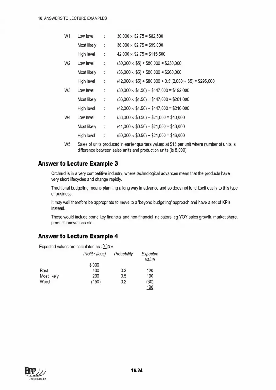
16: ANSWERS TO LECTURE EXAMPLES
16.24
W1 Low level : 30,000 × $2.75 = $82,500
Most likely : 36,000 × $2.75 = $99,000
High level : 42,000 × $2.75 = $115,500
W2 Low level : (30,000 × $5) + $80,000 = $230,000
Most likely : (36,000 × $5) + $80,000 = $260,000
High level : (42,000 × $5) + $80,000 + 0.5 (2,000 × $5) = $295,000
W3 Low level : (30,000 × $1.50) + $147,000 = $192,000
Most likely : (36,000 × $1.50) + $147,000 = $201,000
High level : (42,000 × $1.50) + $147,000 = $210,000
W4 Low level : (38,000 × $0.50) + $21,000 = $40,000
Most likely : (44,000 × $0.50) + $21,000 = $43,000
High level : (50,000 × $0.50) + $21,000 = $46,000
W5 Sales of units produced in earlier quarters valued at $13 per unit where number of units is difference between sales units and production units (ie 8,000)
Answer to Lecture Example 3 Orchard is in a very competitive industry, where technological advances mean that the products have very short lifecycles and change rapidly.
Traditional budgeting means planning a long way in advance and so does not lend itself easily to this type of business.
It may well therefore be appropriate to move to a 'beyond budgeting' approach and have a set of KPIs instead.
These would include some key financial and non-financial indicators, eg YOY sales growth, market share, product innovations etc.
Answer to Lecture Example 4 Expected values are calculated as : ×∑p Profit / (loss) Probability Expected
value $’000 Best 400 0.3 120 Most likely 200 0.5 100 Worst (150) 0.2 (30) 190

16: ANSWERS TO LECTURE EXAMPLES
16.25
Chapter 9a
Answer to Lecture Example 1
b = 2182 - 5,328) x(8
108) x(182 - 2,879) x(8
= 9,5003,376
= 0.3554
a = 8108
– 0.3554 x 8182
= 5.415
y = 5.415 + 0.3554x
where x is advertising expenditure in $000 and y is sales level in '000 units.
x = 20
y = 5.415 + 0.3554 x 20
= 12.523
Sales = 12,523 units
Answer to Lecture Example 2 Quantitative
Time Centred Seasonal Series Moving
average variation
(TS) = Trend (T) (SV) Yr 1 Q3 90 69 1.304 Q4 102 72 1.417 Yr 2 Q1 30 74.63 0.402 Q2 72 78 0.923 Q3 99 81 1.222 Q4 120 84 1.429 Yr 3 Q1 36 88.13 0.409 Q2 90 91.88 0.981

16: ANSWERS TO LECTURE EXAMPLES
16.26
Seasonal variation
Q1 Q2 Q3 Q4 Yr 1 – - 1.304 1.417 Yr 2 0.402 0.923 1.222 1.429 Yr 3 0.409 0.981 - - Average SV 0.406 0.952 1.263 1.423 Rounded SV 0.4 0.9 1.3 1.4 The average quarterly variations should add up to 4.
Trend
This goes from 69 to 91.88 in 7 steps, ie. an average of ((91.88 – 69)/7) = 3 per quarter.
Forecast
Forecast Trend
S.V.
Forecast Sales
Year 4 Q1 101* 0.4 40.4 Q2 104 0.9 93.6 Q3 107 1.3 139.1 Q4 110 1.4 154.0 * Calculated from a starting point of 92 and an increase of 3 per quarter 101 = 92 + (3 x 3)
Answer to Lecture Example 3 Quarter Forecast
Trend
S.V. Forecast
Sales Q1 17 2,360,000* 0.85 2,006,000 Q2 18 2,440,000 1.10 2,684,000 Q3 19 2,520,000 1.15 2,898,000 Q4 20 2,600,000 0.90 2,340,000
* 1,000,000 + (80,000 × 17)
Answer to Lecture Example 4 Sales in 2004 x (1+g)3 = Sales in 2007
(1+g)3 = Sales in 2007 Sales in 2004
(1+g)3 = 260,000 200,000
(1+g)3 = 1.3
1+g = 3 1.3 = 1.09
g = 0.09 = 9%

16: ANSWERS TO LECTURE EXAMPLES
16.27
Chapter 9b
Answer to Lecture Example 1 Output Total time (hrs) Cumulative average
time (hrs) 1 100 100 2 150 75 4 225 56.25 8 337.5 42.1875 Learning rate is the % decrease in cumulative average time as output doubles:
100 r – 75
r = 75/100 x 75% or 0.75
CHECK: 75 x 0.75 = 56.25; 56.25 x 0.75 = 42.1875
Answer to Lecture Example 2 (a) Y = aXb
a = 100 X = 10 b = log 0.75/log 2 = – 0.125/0.301 = –0.415
Y = 100 x 10 – 0.415
= 38.459 hrs
Total time taken to produce 10 batches: 10 × 38.459 = 384.59 hrs
(b) Y = aXb
a = 100 X = 9 b = –0.415
Y = 100 x 9 – 0.415
= 40.1781 hrs
Total time to produce 9 batches = 9 x 40.1781 = 361.60 hrs
∴ Time to produce 10th batch = 384.59 – 361.60 = 22.99 hrs
Answer to Lecture Example 3 (a) Y = aXb
a = 200 X = 10 b = log 0.75/log 2 = – 0.125/0.301 = –0.415
Y = 200 x 10 – 0.415
= 76.92
Total cost to produce 10 batches: 10 × 76.92 = 769.20

16: ANSWERS TO LECTURE EXAMPLES
16.28
(b) Y = aXb
a = 200 X = 9 b = –0.415
Y = 200 x 9-0415
= 80.36
Total cost to produce 9 batches = 9 x 80.36 = 723.24
∴ Cost to produce 10th batch = 769.20 – 723.24 = 45.96
Answer to Lecture Example 4 b = log 0.85/log 2 = –0.2345
(a) to produce the next 16 batches: find time to produce 16 and deduct time to make 1:
y = (200)(16-0.2345 ) = 104.4 hours = average time per batch, thus 16 batches will take
16 x 140.4 = 1,670.4 hours
less time for first batch 200.0 hours 1,470.4 hours
(b) Time for batches:
y = (200)(30-.2345 )= 90.08 x 30 = 2,702 Time for 29 batches:
y = (200)(29-2345 )= 90.80 x 29 = 2,633
Time for 30th batch = 2,702 – 2,633 = 69 hours, so this should be the budgeted hours once the steady state has been achieved.
Chapter 10
Answer to Lecture Example 1 Ideal – demotivates as impossible to achieve
Attainable – best level to set for motivation of employees – It is a target with stretch but it is do-able at a stretch
Current – no incentive to do any more than is currently being done
Basic – often too out-of-date to be relevant and therefore no positive impact – may even be adverse affects
Answer to Lecture Example 2 (a) Price discussions with suppliers
Anticipated inflation Bulk discounts Quality of material purchased Quantity required

16: ANSWERS TO LECTURE EXAMPLES
16.29
(b) Anticipated quantity per unit based on specs
Whether required quality of material is available Amount of wastage from material Amount of rework required – needs understanding of skills / training of labour force
Answer to Lecture Example 3 In times of inflation a decision needs to be made as to what level to set the standard at.
If it is at the inflated price, early in the year a favourable variance due to price may be experienced.
If mid point is chosen the variance may be favourable early in the year and adverse later in the year.
Setting a standard and evaluating performance against it is therefore more difficult. However, inflation is measurable and so its effects can be stripped out so that performance can be measured.
Answer to Lecture Example 4 Sales 18,000 + Closing inventory 11,400 – Opening inventory (15,000) Good production 14,400 Loss 1,600 Gross production 16,000 @ 6kg / unit Material required 96,000 kg

16: ANSWERS TO LECTURE EXAMPLES
16.30
Chapter 11a
Answer to Lecture Example 1 Contribution per unit = 6.95 – (0.60 + 2.00 + 0.50) = 3.85
Operating Statement
$ Budgeted contribution (6 × 100 × $3.85) 2,310 Sales volume variance (W10) 115.5 (F) Standard contribution for actual sales (630 × $3.85) 2,425.5 Sales price variance (W9) 121.50 (F) Cost variances $(F) $(A) Materials Price (W1) 10 Usage (W2) 18 Labour Rate (W3) 150 Idle time (W4) 40 Efficiency (W5) 100 Variable overheads Expenditure (W6) 35 Efficiency (W7) 25 153 225 $ Net cost variances 72 (A) Actual contribution $2,475 Fixed overheads Budgeted (6 × 100 × 1.25) 750 Expenditure variance (W8) – (750) Actual profit (W11) 1,725 Workings
(1) Materials price $ 260 kg should cost (× $1.50) 390 did cost 380 10 (F)
(2) Materials usage 630 meals should use (× 0.4) 252 kg did use 240 kg 12 kg (F) @ $1.50/kg standard $18 (F)
(3) Labour rate 300 hours should cost (× 4) $1,200 did cost $1,350 $ 150 (A)
(4) Labour idle time Hours paid 300 hours Hours worked 290 hours 10 hours (A) × standard cost per hour ($4) $40 (A)

16: ANSWERS TO LECTURE EXAMPLES
16.31
(5) Labour efficiency 630 meals should take (× 0.5) 315 hours did take 290 hours 25 hours × standard cost per hour ($4) $100 (F)
(6) Variable overhead expenditure $ 290 hours should incur ( $1) 290 did incur 325 35 (A)
(7) Variable overhead efficiency As labour 25 hours (F) × standard overhead per labour hour ($1) $25 (F) (8) Fixed overhead expenditure $ Budget = 100 × 6 × 1.25 750 Actual 750 Nil (9) Sales price $ 630 meals should sell for (× 6.95) 4,378.50 did sell for 4,500.00 121.50 (F) (10) Sales volume meals Budget meals 600 Actual meals 630 30 meals × standard contribution per meal ($3.85) $115.50 (F)
(11) Actual profit = revenues – costs
4,500 – (380 – 30) – 1,350 – 325 – 750 = 1,725
Favourable price variance could be due to:
Negotiated better price
• bulk buying → discount • cheaper quality goods • alternative supplier used • price inflation different to anticipated
Favourable usage variance
• less wastage • more efficient may be due to better processes • better grade of staff • better quality of material (unlikely given favourable price variance)
Adverse labour rate
• higher pay rises than anticipated • higher skilled workers than expected • overtime worked

16: ANSWERS TO LECTURE EXAMPLES
16.32
Favourable efficiency variance
• better processes • better materials ∴ less rework • higher skilled staff • learning effect • training
Idle time – given in question
Adverse variable overheads expenditure variance
• rate rise • alternative suppliers • standard too low • excessive use
Favourable efficiency variance (as labour)
Answer to Lecture Example 2 Total variance
$ Fixed overhead incurred 750.00 Fixed overhead absorbed (630 meals x $1.25 per meal) 787.50 Over-absorption 37.50 (F)
Expenditure variance
Budgeted expenditure 750 Actual expenditure 750 0 Volume variance Budget meals 600 Actual meals 630 30 × std cost ($1.25) $37.50 (F) Fixed overhead efficiency variance As labour 25 hours (F) × standard overhead per labour hour ($2.50) $62.50 (F) Fixed overhead capacity variance Hours Budget hours (100 × 6 × 30mins) 300 Actual hours 290 10A × standard overhead per labour hour ($2.50) ($25.00) (A)
Sales volume variance
Budget meals 600 Actual meals 630 30 × std profit ($2.60) $78 (F)

16: ANSWERS TO LECTURE EXAMPLES
16.33
Operating Statement
$ Budgeted profit (6 × 100 × $2.60) 1,560 Sales volume variance (30 × $2.60) 78 (F) Sales price variance 121.50 (F)
Cost variances $(F) $(A) Materials Price 10 Usage 18 Labour Rate 150 Idle time 40 Efficiency 100 Variable overheads Expenditure 35 Efficiency 25 Fixed overheads Expenditure - - Efficiency 62.50 Capacity 25.00 190.5 225 34.50 (A) Actual profit 1,725
Answer to Lecture Example 3 Hours Idle time should be (9,500 @ 5%) 475 Actual Idle time 550 Excess Idle time 75 Valued @ $7 / hour $525
Answer to Lecture Example 4 • Regular maintenance of machinery
• Training
• Monitoring reliability of suppliers eg late deliveries
• Reporting / monitoring wastage
• Forecasting demand so can forecast labour / material requirements
Answer to Lecture Example 5 Expenditure variance 540 orders should cost ($3 (W1)) 1,620 But did cost 2,275 655 (A)
(W1) = 1,500/500 = 3
Efficiency variance Orders 1,200 units should take (0.5hrs (W2)) 600 But did take 540 Efficiency variance in orders 60 (F) × standard cost per order @$3 180 (F)
(W2) = 500 orders ÷ 1,000 units = 0.5 orders

16: ANSWERS TO LECTURE EXAMPLES
16.34
Answer to Lecture Example 6
Some examples would include:
Price / rate variance
Favourable – this may indicate buying a material / employing labour too cheaply which may have quality implications.
Adverse – a decision to purchase better quality materials may be the right thing to do and lead to better efficiency.
Usage / efficiency variances
Favourable – this may indicate that too little material or time is being used which may result in poor quality goods.
Sales price variance
Favourable – it may be that price has been raised too high so that volume and overall revenue is down.
Adverse – this may have been reduced in order to drive more sales.
Answer to Lecture Example 7 Price variance Usage variance January 20.8% – February 17.2% 6.7% March 11.1% 12.5%
% 20 – × 18 – 16 – 14 – 12 – 10 – 8 – 6 – 4 – 2 –
0 Jan Feb March
Answer to Lecture Example 8 1% significance rule means we'll investigate variances outside 99% of the population. This gives an acceptable range of 2.58 standard deviations.
Standard deviation is 3,000 × 2.58 = 7,740 above or below 50,000. 55,000 within that so no need to investigate.
×
× usage variance
× price
variance

16: ANSWERS TO LECTURE EXAMPLES
16.35
Chapter 11b
Answer to Lecture Example 1 Total mix variance
Std Mix Actual Mix Difference x $std Variance Onions 750 600 150 (F) $2 300 (F) Tomatoes 750 900 150 (A) $4 600 (A) 1,500 1,500 300 (A)
Total yield variance Std in Std mix Actual in Std
mix Difference x $std Variance
Onions 500 750 250 (A) $2 500 (A) Tomatoes 500 750 250 (A) $4 1,000 (A) 1,000 1,500 1,500 (A)
OR
Used, in total, 500 kg more than budget.
500 kg × Average cost/kg ($30/10 kg)
= 500 × $3
= $1,500 A
OR
Batches
1,500 kg of input should yield )5 5(
500,1+
150
1,500 kg of input and yield 100 50 A Value at std cost per batch ($30) $1,500 A The material mix shows an increase in costs caused by the use of more of the more expensive ingredients.
The adverse yield variance is because we used more ingredients than expected to make 100 batches of sauce, ie. there is a reduction in output compared with standard, a reduction in productivity.
Answer to Lecture Example 2 An adverse mix variance may cause a company to buy a cheaper ingredient / component. Whilst improving the mix variance this may lead to an adverse yield variance because that item is of a lower quality. This in turn may impact sales.
It is therefore important that the price, mix and yield variances are looked at in conjunction with one another.
Answer to Lecture Example 3
Mix Act Qty
Std Mix Act Qty Act Mix
Diff Std cost $ Var $
A 1,000 1,040 (40) 80 (3,200) J 600 560 40 100 4,000 H 400 400 120 0 2,000 2,000 800 F

16: ANSWERS TO LECTURE EXAMPLES
16.36
Yield Std Qty
Std Mix Act Qty Std Mix
Diff Std cost $ Var $
A 1,056 1,000 560) 80 4,480 J 633 600 330 100 3,300 H 422 400 222 120 2,640 2,111 (w1) 2,000 10,420 F
(W1) Standard quantity = 1,900/0.9 = 2,111
or
(W2) Standard cost of 1 kg of output is 90
9,400 = 104.44
Answer to Lecture Example 4 Total Variance
Price $ Actual purchases should cost (54,000 × $9) 486,000 Actual purchases did cost (513,000) (27,000)(A) Usage Kg Actual production should use (14,000 × 4kg) 56,000 Actual production did use (54,000) 2,000 (F) @ original standard cost $18,000 (F) Total variance $9,000 (A) Price variance
Planning
$ Actual purchases should cost @ standard cost ($9) 486,000 Actual purchases @ revised standard ($9.30) (502,200) (16,200) (A) Operational
$ Actual purchases @ revised standard ($9.30) 502,200 Actual purchases did cost 513,000 (10,800) (A) Total price variance $(27,000) (A)
Usage variance
Planning
Kg Actual production should use @ original standard (4 kg) 56,000 Actual production should use @revised standard (3.8 kg) 53,200 2,800 (F) Value @ original standard cost ($9) $25,200 (F)
kg Actual input should yield (2,000 × 0.9) 1,800 Actual input did yield (1,900) 100 F Value at std cost per kg (W2) $104.44 $10,440 F

16: ANSWERS TO LECTURE EXAMPLES
16.37
Operational Kg Actual production should use @ revised standard (3.8 kg) 53,200 Did use 54,000 (800) (A) Value at original standard cost ($9) $(7,200) (A) Total Usage variance $18,000 (F)
Answer to Lecture Example 5 Materials price variances
Planning $ 5,150 litres @ original standard ($1/litre) 5,150.00 And @revised standard ($0.95/litre) 4,892.50 257.50 (F) Operational $ 5,150 litres @ revised standard ($0.95/litre) 4,892.50 And @ actual (per question) 5,120.00 227.50 (A) Materials usage variances
Planning Litres 5,200 units should use @ original standard (1litre/unit) 5,200 And @ revised standard (1.2 litres/unit) 6,240 1,040 Value @ original standard cost ($1) $1,040 (A) Operational
Litres 5,200 units should use @ revised standard 6,240 And @ actual (per question) 5,150 1,090 Value @ original standard cost ($1) $1,090 (F) Labour rate variances
Planning $ 10,200 hours @ original standard ($2.50/hour) 25,500 And @revised standard ($2.60/hour) 26,520 1,020 (A) Operational $ 10,200 hours @ revised standard ($2.60/hour) 26,520 And @ actual (per question) 27,400 880 (A) Sales volume variances
Planning Units Original budgeted sales 5,000 Revised budget sales 4,500 500 (A) @ original contribution / unit $8.60 $4,300 (A)

16: ANSWERS TO LECTURE EXAMPLES
16.38
Operational Units Revised budget sales 4,500 Actual sales 5,100 600 (F) @ original contribution / unit $8.60 5,160 (F)
Chapter 12
Answer to Lecture Example 1 • Globalisation (internationally dispersed businesses) • Multinational companies • Changing attitudes to employment • More companies competing to sell same products and services • More demanding customers • Increased emphasis on quality and reliability of output • Increased importance of customisation of products and services • Introduction of new technologies • Cost is not the only competitive weapon nowadays
Answer to Lecture Example 2 Advantages
– No capital tied up in inventory – Storage space saved – Fewer holding costs of inventory – Less material wastage/obsolescence
Disadvantages
– Dependant on suppliers – needs close relationships to guarantee quality and timeliness – May pay more to ensure reliability – Reduce no. of suppliers, may reduce flexibility – Need performance measures around quality not necessarily around cost
Chapter 13
Answer to Lecture Example 1 Receivables
Improved credit control procedures
• Efficient internal controls to ensure that all despatches are invoiced without delay
• Attempt to move customers onto efficient payment methods to reduce the length of time from a customer initiating payment to the eventual receipt of cleared funds
• Prompt lodgement of payments received from customers to reduce total float time
• Factoring or invoice discounting to reduce the period from making a credit sale to the eventual receipt of payment

16: ANSWERS TO LECTURE EXAMPLES
16.39
Answer to Lecture Example 2 Payables
Delay payment
But this should not be done beyond the terms of the credit agreement. The following also needs to be taken into consideration
1 By delaying payment valuable discounts may be lost
2 Suppliers may become unwilling to extend more credit
3 Suppliers may begin to insist on payment in advance
4 Prices may be increased for future orders
5 Reputation as a slow payer may damage the company’s image and credit rating.
Answer to Lecture Example 3 (a) The gross profit margin is
20X4 20X5 2,600/14,400 18.1% 4,400/17,000 25.9%
(b) The net profit margin is
20X4 20X5 1,400/14,400 9.7% 2,400/17,000 14.1%
(c) The return on capital employed is
20X4 20X5 (2,600 – 1,000)/6,700 23.9% 2,400/5,720 42.0%
(d) The acid test ratio is 20X4 20X5 (2,000 + 2,400)/1,500 2.9:1 (1,600 + 820)/2,700 0.9:1
(e) The asset turnover is
20X4 20X5 14,400/6,700 2.1 times 17,000/5,720 3.0 times
(f) The inventory turnover period in days is
20X4 20X5 1,300/11,800 × 365 40 days 2,000/12,600 × 365 58 days
(g) The gearing ratio is
20X4 20X5 2,600/6,700 × 100 38.9 % 0 %

16: ANSWERS TO LECTURE EXAMPLES
16.40
Answer to Lecture Example 4 Number of returning customers
Number of new customers
Customer comment card scores
Level of training of each employee
Employee product knowledge
Answer to Lecture Example 5 Postpone repair / maintenance expt until following year – machine break downs etc leading to more wastage / idle time & lower output
Cut training costs / don’t recruit – fewer skills may lead to more wastage / lower quality product
Reduce R&D – lowers chance of development and keeping up with marketplace
Answer to Lecture Example 6 Evaluate performance / reward performance over long term as well as short term.
Link bonuses to share price
Targets could be based on quality measures
Answer to Lecture Example 7 Customer – no. of complaints
– no. of returning customers – customer satisfaction scores
Internal – staff turnover – time taken to deliver meal to guest
Innovation and learning – no. days staff training per yr – no. new dishes on menu
Financial – spend per guest – food margin % – drink margin %
Chapter 14
Answer to Lecture Example 1 (a) ROI as it is a relative measure, and takes into account size of investment.
(b) Vittorio: Current ROI = 000,500000,90 = 18%
ROI of equipment = %15000,8200,1
=
ie less than current (18%) so would turn down.
However 15% is better than company requirement (12%) so should have been accepted.

16: ANSWERS TO LECTURE EXAMPLES
16.41
Dugaldo: ROI of current = 0
000,5000,20000,60 −− = Huge!
ROI of replacement = 000,75
000,15000,60 − = 60%
Replacement is not as good as current so Dugaldo rejects.
60% > 12% so company would accept replacement.
Answer to Lecture Example 2 (a) Vittorio:
$ Cost saving (profit) of proposal = 1,200 Imputed interest = 12% × 8,000 = (960) Residual income 240 (Positive so accept) Dugaldo:
Profit from proposal = (60,000 – 15,000) = 45,000 Existing profit = (60,000 – 5,000 – 20,000) = 35,000 Incremental profit 10,000 Imputed interest = 12% × 75,000 (9,000) Incremental RI 1,000 (Positive so accept)
Answer to Lecture Example 3 • ROI gives a % – comparisons easier • ROI does not require specific cost of capital • ROI may lead to wrong decision making – dysfunctional behaviour • RI generally results in maximising company wealth • RI gives an absolute figure • Both distorted by age of assets • Both use profit which can be manipulated
Answer to Lecture Example 4 Market based transfer price
Advantages
Results in goal congruent behaviour – S will supply. R will benefit from cheaper admin / selling costs etc
Maintains divisional autonomy
Performance measurement possible
Disadvantages
Market price may fluctuate Imperfect market conditions would mean price would have to fall to sell more External market may not exist
Answer to Lecture Example 5 (a) There is no incentive for the receiving division to buy internally. If they can they will buy externally
this may be sub optimal.
(b) Does the company want the transfer to take place?

16: ANSWERS TO LECTURE EXAMPLES
16.42
$ Cash leaving group if transfer 20 Cash leaving group if external supply 26 Gain from transfer 6 The company wishes an internal transfer to take place.
Division S requires a price in excess of $20 to cover its variable costs. Division R requires a price less than $26 to ensure it purchases internally.
A price in the range $20 – $26 will ensure the transfer takes place. Within this range, negotiation will occur.
Answer to Lecture Example 6 (i) Spare capacity = no opportunity cost
Minimum acceptable to A = variable cost of producing Y = $35 Maximum payable by B = external market price = $38 Therefore transfer price should be in the range of $35 – $38
(ii) Able at full capacity = opportunity cost
Minimum acceptable to A = variable cost of producing Y + opportunity cost of transfer= $35 + (w1) $10 = $45
Maximum payable by B = external market price = $38
Therefore do not transfer. The group is better of continuing to produce and sell X and to buy Y from an external supplier
(W1) Opportunity cost of transfer is the loss of one unit of X ie $42 – $32 = $10
Answer to Lecture Example 7 (a) 2/3 of A’s output is transferred to B rest sold externally.
The transfer price is cost plus. Assuming that this is actual cost not standard. The problem with setting this as the transfer price is that as the majority of A’s costs get passed onto B there is no incentive to control costs or drive efficiencies within A as all of its efficiencies from 2/3 of its production are passed onto B.
May dissuade A from trying to sell externally as there is very little extra incentive from doing so.
Internal transfers will have a big impact on A’s ROI.
B has no control over the cost it pays A but then passes all its costs onto C. All of the problems noted for A also therefore apply here.
B needs close liaison with both of the other departments and so to encourage them to be independent goes against how the company needs to operate.
Again the final division (C) has no say over its costs so to use ROI which is essentially a profit based measure is not appropriate and all the behavioural implications noted above still apply.
For both receiving divisions if the goods are available elsewhere, these may be at a lower price than the internal transfer price and so the divisions would rather buy externally. If they do this will not be in the best interests of the company. If they don’t then this will lead to frustration that their profit & ROI is not as good as it could be through no fault of their own.
(b) The best transfer price that can be set for a firm is that using opportunity cost. The transfer price should be in the range of VC plus opportunity cost for the seller and external market price for the buyer.
If an external market price is available it would be sensible to set this as a transfer price.
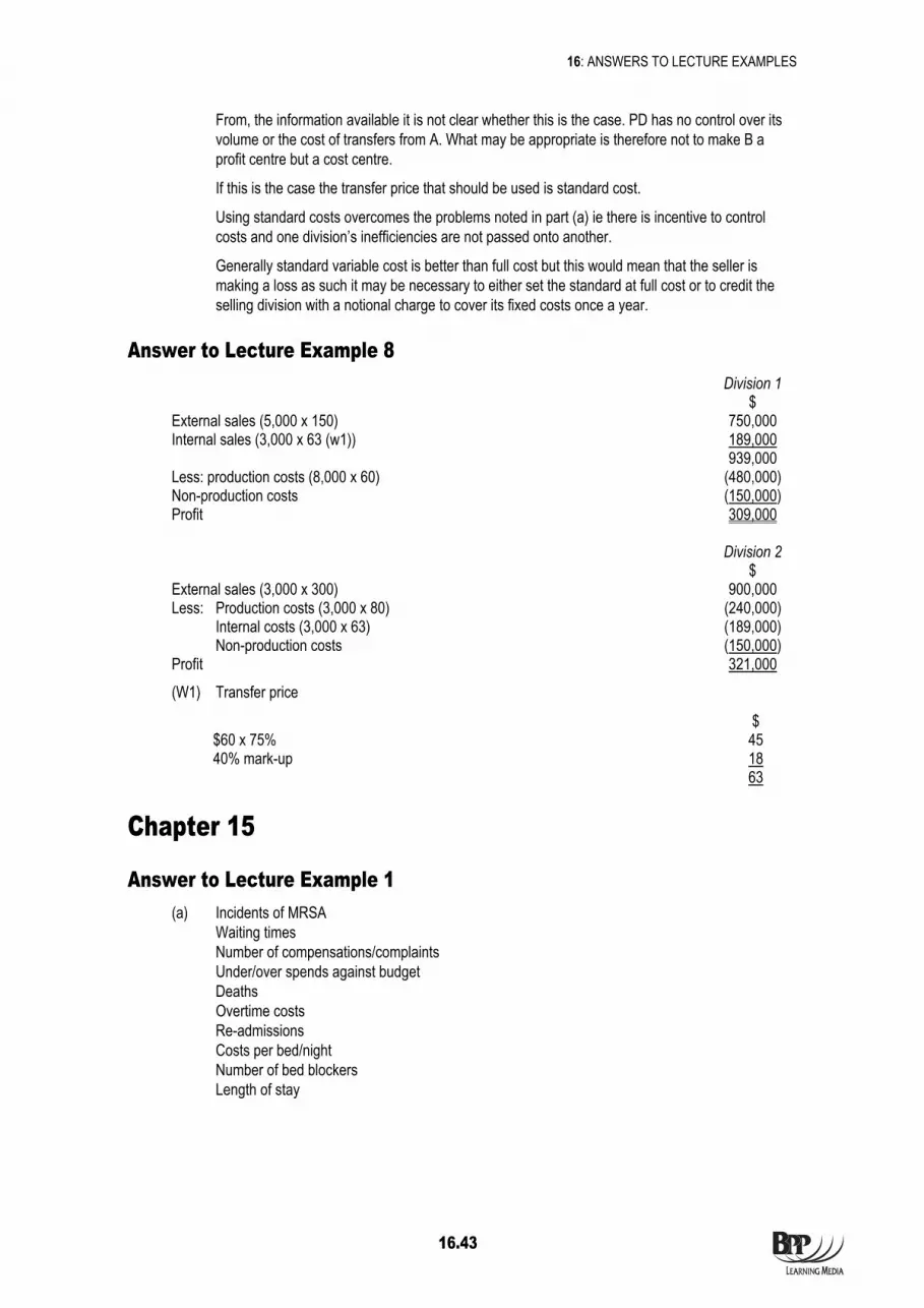
16: ANSWERS TO LECTURE EXAMPLES
16.43
From, the information available it is not clear whether this is the case. PD has no control over its volume or the cost of transfers from A. What may be appropriate is therefore not to make B a profit centre but a cost centre.
If this is the case the transfer price that should be used is standard cost.
Using standard costs overcomes the problems noted in part (a) ie there is incentive to control costs and one division’s inefficiencies are not passed onto another.
Generally standard variable cost is better than full cost but this would mean that the seller is making a loss as such it may be necessary to either set the standard at full cost or to credit the selling division with a notional charge to cover its fixed costs once a year.
Answer to Lecture Example 8 Division 1 $ External sales (5,000 x 150) 750,000 Internal sales (3,000 x 63 (w1)) 189,000 939,000 Less: production costs (8,000 x 60) (480,000) Non-production costs (150,000) Profit 309,000
Division 2 $ External sales (3,000 x 300) 900,000 Less: Production costs (3,000 x 80) (240,000) Internal costs (3,000 x 63) (189,000) Non-production costs (150,000) Profit 321,000 (W1) Transfer price
$ $60 x 75% 45 40% mark-up 18 63
Chapter 15
Answer to Lecture Example 1 (a) Incidents of MRSA
Waiting times Number of compensations/complaints Under/over spends against budget Deaths Overtime costs Re-admissions Costs per bed/night Number of bed blockers Length of stay

16: ANSWERS TO LECTURE EXAMPLES
16.44
(b) Common problems are likely to include:
– Concentration on one factor at detriment of others. – How can it be made directly comparable (poor areas of country v affluent areas). – Creative accounting/Fraud. – Self fulfilling prophecy (downward spiral).
Answer to Lecture Example 2 Effectiveness – Achieving target pass rates of grades (Objective) – Proportion of graduates employed within a year.
Efficiency – Cost of books per student (Input to output ratio) – Staff hours per student – Teaching cost per student – Total cost of producing a graduate.
Economy – Value for money in sourcing lecture (Cost of inputs) staff of appropriate quality – Competitive tendering for
– computers – security – cleaning
Answer to Lecture Example 3 Stakeholders
Internal Employee turnover Career progression paths
External
No staff Taxation Pollution
Connected
P/E ratio EPS growth Interest cover Customer service Quality and reliability Adherence to payment terms
Economic environment Monitor economic growth Interest rates Inflation Employment
Competition Track competitors' pricing Market share
END OF ANSWERS TO LECTURE EXAMPLES

17.1
Question andAnswer bank

17.2
Index to Question and Answer bank
Page
Questions Answers
1 Abkaber ....................................................................................................................................... 17.3....................17.10 2 Cost management techniques..................................................................................................... 17.4....................17.14 3 HYC............................................................................................................................................. 17.4....................17.15 4 Stow Health Centre ..................................................................................................................... 17.5....................17.17 5 Dench .......................................................................................................................................... 17.6....................17.19 6 McDreamy ................................................................................................................................... 17.7....................17.20 7 ACCA-Chem................................................................................................................................ 17.8 ...................17.23 8 Divisional performance measures ............................................................................................... 17.9....................17.25 9 Non-profit seeking organisations ................................................................................................. 17.9....................17.27

17: QUESTION AND ANSWER BANK
17.3
Questions
1 Abkaber (Study Text question 3) Exam standard Abkaber assembles three types of motorcycle at the same factory: the 50cc Sunshine; the 250cc Roadster and the 1000cc Fireball. It sells the motorcycles throughout the world. In response to market pressures Abkaber has invested heavily in new manufacturing technology in recent years and, as a result, has significantly reduced the size of its workforce.
Historically, the company has allocated all overhead costs using total direct labour hours, but is now considering introducing Activity Based Costing (ABC). Abkaber's accountant has produced the following analysis. Annual Annual direct Raw output labour Selling material (units) Hours price cost ($ per unit) ($ per unit) Sunshine 2,000 200,000 4,000 400 Roadster 1,600 220,000 6,000 600 Fireball 400 80,000 8,000 900 The three cost drivers that generate overheads are:
Deliveries to retailers – the number of deliveries of motorcycles to retail showrooms
Set-ups – the number of times the assembly line process is re-set to accommodate a production run of a different type of motorcycle
Purchase orders – the number of purchase orders.
The annual cost driver volumes relating to each activity and for each type of motorcycle are as follows:
Number of Number of deliveries Number of purchase to retailers set-ups orders Sunshine 100 35 400 Roadster 80 40 300 Fireball 70 25 100 The annual overhead costs relating to these activities are as follows:
$ Deliveries to retailers 2,400,000 Set-up costs 6,000,000 Purchase orders 3,600,000 All direct labour is paid at $5 per hour. The company holds no inventories.
At a board meeting there was some concern over the introduction of activity based costing.
The finance director argued: 'I very much doubt whether selling the Fireball is viable but I am not convinced that activity based costing would tell us any more than the use of labour hours in assessing the viability of each product.'
The marketing director argued: 'I am in the process of negotiating a major new contract with a motorcycle rental company for the Sunshine model. For such a big order they will not pay our normal prices but we need to at least cover our incremental costs. I am not convinced that activity based costing would achieve this as it merely averages costs for our entire production.'
The managing director argued: 'I believe that activity based costing would be an improvement but it still has its problems. For instance if we carry out an activity many times surely we get better at it and costs

17: QUESTION AND ANSWER BANK
17.4
fall rather than remain constant. Similarly, some costs are fixed and do not vary either with labour hours or any other cost driver'.
The chairman argued: 'I cannot see the problem. The overall profit for the company is the same no matter which method of allocating overheads we use. It seems to make no difference to me'.
Required
(a) Calculate the total profit on each of Abkaber's three types of product using each of the following methods to attribute overheads:
(i) the existing method based upon labour hours; and
(ii) activity based costing. (13 marks)
(b) Write a report to the directors of Abkaber, as its management accountant. The report should:
(i) evaluate the labour hours and the activity based costing methods in the circumstances of Abkaber; and
(ii) examine the implications of activity based costing for Abkaber, and in so doing evaluate the issues raised by each of the directors.
Refer to your calculations in requirement (a) above where appropriate. (12 marks)
(Total = 25 marks)
2 Cost management techniques (Study Text question 5) Exam standard Traditional cost control systems focused on cost containment rather than cost reduction. Today, cost management focuses on process improvement and the identification of how processes can be more effectively and efficiently performed to result in cost reductions.
Required
Discuss how the cost management techniques of target costing and life cycle costing differ from the traditional cost containment approach and how each seeks to achieve cost reduction. (10 marks)
3 HYC (Study Text question 7) Exam standard
HYC makes three products H, Y and C. All three products must be offered for sale each month in order to be able to provide a complete market service. The products are fragile and their quality deteriorates rapidly once they are manufactured.
The products are produced on two types of machine and worked on by a single grade of direct labour. Five direct employees are paid $8 per hour for a guaranteed minimum of 160 hours each per month.
All of the products are first moulded on a machine type 1 and then finished and sealed on a machine type 2.
The machine hour requirements for each of the products are as follows.
Product H Product Y Product C Hours per unit Hours per unit Hours per unit Machine type 1 1.5 4.5 3.0 Machine type 2 1.0 2.5 2.0
The capacity of the available machines type 1 and 2 are 600 hours and 500 hours per month respectively.

17: QUESTION AND ANSWER BANK
17.5
Details of the selling prices, unit costs and monthly demand for the three products are as follows.
Product H Product Y Product C $ per unit $ per unit $ per unit Selling price 91 174 140 Component cost 22 19 16 Other direct material cost 23 11 14 Direct labour cost at $8 per hour
6 48 36
Overheads 24 62 52 Profit 16 34 22 Maximum monthly demand (units)
120 70 60
Although HYC uses marginal costing and contribution analysis as the basis for its decision making activities, profits are reported in the monthly management accounts using the absorption costing basis. Finished goods inventories are valued in the monthly management accounts at full absorption cost.
Required
(a) Calculate the machine utilisation rate for each machine each month and explain which of the machines is the bottleneck/limiting factor. (5 marks)
(b) Using the current system of marginal costing and contribution analysis, calculate the profit maximising monthly output of the three products. (5 marks)
(c) Explain why throughput accounting might provide more relevant information in HYC’s circumstances. (5 marks)
(d) Using a throughput approach, calculate the throughput-maximising monthly output of the three products. (5 marks)
(e) Explain the throughput accounting approach to optimising the level of inventory and its valuation. Contrast this approach to the current system employed by HYC. (5 marks)
(Total = 25 marks)
4 Stow Health Centre (Study Text question 11) Exam standard
Stow Health Centre specialises in the provision of sports/exercise and medical/dietary advice to clients. The service is provided on a residential basis and clients stay for whatever number of days suits their needs.
Budgeted estimates for the year ending 31 June 20X1 are as follows.
(a) The maximum capacity of the centre is 50 clients per day for 350 days in the year.
(b) Clients will be invoiced at a fee per day. The budgeted occupancy level will vary with the client fee level per day and is estimated at different percentages of maximum capacity as follows.
Client fee per day
Occupancy level
Occupancy as percentage of maximum capacity
$180 High 90% $200 Most likely 75% $220 Low 60%

17: QUESTION AND ANSWER BANK
17.6
(c) Variable costs are also estimated at one of three levels per client day. The high, most likely and low levels per client day are $95, $85 and $70 respectively.
The range of cost levels reflects only the possible effect of the purchase prices of goods and services.
Required
(a) Prepare a summary which shows the budgeted contribution earned by Stow Health Centre for the year ended 30 June 20X1 for each of nine possible outcomes. (7 marks)
(b) State the client fee strategy for the year to 30 June 20X1 which will result from the use of each of the following decision rules.
(i) Maximax (ii) Maximin (iii) Minimax regret
Your answer should explain the basis of operation of each rule. Use the information from your answer to (a) as relevant and show any additional working calculations as necessary. (12 marks)
(c) The probabilities of variable cost levels occurring at the high, most likely and low levels provided in the question are estimated as 0.1, 0.6 and 0.3 respectively.
Using the information available, determine the client fee strategy which will be chosen where maximisation of expected value of contribution is used as the decision basis. (6 marks)
(Total = 25 marks)
5 Dench (Study Text question 15) Exam standard Dench manufacturing has received a special order from Sands to produce 225 components to be incorporated into Sand’s product. The components have a high cost, due to the expertise required for their manufacture. Dench produces the components in batches of 15, and as the ones required are to be custom-made to Sands’ specifications, a “prototype” batch was manufactured with the following costs:
$ Materials 4 kg of A, $7.50/kg 30 2 kg of B, $15/kg 30 Labour 20 hrs skilled, $15/hr
300
5 hrs semi-skilled, $8/hr 40 Variable Overhead 25 labour hours, $4/hr 100 500 Additional information with respect to the workforce is noted below:
Skilled virtually a permanent workforce that has been employed by Dench for a long period of time. These workers have a great deal of experience in manufacturing components similar to those required by Sands, and turnover is virtually non-existent.
Semi-Skilled hired by Dench on an “as needed” basis. These workers would have had some prior experience, but Dench management believe the level to be relatively insignificant. Past experience shows turnover rate to be quite high, even for short employment periods.

17: QUESTION AND ANSWER BANK
17.7
Dench’s plans are to exclude the prototype batch from Sands’ order. Management believes a 80% learning rate effect is experienced in this manufacturing process, and would like a cost estimate for the 225 components prepared on that basis.
Required
(a) Prepare the cost estimate, assuming an 80% learning rate is experienced, and (7 marks)
(b) Briefly discuss some of the factors that can limit the use of learning curve theory in practice. (5 marks)
6 McDreamy (Study Text question 16) Exam standard
McDreamy is in an industry sector which is recovering from the recent recession. The directors of the company hope next year to be operating at 85% of capacity, although currently the company is operating at only 65% of capacity. 65% of capacity represents output of 10,000 units of the single product which is produced and sold. One hundred direct workers are employed on production for 200,000 hours in the current year.
The flexed budgets for the current year are as follows.
Capacity level 55% 65% 75% $ $ $ Direct materials 846,200 1,000,000 1,153,800 Direct wages 1,480,850 1,750,000 2,019,150 Production overhead 596,170 650,000 703,830 Selling and distribution overhead 192,310 200,000 207,690 Administration overhead 120,000 120,000 120,000 Total costs 3,235,530 3,720,000 4,204,470 Profit in any year is budgeted to be 162/3% of sales.
The following percentage increases in costs are expected for next year. Increase % Direct materials 6.0 Direct wages 3.0 Variable production overhead 7.0 Variable selling and distribution overhead 7.0 Fixed production overhead 10.0 Fixed selling and distribution overhead 7.5 Administration overhead 10.0 Required
(a) Prepare for next year a flexible budget statement on the assumption that the company operates at 85% of capacity; your statement should show both contribution and profit. (12 marks)
(b) State three problems which may arise from the change in capacity level. (3 marks)
(c) Explain in detail what is meant by the principle of controllability. (10 marks)
(Total = 25 marks)

17: QUESTION AND ANSWER BANK
17.8
7 ACCA-Chem (Study Text question 17) Exam standard
(a) ACCA-Chem Co manufacture a single product, product W, and have provided you with the following information which relates to the period which has just ended. Standard cost per batch of product W Materials:
Material Price per kilo Total Kilos $ $
F 15 4 60 G 12 3 36 H 8 6 48
35 144 Less: Standard loss 3 Standard yield 32 Labour: Rate per hour Hours $ Department P 4 10 40 Department Q 2 6 12 196 Budgeted sales for the period are 4,096 kilos at $16 per kilo. There were no budgeted opening or closing inventories of product W. The actual materials and labour used for 120 batches were as follows. Materials:
Material Price per kilo Total Kilos $ $
F 1,680 4.25 7,140 G 1,650 2.80 4,620 H 870 6.40 5,568
4,200 17,328 Less: Actual loss 552 Actual yield 3,648 Labour: Rate per hour Hours $ Department P 600 10.60 6,360 Department Q 270 5.60 1,512 25,200 All of the production of W was sold during the period for $16.75 per kilo. Required (i) Calculate the following material variances. (1) Price (2) Usage (3) Mix (4) Yield (8 marks)
(ii) Calculate the following labour variances for each of the production departments. (1) Cost (2) Efficiency (3) Rate (4 marks)
(iii) Calculate the sales variances. (3 marks)
(iv) Comment on your findings to help explain what has happened to the yield variance. (5 marks)
(b) Briefly explain how time series analysis can assist the management accountant. (5 marks)
(Total = 25 marks)

17: QUESTION AND ANSWER BANK
17.9
8 Divisional performance measures (Study Text question 20) Exam standard (a) Compare and contrast the use of residual income and return on investment in divisional
performance measurement, stating the advantages and disadvantages of each. (9 marks)
(b) Division Y of Chardonnay currently has capital employed of £100,000 and earns an annual profit after depreciation of £18,000. The divisional manager is considering an investment of £10,000 in an asset which will have a ten-year life with no residual value and will earn a constant annual profit after depreciation of £1,600. The cost of capital is 15%.
Calculate the following and comment on the results.
(i) The return on divisional investment, before and after the new investment (ii) The divisional residual income before and after the new investment (7 marks)
(c) Explain the potential benefits of operating a transfer pricing system within a divisionalised company. (8 marks)
(Total = 25 marks)
9 Non-profit seeking organisations (Study Text question 21) Exam standard (a) The absence of the profit measure in non-profit seeking organisations causes problems for the
measurement of their efficiency and effectiveness.
Required
(i) Explain why the absence of the profit measure should be a cause of the problems referred to. (9 marks)
(ii) Explain how these problems extend to activities within business entities which have a profit motive. Support your answer with examples. (5 marks)
(b) A public health clinic is the subject of a scheme to measure its efficiency and effectiveness. Amongst a number of factors, the 'quality of care provided' has been included as an aspect of the clinic's service to be measured. Three features of 'quality of care provided' have been listed.
(i) Clinic's adherence to appointment times (ii) Patients' ability to contact the clinic and make appointment without difficulty (iii) The provision of a comprehensive patient health monitoring programme
Required
(i) Suggest a set of quantitative measures which can be used to identify the effective level of achievement of each of the features listed. (9 marks)
(ii) Indicate how these measures could be combined into a single 'quality of care' measure. (2 marks)
(Total = 25 marks)
END OF ANSWER BANK END OF QUESTION BANK

17: QUESTION AND ANSWER BANK
17.10
Answers
1 Abkaber Top tips. Part (a) is fairly straightforward requiring the calculation of profit for the three products under both absorption costing and ABC. Under ABC make sure you calculate the costs per cost driver.
Part (b) required a discussion of the impact of ABC and an analysis of each of the directors' comments. It is important for the students to apply their understanding of ABC to each of these comments.
(a) (i) Existing method Sunshine Roadster Fireball $ $ $ Direct labour ($5 per hr) (W1) 1,000,000 1,100,000 400,000 Materials (W2) 800,000 960,000 360,000 Overheads (at $24) (W3) 4,800,000 5,280,000 1,920,000 Total costs 6,600,000 7,340,000 2,680,000 Output (Units) 2,000 1,600 400 $ $ $ Selling price 4,000 6,000 8,000 Cost per unit (W4) 3,300 4,587.5 6,700 700 1,412.5 1,300 Total profit $ $ $ (output in units × profit/unit) 1,400,000 2,260,000 520,000
Total profit = $4,180,000
Workings
1 Labour cost
Sunshine 200,000 hrs × $5 per hour = 1,000,000 Roadster 220,000 hrs × $5 per hour = 1,100,000 Fireball 80,000 hrs × $5 per hour = 400,000
2 Material cost
Sunshine 2,000 × 400 = 800,000 Roadster 1,600 × 600 = 960,000 Fireball 400 × 900 = 360,000
3 Overhead per labour hour $ Total overhead cost = 12,000,000 Total labour hours = 500,000 hrs Overhead per labour hour =
500,000
0£12,000,00 = $24
4 Cost per unit
Sunshine: produced Units
costs Total =
2,0006,600,000
= $3,300
Roadster: produced Units
costs Total =
1,6007,340,000
= $4,587.50
Fireball: produced Units
costs Total =
4002,680,000
= $6,700

17: QUESTION AND ANSWER BANK
17.11
(ii) Activity based costing Sunshine Roadster Fireball $ $ $ Direct labour ($5 per hr) (as (W1) above)
1,000,000 1,100,000 400,000
Materials (as (W2) above) 800,000 960,000 360,000 Overheads Deliveries (W5(a)) 960,000 768,000 672,000 Set up costs (W5(b)) 2,100,000 2,400,000 1,500,000 Purchase orders (W5(c)) 1,800,000 1,350,000 450,000 6,660,000 6,578,000 3,382,000 Output units 2,000 1,600 400 $ $ $ Selling price 4,000 6,000 8,000 Cost per unit (W4) 3,330 4,111.25 8,455 Profit/(loss) per unit 670 1,888.75 (455) Total profit/(loss) $1,340,000 $3,022,000 ($182,000) Total profit = $4,580,000
Workings
5 Overheads
$
deliveries of number Totalretailers to deliveries ofcost Overhead
=250
2,400,000
= $9,600
ups-set of number Totalups-set ofcost Overhead
= 100
6,000,000
= $60,000
orders purchase of number Totalorders purchase ofcost Overhead
=800
3,600,000
= $4,500
5(a) Deliveries overheads
Sunshine $9,600 × 100 = $960,000 Roadster $9,600 × 80 = $768,000 Fireball $9,600 × 70 = $672,000
5(b) Set-up cost overheads
Sunshine $60,000 × 35 = $2,100,000 Roadster $60,000 × 40 = $2,400,000 Fireball $60,000 × 25 = $1,500,000
5(c) Purchase order overheads
Sunshine $4,500 × 400 = $1,800,000 Roadster $4,500 × 300 = $1,350,000 Fireball $4,500 × 100 = $450,000

17: QUESTION AND ANSWER BANK
17.12
(b) REPORT
To: Directors, Abkaber From: Management accountant Subject: The implications of activity based costing Date: 12.12.X2
(i) Labour hours and activity based costing allocation
Labour hours
For the allocation of overheads on the basis of labour hours to be appropriate, there would need to be a direct relationship between overheads and labour hours. From the information available, this does not appear to be the case.
A traditional method of cost allocation, such as the one based on labour hours, was developed when an enterprise produced a narrow range of products which underwent similar operations and consumed similar proportions of overheads. Moreover, when such methods were being widely used, overhead costs were only a very small proportion of total costs, with direct labour and material costs accounting for the largest proportion of total costs.
Abkaber has invested in new technology and as a result has significantly reduced the size of its workforce. Direct labour costs now account for a relatively smaller proportion of total costs with overheads making up the highest single cost item. Allocation of overheads on the basis of labour costs would tend to allocate too great a proportion of overheads to the higher volume Sunshine than the lower volume Fireball, ignoring the fact that the lower volume product may require relatively more support services. It therefore seems likely that attributing overheads on the basis of labour hours may lead to inappropriate decisions.
Activity based costing
Activity based costing attempts to overcome this problem by identifying the factors which cause the costs of an organisation's major activities.
The idea behind activity based costing is that activities such as ordering, materials handling, deliveries and set up cause costs. Producing goods creates demand for activities. Costs are assigned to a product on the basis of the product's consumption of activities.
Supporters of ABC argue that it is activities that generate costs, not labour hours.
The accuracy of any ABC system will depend on the appropriateness of the activities as cost drivers. Each cost driver selected should be appropriate to the overheads to which it relates. There should be a direct and proportionate relationship between the relevant overhead costs and the cost driver selected.
The labour hours costing system and ABC result in markedly different profit figures, especially with respect to the Fireball which appears profitable under the first system but loss making under ABC.
The reason for this is that, although the Fireball uses twice as many hours per unit as the Sunshine, its low output volume of only 400 units (compared with 2,000 units of Sunshine) means that a proportionately lower amount of overheads is absorbed.
Under activity based costing, the Fireball shows a loss because ABC recognises the relatively high set-up costs, deliveries and purchase orders.

17: QUESTION AND ANSWER BANK
17.13
(ii) Finance director's comments
The finance director is questioning the viability of the Fireball, but doubts whether ABC provides more information than the labour hours costing method.
ABC helps the company focus on the fact that the low volumes of Fireball involve a disproportionate amount of set-up costs, deliveries and purchase orders, resulting in a relatively higher allocation of overheads.
It may be the case that a review of current activities relating to Fireball may reduce costs. There are also other, non-financial, considerations for continuing to produce the Fireball. As the more expensive of the three products, it may have brand value and help raise the reputation of the company as well as that of the other models.
Marketing director's comments
The marketing director is questioning the suitability of ABC in helping price a major new contract.
(1) The accuracy of ABC depends on the appropriateness of the cost drivers identified. Although more appropriate than the labour hours allocation basis, for the type of one-off decision the marketing director needs to make, an incremental cost approach may be better.
(2) There may be factors both financial and non-financial that ABC may not be able to capture. For example, there may be costs common to more than one product, interdependencies between costs and revenues, or interdependencies between the sales volumes of the different products.
The relationship between costs and activities is based on historic observations which may not be a reliable guide to the future.
Managing director's comments
The MD is correct to question the fact that ABC assumes that the cost per activity is constant. In practice, the existence of a learning curve may mean that the costs per activity are going down as the activity is repeated.
The MD is correct in questioning the inclusion of fixed costs which do not vary with either labour hours or any cost driver and thus show no cause and effect relationship under ABC.
Chairman's comments
As (i) and (ii) above illustrate, the overall profit under the two methods is the same. However, it would not be appropriate to dismiss the two approaches as irrelevant.
(1) If the company carried inventory, then the method of cost allocation would affect the inventory valuation and consequently profit.
(2) It is important to understand both the strengths and limitations of ABC as a decision making tool. Although it may appear to be more appropriate than labour hours in the allocation of overheads there are financial and non-financial factors that ABC does not capture. A decision to discontinue production of the Fireball should not be made without the consideration of these factors. These may include:
– Existence of a learning curve – The inclusion of fixed costs that do not vary with level of activity – Interdependencies of cost and revenues – Interdependencies of sales of the three products
Further considerations
Abkaber will need to continue evaluating the activities identified and the relationship between cost drivers and overheads.

17: QUESTION AND ANSWER BANK
17.14
2 Cost management techniques Top tips. To earn good marks for this question you would need to mention the traditional cost containment approaches.
Answer plan
• Two parts to the answer – target costing – life cycle costing
• Within each part refer to – traditional approach – modern approach
• Remember to mention cost reduction opportunities under each part
(a) Target costing
Traditional approach
The traditional approach to product costing, which is dominated by standard costing, is first to develop a product. An expected standard cost is then determined and a selling price (probably based on cost) is set, with a resulting profit or loss.
Costs are controlled at monthly intervals through variance analysis. The standard cost, once set, is only revised for changes of a permanent or reasonably long-term nature.
Target costing approach
This is to develop a product concept and then determine the price that customers would be willing to pay for it. A desired profit margin is then deducted from the price to leave a figure representing total cost. This is the target cost.
If the target cost is vastly different from the cost at which the product can be produced, the product may need to be redesigned or may even be scrapped if the target is impossible to achieve.
Management may decide to go ahead and manufacture a product with a target cost well below the currently attainable cost. In such circumstances they will set benchmarks for improvement towards the target cost, by specified dates. Reducing the number of components, cutting out non-value-added activities and so on are possible cost reduction approaches.
Once the product goes into production, the target cost will gradually be reduced, the reductions being incorporated into the budgeting process.
Target costing and cost reduction opportunities
To remain competitive, organisations must continually redesign their products. Far more so than in the past, when cost reduction during the production process was important, a product's planning, development and design stages are therefore critical to an organisation's cost reduction process. Target costing, by focusing on costs incurred at all steps of a product's life (not just the production stage), gives added emphasis to cost reduction at this vital stage.
(b) Life cycle costing
Traditional approach
Traditional management accounting practice is, in general, to report costs at the physical production stage of the life cycle of a product; cost are not accumulated over the entire life cycle. This means a product's profitability is not assessed over its entire life but rather on a periodic basis. Costs tend to be accumulated according to function; research, design,

17: QUESTION AND ANSWER BANK
17.15
development and customer service costs incurred on all products during a period are totalled and are recorded as a period expense, effectively hiding them from cost reduction opportunities.
Life cycle approach
Using life cycle costing, however, such costs are traced to individual products over complete life cycles (from the product's inception to its decline). This overview of a product's profitability is of utmost importance when assessing cost reduction opportunities.
Life cycle costing and cost reduction
One of the principal ideas of life cycle costing is that the profit generated by a product must cover not only production costs, but the costs associated with the pre- and post-production stages (such as costs of research, design and testing, and costs of distribution and customer service). It has been claimed that up to 90% of a product's life cycle costs will be determined 'up front' by decisions made very early within the life cycle (production costs are based on design decisions, for example). The application of life cycle costing will therefore ensure that cost control and cost reduction will be carried out at the early stages, as well as during the production stage.
3 HYC Top tips. Show your workings and use a clear layout. Make sure you spend an equal amount of time on the discussions as on the calculations.
(a) Product Machine hours required H Y C Total Type 1 180 315 180 675 Type 2 120 175 120 415 Machine utilisation rate:
Machine type 1 = 675/600 = 112.5% Machine type 2 = 415/500 = 83.0%
Machine type 1 has the highest utilisation rate and the rate is above 100 per cent. Therefore machine type 1 is the bottleneck/limiting factor.
(b) Product H Y C Contribution per unit 40 96 74 Machine type 1 hours 1.5 4.5 3.0 Contribution per hour 26.67 21.33 24.67 Ranking 1 3 2
Allocation of machine type 1 hours according to this ranking:
Product H 120 units using 180 hours Product C 60 units using 180 hours 360 hours used Product Y (240/4.5) 53 units using 238.5 hours 598.5 hours used
(c) A major concept underlying throughput accounting is that the majority of costs, with the exception of material and component costs, are fixed.
In HYC's case it is clear that the labour cost, which is treated as a variable cost in traditional marginal costing, is indeed a fixed cost. The employees are paid for a guaranteed 800 hours (160 × 5) each month, whereas the number of labour hours required to meet the maximum demand can be calculated as 780 hours as follows.

17: QUESTION AND ANSWER BANK
17.16
Product H Y C Total Labour hours per unit 0.75 6 4.5 Maximum demand (units) 120 70 60 Total hours required per month
90 420 270 780
Therefore labour is a fixed cost that will not alter within the relevant range of activity. Throughput accounting recognises this in the calculation of throughput.
Furthermore, given the perishable nature of HYC's products, the throughput accounting approach to inventory minimisation and maximisation of throughput would be more appropriate.
(d) Product H Y C per unit per unit per unit Sales revenue 91 174 140 Component cost 22 19 16 Other direct material 23 11 14 Throughput per unit 46 144 110 Machine type 1 hours 1.5 4.5 3.0 Throughput per hour 30.67 32.00 36.76 Ranking 3 2 1 Allocation of machine type 1 hours according to this ranking:
Product C 60 units using 180 hours Product Y 70 units using 315 hours 495 hours used Product H (105/1.5) 70 units using 105 hours 600 hours used
(e) The conventional cost accounting approach used by HYC views inventory as an asset. In the throughput accounting approach inventory is not viewed as an asset, but rather as a result of unsynchronised manufacturing. The existence of inventory is thus viewed as a breakdown in synchronisation and a barrier to generating profits.
In throughput accounting the ideal inventory level is zero, with the exception that a buffer inventory should be held prior to the bottleneck machine.
As regards the valuation of inventory, the throughput philosophy is that no value is added to inventory items and no profit is earned until the items are actually sold. Thus inventory is valued at its material cost only until it is sold.
This approach to inventory valuation is in contrast to the full absorption costing system used by HYC. The latter approach encourages managers to produce output just to add to work in progress or finished goods inventory, since this helps with the absorption of overheads and boosts reported profits. This behaviour will be avoided and managers will be more likely to be willing to minimise inventory if it is valued at material cost only.

17: QUESTION AND ANSWER BANK
17.17
4 Stow Health Centre Top tips. Did you get confused in part (a)? The occupancy level will vary with the client fee per day, while the variable cost per client day is independent. In other words, at each of the three different levels of client fee per day, there are three possible levels of variable cost per client and so 3 × 3 = 9 possible levels of contribution per client day.
The most tricky aspect of part (b) was dealing with the minimax regret decision rule. This rule involves choosing the strategy which will minimise the maximum regret (ie drop in contribution) from choosing one option instead of the best option. This requires you to draw up an opportunity loss table. This will show the drop in contribution at each level of variable cost from choosing a level of client fee which is not the best option. For example, at a variable cost of $95 per day, the best strategy would be a client fee of $200 per day. The opportunity loss from using a fee of $180 would be the difference between the contributions at the two fee levels.
For part (c) you simply need to calculate an EV of variable cost per day. You are then faced with a situation of one level of client fee per day and one level of variable cost per day at each level of 'demand'.
(a) We need to calculate budgeted contribution and so the summary will need to show the various income (fee) and variable cost levels. Total
Number of Client fee Variable cost Contribution contribution client days per day per client day per client day this year
(W1) $ $ $ $ (W2) 15,750 180 95 85 1,338,750 15,750 180 85 95 1,496,250 15,750 180 70 110 1,732,500 13,125 200 95 105 1,378,125 13,125 200 85 115 1,509,375 13,125 200 70 130 1,706,250 10,500 220 95 125 1,312,500 10,500 220 85 135 1,417,500 10,500 220 70 150 1,575,000
Workings
1 Maximum capacity = 50 × 350 = 17,500 High occupancy level = 90% × 17,500 = 15,750 Most likely occupancy level = 75% × 17,500 = 13,125 Low occupancy level = 60% × 17,500 = 10,500
2 Number of client days × contribution per client day
(b) (i) The maximax decision rule involves choosing the outcome with the best possible result, in this instance choosing the outcome which maximises contribution. The decision maker would therefore choose a client fee of $180 per day, which could result in a contribution of $1,732,500.
(ii) The maximin decision rule involves choosing the outcome that offers the least unattractive worst outcome, in this instance choosing the outcome which maximises the minimum contribution. The decision maker would therefore choose a client fee of $200 per day, which has a lowest possible contribution of $1,378,125. This is better than the worst possible outcomes from client fees per day of $180 and $220, which would provide contributions of $1,338,750 and $1,312,500 respectively.
(iii) The minimax regret decision rule involves choosing the outcome that minimises the maximum regret from making the wrong decision, in this instance choosing the outcome which minimises the opportunity lost from making the wrong decision.

17: QUESTION AND ANSWER BANK
17.18
We can use the calculations performed in (a) to draw up an opportunity loss table.
Maximum Variable cost per day regret Client fee per day $95 $85 $70
$ $ $ $ $ 180 39,375 (W1) 13,125 (W4) 0 (W7) 39,375 200 0 (W2) 0 (W5) 26,250 (W8) 26,250 220 65,625 (W3) 91,875 (W6) 157,500 (W9) 157,500
The minimax regret decision strategy would be to choose a client fee of $200 to minimise the maximum regret at $26,250.
Workings
1 At a variable cost of $95 per day, the best strategy would be a client fee of $200 per day. The opportunity loss from using a fee of $180 would be $(1,378,125 – 1,338,750) = $39,375.
2 The opportunity loss in this case is $(1,378,125 – 1,378,125) = $0.
3 The opportunity loss in this case is $(1,378,125 – 1,312,500) = $65,625.
4 At a variable cost of $85 per day, the best strategy would be a client fee of $200 per day. The opportunity loss from using a fee of $180 would be $(1,509,375 – 1,496,250)= $13,125.
5 The opportunity loss in this case is $(1,509,375 – 1,509,375) = 0.
6 The opportunity loss in this case is $(1,509,375 – 1,417,500) = $91,875.
7 At a variable cost of $70 per day, the best strategy would be client fee of $180 per day. The opportunity loss from using a fee of $180 would be $(1,732,500 – 1,732,500) = $0.
8 The opportunity loss in this case is $(1,732,500 – 1,706,250) = $26,250.
9 The opportunity loss in this case is $(1,732,500 – 1,575,000) = $157,500.
(c) Expected value of variable costs = (0.1 × $95) + (0.6 × $85) + (0.3 × $70) = $81.50.
We can now calculate an expected value of budgeted contribution at each client fee per day level. EV of EV of total
Number of Client fee EV of variable contribution annual client days per day cost per day per client day contribution
$ $ $ $ 15,750 180 81.50 98.50 1,551,375.00 13,125 200 81.50 118.50 1,555,312.50 10,500 220 81.50 138.50 1,454,250.00
If maximisation of EV of contribution is used as the decision basis, a client fee of $200 per day will be selected, with an EV of contribution of $1,555,312.50 (although this is very close to the EV of contribution which results from a client fee of $180).

17: QUESTION AND ANSWER BANK
17.19
5 Dench (a) Cost estimate for 225 components is based upon the following assumptions:
(1) The first batch of 15 is excluded from the order (and total cost for first batch is likewise excluded); and
(2) The 80% learning rate only applies to the skilled workforce, (and related variable overhead) due to their high level of expertise/low turnover rate.
Cumulative Cumulative Total Cum ave Batches Units Time time/batch
1 15 20 hr 20 hr 2 30 32 hr 16 hr 4 60 51.2 hr 12.8hr 8 120 81.92 hr 10.24hr
16 240 131.072 hr 8.192hr Total cost for 16 batches (240 components) $ Material A: $30 batch 480 Material B: $30/batch 480 Labour: Skilled 131.072 hr @ $15/hr 1,966 Semi-skilled $40/batch 640 Variable OH: 131.072 hr @ $4/hr 524 5 hr/batch at $4/hr 320 4,410 Less: Cost for 1st batch (15 components) (500) ∴cost for 225 components 3,910
(b) The limited use of learning curve theory is due to several factors:
(i) The learning curve phenomenon is not always present.
(ii) It assumes stable conditions at work (eg of the labour force and labour mix) which will enable learning to take place. This is not always practicable (eg because of labour turnover).
(iii) It must also assume a certain degree of motivation amongst employees.
(iv) Extensive breaks between production of items must not be too long, or workers will ‘forget’ and the learning process would have to begin all over again.
(v) It is difficult to obtain enough accurate data to decide what the learning curve is.

17: QUESTION AND ANSWER BANK
17.20
6 McDreamy Top tips. Make sure you read the question carefully especially on the calculation of capacity levels. Note that at 65% capacity 10,000 units are produced.
Part (b) requires you to apply your knowledge and part (c) is a straightforward regurgitation of text book knowledge.
(a) Flexible budget statement for next year operating at 85% capacity
Workings Output 1 13,077 units $ $ Sales revenue 9 5,911,484 Variable costs Direct materials 2 1,386,162 Direct wages 3 2,357,129 Variable production overhead 4 489,734 Variable selling and distribution overhead 5 69,962 4,302,987 Contribution 1,608,497 Fixed costs Production overhead 6 330,000 Selling and distribution overhead 7 161,250 Administration overhead 8 132,000 623,250 Profit 985,247
Workings
1 65% of capacity = 10,000 units ∴100% of capacity = 10,000 ÷ 0.65 = 15,385 units ∴ 85% of capacity = (10,000 ÷ 0.65) × 0.85 = 13,077 units ∴ 75% of capacity = 11,538 ∴ 55% of capacity = 8,462
2 Current direct material cost per unit = $1,000,000 ÷ 10,000 = $100 per unit
∴ Flexible budget allowance for next year = $100 × 1.06 × 13,077 = $1,386,162
3 Current direct wages cost per unit = $1,750,000 ÷ 10,000 = $175 per unit
∴ Flexible budget allowance for next year = $175 × 1.03 × 13,077 = $2,357,129
4 Production overhead increases by $53,830 for an increase in activity of (10,000 – 8,462) units
∴Variable production overhead per unit = $35 ∴Variable overhead allowance for 85% capacity = 13,077 × $35 = $457,695 Plus 7% increase $32,039 Total allowance $489,734
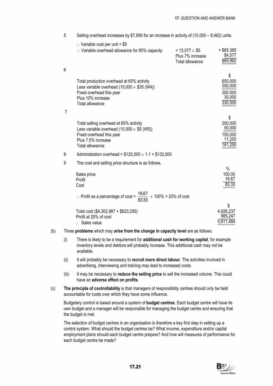
17: QUESTION AND ANSWER BANK
17.21
5 Selling overhead increases by $7,690 for an increase in activity of (10,000 – 8,462) units.
∴Variable cost per unit = $5 ∴Variable overhead allowance for 85% capacity = 13,077 × $5 = $65,385 Plus 7% increase $4,577 Total allowance $69,962
6 $ Total production overhead at 65% activity 650,000Less variable overhead (10,000 × $35 (W4)) 350,000Fixed overhead this year 300,000Plus 10% increase 30,000Total allowance 330,000
7 $ Total selling overhead at 65% activity 200,000 Less variable overhead (10,000 × $5 (W5)) 50,000 Fixed overhead this year 150,000 Plus 7.5% increase 11,250 Total allowance 161,250
8 Administration overhead = $120,000 × 1.1 = $132,000
9 The cost and selling price structure is as follows. % Sales price 100.00 Profit 16.67 Cost 83.33
∴Profit as a percentage of cost = 33.8367.16 × 100% = 20% of cost
$ Total cost ($4,302,987 + $623,250) 4,926,237 Profit at 20% of cost 985,247 ∴ Sales value 5,911,484
(b) Three problems which may arise from the change in capacity level are as follows.
(i) There is likely to be a requirement for additional cash for working capital, for example inventory levels and debtors will probably increase. This additional cash may not be available.
(ii) It will probably be necessary to recruit more direct labour. The activities involved in advertising, interviewing and training may lead to increased costs.
(iii) It may be necessary to reduce the selling price to sell the increased volume. This could have an adverse effect on profits.
(c) The principle of controllability is that managers of responsibility centres should only be held accountable for costs over which they have some influence.
Budgetary control is based around a system of budget centres. Each budget centre will have its own budget and a manager will be responsible for managing the budget centre and ensuring that the budget is met.
The selection of budget centres in an organisation is therefore a key first step in setting up a control system. What should the budget centres be? What income, expenditure and/or capital employment plans should each budget centre prepare? And how will measures of performance for each budget centre be made?

17: QUESTION AND ANSWER BANK
17.22
Budgetary control and budget centres are therefore part of the overall system of responsibility accounting within an organisation.
Controllable costs are items of expenditure which can be directly influenced by a given manager within a given time span.
Care must be taken to distinguish between controllable costs and uncontrollable costs in variance reporting. The controllability principle is that managers of responsibility centres should only be held accountable for costs over which they have some influence. From a motivation point of view this is important because it can be very demoralising for managers who feel that their performance is being judged on the basis of something over which they have no influence. It is also important from a control point of view in that control reports should ensure that information on costs is reported to the manager who is able to take action to control them.
Responsibility accounting attempts to associate costs, revenues, assets and liabilities with the managers most capable of controlling them. As a system of accounting, it therefore distinguishes between controllable and uncontrollable costs.
Most variable costs within a department are thought to be controllable in the short term because managers can influence the efficiency with which resources are used, even if they cannot do anything to raise or lower price levels.
A cost which is not controllable by a junior manager might be controllable by a senior manager. For example, there may be high direct labour costs in a department caused by excessive overtime working. The junior manager may feel obliged to continue with the overtime to meet production schedules, but his senior may be able to reduce costs by hiring extra full-time staff, thereby reducing the requirements for overtime.
A cost which is not controllable by a manager in one department may be controllable by a manager in another department. For example, an increase in material costs may be caused by buying at higher prices than expected (controllable by the purchasing department) or by excessive wastage (controllable by the production department) or by a faulty machine producing rejects (controllable by the maintenance department).
Some costs are non-controllable, such as increases in expenditure items due to inflation. Other costs are controllable, but in the long term rather than the short term. For example, production costs might be reduced by the introduction of new machinery and technology, but in the short term, management must attempt to do the best they can with the resources and machinery at their disposal.
It is not always so easy in practice to distinguish controllable from uncontrollable costs. Apportioned overhead costs provide a good example.
Suppose that a manager of a production department in a manufacturing company is made responsible for the costs of his department. These costs include directly attributable overhead items such as the costs of indirect labour employed and indirect materials consumed in the department. The department's overhead costs also include an apportionment of costs from other cost centres, such as rent and rates for the building it shares with other departments and a share of the costs of the maintenance department.
Should the production manager be held accountable for any of these apportioned costs?
(i) Managers should not be held accountable for costs over which they have no control. In this example, apportioned rent and rates costs would not be controllable by the production department manager.
(ii) Managers should be held accountable for costs over which they have some influence. In this example, it is the responsibility of the maintenance department manager to keep maintenance costs within budget. But their costs will be partly variable and partly fixed, and the variable cost element will depend on the volume of demand for their services. If the production department's staff treat their equipment badly we might expect higher repair

17: QUESTION AND ANSWER BANK
17.23
costs, and the production department manager should therefore be made accountable for the repair costs that his department makes the maintenance department incur on its behalf.
(iii) Charging the production department with some of the costs of the maintenance department prevents the production department from viewing the maintenance services as 'free services'. Over-use would be discouraged and the production manager is more likely to question the activities of the maintenance department possibly resulting in a reduction in maintenance costs or the provision of more efficient maintenance services.
7 ACCA-Chem Text references. Variance calculations are explained in Chapter 11 of your Study Text and time series is covered in Chapter 9a.
Top tips. We have calculated the variances in (a)(i)(3) in terms of kilograms rather than batches and have followed the methodology adopted in the BPP Study Text for Paper F5. You may well have used a different approach to arrive at the same answer.
There are quite a lot of calculations in this question. Whilst it's easy to say that you should split your time so that you spend enough time on the written elements, written element (a) (v) is dependent upon your answer to the earlier calculations. However (b) can be done separately, and it may be best to do (b) first as it is a straightforward test of your knowledge of time series.
Work through (a) (v) carefully, and make sure you understand the link between the different variances.
(a) (i) (1) Price variances $ $ Material F 1,680 kgs should have cost (× $4) 6,720 but did cost (× $4.25) 7,140 420 (A) Material G 1,650 kgs should have cost (× $3) 4,950 but did cost (× $2.80) 4,620 330 (F) Material H 870 kgs should have cost (× $6) 5,220 but did cost (× $6.40) 5,568 348 (A) Total material price variance 438 (A)
(2) Usage variances F G H
1 kg of output of 15/35 × 35/32 12/35 × 35/32 8/35 × 35/32 product W should need = 0.46875 kgs = 0.375 kgs = 0.25 kgs 3,648 kgs of output of
product W should need 1,710 kgs 1,368 kgs 912 kgs but did need 1,680 kgs 1,650 kgs 870 kgs Usage variance in kgs 30 kgs(F) 282 kgs (A) 42 kgs(F) × standard price per kg × $4 × $3 × $6 Usage variance in $ $120 (F) $846 (A) $252 (F) Total material usage variance = $474 (A)

17: QUESTION AND ANSWER BANK
17.24
(3) Mix variances
Standard mix for actual use Total kgs used = 4,200 kgs Kgs F 15/35 × 4,200 = 1,800 G 12/35 × 4,200 = 1,440 H 8/35 × 4,200 = 960 4,200 Actual usage in standard Actual usage Standard cost mix in actual mix Variance per kg Variance Kgs Kgs Kgs $ $ F 1,800 1,680 120 (F) 4 480 (F) G 1,440 1,650 210 (A) 3 630 (A) H 960 870 90 (F) 6 540 (F) 4,200 4,200 – 390 (F)
Total mix variance = $390 (F)
(4) Yield variance
Each kg of Product W requires (1 × 35/32) kg of input costing $4.50 ($144/32) 4,200 kgs should have yielded (÷ 35/32) 3,840 kgs but did yield 3,648 kgs Yield variance in kgs 192 (A) × standard cost per kg × $4.50 Total material yield variance $864 (A)
(ii) (1) Dept P Dept Q Total $ $ $ 120 batches should have cost (× $40) 4,800 (× $12) 1,440 6,240 but did cost 6,360 1,512 7,872 Labour cost variance 1,560 (A) 72 (A) 1,632 (A)
(2) Dept P Dept Q Total 120 batches should have taken (× 4) 480 hrs (× 2) 240 hrs but did take 600 hrs 270 hrs 120 hrs (A) 30 hrs (A) × standard rate per hour × $10 × $6 Labour efficiency variance $1,200 (A) $180 (A) $1,380 (A)
(3) Dept P Dept Q Total $ $ $ 600 hrs/270 hrs should have cost (× $10) 6,000 (× $6) 1,620 7,620 but did cost 6,360 1,512 7,872 Labour rate variance 360 (A) 108 (F) 252 (A)
(iii) $ 3,648 kgs should have sold for (× $16) 58,368 but did sell for (× $16.75) 61,104 Selling price variance 2,736 (F) Budgeted sales for period 4,096 kgs Actual sales volume 3,648 kgs Volume variance in kgs 448 kgs(A) × standard profit per kg ($(16 – (196/32)) × $9.875 Sales volume profit variance $4,424 (A)

17: QUESTION AND ANSWER BANK
17.25
(iv) Adverse yield variance An analysis of the materials mix variance (see (a)(i)(3)) shows that 120 kgs of F and 90 kgs of H (the more expensive materials) were replaced by 210 kgs of G (the cheapest material). This substitution of cheaper material could have led to the adverse yield variance. It is also possible that the yield variance was because the material G that was used was of a lower than standard quality since it was purchased at a price below its standard price. Adverse efficiency variance The adverse labour efficiency variance may have been due to Material G taking longer to process than normal because it was of a poor quality. Alternatively, the fact that in Department Q the actual rate was less than the standard rate could mean that less skilled labour was used than provided for in the standard, and that this then lowered productivity with the result that the yield was lower than expected.
(b) Use of time series A time series is a series of figures or values recorded over time, for example monthly sales levels. The analysis of such a series can assist the management accountant to make assumptions about the future for budgeting purposes, for example. It is especially useful when attempting to forecast sales and helps with the following. (i) Extrapolation of past figures into the future (trend analysis)
This assumes that historical relationships between figures will continue. This is manifestly dangerous and can result in firms being caught out at the beginning of an economic recession when they have continued to extrapolate growth in their forecasts without taking account of signs of change in the external operating environment.
(ii) Identification of seasonal variations
This can be helpful when sales are known to have a strong seasonal component, such as sales of Christmas decorations.
(iii) Identification of cyclical variations on a scale longer than seasonal variations
These are generally related to the larger economic cycle and should therefore be used in conjunction with general economic forecasts, not in isolation. If time series data is built up over a period, it may also assist in the identification of events which are abnormal and which could signal the start of a major structural change in the market. As the examples show, however, time series analysis should not be used in isolation but as part of a range of techniques when attempting to forecast the future.
8 Divisional performance measures Top tips. Parts (a) and (b) require you to demonstrate knowledge you should have picked up directly from the Text. No application skills are required at all in this instance.
That being said, it is vital that you do not learn the advantages and disadvantages of ROI and RI in a parrot fashion as they underlie the very core of the subject. You must understand how and why ROI affects managerial behaviour, for example. You are just as likely to get a written question on this area as a calculation-based one.
The calculations required in (b) should not have caused you any problems.
Part (c) is basic book knowledge and so you should have been able to score quite a few of the marks available.
(a) The residual income (RI) for a division is calculated by deducting from the divisional profit an imputed interest charge, based on the investment in the division.

17: QUESTION AND ANSWER BANK
17.26
The return on investment (ROI) is the divisional profit expressed as a percentage of the investment in the division.
Both methods use the same basic figure for profit and investment, but residual income produces an absolute measure whereas the return on investment is expressed as a percentage.
Both methods suffer from disadvantages in measuring the profit and the investment in a division which include the following.
(i) Assets must be valued consistently at historical cost or at replacement cost. Neither valuation basis is ideal.
(ii) Divisions might use different bases to value inventory and to calculate depreciation.
(iii) Any charges made for the use of head office services or allocations of head office assets to divisions are likely to be arbitrary.
In addition, return on investment suffers from the following disadvantages.
(i) Rigid adherence to the need to maintain ROI in the short term can discourage managers from investing in new assets, since average divisional ROI tends to fall in the early stages of a new investment. Residual income can overcome this problem by highlighting projects which return more than the cost of capital.
(ii) It can be difficult to compare the percentage ROI results of divisions if their activities are very different: residual income can overcome this problem through the use of different interest rates for different divisions.
(b) (i) Return on divisional investment (ROI)
Before investment After investment Divisional profit £18,000 £19,600 Divisional investment £100,000 £110,000 Divisional ROI 18.0% 17.8% The ROI will fall in the short term if the new investment is undertaken. This is a problem which often arises with ROI, as noted in part (a) of this solution.
(ii) Divisional residual income Before investment After investment £ £ Divisional profit 18,000 19,600 Less imputed interest: £100,000 × 15% 15,000 £110,000 × 15% 16,500 Residual income 3,000 3,100 The residual income will increase if the new investment is undertaken. The use of residual income has highlighted the fact that the new project returns more than the cost of capital (16% compared with 15%).
(c) Potential benefits of operating a transfer pricing system within a divisionalised company
(i) It can lead to goal congruence by motivating divisional managers to make decisions, which improve divisional profit and improve profit of the organisation as a whole.
(ii) It can prevent dysfunctional decision making so that decisions taken by a divisional manager are in the best interests of his own part of the business, other divisions and the organisation as a whole.
(iii) Transfer prices can be set at a level that enables divisional performance to be measured 'commercially'. A transfer pricing system should therefore report a level of divisional profit that is a reasonable measure of the managerial performance of the division.

17: QUESTION AND ANSWER BANK
17.27
(iv) It should ensure that divisional autonomy is not undermined. A well-run transfer pricing system helps to ensure that a balance is kept between divisional autonomy to provide incentives and motivation, and centralised authority to ensure that the divisions are all working towards the same target, the benefit of the organisation as a whole.
9 Non-profit seeking organisations Top tips. Like many examination questions, part (a) can be answered by taking a logical, structured approach that is offered to you by the wording of the question itself. You can take (1) efficiency and (2) effectiveness in turn (this solution opts to deal with effectiveness first) and explain for each why the absence of a profit measure causes problems. This suggest that you need to explain why the presence of a profit measure helps with the assessment of efficiency and effectiveness.
Take note of the examples about objectives we have provided in part (a)(i) – they may prove useful in your exam as this requirement is perhaps one of the more likely to appear on the subject of non-profit seeking organisations.
Note the need to provide examples in part (a)(ii) – this means at least one! As well as the given similarity between profit-seeking and non-profit seeking organisations, don't forget that the distinctions between the two types of organisation are becoming blurred.
For part (b), remember that indicators need to be compared against a yardstick to be of any use for performance measurement purposes. The fact that 8% of appointments were cancelled is useless information. When considered in conjunction with a target of 5%, it becomes useful!
(a) (i) Effectiveness refers to the use of resources so as to achieve desired ends or objectives or outputs.
In a profit-making organisation, objectives can be expressed financially in terms of a target profit or return. The organisation, or profit centres within the organisation, can be judged to have operated effectively if they have achieved a target profit within a given period.
In non-profit seeking organisations, effectiveness cannot be measured in this way. The organisation's objectives cannot be expressed in financial terms at all, and non-financial objectives need to be established. The effectiveness of performance could be measured in terms of whether targeted non-financial objectives have been achieved, but there are several problems involved in trying to do this.
(1) The organisation might have several different objectives which are difficult to reconcile with each other. Achieving one objective might only be possible at the expense of failing to achieve another. For example, schools have the objective of providing education. They teach a certain curriculum, but by opting to educate students in some subjects, there is no time available to provide education in other subjects.
(2) A non-profit seeking organisation will invariably be restricted in what it can achieve by the availability of funds. The health service, for example, has the objective of providing health care, but since funds are restricted there is a limit to the amount of care that can be provided, and there will be competition for funds between different parts of the service.
(3) The objectives of non-profit seeking organisations are also difficult to establish because the quality of the service provided will be a significant feature of their service. For example, a local authority has, amongst its various different objectives, the objective of providing a rubbish collection service. The effectiveness of this service can only be judged by establishing what standard or quality of service is required.

17: QUESTION AND ANSWER BANK
17.28
(4) With differing objectives, none of them directly comparable, and none that can be expressed in profit terms, human judgement is likely to be involved in deciding whether an organisation has been effective or not. This is most clearly seen in government organisations where political views cloud opinion about the government's performance.
Efficiency refers to the rate at which resources are consumed to achieve desired ends. Efficiency measurements compare the output produced by the organisation with the resources employed or used up to achieve the output. They are used to control the consumption of resources, so that the maximum output is achieved by a given amount of input resources, or a certain volume of output is produced within the minimum resources being used up.
In profit-making organisations, the efficiency of the organisation as a whole can be measured in terms of return on capital employed. Individual profit centres or operating units within the organisation can also have efficiency measured by relating the quantity of output produced, which has a market value and therefore a quantifiable financial value, to the resources (and their costs) required to make the output.
In non-profit seeking organisations, output does not usually have a market value, and it is therefore more difficult to measure efficiency. This difficulty is compounded by the fact that since these organisations often have several different objectives, it is difficult to compare the efficiency of one operation with the efficiency of another. For example, with the police force, it might be difficult to compare the efficiency of a serious crimes squad with the efficiency of the traffic police, because each has its own 'outputs' that are not easily comparable in terms of 'value achieved'.
In spite of the difficulties of measuring effectiveness and efficiency, control over the performance of non-profit seeking organisations can only be satisfactorily achieved by assessments of 'value for money' (economy, efficiency and effectiveness).
(ii) The same problems extend to support activities within profit-motivated organisations, where these activities are not directly involved in the creation of output and sales. Examples include research and development, the personnel function, the accountancy function and so on.
(1) Some of the outputs of these functions cannot be measured in market values.
(2) The objectives of the functions are not easily expressed in quantifiable terms.
Examples
(1) Within the personnel department, outputs from activities such as training and some aspects of recruitment can be given market price values by estimating what the same services would cost if provided by an external organisation. Other activities, however, do not have any such market valuation. Welfare is an example. Its objective is to provide support for employees in their personal affairs, but since this objective cannot easily be expressed as quantifiable targets, and does not have a market price valuation, the effectiveness and efficiency of work done by welfare staff cannot be measured easily.
(2) Within the accountancy department, outputs from management accountants are management information. This does not have an easily-measured market value, and information's value depends more on quality than quantity. The contribution of management accounting to profitability is difficult to judge, and so the efficiency and effectiveness of the function are difficult to measure.
(b) (i) To measure effectiveness, we need to establish objectives or targets for performance. Since these cannot be expressed financially, non-financial targets must be used. The effective level of achievement could be measured by comparing actual performance against target.

17: QUESTION AND ANSWER BANK
17.29
Adherence to appointment times
(1) Percentage of appointments kept on time (2) Percentage of appointments no more than 10 minutes late (3) Percentage of appointments kept within 30 minutes of schedule (4) Percentage of cancelled appointments (5) Average delay in appointments
A problem with these measures is that there is an implied assumption that all patients will be at the clinic by their appointed time. In practice, this will not always be the case.
Patients' ability to contact the clinic and make appointments
(1) Percentage of patients who can make an appointment at their first preferred time, or at the first date offered to them
(2) Average time from making an appointment to the appointment date
(3) Number of complaints about failure to contact the clinic, as a percentage of total patients seen
(4) If the telephone answering system provides for queuing of calls, the average waiting-for-answer times for callers and the percentage of abandoned calls
Comprehensive monitoring programme
Measures might be based on the definition of each element or step within a monitoring programme for a patient, It would then be possible to measure the following.
(1) Percentage of patients receiving every stage of the programme (and percentage receiving every stage but one, every stage but two, and so on)
(2) If each stage has a scheduled date for completion, the average delay for patients in the completion of each stage
(ii) A single quality of care measure would call for subjective judgements about the following.
(1) The key objective/objectives for each of the three features of service (2) The relative weighting that should be given to each
The objectives would have to be measured on comparable terms, and since money values are inappropriate, an index based on percentage or a points-scoring system of measurement might be used. A target index or points score for achievement could then be set, and actual results compared against the target.

17: QUESTION AND ANSWER BANK
17.30
END OF ANSWER BANK

18.1
Appendix A:Pilot paper

18: APPENDIX A: PILOT PAPER
18.2

18: APPENDIX A: PILOT PAPER
18.3

18: APPENDIX A: PILOT PAPER
18.4

18: APPENDIX A: PILOT PAPER
18.5

18: APPENDIX A: PILOT PAPER
18.6

18: APPENDIX A: PILOT PAPER
18.7

18: APPENDIX A: PILOT PAPER
18.8
END OF APPENDIX A

19.1
Appendix B:Relevant articles

19: APPENDIX B: RELEVANT ARTICLES
19.2

19: APPENDIX B: RELEVANT ARTICLES
19.3

19: APPENDIX B: RELEVANT ARTICLES
19.4
END OF APPENDIX B

20.1
Mathematicalformulae

20: APPENDIX C: MATHEMATICAL FORMULAE
20.2
Mathematical formulae
Learning curve
Y = axb
Where y = average cost per batch a = cost of first batch x = total number of batches produced b = learning factor (log LR/log 2) LR = the learning rate as a decimal
Regression analysis
y = a + bx
b = 22 )x(xn
yxxyn
∑−∑
∑∑−∑
a = n
xbny ∑−
∑
Demand curve
P = a – bQ
b = quantity in change
price in change
a = price when Q = 0
END OF MATHEMATICAL FORMULAE


![[Info] FAQs - Contractor Performance Management System](https://img.dokumen.tips/doc/110x75/63249d7b117b4414ec0cd886/info-faqs-contractor-performance-management-system.jpg)


