Package 'car' - Microsoft R Application Network

Package ‘car’December 23, 2019

Version 3.0-6

Date 2019-12-20

Title Companion to Applied Regression

Depends R (>= 3.5.0), carData (>= 3.0-0)

Imports abind, MASS, mgcv, nnet, pbkrtest (>= 0.4-4), quantreg,grDevices, utils, stats, graphics, maptools, rio, lme4, nlme

Suggests alr4, boot, coxme, leaps, lmtest, Matrix, MatrixModels, rgl(>= 0.93.960), sandwich, SparseM, survival, survey

ByteCompile yes

LazyLoad yes

Description Functions to Accompany J. Fox and S. Weisberg,An R Companion to Applied Regression, Third Edition, Sage, 2019.

License GPL (>= 2)

URL https://r-forge.r-project.org/projects/car/,

https://CRAN.R-project.org/package=car,

http://socserv.socsci.mcmaster.ca/jfox/Books/Companion/index.html

Author John Fox [aut, cre],Sanford Weisberg [aut],Brad Price [aut],Daniel Adler [ctb],Douglas Bates [ctb],Gabriel Baud-Bovy [ctb],Ben Bolker [ctb],Steve Ellison [ctb],David Firth [ctb],Michael Friendly [ctb],Gregor Gorjanc [ctb],Spencer Graves [ctb],Richard Heiberger [ctb],Pavel Krivitsky [ctb],Rafael Laboissiere [ctb],Martin Maechler [ctb],

1

https://r-forge.r-project.org/projects/car/

https://CRAN.R-project.org/package=car

http://socserv.socsci.mcmaster.ca/jfox/Books/Companion/index.html

2 R topics documented:

Georges Monette [ctb],Duncan Murdoch [ctb],Henric Nilsson [ctb],Derek Ogle [ctb],Brian Ripley [ctb],William Venables [ctb],Steve Walker [ctb],David Winsemius [ctb],Achim Zeileis [ctb],R-Core [ctb]

Maintainer John Fox <[email protected]>

Repository CRAN

Repository/R-Forge/Project car

Repository/R-Forge/Revision 617

Repository/R-Forge/DateTimeStamp 2019-12-20 14:33:56

Date/Publication 2019-12-23 11:10:02 UTC

NeedsCompilation no

R topics documented:Anova . . . . . . . . . . . . . . . . . . . . . . . . . . . . . . . . . . . . . . . . . . . . 4avPlots . . . . . . . . . . . . . . . . . . . . . . . . . . . . . . . . . . . . . . . . . . . . 11bcPower . . . . . . . . . . . . . . . . . . . . . . . . . . . . . . . . . . . . . . . . . . . 13Boot . . . . . . . . . . . . . . . . . . . . . . . . . . . . . . . . . . . . . . . . . . . . . 15boxCox . . . . . . . . . . . . . . . . . . . . . . . . . . . . . . . . . . . . . . . . . . . 18boxCoxVariable . . . . . . . . . . . . . . . . . . . . . . . . . . . . . . . . . . . . . . . 21Boxplot . . . . . . . . . . . . . . . . . . . . . . . . . . . . . . . . . . . . . . . . . . . 22boxTidwell . . . . . . . . . . . . . . . . . . . . . . . . . . . . . . . . . . . . . . . . . 23brief . . . . . . . . . . . . . . . . . . . . . . . . . . . . . . . . . . . . . . . . . . . . . 25car-defunct . . . . . . . . . . . . . . . . . . . . . . . . . . . . . . . . . . . . . . . . . 28car-deprecated . . . . . . . . . . . . . . . . . . . . . . . . . . . . . . . . . . . . . . . . 29car-internal.Rd . . . . . . . . . . . . . . . . . . . . . . . . . . . . . . . . . . . . . . . 30carHexsticker . . . . . . . . . . . . . . . . . . . . . . . . . . . . . . . . . . . . . . . . 30carPalette . . . . . . . . . . . . . . . . . . . . . . . . . . . . . . . . . . . . . . . . . . 31carWeb . . . . . . . . . . . . . . . . . . . . . . . . . . . . . . . . . . . . . . . . . . . 32ceresPlots . . . . . . . . . . . . . . . . . . . . . . . . . . . . . . . . . . . . . . . . . . 33compareCoefs . . . . . . . . . . . . . . . . . . . . . . . . . . . . . . . . . . . . . . . . 35Contrasts . . . . . . . . . . . . . . . . . . . . . . . . . . . . . . . . . . . . . . . . . . 36crPlots . . . . . . . . . . . . . . . . . . . . . . . . . . . . . . . . . . . . . . . . . . . . 38deltaMethod . . . . . . . . . . . . . . . . . . . . . . . . . . . . . . . . . . . . . . . . . 40densityPlot . . . . . . . . . . . . . . . . . . . . . . . . . . . . . . . . . . . . . . . . . 44dfbetaPlots . . . . . . . . . . . . . . . . . . . . . . . . . . . . . . . . . . . . . . . . . 47durbinWatsonTest . . . . . . . . . . . . . . . . . . . . . . . . . . . . . . . . . . . . . . 49Ellipses . . . . . . . . . . . . . . . . . . . . . . . . . . . . . . . . . . . . . . . . . . . 50Export . . . . . . . . . . . . . . . . . . . . . . . . . . . . . . . . . . . . . . . . . . . . 54hccm . . . . . . . . . . . . . . . . . . . . . . . . . . . . . . . . . . . . . . . . . . . . . 55

R topics documented: 3

hist.boot . . . . . . . . . . . . . . . . . . . . . . . . . . . . . . . . . . . . . . . . . . . 57Import . . . . . . . . . . . . . . . . . . . . . . . . . . . . . . . . . . . . . . . . . . . . 60infIndexPlot . . . . . . . . . . . . . . . . . . . . . . . . . . . . . . . . . . . . . . . . . 61influence.mixed.models . . . . . . . . . . . . . . . . . . . . . . . . . . . . . . . . . . . 62influencePlot . . . . . . . . . . . . . . . . . . . . . . . . . . . . . . . . . . . . . . . . 65invResPlot . . . . . . . . . . . . . . . . . . . . . . . . . . . . . . . . . . . . . . . . . . 66invTranPlot . . . . . . . . . . . . . . . . . . . . . . . . . . . . . . . . . . . . . . . . . 68leveneTest . . . . . . . . . . . . . . . . . . . . . . . . . . . . . . . . . . . . . . . . . . 70leveragePlots . . . . . . . . . . . . . . . . . . . . . . . . . . . . . . . . . . . . . . . . 71linearHypothesis . . . . . . . . . . . . . . . . . . . . . . . . . . . . . . . . . . . . . . 73logit . . . . . . . . . . . . . . . . . . . . . . . . . . . . . . . . . . . . . . . . . . . . . 79mcPlots . . . . . . . . . . . . . . . . . . . . . . . . . . . . . . . . . . . . . . . . . . . 81mmps . . . . . . . . . . . . . . . . . . . . . . . . . . . . . . . . . . . . . . . . . . . . 83ncvTest . . . . . . . . . . . . . . . . . . . . . . . . . . . . . . . . . . . . . . . . . . . 87outlierTest . . . . . . . . . . . . . . . . . . . . . . . . . . . . . . . . . . . . . . . . . . 88panel.car . . . . . . . . . . . . . . . . . . . . . . . . . . . . . . . . . . . . . . . . . . . 90poTest . . . . . . . . . . . . . . . . . . . . . . . . . . . . . . . . . . . . . . . . . . . . 91powerTransform . . . . . . . . . . . . . . . . . . . . . . . . . . . . . . . . . . . . . . . 92Predict . . . . . . . . . . . . . . . . . . . . . . . . . . . . . . . . . . . . . . . . . . . . 96qqPlot . . . . . . . . . . . . . . . . . . . . . . . . . . . . . . . . . . . . . . . . . . . . 97recode . . . . . . . . . . . . . . . . . . . . . . . . . . . . . . . . . . . . . . . . . . . . 100regLine . . . . . . . . . . . . . . . . . . . . . . . . . . . . . . . . . . . . . . . . . . . 101residualPlots . . . . . . . . . . . . . . . . . . . . . . . . . . . . . . . . . . . . . . . . . 102S . . . . . . . . . . . . . . . . . . . . . . . . . . . . . . . . . . . . . . . . . . . . . . . 106scatter3d . . . . . . . . . . . . . . . . . . . . . . . . . . . . . . . . . . . . . . . . . . . 111scatterplot . . . . . . . . . . . . . . . . . . . . . . . . . . . . . . . . . . . . . . . . . . 115scatterplotMatrix . . . . . . . . . . . . . . . . . . . . . . . . . . . . . . . . . . . . . . 119ScatterplotSmoothers . . . . . . . . . . . . . . . . . . . . . . . . . . . . . . . . . . . . 122showLabels . . . . . . . . . . . . . . . . . . . . . . . . . . . . . . . . . . . . . . . . . 125sigmaHat . . . . . . . . . . . . . . . . . . . . . . . . . . . . . . . . . . . . . . . . . . 127some . . . . . . . . . . . . . . . . . . . . . . . . . . . . . . . . . . . . . . . . . . . . . 128spreadLevelPlot . . . . . . . . . . . . . . . . . . . . . . . . . . . . . . . . . . . . . . . 129subsets . . . . . . . . . . . . . . . . . . . . . . . . . . . . . . . . . . . . . . . . . . . . 132symbox . . . . . . . . . . . . . . . . . . . . . . . . . . . . . . . . . . . . . . . . . . . 133Tapply . . . . . . . . . . . . . . . . . . . . . . . . . . . . . . . . . . . . . . . . . . . . 135testTransform . . . . . . . . . . . . . . . . . . . . . . . . . . . . . . . . . . . . . . . . 136TransformationAxes . . . . . . . . . . . . . . . . . . . . . . . . . . . . . . . . . . . . 138vif . . . . . . . . . . . . . . . . . . . . . . . . . . . . . . . . . . . . . . . . . . . . . . 140wcrossprod . . . . . . . . . . . . . . . . . . . . . . . . . . . . . . . . . . . . . . . . . 142whichNames . . . . . . . . . . . . . . . . . . . . . . . . . . . . . . . . . . . . . . . . 143

Index 145

4 Anova

Anova Anova Tables for Various Statistical Models

Description

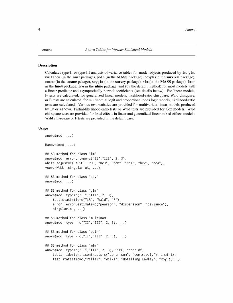
Calculates type-II or type-III analysis-of-variance tables for model objects produced by lm, glm,multinom (in the nnet package), polr (in the MASS package), coxph (in the survival package),coxme (in the coxme pckage), svyglm (in the survey package), rlm (in the MASS package), lmerin the lme4 package, lme in the nlme package, and (by the default method) for most models witha linear predictor and asymptotically normal coefficients (see details below). For linear models,F-tests are calculated; for generalized linear models, likelihood-ratio chisquare, Wald chisquare,or F-tests are calculated; for multinomial logit and proportional-odds logit models, likelihood-ratiotests are calculated. Various test statistics are provided for multivariate linear models producedby lm or manova. Partial-likelihood-ratio tests or Wald tests are provided for Cox models. Waldchi-square tests are provided for fixed effects in linear and generalized linear mixed-effects models.Wald chi-square or F tests are provided in the default case.

Usage

Anova(mod, ...)

Manova(mod, ...)

## S3 method for class 'lm'Anova(mod, error, type=c("II","III", 2, 3),white.adjust=c(FALSE, TRUE, "hc3", "hc0", "hc1", "hc2", "hc4"),vcov.=NULL, singular.ok, ...)

## S3 method for class 'aov'Anova(mod, ...)

## S3 method for class 'glm'Anova(mod, type=c("II","III", 2, 3),

test.statistic=c("LR", "Wald", "F"),error, error.estimate=c("pearson", "dispersion", "deviance"),singular.ok, ...)

## S3 method for class 'multinom'Anova(mod, type = c("II","III", 2, 3), ...)

## S3 method for class 'polr'Anova(mod, type = c("II","III", 2, 3), ...)

## S3 method for class 'mlm'Anova(mod, type=c("II","III", 2, 3), SSPE, error.df,

idata, idesign, icontrasts=c("contr.sum", "contr.poly"), imatrix,test.statistic=c("Pillai", "Wilks", "Hotelling-Lawley", "Roy"),...)

Anova 5

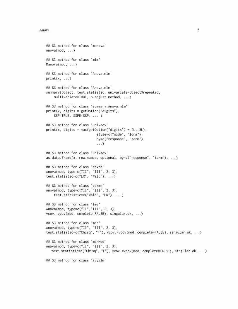
## S3 method for class 'manova'Anova(mod, ...)

## S3 method for class 'mlm'Manova(mod, ...)

## S3 method for class 'Anova.mlm'print(x, ...)

## S3 method for class 'Anova.mlm'summary(object, test.statistic, univariate=object$repeated,

multivariate=TRUE, p.adjust.method, ...)

## S3 method for class 'summary.Anova.mlm'print(x, digits = getOption("digits"),

SSP=TRUE, SSPE=SSP, ... )

## S3 method for class 'univaov'print(x, digits = max(getOption("digits") - 2L, 3L),

style=c("wide", "long"),by=c("response", "term"),...)

## S3 method for class 'univaov'as.data.frame(x, row.names, optional, by=c("response", "term"), ...)

## S3 method for class 'coxph'Anova(mod, type=c("II", "III", 2, 3),test.statistic=c("LR", "Wald"), ...)

## S3 method for class 'coxme'Anova(mod, type=c("II", "III", 2, 3),

test.statistic=c("Wald", "LR"), ...)

## S3 method for class 'lme'Anova(mod, type=c("II","III", 2, 3),vcov.=vcov(mod, complete=FALSE), singular.ok, ...)

## S3 method for class 'mer'Anova(mod, type=c("II", "III", 2, 3),test.statistic=c("Chisq", "F"), vcov.=vcov(mod, complete=FALSE), singular.ok, ...)

## S3 method for class 'merMod'Anova(mod, type=c("II", "III", 2, 3),

test.statistic=c("Chisq", "F"), vcov.=vcov(mod, complete=FALSE), singular.ok, ...)

## S3 method for class 'svyglm'

6 Anova

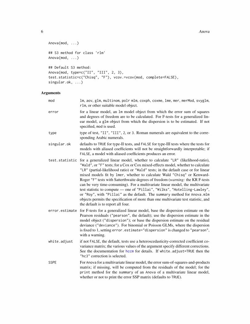
Anova(mod, ...)

## S3 method for class 'rlm'Anova(mod, ...)

## Default S3 method:Anova(mod, type=c("II", "III", 2, 3),test.statistic=c("Chisq", "F"), vcov.=vcov(mod, complete=FALSE),singular.ok, ...)

Arguments

mod lm, aov, glm, multinom, polr mlm, coxph, coxme, lme, mer, merMod, svyglm,rlm, or other suitable model object.

error for a linear model, an lm model object from which the error sum of squaresand degrees of freedom are to be calculated. For F-tests for a generalized lin-ear model, a glm object from which the dispersion is to be estimated. If notspecified, mod is used.

type type of test, "II", "III", 2, or 3. Roman numerals are equivalent to the corre-sponding Arabic numerals.

singular.ok defaults to TRUE for type-II tests, and FALSE for type-III tests where the tests formodels with aliased coefficients will not be straightforwardly interpretable; ifFALSE, a model with aliased coefficients produces an error.

test.statistic for a generalized linear model, whether to calculate "LR" (likelihood-ratio),"Wald", or "F" tests; for a Cox or Cox mixed-effects model, whether to calculate"LR" (partial-likelihood ratio) or "Wald" tests; in the default case or for linearmixed models fit by lmer, whether to calculate Wald "Chisq" or Kenward-Roger "F" tests with Satterthwaite degrees of freedom (warning: the KR F-testscan be very time-consuming). For a multivariate linear model, the multivariatetest statistic to compute — one of "Pillai", "Wilks", "Hotelling-Lawley",or "Roy", with "Pillai" as the default. The summary method for Anova.mlmobjects permits the specification of more than one multivariate test statistic, andthe default is to report all four.

error.estimate for F-tests for a generalized linear model, base the dispersion estimate on thePearson residuals ("pearson", the default); use the dispersion estimate in themodel object ("dispersion"); or base the dispersion estimate on the residualdeviance ("deviance"). For binomial or Poisson GLMs, where the dispersionis fixed to 1, setting error.estimate="dispersion" is changed to "pearson",with a warning.

white.adjust if not FALSE, the default, tests use a heteroscedasticity-corrected coefficient co-variance matrix; the various values of the argument specify different corrections.See the documentation for hccm for details. If white.adjust=TRUE then the"hc3" correction is selected.

SSPE For Anova for a multivariate linear model, the error sum-of-squares-and-productsmatrix; if missing, will be computed from the residuals of the model; for theprint method for the summary of an Anova of a multivariate linear model,whether or not to print the error SSP matrix (defaults to TRUE).

Anova 7

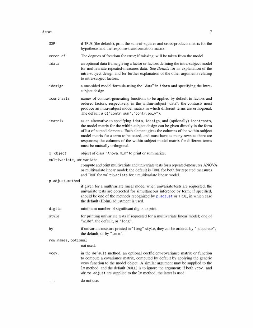
SSP if TRUE (the default), print the sum-of-squares and cross-products matrix for thehypothesis and the response-transformation matrix.

error.df The degrees of freedom for error; if missing, will be taken from the model.

idata an optional data frame giving a factor or factors defining the intra-subject modelfor multivariate repeated-measures data. See Details for an explanation of theintra-subject design and for further explanation of the other arguments relatingto intra-subject factors.

idesign a one-sided model formula using the “data” in idata and specifying the intra-subject design.

icontrasts names of contrast-generating functions to be applied by default to factors andordered factors, respectively, in the within-subject “data”; the contrasts mustproduce an intra-subject model matrix in which different terms are orthogonal.The default is c("contr.sum","contr.poly").

imatrix as an alternative to specifying idata, idesign, and (optionally) icontrasts,the model matrix for the within-subject design can be given directly in the formof list of named elements. Each element gives the columns of the within-subjectmodel matrix for a term to be tested, and must have as many rows as there areresponses; the columns of the within-subject model matrix for different termsmust be mutually orthogonal.

x, object object of class "Anova.mlm" to print or summarize.

multivariate, univariate

compute and print multivariate and univariate tests for a repeated-measures ANOVAor multivariate linear model; the default is TRUE for both for repeated measuresand TRUE for multivariate for a multivariate linear model.

p.adjust.method

if given for a multivariate linear model when univariate tests are requested, theunivariate tests are corrected for simultaneous inference by term; if specified,should be one of the methods recognized by p.adjust or TRUE, in which casethe default (Holm) adjustment is used.

digits minimum number of significant digits to print.

style for printing univariate tests if requested for a multivariate linear model; one of"wide", the default, or "long".

by if univariate tests are printed in "long" style, they can be ordered by "response",the default, or by "term".

row.names, optional

not used.

vcov. in the default method, an optional coefficient-covariance matrix or functionto compute a covariance matrix, computed by default by applying the genericvcov function to the model object. A similar argument may be supplied to thelm method, and the default (NULL) is to ignore the argument; if both vcov. andwhite.adjust are supplied to the lm method, the latter is used.

... do not use.

8 Anova

Details

The designations "type-II" and "type-III" are borrowed from SAS, but the definitions used here donot correspond precisely to those employed by SAS. Type-II tests are calculated according to theprinciple of marginality, testing each term after all others, except ignoring the term’s higher-orderrelatives; so-called type-III tests violate marginality, testing each term in the model after all of theothers. This definition of Type-II tests corresponds to the tests produced by SAS for analysis-of-variance models, where all of the predictors are factors, but not more generally (i.e., when thereare quantitative predictors). Be very careful in formulating the model for type-III tests, or thehypotheses tested will not make sense.

As implemented here, type-II Wald tests are a generalization of the linear hypotheses used to gen-erate these tests in linear models.

For tests for linear models, multivariate linear models, and Wald tests for generalized linear models,Cox models, mixed-effects models, generalized linear models fit to survey data, and in the defaultcase, Anova finds the test statistics without refitting the model. The svyglm method simply calls thedefault method and therefore can take the same arguments.

The standard R anova function calculates sequential ("type-I") tests. These rarely test interestinghypotheses in unbalanced designs.

A MANOVA for a multivariate linear model (i.e., an object of class "mlm" or "manova") can op-tionally include an intra-subject repeated-measures design. If the intra-subject design is absent (thedefault), the multivariate tests concern all of the response variables. To specify a repeated-measuresdesign, a data frame is provided defining the repeated-measures factor or factors via idata, withdefault contrasts given by the icontrasts argument. An intra-subject model-matrix is generatedfrom the formula specified by the idesign argument; columns of the model matrix corresponding todifferent terms in the intra-subject model must be orthogonal (as is insured by the default contrasts).Note that the contrasts given in icontrasts can be overridden by assigning specific contrasts to thefactors in idata. As an alternative, the within-subjects model matrix can be specified directly viathe imatrix argument. Manova is essentially a synonym for Anova for multivariate linear models.

If univariate tests are requested for the summary of a multivariate linear model, the object returnedcontains a univaov component of "univaov"; print and as.data.frame methods are providedfor the "univaov" class.

For the default method to work, the model object must contain a standard terms element, and mustrespond to the vcov, coef, and model.matrix functions. If any of these requirements is missing,then it may be possible to supply it reasonably simply (e.g., by writing a missing vcov method forthe class of the model object).

Value

An object of class "anova", or "Anova.mlm", which usually is printed. For objects of class"Anova.mlm", there is also a summary method, which provides much more detail than the printmethod about the MANOVA, including traditional mixed-model univariate F-tests with Greenhouse-Geisser and Huynh-Feldt corrections.

Warning

Be careful of type-III tests: For a traditional multifactor ANOVA model with interactions, for ex-ample, these tests will normally only be sensible when using contrasts that, for different terms, are

Anova 9

orthogonal in the row-basis of the model, such as those produced by contr.sum, contr.poly, orcontr.helmert, but not by the default contr.treatment. In a model that contains factors, numericcovariates, and interactions, main-effect tests for factors will be for differences over the origin. Incontrast (pun intended), type-II tests are invariant with respect to (full-rank) contrast coding. If youdon’t understand this issue, then you probably shouldn’t use Anova for type-III tests.

Author(s)

John Fox <[email protected]>; the code for the Mauchly test and Greenhouse-Geisser and Huynh-Feldt corrections for non-spericity in repeated-measures ANOVA are adapted from the functionsstats:::stats:::mauchly.test.SSD and stats:::sphericity by R Core; summary.Anova.mlmand print.summary.Anova.mlm incorporates code contributed by Gabriel Baud-Bovy.

References

Fox, J. (2016) Applied Regression Analysis and Generalized Linear Models, Third Edition. Sage.

Fox, J. and Weisberg, S. (2019) An R Companion to Applied Regression, Third Edition, Sage.

Hand, D. J., and Taylor, C. C. (1987) Multivariate Analysis of Variance and Repeated Measures: APractical Approach for Behavioural Scientists. Chapman and Hall.

O’Brien, R. G., and Kaiser, M. K. (1985) MANOVA method for analyzing repeated measures de-signs: An extensive primer. Psychological Bulletin 97, 316–333.

See Also

linearHypothesis, anova anova.lm, anova.glm, anova.mlm, anova.coxph, svyglm.

Examples

## Two-Way Anova

mod <- lm(conformity ~ fcategory*partner.status, data=Moore,contrasts=list(fcategory=contr.sum, partner.status=contr.sum))

Anova(mod)Anova(mod, type=3) # note use of contr.sum in call to lm()

## One-Way MANOVA## See ?Pottery for a description of the data set used in this example.

summary(Anova(lm(cbind(Al, Fe, Mg, Ca, Na) ~ Site, data=Pottery)))

## MANOVA for a randomized block design (example courtesy of Michael Friendly:## See ?Soils for description of the data set)

soils.mod <- lm(cbind(pH,N,Dens,P,Ca,Mg,K,Na,Conduc) ~ Block + Contour*Depth,data=Soils)

Manova(soils.mod)summary(Anova(soils.mod), univariate=TRUE, multivariate=FALSE,

p.adjust.method=TRUE)

10 Anova

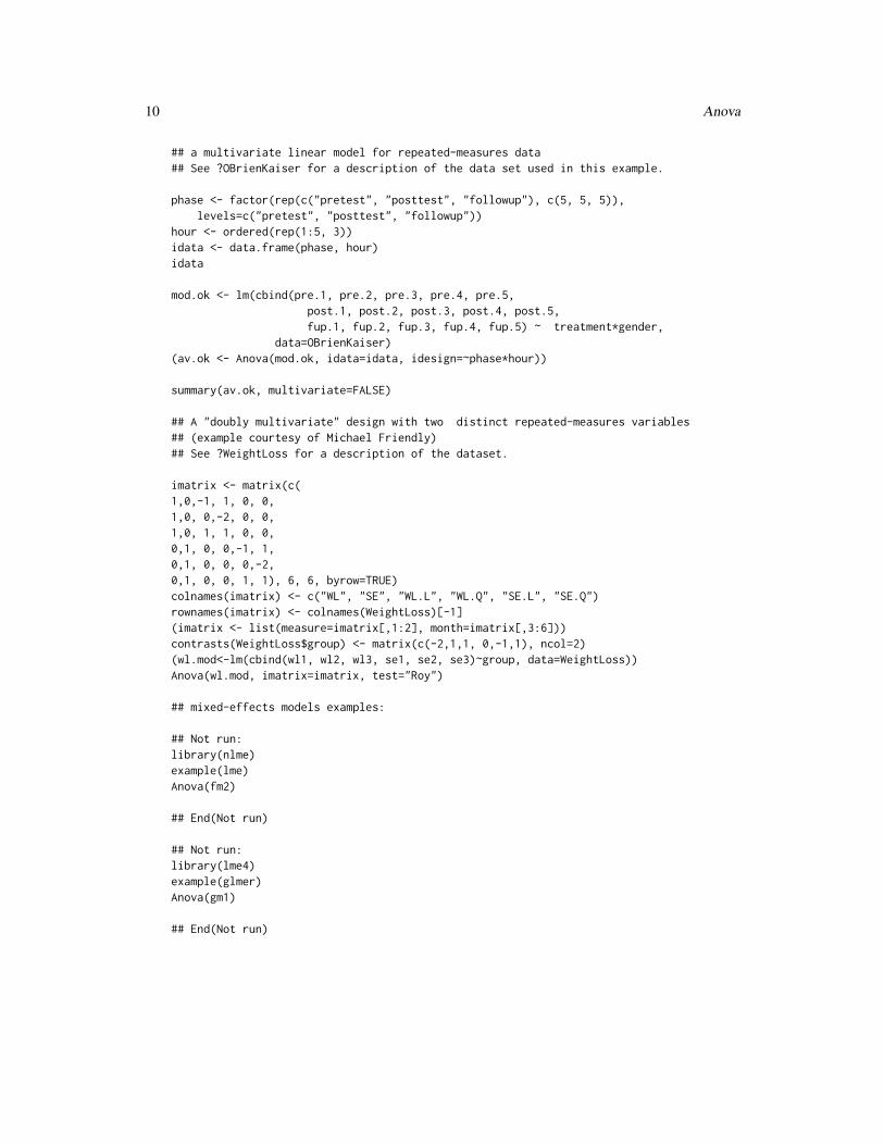
## a multivariate linear model for repeated-measures data## See ?OBrienKaiser for a description of the data set used in this example.

phase <- factor(rep(c("pretest", "posttest", "followup"), c(5, 5, 5)),levels=c("pretest", "posttest", "followup"))

hour <- ordered(rep(1:5, 3))idata <- data.frame(phase, hour)idata

mod.ok <- lm(cbind(pre.1, pre.2, pre.3, pre.4, pre.5,post.1, post.2, post.3, post.4, post.5,fup.1, fup.2, fup.3, fup.4, fup.5) ~ treatment*gender,

data=OBrienKaiser)(av.ok <- Anova(mod.ok, idata=idata, idesign=~phase*hour))

summary(av.ok, multivariate=FALSE)

## A "doubly multivariate" design with two distinct repeated-measures variables## (example courtesy of Michael Friendly)## See ?WeightLoss for a description of the dataset.

imatrix <- matrix(c(1,0,-1, 1, 0, 0,1,0, 0,-2, 0, 0,1,0, 1, 1, 0, 0,0,1, 0, 0,-1, 1,0,1, 0, 0, 0,-2,0,1, 0, 0, 1, 1), 6, 6, byrow=TRUE)colnames(imatrix) <- c("WL", "SE", "WL.L", "WL.Q", "SE.L", "SE.Q")rownames(imatrix) <- colnames(WeightLoss)[-1](imatrix <- list(measure=imatrix[,1:2], month=imatrix[,3:6]))contrasts(WeightLoss$group) <- matrix(c(-2,1,1, 0,-1,1), ncol=2)(wl.mod<-lm(cbind(wl1, wl2, wl3, se1, se2, se3)~group, data=WeightLoss))Anova(wl.mod, imatrix=imatrix, test="Roy")

## mixed-effects models examples:

## Not run:library(nlme)example(lme)Anova(fm2)

## End(Not run)

## Not run:library(lme4)example(glmer)Anova(gm1)

## End(Not run)

avPlots 11

avPlots Added-Variable Plots

Description

These functions construct added-variable, also called partial-regression, plots for linear and gener-alized linear models.

Usage

avPlots(model, terms=~., intercept=FALSE, layout=NULL, ask, main, ...)

avp(...)

avPlot(model, ...)

## S3 method for class 'lm'avPlot(model, variable,id=TRUE, col = carPalette()[1], col.lines = carPalette()[2],xlab, ylab, pch = 1, lwd = 2,main=paste("Added-Variable Plot:", variable),grid=TRUE,ellipse=FALSE,marginal.scale=FALSE, ...)

## S3 method for class 'glm'avPlot(model, variable,id=TRUE,col = carPalette()[1], col.lines = carPalette()[2],xlab, ylab, pch = 1, lwd = 2, type=c("Wang", "Weisberg"),main=paste("Added-Variable Plot:", variable), grid=TRUE,ellipse=FALSE, ...)

Arguments

model model object produced by lm or glm.

terms A one-sided formula that specifies a subset of the predictors. One added-variableplot is drawn for each term. For example, the specification terms = ~.-X3 wouldplot against all terms except for X3. If this argument is a quoted name of one ofthe terms, the added-variable plot is drawn for that term only.

intercept Include the intercept in the plots; default is FALSE.

variable A quoted string giving the name of a regressor in the model matrix for the hori-zontal axis.

layout If set to a value like c(1,1) or c(4,3), the layout of the graph will have thismany rows and columns. If not set, the program will select an appropriate layout.If the number of graphs exceed nine, you must select the layout yourself, or you

12 avPlots

will get a maximum of nine per page. If layout=NA, the function does not set thelayout and the user can use the par function to control the layout, for exampleto have plots from two models in the same graphics window.

main The title of the plot; if missing, one will be supplied.ask If TRUE, ask the user before drawing the next plot; if FALSE don’t ask.... avPlots passes these arguments to avPlot. avPlot passes them to plot.id controls point identification; if FALSE, no points are identified; can be a list of

named arguments to the showLabels function; TRUE, the default, is equivalent tolist(method=list(abs(residuals(model,type="pearson")),"x"),n=2,cex=1,col=carPalette()[1],location="lr"),which identifies the 2 points with the largest residuals and the 2 points with themost extreme horizontal values (i.e., largest partial leverage).

col color for points; the default is the second entry in the current car palette (seecarPalette and par).

col.lines color for the fitted line.pch plotting character for points; default is 1 (a circle, see par).lwd line width; default is 2 (see par).xlab x-axis label. If omitted a label will be constructed.ylab y-axis label. If omitted a label will be constructed.type if "Wang" use the method of Wang (1985); if "Weisberg" use the method in the

Arc software associated with Cook and Weisberg (1999).grid If TRUE, the default, a light-gray background grid is put on the graph.ellipse controls plotting data-concentration ellipses. If FALSE (the default), no ellipses

are plotted. Can be a list of named values giving levels, a vector of one ormore bivariate-normal probability-contour levels at which to plot the ellipses;and robust, a logical value determing whether to use the cov.trob function inthe MASS package to calculate the center and covariance matrix for the dataellipses. TRUE is equivalent to list(levels=c(.5,.95),robust=TRUE).

marginal.scale Consider an added-variable plot of Y versus X given Z. If this argument is FALSEthen the limits on the horizontal axis are determined by the range of the residualsfrom the regression of X on Z and the limits on the vertical axis are determinedby the range of the residuals from the regressnio of Y on Z. If the argumentis TRUE, then the limits on the horizontal axis are determined by the range ofX minus it mean, and on the vertical axis by the range of Y minus its means;adjustment is made if necessary to include outliers. This scaling allows visual-ization of the correlations between Y and Z and between X and Z. For example,if the X and Z are highly correlated, then the points will be concentrated on themiddle of the plot.

Details

The function intended for direct use is avPlots (for which avp is an abbreviation).

Value

These functions are used for their side effect id producing plots, but also invisibly return the coor-dinates of the plotted points.

bcPower 13

Author(s)

John Fox <[email protected]>, Sanford Weisberg <[email protected]>

References

Cook, R. D. and Weisberg, S. (1999) Applied Regression, Including Computing and Graphics.Wiley.



Wang, P C. (1985) Adding a variable in generalized linear models. Technometrics 27, 273–276.

Weisberg, S. (2014) Applied Linear Regression, Fourth Edition, Wiley.

See Also

residualPlots, crPlots, ceresPlots, link{dataEllipse}, showLabels, dataEllipse.

Examples

avPlots(lm(prestige ~ income + education + type, data=Duncan))

avPlots(glm(partic != "not.work" ~ hincome + children,data=Womenlf, family=binomial), id=FALSE)

m1 <- lm(partic ~ tfr + menwage + womwage + debt + parttime, Bfox)par(mfrow=c(1,3))# marginal plot, ignoring other predictors:with(Bfox, dataEllipse(womwage, partic, levels=0.5))abline(lm(partic ~ womwage, Bfox), col="red", lwd=2)# AV plot, adjusting for others:avPlots(m1, ~ womwage, ellipse=list(levels=0.5))# AV plot, adjusting and scaling as in marginal plotavPlots(m1, ~ womwage, marginal.scale=TRUE, ellipse=list(levels=0.5))

bcPower Box-Cox, Box-Cox with Negatives Allowed, Yeo-Johnson and BasicPower Transformations

Description

Transform the elements of a vector or columns of a matrix using, the Box-Cox, Box-Cox withnegatives allowed, Yeo-Johnson, or simple power transformations.

14 bcPower

Usage

bcPower(U, lambda, jacobian.adjusted=FALSE, gamma=NULL)

bcnPower(U, lambda, jacobian.adjusted = FALSE, gamma)

bcnPowerInverse(z, lambda, gamma)

yjPower(U, lambda, jacobian.adjusted = FALSE)

basicPower(U,lambda, gamma=NULL)

Arguments

U A vector, matrix or data.frame of values to be transformed

lambda Power transformation parameter with one element for each column of U, usual-lly in the range from −2 to 2.

jacobian.adjusted

If TRUE, the transformation is normalized to have Jacobian equal to one. Thedefault FALSE is almost always appropriate.

gamma For bcPower or basicPower, the transformation is of U + gamma, where gammais a positive number called a start that must be large enough so that U + gammais strictly positive. For the bcnPower, Box-cox power with negatives allowed,see the details below.

z a numeric vector the result of a call to bcnPower with jacobian.adjusted=FALSE.

Details

The Box-Cox family of scaled power transformations equals (xλ − 1)/λ for λ 6= 0, and log(x) ifλ = 0. The bcPower function computes the scaled power transformation of x = U + γ, where γ isset by the user so U + γ is strictly positive for these transformations to make sense.

The Box-Cox family with negatives allowed was proposed by Hawkins and Weisberg (2017). It isthe Box-Cox power transformation of

z = .5(U +√U2 + γ2))

where for this family γ is either user selected or is estimated. gamma must be positive if U includesnegative values and non-negative otherwise, ensuring that z is always positive. The bcnPowertransformations behave similarly to the bcPower transformations, and introduce less bias than isintroduced by setting the parameter γ to be non-zero in the Box-Cox family.

The function bcnPowerInverse computes the inverse of the bcnPower function, so U = bcnPowerInverse(bcnPower(U,lambda=lam,jacobian.adjusted=FALSE,gamma=gam),lambda=lam,gamma=gam)is true for any permitted value of gam and lam.

If family="yeo.johnson" then the Yeo-Johnson transformations are used. This is the Box-Coxtransformation of U +1 for nonnegative values, and of |U |+1 with parameter 2−λ for U negative.

The basic power transformation returnsUλ if λ is not 0, and log(λ) otherwise forU strictly positive.

If jacobian.adjusted is TRUE, then the scaled transformations are divided by the Jacobian, whichis a function of the geometric mean of U for skewPower and yjPower and of U + gamma for

Boot 15

bcPower. With this adjustment, the Jacobian of the transformation is always equal to 1. Jacobianadjustment facilitates computing the Box-Cox estimates of the transformation parameters.

Missing values are permitted, and return NA where ever U is equal to NA.

Value

Returns a vector or matrix of transformed values.

Author(s)

Sanford Weisberg, <[email protected]>

References


Hawkins, D. and Weisberg, S. (2017) Combining the Box-Cox Power and Generalized Log Trans-formations to Accomodate Nonpositive Responses In Linear and Mixed-Effects Linear ModelsSouth African Statistics Journal, 51, 317-328.

Weisberg, S. (2014) Applied Linear Regression, Fourth Edition, Wiley Wiley, Chapter 7.

Yeo, In-Kwon and Johnson, Richard (2000) A new family of power transformations to improvenormality or symmetry. Biometrika, 87, 954-959.

See Also

powerTransform, testTransform

Examples

U <- c(NA, (-3:3))## Not run: bcPower(U, 0) # produces an error as U has negative valuesbcPower(U, 0, gamma=4)bcPower(U, .5, jacobian.adjusted=TRUE, gamma=4)bcnPower(U, 0, gamma=2)basicPower(U, lambda = 0, gamma=4)yjPower(U, 0)V <- matrix(1:10, ncol=2)bcPower(V, c(0, 2))basicPower(V, c(0,1))

Boot Bootstrapping for regression models

Description

This function provides a simple front-end to the boot function in the boot package that is tailoredto bootstrapping based on regression models. Whereas boot is very general and therefore has manyarguments, the Boot function has very few arguments.

16 Boot

Usage

Boot(object, f=coef, labels=names(f(object)), R=999,method=c("case", "residual"), ncores=1, ...)

## Default S3 method:Boot(object, f=coef, labels=names(f(object)),R=999, method=c("case", "residual"), ncores=1,start = FALSE, ...)

## S3 method for class 'lm'Boot(object, f=coef, labels=names(f(object)),R=999, method=c("case", "residual"), ncores=1, ...)

## S3 method for class 'glm'Boot(object, f=coef, labels=names(f(object)),R=999, method=c("case", "residual"), ncores=1, ...)

## S3 method for class 'nls'Boot(object, f=coef, labels=names(f(object)),R=999, method=c("case", "residual"), ncores=1, ...)

Arguments

object A regression object of class "lm", "glm" or "nls". The function may work withother regression objects that support the update method and have a subsetargument. See discussion of the default method in the details below.

f A function whose one argument is the name of a regression object that will beapplied to the updated regression object to compute the statistics of interest.The default is coef, to return regression coefficient estimates. For example, f= function(obj) coef(obj)[1]/coef(obj)[2] will bootstrap the ratio of thefirst and second coefficient estimates.

labels Provides labels for the statistics computed by f. Default labels are obtained froma call to f, or generic labels if f does not return names.

R Number of bootstrap samples. The number of bootstrap samples actually com-puted may be smaller than this value if either the fitting method is iterative andfails to converge for some boothstrap samples, or if the rank of a fitted model isdifferent in a bootstrap replication than in the original data.

method The bootstrap method, either “case” for resampling cases or “residuals” for aresidual bootstrap. See the details below. The residual bootstrap is availableonly for lm and nls objects and will return an error for glm objects.

... Arguments passed to the boot function, see boot.

start Should the estimates returned by f be passed as starting values for each bootstrapiteration? Alternatively, start can be a numeric vector of starting values. Thedefault is to use the estimates from the last bootstrap iteration as starting valuesfor the next iteration.

Boot 17

ncores A numeric argument that specifies the number of cores for parallel processingfor unix systems. If less than or equal to 1, no parallel processing wiill be used.Note in a Windows platform will produce a warning and set this argument to 1.

Details

Boot uses a regression object and the choice of method, and creates a function that is passed asthe statistic argument to the boot function in the boot package. The argument R is also passedto boot. If ncores is greater than 1, then the parallel and ncpus arguments to boot are setappropriately to use multiple codes, if available, on your computer. All other arguments to boot arekept at their default values unless you pass values for them.

The methods available for lm and nls objects are “case” and “residual”. The case bootstrap resam-ples from the joint distribution of the terms in the model and the response. The residual bootstrapfixes the fitted values from the original data, and creates bootstraps by adding a bootstrap sample ofthe residuals to the fitted values to get a bootstrap response. It is an implementation of Algorithm6.3, page 271, of Davison and Hinkley (1997). For nls objects ordinary residuals are used in theresampling rather than the standardized residuals used in the lm method. The residual bootstrap forgeneralized linear models has several competing approaches, but none are without problems. If youwant to do a residual bootstrap for a glm, you will need to write your own call to boot.

For the default object to work with other types of regression models, the model must have methodsfor the the following generic functions: residuals(object,type="pearson") must return Pear-son residuals; fitted(object) must return fitted values; hatvalues(object) should return theleverages, or perhaps the value 1 which will effectively ignore setting the hatvalues. In addition,the data argument should contain no missing values among the columns actually used in fitting themodel, as the resampling may incorrectly attempt to include cases with missing values. For lm, glmand nls, missing values cause the return of an error message.

An attempt to fit using a bootstrap sample may fail. In a lm or glm fit, the bootstrap sample couldhave a different rank from the original fit. In an nls fit, convergence may not be obtained for somebootstraps. In either case, NA are returned for the value of the function f. The summary methodshandle the NAs appropriately.

Fox and Weisberg (2017) cited below discusses this function and provides more examples.

Value

See boot for the returned value of the structure returned by this function.

Author(s)

Sanford Weisberg, <[email protected]>. Achim Zeileis added multicore support, and also fixed thedefault method to work for many more regression models.

References

Davison, A, and Hinkley, D. (1997) Bootstrap Methods and their Applications. Oxford: OxfordUniversity Press.

Fox, J. and Weisberg, S. (2019) Companion to Applied Regression, Third Edition. Thousand Oaks:Sage.

18 boxCox

Fox, J. and Weisberg, S. (2019) Bootstrapping Regression Models in R, https://socialsciences.mcmaster.ca/jfox/Books/Companion/appendices/Appendix-Bootstrapping.pdf.

Weisberg, S. (2014) Applied Linear Regression, Fourth Edition, Wiley Wiley, Chapters 4 and 11.

See Also

Functions that work with boot objects from the boot package are boot.array, boot.ci, plot.bootand empinf. Additional functions in the car package are summary.boot, confint.boot, andhist.boot.

Examples

m1 <- lm(Fertility ~ ., swiss)betahat.boot <- Boot(m1, R=199) # 199 bootstrap samples--too small to be usefulsummary(betahat.boot) # default summaryconfint(betahat.boot)hist(betahat.boot)# Bootstrap for the estimated residual standard deviation:sigmahat.boot <- Boot(m1, R=199, f=sigmaHat, labels="sigmaHat")summary(sigmahat.boot)confint(sigmahat.boot)

boxCox Graph the profile log-likelihood for Box-Cox transformations in 1D,or in 2D with the bcnPower family.

Description

Computes and optionally plots profile log-likelihoods for the parameter of the Box-Cox powerfamily, the Yeo-Johnson power family, or for either of the parameters in a bcnPower family. Thisis a slight generalization of the boxcox function in the MASS package that allows for families oftransformations other than the Box-Cox power family. the boxCox2d function produces a contourplot of the two-dimensional likelihood profile for the bcnPower family.

Usage

boxCox(object, ...)

## Default S3 method:boxCox(object,

lambda = seq(-2, 2, 1/10), plotit = TRUE,interp = plotit, eps = 1/50,xlab=NULL, ylab=NULL,family="bcPower",param=c("lambda", "gamma"), gamma=NULL,grid=TRUE, ...)

## S3 method for class 'formula'

https://socialsciences.mcmaster.ca/jfox/Books/Companion/appendices/Appendix-Bootstrapping.pdf


boxCox 19

boxCox(object, lambda = seq(-2, 2, 1/10), plotit = TRUE, family = "bcPower",param = c("lambda", "gamma"), gamma = NULL, grid = TRUE,...)

## S3 method for class 'lm'boxCox(object, lambda = seq(-2, 2, 1/10), plotit = TRUE, ...)

boxCox2d(x, ksds = 4, levels = c(0.5, 0.95, 0.99, 0.999),main = "bcnPower Log-likelihood", grid=TRUE, ...)

Arguments

object a formula or fitted model object of class lm or aov.

lambda vector of values of λ, with default (-2, 2) in steps of 0.1, where the profile log-likelihood will be evaluated.

plotit logical which controls whether the result should be plotted; default TRUE.

interp logical which controls whether spline interpolation is used. Default to TRUE ifplotting with lambda of length less than 100.

eps Tolerance for lambda = 0; defaults to 0.02.

xlab defaults to "lambda" or "gamma".

ylab defaults to "log-Likelihood" or for bcnPower family to the appropriate label.

family Defaults to "bcPower" for the Box-Cox power family of transformations. Ifset to "yjPower" the Yeo-Johnson family, which permits negative responses, isused. If set to bcnPower the function gives the profile log-likelihood for theparameter selected via param.

param Relevant only to family="bcnPower", produces a profile log-likelihood for theparameter selected, maximizing over the remaining parameter.

gamma For use when the family="bcnPower",param="gamma". If this is a vector ofpositive values, then the profile log-likelihood for the location (or start) pa-rameter in the bcnPower family is evaluated at these values of gamma. Ifgamma is NULL, then evaulation is done at 100 equally spaced points betweenmin(.01,gmax -3*sd) and gmax + 3*sd, where gmax is the maximimum likeli-hood estimate of gamma, and sd is the sd of the response. See bcnPower for thedefinition of gamma.

grid If TRUE, the default, a light-gray background grid is put on the graph.

... additional arguments passed to the lm method with boxCox.formula or passedto contour with boxCox2d.

x An object created by a call to powerTransform using family="bcnPower".

ksds Contour plotting of the log-likelihood surface will cover plus of minus ksdsstandard deviations on each axis.

levels Contours will be drawn at the values of levels. For example, levels=c(.5,.99)would display two contours, at the 50% level and at the 99% level.

main Title for the contour plot

20 boxCox

Details

The boxCox function is an elaboration of the boxcox function in the MASS package. The first7 arguments are the same as in boxcox, and if the argument family="bcPower" is used, the re-sult is essentially identical to the function in MASS. Two additional families are the yjPower andbcnPower families that allow a few values of the response to be non-positive. The bcnPower familyhas two parameters: a power λ and a start or location parameter γ, and the boxCox function can beused to obtain a profile log-likelihood for either parameter with λ as the default. Alternatively, theboxCox2d function can be used to get a contour plot of the profile log-likelihood.

Value

Both functions ae designed for their side effects of drawing a graph. The boxCox function returnsa list of the lambda (or possibly, gamma) vector and the computed profile log-likelihood vector,invisibly if the result is plotted. If plotit=TRUE plots log-likelihood vs lambda and indicates a95% confidence interval about the maximum observed value of lambda. If interp=TRUE, splineinterpolation is used to give a smoother plot.

Author(s)


References

Box, G. E. P. and Cox, D. R. (1964) An analysis of transformations. Journal of the Royal Statisisti-cal Society, Series B. 26 211-46.

Cook, R. D. and Weisberg, S. (1999) Applied Regression Including Computing and Graphics. Wi-ley.





Yeo, I. and Johnson, R. (2000) A new family of power transformations to improve normality orsymmetry. Biometrika, 87, 954-959.

See Also

boxcox, yjPower, bcPower, bcnPower, powerTransform, contour

Examples

with(trees, boxCox(Volume ~ log(Height) + log(Girth), data = trees,lambda = seq(-0.25, 0.25, length = 10)))

data("quine", package = "MASS")with(quine, boxCox(Days ~ Eth*Sex*Age*Lrn,

lambda = seq(-0.05, 0.45, len = 20), family="yjPower"))

boxCoxVariable 21

boxCoxVariable Constructed Variable for Box-Cox Transformation

Description

Computes a constructed variable for the Box-Cox transformation of the response variable in a linearmodel.

Usage

boxCoxVariable(y)

Arguments

y response variable.

Details

The constructed variable is defined as y[log(y/y)− 1], where y is the geometric mean of y.

The constructed variable is meant to be added to the right-hand-side of the linear model. The t-testfor the coefficient of the constructed variable is an approximate score test for whether a transforma-tion is required.

If b is the coefficient of the constructed variable, then an estimate of the normalizing power trans-formation based on the score statistic is 1 − b. An added-variable plot for the constructed variableshows leverage and influence on the decision to transform y.

Value

a numeric vector of the same length as y.

Author(s)

John Fox <[email protected]>

References

Atkinson, A. C. (1985) Plots, Transformations, and Regression. Oxford.

Box, G. E. P. and Cox, D. R. (1964) An analysis of transformations. JRSS B 26 211–246.



See Also

boxcox, powerTransform, bcPower

22 Boxplot

Examples

mod <- lm(interlocks + 1 ~ assets, data=Ornstein)mod.aux <- update(mod, . ~ . + boxCoxVariable(interlocks + 1))summary(mod.aux)# avPlots(mod.aux, "boxCoxVariable(interlocks + 1)")

Boxplot Boxplots With Point Identification

Description

Boxplot is a wrapper for the standard R boxplot function, providing point identification, axislabels, and a formula interface for boxplots without a grouping variable.

Usage

Boxplot(y, ...)

## Default S3 method:Boxplot(y, g, id=TRUE, xlab, ylab, ...)

## S3 method for class 'formula'Boxplot(formula, data=NULL, subset, na.action=NULL,

id=TRUE, xlab, ylab, ...)

## S3 method for class 'list'Boxplot(y, xlab="", ylab="", ...)

## S3 method for class 'data.frame'Boxplot(y, id=TRUE, ...)

## S3 method for class 'matrix'Boxplot(y, ...)

Arguments

y a numeric variable for which the boxplot is to be constructed; a list of numericvariables, each element of which will be treated as a group; a numeric data frameor a numeric matrix, each of whose columns will be treated as a group.

g a grouping variable, usually a factor, for constructing parallel boxplots.

id a list of named elements giving one or more specifications for labels of indi-vidual points ("outliers"): n, the maximum number of points to label (default10); location, "lr" (left or right) of points or "avoid" to try to avoid over-plotting; method, one of "y" (automatic, the default), "identify" (interactive),or "none"; col for labels (default is the first color in carPalette() ); and cexsize of labels (default is 1). Can be FALSE to suppress point identification or

boxTidwell 23

TRUE (the default) to use all defaults. This is similar to how showLabels han-dles point labels for other functions in the car package, except that the usualdefault is id=FALSE.

xlab, ylab text labels for the horizontal and vertical axes; if missing, Boxplot will use thevariable names, or, in the case of a list, data frame, or matrix, empty labels.

formula a ‘model’ formula, of the form ~ y to produce a boxplot for the variable y, or ofthe form y ~ g, y ~ g1*g2*..., or y ~ g1 + g2 + ... to produce parallel boxplotsfor y within levels of the grouping variable(s) g, etc., usually factors.

data, subset, na.action

as for statistical modeling functions (see, e.g., lm).

... further arguments, such as at, to be passed to boxplot.

Author(s)

John Fox <[email protected]>, with a contribution from Steve Ellison to handle at argument (seeboxplot).

References


See Also

boxplot

Examples

Boxplot(~income, data=Prestige, id=list(n=Inf)) # identify all outliersBoxplot(income ~ type, data=Prestige)Boxplot(income ~ type, data=Prestige, at=c(1, 3, 2))Boxplot(k5 + k618 ~ lfp*wc, data=Mroz)with(Prestige, Boxplot(income, id=list(labels=rownames(Prestige))))with(Prestige, Boxplot(income, type, id=list(labels=rownames(Prestige))))Boxplot(scale(Prestige[, 1:4]))

boxTidwell Box-Tidwell Transformations

Description

Computes the Box-Tidwell power transformations of the predictors in a linear model.

24 boxTidwell

Usage

boxTidwell(y, ...)

## S3 method for class 'formula'boxTidwell(formula, other.x=NULL, data=NULL, subset,na.action=getOption("na.action"), verbose=FALSE, tol=0.001,max.iter=25, ...)

## Default S3 method:boxTidwell(y, x1, x2=NULL, max.iter=25, tol=0.001,verbose=FALSE, ...)

## S3 method for class 'boxTidwell'print(x, digits=getOption("digits") - 2, ...)

Arguments

formula two-sided formula, the right-hand-side of which gives the predictors to be trans-formed.

other.x one-sided formula giving the predictors that are not candidates for transforma-tion, including (e.g.) factors.

data an optional data frame containing the variables in the model. By default thevariables are taken from the environment from which boxTidwell is called.

subset an optional vector specifying a subset of observations to be used.na.action a function that indicates what should happen when the data contain NAs. The

default is set by the na.action setting of options.verbose if TRUE a record of iterations is printed; default is FALSE.tol if the maximum relative change in coefficients is less than tol then convergence

is declared.max.iter maximum number of iterations.y response variable.x1 matrix of predictors to transform.x2 matrix of predictors that are not candidates for transformation.... not for the user.x boxTidwell object.digits number of digits for rounding.

Details

The maximum-likelihood estimates of the transformation parameters are computed by Box and Tid-well’s (1962) method, which is usually more efficient than using a general nonlinear least-squaresroutine for this problem. Score tests for the transformations are also reported.

Value

an object of class boxTidwell, which is normally just printed.

brief 25

Author(s)


References

Box, G. E. P. and Tidwell, P. W. (1962) Transformation of the independent variables. Technometrics4, 531-550.



Examples

boxTidwell(prestige ~ income + education, ~ type + poly(women, 2), data=Prestige)

brief Print Abbreviated Ouput

Description

Print data objects and statistical model summaries in abbreviated form.

Usage

brief(object, ...)

## S3 method for class 'data.frame'brief(object, rows = if (nr <= 10) c(nr, 0) else c(3, 2),

cols, head=FALSE, tail=FALSE, elided = TRUE,classes = inherits(object, "data.frame"), ...)

## S3 method for class 'matrix'brief(object, rows = if (nr <= 10) c(nr, 0) else c(3, 2), ...)

## S3 method for class 'numeric'brief(object, rows = c(2, 1), elided = TRUE, ...)## S3 method for class 'integer'brief(object, rows = c(2, 1), elided = TRUE, ...)## S3 method for class 'character'brief(object, rows = c(2, 1), elided = TRUE, ...)## S3 method for class 'factor'brief(object, rows=c(2, 1), elided=TRUE, ...)

## S3 method for class 'list'brief(object, rows = c(2, 1), elided = TRUE, ...)

## S3 method for class 'function'brief(object, rows = c(5, 3), elided = TRUE, ...)

26 brief

## S3 method for class 'lm'brief(object, terms = ~ .,

intercept=missing(terms), pvalues=FALSE,digits=3, horizontal=TRUE, vcov., ...)

## S3 method for class 'glm'brief(object, terms = ~ .,

intercept=missing(terms), pvalues=FALSE,digits=3, horizontal=TRUE, vcov., dispersion, exponentiate, ...)

## S3 method for class 'multinom'brief(object, terms = ~ .,

intercept=missing(terms), pvalues=FALSE,digits=3, horizontal=TRUE, exponentiate=TRUE, ...)

## S3 method for class 'polr'brief(object, terms = ~ .,

intercept, pvalues=FALSE,digits=3, horizontal=TRUE, exponentiate=TRUE, ...)

## Default S3 method:brief(object, terms = ~ .,

intercept=missing(terms), pvalues=FALSE,digits=3, horizontal=TRUE, ...)

Arguments

object a data or model object to abbreviate.

rows for a matrix or data frame, a 2-element integer vector with the number of rows toprint at the beginning and end of the display; for a vector or factor, the numberof lines of output to show at the beginning and end; for a list, the number ofelements to show at the beginning and end; for a function, the number of linesto show at the beginning and end.

cols for a matrix or data frame, a 2-element integer vector with the number of columnsto print at the beginning (i.e., left) and end (right) of the display.

head, tail alternatives to the rows argument; if TRUE, print the first or last 6 rows; can alsobe the number of the first or last few rows to print; only one of heads and tailsshould be specified; ignored if FALSE (the default).

elided controls whether to report the number of elided elements, rows, or columns;default is TRUE.

classes show the class of each column of a data frame at the top of the column; theclasses are shown in single-character abbreviated form—e.g., [f] for a factor,[i] for an integer variable, [n] for a numeric variable, [c] for a character vari-able.

terms a one-sided formula giving the terms to summarize; the default is ~ .—i.e., tosummarize all terms in the model.

brief 27

intercept whether or not to include the intercept; the default is TRUE unless the termsargument is given, in which case the default is FALSE; ignored for polr models.

pvalues include the p-value for each coefficient in the table; default is FALSE.

exponentiate for a "glm" or "glmerMod" model using the log or logit link, or a "polr"or "multinom" model, show exponentiated coefficient estimates and confidencebounds.

digits significant digits for printing.

horizontal if TRUE (the default), orient the summary produced by brief horizontally, whichtypically saves space.

dispersion see summary.glm

vcov. either a matrix giving the estimated covariance matrix of the estimates, or a func-tion that when called with object as an argument returns an estimated covari-ance matrix of the estimates. The default vcov. = vcov(object,complete=FALSE)uses the usual estimated covariance matrix with NA for any row and columnwith aliased regressors. Other choices include the functions documented athccm, and a bootstrap estimate vcov.=vcov(Boot(object)); see the documen-tation for Boot. For the glm method, if the vcov. or dispersion argument isspecified, then Wald-based confidence limits are computed; otherwise the re-ported confidence limits are computed by profiling the likelihood. NOTES: (1)The dispersion and vcov. arguments may not both be specified. (2) Settingvcov.=vcov returns an error if the model includes aliased terms; use vcov.=vcov(object,complete=FALSE).(3) The hccm method will generally return a matrix of full rank even if the modelhas aliased terms. Similarly vcov.=vcov(Boot(object)) may return a fullrank matrix, or it will a matrix with NA corresponding to aliased regressors ifsame regressors are aliased in every bootstrap sample.

... arguments to pass down.

Value

Invisibly returns object for a data object, or summary for a model object.

Note

The method brief.matrix calls brief.data.frame.

Author(s)


References


See Also

S

28 car-defunct

Examples

brief(rnorm(100))brief(Duncan)brief(OBrienKaiser, elided=TRUE)brief(matrix(1:500, 10, 50))brief(lm)

mod.prestige <- lm(prestige ~ education + income + type, Prestige)brief(mod.prestige, pvalues=TRUE)brief(mod.prestige, ~ type)mod.mroz <- glm(lfp ~ ., data=Mroz, family=binomial)brief(mod.mroz)

car-defunct Defunct Functions in the car Package

Description

These functions are were deprecated in 2009 and are now defunct.

Usage

av.plot(...)av.plots(...)box.cox(...)bc(...)box.cox.powers(...)box.cox.var(...)box.tidwell(...)cookd(...)confidence.ellipse(...)ceres.plot(...)ceres.plots(...)cr.plot(...)cr.plots(...)data.ellipse(...)durbin.watson(...)levene.test(...)leverage.plot(...)leverage.plots(...)linear.hypothesis(...)ncv.test(...)outlier.test(...)qq.plot(...)skewPower(...)spread.level.plot(...)

car-deprecated 29

Arguments

... pass arguments down.

Details

av.plot and av.plots are replaced by avPlot and avPlots functions.

box.cox and bc are now replaced by bcPower.

box.cox.powers is replaced by powerTransform.

box.cox.var is replaced by boxCoxVariable.

box.tidwell is replaced by boxTidwell.

cookd is replaced by cooks.distance in the stats package.

confidence.ellipse is replaced by confidenceEllipse.

ceres.plot and ceres.plots are now replaced by the ceresPlot and ceresPlots functions.

cr.plot and cr.plots are now replaced by the crPlot and crPlots functions.

data.ellipse is replaced by dataEllipse.

durbin.watson is replaced by durbinWatsonTest.

levene.test is replaced by leveneTest function.

leverage.plot and leverage.plots are now replaced by the leveragePlot and leveragePlotsfunctions.

linear.hypothesis is replaced by the linearHypothesis function.

ncv.test is replaced by ncvTest.

outlier.test is replaced by outlierTest.

qq.plot is replaced by qqPlot.

skewPower is replaced by bcnPower.

spread.level.plot is replaced by spreadLevelPlot.

car-deprecated Deprecated Functions in the car Package

Description

These functions are provided for compatibility with older versions of the car package only, andmay be removed eventually. Commands that worked in versions of the car package prior to version3.0-0 will not necessarily work in version 3.0-0 and beyond, or may not work in the same manner.

Usage

bootCase(...)

nextBoot(...)

30 carHexsticker

Arguments

... arguments to pass to methods.

Details

These functions are replaced by Boot.

See Also

See Also Boot

car-internal.Rd Internal Objects for the car package

Description

These objects (currently only the .carEnv environment) are exported for technical reasons and arenot for direct use.

Author(s)


carHexsticker View the Official Hex Sticker for the car Package

Description

Open the official hex sticker for the car package in your browser

Usage

carHexsticker()

Value

Used for its side effect of openning the hex sticker for the car package in your browser.

Author(s)


Examples

## Not run:carHexsticker()

## End(Not run)

carPalette 31

carPalette Set or Retrieve car Package Color Palette

Description

This function is used to set or retrieve colors to be used in car package graphics functions.

Usage

carPalette(palette)

Arguments

palette if missing, returns the colors that will be used in car graphics; if present, thecolors to be used in graphics will be set. The palette argument may also beone of "car" or "default" to use the default car palette (defined below), "R" touse the default R palette, or "colorblind" to use a colorblind-friendly palette(from https://jfly.uni-koeln.de/color/).

Details

This function sets or returns the value of options(carPalette=pallete) that will be use in cargraphics functions to determine colors. The default is c("black","blue","magenta","cyan","orange","gray","green3","red")),which is nearly a permutation of the colors returned by the standard palette function that mini-mizes the use of red and green in the same graph, and that substitutes orange for the often hard tosee yellow.

Value

Invisibly returns the previous value of the car palette.

Author(s)

Sanford Weisberg and John Fox

References


See Also

palette, colors

https://jfly.uni-koeln.de/color/

32 carWeb

Examples

# Standard color palettepalette()# car standard color palettecarPalette()# set colors to all blackcarPalette(rep("black", 8))# Use a custom color palette with 12 distinct colorscarPalette(sample(colors(distinct=TRUE), 12))# restore defaultcarPalette("default")

carWeb Access to the R Companion to Applied Regression Website

Description

This function will access the website for An R Companion to Applied Regression, or setup files ordata.

Usage

carWeb(page = c("webpage", "errata", "taskviews"), script, data, setup)

Arguments

page A character string indicating what page to open. The default "webpage" willopen the main web page, "errata" displays the errata sheet for the book, "taskviews"fetches and displays a list of available task views from CRAN.

script The quoted name of a chapter in An R Companion to Applied Regression, like"chap-1", "chap-2", up to "chap-10". All the R commands used in that chap-ter will be displayed in your browser, where you can save them as a text file.

data The quoted name of a data file in An R Companion to Applied Regression,like "Duncan.txt" or "Prestige.txt". The file will be opened in your webbrowser. You do not need to specify the extension .txt

setup If TRUE this command will download a number of files to your computer that arediscussed in Fox and Weisberg (2019), beginning in Chapter 1.

Value

Either displays a web page or a PDF document or downloads files to your working directory.

Author(s)

Sanford Weisberg, based on the function UsingR in the UsingR package by John Verzani

ceresPlots 33

References


Examples

## Not run:carWeb()carWeb(setup=TRUE)

## End(Not run)

ceresPlots Ceres Plots

Description

These functions draw Ceres plots for linear and generalized linear models.

Usage

ceresPlots(model, terms = ~., layout = NULL, ask, main,...)

ceresPlot(model, ...)

## S3 method for class 'lm'ceresPlot(model, variable, id=FALSE,line=TRUE, smooth=TRUE, col=carPalette()[1], col.lines=carPalette()[-1],xlab, ylab, pch=1, lwd=2, grid=TRUE, ...)

## S3 method for class 'glm'ceresPlot(model, ...)

Arguments


terms A one-sided formula that specifies a subset of the regressors. One component-plus-residual plot is drawn for each term. The default ~. is to plot against allnumeric predictors. For example, the specification terms = ~ . -X3 would plotagainst all predictors except for X3. Factors and nonstandard predictors such asB-splines are skipped. If this argument is a quoted name of one of the regressors,the component-plus-residual plot is drawn for that predictor only.

layout If set to a value like c(1,1) or c(4,3), the layout of the graph will have thismany rows and columns. If not set, the program will select an appropriate layout.If the number of graphs exceed nine, you must select the layout yourself, or youwill get a maximum of nine per page. If layout=NA, the function does not set the

34 ceresPlots

layout and the user can use the par function to control the layout, for exampleto have plots from two models in the same graphics window.

ask If TRUE, ask the user before drawing the next plot; if FALSE, the default, don’task. This is relevant only if not all the graphs can be drawn in one window.

main Overall title for any array of cerers plots; if missing a default is provided.

... ceresPlots passes these arguments to ceresPlot. ceresPlot passes them toplot.

variable A quoted string giving the name of a variable for the horizontal axis

id controls point identification; if FALSE (the default), no points are identified; canbe a list of named arguments to the showLabels function; TRUE is equivalent tolist(method=list(abs(residuals(model,type="pearson")),"x"),n=2,cex=1,col=carPalette()[1],location="lr"),which identifies the 2 points with the largest residuals and the 2 points with themost extreme horizontal (X) values.

line TRUE to plot least-squares line.

smooth specifies the smoother to be used along with its arguments; if FALSE, no smootheris shown; can be a list giving the smoother function and its named arguments;TRUE, the default, is equivalent to list(smoother=loessLine). See ScatterplotSmoothersfor the smoothers supplied by the car package and their arguments. Ceres plotsdo not support variance smooths.

col color for points; the default is the first entry in the current car palette (seecarPalette and par).

col.lines a list of at least two colors. The first color is used for the ls line and the secondcolor is used for the fitted lowess line. To use the same color for both, use, forexample, col.lines=c("red","red")

xlab,ylab labels for the x and y axes, respectively. If not set appropriate labels are createdby the function.

pch plotting character for points; default is 1 (a circle, see par).

lwd line width; default is 2 (see par).

grid If TRUE, the default, a light-gray background grid is put on the graph

Details

Ceres plots are a generalization of component+residual (partial residual) plots that are less prone toleakage of nonlinearity among the predictors.

The function intended for direct use is ceresPlots.

The model cannot contain interactions, but can contain factors. Factors may be present in the model,but Ceres plots cannot be drawn for them.

Value

NULL. These functions are used for their side effect: producing plots.

Author(s)


compareCoefs 35

References




See Also

crPlots, avPlots, showLabels

Examples

ceresPlots(lm(prestige~income+education+type, data=Prestige), terms= ~ . - type)

compareCoefs Print estimated coefficients and their standard errors in a table forseveral regression models.

Description

This function extracts estimates of regression parameters and their standard errors from one or moremodels and prints them in a table.

Usage

compareCoefs(..., se = TRUE, zvals = FALSE, pvals = FALSE, vcov.,print = TRUE, digits = 3)

Arguments

... One or more regression-model objects. These may be of class lm, glm, nlm,or any other regression method for which the functions coef and vcov returnappropriate values, or if the object inherits from the mer class created by thelme4 package or lme in the nlme package.

se If TRUE, the default, show standard errors as well as estimates.zvals If TRUE (the default is FALSE), print Wald statistics, the ratio of each coefficient

to its standard error.pvals If codeTRUE (the default is FALSE), print two-sided p-values from the standard

normal distribution corresponding to the Wald statistics.vcov. an optional argument, specifying a function to be applied to all of the models,

returning a coefficient covariance matrix for each, or a list with one elementfor each model, with each element either containing a function to be applied tothe corresponding model or a coefficient covariance matrix for that model. Ifomitted, vcov is applied to each model.

print If TRUE, the defualt, the results are printed in a nice format using printCoefmat.If FALSE, the results are returned as a matrix

digits Passed to the printCoefmat function for printing the result.

36 Contrasts

Value

This function is mainly used for its side-effect of printing the result. It also invisibly returns a matrixof estimates, standard errors, Wald statistics, and p-values.

Author(s)


References


Examples

mod1 <- lm(prestige ~ income + education, data=Duncan)mod2 <- update(mod1, subset=-c(6,16))mod3 <- update(mod1, . ~ . + type)mod4 <- update(mod1, . ~ . + I(income + education)) # aliased coef.compareCoefs(mod1)compareCoefs(mod1, mod2, mod4)compareCoefs(mod1, mod2, mod3, zvals=TRUE, pvals=TRUE)compareCoefs(mod1, mod2, se=FALSE)compareCoefs(mod1, mod1, vcov.=list(vcov, hccm))

Contrasts Functions to Construct Contrasts

Description

These are substitutes for similarly named functions in the stats package (note the uppercase letterstarting the second word in each function name). The only difference is that the contrast functionsfrom the car package produce easier-to-read names for the contrasts when they are used in statisticalmodels.

The functions and this documentation are adapted from the stats package.

Usage

contr.Treatment(n, base = 1, contrasts = TRUE)

contr.Sum(n, contrasts = TRUE)

contr.Helmert(n, contrasts = TRUE)

Arguments

n a vector of levels for a factor, or the number of levels.base an integer specifying which level is considered the baseline level. Ignored if

contrasts is FALSE.contrasts a logical indicating whether contrasts should be computed.

Contrasts 37

Details

These functions are used for creating contrast matrices for use in fitting analysis of variance andregression models. The columns of the resulting matrices contain contrasts which can be used forcoding a factor with n levels. The returned value contains the computed contrasts. If the argumentcontrasts is FALSE then a square matrix is returned.

Several aspects of these contrast functions are controlled by options set via the options command:

decorate.contrasts This option should be set to a 2-element character vector containing the pre-fix and suffix characters to surround contrast names. If the option is not set, then c("[","]")is used. For example, setting options(decorate.contrasts=c(".","")) produces contrastnames that are separated from factor names by a period. Setting options( decorate.contrasts=c("",""))reproduces the behaviour of the R base contrast functions.

decorate.contr.Treatment A character string to be appended to contrast names to signify treat-ment contrasts; if the option is unset, then "T." is used.

decorate.contr.Sum Similar to the above, with default "S.".

decorate.contr.Helmert Similar to the above, with default "H.".

contr.Sum.show.levels Logical value: if TRUE (the default if unset), then level names are usedfor contrasts; if FALSE, then numbers are used, as in contr.sum in the base package.

Note that there is no replacement for contr.poly in the base package (which produces orthogonal-polynomial contrasts) since this function already constructs easy-to-read contrast names.

Value

A matrix with n rows and k columns, with k = n -1 if contrasts is TRUE and k = n if contrasts isFALSE.

Author(s)


References


See Also

contr.treatment, contr.sum, contr.helmert, contr.poly

Examples

# contr.Treatment vs. contr.treatment in the base package:

lm(prestige ~ (income + education)*type, data=Prestige,contrasts=list(type="contr.Treatment"))

## Call:## lm(formula = prestige ~ (income + education) * type, data = Prestige,## contrasts = list(type = "contr.Treatment"))

38 crPlots

#### Coefficients:## (Intercept) income education## 2.275753 0.003522 1.713275## type[T.prof] type[T.wc] income:type[T.prof]## 15.351896 -33.536652 -0.002903## income:type[T.wc] education:type[T.prof] education:type[T.wc]## -0.002072 1.387809 4.290875

lm(prestige ~ (income + education)*type, data=Prestige,contrasts=list(type="contr.treatment"))

## Call:## lm(formula = prestige ~ (income + education) * type, data = Prestige,## contrasts = list(type = "contr.treatment"))#### Coefficients:## (Intercept) income education## 2.275753 0.003522 1.713275## typeprof typewc income:typeprof## 15.351896 -33.536652 -0.002903## income:typewc education:typeprof education:typewc## -0.002072 1.387809 4.290875

crPlots Component+Residual (Partial Residual) Plots

Description

These functions construct component+residual plots, also called partial-residual plots, for linearand generalized linear models.

Usage

crPlots(model, terms = ~., layout = NULL, ask, main,...)

crp(...)

crPlot(model, ...)

## S3 method for class 'lm'crPlot(model, variable, id=FALSE,

order=1, line=TRUE, smooth=TRUE,col=carPalette()[1], col.lines=carPalette()[-1],xlab, ylab, pch=1, lwd=2, grid=TRUE, ...)

crPlots 39

Arguments


terms A one-sided formula that specifies a subset of the regressors. One component-plus-residual plot is drawn for each regressor. The default ~. is to plot againstall numeric regressors. For example, the specification terms = ~ . -X3 wouldplot against all regressors except for X3, while terms = ~ log(X4) would givethe plot for the predictor X4 that is represented in the model by log(X4). If thisargument is a quoted name of one of the predictors, the component-plus-residualplot is drawn for that predictor only.

layout If set to a value like c(1,1) or c(4,3), the layout of the graph will have thismany rows and columns. If not set, the program will select an appropriate layout.If the number of graphs exceed nine, you must select the layout yourself, or youwill get a maximum of nine per page. If layout=NA, the function does not set thelayout and the user can use the par function to control the layout, for exampleto have plots from two models in the same graphics window.

ask If TRUE, ask the user before drawing the next plot; if FALSE, the default, don’task. This is relevant only if not all the graphs can be drawn in one window.

main The title of the plot; if missing, one will be supplied.

... crPlots passes these arguments to crPlot. crPlot passes them to plot.

variable A quoted string giving the name of a variable for the horizontal axis.


order order of polynomial regression performed for predictor to be plotted; default 1.

line TRUE to plot least-squares line.

smooth specifies the smoother to be used along with its arguments; if FALSE, no smootheris shown; can be a list giving the smoother function and its named arguments;TRUE, the default, is equivalent to list(smoother=loessLine). See ScatterplotSmoothersfor the smoothers supplied by the car package and their arguments.


col.lines a list of at least two colors. The first color is used for the ls line and the secondcolor is used for the fitted lowess line. To use the same color for both, use, forexample, col.lines=c("red","red")

xlab,ylab labels for the x and y axes, respectively. If not set appropriate labels are createdby the function.




40 deltaMethod

Details

The function intended for direct use is crPlots, for which crp is an abbreviation.

The model cannot contain interactions, but can contain factors. Parallel boxplots of the partialresiduals are drawn for the levels of a factor.

Value

NULL. These functions are used for their side effect of producing plots.

Author(s)


References




See Also

ceresPlots, avPlots

Examples

crPlots(m<-lm(prestige ~ income + education, data=Prestige))

crPlots(m, terms=~ . - education) # get only one plot

crPlots(lm(prestige ~ log2(income) + education + poly(women,2), data=Prestige))

crPlots(glm(partic != "not.work" ~ hincome + children,data=Womenlf, family=binomial), smooth=list(span=0.75))

deltaMethod Estimate and Standard Error of a Nonlinear Function of EstimatedRegression Coefficients

Description

deltaMethod is a generic function that uses the delta method to get a first-order approximate stan-dard error for a nonlinear function of a vector of random variables with known or estimated covari-ance matrix.

deltaMethod 41

Usage

deltaMethod(object, ...)

## Default S3 method:deltaMethod(object, g., vcov., func=g., constants, level=0.95,rhs, ..., envir=parent.frame())

## S3 method for class 'lm'deltaMethod(object, g., vcov.=vcov(object, complete=FALSE),

parameterNames=names(coef(object)), ..., envir=parent.frame())## S3 method for class 'nls'deltaMethod(object, g., vcov.=vcov(object, complete=FALSE), ..., envir=parent.frame())## S3 method for class 'multinom'deltaMethod(object, g., vcov. = vcov(object, complete=FALSE),

parameterNames = if (is.matrix(coef(object)))colnames(coef(object)) else names(coef(object)), ..., envir=parent.frame())

## S3 method for class 'polr'deltaMethod(object, g., vcov.=vcov(object, complete=FALSE), ..., envir=parent.frame())## S3 method for class 'survreg'deltaMethod(object, g., vcov. = vcov(object, complete=FALSE),

parameterNames = names(coef(object)), ..., envir=parent.frame())## S3 method for class 'coxph'deltaMethod(object, g., vcov. = vcov(object, complete=FALSE),

parameterNames = names(coef(object)), ..., envir=parent.frame())## S3 method for class 'mer'deltaMethod(object, g., vcov. = vcov(object, complete=FALSE),

parameterNames = names(fixef(object)), ..., envir=parent.frame())## S3 method for class 'merMod'deltaMethod(object, g., vcov. = vcov(object, complete=FALSE),

parameterNames = names(fixef(object)), ..., envir=parent.frame())## S3 method for class 'lme'deltaMethod(object, g., vcov. = vcov(object, complete=FALSE),

parameterNames = names(fixef(object)), ..., envir=parent.frame())## S3 method for class 'lmList'deltaMethod(object, g., ..., envir=parent.frame())

Arguments

object For the default method, object is either (1) a vector of p named elements, sonames(object) returns a list of p character strings that are the names of the ele-ments of object; or (2) a model object for which there are coef and vcov meth-ods, and for which the named coefficient vector returned by coef is asymptoti-cally normally distributed with asymptotic covariance matrix returned by vcov.For the other methods, object is a regression object for which coef(object)or fixef(object) returns a vector of parameter estimates.

g. A quoted string that is the function of the parameter estimates to be evaluated;see the details below.

42 deltaMethod

vcov. The (estimated) covariance matrix of the coefficient estimates. For the defaultmethod, this argument is required. For all other methods, this argument musteither provide the estimated covariance matrix or a function that when appliedto object returns a covariance matrix. The default is to use the function vcov.

func A quoted string used to annotate output. The default of func = g. is usuallyappropriate.

parameterNames A character vector of length p that gives the names of the parameters in the sameorder as they appear in the vector of estimates. This argument will be useful ifsome of the names in the vector of estimates include special characters, likeI(x2^2), or x1:x2 that will confuse the numerical differentiation function. Seedetails below.

constants This argument is a named vector whose elements are constants that are used inthe f argument. It isn’t generally necessary to specify this argument but it maybe convenient to do so.

level level for confidence interval, default 0.95.rhs hypothesized value for the specified function of parameters; if absent no hypoth-

esis test is performed.... Used to pass arguments to the generic method.envir Environment in which g. is evaluated; not normally specified by the user.

Details

Suppose x is a random vector of length p that is at least approximately normally distributed withmean β and estimated covariance matrix C. Then any function g(β) of β, is estimated by g(x),which is in large samples normally distributed with mean g(β) and estimated variance h′Ch, whereh is the first derivative of g(β) with respect to β evaluated at x. This function returns both g(x) andits standard error, the square root of the estimated variance.

The default method requires that you provide x in the argument object, C in the argument vcov.,and a text expression in argument g. that when evaluated gives the function g. The call names(object)must return the names of the elements of x that are used in the expression g..

Since the delta method is often applied to functions of regression parameter estimates, the argu-ment object may be the name of a regression object from which the estimates and their esti-mated variance matrix can be extracted. In most regression models, estimates are returned by thecoef(object) and the variance matrix from vcov(object). You can provide an alternative func-tion for computing the sample variance matrix, for example to use a sandwich estimator.

For mixed models using lme4 or nlme, the coefficient estimates are returned by the fixef function,while for multinom, lmList and nlsList coefficient estimates are returned by coef as a matrix.Methods for these models are provided to get the correct estimates and variance matrix.

The argument g. must be a quoted character string that gives the function of interest. For example, ifyou set m2 <-lm(Y ~ X1 + X2 + X1:X2), then deltaMethod(m2,"X1/X2") applies the delta methodto the ratio of the coefficient estimates for X1 and X2. The argument g. can consist of constants andnames associated with the elements of the vector of coefficient estimates.

In some cases the names may include characters such as the colon : used in interactions, or mathe-matical symbols like + or - signs that would confuse the function that computes numerical deriva-tives, and for this case you can replace the names of the estimates with the parameterNames argu-ment. For example, the ratio of the X2 main effect to the interaction term could be computed using

deltaMethod 43

deltaMethod(m2,"b1/b3",parameterNames=c("b0","b1","b2","b3")). The name “(Intercept)”used for the intercept in linear and generalized linear models is an exception, and it will be correctlyinterpreted by deltaMethod. Another option is to use back-ticks to quote nonstandard R names, asin deltaMethod(m2,"X1/`X1:X2`").

For multinom objects, the coef function returns a matrix of coefficients, with each row giving theestimates for comparisons of one category to the baseline. The deltaMethod function applies thedelta method to each row of this matrix. Similarly, for lmList and nlsList objects, the deltamethod is computed for each element of the list of models fit.

For nonlinear regression objects produced by the nls function, the call coef(object) returnsthe estimated coefficient vectors with names corresponding to parameter names. For example, m2<-nls(y ~ theta/(1 + gamma * x),start = list(theta=2,gamma=3)) will have parameters namedc("theta","gamma"). In many other familiar regression models, such as those produced by lm andglm, the names of the coefficient estimates are the corresponding regressor names, not parameternames.

For mixed-effects models fit with lmer and glmer from the lme4 package or lme and nlme from thenlme package, only fixed-effect coefficients are considered.

For regression models for which methods are not provided, you can extract the named vector of co-efficient estimates and and estimate of its covariance matrix and then apply the default deltaMethodfunction.

Note: Earlier versions of deltaMethod included an argument parameterPrefix that implementedthe same functionality as the parameterNames argument, but which caused several problems thatwere not easily fixed without the change in syntax.

Value

An object of class "deltaMethod", inheriting from "data.frame", for which a print method isprovided. The object contains columns named Estimate for the estimate, SE for its standard error,and columns for confidence limits and possibly a hypothesis test. The value of g. is given as a rowlabel.

Author(s)

Sanford Weisberg, <[email protected]>, John Fox <[email protected]>, and Pavel Krivitsky.

References



Weisberg, S. (2014) Applied Linear Regression, Fourth Edition, Wiley, Section 6.1.2.

See Also

First derivatives of g. are computed using symbolic differentiation by the function D.

44 densityPlot

Examples

m1 <- lm(time ~ t1 + t2, data = Transact)deltaMethod(m1, "b1/b2", parameterNames= paste("b", 0:2, sep=""))deltaMethod(m1, "t1/t2", rhs=1) # use names of preds. rather than coefs.deltaMethod(m1, "t1/t2", vcov=hccm) # use hccm function to est. vars.deltaMethod(m1, "1/(Intercept)")# The next example invokes the default method by extracting the# vector of estimates and covariance matrix explicitlydeltaMethod(coef(m1), "t1/t2", vcov.=vcov(m1))

densityPlot Nonparametric Density Estimates

Description

densityPlot contructs and graphs nonparametric density estimates, possibly conditioned on a fac-tor, using the standard R density function or by default adaptiveKernel, which computes anadaptive kernel density estimate. depan provides the Epanechnikov kernel and dbiwt provides thebiweight kernel.

Usage

densityPlot(x, ...)

## Default S3 method:densityPlot(x, g, method=c("adaptive", "kernel"),

bw=if (method == "adaptive") bw.nrd0 else "SJ", adjust=1,kernel, xlim, ylim,normalize=FALSE, xlab=deparse(substitute(x)), ylab="Density", main="",col=carPalette(), lty=seq_along(col), lwd=2, grid=TRUE,legend=TRUE, show.bw=FALSE, rug=TRUE, ...)

## S3 method for class 'formula'densityPlot(formula, data=NULL, subset,

na.action=NULL, xlab, ylab, main="", legend=TRUE, ...)

adaptiveKernel(x, kernel=dnorm, bw=bw.nrd0, adjust=1.0, n=500,from, to, cut=3, na.rm=TRUE)

depan(x)dbiwt(x)

Arguments

x a numeric variable, the density of which is estimated; for depan and dbiwt, theargument of the kernel function.

g an optional factor to divide the data.

densityPlot 45

formula an R model formula, of the form ~ variable to estimate the unconditional den-sity of variable, or variable ~ factor to estimate the density of variablewithin each level of factor.

data an optional data frame containing the data.

subset an optional vector defining a subset of the data.

na.action a function to handle missing values; defaults to the value of the R na.actionoption, initially set to na.omit.

method either "adaptive" (the default) for an adaptive-kernel estimate or "kernel" fora fixed-bandwidth kernel estimate.

bw the geometric mean bandwidth for the adaptive-kernel or bandwidth of the ker-nel density estimate(s). Must be a numerical value or a function to computethe bandwidth (default bw.nrd0) for the adaptive kernel estimate; for the kernelestimate, may either the quoted name of a rule to compute the bandwidth, or anumeric value. If plotting by groups, bw may be a vector of values, one for eachgroup. See density and bw.SJ for details of the kernel estimator.

adjust a multiplicative adjustment factor for the bandwidth; the default, 1, indicatesno adjustment; if plotting by groups, adjust may be a vector of adjustmentfactors, one for each group. The default bandwidth-selection rule tends to givea value that’s too large if the distribution is asymmetric or has multiple modes;try setting adjust < 1, particularly for the adaptive-kernel estimator.

kernel for densityPlot this is the name of the kernel function for the kernel esti-mator (the default is "gaussian", see density); or a kernel function for theadaptive-kernel estimator (the default is dnorm, producing the Gaussian kernel).For adaptivekernel this is a kernel function, defaulting to dnorm, which is theGaussian kernel (standard-normal density).

xlim, ylim axis limits; if missing, determined from the range of x-values at which the den-sities are estimated and the estimated densities.

normalize if TRUE (the default is FALSE), the estimated densities are rescaled to integrate ap-proximately to 1; particularly useful if the density is estimated over a restricteddomain, as when from or to are specified.

xlab label for the horizontal-axis; defaults to the name of the variable x.

ylab label for the vertical axis; defaults to "Density".

main plot title; default is empty.

col vector of colors for the density estimate(s); defaults to the color carPalette.

lty vector of line types for the density estimate(s); defaults to the successive inte-gers, starting at 1.

lwd line width for the density estimate(s); defaults to 2.

grid if TRUE (the default), grid lines are drawn on the plot.

legend a list of up to two named elements: location, for the legend when densities areplotted for several groups, defaults to "upperright" (see legend); and titleof the legend, which defaults to the name of the grouping factor. If TRUE, thedefault, the default values are used; if FALSE, the legend is suppressed.

n number of equally spaced points at which the adaptive-kernel estimator is eval-uated; the default is 500.

46 densityPlot

from, to, cut the range over which the density estimate is computed; the default, if missing,is min(x) -cut*bw,max(x) + cut*bw.

na.rm remove missing values from x in computing the adaptive-kernel estimate? Thedefault is TRUE.

show.bw if TRUE, show the bandwidth(s) in the horizontal-axis label or (for multiplegroups) the legend; the default is FALSE.

rug if TRUE (the default), draw a rug plot (one-dimentional scatterplot) at the bottomof the density estimate.

... arguments to be passed down.

Details

If you use a different kernel function than the default dnorm that has a standard deviation differentfrom 1 along with an automatic rule like the default function bw.nrd0, you can attach an attributeto the kernel function named "scale" that gives its standard deviation. This is true for the twosupplied kernels, depan and dbiwt

Value

densityPlot invisibly returns the "density" object computed (or list of "density" objects) anddraws a graph. adaptiveKernel returns an object of class "density" (see density).

Author(s)


References


W. N. Venables and B. D. Ripley (2002) Modern Applied Statistics with S. New York: Springer.

B.W. Silverman (1986) Density Estimation for Statistics and Data Analysis. London: Chapman andHall.

See Also

density, bw.SJ, plot.density

Examples

densityPlot(~ income, show.bw=TRUE, method="kernel", data=Prestige)densityPlot(~ income, show.bw=TRUE, data=Prestige)densityPlot(~ income, from=0, normalize=TRUE, show.bw=TRUE, data=Prestige)

densityPlot(income ~ type, data=Prestige)densityPlot(~ income, show.bw=TRUE, method="kernel", data=Prestige)densityPlot(~ income, show.bw=TRUE, data=Prestige)densityPlot(~ income, from=0, normalize=TRUE, show.bw=TRUE, data=Prestige)

densityPlot(income ~ type, kernel=depan, data=Prestige)

dfbetaPlots 47

densityPlot(income ~ type, kernel=depan, legend=list(location="top"), data=Prestige)

plot(adaptiveKernel(UN$infantMortality, from=0, adjust=0.75), col="magenta")lines(density(na.omit(UN$infantMortality), from=0, adjust=0.75), col="blue")rug(UN$infantMortality, col="cyan")legend("topright", col=c("magenta", "blue"), lty=1,

legend=c("adaptive kernel", "kernel"), inset=0.02)

plot(adaptiveKernel(UN$infantMortality, from=0, adjust=0.75), col="magenta")lines(density(na.omit(UN$infantMortality), from=0, adjust=0.75), col="blue")rug(UN$infantMortality, col="cyan")legend("topright", col=c("magenta", "blue"), lty=1,

legend=c("adaptive kernel", "kernel"), inset=0.02)

dfbetaPlots dfbeta and dfbetas Index Plots

Description

These functions display index plots of dfbeta (effect on coefficients of deleting each observationin turn) and dfbetas (effect on coefficients of deleting each observation in turn, standardized by adeleted estimate of the coefficient standard error). In the plot of dfbeta, horizontal lines are drawnat 0 and +/- one standard error; in the plot of dfbetas, horizontal lines are drawn and 0 and +/- 1.

Usage

dfbetaPlots(model, ...)

dfbetasPlots(model, ...)

## S3 method for class 'lm'dfbetaPlots(model, terms= ~ ., intercept=FALSE, layout=NULL, ask,

main, xlab, ylab, labels=rownames(dfbeta),id.method="y",id.n=if(id.method[1]=="identify") Inf else 0, id.cex=1,

id.col=carPalette()[1], id.location="lr", col=carPalette()[1], grid=TRUE, ...)

## S3 method for class 'lm'dfbetasPlots(model, terms=~., intercept=FALSE, layout=NULL, ask,

main, xlab, ylab,labels=rownames(dfbeta), id.method="y",id.n=if(id.method[1]=="identify") Inf else 0, id.cex=1,

id.col=carPalette()[1], id.location="lr", col=carPalette()[1], grid=TRUE, ...)

48 dfbetaPlots

Arguments


terms A one-sided formula that specifies a subset of the terms in the model. Onedfbeta or dfbetas plot is drawn for each regressor. The default ~. is to plotagainst all terms in the model with the exception of an intercept. For example,the specification terms = ~.-X3 would plot against all terms except for X3. Ifthis argument is a quoted name of one of the terms, the index plot is drawn forthat term only.

intercept Include the intercept in the plots; default is FALSE.


main The title of the graph; if missing, one will be supplied.

xlab Horizontal axis label; defaults to "Index".

ylab Vertical axis label; defaults to coefficient name.

ask If TRUE, ask the user before drawing the next plot; if FALSE, the default, don’task.

... optional additional arguments to be passed to plot, points, and showLabels.id.method, labels, id.n, id.cex, id.col, id.location

Arguments for the labelling of points. The default is id.n=0 for labeling nopoints. See showLabels for details of these arguments.

col color for points; defaults to the first entry in the color carPalette.


Value


Author(s)


References



See Also

dfbeta ,dfbetas

durbinWatsonTest 49

Examples

dfbetaPlots(lm(prestige ~ income + education + type, data=Duncan))

dfbetasPlots(glm(partic != "not.work" ~ hincome + children,data=Womenlf, family=binomial))

durbinWatsonTest Durbin-Watson Test for Autocorrelated Errors

Description

Computes residual autocorrelations and generalized Durbin-Watson statistics and their bootstrappedp-values. dwt is an abbreviation for durbinWatsonTest.

Usage

durbinWatsonTest(model, ...)

dwt(...)

## S3 method for class 'lm'durbinWatsonTest(model, max.lag=1, simulate=TRUE, reps=1000,

method=c("resample","normal"),alternative=c("two.sided", "positive", "negative"), ...)

## Default S3 method:durbinWatsonTest(model, max.lag=1, ...)

## S3 method for class 'durbinWatsonTest'print(x, ...)

Arguments

model a linear-model object, or a vector of residuals from a linear model.

max.lag maximum lag to which to compute residual autocorrelations and Durbin-Watsonstatistics.

simulate if TRUE p-values will be estimated by bootstrapping.

reps number of bootstrap replications.

method bootstrap method: "resample" to resample from the observed residuals; "normal"to sample normally distributed errors with 0 mean and standard deviation equalto the standard error of the regression.

alternative sign of autocorrelation in alternative hypothesis; specify only if max.lag = 1; ifmax.lag > 1, then alternative is taken to be "two.sided".


x durbinWatsonTest object.

50 Ellipses

Value

Returns an object of type "durbinWatsonTest".

Note

p-values are available only from the lm method.

Author(s)


References


Examples

durbinWatsonTest(lm(fconvict ~ tfr + partic + degrees + mconvict, data=Hartnagel))

Ellipses Ellipses, Data Ellipses, and Confidence Ellipses

Description

These functions draw ellipses, including data ellipses, and confidence ellipses for linear, generalizedlinear, and possibly other models.

Usage

ellipse(center, shape, radius, log="", center.pch=19, center.cex=1.5,segments=51, draw=TRUE, add=draw, xlab="", ylab="",col=carPalette()[2], lwd=2, fill=FALSE, fill.alpha=0.3, grid=TRUE, ...)

dataEllipse(x, y, groups, group.labels=group.levels, ellipse.label,weights, log="", levels=c(0.5, 0.95), center.pch=19,center.cex=1.5, draw=TRUE, plot.points=draw, add=!plot.points, segments=51,robust=FALSE, xlab=deparse(substitute(x)), ylab=deparse(substitute(y)),col=if (missing(groups)) carPalette()[1:2] else carPalette()[1:length(group.levels)],pch=if (missing(groups)) 1 else seq(group.levels),lwd=2, fill=FALSE, fill.alpha=0.3, grid=TRUE, id=FALSE, ...)

confidenceEllipse(model, ...)

## S3 method for class 'lm'confidenceEllipse(model, which.coef, vcov.=vcov,L, levels=0.95, Scheffe=FALSE, dfn,center.pch=19, center.cex=1.5, segments=51, xlab, ylab,

Ellipses 51

col=carPalette()[2], lwd=2, fill=FALSE, fill.alpha=0.3, draw=TRUE, add=!draw, ...)

## S3 method for class 'glm'confidenceEllipse(model, chisq, ...)

## Default S3 method:confidenceEllipse(model, which.coef, vcov.=vcov,L, levels=0.95, Scheffe=FALSE, dfn,center.pch=19, center.cex=1.5, segments=51, xlab, ylab,col=carPalette()[2], lwd=2, fill=FALSE, fill.alpha=0.3, draw=TRUE, add=!draw, ...)

Arguments

center 2-element vector with coordinates of center of ellipse.

shape 2× 2 shape (or covariance) matrix.

radius radius of circle generating the ellipse.

log when an ellipse is to be added to an existing plot, indicates whether computa-tions were on logged values and to be plotted on logged axes; "x" if the x-axisis logged, "y" if the y-axis is logged, and "xy" or "yx" if both axes are logged.The default is "", indicating that neither axis is logged.

center.pch character for plotting ellipse center; if FALSE or NULL the center point isn’t plot-ted.

center.cex relative size of character for plotting ellipse center.

segments number of line-segments used to draw ellipse.

draw if TRUE produce graphical output; if FALSE, only invisibly return coordinates ofellipse(s).

add if TRUE add ellipse(s) to current plot.

xlab label for horizontal axis.

ylab label for vertical axis.

x a numeric vector, or (if y is missing) a 2-column numeric matrix.

y a numeric vector, of the same length as x.

groups optional: a factor to divide the data into groups; a separate ellipse will be plottedfor each group (level of the factor).

group.labels labels to be plotted for the groups; by default, the levels of the groups factor.

ellipse.label a label for the ellipse(s) or a vector of labels; if several ellipses are drawn andjust one label is given, then that label will be repeated. The default is not to labelthe ellipses.

weights a numeric vector of weights, of the same length as x and y to be used by cov.wtor cov.trob in computing a weighted covariance matrix; if absent, weights of1 are used.

plot.points if FALSE data ellipses are drawn, but points are not plotted.

levels draw elliptical contours at these (normal) probability or confidence levels.

52 Ellipses

robust if TRUE use the cov.trob function in the MASS package to calculate the centerand covariance matrix for the data ellipse.

model a model object produced by lm or glm.

which.coef 2-element vector giving indices of coefficients to plot; if missing, the first twocoefficients (disregarding the regression constant) will be selected.

vcov. a coefficient-covariance matrix or a function (such as hccm) to compute thecoefficent-covariance matrix from model; the default is the vcov function.

L As an alternative to selecting coefficients to plot, a transformation matrix can bespecified to compute two linear combinations of the coefficients; if the L matrixis given, it takes precedence over the which.coef argument. L should have tworows and as many columns as there are coefficients. It can be given directlyas a numeric matrix, or specified by a pair of character-valued expressions, inthe same manner as for the link{linearHypothesis} function, but with noright-hand side.

Scheffe if TRUE scale the ellipse so that its projections onto the axes give Scheffe confi-dence intervals for the coefficients.

dfn “numerator” degrees of freedom (or just degrees of freedom for a GLM) fordrawing the confidence ellipse. Defaults to the number of coefficients in themodel (disregarding the constant) if Scheffe is TRUE, or to 2 otherwise; select-ing dfn = 1 will draw the “confidence-interval generating” ellipse, with projec-tions on the axes corresponding to individual confidence intervals with the statedlevel of coverage.

chisq if TRUE, the confidence ellipse for the coefficients in a generalized linear modelare based on the chisquare statistic, if FALSE on the $F$-statistic. This corre-sponds to using the default and linear-model methods respectively.

col color for lines and ellipse center; the default is the second entry in the currentcar palette (see carPalette and par). For dataEllipse, two colors can begiven, in which case the first is for plotted points and the second for lines andthe ellipse center; if ellipses are plotted for groups, then this is a vector of colorsfor the groups.

pch for dataEllipse this is the plotting character (default, symbol 1, a hollow cir-cle) to use for the points; if ellipses are plotted by groups, then this a vector ofplotting characters, with consecutive symbols starting with 1 as the default.


fill fill the ellipse with translucent color col (default, FALSE)?

fill.alpha transparency of fill (default = 0.3).

... other plotting parameters to be passed to plot and line.

id controls point identification; if FALSE (the default), no points are identified; canbe a list of named arguments to the showLabels function; TRUE is equivalent tolist(method="mahal",n=2,cex=1,col=carPalette()[1],location="lr")(with the default col actually dependent on the number of groups), which iden-tifies the 2 points with the largest Mahalanobis distances from the center of thedata.


Ellipses 53

Details

The ellipse is computed by suitably transforming a unit circle.

dataEllipse superimposes the normal-probability contours over a scatterplot of the data.

Value

These functions are mainly used for their side effect of producing plots. For greater flexibility(e.g., adding plot annotations), however, ellipse returns invisibly the (x, y) coordinates of thecalculated ellipse. dataEllipse and confidenceEllipse return invisibly the coordinates of oneor more ellipses, in the latter instance a list named by levels.

Author(s)

Georges Monette, John Fox <[email protected]>, and Michael Friendly.

References



Monette, G. (1990) Geometry of multiple regression and 3D graphics. In Fox, J. and Long, J. S.(Eds.) Modern Methods of Data Analysis. Sage.

See Also

cov.trob, cov.wt, linearHypothesis.

Examples

dataEllipse(Duncan$income, Duncan$education, levels=0.1*1:9,ellipse.label=0.1*1:9, lty=2, fill=TRUE, fill.alpha=0.1)

confidenceEllipse(lm(prestige~income+education, data=Duncan), Scheffe=TRUE)

confidenceEllipse(lm(prestige~income+education, data=Duncan), vcov.=hccm)

confidenceEllipse(lm(prestige~income+education, data=Duncan),L=c("income + education", "income - education"))

wts <- rep(1, nrow(Duncan))wts[c(6, 16)] <- 0 # delete Minister, Conductorwith(Duncan, {dataEllipse(income, prestige, levels=0.68)dataEllipse(income, prestige, levels=0.68, robust=TRUE,

plot.points=FALSE, col="green3")dataEllipse(income, prestige, weights=wts, levels=0.68,

plot.points=FALSE, col="brown")dataEllipse(income, prestige, weights=wts, robust=TRUE, levels=0.68,plot.points=FALSE, col="blue")})

54 Export

with(Prestige, dataEllipse(income, education, type,id=list(n=2, labels=rownames(Prestige)), pch=15:17,xlim=c(0, 25000), center.pch="+",group.labels=c("Blue Collar", "Professional", "White Collar"),ylim=c(5, 20), level=.95, fill=TRUE, fill.alpha=0.1))

Export Export a data frame to disk in one of many formats

Description

Uses the export function in the rio package to export a file to disk. This function adds an argumentfor converting row.names to a column in the resulting file.

Usage

Export(x, file, format, ..., keep.row.names)

Arguments

x A data frame or matrix to be written to a file.

file A character string naming a file. If the file name has an extension, such as .xlsx,the extention is used to infer the type of file to be exported. See export for thefile types supported.

format see export.

... Additional arguments; see export.

keep.row.names If set to TRUE, then the data frame’s row.names are appended to the left of thedata frame with the name "id". If set to quoted character string, the row.namesare added using the character string as its name. If set to FALSE row.names arelost.

Details

This is a convenience function in the car package for exporting (writing) a data frame to a filein a wide variety of formats including csv, Microsoft Excel. It optionally allows converting therow.names for the data frame to a column before writing. It then calls export in the rio package.That function in turn uses many other packages and functions for writing the function to a file.

Value

The name of the output file as a character string (invisibly).

Author(s)

Sanford Weisberg <[email protected]>

hccm 55

References

Chung-hong Chan, Geoffrey CH Chan, Thomas J. Leeper, and Jason Becker (2017). rio: A Swiss-army knife for data file I/O. R package version 0.5.0.

See Also

export, Import

Examples

Export(Duncan, "Duncan.csv", keep.row.names="occupation")Duncan2 <- Import("Duncan.csv") # Automatically restores row.namesidentical(Duncan, Duncan2)# cleanupunlink("Duncan.csv")

hccm Heteroscedasticity-Corrected Covariance Matrices

Description

Calculates heteroscedasticity-corrected covariance matrices linear models fit by least squares orweighted least squares. These are also called “White-corrected” or “White-Huber” covariance ma-trices.

Usage

hccm(model, ...)

## S3 method for class 'lm'hccm(model, type=c("hc3", "hc0", "hc1", "hc2", "hc4"),singular.ok=TRUE, ...)

## Default S3 method:hccm(model, ...)

Arguments

model a unweighted or weighted linear model, produced by lm.

type one of "hc0", "hc1", "hc2", "hc3", or "hc4"; the first of these gives the classicWhite correction. The "hc1", "hc2", and "hc3" corrections are described inLong and Ervin (2000); "hc4" is described in Cribari-Neto (2004).

singular.ok if FALSE (the default is TRUE), a model with aliased coefficients produces anerror; otherwise, the aliased coefficients are ignored in the coefficient covariancematrix that’s returned.

... arguments to pass to hccm.lm.

56 hccm

Details

The original White-corrected coefficient covariance matrix ("hc0") for an unweighted model is

V (b) = (X ′X)−1X ′diag(e2i )X(X ′X)−1

where e2i are the squared residuals, and X is the model matrix. The other methods represent ad-justments to this formula. If there are weights, these are incorporated in the corrected covariancematrix.

The function hccm.default simply catches non-lm objects.

Value

The heteroscedasticity-corrected covariance matrix for the model.

Author(s)


References



Cribari-Neto, F. (2004) Asymptotic inference under heteroskedasticity of unknown form. Compu-tational Statistics and Data Analysis 45, 215–233.

Long, J. S. and Ervin, L. H. (2000) Using heteroscedasity consistent standard errors in the linearregression model. The American Statistician 54, 217–224.

White, H. (1980) A heteroskedastic consistent covariance matrix estimator and a direct test of het-eroskedasticity. Econometrica 48, 817–838.

Examples

options(digits=4)mod<-lm(interlocks~assets+nation, data=Ornstein)vcov(mod)## (Intercept) assets nationOTH nationUK nationUS## (Intercept) 1.079e+00 -1.588e-05 -1.037e+00 -1.057e+00 -1.032e+00## assets -1.588e-05 1.642e-09 1.155e-05 1.362e-05 1.109e-05## nationOTH -1.037e+00 1.155e-05 7.019e+00 1.021e+00 1.003e+00## nationUK -1.057e+00 1.362e-05 1.021e+00 7.405e+00 1.017e+00## nationUS -1.032e+00 1.109e-05 1.003e+00 1.017e+00 2.128e+00hccm(mod)## (Intercept) assets nationOTH nationUK nationUS## (Intercept) 1.664e+00 -3.957e-05 -1.569e+00 -1.611e+00 -1.572e+00## assets -3.957e-05 6.752e-09 2.275e-05 3.051e-05 2.231e-05## nationOTH -1.569e+00 2.275e-05 8.209e+00 1.539e+00 1.520e+00## nationUK -1.611e+00 3.051e-05 1.539e+00 4.476e+00 1.543e+00## nationUS -1.572e+00 2.231e-05 1.520e+00 1.543e+00 1.946e+00

hist.boot 57

hist.boot Methods Functions to Support boot Objects

Description

The Boot function in the car package uses the boot function from the boot package to do a straight-forward case or residual bootstrap for many regression objects. These are method functions for stan-dard generics to summarize the results of the bootstrap. Other tools for this purpose are available inthe boot package.

Usage

## S3 method for class 'boot'hist(x, parm, layout = NULL, ask, main = "", freq = FALSE,

estPoint = TRUE, point.col = carPalette()[1], point.lty = 2, point.lwd = 2,estDensity = !freq, den.col = carPalette()[2], den.lty = 1, den.lwd = 2,estNormal = !freq, nor.col = carPalette()[3], nor.lty = 2, nor.lwd = 2,ci = c("bca", "none", "perc", "norm"), level = 0.95,legend = c("top", "none", "separate"), box = TRUE, ...)

## S3 method for class 'boot'summary(object, parm, high.moments = FALSE, extremes = FALSE, ...)

## S3 method for class 'boot'confint(object, parm, level = 0.95, type = c("bca", "norm",

"basic", "perc"), ...)

## S3 method for class 'boot'Confint(object, parm, level = 0.95, type = c("bca", "norm",

"basic", "perc"), ...)

## S3 method for class 'boot'vcov(object, ...)

Arguments

x, object An object created by a call to boot in the boot package, or to Boot in the carpackage of class "boot".

parm A vector of numbers or coefficient names giving the coefficients for which ahistogram or confidence interval is desired. If numbers are used, 1 correspondsto the intercept, if any. The default is all coefficients.


58 hist.boot

ask If TRUE, ask the user before drawing the next plot; if FALSE, don’t ask.

main Main title for the graphs. The default is main="" for no title.

freq The default for the generic hist function is freq=TRUE to give a frequency his-togram. The default for hist.boot is freq=FALSE to give a density histogram.A density estimate and/or a fitted normal density can be added to the graph iffreq=FALSE but not if freq=TRUE.

estPoint, point.col, point.lty, point.lwd

If estPoint=TRUE, the default, a vertical line is drawn on the histgram at thevalue of the point estimate computed from the complete data. The remainingthree optional arguments set the color, line type and line width of the line that isdrawn.

estDensity, den.col, den.lty, den.lwd

If estDensity=TRUE andfreq=FALSE, the default, a kernel density estimate isdrawn on the plot with a call to the density function with no additional argu-ments. The remaining three optional arguments set the color, line type and linewidth of the lines that are drawn.

estNormal, nor.col, nor.lty, nor.lwd

If estNormal=TRUE andfreq=FALSE, the default, a normal density with meanand sd computed from the data is drawn on the plot. The remaining three op-tional arguments set the color, line type and line width of the lines that are drawn.

ci A confidence interval based on the bootstrap will be added to the histogramusing the BCa method if ci="bca" the percentile method if ci="perc", or thenormal method if ci="norm". No interval is drawn if ci="none". The defaultis "bca". The interval is indicated by a thick horizontal line at y=0. For somebootstraps the BCa method is unavailable, in which case a warning is issued andci="perc" is substituted. If you wish to see all the options at once, see boot.ci.The normal method is computed as the (estimate from the original data) minusthe bootstrap bias plus or minus the standard deviation of the bootstrap replicatestimes the appropriate quantile of the standard normal distribution.

legend A legend can be added to the (array of) histograms. The value “"top"” puts atthe top-left of the plots. The value “"separate"” puts the legend in its own graphfollowing all the histograms. The value “"none"” suppresses the legend.

box Add a box around each histogram.

... Additional arguments passed to hist; for other methods this is included forcompatibility with the generic method. For example, the argument border=par()$bgin hist will draw the histogram transparently, leaving only the density esti-mates. With the vcov function, the additional arguments are passed to cov. Seethe Value section, below.

high.moments Should the skewness and kurtosis be included in the summary? Default isFALSE.

extremes Should the minimum, maximum and range be included in the summary? Defaultis FALSE.

level Confidence level, a number between 0 and 1. In confint, level can be a vec-tor; for example level=c(.50,.90,.95) will return the following estimatedquantiles: c(.025,.05,.25,.75,.95,.975).

hist.boot 59

type Selects the confidence interval type. The types implemented are the "percentile"method, which uses the function quantile to return the appropriate quantilesfor the confidence limit specified, the default bca which uses the bias-correctedand accelerated method presented by Efron and Tibshirani (1993, Chapter 14).For the other types, see the documentation for boot.

Value

hist is used for the side-effect of drawing an array of historgams of each column of the first ar-gument. summary returns a matrix of summary statistics for each of the columns in the bootstrapobject. The confint method returns confidence intervals. Confint appends the estimates based onthe original fitted model to the left of the confidence intervals.

The vcov returns the sample covariance of the bootstrap sample estimates. If any of the bootstrapreplications returned an NA value, then vcov will return a matrix of NAs. You can compute thecovariance of the complete cases by adding the argument use="complete.obs" to the call to vcov;see cov.

Author(s)


References

Efron, B. and Tibsharini, R. (1993) An Introduction to the Bootstrap. New York: Chapman andHall.

Fox, J. and Weisberg, S. (2019) An R Companion to Applied Regression, Third Edition. ThousandOaks: Sage.

Fox, J. and Weisberg, S. (2018) Bootstrapping Regression Models in R, https://socialsciences.mcmaster.ca/jfox/Books/Companion/appendices/Appendix-Bootstrapping.pdf.

Weisberg, S. (2013) Applied Linear Regression, Fourth Edition, Wiley

See Also

See Also Boot, hist, density, Fox and Weisberg (2017), cited above

Examples

m1 <- lm(Fertility ~ ., swiss)betahat.boot <- Boot(m1, R=99) # 99 bootstrap samples--too small to be usefulsummary(betahat.boot) # default summaryconfint(betahat.boot)hist(betahat.boot)



60 Import

Import Import data from many file formats

Description

Use the import function from the rio package to read a data.frame from a variety of file types. TheImport function includes 3 additional arguments adding row names and for converting characterand logical variables to factors.

Usage

Import(file, format, ..., row.names=TRUE,stringsAsFactors = default.stringsAsFactors())

Arguments

file A character string naming a file, URL, or single-file .zip or .tar archive. See thedetails below. If the file name has an extention like .xlsx or .csv then the typeof file is inferred from the extension.

format If an extension is not present in the file name or it is wrong, the file format canbe set with this argument; see import.

... Additional arguments passed to import.

row.names If TRUE, the default, the left-most character variable that has all unique elementsis removed from the data frame and set to be row.names. To match import, setrow.names=FALSE.

stringsAsFactors

If TRUE, then character variables that do not have all unique elements are con-verted to factors. The default is determined by the value of options("stringsAsFactors")whose "factory fresh" default is equal to TRUE. To get the default behavior of theimport function, set stringsAsFractors=FALSE.

Details

This function always calls the import function to read a data frame from a file. Many type offile are supported. The Import function allows the user to set row.names, and automaticallyconvert character and logical variables to factors, but only if the format of the file is one of"txt","csv","xlsx","xls","ods". Many more details are given at the man page for import.

Value

A data frame. See import for more details

Author(s)


infIndexPlot 61

See Also

import, Export

Examples

head(Duncan, 3) # first three rowsExport(Duncan, "Duncan.csv", keep.row.names="occupation")Duncan2 <- Import("Duncan.csv") # Automatically restores row.names and factorshead(Duncan2, 3) # first three rowsidentical(Duncan, Duncan2)# cleanupunlink("Duncan.csv")

infIndexPlot Influence Index Plot

Description

Provides index plots of influence and related diagnostics for a regression model.

Usage

infIndexPlot(model, ...)

influenceIndexPlot(model, ...)

## S3 method for class 'lm'infIndexPlot(model, vars=c("Cook", "Studentized", "Bonf", "hat"),

id=TRUE, grid=TRUE, main="Diagnostic Plots", ...)

## S3 method for class 'influence.merMod'infIndexPlot(model,

vars = c("dfbeta", "dfbetas", "var.cov.comps","cookd"), id = TRUE, grid = TRUE, main = "Diagnostic Plots", ...)

## S3 method for class 'influence.lme'infIndexPlot(model,

vars = c("dfbeta", "dfbetas", "var.cov.comps","cookd"), id = TRUE, grid = TRUE, main = "Diagnostic Plots", ...)

Arguments

model A regression object of class lm, glm, or lmerMod, or an influence object for almer, glmer, or lme object (see influence.mixed.models). The "lmerMod"method calls the "lm" method and can take the same arguments.

vars All the quantities listed in this argument are plotted. Use "Cook" for Cook’sdistances, "Studentized" for Studentized residuals, "Bonf" for Bonferroni p-values for an outlier test, and and "hat" for hat-values (or leverages) for a linear

62 influence.mixed.models

or generalized linear model, or "dfbeta", "dfbetas", "var.cov.comps", and"cookd" for an influence object derived from a mixed model. Capitalization isoptional. All but "dfbeta" and "dfbetas" may be abbreviated by the first oneor more letters.

main main title for graph

id a list of named values controlling point labelling. The default, TRUE, is equiva-lent to id=list(method="y",n=2,cex=1,col=carPalette()[1],location="lr");FALSE suppresses point labelling. See showLabels for details.


... Arguments passed to plot

Value

Used for its side effect of producing a graph. Produces index plots of diagnostic quantities.

Author(s)

Sanford Weisberg <[email protected]> and John Fox

References


Fox, J. (2016) Applied Regression Analysis and Generalized Linear Models, Third Edition. Sage.Fox, J. and Weisberg, S. (2019) An R Companion to Applied Regression, Third Edition, Sage.


See Also

cooks.distance, rstudent, outlierTest, hatvalues, influence.mixed.models.

Examples

influenceIndexPlot(lm(prestige ~ income + education + type, Duncan))

influence.mixed.models

Influence Diagnostics for Mixed-Effects Models

Description

These functions compute deletion influence diagnostics for linear mixed-effects models fit by lmerin the lme4 package and lme in the nlme package and for generalized linear mixed-effects models fitby glmer in the lme4 package. The main functions are methods for the influence generic function.Other functions are provided for computing dfbeta, dfbetas, cooks.distance, and influenceon variance-covariance components based on the objects computed by influence.merMod andinfluence.lme.

influence.mixed.models 63

Usage

## S3 method for class 'merMod'influence(model, groups, data, maxfun=1000, ncores=1, ...)## S3 method for class 'lme'influence(model, groups, data, ncores=1, ...)

## S3 method for class 'influence.merMod'cooks.distance(model, ...)## S3 method for class 'influence.lme'cooks.distance(model, ...)## S3 method for class 'influence.merMod'dfbeta(model, which = c("fixed", "var.cov"), ...)## S3 method for class 'influence.lme'dfbeta(model, which = c("fixed", "var.cov"), ...)## S3 method for class 'influence.merMod'dfbetas(model, ...)## S3 method for class 'influence.lme'dfbetas(model, ...)

Arguments

model in the case of influence.merMod or influence.lme, a model of class "merMod"or "lme"; in the case of cooks.distance, dfbeta, or dfbetas, an object re-turned by influence.merMod or influence.lme.

groups a character vector containing the name of a grouping factor or names of group-ing factors; if more than one name is supplied, then groups are defined by allcombinations of levels of the grouping factors that appear in the data. If omit-ted, then each individual row of the data matrix is treated as a "group" to bedeleted in turn.

data an optional data frame with the data to which model was fit; influence.merModcan usually reconstruct the data, and influence.lme can access the data unlesskeep.data=FALSE was specified in the call to lme, so it’s usually unnecessaryto supply the data argument.

maxfun The maximum number of function evaluations (for influence.merMod) to per-form after deleting each group; the defaults are large enough so that the iterationswill typically continue to convergence. Setting to maxfun=20 for an lmer modelor 100 for a glmer model will typically produce a faster reasonable approxima-tion. An even smaller value can be used if interest is only in influence on thefixed effects.

ncores number of cores for parallel computation of diagnostics; if 1 (the default), thecomputation isn’t parallelized; if Inf, all of the available physical cores (notnecessarily logical cores — see detectCores) on the computer will be used.

which if "fixed.effects" (the default), return influence on the fixed effects; if "var.cov",return influence on the variance-covariance components.

... ignored.

64 influence.mixed.models

Details

influence.merMod and influence.lme start with the estimated variance-covariance componentsfrom model and then refit the model omitting each group in turn, not necessarily iterating to com-pletion. For example, maxfun=20 takes up to 20 function evaluations step away from the ML orREML solution for the full data, which usually provides decent approximations to the fully iteratedestimates.

The other functions are methods for the dfbeta, dfbetas, and cooks.distance generics, to be ap-plied to the "influence.merMod" or "influence.lme" object produced by the influence func-tion; the dfbeta methods can also return influence on the variance-covariance components.

Value

influence.merMod and influence.lme return objects of class "influence.merMod" and "influence.lme"respectively, each of which contains the following elements:

"fixed.effects" the estimated fixed effects for the model.

"fixed.effects[-groups]" a matrix with columns corresponding to the fixed-effects coefficientsand rows corresponding to groups, giving the estimated fixed effects with each group deletedin turn; groups is formed from the name(s) of the grouping factor(s).

"var.cov.comps" the estimated variance-covariance parameters for the model.

"var.cov.comps[-groups]" a matrix with the estimated covariance parameters (in columns) witheach group deleted in turn.

"vcov" The estimated covariance matrix of the fixed-effects coefficients.

"vcov[-groups]" a list each of whose elements is the estimated covariance matrix of the fixed-effects coefficients with one group deleted.

"groups" a character vector giving the names of the grouping factors.

"deleted" the possibly composite grouping factor, each of whose elements is deleted in turn.

"converged" for influence.merMod, a logical vector indicating whether the computation con-verged for each group.

"function.evals" for influence.merMod, a vector of the number of function evaluations per-formed for each group.

For plotting "influence.merMod" and "influence.lme" objects, see infIndexPlot.

Author(s)

J. Fox <[email protected]>

References


See Also

lmer, glmer, lme, infIndexPlot.

influencePlot 65

Examples

if (require("lme4")){print(fm1 <- lmer(Reaction ~ Days + (Days | Subject),

sleepstudy)) # from ?lmerinfIndexPlot(influence(fm1, "Subject"))}

if (require("lme4")){gm1 <- glmer(cbind(incidence, size - incidence) ~ period + (1 | herd),

data = cbpp, family = binomial)infIndexPlot(influence(gm1, "herd", maxfun=100))gm1.11 <- update(gm1, subset = herd != 11) # check deleting herd 11compareCoefs(gm1, gm1.11)}

influencePlot Regression Influence Plot

Description

This function creates a “bubble” plot of Studentized residuals versus hat values, with the areas of thecircles representing the observations proportional to the value Cook’s distance. Vertical referencelines are drawn at twice and three times the average hat value, horizontal reference lines at -2, 0,and 2 on the Studentized-residual scale.

Usage

influencePlot(model, ...)

## S3 method for class 'lm'influencePlot(model, scale=10,xlab="Hat-Values", ylab="Studentized Residuals", id=TRUE, ...)

## S3 method for class 'lmerMod'influencePlot(model, ...)

Arguments

model a linear, generalized-linear, or linear mixed model; the "lmerMod" method callsthe "lm" method and can take the same arguments.

scale a factor to adjust the size of the circles.xlab, ylab axis labels.id settings for labelling points; see link{showLabels} for details. To omit point

labelling, set id=FALSE; the default, id=TRUE is equivalent to id=list(method="noteworthy",n=2,cex=1,col=carPalette()[1],location="lr").The default method="noteworthy" is used only in this function and indicatessetting labels for points with large Studentized residuals, hat-values or Cook’sdistances. Set id=list(method="identify") for interactive point identifica-tion.

... arguments to pass to the plot and points functions.

66 invResPlot

Value

If points are identified, returns a data frame with the hat values, Studentized residuals and Cook’sdistance of the identified points. If no points are identified, nothing is returned. This function isprimarily used for its side-effect of drawing a plot.

Author(s)

John Fox <[email protected]>, minor changes by S. Weisberg <[email protected]>

References



See Also

cooks.distance, rstudent, hatvalues, showLabels

Examples

influencePlot(lm(prestige ~ income + education, data=Duncan))## Not run:influencePlot(lm(prestige ~ income + education, data=Duncan),

id=list(method="identify"))

## End(Not run)

invResPlot Inverse Response Plots to Transform the Response

Description

For a lm model, draws an inverse.response plot with the response Y on the vertical axis and thefitted values Y on the horizontal axis. Uses nls to estimate λ in the function Y = b0 + b1Y

λ. Addsthe fitted curve to the plot. invResPlot is an alias for inverseResponsePlot.

Usage

inverseResponsePlot(model, lambda=c(-1,0,1), robust=FALSE, xlab=NULL, ...)

## S3 method for class 'lm'inverseResponsePlot(model, lambda=c(-1, 0, 1),

robust=FALSE, xlab=NULL, id=FALSE, ...)

invResPlot(model, ...)

invResPlot 67

Arguments

model A "lm" regression object.

lambda A vector of values for lambda. A plot will be produced with curves correspond-ing to these lambdas and to the nonlinear least squares estimate of lambda.

robust If TRUE, then estimation uses Huber M-estimates with the median absolute de-viation to estimate scale and k= 1.345. The default is FALSE.

xlab The horizontal axis label. If NULL, it is constructed by the function.

id controls point identification; if FALSE (the default), no points are identified; canbe a list of named arguments to the showLabels function; TRUE is equivalent tolist(method=list(method="x",n=2,cex=1,col=carPalette()[1],location="lr"),which identifies the 2 points with the most extreme horizontal (X) values.

... Other arguments passed to invTranPlot and then to plot.

Value

As a side effect, a plot is produced with the response on the horizontal axis and fitted values on thevertical axis. Several lines are added to be plot as the ols estimates of the regression of Y on Y λ,interpreting λ = 0 to be natural logarithms.

Numeric output is a list with elements

lambda Estimate of transformation parameter for the response

RSS The residual sum of squares at the minimum if robust=FALSE. If robust =TRUE, the value of Huber objective function is returned.

Author(s)

Sanford Weisberg, [email protected]

References

Fox, J. and Weisberg, S. (2011) An R Companion to Applied Regression, Second Edition, Sage.

Prendergast, L. A., & Sheather, S. J. (2013) On sensitivity of inverse response plot estimation andthe benefits of a robust estimation approach. Scandinavian Journal of Statistics, 40(2), 219-237.

Weisberg, S. (2014) Applied Linear Regression, Fourth Edition, Wiley, Chapter 7.

See Also

invTranPlot, powerTransform, showLabels

Examples

m2 <- lm(rate ~ log(len) + log(adt) + slim + shld + log(sigs1), Highway1)invResPlot(m2)

68 invTranPlot

invTranPlot Choose a Predictor Transformation Visually or Numerically

Description

invTranPlot draws a two-dimensional scatterplot of Y versus X , along with the OLS fit from theregression of Y on (Xλ − 1)/λ. invTranEstimate finds the nonlinear least squares estimate of λand its standard error.

Usage

invTranPlot(x, ...)

## S3 method for class 'formula'invTranPlot(x, data, subset, na.action, id=FALSE, ...)

## Default S3 method:invTranPlot(x, y, lambda=c(-1, 0, 1), robust=FALSE,

lty.lines=rep(c("solid", "dashed", "dotdash", "longdash", "twodash"),length=1 + length(lambda)), lwd.lines=2,col=carPalette()[1], col.lines=carPalette(),xlab=deparse(substitute(x)), ylab=deparse(substitute(y)),family="bcPower", optimal=TRUE, key="auto", id=FALSE,grid=TRUE, ...)

invTranEstimate(x, y, family="bcPower", confidence=0.95, robust=FALSE)

Arguments

x The predictor variable, or a formula with a single response and a single predictor

y The response variable

data An optional data frame to get the data for the formula

subset Optional, as in lm, select a subset of the cases

na.action Optional, as in lm, the action for missing data

lambda The powers used in the plot. The optimal power than minimizes the residualsum of squares is always added unless optimal is FALSE.

robust If TRUE, then the estimated transformation is computed using Huber M-estimationwith the MAD used to estimate scale and k=1.345. The default is FALSE.

family The transformation family to use, "bcPower", "yjPower", or a user-definedfamily.

confidence returns a profile likelihood confidence interval for the optimal transformationwith this confidence level. If FALSE, or if robust=TRUE, no interval is returned.

optimal Include the optimal value of lambda?

invTranPlot 69

lty.lines line types corresponding to the powers

lwd.lines the width of the plotted lines, defaults to 2 times the standard

col color(s) of the points in the plot. If you wish to distinguish points accordingto the levels of a factor, we recommend using symbols, specified with the pchargument, rather than colors.

col.lines color of the fitted lines corresponding to the powers. The default is to use thecolors returned by carPalette

key The default is "auto", in which case a legend is added to the plot, either abovethe top marign or in the bottom right or top right corner. Set to NULL to suppressthe legend.

xlab Label for the horizontal axis.

ylab Label for the vertical axis.

id controls point identification; if FALSE (the default), no points are identified; canbe a list of named arguments to the showLabels function; TRUE is equivalent tolist(method=list(method="x",n=2,cex=1,col=carPalette()[1],location="lr"),which identifies the 2 points with the most extreme horizontal values — i.e., theresponse variable in the model.

... Additional arguments passed to the plot method, such as pch.


Value

invTranPlot plots a graph and returns a data frame with λ in the first column, and the residual sumof squares from the regression for that λ in the second column.

invTranEstimate returns a list with elements lambda for the estimate, se for its standard error,and RSS, the minimum value of the residual sum of squares.

Author(s)


References

Fox, J. and Weisberg, S. (2011) An R Companion to Applied Regression, Second Edition, Sage.

Prendergast, L. A., & Sheather, S. J. (2013) On sensitivity of inverse response plot estimation andthe benefits of a robust estimation approach. Scandinavian Journal of Statistics, 40(2), 219-237.

Weisberg, S. (2014) Applied Linear Regression, Fourth Edition, Wiley, Chapter 7.

See Also

inverseResponsePlot,optimize

Examples

with(UN, invTranPlot(ppgdp, infantMortality))with(UN, invTranEstimate(ppgdp, infantMortality))

70 leveneTest

leveneTest Levene’s Test

Description

Computes Levene’s test for homogeneity of variance across groups.

Usage

leveneTest(y, ...)## S3 method for class 'formula'leveneTest(y, data, ...)## S3 method for class 'lm'leveneTest(y, ...)## Default S3 method:leveneTest(y, group, center=median, ...)

Arguments

y response variable for the default method, or a lm or formula object. If y isa linear-model object or a formula, the variables on the right-hand-side of themodel must all be factors and must be completely crossed.

group factor defining groups.

center The name of a function to compute the center of each group; mean gives theoriginal Levene’s test; the default, median, provides a more robust test.

data a data frame for evaluating the formula.

... arguments to be passed down, e.g., data for the formula and lm methods; canalso be used to pass arguments to the function given by center (e.g., center=meanand trim=0.1 specify the 10% trimmed mean).

Value

returns an object meant to be printed showing the results of the test.

Note

adapted from a response posted by Brian Ripley to the r-help email list.

Author(s)

John Fox <[email protected]>; original generic version contributed by Derek Ogle

References



leveragePlots 71

Examples

with(Moore, leveneTest(conformity, fcategory))with(Moore, leveneTest(conformity, interaction(fcategory, partner.status)))leveneTest(conformity ~ fcategory*partner.status, data=Moore)leveneTest(lm(conformity ~ fcategory*partner.status, data=Moore))leveneTest(conformity ~ fcategory*partner.status, data=Moore, center=mean)leveneTest(conformity ~ fcategory*partner.status, data=Moore, center=mean, trim=0.1)

leveragePlots Regression Leverage Plots

Description

These functions display a generalization, due to Sall (1990) and Cook and Weisberg (1991), ofadded-variable plots to multiple-df terms in a linear model. When a term has just 1 df, the leverageplot is a rescaled version of the usual added-variable (partial-regression) plot.

Usage

leveragePlots(model, terms = ~., layout = NULL, ask,main, ...)

leveragePlot(model, ...)

## S3 method for class 'lm'leveragePlot(model, term.name,id=TRUE, col=carPalette()[1], col.lines=carPalette()[2], lwd=2,xlab, ylab, main="Leverage Plot", grid=TRUE, ...)

## S3 method for class 'glm'leveragePlot(model, ...)

Arguments

model model object produced by lm

terms A one-sided formula that specifies a subset of the numeric regressors, factorsand interactions. One added-variable plot is drawn for each term, either a maineffect or an interactions. The default ~. is to plot against all terms in the model.For example, the specification terms = ~ . -X3 would plot against all predictorsexcept for X3. If this argument is a quoted name of one of the predictors, theadded-variable plot is drawn for that predictor only. The plots for main effectswith interactions present violate the marginality principle and may not be easilyinterpreted.

layout If set to a value like c(1,1) or c(4,3), the layout of the graph will have thismany rows and columns. If not set, the program will select an appropriate layout.If the number of graphs exceed nine, you must select the layout yourself, or you

72 leveragePlots

will get a maximum of nine per page. If layout=NA, the function does not set thelayout and the user can use the par function to control the layout, for exampleto have plots from two models in the same graphics window.

ask if TRUE, a menu is provided in the R Console for the user to select the term(s) toplot.

xlab, ylab axis labels; if missing, labels will be supplied.

main title for plot; if missing, a title will be supplied.

... arguments passed down to method functions.

term.name Quoted name of term in the model to be plotted; this argument is omitted forleveragePlots.

id controls point identification; if FALSE, no points are identified; can be a list ofnamed arguments to the showLabels function; TRUE, the default, is equivalent tolist(method=list(abs(residuals(model,type="pearson")),"x"),n=2,cex=1,col=carPalette()[1],location="lr"),which identifies the 2 points with the largest residuals and the 2 points with thegreatest partial leverage.

col color(s) of points

col.lines color of the fitted line



Details

The function intended for direct use is leveragePlots.

The model can contain factors and interactions. A leverage plot can be drawn for each term in themodel, including the constant.

leveragePlot.glm is a dummy function, which generates an error message.

Value


Author(s)


References

Cook, R. D. and Weisberg, S. (1991). Added Variable Plots in Linear Regression. In Stahel, W. andWeisberg, S. (eds.), Directions in Robust Statistics and Diagnostics. Springer, 47-60.



Sall, J. (1990) Leverage plots for general linear hypotheses. American Statistician 44, 308–315.

See Also

avPlots

linearHypothesis 73

Examples

leveragePlots(lm(prestige~(income+education)*type, data=Duncan))

linearHypothesis Test Linear Hypothesis

Description

Generic function for testing a linear hypothesis, and methods for linear models, generalized linearmodels, multivariate linear models, linear and generalized linear mixed-effects models, generalizedlinear models fit with svyglm in the survey package, robust linear models fit with rlm in the MASSpackage, and other models that have methods for coef and vcov. For mixed-effects models, thetests are Wald chi-square tests for the fixed effects.

Usage

linearHypothesis(model, ...)

lht(model, ...)

## Default S3 method:linearHypothesis(model, hypothesis.matrix, rhs=NULL,test=c("Chisq", "F"), vcov.=NULL, singular.ok=FALSE, verbose=FALSE,

coef. = coef(model), ...)

## S3 method for class 'lm'linearHypothesis(model, hypothesis.matrix, rhs=NULL,

test=c("F", "Chisq"), vcov.=NULL,white.adjust=c(FALSE, TRUE, "hc3", "hc0", "hc1", "hc2", "hc4"),singular.ok=FALSE, ...)

## S3 method for class 'glm'linearHypothesis(model, ...)

## S3 method for class 'nlsList'linearHypothesis(model, ..., vcov., coef.)

## S3 method for class 'mlm'linearHypothesis(model, hypothesis.matrix, rhs=NULL, SSPE, V,

test, idata, icontrasts=c("contr.sum", "contr.poly"), idesign, iterms,check.imatrix=TRUE, P=NULL, title="", singular.ok=FALSE, verbose=FALSE, ...)

## S3 method for class 'polr'linearHypothesis(model, hypothesis.matrix, rhs=NULL, vcov.,verbose=FALSE, ...)

74 linearHypothesis

## S3 method for class 'linearHypothesis.mlm'print(x, SSP=TRUE, SSPE=SSP,

digits=getOption("digits"), ...)

## S3 method for class 'lme'linearHypothesis(model, hypothesis.matrix, rhs=NULL,vcov.=NULL, singular.ok=FALSE, verbose=FALSE, ...)

## S3 method for class 'mer'linearHypothesis(model, hypothesis.matrix, rhs=NULL,vcov.=NULL, test=c("Chisq", "F"), singular.ok=FALSE, verbose=FALSE, ...)

## S3 method for class 'merMod'linearHypothesis(model, hypothesis.matrix, rhs=NULL,

vcov.=NULL, test=c("Chisq", "F"), singular.ok=FALSE, verbose=FALSE, ...)

## S3 method for class 'svyglm'linearHypothesis(model, ...)

## S3 method for class 'rlm'linearHypothesis(model, ...)

matchCoefs(model, pattern, ...)

## Default S3 method:matchCoefs(model, pattern, coef.=coef, ...)

## S3 method for class 'lme'matchCoefs(model, pattern, ...)

## S3 method for class 'mer'matchCoefs(model, pattern, ...)

## S3 method for class 'merMod'matchCoefs(model, pattern, ...)

## S3 method for class 'mlm'matchCoefs(model, pattern, ...)

Arguments

model fitted model object. The default method of linearHypothesis works for mod-els for which the estimated parameters can be retrieved by coef and the corre-sponding estimated covariance matrix by vcov. See the Details for more infor-mation.

hypothesis.matrix

matrix (or vector) giving linear combinations of coefficients by rows, or a char-

linearHypothesis 75

acter vector giving the hypothesis in symbolic form (see Details).

rhs right-hand-side vector for hypothesis, with as many entries as rows in the hy-pothesis matrix; can be omitted, in which case it defaults to a vector of zeroes.For a multivariate linear model, rhs is a matrix, defaulting to 0. This argumentisn’t available for F-tests for linear mixed models.

singular.ok if FALSE (the default), a model with aliased coefficients produces an error; ifTRUE, the aliased coefficients are ignored, and the hypothesis matrix should nothave columns for them. For a multivariate linear model: will return the hypoth-esis and error SSP matrices even if the latter is singular; useful for computingunivariate repeated-measures ANOVAs where there are fewer subjects than dffor within-subject effects.

idata an optional data frame giving a factor or factors defining the intra-subject modelfor multivariate repeated-measures data. See Details for an explanation of theintra-subject design and for further explanation of the other arguments relatingto intra-subject factors.

icontrasts names of contrast-generating functions to be applied by default to factors andordered factors, respectively, in the within-subject “data”; the contrasts mustproduce an intra-subject model matrix in which different terms are orthogonal.

idesign a one-sided model formula using the “data” in idata and specifying the intra-subject design.

iterms the quoted name of a term, or a vector of quoted names of terms, in the intra-subject design to be tested.

check.imatrix check that columns of the intra-subject model matrix for different terms are mu-tually orthogonal (default, TRUE). Set to FALSE only if you have already checkedthat the intra-subject model matrix is block-orthogonal.

P transformation matrix to be applied to the repeated measures in multivariaterepeated-measures data; if NULL and no intra-subject model is specified, noresponse-transformation is applied; if an intra-subject model is specified via theidata, idesign, and (optionally) icontrasts arguments, then P is generatedautomatically from the iterms argument.

SSPE in linearHypothesis method for mlm objects: optional error sum-of-squares-and-products matrix; if missing, it is computed from the model. In printmethod for linearHypothesis.mlm objects: if TRUE, print the sum-of-squaresand cross-products matrix for error.

test character string, "F" or "Chisq", specifying whether to compute the finite-sample F statistic (with approximate F distribution) or the large-sample Chi-squared statistic (with asymptotic Chi-squared distribution). For a multivariatelinear model, the multivariate test statistic to report — one or more of "Pillai","Wilks", "Hotelling-Lawley", or "Roy", with "Pillai" as the default.

title an optional character string to label the output.

V inverse of sum of squares and products of the model matrix; if missing it iscomputed from the model.

vcov. a function for estimating the covariance matrix of the regression coefficients,e.g., hccm, or an estimated covariance matrix for model. See also white.adjust.

76 linearHypothesis

coef. a vector of coefficient estimates. The default is to get the coefficient estimatesfrom the model argument, but the user can input any vector of the correct length.

white.adjust logical or character. Convenience interface to hccm (instead of using the argu-ment vcov.). Can be set either to a character value specifying the type argumentof hccm or TRUE, in which case "hc3" is used implicitly. The default is FALSE.

verbose If TRUE, the hypothesis matrix, right-hand-side vector (or matrix), and estimatedvalue of the hypothesis are printed to standard output; if FALSE (the default), thehypothesis is only printed in symbolic form and the value of the hypothesis isnot printed.

x an object produced by linearHypothesis.mlm.

SSP if TRUE (the default), print the sum-of-squares and cross-products matrix for thehypothesis and the response-transformation matrix.

digits minimum number of signficiant digits to print.

pattern a regular expression to be matched against coefficient names.


Details

linearHypothesis computes either a finite-sample F statistic or asymptotic Chi-squared statisticfor carrying out a Wald-test-based comparison between a model and a linearly restricted model. Thedefault method will work with any model object for which the coefficient vector can be retrievedby coef and the coefficient-covariance matrix by vcov (otherwise the argument vcov. has to be setexplicitly). For computing the F statistic (but not the Chi-squared statistic) a df.residual methodneeds to be available. If a formula method exists, it is used for pretty printing.

The method for "lm" objects calls the default method, but it changes the default test to "F", supportsthe convenience argument white.adjust (for backwards compatibility), and enhances the outputby the residual sums of squares. For "glm" objects just the default method is called (bypassing the"lm" method). The svyglm method also calls the default method.

The function lht also dispatches to linearHypothesis.

The hypothesis matrix can be supplied as a numeric matrix (or vector), the rows of which specifylinear combinations of the model coefficients, which are tested equal to the corresponding entriesin the right-hand-side vector, which defaults to a vector of zeroes.

Alternatively, the hypothesis can be specified symbolically as a character vector with one or moreelements, each of which gives either a linear combination of coefficients, or a linear equation in thecoefficients (i.e., with both a left and right side separated by an equals sign). Components of a linearexpression or linear equation can consist of numeric constants, or numeric constants multiplyingcoefficient names (in which case the number precedes the coefficient, and may be separated fromit by spaces or an asterisk); constants of 1 or -1 may be omitted. Spaces are always optional.Components are separated by plus or minus signs. Newlines or tabs in hypotheses will be treatedas spaces. See the examples below.

If the user sets the arguments coef. and vcov., then the computations are done without referenceto the model argument. This is like assuming that coef. is normally distibuted with estimated vari-ance vcov. and the linearHypothesis will compute tests on the mean vector for coef., withoutactually using the model argument.

linearHypothesis 77

A linear hypothesis for a multivariate linear model (i.e., an object of class "mlm") can optionallyinclude an intra-subject transformation matrix for a repeated-measures design. If the intra-subjecttransformation is absent (the default), the multivariate test concerns all of the corresponding coef-ficients for the response variables. There are two ways to specify the transformation matrix for therepeated measures:

1. The transformation matrix can be specified directly via the P argument.

2. A data frame can be provided defining the repeated-measures factor or factors via idata,with default contrasts given by the icontrasts argument. An intra-subject model-matrix isgenerated from the one-sided formula specified by the idesign argument; columns of themodel matrix corresponding to different terms in the intra-subject model must be orthogonal(as is insured by the default contrasts). Note that the contrasts given in icontrasts canbe overridden by assigning specific contrasts to the factors in idata. The repeated-measurestransformation matrix consists of the columns of the intra-subject model matrix correspondingto the term or terms in iterms. In most instances, this will be the simpler approach, andindeed, most tests of interests can be generated automatically via the Anova function.

matchCoefs is a convenience function that can sometimes help in formulating hypotheses; forexample matchCoefs(mod,":") will return the names of all interaction coefficients in the modelmod.

Value

For a univariate model, an object of class "anova" which contains the residual degrees of freedomin the model, the difference in degrees of freedom, Wald statistic (either "F" or "Chisq"), andcorresponding p value. The value of the linear hypothesis and its covariance matrix are returnedrespectively as "value" and "vcov" attributes of the object (but not printed).

For a multivariate linear model, an object of class "linearHypothesis.mlm", which contains sums-of-squares-and-product matrices for the hypothesis and for error, degrees of freedom for the hypoth-esis and error, and some other information.

The returned object normally would be printed.

Author(s)

Achim Zeileis and John Fox <[email protected]>

References



Hand, D. J., and Taylor, C. C. (1987) Multivariate Analysis of Variance and Repeated Measures: APractical Approach for Behavioural Scientists. Chapman and Hall.

O’Brien, R. G., and Kaiser, M. K. (1985) MANOVA method for analyzing repeated measures de-signs: An extensive primer. Psychological Bulletin 97, 316–333.

See Also

anova, Anova, waldtest, hccm, vcovHC, vcovHAC, coef, vcov

78 linearHypothesis

Examples

mod.davis <- lm(weight ~ repwt, data=Davis)

## the following are equivalent:linearHypothesis(mod.davis, diag(2), c(0,1))linearHypothesis(mod.davis, c("(Intercept) = 0", "repwt = 1"))linearHypothesis(mod.davis, c("(Intercept)", "repwt"), c(0,1))linearHypothesis(mod.davis, c("(Intercept)", "repwt = 1"))

## use asymptotic Chi-squared statisticlinearHypothesis(mod.davis, c("(Intercept) = 0", "repwt = 1"), test = "Chisq")

## the following are equivalent:## use HC3 standard errors via white.adjust option

linearHypothesis(mod.davis, c("(Intercept) = 0", "repwt = 1"),white.adjust = TRUE)

## covariance matrix *function*linearHypothesis(mod.davis, c("(Intercept) = 0", "repwt = 1"), vcov = hccm)

## covariance matrix *estimate*linearHypothesis(mod.davis, c("(Intercept) = 0", "repwt = 1"),

vcov = hccm(mod.davis, type = "hc3"))

mod.duncan <- lm(prestige ~ income + education, data=Duncan)

## the following are all equivalent:linearHypothesis(mod.duncan, "1*income - 1*education = 0")linearHypothesis(mod.duncan, "income = education")linearHypothesis(mod.duncan, "income - education")linearHypothesis(mod.duncan, "1income - 1education = 0")linearHypothesis(mod.duncan, "0 = 1*income - 1*education")linearHypothesis(mod.duncan, "income-education=0")linearHypothesis(mod.duncan, "1*income - 1*education + 1 = 1")linearHypothesis(mod.duncan, "2income = 2*education")

mod.duncan.2 <- lm(prestige ~ type*(income + education), data=Duncan)coefs <- names(coef(mod.duncan.2))

## test against the null model (i.e., only the intercept is not set to 0)linearHypothesis(mod.duncan.2, coefs[-1])

## test all interaction coefficients equal to 0linearHypothesis(mod.duncan.2, coefs[grep(":", coefs)], verbose=TRUE)linearHypothesis(mod.duncan.2, matchCoefs(mod.duncan.2, ":"), verbose=TRUE) # equivalentlh <- linearHypothesis(mod.duncan.2, coefs[grep(":", coefs)])attr(lh, "value") # value of linear functionattr(lh, "vcov") # covariance matrix of linear function

## a multivariate linear model for repeated-measures data## see ?OBrienKaiser for a description of the data set used in this example.

mod.ok <- lm(cbind(pre.1, pre.2, pre.3, pre.4, pre.5,

logit 79

post.1, post.2, post.3, post.4, post.5,fup.1, fup.2, fup.3, fup.4, fup.5) ~ treatment*gender,

data=OBrienKaiser)coef(mod.ok)

## specify the model for the repeated measures:phase <- factor(rep(c("pretest", "posttest", "followup"), c(5, 5, 5)),

levels=c("pretest", "posttest", "followup"))hour <- ordered(rep(1:5, 3))idata <- data.frame(phase, hour)idata

## test the four-way interaction among the between-subject factors## treatment and gender, and the intra-subject factors## phase and hour

linearHypothesis(mod.ok, c("treatment1:gender1", "treatment2:gender1"),title="treatment:gender:phase:hour", idata=idata, idesign=~phase*hour,iterms="phase:hour")

## mixed-effects models examples:

## Not run:library(nlme)example(lme)linearHypothesis(fm2, "age = 0")

## End(Not run)

## Not run:library(lme4)example(glmer)linearHypothesis(gm1, matchCoefs(gm1, "period"))

## End(Not run)

logit Logit Transformation

Description

Compute the logit transformation of proportions or percentages.

Usage

logit(p, percents=range.p[2] > 1, adjust)

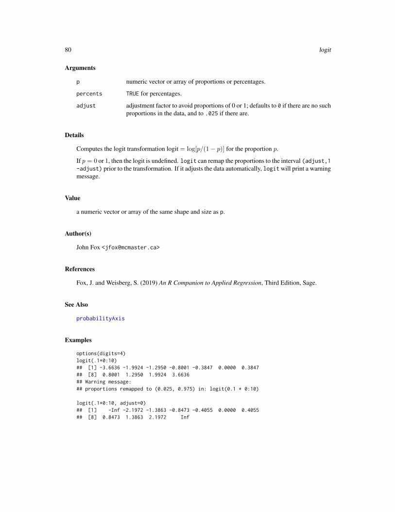
80 logit

Arguments

p numeric vector or array of proportions or percentages.

percents TRUE for percentages.

adjust adjustment factor to avoid proportions of 0 or 1; defaults to 0 if there are no suchproportions in the data, and to .025 if there are.

Details

Computes the logit transformation logit = log[p/(1− p)] for the proportion p.

If p = 0 or 1, then the logit is undefined. logit can remap the proportions to the interval (adjust,1-adjust) prior to the transformation. If it adjusts the data automatically, logit will print a warningmessage.

Value

a numeric vector or array of the same shape and size as p.

Author(s)


References


See Also

probabilityAxis

Examples

options(digits=4)logit(.1*0:10)## [1] -3.6636 -1.9924 -1.2950 -0.8001 -0.3847 0.0000 0.3847## [8] 0.8001 1.2950 1.9924 3.6636## Warning message:## proportions remapped to (0.025, 0.975) in: logit(0.1 * 0:10)

logit(.1*0:10, adjust=0)## [1] -Inf -2.1972 -1.3863 -0.8473 -0.4055 0.0000 0.4055## [8] 0.8473 1.3863 2.1972 Inf

mcPlots 81

mcPlots Draw Linear Model Marginal and Conditional Plots in Parallel orOverlaid

Description

the mcPlot function draws two graphs or overlays the two graphs. For a response Y and a regressorX, the first plot is the marginal plot of Y versus X with both variables centered, visualizing theconditional distribution of Y given X ignoring all other regressors. The second plot is an added-variable for X after all other regressors, visualizing the conditional distribution of Y given X afteradjusting for all other predictors. The added variable plot by default is drawn using the same xlimand ylim as the centered marginal plot to emphasize that conditioning removes variation in both theregressor and the response.The plot is primarily intended as a pedagogical tool for understandingcoefficients in first-order models.

Usage

mcPlots(model, terms=~., layout=NULL, ask, overlaid=TRUE, ...)

mcPlot(model, ...)

## S3 method for class 'lm'mcPlot(model, variable, id=FALSE,

col.marginal=carPalette()[2], col.conditional=carPalette()[3],col.arrows="gray", pch = c(16,1), lwd = 2, grid=TRUE,ellipse=FALSE, overlaid=TRUE, new=TRUE, title=TRUE, ...)

Arguments

model model object produced by lm.terms A one-sided formula that specifies a subset of the predictors. One added-variable

plot is drawn for each regressor and for each basis vector used to define a factor.For example, the specification terms = ~ . -X3 would plot against all terms ex-cept for X3. If this argument is a quoted name of one of the regressors or factors,the added-variable plot is drawn for that regressor or factor only. Unlike othercar functions, the formula should include the names of regressors, not predic-tors. That is, if log(X4) is used to represent a predictor X4, the formula shouldspecify terms = ~ log(X4).

variable A quoted string giving the name of a numeric predictor in the model matrix forthe horizontal axis. To plot against a factor, you need to specify the full nameof one of the indicator variables that define the factor. For example, for a factorcalled type with levels A, B and C, using the usual drop-first level parameteriza-tion of the factor, the regressors for type would be typeB or typeC. Similarly,to plot against the regressor log(X4), you must specify "log((X4)", not "X4".

layout If set to a value like c(1,2) or c(6,2), the layout of the graph will have thismany rows and columns. If not set, behavior depends on the value of theoverlaid argument; see the details

82 mcPlots

ask If TRUE, ask the user before drawing the next plot; if FALSE don’t ask.

... mcPlots passes these arguments to mcPlot. mcPlot passes arguments to plot.


overlaid If TRUE, the default, overlay the marginal and conditional plots on the samegraph; otherwise plot them side-by-side. See the details below

col.marginal, col.conditional

colors for points, lines, ellipses in the marginal and conditional plots, respec-tively. The defaults are determined by the carPalette function.

col.arrows color for the arrows with overlaid=TRUE

pch Plotting character for marginal and conditional plots, respectively.



ellipse Arguments to pass to the dataEllipse function, in the form of a list with namedelements; e.g., ellipse.args=list(robust=TRUE)) will cause the ellipse tobe plotted using a robust covariance-matrix. if FALSE, the default, no ellipseis plotted. TRUE is equivalent to ellipse=list(levels=0.5), which plots abivariate-normal 50 percent concentration ellipse.

new if TRUE, the default, the plot window is reset when overlaid=FALSE usingpar{mfrow=c(1,2)}. If FALSE, the layout of the plot window is not reset. Userswill ordinarily ignore this argument.

title If TRUE, the default, the standard main argument in plot is used to add a stan-dard title to each plot. If FALSE no title is used.

Details

With an lm object, suppose the response is Y, X is a numeric regressor of interest, and Z is allthe remaining predictors, possibly including interactions and factors. This function produces twographs. The first graph is the marginal plot of Y versus X, with each variable centered aroundits mean. The second conditional plot is the added-variable plot of e(Y|Z) versus e(X|Z) wheree(a|b) means the Pearson residuals from the regression of a on b. If overlaid=TRUE, these twoplots are overlaid in one graph, with the points in different colors. In addition, each point in themarginal plot is joined to its value in the conditional plot by an arrow. Least squares regressionlines fit to the marginal and conditional graphs are also shown; data ellipsoids can also be added.If overlaid=FALSE, then the two graphs are shown in side-by-side plots as long as the secondargument to layout is equal to 2, or layout is set by the function. The arrows are omitted if thegraphs are not overlaid.

These graphs are primarily for teaching, as the marginal plot shows the relationship between Y andX ignoring Z, while the conditional is the relationship between Y and X given X. By keeping thescales the same in both graphs the effect of conditioning on both X and Y can be visualized.

This function is intended for first-order models with numeric predictors only. For a factor, one (pair)of mcPlots will be produced for each of the dummy variables in the basis for the factor, and the

mmps 83

resulting plots are not generally meaningful because they depend on parameterization. If the meanfunction includes interactions, then mcPlots for main effects may violate the hierarchy principle,and may also be of little interest. mcPlots for interactions of numerical predictors, however, can beuseful.

These graphs are closely related to the ARES plots proposed by Cook and Weisberg (1989). Thisplot would benefit from animation.

Value

These functions are used for their side effect of producing plots.

Author(s)


References

Cook, R. D. and Weisberg, S. (1989) Regression diagnostics with dynamic graphics, Technometrics,31, 277.




See Also

avPlots, residualPlots, crPlots, ceresPlots, dataEllipse

Examples

m1 <- lm(partic ~ tfr + menwage + womwage + debt + parttime, data = Bfox)mcPlot(m1, "womwage")mcPlot(m1, "womwage", overlaid=FALSE, ellipse=TRUE)

mmps Marginal Model Plotting

Description

For a regression object, draw a plot of the response on the vertical axis versus a linear combina-tion u of regressors in the mean function on the horizontal axis. Added to the plot are a smoothfor the graph, along with a smooth from the plot of the fitted values on u. mmps is an alias formarginalModelPlots, and mmp is an alias for marginalModelPlot.

84 mmps

Usage

marginalModelPlots(...)

mmps(model, terms= ~ ., fitted=TRUE, layout=NULL, ask,main, groups, key=TRUE, ...)

marginalModelPlot(...)

mmp(model, ...)

## S3 method for class 'lm'mmp(model, variable, sd = FALSE,

xlab = deparse(substitute(variable)),smooth=TRUE, key=TRUE, pch, groups=NULL, ...)

## Default S3 method:mmp(model, variable, sd = FALSE,

xlab = deparse(substitute(variable)), ylab, smooth=TRUE,key=TRUE, pch, groups=NULL,col.line = carPalette()[c(2, 8)], col=carPalette()[1],id=FALSE, grid=TRUE, ...)

## S3 method for class 'glm'mmp(model, variable, sd = FALSE,

xlab = deparse(substitute(variable)), ylab,smooth=TRUE, key=TRUE, pch, groups=NULL,col.line = carPalette()[c(2, 8)], col=carPalette()[1],id=FALSE, grid=TRUE, ...)

Arguments

model A regression object, usually of class either lm or glm, for which there is apredict method defined.

terms A one-sided formula. A marginal model plot will be drawn for each term on theright-side of this formula that is not a factor. The default is ~ ., which specifiesthat all the terms in formula(object) will be used. If a conditioning argumentis given, eg terms = ~. | a, then separate colors and smoothers are used for eachunique non-missing value of a. See examples below.

fitted If TRUE, the default, then a marginal model plot in the direction of the fittedvalues for a linear model or the linear predictor of a generalized linear modelwill be drawn.


mmps 85

ask If TRUE, ask before clearing the graph window to draw more plots.

main Main title for the array of plots. Use main="" to suppress the title; if missing, atitle will be supplied.

... Additional arguments passed from mmps to mmp and then to plot. Users shouldgenerally use mmps, or equivalently marginalModelPlots.

variable The quantity to be plotted on the horizontal axis. If this argument is missing,the horizontal variable is the linear predictor, returned by predict(object)for models of class lm, with default label "Fitted values", or returned bypredict(object,type="link") for models of class glm, with default label"Linear predictor". It can be any other vector of length equal to the num-ber of observations in the object. Thus the mmp function can be used to get amarginal model plot versus any regressor or predictor while the mmps functioncan be used only to get marginal model plots for the first-order regressors in theformula. In particular, terms defined by a spline basis are skipped by mmps, butyou can use mmp to get the plot for the variable used to define the splines.

sd If TRUE, display sd smooths. For a binomial regression with all sample sizesequal to one, this argument is ignored as the SD bounds don’t make any sense.


ylab label for vertical axis, defaults to name of response.

smooth specifies the smoother to be used along with its arguments; if FALSE, no smootheris shown; can be a list giving the smoother function and its named arguments;TRUE, the default, is equivalent to list(smoother=loessLine,span=2/3) forlinear models and list(smoother=gamLine,k=3) for generalized linear mod-els. See ScatterplotSmoothers for the smoothers supplied by the car packageand their arguments; the spread argument is not supported for marginal modelplots.

groups The name of a vector that specifies a grouping variable for separate colors/smoothers.This can also be specified as a conditioning argument on the terms argument.

key If TRUE, include a key at the top of the plot, if FALSE omit the key. If groupingis present, the key is only printed for the upper-left plot.

id controls point identification; if FALSE (the default), no points are identified; canbe a list of named arguments to the showLabels function; TRUE is equivalent tolist(method="y",n=2,cex=1,col=carPalette()[1],location="lr"), whichidentifies the 2 points with the most unusual response (Y) values.

pch plotting character to use if no grouping is present.

col.line colors for data and model smooth, respectively. The default is to use carPalette,carPalette()[c(2,8)], blue and red.

col color(s) for the plotted points.


Details

mmp and marginalModelPlot draw one marginal model plot against whatever is specified as thehorizontal axis. mmps and marginalModelPlots draws marginal model plots versus each of the

86 mmps

terms in the terms argument and versus fitted values. mmps skips factors and interactions if they arespecified in the terms argument. Terms based on polynomials or on splines (or potentially any termthat is represented by a matrix of regressors) will be used to form a marginal model plot by returninga linear combination of the terms. For example, if you specify terms = ~ X1 + poly(X2,3) andpoly(X2,3) was part of the original model formula, the horizontal axis of the marginal model plotfor X2 will be the value of predict(model,type="terms")[,"poly(X2,3)"]). If the predictmethod for the model you are using doesn’t support type="terms", then the polynomial/splineterm is skipped. Adding a conditioning variable, e.g., terms = ~ a + b | c, will produce marginalmodel plots for a and b with different colors and smoothers for each unique non-missing value of c.

For linear models, the default smoother is loess. For generalized linear models, the default smootheruses gamLine, fitting a generalized additive model with the same family, link and weights as the fitof the model. SD smooths are not computed for for generalized linear models.

For generalized linear models the default number of elements in the spline basis is k=3; this is doneto allow fitting for predictors with just a few support points. If you have many support points youmay wish to set k to a higher number, or k=-1 for the default used by gam.

Value

Used for its side effect of producing plots.

Author(s)


References

Cook, R. D., & Weisberg, S. (1997). Graphics for assessing the adequacy of regression models.Journal of the American Statistical Association, 92(438), 490-499.

Fox, J. and Weisberg, S. (2019) An R Companion to Applied Regression, Third Edition. Sage.

Weisberg, S. (2005) Applied Linear Regression, Third Edition, Wiley, Section 8.4.

See Also

ScatterplotSmoothers, plot

Examples

c1 <- lm(infantMortality ~ ppgdp, UN)mmps(c1)c2 <- update(c1, ~ log(ppgdp))mmps(c2)# include SD linesp1 <- lm(prestige ~ income + education, Prestige)mmps(p1, sd=TRUE)# condition on type:mmps(p1, ~. | type)# logisitic regression example# smoothers return warning messages.# fit a separate smoother and color for each type of occupation.

ncvTest 87

m1 <- glm(lfp ~ ., family=binomial, data=Mroz)mmps(m1)

ncvTest Score Test for Non-Constant Error Variance

Description

Computes a score test of the hypothesis of constant error variance against the alternative that theerror variance changes with the level of the response (fitted values), or with a linear combination ofpredictors.

Usage

ncvTest(model, ...)

## S3 method for class 'lm'ncvTest(model, var.formula, ...)

## S3 method for class 'glm'ncvTest(model, ...) # to report an error

Arguments

model a weighted or unweighted linear model, produced by lm.

var.formula a one-sided formula for the error variance; if omitted, the error variance dependson the fitted values.

... arguments passed down to methods functions; not currently used.

Details

This test is often called the Breusch-Pagan test; it was independently suggested with some extensionby Cook and Weisberg (1983).

ncvTest.glm is a dummy function to generate an error when a glm model is used.

Value

The function returns a chisqTest object, which is usually just printed.

Author(s)

John Fox <[email protected]>, Sandy Weisberg <[email protected]>

88 outlierTest

References

Breusch, T. S. and Pagan, A. R. (1979) A simple test for heteroscedasticity and random coefficientvariation. Econometrica 47, 1287–1294.

Cook, R. D. and Weisberg, S. (1983) Diagnostics for heteroscedasticity in regression. Biometrika70, 1–10.




See Also

hccm, spreadLevelPlot

Examples

ncvTest(lm(interlocks ~ assets + sector + nation, data=Ornstein))

ncvTest(lm(interlocks ~ assets + sector + nation, data=Ornstein),~ assets + sector + nation, data=Ornstein)

outlierTest Bonferroni Outlier Test

Description

Reports the Bonferroni p-values for testing each observation in turn to be a mean-shift outlier, basedStudentized residuals in linear (t-tests), generalized linear models (normal tests), and linear mixedmodels.

Usage

outlierTest(model, ...)

## S3 method for class 'lm'outlierTest(model, cutoff=0.05, n.max=10, order=TRUE,labels=names(rstudent), ...)

## S3 method for class 'lmerMod'outlierTest(model, ...)

## S3 method for class 'outlierTest'print(x, digits=5, ...)

outlierTest 89

Arguments

model an lm, glm, or lmerMod model object; the "lmerMod" method calls the "lm"method and can take the same arguments.

cutoff observations with Bonferroni p-values exceeding cutoff are not reported, un-less no observations are nominated, in which case the one with the largest Stu-dentized residual is reported.

n.max maximum number of observations to report (default, 10).

order report Studenized residuals in descending order of magnitude? (default, TRUE).

labels an optional vector of observation names.

... arguments passed down to methods functions.

x outlierTest object.

digits number of digits for reported p-values.

Details

For a linear model, p-values reported use the t distribution with degrees of freedom one less than theresidual df for the model. For a generalized linear model, p-values are based on the standard-normaldistribution. The Bonferroni adjustment multiplies the usual two-sided p-value by the number ofobservations. The lm method works for glm objects. To show all of the observations set cutoff=Infand n.max=Inf.

Value

an object of class outlierTest, which is normally just printed.

Author(s)

John Fox <[email protected]> and Sanford Weisberg

References

Cook, R. D. and Weisberg, S. (1982) Residuals and Influence in Regression. Chapman and Hall,https://conservancy.umn.edu/handle/11299/37076.




Williams, D. A. (1987) Generalized linear model diagnostics using the deviance and single casedeletions. Applied Statistics 36, 181–191.

Examples

outlierTest(lm(prestige ~ income + education, data=Duncan))

https://conservancy.umn.edu/handle/11299/37076

90 panel.car

panel.car Panel Function for Coplots

Description

a panel function for use with coplot that plots points, a lowess line, and a regression line.

Usage

panel.car(x, y, col, pch, cex=1, span=0.5, lwd=2,reg.line=lm, lowess.line=TRUE, ...)

Arguments

x vector giving horizontal coordinates.

y vector giving vertical coordinates.

col point color.

pch plotting character for points.

cex character expansion factor for points.

span span for lowess smoother.

lwd line width, default is 2.

reg.line function to compute coefficients of regression line, or FALSE for no line.

lowess.line if TRUE plot lowess smooth.

... other arguments to pass to functions lines and regLine.

Value

NULL. This function is used for its side effect: producing a panel in a coplot.

Author(s)


See Also

coplot, regLine

Examples

coplot(prestige ~ income|education, panel=panel.car,col="red", data=Prestige)

poTest 91

poTest Test for Proportional Odds in the Proportional-Odds Logistic-Regression Model

Description

The poTest function implements tests proposed by Brant (1990) for proportional odds for logisticmodels fit by the polr function in the MASS package.

Usage

poTest(model, ...)## S3 method for class 'polr'poTest(model, ...)## S3 method for class 'poTest'print(x, digits=3, ...)

Arguments

model a proptional-odds logit model fit by polr.

x an object produced by poTest.

digits number of significant digits to print.

... ignored.

Value

poTest returns an object meant to be printed showing the results of the tests.

Author(s)


References

R. Brant, "Assessing proportionality in the proportional odds model for ordinal logistic regression."Biometrics 46: 1171–1178, 1990.

Examples

if (require("MASS")){.W <- Womenlf.W$partic <- factor(.W$partic, levels=c("not.work", "parttime", "fulltime"))poTest(polr(partic ~ hincome + children + region, data=.W))

}

92 powerTransform

powerTransform Finding Univariate or Multivariate Power Transformations

Description

powerTransform uses the maximum likelihood-like approach of Box and Cox (1964) to selecta transformatiion of a univariate or multivariate response for normality, linearity and/or constantvariance. Available families of transformations are the default Box-Cox power family and twoadditioal families that are modifications of the Box-Cox family that allow for (a few) negativeresponses. The summary method automatically computes two or three likelihood ratio type testsconcerning the transformation powers.

Usage

powerTransform(object, ...)

## Default S3 method:powerTransform(object, family="bcPower", ...)

## S3 method for class 'lm'powerTransform(object, family="bcPower", ...)

## S3 method for class 'formula'powerTransform(object, data, subset, weights, na.action,

family="bcPower", ...)

## S3 method for class 'lmerMod'powerTransform(object, family="bcPower", ...)

Arguments

object This can either be an object of class lm or lmerMod, a formula, or a matrix orvector; see below.

family The quoted name of a family of transformations. The available options are"bcPower" for the default for the Box-Cox power family; "bcnPower" for atwo-parameter modification of the Box-Cox family that allows negative responses(Hawkins and Weisberg (2017)), and the "yjPower" family (Yeo and John-son(2000)), another modifiation of the Box-Cox family that allows a few nega-tive values. All three families are documented at bcPower.

data A data frame or environment, as in ‘lm’.subset Case indices to be used, as in ‘lm’.weights Weights as in ‘lm’.na.action Missing value action, as in ‘lm’.... Additional arguments that used in the interative algorithm; defaults are generally

adequate. For use with the bcnPower family, a convergence criterion can beset with conv=.0001 the default, and a minimum positive value of the locationparameter can be set, with default gamma.min=.1.

powerTransform 93

Details

This function implements the Box and Cox (1964) method of selecting a power transformation of avariable toward normality, and its generalization by Velilla (1993) to a multivariate response. Cookand Weisberg (1999) and Weisberg (2014) suggest the usefulness of transforming a set of predictorsz1,z2,z3 for multivariate normality. It also includes two additional families that allow for negativevalues.

If the object argument is of class ‘lm’ or ‘lmerMod’, the Box-Cox procedure is applied to theconditional distribution of the response given the predictors. For ‘lm’ objects, the respose may bemultivariate, and each column will have its own transformation. With ‘lmerMod’ the response mustbe univariate.

The object argument may also be a formula. For example, z ~ x1 + x2 + x3 will estimate a trans-formation for the response z from a family after fitting a linear model with the given formula.cbind(y1,y2,y3) ~ 1 specifies transformations to multivariate normality with no predictors. Avector value for object, for example powerTransform(ais$LBM), is equivalent topowerTransform(LBM~ 1,ais). Similarly, powerTransform(cbind(ais$LBM,ais$SSF)), where the first argument is amatrix rather than a formula is equivalent to specification of a mulitvariate linear model powerTransform(cbind(LBM,SSF)~ 1,ais).

Three families of power transformations are available. The default Box-Cox power family (family="bcPower")of power transformations effectively replaces a vector by that vector raised to a power, generallyin the range from -3 to 3. For powers close to zero, the log-transformtion is suggested. In prac-tical situations, after estimating a power using the powerTransform function, a variable would bereplaced by a simple power transformation of it, for example, if λ ≈ 0.5, then the correspodingvariable would be replaced by its square root; if λ is close enough to zero, the the variable would bereplaced by its natural logarithm. The Box-Cox family requires the responses to be strictly positive.

The family="bcnPower", or Box-Cox with negatives, family proposed by Hawkins and Weisberg(2017) allows for (a few) non-positive values, while allowing for the transformed data to be inter-preted similarly to the interpretation of Box-Cox transformed values. This family is the Box-Coxtransformation of z = .5∗(y+(y2+γ2)1/2) that depends on a location parameter γ. The quantity zis positive for all values of y. If γ = 0 and y is strictly positive, then the Box-Cox and the bcnPowertransformations are identical. When fitting the Box-Cox with negatives family, lambda is restrictedto the range [-3, 3], and gamma is restricted to the range from gamma.min=.1 to the largest positivevalue of the variable, since values outside these ranges are unreasonable in practice. The value ofgamma.min can be changed with an argument to powerTransform.

The final family family="yjPower" uses the Yeo-Johnson transformation, which is the Box-Coxtransformation of U + 1 for nonnegative values, and of |U |+ 1 with parameter 2−λ for U negativeand thus it provides a family for fitting when (a few) observations are negative. Because of theunusual constraints on the powers for positive and negative data, this transformation is not usedvery often, as results are difficult to interpret. In practical problems, a variable would be replacedby its Yeo-Johnson transformation computed using the yjPower function.

The function testTransform is used to obtain likelihood ratio tests for any specified value for thetransformation parameter(s).

Computations maximize the likelihood-like functions described by Box and Cox (1964) and byVelilla (1993). For univariate responses, the computations are very stable and problems are unlikely,although for ‘lmer’ models computations may be very slow because the model is refit many times.For multivariate responses with the bcnPower family, the computing algorithm may fail. In this casewe recommend adding the argument itmax = 1 to the call to powerTransform. This will return the

94 powerTransform

starting value estimates of the transformation parameters, fitting a d-dimensional response as if allthe d responses were independent.

Value

An object of class powerTransform or class bcnPowerTransform if family="bcnPower" that in-herits from powerTransform is returned, including the components listed below.

A summary method presents estimated values for the transformation power lambda and for the‘bcnPower’ family the location parameter gamma as well. Standard errors and Wald 95% confidenceintervals based on the standard errors are computed from the inverse of the sample Hessian matrixevaluted at the estimates. The interval estimates for the gamma parameters will generally be verywide, reflecting little information available about the location parameter. Likelihood ratio type testsare also provided. For the ‘bcnPower’ family these are based on the profile loglikelihood for lambdaalone; that is, we treat gamma as a nusiance parameter and average over it.

The components of the returned object includes

lambda Estimated transformation parameter

roundlam Convenient rounded values for the estimates. These rounded values will usuallybe the desired transformations.

gamma Estimated location parameters for bcnPower, NULL otherwise

invHess Estimated covariance matrix of the estimated parameters

llik Value of the log-likelihood at the estimates

The summary method for powerTransform returns an array with columns labeled "Est Power" forthe value of lambda that maximizes the likelihood; "Rounded Pwr" for roundlam, and columns"Wald Lwr Bnd" and "Wald Ur Bnd" for a 95 percent Wald normal theory confidence interval forlambda computed as the estimate plus or minus 1.96 times the standard error.

Author(s)


References





Velilla, S. (1993) A note on the multivariate Box-Cox transformation to normality. Statistics andProbability Letters, 17, 259-263.


Yeo, I. and Johnson, R. (2000) A new family of power transformations to improve normality orsymmetry. Biometrika, 87, 954-959.

powerTransform 95

See Also

testTransform, bcPower, bcnPower, transform, optim, boxCox.

Examples

# Box Cox Method, univariatesummary(p1 <- powerTransform(cycles ~ len + amp + load, Wool))# fit linear model with transformed response:coef(p1, round=TRUE)summary(m1 <- lm(bcPower(cycles, p1$roundlam) ~ len + amp + load, Wool))

# Multivariate Box Cox uses Highway1 datasummary(powerTransform(cbind(len, adt, trks, sigs1) ~ 1, Highway1))

# Multivariate transformation to normality within levels of 'htype'summary(a3 <- powerTransform(cbind(len, adt, trks, sigs1) ~ htype, Highway1))

# test lambda = (0 0 0 -1)testTransform(a3, c(0, 0, 0, -1))

# save the rounded transformed values, plot them with a separate# color for each highway typetransformedY <- bcPower(with(Highway1, cbind(len, adt, trks, sigs1)),

coef(a3, round=TRUE))## Not run: scatterplotMatrix( ~ transformedY|htype, Highway1)

# With negative responses, use the bcnPower familym2 <- lm(I1L1 ~ pool, LoBD)summary(p2 <- powerTransform(m2, family="bcnPower"))testTransform(p2, .5)summary(powerTransform(update(m2, cbind(LoBD$I1L2, LoBD$I1L1) ~ .), family="bcnPower"))

## Not run:# tajes a few seconds:# multivariate bcnPower, with 8 responsessummary(powerTransform(update(m2, as.matrix(LoBD[, -1]) ~ .), family="bcnPower"))# multivariate bcnPower, fit with one iteration using starting values as estimatessummary(powerTransform(update(m2, as.matrix(LoBD[, -1]) ~ .), family="bcnPower", itmax=1))

## End(Not run)

# mixed effects model## Not run:

# uses the lme4 packagedata <- reshape(LoBD[1:20, ], varying=names(LoBD)[-1], direction="long", v.names="y")names(data) <- c("pool", "assay", "y", "id")data$assay <- factor(data$assay)require(lme4)m2 <- lmer(y ~ pool + (1|assay), data)summary(l2 <- powerTransform(m2, family="bcnPower", verbose=TRUE))

## End(Not run)

96 Predict

Predict Model Predictions

Description

Predict is a generic function with, at present, a single method for "lm" objects, Predict.lm, whichis a modification of the standard predict.lm method in the stats package, but with an additionalvcov. argument for a user-specified covariance matrix for intreval estimation.

Usage

Predict(object, ...)

## S3 method for class 'lm'Predict(object, newdata, se.fit = FALSE,scale = NULL, df = Inf,interval = c("none", "confidence", "prediction"),level = 0.95, type = c("response", "terms"),terms = NULL, na.action = na.pass,pred.var = res.var/weights, weights = 1, vcov., ...)

Arguments

object a model object for which predictions are desired.newdata, se.fit, scale, df, interval, level, type, terms, na.action, pred.var, weights

see predict.lm.

vcov. optional, either a function to compute the coefficient covariance matrix of object(e.g., hccm) or a coefficient covariance matrix (as returned, e.g., by hccm).

... arguments to pass down to Predict or predict methods.

Details

If there is no appropriate method for Predict, then a predict method is invoked. If there is aspecific predict method for the primary class of object but only an inherited Predict method,then the predict method is invoked. Thus an object of class c("glm","lm") will invoke methodpredict.glm rather than Predict.lm, but an object of class c("aov","lm") will invoke Predict.lmrather than predict.lm.

Value

See predict and predict.lm.

Author(s)


qqPlot 97

References


See Also

predict, predict.lm

Examples

mod <- lm(interlocks ~ log(assets), data=Ornstein)newd <- data.frame(assets=exp(4:12))(p1 <- predict(mod, newd, interval="prediction"))p2 <- Predict(mod, newd, interval="prediction", vcov.=vcov)all.equal(p1, p2) # the same

(predict(mod, newd, se=TRUE))(p3 <- Predict(mod, newd, se=TRUE, vcov.=hccm)) # larger SEsp4 <- Predict(mod, newd, se=TRUE, vcov.=hccm(mod, type="hc3"))all.equal(p3, p4) # the same

qqPlot Quantile-Comparison Plot

Description

Plots empirical quantiles of a variable, or of studentized residuals from a linear model, againsttheoretical quantiles of a comparison distribution. Includes options not avaiable in the qqnormfunction.

Usage

qqPlot(x, ...)

qqp(...)

## Default S3 method:qqPlot(x, distribution="norm", groups, layout,

ylim=range(x, na.rm=TRUE), ylab=deparse(substitute(x)),xlab=paste(distribution, "quantiles"), glab=deparse(substitute(groups)),main=NULL, las=par("las"),envelope=.95, col=carPalette()[1], col.lines=carPalette()[2],lwd=2, pch=1, cex=par("cex"),line=c("quartiles", "robust", "none"), id=TRUE, grid=TRUE, ...)

## S3 method for class 'formula'qqPlot(formula, data, subset, id=TRUE, ylab, glab, ...)

## S3 method for class 'lm'

98 qqPlot

qqPlot(x, xlab=paste(distribution, "Quantiles"),ylab=paste("Studentized Residuals(",

deparse(substitute(x)), ")", sep=""),main=NULL, distribution=c("t", "norm"),line=c("robust", "quartiles", "none"), las=par("las"),simulate=TRUE, envelope=.95, reps=100,col=carPalette()[1], col.lines=carPalette()[2], lwd=2, pch=1, cex=par("cex"),id=TRUE, grid=TRUE, ...)

Arguments

x vector of numeric values or lm object.

distribution root name of comparison distribution – e.g., "norm" for the normal distribution;t for the t-distribution.

groups an optional factor; if specified, a QQ plot will be drawn for x within each levelof groups.

layout a 2-vector with the number of rows and columns for plotting by groups – forexample c(1,3) for 1 row and 3 columns; if omitted, the number of rowsand columns will be selected automatically; the specified number of rows andcolumns must be sufficient to accomodate the number of groups; ignored if thereis no grouping factor.

formula one-sided formula specifying a single variable to be plotted or a two-sided for-mula of the form variable ~ factor, where a QQ plot will be drawn for variablewithin each level of factor.

data optional data frame within which to evaluage the formula.

subset optional subset expression to select cases to plot.

ylim limits for vertical axis; defaults to the range of x. If plotting by groups, a com-mon y-axis is used for all groups.

ylab label for vertical (empirical quantiles) axis.

xlab label for horizontal (comparison quantiles) axis.

glab label for the grouping variable.

main label for plot.

envelope confidence level for point-wise confidence envelope, or FALSE for no envelope.

las if 0, ticks labels are drawn parallel to the axis; set to 1 for horizontal labels (seepar).


col.lines color for lines; the default is the second entry in the current car palette.


cex factor for expanding the size of plotted symbols; the default is 1.

id controls point identification; if FALSE, no points are identified; can be a list ofnamed arguments to the showLabels function; TRUE is equivalent to list(method="y",n=2,cex=1,col=carPalette()[1],location="lr"),which identifies the 2 points with the 2 points with the most extreme verical val-ues — studentized residuals for the "lm" method. Points labels are by default

qqPlot 99

taken from the names of the variable being plotted is any, else case indices areused. Unlike most graphical functions in car, the default is id=TRUE to includepoint identification.


line "quartiles" to pass a line through the quartile-pairs, or "robust" for a robust-regression line; the latter uses the rlm function in the MASS package. Specifyingline = "none" suppresses the line.

simulate if TRUE calculate confidence envelope by parametric bootstrap; for lm objectonly. The method is due to Atkinson (1985).

reps integer; number of bootstrap replications for confidence envelope.

... arguments such as df to be passed to the appropriate quantile function.


Details

Draws theoretical quantile-comparison plots for variables and for studentized residuals from a linearmodel. A comparison line is drawn on the plot either through the quartiles of the two distributions,or by robust regression.

Any distribution for which quantile and density functions exist in R (with prefixes q and d, respec-tively) may be used. When plotting a vector, the confidence envelope is based on the SEs of theorder statistics of an independent random sample from the comparison distribution (see Fox, 2016).Studentized residuals from linear models are plotted against the appropriate t-distribution with apoint-wise confidence envelope computed by default by a parametric bootstrap, as described byAtkinson (1985). The function qqp is an abbreviation for qqPlot.

Value

These functions return the labels of identified points, unless a grouping factor is employed, in whichcase NULL is returned invisibly.

Author(s)


References



Atkinson, A. C. (1985) Plots, Transformations, and Regression. Oxford.

See Also

qqplot, qqnorm, qqline, showLabels

100 recode

Examples

x<-rchisq(100, df=2)qqPlot(x)qqPlot(x, dist="chisq", df=2)

qqPlot(~ income, data=Prestige, subset = type == "prof")qqPlot(income ~ type, data=Prestige, layout=c(1, 3))

qqPlot(lm(prestige ~ income + education + type, data=Duncan),envelope=.99)

recode Recode a Variable

Description

Recodes a numeric vector, character vector, or factor according to simple recode specifications.Recode is an alias for recode that avoids name clashes with packages, such as Hmisc, that have arecode function.

Usage

recode(var, recodes, as.factor, as.numeric=TRUE, levels)

Recode(...)

Arguments

var numeric vector, character vector, or factor.

recodes character string of recode specifications: see below.

as.factor return a factor; default is TRUE if var is a factor, FALSE otherwise.

as.numeric if TRUE (the default), and as.factor is FALSE, then the result will be coerced tonumeric if all values in the result are numerals—i.e., represent numbers.

levels an optional argument specifying the order of the levels in the returned factor; thedefault is to use the sort order of the level names.

... arguments to be passed to recode.

Details

Recode specifications appear in a character string, separated by semicolons (see the examples be-low), of the form input=output. If an input value satisfies more than one specification, then thefirst (from left to right) applies. If no specification is satisfied, then the input value is carried overto the result. NA is allowed on input and output. Several recode specifications are supported:

single value For example, 0=NA.

vector of values For example, c(7,8,9)='high'.

regLine 101

range of values For example, 7:9='C'. The special values lo and hi may appear in a range. Forexample, lo:10=1. Note: : is not the R sequence operator. In addition you may not use :with the collect operator, so for example c(1,3,5:7) will cause an error.

else everything that does not fit a previous specification. For example, else=NA. Note that elsematches all otherwise unspecified values on input, including NA.

If all of the output values are numeric, and if as.factor is FALSE, then a numeric result is returned;if var is a factor, then by default so is the result.

Value

a recoded vector of the same length as var.

Author(s)


References


See Also

cut, factor

Examples

x<-rep(1:3,3)x## [1] 1 2 3 1 2 3 1 2 3recode(x, "c(1,2)='A';else='B'")## [1] "A" "A" "B" "A" "A" "B" "A" "A" "B"Recode(x, "1:2='A'; 3='B'")## [1] "A" "A" "B" "A" "A" "B" "A" "A" "B"

regLine Plot Regression Line

Description

Plots a regression line on a scatterplot; the line is plotted between the minimum and maximumx-values.

Usage

regLine(mod, col=carPalette()[2], lwd=2, lty=1,...)

102 residualPlots

Arguments

mod a model, such as produced by lm, that responds to the coef function by returninga 2-element vector, whose elements are interpreted respectively as the interceptand slope of a regresison line.

col color for points and lines; the default is the second entry in the current carpalette (see carPalette and par).


lty line type; default is 1, a solid line (see par).

... optional arguments to be passed to the lines plotting function.

Details

In contrast to abline, this function plots only over the range of the observed x-values. The x-valuesare extracted from mod as the second column of the model matrix.

Value

NULL. This function is used for its side effect: adding a line to the plot.

Author(s)


See Also

abline, lines

Examples

plot(repwt ~ weight, pch=c(1,2)[sex], data=Davis)regLine(lm(repwt~weight, subset=sex=="M", data=Davis))regLine(lm(repwt~weight, subset=sex=="F", data=Davis), lty=2)

residualPlots Residual Plots for Linear and Generalized Linear Models

Description

Plots the residuals versus each term in a mean function and versus fitted values. Also computes acurvature test for each of the plots by adding a quadratic term and testing the quadratic to be zero.For linear models, this is Tukey’s test for nonadditivity when plotting against fitted values.

residualPlots 103

Usage

### This is a generic function with only one required argument:

residualPlots (model, ...)

## Default S3 method:residualPlots(model, terms = ~., layout = NULL, ask,

main = "", fitted = TRUE, AsIs=TRUE, plot = TRUE,tests = TRUE, groups, ...)

## S3 method for class 'lm'residualPlots(model, ...)

## S3 method for class 'glm'residualPlots(model, ...)

### residualPlots calls residualPlot, so these arguments can be### used with either function

residualPlot(model, ...)

## Default S3 method:residualPlot(model, variable = "fitted", type = "pearson",

groups, plot = TRUE, linear = TRUE,quadratic = if(missing(groups)) TRUE else FALSE,smooth=FALSE, id=FALSE,col = carPalette()[1], col.quad = carPalette()[2], pch=1,xlab, ylab, lwd = 1, lty = 1,grid=TRUE, key=!missing(groups), ...)

## S3 method for class 'lm'residualPlot(model, ...)

## S3 method for class 'glm'residualPlot(model, variable = "fitted", type = "pearson",

plot = TRUE, quadratic = FALSE, smooth=TRUE, ...)

Arguments

model A regression object.

terms A one-sided formula that specifies a subset of the factors and the regressors thatappear in the formula that defined the model. The default ~ . is to plot againstall first-order terms, both regressors and factors. Higher order terms are skipped.For example, the specification terms = ~ . -X3 would plot against all regressorsexcept for X3. To get a plot against fitted values only, use the arguments terms =~ 1. Interactions are skipped. For polynomial terms, the plot is against the first-order variable (which may be centered and scaled depending on how the polyfunction is used). Plots against factors are boxplots. Plots against other matrix

104 residualPlots

terms, like splines, use the result of predict(model),type="terms")[,variable])as the horizontal axis; if the predict method doesn’t permit this type, then ma-trix terms are skipped.A grouping variable can also be specified in the terms, so, for example terms=~ .|type would use the factor type to set a different color and symbol for eachlevel of type. Any fits in the plots will also be done separately for each level ofgroup.


ask If TRUE, ask the user before drawing the next plot; if FALSE, don’t ask.

main Main title for the graphs. The default is main="" for no title.

fitted If TRUE, the default, include the plot against fitted values.

AsIs If FALSE, terms that use the “as-is” function I are skipped; if TRUE, the default,they are included.

plot If TRUE, draw the plot(s).

tests If TRUE, display the curvature tests. With glm’s, the argument start is ignoredin computing the curvature tests.

... Additional arguments passed to residualPlot and then to plot.

variable Quoted variable name for the factor or regressor to be put on the horizontal axis,or the default "fitted" to plot versus fitted values.

type Type of residuals to be used. Pearson residuals are appropriate for lm objectssince these are equivalent to ordinary residuals with ols and correctly weightedresiduals with wls. Any quoted string that is an appropriate value of the typeargument to residuals.lm or "rstudent" or "rstandard" for Studentized orstandardized residuals.

groups A grouping indicator. Points in different groups will be plotted with differentcolors and symbols. If missing, no grouping is used. In residualPlots, thegrouping variable can also be set in the terms argument, as described above.The default is no grouping. If used, the groups argument shoud be a vectorof values of the same length as the vector of residuals, for example groups =subject where subject indicates the grouping.

linear If TRUE, adds a horizontal line at zero if no groups. With groups, display thewithin level of groups ols regression of the residuals as response and the hori-zontal axis as the regressor.

quadratic if TRUE, fits the quadratic regression of the vertical axis on the horizontal axisand displays a lack of fit test. Default is TRUE for lm and FALSE for glm or ifgroups not missing.

smooth specifies the smoother to be used along with its arguments; if FALSE, which isthe default except for generalized linear models, no smoother is shown; can be alist giving the smoother function and its named arguments; TRUE is equivalent to

residualPlots 105

list(smoother=loessLine,span=2/3,col=carPalette()[3]), which is thedefault for a GLM. See ScatterplotSmoothers for the smoothers supplied bythe car package and their arguments.

id controls point identification; if FALSE (the default), no points are identified; canbe a list of named arguments to the showLabels function; TRUE is equivalent tolist(method="r",n=2,cex=1,col=carPalette()[1],location="lr"), whichidentifies the 2 points with the largest absolute residuals.

col default color for points. If groups is set, col can be a list at least as long as thenumber of levels for groups giving the colors for each groups.

col.quad default color for quadratic fit if groups is missing. Ignored if groups are used.

pch plotting character. The default is pch=1. If groups are used, pch can be set to avector at least as long as the number of groups.

xlab X-axis label. If not specified, a useful label is constructed by the function.

ylab Y-axis label. If not specified, a useful label is constructed by the function.

lwd line width for lines.

lty line type for quadratic.


key Should a key be added to the plot? Default is !is.null(groups).

Details

residualPlots draws one or more residuals plots depending on the value of the terms and fittedarguments. If terms = ~ ., the default, then a plot is produced of residuals versus each first-orderterm in the formula used to create the model. Interaction terms, spline terms, and polynomial termsof more than one predictor are skipped. In addition terms that use the “as-is” function, e.g., I(X^2),will also be skipped unless you set the argument AsIs=TRUE. A plot of residuals versus fitted valuesis also included unless fitted=FALSE.

In addition to plots, a table of curvature tests is displayed. For plots against a term in the modelformula, say X1, the test displayed is the t-test for for I(X1^2) in the fit of update,model,~. +I(X1^2)). Econometricians call this a specification test. For factors, the displayed plot is a boxplot,no curvature test is computed, and grouping is ignored. For fitted values in a linear model, the test isTukey’s one-degree-of-freedom test for nonadditivity. You can suppress the tests with the argumenttests=FALSE. If grouping is used curvature tests are not displayed.

residualPlot, which is called by residualPlots, should be viewed as an internal function, andis included here to display its arguments, which can be used with residualPlots as well. TheresidualPlot function returns the curvature test as an invisible result.

residCurvTest computes the curvature test only. For any factors a boxplot will be drawn. Forany polynomials, plots are against the linear term. Other non-standard predictors like B-splines areskipped.

Value

For lm objects, returns a data.frame with one row for each plot drawn, one column for the curvaturetest statistic, and a second column for the corresponding p-value. This function is used primarilyfor its side effect of drawing residual plots.

106 S

Author(s)


References


Weisberg, S. (2014) Applied Linear Regression, Fourth Edition, Wiley, Chapter 8

See Also

See Also lm, identify, showLabels

Examples

m1 <- lm(prestige ~ income, data=Prestige)residualPlots(m1)residualPlots(m1, terms= ~ 1 | type) # plot vs. yhat grouping by type

S Modified Functions for Summarizing Linear, Generalized Linear, andSome Other Models

Description

car package replacements for the summary (S) and confint (Confint) functions for lm, glm,multinom, and polr objects, with additional arguments but the same defaults as the original func-tions. The Confint method for "polr" objects profiles the likelihood to get confidence intervalsfor the regression parameters but uses Wald intervals for the thresholds. Default methods that callthe standard R summary and confint functions are provided for the S and Confint generics, so thecar functions should be safe to use in general. The default method for Confint also assumes thatthere is an appropriate coef method. For briefer model summaries, see brief.

Usage

S(object, brief, ...)

## S3 method for class 'lm'S(object, brief=FALSE,

correlation = FALSE, symbolic.cor = FALSE,vcov. = vcov(object, complete=FALSE), header = TRUE,resid.summary = FALSE, adj.r2 = FALSE,...)

## S3 method for class 'glm'S(object, brief=FALSE,

exponentiate, dispersion, correlation = FALSE, symbolic.cor = FALSE,

S 107

vcov. = vcov(object, complete=FALSE), header = TRUE,resid.summary = FALSE, ...)

## S3 method for class 'multinom'S(object, brief=FALSE, exponentiate=FALSE, ...)

## S3 method for class 'polr'S(object, brief=FALSE, exponentiate=FALSE, ...)

## S3 method for class 'lme'S(object, brief=FALSE, correlation=FALSE, ...)

## S3 method for class 'lmerMod'S(object, brief=FALSE, KR=FALSE, correlation=FALSE, ...)

## S3 method for class 'glmerMod'S(object, brief=FALSE, correlation=FALSE, exponentiate, ...)

## Default S3 method:S(object, brief, ...)

## S3 method for class 'S.lm'print(x, digits = max(3, getOption("digits") - 3),

symbolic.cor = x$symbolic.cor, signif.stars = getOption("show.signif.stars"), ...)

## S3 method for class 'S.glm'print(x, digits = max(3L, getOption("digits") - 3L),

symbolic.cor = x$symbolic.cor, signif.stars = getOption("show.signif.stars"), ...)

## S3 method for class 'S.multinom'print(x, digits = max(3, getOption("digits") - 3),

signif.stars = getOption("show.signif.stars"), ...)

## S3 method for class 'S.polr'print(x, digits = max(3, getOption("digits") - 3),


## S3 method for class 'S.lme'print(x, digits=max(3, getOption("digits") - 3),


## S3 method for class 'S.lmerMod'print(x, digits=max(3, getOption("digits") - 3),


## S3 method for class 'S.glmerMod'print(x, digits=max(3, getOption("digits") - 3),


108 S

Confint(object, ...)

## S3 method for class 'lm'Confint(object, estimate=TRUE,

parm, level=0.95, vcov.=vcov(object, complete=FALSE), ...)

## S3 method for class 'glm'Confint(object, estimate=TRUE, exponentiate=FALSE,

vcov., dispersion, type=c("LR", "Wald"), ...)

## S3 method for class 'polr'Confint(object, estimate=TRUE, exponentiate=FALSE,

thresholds=!exponentiate, ...)

## S3 method for class 'multinom'Confint(object, estimate=TRUE, exponentiate=FALSE, ...)

## S3 method for class 'lme'Confint(object, estimate=TRUE, level=0.95, ...)

## S3 method for class 'lmerMod'Confint(object, estimate=TRUE, level=0.95, ...)

## S3 method for class 'glmerMod'Confint(object, estimate=TRUE, level=0.95,

exponentiate=FALSE, ...)

## Default S3 method:Confint(object, estimate=TRUE, level=0.95, vcov., ...)

Arguments

object a model object, e.g., of class "lm" as produced by a call to lm.

exponentiate for a "glm" or "glmerMod" model using the log or logit link, or a "polr"or "multinom" model, show exponentiated coefficient estimates and confidencebounds.

correlation, symbolic.cor

see summary.lm

x, digits, signif.stars

see summary.lm

dispersion see summary.glm

vcov. either a matrix giving the estimated covariance matrix of the estimates, or afunction that when called with object as an argument returns an estimated co-variance matrix of the estimates. The default of vcov. = vcov uses the usualestimated covariance matrix. Other choices include the functions documentedat hccm. See example below for using a bootstrap to estimate the covariance

S 109

matrix. For the glm methods of Confint and S, if the vcov. or dispersion ar-gument is specified, then Wald-based confidence limits are computed; otherwisethe reported confidence limits are computed by profiling the likelihood. NOTE:The dispersion and vcov. arguments may not both be specified.

header if TRUE, print the header for the summary output, default is TRUE

resid.summary if TRUE, print the five-number summary of the residuals in the summary, defaultsto FALSE

adj.r2 if TRUE, print the adjusted r-squared in the summary, default is FALSE

brief if TRUE, set header, resid.summary and adj.r.squared to FALSE, and sup-press exponeniated coefficients for GLMs with log or logit link.

KR if TRUE (default is FALSE), compute Kenward-Roger standard errors and Sat-terthwaite degrees of freedom for t-tests. Warning: This computation can bevery time-consuming.

parm, level see confint

estimate show the estimated coefficients in the confidence-interval table; default is TRUE.

thresholds show confidence intervals for the estimated thresholds in the "polr" model.

type if "LR" (the default) compute confidence intervals based on the LR statistics byprofiling the likelihood; if "Wald" base confidence intervals on the Wald statisticusing the coefficient standard error and the normal distribution.

... additional arguments to be passed down, for consistency with summary andconfint methods

Details

All these functions mimic functions in the stats and other standard R packages for summarizingaspects of linear, generalized linear, and some other statistical models.

The S and Confint functions add support for the vcov. argument for linear models, which allowsspecifying a covariance matrix for the regression coefficients other than the usual covariance matrixreturned by the function vcov. This argument may be either the name of a function, so that the callto vcov.(object) returns a covariance matrix, or else vcov. is set equal to a covariance matrix. Forexample, setting vcov.=hccm uses ’proposal 3’ described by Long and Ervin (2000) for a sandwichcoefficient-variance estimator that may be robust against nonconstant variance (see hccm). Settingvcov. = hccm(object,type = "hc2") would use the matrix returned by the hccm function usingproposal 2. For use with a bootstrap, see the examples below. The overall F-test in the S.lm outputuses the supplied covariance matrix in a call to the linearHypothesis function.

The supplied print method for S.lm (and for other S methods) has additional arguments to cus-tomize the standard summary.lm output. Standard output is obtained by setting resid.summary=TRUE,adj.r2=TRUE.

Using a heterscedasticy-corrected covariance matrix computed using hccm with GLMs other thanGaussian is not justified; see the article by Freedman (2006).

The Summary.glm method for models fit with the log or logit link by default prints a table of expo-nentiated coefficients and their confidence limits; Summary.multinom and Summary.polr option-ally print tables of exponentiated coefficients.

110 S

Value

The S.lm and S.glm functions return a list with all the elements shown at summary.lm and summary.glm.The S.multinom and S.polr functions return a list with all the elements shown at summary.multinomand summary.polr plus potentially a table of exponentiated coefficients and confidence bounds.

The Confint.lm function returns either the output from confint.lm if vcov. = vcov or Wald-typeconfidence intervals using the supplied covariance matrix for any other choice of vcov..

Finally, Confint applied to any object that does not inherit from "lm", "multinom", or "polr" sim-ply calls confint, along with, by default, using coef to add a column of estimates to the confidencelimits.

Author(s)


References

Freedman, David A. (2006). On the so-called Huber sandwich estimator and robust standard errors.The American Statistician, 60, 299-302.

Long, J. S. and Ervin, L. H. (2000) Using heteroscedasity consistent standard errors in the linearregression model. The American Statistician 54, 217–224.

White, H. (1980) A heteroskedastic consistent covariance matrix estimator and a direct test of het-eroskedasticity. Econometrica 48, 817–838.

See Also

brief, summary, confint, coef, summary.lm, confint, vcov.lm, hccm, Boot, linearHypothesis

Examples

mod.prestige <- lm(prestige ~ education + income + type, Prestige)S(mod.prestige, vcov.=hccm)S(mod.prestige, brief=TRUE)Confint(mod.prestige, vcov.=hccm)

# A logit modelmod.mroz <- glm(lfp ~ ., data=Mroz, family=binomial)S(mod.mroz)

## Not run:# Using the bootstrap for standard errorsb1 <- Boot(mod.prestige)S(mod.prestige, vcov.= vcov(b1))Confint(b1) # run with the boot object to get corrected confidence intervals

## End(Not run)

scatter3d 111

scatter3d Three-Dimensional Scatterplots and Point Identification

Description

The scatter3d function uses the rgl package to draw 3D scatterplots with various regressionsurfaces. The function Identify3d allows you to label points interactively with the mouse: Pressthe right mouse button (on a two-button mouse) or the centre button (on a three-button mouse), draga rectangle around the points to be identified, and release the button. Repeat this procedure for eachpoint or set of “nearby” points to be identified. To exit from point-identification mode, click theright (or centre) button in an empty region of the plot.

Usage

scatter3d(x, ...)

## S3 method for class 'formula'scatter3d(formula, data, subset, radius, xlab, ylab, zlab, id=FALSE, ...)

## Default S3 method:scatter3d(x, y, z,xlab=deparse(substitute(x)), ylab=deparse(substitute(y)),zlab=deparse(substitute(z)), axis.scales=TRUE, axis.ticks=FALSE,revolutions=0,bg.col=c("white", "black"),axis.col=if (bg.col == "white") c("darkmagenta", "black", "darkcyan")

else c("darkmagenta", "white", "darkcyan"),surface.col=carPalette()[-1], surface.alpha=0.5,neg.res.col="magenta", pos.res.col="cyan",square.col=if (bg.col == "white") "black" else "gray",point.col="yellow", text.col=axis.col,grid.col=if (bg.col == "white") "black" else "gray",fogtype=c("exp2", "linear", "exp", "none"),residuals=(length(fit) == 1),surface=TRUE, fill=TRUE,grid=TRUE, grid.lines=26, df.smooth=NULL, df.additive=NULL,sphere.size=1, radius=1, threshold=0.01, speed=1, fov=60,fit="linear", groups=NULL, parallel=TRUE,ellipsoid=FALSE, level=0.5, ellipsoid.alpha=0.1, id=FALSE,model.summary=FALSE, ...)

Identify3d(x, y, z, axis.scales=TRUE, groups = NULL, labels = 1:length(x),col = c("blue", "green", "orange", "magenta", "cyan", "red", "yellow", "gray"),offset = ((100/length(x))^(1/3)) * 0.02)

112 scatter3d

Arguments

formula “model” formula, of the form y ~ x + z or to plot by groups y ~ x + z | g, whereg evaluates to a factor or other variable dividing the data into groups.

data data frame within which to evaluate the formula.

subset expression defining a subset of observations.

x variable for horizontal axis.

y variable for vertical axis (response).

z variable for out-of-screen axis.xlab, ylab, zlab

axis labels.

axis.scales if TRUE, label the values of the ends of the axes. Note: For Identify3d to workproperly, the value of this argument must be the same as in scatter3d.

axis.ticks if TRUE, print interior axis-“tick” labels; the default is FALSE. (The code for thisoption was provided by David Winsemius.)

revolutions number of full revolutions of the display.

bg.col background colour; one of "white", "black".

axis.col colours for axes; if axis.scales is FALSE, then the second colour is used for allthree axes.

surface.col vector of colours for regression planes, used in the order specified by fit; formulti-group plots, the colours are used for the regression surfaces and points inthe several groups.

surface.alpha transparency of regression surfaces, from 0.0 (fully transparent) to 1.0 (opaque);default is 0.5.

neg.res.col, pos.res.col

colours for lines representing negative and positive residuals.

square.col colour to use to plot squared residuals.

point.col colour of points.

text.col colour of axis labels.

grid.col colour of grid lines on the regression surface(s).

fogtype type of fog effect; one of "exp2", "linear", "exp", "none".

residuals plot residuals if TRUE; if residuals="squares", then the squared residuals areshown as squares (using code adapted from Richard Heiberger). Residuals areavailable only when there is one surface plotted.

surface plot surface(s) (TRUE or FALSE).

fill fill the plotted surface(s) with colour (TRUE or FALSE).

grid plot grid lines on the regression surface(s) (TRUE or FALSE).

grid.lines number of lines (default, 26) forming the grid, in each of the x and z directions.

df.smooth degrees of freedom for the two-dimensional smooth regression surface; if NULL(the default), the gam function will select the degrees of freedom for a smoothingspline by generalized cross-validation; if a positive number, a fixed regressionspline will be fit with the specified degrees of freedom.

scatter3d 113

df.additive degrees of freedom for each explanatory variable in an additive regression; ifNULL (the default), the gam function will select degrees of freedom for the smooth-ing splines by generalized cross-validation; if a positive number or a vector oftwo positive numbers, fixed regression splines will be fit with the specified de-grees of freedom for each term.

sphere.size general size of spheres representing points; the actual size is dependent on thenumber of observations.

radius relative radii of the spheres representing the points. This is normally a vectorof the same length as the variables giving the coordinates of the points, and forthe formula method, that must be the case or the argument may be omitted, inwhich case spheres are the same size; for the default method, the default forthe argument, 1, produces spheres all of the same size. The radii are scaled sothat their median is 1.

threshold if the actual size of the spheres is less than the threshold, points are plottedinstead.

speed relative speed of revolution of the plot.

fov field of view (in degrees); controls degree of perspective.

fit one or more of "linear", "quadratic", "smooth", "additive"; to displayfitted surface(s); partial matching is supported – e.g., c("lin","quad").

groups if NULL (the default), no groups are defined; if a factor, a different surface orset of surfaces is plotted for each level of the factor; in this event, the coloursin surface.col are used successively for the points, surfaces, and residualscorresponding to each level of the factor.

parallel when plotting surfaces by groups, should the surfaces be constrained to be par-allel? A logical value, with default TRUE.

ellipsoid plot concentration ellipsoid(s) (TRUE or FALSE).

level expected proportion of bivariate-normal observations included in the concentra-tion ellipsoid(s); default is 0.5.

ellipsoid.alpha

transparency of ellipsoids, from 0.0 (fully transparent) to 1.0 (opaque); defaultis 0.1.

id FALSE, TRUE, or a list controlling point identification, similar to showLabels for2D plots (see Details).

model.summary print summary or summaries of the model(s) fit (TRUE or FALSE). scatter3drescales the three variables internally to fit in the unit cube; this rescaling willaffect regression coefficients.

labels text labels for the points, one for each point; defaults to the observation indices.

col colours for the point labels, given by group. There must be at least as manycolours as groups; if there are no groups, the first colour is used. Normally, thecolours would correspond to the surface.col argument to scatter3d.

offset vertical displacement for point labels (to avoid overplotting the points).


114 scatter3d

Details

The id argument to scatter3d can be FALSE, TRUE (in which case 2 points will be identifiedaccording to their Mahalanobis distances from the center of the data), or a list containing any or allof the following elements:

method if "mahal" (the default), relatively extreme points are identified automatically accordingto their Mahalanobis distances from the centroid (point of means); if "identify", pointsare identified interactively by right-clicking and dragging a box around them; right-click inan empty area to exit from interactive-point-identification mode; if "xz", identify extremepoints in the predictor plane; if "y", identify unusual values of the response; if "xyz" identifyunusual values of an variable; if "none", no point identification. See showLabels for moreinformation.

n Number of relatively extreme points to identify automatically (default, 2, unless method="identify",in which case identification continues until the user exits).

labels text labels for the points, one for each point; in the default method defaults to the observa-tion indices, in the formula method to the row names of the data.

offset vertical displacement for point labels (to avoid overplotting the points).

Value

scatter3d does not return a useful value; it is used for its side-effect of creating a 3D scatterplot.Identify3d returns the labels of the identified points.

Note

You have to install the rgl package to produce 3D plots. On a Macintosh (but not on Windows orLinux), you may also need to install the X11 windowing system. Go to https://www.xquartz.org/ and click on the link for XQuartz. Double-click on the downloaded disk-image file, andthen double-click on XQuartz.pkg to start the installer. You may take all of the defaults in theinstallation. After XQuartz is installed, you should restart your Macintosh.

Author(s)


References


See Also

rgl-package, gam

Examples

if(interactive() && require(rgl) && require(mgcv)){scatter3d(prestige ~ income + education, data=Duncan, id=list(n=3))Sys.sleep(5) # wait 5 secondsscatter3d(prestige ~ income + education | type, data=Duncan)

https://www.xquartz.org/

https://www.xquartz.org/

scatterplot 115

Sys.sleep(5)scatter3d(prestige ~ income + education | type, surface=FALSE,ellipsoid=TRUE, revolutions=3, data=Duncan)scatter3d(prestige ~ income + education, fit=c("linear", "additive"),data=Prestige)Sys.sleep(5)scatter3d(prestige ~ income + education | type,

radius=(1 + women)^(1/3), data=Prestige)}## Not run:# drag right mouse button to identify points, click right button in open area to exitscatter3d(prestige ~ income + education, data=Duncan, id=list(method="identify"))scatter3d(prestige ~ income + education | type, data=Duncan, id=list(method="identify"))

## End(Not run)

scatterplot Enhanced Scatterplots with Marginal Boxplots, Point Marking,Smoothers, and More

Description

This function uses basic R graphics to draw a two-dimensional scatterplot, with options to allow forplot enhancements that are often helpful with regression problems. Enhancements include addingmarginal boxplots, estimated mean and variance functions using either parametric or nonparametricmethods, point identification, jittering, setting characteristics of points and lines like color, size andsymbol, marking points and fitting lines conditional on a grouping variable, and other enhance-ments. sp is an abbreviation for scatterplot.

Usage

scatterplot(x, ...)

## S3 method for class 'formula'scatterplot(formula, data, subset, xlab, ylab, id=FALSE,

legend=TRUE, ...)

## Default S3 method:scatterplot(x, y, boxplots=if (by.groups) "" else "xy",

regLine=TRUE, legend=TRUE, id=FALSE, ellipse=FALSE, grid=TRUE,smooth=TRUE,groups, by.groups=!missing(groups),xlab=deparse(substitute(x)), ylab=deparse(substitute(y)),log="", jitter=list(), cex=par("cex"),col=carPalette()[-1], pch=1:n.groups,reset.par=TRUE, ...)

sp(x, ...)

116 scatterplot

Arguments

x vector of horizontal coordinates (or first argument of generic function).

y vector of vertical coordinates.

formula a model formula, of the form y ~ x or, if plotting by groups, y ~ x | z, wherez evaluates to a factor or other variable dividing the data into groups. If x is afactor, then parallel boxplots are produced using the Boxplot function.

data data frame within which to evaluate the formula.


boxplots if "x" a marginal boxplot for the horizontal x-axis is drawn below the plot; if"y" a marginal boxplot for vertical y-axis is drawn to the left of the plot; if "xy"both marginal boxplots are drawn; set to "" or FALSE to suppress both boxplots.

regLine controls adding a fitted regression line to the plot. if regLine=FALSE, no lineis drawn. If TRUE, the default, an OLS line is fit. This argument can also be a list.The default of TRUE is equivalent to regLine=list(method=lm,lty=1,lwd=2,col=col),which specifies using the lm function to estimate the fitted line, to draw a solidline (lty=1) of width 2 times the nominal width (lwd=2) in the color given bythe first element of the col argument described below.

legend when the plot is drawn by groups and legend=TRUE, controls placement andproperties of a legend; if FALSE, the legend is suppressed. Can be a list of namedarguments, as follows: title for the legend; inset, giving space as a proportionof the axes to offset the legend from the axes; coords specifying the position ofthe legend in any form acceptable to the legend function or, if not given, the leg-end is placed above the plot in the upper margin; columns for the legend, deter-mined automatically to prefer a horizontal layout if not given explicitly; cex giv-ing the relative size of the legend symbols and text. TRUE (the default) is equiv-alent to list(title=deparse(substitute(groups)),inset=0.02,cex=1).

id controls point identification; if FALSE (the default), no points are identified; canbe a list of named arguments to the showLabels function; TRUE is equivalent tolist(method="mahal",n=2,cex=1,col=carPalette()[-1],location="lr"),which identifies the 2 points (in each group) with the largest Mahalanobis dis-tances from the center of the data. See showLabels for a description of the otherarguments. The default behavior of id is not the same in all graphics functionsin car, as the method used depends on the type of plot.

ellipse controls plotting data-concentration ellipses. If FALSE (the default), no ellipsesare plotted. Can be a list of named values giving levels, a vector of one or morebivariate-normal probability-contour levels at which to plot the ellipses; robust,a logical value determing whether to use the cov.trob function in the MASSpackage to calculate the center and covariance matrix for the data ellipses; andfill and fill.alpha, which control whether the ellipse is filled and the trans-parency of the fill. TRUE is equivalent to list(levels=c(.5,.95),robust=TRUE,fill=TRUE,fill.alpha=0.2).


smooth specifies a nonparametric estimate of the mean or median function of the verticalaxis variable given the horizontal axis variable and optionally a nonparametricestimate of the conditional variance. If smooth=FALSE neither function is drawn.If smooth=TRUE, then both the mean function and variance funtions are drawn

scatterplot 117

for ungrouped data, and the mean function only is drawn for grouped data. Thedefault smoother is loessLine, which uses the loess function from the statspackage. This smoother is fast and reliable. See the details below for changingthe smoother, line type, width and color, of the added lines, and adding argu-ments for the smoother.

groups a factor or other variable dividing the data into groups; groups are plotted withdifferent colors, plotting characters, fits, and smooths. Using this argument isequivalent to specifying the grouping variable in the formula.

by.groups if TRUE (the default when there are groups), regression lines are fit by groups.



log same as the log argument to plot, to produce log axes.

jitter a list with elements x or y or both, specifying jitter factors for the horizontal andvertical coordinates of the points in the scatterplot. The jitter function is usedto randomly perturb the points; specifying a factor of 1 produces the defaultjitter. Fitted lines are unaffected by the jitter.

col with no grouping, this specifies a color for plotted points; with grouping, thisargument should be a vector of colors of length at least equal to the number ofgroups. The default is value returned by carPalette[-1].

pch plotting characters for points; default is the plotting characters in order (see par).

cex sets the size of plotting characters, with cex=1 the standard size. You can also setthe sizes of other elements with the arguments cex.axis, cex.lab, cex.main,and cex.sub. See par.

reset.par if TRUE (the default) then plotting parameters are reset to their previous valueswhen scatterplot exits; if FALSE then the mar and mfcol parameters are al-tered for the current plotting device. Set to FALSE if you want to add graphicalelements (such as lines) to the plot.

... other arguments passed down and to plot. For example, the argument las setsthe style of the axis labels, and xlim and ylim set the limits on the horizontaland vertical axes, respectively; see par.

Details

Many arguments to scatterplot were changed in version 3 of car to simplify use of this function.

The smooth argument is usually either set to TRUE or FALSE to draw, or omit, the smoother. Alter-natively smooth can be set to a list of arguments. The default behavior of smooth=TRUE is equiva-lent to smooth=list(smoother=loessLine,var=!by.groups,lty.var=2,lty.var=4), specify-ing the smoother to be used, including the variance smooth, and the line widths and types for thecurves. You can also specify the colors you want to use for the mean and variance smooths withthe arguments col.smooth and col.var. Alternative smoothers are gamline which uses the gamfunction from the mgcv package, and quantregLine which uses quantile regression to estimatethe median and quartile functions using rqss from the quantreg package. All of these smoothershave one or more arguments described on their help pages, and these arguments can be added tothe smooth argument; for example, smooth = list(span=1/2) would use the default loessLinesmoother, include the variance smooth, and change the value of the smoothing parameter to 1/2.

118 scatterplot

For loessLine and gamLine the variance smooth is estimated by separately smoothing the squaredpositive and negative residuals from the mean smooth, using the same type of smoother. The dis-played curves are equal to the mean smooth plus the square root of the fit to the positive squaredresiduals, and the mean fit minus the square root of the smooth of the negative squared residuals.The lines therefore represent the comnditional variabiliity at each value on the horizontal axis. Be-cause smoothing is done separately for positive and negative residuals, the variation shown willgenerally not be symmetric about the fitted mean function. For the quantregLine method, thecenter estimates the median for each value on the horizontal axis, and the variability estimates thelower and upper quartiles of the estimated conditional distribution for each value of the horizontalaxis.

The sub-arguments spread, lty.spread and col.spread of the smooth argument are equivalentto the newer var, col.var and lty.var, respectively, recognizing that the spread is a measuure ofconditional variability.

Value

If points are identified, their labels are returned; otherwise NULL is returned invisibly.

Author(s)


References


See Also

boxplot, jitter, legend, scatterplotMatrix, dataEllipse, Boxplot, cov.trob, showLabels,ScatterplotSmoothers.

Examples

scatterplot(prestige ~ income, data=Prestige, ellipse=TRUE)

scatterplot(prestige ~ income, data=Prestige, smooth=list(smoother=quantregLine))

# use quantile regression for median and quartile fitsscatterplot(prestige ~ income | type, data=Prestige,

smooth=list(smoother=quantregLine, var=TRUE, span=1, lwd=4, lwd.var=2))

scatterplot(prestige ~ income | type, data=Prestige, legend=list(coords="topleft"))

scatterplot(vocabulary ~ education, jitter=list(x=1, y=1),data=Vocab, smooth=FALSE, lwd=3)

scatterplot(infantMortality ~ ppgdp, log="xy", data=UN, id=list(n=5))

scatterplot(income ~ type, data=Prestige)

## Not run:

scatterplotMatrix 119

# remember to exit from point-identification modescatterplot(infantMortality ~ ppgdp, id=list(method="identify"), data=UN)

## End(Not run)

scatterplotMatrix Scatterplot Matrices

Description

This function provides a convenient interface to the pairs function to produce enhanced scatterplotmatrices, including univariate displays on the diagonal and a variety of fitted lines, smoothers,variance functions, and concentration ellipsoids. spm is an abbreviation for scatterplotMatrix.

Usage

scatterplotMatrix(x, ...)

## S3 method for class 'formula'scatterplotMatrix(formula, data=NULL, subset, ...)

## Default S3 method:scatterplotMatrix(x, smooth = TRUE,

id = FALSE, legend = TRUE, regLine = TRUE,ellipse = FALSE, var.labels = colnames(x), diagonal = TRUE,plot.points = TRUE, groups = NULL, by.groups = TRUE,use = c("complete.obs", "pairwise.complete.obs"), col =carPalette()[-1], pch = 1:n.groups, cex = par("cex"),cex.axis = par("cex.axis"), cex.labels = NULL,cex.main = par("cex.main"), row1attop = TRUE, ...)

spm(x, ...)

Arguments

x a data matrix or a numeric data frame.

formula a one-sided “model” formula, of the form ~ x1 + x2 + ... + xk or ~ x1 + x2 +... + xk | z where z evaluates to a factor or other variable to divide the datainto groups.

data for scatterplotMatrix.formula, a data frame within which to evaluate theformula.


smooth specifies a nonparametric estimate of the mean or median function of the verticalaxis variable given the horizontal axis variable and optionally a nonparametricestimate of the spread or variance function. If smooth=FALSE neither function

120 scatterplotMatrix

is drawn. If smooth=TRUE, then both the mean function and variance funtionsare drawn for ungrouped data, and the mean function only is drawn for groupeddata. The default smoother is loessLine, which uses the loess function fromthe stats package. This smoother is fast and reliable. See the details belowfor changing the smoother, line type, width and color, of the added lines, andadding arguments for the smoother.

id controls point identification; if FALSE (the default), no points are identified; canbe a list of named arguments to the showLabels function; TRUE is equivalentto list(method="mahal",n=2,cex=1,location="lr"), which identifies the2 points (in each group, if by.groups=TRUE) with the largest Mahalanobis dis-tances from the center of the data; list(method="identify") for interactivepoint identification is not allowed.

legend controls placement of a legend if the plot is drawn by groups; if FALSE, thelegend is suppressed. Can be a list with the named elementcoords specifying theposition of the legend in any form acceptable to the legend function; TRUE (thedefault) is equivalent to list(coords=NULL), for which placement will vary bythe the value of the diagonal argument—e.g., "topright" for diagonal=TRUE.

regLine controls adding a fitted regression line to each plot, or to each group of points ifby.groups=TRUE. If regLine=FALSE, no line is drawn. This argument can alsobe a list with named list, with default regLine=TRUE equivalent to regLine =list(method=lm,lty=1,lwd=2,col=col[1]) specifying the name of the func-tion that computes the line, with line type 1 (solid) of relative line width 2 and thecolor equal to the first value in the argument col. Setting method=MASS::rlmwould fit using a robust regression.

ellipse controls plotting data-concentration ellipses. If FALSE (the default), no ellipsesare plotted. Can be a list of named values giving levels, a vector of one or morebivariate-normal probability-contour levels at which to plot the ellipses; robust,a logical value determing whether to use the cov.trob function in the MASSpackage to calculate the center and covariance matrix for the data ellipses; andfill and fill.alpha, which control whether the ellipse is filled and the trans-parency of the fill. TRUE is equivalent to list(levels=c(.5,.95),robust=TRUE,fill=TRUE,fill.alpha=0.2).

var.labels variable labels (for the diagonal of the plot).diagonal contents of the diagonal panels of the plot. If diagonal=TRUE adaptive kernel

density estimates are plotted, separately for each group if grouping is present.diagonal=FALSE suppresses the diagonal entries. See details below for otherchoices for the diagonal.

plot.points if TRUE the points are plotted in each off-diagonal panel.groups a factor or other variable dividing the data into groups; groups are plotted with

different colors and plotting characters.by.groups if TRUE, the default, regression lines and smooths are fit by groups.use if "complete.obs" (the default), cases with missing data are omitted; if "pairwise.complete.obs"),all

valid cases are used in each panel of the plot.

pch plotting characters for points; default is the plotting characters in order (see par).col colors for points; the default is carPalette starting at the second color. The

color of the regLine and smooth are the same as for points but can be changedusing the the regLine and smooth arguments.

scatterplotMatrix 121

cex relative size of plotted points

cex.axis relative size of axis labels

cex.labels relative size of labels on the diagonal

cex.main relative size of the main title, if any

row1attop If TRUE (the default) the first row is at the top, as in a matrix, as opposed to atthe bottom, as in graph (argument suggested by Richard Heiberger).


Details

Many arguments to scatterplotMatrix were changed in version 3 of car, to simplify use of thisfunction.

The smooth argument is usually either set to TRUE or FALSE to draw, or omit, the smoother. Alterna-tively smooth can be set to a list of arguments. The default behavior of smooth=TRUE is equivalent tosmooth=list(smoother=loessLine,spread=TRUE,lty.smooth=1,lwd.smooth=1.5,lty.spread=3,lwd.spread=1),specifying the smoother to be used, including the spread or variance smooth, and the line widthsand types for the curves. You can also specify the colors you want to use for the mean and variancesmooths with the arguments col.smooth and col.spread. Alternative smoothers are gamlinewhich uses the gam function from the mgcv package, and quantregLine which uses quantile re-gression to estimate the median and quartile functions using rqss from the quantreg package. Allof these smoothers have one or more arguments described on their help pages, and these argu-ments can be added to the smooth argument; for example, smooth = list(span=1/2) would usethe default loessLine smoother, include the variance smooth, and change the value of the smooth-ing parameter to 1/2. For loessLine and gamLine the variance smooth is estimated by separatelysmoothing the squared positive and negative residuals from the mean smooth, using the same typeof smoother. The displayed curves are equal to the mean smooth plus the square root of the fit tothe positive squared residuals, and the mean fit minus the square root of the smooth of the negativesquared residuals. The lines therefore represent the comnditional variabiliity at each value on thehorizontal axis. Because smoothing is done separately for positive and negative residuals, the vari-ation shown will generally not be symmetric about the fitted mean function. For the quantregLinemethod, the center estimates the median for each value on the horizontal axis, and the spread esti-mates the lower and upper quartiles of the estimated conditional distribution for each value of thehorizontal axis.

The sub-arguments spread, lty.spread and col.spread of the smooth argument are equivalentto the newer var, col.var and lty.var, respectively, recognizing that the spread is a measuure ofconditional variability.

By default the diagonal argument is used to draw kernel density estimates of the variables by settingdiagonal=TRUE, which is equivalent to setting diagonal = list(method="adaptiveDensity",bw=bw.nrd0,adjust=1,kernel=dnorm,na.rm=TRUE).The additional arguments shown are descibed at adaptiveKernel. The other methods avaliable,with their default arguments, are diagonal=list(method="density",bw="nrd0",adjust=1,kernel="gaussian",na.rm=TRUE)which uses density for nonadaptive kernel density estimation; diagonal=list(method ="histogram",breaks="FD")which uses hist for drawing a histogram that ignores grouping, if present; diagonal=list(method="boxplot")with no additional arguments which draws (parallel) boxplots; diagonal=list(method="qqplot")with no additional arguments which draws a normal QQ plot; and diagonal=list(method="oned")with no additional arguments which draws a rug plot tilted to the diagonal, as suggested by RichardHeiberger.

122 ScatterplotSmoothers

Earlier versions of scatterplotMatrix included arguments transform and family to estimatepower transformations using the powerTransform function before drawing the plot. The samefunctionality can be achieved by calling powerTransform directly to estimate a transformation,saving the transformed variables, and then plotting.

Value

NULL, returned invisibly. This function is used for its side effect: producing a plot. If point identifi-cation is used, a vector of identified points is returned.

Author(s)


References


See Also

pairs, scatterplot, dataEllipse, powerTransform, bcPower, yjPower, cov.trob, showLabels,ScatterplotSmoothers.

Examples

scatterplotMatrix(~ income + education + prestige | type, data=Duncan)scatterplotMatrix(~ income + education + prestige | type, data=Duncan,

regLine=FALSE, smooth=list(spread=FALSE))scatterplotMatrix(~ income + education + prestige,

data=Duncan, id=TRUE, smooth=list(method=gamLine))

ScatterplotSmoothers Smoothers to Draw Lines on Scatterplots

Description

These smoothers are used to draw nonparametric-regression lines on scatterplots produced by thescatterplot, scatterplotMatrix and several other car functions. The functions are not meantto be called directly by the user, although the user can supply options via the smoother.argsargument, the contents of which vary by the smoother (see Details below). The gamLine smootheruses the gam function in the mgcv package, the loessLine smoother uses the loess function in thestats package, and the quantregLine smoother uses the rqss function in the quantreg package.

ScatterplotSmoothers 123

Usage

gamLine(x, y, col=carPalette()[1], log.x=FALSE, log.y=FALSE, var=FALSE, spread=var,smoother.args=NULL, draw=TRUE, offset=0)

loessLine(x, y, col=carPalette()[1], log.x=FALSE, log.y=FALSE, var=FALSE, spread=var,smoother.args=NULL, draw=TRUE, offset=0)

quantregLine(x, y, col=carPalette()[1], log.x=FALSE, log.y=FALSE, var=FALSE, spread=var,smoother.args=NULL, draw=TRUE, offset=0)

Arguments

x horizontal coordinates of points.

y vertical coordinates of points.

col line color.

log.x should be set to TRUE (default is FALSE) if the horizontal axis is logged.

log.y should be set to TRUE (default is FALSE) if the vertical axis is logged.

spread, var the default is to plot only an estimated mean or median function. If either ofthese arguments is TRUE, then a measure of variability is also plotted.

smoother.args additional options accepted by the smoother, in the form of a list of named values(see Details below).

draw if TRUE, the default, draw the smoother on the currently active graph. If FALSE,return a list with coordinates x and y for the points that make up the smooth andif requested x.pos,y.pos,x.neg,y.neg for the spread smooths.

offset For use when spread=TRUE, the vertical axis is sqrt(offset^2 + variancesmooth).

Details

The function loessLine is a re-implementation of the loess smoother that was used in car priorto September 2012. The main enhancement is the ability to set more arguments through thesmoother.args argument.

The function gamLine is more general than the loess fitting because it allows fitting a generalizedadditive model using splines. You can specify an error distribution and link function.

The function quantregLine fits an additive model using splines with estimation based on L1 re-gression for the median and quantile regression if you ask for the spread. It is likely to be morerobust than the other smoothers.

The argument smoother.args is a list of named elements used to pass additional arguments to thesmoother. As of November, 2016, the smoother is evaluated at an equally spaced grid of 50 pointsin the range of the horizontal variable. With any of the smoothers you can change to say 100 evalu-ation points by using the argument smoother.args=list(evaluation=100). As of version 3.0-1,the arguments in smoother.args col.var, lty.var and lwd.var are equivalent to col.spread,lty.spread and lwd.spread, respectively.

124 ScatterplotSmoothers

For loessLine the default value is smoother.args=list(lty.smooth=1,lwd.smooth=2,lty.spread=4,lwd.spread=2,span=2/3(prior to 11/2016,span was 1/2),degree=1,family="symmetric",iterations=4). The ar-guments lty.smooth and lwd.smooth are the type and width respectively of the mean or mediansmooth, lty.spread and lwd.spred are the type and color of the spread smooths if requested. Thearguments span, degree and family are passed to the loess function, iterations=4 robustnessiterations.

For gamLine the default is smoother.args=list(lty.smooth=1,lwd.smooth=2,lty.spread=4,lwd.spread=2,k=-1,bs="tp",family="gaussian",link=NULL,weights=NULL)The first four arguments are as for loessLine. The next two arguments are passed to the gam func-tion to control the smoothing: k=-1 allows gam to choose the number of splines in the basis function;bs="tp" provides the type of spline basis to be used with "tp" for the default thin-plate splines.The last three arguments allow providing a family, link and weights as in generalized linear models.See examples below. The spread argument is ignored unless family="gaussian" and link=NULL.

For quantregLine the default is smoother.args=list(lty.smooth=1,lwd.smooth=2,lty.spread=4,lwd.spread=2,lambda=IQR(x)).The first four arguments are as for loessLine. The last argument is passed to the qss function inquantreg. It is a smoothing parameter, here a robust estimate of the scale of the horizontal axisvariable. This is an arbitrary choice, and may not work well in all circumstances.

Author(s)

John Fox <[email protected]> and Sanford Weisberg <[email protected]>.

See Also

scatterplot, scatterplotMatrix, gam, loess, and rqss.

Examples

scatterplot(prestige ~ income, data=Prestige)scatterplot(prestige ~ income, data=Prestige, smooth=list(smoother=gamLine))scatterplot(prestige ~ income, data=Prestige,

smooth=list(smoother=quantregLine))

scatterplot(prestige ~ income | type, data=Prestige)scatterplot(prestige ~ income | type, data=Prestige,

smooth=list(smoother=gamLine))scatterplot(prestige ~ income | type, data=Prestige,

smooth=list(smoother=quantregLine))scatterplot(prestige ~ income | type, data=Prestige, smooth=FALSE)

scatterplot(prestige ~ income | type, data=Prestige, spread=TRUE)scatterplot(prestige ~ income | type, data=Prestige,

smooth=list(smoother=gamLine), spread=TRUE)scatterplot(prestige ~ income | type, data=Prestige,

smooth=list(smoother=quantregLine), spread=TRUE)

scatterplot(weight ~ repwt | sex, spread=TRUE, data=Davis,smooth=list(smoother=loessLine))

scatterplot(weight ~ repwt | sex, spread=TRUE, data=Davis,smooth=list(smoother=gamLine)) # messes up

scatterplot(weight ~ repwt | sex, spread=TRUE, data=Davis,

showLabels 125

smooth=list(smoother=quantregLine)) # robust

set.seed(12345)w <- 1 + rpois(100, 5)x <- rnorm(100)p <- 1/(1 + exp(-(x + 0.5*x^2)))y <- rbinom(100, w, p)scatterplot(y/w ~ x, smooth=list(smoother=gamLine, family="binomial",

weights=w))scatterplot(y/w ~ x, smooth=list(smoother=gamLine, family=binomial,

link="probit", weights=w))scatterplot(y/w ~ x, smooth=list(smoother=loessLine), reg=FALSE)

y <- rbinom(100, 1, p)scatterplot(y ~ x, smooth=list(smoother=gamLine, family=binomial))

showLabels Functions to Identify and Mark Extreme Points in a 2D Plot.

Description

This function is called by several graphical functions in the car package to mark extreme pointsin a 2D plot. Although the user is unlikely to call this function directly, the documentation belowapplies to all these other functions.

Usage

showLabels(x, y, labels=NULL, method="identify",n = length(x), cex=1, col=carPalette()[1], location=c("lr", "ab", "avoid"), ...)

Arguments

x Plotted horizontal coordinates.

y Plotted vertical coordinates.

labels Plotting labels. When called from within a car plotting function, the labels areautomatically obtained from the row names in the data frame used to create themodeling object. If labels=NULL, case numbers will be used. If labels are long,the substr or abbreviate functions can be used to shorten them. Users maysupply their own labels as a character vector of length equal to the number ofplotted points. For use with car plotting functions, the number of plotted pointsis equal to the number of rows of data that have neither missing values nor areexcluded using the ‘subset’ argument. When called directly, the length of labelsshoud equal the length of x.

method How points are to be identified. See Details below.

n Number of points to be identified. If set to 0, no points are identified.

cex Controls the size of the plotted labels. The default is 1.

126 showLabels

col Controls the color of the plotted labels. The default is the first element returnedby carPalette().

location Where should the label be drawn? The default is "lr" to draw the label to theleft of the point for points in the right-half of the graph and to the right for pointsin the left-half. The other option is "ab" for above the point for points belowthe middle of the graph and above the point below the middle. Finally, "avoid"tries to avoid over-plotting labels.

... not used.

Details

The argument method determine how the points to be identified are selected. For the default valueof method="identify", the identify function is used to identify points interactively using themouse. Up to n points can be identified, so if n=0, which is the default in many functions in the carpackage, then no point identification is done.

Automatic point identification can be done depending on the value of the argument method.

• method = "x" select points according to their value of abs(x -mean(x))

• method = "y" select points according to their value of abs(y -mean(y))

• method = "r" select points according to their value of abs(y), as may be appropriate in resid-ual plots, or others with a meaningful origin at 0

• method = "mahal" Treat (x,y) as if it were a bivariate sample, and select cases according totheir Mahalanobis distance from (mean(x),mean(y))

• method can be a vector of the same length as x consisting of values to determine the points tobe labeled. For example, for a linear model m, setting method=cooks.distance(m) will labelthe points corresponding to the largest values of Cook’s distance, or method = which(abs(residuals(m,type="pearson"))> 2 would label all observations with Pearson residuals greater than 2 in absolute value. Warn-ing: If missing data are present, points may be incorrectly labelled.

• method can be a vector of case numbers or case-labels, in which case those cases will belabeled. Warning: If missing data are present, a list of case numbers may identify the wrongpoints. A list of case labels, however, will work correctly with missing values.

• method = "none" causes no point labels to be shown.

With showLabels, the method argument can be a list, so, for example method=list("x","y")would label according to the horizontal and vertical axes variables.

Finally, if the axes in the graph are logged, the function uses logged-variables where appropriate.

Value

A function primarily used for its side-effect of drawing point labels on a plot. Returns invisibly thelabels of the selected points, or NULL if no points are selected. Although intended for use withother functions in the car package, this function can be used directly.

Author(s)


sigmaHat 127

References


See Also

avPlots, residualPlots, crPlots, leveragePlots

Examples

plot(income ~ education, Prestige)with(Prestige, showLabels(education, income,

labels = rownames(Prestige), method=list("x", "y"), n=3))m <- lm(income ~ education, Prestige)plot(income ~ education, Prestige)abline(m)with(Prestige, showLabels(education, income,

labels=rownames(Prestige), method=abs(residuals(m)), n=4))

sigmaHat Return the scale estimate for a regression model

Description

This function provides a consistent method to return the estimated scale from a linear, generalizedlinear, nonlinear, or other model.

Usage

sigmaHat(object)

Arguments

object A regression object of type lm, glm or nls

Details

For an lm or nls object, the returned quantity is the square root of the estimate of σ2. For a glmobject, the returned quantity is the square root of the estimated dispersion parameter.

Value

A nonnegative number

Author(s)


128 some

Examples

m1 <- lm(prestige ~ income + education, data=Duncan)sigmaHat(m1)

some Sample a Few Elements of an Object

Description

Randomly select a few elements of an object, typically a data frame, matrix, vector, or list. If theobject is a data frame or a matrix, then rows are sampled.

Usage

some(x, ...)

## S3 method for class 'data.frame'some(x, n=10, cols=NULL, ...)

## S3 method for class 'matrix'some(x, n=10, cols=NULL, ...)

## Default S3 method:some(x, n=10, ...)

Arguments

x the object to be sampled.

n number of elements to sample.

cols if NULL, use all columns, if a vector of column names or numbers, use only thecolumns indicated

... arguments passed down.

Value

Sampled elements or rows.

Note

These functions are adapted from head and tail in the utils package.

Author(s)


spreadLevelPlot 129

References


See Also

head, tail, brief.

Examples

some(Duncan)some(Duncan, cols=names(Duncan)[1:3])

spreadLevelPlot Spread-Level Plots

Description

Creates plots for examining the possible dependence of spread on level, or an extension of theseplots to the studentized residuals from linear models.

Usage

spreadLevelPlot(x, ...)

slp(...)

## S3 method for class 'formula'spreadLevelPlot(x, data=NULL, subset, na.action,

main=paste("Spread-Level Plot for", varnames[response],"by", varnames[-response]), ...)

## Default S3 method:spreadLevelPlot(x, by, robust.line=TRUE,start=0, xlab="Median", ylab="Hinge-Spread",point.labels=TRUE, las=par("las"),main=paste("Spread-Level Plot for", deparse(substitute(x)),"by", deparse(substitute(by))),col=carPalette()[1], col.lines=carPalette()[2],

pch=1, lwd=2, grid=TRUE, ...)

## S3 method for class 'lm'spreadLevelPlot(x, robust.line=TRUE,xlab="Fitted Values", ylab="Absolute Studentized Residuals", las=par("las"),main=paste("Spread-Level Plot for\n", deparse(substitute(x))),pch=1, col=carPalette()[1], col.lines=carPalette()[2:3], lwd=2, grid=TRUE,

id=FALSE, smooth=TRUE, ...)

130 spreadLevelPlot

## S3 method for class 'spreadLevelPlot'print(x, ...)

Arguments

x a formula of the form y ~ x, where y is a numeric vector and x is a factor, or anlm object to be plotted; alternatively a numeric vector.

data an optional data frame containing the variables to be plotted. By default the vari-ables are taken from the environment from which spreadLevelPlot is called.

subset an optional vector specifying a subset of observations to be used.

na.action a function that indicates what should happen when the data contain NAs. Thedefault is set by the na.action setting of options.

by a factor, numeric vector, or character vector defining groups.

robust.line if TRUE a robust line is fit using the rlm function in the MASS package; if FALSEa line is fit using lm.

start add the constant start to each data value.

main title for the plot.



point.labels if TRUE label the points in the plot with group names.



col.lines for the default method, the line color, defaulting to the second entry in the carcolor palette; for the "lm" method, a vector of two colors for, respectively, thefitted straight line and a nonparametric regression smooth line, default to thesecond and third entries in the car color palette.




id controls point identification; if FALSE (the default), no points are identified; canbe a list of named arguments to the showLabels function; TRUE is equivalent tolist(method=list("x","y"),n=2,cex=1,col=carPalette()[1],location="lr"),which identifies the 2 points the most extreme horizontal ("X", absolute studen-tized residual) values and the 2 points with the most extreme horizontal ("Y",fitted values) values.

smooth specifies the smoother to be used along with its arguments; if FALSE, no smootheris shown; can be a list giving the smoother function and its named arguments;TRUE, the default, is equivalent to list(smoother=loessLine). See ScatterplotSmoothersfor the smoothers supplied by the car package and their arguments.

... arguments passed to plotting functions.

spreadLevelPlot 131

Details

Except for linear models, computes the statistics for, and plots, a Tukey spread-level plot of log(hinge-spread) vs. log(median) for the groups; fits a line to the plot; and calculates a spread-stabilizingtransformation from the slope of the line.

For linear models, plots log(abs(studentized residuals) vs. log(fitted values). Point labeling wasadded in November, 2016.

The function slp is an abbreviation for spreadLevelPlot.

Value

An object of class spreadLevelPlot containing:

Statistics a matrix with the lower-hinge, median, upper-hinge, and hinge-spread for eachgroup. (Not for an lm object.)

PowerTransformation

spread-stabilizing power transformation, calculated as 1 − slope of the line fitto the plot.

Author(s)


References



Hoaglin, D. C., Mosteller, F. and Tukey, J. W. (Eds.) (1983) Understanding Robust and ExploratoryData Analysis. Wiley.

See Also

hccm, ncvTest

Examples

spreadLevelPlot(interlocks + 1 ~ nation, data=Ornstein)slp(lm(interlocks + 1 ~ assets + sector + nation, data=Ornstein))

132 subsets

subsets Plot Output from regsubsets Function in leaps package

Description

The regsubsets function in the leaps package finds optimal subsets of predictors based on somecriterion statistic. This function plots a measure of fit against subset size.

Usage

subsets(object, ...)

## S3 method for class 'regsubsets'subsets(object,

names=abbreviate(object$xnames, minlength = abbrev),abbrev=1, min.size=1, max.size=length(names),legend="interactive",statistic=c("bic", "cp", "adjr2", "rsq", "rss"),las=par('las'), cex.subsets=1, ...)

Arguments

object a regsubsets object produced by the regsubsets function in the leaps pack-age.

names a vector of (short) names for the predictors, excluding the regression intercept, ifone is present; if missing, these are derived from the predictor names in object.

abbrev minimum number of characters to use in abbreviating predictor names.

min.size minimum size subset to plot; default is 1.

max.size maximum size subset to plot; default is number of predictors.

legend If not FALSE, in which case the legend is suppressed, the coordinates at whichto place a legend of the abbreviated predictor names on the plot, in a form rec-ognized by the legend function. If "interactive", the legend is placed on theplot interactively with the mouse. By expanding the left or right plot margin,you can place the legend in the margin, if you wish (see par).

statistic statistic to plot for each predictor subset; one of: "bic", Bayes InformationCriterion; "cp", Mallows’s Cp; "adjr2", R2 adjusted for degrees of freedom;"rsq", unadjusted R2; "rss", residual sum of squares.


cex.subsets can be used to change the relative size of the characters used to plot the regres-sion subsets; default is 1.

... arguments to be passed down to subsets.regsubsets and plot.

symbox 133

Value

NULL if the legend is TRUE; otherwise a data frame with the legend.

Author(s)

John Fox

References



See Also

regsubsets

Examples

if (require(leaps)){subsets(regsubsets(undercount ~ ., data=Ericksen),

legend=c(3.5, -37))}

symbox Boxplots for transformations to symmetry

Description

symbox first transforms x to each of a series of selected powers, with each transformation standard-ized to mean 0 and standard deviation 1. The results are then displayed side-by-side in boxplots,permiting a visual assessment of which power makes the distribution reasonably symmetric.

Usage

symbox(x, ...)## S3 method for class 'formula'symbox(formula, data=NULL, subset, na.action=NULL, ylab, ...)## Default S3 method:symbox(x, powers = c(-1, -0.5, 0, 0.5, 1), start,trans=bcPower, xlab="Powers", ylab, ...)

134 symbox

Arguments

x a numeric vector.

formula a one-sided formula specifying a single numeric variable.

data, subset, na.action

as for statistical modeling functions (see, e.g., lm).

xlab, ylab axis labels; if ylab is missing, a label will be supplied.

powers a vector of selected powers to which x is to be raised. For meaningful compari-son of powers, 1 should be included in the vector of powers.

start a constant to be added to x. If start is missing and trans is bcPower (thedefault) or bcnPower, then a start will be automatically generated if there arezero or negative values in x, and a warning will be printed; the auto-generatedstart is the absolute value of the minimum x plus 1 percent of the range of x.

trans a transformation function whose first argument is a numeric vector and whosesecond argument is a transformation parameter, given by the powers argument;the default is bcPower, and another possibility is yjPower. bcnPower may alsobe used, in which case the gamma parameter is set to the value of start.


Value

as returned by boxplot.

Author(s)

Gregor Gorjanc, John Fox <[email protected]>.

References


See Also

boxplot, boxcox, bcPower, yjPower

Examples

symbox(~ income, data=Prestige)

Tapply 135

Tapply Apply a Function to a Variable Within Factor Levels

Description

Applies a function, typically to compute a single statistic, like a mean, median, or standard devia-tion, within levels of a factor or within combinations of levels of two or more factors to produce atable of statistics. This function provides a formula interface to the standard R tapply function.

Usage

Tapply(formula, fun, data, na.action = na.pass, ..., targs = list())

Arguments

formula a two-sided formula of the form variable ~ factor.1 + factor.2 + ... + factor.nor, equivalently, variable ~ factor.1*factor.2* ... *factor.n. The vari-ables on the right-hand side of the formula are normally factors or are otherwisecoerced to factors.

fun a function, like mean, median, or sd, that takes a vector first argument and typi-cally returns a single number as its value.

data an optional data frame within which to find the variable and factor(s).

na.action a function to handle missing values, as in statistical modeling functions like lm;the default is na.pass.

... arguments to pass to the function given in the fun argument, such as (commonly)na.rm=TRUE.

targs a list of optional arguments to pass to tapply.

Details

The function given by fun is applied to the values of the left-hand-side variable in formula within(combination of) levels of the factor(s) given in the right-hand side of formula, producing a tableof statistics.

Value

The object returned by tapply, typically simply printed.

Author(s)


References


136 testTransform

See Also

tapply.

Examples

Tapply(conformity ~ partner.status + fcategory, mean, data=Moore)Tapply(conformity ~ partner.status + fcategory, mean, data=Moore,

trim=0.2)

Moore[1, 2] <- NATapply(conformity ~ partner.status + fcategory, mean, data=Moore)Tapply(conformity ~ partner.status + fcategory, mean, data=Moore,

na.rm=TRUE)Tapply(conformity ~ partner.status + fcategory, mean, data=Moore,

na.action=na.omit) # equivalentremove("Moore")

testTransform Likelihood-Ratio Tests for Univariate or Multivariate Power Transfor-mations to Normality

Description

testTransform computes likelihood ratio tests for particular values of the power parameter basedon powerTransform objects.

Usage

testTransform(object, lambda)

## S3 method for class 'powerTransform'testTransform(object, lambda=rep(1, dim(object$y)[2]))

## S3 method for class 'lmerModpowerTransform'testTransform(object, lambda=1)

## S3 method for class 'bcnPowerTransformlmer'testTransform(object, lambda=1)

Arguments

object An object created by a call to powerTransform.

lambda A vector of powers of length equal to the number of variables transformed.

testTransform 137

Details

The function powerTransform is used to estimate a power transformation for a univariate or multi-variate sample or multiple linear regression problem, using the method of Box and Cox (1964). Itis usual to round the estimates to nearby convenient values, and this function is use to compulte alikelihood ratio test for values of the transformation parameter other than the ml-type estimate.

For one-parameter families of transformations, namely the Box-Cox power family bcPower and theYeo-Johnson power family yjPower, this function computes a test based on twice the difference inthe log-likelihood between the maximum likelihood-like estimate and the log-likelihood evaluatedat the value of lambda specified.

For the bcnPower Box-Cox power with negatives allowed, the test is based on the profile loglike-lihood maximizing over the location (or gamma) parameter(s). Thus, gamma is treated as a nusianceparameter.

Value

A data frame with one row giving the value of the test statistic, its degrees of freedom, and a p-value.The test is the likelihood ratio test, comparing the value of the log-likelihood at the hypothesizedvalue to the value of the log-likelihood at the maximum likelihood estimate.

Author(s)


References





See Also

powerTransform and bcnPower for examples of the use of this function and other tests that mightbe of interest in some circumstances.

Examples

summary(a3 <- powerTransform(cbind(len, adt, trks, sigs1) ~ htype, Highway1))# test lambda = (0 0 0 -1)testTransform(a3, c(0, 0, 0, -1))summary(q1 <- powerTransform(lm(cbind(LoBD$I1L2, LoBD$I1L1) ~ pool, LoBD), family="bcnPower"))testTransform(q1, c(.3, .8))

138 TransformationAxes

TransformationAxes Axes for Transformed Variables

Description

These functions produce axes for the original scale of transformed variables. Typically these wouldappear as additional axes to the right or at the top of the plot, but if the plot is produced withaxes=FALSE, then these functions could be used for axes below or to the left of the plot as well.

Usage

basicPowerAxis(power, base=exp(1),side=c("right", "above", "left", "below"),at, start=0, lead.digits=1, n.ticks, grid=FALSE, grid.col=gray(0.50),grid.lty=2,axis.title="Untransformed Data", cex=1, las=par("las"))

bcPowerAxis(power, side=c("right", "above", "left", "below"),at, start=0, lead.digits=1, n.ticks, grid=FALSE, grid.col=gray(0.50),grid.lty=2,axis.title="Untransformed Data", cex=1, las=par("las"))

bcnPowerAxis(power, shift, side=c("right", "above", "left", "below"),at, start=0, lead.digits=1, n.ticks, grid=FALSE, grid.col=gray(0.50),grid.lty=2,axis.title="Untransformed Data", cex=1, las=par("las"))

yjPowerAxis(power, side=c("right", "above", "left", "below"),at, lead.digits=1, n.ticks, grid=FALSE, grid.col=gray(0.50),

grid.lty=2,axis.title="Untransformed Data", cex=1, las=par("las"))

probabilityAxis(scale=c("logit", "probit"),side=c("right", "above", "left", "below"),at, lead.digits=1, grid=FALSE, grid.lty=2, grid.col=gray(0.50),

axis.title = "Probability", interval = 0.1, cex = 1, las=par("las"))

Arguments

power power for Box-Cox, Box-Cox with negatives, Yeo-Johnson, or simple powertransformation.

shift the shift (gamma) parameter for the Box-Cox with negatives family.

scale transformation used for probabilities, "logit" (the default) or "probit".

side side at which the axis is to be drawn; numeric codes are also permitted: side =1 for the bottom of the plot, side=2 for the left side, side = 3 for the top, side= 4 for the right side.

TransformationAxes 139

at numeric vector giving location of tick marks on original scale; if missing, thefunction will try to pick nice locations for the ticks.

start if a start was added to a variable (e.g., to make all data values positive), it cannow be subtracted from the tick labels.

lead.digits number of leading digits for determining ‘nice’ numbers for tick labels (defaultis 1.

n.ticks number of tick marks; if missing, same as corresponding transformed axis.

grid if TRUE grid lines for the axis will be drawn.

grid.col color of grid lines.

grid.lty line type for grid lines.

axis.title title for axis.

cex relative character expansion for axis label.


base base of log transformation for power.axis when power = 0.

interval desired interval between tick marks on the probability scale.

Details

The transformations corresponding to the three functions are as follows:

basicPowerAxis: Simple power transformation, x′ = xp for p 6= 0 and x′ = log x for p = 0.

bcPowerAxis: Box-Cox power transformation, x′ = (xλ − 1)/λ for λ 6= 0 and x′ = log x forλ = 0.

bcnPowerAxis: Box-Cox with negatives power transformation, the Box-Cox power transformationof z = .5 ∗ (y + (y2 + γ2)1/2), where γ is strictly positive if y includes negative values andnon-negative otherwise. The value of z is always positive.

yjPowerAxis: Yeo-Johnson power transformation, for non-negative x, the Box-Cox transforma-tion of x+ 1; for negative x, the Box-Cox transformation of |x|+ 1 with power 2− p.

probabilityAxis: logit or probit transformation, logit = log[p/(1 − p)], or probit = Φ−1(p),where Φ−1 is the standard-normal quantile function.

These functions will try to place tick marks at reasonable locations, but producing a good-lookinggraph sometimes requires some fiddling with the at argument.

Value

These functions are used for their side effects: to draw axes.

Author(s)


References


140 vif

See Also

basicPower, bcPower, yjPower, logit.

Examples

UN <- na.omit(UN)par(mar=c(5, 4, 4, 4) + 0.1) # leave space on right

with(UN, plot(log(ppgdp, 10), log(infantMortality, 10)))basicPowerAxis(0, base=10, side="above",

at=c(50, 200, 500, 2000, 5000, 20000), grid=TRUE,axis.title="GDP per capita")

basicPowerAxis(0, base=10, side="right",at=c(5, 10, 20, 50, 100), grid=TRUE,axis.title="infant mortality rate per 1000")

with(UN, plot(bcPower(ppgdp, 0), bcPower(infantMortality, 0)))bcPowerAxis(0, side="above",

grid=TRUE, axis.title="GDP per capita")bcPowerAxis(0, side="right",

grid=TRUE, axis.title="infant mortality rate per 1000")

with(UN, qqPlot(logit(infantMortality/1000)))probabilityAxis()

with(UN, qqPlot(qnorm(infantMortality/1000)))probabilityAxis(at=c(.005, .01, .02, .04, .08, .16), scale="probit")

qqPlot(bcnPower(Ornstein$interlocks, lambda=1/3, gamma=0.1))bcnPowerAxis(1/3, 0.1, at=c(o=0, 5, 10, 20, 40, 80))

vif Variance Inflation Factors

Description

Calculates variance-inflation and generalized variance-inflation factors for linear, generalized linear,and other models.

Usage

vif(mod, ...)

## Default S3 method:vif(mod, ...)

## S3 method for class 'merMod'vif(mod, ...)

vif 141

Arguments

mod for the default method, an object that responds to coef, vcov, and model.matrix,such as an lm or glm object.

... not used.

Details

If all terms in an unweighted linear model have 1 df, then the usual variance-inflation factors arecalculated.

If any terms in an unweighted linear model have more than 1 df, then generalized variance-inflationfactors (Fox and Monette, 1992) are calculated. These are interpretable as the inflation in size ofthe confidence ellipse or ellipsoid for the coefficients of the term in comparison with what wouldbe obtained for orthogonal data.

The generalized vifs are invariant with respect to the coding of the terms in the model (as long asthe subspace of the columns of the model matrix pertaining to each term is invariant). To adjust forthe dimension of the confidence ellipsoid, the function also prints GV IF 1/(2×df) where df is thedegrees of freedom associated with the term.

Through a further generalization, the implementation here is applicable as well to other sorts ofmodels, in particular weighted linear models, generalized linear models, and mixed-effects models.

Value

A vector of vifs, or a matrix containing one row for each term in the model, and columns for theGVIF, df, and GV IF 1/(2×df).

Author(s)

Henric Nilsson and John Fox <[email protected]>

References

Fox, J. and Monette, G. (1992) Generalized collinearity diagnostics. JASA, 87, 178–183.



Examples

vif(lm(prestige ~ income + education, data=Duncan))vif(lm(prestige ~ income + education + type, data=Duncan))

142 wcrossprod

wcrossprod Weighted Matrix Crossproduct

Description

Given matrices x and y as arguments and an optional matrix or vector of weights, w, return aweighted matrix cross-product, t(x) w y. If no weights are supplied, or the weights are constant,the function uses crossprod for speed.

Usage

wcrossprod(x, y, w)

Arguments

x,y x, y numeric matrices; missing(y) is taken to be the same matrix as x. Vectorsare promoted to single-column or single-row matrices, depending on the context.

w A numeric vector or matrix of weights, conformable with x and y.

Value

A numeric matrix, with appropriate dimnames taken from x and y.

Author(s)

Michael Friendly, John Fox <[email protected]>

See Also

crossprod

Examples

set.seed(12345)n <- 24drop <- 4sex <- sample(c("M", "F"), n, replace=TRUE)x1 <- 1:nx2 <- sample(1:n)extra <- c( rep(0, n - drop), floor(15 + 10 * rnorm(drop)) )y1 <- x1 + 3*x2 + 6*(sex=="M") + floor(10 * rnorm(n)) + extray2 <- x1 - 2*x2 - 8*(sex=="M") + floor(10 * rnorm(n)) + extra# assign non-zero weights to 'dropped' obswt <- c(rep(1, n-drop), rep(.2,drop))

X <- cbind(x1, x2)Y <- cbind(y1, y2)wcrossprod(X)wcrossprod(X, w=wt)

whichNames 143

wcrossprod(X, Y)wcrossprod(X, Y, w=wt)

wcrossprod(x1, y1)wcrossprod(x1, y1, w=wt)

whichNames Position of Row Names

Description

These functions return the indices of the supplied row names of a data frame or names of anotherobject, such as a vector or list. whichNames is just an alias for which.names.

Usage

whichNames(names, object, ...)

which.names(names, object, ...)

## S3 method for class 'data.frame'whichNames(names, object, ...)

## Default S3 method:whichNames(names, object, ...)

Arguments

names a name or character vector of names.

object a data frame or an object with a names attribute.

... not used.

Value

Returns the index or indices of names in row names of the data frame or names of an object ofanother class.

Author(s)


References


144 whichNames

Examples

whichNames(c('minister', 'conductor'), Duncan)

Index

∗Topic algebrawcrossprod, 142

∗Topic aplotEllipses, 50panel.car, 90regLine, 101TransformationAxes, 138

∗Topic arraywcrossprod, 142

∗Topic colorcarPalette, 31

∗Topic connectionsExport, 54Import, 60

∗Topic distributionqqPlot, 97

∗Topic hplotavPlots, 11Boxplot, 22ceresPlots, 33crPlots, 38densityPlot, 44dfbetaPlots, 47Ellipses, 50infIndexPlot, 61invResPlot, 66invTranPlot, 68leveragePlots, 71mcPlots, 81mmps, 83residualPlots, 102scatter3d, 111scatterplot, 115scatterplotMatrix, 119ScatterplotSmoothers, 122spreadLevelPlot, 129subsets, 132symbox, 133

∗Topic htest

Anova, 4leveneTest, 70linearHypothesis, 73ncvTest, 87outlierTest, 88poTest, 91

∗Topic interfacecarWeb, 32

∗Topic manipboxCoxVariable, 21brief, 25logit, 79recode, 100Tapply, 135

∗Topic misccar-internal.Rd, 30carHexsticker, 30Tapply, 135

∗Topic modelsAnova, 4Contrasts, 36deltaMethod, 40influence.mixed.models, 62linearHypothesis, 73poTest, 91Predict, 96S, 106

∗Topic printcompareCoefs, 35

∗Topic regressionAnova, 4avPlots, 11bcPower, 13Boot, 15boxCox, 18boxCoxVariable, 21boxTidwell, 23car-deprecated, 29ceresPlots, 33

145

146 INDEX

Contrasts, 36crPlots, 38deltaMethod, 40dfbetaPlots, 47durbinWatsonTest, 49hccm, 55hist.boot, 57infIndexPlot, 61influencePlot, 65invResPlot, 66invTranPlot, 68leveragePlots, 71linearHypothesis, 73mcPlots, 81mmps, 83ncvTest, 87outlierTest, 88powerTransform, 92qqPlot, 97residualPlots, 102S, 106sigmaHat, 127spreadLevelPlot, 129subsets, 132testTransform, 136vif, 140

∗Topic tsdurbinWatsonTest, 49

∗Topic univarqqPlot, 97

∗Topic utilitiesExport, 54Import, 60showLabels, 125some, 128whichNames, 143

.carEnv (car-internal.Rd), 30

abbreviate, 125abline, 102adaptiveKernel, 121adaptiveKernel (densityPlot), 44Anova, 4, 77anova, 9, 77anova.coxph, 9anova.glm, 9anova.lm, 9anova.mlm, 9as.data.frame.univaov (Anova), 4

av.plot (car-defunct), 28av.plots (car-defunct), 28avp (avPlots), 11avPlot, 29avPlot (avPlots), 11avPlots, 11, 29, 35, 40, 72, 83, 127

basicPower, 140basicPower (bcPower), 13basicPowerAxis (TransformationAxes), 138bc (car-defunct), 28bcnPower, 19, 20, 29, 95, 134, 137bcnPower (bcPower), 13bcnPowerAxis (TransformationAxes), 138bcnPowerInverse (bcPower), 13bcPower, 13, 20, 21, 29, 92, 95, 122, 134, 137,

140bcPowerAxis (TransformationAxes), 138Boot, 15, 27, 30, 59, 110boot, 16, 17, 57, 59boot.array, 18boot.ci, 18, 58bootCase (car-deprecated), 29box.cox (car-defunct), 28box.tidwell (car-defunct), 28boxCox, 18, 95boxcox, 20, 21, 134boxCox2d (boxCox), 18boxCoxVariable, 21, 29Boxplot, 22, 116, 118boxplot, 22, 23, 118, 134boxTidwell, 23, 29brief, 25, 106, 110, 129bw.nrd0, 45bw.SJ, 45, 46

car-defunct, 28car-deprecated, 29car-internal.Rd, 30carHexsticker, 30carPalette, 12, 31, 34, 39, 45, 48, 52, 69, 82,

85, 98, 102, 117, 120, 130carWeb, 32ceres.plot (car-defunct), 28ceres.plots (car-defunct), 28ceresPlot, 29ceresPlot (ceresPlots), 33ceresPlots, 13, 29, 33, 40, 83coef, 41, 77, 106, 110, 141

INDEX 147

colors, 31compareCoefs, 35confidence.ellipse (car-defunct), 28confidenceEllipse, 29confidenceEllipse (Ellipses), 50Confint (S), 106confint, 106, 109, 110Confint.boot (hist.boot), 57confint.boot, 18confint.boot (hist.boot), 57confint.lm, 110contour, 20contr.Helmert (Contrasts), 36contr.helmert, 9, 37contr.poly, 9, 37contr.Sum (Contrasts), 36contr.sum, 9, 37contr.Treatment (Contrasts), 36contr.treatment, 9, 37Contrasts, 36cookd (car-defunct), 28cooks.distance, 29, 62, 64, 66cooks.distance.influence.lme

(influence.mixed.models), 62cooks.distance.influence.merMod

(influence.mixed.models), 62coplot, 90cov, 58, 59cov.trob, 12, 51, 53, 116, 118, 120, 122cov.wt, 51, 53cr.plot (car-defunct), 28cr.plots (car-defunct), 28crossprod, 142crp (crPlots), 38crPlot, 29crPlot (crPlots), 38crPlots, 13, 29, 35, 38, 83, 127cut, 101

D, 43data.ellipse (car-defunct), 28dataEllipse, 13, 29, 82, 83, 118, 122dataEllipse (Ellipses), 50dbiwt (densityPlot), 44deltaMethod, 40density, 44–46, 59, 121densityPlot, 44depan (densityPlot), 44detectCores, 63

dfbeta, 48, 62, 64dfbeta.influence.lme

(influence.mixed.models), 62dfbeta.influence.merMod

(influence.mixed.models), 62dfbetaPlots, 47dfbetas, 48, 62, 64dfbetas.influence.lme

(influence.mixed.models), 62dfbetas.influence.merMod

(influence.mixed.models), 62dfbetasPlots (dfbetaPlots), 47durbin.watson (car-defunct), 28durbinWatsonTest, 29, 49dwt (durbinWatsonTest), 49

ellipse (Ellipses), 50Ellipses, 50empinf, 18Export, 54, 61export, 54, 55

factor, 101

gam, 86, 112, 114, 117, 121, 122, 124gamLine (ScatterplotSmoothers), 122glm, 106glmer, 62, 64

hatvalues, 62, 66hccm, 6, 27, 52, 55, 75–77, 88, 96, 108–110,

131head, 129hist, 59, 121hist.boot, 18, 57

identify, 106, 126Identify3d (scatter3d), 111Import, 55, 60import, 60, 61infIndexPlot, 61, 64influence, 62influence.lme (influence.mixed.models),

62influence.merMod

(influence.mixed.models), 62influence.mixed.models, 61, 62, 62influence.plot (influencePlot), 65influenceIndexPlot (infIndexPlot), 61

148 INDEX

influencePlot, 65inverseResponsePlot, 69inverseResponsePlot (invResPlot), 66invResPlot, 66invTranEstimate (invTranPlot), 68invTranPlot, 67, 68

jitter, 117, 118

legend, 45, 116, 118, 120, 132levene.test (car-defunct), 28leveneTest, 29, 70leverage.plot (car-defunct), 28leverage.plots (car-defunct), 28leveragePlot, 29leveragePlot (leveragePlots), 71leveragePlots, 29, 71, 127lht (linearHypothesis), 73linear.hypothesis (car-defunct), 28linearHypothesis, 9, 29, 53, 73, 109, 110lines, 102lm, 23, 68, 92, 106, 108, 134, 135lme, 62, 64lmer, 62, 64loess, 117, 120, 122, 124loessLine, 117, 120loessLine (ScatterplotSmoothers), 122logit, 79, 140

makeHypothesis (linearHypothesis), 73Manova (Anova), 4marginalModelPlot (mmps), 83marginalModelPlots (mmps), 83matchCoefs (linearHypothesis), 73mcPlot (mcPlots), 81mcPlots, 81mmp (mmps), 83mmps, 83model.matrix, 141multinom, 106

na.omit, 45na.pass, 135ncv.test (car-defunct), 28ncvTest, 29, 87, 131nextBoot (car-deprecated), 29

optim, 95optimize, 69

outlier.test (car-defunct), 28outlierTest, 29, 62, 88

p.adjust, 7pairs, 122palette, 31panel.car, 90par, 12, 34, 39, 52, 72, 82, 98, 99, 102, 117,

120, 130, 132, 139plot, 48, 86, 117plot.boot, 18plot.density, 46points, 48polr, 91, 106poTest, 91powerTransform, 15, 19–21, 29, 67, 92, 122,

137Predict, 96predict, 96, 97predict.lm, 96, 97print.Anova.mlm (Anova), 4print.boxTidwell (boxTidwell), 23print.durbinWatsonTest

(durbinWatsonTest), 49print.linearHypothesis.mlm

(linearHypothesis), 73print.outlierTest (outlierTest), 88print.poTest (poTest), 91print.S.glm (S), 106print.S.glmerMod (S), 106print.S.lm (S), 106print.S.lme (S), 106print.S.lmerMod (S), 106print.S.multinom (S), 106print.S.polr (S), 106print.spreadLevelPlot

(spreadLevelPlot), 129print.summary.Anova.mlm (Anova), 4print.univaov (Anova), 4printCoefmat, 35printHypothesis (linearHypothesis), 73probabilityAxis, 80probabilityAxis (TransformationAxes),

138

qq.plot (car-defunct), 28qqline, 99qqnorm, 97, 99qqp (qqPlot), 97

INDEX 149

qqPlot, 29, 97qqplot, 99qss, 124quantregLine (ScatterplotSmoothers), 122

Recode (recode), 100recode, 100regLine, 90, 101regsubsets, 132, 133regular expression, 76residCurvTest (residualPlots), 102residualPlot (residualPlots), 102residualPlots, 13, 83, 102, 127residuals.lm, 104rqss, 117, 121, 122, 124rstudent, 62, 66

S, 27, 106scatter3d, 111scatterplot, 115, 122, 124scatterplotMatrix, 118, 119, 122, 124ScatterplotSmoothers, 34, 39, 85, 86, 105,

118, 122, 122, 130showLabels, 12, 13, 23, 34, 35, 39, 48, 52, 62,

66, 67, 69, 72, 82, 85, 98, 99, 105,106, 113, 114, 116, 118, 120, 122,125, 130

sigmaHat, 127skewPower (car-defunct), 28slp (spreadLevelPlot), 129some, 128sp (scatterplot), 115spm (scatterplotMatrix), 119spread.level.plot (car-defunct), 28spreadLevelPlot, 29, 88, 129subsets, 132substr, 125summary, 106, 110summary.Anova.mlm (Anova), 4summary.boot, 18summary.boot (hist.boot), 57summary.glm, 27, 108, 110summary.lm, 108, 110summary.multinom, 110svyglm, 9symbox, 133

tail, 129Tapply, 135

tapply, 135, 136testTransform, 15, 93, 95, 136transform, 95TransformationAxes, 138tukeyNonaddTest (residualPlots), 102

vcov, 41, 77, 109, 141vcov.boot (hist.boot), 57vcov.lm, 110vcovHAC, 77vcovHC, 77vif, 140

waldtest, 77wcrossprod, 142which.names (whichNames), 143whichNames, 143

yjPower, 20, 93, 122, 134, 137, 140yjPower (bcPower), 13yjPowerAxis (TransformationAxes), 138

Documents

Package 'car' - Microsoft R Application Network