Orifice Impedance under Grazing Flow: Modal Expansion Approach

Orifice Impedance under Grazing Flow: Modal

Expansion Approach

G. Kooijman∗

Department of Applied Physics, Eindhoven University of Technology, The Netherlands

Y. Auregan†

Laboratoire d’Acoustic de l’Universite du Maine, Le Mans, France

A. Hirschberg‡

Department of Applied Physics, Eindhoven University of Technology, The Netherlands

Engineering Fluid Dynamics Laboratory, University of Twente, Enschede, The Netherlands

Acoustic lining is used in jet engines to reduce noise radiation. The liners consist of

up to several layers of perforated plate backed with honeycomb structure. A key aspect

in their performance is the influence of the grazing flow on the perforates’ impedance.

In our research we concentrate on the effect of flow on a single orifice. Comparison of

previous experiments with existing theory was unsatisfactory. Especially we concluded

that the boundary layer thickness of the grazing flow is an important factor. In this paper

we present a theoretical model, which accounts for boundary layer characteristics. Two

parallel 2D ducts with partially an interconnection, representing the orifice domain, are

considered. The eigen modes in the ducts and orifice domain are solved numerically for any

given flow profile. By subsequent matching of the modal expansions of the acoustical field

between the domains, the acoustic impedance of the orifice is determined. Comparison

with impedance tube measurements shows reasonably good agreement for both resistance

and end correction. However, numerical convergence of the model is not yet established.

I. Introduction

Acoustic liners are used in walls of exhaust systems of combustion engines and jet engine in- and outlets.They consist of one or more layers of perforated plate backed with honeycomb structure. A crucial aspect inthe acoustic behavior of these liners is the influence of the grazing flow on the impedance of the orifices (i.e.perforates). Although a significant number of publications have appeared on this subject in the past, e.g. byRonneberger,1 Goldman and Panton,2 Kirby and Cummings,3 and Cummings,4 there is still not a completeunderstanding of all aspects of the problem. Therefore it remains a topic worthwhile investigating. In ourprevious work5 a single microphone method was used to investigate the effect of grazing flow on orificeimpedance. The results confirmed earlier experiments by Golliard.6 A clear influence of boundary layerthickness could be observed. Comparison of both the experimental results5,6 with the theory of Howe,7,8

showed a drastic inconsistency between the predicted and measured reactance and to some extent qualitativeagreement for the resistance. This qualitative agreement was partly obtained by assuming that entrainment offlow at the opposite side of an orifice (which can be included in the theory) plays an important role. However,it has to be noted here that this theory considers infinitely thin boundary layers and therefore cannot directlyinclude possible effects of the boundary layer profile. Our current research includes experiments as well asthe development of a theoretical analysis. The theoretical analysis, which will be discussed in this paper, isbased on modal expansions of the pressure fields, and includes the possibility to investigate the influence ofboundary layer characteristics. A brief comparison with experimental results will be made.

∗PhD student, email: [email protected]†CR CNRS‡Professor

1 of 9

American Institute of Aeronautics and Astronautics

11th AIAA/CEAS Aeroacoustics Conference (26th AIAA Aeroacoustics Conference)23 - 25 May 2005, Monterey, California

AIAA 2005-2857

Copyright © 2005 by G. Kooijman, Y. Aurégan and A. Hirschberg. Published by the American Institute of Aeronautics and Astronautics, Inc., with permission.

II. Theoretical model: modal expansion

The theoretical analysis is based on the matching of modal expansions for the pressure fields in dif-ferent domains. The two-dimensional problem considered is sketched in figure 1. Two parallel ductswith height h′

1 and h′

2 are connected through an orifice with width L′. In the lower duct a parallelmean flow in the x′-direction is present with a certain boundary layer profile. There is no mean flowin the upper duct. At the orifice the mean flow is assumed to be unaltered. The complete geome-try is split into 5 regions, as indicated in figure 1 by the boxed numbers. In each region the pres-sure disturbance will consist of acoustic waves travelling to the positive x′-direction, indicated in figure1 with superscript +, and acoustic waves travelling to the negative x′-direction, indicated superscript −.

2

1

3 5

4

h 3 �

h 1 �

p 2 +

p 2 -

p 1 +

p 1 -

p 1 h

p 5 +

p 5 -

p 4 +

p 4 -

p 4 h

p 3 +

p 3 -

p 3 h

h 2 �

u � 0 ( y )

L �x �

y �

2

1

3 5

4

h 3 �

h 1 �

p 2 +

p 2 -

p 1 +

p 1 -

p 1 h

p 5 +

p 5 -

p 4 +

p 4 -

p 4 h

p 3 +

p 3 -

p 3 h

h 2 �

u � 0 ( y )

L �x �

y �

Figure 1. Schematic representation of the theoreticalproblem analyzed.

In the regions with mean flow also hydrodynamicpressure disturbances travelling in the flow direc-tion can be present, these are indicated super-script h. The approach is to expand the pressureand velocity disturbance in each region in modes.By matching pressure and velocity disturbance atthe interfaces between region 3 and regions 1 to4 a scattering matrix will be found. This ma-trix relates the modes in region 1 to 4 travellingto region 3 to the modes in region 1 to 4 travel-ling away from region 3. At low frequencies onlyplane waves are propagating in the ducts. Animpedance of the orifice can be defined on the ba-sis of the ratio of incoming and reflected acousticalwaves.

A. Finding the modes

The following two equations, derived in the appendix, are to be solved in each region:

ρ0(∂v′

∂t′+ u′

0

∂v′

∂x′) = −

∂p′

∂y′(1)

1

c20

(∂

∂t′+ u′

0

∂

∂x′)2p′ − (

∂2

∂x′2+

∂2

∂y′2)p′ = 2ρ0

du′

0

dy′

∂v′

∂x′(2)

Here ρ0 is the mean density, c0 the mean speed of sound and u′

0 is the mean flow velocity. u′ and v′ are thelinear velocity disturbances in respectively the x′- and y′-direction, and p′ is the linear pressure disturbance.The accents here indicate quantities with dimension. The variables are non-dimensionalized according to:

p =1

ρ0c20

p′ (x, y, h1,2,3, L) =ω

c0

(x′, y′, h′

1,2,3, L′)

(u, v) =1

c0

(u′, v′) t = ωt′

M = M0f(y) =1

c0

u′

0 (3)

with M the Mach number, M0 the average Mach number, and f(y) a function describing the profile of themean flow. ω is the radian frequency of sound. With the above, the dimensionless form of equations (1,2) is:

(∂

∂t+ M0f

∂

∂x)v = −

∂p

∂y(4)

(∂

∂t+ M0f

∂

∂x)2p − (

∂2

∂x2+

∂2

∂y2)p = 2M0

df

dy

∂v

∂x(5)

2 of 9


For p and v we take the form:

p = P (y)e−ik′x′

eiωt′ = P (y)e−ikxeit

v = V (y)e−ik′x′

eiωt′ = V (y)e−ikxeit (6)

which in fact represents a single mode. The wavenumber k′ of the mode is made dimensionless with k =k′

k0

= c0k′

w. Furthermore, we now have ∂

∂t= i and ∂

∂x= −ik, reducing equations (4,5) into:

iV − iM0fkV = −dP

dy(7)

(1 − M20 f2)k2P + 2M0fkP − P −

d2P

dy2= −2iM0fakV (8)

with fa = dfdy

. The equations above are now discretized by taking N1 points in the y-direction in region 1

and 4, N2 points in region 2 and 5 and N3 points in region 3. The spacing between the points hi

Niis equal

in all regions (so N3 = N1 + N2). The first and last point in a region is a half spacing ( hi

2Ni) from the wall.

The discrete form of equations (7,8) is then given by the following matrix equations:

iI−→V − iM0fk

−→V = −D1

−→P (9)

(I − M20 f2)k2−→P + 2M0fk

−→P −

−→P − D2

−→P = −2iM0fak

−→V (10)

Here I is the Ni×Ni identity matrix.−→P and

−→V are Ni×1 column vectors giving the value of P (y) and V (y)

at the discrete points. f , f2 and fa are Ni ×Ni matrices with on the diagonal the values of f(y), f 2(y) and

fa(y) respectively at the discrete points. D1 and D2 are the Ni × Ni matrices giving the first respectively

second order derivative with respect to y, and account for the boundary condition ∂p∂y

= 0 at the duct walls.

Introducing−→Q = k

−→P , equations (9) and (10) can be written as a single matrix equation:

k

I − M20 f2 2iM0fa 0

0 iM0f 0

0 0 I

︸︷︷︸

MB

−→Q−→V−→P

︸︷︷︸−→X

=

−2M0f 0 I + D2

0 iI D1

I 0 0

︸︷︷︸

MA

−→Q−→V−→P

︸︷︷︸−→X

(11)

In case of (partially) no flow, a number of rows and columns in the middle of MB , concerning equations

for and/or with−→V , equal 0. These rows and columns as well as the corresponding ones in MA, and the

corresponding part of−→V are dropped. So in case of the problem sketched in figure 1, all of the middle N2

rows and columns as well as−→V are skipped for regions 2 and 4 where no mean flow is present. For region 3 the

last N2 rows and columns of the middle part and the last N2 elements of−→V are skipped, corresponding with

the no flow part of this region. Solving the eigenvalue problem k−→X = (MB)−1MA

−→X , equation (11), gives

the (eigen)modes−→X e and the corresponding eigenvalues, i.e. dimensionless wave numbers ke. In general Ni

acoustic modes ’travelling’ to the positive x-direction as well as Ni acoustic modes ’travelling’ to the negativex-direction will be found. The number of hydrodynamic modes equals the number of points where meanflow is present. So in region 1 and 4 N1 ’positive’ acoustic, ’negative’ acoustic, and hydrodynamic modeswill be found. In region 2 and 5 N2 ’positive’- and ’negative’ acoustic modes are found. And in region 3 N3

’positive’- and ’negative’ acoustic modes and N1 hydrodynamic modes are found.

B. Mode matching

At the interface between region 1 and 3 continuity of−→Q ,

−→P and

−→V is demanded. At the interface between

region 2 and 3 continuity of−→Q and

−→P is demanded. Taking x = 0 at these interfaces, the following equation

3 of 9


holds:

Q+e,1 Q−

e,1 Qhe,1 0 0

0 0 0 Q+e,2 Q−

e,2

V +e,1 V −

e,1 V he,1 0 0

P+e,1 P−

e,1 Phe,1 0 0

0 0 0 P+e,2 P−

e,2

︸︷︷︸

TA

−→C+

1−→C−

1−→Ch

1−→C+

2−→C−

2

︸︷︷︸−→C left

=

Q+e,3 Q−

e,3 Qhe,3

V +e,3 V −

e,3 V he,3

P+e,3 P−

e,3 Phe,3

︸︷︷︸

TB

−→C+

3−→C−

3−→Ch

3

︸︷︷︸−→C 3

(12)

where the columns of Qe,i, Ve,i and Pe,i are the eigenmodes−−→Qe,i,

−→Ve,i and

−−→Pe,i in region i. The coefficients

of the modes are given in the column vectors−→C i. A sorting of the positive- and negative acoustic and

hydrodynamic modes is made, indicated by the additional superscripts +, − and h respectively. Fromequation (12) we have:

−→C left = T

−→C 3 (13)

with T = (TA)−1TB . For the matching at the interfaces between region 3 and 4 and 3 and 5 we perform a

shift x → x − L, to obtain:

−→C right ≡

−→C+

4−→C−

4−→Ch

4−→C+

5−→C−

5

= T

−→C+

3 ’−→C−

3 ’−→Ch

3 ’

(14)

where:

−→C+

3 ’−→C−

3 ’−→Ch

3 ’

=

. . .

e−ikeL

. . .

·

−→C+

3−→C−

3−→Ch

3

(15)

The matrix in the equation above gives the propagation of the modes in region 3. Furthermore the matrixT is exactly the same in equations (13) and (14), because the eigen modes in regions 1 and 4 and regions 2and 5 are equal. From equations (13,14,15), the scattering matrix S can be determined:

−→C−

1−→C−

2−→C+

4−→Ch

4−→C+

5

= S

−→C+

1−→Ch

1−→C+

2−→C−

4−→C−

5

(16)

which relates all modes travelling away from the aperture region to all modes travelling into the apertureregion.

III. Results

A Matlab r© script is written in order to solve the modes (equation (11)), and to perform the subsequentmode matching. From hereon we take for the duct heights h3 = h, h1,2,4,5 = h

2, and for the number of points

4 of 9


in the ducts N1,2,4,5 = N , N3 = 2N . For the differential matrices D1 and D2 we take:

D1 =Ni

2hi

−1 1 0

−1 0 1 0. . .

. . .. . .

0 −1 0 1

0 −1 1

, D2 = (Ni

hi

)2

−1 1 0

1 −2 1 0. . .

. . .. . .

0 1 −2 1

0 1 −1

(17)

accurate to order ( hi

Ni)2. For the profile of the mean flow:

f(y) =2F + 1

2F(1 − (

2y

h)2F ) (18)

is taken, where F is a boundary layer parameter. The non-dimensionalized boundary layer displacementthickness δ1 is given by:

δ1

h=

1

4F + 2(19)

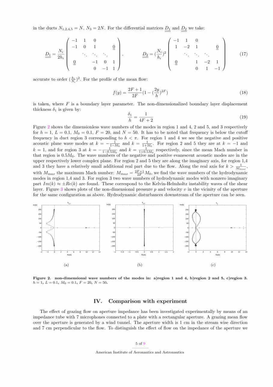
Figure 2 shows the dimensionless wave numbers of the modes in region 1 and 4, 2 and 5, and 3 respectivelyfor h = 1, L = 0.1, M0 = 0.1, F = 20, and N = 50. It has to be noted that frequency is below the cutofffrequency in duct region 3 corresponding to h < π. For region 1 and 4 we see the negative and positiveacoustic plane wave modes at k = − 1

1−M0

and k = 11+M0

. For region 2 and 5 they are at k = −1 and

k = 1, and for region 3 at k = − 11−0.5M0

and k = 11+0.5M0

respectively, since the mean Mach number inthat region is 0.5M0. The wave numbers of the negative and positive evanescent acoustic modes are in theupper respectively lower complex plane. For region 2 and 5 they are along the imaginary axis, for region 1,4and 3 they have a relatively small additional real part due to the flow. Along the real axis for k > 1

Mmax,

with Mmax the maximum Mach number: Mmax = 2F+12F

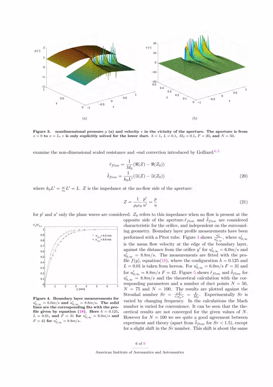
M0, we find the wave numbers of the hydrodynamicmodes in region 1,4 and 3. For region 3 two wave numbers of hydrodynamic modes with nonzero imaginarypart Im(k) ≈ ±Re(k) are found. These correspond to the Kelvin-Helmholtz instability waves of the shearlayer. Figure 3 shows plots of the non-dimensional pressure p and velocity v in the vicinity of the aperturefor the same configuration as above. Hydrodynamic disturbances downstream of the aperture can be seen.

−4 −2 0 2 4 6 8 10 12 14

−200

−150

−100

−50

0

50

100

150

200

k1,4

Re(k)

Im(k)

(a)

−2 −1.5 −1 −0.5 0 0.5 1 1.5 2

−200

−150

−100

−50

0

50

100

150

200

k2,5

Re(k)

Im(k)

(b)

−2 0 2 4 6 8 10 12 14

−200

−150

−100

−50

0

50

100

150

200

k3

Re(k)

Im(k)

(c)

Figure 2. non-dimensional wave numbers of the modes in: a)region 1 and 4, b)region 2 and 5, c)region 3.h = 1, L = 0.1, M0 = 0.1, F = 20, N = 50.

IV. Comparison with experiment

The effect of grazing flow on aperture impedance has been investigated experimentally by means of animpedance tube with 7 microphones connected to a plate with a rectangular aperture. A grazing mean flowover the aperture is generated by a wind tunnel. The aperture width is 1 cm in the stream wise directionand 7 cm perpendicular to the flow. To distinguish the effect of flow on the impedance of the aperture we

5 of 9


−1−0.5

00.5

1

0

0.5

1−2

−1

0

1

2

xy

p [−]

(a)

−1−0.5

00.5

1

00.1

0.20.3

0.40.5−20

−10

0

10

20

xy

v [−]

(b)

Figure 3. nondimensional pressure p (a) and velocity v in the vicinity of the aperture. The aperture is fromx = 0 to x = L, v is only explicitly solved for the lower duct. h = 1, L = 0.1, M0 = 0.1, F = 20, and N = 50.

examine the non-dimensional scaled resistance and -end correction introduced by Golliard:6,5

rflow =1

M0

(<(Z) −<(Z0))

δflow =1

k0L′(=(Z) −=(Z0)) (20)

where k0L′ = ω

c0

L′ = L. Z is the impedance at the no-flow side of the aperture:

Z =1

ρ0c0

p′

u′=

p

u(21)

for p′ and u′ only the plane waves are considered. Z0 refers to this impedance when no flow is present at the

0 1 2 3 4 5 6 70

0.1

0.2

0.3

0.4

0.5

0.6

0.7

0.8

0.9

1

y’ [mm]

u’0/u’

0,∞

* u’0,∞

= 6.0 m/s

+ u’0,∞

= 8.8 m/s

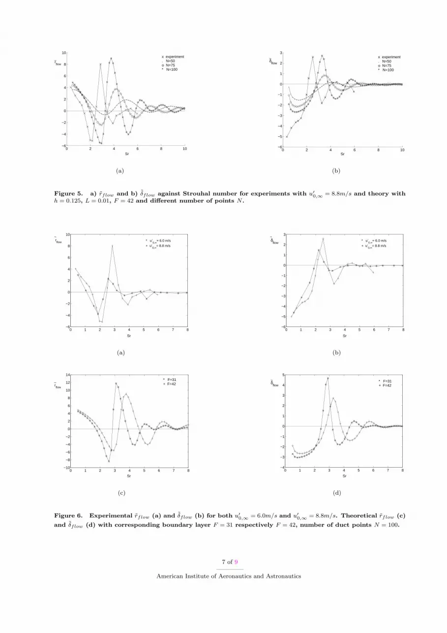
Figure 4. Boundary layer measurements foru′0,∞ = 6.0m/s and u′

0,∞ = 8.8m/s. The solidlines are the corresponding fits with the pro-file given by equation (18). Here h = 0.125,L = 0.01, and F = 31 for u′

0,∞ = 6.0m/s and

F = 42 for u′0,∞ = 8.8m/s.

opposite side of the aperture.rflow and δflow are consideredcharacteristic for the orifice, and independent on the surround-ing geometry. Boundary layer profile measurements have been

performed with a Pitot tube. Figure 4 showsu′

0

u′

0,∞

, where u′

0,∞

is the mean flow velocity at the edge of the boundary layer,against the distance from the orifice y′ for u′

0,∞ = 6.0m/s andu′

0,∞ = 8.8m/s. The measurements are fitted with the pro-file f(y), equation(18), where the configuration h = 0.125 andL = 0.01 is taken from hereon. For u′

0,∞ = 6.0m/s F = 31 and

for u′

0,∞ = 8.8m/s F = 42. Figure 5 shows rflow and δflow foru′

0,∞ = 8.8m/s and the theoretical calculation with the cor-responding parameters and a number of duct points N = 50,N = 75 and N = 100. The results are plotted against theStrouhal number Sr = ωL′

<u′

0>

= LM0

. Experimentally Sr is

varied by changing frequency. In the calculations the Machnumber is varied for convenience. It can be seen that the the-oretical results are not converged for the given values of N .However for N = 100 we see quite a good agreement betweenexperiment and theory (apart from δflow for Sr < 1.5), exceptfor a slight shift in the Sr number. This shift is about the same

6 of 9


0 2 4 6 8 10−6

−4

−2

0

2

4

6

8

10

Sr

rflow

~ x experiment. N=50 o N=75 * N=100

(a)

0 2 4 6 8 10−6

−5

−4

−3

−2

−1

0

1

2

3x experiment. N=50 o N=75 * N=100

Sr

δflow

~

(b)

Figure 5. a) rflow and b) δflow against Strouhal number for experiments with u′0,∞ = 8.8m/s and theory with

h = 0.125, L = 0.01, F = 42 and different number of points N .

0 1 2 3 4 5 6 7 8−6

−4

−2

0

2

4

6

8

10

Sr

rflow

~ * u’

0,∞= 6.0 m/s

+ u’0,∞= 8.8 m/s

(a)

0 1 2 3 4 5 6 7 8−6

−5

−4

−3

−2

−1

0

1

2

3

Sr

δflow

~ * u’

0,∞= 6.0 m/s

+ u’0,∞= 8.8 m/s

(b)

0 1 2 3 4 5 6 7 8−10

−8

−6

−4

−2

0

2

4

6

8

10

12

14* F=31+ F=42

Sr

rflow

~

(c)

0 1 2 3 4 5 6 7 8−4

−3

−2

−1

0

1

2

3

4

5

* F=31+ F=42

~ δ

flow

Sr

(d)

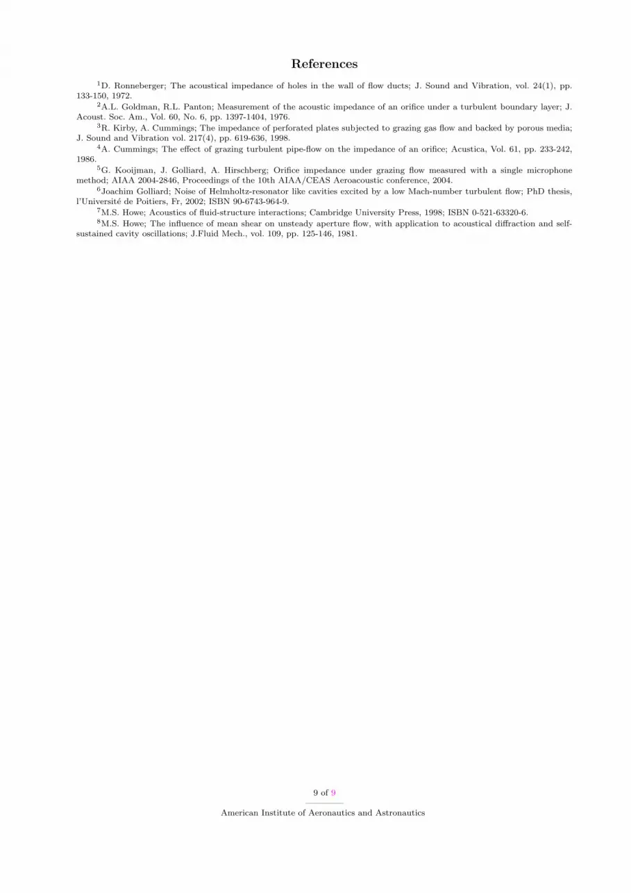
Figure 6. Experimental rflow (a) and δflow (b) for both u′0,∞ = 6.0m/s and u′

0,∞ = 8.8m/s. Theoretical rflow (c)

and δflow (d) with corresponding boundary layer F = 31 respectively F = 42, number of duct points N = 100.

7 of 9


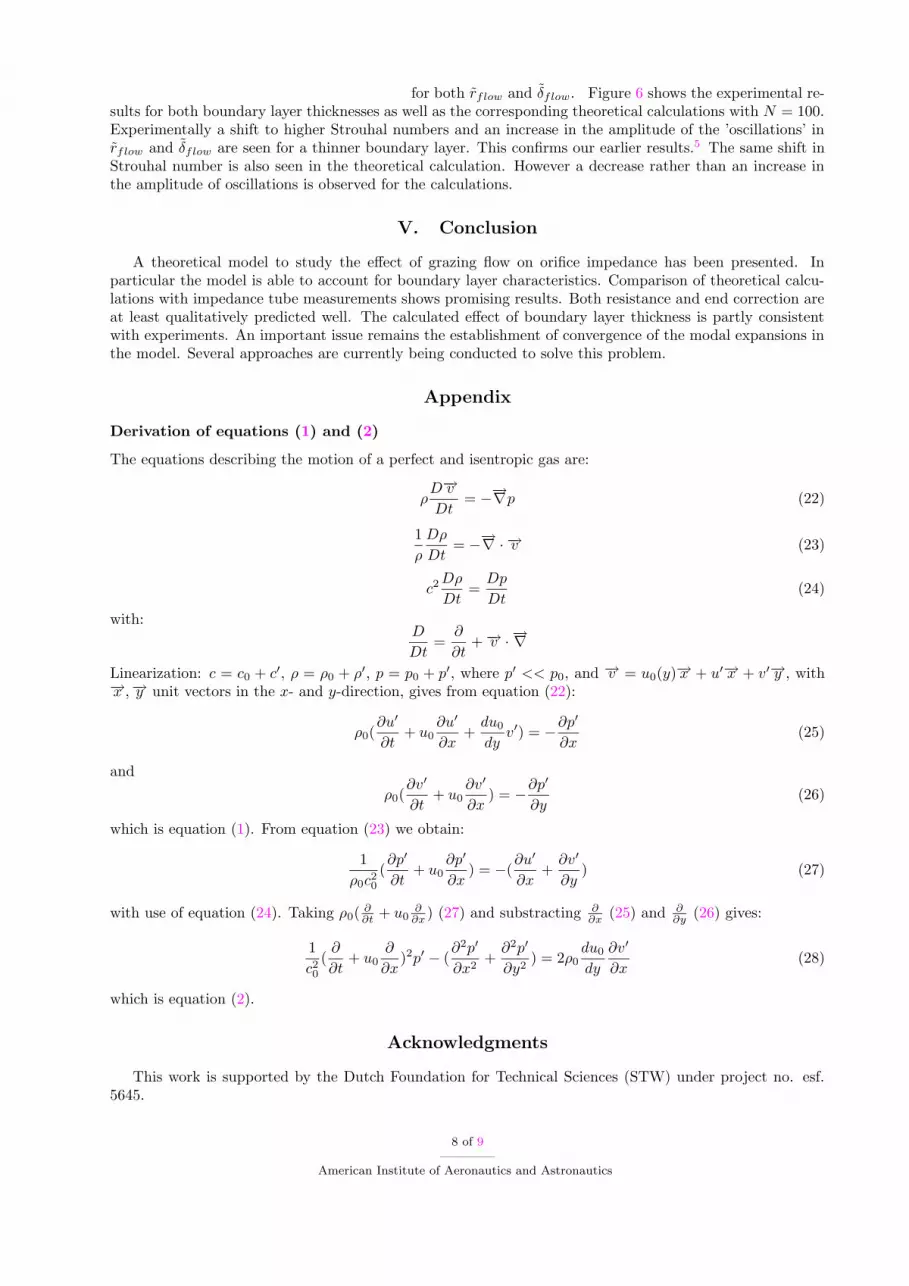
for both rflow and δflow. Figure 6 shows the experimental re-sults for both boundary layer thicknesses as well as the corresponding theoretical calculations with N = 100.Experimentally a shift to higher Strouhal numbers and an increase in the amplitude of the ’oscillations’ inrflow and δflow are seen for a thinner boundary layer. This confirms our earlier results.5 The same shift inStrouhal number is also seen in the theoretical calculation. However a decrease rather than an increase inthe amplitude of oscillations is observed for the calculations.

V. Conclusion

A theoretical model to study the effect of grazing flow on orifice impedance has been presented. Inparticular the model is able to account for boundary layer characteristics. Comparison of theoretical calcu-lations with impedance tube measurements shows promising results. Both resistance and end correction areat least qualitatively predicted well. The calculated effect of boundary layer thickness is partly consistentwith experiments. An important issue remains the establishment of convergence of the modal expansions inthe model. Several approaches are currently being conducted to solve this problem.

Appendix

Derivation of equations (1) and (2)

The equations describing the motion of a perfect and isentropic gas are:

ρD−→v

Dt= −

−→∇p (22)

1

ρ

Dρ

Dt= −

−→∇ · −→v (23)

c2 Dρ

Dt=

Dp

Dt(24)

with:D

Dt=

∂

∂t+ −→v ·

−→∇

Linearization: c = c0 + c′, ρ = ρ0 + ρ′, p = p0 + p′, where p′ << p0, and −→v = u0(y)−→x + u′−→x + v′−→y , with−→x ,−→y unit vectors in the x- and y-direction, gives from equation (22):

ρ0(∂u′

∂t+ u0

∂u′

∂x+

du0

dyv′) = −

∂p′

∂x(25)

and

ρ0(∂v′

∂t+ u0

∂v′

∂x) = −

∂p′

∂y(26)

which is equation (1). From equation (23) we obtain:

1

ρ0c20

(∂p′

∂t+ u0

∂p′

∂x) = −(

∂u′

∂x+

∂v′

∂y) (27)

with use of equation (24). Taking ρ0(∂∂t

+ u0∂∂x

) (27) and substracting ∂∂x

(25) and ∂∂y

(26) gives:

1

c20

(∂

∂t+ u0

∂

∂x)2p′ − (

∂2p′

∂x2+

∂2p′

∂y2) = 2ρ0

du0

dy

∂v′

∂x(28)

which is equation (2).

Acknowledgments

This work is supported by the Dutch Foundation for Technical Sciences (STW) under project no. esf.5645.

8 of 9


References

1D. Ronneberger; The acoustical impedance of holes in the wall of flow ducts; J. Sound and Vibration, vol. 24(1), pp.133-150, 1972.

2A.L. Goldman, R.L. Panton; Measurement of the acoustic impedance of an orifice under a turbulent boundary layer; J.Acoust. Soc. Am., Vol. 60, No. 6, pp. 1397-1404, 1976.

3R. Kirby, A. Cummings; The impedance of perforated plates subjected to grazing gas flow and backed by porous media;J. Sound and Vibration vol. 217(4), pp. 619-636, 1998.

4A. Cummings; The effect of grazing turbulent pipe-flow on the impedance of an orifice; Acustica, Vol. 61, pp. 233-242,1986.

5G. Kooijman, J. Golliard, A. Hirschberg; Orifice impedance under grazing flow measured with a single microphonemethod; AIAA 2004-2846, Proceedings of the 10th AIAA/CEAS Aeroacoustic conference, 2004.

6Joachim Golliard; Noise of Helmholtz-resonator like cavities excited by a low Mach-number turbulent flow; PhD thesis,l’Universite de Poitiers, Fr, 2002; ISBN 90-6743-964-9.

7M.S. Howe; Acoustics of fluid-structure interactions; Cambridge University Press, 1998; ISBN 0-521-63320-6.8M.S. Howe; The influence of mean shear on unsteady aperture flow, with application to acoustical diffraction and self-

sustained cavity oscillations; J.Fluid Mech., vol. 109, pp. 125-146, 1981.

9 of 9


Documents

Orifice Impedance under Grazing Flow: Modal Expansion Approach