455

Proc. Estonian Acad. Sci. Eng., 2007, 13, 4, 455–478

Smart sensor systems using impedance spectroscopy

Hans-Rolf Tränklera, Olfa Kanounb, Mart Minc,d and Marek Ristc

a Department of Measurement and Automation, University of Bundeswehr Munich, Werner-

Heisenberg-Weg 39, 85579 Neubiberg, Germany; ima@unibw.de b Chair of Metrology, University of Kassel, Wilhelmsöher Allee 73, 34121 Kassel, Germany;

kanoun@ieee.org c Department of Electronics, Tallinn University of Technology, Ehitajate tee 5, 19086 Tallinn,

Estonia; min@edu.ttu.ee d Institut für Bioprozess- und Analysenmesstechnik, Rosenhof, 37308 Heilbad Heiligenstadt,

Germany; mart.min@iba-heiligenstadt.de Received 5 November 2007 Abstract. Extracting relevant information from impedance spectra is a big challenge if we consider different mechanisms, including cable and contacting effects, material properties and system instability. A particularly important prerequisite is that these effects depend differently on the frequency and that some measures can be taken to eliminate effects of irrelevant mechanisms. The common way in signal processing is to model the impedance spectrum by means of equivalent circuits and to extract the quantity of interest using optimization techniques. The more effects and mechanisms are represented in an impedance spectrum, the more unknown parameters are needed for accurate modelling. The parameter extraction process becomes thereby difficult to solve and needs a lot of trials and a priori knowledge. It is therefore important that mechanisms with minor influence are eliminated or neglected. Other possibilities for signal processing provide mathematical data fusion methods. Statistical methods like principal component analysis can be used for extracting specific information from the measured data. The paper considers different applications (electrochemical, biomedical, moisture analysis, battery diagnosing) of electrical impedance spectroscopy. Key words: electrical impedance, electrochemical impedance, bioimpedance, mathematical models, impedance spectroscopy.

1. INTRODUCTION Impedance spectroscopy is an established method for the measurement of

material properties in corrosion research, material interfaces, characterization of chemical processes, recently also in life sciences as biology, bioprocessing and

456

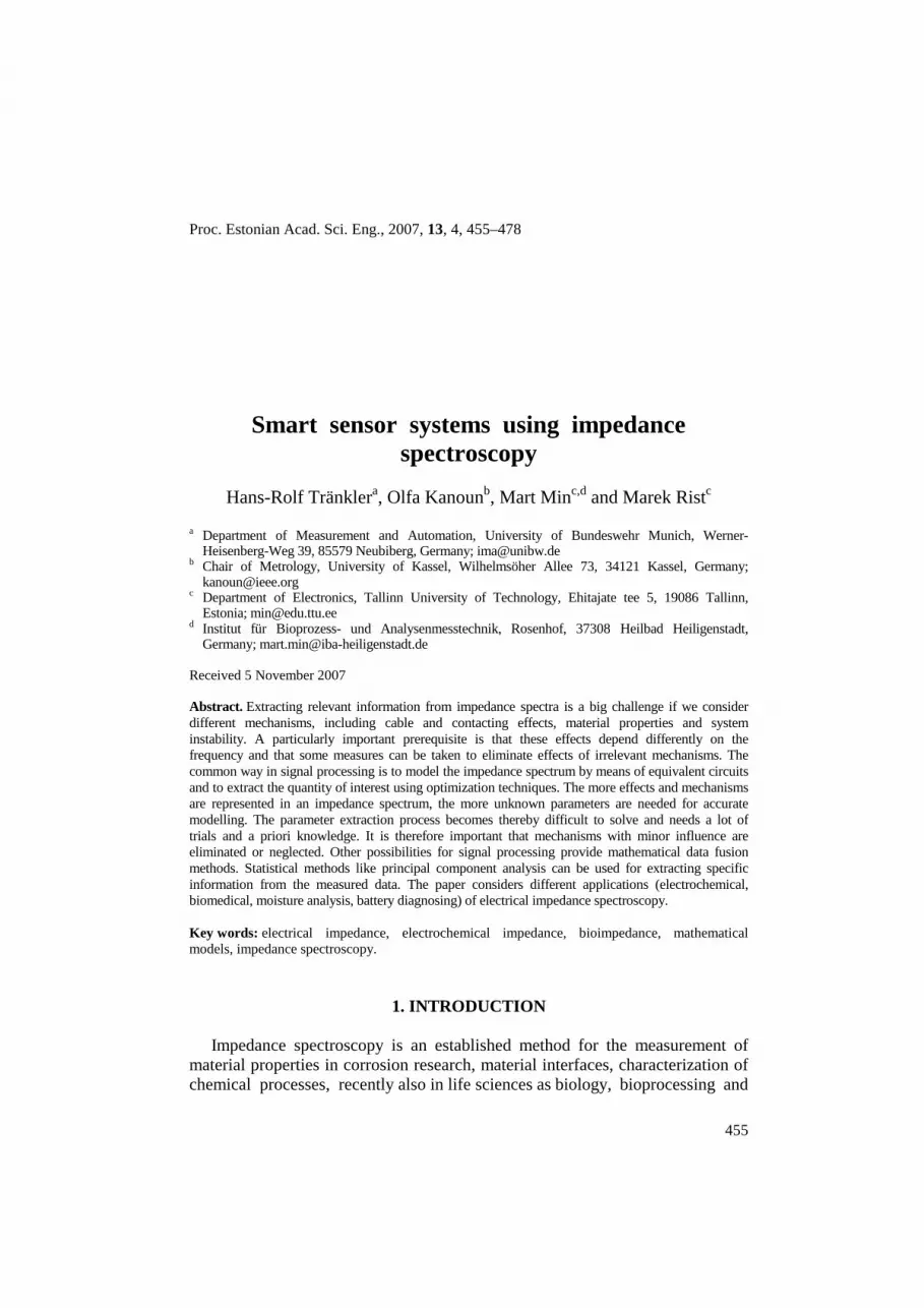
Fig. 1. Impedance spectroscopy.

medical diagnostics. The principle of this measurement technique is to measure impedance at a device, material, or process using time varying currents or voltages.

The efficiency of this method relies on of the possibility to get information in three dimensions: the real and imaginary parts of the impedance and the frequency. For example, if it is applied to an electrochemical system, the impedance spectro-scopy can provide information on reaction parameters, corrosion rates, oxide integrity, surface porosity, coating integrity, inhibitor function, mass transport, and many other electrode/interface characteristics [1]. However, effective utilization of this spectroscopy technique requires a comprehensive exposure of the theory, measurement and signal processing techniques (Fig. 1).

2. EXPERIMENTAL SET-UP Investigation of experimental set-ups is very important for impedance spectro-

scopy. The excitation signal, used for impedance measurement, should be accurately known. The measurement should be carried out in a linear range and with sufficient resolution. The impedance under investigation should be maintained in a stable state, this is especially critical for electrochemical and biological systems.

457

Fig. 2. Influence of objects in the stray field.

The measured impedance spectrum includes all effects, such as connecting

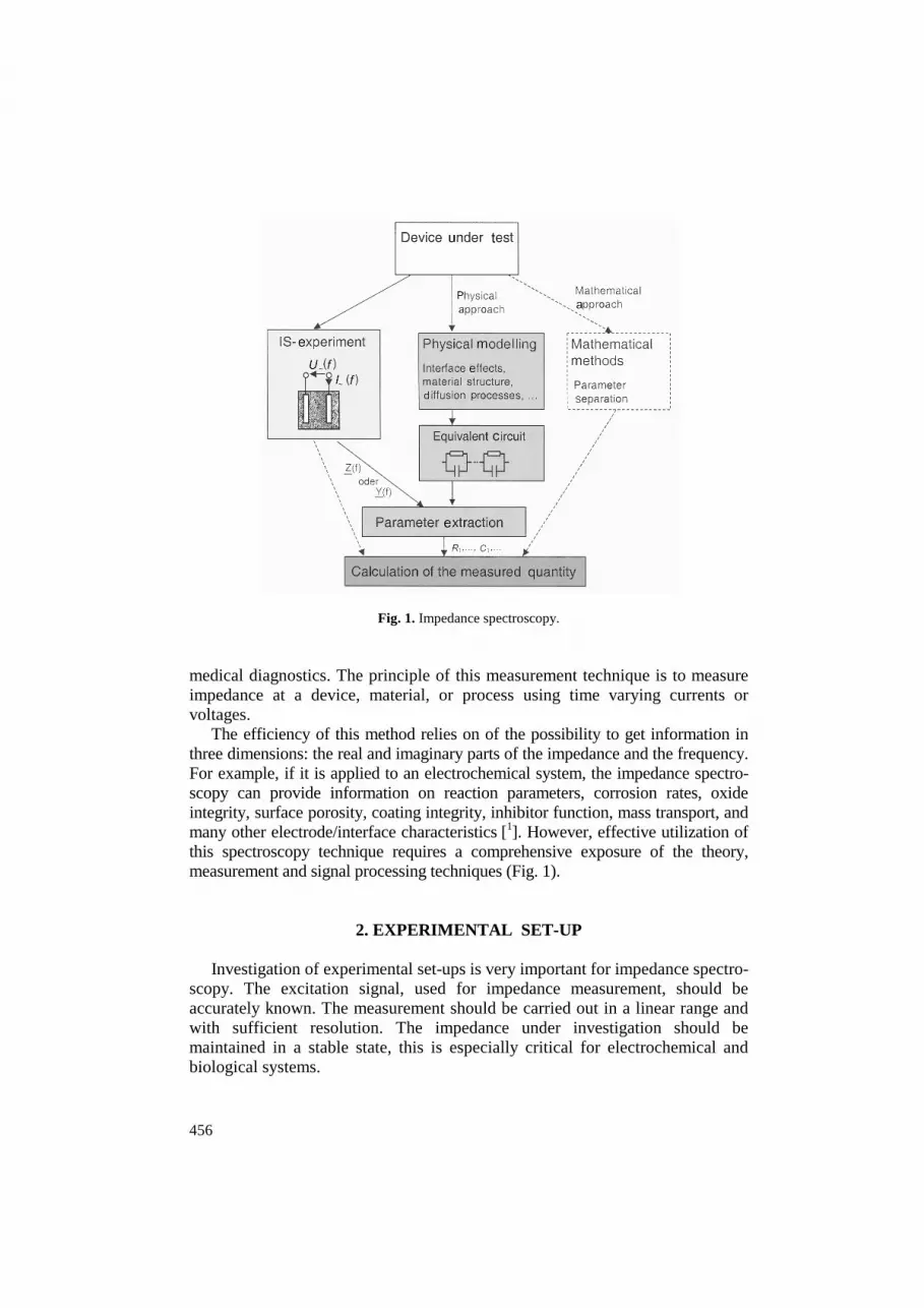
cables and contact double layers, and parasitic effects. If these effects are not identified and eliminated, they lead to systematic errors during information extraction from the impedance spectrum. It is important to be able to assign parts of the impedance spectrum to their causes in order to have a comprehensible modelling and precise information extraction. For example, to measure the impedance spectrum of composite materials, it is important to have a probe of certain geometrical dimensions in order to have repeatability of the measure-ments.

The geometry of electrodes is important to have sensitive measurements [2]. The electrode geometry is a decisive factor in order to avoid parasitic effects in the stray field (Fig. 2). Compensation of cable effects is very important because the cables have frequency-dependent impedance even at comparatively low frequencies. An effective method for compensation of the cable effect is the use of the frequency-dependent impedance of cables with open ends, superposed to the impedance of the device under test in parallel [3]. The complex impedance of the device under test objZ can be calculated as

meas cableobj

meas cable

,Z Z

ZZ Z

⋅=

− (1)

where measZ is the measured complex impedance, cableZ is the complex impedance of the cable with opened ends and objZ is the complex impedance of the device under test.

3. INVESTIGATION OF DATA CONSISTENCY The quality of measurement data can be investigated by means of the

Kramers–Kronig relation [4]. This method originates from the IR-Spectroscopy and gives relationships between the real r( )Z and imaginary i( )Z parts of an impedance under assumptions of stability, causality and linearity as

r ri 2 2

0

( ) ( )2( ) d ,

Z x ZZ x

x

ωωωπ ω

∞ − = − − ∫ (2)

458

i ir r 2 2

0

( ) ( )2( ) ( ) d ,

xZ x ZZ Z x

x

ω ωωπ ω

∞ −= ∞ +−∫ (3)

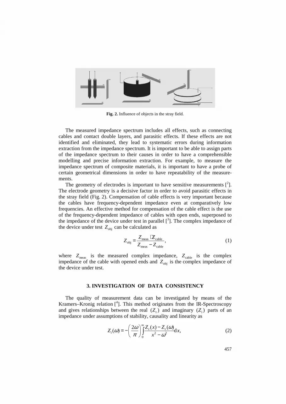
where ω is the angular frequency. An easy way for applying the Kramers–Kronig (KK) method is to use measure-

ment models, consisting of a set of series connected RC circuits [5] (Fig. 3), which gives an acceptable fit of the investigated impedance measurements.

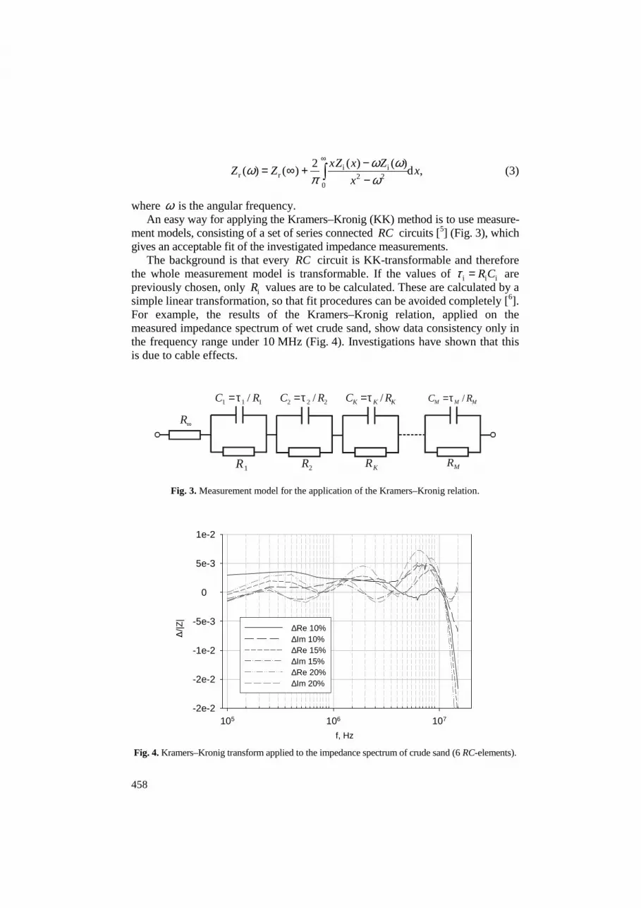
The background is that every RC circuit is KK-transformable and therefore the whole measurement model is transformable. If the values of i i iR Cτ = are previously chosen, only iR values are to be calculated. These are calculated by a simple linear transformation, so that fit procedures can be avoided completely [6]. For example, the results of the Kramers–Kronig relation, applied on the measured impedance spectrum of wet crude sand, show data consistency only in the frequency range under 10 MHz (Fig. 4). Investigations have shown that this is due to cable effects.

111 / RC τ= 222 / RC τ=

1R 2R KR MR

MMM RC /τ=KKK RC /τ=

∞R

Fig. 3. Measurement model for the application of the Kramers–Kronig relation.

f [Hz]

105 106 107

∆ /|Z

|

-2e-2

-2e-2

-1e-2

-5e-3

0

5e-3

1e-2

∆Re 10%∆Im 10%∆Re 15%∆Im 15%∆Re 20%∆Im 20%

Fig. 4. Kramers–Kronig transform applied to the impedance spectrum of crude sand (6 RC-elements).

f, Hz

∆

/|Z|

459

4. MODELLING OF THE IMPEDANCE SPECTRA Many elements can be used for modelling of the impedance spectra (Table 1).

Additionally to the ideal resistors, capacitors and inductances, different distributed circuit elements can be used.

The constant phase element (CPE) is generally used in order to describe parts of the spectrum with a constant phase. These are due to distributed parameters at the electrode interface or in the measured solid, and are used in the circuits ,ARCε

ARCZ and ARCY (Table 1). The Warburg impedance is used for the description of diffusion processes.

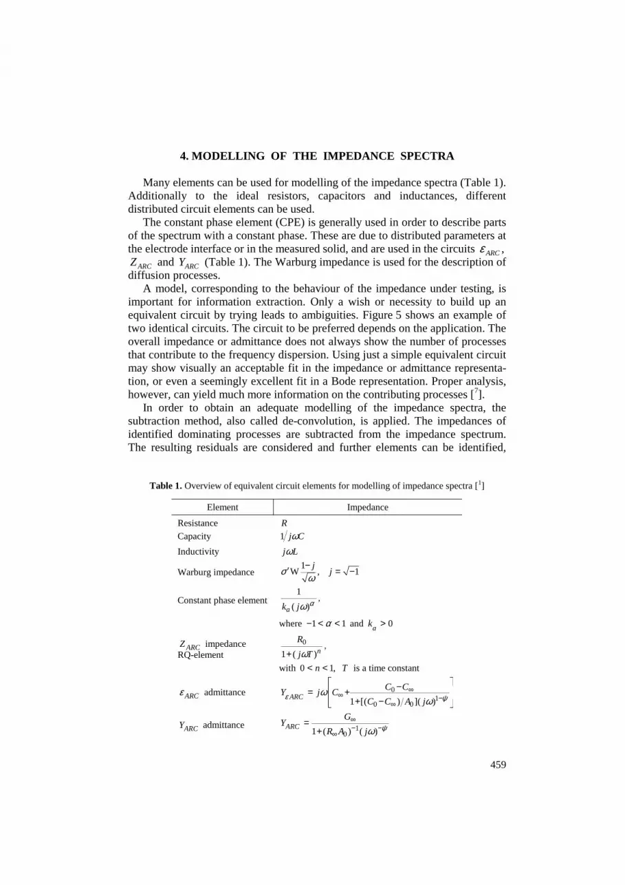
A model, corresponding to the behaviour of the impedance under testing, is important for information extraction. Only a wish or necessity to build up an equivalent circuit by trying leads to ambiguities. Figure 5 shows an example of two identical circuits. The circuit to be preferred depends on the application. The overall impedance or admittance does not always show the number of processes that contribute to the frequency dispersion. Using just a simple equivalent circuit may show visually an acceptable fit in the impedance or admittance representa-tion, or even a seemingly excellent fit in a Bode representation. Proper analysis, however, can yield much more information on the contributing processes [7].

In order to obtain an adequate modelling of the impedance spectra, the subtraction method, also called de-convolution, is applied. The impedances of identified dominating processes are subtracted from the impedance spectrum. The resulting residuals are considered and further elements can be identified,

Table 1. Overview of equivalent circuit elements for modelling of impedance spectra [1]

Element Impedance

Resistance R Capacity 1 j Cω

Inductivity j Lω

Warburg impedance 1

W , 1j

jσω

−′ = −

Constant phase element ,1

( )ak j αω

where 1 1α− < < and 0ak >

ARCZ impedance RQ-element

0 ,1 ( )n

R

j Tω+

with 0 1,n< < T is a time constant

ARCε admittance 01

0 01 [( ) ]( )ARC

C CY j C

C C A jε ψ

ωω

∞∞ −

∞

−= ++ −

ARCY admittance 101 ( ) ( )

ARCG

YR A j ψω

∞− −

∞=

+

460

0 0.1 0.2 0.3 0.4 0.5 0.6 0.7 0.8 - 0.3

- 0.24

- 0.18

- 0.12

- 0.06

0

Im(Z )

Re(Z )

Circuit 1 Circuit 2

0 0.1 0.2 0.3 0.4 0.5 0.6 0.7 0.8 – 0.3

– 0.24

– 0.18

– 0.12

– 0.06

0

Im(Z )

Re(Z )

Circuit 1 Circuit 2 Circuit 1 Circuit 2

R 2 R 1

C 1

C 2

2 1

1

2

C 3 C 4

R 3 R 4

3 4

3 4

Circuit 1 Circuit 2

Fig. 5. Different circuits having similar complex impedance R1 = 0.519 Ω, C1 = 9.61 µF, R2 = 0.281 Ω, C2 = 5.45 10–4 F, R3 = 0.498 Ω, C3 = 10.5 µF, R4 = 0.302 Ω, C4 = 550 µF. until a minimal residual part is reached. The impedance to be measured is the serial combination of all identified impedance elements. In this process it is important to understand the influence of propagating subtraction errors, which are not relevant because the subtraction is carried out only during the pre-analysis phase. For information extraction, a full complex non-linear least square procedure is carried out [7]. It is always important to consider the behaviour of the impedance spectrum in connection with the processes taking place.

5. PARAMETER EXTRACTION

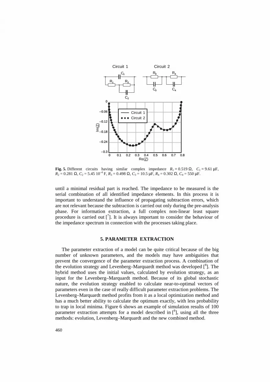
The parameter extraction of a model can be quite critical because of the big number of unknown parameters, and the models may have ambiguities that prevent the convergence of the parameter extraction process. A combination of the evolution strategy and Levenberg–Marquardt method was developed [8]. The hybrid method uses the initial values, calculated by evolution strategy, as an input for the Levenberg–Marquardt method. Because of its global stochastic nature, the evolution strategy enabled to calculate near-to-optimal vectors of parameters even in the case of really difficult parameter extraction problems. The Levenberg–Marquardt method profits from it as a local optimization method and has a much better ability to calculate the optimum exactly, with less probability to trap in local minima. Figure 6 shows an example of simulation results of 100 parameter extraction attempts for a model described in [8], using all the three methods: evolution, Levenberg–Marquardt and the new combined method.

Re(Z)

Im(Z

)

461

Fig. 6. Results of parameter estimation using the evolution, Levenberg–Marquardt and the combined method [8].

In some cases it is impossible to calculate all the unknown parameters of an

impedance model at the same time. If the observed mechanisms are related to definite frequency ranges, the parameter extraction can be carried out by using a different model for each frequency band with certain dominating mechanisms. The limits of the frequency bands are determined automatically from charac-teristic patterns within measurement data. In this case, the total fit can be biased, but it can be used in the cases, where a big number of unknown parameters is unavoidable.

In the case of battery diagnostics [6], the diffusion processes take place at very low frequencies. The transfer reaction takes place at middle frequencies. The porosity of the electrode is effective at high frequencies. For the modelling of a mechanism, at least 2–3 parameters are necessary. Therefore a lot of unknown parameters should be determined by optimization.

6. MATHEMATICAL APPROACH If equivalent circuits are used for validation of the impedance spectra, they

represent also the a priori knowledge used during in situ measurements. The results are parameters of the model. A novel approach, which is based on statistical multivariate analysis, is presented in [9]. In this case the a priori knowledge used during in situ measurement consists of the experience from many measurements gained from various experiments. A feature extraction and the principal component analysis (PCA) were used for data reduction.

The principal component analysis belongs to the statistical methods of multi-variate analysis [4]. It is capable to reduce dimensionality of data by eliminating redundancy without significant losses of information content and without a need

462

Fig. 7. Variance of the first 10 principal components [9].

Fig. 8. Soil type classification by PCA [9].

for any physical knowledge about the investigated impedance. Though this method is principally useful for processing of impedance spectra, it has still been rarely applied [5].

Dimensionality reduction of data is achieved by a transformation of original variables to a new set of uncorrelated variables – to the principal components. Generally, only few principal components retain the most of the variation present in input data. After transformation, it is sufficient to analyse only these few principal components without significant loss of information. For example, PCA was applied to soil type classification (Figs. 7 and 8). We can see that the first four components have up to 100% variance in total, and are therefore sufficient to show the whole data variance.

Only the first two principal components are already sufficient to characterize the soil type. Figure 8 shows that soil types may be recognized and differentiated from each other.

7. APPLICATIONS IN THE BIOIMPEDANCE CONTROLLED PACEMAKER

7.1. Explaining the problem Artificial cardiac pacing has become an important method of treating cardiac

rhythm abnormalities. The pacing rate ( )PR of implanted pacemakers must be adaptive to the patient’s physical workload to ensure the required cardiac output ( ),CO which is the product of stroke volume ( )SV and heart rate ( ).HR Several kinds of body sensors (Fig. 9) are used to determine the level of physical work-

Index of principal components

Var

ianc

e, %

463

Fig. 9. Adaptive pacing rate control and simplified presentation of the cardio-vascular system.

load bodyW of the body (e.g. activity and acceleration sensors), but the most reliable method is based on the minute volume ( )MV of respiration [10]. The MV sensor measures variations of the lung’s impedance. Typically, but not always, the required pacing rate PR follows almost linearly the minute volume MV of respiration [11].

The problem is that the ability of the unhealthy heart to follow the needs of the patient’s body, is restricted – the heart cannot operate at very high and low rates because the myocardium energy supply E reduces in both cases (in comparison with the energy consumption ).W Energy supply is proportional to the blood inflow, equal to ,P R∆ where P∆ is the blood pressure difference, and R is the hydraulic resistance of the vascular system of heart (Fig. 9). The limits of the pacing rate, between which the heart can operate without any danger to the myocardium, vary depending on the current status of the diseased organism [11–13]. In state-of-the-art medical practice, however, the settings are typically determined as constants before implantation of the pacemaker [12].

The crisp values are not only uncomfortable but also dangerous to the patients, e.g., in cases like quick rising from supine or sitting posture, serious wounding and bleeding, taking warm bath or shower, etc. The rapidly increasing blood flow into the body takes partly away the blood flow to the brain. The brain needs more blood, but the cardiac output can not be increased due to rigidly limited pacing rate. The patient can lose consciousness, but in the worst case, brain damages can take place [13]. The flexible “floating” limits could cope the patients needs for a short time, but one must take into account that a sudden

Cardiac output CO = HR × SV

Veins

∆P

LLuunnggss

O2

Arteries

Pacing rate PR

Skeletal muscles and other tissues

Activity acceleration Minute volume MV

Myocardium

∆P R

Heart rate Stroke volume

Respiration rate Tidal volume

Minute volume MV = RR × TV

464

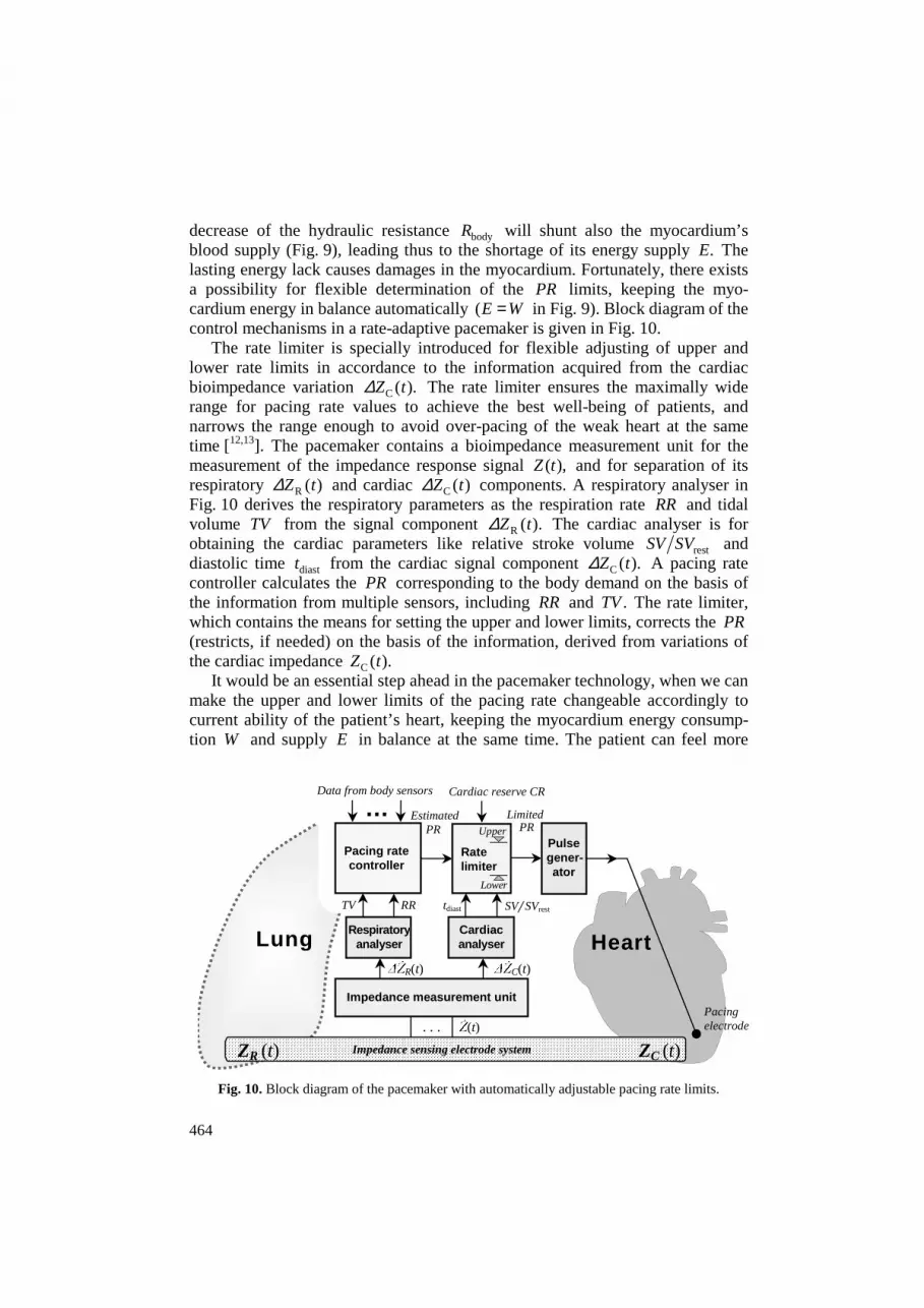
decrease of the hydraulic resistance bodyR will shunt also the myocardium’s blood supply (Fig. 9), leading thus to the shortage of its energy supply .E The lasting energy lack causes damages in the myocardium. Fortunately, there exists a possibility for flexible determination of the PR limits, keeping the myo-cardium energy in balance automatically (E W= in Fig. 9). Block diagram of the control mechanisms in a rate-adaptive pacemaker is given in Fig. 10.

The rate limiter is specially introduced for flexible adjusting of upper and lower rate limits in accordance to the information acquired from the cardiac bioimpedance variation C ( ).Z t∆ The rate limiter ensures the maximally wide range for pacing rate values to achieve the best well-being of patients, and narrows the range enough to avoid over-pacing of the weak heart at the same time [12,13]. The pacemaker contains a bioimpedance measurement unit for the measurement of the impedance response signal ( ),Z t and for separation of its respiratory R ( )Z t∆ and cardiac C ( )Z t∆ components. A respiratory analyser in Fig. 10 derives the respiratory parameters as the respiration rate RR and tidal volume TV from the signal component R ( ).Z t∆ The cardiac analyser is for obtaining the cardiac parameters like relative stroke volume restSV SV and diastolic time diastt from the cardiac signal component C ( ).Z t∆ A pacing rate controller calculates the PR corresponding to the body demand on the basis of the information from multiple sensors, including RR and .TV The rate limiter, which contains the means for setting the upper and lower limits, corrects the PR (restricts, if needed) on the basis of the information, derived from variations of the cardiac impedance C ( ).Z t

It would be an essential step ahead in the pacemaker technology, when we can make the upper and lower limits of the pacing rate changeable accordingly to current ability of the patient’s heart, keeping the myocardium energy consump-tion W and supply E in balance at the same time. The patient can feel more

Fig. 10. Block diagram of the pacemaker with automatically adjustable pacing rate limits.

Estimated PR

tdiast

Upper

Rate limiter

Lower

SV/ SVrest

Limited PR

Heart

Pacing electrode

Pacing rate controller

…

Data from body sensors

Pulse gener-

ator

TV RR

∆ŻC(t)

Lung Respiratory analyser

Cardiac reserve CR

Impedance sensing electrode system ZR (t) ZC (t)

Cardiac analyser

. . . Ż(t)

∆ŻR(t)

Impedance measurement unit

465

healthy in various everyday life conditions from peaceful sleep to moderate work, including sudden changes in hydraulic resistance of the vascular system. The variable limits can leave more space for the pacing rate to vary accordingly to the body’s demand. It is important to underline that the energy supply of both, the patient’s organism (body), and the heart (myocardium), is of primary importance, not the heart (pacing) rate. The pacing rate PR is just a parameter (the only one, unfortunately), which is available for controlling the heart with the pacemaker.

7.2. Energy balance considerations at higher pacing rates

Calculation is based on keeping the balance between the energy consumption

and energy supply of the myocardium (Figs. 9 and 10) at higher workloads [11–14]. The demanded energy consumption (myocardium’s work) demS can be found from the volume–pressure loop area (Fig. 11a):

dem ,W S P SV∆= ≅ ⋅ (4)

where P∆ is the mean value of the ventricular pressure variations, and SV is the stroke volume.

The myocardium’s energy supply can be derived from the time response curve of the ventricular pressure in Fig. 11b, where the area supS is proportional to energy supply sup( ).E S∼ To get the physical energy dimension for the geometrical area sup ,S a formal coefficient K is introduced:

sup diast( )E S K Pt K∆= = . (5)

Fig. 11. Ventricular pressure-volume loop (a) and variation of the arterial pressure (b): 1 – HR = HRinit (e.g. 60 bpm), 2 – HR = 2HRinit (e.g. 120 bpm).

tsyst SV Volume

Pressure P

Sdem

Pressure P

Time

Ssup

a b

Pas

Pved

Pad

Pas

∆P

Pa

Pved

Pad

Pves Pve

Pves

∆P

Pa

Pve

Arterial pressure

tdiast

Ventricular pressure

466

The energy balance ( )W E= gives diast ,SV t K= which means that when

diast ,SV t K> then the PR must be reduced (limited), because the myocardium cannot get sufficient amount of energy E although the patient’s organism (body) needs an increase of .PR The actual value of upperPRL can be calculated from the measured relative stroke volume restSV SV and diastolic time diastt if the values of rest ,HR restSV and CR are known. A remark: there is no need for pressure measurement, because the pressure P∆ cancels out when .W E=

7.3. Considerations for restricting lower pacing rates

The lower pacing rate must be high enough to avoid myocardium’s hypoxia,

which can appear due to slow influx of the blood, and to prevent overloading of the ventricle, which can lead to unreversable over-stretching of the myo-cardium [12,15]. At the same time, its value should be low enough to avoid disturbing peaceful sleep. The lower pacing rate limit, ,lowerPRL must always ensure the minimal energy required by the patient’s organism. This means that the current cardiac output CO SV PR= ⋅ should never be lower than at the rest state restCO [6], that is, the value of rest .lowerPRL CO SV> Expressing

rest rest rest ,CO HR SV= ⋅ we obtain:

restrest .

SVlowerPRL HR

SV> ⋅ (6)

In addition, the maximal value of the stroke volume SV must be also limited to avoid stretching out the ventricle, that is rest ,SV SVλ< ⋅ where λ varies from 1.2 to 1.5, depending on the myocardium’s health. The lowerPRL is calculated measuring currently the actual relative stroke volume rest ,SV SV knowing the values of rest ,SV restHR and .λ

7.4. Bioimpedance measurement

The intracardiac bioimpedance is measured by the aid of electrodes on the

pacing lead, which is placed inside the heart. The impedance of lungs has relatively strong effect upon the significant electrical impedance between the pacemaker’s metallic case and the tip electrode, placed to the apex of the ventricle (Fig. 12). The respiratory component R ( )Z t can be filtered out from the composite impedance signal and used as information, reflecting the minute ventilation ,MV which is in good correlation with aerobic energy consumption

body.W Calculation of the pacing rate limits ( )PRL is based on the information that is acquired from the same impedance response signal as the variation of the cardiac component C ( ),Z t∆ changing together with the heart beating as shown in Fig. 12 [12–15]. Additionally, the ventricular impedance V ( )Z t is measured for better determination of basic parameters, such as the stroke volume ,SV diastolic time diast ,t energy supply E and consumption W [16–20], which are all needed for the calculation of the .PRL

467

Fig. 12. Measurement of the intracardiac electrical bioimpedance by the implanted cardiac pace-maker and an example of a typical result.

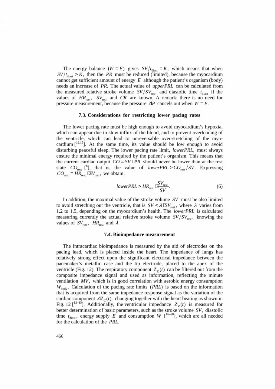
Figure 13 shows a pacemaker [21], where together with the ventricular impedance VZ also arterial impedances A1Z and A2Z are measured using addi-tional electrodes E1 and E2. The arterial impedance AZ helps to estimate the ratio of diastolic and systolic arterial pressures through arterial volumes, without using the pressure sensors. Several arterial impedances (multipoint measurement) enable to estimate more important diagnostic parameters as the velocity of pulse wave propagation, elasticity of arteries and different arterial blood flow para-meters, hydraulic resistance of periphery arteries, etc.

7.5. Summary

The proposed solution has several advantages in comparison with other methods of flexible pacing rate control (limiting). It can be stated that the proposed method for flexible control of the “floating” pacing rate limits can give the opprtunity for elaboration of a new generation of rate-adaptive cardiac pacemakers, which use the bioimpedance-based feedback information from the myocardium. Application of the proposed method is technically simple, but gives a significant advantage – the pacemaker patients can live more normal and healthy lives than ever before.

Lung ZR

ZV

excitation current, iexc

VZv

Bio-impedance measurement unit and pacing rate controller

0 1 2 3 4 5 6

Respiratory wave ∆ZR(t)

Cardiac wave ∆ZC(t)

Time, s

468

Fig. 13. Measurement of the intracardiac and arterial bioimpedances by the implanted cardiac pacemaker.

8. SOIL MOISTURE MEASUREMENT Frequently only two RC elements are used for modelling the impedance

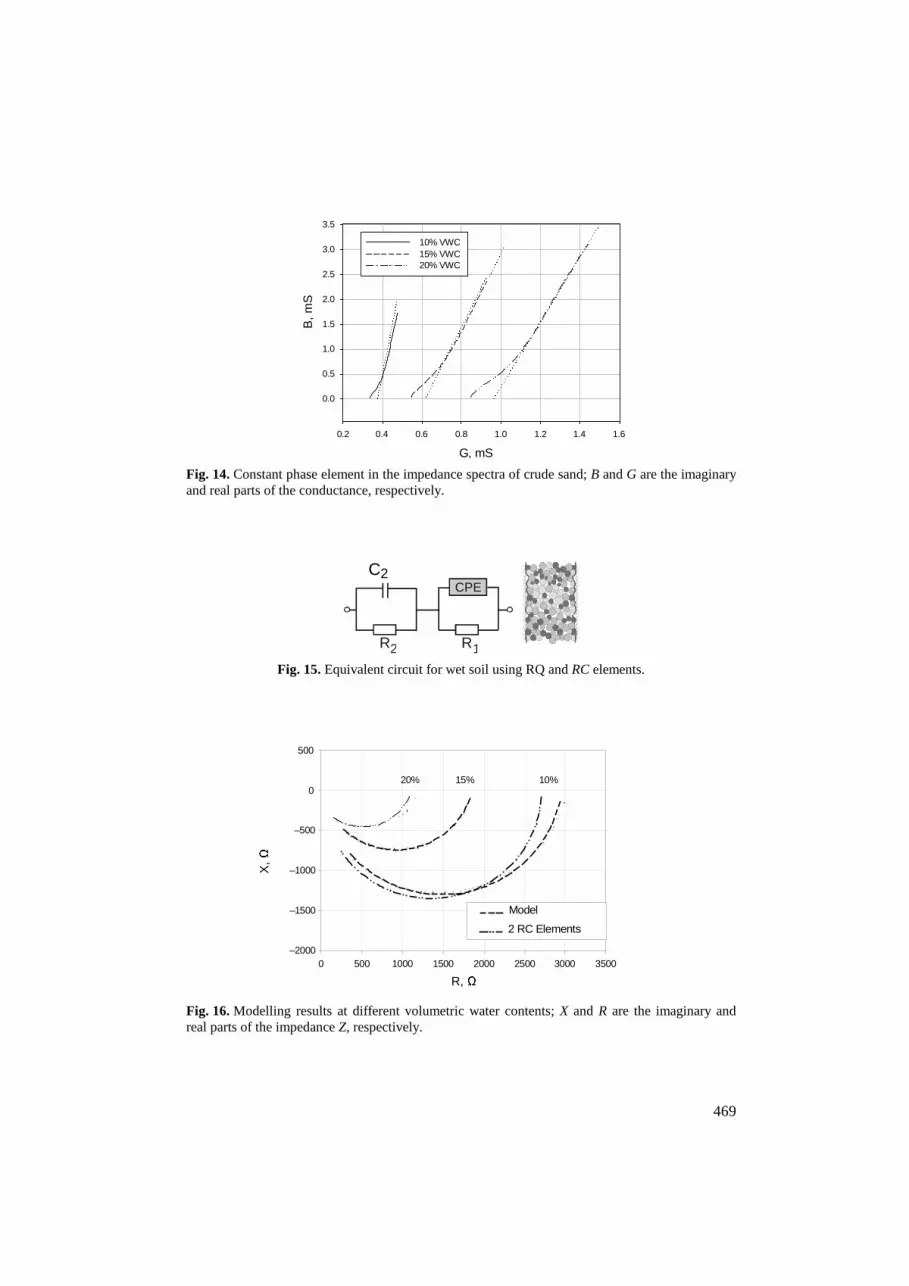
spectrum of wet soil [22]. Thereby, the modelling accuracy reached is not sufficient for the 10% VWC (volumetric water content), see Figs. 14 to 17. In [23] the use of constant phase elements was investigated. The observed flat behaviour of the impedance spectrum in the Y plane was modelled using a ARCZ impedance (Fig. 14). The remaining impedance has the behaviour of a RC-circuit (Fig. 15):

0

1 2mod

2 21 1

,11 ( )R

R RZ

j R Cj R C ωω= +

++ (7)

where 0 0( 1 1)R R− < < and 1C are the coefficients of the CPE. The capacitance 1C changes the distribution of the frequencies on the

impedance arc (Fig. 16) in the Z plane and on the constant phase line in the Y plane. The resistance 0R changes the flat behaviour of impedance arc in the Z plane and the gradient of the constant phase line in the Y plane.

The modelling results in Fig. 16 show significant improvements relative to the use of 2 RC elements [22].

The residuals, shown in Fig. 17, are reached by using the whole frequency range. Generally, the improvements can be reached if the Kramers–Kronig results are used as weighing factors during the fitting procedure.

ZA2

ZV

Bioimpedance measurement unit, cardiac monitor and pacing rate controller

E1

ZA1

E2

Aorta

Arteria subclavia

HHeeaarrtt

PPaacceemmaakkeerr

excitation currents

469

G, mS

0.2 0.4 0.6 0.8 1.0 1.2 1.4 1.6

B, m

S

0.0

0.5

1.0

1.5

2.0

2.5

3.0

3.5 10% VWC 15% VWC 20% VWC

Fig. 14. Constant phase element in the impedance spectra of crude sand; B and G are the imaginary and real parts of the conductance, respectively.

CPE

R R2 1

Fig. 15. Equivalent circuit for wet soil using RQ and RC elements.

R, Ω

0 500 1000 1500 2000 2500 3000 3500

X, Ω

–2000

–1500

–1000

–500

0

500

10% 15% 20%

2 RC Elements Model

Fig. 16. Modelling results at different volumetric water contents; X and R are the imaginary and real parts of the impedance Z, respectively.

B, m

S

C2

X, Ω

R, Ω

470

f in MHz0 2 4 6 8 10 12 14 16

|Z-Z

mod

|/|Z

|in

%

0

1

2

3

4

5

10% VWG15% VWG20% VWG

Fig. 17. Relative errors of the impedance at different VWCs.

9. BATTERY DIAGNOSING

9.1. Theoretical background To characterize aging of batteries is very challenging since the state of health

of a battery depends on its operation. Several methods are available for the characterization of aging processes, differing in accuracy and complexity. The advantage of impedance spectroscopy is the big amount of information it can provide for the insight into aging mechanisms. Depending on the frequency, it provides the possibility to differentiate between various contributing pro-cesses [6]. In order to employ this method, some obstacles should be overcome. It requires fast impedance measurement processes in order to reduce measurement time and to maintain a constant state of the battery during measurements. An easily applicable accurate model and a robust method for model parameter estimations are necessary for the extraction of information.

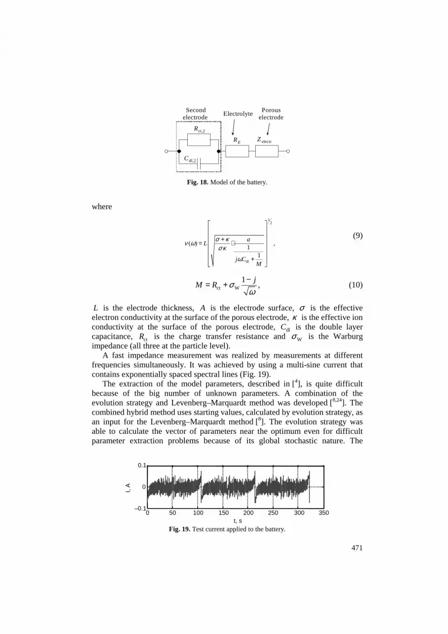
The complexity of electrochemical mechanisms, taking place within a battery, and especially electrode porosity, lead generally to a big number of model parameters. These are difficult to extract from measurements because of the non-linear dependence of the models on their parameters [6,24] and of over-lapping of the frequency ranges corresponding to different effects. In order to be able to consider electrode porosity and other prior knowledge about the battery, we proposed in [24] to use a model (Fig. 18), considering the porosity of one electrode.

The porous electrode was modelled by the following equation:

electrelectr

2 ( )cosh ( ( ))( ) 1 ,

sinh ( ( ))

LAZ

σ κ κ σ ν ωωσ κ ν ν ω

+ += + + (8)

f, MHz

|Z–Z

mod

|/|Z

|, %

471

2 , dl C

2 , ct R

E R electr Z

Electrolyte Porous

electrode Second

electrode

Fig. 18. Model of the battery.

where

12

dl

( ) ,1

1

aL

j CM

σ κν ωσκ

ω

+ = ⋅

+

(9)

ct W

1,

jM R σ

ω−= + (10)

L is the electrode thickness, A is the electrode surface, σ is the effective electron conductivity at the surface of the porous electrode, κ is the effective ion conductivity at the surface of the porous electrode, dlC is the double layer capacitance, ctR is the charge transfer resistance and Wσ is the Warburg impedance (all three at the particle level).

A fast impedance measurement was realized by measurements at different frequencies simultaneously. It was achieved by using a multi-sine current that contains exponentially spaced spectral lines (Fig. 19).

The extraction of the model parameters, described in [4], is quite difficult because of the big number of unknown parameters. A combination of the evolution strategy and Levenberg–Marquardt method was developed [8,24]. The combined hybrid method uses starting values, calculated by evolution strategy, as an input for the Levenberg–Marquardt method [8]. The evolution strategy was able to calculate the vector of parameters near the optimum even for difficult parameter extraction problems because of its global stochastic nature. The

0 50 100 150 200 250 300 350 –0.1

0

0.1

I, A

t, s Fig. 19. Test current applied to the battery.

472

Levenberg–Marquardt method uses it as a local optimization method, and is then better able to calculate the optimum exactly with less probability to trap in local minima. Figure 20 shows an example of simulation using all the three methods: evolution, Levenberg–Marquardt, and the new combined method.

An extensive experimental investigation of lithium-ion batteries was carried out in [6]. The outcome shows that significant improvements in battery diagnosis can be obtained. It was possible to identify different effects from the impedance spectrum covering a wide frequency range (Fig. 21). Based on this method, the battery capacity can be measured with an accuracy of 10%.

Fig. 20. Parameter estimation using different methods.

0 0.02 0.06 0.1 0.14 0.18

- 0.08

- 0.04

0 cycle 0 - 200

charge transfer reaction diffusion

porosity

inductivity

f

Fig. 21. Impedance spectrum of a discharged Li-ion battery due to ageing mechanism over 200 cycles in the frequency range between 3 mHz and 1031 Hz.

[Re(Z)–min(Re(Z)], Ω

Im(Z

), Ω

473

9.2. Designing a battery diagnosing instrument An handheld device for measuring the impedance of lithium-ion batteries was

developed in cooperation between the Department of Measurement and Automa-tion at the University of Bundeswehr Munich and the Institute of Electronics at Tallinn University of Technology. The impedance range of a typical Li-ion battery lies between 50 mΩ and 1 Ω at room temperature. The large frequency range of interest from 10 mHz to 10 kHz, was specified on the basis of research done by Uwe Tröltzsch [6].

The impedance of Li-ion batteries is greatly dependent on temperature. The overall cell impedance increases from nearly 0.05 Ω at the room temperature, up to 8 Ω at – 40 °C. Therefore the temperature information must be recorded together with the impedance data [25]. Lithium-ion batteries exhibit unknown cell potential, usually between 3 to 4.2 V DC. This cell voltage depends on the general condition and the state of charge of the battery. It is important to ensure that the state of charge remains constant during the measurement.

Considering the properties of the Li-ion battery, the operating principles of the measurement device were set and the block diagram of the proposed solution is shown in Fig. 22.

Fig. 22. Li-ion impedance measurement device.

474

The device uses frequency sweeping of the sine wave excitation signal. The signal source is based on the direct digital synthesis (DDS). The DDS was chosen due to its high frequency resolution and wide-band operation. The excitation of the battery is performed through a voltage-controlled current source. This method is much more suitable (inhibiting DC potential) for the measurement of low impedances at sub-hertz frequencies than auto-balancing bridge or voltage divider methods [1]. Current source realizes the potentiostatic control via feed-back by its nature, and the excitation current does not depend on the unknown DC potential of the unknown impedance [26]. There is also no reason to measure the current, flowing through the impedance. As the impedance is below 1 Ω, the four-wire measurement set-up is mandatory. In this case, different pairs of wires are used for current injection into the battery under test and for the measurement of the voltage response across the battery, thus minimizing the errors caused by resistances of contacts and measurement wires [27].

The response is amplified using an instrumentation amplifier and digitized by an 18-bit analogue–digital converter (ADC). The 18-bit resolution was selected in order to measure the mV range AC response at the presence of unknown cell potential up to 4.2 V. The separation of real and imaginary components of the response signal is performed by a microcontroller MSP430F1611 from Texas Instruments. The signal samples are taken at specific moments and multiplied then either by – 1 or + 1, synchronously with in-phase and quadrature reference signals. This process is performed over an integer number of excitation periods. Integrating of the multiplication products results in real and imaginary values of the response voltage. The in-phase reference is acquired from the DDS source directly, and the quadrature reference is generated by delaying the in-phase reference by a quarter of the generated signal period. The measured results can be shown on the implemented LCD display or downloaded to the computer through the USB interface.

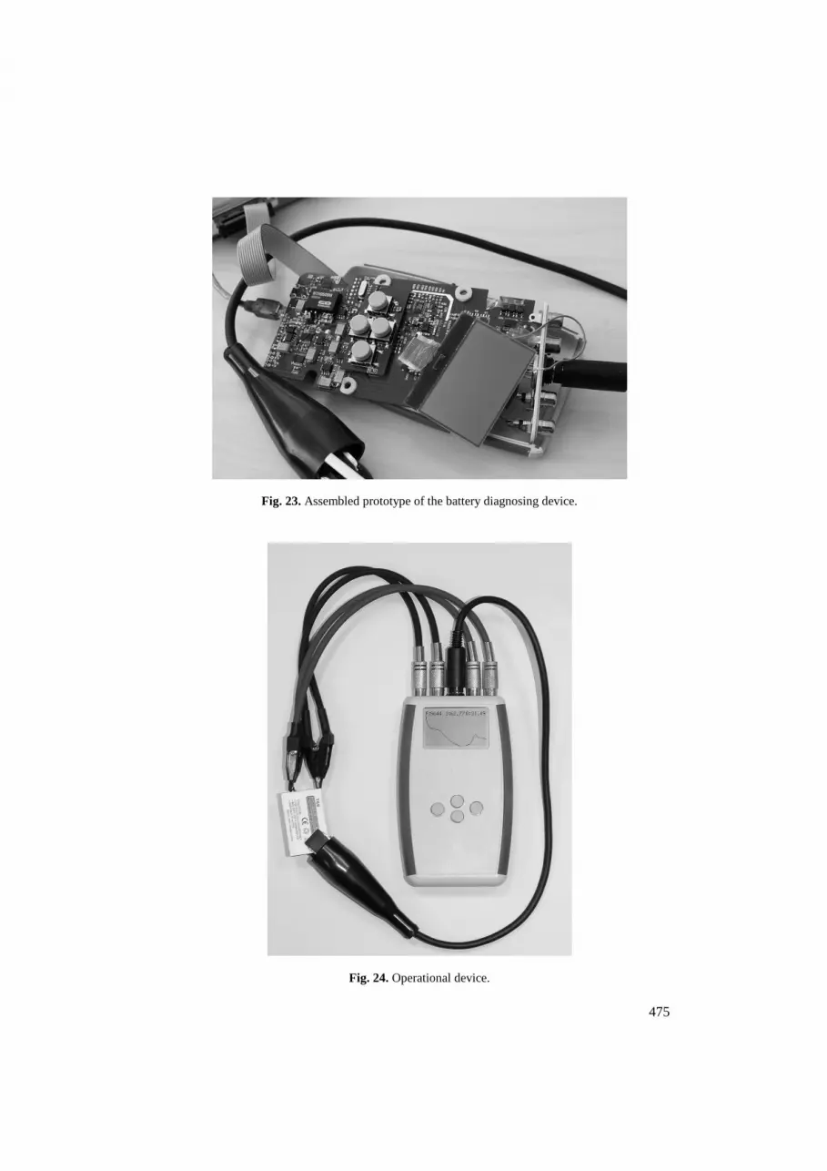
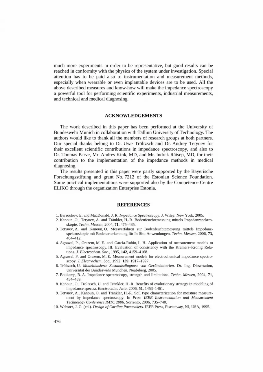
Figure 23 shows an assembled PCB of the prototype device, and a photo of the device, measuring a Li-ion battery of Ericsson cellular phone is shown in Fig. 24. The frequency sweep was configured to run from ~ 7 mHz to 9644 Hz in one octave increments, and the results are shown in the form of the Nyquist diagram.

10. CONCLUSIONS

In impedance spectroscopy, the experimental aspects and signal processing methods are both very important prerequisites for the extraction of information with acceptable accuracy. Two principally different methods of signal processing can be used. Using equivalent circuit models requires modelling of the impedance spectrum in conformity to physical, chemical and biological processes, taking place in the impedance under investigation. Extraction of model parameters is a matter of concern and can be supported by different methods of optimization and also by some other case-specific measures. Using a mathematical approach needs

475

Fig. 23. Assembled prototype of the battery diagnosing device.

Fig. 24. Operational device.

476

much more experiments in order to be representative, but good results can be reached in conformity with the physics of the system under investigation. Special attention has to be paid also to instrumentation and measurement methods, especially when wearable or even implantable devices are to be used. All the above described measures and know-how will make the impedance spectroscopy a powerful tool for performing scientific experiments, industrial measurements, and technical and medical diagnosing.

ACKNOWLEDGEMENTS The work described in this paper has been performed at the University of

Bundeswehr Munich in collaboration with Tallinn University of Technology. The authors would like to thank all the members of research groups at both partners. Our special thanks belong to Dr. Uwe Tröltzsch and Dr. Andrey Tetyuev for their excellent scientific contributions in impedance spectroscopy, and also to Dr. Toomas Parve, Mr. Andres Kink, MD, and Mr. Indrek Rätsep, MD, for their contribution to the implementation of the impedance methods in medical diagnosing.

The results presented in this paper were partly supported by the Bayerische Forschungsstiftung and grant No. 7212 of the Estonian Science Foundation. Some practical implementations were supported also by the Competence Centre ELIKO through the organization Enterprise Estonia.

REFERENCES

1. Barsoukov, E. and MacDonald, J. R. Impedance Spectroscopy. J. Wiley, New York, 2005. 2. Kanoun, O., Tetyuev, A. and Tränkler, H.-R. Bodenfeuchtemessung mittels Impedanzspektro-

skopie. Techn. Messen, 2004, 71, 475–485. 3. Tetyuev, A. and Kanoun, O. Messverfahren zur Bodenfeuchtemessung mittels Impedanz-

spektroskopie mit Bodenarterkennung für In-Situ Anwendungen. Techn. Messen, 2006, 73, 404–412.

4. Agrawal, P., Orazem, M. E. and Garcia-Rubio, L. H. Application of measurement models to impedance spectroscopy, III. Evaluation of consistency with the Kramers–Kronig Rela-tions. J. Electrochem. Soc., 1995, 142, 4159–4168.

5. Agrawal, P. and Orazem, M. E. Measurement models for electrochemical impedance spectro-scopy. J. Electrochem. Soc., 1992, 139, 1917–1927.

6. Tröltzsch, U. Modellbasierte Zustandsdiagnose von Gerätebatterien. Dr. Ing. Dissertation, Universität der Bundeswehr München, Neubiberg, 2005.

7. Boukamp, B. A. Impedance spectroscopy, strength and limitations. Techn. Messen, 2004, 71, 454–459.

8. Kanoun, O., Tröltzsch, U. and Tränkler, H.-R. Benefits of evolutionary strategy in modeling of impedance spectra. Electrochim. Acta, 2006, 51, 1453–1461.

9. Tetyuev, A., Kanoun, O. and Tränkler, H.-R. Soil type characterization for moisture measure-ment by impedance spectroscopy. In Proc. IEEE Instrumentation and Measurement Technology Conference IMTC 2006. Sorrento, 2006, 735–740.

10. Webster, J. G. (ed.). Design of Cardiac Pacemakers. IEEE Press, Piscataway, NJ, USA, 1995.

477

11. Min, M., Parve, T. and Kink, A. Thoracic bioimpedance as a basis for pacing control. In Annals of the New York Academy of Sciences. Electrical Bio-Impedance Methods: Application to Medicine and Biotechnology. New York, 1999, 873, 155–166.

12. Min, M., Kink, A., Parve, T. and Rätsep, I. Bioimpedance based control of rate limit in artificial cardiac pacing. In Proc. IASTED International Conference on Biomedical Engineering BioMED 2005. Innsbruck, 2005. ACTA Press, Calgary, Alberta, Canada, 2005, 697–703.

13. Kink, A., Salo, R. W., Min, M., Parve, T. and Rätsep, I. Intracardiac electrical bioimpedance as a basis for controlling of pacing rate limits. In Proc. IEEE Engineering in Medicine and Biology Conference EMBC2006. New York, 2006. IEEE Press, 2006, 6308–6311.

14. Min, M., Kink, A. and Parve, T. Rate Adaptive Pacemaker. US Patent 6, 885, 892. Publ. April 26, 2005.

15. Min, M., Kink, A. and Parve, T. Rate Adaptive Pacemaker Using Impedance Measurements and Stroke Volume Calculations. US Patent 6, 975, 903, Dec. 13, 2005.

16. Ericsson, A. B. Cardioplegia and Cardiac Function Evaluated by Left Ventricular P-V Rela-tions. PhD Thesis, Karolinska Institutet, Stockholm, 2000.

17. Söderqvist, E. Left Ventricular Volumetry Technique Applied to a Pressure Guide Wire. Licentiate Thesis, Royal Institute of Technology, Stockholm, 2002.

18. Denslow, S. Relationship between PVA and myocardial oxygen consumption can be derived from thermodynamics. Am. J. Physiol. Heart Circ. Physiol., 1996, 270, H730–H740.

19. Salo, R. W., O’Donoghue, S. and Platia, E. V. The use of intracardiac impedance-based indicators to optimize pacing rate. In Clinical Cardiac Pacing (Ellenbogen, K. A., Kay, G. N. and Wilkoff, B. L., eds.). W. B. Saunders Co., Philadelphia, PA, 1995, 234–249.

20. Salo, R. W. Application of impedance volume measurement to implantable devices. Int. J. Bioelectromagn., 2003, 5, 57–60.

21. Kink, A., Min, M., Parve, T. and Rätsep, I. Device and Method for Monitoring of Cardiac Pacing Rate. US Patent Application 11/847430, applied August 30, 2007.

22. Flaschke, T. Modellierung zur Material-unabhängigen Bodenfeuchtemessung mit Methoden der Impedanz- Sensorik Fortschritt-Berichte. VDI, Reihe 8, Nr. 889, VDI Verlag, 2001.

23. Kanoun, O. Modeling of Impedance Spectra for Moisture Measurement in Crude Sand. In Proc. IEEE International Conference on Systems, Signals & Devices SSD'05. Sousse, Tunisia, 2005, 1664–1672.

24. Tröltzsch, U., Kanoun, O. and Tränkler, H.-R. Characterizing aging effects of lithium ion batteries by impedance spectroscopy. Electrochim. Acta, 2006, 51, 1664–1672.

25. Buchmann, I. Batteries in a Portable World. Cadex Electronics Inc., Richmond, Canada, 2001. 26. Tietze, U. and Schenk, C. Electronic Circuits Design and Applications. Springer-Verlag,

Berlin, 1991. 27. Impedance Measurement Handbook. Agilent Technologies, Palo Alto, USA, 2006.

Impedants-spektroskoopiat kasutavad targad sensorsüsteemid

Hans-Rolf Tränkler, Olfa Kanoun, Mart Min ja Marek Rist

Nii eksperimenditehnika kui ka signaalitöötluse meetodid on olulised suure

täpsusega info saamiseks impedantsspektroskoopia abil. Signaalitöötlusel ja mudelite koostamisel saab kasutada kaht põhimõtteliselt erinevat meetodit. Ekvi-valentskeemide meetodi kasutamine eeldab impedantsspektri modelleerimist kooskõlas füüsikaliste, keemiliste ja bioloogiliste protsessidega, mis leiavad aset uurimise all olevas impedantsis. Mudeli parameetrite saamine tekitab seejuures

478

probleeme, mida saab lahendada optimeerimis- ja mitmesuguste teiste meetodite abil. Matemaatiline lähenemine vajab palju rohkem eksperimente selleks, et saada usaldusväärset tulemust. Eriline tähelepanu peaks kuuluma mõõtmismeeto-ditele ja -vahenditele, eriti kui nähakse ette rakendusi kantavates või implantee-ritavates seadmetes. Ülaltoodu arvestamine teeb impedantsspektroskoopiast võimsa vahendi teaduseksperimentide teostamiseks ja rakendamiseks tehnilises ning meditsiinilises diagnostikas.