Estuaries and CoastsDOI 10.1007/s12237-012-9524-9

Grazing Constants are Not Constant: MicrozooplanktonGrazing is a Function of Phytoplankton Production in anAustralian Lagoon

Brian G. Sanderson · Anna M. Redden · Kylie Evans

Received: 22 August 2011 / Revised: 28 May 2012 / Accepted: 29 May 2012© Coastal and Estuarine Research Federation 2012

Abstract Twenty-one dilution method experimentswere used to measure phytoplankton growth rate, graz-ing rate by microzooplankton, and phytoplankton con-centrations that saturate grazing in Tuggerah Lake—alarge lagoon in New South Wales, Australia. Individ-ual experiments conformed to the saturating grazingmodel with no evidence of a threshold phytoplanktonconcentration to initiate grazing. Phytoplankton con-centrations that saturated grazing were highly variablebetween experiments and were positively correlatedwith chlorophyll a concentration in the lagoon. Plank-ton models often use a saturating grazing function that

B. G. Sanderson (B)Department of Environment and Climate Change,PO Box A290, Sydney South NSW 1232, Australiae-mail: bxs@eastlink.ca

A. M. ReddenAcadia Centre for Estuarine Research, Acadia University,PO Box 115, Wolfville, NS B4P 2R6, Canadae-mail: anna.redden@acadiau.ca

K. EvansUniversity of Newcastle, Central Coast Campus,PO Box 127, Ourimbah, NSW 2258, Australia

Present Address:B. G. Sanderson15 Beckwith St, Wolfville, NS, Canada B4P 1R3

Present Address:K. EvansCharlton Christian College, PO Box 605, Toronto,NSW 2283, Australiae-mail: kylie.evans@charlton.nsw.edu.au

includes several constants, but constants are found tobe variable from one dilution experiment to the next.Another formulation is proposed in which grazing isa quadratic function of phytoplankton growth. Thisenables the 21 measurements of zooplankton grazingto be fitted using only two invariant parameters. Noevidence is found for saturation of microzooplanktongrazing when it is calculated as a function of phyto-plankton growth. When phytoplankton growth is high,about 80% of it is grazed. When phytoplankton growthis low, about 45% is grazed. Calculations illustrate thatthis type of grazing stabilizes the planktonic producersand grazers, as expected.

Keywords Grazing rate · Saturated grazing ·Microzooplankton · Growth rate · Phytoplankton ·Plankton model · NPZ model · Invariants

Introduction

Tuggerah Lake (33.345◦S, 151.504◦E) is one of thelarger of more than 200 lagoons in New South Wales,Australia (Fig. 1). The response of these lagoonsto nutrient inputs has become a matter of concernas coastal catchments become increasingly urbanized(Young et al. 1996). Eutrophication which is often asso-ciated with increased chlorophyll a in the water columnand ecological modeling by Webster and Harris (2004)indicated that a transition from macrophyte to planktondominance may be an outcome for shallow lagoonslike Tuggerah Lake. It is desirable to measure phyto-plankton growth and grazing by microzooplankton be-cause these are important processes in such ecologicalmodeling.

Estuaries and Coasts

The Entrance

TuggerahLake

Budgewoi Lake

Munmorah Lake

Wyong R

Ourimbah

Ck

2 km

Nor

th

Pacific

Ocean

Norah Head

Fig. 1 Bathymetry of the Tuggerah Lake system, NSW,Australia. The shoreline contour is at 0 m (Australian HeightDatum). The contour interval is 1 m. In Tuggerah Lake, locationsof sampling stations (north, middle, south) are indicated withbold plus signs

Variable phytoplankton populations are often mod-eled in terms of invariant parameters that enable phy-toplankton growth rate to be determined as a functionof variables such as photosynthetically available radi-ation and the concentrations of various bioavailablenutrients (Monod 1942; Steele 1962; Droop 1973; Flynn2001). Similarly, grazing rates are often calculated fromsystem variables, such as phytoplankton concentration,using various formulations that have invariant para-meters (Steele 1976; Vanni et al. 1992; Murray andParslow 1999a). Franks (2002) reviews some of themany functional forms that might be used to determinephytoplankton growth rate and zooplankton grazingrate in models that include nutrients, phytoplankton,and zooplankton.

An ecological model of Tuggerah Lake requires aspecific formulation of microzooplankton grazing. It isexpected that the formulation will involve constantsthat must also be determined. The objective of thepresent work is to obtain a formulation for microzoo-plankton grazing (with measured constants) that mightbe used within an ecological model.

Methods

Landry and Hassett (1982) developed the dilutionmethod to simultaneously estimate rates of phytoplank-

ton growth μ and microzooplankton grazing g. Whenphytoplankton concentrations were sufficiently high,Redden et al. (2002) showed how dilution experimentscould also be used to determine the phytoplanktonconcentration Ps at which microzooplankton grazingsaturated. The basic idea is to incubate bottles con-taining some fraction D of whole seawater mixed witha fraction 1 − D of filtered seawater. Phytoplanktongrowth within a bottle is then fitted to the followingequation:

dpdt

=

⎧⎪⎪⎪⎪⎨

⎪⎪⎪⎪⎩

μp − gDp if p < Ps

Landry and Hassett (1982)

μp − gDPs if p ≥ Ps

Redden et al. (2002)

(1)

where p is the phytoplankton concentration within abottle.

Twenty-one dilution experiments were undertakenon 10 occasions between August 2001 (winter) andMarch 2002 (fall), with most measurements made inspring and summer. Water was collected from three sta-tions in Tuggerah Lake (Fig. 1) with the measurementeffort focused on the middle station and the summerperiod. Concurrent water quality measurements (tem-perature, salinity, dissolved oxygen, and turbidity) withdepth were made using a calibrated YeoKal 611 WaterQuality Analyzer.

Three 22-L carboys of seawater were collected foreach experiment. Each carboy was filled with waterfrom a depth of ∼ 0.5 m by holding the inverted carboyunder water over the side of a boat, with the lid offand tap open, allowing water to gently flow in. Toproduce the dilution medium, the water of one carboywas filtered under pressure through a glass fiber filterand then through a 0.2-µm membrane filter.

Whole seawater from the second carboy was com-bined with the dilution medium to make a series of 2-Lbottles containing 100, 80, 60, 40, 20, and 10% wholeseawater. If chlorophyll a levels were high, an addi-tional bottle was prepared with 5% whole seawater.Gentle pouring techniques and silicon tubing attachedto carboy taps helped reduce turbulence and splashingwhich potentially damage nanoflagellates and ciliateswhen preparing the dilutions. Bottles were carefullyfilled to minimize bubble formation and trapping ofmicrozooplankton.

Nitrogen is generally believed to be more limitingthan phosphorus in coastal marine waters (Ryther andDunstan 1971), and Harris (2001) finds evidence for

Estuaries and Coasts

nitrogen limitation in many Australian lagoons andestuaries. Nitrogen, in the form of NH4Cl, was added insufficient quantity to allow up to three phytoplanktondoublings without nitrogen limitation (i.e., between 7and 30 µM per bottle). A pair of 2-L control bottles,containing 10 and 100% whole seawater, was preparedwithout added nutrient and incubated with all theother 2-L bottles in the dilution series. To obtain ini-tial chlorophyll a concentrations, two replicate sampleswere taken from each of the dilution treatments andpassed through a 0.2-µm membrane filter. The chloro-phyll a was extracted by placing each filter in a vial with2 mL 90% acetone and refrigerating in the dark for24–48 h.

Bottles were incubated in Tuggerah Lake for 24 hby using Velcro to attach them on a platform. Floatswere used to suspend the platform at a depth of0.5 m (Williams 2003). The incubation period typicallystarted at about noon on the day of sample collection.After incubation, the final chlorophyll a concentra-tions were obtained by the same filtering and extrac-tion procedure used to obtain the initial chlorophyll aconcentrations. Extracted chlorophyll a was measuredspectrofluorometrically, using a calibrated HitachiF-3000 Spectrofluorometer.

For each station, undiluted water samples (250 mL),before and after incubation (with NH+4 enrichment),were preserved with acid Lugol’s iodine and storedaway from light until they could be examined for phy-toplankton cell identification and enumeration. Priorto counting, 100-mL subsamples were concentratedby letting them stand in the dark for 48 h before si-phoning off 90 mL of supernatant fluid. Phytoplanktonidentification, to the lowest possible taxon, and enu-meration were performed using a standard compoundmicroscope (max magnification ×400) and the Lundcell technique (Lund et al. 1958). Phytoplankton<5 µm were included under the categories “uniden-tified flagellates” or “unidentified nonflagellate” taxa.

Of the three 22-L carboys regularly collected at eachstation, one was poured through a 15-µm plankton net;organisms larger than 15 µm were collected in a 125-mL sample container and preserved with buffered for-malin (to 2–3%). Prior to microscopic analysis, knownvolumes of each sample were rinsed through a 50-µmmesh, to remove material and organisms too small to beviewed at ×160 magnification. Microzooplankton sub-samples retained by the 50-µm mesh were transferredto a grid-lined petri dish for enumeration using a dis-secting microscope. Further subsamples were counteduntil a minimum of 200 organisms were identified andcounted per sample.

Physical measurements and modeling are used toprovide context with which to understand results fromthe series of dilution experiments. Physical quantitiessuch as solar radiation, catchment discharge, water resi-dence time, temperature, and salinity were obtained forthe period January 2001 to April 2002.

The Bureau of Meteorology provided hourly windspeed and direction, air temperature, and humidity asmeasured at Norah Head (Fig. 1). Manly HydraulicsLaboratory provided water level measurements ofTuggerah Lake as well measurements from Sydney,Australia which closely match the ocean adjacentTuggerah Lake.

Weber (personal communication) provided catch-ment discharge obtained from catchment model-ing. An IHACRES rainfall-runoff model Croke andJakeman (2004) was used for the larger, predominatelynonurban headwater subcatchments, and the MUSICurban stormwater model (www.ewater.com.au/music)was used for the smaller, predominately urban sub-catchments fringing the lake (Brennan et al. 2010).

Salinity and water residence time were modeledwith each basin represented by a box with area anddepth according to the measured bathymetry. Catch-ment discharge, evaporation, precipitation, wind stress,and tides were used to drive this box-model formu-lation of the Tuggerah Lakes. Water level gradientsdrove exchange between basins, and exchange withthe ocean was calculated following Sanderson andBaginska (2007).

The Bureau of Meteorology calculates global solarexposure (GSE) from satellite measurements. GSE atthe Narara Research Station 33.3949◦S, 151.3289◦N wasused to estimate daily averaged solar radiation in orderto provide a context for phytoplankton growth. Watertemperature was calculated from solar radiation, windstress, sensible and latent heat fluxes (Price et al. 1978),and long-wave radiation (Josey et al. 2003).

Results

Dilution series could be fitted using either the methodof Landry and Hassett (1982) or the extension given byRedden et al. (2002). Figure 2 shows that phytoplank-ton growth was lower for the control bottles (no addednitrogen) which is consistent with nitrogen being thelimiting nutrient.

Table 1 presents results from the 21 dilution exper-iments. In situ chlorophyll a concentrations P0 weregenerally higher in January and February (summer),

Estuaries and Coasts

−0.4 −0.2 0 0.2 0.4 0.6 0.8 1 1.2

−0.4

−0.2

0

0.2

0.4

0.6

0.8

1

1.2

1.4

μ (d−1)

Con

trol

val

ue fo

r μ (

d−1 )

saturatedunsaturated

Fig. 2 Phytoplankton growth rates were calculated from exper-iments with control values of μ and plotted against those fromthe N-enhanced dilution series. Points plotted with circles areinstances when zooplankton grazing saturated, crosses are usedwhen grazing did not saturate

and those were also the months during which satu-rated grazing was most likely to be observed. Phyto-plankton cell density ranged from <1,000 cells mL−1

in samples collected during August–December 2001 tomostly >2,000 cells mL−1 during January–March 2002.Density of microzooplankton larger than 50 µm (Z50)is substantially higher in summer than in the coolermonths (August–October). Williams (2003) tabulatesand graphs the composition of microzooplankton andphytoplankton communities.

Unidentified nanoplankton flagellates were the mostnumerous phytoplankton in Tuggerah Lake, exceptfor the middle station on 19 September 2001 whenDinophyceae dominated. Diatoms represented up to30% of the assemblage during summer but less than10% of the assemblage in almost all samples takenduring autumn, winter, and spring. Dinophyceae wascommonly present but almost always dominated byeither diatoms or unidentified nanoflagellates. A finalgroup—consisting of Chrysophyseae, Prasinophyceae,Euglenophycea, and Chryptophyceae—comprised anegligible part of the assemblage except on 8 February2002, following a catchment discharge event, when they

Table 1 Results from the Tuggerah Lake dilution study

Site/date P0 μ g Ps Z50 p valueyyyy/mm/dd µg chl L−1 day−1 day−1 µg chl L−1 count L−1

North2001/09/19 2.29 (0.11) 1.10 (0.03) 0.34 (0.06) nd <0.0012002/01/08 9.01 (0.20) 0.56 (0.02) 0.25 (0.03) 406 <0.0012002/02/08 12.65 (0.28) 0.89 (0.03) 1.70 (0.16) 4.62 (0.43) 2468 <0.0012002/02/20 5.29 (0.25) 0.77 (0.05) 1.39 (0.31) 1.86 (0.19) 443 <0.052002/03/19 5.60 (0.02) 0.17 (0.02) 0.21 (0.03) 1567 <0.001

Middle2001/08/06 2.03 (0.07) 0.37 (0.03) 0.12 (0.04) 17 <0.052001/09/19 1.49 (0.03) 1.07 (0.04) 0.26 (0.07) 18 <0.012001/10/11 2.51 (0.12) 0.17 (0.01) −0.11 (0.02) 95 <0.0012001/12/11 6.98 (0.40) 0.61 (0.03) 0.27 (0.04) 338 <0.0012002/01/08 8.47 (0.35) 0.51 (0.03) 0.19 (0.05) 390 <0.012002/01/21 7.77 (0.07) 1.08 (0.02) 0.81 (0.06) 6.52 (0.20) 192 <0.0012002/01/30 a 11.23 (0.31) 0.51 (0.06) 1.02 (0.34) 4.12 (0.47) 241 <0.052002/01/30 b 11.85 (0.28) 0.82 (0.05) 1.01 (0.15) 8.09 (0.04) nd <0.0012002/02/08 11.15 (0.23) 0.94 (0.03) 1.23 (0.08) 7.08 (0.36) 728 <0.0012002/02/20 6.56 (0.13) 0.81 (0.04) 1.88 (0.23) 2.31 (0.08) 406 <0.012002/03/19 4.99 (0.06) 0.38 (0.01) 0.60 (0.04) 2.41 (0.10) 494 <0.001

South2001/09/19 1.03 (0.02) 1.12 (0.03) 0.42 (0.05) nd <0.0012002/01/08 8.75 (0.55) 0.56 (0.02) 0.72 (0.06) 5.21 (0.25) 514 <0.0012002/02/08 11.77 (0.30) 0.91 (0.08) 1.58 (0.29) 6.36 (0.24) 492 <0.012002/02/20 5.97 (0.09) 0.96 (0.04) 2.08 (0.27) 2.15 (0.13) 329 <0.012002/03/19 9.83 (0.24) 0.30 (0.01) 0.15 (0.02) 159 <0.001

Lowercase letters indicate that the replicate experiment was conducted on 2002/01/30 when samples were collected from sites separatedby ∼100 m in order to assess variability at scales much smaller than the station separation. The p value is for regression of the dilutionseriesP0 in situ chlorophyll a, Z50 density of microzooplankton larger than 50 µm, nd samples were lost or not collected

Estuaries and Coasts

comprised 35% of the assemblage at the north station(nearest Wyong River) and about 20% at each of theother stations.

Crustacean nauplii represented the largest fractionof the microzooplankton (>50 µm) community onevery sampling occasion, with two exceptions whenephemeral populations of tintinnids (ciliates) wereabundant. Tintinnids were generally low in abundance(<10 L−1) except on 8 February 2002 when tintinnidswere present at abundances of 1,900, 410, and 350 L−1

at the north, middle, and south stations, respectively.Within a week, tintinnids were reduced to ≈10 L−1.A month later, on 19 March 2002, tintinnids wereabundant (980 L−1) at the north station but were lowin numbers at the other two stations. Tintinnid countsin the present study appear to be at least as patchyand ephemeral as measurements made elsewhere(Urrutxurtu 2004; Barria de Cao et al. 2005). Highmicrozooplankton counts associated with tintinnids arenot associated with proportionate increases in grazingrate (Table 1).

Figure 3 shows catchment discharge and salinity inTuggerah Lake. Modeled salinity closely follows mea-surements and indicates stable conditions with salinityslowly increasing from July 2001 until a minor dischargeevent on 4 February 2002. Residence time for waterwithin Tuggerah Lake is approximately 60 days whichis substantially more than the time between dilutionexperiments undertaken during summer.

Most catchment discharge enters Tuggerah Lakesvia the Wyong River and Ourimbah Creek so the mid-dle sampling station is located within a triangle that

Jan01 Apr01 Jul01 Oct01 Jan02 Apr020

20

40

60

80

100

Time (month year)

Dis

char

ge (

m3 s

−1 ) A

Jan01 Apr01 Jul01 Oct01 Jan02 Apr020

10

20

30

40

Time (month year)

Sal

inity

(pp

t)

modelmeasure

B

Fig. 3 Vertical bars indicate times of dilution experiments.a Catchment discharge into Tuggerah Lake. b Modeled salinityof Tuggerah Lake with measurements plotted as circles

Jan01 Apr01 Jul01 Oct01 Jan02 Apr020

100

200

300

400

500

Time (month year)

Rad

iatio

n (W

m−

2 ) A

Jan01 Apr01 Jul01 Oct01 Jan02 Apr0210

15

20

25

30

Time (month year)

Tem

pera

ture

(o C

) B

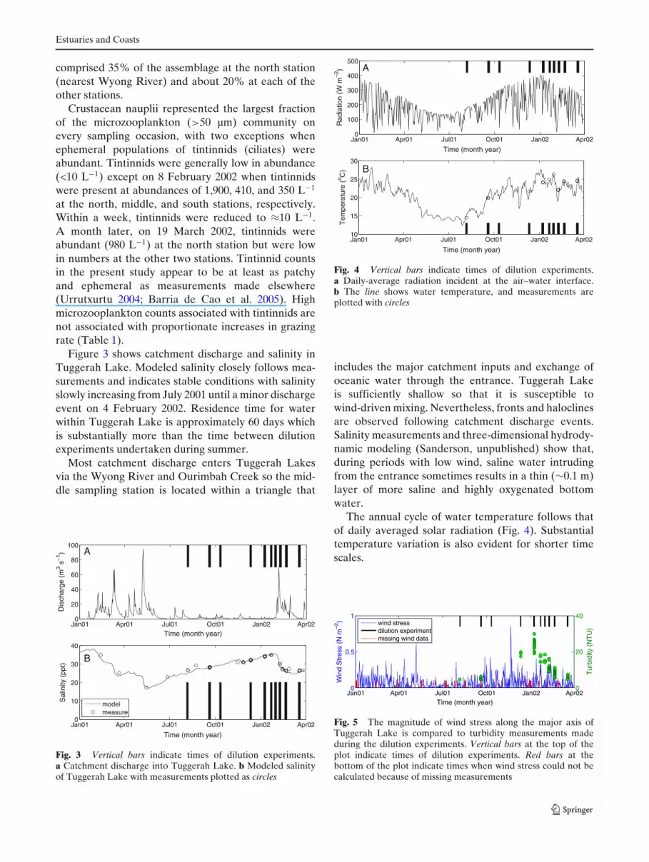
Fig. 4 Vertical bars indicate times of dilution experiments.a Daily-average radiation incident at the air–water interface.b The line shows water temperature, and measurements areplotted with circles

includes the major catchment inputs and exchange ofoceanic water through the entrance. Tuggerah Lakeis sufficiently shallow so that it is susceptible towind-driven mixing. Nevertheless, fronts and haloclinesare observed following catchment discharge events.Salinity measurements and three-dimensional hydrody-namic modeling (Sanderson, unpublished) show that,during periods with low wind, saline water intrudingfrom the entrance sometimes results in a thin (∼0.1 m)layer of more saline and highly oxygenated bottomwater.

The annual cycle of water temperature follows thatof daily averaged solar radiation (Fig. 4). Substantialtemperature variation is also evident for shorter timescales.

Jan01 Apr01 Jul01 Oct01 Jan02 Apr020

0.5

1

Time (month year)

Win

d S

tres

s (N

m−

2 )

0

20

40

Tur

bidi

ty (

NT

U)

wind stressdilution experimentmissing wind data

Fig. 5 The magnitude of wind stress along the major axis ofTuggerah Lake is compared to turbidity measurements madeduring the dilution experiments. Vertical bars at the top of theplot indicate times of dilution experiments. Red bars at thebottom of the plot indicate times when wind stress could not becalculated because of missing measurements

Estuaries and Coasts

Wind measurements were also used to calculate thecomponent of wind stress acting along the major axis ofTuggerah Lake (30◦N). Strong winds with large fetchgenerate the largest waves and are most likely to resus-pend bottom material. Turbidity measurements madeat the times of dilution experiments are plotted in Fig. 5.Turbidity is higher in the warm windy months than inthe cold calm months.

Analysis

Chlorophyll a concentrations within Tuggerah Lakevaried seasonally (Fig. 6) being low in winter, risingto a peak in early February, and subsequently declin-ing. This seasonal change follows the cycle of solarradiation and water temperature (Fig. 4), but this doesnot necessarily mean that either water temperature orradiation is directly limiting phytoplankton growth andabundance. While radiation is lower in winter, the windstress is also lower and the water is less turbid (Fig. 5),so it is doubtful that low phytoplankton abundancein winter is due to a lack of photosynthetically activeradiation.

Chlorophyll a concentrations are generally consis-tent between the three sampling stations (Fig. 6) asmight be expected given the relatively long residencetime scale and the susceptibility of this shallow lagoonto wind-driven mixing. There is an interesting exceptionon 19 March 2002 when chlorophyll a at the southstation is almost twice that at the middle and northstations. Field notes recorded freshening NNW winddeveloping as samples were collected first from thenorth station, then the middle station, and finally thesouth station. Meteorological measurements made atNorah Head confirm that winds increased from 4 m s−1

at the start of sample collection to 9 m s−1 shortlyafter the south station was sampled. Salinity profiles

Aug01 Sep01 Oct01 Nov01 Dec01 Jan02 Feb02 Mar02 Apr020

5

10

15

Time (month/year)

P0 (

μg c

hl−

a L−

1 )

North StationMiddle StationSouth Station

Fig. 6 Chlorophyll a is plotted at times of dilution experiments.Variation between stations is small except on 19 March 2002

at the north and middle stations were 26.5 ppt exceptfor a thin bottom layer of 31–32 ppt water, so buoy-ancy forces would suppress turbulence and sedimentresuspension and entrainment into the water column.Salinity was uniform through the water column at thesouth station, consistent with mixing and baroclinicadjustment to the wind stress. Turbidity was 6 NTUat the north station, 5 NTU at the middle station, andwas almost uniform through the water column at bothof these stations. In contrast, turbidity at the southstation was 12 NTU near the surface, 15 NTU at 1 m,and 37 NTU at 2-m depth. This wind event causedsome resuspension of benthic material at the southstation. Shallow Australian lagoons are well known tohave abundant benthic microalgae (BMA) (Eyre andFerguson 2002). Resuspended BMA are suspected tohave contributed to the higher chlorophyll a concentra-tion at the south station on 19 March 2002 (Fig. 6). Theobserved number of algal taxa was also twice as high atthe south station as at other stations and included morediatoms. Wind-driven mixing is the physical mechanismthat can be expected to generally homogenize Tug-gerah Lake, but wind-driven entrainment of bottomsubstrate into the water column can cause short-termspatial heterogeneity of phytoplankton.

0 50 100 150 200 250 300 350 400 450

0

0.2

0.4

0.6

0.8

1

Daily−Average Incident Radiation (W m−2)

μ (d

−1 )

6 Aug 2001Sep − Feb 200219 March 2002(I/I

0)exp(1−I/I

0)

Fig. 7 Measurements of phytoplankton growth rate μ areplotted against daily-averaged solar radiation. Solar radia-tion was calculated from global solar exposure (GSE) at theNarara Research Station (Gosford). The Bureau of Meteorology(Australia) derives GSE from satellite data. The dashed lineshows normalized productivity response to light intensity withoptimal intensity set to I0 = 250 W m−2. On 8 January 2002,the north and south stations gave identical values for μ, so theseappear as a single point on the plot

Estuaries and Coasts

Table 2 Mean growth rates and grazing rates with nitrogen added and without added nitrogen (control bottles)

μ (day−1) g (day−1)

All 21 experiments Control 0.04 ± 0.07Nitrogen added 0.68 ± 0.07

10 experiments without saturating grazing Control 0.00 ± 0.07 0.25 ± 0.09Nitrogen added 0.60 ± 0.12 0.21 ± 0.05

The standard error of the means are also given

York et al. (2011) make a plausible suggestion thatthe need to process nonfood particles may sometimescause grazing to saturate, or even become minimal,in turbid estuarine systems. We measured turbidity ateach sampling station, except for that of the dilutionexperiment on 2001/10/11. Turbidity was unrelated towhether or not grazing was saturated.

Dilution experiments were done under natural lightconditions on dates that assured sufficient light forgrowth (Fig. 7). Low phytoplankton growth rates μ

were often obtained even though light conditions didnot appear to be limiting. Treatment bottles in thedilution series had added nitrogen, so neither lightnor nitrogen should have been limiting phytoplanktongrowth rates. Each dilution experiment included twocontrol bottles without added nitrogen. Phytoplanktongrowth rates in control bottles were always less thanfor the corresponding dilution series (Table 2, Fig. 2),indicating that nitrogen limited in situ phytoplanktongrowth in Tuggerah Lake. There are other nutrients, in-cluding micronutrients, that might have limited growthrates, but these have not been measured. Clearly, thereis a great deal of variability in the phytoplanktongrowth rate that is not explained by the availability ofnitrogen and light. A more general formulation for thephytoplankton equation is used below to interpret vari-

ability of quantities measured by the present dilutionexperiments.

Following Franks (2002), and many others, the equa-tion for phytoplankton concentration P can be written

dPdt

= a(I)b(N)P − c(P)Z − d(P)P (2)

where a(I) and b(N) represent the dependence ofphytoplankton growth on light I and nutrients N,respectively. The grazing factor c(P) is commonlyconsidered to be a function of P in order torepresent threshold values Pt below which there is nograzing, saturation of grazing at high phytoplanktonconcentration Ps, and acclimation of zooplankton toambient phytoplankton concentrations (Franks 2002).Similarly, phytoplankton may suffer losses d(P)P thatare unrelated to zooplankton.

The functional dependence of c(P) and d(P) is criti-cal in interpreting the dilution method in the context ofthe phytoplankton equation. Laboratory studies com-monly demonstrate that the ingestion rate of a grazersaturates with increasing prey concentration (Jeonget al. 2007). We consider functional forms similar tothose presented by Franks (2002)

c(P) =

⎧⎪⎪⎪⎪⎪⎪⎪⎪⎪⎪⎪⎪⎪⎪⎪⎪⎪⎪⎪⎪⎨

⎪⎪⎪⎪⎪⎪⎪⎪⎪⎪⎪⎪⎪⎪⎪⎪⎪⎪⎪⎪⎩

γ P Linear, Lotka–Volterra

γ min(P, Ps) Bilinear with saturation

γ Ps max(P − Pt, 0)

Ps + max(P − Pt, 0)Saturating with lower feeding threshold Pt

γ Ps Pn

Pns + Pn

n = 1, 2, ... Saturating with curvature given by n

γ Ps[1 − exp(−P/Ps)] Saturating (Ivlev)

γ Ps[1 − exp(− max(P − Pt, 0)/Ps)] Saturating (Ivlev) with feeding threshold Pt

γ P[1 − exp(−P/Ps)] Acclimating to ambient food.

(3)

Estuaries and Coasts

The above equations are slightly modified from Franks(2002) in order to prevent c from sometimes beingnegative and, where appropriate, to give the differentfunctional forms (Fig. 8) common asymptotic values.Thus, in the limit Pt → 0, saturating grazing with alower feeding threshold reduces to saturating grazingwith curvature n = 1. When P � Ps and n = 1, sat-urating grazing with curvature reduces to the linearform used in the Lotka–Volterra equations. Grazingthat is bilinear with saturation will reduce to lineargrazing when P < Ps. Similarly, the saturating Ivlevgrazing with feeding threshold reduces to saturatingIvlev as Pt → 0 and thence to the linear form whenP � Ps.

Obvious physiological limits dictate that grazingrate of a finite concentration of zooplankton cannotincrease indefinitely, so c(P) must saturate when Pbecomes sufficiently large. The five saturating for-mulations in Eq. 3 all tend to c = γ Ps as P be-comes very large. There is no saturation for the linear(Lotka–Volterra) formulation, and so this formula-tion can only apply when P is small. Similarly, theformulation for c(P) that acclimates to ambient foodwill increase linearly for large P, and so it can onlyapply for small P. Also, for P � Ps, the acclimat-ing formulation is very similar to saturating grazingwith curvature n = 2, which amounts to a trend to-wards the formulations that have a lower grazingthreshold.

In the context of the dilution method, it is convenientto consider a trilinear formulation for c(P) that includes

0 0.5 1 1.5 2 2.5 3 3.5 40

0.5

1

1.5

P/Ps

c/(γ

P s)

γPγ min(P,P

s)

γPsmax(P−P

t,0)/(P

s+max(P−P

t,0))

γPsPn/(P

s+Pn), n=2

γPs(1−exp(−P/P

s))

γPs(1−exp(−max(P−P

t,0)/P

s))

γP(1−exp(−P/Ps))

Fig. 8 Functional forms for the grazing factor c are plotted, seeEq. 3. The lower threshold for grazing is set to Pt = 0.3Ps

threshold and saturation concentrations of phytoplank-ton for grazing

c(P) = γ max(min(P, Ps) − Pt, 0)

=

⎧⎪⎨

⎪⎩

0 if P < Pt

γ (P − Pt) if Pt ≤ P < Ps

γ (Ps − Pt) if P ≥ Ps

(4)

This function extends the bilinear with saturation func-tion to include a lower feeding threshold Pt in a waythat conforms to the other functions in Eq. 3 in theappropriate limiting cases.

The d(P) in Eq. 2 represents phytoplankton lossesdue to things other than zooplankton grazing, such asrespiration, senescence, physical or chemical stresses,and viral or bacterial infection. Franks (2002) considersd(P) to either be a constant or a linear function of P.Generally, we may write

d(P) = d0 + d1 P (5)

to represent both a linear loss d0 P and a quadratic lossd1 P2 in Eq. 2.

A great many functional forms have been proposedfor a, b , c, and d. Additionally, each functional formmay involve many constants. Furthermore, these con-stants may be different for different planktonic speciesor for epigenetic changes associated with the envi-ronment or stages in their life cycle. The basic ideaof plankton modeling, indeed all modeling, is to f indthose quantities that are both invariant and useful forcalculating a wide range of variables. Obviously, ourmeasurements are not sufficient to calculate all the in-variants that would be required to specify a dynamicallycomplete plankton model. Nevertheless, it is instructiveto use Eqs. 4 and 5 to put Eq. 2 into a form thatapplies to a dilution experiment in order to discover anyinformation contained within the dilution experimentsthat might guide plankton modeling. To this end, werewrite Eq. 2 so that it applies to the concentration ofphytoplankton p = DP and zooplankton z = DZ inan incubation bottle that has some fraction D of thewhole seawater, the other fraction 1 − D being filteredseawater:

dpdt

=

⎧⎪⎪⎪⎪⎪⎪⎨

⎪⎪⎪⎪⎪⎪⎩

[a(I)b(N) − d0 − d1 P0

]p if p < Pt

[a(I)b(N) − d0 − d1 P0

]p if Pt ≤ p < Ps

−γ Z D(p − Pt)[a(I)b(N) − d0 − d1 P0

]p if p ≥ Ps

−γ Z D(Ps − Pt)

(6)

Estuaries and Coasts

Table 3 Correlations between pairs of measured variables for the 10 experiments in which grazing was not saturated

g P0 Z50

μ 0.78, p value = 0.008 −0.47, p value = 0.17 −0.40, p value = 0.33g −0.08, p value = 0.8 0.26, p value = 0.5P0 0.23, p value = 0.6

The probability that the correlation arises by chance is denoted by the p value value. Correlations are written in a bold font when theyare deemed both statistically significant and large enough to have dynamical importance

The d1 P term in Eq. 5 has been rewritten in Eq. 6 asd1 P0 where P0 is the concentration of phytoplanktonas collected, without dilution and prior to incubation.Here, the assumption is that the density-dependent lossfactor d1 (perhaps due to waste products, viruses, orbacteria) is mostly associated with the initial conditionsand is unaffected by dilution with filtered seawater.Similarly, the dilution method relies on an assumptionthat Z does not change through the period for whichthe zooplankton are incubated.

The phytoplankton growth rate μ, determined by thedilution method, is the difference between the growthrate ab and a loss rate d = d0 + d1 P0 (where d0 and d1

are hoped to be invariant) so μ = ab − d0 − d1 P0. The21 values measured for μ and corresponding values ofP0 have a correlation coefficient of only −0.01 whichhas a 0.96 probability of being caused by chance. It isreasonable to set d1 = 0.

Growth rates μ obtained from the dilution experi-ment were always positive in Table 1, but when growthrates are computed from the control bottles, they areoften negative with a range from −0.45 to 0.75 day−1

and have an average value that is effectively zero(Table 2). It is clear, therefore, that the growth rate cal-culated by the dilution measurements includes within itthe linear loss term d0. While the present measurementscannot unambiguously determine d0, they do indicatethat d0 is less than 0.45 day−1. Similarly, in Table 1, thelargest values for μ are indicative of ab under goodgrowing conditions. Some of the variability in Fig. 7might be explained by d0 not being invariant, but thevariability of μ in Fig. 7 seems so great that ab cannot

be considered invariant even when light and nitrogenare not limiting.

If there is a lower threshold for grazing, then it isclear from Eq. 6 that it will cause the slope of a dilutionplot to approach zero for 0 < D < Pt/P0. None of thedilution series exhibited this behavior, except those forwhich grazing was close to zero at all dilutions. Dilutionseries used for the present study would be able toclearly resolve values of Pt ≥ P0/5. If nonzero valuesfor Pt exist, then they are smaller than P0/5.

The formulation of grazing in Eq. 3 is related toestimates of grazing rate by g = c(P)Z/ min(P0, Ps).The dilution experiments assume c(P) = γ min(P0, Ps),so consistency requires that measurements of grazingrate g be uncorrelated with the in situ phytoplanktonconcentration P0, which is the case (Tables 3 and 4). Inprinciple, γ can be obtained from the dilution experi-ments using γ = g/Z , but our measurements of Z50 area poor estimate for Z . Even if there was some reliableand practical way to estimate Z , it seems improbablethat γ would turn out to be an invariant quantity, giventhe variability of g.

Considering saturated and unsaturated grazing sep-arately, grazing rate g is not significantly correlatedto Z50 and P0 is poorly correlated to Z50 (Tables 3and 4). Using measurements from all 21 experimentsgives a correlation coefficient between P0 and Z50

of 0.44 which might be considered to be statisticallymeaningful (p value = 0.07). This suggests that grazingadjusts to stabilize the microzooplankton and phyto-plankton communities so that they change somewhat insynchrony, 44% of their variance being in common. We

Table 4 Correlations between all pairs of measured variables for the 10 experiments in which grazing was saturated

g Ps P0 Z50

μ 0.52, p value = 0.025 0.36, p value = 0.27 0.22, p value = 0.53 0.15, p value = 0.67g −0.35, p value = 0.29 0.004, p value = 0.99 0.27, p value = 0.45Ps 0.75, p value = 0.008 0.12, p value = 0.74P0 0.52, p value = 0.12

The probability that the correlation arises by chance is denoted by the p value. Correlations are written in a bold font when they aredeemed both statistically significant and large enough to have dynamical importance

Estuaries and Coasts

note, however, that Z50 only includes microzooplank-ton larger than 50 µm.

The chlorophyll a concentration at which micro-zooplankton grazing saturates Ps is strongly corre-lated with the ambient phytoplankton concentration P0

(Table 4). This correlation is unlikely to be a conse-quence of microzooplankton becoming more abundantas phytoplankton become more abundant because Ps isquite unrelated to Z50, even though Z50 does increasewith P0. The correlation between Ps and P0 suggeststhat the microzooplankton community adjusts, in someunknown way, to take advantage of the availability ofphytoplankton and that the adjustment will tend tostabilize the phytoplankton population.

Phytoplankton growth rate μ is tightly correlatedwith the grazing rate g when grazing does not sat-urate (Table 3) and substantially correlated whengrazing does saturate (Table 4). This raises the pos-sibility that zooplankton respond to increased phy-toplankton growth by increasing grazing. Figure 9plots the grazing G = g min(P, Ps) against the phyto-plankton production Pr = μP. There is a very clearrelationship between phytoplankton production andmicrozooplankton grazing—in spite of the fact that thecomponent factors g, μ, Ps, and P are so highly andhaphazardly variable. Contrary to common formula-tions (Eq. 3), the invariants are to be found in the

−2 0 2 4 6 8 10 12−2

0

2

4

6

8

10

12

μ P0 (μg Chl−a L−1 d−1)

g m

in(P

0,Ps)

(μg

Chl

−a

L−1 d

−1 )

Tuggerah Lakes Dilution Expt 2001−2002

Fig. 9 Grazing plotted as a function of primary production. Thesolid black line shows a best fit and the dashed red line marksthe diagonal. The f itted curve has an R2 value of 0.94, p value <

0.0001, and N = 21 experiments

relationship between microzooplankton grazing G =g min(P, Ps) and phytoplankton production Pr. It seemsthat, in Tuggerah Lake, microzooplankton are tightlycoupled to phytoplankton production. The fitted curvein Fig. 9 gives the following relationship:

G =

⎧⎪⎪⎨

⎪⎪⎩

0.46(±0.10)Pr if 0 < Pr < 11

+0.033(±0.005)P2r

0.82Pr extrapolating, if Pr ≥ 11

(7)

where the units for Pr are in micrograms chlorophylla (chl a) per liter per day. The standard errors of theempirically determined parameters are given by thebracketted terms within Eq. 7. Grazing G approaches0 as phytoplankton production Pr approaches 0. Thecurvature in Eq. 7 is indicative of some lower thresholdin Pr below which grazing is disproportionately dimin-ished (perhaps stopped). There is no indication that Gsaturates over the measured range of Pr.

An Illustrative Model

A simple model can illustrate how grazing G as afunction of primary production Pr might work withinthe context of a system of ecological equations thatis relevant to the enrichment problem. Let reminer-alization Remin be proportional to the product of aremineralization rate with detritus R. Assume that theremineralization rate is controlled by temperature. Toa first approximation, temperature is modified from itsaverage value by an annual cycle with peak tempera-ture at the end of January. Thus, remineralization mightbe represented by the functional form in a similar wayto the annual cycle of water temperature:

Remin = 0.05(

1 + 0.8 cos2π(t − 30)

365

)

R (8)

where t is the days relative to the beginning of the year,with remineralization peaking at the end of January.Detrital material is added by phytoplankton and micro-zooplankton loss terms:

dRdt

= −Remin + 0.03P + 0.03Z . (9)

Phytoplankton growth Pr is limited only by bioavail-able nitrogen N according to a Monod function:

Pr = 0.6N

N + 2P. (10)

Estuaries and Coasts

So the equation for N becomes

dNdt

= Remin − Pr. (11)

The phytoplankton P equation includes phytoplank-ton production Pr, microzooplankton grazing G, and alinear loss term:

dPdt

= Pr − G − 0.03P. (12)

Here, G is given by substituting Eq. 10 into Eq. 7. Thezooplankton equation is closed with a linear loss term:

dZdt

= G − 0.03Z . (13)

The above equations have mass variables (R, N, P, Z )

normalized to chlorophyll a in units of micrograms chla per liter.

The enrichment E = R + N + P + Z was defined asthe total concentration of biologically active material.Equations 9, 11, 12, and 13 do not include sources andsinks, so they only transfer material from one formto another and the enrichment E is a constant that isspecified by initial conditions. Figure 10 shows the so-lution when Eqs. 9–13 are solved for an initial conditionin which E = 20.4 µg chl a L−1. The modeled P (Fig. 10)is qualitatively similar to the observed seasonal changes(Fig. 6). Similarly, observations showed that microzoo-plankton larger than 50 µm were less abundant duringthe cool months (August through early October) thanin the warm summer months.

Seasonality of the remineralization rate driveschanges in P that are closely followed by the micro-

Dec Jan Feb Mar Apr May Jun Jul Aug Sep Oct Nov Dec Jan0

5

10

15

Month

Con

cent

ratio

n (μ

g ch

l−a

L−

1 )

R, detritusN bioavailable nitrogenP phytoplanktonZ zooplankton

Fig. 10 Simulations of phytoplankton P, microzooplankton Z ,detritus R, and bioavailable nitrogen N using grazing as a func-tion of phytoplankton production

Dec Jan Feb Mar Apr May Jun Jul Aug Sep Oct Nov Dec Jan0

1

2

3

4

5

6

7

8

9

10

P (

)μg

chl

−a

L−1

Month

RNPZRPZRP

Fig. 11 Solutions for phytoplankton obtained using RNPZEqs. 9–13, RPZ equations which short-circuit (Eq. 11), RP equa-tions which short-circuit (Eqs. 11 and 13)

zooplankton Z . Increasing E amounts to make thesystem more eutrophic. With a linear zooplankton lossterm 0.03Z , the above equations have solutions inwhich all dependent variables (R, N, P, Z ) increaseapproximately linearly with increasing E. A quadraticzooplankton loss (Murray and Parslow 1999a) causesZ to increase as E to a power of about 0.6 with othervariables (D, N, P) increasing as E raised to powers alittle greater than 1.

Values of bioavailable nutrient are small comparedto the reservoir of detritus, also phytoplankton rapidlyuptake bioavailable material (Fig. 10). It follows that, toa good approximation, the equation for N (Eq. 11) canbe eliminated by setting Pr = Remin (Fig. 11). Grazingis not calculated as a function of Z , measurement ofZ is difficult, and the loss term for Z is debatable(Franks 2002), which raises the possibility that an equa-tion for Z may not be required or even justified. Toshort-circuit the zooplankton equation, recycle grazingG directly to detritus. This makes the annual cyclefor P a little more pronounced (Fig. 11). Given theuncertainties in the constants and formulations of termsthat transfer material from one form to another, it isdifficult to argue that the two equations that solve forR and P are inferior to four equations that solve for R,N, P, and Z .

Discussion

Ecosystem models for coastal embayments and lagoonsmay consider many state variables with even moreconstants to parameterize a great many mechanisms

Estuaries and Coasts

that transfer material between variables (Barciela et al.1999; Murray and Parslow 1999b; Webster and Harris2004). Formulations for mechanisms that transfer ma-terial from one form to another are not unambiguouslyknown and usually depend upon constants that may bepoorly known in the context of any particular ecosys-tem at any particular time.

Measuring model constants is made even moredifficult because there is also some ambiguity as towhat variable should account for what organism orensemble of organisms. Lawson et al. (2007) find thatwind-driven resuspension controls light availability ina shallow lagoon which is consistent with our observa-tion of wind sometimes influencing both turbidity andchlorophyll a in the water column. In shallow lagoons,a negatively buoyant diatom might be considered tobe either a water column variable, phytoplankton, orBMA depending upon wind stress-induced BMA resus-pension. Zooplankton larger than 200 µm have a dielcycle of vertical migration in this shallow (∼2 m) lagoon(Redden, unpublished data). The ecosystem model ofWebster and Harris (2004) includes BMA and benthicgrazing but does not include resuspension, settling,or vertical migration of zooplankton. Similarly, thedilution experiments presently reported are all basedon samples collected in the morning—usually in calmconditions—so, from a modeling viewpoint, grazingrate and phytoplankton growth rate are incompletelydetermined by the present measurements.

Flynn (2001) proposed a formulation for phyto-plankton growth that depended upon nine state vari-ables (such as light, temperature, and multiple nutri-ents) and utilized an even greater number of constants.Obviously, our measurements fall far short of providinga test of the applicability of such a complex formulationwithin an ecology model for Tuggerah Lake. In view ofsuch unresolved complexity, it is not surprising that ourdilution experiments obtained values for μ that varyfrom 0.17 to 1.12 day−1 even though nitrogen and lightwere not thought to be limiting phytoplankton growthin the incubation bottles.

Presently, we had thought to use the dilution methodin order to determine constants, like Ps, that ap-pear in commonly used formulations (Franks 2002)for zooplankton grazing on phytoplankton. The phyto-plankton concentration at which grazing saturated Ps

turned out to be highly variable between stations withinTuggerah Lake and variable with respect to time. Con-sidering the middle station, Ps varied by a factor of∼ 3.5 whereas corresponding in situ phytoplanktonconcentrations P0 varied by a factor of ∼ 2.4. This con-founds modeling because the “independent constant”f luctuates more than the dependent variable. The vari-

ation is not entirely random, however, because it wasfound that Ps correlated strongly with the phytoplank-ton concentrations P0 within the lagoon. One mightbe tempted to create a submodel Ps(P0) but for theconfounding facts that (1) measured grazing rate g isalso highly variable and (2) accurate measurement ofZ is difficult. Our measurements of the microzooplank-ton abundance Z50 and composition are inadequatefor attempting any mechanistic understanding of thecorrelation between Ps and P0. Measuring fluorescenceprovides a real-time automated measurement of P,and some fluorometers even distinguish some classesof phytoplankton (See et al. 2005). Unfortunately,there is no similar practical way to measure Z whichmakes it profoundly difficult to understand grazing anddifficult to validate modeled values of Z . Conveniently,Eq. 7 calculates grazing G without explicitly needing tospecify Z .

Some dilution experiments obtain low grazing whenphytoplankton biomass P0 is high (Kamiyama 1994;Murray and Hollibaugh 1998; York et al. 2011). Re-viewing these works, we see that the authors are reallytalking about grazing rate g and not grazing G. In ouranalysis, we demonstrate that a conventional saturatingmodel c(P) = γ min(P0, Ps) requires that there shouldbe no relationship between g and P0, consistent withour measurements. It is entirely unsurprising, there-fore, that our results also sometimes show small g whenP0 is large.

A fundamental premise of many models for graz-ing, extending back to the Lotka–Volterra formula-tion, is that grazing depends upon the concentrationof phytoplankton. Laboratory measurements are of-ten designed to measure grazing as a function c(P)

of phytoplankton concentration P (Jeong et al. 2007;Hansen et al. 1997), so it is hardly surprising when thefunction turns out to saturate at some concentrationPs. It is convenient to use a specific saturating func-tion to model plankton ecology in Australian lagoons(Webster and Harris 2004). Inconveniently, each di-lution experiment in Tuggerah Lake conformed to adifferent saturating function. Hansen et al. (1997) sug-gest that models might roughly estimate grazing fromtaxonomy, body size, temperature, and prey size. Thispresents a problem of spiraling complexity for ecologi-cal modeling, requiring not only accurate modeling ofZ but also taxonomy, body size, and prey size. Theabove difficulties are bypassed by Eq. 7.

Like York et al. (2011), the present measurementsshow that microzooplankton grazing rate g is stronglycorrelated to phytoplankton growth rate μ. This sug-gests a different paridigm—microzooplankton may bemore strongly activated to graze upon new growth

Estuaries and Coasts

rather than standing stock or to graze more whenphytoplankton are growing quickly. In Tuggerah Lake,microzooplankton grazing G was found to be far moreclosely related to phytoplankton production Pr than itwas to the standing stock P0. Such harvesting mightbe consistent with new phytoplankton growth eitherbeing higher quality food or being less able to avoidgrazing. Laboratory studies demonstrate that grazingcan depend upon food quality (Gulati and Demott1997).

We show that a much greater fraction of the phy-toplankton production is grazed when growth is largethan when growth is small. From an ecological pointof view, such grazing enhances system stability. It playsa stabilizing role similar to having a threshold phyto-plankton concentration for grazing; only now grazingturns off as growth turns off, leaving some standingstock to rebuild the phytoplankton concentration whenconditions are better for growth. The mechanism isunclear, but a similar stabilizing behavior that enhancesoverall production has been observed elsewhere. Theprowess of large vertebrate predators is often wellmatched by the defenses of their prey, so often, it is theyoung, old, and sick that are eaten (Colinvaux 1978).Human farmers use overwhelming prowess and a de-liberate management strategy to harvest excess produc-tion while preserving their breeding stock. Some fishalso appear to farm their food source—cultivationalmutualism between the damselfish Stegastes nigricansand algae of the genus Polysiphonia is widespread inthe Indo-West Pacific (Hata et al. 2010). Similar toEq. 7, but with a reversal of the implied cause andeffect, Kaehler and Froneman (1999) show that graz-ing by a territorial limpet, or simulated grazing, canincrease growth of a crustose alga.

At any particular time and site, c(P) is a saturatingfunction γ min(P, Ps) of phytoplankton concentration,but the saturating function differs from time to time andfrom site to site. Yet these differences act to produce aquite different description (7) of grazing as a functionof phytoplankton production G(μP) and this descrip-tion applies throughout Tuggerah Lake over the longerterm. Combining formulations suggests

G(μP) = c(P)Z = g min(P, Ps). (14)

Or using Eq. 7 and the bilinear saturating form in Eq. 3gives

μP min(0.46 + 0.033μP, 0.82) = γ min(P, Ps)Z

= g min(P, Ps). (15)

Presently, we have measured different values of μ, Ps,and g at various values of phytoplankton concentration

P = P0 within Tuggerah Lake. We have determinedthat Ps increases with P0. There must be other rela-tionships between the parameters μ, Ps, g, andγ andthe variables P0 and Z . Progress towards determin-ing these relationships is impeded by not having ac-curate and functionally well-defined measurements ofZ . Even if biomass for the microzooplankton was wellknown, the relationships that we seek might dependmore upon body size and species composition (Hansenet al. 1997).

We might think of Eq. 7 as a relationship that ap-plies at the level of an ecosystem description whereasc(P), γ, andPs apply most naturally at the level ofspecies (at a specific phase of their life cycle). A sat-isfactory bridge between these levels has not beenachieved by the present work. A possible advantageof Eq. 7 is that it replaces phenomena that are at thelevel of species with an empirical relationship that isat the ecosystem level. Of course, Eq. 7 is specific tothe present measurements in Tuggerah Lake so it maybe no more useful for generalizing to other circum-stances than a particular saturating c(P) grazing formu-lation (with fixed parameters) is useful for describingTuggerah Lake at different times. York et al. (2011)did not tabulate values of Ps; otherwise, their resultscould be used to explore the broader applicability ofempirical relationships like Eq. 7.

Franks (2002) defends nutrient–phytoplankton–zooplankton (NPZ) models against those who dismissthem as being too simple relative to the complexity ofreal-ocean ecology. Obviously, a complex model (e.g.,Baretta et al. 1995) might well include a NPZ modelwithin it so the NPZ model really needs no defense.Regardless of complexity, each dynamical term within amodel can only be justified by its fidelity to mechanism-specific measurements and its contribution of some-thing more than uncertainty to the solution obtained bythe entire model.

The present work also shines light upon the issue ofcomplexity. Our formulation for grazing was illustratedin the context of a detritus-NPZ model. Yet the solutionfor P is little changed when remineralized material ismodeled as being transferred directly to phytoplanktongrowth and when grazed phytoplankton contributesdirectly to detritus. In that way, the complexity of themodel is greatly reduced while eliminating two vari-ables that have not been measured. Z is an ambigu-ous quantity (i.e., which properties of which speciesat which stage in their life cycle) that is extremelydifficult to measure. N is better defined (nitrates plusammonium and perhaps urea) but tedious to measure.In such circumstances, a simplified model, in keepingwith Eq. 7, seems reasonable.

Estuaries and Coasts

Conclusions

Formulation of plankton models requires specificationof constants. Dilution experiments in Tuggerah Lakeshow that some of these constants are quite variable.This makes it difficult to specify a saturating grazingfunction in modeling applications.

Our dilution measurements show a quadratic re-lationship between microzooplankton grazing G andphytoplankton production Pr. Grazing is reduced whenphytoplankton production is low, thus stabilizing thesystem. This relationship can be easily adopted withina plankton model.

Acknowledgements We thank Dave Rissik at the Departmentof Infrastructure Planning and Natural Resources for providingproject funding. Laboratory facilities were provided by The Uni-versity of Newcastle, Central Coast Campus. Tim Alexander andDonna Cohen assisted with the laboratory work. Phytoplanktontaxonomist, Penny Ajani, conducted the phytoplankton counts.Tony Weber and Natasha Herron undertook the catchmentmodeling. Suggestions by an anonymous reviewer improved themanuscript presentation.

References

Barciela, R.M., E. Garcia, and E. Fernandez. 1999. Modellingprimary production in a coastal embayment affected by up-welling using dynamic ecosystem models and artificial neuralnetworks. Ecological Modelling 120:199–211.

Baretta, J.W., W. Ebenhoh, and P. Ruardij. 1995. The Europeanregional seas ecosystem model, a complex marine ecosystemmodel. Netherlands Journal of Sea Research 33:233–246.

Barria de Cao, M.S., D. Beigt, and G. Piccolo. 2005. Temporalvariability of diversity and biomass of tintinnids (Ciliophora)in a southwestern Atlantic temperate estuary. Journal ofPlankton Research 27:1103–1111.

Brennan, K., B. Sanderson, A. Ferguson, T. Weber, and S. Claus.2010. Tuggerah Lakes estuary modelling. Department of En-vironment, Climate Change and Water, New South Wales,Australia.

Droop, M.R. 1973. Some thoughts on nutrient limitation in algae.Journal of Phycology 9:264–272.

Colinvaux, P. 1978. Why big fierce animals are rare: An ecologist’sperspective. New Jersey: Princeton University Press.

Croke, B.F.W, and A.J. Jakeman. 2004. A catchment moisturedeficit module for the IHACRES rainfall-runoff model.Environmental Modelling & Software 19:1–5.

Eyre, B.D., and A.J.P. Ferguson. 2002. Comparison of car-bon production and decomposition, benthic nutrient fluxesand denitrification in seagrass, phytoplankton, benthicmicroalgae- and macroalgae-dominated warm-temperateAustralian lagoons. Marine Ecology Progress Series 229:43–59.

Flynn, K.J. 2001. A mechanistic model for describing dynamicmulti-nutrient, light, temperature interactions in phyto-plankton. Journal of Plankton Research 23(9):977–997.

Franks, P.J.S. 2002. NPZ models of plankton dynamics: Theirconstruction, coupling to physics, and application. Journal ofOceanography 58:379–387.

Gulati R., and W. Demott. 1997. The role of food quality forzooplankton: Remarks on the state-of-the-art, perspectivesand priorities. Freshwater Biology 38:753–768.

Hansen, P.J., P.K. Bjornsen, and B.W. Hansen. 1997. Zoo-plankton grazing and growth: Scaling within the 2-2,000-μm body size range. Limnology and Oceanography 42:687–704.

Harris, G.P. 2001. The biogeochemistry of nitrogen and phos-phorus in Australian catchments, rivers and estuaries:Effects of land use and flow regulation and compar-isons with global patterns. Marine and Freshwater Research5:139–149.

Hata, H., K. Watanabe, and M. Kato. 2010. Geographic vari-ation in the damselfish-red alga cultivation mutualism inthe Indo-West Pacific. BMC Evolutionary Biology 201010:185.

Jeong, H.J., J.H. Ha, Y.D. Yoo, J.Y. Park, J.H. Kim, N.S. Kang,et al. 2007. Feeding by the Pf iesteria-like heterotrophic di-noflagellate Luciella masanensis. The Journal of EukaryoticMicrobiology 54:231–241.

Josey, S.A., R.W. Pascal, P.K. Taylor, and M.J. Yelland. 2003.A new formula for determining the atmospheric longwaveflux at the ocean surface at mid-high latitudes. Journal ofGeophysical Research 108:3108–3016.

Kaehler, S., and P.W. Froneman. 1999. Temporal variability inthe effects of grazing by the territorial limpet Patella longi-costa on the productivity of the crustose alga Ralfsia verru-cosa. South African Journal of Science 95:121–122.

Kamiyama, T. 1994. The impact of grazing by microzooplank-ton in northern Hiroshima Bay, the Seto Inland Sea, Japan.Marine Biology 119:77–88.

Landry, M.R., and R.P. Hassett. 1982. Estimating the graz-ing impact of marine microzooplankton. Marine Biology67:283–288.

Lawson S.E., P.L. Wiberg, K.J. McGlathery, and D.C. Fugate.2007. Wind-driven sediment suspension controls light avail-ability in a shallow coastal lagoon. Estuaries and Coasts30(1):102–112.

Lund, J.W., C. Kipling, and E.D. Le Cren. 1958. An invertedmicroscope method of estimating algal numbers and thestatistical basis of estimates by counting. Hydrobiologia11:143–170.

Monod, J. 1942. Recherches sur la Croissance des Cultures Bac-teriennes. Actualites scientifiques et industrielles. AnnualReview of Microbiology 3:3–71.

Murrell, M.C., and J.T. Hollibaugh. 1998. Microzooplanktongrazing in northern San Francisco Bay measured by the dilu-tion method. Aquatic Microbial Ecology 15:53–63.

Murray, A.G., and J.S. Parslow. 1999a. The analysis of alterna-tive formulations in a simple model of a coastal ecosystem.Ecological Modelling 119:149–166.

Murray, A.G., and J.S. Parslow. 1999b. Modelling of nutri-ent impacts in Port Phillip Bay—A semi-enclosed marineAustralian ecosystem. Marine and Freshwater Research50:597–611.

Price, J.F., C.N.K. Mooers, and J.C. Van Leer. 1978. Observa-tion and simulation of storm-induced mixed-layer deepen-ing. Journal of Physical Oceanography 8:582–599.

Redden, A.M., B.G. Sanderson, and D. Rissik. 2002. Extend-ing the analysis of the dilution method to obtain thephytoplankton concentration at which microzooplanktongrazing becomes saturated. Marine Ecology Progress Series226:27–33.

Ryther, J.H., and W.M. Dunstan. 1971. Nitrogen, phospho-rus, and eutrophication in the coastal marine environment.Science 171:1008–1112.

Estuaries and Coasts

Sanderson, B.G., and B. Baginska. 2007. Calculating flow intocoastal lakes from water level measurements. EnvironmentalModelling & Software 22(6):774–786.

See, J.H., L. Campbell, T.L. Richardson, J.L. Pinckney, R. Shen,and N.L. Guinasso Jr. 2005. Combining new technologiesfor determination of phytoplankton community structurein the Northern Gulf of Mexico. Journal of Phycology41:305–310.

Steele, J.H. 1962. Environmental control of photosynthesis in thesea. Limnology and Oceanography 7:137–150.

Steele, J.S. 1976. The role of predation in ecosystem models.Marine Biology 35:9–11.

Urrutxurtu, I. 2004. Seasonal succession of tintinnids in theNervion River estuary, Basque Country, Spain. Journal ofPlankton Research 26:307–314.

Vanni, M.J., S.R. Carpenter, and C. Luecke. 1992. A simulationmodel of the interactions among nutrients, phytoplankton,

and zooplankton in Lake Mendota. In Food web manage-ment: A case study of Lake Mendota, ed. J.F. Kitchell, 427–449. Berlin: Springer, 553 pp.

Webster, I.T., and G.P. Harris. 2004. Anthropogenic impactson the ecosystems of coastal lagoons: Modelling fundamen-tal biogeochemical processes and management implications.Marine and Freshwater Research 55:67–78.

Williams, K. 2003. An examination of planktonic processes inTuggerah Lake and Dee Why Lagoon. B.Sc. Honours The-sis. School of Applied Sciences, University of Newcastle,89 pp.

York, J.K., B.A. Costas, and G.B. McManus. 2011. Microzoo-plankton grazing in green water—Results from two contrast-ing estuaries. Estuaries and Coasts 34:373–385.

Young, W.J., F.M. Marston, and J.R. Davis. 1996. Nutrientexports and land use in Australian catchments. Journal ofEnvironmental Management 47:165–183.