Embed Size (px)
Citation preview
arX
iv:0
909.
4734
v2 [
mat
h.C
A]
5 J
an 2
010
ON THE HORMANDER CLASSES OF BILINEAR
PSEUDODIFFERENTIAL OPERATORS
ARPAD BENYI, DIEGO MALDONADO, VIRGINIA NAIBO, AND RODOLFO H. TORRES
Abstract. Bilinear pseudodifferential operators with symbols in the bilinear ana-log of all the Hormander classes are considered and the possibility of a symboliccalculus for the transposes of the operators in such classes is investigated. Preciseresults about which classes are closed under transposition and can be characterizedin terms of asymptotic expansions are presented. This work extends the results formore limited classes studied before in the literature and, hence, allows the use of thesymbolic calculus (when it exists) as an alternative way to recover the boundednesson products of Lebesgue spaces for the classes that yield operators with bilinearCalderon-Zygmund kernels. Some boundedness properties for other classes withestimates in the form of Leibniz’ rule are presented as well.
1. Introduction
Many linear operators encountered in analysis are best understood when repre-sented as singular integral operators in the space domain, while others are bettertreated as pseudo-differential operators in the frequency domain. In some particularsituations both representations are readily available. In many others, however, one ofthem is only given abstractly, and through the existence of a distributional kernel orsymbol which is hard or impossible to compute. Both representations have proved tobe tremendously useful. The representation of operators as pseudodifferential onesusually yields simple L2 estimates, explicit formulas for the calculus of transposesand composition, and invariance properties under change of coordinates in smoothsituations. As it is known, this makes pseudodifferential operators an invaluable toolin the study of partial differential equations and they are employed to construct para-metrices and study regularity properties of solutions. The integral representation onthe other hand, is often best suited for other Lp estimates and motivates or indicateswhat results should hold in other metric and measure theoretic situations where theFourier transform is no longer available. This has found numerous applications incomplex analysis, operator theory, and also in problems in partial differential equa-tions where the domains or functions involved have a minimum amount of regularity.
Date: January 5, 2010.2000 Mathematics Subject Classification. Primary 35S05, 47G30; Secondary 42B15, 42B20.Key words and phrases. Bilinear pseudodifferential operators, bilinear Hormander classes, sym-
bolic calculus, Calderon-Zygmund theory.Second author partially supported by the NSF under grant DMS 0901587. Fourth author sup-
ported in part by NSF under grant DMS 0800492 and a General Research Fund allocation of theUniversity of Kansas.
1
2 ARPAD BENYI, DIEGO MALDONADO, VIRGINIA NAIBO, AND RODOLFO H. TORRES
Work on singular integral and pseudodifferential operators started with explicitclassical examples and was then directed to attack specific applications in other areas.Switching back and forth, many efforts where also oriented to the understandingof naturally appearing technical questions and to the testing of the full power ofnew techniques as they developed. In fact, sometimes the technical analytic toolsstudied preceded the applications in which they were much later used. The Calderon-Zygmund theory and the related real variable techniques played a tremendous role inall these accomplishments. This is explained in detail from both the historical andtechnical points of view in, for example, the book by Stein [28].The study of bilinear operators within harmonic analysis is following a similar
path. The first systematic treatment of bilinear singular integrals and pseudodiffer-ential operators in the early work of Coifman and Meyer [13], [15] originated fromspecific problems about Calderon’s commutators, and soon lead to the study of gen-eral boundedness properties of pseudodifferential operators [14]. Later on, the workof Lacey and Thiele [22], [23] on a specific singular integral operator (the bilinearHilbert transform which also goes back to Calderon) and the new techniques devel-oped by them immediately suggested the study of other bilinear operators and theneed to understand and characterize their boundedness and computational proper-ties. See for example Gilbert and Nahmod [16], Muscalu et al. [25], Grafakos and Li[17], Benyi et al. [3], to name a few. The development of the symbolic calculus forbilinear pseudodifferential operators started in Benyi and Torres [7] and was contin-ued in Benyi et al. [5]. Other results specific to bilinear pseudodifferential operatorswere obtained in Benyi et al. [8], [2], [4], [6] and, much recently, in Bernicot [9] andBernicot and Torres [10]. As in the linear case, many of the results obtained weremotivated too by the Calderon-Zygmund theory and its bilinear counterpart as de-veloped in Grafakos and Torres [18]; see also Christ and Journe [12], Kenig and Stein[19], Maldonado and Naibo [24]. The literature is by now vast, see [27] for furtherreferences.We want to contribute with this article to the understanding of the properties of
all the bilinear analogs of the linear Hormander classes of pseudodifferential opera-tors. These bilinear classes are denoted by BSm
ρ,δ (see the next section for technicaldefinitions). Only some particular cases of them have been studied before; mainly thecases when ρ = 1 or when ρ = δ = 0. The symbolic calculus has only been developedfor the case ρ = 1 and δ = 0. Our goal is to complete the symbolic calculus for allthe possible (and meaningful) values of δ and ρ.We could quote from the introduction of Hormander’s work [20]: “In this work the
use of Fourier transformations has been emphasized; as a result no singular integraloperators are apparent...”, but we are clearly guided by previous works that relate, inthe case of operators of order zero, to bilinear Calderon-Zygmund singular integrals.In fact, the existence of calculus for BS0
1,δ, δ < 1, gives an alternative way to provethe boundedness of such operators in the optimal range of Lp spaces directly from themultilinear T1-Theorem in [18]. That is, without using Littlewood-Paley argumentsas in the already cited monograph [14] or the work [2].
ON THE HORMANDER CLASSES OF BILINEAR PSEUDODIFFERENTIAL OPERATORS 3
While the composition of pseudodifferential operators (with linear ones) forces oneto study different classes of operators introduced in [5], previous results in the subjectleft some level of uncertainty about whether the computation of transposes could stillbe accomplished within some other bilinear Hormander classes. The forerunner work[7] dealt mainly with the class BS0
1,0 and a significant part of the proofs given in [7]relied on the so-called Peetre inequality which does not go through in general for othervalues of ρ 6= 1, δ 6= 0,m 6= 0. We resolve this problem in the present article usingideas inspired in part by some computations in Kumano-go [21], and developing thecalculus of transposes for all the bilinear Hormander classes for which such calculusis possible. The excluded classes are the ones for which ρ = δ = 1. This restrictionis really necessary as proved in [7]. In fact, as the linear class S0
1,1, the class BS01,1
is forbidden in the sense that two related pathologies occur: it is not closed undertransposition and it contains operators which fail to be bounded on product of Lp
spaces, even though the associated kernels for operators in this class are of bilinearCalderon-Zygmund type.The analogy between results in the linear and multilinear situations is in general
only a guide to what could be expected to transfer from one context to the other.Some multilinear results arise as natural counterparts to linear ones, but often thetechniques employed need to be substantially sharpened or replaced by new ones. Itis actually far more complicated to prove the existence of calculus in the bilinear casethan in the linear one. Some properties of the symbols of bilinear pseudodifferentialoperators on Rn can be guessed from those of linear operators in R2n. Though someof our computations are reminiscent of those for linear pseudodifferential operators orFourier integral operators, the calculus of transposes for bilinear operators does notfollow from the linear results by doubling the number of dimensions. Boundednessresults cannot be obtained in this fashion either. The essential obstruction is thefact that the integral of a function of two n-dimensional variables (x, y) ∈ R2n yieldsno information about the (n-dimensional) integral of its restriction to the diagonal(x, x), x ∈ Rn. On the other hand, a few point-wise estimates can be obtained in amore direct way from the linear case using the method of doubling the dimensions.For example, it is useful to establish first precise point-wise estimates on the bilinearkernels associated to the operators in various Hormander classes. We are able toderive them from the linear ones investigated by Alvarez-Hounie [1].It is interesting too that some results do not extend to the multilinear context. A
notorious example is the Calderon-Vaillancourt result in [11] for the L2 boundednessof the class S0
0,0. One may expect the class BS00,0 to map, say, L2×L2 into L1, but this
fails unless additional conditions on the symbol are imposed; see [8]. Such class onlymaps into an optimal modulation space (M1,∞) which is larger than L1. See also [4]and [6] for more details. Similarly (and using duality and the existence of the calculusfor transposes), it is natural to ask whether the class BS0
ρ,δ, with 0 < δ < ρ < 1 maps
L2 ×L∞ into L2 – recall that Hormander’s results in [20] give that S0ρ,δ maps L2 into
L2 for the same range of ρ and δ. Alternatively, it may only be possible to obtain theboundedness from L2 ×X into L2, where X is a space smaller than L∞. Though wedo not know the answer to the former questions, we give a result in the direction of
4 ARPAD BENYI, DIEGO MALDONADO, VIRGINIA NAIBO, AND RODOLFO H. TORRES
the latter. We also obtain some other new boundedness properties involving Sobolevspaces which take the form of fractional Leibniz’ rules.In the next section we present the technical definitions and the precise statements
of our results about symbolic calculus. Sections 3 and 4 contain the proofs of thoseresults. Section 5 contains the results about the point-wise estimates for the kernels,while Section 6 has the boundedness results alluded to before.
Acknowledgement. The authors would like to thank Kasso Okoudjou for usefuldiscussions regarding the results presented here and to the anonymous referee forhis/her comments and suggestions.
2. Symbolic calculus in the bilinear Hormander classes
We start by recalling the linear pseudodifferential operators in the general Hormanderclasses Sm
ρ,δ. These are operators of the form
Tσ(f)(x) =
∫
Rn
σ(x, ξ)f(ξ)eix·ξ dξ
where the symbol σ satisfies the estimates
|∂αx∂βξ σ(x, ξ)| ≤ Cαβ(1 + |ξ|)m+δ|α|−ρ|β|,
for all x, ξ ∈ Rn, all multi-indices α, β, and some positive constants Cαβ. Theseoperators are a priori defined for appropriate test functions.In this article we study the natural bilinear analog
Tσ(f, g)(x) =
∫
Rn
∫
Rn
σ(x, ξ, η)f(ξ)g(η)eix·(ξ+η) dξdη,
where the symbol σ satisfies now the estimates
(2.1) |∂αx∂βξ ∂
γησ(x, ξ, η)| ≤ Cαβγ(1 + |ξ|+ |η|)m+δ|α|−ρ(|β|+|γ|),
also for all x, ξ, η ∈ Rn, all multi-indices α, β, γ and some positive constants Cαβγ.The class of all symbols satisfying (2.1) is denoted by BSm
ρ,δ(Rn), or simply BSm
ρ,δ
when it is clear from the context to which space the variables x, ξ, η belong to.The transposes of such operators are defined as usual by the duality relations
〈T (f, g), h〉 = 〈T ∗1(h, g), f〉 = 〈T ∗2(f, h), g〉.
We will write
σ ∼
∞∑
j=0
σj
if there is a non-increasing sequence mN ց −∞ such that
σ −N−1∑
j=0
σj ∈ BSmN
ρ,δ ,
for all N > 0.The spaces of test functions that we will use will be the space C∞
c of infinitelydifferentiable functions with compact support or the Schwartz space S. When given

ON THE HORMANDER CLASSES OF BILINEAR PSEUDODIFFERENTIAL OPERATORS 5
their usual topologies, their duals are D′ and S ′, the spaces of distributions and oftempered distributions, respectively. We will also consider Cs
c , s ∈ N, the spaceof functions with compact support and continuous derivatives up to order s; W s,2,the Sobolev space of functions having derivatives in L2 up to order s; and W s,∞
0 ,the completion of Cs
c with respect to the norm sup|γ|≤s ‖Dγg‖L∞ . Unless specified
otherwise, the underlying space will be assumed to be Rn.We develop a symbolic calculus for bilinear pseudodifferential operators with sym-
bols in all the bilinear Hormander classes BSmρ,δ, m ∈ R, 0 ≤ δ ≤ ρ ≤ 1, δ < 1.
Our first two theorems state that the Hormander classes are closed under transpo-sition and that the symbols of the transposed operators have appropriate asymptoticexpansions.
Theorem 1 (Invariance under transposition). Assume that 0 ≤ δ ≤ ρ ≤ 1, δ < 1,and σ ∈ BSm
ρ,δ. Then, for j = 1, 2, T ∗jσ = Tσ∗j , where σ∗j ∈ BSm
ρ,δ.
Theorem 2 (Asymptotic expansion). If 0 ≤ δ < ρ ≤ 1 and σ ∈ BSmρ,δ, then σ
∗1 and
σ∗2 have asymptotic expansions
σ∗1 ∼∑
α
i|α|
α!∂αx∂
αξ (σ(x,−ξ − η, η))
and
σ∗2 ∼∑
α
i|α|
α!∂αx∂
αη (σ(x, ξ,−ξ − η)).
More precisely, if N ∈ N then
(2.2) σ∗1 −∑
|α|<N
i|α|
α!∂αx∂
αξ (σ(x,−ξ − η, η)) ∈ BS
m+(δ−ρ)Nρ,δ
and
(2.3) σ∗2 −∑
|α|<N
i|α|
α!∂αx∂
αη (σ(x, ξ,−ξ − η)) ∈ BS
m+(δ−ρ)Nρ,δ .
In relation to asymptotic expansions we also prove the following two theorems.
Theorem 3. Assume that aj ∈ BSmj
ρ,δ , j ≥ 0 and mj ց −∞ as j → ∞. Then, there
exists a ∈ BSm0
ρ,δ such that a ∼
∞∑
j=0
aj. Moreover, if
b ∈ BS∞ρ,δ = ∪
mBSm
ρ,δ and b ∼∞∑
j=0
aj,
then
a− b ∈ BS−∞ρ,δ = ∩
mBSm
ρ,δ.

6 ARPAD BENYI, DIEGO MALDONADO, VIRGINIA NAIBO, AND RODOLFO H. TORRES
Theorem 4. Assume that aj ∈ BSmj
ρ,δ , j ≥ 0 and mj ց −∞ as j → ∞. Leta ∈ C∞(Rn × Rn × Rn) be such that
(2.4) |∂αx∂βξ ∂
γηa(x, ξ, η)| ≤ Cαβγ(1 + |ξ|+ |η|)µ,
for some positive constants Cαβγ and µ = µ(α, β, γ). If there exist µN → ∞ suchthat
(2.5) |a(x, ξ, η)−N∑
j=0
aj(x, ξ, η)| ≤ CN(1 + |ξ|+ |η|)−µN ,
then a ∈ BSm0
ρ,δ and a ∼
∞∑
j=0
aj.
The continuity on Lebesgue spaces of bilinear pseudodifferential operators withsymbols in the class BS0
1,δ with 0 ≤ δ < 1 has been intensely addressed in theliterature. It is nowadays a well-known fact that the bilinear kernels associated tobilinear operators with symbols in BS0
1,δ, 0 ≤ δ < 1, are bilinear Calderon-Zygmundoperators in the sense of Grafakos and Torres [18]. Recall the following result ([18,Corollary 1]) which is an application of the bilinear T1-Theorem therein:If T and its transposes, T ∗1 and T ∗2, have symbols in BS0
1,1, then they can beextended as bounded operators from Lp×Lq into Lr for 1 < p, q <∞ and 1/p+1/q =1/r.As mentioned in the introduction, and sinceBS0
1,δ ⊂ BS01,1, we can directly combine
this result with Theorem 1 to recover the following optimal version of a known fact.
Corollary 5. If σ is a symbol in BS01,δ, 0 ≤ δ < 1, then Tσ has a bounded extension
from Lp × Lq into Lr, for all 1 < p, q <∞, 1/p+ 1/q = 1/r.
3. Proofs of Theorem 1 and Theorem 2
In the following, we assume that the symbol σ has compact support (in all threevariables x, ξ, and η) so that the calculations in the proofs of Theorem 1 and Theo-rem 2 are properly justified. All estimates are obtained with constants independentof the support of σ and an approximation argument can be used to obtain the resultsfor symbols that do not have compact support; see [7] for further details regardingsuch an approximation argument.We restrict the proofs of Theorem 1 and Theorem 2 to the first transpose of Tσ
(j = 1). As in [7], we rewrite T ∗1σ as a compound operator. We have
T ∗1(h, g)(x) =
∫
y
∫
η
∫
ξ
c(y, ξ, η)h(y)g(η)e−i(y−x)·ξeix·ηdξdηdy,
where
c(y, ξ, η) = σ(y,−ξ − η, η).
ON THE HORMANDER CLASSES OF BILINEAR PSEUDODIFFERENTIAL OPERATORS 7
Straightforward calculations show that c satisfies the same differential inequalitiesas σ. Indeed, by the Leibniz rule we can write
|∂αy ∂βξ ∂
γη c(y, ξ, η)| .
∑
|γ1|+|γ2|=|γ|
|∂αy ∂βξ ∂
γ1η2∂
γ2η3σ(y,−ξ − η, η)|
.∑
(1 + |ξ + η|+ |η|)m+δ|α|−ρ(|β|+|γ1|+|γ2|)
. (1 + |ξ|+ |η|)m+δ|α|−ρ(|β|+|γ|),
(3.1)
with constants of the form∑
|γ1|+|γ2|=|γ|Cαβγj2m+δ|α|+ρ(|β|+|γ|).
By appropriately changing variables of integration the symbol of T ∗1 is given interms of c by the following expressin:
(3.2) a(x, ξ, η) =
∫ ∫c(x+ y, z + ξ, η)e−iz·y dydz.
Proof of Theorem 1. We will use the representation (3.2) of a to show that a ∈ BSmρ,δ.
By (3.1) and since ∂αx∂βξ ∂
γηa(x, ξ, η) =
∫ ∫∂αx∂
βξ ∂
γη c(x + y, z + ξ, η)e−iz·y dydz, it is
enough to work with α = β = γ = 0. Our techniques are inspired in part by ideas in[21, Lemma 2.4, page 69].In the following, fix ξ ∈ Rn, η ∈ Rn, and set A := 1 + |ξ| + |η|. We have to prove
that|a(x, ξ, η)| . Am
with a constant independent of the support of σ.Let l0 ∈ N, 2l0 > n. Writing
e−iz·y = (1 + A2δ |y|2)−l0(1 + A2δ(−∆z))l0e−iz·y,
integration by parts gives
(3.3) a(x, ξ, η) =
∫ ∫q(x, y, z, ξ, η)e−iz·y dydz,
where
q(x, y, z, ξ, η) =(1 + A2δ(−∆z))
l0c(x+ y, z + ξ, η)
(1 + A2δ |y|2)l0.
We now estimate (−∆y)lq for l ∈ N.
(−∆y)lq =
∑
|α|=2l
αi even
Cα ∂αy q(x, y, z, ξ, η)
(3.4)
=∑
|α|=2l
αi even
∑
β≤α
Cαβ ∂βy
((1 + A2δ |y|2)−l0
)∂α−βy
((1 + A2δ(−∆z))
l0c(x+ y, z + ξ, η)).
Note that
(3.5)∣∣∂βy((1 + A2δ |y|2)−l0
)∣∣ ≤ Cβl0 Aδ|β|(1 + A2δ |y|2
)−l0.
8 ARPAD BENYI, DIEGO MALDONADO, VIRGINIA NAIBO, AND RODOLFO H. TORRES
Moreover, if Pl0 = γ = (γ1, · · · , γn) : γi even and |γ| = 2j, j = 0, · · · , l0 , then
(1 + A2δ(−∆z))l0c(x+ y, z + ξ, η) =
∑
γ∈Pl0
CγAδ|γ|∂γξ c(x+ y, z + ξ, η),
and therefore
|∂α−βy
((1 + A2δ(−∆z))
l0c(x+ y, z + ξ, η))|
≤∑
γ∈Pl0
CγαβAδ|γ|(1 + |z + ξ|+ |η|)m+δ(|α|−|β|)−ρ|γ|.(3.6)
From (3.4), (3.5) and (3.6), we get
∣∣(−∆y)lq∣∣ .
(3.7)
(1 + A2δ |y|2
)−l0∑
|α|=2l
αi even
∑
β≤α
Cαβl0 Aδ|β|
∑
γ∈Pl0
CγαβAδ|γ|(1 + |z + ξ|+ |η|)m+δ(|α|−|β|)−ρ|γ|.
Define the sets
Ω1 = z : |z| ≤ Aδ
2, Ω2 = z : Aδ
2≤ |z| ≤ A
2, Ω3 = z : |z| ≥ A
2.
We then have
a(x, ξ, η) =
∫
Ω1
∫
y
· · ·+
∫
Ω2
∫
y
· · ·+
∫
Ω3
∫
y
· · · := I1 + I2 + I3.
Note that
(3.8)1
2A ≤ 1 + |z + ξ|+ |η| ≤
3
2A, z ∈ Ω1 ∪ Ω2.
and
(3.9) 1 + |z + ξ|+ |η| ≤ A+ |z| ≤ 3 |z| , z ∈ Ω3.
Estimation for I1. The estimate (3.7) with l = 0, (3.8), and δ − ρ ≤ 0 give, forz ∈ Ω1,
|q| ≤ (1 + A2δ |y|2)−l0∑
γ∈Pl0
CγAδ|γ|(1 + |z + ξ|+ |η|)m−ρ|γ|
≤ (1 + A2δ |y|2)−l0∑
γ∈Pl0
CγAm+(δ−ρ)|γ|
. (1 + A2δ |y|2)−l0Am.
Therefore, since 2l0 > n,
|I1| . Am
∫
Ω1
∫
y
1
(1 + A2δ |y|2)l0dydz ∼ Am.

ON THE HORMANDER CLASSES OF BILINEAR PSEUDODIFFERENTIAL OPERATORS 9
Estimation for I2. Integration by parts gives∫
y
q(x, y, z, ξ, η)e−iz·y dy =1
|z|2l0
∫
y
q(x, y, z, ξ, η)(−∆y)l0e−iz·y dy
=1
|z|2l0
∫
y
(−∆y)l0(q(x, y, z, ξ, η))e−iz·y dy.
Using (3.7) with l = l0, (3.8), and δ − ρ ≤ 0 we get, for z ∈ Ω2,∣∣(−∆y)
l0q∣∣
≤(1 + A2δ |y|2
)−l0∑
|α|=2l0αi even
∑
β≤α
Cαβl0 Aδ|β|
∑
γ∈Pl0
cγαβAδ|γ|Am+δ(|α|−|β|)−ρ|γ|
≤(1 + A2δ |y|2
)−l0∑
|α|=2l0αi even
∑
β≤α
Cαβl0
∑
γ∈Pl0
cγαβAm+δ|α|+(δ−ρ)|γ|
.Am+2l0δ
(1 + A2δ |y|2
)l0 .
Recalling that 2l0 > n, we get
|I2| ≤
∫
Ω2
1
|z|2l0
∫
y
Am+2l0δ
(1 + A2δ |y|2
)l0 dydz
. Am+2l0δ−δn
∫
|z|≥Aδ
2
|z|−2l0 dz ∼ Am.
Estimation for I3. Let l ∈ N to be chosen later. Again, integration by parts gives∫
y
q(x, y, z, ξ, η)e−iz·y dy =1
|z|2l
∫
y
q(x, y, z, ξ, η)(−∆y)le−iz·y dy
=1
|z|2l
∫
y
(−∆y)l(q(x, y, z, ξ, η))e−iz·y dy.
Using (3.7) and (3.9), and defining m+ = max(0,m), we get, for z ∈ Ω3,∣∣(−∆y)
lq∣∣
.(1 + A2δ |y|2
)−l0∑
|α|=2l
αi even
∑
β≤α
Cαβl0 Aδ|β|
∑
γ∈Pl0
CγαβAδ|γ|(1 + |z + ξ|+ |η|)m+δ(|α|−|β|)−ρ|γ|
.(1 + A2δ |y|2
)−l0∑
|α|=2l
αi even
∑
β≤α
Cαβl0
∑
γ∈Pl0
Cγ,α,β |z|δ(|β|+|γ|) |z|m++δ(|α|−|β|)
.(1 + A2δ |y|2
)−l0|z|m++δ(2l+2l0) .
10 ARPAD BENYI, DIEGO MALDONADO, VIRGINIA NAIBO, AND RODOLFO H. TORRES
We then have
|I3| .
∫
Ω3
1
|z|2l
∫
y
(1 + A2δ |y|2
)−l0|z|m++δ(2l+2l0) dydz
∼
∫
|z|≥A2
|z|m++2l0δ+2l(δ−1) dz
∫
y
(1 + A2δ |y|2
)−l0dy
∼ A−δn
∫
|z|≥A2
|z|m++2l0δ+2l(δ−1) dz.
We now choose l ∈ N sufficiently large so that
m+ + 2l0δ + 2l(δ − 1) < −n and − δn+m+ + 2l0δ + 2l(δ − 1) + n < m.
The existence of such an l is guaranteed by the condition 0 ≤ δ < 1.Finally,
|I3| . A−δn+m++2l0δ+2l(δ−1)+n ≤ Am.
Proof of Theorem 2. As in the proof of Theorem 1 we use the representation (3.2)for the symbol of T ∗1. Define
aα(x, ξ, η) :=i|α|
α!∂αx∂
αξ c(x, ξ, η) =
1
α!
∫ ∫∂αξ c(x+ y, ξ, η) e−iz·y zα dydz.
By the estimates (3.1), aα ∈ BSm+(δ−ρ)|α|ρ,δ with constants independent of the support
of σ. We will show that(3.10)∣∣∣∣∣∣∂α1
x ∂α2
ξ ∂α3
η (a(x, ξ, η)−∑
|α|<N
aα(x, ξ, η))
∣∣∣∣∣∣≤ C(1 + |ξ|+ |η|)m+(δ−ρ)N+δ|α1|−ρ(|α2|+|α3|),
where C = Cα1α2α3N is independent of the support of σ. This then shows that a −∑|α|<N aα ∈ BS
m+(δ−ρ)Nδ,ρ and therefore we have (2.2). Now, by Taylor’s theorem
a(x, ξ, η)−∑
|α|<N
aα(x, ξ, η) =∑
|α|=N
1
α!
∫ ∫∂αξ c(x+ y, ξ + tz, η) zα e−iz·y dydz,
where t ∈ (0, 1) and t = t(x, y, ξ, z, η). Note that, because of the estimates (3.1), it isenough to prove (3.10) for α1 = α2 = α3 = 0.Inequality (3.10) follows from computations similar to the ones in Theorem 1. We
include them here for the reader’s convenience and for completeness.Fix N ∈ N0 and a multiindex α with |α| = N. For l0 ∈ N, integration by parts
gives
(3.11) Iα :=
∫ ∫∂αξ c(x+y, ξ+ tz, η) z
α e−iz·y dydz =
∫ ∫q(x, y, z, ξ, η)e−iz·y dydz,
where
q(x, y, z, ξ, η) =(1 + A2δ(−∆z))
l0(∂αξ c(x+ y, ξ + tz, η) zα)
(1 + A2δ |y|2)l0.
ON THE HORMANDER CLASSES OF BILINEAR PSEUDODIFFERENTIAL OPERATORS 11
We now estimate (−∆y)lq for l ∈ N.
(−∆y)lq =
∑
|ν|=2l
νi even
Cν ∂νy q(x, y, z, ξ, η)
(3.12)
=∑
|ν|=2l
νi evenβ≤ν
Cνβ ∂βy
((1 + A2δ |y|2)−l0
)∂ν−βy
((1 + A2δ(−∆z))
l0(∂αξ c(x+ y, ξ + tz, η) zα)).
As before, if Pl0 = γ = (γ1, · · · , γn) : γi even and |γ| = 2j, j = 1, · · · , l0 , then
(1 + A2δ(−∆z))l0(∂αξ c(x+ y, ξ + tz, η) zα) =
∑
γ∈Pl0
CγAδ|γ|∂γz (∂
αξ c(x+ y, ξ + tz, η) zα)
=∑
γ∈Pl0
ω≤γ,ω≤α
Cγω Aδ|γ| ∂ωz z
α (∂α+γ−ωξ c)(x+ y, ξ + tz, η) t|γ|−|ω|,
and therefore
|∂ν−βy
((1 + A2δ(−∆z))
l0(∂αξ c(x+ y, ξ + tz, η) zα))|
≤∑
γ∈Pl0
ω≤γ,ω≤α
Cγωνβ Aδ|γ| |z|N−|ω| (1 + |ξ + tz|+ |η|)m+δ(|ν|−|β|)−ρ(N+|γ|−|ω|).(3.13)
From (3.12), (3.5) and (3.13), we get
∣∣(−∆y)lq∣∣ .
(1 + A2δ |y|2
)−l0
(3.14)
×∑
|ν|=2l,νi even
β≤ν,γ∈Pl0
ω≤γ,ω≤α
Cγωνβl0 Aδ(|β|+|γ|) |z|N−|ω| (1 + |ξ + tz|+ |η|)m+δ(|ν|−|β|)−ρ(N+|γ|−|ω|).
Letting again
Ω1 = z : |z| ≤ Aδ
2, Ω2 = z : Aδ
2≤ |z| ≤ A
2, Ω3 = z : |z| ≥ A
2,
we have
Iα =
∫
Ω1
∫
y
· · ·+
∫
Ω2
∫
y
· · ·+
∫
Ω3
∫
y
· · · := I1 + I2 + I3.
Note that
(3.15)1
2A ≤ 1 + |ξ + tz|+ |η| ≤
3
2A, z ∈ Ω1 ∪ Ω2, t ∈ (0, 1),
and
(3.16) 1 + |ξ + tz|+ |η| ≤ A+ |z| ≤ 3 |z| , z ∈ Ω3, t ∈ (0, 1).
The estimates in (3.10) for α1 = α2 = α3 = 0 follow if we prove that
|Ii| . Am+(δ−ρ)N , i = 1, 2, 3.
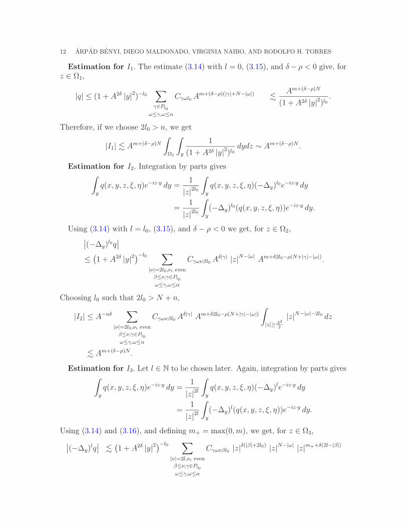
12 ARPAD BENYI, DIEGO MALDONADO, VIRGINIA NAIBO, AND RODOLFO H. TORRES
Estimation for I1. The estimate (3.14) with l = 0, (3.15), and δ− ρ < 0 give, forz ∈ Ω1,
|q| ≤ (1 + A2δ |y|2)−l0∑
γ∈Pl0
ω≤γ,ω≤α
Cγωl0 Am+(δ−ρ)(|γ|+N−|ω|) .
Am+(δ−ρ)N
(1 + A2δ |y|2)l0.
Therefore, if we choose 2l0 > n, we get
|I1| . Am+(δ−ρ)N
∫
Ω1
∫
y
1
(1 + A2δ |y|2)l0dydz ∼ Am+(δ−ρ)N .
Estimation for I2. Integration by parts gives∫
y
q(x, y, z, ξ, η)e−iz·y dy =1
|z|2l0
∫
y
q(x, y, z, ξ, η)(−∆y)l0e−iz·y dy
=1
|z|2l0
∫
y
(−∆y)l0(q(x, y, z, ξ, η))e−iz·y dy.
Using (3.14) with l = l0, (3.15), and δ − ρ < 0 we get, for z ∈ Ω2,∣∣(−∆y)
l0q∣∣
≤(1 + A2δ |y|2
)−l0∑
|ν|=2l0,νi even
β≤ν,γ∈Pl0
ω≤γ,ω≤α
Cγωνβl0 Aδ|γ| |z|N−|ω| Am+δ2l0−ρ(N+|γ|−|ω|).
Choosing l0 such that 2l0 > N + n,
|I2| ≤ A−nδ∑
|ν|=2l0,νi even
β≤ν,γ∈Pl0
ω≤γ,ω≤α
Cγωνβl0 Aδ|γ| Am+δ2l0−ρ(N+|γ|−|ω|)
∫
|z|≥Aδ
2
|z|N−|ω|−2l0 dz
. Am+(δ−ρ)N .
Estimation for I3. Let l ∈ N to be chosen later. Again, integration by parts gives∫
y
q(x, y, z, ξ, η)e−iz·y dy =1
|z|2l
∫
y
q(x, y, z, ξ, η)(−∆y)le−iz·y dy
=1
|z|2l
∫
y
(−∆y)l(q(x, y, z, ξ, η))e−iz·y dy.
Using (3.14) and (3.16), and defining m+ = max(0,m), we get, for z ∈ Ω3,
∣∣(−∆y)lq∣∣ .
(1 + A2δ |y|2
)−l0∑
|ν|=2l,νi even
β≤ν,γ∈Pl0
ω≤γ,ω≤α
Cγωνβl0 |z|δ(|β|+2l0) |z|N−|ω| |z|m++δ(2l−|β|)

ON THE HORMANDER CLASSES OF BILINEAR PSEUDODIFFERENTIAL OPERATORS 13
We then have
|I3| . A−δn∑
|ν|=2l,νi even
β≤ν,γ∈Pl0
ω≤γ,ω≤α
Cγωνβl0
∫
|z|≥A2
|z|m++2l(δ−1)+2l0δ+N dz.
Choosing l ∈ N sufficiently large so that
m++2l(δ−1)+2l0δ+N < −n and −δn+m++2l(δ−1)+2l0δ+N+n < m+(δ−ρ)N,
we obtain
|I3| . A−δn+m++2l(δ−1)+2l0δ+N+n ≤ Am+(δ−ρ)N .
4. Proofs of Theorem 3 and Theorem 4
Proof of Theorem 3. The second part of the statement is immediate if we write forall N > 0,
a− b = (a−N−1∑
j=0
aj)− (b−N−1∑
j=0
aj) ∈ BSmN
ρ,δ ,
and recall that mN ց −∞ as N → ∞.For the proof of the first part of Theorem 3 we proceed by explicitly constructing
a. Let ψ ∈ C∞c (Rn × Rn) such that 0 ≤ ψ ≤ 1, ψ(ξ, η) = 0 on (ξ, η) : |ξ|+ |η| ≤ 1
and ψ(ξ, η) = 1 on (ξ, η) : |ξ|+ |η| ≥ 2. Define
a(x, ξ, η) =∞∑
j=0
ψ(ǫjξ, ǫjη)aj(x, ξ, η),
where ǫj ց 0 as j → ∞ is an appropriately chosen sequence of numbers in (0, 1) sothat a ∈ BSm0
ρ,δ . The choice of this sequence will be made explicit below.For each fixed ǫ ∈ (0, 1) we have
(a) ψ(ǫξ, ǫη) = 0 for |ξ|+ |η| ≤ 1/ǫ;(b) ψ(ǫξ, ǫη) = 1 for |ξ|+ |η| ≥ 2/ǫ;
(c) For all β, γ such that |β| + |γ| ≥ 1, ∂βξ ∂γηψ(ǫξ, ǫη) = 0 for |ξ| + |η| ≤ 1/ǫ or
|ξ|+ |η| ≥ 2/ǫ;
(d) |∂βξ ∂γηψ(ǫξ, ǫη)| ≤ cβγǫ
|β|+|γ|.
In particular, because of (a) and (b) (that is, we only care about pairs (ξ, η) suchthat 1/ǫ < |ξ|+ |η| < 2/ǫ), (d) is equivalent to
(e) |∂βξ ∂γηψ(ǫξ, ǫη)| ≤ cβγ(1 + |ξ|+ |η|)−|β|−|γ|.
This in turn is equivalent to saying that the family ψ(ǫξ, ǫη)0<ǫ<1 represents abounded set in BS0
1,0 (endowed with the topology induced by appropriate semi-norms;see [7]).
14 ARPAD BENYI, DIEGO MALDONADO, VIRGINIA NAIBO, AND RODOLFO H. TORRES
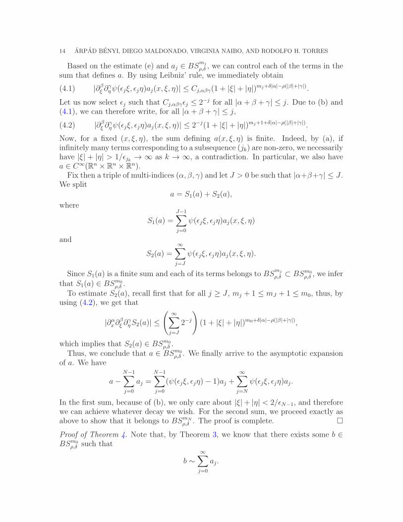
Based on the estimate (e) and aj ∈ BSmj
ρ,δ , we can control each of the terms in thesum that defines a. By using Leibniz’ rule, we immediately obtain
(4.1) |∂βξ ∂γηψ(ǫjξ, ǫjη)aj(x, ξ, η)| ≤ Cj,αβγ(1 + |ξ|+ |η|)mj+δ|α|−ρ(|β|+|γ|).
Let us now select ǫj such that Cj,αβγǫj ≤ 2−j for all |α+ β + γ| ≤ j. Due to (b) and(4.1), we can therefore write, for all |α + β + γ| ≤ j,
(4.2) |∂βξ ∂γηψ(ǫjξ, ǫjη)aj(x, ξ, η)| ≤ 2−j(1 + |ξ|+ |η|)mj+1+δ|α|−ρ(|β|+|γ|).
Now, for a fixed (x, ξ, η), the sum defining a(x, ξ, η) is finite. Indeed, by (a), ifinfinitely many terms corresponding to a subsequence (jk) are non-zero, we necessarilyhave |ξ| + |η| > 1/ǫjk → ∞ as k → ∞, a contradiction. In particular, we also havea ∈ C∞(Rn × Rn × Rn).Fix then a triple of multi-indices (α, β, γ) and let J > 0 be such that |α+β+γ| ≤ J .
We splita = S1(a) + S2(a),
where
S1(a) =J−1∑
j=0
ψ(ǫjξ, ǫjη)aj(x, ξ, η)
and
S2(a) =∞∑
j=J
ψ(ǫjξ, ǫjη)aj(x, ξ, η).
Since S1(a) is a finite sum and each of its terms belongs to BSmj
ρ,δ ⊂ BSm0
ρ,δ , we inferthat S1(a) ∈ BSm0
ρ,δ .To estimate S2(a), recall first that for all j ≥ J , mj + 1 ≤ mJ + 1 ≤ m0, thus, by
using (4.2), we get that
|∂αx∂βξ ∂
γηS2(a)| ≤
(∞∑
j=J
2−j
)(1 + |ξ|+ |η|)m0+δ|α|−ρ(|β|+|γ|),
which implies that S2(a) ∈ BSm0
ρ,δ .Thus, we conclude that a ∈ BSm0
ρ,δ . We finally arrive to the asymptotic expansionof a. We have
a−N−1∑
j=0
aj =N−1∑
j=0
(ψ(ǫjξ, ǫjη)− 1)aj +∞∑
j=N
ψ(ǫjξ, ǫjη)aj.
In the first sum, because of (b), we only care about |ξ|+ |η| < 2/ǫN−1, and thereforewe can achieve whatever decay we wish. For the second sum, we proceed exactly asabove to show that it belongs to BSmN
ρ,δ . The proof is complete.
Proof of Theorem 4. Note that, by Theorem 3, we know that there exists some b ∈BSm0
ρ,δ such that
b ∼
∞∑
j=0
aj.
ON THE HORMANDER CLASSES OF BILINEAR PSEUDODIFFERENTIAL OPERATORS 15
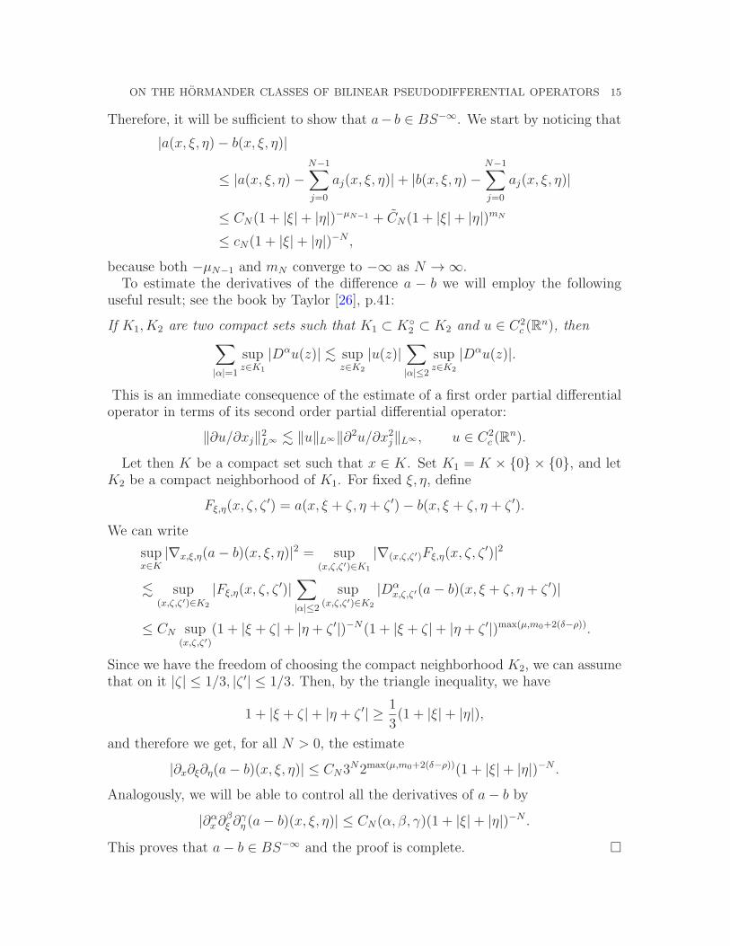
Therefore, it will be sufficient to show that a− b ∈ BS−∞. We start by noticing that
|a(x, ξ, η)− b(x, ξ, η)|
≤ |a(x, ξ, η)−N−1∑
j=0
aj(x, ξ, η)|+ |b(x, ξ, η)−N−1∑
j=0
aj(x, ξ, η)|
≤ CN(1 + |ξ|+ |η|)−µN−1 + CN(1 + |ξ|+ |η|)mN
≤ cN(1 + |ξ|+ |η|)−N ,
because both −µN−1 and mN converge to −∞ as N → ∞.To estimate the derivatives of the difference a − b we will employ the following
useful result; see the book by Taylor [26], p.41:
If K1, K2 are two compact sets such that K1 ⊂ K2 ⊂ K2 and u ∈ C2
c (Rn), then
∑
|α|=1
supz∈K1
|Dαu(z)| . supz∈K2
|u(z)|∑
|α|≤2
supz∈K2
|Dαu(z)|.
This is an immediate consequence of the estimate of a first order partial differentialoperator in terms of its second order partial differential operator:
‖∂u/∂xj‖2L∞ . ‖u‖L∞‖∂2u/∂x2j‖L∞ , u ∈ C2
c (Rn).
Let then K be a compact set such that x ∈ K. Set K1 = K × 0 × 0, and letK2 be a compact neighborhood of K1. For fixed ξ, η, define
Fξ,η(x, ζ, ζ′) = a(x, ξ + ζ, η + ζ ′)− b(x, ξ + ζ, η + ζ ′).
We can write
supx∈K
|∇x,ξ,η(a− b)(x, ξ, η)|2 = sup(x,ζ,ζ′)∈K1
|∇(x,ζ,ζ′)Fξ,η(x, ζ, ζ′)|2
. sup(x,ζ,ζ′)∈K2
|Fξ,η(x, ζ, ζ′)|∑
|α|≤2
sup(x,ζ,ζ′)∈K2
|Dαx,ζ,ζ′(a− b)(x, ξ + ζ, η + ζ ′)|
≤ CN sup(x,ζ,ζ′)
(1 + |ξ + ζ|+ |η + ζ ′|)−N(1 + |ξ + ζ|+ |η + ζ ′|)max(µ,m0+2(δ−ρ)).
Since we have the freedom of choosing the compact neighborhood K2, we can assumethat on it |ζ| ≤ 1/3, |ζ ′| ≤ 1/3. Then, by the triangle inequality, we have
1 + |ξ + ζ|+ |η + ζ ′| ≥1
3(1 + |ξ|+ |η|),
and therefore we get, for all N > 0, the estimate
|∂x∂ξ∂η(a− b)(x, ξ, η)| ≤ CN3N2max(µ,m0+2(δ−ρ))(1 + |ξ|+ |η|)−N .
Analogously, we will be able to control all the derivatives of a− b by
|∂αx∂βξ ∂
γη (a− b)(x, ξ, η)| ≤ CN(α, β, γ)(1 + |ξ|+ |η|)−N .
This proves that a− b ∈ BS−∞ and the proof is complete.
16 ARPAD BENYI, DIEGO MALDONADO, VIRGINIA NAIBO, AND RODOLFO H. TORRES
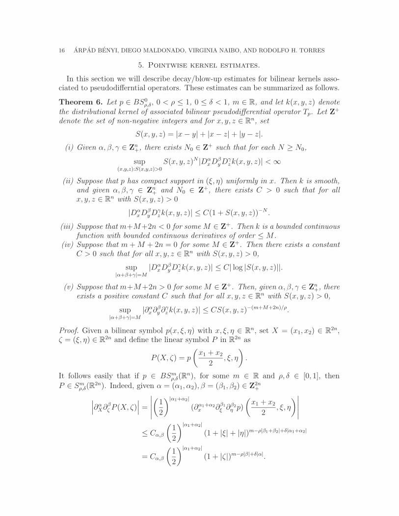
5. Pointwise kernel estimates.
In this section we will describe decay/blow-up estimates for bilinear kernels asso-ciated to pseudodifferntial operators. These estimates can be summarized as follows.
Theorem 6. Let p ∈ BS0ρ,δ, 0 < ρ ≤ 1, 0 ≤ δ < 1, m ∈ R, and let k(x, y, z) denote
the distributional kernel of associated bilinear pseudodifferential operator Tp. Let Z+
denote the set of non-negative integers and for x, y, z ∈ Rn, set
S(x, y, z) = |x− y|+ |x− z|+ |y − z|.
(i) Given α, β, γ ∈ Zn+, there exists N0 ∈ Z+ such that for each N ≥ N0,
sup(x,y,z):S(x,y,z)>0
S(x, y, z)N |DαxD
βyD
γzk(x, y, z)| <∞
(ii) Suppose that p has compact support in (ξ, η) uniformly in x. Then k is smooth,and given α, β, γ ∈ Zn
+ and N0 ∈ Z+, there exists C > 0 such that for allx, y, z ∈ Rn with S(x, y, z) > 0
|DαxD
βyD
γzk(x, y, z)| ≤ C(1 + S(x, y, z))−N .
(iii) Suppose that m+M+2n < 0 for someM ∈ Z+. Then k is a bounded continuousfunction with bounded continuous derivatives of order ≤M .
(iv) Suppose that m+M + 2n = 0 for some M ∈ Z+. Then there exists a constantC > 0 such that for all x, y, z ∈ Rn with S(x, y, z) > 0,
sup|α+β+γ|=M
|DαxD
βyD
γzk(x, y, z)| ≤ C| log |S(x, y, z)||.
(v) Suppose that m+M+2n > 0 for someM ∈ Z+. Then, given α, β, γ ∈ Zn+, there
exists a positive constant C such that for all x, y, z ∈ Rn with S(x, y, z) > 0,
sup|α+β+γ|=M
|∂αx∂βy ∂
γz k(x, y, z)| ≤ CS(x, y, z)−(m+M+2n)/ρ.
Proof. Given a bilinear symbol p(x, ξ, η) with x, ξ, η ∈ Rn, set X = (x1, x2) ∈ R2n,ζ = (ξ, η) ∈ R2n and define the linear symbol P in R2n as
P (X, ζ) = p
(x1 + x2
2, ξ, η
).
It follows easily that if p ∈ BSmρ,δ(R
n), for some m ∈ R and ρ, δ ∈ [0, 1], then
P ∈ Smρ,δ(R
2n). Indeed, given α = (α1, α2), β = (β1, β2) ∈ Z2n+
∣∣∣∂αX∂βζ P (X, ζ)∣∣∣ =
∣∣∣∣∣
(1
2
)|α1+α2|
(∂α1+α2
x ∂β1
ξ ∂β2
η p)
(x1 + x2
2, ξ, η
)∣∣∣∣∣
≤ Cα,β
(1
2
)|α1+α2|
(1 + |ξ|+ |η|)m−ρ|β1+β2|+δ|α1+α2|
= Cα,β
(1
2
)|α1+α2|
(1 + |ζ|)m−ρ|β|+δ|α|.
ON THE HORMANDER CLASSES OF BILINEAR PSEUDODIFFERENTIAL OPERATORS 17
In R2n, for the associated linear operator TP we now have
TP (F )(X) =
∫
R2n
P (X, ζ)eiX·ζF (ζ)dζ
=
∫
Rn
∫
Rn
p
(x1 + x2
2, ξ, η
)eix1·ξeix2·ηF (ξ, η) dξdη,
and also
TP (F )(X) =
∫
R2n
K(X, Y )F (Y )dY,
where
K(X, Y ) = F2n(P (X, ·))(Y −X), X, Y ∈ R2n,
and F2n denotes the Fourier transform in R2n. Next, for the bilinear symbol p wewrite
Tp(f, g)(x) =
∫
Rn
∫
Rn
p(x, ξ, η)eix·(ξ+η)f(ξ)g(η)dξdη
=
∫
Rn
∫
Rn
p(x, ξ, η)eix·ξeix·ηf ⊗ g(ξ, η)dξdη
= TP (f ⊗ g)(x, x)
=
∫
Rn
∫
Rn
K((x, x), (y, z))(f ⊗ g)(y, z)dydz
=
∫
Rn
∫
Rn
K((x, x), (y, z))f(y)g(z)dydz.
Therefore, the distributional bilinear kernel k(x, y, z) of the bilinear operator Tp isgiven by
k(x, y, z) = K((x, x), (y, z)), x, y, z ∈ Rn,
where K(X, Y ) is the distributional linear kernel associated to the linear operator TPin R2n. Finally, the pointwise estimates for linear kernels associated to symbols inSmρ,δ(R
2n) in [1, Theorem 1.1] imply the desired pointwise estimates for the bilinearkernel k(x, y, z).
6. An L2 ×W s,∞0 → L2 boundedness property.
If σ ∈ BS0ρ,δ, by freezing g, Tσ(·, g) can be regarded as a linear pseudodifferential
operator (with symbol depending on g), that is,
Tσ(f, g)(x) =
∫
ξ
σg(x, ξ)f(ξ)eiξx dξ,
where
σg(x, ξ) =
∫
η
σ(x, ξ, η)g(η)eiηx dη.
18 ARPAD BENYI, DIEGO MALDONADO, VIRGINIA NAIBO, AND RODOLFO H. TORRES
Moreover, the well-known L2 boundedness of a linear pseudodifferential operatorasserts that if τ ∈ S0
ρ,δ, 0 ≤ δ ≤ ρ ≤ 1, δ < 1, there exist constants C0 and k ∈ N
(independent of τ) such that
‖Tτ (u)‖L2 ≤ C0 |τ |k ‖u‖L2 , u ∈ S(Rn),
where
|τ |k = max|α|,|β|≤k
supx, ξ
∣∣∣∂αx∂βξ τ(x, ξ)∣∣∣ (1 + |ξ|)−δ|α|+ρ|β|.
In fact, k can be taken equal to [n/2] + 1, see [14, p. 30].
Theorem 7. Let σ ∈ BS0ρ,δ, 0 ≤ δ ≤ ρ ≤ 1, δ < 1. Then
Tσ : L2 ×W s,∞0 → L2,
where s is any integer satisfying
(6.1) s >[n/2] + 1
1− δ+ n.
Moreover, if g ∈ Csc (R
n) then σg ∈ S0ρ,δ, and
|σg|[n/2]+1 . ‖g‖W s,∞0
:= sup|γ|≤s
‖Dγg‖L∞
with a constant depending only on the BS0ρ,δ-norm of σ up to order n+ 2.
Remark 6.1. Note that Theorem 7 includes the case 0 ≤ ρ = δ < 1 and, in particular,the case ρ = δ = 0, where, as pointed out in the introduction, the mapping fromL2(Rn)× L∞(Rn) into L2(Rn) fails.
Proof. Let g ∈ Csc (R
n) and σ ∈ BS0ρ,δ, 0 ≤ δ ≤ ρ ≤ 1, δ < 1. We assume σ has
compact support so all calculations below can be justified. However, all constantsare independent of the support of σ and a limiting argument proves the result whenσ does not have compact support (see [7]).Fix multiindices α and β such that |α| , |β| ≤ [n/2] + 1. Define A = 1+ |ξ| and let
l0 ∈ N (to be chosen later) and Pl0 = γ = (γ1, · · · , γn) : γi is even and |γ| = 2j, j =0, . . . , l0. We have,
∂αx∂βξ σg(x, ξ) =
∑
γ≤α
cγ,α
∫
z
∫
y
∂γx∂βξ σ(x, ξ, z)z
α−γeizyg(x− y) dydz
=∑
γ≤α
cγ,α
∫
z
∫
y
(1 + A2δ(−∆z))l0(∂γx∂
βξ σ(x, ξ, z)z
α−γ)eizyg(x− y)
(1 + A2δ |y|2)l0dydz
=∑
γ≤α,θ∈Pl0
cγ,α,θ
∫
z
∫
y
Aδ|θ|∂θz (∂γx∂
βξ σ(x, ξ, z)z
α−γ)eizyg(x− y)
(1 + A2δ |y|2)l0dydz
=∑
γ≤α,θ∈Pl0
ω≤minθ,α−γ
cγ,α,θ,ω
∫
z
∫
y
Aδ|θ|∂γx∂βξ ∂
θ−ωz σ(x, ξ, z)zα−γ−ω eizyg(x− y)
(1 + A2δ |y|2)l0dydz.
ON THE HORMANDER CLASSES OF BILINEAR PSEUDODIFFERENTIAL OPERATORS 19
Fix γ ≤ α, θ ∈ Pl0 , ω ≤ minθ, α− γ and set
p(x, ξ) =
∫
z
∫
y
Aδ|θ|∂γx∂βξ ∂
θ−ωz σ(x, ξ, z)zα−γ−ω eizyg(x− y)
(1 + A2δ |y|2)l0dydz.
Define the sets
Ω1 = z : |z| ≤ Aδ
2, Ω2 = z : Aδ
2≤ |z| ≤ A
2, Ω3 = z : |z| ≥ A
2.
We then have
p(x, ξ) =
∫
Ω1
∫
y
· · ·+
∫
Ω2
∫
y
· · ·+
∫
Ω3
∫
y
· · · := I1 + I2 + I3.
Note that
A ≤ 1 + |ξ|+ |z| ≤ 2A, z ∈ Ω1 ∪ Ω2
and that
|z| ≤ 1 + |ξ|+ |z| ≤ 2 |z| , z ∈ Ω3
Estimation for I1. Choose l0 such that 2l0 > n. Then
|I1| . Aδ|θ|‖g‖L∞
∫
y
∫
|z|≤Aδ
2
(1 + |ξ|+ |z|)δ|γ|−ρ(|β|+|θ|−|ω|) |z||α|−|γ|−|ω|
(1 + A2δ |y|2)l0dzdy
∼ Aδ|θ|‖g‖L∞Aδ|γ|−ρ(|β|+|θ|−|ω|)A−δnAδ(|α|−|γ|−|ω|+n)
= A(δ−ρ)(|θ|−|w|)Aδ|α|−ρ|β|‖g‖L∞
≤ Aδ|α|−ρ|β|‖g‖L∞ .
Note that in the last inequality we have used that δ ≤ ρ and |θ| − |w| ≥ 0.
Estimation for I2. Let l ∈ N to be chosen later. We have
I2 =
∫
Ω2
∫
y
Aδ|θ|∂γx∂βξ ∂
θ−ωz σ(x, ξ, z)zα−γ−ω g(x− y)
(1 + A2δ |y|2)l0
(−∆y)l(eizy)
|z|2ldydz
=
∫
Ω2
Aδ|θ| zα−γ−ω
|z|2l∂γx∂
βξ ∂
θ−ωz σ(x, ξ, z)
∫
y
(−∆y)l
(g(x− y)
(1 + A2δ |y|2)l0
)eizy dy dz.
Now,
∣∣∣∣(−∆y)l
(g(x− y)
(1 + A2δ |y|2)l0
)∣∣∣∣ =
∣∣∣∣∣∣∣∣
∑
|µ|=2l
µieven,ν≤µ
Cνµ∂νy ((1 + A2δ |y|2)−l0)∂µ−ν
y g(x− y)
∣∣∣∣∣∣∣∣
≤∑
|µ|=2l
µieven,ν≤µ
Cνµl0‖Dµ−νg‖L∞Aδ|ν|(1 + A2δ |y|2)−l0 .
20 ARPAD BENYI, DIEGO MALDONADO, VIRGINIA NAIBO, AND RODOLFO H. TORRES
Therefore,
|I2| ≤
∫
Ω2
Aδ|θ| |zα−γ−ω|
|z|2l
∣∣∣∂γx∂βξ ∂θ−ωz σ(x, ξ, z)
∣∣∣∑
|µ|=2l
µieven,ν≤µ
Cνµl0‖Dµ−νg‖L∞Aδ|ν|A−δn dz
≤∑
|µ|=2l
µieven,ν≤µ
Cνµl0‖Dµ−νg‖L∞Aδ(|θ|+|ν|−n)
∫
Ω2
|z||α|−|γ|−|ω|−2l (A+ |z|)δ|γ|−ρ(|β|+|θ|−|ω|) dz
≤ Aδ(|θ|+2l−n)‖g‖W 2l,∞0
Aδ|γ|−ρ(|β|+|θ|−|ω|)Aδ(|α|−|γ|−|ω|−2l+n),
where we have used that A+ |z| ∼ A on Ω2 and l has been chosen so that
(6.2) |α| − |γ| − |ω| − 2l + n < 0.
Thus we obtain,
|I2| ≤ C Aδ(|θ|+2l−n)‖g‖W 2l,∞0
Aδ|γ|−ρ(|β|+|θ|−|ω|)Aδ(|α|−|γ|−|ω|−2l+n)
= C Aδ|α|−ρ|β|A(δ−ρ)(|θ|−|w|)‖g‖W 2l,∞0
≤ C Aδ|α|−ρ|β|‖g‖W 2l,∞0
,
since (δ − ρ)(|θ| − |w|) ≤ 0.
Estimation for I3. Here we impose some extra conditions to l above. As in theestimation for B2 we have
|I3| ≤∑
|µ|=2l
µieven,ν≤µ
Cνµl0‖Dµ−νg‖L∞Aδ(|θ|+|ν|−n)
∫
Ω3
|z||α|−|γ|−|ω|−2l (A+ |z|)δ|γ|−ρ(|β|+|θ|−|ω|) dz.
Using that A+ |z| ∼ |z| in Ω3 we have
|I3| ≤ C ‖g‖W 2l,∞0
Aδ(|θ|+2l−n)
∫
Ω3
|z||α|−|γ|−|ω|−2l+δ|γ|−ρ(|β|+|θ|−|ω|) dz.
Now, let us choose l as in the estimation of I2 and satisfying
|α| − |γ| − |ω| − 2l + δ |γ| − ρ(|β|+ |θ| − |ω|) + n < 0.
For example, any choice of l such that 2l > |α| + n satisfies the inequality above.Then,
|I3| ≤ C Aδ(|θ|+2l−n)A|α|−|γ|−|ω|−2l+δ|γ|−ρ(|β|+|θ|−|ω|)+n ‖g‖W 2l,∞0
= C Aδ|γ|−ρ|β|A(δ−1)(2l−n)+|α|−|γ|A(δ−ρ)|θ|A(ρ−1)|ω| ‖g‖W 2l,∞0
.
Since δ < 1, we can choose l sufficiently large so that
(6.3) (δ − 1)(2l − n) + |α| − |γ| ≤ 0
and since δ − ρ ≤ 0, ρ− 1 ≤ 0 and |γ| ≤ |α| we obtain
|I3| ≤ C Aδ|α|−ρ|β| ‖g‖W 2l,∞0
.

ON THE HORMANDER CLASSES OF BILINEAR PSEUDODIFFERENTIAL OPERATORS 21
Finally, by choosing l = s/2, with s as in (6.1), we guarantee that both conditions(6.2) and (6.3) are satisfied, and the proof is complete.
Corollary 8. Let m ≥ 0 and σ ∈ BSmρ,δ, 0 ≤ δ ≤ ρ ≤ 1, δ < 1. Then, if s is any
integer satisfying (6.1), the following fractional Leibniz rule-type inequality holds true
(6.4) ‖Tσ(f, g)‖L2 ≤ C(‖f‖Wm,2 ‖g‖W s,∞
0
+ ‖f‖W s,∞0
‖g‖Wm,2
), f, g ∈ C∞
c (Rn).
Proof. Corollary 8 follows from Theorem 7 and composition with Bessel potentialsof order m, along the lines of Theorem 2 in [5]. We only need to notice that, ifσ ∈ BSm
ρ,δ and φ is a C∞ function on R such that 0 ≤ φ ≤ 1, supp(φ) ⊂ [−2, 2] andφ(r) + φ(1/r) = 1 on [0,∞), then, the symbols σ1 and σ2 defined by
σ1(x, ξ, η) = σ(x, ξ, η)φ
(1 + |ξ|2
1 + |η|2
)(1 + |ξ|2)−m/2
and
σ2(x, ξ, η) = σ(x, ξ, η)φ
(1 + |η|2
1 + |ξ|2
)(1 + |η|2)−m/2
satisfy σ1, σ2 ∈ BS0ρ,δ, and the corresponding operators Tσ, Tσ1
, and Tσ2are related
throughTσ(f, g) = Tσ1
(Jmf, g) + Tσ2(f, Jmg),
where Jm denotes the linear Fourier multiplier with symbol (1 + |ξ|2)m/2.
References
[1] L. Alvarez and J. Hounie, Estimates for the kernel and continuity properties of pseudo-differential operators, Ark. Mat. 28 (1990), 1–22.
[2] A. Benyi, Bilinear pseudodifferential operators with forbidden symbols on Lipschitz and Besovspaces, J. Math. Anal. Appl. 284 (2003), 97–103.
[3] A. Benyi, C. Demeter, A. Nahmod, C. M. Thiele, R. H. Torres, and P. Villarroya, Modulationinvariant bilinear T(1) theorem, J. Anal. Math., to appear.
[4] A. Benyi, K. Grochenig, C. Heil, and K.A. Okoudjou, Modulation spaces and a class of boundedmultilinear pseudodifferential operators, J. Operator Theory 54.2 (2005), 301–313.
[5] A. Benyi, A. Nahmod, and R. H. Torres, Sobolev space estimates and symbolic calculus forbilinear pseudodifferential operators, J. Geom. Anal. 16.3 (2006), 431–453.
[6] A. Benyi and K. Okoudjou, Modulation space estimates for multilinear pseudodifferential oper-ators, Studia Math. 172.2 (2006), 169–180.
[7] A. Benyi and R. H. Torres, Symbolic calculus and the transposes of bilinear pseudodifferentialoperators, Comm. Partial Diff. Eq. 28 (2003), 1161–1181.
[8] A. Benyi and R. Torres, Almost orthogonality and a class of bounded bilinear pseudodifferentialoperators, Math. Res. Lett. 11.1 (2004), 1–12.
[9] F. Bernicot, Local estimates and global continuities in Lebesgue spaces for bilinear operators,Anal. PDE 1 (2008), 1–27.
[10] F. Bernicot and R. H. Torres, Sobolev space estimates for a class of bilinear pseudodifferntialoperators lacking symbolic calculus, in preparation.
[11] A. Calderon and R. Vaillancourt, On the boundedness of pseudo-differential operators, J. MathSoc. Japan 23 (1971), 374–378.
[12] M. Christ and J-L. Journe, Polynomial growth estimates for multilinear singular integral oper-ators, Acta Math. 159 (1987), 51–80.
22 ARPAD BENYI, DIEGO MALDONADO, VIRGINIA NAIBO, AND RODOLFO H. TORRES
[13] R. R. Coifman and Y. Meyer, On commutators of singular integrals and bilinear singular inte-grals, Trans. Amer. Math. Soc. 212 (1975), 315–331.
[14] R. R. Coifman and Y. Meyer, Au-dela des operateurs pseudo-differentiels. Second Edition.Asterisque 57, 1978.
[15] R. R. Coifman and Y. Meyer, Commutateurs d’integrales singuliers et operateurs multilineaires,Ann. Inst. Fourier Grenoble 28 (1978), 177–202.
[16] J. Gilbert and A. Nahmod, Boundedness of bilinear operators with non-smooth symbols, Math.Res. Letters 7 (2000), 767–778.
[17] L. Grafakos and X. Li, The disc as a bilinear multiplier., Amer. J. Math. 128 (2006), 91–119.[18] L. Grafakos and R. H. Torres, Multilinear Calderon-Zygmund theory, Adv. in Math. 165 (2002),
124–164.[19] C. Kenig and E. M. Stein, Multilinear estimates and fractional integration, Math. Res. Lett. 6
(1999), 1–15.[20] L. Hormander, Pseudo-differential operators and hypoelliptic equations, Singular integrals, Proc.
Sympos. Pure Math., Vol. X, Chicago, Ill., 1966, 138–183, Amer. Math. Soc., Providence, R.I.,1967.
[21] H. Kumano-go, Pseudodifferential operators, MIT Press, 1981.[22] M. Lacey and C. Thiele, Lp bounds for the bilinear Hilbert transform, 2 < p < ∞, Ann. of
Math. 146 (1997), 693–724.[23] M. Lacey and C. Thiele, On Calderon’s conjecture, Ann. of Math. 149 (1999), 475–496.[24] D. Maldonado and V. Naibo, Weighted norm inequalities for paraproducts and bilinear pseudo-
differential operators with mild regularity, J. Fourier Anal. Appl., 15 (2), (2009), 218–261.[25] C. Muscalu, T. Tao, and C. Thiele, Multilinear operators given by singular multipliers, J. Amer.
Math. Soc. 15 (2002), 469–496.[26] M. Taylor, Pseudodifferential operators, Princeton University Press, 1981.[27] R. H. Torres, Multilinear singular integral operators with variable coefficients, Rev. Un. Mat.
Argentina, 50 (2009), 157–174.[28] E. M. Stein, Harmonic Analysis: Real Variable Methods, Orthogonality, and Oscillatory Inte-
grals, Princeton University Press, Princeton, 1993.
Arpad Benyi, Department of Mathematics, 516 High St, Western Washington Uni-
versity, Bellingham, WA 98225, USA.
E-mail address : [email protected]
Diego Maldonado, Department of Mathematics, 138 Cardwell Hall, Kansas State
University, Manhattan, KS 66506, USA.
E-mail address : [email protected]
Virginia Naibo, Department of Mathematics, 138 Cardwell Hall, Kansas State
University, Manhattan, KS 66506, USA.
E-mail address : [email protected]
Rodolfo Torres, Department of Mathematics, University of Kansas, Lawrence,
KS 66045, USA.
E-mail address : [email protected]


