Embed Size (px)
Citation preview
Reduction of Indefinite Quadratic Programs to Bilinear Programs
PIERRE HANSEN GERAD, Ecole des Hautes ktudes Commerciales, Departement des Mithodes Quantitatives et Systemes d’lnformation, 5255 avenue Decelles, H3 Tl V6, Montreal, Canada, and RUTCOR, Rutgers University, New Jersey 08904, U.S.A.
BRIGITTE JAUMARD Princeton University, Department of Civil Engineering and Operations Research, New Jersey 08544-5263, U.S.A., and GERAD, .&ole Polytechnique de Montreal, Departement de Mathkmatiques Appliquees, Succursale A, Case Postale 6079, Montreal (Quebec) H3C 3A7, Canada.
(Received: 5 July 1991; accepted: 8 October 1991)
Abstract. Indefinite quadratic programs with quadratic constraints can be reduced to bilinear pro- grams with bilinear constraints by duplication of variables. Such reductions are studied in which: (i) the number of additional variables is minimum or (ii) the number of complicating variables, i.e., variables to be fixed in order to obtain a linear program, in the resulting bilinear program is minimum. These two problems are shown to be equivalent to a maximum bipartite subgraph and a maximum stable set problem respectively in a graph associated with the quadratic program. Non-polynomial but practically efficient algorithms for both reductions are thus obtained. Reduction of more general global optimization problems than quadratic programs to bilinear programs is also briefly discussed.
Key words. Quadratic program, bilinear program, global optimization, reduction.
1. Introduction
A quadratic program can be written as follows, in its most general form:
Problem (Q) = <
n n n min C 2 qjjXjxj + C 9ixi + 40
;=I j=i i=l
subject to:
j=l j=i k=1,2,...,m
. XjER i=1,2 )...) y1,
where the coefficients qji, qi, qo, ri, r:, rt (i, j = 1,2,. . . , n; j 2 i; k = 1,2,. . . ) m) are real numbers. No assumptions are made on convexity or concavity of the objective function or the constraints left-hand sides. The con- straints possibly include nonnegativity and/or range ones. Without loss of generality, some or all of the constraints of (Q) may be assumed to be equalities. Problem (Q) thus consists in minimizing an indefinite quadratic function subject
Journal of Global Optimization 2: 41-60, 1992. 0 1992 Kluwer Academic Publishers. Printed in the Netherlands.
42 PIERRE HANSEN AND BRIGITTE JAUMARD
to indefinite quadratic constraints. It has numerous applications in various fields. Many of them are gathered in the recent book of Floudas and Pardalos [22].
General quadratic programs (Q) appear to be very difficult to solve exactly, i.e., as global optimization ones. Many algorithms are available for particular cases, e.g., Baron [7], Ecker and Niemi [18] and Pham [38] for convex programs; Reeves [41] for separable programs; Kough [32], Benacer and Pham Dinh [9], Pardalos, Glick and Rosen [34], Phillips and Rosen [39] for programs with indefinite objective function and linear constraints; and A&Khayyal, Horst and Pardalos [3] for programs with concave objective function and separable con- straints. Numerous algorithms have also been proposed for the minimization of concave quadratic functions subject to linear constraints, see Pardalos and Rosen [35] [36], Horst and Tuy [29] for surveys. In contrast, few papers address the general case of problem ( Q), and we have found none which present a direct approach. The solution approach explored up to now consists in reducing problem (Q) to another more tractable one, and possibly deriving improved algorithms for the latter. Pham Dinh and El Bernoussi [37] and Tuy 1461 express problem (Q) as a d.-c. program (i.e., a problem in which the objective function and constraints left-hand sides are differences of convex functions) and solve it by outer- approximation. It has long been known (Konno [30], Pardalos and Rosen [36]) that indefinite quadratic programs with linear constraints can be reduced to bilinear programs with separable constraints (see below) by duplication of vari- ables. Floudas, Aggarwal and Ciric [21] extend this result, noting that problem (Q) can be reduced in a similar way to a general bilinear program, i.e., minimization of a bilinear function subject to bilinear constraints. Such programs may be written as follows:
’ min i: E cijxiy, + i1 c:xi + g clYi + CO 1=1 j=l
subject to:
Prob1em tB) =< 2 2 +yj + g1 ai.” + ,$, gkyi + u; s 0 k = 1,2, . . . , m i=l ]=I xiER i=l,2 ,..., n, y,ER! i=1,2 ,..., p, .
wherethecoefficientscij,cl,c~,aif,a:”,a~k,a~(i=1,2 ,..., n;j=1,2 ,..., p; k = 1,2,. . . , m) are real numbers. Again the constraints may include non- negativity and/or range ones, as well as equalities. Problem (B) is linear in the x variables for fixed values of the y variables, and linear in the y variables for fixed values of the x variables. It appears to have first been considered by Wolsey [48], although a particular case also involving bilinear constraints, the modular design problem, was previously studied by Evans [19] (see Al-Khayyal [l] for further references on that problem). The largest part of the work on bilinear program- ming concerns the case of separable constraints, in which the constraints are linear
REDUCTION OF QUADRATIC TO BILINEAR PROGRAMS 43
and decompose into two subsets involving the x or the y variables exclusively, see Pardalos and Rosen [36] for a survey. Bilinear programs with joint linear constraints are studied by Al-Khayyal and Falk [2]. Problem (B) can be solved by generalized Benders decomposition (Wolsey [48], SimCes [44], Flippo [20], Floudas and Visweswaran [23], Visweswaran and Floudas [47]), branch-and- bound (SimGes [44], Al-Khayyal [l]) and linearization (Sherali and Alameddine t4m
Reduction of problem (Q) to problem (B) can be done in many ways and the choice of a way clearly influences the ease of solution of the resulting bilinear problem. In this paper we propose optimal reduction methods for two criteria: (i) the number of additional variables, discussed in Section 2, and (ii) the number of complicating variables (i.e., the number of variables which yield, after fixation, an easy-to-solve problem, here a linear program, see Geoffrion [26]), considered in Section 3. In the case of problem (B) the latter number is the smallest of the number of x and of y variables, omitting variables appearing only in linear terms. Reduction to problem (B) of more general global optimization problems than problem (Q) is briefly discussed in Section 4.
We only consider here reductions based on duplication of variables. While elimination of variables offers further possibilities when problem (Q) contains some linear equality constraints, we do not study them in this paper. Nor do we consider here reductions of problem (Q) to other problems than problem (B), as, e.g., biconvex programs, while acknowledging that such reductions might lead, in some cases, to easier to solve problems.
2. Short Reductions
In this section we consider reductions of Problem (Q) to problem (B) which involve the minimum number of additional variables X; (and new constraints xi = xl). We call such reductions short. While there may be, even in the absence of linear constraints, other ways than duplication of variables to reduce problem (Q) to problem (B), which could possibly involve less additional variables for some particular values of the coeficients, we do not consider them here. Thus the reductions studied rely only on the structure of problem (Q), i.e., the information that coefficients are or are not equal to 0.
A few graph theoretic concepts will be needed, see Berge [lo] for basic definitions. Let us define the co-occurrence graph G = (V, E) of problem (Q) as follows: a vertex vi is associated with each variable xi ( j = 1,2, . . . , n) and an edge {vi, vi} belongs to E if and only if either qij # 0 or r: # 0 for some k (k = 1,2,. . . , m), i.e., if both variables xi and xi appear in a term of the objective function or the constraints. If this condition holds for i = j, i.e., qii f 0 or r-if0 for some k (k=1,2,. . . , m), the edge is a loop. Recall that a set S of vertices of V is stable if no two of its vertices are adjacent, i.e., the two endpoints of an edge. The complement in V of a stable set S of G is a transversal of G. The
44 PIERRE HANSEN AND BRIGITTE JAUMARD
stability number of graph G, noted cw(G), is the maximum number of vertices in a stable set of G. A set C of vertices of V is a clique if any two of its vertices are adjacent. A graph G is bipartite it its vertex set V can be partitioned into two sets VI and V, such that any edge of E joins a vertex of VI to a vertex of V, . A subgruph G, = (A, EA) of G is a graph obtained by keeping all vertices of a subset A of V and all edges of E joining two vertices of A, including loops. A subgraph G, of G is a maximum bipartite subgraph if it is bipartite and has a maximum number of vertices subject to that condition. Let a*(G) denote this number of vertices. We call (Y*(G) the bipartition number of G.
THEOREM 1. A quadratic program (Q) with n variables and co-occurrence graph G with bipartition number CQ( G) has a short reduction to a bilinear program (B) with n - (Y*(G), but no fewer, additional variables.
Proof. Let us first show that at most n - a,(G) additional variables are needed. Let G, = (A, EA), where A = VI U V, , be a maximum bipartite subgraph of the co-occurrence graph G associated with (Q). Hence, (Al = a,(G). Let WI = V\A. Duplicate the vertices of WI and denote by W, the corresponding vertex set, i.e., W, = {uJ 1 uj E WI}. Construct anew graph G’ = (V U W, , E’) where E’=E,UE,UE,UE, with E,={{vi, u~}EEIzI~EV, and u,EW,}; E2={{ui, ui} ] {ui,uj}EE, uiEVl and u~EW,} and E,={{uj, uj}) ui~W, and there is a loop at vertex u,} U {{ ui , vi} ( i <i, {ui , u,} E E, ui E WI and uj E WI}. G” is a bipartite graph with edges joining vertices of VI U WI to vertices of V, U W, . Note that each product of variables (including squares) in problem (Q) is associated with an edge of G’. Whenever a product xixi is associated with an edge {vi, u;} of E, U E, , replace xi by XI and add the constraint xj = xi. This yields a bilinear program with as variables of the first set (variables x in the definition of program (B)) those associated with vertices of VI U WI, and as variables of the second set (variables y in the definition of program (B)) those associated with vertices of V, U W, .
We now show that at least n - (Ye additional variables are needed. Assume problem ($3) can be reduced to problem (B) by introducing less than IZ - a;(G) additional variables. Consider then the subgraph G, = (II, ED) of the co-occur- rence graph G associated with (Q), induced by the set D of vertices associated with variables which have not been duplicated in the reduction. As G, is associated with a bilinear subproblem (i.e., a problem obtained by deleting some terms in the objective function and/or constraints of the resulting problem (B)), it must be bipartite. However, by the above assumption, IDI > a,(G), a contradiction. n
Finding a maximum bipartite subgraph of a graph G is NP-hard (Garey, Johnson and Stockmeyer [25]). However, this problem can be solved in practice for graphs of moderate size. Indeed, first note that additional variables must be introduced for all squared variables. The corresponding vertices in G may therefore be
REDUCTION OF QUADRATIC TO BILINEAR PROGRAMS 45
deleted. Finding (Ye in the resulting graph can then be reduced to a maximum stable set problem by using Theorem 13, Chapter 16 of Berge [lo]. Two copies of the graph are made and homologous vertices uj and cj are joined by edges. This leads to a graph G + K,, the sum of graph G and an edge, according to the definition of the graph sum operation (see Berge [lo], p. 304). Then any maximum stable set in graph G + K2 is associated with a maximum bipartite subgraph of G. Recent algorithms for the maximum clique or stable set problem (Carraghan and Pardalos [13], Friden, Hertz and de Werra [24], Balas and Yu [6]) allow the solution of problems with several hundreds of variables.
EXAMPLE 1. (Colville problem 3 [14], Hock and Schittkowski problem 83 PW.
2 mm c1x3 + c2xIx5 + c3x1 - cq subject to:
Problem (Q,) 0 =z a, + u2x2x5 + u3x,x4 - u4x3x5 d 92
I'
90 G a5 + a6x2x5 + u,x,x2 + u,x: G 110 20 s a, + U10X3X5 + UllX1X3 + U12X3X4 G 25 ljSxjduj j=1,2,3,4,5.
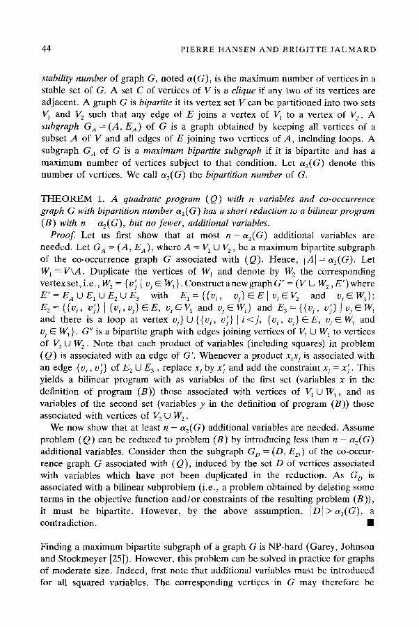
Coefficients ck (k = 1,2,3,4) and ak (k = 1,2, . . . ,12) as well as bounds Zj and uj are positive; values are given in Hock and Schittkowski [28]. The co-occurrence graph G, of problem (Q,) is represented on Figure 1. As it contains a loop at vertex u3, variable x3 must be duplicated. Vertex u3 can thus be omitted when determining a maximum bipartite subgraph of G, .
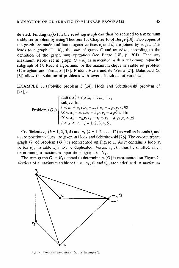
The sum graph G, + K, defined to determine LYE is represented on Figure 2. Vertices of a maximum stable set, i.e., ul, i7* and cd, are underlined. A maximum
Fig. 1. Co-occurrence graph G, for Example 1.
46 PIERRE HANSEN AND BRIGITTE JAUMARD
Fig. 2. Sum graph G, + K, for Example 1.
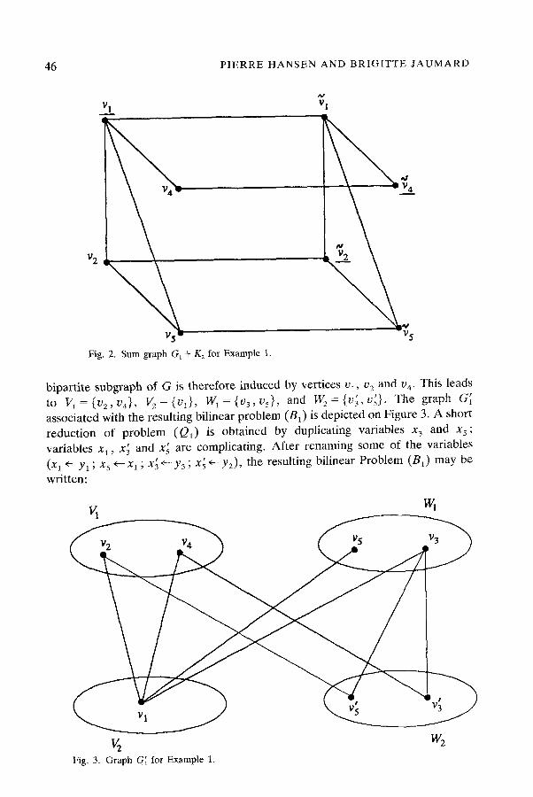
bipartite subgraph of G is therefore induced by vertices ul, u2 and v4. This leads to Vl={u,,uq}, Vz={uI}, WI=(u,,u5}, and Wz=(u;,u~}. The graph G; associated with the resulting bilinear problem (B,) is depicted on Figure 3. A short reduction of problem (Q,) is obtained by duplicating variables x3 and x5 ; variables x1, x; and xi are complicating. After renaming some of the variables (x1 +y, ; xg +x1 ; x; +Y3 ; x; ty,), the resulting bilinear Problem (I?,) may be written:
Fig. 3. Graph G; for Example 1.
REDUCTION OF QUADRATIC TO BILINEAR PROGRAMS 47
Problem (B,)
’ min c1x3y3 + c2xIy, + c3y, - c4 subject to: 0 d a, + a,x,y, + a,x,y, - a,x,y, s 92 90 d a5 + a,x,y, + a,x,y, + a,n,y, C 110 20 G a, + a,,x,y, + a,,x,y, + a,,x,y, < 25
Xl = Yz x3 = Y3 l,Sx,Cu,
3. Narrow Reduction
We now consider reductions of problem (Q) to a problem (B) with the minimum number of complicating variables. We call such reductions narrow. Again we consider only reductions relying solely on the structure of problem ((2).
THEOREM 2. A quadratic program (Q) with n variables and co-occurrence graph G with stability number a(G) has a narrow reduction to a bilinear program (B) with n - a(G), but no fewer, complicating variables.
Proof. Let us first show that at most n - a(G) complicating variables are needed. Let S c V denote a maximum stable set of G. Hence, ISI = a(G). Let IV, = V\S. Duplicate the vertices of WI and denote by W, the corresponding vertex set, i.e., W, = {u; 1 USE WI}. Construct a new graph G’ = (VU W,, E’) where E’=E,UEzUE3 with E,={{ui, uj}EE( uiES and viEWI}; E,= {{ui, u;}) {ui, uj}eE, i>j, uiEW, and ujEWI} and E3={{ui, uJ} ( viEWI and there is a loop at vertex uj in G}.
Each product of variables (including squares) in problem (Q) is associated with an edge of G’. Whenever a product xixj is associated with an edge {vi, u;} of E, U E, , replace xi by X; and add the constraint xi = xi. This yields a bilinear program with as variables of the first set (variables x in the definition of program (B)) those associated with the vertices of WI and as variables of the second set (variables y in the definition of program (B)) those associated with the vertices of W, U S. Thus, at most (WI] = n - a(G) complicating variables are needed.
We now show that at least n - a(G) complicating variables are required. Consider a narrow reduction of problem (Q) and an associated bipartite graph G’ = (VI U V, , E’) where VI is the set of vertices associated with the variables of the first set in program (B) and Vz is the set of vertices associated with the variables of the second set. Hence IV11 =S IV,1 . Duplicating a vertex uj of a graph G by a vertex uJ , while keeping the same set of edges (those incident with uj in the original graph being incident either with uj or with uJ) increases a(G) by at most 1. By iteration, if 4 is the number of additional variables needed, a(G’) s a(G) + 4. As V, is stable, it follows that IF’,\ B n + q - cy(G’) since IV, U V,( = n + q. Hence IV,\ 3 n + q - (a(G) + q) = n - a(G). n
48 PIERRE HANSEN AND BRIGITTE JAUMARD
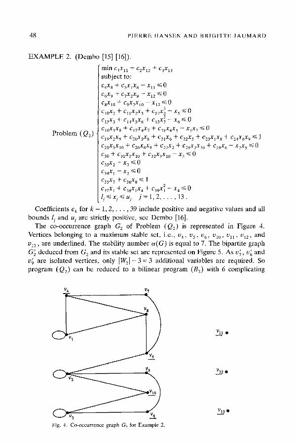
EXAMPLE 2. (Dembo [15] [16]).
Problem (Q,) C16X1X8 + c,,x,x, + c1*x4xs - x5x, Q 0 c19x2xg + c2()xgxs + C,lX6 + c*zxz + c2jx*xg + c2‘$xgxg G 1 C&3X10 + C26jXgX9 + C27X2 + C2$2Xlo + C29Xfj - X2X9 c 0
c3,, + c31x2x10 + c32x3x10 - x2 s o
c33x2 - x3 60 $X1 - x2 s 0
c35x7 + c36x8 G 1 c37x1 + c38x1x4 + c,,x; - x4 6 0 li~xi~ui j=1,2,. . . ,13.
min clxll + c2xIz + c3x13 subject to: c&t* + c5x1xs - Xl1 =s 0 c&d9 + c,x2x9 - Xl2 =s 0 CSXIO + C9X3X10 - Xl3 s 0
‘C10X2 + CllX2X5 + c,,x; - x5 s 0 C13X3 + C14X3X6 + c*5x: - X6 s 0
Coefficients ck for k = 1,2, . . . ,39 include positive and negative values and all bounds Zj and uj are strictly positive, see Dembo [16].
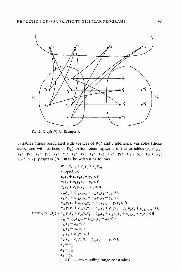
The co-occurrence graph G, of Problem (Q,) is represented in Figure 4. Vertices belonging to a maximum stable set, i.e., uq, ug, u6, uIo, urr, u12, and u13, are underlined. The stability number a(G) is equal to 7. The bipartite graph G; deduced from G, and its stable set are represented on Figure 5. As u; , VA and ZIG are isolated vertices, only /W,l - 3 = 3 additional variables are required. So program (Q,) can be reduced to a bilinear program (B2) with 6 complicating
51 0 -
v12 l -
v13 l -
Fig. 4. Co-occurrence graph GZ for Example 2.
REDUCTION OF QUADRATIC TO BILINEAR PROGRAMS 49
Fig. 5. Graph G; for Example 1
variables (those associated with vertices of WI) and 3 additional variables (those associated with vertices of W,). After renaming some of the variables (x, ty, ; X5-y,; X6‘+y6; x7+--x4; x8+$; “9+-X6; X10+Y,; xll’Y8; X12+-Y9;
x13 +y,,), program (B,) may be written as follows:
Problem (I$)
I min cd5 + c2Yg + c3Ylo subject to: c4xS + c5Ylx5 - YS So ‘gx6 + c7Y2x6 - Y9 So CsY7 + C9Y7X3 - YlO so c10x2 + cllY5x2 + ‘12’2Y2 - Y5 do c13x3 + c14Y6x3 + ‘1Sx3Y3 - YS So c16Ylx, + c17Y4x4 + ‘lS’SY4 - Y5’4 do c19Y2x6 + cZOY,x, + ‘2lY6 + ‘22YS + ‘23Ylx5 + ‘24YSx6 so
c25Y7x3 + c26Y6x6 + c27x2 + ‘2Sx2Y7 + ‘29Y6 - Y2x6 So
c30 + c31x2Y7 + ‘32’3Y7 - x2 =% ’
c33x2 - x3 SO
C34Xl - x2. -=o c3sx4 + CS6X5 =z 1
c37x1 + ‘3SxlY4 + c39xlYl - Y4 co Xl = Yl x2 = Y2
x3 = Y3 and the corresponding range constraints.
50 PIERRE HANSEN AND BRIGITTE JAUMARD
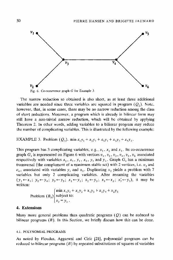
y2 Fig. 6. Co-occurrence graph G for Example 3.
‘6
The narrow reduction so obtained is also short, as at least three additional variables are needed since three variables are squared in program (Q,). Note, however, that, in some cases, there may be no narrow reduction among the class of short reductions. Moreover, a program which is already in bilinear form may still have a non-trivial narrow reduction, which will be obtained by applying Theorem 2. In other words, adding variables to a bilinear program may reduce the number of complicating variables. This is illustrated by the following example:
EXAMPLE 3. Problem (Q3). min xlyl + xzYl + x3Yl + X3Y2 + X3Y3.
This program has 3 complicating variables, e.g., x1, x2 and x3. Its co-occurrence graph G, is represented on Figure 6 with vertices u1 , u2, ug, v4, u5, ug associated respectively with variables x1, x2, y, , x3, y, and y3. Graph G, has a minimum transversal (the complement of a maximum stable set) with 2 vertices, i.e. u3 and u4, associated with variables y, and x3. Duplicating x3 yields a problem with 7 variables but only 2 complicating variables. After renaming the variables (Yl +x 1; yz+y4; Y,+Y~; xl+yl; x,+Y,; X,+X,; 4+y3>, it may be written:
I
min xlyl + ~0, + xly3 + xzy4 + x0, Problem (B3) subject to:
x2 = Y, .
4. Extensions Many more general problems than quadratic programs (Q) can be reduced to bilinear programs (B). In this Section, we briefly discuss how this can be done.
4.1. POLYNOMIAL PROGRAMS
As noted by Floudas, Aggarwal and Ciric [Zl], polynomial programs can be reduced to bilinear programs (B) by repeated substitutions of squares of variables
REDUCTION OF QUADRATIC TO BILINEAR PROGRAMS 51
or products of two variables by additional variables. Note that substitutions of additional variables to products of more than 2 variables or to variables raised to powers higher than 2 could also be used. They sometimes lead to shorter reductions as shown in the Example 4 below. We first consider the case of a single product of variables:
PROPOSITION 1. Minimization of a product of k (k 2 3) variables can be reduced to a bilinear program (B) with k - 1 complicating variables by introducing k - 2 additional variables. Moreover, both of these numbers are minimum.
Proof. We first show that at most k - 1 complicating variables and k - 2 additional variables are needed to obtain a bilinear program. Let Il%, xi be the product to be minimized: define k - 2 new variables by y, = x1x2, yj = yj-lxj+l forj=2,3,. . . , k - 2; then the product may be written as Y~-~x~. Moreover, the set {x1, Y,, yz, . . . , y,-,} can be chosen as set of complicating variables.
We now show that at least k - 1 complicating variables and k - 2 additional variables are required. At each successive substitution reduces the number of variables in the product by one, k - 2 additional variables are needed. Moreover, it is easy to show that each initial or additional variable must appear in exactly one product of the resulting bilinear program (B). So the co-occurrence graph G of program (B) is a perfect matching on 2k - 2 vertices and has a minimum transversal containing n - a(G) = k - 1 vertices. n
An immediate application of Proposition 1 is to multiplicative programs (Konno and Kuno [31], Thoai 1451) . m which the objective function is a product of k 3 2 linear functions and the constraints are linear or convex. If k = 2, the most frequently studied case, two variables are set equal to the linear factors and any one of them can be chosen as unique complicating variable when constraints are linear.
PROPOSITION 2. Minimization of a product II,,, x9 of variables raised to positive integer powers pi (with at least pi 3 2 for some j E J) can be reduced to a bilinear program with CjG, pj - 2 + max(2 - 1 J(, 0} additional variables or with 1 J(, but no fewer than (JI - 1, complicating variables.
Proof. Let us first write IljeJ x9 as a product of CjeJ pi variables, with repetitions. Then if ] Jl> 1 a similar reasoning to the proof of Proposition 1 shows that CjsJ pi - 2 additional variables suffice; if ) Jl = 1 (i.e., J = {i}) p, - 1 addi- tional variables suffice. Again from Proposition 1 at least 1 JJ - 1 complicating variables are needed. Reducing separately each ~3 with pi 2 2 in the product yields a bilinear program with I J\ complicating variables, i.e., the variables xi themselves. n
The bound on the number of additional variables of Proposition 2 is not always sharp, as we now show:

52 PIERRE HANSEN AND BRIGITTE JAUMARD
EXAMPLE 4. min xfxix:.
The reduction of Proposition 1 leads to, e.g., y, =x1x2, y, = xly,, y, = x2y2, y, = x3y, and the product becomes equal to x3y,, with 4 additional variables. However, the reduction y1 = x1x2, y, = n3yl, y, = x3y1 makes the product equal to y2y, and uses only 3 additional variables.
Let us now consider a general polynomial program:
i=1,2 ,..., m,
where the, c, for k = 1,2, . . . , K0 and aik for k = 1,2, . . . , Ki and i = 1, 2, . . . , m are real numbers, the pi and pij for the same index sets are positive integers. Again the constraints may contain non-negativity or range ones as well as equalities.
In order to partially extend Propositions 1 and 2 to the case of program (P), we need some more definitions. Recall that a hypergruph H = (V, E) (cf Berge [ll]) is a finite set of subsets Ei (called edges) of a set V of elements (called vertices). The co-occurrence hypergraph H of program (P) is defined by associating vertices ujEV with variables xj (j=l, 2,. . . , n) and taking as edges the vertex sets corresponding to the variables of each product of variables in (P) (without repetition). The Z-section of a hypergraph H is the graph Hz = (V, E(H)) obtained by taking the same set V of vertices as in H and as edges all pairs of vertices belonging both to the same edge of H. A partial subgraph C = (V, E,) of Hz will be called an edge-edge covering of H if the vertex set of each edge Ei of H contains the endpoints (E, 1 - 2 edges of C which do not induce any cycle (in other words, each edge must contain one or two disjoint trees of C with a total length of ( Ei/ - 2). Note than any reduction of problem (P) to a bilinear program (B) induces an edge-edge covering of H. Edges correspond to pairs of vertices associated with variables xk , xI for substitutions of the form yj = y,x,, and recursively to the highest indexed variable in the expression of y, or y, for substitutions of the form yj = xkxI or yi = y,y,.
PROPOSITION 3. Let (P) be a polynomial program with n variables of which t have degree greater than or equal to 2, and a co-occurrence hypergraph H. Let % denote the set of edge-edge coverings of H. Then the number of additional variables in any reduction of (P) to a bilinear program (B) is at least
t+rnTl(E,l.
REDUCTION OF QUADRATIC TO BILINEAR PROGRAMS 53
Proof. Terms of the form xy or $0 with pi 2 2 or pij 3 2 may be reduced first. This takes at least t additional variables and does not modify the co-occurrence hypergraph H. Then, to reduce terms with more than 2 variables, additional variables corresponding to an edge-edge covering of H must be used. There are at least min,,, jE,-j of them. n
The bound of Proposition 3 is often loose, but is sufficient to show that some reductions of polynomial to bilinear programs are short.
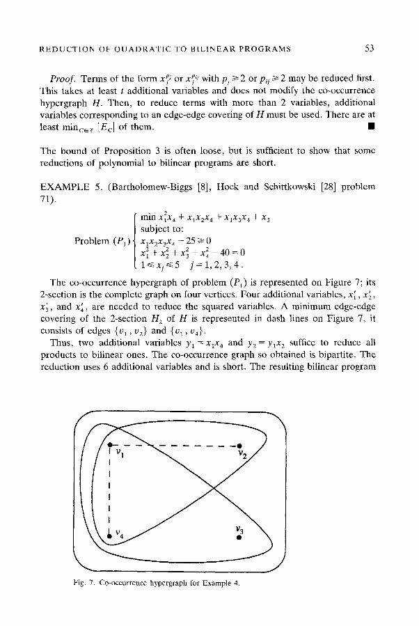
EXAMPLE 5. (Bartholomew-Biggs 181, Hock and Schittkowski [ZS] problem 71).
I
min .x:x, + x1+x4 + x1x3x4 + x3 subject to:
Problem (PI) x1x2x3x4 -25>0 xf + x; + x; + x’, - 40 = 0 1dxjc5 j=1,2,3,4.
The co-occurrence hypergraph of problem (P,) is represented on Figure 7; its 2-section is the complete graph on four vertices. Four additional variables, xi, xi, xi, and xi, are needed to reduce the squared variables. A minimum edge-edge covering of the 2-section Hz of H is represented in dash lines on Figure 7, it consists of edges { LJ, , u2} and {ul, uq).
Thus, two additional variables y1 = xlxq and y, = y,x, suffice to reduce all products to bilinear ones. The co-occurrence graph so obtained is bipartite. The reduction uses 6 additional variables and is short. The resulting bilinear program
Fig. 7. Co-occurrence hypergraph for Example 4.
54 PIERRE HANSEN AND BRIGITTE JAUMARD
(B4) has 4 complicating variables. It may be written:
Problem (B4)
‘min xiy, + y, + x3y, + xj subject to: x,y,-2530
xlYl+ X2Yz + X3Y3 + X4Y4 - 40 = 0
Y, = XlY4
Y, = X2Y5
Xl =Yl x2 = Y,
x3 = Y3
x4 = Y,
and the corresponding range constraints.
Considering now complicating variables yields stronger results. Indeed a lower bound generalizing the lower bound of Theorem 2 can be obtained.
THEOREM 3. Let (P) be a polynomial program with co-occurrence hy- pergraph H with 2-section H2. Then the number of complicating variables in any reduction of (P) to a bilinear program (B) is at least
where a(H2) is the stability number of Hz. Proof. Using a similar reasoning than in Proposition 1, at least k - 1 complicat-
ing variables in (B) are associated with any product of k variables in (P). Moreover, these complicating variables must either be variables of that product or additional variables associated, directly or indirectly, with variables of that product only. So the number of complicating variables is not less than the number of vertices in a set containing (Ejl - 1 vertices from each edge of H. This number is bounded in turn by n - a(H2). n
Again, the bound is not always sharp but is reached for some problems. The 2-section H2 of H for Example 5 is equal to the complete graph on four vertices with loops at all of them. So cy(Hz) = 0 and the reduction given above is narrow.
4.2. HYPERBOLIC PROGRAMS
We call hyperbolic programs those programs in which the objective function and left-hand sides of the constraints can be expressed, possibly after reduction to common denominators, as ratios of polynomials. If the denominators in the constraints are non-negative or non-positive, these constraints can be expressed as
REDUCTION OF QUADRATIC TO BILINEAR PROGRAMS 55
polynomials after multiplication by the denominator, but the sign of these denominators may be undetermined or unknown. Hyperbolic programs comprise all programs in which the objective and left-hand sides of constraints are obtained from constants and variables by operations of addition, subtraction, multiplication and division. These expressions need not be given as ratios of polynomials and reduction to such a form may be cumbersome. So ratios within larger expressions may first be removed. This is done by introducing a new variable equal to the inverse of the denominator, in a straightforward way when the sign of the latter is determined.
EXAMPLE 6. (Modification of the gravel box problem of Duffin, Peterson and Zener [17], Gochet and Smeers [27]).
40 mm - + 20x,x, + 40X,X, + 10X,X, x1x2x3
Problem (H,) subject to:
I --x,-x2-xx,+8~0 x17x2, x,>o.
Setting y, = l/(x,x,x,), introducing two additional variables y2 = yIx, and ys = yzx2 to reduce the product ylx,x,x3 and one additional variable xi = x3 to reduce the set of terms x2x3, x1x2 and x1x3, (which correspond to an odd cycle of G) yields a short and narrow reduction. The resulting bilinear program (B5) has 3 complicating variables, i.e., x1, y, and x3. It may be written after renaming some of the variables (x, ty,; yz +.x2; x; ty,):
Problem (B5)
min 4Oy, + 2Ox,y, + 4Ox,y, + lOx,y, subject to -x1-yz-x3+8~0
x2 = XlYl Y3 = X2Y2
X3Y3 = 1 x3 = Y4
all variables being strictly positive. Another class of programs in which a single additional and complicating
variable is needed, as in the multiplicative programs discussed above, are the linear hyperbolic programs (e.g., Avriel et al. [4]). In such programs, a ratio of non-negative linear functions is to be minimized subject to linear constraints. Under the mild restriction that the feasible set does not reduce to a vector giving the value 0 to the denominator of the objective function (which can be easily checked) the above transformation applies in a straightforward way. (Note that
56 PIERRE HANSEN AND BRIGITTE JAUMARD
problems in which the ratio is to be maximized can be reduced to the minimiza- tion case by exchanging the numerator and the denominator).
If the sign of the denominator is unknown and a value of 0 cannot be ruled out a priori, reduction is more difficult. In addition to setting y, = 1 /[h(x)] where the sign of h(x) is unknown, one must add the pair of disjunctive constraints h(x) 3 E or h(x) 4 -E where E is a small constant. The latter can be reduced to usual constraints involving a O-l variable by standard techniques, e.g., by setting (2y, - 1)/z(x) i F where y, is a O-l variable. Reduction of O-l variables is discussed below. Various forms of generalized and of nonlinear fractional pro- grams (Bernard and Ferland [12], Avriel et al. [4]) can be reduced to bilinear programs by combining standard techniques to express the minimum of a set of functions (to be maximized) with those given above.
4.3. FRACTIONAL EXPONENTS, TRIGONOMETRIC AND TRANSCENDENTAL
FUNCTIONS, INTEGER AND O-l VARIABLES
Several further classes of programs can be reduced to polynomial and hence to bilinear programs. Problems with variables having fractional exponents, e.g., signomial geometric programs (Avriel and Williams [5]) can be reduced noting that y = xpiq where p and q are pairwise prime is equivalent to xp = yq (such a reduction is used implicitly in an example of Floudas, Aggarwal and Ciric [21]) and then applying techniques described above. Note that each variable with fractional exponent is associated with 2 complicating variables.
EXAMPLE 7. (Stephanopoulos and Westerberg [43], Floudas, Aggarwal and Ciric [21]).
Problem (G,) x1 +2x, c-4 xy?+2xq44 Xl a3 x3 =s 1 Xl, x2 > x3 7 x4 G= 0
min x1 ‘.’ + x;.” - 6x, - 4x, - 3x, subject to: -3x, +x,-3x,=0
The only nonlinear terms are the first two in the objective function, They are replaced by additional variables y, and y, ; then the constraints xi = y: and x: = yz are reduced to bilinear ones using 12 more additional variables. The resulting bilinear program (B6) has 4 complicating variables, i.e., x1, x2, yr and y2. After renaming some of the variables ( yr +x3 ; y, +x4 ; x3 +- y,, ; x4 +-yl,), it may be written:
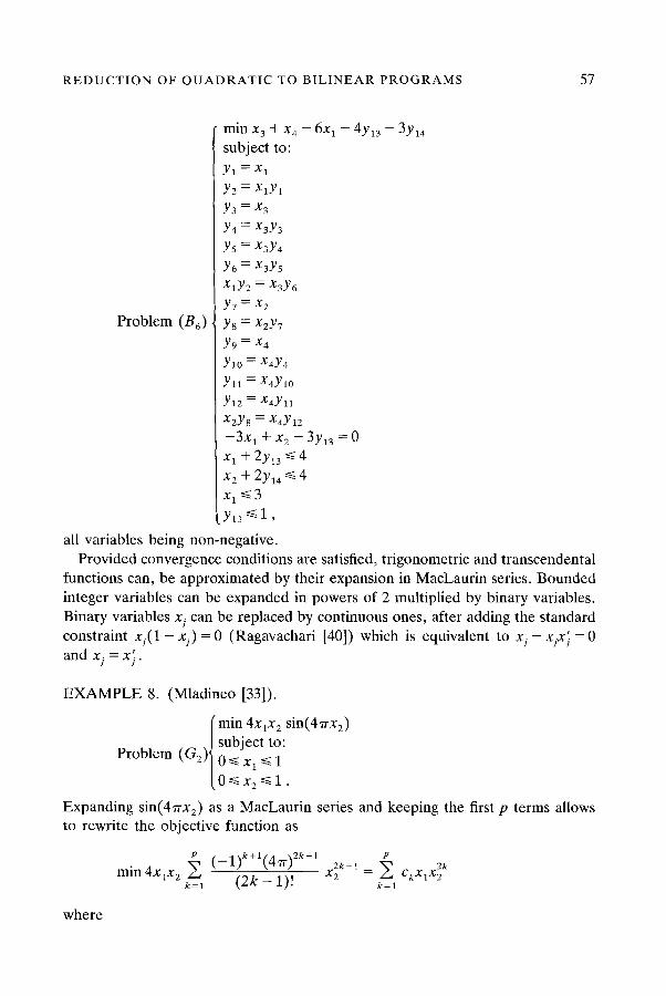
REDUCTION OF QUADRATIC TO BILINEAR PROGRAMS 57
Problem (B6)
min x3 + x4 - 6x, - 4y,, - 3y,, subject to: Yl = Xl
Y2 =xlYl
Y3 = x3
Y4 = X3Y3
Ys = X3Y4
Y6 = x3Y5
xlY2 =x3Y6
Y7 = x2
YS =x2Y7
Y, =x4
Y 10 = X4Y4
Yll = X4Y 10
Yl2 = X4Yll
x2Y8 ='4Y12
-3x, + x2 - 3y,, = 0 xl+2yl,s4 x2+2y,,s4 x,s3
Y13 =z 1 )
all variables being non-negative. Provided convergence conditions are satisfied, trigonometric and transcendental
functions can, be approximated by their expansion in MacLaurin series. Bounded integer variables can be expanded in powers of 2 multiplied by binary variables. Binary variables xi can be replaced by continuous ones, after adding the standard constraint xj(l - xi) = 0 (Ragavachari [40]) which is equivalent to xi - xix; = 0 and xi = xi.
EXAMPLE 8. (Mladineo [33]).
min 4x,x, sin(47rx,)
Problem (G2) subject to: ()qxl 6 1
Expanding sin(4rx,) as a MacLaurin series and keeping the first p terms allows to rewrite the objective function as
min 4x,x, jl ‘-lpy’ xi,-, = ;l CkX1gk
where
58 PIERRE HANSEN AND BRIGITTE JAUMARD
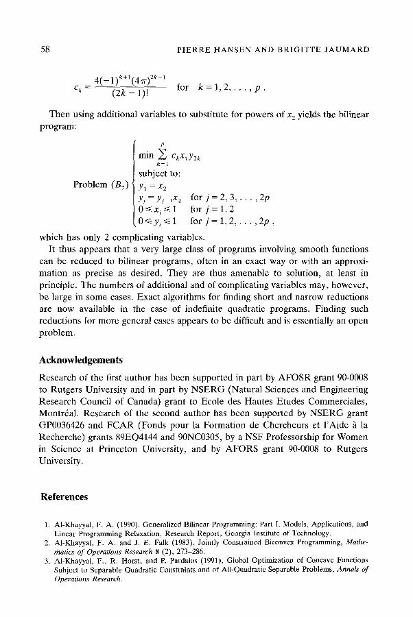
Ck = 4(-v+1(4792kP1 for k= 1 2 (2k - l)! > ,.‘.> .
p
Then using additional variables to substitute for powers of x2 yields the bilinear program:
min c ckxlY2k k=l
subject to: Problem (B7) Y, = x2
yi=yi-1x2 for j=2,3 ,..., 2p O~.Xi<l for j=1,2
.OGYiS1 for j = 1,2, . . . ,2p ,
which has only 2 complicating variables. It thus appears that a very large class of programs involving smooth functions
can be reduced to bilinear programs, often in an exact way or with an approxi- mation as precise as desired. They are thus amenable to solution, at least in principle. The numbers of additional and of complicating variables may, however, be large in some cases. Exact algorithms for finding short and narrow reductions are now available in the case of indefinite quadratic programs. Finding such reductions for more general cases appears to be difficult and is essentially an open problem.
P
Acknowledgements
Research of the first author has been supported in part by AFOSR grant 90-0008 to Rutgers University and in part by NSERG (Natural Sciences and Engineering Research Council of Canada) grant to Ecole des Hautes Etudes Commerciales, Montreal. Research of the second author has been supported by NSERG grant GPO036426 and FCAR (Fonds pour la Formation de Chercheurs et 1’Aide h la Recherche) grants 89EQ4144 and 90NC0305, by a NSF Professorship for Women in Science at Princeton University, and by AFORS grant 90-0008 to Rutgers University.
References
1. Al-Khayyal, F. A. (1990), Generalized Bilinear Programming: Part I. Models, Applications, and Linear Programming Relaxation, Research Report, Georgia Institute of Technology.
2. Al-Khayyal, F. A. and J. E. Falk (1983), Jointly Constrained Biconvex Programming, Mathe- matics of Operations Research 8 (2), 273-286.
3. Al-Khayyal, F., R. Horst, and P. Pardalos (1991), Global Optimization of Concave Functions Subject to Separable Quadratic Constraints and of All-Quadratic Separable Problems, Annals of Operations Research.

REDUCTION OF QUADRATIC TO BILINEAR PROGRAMS 59
4. Avriel, M., W. E. Diernert, S. Schaible, and I. Zang (1988), Generalized Concavity, New York: Plenum Press.
5. Avriel, M. and A. C. Williams (1971), An Extension of Geometric Programming with Applica- tions in Engineering Optimization, Journal of Engineering Mathematics 5 (3), 187-194.
6. Balas, E. and C. S. Yu (1986), Finding a Maximum Clique in an Arbitrary Graph, SIAM Journal on Computing 15. 1054-1068.
7. Baron, D. P. (1972), Quadratic Programming with Quadratic Constraints, Naval Research Logistics Quarterly 19, 2.53-260.
8. Bartholomew-Biggs, M. C. (1976), A Numerical Comparison between Two Approaches to Nonlinear Programming Problems, Technical Report # 77, Numerical Optimization Center, Hatfield, England.
9. Benacer, R. and T. Pham Dinh (1986), Global Maximization of a Nondefinite Quardatic Function over a Convex Polyhedron, pp. 65-76 in J.-B. Hirriart-Urruty (ed.), Fermat Days 1985: Mathe- matics for Optimization, Amsterdam: North-Holland.
10. Berge, C. (1983), Graphes, 3rd ed., Paris: Gauthier-Villars. 11. Berge, C. (1987), Hypergraphes, Paris, Gauthier-Villars. 12. Bernard, J. C. and J. A. Ferland (1989), Convergence of Interval-Type Algorithms for General-
ized Fractional Programming, Mathematical Programming 43, 349-363. 13. Carraghan, R. and P. M. Pardalos (1990), An Exact Algorithm for the Maximum Clique Problem,
Operations Research Letters 9, 375-382. 14. Colville, A. R. (1986), A Comparative Study on Nonlinear Programming Codes, IBM Scientific
Center Report 320-2949, New York. 15. Dembo, R. S. (1972), Solution of Complementary Geometric Programming Problems, M.Sc.
Thesis, Technion, Haifa. 16. Dembo, R. S. (1976), A Set of Geometric Programming Test Problems and Their Solutions,
Mathematical Programming 10, 192-213. 17. Duffin, R. J., E. L. Peterson, and C. Zener (1967), Geometric Programming: Theory and
Applications, New York: Wiley. 18. Ecker, J. G. and R. D. Niemi (1975), A Dual Method for Quadratic Programs with Quadratic
Constraints, SIAM Journal on Applied Mathematics 28, 568-576. 19. Evans, D. H. (1963), Modular Design - A Special Case in Nonlinear Programming, Operations
Research 11, 637-647. 20. Flippo, 0. E. (1989), Stability, Duality and Decomposition in General Mathematical Program-
ming, Rotterdam: Erasmus University Press. 21. Floudas, C. A., A. Aggarwal, and A. R. Ciric (1989), Global Optimum Search for Nonconvex
NLP and MINLP Problems, Computers and Chemical Engineering 13 (lo), 1117-1132. 22. Floudas, C. A. and P. Pardalos (1990), A Collection of Test Problems for Constrained Global
Optimization, Lecture Notes in Computer Science, 455, Berlin: Springer-Verlag. 23. Floudas, C. A. and V. Visweswaran (1990), A Global Optimization Algorithm (GOP) for Certain
Classes of Nonconvex NLPs - I. Theory, Computers and Chemical Engineering 14 (12), 1397- 1417.
24. Friden, C., A. Hertz, and D. de Werra (1990), Tabaris: An Exact Algorithm Based on Tabu Search for Finding a Maximum Independent Set in a Graph, Computers and Operations Research 17 (S), 437-445.
25. Garey, M. R., D. S. Johnson, and L. Stockmeyer (1976), Some Simplified NP-Complete Graph Problems, Theoretical Computer Science 1, 237-267.
26. Geoffrion, A. M. (1972), Generalized Benders Decomposition, Journal of Optimization Theory and Its Applications 10, 237-260.
27. Gochet, W. and Y. Smeers (1979), A Branch and Bound Method for Reversed Geometric Programming, Operations Research 27, 982-996.
28. Hock, W. and K. Schittkowski (1981), Test Examples for Nonlinear Programming Codes, Lecture Notes in Economics and Mathematical Systems #187, Berlin: Springer-Verlag.
29. Horst, R. and H. Tuy (1990), Global Optimization, Deterministic Approaches, Berlin: Springer- Verlag.
30. Konno, H. (1976), Maximizing a Convex Quadratic Function Subject to Linear Constraints Mathematical Programming 11, 117-127.
60 PIERRE HANSEN AND BRIGITTE JAUMARD
31. Konno, H. and T. Kuno (1989), Linear Multiplicative Programming, Preprint IHSS 89-13, Tokyo Institute of Technology.
32. Kough, P. F. (1979), The Indefinite Quadratic Programming Problem, Operations Research 27, 516-533.
33. Mladineo, R. H. (1986), An Algorithm for Finding the Global Maximum of a Multimodal, Multivariate Function, Muthematical Programming 34, 188-200.
34. Pardalos, P. M., J. H. Glick, and J. B. Rosen (1987), Global Minimization of Indefinite Quadratic Problems, Computing 39, 281-291.
35. Pardalos, P. M. and J. B. Rosen (1986), Methods for Global Concave Minimization: A Bibliographic Survey, SIAM Review 28 (3), 367-379.
36. Pardalos, P. M. and J. B. Rosen (1987), Constrained Global Optimization: Algorithms and Applications, Lecture Notes in Computer Science #268, Berlin: Springer Verlag.
37. Pham Dinh, T. and S. El Bernoussi (1989), Numerical Methods for Solving a Class of Global Nonconvex Optimization Problems, International Series of Numerical Mathematics 87, 97-132.
38. Phan, H. (1982), Quadratically Constrained Quadratic Programming: Some Applications and a Method of Solution, Zeitschrift fiir Operations Research 26, 105-119.
39. Phillips, A. T. and J. B. Rosen, (1990), Guaranteed &-Approximate Solution to Indefinite Global Optimization, Naval Research Logistics 37, 499-514.
40. Ragavachari, M. (1989), On Connections between Zero-One Integer Programming and Concave Programming under Linear Constraints, Operations Research 17, 680-684.
41. Reeves, G. R. (1975), Global Minimization in Nonconvex All-Quadratic Programming, Munage- ment Science 22, 76-86.
42. Sherali, H. and A. Alameddine (1990), A New Reformulation-Linearization Technique for Bilinear Programming Problems, Research Report, Department of Industrial and Systems En- gineering, Virginia Polytechnic Institute.
43. Stephanopoulos, G. and A. W. Westerberg (1975), The Use of Hestenes’ Method of Multipliers to Resolve Dual Gaps in Engineering System Optimization, Journal of Optimization Theory and Applications 15, 285-309.
44. Simses, L. M. C. (1987), Search for the Global Optimum of Least Volume Trusses, Engineering Optimization 11, 49-67.
45. Thoai, N. V (1990), Application of Decomposition Techniques in Global Optimization to the Convex Multiplicative Programming Problem, Paper presented at the Second Workshop on Global Optimization, Sopron, Hungary.
46. Tuy, H. (1986), A General Deterministic Approach to Global Optimization via d.-c. Program- ming, pp. 137-162, in J. B. Hirriart-Urruty (ed.), Fermat Days 1985: Mathematics for Optimiza- tion, Amsterdam: North-Holland.
47. Visweswaran, V and C. A. Floudas (1990), A Global Optimization Algorithm (GOP) for Certain Classes of Nonconvex NLPs - II. Application of Theory and Test Problems, Computers and Chemical Engineering 14 (12), 1419-1434.
48. Wolsey, L. A. (1981), A Resource Decomposition Algorithm for General Mathematical Pro- grams, Mathematical Programming Study 14, 244-257.