Embed Size (px)
Citation preview

Journal of Statistical Planning andInference 136 (2006) 159–182
www.elsevier.com/locate/jspi
On some properties of a class of weightedquasi-binomial distributions
Subrata Chakrabortya,∗, Kishore K. DasbaDepartment of Statistics, Dibrugarh University, Dibrugarh 786004, Assam, India
bDepartment of Statistics, Gauhati University, Guwahati, Assam, India
Received 15 December 2002; accepted 18 June 2004Available online 14 August 2004
Abstract
A class of weighted quasi-binomial distributions has been derived as weighted distribution of QBDI (Sankhya 36 (Ser. B, Part 4) 391). The moments, inverse moments, recurrence relations amongmoments, bounds for mode, problem of estimation and fitting of data from real life situations usingdifferent methods and limiting distributions of the class have been studied. Consul’s (Comm. Statist.Theory Methods 19(2) (1990) 477) results on QBD I have been seen as particular cases.© 2004 Elsevier B.V. All rights reserved.
MSC:60E05; 62E15; 62F10
Keywords:Quasi-binomial distributions; Weighted quasi-binomial distribution; Moments; Inverse moments;Recurrence relation; Limiting distributions
1. Introduction
Consul (1974)first introduced the notion of urn model with pre-determined strategywith a two urn model and developed quasi-binomial distribution (QBD) I with probabilityfunction (p.f.)
Pr(X = k)=(nk
)p(p + k�)k−1(1− p − k�)n−k,
k = 0(1)n, −p/n���(1− p)/n (1)
∗ Corresponding author.E-mail address:[email protected](S. Chakraborty).
0378-3758/$ - see front matter © 2004 Elsevier B.V. All rights reserved.doi:10.1016/j.jspi.2004.05.015

160 S. Chakraborty, K.K. Das / Journal of Statistical Planning and Inference 136 (2006) 159–182
using samplingwith replacement schemes.Hegave justification andmentionedapplicationsof these distributions in various fields.Consul and Mittal (1975)defined QBD II using afour urn model with a pre-determined strategy as
Pr(X = k)=(nk
) p(1− p − n�)(1− n�) (p + k�)k−1(1− p − k�)n−k−1,
k = 0(1)n; −p/n���(1− p)/n (2)
and indicated a large number of possible applications.Janardan (1975)obtained QBD as aparticular case of his Quasi-Polya distribution.Berg (1985)generated QBD I from modified Charlier type B expansions, also obtaining
its mean, variance. He mentioned as to how Abel’s generalisation of the binomial identity(Riordan, 1968) is related to the QBDs.Berg and Mutafchiev (1990)have mentioned thatnewmodifiedQBDs can be developed usingAbel’s generalisations of the binomial formula.They also indicated how differentAbel identities can be used to define newweighted QBDsand also have shown applications of some QBD and modified QBDs in random mappingproblems.Charalambides (1990)in his paper onAbel series distribution (ASD) mentionedabout QBD I and QBD II. He also obtained�, �(2) and�2 for QBD I, QBD II from thoseof the ASD by using generating function and Bell polynomial (Riordan, 1968). But theformulas for�(2), �
2 were not in compact form.Consul (1990)studied properties of QBD Iwith p.f. (1) with deduction of moments, inverse moments, maximum likelihood estimationand data fitting.Berg and Nowicki (1991)show how QBD I arises in connection withthe distribution of the size of the forest consisting of all trees rooted in a loop in randommapping. (see alsoJaworski, 1984). They also indicated how difficult it is to do inferencewith QBD and show however, that for large sample size QBD approaches generalisedPoisson distribution (GPD) is used. (Consul and Jain, 1973a). As pointed out inBerg andMutafchiev (1990), Mishra et al. (1992)andDas (1993, 1994)used Abel’s generalisationof binomial identities (Riordan, 1968) to define a class of distributions called the class ofquasi-binomial distributions having p.f.
Pr(X = k)=(nk
) (p + k�)k+s(1− p − k�)n−k+tBn(p, q; s, t;�)
, k = 0(1)n, (3)
wheresandt are integers,p + q + n� = 1 and
Bn(p, q; s, t;�)=n∑k=0
(nk
)(p + k�)k+s(1− p − k�)n−k+t (4)
and obtained QBD I, QBD II and some new QBDs by choosing different values forsandtin the p.f. (3) as follows. For
(i) s = −1, t = 0 , QBD type I (Consul, 1974).(ii) s = −1, t = −1, QBD type II (Consul and Mittal, 1975).(iii) s = −2, t = 0, QBD type III (Das, 1993, 1994).(iv) s = −2, t = −1, QBD type IV (Das, 1993, 1994).(v) s = 0, t = 0, QBD type VII (Das, 1993, 1994).

S. Chakraborty, K.K. Das / Journal of Statistical Planning and Inference 136 (2006) 159–182161
We have noticed an error in the formula for therth factorial moment for (3) presented inDas (1993, 1994). Mishra and Singh (2000)obtained first four moments about origin forQBD I by defining factorial power series.Chakraborty and Das (2000)andChakraborty(2001)obtained QBD I as a particular case of a Unified probability model and QBD II froma generalised probability model (Chakraborty, 2001).Since the class of distribution in (3) contains some well-known distributions such as
QBD I, QBD II, besides many newQBDs, we have considered the study of some importantaspects of this class of distributions in the present article. In Section 2 of this paper we firstshow how the class of distribution in (3) can be derived as a class of weighted distributionsof QBD I given in Eq. (1) by choosing different weight functions and called the class asweighted quasi-binomial distributions (WQBD).In the next section we present formulas for factorial moments, noncentral moments about
origin, central moments in general and in particular for QBD I and QBD II and we obtainmean, variance,�3 and�4. In Section 4 two general results for inverse moments and someimportant particular cases are stated besides some results on the inverse factorial moments.Here we have usedAbel’s summation formulas, umbral notations (Riordan, 1958, 1968)
and some generalisations (Chakraborty, 2001) thereof, which have led to considerable sim-plification of the otherwise complicated formulae and their proofs.A list of identities relatedto a class ofAbel’s generalisations of binomial identities has been presented in the appendixat the end.In Section 5 we state a general result on the mode of the class of distributions, while
in Section 6, we study the problem of parameter estimation by various methods includingthe maximum likelihood (ML) method and present some data fitting using ML method ofestimation of the parameters with four illustrations.In the final section we show how for large values ofnunder certain conditions the class of
WQBD approaches the class of weighted generalised Poisson distributions (Chakraborty,2001).
2. A class of weighted QBDs
The weighted probability mass function (p.m.f.)Q(x) corresponding to the p.m.f.p(x)of the random variableXwith weight functionw(x) is given by
Q(x)= w(x)p(x)∑xw(x)p(x)
.
In casew(x) = x, the distribution is said to be size biased or mean weighted distribution(seeJohnson et al., 1992, p. 145).
Definition 1. A random variableX is said to follow a class ofWQBD if its p.f. has the form
Pr(X = k)=(nk
) (p + k�)k+s(q + (n− k)�)n−k+tBn(p, q; s, t;�)
, (5)

162 S. Chakraborty, K.K. Das / Journal of Statistical Planning and Inference 136 (2006) 159–182
Bn(p, q; s, t;�)=n∑k=0
(nk
)(p + k�)k+s(q + (n− k)�)n−k+t , (Riordan, 1968),
(6)
wherep andq are the non-negative fractions,p + q + n� = 1; −p/n<�<(1− p)/nands, t integers.Alternatively, (5) can also be written as
Pr(X = k)=(nk
) (p + k�)k+s(1− p − k�)n−k+tBn(p,1− p − n�; s, t;�)
. (7)
Theorem 1. If X ∼ QBD I (Consul, 1974)with n, p,�, then the weighted distribution ofX with weightw(x)= x(s+1)(n− x)(t), wherex(r) = x(x − 1) · · · (x − r + 1) is given by(
n−t−s−1k−s−1
){p + (s + 1)� + (k − s − 1)�}k−s−1+s
Bn−s−t−1(p + (s + 1)�,1− p − (n− t)�; s, t;�){1− p − (s + 1)�
− (k − s − 1)�}n−t−s−k+s+t , k = 0(1)n. (8)
Hence, the distribution ofY =X − s − 1 is given by
Pr(Y = k)=(mk
)(p′ + k�)k+s(1− p′ − k�)m−k+t
Bm(p′,1− p′ −m�; s, t;�), k = 0(1)m, (9)
wherem= n− s − t − 1, p′ = p+ (s + 1)� and−p′/m<�<(1− p′)/m, which is theclass of QBD given in (7).Some important observations : denoting class (7) byWQBD(n;p,�; s, t), it can be seen
that the form of the weighted QBD I (8) is
1+ s +WQBD(n− s − t − 1;p + (s + 1)�,�; s, t).In particular, for
I. s = 0, t = 0, we get when� = 0 the size biased form of binomial distribution (Johnsonet al., 1992, p. 146) as
1+ Binomial(n− 1;p).II. s = 0, t = 0, the size-biased form of QBD I becomes
1+WQBD(n− 1;p + �,�;0,0).
Theorem 2. If X ∼ QBD I (Consul, 1974)with n, p,�, then the weighted distribution ofX with weightw(x)= (p + x�)s+1(1− p − x�)t is given by(7).
Note: FollowingGupta (1975)we may refer the class of distributions having the p.f. (8)as a class of mixed moment distribution ofX ∼ QBD I(n, p,�) having p.f. (1).
S. Chakraborty, K.K. Das / Journal of Statistical Planning and Inference 136 (2006) 159–182163
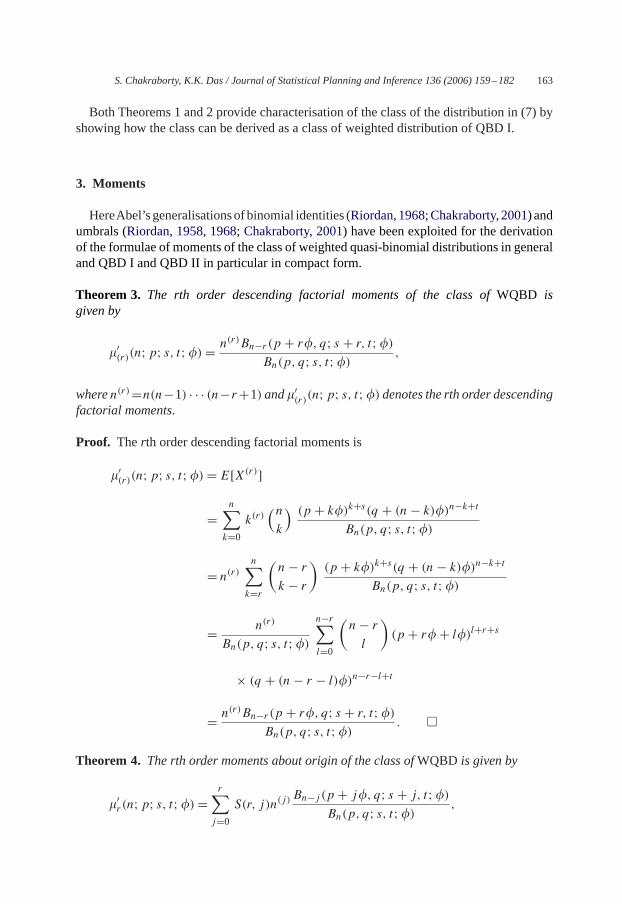
Both Theorems 1 and 2 provide characterisation of the class of the distribution in (7) byshowing how the class can be derived as a class of weighted distribution of QBD I.
3. Moments
HereAbel’sgeneralisationsofbinomial identities (Riordan,1968;Chakraborty, 2001)andumbrals (Riordan, 1958, 1968; Chakraborty, 2001) have been exploited for the derivationof the formulae of moments of the class of weighted quasi-binomial distributions in generaland QBD I and QBD II in particular in compact form.
Theorem 3. The rth order descending factorial moments of the class ofWQBD isgiven by
�′(r)(n;p; s, t;�)= n
(r)Bn−r (p + r�, q; s + r, t;�)Bn(p, q; s, t;�)
,
wheren(r)=n(n−1) · · · (n−r+1) and�′(r)(n;p; s, t;�) denotes the rth order descending
factorial moments.
Proof. Therth order descending factorial moments is
�′(r)(n;p; s, t;�)= E[X(r)]
=n∑k=0
k(r)(nk
) (p + k�)k+s(q + (n− k)�)n−k+tBn(p, q; s, t;�)
= n(r)n∑k=r
(n− rk − r
)(p + k�)k+s(q + (n− k)�)n−k+t
Bn(p, q; s, t;�)
= n(r)
Bn(p, q; s, t;�)
n−r∑l=0
(n− rl
)(p + r� + l�)l+r+s
× (q + (n− r − l)�)n−r−l+t
= n(r)Bn−r (p + r�, q; s + r, t;�)
Bn(p, q; s, t;�). �
Theorem 4. The rth order moments about origin of the class ofWQBD is given by
�′r (n;p; s, t;�)=
r∑j=0
S(r, j)n(j)Bn−j (p + j�, q; s + j, t;�)
Bn(p, q; s, t;�),

164 S. Chakraborty, K.K. Das / Journal of Statistical Planning and Inference 136 (2006) 159–182
whereS(r, j) are the Stirling numbers of the second kind(Riordan, 1958and Johnson etal., 1992)defined as
S(i, j)= �j 0i
j ! f or i�j
= 0 f or i < j
= 1 f or j = 1 or i = jalsoS(i + 1, j)= jS(i, j)+ S(i, j − 1).
Proof. The rth order moments about origin is
�′r (n;p; s, t;�)= E[Xr ] =
r∑j=0
S(r, j)�′(j)(n;p; s, t;�)
=r∑j=0
S(r, j)n(j)Bn−j (p + j�, q; s + j, t;�)
Bn(p, q; s, t;�).
Theorem 5. The rth order moment about the mean of the class ofWQBD is given by
�r (n;p; s, t;�)= 1
Bn(p, q; s, t;�)
r∑j=0
j∑�=0
(r
j
)(−1)r−j�′
1r−jS(j, �)n(�)
Bn−�(p + ��, q; s + �, t;�).
Proof. The rth order moments about mean is
�r (n;p; s, t;�)= E[X − �′1]r =
r∑j=0
(r
j
)(−1)r−j (�′
1)r−j�′
j
= (�′1)rr∑j=0
(r
j
)(−1)r−j
(�′1)j
�′j
Now on using Theorem 4 we get
= �′1r
Bn(p, q; s, t;�)
r∑j=0
j∑�=0
(r
j
)(−1)r−j
�′1jS(j, �)n(�)Bn−�(p + ��, q; s + �, t;�).
3.1. Recurrence relation of moments
�′r (n;p; s, t;�)= nBn−1(p + �, q; s + 1, t;�)
Bn(p, q; s, t;�)
×r−1∑j=0
(r − 1
j
)�′j (n− 1;p + �; s + 1, t;�).

S. Chakraborty, K.K. Das / Journal of Statistical Planning and Inference 136 (2006) 159–182165
Repeated application of the above relation gives
�′r (n;p; s, t;�)= n
(2)Bn−2(p + 2�, q; s + 2, t;�)Bn(p, q; s, t;�)
r−1∑j=0
j−1∑�=0
(r − 1
j
) (j − 1
�
)�′
�(n− 2;p + 2�; s + 2, t;�).
All the relations stated above for the class of WQBD are of general nature. Using differentcombinations of integer values ofr, s andt, the different moments of the different quasi-binomial distributions belonging to theWQBD class may be obtained. It may be noted thatin all the results above,p + q + n� = 1, that is,q = 1− p − n�.
3.2. First four central moments of some of theWQBDs
3.2.1. Moments of the QBD I
�′1 = np
n−1∑�=0
(n− 1)(�)��,
�2 = n(2)pn−2∑�=0
�∑w=0
(n− 2)(�)��(p + 2� + w�)+ npn−1∑�=0
(n− 1)(�)��
− n2p2n−1∑�=0
{(n− 1)(�)��}2 +n−1∑i �=j=0
(n− 1)(i)(n− j)(j)�i+j .
It can be verified that the above results are equal to those ofConsul (1990):
�3 = (2�′13 − 3�′
12 + �′
1)+ 3p(1− �′1)
n−2∑�=0
�∑w=0
n(�+2)��(p + 2� + w�)
+ pn−3∑�=0
�∑w=0
n(�+3)��+1w(� − w + 1)(p + 3� + w�)
+ pn−3∑�=0
�∑w=0
w∑�=0
n(�+3)��(p + 3� + ��)(p + 3� + (w − �)�).
�4 = p[p−1�′14 + n(1+ ��)n−1{−4�′
13 + 6�′
12 − 4�′
1 + 1}+ n(2)(1+ �� + �′(p + 2�)�)n−2{6�′
12 − 12�′
1 + 7}+ n(3)[(1+ �� + �′(p + 3�;2)�)n−3 + (1+ �(2)�
+ �′(p + 2�)�)n−3]{−4�′1 + 6}
+ n(4)[(1+ �� + ��′(p + 4�;3))n + 3(1+ ��(2)+ ��′(p + 4�)+ ��′(p + 4�))n
+ (1+ ��(2)+ ��′(0)+ ��′(p + 4�))n
+ (1+ ��(3)+ �′(p + 4�))n].

166 S. Chakraborty, K.K. Das / Journal of Statistical Planning and Inference 136 (2006) 159–182
3.2.2. Moments of the QBD II
�′1 = np
1− n� ,
�2 = np
1− n�
[n−2∑�=0
(n− 1)(�+1)��(p + 2� + ��)+ 1− n(� + p)1− n�
],
�3 = (2�′13 − 3�′
12 + 1)+ p
1− n�
[3n(2)p(1− �′
1)
n−2∑�=0
(n− 2)���(p + 2� + ��)
+ n(3){n−3∑�=0
�∑w=0
(n− 3)(�)��(p + 3� + w�)(p + 3� + (� − w)�)
+n−3∑�=0
�∑w=0
(n− 3)(�)w��+1(p + 3� + w�)
}].
�4 = �′14 + p
1− n� [n(−4�′13 + 6�′
12 − 4�′
1 + 1)
+ n(2)(6�′12 − 12�′
1 + 7)(1+ ��′(p + 2�))n−2 + n(3)(−4�′1 + 6).
{(1+ ��′(p + 3�;2))n−3 + (1+ �� + ��′(p + 3�))n−3}+ n(4){Bn(p + 4�, q;3,0;�)+ n�Bn−1(p + 4�, q + �;3,0;�)}].
Further expansion has been avoided as the expression becomes too long.Where
�k ≡ �k = k!, �k(j) ≡ �k(j)= (� + · · · + �︸ ︷︷ ︸j terms
)k =(k + j − 1
k
)k!,
�′k(x) ≡ �′k(x)= k!(x + kz), �′
k(x) ≡ �′k(x)= (kz) k! (x + kz),′k(x) ≡ ′k(x)= (kz) (kz) k! (x + kz) and�′k(x; j)= [�′(x)+ · · · + �′(x)︸ ︷︷ ︸
j terms
]k
(Riordan,1968;Chakraborty,2001).
4. Inverse moments
The importance of inverse or negative moments is well known in the estimation of theparameters of a model and also for testing the efficiency of various estimates. Besides theyare equally useful in life testing and in survey sampling, where ratio estimates are beingemployed.Consul (1990)gave a detailed account of negative moments of QBD I. In thissection similar properties have been studied for the class of WQBD by deriving generalformulas and listing some particular cases for QBD I and QBD II.
S. Chakraborty, K.K. Das / Journal of Statistical Planning and Inference 136 (2006) 159–182167
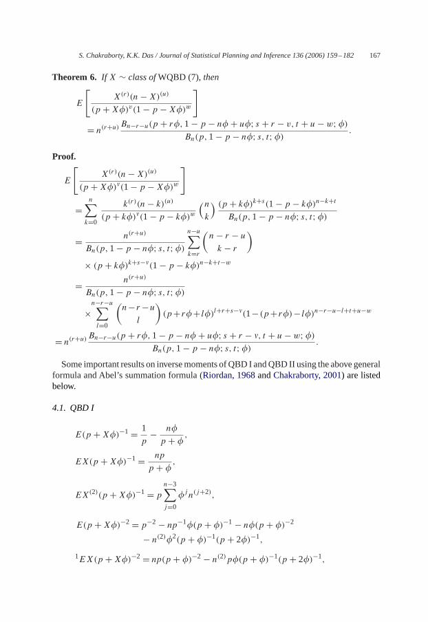
Theorem 6. If X ∼ class ofWQBD (7), then
E
[X(r)(n−X)(u)
(p +X�)v(1− p −X�)w
]
= n(r+u) Bn−r−u(p + r�,1− p − n� + u�; s + r − v, t + u− w;�)Bn(p,1− p − n�; s, t;�)
.
Proof.
E
[X(r)(n−X)(u)
(p +X�)�(1− p −X�)w
]
=n∑k=0
k(r)(n− k)(u)(p + k�)�(1− p − k�)w
(nk
) (p + k�)k+s(1− p − k�)n−k+tBn(p,1− p − n�; s, t;�)
= n(r+u)
Bn(p,1− p − n�; s, t;�)
n−u∑k=r
(n− r − uk − r
)× (p + k�)k+s−�(1− p − k�)n−k+t−w
= n(r+u)
Bn(p,1− p − n�; s, t;�)
×n−r−u∑l=0
(n− r−ul
)(p+ r�+ l�)l+r+s−�(1− (p+ r�)− l�)n−r−u−l+t+u−w
= n(r+u) Bn−r−u(p + r�,1− p − n� + u�; s + r − �, t + u− w;�)Bn(p,1− p − n�; s, t;�)
.
Some important results on inversemoments ofQBD I andQBD II using the above generalformula and Abel’s summation formula (Riordan, 1968andChakraborty, 2001) are listedbelow.
4.1. QBD I
E(p +X�)−1 = 1
p− n�p + �
,
EX(p +X�)−1 = np
p + �,
EX(2)(p +X�)−1 = pn−3∑j=0
�j n(j+2),
E(p +X�)−2 = p−2 − np−1�(p + �)−1 − n�(p + �)−2
− n(2)�2(p + �)−1(p + 2�)−1,
1EX(p +X�)−2 = np(p + �)−2 − n(2)p�(p + �)−1(p + 2�)−1,

168 S. Chakraborty, K.K. Das / Journal of Statistical Planning and Inference 136 (2006) 159–182
EX(2)(p +X�)−2 = n(2)p
p + 2�,
EX2(p +X�)−2 = np(p + �)−2 + n(2)p2(p + �)−1(p + 2�)−1,
EX(3)(p +X�)−2 = pn−3∑j�0
�j n(j+3),
EX2(X − 1)(p +X�)−2 = pn−3∑j=0
�j n(j+3) + 2pn(2)(p + 2�)−1,
E(p +X�)−3 = p−3 − n�(p + �)−1[p−2 + p−1(p + �)−1 + (p + �)−2]+n(2)�2(p+�)−1(p+2�)−1[p−1+ (p+2�)−2+ (p + �)−1
(p + 2�)−1] + n(3)�3(p + �)−1(p + 2�)−1(p + 3�)−1,
EX(p +X�)−3 = np(p + �)−3 − n(2)p�[(p + �)−1(p + 2�)−2 + (p + �)−2
(p + 2�)−1] + n(3)�2p(p + �)−1(p + 2�)−1(p + 3�)−1,
EX(2)(p +X�)−3 = n(2)p(p + 2�)−2 − n(3)p�(p + 2�)−1(p + 3�)−1,
EX(3)(p +X�)−3 = n(3)p
p + 3�,
E(1− p −X�)−1 = 1− n�1− p − n� ,
EX(1− p −X�)−1 = np
1− p − n� ,
E(1− p − x�)−2 = 1
1− p − n�[
1− n�1− p − n� − n� 1− (n− 1)�
1− p − n� + �
],
1EX(1− p −X�)−2 = np
1− p − n�[
1
1− p − n� − (n− 1)�1− p − (n− 1)�
],
E(n−X)(1− p −X�)−2 = n(1− (n− 1)�)1− p − (n− 1)�
,
E(n−X)X(1− p −X�)−2 = n(2)p
1− p − (n− 1)�,
E(n−X)X(2)(1− p −X�)−2 = p
1− p − (n− 1)�
n−3∑�=0
n(�+3)��(p + (� + 2)�),
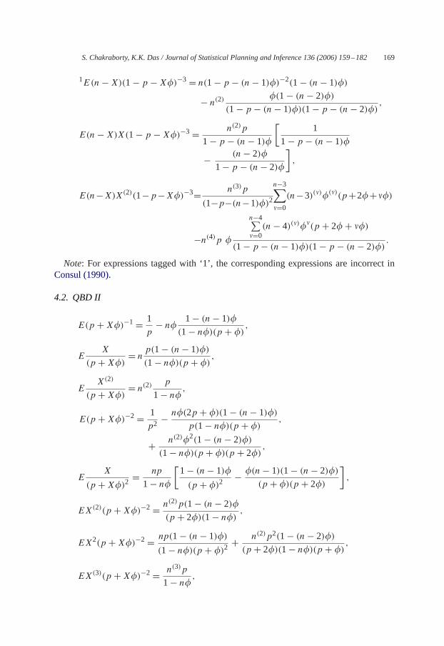
S. Chakraborty, K.K. Das / Journal of Statistical Planning and Inference 136 (2006) 159–182169
1E(n−X)(1− p −X�)−3 = n(1− p − (n− 1)�)−2(1− (n− 1)�)
− n(2) �(1− (n− 2)�)(1− p − (n− 1)�)(1− p − (n− 2)�)
,
E(n−X)X(1− p −X�)−3 = n(2)p
1− p − (n− 1)�
[1
1− p − (n− 1)�
− (n− 2)�1− p − (n− 2)�
],
E(n−X)X(2)(1−p−X�)−3= n(3)p
(1−p−(n−1)�)2
n−3∑�=0
(n−3)(�)�(�)(p+2�+��)
−n(4)p �
n−4∑�=0(n− 4)(�)��(p + 2� + ��)
(1− p − (n− 1)�)(1− p − (n− 2)�).
Note: For expressions tagged with ‘1’, the corresponding expressions are incorrect inConsul (1990).
4.2. QBD II
E(p +X�)−1 = 1
p− n� 1− (n− 1)�
(1− n�)(p + �),
EX
(p +X�)= n p(1− (n− 1)�)(1− n�)(p + �)
,
EX(2)
(p +X�)= n(2) p
1− n� ,
E(p +X�)−2 = 1
p2− n�(2p + �)(1− (n− 1)�)
p(1− n�)(p + �),
+ n(2)�2(1− (n− 2)�)(1− n�)(p + �)(p + 2�)
,
EX
(p +X�)2= np
1− n�[1− (n− 1)�
(p + �)2− �(n− 1)(1− (n− 2)�)
(p + �)(p + 2�)
],
EX(2)(p +X�)−2 = n(2)p(1− (n− 2)�(p + 2�)(1− n�) ,
EX2(p +X�)−2 = np(1− (n− 1)�)
(1− n�)(p + �)2+ n(2)p2(1− (n− 2)�)(p + 2�)(1− n�)(p + �)
,
EX(3)(p +X�)−2 = n(3)p
1− n� ,

170 S. Chakraborty, K.K. Das / Journal of Statistical Planning and Inference 136 (2006) 159–182
EX2(X − 1)(p +X�)−2 = n(2)p
1− n�[(n− 2)+ 2(1− (n− 2)�)
p + 2�
],
EX(p +X�)−3 = np
(1− n�)(p + �)
[1+ 1− p − n�
p + �
]+ n
(2)p�1− n�[
1+ (1− p − n�)(p + 2�)
+ 1
p + �+ 1− p − n�(p + �)(p + 2�)
]
+ n(3)p�2(1− p − n�)(1− n�)(p + 2�)(p + 3�)
,
EX(2)(p +X�)−3 = p
1− n�
[n(2)(1− (n− 2)�)
p + 2�− n
(3)�(1− (n− 3)�)(p + 2�)(p + 3�)
],
EX(3)(p +X�)−3 = n(3)p(1− (n− 3)�)(1− n�)(p + 3�)
,
E(1− p −X�)−1 = 1
1− p − n� − np(1− (n− 1)�)1− n� ,
EX(1− p −X�)−1 = p
1− n�
[n
1− p − n� − n(2)�1− p − (n− 1)�
],
E(1− p − x�)−2 = 1
1− n�[
1− n�(1− p − n�)2
− n� (2− 2p − (2n− 1)�)(1− (n− 1)�)
(1− p − n�)(1− p − (n− 1)�)2
+ n(2)�2 1− (n− 2)�(1− p − (n− 1)�)(1− p − (n− 2)�)
],
EX(1− p −X�)−2 = np
1− n�
[(1− p − n�)2
1− p − (n− 2)�
− (n− 1)(2− 2p − (2n− 1)�)
(1− p − n�)(1− p − (n− 1)�)2
+ (n− 1)(2)�2
1− p − (n− 1)�
],
E(n−X)(1− p −X�)−2 = n(1− p − n�)1− n�
[1− (n− 1)�
1− p − (n− 1)�
− �(n− 1)(1− (n− 2)�)(1− p − (n− 1)�)(1− p − (n− 2)�)
],

S. Chakraborty, K.K. Das / Journal of Statistical Planning and Inference 136 (2006) 159–182171
E(n−X)X(1− p −X�)−2 = n(2)p(1− p − n�)(1− n�)(1− p − (n− 1)�)
[1
1− p − (n− 1)�
− �(n− 2)
1− p − (n− 2)�
],
E
[(n−X)X(2)(1− p −X�)2
]= n
(3)p(1− p − n�)1− n�
[∑n−3�=0 ��(n− 3)(�)(p + 2� + ��)
(1− p − (n− 1)�)2
− (n− 3)�∑n−4
�=0 ��(n− 4)(�)(p + 2� + ��)(1− p − (n− 1)�)(1− p − (n− 2)�)
],
E
[(n−X)
(1− p −X�)3
]= n(1− p − n�)
1− n�[
1− (n− 1)�
(1− p − (n− 1)�)3
− (n− 1)�(2p + 3�)(1− (n− 2)�)
(1− p − (n− 1)�)2(1− p − (n− 2)�)2
+ (n−1)(2)�2(1− (n−3)�)(1−p− (n−1)�)(1−p− (n−2)�)(1− p − (n− 3)�)
],
E(n−X)X(1−p−X�)−3= n(2)p(1−p−n�)(1−n�)(1−p− (n−1)�)
[1
(1−p− (n−1)�)2
− (n− 2)�(2p + 3�)
(1− p − (n− 1)�)(1− p − (n− 2)�)2
+ (n− 2)(2)�2
(1− p − (n− 2)�)(1− p − (n− 3)�)
].
4.3. Inverse factorial moments
Theorem 7. If X ∼ class ofWQBD (7), then
E
[1
(X+1)[r]
]= E
[1
(X + r)(r)]
= Bn+r (p − r�,1− p − n�; s − r, t;�)
(n+ 1)[r]Bn(p,1− p − n�; s, t;�)
−∑r−1l�0
(n+rl
)(p− r�+ l�)l+(s−r)(1−p+ (r − l)�)n+r−l+t(n+1)[r]Bn(p,1−p−n�; s, t;�)
,
whereX[r] =X(X + 1) · · · (X + r − 1).

172 S. Chakraborty, K.K. Das / Journal of Statistical Planning and Inference 136 (2006) 159–182
Proof.
E
[1
(X + 1)[r]
]= E
[1
(X + r)(r)]
=n∑k=0
1
(k + 1)[r](nk
) (p + k�)k+s(1− p − k�)n−k+tBn(p,1− p − n�; s, t;�)
=∑nk=0
(n+rk+r
)(p − r� + (k + r)�)k+r+s−r (1− (p − r�)− (k + r)�)n+r−(k+r)+t
(n+ 1)[r]Bn(p,1− p − n�; s, t;�)
=∑n+rl=r
(n+rl
)(p − r� + l�)l+s−r (1− (p − r�)− l�)n+r−l+t(n+ 1)[r]Bn(p,1− p − n�; s, t;�)
=∑n+rl=0
(n+rl
)(p − r� + l�)l+s−r (1− (p − r�)− l�)n+r−l+t(n+ 1)[r]Bn(p,1− p − n�; s, t;�)
−∑r−1l=0
(n+rl
)(p − r� + l�)l+s−r (1− (p − r�)− l�)n+r−l+t(n+ 1)[r]Bn(p,1− p − n�; s, t;�)
= Bn+r (p − r�,1− p − n�; s − r, t;�)
(n+ 1)[r]Bn(p,1− p − n�; s, t;�)
−∑r−1l�0
(n+rl
)(p − r� + l�)l+(s−r)(1− p + (r − l)�)n+r−l+t(n+ 1)[r]Bn(p,1− p − n�; s, t;�)
.
Putting� = 0, we get for binomial distribution (Johnson et al., 1992, p. 109) withparametersn, p
E
[1
(X + r)(r)]
= 1− ∑r−1l=0
(n+rl
)pl(1− p)n+r−l
(n+ r)(r)pr .
In particular, the following results can be derived for
4.3.1. QBD I
E
[1
X + 1
]= p
(n+ 1)(p − �)2[1− (n+ 1)� − (1− p + �)n+1],
E
[1
(X + 1)(X + 2)
]= p(p − �)−2(p − 2�)−3
(n+ 1)(n+ 2)[p(p − �)2
− p�(n+ 2)(p − 2�)(2p − 3�)
+ (n+ 1)(n+ 2)(p − �)(p − 2�)2
− (p − �)2(1− p + 2�)n+2
− (n+ 2)(p − 2�)3(1− p + �)n+1].

S. Chakraborty, K.K. Das / Journal of Statistical Planning and Inference 136 (2006) 159–182173
4.3.2. QBD II
E
[1
X + 1
]
= p(1− (n+1)�)+�(n+1)(1−n�)(p−�)+p(1−p − n�)(1− p + �)n
(n+ 1)(1− n�)(p − �)2,
E
[1
(X + 1)(X + 2)
]= 1
(n+ 1)(n+ 2)(1− n�)(p − �)2(p − 2�)3{p(p − �)(1− (n+ 2)�)
+ np�(2p − 3�)(1− (n+ 1)�)(p − 2�)+ n(2)�2(1− n�)(p − 2�)2
− (p − �)p(1− p − n�)(1− p − 2�)n+1
+ (n+ 2)p(1− p − n�)(p − 2�)3(1− p + �)n(p − �)−1}.
5. Mode of the class of WQBDs
Consul (1990)obtained bounds for the mode of QBD I. Here an attempt has been madeto find similar results for the class of WQBDs.
Theorem 8. Denoting the mode by m, it is observed that m lies between l and u where l isthe real positive root of the equation
�2m3 − [2n− 1+ 2(t − 1)]m2�2 + [1− p(1+ (s + 1)� − 2�− 2n� + n� + (t − 1)�)− 2� + (s + 1)�(1− n� − (t − 1)�)
− 2n�(1− n� − (t − 1)�)]m+ (1− p)2+ n(p + (s + 1)�)(1− p − n� − (t − 1)�)>0
and
u= (n+ 1)(p + (s − 1)�)1− (n− (t + s)+ 2)�
.
Proof. Similar to the one provided for QBD I inConsul (1990).
It is seen that fors = −1, t = 0 the above result reduces to the bound given byConsul(1990).(We have noticed some printing errors, in theConsul (1990)result. Like in Eq. (4.2) the
last expression should be(1− p −m� + �) not (1− p −m� − �) and in the line beforethe line preceding Eq. (4.2) one more expression(1− p−M�) should be multiplied withthe expressions in the right-hand side of the inequality.)Similar bounds for other distributions belonging to theWQBDclass can be easily derived
using the above result.
174 S. Chakraborty, K.K. Das / Journal of Statistical Planning and Inference 136 (2006) 159–182
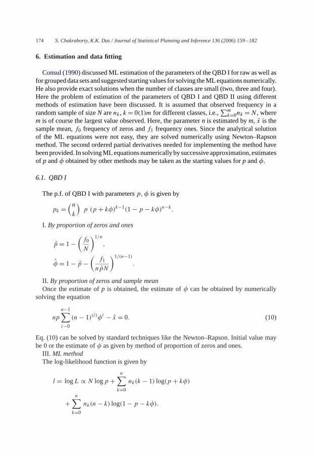
6. Estimation and data fitting
Consul (1990)discussedML estimation of the parameters of theQBD I for raw aswell asforgroupeddatasetsandsuggestedstartingvalues for solving theMLequationsnumerically.He also provide exact solutions when the number of classes are small (two, three and four).Here the problem of estimation of the parameters of QBD I and QBD II using differentmethods of estimation have been discussed. It is assumed that observed frequency in arandom sample of sizeN arenk, k = 0(1)m for different classes, i.e.,
∑mk=0nk =N , where
m is of course the largest value observed. Here, the parametern is estimated bym, x is thesample mean,f0 frequency of zeros andf1 frequency ones. Since the analytical solutionof the ML equations were not easy, they are solved numerically using Newton–Rapsonmethod. The second ordered partial derivatives needed for implementing the method havebeenprovided. In solvingMLequationsnumerically bysuccessiveapproximation, estimatesof p and� obtained by other methods may be taken as the starting values forp and�.
6.1. QBD I
The p.f. of QBD I with parametersp,� is given by
pk =(nk
)p (p + k�)k−1(1− p − k�)n−k.
I. By proportion of zeros and ones
p = 1−(f0
N
)1/n
,
� = 1− p −(f1
npN
)1/(n−1)
.
II. By proportion of zeros and sample meanOnce the estimate ofp is obtained, the estimate of� can be obtained by numerically
solving the equation
np
n−1∑i−0
(n− 1)(i)�i − x = 0. (10)
Eq. (10) can be solved by standard techniques like the Newton–Rapson. Initial value maybe 0 or the estimate of� as given by method of proportion of zeros and ones.III. ML methodThe log-likelihood function is given by
l = logL ∝ N logp +n∑k=0
nk(k − 1) log(p + k�)
+n∑k=0
nk(n− k) log(1− p − k�).

S. Chakraborty, K.K. Das / Journal of Statistical Planning and Inference 136 (2006) 159–182175
The two likelihood equations obtained by partially differentiatingl w.r.t.p and� are
�l�p
= Np
+n∑k=0
nk(k − 1)
p + k� −n∑k=0
nk(n− k)1− p − k� = 0,
⇒ h= 0, say.
�l��
=n∑k=0
nk(k − 1)k
p + k� −n∑k=0
nk(n− k)k1− p − k� = 0,
⇒ g = 0, say.
The partial derivatives ofh andgw.r.t.p and� are
�h�p
= − Np2
−n∑k=0
nk(k − 1)
(p + k�)2 −n∑k=0
nk(n− k)(1− p − k�)2 ,
�g�p
= −n∑k=0
nk(k − 1)k
(p + k�)2 −n∑k=0
nk(n− k)k(1− p − k�)2 ,
�g��
= −n∑k=0
nk(k − 1)k2
(p + k�)2 −n∑k=0
nk(n− k)k2(1− p − k�)2 .
It may be noted that
�h��
= �g�p.
[It may be noted that in Section 7 ofConsul (1990)in p. 496 the expressions for the secondorder partial derivatives of likelihood function given in Eqs. (7.7) and (7.8) were incorrect.Also the initial value formula in Eq. (7.14) in p. 497 may lead to complex values for theinitial value for�.]
6.2. QBD II
The p.f. of QBD II is given by
pk =[p(1− p − n�)
1− n�] (nk
)(p + k�)k−1(1− p − k�)n−k−1, 1− n� �= 0.
I. By proportion of zeros and onesFirst, the estimate of the parameterp is obtained by numerically solving the following
equation(1− p − (1− p)n − p0
n[(1− p)n−1 − p0]) [np
(1− p − (1− p)n − p0
(1− p)n−1 − p0
)]1/(n−2)
−[p
(1− (1− p)n − p0
(1− p)n−1 − p0
)]1/(n−2)
= 0 (11)

176 S. Chakraborty, K.K. Das / Journal of Statistical Planning and Inference 136 (2006) 159–182
Using the Newton–Rapson method, one can get a root of (11). Then the estimate of theparameter� is obtained from the equation
n� = (1− p)n − p0(1− p)n−1 − p0
(12)
II. Sample proportion of zeros and the meanThe estimate ofp is obtained by numerically solving the following equation:
p(1− p)n−1(n− x)− np0p = 0,
then substituting the value ofp in (12),� can be estimated.III. ML methodThe log-likelihood function is given by
l = logL ∝ N log
[p(1− p − n�)
1− n�]
+n∑k=0
nk(k − 1) log(p + k�)
+n∑k=0
nk(n− k − 1) log(1− p − k�).
The two likelihood equations obtained by partially differentiatingl w.r.t.p and� are
�l�p
= Np
− N
1− p − n� +n∑k=0
nk(k − 1)
p + k� −n∑k=0
nk(n− k − 1)
1− p − k� = 0
⇒ g = 0, say,
�l��
= − nNp
(1− p − n�)(1− n�) +n∑k=0
nk(k − 1)k
p + k� −n∑k=0
nk(n− k − 1)k
1− p − k� = 0
⇒ h= 0, say.
The partial derivatives ofg andhw.r.t.p and� are
�g�p
= − Np2
− N
(1− p − n�)2 −n∑k=0
nk(k − 1)
(p + k�)2 −n∑k=0
nk(n− k − 1)
(1− p − k�)2 ,
�g��
= − nN
(1− p − n�)2 −n∑k=0
nk(k − 1)k
(p + k�)2 −n∑k=0
nk(n− k − 1)k
(1− p − k�)2 ,
�h��
= n2Np(2− p − 2n�)
(1− p − n�)2(1− np)2 −n∑k=0
nk(k − 1)k2
(p + k�)2 −n∑k=0
nk(n− k − 1)k2
(1− p − k�)2 .
It may be noted that
�h�p
= �g��.

S. Chakraborty, K.K. Das / Journal of Statistical Planning and Inference 136 (2006) 159–182177
Table 1Observed and expected frequencies of European Corn borer in 1296 Corn plants
No. of borers per plant Observed no. of plants QBD I QBD II
0 907 906.41 906.451 275 277.40 277.262 88 85.90 86.013 23 22.59 22.60� 4 3 3.70 3.68
p 0.0855 0.0797
� 0.0591 0.05572 0.0758 0.0677d.f. 1 1
6.3. Some examples of data fitting
Example 1. Here, McGuire, Brindley and Bancroft’s data on the European Corn borer,used byShumway and Gurland (1960), Crow and Bardwell (1965)andConsul (1990)areconsidered.SeeTable 1.As measured by 2, QBD II gives better fit.
Example 2. Classical data derived from haemacytometer yeast cell counts observed by‘Student’ in 400 squares (Crow and Bardwell, 1965; Consul, 1990), see alsoHand et al.(1994).SeeTable 2.Here both the models give almost equally good fit, but QBD II is better. It may be noted
that for this set of data, Neyman Type A model provides better fitting than the QBDs (seeConsul, 1990, p. 500).
Example 3. Taken fromOrd et al. (1979), based on field data on D. bimaculatus by timeof the day.SeeTable 3.While both the models are equally good it can be seen that only the QBD II preserves
the symmetry of the original data. It should be noted here that QBD II is a symmetricdistribution when� = (1− 2p)/n.
Example 4. This data about the incidence of flying bombs in an area in south Londonduring World War II is taken fromFeller (1968)used byClarke (1946).
SeeTable 4.Clearly from the values ofz and expected frequencies, both the models are equally
good.

178 S. Chakraborty, K.K. Das / Journal of Statistical Planning and Inference 136 (2006) 159–182
Table 2Distribution of yeast cells per square in a haemacytometer
No. of cells per square Observed no. of squares QBD I QBD II
0 213 215.73 215.721 128 118.28 118.292 37 47.23 47.253 18 14.89 14.894 3 3.43 3.425 1 0.44 0.44
p 0.1162 0.1110
� 0.0391 0.03762 3.6087 3.6082d.f. 1 1
Table 3Distribution of number of seeds by time of day
Time Observed no. seeds QBD I QBD II
0 7 6.50 6.771 4 5.38 4.952 5 4.55 4.283 5 4.18 4.284 4 4.40 4.955 7 6.99 6.77
p 0.2729 0.1934
� 0.1346 0.12262 0.4575 0.6225d.f. 2 2
Table 4Distribution of number of hits per square
No. of hits No. of 1/4 km squares QBD I QBD II
0 229 231.35 231.351 211 203.60 203.592 93 100.24 100.263 35 33.01 33.014 7 7.04 7.045 1 0.76 0.76
p 0.1668 0.1619
� 0.0263 0.02572 0.9409 0.9344d.f. 2 2
S. Chakraborty, K.K. Das / Journal of Statistical Planning and Inference 136 (2006) 159–182179
7. Limiting distribution
Theorem 9. Asn→ ∞ andp,� → 0 such thatnp = �, n� = the class of WQBD(7)tends to the class of weighted GPD(Chakraborty, 2001)class with parameters(�; s;).Tables 1–4.
Proof. Since
limn→∞ n
s(nk
)(p + k�)k+s(1− p − k�)n−k+t = 1
k! (� + k)k+se−(�+k), (13)
hence,
limn→∞ n
sBn(p,1− p − n�; s, t;�)→ e−�K(�; s;),
whereK(a; s; z)= ∑i�0 (1/i!)e−iz(a + iz)i+s (Nandi et al., 1999; Chakraborty, 2001).
Therefore,(nk
)(p + k�)k+s(1− p − k�)n−k+tBn(p,1− p − n�; s, t;�)
→ (� + k)k+se−k
k!K(�; s;).
In particular it can be easily seen that both QBD I and QBD II tend to GPD (Consul andJain 1973a, b).
Appendix A.
Some results related to a class of Abel’s generalisations of binomial identities(Chakraborty, 2001; Riordan, 1968) which are used repeatedly in deriving many resultsof the paper have been presented here.The general form of the class of the Able sums is given by
Bn(a1, a2; s, t; z)=n∑k=0
(nk
)(a1 + kz)k+s(a2 + (n− k)z)n−k+t .
The parameterzwill not be disposed of as it is important in the context of the present work.For z= 1,Bn(a1, a2; s, t; z) reduces toAn(a1, a2; s, t) of Riordan (1968).
Bn(a1, a2; −4,0; z)= a−4
1 (a1 + a2 + nz)n − nza−11 (a + z)−1[a−2
1 + a−11 (a1 + z)−1
+ (a1 + z)−2](a1 + a2 + nz)n−1 + n(2)z2a−11 (a1 + z)−1(a1 + 2z)−1[a−1
1
+ (a1 + 2z)−2 + (a1 + z)−1(a1 + 2z)−1](a1 + a2 + nz)n−2
+ n(3)z3a−11 (a1 + z)−1(a1 + 2z)−1(a1 + 3z)−1(a1 + a2 + nz)n−3,

180 S. Chakraborty, K.K. Das / Journal of Statistical Planning and Inference 136 (2006) 159–182
Bn(a1, a2; −3,0; z)= a−3
1 (a1 + z)−2(a1 + 2z)−1[(a1 + z)2(a1 + 2z)(a1 + a2 + nz)n− nza1(a1 + 2z)(2a1 + z)(a1 + a2 + nz)n−1 + n(n− 1)a21z
2(a1 + z)× (a1 + a2 + nz)n−2],
Bn(a1, a2; −2,0; z)= a−21 (a1 + z)−1[(a1 + z)(a1 + a2 + nz)n− nza1(a1 + a2 + nz)n−1],
Bn(a1, a2; −1,0; z)= a−11 (a1 + a2 + nz)n,
Bn(a1, a2;0,0; z)= (a1 + a2 + nz+ z�)n,Bn(a1, a2;1,0; z)= (a1 + a2 + nz+ z� + z�′(a1))n,
Bn(a1, a2;2,0; z)= (a1 + a2 + nz+ z� + z�′(a1;2))n+ (a1 + a2 + nz+ z�(2)+ z�′(a1))n,
Bn(a1, a2;3,0; z)= (a1 + a2 + nz+ z� + z�′(a1;3))n+ 3(a1 + a2 + nz+ z�(2)+ z�′(a1)+ z�′(a1))n
+ (a1 + a2 + nz+ z�(2)+ z�′(0)+ z�′(a1))n
+ (a1 + a2 + nz+ z�(3)+ z′(a1))n,
Bn(a1, a2; −3,−1; z)= a1 + a2a31a2
(a1 + a2 + nz)n−1 − nz(2a1 + z)(a1 + a2 + z)a21(a1 + z)2a2
(a1 + a2 + nz)n−2 + n(n− 1)z2(a1 + a2 + 2z)
a1(a1 + z)(a1 + 2z)a2(a1 + a2 + nz)n−3,
Bn(a1, a2; −2,−1; z)= a1 + a2a21a2
(a1 + a2 + nz)n−1 − nz(a1 + a2 + z)(a1 + z)a2a1
(a1 + a2 + nz)n−2,
Bn(a1, a2; −1,−1; z)= a1 + a2a1a2
(a1 + a2 + nz)n−1,
Bn(a1, a2; −2,1; z)= 1
a21(a1 + a2 + nz+ z�′(a2))n
− nz
a1(a1 + z) (a1 + a2 + nz+ z�′(a2))n−1,
Bn(a1, a2; −1,1; z)= a−11 (a1 + a2 + nz+ z�′(a2))n,
Bn(a1, a2;1,1; z)= (a1 + a2 + nz+ z� + z�′(a1)+ z�′(a2))n,
Bn(a1, a2; −1,2; z)= a−11 [(a1 + a2 + nz+ z�′(a2;2))n× (a1 + a2 + nz+ z� + z�′(a2))n],

S. Chakraborty, K.K. Das / Journal of Statistical Planning and Inference 136 (2006) 159–182181
Bn(a1, a2;1,2; z)= (a1 + a2 + nz+ z� + z�′(a1)+ z�′(a2;2))n,Bn(a1, a2;2,2; z)= [(a1 + a2 + nz+ �z+ z�′(a1;2))n
× (a1 + a2 + nz+ z�(2)+ z�′(a1)+ z�′(a2;2))n+ (a1 + a2 + nz+ z�(2)+ z�′(a1;2)+ z�′(a2))n
+ (a1 + a2 + nz+ z�(3)+ z�′(a1)+ z�′(a2))n],
Bn(a1, a2; −2,−2; z)= a1 + a2a21a
22
(a1 + a2 + nz)n−1
− nz(a1 + a2 + z)a21a
22(a1 + z)(a2 + z) (a1 + a2 + nz)n−2
{a2(a1 + z)+ a1(a2 + z)} + n(2)z2(a1 + a2 + 2z)
a1a2(a1 + z)(a2 + z)(a1 + a2 + nz)n−3,
where
�k ≡ �k = k!,
�k(j) ≡ �k(j)= (� + · · · + �︸ ︷︷ ︸j terms
)k =(k + j − 1
k
)k!,
�′k(x) ≡ �′k(x)= k!(x + kz),
�′k(x) ≡ �′k(x)= (kz)k! (x + kz),
′k(x) ≡ ′k(x)= (kz) (kz)k!(x + kz)
and
�′k(x; j)= [�′(x)+ · · · + �′(x)︸ ︷︷ ︸j terms
]k.
wherein ‘z’ is of course the ‘z’ in Bn(a1, a2; s, t; z). Puttingz = 1, all the correspondingresults forAn(a1, a2; s, t) tabulated in p. 23 ofRiordan (1968)can be obtained.It may be noted here thatBn(a1, a2; s, t; z)= Bn(a2, a1; t, s; z).
References
Berg, S., 1985. Generating discrete distributions from modified Charlier type B expansions. Contributions toProbability and Statistics in honour of Gunnar Blom, Lund, pp. 39–48.
Berg, S., Mutafchiev, L., 1990. Random mapping with an attracting center: Lagrangian distributions and aregression function. J. Appl. Probab. 27, 622–636.
Berg, S., Nowicki, K., 1991. Statistical inference for a class ofmodified power series distributionswith applicationsto random mapping theory. J. Statist. Plann. Inference 28, 247–261.
Chakraborty, S., 2001. Some aspects of discrete probability distributions. Ph. D. Thesis, Tezpur University, Tezpur,Assam, India.

182 S. Chakraborty, K.K. Das / Journal of Statistical Planning and Inference 136 (2006) 159–182
Chakraborty, S., Das, K., 2000. An unified discrete probability model. J. Assam Science Society 41 (1), 15–25.Charalambides, C., 1990.Abel series distributionswith applications to fluctuation of sample functions of stochastic
processes. Comm. Statist. Theory Methods 19, 317–335.Clarke, R., 1946. An application of the Poisson distribution. J. Inst. Actuaries 72, 48.Consul, P., 1974. A simple urn model dependent upon predetermined strategy. Sankhy¯a 36 (Series B, Part 4), 391
–399.Consul, P., 1990. On some properties and applications of quasi-binomial distribution. Comm. Statist. Theory
Methods 19 (2), 477–504.Consul, P., Jain, G., 1973a. A generalization of the Poisson distribution. Technometrics 15, 791–799.Consul, P., Jain, G., 1973b. On some interesting properties of the generalized Poisson distribution. Biometrische
Z. 15, 495–500.Consul, P., Mittal, S., 1975. A new urn model with predetermined strategy. Biometrische Z. 17, 67–75.Crow, E., Bardwell, G., 1965. Estimation of the parameters of the hyper-Poisson distributions. In: Patil, G.P. (Ed.),
Classical and Contagious Discrete Distributions, Calcutta Statistical Publishing Society, Calcutta; PeragamonPress, Oxford, pp. 127-140.
Das, K., 1993. Some aspects of a class of quasi-binomial distributions. Assam Statist. Rev. 7 (1), 33–40.Das, K., 1994. Some aspects of discrete distributions. Ph. D. Thesis, Gauhati University, Guwahati 781014,Assam,
India.Feller, W., 1968. An Introduction to Probability Theory and its Applications, vol. 1, third ed.. Wiley, NewYork.Gupta, R., 1975. Some characterisations of discrete distributions by properties of their moment distributions.
Comm. Statist. 4, 761–765.Hand, D., Daly, F., Lunn, A., McConway, K., Ostrooski, E., 1994. A Handbook of Small Data Sets, Chapman &
Hall, London, UK.Janardan, K., 1975. Markov-Polya urn model with predetermined strategies—I. Gujrat Statist. Rev. 2 (1), 17–32.Jaworski, J., 1984. On random mapping(t, pj ). J. Appl. Probab. 21, 186–191.Johnson, N., Kotz, S., Kemp, A., 1992. Univariate Discrete Distributions, Second ed. Wiley, NewYork.Mishra, A., Tiwary, D., Singh, S., 1992. A class of quasi-binomial distributions. Sankhy¯a, Ser. B 54 (1), 67–76.Mishra, A., Singh, A., 2000. Moments of the quasi-binomial distribution. Assam Statist. Rev. 13 (1), 13–20.Nandi, S., Nath, D., Das, K., 1999. A class of generalized Poisson distribution. Statistica LIX (4), 487–498.Ord, J., Patil, G., Tallie, C., 1979. Statistical distribution in ecology, International Publishing House, USA.Riordan, J., 1958. An Introduction to Combinatorial Theory, Wiley, NewYork.Riordan, J., 1968. Combinatorial Identities, Wiley, NewYork.Shumway, R., Gurland, J., 1960. A fitting procedure for some generalized Poisson distributions. Skandinavisk
Aktuarietidskrift 43, 87–108.