Embed Size (px)
Citation preview
1
ON MONITORING MIXTURE WEIBULL PROCESSES
USING MIXTURE QUANTITY CHARTS
Zaheer Ahmed, Muhammad Riaz and Muhammad Aslam
ABSTRACT
The study proposes a cumulative quantity control chart, based on the mixture of two
components Weibull model, namely -chart. The design structure of the proposed chart
is developed by using the cumulative quantity examined between non-conformities ( ) as the
charting statistic. The performance of the proposed -chart is evaluated in terms of
some popular measures like average run length and average length of inspection, and the
existing cumulative quantity control chart is discussed as its special case. An extension of the
proposal is also suggested in the form of -chart based on the cumulative quantity
between non-conformities until nonconformities happened in one or both components of
the mixture model. The implementation of the proposed chart is also shown on a dataset for
practical demonstration.
KEY WORDS:
Average Run Length ( ); Average Length of Inspection ( ); CQC Chart; MWQ-chart;
Nonconformities.
2
1. INTRODUCTION
Control chart is one of the popular tools among the “magnificent seven” and is commonly
used for monitoring the discrete and/or continuous variables. These charts may be classified
into variable and attribute control charts. In the list of attribute charts, the and control
charts are quite popular for nonconformities. The control structure for these charts may be
constructed using the Poisson distribution and under certain circumstances normal
approximation theory may also serve the purpose. For constant events occurrence rates,
cumulative quantity/time control charts are suggested in literature like CQC chart, CQC-
chart, -chart (cf. Chan et al. (2000), Xie et al. (2002a&b) among others). In CCC and CQC
charts, the plotting statistic is the cumulative count and quantity until one nonconforming
item and nonconformities are observed. Chan et al. (2002) proposed the cumulative
probability control chart (CPC) to overcome the drawbacks of CQC and CCC control charts.
In (CPC) chart the plotted statistic is the cumulative probability instead of cumulative count
and cumulative quantity. Mehmood at el. (2012) suggested control charts for location based
on different sampling schemes. Different type of ranked set sampling strategies for
monitoring the process mean are suggested by Al-Omari and Haq (2011). Following these
authors, Majeed et al. (2012) proposed MCCC-chart for mixture Geometric process
characteristics when population of nonconforming items consists of two sub-populations due
to two types of defects.
Taking the inspiration from the said approaches, this study is planned to introduce a
mixture quantity control chart based on the mixture of Weibull distributed processes (namely
MWQ-chart) when population of nonconformities consists of two sub-populations due to two
types of nonconformities. The study proposal covers both the classical and Bayesian setups
3
for process monitoring. The rest of the article is arranged as: Section 2 outlines the CQC-
chart based on simple Weibull model and introduces the MWQ-chart followed by the
description about the Bayes estimates and the corresponding Bayes posterior risks using
informative and uninformative priors under different Loss Functions; Section 3 provides the
control structure of the proposed MWQ-chart and discusses its special cases; Section 4
evaluates the performance of the proposals and provides some comparisons; for
demonstration purposes, an application of the proposed chart with a real dataset is given in
Section 5; finally, Section 6 includes some concluding remarks and suggestions for the future
research.
2. CHART FOR MIXTURE WEIBULL MODELS
In many reliability applications, Weibull model appears as an appropriate choice for the
Time Between Events (TBE) data which may cover increasing/decreasing and constant event
occurrence rates. Let the said rate for poisson process and represents the cumulative
quantity monitored between nonconformities, are distributed Weibully with mean (
⁄ ) ( and being the scale and shape parameters respectively) and cumulative
distribution function (CDF) given as:
( ) ( ) (1)
The CQC-chart for the said process behavior is defined in the form of its control limits (i.e.
Upper Control Limit (UCL), Central Line (CL) and Lower Control Limit (LCL)) by Xie et al.
(2002a) and is given as:
UCL: (
)
[ (
)]
, CL: (
)
[ ( )]
, LCL (
)
[ (
)]
where represents the false alarm rate and serves the purpose of plotting quantity for
process monitoring. The one sided versions may easily be defined on the similar lines.
4
In many practical situations of reliability monitoring the two components mixture of
Weibull models suitably models the phenomenon of two types of nonconformities e.g. the
fracture of silica optical fibers are due to strength of optical fibers and ceramic materials
which leads to a mixture Weibull model. For such processes we develop the structure of the
mixture cumulative quantity control chart (MWQ-chart) under classical and Bayesian
frameworks. Let and represent the fractions of nonconformities produced by Poisson
process from sub-populations I and II respectively then the distribution of (that becomes a
two component Weibull distribution) and its corresponding CDF are given as:
( ) ( ) ( ) ( ) (2)
( ) ( ) ( ) ( ) ( )
where ( ) and ( ) represent the two density functions and ( ) and ( ) are the
corresponding CDFs for the said mixture Weibull model. The quantities and
represent mixing proportions such that 0 1. By substitutions, (3) may be expressed as:
( ) { ( )} ( ){ (
)} ( )
The scale parameters and , and the separating quantity are generally unknown
and hence need to be estimated. We estimate these quantities here using Maximum
Likelihood Estimation (MLE) and Bayesian Estimation particularly the Bayes Estimates
(BEs) of these unknown parameters using different loss functions. The loss functions
considered here include Squared Error Loss Function (SELF), Quadratic Loss Function
(QLF), Weighted Loss Function (WLF) and Precautionary Loss Function (PLF). The prior
choices covered are Uniform Prior (UP), Jeffreys Prior (JP) and Informative Prior (IP). The
Bayes Posterior Risks (BPRs) are also worked out for the above mentioned cases.
MLEs: For a two-component mixture with items under study, let be the failures due to
reason 1; for reason 2 and represents the survivals at time/quantity when
testing is stopped. Then the likelihood expression is given as (cf. Mendenhall and Hader
(1958)):
5
( ) {∏ ( )
}{∏( ) ( )
} { ( )}
where is defined as the th failure belonging to sub-populations, where
and . For the MLEs of and of the aforementioned mixture model we have the
following non-closed form expressions given as:
∑ ( )
( ) (
)
{ ( ) ( ) (
)}
∑ ( )
( ) (
)
{ ( ) ( ) (
)}
( )
( )( ){ (
) ( )}
{ ( ) ( ) (
)}
These expressions can be solved iteratively using a suitable package like SAS .
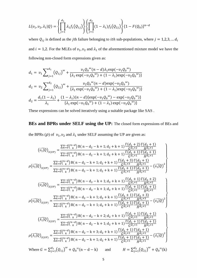
BEs and BPRs under SELF using the UP: The closed form expressions of BEs and
the BPRs ( ) of and under SELF assuming the UP are given as:
( ) ( ) ∑ (
)
( ) ( )
( )
∑ ( )
( ) ( )
( )
( ) ( ) ∑ ( ) ( )
( )
( )
∑ ( )
( ) ( )
( )
( )
}
( ) ( ) ∑ (
)
( ) ( )
( )
∑ ( )
( ) ( )
( )
( ) ( ) ∑ ( ) ( )
( )
( )
∑ ( )
( ) ( )
( )
( )
}
( ) ( ) ∑ (
)
( ) ( )
( )
∑ ( )
( ) ( )
( )
( ) ( ) ∑ ( ) ( )
( )
( )
∑ ( )
( ) ( )
( )
( )
}
Where ∑ ( )
( ) and ∑ ( )
( )
6
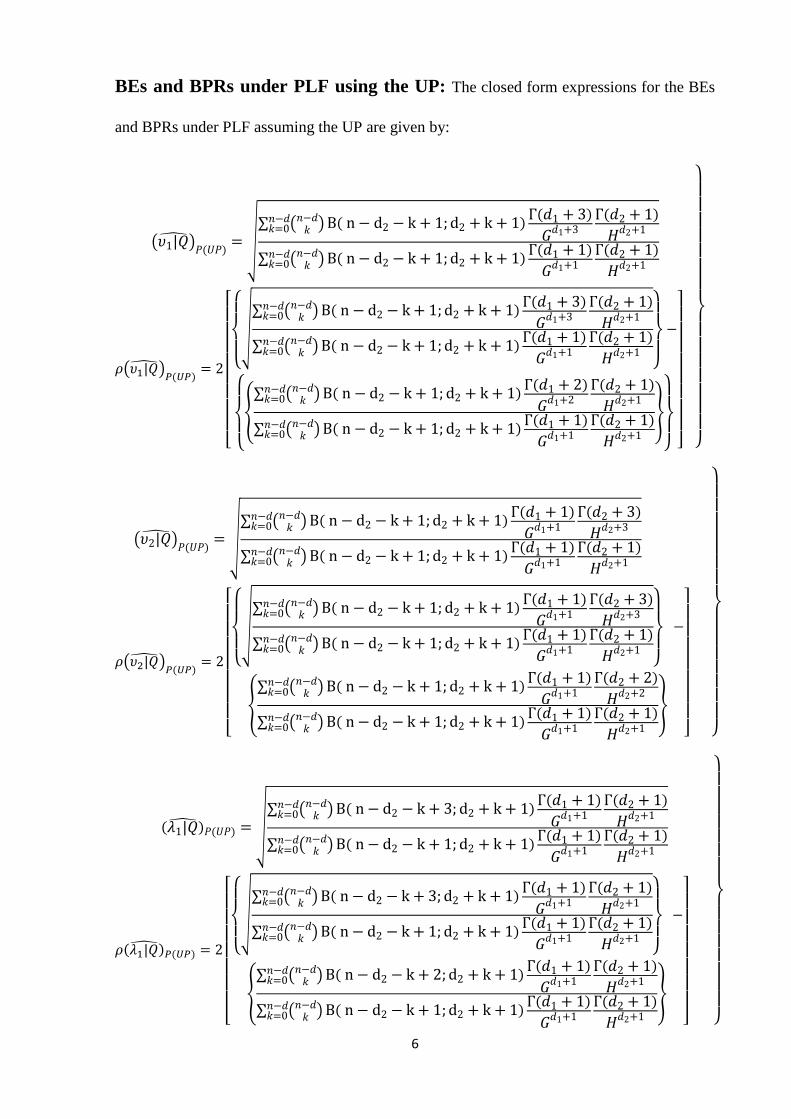
BEs and BPRs under PLF using the UP: The closed form expressions for the BEs
and BPRs under PLF assuming the UP are given by:
( ) ( ) √∑ ( ) ( )
( )
( )
∑ ( ) ( )
( )
( )
( ) ( )
[
{
√
∑ ( ) ( )
( )
( )
∑ ( ) ( )
( )
( )
}
{
{
∑ ( ) ( )
( )
( )
∑ ( ) ( )
( )
( )
}
}
]
}
( ) ( ) √∑ ( ) ( )
( )
( )
∑ ( ) ( )
( )
( )
( ) ( )
[
{
√
∑ ( ) ( )
( )
( )
∑ ( ) ( )
( )
( )
}
{
∑ ( ) ( )
( )
( )
∑ ( ) ( )
( )
( )
}
]
}
( ) ( ) √
∑ ( ) ( )
( )
( )
∑ ( ) ( )
( )
( )
( ) ( )
[
{
√
∑ ( ) ( )
( )
( )
∑ ( ) ( )
( )
( )
}
{
∑ ( ) ( )
( )
( )
∑ ( ) ( )
( )
( )
}
]
}
7
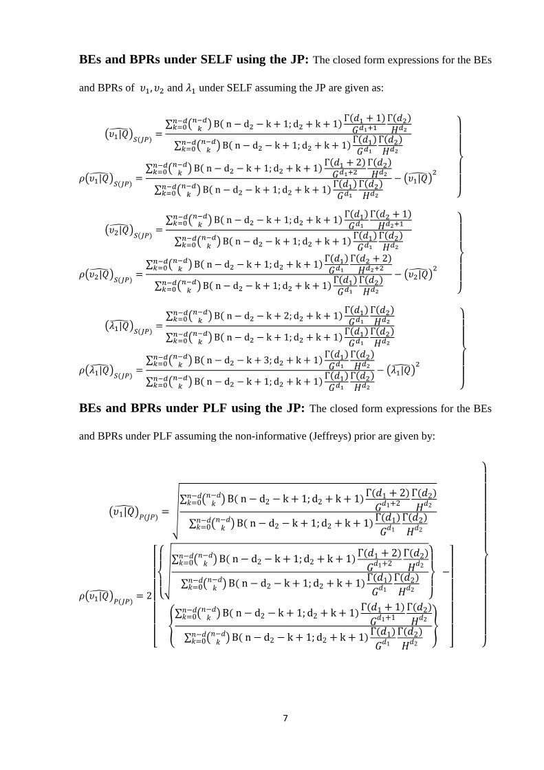
BEs and BPRs under SELF using the JP: The closed form expressions for the BEs
and BPRs of and under SELF assuming the JP are given as:
( ) ( ) ∑ (
)
( ) ( )
( )
∑ ( )
( ) ( )
( )
( ) ( ) ∑ ( ) ( )
( )
( )
∑ ( )
( ) ( )
( )
( )
}
( ) ( ) ∑ (
)
( ) ( )
( )
∑ ( )
( ) ( )
( )
( ) ( ) ∑ ( ) ( )
( )
( )
∑ ( )
( ) ( )
( )
( )
}
( ) ( ) ∑ (
)
( ) ( )
( )
∑ ( )
( ) ( )
( )
( ) ( ) ∑ ( ) ( )
( )
( )
∑ ( )
( ) ( )
( )
( )
}
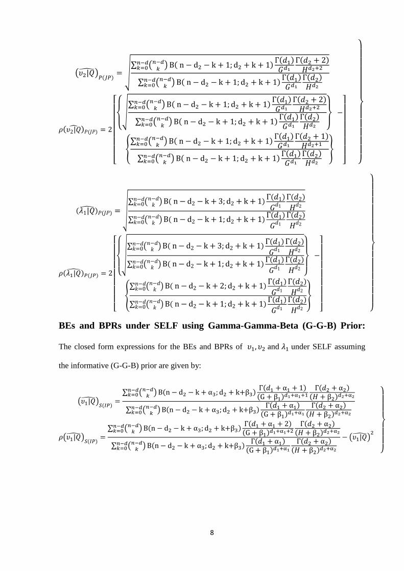
BEs and BPRs under PLF using the JP: The closed form expressions for the BEs
and BPRs under PLF assuming the non-informative (Jeffreys) prior are given by:
( ) ( ) √∑ ( ) ( )
( )
( )
∑ ( ) ( )
( )
( )
( ) ( )
[
{
√
∑ ( ) ( )
( )
( )
∑ ( ) ( )
( )
( )
}
{
∑ ( ) ( )
( )
( )
∑ ( ) ( )
( )
( )
}
]
}
8
( ) ( ) √∑ (
)
( ) ( )
( )
∑ ( )
( ) ( )
( )
( ) ( )
[
{
√∑ (
)
( ) ( )
( )
∑ ( )
( ) ( )
( ) }
{∑ (
)
( ) ( )
( )
∑ ( )
( ) ( )
( )
}
]
}
( ) ( ) √
∑ ( ) ( )
( )
( )
∑ ( ) ( )
( )
( )
( ) ( )
[
{
√
∑ ( ) ( )
( )
( )
∑ ( ) ( )
( )
( )
}
{
∑ ( ) ( )
( )
( )
∑ ( ) ( )
( )
( )
}
]
}
BEs and BPRs under SELF using Gamma-Gamma-Beta (G-G-B) Prior:
The closed form expressions for the BEs and BPRs of and under SELF assuming
the informative (G-G-B) prior are given by:
( ) ( ) ∑ (
)
( ) ( )( )
( )( )
∑ ( )
( ) ( )( )
( )( )
( ) ( ) ∑ ( ) ( )
( )( )
( )( )
∑ ( )
( ) ( )( )
( )( )
( )
}
9
( ) ( ) ∑ (
)
( ) ( )( )
( )( )
∑ ( )
( ) ( )( )
( )( )
( ) ( ) ∑ ( ) ( )
( )( )
( )( )
∑ ( )
( ) ( )( )
( )( )
( )
}
( ) ( )
∑ ( )
( ) ( )
( )
( )
( )
∑ ( )
( ) ( )
( )
( )
( )
( ) ( )
∑ ( )
( ) ( )
( )
( )
( )
∑ ( )
( ) ( )
( )
( )
( )
( )
}
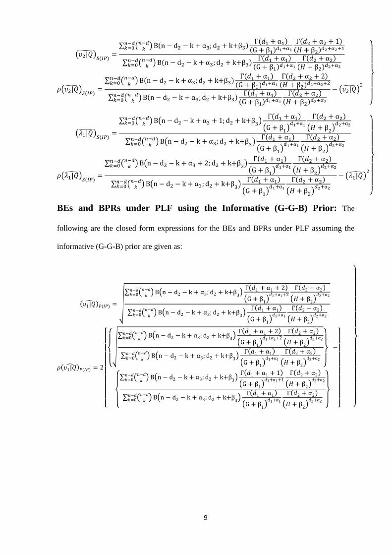
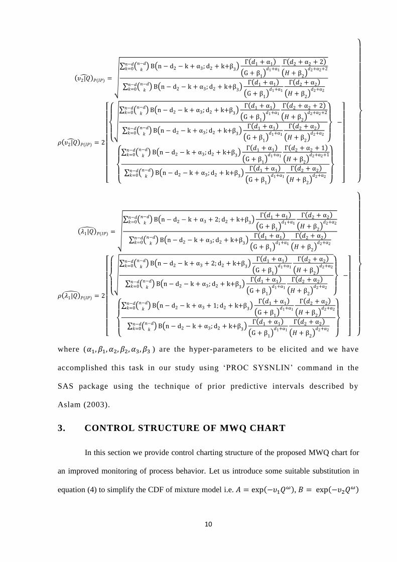
BEs and BPRs under PLF using the Informative (G-G-B) Prior: The
following are the closed form expressions for the BEs and BPRs under PLF assuming the
informative (G-G-B) prior are given as:
( ) ( ) √
∑ ( )
( ) ( )
( )
( )
( )
∑ ( )
( ) ( )
( )
( )
( )
( ) ( )
[
{
√
∑ ( )
( ) ( )
( )
( )
( )
∑ ( )
( ) ( )
( )
( )
( )
}
{
∑ (
)
( ) ( )
( )
( )
( )
∑ ( )
( ) ( )
( )
( )
( )
}
]
}
10
( ) ( ) √
∑ ( )
( ) ( )
( )
( )
( )
∑ ( )
( ) ( )
( )
( )
( )
( ) ( )
[
{
√
∑ ( )
( ) ( )
( )
( )
( )
∑ ( )
( ) ( )
( )
( )
( )
}
{
∑ (
)
( ) ( )
( )
( )
( )
∑ ( )
( ) ( )
( )
( )
( )
}
]
}
( ) ( ) √
∑ ( )
( ) ( )
( )
( )
( )
∑ ( )
( ) ( )
( )
( )
( )
( ) ( )
[
{
√
∑ ( )
( ) ( )
( )
( )
( )
∑ ( )
( ) ( )
( )
( )
( )
}
{
∑ (
)
( ) ( )
( )
( )
( )
∑ ( )
( ) ( )
( )
( )
( )
}
]
}
where ( ) are the hyper-parameters to be elicited and we have
accomplished this task in our study using ‘PROC SYSNLIN’ command in the
SAS package using the technique of prior predictive intervals described by
Aslam (2003).
3. CONTROL STRUCTURE OF MWQ CHART
In this section we provide control charting structure of the proposed MWQ chart for
an improved monitoring of process behavior. Let us introduce some suitable substitution in
equation (4) to simplify the CDF of mixture model i.e. ( ), (
)
11
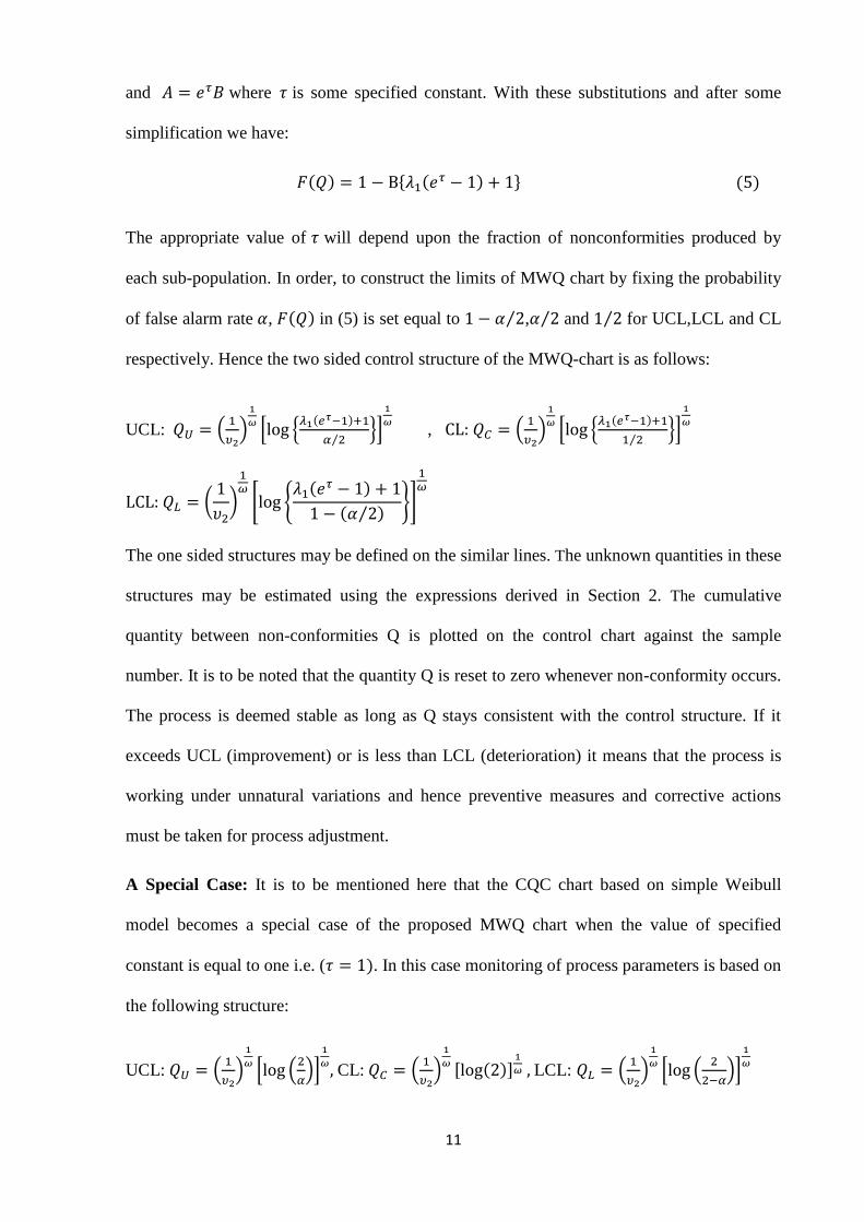
and where is some specified constant. With these substitutions and after some
simplification we have:
( ) { ( ) } ( )
The appropriate value of will depend upon the fraction of nonconformities produced by
each sub-population. In order, to construct the limits of MWQ chart by fixing the probability
of false alarm rate , ( ) in (5) is set equal to ⁄ , ⁄ and ⁄ for UCL,LCL and CL
respectively. Hence the two sided control structure of the MWQ-chart is as follows:
UCL: (
)
[ {
( )
⁄}]
, (
)
[ {
( )
⁄}]
(
)
[ {
( )
( ⁄ )}]
The one sided structures may be defined on the similar lines. The unknown quantities in these
structures may be estimated using the expressions derived in Section 2. The cumulative
quantity between non-conformities Q is plotted on the control chart against the sample
number. It is to be noted that the quantity Q is reset to zero whenever non-conformity occurs.
The process is deemed stable as long as Q stays consistent with the control structure. If it
exceeds UCL (improvement) or is less than LCL (deterioration) it means that the process is
working under unnatural variations and hence preventive measures and corrective actions
must be taken for process adjustment.
A Special Case: It is to be mentioned here that the CQC chart based on simple Weibull
model becomes a special case of the proposed MWQ chart when the value of specified
constant is equal to one i.e. ( ). In this case monitoring of process parameters is based on
the following structure:
UCL: (
)
[ (
)]
CL: (
)
[ ( )]
LCL: (
)
[ (
)]
12
4. PERFORMANCE EVALUATIONS
This section is devoted to evaluate the performance of the proposal of the study for an
effective monitoring of process ability. We have used different popular performance
measures including Average Run Length (ARL) and Average Length of Inspection (ALI) for
different objectives.
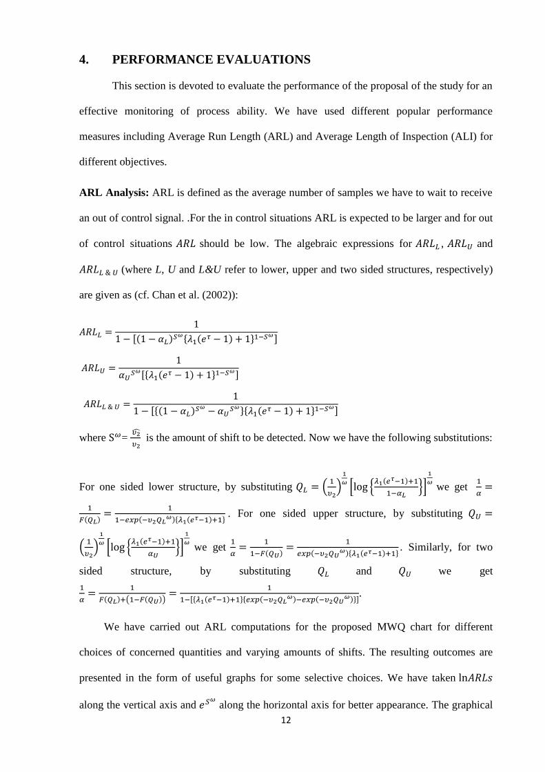
ARL Analysis: ARL is defined as the average number of samples we have to wait to receive
an out of control signal. .For the in control situations ARL is expected to be larger and for out
of control situations should be low. The algebraic expressions for , and
(where L, U and L&U refer to lower, upper and two sided structures, respectively)
are given as (cf. Chan et al. (2002)):
[( ) { (
) } ]
[{ (
) } ]
[{( )
}{ ( ) }
]
where =
is the amount of shift to be detected. Now we have the following substitutions:
For one sided lower structure, by substituting (
)
[ {
( )
}]
we get
( )
( ){ ( ) }
. For one sided upper structure, by substituting
(
)
[ {
( )
}]
we get
( )
( ){ ( ) }
. Similarly, for two
sided structure, by substituting and we get
( ) ( ( ))
[{ ( ) }{ ( ) (
)}].
We have carried out ARL computations for the proposed MWQ chart for different
choices of concerned quantities and varying amounts of shifts. The resulting outcomes are
presented in the form of useful graphs for some selective choices. We have taken
along the vertical axis and
along the horizontal axis for better appearance. The graphical
13
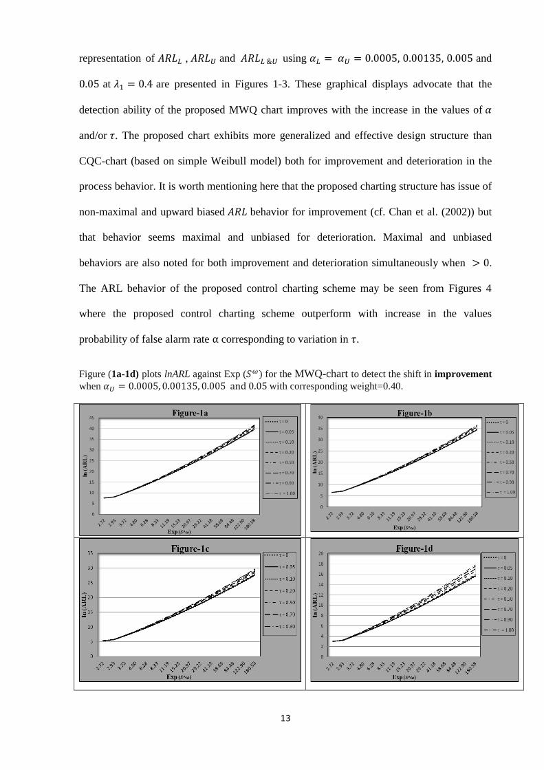
representation of , and using and
at are presented in Figures 1-3. These graphical displays advocate that the
detection ability of the proposed MWQ chart improves with the increase in the values of
and/or . The proposed chart exhibits more generalized and effective design structure than
CQC-chart (based on simple Weibull model) both for improvement and deterioration in the
process behavior. It is worth mentioning here that the proposed charting structure has issue of
non-maximal and upward biased behavior for improvement (cf. Chan et al. (2002)) but
that behavior seems maximal and unbiased for deterioration. Maximal and unbiased
behaviors are also noted for both improvement and deterioration simultaneously when .
The ARL behavior of the proposed control charting scheme may be seen from Figures 4
where the proposed control charting scheme outperform with increase in the values
probability of false alarm rate corresponding to variation in .
Figure (1a-1d) plots lnARL against Exp ( ) for the MWQ-chart to detect the shift in improvement
when with corresponding weight=0.40.
14
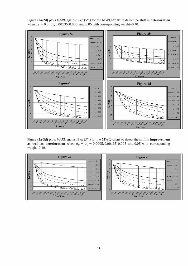
Figure (2a-2d) plots lnARL against Exp ( ) for the MWQ-chart to detect the shift in deterioration
when with corresponding weight=0.40.
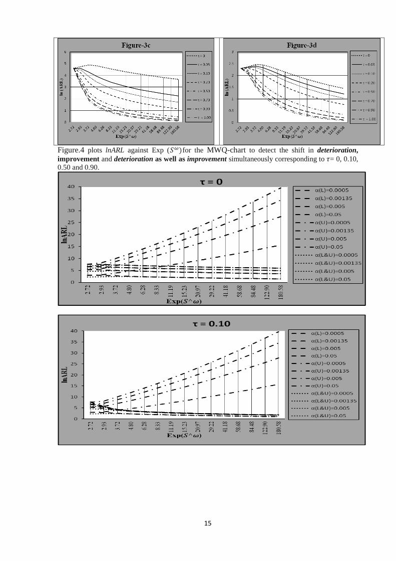
Figure (3a-3d) plots lnARL against Exp ( ) for the MWQ-chart to detect the shift in improvement
as well as deterioration when with corresponding
weight=0.40.
15
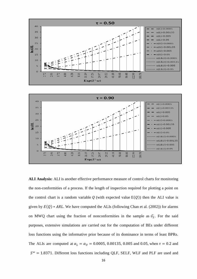
Figure.4 plots lnARL against Exp ( )for the MWQ-chart to detect the shift in deterioration,
improvement and deterioration as well as improvement simultaneously corresponding to = 0, 0.10,
0.50 and 0.90.
16
ALI Analysis: ALI is another effective performance measure of control charts for monitoring
the non-conformities of a process. If the length of inspection required for plotting a point on
the control chart is a random variable (with expected value ( )) then the ALI value is
given by ( ) . We have computed the ALIs (following Chan et al. (2002)) for alarms
on MWQ chart using the fraction of nonconformities in the sample as . For the said
purposes, extensive simulations are carried out for the computation of BEs under different
loss functions using the informative prior because of its dominance in terms of least BPRs.
The ALIs are computed at and when and
. Different loss functions including QLF, SELF, WLF and PLF are used and
17
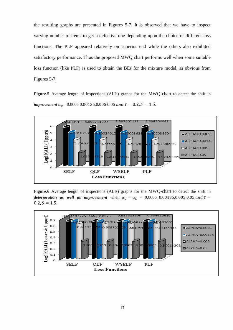
the resulting graphs are presented in Figures 5-7. It is observed that we have to inspect
varying number of items to get a defective one depending upon the choice of different loss
functions. The PLF appeared relatively on superior end while the others also exhibited
satisfactory performance. Thus the proposed MWQ chart performs well when some suitable
loss function (like PLF) is used to obtain the BEs for the mixture model, as obvious from
Figures 5-7.
Figure.5 Average length of inspections (ALIs) graphs for the MWQ-chart to detect the shift in
improvement = 0.0005 .
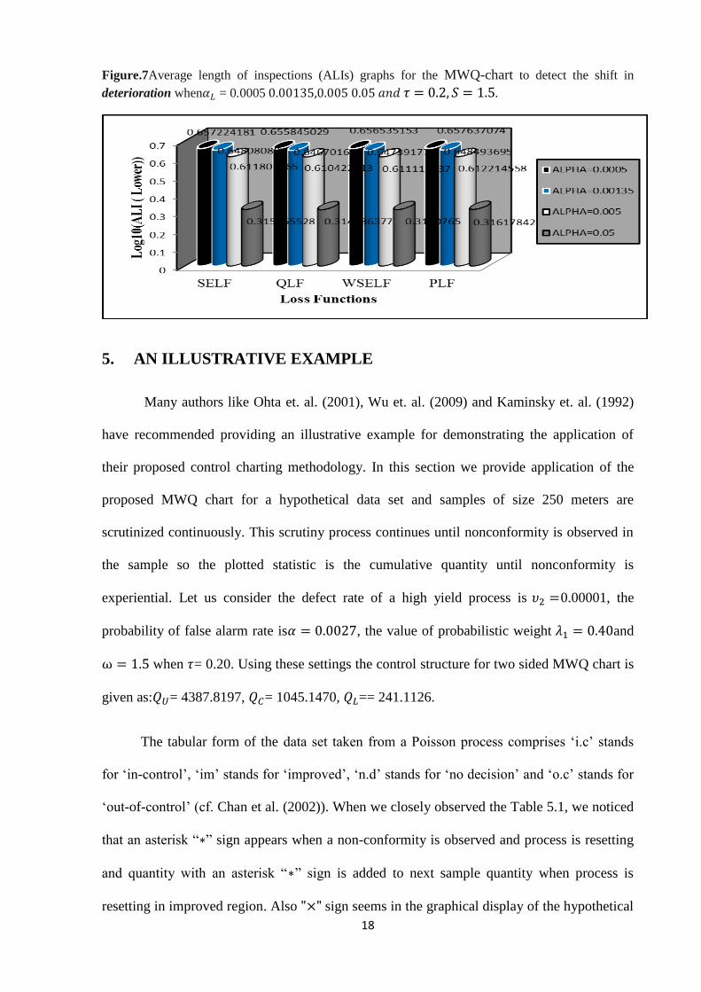
Figure.6 Average length of inspections (ALIs) graphs for the MWQ-chart to detect the shift in
deterioration as well as improvement when = 0.0005 .
18
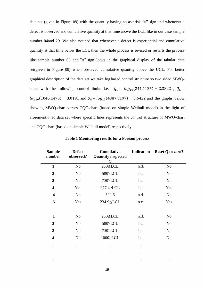
Figure.7Average length of inspections (ALIs) graphs for the MWQ-chart to detect the shift in
deterioration when = 0.0005 .
5. AN ILLUSTRATIVE EXAMPLE
Many authors like Ohta et. al. (2001), Wu et. al. (2009) and Kaminsky et. al. (1992)
have recommended providing an illustrative example for demonstrating the application of
their proposed control charting methodology. In this section we provide application of the
proposed MWQ chart for a hypothetical data set and samples of size 250 meters are
scrutinized continuously. This scrutiny process continues until nonconformity is observed in
the sample so the plotted statistic is the cumulative quantity until nonconformity is
experiential. Let us consider the defect rate of a high yield process is 0.00001, the
probability of false alarm rate is , the value of probabilistic weight and
when = 0.20. Using these settings the control structure for two sided MWQ chart is
given as: = 4387.8197, = 1045.1470, == 241.1126.
The tabular form of the data set taken from a Poisson process comprises ‘i.c’ stands
for ‘in-control’, ‘im’ stands for ‘improved’, ‘n.d’ stands for ‘no decision’ and ‘o.c’ stands for
‘out-of-control’ (cf. Chan et al. (2002)). When we closely observed the Table 5.1, we noticed
that an asterisk “ ” sign appears when a non-conformity is observed and process is resetting
and quantity with an asterisk “ ” sign is added to next sample quantity when process is
resetting in improved region. Also sign seems in the graphical display of the hypothetical
19
data set (given in Figure 09) with the quantity having an asterisk “ ” sign and whenever a
defect is observed and cumulative quantity at that time above the LCL like in our case sample
number 04and 29. We also noticed that whenever a defect is experiential and cumulative
quantity at that time below the LCL then the whole process is revised or restarts the process
like sample number 05 and sign looks in the graphical display of the tabular data
set(given in Figure 09) when observed cumulative quantity above the UCL. For better
graphical description of the data set we take log based control structure so two sided MWQ-
chart with the following control limits i.e. = ( ) , =
( ) and = ( ) and the graphs below
showing MWQ-chart verses CQC-chart (based on simple Weibull model) in the light of
aforementioned data set where specific lines represents the control structure of MWQ-chart
and CQC-chart (based on simple Weibull model) respectively.
Table 1 Monitoring results for a Poisson process
Sample
number
Defect
observed?
Cumulative
Quantity inspected
Q
Indication Reset Q to zero?
1 No 250 LCL n.d. No
2 No 500≥LCL i.c. No
3 No 750≥LCL i.c. No
4 Yes 977.4≥LCL i.c. Yes
4 No *22.6 n.d. No
5 Yes
234.9 LCL
o.c.
Yes
1 No 250 LCL n.d. No
2 No 500≥LCL i.c. No
3 No 750≥LCL i.c. No
4 No 1000≥LCL i.c. No
. . . . .
. . . . .
. . . . .
20
17 No 4250≥LCL i.c. No
18 No 4500>UCL Im. No
. . . . .
. . . . .
. . . . .
28 No 7000>UCL Im. No
29 Yes 7155.2>UCL Im. Yes
29 No *94.8 n.d. No
30
.
No
.
344.8≤LCL
.
n.d.
.
No
.
. . . . .
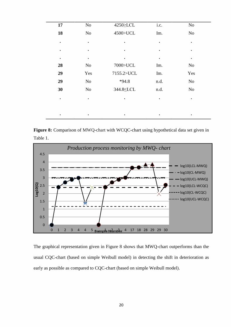
Figure 8: Comparison of MWQ-chart with WCQC-chart using hypothetical data set given in
Table 1.
The graphical representation given in Figure 8 shows that MWQ-chart outperforms than the
usual CQC-chart (based on simple Weibull model) in detecting the shift in deterioration as
early as possible as compared to CQC-chart (based on simple Weibull model).
0
0.5
1
1.5
2
2.5
3
3.5
4
4.5
0 1 2 3 4 4 5 1 2 3 4 17 18 28 29 29 30
Log1
0(Q
)
Production process monitoring by MWQ- chart
log10(LCL-MWQ)
log10(CL-MWQ)
log10(UCL-MWQ)
log10(LCL-WCQC)
log10(CL-WCQC)
log10(UCL-WCQC)
21
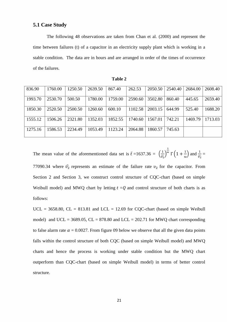
5.1 Case Study
The following 48 observations are taken from Chan et al. (2000) and represent the
time between failures (t) of a capacitor in an electricity supply plant which is working in a
stable condition. The data are in hours and are arranged in order of the times of occurrence
of the failures.
Table 2
836.90 1760.00 1250.50 2639.50 867.40 262.53 2050.50 2540.40 2684.00 2608.40
1993.70 2530.70 500.50 1780.00 1759.00 2590.60 3502.80 860.40 445.65 2659.40
1850.30 2520.50 2500.50 1260.60 600.10 1102.58 2003.15 644.99 525.40 1688.20
1555.12 1506.26 2321.80 1352.03 1852.55 1740.60 1567.01 742.21 1469.79 1713.03
1275.16 1586.53 2234.49 1053.49 1123.24 2064.88 1860.57 745.63
The mean value of the aforementioned data set is =1637.36 = (
)
(
) and
=
77090.34 where represents an estimate of the failure rate for the capacitor. From
Section 2 and Section 3, we construct control structure of CQC-chart (based on simple
Weibull model) and MWQ chart by letting = and control structure of both charts is as
follows:
UCL = 3658.80, CL = 813.81 and LCL = 12.69 for CQC-chart (based on simple Weibull
model) and UCL = 3689.05, CL = 878.80 and LCL = 202.71 for MWQ chart corresponding
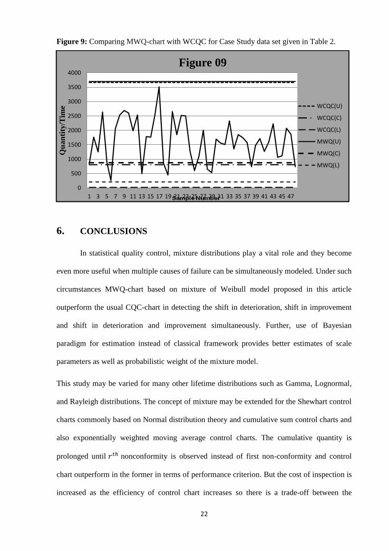
to false alarm rate = 0.0027. From figure 09 below we observe that all the given data points
falls within the control structure of both CQC (based on simple Weibull model) and MWQ
charts and hence the process is working under stable condition but the MWQ chart
outperform than CQC-chart (based on simple Weibull model) in terms of better control
structure.
22
Figure 9: Comparing MWQ-chart with WCQC for Case Study data set given in Table 2.
6. CONCLUSIONS
In statistical quality control, mixture distributions play a vital role and they become
even more useful when multiple causes of failure can be simultaneously modeled. Under such
circumstances MWQ-chart based on mixture of Weibull model proposed in this article
outperform the usual CQC-chart in detecting the shift in deterioration, shift in improvement
and shift in deterioration and improvement simultaneously. Further, use of Bayesian
paradigm for estimation instead of classical framework provides better estimates of scale
parameters as well as probabilistic weight of the mixture model.
This study may be varied for many other lifetime distributions such as Gamma, Lognormal,
and Rayleigh distributions. The concept of mixture may be extended for the Shewhart control
charts commonly based on Normal distribution theory and cumulative sum control charts and
also exponentially weighted moving average control charts. The cumulative quantity is
prolonged until nonconformity is observed instead of first non-conformity and control
chart outperform in the former in terms of performance criterion. But the cost of inspection is
increased as the efficiency of control chart increases so there is a trade-off between the
0
500
1000
1500
2000
2500
3000
3500
4000
1 3 5 7 9 11 13 15 17 19 21 23 25 27 29 31 33 35 37 39 41 43 45 47
Qu
an
tity
/Tim
e Figure 09
WCQC(U)
WCQC(C)
WCQC(L)
MWQ(U)
MWQ(C)
MWQ(L)
23
performance of control chart and cost of inspection. Furthermore, multivariate generalization
of MWQ-chart may be prospective theme for additional research in this region.
REFERENCES
Al-Omari, A. I., and Haq, A. (2011). Improved Quality Control Charts for Monitoring the
Process Mean, Using Double-Ranked Set Sampling Methods, Journal of Applied Statistics, 3
9(4), 745-763.
Aslam, M. (2003). An application of Prior Predictive distribution to elicit the prior density.
Journal of Statistical Theory and Application, 2 (1), 70- 83.
Chan, L.Y., Xie, M. and Goh, T.N. (2000). Cumulative quantity control charts for monitoring
production processes. International Journal of Production Research, 38(2), 397-408.
Chan, L.Y., Lin, D.K.J., Xie, M. and Goh, T.N. (2002). Cumulative probability control charts
for geometric and exponential process characteristics. International Journal of Production
Research, 40(1), 133-150.
Kaminsky, F. C., Benneyan, R. D., Davis, R. D. and Burke, R. J. (1992). Statistical control
charts based on a geometric distribution, Journal of Quality Technology, 24(2), 63-69.
Majeed, Y.M., Aslam, M. and Riaz, M. (2012). Mixture cumulative count control chart for
mixture geometric process characteristics. Quality and Quantity, 47 (4), 2289-2307.
Mendenhall, W. and Hadar, R. J. (1958). Estimation of parameters of mixed exponentially
dis-tributed failure time distributions from censored life test data. Biometrika, 45 (3-4) ; 504-
520.
Ohta, H., Kusukawa, E. and Rahim, A. (2001). A CCC-r chart for high-yield processes,
Quality and Reliability Engineering International, 17, 439-446.
Mehmood, R., Riaz, M., and Does, R. J. M. M. (2012). Control charts for location based on
different sampling schemes, Journal of Applied Statistics, 40(3), 483-494.
Wu, Z., Jiao, J.X. and He, Z. (2009). A control scheme for monitoring the frequency and
magnitude of an event, International Journal of Production Research, 47(11), 2887-2902.
Xie, M., Goh, T.N. and Kuralmani, V. (2002a). Statistical Models and Control charts for
High-quality Processes. Boston, Kluwer Academic Publisher.
Xie, M., Goh, T.N. and Ranjan, P. (2002b). Some effective control chart procedures for
reliability monitoring. Reliability Engineering and System Safety, 77, 143-150.


