arX

iv:h

ep-t

h/96

0114

7v1

26

Jan

1996

DAMTP 95-20

To appear in Nonlinearity

Octahedral and Dodecahedral Monopoles

Conor J. Houghton

and

Paul M. Sutcliffe∗

Department of Applied Mathematics and Theoretical Physics

University of Cambridge

Silver St., Cambridge CB3 9EW, England

c.j.houghton@damtp.cam.ac.uk & p.m.sutcliffe@damtp.cam.ac.uk

May 1995

Abstract

It is shown that there exists a charge five monopole with octahedral symmetry

and a charge seven monopole with icosahedral symmetry. A numerical implemen-

tation of the ADHMN construction is used to calculate the energy density of these

monopoles and surfaces of constant energy density are displayed. The charge five and

charge seven monopoles look like an octahedron and a dodecahedron respectively. A

scattering geodesic for each of these monopoles is presented and discussed using ra-

tional maps. This is done with the aid of a new formula for the cluster decomposition

of monopoles when the poles of the rational map are close together.

∗Address from September 1995, Institute of Mathematics, University of Kent at Canterbury, Canterbury

CT2 7NZ. Email P.M.Sutcliffe@ukc.ac.uk

1

1 Introduction

BPS monopoles are topological solitons in a three dimensional SU(2) Yang-Mills-Higgsgauge theory, in the limit of vanishing Higgs potential. They are solutions to the Bogomolnyequation

DAΦ = ⋆FA (1.1)

where DA is the covariant derivative, with A an su(2)-valued gauge potential 1-form, FA

its gauge field 2-form and ⋆ the Hodge dual on IR3. The Higgs field, Φ, is an su(2)-valued

scalar field and is required to satisfy

‖Φ‖ r→∞−→ 1 (1.2)

where r = |x| and ‖Φ‖2 = −12trΦ2. The boundary condition (1.2) can be considered to be

a residual finite energy condition, derived from the now vanished Higgs potential.The Higgs field at infinity induces a map between spheres:

Φ : S2(∞) → S2(1) (1.3)

where S2(∞) is the two-sphere at spatial infinity and S2(1) is the two-sphere of vacuumconfigurations given by {Φ ∈ su(2) : ‖Φ‖ = 1}. The degree of this map is a non-negativeinteger k which (in suitable units) is the total magnetic charge. We shall refer to a monopolewith magnetic charge k as a k-monopole. The total energy of a k-monopole is equal to8πk and the energy density may be expressed [19] in the convenient form

E = △‖Φ‖2 (1.4)

where △ denotes the laplacian on IR3.

Monopoles correspond to certain algebraic curves, called spectral curves, in the mini-twistor space TT∼=TCIP

1 [19, 7, 8]. This space is isomorphic to the space of directed linesin IR

3. If ζ is the standard inhomogeneous coordinate on the base space, it corresponds tothe direction of a line in IR

3. The fibre coordinate, η, is a complex coordinate in a planeorthogonal to this line. The spectral curve of a monopole is the set of lines along whichthe differential equation

(DA − iΦ)v = 0 (1.5)

has bounded solutions in both directions. The spectral curve of a k-monopole takes theform

ηk + ηk−1a1(ζ) + . . . + ηrak−r(ζ) + . . . + ηak−1(ζ) + ak(ζ) = 0 (1.6)

where, for 1 ≤ r ≤ k, ar(ζ) is a polynomial in ζ of maximum degree 2r. However, generalcurves of this form will only correspond to k-monopoles if they satisfy the reality condition

ar(ζ) = (−1)rζ2rar(−1

ζ) (1.7)

2

and some difficult non-singularity conditions [7]. In [6] the concept of a strongly centredmonopole is introduced. A strongly centred monopole is centred on the origin and itsrational map has total phase one. If a monopole is strongly centred its spectral curvesatisfies

a1(ζ) = 0. (1.8)

Even though the Bogomolny equation is integrable, it is not easily solved. Explicitsolutions are only known in the cases of 1-monopole [17], 2-monopoles [19, 20] and axisym-metric monopoles of higher charges [16]. Recently, progress has been made in understand-ing multi-monopoles. Hitchin, Manton and Murray [6] have demonstrated the existence ofmonopoles corresponding to the spectral curves

η3 + iΓ(1/6)3Γ(1/3)3

48√

3π3/2ζ(ζ4 − 1) = 0 (1.9)

η4 +3Γ(1/4)8

64π2(ζ8 + 14ζ4 + 1) = 0. (1.10)

The first spectral curve (1.9) has tetrahedral symmetry, the second (1.10) has octahedralsymmetry. In [9] we computed numerically and displayed surfaces of constant energydensity for these monopoles. We noted that the charge four monopole looks like a cube,rather than an octahedron. We therefore refer to this 4-monopole as a cubic monopole.

Hitchin, Manton and Murray [6] also prove that although

ζ111 ζ0 + 11ζ6

1ζ60 − ζ1ζ

110 (1.11)

is an icosahedrally invariant homogeneous polynomial of degree 12, the invariant algebraiccurve

η6 + aζ(ζ10 + 11ζ5 − 1) = 0 (1.12)

does not correspond to a monopole for any value of a. However, based upon considerationsof the symmetries of rational maps for infinite curvature hyperbolic monopoles, Atiyah hassuggested, [1] 1 that there may be an icosahedrally invariant 7-monopole. In this paper,we prove that this suggestion is correct by demonstrating that the algebraic curve

η7 +Γ(1/6)6Γ(1/3)6

64π3ζ(ζ10 + 11ζ5 − 1)η = 0 (1.13)

is the spectral curve of a monopole. Using our numerical scheme introduced in [9], we thencompute its energy density. On examining surfaces of constant energy density, we find thatthe charge seven monopole looks like a dodecahedron.

In each of the cases examined so far, the minimum charge monopole with the symmetryof a regular solid has charge k = 1

2(F + 2), where F is the smallest number of faces of a

regular solid with that symmetry. This leads us to conjecture that the minimum chargemonopole resembling a regular solid with F faces has charge k = 1

2(F +2). For the dodec-

ahedron F = 12, which gives k = 7. In fact, this conjecture was one of the motivations for

1We thank Nick Manton for drawing this to our attention

3

our consideration of charge seven when searching for an icosahedrally symmetric monopole.In this paper, we demonstrate that our conjecture is also correct for the octahedron byproving that the octahedrally symmetric algebraic curve

η5 +3Γ(1

4)8

16π2(ζ8 + 14ζ4 + 1)η = 0 (1.14)

is the spectral curve of a 5-monopole. We display its energy density and confirm thatit looks like an octahedron. It remains to be verified that an icosahedrally symmetricmonopole of charge eleven exists and resembles an icosahedron.

It is interesting that numerical evidence suggests that similar results hold in the caseof static minimum energy multi-skyrmion solutions. In [4] Braaten, Townsend and Carsonuse a discretization of the Skyrme model on a cubic lattice to calculate such solutions forbaryon numbers B = 3, 4, 5 and 6. They find that surfaces of constant baryon numberdensity resemble solids with 2B−2 faces. Furthermore, the fields describing solutions withB = 3 and B = 4 are seen to possess tetrahedral and octahedral symmetry. However, theyconclude that the solution for B = 5 seems only to have D2d symmetry. This contrastswith the existence of a charge five monopole with octahedral symmetry.

Approximations to the B = 3 and B = 4 skyrmions have been calculated by computingthe holonomies of Yang-Mills instantons [13]. These instanton generated Skyrme fieldsalso have tetrahedral and octahedral symmetry respectively. Given the numerical evidencefor an apparent difference between charge five monopoles and skyrmions, it would beinstructive to construct instanton-generated Skyrme fields with baryon number five. Itmay be that an octahedrally symmetric 5-skyrmion simply does not exist. However, theinstanton construction could shed some light on other possibilities; for example, that sucha skyrmion exists but it does not have minimum energy. A second possibility is thatthe numerical scheme used in [4] is responsible for no such skyrmion being found. Forparticular orientations, an octahedron will not fit inside a cubic lattice; in the sense of allthe vertices of the octahedron sitting on lattice sites. The discretization could then resultin the octahedron being squashed into a shape similar to that found in [4]. Of course, atthe moment, all these possibilities are pure speculation. What is clear from our resultsis that the B = 7 skyrmion should now be investigated, as there is some interest in thepossibility that this is icosahedrally symmetric.

In Section 2, we outline the ADHMN construction as applied to symmetric monopoles.In Sections 3 and 4, we present our results on dodecahedral and octahedral monopoles.Finally, in Section 5, we discuss rational maps and geodesic monopole scattering relatedto these symmetric monopoles. This is done with the aid of a new formula for the clusterdecomposition of monopoles when the poles of the rational map are close together.

2 The Nahm Equations

The main difficulty in proving that an algebraic curve is the spectral curve of amonopole lies in demonstrating satisfaction of the non-singularity conditions. However,

4

there is a reciprocal formulation of the Bogomolny equation in which non-singularity ismanifest. This formulation is the Atiyah-Drinfeld-Hitchin-Manin-Nahm (ADHMN) con-struction [15, 8]. This is an equivalence between k-monopoles and Nahm data (T1, T2, T3),which are three k × k matrices depending on a real parameter s ∈ [0, 2] and satisfying:

(i) Nahm’s equationdTi

ds=

1

2ǫijk[Tj , Tk] (2.1)

(ii) Ti(s) is regular for s ∈ (0, 2) and has simple poles at s = 0 and s = 2,

(iii) the matrix residues of (T1, T2, T3) at each pole form the irreducible k-dimensionalrepresentation of SU(2),

(iv) Ti(s) = −T †i (s),

(v) Ti(s) = T ti (2 − s).

It should be noted that in this paper we shall not search for a basis in which property(v) is explicit, but rely on a general argument that such a basis exists (see [6]).

Explicitly, the spectral curve may be read off from the Nahm data as the equation

det(η + (T1 + iT2) − 2iT3ζ + (T1 − iT2)ζ2) = 0. (2.2)

It is obvious from (2.2) that the strong centering condition (1.8) is equivalent to

(vi) trTi(s) = 0.

To extract the monopole fields (Φ, A) from the Nahm data requires the computationof a basis for the kernel of a linear differential operator constructed out of the Nahmdata, followed by some integrations. We have developed a numerical algorithm which canperform all these required tasks, the details are included in [9]. The algorithm takes asinput the Nahm data and outputs the energy density of the corresponding monopole. Itwill be applied to the Nahm data which we construct in this paper.

As in [9] we use the discrete symmetry group G of the conjectured monopole to reducethe number of Nahm equations. Since the Nahm matrices are traceless, they transformunder the rotation group as

3 ⊗ sl(k) ∼= 3 ⊗ (2k − 1 ⊕ 2k − 3 ⊕ . . . ⊕ 3)∼= (2k + 1u ⊕ 2k − 1m ⊕ 2k − 3l) ⊕ . . .

. . . ⊕(2r + 1u ⊕ 2r − 1m ⊕ 2r − 3l) ⊕ . . . ⊕ (5u ⊕ 3m ⊕ 1l) (2.3)

5

where r denotes the unique irreducible r dimensional representation of su(2) and the sub-scripts u, m and l (which stand for upper, middle and lower) are a convenient notationallowing us to distinguish between 2r + 1 dimensional representations occuring as

3 ⊗ 2r − 1 ∼= 2r + 1u ⊕ 2r − 1m ⊕ 2r − 3l,

3 ⊗ 2r + 1 ∼= 2r + 3u ⊕ 2r + 1m ⊕ 2r − 1l

and3 ⊗ 2r + 3 ∼= 2r + 5u ⊕ 2r + 3m ⊕ 2r + 1l.

We can then use invariant homogeneous polynomials over CIP1 to construct G-invariant

Nahm triplets. The vector space of degree 2r homogeneous polynomials a2rζ2r1 +a2r−1ζ

2r−11 ζ0+

. . . + a0ζ2r0 is the carrier space for 2r + 1 under the identification

X = ζ1∂

∂ζ0; Y = ζ0

∂

∂ζ1; H = −ζ0

∂

∂ζ0+ ζ1

∂

∂ζ1. (2.4)

where X, Y and H are the basis of su(2) satisfying

[X, Y ] = H, [H, X] = 2X, [H, Y ] = −2Y. (2.5)

As explained in [6, 9] if p(ζ0, ζ1) is a G-invariant homogeneous polynomial we can constructa G-invariant 2r + 1u charge k Nahm triplet by the following scheme.

(i) The inclusion

2r + 1 →֒ 3 ⊗ 2r − 1 ∼= 2r + 1u ⊕ 2r − 1m ⊕ 2r − 3l (2.6)

is given on polynomials by

p(ζ0, ζ1) 7→ ξ21 ⊗ p11(ζ0, ζ1) + 2ξ0ξ1 ⊗ p10(ζ0, ζ1) + ξ2

0 ⊗ p00(ζ0, ζ1) (2.7)

where we have used the notation

pab(ζ0, ζ1) =∂2p

∂ζa∂ζb(ζ0, ζ1). (2.8)

(ii) The polynomial expression ξ21 ⊗ p11(ζ0, ζ1) + 2ξ0ξ1 ⊗ p10(ζ0, ζ1) + ξ2

0 ⊗ p00(ζ0, ζ1) isrewritten in the form

ξ21 ⊗ q11(ζ0

∂

∂ζ1

)ζ2r1 + (ξo

∂

∂ξ1

)ξ21 ⊗ q10(ζ0

∂

∂ζ1

)ζ2r1 +

1

2(ξo

∂

∂ξ1

)2ξ21 ⊗ q00(ζ0

∂

∂ζ1

)ζ2r1 . (2.9)

(iii) This then defines a triplet of k × k matrices. Given a k × k representation of X, Yand H above, the invariant Nahm triplet is given by:

(S ′1, S

′2, S

′3) = (q11(adY )Xr, q10(adY )Xr, q00(adY )Xr), (2.10)

6

where adY denotes the adjoint action of Y and is given on a general matrix M by adY M =[M, Y ].

(iv) The Nahm isospace basis is transformed. This transformation is given by

(S1, S2, S3) = (1

2S ′

1 + S ′3,−

i

2S ′

1 + iS ′3,−iS ′

2). (2.11)

Relative to this basis the SO(3)-invariant Nahm triplet corresponding to the 1l represen-tation in (2.3) is given by (ρ1, ρ2, ρ3) where

ρ1 = X − Y ; ρ2 = i(X + Y ); ρ3 = iH. (2.12)

It is also necessary to construct invariant Nahm triplets lying in the 2r + 1m represen-tations. To do this, we first construct the corresponding 2r + 1u triplet. We then writethis triplet in the canonical form

[c0 + c1(adY ⊗ 1 + 1 ⊗ adY ) + . . . + ci(adY ⊗ 1 + 1 ⊗ adY )i (2.13)

+ . . . + c2r(adY ⊗ 1 + 1 ⊗ adY )2r] X ⊗ Xr

and map this isomorphically into 2r + 1m by mapping the highest weight vector X ⊗ Xr

to the highest weight vector

X ⊗ adY Xr+1 − 1

r + 1adY X ⊗ Xr+1. (2.14)

3 Dodecahedral Seven Monopole

The minimum degree icosahedrally invariant homogeneous polynomial is [12]

ζ111 ζ0 + 11ζ6

1ζ60 − ζ1ζ

110 . (3.1)

Polarizing this gives

ξ21⊗(110ζ9

1ζ0+330ζ41ζ

60)+2ξ1ξ0⊗(11ζ10

1 +396ζ51ζ

50 −11ζ11

0 )+ξ20⊗(330ζ6

1ζ40 −110ζ1ζ

90 ). (3.2)

This is proportional to

ξ21 ⊗ (ζ0

∂

∂ζ1

+1

5040(ζ0

∂

∂ζ1

)6)ζ101 + 2ξ1ξ0 ⊗ (1 +

1

840(ζ0

∂

∂ζ1

)5 − 1

10!(ζ0

∂

∂ζ1

)10)ζ101

+ ξ20 ⊗ (

1

168(ζ0

∂

∂ζ1)4 − 1

9!(ζ0

∂

∂ζ1)9)ζ10

1 (3.3)

which gives matrices

X ⊗ (adY +1

5040(adY )6)X5 + adY X ⊗ (1 +

1

840(adY )5 − 1

10!(adY )10)X5

+1

2(adY )2X ⊗ (

1

168(adY )4 − 1

9!(adY )9)X5. (3.4)

7

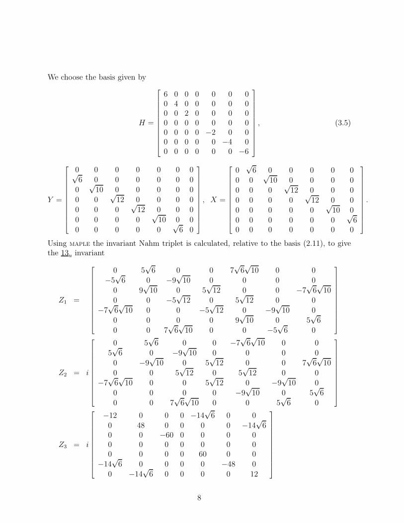
We choose the basis given by

H =

6 0 0 0 0 0 00 4 0 0 0 0 00 0 2 0 0 0 00 0 0 0 0 0 00 0 0 0 −2 0 00 0 0 0 0 −4 00 0 0 0 0 0 −6

, (3.5)

Y =

0 0 0 0 0 0 0√6 0 0 0 0 0 0

0√

10 0 0 0 0 0

0 0√

12 0 0 0 0

0 0 0√

12 0 0 0

0 0 0 0√

10 0 0

0 0 0 0 0√

6 0

, X =

0√

6 0 0 0 0 0

0 0√

10 0 0 0 0

0 0 0√

12 0 0 0

0 0 0 0√

12 0 0

0 0 0 0 0√

10 0

0 0 0 0 0 0√

60 0 0 0 0 0 0

.

Using MAPLE the invariant Nahm triplet is calculated, relative to the basis (2.11), to givethe 13u invariant

Z1 =

0 5√

6 0 0 7√

6√

10 0 0

−5√

6 0 −9√

10 0 0 0 0

0 9√

10 0 5√

12 0 0 −7√

6√

10

0 0 −5√

12 0 5√

12 0 0

−7√

6√

10 0 0 −5√

12 0 −9√

10 0

0 0 0 0 9√

10 0 5√

6

0 0 7√

6√

10 0 0 −5√

6 0

Z2 = i

0 5√

6 0 0 −7√

6√

10 0 0

5√

6 0 −9√

10 0 0 0 0

0 −9√

10 0 5√

12 0 0 7√

6√

10

0 0 5√

12 0 5√

12 0 0

−7√

6√

10 0 0 5√

12 0 −9√

10 0

0 0 0 0 −9√

10 0 5√

6

0 0 7√

6√

10 0 0 5√

6 0

Z3 = i

−12 0 0 0 −14√

6 0 0

0 48 0 0 0 0 −14√

60 0 −60 0 0 0 00 0 0 0 0 0 00 0 0 0 60 0 0

−14√

6 0 0 0 0 −48 0

0 −14√

6 0 0 0 0 12

8

To calculate the 13m invariant we put (3.4) in the form (2.14). It is proportional to

[11!(adY ⊗1+1⊗adY )+7920(adY ⊗1+1⊗adY )6−(adY ⊗1+1⊗adY )11]X⊗X5. (3.6)

Then using the isomorphism mentioned earlier we obtain matrices

Y1 =

0√

6 0 0 −√

6√

10 0 12√6 0 −3

√10 0 0 12 0

0 −3√

10 0 5√

12 0 0 −√

6√

10

0 0 5√

12 0 −5√

12 0 0

−√

6√

10 0 0 −5√

12 0 3√

10 0

0 12 0 0 3√

10 0 −√

6

12 0 −√

6√

10 0 0 −√

6 0

Y2 = i

0√

6 0 0√

6√

10 0 12

−√

6 0 −3√

10 0 0 −12 0

0 3√

10 0 5√

12 0 0√

6√

10

0 0 −5√

12 0 −5√

12 0 0

−√

6√

10 0 0 5√

12 0 3√

10 0

0 12 0 0 −3√

10 0 −√

6

−12 0 −√

6√

10 0 0√

6 0

Y3 = i

0 0 0 0 0 −10√

6 0

0 0 0 0 0 0 10√

60 0 0 0 0 0 00 0 0 0 0 0 00 0 0 0 0 0 0

10√

6 0 0 0 0 0 0

0 −10√

6 0 0 0 0 0

.

In order to derive the reduced Nahm equations we examine, the commutation relations.The required relations involving ρ matrices and Z matrices are

[ρ1, ρ2] = 2ρ3

[Z1, Z2] = −750ρ3 + 90Z3 (3.7)

[Z1, ρ2] + [ρ1, Z2] = −10Z3.

Because of the closed form of these relations, it is possible to derive a consistent set ofNahm equations from the icosahedrally invariant Nahm data

Ti(s) = x(s)ρi + z(s)Zi, i ∈ {1, 2, 3}. (3.8)

That is, we can consistently ignore the invariant Nahm triplet (Y1, Y2, Y3). In fact, if we addy(s)Yi to (3.8), we cannot simultaneously satisfy Ti(s) = −T †

i (s) and the reality condition

9

(1.7) for non-trivial y(s). Combining (3.7) and (3.8) gives the reduced Nahm equations

dx

ds= 2x2 − 750z2 (3.9)

dz

ds= −10xz + 90z2

with corresponding spectral curve

η[η6 + aζ(ζ10 + 11ζ5 + 1)] = 0 (3.10)

wherea = 552960(14xz − 175z2)(x + 5z)4 (3.11)

is a constant.To solve equations (3.9), let u = x + 5z and v = x − 30z so that

du

ds= 2uv

dv

ds= 6u2 − 4v2

a = 110592(u6 − v2u4) ≡ 110592κ6. (3.12)

Using the constant to eliminate v, the equation for u becomes

du

ds= −2u2

√1 − κ6u−6. (3.13)

If we let u = −κ√

℘(t), where t = 2κs, then ℘(t) is the Weierstrass function satisfying

℘′2 = 4(℘3 − 1) (3.14)

where, in the above and what follows, primed functions are differentiated with respect totheir arguments. Thus the Nahm equations are solved by

x(s) =2κ

7

[

−3√

℘(2κs) +℘′(2κs)

4℘(2κs)

]

(3.15)

z(s) = − κ

35

[

√

℘(2κs) +℘′(2κs)

2℘(2κs)

]

. (3.16)

These functions are analytic in s ∈ (0, 2) and have simple poles at s = 0, 2 providedκ = ω, where 2ω is the real period of ℘(t). Since ω is explicitly known for this Weierstrassfunction, we have

κ =Γ(1/6)Γ(1/3)

8√

3π(3.17)

10

and so

a = 110592κ6 =Γ(1/6)6Γ(1/3)6

64π3. (3.18)

Near s = 0

℘(2κs) ∼(

1

2κs

)2

(3.19)

and so the residues of x and z are −1/2 and 0 respectively. At s = 2 they are, respectively,−5/14 and −1/35. At both poles the eigenvalues of the matrix residue of iT3 may becalculated and are {±3,±2,±1, 0}. This demonstrates that the matrix residues definethe irreducible 7-dimensional representation at each end of the interval. Hence, we haveproved the existence of a 7-monopole with icosahedral symmetry given by the spectralcurve (1.13).

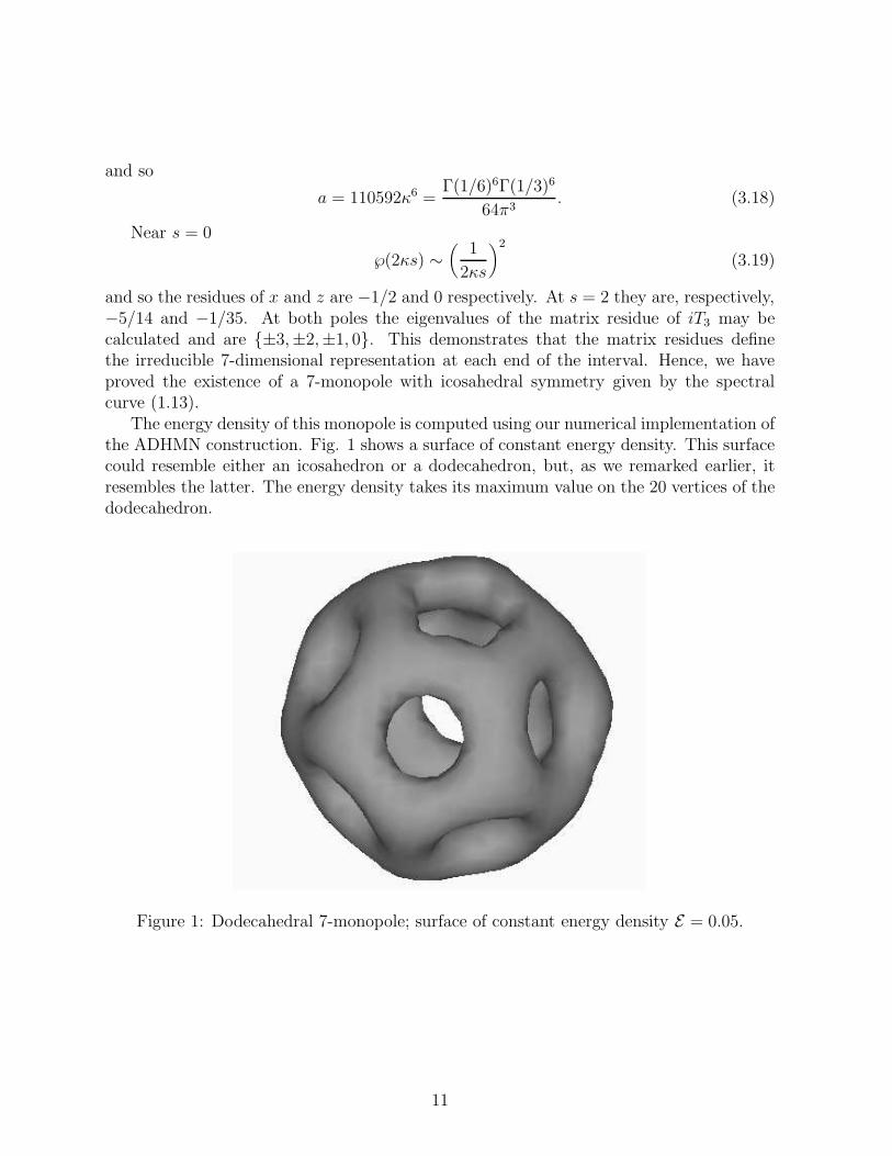
The energy density of this monopole is computed using our numerical implementation ofthe ADHMN construction. Fig. 1 shows a surface of constant energy density. This surfacecould resemble either an icosahedron or a dodecahedron, but, as we remarked earlier, itresembles the latter. The energy density takes its maximum value on the 20 vertices of thedodecahedron.

Figure 1: Dodecahedral 7-monopole; surface of constant energy density E = 0.05.

11

4 Octahedral Five Monopole

The lowest degree octahedrally invariant homogeneous polynomial is [12]

ζ81 + 14ζ4

1ζ40 + ζ8

0 . (4.1)

Polarizing this gives

ξ21 ⊗ (56ζ6

1 + 168ζ21ζ

40) + 2ξ1ξ0 ⊗ (224ζ3

1ζ30 ) + ξ2

0 ⊗ (56ζ60 + 168ζ4

1ζ20 ) (4.2)

which we write in the form

ξ21 ⊗ (56+

7

15(ζ0

∂

∂ζ1

)4)ζ61 +2ξ1ξ0⊗

28

15(ζ0

∂

∂ζ1

)3ζ61 + ξ2

0 ⊗ (7

90(ζ0

∂

∂ζ1

)6 +28

5(ζ0

∂

∂ζ1

)2)ζ61 (4.3)

giving matrices

X⊗(56+7

15(adY )4)X3+(adY )X⊗ 28

15(adY )3X3+

1

2(adY )2X⊗(

7

90(adY )6+

28

5(adY )2)X3.

(4.4)If we represent the su(2) basis (2.5) by

H =

−4 0 0 0 00 −2 0 0 00 0 0 0 00 0 0 2 00 0 0 0 4

, X = −i

0 0 0 0 02 0 0 0 0

0√

6 0 0 0

0 0√

6 0 00 0 0 2 0

, Y = i

0 2 0 0 0

0 0√

6 0 0

0 0 0√

6 00 0 0 0 20 0 0 0 0

.

this gives the invariant Nahm triplet in 9u

Y1 = i

0 −6 0 10 0

−6 0 2√

6 0 10

0 2√

6 0 2√

6 0

10 0 2√

6 0 −60 10 0 −6 0

, Y2 =

0 −6 0 −10 0

6 0 2√

6 0 −10

0 −2√

6 0 2√

6 0

10 0 −2√

6 0 −60 10 0 6 0

,

Y3 = i

8 0 0 0 00 −16 0 0 00 0 0 0 00 0 0 16 00 0 0 0 −8

.

The 9u invariant (4.4) is written in the form (2.14) as

[

56 +7

15(adY ⊗ 1 + 1 ⊗ adY )4 +

1

720(adY ⊗ 1 + 1 ⊗ adY )8

]

X ⊗ X3 (4.5)

12

which when mapped using the isomorphism produces the invariant Nahm triplet in 9m

Z1 = i

0 −1 0 −1 0

1 0√

6 0 1

0 −√

6 0 −√

6 0

1 0√

6 0 10 −1 0 −1 0

, Z2 =

0 −1 0 1 0

−1 0√

6 0 −1

0√

6 0 −√

6 0

1 0 −√

6 0 10 −1 0 1 0

,

Z3 = i

0 0 0 0 40 0 0 0 00 0 0 0 00 0 0 0 0

−4 0 0 0 0

.

In a similar fashion to the icosahedral case, we can consistently consider Nahm data ofthe form Ti(s) = x(s)ρi + y(s)Yi. The Nahm equations become

dx

ds= 2x2 − 48y2, (4.6)

dy

ds= −6xy − 8y2 (4.7)

and the spectral curve isη5 + 768κ4η(ζ8 + 14ζ4 + 1) = 0 (4.8)

whereκ4 = 5y(x + 3y)(x− 2y)2. (4.9)

Equations (4.6-4.7) are identical to those for the charge four cubic monopole [6] and aresolved by

x =2κ(5℘2(u) − 3)

5℘′(u), (4.10)

y =2κ

5℘′(u), (4.11)

where u = 2κs and ℘ is the Weierstrass elliptic function satisfying

℘′2 = 4(℘3 − ℘). (4.12)

As in [6], the argument of κ is chosen to be π/4 and u lies on the line from 0 to ω2 = ω1+ω3,where 2ω1 is the real period of the elliptic function (4.12) and 2ω3 is the imaginary period.By examining the eigenvalues of the residue of iT3 we see the boundary conditions at s = 0and s = 2 are satisfied provided,

ω2 = 4κ. (4.13)

13

This period may be explicitly calculated, with the result that there exists an octahedralmonopole with spectral curve

η5 +3Γ(1

4)8

16π2(ζ8 + 14ζ4 + 1)η = 0. (4.14)

Note that the spectral curve (1.10) of the cubic 4-monopole is

η4 + Ξ(ζ8 + 14ζ4 + 1)η = 0 (4.15)

for some constant Ξ and the spectral curve (4.14) of the octahedral 5-monopole is

η[

η4 + 4Ξ(ζ8 + 14ζ4 + 1)η]

= 0 (4.16)

where Ξ is the same constant. The spectral curve of the octahedral 5-monopole is thereforegiven by a multiplication by η of the cubic 4-monopole spectral curve, up to the factorof 4 in the constant. Rather remarkably, this is exactly how the spectral curve of theaxisymmetric 3-monopole is obtained from that of the axisymmetric 2-monopole. The twospectral curves in this case being [7]

η2 +π2

4ζ2 = 0 (4.17)

η[

η2 + π2ζ2]

= 0. (4.18)

The energy density of the 2-monopole described by (4.17) is axially symmetric, so that asurface of constant energy density is toroidal. This is also true of the 3-monopole (4.18)and the only modification is that the torus is slightly larger in size. This suggests that theoctahedral 5-monopole may resemble a cube, since the cubic 4-monopole does so, with theonly modification being that the cube will be slightly larger. The fact that equations (4.6-4.7) are identical to those obtained in the cubic 4-monopole reduction of Nahm’s equationsalso supports this hypothesis.

Using our numerical scheme, we have calculated the energy density of the octahedral5-monopole. Fig. 2 shows a surface of constant energy density for this monopole. Itresembles an octahedron (not a cube) with the energy density taking its maximum valueon the six vertices of the octahedron. We found this result quite surprising, given thecomments above. However, it is good news for our conjecture of Section 1, which claimedthat this monopole would look like an octahedron.

5 Rational Maps and Geodesic Scattering

The k-monopole moduli space Mk is the space of gauge inequivalent k-monopolesolutions to the Bogomolny equation (1.1). The motion of slow moving monopoles can beapproximated by geodesic motion in this moduli space [14, 18]. In this Section, we shall userational maps to present geodesics containing the octahedral and dodecahedral monopoles.

14

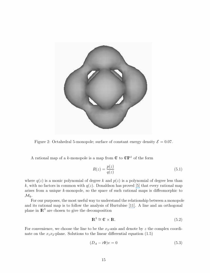
Figure 2: Octahedral 5-monopole; surface of constant energy density E = 0.07.

A rational map of a k-monopole is a map from C to CIP1 of the form

R(z) =p(z)

q(z)(5.1)

where q(z) is a monic polynomial of degree k and p(z) is a polynomial of degree less thank, with no factors in common with q(z). Donaldson has proved [5] that every rational maparises from a unique k-monopole, so the space of such rational maps is diffeomorphic toMk.

For our purposes, the most useful way to understand the relationship between a monopoleand its rational map is to follow the analysis of Hurtubise [11]. A line and an orthogonalplane in IR

3 are chosen to give the decomposition

IR3 ∼= C × IR. (5.2)

For convenience, we choose the line to be the x3-axis and denote by z the complex coordi-nate on the x1x2-plane. Solutions to the linear differential equation (1.5)

(DA − iΦ)v = 0 (5.3)

15

are considered along lines parallel to the x3-axis. This equation has two independentsolutions. A basis (v0, v1) for the solutions can be chosen such that

limx3→∞

v0(x3)x−k/23 ex3 = e0, (5.4)

limx3→∞

v1(x3)xk/23 e−x3 = e1

where e0, e1 are constant in some asymptotically flat gauge. Thus v0 is bounded and v1 isunbounded as x3 → ∞. Similarly, there is a basis (v′

0, v′1) such that v′

0 is bounded and v′1

is unbounded as x3 → −∞. We consider the scattering along all lines and write

v′0 = a(z)v0 + b(z)v1, (5.5)

v0 = a′(z)v′0 + b(z)v′

1. (5.6)

The rational map is given by

R(z) =a(z)

b(z). (5.7)

Furthermore, since the spectral curve P (η, ζ) of a monopole corresponds to the boundedsolutions to (1.5),

b(z) = P (z, 0). (5.8)

Finally, it can be shown, [2] pp. 127-128, that the full scattering data are given by[

a b−b′ −a′

](

v0

v1

)

=

(

v′0

v′1

)

(5.9)

whereaa′ = 1 + b′b. (5.10)

The advantage of rational maps is that monopoles are easily described in this approach,since one simply writes down any rational map. The disadvantage is that the rational maptells us very little about the monopole. In particular, since the construction of the rationalmap requires the choice of a direction in IR

3 it is not possible to study the full symmetriesof a monopole from its rational map. However, the following isometries are known [6]. Letλ ∈ U(1) and ν ∈ C define a rotation and translation respectively in the plane C. Letx ∈ IR define a translation perpendicular to the plane and let µ ∈ U(1) be a constantgauge transformation. Under the composition of these transformation a rational map R(z)transforms as

R(z) → µ2e2xλ−2kR(λ−1(z − ν)). (5.11)

Furthermore, under space inversion, x3 → −x3, R(z) = p(z)/q(z) transforms as

p(z)

q(z)→ I(p)(z)

q(z)(5.12)

where I(p)(z) is the unique polynomial of degree less than k such that (I(p)p)(z) = 1 modq(z).

16

We note that this implies that the rational map of a charge L axisymmetric monopolelying a distance x above the plane is

e2x+iχ

zL(5.13)

and that the full scattering data for such a monopole are[

e2x+iχ zL

0 −e−(2x+iχ)

]

. (5.14)

Using (5.11) and (5.12), it is easy to show that (up to a choice of orientation) themost general rational map of a strongly centred 5-monopole, which is invariant under bothinversion and C4 rotation around the x3 axis is

R5(z) =2az4 + 1

z5 + az(5.15)

with a ∈ (0,∞). It is a one parameter family of based rational maps, corresponding togeodesic scattering of 5-monopoles. Since the octahedral monopole satisfies this symmetry,it must lie on this geodesic.

Similarly, by imposing a C10 symmetry on 7-monopoles, generated by simultaneousinversion and rotation by π

5, there is again a unique (up to orientation) one parameter

family of maps given by

R7(z) =az5 + 1

z7(5.16)

with a ∈ (−∞,∞). The dodecahedral monopole satisfies this symmetry and must liesomewhere on the geodesic.

We can understand these scattering processes by examining the rational maps R5(z)and R7(z) for extreme values of the parameter a. It is known [6, 3] that for a rational mapp(z)/q(z) with well separated poles β1, . . . , βk the corresponding monopole is approximatelycomposed of unit charge monopoles located at the points (x1, x2, x3), where x1 + ix2 = βi

and x3 = 12log |p(βi)|. This approximation applies only when the values of the numerator

at the poles is small compared to the distance between the poles. Thus, for large values ofa, R5(z) corresponds to a monopole located at the origin and a monopole a distance ±aalong each of the diagonals x1 = ±x2. This interpretation breaks down for a ∼ 1. Thepoles of R7(z) are never well separated, so there is no region in which this approximationcan be applied to this rational map.

In [2] pp. 25-26 it is argued that for monopoles strung out in well separated clustersalong, or nearly along, the x3 axis the first term in a large z expansion of the rational mapR(z) will be e2x+iχ/zL where L is the charge of the topmost cluster and x is its elevationabove the plane. We would like to extend this and argue that if the next highest clusterhas charge M and is y above the plane then the first two terms in the large z expansion ofthe rational map will be given by

R(z) ∼ e2x+iχ

zL+

e2y+iφ

z2L+M+ ... (5.17)

17

Assume the topmost cluster, (A1, φ1) is well separated from the other monopoles. Letv′′0 be the solution bounded at x3 → −∞. For z large, we are considering scattering along

lines well removed from the spectral lines and so in the region of (A1, φ1) the solutionis dominated by the exponentially growing one and is therefore close to v′′

0 . Thus thedominant term in the rational map is the effect of scattering off (A1, φ1).

We now consider the second highest monopole cluster (A2, φ2). Since it is separatedfrom the monopoles below it the incoming solution is close to v′′

0 . If we call the boundedsolution leaving the (A2, φ2) region v′

0 and the unbounded one v′1 we have from (5.14)

v′′0 = e2y+iφv′

0 + zMv′1. (5.18)

Subsequent scattering off (A1, φ1) gives

v′0 = −e−2x−iχv1 (5.19)

v′1 = e2x+iχv0 + zLv1

where v0 and v1 are respectively the unbounded and bounded solutions as x3 → ∞. Sub-stituting (5.19) into (5.18) we find that

v′′0 = zMe2x+iχv0 + (zM+L − e−2(x−y)−i(χ−φ))v1 (5.20)

and so the rational map is dominated by

R(z) ∼ zMe2x+iχ

zM+L − e−2(x−y)−i(χ−φ)(5.21)

and so since x ≫ y ≫ 1

R(z) − e2x+iχ

zL∼ e2y+iφ

z2L+M(5.22)

as required. Obviously this type of argument could be extended to further monopoles alongthe line, but we do not need to do so here.

We can now see that R5(z) describes four monopoles approaching a monopole at theorigin along the negative and positive directions of the x1 and x2 axis. At some point,the monopoles coalesce to form the octahedral 5-monopole. As a → 0, we see from (5.17)that one monopole travels up the x3-axis and three remain in a cluster at the origin. Byinversion the fifth monopole travels down the x3-axis. In the a = 0 limit, there are sphericalunit charge monopoles at (0, 0,±∞) and a toroidal 3-monopole centred on the origin.

Similarly the rational map R7(z) corresponds to two 2-monopole clusters approachinga toroidal 3-monopole along the positive and negative x3-axis. At some negative value ofa, say a = −d, they coalesce to form a dodecahedron oriented so that two faces are parallelto the x1x2-plane. Then at a = 0 they form a toroidal 7-monopole. At a = d they formanother dodecahedron, rotated π/5 relative to the previous one. Finally, for large values ofa the rational map corresponds to a toroidal 3-monopole at the origin and two 2-monopoleclusters receding along the positive and negative x3-axis.

Recently, we have been investigating a whole family of scattering geodesics similar to theone above. One of the interesting features of these scattering processes is the complicatedmotion of the zeros of the Higgs field. A detailed investigation will be presented elsewhere[10].

18

6 Conclusion

By explicit construction of the spectral curves, we have proved the existence of a chargeseven monopole with icosahedral symmetry and a charge five monopole with octahedralsymmetry. Numerical computation of the monopole energy density reveals that the formerlooks like a dodecahedron and the latter an octahedron. The energy density is maximalon the vertices of these two regular solids.

Using Donaldson’s rational map formulation we have presented a totally geodesic one-dimensional submanifold of the monopole moduli space which contains the dodecahedral7-monopole and one which contains the octahedral 5-monopole. In the moduli space ap-proximation of soliton dynamics, these submanifolds describe a new type of novel multi-monopole scattering which requires further investigation.

Acknowledgements

Many thanks to Nigel Hitchin and Nick Manton for useful discussions. CJH thanks theEPSRC for a research studentship and the British Council for a FCO award. PMS thanksthe EPSRC for a research fellowship.

References

[1] M.F. Atiyah, private communication.

[2] M.F. Atiyah and N.J. Hitchin, ‘The geometry and dynamics of magnetic monopoles’,Princeton University Press, 1988.

[3] R. Bielawski, ‘Monopoles, particles and rational functions’, McMaster preprint, 1994.

[4] E. Braaten, S. Townsend and L. Carson, ‘Novel structure of static multisoliton solu-

tions in the Skyrme model’, Phys. Lett. 235B, 147 (1990).

[5] S.K. Donaldson, ‘Nahm’s equations and the classification of monopoles’, Commun.Math. Phys. 96, 387 (1984).

[6] N.J. Hitchin, N.S. Manton and M.K. Murray, ‘Symmetric monopoles’, Nonlinearity,8, 661 (1995).

[7] N.J. Hitchin, ‘Monopoles and geodesics’, Commun. Math. Phys. 83, 579 (1982).

[8] N.J. Hitchin, ‘On the construction of monopoles’, Commun. Math. Phys. 89, 145(1983).

[9] C.J. Houghton and P.M. Sutcliffe, ‘Tetrahedral and cubic monopoles’, Cambridgepreprint DAMTP 95-13.

19

[10] C.J. Houghton and P.M. Sutcliffe, ‘Monopole scattering with a twist’, Cambridgepreprint DAMTP 95-28.

[11] J. Hurtubise, ‘Monopoles and rational maps: a note on a theorem of Donaldson’,Commun. Math. Phys. 100, 463 (1985).

[12] F. Klein, ‘Lectures on the icosahedron’, London, Kegan Paul, 1913.

[13] R.A. Leese and N.S. Manton, ‘Stable instanton-generated Skrme fields with baryon

numbers three and four’, Nucl. Phys. 572A, 675 (1994).

[14] N.S. Manton, ‘A remark on the scattering of BPS monopoles’, Phys. Lett. 110B, 54(1982).

[15] W. Nahm, ‘The construction of all self-dual multimonopoles by the ADHM method’,in Monopoles in quantum field theory, eds. N.S. Craigie, P. Goddard and W. Nahm,World Scientific, 1982.

[16] M.K. Prasad, ‘Yang-Mills-Higgs monopole solutions of arbitrary topological charge’,Commun. Math. Phys. 80, 137 (1981).

[17] M.K. Prasad and C.M. Sommerfield, ‘Exact classical solution for the ’t Hooft monopole

and the Julia-Zee dyon’, Phys. Rev. Lett. 35, 760 (1975).

[18] D. Stuart, ‘The geodesic approximation for the Yang-Mills-Higgs equation’, Commun.Math. Phys. 166, 149 (1994).

[19] R.S. Ward, ‘A Yang-Mills-Higgs monopole of charge two’, Commun. Math. Phys. 79,317 (1981);

[20] R.S. Ward, ‘Two Yang-Mills-Higgs monopoles close together’, Phys. Lett. B102, 136(1981).

20