Massive Magnetic Monopoles in Cosmology and Astrophysics

Massive Magnetic Monopoles in Cosmology and Astrophysics

EDWARD W. KOLB” Theoretical Division

Los Alamos National Laboratory Los Alamos, New Mexico 87545

INTRODUCTION

Just over 50 years ago, P. A. M. Dirac showed that the existence of magnetic monopoles implies that the electric charge, e, and the magnetic charge, g, are quantized:’

eg = n / 2 (n , integer) (1)

This would offer an explanation for the fact that the magnitude of the proton charge is exactly equal to the magnitude of the electron charge (rather than say 3 ~ / 17 times the electron charge). However, it was realized that the theory had the shortcoming that monopoles had to be introduced as new dynamical degrees of freedom, and that monopole properties such as mass, spin, etc., were free parameters.

This situation changed in 1974, when ’t Hooft and Polyakov demonstrated that monopoles must occur in certain classes of gauge theorie~.~” Among the classes of gauge theories with monopoles are the grand unified theories (GUTs), which attempt to unify the strong and electroweak interactions. In these theories, all the monopole properties are calculable. I n this paper, I will consider only the monopoles in grand unified models based on SU(5). The specialization to SU(5) is for convenience only; the same conclusions would obtain in any GUT.

In order to discuss the astrophysical and cosmological consequences of these monopoles, it is necessary to understand their origin and their structure. Monopoles in GUTs arise from “knots” in the Higgs field. The Higgs field is necessary to break the SU(5) symmetry down to the unbroken symmetry observed today, SU(3)c x U(l)em. The SU(3)c is the color symmetry of the strong interactions, and U(l)em is quantum electrodynamics. This symmetry breaking occurs in two stages. The first stage of symmetry breaking occurs a t a mass scale of about I O l 5 GeV, and breaks SU(5) down to SU(3)c x SU(2), x U(I),, where SU(2)L x U(1), is the symmetry of the electroweak interactions. The second stage of symmetry breaking occurs a t a mass scale of about 10 GeV, and breaks SU(2)L x U(1), to U( l)em. The monopoles appear a t the first stage of symmetry breaking; in general, they appear whenever a simple group, G, breaks to a symmetry that contains a U(1) factor, G - G x U(1). The Higgs field responsible for the breaking is, in general, a tensor in group space, and the “direction” of the symmetry breaking is not determined. In a gauge theory, the Higgs

“Supported in part by the Department of Energy. Present affiliation: Theoretical Astrophysics Group MS 209, Fermi National Accelerator Laboratory, P.O. Box 500, Batavia, Ill. 60510.

33

34 ANNALS NEW YORK ACADEMY OF SCIENCES

field may be locally gauge rotated in any direction in the group space. However, the topology of mappings of manifolds in real space onto the group is gauge invariant, and topologically nontrivial defects cannot be eliminated by nonsingular gauge transforma- tions. These topological defects, or knots, correspond to magnetic monopoles.

The G U T monopole shown in FIGURE 1 has an onion-skin structure that reflects the pattern of symmetry breaking. At small distances, less than cm, the monopole has many degrees of freedom excited, gluons (g), photons (y), and the “end of the alphabet” gauge fields including the weak bosons ( W, Z) and the baryon numbers violating bosons of SU(5) ‘(A’, v). There are also the supermassive Higgs bosons of SU(5) (S), and the Higgs bosons of the Weinberg-Salam model (4). At distances greater than m i ’ cm), the X , Y, and S fields are no longer excited. At distances greater than m i ’ (-10-l6 cm), the W, Z, and 4 fields are no longer excited. At distances greater than AQEo ( - l O - I 4 cm), the gluon fields are screened. Only at distances greater than cm does the GUT monopole resemble a classical Dirac monopole.

The mass of the G U T monopole is

m,,, = (4) = mx/a 2 1OI6 GeV (2)

where (4) is the vacuum expectation value of the Higgs field responsible for the SU(5) breaking. In GUTS, the monopole mass must be greater than about 10l6 GeV, since the limit on the proton lifetime requires rnx to be greater than about l O I 4 GeV. This enormous mass for the monopole (my 2 10l6 GeV = g) prevents their creation in accelerators. Only in the early universe can the energy be found to create the monopoles.

MONOPOLES FROM THE EARLY UNIVERSE

The enormous mass of GUT monopoles leads one naturally to the early universe for production of There are two sources of monopole creation in the early universe: thermal production, and spontaneous production in the phase transition. As

\ \\

/ /

/

FIGURE 1. The onion-skin structure of the monopole in grand unified theories.

KOLB MASSIVE MAGNETIC MONOPOLES 35

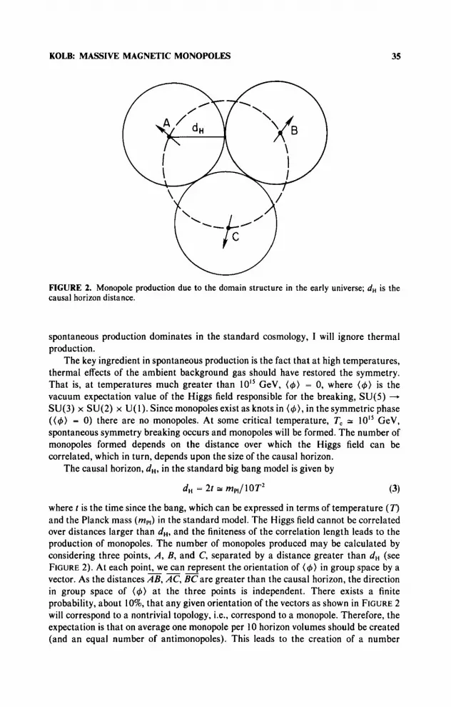
FIGURE 2. Monopole production due to the domain structure in the early universe; dH is the causal horizon distance.

spontaneous production dominates in the standard cosmology, I will ignore thermal production.

The key ingredient in spontaneous production is the fact that a t high temperatures, thermal effects of the ambient background gas should have restored the symmetry. That is, at temperatures much greater than 10” GeV, (4) = 0, where (4 ) is the vacuum expectation value of the Higgs field responsible for the breaking, SU(5) -+

SU(3) x SU(2) x U( I) . Since monopoles exist as knots in (+), in the symmetric phase ( (4) = 0) there are no monopoles. At some critical temperature, T, = lOI5 GeV, spontaneous symmetry breaking occurs and monopoles will be formed. The number of monopoles formed depends on the distance over which the Higgs field can be correlated, which in turn, depends upon the size of the causal horizon.

The causal horizon, dH, in the standard big bang model is given by

d , = 2t = mpl/10T2 (3)

where t is the time since the bang, which can be expressed in terms of temperature ( r ) and the Planck mass (mPJ in the standard model. The Higgs field cannot be correlated over distances larger than d,, and the finiteness of the correlation length leads to the production of monopoles. The number of monopoles produced may be calculated by considering three points, A, B, and C, separated by a distance greater than d , (see FIGURE 2). At each point, we can represent the orientation of ( 4 ) in group space by a vector. As the distances AB, AC, BCare greater than the causal horizon, the direction in group space of (4 ) a t the three points is independent. There exists a finite probability, about lo%, that any given orientation of the vectors as shown in FIGURE 2 will correspond to a nontrivial topology, i.e., correspond to a monopole. Therefore, the expectation is that on average one monopole per 10 horizon volumes should be created (and an equal number of antimonopoles). This leads to the creation of a number

_ _ _


density of monopole-antimonopole pairs of

n, = n a = 0.1 di ’ = lo’ TPlmh (4)

It is convenient to compare this number density to the photon number density a t T =

T,, n7 = T:

After creation of the monopoles, monopole-antimonopole pairs can annihilate. This annihilation causes the monopole density to decrease as (ignoring monopole-antimonopole creation in collisions)

dn, d n a R _ _ _ _ = - (n,npc,,IvI) - 3- dt dt R nM

-

where aA is the M a annihilation cross section. The classical calculation of aA involves monopole-antimonopole capture into a bound state, with subsequent emission of radiation until the eventual anr~ihilation.’-~ The solution to Equation 6 results in a “freeze out” density of monopoles of about

This freeze out occurs because as the monopole-antimonopole density becomes too small, a monopole cannot find an antimonopole to annihilate.

The ratio in Equation 7 is roughly constant during the subsequent evolution of the universe. Therefore, today the monopoles would contribute an energy density of

(8)

There are about 400 cm-3 photons in the universe today, and if the monopole mass is 10l6 GeV (lo-* g), the monopoles would contribute an energy density of

p,a = mMnM = lo-‘’ my n,

pMM 2 10-l’ g cm-3 1OI4 pc (9)

where pc is the critical density. Since observationally we know the total energy density of the universe must be less than 2p,, the energy density in Equation 9 is about 14 orders of magnitude too large. Therefore, there must be some way either to avoid making so many monopoles, or to efficiently annihilate the monopoles.

The obvious lesson is that we are missing something very fundamental in the simple picture of the early universe we have just discussed. Below we discuss some proposals that have been made to alleviate the monopole problem.

Prevent Symmetry Restoration

The monopoles are formed in the phase transition; if one could avoid the phase transition, monopoles would not be produced. One possible way to avoid the phase transition is to assume that the universe had a maximum temperature, TMAX, less than

KOLB: MASSIVE MAGNETIC MONOPOLES 37

the critical temperature, T,. This assumption has the unwanted feature that baryon production is difficult, since temperatures of the order T, = mx are necessary to make baryons. There may be a narrow range for TMAX, where TMAX S T,, and TMAX is still large enough to produce baryons; but unless there is some physical reason for TMAX to be in that narrow range, this solution cannot be taken seriously. One possible physical reason for TMAX 5 T, can arise in grand unified models that are not asymptotically free.’ Such asymptotically nonfree models are considered ugly on esthetic grounds, but quite naturally arise in complicated GUTS.’

Another possible way to prevent the universe from being in the symmetric state is to assume that there is a large fermion asymmetry that prevents high-temperature restoration of symmetry.* Such an initial large fermion member may have further implications for cosmology, e.g., for the neutrino number of the universe.’

Enhance Annihilation

Let us suppose that spontaneous production of monopoles proceeds as discussed above, and try to find a way to get rid of them by annihilation. To do this, it is necessary that Equation 6 be insufficient to describe the annihilation.

One possibility in enhancing annihilation is to assume that the monopoles are clumped, and nM appearing in Equation 6 is larger than the value obtained in uniform expansion. The gravitational attraction of monopoles provides just such a mechanism. The possibility that monopoles form bound objects and annihilate was suggested by Preskill,’ and examined in detail by several groups.69’0.” All have concluded that the mechanism of gravitational clumping cannot solve the monopole problem.

Another possibility is that when the monopoles and antimonopoles form, they are connected by strings, and are confined.’* A basic assumption in Equation 6 is that the initial states are uncorrelated in the scattering. If monopoles are connected to antimonopoles by strings, the initial state is correlated, and the annihilation rate will be much enhanced. Although the physics behind the motivation is somewhat uncertain, there is a t least some reason to believe in monopole confinement since monopole confinement could be an artifact of the non-Abelian nature of the monopole. In QED, the electric mass of the photon, m:, and the magnetic mass of the photon, my8, are given by” -

(rn:)2 = &(w = 0, k = 0) = 2 T 2 - (rn?*)’ = II i j (w = 0, k = 0) = 0

where II, is the photon self-energy. The vanishing of the magnetic photon mass persists to all orders in perturbation theory, and means that the magnetic field is unscreened while the electric field is screened. To one loop, the electric and magnetic gluon masses are given by Equation 10. The fact that the electric mass of the gluon is nonzero means that chromoelectric fields are screened, and quarks are free a t high temperatures. Although to one loop the gluon magnetic mass is zero, it is possible that higher-order calculations can lead to a nonzero magnetic gluon mass. In this case the plasma would not be a magnetic conductor, but rather the plasma would be a magnetic superconductor with the magnetic flux lines confined to flux tubes. Monopole- antimonopole pairs would be connected by these flux tubes, and confined.


Postpone the Phase Transition

The number of monopoles created in the transition is proportional to T:/m:l. If the critical temperature is less than about 10” GeV, an acceptable monopole density would result. One method of postponing the phase transition involves ~upercool ing , ’~~’~ and was the original motivation of the inflationary universe. Another possibility is an intermediate symmetry as proposed by Langacher and Pi,’“ where the U( 1) appear- ance is postponed until T 5 10” GeV.

In conclusion, the dearth of monopoles in the universe gives us very important information about the early universe. Unfortunately, it is not clear how to interpret the information. Perhaps one of the scenarios for monopole suppression discussed above is the solution to the “monopole problem,” but it is just as likely that the solution has not yet been found. Some of the solutions discussed above get rid of all the monopoles. Some of the solutions get rid of some of the monopoles. The obvious next step is to look for monopoles today. The next section discusses limits on the present monopole flux, both astrophysical limits and experimental limits.

GALACTIC MAGNETIC MONOPOLES

So far we have seen that massive magnetic monopoles are predicted to exist in grand unified theories, and should have been copiously produced in the big bang. In fact, the predicted density of monopoles is so large that some mechanism must either suppress their production or efficiently reduce their number after creation. If monopoles could be detected, knowledge of the present monopole flux would help in determining the suppression mechanism.

Before discussing terrestrial experiments, it is useful to discuss some astrophysical limits. The first limit comes from the mass density of the universe. The “critical density” of the universe is (Ho is the Hubble constant)

3Ht pc=-- - 2 x

8n C Hioo g cm-’

where HIM) = Ho/lOO km s - ’ Mpc-’. We know observationally that the energy density of the universe is less than 2p,. This implies that the average number density of monopoles, ( n M ) , is limited by requiring that the energy density of the monopoles is less than 2pc

PM = ( n M ) m M 5 2pC

GeV - cm-’ ( f l M ) 5 4 x m M

In order to compare with experiments, we must form a flux from the density. If we assume the monopoles are completely uniform throughout the universe, they would be cold, and the relevant velocity would be the velocity of our galaxy relative to the cold monopoles. This velocity is our peculiar velocity relative to the 3K background


radiation,”-I9 vM L= lo-’ c. Therefore, the flux of monopoles in the universe must be

i t is perhaps more reasonable to assume that the monopoles are clumped, and that their density in our galaxy is enhanced over the average density throughout the universe, as are the protons. In that case, the relevant mass density limit is roughly lo6 pc , and the relevant velocity would be the galactic virial velocity, again about lo-’ c. The limit in this case is

The best astrophysical limit comes from the observation of large-scale galactic magnetic fields. The original argument is due to Parker.’”’’ He argued that if the galactic magnetic fields are due to currents, then monopoles drain energy from the field as they are accelerated. The rate of extracting energy from the magnetic field is FMBc, where Bc is the galactic magnetic field (Bc = gauss). The energy in the magnetic field is B ; / ~ T , and this energy will be drained on a time scale

B ’ / ~ T 78 = - 4a FMB

In order for magnetic fields to survive, this time scale must be less than the time scale for regeneration of the magnetic field, which is the order of the galactic rotation time, about lo* years.’”’’ The requirement T~ 2 10’ years requires

FM 5 cm-2 s-’ sr-’ (16)

Equation 16 has become known as the “Parker limit.” More detailed studies have closed several loopholes in the simple argument given a b ~ v e , ’ ~ and have concluded that the limit (16) is probably good to an order of magnitude for reasonable values of the monopole mass. It is possible to evade the Parker limit if the monopoles themselves are the sources of the magnetic field.23.24 This scenario is hard to imagine, since it needs large magnetic charge fluctuations. However, it potentially weakens the Parker limit by about 5 orders of magnitude.

The uncertainty in the astrophysical limits is easily matched by the uncertainties in terrestrial searches. The largest source of uncertainty comes from the difficulty in calculating the energy loss from slowly moving monopoles. For a discussion of the difficulties of such a calculation, see Ahlen and Kinoshita” (see also Reference 26). They find an energy loss for massive, slowly moving monopoles in silicon of (for p 5 0.01)

where @ is the monopole velocity. There are several things to note about this result.


1. It is linear in /3. 2. It is a t least as large as the energy loss for slowly moving protons. 3. It agrees with previous calculations.

All reported experiments that detect monopoles by ionization depend on calculations of the monopole ionization. Although different experiments use slightly different values for the ionization, it is still interesting to compare some quoted limits:

FM 5 3 x lo-’’ crn-’s-Isr-’ (3 x S /3 c lo-’) (18b)

F,,, 5 lo-’’ cm-’s-’ sr-’ (2 x 5 @ 5 3 x (184

(184

( W

F,,, 5 2 x lo-’’ cm-’s-I sr-’ (lo-’ 5 p)

(10-3 5 p 5 10-2) F,,, 5 3 x lo-’’ crn-’s-’sr-I

where the limits quoted in (18aH18e) are given in References 27-3 1 respectively. The cleanest way to look for monopoles is the superconducting search done by

Cabrera.” This method is based on the change in the macroscopic quantum state of a superconducting ring when a magnetic charge passes through the ring. The magnetic flux through the superconducting ring changes the current, which is detected by a SQUID. This method is clean, since it is independent of the monopole mass, monopole velocity, monopole electric charge, and energy loss calculations. Cabrera has reported a

and a candidate event. If we assume the candidate event was the actual detection of a magnetic monopole, the flux of 6 x lo-’’ cm-’ s-’ sr-’ represents the actual monopole flux.

Although one event does not give unequivocal evidence for the existence of magnetic monopoles, it is interesting to assume this event is the result of a flux given in Equation 18 and examine the consequences. First, it is obviously in conflict with the ionization searches discussed above. This would mean that either the monopoles are very slow (0 c< galactic virial velocity) or the ionization calculations are in serious error. The Cabrera flux is also in serious disagreement with the Parker limit. Either we do not understand galactic magnetic fields, or the monopole flux on earth is much different than the average galactic flux. The latter possibility has been examined by Dimopoulos, Glashow, Prucell, and Wilczek.” They suggested that there is a “cloud” of monopoles orbiting the sun, which enhances the monopole flux a t the earth by a factor of 10’ relative to the average galactic flux. In this manner it may be possible to reconcile the Cabrera flux with the Parker limit.

In conclusion, there is one hint that monopoles exist in our galaxy. If this hint proves correct, it may have drastic implications for our understanding of galactic magnetic fields.


MONOPOLE-INDUCED PROTON DECAY

Two dramatic predictions of GUTS are proton decay, and the existence of magnetic monopoles. Recent model calculations by R ~ b a k o v , ~ ~ . ~ ’ calla^^,'"^' and Wilczek3’ have suggested that proton decay in the presence of a monopole occurs a t a much faster rate than one might guess on dimensional grounds.

A naive dimensional estimate of the cross section pM - MX, where X denotes the proton decay products, might be (rA8 = mi2, where mM is the monopole mass. However Rubakov and Callan have argued that the cross section is independent of the mass of the monopole, and it is related instead to the mass scale of color confinement, about 1 GeV. We shall parameterize the cross section for monopole-induced proton decay by a mass scale A:

a 10-z7 a,=---- cm2

A’ - AiCv

where keV = A/ l GeV. If the conjecture of Callan and Rubakov is correct, then

There are two obvious questions to be asked about monopole-induced proton decay. First, does it open up new methods for detecting cosmic monopoles? Second, does monopole-induced proton decay have any important astrophysical consequences? The answer to both questions is yes!

If monopoles induce proton decay while traversing a proton-decay detector, then proton-decay detectors would make the most sensitive monopole telescopes. A prelimi- nary study by the Irvine-Michigan-Brookhaven proton decay collaboration has concluded that with minor modifications, the detector would have a sensitivity to a monopole flux of about 10-15cm-2 s-I sr-’, if aAB = cm2.40 This is several orders of magnitude better than the limits in (18).

If monopoles induce proton decay, they would have a drastic effect on the x-ray luminosity of neutron star^.^'.^' By using the limit on the neutron star luminosity, it is possible to place a limit on the product of the galactic monopole flux and baryon- violating cross section, which suggests that the phenomenon of monopole-induced proton decay is not likely to be detected terrestrially.

and to be as old as the galaxy itself. During the lifetime of the neutron star, the neutron star would have been subjected to a galactic monopole flux FM. This resulted in a number of neutron star/monopole collisions given by

A G c V 1.

Neutron stars are believed to be plentiful in our

where fNS is the lifetime of the neutron star, and A, is the “capture” area given by


In Equation 22, MNs and RNS are the mass and radius of the neutron star, vM is the galactic velocity of the monopole, and Rs is the Schwarzschild radius of the neutron star. Putting in values of MNs = 1 M,, RNs - lo6 cm

(23) NM - loJ6 FM(cm-’ SKI sr-’)

The monopole will be trapped in the neutron star, mainly through energy loss in scattering with electron^.*^^'^*^' This results in an energy loss of

d E - = B 10” GeV cm-’ d x

where (3 is the monopole velocity in the star (B lo-’ is escape velocity). If p 2 lo-’, the monopole will lose about 10I6 GeV traversing the star (if /3 5 lo-’, the monopole must be trapped). The initial energy of the monopole in the galaxy was

1 2 EO = - mM vM 2

2 - 5 109- IOl:;eV [ - GeV

Therefore, if the monopoles have typical virial velocities of lo-’, monopoles of mass less than 10’’ GeV (10’ mpl!) will be trapped.

The monopoles trapped in the star catalyze nucleon decay, and release energy at a rate

L M = mN nN a,u I v I = 8.5 x 10’’ A& ergs-’ monopole-’ (26)

where mN is the nucleon mass, nN is the nucleon density, and we have used I v I = lo-’, the nucleon Fermi velocity.

Combining (23) and (26), the energy produced in the neutron star by monopole- induced nucleon decay is

L = 2 x los4 F,,,(cm-’s-’ sr-I) erg s-’ (27)

This luminosity is the toral luminosity, which in general may be emitted as photons and neutrinos. The best limit on the photon luminosity comes from recent surveys for serendipitous x-ray These surveys could detect an x-ray luminosity of L7 =

10” erg SKI at a distance of 1 k p ~ . ~ ~ ” ’ Estimates based on the current pulsar birth rate in the solar neighborhood indicate that there should be an old .neutron star density of nNS 2 4 x lo-’ pc-’. Therefore, it is reasonable as an extremely conservative estimate to take 10’’ erg s- ‘ as the maximum luminosity of old neutron stars.

The relationship between the x-ray luminosity and the total luminosity depends on the structure of the neutron star. The smallest Lr/L‘ ratio results for zero surface magnetic field, and for pion condensation in the neutron star interior. In this case, L7 5 10’’ erg SKI corresponds to a total luminosity of about loJ3 erg s - ’ . ~ * It is also important to note that a photon luminosity of 10’’ erg s-’ corresponds to a surface temperature of


Ts = 0.04 keV. About 80% of the energy radiated a t this temperature will be in the window of the Einstein satellite.

A maximum total luminosity of lo” erg s-’ requires

FM(cm-2 s-I sr-I) A&, < 5 x (28)

Therefore, if monopoles catalyze proton decay at a strong rate (AGcv = l ) , the flux limit of (28) is about 6 orders of magnitude better than the Parker limit discussed in the previous section. This limit is also 6 orders of magnitude below the possible limit for detection reported by the IMB group.

Conversely, if proton decay detectors do see monopoles, something very basic is very wrong in our understanding of neutron stars.

CONCLUSIONS

Not only do magnetic monopoles provide a natural explanation for charge quantiza- tion, but they must exist in grand unified theories. In such theories, the monopole is very massive, and the early universe is probably the only source for production.

The early universe should have provided a plentiful supply of monopoles. In fact, the simplest prediction one might make results in a monopole density l O I 4 orders of magnitude too large. This important cosmological probe of the early universe tells us that either the simple picture of unification or the simple picture of the early universe is seriously wrong. There have been several proposals to solve the monopole problem, they all have important implications for cosmology, and could potentially alter our picture of the early universe. Detection of a monopole would be strong evidence that the universe was once at a temperature greater than 10’’ GeV.

There have been several recent terrestrial searches for massive magnetic monopoles. One experiment can be interpreted as detection of a m~nopole. ’~ If this experiment is confirmed, then the flux of magnetic monopoles would be many orders of magnitude too large for us to understand the existence of galactic magnetic fields.

There are theoretical indications that the cross section for monopole-induced proton decay is a strong cross section. If this is true, then a galactic monopole flux greater than cm-2s-I sr-’ would result in an enormous x-ray luminosity for neutron stars. Therefore, a detection of monopoles on earth would not only mean that galactic magnetic fields do not exist, but that neutron stars do not exist.

Not only do magnetic monopoles provide a probe of particle physics, but potentially are a great source of information in astrophysics.

REFERENCES

1. DIRAC, P. A. M. 1931. Proc. R. Soc. 133 60. 2. ’T HOOFT, G. 1974. Nucl. Phys. B79 276. 3. POLYAKOV, A. M. 1974. JETP Lett. 2 0 194. 4. ZEL’DOVICH, YA. B. & M. Yu. KHLOPOV. 1978. Phys. Lett. 79B: 239. 5. PRESKILL, J. P. 1979. Phys. Rev. Lett. 4 3 1365. 6 . DICUS, D. A,, D. N. PAGE & V. L. TEPTLITZ. 1982. Phys. Rev. D26 1306. 7. HARVEY, J. A., E. W. KOLB & S. WOLFRAM. 1983. Phys. Rev. D27: 315.


8. 9.

10. 11. 12. 13. 14. 15. 16. 17. 18. 19. 20. 21. 22. 23. 24. 25. 26. 27. 28. 29. 30. 31. 32. 33. 34. 35. 36. 37. 38. 39. 40. 41. 42. 43. 44. 45. 46. 47. 48.

LINDE, A. 1976. Phys. Rev. D14 3345. HARVEY, J . A. & E. W. KOLB. 1981. Phys. Rev. D 2 4 2090. GOLDMAN, T., E. W. KOLB & D. TOUSSAINT. 1981. Phys. Rev. D23 867. FRY, J. N. 1981. Astrophys. J. 2 4 6 L93. . LAZARIDES, G . & Q. SHAFI. 1980. Phys. Lett. 948: 149. GROSS, D. J., R. D. PlSARSKl & L. G . YAFFE. 1981. Rev. Mod. Phys. 5 3 43.

EINHORN, M. B., D. L. STEIN I% D. TOUSSAINT. 1980. Phys. Rev. D21: 3295. GUTH. A. H. & S.-H. H. TYE. 1980. Phys. Rev. Lett. 4 4 631.

LANGACKER, P. & S.-Y. Pi. 1980. Phys. Rev. Lett. 4 5 1. SMOOT, G. F. & P. M. LUBIN. 1979. Astrophys. J. 234: L83. FABBRI, R., e t d . 1980. Phys. Rev. Lett. 4 4 1563. BOUGHN, S. P., E. S. CHENG, & D. T. WILKINSON. 1981. Astrophys. J. 2 4 3 L113. PARKER, E. N. 1970. Astrophys. J. 160 383. PARKER, E. N. 1971. Astrophys. J. 163 225. PARKER, E. N. 1971. Astrophys. J. 166: 295. TURNER, M. S., E. N. PARKER & T. J. BOGDAN. 1981. Phys. Rev. D26 1296. SALPETER, E. E., S. L. SHAPIRO & I. WASSERMAN. 1982. Phys. Rev. Lett. 4 9 11 14. AHLEN, S. P. & K. KINOSHITA. 1982. Phys. Rev. 2 6 D 2347. DRELL, S. D. 1983. Phys. Rev. Lett. 5 0 644. SOKOLOWSKI, J . K. & L. R. SULAK. University of Michigan Report. Ann Arbor, Mich. ULMAN, J. D. 1981. Phys. Rev. Lett. 47: 289. GROOM, D. E., er al. University of Utah Report. Salt Lake City, Utah. BONARELLI, R., er a/. 1982. Phys. Lett. 1128: 102. BARTELT, J., er al. 1983. Phys. Rev. Lett 5 0 655. CABRERA, B. 1982. Phys. Rev. Lett. 48: 1378. DIMOPOULOS, s., S. L. CLASHOW, E. M. PURCELL & F. WILCZEK. 1982. Nature 2 9 8 824. RUBAKOV, V. A. 1982. Nucl. Phys. B203 31 1. RUBAKOV, V. A. 1981. Zheft Pis’ma 3 3 658. CALLAN, C. G . 1982. Phys. Rev. D25: 2141. CALLAN, C. G. 1982. Phys. Rev. D26 2058. CALLAN, C. G. 1982. Nucl. Phys. B204. WILCZEK, F. 1982. Phys. Rev. Lett. 48: 1146. ERREDE, S. Private communication. KOLB, E. W., S. A. COLGATE & J. A. HARVEY. 1982. Phys. Rev. Lett. 4 9 1373.

LAMB, D. Q., F. K. LAMB & D. PINES. 1973. Nature 246 52. HILLS, J. G. 1978. Astrophys. J. 219 550. HILLS, J . G. 1980. Astrophys. J. 240 242. CORDOVA, F. S., K. 0. MASON & J. E. NELSON. 1981. Astrophys. J. 245: 609. REICHERT, G. A., K. 0. MASON, J. R. THORSTENSEN & S. BOWYER. In preparation. VAN RIPER, K. A. & D. Q. LAMB. 1981. Astrophys. J. 244 LI 3.

DIMOPOULOS, s., J . P. PRESKlLL & F. WILCZEK. 1982. Phy. Lett. 119B: 320.

Documents

Massive Magnetic Monopoles in Cosmology and Astrophysics