Numerical Modelling of the T-bar penetrometer

Miguel Bernardes de Almeida

Thesis to obtain the Master of Science Degree in

Civil Engineering

Supervisor:

Prof. Drª. Teresa Maria Bodas de Araújo Freitas

Examination Committee

Chairperson: Professor Doutor António Manuel Figueiredo Pinto da Costa

Supervisor: Professora Doutora Teresa Maria Bodas de Araújo Freitas

Member of the Committee: Professor Doutor Jaime Alberto dos Santos

October 2020

ii

iii

Abstract

This thesis focus on better understanding and characterising the correlations between the measured

data during in-situ penetration testing and the geotechnical properties of the soil found at offshore

sites.

This work features FEM studies on the penetration of a T-bar penetrometer through soft deep seabed

clay, both in wished-in-place and pushed-in-place scenarios, starting from different depths. Initially

small-deformation analyses of the wished-in-place scenario are performed using the Plaxis software.

Subsequently analyses are undertaken using the Coupled Eulerian-Lagrangian (CEL) approach in

the ABAQUS software, which allows the explicit simulation of the T-bar penetration that involves very

large deformations. From these analyses, the influence of different parameters on the derived T-bar

bearing factor is studied. Such study is compared with previous works found in literature.

There is good agreement between the results obtained with the Plaxis software and the exact solution

reported in the work of Randolph and Andersen (2006). For the CEL analyses assuming a smooth T-

bar, a good agreement was achieved between the numerical results and the analytical solutions by

Randolph and Andersen (2006). However, it was observed an increasing difference as the roughness

coefficient of the soil – T-bar contact increased. The reasons for these discrepancies were not

possible to confirm. It has been reported that the contact algorithm employed through the CEL

technique presents limitations in modelling the contact stresses between the Lagrangian and Eulerian

part and the same is likely to occur in the simulation of contact shear stresses, even during the

mobilisation of the full-flow mechanism.

Keywords: T-Bar penetrometer; large deformations; Coupled Eulerian-Lagrangian (CEL); Full-flow

mechanism

iv

v

Resumo

O foco deste trabalho é compreender melhor as correlações entre as quantidades medidas durante

o ensaio de penetração in-situ e as características geotécnicas do solo típico de zonas offshore,

tendo em vista a sua melhor caracterização.

Este trabalho apresenta estudos de modelação em elementos finitos da penetração de um

penetrómetro T-bar a partir de diferentes profundidades. Estas análises serão executadas nos

cenários de modelação wished-in-place e pushed-in-place. Numa fase inicial as análises são

realizadas no software Plaxis. Posteriormente as análises são realizadas através da abordagem

Coupled Eulerian-Lagrangian (CEL) no software ABAQUS, que permite modelar de forma explicita o

avanço do penetrómetro, o que envolve muito grandes deformações. A partir destas análises é

estudada a influência de diferentes parâmetros no valor do coeficiente de capacidade NT-bar. Tal

estudo é comparado com estudos semelhantes anteriores.

Há uma boa concordância entre os resultados obtidos com o software Plaxis e a solução analítica

reportada em Randolph e Andersen (2006). Relativamente aos resultados obtidos com o software

ABAQUS utilizando a abordagem CEL, verifica-se também uma boa concordância para o caso em

que o T-bar é liso. No entanto observa-se uma discrepância crescente com o aumento da rugosidade

do T-bar. Não foi possível confirmar a razão para esta discrepância. Em estudos anteriores tem sido

reportado que o algoritmo de contato empregue pela abordagem CEL apresenta limitações na

modelação das tensões de contacto entre a parte Euleriana e Lagrangiana, o que poderá estar a

influenciar a simulação das tensões de corte no contacto solo - T-bar.

Palavras-chave: T-bar; Grandes deformações; Coupled Eulerian-Lagrangian (CEL); Mecanismo de

full-flow

vi

Declaration

I declare that this document is an original work of my own authorship and that it fulfills all the

requirements of the Code of Conduct and Good Practices of the Universidade de Lisboa.

vii

Acknowledgements

To my supervisor Professor Teresa Freitas for her fundamental support and guidance throughout this

work for which without it this thesis elaboration would not be possible.

To my family for their support in all of my choices throughout my civil engineering journey and the

celebration of every small victory.

To the friends and colleagues that I made and met in the course of my degree, for making me the

person and the professional I am today.

To my friend Reydleon Paulo for his energy and insights on the details that this work entailed.

To all my Erasmus friends and colleagues for helping me practice my English and teaching me that

friends are around the globe.

To all the teachers I’ve met throughout this learning endeavor in this great university for the

challenges they provided.

viii

ix

Table of contents

Abstract ............................................................................................................................................. iii

Resumo .............................................................................................................................................. v

Acknowledgements .......................................................................................................................... vii

Table of contents ............................................................................................................................... ix

List of figures ..................................................................................................................................... xi

List of tables .................................................................................................................................... xiii

List of symbols................................................................................................................................. xiv

1. Introduction .................................................................................................................................1

1.1. Relevance ...........................................................................................................................1

1.2. Objectives of the thesis.......................................................................................................2

1.3. Layout of the thesis ............................................................................................................2

2. State of the art ............................................................................................................................4

2.1. Introductory remarks ...........................................................................................................4

2.2. Description of in situ penetration tests ................................................................................5

2.3. Numerical methods for the analysis of large deformation problems ...................................9

2.4. Mechanism during T-bar penetration ................................................................................12

2.5. Analysis and interpretation of full-flow T-bar penetration ..................................................15

2.6. Analysis and interpretation of T-bar at shallow depth .......................................................20

3. Numerical analysis with Plaxis software ...................................................................................26

3.1. Introduction .......................................................................................................................26

3.2. Description of the analyses ...............................................................................................27

3.3. Soil constitutive models ....................................................................................................29

3.3.1. Isotropic Tresca model .............................................................................................29

3.3.2. NGI-ADP model ........................................................................................................30

3.4. Analysis results with Tresca model ...................................................................................34

3.5. Analysis results with the NGI-ADP model .........................................................................36

4. Coupled Eulerian-Lagrangian WIP Analysis .............................................................................38

4.1. Introduction .......................................................................................................................38

4.2. Wished-in-place analyses .................................................................................................38

4.2.1. Soil and T-bar properties ..........................................................................................41

4.2.2. Interface roughness ..................................................................................................42

4.2.3. Boundary conditions .................................................................................................43

4.2.4. Analysis Procedure ...................................................................................................44

4.2.5. Mesh .........................................................................................................................45

4.3. Mesh sensitivity study .......................................................................................................47

x

4.4. Parameter sensitivity study ...............................................................................................50

4.5. Interface roughness study ................................................................................................54

5. Coupled Eulerian-Lagrangian PIP analyses .............................................................................63

5.1. Introduction .......................................................................................................................63

5.2. Pushed-in-place analyses.................................................................................................63

5.2.1. Soil and T-bar properties ..........................................................................................63

5.2.2. Boundary conditions .................................................................................................64

5.2.3. Procedure .................................................................................................................64

5.2.4. Mesh .........................................................................................................................64

5.3. Mesh sensitivity study .......................................................................................................65

5.4. Evolution of the penetration mechanism with depth .........................................................66

5.5. Parameter sensitivity study ...............................................................................................68

6. Conclusions and future development .......................................................................................72

6.1. Conclusions ......................................................................................................................72

6.2. Future developments ........................................................................................................73

7. Bibliography ..............................................................................................................................74

xi

List of figures

Figure 2.1 - Simplified view on the cone penetrometer ......................................................................5

Figure 2.2 - Terminology for the CPTu (Lunne, Tom; Robertson, Peter. K.; Powell, 1997) ................6

Figure 2.3 - Flow mechanism of soil around CPTu and full-flow penetrometers (Tian et al., 2011)....7

Figure 2.4 - Typical dimensions for field versions of full-flow penetrometers (Zhou and Randolph,

2009) ..................................................................................................................................................8

Figure 2.5 - Eulerian and Lagrangian mesh behaviour after deformation occurs ...............................9

Figure 2.6 - Soil heave due to shallow pipe penetration for Su/γ’d = 0.2(a) and 10.0 (b) (Tho et

al.,2012) ...........................................................................................................................................13

Figure 2. 7 – Deep-cavity flow mechanism before (a) and after (b) being operative (Tho et al., 2012)

.........................................................................................................................................................13

Figure 2.8 – Soil flow vectors present in: (a) deep-cavity flow mechanism; (b) full-flow mechanism

(Tho et al., 2012) ..............................................................................................................................14

Figure 2.9- Theoretical factors for the cone, T-bar and ball penetrometer plotted against adhesion

factor (Randolph, 2004) ....................................................................................................................16

Figure 2.10 - Normalised resistance profiles for T-bar penetrometers with various aspect ratios and

ball penetrometer plotted: (a) against nondimensional velocity, V; (b) against V' = vde/cv (Chung et.

al 2006) ............................................................................................................................................16

Figure 2.11 – Influence of rigidity index on: (a) CPTu; (b) T-bar; (c) Ball penetrometer (Low et al.,

2010) ................................................................................................................................................18

Figure 2.12 – Slight dependence on strength anisotropy of: (a) T-bar; (b) Ball penetrometer (Low et

al., 2010) ..........................................................................................................................................18

Figure 2.13 - Variation of qT-bar / σ'V with normalised velocity at different σ'V levels for a fixed d

and OCR (Lehane et al., 2009) ........................................................................................................19

Figure 2.14 - Pipe-soil embedment cases (Adapted from Merifield et al., 2009) ..............................20

Figure 2.15 - LDFE results: variation in bearing factor, NT, with normalised embedment, w = w/D

(White et al., 2010) ...........................................................................................................................21

Figure 2.16 - Idealised behaviour associated with shallow and deep T-bar penetration: variation in

bearing factor with depth on the left and shallow and deep failure mechanisms on the right (White et

al., 2010) ..........................................................................................................................................22

Figure 2.17 - Deep soil flow mechanism for: Su/ γ'D=0.2 (a); Su/ γ'D=10.0 (b) (Tho et al., 2012) .....23

Figure 2.18 – Bearing factor corrected for soil buoyancy plotted against normalised depths (Tho et

al. 2012) ...........................................................................................................................................23

Figure 2.19 – Normalised depth required to mobilise deep-cavity flow and full-flow mechanisms

plotted against Su/ γ'D Tho et al.(2012) ............................................................................................24

Figure 3.1 - Variation of T-bar factor with surface roughness for simple Tresca Model (Randolph

and Andersen, 2006) ........................................................................................................................27

Figure 3.2 – (a) Geometry of the model; (b) Display and meshing adopted for the model ...............28

Figure 3.3 – Generalised Undrained Modulus Ratios versus OCR and PI (Kulhawy and Maine,

1990) ................................................................................................................................................30

Figure 3. 4 - Active and passive plane-strain on a loaded soil wedge ..............................................31

Figure 3. 5 – (a) Strain curves generated by the NGI-ADP model for the three different shear

modes; (b) Active and passive zone according to the stress state induced by loading ....................32

Figure 3.6 – Evolution of T-bar resistance during penetration, for α = 0.5 with the Tresca soil model

.........................................................................................................................................................35

Figure 3.7 – Variation of NT-bar factor with the surface roughness coefficient α ................................35

Figure 3.8 - Shear strain contours at the end of displacement and shearing modes for the isotropic

approach ..........................................................................................................................................36

Figure 3. 9 - Normalised resistance response for α = 0.5 at the NGI-ADP model analysis ..............37

Figure 4.1 – Initial model geometry adopted for the WIP analyses ..................................................39

Figure 4.2 – Reference point located on the crown of the T-bar.......................................................40

xii

Figure 4. 3 – Mould adopted for the WIP model ...............................................................................40

Figure 4.4 – Initial model assembly adopted for the WIP analyses ..................................................41

Figure 4.5. – Generalised Undrained Modulus Ratios versus OCR and PI (Kulhawy and Maine

1990) ................................................................................................................................................42

Figure 4.6 – Rigid body constraint applied to the T-bar penetrometer ..............................................43

Figure 4.7 – Display of boundary conditions in the WIP model ........................................................43

Figure 4.8 – Initial stress state around the T-bar: horizontal stresses on the first row and vertical

stresses on second row; Reference analysis on the first column and weightless analysis on the

second column .................................................................................................................................45

Figure 4.9 – (a) Geometry and domain of the WIP model; (b) adopted element size and meshing

bias for WIP_2 model .......................................................................................................................46

Figure 4.10 - Eulerian and void material displayed by blue and red elements, respectively .............47

Figure 4.11- NT-Bar plotted against normalised displacement for each mesh of WIP analyses .........48

Figure 4.12 – CEL results for a WIP analysis for α=0.5 compared to the exact solution ..................49

13 – (a) Velocity vectors on the upper part of the T-bar during penetration; (b) velocity magnitude

bands of the soil particles, in m/s, around the T-bar .........................................................................49

Figure 4. 14 - Measured NT-Bar plotted against normalised displacement for base and test

analyses ...........................................................................................................................................50

Figure 4.15 – Measured NT-Bar plotted against normalised displacement for base and test

analyses ...........................................................................................................................................51

Figure 4.16 – Absence and presence of void gaps above the T-bar penetrometer for the: a) Base

analysis (SU100_E100); (b) SU200_E200; (c) SU300_E300 ...........................................................52

Figure 4.17 – Measured NT-Bar plotted against normalised displacement for base and test analyses

.........................................................................................................................................................53

Figure 4.18 - Absence and presence of void gaps above the T-bar penetrometer for the: a) Base

analysis (SU100) ; (b) SU200; (c) SU400 .........................................................................................53

Figure 4. 19 – Measured NT-Bar plotted against normalised displacement for base and test analyses

.........................................................................................................................................................54

Figure 4.20 - Variation of NT-Bar with the surface roughness coefficient α on Abaqus ...................55

Figure 4.21 - Variation of NT-bar factor with the surface roughness coefficient α on Plaxis and

Abaqus .............................................................................................................................................56

Figure 4.22 - Measured NT-Bar plotted against normalised displacement for base and test analyses

.........................................................................................................................................................57

Figure 4.23 - Measured NT-Bar plotted against normalised displacement for base and test analyses

.........................................................................................................................................................57

Figure 4.24 - Measured NT-Bar plotted against normalised displacement for base and test analyses

.........................................................................................................................................................58

Figure 4. 25 – Absence and presence of void gaps above the T-bar penetrometer for these

analyses: a) SOIL_D2000-R; (b) 005DPS-R; (c) SOIL_D100-R ......................................................59

Figure 4. 26 - Measured NT-Bar plotted against normalised displacement for base and test analyses

.........................................................................................................................................................60

Figure 4.27 - Absence and presence of void gaps above the T-bar penetrometer for these analyses:

a) ALPHA_0-R; (b) ALPHA_0_SU50-R; (c) ALPHA_0_SU200-R ....................................................60

Figure 4.28 - Variation of NT-bar factor with the adjusted surface roughness coefficient α on Abaqus

.........................................................................................................................................................62

Figure 5.1 – PIP domain model ........................................................................................................63

Figure 5.2 - Adopted element size and meshing bias for PIP_2 model ............................................65

Figure 5.3 – T-bar reaction developed during penetration plotted against normalised penetration

depth for each mesh of PIP analyses ...............................................................................................66

Figure 5.4 – Evolution of the velocity vectors and flow mechanism around the T-bar as it penetrates

the soil, for the PIP scenario at a normalised depth of: (a) 0.25 d; (b) 1 d; (c) 3 d; (d) 4 d; (e) 7 d ...67

xiii

Figure 5.5 – Evolving topology and flow mechanism around the T-bar as it penetrates the soil, for

the PIP scenario at a normalised depth of: (a) 0.25 d; (b) 1 d; (c) 3 d; (d) 4 d; (e) 7 d .....................68

Figure 5.6 - Evolution of NT-bar with normalized depth - variation in the penetration rate, PIP scenario

.........................................................................................................................................................69

Figure 5.7 – Variation of the NT-bar with the undrained resistance for the PIP scenario ....................70

Figure 5.8 - Variation of the NT-bar with the Young’s Modulus for the PIP scenario ...........................71

List of tables

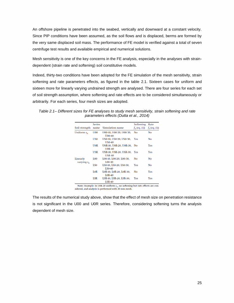
Table 2.1– Different sizes for FE analyses to study mesh sensitivity, strain softening and rate

parameters effects (Dutta et al., 2014) .............................................................................................25

Table 3.1 – Relevant mechanical properties adopted for the T-bar ..................................................28

Table 3.2 – Adopted soil properties for the Mohr-Coulomb soil model .............................................30

Table 3.3– Input parameters for the NGI-ADP soil model ................................................................32

Table 3.4 – Anisotropic strain-softening parameters for a clay studied in Randolph and Andersen

(2006) ...............................................................................................................................................33

Table 3 5 - Adopted input parameters for the NGI-ADP model in Plaxis 2019 2D............................34

Table 4.1 – Parameters adopted for the study on the NT-Bar mesh size sensitivity ...........................48

Table 4.2 – Relevant parameters adopted for the analyses studying the penetration rate influence

on NT-bar factor ...............................................................................................................................50

Table 4.3 - Relevant parameters adopted for the analyses studying the Su and E influence on the

NT-bar .................................................................................................................................................51

Table 4.4 - Relevant parameters adopted for the analyses that study the Su and E/Su ratio

influence on the NT-bar .......................................................................................................................52

Table 4.5 - Relevant parameters adopted for the analyses that study E and E/Su ratio influence on

the NT-bar ...........................................................................................................................................54

Table 4. 6 - Relevant parameters adopted for the study of the influence of the shear stress limit on

the NT-bar, for the newly adopted initial modelling conditions .........................................................55

Table 4.7 - Relevant parameters adopted for the study of the influence of the T-bar density on the

NT-bar, for the newly adopted initial modelling conditions ..................................................................57

Table 4.8 - Relevant parameters adopted for the study of the influence of soil density and

penetration rate on the NT-bar, for the newly adopted initial modelling conditions .............................58

Table 4.9 - Relevant parameters adopted for the study of the influence of undrained resistance and

interface roughness on the NT-bar, for the newly adopted initial modelling conditions .......................59

Table 5.1 - Parameters adopted for the study on the NT-Bar mesh size sensitivity ............................65

Table 5.2 - Relevant parameters adopted for the analyses that study the penetration rate influence

on the evolution of the assessed NT-bar .............................................................................................69

Table 5.3 - Relevant parameters adopted for the analyses that study the undrained strength

influence on the evolution of the assessed NT-bar..............................................................................70

Table 5.4 – Relevant parameters adopted for the analyses that study the Young’s Modulus

influence on the evolution of the assessed NT-bar..............................................................................71

xiv

List of symbols

Acronyms

AM Adaptive Meshing

ALE Arbitrary Lagrangian-Eulerian

CEL Coupled Eulerian-Lagrangian

CPT Cone Penetration Test

CPTu Cone Penetration Test Undrained

DPS Diameters Per Second

DSS Direct Shear Stress

EVF Eulerian Volume Fraction

FE Finite Element

FEM Finite Element Method

ISSMFE International Society of Soil Mechanics and Foundation Engineering

ISSMGE International Society of Soil Mechanics and Geotechnical Engineering

IRTP International Reference Test Procedure

LDFE Large Deformation Finite Element

OCR Overconsolidation Ratio

PI Plasticity Index

PIP Pushed-in-place

RITSS Remeshing and Interpolation Technique with Small Strain

TL Total Lagrangian

TC Triaxial Compression

TE Triaxial Extension

UL Updated Lagrangian

WIP Wished-in-place

xv

Latin Upper-case letters

As Submerged area of the T-bar penetrometer

d Diameter of the penetrometer

E Young Modulus

EA Axial stiffness

EI Bending stiffness

Eu Undrained Young Modulus

G Shear modulus

Gur Unloading/reloading shear modulus

𝐼𝑟 Rigidity index

K0 Earth pressure coefficient at rest

𝑁𝑏 Buoyancy bearing factor

NT-bar, 𝑁𝑇 T-bar penetrometer bearing capacity factor

𝑁𝑇−𝑆ℎ𝑎𝑙𝑙𝑜𝑤 Shallow T-bar penetrometer bearing capacity factor

𝑁𝑇−𝐷𝑒𝑒𝑝 Deep T-bar penetrometer bearing capacity factor

QT-bar Tip resistance measured by the T-bar penetrometer

RInter Interface roughness coefficient

Su Undrained resistance

Su,avg Average undrained resistance

Su,ref A Reference active shear strength

Su A

Active shear strength

Su P Passive shear strength

SuC,TX Undrained strength derived from the triaxial compression test

SuE,TX Undrained strength derived from the triaxial extension test

Su DSS Undrained strength derived from the direct shear test

𝑉 Regular nondimensional velocity

xvi

𝑉′ Alternative nondimensional velocity

Latin Lower-case letters

𝑏 Relative magnitude of the intermediate principle stress

𝑐𝑣 Coefficient of consolidation

𝑑 Diameter of the penetrometer

𝑑𝑒 Diameter of a circle with projected area equivalent to that of the penetrometer

q Tip resistance measured by the penetrometer

𝑢2 Pore pressure filter location at the base of the cone penetrometer

𝑤 Embedment depth of the penetrometer

�̂� Normalised embedment depth of the penetrometer

�̂�𝑑𝑒𝑒𝑝 Normalised embedment depth when 𝑁𝑇−𝑆ℎ𝑎𝑙𝑙𝑜𝑤 transitions to 𝑁𝑇−𝐷𝑒𝑒𝑝

Greek letters

α Interface roughness coefficient

Inclination between the major principal stress and the vertical stresses direction

γ’ Submerged soil unit weight

γf C Shear strain at failure in triaxial compression

γf DSS Shear strain at failure in direct simple shear

γf E Shear strain at failure in triaxial extension

Δ In situ stress ratio

𝜈 Poisson’s ratio

𝜈u Undrained Poisson’s ratio

σ’ Soil effective stress

𝜎1 Major principle stress

xvii

𝜎2 Intermediate stress

𝜎3 Minor principle stress

𝜎𝑣 Vertical stresses in the soil

𝜎ℎ Horizontal stresses in the soil

𝜏0 Initial shear stress

xviii

1

1. Introduction

1.1. Relevance

There are several situations in geotechnical engineering that comprise the penetration of slender

elements into the soil, where the in situ SPT and CPTu, as well as the installation of driven piles, are

good examples.

One of the most important fields of interest in offshore engineering is the assessment of the

engineering and physical properties of the soil that is going to receive the man-made infrastructure,

as well as to predict the behaviour of the interaction between these two elements. This is crucial for

the longevity and well-functioning of the structure since without it, these criteria would be violated.

In regards to offshore geotechnical site investigation, extracting soil samples from the bottom of the

sea and testing them in laboratory is quite expensive. Therefore, in-situ testing resorting to

penetrometers is commonly performed and used to study the geomechanical properties of the soft

seabed soil. However, the usage of the typical piezocone test results in less accurate data retrieved

since the environment at an offshore site is much different from the typical surface on land.

Although being widely used for decades in the past century, the usage of the CPTu to assess the

undrained shear strength and excess pore water pressure is not recommended since high water

depth affects the load cell sensitivity. Indeed, its cone shaped geometry is responsible for this effect

which results in considerable reading errors, which tend to increase the deeper the seabed is located.

Different shaped penetrometers were proposed and tested where the soil flow mechanism that they

produced showed to be easier to understand by researchers and engineers and less prone to the

complications related with the CPTu usage on offshore soil characterisation.

Bearing capacity factors are used to relate the undrained shear strength extracted from laboratory

tests and the measured penetration resistance. Hence, in order to assess the undrained shear

strength correctly, there is a need to infer the bearing factor that counts with the majority of the several

geomechanical properties and phenomena involved in the seabed penetration.

This is where the numerical modelling is crucial as it can validate empiric studies and produce

parametric studies for a cheaper cost, resulting in a deep understanding of the interaction between

geomechanical properties as the soil is penetrated.

2

1.2. Objectives of the thesis

The objective of this thesis is to model deep seabed penetration by the T-bar penetrometer resorting

to different finite element formulations, to better understand the soil behaviour during offshore in-situ

testing and to better characterise the empirical correlations existing between the quantities measured

in the these tests and geotechnical parameters of the soil.

The simulation of soft seabed soil penetration will be done resorting to Plaxis and Abaqus FEM

software. The properties and guidelines followed in studies found in literature are taken into account

when constructing the models in these FEM programs. This is done to calibrate the models produced

in this thesis to work as the likes employed in previous works. From that point, the results deriving

from the studies produced in this work can then be compared with the ones deriving from similar

studies found in literature. What is more, other studies can then be developed for further

investigations.

1.3. Layout of the thesis

This work is organised into six chapters. The first chapter presents the scope of this work, along with

its objectives, subjects that are approached in this thesis, and a brief summary of what each chapter

presents.

The state of the art is found in the second chapter, where a brief history is told on the use of several

penetrometers and numerical modelling techniques throughout this last century until today, along with

the development and evolution of the same techniques, the challenges they posed to engineers and

researchers and the evolution of the empirical correlations they established, resulting from their

studies. Due focus is given to the study and interpretation of the full-flow penetrometers, especially

the T-bar penetrometer and its full-flow mechanism associated, from shallow to greater depths of soil

penetration.

In the third chapter we proceed to the study of the T-bar penetration in the using the finite element

software Plaxis that uses a Lagrangian framework. The goal of this study is to achieve the same

correlation between the T-bar bearing factor and the interface roughness coefficient, achieved by

Randolph and Andersen (2006) for isotropic and anisotropic finite element analyses. This is done by

resorting to two different constitutive models. First, the classic Tresca model for isotropic analysis and

secondly, the relatively new NGI-ADP constitutive model to explore anisotropy effects on soil. The

analyses and soil constitutive models are also described in detail.

In the fourth chapter we proceed to the study of the T-bar penetration while resorting to the more

sophisticated Coupled Eulerian-Lagrangian framework of LDFE analysis, resorting to the Abaqus

FEM software. This chapter features two parametric studies comprised of several analyses in the

WIP scenario. The objective is to obtain a good agreement between the correlations produced in this

3

part of the thesis and the correlations produced in similar studies belonging to previous works, as well

laying the simulation groundwork necessary for more studies to be developed in the PIP scenario,

addressed in Chapter 5.

In the fifth chapter we proceed to the study of the soft sedimentary soil penetration by the T-bar

penetrometer, in the PIP scenario. The model calibrated in the previous chapter is used as a starting

point to further proceed to the study of the dependence of the T-bar bearing factor on several

geotechnical and mechanical properties. The major difference in this Chapter is the capture of the

evolution of the flow mechanism and the associated T-bar bearing factor as the T-bar penetrates the

soil from the seabed until a considerable depth is achieved. In addition, a similar parametric study is

performed for this PIP modelling scenario, where the results are to be compared with similar results

deriving from other works as well as with the results obtained from the studies performed in the

previous Chapter.

The sixth and final chapter holds the conclusions and recommendations for further work.

4

2. State of the art

2.1. Introductory remarks

The growing importance of offshore infrastructure engineering has had a significant impact

throughout the years on the need for a better understanding of the mechanisms influencing the

assessment of geotechnical properties, at deep seabed environment. This has an impact on the on-

bottom stability and service of deep sea structures.

Research and investigations were made to understand the interaction of the pipeline with the fine

grained soil found at the seabed of offshore locations. It is known that the behaviour mechanisms and

these interactions differ greatly between shallow and greater depths. Therefore, efforts were made to

study these phenomena.

5

2.2. Description of in situ penetration tests

In order to avoid high costs in obtaining high quality samples of soil from the bottom of the sea, to

study in laboratory, offshore and geotechnical engineers were led to rely more on in-situ testing. By

resorting to field vane and cone penetration tests, the geotechnical parameters of the soil in question

were able to be characterised and assessed.

The vane shear test consists of a four-blade stainless steel vane attached to a steel rod that is pushed

to the ground and at designated locations, is turned. It is able to provide reliable measurements of

remoulded and intact undrained shear strength of fully saturated clays without disturbance. But,

despite being relatively simple to use, quick and cost effective, it does not provide a continuous

strength profile.

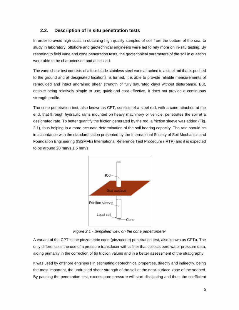
The cone penetration test, also known as CPT, consists of a steel rod, with a cone attached at the

end, that through hydraulic rams mounted on heavy machinery or vehicle, penetrates the soil at a

designated rate. To better quantify the friction generated by the rod, a friction sleeve was added (Fig.

2.1), thus helping in a more accurate determination of the soil bearing capacity. The rate should be

in accordance with the standardisation presented by the International Society of Soil Mechanics and

Foundation Engineering (ISSMFE) International Reference Test Procedure (IRTP) and it is expected

to be around 20 mm/s ± 5 mm/s.

Figure 2.1 - Simplified view on the cone penetrometer

A variant of the CPT is the piezometric cone (piezocone) penetration test, also known as CPTu. The

only difference is the use of a pressure transducer with a filter that collects pore water pressure data,

aiding primarily in the correction of tip friction values and in a better assessment of the stratigraphy.

It was used by offshore engineers in estimating geotechnical properties, directly and indirectly, being

the most important, the undrained shear strength of the soil at the near-surface zone of the seabed.

By pausing the penetration test, excess pore pressure will start dissipating and thus, the coefficient

6

of consolidation can be assessed. Furthermore, it is used by many geotechnical engineers to

determine the stratigraphy and existing material under the soil’s surface, as it is cost-effective and

simple to use.

Generally, the piezocone testing should be in accordance with internationally recognised guidelines

and standards. Among many, the IRTP published by the International Society of Soil Mechanics and

Geotechnical Engineering (ISSMGE, 1999) is notable (Lunne et al. , 2011).

Although cones with a diameter of 36.5 mm can be found, the ISOTP-1 proposes diameters of 40.5,

50 and 60 mm.

Cone penetration in fine grained soils, such as clays and silts, is generally undrained. With the

generation of pore water pressure in the soil, the pore pressure will act on the shoulder area behind

the cone and friction sleeves, thus influencing the total stress determined from these two zones. This

effect is known as the “unequal area effect” and is identified when the total cone resistance, is not

equal to the water pressure. This difference is expected to be of greater dimensions when deep water

studies are carried with the CPTu.

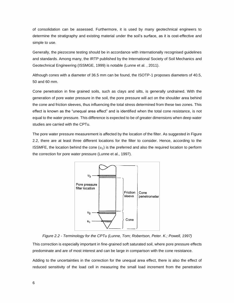
The pore water pressure measurement is affected by the location of the filter. As suggested in Figure

2.2, there are at least three different locations for the filter to consider. Hence, according to the

ISSMFE, the location behind the cone (𝑢2) is the preferred and also the required location to perform

the correction for pore water pressure (Lunne et al., 1997).

Figure 2.2 - Terminology for the CPTu (Lunne, Tom; Robertson, Peter. K.; Powell, 1997)

This correction is especially important in fine-grained soft saturated soil, where pore pressure effects

predominate and are of most interest and can be large in comparison with the cone resistance.

Adding to the uncertainties in the correction for the unequal area effect, there is also the effect of

reduced sensitivity of the load cell in measuring the small load increment from the penetration

7

resistance in comparison with the high ambient pressure, at deep sea sites, decreasing the accuracy

of the CPTu.

By the time of 1997, the theoretical and modelling methods that considered the distribution of pore

pressures and stress around the cone were not decent enough to be relied on. Hence, engineers and

researchers were left to a simpler approach which consisted in obtaining high-quality, high-cost

undisturbed samples to measure strength parameters and other needed soil parameters.

Therefore, considering the disadvantages of the use of the piezocone in assessing the deep soil

shear strength and the high costs related to obtaining high-quality samples, engineers were faced

with the need for an alternative to this tool.

By resorting to full-flow penetrometers, such as the T-bar and Ball penetrometer, engineers could

take advantage from the respective failure mechanism, that greatly characterises these

penetrometers, to improve the characterisation of deep soil geotechnical properties.

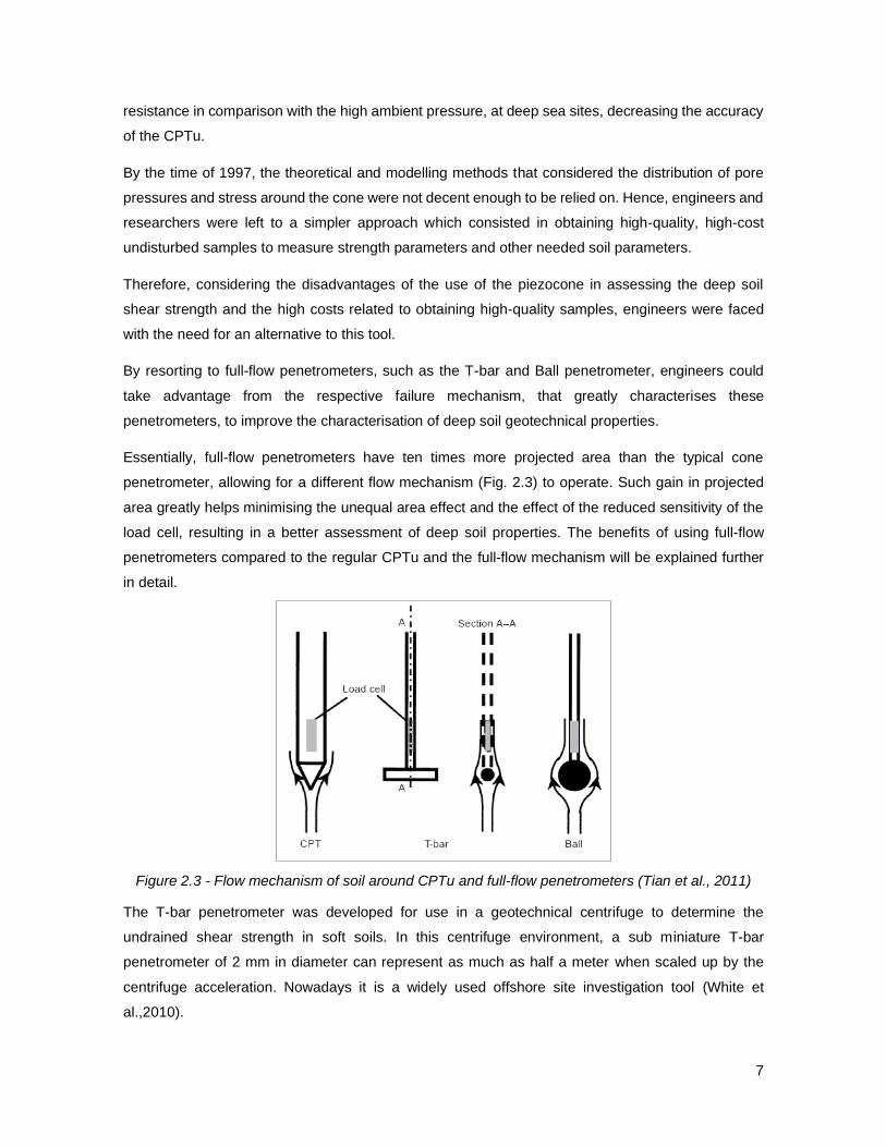
Essentially, full-flow penetrometers have ten times more projected area than the typical cone

penetrometer, allowing for a different flow mechanism (Fig. 2.3) to operate. Such gain in projected

area greatly helps minimising the unequal area effect and the effect of the reduced sensitivity of the

load cell, resulting in a better assessment of deep soil properties. The benefits of using full-flow

penetrometers compared to the regular CPTu and the full-flow mechanism will be explained further

in detail.

Figure 2.3 - Flow mechanism of soil around CPTu and full-flow penetrometers (Tian et al., 2011)

The T-bar penetrometer was developed for use in a geotechnical centrifuge to determine the

undrained shear strength in soft soils. In this centrifuge environment, a sub miniature T-bar

penetrometer of 2 mm in diameter can represent as much as half a meter when scaled up by the

centrifuge acceleration. Nowadays it is a widely used offshore site investigation tool (White et

al.,2010).

8

The first difference that can be observed between the T-bar penetrometer and the piezocone is that

a T shape tip replaces the cone tip at the penetrating end, usually having a diameter of 40 mm and

250 mm in length as shown in Figure 2.4. Another difference, and of most relevance, is the absence

of the pressure transducer and the friction sleeve. Since the projected figure of the T-bar is a

rectangle, the consolidation around the cylindrical penetrometer would not be the straightforward

radial, but instead a 3D one, difficult to interpret, making the employment of the transducer almost

meaningless, even at the 𝑢2 location. In addition, due to a different flow mechanism being operative,

the sleeve friction acting on the sleeve is negligible, hence the absence of the friction sleeve.

The ball penetrometer designation follows the same logic as the T-bar where a sphere makes now

the end of the penetrometer. However, since the projected figure is a circle, a pressure transducer

can be employed around the sphere. Even though the T-bar penetration can be modelled in plane

strain, which facilitates numerical modelling, the pore water pressure can only be assessed in the ball

penetrometer, making it an also reliable, if not better option.

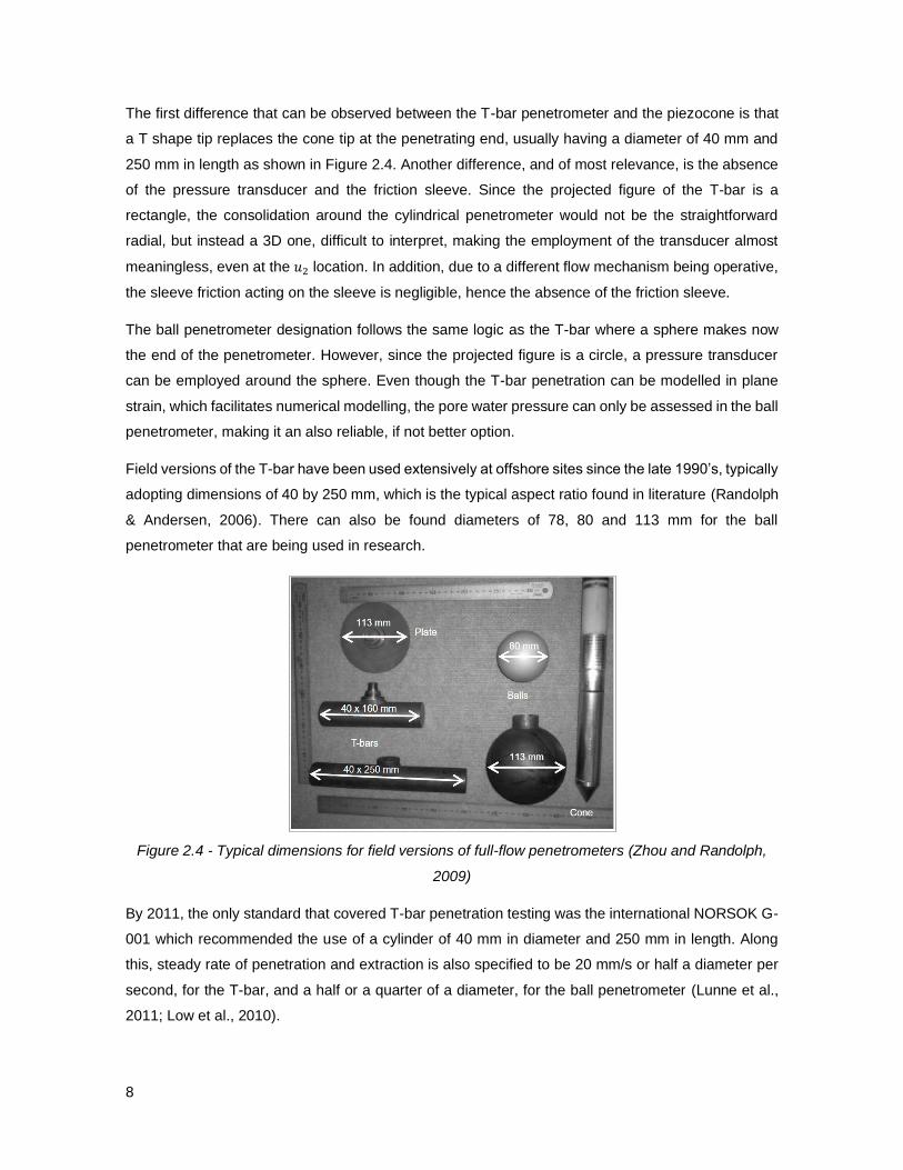
Field versions of the T-bar have been used extensively at offshore sites since the late 1990’s, typically

adopting dimensions of 40 by 250 mm, which is the typical aspect ratio found in literature (Randolph

& Andersen, 2006). There can also be found diameters of 78, 80 and 113 mm for the ball

penetrometer that are being used in research.

Figure 2.4 - Typical dimensions for field versions of full-flow penetrometers (Zhou and Randolph,

2009)

By 2011, the only standard that covered T-bar penetration testing was the international NORSOK G-

001 which recommended the use of a cylinder of 40 mm in diameter and 250 mm in length. Along

this, steady rate of penetration and extraction is also specified to be 20 mm/s or half a diameter per

second, for the T-bar, and a half or a quarter of a diameter, for the ball penetrometer (Lunne et al.,

2011; Low et al., 2010).

9

2.3. Numerical methods for the analysis of large deformation problems

Physical and theoretical analysis backing in-situ and laboratorial testing had been the typical

approach to investigate and analyse the phenomena that characterises deep seabed environment.

However, it may have considerable costs (both time and money) associated and an alternative was

in need. The numerical method approach, based on finite element analysis, serves as a good

alternative as it complements the correlations from the results deriving from the traditional

approaches.

Offshore engineers require valid, yet accessible, numerical approaches to consistently simulate large

deformation penetration problems, like the vertical penetration of partially embedded pipelines or the

transition from intact undisturbed soil ahead of a penetrometer to partially remoulded in the wake of

the penetrometer (Dutta et al., 2014; Zhou & Randolph, 2009).

When it comes to finite element analysis, there are three main approaches to deal with continuum

mechanics problems, namely, the Eulerian, total Lagrangian and updated Lagrangian formulations

(Hu & Randolph, 1998).

In the Eulerian approach, the finite element mesh is stationary while the material is allowed to move

from element to element. The spatial position of the nodes is fixed, and the finite element mesh suffers

zero distortion during the analysis despite the material undergoing large deformation, as displayed in

Figure 2.5 (Hu & Randolph, 1998).

Both total Lagrangian (TL) and updated Lagrangian (UL) approaches are commonly used to model

the response of solids. These two approaches can deal with small to moderate deformations. What

distinguishes these two methods is the reference state for the body, which is taken at time equal zero

in the TL approach, while the updated geometry is used in the UL approach (Hu & Randolph, 1998).

Figure 2.5 - Eulerian and Lagrangian mesh behaviour after deformation occurs

10

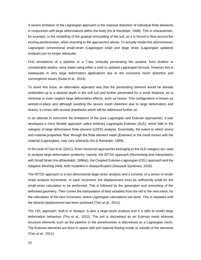
A severe limitation of the Lagrangian approach is the massive distortion of individual finite elements

in conjunction with large deformations within the body (Hu & Randolph, 1998). This is characteristic,

for example, in the modelling of the gradual remoulding of the soil, as it is forced to flow around the

moving penetrometer, when resorting to the approaches above. To actually model this phenomenon,

Lagrangian conventional small-strain (Lagrangian total) and large strain (Lagrangian updated)

analyses are no longer adequate.

First simulations of a pipeline or a T-bar vertically penetrating the seabed, from shallow to

considerable depths, were made using either a total or updated Lagrangian formula. However this is

inadequate in very large deformation applications due to the excessive mesh distortion and

convergence issues (Dutta et al., 2014).

To avoid this issue, an alternative approach was that the penetrating element would be already

embedded up to a desired depth in the soft soil and further penetrated for a small distance, as to

minimise or even neglect large deformation effects, such as heave. This configuration is known as

wished-in-place and although avoiding the severe mesh distortion due to large deformation and

strains, it comes with several drawbacks which will be addressed further on.

In an attempt to overcome the limitations of the pure Lagrangian and Eulerian approaches, it was

developed a more flexible approach called Arbitrary Lagrangian-Eulerian (ALE), which falls in the

category of large deformation finite element (LDFE) analysis. Essentially, the extent to which stress

and material properties ‘flow’ through the finite element mesh (Eulerian) or the mesh moves with the

material (Lagrangian), may vary arbitrarily (Hu & Randolph, 1998).

In the work of Tian et al. (2011), three numerical approaches belonging to the ALE category are used

to analyse large deformation problems, namely, the RITSS approach (Remeshing and Interpolation

with Small Strain (Hu &Randolph, 1998a)), the Coupled Eulerian-Lagrangian (CEL) approach and the

Adaptive Meshing (AM), both modelled in Abaqus/Explicit (Dassault Systèmes, 2010).

The RITSS approach is a two-dimensional large-strain analysis and it consists of a series of small-

strain analysis increments. In each increment, the displacement must be sufficiently small for the

small-strain calculation to be performed. This is followed by the generation and remeshing of the

deformed geometry. Then comes the interpolation of field variables from the old to the new mesh, for

the calculation of the next increment, where Lagrangian calculations are done. This is repeated until

the desired displacement has been achieved (Tian et al., 2011).

The CEL approach, built-in in Abaqus, is also a large-strain analysis and it is able to model large

deformation behaviour (Tho et al., 2012). The soil is discretised as an Eulerian mesh whereas

structure elements such as the pipeline or the penetrometer is discretised as a Lagrangian mesh.

The Eulerian elements are fixed in space with soil material flowing inside or outside of the elements

(Tian et al., 2011).

11

The interaction between Eulerian material and Lagrangian surfaces is imposed through Eulerian–

Lagrangian contact based on an enhanced immersed boundary method. In this method, the

Lagrangian structure occupies void regions inside the Eulerian mesh and the contact algorithm

automatically computes and tracks the interface between the Lagrangian structure and the Eulerian

materials by imposing a constraint where the Eulerian material cannot flow past the Lagrangian

surface, into the void regions (Tho et al., 2012).

The CEL analysis technique in Abaqus/Explicit (SIMULIA 2010) can be employed for simulating the

penetration of elements into the deep seabed soil. In order to simulate the penetration of a pipe

section, resembling the T-bar, into the soil, a two-dimensional plane strain model would suffice.

However, the Eulerian analysis feature in Abaqus is only available in a three-dimensional modelling

space.

As workaround, a three-dimensional finite element model with one element of width, perpendicular to

the plane direction, is created in Abaqus/CAE. The pipe is modelled as a Lagrangian rigid body and

the soil domain is modelled as an Eulerian deformable body.

The AM approach is similar to the RITSS approach in principal, except that the mesh topology is

unchanged. The nodes in specified adaptive domains are frequently adapted to maintain a

reasonable element shape during large deformation analysis. However, the number of elements and

their connectivity is not altered. (Tian et al., 2011)

12

2.4. Mechanism during T-bar penetration

The most prominent characteristic of the T-bar penetrometer is the mobilisation of the full-flow

mechanism that allows the soft sediments to flow through the penetrating cylinder. By attaching a

cylinder, a ball or even a plate to the penetrating rod, not only the projected area of the penetrometer

increases immensely, but it also allows for partial remoulding of the soil.

The full-flow mechanism distinguishes itself immensely from the piezocone “pushing” mechanism,

since the penetration resistance assessed through the first is mainly attributed to the soil flow around

the penetrometer, rather than the addition of volume into the ground, as portrayed by the latter. This

reflects in a more accurate and less scattered measurements of resistance, much less dependency

of the same on secondary soil characteristics and well-established plasticity solutions linking

measured resistance to undrained shear strength (Amuda et al., 2018).

However, the full-flow mechanism is only operative from a certain penetration depth and in certain

conditions. Indeed, different failure mechanisms will operate, starting from the penetration of the

seabed, until greater depths are reached. In later subchapters, it will be discussed in detail which soil

characteristics have effect on the developing and transition of these different failure mechanisms.

The evolution of the penetration resistance with depth was first studied in a discontinuous manner, at

shallow and deep penetrations, where distinct failure mechanisms operated. Attending this manner,

a particular depth range in between is ignored, which is characteristic for having its own distinct failure

mechanism, and in turn, bridges both shallow and deep failure mechanisms associated with T-bar

penetration.

The work of Tho et al. (2012) comes to suggest a continuous manner of analysis, in the sense that

the effects of evolving seabed topology are taken into consideration and the intermediate flow

mechanism, later labelled as deep-cavity flow mechanism, is identified.

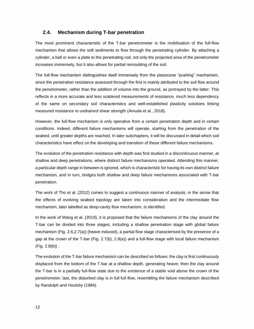
In the work of Wang et al. (2019), it is proposed that the failure mechanisms of the clay around the

T-bar can be divided into three stages, including a shallow penetration stage with global failure

mechanism (Fig. 2.6,2.7(a)) (heave induced), a partial flow stage characterised by the presence of a

gap at the crown of the T-bar (Fig. 2.7(b), 2.8(a)) and a full-flow stage with local failure mechanism

(Fig. 2.8(b)) .

The evolution of the T-bar failure mechanism can be described as follows: the clay is first continuously

displaced from the bottom of the T-bar at a shallow depth, generating heave; then the clay around

the T-bar is in a partially full-flow state due to the existence of a stable void above the crown of the

penetrometer; last, the disturbed clay is in full full-flow, resembling the failure mechanism described

by Randolph and Houlsby (1984).

13

(a) (b)

Figure 2.6 - Soil heave due to shallow pipe penetration for Su/γ’d = 0.2(a) and 10.0 (b) (Tho et al.,2012)

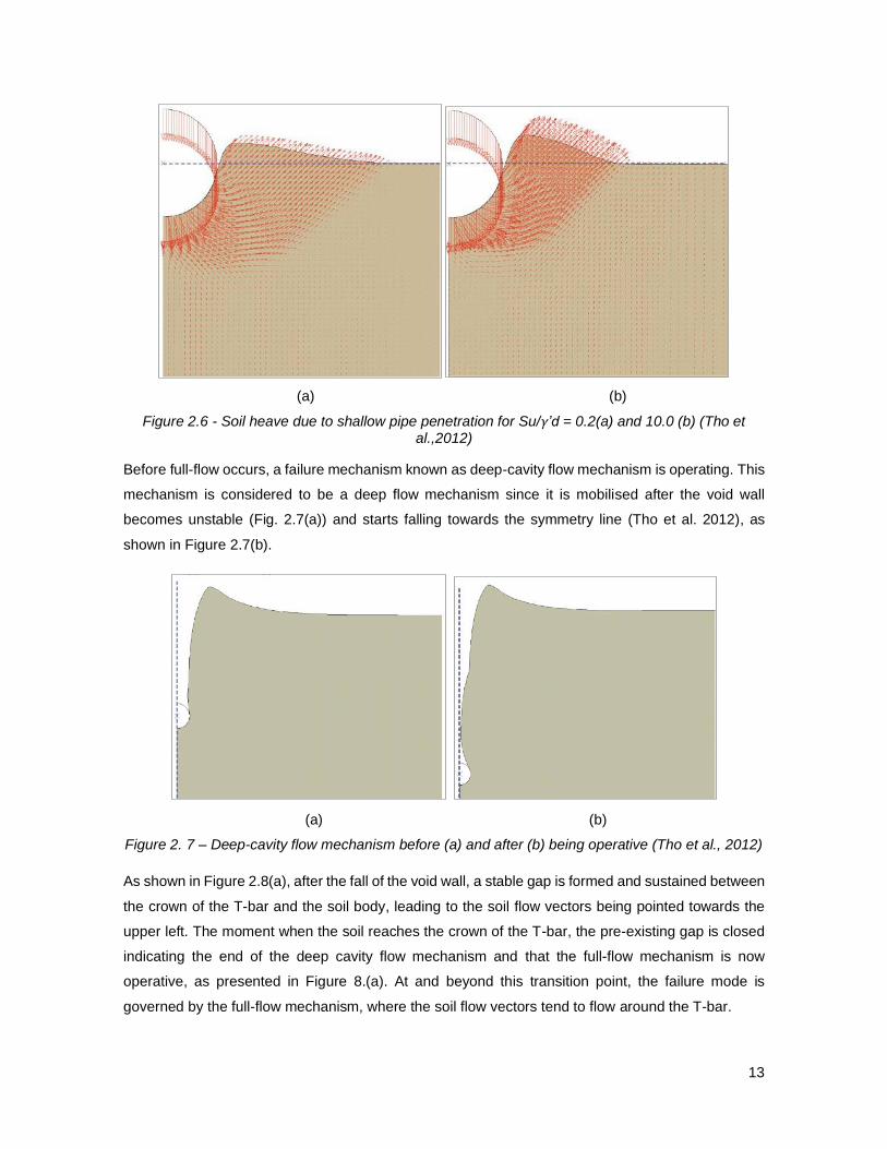
Before full-flow occurs, a failure mechanism known as deep-cavity flow mechanism is operating. This

mechanism is considered to be a deep flow mechanism since it is mobilised after the void wall

becomes unstable (Fig. 2.7(a)) and starts falling towards the symmetry line (Tho et al. 2012), as

shown in Figure 2.7(b).

(a) (b)

Figure 2. 7 – Deep-cavity flow mechanism before (a) and after (b) being operative (Tho et al., 2012)

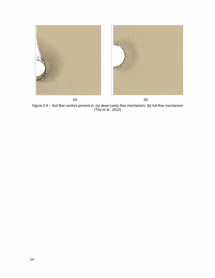
As shown in Figure 2.8(a), after the fall of the void wall, a stable gap is formed and sustained between

the crown of the T-bar and the soil body, leading to the soil flow vectors being pointed towards the

upper left. The moment when the soil reaches the crown of the T-bar, the pre-existing gap is closed

indicating the end of the deep cavity flow mechanism and that the full-flow mechanism is now

operative, as presented in Figure 8.(a). At and beyond this transition point, the failure mode is

governed by the full-flow mechanism, where the soil flow vectors tend to flow around the T-bar.

14

(a) (b)

Figure 2.8 – Soil flow vectors present in: (a) deep-cavity flow mechanism; (b) full-flow mechanism (Tho et al., 2012)

15

2.5. Analysis and interpretation of full-flow T-bar penetration

The conventional interpretation of the T-bar penetration test is to convert the measured penetration

resistance, 𝑞, to soil strength, 𝑆𝑢, using a single bearing factor associated with flow of soil around the

bar, 𝑁𝑇 = 𝑞 / 𝑆𝑢. This interpretation is based on plasticity solutions by Randolph and Houlsby (1984)

but it lacks corrections concerning secondary soil characteristics and different failure mechanisms,

operating at different depths, that are not taken into account (White et al., 2010).

Hence, large deformation finite elements (LDFE) analysis was necessary to properly evaluate the

influence of these phenomena on the measured resistance by the T-bar penetrometer. With this, the

penetration of soil for several diameters could be analysed and the partial remoulding of the soil, as

the T-bar advances, is revealed.

In the work of White et al. (2010), after studying the effects of soil buoyancy on the penetration

resistance resorting to centrifuge T-bar penetration testing and LDFE analysis, it was concluded that

the buoyancy component of correction was applicable at all depths, from shallow penetration, to

depths were the full-flow mechanism is observed.

In the work of Randolph and Andersen (2006), the proposed strain path method within the upper

bound mechanism made possible to quantify the effects of strain rate dependency and gradual

softening of the soil on the T-bar resistance.

After several cycles of penetration and extraction, the soil is assumed to be fully remoulded. Thus, it

ceases to be affected by strain softening and only strain rate effects are expected to affect the

interpretation of the T-bar resistance. The analyses showed that for perfectly plastic soil response,

the FE results for isotropic soil agreed well with plasticity solutions. It was also shown that the effect

of anisotropy was less than 5%, provided the T-bar resistance was normalised by the average shear

strength from the laboratory tests.

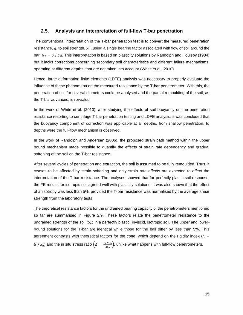
The theoretical resistance factors for the undrained bearing capacity of the penetrometers mentioned

so far are summarised in Figure 2.9. These factors relate the penetrometer resistance to the

undrained strength of the soil (𝑆𝑢) in a perfectly plastic, inviscid, isotropic soil. The upper and lower-

bound solutions for the T-bar are identical while those for the ball differ by less than 5%. This

agreement contrasts with theoretical factors for the cone, which depend on the rigidity index (𝐼𝑟 =

𝐺 / 𝑆𝑢) and the in situ stress ratio (𝛥 = 𝜎𝑣−𝜎ℎ

2𝑆𝑢), unlike what happens with full-flow penetrometers.

16

Figure 2.9- Theoretical factors for the cone, T-bar and ball penetrometer plotted against adhesion factor (Randolph, 2004)

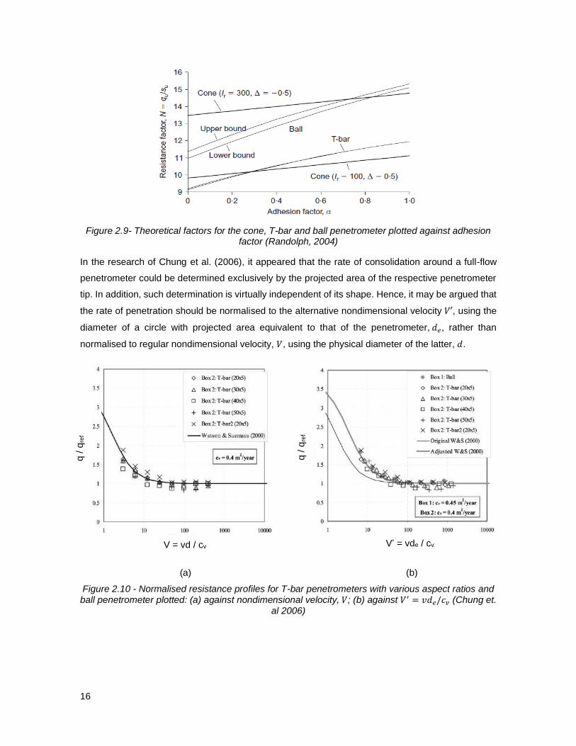
In the research of Chung et al. (2006), it appeared that the rate of consolidation around a full-flow

penetrometer could be determined exclusively by the projected area of the respective penetrometer

tip. In addition, such determination is virtually independent of its shape. Hence, it may be argued that

the rate of penetration should be normalised to the alternative nondimensional velocity 𝑉′, using the

diameter of a circle with projected area equivalent to that of the penetrometer, 𝑑𝑒, rather than

normalised to regular nondimensional velocity, 𝑉, using the physical diameter of the latter, 𝑑.

(a) (b)

Figure 2.10 - Normalised resistance profiles for T-bar penetrometers with various aspect ratios and ball penetrometer plotted: (a) against nondimensional velocity, 𝑉; (b) against 𝑉′ = 𝑣𝑑𝑒/𝑐𝑣 (Chung et.

al 2006)

q /

qre

f

q /

qre

f

V = vd / cv V’ = vde / cv

17

The original profile for the T-bar was shifted horizontally to the right by a factor of 2.26, in Figure

2.10(b)), which equals the ratio of the equivalent diameter over the physical diameter, for the T-bar.

The fact that normalised data appears to fit relatively better to the adjusted backbone curve plotted

against 𝑉′ (Fig. 2.10(b)) compared to when plotted against 𝑉 (Fig. 2.10(a)), suggests dependency of

the consolidation rate on the projected area of the penetrometer rather than its physical diameter.

In the numerical study of Zhou and Randolph (2009), the objective was to quantify the separate and

combined effects of strain rate dependency and strain softening on the T-bar penetration resistance

resorting to a LDFE approach, previously described by the same researchers. This technique allows

for the simulation of soil flow past the T-bar, modelling both the increase in shear strength owing to

high-strain rates and the gradual strength degradation as the soil is remoulded.

In addition to what was previously mentioned, the moment when full-flow develops coincides with the

instant when the bearing factor, NT, reaches a steady value. Furthermore, the depth at which the

transition from deep-cavity to full-flow mechanism is reached, may go up to several diameters and is

shown to depend on the normalised soil strength, Su/γ’d. Where Su is the undrained shear strength,

γ’ is the submerged unit weight of the soil and d is the diameter of the T-bar.

This mechanism can be analysed through numerical modelling, where it can be assumed either one

of two conditions. One, where LDFE and pushed-in-place (PIP) conditions are adopted, i.e., the T-

bar starts penetrating the seabed surface until it reaches a certain depth, where the evolving topology

of the seabed is taken into account and the eventual occurring gap might close. The other, where

wished-in-place (WIP) conditions are assumed and right from the start of the penetration, at an

already designated depth, the full-flow mechanism is already operative and the aforementioned gap

is inexistent.

In several works, after performing in-situ tests resorting to penetrometers, the respective resistance

factor for the estimation of undrained shear strengths is derived. Then, these factors were compared

with existing theoretical solutions and resistance factors derived from laboratory tests to evaluate the

important influence that particular soil characteristics have on the assessment of that factor, for each

type of penetrometer.

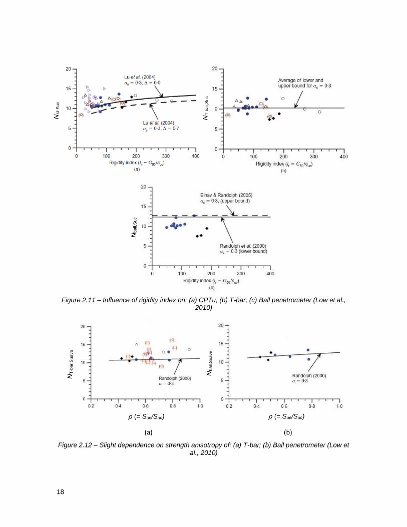
The work of Low et al. (2010) follows this procedure and the results show similar levels of variability

on the resistance factors for the piezocone, T-bar and ball penetrometer. Correlations of these factors

with specific secondary soil characteristics, indicated that the piezocone resistance factors were more

influenced by rigidity index (Fig. 2.11(a), (b) and (c)), or soil stiffness, strength sensitivity and strain

rate dependency of strength, than the full-flow penetrometers. As depicted in Figure 2.12 (a) and (b),

the effect of strength anisotropy was only apparent in resistance factors for full-flow devices but it can

be taken as insignificant if the penetration resistance is normalised by the average shear strength.

18

Figure 2.11 – Influence of rigidity index on: (a) CPTu; (b) T-bar; (c) Ball penetrometer (Low et al., 2010)

(a) (b)

Figure 2.12 – Slight dependence on strength anisotropy of: (a) T-bar; (b) Ball penetrometer (Low et al., 2010)

Nkt-

Suc

NT

-bar,

Suc

Nball,

Suc

NT

-bar,

Suave

Nball,

Suave

ρ (= Sue/Suc) ρ (= Sue/Suc)

19

In the Figures above, in the subscript 𝑘𝑡, refers to the piezocone, the subscript T-bar and ball refer to

the full-flow penetrometers and 𝑆𝑢𝑐 relates to the triaxial compression undrained strength, 𝑆𝑢𝑎𝑣𝑒, to

the average of the undrained shear strength measure in triaxial compression, extension and simple

shear and 𝑆𝑢𝑣𝑎𝑛𝑒, to the field vane shear test.

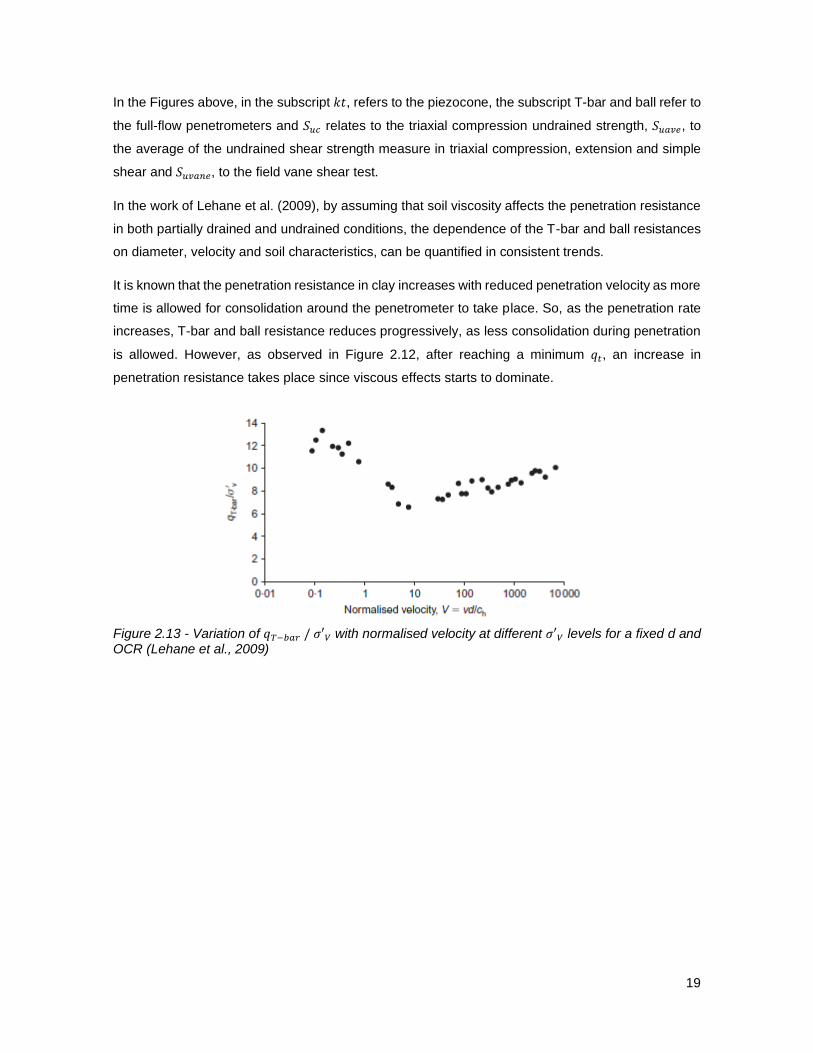
In the work of Lehane et al. (2009), by assuming that soil viscosity affects the penetration resistance

in both partially drained and undrained conditions, the dependence of the T-bar and ball resistances

on diameter, velocity and soil characteristics, can be quantified in consistent trends.

It is known that the penetration resistance in clay increases with reduced penetration velocity as more

time is allowed for consolidation around the penetrometer to take place. So, as the penetration rate

increases, T-bar and ball resistance reduces progressively, as less consolidation during penetration

is allowed. However, as observed in Figure 2.12, after reaching a minimum 𝑞𝑡, an increase in

penetration resistance takes place since viscous effects starts to dominate.

Figure 2.13 - Variation of 𝑞𝑇−𝑏𝑎𝑟 / 𝜎′𝑉 with normalised velocity at different 𝜎′𝑉 levels for a fixed d and OCR (Lehane et al., 2009)

20

2.6. Analysis and interpretation of T-bar at shallow depth

Particular attention should be given to the shallow depths of the seabed, namely the upper 0.5 m of

soil, where near-surface effects exist and cannot be neglected since they affect the conventional

relationship between penetration resistance and soil strength represented by Eq. 1.

𝑁𝑇 = 𝑞 / 𝑆𝑢 (2.1)

To overcome this issue, pushed-in-place finite element analyses were carried out, following the ALE

remeshing technique for penetrations up to 0.5 meters of the deep seabed.

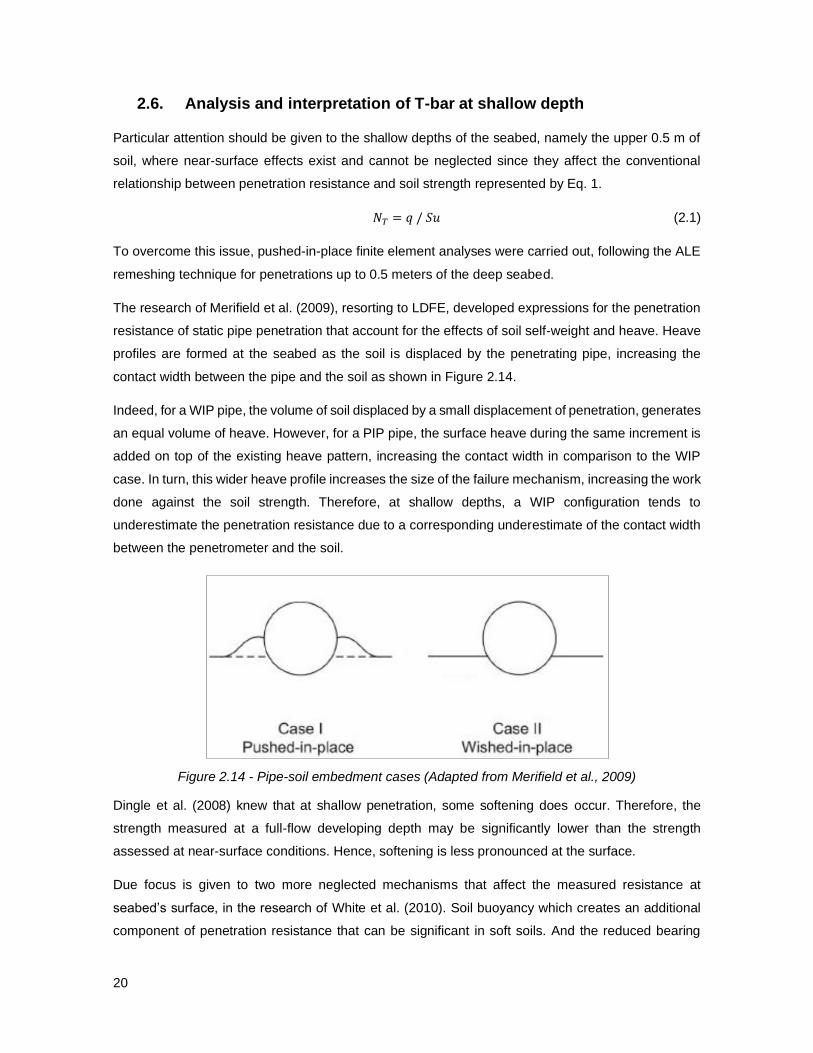
The research of Merifield et al. (2009), resorting to LDFE, developed expressions for the penetration

resistance of static pipe penetration that account for the effects of soil self-weight and heave. Heave

profiles are formed at the seabed as the soil is displaced by the penetrating pipe, increasing the

contact width between the pipe and the soil as shown in Figure 2.14.

Indeed, for a WIP pipe, the volume of soil displaced by a small displacement of penetration, generates

an equal volume of heave. However, for a PIP pipe, the surface heave during the same increment is

added on top of the existing heave pattern, increasing the contact width in comparison to the WIP

case. In turn, this wider heave profile increases the size of the failure mechanism, increasing the work

done against the soil strength. Therefore, at shallow depths, a WIP configuration tends to

underestimate the penetration resistance due to a corresponding underestimate of the contact width

between the penetrometer and the soil.

Figure 2.14 - Pipe-soil embedment cases (Adapted from Merifield et al., 2009)

Dingle et al. (2008) knew that at shallow penetration, some softening does occur. Therefore, the

strength measured at a full-flow developing depth may be significantly lower than the strength

assessed at near-surface conditions. Hence, softening is less pronounced at the surface.

Due focus is given to two more neglected mechanisms that affect the measured resistance at

seabed’s surface, in the research of White et al. (2010). Soil buoyancy which creates an additional

component of penetration resistance that can be significant in soft soils. And the reduced bearing

21

factor owing to the evolution of the shallow failure mechanism with depth, prior to the mobilisation of

the actual full-flow mechanism.

Soil heave has the effect of enhancing buoyancy effect such that the buoyancy bearing factor, 𝑁𝑏,

can be accounted for when assessing the measured resistance (Eq. 2.2). The correction to soil

buoyancy of the measured resistance, 𝑞, leads to a resistance that derives from the soil strength

alone (Eq. 2.3), 𝑞𝑠𝑜𝑖𝑙 , and thus, the corresponding bearing factor in Eq. 2.4.

𝑞 = 𝑁𝑇𝑆𝑢 + 𝑁𝑏 𝛾′𝑤 (2.2)

𝑞𝑠𝑜𝑖𝑙 = 𝑞 − 𝑁𝑏 𝛾′𝑤 (2.3)

𝑁𝑇 = 𝑞𝑠𝑜𝑖𝑙 / 𝑆𝑢 (2.4)

Where the buoyancy bearing factor, applied to the in situ vertical stress (𝛾′𝑤), aids in incorporating

the buoyancy effect at shallow penetration.

As the bar becomes embedded, it becomes increasingly buoyant since the soil density is higher than

the water density. Thus, 𝑁𝑏 varies, reflecting the changing profile of 𝑓𝑏 with the evolution of the failure

mechanism with depth, affecting the resistance that derives from soil buoyancy.

In the same work, the approach adopted was to define a critical depth, �̂�𝑑𝑒𝑒𝑝, at which the failure

mechanism transitions from a shallow to a full-flow mechanism and the bearing factor is expected to

alter from 𝑁𝑇−𝑆ℎ𝑎𝑙𝑙𝑜𝑤 to 𝑁𝑇−𝐷𝑒𝑒𝑝. This was achieved by performing LDFE on soft soils where the values

of 𝑆𝑢/ 𝛾′𝐷 varied.

Figure 2.15 - LDFE results: variation in bearing factor, 𝑁𝑇, with normalised embedment, 𝑤 ̂ = 𝑤/𝐷 (White et al., 2010)

22

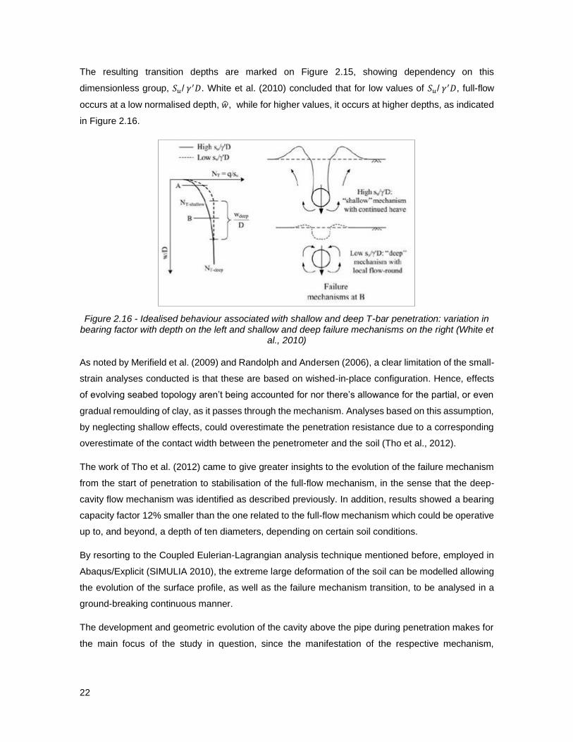
The resulting transition depths are marked on Figure 2.15, showing dependency on this

dimensionless group, 𝑆𝑢/ 𝛾′𝐷. White et al. (2010) concluded that for low values of 𝑆𝑢/ 𝛾′𝐷, full-flow

occurs at a low normalised depth, �̂�, while for higher values, it occurs at higher depths, as indicated

in Figure 2.16.

Figure 2.16 - Idealised behaviour associated with shallow and deep T-bar penetration: variation in bearing factor with depth on the left and shallow and deep failure mechanisms on the right (White et

al., 2010)

As noted by Merifield et al. (2009) and Randolph and Andersen (2006), a clear limitation of the small-

strain analyses conducted is that these are based on wished-in-place configuration. Hence, effects

of evolving seabed topology aren’t being accounted for nor there’s allowance for the partial, or even

gradual remoulding of clay, as it passes through the mechanism. Analyses based on this assumption,

by neglecting shallow effects, could overestimate the penetration resistance due to a corresponding

overestimate of the contact width between the penetrometer and the soil (Tho et al., 2012).

The work of Tho et al. (2012) came to give greater insights to the evolution of the failure mechanism

from the start of penetration to stabilisation of the full-flow mechanism, in the sense that the deep-

cavity flow mechanism was identified as described previously. In addition, results showed a bearing

capacity factor 12% smaller than the one related to the full-flow mechanism which could be operative

up to, and beyond, a depth of ten diameters, depending on certain soil conditions.

By resorting to the Coupled Eulerian-Lagrangian analysis technique mentioned before, employed in

Abaqus/Explicit (SIMULIA 2010), the extreme large deformation of the soil can be modelled allowing

the evolution of the surface profile, as well as the failure mechanism transition, to be analysed in a

ground-breaking continuous manner.

The development and geometric evolution of the cavity above the pipe during penetration makes for

the main focus of the study in question, since the manifestation of the respective mechanism,

23

observed in figure, significantly influences the bearing capacity factor. As long as the stable void is

observed, the full-flow mechanism is not operative and the bearing factor associated is 𝑁𝑇−𝑆ℎ𝑎𝑙𝑙𝑜𝑤.

(a) (b)

Figure 2.17 - Deep soil flow mechanism for: 𝑆𝑢/ 𝛾′𝐷=0.2 (a); 𝑆𝑢/ 𝛾′𝐷=10.0 (b) (Tho et al., 2012)

Figure 2.18 shows two significant value trends for the bearing-capacity factor, 8.0 and 9.14. The value

of 8.0 was found to be approximately the bearing factor associated with the deep-cavity flow

mechanism and appeared to be in agreement with the upper-bound solution on an extension of the

Randolph and Houlsby solution, as derived by Aubeny et al. (2005). Whereas the value of 9.14

corresponds to the lower-bound bearing factor for the full-flow mechanism deduced by Randolph and

Houlsby (1984).

Figure 2.18 – Bearing factor corrected for soil buoyancy plotted against normalised depths (Tho et al. 2012)

24

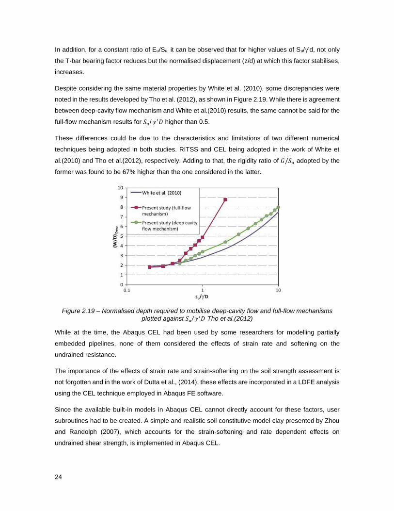
In addition, for a constant ratio of Eu/Su, it can be observed that for higher values of Su/γ’d, not only

the T-bar bearing factor reduces but the normalised displacement (z/d) at which this factor stabilises,

increases.

Despite considering the same material properties by White et al. (2010), some discrepancies were

noted in the results developed by Tho et al. (2012), as shown in Figure 2.19. While there is agreement

between deep-cavity flow mechanism and White et al.(2010) results, the same cannot be said for the

full-flow mechanism results for 𝑆𝑢/ 𝛾′𝐷 higher than 0.5.

These differences could be due to the characteristics and limitations of two different numerical

techniques being adopted in both studies. RITSS and CEL being adopted in the work of White et

al.(2010) and Tho et al.(2012), respectively. Adding to that, the rigidity ratio of 𝐺/𝑆𝑢 adopted by the

former was found to be 67% higher than the one considered in the latter.

Figure 2.19 – Normalised depth required to mobilise deep-cavity flow and full-flow mechanisms

plotted against 𝑆𝑢/ 𝛾′𝐷 Tho et al.(2012)

While at the time, the Abaqus CEL had been used by some researchers for modelling partially

embedded pipelines, none of them considered the effects of strain rate and softening on the

undrained resistance.

The importance of the effects of strain rate and strain-softening on the soil strength assessment is

not forgotten and in the work of Dutta et al., (2014), these effects are incorporated in a LDFE analysis

using the CEL technique employed in Abaqus FE software.

Since the available built-in models in Abaqus CEL cannot directly account for these factors, user

subroutines had to be created. A simple and realistic soil constitutive model clay presented by Zhou

and Randolph (2007), which accounts for the strain-softening and rate dependent effects on

undrained shear strength, is implemented in Abaqus CEL.

25

An offshore pipeline is penetrated into the seabed, vertically and downward at a constant velocity.

Since PIP conditions have been assumed, as the soil flows and is displaced, berms are formed by

the very same displaced soil mass. The performance of FE model is verified against a total of seven

centrifuge test results and available empirical and numerical solutions.

Mesh sensitivity is one of the key concerns in the FE analysis, especially in the analyses with strain-

dependent (strain rate and softening) soil constitutive models.

Indeed, thirty-two conditions have been adopted for the FE simulation of the mesh sensitivity, strain

softening and rate parameters effects, as figured in the table 2.1. Sixteen cases for uniform and

sixteen more for linearly varying undrained strength are analysed. There are four series for each set

of soil strength assumption, where softening and rate effects are to be considered simultaneously or

arbitrarily. For each series, four mesh sizes are adopted.

Table 2.1– Different sizes for FE analyses to study mesh sensitivity, strain softening and rate parameters effects (Dutta et al., 2014)

The results of the numerical study above, show that the effect of mesh size on penetration resistance

is not significant in the U00 and U0R series. Therefore, considering softening turns the analysis

dependent of mesh size.

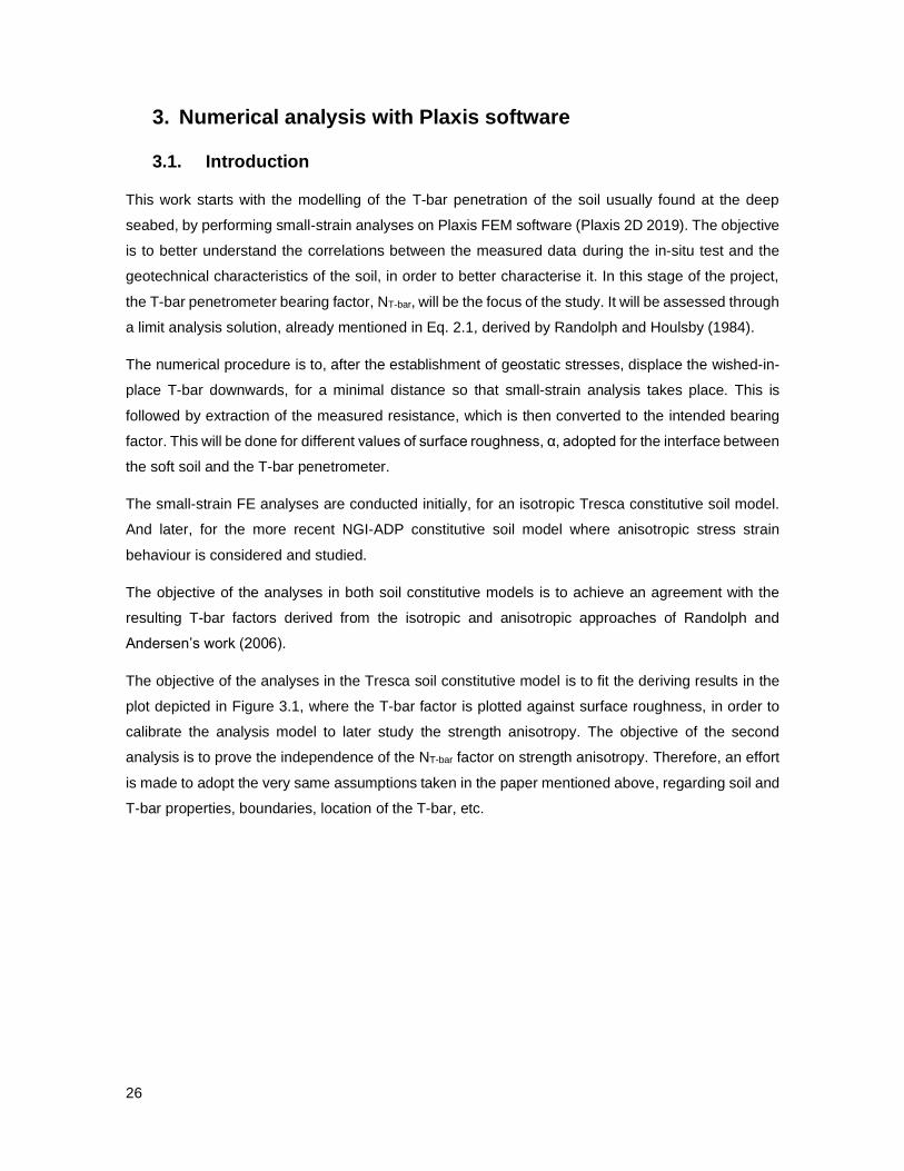
26

3. Numerical analysis with Plaxis software

3.1. Introduction

This work starts with the modelling of the T-bar penetration of the soil usually found at the deep

seabed, by performing small-strain analyses on Plaxis FEM software (Plaxis 2D 2019). The objective

is to better understand the correlations between the measured data during the in-situ test and the

geotechnical characteristics of the soil, in order to better characterise it. In this stage of the project,

the T-bar penetrometer bearing factor, NT-bar, will be the focus of the study. It will be assessed through

a limit analysis solution, already mentioned in Eq. 2.1, derived by Randolph and Houlsby (1984).

The numerical procedure is to, after the establishment of geostatic stresses, displace the wished-in-

place T-bar downwards, for a minimal distance so that small-strain analysis takes place. This is

followed by extraction of the measured resistance, which is then converted to the intended bearing

factor. This will be done for different values of surface roughness, α, adopted for the interface between

the soft soil and the T-bar penetrometer.

The small-strain FE analyses are conducted initially, for an isotropic Tresca constitutive soil model.

And later, for the more recent NGI-ADP constitutive soil model where anisotropic stress strain

behaviour is considered and studied.

The objective of the analyses in both soil constitutive models is to achieve an agreement with the

resulting T-bar factors derived from the isotropic and anisotropic approaches of Randolph and

Andersen’s work (2006).

The objective of the analyses in the Tresca soil constitutive model is to fit the deriving results in the

plot depicted in Figure 3.1, where the T-bar factor is plotted against surface roughness, in order to

calibrate the analysis model to later study the strength anisotropy. The objective of the second

analysis is to prove the independence of the NT-bar factor on strength anisotropy. Therefore, an effort

is made to adopt the very same assumptions taken in the paper mentioned above, regarding soil and

T-bar properties, boundaries, location of the T-bar, etc.

27

Figure 3.1 - Variation of T-bar factor with surface roughness for simple Tresca Model (Randolph and Andersen, 2006)

3.2. Description of the analyses

The domain of the analysis is displayed in Figure 3.2(a). It holds the soil and the wished-in-place

(WIP) T-bar penetrometer, for both the Tresca and NGI-ADP soil model.

The soil elements at the vertical boundaries are impeded to move vertically. At the bottom boundary

the elements are impeded to move horizontally whereas at the upper boundary the elements are free

to move in any direction.

A 15-node type of element meshing was adopted and three mesh zones are generated, one that is

coarser at the periphery and two finer mesh zones found in the centre, as observed in Figure 3.2(b).

The coarseness decreases as one moves to the centre, to better capture the small displacement of

soil by the penetrating T-bar.

It would be expected that due to symmetry, the size of the domain in analysis could be reduced to

half, but instead, the complete domain was modelled. This is due to a limitation imposed by the Plaxis

software where half-pipes cannot be modelled. The penetration of the T-bar is assumed to work in

plane strain conditions as there is no significant gain in total shearing resistance in considering the

finite length of the bar.

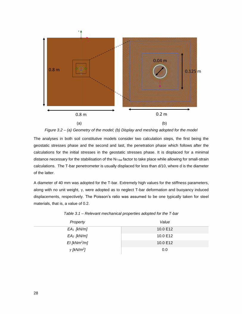
28

(a) (b)

Figure 3.2 – (a) Geometry of the model; (b) Display and meshing adopted for the model

The analyses in both soil constitutive models consider two calculation steps, the first being the

geostatic stresses phase and the second and last, the penetration phase which follows after the

calculations for the initial stresses in the geostatic stresses phase. It is displaced for a minimal

distance necessary for the stabilisation of the NT-bar factor to take place while allowing for small-strain

calculations. The T-bar penetrometer is usually displaced for less than d/10, where d is the diameter

of the latter.

A diameter of 40 mm was adopted for the T-bar. Extremely high values for the stiffness parameters,

along with no unit weight, γ, were adopted as to neglect T-bar deformation and buoyancy induced

displacements, respectively. The Poisson’s ratio was assumed to be one typically taken for steel

materials, that is, a value of 0.2.

Table 3.1 – Relevant mechanical properties adopted for the T-bar

Property Value

EA1 [kN/m] 10.0 E12

EA2 [kN/m] 10.0 E12

EI [kNm2/m] 10.0 E12

γ [kN/m2] 0.0

29

3.3. Soil constitutive models

In this thesis, two soil constitutive models were adopted to model the stress-strain behaviour of the

analyses in question. The isotropic Tresca model and the anisotropic NGI-ADP model were then

implemented.

3.3.1. Isotropic Tresca model

Since we are dealing with cohesive soils, the Mohr-Coulomb constitutive model was adopted in

Plaxis. The undrained behaviour of the type C was adopted and parameters like Poisson ratio and K0

were altered so that the soil behaviour could be modelled through the Tresca isotropic model. This

model specifies the failure criterion to be a constant critical value of the maximum (yielding) shear

stress in the isotropic material. The undrained shear strength comes as half of the difference between

the major and minor principal stresses, as presented in Eq. 3.1.

𝑆𝑢 =𝜎1−𝜎3

2 (Eq. 3.1)

The undrained behaviour is simulated using a total stress analysis where all parameters are defined

as undrained. In these conditions, all results referring to effective stresses are in fact total stresses

since it is not possible to obtain information about the pore water pressure. Additionally, the stiffness

and strength parameters are modelled using the undrained Young’s Modulus, Eu, and undrained

shear strength, Su, respectively.

The ground water table was put at the bottom of the model domain. The soil is considered to be

saturated, with an effective unit weight of 6.0 kN/m2, constant with depth, typical of the soil in study

(Tho et al., 2012).

Since undrained behaviour of the type C was chosen to model both analyses, a Poisson’s ratio of

0.495 is adopted since a value close to 0.5 is suggested by the Plaxis 2019 2D Manual.

For both the isotropic and anisotropic analyses, the lateral earth pressure coefficient at rest, K0, takes

the value of 1.0, as to generate an isotropic initial stress condition and to keep the Tresca failure

criterion safe from being violated.

As for the surface roughness coefficient, 𝛼, associated with the interface between both materials,

takes the form of Rinter in Plaxis 2019 2D, which varies between 0 (no shear strength is mobilised at

the interface) and 1 (the total undrained shear resistance of the soil is mobilised at the interface).

Regarding the undrained shear strength, a value of 0.5 kPa will be adopted, as it falls in a realistic

range of 0.48 to 2.48 kPa for soils in the conditions already depicted above (Tho et al., 2012).

In order to infer the undrained Young modulus of the undrained clay, a kind of clay already studied

that resembled the typically found at deep offshore sites, had to be taken as reference. In the work

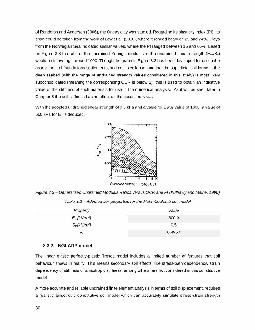
30

of Randolph and Andersen (2006), the Onsøy clay was studied. Regarding its plasticity index (PI), its

span could be taken from the work of Low et al. (2010), where it ranged between 29 and 74%. Clays

from the Norwegian Sea indicated similar values, where the PI ranged between 15 and 66%. Based

on Figure 3.3 the ratio of the undrained Young’s modulus to the undrained shear strength (Eus/Su)

would be in average around 1000. Though the graph in Figure 3.3 has been developed for use in the

assessment of foundations settlements, and not its collapse, and that the superficial soil found at the

deep seabed (with the range of undrained strength values considered in this study) is most likely

subconsolidated (meaning the corresponding OCR is below 1), this is used to obtain an indicative

value of the stiffness of such materials for use in the numerical analysis. As it will be seen later in

Chapter 5 the soil stiffness has no effect on the assessed NT-bar.

With the adopted undrained shear strength of 0.5 kPa and a value for Eu/Su value of 1000, a value of

500 kPa for Eu is deduced.

Figure 3.3 – Generalised Undrained Modulus Ratios versus OCR and PI (Kulhawy and Maine, 1990)

Table 3.2 – Adopted soil properties for the Mohr-Coulomb soil model

Property Value

Eu [kN/m2] 500.0

Su [kN/m2] 0.5

νu 0.4950

3.3.2. NGI-ADP model

The linear elastic perfectly-plastic Tresca model includes a limited number of features that soil

behaviour shows in reality. This means secondary soil effects, like stress-path dependency, strain

dependency of stiffness or anisotropic stiffness, among others, are not considered in this constitutive

model.

A more accurate and reliable undrained finite element analysis in terms of soil displacement, requires

a realistic anisotropic constitutive soil model which can accurately simulate stress-strain strength

31

response for different shear modes. This need cannot be stressed enough since shear strength

anisotropy is more significant for sensitive clays (Grimstad et al., 2012), which resemble the soil

studied in this project.

Recently, Grimstad et al. (2012) have proposed the NGI-ADP constitutive soil model, which can

realistically simulate the anisotropic undrained stress strain response and undrained shear strength

of clays.

Each triaxial test has an angle α and a parameter b characterising the stress path during the triaxial

shear tests and direct shear tests (Fig. 3.4). The angle α gives the inclination between the major

principal stress and the vertical stresses direction. The parameter b dictates the relative magnitude

of the intermediate principle stress, 𝑏 = 𝜎2−𝜎3

𝜎1−𝜎3, associated with each mode of shear in the triaxial tests

and direct shear test. It is impossible to study the anisotropy influence on a certain soil while resorting

to these three tests only since b and α cannot be separated. This is due to the impossibility of running

a triaxial compression test with the major principal stress directed horizontally or a triaxial extension

test with the major principal stress directed vertically.

Figure 3. 4 - Active and passive plane-strain on a loaded soil wedge

Therefore, we resort to the NGI-ADP since it can separate the influences of induced anisotropy (b),

and the influence of inherent anisotropy (α) by taking as inputs the failure shear strain and

corresponding undrained shear strength for the three directions of shear depicted by triaxial

compression (TC), triaxial extension (TE) and direct shear stress (DSS). This soil model is based on

the classical elasto-plastic constitutive model. From the shear strains, a non-linear hardening

relationship is defined. Whereas from the shear strengths, the anisotropic failure criterion is

formulated, resulting in a modification of the classical Tresca yield criterion. In this manner, it is

possible to explore and study the effects of induced and inherent anisotropy in the soil stress-strain

strength relationship. Such anisotropy is characteristic of onshore and offshore clays and silts.

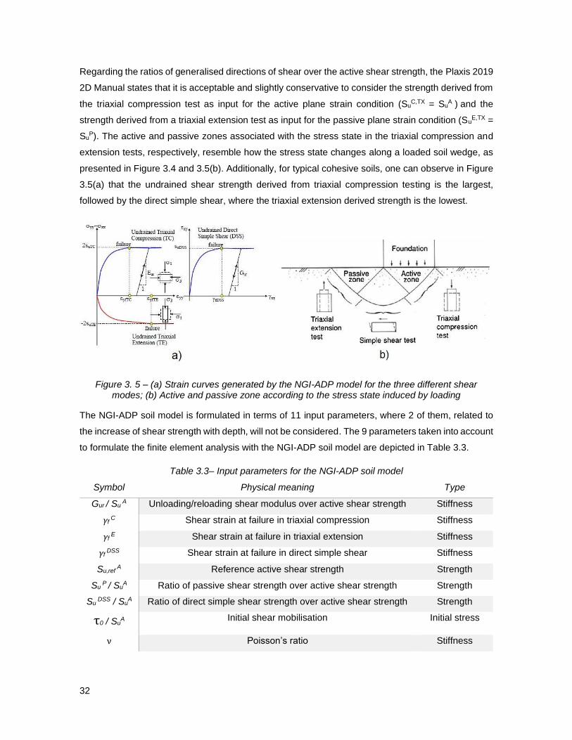
32

Regarding the ratios of generalised directions of shear over the active shear strength, the Plaxis 2019

2D Manual states that it is acceptable and slightly conservative to consider the strength derived from

the triaxial compression test as input for the active plane strain condition (SuC,TX = Su

A ) and the

strength derived from a triaxial extension test as input for the passive plane strain condition (SuE,TX =

SuP). The active and passive zones associated with the stress state in the triaxial compression and

extension tests, respectively, resemble how the stress state changes along a loaded soil wedge, as

presented in Figure 3.4 and 3.5(b). Additionally, for typical cohesive soils, one can observe in Figure

3.5(a) that the undrained shear strength derived from triaxial compression testing is the largest,

followed by the direct simple shear, where the triaxial extension derived strength is the lowest.

Figure 3. 5 – (a) Strain curves generated by the NGI-ADP model for the three different shear modes; (b) Active and passive zone according to the stress state induced by loading

The NGI-ADP soil model is formulated in terms of 11 input parameters, where 2 of them, related to

the increase of shear strength with depth, will not be considered. The 9 parameters taken into account

to formulate the finite element analysis with the NGI-ADP soil model are depicted in Table 3.3.

Table 3.3– Input parameters for the NGI-ADP soil model

Symbol Physical meaning Type

Gur / Su A Unloading/reloading shear modulus over active shear strength Stiffness

γf C Shear strain at failure in triaxial compression Stiffness

γf E Shear strain at failure in triaxial extension Stiffness

γf DSS Shear strain at failure in direct simple shear Stiffness

Su,ref A

Reference active shear strength Strength

Su P / Su

A Ratio of passive shear strength over active shear strength Strength

Su DSS / Su

A Ratio of direct simple shear strength over active shear strength Strength

τ0 / SuA Initial shear mobilisation Initial stress

ν Poisson’s ratio Stiffness

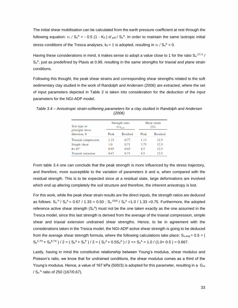
33

The initial shear mobilisation can be calculated from the earth pressure coefficient at rest through the

following equation: 𝜏0 / SuA = - 0.5 (1 - K0 ) σ’yy0 / Su

A. In order to maintain the same isotropic initial

stress conditions of the Tresca analyses, k0 = 1 is adopted, resulting in 𝜏0 / SuA = 0.

Having these considerations in mind, it makes sense to adopt a value close to 1 for the ratio Su CT,X /

SuA, just as predefined by Plaxis at 0.99, resulting in the same strengths for triaxial and plane strain

conditions.

Following this thought, the peak shear strains and corresponding shear strengths related to the soft

sedimentary clay studied in the work of Randolph and Andersen (2006) are extracted, where the set

of input parameters depicted in Table 2 is taken into consideration for the deduction of the input

parameters for the NGI-ADP model.

Table 3.4 – Anisotropic strain-softening parameters for a clay studied in Randolph and Andersen (2006)

From table 3.4 one can conclude that the peak strength is more influenced by the stress trajectory,

and therefore, more susceptible to the variation of parameters b and α, when compared with the

residual strength. This is to be expected since at a residual state, large deformations are involved

which end up altering completely the soil structure and therefore, the inherent anisotropy is lost.

For this work, while the peak shear strain results are the direct inputs, the strength ratios are deduced

as follows: Su P / Su

A = 0.67 / 1.33 = 0.50 ; Su DSS / Su

A =1.0 / 1.33 =0.75. Furthermore, the adopted

reference active shear strength (SuA) must not be the one taken exactly as the one assumed in the

Tresca model, since this last strength is derived from the average of the triaxial compression, simple

shear and triaxial extension undrained shear strengths. Hence, to be in agreement with the

considerations taken in the Tresca model, the NGI-ADP active shear strength is going to be deduced

from the average shear strength formula, where the following calculations take place: Su,avg = 0.5 = (

SuC,TX + Su

E,TX ) / 2 = ( SuA + Su

P ) / 2 = ( SuA + 0.5Su

A ) / 2 => SuA = 1.0 / (1.0+ 0.5 ) = 0.667.

Lastly, having in mind the constitutive relationship between Young’s modulus, shear modulus and

Poisson’s ratio, we know that for undrained conditions, the shear modulus comes as a third of the

Young’s modulus. Hence, a value of 167 kPa (500/3) is adopted for this parameter, resulting in a Gur

/ Su A ratio of 250 (167/0.67).

34

With these assumptions and calculations concluded, Table 5 depicts the set of inputs taken for the

NGI-ADP model.

Table 3 5 - Adopted input parameters for the NGI-ADP model in Plaxis 2019 2D

Parameter Value

Gur / Su A 250

γf C 1.130

γf E 4.500

γf DSS 3.750

Su,ref A [kPa] 0.667

Su P / Su

A 0.500

Su DSS / Su

A 0.750

τ0 / SuA 0

ν 0.4950

3.4. Analysis results with Tresca model

A simple parametric study was conducted where nine analyses were performed, under the Tresca

model, for nine different values of surface roughness, α.

Displacements in the order of d/40 to d/10 meters, as α decreased, were found to be the necessary

amount of prescribed displacement in order to attain a stabilised T-bar bearing factor while the

conditions were met for the small-strain analyses to take place.

Typical displacement-QT-bar results deriving from the isotropic analysis and relative to the particular

case of α =0.5, are displayed in Figure 3.6 below.

The NT-bar factor is deduced through the following calculation: NT-bar = 0.2172/(0.04*1*0.5) = 10.86,

where 0.2172 is the stabilised value of QT-bar, the 0.04*1 relates to the projected area of the 40 mm

diameter T-bar penetrometer and 0.5 is the undrained shear strength adopted for the soil in study

(Su,avg).

The corresponding NT-bar factor to the QT-bar tip resistance rises to a constant and stable value of 10.86

at a displacement of 1.6% of the diameter. This is compared with a NT-bar of 10.86 and a respective

displacement of 1.2% of the diameter deriving from the isotropic analyses results of Randolph and

Andersen (2006). Therefore, a good agreement relative to the NT-bar factor was achieved. However,

since different rigidity parameters were used in both works, a slight difference in displacements at

yield was attained.

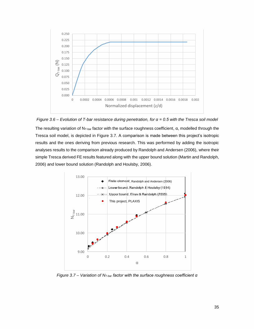
35

Figure 3.6 – Evolution of T-bar resistance during penetration, for α = 0.5 with the Tresca soil model

The resulting variation of NT-bar factor with the surface roughness coefficient, α, modelled through the

Tresca soil model, is depicted in Figure 3.7. A comparison is made between this project’s isotropic

results and the ones deriving from previous research. This was performed by adding the isotropic

analyses results to the comparison already produced by Randolph and Andersen (2006), where their

simple Tresca derived FE results featured along with the upper bound solution (Martin and Randolph,

2006) and lower bound solution (Randolph and Houlsby, 2006).

Figure 3.7 – Variation of NT-bar factor with the surface roughness coefficient α

0.000

0.025

0.050

0.075

0.100

0.125

0.150

0.175

0.200

0.225

0.250

0 0.0002 0.0004 0.0006 0.0008 0.001 0.0012 0.0014 0.0016 0.0018 0.002

QT

-bar(N

)

Normalized displacement (z/d)

9.00

10.00

11.00

12.00

13.00

0 0.2 0.4 0.6 0.8 1

NT

-bar

α

This project, PLAXIS

, Randolph and Andersen (2006)

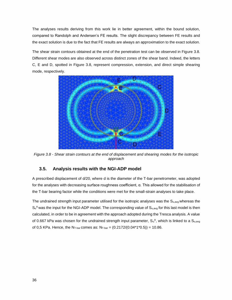
36

The analyses results deriving from this work lie in better agreement, within the bound solution,

compared to Randolph and Andersen’s FE results. The slight discrepancy between FE results and

the exact solution is due to the fact that FE results are always an approximation to the exact solution.

The shear strain contours obtained at the end of the penetration test can be observed in Figure 3.8.

Different shear modes are also observed across distinct zones of the shear band. Indeed, the letters

C, E and D, spotted in Figure 3.8, represent compression, extension, and direct simple shearing

mode, respectively.

Figure 3.8 - Shear strain contours at the end of displacement and shearing modes for the isotropic approach

3.5. Analysis results with the NGI-ADP model

A prescribed displacement of d/20, where d is the diameter of the T-bar penetrometer, was adopted

for the analyses with decreasing surface roughness coefficient, α. This allowed for the stabilisation of

the T-bar bearing factor while the conditions were met for the small-strain analyses to take place.

The undrained strength input parameter utilised for the isotropic analyses was the Su,avg whereas the

SuA was the input for the NGI-ADP model. The corresponding value of Su,avg for this last model is then

calculated, in order to be in agreement with the approach adopted during the Tresca analysis. A value

of 0.667 kPa was chosen for the undrained strength input parameter, SuA, which is linked to a Su,avg

of 0,5 KPa. Hence, the NT-bar comes as: NT-bar = (0.2172/(0.04*1*0.5)) = 10.86.

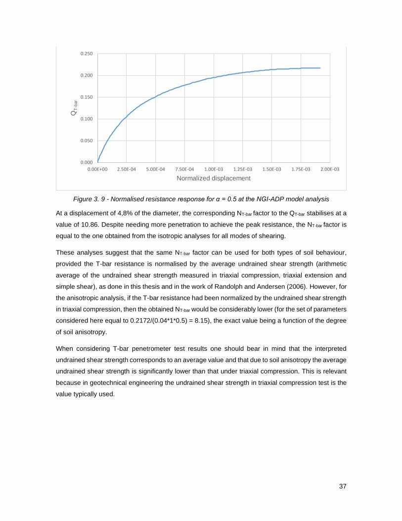
37

Figure 3. 9 - Normalised resistance response for α = 0.5 at the NGI-ADP model analysis

At a displacement of 4,8% of the diameter, the corresponding NT-bar factor to the QT-bar stabilises at a

value of 10.86. Despite needing more penetration to achieve the peak resistance, the NT-bar factor is

equal to the one obtained from the isotropic analyses for all modes of shearing.

These analyses suggest that the same NT-bar factor can be used for both types of soil behaviour,

provided the T-bar resistance is normalised by the average undrained shear strength (arithmetic

average of the undrained shear strength measured in triaxial compression, triaxial extension and

simple shear), as done in this thesis and in the work of Randolph and Andersen (2006). However, for

the anisotropic analysis, if the T-bar resistance had been normalized by the undrained shear strength

in triaxial compression, then the obtained NT-bar would be considerably lower (for the set of parameters

considered here equal to 0.2172/(0.04*1*0.5) = 8.15), the exact value being a function of the degree

of soil anisotropy.

When considering T-bar penetrometer test results one should bear in mind that the interpreted

undrained shear strength corresponds to an average value and that due to soil anisotropy the average

undrained shear strength is significantly lower than that under triaxial compression. This is relevant

because in geotechnical engineering the undrained shear strength in triaxial compression test is the

value typically used.

0.000

0.050

0.100

0.150

0.200

0.250

0.00E+00 2.50E-04 5.00E-04 7.50E-04 1.00E-03 1.25E-03 1.50E-03 1.75E-03 2.00E-03

QT

-bar

Normalized displacement

38

4. Coupled Eulerian-Lagrangian WIP Analysis

4.1. Introduction

Following the work produced in Plaxis 2019 2D, we move on to the Coupled Eulerian-Lagrangian

(CEL) numerical modelling approach, employed through Abaqus/CAE 2016. This part of the project

comprises a series of FE analyses that cover the penetration of soft clay by the T-bar penetrometer

under the wished-in-place (WIP) approach on soil penetration.

In most cases, the FE programs based in the Lagrangian framework cannot deal with very large

deformation due to excessive mesh distortion and convergence issues. Therefore, to calculate the

penetration resistance of soil derived from T-bar penetration, some researches focused on FE

analysis of WIP pipes, where they are initially found at a designated embedment depth and then

subjected to (a small) further displacement.

Initially, the WIP scenario is going to be explored for two main reasons. First, to compare the resulting

T-bar bearing factors with the ones deriving from the FE analyses performed with Plaxis. Second, to

compare the same T-bar bearing factors with the ones derived from other studies found in literature

and to also work as a starting point for the development of the more complex PIP analyses, performed

in the next Chapter.

There is an additional interest in capturing the mobilisation of the full-flow mechanism along with the

displacement of soil around the T-bar, which is something that was not possible to do in the Plaxis

analyses. The actual displacement of soil around the T-bar involves very large deformations of the

soil, which the conventional Lagrangian approach, adopted in Plaxis, cannot deal with as discussed

above.

Therefore, we resort to the CEL technique available in the commercial software Abaqus/CAE 2016.

This approach belongs to the Arbitrary Lagrangian Eulerian approach (ALE), which itself falls in the

Large Deformation Finite Element (LDFE) category of analysis. Thus, the large deformation

phenomena involved in the penetration of the soil can now be captured.

4.2. Wished-in-place analyses

These analyses will focus on the study of the influence of the surface roughness on the T-bar bearing

factor, NT-bar. The resulting bearing factors will then be compared with the bearing factors deriving

from the same type of study performed in Plaxis and in studies found in literature.

An important aspect of the CEL approach is the possibility to model the displacement of Lagrangian

material through an Eulerian mesh, in a WIP scenario, where the former is already found embedded

in the latter, at a designated depth.

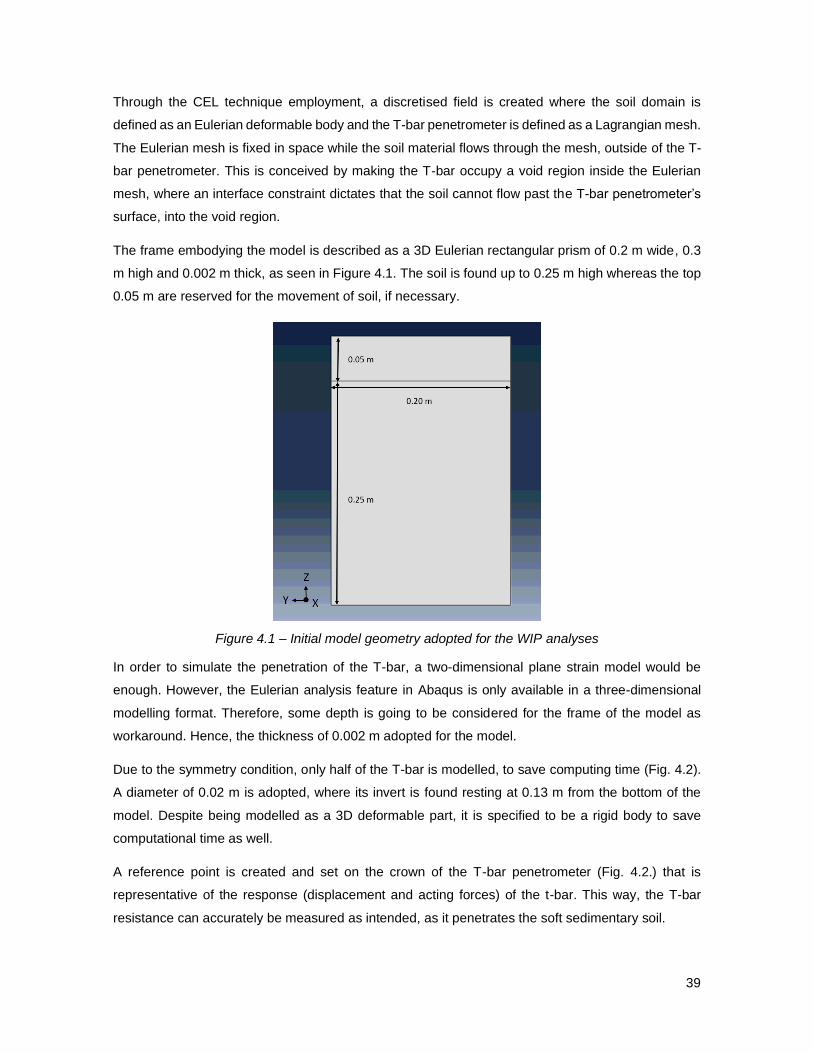
39

Through the CEL technique employment, a discretised field is created where the soil domain is

defined as an Eulerian deformable body and the T-bar penetrometer is defined as a Lagrangian mesh.

The Eulerian mesh is fixed in space while the soil material flows through the mesh, outside of the T-

bar penetrometer. This is conceived by making the T-bar occupy a void region inside the Eulerian

mesh, where an interface constraint dictates that the soil cannot flow past the T-bar penetrometer’s

surface, into the void region.

The frame embodying the model is described as a 3D Eulerian rectangular prism of 0.2 m wide, 0.3

m high and 0.002 m thick, as seen in Figure 4.1. The soil is found up to 0.25 m high whereas the top

0.05 m are reserved for the movement of soil, if necessary.

Figure 4.1 – Initial model geometry adopted for the WIP analyses

In order to simulate the penetration of the T-bar, a two-dimensional plane strain model would be

enough. However, the Eulerian analysis feature in Abaqus is only available in a three-dimensional

modelling format. Therefore, some depth is going to be considered for the frame of the model as

workaround. Hence, the thickness of 0.002 m adopted for the model.

Due to the symmetry condition, only half of the T-bar is modelled, to save computing time (Fig. 4.2).

A diameter of 0.02 m is adopted, where its invert is found resting at 0.13 m from the bottom of the

model. Despite being modelled as a 3D deformable part, it is specified to be a rigid body to save

computational time as well.

A reference point is created and set on the crown of the T-bar penetrometer (Fig. 4.2.) that is

representative of the response (displacement and acting forces) of the t-bar. This way, the T-bar

resistance can accurately be measured as intended, as it penetrates the soft sedimentary soil.

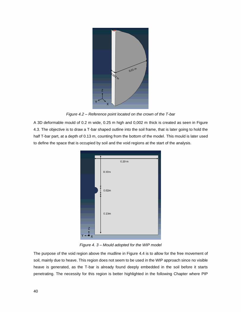
40

Figure 4.2 – Reference point located on the crown of the T-bar

A 3D deformable mould of 0.2 m wide, 0.25 m high and 0,002 m thick is created as seen in Figure

4.3. The objective is to draw a T-bar shaped outline into the soil frame, that is later going to hold the

half T-bar part, at a depth of 0.13 m, counting from the bottom of the model. This mould is later used

to define the space that is occupied by soil and the void regions at the start of the analysis.

Figure 4. 3 – Mould adopted for the WIP model

The purpose of the void region above the mudline in Figure 4.4 is to allow for the free movement of

soil, mainly due to heave. This region does not seem to be used in the WIP approach since no visible

heave is generated, as the T-bar is already found deeply embedded in the soil before it starts

penetrating. The necessity for this region is better highlighted in the following Chapter where PIP

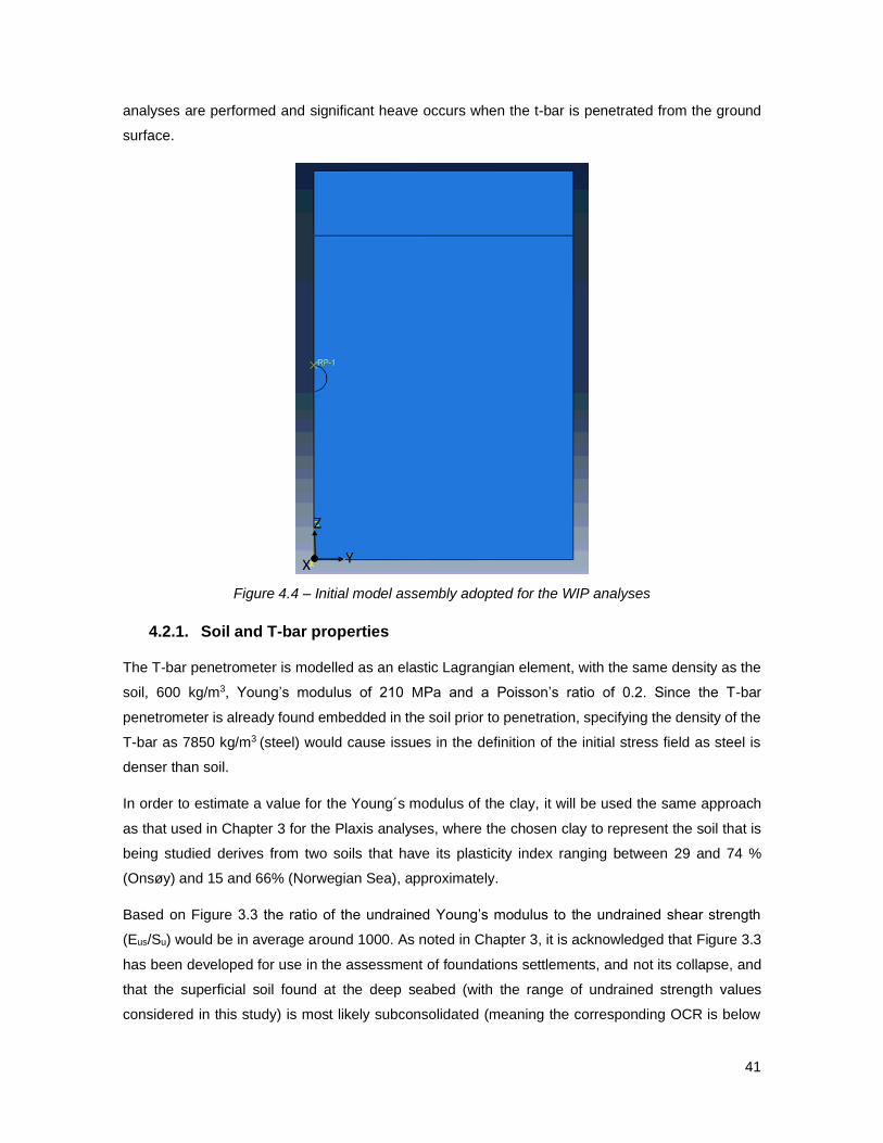
41

analyses are performed and significant heave occurs when the t-bar is penetrated from the ground

surface.

Figure 4.4 – Initial model assembly adopted for the WIP analyses

4.2.1. Soil and T-bar properties

The T-bar penetrometer is modelled as an elastic Lagrangian element, with the same density as the

soil, 600 kg/m3, Young’s modulus of 210 MPa and a Poisson’s ratio of 0.2. Since the T-bar

penetrometer is already found embedded in the soil prior to penetration, specifying the density of the

T-bar as 7850 kg/m3 (steel) would cause issues in the definition of the initial stress field as steel is

denser than soil.

In order to estimate a value for the Young´s modulus of the clay, it will be used the same approach

as that used in Chapter 3 for the Plaxis analyses, where the chosen clay to represent the soil that is

being studied derives from two soils that have its plasticity index ranging between 29 and 74 %

(Onsøy) and 15 and 66% (Norwegian Sea), approximately.

Based on Figure 3.3 the ratio of the undrained Young’s modulus to the undrained shear strength

(Eus/Su) would be in average around 1000. As noted in Chapter 3, it is acknowledged that Figure 3.3

has been developed for use in the assessment of foundations settlements, and not its collapse, and

that the superficial soil found at the deep seabed (with the range of undrained strength values

considered in this study) is most likely subconsolidated (meaning the corresponding OCR is below

42

1). However, this is used to obtain an indicative value of the stiffness of such materials for use in the

numerical analysis. As it will be shown later in Chapter 5 the soil stiffness has no effect on the

assessed NT-bar.

Figure 4.5. – Generalised Undrained Modulus Ratios versus OCR and PI (Kulhawy and Maine 1990)

In respect to the undrained shear strength of the soil, values ranging between 100 and 500 Pa are

adopted as these values are typical of the very soft clay materials at the surface of the seabed.

The soft sedimentary soil is modelled as a linear elastic perfectly plastic isotropic material, following

the Tresca failure criterion. It has a density of 600 kg/m3 constant with depth, a Young’s modulus also

constant in depth of value between 100 and 500 kPa, as to respect a Eu/Su ratio in the range proposed

in Figure 4.5. A Poisson’s ratio of 0.499 is adopted as undrained conditions are to be attained.

4.2.2. Interface roughness

Different scenarios are considered regarding the interaction of the soil and the t-bar, namely the

magnitude of the shear stresses that can be mobilized in the contact. The interface roughness

coefficient, α is the ratio of the maximum mobilized shear stress at the soil t-bar contact and the soil

undrained shear strength. The tangential behaviour is characterized by an isotropic penalty

formulation, adopting a very high value for the friction coefficient and a shear stress limit equal to

αSu. A rigid body constraint is also attributed to the T-bar penetrometer, with the reference point of

the rigid body located at the crown of the T-bar, as seen in Figure 4.6. The purpose of this constraint

is to prevent any potential deformation of the T-bar penetrometer while penetrating the soil.

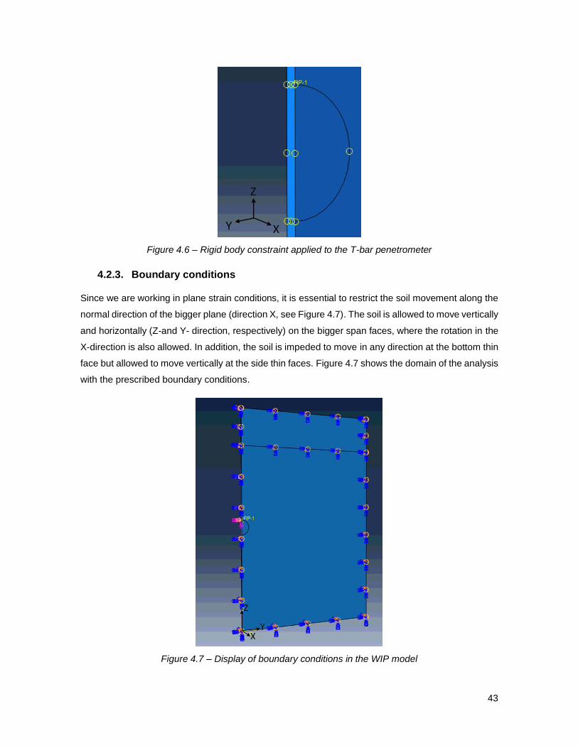
43

Figure 4.6 – Rigid body constraint applied to the T-bar penetrometer

4.2.3. Boundary conditions

Since we are working in plane strain conditions, it is essential to restrict the soil movement along the

normal direction of the bigger plane (direction X, see Figure 4.7). The soil is allowed to move vertically

and horizontally (Z-and Y- direction, respectively) on the bigger span faces, where the rotation in the

X-direction is also allowed. In addition, the soil is impeded to move in any direction at the bottom thin

face but allowed to move vertically at the side thin faces. Figure 4.7 shows the domain of the analysis

with the prescribed boundary conditions.

Figure 4.7 – Display of boundary conditions in the WIP model

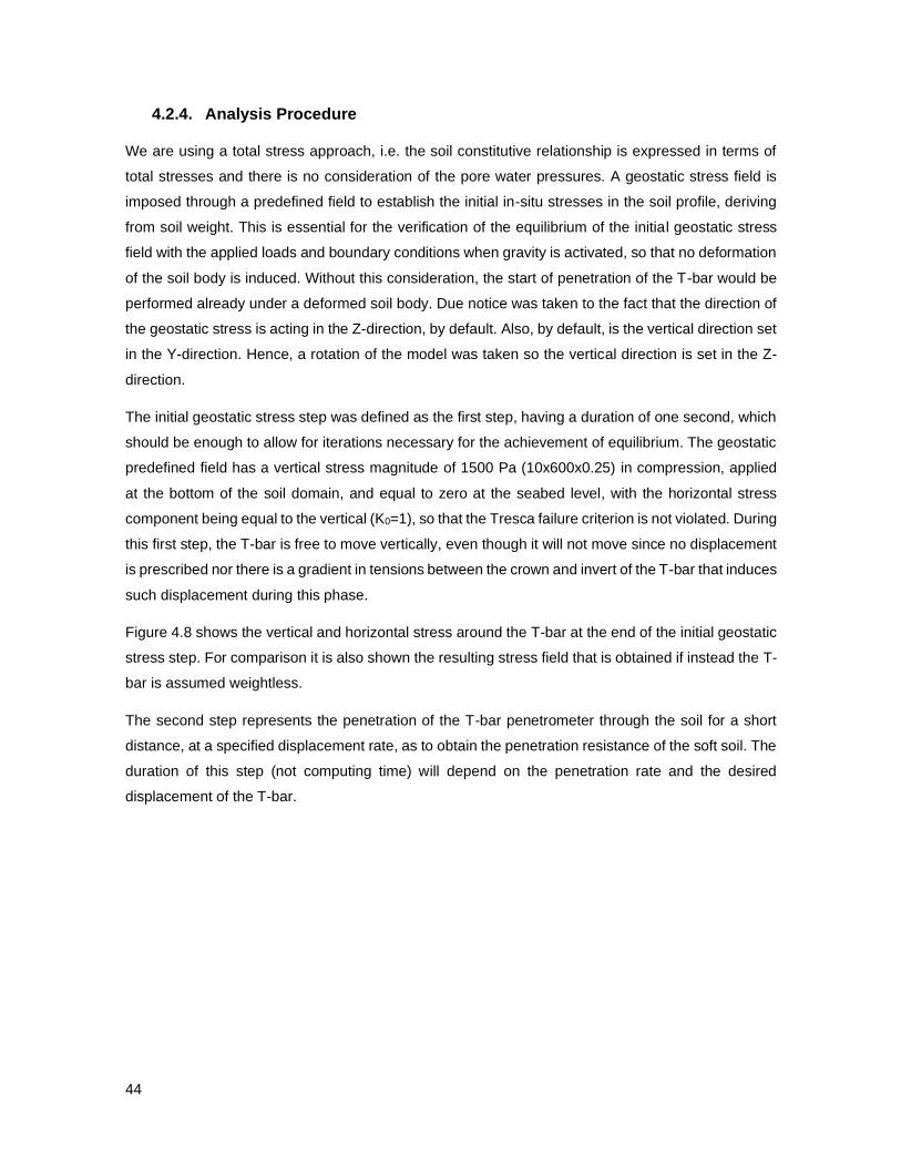
44

4.2.4. Analysis Procedure

We are using a total stress approach, i.e. the soil constitutive relationship is expressed in terms of

total stresses and there is no consideration of the pore water pressures. A geostatic stress field is

imposed through a predefined field to establish the initial in-situ stresses in the soil profile, deriving

from soil weight. This is essential for the verification of the equilibrium of the initial geostatic stress

field with the applied loads and boundary conditions when gravity is activated, so that no deformation

of the soil body is induced. Without this consideration, the start of penetration of the T-bar would be

performed already under a deformed soil body. Due notice was taken to the fact that the direction of

the geostatic stress is acting in the Z-direction, by default. Also, by default, is the vertical direction set

in the Y-direction. Hence, a rotation of the model was taken so the vertical direction is set in the Z-

direction.

The initial geostatic stress step was defined as the first step, having a duration of one second, which

should be enough to allow for iterations necessary for the achievement of equilibrium. The geostatic

predefined field has a vertical stress magnitude of 1500 Pa (10x600x0.25) in compression, applied

at the bottom of the soil domain, and equal to zero at the seabed level, with the horizontal stress

component being equal to the vertical (K0=1), so that the Tresca failure criterion is not violated. During

this first step, the T-bar is free to move vertically, even though it will not move since no displacement

is prescribed nor there is a gradient in tensions between the crown and invert of the T-bar that induces

such displacement during this phase.

Figure 4.8 shows the vertical and horizontal stress around the T-bar at the end of the initial geostatic

stress step. For comparison it is also shown the resulting stress field that is obtained if instead the T-

bar is assumed weightless.

The second step represents the penetration of the T-bar penetrometer through the soil for a short

distance, at a specified displacement rate, as to obtain the penetration resistance of the soft soil. The

duration of this step (not computing time) will depend on the penetration rate and the desired

displacement of the T-bar.

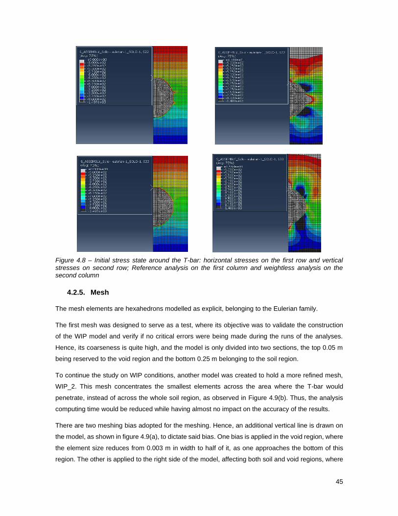
45

Figure 4.8 – Initial stress state around the T-bar: horizontal stresses on the first row and vertical stresses on second row; Reference analysis on the first column and weightless analysis on the second column

4.2.5. Mesh

The mesh elements are hexahedrons modelled as explicit, belonging to the Eulerian family.

The first mesh was designed to serve as a test, where its objective was to validate the construction

of the WIP model and verify if no critical errors were being made during the runs of the analyses.

Hence, its coarseness is quite high, and the model is only divided into two sections, the top 0.05 m

being reserved to the void region and the bottom 0.25 m belonging to the soil region.

To continue the study on WIP conditions, another model was created to hold a more refined mesh,

WIP_2. This mesh concentrates the smallest elements across the area where the T-bar would

penetrate, instead of across the whole soil region, as observed in Figure 4.9(b). Thus, the analysis

computing time would be reduced while having almost no impact on the accuracy of the results.

There are two meshing bias adopted for the meshing. Hence, an additional vertical line is drawn on

the model, as shown in figure 4.9(a), to dictate said bias. One bias is applied in the void region, where

the element size reduces from 0.003 m in width to half of it, as one approaches the bottom of this

region. The other is applied to the right side of the model, affecting both soil and void regions, where

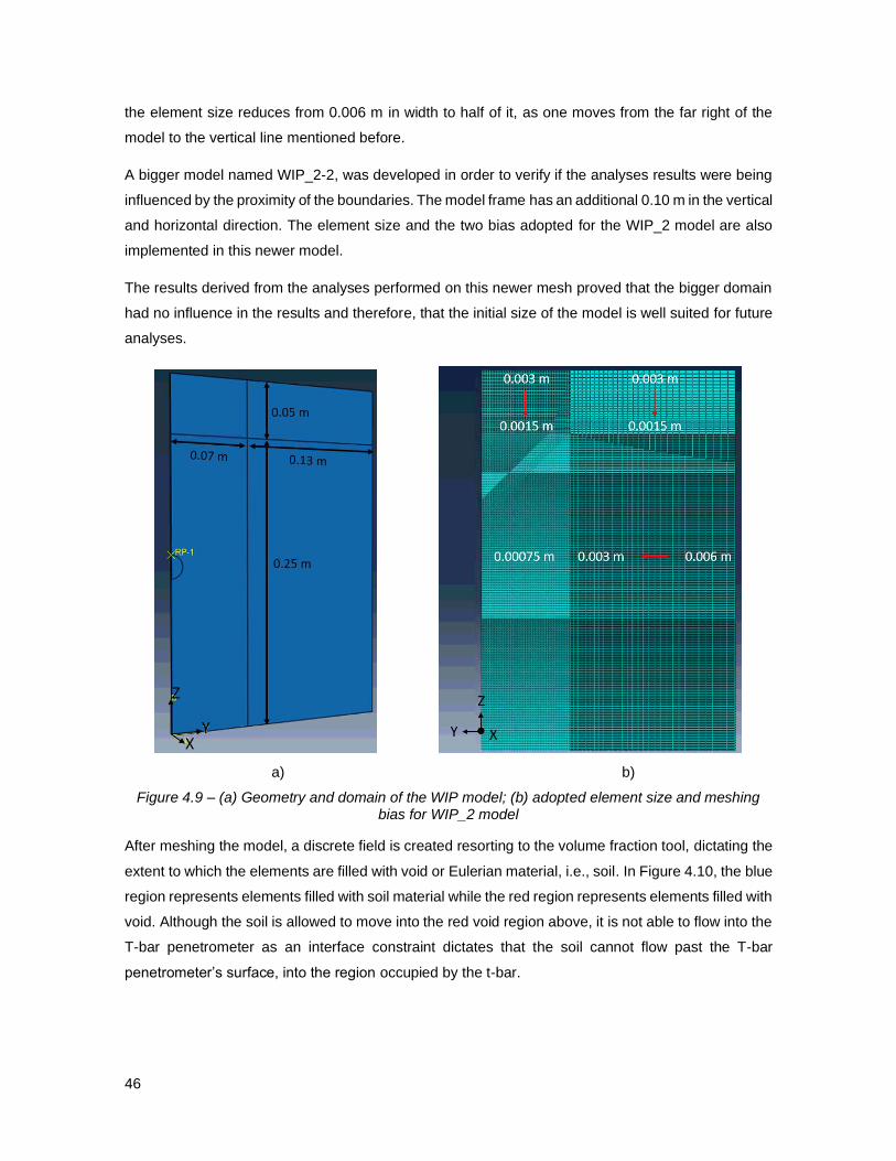
46

the element size reduces from 0.006 m in width to half of it, as one moves from the far right of the

model to the vertical line mentioned before.

A bigger model named WIP_2-2, was developed in order to verify if the analyses results were being

influenced by the proximity of the boundaries. The model frame has an additional 0.10 m in the vertical

and horizontal direction. The element size and the two bias adopted for the WIP_2 model are also

implemented in this newer model.

The results derived from the analyses performed on this newer mesh proved that the bigger domain

had no influence in the results and therefore, that the initial size of the model is well suited for future

analyses.

a) b)

Figure 4.9 – (a) Geometry and domain of the WIP model; (b) adopted element size and meshing bias for WIP_2 model

After meshing the model, a discrete field is created resorting to the volume fraction tool, dictating the

extent to which the elements are filled with void or Eulerian material, i.e., soil. In Figure 4.10, the blue

region represents elements filled with soil material while the red region represents elements filled with

void. Although the soil is allowed to move into the red void region above, it is not able to flow into the

T-bar penetrometer as an interface constraint dictates that the soil cannot flow past the T-bar

penetrometer’s surface, into the region occupied by the t-bar.

47

Figure 4.10 - Eulerian and void material displayed by blue and red elements, respectively

4.3. Mesh sensitivity study

A reduction in element size can lead to more accurate results (from a numerical point of view) but at

the cost of a much longer computing time. This section presents a mesh sensitivity study to define a

optimum size mesh that leads to reliable numerical analysis without spending too much computing

time. Therefore, a mesh refinement study is fundamental in order to develop said mesh.

Two additional models were developed so the results derived from the analyses performed on these

models could be compared with the ones deriving from the WIP_2 model. Only the region where the

T-bar is displaced is going to suffer changes regarding the mesh element size. WIP_3 has the mesh

element size increased to 0.00125 m. In turn, the WIP_4 mesh has the mesh element size reduced

to 0.000625 m. In mesh WIP_3 there are 8 elements across the radius of the t-bar, in mesh WIP_4

there are 16 elements whereas in mesh WIP_2 there are 13.

One analysis was performed for each mesh, where the mesh itself was the only difference between

analyses. The parameters used in the three analyses are presented in Table 4.1. After performing

each analysis, the data referring to the evolution of the reaction of the T-bar penetrometer with the

time it was exported to Excel. Based on this data the NT-Bar was calculated following the bearing

capacity formula described by Randolph and Houlsby (1984), 𝑁𝑇 =𝑞

𝑆𝑢 and considering the average

recorded reaction once this has stabilised. Figure 4.11 shows how the T-bar reaction evolves with

time during the penetration of the T-bar for each mesh.

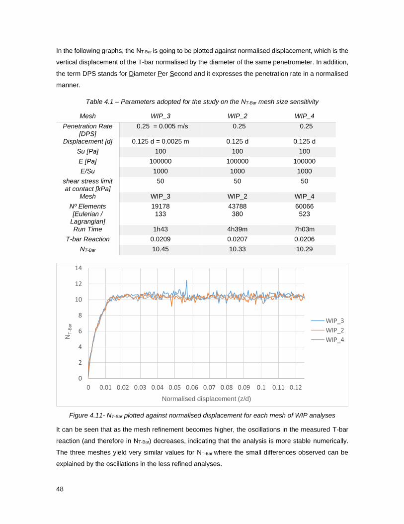
48

In the following graphs, the NT-Bar is going to be plotted against normalised displacement, which is the

vertical displacement of the T-bar normalised by the diameter of the same penetrometer. In addition,

the term DPS stands for Diameter Per Second and it expresses the penetration rate in a normalised

manner.

Table 4.1 – Parameters adopted for the study on the NT-Bar mesh size sensitivity

Mesh WIP_3 WIP_2 WIP_4

Penetration Rate [DPS]

0.25 = 0.005 m/s 0.25 0.25

Displacement [d] 0.125 d = 0.0025 m 0.125 d 0.125 d

Su [Pa] 100 100 100

E [Pa] 100000 100000 100000

E/Su 1000 1000 1000

shear stress limit at contact [kPa]

50 50 50

Mesh WIP_3 WIP_2 WIP_4

Nº Elements [Eulerian /

Lagrangian]

19178 133

43788 380

60066 523

Run Time 1h43 4h39m 7h03m

T-bar Reaction 0.0209 0.0207 0.0206

NT-Bar 10.45 10.33 10.29

Figure 4.11- NT-Bar plotted against normalised displacement for each mesh of WIP analyses

It can be seen that as the mesh refinement becomes higher, the oscillations in the measured T-bar

reaction (and therefore in NT-Bar) decreases, indicating that the analysis is more stable numerically.

The three meshes yield very similar values for NT-Bar where the small differences observed can be

explained by the oscillations in the less refined analyses.

0

2

4

6

8

10

12

14

0 0.01 0.02 0.03 0.04 0.05 0.06 0.07 0.08 0.09 0.1 0.11 0.12

NT

-Bar

Normalised displacement (z/d)

WIP_3

WIP_2

WIP_4

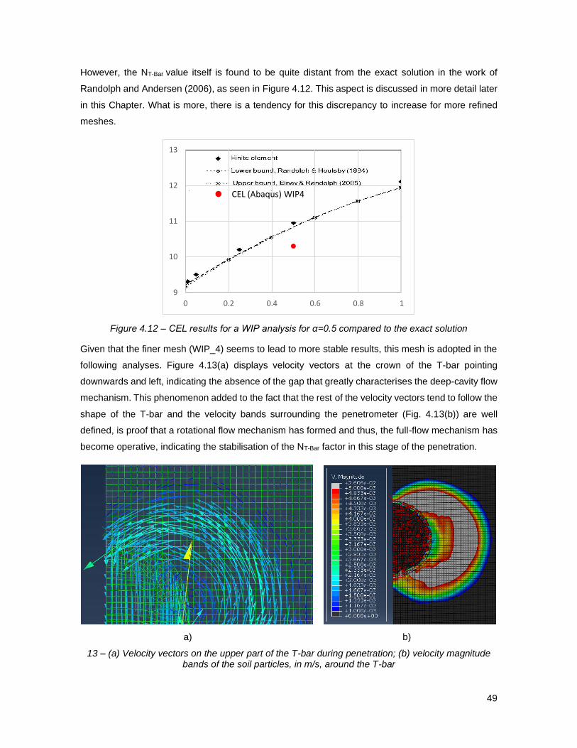
49

However, the NT-Bar value itself is found to be quite distant from the exact solution in the work of

Randolph and Andersen (2006), as seen in Figure 4.12. This aspect is discussed in more detail later

in this Chapter. What is more, there is a tendency for this discrepancy to increase for more refined

meshes.

Figure 4.12 – CEL results for a WIP analysis for α=0.5 compared to the exact solution

Given that the finer mesh (WIP_4) seems to lead to more stable results, this mesh is adopted in the

following analyses. Figure 4.13(a) displays velocity vectors at the crown of the T-bar pointing

downwards and left, indicating the absence of the gap that greatly characterises the deep-cavity flow

mechanism. This phenomenon added to the fact that the rest of the velocity vectors tend to follow the

shape of the T-bar and the velocity bands surrounding the penetrometer (Fig. 4.13(b)) are well

defined, is proof that a rotational flow mechanism has formed and thus, the full-flow mechanism has

become operative, indicating the stabilisation of the NT-Bar factor in this stage of the penetration.

a) b)

13 – (a) Velocity vectors on the upper part of the T-bar during penetration; (b) velocity magnitude bands of the soil particles, in m/s, around the T-bar

9

10

11

12

13

0 0.2 0.4 0.6 0.8 1

CEL (Abaqus) WIP4

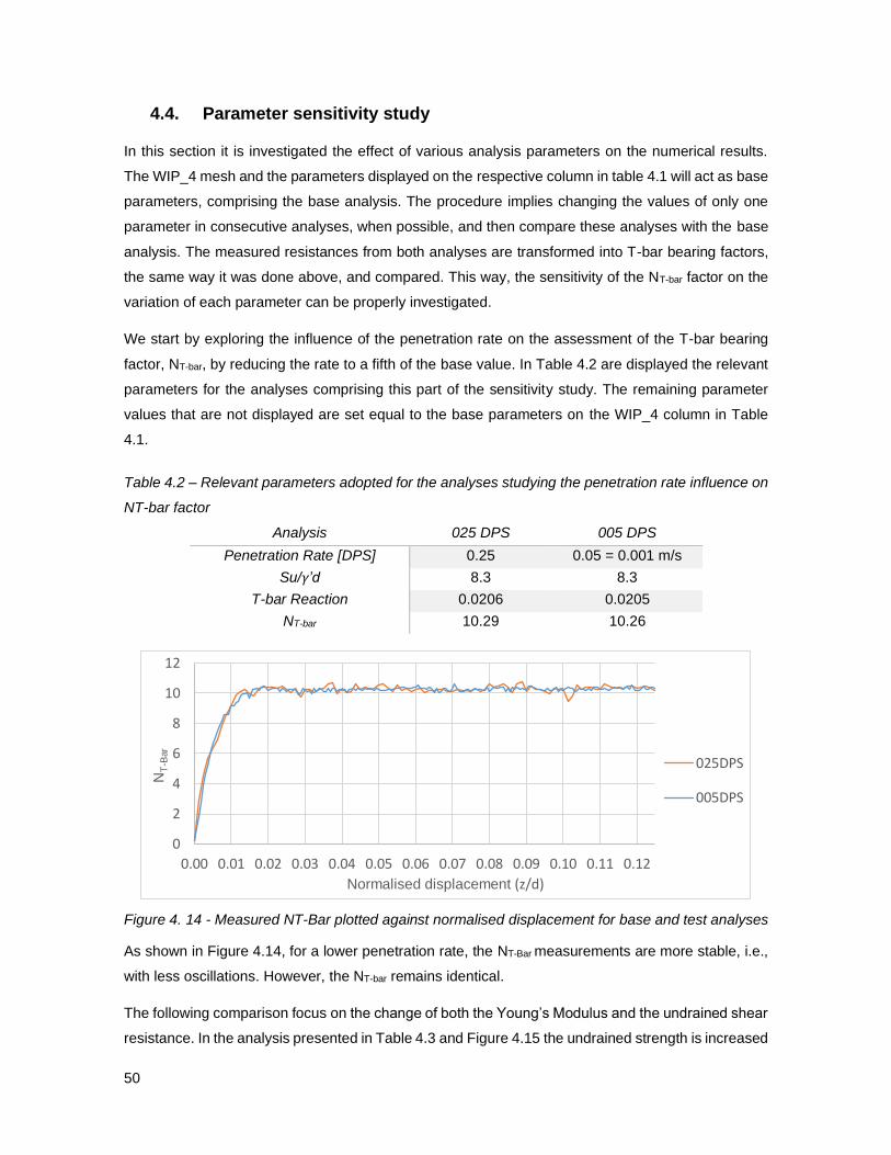
50

4.4. Parameter sensitivity study

In this section it is investigated the effect of various analysis parameters on the numerical results.

The WIP_4 mesh and the parameters displayed on the respective column in table 4.1 will act as base

parameters, comprising the base analysis. The procedure implies changing the values of only one

parameter in consecutive analyses, when possible, and then compare these analyses with the base

analysis. The measured resistances from both analyses are transformed into T-bar bearing factors,

the same way it was done above, and compared. This way, the sensitivity of the NT-bar factor on the

variation of each parameter can be properly investigated.

We start by exploring the influence of the penetration rate on the assessment of the T-bar bearing

factor, NT-bar, by reducing the rate to a fifth of the base value. In Table 4.2 are displayed the relevant

parameters for the analyses comprising this part of the sensitivity study. The remaining parameter

values that are not displayed are set equal to the base parameters on the WIP_4 column in Table

4.1.

Table 4.2 – Relevant parameters adopted for the analyses studying the penetration rate influence on

NT-bar factor

Analysis 025 DPS 005 DPS

Penetration Rate [DPS] 0.25 0.05 = 0.001 m/s

Su/γ’d 8.3 8.3

T-bar Reaction 0.0206 0.0205

NT-bar 10.29 10.26

Figure 4. 14 - Measured NT-Bar plotted against normalised displacement for base and test analyses

As shown in Figure 4.14, for a lower penetration rate, the NT-Bar measurements are more stable, i.e.,

with less oscillations. However, the NT-bar remains identical.

The following comparison focus on the change of both the Young’s Modulus and the undrained shear

resistance. In the analysis presented in Table 4.3 and Figure 4.15 the undrained strength is increased

0

2

4

6

8

10

12

0.00 0.01 0.02 0.03 0.04 0.05 0.06 0.07 0.08 0.09 0.10 0.11 0.12

NT

-Bar

Normalised displacement (z/d)

025DPS

005DPS

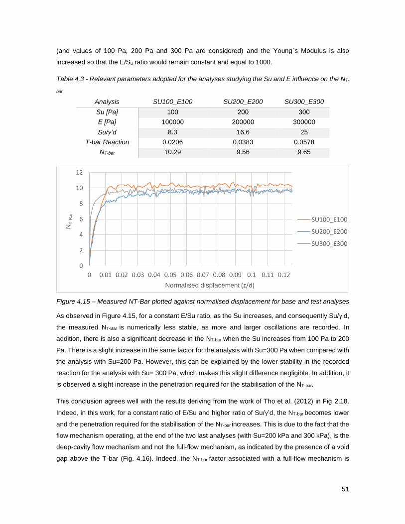
51

(and values of 100 Pa, 200 Pa and 300 Pa are considered) and the Young´s Modulus is also

increased so that the E/Su ratio would remain constant and equal to 1000.

Table 4.3 - Relevant parameters adopted for the analyses studying the Su and E influence on the NT-

bar

Analysis SU100_E100 SU200_E200 SU300_E300

Su [Pa] 100 200 300

E [Pa] 100000 200000 300000

Su/γ’d 8.3 16.6 25

T-bar Reaction 0.0206 0.0383 0.0578

NT-bar 10.29 9.56 9.65

Figure 4.15 – Measured NT-Bar plotted against normalised displacement for base and test analyses

As observed in Figure 4.15, for a constant E/Su ratio, as the Su increases, and consequently Su/γ’d,

the measured NT-Bar is numerically less stable, as more and larger oscillations are recorded. In

addition, there is also a significant decrease in the NT-bar when the Su increases from 100 Pa to 200

Pa. There is a slight increase in the same factor for the analysis with Su=300 Pa when compared with

the analysis with Su=200 Pa. However, this can be explained by the lower stability in the recorded

reaction for the analysis with Su= 300 Pa, which makes this slight difference negligible. In addition, it

is observed a slight increase in the penetration required for the stabilisation of the NT-bar.

This conclusion agrees well with the results deriving from the work of Tho et al. (2012) in Fig 2.18.

Indeed, in this work, for a constant ratio of E/Su and higher ratio of Su/γ’d, the NT-bar becomes lower

and the penetration required for the stabilisation of the NT-bar increases. This is due to the fact that the

flow mechanism operating, at the end of the two last analyses (with Su=200 kPa and 300 kPa), is the

deep-cavity flow mechanism and not the full-flow mechanism, as indicated by the presence of a void

gap above the T-bar (Fig. 4.16). Indeed, the NT-bar factor associated with a full-flow mechanism is

0

2

4

6

8

10

12

0 0.01 0.02 0.03 0.04 0.05 0.06 0.07 0.08 0.09 0.1 0.11 0.12

NT

-Bar

Normalised displacement (z/d)

SU100_E100

SU200_E200

SU300_E300

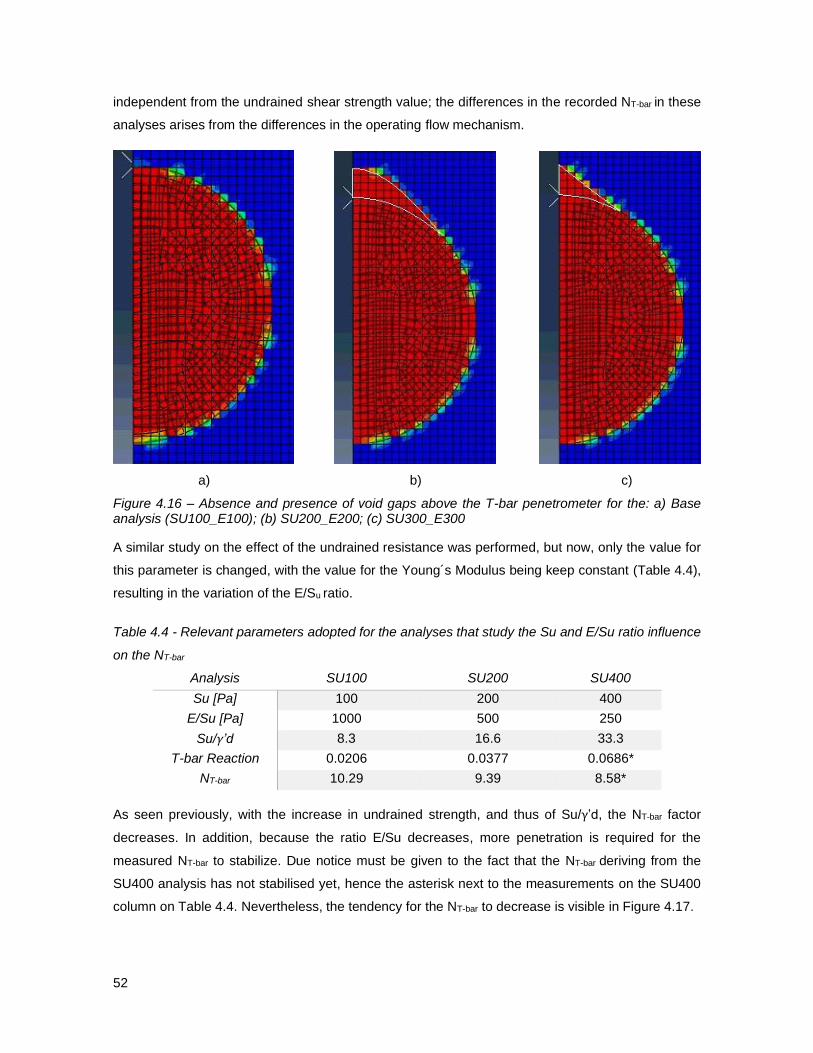
52

independent from the undrained shear strength value; the differences in the recorded NT-bar in these

analyses arises from the differences in the operating flow mechanism.

a) b) c)

Figure 4.16 – Absence and presence of void gaps above the T-bar penetrometer for the: a) Base analysis (SU100_E100); (b) SU200_E200; (c) SU300_E300

A similar study on the effect of the undrained resistance was performed, but now, only the value for

this parameter is changed, with the value for the Young´s Modulus being keep constant (Table 4.4),

resulting in the variation of the E/Su ratio.

Table 4.4 - Relevant parameters adopted for the analyses that study the Su and E/Su ratio influence

on the NT-bar

Analysis SU100 SU200 SU400

Su [Pa] 100 200 400

E/Su [Pa] 1000 500 250

Su/γ’d 8.3 16.6 33.3

T-bar Reaction 0.0206 0.0377 0.0686*

NT-bar 10.29 9.39 8.58*

As seen previously, with the increase in undrained strength, and thus of Su/γ’d, the NT-bar factor

decreases. In addition, because the ratio E/Su decreases, more penetration is required for the

measured NT-bar to stabilize. Due notice must be given to the fact that the NT-bar deriving from the

SU400 analysis has not stabilised yet, hence the asterisk next to the measurements on the SU400

column on Table 4.4. Nevertheless, the tendency for the NT-bar to decrease is visible in Figure 4.17.

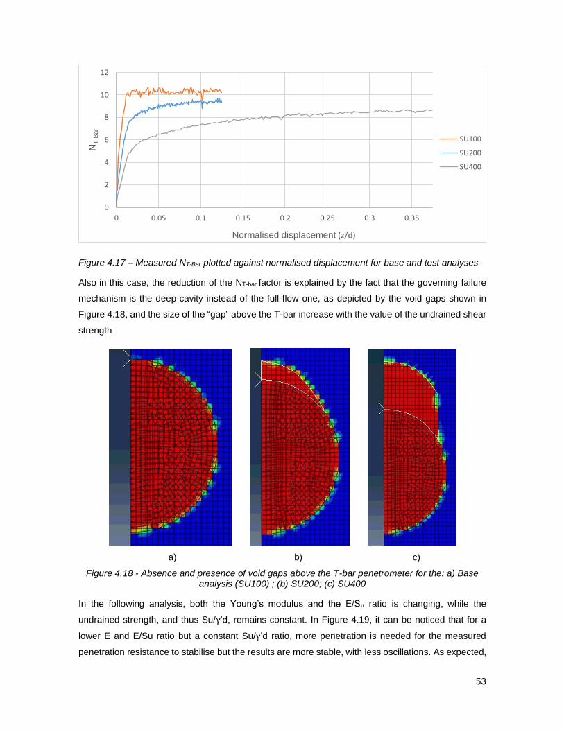
53

Figure 4.17 – Measured NT-Bar plotted against normalised displacement for base and test analyses

Also in this case, the reduction of the NT-bar factor is explained by the fact that the governing failure

mechanism is the deep-cavity instead of the full-flow one, as depicted by the void gaps shown in

Figure 4.18, and the size of the “gap” above the T-bar increase with the value of the undrained shear

strength

a) b) c)

Figure 4.18 - Absence and presence of void gaps above the T-bar penetrometer for the: a) Base analysis (SU100) ; (b) SU200; (c) SU400

In the following analysis, both the Young’s modulus and the E/Su ratio is changing, while the

undrained strength, and thus Su/γ’d, remains constant. In Figure 4.19, it can be noticed that for a

lower E and E/Su ratio but a constant Su/γ’d ratio, more penetration is needed for the measured

penetration resistance to stabilise but the results are more stable, with less oscillations. As expected,

0

2

4

6

8

10

12

0 0.05 0.1 0.15 0.2 0.25 0.3 0.35

NT

-Bar

Normalised displacement (z/d)

SU100

SU200

SU400

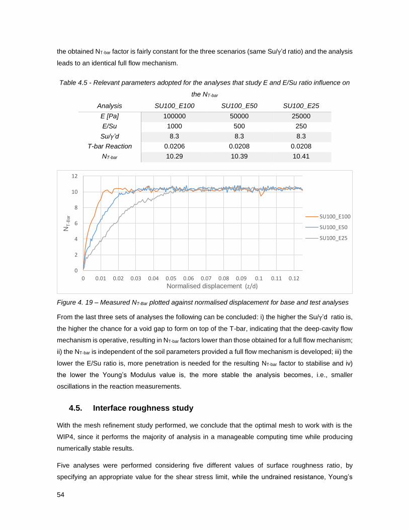
54

the obtained NT-bar factor is fairly constant for the three scenarios (same Su/γ’d ratio) and the analysis

leads to an identical full flow mechanism.

Table 4.5 - Relevant parameters adopted for the analyses that study E and E/Su ratio influence on

the NT-bar

Analysis SU100_E100 SU100_E50 SU100_E25

E [Pa] 100000 50000 25000

E/Su 1000 500 250

Su/γ’d 8.3 8.3 8.3

T-bar Reaction 0.0206 0.0208 0.0208

NT-bar 10.29 10.39 10.41

Figure 4. 19 – Measured NT-Bar plotted against normalised displacement for base and test analyses

From the last three sets of analyses the following can be concluded: i) the higher the Su/γ’d ratio is,

the higher the chance for a void gap to form on top of the T-bar, indicating that the deep-cavity flow

mechanism is operative, resulting in NT-bar factors lower than those obtained for a full flow mechanism;

ii) the NT-bar is independent of the soil parameters provided a full flow mechanism is developed; iii) the

lower the E/Su ratio is, more penetration is needed for the resulting NT-bar factor to stabilise and iv)

the lower the Young’s Modulus value is, the more stable the analysis becomes, i.e., smaller

oscillations in the reaction measurements.

4.5. Interface roughness study

With the mesh refinement study performed, we conclude that the optimal mesh to work with is the

WIP4, since it performs the majority of analysis in a manageable computing time while producing

numerically stable results.

Five analyses were performed considering five different values of surface roughness ratio, by

specifying an appropriate value for the shear stress limit, while the undrained resistance, Young’s

0

2

4

6

8

10

12

0 0.01 0.02 0.03 0.04 0.05 0.06 0.07 0.08 0.09 0.1 0.11 0.12

NT

-Bar

Normalised displacement (z/d)

SU100_E100

SU100_E50

SU100_E25

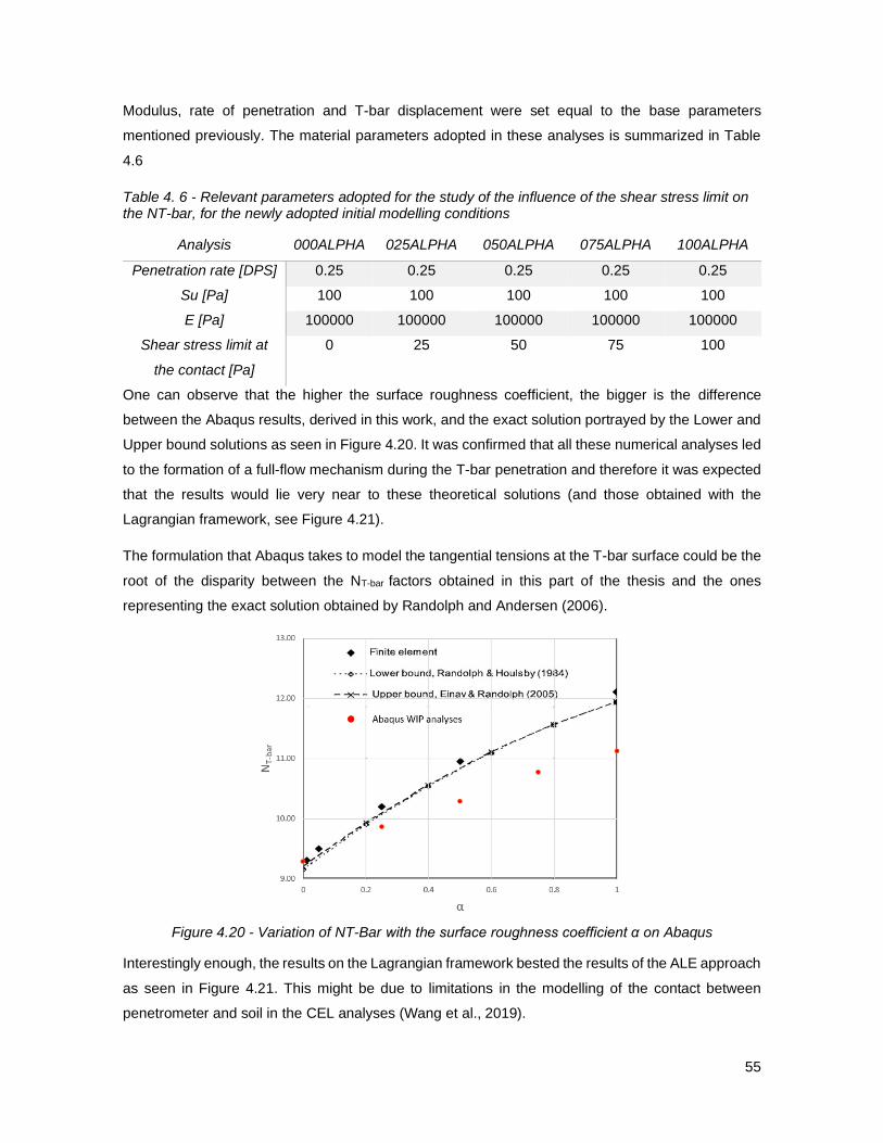
55

Modulus, rate of penetration and T-bar displacement were set equal to the base parameters

mentioned previously. The material parameters adopted in these analyses is summarized in Table

4.6

Table 4. 6 - Relevant parameters adopted for the study of the influence of the shear stress limit on the NT-bar, for the newly adopted initial modelling conditions

Analysis 000ALPHA 025ALPHA 050ALPHA 075ALPHA 100ALPHA

Penetration rate [DPS] 0.25 0.25 0.25 0.25 0.25

Su [Pa] 100 100 100 100 100

E [Pa] 100000 100000 100000 100000 100000

Shear stress limit at

the contact [Pa]

0 25 50 75 100

One can observe that the higher the surface roughness coefficient, the bigger is the difference

between the Abaqus results, derived in this work, and the exact solution portrayed by the Lower and

Upper bound solutions as seen in Figure 4.20. It was confirmed that all these numerical analyses led

to the formation of a full-flow mechanism during the T-bar penetration and therefore it was expected

that the results would lie very near to these theoretical solutions (and those obtained with the

Lagrangian framework, see Figure 4.21).

The formulation that Abaqus takes to model the tangential tensions at the T-bar surface could be the

root of the disparity between the NT-bar factors obtained in this part of the thesis and the ones

representing the exact solution obtained by Randolph and Andersen (2006).

Figure 4.20 - Variation of NT-Bar with the surface roughness coefficient α on Abaqus

Interestingly enough, the results on the Lagrangian framework bested the results of the ALE approach

as seen in Figure 4.21. This might be due to limitations in the modelling of the contact between

penetrometer and soil in the CEL analyses (Wang et al., 2019).

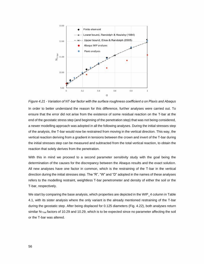
56

Figure 4.21 - Variation of NT-bar factor with the surface roughness coefficient α on Plaxis and Abaqus

In order to better understand the reason for this difference, further analyses were carried out. To

ensure that the error did not arise from the existence of some residual reaction on the T-bar at the

end of the geostatic stress step (and beginning of the penetration step) that was not being considered,

a newer modelling approach was adopted in all the following analyses. During the initial stresses step

of the analysis, the T-bar would now be restrained from moving in the vertical direction. This way, the

vertical reaction deriving from a gradient in tensions between the crown and invert of the T-bar during

the initial stresses step can be measured and subtracted from the total vertical reaction, to obtain the

reaction that solely derives from the penetration.

With this in mind we proceed to a second parameter sensitivity study with the goal being the

determination of the causes for the discrepancy between the Abaqus results and the exact solution.

All new analyses have one factor in common, which is the restraining of the T-bar in the vertical

direction during the initial stresses step. The “R”, “W” and “D” adopted in the names of these analyses

refers to the modelling restraint, weightless T-bar penetrometer and density of either the soil or the

T-bar, respectively.

We start by comparing the base analysis, which properties are depicted in the WIP_4 column in Table

4.1, with its sister analysis where the only variant is the already mentioned restraining of the T-bar

during the geostatic step. After being displaced for 0.125 diameters (Fig. 4.22), both analyses return

similar NT-bar factors of 10.29 and 10.29, which is to be expected since no parameter affecting the soil

or the T-bar was altered.

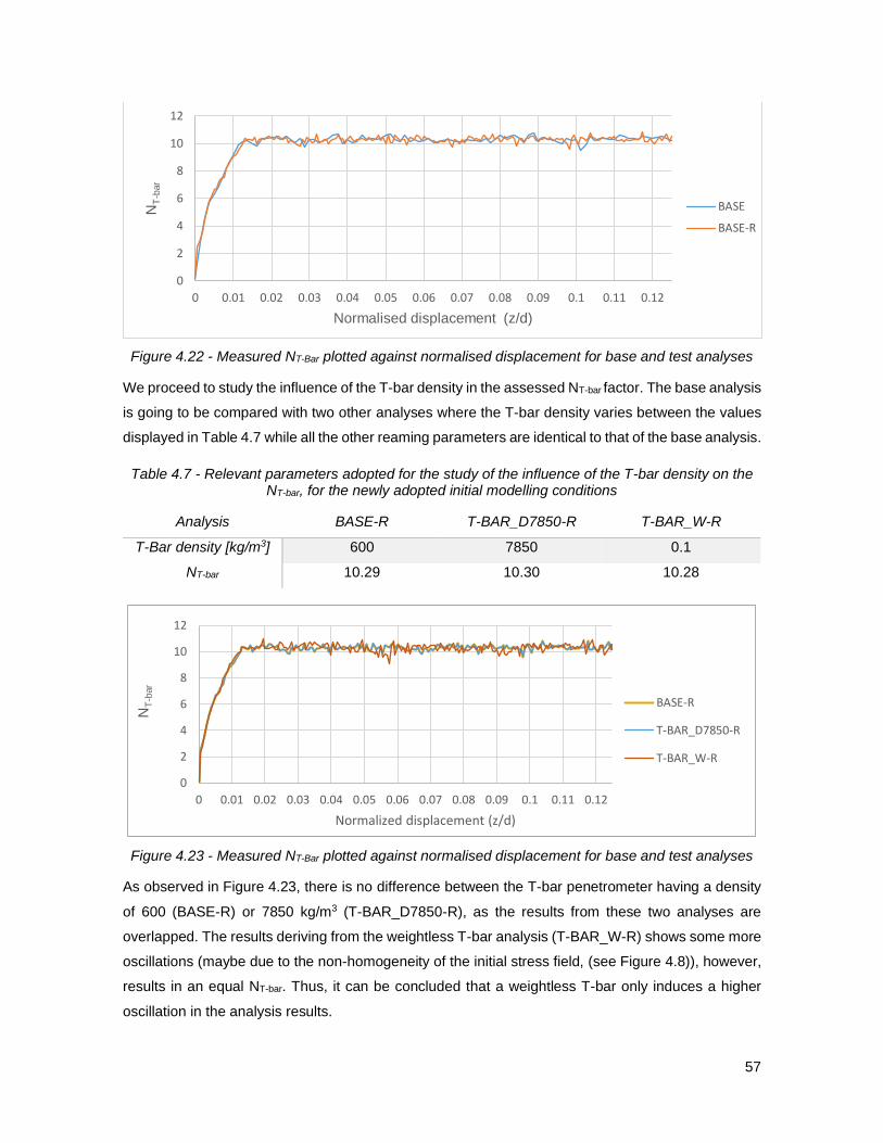
57

Figure 4.22 - Measured NT-Bar plotted against normalised displacement for base and test analyses

We proceed to study the influence of the T-bar density in the assessed NT-bar factor. The base analysis

is going to be compared with two other analyses where the T-bar density varies between the values

displayed in Table 4.7 while all the other reaming parameters are identical to that of the base analysis.

Table 4.7 - Relevant parameters adopted for the study of the influence of the T-bar density on the NT-bar, for the newly adopted initial modelling conditions

Analysis BASE-R T-BAR_D7850-R T-BAR_W-R

T-Bar density [kg/m3] 600 7850 0.1

NT-bar 10.29 10.30 10.28

Figure 4.23 - Measured NT-Bar plotted against normalised displacement for base and test analyses

As observed in Figure 4.23, there is no difference between the T-bar penetrometer having a density

of 600 (BASE-R) or 7850 kg/m3 (T-BAR_D7850-R), as the results from these two analyses are

overlapped. The results deriving from the weightless T-bar analysis (T-BAR_W-R) shows some more

oscillations (maybe due to the non-homogeneity of the initial stress field, (see Figure 4.8)), however,

results in an equal NT-bar. Thus, it can be concluded that a weightless T-bar only induces a higher

oscillation in the analysis results.

0

2

4

6

8

10

12

0 0.01 0.02 0.03 0.04 0.05 0.06 0.07 0.08 0.09 0.1 0.11 0.12

NT

-bar

Normalised displacement (z/d)

BASE

BASE-R

0

2

4

6

8

10

12

0 0.01 0.02 0.03 0.04 0.05 0.06 0.07 0.08 0.09 0.1 0.11 0.12

NT

-bar

Normalized displacement (z/d)

BASE-R

T-BAR_D7850-R

T-BAR_W-R

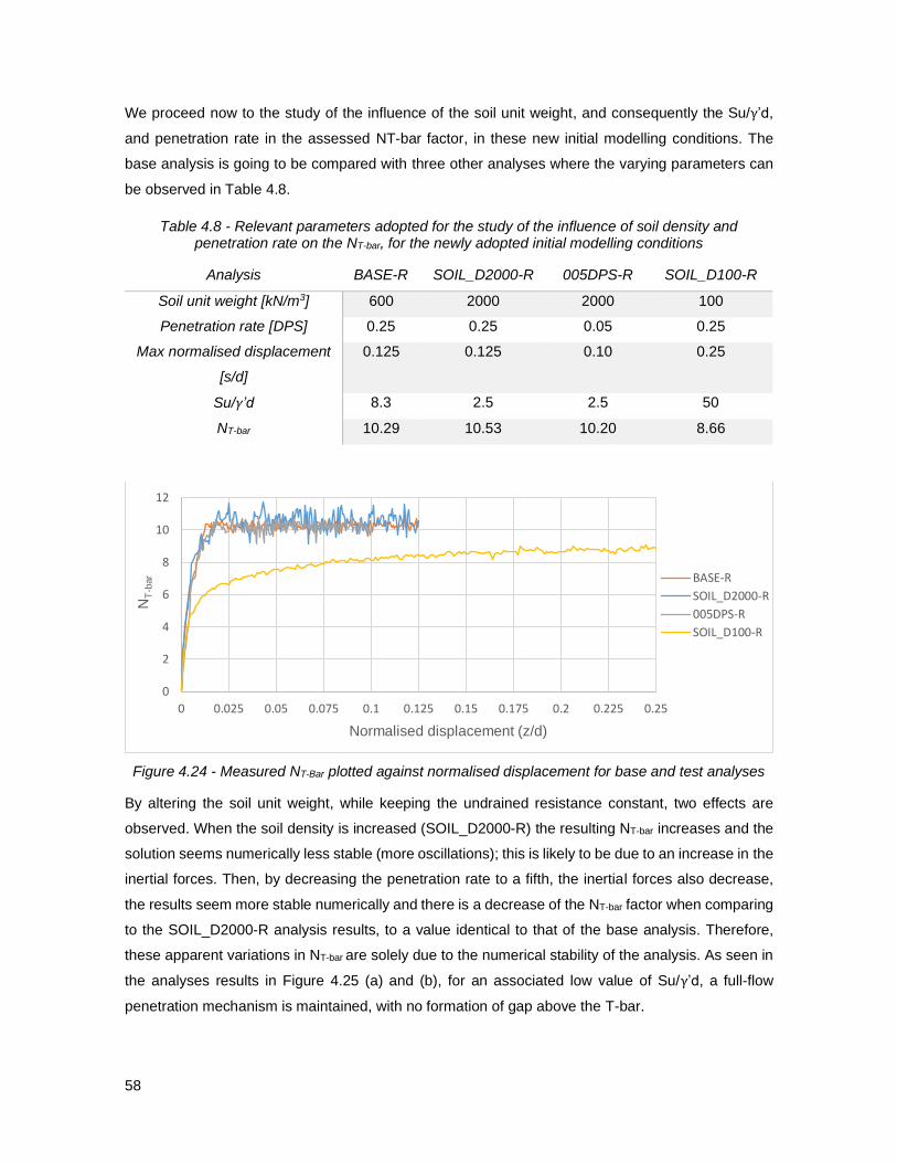
58

We proceed now to the study of the influence of the soil unit weight, and consequently the Su/γ’d,

and penetration rate in the assessed NT-bar factor, in these new initial modelling conditions. The

base analysis is going to be compared with three other analyses where the varying parameters can

be observed in Table 4.8.

Table 4.8 - Relevant parameters adopted for the study of the influence of soil density and penetration rate on the NT-bar, for the newly adopted initial modelling conditions

Analysis BASE-R SOIL_D2000-R 005DPS-R SOIL_D100-R

Soil unit weight [kN/m3] 600 2000 2000 100

Penetration rate [DPS] 0.25 0.25 0.05 0.25

Max normalised displacement

[s/d]

0.125 0.125 0.10 0.25

Su/γ’d 8.3 2.5 2.5 50

NT-bar 10.29 10.53 10.20 8.66

Figure 4.24 - Measured NT-Bar plotted against normalised displacement for base and test analyses

By altering the soil unit weight, while keeping the undrained resistance constant, two effects are

observed. When the soil density is increased (SOIL_D2000-R) the resulting NT-bar increases and the

solution seems numerically less stable (more oscillations); this is likely to be due to an increase in the

inertial forces. Then, by decreasing the penetration rate to a fifth, the inertial forces also decrease,

the results seem more stable numerically and there is a decrease of the NT-bar factor when comparing

to the SOIL_D2000-R analysis results, to a value identical to that of the base analysis. Therefore,

these apparent variations in NT-bar are solely due to the numerical stability of the analysis. As seen in

the analyses results in Figure 4.25 (a) and (b), for an associated low value of Su/γ’d, a full-flow

penetration mechanism is maintained, with no formation of gap above the T-bar.

0

2

4

6

8

10

12

0 0.025 0.05 0.075 0.1 0.125 0.15 0.175 0.2 0.225 0.25

NT

-bar

Normalised displacement (z/d)

BASE-R

SOIL_D2000-R

005DPS-R

SOIL_D100-R

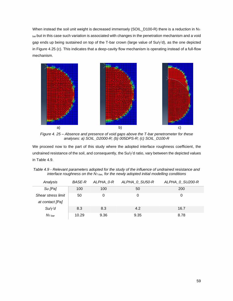
59

When instead the soil unit weight is decreased immensely (SOIL_D100-R) there is a reduction in NT-

bar but in this case such variation is associated with changes in the penetration mechanism and a void

gap ends up being sustained on top of the T-bar crown (large value of Su/γ’d), as the one depicted

in Figure 4.25 (c). This indicates that a deep-cavity flow mechanism is operating instead of a full-flow

mechanism.

a) b) c)

Figure 4. 25 – Absence and presence of void gaps above the T-bar penetrometer for these analyses: a) SOIL_D2000-R; (b) 005DPS-R; (c) SOIL_D100-R

We proceed now to the part of this study where the adopted interface roughness coefficient, the

undrained resistance of the soil, and consequently, the Su/γ’d ratio, vary between the depicted values

in Table 4.9.

Table 4.9 - Relevant parameters adopted for the study of the influence of undrained resistance and interface roughness on the NT-bar, for the newly adopted initial modelling conditions

Analysis BASE-R ALPHA_0-R ALPHA_0_SU50-R ALPHA_0_SU200-R

Su [Pa] 100 100 50 200

Shear stress limit

at contact [Pa]

50 0 0 0

Su/γ’d 8.3 8.3 4.2 16.7

NT-bar 10.29 9.36 9.35 8.78

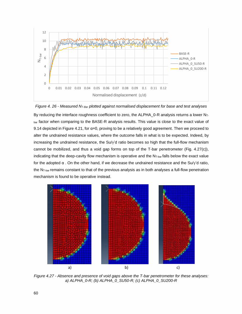
60

Figure 4. 26 - Measured NT-Bar plotted against normalised displacement for base and test analyses

By reducing the interface roughness coefficient to zero, the ALPHA_0-R analysis returns a lower NT-

bar factor when comparing to the BASE-R analysis results. This value is close to the exact value of

9.14 depicted in Figure 4.21, for α=0, proving to be a relatively good agreement. Then we proceed to

alter the undrained resistance values, where the outcome falls in what is to be expected. Indeed, by

increasing the undrained resistance, the Su/γ’d ratio becomes so high that the full-flow mechanism

cannot be mobilized, and thus a void gap forms on top of the T-bar penetrometer (Fig. 4.27(c)),

indicating that the deep-cavity flow mechanism is operative and the NT-bar falls below the exact value

for the adopted α . On the other hand, if we decrease the undrained resistance and the Su/γ’d ratio,

the NT-bar remains constant to that of the previous analysis as in both analyses a full-flow penetration

mechanism is found to be operative instead.

a) b) c)

Figure 4.27 - Absence and presence of void gaps above the T-bar penetrometer for these analyses: a) ALPHA_0-R; (b) ALPHA_0_SU50-R; (c) ALPHA_0_SU200-R

0

2

4

6

8

10

12

0 0.01 0.02 0.03 0.04 0.05 0.06 0.07 0.08 0.09 0.1 0.11 0.12

NT

-bar

Normalised displacement (z/d)

BASE-R

ALPHA_0-R

ALPHA_0_SU50-R

ALPHA_0_SU200-R

61

Having in mind the sets of analyses performed above, the following conclusions can be drawn:

- For relatively low values of Su/γ’d ratio (below and around 8, for the geometry of the problem

considered here), the full-flow mechanism ends up always being mobilised by the end of the

penetration. In this case, the assessed NT-bar is independent of the soil and T-bar properties

and the observed differences between the readings of different analyses are due to their

difference in numerical stability. The analyses carried out with the CEL methodology

(employed through Abaqus) can capture almost perfectly the NT-bar solution for the case

where the shear stress limit at contact is equal to zero, i.e., the surface roughness coefficient

is null (smooth T-bar). However, for values higher than zero, the Abaqus analysis is

consistently underestimating the NT-bar. The reasons behind this discrepancy are not entirely

understood but are thought to be due to the limitations of the CEL methodology in modelling

the stresses at the soil-T-bar interface.

- For higher values of Su/γ’d ratio mentioned above, the full-flow mechanism cannot be

mobilised and in turn the formation of a void gap above the T-bar is observed during its

penetration, indicating that the deep-cavity flow mechanism is being mobilised. Additionally,

the resulting NT-bar is considerably lower than the one associated with the full-flow mechanism.

- In the analyses carried out in this work, the WIP T-bar starts penetrating from a normalised

embedment depth of 6 diameters. According to the work of Tho et al. (2012) (see also Figure

2.19) for a smooth pipe (alfa=0), for a Su/γ’d ratio equal to 8 at about 6 d the mechanism is

still that of deep-cavity corresponding to a lower NT-bar of about 8. In addition for a smooth

pipe and Su/γ’d=8 a full flow mechanism was likely to only develop for depths well in excess

of 10 d. In the analyses carried in this thesis where the adopted Su/γ’d ratio has a value of

8.3 and α equal to zero, the full-flow mechanism is observed at a depth of 6 d, contradicting

what would be expected. The reason for this difference is not clear. Nonetheless, an average

NT-Bar value of 9.3, resultant from the analyses where the full-flow mechanism is mobilised

(from this work) is similar to the analytical value of 9.14. The reason behind these

discrepancies might be due to the fact that different penetration scenarios are considered. In

the work of comparison, the PIP penetration scenario is adopted whereas in this work, the

WIP scenario is adopted.

Further analyses were conducted to investigate the constitutive law adopted by Abaqus/CEL that

characterises the soil-T-bar contact interface and in particular to study the effect of the contact

tangential stiffness. The obtained results do not differ from the ones mentioned above and support

the belief that there was no error in the way the contact was being specified.

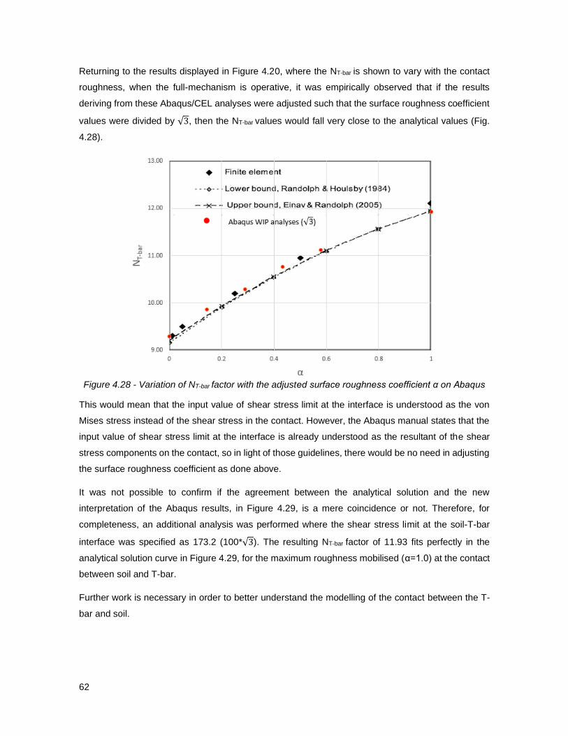
62

Returning to the results displayed in Figure 4.20, where the NT-bar is shown to vary with the contact

roughness, when the full-mechanism is operative, it was empirically observed that if the results

deriving from these Abaqus/CEL analyses were adjusted such that the surface roughness coefficient

values were divided by √3, then the NT-bar values would fall very close to the analytical values (Fig.

4.28).

Figure 4.28 - Variation of NT-bar factor with the adjusted surface roughness coefficient α on Abaqus

This would mean that the input value of shear stress limit at the interface is understood as the von

Mises stress instead of the shear stress in the contact. However, the Abaqus manual states that the

input value of shear stress limit at the interface is already understood as the resultant of the shear

stress components on the contact, so in light of those guidelines, there would be no need in adjusting

the surface roughness coefficient as done above.

It was not possible to confirm if the agreement between the analytical solution and the new

interpretation of the Abaqus results, in Figure 4.29, is a mere coincidence or not. Therefore, for

completeness, an additional analysis was performed where the shear stress limit at the soil-T-bar

interface was specified as 173.2 (100*√3). The resulting NT-bar factor of 11.93 fits perfectly in the

analytical solution curve in Figure 4.29, for the maximum roughness mobilised (α=1.0) at the contact

between soil and T-bar.

Further work is necessary in order to better understand the modelling of the contact between the T-

bar and soil.

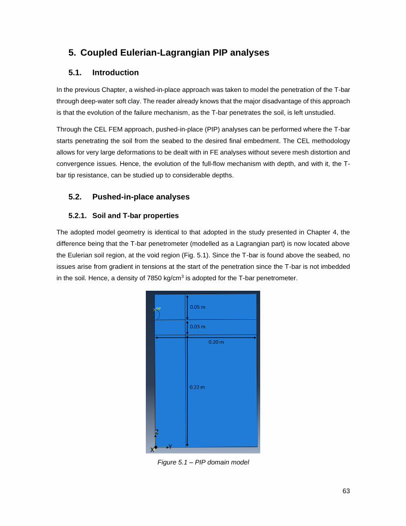
63

5. Coupled Eulerian-Lagrangian PIP analyses

5.1. Introduction

In the previous Chapter, a wished-in-place approach was taken to model the penetration of the T-bar

through deep-water soft clay. The reader already knows that the major disadvantage of this approach

is that the evolution of the failure mechanism, as the T-bar penetrates the soil, is left unstudied.

Through the CEL FEM approach, pushed-in-place (PIP) analyses can be performed where the T-bar

starts penetrating the soil from the seabed to the desired final embedment. The CEL methodology

allows for very large deformations to be dealt with in FE analyses without severe mesh distortion and

convergence issues. Hence, the evolution of the full-flow mechanism with depth, and with it, the T-

bar tip resistance, can be studied up to considerable depths.

5.2. Pushed-in-place analyses

5.2.1. Soil and T-bar properties

The adopted model geometry is identical to that adopted in the study presented in Chapter 4, the

difference being that the T-bar penetrometer (modelled as a Lagrangian part) is now located above

the Eulerian soil region, at the void region (Fig. 5.1). Since the T-bar is found above the seabed, no

issues arise from gradient in tensions at the start of the penetration since the T-bar is not imbedded

in the soil. Hence, a density of 7850 kg/cm3 is adopted for the T-bar penetrometer.

Figure 5.1 – PIP domain model

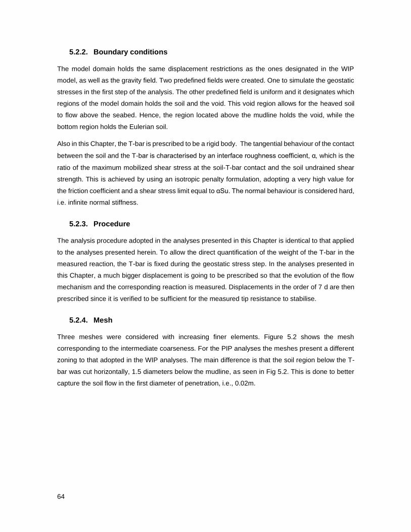
64

5.2.2. Boundary conditions

The model domain holds the same displacement restrictions as the ones designated in the WIP

model, as well as the gravity field. Two predefined fields were created. One to simulate the geostatic

stresses in the first step of the analysis. The other predefined field is uniform and it designates which

regions of the model domain holds the soil and the void. This void region allows for the heaved soil

to flow above the seabed. Hence, the region located above the mudline holds the void, while the

bottom region holds the Eulerian soil.

Also in this Chapter, the T-bar is prescribed to be a rigid body. The tangential behaviour of the contact

between the soil and the T-bar is characterised by an interface roughness coefficient, α which is the

ratio of the maximum mobilized shear stress at the soil-T-bar contact and the soil undrained shear

strength. This is achieved by using an isotropic penalty formulation, adopting a very high value for

the friction coefficient and a shear stress limit equal to αSu. The normal behaviour is considered hard,

i.e. infinite normal stiffness.

5.2.3. Procedure

The analysis procedure adopted in the analyses presented in this Chapter is identical to that applied

to the analyses presented herein. To allow the direct quantification of the weight of the T-bar in the

measured reaction, the T-bar is fixed during the geostatic stress step. In the analyses presented in

this Chapter, a much bigger displacement is going to be prescribed so that the evolution of the flow

mechanism and the corresponding reaction is measured. Displacements in the order of 7 d are then

prescribed since it is verified to be sufficient for the measured tip resistance to stabilise.

5.2.4. Mesh

Three meshes were considered with increasing finer elements. Figure 5.2 shows the mesh

corresponding to the intermediate coarseness. For the PIP analyses the meshes present a different

zoning to that adopted in the WIP analyses. The main difference is that the soil region below the T-

bar was cut horizontally, 1.5 diameters below the mudline, as seen in Fig 5.2. This is done to better

capture the soil flow in the first diameter of penetration, i.e., 0.02m.

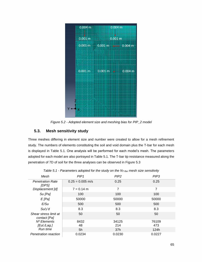
65

Figure 5.2 - Adopted element size and meshing bias for PIP_2 model

5.3. Mesh sensitivity study

Three meshes differing in element size and number were created to allow for a mesh refinement

study. The numbers of elements constituting the soil and void domain plus the T-bar for each mesh

is displayed in Table 5.1. One analysis will be performed for each model’s mesh. The parameters

adopted for each model are also portrayed in Table 5.1. The T-bar tip resistance measured along the

penetration of 7D of soil for the three analyses can be observed in Figure 5.3

Table 5.1 - Parameters adopted for the study on the NT-Bar mesh size sensitivity

Mesh PIP1 PIP2 PIP3

Penetration Rate [DPS]

0.25 = 0.005 m/s 0.25 0.25

Displacement [d] 7 = 0.14 m 7 7

Su [Pa] 100 100 100

E [Pa] 50000 50000 50000

E/Su 500 500 500

Su/γ’d 8.3 8.3 8.3

Shear stress limit at contact [Pa]

50 50 50

Nº Elements [Eul./Lag.]

8432 48

34125 214

76109 473

Run time 5h 37h 124h

Penetration reaction 0.0234 0.0230 0.0227

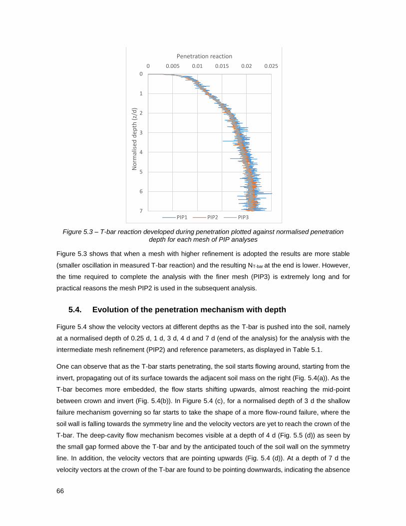
66

Figure 5.3 – T-bar reaction developed during penetration plotted against normalised penetration depth for each mesh of PIP analyses

Figure 5.3 shows that when a mesh with higher refinement is adopted the results are more stable

(smaller oscillation in measured T-bar reaction) and the resulting NT-bar at the end is lower. However,

the time required to complete the analysis with the finer mesh (PIP3) is extremely long and for

practical reasons the mesh PIP2 is used in the subsequent analysis.

5.4. Evolution of the penetration mechanism with depth

Figure 5.4 show the velocity vectors at different depths as the T-bar is pushed into the soil, namely

at a normalised depth of 0.25 d, 1 d, 3 d, 4 d and 7 d (end of the analysis) for the analysis with the

intermediate mesh refinement (PIP2) and reference parameters, as displayed in Table 5.1.

One can observe that as the T-bar starts penetrating, the soil starts flowing around, starting from the

invert, propagating out of its surface towards the adjacent soil mass on the right (Fig. 5.4(a)). As the

T-bar becomes more embedded, the flow starts shifting upwards, almost reaching the mid-point

between crown and invert (Fig. 5.4(b)). In Figure 5.4 (c), for a normalised depth of 3 d the shallow

failure mechanism governing so far starts to take the shape of a more flow-round failure, where the

soil wall is falling towards the symmetry line and the velocity vectors are yet to reach the crown of the

T-bar. The deep-cavity flow mechanism becomes visible at a depth of 4 d (Fig. 5.5 (d)) as seen by

the small gap formed above the T-bar and by the anticipated touch of the soil wall on the symmetry

line. In addition, the velocity vectors that are pointing upwards (Fig. 5.4 (d)). At a depth of 7 d the

velocity vectors at the crown of the T-bar are found to be pointing downwards, indicating the absence

0

1

2

3

4

5

6

7

0 0.005 0.01 0.015 0.02 0.025

No

rmal

ised

dep

th (

z/d

)

Penetration reaction

PIP1 PIP2 PIP3

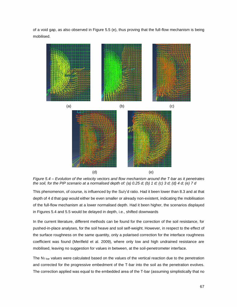
67

of a void gap, as also observed in Figure 5.5 (e), thus proving that the full-flow mechanism is being

mobilised.

(a) (b) (c)

(d) (e)

Figure 5.4 – Evolution of the velocity vectors and flow mechanism around the T-bar as it penetrates the soil, for the PIP scenario at a normalised depth of: (a) 0.25 d; (b) 1 d; (c) 3 d; (d) 4 d; (e) 7 d

This phenomenon, of course, is influenced by the Su/γ’d ratio. Had it been lower than 8.3 and at that

depth of 4 d that gap would either be even smaller or already non-existent, indicating the mobilisation

of the full-flow mechanism at a lower normalised depth. Had it been higher, the scenarios displayed

in Figures 5.4 and 5.5 would be delayed in depth, i.e., shifted downwards

In the current literature, different methods can be found for the correction of the soil resistance, for

pushed-in-place analyses, for the soil heave and soil self-weight. However, in respect to the effect of

the surface roughness on the same quantity, only a polarised correction for the interface roughness

coefficient was found (Merifield et al. 2009), where only low and high undrained resistance are

mobilised, leaving no suggestion for values in between, at the soil-penetrometer interface.

The NT-bar values were calculated based on the values of the vertical reaction due to the penetration

and corrected for the progressive embedment of the T-bar into the soil as the penetration evolves.

The correction applied was equal to the embedded area of the T-bar (assuming simplistically that no

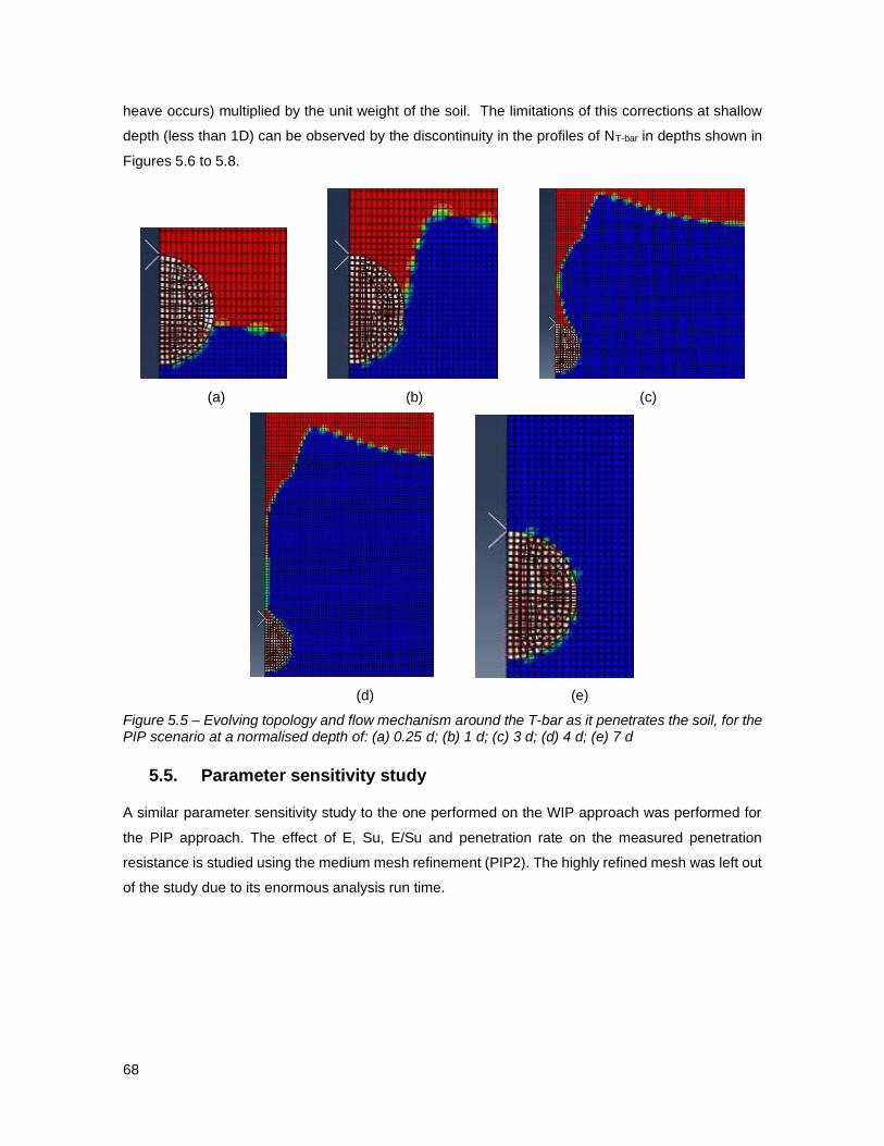
68

heave occurs) multiplied by the unit weight of the soil. The limitations of this corrections at shallow

depth (less than 1D) can be observed by the discontinuity in the profiles of NT-bar in depths shown in

Figures 5.6 to 5.8.

(a) (b) (c)

(d) (e)

Figure 5.5 – Evolving topology and flow mechanism around the T-bar as it penetrates the soil, for the PIP scenario at a normalised depth of: (a) 0.25 d; (b) 1 d; (c) 3 d; (d) 4 d; (e) 7 d

5.5. Parameter sensitivity study

A similar parameter sensitivity study to the one performed on the WIP approach was performed for

the PIP approach. The effect of E, Su, E/Su and penetration rate on the measured penetration

resistance is studied using the medium mesh refinement (PIP2). The highly refined mesh was left out

of the study due to its enormous analysis run time.

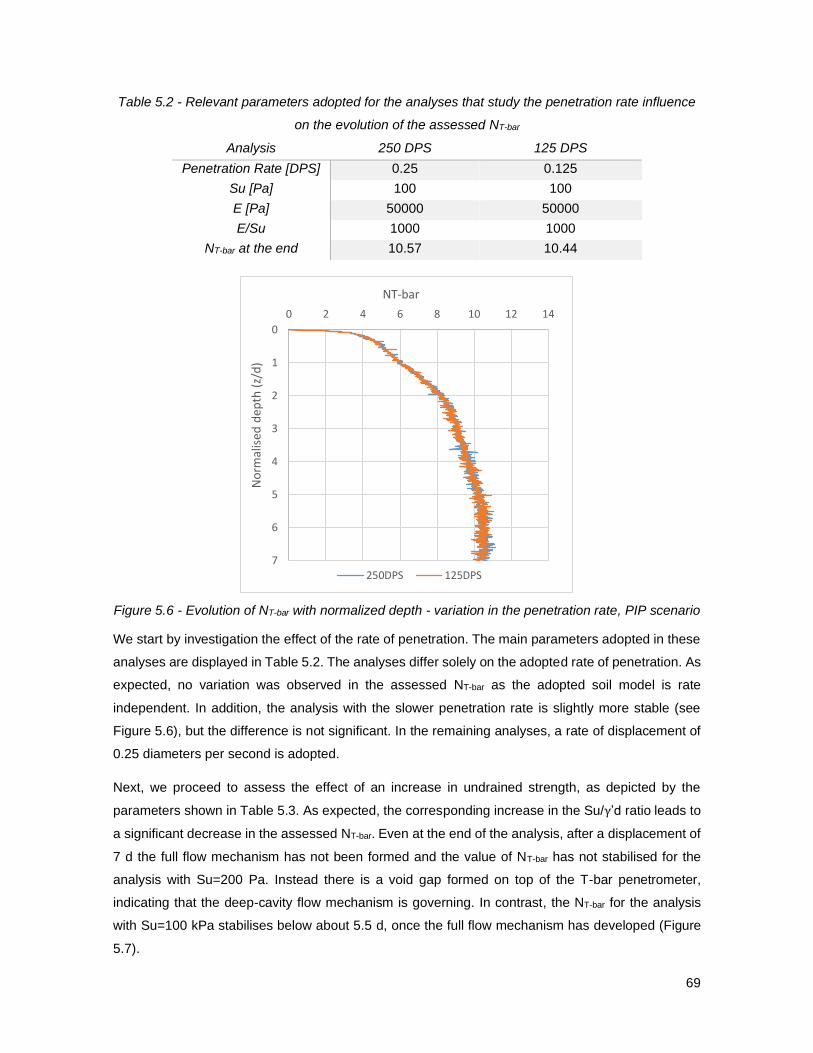
69

Table 5.2 - Relevant parameters adopted for the analyses that study the penetration rate influence

on the evolution of the assessed NT-bar

Analysis 250 DPS 125 DPS

Penetration Rate [DPS] 0.25 0.125

Su [Pa] 100 100

E [Pa] 50000 50000

E/Su 1000 1000

NT-bar at the end 10.57 10.44

Figure 5.6 - Evolution of NT-bar with normalized depth - variation in the penetration rate, PIP scenario

We start by investigation the effect of the rate of penetration. The main parameters adopted in these

analyses are displayed in Table 5.2. The analyses differ solely on the adopted rate of penetration. As

expected, no variation was observed in the assessed NT-bar as the adopted soil model is rate

independent. In addition, the analysis with the slower penetration rate is slightly more stable (see

Figure 5.6), but the difference is not significant. In the remaining analyses, a rate of displacement of

0.25 diameters per second is adopted.

Next, we proceed to assess the effect of an increase in undrained strength, as depicted by the

parameters shown in Table 5.3. As expected, the corresponding increase in the Su/γ’d ratio leads to

a significant decrease in the assessed NT-bar. Even at the end of the analysis, after a displacement of

7 d the full flow mechanism has not been formed and the value of NT-bar has not stabilised for the

analysis with Su=200 Pa. Instead there is a void gap formed on top of the T-bar penetrometer,

indicating that the deep-cavity flow mechanism is governing. In contrast, the NT-bar for the analysis

with Su=100 kPa stabilises below about 5.5 d, once the full flow mechanism has developed (Figure

5.7).

0

1

2

3

4

5

6

7

0 2 4 6 8 10 12 14

No

rmal

ised

dep

th (

z/d

)

NT-bar

250DPS 125DPS

70

These results are in agreement with the results obtained in Chapter 4, as at a depth of 6D a full flow

penetration mechanism is observed for the analysis with Su=100 Pa (Su/γ’d=8.3) but not for the

analysis with Su=200 Pa (Su/γ’d=16.6).

Table 5.3 - Relevant parameters adopted for the analyses that study the undrained strength influence on the evolution of the assessed NT-bar

Analysis SU 100 SU 200

Penetration Rate [DPS]

0.25 0.25

Displacement 7 d 7 d

Su [Pa] 100 200

E [Pa] 100000 200000

E/Su 1000 1000

Su/γ’d 8.3 16.6

NT-bar at the end

10.47 9.65

Figure 5.7 – Variation of the NT-bar with the undrained resistance for the PIP scenario

Finally, we look into the influence of the soil Young’s Modulus on the assessed NT-bar. In Table 5.4

there are depicted the relevant parameters adopted for this part of the study. Figure 5.8 shows the

evolution of the NT-bar with depth. As expected, the only difference observed is that from the analysis

with lower E, the oscillations in the readings are lower, indicating a more numerically stable reading.

In addition, the resulting NT-bar at the end shows no difference, which is to be expected as this bearing

factor is not dependent of E.

0

1

2

3

4

5

6

7

0 2 4 6 8 10 12 14

No

rmal

ised

dep

th (

z/d

)

NT-bar

SU200 SU100

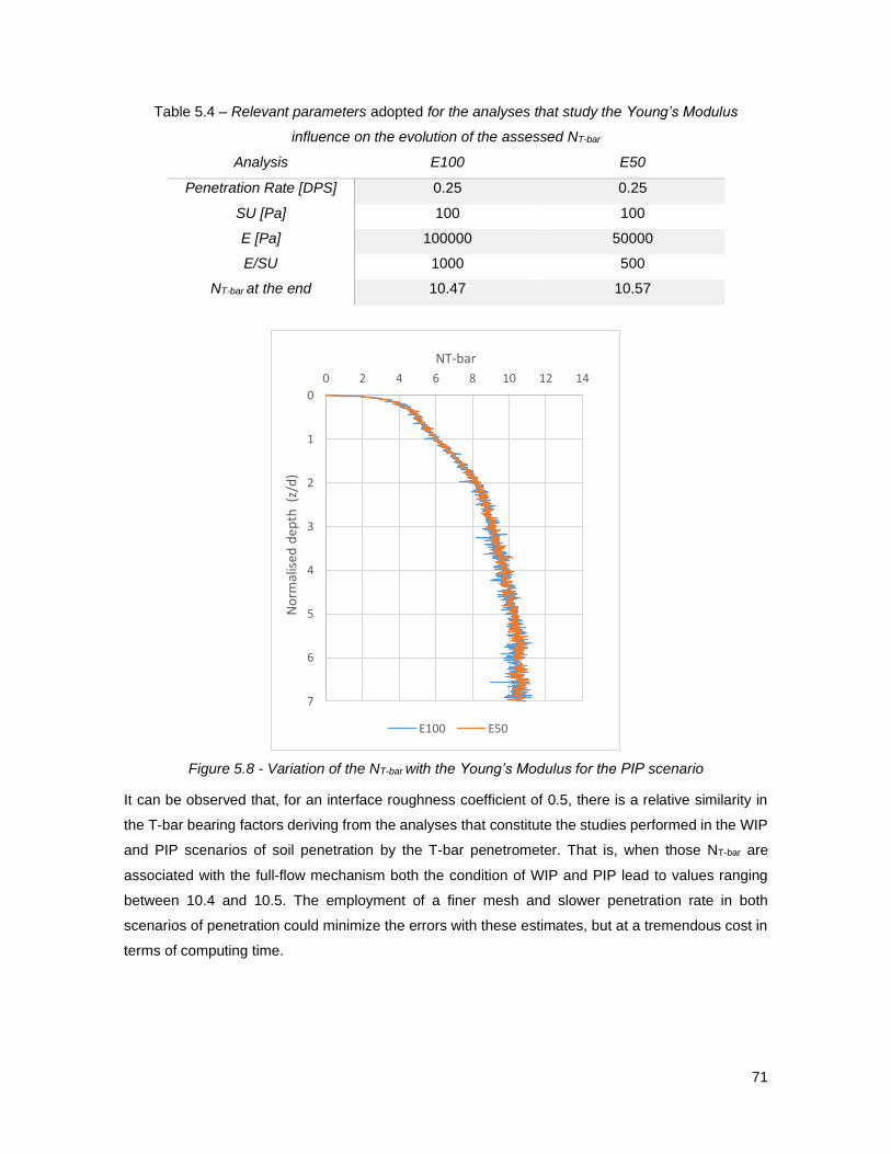
71

Table 5.4 – Relevant parameters adopted for the analyses that study the Young’s Modulus

influence on the evolution of the assessed NT-bar

Analysis E100 E50

Penetration Rate [DPS] 0.25 0.25

SU [Pa] 100 100

E [Pa] 100000 50000

E/SU 1000 500

NT-bar at the end 10.47 10.57

Figure 5.8 - Variation of the NT-bar with the Young’s Modulus for the PIP scenario

It can be observed that, for an interface roughness coefficient of 0.5, there is a relative similarity in

the T-bar bearing factors deriving from the analyses that constitute the studies performed in the WIP

and PIP scenarios of soil penetration by the T-bar penetrometer. That is, when those NT-bar are

associated with the full-flow mechanism both the condition of WIP and PIP lead to values ranging

between 10.4 and 10.5. The employment of a finer mesh and slower penetration rate in both

scenarios of penetration could minimize the errors with these estimates, but at a tremendous cost in

terms of computing time.

0

1

2

3

4

5

6

7

0 2 4 6 8 10 12 14

No

rmal

ised

dep

th (

z/d

)

NT-bar

E100 E50

72

6. Conclusions and future development

6.1. Conclusions

The results of the FE analyses performed in Plaxis with an isotropic and an anisotropic soil model

suggest that the value of NT-bar factor is independent of the soil anisotropy and for the case when the

interface roughness coefficient is equal to 0,5, then the NT-bar is equal to 10.86. However that is the

case provided the T-bar resistance is normalised by the average undrained shear strength (arithmetic

average of the undrained shear strength measured in triaxial compression, triaxial extension and

simple shear).

When considering T-bar penetrometer test results one should bear in mind that the interpreted

undrained shear strength corresponds to an average value and that due to soil anisotropy the average

undrained shear strength is significantly lower than that under triaxial compression. This is relevant

because in geotechnical engineering the undrained shear strength in triaxial compression test is the

value typically used.

In addition, the values of NT-bar obtained with Plaxis are in very good agreement with the solution

reported by Randolph and Andersen (2006), for the full range of values of interface roughness

coefficient.

Based on the analyses carried out with ABAQUS for the WIP scenario, the influence of a series of

parameters on the value of NT-bar was investigated. The observed dependence and independence of

certain geotechnical and mechanical properties in the parametric studies was logical and expected.

Furthermore, the analyses showed how the recorded NT-bar was influenced whether the full-flow

mechanism did or did not mobilise. When the full-flow mechanism developed, the recorded value of

NT-bar was in good agreement to that reported by Randolph and Andersen (2006), for the case of a

smooth T-bar (zero interface roughness coefficient), but the values diverged as the interface

roughness coefficient increased.

For the PIP analyses, it was verified that the resulting NT-bar, in average, is similar to the ones resulting

from the WIP studies at a full-flow stage. That is, after the PIP derived results were corrected for the

progressive embedment of the T-bar into the soil and the evolving penetration. This proves that even

though the NT-bar obtained at the end of the WIP and PIP analyses did not match the exact solution,

the full-flow mechanism can be achieved by two different modelling approaches.

The modelling of the interface between the penetrometer and the soil in LDFE analysis is a known

challenging problem to solve in numerical modelling (Wang et al., 2019). Indeed, as concluded at the

end of the previous two chapters, the observed discrepancy between the results obtained through

the LDFE analyses and the values constituting the exact solution can be attributed to a limited contact

73

algorithm adopted for the simulation of the tangential stresses at the soil-penetrometer interface,

employed through CEL.

6.2. Future developments

A new methodology should be developed in order to correctly simulate the tangential stresses at the

interface between soil and penetrometer. After this issue is solved, more complex studies could be

performed in the same FEM platform. An alternative to the CEL methodology would be the use of the

RITSS technique, which also falls in the ALE category of remeshing, being able to simulate LDFE

problems.

A ball penetrometer, which is geometrically axisymmetric, could be a viable alternative to the T-bar

in the characterisation of near-surface soil strength and as such it should also be investigated in

detail.

Additionally, it is suggested the development of further work on the effect of normalised strength on

the location of the transition depth, where the failure mechanism transitions, from deep cavity to full-

flow mechanism as available studies tend to focus on a limited range of scenarios.

74

7. Bibliography

Amuda, A. G., Hasan, A., Sahdi, F., & Taib, S. N. L. (2018). Variable penetration rate testing for

shear strength of peat – a review. International Journal of Geotechnical Engineering,

6362(May), 1–13. https://doi.org/10.1080/19386362.2018.1464816

Dutta, S., Hawlader, B., & Phillips, R. (2015). Finite element modeling of partially embedded

pipelines in clay seabed using Coupled Eulerian–Lagrangian method. Canadian Geotechnical

Journal, 52(1), 58–72. https://doi.org/10.1139/cgj-2014-0045

Grimstad, G., Andresen, L., and Jostad, H. P. (2012) "NGI-ADP: Anisotropic shear strength model

for clay". International Journal for Numerical and Analytical Methods in Geomechanics, 36, pp

483–497.

Hu, Y., & Randolph, M. F. (1998). A practical numerical approach for large deformation problems in

soil. International Journal for Numerical and Analytical Methods in Geomechanics, 22(5),

327–350. https://doi.org/10.1002/(SICI)1096-9853(199805)22:5<327::AID-NAG920>3.0.CO;2-

X

Lehane, B. M., O’loughlin, C. D., Gaudin, C., & Randolph, M. F. (2009). Rate effects on

penetrometer resistance in kaolin. Geotechnique, 59(1), 41–52.

https://doi.org/10.1680/geot.2007.00072

Low, H. E., Lunne, T., Andersen, K. H., Sjursen, M. A., Li, X., & Randolph, M. F. (2010). Estimation of

intact and remoulded undrained shear strengths from penetration tests in soft clays.

Geotechnique, 60(11), 843–859. https://doi.org/10.1680/geot.9.P.017

Lunne, Tom; Robertson, Peter. K.; Powell, J. J. M. (1997). Cone penetration testing in geotechnical

partice. Geotechnical Practice. Retrieved from http://www.pkg-

bialystok.pb.edu.pl/pliki/Ankieta_do_zadania_2_1_mgr_inz_Mariusz_Leszczynski.doc

Lunne, T., Andersen, K. H., Low, H. E., Randolph, M. F., & Sjursen, M. (2011). Guidelines for

offshore in situ testing and interpretation in deepwater soft clays. Canadian Geotechnical

Journal, 48(4), 543–556. https://doi.org/10.1139/t10-088

Randolph, M. F., & Andersen, K. H. (2006). Numerical simulation of T-bar penetration in soft clay.

International Journal of Geomechanics, 6(6), 411–420. https://doi.org/10.1061/(ASCE)1532-

3641(2006)6:6(411)

75

Tho, K. K., Leung, C. F., Chow, Y. K., & Palmer, A. C. (2012). Deep cavity flow mechanism of pipe

penetration in clay. Canadian Geotechnical Journal, 49(1), 59–69.

https://doi.org/10.1139/T11-088

Tian, Y., Wang, D., & Cassidy, M. J. (2011). Large deformation finite element analysis of offshore

penetration tests. Computational Geomechanics, COMGEO II - Proceedings of the 2nd

International Symposium on Computational Geomechanics, 925–933.

Wang, T., Liu, W., Wu, R., & Bao, X. (2019). Simulation of T-bar penetration in soft clay with

adhesive contact. Marine Georesources and Geotechnology, 0(0), 1–10.

https://doi.org/10.1080/1064119X.2018.1564091

White, D. J., Gaudin, C., Boylan, N., & Zhou, H. (2010). Interpretation of T-bar penetrometer tests

at shallow embedment and in very soft soils. Canadian Geotechnical Journal, 47(2), 218–229.

https://doi.org/10.1139/T09-096

Zhou, H., & Randolph, M. F. (2009). Resistance of full-flow penetrometers in rate-dependent and

strain-softening clay. Geotechnique, 59(2), 79–86. https://doi.org/10.1680/geot.2007.00164