Embed Size (px)
Citation preview
HAL Id: tel-03112849https://tel.archives-ouvertes.fr/tel-03112849v2
Submitted on 2 Sep 2021
HAL is a multi-disciplinary open accessarchive for the deposit and dissemination of sci-entific research documents, whether they are pub-lished or not. The documents may come fromteaching and research institutions in France orabroad, or from public or private research centers.
L’archive ouverte pluridisciplinaire HAL, estdestinée au dépôt et à la diffusion de documentsscientifiques de niveau recherche, publiés ou non,émanant des établissements d’enseignement et derecherche français ou étrangers, des laboratoirespublics ou privés.
Numerical methods by optimal quantization in financeThibaut Montes
To cite this version:Thibaut Montes. Numerical methods by optimal quantization in finance. Probability [math.PR].Sorbonne Université, 2020. English. NNT : 2020SORUS156. tel-03112849v2
Méthodes numériques parquantification optimale en finance
Numerical methods by optimal quantization in finance
Thibaut Montes
Laboratoire de Probabilités, Statistique et Modélisation - UMR 8001Sorbonne Université
Thèse pour l’obtention du grade de :Docteur de l’université Sorbonne Université
Sous la direction de : Gilles PagèsVincent Lemaire
Rapportée par : Giorgia CallegaroBenoîte de Saporta
Présentée devant un jury composé de : Giorgia Callegaro (rapporteure)Benoîte De Saporta (rapporteure)Jean-Michel Fayolle (invité)Benjamin Jourdain (président)Idris Kharroubi (examinateur)Vincent Lemaire (co-directeur de thèse)Gilles Pagès (directeur de thèse)Huyên Pham (examinateur)Abass Sagna (examinateur)
École Doctorale de Sciences Mathématiques deParis-CentreSection Mathématiques appliquées Mercredi 24 Juin 2020

Remerciements
Tout d’abord, je souhaite exprimer ma gratitude envers mes directeurs de thèse Vincent Lemaireet Gilles Pagès qui m’ont accompagné tout au long de mon doctorat, m’ont fait confiance etont toujours été disponibles pour répondre à mes questions. J’ai énormément appris à leurscôtés et leur en suis extrêmement reconnaissant. Leur supervision complémentaire est tout ceque je souhaite à leurs futurs doctorants. Elle m’a permis d’accomplir plus, à la fois en théorieet en pratique, que je n’aurais pu l’imaginer au début du doctorat. Je remercie égalementJean-Michel Fayolle pour avoir rendu possible cette thèse CIFRE et de s’être investi pour rendrepossible le dialogue entre ma recherche académique et les développements pratiques d’ICA.
Merci à mes deux rapporteures Giorgia Callegaro et Benoîte de Saporta d’avoir pris letemps de lire mon manuscrit de thèse. J’ai été très honoré de la confiance dont leurs rapportstémoignent. Je tiens également à exprimer toute ma reconnaissance envers Benjamin Jourdain,Idris Kharroubi, Huyên Pham et Abass Sagna d’avoir accepté de faire partie de mon jury dethèse.
Je tiens également à remercier l’ensemble des doctorants que j’ai eu la chance de croiserdurant ma thèse. On ne peut pas ne pas citer les thésards du bureau 201/3 (Léa, Rancy,Guillermo, Armand, Nicolas et Nicolas, Romain et Babacar) pour les cafés, les déjeuners ensoum-soum au Restaurant du Personnel et les bières partagées. Je n’oublie pas non plus tousles autres doctorants que j’ai eu la chance de rencontrer et d’apprendre à connaitre durantles différentes conférences (le CEMRACS avec ses calanques - Métabief et son restaurant deraclette - Padoue et ses spritz). Je souhaite également remercier mes collègues chez ICA avecqui j’ai pu échanger, autour d’un café, d’un déjeuner ou d’un jogging, en particulier, Guillaume,Eric, Vincent, Emmanuel et Lauriane.
Je voudrais ensuite remercier ma famille, Jeanine ma maman, Amélie ma soeur, Joëlle mamarraine, mes oncles et tantes Michel et Elisabeth, Monique et Michel ainsi que mes cousines etcousins, pour avoir toujours cru en moi et avoir été présent, surtout dans les moments difficiles.Je tiens également à remercier Hélène, la maman de Julie, et toute la famille Besnard-Corblet-Hatzopoulos pour m’avoir soutenu et encouragé dès notre rencontre et encore plus durant mathèse.
Je souhaiterais également remercier tous mes amis pour de merveilleux moments partagéset qui, par effet de bord, m’ont aidé à écrire cette thèse en rendant la vie plus douce. Enparticulier, je remercie Juju pour toutes ces années d’amitiés qui me sont précieuses ; Pierre,

iv
Patrick et Cécile pour toutes ces soirées / week-ends gastronomalcooliques ; les Scubes et leur+1 (Grégory, Henrik et Anita, Howon, Laure, Léa, Julien et Christina, Anh-Mai, Thomas,Jérôme, Vincent et Gamze, Juliette) pour leur bonne humeur permanente ; Laurène et Robinpour ces longues et étranges heures passées à l’opéra ; Kevin et John pour leurs soirées à thèmeet pour finir Karine et Myriam pour ces très bonnes années à Aix-en-Provence.
Enfin et surtout, merci Pauline pour ton soutien inconditionnel et pour avoir toujours cruen moi. Tu m’as toujours poussé à aller plus loin, à prendre confiance en moi et ce depuis ledébut de notre rencontre. Merci pour avoir toujours pris le temps de m’écouter (même lorsqueje radote "un peu").
Abstract
This thesis is divided into four parts that can be read independently. In this manuscript,we make some contributions to the theoretical study and financial applications of optimalquantization.
In the first part, we recall the theoretical foundations of optimal quantization as well as theclassical numerical methods to build optimal quantizers.
The second part focuses on the problem of numerical integration in dimension 1. Thisproblem arises when one wishes to numerically compute expectations, such as the valuation ofderivatives in finance that are expressed as the expectation of a function of a single financialasset. We recall the existing strong and weak error results and extend the results of order 2convergence rate to other function classes with less regularity. In a second step, we present aweak error development result in one dimension and a second development in a higher dimensionwhen the chosen quantizer is a product quantizer.
In the third part, we look at a first numerical application. We introduce a stationaryHeston model in which the initial condition of volatility, instead of being deterministic as in thestandard model, is assumed to be randomly distributed with the stationary distribution of theCIR EDS governing volatility. This variant of the original Heston model produces for Europeanoptions on short maturities a steeper smile of implied volatility than the standard model. Wethen develop a product recursive quantization-based numerical method for the valuation ofBermudan options and barriers.
The fourth and last part deals with a second numerical application, the pricing of Bermudanexchange rate options in a 3 factor model, i.e. where the exchange rate, domestic and foreigninterest rates are stochastic. These products are known in the markets as PRDC (Power ReverseDual Currency). We propose two schemes to evaluate this type of options, both based onoptimal product quantization and establish a priori error estimates.

Résumé
Cette thèse est divisée en quatres parties pouvant être lues indépendamment. Dans cemanuscrit, nous apportons quelques contributions à l’étude théorique et aux applications enfinance de la quantification optimale.
Dans la première partie, nous rappelons les fondements théoriques de la quantificationoptimale ainsi que les méthodes numériques classiques pour construire des quantifieurs optimaux.
La seconde partie se concentre sur le problème d’intégration numérique en dimension 1.Ce problème apparait lorsque l’on souhaite calculer numériquement des espérances, tel quel’évaluation de produits dérivés en finance qui s’expriment sous la forme d’un calcul d’espéranced’une fonction d’un unique actif financier. Nous y rappelons les résultats d’erreurs forts et faiblesexistants et étendons les résultats des convergences d’ordre 2 à d’autres classes de fonctionsmoins réguliers. Dans un deuxième temps, nous présentons un résultat de développementd’erreur faible en dimension 1 et un second développement en dimension supérieure pour unquantifieur produit.
Dans la troisième partie, nous nous intéressons à une première application numérique.Nous introduisons un modèle de Heston stationnaire dans lequel la condition initiale de lavolatilité, au lieu d’être déterministe comme dans le modèle standard, est supposée aléatoirede loi la distribution stationnaire de l’EDS du CIR régissant la volatilité. Cette variante dumodèle d’Heston original produit pour les options européennes sur les maturités courtes unsmile de volatilité implicite plus prononcé que le modèle standard. Nous développons ensuiteune méthode numérique à base de quantification récursive produit pour l’évaluation d’optionsbermudiennes et barrières.
La quatrième et dernière partie traite d’une deuxième application numérique, l’évaluationd’options bermudiennes sur taux de change dans un modèle 3 facteurs, i.e où le taux de change,les taux d’intérêts domestiques et étrangers sont stochastiques. Ces produits sont connus surles marchés sous le noms de PRDC (Power Reverse Dual Currency). Nous proposons deuxschémas pour évaluer ce type d’options toutes deux basées sur de la quantification optimaleproduit et établissons des estimations d’erreur à priori.

Contents
List of Figures xiii
List of Tables xvii
List of Algorithms xix
1 Introduction 11.1 Optimal Quantization . . . . . . . . . . . . . . . . . . . . . . . . . . . . . . . . 1
1.1.1 Definitions and key findings . . . . . . . . . . . . . . . . . . . . . . . . . 11.1.2 Construction of an optimal quantizer . . . . . . . . . . . . . . . . . . . . 4
1.2 Numerical integration . . . . . . . . . . . . . . . . . . . . . . . . . . . . . . . . 81.2.1 Convergence rate of the weak error . . . . . . . . . . . . . . . . . . . . . 81.2.2 Weak error expansion of higher order . . . . . . . . . . . . . . . . . . . . 101.2.3 Variance reduction . . . . . . . . . . . . . . . . . . . . . . . . . . . . . . 12
1.3 Examples of applications in finance . . . . . . . . . . . . . . . . . . . . . . . . . 141.3.1 Stationary Heston Model . . . . . . . . . . . . . . . . . . . . . . . . . . 141.3.2 Pricing of Bermudan options in a 3-factor model (PRDC) . . . . . . . . 20
2 Introduction - Français 272.1 Quantification Optimale . . . . . . . . . . . . . . . . . . . . . . . . . . . . . . . 27
2.1.1 Définitions et principaux résultats . . . . . . . . . . . . . . . . . . . . . 272.1.2 Construction d’un quantifieur optimal . . . . . . . . . . . . . . . . . . . 30
2.2 Intégration numérique . . . . . . . . . . . . . . . . . . . . . . . . . . . . . . . . 342.2.1 Convergence faible . . . . . . . . . . . . . . . . . . . . . . . . . . . . . . 352.2.2 Développement d’erreur faible d’ordre supérieur . . . . . . . . . . . . . 372.2.3 Réduction de variance . . . . . . . . . . . . . . . . . . . . . . . . . . . . 39
2.3 Exemples d’applications à la finance . . . . . . . . . . . . . . . . . . . . . . . . 412.3.1 Modèle d’Heston Stationnaire . . . . . . . . . . . . . . . . . . . . . . . . 412.3.2 Évaluation d’options bermudiennes dans un modèle 3 facteurs (PRDC) 47
x Contents
3 Optimization of Optimal Quantizers 553.1 Theoretical foundations . . . . . . . . . . . . . . . . . . . . . . . . . . . . . . . 553.2 How to build an optimal quantizer? . . . . . . . . . . . . . . . . . . . . . . . . . 58
3.2.1 Real valued random variables: d “ 1 . . . . . . . . . . . . . . . . . . . . 583.2.2 Higher dimension: d ě 2 . . . . . . . . . . . . . . . . . . . . . . . . . . . 71
Appendix 3.A Proof for the formulas of FX and KX . . . . . . . . . . . . . . . . . . 80
4 New Weak Error bounds and expansions for Optimal Quantization 854.1 About optimal quantization (d “ 1) . . . . . . . . . . . . . . . . . . . . . . . . 904.2 Weak Error bounds for Optimal Quantization (d “ 1) . . . . . . . . . . . . . . 96
4.2.1 Piecewise affine functions . . . . . . . . . . . . . . . . . . . . . . . . . . 964.2.2 Lipschitz Convex functions . . . . . . . . . . . . . . . . . . . . . . . . . 984.2.3 Differentiable functions . . . . . . . . . . . . . . . . . . . . . . . . . . . 102
4.3 Weak Error and Richardson-Romberg Extrapolation . . . . . . . . . . . . . . . 1064.3.1 In dimension one . . . . . . . . . . . . . . . . . . . . . . . . . . . . . . . 1074.3.2 A first extension in higher dimension . . . . . . . . . . . . . . . . . . . . 108
4.4 Applications . . . . . . . . . . . . . . . . . . . . . . . . . . . . . . . . . . . . . . 1114.4.1 Quantized Control Variates in Monte Carlo simulations . . . . . . . . . 1114.4.2 Numerical results . . . . . . . . . . . . . . . . . . . . . . . . . . . . . . . 114
5 Stationary Heston model: Calibration and Pricing of exotics using ProductRecursive Quantization 1255.1 The Heston Model . . . . . . . . . . . . . . . . . . . . . . . . . . . . . . . . . . 1275.2 Pricing of European Options and Calibration . . . . . . . . . . . . . . . . . . . 129
5.2.1 European options . . . . . . . . . . . . . . . . . . . . . . . . . . . . . . . 1295.2.2 Calibration . . . . . . . . . . . . . . . . . . . . . . . . . . . . . . . . . . 132
5.3 Toward the pricing of Exotic Options . . . . . . . . . . . . . . . . . . . . . . . . 1385.3.1 Discretization scheme of a stochastic volatility model . . . . . . . . . . . 1385.3.2 Hybrid Product Recursive Quantization . . . . . . . . . . . . . . . . . . 1405.3.3 Backward algorithm for Bermudan and Barrier options . . . . . . . . . 1505.3.4 Numerical illustrations . . . . . . . . . . . . . . . . . . . . . . . . . . . . 153
Appendix 5.A Discretization scheme for the volatility preserving the positivity . . . 157Appendix 5.B Lp-linear growth of the hybrid scheme . . . . . . . . . . . . . . . . . 158Appendix 5.C Proof of the L2-error estimation of Proposition 5.3.4 . . . . . . . . . 160Appendix 5.D Quadratic Optimal Quantization: Generic Approach . . . . . . . . . 164
6 Quantization-based Bermudan option pricing in the FX world 1696.1 Diffusion Models . . . . . . . . . . . . . . . . . . . . . . . . . . . . . . . . . . . 1736.2 Bermudan options . . . . . . . . . . . . . . . . . . . . . . . . . . . . . . . . . . 176
6.2.1 Product Description . . . . . . . . . . . . . . . . . . . . . . . . . . . . . 176
Contents xi
6.2.2 Backward Dynamic Programming Principle . . . . . . . . . . . . . . . . 1776.3 Bermudan pricing using Optimal Quantization . . . . . . . . . . . . . . . . . . 182
6.3.1 About Optimal Quantization . . . . . . . . . . . . . . . . . . . . . . . . 1836.3.2 Quantization tree approximation: Markov case . . . . . . . . . . . . . . 1866.3.3 Quantization tree approximation: Non Markov case . . . . . . . . . . . 189
6.4 Numerical experiments . . . . . . . . . . . . . . . . . . . . . . . . . . . . . . . . 1956.4.1 European Option . . . . . . . . . . . . . . . . . . . . . . . . . . . . . . . 2006.4.2 Bermudan option . . . . . . . . . . . . . . . . . . . . . . . . . . . . . . . 204
Appendix 6.A W f is a Brownian motion under the domestic risk-neutral measure . 211Appendix 6.B FX Derivatives - European Call . . . . . . . . . . . . . . . . . . . . . 212
References 217

List of Figures
1.1 Two quantizations of size N “ 100 of a centered Gaussian vector with identitycovariance matrix. . . . . . . . . . . . . . . . . . . . . . . . . . . . . . . . . . . 3
1.2 Optimal Quantization of size N “ 11 of a standard Gaussian N p0, 1q. . . . . . 51.3 Two quantizations of size N “ 200 of a centered Gaussian vector with unit
covariance matrix. . . . . . . . . . . . . . . . . . . . . . . . . . . . . . . . . . . 61.4 Implicit volatility surface of the Euro Stoxx 50 on September 26, 2019. . . . 161.5 Implied volatility for 22 and 50 days maturity options after calibration without
penalty. . . . . . . . . . . . . . . . . . . . . . . . . . . . . . . . . . . . . . . . . 171.6 Implied volatility for maturity options 22 (left) and 50 (right) days after calibra-
tion with penalty. . . . . . . . . . . . . . . . . . . . . . . . . . . . . . . . . . . . 181.7 Example of a PRDC payoff. . . . . . . . . . . . . . . . . . . . . . . . . . . . . . 221.8 Pricing of Bermudan PRDC options yearly exercisable and maturing at 2, 5 or
10 years in a 3 factor model. . . . . . . . . . . . . . . . . . . . . . . . . . . . . . 25
2.1 Deux quantifications de taille N “ 100 d’un vecteur gaussien centré et de matricede variance-covariance unitaire. . . . . . . . . . . . . . . . . . . . . . . . . . . . 29
2.2 Quantification optimale de taille N “ 11 d’une gaussienne centrée réduite N p0, 1q. 312.3 Deux quantifications de taille N “ 200 d’un vecteur gaussien centré et de matrice
de variance-covariance unitaire. . . . . . . . . . . . . . . . . . . . . . . . . . . . 322.4 Surface de volatilité implicite de l’Euro Stoxx 50 à la date du 26 Septembre
2019. . . . . . . . . . . . . . . . . . . . . . . . . . . . . . . . . . . . . . . . . . . 432.5 Volatilité implicite pour des options de maturité 22 et 50 jours après calibration
sans pénalisation. . . . . . . . . . . . . . . . . . . . . . . . . . . . . . . . . . . . 442.6 Volatilité implicite pour des options de maturité 22 et 50 jours après calibration
avec pénalisation. . . . . . . . . . . . . . . . . . . . . . . . . . . . . . . . . . . . 452.7 Exemple de payoff d’un PRDC. . . . . . . . . . . . . . . . . . . . . . . . . . . . 502.8 Évaluation d’options PRDC bermudiennes exerçable annuellement et de maturité
2, 5 ou 10 ans dans un modèle 3 facteurs. . . . . . . . . . . . . . . . . . . . . . 53
3.1 Two quantizations of size N “ 100 of a 2-dimensional standard Gaussian vector. 56
xiv List of Figures
3.2 Optimal quantization of size N “ 11 of a standard normal distribution N p0, 1q. 593.3 Optimal quantization of size N “ 200 of pW1, suptPr0,1sWt
q using the randomizedLloyd method. . . . . . . . . . . . . . . . . . . . . . . . . . . . . . . . . . . . . 75
3.4 Example of division of a Voronoï cell CipΓN q into 5 triangles. . . . . . . . . . . 773.5 Two optimal quantizations of size N “ 100 and N “ 200 of a 2-dimensional
standard Gaussian vector. . . . . . . . . . . . . . . . . . . . . . . . . . . . . . . 79
4.1 Pricing of a Call option in a Black-Scholes model with optimal quantization. . 1164.2 Pricing of a Put-On-Call option in a Black-Scholes model with optimal quantization.1184.3 Pricing of an Exchange spread option in a Black-Scholes model with optimal
quantization. . . . . . . . . . . . . . . . . . . . . . . . . . . . . . . . . . . . . . 1194.4 Pricing of an Exchange spread option in a Black-Scholes model with optimal
quantization (with Richardson-Romberg extrapolation). . . . . . . . . . . . . . 1204.5 Behavior in function of N of the pricing of a Basket option in a Black-Scholes
model with Monte Carlo using quantization-based control variates. . . . . . . . 123
5.1 Implied volatility surface of the Euro Stoxx 50 as of the 26th of September 2019.1325.2 Implied volatilities for 22 and 50 days expiry options after calibration without
penalization. . . . . . . . . . . . . . . . . . . . . . . . . . . . . . . . . . . . . . 1345.3 Implied volatilities for 7 and 14 days expiry options after calibration without
penalization. . . . . . . . . . . . . . . . . . . . . . . . . . . . . . . . . . . . . . 1345.4 Term-structure of the volatility in function of T and K of both Heston models
(stationary and standard) after calibration without penalization. . . . . . . . . 1355.5 Relative error between market and models implied volatility after calibration
without penalization. . . . . . . . . . . . . . . . . . . . . . . . . . . . . . . . . . 1365.6 Implied volatilities for 22 and 50 days expiry options after calibration with
penalization. . . . . . . . . . . . . . . . . . . . . . . . . . . . . . . . . . . . . . 1375.7 Implied volatilities for 7 and 14 days expiry options after calibration with
penalization. . . . . . . . . . . . . . . . . . . . . . . . . . . . . . . . . . . . . . 1375.8 Relative error between market and models implied volatility after calibration
with penalization. . . . . . . . . . . . . . . . . . . . . . . . . . . . . . . . . . . . 1385.9 Example of recursive quantization of the volatility process in the Heston model
for one time-step. . . . . . . . . . . . . . . . . . . . . . . . . . . . . . . . . . . . 1415.10 Rescaled Recursive quantization of the boosted-volatility process with its associ-
ated weights from t “ 0 to t “ 60 days with a time step of 5 days with grids ofsize N “ 10. . . . . . . . . . . . . . . . . . . . . . . . . . . . . . . . . . . . . . . 145
5.11 Prices of Bermudan options in the stationary Heston model given by producthybrid recursive quantization. . . . . . . . . . . . . . . . . . . . . . . . . . . . . 155
List of Figures xv
5.12 Prices of Barrier options with strike K “ 100 in the stationary Heston modelgiven by product hybrid recursive quantization. . . . . . . . . . . . . . . . . . . 156
6.1 Example of a PRDC payoff . . . . . . . . . . . . . . . . . . . . . . . . . . . . . 1776.2 Domain of integration for probabilities of correlated two-dimensional Gaussian
random vector. . . . . . . . . . . . . . . . . . . . . . . . . . . . . . . . . . . . . 1996.3 Relative errors for both methods based on product quantization for 2Y, 5Y and
10Y European options pricing (with zero correlations and σd “ σf “ 50bp). . . 2026.4 Relative errors for both methods based on product quantization for 2Y, 5Y and
10Y European options pricing (with zero correlations and σd “ σf “ 500bp). . . 2026.5 Relative errors for the non-Markovian method for 2Y, 5Y and 10Y European
options pricing (with correlations). . . . . . . . . . . . . . . . . . . . . . . . . . 2046.6 Price with the two methods based on product quantization for 2Y, 5Y and 10Y
yearly exercisable Bermudan options (with zero correlations and σd “ σf “ 50bp).2056.7 Relative differences between the two methods based on product quantization for
2Y, 5Y and 10Y yearly exercisable Bermudan options (with zero correlationsand σd “ σf “ 50bp). . . . . . . . . . . . . . . . . . . . . . . . . . . . . . . . . . 206
6.8 Relative differences between the two methods based on product quantization for2Y, 5Y and 10Y bi-annual exercisable Bermudan options (with zero correlationsand σd “ σf “ 50bp). . . . . . . . . . . . . . . . . . . . . . . . . . . . . . . . . . 206
6.9 Price with the two methods based on product quantization for 2Y, 5Y and 10Yyearly exercisable Bermudan options (with zero correlations and σd “ σf “ 500bp).207
6.10 Relative differences between the two methods based on product quantization for2Y, 5Y and 10Y yearly exercisable Bermudan options (with zero correlationsand σd “ σf “ 500bp). . . . . . . . . . . . . . . . . . . . . . . . . . . . . . . . . 207
6.11 Price of 2Y, 5Y and 10Y yearly exercisable Bermudan options using the non-Markovian method (with zero correlations and σd “ σf “ 50bp). . . . . . . . . 209

List of Tables
3.1 Optimal quantization of the Gaussian distribution (with µ “ 0 and σ “ 1) usingfixed-point search. . . . . . . . . . . . . . . . . . . . . . . . . . . . . . . . . . . 69
3.2 Optimal quantization of the Gaussian distribution (with µ “ 0 and σ “ 1) usinggradient descent. . . . . . . . . . . . . . . . . . . . . . . . . . . . . . . . . . . . 70
3.3 Optimal quantization of the log-normal distribution (with µ “ 0 and σ “ 1). . . 713.4 Optimal quantization of the exponential distribution (with λ “ 1). . . . . . . . 71
4.1 Pricing of a Basket option in a Black-Scholes model with Monte Carlo usingquantization-based control variates. . . . . . . . . . . . . . . . . . . . . . . . . . 122
5.1 Parameters obtained for both models after calibration without penalization. . . 1355.2 Parameters obtained for both models after calibration with penalization. . . . . 1365.3 Pricing of European options in a Stationary Heston model with product hybrid
recursive quantization with time-step n “ 180. . . . . . . . . . . . . . . . . . . 1545.4 Pricing of European options in a Stationary Heston model with product hybrid
recursive quantization with grids of size pN1, N2q “ p50, 10q. . . . . . . . . . . . 155
6.1 Market values for the three factors model. . . . . . . . . . . . . . . . . . . . . . 2006.2 PRDC product description. . . . . . . . . . . . . . . . . . . . . . . . . . . . . . 2006.3 Prices given by closed-form formula of European options with zero correlations. 2016.4 Computation times for European options pricing with zero correlations using
both methods based on product quantization. . . . . . . . . . . . . . . . . . . . 2036.5 Prices given by closed-form formula of European options with correlations. . . 2036.6 Computation times for European options pricing with correlations using the
non-Markovian method. . . . . . . . . . . . . . . . . . . . . . . . . . . . . . . . 2046.7 Computation times for Bermudan yearly exercisable options pricing with zero
correlations using both methods based on product quantization. . . . . . . . . . 2086.8 Computation times for Bermudan yearly exercisable options pricing with corre-
lations using the non-Markovian method. . . . . . . . . . . . . . . . . . . . . . 209

List of Algorithms
1 Lloyd method. . . . . . . . . . . . . . . . . . . . . . . . . . . . . . . . . . . . . . 632 Anderson acceleration applied to Lloyd method. . . . . . . . . . . . . . . . . . . 653 Mean-field CLVQ. . . . . . . . . . . . . . . . . . . . . . . . . . . . . . . . . . . . 664 Newton Raphson algorithm. . . . . . . . . . . . . . . . . . . . . . . . . . . . . . 675 Newton Raphson algorithm with Levenberg-Marquart method. . . . . . . . . . . 686 Randomized Lloyd method. . . . . . . . . . . . . . . . . . . . . . . . . . . . . . . 737 Competitive Learning Vector Quantization (CLVQ) algorithm. . . . . . . . . . . 74

Chapter 1
Introduction
1.1 Optimal Quantization
This thesis is devoted to various theoretical aspects of optimal quantification in relation tonumerical integration as well as several applications in finance. Optimal quantization was firstintroduced by Sheppard in 1897 in [She97]. His work focused on the optimal quantization of theuniform distribution over unit hypercubes. It was then extended to more general laws with orwithout compact support, motivated by applications to signal transmission in the Bell Laboratoryin the 1950s (see [GG82]). Optimal quantization is also linked to an unsupervised learningcomputational statistical method. Indeed, the “k-means” method, which is a nonparametricautomatic classification method consisting, given a set of points and an integer k, in dividingthe points into k classes (“clusters”), is based on the same algorithm as the Lloyd method usedto build an optimal quantizer. The “k-means” problem was formulated by Steinhaus in [Ste56]and then taken up a few years later by MacQueen in [Mac67]. In the 90s, optimal quantizationwas first used for numerical integration purposes for the approximation of expectations, see[Pag98], and later used for the approximation of conditional expectations: see [BPP01; BP03;BPP05] for optimal stopping problems applied to the pricing of American options, [PP05;PRS05] for non-linear filtering problems, [BDD13; PCR09; PPP04a; PPP04b] for stochasticcontrol problems, [Gob+05] for discretization and simulation of Zakai and McKean-Vlasovequations and [BSD12; DD12] in the presence of piecewise deterministic Markov processes(PDMP).
1.1.1 Definitions and key findings
LetX be a random vector with values inRd provided with a |¨| norm, here always Euclidean, withdistribution PX , defined on a probability space pΩ,A,Pq such that X P L2
Rd . The quantizationof X consists in approximating X by a random vector qpXq where q is a Borelian function withvalues in ΓN “ txN1 , . . . , x
NNu Ă Rd. In addition, we can see that distpX, qpXqq ě distpX,ΓN q
with equality if and only if q is a nearest neighbor projection, denoted q “ ProjΓN. This
2 Introduction
nearest neighbor projection ProjΓNis associated biunivocally with a Voronoï Borelian partition
`
CipΓN q˘
1ďiďNof Rd such that
CipΓN q Ă
ξ P R, |ξ ´ xNi | ď minj‰i
|ξ ´ xNj |(
.
Thus, the associated nearest neighbor projection is defined by
ProjΓNpξq “
Nÿ
i“1xNi 1ξPCipΓN q .
Such quantization is called “Voronoï ”. We will note pXΓN the closest neighbor projection of Xon ΓN “ txN1 , . . . , x
NNu, then
pXΓN “ ProjΓNpXq.
We lighten the notation from pXΓN to pXN for clarity.Then, the law of a quantizer pXN is entirely characterized by the centroid grid ΓN “
txNi , 1 ď i ď Nu in which the quantizer takes its values and the N -tuple of the weights pNiwhich represent the probability that pXN is equal to xNi or, equivalently, that X belongs to theVoronoï cell i, i.e.
pNi “ P`
pXN “ xNi˘
“ P`
X P CipΓN q˘
, i “ 1, . . . , N.
In this thesis, we’ll be working primarily with optimal quadratic quantization. The termoptimal comes from the fact that we look for the best approximation of X in the sense that wewill want to minimize the distance between the random vectors X and pXN by optimizing thegrid ΓN for a given size N . This distance is measured in L2-norm, hence the term quadratic.The distance between X and pXN , denoted as X ´ pXN2, is called the mean quantization error.But we often reason in terms of distortion which is none other than the square of the meanquantization error. For a N -tuple, it is defined by
Q2,N : x “ pxN1 , . . . , xNN q ÞÝÑ E
”
mini“1,...,N
|X ´ xNi |2ı
“ X ´ pXN22 .
So, we’re looking for the grid ΓN with cardinal at most N such that the quantifier pXN “
ProjΓNpXq minimizes
minΓN ĂRd,|ΓN |ďN
X ´ pXN22 .
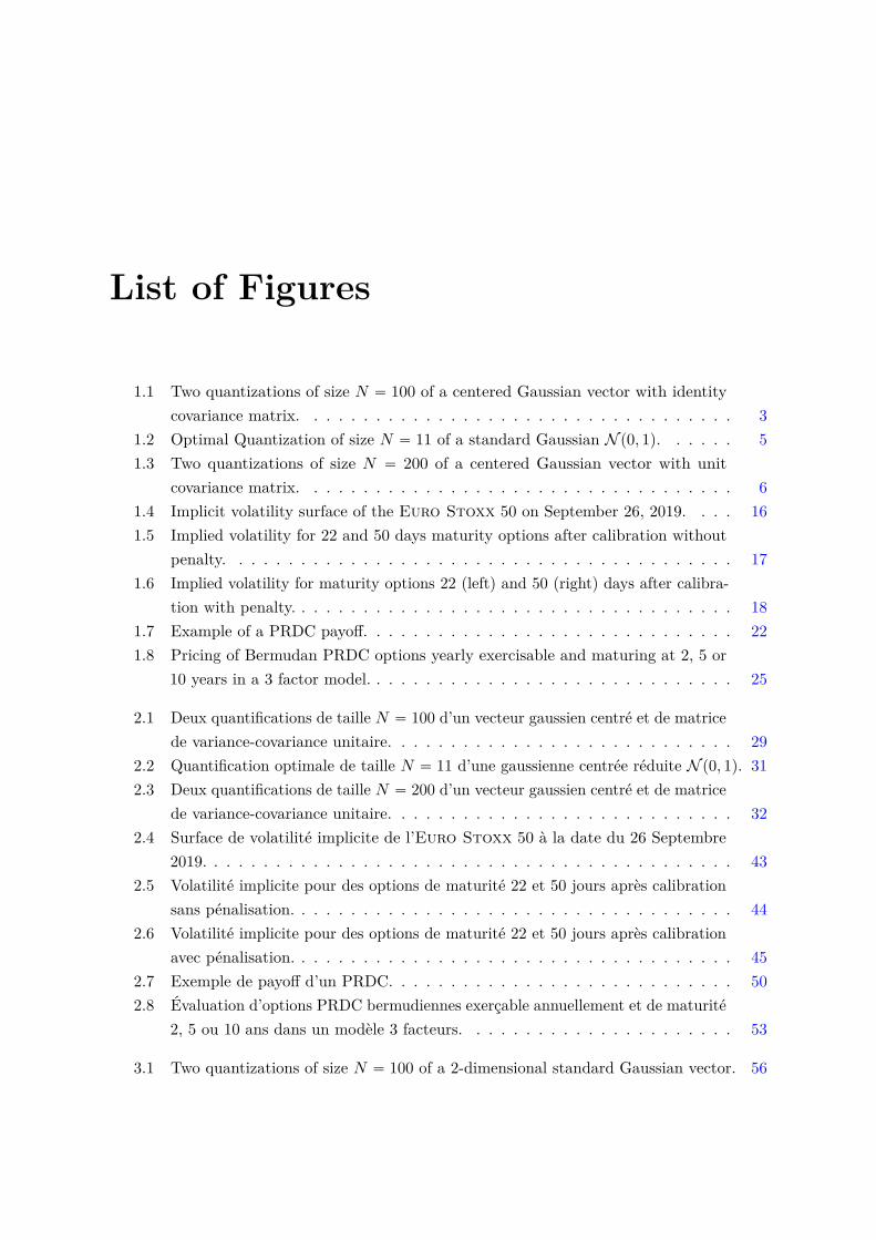
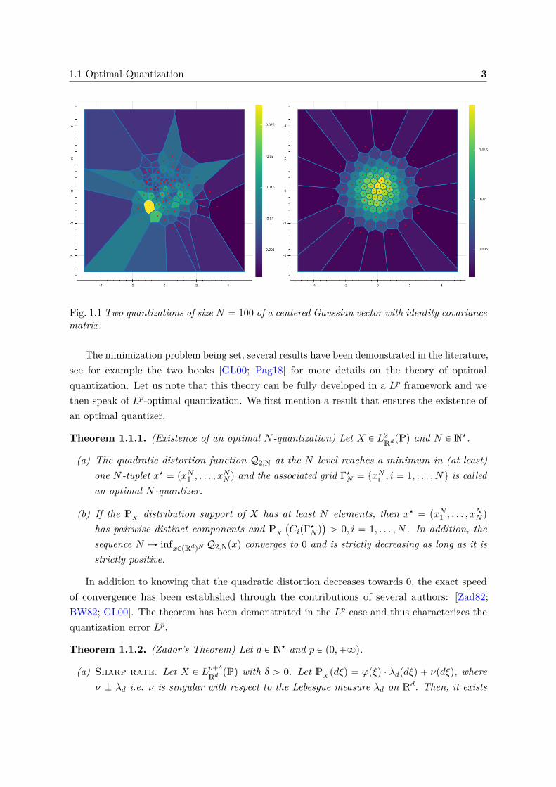
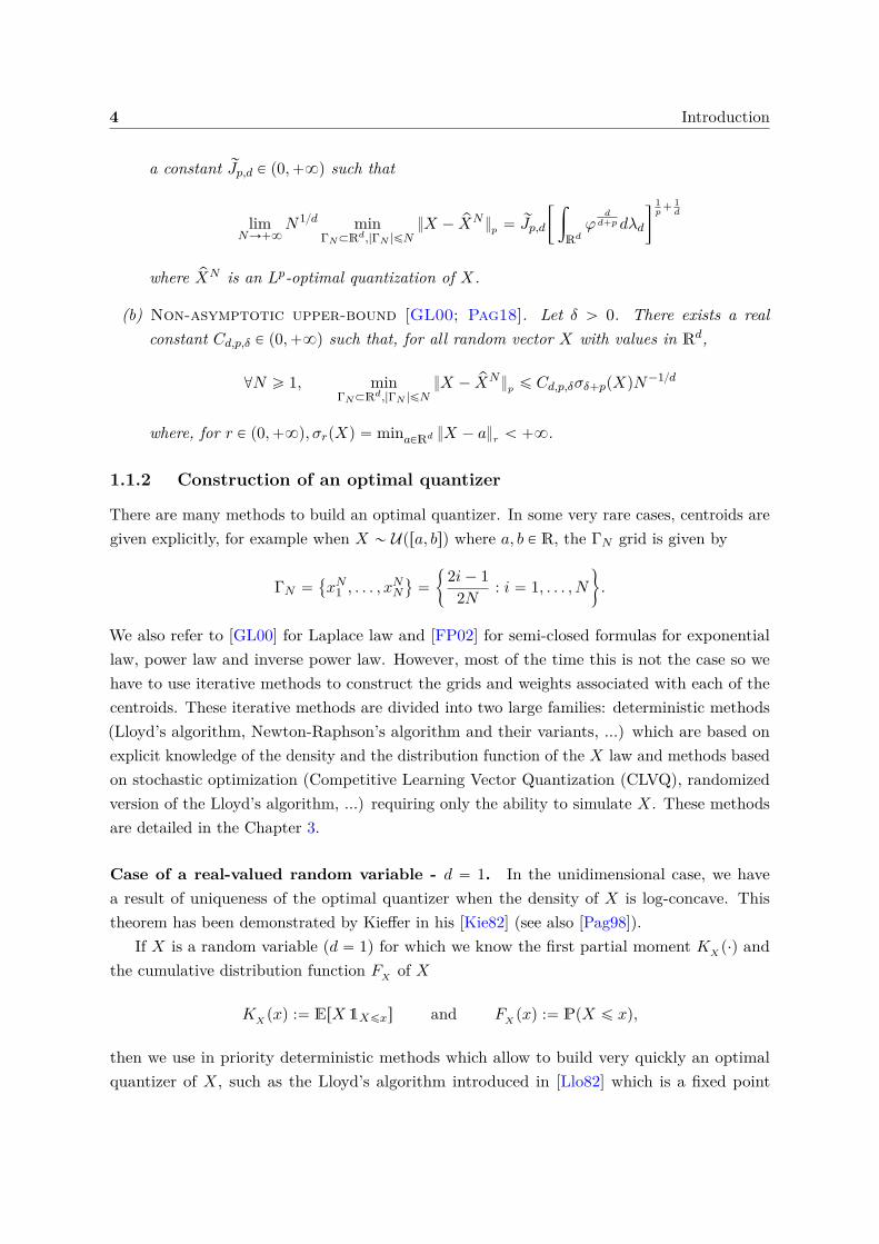
Such a grid always exists when X P L2 (see Theorem 1.1.1 below). In the Figure 1.1, we presenttwo quantizations of size N “ 100 of a centered Gaussian vector with identity covariance matrix.On the left, we represent an i.i.d. sample of the Gaussian vector and on the right an optimalquantizer. The color of each cell represents the probability pNi associated to the cell CipΓN q ofcentroid xNi (red dot).
1.1 Optimal Quantization 3
Fig. 1.1 Two quantizations of size N “ 100 of a centered Gaussian vector with identity covariancematrix.
The minimization problem being set, several results have been demonstrated in the literature,see for example the two books [GL00; Pag18] for more details on the theory of optimalquantization. Let us note that this theory can be fully developed in a Lp framework and wethen speak of Lp-optimal quantization. We first mention a result that ensures the existence ofan optimal quantizer.
Theorem 1.1.1. (Existence of an optimal N -quantization) Let X P L2RdpPq and N P N‹.
(a) The quadratic distortion function Q2,N at the N level reaches a minimum in (at least)one N -tuplet x‹ “ pxN1 , . . . , x
NN q and the associated grid Γ‹
N “ txNi , i “ 1, . . . , Nu is calledan optimal N -quantizer.
(b) If the PX distribution support of X has at least N elements, then x‹ “ pxN1 , . . . , xNN q
has pairwise distinct components and PX
`
CipΓ‹N q
˘
ą 0, i “ 1, . . . , N . In addition, thesequence N ÞÑ infxPpRdqN Q2,Npxq converges to 0 and is strictly decreasing as long as it isstrictly positive.
In addition to knowing that the quadratic distortion decreases towards 0, the exact speedof convergence has been established through the contributions of several authors: [Zad82;BW82; GL00]. The theorem has been demonstrated in the Lp case and thus characterizes thequantization error Lp.
Theorem 1.1.2. (Zador’s Theorem) Let d P N‹ and p P p0,`8q.
(a) Sharp rate. Let X P Lp`δ
Rd pPq with δ ą 0. Let PX pdξq “ φpξq ¨ λdpdξq ` νpdξq, whereν K λd i.e. ν is singular with respect to the Lebesgue measure λd on Rd. Then, it exists
4 Introduction
a constant rJp,d P p0,`8q such that
limNÑ`8
N1d minΓN ĂRd,|ΓN |ďN
X ´ pXNp “ rJp,d
„ż
Rdφ
dd`pdλd
ȷ1p
` 1d
where pXN is an Lp-optimal quantization of X.
(b) Non-asymptotic upper-bound [GL00; Pag18]. Let δ ą 0. There exists a realconstant Cd,p,δ P p0,`8q such that, for all random vector X with values in Rd,
@N ě 1, minΓN ĂRd,|ΓN |ďN
X ´ pXNp ď Cd,p,δσδ`ppXqN´1d
where, for r P p0,`8q, σrpXq “ minaPRd X ´ ar ă `8.
1.1.2 Construction of an optimal quantizer
There are many methods to build an optimal quantizer. In some very rare cases, centroids aregiven explicitly, for example when X „ Upra, bsq where a, b P R, the ΓN grid is given by
ΓN “
xN1 , . . . , xNN
(
“
"
2i´ 12N : i “ 1, . . . , N
*
.
We also refer to [GL00] for Laplace law and [FP02] for semi-closed formulas for exponentiallaw, power law and inverse power law. However, most of the time this is not the case so wehave to use iterative methods to construct the grids and weights associated with each of thecentroids. These iterative methods are divided into two large families: deterministic methods(Lloyd’s algorithm, Newton-Raphson’s algorithm and their variants, ...) which are based onexplicit knowledge of the density and the distribution function of the X law and methods basedon stochastic optimization (Competitive Learning Vector Quantization (CLVQ), randomizedversion of the Lloyd’s algorithm, ...) requiring only the ability to simulate X. These methodsare detailed in the Chapter 3.
Case of a real-valued random variable - d “ 1. In the unidimensional case, we havea result of uniqueness of the optimal quantizer when the density of X is log-concave. Thistheorem has been demonstrated by Kieffer in his [Kie82] (see also [Pag98]).
If X is a random variable (d “ 1) for which we know the first partial moment KX p¨q andthe cumulative distribution function FX of X
KX pxq :“ ErX 1Xďxs and FX pxq :“ PpX ď xq,
then we use in priority deterministic methods which allow to build very quickly an optimalquantizer of X, such as the Lloyd’s algorithm introduced in [Llo82] which is a fixed point
1.1 Optimal Quantization 5
search algorithm. It is also possible to apply the Newton-Raphson algorithm by computingthe Hessian of the quadratic distortion function (see [PP03] for a detailed example appliedto a normal random variable). Other deterministic gradient descents can be used such asLevenberg-Marquardt or quasi-Newton methods. Otherwise, stochastic optimization-basedmethods such as the stochastic version of the Lloyd’s algorithm or a stochastic gradient descentare used (see [Pag98]).
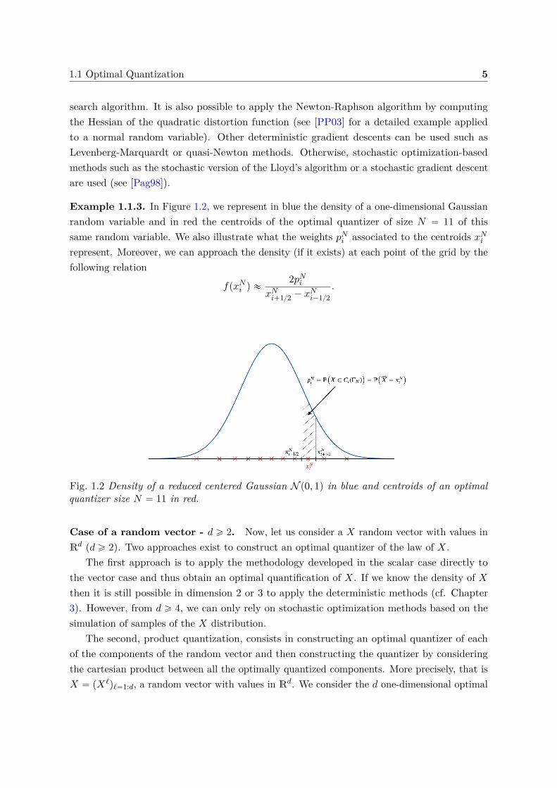
Example 1.1.3. In Figure 1.2, we represent in blue the density of a one-dimensional Gaussianrandom variable and in red the centroids of the optimal quantizer of size N “ 11 of thissame random variable. We also illustrate what the weights pNi associated to the centroids xNirepresent. Moreover, we can approach the density (if it exists) at each point of the grid by thefollowing relation
fpxNi q «2pNi
xNi`12 ´ xNi´12.
Fig. 1.2 Density of a reduced centered Gaussian N p0, 1q in blue and centroids of an optimalquantizer size N “ 11 in red.
Case of a random vector - d ě 2. Now, let us consider a X random vector with values inRd (d ě 2). Two approaches exist to construct an optimal quantizer of the law of X.
The first approach is to apply the methodology developed in the scalar case directly tothe vector case and thus obtain an optimal quantification of X. If we know the density of Xthen it is still possible in dimension 2 or 3 to apply the deterministic methods (cf. Chapter3). However, from d ě 4, we can only rely on stochastic optimization methods based on thesimulation of samples of the X distribution.
The second, product quantization, consists in constructing an optimal quantizer of eachof the components of the random vector and then constructing the quantizer by consideringthe cartesian product between all the optimally quantized components. More precisely, that isX “ pXℓqℓ“1:d, a random vector with values in Rd. We consider the d one-dimensional optimal
6 Introduction
quantifiers pXℓ of size N ℓ of each of the marginal Xℓ. Each quantizer pXℓ takes its values fromthe grid ΓNℓ
ℓ “
zℓiℓ , iℓ P t1, ¨ ¨ ¨ , Nℓu(
. Thus, the quantizer product of X takes its values in thegrid ΓN which is the Cartesian product of the one-dimensional grids, i.e. ΓN “
śdℓ“1 ΓNℓ
ℓ ofsize N “ N1 ˆ ¨ ¨ ¨ ˆNd or, equivalently,
ΓN “
px1i1 , ¨ ¨ ¨ , xℓiℓ , ¨ ¨ ¨ , xdidq, iℓ P t1, ¨ ¨ ¨ , Nℓu, ℓ P t1, ¨ ¨ ¨ , du
(
.
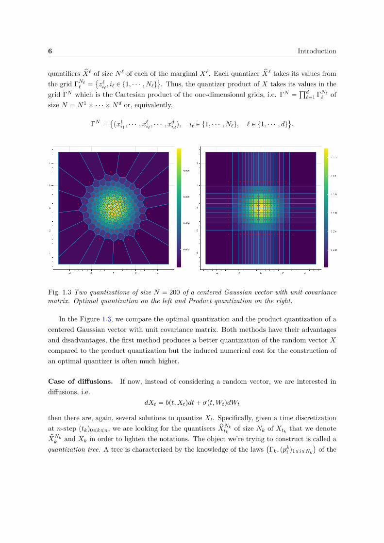
Fig. 1.3 Two quantizations of size N “ 200 of a centered Gaussian vector with unit covariancematrix. Optimal quantization on the left and Product quantization on the right.
In the Figure 1.3, we compare the optimal quantization and the product quantization of acentered Gaussian vector with unit covariance matrix. Both methods have their advantagesand disadvantages, the first method produces a better quantization of the random vector Xcompared to the product quantization but the induced numerical cost for the construction ofan optimal quantizer is often much higher.
Case of diffusions. If now, instead of considering a random vector, we are interested indiffusions, i.e.
dXt “ bpt,Xtqdt` σpt,WtqdWt
then there are, again, several solutions to quantize Xt. Specifically, given a time discretizationat n-step ptkq0ďkďn, we are looking for the quantisers pXNk
tkof size Nk of Xtk that we denote
pXNkk and Xk in order to lighten the notations. The object we’re trying to construct is called a
quantization tree. A tree is characterized by the knowledge of the laws`
Γk, ppki q1ďiďNk
˘
of the
1.1 Optimal Quantization 7
quantizers p pXkq0ďkďn and of the transition probabilities pki,j .
P`
pXk`1 “ xk`1j | pXk “ xki
˘
.
We will not present all the existing approaches that allow us to address the problem ofquantization of diffusion but only those that allow us to use deterministic numerical methodsfor the optimization of the grids. For other approaches, based on stochastic algorithms we referto the series of papers [BPP01; BP03].
Quantization of marginal laws. The problem of quantization of a diffusion has beeninitiated and developed in a series of articles [PPP04b; BPP05; BBP09; BBP10; CFG19]. If Xk
can be simulated exactly, that is without the help of a time discretization scheme, and that weknow the marginal law of Xk, at each instant tk, then we are brought back to the case of thequantization of a random vector. Indeed, we can optimally quantize each random vector Xk
using deterministic numerical methods if d ď 2, producing an optimal quantization tree, or wecan optimally quantize each of its components and then construct a product quantization ofXk, producing a product quantization tree.
Example 1.1.4. If we consider a Black-Scholes model with constant volatility σ and constantinterest rates r
dSt “ Stprdt` σdWtq, avec S0 “ s0,
then we have an explicit form for St
St “ S0 epr´σ22qt`σWt
so for a given date t, logpStS0q „ N`
pr´ σ22qt, σ2t˘
so we can optimally quantize St at eachinstant that interests us using deterministic methods (cf. Chapter 3). We can also quantize theBrownian Wt which is “more universal”.
Recursive quantization. In the case where we do not know by the marginal law ofXk and that we need to use a discretization scheme (Euler-Maruyama, Milstein, ...), we willuse a method called recursive quantization. Recursive quantization (also called Markovianquantization) was first introduced in [PPP04b] and then studied in depth in [PS15] for the caseof a one-dimensional diffusion discretized by an Euler-Maruyama scheme. A fast algorithmbased on deterministic methods to build the quantization tree is developed and analyzed.Subsequently, fast recursive quantization was extended to higher order one-dimensional schemesby [McW+18] and to higher dimensions by product quantization (see [PS18b; FSP18; Rud+17;CFG18; CFG17]). This method consists in building recursively in k the quantizers pXNk
k via therecursion
pXNkk “ ProjΓNk
`
rXk
˘
avec rXk “ Ek´1`
pXNk´1k´1 , Zk
˘
8 Introduction
where Ek´1 is a discretization scheme.
1.2 Numerical integration
A common problem in practice is to calculate the expectation of a function of X when X is avariable or a random vector, i.e. E
“
fpXq‰
. However, except in very particular cases, it is notpossible to calculate explicitly this quantity, it is the case for example if X “ XT the valueof a diffusion at the date T . This is why it is necessary to use numerical integration methods.[Pag98] introduces a cubature method based on optimal quantization in order to approximateexpectations of the form E
“
fpXq‰
. Let us consider pXN an optimal quantizer of X, the factthat pXN is discrete allows us to easily define the following cubature formula
E“
fp pXN q‰
“
Nÿ
i“1pNi fpxNi q. (1.1)
Furthermore, given that pXN was constructed as the best discrete approximation of X ofcardinal at most N then it seems reasonable to think that E
“
fp pXN q‰
is a good approximationof E
“
fpXq‰
.In the Chapter 4, taken from the article “New Weak Error bounds and expansions for Optimal
Quantization” published in Journal of Computational and Applied Mathematics, see [LMP19],we present new results in the real case concerning the error induced by the quantization-basedapproximation of expectation E
“
fpXq‰
. This is a joint work with Vincent Lemaire and GillesPagès and it is accessible in arXiv or HAL. These “weak” results are summarized below.
1.2.1 Convergence rate of the weak error
In the first part of Chapter 4, we are interested in the rate of convergence from E“
fp pXN q‰
toE“
fpXq‰
as a function of N for different classes of functions f when X is a random variablewith values in R, i.e we look for the largest α ą 0 such that, for any function f in this class F ,
limNNα
ˇ
ˇE“
fpXq‰
´ E“
fp pXN q‰ˇ
ˇ ď Cf,X ă `8.
If we naively upper-bound the weak error by the strong error along the Lipschitz continuousfunctions, we obtain the following upper-bound (with α “ 1) for a sequence of N -quanifiersL2-optimal N -quantifiers
Nˇ
ˇE“
fpXq‰
´ E“
fp pXN q‰ˇ
ˇ ď N rf sLipX ´ pXN1 ď N rf sLipX ´ pXN2NÑ`8ÝÝÝÝÝÑ Cf ă `8
1.2 Numerical integration 9
where Zador’s Theorem (1.1.2) was used. Moreover, if we consider fpxq “ distpx,ΓN q then f isa Lipschitz continuous function and we have
Nˇ
ˇE“
fpXq‰
´ E“
fp pXN q‰ˇ
ˇ “ NX ´ pXN1 ď NX ´ pXN2NÑ`8ÝÝÝÝÝÑ Cf ă `8.
For some classes of functions we can prove that the cubature formula induces a weak errorof order 2 (α “ 2). For example, if we consider functions that are derivable with a Lipschitzcontinuous derivative then we have an error of order 2, see [Pag98]. Indeed, we use a Taylorexpansion with an integral remainder of the form
fpxq “ fpyq ` f 1pyqpx´ yq `
ż 1
0
`
f 1ptx` p1 ´ tqyq ´ f 1pyq˘
px´ yqdt
and the stationarity property of an optimal quadratic quantizer as follows
E“
X | pXN‰
“ pXN .
The first term in the Taylor expansion is zero because
E“
f 1p pXN qpX´ pXN q‰
“ E”
f 1p pXN qE“
X´ pXN | pXN‰
ı
“ E”
f 1p pXN q`
E“
X | pXN‰
´ pXN˘
ı
“ 0.
Thus, using Lipschitz’s property of the derivative and Zador’s theorem, we get a weak error oforder 2, as expected.
N2ˇˇE
“
fpXq‰
´ E“
fp pXN q‰ˇ
ˇ ď N2ż 1
0E“ˇ
ˇf 1ptX ` p1 ´ tq pXN q ´ f 1p pXN qˇ
ˇ|X ´ pXN |‰
dt
ďrf 1sLip
2 N2X ´ pXN22NÑ`8ÝÝÝÝÝÑ Cf ă `8.
In the first part of Chapter 4, we extend these results concerning the convergence rate ofthe weak error of order higher than 1 to a wider class of functions with less regularity, moreprecisely, functions that are either :
‚ Lipschitz continuous piecewise affine functions with finitely many breaks of affinity,
‚ Lipschitz continuous convex functions,
‚ differentiable functions with piecewise-defined locally Lipschitz derivative (K breaks ofaffinity ta1, . . . , aKu, such that ´8 “ a0 ă a1 ă ¨ ¨ ¨ ă aK ă aK`1 “ `8 and the locallyLipschitz property of the derivative is defined by
@k “ 0, . . . ,K, @x, y P pak, ak`1q |f 1pxq ´ f 1pyq| ď rf 1sk,Lip,loc
|x´ y|`
gkpxq ` gkpyq˘
where gk : pak, ak`1q Ñ R` are non-negative Borel functions,
10 Introduction
‚ differentiable functions with piecewise-defined locally α-Hölder derivative (K breaks ofaffinity ta1, . . . , aKu, such that ´8 “ a0 ă a1 ă ¨ ¨ ¨ ă aK ă aK`1 “ `8 and the locallyα-Hölder property of the derivative is defined by
@k “ 0, . . . ,K, @x, y P pak, ak`1q, |f 1pxq ´ f 1pyq| ď rf 1sk,α,loc
|x´ y|α`
gkpxq ` gkpyq˘
where gk : pak, ak`1q Ñ R` are non-negative Borel functions,
For the first three classes of functions, we show that the weak error is of order 2 and for thelast one, of order 1 ` α.
In the numerical part, we illustrate this result by evaluating the price of a European Callin a Black-Scholes model given by
I0 :“ E“
e´rT pST ´Kq`
‰
where St “ S0 epr´σ22qt`σWt with pWtqtPr0,T s a Brownian motion. In order to approximate,with the help of quantization, the price of the European Call we can rewrite I0 in two differentways
I0 “ E“
φpST q‰
“ E“
fpWT q‰
where φ is a piecewise affine function with one affinity break and f is a differentiable functionwith a piecewise locally Lipschitz continuous derivative. Thus, when considering quantizers ofST or WT and using the cubature formula, we observe, for both approximations, a weak errorof order 2.
1.2.2 Weak error expansion of higher order
In the second part of Chapter 4, we are interested by the weak error expansion of the approxi-mation of E
“
fpXq‰
by E“
fp pXN q‰
. That is, we’re looking expansion of the form
E“
fpXq‰
“ E“
fp pXN q‰
`c2N2 `OpN´p2`βqq
where β P p0, 1s. In the previous section, we have already shown that the optimal quantization-based cubature formula approximation induces an error term of order OpN´2q in the best case.Here, we seek to refine the previous results in order to obtain a “controlled” error expansion oforder 2 and not a simple convergence rate of order 2.
In Section 4.3, we show that this expansion exists if the function f : R Ñ R is twicedifferentiable with a Lipschtiz continuous second derivative. This result uses a Taylor expansionof order 2 with an integral remainder of the form
fpxq “ fpyq ` f 1pyqpx´ yq `12f
2pyqpx´ yq2 `
ż 1
0p1 ´ tq
`
f2ptx` p1 ´ tqyq ´ f2pyq˘
px´ yq2dt
1.2 Numerical integration 11
where we take the expectation on both sides of the equality and replace x and y with X andpXN , respectively. The second term on the righthand side is cancelled using the stationarityproperty of the optimal quadratic quantizer. For the third term, we rely on [Del+04] (Theorem6) which states that @g : R Ñ R such that E
“
gpXq‰
ă `8
limNN2E
“
gp pXN q|X ´ pXN |2‰
“ Q2pPX q
ż
gpξqPX pdξq
that we apply to g “ f2 where Q2pPX q is the Zador’s constant. Thus, we already have the firsttwo terms in the expansion of the error. For the last term, we use the Lipschitz property ofthe second derivative and the rest of the proof is based mainly on a result initially establishedin [GLP08] and then recently extended in [PS18a], known as “Lr-Ls distortion mismatch”,which is formulated as follows : what can be said about the convergence rate of E
“
|X ´ pXN |s‰
knowing that pXN is a Lr-optimal quantizer when s ą r and X P Ls? We cite this theorem ford “ 1, which is the case we’re interested in.
Theorem 1.2.1 (Lr-Ls-distorsion mismatch). Let X : pΩ,A,Pq Ñ R a random variable andr P p0,`8q. Let PX pdξq “ φpξq ¨ λpdξq ` νpdξq, where ν K λ i.e. ν is singular with respectto the Lebesgue measure λ on R and φ is not identically null. Let pΓN qNě1 a sequence ofLr-optimal quantization grids and s P pr, r ` 1q. If
X P Ls
1`r´s`δ
pPq
for a δ ą0, solim sup
NNX ´ pXNs ă `8.
So, applying this theorem with r “ 2 and s “ 2 ` β, we get a OpN´p2`βqq for the last termand @β P p0, 1q, we have the following expansion
E“
fpXq‰
“ E“
fp pXN q‰
`c2N2 `OpN´p2`βqq.
This error expansion allows us to theoretically justify the use of Richardson-Rombergextrapolation which aims to kill the first error term of the expansion by linearly combining twoquantification cubature formulas, respectively at N and M points, i.e.
E“
fpXq‰
“ E
«
M2fp pXM q ´N2fp pXN q
M2 ´N2
ff
`OpN´p2`βqq
for M “ kN with k ą 1.
12 Introduction
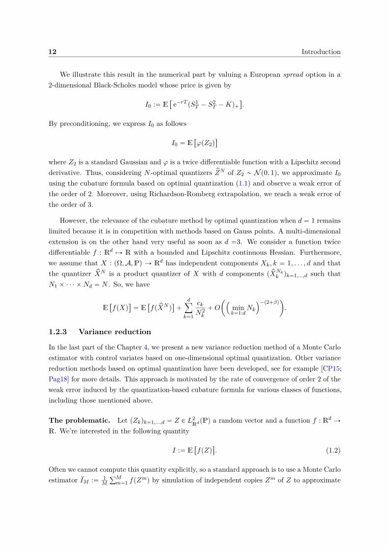
We illustrate this result in the numerical part by valuing a European spread option in a2-dimensional Black-Scholes model whose price is given by
I0 :“ E“
e´rT pS1T ´ S2
T ´Kq`
‰
.
By preconditioning, we express I0 as follows
I0 “ E“
φpZ2q‰
where Z2 is a standard Gaussian and φ is a twice differentiable function with a Lipschitz secondderivative. Thus, considering N -optimal quantizers pZN of Z2 „ N p0, 1q, we approximate I0
using the cubature formula based on optimal quantization (1.1) and observe a weak error ofthe order of 2. Moreover, using Richardson-Romberg extrapolation, we reach a weak error ofthe order of 3.
However, the relevance of the cubature method by optimal quantization when d “ 1 remainslimited because it is in competition with methods based on Gauss points. A multi-dimensionalextension is on the other hand very useful as soon as d “3. We consider a function twicedifferentiable f : Rd ÞÑ R with a bounded and Lipschitz continuous Hessian. Furthermore,we assume that X : pΩ,A,Pq Ñ Rd has independent components Xk, k “ 1, . . . , d and thatthe quantizer pXN is a product quantizer of X with d components p pXNk
k qk“1,...,d such thatN1 ˆ ¨ ¨ ¨ ˆNd “ N . So, we have
E“
fpXq‰
“ E“
fp pXN q‰
`
dÿ
k“1
ckN2k
`O
ˆ
´
mink“1:d
Nk
¯´p2`βq˙
.
1.2.3 Variance reduction
In the last part of the Chapter 4, we present a new variance reduction method of a Monte Carloestimator with control variates based on one-dimensional optimal quantization. Other variancereduction methods based on optimal quantization have been developed, see for example [CP15;Pag18] for more details. This approach is motivated by the rate of convergence of order 2 of theweak error induced by the quantization-based cubature formula for various classes of functions,including those mentioned above.
The problematic. Let pZkqk“1,...,d “ Z P L2RdpPq a random vector and a function f : Rd Ñ
R. We’re interested in the following quantity
I :“ E“
fpZq‰
. (1.2)
Often we cannot compute this quantity explicitly, so a standard approach is to use a Monte Carloestimator sIM :“ 1
M
řMm“1 fpZmq by simulation of independent copies Zm of Z to approximate
1.2 Numerical integration 13
I. The convergence of the method and its rate are determined by the strong law of largenumbers and the central limit theorem, respectively, which ensure, if Z is of integrable square,that
sIMp.s.ÝÝÑ E
“
fpZq‰
and?M
´
sIM ´ E“
fpZq‰
¯
LÝÑ N
`
0, σ2fpZq
˘
when M Ñ `8
where σ2fpZq
“ Var`
fpZq˘
. We notice that, for a given simulation size M , the limiting factor ofthe method is σ2
fpXq, so variance reduction methods were developed in order to reduce the value
of σ2fpXq
and accelerate the convergence of the Monte Carlo estimator to I. The reader can referto [Pag18; Gla13] for more details on Monte Carlo simulation and variance reduction methodsin general such as control variates, antithetic method, stratification, importance sampling, ...
A new method of variance reduction by quantized control variable. Let ΞN be arandom vector with values in Rd defined by
ΞN :“ pΞNk qk“1,...,d,
which will be our d-dimensional control variable, each ΞNk component is given by
ΞNk :“ fkpZkq ´ E“
fkp pZNk q‰
,
where fkpzq :“ fpErZ1s, . . . ,ErZk´1s, z,ErZk`1s, . . . ,ErZdsq and pZNk is an optimal quantizationof size N of Zk. We use here a unidimensional optimal quantization in order to take advantageof the weak error results previously shown, indeed the functions fk : R Ñ R are part of theclasses of functions allowing us to reach a weak error of order 2. We introduce Iλ,N as anapproximation for (1.2)
Iλ,N “ E“
fpZq ´ xλ,ΞNy‰
“ E
«
fpZq ´
dÿ
k“1λkfkpZkq
ff
`
dÿ
k“1λk E
“
fkp pZNk q‰
(1.3)
where λ P Rd. The terms E“
fkp pZNk q‰
in (1.3) can be easily and quickly computed using thediscreteness of quantizers.
At this point, we can define pIλ,NM
the Monte Carlo estimator associated to Iλ,N
pIλ,NM
“1M
Mÿ
m“1
˜
fpZmq ´
dÿ
k“1λkfkpZmk q
¸
`
dÿ
k“1λk E
“
fkp pZNk q‰
.
It is important to notice that we introduce a bias when using such control variates, indeedfor every k P t1, . . . , nu, ErΞNk s ‰ 0 because E
“
fkp pZNk q‰
is an approximation of E“
fkpZkq‰
.However, the quantity that really interests us is not the bias induced by the estimator pIλ,N
Mbut
14 Introduction
rather the Mean Squared Error (MSE) giving us a bias-variance decomposition
MSEppIλ,NM
q “
˜
dÿ
k“1λk
´
E“
fkp pZNk q‰
´ E“
fkpZkq‰
¯
¸2
looooooooooooooooooooooooomooooooooooooooooooooooooon
biais2
`1MVar
˜
fpZq ´
dÿ
k“1λkfkpZkq
¸
loooooooooooooooooomoooooooooooooooooon
Variance du Monte Carlo
.
Thus, we can take higher values of N to make the bias term negligible compared to thevariance of the estimator while controlling the total cost induced by the Monte Carlo estimator.In practice, we do not need to take very high values for N . Indeed, the bias term converges to0 as N´4 if f belongs to the right class of functions, so taking optimal quantifiers of size 200 ismore than enough to make the bias negligible compared to the variance of the Monte Carloestimator. We develop this point in the third part of the Chapter 4.
In the numerical part of the Chapter 4, we apply the variance reduction method to thevaluation of a basket option in a Black-Scholes model in dimension d. The control variate allowsus to divide the variance of the Monte Carlo estimator by 100 for small dimensions (d “ 2 ord “ 3) and by 6 for larger dimensions (d “ 10). We also observe that the bias induced by thequantification becomes negligible for grids with a size greater than 100 (N ą 100).
1.3 Examples of applications in finance
1.3.1 Stationary Heston Model
In Chapter 5, we are interested in the stationary Heston model and more precisely in theevaluation of European, Bermuda and barrier options in this model as well as the calibrationof the model. Chapter 5 corresponds to the preprint “Stationary Heston model: Calibrationand Pricing of exotics using Product Recursive Quantization” accessible in arXiv or HAL (see[LMP20]). This article is a joint work with Vincent Lemaire and Gilles Pagès.
The standard Heston model was originally introduced by Heston in [Hes93]. It is a stochasticvolatility model where the initial volatility condition is assumed deterministic. This model hasbecome very popular mainly for the following two reasons: it is a stochastic volatility modelso it introduces a smile in the surface of the implied volatility as observed in the market andthe characteristic function of this model is given by a semi closed-form formula which allowsus to value European options (Call & Put) almost instantaneously (see Carr & Madan in[CM99]). However, a remark often made about this model is that the smile of implied volatilityis not steep enough for short maturities compared to what is observed in the market (see[Gat11]). Noticing that the volatility process is ergodic with a single invariant distributionν “ Γpα, βq where the α and β parameters depend on the volatility diffusion parameters, ithas been proposed by Pagès & Panloup in [PP09] to directly consider that the process evolvesunder its stationary regime instead of starting it at time 0 from a deterministic value. This

1.3 Examples of applications in finance 15
choice has the effect of accentuating the volatility smile for short maturities while keeping thesame behavior as the standard model for longer maturities. Later, the short and long-termbehavior of the implied volatility generated by such a model was studied by Jacquier & Shi in[JS17].
Thus, the diffusion of the asset-volatility couple pSpνq
t , vνt q in the stationary Heston model isdefined by
$
’
’
&
’
’
%
dSpνq
t
Spνq
t
“ pr ´ qqdt`a
vνt`
ρdĂWt `a
1 ´ ρ2dWt
˘
dvνt “ κpθ ´ vνt qdt` ξa
vνt dĂWt
where vν0 „ Lpνq „ Γpα, βq with β “ 2κξ2, α “ θβ.
Valuation of European Options. First of all, in the first part of the Chapter 5, we recallthe method used for the valuation of a Call in the standard Heston model. Starting from theknowledge of the characteristic function ψ
`
λpvq, u, T˘
of the logarithm of the asset at date T(see [SST04; Gat11; Alb+07] for a robust choice of formula), the price of the Call of strike Kand maturity T on the asset Spvq
T in the standard Heston model where the volatility has asinitial condition v P R is given by
Cpϕpvq,K, T q “ E“
e´rT pSpvq
T ´Kq`
‰
“ s0 e´qT P1`
λpvq,K, T˘
´K e´rT P2`
λpvq,K, T˘
where the quantities P1`
λpvq,K, T˘
and P2`
λpvq,K, T˘
are defined by
P1`
λpvq,K, T˘
“12 `
1π
ż `8
0Re
ˆ
e´iu logpKq
iu
ψ`
λpvq, u´ i, T˘
s0 epr´qqT
˙
du
P2`
λpvq,K, T˘
“12 `
1π
ż `8
0Re
ˆ
e´iu logpKq
iu ψ`
λpvq, u, T˘
˙
du
with i the base of imaginary numbers (such that i2 “ ´1).
From this formula, we derive a method to compute the price I0 of a Call in the stationaryHeston model. Indeed, by preconditioning by vν0 , we have
I0 “ E“
e´rT φpSpνq
T q‰
“ E“
Cpϕpvν0 q,K, T q‰
.
Thus, in order to obtain an approximation of I0, we propose two methods. The first, basedon optimal quantization, consists in building an optimal quantizer of the gamma law Γpα, βq
and then to use the cubature formula studied in the Chapter 4. The second method is to use aquadrature formula based on Laguerre polynomials.
Calibration. Once we are able to price European options in the stationary Heston model,we calibrate the model on market data to study the behavior of short-term implied volatility.
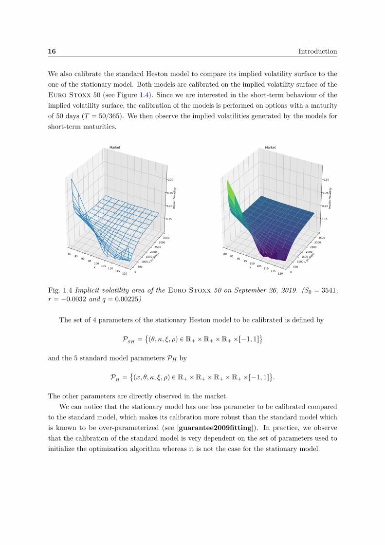
16 Introduction
We also calibrate the standard Heston model to compare its implied volatility surface to theone of the stationary model. Both models are calibrated on the implied volatility surface of theEuro Stoxx 50 (see Figure 1.4). Since we are interested in the short-term behaviour of theimplied volatility surface, the calibration of the models is performed on options with a maturityof 50 days (T “ 50365). We then observe the implied volatilities generated by the models forshort-term maturities.
K
8085
9095
100105
110115
120
T (in days)
0500
10001500
20002500
30003500
Implied Vo
latility
0.15
0.20
0.25
0.30
Market
K
8085
9095
100105
110115
120
T (in days)
0500
10001500
20002500
30003500
Implied Vo
latility
0.15
0.20
0.25
0.30
Market
Fig. 1.4 Implicit volatility area of the Euro Stoxx 50 on September 26, 2019. (S0 “ 3541,r “ ´0.0032 and q “ 0.00225)
The set of 4 parameters of the stationary Heston model to be calibrated is defined by
PSH “
pθ, κ, ξ, ρq P R` ˆR` ˆR` ˆr´1, 1s(
and the 5 standard model parameters PH by
PH “
px, θ, κ, ξ, ρq P R` ˆR` ˆR` ˆR` ˆr´1, 1s(
.
The other parameters are directly observed in the market.We can notice that the stationary model has one less parameter to be calibrated compared
to the standard model, which makes its calibration more robust than the standard model whichis known to be over-parameterized (see [guarantee2009fitting]). In practice, we observethat the calibration of the standard model is very dependent on the set of parameters used toinitialize the optimization algorithm whereas it is not the case for the stationary model.
1.3 Examples of applications in finance 17
For the calibration of the models, the standard method consists in solving the followingoptimization problem
minϕPP
ÿ
K
ˆ
σMarketiv pK,T q ´ σModel
iv pϕ,K, T q
σMarketiv pK,T q
˙2
where the quantities σMarketiv pK,T q and σModel
iv pϕ,K, T q are, respectively, market implied volatil-ities and those calculated with a Heston model of parameter ϕ “ pθ, κ, ξ, ρq or ϕ “ px, θ, κ, ξ, ρq
in appropriate cases.
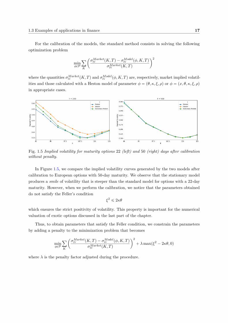
Fig. 1.5 Implied volatility for maturity options 22 (left) and 50 (right) days after calibrationwithout penalty.
In Figure 1.5, we compare the implied volatility curves generated by the two models aftercalibration to European options with 50-day maturity. We observe that the stationary modelproduces a smile of volatility that is steeper than the standard model for options with a 22-daymaturity. However, when we perform the calibration, we notice that the parameters obtaineddo not satisfy the Feller’s condition
ξ2 ď 2κθ
which ensures the strict positivity of volatility. This property is important for the numericalvaluation of exotic options discussed in the last part of the chapter.
Thus, to obtain parameters that satisfy the Feller condition, we constrain the parametersby adding a penalty to the minimization problem that becomes
minϕPP
ÿ
K
ˆ
σMarketiv pK,T q ´ σModel
iv pϕ,K, T q
σMarketiv pK,T q
˙2` λmaxpξ2 ´ 2κθ, 0q
where λ is the penalty factor adjusted during the procedure.
18 Introduction
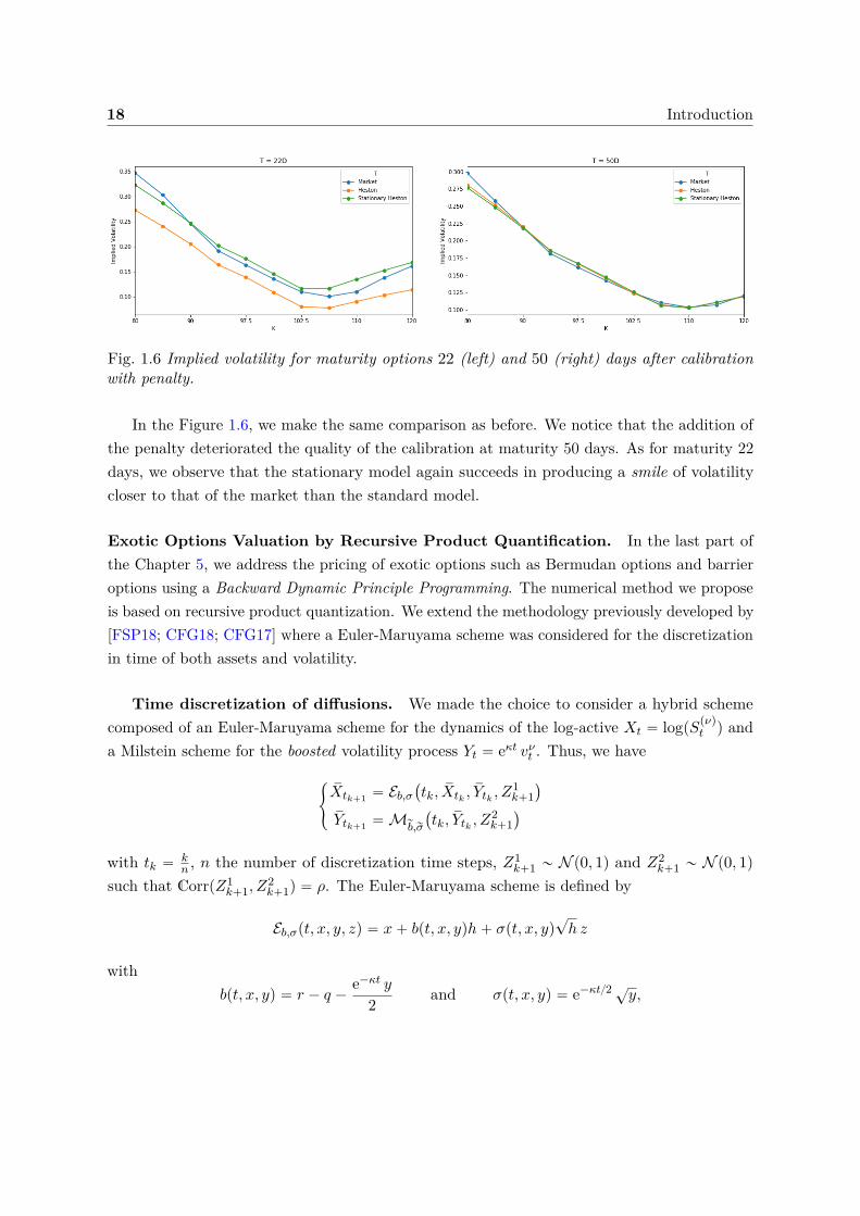
Fig. 1.6 Implied volatility for maturity options 22 (left) and 50 (right) days after calibrationwith penalty.
In the Figure 1.6, we make the same comparison as before. We notice that the addition ofthe penalty deteriorated the quality of the calibration at maturity 50 days. As for maturity 22days, we observe that the stationary model again succeeds in producing a smile of volatilitycloser to that of the market than the standard model.
Exotic Options Valuation by Recursive Product Quantification. In the last part ofthe Chapter 5, we address the pricing of exotic options such as Bermudan options and barrieroptions using a Backward Dynamic Principle Programming. The numerical method we proposeis based on recursive product quantization. We extend the methodology previously developed by[FSP18; CFG18; CFG17] where a Euler-Maruyama scheme was considered for the discretizationin time of both assets and volatility.
Time discretization of diffusions. We made the choice to consider a hybrid schemecomposed of an Euler-Maruyama scheme for the dynamics of the log-active Xt “ logpS
pνq
t q anda Milstein scheme for the boosted volatility process Yt “ eκt vνt . Thus, we have
#
sXtk`1 “ Eb,σ`
tk, sXtk ,sYtk , Z
1k`1
˘
sYtk`1 “ Mrb,rσ
`
tk, sYtk , Z2k`1
˘
with tk “ kn , n the number of discretization time steps, Z1
k`1 „ N p0, 1q and Z2k`1 „ N p0, 1q
such that CorrpZ1k`1, Z
2k`1q “ ρ. The Euler-Maruyama scheme is defined by
Eb,σpt, x, y, zq “ x` bpt, x, yqh` σpt, x, yq?h z
withbpt, x, yq “ r ´ q ´
e´κt y
2 and σpt, x, yq “ e´κt2 ?y,
1.3 Examples of applications in finance 19
and the Milstein schema put into its canonical form
Mrb,rσ
pt, x, zq “ x´rσpt, xq
2rσ1xpt, xq
` h
ˆ
rbpt, xq ´prσrσ1
xqpt, xq
2
˙
`prσrσ1
xqpt, xqh
2
ˆ
z `1
?hrσ1
xpt, xq
˙2
withrbpt, xq “ eκt κθ, rσpt, xq “ ξ
?x eκt2 and rσ1
xpt, xq “ξ eκt2
2?x.
Product Markovian Recursive Quantization. Once the choice of the discretizationscheme in time has been made, we are interested in the discretization in space of the asset-volatility couple.
To do this, we first construct a Markovian quantization tree ppYtk qk“0,...,n. It is advantageousto notice that the volatility is autonomous and therefore we face a one-dimensional problem.Thus, the quantizers pYtk are recursively constructed, i.e. pYtk`1 is an optimal quantizer of rYtk`1
defined byrYtk`1 “ M
rb,rσ
`
tk, pYtk , Z2k`1
˘
, pYtk`1 “ ProjΓYN2,k`1
`
rYtk`1
˘
.
Numerically, we use the methods based on deterministic algorithms for the 1 dimensiondeveloped in Chapter 3.
Now, using the fact that Yt has already been quantized, we construct a Markov quantizationtree p pXtk qk“0,...,n of Xt. Again we are brought back to a one-dimensional problem and weconstruct the quantizers pXtk recursively, i.e. pXtk`1 is an optimal quantizer of rXtk`1 defined by
rXtk`1 “ Eb,σ`
tk, pXtk ,pYtk , Z
1k`1
˘
, pXtk`1 “ ProjΓXN1,k`1
`
rXtk`1
˘
.
In order to alleviate the notations, we shall denote pXk and pYk instead of pXtk and pYtk .
Now that we have calibrated the stationary Heston model and are able to construct aquantization tree for the asset-volatility couple, we are interested in the evaluation of exoticoptions and more specifically Bermudan or barrier options.
Bermudan options. The price on date tk of a Bermudan option exercisable on datesttk, ¨ ¨ ¨ , tnu with payoff ψtk pXtk , Ytk q on the date tk is given by the Snell envelope Vk
Vk “ supτPT n
k
E”
e´rτ ψτ pXτ , Yτ q | F tk
ı
,
where T nk represents the set of stopping times τ taking values in ttk, t1, . . . , tnu. The Backward
Dynamic Principle Programming allows to rewrite Vk as follows#
Vn “ e´rtn ψnpXn, Ynq,
Vk “ max`
e´rtk ψkpXk, Ykq,ErVk`1 | Fks˘
, 0 ď k ď n´ 1.
20 Introduction
We then apply the methodology employed by [BP03; BPP05; Pag18] which consists inreplacing Xk and Yk by the quantizers pXk and pYk. By construction of the recursive quantization,the couple p pXk, pYkq is Markovian so we obtain the following Quantized Backward DynamicPrinciple Programming
#
pVn “ ψnp pXn, pYnq,
pVk “ max`
ψkp pXk, pYkq,ErpVk`1 | p pXk, pYkqs˘
, k “ 0, . . . , n´ 1.
Finally, the price of the Bermudan option is given by E“
pV0‰
.
Barrier Options. The price on date tk of a barrier option with maturity T , payoff f andbarrier L is given by
PUO “ e´rT E“
fpXT q1suptPr0,T s XtďL
‰
.
For the valuation of the barrier option, we apply the algorithm based on the conditional law ofEuler’s scheme, see [Gla13; Sag10; Pag18]. Thus, once the asset-volatility couple is discretizedin time, the price PUO is rewritten as follows
sPUO “ e´rT E“
fp sXT q1suptPr0,T ssXtďL
‰
“ e´rT E
„
fp sXT q
n´1ź
k“0Gk
p sXk,sYkq, sXk`1pLq
ȷ
whereGkpx,yq,zpuq “
´
1 ´ e´2n px´uqpz´uq
T σ2ptk,x,yq
¯
1tuěmaxpx,zqu .
Finally, replacing sXk and sYk by pXk and pYk and using a recursive algorithm to approachsPUO by ErpV0s, we have
$
&
%
pVn “ e´rT fp pXnq,
pVk “ E“
Gkp pXk,pYkq, pXk`1
pLq pVk`1 | p pXk, pYkq‰
, 0 ď k ď n´ 1.
1.3.2 Pricing of Bermudan options in a 3-factor model (PRDC)
In the Chapter 6, we address the problem of Bermudan exchange rate option pricing wherestochastic domestic and foreign interest rates are considered. In this case, we refer to a three-factor model. Chapter 6 corresponds to the article “Quantization-based Bermudan optionpricing in the FX world” submitted to Journal of Computational Finance and accessible inarXiv or HAL (see [Fay+19]). This article is a joint work with Jean-Michel Fayolle, VincentLemaire and Gilles Pagès.
The need to evaluate such products originated in Japan at the end of the 20th century.Indeed, the persistence of low interest rates during the last decades of the century was one ofthe main reasons that led to the creation of exchange rate structured financial products. These
1.3 Examples of applications in finance 21
products met the need of investors seeking higher coupons than those based on the yen. Asfinancial products became more and more complex, they became known as power reverse dualcurrency (PRDC) products, see [Wys17].
Even though these products were issued towards the end of the 20th century, they are stillpresent in banks’ portfolios and must be taken into account when evaluating counterparty risksuch as Credit Valuation Adjustment (CVA), Debt Valuation Adjustment (DVA), FundingValuation Adjustment (FVA), Capital Valuation Adjustment (KVA), ...., in short xVA (see[BMP13; CBB14; Gre15] for more details on the subject).
The model. P pt, T q is defined as the value at time t of one unit of the selected currencydelivered (i.e. paid) at time T , also known as the zero coupon price or discount factor. We willnote the zero coupon with superscript d when we speak of a zero coupon in the domestic currency(P dpt, T q) and with superscript f for the zero coupon in the foreign currency. The model usedfor the diffusion of the domestic and foreign zero coupons belongs to the Heath-Jarrow-Morton(HJM) family of yield curve models. For more details and theory on its models, we may referto the following articles [EFG96; EMV92; HJM92; BS73].
Thus the diffusion of the domestic zero-coupon curve under the domestic risk-neutralprobability P is given by
dP dpt, T q
P dpt, T q“ rdt dt` σdpT ´ tqdW d
t ,
where W d is a P-Brownian Motion, rdt is the instantaneous domestic rate at time t and σd
is the volatility. For the foreign zero-coupon curve, the dynamic is given, under the foreignrisk-neutral probability rP, by the diffusion
dP f pt, T q
P f pt, T qP f pt, T q “ rft dt` σf pT ´ tqdĂW f
t ,
where ĂW f is a rP-Brownian Motion, rft is the instantaneous foreign rate at time t and σf is thevolatility. The two probabilities rP and P are supposed to be equivalent, i.e. rP „ P and thereis ρdf defined as the limit of the quadratic variation xW d,ĂW f yt “ ρdf t.
For the exchange rate (FX), we refer to St as the value at time t ą0 of one unit of foreigncurrency in the domestic currency. The dynamics of pStqtě0 is of Black-Scholes type and givenby
dStSt
“ prdt ´ rft qdt` σSdWSt ,
where rdt is the instantaneous rate of the domestic currency at time t, rft is the instantaneousrate of the foreign currency at time t, σS is the volatility and WS is a standard Brownianmotion under the domestic risk-neutral probability.
22 Introduction
The problem. Our objective is to price Bermudan options on the exchange rate St exercisableat n` 1 dates: tt0, . . . , tnu. Thus, the date price tk of the Bermuda option is given by the Snellenvelope Vk of the obstacle
`
e´ştk0 rd
sds ψtk pStk q˘
k“0:n.
Vk “ supτPT n
k
E“
e´şτ0 r
dsds ψτ pSτ q | F tk
‰
where τ is a stopping-time with values in ttk, . . . , tnu and T nk represents all such stopping-time.
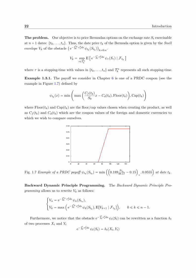
Example 1.3.1. The payoff we consider in Chapter 6 is one of a PRDC coupon (see theexample in Figure 1.7) defined by
ψtk pxq “ min˜
maxˆ
Cf ptkq
S0x´ Cdptkq,Floorptkq
˙
,Capptkq
¸
where Floorptkq and Capptkq are the floor/cap values chosen when creating the product, as wellas Cf ptkq and Cdptkq which are the coupon values of the foreign and domestic currencies towhich we wish to compare ourselves.
Fig. 1.7 Example of a PRDC payoff ψtk pStk q “ min´´
0.189 Stk88.17 ´ 0.15
¯
`, 0.0555
¯
at date tk.
Backward Dynamic Principle Programming. The Backward Dynamic Principle Pro-gramming allows us to rewrite Vk as follows:
$
&
%
Vn “ e´ştn0 rd
sds ψnpStnq,
Vk “ max´
e´ştk0 rd
sds ψkpStk q,ErVk`1 | F tk s
¯
, 0 ď k ď n´ 1.
Furthermore, we notice that the obstacle e´şt0 r
dsds ψtpStq can be rewritten as a function ht
of two processes Xt and Yt
e´şt0 r
dsds ψtpStq “ htpXt, Ytq
1.3 Examples of applications in finance 23
where the couple pX,Y q is defined by
pXt, Ytq “
ˆ
σSWSt ` σf
ż t
0pt´ sqdW f
s ,´σd
ż t
0pt´ sqdW d
s
˙
.
Thus, this new expression for the obstacle allows us to rewrite the Snell envelope problemin the form of
Vk “ supτPT n
k
E“
hτ pXτ , Yτ q | F tk
‰
.
However, the couple pXk, Ykq is not Markovian and this poses a problem in the Principle of Dynamic Programmingbecause the conditioning that appears in the conditional expectation cannot be replaced bypXk, Ykq. This is why we are led to consider the random vector pX,W f , Y,W dq which isMarkovian. Thus the Backward Dynamic Principle Programming can be rewritten as follows
$
&
%
Vn “ hnpXn, Ynq,
Vk “ max´
hkpXk, Ykq,E“
Vk`1 | pXk,Wfk , Yk,W
dk q‰
¯
, 0 ď k ď n´ 1.(1.4)
Quantization based numerical solution. We are now interested in the practical part ofnumerically computing the values Vk. In the Chapter 6, we have opted for a numerical methodbased on optimal quantization as introduced in [BPP01] and developed in [BP03; PPP04b;BPP05] for the evaluation of Bermudan options but with the variant that consists in using aproduct optimal quantization tree. This approach has the advantage of being fast, stable andaccurate in small dimensions. However, as the dimension grows, the computation time can bevery expensive and the convergence speed of the method is degraded because of the “curse ofdimension” that affects the optimal quantization.
The first idea we present, when we want to discretize (1.4) by optimal quantization, is themost natural one. We replace the random variables Xk, W f
k , Yk and W dk by their optimal
quantization pXk, xW fk , pYk and xW d
k , of size NXk , NW f
k , NW f
k , NYk and NW d
k respectively, andwe “force”, in a certain sense, the Markov property by introducing the “forced” QuantizedBackward Dynamic Principle Programming defined by
$
&
%
pVn “ hnp pXn, pYnq,
pVk “ max´
hkp pXk, pYkq,E“
pVk`1 | p pXk,xWfk ,
pYk,xWdk q‰
¯
, 0 ď k ď n´ 1.
The term “forced” is justified because p pXk,xWfk ,
pYk,xWdk qk is not a Markov chain so this Backward
Dynamic Principle Programming is not naturally associated to the Snell envelope. We denoteby Nk “ NX
k ˆNW f
k ˆNYk ˆNW d
k the global size of the quantization grid produced.
For this approximation, we provide an a priori quadratic error for Vk ´ pVk2 , k “ 0, . . . , n.
24 Introduction
Theorem 1.3.2. If the payoff functions pψtk qk“0:n are Lipschitz continuous with compactlysupported (right) derivative. Then the quadratic error induced by the quantization approximationp pXk,xW
fk ,
pYk,xWdk q is upper-bounded by
›
›Vk ´ pVk›
›
2ď
ˆ nÿ
l“k
CXl
›
›Xl ´ pXl
›
›
22p
` CYl
›
›Yl ´ pYl›
›
22p
` CW dl
›
›W dl ´ xW d
l
›
›
22p
` CW f
l
›
›W fl ´ xW f
l
›
›
22p
˙12,
where 1 ă p ă 32 and q ě 1 such that 1p ` 1
q “ 1 and the constants CXl, CW d
l, CYl
, CW f
lare
finite. So, by taking sN “ minkNk, we have
limsNÑ`8
›
›Vk ´ pVk›
›
22
“ 0.
The major problem with the approach we have just presented is the algorithmic complexityassociated with this method due to the size of the product quantization grids. This complexitymakes the computation of the conditional expectations appearing in the backward dynamicprogramming principle very expensive. Our objective is thus to reduce the size of the problem.To do so, we remove the processes W d and W f from the product-quantization tree to keep onlyX and Y . By doing so, we lose the Markov property of the random vector we are considering,but we significantly reduce the numerical complexity of the problem. In this context, (1.4) isapproached by
$
&
%
pVn “ hnp pXn, pYnq,
pVk “ max´
hkp pXk, pYkq,E“
pVk`1 | p pXk, pYkq‰
¯
, 0 ď k ď n´ 1.
We denote Nk “ NXk ˆNY
k the size of the quantization grid.
Again, we provide an a priori quadratic error for Vk ´ pVk2 , k “ 0, . . . , n.
Theorem 1.3.3. If the payoff functions pψtk qk“0:n are Lipschitz continuous with compactlysupported (right) derivative. Then the quadratic error induced by the quantization approximationp pXk, pYkq is upper-bounded by
›
›Vk ´ pVk›
›
2ď
ˆ n´1ÿ
l“k
CW f
l`1
›
›W fl`1 ´ ErW f
l`1 | pXl, Ylqs›
›
22p
` CW dl`1
›
›W dl`1 ´ ErW d
l`1 | pXl, Ylqs›
›
22p
` CXl
›
›Xl ´ pXl
›
›
22p
` CYl
›
›Yl ´ pYl›
›
22p
˙12
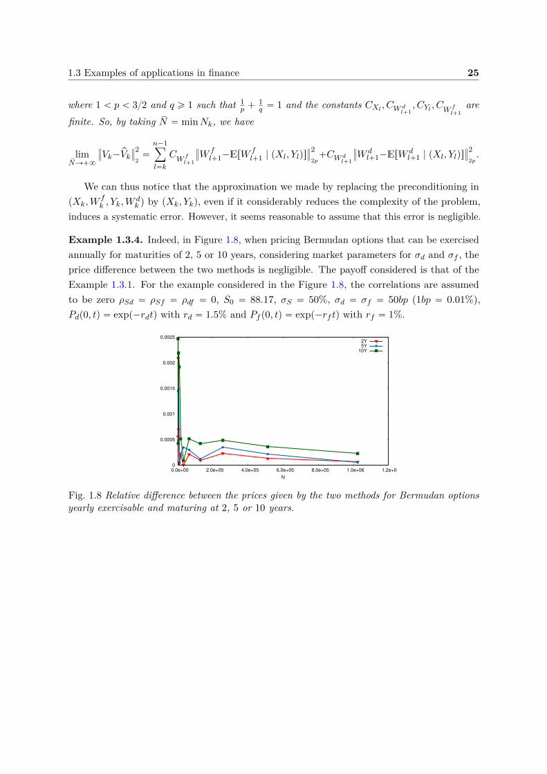
1.3 Examples of applications in finance 25
where 1 ă p ă 32 and q ě 1 such that 1p ` 1
q “ 1 and the constants CXl, CW d
l`1, CYl
, CW f
l`1are
finite. So, by taking sN “ minNk, we have
limsNÑ`8
›
›Vk´pVk›
›
22
“
n´1ÿ
l“k
CW f
l`1
›
›W fl`1´ErW f
l`1 | pXl, Ylqs›
›
22p
`CW dl`1
›
›W dl`1´ErW d
l`1 | pXl, Ylqs›
›
22p.
We can thus notice that the approximation we made by replacing the preconditioning inpXk,W
fk , Yk,W
dk q by pXk, Ykq, even if it considerably reduces the complexity of the problem,
induces a systematic error. However, it seems reasonable to assume that this error is negligible.
Example 1.3.4. Indeed, in Figure 1.8, when pricing Bermudan options that can be exercisedannually for maturities of 2, 5 or 10 years, considering market parameters for σd and σf , theprice difference between the two methods is negligible. The payoff considered is that of theExample 1.3.1. For the example considered in the Figure 1.8, the correlations are assumedto be zero ρSd “ ρSf “ ρdf “ 0, S0 “ 88.17, σS “ 50%, σd “ σf “ 50bp (1bp “ 0.01%),Pdp0, tq “ expp´rdtq with rd “ 1.5% and Pf p0, tq “ expp´rf tq with rf “ 1%.
0
0.0005
0.001
0.0015
0.002
0.0025
0.0e+00 2.0e+05 4.0e+05 6.0e+05 8.0e+05 1.0e+06 1.2e+06
N
2Y
5Y
10Y
Fig. 1.8 Relative difference between the prices given by the two methods for Bermudan optionsyearly exercisable and maturing at 2, 5 or 10 years.

Chapter 2
Introduction - Français
2.1 Quantification Optimale
Cette thèse est consacrée à divers aspects théoriques de la quantification optimale en lien avecl’intégration numérique ainsi que diverses applications à la finance. La quantification optimalea initialement été introduite par Sheppard en 1897 dans [She97]. Ses travaux ont porté sur laquantification optimale de la distribution uniforme sur les hypercubes unités. Elle a ensuiteété étendue à des lois plus générales à support compact ou non, motivé par des applicationsà la transmission du signal dans le Laboratoire Bell dans les années 50 (voir [GG82]). Laquantification optimale est également liée à une méthode de statistique computationnelled’apprentissage non-supervisé. En effet la méthode des “k-means” qui est une méthode declassification automatique non paramétrique consistant, étant donné un ensemble de points etun entier k, à diviser les points en k classes (“clusters”) se base sur le même algorithme que laméthode de Lloyd utilisée pour construire un quantifieur optimal. La problème des “k-means”fût formulé par Steinhaus dans [Ste56] puis reprise quelques années plus tard par MacQueendans [Mac67]. Dans les années 90, la quantification optimale fût d’abord utilisée à des finsd’intégration numérique pour l’approximation d’espérances, voir [Pag98], et plus tard utiliséepour l’approximation d’espérances conditionnelles : voir [BPP01; BP03; BPP05] pour desproblèmes d’arrêt optimal appliqué à l’évaluation d’options américaines, [PP05; PRS05] pourdes problèmes de filtrage non-linéaire, [BDD13; PCR09; PPP04a; PPP04b] pour des problèmesde contrôle stochastique, [Gob+05] pour la discrétisation et la simulation d’équations de Zakaiet de McKean-Vlasov et [BSD12; DD12] en présence de processus de Markov déterministe parmorceaux (PDMP).
2.1.1 Définitions et principaux résultats
Soit X un vecteur aléatoire à valeurs dans Rd muni d’une norme | ¨ |, ici toujours euclidienne,avec distribution PX , défini sur un espace de probabilité pΩ,A,Pq tel que X P L2
RdpΩ,A,Pq.La quantification de X consiste à approcher X par un vecteur aléatoire qpXq où q est une
28 Introduction - Français
fonction borélienne à valeurs dans ΓN “ txN1 , . . . , xNNu Ă Rd. De plus, on peut remarquer
que distpX, qpXqq ě distpX,ΓN q avec égalité si et seulement si q est une projection au plusproche voisin, notée q “ ProjΓN
. Cette projection au plus proche voisin ProjΓNest associé
biunivoquement à une partition borélienne de Voronoï`
CipΓN q˘
1ďiďNde Rd vérifiant
CipΓN q Ă
ξ P R, |ξ ´ xNi | ď minj‰i
|ξ ´ xNj |(
.
Ainsi, la projection au plus proche voisin associée est définie par
ProjΓNpξq “
Nÿ
i“1xNi 1ξPCipΓN q .
Une telle quantification est dite “Voronoï ”. Nous noterons pXΓN la projection au plus prochevoisin de X sur ΓN “ txN1 , . . . , x
NNu, ainsi
pXΓN “ ProjΓNpXq.
On allégera la notation de pXΓN en pXN pour plus de clarté.Ainsi, la loi d’un quantifieur pXN est entièrement caractérisée par la grille des centroïdes
ΓN “ txNi , 1 ď i ď Nu dans laquelle le quantifieur prend ses valeurs et le N -uplet des poidspNi qui représentent la probabilité que pXN soit égal à xNi ou, de façon équivalente, que Xappartienne à la cellule de Voronoï i, i.e.
pNi “ P`
pXN “ xNi˘
“ P`
X P CipΓN q˘
, i “ 1, . . . , N.
Dans cette thèse, nous travaillerons essentiellement avec de la quantification optimalequadratique. Le terme optimale provient du fait que l’on cherche la meilleure approximation deX dans le sens où l’on va vouloir minimiser la distance entre les vecteurs aléatoires X et pXN
en optimisant la grille ΓN pour une taille N donnée. Cette distance est mesurée en norme L2,d’où le terme quadratique. La distance entre X et pXN , que l’on note X ´ pXN2 , est appeléeerreur de quantification moyenne. Mais on raisonne souvent en terme de distorsion qui n’estautre que le carré de l’erreur de quantification moyenne. Pour un N -uplet, elle est définie par
Q2,N : x “ pxN1 , . . . , xNN q ÞÝÑ E
”
mini“1,...,N
|X ´ xNi |2ı
“ X ´ pXN22 .
Ainsi, nous cherchons la grille ΓN de cardinal au plus N tel que le quantifeur pXN “ ProjΓNpXq
minimisemin
ΓN ĂRd,|ΓN |ďNX ´ pXN2
2 .
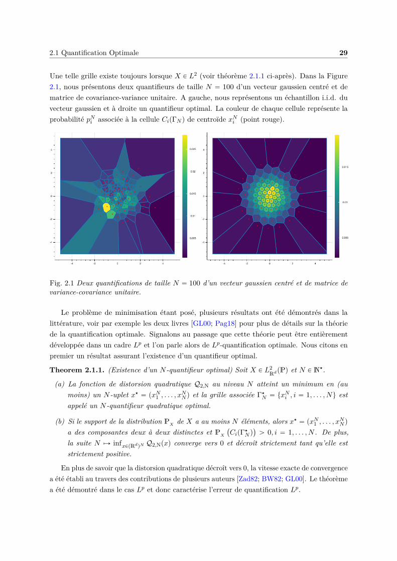
2.1 Quantification Optimale 29
Une telle grille existe toujours lorsque X P L2 (voir théorème 2.1.1 ci-après). Dans la Figure2.1, nous présentons deux quantifieurs de taille N “ 100 d’un vecteur gaussien centré et dematrice de covariance-variance unitaire. A gauche, nous représentons un échantillon i.i.d. duvecteur gaussien et à droite un quantifieur optimal. La couleur de chaque cellule représente laprobabilité pNi associée à la cellule CipΓN q de centroïde xNi (point rouge).
Fig. 2.1 Deux quantifications de taille N “ 100 d’un vecteur gaussien centré et de matrice devariance-covariance unitaire.
Le problème de minimisation étant posé, plusieurs résultats ont été démontrés dans lalittérature, voir par exemple les deux livres [GL00; Pag18] pour plus de détails sur la théoriede la quantification optimale. Signalons au passage que cette théorie peut être entièrementdéveloppée dans un cadre Lp et l’on parle alors de Lp-quantification optimale. Nous citons enpremier un résultat assurant l’existence d’un quantifieur optimal.
Theorem 2.1.1. (Existence d’un N -quantifieur optimal) Soit X P L2RdpPq et N P N‹.
(a) La fonction de distorsion quadratique Q2,N au niveau N atteint un minimum en (aumoins) un N-uplet x‹ “ pxN1 , . . . , x
NN q et la grille associée Γ‹
N “ txNi , i “ 1, . . . , Nu estappelé un N -quantifieur quadratique optimal.
(b) Si le support de la distribution PX de X a au moins N éléments, alors x‹ “ pxN1 , . . . , xNN q
a des composantes deux à deux distinctes et PX
`
CipΓ‹N q
˘
ą 0, i “ 1, . . . , N . De plus,la suite N ÞÑ infxPpRdqN Q2,Npxq converge vers 0 et décroît strictement tant qu’elle eststrictement positive.
En plus de savoir que la distorsion quadratique décroît vers 0, la vitesse exacte de convergencea été établi au travers des contributions de plusieurs auteurs [Zad82; BW82; GL00]. Le théorèmea été démontré dans le cas Lp et donc caractérise l’erreur de quantification Lp.
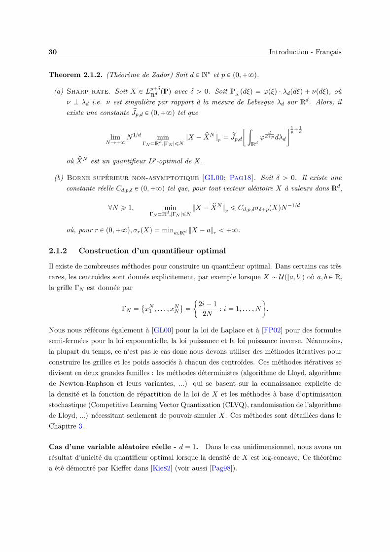
30 Introduction - Français
Theorem 2.1.2. (Théorème de Zador) Soit d P N‹ et p P p0,`8q.
(a) Sharp rate. Soit X P Lp`δ
Rd pPq avec δ ą 0. Soit PX pdξq “ φpξq ¨ λdpdξq ` νpdξq, oùν K λd i.e. ν est singulière par rapport à la mesure de Lebesgue λd sur Rd. Alors, ilexiste une constante rJp,d P p0,`8q tel que
limNÑ`8
N1d minΓN ĂRd,|ΓN |ďN
X ´ pXNp “ rJp,d
„ż
Rdφ
dd`pdλd
ȷ1p
` 1d
où pXN est un quantifieur Lp-optimal de X.
(b) Borne supérieur non-asymptotique [GL00; Pag18]. Soit δ ą 0. Il existe uneconstante réelle Cd,p,δ P p0,`8q tel que, pour tout vecteur aléatoire X à valeurs dans Rd,
@N ě 1, minΓN ĂRd,|ΓN |ďN
X ´ pXNp ď Cd,p,δσδ`ppXqN´1d
où, pour r P p0,`8q, σrpXq “ minaPRd X ´ ar ă `8.
2.1.2 Construction d’un quantifieur optimal
Il existe de nombreuses méthodes pour construire un quantifieur optimal. Dans certains cas trèsrares, les centroïdes sont donnés explicitement, par exemple lorsque X „ Upra, bsq où a, b P R,la grille ΓN est donnée par
ΓN “
xN1 , . . . , xNN
(
“
"
2i´ 12N : i “ 1, . . . , N
*
.
Nous nous référons également à [GL00] pour la loi de Laplace et à [FP02] pour des formulessemi-fermées pour la loi exponentielle, la loi puissance et la loi puissance inverse. Néanmoins,la plupart du temps, ce n’est pas le cas donc nous devons utiliser des méthodes itératives pourconstruire les grilles et les poids associés à chacun des centroïdes. Ces méthodes itératives sedivisent en deux grandes familles : les méthodes déterministes (algorithme de Lloyd, algorithmede Newton-Raphson et leurs variantes, ...) qui se basent sur la connaissance explicite dela densité et la fonction de répartition de la loi de X et les méthodes à base d’optimisationstochastique (Competitive Learning Vector Quantization (CLVQ), randomisation de l’algorithmede Lloyd, ...) nécessitant seulement de pouvoir simuler X. Ces méthodes sont détaillées dans leChapitre 3.
Cas d’une variable aléatoire réelle - d “ 1. Dans le cas unidimensionnel, nous avons unrésultat d’unicité du quantifieur optimal lorsque la densité de X est log-concave. Ce théorèmea été démontré par Kieffer dans [Kie82] (voir aussi [Pag98]).
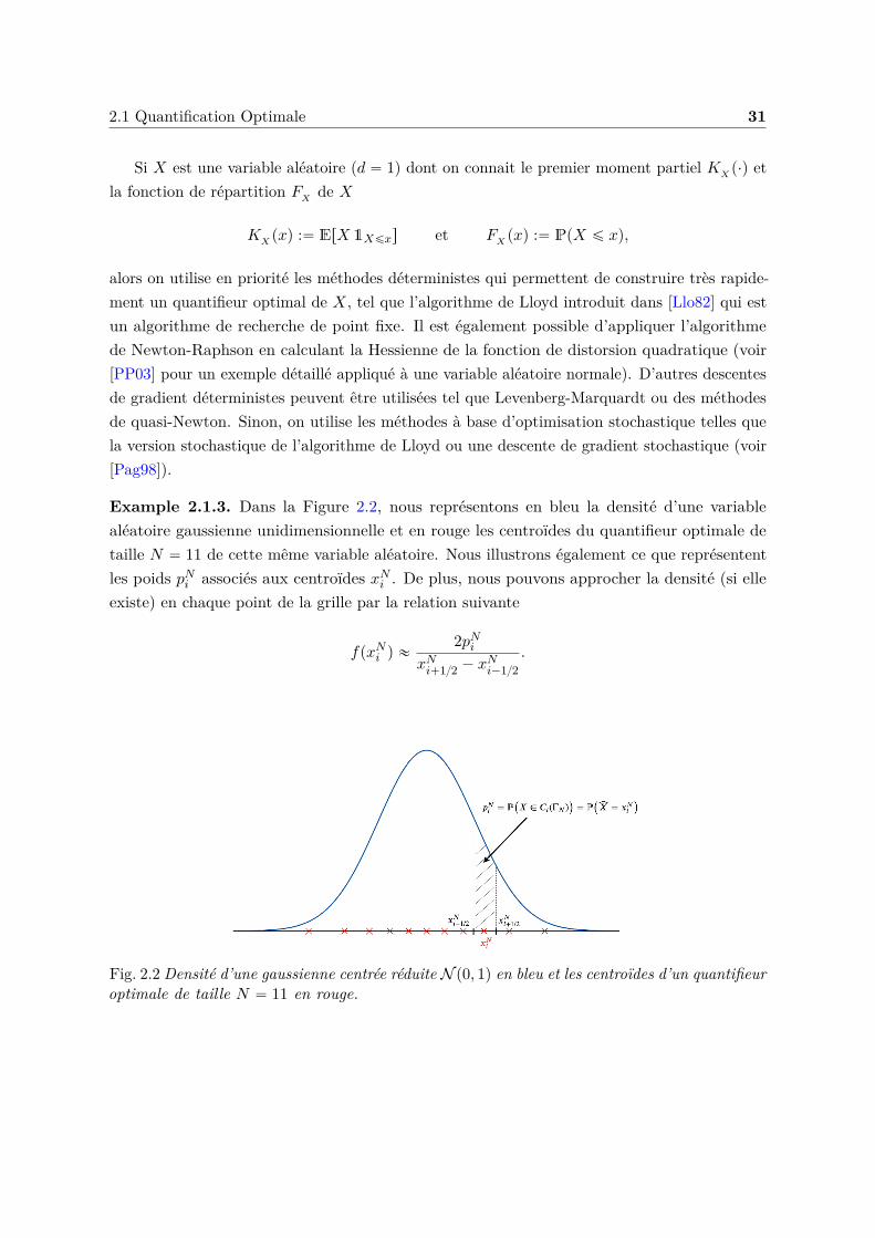
2.1 Quantification Optimale 31
Si X est une variable aléatoire (d “ 1) dont on connait le premier moment partiel KX p¨q etla fonction de répartition FX de X
KX pxq :“ ErX 1Xďxs et FX pxq :“ PpX ď xq,
alors on utilise en priorité les méthodes déterministes qui permettent de construire très rapide-ment un quantifieur optimal de X, tel que l’algorithme de Lloyd introduit dans [Llo82] qui estun algorithme de recherche de point fixe. Il est également possible d’appliquer l’algorithmede Newton-Raphson en calculant la Hessienne de la fonction de distorsion quadratique (voir[PP03] pour un exemple détaillé appliqué à une variable aléatoire normale). D’autres descentesde gradient déterministes peuvent être utilisées tel que Levenberg-Marquardt ou des méthodesde quasi-Newton. Sinon, on utilise les méthodes à base d’optimisation stochastique telles quela version stochastique de l’algorithme de Lloyd ou une descente de gradient stochastique (voir[Pag98]).
Example 2.1.3. Dans la Figure 2.2, nous représentons en bleu la densité d’une variablealéatoire gaussienne unidimensionnelle et en rouge les centroïdes du quantifieur optimale detaille N “ 11 de cette même variable aléatoire. Nous illustrons également ce que représententles poids pNi associés aux centroïdes xNi . De plus, nous pouvons approcher la densité (si elleexiste) en chaque point de la grille par la relation suivante
fpxNi q «2pNi
xNi`12 ´ xNi´12.
Fig. 2.2 Densité d’une gaussienne centrée réduite N p0, 1q en bleu et les centroïdes d’un quantifieuroptimale de taille N “ 11 en rouge.
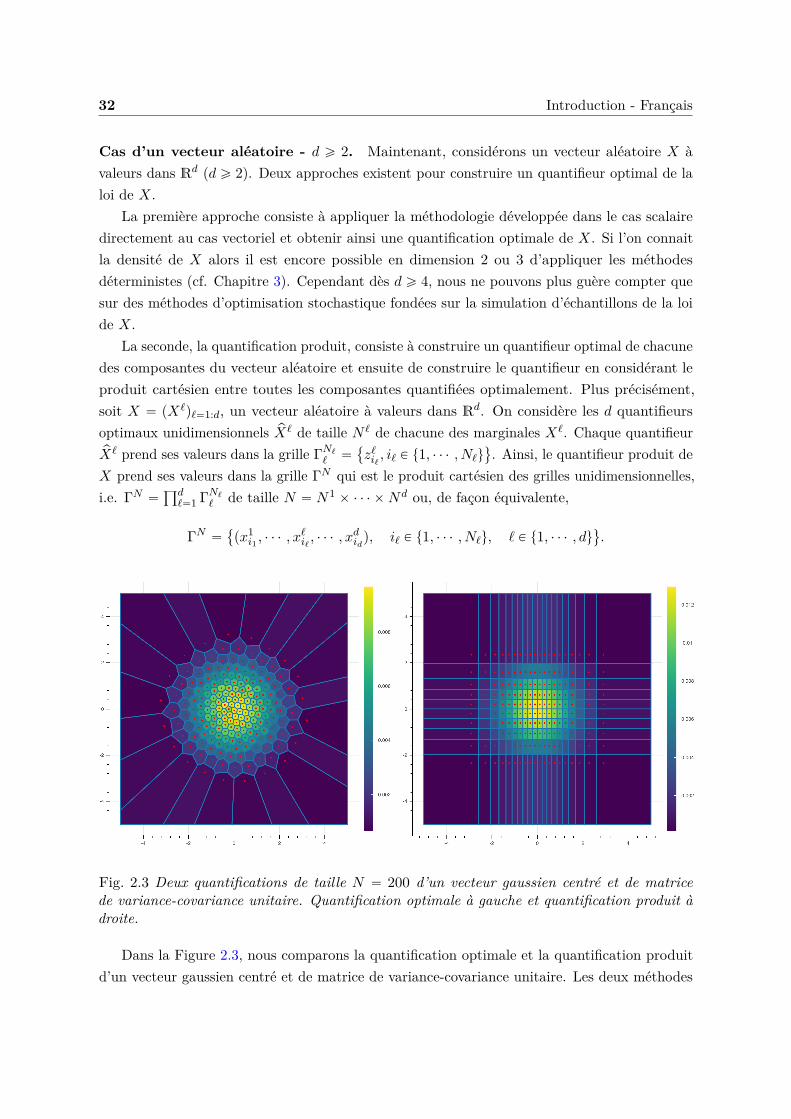
32 Introduction - Français
Cas d’un vecteur aléatoire - d ě 2. Maintenant, considérons un vecteur aléatoire X àvaleurs dans Rd (d ě 2). Deux approches existent pour construire un quantifieur optimal de laloi de X.
La première approche consiste à appliquer la méthodologie développée dans le cas scalairedirectement au cas vectoriel et obtenir ainsi une quantification optimale de X. Si l’on connaitla densité de X alors il est encore possible en dimension 2 ou 3 d’appliquer les méthodesdéterministes (cf. Chapitre 3). Cependant dès d ě 4, nous ne pouvons plus guère compter quesur des méthodes d’optimisation stochastique fondées sur la simulation d’échantillons de la loide X.
La seconde, la quantification produit, consiste à construire un quantifieur optimal de chacunedes composantes du vecteur aléatoire et ensuite de construire le quantifieur en considérant leproduit cartésien entre toutes les composantes quantifiées optimalement. Plus précisément,soit X “ pXℓqℓ“1:d, un vecteur aléatoire à valeurs dans Rd. On considère les d quantifieursoptimaux unidimensionnels pXℓ de taille N ℓ de chacune des marginales Xℓ. Chaque quantifieurpXℓ prend ses valeurs dans la grille ΓNℓ
ℓ “
zℓiℓ , iℓ P t1, ¨ ¨ ¨ , Nℓu(
. Ainsi, le quantifieur produit deX prend ses valeurs dans la grille ΓN qui est le produit cartésien des grilles unidimensionnelles,i.e. ΓN “
śdℓ“1 ΓNℓ
ℓ de taille N “ N1 ˆ ¨ ¨ ¨ ˆNd ou, de façon équivalente,
ΓN “
px1i1 , ¨ ¨ ¨ , xℓiℓ , ¨ ¨ ¨ , xdidq, iℓ P t1, ¨ ¨ ¨ , Nℓu, ℓ P t1, ¨ ¨ ¨ , du
(
.
Fig. 2.3 Deux quantifications de taille N “ 200 d’un vecteur gaussien centré et de matricede variance-covariance unitaire. Quantification optimale à gauche et quantification produit àdroite.
Dans la Figure 2.3, nous comparons la quantification optimale et la quantification produitd’un vecteur gaussien centré et de matrice de variance-covariance unitaire. Les deux méthodes
2.1 Quantification Optimale 33
ont leurs avantages et leurs inconvénients, la première méthode produit une meilleure quan-tification du vecteur aléatoire X comparée à la quantification-produit mais le coût numériqueinduit pour la construction d’un quantifieur optimal est souvent beaucoup plus élevé.
Cas des diffusions. Si maintenant, au lieu de considérer un vecteur aléatoire, nous nousintéressons aux diffusions, i.e.
dXt “ bpt,Xtqdt` σpt,WtqdWt
alors il existe, là encore, plusieurs solutions pour quantifier Xt. Plus précisément, étant donnéune discrétisation en temps à n-pas ptkq0ďkďn, nous cherchons les quantifieurs pXNk
tkde taille
Nk de Xtk que nous noterons pXNkk et Xk afin d’alléger les notations. L’objet que l’on cherche à
construire est dénommé arbre de quantification. Un arbre est caractérisé par la connaissancedes lois
`
Γk, ppki q1ďiďNk
˘
des quantifeurs p pXkq0ďkďn et des probabilités de transition pki,j
P`
pXk`1 “ xk`1j | pXk “ xki
˘
.
Nous ne présenterons pas toutes les approches existantes qui permettent d’aborder leproblème de schémas quantifiés de discrétisation d’une diffusion mais seulement celles qui nouspermettent d’utiliser des méthodes numériques déterministes d’optimisation des grilles. Pourles autres approches, basées sur des algorithmes stochastiques nous renvoyons à la série depapiers [BPP01; BP03].
Quantification des lois marginales. Le problème de la quantification d’une diffusiona été initié et développé dans une série d’articles [PPP04b; BPP05; BBP09; BBP10; CFG19].Si Xk peut être simulé de façon exacte, c’est à dire sans l’aide d’un schéma de discrétisation entemps, et que nous connaissons la loi marginale de Xk, à chaque instant tk, alors nous sommesramenés au cas de la quantification d’un vecteur aléatoire. En effet, nous pouvons quantifieroptimalement chaque vecteur aléatoire Xk à l’aide de méthodes numériques déterministes sid ď 2, ce qui produit un arbre de quantification optimal, ou quantifier optimalement chacunede ses composantes pour ensuite construire une quantification produit des Xk, produisant unarbre de quantification produit.
Example 2.1.4. Si l’on considère un modèle de Black-Scholes à volatilité constante σ et avectaux d’intérêts constants r
dSt “ Stprdt` σdWtq, avec S0 “ s0,
alors nous avons une forme explicite pour St
St “ S0 epr´σ22qt`σWt
34 Introduction - Français
donc pour un instant donné t, logpStS0q „ N`
pr ´ σ22qt, σ2t˘
donc nous pouvons quantifieroptimalement St à chaque instant qui nous intéresse à l’aide de méthodes déterministes (cf.Chapitre 3). Nous pouvons également quantifier le Brownien Wt qui est “plus universel”.
Quantification récursive. Dans le cas où nous ne connaissons pas la loi marginale de Xk
et que sommes obligés d’utiliser un schéma de discrétisation (type Euler-Maruyama, Milstein,...), nous allons utiliser une méthode appelée quantification récursive. La quantification récursive(aussi appelée quantification Markovienne) a d’abord été introduite dans [PPP04b] puis étudiéeen profondeur dans [PS15] pour le cas d’une diffusion unidimensionnelle discrétisée par unschéma d’Euler-Maruyama. Un algorithme rapide fondé sur des méthodes déterministes pourconstruire l’arbre de quantification y est développé et analysé. Par la suite, la quantificationrécursive rapide a été étendue à des schémas unidimensionnels d’ordre supérieur par [McW+18]et à des dimensions supérieures par quantification de produit (voir [PS18b; FSP18; Rud+17;CFG18; CFG17]). Cette méthode consiste à construire récursivement en k les quantifeurs pXNk
k
via la récursionpXNkk “ ProjΓNk
`
rXk
˘
avec rXk “ Ek´1`
pXNk´1k´1 , Zk
˘
où Ek´1 est un schéma de discrétisation.
2.2 Intégration numérique
Un problème courant en pratique est de calculer l’espérance d’une fonction de X lorsque Xest une variable ou un vecteur aléatoire, c’est à dire E
“
fpXq‰
. Or, sauf dans des cas trèsparticuliers, il n’est pas possible de calculer explicitement cette quantité, c’est le cas par exemplesi X “ XT la valeur d’une diffusion à la date T . C’est pourquoi il est nécessaire de faire appelà des méthodes d’intégration numérique. [Pag98] introduit une méthode de cubature à basede quantification optimale afin de pouvoir approcher des espérances de la forme E
“
fpXq‰
.Considérons pXN un quantifieur optimale de X, le fait que pXN soit discret nous permet dedéfinir facilement la formule de cubature suivante
E“
fp pXN q‰
“
Nÿ
i“1pNi fpxNi q. (2.1)
De plus, étant donné que pXN a été construite comme étant la meilleur approximation discrètede X de cardinal au plus N alors il nous semble raisonnable de penser que E
“
fp pXN q‰
est unebonne approximation de E
“
fpXq‰
.Dans le Chapitre 4, tiré de l’article “New Weak Error bounds and expansions for Op-
timal Quantization” publié dans Journal of Computational and Applied Mathematics, voir[LMP19], nous présentons de nouveaux résultats dans le cas réel concernant l’erreur induitepar l’approximation à base de quantification de l’espérance E
“
fpXq‰
. Ce travail est un travail
2.2 Intégration numérique 35
commun avec Vincent Lemaire et Gilles Pagès et il est accessible sur arXiv ou HAL. Cesrésultats “faible” sont résumés ci-après.
2.2.1 Convergence faible
Dans la première partie du Chapitre 4, nous nous intéressons à la vitesse de convergence deE“
fp pXN q‰
vers E“
fpXq‰
en fonction de N pour différentes classes de fonctions f lorsque Xest une variable aléatoire à valeurs dans R, i.e nous recherchons le plus grand α ą 0 tel que,pour toute fonction f dans cette classe F ,
limNNα
ˇ
ˇE“
fpXq‰
´ E“
fp pXN q‰ˇ
ˇ ď Cf,X ă `8.
Si l’on majore de façon naïve l’erreur faible par l’erreur forte le long des fonctions lips-chitziennes, on obtient la majoration suivante (avec α “ 1) pour une suite de N -quantifieursL2-optimaux
Nˇ
ˇE“
fpXq‰
´ E“
fp pXN q‰ˇ
ˇ ď N rf sLipX ´ pXN1 ď N rf sLipX ´ pXN2NÑ`8ÝÝÝÝÝÑ Cf ă `8
où le Théorème de Zador (théorème 2.1.2) a été utilisé. De plus, si nous considérons fpxq “
distpx,ΓN q alors f est une fonction lipschitzienne et nous avons
Nˇ
ˇE“
fpXq‰
´ E“
fp pXN q‰ˇ
ˇ “ NX ´ pXN1 ď NX ´ pXN2NÑ`8ÝÝÝÝÝÑ Cf ă `8.
Pour certaines classes de fonctions nous pouvons démontrer que la formule de cubature induitune erreur faible d’ordre 2 (α “ 2). Par exemple, si nous considérons les fonctions dérivablesavec une dérivée lipschitzienne alors nous avons une erreur d’ordre 2, voir [Pag98]. En effet,nous utilisons un développement de Taylor avec reste intégral de la forme
fpxq “ fpyq ` f 1pyqpx´ yq `
ż 1
0
`
f 1ptx` p1 ´ tqyq ´ f 1pyq˘
px´ yqdt
et la propriété de stationnarité d’un quantifieur quadratique optimale suivante
E“
X | pXN‰
“ pXN .
Le premier terme du développement de Taylor vaut zéro car
E“
f 1p pXN qpX´ pXN q‰
“ E”
f 1p pXN qE“
X´ pXN | pXN‰
ı
“ E”
f 1p pXN q`
E“
X | pXN‰
´ pXN˘
ı
“ 0.
36 Introduction - Français
Ainsi, en utilisant la propriété de Lipschitz de la dérivée et le théorème de Zador, nous obtenonsune erreur faible d’ordre 2 comme convenu
N2ˇˇE
“
fpXq‰
´ E“
fp pXN q‰ˇ
ˇ ď N2ż 1
0E“ˇ
ˇf 1ptX ` p1 ´ tq pXN q ´ f 1p pXN qˇ
ˇ|X ´ pXN |‰
dt
ďrf 1sLip
2 N2X ´ pXN22NÑ`8ÝÝÝÝÝÑ Cf ă `8.
Dans la première partie du Chapitre 4, nous étendons ces résultats concernant la vitesse deconvergence de l’erreur faible d’ordre supérieur à 1 à une plus vaste classe de fonctions ayantmoins de régularité, plus précisément, les fonctions qui sont soit :
‚ continues et affines par morceaux avec un nombre fini de ruptures d’affinités,
‚ Lipschitz convexe,
‚ dérivables avec une dérivée définie par morceaux (nombre fini de morceaux K aux pointsta1, . . . , aKu tel que ´8 “ a0 ă a1 ă ¨ ¨ ¨ ă aK ă aK`1 “ `8) qui soit localementlipschitzienne, c’est à dire
@k “ 0, . . . ,K, @x, y P pak, ak`1q |f 1pxq ´ f 1pyq| ď rf 1sk,Lip,loc
|x´ y|`
gkpxq ` gkpyq˘
où gk : pak, ak`1q Ñ R` sont des fonctions boréliennes à valeurs positives,
‚ dérivables avec une dérivée définie par morceaux (nombre fini de morceaux K aux pointsta1, . . . , aKu tel que ´8 “ a0 ă a1 ă ¨ ¨ ¨ ă aK ă aK`1 “ `8) qui soit localementα-Hölder, c’est à dire
@k “ 0, . . . ,K, @x, y P pak, ak`1q, |f 1pxq ´ f 1pyq| ď rf 1sk,α,loc
|x´ y|α`
gkpxq ` gkpyq˘
où gk : pak, ak`1q Ñ R` sont des fonctions boréliennes à valeurs positives.
Pour les trois premières classes de fonctions, nous démontrons que l’erreur faible est d’ordre 2et pour la dernière, d’ordre 1 ` α.
Dans la partie numérique, nous illustrons ce résultat en évaluant le prix d’un Call européendans un modèle de Black-Scholes donné par
I0 :“ E“
e´rT pST ´Kq`
‰
où St “ S0 epr´σ22qt`σWt avec pWtqtPr0,T s un mouvement brownien. Afin d’approcher, à l’aidede la quantification, le prix du Call européen nous pouvons réécrire I0 de deux façon différentes
I0 “ E“
φpST q‰
“ E“
fpWT q‰
2.2 Intégration numérique 37
où φ est une fonction affine par morceaux avec une rupture d’affinité et f est une fonctiondérivable avec une dérivée définie par morceaux localement lipschitzienne. Ainsi, en considérantdes quantifieurs de ST ou WT et en utilisant la formule de cubature, nous observons, pour lesdeux approximations, une erreur faible d’ordre 2.
2.2.2 Développement d’erreur faible d’ordre supérieur
Dans la seconde partie du Chapitre 4, nous nous intéressons au développement d’erreur faiblede l’approximation de E
“
fpXq‰
par E“
fp pXN q‰
. C’est à dire que nous cherchons à obtenir undéveloppement de la forme
E“
fpXq‰
“ E“
fp pXN q‰
`c2N2 `OpN´p2`βqq
où β P p0, 1s. Dans la section précédente, nous avons déjà montré que l’approximation parformule de cubature à base de quantification optimale induit un terme d’erreur d’ordre OpN´2q
dans le meilleur des cas. Ici, nous cherchons à raffiner les résultats précédents afin d’obtenirun développement d’erreur à l’ordre 2 “contrôlé” et non une simple vitesse de convergence àl’ordre 2.
Dans la Section 4.3, nous démontrons que ce développement existe si la fonction f : R Ñ
R est deux fois dérivables avec une dérivée seconde lipschitzienne. Ce résultat utilise undéveloppement de Taylor d’ordre 2 avec reste intégral de la forme
fpxq “ fpyq ` f 1pyqpx´ yq `12f
2pyqpx´ yq2 `
ż 1
0p1 ´ tq
`
f2ptx` p1 ´ tqyq ´ f2pyq˘
px´ yq2dt
où l’on prend l’espérance de chaque côté de l’égalité et on remplace x et y par X et pXN ,respectivement. Le deuxième terme à droite est annulé en utilisant la propriété de stationnaritédu quantifieur quadratique optimal. Pour le troisième terme, nous nous appuyons sur [Del+04](Théorème 6) qui stipule que @g : R Ñ R tel que E
“
gpXq‰
ă `8
limNN2E
“
gp pXN q|X ´ pXN |2‰
“ Q2pPX q
ż
gpξqPX pdξq
que l’on applique à g “ f2 où Q2pPX q est la constante de Zador. Ainsi, nous avons déjà lesdeux premiers termes dans le développement de l’erreur. Pour le dernier terme, on utilise lapropriété de Lipschitz de la dérivée seconde et le reste de la preuve se fonde principalementsur un résultat initialement établi dans [GLP08] puis récemment étendu dans [PS18a], connusous le nom de “Lr-Ls distorsion mismatch”, qui se formule ainsi : que peut-on dire du taux deconvergence de E
“
|X ´ pXN |s‰
sachant que pXN est un quantifieur Lr-optimal lorsque s ą r etX P Ls ? Nous citons ce théorème pour d “ 1, qui est le cas qui nous intéresse.
38 Introduction - Français
Theorem 2.2.1 (Lr-Ls-distorsion mismatch). Soit X : pΩ,A,Pq Ñ R une variable aléatoireet r P p0,`8q. Soit PX pdξq “ φpξq ¨ λpdξq ` νpdξq, où ν K λ i.e. ν est singulier par rapportà la mesure de Lebesgue λ sur R et φ est non-identiquement nul. Soit pΓN qNě1 une suite degrilles Lr-optimales et s P pr, r ` 1q. Si
X P Ls
1`r´s`δ
pPq
pour un δ ą 0, alorslim sup
NNX ´ pXNs ă `8.
Ainsi, en appliquant ce théorème avec r “ 2 et s “ 2 ` β, nous obtenons un OpN´p2`βqq
pour le dernier terme et @β P p0, 1q, nous avons l’expansion suivante
E“
fpXq‰
“ E“
fp pXN q‰
`c2N2 `OpN´p2`βqq.
Ce développement d’erreur nous permet de justifier théoriquement l’usage d’extrapolationde Richardson-Romberg qui a pour but de tuer le premier terme d’erreur du développement encombinant linéairement deux formules de cubature par quantification, respectivement à N etM points, i.e.
E“
fpXq‰
“ E
«
M2fp pXM q ´N2fp pXN q
M2 ´N2
ff
`OpN´p2`βqq
pour M “ kN avec k ą 1.
Nous illustrons ce résultat dans la partie numérique en évaluant une option européenne surspread dans un modèle de Black-Scholes en dimension 2 dont le prix est donné par
I0 :“ E“
e´rT pS1T ´ S2
T ´Kq`
‰
.
En pré-conditionnant, nous exprimons I0 comme suit
I0 “ E“
φpZ2q‰
où Z2 est une gaussienne centrée réduite et φ est une fonction deux fois dérivables avec unedérivée seconde lipschitzienne. Ainsi, en considérant des N -quantifieurs optimaux pZN deZ2 „ N p0, 1q, nous approchons I0 à l’aide de la formule de cubature à base de quantificationoptimale (2.1) et observons une erreur faible d’ordre 2. De plus, en utilisant l’extrapolation deRichardson-Romberg, nous atteignons une erreur faible d’ordre 3.
Cependant, l’intérêt de la méthode de cubature par quantification optimale lorsque d “ 1reste limité car elle est notamment en compétition avec les méthodes utilisant des points deGauss. Une extension multi-dimensionelle est en revanche très utile dès que d ě 3. On considère
2.2 Intégration numérique 39
une fonction deux fois différentiables f : Rd ÞÑ R avec une Hessienne bornée et lipschitzienne. Deplus, nous supposons que X : pΩ,A,Pq Ñ Rd a des composantes indépendantes Xk, k “ 1, . . . , det que le quantifieur pXN est un quantifieur produit de X à d composantes p pXNk
k qk“1,...,d telque N1 ˆ ¨ ¨ ¨ ˆNd “ N . Ainsi, nous avons
E“
fpXq‰
“ E“
fp pXN q‰
`
dÿ
k“1
ckN2k
`O
ˆ
´
mink“1:d
Nk
¯´p2`βq˙
.
2.2.3 Réduction de variance
Dans la dernière partie du Chapitre 4, nous présentons une nouvelle méthode de réduction devariance d’un estimateur Monte Carlo avec des variables de contrôle à base de quantificationoptimale unidimensionnelle. D’autres méthodes de réduction de variance à base de quantificationoptimale ont été développées, voir par exemple [CP15; Pag18] pour plus de détails. Cetteapproche est motivée par la vitesse de convergence d’ordre 2 de l’erreur faible induite par laformule de cubature à base de quantification pour diverses classes de fonctions, notammentcelles évoquées ci-avant.
Le problème. Soit pZkqk“1,...,d “ Z P L2RdpPq un vecteur aléatoire et une fonction f : Rd Ñ
R. Nous nous intéressons à la quantité suivante
I :“ E“
fpZq‰
. (2.2)
Bien souvent, nous ne pouvons pas calculer explicitement cette quantité, c’est pourquoi uneapproche standard est de faire appel à un estimateur Monte Carlo sIM :“ 1
M
řMm“1 fpZmq en
simulant des copies indépendantes Zm de Z pour approcher I. La convergence de la méthodeet sa vitesse sont déterminées par la loi forte des grands nombres et le théorème central limite,respectivement, qui assurent, si Z est de carré intégrable, que
sIMp.s.ÝÝÑ E
“
fpZq‰
et?M
´
sIM ´ E“
fpZq‰
¯
LÝÑ N
`
0, σ2fpZq
˘
lorsque M Ñ `8
où σ2fpZq
“ Var`
fpZq˘
. On remarque que, pour une taille de simulation M donnée, le facteurlimitant de la méthode est σ2
fpXq, c’est pourquoi des méthodes de réduction de variance qui
consistent à réduire la valeur de σ2fpXq
pour accélérer la convergence de l’estimateur MonteCarlo vers I ont été développées. Le lecteur peut se référer à [Pag18; Gla13] pour plus dedétails sur la simulation de Monte Carlo et les méthodes de réduction de variance en généraltelles que les variables de contrôle, la méthode antithétique, la stratification, l’échantillonnagepréférentiel, ...
40 Introduction - Français
Une nouvelle méthode de réduction de variance par variable de contrôle quantifiée.Soit ΞN , un vecteur aléatoire à valeurs dans Rd défini par
ΞN :“ pΞNk qk“1,...,d,
qui sera notre variable de contrôle d-dimensionnelle, chaque composante ΞNk est donnée par
ΞNk :“ fkpZkq ´ E“
fkp pZNk q‰
,
où fkpzq :“ fpErZ1s, . . . ,ErZk´1s, z,ErZk`1s, . . . ,ErZdsq et pZNk est une quantification optimalede taille N de Zk. Nous utilisons ici une quantification optimale unidimensionnelle afin de tirerprofit des résultats d’erreur faible précédemment démontrés, en effet les fonctions fk : R Ñ R
font parties des classes de fonctions nous permettant d’atteindre une erreur faible d’ordre 2.On introduit Iλ,N comme approximation pour (2.2)
Iλ,N “ E“
fpZq ´ xλ,ΞNy‰
“ E
«
fpZq ´
dÿ
k“1λkfkpZkq
ff
`
dÿ
k“1λk E
“
fkp pZNk q‰
(2.3)
où λ P Rd. Les termes E“
fkp pZNk q‰
dans (2.3) peuvent être aisément et rapidement calculés enutilisant le caractère discret des quantifieurs.
À ce stade, on peut définir pIλ,NM
l’estimateur de Monte Carlo associé à Iλ,N
pIλ,NM
“1M
Mÿ
m“1
˜
fpZmq ´
dÿ
k“1λkfkpZmk q
¸
`
dÿ
k“1λk E
“
fkp pZNk q‰
.
Il est important de remarquer que nous introduisons un biais en utilisant une telle variablede contrôle, en effet pour tout k P t1, . . . , nu, ErΞNk s ‰ 0 car E
“
fkp pZNk q‰
est une approximationde E
“
fkpZkq‰
. Cependant, la quantité qui nous intéresse réellement n’est pas le biais induitpar l’estimateur pIλ,N
Mmais plutôt l’erreur quadratique moyenne ou Mean Squared Error (MSE)
nous donnant une décomposition biais-variance
MSEppIλ,NM
q “
˜
dÿ
k“1λk
´
E“
fkp pZNk q‰
´ E“
fkpZkq‰
¯
¸2
looooooooooooooooooooooooomooooooooooooooooooooooooon
biais2
`1MVar
˜
fpZq ´
dÿ
k“1λkfkpZkq
¸
loooooooooooooooooomoooooooooooooooooon
Variance du Monte Carlo
.
Ainsi, nous pouvons prendre des valeurs de N plus élevées pour rendre le terme de biaisnégligeable comparé à la variance de l’estimateur tout en contrôlant le coût total induit parl’estimateur Monte Carlo. En pratique, nous n’avons pas besoin de prendre des valeurs trèsélevées pour N . En effet, le terme de biais converge vers 0 comme N´4 si f appartient à labonne classe de fonctions, donc prendre des quantificateurs optimaux de taille 200 est largement
2.3 Exemples d’applications à la finance 41
suffisant pour rendre le biais négligeable comparé à la variance de l’estimateur de Monte Carlo.Nous développons ce point dans la troisième partie du Chapitre 4.
Dans la partie numérique du Chapitre 4, nous appliquons la méthode de réduction devariance à l’évaluation d’une option panier dans un modèle de Black-Scholes en dimension d.La variable de contrôle nous permet de diviser la variance de l’estimateur Monte Carlo par100 en petite dimension (d “ 2 ou d “ 3) et par 6 en plus grande dimension (d “ 10). Nousobservons également que le biais induit par la quantification devient négligeable pour des grillesdont la taille est supérieure à 100 (N ą 100).
2.3 Exemples d’applications à la finance
2.3.1 Modèle d’Heston Stationnaire
Dans le Chapitre 5, nous nous intéressons au modèle d’Heston stationnaire et plus précisémentà l’évaluation d’options européennes, bermudiennes et barrières dans ce modèle ainsi qu’à lacalibration du modèle. Le Chapitre 5 est tiré du preprint “Stationary Heston model: Calibrationand Pricing of exotics using Product Recursive Quantization” accessible sur arXiv ou HAL(voir [LMP20]). Cet article est un travail commun avec Vincent Lemaire et Gilles Pagès.
Le modèle d’Heston standard fut introduit à l’origine par Heston dans [Hes93]. C’est unmodèle à volatilité stochastique où la condition initiale de la volatilité est supposée déterministe.Ce modèle a acquis une forte popularité principalement pour les deux raisons suivantes : c’estun modèle à volatilité stochastique donc il introduit un smile dans la surface de la volatilitéimplicite telle qu’observée dans le marché et la fonction caractéristique de ce modèle est donnéepar formule semi-fermée ce qui nous permet d’évaluer les options européennes (Call & Put)presque instantanément (voir Carr & Madan dans [CM99]). Cependant, une remarque souventfaite sur ce modèle concerne le smile de volatilité implicite qui n’est pas assez pentu pour desmaturités courtes comparé à ce que l’on observe sur le marché (voir [Gat11]). En remarquantque le processus de volatilité est ergodique avec une distribution invariante unique ν “ Γpα, βq
où les paramètres α et β dépendent des paramètres de diffusion de la volatilité, il a été proposépar Pagès & Panloup dans [PP09] de considérer directement que le processus évolue sous sonrégime stationnaire au lieu de le démarrer au temps 0 à partir d’une valeur déterministe. Cechoix a pour effet d’accentuer le smile de volatilité des maturités courtes tout en gardant lemême comportement que le modèle standard pour les maturités plus longues. Plus tard, lecomportement à court et long terme de la volatilité implicite générée par un tel modèle a étéétudié par Jacquier & Shi dans [JS17].
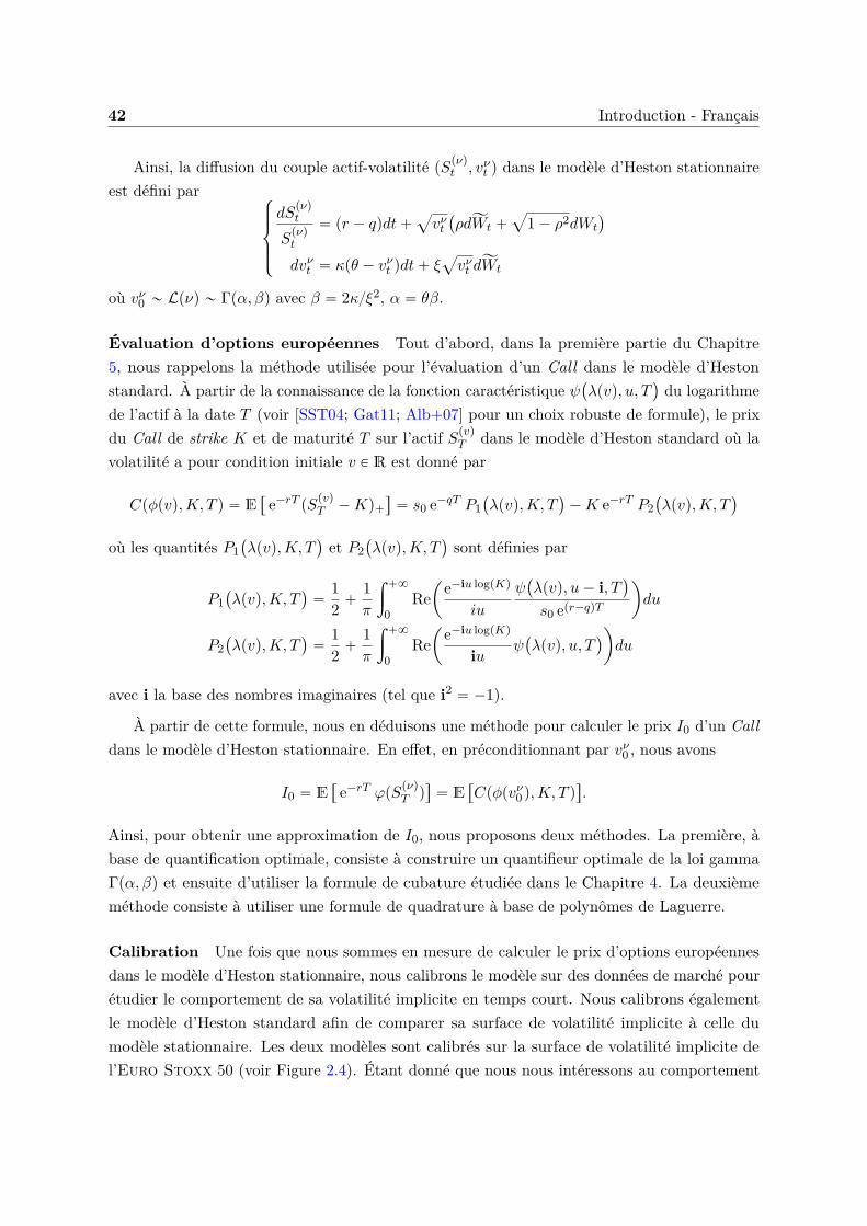
42 Introduction - Français
Ainsi, la diffusion du couple actif-volatilité pSpνq
t , vνt q dans le modèle d’Heston stationnaireest défini par
$
’
’
&
’
’
%
dSpνq
t
Spνq
t
“ pr ´ qqdt`a
vνt`
ρdĂWt `a
1 ´ ρ2dWt
˘
dvνt “ κpθ ´ vνt qdt` ξa
vνt dĂWt
où vν0 „ Lpνq „ Γpα, βq avec β “ 2κξ2, α “ θβ.
Évaluation d’options européennes Tout d’abord, dans la première partie du Chapitre5, nous rappelons la méthode utilisée pour l’évaluation d’un Call dans le modèle d’Hestonstandard. À partir de la connaissance de la fonction caractéristique ψ
`
λpvq, u, T˘
du logarithmede l’actif à la date T (voir [SST04; Gat11; Alb+07] pour un choix robuste de formule), le prixdu Call de strike K et de maturité T sur l’actif Spvq
T dans le modèle d’Heston standard où lavolatilité a pour condition initiale v P R est donné par
Cpϕpvq,K, T q “ E“
e´rT pSpvq
T ´Kq`
‰
“ s0 e´qT P1`
λpvq,K, T˘
´K e´rT P2`
λpvq,K, T˘
où les quantités P1`
λpvq,K, T˘
et P2`
λpvq,K, T˘
sont définies par
P1`
λpvq,K, T˘
“12 `
1π
ż `8
0Re
ˆ
e´iu logpKq
iu
ψ`
λpvq, u´ i, T˘
s0 epr´qqT
˙
du
P2`
λpvq,K, T˘
“12 `
1π
ż `8
0Re
ˆ
e´iu logpKq
iu ψ`
λpvq, u, T˘
˙
du
avec i la base des nombres imaginaires (tel que i2 “ ´1).
À partir de cette formule, nous en déduisons une méthode pour calculer le prix I0 d’un Calldans le modèle d’Heston stationnaire. En effet, en préconditionnant par vν0 , nous avons
I0 “ E“
e´rT φpSpνq
T q‰
“ E“
Cpϕpvν0 q,K, T q‰
.
Ainsi, pour obtenir une approximation de I0, nous proposons deux méthodes. La première, àbase de quantification optimale, consiste à construire un quantifieur optimale de la loi gammaΓpα, βq et ensuite d’utiliser la formule de cubature étudiée dans le Chapitre 4. La deuxièmeméthode consiste à utiliser une formule de quadrature à base de polynômes de Laguerre.
Calibration Une fois que nous sommes en mesure de calculer le prix d’options européennesdans le modèle d’Heston stationnaire, nous calibrons le modèle sur des données de marché pourétudier le comportement de sa volatilité implicite en temps court. Nous calibrons égalementle modèle d’Heston standard afin de comparer sa surface de volatilité implicite à celle dumodèle stationnaire. Les deux modèles sont calibrés sur la surface de volatilité implicite del’Euro Stoxx 50 (voir Figure 2.4). Étant donné que nous nous intéressons au comportement
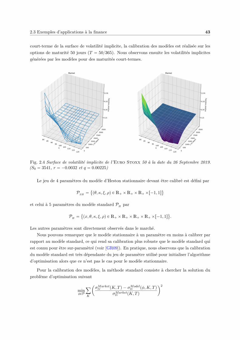
2.3 Exemples d’applications à la finance 43
court-terme de la surface de volatilité implicite, la calibration des modèles est réalisée sur lesoptions de maturité 50 jours (T “ 50365). Nous observons ensuite les volatilités implicitesgénérées par les modèles pour des maturités court-termes.
K
8085
9095
100105
110115
120
T (in days)
0500
10001500
20002500
30003500
Implied Vo
latility
0.15
0.20
0.25
0.30
Market
K
8085
9095
100105
110115
120
T (in days)
0500
10001500
20002500
30003500
Implied Vo
latility
0.15
0.20
0.25
0.30
Market
Fig. 2.4 Surface de volatilité implicite de l’Euro Stoxx 50 à la date du 26 Septembre 2019.(S0 “ 3541, r “ ´0.0032 et q “ 0.00225)
Le jeu de 4 paramètres du modèle d’Heston stationnaire devant être calibré est défini par
PSH “
pθ, κ, ξ, ρq P R` ˆR` ˆR` ˆr´1, 1s(
et celui à 5 paramètres du modèle standard PH par
PH “
px, θ, κ, ξ, ρq P R` ˆR` ˆR` ˆR` ˆr´1, 1s(
.
Les autres paramètres sont directement observés dans le marché.Nous pouvons remarquer que le modèle stationnaire à un paramètre en moins à calibrer par
rapport au modèle standard, ce qui rend sa calibration plus robuste que le modèle standard quiest connu pour être sur-paramètré (voir [GR09]). En pratique, nous observons que la calibrationdu modèle standard est très dépendante du jeu de paramètre utilisé pour initialiser l’algorithmed’optimisation alors que ce n’est pas le cas pour le modèle stationnaire.
Pour la calibration des modèles, la méthode standard consiste à chercher la solution duproblème d’optimisation suivant
minϕPP
ÿ
K
ˆ
σMarketiv pK,T q ´ σModel
iv pϕ,K, T q
σMarketiv pK,T q
˙2
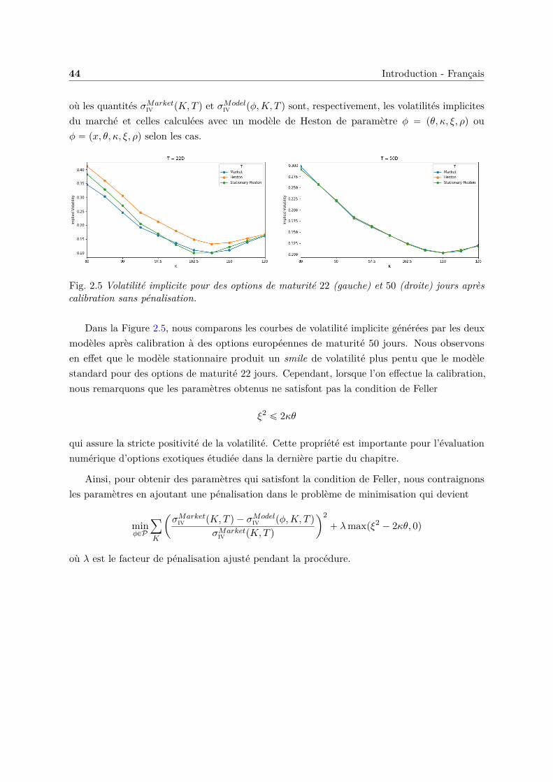
44 Introduction - Français
où les quantités σMarketiv pK,T q et σModel
iv pϕ,K, T q sont, respectivement, les volatilités implicitesdu marché et celles calculées avec un modèle de Heston de paramètre ϕ “ pθ, κ, ξ, ρq ouϕ “ px, θ, κ, ξ, ρq selon les cas.
Fig. 2.5 Volatilité implicite pour des options de maturité 22 (gauche) et 50 (droite) jours aprèscalibration sans pénalisation.
Dans la Figure 2.5, nous comparons les courbes de volatilité implicite générées par les deuxmodèles après calibration à des options européennes de maturité 50 jours. Nous observonsen effet que le modèle stationnaire produit un smile de volatilité plus pentu que le modèlestandard pour des options de maturité 22 jours. Cependant, lorsque l’on effectue la calibration,nous remarquons que les paramètres obtenus ne satisfont pas la condition de Feller
ξ2 ď 2κθ
qui assure la stricte positivité de la volatilité. Cette propriété est importante pour l’évaluationnumérique d’options exotiques étudiée dans la dernière partie du chapitre.
Ainsi, pour obtenir des paramètres qui satisfont la condition de Feller, nous contraignonsles paramètres en ajoutant une pénalisation dans le problème de minimisation qui devient
minϕPP
ÿ
K
ˆ
σMarketiv pK,T q ´ σModel
iv pϕ,K, T q
σMarketiv pK,T q
˙2` λmaxpξ2 ´ 2κθ, 0q
où λ est le facteur de pénalisation ajusté pendant la procédure.
2.3 Exemples d’applications à la finance 45
Fig. 2.6 Volatilité implicite pour des options de maturité 22 (gauche) et 50 (droite) jours aprèscalibration avec pénalisation.
Dans la Figure 2.6, nous effectuons la même comparaison que précédement. Nous remarquonsque l’ajout de la pénalisation a dégradé la qualité de la calibration à la maturité 50 jours. Pource qui est de la maturité 22 jours, nous observons que le modèle stationnaire arrive là encore, àproduire un smile de volatilité plus proche de celui du marché que le modèle standard.
Évaluation d’options exotiques par quantification produit récursive Dans la dernièrepartie du Chapitre 5, nous traitons de l’évaluation des options exotiques telles que les optionsbermudiennes et les options à barrière à l’aide d’un principe de programmation dynamique. Laméthode numérique que nous proposons est fondée sur de la quantification produit récursive.Nous étendons la méthodologie précédemment développée par [FSP18; CFG18; CFG17] oùun schéma d’Euler-Maruyama était considéré pour discrétiser en temps à la fois l’actif et lavolatilité.
Discrétisation en temps des diffusions Nous avons fait le choix de considérer unschéma hybride composé d’un schéma d’Euler-Maruyama pour la dynamique du log-actifXt “ logpS
pνq
t q et d’un schéma de Milstein pour le processus de volatilité boosté Yt “ eκt vνt .Ainsi, nous avons
#
sXtk`1 “ Eb,σ`
tk, sXtk ,sYtk , Z
1k`1
˘
sYtk`1 “ Mrb,rσ
`
tk, sYtk , Z2k`1
˘
avec tk “ kn , n le nombre de pas de temps de discrétisation, Z1
k`1 „ N p0, 1q et Z2k`1 „ N p0, 1q
tel que CorrpZ1k`1, Z
2k`1q “ ρ. Le schéma d’Euler-Maruyama est défini par
Eb,σpt, x, y, zq “ x` bpt, x, yqh` σpt, x, yq?h z
avecbpt, x, yq “ r ´ q ´
e´κt y
2 and σpt, x, yq “ e´κt2 ?y,
46 Introduction - Français
et le schéma de Milstein mis sous sa forme canonique
Mrb,rσ
pt, x, zq “ x´rσpt, xq
2rσ1xpt, xq
` h
ˆ
rbpt, xq ´prσrσ1
xqpt, xq
2
˙
`prσrσ1
xqpt, xqh
2
ˆ
z `1
?hrσ1
xpt, xq
˙2
avecrbpt, xq “ eκt κθ, rσpt, xq “ ξ
?x eκt2 and rσ1
xpt, xq “ξ eκt2
2?x.
Quantification Markovienne produit recursive Une fois le choix du schéma de dis-crétisation en temps fait, nous nous intéressons à la discrétisation en espace du couple actif-volatilité.
Pour cela, nous construisons tout d’abord un arbre de quantification Markovien ppYtk qk“0,...,n.Il est avantageux de remarquer que la volatilité est autonome et donc nous faisons face à unproblème unidimensionnel. Ainsi, les quantifieurs pYtk sont construits récursivement, c’est à direque pYtk`1 est un quantifieur optimal de rYtk`1 défini par
rYtk`1 “ Mrb,rσ
`
tk, pYtk , Z2k`1
˘
, pYtk`1 “ ProjΓYN2,k`1
`
rYtk`1
˘
.
Numériquement, nous utilisons les méthodes à base d’algorithmes déterministes pour la dimen-sion 1 développées dans le Chapitre 3.
Maintenant, en utilisant le fait que Yt a déjà été quantifié, nous construisons un arbre dequantification Markovien p pXtk qk“0,...,n de Xt. Là encore nous sommes ramenés à un problèmeunidimensionnel et nous construisons les quantifieurs pXtk récursivement, c’est à dire que pXtk`1
est un quantifieur optimal de rXtk`1 défini par
rXtk`1 “ Eb,σ`
tk, pXtk ,pYtk , Z
1k`1
˘
, pXtk`1 “ ProjΓXN1,k`1
`
rXtk`1
˘
.
Afin de simplifier les notations, nous notons dans la suite pXk et pYk à la place de pXtk et pYtk .
Maintenant que nous avons calibré le modèle d’Heston stationnaire et que nous sommescapable de construire un arbre de quantification pour le couple actif-volatilité, nous nousintéressons à l’évaluation d’options exotiques et plus précisément des options bermudiennes oubarrières.
Options bermudiennes Le prix à la date tk d’une option bermudienne pouvant s’exerceraux dates ttk, ¨ ¨ ¨ , tnu et de payoff ψtk pXtk , Ytk q à la date tk est donné par l’enveloppe de SnellVk
Vk “ supτPT n
k
E”
e´rτ ψτ pXτ , Yτ q | F tk
ı
,
2.3 Exemples d’applications à la finance 47
où T nk représente l’ensemble des temps d’arrêt τ à valeurs dans ttk, t1, . . . , tnu. Le Principe de
Programmation Dynamique permet de réécrire Vk comme suit#
Vn “ e´rtn ψnpXn, Ynq,
Vk “ max`
e´rtk ψkpXk, Ykq,ErVk`1 | Fks˘
, 0 ď k ď n´ 1.
Nous appliquons ensuite la méthodologie employée par [BP03; BPP05; Pag18] qui consisteà remplacer Xk et Yk par les quantifieurs pXk et pYk. Par construction de la quantificationrécursive, le couple p pXk, pYkq est Markovien ainsi nous obtenons le Principe de ProgrammationDynamique Quantifié suivant
#
pVn “ ψnp pXn, pYnq,
pVk “ max`
ψkp pXk, pYkq,ErpVk`1 | p pXk, pYkqs˘
, k “ 0, . . . , n´ 1.
Finalement, le prix de l’option bermudienne est donné par E“
pV0‰
.
Options barrières Le prix à la date tk d’une option barrière Up-and-Out de maturité T ,de payoff terminal f et de barrière L est donné par
PUO “ e´rT E“
fpXT q1suptPr0,T s XtďL
‰
.
Pour l’évaluation de l’option barrière, nous appliquons l’algorithme basé sur la loi conditionnelledu schéma d’Euler, voir [Gla13; Sag10; Pag18]. Ainsi, une fois le couple actif-volatilité discrétiséen temps, le prix PUO se réécrit de la façon suivante
sPUO “ e´rT E“
fp sXT q1suptPr0,T ssXtďL
‰
“ e´rT E
„
fp sXT q
n´1ź
k“0Gk
p sXk,sYkq, sXk`1pLq
ȷ
oùGkpx,yq,zpuq “
´
1 ´ e´2n px´uqpz´uq
T σ2ptk,x,yq
¯
1tuěmaxpx,zqu .
Finalement, en remplaçant sXk et sYk par pXk et pYk et en utilisant un algorithme récursif afind’approcher sPUO par ErpV0s, nous obtenons
$
&
%
pVn “ e´rT fp pXnq,
pVk “ E“
Gkp pXk,pYkq, pXk`1
pLq pVk`1 | p pXk, pYkq‰
, 0 ď k ď n´ 1.
2.3.2 Évaluation d’options bermudiennes dans un modèle 3 facteurs (PRDC)
Dans le Chapitre 6, nous nous intéressons au problème d’évaluation d’option bermudiennes surtaux de change où l’on considère des taux d’intérêts domestiques et étrangers stochastiques.
48 Introduction - Français
Dans ce cas, on fait référence à un modèle 3 facteurs. Le Chapitre 6 correspond à l’article“Quantization-based Bermudan option pricing in the FX world” soumis à Journal of Compu-tational Finance et accessible sur arXiv ou HAL (voir [Fay+19]). Cet article est un travailcommun avec Jean-Michel Fayolle, Vincent Lemaire et Gilles Pagès.
Le besoin d’évaluer de tels produits est né au Japon à la fin du XXe siècle. En effetla persistance des taux d’intérêt bas durant les dernières décennies du siècle a été l’une desprincipales raisons qui ont conduit à la création de produits financiers structurés sur taux dechange. Ces produits répondaient au besoin des investisseurs souhaitant obtenir des couponsplus élevés que ceux fondés sur le yen. Au fur et à mesure, les produits financiers se sontcomplexifiés pour en arriver aux produits appelés : power reverse dual currency (PRDC), voir[Wys17].
Même si ces produits ont été émis vers la fin du XXe siècle, ils sont toujours présents dansles portefeuilles des banques et doivent être pris en compte lors de l’évaluation des calculs derisque de contrepartie tels que l’ajustement de valeur de crédit (Credit Valuation Adjustment -CVA), l’ajustement de valeur de la dette (Debt Valuation Adjustment - DVA), l’ajustementde valeur du financement (Funding Valuation Adjustment - FVA), l’ajustement de valeur ducapital (Capital Valuation Adjustment - KVA), ...., en bref xVA (voir [BMP13; CBB14; Gre15]pour plus de détails sur le sujet).
Le modèle. On définit P pt, T q comme étant la valeur à l’instant t d’une unité de la devisechoisie livrée (c’est-à-dire payée) à l’instant T , également connue sous le nom de prix du zérocoupon ou facteur d’actualisation. Nous noterons le zéro coupon avec d en exposant lorsque nousparlerons de zéro coupon dans la devise domestique (P dpt, T q) et avec f en exposant pour le zérocoupon dans la devise étrangère. Le modèle utilisé pour diffuser les zéro coupons domestique etétranger se place dans la famille des modèles de courbe de rendement Heath-Jarrow-Morton(HJM). Pour plus de détails et de théorie sur ses modèles, on peut se référer aux articles suivants[EFG96; EMV92; HJM92; BS73].
Ainsi la diffusion de la courbe des zéro coupons domestiques sous la probabilité risque-neutredomestique P est donnée par
dP dpt, T q
P dpt, T q“ rdt dt` σdpT ´ tqdW d
t ,
où W d est un P-mouvement brownien, rdt est le taux instantané domestique au temps t et σdest la volatilité. Pour la courbe des zéro coupons étrangers, la dynamique est donnée, sous laprobabilité risque-neutre étrangère rP, par la diffusion
dP f pt, T q
P f pt, T qP f pt, T q “ rft dt` σf pT ´ tqdĂW f
t ,
2.3 Exemples d’applications à la finance 49
où ĂW f est un rP-mouvement brownien, rft est le taux instantané étranger au moment t et σf estla volatilité. Les deux probabilités rP et P sont supposées être équivalentes, c’est-à-dire rP „ P
et il existe ρdf défini comme limite de la variation quadratique croisée xW d,ĂW f yt “ ρdf t.Pour le taux de change (FX), nous désignons par St la valeur au temps t ą 0 d’une unité
de monnaie étrangère dans la monnaie domestique. La dynamique de pStqtě0 est de typeBlack-Scholes sous la forme
dStSt
“ prdt ´ rft qdt` σSdWSt ,
où rdt est le taux instantané de la monnaie domestique au temps t, rft est le taux instantanéde la monnaie étrangère au temps t, σS est la volatilité et WS est un mouvement brownienstandard sous la probabilité risque-neutre.
La problématique. Notre objectif est d’évaluer le prix d’options bermudiennes sur le taux dechange St pouvant être exercé à n` 1 dates: tt0, . . . , tnu. Ainsi, le prix à la date tk de l’optionbermudienne est donné par l’enveloppe de Snell Vk de l’obstacle
`
e´ştk0 rd
sds ψtk pStk q˘
k“0:n
Vk “ supτPT n
k
E“
e´şτ0 r
dsds ψτ pSτ q | F tk
‰
où τ est un temps d’arrêt à valeurs dans ttk, . . . , tnu et T nk représente l’ensemble de ces temps
d’arrêt.
Example 2.3.1. Le payoff que nous considérons dans le Chapitre 6 est un celui d’un couponde PRDC (voir l’exemple dans la Figure 2.7) défini par
ψtk pxq “ min˜
maxˆ
Cf ptkq
S0x´ Cdptkq,Floorptkq
˙
,Capptkq
¸
où Floorptkq et Capptkq sont les valeurs plancher choisies lors de la création du produit, ainsique Cf ptkq et Cdptkq qui sont les valeurs des coupon des monnaies étrangères et domestiquesauxquels nous souhaitons nous comparer.
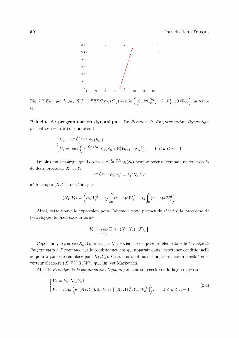
50 Introduction - Français
Fig. 2.7 Exemple de payoff d’un PRDC ψtk pStk q “ min´´
0.189 Stk88.17 ´ 0.15
¯
`, 0.0555
¯
au tempstk.
Principe de programmation dynamique. Le Principe de Programmation Dynamiquepermet de réécrire Vk comme suit:
$
&
%
Vn “ e´ştn0 rd
sds ψnpStnq,
Vk “ max´
e´ştk0 rd
sds ψkpStk q,ErVk`1 | F tk s
¯
, 0 ď k ď n´ 1.
De plus, on remarque que l’obstacle e´şt0 r
dsds ψtpStq peut se réécrire comme une fonction ht
de deux processus Xt et Yte´
şt0 r
dsds ψtpStq “ htpXt, Ytq
où le couple pX,Y q est défini par
pXt, Ytq “
ˆ
σSWSt ` σf
ż t
0pt´ sqdW f
s ,´σd
ż t
0pt´ sqdW d
s
˙
.
Ainsi, cette nouvelle expression pour l’obstacle nous permet de réécrire la problème del’enveloppe de Snell sous la forme
Vk “ supτPT n
k
E“
hτ pXτ , Yτ q | F tk
‰
.
Cependant, le couple pXk, Ykq n’est pas Markovien et cela pose problème dans le Principe deProgrammation Dynamique car le conditionnement qui apparait dans l’espérance conditionnellene pourra pas être remplacé par pXk, Ykq. C’est pourquoi nous sommes amenés à considérer levecteur aléatoire pX,W f , Y,W dq qui, lui, est Markovien.
Ainsi le Principe de Programmation Dynamique peut se réécrire de la façon suivante$
&
%
Vn “ hnpXn, Ynq,
Vk “ max´
hkpXk, Ykq,E“
Vk`1 | pXk,Wfk , Yk,W
dk q‰
¯
, 0 ď k ď n´ 1.(2.4)
2.3 Exemples d’applications à la finance 51
Résolution numérique par quantification. Nous nous intéressons maintenant à la partiepratique qui consiste à calculer numériquement les valeurs de Vk. Dans le Chapitre 6, nous avonsopté pour une méthode numérique à base de quantification optimale telle qu’introduite dans[BPP01] et développée dans [BP03; PPP04b; BPP05] pour l’évaluation d’options bermudiennesmais avec la variante consistant à utiliser un arbre de quantification optimale produit. Cetteapproche a pour avantage d’être rapide, stable et précise en petite dimension. Cependantlorsque la dimension croît, elle peut être très coûteuse en temps de calcul et la vitesse deconvergence de la méthode se dégrade à cause de la “malédiction de la dimension” qui touchela quantification optimale.
La première idée que nous présentons, lorsque l’on souhaite discrétiser (2.4) par quantificationoptimale, est la plus naturelle. Nous remplaçons les variables aléatoires Xk, W f
k , Yk and W dk
par leur quantification optimale pXk, xW fk , pYk et xW d
k , de taille NXk , NW f
k , NW f
k , NYk et NW d
k
respectivement, et nous “forçons”, en un certains sens, la propriété de Markov en introduisantle Principe de Programmation Dynamique Quantifié "forcé" défini par
$
&
%
pVn “ hnp pXn, pYnq,
pVk “ max´
hkp pXk, pYkq,E“
pVk`1 | p pXk,xWfk ,
pYk,xWdk q‰
¯
, 0 ď k ď n´ 1.
Le terme "forcé" se justifie car p pXk,xWfk ,
pYk,xWdk qk n’est pas une chaine de Markov donc ce
principe de programmation dynamique n’est pas naturellement associé à une enveloppe de Snell.Nous désignons par Nk “ NX
k ˆNW f
k ˆNYk ˆNW d
k la taille globale de la grille de quantificationproduit.
Pour cette approximation, nous fournissons une erreur quadratique à priori pour Vk ´
pVk2 , k “ 0, . . . , n.
Theorem 2.3.2. Si les fonctions pψtk qk“0:n sont dérivables à droite avec une dérivée bornéeà support compact. Alors l’erreur quadratique induite par l’approximation par quantificationp pXk,xW
fk ,
pYk,xWdk q est bornée par
›
›Vk ´ pVk›
›
2ď
ˆ nÿ
l“k
CXl
›
›Xl ´ pXl
›
›
22p
` CYl
›
›Yl ´ pYl›
›
22p
` CW dl
›
›W dl ´ xW d
l
›
›
22p
` CW f
l
›
›W fl ´ xW f
l
›
›
22p
˙12,
où 1 ă p ă 32 et q ě 1 tel que 1p ` 1
q “ 1 et les constantes CXl, CW d
l, CYl
, CW f
lsont finies.
Ainsi, en prenant sN “ minkNk, nous avons
limsNÑ`8
›
›Vk ´ pVk›
›
22
“ 0.
Le problème majeur de l’approche que nous venons de présenter est la complexité algo-rithmique associée à cette méthode due à la taille des grilles de quantification-produit. Cette
52 Introduction - Français
complexité rend très coûteux le calcul des espérances conditionnelles apparaissant dans leprincipe de programmation dynamique. Notre objectif est donc de réduire la dimension duproblème. Pour cela, nous enlevons les processus W d et W f de l’arbre de quantification-produitpour ne garder que X et Y . Ce faisant, nous perdons la propriété de markovianité du vecteuraléatoire que nous considérons mais nous réduisons considérablement la complexité numériquedu problème. Dans ce cadre, (2.4) est approchée par
$
&
%
pVn “ hnp pXn, pYnq,
pVk “ max´
hkp pXk, pYkq,E“
pVk`1 | p pXk, pYkq‰
¯
, 0 ď k ď n´ 1.
Nous notons Nk “ NXk ˆNY
k la taille de la grille de quantification.Là encore, nous fournissons une erreur quadratique à priori pour Vk ´ pVk2 , k “ 0, . . . , n
basé sur les erreurs de quantification moyennes Xl ´ pXl2p et Yl ´ pYl2p mais également surles erreurs que nous faisons en ne prenant pas en compte les mouvements browniens dans leconditionnement.
Theorem 2.3.3. Si les fonctions pψtk qk“0:n sont dérivables à droite avec une dérivée bornéeà support compact alors l’erreur quadratique induite par l’approximation par quantificationp pXk, pYkq est bornée par
›
›Vk ´ pVk›
›
2ď
ˆ n´1ÿ
l“k
CW f
l`1
›
›W fl`1 ´ ErW f
l`1 | pXl, Ylqs›
›
22p
` CW dl`1
›
›W dl`1 ´ ErW d
l`1 | pXl, Ylqs›
›
22p
` CXl
›
›Xl ´ pXl
›
›
22p
` CYl
›
›Yl ´ pYl›
›
22p
˙12
où 1 ă p ă 32 et q ě 1 tel que 1p ` 1
q “ 1 et les constantes CXl, CW d
l`1, CYl
, CW f
l`1sont finies.
Ainsi, en prenant sN “ minNk, nous avons
limsNÑ`8
›
›Vk´pVk›
›
22
“
n´1ÿ
l“k
CW f
l`1
›
›W fl`1´ErW f
l`1 | pXl, Ylqs›
›
22p
`CW dl`1
›
›W dl`1´ErW d
l`1 | pXl, Ylqs›
›
22p.
Nous pouvons ainsi remarquer que l’approximation que nous avons faite en remplaçant lepréconditionnement en pXk,W
fk , Yk,W
dk q par pXk, Ykq, même s’il réduit considérablement la
complexité du problème induit une erreur systématique. Cependant, il semble raisonnable depenser que cette erreur est négligeable.
Example 2.3.4. En effet, dans la Figure 2.8, lors de l’évaluation d’options bermudiennespouvant être exercées annuellement pour des maturités de 2, 5 ou 10 ans, en considérantdes paramètres de marché pour σd et σf , la différence de prix entre les deux méthodes estnégligeable. Le payoff considéré est celui de l’exemple 2.3.1. Pour l’exemple considéré dans laFigure 2.8, les corrélations sont supposées nulles ρSd “ ρSf “ ρdf “ 0, S0 “ 88.17, σS “ 50%,
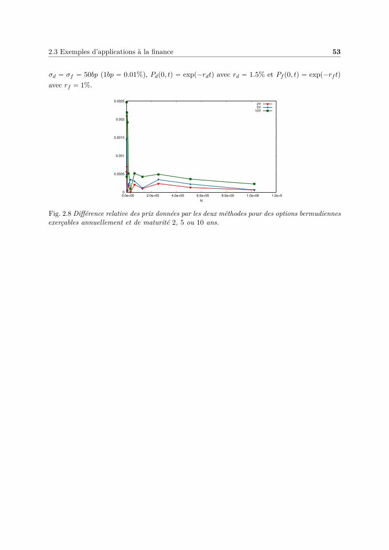
2.3 Exemples d’applications à la finance 53
σd “ σf “ 50bp (1bp “ 0.01%), Pdp0, tq “ expp´rdtq avec rd “ 1.5% et Pf p0, tq “ expp´rf tq
avec rf “ 1%.
0
0.0005
0.001
0.0015
0.002
0.0025
0.0e+00 2.0e+05 4.0e+05 6.0e+05 8.0e+05 1.0e+06 1.2e+06
N
2Y
5Y
10Y
Fig. 2.8 Différence relative des prix données par les deux méthodes pour des options bermudiennesexerçables annuellement et de maturité 2, 5 ou 10 ans.

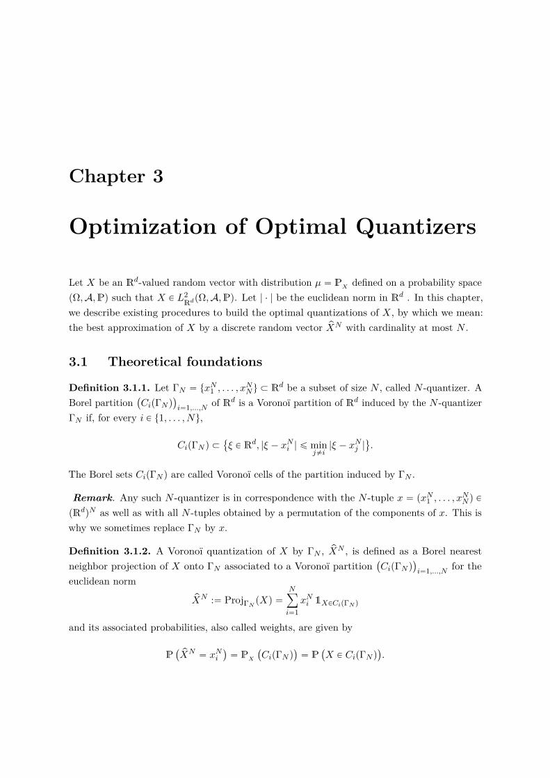
Chapter 3
Optimization of Optimal Quantizers
Let X be an Rd-valued random vector with distribution µ “ PX defined on a probability spacepΩ,A,Pq such that X P L2
RdpΩ,A,Pq. Let | ¨ | be the euclidean norm in Rd . In this chapter,we describe existing procedures to build the optimal quantizations of X, by which we mean:the best approximation of X by a discrete random vector pXN with cardinality at most N .
3.1 Theoretical foundations
Definition 3.1.1. Let ΓN “ txN1 , . . . , xNNu Ă Rd be a subset of size N , called N -quantizer. A
Borel partition`
CipΓN q˘
i“1,...,N of Rd is a Voronoï partition of Rd induced by the N -quantizerΓN if, for every i P t1, . . . , Nu,
CipΓN q Ă
ξ P Rd, |ξ ´ xNi | ď minj‰i
|ξ ´ xNj |(
.
The Borel sets CipΓN q are called Voronoï cells of the partition induced by ΓN .
Remark. Any such N -quantizer is in correspondence with the N -tuple x “ pxN1 , . . . , xNN q P
pRdqN as well as with all N -tuples obtained by a permutation of the components of x. This iswhy we sometimes replace ΓN by x.
Definition 3.1.2. A Voronoï quantization of X by ΓN , pXN , is defined as a Borel nearestneighbor projection of X onto ΓN associated to a Voronoï partition
`
CipΓN q˘
i“1,...,N for theeuclidean norm
pXN :“ ProjΓNpXq “
Nÿ
i“1xNi 1XPCipΓN q
and its associated probabilities, also called weights, are given by
P`
pXN “ xNi˘
“ PX
`
CipΓN q˘
“ P`
X P CipΓN q˘
.
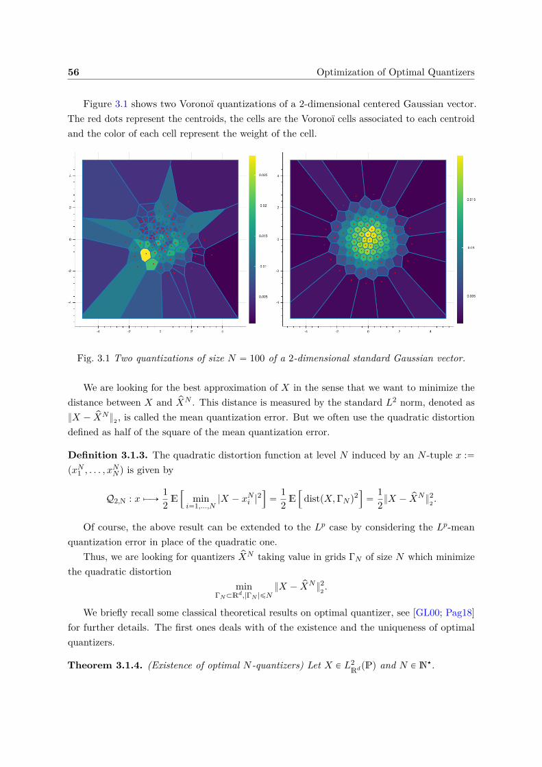
56 Optimization of Optimal Quantizers
Figure 3.1 shows two Voronoï quantizations of a 2-dimensional centered Gaussian vector.The red dots represent the centroids, the cells are the Voronoï cells associated to each centroidand the color of each cell represent the weight of the cell.
Fig. 3.1 Two quantizations of size N “ 100 of a 2-dimensional standard Gaussian vector.
We are looking for the best approximation of X in the sense that we want to minimize thedistance between X and pXN . This distance is measured by the standard L2 norm, denoted asX ´ pXN2 , is called the mean quantization error. But we often use the quadratic distortiondefined as half of the square of the mean quantization error.
Definition 3.1.3. The quadratic distortion function at level N induced by an N -tuple x :“pxN1 , . . . , x
NN q is given by
Q2,N : x ÞÝÑ12 E
”
mini“1,...,N
|X ´ xNi |2ı
“12 E
”
distpX,ΓN q2ı
“12X ´ pXN2
2 .
Of course, the above result can be extended to the Lp case by considering the Lp-meanquantization error in place of the quadratic one.
Thus, we are looking for quantizers pXN taking value in grids ΓN of size N which minimizethe quadratic distortion
minΓN ĂRd,|ΓN |ďN
X ´ pXN22 .
We briefly recall some classical theoretical results on optimal quantizer, see [GL00; Pag18]for further details. The first ones deals with of the existence and the uniqueness of optimalquantizers.
Theorem 3.1.4. (Existence of optimal N -quantizers) Let X P L2RdpPq and N P N‹.
3.1 Theoretical foundations 57
(a) The quadratic distortion function Q2,N at level N attains a minimum at a N-tuplex‹ “ pxN1 , . . . , x
NN q and Γ‹
N “ txNi , i “ 1, . . . , Nu is a quadratic optimal quantizer at levelN .
(b) If the support of the distribution PX of X has at least N elements, then x‹ “ pxN1 , . . . , xNN q
has pairwise distinct components, PX
`
CipΓ‹N q
˘
ą 0, i “ 1, . . . , N . Furthermore, thesequence N ÞÑ infxPpRdqN Q2,Npxq converges to 0 and is decreasing as long as it is positive.
The next results deal with the asymptotic behavior of the distortion. We saw in Theorem3.1.4 that the infimum of the quadratic distortion converges to 0 as N goes to infinity. The nexttheorem, known as Zador’s Theorem, analyzes the sharp rate of convergence of the quantizationerror. This result has been proved in the case of the Lp-optimal quantization.
Theorem 3.1.5. (Zador’s Theorem) Let p P p0,`8q.
(a) Sharp rate [Zad82; GL00]. Let X P Lp`δ
Rd pPq for some δ ą 0. Let PX pdξq “
φpξq ¨ λpdξq ` νpdξq, where ν K λ i.e. ν is singular with respect to the Lebesgue measureλ on Rd. Then, there is a constant rJp,d P p0,`8q such that
limNÑ`8
N1d minΓN ĂRd,|ΓN |ďN
X ´ pXNp “ rJp,d
„ż
Rdφ
dd`pdλd
ȷ1p
` 1d
where pXN is an Lp-optimal quantization of X.
(b) Non asymptotic upper-bound [GL00; Pag18]. Let δ ą 0. There exists a real constantCd,p,δ P p0,`8q such that, for every Rd-valued random vector X,
@N ě 1, minΓN ĂRd,|ΓN |ďN
X ´ pXNp ď Cd,p,δσδ`ppXqN´1d
where, for r P p0,`8q, σrpXq “ minaPRd X ´ ar ă `8 is the Lr-pseudo-standarddeviation.
Another really interesting property concerning quadratic optimal quantizers is the station-arity property which is closely linked to the Lloyd method defined later in Section 3.2.1.1.
Proposition 3.1.6. (Stationarity) Assume that the support of PX has at least N elements.Any L2-optimal N -quantizer ΓN P pRdqN is stationary in the following sense: for every Voronoïquantization pXN of X,
E“
X | pXN‰
“ pXN .
Moreover P`
X PŤ
i“1,...,N BCipΓN q˘
“ 0, so all optimal quantization induced by ΓN a.s.coincide.
58 Optimization of Optimal Quantizers
3.2 How to build an optimal quantizer?
In this part, we focus our efforts on the following minimization problem
arg minpRdqN
Q2,N (3.1)
and more exactly, how to build an optimal quadratic quantizer? For that, we differentiate theL2-distortion function Q2,N at level N . The approaches for solving the above minimizationproblem can be divided in two families: the fixed-point methods and the gradient descentmethods. Both are linked to the distortion’s gradient that we define below.
Proposition 3.2.1 ([Pag18]). The distortion function Q2,N is continuously differentiable atN -tuples x P pRdqN satisfying
x has pairwise distinct components and P
ˆ
X Pď
i“1,...,NBCipΓN q
˙
“ 0
with a gradient ∇ Q2,N “
´
B Q2,NBxN
i
¯
1ďiďNgiven by
B Q2,NBxNi
pxq “ E
„
B q2,NBxNi
px,Xq
ȷ
“
ż
Rd
B q2,NBxNi
px, ξqPX pdξq,
the local gradient being given by
B q2,NBxNi
px, ξq “ 2pxNi ´ ξq1ProjΓNpξq“xN
i, 1 ď i ď N. (3.2)
Equivalently, the gradient can also be written as
∇ Q2,Npxq “ 2„ż
CipΓN q
pxNi ´ ξqPX pdξq
ȷ
i“1,...,N“ 2
”
E“
1XPCipΓN qpxNi ´Xq
‰
ı
i“1,...,N. (3.3)
The latter expression is useful for numerical methods based on deterministic procedures whilethe former featuring a local gradient is handy when we work with stochastic algorithms.
3.2.1 Real valued random variables: d “ 1
In the first part of this section, we focus on the scalar case, when X is a random variable takingvalues in R. Hence the Voronoï cells are intervals in R and if we consider that the quantizerspxNi qi are ordered: xN1 ă xN2 ă ¨ ¨ ¨ ă xNN´1 ă xNN , then the Voronoï cells are given by
CipΓN q “`
xNi´12, xNi`12
‰
, i “ 1, . . . , N ´ 1, CN pΓN q “`
xNN´12, xNN`12
˘
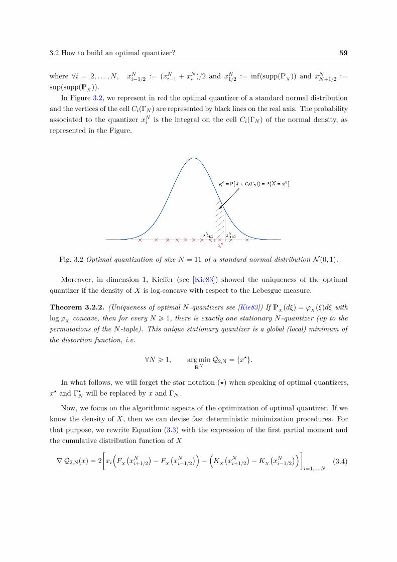
3.2 How to build an optimal quantizer? 59
where @i “ 2, . . . , N, xNi´12 :“ pxNi´1 ` xNi q2 and xN12 :“ infpsupppPX qq and xNN`12 :“suppsupppPX qq.
In Figure 3.2, we represent in red the optimal quantizer of a standard normal distributionand the vertices of the cell CipΓN q are represented by black lines on the real axis. The probabilityassociated to the quantizer xNi is the integral on the cell CipΓN q of the normal density, asrepresented in the Figure.
Fig. 3.2 Optimal quantization of size N “ 11 of a standard normal distribution N p0, 1q.
Moreover, in dimension 1, Kieffer (see [Kie83]) showed the uniqueness of the optimalquantizer if the density of X is log-concave with respect to the Lebesgue measure.
Theorem 3.2.2. (Uniqueness of optimal N -quantizers see [Kie83]) If PX pdξq “ φX pξqdξ withlogφX concave, then for every N ě 1, there is exactly one stationary N -quantizer (up to thepermutations of the N -tuple). This unique stationary quantizer is a global (local) minimum ofthe distortion function, i.e.
@N ě 1, arg minRN
Q2,N “ tx‹u.
In what follows, we will forget the star notation (‹) when speaking of optimal quantizers,x‹ and Γ‹
N will be replaced by x and ΓN .
Now, we focus on the algorithmic aspects of the optimization of optimal quantizer. If weknow the density of X, then we can devise fast deterministic minimization procedures. Forthat purpose, we rewrite Equation (3.3) with the expression of the first partial moment andthe cumulative distribution function of X
∇ Q2,Npxq “ 2„
xi
´
FX
`
xNi`12˘
´ FX
`
xNi´12˘
¯
´
´
KX
`
xNi`12˘
´KX
`
xNi´12˘
¯
ȷ
i“1,...,N(3.4)
60 Optimization of Optimal Quantizers
where KX p¨q and FX p¨q are, respectively, the first partial moment and the cumulative distributionfunction of X
KX pxq :“ ErX 1Xďxs and FX pxq :“ PpX ď xq.
In the one dimensional case, we have access to a closed-form formula (or efficient numericalimplementation) of the density function, the cumulative distribution function and partial firstmoment for a lot of random variables. We summarize below, for several random variables X,KX p¨q, FX p¨q and φX p¨q, the first partial moment, the cumulative distribution function and thedensity of X, respectively.
• Standard normal distribution: X „ N p0, 1q
φX pξq “e´ξ22?
2π, FX pξq “ N pξq, KX pξq “ ´φX pξq.
• Log-normal distribution: X “ exppµ` σZq with µ P R and σ ą 0 where Z „ N p0, 1q
φX pξq “1ξσφZ
´ logpξq ´ µ
σ
¯
, FX pξq “ N´ logpξq ´ µ
σ
¯
,
KX pξq “ eµ`σ22 N´ logpξq ´ µ´ σ2
σ
¯
with φZ the density of Z.
• Exponential distribution: X „ Epλq with λ ą 0
φX pξq “ λ e´λξ, FX pξq “ 1 ´ e´λξ, KX pξq “ ´ e´λξ´
ξ `1λ
¯
`1λ.
• Gamma distribution: X „ Γpα, βq with α, β ą 0
φX pξq “βα
Γpαqξα´1 e´βξ, FX pξq “
γpα, βξq
Γpαq, KX pξq “ FX pξq ´
ξ
βφX pξq,
where Γp¨q is the gamma function and γps, xq “şx0 t
s´1e´tdt is the lower incomplete gammafunction. Optimized numerical implementations for both functions can easily be find in anyprogramming language.
• Non-central χ2p1q distribution: X „ χ2p1q “ pZ `mq2 with m P R where Z „ N p0, 1q
φX pξq “φZ
`
m`?ξ˘
` φZ
`
m´?ξ˘
2?ξ
, FX pξq “ N`
m`a
ξ˘
´ N`
m´a
ξ˘
,
KX pξq “`
m´a
ξ˘
N`
m`a
ξ˘
´`
m`a
ξ˘
N`
m´a
ξ˘
``
1 `m2˘FX pξq.
3.2 How to build an optimal quantizer? 61
• Supremum of the Brownian bridge: X “ suptPr0,1s |Wt ´ tW1|. This distribution is alsoknown as the Kolmogorov-Smirnov distribution.
φX pξq “ 8ξÿ
kě1p´1qk´1k2 e´2k2ξ2
, FX pξq “ 1 ´ 2ÿ
kě1p´1qk´1 e´2k2ξ2
,
KX pξq “?
2πÿ
kě1
p´1qk´1
k
´
N p2kξq ´12
¯
´ ξp1 ´ FX pξqq,
where N pxq denotes the cumulative distribution function of the normal distribution. The proofof the formulas above are given in Appendix 3.A.
• Symmetric random variable For some random variables X, we have no access to closed-form formulas for φX , FX and KX but if X is symmetric and we have an explicit expressionfor its characteristic function χpuq “ E
“
eiuX ‰
, where i is the imaginary number, s.t. i2 “ ´1,then the functions φX , FX and KX can be written as alternate series using Fourier transform.This method was introduced in chapter 5 of [Pag18]. The proof of the formulas below are givenin Appendix 3.A. For ξ ě 0, we have
φX pξq “1πξ
ÿ
kě0p´1qk
ż π
0cospuqχ
´u` kπ
ξ
¯
du,
FX pξq “12 `
1π
ÿ
kě0p´1qk
ż π
0
sinpuq
u` kπχ´u` kπ
ξ
¯
du,
KX pξq “ ´C ` ξ´
FX pξq ´12
¯
`ξ
π
ÿ
kě0
ż π
0
1 ´ p´1qk cospuq
pu` kπq2 χ´u` kπ
ξ
¯
du,
where C “ ErX`s and for ξ ă 0
φX pξq “ φX p´ξq, FX pξq “ 1 ´ FX p´ξq, KX pξq “ KX p´ξq.
Example 3.2.3. We give some examples of symmetric random variables where we can use theabove formulas based on Fourier in order to obtain the functions φX , FX and KX .
∗ One-sided Lévy’s area: X „ş10 W
1s dW
2s where pW 1,W 2q is a 2-dimensional standard
Brownian motion. The characteristic function of the Lévy’s area is given by
χpuq “1
a
coshpuqand C “ 0.24852267 ˘ 2.033 ˆ 10´7,
where C has been computed using a ML2R estimator.
∗ Standard normal distribution: X „ N p0, 1q. Although we have explicit formulas forthe desired functions, we can still use the above formulas based on alternating series to the
62 Optimization of Optimal Quantizers
Gaussian case in order to validate the methodology. For the normal distribution, we have
χpuq “ e´u22 and C “1
?2π.
• Closed-form formula of the characteristic function Another method, introduced in[CFG19] for the quantization of a positive diffusion pStqtPr0,T s at time T , is based on Fourierinversion in order to determine a computable expression of the density and the cumulativedistribution function. They use the fact that the conditional characteristic function of X “
logpST q is explicitly known or can be computed efficiently and denoted
χpuq “ E“
eiu logpST q‰
, u P R .
Using the knowledge of the characteristic function of X, they obtain
PpST P dzq “
ˆ
1π
1z
ż `8
0Re
`
e´i logpzqξ χpuq˘
du
˙
dz
PpST ď zq “12 ´
1π
ż `8
0Re
ˆ
e´iu logpzq χpuq
iu
˙
du, z P p0,`8q.
Hence, based on these formulas, they devise a Newton-Raphson algorithm (as detailed inAlgorithm 4) for the optimization of an optimal quantizer of ST .
Remark. Let ΓN “ txN1 , . . . , xNNu be an N -quantizer of X. In the one-dimensional case, when
we know the cumulative distribution function of X as detailed above, we can deduce directlythe probabilities pNi “ P
`
pXN “ xNi˘
, indeed
pNi “ P`
pXN “ xNi˘
“ P`
X P CipΓN q˘
“ FX
`
xNi`12˘
´ FX
`
xNi´12˘
.
3.2.1.1 Fixed-point search (Lloyd method)
Starting from Equation (3.4), when we search a zero of the gradient, we derive a fixed-pointproblem. Let Λi : RN ÞÑ R defined by
Λipxq “KX
`
xNi`12˘
´KX
`
xNi´12˘
FX
`
xNi`12˘
´ FX
`
xNi´12˘ (3.5)
then∇ Q2,Npxq “ 0 ðñ @i “ 1, . . . , N xi “ Λipxq.
Hence, from this equality, we deduce a fixed-point search algorithm. This method, known asthe Lloyd method, was first devised by Lloyd in [Llo82]. The convergence at an exponentialrate of the algorithm was shown by Kieffer in [Kie82].
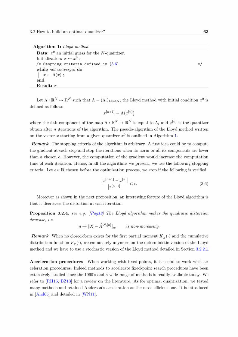
3.2 How to build an optimal quantizer? 63
Algorithm 1: Lloyd method.Data: x0 an initial guess for the N -quantizer.Initialization: x Ð x0 ;/* Stopping criteria defined in (3.6) */while not converged do
x Ð Λpxq ;endResult: x
Let Λ : RN ÞÑ RN such that Λ “ pΛiq1ďiďN , the Lloyd method with initial condition x0 isdefined as follows
xrn`1s “ Λ`
xrns˘
where the i-th component of the map Λ : RN Ñ RN is equal to Λi and xrns is the quantizerobtain after n iterations of the algorithm. The pseudo-algorithm of the Lloyd method writtenon the vector x starting from a given quantizer x0 is outlined in Algorithm 1.
Remark. The stopping criteria of the algorithm is arbitrary. A first idea could be to computethe gradient at each step and stop the iterations when its norm or all its components are lowerthan a chosen ϵ. However, the computation of the gradient would increase the computationtime of each iteration. Hence, in all the algorithms we present, we use the following stoppingcriteria. Let ϵ P R chosen before the optimization process, we stop if the following is verified
ˇ
ˇxrn`1s ´ xrnsˇ
ˇ
ˇ
ˇxrn`1sˇ
ˇ
ď ϵ. (3.6)
Moreover as shown in the next proposition, an interesting feature of the Lloyd algorithm isthat it decreases the distortion at each iteration.
Proposition 3.2.4. see e.g. [Pag18] The Lloyd algorithm makes the quadratic distortiondecrease, i.e.
n ÞÑ X ´ pXN,rns2 , is non-increasing.
Remark. When no closed-form exists for the first partial moment KX p¨q and the cumulativedistribution function FX p¨q, we cannot rely anymore on the deterministic version of the Lloydmethod and we have to use a stochastic version of the Lloyd method detailed in Section 3.2.2.1.
Acceleration procedures When working with fixed-points, it is useful to work with ac-celeration procedures. Indeed methods to accelerate fixed-point search procedures have beenextensively studied since the 1960’s and a wide range of methods is readily available today. Werefer to [RH15; BZ13] for a review on the literature. As for optimal quantization, we testedmany methods and retained Anderson’s acceleration as the most efficient one. It is introducedin [And65] and detailed in [WN11].
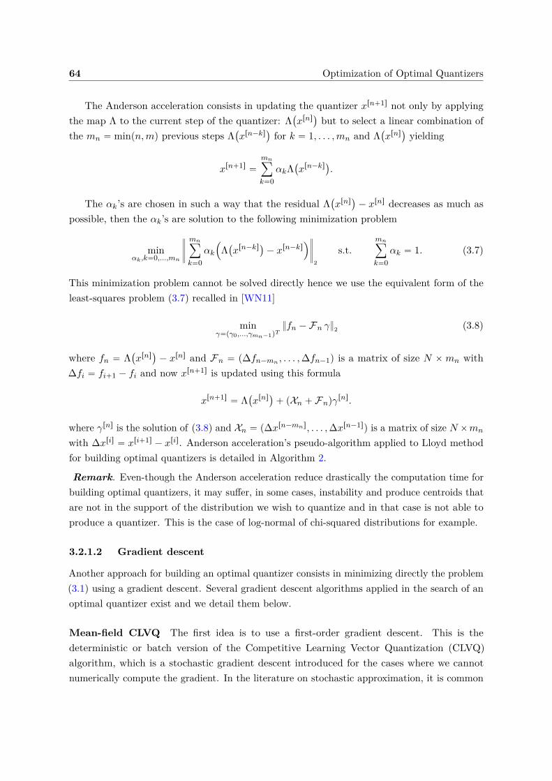
64 Optimization of Optimal Quantizers
The Anderson acceleration consists in updating the quantizer xrn`1s not only by applyingthe map Λ to the current step of the quantizer: Λ
`
xrns˘
but to select a linear combination ofthe mn “ minpn,mq previous steps Λ
`
xrn´ks˘
for k “ 1, . . . ,mn and Λ`
xrns˘
yielding
xrn`1s “
mnÿ
k“0αkΛ
`
xrn´ks˘
.
The αk’s are chosen in such a way that the residual Λ`
xrns˘
´ xrns decreases as much aspossible, then the αk’s are solution to the following minimization problem
minαk,k“0,...,mn
›
›
›
›
mnÿ
k“0αk
´
Λ`
xrn´ks˘
´ xrn´ks¯
›
›
›
›
2
s.t.mnÿ
k“0αk “ 1. (3.7)
This minimization problem cannot be solved directly hence we use the equivalent form of theleast-squares problem (3.7) recalled in [WN11]
minγ“pγ0,...,γmn´1qT
fn ´ Fn γ2 (3.8)
where fn “ Λ`
xrns˘
´ xrns and Fn “ p∆fn´mn , . . . ,∆fn´1q is a matrix of size N ˆ mn with∆fi “ fi`1 ´ fi and now xrn`1s is updated using this formula
xrn`1s “ Λ`
xrns˘
` pXn ` Fnqγrns.
where γrns is the solution of (3.8) and Xn “ p∆xrn´mns, . . . ,∆xrn´1sq is a matrix of size N ˆmn
with ∆xris “ xri`1s ´ xris. Anderson acceleration’s pseudo-algorithm applied to Lloyd methodfor building optimal quantizers is detailed in Algorithm 2.
Remark. Even-though the Anderson acceleration reduce drastically the computation time forbuilding optimal quantizers, it may suffer, in some cases, instability and produce centroids thatare not in the support of the distribution we wish to quantize and in that case is not able toproduce a quantizer. This is the case of log-normal of chi-squared distributions for example.
3.2.1.2 Gradient descent
Another approach for building an optimal quantizer consists in minimizing directly the problem(3.1) using a gradient descent. Several gradient descent algorithms applied in the search of anoptimal quantizer exist and we detail them below.
Mean-field CLVQ The first idea is to use a first-order gradient descent. This is thedeterministic or batch version of the Competitive Learning Vector Quantization (CLVQ)algorithm, which is a stochastic gradient descent introduced for the cases where we cannotnumerically compute the gradient. In the literature on stochastic approximation, it is common
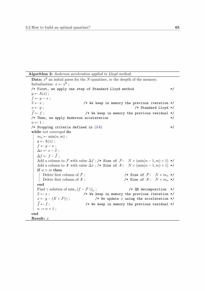
3.2 How to build an optimal quantizer? 65
Algorithm 2: Anderson acceleration applied to Lloyd method.Data: x0 an initial guess for the N -quantizer, m the deepth of the memory.Initialization: x Ð x0 ;/* First, we apply one step of Standard Lloyd method */g Ð Λpxq ;f Ð g ´ x ;rx Ð x ; /* We keep in memory the previous iteration */x Ð g ; /* Standard Lloyd */rf Ð f ; /* We keep in memory the previous residual *//* Then, we apply Anderson acceleration */n Ð 1 ;/* Stopping criteria defined in (3.6) */while not converged do
mn Ð minpn,mq ;g Ð Λpxq ;f Ð g ´ x ;∆x Ð x´ rx ;∆f Ð f ´ rf ;Add a column to F with value ∆f ; /* Size of F: N ˆ pminpn´ 1,mq ` 1q */Add a column to X with value ∆x ; /* Size of X : N ˆ pminpn´ 1,mq ` 1q */if n ą m then
Delete first column of F ; /* Size of F: N ˆmn */Delete first column of X ; /* Size of X : N ˆmn */
endFind γ solution of minγ f ´ F γ2 ; /* QR decomposition */rx Ð x ; /* We keep in memory the previous iteration */x Ð g ´ pX ` Fqγ ; /* We update x using the acceleration */rf Ð f ; /* We keep in memory the previous residual */n Ñ n` 1 ;
endResult: x
66 Optimization of Optimal Quantizers
Algorithm 3: Mean-field CLVQ.Data: x0 an initial guess for the N -quantizer.Initialization: x Ð x0 ;/* Stopping criteria defined in (3.6) */while not converged do
γ Ð update_steppγq ;x Ð x´ γ∇ Q2,Npxq ;
endResult: x
to name the vector field hpθq “ Hpθ, Zq the mean vector field of the algorithm and, by extension,the deterministic recursive algorithm the mean-field algorithm or the mean algorithm. It wasfar before the emergence of “mean field games”. In the one dimensional case, the gradientis easily computable using the expression of FX and KX hence we devise a gradient descentdirectly on the distortion. Starting from a given initial condition x0, the quantizer after n` 1iterations is given by
xrn`1s “ xrns ´ γn`1∇ Q2,N`
xrns˘
where γn`1 P p0, 1q is either taken constant (γn`1 “ γ) or updated at each step using a linesearch (see [Bon+06; Swa69]) or using the Barzilai–Borwein method (see [BB88]). We considerγn`1 P p0, 1q in order to preserve the non-decreasing order of the quantizer after each iteration.
The pseudo-algorithm of the mean-field CLVQ is detailed in Algorithm 3 and the update_stepfunction is chosen before the optimization.
Newton Raphson method One can optimize the algorithm defined above using a second-order method where the step γn`1 is chosen optimally at each step and is set as the inverse ofthe Hessian matrix of the distortion function. Again, starting from a initial condition x0 atstep 0, we have
xrn`1s “ xrns ´
´
∇2 Q2,N`
xrns˘
¯´1´∇ Q2,N
`
xrns˘
¯
(3.9)
with ∇2 Q2,Npxq the Hessian matrix for x “ px1, . . . , xN q
∇2 Q2,Npxq “
„
B2 Q2,NBxiBxj
pxq
ȷ
1ďi,jďN
.
The Hessian matrix tridiagonal and since we have access to X’s density and cumulativedistribution functions, each component of the matrix can be computed efficiently with the
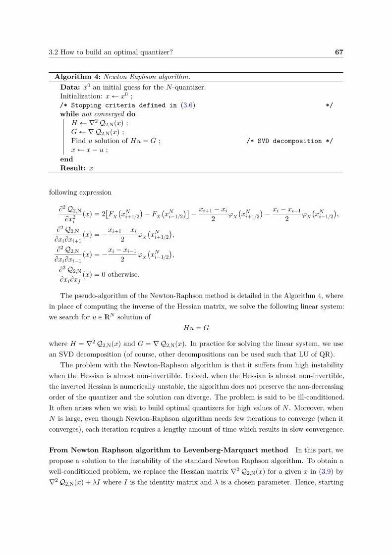
3.2 How to build an optimal quantizer? 67
Algorithm 4: Newton Raphson algorithm.Data: x0 an initial guess for the N -quantizer.Initialization: x Ð x0 ;/* Stopping criteria defined in (3.6) */while not converged do
H Ð ∇2 Q2,Npxq ;G Ð ∇ Q2,Npxq ;Find u solution of Hu “ G ; /* SVD decomposition */x Ð x´ u ;
endResult: x
following expression
B2 Q2,NBx2
i
pxq “ 2“
FX
`
xNi`12˘
´ FX
`
xNi´12˘‰
´xi`1 ´ xi
2 φX
`
xNi`12˘
´xi ´ xi´1
2 φX
`
xNi´12˘
,
B2 Q2,NBxiBxi`1
pxq “ ´xi`1 ´ xi
2 φX
`
xNi`12˘
,
B2 Q2,NBxiBxi´1
pxq “ ´xi ´ xi´1
2 φX
`
xNi´12˘
,
B2 Q2,NBxiBxj
pxq “ 0 otherwise.
The pseudo-algorithm of the Newton-Raphson method is detailed in the Algorithm 4, wherein place of computing the inverse of the Hessian matrix, we solve the following linear system:we search for u P RN solution of
Hu “ G
where H “ ∇2 Q2,Npxq and G “ ∇ Q2,Npxq. In practice for solving the linear system, we usean SVD decomposition (of course, other decompositions can be used such that LU of QR).
The problem with the Newton-Raphson algorithm is that it suffers from high instabilitywhen the Hessian is almost non-invertible. Indeed, when the Hessian is almost non-invertible,the inverted Hessian is numerically unstable, the algorithm does not preserve the non-decreasingorder of the quantizer and the solution can diverge. The problem is said to be ill-conditioned.It often arises when we wish to build optimal quantizers for high values of N . Moreover, whenN is large, even though Newton-Raphson algorithm needs few iterations to converge (when itconverges), each iteration requires a lengthy amount of time which results in slow convergence.
From Newton Raphson algorithm to Levenberg-Marquart method In this part, wepropose a solution to the instability of the standard Newton Raphson algorithm. To obtain awell-conditioned problem, we replace the Hessian matrix ∇2 Q2,Npxq for a given x in (3.9) by∇2 Q2,Npxq ` λI where I is the identity matrix and λ is a chosen parameter. Hence, starting
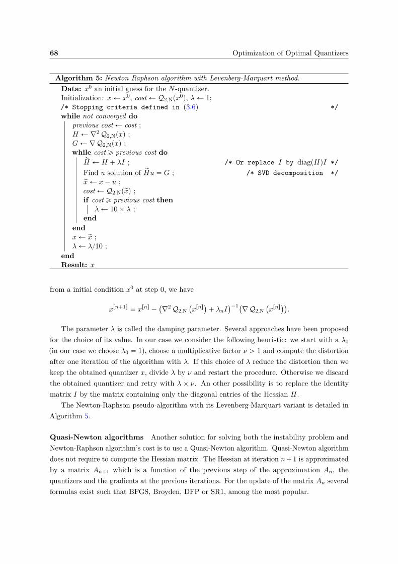
68 Optimization of Optimal Quantizers
Algorithm 5: Newton Raphson algorithm with Levenberg-Marquart method.Data: x0 an initial guess for the N -quantizer.Initialization: x Ð x0, cost Ð Q2,Npx0q, λ Ð 1;/* Stopping criteria defined in (3.6) */while not converged do
previous cost Ð cost ;H Ð ∇2 Q2,Npxq ;G Ð ∇ Q2,Npxq ;while cost ě previous cost do
rH Ð H ` λI ; /* Or replace I by diagpHqI */Find u solution of rHu “ G ; /* SVD decomposition */rx Ð x´ u ;cost Ð Q2,Nprxq ;if cost ě previous cost then
λ Ð 10 ˆ λ ;end
endx Ð rx ;λ Ð λ10 ;
endResult: x
from a initial condition x0 at step 0, we have
xrn`1s “ xrns ´`
∇2 Q2,N`
xrns˘
` λnI˘´1`∇ Q2,N
`
xrns˘˘
.
The parameter λ is called the damping parameter. Several approaches have been proposedfor the choice of its value. In our case we consider the following heuristic: we start with a λ0
(in our case we choose λ0 “ 1), choose a multiplicative factor ν ą 1 and compute the distortionafter one iteration of the algorithm with λ. If this choice of λ reduce the distortion then wekeep the obtained quantizer x, divide λ by ν and restart the procedure. Otherwise we discardthe obtained quantizer and retry with λ ˆ ν. An other possibility is to replace the identitymatrix I by the matrix containing only the diagonal entries of the Hessian H.
The Newton-Raphson pseudo-algorithm with its Levenberg-Marquart variant is detailed inAlgorithm 5.
Quasi-Newton algorithms Another solution for solving both the instability problem andNewton-Raphson algorithm’s cost is to use a Quasi-Newton algorithm. Quasi-Newton algorithmdoes not require to compute the Hessian matrix. The Hessian at iteration n` 1 is approximatedby a matrix An`1 which is a function of the previous step of the approximation An, thequantizers and the gradients at the previous iterations. For the update of the matrix An severalformulas exist such that BFGS, Broyden, DFP or SR1, among the most popular.
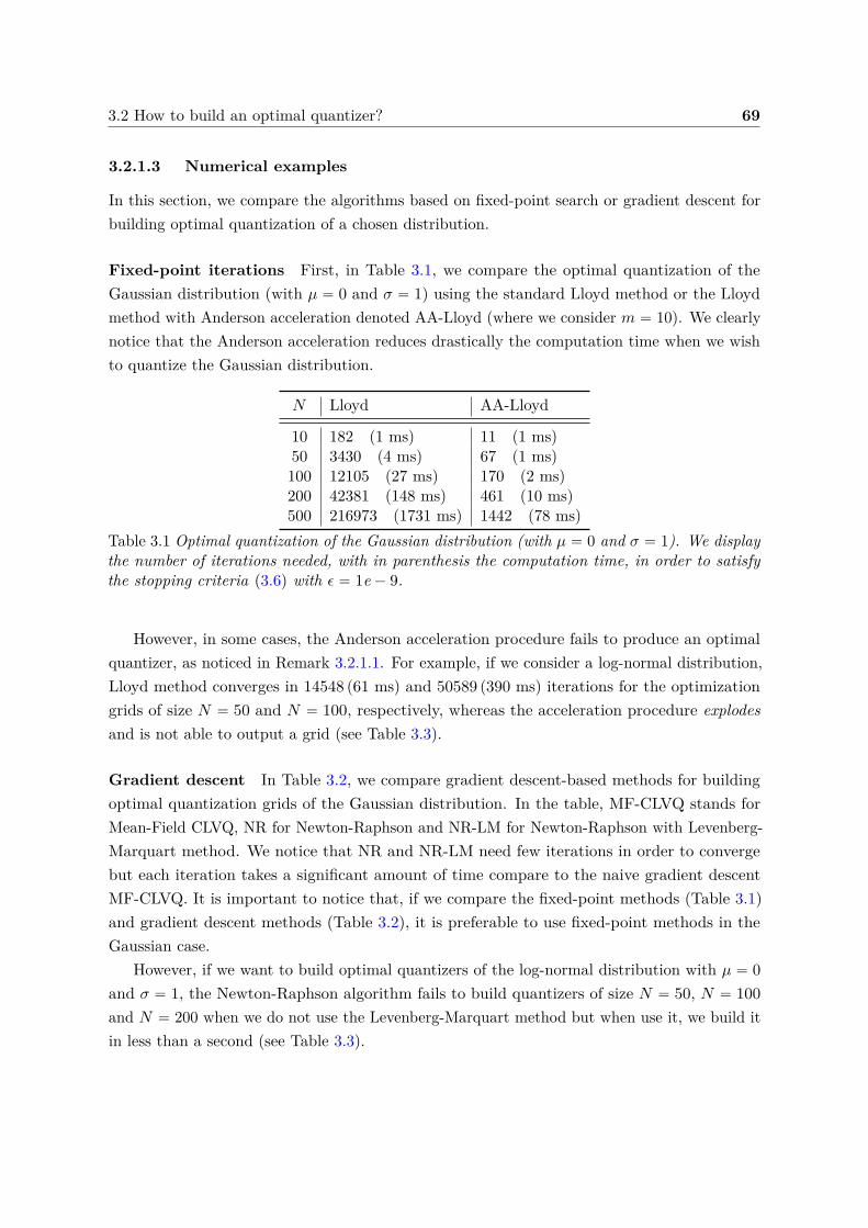
3.2 How to build an optimal quantizer? 69
3.2.1.3 Numerical examples
In this section, we compare the algorithms based on fixed-point search or gradient descent forbuilding optimal quantization of a chosen distribution.
Fixed-point iterations First, in Table 3.1, we compare the optimal quantization of theGaussian distribution (with µ “ 0 and σ “ 1) using the standard Lloyd method or the Lloydmethod with Anderson acceleration denoted AA-Lloyd (where we consider m “ 10). We clearlynotice that the Anderson acceleration reduces drastically the computation time when we wishto quantize the Gaussian distribution.
N Lloyd AA-Lloyd
10 182 p1 msq 11 p1 msq
50 3430 p4 msq 67 p1 msq
100 12105 p27 msq 170 p2 msq
200 42381 p148 msq 461 p10 msq
500 216973 p1731 msq 1442 p78 msq
Table 3.1 Optimal quantization of the Gaussian distribution (with µ “ 0 and σ “ 1). We displaythe number of iterations needed, with in parenthesis the computation time, in order to satisfythe stopping criteria (3.6) with ϵ “ 1e ´ 9.
However, in some cases, the Anderson acceleration procedure fails to produce an optimalquantizer, as noticed in Remark 3.2.1.1. For example, if we consider a log-normal distribution,Lloyd method converges in 14548 p61 msq and 50589 p390 msq iterations for the optimizationgrids of size N “ 50 and N “ 100, respectively, whereas the acceleration procedure explodesand is not able to output a grid (see Table 3.3).
Gradient descent In Table 3.2, we compare gradient descent-based methods for buildingoptimal quantization grids of the Gaussian distribution. In the table, MF-CLVQ stands forMean-Field CLVQ, NR for Newton-Raphson and NR-LM for Newton-Raphson with Levenberg-Marquart method. We notice that NR and NR-LM need few iterations in order to convergebut each iteration takes a significant amount of time compare to the naive gradient descentMF-CLVQ. It is important to notice that, if we compare the fixed-point methods (Table 3.1)and gradient descent methods (Table 3.2), it is preferable to use fixed-point methods in theGaussian case.
However, if we want to build optimal quantizers of the log-normal distribution with µ “ 0and σ “ 1, the Newton-Raphson algorithm fails to build quantizers of size N “ 50, N “ 100and N “ 200 when we do not use the Levenberg-Marquart method but when use it, we build itin less than a second (see Table 3.3).
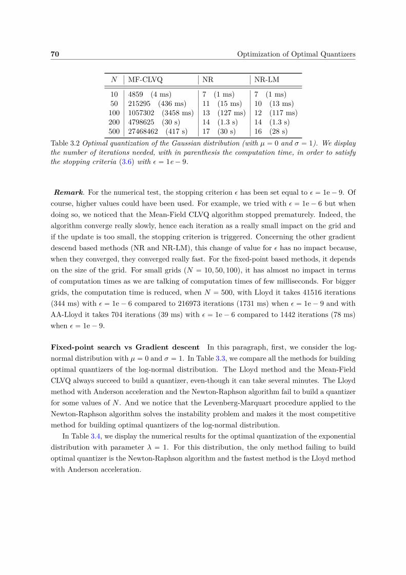
70 Optimization of Optimal Quantizers
N MF-CLVQ NR NR-LM
10 4859 p4 msq 7 p1 msq 7 p1 msq
50 215295 p436 msq 11 p15 msq 10 p13 msq
100 1057302 p3458 msq 13 p127 msq 12 p117 msq
200 4798625 p30 sq 14 p1.3 sq 14 p1.3 sq
500 27468462 p417 sq 17 p30 sq 16 p28 sq
Table 3.2 Optimal quantization of the Gaussian distribution (with µ “ 0 and σ “ 1). We displaythe number of iterations needed, with in parenthesis the computation time, in order to satisfythe stopping criteria (3.6) with ϵ “ 1e ´ 9.
Remark. For the numerical test, the stopping criterion ϵ has been set equal to ϵ “ 1e ´ 9. Ofcourse, higher values could have been used. For example, we tried with ϵ “ 1e ´ 6 but whendoing so, we noticed that the Mean-Field CLVQ algorithm stopped prematurely. Indeed, thealgorithm converge really slowly, hence each iteration as a really small impact on the grid andif the update is too small, the stopping criterion is triggered. Concerning the other gradientdescend based methods (NR and NR-LM), this change of value for ϵ has no impact because,when they converged, they converged really fast. For the fixed-point based methods, it dependson the size of the grid. For small grids (N “ 10, 50, 100), it has almost no impact in termsof computation times as we are talking of computation times of few milliseconds. For biggergrids, the computation time is reduced, when N “ 500, with Lloyd it takes 41516 iterationsp344 msq with ϵ “ 1e ´ 6 compared to 216973 iterations p1731 msq when ϵ “ 1e ´ 9 and withAA-Lloyd it takes 704 iterations p39 msq with ϵ “ 1e ´ 6 compared to 1442 iterations p78 msq
when ϵ “ 1e ´ 9.
Fixed-point search vs Gradient descent In this paragraph, first, we consider the log-normal distribution with µ “ 0 and σ “ 1. In Table 3.3, we compare all the methods for buildingoptimal quantizers of the log-normal distribution. The Lloyd method and the Mean-FieldCLVQ always succeed to build a quantizer, even-though it can take several minutes. The Lloydmethod with Anderson acceleration and the Newton-Raphson algorithm fail to build a quantizerfor some values of N . And we notice that the Levenberg-Marquart procedure applied to theNewton-Raphson algorithm solves the instability problem and makes it the most competitivemethod for building optimal quantizers of the log-normal distribution.
In Table 3.4, we display the numerical results for the optimal quantization of the exponentialdistribution with parameter λ “ 1. For this distribution, the only method failing to buildoptimal quantizer is the Newton-Raphson algorithm and the fastest method is the Lloyd methodwith Anderson acceleration.
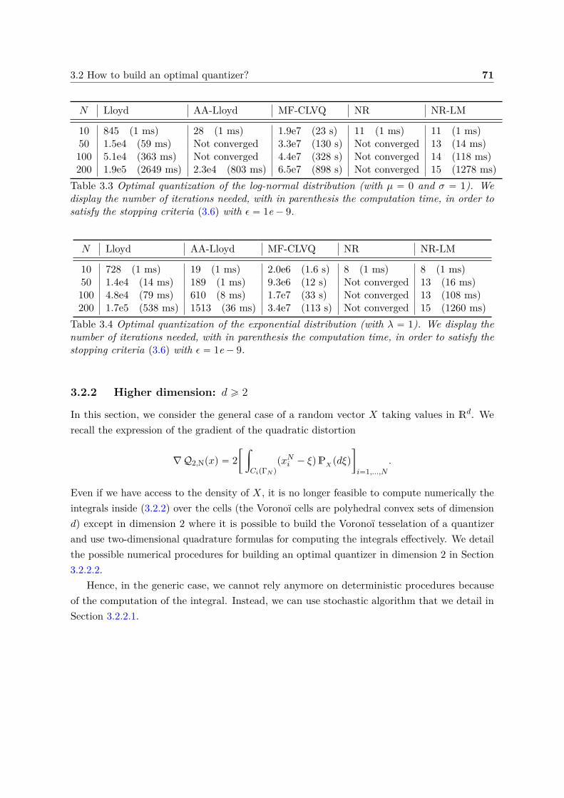
3.2 How to build an optimal quantizer? 71
N Lloyd AA-Lloyd MF-CLVQ NR NR-LM
10 845 p1 msq 28 p1 msq 1.9e7 p23 sq 11 p1 msq 11 p1 msq
50 1.5e4 p59 msq Not converged 3.3e7 p130 sq Not converged 13 p14 msq
100 5.1e4 p363 msq Not converged 4.4e7 p328 sq Not converged 14 p118 msq
200 1.9e5 p2649 msq 2.3e4 p803 msq 6.5e7 p898 sq Not converged 15 p1278 msq
Table 3.3 Optimal quantization of the log-normal distribution (with µ “ 0 and σ “ 1). Wedisplay the number of iterations needed, with in parenthesis the computation time, in order tosatisfy the stopping criteria (3.6) with ϵ “ 1e ´ 9.
N Lloyd AA-Lloyd MF-CLVQ NR NR-LM
10 728 p1 msq 19 p1 msq 2.0e6 p1.6 sq 8 p1 msq 8 p1 msq
50 1.4e4 p14 msq 189 p1 msq 9.3e6 p12 sq Not converged 13 p16 msq
100 4.8e4 p79 msq 610 p8 msq 1.7e7 p33 sq Not converged 13 p108 msq
200 1.7e5 p538 msq 1513 p36 msq 3.4e7 p113 sq Not converged 15 p1260 msq
Table 3.4 Optimal quantization of the exponential distribution (with λ “ 1). We display thenumber of iterations needed, with in parenthesis the computation time, in order to satisfy thestopping criteria (3.6) with ϵ “ 1e ´ 9.
3.2.2 Higher dimension: d ě 2
In this section, we consider the general case of a random vector X taking values in Rd. Werecall the expression of the gradient of the quadratic distortion
∇ Q2,Npxq “ 2„ż
CipΓN q
pxNi ´ ξqPX pdξq
ȷ
i“1,...,N.
Even if we have access to the density of X, it is no longer feasible to compute numerically theintegrals inside (3.2.2) over the cells (the Voronoï cells are polyhedral convex sets of dimensiond) except in dimension 2 where it is possible to build the Voronoï tesselation of a quantizerand use two-dimensional quadrature formulas for computing the integrals effectively. We detailthe possible numerical procedures for building an optimal quantizer in dimension 2 in Section3.2.2.2.
Hence, in the generic case, we cannot rely anymore on deterministic procedures becauseof the computation of the integral. Instead, we can use stochastic algorithm that we detail inSection 3.2.2.1.
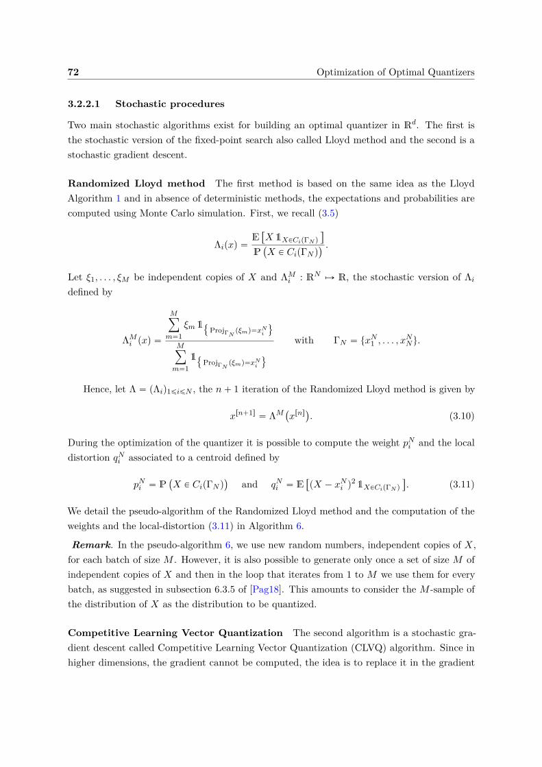
72 Optimization of Optimal Quantizers
3.2.2.1 Stochastic procedures
Two main stochastic algorithms exist for building an optimal quantizer in Rd. The first isthe stochastic version of the fixed-point search also called Lloyd method and the second is astochastic gradient descent.
Randomized Lloyd method The first method is based on the same idea as the LloydAlgorithm 1 and in absence of deterministic methods, the expectations and probabilities arecomputed using Monte Carlo simulation. First, we recall (3.5)
Λipxq “E“
X 1XPCipΓN q
‰
P`
X P CipΓN q˘ .
Let ξ1, . . . , ξM be independent copies of X and ΛMi : RN ÞÑ R, the stochastic version of Λi
defined by
ΛMi pxq “
Mÿ
m“1ξm 1ProjΓN
pξmq“xNi
(
Mÿ
m“11
ProjΓNpξmq“xN
i
(
with ΓN “ txN1 , . . . , xNNu.
Hence, let Λ “ pΛiq1ďiďN , the n` 1 iteration of the Randomized Lloyd method is given by
xrn`1s “ ΛM`
xrns˘
. (3.10)
During the optimization of the quantizer it is possible to compute the weight pNi and the localdistortion qNi associated to a centroid defined by
pNi “ P`
X P CipΓN q˘
and qNi “ E“
pX ´ xNi q2 1XPCipΓN q
‰
. (3.11)
We detail the pseudo-algorithm of the Randomized Lloyd method and the computation of theweights and the local-distortion (3.11) in Algorithm 6.
Remark. In the pseudo-algorithm 6, we use new random numbers, independent copies of X,for each batch of size M . However, it is also possible to generate only once a set of size M ofindependent copies of X and then in the loop that iterates from 1 to M we use them for everybatch, as suggested in subsection 6.3.5 of [Pag18]. This amounts to consider the M -sample ofthe distribution of X as the distribution to be quantized.
Competitive Learning Vector Quantization The second algorithm is a stochastic gra-dient descent called Competitive Learning Vector Quantization (CLVQ) algorithm. Since inhigher dimensions, the gradient cannot be computed, the idea is to replace it in the gradient
3.2 How to build an optimal quantizer? 73
Algorithm 6: Randomized Lloyd method.Data: x0 an initial guess for the N -quantizer, M : number of copies of X to generate.Initialization: x Ð x0;/* Vector of size N of probabilities init with 0 P R */Initialization: p Ð 0 ;/* Vector of size N of local-distortions init with 0 P R */Initialization: q Ð 0 ;/* Vector of size N for the sum in numerator of (3.10) init with 0 P Rd
*/Initialization: sum_nearest Ð 0 ;/* Stopping criteria defined in (3.6) */while not converged do
for m “ 1 to M by 1 do/* Generate an iid copy of X */ξ Ð randomGenerationpq ;/* Return the index and the distance to the closest centroid of ξ
*/i, dist Ð closest_centroidpx, ξ, dist, iq ;ppiq Ð ppiq ` 1;sum_nearestpiq Ð sum_nearestpiq ` ξ;qpiq Ð qpiq ` pdistq2 ;
endfor i “ 1 to N by 1 do
xpiq Ð sum_nearestpiqppiq ;ppiq Ð ppiqM ;qpiq Ð qpiqM ;
endendResult: x, p, q
74 Optimization of Optimal Quantizers
Algorithm 7: Competitive Learning Vector Quantization (CLVQ) algorithm.Data: x0 an initial guess for the N -quantizer, M : number of copies of X to generate.Initialization: x Ð x0;/* Vector of size N of probabilities init with 0 P R */Initialization: p Ð 0 ;/* Vector of size N of local-distortions init with 0 P R */Initialization: q Ð 0 ;Initialization: n Ð 0 ; /* Counter *//* Stopping criteria defined in (3.6) */while not converged do
/* Generate an iid copy of X */ξ Ð randomGenerationpq ;γ Ð update_steppγq ;/* Return the index and the distance to the closest centroid of ξ */i, dist Ð closest_centroidpx, ξ, dist, indexq ;xpiq Ð p1 ´ γqxpiq ` γ ξ ;ppiq Ð ppiq ` 1;qpiq Ð qpiq ` pdistq2 ;n Ð n` 1 ;
endfor i “ 1 to N by 1 do
ppiq Ð ppiqn ;qpiq Ð qpiqn ;
endResult: x, p, q
descent by the local-gradient defined in (3.2). Let ξ1, . . . , ξn, . . . a sequence of independentcopies of X, the n` 1 iterate of the CLVQ algorithm is given by
xrn`1s “ xrns ´ γn`1∇ q2,Npxrns, ξn`1q
where ∇ q2,N “
´
B q2,NBxN
i
¯
1ďiďNand for the choice on the learning rate we refer to the section 6.3.5
in [Pag18]. Again, during optimization we can compute the weights pNi and the local distortionsqNi associated to the centroids. We detail the pseudo-algorithm of the CLVQ algorithm and thecomputation of the weights and the local-distortion in Algorithm 7.
Remark. Two developments of the CLVQ algorithm can be considered.The first one consists in using the averaging algorithm of Rupper and Polyak, yielding the
averaged quantizer rxrn`1s defined by$
’
’
&
’
’
%
xrn`1s “ xrns ´ γn`1∇ q2,Npxrns, ξn`1q
rxrn`1s “1
n` 1
n`1ÿ
i“1xris.
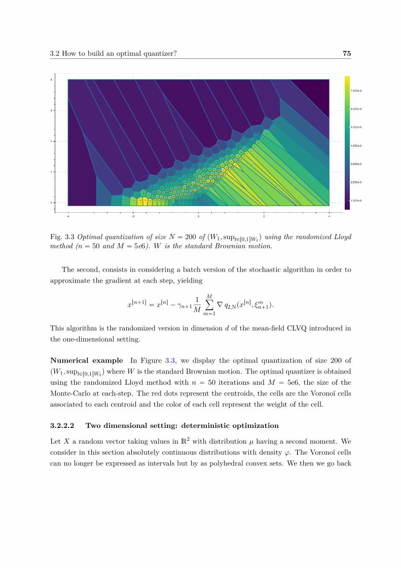
3.2 How to build an optimal quantizer? 75
Fig. 3.3 Optimal quantization of size N “ 200 of pW1, suptPr0,1sWtq using the randomized Lloyd
method (n “ 50 and M “ 5e6). W is the standard Brownian motion.
The second, consists in considering a batch version of the stochastic algorithm in order toapproximate the gradient at each step, yielding
xrn`1s “ xrns ´ γn`11M
Mÿ
m“1∇ q2,Npxrns, ξmn`1q.
This algorithm is the randomized version in dimension d of the mean-field CLVQ introduced inthe one-dimensional setting.
Numerical example In Figure 3.3, we display the optimal quantization of size 200 ofpW1, suptPr0,1sWt
q where W is the standard Brownian motion. The optimal quantizer is obtainedusing the randomized Lloyd method with n “ 50 iterations and M “ 5e6, the size of theMonte-Carlo at each-step. The red dots represent the centroids, the cells are the Voronoï cellsassociated to each centroid and the color of each cell represent the weight of the cell.
3.2.2.2 Two dimensional setting: deterministic optimization
Let X a random vector taking values in R2 with distribution µ having a second moment. Weconsider in this section absolutely continuous distributions with density φ. The Voronoï cellscan no longer be expressed as intervals but by as polyhedral convex sets. We then we go back
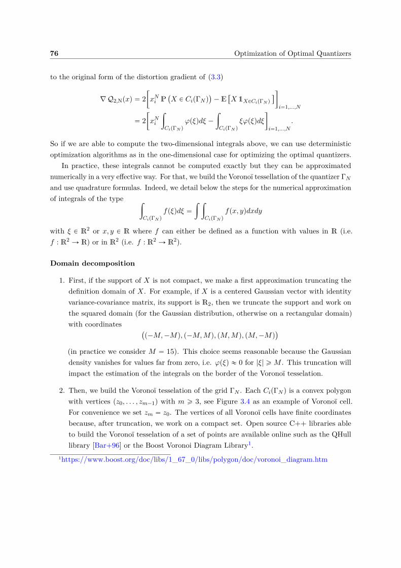
76 Optimization of Optimal Quantizers
to the original form of the distortion gradient of (3.3)
∇ Q2,Npxq “ 2„
xNi P`
X P CipΓN q˘
´ E“
X 1XPCipΓN q
‰
ȷ
i“1,...,N
“ 2„
xNi
ż
CipΓN q
φpξqdξ ´
ż
CipΓN q
ξφpξqdξ
ȷ
i“1,...,N.
So if we are able to compute the two-dimensional integrals above, we can use deterministicoptimization algorithms as in the one-dimensional case for optimizing the optimal quantizers.
In practice, these integrals cannot be computed exactly but they can be approximatednumerically in a very effective way. For that, we build the Voronoï tessellation of the quantizer ΓNand use quadrature formulas. Indeed, we detail below the steps for the numerical approximationof integrals of the type
ż
CipΓN q
fpξqdξ “
ż ż
CipΓN q
fpx, yqdxdy
with ξ P R2 or x, y P R where f can either be defined as a function with values in R (i.e.f : R2 Ñ R) or in R2 (i.e. f : R2 Ñ R2).
Domain decomposition
1. First, if the support of X is not compact, we make a first approximation truncating thedefinition domain of X. For example, if X is a centered Gaussian vector with identityvariance-covariance matrix, its support is R2, then we truncate the support and work onthe squared domain (for the Gaussian distribution, otherwise on a rectangular domain)with coordinates
`
p´M,´Mq, p´M,Mq, pM,Mq, pM,´Mq˘
(in practice we consider M “ 15). This choice seems reasonable because the Gaussiandensity vanishes for values far from zero, i.e. φpξq « 0 for |ξ| ě M . This truncation willimpact the estimation of the integrals on the border of the Voronoï tesselation.
2. Then, we build the Voronoï tesselation of the grid ΓN . Each CipΓN q is a convex polygonwith vertices pz0, . . . , zm´1q with m ě 3, see Figure 3.4 as an example of Voronoï cell.For convenience we set zm “ z0. The vertices of all Voronoï cells have finite coordinatesbecause, after truncation, we work on a compact set. Open source C++ libraries ableto build the Voronoï tesselation of a set of points are available online such as the QHulllibrary [Bar+96] or the Boost Voronoi Diagram Library1.
1https://www.boost.org/doc/libs/1_67_0/libs/polygon/doc/voronoi_diagram.htm
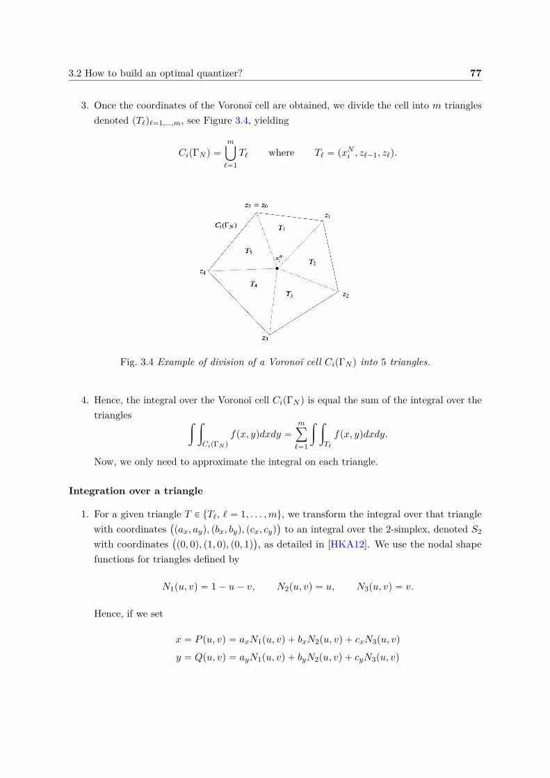
3.2 How to build an optimal quantizer? 77
3. Once the coordinates of the Voronoï cell are obtained, we divide the cell into m trianglesdenoted pTℓqℓ“1,...,m, see Figure 3.4, yielding
CipΓN q “
mď
ℓ“1Tℓ where Tℓ “ pxNi , zℓ´1, zℓq.
Fig. 3.4 Example of division of a Voronoï cell CipΓN q into 5 triangles.
4. Hence, the integral over the Voronoï cell CipΓN q is equal the sum of the integral over thetriangles
ż ż
CipΓN q
fpx, yqdxdy “
mÿ
ℓ“1
ż ż
Tℓ
fpx, yqdxdy.
Now, we only need to approximate the integral on each triangle.
Integration over a triangle
1. For a given triangle T P tTℓ, ℓ “ 1, . . . ,mu, we transform the integral over that trianglewith coordinates
`
pax, ayq, pbx, byq, pcx, cyq˘
to an integral over the 2-simplex, denoted S2
with coordinates`
p0, 0q, p1, 0q, p0, 1q˘
, as detailed in [HKA12]. We use the nodal shapefunctions for triangles defined by
N1pu, vq “ 1 ´ u´ v, N2pu, vq “ u, N3pu, vq “ v.
Hence, if we set
x “ P pu, vq “ axN1pu, vq ` bxN2pu, vq ` cxN3pu, vq
y “ Qpu, vq “ ayN1pu, vq ` byN2pu, vq ` cyN3pu, vq
78 Optimization of Optimal Quantizers
we haveż ż
Tfpx, yqdxdy “ 2AT
ż ż
S2
f`
P pu, vq, Qpu, vq˘
dudv
where AT is the area of the triangle T
AT “ˇ
ˇpbx ´ axqpcy ´ ayq ´ pcx ´ axqpby ´ ayqˇ
ˇ.
2. Now, we use a quadrature formula of degree n for general triangular elements which yieldsż ż
Tfpx, yqdxdy « AT
ÿ
k
ωkf`
P puk, vkq, Qpuk, vkq˘
where the points puk, vkq and the weights ωk are provided by the quadrature of order n forthe standard triangles as suggested in [Den10] (we considered Gaussian quadrature pointsfor the optimal quantization of Gaussian random vector but any quadrature formula canbe used in order to build an optimal quantizer of a chosen random vector X).
Fixed-point search Now, that we are able to evaluate the quantities inside the gradientof the distortion, as in the scalar case, we can implement a fixed-point search using theLloyd Algorithm 1 with this time the fixed-point operator Λ : pR2qN Ñ pR2qN defined asΛ “ pΛiq1ďiďN defined by
Λipxq “E“
X 1XPCipΓN q
‰
P`
X P CipΓN q˘ “
ż
CipΓN q
ξφpξqdξ
ż
CipΓN q
φpξqdξ.
Hence, starting from an initial condition x0 we can apply the Algorithm 1 with Λ definedabove where the integrals are approximated using the methodology detailed above.
Gradient descent Again, using that for a given quantizer x “ pxN1 , . . . , xNN q we are able to
compute the gradient of the distortion, we can apply the mean-field CLVQ gradient descentAlgorithm 3 using the following expression for the gradient
∇ Q2,Npxq “ 2„
xNi
ż
CipΓN q
φpξqdξ ´
ż
CipΓN q
ξφpξqdξ
ȷ
i“1,...,N.
Numerical example We apply this methodology for building optimal quantizers of thetwo-dimensional Gaussian random vector N p0, I2q where I2 is the identity matrix. We use theknowledge of the density, set M “ 15 (the value of the squared domain coordinates) and applythe Lloyd method. We display two optimal quantizations of size 100 and 200.
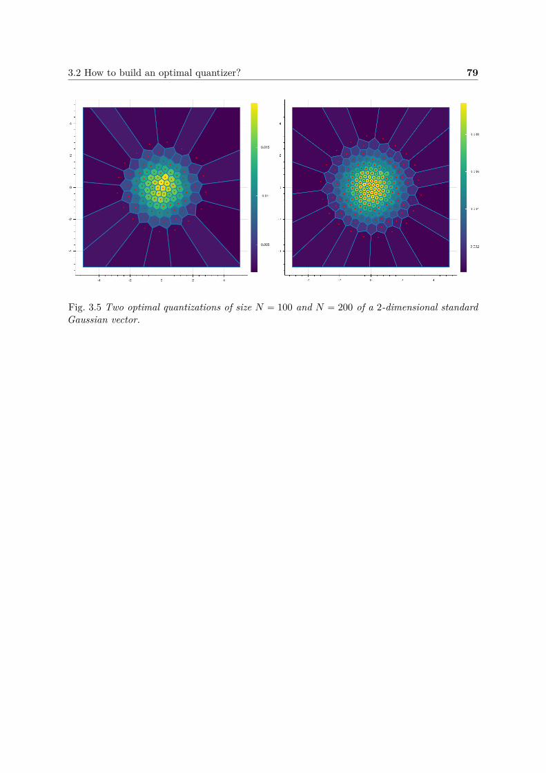
3.2 How to build an optimal quantizer? 79
Fig. 3.5 Two optimal quantizations of size N “ 100 and N “ 200 of a 2-dimensional standardGaussian vector.
80 Optimization of Optimal Quantizers
Appendix 3.A Proof for the formulas of FX
and KX
Supremum of the Brownian bridge Let X “ suptPr0,1s |Wt ´ tW1| denotes the supremumof the standard Brownian bridge. This distribution is also known as the Kolmogorov-Smirnovdistribution. Let x ě 0, the distribution is characterized by its survival function
PpX ě xq “ 2ÿ
kě1p´1qk´1 e´2k2x2
.
The cumulative distribution function is given by FX pxq “ 1 ´ PpX ě xq, then
FX pxq “ 1 ´ 2ÿ
kě1p´1qk´1 e´2k2x2
.
In order to obtain the density φX , we compute the derivative of FX
φX pxq “BFX pxq
Bx“ 8x
ÿ
kě1p´1qk´1k2 e´2k2x2
,
yielding the desired formula.Now, using the definition of the cumulated partial first moment function KX of X
KX pxq “ E“
X 1Xďx
‰
“
ż x
0ξφX pξqdξ
“ xFX pxq ´
ż x
0FX pξqdξ
“ x´
1 ´ 2ÿ
kě1p´1qk´1 e´2k2x2
¯
´
ż x
0
´
1 ´ 2ÿ
kě1p´1qk´1 e´2k2ξ2
¯
dξ
“ ´x`
1 ´ FX pxq˘
` 2ÿ
kě1p´1qk´1
ż x
0e´2k2ξ2
dξ.
Moreover, asż x
0e´2k2ξ2
dξ “
ż 2kx
0e´ξ22 dξ
2k ,
we haveKX pxq “ 2
ÿ
kě1p´1qk´1
ż 2kx
0e´ξ22 dξ
2k ´ x`
1 ´ FX pxq˘
“?
2πÿ
kě1
p´1qk´1
k
´
N p2kxq ´12
¯
´ x`
1 ´ FX pxq˘
,
which concludes the proof.
Symmetric random variable Let X be a symmetric random variable with characteristicfunction χpuq “ E
“
eiuX ‰
, where i is the imaginary number, s.t. i2 “ ´1. As X is symmetric,
3.A Proof for the formulas of FX and KX 81
the characteristic function is χ is real-valued and even: χpuq “ E“
eiuX ‰
“ E“
e´iuX ‰
“ χp´uq.Let x ą 0.
• First, we express the density of X as an alternate series and show that it is even. Bydefinition, φX pxq “ 1
2πş
Reixu χpuqdu and we deduce that the density is even
φX p´xq “1
2π
ż
R
eixu χpuqdu
“ ´1
2π
ż ´8
`8
e´ixv χp´vqdv pv “ ´uq
“1
2π
ż
R
e´ixv χpvqdv “ φX pxq.
ThenφX pxq “
12π
ż
R
eixu χpuqdu “1π
ż `8
0eixu χpuqdu
andφX p0q “
1π
ż `8
0χpuqdu.
Hence, we deduce the first desired expression of φX
φX pxq “φX pxq ` φX p´xq
2 “1
2π
ż `8
0
`
eixu ` e´ixu ˘χpuqdu
“1π
ż `8
0cospxuqχpuqdu
“1πx
ż `8
0cospvqχ
´v
x
¯
dv. pv “ uxq
From this expression, we express φX as an alternate series
φX pxq “1πx
ż `8
0cospuqχ
´u
x
¯
du
“1πx
ÿ
kě0
ż πpk`1q
πkcospuqχ
´u
x
¯
du
“1πx
ÿ
kě0p´1qk
ż π
0cospuqχ
´u` kπ
x
¯
du.
82 Optimization of Optimal Quantizers
• Now, we focus on the cumulative distribution function FX . As X is symmetric, thenFX p0q “ 1
2 and for every x ą 0
FX pxq “12 `
ż x
0φX pξqdξ
“12 `
ż x
0
1π
ż `8
0cospξuqχpuqdudξ
“12 `
1π
ż `8
0
´
ż x
0cospξuqdξ
¯
χpuqdu
“12 `
1π
ż `8
0
sinpxuq
uχpuqdu
“12 `
1π
ż `8
0
sinpvq
vχ´v
x
¯
dv. pv “ uxq
Then, we deduce FX p´xq
FX p´xq “
ż ´x
´8
φX pξqdξ “ 1 ´
ż 8
´xφX pξqdξ
“12 ´
ż 0
´xφX pξqdξ “
12 ´
ż x
0φX pξqdξ
“ 1 ´ FX pxq.
Finally, we express FX as an alternate series using the same argument as for the density
FX pxq “12 `
1π
ż `8
0
sinpuq
uχ´u
x
¯
du
“12 `
1π
ÿ
kě0p´1qk
ż π
0
sinpuq
u` kπχ´u` kπ
x
¯
du.
• Next, we focus on the first partial moment function KX . Let x ą 0, first, we show that KX
is even
KX pxq “
ż x
´8
ξφX pξqdξ
“ KX p´xq `
ż x
´xξφX pξqdξ
“ KX p´xq `
ż 0
´xuφX puqdu`
ż x
0vφX pvqdv
“ KX p´xq ´
ż ´x
0uφX puqdu`
ż x
0vφX pvqdv
“ KX p´xq ´
ż x
0wφX p´wqdw `
ż x
0vφX pvqdv pw “ ´uq
“ KX p´xq
3.A Proof for the formulas of FX and KX 83
because φX is even. Moreover,
KX p0q “
ż 0
´8
ξφX pξqdξ “ ´
ż 8
0ξφX pξqdξ “ ´
ż
R
ξφX pξq1ξą0 dξ “ ´ErX`s.
Now, we express KX as an alternate series
KX pxq “ ´ErX`s `
ż x
0ξφX pξqdξ
“ ´ErX`s ` xFX pxq ´
ż x
0FX pξqdξ
“ ´ErX`s ` xFX pxq ´
ż x
0
ˆ
12 `
1π
ż `8
0
sinpuξq
uχpuqdu
˙
dξ
“ ´ErX`s ` x´
FX pxq ´12
¯
´1π
ż `8
0
´ cospuxq ` 1u
χpuq
udu
“ ´ErX`s ` x´
FX pxq ´12
¯
´x
π
ż `8
0
1 ´ cospvq
v2 χ´v
x
¯
dv. pv “ uxq
Finally, we express KX as an alternate series
KX pxq “ ´ErX`s ` x´
FX pxq ´12
¯
´x
π
ż `8
0
1 ´ cospuq
u2 χ´u
x
¯
du
“ ´ErX`s ` x´
FX pxq ´12
¯
´x
π
ÿ
kě0
ż π
0
1 ´ p´1qk cospuq
pu` kπq2 χ´u` kπ
x
¯
du.

Chapter 4
New Weak Error bounds andexpansions for Optimal Quantization
This chapter corresponds to the article “New Weak Error bounds and expansions for OptimalQuantization” published in Journal of Computational and Applied Mathematics (see [LMP19]).This paper is a joint work with Vincent Lemaire and Gilles Pagès and it is accessible in arXivor HAL.
Abstract We propose new weak error bounds and expansion in dimension one for optimalquantization-based cubature formula for different classes of functions, such that piecewiseaffine functions, Lipschitz convex functions or differentiable function with piecewise-definedlocally Lipschitz or α-Hölder derivatives. These new results rest on the local behaviours ofoptimal quantizers, the Lr-Ls distribution mismatch problem and Zador’s Theorem. This newexpansion supports the definition of a Richardson-Romberg extrapolation yielding a better rateof convergence for the cubature formula. An extension of this expansion is then proposed inhigher dimension for the first time. We then propose a novel variance reduction method forMonte Carlo estimators, based on one dimensional optimal quantizers.
Introduction
Optimal quantization was first introduced in [She97], Sheppard worked on optimal quantizationof the uniform distribution on unit hypercubes. It was then extended to more general distribu-tions with applications to Signal transmission at the Bell Laboratory in the 50’s (see [GG82])and then developed as a numerical method in the early 90’s, for expectation approximations(see [Pag98]) and later for conditional expectation approximations (see [PPP04b; BPP01; BP03;BPP05]).
In modern terms, vector quantization consists in finding the projection for the Lp-Wassersteindistance of a probability measure on Rd with a finite p-th moment on the convex subset of
86 New Weak Error bounds and expansions for Optimal Quantization
Γ-supported probability measure, where Γ is a finite subset of Rd and 0 ă p ă `8. The aimof Optimal Quantization is to determine the set ΓN :“ txN1 , . . . , x
NNu Ă Rd with cardinality
at most N which minimizes this distance among all such sets Γ. Formally, if we consider arandom vector X P LppPq, we search for ΓN , the solution to the following problem
minΓN ĂR,|ΓN |ďN
X ´ pXΓN p
where pXΓN denotes the projection of X onto ΓN (often pXΓN is denoted by pXN in order toalleviate the notations). The term X ´ pXΓN p is often referred to as the distortion of order p.The existence of an optimal quantizer at a given level N has been shown in [GL00; Pag98] andin the one-dimensional case if the distribution of X is absolutely continuous with a log-concavedensity then there exists a unique optimal quantizer at level N . In the present paper we willconsider one dimensional optimal quantizers. Moreover, we are not only interested by theexistence of such a quantizer but also in the asymptotic behaviour of the distortion because itis an important feature for the method in order to determine the level of the error introducedby the approximation. The question concerning the sharp rate of convergence of X ´ pXNp
as N goes to infinity is answered by Zador’s Theorem. For X P Lp`δpPq, δ ą 0, such thatPX pdξq “ φpξq ¨ λpdξq ` νpdξq, where ν K λ is the singular component of PX with respect tothe Lebesgue measure λ on Rd, the rate of convergence is given by
limNÑ`8
N1d X ´ pXNp “ rJp,d
„ż
Rdφ
dd`pdλd
ȷ1p
` 1d
where φ is the density of X, λd is the Lebesgue measure on Rd and rJp,d “ infNě1N1d U´ pUNp ,
UL„ U
`
p0, 1qd˘
. For more insights on the mathematical/probabilistic aspects of Optimalquantization theory, we refer to [GL00; Pag15].
The reason for which we are interested in this optimal quantizer is numerical integration.The discrete feature of the optimal quantizer pXN allows us to define, for every continuousfunction f : Rd ÝÑ R, such that fpXq P L2pPq, the following quantization-based cubatureformula
E“
fp pXN q‰
“
Nÿ
i“1pifpxNi q
where pi “ Pp pXN “ xNi q. Indeed, as pXN is constructed as the best discrete approximationof X in LppPq, it is reasonable to approximate E
“
fpXq‰
by E“
fp pXN q‰
which is useful fornumerical integrations problems.
The problem of numerical integration appears a lot in applied fields, such as Physics,Computer Sciences or Numerical Probability. For example, in Quantitative Finance, many
87
quantities of interest are of the form
E“
fpStq‰
for some t ą 0,
where f : Rd ÝÑ R is a Borel function and pSsqsPr0,ts is a diffusion process solution to aStochastic Differential Equation (SDE)
St “ S0 `
ż t
0bps, Ssqds`
ż t
0σps, SsqdWs, S0 “ s0,
where W is a standard Brownian motion living on a probability space pΩ,A,Pq and b andσ are Lipschitz continuous in x uniformly with respect to s P r0, ts, which are the standardassumptions in order to ensure existence and uniqueness of a strong solution to the SDE. Sinceit is often impossible to compute E
“
fpStq‰
directly, it has been proposed in [Pag98] to computean optimal quantizer pXN of X where X is a random variable having the same distribution asSt and to use the previously defined quantization-based cubature formula as an approximation.
Another approach, often used in order to approximate E“
fpXq‰
, is to perform a MonteCarlo simulation pIM :“
řMm“1 fpXmq, where pXmqm“1,...,M is a sequence of independent copies
of X. The method’s rate of convergence is determined by the strong law of numbers and thecentral limit theorem, which says that if X is square integrable, then
?M
´
pIM ´ E“
fpXq‰
¯
LÝÑ N
`
0, σ2fpXq
˘
as M Ñ `8
where σ2fpXq
“ Var`
fpXq˘
. One notices that, for a given M , the limiting factor of the methodis σ2
fpXq. Hence, a lot of methods have been developed in order to reduce the variance term:
antithetic variables, control variates, importance sampling, etc. The reader can refer to [Pag18;Gla13] for more details concerning the Monte Carlo methodology and the variance reductionmethods.
In this paper we propose a novel variance reduction method of Monte Carlo estimatorthrough quantization. Our method innovates in that it uses a linear combination of onedimensional control variates to reduce the variance of a higher dimensional problem. Moreprecisely, we introduce a quantization-based control variates ΞNk for k “ 1, . . . , d. If oneconsiders a function f : Rd ÞÑ R, we approximate E
“
fpXq‰
by
E“
fpXq ´ xλ,ΞNy‰
with x¨, ¨y the scalar product in Rd and pΞNk qk“1,...,d :“ fkpXkq ´ E“
fkp pXNk q
‰
, where Xk is thek-th component of X, pXN
k is an optimal quantizer of Xk of size N and fk : R ÞÑ R is designedfrom f . Looking closely at the introduced control variates, one notices that we introduce abias in the approximation. However, as since it is closely linked to weak error, this bias can becontrolled. The present paper focuses on the weak error’s rate of convergence.
88 New Weak Error bounds and expansions for Optimal Quantization
First, we place ourselves in the case where X is a random variable in dimension one and weconsider a quadratic optimal quantizer. We work on the rate of convergence of the weak errorinduced by the expectation approximation by an optimal quantization-based cubature formulafor different classes of functions f
limNÑ`8
Nαˇ
ˇE“
fpXq‰
´ E“
fp pXN q‰ˇ
ˇ ď Cf,X ă `8.
The first classical result concerns Lipschitz continuous functions. Using directly the Lipschitzcontinuity property of f and Zador’s Theorem a rate of order α “ 1 can be obtained. Moreover,if we consider the supremum among all functions with a Lipschitz constant upper-bounded by1, then
N suprf s
Lipď1
ˇ
ˇE“
fpXq‰
´ E“
fp pXN q‰ˇ
ˇ “ NX ´ pXN1 ď NX ´ pXN2NÑ`8ÝÝÝÝÝÑ Cf ă `8.
A faster rate (α “ 2) can be attained for differentiable functions with Lipschitz continuousderivative, using a Taylor expansion with integral remainder and the following stationarityproperty of quadratic optimal quantizers
E“
X | pXN‰
“ pXN .
Moreover, considering the supremum among all functions where the Lipschitz constant of thederivative is upper-bounded by 1, we have
N2 suprf 1s
Lipď1
ˇ
ˇE“
fpXq‰
´ E“
fp pXN q‰ˇ
ˇ “12N
2X ´ pXN22NÑ`8ÝÝÝÝÝÑ Cf ă `8
where the limit is given by Zador’s Theorem. A detailed summary about this results can befound in [Pag18].
In the first part of this paper, we extend this improved rate (α “ 2) to classes of lesssmooths functions in one dimension. These new results enable us to design efficient variancereduction methods in higher dimensional settings with in view applications to option pricing.The new results concerns the following classes of functions
• Lipschitz continuous piecewise affine functions with finitely many breaks of affinity. Weuse the stationarity property of the optimal quantizer on the cells where there is no breakof affinity and then we control the error on the remaining cells using results on the localbehaviour of the quantizer.
• Lipschitz continuous convex functions, using local behaviours results on optimal quantizers.We use a representation formula for convex functions as integrals of Ridge functionscombined with the local behaviour result in order to control the error again.
89
• Differentiable functions with piecewise-defined locally Lipschitz derivative. The functionshave K breaks of affinity ta1, . . . , aKu, such that ´8 “ a0 ă a1 ă ¨ ¨ ¨ ă aK ă aK`1 “
`8 and the locally Lipschitz property of the derivative is defined by
@k “ 0, . . . ,K, @x, y P pak, ak`1q |f 1pxq ´ f 1pyq| ď rf 1sk,Lip,loc
|x´ y|`
gkpxq ` gkpyq˘
where gk : pak, ak`1q Ñ R` are non-negative Borel functions. We use the locally Lipschitzproperty of the derivative combined with the Lr-Ls distortion Theorem and Zador’sTheorem on the cells where there is no break of affinity and then we control the error onthe remaining cells using results on the local behaviour of the quantizer.
• Differentiable functions with piecewise-defined locally α-Hölder derivative. The functionshave K breaks of affinity ta1, . . . , aKu, such that ´8 “ a0 ă a1 ă ¨ ¨ ¨ ă aK ă aK`1 “
`8 and the locally α-Hölder property of the derivative is defined by
@k “ 0, . . . ,K, @x, y P pak, ak`1q, |f 1pxq ´ f 1pyq| ď rf 1sk,α,loc
|x´ y|α`
gkpxq ` gkpyq˘
where gk : pak, ak`1q Ñ R` are non-negative Borel functions. For this class of functions,the rate of convergence is of order 1 ` α. The result is obtained using the same ideas asin the locally Lipschitz case.
Hence, for all this classes of functions, except the last one, we have
limNÑ`8
N2ˇˇE
“
fpXq‰
´ E“
fp pXN q‰ˇ
ˇ ď Cf,X ă `8.
In the second part of the paper we deal with the weak error expansion of the approximationof E
“
fpXq‰
by E“
fp pXN q‰
. First, we place ourselves in the one dimensional case by consideringa twice differentiable function f : R ÞÑ R with a bounded Lipschitz continuous second derivativeand X : pΩ,A,Pq Ñ R. Through a second order Taylor expansion and with the help ofCorollary 4.1.7, Theorem 4.1.12 and the Lr-Ls distortion mismatch Theorem we obtain
E“
fpXq‰
“ E“
fp pXN q‰
`c2N2 `OpN´p2`βqq
where β P p0, 1q. This expression suggests to use a Richardson-Romberg extrapolation in orderto kill the first term of the expansion which yields
E“
fpXq‰
“ E
«
M2fp pXM q ´N2fp pXN q
M2 ´N2
ff
`OpN´p2`βqq.
Second, we present a result in higher dimension when considering a twice differentiable functionf : Rd ÞÑ R with a bounded Lipschitz continuous Hessian, X : pΩ,A,Pq Ñ Rd with independentcomponents pXkqk“1,...,d and pXN a product quantizer of X with d components p pXNk
k qk“1,...,d
90 New Weak Error bounds and expansions for Optimal Quantization
such that N1 ˆ ¨ ¨ ¨ ˆNd » N . Using product quantizer allows us to rely on the one dimensionalresults for quadratic optimal quantizers and in that case we have
E“
fpXq‰
“ E“
fp pXN q‰
`
dÿ
k“1
ckN2k
`O
ˆ
´
mink“1:d
Nk
¯´p2`βq˙
.
The paper is organized as follows. First we recall some basic facts and deeper results aboutoptimal quantization in Section 4.1. In Section 4.2, we present our new results on weak errorfor some classes of functions. Then, we see in Section 4.3 how to derive weak error expansionallowing us to specify the right hypothesis under which we can use a Richardson-Rombergextrapolation. Finally, we conclude with some applications. The first one is the introduction ofour novel variance reduction involving optimal quantizers. The last one illustrates numericallythe results shown in Section 4.2 and 4.3, by considering a Black-Scholes model and pricingdifferent types of European Options. We also propose a numerical example for the variancereduction.
4.1 About optimal quantization (d “ 1)
Let X be a R-valued random variable with distribution PX defined on a probability spacepΩ,A,Pq such that X P L2pPq.
Definition 4.1.1. Let ΓN “ txN1 , . . . , xNNu Ă R be a subset of size N , called N -quantizer. A
Borel partition`
CipΓN q˘
i“1,...,N of R is a Voronoï partition of R induced by the N -quantizerΓN if, for every i “ 1, . . . , N ,
CipΓN q Ă
ξ P R, |ξ ´ xNi | ď minj‰i
|ξ ´ xNj |(
.
The Borel sets CipΓN q are called Voronoï cells of the partition induced by ΓN .
One can always consider that the quantizers are ordered: xN1 ă xN2 ă ¨ ¨ ¨ ă xNN´1 ă xNN andin that case the Voronoï cells are given by
CkpΓN q “ pxNk´12, xNk`12s, k “ 1, . . . , N ´ 1, CN pΓN q “ pxNN´12, x
NN`12q
where @k “ 2, . . . , N, xNk´12 :“ xNk´1`xN
k
2 and xN12 :“ inf`
supppPX q˘
and xNN`12 :“ sup`
supppPX q˘
.
Definition 4.1.2. Let ΓN “ txN1 , . . . , xNNu be an N -quantizer. The nearest neighbour projec-
tion ProjΓN: R Ñ txN1 , . . . , x
NNu induced by a Voronoï partition
`
CipΓN q˘
i“1,...,N is definedby
@ξ P R, ProjΓNpξq :“
Nÿ
i“1xNi 1ξPCipΓN q .
4.1 About optimal quantization (d “ 1) 91
We can now define the quantization of X by composing ProjΓNand X
pXΓN “ ProjΓNpXq “
Nÿ
i“1xNi 1XPCipΓN q
and the point-wise error induced by the replacement of X by pXΓN given by
|X ´ pXΓN | “ dist`
X, txN1 , . . . , xNNu
˘
“ mini“1,...,N
|X ´ xNi |.
In order to alleviate the notations, from now on we write pXN in place of pXΓN .
Definition 4.1.3. The L2-mean (or mean quadratic) quantization error induced by the replace-ment of X by the quantization of X using a N -quantizer ΓN Ă R is defined as the quadraticnorm of the point-wise error previously defined
X ´ pXN2 :“ˆ
E”
mini“1,...,N
|X ´ xNi |2ı
˙12“
ˆż
R
mini“1,...,N
|ξ ´ xNi |2PX pdξq
˙12.
It is convenient to define the quadratic distortion function at level N as the squared meanquadratic quantization error on pRqN :
Q2,N : x “ pxN1 , . . . , xNN q ÞÝÑ E
”
mini“1,...,N
|X ´ xNi |2ı
“ X ´ pXN22 .
Remark. All these definitions can be extended to the Lp case. For example the Lp-meanquantization error induced by a quantizer of size N is
X ´ pXNp :“ˆ
E”
mini“1,...,N
|X ´ xNi |pı
˙1p
“
ˆż
R
mini“1,...,N
|X ´ xNi |pPX pdξq
˙1p
.
We briefly recall some classical theoretical results, see [GL00; Pag18] for further details.
Theorem 4.1.4. (Existence of optimal N-quantizers) Let X P L2pPq and N P N˚.
(a) The quadratic distortion function Q2,N at level N attains a minimum at an N-tuplexpNq “ pxN1 , . . . , x
NN q and ΓN “ txNi , i “ 1, . . . , Nu is a quadratic optimal quantizer at
level N .
(b) If the support of the distribution PX of X has at least N elements, then xpNq “
pxN1 , . . . , xNN q has pairwise distinct components, PX
`
CipxpNqq
˘
ą 0, i “ 1, . . . , N . Fur-thermore, the sequence N ÞÑ infxPpRqN Q2,Npxq converges to 0 and is decreasing as longas it is positive.
Following the existence of a minimum for Q2,N at xpNq, we can define an optimal quadraticN -quantizer.
92 New Weak Error bounds and expansions for Optimal Quantization
Definition 4.1.5. A grid associated to any N -tuple solution to the above distortion minimiza-tion problem is called an optimal quadratic N -quantizer.
A really interesting and useful property concerning quadratic optimal quantizers is thestationarity property.
Proposition 4.1.6. (Stationarity) Assume that the support of PX has at least N elements.Any L2-optimal N -quantizer ΓN P pRqN is stationary in the following sense: for every Voronoïquantization pXN of X,
E“
X | pXN‰
“ pXN .
Corollary 4.1.7. If pXN is a L2-optimal quantization of X, hence has the above stationarityproperty, and fpXq P L2pPq with f : R Ñ R then
E“
fp pXN qpX ´ pXN q‰
“ 0.
Proof. The proof is straightforward, indeed
E“
fp pXN qpX ´ pXN q‰
“ E”
E“
fp pXN qpX ´ pXN q | pXN‰
ı
“ E“
fp pXN qErX ´ pXN | pXN s‰
“ E”
fp pXN q`
E“
X | pXN‰
´ pXN˘
ı
“ 0.
We now take a look at the asymptotic behaviour in N of the quadratic mean quantizationerror. We saw in Theorem 4.1.4 that the infimum of the quadratic distortion converges to 0as N goes to infinity. The next Theorem, known as Zador’s Theorem, analyzes the rate ofconvergence of the Lp-mean quantization error.
Theorem 4.1.8. (Zador’s Theorem) Let p P p0,`8q.
(a) Sharp rate. Let X P Lp`δpPq for some δ ą 0. Let PX pdξq “ φpξq ¨λpdξq `νpdξq, whereν K λ is the singular component of PX with respect to the Lebesgue measure λ on R.Then
limNÑ`8
N minΓN ĂR,|ΓN |ďN
X ´ pXNp “ rJp,1
„ż
R
φ1
1`pdλ
ȷ1` 1p
with rJp,1 “ 12ppp`1q
.
(b) Non asymptotic upper-bound. Let δ ą 0. There exists a real constant C1,p,δ P p0,`8q
such that, for every R-valued random variable X,
@N ě 1, minΓN ĂR,|ΓN |ďN
X ´ pXNp ď C1,p,δσδ`ppXqN´1
where, for r P p0,`8q, σrpXq “ minaPR X ´ ar ă `8.
4.1 About optimal quantization (d “ 1) 93
Now, we state some intuitive but remarkable results concerning the local behaviour of theoptimal quantizers.
Lemma 4.1.9. Let PX be a distribution on the real line with connected support IPX
:“supppPX q. Let ΓN “ txN1 , . . . , x
NNu be a sequence of r-optimal quantizers, r ą 0. Let ra, bs, be
a closed interval thenď
N
ď
CipΓN qXra,bs‰H
CipΓN q Ă K0
where K0 is a compact set.
Proof. First, if `8 R IPX
then the upper-bound of K0 is the upper-bound of IPX
otherwise if`8 P IP
X, let b0 P IP
Xsuch that b0 ă b, as PX has a density, then PX
`
tb0u˘
“ PX
`
tbu˘
“ 0.Considering the weighted empirical measure
PxXN
:“Nÿ
i“1PX
`
CipΓN q˘
δxNi
NÑ`8ÝÝÝÝÝÑ PX
then PxXN
`
rb0, bs˘ NÑ`8
ÝÝÝÝÝÑ PX
`
rb0, bs˘
ă PX
`
rb0,`8q˘
. Moreover, one notices that
PxXN
`
rb0, bs˘
“ PX
¨
˝
ď
iPtib0 ,...,ibu
CipΓN q
˛
‚“ PxXN
¨
˝
ď
iPtib0 ,...,ibu
CipΓN q
˛
‚
where xNiu is the centroid of the cell that contains u. Then, as rb0, xNib`12s Ă
Ť
iPtib0 ,...,ibu CipΓN q
PX
`
rb0, xNib`12s
˘
ď PxXN
`
rb0, bs˘ NÑ`8
ÝÝÝÝÝÑ PX
`
rb0, bs˘
ă PX
`
rb0,`8q˘
hence, lim supN xNib`12 ă `8 and supN xNib`12 ă `8, which gives us the upper-bound of K0:supN xNib`12.
Finally, if ´8 R IPX
then the lower-bound of K0 is the lower-bound of IPX
otherwiseif ´8 P IP
X, then following the same idea as above, we can apply the same deductions in
order to show that infN xNia´12 ą ´8 which gives us the lower-bound of K0: infN xNia´12. Inconclusion, K0 :“ supppPX q
Ş
rinfN xNia´12, supN xNib`12s.
The next result, proved in [DFP04], deals with the local behaviour of optimal quantizer,more precisely it characterises the rate of convergence, in function of N , of the weights and thelocal distortions associated to an optimal quantizer. This is the key result of the first part of thispaper. It allows us to extend the weak error bound of order two to less regular functions thanthose originally considered in [Pag98], namely differentiable functions with Lipschitz continuousderivative.
Theorem 4.1.10. (Local behaviour of optimal quantizers) Let PX be a distribution on thereal line with connected support supppPX q. Assume that PX has a probability density function
94 New Weak Error bounds and expansions for Optimal Quantization
φ which is positive and Lipschitz continuous on every compact set of the interior pm,mq ofsupppPX q. Let ΓN “ txN1 , . . . , x
NNu be a sequence of stationary and Lr optimal quantizers,
r ą 0.
(a) The sequence of functions pψN qNě1 defined by
ψN pξq :“ NNÿ
i“11CipΓN qpξqPX
`
CipΓN q˘
, N ě 1,
converges uniformly on compact sets of pm,mq towards cφ,1pr`1qφr
r`1 , with cφ,1pr`1q “
φ´1p1`rq1p1`rq
i.e., for every ra, bs Ă pm,mq, a ă b,
supti:xN
i Pra,bsu
ˇ
ˇ
ˇN PX
`
CipΓN q˘
´ cφ,1pr`1qφr
r`1 pxNi q
ˇ
ˇ
ˇ
NÑ`8ÝÝÝÝÝÑ 0. (4.1)
The local distortion is asymptotically uniformly distributed i.e., for every ra, bs Ă pm,mq,
supti:xN
i Pra,bsu
ˇ
ˇ
ˇ
ˇ
N r`1ż
CipΓN q
|xNi ´ ξ|r PX pdξq ´φ1pr`1q
2rpr ` 1q
ˇ
ˇ
ˇ
ˇ
NÑ`8ÝÝÝÝÝÑ 0. (4.2)
(b) Moreover, if PX has a compact support rm,ms and φ is bounded away from 0 on thewhole interval rm,M s, then all the above convergences hold uniformly on rm,ms.
The next result is a weaker version of Theorem 4.1.10 but it is a really useful tool whendealing with weak error induced by quantization-based cubature formulas.
Corollary 4.1.11. Under the same hypothesis as in Theorem 4.1.10 and if 1 ď s ď r, we havethe following result, for every i P t1, . . . , Nu,
lim supN
N s`1ż
CipΓN q
|xNi ´ ξ|sPX pdξq “ lim supN
N s`1E“
| pXN ´X|s 1t pXN “xN
i u
‰
ă `8.
Proof. If s “ 1, using Schwarz’s inequality
ż
CipΓN q
|xNi ´ ξ|PX pdξq ď
ˆż
CipΓN q
|xNi ´ ξ|2PX pdξq ¨ PX
`
CipΓN q˘
˙12
ðñ N2ż
CipΓN q
|xNi ´ ξ|PX pdξq ď
ˆ
N3ż
CipΓN q
|xNi ´ ξ|2PX pdξq ¨N PX
`
CipΓN q˘
˙12.
And applying Theorem 4.1.10 with PX “ φ ¨ λ and r “ 2, one derives
lim supN
N2ż
CipΓN q
|xNi ´ ξ|PX pdξq ď1
2?
3`
cφ,13φ13φ238
˘12 ă `8.
4.1 About optimal quantization (d “ 1) 95
Otherwise, for 1 ă s ă r, using Hölder’s inequality with p “ 1s and q “ 1
1´s
ż
CipΓN q
|xNi ´ ξ|sPX pdξq ď
ˆż
CipΓN q
|xNi ´ ξ|psPX pdξq
˙1pˆż
CipΓN q
PX pdξq
˙1q
ď
ˆż
CipΓN q
|xNi ´ ξ|PX pdξq
˙s´
PX
`
CipΓN q˘
¯1´s
ðñ N s`1ż
CipΓN q
|xNi ´ ξ|sPX pdξq ď N s`1ˆż
CipΓN q
|xNi ´ ξ|PX pdξq
˙s´
PX
`
CipΓN q˘
¯1´s
ď
ˆ
N2ż
CipΓN q
|xNi ´ ξ|PX pdξq
˙s´
N PX
`
CipΓN q˘
¯1´s.
And using the result proved above for s “ 1 and (4.1), we obtain the desired result
lim supN
N s`1ż
CipΓN q
|xNi ´ ξ|sPX pdξq
ď lim supN
ˆ
N2ż
CipΓN q
|xNi ´ ξ|PX pdξq
˙s´
N PX
`
CipΓN q˘
¯1´s
ď
ˆ
112φ13
˙s2ˆ
cφ,13φ238
˙1´ s2
ă `8.
The following result will be useful in the last part of the paper, which is the Theorem 6 in[Del+04].
Theorem 4.1.12. Let pΓN qNě1 a sequence of optimal quantizers for PX . Then
limNÑ`8
N2E“
gp pXN q|X ´ pXN |2‰
“ Q2pPX q
ż
gpξqPX pdξq
for every function g : R Ñ R such that E“
gpXq‰
ă `8, with Q2pPX q the Zador’s constant.
The last result we state is an answer to the following question: what can we say about therate of convergence of E
“
|X ´ pXN |2`β‰
knowing that pXN is a quadratic optimal quantization?This problem is known as the distortion mismatch problem and has been first addressed in[GLP08] and the results have been extended in Theorem 4.3 of [PS18a].
Theorem 4.1.13. [Lr-Ls-distortion mismatch] Let X : pΩ,A,Pq Ñ R be a random variableand let r P p0,`8q. Assume that the distribution PX of X has a non-zero absolutely continuouscomponent with density φ, i.e. PX pdξq “ φpξq ¨ λpdξq ` νpdξq, where ν K λ is the singularcomponent of PX with respect to the Lebesgue measure λ on R and φ is non-identically null.
96 New Weak Error bounds and expansions for Optimal Quantization
Let pΓN qNě1 be a sequence of Lr-optimal grids. Let s P pr, r ` 1q. If
X P Ls
1`r´s`δ
pPq
for some δ ą 0, thenlim sup
NNX ´ pXNs ă `8.
4.2 Weak Error bounds for Optimal Quantization (d “ 1)
Let X P L2pPq and pXN a quadratic optimal quantizer of X which takes its values in the finitegrid ΓN “ txN1 , . . . , x
NNu of size N . We consider a function f : R Ñ R with fpXq P L2pPq. One
of the application of the framework developed above is the approximation of expectations ofthe form E
“
fpXq‰
. Indeed, as pXN is close to X in L2pPq, a natural idea is to replace X bypXN inside the expectation
E“
fp pXN q‰
“
Nÿ
i“1fpxNi qPX
`
CipΓN q˘
.
The above formula is referred as the quantization-based cubature formula to approximateE“
fpXq‰
. Now, we need to have an idea of the error we make when doing such an approximationand what is its rate of convergence as N tends to infinity? For that, we want to find the largestα P R, such that the beyond limit is bounded
limNÑ`8
Nαˇ
ˇE“
fpXq‰
´ E“
fp pXN q‰ˇ
ˇ ď Cf,X ă `8. (4.3)
The first class of function we consider is the class of Lipschitz continuous functions, moreprecisely piecewise affine functions and convex Lipschitz continuous functions. Then we dealwith differentiable functions with piecewise-defined derivatives.
4.2.1 Piecewise affine functions
We improve the standard rate of convergence which is of order 1 for Lipschitz continuousfunctions by considering a subclass of the Lipschitz continuous functions, namely piecewiseaffine functions. This new result shows that the weak error induced is of order 2 (α “ 2 in(4.3)).
Lemma 4.2.1. Assume that the distribution PX “ φ¨λ of X satisfies the conditions of Theorem4.1.10. Let f : R Ñ R be a Borel function.
4.2 Weak Error bounds for Optimal Quantization (d “ 1) 97
(a) If f is a continuous piecewise affine function with finitely many breaks of affinity, thenthere exists a real constant Cf,X ą 0 such that
lim supN
N2ˇˇE
“
fpXq‰
´ E“
fp pXN q‰ˇ
ˇ ď Cf,X ă `8.
(b) However, if f is not supposed continuous but is still a piecewise affine function withfinitely many breaks of affinity, then there exists a real constant Cf,X ą 0 such that
lim supN
Nˇ
ˇE“
fpXq‰
´ E“
fp pXN q‰ˇ
ˇ ď Cf,X ă `8.
Proof. Let I be a compact interval containing all the affinity breaks of f denoted a1, . . . , aℓ.
(a) Let f supposed to be continuous. Note that f is Lipschitz continuous (with coefficientdenoted rf sLip :“ maxi“1,...,ℓ |ai|). Let ΓN “ txN1 , . . . , x
NNu be an L2- optimal quantizer at level
N ě 1.
E“
fpXq‰
´ E“
fp pXN q‰
“
Nÿ
i“1
ż
CipΓN q
`
fpξq ´ fpxNi q˘
PX pdξq
“ÿ
iPJNf
ż
CipΓN q
`
fpξq ´ fpxNi q˘
PX pdξq (4.4)
where JNf “ ti : CipΓN q contains an affinity breaku since all other terms are 0. Indeed, asfpξq “ αiξ ` βi on CipΓN q and using Corollary 4.1.7
ż
CipΓN q
`
fpξq ´ fpxNi q˘
PX pdξq “ αiE“
pX ´ pXN q1t pXN “xN
i u
‰
“ 0.
Now, taking the absolute value in (4.4), we have
ˇ
ˇE“
fpXq‰
´ E“
fp pXN q‰ˇ
ˇ ď cardpJNf q maxiPJN
f
ż
CipΓN q
|fpξq ´ fpxNi q|PX pdξq
ď cardpJNf qrf sLip maxiPJN
f
ż
CipΓN q
|ξ ´ xNi |PX pdξq (4.5)
and using Corollary 4.1.11 with s “ 1, we have the desired result, with an explicit asymptoticupper bound,
lim supN
N2ˇˇE
“
fpXq‰
´ E“
fp pXN q‰ˇ
ˇ ď rf sLip limN
cardpJNf q maxiPJN
f
N2ż
CipΓN q
|ξ ´ xNi |PX pdξq
ă rf sLip
ℓ
2?
3`
cφ,13φ13φ138
˘12
ă `8.
98 New Weak Error bounds and expansions for Optimal Quantization
(b) The sum in (4.4) in the discontinuous case is still true. However, the bound in (4.5) changesand becomes
ˇ
ˇE“
fpXq‰
´ E“
fp pXN q‰ˇ
ˇ ď 2ℓf8,K0
maxiPJN
f
PX
`
CipΓN q˘
where f8,K0
denotes the maximum of |f | on K0 and K0 is defined as the compact appearingin Lemma 4.1.9 stating that the union over all N of all the cells where their intersection withthe interval ra1, aℓs is non empty lies in a compact K0, namely
ď
N
ď
CipΓN qXra1,aℓs‰H
CipΓN q Ă K0.
The desired limit is obtained using Theorem 4.1.10.
4.2.2 Lipschitz Convex functions
Thanks to the previous result on piecewise-affine functions, we can extend the rate of convergenceof order 2 to a bigger class of functions: Lipschitz convex functions.
We recall that a real-valued function f defined on a non-trivial interval I Ă R is convex if
f`
tx` p1 ´ tqy˘
ď tfpxq ` p1 ´ tqfpyq,
for every t P r0, 1s and x, y P I. If f : I Ñ R is supposed to be a convex function, then its rightand left derivatives exist, are non-decreasing on I and @x P I , f 1
´pxq ď f 1`pxq. Moreover, as f
is supposed to be Lipschitz continuous, then f 1´ and f 1
` are bounded on I by rf sLip .
Remark. One of the very interesting properties of convex functions when dealing withstationary quantizers follows from Jensen’s inequality. Indeed, for every convex functionf : I Ñ R such that fpXq P L1pPq,
E”
f`
E“
X | pXN‰˘
ı
ď E”
E“
fpXq | pXN‰
ı
so that,E“
fp pXN q‰
ď E“
fpXq‰
.
This means that the quantization-based cubature formula used to approximate E“
fpXq‰
is alower-bound of the expectation.
We present, here, a more convenient and general form of the well known Carr-Madanformula representation (see [CM01]).
Proposition 4.2.2. Let f : I Ñ R be a Lipschitz convex function and let I be any intervalnon trivial (‰ H, tau) with endpoints a, b P R. Then, there exists a unique finite non-negative
4.2 Weak Error bounds for Optimal Quantization (d “ 1) 99
Borel measure ν :“ νf on I such that, for every c P I,
@x P I, fpxq “ fpcq ` px´ cqf 1`pcq `
ż
ra,csXIpu´ xq`νpduq `
ż
pc,bsXIpx´ uq`νpduq.
Proof. Let f : I Ñ R be a Lipschitz convex function. We can define the non-negative finitemeasure ν :“ νf on I by setting
@x, y P I, x ď y, ν`
px, ys˘
“ f 1`pyq ´ f 1
`pxq.
The finiteness of ν is induced by the Lipschitz continuity of f as the left and right derivativesare bounded by rf sLip “ maxpf 1
`8 , f1´8q. Let c P I, for every x ě c, we have the following
representation of fpxq:
fpxq “ fpcq `
ż x
cf 1
`puqdu
“ fpcq ` xf 1`pcq `
ż x
cνppc, usqdu
“ fpcq ` xf 1`pcq `
ż ż
1pc,xspuq1pc,uspvqνpdvq du
“ fpcq ` xf 1`pcq `
ż
pc,xs
px´ vqdu νpdvq
“ fpcq ` xf 1`pcq `
ż
pc,bsXIpx´ vq`νpdvq
using Fubini’s Theorem and noting that 1pc,xspuq1pc,uspvq “ 1pc,xspvq1rv,xspuq. Similarly forx ď c
fpxq “ fpcq ` xf 1`pcq `
ż
ra,csXIpu´ xq`νpduq.
Then,
@x P R, fpxq “ fpcq ` xf 1`pcq `
ż
ra,csXIpu´ xq`νpduq `
ż
pc,bsXIpx´ uq`νpduq.
We can now use the representation of convex functions given above and extend the resultconcerning the weak error of order 2 (α “ 2 in (4.3)).
Proposition 4.2.3. We assume that the distribution PX “ φ ¨ λ of X satisfies the conditionsof Theorem 4.1.10. Let I be any non-trivial interval and let f : I Ñ R be a Lipschitz convexfunction with second derivative ν (see Proposition 4.2.2). If IP
XX supppνq is compact, with
100 New Weak Error bounds and expansions for Optimal Quantization
IPX
:“ supppPX q, then there exists a real constant Cf,X ą 0 such that
lim supN
N2ˇˇE
“
fpXq‰
´ E“
fp pXN q‰ˇ
ˇ ď Cf,X ă `8.
Remark. Assuming that supppνq is compact actually means that f is affine outside a compactset, namely that there exist αp˘q and βp˘q such that fpxq “ αp`qx` βp`q, for x large enough(x ě K`) and fpxq “ αp´qx ` βp´q, for x small enough (x ď K´). Therefore, this class offunctions contains all classical vanilla financial payoffs: call, put, butterfly, saddle, straddle,spread, etc. Moreover, if IP
Xis compact, such as in the uniform distribution, then there is no
need for the hypothesis on ν and we could consider any Lipschitz convex functions we want.The hypothesis on the intersection allows us to consider more cases.
Proof. First we decompose the expectations across the Voronoï cells as follows
E“
fpXq ´ fp pXN q‰
“
Nÿ
i“1E”
`
fpXq ´ fp pXN q˘
1tXPCipΓN qu
ı
“
Nÿ
i“1E”
`
fpXq ´ fpxNi q˘
1tXPpxNi´12,x
Ni`12su
ı
.
We use the integral representation of the convex function f , of the Proposition 4.2.2, withx :“ X and c :“ xi and with the stationarity conditional property given by Corollary 4.1.7, thefirst term cancels out, for every i,
E”
pX ´ xNi qf 1`pxNi q1tXPCipΓN qu
ı
“ 0.
Hence, we obtain
E”
`
fpXq ´ fpxNi q˘
1tXPpxNi´12,x
Ni`12su
ı
“ E
«
ˆż
ra,xNi sXI
pu´Xq`νpduq `
ż
pxNi ,bsXI
pX ´ uq`νpduq
˙
1tXPpxNi´12,x
Ni`12su
ff
“ E
„ż
pxNi´12,x
Ni s
pu´Xq`νpduq1tXPpxNi´12,x
Ni su
ȷ
(4.6)
` E
„ż
pxNi ,x
Ni`12q
pX ´ uq`νpduq1tXPrxNi ,x
Ni`12su
ȷ
.
The interval pxNi´12, xNi s in the integral is left-open because when u “ xNi´12, as X P pxNi´12, x
Ni s,
pu´Xq` “ 0. The same remark can be made concerning the right open-bound of the interval
4.2 Weak Error bounds for Optimal Quantization (d “ 1) 101
pxNi , xNi`12q in the integral. Now, using a crude upper-bound for (4.6), we get
E”
`
fpXq ´ fpxNi q˘
1tXPpxNi´12,x
Ni`12su
ı
ď E”
pxNi ´Xqν`
pxNi´12, xNi s
˘
1tXPpxNi´12,x
Ni su
ı
` E”
pX ´ xNi qν`
pxNi , xNi`12q
˘
1tXPrxNi ,x
Ni`12su
ı
ď E“
|xNi ´X|1tXPCipΓN qu
‰
ν`
CipΓN q˘
as ν`
pxNi´12, xNi`12q
˘
ď ν`
CipΓN q˘
. Hence
0 ď E“
fpXq ´ fp pXN q‰
ď
Nÿ
i“1E“
|xNi ´X|1tXPCipΓN qu
‰
ν`
CipΓN q˘
ď
Nÿ
i“1E“
|xNi ´X|1tXPCipΓN qu
‰
1txNi PJνu ν
`
CipΓN q˘
with Jν :“ rinfN xNia´12, supN xNib`12s where xNia and xNib are the centroids of the optimalquantizer of size N that contains, respectively, the infimum and the supremum of the supportof ν, denoted by a and b, respectively. Hence, xNia´12 is the lower bound of the Voronoï cellCiapΓN q associated to the centroid xNia and xNib`12 is the upper bound of the Voronoï cellCibpΓN q associated to the centroid xNib . If a is not contained in IP
X, then the lower bound of
Jν is set to a, and the same hold for b: if it is not contained in IPX
, the upper bound of Jν isset to b. Then,
N2E“
fpXq ´ fp pXN q‰
ď N2Nÿ
i“1E“
|xNi ´X|1tXPCipΓN qu
‰
1txNi PJνu νpCipΓN qq
ď N2 supi:xN
i PIPX
XJν
E“
| pXN ´X|1tXPCipΓN qu
‰
Nÿ
i“1νpCipΓN qq
ď νpIPX
qN2 supi:xN
i PIPX
XJν
E“
| pXN ´X|1tXPCipΓN qu
‰
yielding the desired result with Theorem 4.1.10 if IPX
X Jν is compact.Under the hypothesis IP
XX supppνq compact, then by Lemma 4.1.9,
ď
N
ď
xNi PIP
XX supppνq
CipΓN q Ăď
N
ď
CipΓN qXIPX
X supppνq‰H
CipΓN q Ă K0,
with K0 :“ IPX
X Jν compact, which is what we were looking for.
Proposition 4.2.4. Assume that the distribution PX “ φ ¨ λ of X satisfies the conditions ofTheorem 4.1.10 not only on compact sets but uniformly. Let I be any non-trivial interval thenfor every function f : I Ñ R Lipschitz convex with second derivative ν defined as in Proposition
102 New Weak Error bounds and expansions for Optimal Quantization
4.2.2, there exists a real constant Cf,X ą 0 such that
lim supN
N2ˇˇE
“
fpXq‰
´ E“
fp pXN q‰ˇ
ˇ ď Cf,X ă `8.
Proof. This proof is exactly the same as above the Proposition.
Remark. It has not be shown yet that Gaussian or Exponential random variables satisfy theconditions of Theorem 4.1.10 uniformly but empirical tests tend to confirm that they exhibitthe error bound property for Lipschitz convex functions. More details are given in the numericalpart.
4.2.3 Differentiable functions
In the following proposition, we deal with functions that are piecewise-defined and wheretheir piecewise-defined derivatives are supposed to be locally-Lipschitz continuous or locallyα-Hölder continuous on the non-bounded parts of the interval. We define below what we meanby locally-Lipschitz and locally α-Hölder.
Definition 4.2.5. • A function f : I Ñ R is supposed to be locally-Lipschitz continuous,if
@x, y P I |fpxq ´ fpyq| ď rf sLip,loc
|x´ y|`
gpxq ` gpyq˘
where rf sLip,loc
is a real constant and g : R Ñ R`.
• A function f : I Ñ R is supposed to be locally α-Hölder continuous, if
@x, y P I |fpxq ´ fpyq| ď rf sα,loc
|x´ y|α`
gpxq ` gpyq˘
where rf sα,loc
is a real constant and g : R Ñ R`.
Proposition 4.2.6. Assume that the distribution PX of X satisfies the conditions of the Lr-Ls-distortion mismatch Theorem 4.1.13 and Theorem 4.1.10 concerning the local behaviours ofoptimal quantizers. If f : R Ñ R is a piecewise-defined continuous function with finitely manybreaks of affinity ta1, . . . , aKu, where ´8 “ a0 ă a1 ă ¨ ¨ ¨ ă aK ă aK`1 “ `8, such that thepiecewise-defined derivatives denoted pf 1
kqk“0,...,d are either
(a) locally-Lipschitz continuous on pak, ak`1q where D qk ą 3 such that the qk-th power of gk :pak, ak`1q Ñ R` defined in Definition 4.2.5 are convex and
`
gkpXqqk
˘
k“1,...,K ă `8.Then there exists a real constant Cf,X ą 0 such that
lim supN
N2ˇˇE
“
fpXq‰
´ E“
fp pXN q‰ˇ
ˇ ď Cf,X ă `8.
4.2 Weak Error bounds for Optimal Quantization (d “ 1) 103
(b) or locally α-Hölder continuous on pak, ak`1q, α P p0, 1q, where D qk ą 32´α such that
the qk-th power of gk : pak, ak`1q Ñ R` defined in Definition 4.2.5 are convex and`
gkpXqqk
˘
k“1,...,K ă `8. Then there exists a real constant Cf,X ą 0 such that
lim supN
N1`αˇ
ˇE“
fpXq‰
´ E“
fp pXN q‰ˇ
ˇ ď Cf,X ă `8.
Proof. (a) Let ΓN “ txN1 , . . . , xNNu be a L2- optimal quantizer at level N ě 1. In the first
place, we define the set of all the indexes of the Voronoï cells that contains a break of affinity
INreg “
i “ 1, . . . , N : CipΓN q X ra1, aKs ‰ H(
.
Hence,
E“
fp pXN q‰
´ E“
fpXq‰
“ÿ
iPINreg
ż
CipΓN q
`
fpxNi q ´ fpξq˘
PX pdξq
looooooooooooooooooooooomooooooooooooooooooooooon
pAq
`ÿ
iRINreg
ż
CipΓN q
`
fpxNi q ´ fpξq˘
PX pdξq
looooooooooooooooooooooomooooooooooooooooooooooon
pBq
.
First, we deal with the pBq term. As, i R INreg, f is differentiable in CipΓN q and admits afirst-order Taylor expansion at the point xNi , moreover by Corollary 4.1.7,
ş
CipΓN qf 1pxNi qpξ ´
xNi qPX pdξq “ 0, henceż
CipΓN q
`
fpxNi q ´ fpξq˘
PX pdξq “
ż
CipΓN q
ż 1
0
`
f 1pxNi q ´ f 1ptxNi ` p1 ´ tqξq˘
pxNi ´ ξqdtPX pdξq.
Now, we take the absolute value and we use the locally Lipschitz property of the derivative,yieldingˇ
ˇ
ˇ
ˇ
ż
CipΓN q
`
fpxNi q ´ fpξq˘
PX pdξq
ˇ
ˇ
ˇ
ˇ
ď
ż
CipΓN q
ż 1
0|f 1pxNi q ´ f 1ptxNi ` p1 ´ tqξq||xNi ´ ξ|dtPX pdξq
ď rf 1sk,Lip,loc
ż
CipΓN q
ż 1
0p1 ´ tq|xNi ´ ξ|2
`
gkipxNi q ` gki
ptxNi ` p1 ´ tqξq˘
dtPX pdξq,
(4.7)with ki :“ tk “ 0, . . . , d : xi P pak, ak`1qu. Under the convex hypothesis of gqki
ki, we have that
gkiptxNi ` p1 ´ tqξq ď max
`
gkipxNi q, gki
pξq˘
ď gkipxNi q ` gki
pξq,
104 New Weak Error bounds and expansions for Optimal Quantization
thusż
CipΓN q
ż 1
0p1 ´ tq|xNi ´ ξ|2
`
gkpxNi q ` gkptxNi ` p1 ´ tqξq˘
dtPX pdξq
ď12
ż
CipΓN q
|xNi ´ ξ|2`
2gkpxNi q ` gkpξq˘
PX pdξq.
Now, taking the sum over all i R INreg and denoting rf 1sLip,loc
:“ maxkrf 1sk,Lip,loc
ˇ
ˇpBqˇ
ˇ ď12 rf 1s
Lip,loc
ÿ
iRINreg
ż
CipΓN q
|xNi ´ ξ|2`
2gkipxNi q ` gki
pξq˘
PX pdξq
ďK
2 rf 1sLip,loc
maxkE”
| pXN ´X|2`
2gkp pXN q ` gkpXq˘
ı
ďK
2 rf 1sLip,loc
maxk
pXN ´X22pk
`
2gkp pXN qqk` gkpXqqk
˘
ďK
2 rf 1sLip,loc
pXN ´X22p
maxk
`
2gkp pXN qqk` gkpXqqk
˘
ď3K2 rf 1s
Lip,loc pXN ´X2
2pmaxk
gkpXqqk
(4.8)
using Hölder inequality, such that 1pk
` 1qk
ă 1 and the convexity of gqk . Under the hypothesisqk ą 3, pk has to be in contained in the interval p1, 32q, hence p is defined as p :“ maxk pkand using the non-decreasing property of the Lp norm, we obtain the fourth inequality in (4.8).Now, if we use the Lr-Ls-distortion mismatch Theorem 4.1.13 with r “ 2 and s “ 2p ă 3 underthe condition X P L
2p3´2p
`δpPq, we have
N2ˇˇpBq
ˇ
ˇ ď N2 3K2 rf 1s
Lip,loc pXN ´X2
2pmaxk
gkpXqqk
NÑ`8ÝÝÝÝÝÑ C2 ă `8.
(4.9)
Secondly, we take care of the pAq term. Using Lemma 4.1.9 stating that the union over all Nof all the cells where their intersection with the interval ra1, aKs is non empty lies in a compactK0, namely
ď
N
ď
CipΓN qXra1,aK s‰H
CipΓN q Ă K0
and using that f 1 is bounded on K0 by rf 1sLip,K0, we can use the following integral representation
of ffpxq “
ż x
0f 1puqdu` fp0q
4.2 Weak Error bounds for Optimal Quantization (d “ 1) 105
and the stationarity property of the optimal quantizer on CipΓN q, yielding
ˇ
ˇ
ˇ
ˇ
ż
CipΓN q
`
fpxNi q ´ fpξq˘
PX pdξq
ˇ
ˇ
ˇ
ˇ
“
ˇ
ˇ
ˇ
ˇ
ż
CipΓN q
ż xNi
ξf 1puqduPX pdξq
ˇ
ˇ
ˇ
ˇ
ď rf 1sLip,K0
ż
CipΓN q
|ξ ´ xNi |PX pdξq.
Now, we sum among all i P INreg
ˇ
ˇpAqˇ
ˇ ď rf 1sLip,K0
ÿ
iPINreg
ż
CipΓN q
|ξ ´ xNi |PX pdξq.
Hence, using the result concerning the local behaviour of optimal quantizers Corollary 4.1.11 asra1, aKs is compact, we have
N2ˇˇpAq
ˇ
ˇ ď N2rf 1sLip,K0
ÿ
iPINreg
ż
CipΓN q
|ξ ´ xNi |PX pdξq
ď N2Krf 1sLip,K0sup
i:xNi PK0
ż
CipΓN q
|ξ ´ xNi |PX pdξq
NÑ`8ÝÝÝÝÝÑ C1 ă `8. (4.10)
Finally, using (4.10) and (4.9), we have the desired result
N2ˇˇE
“
fpXq‰
´ E“
fp pXN q‰ˇ
ˇ ď N2´
ˇ
ˇpAqˇ
ˇ `ˇ
ˇpBqˇ
ˇ
¯
NÑ`8ÝÝÝÝÝÑ C1 ` C2 ă `8.
(b) When the piecewise-defined derivatives are locally α-Hölder continuous on p´8, a1s andraK ,`8q, α P p0, 1q, the proof is very close to the locally Lipschitz case. Indeed, the firstdifference is in (4.7), where the |xNi ´ ξ|2 is replaced by |xNi ´ ξ|1`α and the constant is theone of the locally α-Hölder hypothesis. This implies that (4.8) is replaced by
|pBq| ď3Krf 1s
Hol,loc
2 pXN ´X1`αp1`αqp
maxk
gkpXqqk.
Finally, using the Lr-Ls-distortion mismatch Theorem 4.1.13 with r “ 2 and s “ p1 ` αqp ă 3under the condition X P L
p1`αqp3´p1`αqp
`δpPq, we have
N1`α|pBq| ď N1`α 3Krf 1sHol,loc
2 pXN ´X1`αp1`αqp
maxk
gkpXqqk
NÑ`8ÝÝÝÝÝÑ C3 ă `8.
The other parts of the proof are identical, yielding the desired result.
106 New Weak Error bounds and expansions for Optimal Quantization
Remark. If one strengthens the hypothesis concerning the piecewise locally Lipschitz continu-ous derivative and considers in place that the derivative is piecewise Lipschitz continuous, thenthe hypothesis that X should satisfy the conditions of Theorem 4.1.13 can be relaxed. Indeed,the term 3K
2 rf 1sLip,loc
pXN ´ X22p
maxk gkpXqqkin (4.8) would become 1
2 rf 1sLip pXN ´ X22
and we would conclude using Zador’s Theorem 4.1.8.
4.3 Weak Error and Richardson-Romberg Extrapolation
One can improve the previous speeds of convergence using Richardson-Romberg extrapolationmethod. The Richardson extrapolation is a method that was originally introduced in numericalanalysis by Richardson in 1911 (see [Ric10]) and developed later by Romberg in 1955 (see[Rom55]) whose aim was to speed-up the rate of convergence of a sequence, to accelerate theresearch of a solution of an ODE’s or to approximate more precisely integrals.
[TT90] and [Pag07; Pag18] used this concept for the computation of the expectationE“
fpXT q‰
of a diffusion pXtqtPr0,T s that cannot be simulated exactly at a given time T but canbe approximated by a simulable process rX
phq
T using a Euler scheme with time step h “ T n
and n the number of time step. The main idea is to use the weak error expansion of theapproximation in order to highlight the term we would kill. For example, using the followingweak time discretization error of order 1
E“
fpXT q‰
“ E“
fp rXphq
T q‰
`c1n
`Opn´2q,
one reduces the error of the approximation using a linear combination of the approximatingprocess rX
phq
T and a refiner process rXph2q
T , namely
E“
fpXT q‰
“ E“
2fp rXph2q
T q ´ fp rXphq
T q‰
´12c2n2 `Opn´2q.
Our goal within the optimal quantization framework is to improve the speed of convergence ofthe cubature formula using the same ideas. Let us consider a random variable X : pΩ,A,Pq Ñ R
and a quadratic-optimal quantizer pXN of X. In our case we show that, if we are in dimensionone there exists, for some functions f , a weak error expansion of the form:
E“
fpXq‰
“ E“
fp pXN q‰
`c2N2 `OpN´p2`βqq
with β P p0, 1q. We present in Section 4.3.2 a similar result in higher dimension.
4.3 Weak Error and Richardson-Romberg Extrapolation 107
4.3.1 In dimension one
This first result is focused on function f : R Ñ R with Lipschitz continuous second derivative.In that case, we have a weak error quantization of order two. The first term of the expansion isequal to zero, thanks to the stationarity of the quadratic optimal quantizer.
Proposition 4.3.1. Let f : R Ñ R be a twice differentiable function with Lipschitz continuoussecond derivative. Let X : pΩ,A,Pq Ñ R be a random variable and the distribution of PX ofX has a non-zero absolutely continuous density φ and, for every N ě 1, let ΓN be an optimalquantizer at level N ě 1 for X. Then, @β P p0, 1q, we have the following expansion
E“
fpXq‰
“ E“
fp pXN q‰
`c2N2 `OpN´p2`βqq.
Moreover, if φ : ra, bs Ñ R` is a Lipschitz continuous probability density function, boundedaway from 0 on ra, bs then we can choose β “ 1, yielding
E“
fpXq‰
“ E“
fp pXN q‰
`c2N2 `OpN´3q.
Proof. If f is twice differentiable with Lipschitz continuous second derivatives, we have thefollowing expansion
fpxq “ fpyq ` f 1pyqpx´ yq `12f
2pyqpx´ yq2 `
ż 1
0p1 ´ tq
`
f2ptx` p1 ´ tqyq ´ f2pyq˘
px´ yq2dt
hence replacing x and y by X and pXN respectively and taking the expectation yields
E“
fpXq‰
“ E“
fp pXN q‰
`12 E
“
f2p pXN q|X ´ pXN |2‰
`RpX, pXN q
where RpX, pXq “ş10p1 ´ tqE
“`
f2ptX ` p1 ´ tq pXq ´ f2p pXq˘
|X ´ pX|2‰
dt.First, using Theorem 4.1.12 with f2, we have the following limit
limNÑ`8
N2E“
f2p pXN q|X ´ pXN |2‰
“ Q2pPX q
ż
f2pξqPX pdξq,
henceE“
fpXq‰
“ E“
fp pXN q‰
`c2N2 `RpX, pXN q.
Now, we look closely at asymptotic behaviour of RpX, pXN q. One notices that, if we consider aLipschitz continuous function g : R Ñ R, for any fixed αP p0, 1q,
@x, yP R, |gpxq ´ gpyq| ď 2gα8
rgs1´αLip
|x´ y|1´α.
108 New Weak Error bounds and expansions for Optimal Quantization
In our case, taking g ” f2, we have
E”
`
f2ptX ` p1 ´ tq pXN q ´ f2p pXN q˘
|X ´ pXN |2ı
ď E”
2f2α8
rf2s1´αLip
t1´α|X ´ pXN |1´α|X ´ pXN |2ı
ď Cβ,f2tβ E“
|X ´ pXN |2`β‰
with 0 ă β ă 1 where β “ 1 ´ α, hence
RpX, pXN q ď rCβ,f2 E“
|X ´ pXN |2`β‰
,
with rCβ,f2 “ Cβ,f21
p2`βqp1`βq. Using now Theorem 4.1.13 with r “ 2 and s “ 2 ` β, we have
the desired result: E“
|X ´ pXN |2`β‰
“ OpN´p2`βqq and finally
E“
fpXq‰
“ E“
fp pXN q‰
`c2N2 `OpN´p2`βqq,
for every β P p0, 1q. If moreover, the density φ of X is Lipschitz continuous, bounded awayfrom 0 on ra, bs then we can take β “ 1.
Now, following the Richardson-Romberg idea, we could combine approximations withoptimal quantizers pXN of size N and pX
rN of size rN , with rN ą N in order to kill the residualterm, leading
E“
fpXq‰
“ E
«
rN2fp pXrN q ´N2fp pXN q
rN2 ´N2
ff
`OpN´p2`βqq. (4.11)
Remark. For the choice of rN , we consider rN :“ k ˆ N . A natural choice for k could bek “ 2 or k “
?2 but note that the complexity is proportional to pk ` 1qN . In practice it is
therefore preferable to take a small k that does not increase complexity too much. For thenumerical example, we choose rN :“ k ˆ N with k “ 1.2, this is arbitrary and probably notoptimal, however even with this k, we attain a weak error of order 3.
4.3.2 A first extension in higher dimension
In this part, we give a first result on higher dimension concerning the weak error expansionof E
“
fpXq‰
when approximated by E“
fp pXN q‰
. In the next part, we use the following matrixnorm: let M P Rdˆd, then |||M ||| :“ supu:|u|“1 |uTMu|.
Proposition 4.3.2. Let f : Rd Ñ R be a twice differentiable function with a bounded andLipschtiz Hessian H, namely @x, y P Rd, |||Hpxq ´Hpyq||| ď rHsLip |x´ y|. Let X : pΩ,A,Pq Ñ
Rd be a random vector with independent components pXkqk“1,...,d. For every pNkqk“1,...,d ě 1,let p pXNd
d qk“1,...,d be quadratic optimal quantizers of pXkqk“1,...,d taking values in the grids
4.3 Weak Error and Richardson-Romberg Extrapolation 109
pΓNkqk“1,...,d respectively and we define pXN as the product quantizer X taking values in the
finite grid ΓN :“Â
k“1,...,d ΓNdof size N :“ N1 ˆ ¨ ¨ ¨ ˆ Nd. Then, we have the following
expansion
E“
fpXq‰
“ E“
fp pXN q‰
`
dÿ
k“1
ckN2k
`O
ˆ
´
mink“1:d
Nk
¯´p2`βq˙
.
Proof. If f is twice differentiable, hence we have the following Taylor’s expansion
fpxq “ fpaq ` ∇fpaqpx´ aq `12Hpaq ¨ px´ aqb2
`
ż 1
0p1 ´ tq
`
Hptx` p1 ´ tqaq ´Hpaq˘
¨ px´ aqb2dt
where the notation fpx, aq ¨ px´ aqb2 stands for px´ aqT fpx, aqpx´ aq. Replacing x and a byX and pXN respectively and taking the expectation
E“
fpXq‰
“ E“
fp pXN q‰
` E“
∇fp pXN qpX ´ pXN q‰
`12 E
“
Hp pXN q ¨ pX ´ pXN qb2‰
`
ż 1
0p1 ´ tqE
”
`
HptX ` p1 ´ tq pXN q ´Hp pXN q˘
¨ pX ´ pXN qb2ı
dt.
Noticing that, by Corollary 4.1.7,
E“
∇fp pXN qpX ´ pXN q‰
“
dÿ
k“1E
„
Bf
Bxkp pXN qpXk ´ pXNk
k q
ȷ
“
dÿ
k“1E
«
E
„
Bf
Bxkp pXN qpXk ´ pXNk
k q | pX´k
ȷ
ff
“ 0.
where pX´k denotes p pXN11 , . . . , pX
Nk´1k´1 , pX
Nk`1k`1 , . . . , pXNd
d q. Hence
E“
fpXq‰
“ E“
fp pXN q‰
`12 E
“
Hp pXN q ¨ pX ´ pXN qb2‰
`
ż 1
0p1 ´ tqE
”
`
HptX ` p1 ´ tq pXN q ´Hp pXN q˘
¨ pX ´ pXN qb2ı
dt(4.12)
110 New Weak Error bounds and expansions for Optimal Quantization
and looking at the second term in (4.12)
E“
Hp pXN q ¨ pX ´ pXN qb2‰
“
dÿ
k“1E
„
B2f
Bx2k
p pXN q|Xk ´ pXNkk |2
ȷ
` 2ÿ
k‰l
E
„
B2f
BxkBxlp pXN qpXk ´ pXNk
k qpXl ´ pXNll q
ȷ
“
dÿ
k“1E
«
E
„
B2f
Bx2k
p pXN q|Xk ´ pXNkk |2 | pX´k
ȷ
ff
` 2ÿ
k‰l
E
«
E
„
B2f
BxkBxlp pXN qpXk ´ pXNk
k q | Xl
ȷ
loooooooooooooooooooooomoooooooooooooooooooooon
“0
pXl ´ pXNll q
ff
“
dÿ
k“1E
«
E
„
B2f
Bx2k
p pXN q|Xk ´ pXNkk |2 | pX´k
ȷ
ff
“
dÿ
k“1E
«
E
„
B2f
Bx2k
px1, . . . , xk´1, pXNkk , xk`1, . . . , xdq|Xk ´ pXNk
k |2ȷˇ
ˇ
ˇ
ˇ
pX´k“x´k
ff
“
dÿ
k“1E”
E“
gk,x´kp pXNk
k q|Xk ´ pXNkk |2
‰ˇ
ˇ
pX´k“x´k
ı
.
Now, using Theorem 4.1.12, we have the following limits, for each k
limNkÑ`8
N2k E
“
gk,x´kp pXNk
k q|Xk ´ pXNkk |2
‰
“ Q2pPXkq
ż
gk,x´kpξqPX pdξq.
Giving us the first part of the desired result
E“
fpXq‰
“ E“
fp pXN q‰
`
dÿ
k“1
ckN2k
`
ż 1
0p1´tqE
”
`
HptX`p1´tq pXN q´Hp pXN q˘
¨pX´ pXN qb2ı
dt
with ck :“ 12Q2pPXk
qş ş
gk,x´kpxqPXk
pdxqPX´kpdyq. Now, we take care of the integral part,
we proceed using the same methodology as in the one dimensional case, using the hypothesison the Hessian
E”
ˇ
ˇ
`
HptX ` p1 ´ tq pXN q ´Hp pXN q˘
¨ pX ´ pXN qb2ˇˇ
ı
ď 2tβrHsβLip
|||H|||1´β8
E“
|X ´ pXN |2`β‰
with β P p0, 1q and |||H|||8
:“ supxPRd |||Hpxq|||. Hence
ż 1
0p1 ´ tqE
”
`
HptX ` p1 ´ tq pXN q ´Hp pXN q˘
¨ pX ´ pXN qb2ı
dt
ď1
p2 ` βqp1 ` βqCH,X E
“
|X ´ pXN |2`β‰
.
4.4 Applications 111
Using now Theorem 4.1.13, let s “ 2 ` β, we have the desired result: E“
|Xk ´ pXNkk |2`β
‰
“
OpN´p2`βq
k q and finally
E“
fpXq‰
“ E“
fp pXN q‰
`
dÿ
k“1
ckN2k
`O
ˆ
´
mink“1:d
Nk
¯´p2`βq˙
,
for every β P p0, 1q. If moreover, the densities φk of Xk, for all k “ 1, . . . , k, are Lipschitzcontinuous, bounded away from 0 on ra, bs then we can take β “ 1.
Remark. Even-though, we could be interested by considering non-independent componentspXkqk“1,...,d, the independence hypothesis on the components is necessary in the proof becausewe proceed component by component. For example the first order term of the expansion wouldnot be null by stationarity if the components are not independent.
4.4 Applications
4.4.1 Quantized Control Variates in Monte Carlo simulations
Let Z P L2pPq be a random vector with components pZkqk“1,...,d, we assume that we have aclosed-form for ErZks, k “ 1, . . . , d, and f : Rd Ñ R our function of interest. We are interestedin the quantity
I :“ E“
fpZq‰
. (4.13)
The standard method for approximating (4.13) if we are able to simulate independent copies ofZ is to devise a Monte Carlo estimator. In this part, we present a reduction variance methodbased on quantized control variates. Let ΞN our d dimensional control variate
ΞN :“ pΞNk qk“1,...,d
where each component ΞNk is defined by
ΞNk :“ fkpZkq ´ E“
fkp pZNk q‰
,
with fkpzq :“ fpErZ1s, . . . ,ErZk´1s, z,ErZk`1s, . . . ,ErZdsq and pZNk is an optimal quantizer ofcardinality N of the component Zk. One notices that the complexity for the evaluation of fk isthe same as the one of f . Now, defining Xλ :“ fpZq ´ xλ,ΞNy where λ P Rd, we can introduce
112 New Weak Error bounds and expansions for Optimal Quantization
Iλ,N as an approximation for (4.13)
Iλ,N :“ E“
Xλ‰
“ E“
fpZq ´ xλ,ΞNy‰
“ E
«
fpZq ´
dÿ
k“1λkfkpZkq
ff
`
dÿ
k“1λk E
“
fkp pZNk q‰
.
(4.14)
The terms E“
fkp pZNk q‰
in (4.14) can be computed easily using the quantization-based cubatureformula if we known the grids of the quantizers p pZNk qk“1,...,d and their associated weights.
Remark. We look for the λmin minimizing the variance of Xλ
VarpXλminq “ min
Var`
fpZq ´ xλ,ΞNy˘
, λ P Rd(
.
The solution of the above optimization problem is the solution of following system
DpZq ¨ λ “ B
where DpZq, the covariance-variance matrix of`
fkpZkq˘
k“1,...,d, and B are given by
DpZq “
¨
˚
˚
˝
Var`
f1pZ1q˘
¨ ¨ ¨ Cov`
f1pZ1q, fdpZdq˘
... . . . ...Cov
`
fdpZdq, f1pZ1q˘
¨ ¨ ¨ Var`
fdpZdq˘
˛
‹
‹
‚
, B “
¨
˚
˚
˝
Cov`
fpZq, f1pZ1q˘
...Cov
`
fpZq, fdpZdq˘
˛
‹
‹
‚
.
The solution to this optimization problem can easily be solved numerically using any library oflinear algebra able to solve linear systems thanks to QR or LU decompositions.
Remark. If the Zk’s are independent hence λ can be determined easily. Indeed, in that casethe matrix DpZq is diagonal. Then, the λk’s are given by
λk “Cov
`
fkpZkq, fpZq˘
Var`
fkpZkq˘ .
Now, we can define pIλ,NM
the associated Monte Carlo estimator of Iλ,N
pIλ,NM
“1M
Mÿ
m“1
˜
fpZmq ´
dÿ
k“1λkfkpZmk q
¸
`
dÿ
k“1λk E
“
fkp pZNk q‰
.
One notices that E“
I ´ Iλ,N‰
‰ 0, with bias equal tořdk“1 λk
`
E“
fkp pZNk q‰
´ E“
fkpZkq‰˘
.However the quantity we are really interested by is not the bias but the MSE (Mean Squared
4.4 Applications 113
Error), yielding a bias-variance decomposition
MSEppIλ,NM
q “
˜
dÿ
k“1λk
´
E“
fkp pZNk q‰
´ E“
fkpZkq‰
¯
¸2
looooooooooooooooooooooooomooooooooooooooooooooooooon
bias2
`1MVar
˜
fpZq ´
dÿ
k“1λkfkpZkq
¸
loooooooooooooooooomoooooooooooooooooon
Monte Carlo variance
.
Our aim is to minimize the cost of the Monte Carlo simulation for a given MSE or upper-boundof the MSE. Consequently, for a given Monte Carlo estimator pIλ,N
Mour minimization problem
readsinf
MSEppIλ,NM qďϵ2
CostppIλ,NM
q. (4.15)
Let κ “ Costpfpzqq for a given z P Rd, the cost of a standard Monte Carlo estimator pIM of sizeM is CostppIM q “ κM . In our controlled case, if we neglect the cost for building an optimalquantizer, the global complexity associated to the Monte-Carlo estimator pIλ,N
Mis given by
CostppIλ,NM
q “ κ`
pd` 1qM ` dN˘
where the cost of the computation of fpzq ´λřdk“1 fkpzq is upper-bounded by pd` 1qκ whereas
κdN is the cost of the quantized part. Indeed, there is d expectations of functions of N -quantizers to compute, inducing a cost of order κdN . Some optimizations can be implementedwhen computing fkpzq, in that case Costpfkpzqq ă κ. So, (4.15) becomes
infMSEppIλ,N
M qďϵ2κ`
pd` 1qM ` dN˘
.
Moreover, using the results in the first part of the paper concerning the weak error, we coulddefine an upper-bound for the MSEppIλ,N
Mq, indeed if each fk is in a class of function where the
weak error of order two is attained when using a quantization-based cubature formula then
MSEppIλ,NM
q “
˜
dÿ
k“1λk
´
E“
fkp pZNk q‰
´ E“
fkpZkq‰
¯
¸2
`σ2λ
Mď
C
N4 `σ2λ
M
with σ2λ :“ Var
`
fpZq ´řdk“1 λkfkpZkq
˘
. Now, our minimization problem becomes
infC
N4 `σ2
λM
ďϵ2
κ`
pd` 1qM ` dN˘
.
CN4 corresponds to the squared empirical bias and σ2
λM to the empirical variance, hence a standard
approach when dealing with this kind of problem, is to equally divide ϵ2 between the bias and
114 New Weak Error bounds and expansions for Optimal Quantization
the variance: CN4 “ ϵ2
2 and σ2λM “ ϵ2
2 yielding
N “ Opϵ´ 12 q and M “ Opϵ´2q,
hence the cost would be of order Opϵ´2q. However, as the cost is additive and in the case whereσ2λ is close to Var
`
fpZq˘
, meaning that the control variate does not really reduce the variance,we want to reduce the bias as much as we can. So another idea could be to choose both termsM and N of order Opϵ´2q, because the impact on the cost of the Monte Carlo is at least ofthis order. Then, we search θ P p0, 1q defined by
θϵ2 “C
N4 and p1 ´ θqϵ2 “σ2λ
M,
such that the impact on the cost of the Monte Carlo part and the quantization part are of sameorder: Opϵ´2q. In that case, θ is given by
#
θϵ2 “ CN4
κdN “ Opϵ´2qùñ θ “ Opϵ6q.
In practice, we do take not that high value for N . Indeed, the bias converges to 0 as N´4, sotaking optimal quantizers of size 200 or 500 is enough for considering that the bias is negligiblecompared to the residual variance of the Monte Carlo estimator.
Remark. Now, if we consider that we have no closed-form for ErZks, k “ 1, . . . , d, then weneed to approximate them by mk (this would impact the total cost of the method, as one wouldneed to use a numerical method for computing the mk’s but this can be done once and for allbefore estimating pIλ,N
M). These approximations yield different control variates: the functions
rfkpzq :“ fpm1, . . . ,mk´1, z,mk`1, . . . ,mdq, inducing a different MSE
MSEppIrλ,NM
q “
˜
dÿ
k“1
rλk
´
E“
rfkp pZNk q‰
´ E“
rfkpZkq‰
¯
¸2
`rσ2rλ
M
with rσ2rλ
:“ Var`
fpZq ´řdk“1
rλk rfkpZkq˘
and rλk, k “ 1, . . . , d. Finally, we can conclude in thesame way as before if the rfk’s are in a class of function where the weak error of order two isattained when using a quantization-based cubature formula.
4.4.2 Numerical results
Let pStqtPr0,T s be a geometric Brownian motion representing the dynamic of a Black-Scholesasset between time t “ 0 and time t “ T defined by
St “ S0 epr´σ22qt`σWt
4.4 Applications 115
with pWtqtPr0,T s a standard Brownian motion defined on a probability space pΩ,A,Pq, r theinterest rate and σ the volatility. When considering to use optimal quantization with a Black-Scholes asset, we have two possibilities: either we take an optimal quantizer of a normaldistribution as WT „ N p0, T q or we build an optimal quantizer of a log-normal distribution aslogpepr´σ22qT`σWT q „ N
`
pr ´ σ22qT, σ2T˘
. In this part we consider both approaches sinceeach one has its benefits and drawbacks.
Optimal Quantizers of log-normal random variables need to be computed each time weconsider different parameters for the Black-Scholes asset. Indeed, the only operations preservingthe optimality of the quantizers are translations and scaling. However, this transformations arenot enough if one wishes to build an optimal quantizer of a Log-Normal random variables withparameters µ and σ from an optimal quantizer of a standardized Log-Normal random variable.However, if one looses time by computing for each set of parameters an optimal quantizer forthe log-normal random variable, it gains in precision.
Now, if we consider the case of optimal quantizers of normal random variables, we loose inprecision because we do not quantize directly our asset but the optimal quantizers of normalrandom variables can be computed once and for all and stored on a file. Indeed, we can buildevery normal random variable from a standard normal random variable using translationsand scaling. Moreover, high precision grids of the N p0, 1q-distribution are in free access fordownload at the website: www.quantize.maths-fi.com.
Substantial details concerning the optimization problem and the numerical methods forbuilding quadratic optimal quantizers can be found in [Pag18; PP03; PPP04b; McW+18]. Inour case, we chose to build all the optimal quantizers with the Newton-Raphson algorithm (see[PP03] for more details on the gradient and Hessian formulas for the N p0, 1q-distribution and[McW+18] for other distributions) modified with the Levenberg-Marquardt procedure whichimproves the robustness of the method.
4.4.2.1 Vanilla Call
The payoff of a Call expiring at time T is
pST ´Kq`
with K the strike and T the maturity of the option. Its price, in the special case of Black-Scholesmodel, is given by the following closed formula
I0 :“ E“
e´rT pST ´Kq`
‰
“ CallBS pS0,K, r, σ, T q “ S0 N pd1q ´K e´rT N pd2q (4.16)
where N pxq is the cumulative distribution function of the standard normal distribution, d1 :“logpS0Kq`pr`σ22qT
σ?T
and d2 :“ d1 ´ σ?T . Although the price of a Call in the Black-Scholes
model can be expressed in a closed form, it is a good exercise to test new numerical methods
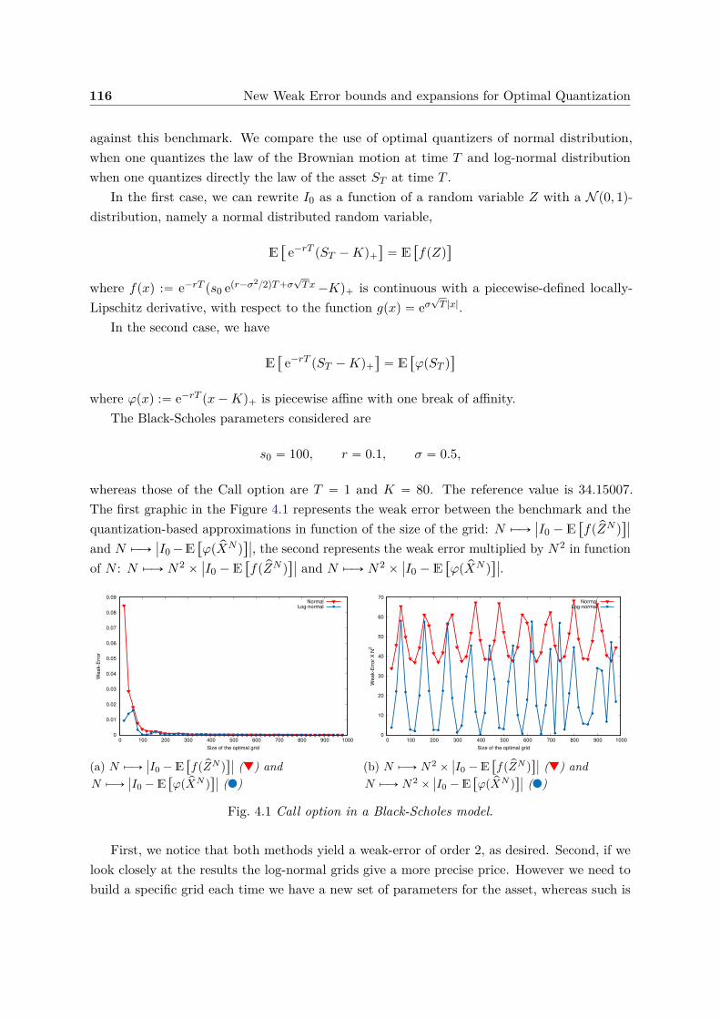
116 New Weak Error bounds and expansions for Optimal Quantization
against this benchmark. We compare the use of optimal quantizers of normal distribution,when one quantizes the law of the Brownian motion at time T and log-normal distributionwhen one quantizes directly the law of the asset ST at time T .
In the first case, we can rewrite I0 as a function of a random variable Z with a N p0, 1q-distribution, namely a normal distributed random variable,
E“
e´rT pST ´Kq`
‰
“ E“
fpZq‰
where fpxq :“ e´rT ps0 epr´σ22qT`σ?Tx ´Kq` is continuous with a piecewise-defined locally-
Lipschitz derivative, with respect to the function gpxq “ eσ?T |x|.
In the second case, we have
E“
e´rT pST ´Kq`
‰
“ E“
φpST q‰
where φpxq :“ e´rT px´Kq` is piecewise affine with one break of affinity.The Black-Scholes parameters considered are
s0 “ 100, r “ 0.1, σ “ 0.5,
whereas those of the Call option are T “ 1 and K “ 80. The reference value is 34.15007.The first graphic in the Figure 4.1 represents the weak error between the benchmark and thequantization-based approximations in function of the size of the grid: N ÞÝÑ
ˇ
ˇI0 ´ E“
fp pZN q‰ˇ
ˇ
and N ÞÝÑˇ
ˇI0 ´E“
φp pXN q‰ˇ
ˇ, the second represents the weak error multiplied by N2 in functionof N : N ÞÝÑ N2 ˆ
ˇ
ˇI0 ´ E“
fp pZN q‰ˇ
ˇ and N ÞÝÑ N2 ˆˇ
ˇI0 ´ E“
φp pXN q‰ˇ
ˇ.
0
0.01
0.02
0.03
0.04
0.05
0.06
0.07
0.08
0.09
0 100 200 300 400 500 600 700 800 900 1000
Weak-E
rror
Size of the optimal grid
NormalLog-normal
(a) N ÞÝÑˇ
ˇI0 ´ E“
fp pZN q‰ˇ
ˇ () andN ÞÝÑ
ˇ
ˇI0 ´ E“
φp pXN q‰ˇ
ˇ ()
0
10
20
30
40
50
60
70
0 100 200 300 400 500 600 700 800 900 1000
Weak-E
rror
X N
2
Size of the optimal grid
NormalLog-normal
(b) N ÞÝÑ N2 ˆˇ
ˇI0 ´ E“
fp pZN q‰ˇ
ˇ () andN ÞÝÑ N2 ˆ
ˇ
ˇI0 ´ E“
φp pXN q‰ˇ
ˇ ()
Fig. 4.1 Call option in a Black-Scholes model.
First, we notice that both methods yield a weak-error of order 2, as desired. Second, if welook closely at the results the log-normal grids give a more precise price. However we need tobuild a specific grid each time we have a new set of parameters for the asset, whereas such is
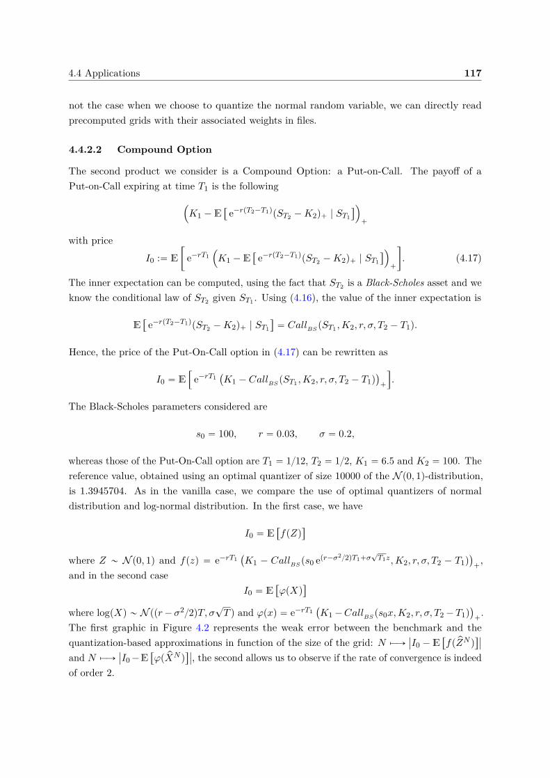
4.4 Applications 117
not the case when we choose to quantize the normal random variable, we can directly readprecomputed grids with their associated weights in files.
4.4.2.2 Compound Option
The second product we consider is a Compound Option: a Put-on-Call. The payoff of aPut-on-Call expiring at time T1 is the following
´
K1 ´ E“
e´rpT2´T1qpST2 ´K2q` | ST1
‰
¯
`
with priceI0 :“ E
„
e´rT1´
K1 ´ E“
e´rpT2´T1qpST2 ´K2q` | ST1
‰
¯
`
ȷ
. (4.17)
The inner expectation can be computed, using the fact that ST2 is a Black-Scholes asset and weknow the conditional law of ST2 given ST1 . Using (4.16), the value of the inner expectation is
E“
e´rpT2´T1qpST2 ´K2q` | ST1
‰
“ CallBS pST1 ,K2, r, σ, T2 ´ T1q.
Hence, the price of the Put-On-Call option in (4.17) can be rewritten as
I0 “ E”
e´rT1`
K1 ´ CallBS pST1 ,K2, r, σ, T2 ´ T1q˘
`
ı
.
The Black-Scholes parameters considered are
s0 “ 100, r “ 0.03, σ “ 0.2,
whereas those of the Put-On-Call option are T1 “ 112, T2 “ 12, K1 “ 6.5 and K2 “ 100. Thereference value, obtained using an optimal quantizer of size 10000 of the N p0, 1q-distribution,is 1.3945704. As in the vanilla case, we compare the use of optimal quantizers of normaldistribution and log-normal distribution. In the first case, we have
I0 “ E“
fpZq‰
where Z „ N p0, 1q and fpzq “ e´rT1`
K1 ´ CallBS ps0 epr´σ22qT1`σ?T1z,K2, r, σ, T2 ´ T1q
˘
`,
and in the second caseI0 “ E
“
φpXq‰
where logpXq „ N ppr´σ22qT, σ?T q and φpxq “ e´rT1
`
K1 ´CallBS ps0x,K2, r, σ, T2 ´T1q˘
`.
The first graphic in Figure 4.2 represents the weak error between the benchmark and thequantization-based approximations in function of the size of the grid: N ÞÝÑ
ˇ
ˇI0 ´ E“
fp pZN q‰ˇ
ˇ
and N ÞÝÑˇ
ˇI0 ´E“
φp pXN q‰ˇ
ˇ, the second allows us to observe if the rate of convergence is indeedof order 2.
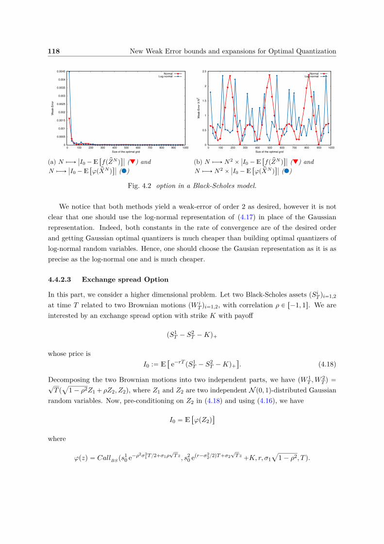
118 New Weak Error bounds and expansions for Optimal Quantization
0
0.0005
0.001
0.0015
0.002
0.0025
0.003
0.0035
0.004
0.0045
0 100 200 300 400 500 600 700 800 900 1000
Weak-E
rror
Size of the optimal grid
NormalLog-normal
(a) N ÞÝÑˇ
ˇI0 ´ E“
fp pZN q‰ˇ
ˇ () andN ÞÝÑ
ˇ
ˇI0 ´ E“
φp pXN q‰ˇ
ˇ ()
0
0.5
1
1.5
2
2.5
0 100 200 300 400 500 600 700 800 900 1000
Weak-E
rror
X N
2
Size of the optimal grid
NormalLog-normal
(b) N ÞÝÑ N2 ˆˇ
ˇI0 ´ E“
fp pZN q‰ˇ
ˇ () andN ÞÝÑ N2 ˆ
ˇ
ˇI0 ´ E“
φp pXN q‰ˇ
ˇ ()
Fig. 4.2 option in a Black-Scholes model.
We notice that both methods yield a weak-error of order 2 as desired, however it is notclear that one should use the log-normal representation of (4.17) in place of the Gaussianrepresentation. Indeed, both constants in the rate of convergence are of the desired orderand getting Gaussian optimal quantizers is much cheaper than building optimal quantizers oflog-normal random variables. Hence, one should choose the Gausian representation as it is asprecise as the log-normal one and is much cheaper.
4.4.2.3 Exchange spread Option
In this part, we consider a higher dimensional problem. Let two Black-Scholes assets pSiT qi“1,2
at time T related to two Brownian motions pW iT qi“1,2, with correlation ρ P r´1, 1s. We are
interested by an exchange spread option with strike K with payoff
pS1T ´ S2
T ´Kq`
whose price isI0 :“ E
“
e´rT pS1T ´ S2
T ´Kq`
‰
. (4.18)
Decomposing the two Brownian motions into two independent parts, we have pW 1T ,W
2T q “
?T p
a
1 ´ ρ2Z1 ` ρZ2, Z2q, where Z1 and Z2 are two independent N p0, 1q-distributed Gaussianrandom variables. Now, pre-conditioning on Z2 in (4.18) and using (4.16), we have
I0 “ E“
φpZ2q‰
where
φpzq “ CallBS ps10 e´ρ2σ2
1T 2`σ1ρ?Tz, s2
0 epr´σ222qT`σ2
?Tz `K, r, σ1
a
1 ´ ρ2, T q.
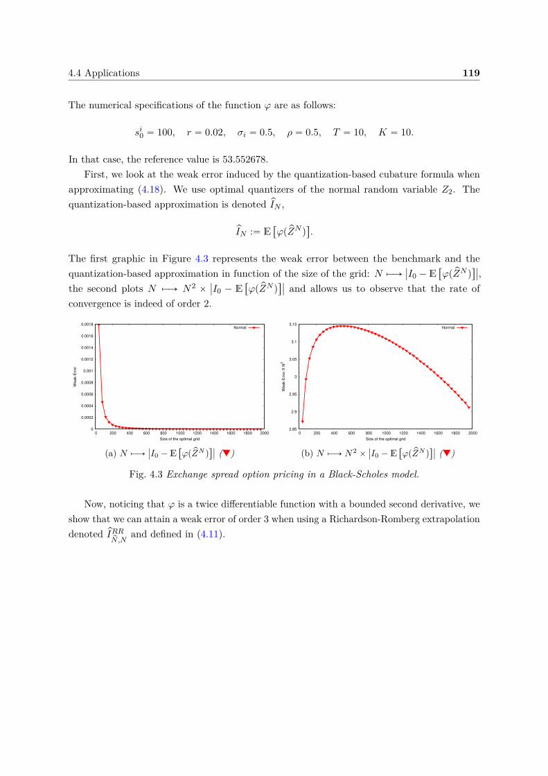
4.4 Applications 119
The numerical specifications of the function φ are as follows:
si0 “ 100, r “ 0.02, σi “ 0.5, ρ “ 0.5, T “ 10, K “ 10.
In that case, the reference value is 53.552678.First, we look at the weak error induced by the quantization-based cubature formula when
approximating (4.18). We use optimal quantizers of the normal random variable Z2. Thequantization-based approximation is denoted pIN ,
pIN :“ E“
φp pZN q‰
.
The first graphic in Figure 4.3 represents the weak error between the benchmark and thequantization-based approximation in function of the size of the grid: N ÞÝÑ
ˇ
ˇI0 ´ E“
φp pZN q‰ˇ
ˇ,the second plots N ÞÝÑ N2 ˆ
ˇ
ˇI0 ´ E“
φp pZN q‰ˇ
ˇ and allows us to observe that the rate ofconvergence is indeed of order 2.
0
0.0002
0.0004
0.0006
0.0008
0.001
0.0012
0.0014
0.0016
0.0018
0 200 400 600 800 1000 1200 1400 1600 1800 2000
Weak-E
rror
Size of the optimal grid
Normal
(a) N ÞÝÑˇ
ˇI0 ´ E“
φp pZN q‰ˇ
ˇ ()
2.85
2.9
2.95
3
3.05
3.1
3.15
0 200 400 600 800 1000 1200 1400 1600 1800 2000
Weak-E
rror
X N
2
Size of the optimal grid
Normal
(b) N ÞÝÑ N2 ˆˇ
ˇI0 ´ E“
φp pZN q‰ˇ
ˇ ()
Fig. 4.3 Exchange spread option pricing in a Black-Scholes model.
Now, noticing that φ is a twice differentiable function with a bounded second derivative, weshow that we can attain a weak error of order 3 when using a Richardson-Romberg extrapolationdenoted pIRR
rN,Nand defined in (4.11).
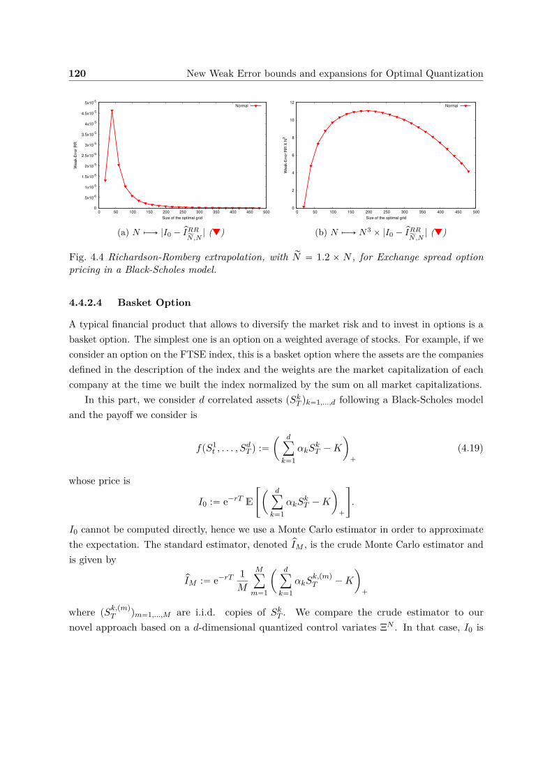
120 New Weak Error bounds and expansions for Optimal Quantization
0
5x10⁻⁶
1x10⁻⁵
1.5x10⁻⁵
2x10⁻⁵
2.5x10⁻⁵
3x10⁻⁵
3.5x10⁻⁵
4x10⁻⁵
4.5x10⁻⁵
5x10⁻⁵
0 50 100 150 200 250 300 350 400 450 500
Weak-E
rror
RR
Size of the optimal grid
Normal
(a) N ÞÝÑ |I0 ´ pIRRĂN,N
| ()
0
2
4
6
8
10
12
0 50 100 150 200 250 300 350 400 450 500
Weak-E
rror
RR
X N
3
Size of the optimal grid
Normal
(b) N ÞÝÑ N3 ˆ |I0 ´ pIRRĂN,N
| ()
Fig. 4.4 Richardson-Romberg extrapolation, with rN “ 1.2 ˆ N , for Exchange spread optionpricing in a Black-Scholes model.
4.4.2.4 Basket Option
A typical financial product that allows to diversify the market risk and to invest in options is abasket option. The simplest one is an option on a weighted average of stocks. For example, if weconsider an option on the FTSE index, this is a basket option where the assets are the companiesdefined in the description of the index and the weights are the market capitalization of eachcompany at the time we built the index normalized by the sum on all market capitalizations.
In this part, we consider d correlated assets pSkT qk“1,...,d following a Black-Scholes modeland the payoff we consider is
fpS1t , . . . , S
dT q :“
ˆ dÿ
k“1αkS
kT ´K
˙
`
(4.19)
whose price is
I0 :“ e´rT E
«
ˆ dÿ
k“1αkS
kT ´K
˙
`
ff
.
I0 cannot be computed directly, hence we use a Monte Carlo estimator in order to approximatethe expectation. The standard estimator, denoted pIM , is the crude Monte Carlo estimator andis given by
pIM :“ e´rT 1M
Mÿ
m“1
ˆ dÿ
k“1αkS
k,pmq
T ´K
˙
`
where pSk,pmq
T qm“1,...,M are i.i.d. copies of SkT . We compare the crude estimator to ournovel approach based on a d-dimensional quantized control variates ΞN . In that case, I0 is
4.4 Applications 121
approximated by IN defined by
IN :“ e´rT E
«
ˆ dÿ
k“1αkS
kT ´K
˙
`
´ xλ,ΞNy
ff
where ΞN is defined later, yielding the following Monte Carlo estimator
pIλ,NM :“ e´rT 1M
Mÿ
m“1
ˆ dÿ
k“1αkS
k,pmq
T ´K
˙
`
´ xλ,ΞN,pmqy.
We propose two different control variates ΞN based on optimal quantizers either of log-normalrandom variables or of Gaussian random variables.
1. The control variate, denoted ΞN , is defined by, @k “ 1, . . . , d
ΞNk :“ fpErS1T s, . . . , SkT , . . . ,ErSdT sq ´ E
“
fpErS1T s, . . . , pSk,NT , . . . ,ErSdT sq
‰
where ppSk,NT qk“1,...,d are optimal quantizers of cardinality N of SkT . In that case, the
Monte Carlo estimator is denoted pIλ,N
M .
2. The control variate, denoted rΞN , is using another representation of the payoff (4.19),using d Gaussian random variables i.i.d in place of the assets SkT because the d underlyingcorrelated Brownian Motions can be expressed from d rescaled independent Gaussianrandom variables, thus we define φ our new representation for the payoff as
φpZ1, . . . , Zdq :“ fpS1T , . . . , S
dT q
where pZkqk“1,...,d are i.i.d Gaussian random variables. Now, defining our control variateswith the function φ, @k “ 1, . . . , d
rΞNk :“ φp0, . . . , Zk, . . . , 0q ´ E“
φp0, . . . , pZN , . . . , 0q‰
where p pZN qk“1,...,d is an optimal quantizer of Z „ N p0, 1q. In that case, the Monte Carloestimator is denoted p
rIλ,NM .
The Black-Scholes parameters considered are
si0 “ 100, r “ 2%, σi “i
d` 1 , ρ “ 0.5,
and the specifications of the product are
K “ 100, αi “2i
dpd` 1q, T “ 1
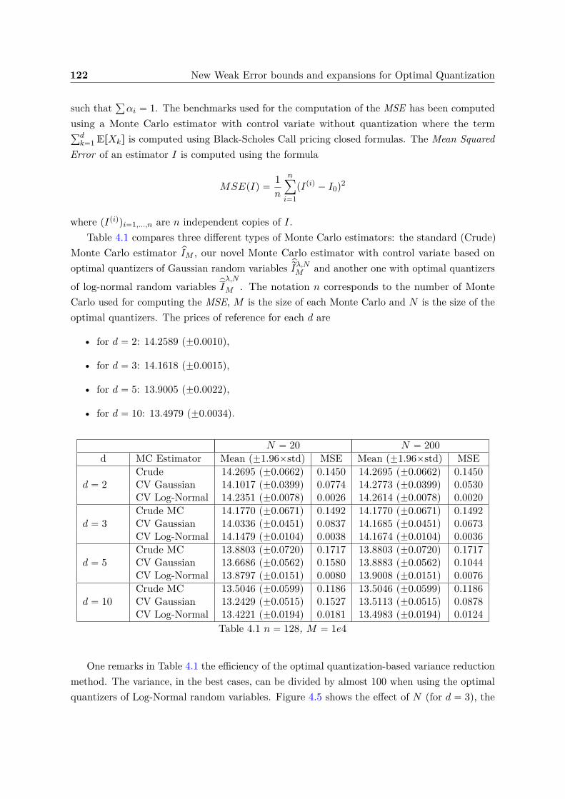
122 New Weak Error bounds and expansions for Optimal Quantization
such thatř
αi “ 1. The benchmarks used for the computation of the MSE has been computedusing a Monte Carlo estimator with control variate without quantization where the termřdk“1ErXks is computed using Black-Scholes Call pricing closed formulas. The Mean Squared
Error of an estimator I is computed using the formula
MSEpIq “1n
nÿ
i“1pIpiq ´ I0q2
where pIpiqqi“1,...,n are n independent copies of I.Table 4.1 compares three different types of Monte Carlo estimators: the standard (Crude)
Monte Carlo estimator pIM , our novel Monte Carlo estimator with control variate based onoptimal quantizers of Gaussian random variables p
rIλ,NM and another one with optimal quantizersof log-normal random variables pI
λ,N
M . The notation n corresponds to the number of MonteCarlo used for computing the MSE, M is the size of each Monte Carlo and N is the size of theoptimal quantizers. The prices of reference for each d are
• for d “ 2: 14.2589 p˘0.0010q,
• for d “ 3: 14.1618 p˘0.0015q,
• for d “ 5: 13.9005 p˘0.0022q,
• for d “ 10: 13.4979 p˘0.0034q.
N “ 20 N “ 200d MC Estimator Mean (˘1.96ˆstd) MSE Mean (˘1.96ˆstd) MSE
d “ 2Crude 14.2695 p˘0.0662q 0.1450 14.2695 p˘0.0662q 0.1450CV Gaussian 14.1017 p˘0.0399q 0.0774 14.2773 p˘0.0399q 0.0530CV Log-Normal 14.2351 p˘0.0078q 0.0026 14.2614 p˘0.0078q 0.0020
d “ 3Crude MC 14.1770 p˘0.0671q 0.1492 14.1770 p˘0.0671q 0.1492CV Gaussian 14.0336 p˘0.0451q 0.0837 14.1685 p˘0.0451q 0.0673CV Log-Normal 14.1479 p˘0.0104q 0.0038 14.1674 p˘0.0104q 0.0036
d “ 5Crude MC 13.8803 p˘0.0720q 0.1717 13.8803 p˘0.0720q 0.1717CV Gaussian 13.6686 p˘0.0562q 0.1580 13.8883 p˘0.0562q 0.1044CV Log-Normal 13.8797 p˘0.0151q 0.0080 13.9008 p˘0.0151q 0.0076
d “ 10Crude MC 13.5046 p˘0.0599q 0.1186 13.5046 p˘0.0599q 0.1186CV Gaussian 13.2429 p˘0.0515q 0.1527 13.5113 p˘0.0515q 0.0878CV Log-Normal 13.4221 p˘0.0194q 0.0181 13.4983 p˘0.0194q 0.0124
Table 4.1 n “ 128, M “ 1e4
One remarks in Table 4.1 the efficiency of the optimal quantization-based variance reductionmethod. The variance, in the best cases, can be divided by almost 100 when using the optimalquantizers of Log-Normal random variables. Figure 4.5 shows the effect of N (for d “ 3), the
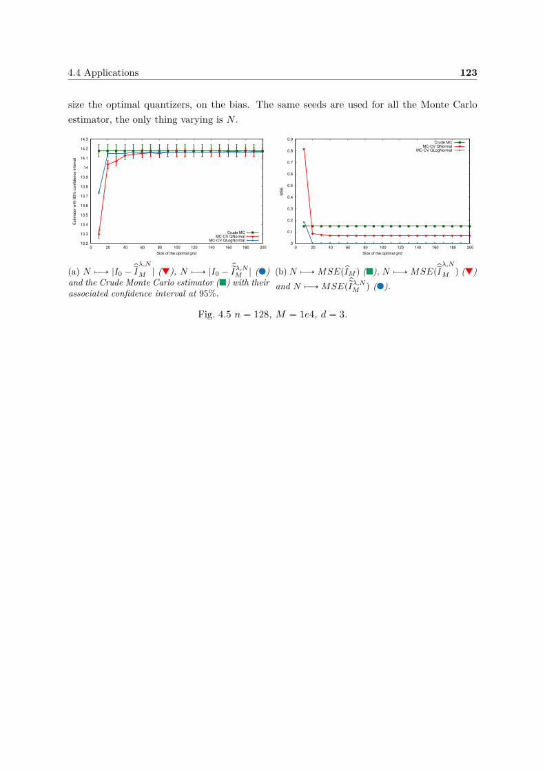
4.4 Applications 123
size the optimal quantizers, on the bias. The same seeds are used for all the Monte Carloestimator, the only thing varying is N .
13.2
13.3
13.4
13.5
13.6
13.7
13.8
13.9
14
14.1
14.2
14.3
0 20 40 60 80 100 120 140 160 180 200
Estim
ato
r w
ith 9
5%
confidence inte
rval
Size of the optimal grid
Crude MCMC-CV QNormal
MC-CV QLogNormal
(a) N ÞÝÑ |I0 ´pI
λ,N
M | (), N ÞÝÑ |I0 ´p
rIλ,NM | ()
and the Crude Monte Carlo estimator () with theirassociated confidence interval at 95%.
0
0.1
0.2
0.3
0.4
0.5
0.6
0.7
0.8
0.9
0 20 40 60 80 100 120 140 160 180 200
MS
E
Size of the optimal grid
Crude MCMC-CV QNormal
MC-CV QLogNormal
(b) N ÞÝÑ MSEppIM q (), N ÞÝÑ MSEppI
λ,N
M q ()and N ÞÝÑ MSEp
p
rIλ,NM q ().
Fig. 4.5 n “ 128, M “ 1e4, d “ 3.

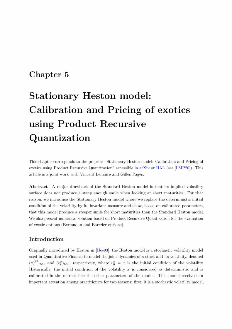
Chapter 5
Stationary Heston model:Calibration and Pricing of exoticsusing Product RecursiveQuantization
This chapter corresponds to the preprint “Stationary Heston model: Calibration and Pricing ofexotics using Product Recursive Quantization” accessible in arXiv or HAL (see [LMP20]). Thisarticle is a joint work with Vincent Lemaire and Gilles Pagès.
Abstract A major drawback of the Standard Heston model is that its implied volatilitysurface does not produce a steep enough smile when looking at short maturities. For thatreason, we introduce the Stationary Heston model where we replace the deterministic initialcondition of the volatility by its invariant measure and show, based on calibrated parameters,that this model produce a steeper smile for short maturities than the Standard Heston model.We also present numerical solution based on Product Recursive Quantization for the evaluationof exotic options (Bermudan and Barrrier options).
Introduction
Originally introduced by Heston in [Hes93], the Heston model is a stochastic volatility modelused in Quantitative Finance to model the joint dynamics of a stock and its volatility, denotedpS
pxq
t qtě0 and pvxt qtě0, respectively, where vx0 “ x is the initial condition of the volatility.Historically, the initial condition of the volatility x is considered as deterministic and iscalibrated in the market like the other parameters of the model. This model received animportant attention among practitioners for two reasons: first, it is a stochastic volatility model,
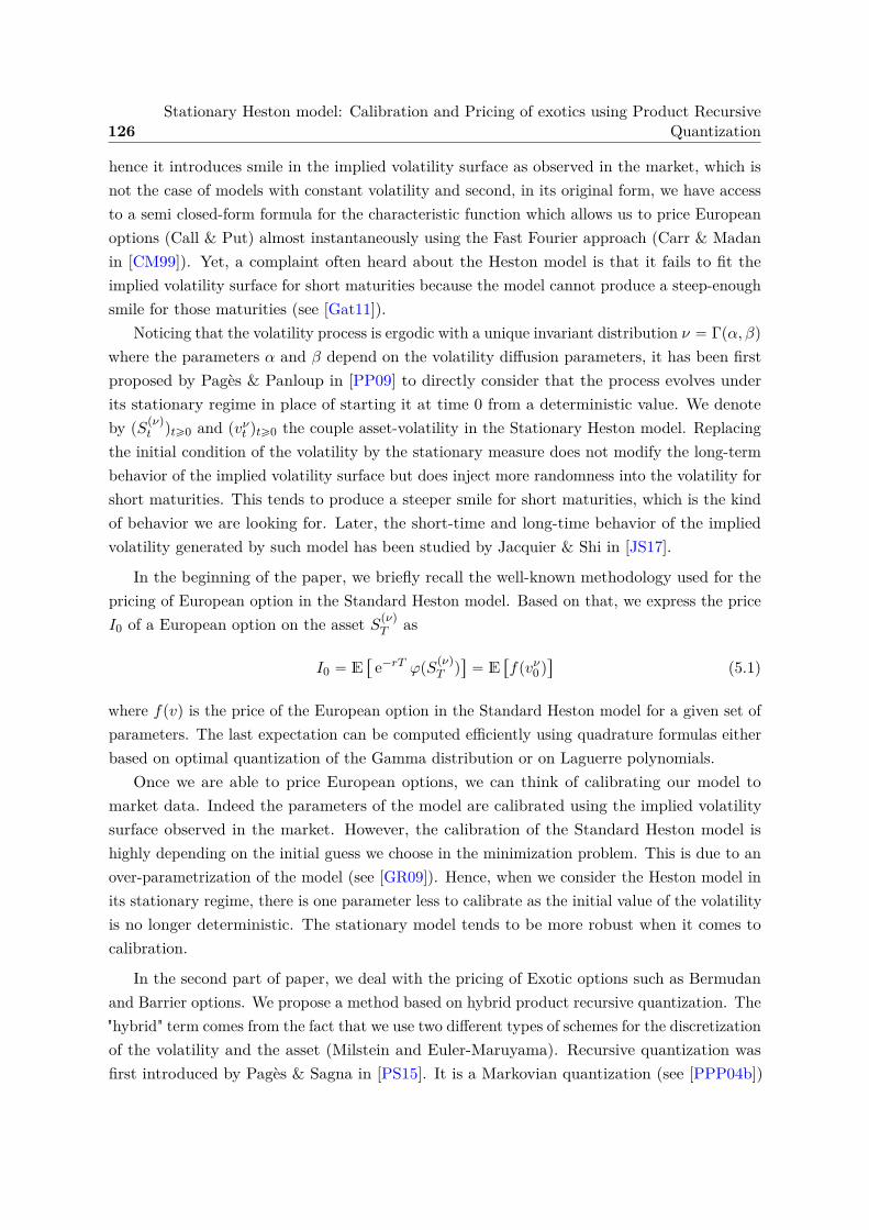
126Stationary Heston model: Calibration and Pricing of exotics using Product Recursive
Quantization
hence it introduces smile in the implied volatility surface as observed in the market, which isnot the case of models with constant volatility and second, in its original form, we have accessto a semi closed-form formula for the characteristic function which allows us to price Europeanoptions (Call & Put) almost instantaneously using the Fast Fourier approach (Carr & Madanin [CM99]). Yet, a complaint often heard about the Heston model is that it fails to fit theimplied volatility surface for short maturities because the model cannot produce a steep-enoughsmile for those maturities (see [Gat11]).
Noticing that the volatility process is ergodic with a unique invariant distribution ν “ Γpα, βq
where the parameters α and β depend on the volatility diffusion parameters, it has been firstproposed by Pagès & Panloup in [PP09] to directly consider that the process evolves underits stationary regime in place of starting it at time 0 from a deterministic value. We denoteby pS
pνq
t qtě0 and pvνt qtě0 the couple asset-volatility in the Stationary Heston model. Replacingthe initial condition of the volatility by the stationary measure does not modify the long-termbehavior of the implied volatility surface but does inject more randomness into the volatility forshort maturities. This tends to produce a steeper smile for short maturities, which is the kindof behavior we are looking for. Later, the short-time and long-time behavior of the impliedvolatility generated by such model has been studied by Jacquier & Shi in [JS17].
In the beginning of the paper, we briefly recall the well-known methodology used for thepricing of European option in the Standard Heston model. Based on that, we express the priceI0 of a European option on the asset Spνq
T as
I0 “ E“
e´rT φpSpνq
T q‰
“ E“
fpvν0 q‰
(5.1)
where fpvq is the price of the European option in the Standard Heston model for a given set ofparameters. The last expectation can be computed efficiently using quadrature formulas eitherbased on optimal quantization of the Gamma distribution or on Laguerre polynomials.
Once we are able to price European options, we can think of calibrating our model tomarket data. Indeed the parameters of the model are calibrated using the implied volatilitysurface observed in the market. However, the calibration of the Standard Heston model ishighly depending on the initial guess we choose in the minimization problem. This is due to anover-parametrization of the model (see [GR09]). Hence, when we consider the Heston model inits stationary regime, there is one parameter less to calibrate as the initial value of the volatilityis no longer deterministic. The stationary model tends to be more robust when it comes tocalibration.
In the second part of paper, we deal with the pricing of Exotic options such as Bermudanand Barrier options. We propose a method based on hybrid product recursive quantization. The"hybrid" term comes from the fact that we use two different types of schemes for the discretizationof the volatility and the asset (Milstein and Euler-Maruyama). Recursive quantization wasfirst introduced by Pagès & Sagna in [PS15]. It is a Markovian quantization (see [PPP04b])
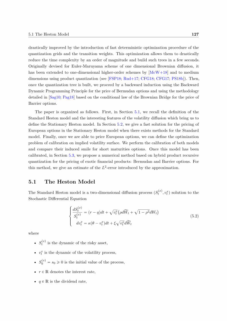
5.1 The Heston Model 127
drastically improved by the introduction of fast deterministic optimization procedure of thequantization grids and the transition weights. This optimization allows them to drasticallyreduce the time complexity by an order of magnitude and build such trees in a few seconds.Originally devised for Euler-Maruyama scheme of one dimensional Brownian diffusion, ithas been extended to one-dimensional higher-order schemes by [McW+18] and to mediumdimensions using product quantization (see [FSP18; Rud+17; CFG18; CFG17; PS18b]). Then,once the quantization tree is built, we proceed by a backward induction using the BackwardDynamic Programming Principle for the price of Bermudan options and using the methodologydetailed in [Sag10; Pag18] based on the conditional law of the Brownian Bridge for the price ofBarrier options.
The paper is organized as follows. First, in Section 5.1, we recall the definition of theStandard Heston model and the interesting features of the volatility diffusion which bring us todefine the Stationary Heston model. In Section 5.2, we give a fast solution for the pricing ofEuropean options in the Stationary Heston model when there exists methods for the Standardmodel. Finally, once we are able to price European options, we can define the optimizationproblem of calibration on implied volatility surface. We perform the calibration of both modelsand compare their induced smile for short maturities options. Once this model has beencalibrated, in Section 5.3, we propose a numerical method based on hybrid product recursivequantization for the pricing of exotic financial products: Bermudan and Barrier options. Forthis method, we give an estimate of the L2-error introduced by the approximation.
5.1 The Heston Model
The Standard Heston model is a two-dimensional diffusion process pSpxq
t , vxt q solution to theStochastic Differential Equation
$
’
’
&
’
’
%
dSpxq
t
Spxq
t
“ pr ´ qqdt`a
vxt`
ρdĂWt `a
1 ´ ρ2dWt
˘
dvxt “ κpθ ´ vxt qdt` ξa
vxt dĂWt
(5.2)
where
• Spxq
t is the dynamic of the risky asset,
• vxt is the dynamic of the volatility process,
• Spxq
0 “ s0 ě 0 is the initial value of the process,
• r P R denotes the interest rate,
• q P R is the dividend rate,
128Stationary Heston model: Calibration and Pricing of exotics using Product Recursive
Quantization
• ρ P r´1, 1s is the correlation between the asset and the volatility,
• pW,ĂW q is a two-dimensional standard Brownian motion,
• θ ě 0 the long run average price variance,
• κ ě 0 the rate at which vxt reverts to θ,
• ξ ě 0 is the volatility of the volatility,
• vx0 “ x ě 0 is the deterministic initial condition of the volatility.
This model is widely used by practitioner for various reasons. One is that it leads tosemi-closed forms for vanilla options based on a fast Fourier transform. The other is that itrepresents well the observed mid and long-term market behavior of the implied volatility surfaceobserved on the market. However, it fails producing or even fitting to the smile observed forshort-term maturities.
Remark (The volatility). One can notice that the volatility process is autonomous thencewe are facing a one dimensional problem. Moreover, the volatility process is following aCox-Ingersoll-Ross (CIR) diffusion also known as the square root diffusion. Existence anduniqueness of a strong solution to this stochastic differential equation has been first shown in[IW81], if x ě 0. Moreover, it has been shown, see [LL11], that if the Feller condition holds,namely ξ2 ď 2κθ, for every x ą 0, then the unique solution pvxt qtě0 satisfies
@t ě 0, Ppτx0 “ `8q “ 1 (5.3)
where τx0 is the first hitting time defined by
τx0 “ inftt ě 0 | vxt “ 0u where inf H “ `8. (5.4)
Moreover, the CIR diffusion admits, as a Markov process, a unique stationary regime, charac-terized by its invariant distribution
ν “ Γpα, βq (5.5)
whereα “ θβ and β “ 2κξ2. (5.6)
Based on the above remarks, the idea is to precisely consider the volatility process under itsstationary regime, i.e., replacing the deterministic initial condition from the Standard Hestonmodel by a ν-distributed random variable independent of pW,ĂW q. We will refer to this modelas the Stationary Heston model. Our first aim is to inject more randomness for short maturities(t small) into the volatility but also to reduce the number of free parameters to stabilize and
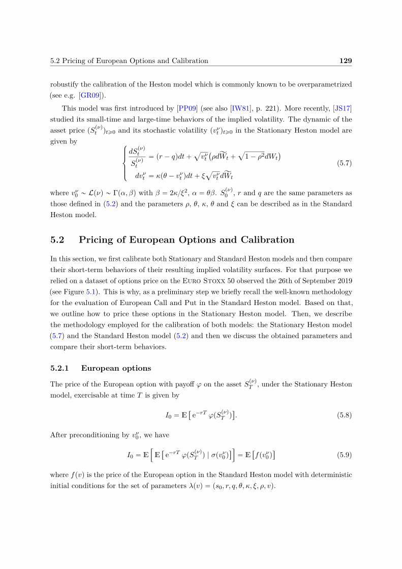
5.2 Pricing of European Options and Calibration 129
robustify the calibration of the Heston model which is commonly known to be overparametrized(see e.g. [GR09]).
This model was first introduced by [PP09] (see also [IW81], p. 221). More recently, [JS17]studied its small-time and large-time behaviors of the implied volatility. The dynamic of theasset price pS
pνq
t qtě0 and its stochastic volatility pvνt qtě0 in the Stationary Heston model aregiven by
$
’
’
&
’
’
%
dSpνq
t
Spνq
t
“ pr ´ qqdt`a
vνt`
ρdĂWt `a
1 ´ ρ2dWt
˘
dvνt “ κpθ ´ vνt qdt` ξa
vνt dĂWt
(5.7)
where vν0 „ Lpνq „ Γpα, βq with β “ 2κξ2, α “ θβ. Spνq
0 , r and q are the same parameters asthose defined in (5.2) and the parameters ρ, θ, κ, θ and ξ can be described as in the StandardHeston model.
5.2 Pricing of European Options and Calibration
In this section, we first calibrate both Stationary and Standard Heston models and then comparetheir short-term behaviors of their resulting implied volatility surfaces. For that purpose werelied on a dataset of options price on the Euro Stoxx 50 observed the 26th of September 2019(see Figure 5.1). This is why, as a preliminary step we briefly recall the well-known methodologyfor the evaluation of European Call and Put in the Standard Heston model. Based on that,we outline how to price these options in the Stationary Heston model. Then, we describethe methodology employed for the calibration of both models: the Stationary Heston model(5.7) and the Standard Heston model (5.2) and then we discuss the obtained parameters andcompare their short-term behaviors.
5.2.1 European options
The price of the European option with payoff φ on the asset Spνq
T , under the Stationary Hestonmodel, exercisable at time T is given by
I0 “ E“
e´rT φpSpνq
T q‰
. (5.8)
After preconditioning by vν0 , we have
I0 “ E”
E“
e´rT φpSpνq
T q | σpvν0 q‰
ı
“ E“
fpvν0 q‰
(5.9)
where fpvq is the price of the European option in the Standard Heston model with deterministicinitial conditions for the set of parameters λpvq “ ps0, r, q, θ, κ, ξ, ρ, vq.
130Stationary Heston model: Calibration and Pricing of exotics using Product Recursive
Quantization
Example 5.2.1 (Call). If φ is the payoff of a Call option then f is simply the price givenby Fourier transform in the Standard Heston model of the European Call Option. The priceat time 0, for a spot price s0, of an European Call Cpλpvq,K, T q with expiry T and strike Kunder the Standard Heston model with parameters λpvq “ ps0, r, q, θ, κ, ξ, ρ, vq is
Cpλpvq,K, T q “ E“
e´rT pSpvq
T ´Kq`
‰
“ e´rT´
E“
Spvq
T 1S
pvq
T ěK
‰
´K E“
1S
pvq
T ěK
‰
¯
“ s0 e´qT P1`
λpvq,K, T˘
´K e´rT P2`
λpvq,K, T˘
(5.10)
with P1`
λpvq,K, T˘
and P2`
λpvq,K, T˘
given by
P1`
λpvq,K, T˘
“12 `
1π
ż `8
0Re
ˆ
e´iu logpKq
iu
ψ`
λpvq, u´ i, T˘
s0 epr´qqT
˙
du
P2`
λpvq,K, T˘
“12 `
1π
ż `8
0Re
ˆ
e´iu logpKq
iu ψ`
λpvq, u, T˘
˙
du
(5.11)
where i is the imaginary unit s.t. i2 “ ´1, ψ`
λpvq, u, T˘
is the characteristic function of thelogarithm of the stock price process at time T . Several representations of the characteristicfunction exist, we choose to use the one proposed by [SST04; Gat11; Alb+07], which isnumerically more stable. It reads
ψ`
λpvq, u, T˘
“ E“
eiu logpSpvq
T q | Spvq
0 , x‰
“ eiuplogps0q`pr´qqT q
ˆ eθκξ´2`
pκ´ρξui´dqT´2 logpp1´g e´dtqp1´gqq
˘
ˆ ev2ξ´2pκ´ρξui´dqp1´e´dtqp1´g e´dtq
(5.12)
with
d “a
pρξui ´ κq2 ´ ξ2p´ui ´ u2q and g “ pκ´ ρξui ´ dqpκ´ ρξui ` dq. (5.13)
Hence, in (5.9), fpvq can be replaced by C`
λpvq,K, T˘
, which yields
I0 “ E“
e´rT pSpνq
T ´Kq`
‰
“ E”
C`
λpvν0 q,K, T˘
ı
. (5.14)
Now, we come to the pricing of European options in the Stationary Heston model, usingthe expression of the density of vν0 „ Γpα, βq, (5.9) reads
I0 “ E“
fpvν0 q‰
“
ż `8
0fpvq
βα
Γpαqvα´1 e´βv dv. (5.15)
Now, several approaches exists in order to approximate this integral on the positive real line.
5.2 Pricing of European Options and Calibration 131
• Quantization based quadrature formulas. One could use a quantization-based cubatureformula with an optimal quantizer of vν0 with the methodology detailed in Appendix 5.D. Giventhat optimal quantizer of size N , pvN0 , we approximate I0 by pIN0
pIN0 “ E“
fppvN0 q‰
“
Nÿ
i“1fpvN0,iqP
`
pvN0 “ vN0,i˘
. (5.16)
Remarks. In one dimension, the minimization problem, that consists in building an optimalquantizer, is invariant by linear transformation. Hence applying a linear transformation to anoptimal quantizer preserves its optimality. For example, if we consider an optimal quantizationpXN of a standard normal distribution N p0, 1q then µ ` σ pXN is an optimal quantizer of anormal distribution N pµ, σ2q and the associated probabilities of each Voronoï centroid stay thesame.
In our case, noticing that if we consider a Gamma random variable X „ Γpα, 1q then therescaling of X by 1β yields Xβ „ Γpα, βq. Hence, for building the optimal quantizer pvN0of vν0 , we can build an optimal quantizer of X „ Γpα, 1q and then rescale it by 1β, yieldingpvN0 “ pXNβ. Our numerical tests showed that it is numerically more stable to use this approach.
In order to build the optimal quantizer, we use Lloyd’s method detailed in Appendix 5.D toX „ Γpα, 1q with the cumulative distribution function FX pxq “ PpX ď xq and the partial firstmoment KX pxq “ ErX 1Xďxs given by
@x ą 0, FX pxq “1
Γpαqγpα, xq, KX pxq “ αFX pxq ´
xα e´x
Γpαq,
otherwise, FX pxq “ 0, KX pxq “ 0,(5.17)
where γpα, xq “şx0 t
α´1 e´t dt is the lower gamma function. And the associated probabilities ofthe optimal quantizer pvN0 are given by (5.113)
P`
pvN0 “ vN0,i˘
“ P`
pXN “ xNi˘
“ FX
`
xNi`12˘
´ FX
`
xNi´12˘
(5.18)
where @i P J2, NK, xNi´12 “xN
i´1`xNi
2 and xN12 “ 0 and xNN`12 “ `8.
• Quadrature formula from Laguerre polynomials. One could also use an algorithm based onfixed point quadratures for the numerical integration. Indeed, noticing that the density we areintegrating against is a gamma density which is exactly the Laguerre weighting function (up toa rescaling). Then, I0 rewrites
I0 “
ż `8
0fpvq
βα
Γpαqvα´1 e´βv dv “
βα
Γpαq
ż `8
0fpvqωpvqdv (5.19)
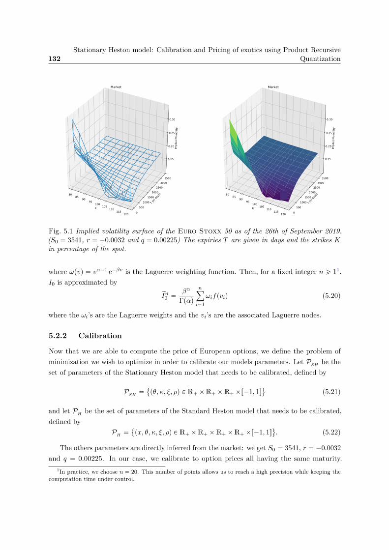
132Stationary Heston model: Calibration and Pricing of exotics using Product Recursive
Quantization
K
8085
9095
100105
110115
120
T (in days)
0500
10001500
20002500
30003500
Implied Vo
latility
0.15
0.20
0.25
0.30
Market
K
8085
9095
100105
110115
120
T (in days)
0500
10001500
20002500
30003500
Implied Vo
latility
0.15
0.20
0.25
0.30
Market
Fig. 5.1 Implied volatility surface of the Euro Stoxx 50 as of the 26th of September 2019.(S0 “ 3541, r “ ´0.0032 and q “ 0.00225) The expiries T are given in days and the strikes Kin percentage of the spot.
where ωpvq “ vα´1 e´βv is the Laguerre weighting function. Then, for a fixed integer n ě 11,I0 is approximated by
rIn0 “βα
Γpαq
nÿ
i“1ωifpviq (5.20)
where the ωi’s are the Laguerre weights and the vi’s are the associated Laguerre nodes.
5.2.2 Calibration
Now that we are able to compute the price of European options, we define the problem ofminimization we wish to optimize in order to calibrate our models parameters. Let PSH be theset of parameters of the Stationary Heston model that needs to be calibrated, defined by
PSH “
pθ, κ, ξ, ρq P R` ˆR` ˆR` ˆr´1, 1s(
(5.21)
and let PH be the set of parameters of the Standard Heston model that needs to be calibrated,defined by
PH “
px, θ, κ, ξ, ρq P R` ˆR` ˆR` ˆR` ˆr´1, 1s(
. (5.22)
The others parameters are directly inferred from the market: we get S0 “ 3541, r “ ´0.0032and q “ 0.00225. In our case, we calibrate to option prices all having the same maturity.
1In practice, we choose n “ 20. This number of points allows us to reach a high precision while keeping thecomputation time under control.
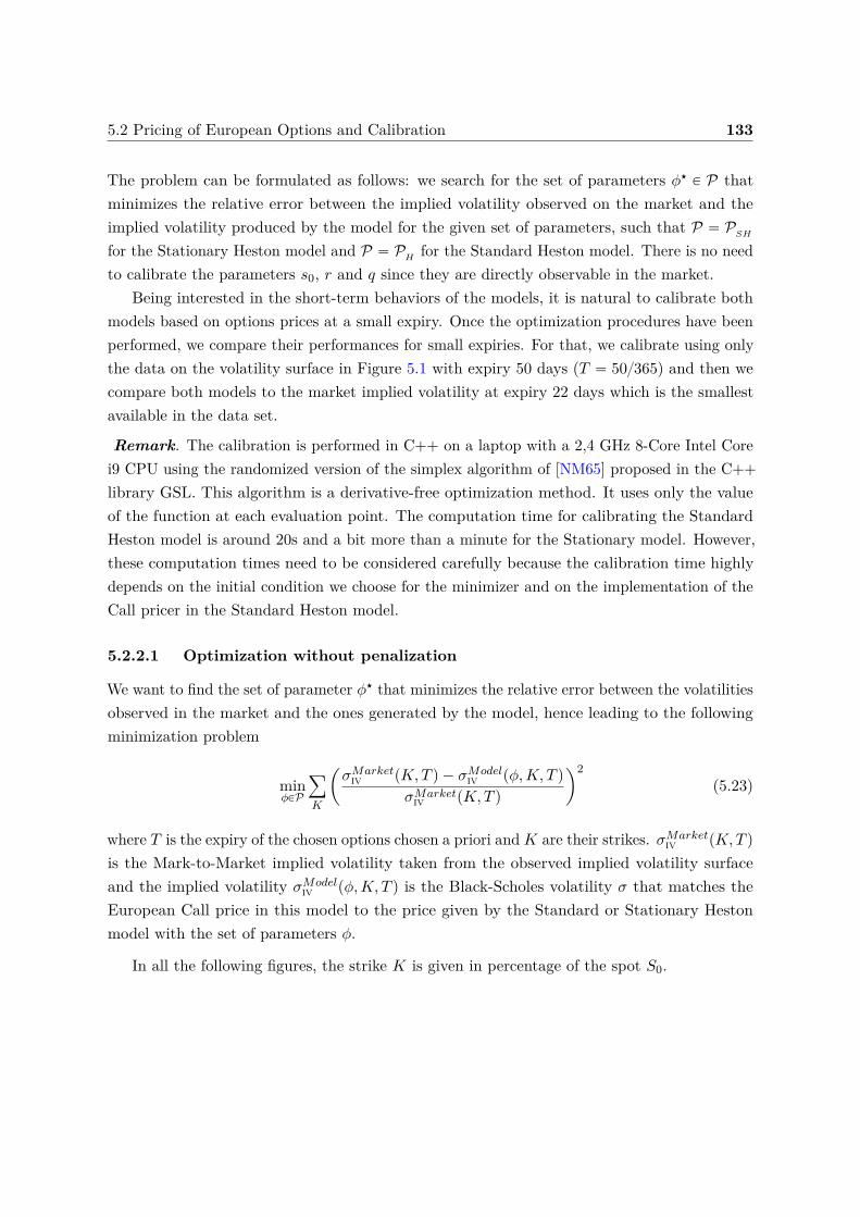
5.2 Pricing of European Options and Calibration 133
The problem can be formulated as follows: we search for the set of parameters ϕ‹ P P thatminimizes the relative error between the implied volatility observed on the market and theimplied volatility produced by the model for the given set of parameters, such that P “ PSH
for the Stationary Heston model and P “ PH for the Standard Heston model. There is no needto calibrate the parameters s0, r and q since they are directly observable in the market.
Being interested in the short-term behaviors of the models, it is natural to calibrate bothmodels based on options prices at a small expiry. Once the optimization procedures have beenperformed, we compare their performances for small expiries. For that, we calibrate using onlythe data on the volatility surface in Figure 5.1 with expiry 50 days (T “ 50365) and then wecompare both models to the market implied volatility at expiry 22 days which is the smallestavailable in the data set.
Remark. The calibration is performed in C++ on a laptop with a 2,4 GHz 8-Core Intel Corei9 CPU using the randomized version of the simplex algorithm of [NM65] proposed in the C++library GSL. This algorithm is a derivative-free optimization method. It uses only the valueof the function at each evaluation point. The computation time for calibrating the StandardHeston model is around 20s and a bit more than a minute for the Stationary model. However,these computation times need to be considered carefully because the calibration time highlydepends on the initial condition we choose for the minimizer and on the implementation of theCall pricer in the Standard Heston model.
5.2.2.1 Optimization without penalization
We want to find the set of parameter ϕ‹ that minimizes the relative error between the volatilitiesobserved in the market and the ones generated by the model, hence leading to the followingminimization problem
minϕPP
ÿ
K
ˆ
σMarketiv pK,T q ´ σModel
iv pϕ,K, T q
σMarketiv pK,T q
˙2(5.23)
where T is the expiry of the chosen options chosen a priori and K are their strikes. σMarketiv pK,T q
is the Mark-to-Market implied volatility taken from the observed implied volatility surfaceand the implied volatility σModel
iv pϕ,K, T q is the Black-Scholes volatility σ that matches theEuropean Call price in this model to the price given by the Standard or Stationary Hestonmodel with the set of parameters ϕ.
In all the following figures, the strike K is given in percentage of the spot S0.
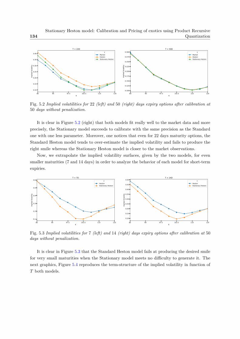
134Stationary Heston model: Calibration and Pricing of exotics using Product Recursive
Quantization
80 90 97.5 102.5 110 120K
0.10
0.15
0.20
0.25
0.30
0.35
0.40
Impl
ied
Vola
tility
T = 22DT
MarketHestonStationary Heston
80 90 97.5 102.5 110 120K
0.100
0.125
0.150
0.175
0.200
0.225
0.250
0.275
0.300
Impl
ied
Vola
tility
T = 50DT
MarketHestonStationary Heston
Fig. 5.2 Implied volatilities for 22 (left) and 50 (right) days expiry options after calibration at50 days without penalization.
It is clear in Figure 5.2 (right) that both models fit really well to the market data and moreprecisely, the Stationary model succeeds to calibrate with the same precision as the Standardone with one less parameter. Moreover, one notices that even for 22 days maturity options, theStandard Heston model tends to over-estimate the implied volatility and fails to produce theright smile whereas the Stationary Heston model is closer to the market observations.
Now, we extrapolate the implied volatility surfaces, given by the two models, for evensmaller maturities (7 and 14 days) in order to analyze the behavior of each model for short-termexpiries.
80 90 97.5 102.5 110 120K
0.1
0.2
0.3
0.4
0.5
0.6
Implied Vo
latility
T = 7DT
HestonStationary Heston
80 90 97.5 102.5 110 120K
0.10
0.15
0.20
0.25
0.30
0.35
0.40
0.45
0.50
Implied Vo
latility
T = 14DT
HestonStationary Heston
Fig. 5.3 Implied volatilities for 7 (left) and 14 (right) days expiry options after calibration at 50days without penalization.
It is clear in Figure 5.3 that the Standard Heston model fails at producing the desired smilefor very small maturities when the Stationary model meets no difficulty to generate it. Thenext graphics, Figure 5.4 reproduces the term-structure of the implied volatility in function ofT both models.
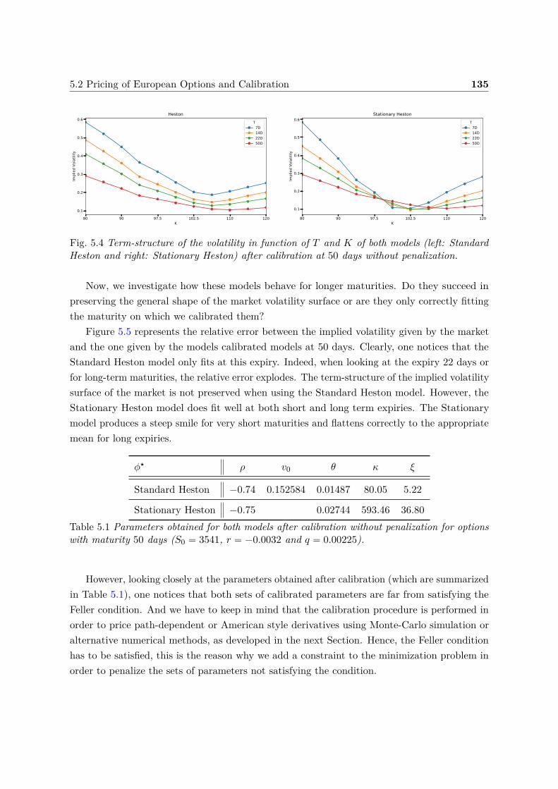
5.2 Pricing of European Options and Calibration 135
80 90 97.5 102.5 110 120K
0.1
0.2
0.3
0.4
0.5
0.6
Implied Vo
latility
HestonT7D14D22D50D
80 90 97.5 102.5 110 120K
0.1
0.2
0.3
0.4
0.5
0.6
Implied Vo
latility
Stationary HestonT7D14D22D50D
Fig. 5.4 Term-structure of the volatility in function of T and K of both models (left: StandardHeston and right: Stationary Heston) after calibration at 50 days without penalization.
Now, we investigate how these models behave for longer maturities. Do they succeed inpreserving the general shape of the market volatility surface or are they only correctly fittingthe maturity on which we calibrated them?
Figure 5.5 represents the relative error between the implied volatility given by the marketand the one given by the models calibrated models at 50 days. Clearly, one notices that theStandard Heston model only fits at this expiry. Indeed, when looking at the expiry 22 days orfor long-term maturities, the relative error explodes. The term-structure of the implied volatilitysurface of the market is not preserved when using the Standard Heston model. However, theStationary Heston model does fit well at both short and long term expiries. The Stationarymodel produces a steep smile for very short maturities and flattens correctly to the appropriatemean for long expiries.
ϕ‹ ρ v0 θ κ ξ
Standard Heston ´0.74 0.152584 0.01487 80.05 5.22
Stationary Heston ´0.75 0.02744 593.46 36.80Table 5.1 Parameters obtained for both models after calibration without penalization for optionswith maturity 50 days (S0 “ 3541, r “ ´0.0032 and q “ 0.00225).
However, looking closely at the parameters obtained after calibration (which are summarizedin Table 5.1), one notices that both sets of calibrated parameters are far from satisfying theFeller condition. And we have to keep in mind that the calibration procedure is performed inorder to price path-dependent or American style derivatives using Monte-Carlo simulation oralternative numerical methods, as developed in the next Section. Hence, the Feller conditionhas to be satisfied, this is the reason why we add a constraint to the minimization problem inorder to penalize the sets of parameters not satisfying the condition.
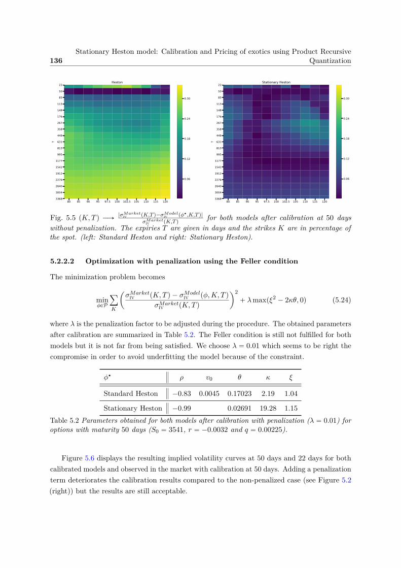
136Stationary Heston model: Calibration and Pricing of exotics using Product Recursive
Quantization
80 85 90 95 97.5 100 102.5 105 110 115 120
22
50
85
113
148
176
267
358
449
631
813
995
1177
1541
1912
2276
2640
3004
3368
T
Heston
80 85 90 95 97.5 100 102.5 105 110 115 120
22
50
85
113
148
176
267
358
449
631
813
995
1177
1541
1912
2276
2640
3004
3368
T
Stationary Heston
0.06
0.12
0.18
0.24
0.30
0.06
0.12
0.18
0.24
0.30
Fig. 5.5 pK,T q ÝÑ|σMarket
iv pK,T q´σModeliv pϕ‹,K,T q|
σMarketiv pK,T q
for both models after calibration at 50 dayswithout penalization. The expiries T are given in days and the strikes K are in percentage ofthe spot. (left: Standard Heston and right: Stationary Heston).
5.2.2.2 Optimization with penalization using the Feller condition
The minimization problem becomes
minϕPP
ÿ
K
ˆ
σMarketiv pK,T q ´ σModel
iv pϕ,K, T q
σMarketiv pK,T q
˙2` λmaxpξ2 ´ 2κθ, 0q (5.24)
where λ is the penalization factor to be adjusted during the procedure. The obtained parametersafter calibration are summarized in Table 5.2. The Feller condition is still not fulfilled for bothmodels but it is not far from being satisfied. We choose λ “ 0.01 which seems to be right thecompromise in order to avoid underfitting the model because of the constraint.
ϕ‹ ρ v0 θ κ ξ
Standard Heston ´0.83 0.0045 0.17023 2.19 1.04
Stationary Heston ´0.99 0.02691 19.28 1.15Table 5.2 Parameters obtained for both models after calibration with penalization (λ “ 0.01) foroptions with maturity 50 days (S0 “ 3541, r “ ´0.0032 and q “ 0.00225).
Figure 5.6 displays the resulting implied volatility curves at 50 days and 22 days for bothcalibrated models and observed in the market with calibration at 50 days. Adding a penalizationterm deteriorates the calibration results compared to the non-penalized case (see Figure 5.2(right)) but the results are still acceptable.
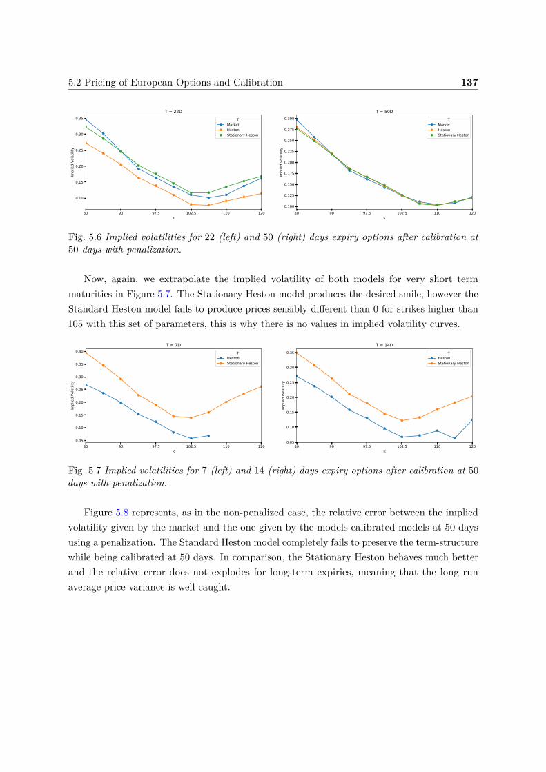
5.2 Pricing of European Options and Calibration 137
80 90 97.5 102.5 110 120K
0.10
0.15
0.20
0.25
0.30
0.35
Implied Vo
latility
T = 22DT
MarketHestonStationary Heston
80 90 97.5 102.5 110 120K
0.100
0.125
0.150
0.175
0.200
0.225
0.250
0.275
0.300
Implied Vo
latility
T = 50DT
MarketHestonStationary Heston
Fig. 5.6 Implied volatilities for 22 (left) and 50 (right) days expiry options after calibration at50 days with penalization.
Now, again, we extrapolate the implied volatility of both models for very short termmaturities in Figure 5.7. The Stationary Heston model produces the desired smile, however theStandard Heston model fails to produce prices sensibly different than 0 for strikes higher than105 with this set of parameters, this is why there is no values in implied volatility curves.
80 90 97.5 102.5 110 120K
0.05
0.10
0.15
0.20
0.25
0.30
0.35
0.40
Implied Vo
latility
T = 7DT
HestonStationary Heston
80 90 97.5 102.5 110 120K
0.05
0.10
0.15
0.20
0.25
0.30
0.35
Implied Vo
latility
T = 14DT
HestonStationary Heston
Fig. 5.7 Implied volatilities for 7 (left) and 14 (right) days expiry options after calibration at 50days with penalization.
Figure 5.8 represents, as in the non-penalized case, the relative error between the impliedvolatility given by the market and the one given by the models calibrated models at 50 daysusing a penalization. The Standard Heston model completely fails to preserve the term-structurewhile being calibrated at 50 days. In comparison, the Stationary Heston behaves much betterand the relative error does not explodes for long-term expiries, meaning that the long runaverage price variance is well caught.
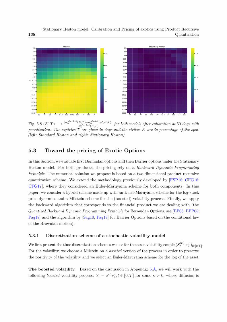
138Stationary Heston model: Calibration and Pricing of exotics using Product Recursive
Quantization
80 85 90 95 97.5 100 102.5 105 110 115 120
22
50
85
113
148
176
267
358
449
631
813
995
1177
1541
1912
2276
2640
3004
3368
T
Heston
80 85 90 95 97.5 100 102.5 105 110 115 120
22
50
85
113
148
176
267
358
449
631
813
995
1177
1541
1912
2276
2640
3004
3368
T
Stationary Heston
0.2
0.4
0.6
0.8
1.0
0.2
0.4
0.6
0.8
1.0
Fig. 5.8 pK,T q ÝÑ|σMarket
iv pK,T q´σModeliv pϕ‹,K,T q|
σMarketiv pK,T q
for both models after calibration at 50 days withpenalization. The expiries T are given in days and the strikes K are in percentage of the spot.(left: Standard Heston and right: Stationary Heston).
5.3 Toward the pricing of Exotic Options
In this Section, we evaluate first Bermudan options and then Barrier options under the StationaryHeston model. For both products, the pricing rely on a Backward Dynamic ProgrammingPrinciple. The numerical solution we propose is based on a two-dimensional product recursivequantization scheme. We extend the methodology previously developed by [FSP18; CFG18;CFG17], where they considered an Euler-Maruyama scheme for both components. In thispaper, we consider a hybrid scheme made up with an Euler-Maruyama scheme for the log-stockprice dynamics and a Milstein scheme for the (boosted) volatility process. Finally, we applythe backward algorithm that corresponds to the financial product we are dealing with (theQuantized Backward Dynamic Programming Principle for Bermudan Options, see [BP03; BPP05;Pag18] and the algorithm by [Sag10; Pag18] for Barrier Options based on the conditional lawof the Brownian motion).
5.3.1 Discretization scheme of a stochastic volatility model
We first present the time discretization schemes we use for the asset-volatility couple pSpνq
t , vνt qtPr0,T s.For the volatility, we choose a Milstein on a boosted version of the process in order to preservethe positivity of the volatility and we select an Euler-Maruyama scheme for the log of the asset.
The boosted volatility. Based on the discussion in Appendix 5.A, we will work with thefollowing boosted volatility process: Yt “ eκt vνt , t P r0, T s for some κ ą 0, whose diffusion is
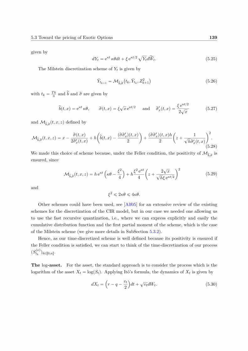
5.3 Toward the pricing of Exotic Options 139
given bydYt “ eκt κθdt` ξ eκt2
a
YtdĂWt. (5.25)
The Milstein discretization scheme of Yt is given by
sYtk`1 “ Mrb,rσ
`
tk, sYtk , Z2k`1
˘
(5.26)
with tk “ Tkn and rb and rσ are given by
rbpt, xq “ eκt κθ, rσpt, xq “ ξ?x eκt2 and rσ1
xpt, xq “ξ eκt2
2?x
(5.27)
and Mrb,rσ
pt, x, zq defined by
Mrb,rσ
pt, x, zq “ x´rσpt, xq
2rσ1xpt, xq
` h
ˆ
rbpt, xq ´prσrσ1
xqpt, xq
2
˙
`prσrσ1
xqpt, xqh
2
ˆ
z `1
?hrσ1
xpt, xq
˙2.
(5.28)We made this choice of scheme because, under the Feller condition, the positivity of M
rb,rσis
ensured, since
Mrb,rσ
pt, x, zq “ h eκt´
κθ ´ξ2
4
¯
` hξ2 eκt
4
ˆ
z `2?x
?hξ eκt2
˙2(5.29)
andξ2 ď 2κθ ď 4κθ.
Other schemes could have been used, see [Alf05] for an extensive review of the existingschemes for the discretization of the CIR model, but in our case we needed one allowing usto use the fast recursive quantization, i.e., where we can express explicitly and easily thecumulative distribution function and the first partial moment of the scheme, which is the caseof the Milstein scheme (we give more details in SubSection 5.3.2).
Hence, as our time-discretized scheme is well defined because its positivity is ensured ifthe Feller condition is satisfied, we can start to think of the time-discretization of our processpS
pνq
tkqkPJ0,nK.
The log-asset. For the asset, the standard approach is to consider the process which is thelogarithm of the asset Xt “ logpStq. Applying Itô’s formula, the dynamics of Xt is given by
dXt “
´
r ´ q ´vt2
¯
dt`?vtdWt. (5.30)
140Stationary Heston model: Calibration and Pricing of exotics using Product Recursive
Quantization
Now, using a standard Euler-Maruyama scheme for the discretization of Xt, we have#
sXtk`1 “ Eb,σ`
tk, sXtk ,sYtk , Z
1k`1
˘
sYtk`1 “ Mrb,rσ
`
tk, sYtk , Z2k`1
˘(5.31)
where Z1k`1 „ N p0, 1q, Z2
k`1 „ N p0, 1q, CorrpZ1k`1, Z
2k`1q “ ρ and
Eb,σpt, x, y, zq “ x` bpt, x, yqh` σpt, x, yq?h z (5.32)
withbpt, x, yq “ r ´ q ´
e´κt y
2 and σpt, x, yq “ e´κt2 ?y. (5.33)
5.3.2 Hybrid Product Recursive Quantization
In this part, we describe the methodology used for the construction of the product recursivequantization tree of the couple log asset- boosted volatility in the Heston model.
In Figure 5.9, as an example, we synthesise the main idea behind the recursive quantizationof a diffusion vt which has been time-discretized with F0pt, x, zq. We start at time t0 “ 0 witha quantizer pv0 taking values in the grid Γt0 “ tv0
1, . . . , v010u of size 10, where each point is
represented by a black bullet (‚) with probability p0i “ Pppv0 “ v0
i q is represented by a bar. Inthe Stationary Heston model, pv0 is an optimal quantization of the Gamma distribution givenby (5.5) and (5.6). Then, starting from this grid, we simulate the process from time t0 to timet1 “ 5 days with our chosen time-discretization scheme F0pt, x, zq, yielding rv1 “ F0pt0, pv0, Z1q,where Z1 is a standardized Gaussian random variable. Each trajectory starts from point v0
i
with probability p0i . And finally we project the obtained distribution at time t1 onto a grid
Γt1 “ tv11, . . . , v
110u of cardinality 10, represented by black triangles (IJ) such that pv1 is an
optimal quantizer of the discretized and simulated process starting from quantizer pv0 at timet0 “ 0.
Remark. In practice, for low dimensions, we do not simulate trajectories. We use theinformation on the law of rv1 conditionally of starting from pv0. The knowledge of the distributionallows us to use deterministic algorithms during the construction of the optimal quantizer of rv1
that are a lot faster than algorithms based on simulation.
In our case, we consider the following stochastic volatility system#
dXt “ bpt,Xt, Ytqdt` σpt,Xt, YtqdWt
dYt “ rbpt, Ytqdt` rσpt, YtqdĂWt
(5.34)
where Wt and ĂWt are two correlated Brownian motions with correlation ρ P r´1, 1s, b and σ
are defined in (5.33) and rb and rσ are defined in (5.27). Our aim is to build a quantization treeof the couple pXt, Ytq at given dates tk, k “ 0, . . . , n based on a recursive product quantization
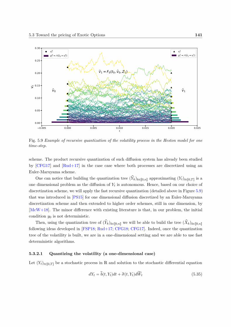
5.3 Toward the pricing of Exotic Options 141
−0.005 0.000 0.005 0.010 0.015 0.020 0.025t
0.00
0.05
0.10
0.15
0.20
0.25
0.30
v t v0
v1= F0(t0, v0,Z1)
v1
v1i
p1i =ℙ( v1= v1
i )v0i
p0i =ℙ( v0= v0
i )
Fig. 5.9 Example of recursive quantization of the volatility process in the Heston model for onetime-step.
scheme. The product recursive quantization of such diffusion system has already been studiedby [CFG17] and [Rud+17] in the case case where both processes are discretized using anEuler-Maruyama scheme.
One can notice that building the quantization tree ppYkqkPJ0,nK approximating pYtqtPr0,T s is aone dimensional problem as the diffusion of Yt is autonomous. Hence, based on our choice ofdiscretization scheme, we will apply the fast recursive quantization (detailed above in Figure 5.9)that was introduced in [PS15] for one dimensional diffusion discretized by an Euler-Maruyamadiscretization scheme and then extended to higher order schemes, still in one dimension, by[McW+18]. The minor difference with existing literature is that, in our problem, the initialcondition y0 is not deterministic.
Then, using the quantization tree of ppYkqkPJ0,nK we will be able to build the tree p pXkqkPJ0,nK
following ideas developed in [FSP18; Rud+17; CFG18; CFG17]. Indeed, once the quantizationtree of the volatility is built, we are in a one-dimensional setting and we are able to use fastdeterministic algorithms.
5.3.2.1 Quantizing the volatility (a one-dimensional case)
Let pYtqtPr0,T s be a stochastic process in R and solution to the stochastic differential equation
dYt “ rbpt, Ytqdt` rσpt, YtqdĂWt (5.35)
142Stationary Heston model: Calibration and Pricing of exotics using Product Recursive
Quantization
where Y0 has the same law than the stationary measure ν: LpY0q “ ν. In order to approximateour diffusion process, we choose a Milstein scheme for the time discretization, as defined in5.28 and we build recursively the Markovian quantization tree ppYtk qkPJ0,nK where pYtk`1 is theVoronoï quantization of rYtk`1 defined by
rYtk`1 “ Mrb,rσ
`
tk, pYtk , Z2k`1
˘
, pYtk`1 “ ProjΓYN2,k`1
`
rYtk`1
˘
(5.36)
and the projection operator ProjΓYN2,k`1
p¨q is defined in (5.105), ΓYN2,k`1“
yk`11 , . . . , ykN2,k`1
(
is
the grid of the optimal quantizer of rYtk`1 and Z2k`1 „ N p0, 1q. In order alleviate the notations,
we will denote rYk and pYk in place of rYtk and pYtk .
The first step consists in building pY0, an optimal quantizer of size N2,0 of Y0. Noticing thatY0 “ vν0 , we use the optimal quantizer we built for the pricing of European options. Then, webuild recursively ppYkqk“1,...,n, where the N2,k-tuple are defined by yk1:N2,k
“`
yk1 , . . . , ykN2,k
˘
, bysolving iteratively the minimization problem defined in the Appendix 5.D in (5.109), with thehelp of Lloyd’s method I. Replacing X by rYk`1 in (5.109) yields
yk`1j “
E”
rYk`1 1Yk`1 PCj
`
ΓYN2,k`1
˘
ı
P´
rYk`1 P Cj`
ΓYN2,k`1
˘
¯
“
E”
Mrb,rσ
`
tk, pYk, Z2k`1
˘
1M
rb,rσ
`
tk,pYk,Z2k`1
˘
PCj
`
ΓYN2,k`1
˘
ı
P´
Mrb,rσ
`
tk, pYk, Z2k`1
˘
P Cj`
ΓYN2,k`1
˘
¯ .
(5.37)
Now, preconditioning by pYk in the numerator and the denominator and using pki “ P`
pYk “ yki˘
,we have
yk`1j “
E
„
E”
Mrb,rσ
`
tk, pYk, Z2k`1
˘
1M
rb,rσ
`
tk,pYk,Z2k`1
˘
PCj
`
ΓYN2,k`1
˘ | pYk
ı
ȷ
E
„
P´
Mrb,rσ
`
tk, pYk, Z2k`1
˘
P Cj`
ΓYN2,k`1
˘
| pYk
¯
ȷ
“
N2,kÿ
i“1E”
Mrb,rσ
`
tk, yki , Z
2k`1
˘
1M
rb,rσ
`
tk,yki ,Z
2k`1
˘
PCj
`
ΓYN2,k`1
˘
ı
pki
N2,kÿ
i“1P´
Mrb,rσ
`
tk, yki , Z
2k`1
˘
P Cj`
ΓYN2,k`1
˘
¯
pki
“
N2,kÿ
i“1
´
Kki
`
yk`1j`12
˘
´Kki
`
yk`1j´12
˘
¯
pki
N2,kÿ
i“1
´
F ki`
yk`1j`12
˘
´ F ki`
yk`1j´12
˘
¯
pki
(5.38)
5.3 Toward the pricing of Exotic Options 143
where Cj`
ΓYN2,k`1
˘
“`
yk`1j´12, y
k`1j`12
‰
is defined in (5.104). F ki and Kki are the cumulative
distribution function and the first partial moment function of Uki „ µki ` κki pZ1k`1 ` λki q2
respectively with
κkj “prσrσ1
xqptk, ykj qh
2 , λkj “1
?hrσ1
xptk, ykj q,
and µkj “ ykj ´σptk, y
kj q
2rσ1xptk, y
kj q
` h
ˆ
rbptk, ykj q ´
prσrσ1xqptk, y
kj q
2
˙
.
(5.39)
The functions F ki and Kki can explicitly be determined in terms of the density and the cumulative
distribution function of the normal distribution.
Lemma 5.3.1. Let U “ µ ` κpZ ` λq2, with µ, κ, λ P R, λ ě 0, κ ą 0 and Z „ N p0, 1q thenthe cumulative distribution function FX and the first partial moment KU of U are given by
FU pxq “`
FZ px`
q ´ FZ px´
q˘
1xąµ
KU pxq “
ˆ
FU pxq`
µ` κpλ2 ` 1q˘
`κ
?2π
´
x´
e´x2
`2 ´x
`e´
x2´2
¯
˙
1xąµ
(5.40)
where x`
“
b
x´µκ ´ λ, x
´“ ´
b
x´µκ ´ λ and FZ is the cumulative distribution function of Z.
Finally, we can apply the Lloyd algorithm defined in Appendix 5.112 with FX and KX
defined by
FX pxq “
N2,kÿ
i“1pki F
ki pxq and KX pxq “
N2,kÿ
i“1pki K
ki pxq. (5.41)
In order to be able to build recursively the tree quantization ppYkqk“0,...,n, we need to haveaccess to the weights pki “ P
`
pYk “ yki˘
, which can be themselves computed recursively, as wellas the conditional probabilities pkij “ P
`
pYk`1 “ yk`1j | pYk “ yki
˘
.
Lemma 5.3.2. The conditional probabilities pkij are given by
pkij “F ki`
yk`1j`12
˘
´ F ki`
yk`1j´12
˘
. (5.42)
And the probabilities pk`1j are given by
pk`1j “
N2,kÿ
i“1pki p
kij . (5.43)
144Stationary Heston model: Calibration and Pricing of exotics using Product Recursive
Quantization
Proof. Thepkij “P
`
pYk`1 “ yk`1j | pYk “ yki
˘
“P´
Mrb,rσ
`
tk, pYk, Z2k`1
˘
P Cj`
ΓYN2,k`1
˘
| pYk “ yki
¯
“P´
Mrb,rσ
`
tk, yki , Z
2k`1
˘
P Cj`
ΓYN2,k`1
˘
¯
“F ki`
yk`1j`12
˘
´ F ki`
yk`1j´12
˘
and
pk`1j “P
`
pYk`1 “ yk`1j
˘
“
N2,kÿ
i“1P`
pYk`1 “ yk`1j | pYk “ yki
˘
P`
pYk “ yki˘
“
N2,kÿ
i“1pki p
kij .
As an illustration, we display in Figure 5.10 the rescaled grids obtained after recursivequantization of the boosted-volatility, where pvk “ e´κtk pYk and ppYkqk“1,...,n are the quantizersbuilt using the fast recursive quantization approach.
5.3.2.2 Quantizing the asset (a one-dimensional case again)
Now, using the fact that pYtqt has already been quantized and the Euler-Maruyama scheme ofpXtqt, as defined (5.32), we define the Markov quantized scheme
rXtk`1 “ Eb,σ`
tk, pXtk ,pYtk , Z
1k`1
˘
, pXtk`1 “ ProjΓXN1,k`1
`
rXtk`1
˘
(5.44)
where the projection operator ProjΓXN1,k`1
p¨q is defined in (5.105), ΓXN1,k`1is the optimal N1,k`1-
quantizer of rXtk`1 and Z1k`1 „ N p0, 1q. Again, in order to simplify the notations, rXtk and pXtk
are denoted in what follows by rXk and pXk.Note that we are still in an one-dimensional case, hence we can apply the same methodology
as developed in Appendix 5.D and build recursively the quantization`
pXk
˘
k“0,...,n as detailedabove, where the N1,k-tuple are defined by xk1:N1,k
“`
xk1, . . . , xkN1,k
˘
. Replacing X by rXk in
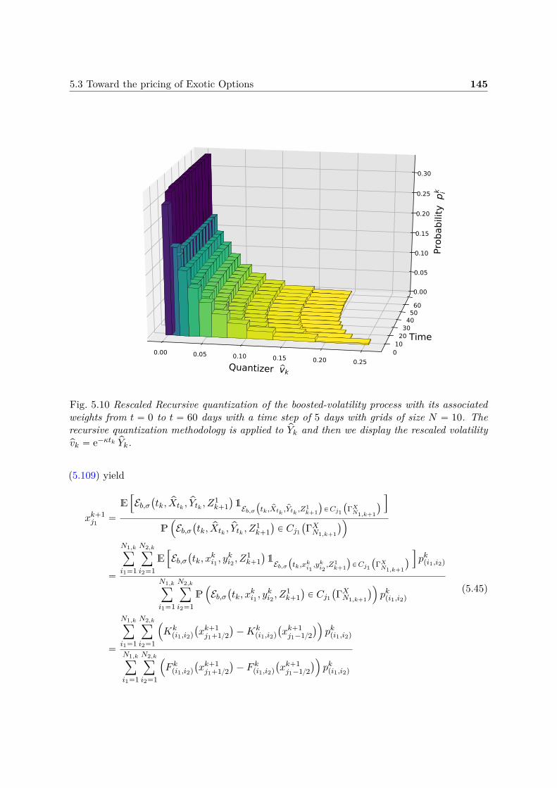
5.3 Toward the pricing of Exotic Options 145
Quantizer vk
0.00 0.05 0.10 0.15 0.20 0.25
Time0102030405060
Prob
abilit
y p
k i
0.00
0.05
0.10
0.15
0.20
0.25
0.30
Fig. 5.10 Rescaled Recursive quantization of the boosted-volatility process with its associatedweights from t “ 0 to t “ 60 days with a time step of 5 days with grids of size N “ 10. Therecursive quantization methodology is applied to pYk and then we display the rescaled volatilitypvk “ e´κtk pYk.
(5.109) yield
xk`1j1
“
E”
Eb,σ`
tk, pXtk ,pYtk , Z
1k`1
˘
1Eb,σ
`
tk, pXtk,pYtk
,Z1k`1
˘
PCj1
`
ΓXN1,k`1
˘
ı
P´
Eb,σ`
tk, pXtk ,pYtk , Z
1k`1
˘
P Cj1`
ΓXN1,k`1
˘
¯
“
N1,kÿ
i1“1
N2,kÿ
i2“1E”
Eb,σ`
tk, xki1 , y
ki2 , Z
1k`1
˘
1Eb,σ
`
tk,xki1,yk
i2,Z1
k`1
˘
PCj1
`
ΓXN1,k`1
˘
ı
pkpi1,i2q
N1,kÿ
i1“1
N2,kÿ
i2“1P´
Eb,σ`
tk, xki1 , y
ki2 , Z
1k`1
˘
P Cj1`
ΓXN1,k`1
˘
¯
pkpi1,i2q
“
N1,kÿ
i1“1
N2,kÿ
i2“1
´
Kkpi1,i2q
`
xk`1j1`12
˘
´Kkpi1,i2q
`
xk`1j1´12
˘
¯
pkpi1,i2q
N1,kÿ
i1“1
N2,kÿ
i2“1
´
F kpi1,i2q
`
xk`1j1`12
˘
´ F kpi1,i2q
`
xk`1j1´12
˘
¯
pkpi1,i2q
(5.45)
146Stationary Heston model: Calibration and Pricing of exotics using Product Recursive
Quantization
where pkpi1,i2q
“ P`
pXk “ xki1 ,pYk “ yki2
˘
and F kpi1,i2q
and Kkpi1,i2q
are the cumulative distributionfunction and the first partial moment function of the normal distribution µk
pi1,i2q` Z1
k`1σkpi1,i2q
and they are defined by
F kpi1,i2qpxq “ FZ
ˆ
x´ µkpi1,i2q
σkpi1,i2q
˙
Kkpi1,i2qpxq “ µkpi1,i2qFZ
ˆ
x´ µkpi1,i2q
σkpi1,i2q
˙
` σkpi1,i2qKZ
ˆ
x´ µkpi1,i2q
σkpi1,i2q
˙
(5.46)
withµkpi1,i2q “ xki1 ` bptk, x
ki1 , y
ki2qh and σkpi1,i2q “ σptk, x
ki1 , y
ki2q
?h (5.47)
and FZ and KZ are the cumulative distribution function and the first partial moment of thestandard normal distribution.
Finally, we apply the Lloyd method defined in Appendix (5.112) with FX and KX definedby
FX pxq “
N1,kÿ
i1“1
N2,kÿ
i2“1pkpi1,i2q F
kpi1,i2qpxq and KX pxq “
N1,kÿ
i1“1
N2,kÿ
i2“1pkpi1,i2q K
kpi1,i2qpxq. (5.48)
The sensitive part concerns the computation of the joint probabilities pkpi1,i2q
. Indeed, theyare needed at each step in order to be able to design recursively the quantization tree.
Lemma 5.3.3. The joint probabilities pkpi1,i2q
are given by the following forward induction
pk`1pj1,j2q
“
N1,kÿ
i“1
N2,kÿ
j“1pkpi1,i2qP
`
pXk`1 “ xk`1j1
, pYk`1 “ yk`1j2
| pXk “ xki1 ,pYk “ yki2
˘
(5.49)
where the joint conditional probabilities P`
pXk`1 “ xk`1j1
, pYk`1 “ yk`1j2
| pXk “ xki1 ,pYk “ yki2
˘
aregiven by the formulas below, depending on the correlation
• if CorrpZ1k`1, Z
2k`1q “ ρ “ 0
P`
pXk`1 “ xk`1j1
, pYk`1 “ yk`1j2
| pXk “ xki1 ,pYk “ yki2
˘
“ pki2j2
”
N`
xki1,i2,j1,`˘
´ N`
xki1,i2,j1,´˘
ı
,
(5.50)where pki2j2 is defined in (5.42) and
xki1,i2,j1,´ “xk`1j1´12 ´ µk
pi1,i2q
σkpi1,i2q
, xki1,i2,j1,` “xk`1j1`12 ´ µk
pi1,i2q
σkpi1,i2q
, (5.51)
with µkpi1,i2q
and σkpi1,i2q
defined in (5.47).
5.3 Toward the pricing of Exotic Options 147
• if CorrpZ1k`1, Z
2k`1q “ ρ ‰ 0
P`
pXk`1 “ xk`1j1
, pYk`1 “ yk`1j2
| pXk “ xki1 ,pYk “ yki2
˘
“ P´
Z1k`1 P
`
xki1,i2,j1,´, xki1,i2,j1,`
‰
, Z2k`1 P
´b
yki2,j2,´ ´ λki2 ,b
yki2,j2,` ´ λki2
ı¯
` P´
Z1k`1 P
`
xki1,i2,j1,´, xki1,i2,j1,`
‰
, Z2k`1 P
”
´
b
yki2,j2,` ´ λki2 ,´b
yki2,j2,´ ´ λki2
¯¯
(5.52)where
yki2,j2,´ “ 0 _yk`1j2´12 ´ µki2
κki2, yki2,j2,` “ 0 _
yk`1j2`12 ´ µki2
κki2, (5.53)
with µki2, κki2 and λki2 defined in (5.39).
Remark. The probability in the right hand side of (5.52) can be computed using the cumulativedistribution function of a correlated bivariate normal distribution2. Indeed, let
Fρpx1, x2q “ PpX1 ď x1, X2 ď x2q
the cumulative distribution function of the correlated centered Gaussian vector pX1, X2q withunit variance and correlation ρ, we have
P`
X1 P ra, bs, X2 P rc, ds˘
“ Fρpb, dq ´ Fρpb, cq ´ Fρpa, dq ` Fρpa, cq (5.54)
with a, c ě ´8 and b, d ď `8.
Proof.
pk`1pj1,j2q
“P`
pXk`1 “ xk`1j1
, pYk`1 “ yk`1j2
˘
“
N1,kÿ
i“1
N2,kÿ
j“1P`
pXk`1 “ xk`1j1
, pYk`1 “ yk`1j2
| pXk “ xki1 ,pYk “ yki2
˘
P`
pXk “ xki1 ,pYk “ yki2
˘
“
N1,kÿ
i“1
N2,kÿ
j“1pkpi1,i2qP
`
pXk`1 “ xk`1j1
, pYk`1 “ yk`1j2
| pXk “ xki1 ,pYk “ yki2
˘
.
2C++ implementation of the upper right tail of a bivariate normal distribution can be found in JohnBurkardt’s website https://people.sc.fsu.edu/~jburkardt/cpp_src/toms462/toms462.html.
148Stationary Heston model: Calibration and Pricing of exotics using Product Recursive
Quantization
• if CorrpZ1k`1, Z
2k`1q “ ρ “ 0
P`
pXk`1 “ xk`1j1
, pYk`1 “ yk`1j2
| pXk “ xki1 ,pYk “ yki2
˘
“ pki2j2 P`
pXk`1 “ xk`1j1
| pXk “ xki1 ,pYk “ yki2
˘
“ pki2j2 P´
sXk`1 P`
xk`1j1´12, x
k`1j1`12
‰
| pXk “ xki1 ,pYk “ yki2
¯
“ pki2j2 P´
Eb,σ`
tk, xki1 , y
ki2 , Z
1k`1
˘
P`
xk`1j1´12, x
k`1j1`12
‰
¯
“ pki2j2
”
N`
xki1,i2,j1,`˘
´ N`
xki1,i2,j1,´˘
ı
,
• if CorrpZ1k`1, Z
2k`1q “ ρ ‰ 0
P`
pXk`1 “ xk`1j1
, pYk`1 “ yk`1j2
| pXk “ xki1 ,pYk “ yki2
˘
“ P´
Eb,σ`
tk, xki1 , y
ki2 , Z
1k`1
˘
P`
xk`1j1´12, x
k`1j1`12
‰
,Mrb,rσ
`
tk, yki2 , Z
2k`1
˘
P`
yk`1j2´12, y
k`1j2`12
‰
¯
“ P´
µkpi1,i2q ` σkpi1,i2qZ1k`1 P
`
xk`1j1´12, x
k`1j1`12
‰
, µki2 ` κki2pZ2k`1 ` λki2q2 P
`
yk`1j2´12, y
k`1j2`12
‰
¯
“ P´
Z1k`1 P
`
xki1,i2,j1,´, xki1,i2,j1,`
‰
, pZ2k`1 ` λki2q2 P
`
yki2,j2,´, yki2,j2,`
‰
¯
“ P´
Z1k`1 P
`
xki1,i2,j1,´, xki1,i2,j1,`
‰
, Z2k`1 P
´b
yki2,j2,´ ´ λki2 ,b
yki2,j2,` ´ λki2
ı¯
` P´
Z1k`1 P
`
xki1,i2,j1,´, xki1,i2,j1,`
‰
, Z2k`1 P
”
´
b
yki2,j2,` ´ λki2 ,´b
yki2,j2,´ ´ λki2
¯¯
.
Remark. Another possibility for the quantization of the Stationary Heston model could be touse optimal quantizers for the volatility at each date tk in place of using recursive quantization.Indeed, the volatility pvtqt being stationary and the fact that we required the volatility to startat time 0 from the invariant measure, we could use the grid of the optimal quantization pv0
of size N of the stationary measure with its associated weights for every dates, hence settingpvk “ pv0. We need as well the transitions from time tk to tk`1 defined by
P`
pvk`1 “ vk`1j2
| pvk “ vki2˘
. (5.55)
These probabilities can be computed using the conditional law of the CIR process describedin [CIR05; And07], which is a non-central chi-square distribution. Then, we would build therecursive quantizer of the log-asset at date pXk`1 with the standard methodology of recursivequantization using the already built quantizers of the volatility pvk and the log-asset pXk at timetk, i.e.
rXk`1 “ Eb,σ`
tk, pXk, pvk, Z1k`1
˘
and pXk`1 “ ProjΓXN1,k`1
`
rXk`1˘
(5.56)
5.3 Toward the pricing of Exotic Options 149
where, this time, the Euler scheme is not defined in function of the boosted-volatility butdirectly in function of the volatility and is given by
Eb,σ`
t, x, v, z˘
“ x` h´
r ´ q ´v
2
¯
`?v
?hz. (5.57)
However, the difficulties with this approach come from the computation of the coupletransitions
P`
pXk`1 “ xk`1j1
, pvk`1 “ vk`1j2
| pXk “ xki1 , pvk “ vki2˘
. (5.58)
Indeed, these probability weights would not be as straightforward to compute as the methodologywe adopt in this paper, namely using time-discretization schemes for both components. Ourapproach allows us to express the conditional probability of the couple as the probability thata correlated bi-variate Gaussian vector lies in a rectangle domain and this can be easily becomputed numerically.
5.3.2.3 About the L2-error
In this part, we study the L2-error induced by the product recursive quantization approximationpUk “ p pXk, pYkq of sUk “ p sXk, sYkq, the time-discretized processes defined in (5.26) and (5.31) by
sUk “ Fk´1psUk´1, Zkq (5.59)
where Zk “ pZ1k , Z
2kq is a standardized correlated Gaussian vector and the hybrid discretization
scheme Fkpu, Zq is given by
Fkpu, Zq “
˜
Eb,σ`
tk, x, y, Z1k`1
˘
Mrb,rσ
`
tk, y, Z2k`1
˘
¸
. (5.60)
We recall the definition of the product recursive quantizer pUk “ p pXk, pYkq. Its first componentpXk is the projection of rXk onto ΓXN1,k
and the second component pYk is the projection of rYk ontoΓYN2,k
, i.e.,pXk`1 “ ProjΓX
N1,k`1
`
rXk`1˘
and pYk`1 “ ProjΓYN2,k`1
`
rYk`1˘
(5.61)
where rXk and rYk are defined in (5.36) and (5.44), respectively. Moreover, if we consider thecouple rUk “ p rXk, rYkq, using the above notations we have
rUk “ Fk´1ppUk´1, Zkq. (5.62)
150Stationary Heston model: Calibration and Pricing of exotics using Product Recursive
Quantization
It has been shown in [FSP18; PS18b] that if, for all k “ 0, . . . , n´ 1, the schemes Fkpu, zq
are Lipschitz in u, then there exists constants j “ 1, . . . , n, Cj ă `8 such that
pUk ´ sUk2 ď
kÿ
j“1Cj
`
N1,j ˆN2,j˘´12 (5.63)
where pUk and sUk are the processes defined in (5.61) and (5.62). The proof of this result isbased on the extension of Pierce’s lemma to the case of product quantization (see Lemma 2.3in [PS18b]).
In our case, the diffusion of the boosted volatility in the CIR model does not have Lipschitzdrift and volatility components, hence the above result from [FSP18; PS18b] does not applyin our context. Even if we can hope to obtain similar results by applying the same kind ofarguments, the results we obtain have to considered carefully. Indeed, when we take the limitin n Ñ `8, the number of time-step, the error upper-bound term goes to infinity. However, inpractice, we consider h “ kT n fixed and then study the behavior of pUk in function of N1,j andN2,j for j ě k. The proof of the following proposition is given in Appendix 5.C.
Proposition 5.3.4. Let b, σ, rb and rσ, defined by (5.27) and (5.33), the coefficients of thelog-asset and the boosted-volatility of the Heston model. Let, for every k “ 0, . . . , n, pUk thehybrid recursive product quantizer at level N1,k ˆN2,k of sUk. Then, for every k “ 0, . . . , n
pUk ´ sUk2 ď
kÿ
j“0
rAj,k`
N1,j ˆN2,j˘´12
`Bk?h (5.64)
whererAj,k “ 2
p´22p C2
pAj,k
ˆ
2pp2 ´1qjβjppU0p2 ` αp
1 ´ 2pp2 ´1qjβjp
1 ´ 2p2 ´1βp
˙1p
(5.65)
with
Aj,k “ 2k´j
2 e?
h2 pk´jq and Bk “ CT phq
k´1ÿ
j“02
k´1´j2 e
?h
2 pk´1´jq (5.66)
whereř
H “ 0 by convention and CT phq “ Op1q.
5.3.3 Backward algorithm for Bermudan and Barrier options
Bermudan Options A Bermudan option is a financial derivative product that gives theright to its owner to buy or sell (or to enter to, in the case of a swap) an underlying productwith a given payoff ψtp¨, ¨q at predefined exercise dates tt0, ¨ ¨ ¨ , tnu. Its price, at time t0 “ 0, isgiven by
supτPtt0,¨¨¨ ,tnu
E”
e´rτ ψτ pXτ , Yτ q | F t0
ı
where Xt and Yt are solutions to the system defined in (5.34).
5.3 Toward the pricing of Exotic Options 151
In this part, we follow the numerical solution first introduced by [BPP05; BP03]. Theyproposed to solve discrete-time optimal stopping problems using a quantization tree of the riskfactors Xt and Yt.
Let FX,Y “ pFq0ďkďn the natural filtration of X and Y . Hence, we can define recursivelythe sequence of random variable Lp-integrable pVkq0ďkďn
#
Vn “ e´rtn ψnpXn, Ynq,
Vk “ max`
e´rtk ψkpXk, Ykq,ErVk`1 | Fks˘
, 0 ď k ď n´ 1(5.67)
called Backward Dynamic Programming Principle. Then
V0 “ sup
Ere´rτ ψτ pXτ , Yτ q | F0s, τ P Θ0,n(
with Θ0,n the set of all stopping times taking values in tt0, ¨ ¨ ¨ , tnu. The sequence pVkq0ďkďn isalso known as the Snell envelope of the obstacle process
`
e´rtk ψkpXk, Ykq˘
0ďkďn. In the end,
ErV0s is the quantity we are interested in. Indeed, ErV0s is the price of the Bermudan optionwhose payoff is ψk and is exercisable at dates tt1, ¨ ¨ ¨ , tnu.
Following what was defined in (5.67), in order to compute ErV0s, we will need to usethe previously defined quantizer of Xk and Yk: pXk and pYk. Hence, for a given global budgetN “ N1,0N2,0`¨ ¨ ¨`N1,nN2,n, the total number of nodes of the tree by the couple p pXk, pYkq0ďkďn,we can approximate the Backward Dynamic Programming Principle (5.67) by the followingsequence involving the couple p pXk, pYkq0ďkďn
#
pVn “ e´rtn ψnp pXn, pYnq,
pVk “ max`
e´rtk ψkp pXk, pYkq,ErpVk`1 | p pXk, pYkqs˘
, k “ 0, . . . , n´ 1.(5.68)
Remark. A direct consequence of choosing recursive Markovian Quantization to spatiallydiscretize the problem is that the sequence p pXk, pYkq0ďkďn is Markovian. Hence ppVkq0ďkďn
defined in (5.68) obeying a Backward Dynamic Programming Principle is the Snell envelope of`
e´rtk ψkp pXk, pYkq˘
0ďkďn. This is the main difference with the first approach of [BPP05; BP03],
where in there case they only had a pseudo-Snell envelope of`
e´rtk ψkp pXk, pYkq˘
0ďkďn.
Using the discrete feature of the quantizers, (5.68) can be rewritten$
’
’
’
’
’
’
’
&
’
’
’
’
’
’
’
%
pvnpxni1 , yni2q “ e´rtn ψnpxni1 , y
ni2q,
i1 “ 1, . . . , N1,n
i2 “ 1, . . . , N2,n
pvkpxki1 , yki2q “ max
´
e´rtk ψkpxki1 , yki2q,
N1,k`1ÿ
j1“1
N2,k`1ÿ
j2“1πkpi1,i2q,pj1,j2qpvk`1pxk`1
j1, yk`1j2
q
¯
,
k “ 0, . . . , n´ 1i1 “ 1, . . . , N1,k
i2 “ 1, . . . , N2,k(5.69)
152Stationary Heston model: Calibration and Pricing of exotics using Product Recursive
Quantization
where πkpi1,i2q,pj1,j2q
“ P`
pXk`1 “ xk`1j1
, pYk`1 “ yk`1j2
| pXk “ xki1 ,pYk “ yki2
˘
is the conditionalprobability weight given in (5.52). Finally, the approximation of the price of the Bermudanoption is given by
E“
pv0px0, pY0q‰
“
N2,0ÿ
i“1pi pv0px0, y
0i q (5.70)
with pi “ P`
pY0 “ y0i
˘
given by (5.18).
Barrier Options A Barrier option is a path-dependent financial product whose payoff atmaturity date T depends on the value of the process XT at time T and its maximum orminimum over the period r0, T s. More precisely, we are interested by options with the followingtypes of payoff h
h “ fpXT q1tsuptPr0,T s XtPIu or h “ fpXT q1tinftPr0,T s XtPIu (5.71)
where I is an unbounded interval of R, usually of the forme p´8, Ls or rL,`8q (L is thebarrier) and f can be any vanilla payoff function (Call, Put, Spread, Butterfly, ...).
In this part, we follow the methodology initiated in [Sag10] in the case of functionalquantization. This work is based on the Brownian bridge method applied to the Euler-Maruyamascheme as described e.g. in [Pag18]. We generalize it to stochastic volatility models and productMarkovian recursive quantization. Xt being discretized by an Euler-Maruyama scheme, yieldingsXk with k “ 0, . . . , n, we can determine the law of maxtPr0,T s
sXt and mintPr0,T ssXt given the
values sXk “ xk, sYk “ yk, k “ 0, . . . , n
L´
maxtPr0,T s
sXt | sXk “ xk, sYk “ yk, k “ 0, . . . , n¯
“ L´
maxk“0,...,n´1
`
Gkpxk,ykq,xk`1
˘´1pUkq
¯
(5.72)
and
L´
mintPr0,T s
sXt | sXk “ xk, sYk “ yk, k “ 0, . . . , n¯
“ L´
maxk“0,...,n´1
`
F kpxk,ykq,xk`1
˘´1pUkq
¯
(5.73)
where pUkqk“0,...,n´1 are i.i.d uniformly distributed random variables over the unit interval andpGk
px,yq,zq´1 and pF k
px,yq,zq´1 are the inverse of the conditional distribution functions Gk
px,yq,z andF k
px,yq,z defined by
Gkpx,yq,zpuq “
´
1 ´ e´2n px´uqpz´uq
T σ2ptk,x,yq
¯
1tuěmaxpx,zqu (5.74)
andF kpx,yq,zpuq “ 1 ´
´
1 ´ e´2n px´uqpz´uq
T σ2ptk,x,yq
¯
1tuďminpx,zqu . (5.75)
Now, using the resulting representation formula for E fp sXT ,maxtPr0,T ssXtq (see e.g. [Sag10;
Pag18]), we have a new representation formula for the price of up-and-out options sPUO and
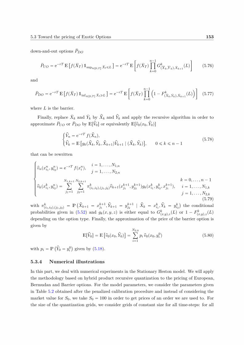
5.3 Toward the pricing of Exotic Options 153
down-and-out options sPDO
sPUO “ e´rT E“
fp sXT q1suptPr0,T ssXtďL
‰
“ e´rT E
„
fp sXT q
n´1ź
k“0Gk
pXk,Y kq, sXk`1pLq
ȷ
(5.76)
and
sPDO “ e´rT E“
fp sXT q1inftPr0,T ssXtěL
‰
“ e´rT E
„
fp sXT q
n´1ź
k“0
´
1 ´ F kp sXk,sYkq, sXk`1
pLq
¯
ȷ
(5.77)
where L is the barrier.
Finally, replace sXk and sYk by pXk and pYk and apply the recursive algorithm in order toapproximate sPUO or sPDO by ErpV0s or equivalently Erpv0px0, pY0qs
#
pVn “ e´rT fp pXnq,
pVk “ E“
gkp pXk, pYk, pXk`1qpVk`1 | p pXk, pYkq‰
, 0 ď k ď n´ 1(5.78)
that can be rewritten$
’
’
’
’
’
’
’
&
’
’
’
’
’
’
’
%
pvnpxni1 , yni2q “ e´rT fpxni q,
i “ 1, . . . , N1,n
j “ 1, . . . , N2,n
pvkpxki1 , yni2q “
N1,k`1ÿ
j1“1
N2,k`1ÿ
j2“1πkpi1,i2q,pj1,j2qpvk`1pxk`1
j1, yk`1j2
qgkpxki1 , yki2 , x
k`1j1
q,
k “ 0, . . . , n´ 1i “ 1, . . . , N1,k
j “ 1, . . . , N2,k(5.79)
with πkpi1,i2q,pj1,j2q
“ P`
pXk`1 “ xk`1j1
, pYk`1 “ yk`1j2
| pXk “ xki1 ,pYk “ yki2
˘
the conditionalprobabilities given in (5.52) and gkpx, y, zq is either equal to Gk
px,yq,zpLq or 1 ´ F kpx,yq,zpLq
depending on the option type. Finally, the approximation of the price of the barrier option isgiven by
ErpV0s “ E“
pv0px0, pY0q‰
“
N2,0ÿ
i“1pi pv0px0, y
0i q (5.80)
with pi “ P`
pY0 “ y0i
˘
given by (5.18).
5.3.4 Numerical illustrations
In this part, we deal with numerical experiments in the Stationary Heston model. We will applythe methodology based on hybrid product recursive quantization to the pricing of European,Bermudan and Barrier options. For the model parameters, we consider the parameters givenin Table 5.2 obtained after the penalized calibration procedure and instead of considering themarket value for S0, we take S0 “ 100 in order to get prices of an order we are used to. Forthe size of the quantization grids, we consider grids of constant size for all time-steps: for all
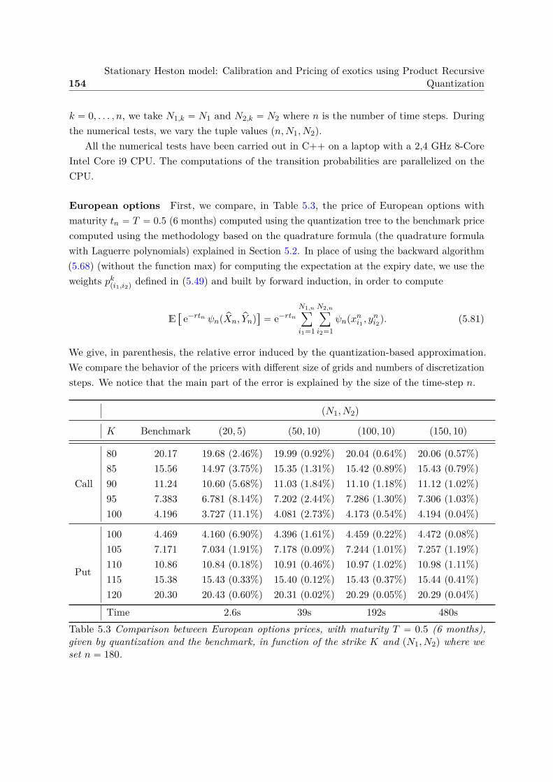
154Stationary Heston model: Calibration and Pricing of exotics using Product Recursive
Quantization
k “ 0, . . . , n, we take N1,k “ N1 and N2,k “ N2 where n is the number of time steps. Duringthe numerical tests, we vary the tuple values pn,N1, N2q.
All the numerical tests have been carried out in C++ on a laptop with a 2,4 GHz 8-CoreIntel Core i9 CPU. The computations of the transition probabilities are parallelized on theCPU.
European options First, we compare, in Table 5.3, the price of European options withmaturity tn “ T “ 0.5 (6 months) computed using the quantization tree to the benchmark pricecomputed using the methodology based on the quadrature formula (the quadrature formulawith Laguerre polynomials) explained in Section 5.2. In place of using the backward algorithm(5.68) (without the function max) for computing the expectation at the expiry date, we use theweights pk
pi1,i2qdefined in (5.49) and built by forward induction, in order to compute
E“
e´rtn ψnp pXn, pYnq‰
“ e´rtn
N1,nÿ
i1“1
N2,nÿ
i2“1ψnpxni1 , y
ni2q. (5.81)
We give, in parenthesis, the relative error induced by the quantization-based approximation.We compare the behavior of the pricers with different size of grids and numbers of discretizationsteps. We notice that the main part of the error is explained by the size of the time-step n.
pN1, N2q
K Benchmark p20, 5q p50, 10q p100, 10q p150, 10q
Call
80 20.17 19.68 p2.46%q 19.99 p0.92%q 20.04 p0.64%q 20.06 p0.57%q
85 15.56 14.97 p3.75%q 15.35 p1.31%q 15.42 p0.89%q 15.43 p0.79%q
90 11.24 10.60 p5.68%q 11.03 p1.84%q 11.10 p1.18%q 11.12 p1.02%q
95 7.383 6.781 p8.14%q 7.202 p2.44%q 7.286 p1.30%q 7.306 p1.03%q
100 4.196 3.727 p11.1%q 4.081 p2.73%q 4.173 p0.54%q 4.194 p0.04%q
Put
100 4.469 4.160 p6.90%q 4.396 p1.61%q 4.459 p0.22%q 4.472 p0.08%q
105 7.171 7.034 p1.91%q 7.178 p0.09%q 7.244 p1.01%q 7.257 p1.19%q
110 10.86 10.84 p0.18%q 10.91 p0.46%q 10.97 p1.02%q 10.98 p1.11%q
115 15.38 15.43 p0.33%q 15.40 p0.12%q 15.43 p0.37%q 15.44 p0.41%q
120 20.30 20.43 p0.60%q 20.31 p0.02%q 20.29 p0.05%q 20.29 p0.04%q
Time 2.6s 39s 192s 480sTable 5.3 Comparison between European options prices, with maturity T “ 0.5 (6 months),given by quantization and the benchmark, in function of the strike K and pN1, N2q where weset n “ 180.
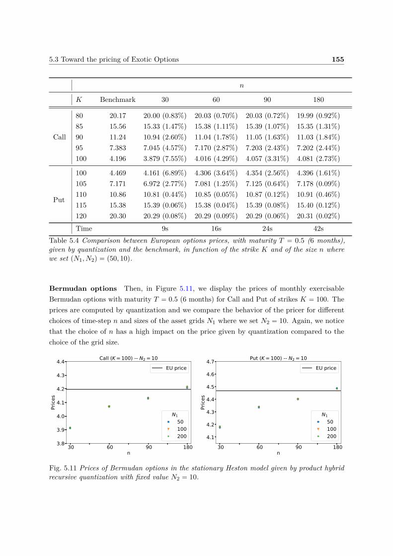
5.3 Toward the pricing of Exotic Options 155
n
K Benchmark 30 60 90 180
Call
80 20.17 20.00 p0.83%q 20.03 p0.70%q 20.03 p0.72%q 19.99 p0.92%q
85 15.56 15.33 p1.47%q 15.38 p1.11%q 15.39 p1.07%q 15.35 p1.31%q
90 11.24 10.94 p2.60%q 11.04 p1.78%q 11.05 p1.63%q 11.03 p1.84%q
95 7.383 7.045 p4.57%q 7.170 p2.87%q 7.203 p2.43%q 7.202 p2.44%q
100 4.196 3.879 p7.55%q 4.016 p4.29%q 4.057 p3.31%q 4.081 p2.73%q
Put
100 4.469 4.161 p6.89%q 4.306 p3.64%q 4.354 p2.56%q 4.396 p1.61%q
105 7.171 6.972 p2.77%q 7.081 p1.25%q 7.125 p0.64%q 7.178 p0.09%q
110 10.86 10.81 p0.44%q 10.85 p0.05%q 10.87 p0.12%q 10.91 p0.46%q
115 15.38 15.39 p0.06%q 15.38 p0.04%q 15.39 p0.08%q 15.40 p0.12%q
120 20.30 20.29 p0.08%q 20.29 p0.09%q 20.29 p0.06%q 20.31 p0.02%q
Time 9s 16s 24s 42sTable 5.4 Comparison between European options prices, with maturity T “ 0.5 (6 months),given by quantization and the benchmark, in function of the strike K and of the size n wherewe set pN1, N2q “ p50, 10q.
Bermudan options Then, in Figure 5.11, we display the prices of monthly exercisableBermudan options with maturity T “ 0.5 (6 months) for Call and Put of strikes K “ 100. Theprices are computed by quantization and we compare the behavior of the pricer for differentchoices of time-step n and sizes of the asset grids N1 where we set N2 “ 10. Again, we noticethat the choice of n has a high impact on the price given by quantization compared to thechoice of the grid size.
30 60 90 180n
3.8
3.9
4.0
4.1
4.2
4.3
4.4
Price
s
Call (K=100) -- N2=10EU price
N150100200
30 60 90 180n
4.1
4.2
4.3
4.4
4.5
4.6
4.7
Price
s
Put (K=100) -- N2=10EU price
N150100200
Fig. 5.11 Prices of Bermudan options in the stationary Heston model given by product hybridrecursive quantization with fixed value N2 “ 10.
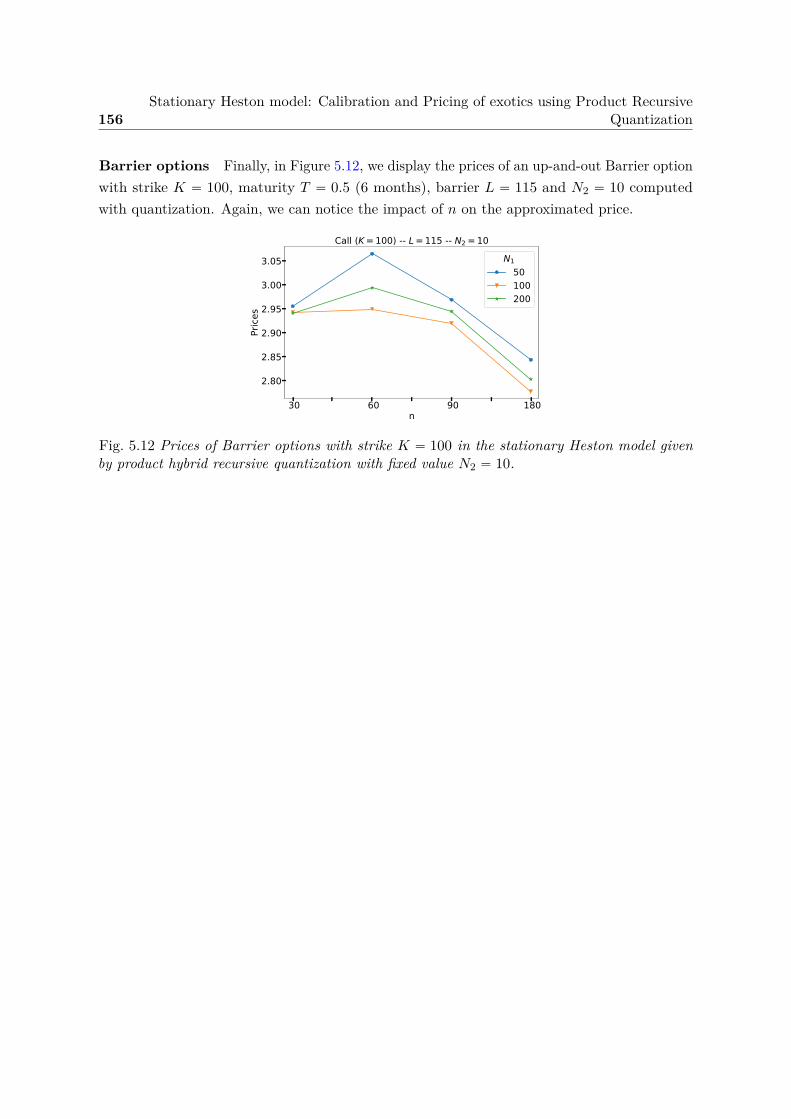
156Stationary Heston model: Calibration and Pricing of exotics using Product Recursive
Quantization
Barrier options Finally, in Figure 5.12, we display the prices of an up-and-out Barrier optionwith strike K “ 100, maturity T “ 0.5 (6 months), barrier L “ 115 and N2 “ 10 computedwith quantization. Again, we can notice the impact of n on the approximated price.
30 60 90 180n
2.80
2.85
2.90
2.95
3.00
3.05Price
sCall (K=100) -- L=115 -- N2=10
N150100200
Fig. 5.12 Prices of Barrier options with strike K “ 100 in the stationary Heston model givenby product hybrid recursive quantization with fixed value N2 “ 10.
5.A Discretization scheme for the volatility preserving the positivity 157
Appendix 5.A Discretization scheme for the volatility preserv-ing the positivity
We recall the dynamics of the volatility
dvt “ κpθ ´ vtqdt` ξ?vtdĂWt
with κ ą 0, θ ą 0 and ξ ą 0. In this section, we discuss the choice of the discretization schemeunder the Feller condition, which ensures the positivity of the process.
Euler-Maruyama scheme. Discretizing the volatility using an Euler-Maruyama scheme
svtk`1 “ svtk ` κpθ ´ svtk qh` ξa
svtk?hZ2
k`1
with tk “ kh, h “ T n and Z2k`1 “ pĂWtk`1 ´ ĂWtk q
?h may look natural. However, such a
scheme clearly does not preserve positivity of the process even if the Feller condition is fulfilledsince
P`
svt1 ă 0˘
“ P
ˆ
Z ă´v0 ´ κpθ ´ v0qh
ξ?v0
?h
˙
ą 0
with Z „ N p0, 1q. This suggests to introduce the Milstein scheme which is quite tractable inone dimension in absence of Lévy areas.
Milstein scheme. The Milstein scheme of the stochastic volatility is given by
svtk`1 “ Mb,σ
`
tk, svtk`1 , Z2k`1
˘
where (see (5.28))
Mb,σpt, x, zq “ x´σpxq
2σ1xpxq
` h
ˆ
bpt, xq ´pσσ1
xqpxq
2
˙
`pσσ1
xqpxqh
2
ˆ
z `1
?hσ1
xpxq
˙2.
with bpxq “ κpθ ´ xq, σpxq “ ξ?x and σ1
xpxq “ξ
2?x. Consequently, under the Feller condition,
the positivity of Mb,σpt, x, zq is ensured if
x ěσpxq
2σ1xpxq
ě 0, bpt, xq ěpσσ1
xqpxq
2 ě 0.
In our case, if the first condition holds true since
σpxq
2σ1xpxq
“ξ?x
2 ξ2
?x
“ x
158Stationary Heston model: Calibration and Pricing of exotics using Product Recursive
Quantization
the second one fails. Indeedpσσ1
xqpxq
2 “ξ?x ξ
2?x
2 “ξ2
4can be bigger than bpt, xq. In order to solve this problem, we consider the following boostedvolatility process
Yt “ eκt vt, t P r0, T s. (5.82)
Milstein scheme for the boosted volatility. Let Yt “ eκt vt, t P r0, T s for some κ ą 0,which satisfies, owing to Itô’s formula
dYt “ eκt κθdt` ξ eκt2a
YtdĂWt.
Remark. The process pYtqtPr0,T s will have a higher variance but, having in mind a quantizedscheme, this has no real impact (by contrast with a Monte Carlo simulation).
Now, if we look at the Milstein discretization scheme of Yt
sYtk`1 “ Mrb,rσ
`
tk, sYtk , Z2k`1
˘
using the notation defined in (5.28) where drift and volatility terms of the boosted process, nowtime-dependents, are given by
rbpt, xq “ eκt κθ, rσpt, xq “ ξ?x eκt2 and rσ1
xpt, xq “ξ eκt2
2?x.
Under the Feller condition, the positivity of the scheme is ensured, since
rσpt, xq
2rσ1xpt, xq
“ x and prσrσ1xqpt, xq
2 “ξ2 eκt
4 ď rbpt, xq “ eκt κθ.
The last inequality is satisfied thanks to the condition ξ2
2κθ ď 1 ensuring the positivity of thescheme.
Appendix 5.B Lp-linear growth of the hybrid scheme
The aim of this section is to show the Lp-linear growth of the scheme Fkpu, zq with u “ px, yq
defined by
Fkpu, Zq “
˜
Eb,σ`
tk, x, y, Z1k`1
˘
Mrb,rσ
`
tk, y, Z2k`1
˘
¸
. (5.83)
where the schemes Eb,σ and Mrb,rσ
are defined in (5.32) and (5.28), respectively.The results on the Lp-linear growth of the schemes are essentially based on the key Lemma
2.1 proved in [PS18b] in Rd that we recall below.
5.B Lp-linear growth of the hybrid scheme 159
Lemma 5.B.1. (a) Let u P Rd and Apuq be a dˆ q-matrix and let apuq P Rd. Let p P r2, 3q.For any centered random vector ζ P Lp
RdpΩ,A,Pq, one has for every h P p0,`8q
E“
|apuq `?hApuqζ|p
‰
ď
ˆ
1 `pp´ 1qpp´ 2q
2 h
˙
|apuq|p`h`
1 `p`hp2 ´1˘ApuqpE
“
|ζ|p‰
(5.84)where Apuq “
`
TrpApuqA‹puqq˘12.
(b) In particular, if |apuq| ď |u|p1 ` Lhq ` Lh and Apuqp ď 2p´1Υpp1 ` |u|pq, then
E“
|apuq `?hApuqζ|p
‰
ď`
eκph L`Kp
˘
h``
eκph `Kph˘
|u|p, (5.85)
where
κp “pp´ 1qpp´ 2q
2 ` 2pL and Kp “ 2p´1Υp`
1 ` p` hp2 ´1˘E
“
|ζ|p‰
. (5.86)
Now, we will apply Lemma 5.B.1 to Fkpu, zq defined in (5.83) further on in order to showits Lp-linear growth. Let apuq P R2 and let Apuq be a 2 ˆ 3-matrix defined by
apuq “
˜
x` h`
r ´e´κtk y
2˘
y ` eκtk κθh
¸
, Apuq “
˜
e´κtk2 ?y 0 0
0 ?y eκtk2 ?
h ξ2 eκtk
4
¸
and ζ “
¨
˚
˝
Z1k`1
Z2k`1
pZ2k`1q2 ´ 1
˛
‹
‚
.
First, we show the linear growth of apuq
|apuq| “
´ˇ
ˇ
ˇx` h
`
r ´e´κtk y
2˘
ˇ
ˇ
ˇ
2`ˇ
ˇy ` eκtk κθhˇ
ˇ
2¯12
“
´
|x|2 ` |y|2 ` h2´
r2 `e´2κtk
4 |y|2¯
` e2κtk κ2θ2h2¯12
ď
´
|u|2´
1 ` h2 e´2κtk
4
¯
` h2`r2 ` e2κtk κ2θ2˘¯12
ď |u|
´
1 ` h2 e´2κtk
4
¯12` h
`
r2 ` e2κtk κ2θ2˘12
ď |u|
´
1 ` hh
2
¯
` h`
r2 ` e2κT κ2θ2˘12
ď |u|p1 ` Lhq ` Lh
160Stationary Heston model: Calibration and Pricing of exotics using Product Recursive
Quantization
where L “ max´
12 ,`
r2 ` e2κT κ2θ2˘12¯
. Then, we study Apuqp
Apuqp “
´
e´κtk |y| ` |y| eκtk `hξ4 e2κtk
16
¯p2
“
´
|y|pe´κtk ` eκtk q ` hξ4 e2κtk
16
¯p2
ď 2p2 ´1
´
|y|p2 pe´κtk ` eκtk q
p2 ` h
p2ξ2p epκtk
4p¯
ď 2p2 ´1
´
|y|p ` 12 pe´κtk ` eκtk q
p2 ` h
p2ξ2p epκtk
4p¯
ď 2p2 ´1 p1 ` eκT q
p2
2
´
|y|p ` 1 ` hp2ξ2p epκT22p´1
1p1 ` eκT q
p2
¯
ď 2p´1Υp`
1 ` |u|p˘
where Υp “p1`eκT q
p2
2 ` hp2 ξ
2p epκT
22p . Hence, by Lemma 5.B.1, the discretization scheme Fk hasan Lp-linear growth
E“
|Fkpu, Zk`1q|p‰
ď αp ` βp|u|p
withαp “
`
eκph L`Kp
˘
h and βp “ eκph `Kph (5.87)
where Kp and κp are defined in the Lemma 5.B.1.
Appendix 5.C Proof of the L2-error estimation of Proposition5.3.4
We have, for every k “ 0, . . . , n´ 1
pUk`1 ´ sUk`1 “ pUk`1 ´ rUk`1 ` rUk`1 ´ sUk`1
“ pUk`1 ´ rUk`1 ` FkppUk, Zk`1q ´ FkpsUk, Zk`1q(5.88)
by the very definition of rUk`1 and sUk`1. Hence,
pUk`1 ´ sUk`12 ď pUk`1 ´ rUk`12 ` rUk`1 ´ sUk`12
ď pUk`1 ´ rUk`12 ` FkppUk, Zk`1q ´ FkpsUk, Zk`1q2 .(5.89)
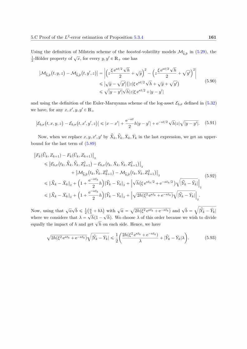
5.C Proof of the L2-error estimation of Proposition 5.3.4 161
Using the definition of Milstein scheme of the boosted-volatility models Mrb,rσ
in (5.29), the12 -Hölder property of
?x, for every y, y1 P R` one has
ˇ
ˇMrb,rσ
`
t, y, z˘
´ Mrb,rσ
`
t, y1, z˘ˇ
ˇ “
ˇ
ˇ
ˇ
ˇ
´
zξ eκt2 ?
h
2 `?y¯2
´
´
zξ eκt2 ?
h
2 `a
y1
¯2ˇ
ˇ
ˇ
ˇ
ďˇ
ˇ
?y ´
a
y1ˇ
ˇ
`
|z|ξ eκt2 ?h`
?y `
a
y1˘
ďa
|y ´ y1|?h|z|ξ eκt2 `|y ´ y1|
(5.90)
and using the definition of the Euler-Maruyama scheme of the log-asset Eb,σ defined in (5.32)we have, for any x, x1, y, y1 P R`
ˇ
ˇEb,σ`
t, x, y, z˘
´ Eb,σ`
t, x1, y1, z˘ˇ
ˇ ď |x´ x1| `e´κt
2 h|y ´ y1| ` e´κt2 ?h|z|
a
|y ´ y1|. (5.91)
Now, when we replace x, y, x1, y1 by pXk, pYk, sXk, sYk in the last expression, we get an upper-bound for the last term of (5.89)›
›FkppUk, Zk`1q ´ FkpsUk, Zk`1q›
›
2
ď›
›Eb,σ`
tk, pXk, pYk, Z1k`1
˘
´ Eb,σ`
tk, sXk, sYk, Z1k`1
˘›
›
2
`›
›Mrb,rσ
`
tk, pYk, Z2k`1
˘
´ Mrb,rσ
`
tk, sYk, Z2k`1
˘›
›
2
ď pXk ´ sXk2 `
´
1 `e´κtk
2 h¯
pYk ´ sYk2 `
›
›
›
?h`
ξ eκtk2 ` e´κtk2 ˘b
|pYk ´ sYk|
›
›
›
2
ď pXk ´ sXk2 `
´
1 `e´κtk
2 h¯
pYk ´ sYk2 `
›
›
›
a
2hpξ2 eκtk ` e´κtk q
b
|pYk ´ sYk|
›
›
›
2.
(5.92)
Now, using that?a
?b ď 1
2`
aλ ` bλ
˘
with?a “
a
2hpξ2 eκtk ` e´κtk q and?b “
b
|pYk ´ sYk|
where we considere that λ “?hp1 ´
?hq. Wo choose λ of this order because we wish to divide
equally the impact of h and get?h on each side. Hence, we have
a
2hpξ2 eκtk ` e´κtk q
b
|pYk ´ sYk| ď12
ˆ
2hpξ2 eκtk ` e´κtk q
λ` |pYk ´ sYk|λ
˙
. (5.93)
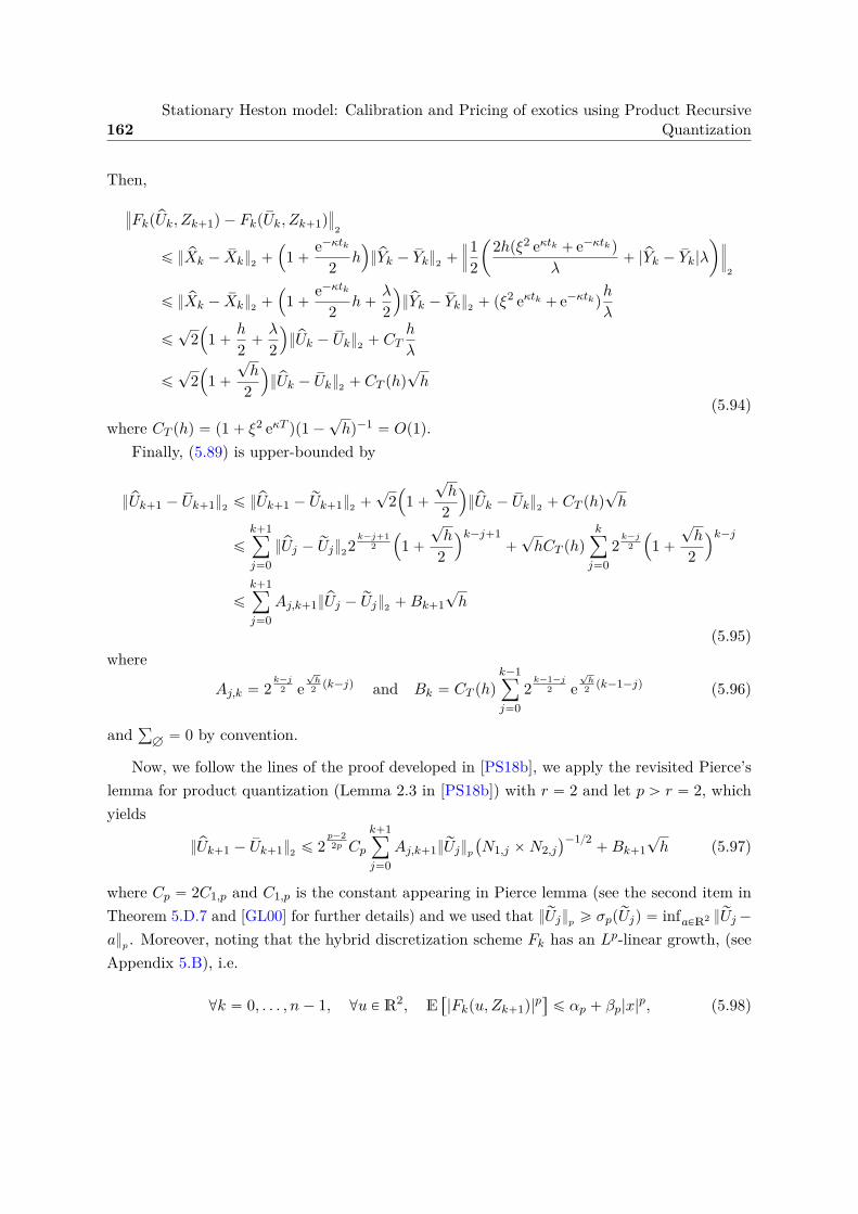
162Stationary Heston model: Calibration and Pricing of exotics using Product Recursive
Quantization
Then,›
›FkppUk, Zk`1q ´ FkpsUk, Zk`1q›
›
2
ď pXk ´ sXk2 `
´
1 `e´κtk
2 h¯
pYk ´ sYk2 `
›
›
›
12
ˆ
2hpξ2 eκtk ` e´κtk q
λ` |pYk ´ sYk|λ
˙
›
›
›
2
ď pXk ´ sXk2 `
´
1 `e´κtk
2 h`λ
2
¯
pYk ´ sYk2 ` pξ2 eκtk ` e´κtk qh
λ
ď?
2´
1 `h
2 `λ
2
¯
pUk ´ sUk2 ` CTh
λ
ď?
2´
1 `
?h
2
¯
pUk ´ sUk2 ` CT phq?h
(5.94)where CT phq “ p1 ` ξ2 eκT qp1 ´
?hq´1 “ Op1q.
Finally, (5.89) is upper-bounded by
pUk`1 ´ sUk`12 ď pUk`1 ´ rUk`12 `?
2´
1 `
?h
2
¯
pUk ´ sUk2 ` CT phq?h
ď
k`1ÿ
j“0pUj ´ rUj22
k´j`12
´
1 `
?h
2
¯k´j`1`
?hCT phq
kÿ
j“02
k´j2
´
1 `
?h
2
¯k´j
ď
k`1ÿ
j“0Aj,k`1pUj ´ rUj2 `Bk`1
?h
(5.95)where
Aj,k “ 2k´j
2 e?
h2 pk´jq and Bk “ CT phq
k´1ÿ
j“02
k´1´j2 e
?h
2 pk´1´jq (5.96)
andř
H “ 0 by convention.
Now, we follow the lines of the proof developed in [PS18b], we apply the revisited Pierce’slemma for product quantization (Lemma 2.3 in [PS18b]) with r “ 2 and let p ą r “ 2, whichyields
pUk`1 ´ sUk`12 ď 2p´22p Cp
k`1ÿ
j“0Aj,k`1rUjp
`
N1,j ˆN2,j˘´12
`Bk`1?h (5.97)
where Cp “ 2C1,p and C1,p is the constant appearing in Pierce lemma (see the second item inTheorem 5.D.7 and [GL00] for further details) and we used that rUjp ě σpprUjq “ infaPR2 rUj ´
ap . Moreover, noting that the hybrid discretization scheme Fk has an Lp-linear growth, (seeAppendix 5.B), i.e.
@k “ 0, . . . , n´ 1, @u P R2, E“
|Fkpu, Zk`1q|p‰
ď αp ` βp|x|p, (5.98)
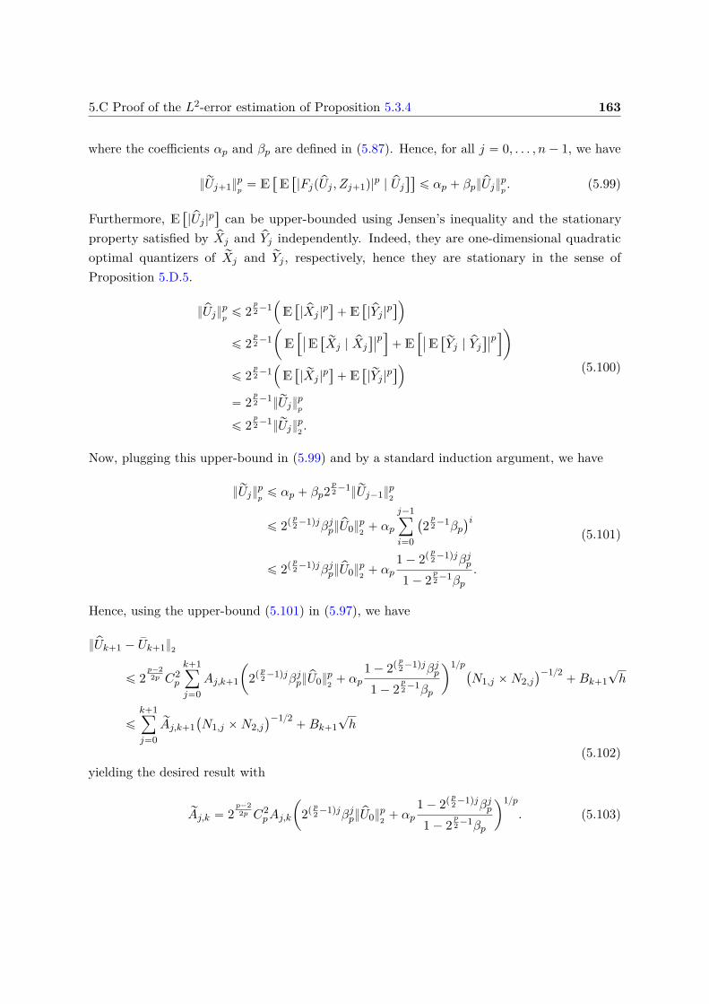
5.C Proof of the L2-error estimation of Proposition 5.3.4 163
where the coefficients αp and βp are defined in (5.87). Hence, for all j “ 0, . . . , n´ 1, we have
rUj`1pp
“ E“
E“
|FjppUj , Zj`1q|p | pUj‰‰
ď αp ` βppUjpp. (5.99)
Furthermore, E“
|pUj |p‰
can be upper-bounded using Jensen’s inequality and the stationaryproperty satisfied by pXj and pYj independently. Indeed, they are one-dimensional quadraticoptimal quantizers of rXj and rYj , respectively, hence they are stationary in the sense ofProposition 5.D.5.
pUjpp
ď 2p2 ´1
´
E“
| pXj |p‰
` E“
|pYj |p‰
¯
ď 2p2 ´1
ˆ
E”
ˇ
ˇE“
rXj | pXj
‰ˇ
ˇ
pı
` E”
ˇ
ˇE“
rYj | pYj‰ˇ
ˇ
pı
˙
ď 2p2 ´1
´
E“
| rXj |p‰
` E“
|rYj |p‰
¯
“ 2p2 ´1rUj
pp
ď 2p2 ´1rUj
p2 .
(5.100)
Now, plugging this upper-bound in (5.99) and by a standard induction argument, we have
rUjpp
ď αp ` βp2p2 ´1rUj´1p2
ď 2pp2 ´1qjβjppU0p2 ` αp
j´1ÿ
i“0
`
2p2 ´1βp
˘i
ď 2pp2 ´1qjβjppU0p2 ` αp
1 ´ 2pp2 ´1qjβjp
1 ´ 2p2 ´1βp
.
(5.101)
Hence, using the upper-bound (5.101) in (5.97), we have
pUk`1 ´ sUk`12
ď 2p´22p C2
p
k`1ÿ
j“0Aj,k`1
ˆ
2pp2 ´1qjβjppU0p2 ` αp
1 ´ 2pp2 ´1qjβjp
1 ´ 2p2 ´1βp
˙1p`
N1,j ˆN2,j˘´12
`Bk`1?h
ď
k`1ÿ
j“0
rAj,k`1`
N1,j ˆN2,j˘´12
`Bk`1?h
(5.102)yielding the desired result with
rAj,k “ 2p´22p C2
pAj,k
ˆ
2pp2 ´1qjβjppU0p2 ` αp
1 ´ 2pp2 ´1qjβjp
1 ´ 2p2 ´1βp
˙1p
. (5.103)
164Stationary Heston model: Calibration and Pricing of exotics using Product Recursive
Quantization
Appendix 5.D Quadratic Optimal Quantization: Generic Ap-proach
Let X be a R-valued random variable with distribution PX defined on a probability spacepΩ,A,Pq such that X P L2
RpΩ,A,Pq.
Definition 5.D.1. Let ΓN “ txN1 , . . . , xNNu Ă R be a subset of size N , called N -quantizer. A
Borel partition pCipΓN qqiPt1,...,Nu of R is a Voronoï partition of R induced by the N -quantizerΓN if, for every i P t1, . . . , Nu,
CipΓN q Ă
ξ P R, |ξ ´ xNi | ď minj‰i
|ξ ´ xNj |(
.
The Borel sets CipΓN q are called Voronoï cells of the partition induced by ΓN .
Remark. Any such N -quantizer is in correspondence with the N -tuple x “ pxN1 , . . . , xNN q P
pRqN as well as with all N -tuples obtained by a permutation of the components of x. This iswhy we will sometimes replace ΓN by x.
If the quantizers are in non-decreasing order: xN1 ă xN2 ă ¨ ¨ ¨ ă xNN´1 ă xNN , then theVoronoï cells are given by
CipΓN q “`
xNi´12, xNi`12
‰
, i P t1, . . . , N ´ 1u, CN pΓN q “`
xNN´12, xNN`12
˘
(5.104)
where @i PP t2, . . . , Nu, xNi´12 “xN
i´1`xNi
2 and xN12 “ ´8 and xNN`12 “ `8.
Definition 5.D.2. The Voronoï quantization of X by ΓN , pXN , is defined as the nearestneighbour projection of X onto ΓN
pXN “ ProjΓNpXq “
Nÿ
i“1xNi 1XPCipΓN q (5.105)
and its associated probabilities, also called weights, are given by
P`
pXN “ xNi˘
“ PX
`
CipΓN q˘
“ P´
X P`
xNi´12, xNi`12
‰
¯
.
Definition 5.D.3. The quadratic distortion function at level N induced by an N -tuplex “ pxN1 , . . . , x
NN q is given by
Q2,N : x ÞÝÑ12 E
”
miniPt1,...,Nu
|X ´ xNi |2ı
“12 E
“
distpX,ΓN q2‰ “12X ´ pXN2
2 .
Of course, the above result can be extended to the Lp case by considering the Lp-meanquantization error in place of the quadratic one.
5.D Quadratic Optimal Quantization: Generic Approach 165
We briefly recall some classical theoretical results, see [GL00; Pag18] for further details.The first one treats of existence of optimal quantizers.
Theorem 5.D.4. (Existence of optimal N -quantizers) Let X P L2RpPq and N P N‹.
(a) The quadratic distortion function Q2,N at level N attains a minimum at a N-tuplex‹ “ pxN1 , . . . , x
NN q and Γ‹
N “
xNi , i P t1, . . . , Nu(
is a quadratic optimal quantizer atlevel N .
(b) If the support of the distribution PX of X has at least N elements, then x‹ “ pxN1 , . . . , xNN q
has pairwise distinct components, PX
`
CipΓ‹N q
˘
ą 0, i P t1, . . . , Nu. Furthermore, thesequence N ÞÑ infxPpRqN Q2,Npxq converges to 0 and is decreasing as long as it is positive.
A really interesting and useful property concerning quadratic optimal quantizers is thestationary property, this property is deeply connected to the addressed problem after for theoptimization of the quadratic optimal quantizers in (5.109).
Proposition 5.D.5. (Stationarity) Assume that the support of PX has at least N elements.Any L2-optimal N -quantizer ΓN P pRqN is stationary in the following sense: for every Voronoïquantization pXN of X,
E“
X | pXN‰
“ pXN .
Moreover P`
X PŤ
i“1,...,N BCipΓN q˘
“ 0, so all optimal quantization induced by ΓN a.s.coincide.
The uniqueness of an optimal N -quantizer, due to Kieffer [Kie82], was shown in dimensionone under some assumptions on the density of X.
Theorem 5.D.6. (Uniqueness of optimal N -quantizers see [Kie82]) If PX pdξq “ φpξqdξ withlogφ concave, then for every N ě 1, there is exactly one stationary N-quantizer (up to thepermutations of the N -tuple). This unique stationary quantizer is a global (local) minimum ofthe distortion function, i.e.
@N ě 1, arg minRN
Q2,N “ tx‹u.
In what follows, we will drop the star notation (‹) when speaking of optimal quantizers, x‹
and Γ‹N will be replaced by x and ΓN .
The next result elucidates the asymptotic behavior of the distortion. We saw in Theorem5.D.4 that the infimum of the quadratic distortion converges to 0 as N goes to infinity. Thenext theorem, known as Zador’s Theorem, establishes the sharp rate of convergence of theLp-mean quantization error.
Theorem 5.D.7. (Zador’s Theorem) Let p P p0,`8q.
166Stationary Heston model: Calibration and Pricing of exotics using Product Recursive
Quantization
(a) Sharp rate [Zad82; GL00]. Let X P Lp`δR pPq for some δ ą 0. Let PX pdξq “
φpξq ¨ λpdξq ` νpdξq, where ν K λ i.e., is singular with respect to the Lebesgue measure λon R. Then, there is a constant rJp,1 P p0,`8q such that
limNÑ`8
N minΓN ĂR,|ΓN |ďN
X ´ pXNp “1
2ppp` 1q
„ż
R
φ1
1`pdλ
ȷ1` 1p
. (5.106)
(b) Non asymptotic upper-bound [GL00; Pag18]. Let δ ą 0. There exists a real constantC1,p P p0,`8q such that, for every R-valued random variable X,
@N ě 1, minΓN ĂR,|ΓN |ďN
X ´ pXNp ď C1,pσδ`ppXqN´1 (5.107)
where, for r P p0,`8q, σrpXq “ minaPR X ´ ar
ă `8 is the Lr-pseudo-standarddeviation.
Now, we will be interested by the construction of such quadratic optimal quantizer. Wedifferentiate Q2,N, whose gradient is given by
∇ Q2,Npxq “
ˆ
E”
pxNi ´Xq1X P
`
xNi´12,x
Ni`12
‰
ı
˙
i“1,...,N. (5.108)
Moreover, if x is solution to the distortion minimization problem then it satisfies
∇ Q2,Npxq “ 0 ðñ xNi “
E”
X 1X P
`
xNi´12,x
Ni`12
‰
ı
P´
X P`
xNi´12, xNi`12
‰
¯ , i “ 1, . . . , N
ðñ xNi “KX
`
xNi`12˘
´KX
`
xNi´12˘
FX
`
xNi`12˘
´ FX
`
xNi´12˘ , i “ 1, . . . , N
(5.109)
where KX p¨q and FX p¨q are the first partial moment and the cumulative distribution respectively,function of X, i.e.
KX pxq “ E“
X 1Xďx
‰
and FX pxq “ P`
X ď x˘
. (5.110)
Hence, one can notices that the optimal quantizer that cancel the gradient defined in (5.109),hence is an optimal quantizer, is a stationary quantizer in the following sense
E“
pxN | X‰
“ pXN . (5.111)
The last equality in (5.109) was the starting point to the development of the first methoddevoted to the numerical computation of optimal quantizers: the Lloyd’s method I. Thismethod was first devised in 1957 by S.P. Lloyd and published later [Llo82]. Starting from a
5.D Quadratic Optimal Quantization: Generic Approach 167
sorted N -tuple xr0s and with the knowledge of the first partial moment KX and the cumulativedistribution function FX of X, the algorithm, which is essentially a deterministic fixed pointmethod, is defined as follows
xN,rn`1s
i “KX
`
xN,rns
i`12˘
´KX
`
xN,rns
i´12˘
FX
`
xN,rns
i`12˘
´ FX
`
xN,rns
i´12˘
, i “ 1, . . . , N. (5.112)
In the seminal paper of [Kie82], it has been shown that`
xrns˘
ně1 converges exponentially fasttoward x, the optimal quantizer, when the density φ of X is log-concave and not piecewiseaffine. Numerical optimizations can be made in order to increase the rate of convergence to theoptimal quantizer such as fixed point search acceleration, for example the Anderson acceleration(see [And65] for the original paper and [WN11] for details on the procedure).
Of course, other algorithms exist, such as the Newton Raphson zero search procedure orits variant the Levenberg–Marquardt algorithm which are deterministic procedures as well ifthe density, the first partial moment and the cumulative distribution function of X are known.Additionally, we can cite stochastic procedures such as the CLVQ procedure (CompetitiveLearning Vector Quantization) which is a zero search stochastic gradient and the randomizedversion of the Lloyd’s method I. For more details, the reader can refer to [Pag18; PY16].
Once the algorithm (5.112) has been converging, we have at hand the quadratic optimalquantizer pXN of X and its associated probabilities given by
P`
pXN “ xni˘
“ FX
`
xNi`12˘
´ FX
`
xNi´12˘
, i “ 1, . . . , n. (5.113)

Chapter 6
Quantization-based Bermudanoption pricing in the FX world
This chapter corresponds to the article “Quantization-based Bermudan option pricing in theFX world” submitted to Journal of Computational Finance and accessible in arXiv or HAL(see [Fay+19]). This article is a joint work with Jean-Michel Fayolle, Vincent Lemaire andGilles Pagès.
Abstract This paper proposes two numerical solution based on Product Optimal Quantizationfor the pricing of Foreign Exchange (FX) linked long term Bermudan options e.g. BermudanPower Reverse Dual Currency options, where we take into account stochastic domestic andforeign interest rates on top of stochastic FX rate, hence we consider a 3-factor model. For thesetwo numerical methods, we give an estimation of the L2-error induced by such approximationsand we illustrate them with market-based examples that highlight the speed of such methods.
Introduction
Persistent low levels of interest rates in Japan in the latter decades of the 20th century wereone of the core sources that led to the creation of structured financial products respondingto the need of investors for coupons higher than the low yen-based ones. This started withrelatively simple dual currency notes in the 80s where coupons were linked to foreign (i.e.non yen-based) currencies enabling payments of coupons significantly higher. As time (andissuers’ competition) went by, such structured notes were iteratively “enhanced” to reverse dualcurrency, power reverse dual currency (PRDC), cancellable power reverse dual currency etc.,each version adding further features such as limits, early repayment options, etc. Finally, inthe early 2000s, the denomination xPRD took root to describe those structured notes typicallylong-dated (over 30y initial term) and based on multiple currencies (see [Wys17]). The totalnotional invested in such notes is likely to be in the hundreds of billions of USD. The valuation
170 Quantization-based Bermudan option pricing in the FX world
of such investments obviously requires the modeling of the main components driving the keyrisks, namely the interest rates of each pair of currencies involved as well as the correspondingexchange rates. In its simplest and most popular version, that means 3 sources of risk: domesticand foreign rates and the exchange rate. The 3-factor model discussed herein is an answer tothat problem.
Gradually, as the note’s features became more and more complex, further refinements to themodeling were needed, for instance requiring the inclusion of the volatility smile, the dependenceof implied volatilities on both the expiry and the strike1 of the option, prevalent in the FXoptions market. Such more complete modeling should ideally consist in successive refinementsof the initial modeling enabling consistency across the various flavors of xPRDs at stake.
The model discussed herein was one of the answers popular amongst practitioners formultiple reasons: it was accounting for the main risks – interest rates in the currencies involvedand exchange rates – in a relatively simple manner and the numerical implementations proposedat that time were based on simple extensions of well-known single dimensional techniquessuch as 3 dimensional trinomial trees, PDE based method (see [Pit05]) or on Monte Carlosimulations.
Despite the qualities of these methods, the calculation time could be rather slow (around 20minutes with a trinomial tree for one price), especially when factoring in the cost for hedging(that is, measuring the sensitivities to all the input parameters) and even more post 2008, wherethe computation of risk measures and their sensitivities to market values became a centralchallenge for the financial markets participants. Indeed, even though these products wereissued towards the end of the 20th century, they are still present in the banks’s books and needto be considered when evaluating counterparty risk computations such as Credit ValuationAdjustment (CVA), Debt Valuation Adjustment (DVA), Funding Valuation Adjustment (FVA),Capital Valuation Adjustment (KVA), ..., in short xVA’s (see [BMP13; CBB14; Gre15] formore details on the subject). Hence, a fast and accurate numerical method is important forbeing able to produce the correct values in a timely manner. The present paper aims atproviding an elegant and efficient answer to that problem of numerical efficiency based onOptimal Quantization. Our novel method allows us reach a computation time of 1 or 2 secondsat the expense of a systematic error that we quantify in Section 6.3.
Let P pt, T q be the value at time t of one unit of the currency delivered (that is, paid) attime T , also known as a zero coupon price or discount factor. A few iterations were needed byresearchers and practitioners before the seminal family of Heath-Jarrow-Morton models cameabout. The general Heath-Jarrow-Morton (HJM) family of yield curve models can be expressedas follows – although originally expressed by its authors in terms of rates dynamics, the two
1In the case of the FX, the implied volatility is expressed in function of the delta.
171
are equivalent, see [HJM92] – in a n-factor setting, we have for the curve P pt, T q that
dP pt, T q
P pt, T q“ rtdt`
ÿ
i
σi`
t, T, P pt, T q˘
dW it (6.1)
where rt is the instantaneous rate at time t (therefore a random variable), W i, i “ 1, ¨ ¨ ¨ , n
are n correlated Brownian motions and σi`
t, T, P pt, T q˘
are volatility functions in the mostgeneral settings (with the obvious constraint that σi
`
T, T, P pT, T q˘
“ 0). Indeed, the generalHJM framework allows for the volatility functions σi
`
t, T, P pt, T q˘
to also depend on the yieldcurve’s (random) levels up to t – actually through forward rates – and therefore be random too.However, it has been demonstrated in [EMV92] that, to keep a tractable version (i.e. a finitenumber of state variables), the volatility functions must be of a specific form, namely, of themean-reverting type (where the mean reversion can also depend on time). We use this way ofexpressing the model as a mean to recall that such model is essentially the usual and well-knownBlack Scholes model applied to all and any zero-coupon prices, with various enhancementsregarding number of factors and volatility functions, to keep the calculations tractable. Forfurther details and theory, one can refer to some of the following articles [EFG96; EMV92;HJM92; BS73]. Of course, such a framework can be applied to any yield curve. In its simplestform (i.e. flat volatility and one-factor), we have under the risk-neutral measure
dP pt, T q
P pt, T q“ rtdt` σpT ´ tqdWt (6.2)
where W is a standard Brownian motion under the risk-neutral probability. In that case, σis the flat volatility, which means the volatility of (zero-coupon) interest rates. That is oftenreferred to as a Hull-White model without mean reversion (see [HW93]) or a continuous-timeversion of the Ho-Lee model. In the rest of the paper, we work with the model presented in(6.2) for the diffusion of the zero coupon although the extension to non-flat volatilities is easilyfeasible.
About the Foreign Exchange (FX) rate, we denote by St the value at time t ą 0 of oneunit of foreign currency in the domestic one. The diffusion is that of a standard Black-Scholesmodel with the following equation
dStSt
“ prdt ´ rft qdt` σSdWSt (6.3)
where rdt is the instantaneous rate of the domestic currency at time t, rft is the instantaneousrate of the foreign currency at time t, σS is the volatility of the FX rate and WS is a standardBrownian motion under the risk-neutral probability.
Let us briefly recall the principle of the adopted numerical method, Optimal quantization.Optimal Quantization is a numerical method whose aim is to approximate optimally, for a
172 Quantization-based Bermudan option pricing in the FX world
given norm, a continuous random signal by a discrete one with a given cardinality at most N .[She97] was the first to work on it for the uniform distribution on unit hypercubes. Since then,it has been extended to more general distributions with applications to Signal transmission inthe 50’s at the Bell Laboratory (see [GG82]). Formally, let Z be an Rd-valued random vectorwith distribution PZ defined on a probability space pΩ,A,Pq such that Z P L2pPq. We searchfor ΓN , a finite subset of Rd defined by ΓN :“ tzN1 , . . . , z
NN u Ă Rd, solution to the following
problemmin
ΓN ĂRd,|ΓN |ďNZ ´ pZN2
where pZN denotes the nearest neighbour projection of Z onto ΓN . This problem can beextended to the Lp-optimal quantization by replacing the L2-norm by the Lp-norm but this notin the scope of this paper. In our case, we mostly consider quadratic one-dimensional optimalquantization, i.e d “ 1 and p “ 2. The existence of an optimal quantizer at level N goes back to[CGM97] (see also [Pag98; GL00] for further developments). In the one-dimensional case, if thedistribution of Z is absolutely continuous with a log-concave density, then there exists a uniqueoptimal quantizer at level N , see [Kie83]. We scale to the higher dimension using OptimalProduct Quantization which deals with multi-dimensional quantizers built by considering thecartesian product of one-dimensional optimal quantizers.
Considering again Z “ pZℓqℓ“1:d, a Rd-valued random vector. First, we look separately ateach component Zℓ independently by building a one-dimensional optimal quantization pZℓ of sizeN ℓ, with quantizer ΓNℓ
ℓ “
zℓiℓ , iℓ P t1, ¨ ¨ ¨ , Nℓu(
and then, by applying the cartesian productbetween the one-dimensional optimal quantizers, we build the product quantizer ΓN “
śdℓ“1 ΓNℓ
ℓ
with cardinality N “ N1 ˆ ¨ ¨ ¨ ˆNd by
ΓN “
pz1i1 , ¨ ¨ ¨ , zℓiℓ , ¨ ¨ ¨ , zdidq, iℓ P t1, ¨ ¨ ¨ , Nℓu, ℓ P t1, ¨ ¨ ¨ , du
(
. (6.4)
Then, in the 90s, [Pag98] developed quantization-based cubature formulas for numericalintegration purposes and expectation approximations. Indeed, let f be a continuous functionf : Rd ÝÑ R such that fpZq P L1pPq, we can define the following quantization-based cubatureformula using the discrete property of the quantizer pZN
E“
fp pZN q‰
“
Nÿ
i“1pifpzNi q
where pi “ Pp pZN “ zNi q. Then, one could want to approximate E“
fpZq‰
by E“
fp pZN q‰
whenthe first expression cannot be computed easily. For example, this case is exactly the problemone encounters when trying to price European options. We know the rate of convergence of theweak error induced by this cubature formula, i.e Dα P p0, 2s, depending on the regularity of f
6.1 Diffusion Models 173
such thatlim
NÑ`8Nα
ˇ
ˇE“
fpZq‰
´ E“
fp pZN q‰ˇ
ˇ ď Cf,X ă `8. (6.5)
For more results on the rate of convergence, the value of α, we refer to [Pag18] for a survey inRd and to [LMP19] for recent improved results in the one-dimensional case.
Later on, in a series of papers, among them [BP03; BPP05] extended this method to thecomputation of conditional expectations allowing to deal with nonlinear problems in financeand, more precisely, to the pricing and hedging of American/Bermudan options, which is thepart we are interested in. These problems are of the form
supτE“
e´şτ0 r
dsds ψτ pSτ q
‰
where`
e´ştk0 rd
sds ψtk pStk q˘
k“0,...,n is the obstacle function and τ : Ω Ñ tt0, t1, . . . , tnu is astopping time for the filtration pF tk qkě0 where F t “ σ
`
Ss, Pdps, T q, P f ps, T q, s ď t
˘
is thenatural filtration to consider because the foreign exchange rate and the zero-coupon curves areobservables in the market.
In this paper, we will present two numerical solutions, motivated by the works describedabove, to the problem of the evaluation of Bermudan option on Foreign Exchange rate withstochastic interest rates. The paper is organised as follows. First, in Section 6.1, we introducethe diffusion models for the zero coupon curves and the foreign exchange rate we work with. InSection 6.2, we describe in details the financial product we want to evaluate: Bermudan optionon foreign exchange rate. In this Section, we express the Backward Dynamic ProgrammingPrinciple and study the regularity of the obstacle process and the value function. Then,in Section 6.3, we propose two numerical solutions for pricing the financial product definedabove based on Product Quantization and we study the L2-error induced by these numericalapproximations. In Section 6.4, several examples are presented in order to compare the twomethods presented in Section 6.3. First, we begin with plain European option, this test iscarried out in order to benchmark the methods because a closed-form formula is known for theprice of a European Call/Put in the 3-factor model. Then, we compare the two methods inthe case of a Bermudan option with several exercise dates. Finally, in Appendix 6.A, we makesome change of numéraire and in Appendix 6.B, we give the closed-form formula for the priceof an European Call, in the 3-factor model, used in Section 6.4 as a benchmark.
6.1 Diffusion Models
Interest Rate Model. We shall denote by P pt, T q the value at time t of one unit of thecurrency delivered (that is, paid) at time T , also known as a zero coupon price or discountfactor. When t is today, this function can usually be derived from the market price of standardproducts, such as bonds and interest rate swaps in the market, along with an interpolation
174 Quantization-based Bermudan option pricing in the FX world
scheme (for the dates different than the maturities of the market rates used). In a simplesingle-curve framework, the derivation of the initial curve, that is, the zero coupons P p0, T q
for T ą 0 is rather simple, through relatively standard methods of curve stripping. In moreenhanced frameworks accounting for multiple yield curves such as having different for curves fordiscounting and forward rates, those methods are somewhat more demanding but still relativelystraightforward. We focus herein on the simple single-curve framework.
In our case we are working with financial products on Foreign Exchange (FX) rates betweenthe domestic and the foreign currency, hence we will be working with zero coupons in thedomestic currency denoted by P dpt, T q and zero coupons in the foreign currency denoted byP f pt, T q. The diffusion of the domestic zero-coupon curve under the domestic risk-neutralprobability P is given by
dP dpt, T q
P dpt, T q“ rdt dt` σdpT ´ tqdW d
t
where W d is a P-Brownian Motion, rdt is the domestic instantaneous rate at time t and σd
is the volatility for the domestic zero coupon curve. For the foreign zero-coupon curve, thediffusion is given, under the foreign neutral probability rP, by
dP f pt, T q
P f pt, T q“ rft dt` σf pT ´ tqdĂW f
t
where ĂW f is a rP-Brownian Motion, rft is the foreign instantaneous rate at time t and σf isthe volatility for the foreign zero coupon curve. The two probabilities rP and P are supposedto be equivalent, i.e rP „ P and it exists ρdf defined as limit of the quadratic variationxW d,ĂW f yt “ ρdf t.
Remarks. Such a framework to model random yield curves has been quite popular withpractitioners due to its elegance, simplicity and intuitive understanding of rates dynamicsthrough time yet providing a comprehensive and consistent modelling of an entire yield curvethrough time. Indeed, it is mathematically and numerically easily tractable. It carries no pathdependency and allows the handling of multiple curves for a given currency as well as multiplecurrencies – and their exchange rates – as well as equities (when one wishes to account forrandom interest rates). It allows negative rates and can be refined by adding factors (Brownianmotions).
However, it cannot easily cope with smile or non-normally distributed shocks or with internalcurve ”oddities” or specifics such as different volatilities for different swap tenors within thesame curve dynamics. Nonetheless, our aim being to propose a model and a numerical methodwhich make possible to produce risk computations (such as xVA’s) in an efficient way, theseproperties are of little importance. That said, when it comes to deal with accounting for randomrates in long-dated derivatives valuations, its benefits far outweigh its limitations and its usefor such applications is popular, see [NP14] for the pricing of swaptions, [Pit05] for PRDCs...
6.1 Diffusion Models 175
Foreign Exchange Model. The diffusion of the foreign exchange (FX) rate defined underthe domestic risk-neutral probability is
dStSt
“ prdt ´ rft qdt` σSdWSt
with WSt a P-Brownian Motion under the domestic risk-neutral probability such that their exist
ρSd and ρSf defined as limit of the quadratic variation xWS ,W dyt “ ρSdt and xWS ,ĂW f yt “ ρSf t,respectively.
Finally, the processes, expressed in the domestic risk-neutral probability P, are$
’
’
’
’
’
’
’
&
’
’
’
’
’
’
’
%
dP dpt, T q
P dpt, T q“ rdt dt` σdpT ´ tqdW d
t
dStSt
“ prdt ´ rft qdt` σSdWSt
dP f pt, T q
P f pt, T q“`
rft ´ ρSfσSσf pT ´ tq˘
dt` σf pT ´ tqdW ft
(6.6)
where W f , defined by dW fs “ dĂW f
s ` ρSfσSds, is a P-Brownian motion, as shown in Appendix6.A. Using Itô’s formula, we can explicitly express the processes$
’
’
’
’
’
’
’
’
’
’
&
’
’
’
’
’
’
’
’
’
’
%
P dpt, T q “ P dp0, T q exp˜
ż t
0
ˆ
rds ´σ2dpT ´ sq2
2
˙
ds` σd
ż t
0pT ´ sqdW d
s
¸
St “ S0 exp˜
ż t
0
ˆ
rds ´ rfs ´σ2S
2
˙
ds` σSWSt
¸
P f pt, T q “ P f p0, T q exp˜
ż t
0
ˆ
rfs ´ ρSfσSσf pT ´ sq ´σ2f pT ´ sq2
2
˙
ds` σf
ż t
0pT ´ sqdW f
s
¸
.
From these equations, we deduce expˆ
´şt0 r
dsds
˙
and expˆ
´şt0 r
fs ds
˙
, by taking T “ t and
using that P dpt, tq “ P f pt, tq “ 1, it follows that$
’
’
’
&
’
’
’
%
expˆ
´
ż t
0rdsds
˙
“ φdptq expˆ
σd
ż t
0pt´ sqdW d
s
˙
expˆ
´
ż t
0rfs ds
˙
“ φf ptq expˆ
σf
ż t
0pt´ sqdW f
s
˙
,
whereφdptq “ P dp0, tq exp
ˆ
´ σ2d
ż t
0
pt´ sq2
2 ds
˙
(6.7)
and
φf ptq “ P f p0, tq exp˜
´
ż t
0
ˆ
ρSfσSσf pt´ sq `σ2f pt´ sq2
2
˙
ds
¸
. (6.8)
176 Quantization-based Bermudan option pricing in the FX world
These expressions for the domestic and the foreign discount factors will be useful in the followingsections of the paper.
6.2 Bermudan options
6.2.1 Product Description
Let pΩ,A,Pq our domestic risk neutral probability space. We want to evaluate the price of aBermudan option on the FX rate St defined by
St “1
expˆ
´şt0 r
dsds
˙S0φf ptq expˆ
´σ2S
2 t` σSWSt ` σf
ż t
0pt´ sqdW f
s
˙
withexp
ˆ
´
ż t
0rdsds
˙
“ φdptq expˆ
σd
ż t
0pt´ sqdW d
s
˙
where the owner of the financial product can exercise its option at predetermined datest0, t1, ¨ ¨ ¨ , tn with payoff ψtk at date tk, where t0 “ 0.
At a given time t, the observables in the market are the foreign exchange rate St and thezero-coupon curves
`
P dpt, T q˘
Tětand
`
P f pt, T q˘
Tět, hence the natural filtration to consider is
F t “ σ`
Ss, Pdps, T q, P f ps, T q, s ď t
˘
“ σ`
WSs ,W
ds ,W
fs , s ď t
˘
. (6.9)
Let τ : Ω Ñ tt0, t1, . . . , tnu a stopping time for the filtration pF tk qkě0 and T the set ofall stopping times for the filtration pF tk qkě0. In this paper, we consider problems where thehorizon is finite then we define T n
k , the set of all stopping times taking finite values
T nk “
τ P T ,Pptk ď τ ď tnq “ 1(
. (6.10)
Hence, the price at time tk of the Bermudan option is given by
Vk “ supτPT n
k
E“
e´şτ0 r
dsds ψτ pSτ q | F tk
‰
and Vk is called the Snell envelope of the obstacle process`
e´ştk0 rd
sds ψtk pStk q˘
k“0:n such that
E“
ψtk pStk q2‰ ă `8, @k “ 0, . . . , n. (6.11)
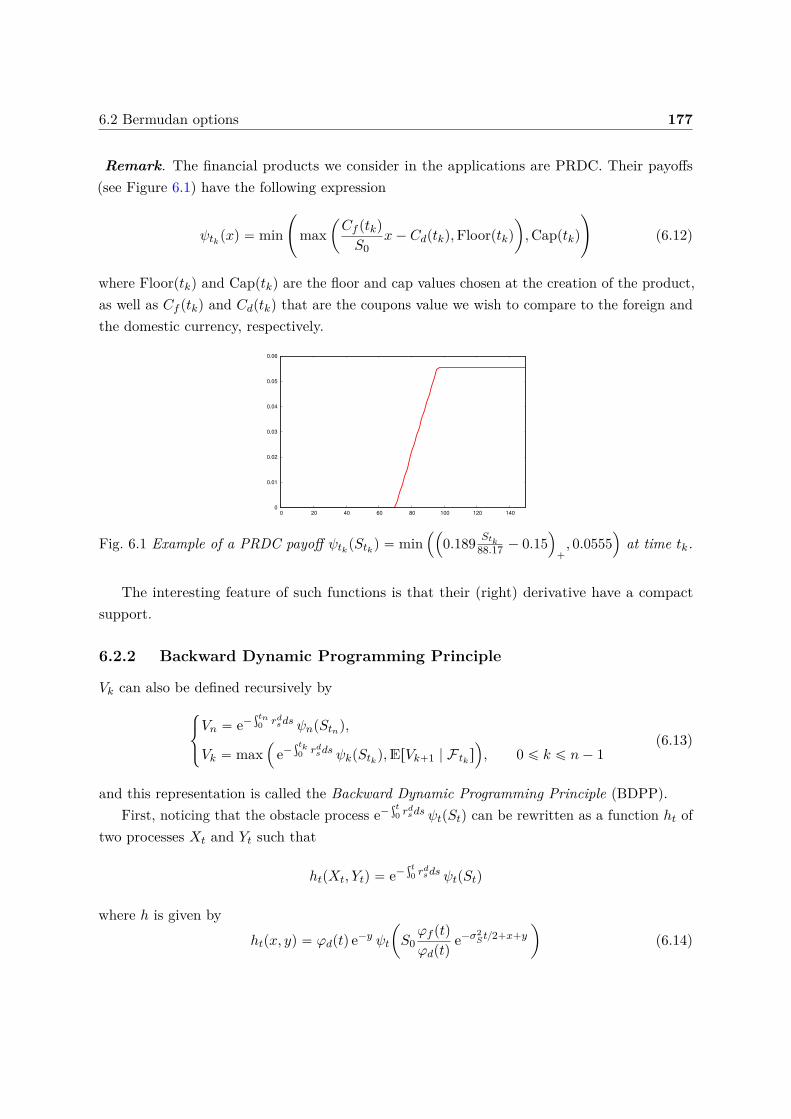
6.2 Bermudan options 177
Remark. The financial products we consider in the applications are PRDC. Their payoffs(see Figure 6.1) have the following expression
ψtk pxq “ min˜
maxˆ
Cf ptkq
S0x´ Cdptkq,Floorptkq
˙
,Capptkq
¸
(6.12)
where Floorptkq and Capptkq are the floor and cap values chosen at the creation of the product,as well as Cf ptkq and Cdptkq that are the coupons value we wish to compare to the foreign andthe domestic currency, respectively.
0
0.01
0.02
0.03
0.04
0.05
0.06
0 20 40 60 80 100 120 140
Fig. 6.1 Example of a PRDC payoff ψtk pStk q “ min´´
0.189 Stk88.17 ´ 0.15
¯
`, 0.0555
¯
at time tk.
The interesting feature of such functions is that their (right) derivative have a compactsupport.
6.2.2 Backward Dynamic Programming Principle
Vk can also be defined recursively by$
&
%
Vn “ e´ştn0 rd
sds ψnpStnq,
Vk “ max´
e´ştk0 rd
sds ψkpStk q,ErVk`1 | F tk s
¯
, 0 ď k ď n´ 1(6.13)
and this representation is called the Backward Dynamic Programming Principle (BDPP).First, noticing that the obstacle process e´
şt0 r
dsds ψtpStq can be rewritten as a function ht of
two processes Xt and Yt such that
htpXt, Ytq “ e´şt0 r
dsds ψtpStq
where h is given byhtpx, yq “ φdptq e´y ψt
ˆ
S0φf ptq
φdptqe´σ2
St2`x`y
˙
(6.14)
178 Quantization-based Bermudan option pricing in the FX world
and pX,Y q is defined by
pXt, Ytq “
ˆ
σSWSt ` σf
ż t
0pt´ sqdW f
s ,´σd
ż t
0pt´ sqdW d
s
˙
. (6.15)
Now, in order to alleviate notations, we denote by Xk “ Xtk , W fk “ W f
tk, Yk “ Ytk ,
W dk “ W d
tk, WS
k “ WStk
and hk “ htk .Using this new form, the Snell envelope becomes
Vk “ supτPT n
k
E“
hτ pXτ , Yτ q | F tk
‰
and the Backward Dynamic Programming Principle (6.13) rewrites$
&
%
Vn “ hnpXn, Ynq,
Vk “ max´
hkpXk, Ykq,E“
Vk`1 | F tk s
¯
, 0 ď k ď n´ 1.(6.16)
Second, in order to solve the problem theoretically by dynamic programming it is requiredto associate a F t-Markov process to this problem and in our case, the simplest of them (i.e. ofminimal dimension) is pXt,W
ft , Yt,W
dt q which is F t-adapted and a Markov process because
$
’
’
’
’
’
’
’
’
’
’
’
’
’
&
’
’
’
’
’
’
’
’
’
’
’
’
’
%
Xk`1 “ Xk ` σfδWfk ` σS
ż tk`1
tk
dWSs ` σf
ż tk`1
tk
ptk`1 ´ sqdW fs
W fk`1 “ W f
k `
ż tk`1
tk
dW fs
Yk`1 “ Yk ´ σdδWdk ´ σd
ż tk`1
tk
ptk`1 ´ sqdW ds
W dk`1 “ W d
k `
ż tk`1
tk
dW ds
where δ “ Tn and can be written as
$
’
’
’
’
’
&
’
’
’
’
’
%
Xk`1 “ Xk ` σfδWfk `G1
k`1
W fk`1 “ W f
k `G2k`1
Yk`1 “ Yk ´ σdδWdk `G3
k`1
W dk`1 “ W d
k `G4k`1,
(6.17)
6.2 Bermudan options 179
where the increments are normally distributed¨
˚
˚
˚
˚
˝
G1k`1
G2k`1
G3k`1
G4k`1
˛
‹
‹
‹
‹
‚
„ N´
µk`1,Σk`1
¯
(6.18)
with
µk`1 “
¨
˚
˚
˚
˚
˝
0000
˛
‹
‹
‹
‹
‚
and Σk`1 “
ˆ
Cov`
Gik`1, Gjk`1
˘
˙
i,j“1:4. (6.19)
One notices that`
pG1k, G
2k, G
3k, G
4kq˘
k“1...,n are i.i.d. Based on Equation (6.17), we deduce theMarkov process transition of pXk,W
fk , Yk,W
dk q, for any integrable function f : R4 Ñ R, given
by
Pfpx, u, y, vq “ E“
fpx` σfδu`G1k`1, u`G2
k`1, y ´ σdδv `G3k`1, v `G4
k`1q‰
. (6.20)
Remark. Using the Markov process pX,W f , Y,W dq newly defined, we rewrite the filtrationF t as
F t “ σ`
WSs ,W
ds ,W
fs , s ď t
˘
“ σ`
Xs,Wfs , Ys,W
ds , s ď t
˘
. (6.21)
Then, using the new expression for the filtration and the Markov property of pXk,Wfk , Yk,W
dk q,
the BDPP (6.16) reads as follows,$
&
%
Vn “ hnpXn, Ynq,
Vk “ max´
hkpXk, Ykq,E“
Vk`1 | pXk,Wfk , Yk,W
dk q‰
¯
, 0 ď k ď n´ 1.(6.22)
Moreover, by backward induction we get Vk “ vkpXk,Wfk , Yk,W
dk q where
$
&
%
vnpXn,Wfn , Yn,W
dnq “ hnpXn, Ynq,
vkpXk,Wfk , Yk,W
dk q “ max
´
hkpXk, Ykq, Pvk`1pXk,Wfk , Yk,W
dk q
¯
, 0 ď k ď n´ 1.(6.23)
Payoff regularity. First, we look at the regularity of the payoff. The next proposition willthen allow us to study the regularity of the value function through the propagation of the localLipschitz property by the transition of the Markov process.
Proposition 6.2.1. If ψtk is are Lipschitz continuous with Lipschitz coefficient rψtk sLip withcompactly supported (right) derivative (such as the payoff defined in (6.12)) then hkpx, yq given
180 Quantization-based Bermudan option pricing in the FX world
by (6.14) is locally Lipschitz continuous, for every x, x1, y, y1 P R
|hkpx, yq ´ hkpx1, y1q| ď e|y|_|y1|`
r sψksLip |x´ x1| ` pφdptkqψtk 8 ` r sψksLipq|y ´ y1|˘
(6.24)
with r sψksLip “ rψtk sLipS0φf ptkq e´σ2Stk2 ψ1
tk8 ec with ψ1
tkthe right derivative of ψtk .
Proof. Let gk be defined by
gkpx, yq “ ψtk
ˆ
S0φf ptkq
φdptkqe´σ2
Stk2`x`y
˙
. (6.25)
As ψ1tk
has a compact support, then it exists c P R such that
|pψtk pexqq1| “ | ex ψ1tk
pexq| ď ψ1tk
8 supxPsuppψ1
tk
ex ď ψ1tk
8 ec . (6.26)
Hence|gkpx, yq ´ gkpx1, y1q| ď
r sψksLip
φdptkq
`
|x´ x1| ` |y ´ y1|˘
(6.27)
with r sψksLip “ rψtk sLipS0φf ptkq e´σ2Stk2 ψ1
tk8 ec. Then for every x, x1, y, y1 P R, we have
|hkpx, yq ´ hkpx1, y1q| “ φdptkqˇ
ˇ e´y gkpx, yq ´ e´y1
gkpx1, y1qˇ
ˇ
ď φdptkq
´
ˇ
ˇ e´y gkpx, yq ´ e´y1
gkpx, yqˇ
ˇ `ˇ
ˇ e´u1
gkpx, yq ´ e´y1
gkpx1, y1qˇ
ˇ
¯
ď φdptkq
´
ˇ
ˇ e´y ´ e´y1 ˇˇ ¨ ψtk 8 ` e´y1 ˇ
ˇgkpx, yq ´ gkpx1, y1qˇ
ˇ
¯
ď e|y|_|y1|`
r sψksLip |x´ x1| ` pφdptkqψtk 8 ` r sψksLipq|y ´ y1|˘
.
(6.28)
The next Lemma shows that the transition of the Markov process propagates the localLipschitz continuity of a function f . This result will be helpful to estimate the error inducedby the numerical approximation (6.23).
Lemma 6.2.2. Let Pfpx, u, y, vq “ E“
fpx` σfδu`G1, u`G2, y ´ σdδv `G3, v `G4q‰
be aMarkov kernel. If the function f satisfies the following local Lipschitz property,
|fpx, u, y, vq ´ fpx1, u1, y1, v1q| ď`
A|x´ x1| `B|u´ u1| ` C|y ´ y1| `D|v ´ v1|˘
ˆ e|y|_|y1|`b|v|_|v1|(6.29)
then
|Pfpx, u, y, vq ´ Pfpx1, u1, y1, v1q| ď`
rA|x´ x1| ` rB|u´ u1| ` rC|y ´ y1| ` rD|v ´ v1|˘
ˆ e|y|_|y1|`rb|v|_|v1| .(6.30)
6.2 Bermudan options 181
Proof. It follows from Jensen’s inequality and our assumption on f
|Pfpx, u, y, vq ´ Pfpx1, u1, y1, v1q|
ď E”
ˇ
ˇfpx` σfδu`G1, u`G2, y ´ σdδv `G3, v `G4q
´ fpx1 ` σfδu1 `G1, u1 `G2, y1 ´ σdδv
1 `G3, v1 `G4qˇ
ˇ
ı
ď`
A|x´ x1| ` pB `Aσfδq|u´ u1| ` C|y ´ y1| ` pD ` Cσdδq|v ´ v1|˘
ˆ e|y|_|y1|`pb`σdδq|v|_|v1|E“
e|G3|`b|G4|‰
ď`
rA|x´ x1| ` rB|u´ u1| ` rC|y ´ y1| ` rD|v ´ v1|˘
ˆ e|y|_|y1|`rb|v|_|v1|
(6.31)
whererA “ AErκs, rB “ pB `AσfδqErκs (6.32)
andrC “ C Erκs, rD “ pD ` CσdδqErκs, rb “ b` σdδ (6.33)
with κ “ expp|G3| ` b|G4|q and Erκs ă `8.
Value function regularity. If the functions pψtk qk“0:n are defined as in Equation (6.12) thenvnpx, u, y, vq preserves a local Lipschitz property. Hence, for every x, x1, u, u1, y, y1, v, v1 P R,
|vnpx, u, y, vq ´ vnpx1, u1, y1, v1q| ď`
An|x´ x1| `Bn|u´ u1| ` Cn|y ´ y1| `Dn|v ´ v1|˘
ˆ e|y|_|y1|`bn|v|_|v1|(6.34)
where
An “ r sψnsLip , Bn “ 0, Cn “ φdptnqψn8 ` r sψnsLip , Dn “ 0, bn “ 0 (6.35)
with r sψnsLip “ rψtnsLipS0φf ptnq expp´σ2Stn2qψ1
tn8 ec. Using now Lemma 6.2.2 recursivelyand the elementary inequality maxpa, b` cq ď maxpa, bq ` c (as x ÞÑ maxpa, xq is 1-Lipschitz),
182 Quantization-based Bermudan option pricing in the FX world
we have
|vkpx, u, y, vq ´ vkpx1, u1, y1, v1q|
ď max`
|hkpx, yq ´ hkpx1, y1q|, |Pvk`1px, u, y, vq ´ Pvk`1px1, u1, y1, v1q|˘
ď maxˆ
e|y|_|y1|`
r sψksLip |x´ x1| ``
φdptkqψtk 8 ` r sψksLip
˘
|y ´ y1|˘
,`
rAk|x´ x1| ` rBk|u´ u1| ` rCk|y ´ y1| ` rDk|v ´ v1|˘
ˆ e|y|_|y1|`rbk|v|_|v1|
˙
ď`
Ak|x´ x1| `Bk|u´ u1| ` Ck|y ´ y1| `Dk|v ´ v1|˘
ˆ e|y|_|y1|`bk|v|_|v1|
(6.36)
where
Ak “ r sψksLip _`
Ak`1Erκk`1s˘
, Bk “ pBk`1 `Ak`1σfδqErκk`1s, bk “ bk`1 ` σdδ
(6.37)and
Ck “`
φdptkqψtk 8 ` r sψksLip
˘
_`
Ck`1Erκk`1s˘
, Dk “ pDk`1 `Ck`1σdδqErκk`1s (6.38)
with κk`1 “ expp|G3k`1| ` bk`1|G4
k`1|q. Or equivalently
Ak “ maxlěk
ˆ
r sψlsLip
lź
j“k`1Erκjs
˙
, Bk “ σfT
n
nÿ
l“k`1maxlďiďn
ˆ
r sψisLip
iź
j“k`1Erκjs
˙
(6.39)
and
Ck “ maxlěk
ˆ
`
φdptlqψl8 ` r sψlsLip
˘
lź
j“k`1Erκjs
˙
,
Dk “ σdT
n
nÿ
l“k`1maxlďiďn
ˆ
`
φdptiqψi8 ` r sψisLip
˘
iź
j“k`1Erκjs
˙
(6.40)
withbk “ σdT
´
1 ´k ´ 1n
¯
. (6.41)
6.3 Bermudan pricing using Optimal Quantization
In this section, we propose two numerical solutions based on Product Optimal Quantizationfor the pricing of Bermudan options on the FX rate St. First, we remind briefly what is anoptimal quantizer and what we mean by a product quantization tree. Second, we presenta first numerical solution, based on quantization of the Markovian tuple pX,W f , Y,W dq, to
6.3 Bermudan pricing using Optimal Quantization 183
solve the numerical problem (6.22) and detail the L2-error induced by this approximation.However, remember that we are looking for a method that makes possible to compute xVA’s riskmeasures in a reasonable time but this solution can be too time consuming in practice due to thedimensionality of the quantized processes. That is why we present a second numerical solutionwhich reduces the dimensionality of the problem by considering an approximate problem, basedon quantization of the non-Markovian couple pX,Y q, introducing a systematic error induced bythe non-markovianity and we study the L2-error produced by this approximation.
6.3.1 About Optimal Quantization
Theoretical background (the one-dimensional case). The aim of Optimal Quantizationis to determine ΓN , a set with cardinality at most N , which minimises the quantization erroramong all such sets Γ. We place ourselves in the one-dimensional case. Let Z be an R-valuedrandom variable with distribution PZ defined on a probability space pΩ,A,Pq such that Z P L2
R.
Definition 6.3.1. Let ΓN “ tz1, . . . , zNu Ă R be a subset of size N , called N -quantizer. ABorel partition
`
CipΓN q˘
iPJ1,NK of R is a Voronoï partition of R induced by the N -quantizerΓN if, for every i “ t1, ¨ ¨ ¨ , Nu,
Ci`
ΓN˘
Ă
!
ξ P R, |ξ ´ zi| ď minj‰i
|ξ ´ zj |)
.
The Borel sets CipΓN q are called Voronoï cells of the partition induced by ΓN .
One can always consider that the quantizers are ordered: z1 ă z2 ă ¨ ¨ ¨ ă zN´1 ă zN andin that case the Voronoï cells are given by
Ck`
ΓN˘
“`
zk´12, zk`12‰
, k P J1, N ´ 1K, CN`
ΓN˘
“`
zN´12, zN`12˘
where @k P t2, ¨ ¨ ¨ , Nu, zk´12 “zk´1`zk
2 and z12 “ inf`
supppPZ q˘
and zN`12 “ sup`
supppPZ q˘
.
Definition 6.3.2. Let ΓN “ tz1, . . . , zNu be an N -quantizer. The nearest neighbour projectionProjΓN
: R Ñ tz1, . . . , zNu induced by a Voronoï partition`
CipΓN q˘
iPt1,¨¨¨ ,Nuis defined by
@ξ P R, ProjΓNpξq “
Nÿ
i“1zi 1ξPCipΓN q .
Hence, we can define the quantization of Z as the nearest neighbour projection of Z onto ΓNby composing ProjΓN
and X
pZΓN “ ProjΓNpZq “
Nÿ
i“1zi 1ZPCipΓN q .
In order to alleviate notations, we write pZN from now on in place of pZΓN .
184 Quantization-based Bermudan option pricing in the FX world
Now that we have defined the quantization of Z, we explain where does the term "optimal"comes from in the term optimal quantization. First, we define the quadratic distortion function.
Definition 6.3.3. The L2-mean quantization error induced by the quantizer pZN is defined as
Z ´ pZN2 “
ˆ
E”
miniPt1,¨¨¨ ,Nu
|Z ´ zi|2ı
˙12“
ˆż
R
miniPt1,¨¨¨ ,Nu
|ξ ´ zi|2PZ pdξq
˙12. (6.42)
It is convenient to define the quadratic distortion function at level N as the squared meanquadratic quantization error on pRqN :
Q2,N : z “`
z1, . . . , zN˘
ÞÝÑ E”
miniPt1,¨¨¨ ,Nu
|Z ´ zi|2ı
“ Z ´ pZN22 .
Remark. All these definitions can be extended to the Lp case. For example the Lp-meanquantization error induced by a quantizer of size N is
Z ´ pZNp “
ˆ
E”
miniPt1,¨¨¨ ,Nu
|Z ´ zi|pı
˙1p
“
ˆż
R
miniPt1,¨¨¨ ,Nu
|Z ´ zi|pPZ pdξq
˙1p
. (6.43)
The existence of a N -tuple zpNq “ pz1, . . . , zN q minimizing the quadratic distortion functionQ2,N at level N has been shown and its associated quantizer ΓN “ tzi, i P t1, ¨ ¨ ¨ , Nuu is calledan optimal quadratic N -quantizer, see e.g. [Pag18] for further details and references. We nowturn to the asymptotic behaviour in N of the quadratic mean quantization error. The nextTheorem, known as Zador’s Theorem, provides the sharp rate of convergence of the Lp-meanquantization error.
Theorem 6.3.4. (Zador’s Theorem) Let p P p0,`8q.
(a) Sharp rate. Let Z P Lp`δR pPq for some δ ą 0. Let PZ pdξq “ φpξq ¨ λpdξq ` νpdξq, where
ν K λ i.e. denotes the singular part of PZ with respect to the Lebesgue measure λ on R.Then,
limNÑ`8
N minΓN ĂR,|ΓN |ďN
Z ´ pZNp “1
2ppp` 1q
„ż
R
φ1
1`pdλ
ȷ1` 1p
. (6.44)
(b) Non asymptotic upper-bound. Let δ ą 0. There exists a real constant C1,p,δ P p0,`8q
such that, for every R-valued random variable Z,
@N ě 1, minΓN ĂR,|ΓN |ďN
Z ´ pZNp ď C1,p,δσδ`ppZqN´1 (6.45)
where, for r P p0,`8q, σrpZq “ minaPR Z ´ ar ă `8.
The next result answers to the following question: what can be said about the convergencerate of E
“
|Z ´ pZN |2`β‰
, knowing that pZN is a quadratic optimal quantization?
6.3 Bermudan pricing using Optimal Quantization 185
This problem is known as the distortion mismatch problem and has been first addressed by[GLP08] and the results have been extended in Theorem 4.3 of [PS18a].
Theorem 6.3.5. [Lr-Ls-distortion mismatch] Let Z : pΩ,A,Pq Ñ R be a random variable andlet r P p0,`8q. Assume that the distribution PZ of Z has a non-zero absolutely continuouscomponent with density φ. Let pΓN qNě1 be a sequence of Lr-optimal grids. Let s P pr, r` 1q. If
Z P Ls
1`r´s`δ
pΩ,A,Pq (6.46)
for some δ ą 0, thenlim sup
NNZ ´ pZNs ă `8. (6.47)
Product Quantization. Now, let Z “ pZℓqℓ“1:d be an Rd-valued random vector withdistribution PZ defined on a probability space pΩ,A,Pq. There are two approaches if onewishes to scale to higher dimensions. Either one applies the above framework directly to therandom vector Z and build an optimal quantizer of Z, or one may consider separately eachcomponent Zℓ independently, build a one-dimensional optimal quantization pZℓ, of size N ℓ, withquantizer ΓNℓ
ℓ “
zℓiℓ , iℓ P t1, ¨ ¨ ¨ , N ℓu(
and then build the product quantizer ΓN “śdℓ“1 ΓNℓ
l
of size N “ N1 ˆ ¨ ¨ ¨ ˆNd defined by
ΓN “
pz1i1 , ¨ ¨ ¨ , zℓiℓ , ¨ ¨ ¨ , zdidq, iℓ P t1, ¨ ¨ ¨ , Nℓu, ℓ P t1, ¨ ¨ ¨ , du
(
. (6.48)
In our case we chose the second approach. Indeed, it is much more flexible when dealing withnormal distribution, like in our case. We do not need to solve the d-dimensional minimizationproblem at each time step. We only need to load precomputed optimal quantizer of standardnormal distribution N p0, 1q and then take advantage of the stability of optimal quantization byrescaling in one dimension in the sense that if ΓN “ tzi, 1 ď i ď Nu is optimal at level N forN p0, 1q then µ` σΓN (with obvious notations) is optimal for N pµ, σ2q.
Even though it exists fast methods for building optimal quantizers in two-dimension based ondeterministic methods like in the one-dimensional case, when dealing with optimal quantizationof bivariate Gaussian vector, we may face numerical instability when the covariance matrixis ill-conditioned: so is the case if the variance of one coordinate is relatively high comparedto the second one (which is our case in this paper). This a major drawback as we are lookingfor a fast numerical solution able to produce prices in a few seconds and this is possible whenusing product optimal quantization.
Quantization Tree. Now, in place of considering a random variable Z, let pZtqtPr0,T s be astochastic process following a Stochastic Differential Equation (SDE)
Zt “ Z0 `
ż t
0bspZsqds`
ż t
0σps, ZsqdWs (6.49)
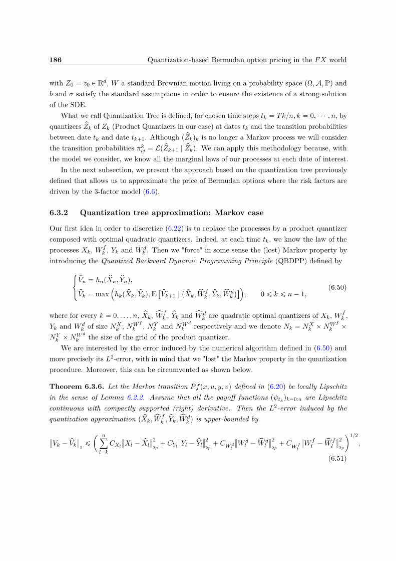
186 Quantization-based Bermudan option pricing in the FX world
with Z0 “ z0 P Rd, W a standard Brownian motion living on a probability space pΩ,A,Pq andb and σ satisfy the standard assumptions in order to ensure the existence of a strong solutionof the SDE.
What we call Quantization Tree is defined, for chosen time steps tk “ Tkn, k “ 0, ¨ ¨ ¨ , n, byquantizers pZk of Zk (Product Quantizers in our case) at dates tk and the transition probabilitiesbetween date tk and date tk`1. Although p pZkqk is no longer a Markov process we will considerthe transition probabilities πkij “ Lp pZk`1 | pZkq. We can apply this methodology because, withthe model we consider, we know all the marginal laws of our processes at each date of interest.
In the next subsection, we present the approach based on the quantization tree previouslydefined that allows us to approximate the price of Bermudan options where the risk factors aredriven by the 3-factor model (6.6).
6.3.2 Quantization tree approximation: Markov case
Our first idea in order to discretize (6.22) is to replace the processes by a product quantizercomposed with optimal quadratic quantizers. Indeed, at each time tk, we know the law of theprocesses Xk, W f
k , Yk and W dk . Then we "force" in some sense the (lost) Markov property by
introducing the Quantized Backward Dynamic Programming Principle (QBDPP) defined by$
&
%
pVn “ hnp pXn, pYnq,
pVk “ max´
hkp pXk, pYkq,E“
pVk`1 | p pXk,xWfk ,
pYk,xWdk q‰
¯
, 0 ď k ď n´ 1,(6.50)
where for every k “ 0, . . . , n, pXk, xW fk , pYk and xW d
k are quadratic optimal quantizers of Xk, W fk ,
Yk and W dk of size NX
k , NW f
k , NYk and NW d
k respectively and we denote Nk “ NXk ˆNW f
k ˆ
NYk ˆNW d
k the size of the grid of the product quantizer.We are interested by the error induced by the numerical algorithm defined in (6.50) and
more precisely its L2-error, with in mind that we "lost" the Markov property in the quantizationprocedure. Moreover, this can be circumvented as shown below.
Theorem 6.3.6. Let the Markov transition Pfpx, u, y, vq defined in (6.20) be locally Lipschitzin the sense of Lemma 6.2.2. Assume that all the payoff functions pψtk qk“0:n are Lipschitzcontinuous with compactly supported (right) derivative. Then the L2-error induced by thequantization approximation p pXk,xW
fk ,
pYk,xWdk q is upper-bounded by
›
›Vk ´ pVk›
›
2ď
ˆ nÿ
l“k
CXl
›
›Xl ´ pXl
›
›
22p
` CYl
›
›Yl ´ pYl›
›
22p
` CW dl
›
›W dl ´ xW d
l
›
›
22p
` CW f
l
›
›W fl ´ xW f
l
›
›
22p
˙12,
(6.51)
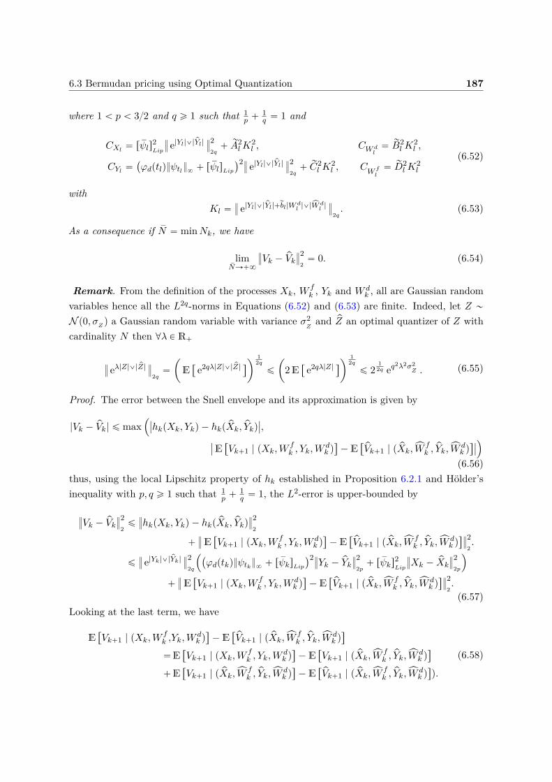
6.3 Bermudan pricing using Optimal Quantization 187
where 1 ă p ă 32 and q ě 1 such that 1p ` 1
q “ 1 and
CXl“ r sψls
2Lip
›
› e|Yl|_|pYl|›
›
22q
` rA2lK
2l , CW d
l“ rB2
lK2l ,
CYl“`
φdptlqψtl8 ` r sψlsLip
˘2›› e|Yl|_|pYl|
›
›
22q
` rC2l K
2l , C
W fl
“ rD2lK
2l
(6.52)
withKl “
›
› e|Yl|_|pYl|`rbl|W
dl |_|xW d
l |›
›
2q. (6.53)
As a consequence if sN “ minNk, we have
limsNÑ`8
›
›Vk ´ pVk›
›
22
“ 0. (6.54)
Remark. From the definition of the processes Xk, W fk , Yk and W d
k , all are Gaussian randomvariables hence all the L2q-norms in Equations (6.52) and (6.53) are finite. Indeed, let Z „
N p0, σZ q a Gaussian random variable with variance σ2Z
and pZ an optimal quantizer of Z withcardinality N then @λ P R`
›
› eλ|Z|_| pZ|›
›
2q“
ˆ
E“
e2qλ|Z|_| pZ|‰
˙1
2q
ď
ˆ
2E“
e2qλ|Z|‰
˙1
2q
ď 21
2q eq2λ2σ2
Z . (6.55)
Proof. The error between the Snell envelope and its approximation is given by
|Vk ´ pVk| ď max´
ˇ
ˇhkpXk, Ykq ´ hkp pXk, pYkqˇ
ˇ,
ˇ
ˇE“
Vk`1 | pXk,Wfk , Yk,W
dk q‰
´ E“
pVk`1 | p pXk,xWfk ,
pYk,xWdk q‰ˇ
ˇ
¯
(6.56)thus, using the local Lipschitz property of hk established in Proposition 6.2.1 and Hölder’sinequality with p, q ě 1 such that 1
p ` 1q “ 1, the L2-error is upper-bounded by
›
›Vk ´ pVk›
›
22
ď›
›hkpXk, Ykq ´ hkp pXk, pYkq›
›
22
`›
›E“
Vk`1 | pXk,Wfk , Yk,W
dk q‰
´ E“
pVk`1 | p pXk,xWfk ,
pYk,xWdk q‰›
›
22.
ď›
› e|Yk|_|pYk|›
›
22q
´
`
φdptkqψtk 8 ` r sψksLip
˘2››Yk ´ pYk
›
›
22p
` r sψks2Lip
›
›Xk ´ pXk
›
›
22p
¯
`›
›E“
Vk`1 | pXk,Wfk , Yk,W
dk q‰
´ E“
pVk`1 | p pXk,xWfk ,
pYk,xWdk q‰›
›
22.
(6.57)Looking at the last term, we have
E“
Vk`1 | pXk,Wfk ,Yk,W
dk q‰
´ E“
pVk`1 | p pXk,xWfk ,
pYk,xWdk q‰
“E“
Vk`1 | pXk,Wfk , Yk,W
dk q‰
´ E“
Vk`1 | p pXk,xWfk ,
pYk,xWdk q‰
`E“
Vk`1 | p pXk,xWfk ,
pYk,xWdk q‰
´ E“
pVk`1 | p pXk,xWfk ,
pYk,xWdk q‰
q.
(6.58)
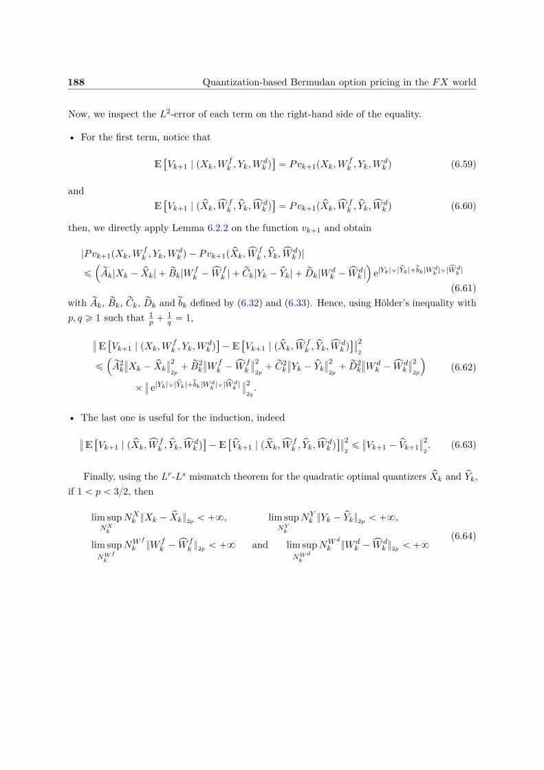
188 Quantization-based Bermudan option pricing in the FX world
Now, we inspect the L2-error of each term on the right-hand side of the equality.
• For the first term, notice that
E“
Vk`1 | pXk,Wfk , Yk,W
dk q‰
“ Pvk`1pXk,Wfk , Yk,W
dk q (6.59)
andE“
Vk`1 | p pXk,xWfk ,
pYk,xWdk q‰
“ Pvk`1p pXk,xWfk ,
pYk,xWdk q (6.60)
then, we directly apply Lemma 6.2.2 on the function vk`1 and obtain
|Pvk`1pXk,Wfk , Yk,W
dk q ´ Pvk`1p pXk,xW
fk ,
pYk,xWdk q|
ď
´
rAk|Xk ´ pXk| ` rBk|W fk ´ xW f
k | ` rCk|Yk ´ pYk| ` rDk|W dk ´ xW d
k |
¯
e|Yk|_|pYk|`rbk|W dk |_|xW d
k |
(6.61)with rAk, rBk, rCk, rDk and rbk defined by (6.32) and (6.33). Hence, using Hölder’s inequality withp, q ě 1 such that 1
p ` 1q “ 1,
›
›E“
Vk`1 | pXk,Wfk , Yk,W
dk q‰
´ E“
Vk`1 | p pXk,xWfk ,
pYk,xWdk q‰›
›
22
ď
´
rA2k
›
›Xk ´ pXk
›
›
22p
` rB2k
›
›W fk ´ xW f
k
›
›
22p
` rC2k
›
›Yk ´ pYk›
›
22p
` rD2k
›
›W dk ´ xW d
k
›
›
22p
¯
ˆ›
› e|Yk|_|pYk|`rbk|W dk |_|xW d
k |›
›
22q.
(6.62)
• The last one is useful for the induction, indeed
›
›E“
Vk`1 | p pXk,xWfk ,
pYk,xWdk q‰
´ E“
pVk`1 | p pXk,xWfk ,
pYk,xWdk q‰›
›
22
ď›
›Vk`1 ´ pVk`1›
›
22. (6.63)
Finally, using the Lr-Ls mismatch theorem for the quadratic optimal quantizers pXk and pYk,if 1 ă p ă 32, then
lim supNX
k
NXk Xk ´ pXk2p ă `8, lim sup
NYk
NYk Yk ´ pYk2p ă `8,
lim supNW f
k
NW f
k W fk ´ xW f
k 2p ă `8 and lim supNW d
k
NW d
k W dk ´ xW d
k 2p ă `8(6.64)
6.3 Bermudan pricing using Optimal Quantization 189
this yields›
›Vk ´ pVk›
›
22
ď›
›Xk ´ pXk
›
›
22p
´
r sψks2Lip
›
› e|Yk|_|pYk|›
›
22q
` rA2kK
2k
¯
`›
›Yk ´ pYk›
›
22p
´
`
φdptkqψtk 8 ` r sψksLip
˘2›› e|Yk|_|pYk|
›
›
22q
` rC2kK
2k
¯
` rB2kK
2k
›
›W fk ´ xW f
k
›
›
22p
` rD2kK
2k
›
›W dk ´ xW d
k
›
›
22p
`›
›Vk`1 ´ pVk`1›
›
22
ď
nÿ
l“k
CXl
›
›Xl ´ pXl
›
›
22p
` CYl
›
›Yl ´ pYl›
›
22p
` CW dl
›
›W dl ´ xW d
l
›
›
22p
` CW f
l
›
›W fl ´ xW f
l
›
›
22p
sNÑ`8ÝÝÝÝÝÑ 0
(6.65)
where Kk “›
› e|Yk|_|pYk|`rbk|W dk |_|xW d
k |›
›
2qand @k “ 1, . . . , n, CXk
, CYk, CW d
k, C
W fk
ă `8.
Remark. The same result can be obtained if we relax the assumption on the payoff ψk. Ifwe only assume the payoff Lipschitz continuous, we have the same limit with the same rate ofconvergence, however the constants CXl
, CYl, CW d
l, C
W fl
are not the same.
To conclude this section, although considering product optimal quantizer in four dimensionsfor pXk,W
fk , Yk,W
dk q seems to be natural, the computational cost associated to the resulting
QBDPP is too high, of order Opnˆ pmaxNkq2q. Moreover the computation of the transitionprobabilities needed for the evaluation of the terms E
“
pVk`1 | p pXk,xWfk ,
pYk,xWdk q‰
are challenging.These transition probabilities cannot be computed using deterministic numerical integrationmethods and we have to use Monte Carlo estimators. Even though it is feasible, it is adrawback for the method since it increases drastically the computation time for calibrating thequantization tree. In the next section we provide a solution to these problems which consists inreducing the dimension of the problem at the price of adding a systematic error, which turnsout to be quite small in practice.
6.3.3 Quantization tree approximation: Non Markov case
In this part, we want to reduce the dimension of the problem in order to scale down thenumerical complexity of the pricer. For that we discard the processes W d and W f in the treeand only keep X and Y . Doing so, we loose the Markovian property of our original model butwe drastically reduce the numerical complexity of the problem. Thence, (6.22) is approximatedby
$
&
%
pVn “ hnp pXn, pYnq,
pVk “ max´
hkp pXk, pYkq,E“
pVk`1 | p pXk, pYkq‰
¯
, 0 ď k ď n´ 1(6.66)
190 Quantization-based Bermudan option pricing in the FX world
where for every k “ 0, . . . , n, pXk and pYk are quadratic optimal quantizers of Xk and Yk of sizeNXk and NY
k , respectively and we denote Nk “ NXk ˆNY
k the size of the grid of the productquantizer.
Theorem 6.3.7. Let the Markov transition Pfpx, u, y, vq be defined by (6.20) be locally Lipschitzin the sense of Lemma 6.2.2. Assume that all the payoff functions pψtk qk“0:n are Lipschitzcontinuous with compactly supported (right) derivative. Then the L2-error, induced by thequantization approximation p pXk, pYkq is upper-bounded by
›
›Vk ´ pVk›
›
2ď
ˆ n´1ÿ
l“k
CW f
l`1
›
›W fl`1 ´ ErW f
l`1 | pXl, Ylqs›
›
22p
` CW dl`1
›
›W dl`1 ´ ErW d
l`1 | pXl, Ylqs›
›
22p
` CXl
›
›Xl ´ pXl
›
›
22p
` CYl
›
›Yl ´ pYl›
›
22p
˙12
(6.67)where 1 ă p ă 32 and q ě 1 such that 1
p ` 1q “ 1, moreover
CXl“ r sψls
2Lip
›
› e|Yl|_|pYl|›
›
22q
` sA2l
›
› esbl|Yl|_|pYl|›
›
22q, C
W fl`1
“ B2l`1
›
›
rκk`1›
›
22q,
CYl“`
φdptlqψtl8 ` r sψlsLip
˘2›› e|Yl|_|pYl|
›
›
22q
` sC2l
›
› esbl|Yl|_|pYl|›
›
22q, CW d
l`1“ D2
l`1›
›
rκk`1›
›
22q.
(6.68)Taking the limit in sN “ minNk, the size of the quadratic optimal quantizers, we have
limsNÑ`8
›
›Vk´pVk›
›
22
“
n´1ÿ
l“k
CW f
l`1
›
›W fl`1´ErW f
l`1 | pXl, Ylqs›
›
22p
`CW dl`1
›
›W dl`1´ErW d
l`1 | pXl, Ylqs›
›
22p.
(6.69)
Proof. We apply the same methodology as in the proof for the Markov case. The error betweenthe Snell envelope and its approximation is given by
|Vk´pVk| ď max´
ˇ
ˇhkpXk, Ykq´hkp pXk, pYkqˇ
ˇ,ˇ
ˇE“
Vk`1 | pXk,Wfk , Yk,W
dk q‰
´E“
pVk`1 | p pXk, pYkq‰ˇ
ˇ
¯
(6.70)thus, using Proposition 6.2.1 and Hölder’s inequality with p, q ě 1 such that 1
p ` 1q “ 1, the
L2-error is given by›
›Vk ´ pVk›
›
22
ď›
›hkpXk, Ykq ´ hkp pXk, pYkq›
›
22
`›
›E“
Vk`1 | pXk,Wfk , Yk,W
dk q‰
´ E“
pVk`1 | p pXk, pYkq‰›
›
22
ď
´
r sψks2Lip
›
›Xk ´ pXk
›
›
22p
``
φdptkqψtk 8 ` r sψksLip
˘2››Yk ´ pYk
›
›
22p
¯
›
› e|Yk|_|pYk|›
›
22q
`›
›E“
Vk`1 | pXk,Wfk , Yk,W
dk q‰
´ E“
pVk`1 | p pXk, pYkq‰›
›
22.
(6.71)
6.3 Bermudan pricing using Optimal Quantization 191
The last term in Equation (6.71) can be decomposed as follows
E“
Vk`1 | pXk,Wfk , Yk,W
dk q‰
´ E“
pVk`1 | p pXk, pYkq‰
“E“
Vk`1 | pXk,Wfk , Yk,W
dk q‰
´ E“
Vk`1 | pXk, Ykq‰
`E“
Vk`1 | pXk, Ykq‰
´ E“
Vk`1 | p pXk, pYkq‰
`E“
Vk`1 | p pXk, pYkq‰
´ E“
pVk`1 | p pXk, pYkq‰
.
(6.72)
And again, each term can be upper-bounded.
• The first can be upper-bounded using what we did above on the value function vk andHölder’s inequality with p, q ě 1 such that 1
p ` 1q “ 1
›
›E“
Vk`1 | pXk,Wfk , Yk,W
dk q‰
´ E“
Vk`1 | pXk, Ykq‰›
›
22
ď›
›Vk`1 ´ E“
Vk`1 | pXk, Ykq‰›
›
22
ď›
›vk`1pXk`1,Wfk`1, Yk`1,W
dk`1q
´ vk`1`
Xk`1,E“
W fk`1 | pXk, Ykq
‰
, Yk`1,E“
W dk`1 | pXk, Ykq
‰˘›
›
22
ď
›
›
›
´
Bk`1ˇ
ˇW fk`1 ´ E
“
W fk`1 | pXk, Ykq
‰ˇ
ˇ `Dk`1ˇ
ˇW dk`1 ´ E
“
W dk`1 | pXk, Ykq
‰ˇ
ˇ
¯
rκk`1
›
›
›
2
2
ď›
›
rκk`1›
›
22q
´
B2k`1
›
›W fk`1 ´ ErW f
k`1 | pXk, Ykqs›
›
22p
`D2k`1
›
›W dk`1 ´ E
“
W dk`1 | pXk, Ykq
‰›
›
22p
¯
(6.73)with coefficients bk`1, Bk`1 and Dk`1 defined in (6.39) and (6.40) and
rκk`1 “ e|Yk`1|`bk`1|W dk`1|_|ErW d
k`1|pXk,Ykqs| . (6.74)
• For the second, we define
rvkpXk, Ykq “ E“
vk`1pXk`1,Wfk`1, Yk`1,W
dk`1q | pXk, Ykq
‰
. (6.75)
Indeed, E“
Vk`1 | pXk, Ykq‰
is only a function of Xk and Yk, as shown below
E“
Vk`1 | pXk, Ykq‰
“ E“
vk`1pXk`1,Wfk`1, Yk`1,W
dk`1q | pXk, Ykq
‰
“ E”
E“
vk`1pXk`1,Wfk`1, Yk`1,W
dk`1q | pXk,W
fk , Yk,W
dk q‰
| pXk, Ykq
ı
“ E“
Pvk`1pXk,Wfk , Yk,W
dk q | pXk, Ykq
‰
.
(6.76)Moreover, we can rewrite W f
k “ λkXk
KK` ξk and W d
k “ rλkYkKK` χk where
λk “CovpXk,W
fk q
VarpXkq, rλk “
CovpYk,Wdk q
VarpYkq
192 Quantization-based Bermudan option pricing in the FX world
and ξk „ N p0, σ2ξk
q and χk „ N p0, σ2χk
q with σ2ξk
“ VarpW fk ´λkXkq and σ2
χk“ VarpW d
k´rλkYkq,then
E“
Pvk`1pXk,Wfk , Yk,W
dk q | pXk, Ykq “ px, yq
‰
“ E“
Pvk`1px, λkx` ξk, y, rλky ` χkq‰ˇ
ˇ
px,yq“pXk,Ykq
(6.77)
yieldingrvkpx, yq “ E
“
Pvk`1px, λkx` ξk, y, rλky ` χkq‰
. (6.78)
Now, using Lemma 6.2.2 on rvk, we haveˇ
ˇ
rvkpx, yq ´ rvkpx1, y1qˇ
ˇ
“
ˇ
ˇ
ˇE“
Pvk`1px, λkx` ξk, y, rλky ` χkq ´ Pvk`1px1, λkx1 ` ξk, y
1, rλky1 ` χkq
‰
ˇ
ˇ
ˇ
ď E
„
ˇ
ˇ
ˇ
`
p rAk ` rBk|λk|q|x´ x1| ` p1 ` rCk|rλk|q|y ´ y1|˘
ep1`rbk|rλk|q|y|_|y1|`rbk|χk|ˇ
ˇ
ˇ
ȷ
ď
´
sAk|x´ x1| ` sCk|y ´ y1|
¯
esbk|y|_|y1|
(6.79)
wheresAk “ p rAk ` rBk|λk|qE
“
erbk|χk|‰
, sCk “ 1 ` rCk|rλk|, (6.80)
sbk “ 1 `rbk|rλk| (6.81)
with rAk, rBk, rCk and rbk defined in (6.32) and (6.33). Hence, using Hölder’s inequality withp, q ě 1 such that 1
p ` 1q “ 1
›
›E“
Vk`1 | pXk, Ykq‰
´ E“
Vk`1 | p pXk, pYkq‰›
›
22
“›
›
rvkpXk, Ykq ´ rvkp pXk, pYkq›
›
22
ď
›
›
›
´
sAkˇ
ˇXk ´ pXk
ˇ
ˇ ` sCkˇ
ˇYk ´ pYkˇ
ˇ
¯
esbk|Yk|_|pYk|›
›
›
2
2
ď›
› esbk|Yk|_|pYk|›
›
22q
´
sA2k
›
›Xk ´ pXk
›
›
22p
` sC2k
›
›Yk ´ pYk›
›
22p
¯
.
(6.82)
• The last one is useful for the induction, indeed
›
›E“
Vk`1 | p pXk, pYkq‰
´ E“
pVk`1 | p pXk, pYkq‰›
›
22
ď›
›Vk`1 ´ pVk`1›
›
22. (6.83)
Finally, using the Lr-Ls mismatch theorem on the quadratic optimal quantizers pXk and pYk,if 1 ă p ă 32, then
lim supNX
k
NXk Xk ´ pXk2p ă `8 and lim sup
NYk
NYk Yk ´ pYk2p ă `8 (6.84)
6.3 Bermudan pricing using Optimal Quantization 193
and›
›Vk´pVk›
›
22
ď›
›Xk ´ pXk
›
›
22p
´
r sψks2Lip
›
› e|Yk|_|pYk|›
›
22q
` sA2k
›
› esbk|Yk|_|pYk|›
›
22q
¯
`›
›Yk ´ pYk›
›
22p
´
`
φdptkqψtk 8 ` r sψksLip
˘2›› e|Yk|_|pYk|
›
›
22q
` sC2k
›
› esbk|Yk|_|pYk|›
›
22q
¯
`B2k`1
›
›
rκk`1›
›
22q
›
›W fk`1 ´ ErW f
k`1 | pXk, Ykqs›
›
22p
`D2k`1
›
›
rκk`1›
›
22q
›
›W dk`1 ´ E
“
W dk`1 | pXk, Ykq
‰›
›
22p
`›
›Vk`1 ´ pVk`1›
›
22
ď
n´1ÿ
l“k
CW f
l`1
›
›W fl`1 ´ ErW f
l`1 | pXl, Ylqs›
›
22p
` CW dl`1
›
›W dl`1 ´ ErW d
l`1 | pXl, Ylqs›
›
22p
` CXl
›
›Xl ´ pXl
›
›
22p
` CYl
›
›Yl ´ pYl›
›
22p
sNÑ`8ÝÝÝÝÝÑ
n´1ÿ
l“k
CW f
l`1
›
›W fl`1 ´ ErW f
l`1 | pXl, Ylqs›
›
22p
` CW dl`1
›
›W dl`1 ´ ErW d
l`1 | pXl, Ylqs›
›
22p.
(6.85)
Practitioner’s corner. Market implied values of σf , σd and σS used for the numericalcomputations are usually of order
σf « 0.005, σd « 0.005, σS « 0.5 (6.86)
and in the most extreme cases, we compute Bermudan options on foreign exchange withmaturity 20 years (T “ 20). Thus, we can estimate the order of the induced systematic error.First, we recall the expression of the related coefficients which depends of
Bk “ σfT
n
nÿ
l“k`1maxlďiďn
ˆ
r sψisLip
iź
j“k`1Erκjs
˙
,
Dk “ σdT
n
nÿ
l“k`1maxlďiďn
ˆ
pφdptiqψi8 ` r sψisLipq
iź
j“k`1Erκjs
˙
(6.87)
withκj “ e|G3
j |`bj |G4j |, rκl`1 “ e|Yl`1|`bl`1|W d
l`1|_|ErW dl`1|pXl,Ylqs| (6.88)
andbk “ σdT
ˆ
1 ´k ´ 1n
˙
. (6.89)
194 Quantization-based Bermudan option pricing in the FX world
Now, considering the case where the payoffs are the same at each exercise date, the Lipschitzconstants can be upper-bounded by r sψsLip :
r sψksLip “ rψtk sLipS0φf ptkq e´σ2Stk2 ψ1
tk8 ec ď S0rψtk sLipψ1
tk8 ec “: r sψsLip (6.90)
and let κ defined by
κ “ maxkErκks “ E
“
e|G30|`b0|G4
0|‰
ď12 E
“
e2|G30| ` e2b0|G4
0|‰
(6.91)
moreover, if Z „ N p0, σ2q then E“
eλ|Z|‰
“ eλ2σ22, thence we can upper-bound κ
κ ď12 E
“
eσ232 ` eb2
02 ‰ “12 E
“
eσ2d96 ` eσ2
dT22 ‰ « 1. (6.92)
κ being bounded, we notice that the main constants B2k and D2
k in the remaining error are oforder σ2
d or σ2f , indeed
Bk ď σfT
nr sψsLippn´ kqκn´k « σf
T
nr sψsLippn´ kq,
Dk ď σdT
n
`
maxlφdptlqψ8 ` r sψsLip
˘
pn´ kqκn´k « σdT
npψ8 ` r sψsLipqpn´ kq.
(6.93)
Furthermore
E“
rκ2qk`1
‰
“ E”
e2q|Yk`1|`2qbk`1|W dk`1|_|ErW d
k`1|pXk,Ykqs|ı
ď12
ˆ
E”
e4q|Yk`1|ı
` E”
e4qbk`1|W dk`1|_|ErW d
k`1|pXk,Ykqs|ı
˙
ď12
ˆ
E”
e4q|Yk`1|ı
` E”
e4qσdpT´tkq|W dk`1|_|ErW d
k`1|pXk,Ykqs|ı
˙
ď12
ˆ
e8q2σ2dT
33 `2 e8q2σ2dpT´tkq2tk`1
˙
(6.94)
and from elementary inequality pa` bq1q ď a1q ` b1q, a, b ě 0, q ě 1
›
›
rκk`1›
›
22q
“ E“
rκ2qk`1
‰1q ď
ˆ
12 e8q2σ2
dT33 ` e8q2σ2
dpT´tkq2tk`1
˙1q
ď
ˆ
12 e8q2σ2
dT33
˙1q
`
ˆ
e8q2σ2dpT´tkq2tk`1
˙1q
ď1
21qe8qσ2
dT33 ` e8qσ2
dpT´tkq2tk`1 .
(6.95)
The two terms on the right-hand side of the inequality do not explode. Indeed, the functiong : t ÞÑ pT ´ tq2t, defined for t P r0, T s with T “ 20, attains its maximum on t “ 203 and
6.4 Numerical experiments 195
gp203q « 1185, hence for the considered values
@k “ 1, . . . , n,›
›
rκk`1›
›
22q
ď Crκ « 6. (6.96)
Finally, rewriting the obtained systematic error induced by the approximation with this newinformations in (6.69) we have
›
›Vk ´ pVk›
›
22
NÑ`8ÝÝÝÝÝÑ
n´1ÿ
l“k
B2l`1
›
›
rκl`1›
›
22q
›
›W dl`1 ´ ErW d
l`1 | pXl, Ylqs›
›
22p
`D2l`1
›
›
rκl`1›
›
22q
›
›W fl`1 ´ ErW f
l`1 | pXl, Ylqs›
›
22p
ďσ2f
´T
n
¯2r sψs2
Lip
n´1ÿ
l“k
pn´ lq2κ2pn´lqCrκ
›
›W dl`1 ´ ErW d
l`1 | pXl, Ylqs›
›
22p
` σ2d
´T
n
¯2`
maxlφdptlqψ8 ` r sψsLip
˘2
ˆ
n´1ÿ
l“k
pn´ lq2κ2pn´lqCrκ
›
›W fl`1 ´ ErW f
l`1 | pXl, Ylqs›
›
22p
ď2σ2f
´T
n
¯2r sψs2
Lip
n´1ÿ
l“k
pn´ lq2κ2pn´lqCrκ
›
›W dl`1
›
›
22p
` 2σ2d
´T
n
¯2`
maxlφdptlqψ8 ` r sψsLip
˘2n´1ÿ
l“k
pn´ lq2κ2pn´lqCrκ
›
›W fl`1
›
›
22p
ď
´
σ2f r sψs2
Lip` σ2
d
`
maxlφdptlqψ8 ` r sψsLip
˘2¯
4 Crκ
π13
´T
n
¯2 n´1ÿ
l“k
tl`1pn´ lq2κ2pn´lq.
(6.97)Hence, the systematic error is upper-bounded by the squared volatilities σ2
d and σ2f . These
parameters being of order 5 ˆ 10´3 at most, the systematic error is negligible as long as thesevolatilities stay reasonably small.
Remark. As in the Markov case, we can extend this result to the case where the payoffspψkqk are Lipschitz continuous, however the residual error can not be as easily estimated andcontrolled.
6.4 Numerical experiments
In this section, we illustrate the theoretical results found in Section 6.3 regarding the pricingof Bermudan options in the 3-factor model described in Section 6.1. First, we detail bothalgorithms and how to compute the quantities that appear in them (conditional expectation,conditional probabilities, ...). Then, we test our two numerical solutions for the pricing ofEuropean options, whose price is known in closed form. European options are Bermudanoptions with only one date of exercise, hence when using the non-Markovian approximate we do
196 Quantization-based Bermudan option pricing in the FX world
not introduce the systematic error shown in Theorem 6.3.7 but pricing these kind of options isa good benchmark in order to test our methodologies. Finally, we evaluate Bermudan optionsand compare our two solutions, the Markovian and the non-Markovian approximation.
We have to keep in mind that the computation time is crucial because these pricers areonly a small block in the complex computation of xVA’s. Indeed, they will be called hundredsof thousands of time each time these risks measures are needed.
All the numerical tests have been carried out in C++ on a laptop with a 2,4 GHz 8-CoreIntel Core i9 CPU. The computations of the transition probabilities and the computations ofthe conditional expectations are parallelized on the CPU.
Remark. The computation times given below measure the time needed for loading the pre-computed optimal grids from files, rescaling the optimal quantizers in order to get the rightvariance, computing the conditional probabilities (the part that demands the most in term ofcomputing power) and finally computing the expectations for the pricing. One has to keep inmind that the complexity is linear in function of n, the number of exercise dates. Indeed, if wedouble the number of exercise dates, we double the number of conditional probability matricesand expectations to compute.
Characterisation of the Quantization Tree. In what follows, we describe the choice ofparameters we made when building the quantization tree: the time discretisation and the sizeof each grid at each time.
• The time discretisation is an easy choice because it is decided by the characteristics ofthe financial product. Indeed, we take only one date (and today’s date) in the tree if wewant to evaluate European options and if we want to evaluate Bermudan options we takeas many discretisation dates (plus today’s date) in the tree as there are exercise dates inthe description of the product.
• Then, we have to decide the size of each grid at each date in the tree. In our case, weconsider grids of same size at each date hence Nk “ N, k “ 1 . . . , n and then we takeNX “ 10NY for both trees. This choice seems to be reasonable because the risk factorXk is prominent, due to the value of σS compare to σd. Now, in the Markovian case, wetake NX “ 4NWf and NY “ 4NWd , indeed the two Brownian Motions are importantonly when we compute the conditional expectation but not when we want to evaluate thepayoffs, hence we want to give as much as possible of the budget N to NX and NY .
The algorithm: Markovian Case. Let pxki1qi1“1:NX , puki2qi2“1:NW f , pyki3qi3“1:NY and pvki4q
i4“1:NW d
be the associated centroids of pXk, xW fk , pYk and xW d
k respectively, at a given time tk with 0 ď k ď n.Using the discrete property of the optimal quantizers, the conditional expectation appearing in
6.4 Numerical experiments 197
(6.50) can be rewritten as
E“
pVk`1 | p pXk,xWfk ,
pYk,xWdk q “
`
xki1 , uki2 , y
ki3 , v
ki4
˘‰
“ E“
pvk`1p pXk`1,xWfk`1,
pYk`1,xWdk`1q | p pXk,xW
fk ,
pYk,xWdk q “
`
xki1 , uki2 , y
ki3 , v
ki4
˘‰
“ÿ
j1,j2,j3,j4
π(m),ki,j pvk`1
`
xk`1j1
, uk`1j2
, yk`1j3
, vk`1j4
˘
(6.98)
where π(m),ki,j , with i “ pi1, i2, i3, i4q and j “ pj1, j2, j3, j4q, is the conditional probability defined
byπ
(m),ki,j “ P
´
`
pXk`1,xWfk`1,
pYk`1,xWdk`1
˘
“`
xk`1j1
, uk`1j2
, yk`1j3
, vk`1j4
˘
|`
pXk,xWfk ,
pYk,xWdk
˘
“`
xki1 , uki2 , y
ki3 , v
ki4
˘
¯
.
Due to the dimension of the problem (4 in this case), we cannot compute these probabilitiesusing deterministic methods, hence one has to simulate trajectories of the processes in order toevaluate them. We refer the reader to [BPP05; BP03; PPP04b] for details on the methodology.
A way to reduce the complexity of the problem is to approximate these probabilitiesby rπ
(m),ki,j , where the conditional part
`
pXk,xWfk ,
pYk,xWdk
˘
“`
xki1 , uki2 , y
ki3 , v
ki4
˘(
is replaced by
pXk,Wfk , Yk,W
dk q “
`
xki1 , uki2 , y
ki3 , v
ki4
˘(
, yielding
rπ(m),ki,j “ P
´
`
pXk`1,xWfk`1,
pYk`1,xWdk`1
˘
“`
xk`1j1
, uk`1j2
, yk`1j3
, vk`1j4
˘
| pXk,Wfk , Yk,W
dk q “
`
xki1 , yki2 , u
ki3 , v
ki4
˘
¯
.(6.99)
The reason for replacing`
pXk,xWfk ,
pYk,xWdk
˘
“`
xki1 , uki2 , y
ki3 , v
ki4
˘(
by
pXk,Wfk , Yk,W
dk q “
`
xki1 , uki2 , y
ki3 , v
ki4
˘(
is explained in the next paragraph dealing with the Non-Markovian casewith lighter notations (see Equation (6.102) and (6.104)). Although, these probabilities areeasier to calculate, one still has to devise a Monte Carlo simulation in order to evaluate them.This simplification will be useful later in the uncorrelated case.
These remarks allow us to rewritte the QBDPP in the Markovian case (6.50) as$
’
’
&
’
’
%
pvn`
xni1 , uni2 , y
ni3 , v
ni4
˘
“ hn`
xni1 , yni3
˘
,
pvk`
xki1 , uki2 , y
ki3 , v
ki4
˘
“ maxˆ
hk`
xki1 , yki3
˘
,ÿ
j1,j2,j3,j4
rπ(m),ki,j pvk`1
`
xk`1j1
, uk`1j2
, yk`1j3
, vk`1j4
˘
˙
.
(6.100)
The algorithm: Non-Markovian case. Let pxki1qi1“1:NX and pyki3qi3“1:NY be the associatedcentroids of pXk and pYk respectively, at a given time tk with 0 ď k ď n. Again, as inthe Markovian case, using the discrete property of the optimal quantizers, the conditional
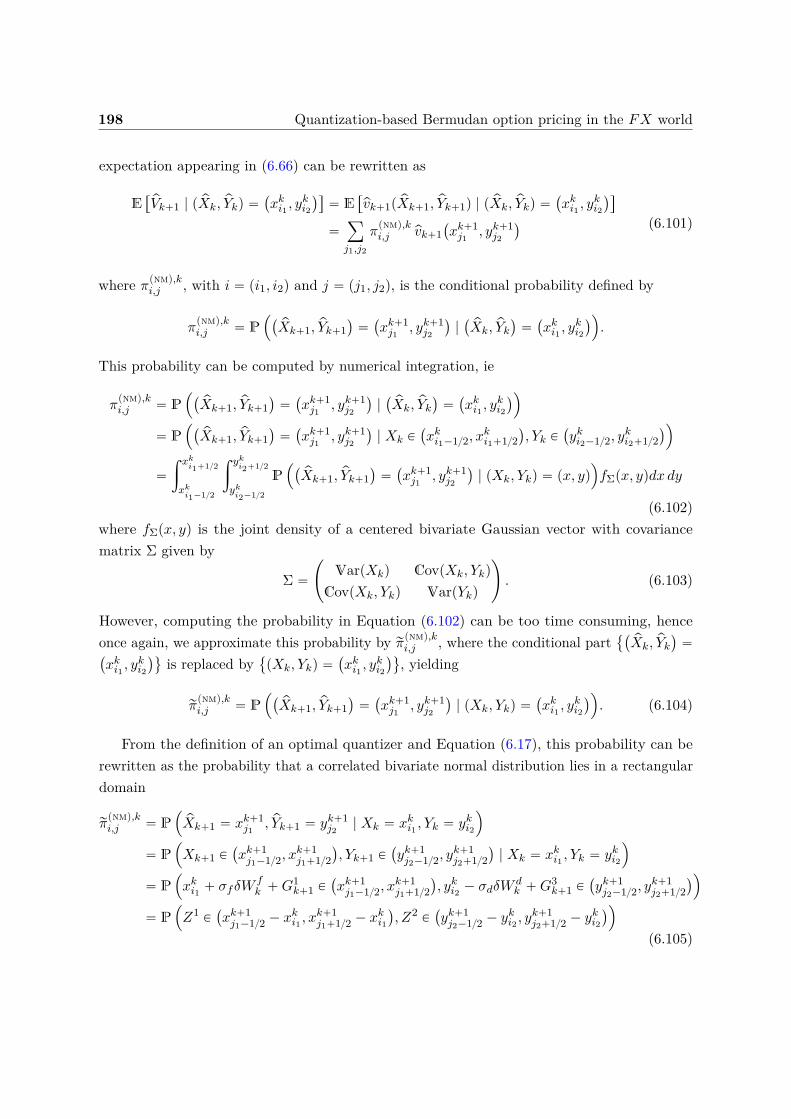
198 Quantization-based Bermudan option pricing in the FX world
expectation appearing in (6.66) can be rewritten as
E“
pVk`1 | p pXk, pYkq “`
xki1 , yki2
˘‰
“ E“
pvk`1p pXk`1, pYk`1q | p pXk, pYkq “`
xki1 , yki2
˘‰
“ÿ
j1,j2
π(nm),ki,j pvk`1
`
xk`1j1
, yk`1j2
˘ (6.101)
where π(nm),ki,j , with i “ pi1, i2q and j “ pj1, j2q, is the conditional probability defined by
π(nm),ki,j “ P
´
`
pXk`1, pYk`1˘
“`
xk`1j1
, yk`1j2
˘
|`
pXk, pYk˘
“`
xki1 , yki2
˘
¯
.
This probability can be computed by numerical integration, ie
π(nm),ki,j “ P
´
`
pXk`1, pYk`1˘
“`
xk`1j1
, yk`1j2
˘
|`
pXk, pYk˘
“`
xki1 , yki2
˘
¯
“ P´
`
pXk`1, pYk`1˘
“`
xk`1j1
, yk`1j2
˘
| Xk P`
xki1´12, xki1`12
˘
, Yk P`
yki2´12, yki2`12
˘
¯
“
ż xki1`12
xki1´12
ż yki2`12
yki2´12
P´
`
pXk`1, pYk`1˘
“`
xk`1j1
, yk`1j2
˘
| pXk, Ykq “ px, yq
¯
fΣpx, yqdx dy
(6.102)where fΣpx, yq is the joint density of a centered bivariate Gaussian vector with covariancematrix Σ given by
Σ “
˜
VarpXkq CovpXk, Ykq
CovpXk, Ykq VarpYkq
¸
. (6.103)
However, computing the probability in Equation (6.102) can be too time consuming, henceonce again, we approximate this probability by rπ
(nm),ki,j , where the conditional part
`
pXk, pYk˘
“`
xki1 , yki2
˘(
is replaced by
pXk, Ykq “`
xki1 , yki2
˘(
, yielding
rπ(nm),ki,j “ P
´
`
pXk`1, pYk`1˘
“`
xk`1j1
, yk`1j2
˘
| pXk, Ykq “`
xki1 , yki2
˘
¯
. (6.104)
From the definition of an optimal quantizer and Equation (6.17), this probability can berewritten as the probability that a correlated bivariate normal distribution lies in a rectangulardomain
rπ(nm),ki,j “ P
´
pXk`1 “ xk`1j1
, pYk`1 “ yk`1j2
| Xk “ xki1 , Yk “ yki2
¯
“ P´
Xk`1 P`
xk`1j1´12, x
k`1j1`12
˘
, Yk`1 P`
yk`1j2´12, y
k`1j2`12
˘
| Xk “ xki1 , Yk “ yki2
¯
“ P´
xki1 ` σfδWfk `G1
k`1 P`
xk`1j1´12, x
k`1j1`12
˘
, yki2 ´ σdδWdk `G3
k`1 P`
yk`1j2´12, y
k`1j2`12
˘
¯
“ P´
Z1 P`
xk`1j1´12 ´ xki1 , x
k`1j1`12 ´ xki1
˘
, Z2 P`
yk`1j2´12 ´ yki2 , y
k`1j2`12 ´ yki2
˘
¯
(6.105)
6.4 Numerical experiments 199
where˜
Z1
Z2
¸
„ N
˜˜
00
¸
,
˜
σ2Z1 ρ
Z1,Z2σZ1σZ2
ρZ1,Z2σZ1σZ2 σ2
Z2
¸¸
(6.106)
with σ2Z1 “ VarpσfδW
fk ` G1
k`1q, σ2Z2 “ Varp´σdδW
dk ` G3
k`1q and ρZ1,Z2 “ CorrpσfδW
fk `
G1k`1,´σdδW
dk `G3
k`1q.The advantage of expressing (6.105) as the probability that a bivariate Gaussian vector
lies in a rectangular domain is that it can be rewritten as a linear combination of bivariatecumulative distribution functions.
Fig. 6.2
Indeed, let pU, V q a two-dimensional correlated and standard-ized normal distribution with correlation ρ and cumulative distri-bution function (CDF) given by F ρU,V pu, vq “ PpU ď u, V ď vq.Fast and efficient numerical implementation of such functionexists (for example, a C++ implementation of the upper righttail of a correlated bivariate normal distribution can be foundin John Burkardt’s website, see [Bur12], which is based on thework of [Don73] and [Owe58]. In our case, we are interested inthe computation of probabilities of the form
P`
U P pu1, u2q, V P pv1, v2q˘
. (6.107)
This probability is represented graphically as the integral of the two-dimensional density overthe rectangular domain in grey in Figure 6.2. Now, using F ρU,V pu, vq, the probability (6.107) isgiven by
P`
U P pu1, u2q, V P pv1, v2q˘
“ F ρU,V pu2, v2q ´ F ρU,V pu1, v2q ´ F ρU,V pu2, v1q ` F ρU,V pu1, v1q.
(6.108)This remark will allow us to reduce drastically the computation time induced by the
evaluation of the conditional probabilities and so, of the conditional expectations.Now, going back to our problem, the QBDPP in the non-Markovian case rewrites (6.66)
$
’
’
&
’
’
%
pvn`
xni1 , yni2
˘
“ hn`
xni1 , yni2
˘
, 1 ď i1 ď NXn , 1 ď i2 ď NY
n ,
pvk`
xki1 , yki2
˘
“ maxˆ
hk`
xki1 , yki2
˘
,ÿ
j1,j2
π(nm),ki,j pvk`1
`
xk`1j1
, yk`1j2
˘
˙
.(6.109)
In order to test numerically the two methods, we will evaluate PRDC European andBermudan options with maturities 2Y , 5Y and 10Y . We describe below the market andproducts parameters we consider. The volatilities of the domestic and the foreign interest ratesare not detailed below because we investigate the behaviour of the methods with respect to σdand σf .
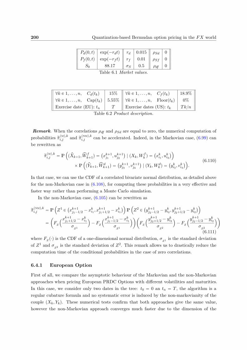
200 Quantization-based Bermudan option pricing in the FX world
Pdp0, tq expp´rdtq rd 0.015 ρSd 0Pf p0, tq expp´rf tq rf 0.01 ρSf 0S0 88.17 σS 0.5 ρdf 0
Table 6.1 Market values.
@k P 1, . . . , n, Cdptkq 15% @k P 1, . . . , n, Cf ptkq 18.9%@k P 1, . . . , n, Capptkq 5.55% @k P 1, . . . , n, Floorptkq 0%Exercise date (EU): tn T Exercise dates (US): tk Tkn
Table 6.2 Product description.
Remark. When the correlations ρdf and ρSd are equal to zero, the numerical computation ofprobabilities rπ
(m),ki,j and rπ
(nm),ki,j can be accelerated. Indeed, in the Markovian case, (6.99) can
be rewritten as
rπ(m),ki,j “ P
´
p pXk`1,xWfk`1q “
`
xk`1j1
, uk`1j2
˘
| pXk,Wfk q “
`
xki1 , uki2
˘
¯
ˆ P´
ppYk`1,xWdk`1q “
`
yk`1j3
, vk`1j4
˘
| pYk,Wdk q “
`
yki3 , vki4
˘
¯
.(6.110)
In that case, we can use the CDF of a correlated bivariate normal distribution, as detailed abovefor the non-Markovian case in (6.108), for computing these probabilities in a very effective andfaster way rather than performing a Monte Carlo simulation.
In the non-Markovian case, (6.105) can be rewritten as
rπ(nm),ki,j “ P
´
Z1 P`
xk`1j1´12 ´ xki1 , x
k`1j1`12 ´ xki1
˘
¯
P´
Z2 P`
yk`1j2´12 ´ yki2 , y
k`1j2`12 ´ yki2
˘
¯
“
ˆ
FZ
´xk`1j1`12 ´ xki1
σZ1
¯
´ FZ
´xk`1j1´12 ´ xki1
σZ1
¯
˙ˆ
FZ
´yk`1j2`12 ´ yki2
σZ2
¯
´ FZ
´yk`1j2´12 ´ yki2
σZ2
¯
˙
(6.111)where FZ p¨q is the CDF of a one-dimensional normal distribution, σ
Z1 is the standard deviationof Z1 and σ
Z2 is the standard deviation of Z2. This remark allows us to drastically reduce thecomputation time of the conditional probabilities in the case of zero correlations.
6.4.1 European Option
First of all, we compare the asymptotic behaviour of the Markovian and the non-Markovianapproaches when pricing European PRDC Options with different volatilities and maturities.In this case, we consider only two dates in the tree: t0 “ 0 an tn “ T , the algorithm is aregular cubature formula and no systematic error is induced by the non-markovianity of thecouple pXk, Ykq. These numerical tests confirm that both approaches give the same value,however the non-Markovian approach converges much faster due to the dimension of the
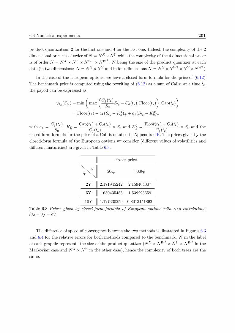
6.4 Numerical experiments 201
product quantization, 2 for the first one and 4 for the last one. Indeed, the complexity of the 2dimensional pricer is of order of N “ NX ˆNY while the complexity of the 4 dimensional priceris of order N “ NX ˆNY ˆNW d
ˆNW f . N being the size of the product quantizer at eachdate (in two dimensions: N “ NX ˆNY and in four dimensions N “ NX ˆNW f
ˆNY ˆNW d).
In the case of the European options, we have a closed-form formula for the price of (6.12).The benchmark price is computed using the rewriting of (6.12) as a sum of Calls: at a time tk,the payoff can be expressed as
ψtk pStk q “ minˆ
maxˆ
Cf ptkq
S0Stk ´ Cdptkq,Floorptkq
˙
,Capptkq
˙
“ Floorptkq ´ akpStk ´K1kq` ` akpStk ´K2
kq`
with ak “Cf ptkq
S0, K1
k “Capptkq ` Cdptkq
Cf ptkqˆ S0 and K2
k “Floorptkq ` Cdptkq
Cf ptkqˆ S0 and the
closed-form formula for the price of a Call is detailed in Appendix 6.B. The prices given by theclosed-form formula of the European options we consider (different values of volatilities anddifferent maturities) are given in Table 6.3.
Exact price
T
σ 50bp 500bp
2Y 2.171945242 2.159404007
5Y 1.630435483 1.539295559
10Y 1.127330259 0.8013151892Table 6.3 Prices given by closed-form formula of European options with zero correlations.(σd “ σf “ σ)
The difference of speed of convergence between the two methods is illustrated in Figures 6.3and 6.4 for the relative errors for both methods compared to the benchmark. N in the labelof each graphic represents the size of the product quantizer (NX ˆNW f
ˆNY ˆNW d in theMarkovian case and NX ˆNY in the other case), hence the complexity of both trees are thesame.
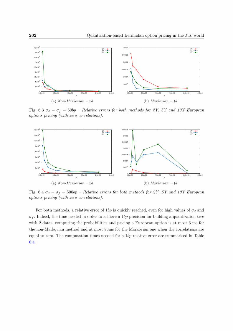
202 Quantization-based Bermudan option pricing in the FX world
0
5x10⁻⁸
1x10⁻⁷
1.5x10⁻⁷
2x10⁻⁷
2.5x10⁻⁷
3x10⁻⁷
3.5x10⁻⁷
4x10⁻⁷
4.5x10⁻⁷
0.0e+00 5.0e+05 1.0e+06 1.5e+06 2.0e+06 2.5e+06
N
2Y
5Y
10Y
(a) Non-Markovian – 2d
0
5x10⁻⁵
0.0001
0.00015
0.0002
0.00025
0.0003
0.0e+00 5.0e+05 1.0e+06 1.5e+06 2.0e+06 2.5e+06
N
2Y
5Y
10Y
(b) Markovian – 4d
Fig. 6.3 σd “ σf “ 50bp – Relative errors for both methods for 2Y, 5Y and 10Y Europeanoptions pricing (with zero correlations).
0
2x10⁻⁶
4x10⁻⁶
6x10⁻⁶
8x10⁻⁶
1x10⁻⁵
1.2x10⁻⁵
1.4x10⁻⁵
1.6x10⁻⁵
0.0e+00 5.0e+05 1.0e+06 1.5e+06 2.0e+06 2.5e+06
N
2Y
5Y
10Y
(a) Non-Markovian – 2d
0
5x10⁻⁵
0.0001
0.00015
0.0002
0.00025
0.0003
0.00035
0.0e+00 5.0e+05 1.0e+06 1.5e+06 2.0e+06 2.5e+06
N
2Y
5Y
10Y
(b) Markovian – 4d
Fig. 6.4 σd “ σf “ 500bp – Relative errors for both methods for 2Y, 5Y and 10Y Europeanoptions pricing (with zero correlations).
For both methods, a relative error of 1bp is quickly reached, even for high values of σd andσf . Indeed, the time needed in order to achieve a 1bp precision for building a quantization treewith 2 dates, computing the probabilities and pricing a European option is at most 6 ms forthe non-Markovian method and at most 85ms for the Markovian one when the correlations areequal to zero. The computation times needed for a 1bp relative error are summarised in Table6.4.
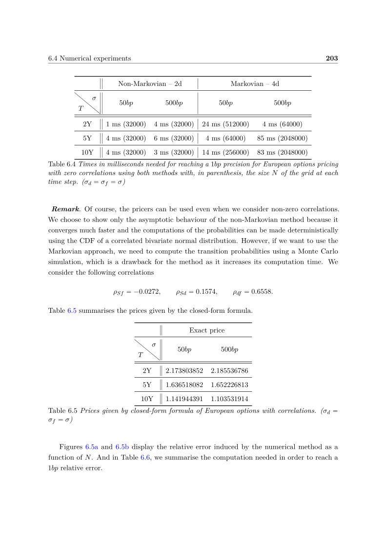
6.4 Numerical experiments 203
Non-Markovian – 2d Markovian – 4d
T
σ 50bp 500bp 50bp 500bp
2Y 1 ms (32000) 4 ms (32000) 24 ms (512000) 4 ms (64000)
5Y 4 ms (32000) 6 ms (32000) 4 ms (64000) 85 ms (2048000)
10Y 4 ms (32000) 3 ms (32000) 14 ms (256000) 83 ms (2048000)Table 6.4 Times in milliseconds needed for reaching a 1bp precision for European options pricingwith zero correlations using both methods with, in parenthesis, the size N of the grid at eachtime step. (σd “ σf “ σ)
Remark. Of course, the pricers can be used even when we consider non-zero correlations.We choose to show only the asymptotic behaviour of the non-Markovian method because itconverges much faster and the computations of the probabilities can be made deterministicallyusing the CDF of a correlated bivariate normal distribution. However, if we want to use theMarkovian approach, we need to compute the transition probabilities using a Monte Carlosimulation, which is a drawback for the method as it increases its computation time. Weconsider the following correlations
ρSf “ ´0.0272, ρSd “ 0.1574, ρdf “ 0.6558.
Table 6.5 summarises the prices given by the closed-form formula.
Exact price
T
σ 50bp 500bp
2Y 2.173803852 2.185536786
5Y 1.636518082 1.652226813
10Y 1.141944391 1.103531914Table 6.5 Prices given by closed-form formula of European options with correlations. (σd “
σf “ σ)
Figures 6.5a and 6.5b display the relative error induced by the numerical method as afunction of N . And in Table 6.6, we summarise the computation needed in order to reach a1bp relative error.
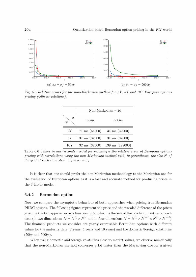
204 Quantization-based Bermudan option pricing in the FX world
0
2x10⁻⁵
4x10⁻⁵
6x10⁻⁵
8x10⁻⁵
0.0001
0.00012
0.00014
0.00016
0.0e+00 5.0e+05 1.0e+06 1.5e+06 2.0e+06 2.5e+06
N
2Y
5Y
10Y
(a) σd “ σf “ 50bp
0
5x10⁻⁵
0.0001
0.00015
0.0002
0.00025
0.0003
0.0e+00 5.0e+05 1.0e+06 1.5e+06 2.0e+06 2.5e+06
N
2Y
5Y
10Y
(b) σd “ σf “ 500bp
Fig. 6.5 Relative errors for the non-Markovian method for 2Y, 5Y and 10Y European optionspricing (with correlations).
Non-Markovian – 2d
T
σ 50bp 500bp
2Y 71 ms (64000) 34 ms (32000)
5Y 31 ms (32000) 31 ms (32000)
10Y 32 ms (32000) 139 ms (128000)Table 6.6 Times in milliseconds needed for reaching a 1bp relative error of European optionspricing with correlations using the non-Markovian method with, in parenthesis, the size N ofthe grid at each time step. (σd “ σf “ σ)
It is clear that one should prefer the non-Markovian methodology to the Markovian one forthe evaluation of European options as it is a fast and accurate method for producing prices inthe 3-factor model.
6.4.2 Bermudan option
Now, we compare the asymptotic behaviour of both approaches when pricing true BermudanPRDC options. The following figures represent the price and the rescaled difference of the pricesgiven by the two approaches as a function of N , which is the size of the product quantizer at eachdate (in two dimensions: N “ NX ˆNY and in four dimensions N “ NX ˆNW f
ˆNY ˆNW d).The financial products we consider are yearly exercisable Bermudan options with differentvalues for the maturity date (2 years, 5 years and 10 years) and the domestic/foreign volatilities(50bp and 500bp).
When using domestic and foreign volatilities close to market values, we observe numericallythat the non-Markovian method converges a lot faster than the Markovian one for a given
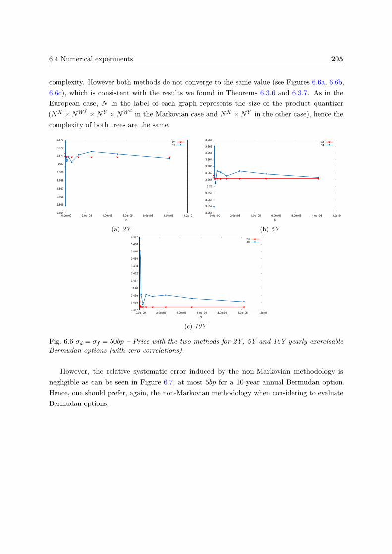
6.4 Numerical experiments 205
complexity. However both methods do not converge to the same value (see Figures 6.6a, 6.6b,6.6c), which is consistent with the results we found in Theorems 6.3.6 and 6.3.7. As in theEuropean case, N in the label of each graph represents the size of the product quantizer(NX ˆNW f
ˆNY ˆNW d in the Markovian case and NX ˆNY in the other case), hence thecomplexity of both trees are the same.
2.864
2.865
2.866
2.867
2.868
2.869
2.87
2.871
2.872
2.873
0.0e+00 2.0e+05 4.0e+05 6.0e+05 8.0e+05 1.0e+06 1.2e+06
N
2d
4d
(a) 2Y
3.256
3.257
3.258
3.259
3.26
3.261
3.262
3.263
3.264
3.265
3.266
3.267
0.0e+00 2.0e+05 4.0e+05 6.0e+05 8.0e+05 1.0e+06 1.2e+06
N
2d
4d
(b) 5Y
3.457
3.458
3.459
3.46
3.461
3.462
3.463
3.464
3.465
3.466
3.467
0.0e+00 2.0e+05 4.0e+05 6.0e+05 8.0e+05 1.0e+06 1.2e+06
N
2d
4d
(c) 10Y
Fig. 6.6 σd “ σf “ 50bp – Price with the two methods for 2Y, 5Y and 10Y yearly exercisableBermudan options (with zero correlations).
However, the relative systematic error induced by the non-Markovian methodology isnegligible as can be seen in Figure 6.7, at most 5bp for a 10-year annual Bermudan option.Hence, one should prefer, again, the non-Markovian methodology when considering to evaluateBermudan options.
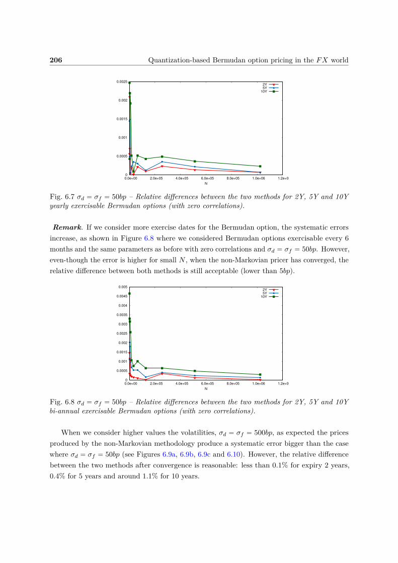
206 Quantization-based Bermudan option pricing in the FX world
0
0.0005
0.001
0.0015
0.002
0.0025
0.0e+00 2.0e+05 4.0e+05 6.0e+05 8.0e+05 1.0e+06 1.2e+06
N
2Y
5Y
10Y
Fig. 6.7 σd “ σf “ 50bp – Relative differences between the two methods for 2Y, 5Y and 10Yyearly exercisable Bermudan options (with zero correlations).
Remark. If we consider more exercise dates for the Bermudan option, the systematic errorsincrease, as shown in Figure 6.8 where we considered Bermudan options exercisable every 6months and the same parameters as before with zero correlations and σd “ σf “ 50bp. However,even-though the error is higher for small N , when the non-Markovian pricer has converged, therelative difference between both methods is still acceptable (lower than 5bp).
0
0.0005
0.001
0.0015
0.002
0.0025
0.003
0.0035
0.004
0.0045
0.005
0.0e+00 2.0e+05 4.0e+05 6.0e+05 8.0e+05 1.0e+06 1.2e+06
N
2Y
5Y
10Y
Fig. 6.8 σd “ σf “ 50bp – Relative differences between the two methods for 2Y, 5Y and 10Ybi-annual exercisable Bermudan options (with zero correlations).
When we consider higher values the volatilities, σd “ σf “ 500bp, as expected the pricesproduced by the non-Markovian methodology produce a systematic error bigger than the casewhere σd “ σf “ 50bp (see Figures 6.9a, 6.9b, 6.9c and 6.10). However, the relative differencebetween the two methods after convergence is reasonable: less than 0.1% for expiry 2 years,0.4% for 5 years and around 1.1% for 10 years.
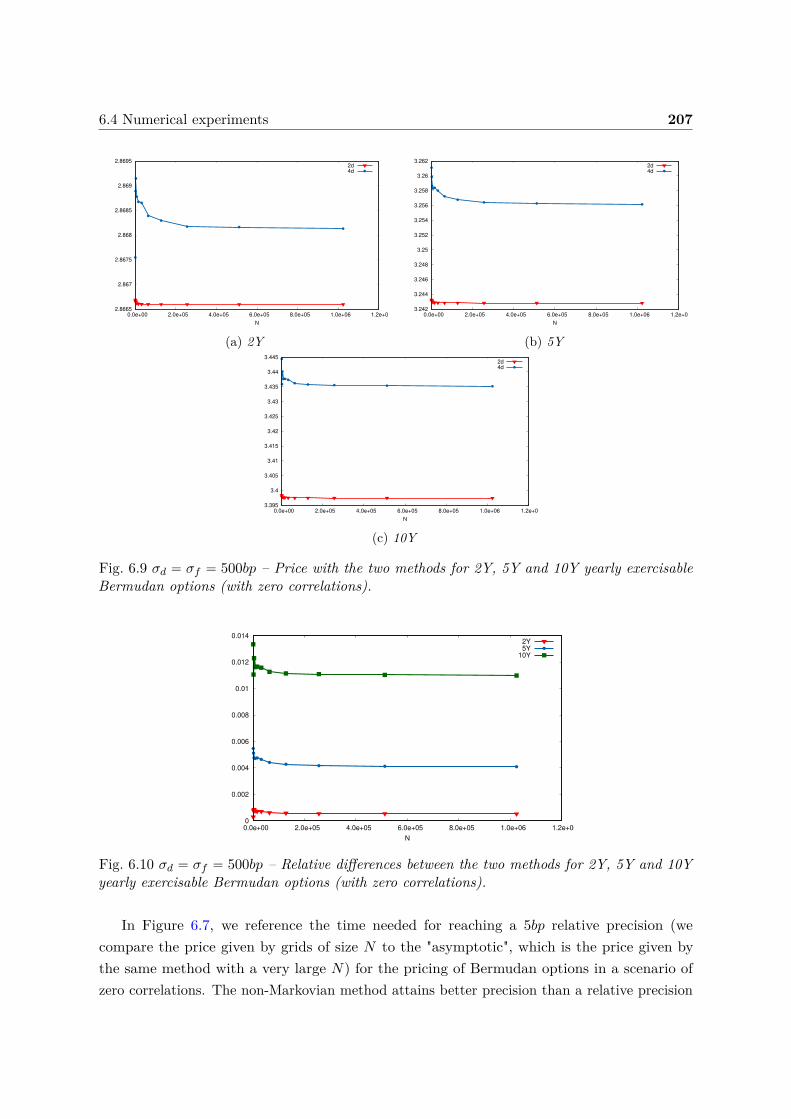
6.4 Numerical experiments 207
2.8665
2.867
2.8675
2.868
2.8685
2.869
2.8695
0.0e+00 2.0e+05 4.0e+05 6.0e+05 8.0e+05 1.0e+06 1.2e+06
N
2d
4d
(a) 2Y
3.242
3.244
3.246
3.248
3.25
3.252
3.254
3.256
3.258
3.26
3.262
0.0e+00 2.0e+05 4.0e+05 6.0e+05 8.0e+05 1.0e+06 1.2e+06
N
2d
4d
(b) 5Y
3.395
3.4
3.405
3.41
3.415
3.42
3.425
3.43
3.435
3.44
3.445
0.0e+00 2.0e+05 4.0e+05 6.0e+05 8.0e+05 1.0e+06 1.2e+06
N
2d
4d
(c) 10Y
Fig. 6.9 σd “ σf “ 500bp – Price with the two methods for 2Y, 5Y and 10Y yearly exercisableBermudan options (with zero correlations).
0
0.002
0.004
0.006
0.008
0.01
0.012
0.014
0.0e+00 2.0e+05 4.0e+05 6.0e+05 8.0e+05 1.0e+06 1.2e+06
N
2Y
5Y
10Y
Fig. 6.10 σd “ σf “ 500bp – Relative differences between the two methods for 2Y, 5Y and 10Yyearly exercisable Bermudan options (with zero correlations).
In Figure 6.7, we reference the time needed for reaching a 5bp relative precision (wecompare the price given by grids of size N to the "asymptotic", which is the price given bythe same method with a very large N) for the pricing of Bermudan options in a scenario ofzero correlations. The non-Markovian method attains better precision than a relative precision
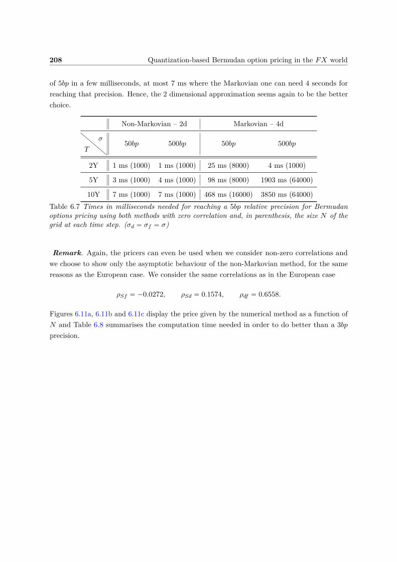
208 Quantization-based Bermudan option pricing in the FX world
of 5bp in a few milliseconds, at most 7 ms where the Markovian one can need 4 seconds forreaching that precision. Hence, the 2 dimensional approximation seems again to be the betterchoice.
Non-Markovian – 2d Markovian – 4d
T
σ 50bp 500bp 50bp 500bp
2Y 1 ms (1000) 1 ms (1000) 25 ms (8000) 4 ms (1000)
5Y 3 ms (1000) 4 ms (1000) 98 ms (8000) 1903 ms (64000)
10Y 7 ms (1000) 7 ms (1000) 468 ms (16000) 3850 ms (64000)Table 6.7 Times in milliseconds needed for reaching a 5bp relative precision for Bermudanoptions pricing using both methods with zero correlation and, in parenthesis, the size N of thegrid at each time step. (σd “ σf “ σ)
Remark. Again, the pricers can even be used when we consider non-zero correlations andwe choose to show only the asymptotic behaviour of the non-Markovian method, for the samereasons as the European case. We consider the same correlations as in the European case
ρSf “ ´0.0272, ρSd “ 0.1574, ρdf “ 0.6558.
Figures 6.11a, 6.11b and 6.11c display the price given by the numerical method as a function ofN and Table 6.8 summarises the computation time needed in order to do better than a 3bpprecision.
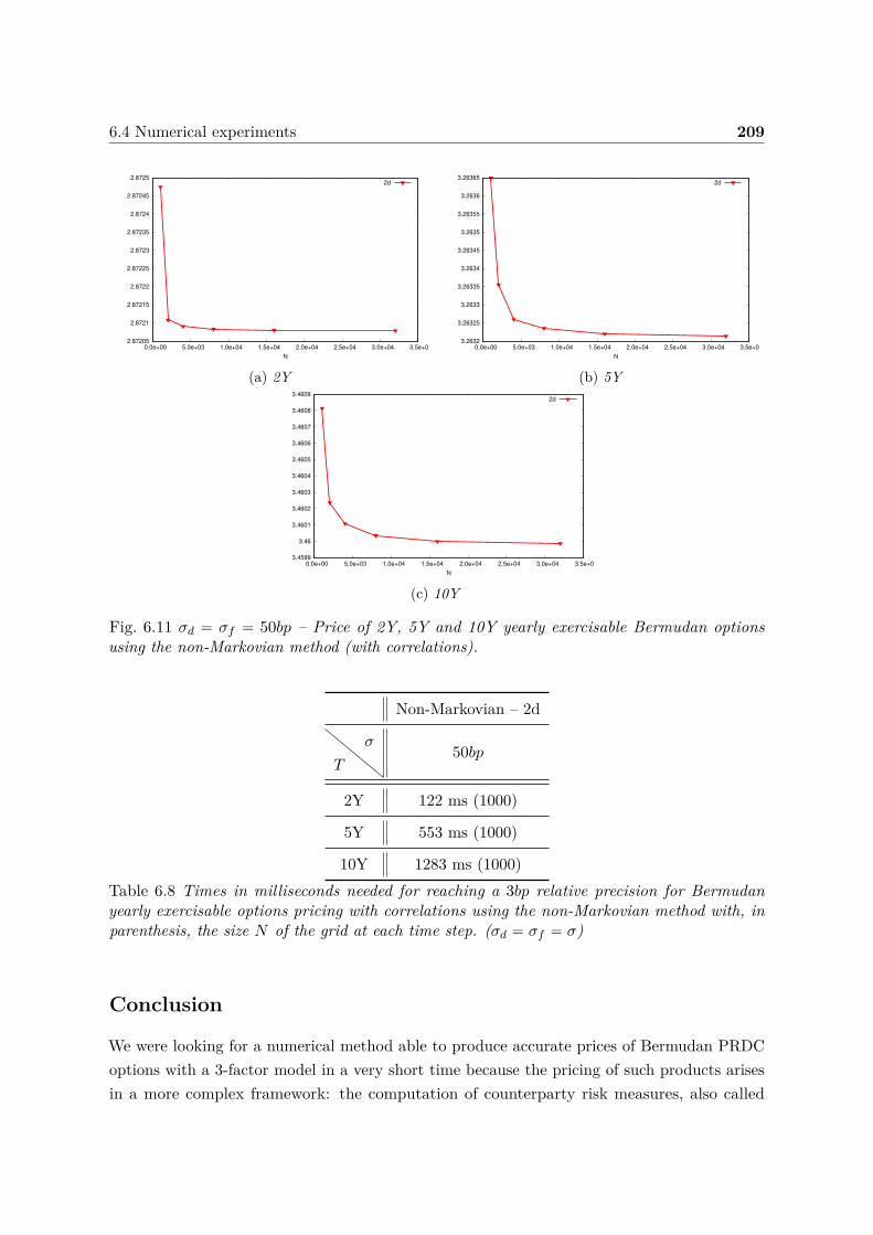
6.4 Numerical experiments 209
2.87205
2.8721
2.87215
2.8722
2.87225
2.8723
2.87235
2.8724
2.87245
2.8725
0.0e+00 5.0e+03 1.0e+04 1.5e+04 2.0e+04 2.5e+04 3.0e+04 3.5e+04
N
2d
(a) 2Y
3.2632
3.26325
3.2633
3.26335
3.2634
3.26345
3.2635
3.26355
3.2636
3.26365
0.0e+00 5.0e+03 1.0e+04 1.5e+04 2.0e+04 2.5e+04 3.0e+04 3.5e+04
N
2d
(b) 5Y
3.4599
3.46
3.4601
3.4602
3.4603
3.4604
3.4605
3.4606
3.4607
3.4608
3.4609
0.0e+00 5.0e+03 1.0e+04 1.5e+04 2.0e+04 2.5e+04 3.0e+04 3.5e+04
N
2d
(c) 10Y
Fig. 6.11 σd “ σf “ 50bp – Price of 2Y, 5Y and 10Y yearly exercisable Bermudan optionsusing the non-Markovian method (with correlations).
Non-Markovian – 2d
T
σ 50bp
2Y 122 ms (1000)
5Y 553 ms (1000)
10Y 1283 ms (1000)Table 6.8 Times in milliseconds needed for reaching a 3bp relative precision for Bermudanyearly exercisable options pricing with correlations using the non-Markovian method with, inparenthesis, the size N of the grid at each time step. (σd “ σf “ σ)
Conclusion
We were looking for a numerical method able to produce accurate prices of Bermudan PRDCoptions with a 3-factor model in a very short time because the pricing of such products arisesin a more complex framework: the computation of counterparty risk measures, also called

210 Quantization-based Bermudan option pricing in the FX world
xVA’s. We proposed two numerical methods based on product optimal quantization with apreference for the non-Markovian one. Indeed, even if we introduce a systematic error with ourapproximation, the error is controlled, as long as the volatilities of the domestic and foreigninterest rates stay reasonable. Moreover, the numerical tests we conducted confirmed that idea:we are able to produce prices of Bermudan options in the 3-factor model in a fast and accurateway.
6.A W f is a Brownian motion under the domestic risk-neutral measure 211
Appendix 6.A W f is a Brownian motion under the domesticrisk-neutral measure
Let pĂW f q a rP-Brownian motion. In this section, we show that the process W f defined by
dW fs “ dĂW f
s ` ρSfσSds (6.112)
is a P-Brownian motion.First, we define the following change of numéraire, where rP is the foreign risk-neutral
probability and P is the domestic risk-neutral probability,r
drP “STS0
expˆ
´
ż T
0rdsds
˙
expˆż T
0rfs ds
˙
dP
“ expˆ
σSWST ´
σ2S
2 T
˙
dP
or equivalently
dP “ expˆ
´ σSWST `
σ2S
2 T
˙
drP
“ expˆ
´ σSpWST ´ σST q ´
σ2S
2 T
˙
drP
“ expˆ
´ σSĂWST ´
σ2S
2 T
˙
drP
(6.113)
where ĂWS is a rP-Brownian motion defined by dĂWSt “ dWS
t ´ σSdt. More details concerningthe definition of the foreign risk-neutral probability can be found in the Chapter 9 of [Shr04].
Now, we are looking for q P R such that dW fs “ dĂW f
s ´ qdt is a P-Brownian motion. Letλ P R and @t ą s
E”
eλ`
pĂW ft ´qtq´pĂW f
s ´qsq
˘
| Fs
ı
“ rE”
eλ`
pĂW ft ´qtq´pĂW f
s ´qsq
˘
´σSpĂWST ´ĂWS
s q´σ2
S2 pT´sq
| Fs
ı
“ rE”
eλ`
pĂW ft ´qtq´pĂW f
s ´qsq
˘
´σSpĂWSt ´ĂWS
s q´σ2
S2 pt´sq
| Fs
ı
“ e´λqpt´sq´σ2
S2 pt´sq
rE”
eλpĂW ft ´ĂW f
s q´σSpĂWSt ´ĂWS
s q | Fs
ı
“ e´λqpt´sq´σ2
S2 pt´sq e
λ22 pt´sq´λσSρSf pt´sq`
σ2S2 pt´sq
“ eλ22 pt´sq e´λqpt´sq´λσSρSf pt´sq
“ eλ22 pt´sq
(6.114)
the last equality is ensured if and only if
0 “ ´λqpt´ sq ´ λσSρSf pt´ sq ðñ q “ ´σSρSf . (6.115)
212 Quantization-based Bermudan option pricing in the FX world
Hence, W f defined bydW f
s “ dĂW fs ` ρSfσSds
is a P-Brownian motion.
Appendix 6.B FX Derivatives - European Call
The payoff at maturity t of a European Call on FX rate is given by
pSt ´Kq`
with K the strike and St the FX rate at time t.Our aim will be to evaluate V0
V0 “ E”
e´şt0 r
dsdspSt ´Kq`
ı
.
Proposition 6.B.1. If we consider a 3-factor model on Foreign Exchange and Zero-coupon asdefined in (6.6), V0 is given by2
V0 “ S0Pf p0, tq N
˜ log´
S0P f p0,tqKP dp0,tq
¯
` µp0, tqσp0, tq
¸
´KP dp0, tq N
˜ log´
S0P f p0,tqKP dp0,tq
¯
´ µp0, tqσp0, tq
¸
with
µp0, tq “
ż t
0
12`
σ2Spsq ` σ2
f ps, tq ` σ2dps, tq
˘
ds
`
ż t
0
`
ρSfσSpsqσf ps, tq ´ ρSdσSpsqσdps, tqds´ ρfdσf ps, tqσdps, tq˘
ds
andσ2p0, tq “ 2µp0, tq.
Proof. In this part, we want to evaluate
V0 “ E”
e´şt0 r
dsdspSt ´Kq`
ı
.
2We ignore the settlements details in the present paper in order to alleviate the notations but the formulacan easily be extended to take them into account.
6.B FX Derivatives - European Call 213
If we consider a 3-factor model on Foreign Exchange and Zero-coupon as defined in (6.6), wehave
V0 “ E”
e´şt0 r
dsdspSt ´Kq`
ı
“ E”
`
e´şt0 r
dsds St ´ e´
şt0 r
dsdsK
˘
`
ı
“ E”
`
e´şt0 r
dsds St ´ e´
şt0 r
dsdsK
˘
1tStěKu
ı
“ E”
e´şt0 r
dsds St 1tStěKu
ı
´K E”
e´şt0 r
dsds 1tStěKu
ı
.
We focus on the first termK E
”
e´şt0 r
dsds 1tStěKu
ı
. (6.116)
We do the following change of numéraire:
drQ
dP“
rZtrZ0
with$
&
%
rZt “ exp´
rYt ´12 ă rY , rY ąt
¯
,
rZ0 “ 1
where rYt “şt0 σdps, tqdW d
s and ă rY , rY ąt“şt0 σ
2dps, tqds.
Hence, we can define the following Brownian Motions ĂW d, ĂW f , ĂWS under rQ:
dĂW ds “ dW d
s ´ d ă Y,W d ąs “ dW ds ´ σdps, tqds,
dĂW fs “ dW f
s ´ d ă Y,W f ąs “ dW fs ´ ρfdσdps, tqds,
dĂWSs “ dWS
s ´ d ă Y,WS ąs “ dWSs ´ ρSdσdps, tqds
214 Quantization-based Bermudan option pricing in the FX world
and St becomes
St “ S0 expˆż t
0
ˆ
rds ´ rfs ´σ2Spsq
2
˙
ds`
ż t
0σSpsqdWS
s
˙
“S0P
f p0, tqP dp0, tq exp
ˆż t
0´
12`
σ2Spsq ` σ2
f ps, tq ´ σ2dps, tq
˘
´ ρSfσSpsqσf ps, tq ds
˙
ˆ expˆż t
0σSpsqdWS
s `
ż t
0σf ps, tqdW f
s ´
ż t
0σdps, tqdW d
s
˙
“S0P
f p0, tqP dp0, tq exp
ˆ
´
ż t
0
12`
σ2Spsq ` σ2
f ps, tq ` σ2dps, tq
˘
ds
˙
ˆ expˆ
´
ż t
0
`
ρSfσSpsqσf ps, tq ´ ρSdσSpsqσdps, tq ´ ρfdσf ps, tqσdps, tq˘
ds
˙
ˆ expˆż t
0σSpsqdĂWS
s `
ż t
0σf ps, tqdĂW f
s ´
ż t
0σdps, tqdĂW d
s
˙
“S0P
f p0, tqP dp0, tq exp
ˆ
´ µp0, tq `
ż t
0σSpsqdĂWS
s `
ż t
0σf ps, tqdĂW f
s ´
ż t
0σdps, tqdĂW d
s
˙
.
Hence, as exp´
´şt0 r
dsds
¯
“ P dp0, tq ˆ rZt, (6.116) becomes
K E”
e´şt0 r
dsds 1tStěKu
ı
“ KP dp0, tqErQ”
1tStěKu
ı
“ KP dp0, tqrQpSt ě Kq
“ KP dp0, tqrQ˜
Z ělog
´
KP dp0,tqS0P f p0,tq
¯
` µp0, tqσp0, tq
¸
“ KP dp0, tqrQ˜
Z ďlog
´
S0P f p0,tqKP dp0,tq
¯
´ µp0, tqσp0, tq
¸
“ KP dp0, tq N
˜ log´
S0P f p0,tqKP dp0,tq
¯
´ µp0, tqσp0, tq
¸
6.B FX Derivatives - European Call 215
where Z „ N p0, 1q with
µp0, tq “
ż t
0
12`
σ2Spsq ` σ2
f ps, tq ` σ2dps, tq
˘
ds
`
ż t
0
`
ρSfσSpsqσf ps, tq ´ ρSdσSpsqσdps, tqds´ ρfdσf ps, tqσdps, tq˘
ds,
σ2p0, tq “ Varˆż t
0σSpsqdĂWS
s `
ż t
0σf ps, tqdĂW f
s ´
ż t
0σdps, tqdĂW d
s
˙
“ Varˆż t
0σSpsqdĂWS
s
˙
`Varˆż t
0σf ps, tqdĂW f
s
˙
`Varˆż t
0σdps, tqdĂW d
s
˙
` 2Covˆż t
0σSpsqdĂWS
s ,
ż t
0σf ps, tqdĂW f
s
˙
´ 2Covˆż t
0σSpsqdĂWS
s ,
ż t
0σdps, tqdĂW d
s
˙
´ 2Covˆż t
0σf ps, tqdĂW f
s ,
ż t
0σdps, tqdĂW d
s
˙
“
ż t
0
`
σ2Spsq ` σ2
f ps, tq ` σ2dps, tq
˘
ds
` 2ż t
0
`
ρSfσSpsqσf ps, tq ´ ρSdσSpsqσdps, tq ´ ρfdσf ps, tqσdps, tq˘
ds.
Now, we deal with the term
E”
e´şt0 r
dsds St 1tStěKu
ı
“ P dp0, tqErQ“
St 1tStěKu
‰
(6.117)
using directly the formula of the first partial moment of a log-normal random variable. LetX „ Log- N pµ, σ2q, then
E“
X 1tXěxu
‰
“ eµ` σ22 N
ˆ
µ` σ2 ´ logpxq
σ
˙
.
Finally, as St “S0P f p0,tqP dp0,tq X with X
rQ„ Log- N p´µp0, tq, σ2p0, tqq, we get
(6.117) “ S0Pf p0, tqErQ
«
X 1!Xě
KP dp0,tq
S0P f p0,tq
)
ff
“ S0Pf p0, tq e´µp0,tq`
σ2p0,tq
2 N
˜
´µp0, tq ` σ2p0, tq ´ log´
KP dp0,tqS0P f p0,tq
¯
σp0, tq
¸
“ S0Pf p0, tq N
˜ log´
S0P f p0,tqKP dp0,tq
¯
` µp0, tqσp0, tq
¸
noticing that µp0, tq “σ2p0,tq
2 .
216 Quantization-based Bermudan option pricing in the FX world
Finally, we get
V0 “ E”
e´şt0 r
dsdspSt ´Kq`
ı
“ E”
e´şt0 r
dsds St 1tStěKu
ı
´K E”
e´şt0 r
dsds 1tStěKu
ı
“ S0Pf p0, tq N
˜ log´
S0P f p0,tqKP dp0,tq
¯
` µp0, tqσp0, tq
¸
´KP dp0, tq N
˜ log´
S0P f p0,tqKP dp0,tq
¯
´ µp0, tqσp0, tq
¸
.
Special case of constant volatility: σSpsq “ σS , σdps, tq “ σd ˆ pt´ sq σf ps, tq “ σf ˆ pt´ sq
µp0, tq “
ż t
0
12`
σ2Spsq ` σ2
f ps, tq ` σ2dps, tq
˘
ds
`
ż t
0
`
ρSfσSpsqσf ps, tq ´ ρSdσSpsqσdps, tq ´ ρfdσf ps, tqσdps, tq˘
ds
“
ż t
0
12`
σ2S ` σ2
f pt´ sq2 ` σ2dpt´ sq2˘ds
`
ż t
0ρSfσSσf pt´ sq ´ ρSdσSσdpt´ sq ´ ρfdσfσdpt´ sq2ds
“12
ˆ
σ2St` σ2
f
t3
3 ` σ2d
t3
3
˙
` ρSfσSσft2
2 ´ ρSdσSσdt2
2 ´ ρfdσfσdt3
3 ,
σ2p0, tq “
ż t
0
`
σ2Spsq ` σ2
f ps, tq ` σ2dps, tq
˘
ds
` 2ż t
0
`
ρSfσSpsqσf ps, tq ´ ρSdσSpsqσdps, tq ´ ρfdσf ps, tqσdps, tq˘
ds
“ 2µp0, tq.
References
[Alb+07] Hansjörg Albrecher, Philipp Arnold Mayer, Wim Schoutens, and Jurgen Tistaert.“The little Heston trap”. English. In: Wilmott 1 (2007), pp. 83–92. issn: 1540-6962.
[Alf05] Aurélien Alfonsi. “On the discretization schemes for the CIR (and Bessel squared)processes”. In: Monte Carlo Methods and Applications mcma 11.4 (2005), pp. 355–384. doi: 10.1515/156939605777438569.
[And07] Leif BG Andersen. “Efficient simulation of the Heston stochastic volatility model”.In: SSRN Electronic Journal (2007). doi: 10.2139/ssrn.946405.
[And65] Donald G Anderson. “Iterative procedures for nonlinear integral equations”. In:Journal of the ACM 12.4 (1965), pp. 547–560. doi: 10.1145/321296.321305.
[BP03] Vlad Bally and Gilles Pagès. “A quantization algorithm for solving multidimen-sional discrete-time optimal stopping problems”. In: Bernoulli 9.6 (2003), pp. 1003–1049. doi: 10.3150/bj/1072215199.
[BPP05] Vlad Bally, Gilles Pagès, and Jacques Printems. “A quantization tree methodfor pricing and hedging multi-dimensional American options”. In: MathematicalFinance 15.1 (2005), pp. 119–168. doi: 10.1111/j.0960-1627.2005.00213.x.
[BPP01] Vlad Bally, Gilles Pagès, and Jacques Printems. “A Stochastic QuantizationMethod for Nonlinear Problems”. In: Monte Carlo Methods and Applications 7(2001), pp. 21–34. doi: 10.1515/mcma.2001.7.1-2.21.
[Bar+96] Bradford C Barber, David P Dobkin, David P Dobkin, and Hannu Huhdanpaa.“The quickhull algorithm for convex hulls”. In: ACM Transactions on MathematicalSoftware (TOMS) 22.4 (1996), pp. 469–483. doi: 10.1145/235815.235821.
[BBP09] Olivier Bardou, Sandrine Bouthemy, and Gilles Pagès. “Optimal quantizationfor the pricing of swing options”. In: Applied Mathematical Finance 16.2 (2009),pp. 183–217. doi: 10.1080/13504860802453218.
[BBP10] Olivier Bardou, Sandrine Bouthemy, and Gilles Pagès. “When are swing optionsbang-bang?” In: International Journal of Theoretical and Applied Finance 13.06(2010), pp. 867–899. doi: 10.1142/S0219024910006030.
218 References
[BB88] Jonathan Barzilai and Jonathan M Borwein. “Two-point step size gradient meth-ods”. In: IMA journal of numerical analysis 8.1 (1988), pp. 141–148. doi: 10.1093/imanum/8.1.141.
[BS73] Fischer Black and Myron Scholes. “The pricing of options and corporate liabilities”.In: Journal of political economy 81.3 (1973), pp. 637–654. doi: 10.1086/260062.
[Bon+06] Joseph-Frédéric Bonnans, Jean Charles Gilbert, Claude Lemaréchal, and ClaudiaA Sagastizábal. Numerical optimization: theoretical and practical aspects. SpringerScience & Business Media, 2006. doi: 10.1007/978-3-540-35447-5.
[BGM97] Alan Brace, Dariusz Gatarek, and Marek Musiela. “The market model of interestrate dynamics”. In: Mathematical finance 7.2 (1997), pp. 127–155. doi: 10.1111/1467-9965.00028.
[BDD13] Adrien Brandejsky, Benoîte De Saporta, and François Dufour. “Optimal stoppingfor partially observed piecewise-deterministic Markov processes”. In: StochasticProcesses and their Applications 123.8 (2013), pp. 3201–3238. doi: 10.1016/j.spa.2013.03.006.
[BSD12] Adrien Brandejsky, Benoîte de Saporta, and François Dufour. “Numerical methodfor expectations of piecewise deterministic Markov processes”. In: Communicationsin Applied Mathematics and Computational Science 7.1 (2012), pp. 63–104. doi:10.2140/camcos.2012.7.63.
[BZ13] Claude Brezinski and Michela Redivo Zaglia. Extrapolation methods: theory andpractice. Vol. 2. Elsevier, 2013. doi: 10.1007/BF02144109.
[BMP13] Damiano Brigo, Massimo Morini, and Andrea Pallavicini. Counterparty creditrisk, collateral and funding: with pricing cases for all asset classes. Vol. 478. JohnWiley & Sons, 2013. doi: 10.1002/9781118818589.
[BW82] James Bucklew and Gary Wise. “Multidimensional asymptotic quantization theorywith r th power distortion measures”. In: IEEE Transactions on InformationTheory 28.2 (1982), pp. 239–247. doi: 10.1109/TIT.1982.1056486.
[Bur12] John Burkardt. C++ library which evaluates the upper right tail of the bivariatenormal distribution. 2012. url: https://people.sc.fsu.edu/~jburkardt/cpp_src/toms462/toms462.html (visited on 04/13/2012).
[CFG18] Giorgia Callegaro, Lucio Fiorin, and Martino Grasselli. “American QuantizedCalibration in Stochastic Volatility”. In: Risk Magazine (2018).
[CFG17] Giorgia Callegaro, Lucio Fiorin, and Martino Grasselli. “Pricing via recursivequantization in stochastic volatility models”. In: Quantitative Finance 17.6 (2017),pp. 855–872. doi: 10.1080/14697688.2016.1255348.
References 219
[CFG19] Giorgia Callegaro, Lucio Fiorin, and Martino Grasselli. “Quantization meetsFourier: a new technology for pricing options”. In: Annals of Operations Research282.1-2 (2019), pp. 59–86. doi: 10.1007/s10479-018-3048-z.
[CM01] Peter Carr and Dilip Madan. “Optimal positioning in derivative securities”. In:Quantitative Finance 1.1 (2001), pp. 19–37. doi: 10.1080/713665549.
[CM99] Peter Carr and Dilip Madan. “Option valuation using the fast Fourier transform”.In: Journal of computational finance 2.4 (1999), pp. 61–73. doi: 10.21314/JCF.1999.043.
[CP15] Sylvain Corlay and Gilles Pagès. “Functional quantization-based stratified samplingmethods”. In: Monte Carlo Methods and Applications 21.1 (2015), pp. 1–32. doi:10.1515/mcma-2014-0010.
[CIR05] John C Cox, Jonathan E Ingersoll Jr, and Stephen A Ross. “A theory of theterm structure of interest rates”. In: Theory of Valuation. World Scientific, 2005,pp. 129–164. doi: 10.2307/1911242.
[CBB14] Stéphane Crépey, Tomasz R Bielecki, and Damiano Brigo. Counterparty risk andfunding: A tale of two puzzles. Chapman and Hall/CRC, 2014. doi: 10.1201/9781315373621.
[CGM97] Juan Cuesta-Albertos, Alfonso Gordaliza, and Carlos Matrán. “Trimmed k-means:an attempt to robustify quantizers”. In: The Annals of Statistics 25.2 (1997),pp. 553–576. doi: 10.1214/aos/1031833664.
[DD12] Benoîte De Saporta and François Dufour. “Numerical method for impulse controlof piecewise deterministic Markov processes”. In: Automatica 48.5 (2012), pp. 779–793. doi: 10.1016/j.automatica.2012.02.031.
[DFP04] Sylvain Delattre, Jean-Claude Fort, and Gilles Pagès. “Local Distortion and µ-Mass of the Cells of One Dimensional Asymptotically Optimal Quantizers”. In:Communications in Statistics - Theory and Methods 33.5 (2004), pp. 1087–1117.doi: 10.1081/STA-120029827.
[Del+04] Sylvain Delattre, Siegfried Graf, Harald Luschgy, and Gilles Pagès. “Quantizationof probability distributions under norm-based distortion measures”. In: Statistics& Decisions 22.4 (2004), pp. 261–282. doi: 10.1016/j.jmaa.2005.06.022.
[Den10] Shaozhong Deng. Quadrature formulas in two dimensions. 2010. url: https ://pdfs.semanticscholar.org/4c92/2ee4effb71a78d9680a8646056e129d22cf1.pdf.
[Don73] Thomas G Donnelly. “Algorithm 462: Bivariate normal distribution”. In: Commu-nications of the ACM 16.10 (1973), p. 638. doi: 10.1145/362375.362414.
[EFG96] Nicole El Karoui, Antoine Frachot, and Hélyette Geman. “A Note on the Behaviorof Long Zero Coupon Rates in a No Arbitrage Framework”. In: Preprint (1996).
220 References
[EMV92] Nicole El Karoui, Ravi Myneni, and Ramanarayanan Viswanathan. “Arbitragepricing and hedging of interest rate claims with state variables, theory and appli-cations”. In: Preprint (1992).
[Fay+19] Jean-Michel Fayolle, Vincent Lemaire, Thibaut Montes, and Gilles Pagès. Quantization-based Bermudan option pricing in the FX world. 2019. arXiv: 1911.05462.
[FSP18] Lucio Fiorin, Abass Sagna, and Gilles Pagès. “Product Markovian Quantization ofa Diffusion Process with Applications to Finance”. In: Methodology and Computingin Applied Probability (2018), pp. 1–32. doi: 10.1007/s11009-018-9652-1.
[FP02] Jean-Claude Fort and Gilles Pagès. “Asymptotics of optimal quantizers for somescalar distributions”. In: Journal of Computational and Applied Mathematics 146.2(2002), pp. 253–275. doi: 10.1016/S0377-0427(02)00359-X.
[Gat11] Jim Gatheral. The volatility surface: a practitioner’s guide. Vol. 357. John Wiley& Sons, 2011. doi: 10.1002/9781119202073.
[GR09] Pierre Gauthier and Pierre-Yves Henri Rivaille. “Fitting the smile, smart pa-rameters for SABR and Heston”. In: SSRN Electronic Journal (2009). doi:10.2139/ssrn.1496982.
[GER95] Hélyette Geman, Nicole El Karoui, and Jean-Charles Rochet. “Changes of nu-meraire, changes of probability measure and option pricing”. In: Journal of Appliedprobability (1995), pp. 443–458. doi: 10.2307/3215299.
[GG82] Allen Gersho and Robert M Gray. “Special issue on Quantization”. In: IEEETransactions on Information Theory 29 (1982).
[Gla13] Paul Glasserman. Monte Carlo methods in financial engineering. Vol. 53. SpringerScience & Business Media, 2013. doi: 10.1007/978-0-387-21617-1.
[Gob+05] Emmanuel Gobet, Gilles Pagès, Huyên Pham, and Jacques Printems. “Discretiza-tion and simulation for a class of SPDEs with applications to Zakai and McKean-Vlasov equations”. In: Preprint, LPMA-958, Univ. Paris 6 (2005).
[GL00] Siegfried Graf and Harald Luschgy. Foundations of Quantization for ProbabilityDistributions. Berlin, Heidelberg: Springer-Verlag, 2000. doi: 10.1007/BFb0103945.
[GLP08] Siegfried Graf, Harald Luschgy, and Gilles Pagès. “Distortion mismatch in thequantization of probability measures”. In: ESAIM: Probability and Statistics 12(2008), pp. 127–153. doi: 10.1051/ps:2007044.
[Gre15] Jon Gregory. The xVA Challenge: counterparty credit risk, funding, collateral andcapital. John Wiley & Sons, 2015. doi: 10.1002/9781119161233.
References 221
[HJM92] David Heath, Robert Jarrow, and Andrew Morton. “Bond pricing and the termstructure of interest rates: A new methodology for contingent claims valuation”.In: Econometrica: Journal of the Econometric Society (1992), pp. 77–105. doi:10.2307/2951677.
[Hes93] Steven L Heston. “A closed-form solution for options with stochastic volatility withapplications to bond and currency options”. In: The review of financial studies6.2 (1993), pp. 327–343. doi: 10.1093/rfs/6.2.327.
[HW93] John Hull and Alan White. “One-factor interest-rate models and the valuationof interest-rate derivative securities”. In: Journal of financial and quantitativeanalysis 28.2 (1993), pp. 235–254. doi: 10.2307/2331288.
[HKA12] Farzana Hussain, MS Karim, and Razwan Ahamad. “Appropriate Gaussian quadra-ture formulae for triangles”. In: International Journal of Applied Mathematics andComputation 4.1 (2012), pp. 24–38.
[IW81] Nobuyuki Ikeda and Shinzo Watanabe. Stochastic differential equations and diffu-sion processes. Vol. 24. North Holland, 1981. doi: 10.1112/blms/14.5.449.
[JS17] Antoine Jacquier and Fangwei Shi. “The Randomized Heston Model”. In: SIAMJournal on Financial Mathematics 10.1 (2017), pp. 89–129. doi: 10.1137/18M1166420.
[Kie82] John C Kieffer. “Exponential rate of convergence for Lloyd’s method I”. In: IEEETransactions on Information Theory 28.2 (1982), pp. 205–210. doi: 10.1109/TIT.1982.1056482.
[Kie83] John C Kieffer. “Uniqueness of locally optimal quantizer for log-concave densityand convex error weighting function”. In: IEEE Transactions on InformationTheory 29.1 (1983), pp. 42–47. doi: 10.1109/TIT.1983.1056622.
[LL11] Damien Lamberton and Bernard Lapeyre. Introduction to stochastic calculus ap-plied to finance. Chapman and Hall/CRC, 2011. doi: 10.1155/S1048953398000094.
[LMP19] Vincent Lemaire, Thibaut Montes, and Gilles Pagès. “New weak error bounds andexpansions for optimal quantization”. In: Journal of Computational and AppliedMathematics (2019), p. 112670. issn: 0377-0427. doi: 10.1016/j.cam.2019.112670.
[LMP20] Vincent Lemaire, Thibaut Montes, and Gilles Pagès. Stationary Heston model:Calibration and Pricing of exotics using Product Recursive Quantization. 2020.arXiv: 2001.03101.
[Llo82] Stuart Lloyd. “Least squares quantization in PCM”. In: IEEE transactions oninformation theory 28.2 (1982), pp. 129–137. doi: 10.1109/TIT.1982.1056489.
[Mac67] James MacQueen. “Some methods for classification and analysis of multivariateobservations”. In: Proceedings of the fifth Berkeley symposium on mathematicalstatistics and probability. Vol. 1. 14. Oakland, CA, USA. 1967, pp. 281–297.
222 References
[McW+18] Thomas A McWalter, Ralph Rudd, Jörg Kienitz, and Eckhard Platen. “Recursivemarginal quantization of higher-order schemes”. In: Quantitative Finance 18.4(2018), pp. 693–706. doi: 10.1080/14697688.2017.1402125.
[NM65] John A Nelder and Roger Mead. “A simplex method for function minimization”.In: The computer journal 7.4 (1965), pp. 308–313.
[NP14] João Pedro Vidal Nunes and Pedro Miguel Silva Prazeres. “Pricing swaptionsunder multifactor Gaussian HJM models”. In: Mathematical Finance 24.4 (2014),pp. 762–789. doi: 10.1111/mafi.12019.
[Owe58] Donald B Owen. Tables for computing bivariate normal probabilities. SandiaCorporation, 1958.
[Pag98] Gilles Pagès. “A space quantization method for numerical integration”. In: Journalof computational and applied mathematics 89.1 (1998), pp. 1–38. doi: 10.1016/S0377-0427(97)00190-8.
[Pag15] Gilles Pagès. “Introduction to vector quantization and its applications for numer-ics”. In: ESAIM: proceedings and surveys 48 (2015), pp. 29–79. doi: 10.1051/proc/201448002.
[Pag07] Gilles Pagès. “Multi-step Richardson-Romberg extrapolation: remarks on variancecontrol and complexity”. In: Monte Carlo Methods and Applications 13.1 (2007),pp. 37–70. doi: 10.1515/MCMA.2007.003.
[Pag18] Gilles Pagès. Numerical Probability: An Introduction with Applications to Finance.Springer, 2018. doi: 10.1007/978-3-319-90276-0.
[PP09] Gilles Pagès and Fabien Panloup. “Approximation of the distribution of a stationaryMarkov process with application to option pricing”. In: Bernoulli 15.1 (2009),pp. 146–177. doi: 10.3150/08-BEJ142.
[PP05] Gilles Pagès and Huyên Pham. “Optimal quantization methods for nonlinearfiltering with discrete-time observations”. In: Bernoulli 11.5 (2005), pp. 893–932.doi: 10.3150/bj/1130077599.
[PPP04a] Gilles Pagès, Huyên Pham, and Jacques Printems. “An optimal Markovian quanti-zation algorithm for multi-dimensional stochastic control problems”. In: Stochasticsand dynamics 4.04 (2004), pp. 501–545. doi: 10.1142/S0219493704001231.
[PPP04b] Gilles Pagès, Huyên Pham, and Jacques Printems. “Optimal Quantization Methodsand Applications to Numerical Problems in Finance”. In: Handbook of computa-tional and numerical methods in finance. Ed. by Svetlozar T Rachev. BirkhäuserBoston, 2004, pp. 253–297. doi: 10.1007/978-0-8176-8180-7_7.
References 223
[PP03] Gilles Pagès and Jacques Printems. “Optimal quadratic quantization for numerics:the Gaussian case”. In: Monte Carlo Methods and Applications 9.2 (2003), pp. 135–165. doi: 10.1515/156939603322663321.
[PS12] Gilles Pagès and Abass Sagna. “Asymptotics of the maximal radius of an Lr-optimal sequence of quantizers”. In: Bernoulli 18.1 (2012), pp. 360–389. doi:10.3150/10-BEJ333.
[PS18a] Gilles Pagès and Abass Sagna. “Improved error bounds for quantization basednumerical schemes for BSDE and nonlinear filtering”. In: Stochastic Processes andtheir Applications 128.3 (2018), pp. 847–883. doi: 10.1016/j.spa.2017.05.009.
[PS15] Gilles Pagès and Abass Sagna. “Recursive marginal quantization of the Eulerscheme of a diffusion process”. In: Applied Mathematical Finance 22.5 (2015),pp. 463–498. doi: 10.1080/1350486X.2015.1091741.
[PS18b] Gilles Pagès and Abass Sagna. “Weak and strong error analysis of recursivequantization: a general approach with an application to jump diffusions”. In: arXivpreprint arXiv:1808.09755 (2018).
[PY16] Gilles Pagès and Jun Yu. “Pointwise convergence of the Lloyd I algorithm inhigher dimension”. In: SIAM Journal on Control and Optimization 54.5 (2016),pp. 2354–2382. doi: 10.1137/151005622.
[PCR09] Huyên Pham, Marco Corsi, and Wolfgang Runggaldier. “Numerical approximationby quantization of control problems in finance under partial observations”. In:Handbook of Numerical Analysis. Vol. 15. Elsevier, 2009, pp. 325–360. doi: 10.1016/S1570-8659(08)00009-4.
[PRS05] Huyên Pham, Wolfgang Runggaldier, and Afef Sellami. “Approximation by quan-tization of the filter process and applications to optimal stopping problems underpartial observation”. In: Monte Carlo Methods and Applications 11.1 (2005),pp. 57–81. doi: 10.1515/1569396054027283.
[Pit05] Vladimir Piterbarg. “A multi-currency model with FX volatility skew”. In: SSRNElectronic Journal (2005). doi: 10.2139/ssrn.685084.
[RH15] Isabelle Ramière and Thomas Helfer. “Iterative residual-based vector methods toaccelerate fixed point iterations”. In: Computers & Mathematics with Applications70.9 (2015), pp. 2210–2226. doi: 10.1016/j.camwa.2015.08.025.
[Ric10] Lewis Fry Richardson and Richard Tetley Glazebrook. “On the approximatearithmetical solution by finite differences of physical problems involving differentialequations, with an application to the stresses in a masonry dam”. In: Proceedingsof the Royal Society of London. Series A, Containing Papers of a Mathematicaland Physical Character 83.563 (1910), pp. 335–336. doi: 10.1098/rspa.1910.0020.
224 References
[Rom55] Werner Romberg. “Vereinfachte numerische integration”. In: Norske Vid. Selsk.Forh. 28 (1955), pp. 30–36.
[Rud+17] Ralph Rudd, Thomas McWalter, Jörg Kienitz, and Eckhard Platen. “Fast quanti-zation of stochastic volatility models”. In: SSRN Electronic Journal (2017). doi:10.2139/ssrn.2956168.
[Sag10] Abass Sagna. “Pricing of barrier options by marginal functional quantization”. In:Monte Carlo Methods and Applications 17.4 (2010), pp. 371–398. doi: 10.1515/mcma.2011.015.
[SST04] Wim Schoutens, Erwin Simons, and Jurgen Tistaert. “A Perfect calibration! Nowwhat?” eng. In: Wilmott Magazine (2004). issn: 1540-6962. doi: 10.1002/wilm.42820040216.
[She97] William Fleetwood Sheppard. “On the Calculation of the most Probable Valuesof Frequency-Constants, for Data arranged according to Equidistant Division of aScale”. In: Proceedings of the London Mathematical Society 1.1 (1897), pp. 353–380.doi: 10.1112/plms/s1-29.1.353.
[Shr04] Steven E Shreve. Stochastic calculus for finance II: Continuous-time models. Vol. 11.Springer Science & Business Media, 2004. doi: 10.1007/978-0-387-22527-2.
[Ste56] Hugo Steinhaus. “Sur la division des corps materiels en parties”. In: Bulletin del’académie polonaise des sciences 1.804 (1956), p. 801. doi: 10.1371/journal.pone.0024999.
[Swa69] William Henry Swann. “A survey of non-linear optimization techniques”. In: FEBSletters 2.S1 (1969), S39–S55. doi: 10.1016/0014-5793(69)80075-X.
[TT90] Denis Talay and Luciano Tubaro. “Romberg extrapolations for numerical schemessolving stochastic differential equations”. In: Structural Safety 8.1-4 (1990), pp. 143–150. doi: 10.1016/0167-4730(90)90036-O.
[Vas77] Oldrich Vasicek. “An equilibrium characterization of the term structure”. In:Journal of financial economics 5.2 (1977), pp. 177–188. doi: 10 . 1016/0304 -405X(77)90016-2.
[WN11] Homer F Walker and Peng Ni. “Anderson acceleration for fixed-point iterations”.In: SIAM Journal on Numerical Analysis 49.4 (2011), pp. 1715–1735. doi: 10.1137/10078356X.
[Wys17] Uwe Wystup. FX options and structured products. John Wiley & Sons, 2017. doi:10.1002/9781118673355.
[Zad82] Paul Zador. “Asymptotic quantization error of continuous signals and the quan-tization dimension”. In: IEEE Transactions on Information Theory 28.2 (1982),pp. 139–149. doi: 10.1109/TIT.1982.1056490.