1

ABADIE, Marc Olivier ; LIMAM, Karim . Numerical evaluation of the particle pollutant

homogeneity and mixing time in a ventilated room. Building and Environment, v. 42, p. 3848-3854,

2007.

Numerical Evaluation of the Particle Pollutant Homogeneity and Mixing Time in a

Ventilated Room

Marc Olivier Abadie a, b

, Karim Limam a

a LEPTAB - University of La Rochelle

Av. M. Crépeau – 17042 La Rochelle – Cedex 01 – France

Current corresponding address:

b Visiting researcher at Thermal Systems Laboratory - LST

Pontifical Catholic University of Parana – PUCPR/CCET

Rua Imaculada Conceição, 1155 – Curitiba – PR – 80215-901 – Brazil

Telephone: +55 41 271-1322 – Fax: +55 41 271-1691

Email: mabadie@univ-lr.fr

Abstract

With the increase of the computational capability, three-dimensional Lagrangian simulation can now be

applied to evaluate the particle pollution evolution in ventilated rooms. The present study deals with the

evaluation of 5.0 micrometers particle dispersion in a prototypical ventilated room of 10m3. Two

ventilation slots and three different airflow rates have been simulated. Particle trajectories have been

calculated using a Lagrangian model. Dispersion of particles has been analyzed for the case of an external

pollution, a homogenous particle injection within the room and some puff releases in different locations.

Discussion about the best procedure to get useful information about the particle cloud is then presented

and illustrated from the simulation results. The definition of two indices based on geometrical and

2

statistical parameters are proposed in order to correctly evaluate the particle cloud homogeneity and

mixing time.

Keywords

Particle, homogeneity, mixing time, ventilation, Lagrangian methodology.

1. Introduction

According to Robinson and Nelson [1], people in developed countries spend more than 80% of their time

in indoor environments. Within few years, air quality inside buildings and more specifically suspended

particle pollution in indoor air becomes of great concern. This trend has been amplified by anthrax threats

following the terrorist attacks of September 11, 2001 and the need to give valuable recommendations and

advices to building first responders to bio-chemical attacks (Price et al. [2]).

Developing indoor particle pollution modeling tools is important to assess a better prediction of human

exposure to particle pollutants. One popular approach is the so-called one-zone or multi-zone model that

is implemented in codes such as COMIS (Feustel and Rayner-Hooson [3]), AIRNET/CONTAM (Walton

[4]) and IAQX (Guo [5]). Those codes allow a fast evaluation of the pollutant transport within buildings,

valuable information in the scope of emergency decisions (shelter-in-place or evacuation). Under the

strong assumption that the pollutant concentration is homogeneous within the zone, they describe the

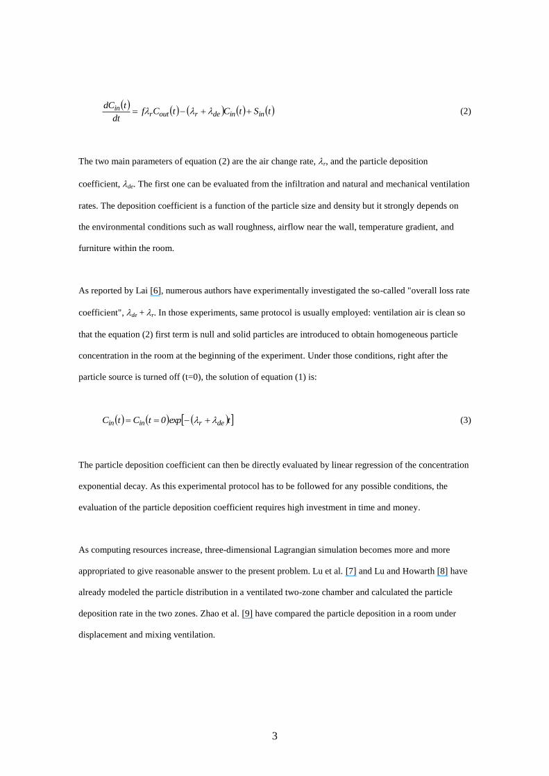
pollutant mass balance in the case of suspended particles as:

tCtDtStCtCf

dt

tdCindeinRininroutr

in (1)

I II III IV V

where I is the particle transport from outdoor to indoor by ventilation (and infiltration), II is the particle

transport from indoor to outdoor by ventilation, III is the particle generation by internal sources, IV is the

resuspension of deposited particle and V is the particle deposition on walls.

Considering that indoor airflows close to walls are not strong enough to resuspend deposited particles, the

resuspension term can usually be neglected and equation (1) is simplified into:

3

tStCtCf

dt

tdCininderoutr

in (2)

The two main parameters of equation (2) are the air change rate, r, and the particle deposition

coefficient, de. The first one can be evaluated from the infiltration and natural and mechanical ventilation

rates. The deposition coefficient is a function of the particle size and density but it strongly depends on

the environmental conditions such as wall roughness, airflow near the wall, temperature gradient, and

furniture within the room.

As reported by Lai [6], numerous authors have experimentally investigated the so-called "overall loss rate

coefficient", de + r. In those experiments, same protocol is usually employed: ventilation air is clean so

that the equation (2) first term is null and solid particles are introduced to obtain homogeneous particle

concentration in the room at the beginning of the experiment. Under those conditions, right after the

particle source is turned off (t=0), the solution of equation (1) is:

texp0tCtC derinin (3)

The particle deposition coefficient can then be directly evaluated by linear regression of the concentration

exponential decay. As this experimental protocol has to be followed for any possible conditions, the

evaluation of the particle deposition coefficient requires high investment in time and money.

As computing resources increase, three-dimensional Lagrangian simulation becomes more and more

appropriated to give reasonable answer to the present problem. Lu et al. [7] and Lu and Howarth [8] have

already modeled the particle distribution in a ventilated two-zone chamber and calculated the particle

deposition rate in the two zones. Zhao et al. [9] have compared the particle deposition in a room under

displacement and mixing ventilation.

4

All those experimental and numerical studies provide deposition coefficient values that can be a posteriori

introduced in a one-zone model to study the indoor air quality under variable particle outdoor

concentrations and sources. As stated before, the one-zone model can be applied if and only if the

pollutant is well-mixed in the zone, so the deposition coefficient has to be evaluated under the same

condition of pollutant homogeneity. Concerning the experimental measurement, millions of particles are

introduced in the room so that the particle cloud can be considered as a continuous phase (like a gaseous

pollutant). Then, the particle concentration can be measured at several points evenly distributed within the

whole volume. The homogeneity will prevail as long as the particle concentrations at the different

locations stay close. In the case of the numerical simulations, it is not millions of particles that are tracked

but only a few thousands because of the time required to calculate their trajectories in the zone. As a

consequence, the method previously described can not be used here as the particle cloud can not be

considered as a continuous phase. The determination of an adapted methodology to evaluate the particle

discrete phase homogeneity from Lagrangian simulation is the goal of the present study. Illustrations are

given for the case of 5.0 µm particle transport in a prototypical ventilated room. Three particle injections

have been investigated: homogenous particle injection within the room at initial time, external pollution

(injection at the inlet), and puff releases in different locations.

2. Methodology

2.1. Simulation

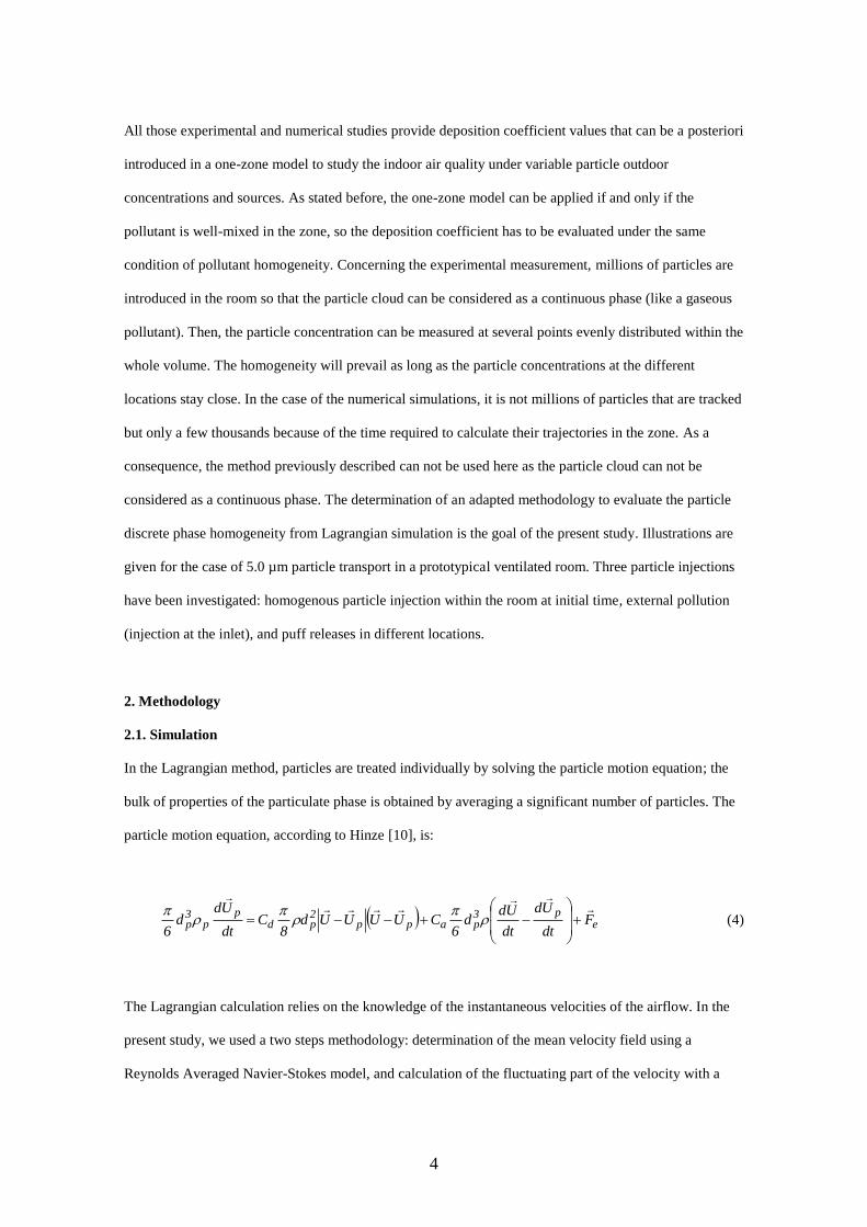
In the Lagrangian method, particles are treated individually by solving the particle motion equation; the

bulk of properties of the particulate phase is obtained by averaging a significant number of particles. The

particle motion equation, according to Hinze [10], is:

ep3

papp2pd

pp

3p F

dt

Ud

dt

Udd

6CUUUUd

8C

dt

Udd

6

(4)

The Lagrangian calculation relies on the knowledge of the instantaneous velocities of the airflow. In the

present study, we used a two steps methodology: determination of the mean velocity field using a

Reynolds Averaged Navier-Stokes model, and calculation of the fluctuating part of the velocity with a

5

modified Gosman and Ioannides model (Abadie et al [11]). In this study, all the mean quantities, such as

the mean fluid velocities, the turbulent kinetic energy and the kinetic energy dissipation rate are computed

by a Computational Fluid Dynamics (CFD) code using a RNG model as recommended by Chen [12]

when dealing with airflows in rooms. Particles are considered to stick the wall at the first particle-wall

interaction; no rebound is taken into account.

Five micrometers particle (p=1000 kg/m3) tracking was performed in the case of a prototypical

ventilated room: length = 2.5 m, height = 2.5 m and width = 1.5 m. The inlet and outlet are located in the

center plane of the room at 0.305 m above the floor or below the ceiling. Table 1 presents the different

configurations (shape and location of the inlet/outlet, air change rate and source location) modeled in this

study. The number of particles in air was 1000 at initial time. The particle calculation time step was 10-4

s. Each simulation was conducted during 1200 s and took 7 days of calculation on a CPU 1.6 GHz for the

longest ones.

2.2. Concentration homogeneity evaluation

As stated in the introduction, when dealing with a continuous pollutant, the concentration homogeneity

can be evaluated by taking several sample points evenly distributed within the zone and calculating the

concentration root-mean-square (equation (5)). If the RMS is lower than 0.1, the concentration is then

considered as homogenous (Mage and Ott [13]). If we apply this procedure to a discrete phase (1000

particles), there is a very low probability that even only one particle can be located at one sample point.

Thus, the solution usually adopted consists in dividing the studied zone into sub-zones and calculating the

RMS based of the number of particles in each sub-zone. The unknowns are the number, the size and the

location of the sub-zones. Each of those parameters acts on the root-mean-square value and consequently,

on the evaluation of the pollutant homogeneity.

N

tCtC

tC

1RMS

N

1i

2i

(5)

6

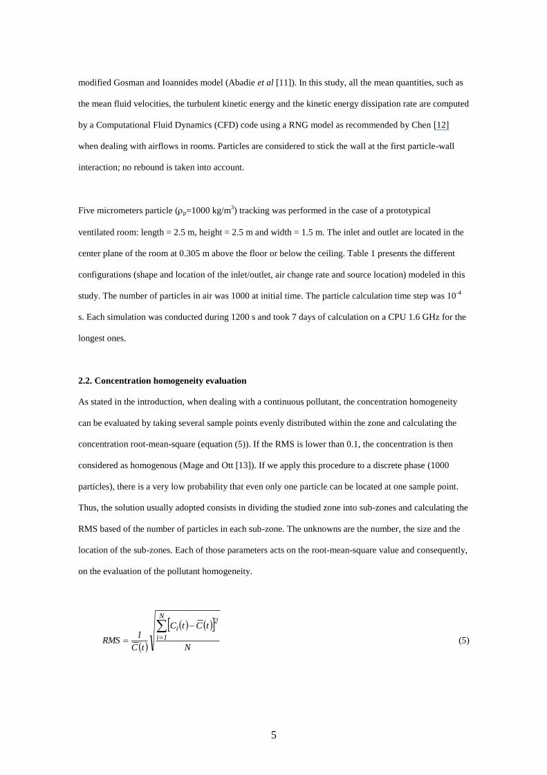
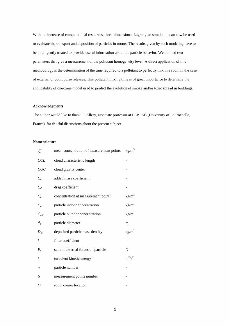
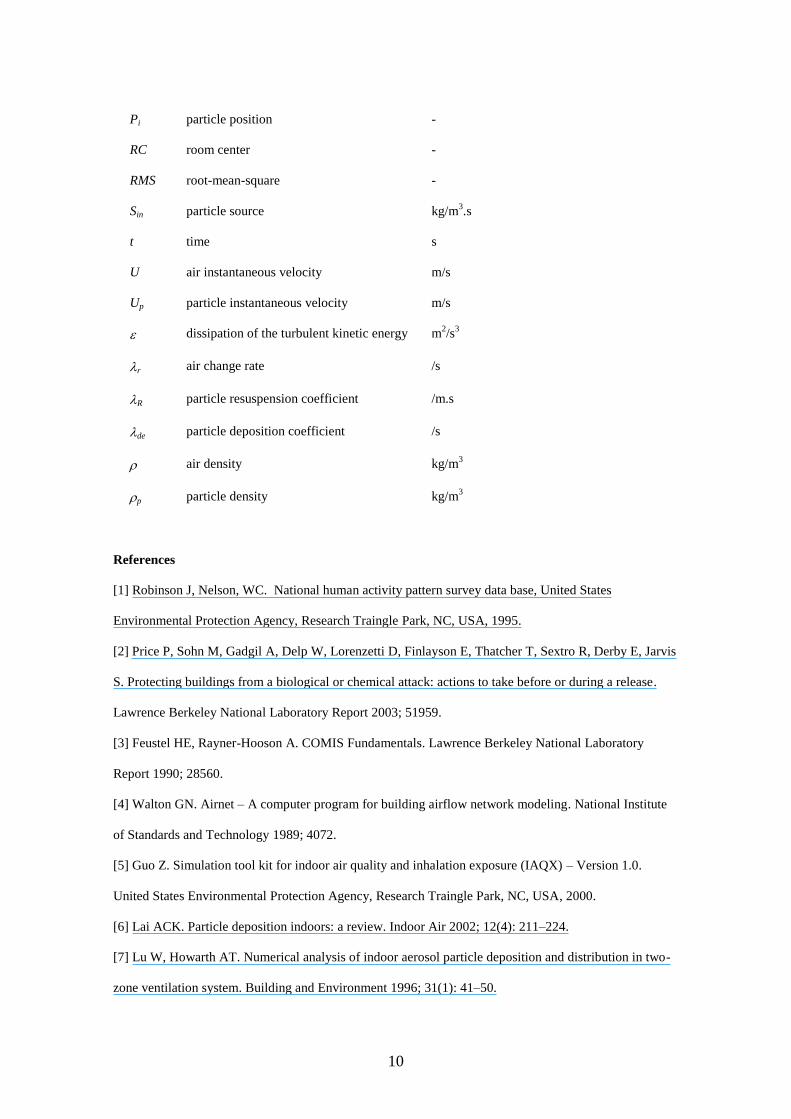
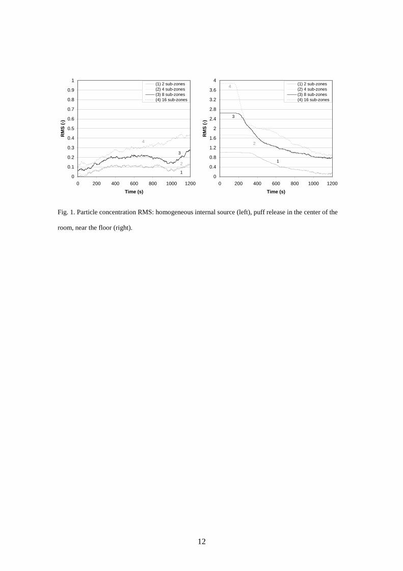
Fig. 1 presents the influence of the sub-zones number on the root-mean-square value in the case of a

homogeneous internal source (left) and a puff release located in the center of the room, near the floor

(right). Both figures illustrate the strong dependency of the RMS on the number of sub-zones used to

evaluate the particle concentration. Using 2 or 4 sub-zones in the first case would lead to consider that the

particle concentration is homogeneous (RMS close to 0.1) whereas using 8 or 16 sub-zones would

indicate heterogeneity. The difference is even higher in the case of a puff release.

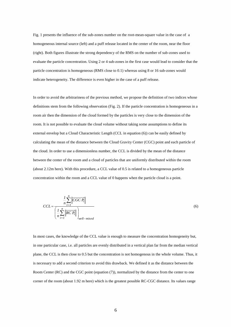
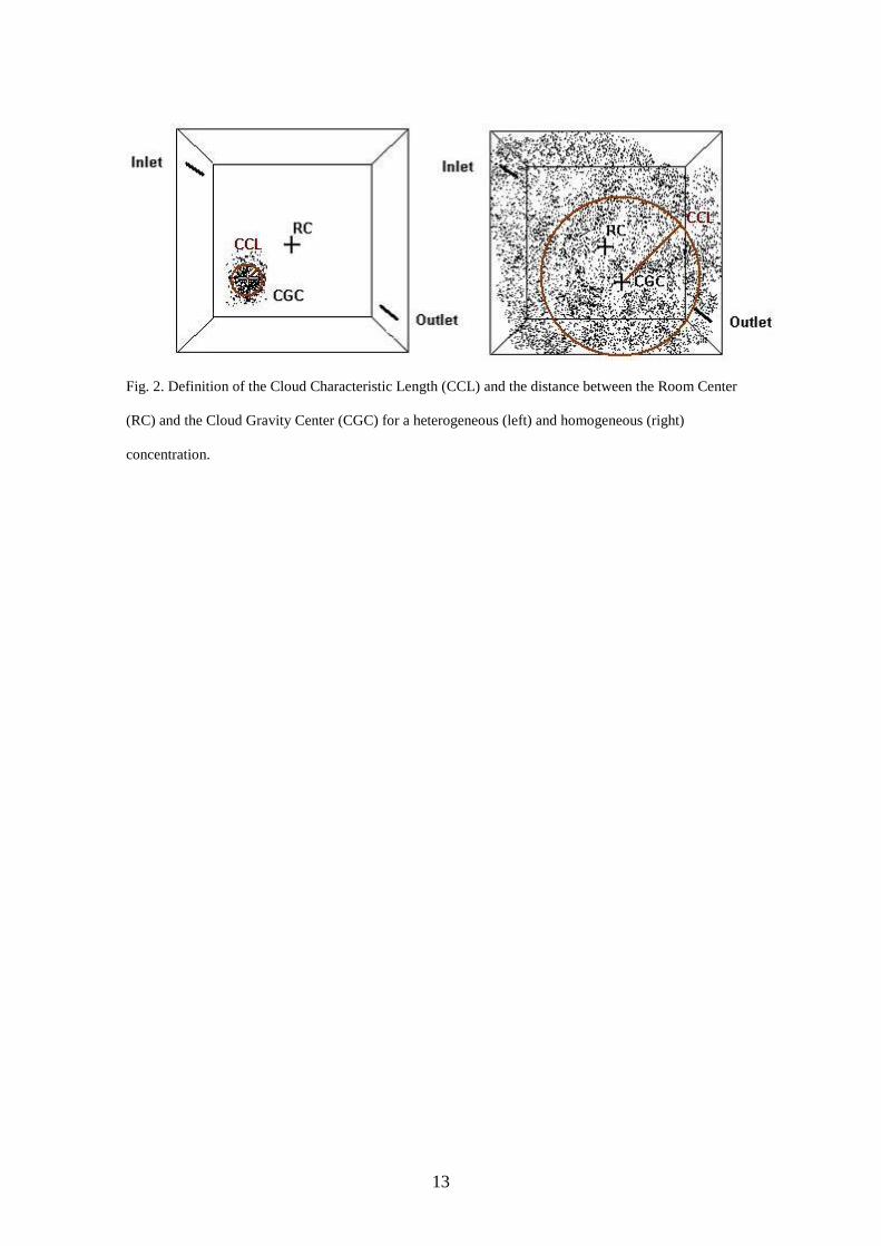
In order to avoid the arbitrariness of the previous method, we propose the definition of two indices whose

definitions stem from the following observation (Fig. 2). If the particle concentration is homogeneous in a

room air then the dimension of the cloud formed by the particles is very close to the dimension of the

room. It is not possible to evaluate the cloud volume without taking some assumptions to define its

external envelop but a Cloud Characteristic Length (CCL in equation (6)) can be easily defined by

calculating the mean of the distance between the Cloud Gravity Center (CGC) point and each particle of

the cloud. In order to use a dimensionless number, the CCL is divided by the mean of the distance

between the center of the room and a cloud of particles that are uniformly distributed within the room

(about 2.12m here). With this procedure, a CCL value of 0.5 is related to a homogeneous particle

concentration within the room and a CCL value of 0 happens when the particle cloud is a point.

mixedwell

n

1i

i

n

1i

i

P CRn

1

P CGCn

1

CCL

(6)

In most cases, the knowledge of the CCL value is enough to measure the concentration homogeneity but,

in one particular case, i.e. all particles are evenly distributed in a vertical plan far from the median vertical

plane, the CCL is then close to 0.5 but the concentration is not homogenous in the whole volume. Thus, it

is necessary to add a second criterion to avoid this drawback. We defined it as the distance between the

Room Center (RC) and the CGC point (equation (7)), normalized by the distance from the center to one

corner of the room (about 1.92 m here) which is the greatest possible RC-CGC distance. Its values range

7

from 0 when the CGC point is located at the center of the room, and 1 when it is in one corner of the

room.

O - CR

CGC - CRCGCRC (7)

Note that considering the RC-CGC distance alone does not worked either to evaluate the concentration

homogeneity. For example, if the particles are located in a zone close to the RC, then the RC-CGC

distance is small but the particles do not occupied the whole volume. To assess the concentration

homogeneity, a CCL value close to 0.5 and a RC-CGC distance near zero are both required.

3. Results

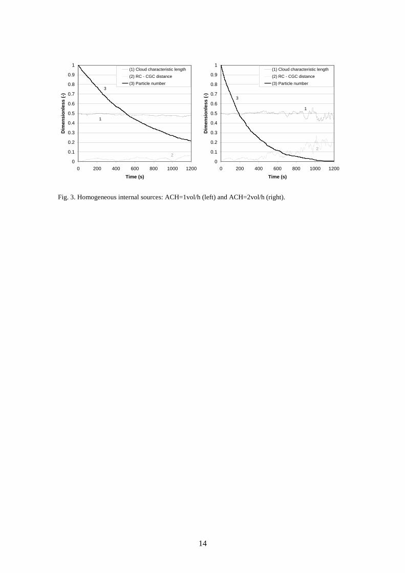
Figs. 3-5 present the evolution of the criteria (1 and 2) and the dimensionless number of particles in air

(3) versus time. Note that the six graphs presented here are for the simulation id 2, 4, 9, 10, 11 and 12

respectively, and are representative of the other configurations.

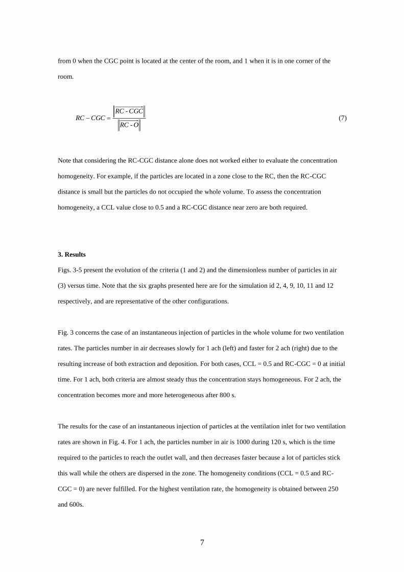
Fig. 3 concerns the case of an instantaneous injection of particles in the whole volume for two ventilation

rates. The particles number in air decreases slowly for 1 ach (left) and faster for 2 ach (right) due to the

resulting increase of both extraction and deposition. For both cases, CCL = 0.5 and RC-CGC = 0 at initial

time. For 1 ach, both criteria are almost steady thus the concentration stays homogeneous. For 2 ach, the

concentration becomes more and more heterogeneous after 800 s.

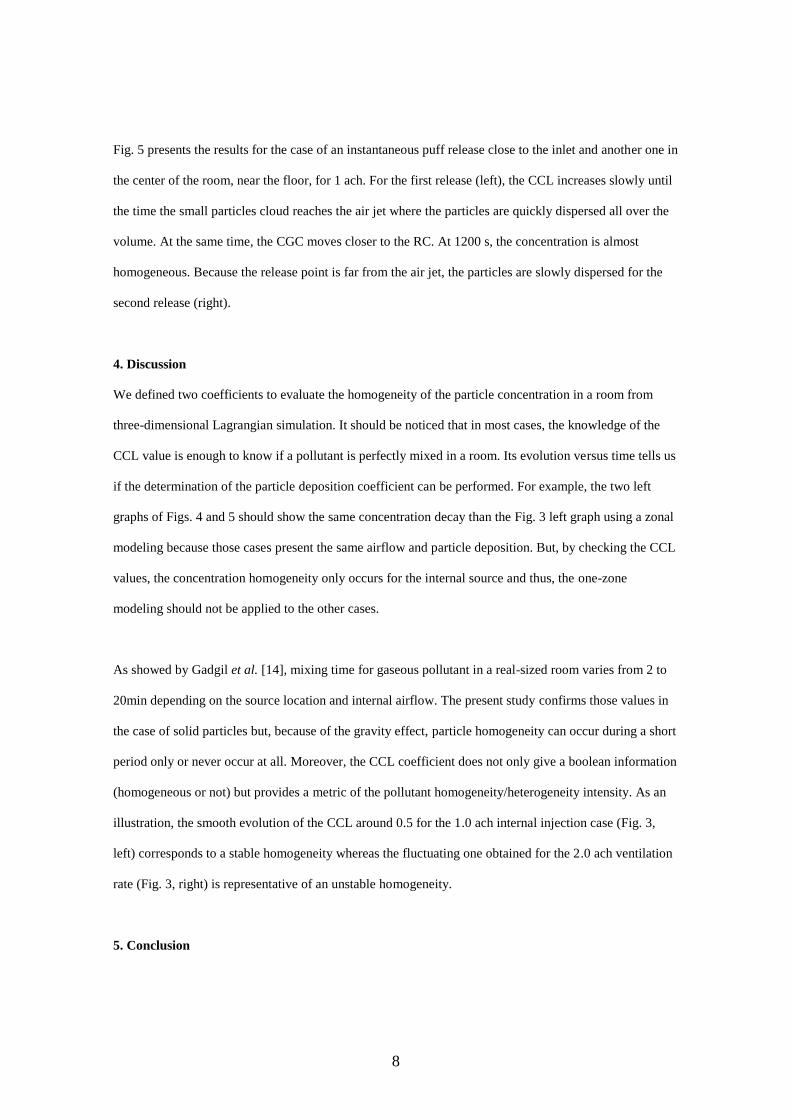
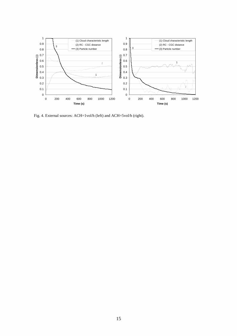
The results for the case of an instantaneous injection of particles at the ventilation inlet for two ventilation

rates are shown in Fig. 4. For 1 ach, the particles number in air is 1000 during 120 s, which is the time

required to the particles to reach the outlet wall, and then decreases faster because a lot of particles stick

this wall while the others are dispersed in the zone. The homogeneity conditions (CCL = 0.5 and RC-

CGC = 0) are never fulfilled. For the highest ventilation rate, the homogeneity is obtained between 250

and 600s.

8

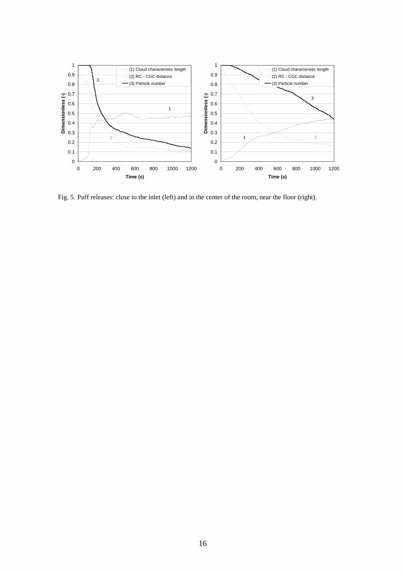
Fig. 5 presents the results for the case of an instantaneous puff release close to the inlet and another one in

the center of the room, near the floor, for 1 ach. For the first release (left), the CCL increases slowly until

the time the small particles cloud reaches the air jet where the particles are quickly dispersed all over the

volume. At the same time, the CGC moves closer to the RC. At 1200 s, the concentration is almost

homogeneous. Because the release point is far from the air jet, the particles are slowly dispersed for the

second release (right).

4. Discussion

We defined two coefficients to evaluate the homogeneity of the particle concentration in a room from

three-dimensional Lagrangian simulation. It should be noticed that in most cases, the knowledge of the

CCL value is enough to know if a pollutant is perfectly mixed in a room. Its evolution versus time tells us

if the determination of the particle deposition coefficient can be performed. For example, the two left

graphs of Figs. 4 and 5 should show the same concentration decay than the Fig. 3 left graph using a zonal

modeling because those cases present the same airflow and particle deposition. But, by checking the CCL

values, the concentration homogeneity only occurs for the internal source and thus, the one-zone

modeling should not be applied to the other cases.

As showed by Gadgil et al. [14], mixing time for gaseous pollutant in a real-sized room varies from 2 to

20min depending on the source location and internal airflow. The present study confirms those values in

the case of solid particles but, because of the gravity effect, particle homogeneity can occur during a short

period only or never occur at all. Moreover, the CCL coefficient does not only give a boolean information

(homogeneous or not) but provides a metric of the pollutant homogeneity/heterogeneity intensity. As an

illustration, the smooth evolution of the CCL around 0.5 for the 1.0 ach internal injection case (Fig. 3,

left) corresponds to a stable homogeneity whereas the fluctuating one obtained for the 2.0 ach ventilation

rate (Fig. 3, right) is representative of an unstable homogeneity.

5. Conclusion

9

With the increase of computational resources, three-dimensional Lagrangian simulation can now be used

to evaluate the transport and deposition of particles in rooms. The results given by such modeling have to

be intelligently treated to provide useful information about the particle behavior. We defined two

parameters that give a measurement of the pollutant homogeneity level. A direct application of this

methodology is the determination of the time required to a pollutant to perfectly mix in a room in the case

of external or point pulse releases. This pollutant mixing time is of great importance to determine the

applicability of one-zone model used to predict the evolution of smoke and/or toxic spread in buildings.

Acknowledgments

The author would like to thank C. Allery, associate professor at LEPTAB (University of La Rochelle,

France), for fruitful discussions about the present subject.

Nomenclature

C mean concentration of measurement points kg/m3

CCL cloud characteristic length -

CGC cloud gravity center -

Ca added mass coefficient -

Cd drag coefficient -

Ci concentration at measurement point i kg/m3

Cin particle indoor concentration kg/m3

Cout particle outdoor concentration kg/m3

dp particle diameter m

Din deposited particle mass density kg/m2

f filter coefficient -

Fe sum of external forces on particle N

k turbulent kinetic energy m2/s

2

n particle number -

N measurement points number -

O room corner location -

10

Pi particle position -

RC room center -

RMS root-mean-square -

Sin particle source kg/m3.s

t time s

U air instantaneous velocity m/s

Up particle instantaneous velocity m/s

dissipation of the turbulent kinetic energy m2/s

3

r air change rate /s

R particle resuspension coefficient /m.s

de particle deposition coefficient /s

air density kg/m3

p particle density kg/m3

References

[1] Robinson J, Nelson, WC. National human activity pattern survey data base, United States

Environmental Protection Agency, Research Traingle Park, NC, USA, 1995.

[2] Price P, Sohn M, Gadgil A, Delp W, Lorenzetti D, Finlayson E, Thatcher T, Sextro R, Derby E, Jarvis

S. Protecting buildings from a biological or chemical attack: actions to take before or during a release.

Lawrence Berkeley National Laboratory Report 2003; 51959.

[3] Feustel HE, Rayner-Hooson A. COMIS Fundamentals. Lawrence Berkeley National Laboratory

Report 1990; 28560.

[4] Walton GN. Airnet – A computer program for building airflow network modeling. National Institute

of Standards and Technology 1989; 4072.

[5] Guo Z. Simulation tool kit for indoor air quality and inhalation exposure (IAQX) – Version 1.0.

United States Environmental Protection Agency, Research Traingle Park, NC, USA, 2000.

[6] Lai ACK. Particle deposition indoors: a review. Indoor Air 2002; 12(4): 211–224.

[7] Lu W, Howarth AT. Numerical analysis of indoor aerosol particle deposition and distribution in two-

zone ventilation system. Building and Environment 1996; 31(1): 41–50.

11

[8] Lu W, Howarth AT, Adam N, Riffat SB. Modelling and measurement of airflow and aerosol particle

distribution in a ventilated two-zone chamber. Building and Environment 1996; 31(5): 417–423.

[9] Zhao B, Zhang Y, Li X, Yang X, Huang D. Comparison of indoor aerosol particle concentration and

deposition in different ventilated rooms by numerical method. Building and Environment 2004; 39(1): 1–

8.

[10] Hinze JO. Turbulence. McGraw-Hill Book Company, Inc, 1987.

[11] Abadie MO, Limam K, Allard F. Prediction of particle deposition in turbulent indoor flows with a 3d

Lagrangian model. 9th

International Conference on Indoor Air Quality and Climate 2004; 4: 554–559.

[12] Chen Q. Comparison of different k- models for indoor airflow computations. Numerical Heat

Transfer 1995; 28(B): 353–369.

[13] Mage DT, Ott WR. Accounting for nonuniform mixing and human exposure in indoor environments,

Characterizing Sources of Indoor Air Pollution and Related Sink Effects. ASTM STP 1996; 1287: 263–

278.

[14] Gadgil AJ, Lobscheid C, Abadie MO, Finlayson EU. Indoor pollutant mixing time in an isothermal

closed room: An Investigation Using CFD. Atmospheric Environment 2003; 37: 5577–5586.

12

0

0.1

0.2

0.3

0.4

0.5

0.6

0.7

0.8

0.9

1

0 200 400 600 800 1000 1200

Time (s)

RM

S (

-)

(1) 2 sub-zones

(2) 4 sub-zones

(3) 8 sub-zones

(4) 16 sub-zones

id 02

1

3

2

4

0

0.4

0.8

1.2

1.6

2

2.4

2.8

3.2

3.6

4

0 200 400 600 800 1000 1200

Time (s)

RM

S (

-)

(1) 2 sub-zones

(2) 4 sub-zones

(3) 8 sub-zones

(4) 16 sub-zones

id 12

1

3

2

4

Fig. 1. Particle concentration RMS: homogeneous internal source (left), puff release in the center of the

room, near the floor (right).

13

Fig. 2. Definition of the Cloud Characteristic Length (CCL) and the distance between the Room Center

(RC) and the Cloud Gravity Center (CGC) for a heterogeneous (left) and homogeneous (right)

concentration.

14

0

0.1

0.2

0.3

0.4

0.5

0.6

0.7

0.8

0.9

1

0 200 400 600 800 1000 1200

Time (s)

Dim

en

sio

nle

ss (

-)

(1) Cloud characteristic length

(2) RC - CGC distance

(3) Particle number

id 05

1

3

2

0

0.1

0.2

0.3

0.4

0.5

0.6

0.7

0.8

0.9

1

0 200 400 600 800 1000 1200

Time (s)

Dim

en

sio

nle

ss (

-)

(1) Cloud characteristic length

(2) RC - CGC distance

(3) Particle number

id 08

1

3

2

Fig. 3. Homogeneous internal sources: ACH=1vol/h (left) and ACH=2vol/h (right).

15

0

0.1

0.2

0.3

0.4

0.5

0.6

0.7

0.8

0.9

1

0 200 400 600 800 1000 1200

Time (s)

Dim

en

sio

nle

ss (

-)

(1) Cloud characteristic length

(2) RC - CGC distance

(3) Particle number

id 09

1

3

2

0

0.1

0.2

0.3

0.4

0.5

0.6

0.7

0.8

0.9

1

0 200 400 600 800 1000 1200

Time (s)

Dim

en

sio

nle

ss (

-)

(1) Cloud characteristic length

(2) RC - CGC distance

(3) Particle number

id 10

1

3

2

Fig. 4. External sources: ACH=1vol/h (left) and ACH=5vol/h (right).

16

0

0.1

0.2

0.3

0.4

0.5

0.6

0.7

0.8

0.9

1

0 200 400 600 800 1000 1200

Time (s)

Dim

en

sio

nle

ss (

-)

(1) Cloud characteristic length

(2) RC - CGC distance

(3) Particle number

id 11

1

3

2

0

0.1

0.2

0.3

0.4

0.5

0.6

0.7

0.8

0.9

1

0 200 400 600 800 1000 1200

Time (s)

Dim

en

sio

nle

ss (

-)

(1) Cloud characteristic length

(2) RC - CGC distance

(3) Particle number

id 12

1

3

2

Fig. 5. Puff releases: close to the inlet (left) and in the center of the room, near the floor (right).

17

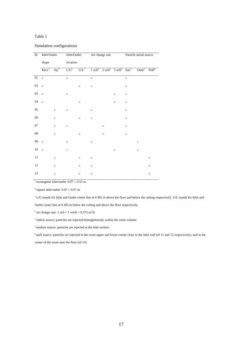
Table 1

Simulation configurations

Id Inlet/Outlet

shape

Inlet/Outlet

location

Air change rate Particle initial source

Rect.a Sq.b L/Uc U/Lc 1 achd 2 achd 5 achd Ind.e Outd.f Puffg

01

02

03

04

05

06

07

08

09

10

11

12

13

a rectangular inlet/outlet: 0.07 0.55 m.

b square inlet/outlet: 0.07 0.07 m.

c L/U stands for Inlet and Outlet center line at 0.305 m above the floor and below the ceiling respectively. U/L stands for Inlet and

Outlet center line at 0.305 m below the ceiling and above the floor respectively.

d air change rate: 1 ach = 1 vol/h = 9.375 m3/h.

e indoor source: particles are injected homogeneously within the room volume.

f outdoor source: particles are injected at the inlet surface.

g puff source: particles are injected in the room upper and lower corner close to the inlet wall (id 11 and 12 respectively), and in the

center of the room near the floor (id 13).