Numerical computation of inverse compete elliptic integrals of first and second kinds

(This is a sample cover image for this issue. The actual cover is not yet available at this time.)

This article appeared in a journal published by Elsevier. The attachedcopy is furnished to the author for internal non-commercial researchand education use, including for instruction at the authors institution

and sharing with colleagues.

Other uses, including reproduction and distribution, or selling orlicensing copies, or posting to personal, institutional or third party

websites are prohibited.

In most cases authors are permitted to post their version of thearticle (e.g. in Word or Tex form) to their personal website orinstitutional repository. Authors requiring further information

regarding Elsevier’s archiving and manuscript policies areencouraged to visit:

http://www.elsevier.com/copyright

http://www.elsevier.com/copyright

Author's personal copy

Journal of Computational and Applied Mathematics 249 (2013) 37–50

Contents lists available at SciVerse ScienceDirect

Journal of Computational and AppliedMathematics

journal homepage: www.elsevier.com/locate/cam

Numerical computation of inverse complete elliptic integralsof first and second kindsToshio Fukushima ∗

National Astronomical Observatory of Japan, 2-21-1, Ohsawa, Mitaka, Tokyo 181-8588, Japan

a r t i c l e i n f o

Article history:Received 13 November 2012Received in revised form 31 January 2013

Keywords:Complete elliptic integralInversion

a b s t r a c t

We developed the numerical procedures to evaluate the inverse functions of the completeelliptic integrals of the first and the second kind, K(m) and E(m), with respect to the pa-rameterm. The evaluation is executed by inverting eight sets of the truncated Taylor seriesexpansions of the integrals in terms ofm or of− log(1−m). The developed procedures are(1) so precise that themaximumabsolute errors are less than 3–5machine epsilons, and (2)30%–40% faster than the evaluation of the integrals themselves by the fastest procedures(Fukushima 2009a, 2011).

© 2013 Elsevier B.V. All rights reserved.

1. Introduction

1.1. Complete elliptic integrals of first and second kinds

The complete elliptic integrals of the first and the second kind are defined [1, Section 19.2(i)] as

K(m) ≡

π/2

0

dθ1 − m sin2 θ

, E(m) ≡

π/2

0

1 − m sin2 θ dθ, (1)

wherem is called the parameter. They appear in various fields of mathematical physics and engineering [2–5]. In discussingthe real-valued integrals, we assume thatm is in the standard domain,

0 ≤ m < 1. (2)

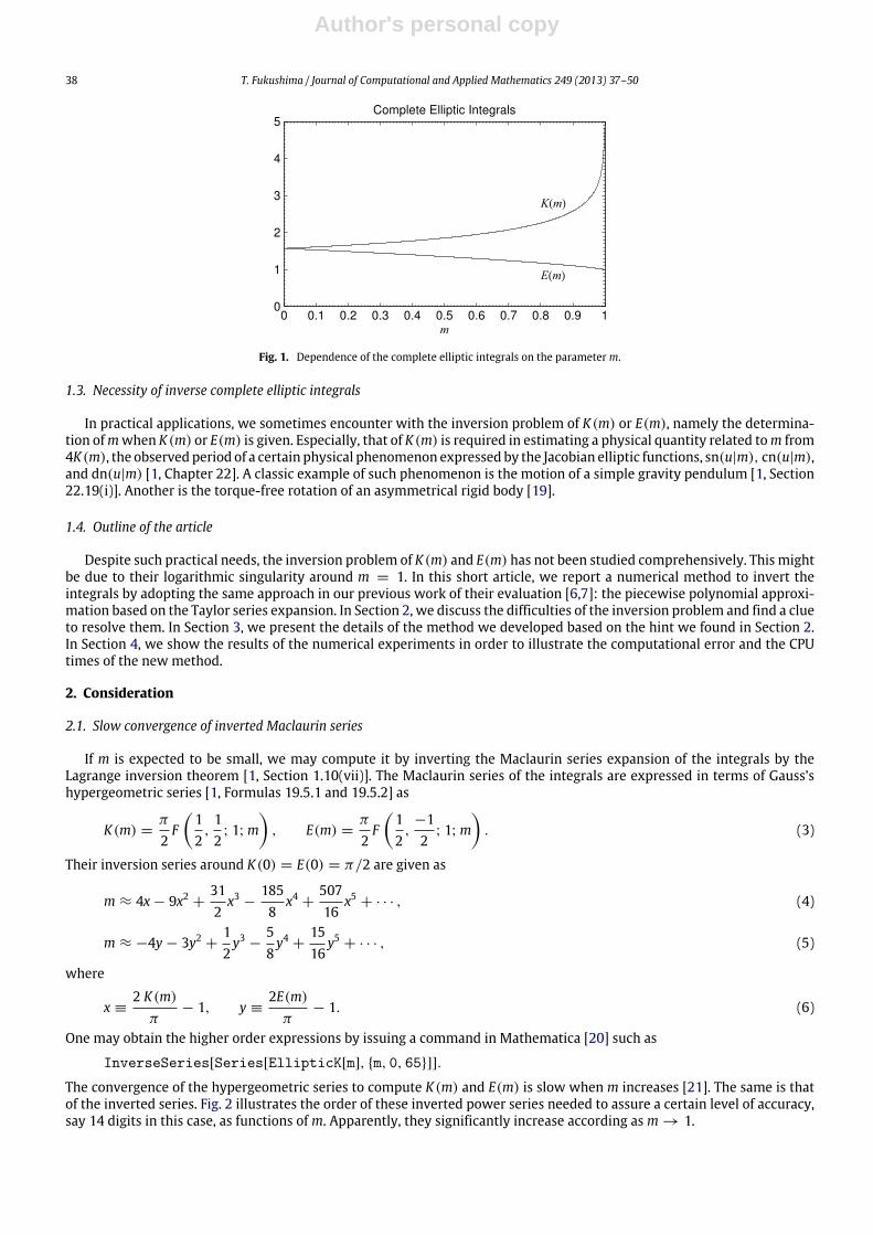
We refer the reader to [6,7] for the process to reduce the other cases to the standard one. See Fig. 1 for the functionaldependence of K(m) and E(m) on the parameterm in the standard domain.

1.2. Numerical computation of complete elliptic integrals

Many methods have been developed to compute the values of K(m) and/or E(m) whenm is given. The popular iterativeschemes are those using (1) the arithmetic–geometric mean [1, Section 19.8(i)], (2) the Landen transformation [8,9], (3)the Bartky transformation [10,11], or (4) the duplication theorems [12,13]. They are useful in computing the integrals inarbitrary precision arithmetic.

For practical purposes, however, their Chebyshev approximations [14–18] are sufficient. Recently, we have developed amethod based on their Taylor series expansions [6]. It is as precise as the Chebyshev approximation and runs twice fasterthan that. Also, we extended it to the case of a general complete elliptic integral of the second kind, αK(m)+βE(m) [7]. Theextended method is as precise as Bulirsch’s cel2 and Carlson’s rf and rd and runs 5–18 times faster than them.

∗ Tel.: +81 422343613.E-mail address: [email protected].

0377-0427/$ – see front matter© 2013 Elsevier B.V. All rights reserved.http://dx.doi.org/10.1016/j.cam.2013.02.003


38 T. Fukushima / Journal of Computational and Applied Mathematics 249 (2013) 37–50

Fig. 1. Dependence of the complete elliptic integrals on the parameterm.

1.3. Necessity of inverse complete elliptic integrals

In practical applications, we sometimes encounter with the inversion problem of K(m) or E(m), namely the determina-tion ofmwhen K(m) or E(m) is given. Especially, that of K(m) is required in estimating a physical quantity related tom from4K(m), the observed period of a certain physical phenomenon expressed by the Jacobian elliptic functions, sn(u|m), cn(u|m),and dn(u|m) [1, Chapter 22]. A classic example of such phenomenon is the motion of a simple gravity pendulum [1, Section22.19(i)]. Another is the torque-free rotation of an asymmetrical rigid body [19].

1.4. Outline of the article

Despite such practical needs, the inversion problem of K(m) and E(m) has not been studied comprehensively. This mightbe due to their logarithmic singularity around m = 1. In this short article, we report a numerical method to invert theintegrals by adopting the same approach in our previous work of their evaluation [6,7]: the piecewise polynomial approxi-mation based on the Taylor series expansion. In Section 2, we discuss the difficulties of the inversion problem and find a clueto resolve them. In Section 3, we present the details of the method we developed based on the hint we found in Section 2.In Section 4, we show the results of the numerical experiments in order to illustrate the computational error and the CPUtimes of the new method.

2. Consideration

2.1. Slow convergence of inverted Maclaurin series

If m is expected to be small, we may compute it by inverting the Maclaurin series expansion of the integrals by theLagrange inversion theorem [1, Section 1.10(vii)]. The Maclaurin series of the integrals are expressed in terms of Gauss’shypergeometric series [1, Formulas 19.5.1 and 19.5.2] as

K(m) =π

2F

12,12; 1;m

, E(m) =

π

2F

12,−12

; 1;m

. (3)

Their inversion series around K(0) = E(0) = π/2 are given as

m ≈ 4x − 9x2 +312

x3 −1858

x4 +50716

x5 + · · · , (4)

m ≈ −4y − 3y2 +12y3 −

58y4 +

1516

y5 + · · · , (5)

where

x ≡2 K(m)

π− 1, y ≡

2E(m)

π− 1. (6)

One may obtain the higher order expressions by issuing a command in Mathematica [20] such as

InverseSeries[Series[EllipticK[m], {m, 0, 65}]].

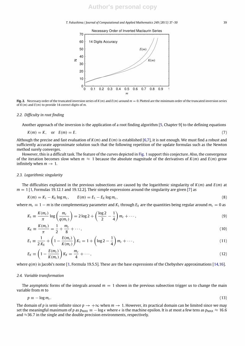
The convergence of the hypergeometric series to compute K(m) and E(m) is slow when m increases [21]. The same is thatof the inverted series. Fig. 2 illustrates the order of these inverted power series needed to assure a certain level of accuracy,say 14 digits in this case, as functions ofm. Apparently, they significantly increase according asm → 1.


T. Fukushima / Journal of Computational and Applied Mathematics 249 (2013) 37–50 39

Fig. 2. Necessary order of the truncated inversion series of K(m) and E(m) aroundm = 0. Plotted are theminimum order of the truncated inversion seriesof K(m) and E(m) to provide 14 correct digits of m.

2.2. Difficulty in root finding

Another approach of the inversion is the application of a root finding algorithm [5, Chapter 9] to the defining equations

K(m) = K , or E(m) = E. (7)

Although the precise and fast evaluation of K(m) and E(m) is established [6,7], it is not enough. We must find a robust andsufficiently accurate approximate solution such that the following repetition of the update formulas such as the Newtonmethod surely converges.

However, this is a difficult task. The feature of the curves depicted in Fig. 1 support this conjecture. Also, the convergenceof the iteration becomes slow when m ≈ 1 because the absolute magnitude of the derivatives of K(m) and E(m) growinfinitely whenm → 1.

2.3. Logarithmic singularity

The difficulties explained in the previous subsections are caused by the logarithmic singularity of K(m) and E(m) atm = 1 [1, Formulas 19.12.1 and 19.12.2]. Their simple expressions around the singularity are given [7] as

K(m) = K1 − KX logmc, E(m) = E1 − EX logmc, (8)

where mc ≡ 1 − m is the complementary parameter and K1 through EX are the quantities being regular aroundmc = 0 as

K1 ≡K(mc)

πlog

mc

q(mc)

= 2 log 2 +

log 22

−14

mc + · · · , (9)

KX ≡K(mc)

π=

12

+mc

8+ · · · , (10)

E1 ≡1

2 KX+

1 −

E(mc)

K(mc)

K1 = 1 +

log 2 −

14

mc + · · · , (11)

EX ≡

1 −

E(mc)

K(mc)

KX =

mc

4+ · · · , (12)

where q(m) is Jacobi’s nome [1, Formula 19.5.5]. These are the base expressions of the Chebyshev approximations [14,16].

2.4. Variable transformation

The asymptotic forms of the integrals around m = 1 shown in the previous subsection trigger us to change the mainvariable fromm to

p ≡ − logmc . (13)

The domain of p is semi-infinite since p → +∞ when m → 1. However, its practical domain can be limited since we mayset the meaningful maximum of p as pMAX ≡ − log ϵ where ϵ is the machine epsilon. It is at most a few tens as pMAX ≈ 16.6and ≈36.7 in the single and the double precision environments, respectively.



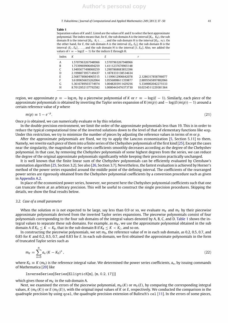
Fig. 3. Dependence of complete elliptic integrals on p. Shown are K(m) and r ≡ − log(E(m) − 1) as functions of the alternate variable, p ≡ − logmc .

If mc is sufficiently small, say less than ϵ, we may retain only the leading terms in Eqs. (9) and (10). Thus, we obtain anasymptotic expression of K ≡ K(m) as

K = 2 log 2 +p2

+ · · · . (14)

This leads to the inversion in terms of p as

p = 2 K − 4 log 2 + · · · . (15)

Namely, p is almost linear with respect to K when K is sufficiently large, say larger than 2. Fig. 3 confirms this conjecture.In the case of E ≡ E(m), we must keep up to the first order terms in Eqs. (11) and (12). Then, we arrive at a little

complicated expression as

E = 1 + (p + 4 log 2 − 1)e−p

4+ · · · . (16)

We rewrite this as

r ≡ − log (E − 1) = p − logp − 14

+ log 2

+ · · · . (17)

The variability of the second term in the right hand side is relatively small as

− 2.264 < − logp − 14

+ log 2

< −0.814, (18)

when 0 < p < 36.7. Thus, we ignore its contribution and obtain a solution as

p ≈ r. (19)

This is a crude approximation. A better solution would be obtained by directly solving Eq. (16) with help of W−1(x),the secondary branch of Lambert W -function [20]. Since the numerical evaluation of W−1(x) is itself a difficult problem[22–24], we do not go further in this direction.

At any rate, Fig. 3 indicates that K and r are almost linear with respect to p. Then, theymay be candidates of the functionsto be expanded in terms of the new variable, p.

3. Method

3.1. Strategy

Based on the discussions in Section 2, we developed amethod to invert K and E with respect tom in the standard domain,0 ≤ m < 1. Let us denote the inverted solutions by mK (K) and mE(E), respectively. They are defined as the functions tosatisfy the relations

K (mK (x)) = x, E (mE(x)) = x. (20)

The key idea is splitting the integral value domain into two regions: that corresponding to not-so-largem, say less than 0.9or so, and the rest.

In the former region, we approximatem by a piecewise polynomial of K or E. Each piece of the approximate polynomialsis obtained by inverting the Taylor series expansion of K(m) and E(m) around a certain reference value of m. In the second



Table 1Separation values ofK and E. Listed are the values ofK and E to select the best approximatepolynomial. The indexmeans that, for K , the sub domain A is the interval [KA, KB), the subdomain B is the interval [KB, KC ) , . . . , and the sub domain H is the interval [KH , ∞). Onthe other hand, for E, the sub domain A is the interval (EB, EA], the sub domain B is theinterval (EC , EB] , . . . , and the sub domain H is the interval [1, EH ]. Also, we added thevalues of r ≡ − log(E − 1) for the indices E through H.

Index K E r

A 1.5707963267948966 1.5707963267948966B 1.7539969906494259 1.4111237670965148C 1.9495677498060259 1.2907868683852396D 2.1998873957149437 1.1878333138534634E 2.5687780604965515 1.1199612906642078 2.1286317858706077F 3.6189656655262064 1.0556008611359877 2.8895565897882066G 5.3616789503774974 1.0048203911429256 5.3349002042275533H 8.7012952137792582 1.0000443476373730 10.0234511229381364

region, we approximate p ≡ − logmc by a piecewise polynomial of K or r ≡ − log(E − 1). Similarly, each piece of theapproximate polynomials is obtained by inverting the Taylor series expansion of K(m(p)) and − log(E(m(p)) − 1) around acertain reference value of pwhere

m(p) ≡ 1 − e−p. (21)

Once p is obtained, we can numerically evaluatem by this relation.In the double precision environment, we limit the order of the approximate polynomials less than 19. This is in order to

reduce the typical computational time of the inverted solutions down to the level of that of elementary functions like exp.Under this restriction, we try to minimize the number of pieces by adjusting the reference values in terms ofm or p.

After the approximate polynomials are fixed, we try to apply the Lanczos economization [5, Section 5.11] to them.Namely,we rewrite each piece of them into a finite series of the Chebyshev polynomials of the first kind [25]. Except the casesnear the singularity, the magnitude of the series coefficients smoothly decreases according as the degree of the Chebyshevpolynomial. In that case, by removing the Chebyshev polynomials of some highest degrees from the series, we can reducethe degree of the original approximate polynomials significantly while keeping their precision practically unchanged.

It is well known that the finite linear sum of the Chebyshev polynomials can be efficiently evaluated by Clenshaw’ssummation algorithm [25, Section 3.2]. See also [26, Section 3.7]. Nevertheless, the fastest evaluation is achieved byHorner’smethod of the power series expanded around the middle point of the defining interval. The coefficients of the rearrangedpower series are rigorously obtained from the Chebyshev polynomial coefficients by a conversion procedure such as givenin Appendix A.2.

In place of the economized power series, however, we present here the Chebyshev polynomial coefficients such that onecan truncate them at an arbitrary precision. This will be useful to construct the single precision procedures. Skipping thedetails, we show the final results below.

3.2. Case of a small parameter

When the solution m is not expected to be large, say less than 0.9 or so, we evaluate mK and mE by their piecewiseapproximate polynomials derived from the inverted Taylor series expansions. The piecewise polynomials consist of fourpolynomials corresponding to the four sub domains of the integral values denoted by A, B, C, and D. Table 1 shows the in-tegral values to separate these sub domains. For example, as mK , we use the approximate polynomial obtained in the subdomain A if KA ≤ K < KB, that in the sub domain B if KB ≤ K < KC , and so on.

In constructing the piecewise polynomials, we set m0, the reference value of m in each sub domain, as 0.2, 0.5, 0.7, and0.85 for K and 0.2, 0.5, 0.7, and 0.83 for E. In each sub domain, we first obtained the approximate polynomials in the formof truncated Taylor series such as

mK =

Nn=0

an (K − K0)n , (22)

where K0 ≡ K (m0) is the reference integral value. We determined the power series coefficients, an, by issuing commandsof Mathematica [20] like

InverseSeries[Series[EllipticK[m], {m, 0.2, 17}]]

which gives those ofmK in the sub domain A.Next, we examined the errors of the piecewise polynomial, mK (K) or mE(E), by comparing the corresponding integral

values, K (mK (K)) or E (mE(E)), with the original input values of K or E, respectively. We conducted the comparison in thequadruple precision by using qcel, the quadruple precision extension of Bulirsch’s cel [11]. In the errors of some pieces,



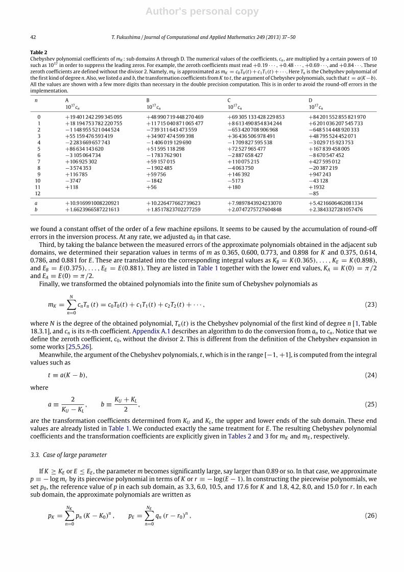
Table 2Chebyshev polynomial coefficients of mK : sub domains A through D. The numerical values of the coefficients, cn , are multiplied by a certain powers of 10such as 1017 in order to suppress the leading zeros. For example, the zeroth coefficients must read +0.19 · · · , +0.48 · · · , +0.69 · · ·, and +0.84 · · ·. Thesezeroth coefficients are defined without the divisor 2. Namely,mK is approximated asmK = c0T0(t)+ c1T1(t)+· · ·. Here Tn is the Chebyshev polynomial ofthe first kind of degree n. Also, we listed a and b, the transformation coefficients from K to t , the argument of Chebyshev polynomials, such that t = a(K−b).All the values are shown with a few more digits than necessary in the double precision computation. This is in order to avoid the round-off errors in theimplementation.

n A B C D1017cn 1017cn 1017cn 1017cn

0 +19401242299345095 +48990719448270469 +69305133428229853 +842015528558219701 +18194753782220755 +11715040871065477 +8613490854834244 +62010362075457332 −1148955521044524 −739311643473559 −653420708906968 −6485144489203333 +55159476593419 +34907474599398 +36436506978491 +487955244520714 −2283669657743 −1406019129690 −1709827595538 −30297159237535 +86634143620 +51595118298 +72527965477 +1678394580056 −3105064734 −1783762901 −2887658427 −86705474527 +106925302 +59157015 +110075215 +4275950128 −3574353 −1902485 −4063750 −203872199 +116785 +59756 +146392 +947243

10 −3747 −1842 −5173 −4312811 +118 +56 +180 +193212 −85

a +10.916991008220921 +10.226477662739623 +7.9897843924233070 +5.4216606462081334b +1.6623966587221613 +1.8517823702277259 +2.0747275727604848 +2.3843327281057476

we found a constant offset of the order of a few machine epsilons. It seems to be caused by the accumulation of round-offerrors in the inversion process. At any rate, we adjusted a0 in that case.

Third, by taking the balance between the measured errors of the approximate polynomials obtained in the adjacent subdomains, we determined their separation values in terms of m as 0.365, 0.600, 0.773, and 0.898 for K and 0.375, 0.614,0.786, and 0.881 for E. These are translated into the corresponding integral values as KB = K(0.365), . . . , KE = K(0.898),and EB = E(0.375), . . . , EE = E(0.881). They are listed in Table 1 together with the lower end values, KA ≡ K(0) = π/2and EA ≡ E(0) = π/2.

Finally, we transformed the obtained polynomials into the finite sum of Chebyshev polynomials as

mK =

Nn=0

cnTn (t) = c0T0(t) + c1T1(t) + c2T2(t) + · · · , (23)

where N is the degree of the obtained polynomial, Tn(t) is the Chebyshev polynomial of the first kind of degree n [1, Table18.3.1], and cn is its n-th coefficient. Appendix A.1 describes an algorithm to do the conversion from an to cn. Notice that wedefine the zeroth coefficient, c0, without the divisor 2. This is different from the definition of the Chebyshev expansion insome works [25,5,26].

Meanwhile, the argument of the Chebyshev polynomials, t , which is in the range [−1, +1], is computed from the integralvalues such as

t ≡ a(K − b), (24)

where

a ≡2

KU − KL, b ≡

KU + KL

2, (25)

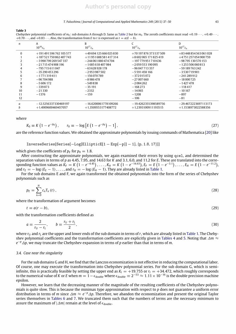
are the transformation coefficients determined from KU and KL, the upper and lower ends of the sub domain. These endvalues are already listed in Table 1. We conducted exactly the same treatment for E. The resulting Chebyshev polynomialcoefficients and the transformation coefficients are explicitly given in Tables 2 and 3 formK and mE , respectively.

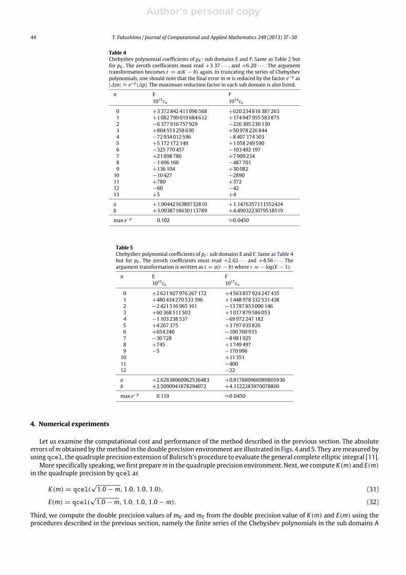
3.3. Case of large parameter

If K ≥ KE or E ≤ EE , the parameterm becomes significantly large, say larger than 0.89 or so. In that case, we approximatep ≡ − logmc by its piecewise polynomial in terms of K or r ≡ − log(E − 1). In constructing the piecewise polynomials, weset p0, the reference value of p in each sub domain, as 3.3, 6.0, 10.5, and 17.6 for K and 1.8, 4.2, 8.0, and 15.0 for r . In eachsub domain, the approximate polynomials are written as

pK =

NKn=0

pn (K − K0)n , pE =

NEn=0

qn (r − r0)n , (26)



Table 3Chebyshev polynomial coefficients of mE : sub domains A through D. Same as Table 2 but for mE . The zeroth coefficients must read +0.19 · · · , +0.49 · · · ,

+0.70 · · ·, and +0.83 · · ·. Also, the transformation from E to t is expressed as t = a(E − b).

n A B C D1018cn 1017cn 1017cn 1017cn

0 +191491596762105577 +49694125666025830 +70197876373537509 +834488545630610281 +187521750862407743 +11951688581417314 +8602065171825419 +47512570549007592 −3990799269547337 −244061880474704 −197779951710636 −987951305701533 −21715474908196 −1685618407984 −2059553190095 −12535060608134 −795715611047 −63628928178 −96047713357 −591897632425 −35290453296 −2953987502 −5591458166 −35307199016 −1771319411 −156070789 −372015072 −2412899127 −96704988 −8986478 −27007660 −180007258 −5606172 −549838 −2084262 −14274789 −339873 −35191 −168273 −118417

10 −21330 −2332 −14065 −1016711 −1376 −159 −1208 −89712 −106 −81

a −12.5256337330469197 −16.6200061778109266 −19.4262355398589756 −29.4672223697113173b +1.4909600469457057 +1.3509553177408772 +1.2393100911193515 +1.1538973022588356

where

K0 ≡ K1 − e−p0

, r0 ≡ − log

E

1 − e−p0

− 1

, (27)

are the reference function values.We obtained the approximate polynomials by issuing commands ofMathematica [20] like

InverseSeries[Series[−Log[EllipticE[1 − Exp[−p]] − 1], {p, 1.8, 17}]]

which gives the coefficients of pE for p0 = 1.8.After constructing the approximate polynomials, we again examined their errors by using qcel, and determined the

separation values in terms of p as 4.45, 7.95, and 14.63 for K and 3.1, 6.0, and 11.2 for E. These are translated into the corre-sponding function values as KF = K

1 − e−4.45

, . . . , KH = K

1 − e−14.63

, EF = E

1 − e−3.1

, . . . , EH = E

1 − e−11.2

,

and rE = − log (EE − 1) , . . . , and rH = − log (EH − 1). They are already listed in Table 1.For the sub domains E and F, we again transformed the obtained polynomials into the form of the series of Chebyshev

polynomials such as

pE =

Nn=0

cnTn (t) , (28)

where the transformation of argument becomes

t ≡ a(r − b), (29)

with the transformation coefficients defined as

a ≡2

rU − rL, b ≡

rU + rL2

, (30)

where rU and rL are the upper and lower ends of the sub domain in terms of r , which are already listed in Table 1. The Cheby-shev polynomial coefficients and the transformation coefficients are explicitly given in Tables 4 and 5. Noting that ∆m ≈

e−p∆p, we may truncate the Chebyshev expansion in terms of p earlier than that in terms ofm.

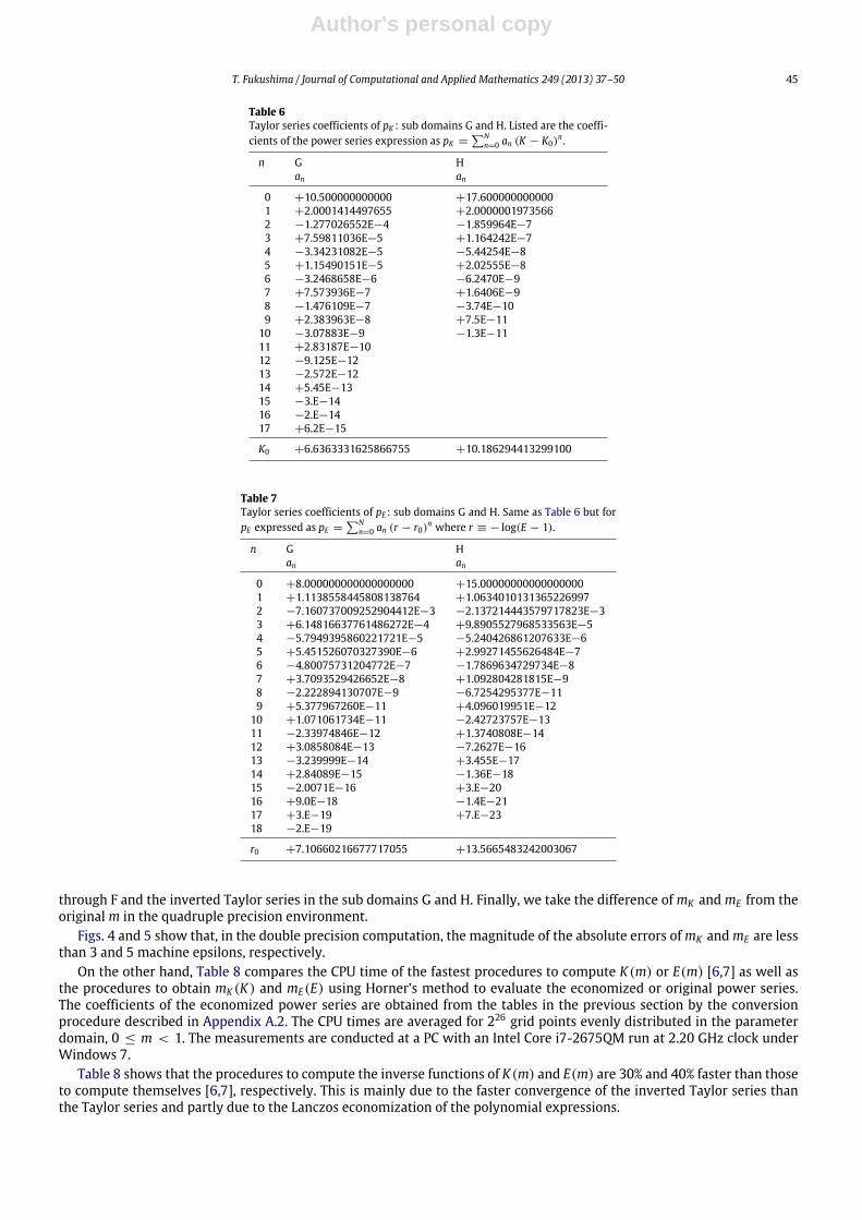
3.4. Case near the singularity

For the sub domains G andH,we find that the Lanczos economization is not effective in reducing the computational labor.Of course, one may execute the transformation into Chebyshev polynomial series. For the sub domain G, which is semi-infinite, this is practically feasible by setting the upper end as KI = +19.755 or rI = +34.472, which roughly correspondsto the numerical value of K or E whenm = 1− ϵdouble where ϵdouble ≡ 2−53

≈ 1.11×10−16 is the double precisionmachineepsilon.

However, we learn that the decreasing manner of the magnitude of the resulting coefficients of the Chebyshev polyno-mials is quite slow. This is because the minimax type approximation with respect to p does not guarantee a uniform errordistribution in terms of m since ∆m ≈ e−p∆p. Therefore, we abandon the economization and present the original Taylorseries themselves in Tables 6 and 7. We truncated them such that the numbers of terms are the necessary minimum toassure the maximum of |∆m| remain at the level of ϵdouble.



Table 4Chebyshev polynomial coefficients of pK : sub domains E and F. Same as Table 2 butfor pK . The zeroth coefficients must read +3.37 · · · , and +6.20 · · · . The argumenttransformation becomes t = a(K − b) again. In truncating the series of Chebyshevpolynomials, one should note that the final error inm is reduced by the factor e−p as|∆m| ≈ e−p

|∆p|. The maximum reduction factor in each sub domain is also listed.

n E F1015cn 1014cn

0 +3372842411096568 +6202348163872631 +1082799019684612 +1749479555838752 −6377916757929 −2263052301303 +804553258630 +509782268444 −72934012596 −84071743035 +5172172149 +10582495906 −325770457 −1034921977 +21898786 +79092348 −1696166 −4877019 +136104 +30082

10 −10427 −289011 +780 +37212 −60 −4213 +5 +4

a +1.9044216389732810 +1.1476357111552424b +3.0938718630113789 +4.4903223079518519

max e−p 0.102 ≈0.0450

Table 5Chebyshev polynomial coefficients of pE : sub domains E and F. Same as Table 4but for pE . The zeroth coefficients must read +2.62 · · · and +4.56 · · · . Theargument transformation is written as t = a(r − b) where r ≡ − log(E − 1).

n E F1015cn 1015cn

0 +2621927976267172 +45638579242474351 +480434270533396 +14489783325314382 −2421516965161 −137878530001463 +60368511503 +10178795860534 −1103238537 −699722471825 +4267375 +37970358266 +654240 −1007609337 −30728 −89819258 +745 +17494979 −5 −170996

10 +1135111 −40012 −22

a +2.62838060962536483 +0.817880966989805936b +2.5090941878294072 +4.1122283970078800

max e−p 0.119 ≈0.0450

4. Numerical experiments

Let us examine the computational cost and performance of the method described in the previous section. The absoluteerrors ofm obtained by themethod in the double precision environment are illustrated in Figs. 4 and 5. They aremeasured byusing qcel, the quadruple precision extension of Bulirsch’s procedure to evaluate the general complete elliptic integral [11].

More specifically speaking, we first preparem in the quadruple precision environment. Next, we compute K(m) and E(m)in the quadruple precision by qcel as

K(m) = qcel(√1.0 − m, 1.0, 1.0, 1.0), (31)

E(m) = qcel(√1.0 − m, 1.0, 1.0, 1.0 − m). (32)

Third, we compute the double precision values of mK and mE from the double precision value of K(m) and E(m) using theprocedures described in the previous section, namely the finite series of the Chebyshev polynomials in the sub domains A



Table 6Taylor series coefficients of pK : sub domains G and H. Listed are the coeffi-cients of the power series expression as pK =

Nn=0 an (K − K0)

n .

n G Han an

0 +10.500000000000 +17.6000000000001 +2.0001414497655 +2.00000019735662 −1.277026552E−4 −1.859964E−73 +7.59811036E−5 +1.164242E−74 −3.34231082E−5 −5.44254E−85 +1.15490151E−5 +2.02555E−86 −3.2468658E−6 −6.2470E−97 +7.573936E−7 +1.6406E−98 −1.476109E−7 −3.74E−109 +2.383963E−8 +7.5E−11

10 −3.07883E−9 −1.3E−1111 +2.83187E−1012 −9.125E−1213 −2.572E−1214 +5.45E−1315 −3.E−1416 −2.E−1417 +6.2E−15

K0 +6.6363331625866755 +10.186294413299100

Table 7Taylor series coefficients of pE : sub domains G and H. Same as Table 6 but forpE expressed as pE =

Nn=0 an (r − r0)n where r ≡ − log(E − 1).

n G Han an

0 +8.000000000000000000 +15.000000000000000001 +1.1138558445808138764 +1.06340101313652269972 −7.160737009252904412E−3 −2.137214443579717823E−33 +6.14816637761486272E−4 +9.8905527968533563E−54 −5.7949395860221721E−5 −5.240426861207633E−65 +5.451526070327390E−6 +2.99271455626484E−76 −4.80075731204772E−7 −1.7869634729734E−87 +3.7093529426652E−8 +1.092804281815E−98 −2.222894130707E−9 −6.7254295377E−119 +5.377967260E−11 +4.096019951E−12

10 +1.071061734E−11 −2.42723757E−1311 −2.33974846E−12 +1.3740808E−1412 +3.0858084E−13 −7.2627E−1613 −3.239999E−14 +3.455E−1714 +2.84089E−15 −1.36E−1815 −2.0071E−16 +3.E−2016 +9.0E−18 −1.4E−2117 +3.E−19 +7.E−2318 −2.E−19

r0 +7.10660216677717055 +13.5665483242003067

through F and the inverted Taylor series in the sub domains G and H. Finally, we take the difference of mK and mE from theoriginalm in the quadruple precision environment.

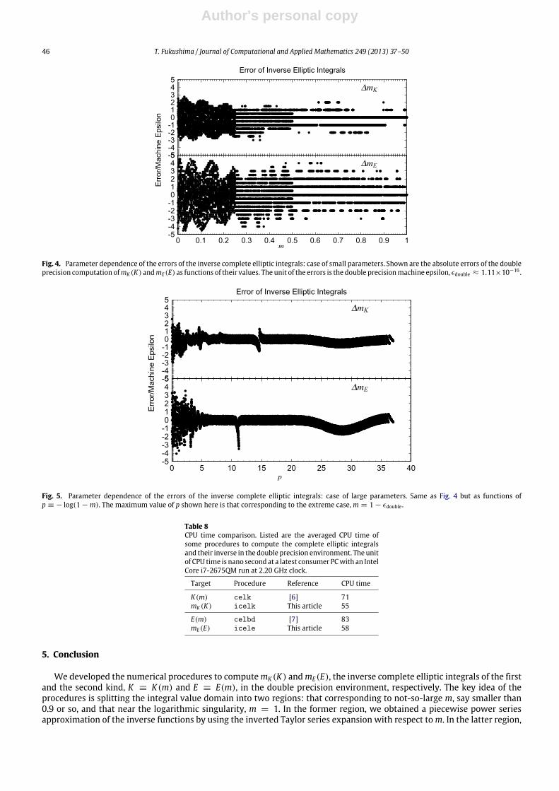
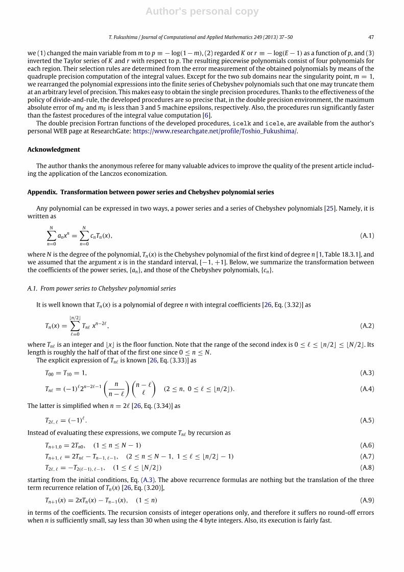
Figs. 4 and 5 show that, in the double precision computation, the magnitude of the absolute errors ofmK andmE are lessthan 3 and 5 machine epsilons, respectively.

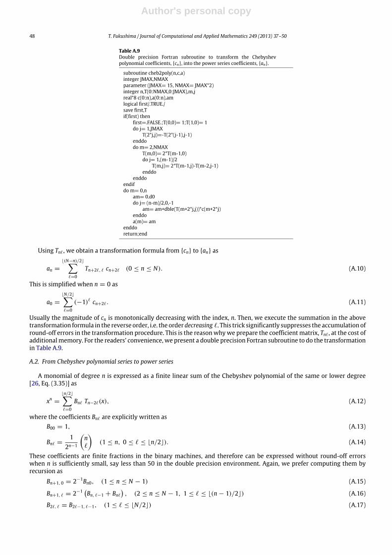
On the other hand, Table 8 compares the CPU time of the fastest procedures to compute K(m) or E(m) [6,7] as well asthe procedures to obtain mK (K) and mE(E) using Horner’s method to evaluate the economized or original power series.The coefficients of the economized power series are obtained from the tables in the previous section by the conversionprocedure described in Appendix A.2. The CPU times are averaged for 226 grid points evenly distributed in the parameterdomain, 0 ≤ m < 1. The measurements are conducted at a PC with an Intel Core i7-2675QM run at 2.20 GHz clock underWindows 7.

Table 8 shows that the procedures to compute the inverse functions of K(m) and E(m) are 30% and 40% faster than thoseto compute themselves [6,7], respectively. This is mainly due to the faster convergence of the inverted Taylor series thanthe Taylor series and partly due to the Lanczos economization of the polynomial expressions.



Fig. 4. Parameter dependence of the errors of the inverse complete elliptic integrals: case of small parameters. Shown are the absolute errors of the doubleprecision computation ofmK (K) andmE(E) as functions of their values. The unit of the errors is the double precisionmachine epsilon, ϵdouble ≈ 1.11×10−16 .

Fig. 5. Parameter dependence of the errors of the inverse complete elliptic integrals: case of large parameters. Same as Fig. 4 but as functions ofp ≡ − log(1 − m). The maximum value of p shown here is that corresponding to the extreme case,m = 1 − ϵdouble .

Table 8CPU time comparison. Listed are the averaged CPU time ofsome procedures to compute the complete elliptic integralsand their inverse in the double precision environment. The unitof CPU time is nano second at a latest consumer PCwith an IntelCore i7-2675QM run at 2.20 GHz clock.

Target Procedure Reference CPU time

K(m) celk [6] 71mK (K) icelk This article 55

E(m) celbd [7] 83mE(E) icele This article 58

5. Conclusion

We developed the numerical procedures to computemK (K) andmE(E), the inverse complete elliptic integrals of the firstand the second kind, K ≡ K(m) and E ≡ E(m), in the double precision environment, respectively. The key idea of theprocedures is splitting the integral value domain into two regions: that corresponding to not-so-large m, say smaller than0.9 or so, and that near the logarithmic singularity, m = 1. In the former region, we obtained a piecewise power seriesapproximation of the inverse functions by using the inverted Taylor series expansion with respect tom. In the latter region,



we (1) changed the main variable fromm to p ≡ − log(1−m), (2) regarded K or r ≡ − log(E −1) as a function of p, and (3)inverted the Taylor series of K and r with respect to p. The resulting piecewise polynomials consist of four polynomials foreach region. Their selection rules are determined from the error measurement of the obtained polynomials by means of thequadruple precision computation of the integral values. Except for the two sub domains near the singularity point, m = 1,we rearranged the polynomial expressions into the finite series of Chebyshev polynomials such that onemay truncate themat an arbitrary level of precision. Thismakes easy to obtain the single precision procedures. Thanks to the effectiveness of thepolicy of divide-and-rule, the developed procedures are so precise that, in the double precision environment, the maximumabsolute error ofmK andmE is less than 3 and 5 machine epsilons, respectively. Also, the procedures run significantly fasterthan the fastest procedures of the integral value computation [6].

The double precision Fortran functions of the developed procedures, icelk and icele, are available from the author’spersonal WEB page at ResearchGate: https://www.researchgate.net/profile/Toshio_Fukushima/.

Acknowledgment

The author thanks the anonymous referee for many valuable advices to improve the quality of the present article includ-ing the application of the Lanczos economization.

Appendix. Transformation between power series and Chebyshev polynomial series

Any polynomial can be expressed in two ways, a power series and a series of Chebyshev polynomials [25]. Namely, it iswritten as

Nn=0

anxn =

Nn=0

cnTn(x), (A.1)

whereN is the degree of the polynomial, Tn(x) is the Chebyshev polynomial of the first kind of degree n [1, Table 18.3.1], andwe assumed that the argument x is in the standard interval, [−1, +1]. Below, we summarize the transformation betweenthe coefficients of the power series, {an}, and those of the Chebyshev polynomials, {cn}.

A.1. From power series to Chebyshev polynomial series

It is well known that Tn(x) is a polynomial of degree nwith integral coefficients [26, Eq. (3.32)] as

Tn(x) =

⌊n/2⌋ℓ=0

Tnℓ xn−2ℓ, (A.2)

where Tnℓ is an integer and ⌊x⌋ is the floor function. Note that the range of the second index is 0 ≤ ℓ ≤ ⌊n/2⌋ ≤ ⌊N/2⌋. Itslength is roughly the half of that of the first one since 0 ≤ n ≤ N .

The explicit expression of Tnℓ is known [26, Eq. (3.33)] as

T00 = T10 = 1, (A.3)

Tnℓ = (−1)ℓ2n−2ℓ−1

nn − ℓ

n − ℓ

ℓ

(2 ≤ n, 0 ≤ ℓ ≤ ⌊n/2⌋). (A.4)

The latter is simplified when n = 2ℓ [26, Eq. (3.34)] as

T2ℓ, ℓ = (−1)ℓ. (A.5)

Instead of evaluating these expressions, we compute Tnℓ by recursion as

Tn+1,0 = 2Tn0, (1 ≤ n ≤ N − 1) (A.6)

Tn+1, ℓ = 2Tnℓ − Tn−1, ℓ−1, (2 ≤ n ≤ N − 1, 1 ≤ ℓ ≤ ⌊n/2⌋ − 1) (A.7)

T2ℓ, ℓ = −T2(ℓ−1), ℓ−1, (1 ≤ ℓ ≤ ⌊N/2⌋) (A.8)

starting from the initial conditions, Eq. (A.3). The above recurrence formulas are nothing but the translation of the threeterm recurrence relation of Tn(x) [26, Eq. (3.20)],

Tn+1(x) = 2xTn(x) − Tn−1(x), (1 ≤ n) (A.9)

in terms of the coefficients. The recursion consists of integer operations only, and therefore it suffers no round-off errorswhen n is sufficiently small, say less than 30 when using the 4 byte integers. Also, its execution is fairly fast.



Table A.9Double precision Fortran subroutine to transform the Chebyshevpolynomial coefficients, {cn}, into the power series coefficients, {an}.

subroutine cheb2poly(n,c,a)integer JMAX,NMAXparameter (JMAX= 15, NMAX= JMAX*2)integer n,T(0:NMAX,0:JMAX),m,jreal*8 c(0:n),a(0:n),amlogical first/.TRUE./save first,Tif(first) then

first=.FALSE.;T(0,0)= 1;T(1,0)= 1do j= 1,JMAX

T(2*j,j)=-T(2*(j-1),j-1)enddodo m= 2,NMAX

T(m,0)= 2*T(m-1,0)do j= 1,(m-1)/2

T(m,j)= 2*T(m-1,j)-T(m-2,j-1)enddo

enddoendifdo m= 0,n

am= 0.d0do j= (n-m)/2,0,-1

am= am+dble(T(m+2*j,j))*c(m+2*j)enddoa(m)= am

enddoreturn;end

Using Tnℓ, we obtain a transformation formula from {cn} to {an} as

an =

⌊(N−n)/2⌋ℓ=0

Tn+2ℓ, ℓ cn+2ℓ (0 ≤ n ≤ N). (A.10)

This is simplified when n = 0 as

a0 =

⌊N/2⌋ℓ=0

(−1)ℓ cn+2ℓ. (A.11)

Usually the magnitude of cn is monotonically decreasing with the index, n. Then, we execute the summation in the abovetransformation formula in the reverse order, i.e. the order decreasing ℓ. This trick significantly suppresses the accumulation ofround-off errors in the transformation procedure. This is the reasonwhywe prepare the coefficientmatrix, Tnℓ, at the cost ofadditionalmemory. For the readers’ convenience, we present a double precision Fortran subroutine to do the transformationin Table A.9.

A.2. From Chebyshev polynomial series to power series

A monomial of degree n is expressed as a finite linear sum of the Chebyshev polynomial of the same or lower degree[26, Eq. (3.35)] as

xn =

⌊n/2⌋ℓ=0

Bnℓ Tn−2ℓ(x), (A.12)

where the coefficients Bnℓ are explicitly written asB00 = 1, (A.13)

Bnℓ =1

2n−1

nℓ

(1 ≤ n, 0 ≤ ℓ ≤ ⌊n/2⌋). (A.14)

These coefficients are finite fractions in the binary machines, and therefore can be expressed without round-off errorswhen n is sufficiently small, say less than 50 in the double precision environment. Again, we prefer computing them byrecursion as

Bn+1, 0 = 2−1Bn0, (1 ≤ n ≤ N − 1) (A.15)

Bn+1, ℓ = 2−1 Bn, ℓ−1 + Bnℓ

, (2 ≤ n ≤ N − 1, 1 ≤ ℓ ≤ ⌊(n − 1)/2⌋) (A.16)

B2ℓ, ℓ = B2ℓ−1, ℓ−1, (1 ≤ ℓ ≤ ⌊N/2⌋) (A.17)



Table A.10Double precision Fortran subroutine to transform the power seriescoefficients, {an}, into the Chebyshev polynomial coefficients, {cn}.

subroutine poly2cheb(n,a,c)integer JMAX,NMAXparameter (JMAX= 15,NMAX= JMAX*2)integer n,m,jreal*8 a(0:n),c(0:n),B(0:NMAX,0:JMAX),cmlogical first/.TRUE./save first,Bif(first) then

first=.FALSE.;B(0,0)= 1.d0;B(1,0)= 1.d0do m= 2,NMAX

B(m,0)= 0.5d0*B(m-1,0)do j= 1,(m-1)/2

B(m,j)= 0.5d0*(B(m-1,j-1)+B(m-1,j))enddoif(m.eq.m/2*2) then

B(m,m/2)= B(m-1,m/2-1)endif

enddoendifdo m= 1,n

cm= 0.d0do j= (n-m)/2,0,-1

cm= cm+B(m+2*j,j)*a(m+2*j)enddoc(m)= c(m)

enddocm= c(n/2*2)do j= n/2-1,1,-1

cm= c(2*j)-cmenddoc(0)= a(0)+cmreturn;end

starting from the initial condition, Eq. (A.13). At any rate, the transformation from {an} to {cn} is of the same form asEq. (A.10) as

cn =

⌊(N−n)/2⌋ℓ=0

Bn+2ℓ, ℓ an+2ℓ (1 ≤ n ≤ N). (A.18)

We anticipate that the magnitude of an is also monotonically decreasing with the index, n. Then, we again execute thesummation in the transformation formula in the reverse order.

As for the most important coefficient, c0, we adopt a different approach. We solve the expression of a0, Eq. (A.11), withrespect to c0. Then, using thus-computed coefficients cn for n = 0 and a0, we evaluate the solution form of c0 by Horner’smethod as

c0 = a0 + (c2 − (c4 − (· · · (cM−2 − cM) · · ·))) , (A.19)

whereM ≡ 2⌊N/2⌋. This technique further reduces the accumulation of round-off errors. Table A.10 lists a double precisionFortran subroutine to do the transformation. We used its quadruple precision extension in deriving the tables in the maintext.

References

[1] F.W.J. Olver, D.W. Lozier, R.F. Boisvert, C.W. Clark (Eds.), NIST Handbook of Mathematical Functions, Cambridge Univ. Press, Cambridge, 2010 (Chapter4). Freely accessible at: http://dlmf.nist.gov/.

[2] P.F. Byrd, M.D. Friedman, Handbook on Elliptic Integrals for Engineers and Physicists, second ed., Springer-Verlag, Berlin, 1971.[3] W.H. Press, B.P. Flannery, S.A. Teukolsky,W.T. Vetterling, Numerical Recipes: The Art of Scientific Computing, Cambridge Univ. Press, Cambridge, 1986.[4] A. Jeffrey, D. Zwillinger (Eds.), Gradshteyn and Ryzhik’s Table of Integrals, Series, and Products, seventh ed., Academic Press, New York, 2007.[5] W.H. Press, S.A. Teukolsky, W.T. Vetterling, B.P. Flannery, Numerical Recipes: The Art of Scientific Computing, third ed., Cambridge Univ. Press,

Cambridge, 2007.[6] T. Fukushima, Fast computation of complete elliptic integrals and Jacobian elliptic functions, Celestial Mech. Dynam. Astronom. 105 (2009) 305–328.[7] T. Fukushima, Precise and fast computation of the general complete elliptic integral of the second kind, Math. Comp. 80 (2011) 1725–1743.[8] R. Bulirsch, Numerical computation of elliptic integrals and elliptic functions, Numer. Math. 7 (1965) 78–90.[9] R. Bulirsch, Numerical computation of elliptic integrals and elliptic functions II, Numer. Math. 7 (1965) 353–354.

[10] R. Bulirsch, An extension of the Bartky-transformation to incomplete elliptic integrals of the third kind, Numer. Math. 13 (1969) 266–284.[11] R. Bulirsch, Numerical computation of elliptic integrals and elliptic functions III, Numer. Math. 13 (1969) 305–315.[12] B.C. Carlson, Computing elliptic integrals by duplication, Numer. Math. 33 (1979) 1–16.[13] B.C. Carlson, E.M. Notis, Algorithm 577. Algorithms for incomplete elliptic integrals, ACM Trans. Math. Software 7 (1981) 398–403.



[14] C. Hastings Jr., Approximations for Digital Computers, Princeton Univ. Press, Princeton, 1955.[15] M. Abramowitz, I.A. Stegun (Eds.), Handbook of Mathematical Functions with Formulas, Graphs, and Mathematical Tables, National Bureau of

Standards, Washington, 1964 (Chapter 17).[16] W.J. Cody, Chebyshev approximations for the complete elliptic integrals K and E, Math. Comp. 19 (1965) 105–112.[17] W.J. Cody, Chebyshev polynomial expansions of complete elliptic integrals K and E, Math. Comp. 19 (1965) 249–259.[18] W.J. Cody, Corrigenda: Chebyshev approximations for the complete elliptic integrals K and E, Math. Comp. 20 (1966) 207.[19] T. Fukushima, Efficient solution of initial-value problem of torque-free rotation, Astron. J. 137 (2009) 210–218.[20] S. Wolfram, The Mathematica Book, fifth ed., Wolfram Research Inc./Cambridge Univ. Press, Cambridge, 2003.[21] E.T. Whittaker, G.N. Watson, A Course of Modern Analysis, fourth ed., Cambridge Univ. Press, Cambridge, 1958.[22] F. Chapeau-Blondeau, A. Monir, Evaluation of the LambertW function and application to generation of generalized Gaussian noise with exponent 1/2,

IEEE Trans. Signal Process. 50 (2002) 2160–2165.[23] D. Veberic, LambertW function for applications in physics, Comput. Phys. Comm. 183 (2012) 2622–2628.[24] T. Fukushima, Precise and fast computation of LambertW -functions without transcendental function evaluations, J. Comput. Appl. Math. 244 (2013)

77–89.[25] T.J. Rivlin, Chebyshev Polynomials, second ed., Wiley-Interscience, New York, 1990.[26] A. Gil, J. Segura, N.M. Temme, Numerical Methods for Special Functions, SIAM, Philadelphia, 2007.

Documents

Numerical computation of inverse compete elliptic integrals of first and second kinds