Embed Size (px)
Citation preview
Some properties of angular integrals
This article has been downloaded from IOPscience. Please scroll down to see the full text article.
2009 J. Phys. A: Math. Theor. 42 265201
(http://iopscience.iop.org/1751-8121/42/26/265201)
Download details:
IP Address: 132.166.22.147
The article was downloaded on 25/01/2010 at 17:12
Please note that terms and conditions apply.
The Table of Contents and more related content is available
HOME | SEARCH | PACS & MSC | JOURNALS | ABOUT | CONTACT US
IOP PUBLISHING JOURNAL OF PHYSICS A: MATHEMATICAL AND THEORETICAL
J. Phys. A: Math. Theor. 42 (2009) 265201 (32pp) doi:10.1088/1751-8113/42/26/265201
Some properties of angular integrals
M Bergere and B Eynard
Institut de Physique Theorique, CEA/DSM/IPhT, CEA/Saclay, CNRS, URA 2306,F-91191 Gif-sur-Yvette Cedex, France
E-mail: [email protected] and [email protected]
Received 22 January 2009, in final form 24 April 2009Published 5 June 2009Online at stacks.iop.org/JPhysA/42/265201
AbstractWe find new representations for Itzykson–Zuber like angular integrals forarbitrary β, in particular for the orthogonal group O(n), the unitary groupU(n) and the symplectic group Sp(2n). We rewrite the Haar measure integral,as a flat Lebesge measure integral, and we deduce some recursion formulae onn. The same methods give also Shatashvili’s type moments. Finally, we provethat, in agreement with Brezin and Hikami’s observation, the angular integralsare linear combinations of exponentials whose coefficients are polynomials inthe reduced variables (xi − xj )(yi − yj ).
PACS number: 02.10.YnMathematics Subject Classification: 15A52
1. Introduction
What we call an angular integral [29] is an integral over a compact Lie group Gβ,n:
G1/2,n = O(n), G1,n = U(n), G2,n = Sp(2n), (1.1)
of the form
Iβ,n(X, Y ) =∫
Gβ,n
dO eTr XOYO−1, (1.2)
where X and Y are two given matrices, and dO is the Haar-invariant measure on the group.We shall also extend Iβ,n to arbitrary β (note that our β is half the one most commonly usedin matrix models; for instance, we have β = 1 in the unitary case).
In this paper, we are going to consider the case where X and Y are diagonal matrices;however, let us first recall the Harish-Chandra case.
The Harish-Chandra case. In the case where X and Y are in the Lie algebra of the group [26](i.e. real anti-symmetric in the O(n) case, anti-Hermitian in the U(n) case and quaternion-anti-self-dual in the Sp(2n) case), the angular integral can be computed with the Weyl-character
1751-8113/09/265201+32$30.00 © 2009 IOP Publishing Ltd Printed in the UK 1
J. Phys. A: Math. Theor. 42 (2009) 265201 M Bergere and B Eynard
formula, and is given by the famous Harish-Chandra formula [14] (which is also a special caseof the Duistermaat–Heckman localization [11]):
(X, Y ) ∈ Lie algebra ⇒∫
dO eTr XOYO−1 = C∑
w∈Weyl
eTr XYw
�β(X)�β(Yw), (1.3)
where C is a normalization constant, w runs over the elements of the Weyl group, and thegeneralized Vandermonde determinant �β(X) is the product of scalar products of positiveroots with X (see [14, 26, 33] for details).
The diagonal case. However, for applications to many physics problems [13, 29], it would bemore interesting to have X and Y in other representations, and in particular X and Y diagonalmatrices.
Since an anti-Hermitian matrix is, up to a multiplication by i, a Hermitian matrix, andsince every Hermitian matrix can be diagonalized with a unitary conjugation, for the unitarygroup, the Harish-Chandra formula applies as well to the case where X and Y are diagonal;this is known as the Itzykson–Zuber formula [22]:{
X = diag(x1, . . . , xn)
Y = diag(y1, . . . , yn)⇒
∫U(n)
dU eTr XUYU−1 = Cn
det exiyj
�(X)�(Y ), (1.4)
where �(X) = �1(X) = ∏i>j (xi − xj ) is the usual Vandermonde determinant.
For the other groups, computing angular integrals has remained an important challengein mathematical physics for a rather long time. Much progress and many formulae have beenfound; however, a formula as compact and convenient as Harish-Chandra is still missing.And in particular, a formula which would allow us to compute multiple matrix integrals,generalizing that the method of Mehta [30], is still missing.
Calogero Hamiltonian. It is known that, in the diagonal case, Iβ,n satisfies the Calogero–Moserequation [2, 7], i.e. is an eigenfunction of the Calogero Hamiltonian:
HCalogero.Iβ,n =(∑
i
y2i
)Iβ,n, (1.5)
HCalogero =∑
i
∂2
∂x2i
+ β∑j �=i
1
xi − xj
(∂
∂xi
− ∂
∂xj
). (1.6)
Many approaches towards computing angular integrals have used that differentialequation. A basis of eigenfunctions of the Calogero Hamiltonian is the Hi–Jack polynomials[5, 7, 10, 28].
In particular, remarkable progress in the computation of Iβ,n was achieved recently byBrezin and Hikami [6]. By decomposing Iβ,n on the suitable basis of zonal polynomials, theywere able to find a recursive algorithm to compute the terms in some power series expansionof Iβ,n, and they obtained a remarkable structure. In particular, they observed that the powerseries reduces to a polynomial when β ∈ N.
Morozov and Shatashvili’s formulae. Another important question for physical applications isnot only to compute the angular integral (the partition function in statistical physics language),but also all its moments, for instance,
Mi,j =∫
Gβ,n
dO eTr XOYO−1‖Oi,j‖2 (1.7)
2
J. Phys. A: Math. Theor. 42 (2009) 265201 M Bergere and B Eynard
and more generally for any indices i1, . . . , i2k, j1, . . . , j2k:∫Gβ,n
dO eTr XOYO−1Oi1,i2Oi3,i4 . . . Oi2k−1,i2k
O−1j1,j2
O−1j3,j4
. . . O−1j2k−1,j2k
. (1.8)
In the U(n) case β = 1, Morozov [32] found a beautiful formula for Mi,j , and Shatashvili[34] found a more general formula for any moments of type (1.8) using the action-anglevariables of Gelfand–Tseytlin corresponding to the integrable structure of this integral.
For β = 1/2, 1, 2, in the Harish-Chandra case where X and Y are in the Lie algebra,a formula for all possible moments was also derived in [33], generalizing Morozov’s one[15, 17].
In this paper, we shall propose new formulae for Mi,j in the diagonal case for arbitrary β,and our method can also be generalized to all moments.Outline of the paper
• Section 1 is an introduction, and we present a summary of the main results of this paper.• In section 2 we set up the notations, and we review some known examples.• In section 3, we show how to transform the angular integral with a Haar measure into a
flat Lebesgue measure integral on a hyperplane. From it, we deduce a recursion formula,as well as a duality formula (the angular integral is an eigenfunction of kernel which isthe Cauchy determinant to the power β).
• In section 4, we discuss the moments of the angular integral. We show that moments canalso be obtained with Lebesgue measure integrals, and we show that they satisfy linearDunkl-like equations. This can be used as a way to recover the Calogero equation for theangular integral.
• In section 5, we rewrite the angular integral as a symmetric sum of exponentials withpolynomial prefactors. Those polynomials are called principal terms and can be computedrecursively. In particular, we prove the conjecture of Brezin and Hikami [6] that theprincipal terms are polynomials in some reduced variables (xi − xj )(yi − yj ).
• In section 5.2, we prove a formula for n = 3 in terms of Bessel polynomials, and wepropose a conjecture formula for arbitrary β and arbitrary n.
• In section 5.4, we focus on the symplectic case β = 2, for which we can improve therecursion formula.
• Section 6 is the conclusion.• The appendices contain useful lemmas and proofs of the most technical theorems.
1.1. Summary of the main results presented in this paper
• We rewrite the angular integral with the Haar measure on the Lie group Gβ,n, as a flatLebesgue measure integral on its Lie algebra (notations are explained in section 3),
Iβ,n(X;Y ) =∫
dO eTr XOYO−1 =∫
dSeTr S∏n
k=1 det(S − ykX)β, (1.9)
as well as its moments,
Mi,j =∫
dO‖Oi,j‖2 eTr XOYO−1
= β
∫dS
eTr S∏nk=1 det(S − ykX)β
((S − yjX)−1)i,i .
(1.10)
3
J. Phys. A: Math. Theor. 42 (2009) 265201 M Bergere and B Eynard
• We show that the Mi,j ’s satisfy a linear functional equation (very similar to Dunkloperators):
∀i, j,∂Mi,j
∂xi
+ β∑k �=i
Mi,j − Mk,j
xi − xk
= Mi,jyj (1.11)
which implies the Calogero equation for Iβ,n = ∑i Mi,j = ∑
j Mi,j :
∑i
∂2Iβ,n
∂x2i
+ β∑j �=i
1
xi − xj
(∂Iβ,n
∂xi
− ∂Iβ,n
∂xj
)=(∑
i
y2i
)Iβ,n. (1.12)
Moreover, the integral of equation (1.10) is a solution of the linear functionalequation (1.11) for any choice of integration domain (as long as there is no boundaryterm when one integrates by parts). We thus have a large set of solutions of the linearequation and also of the Calogero equation.
• We deduce a duality formula,
Iβ,n(X;Y ) = det(X)1−β
∫dλ1 . . . dλn�(�)2β Iβ,n(X,�)∏n
k=1
∏nj=1(λj − yk)β
, (1.13)
and a recursion formula,
Iβ,n(X;Y ) = exn
∑ni=1 yi∏n−1
i=1 (xi − xn)2β−1
∫dλ1, . . . dλn−1
Iβ,n−1(Xn−1,�)�(�)2β e−xn
∑i λi∏n
k=1
∏n−1i=1 (λi − yk)β
,
(1.14)
similar to that of [20].• For β ∈ N, the solution of the recursion can be written in terms of principal terms:
Iβ,n(X, Y ) =∑
σ
e∑n
i=1 xiyσ(i)
�(X)2β�(Yσ )2βIβ,n(X, Yσ ), (1.15)
where∑
σ is the sum over all permutations.The recursion relation (1.14) can be rewritten as a recursion for the principal terms
Iβ,n(X, Y ):
Iβ,n(Xn;Yn) = �(Yn)2β
(β − 1)!n−1
n−1∏i=1
xi,n
(∂
∂ai
)β−1 Iβ,n−1(Xn−1, a) e∑
i xi,n(ai−yi )∏nk=1
∏n−1i=1,�=k(yk − ai)β
∣∣∣∣∣ai=yi
.
(1.16)
• For general n and β integers, we prove the conjecture of Brezin and Hikami [6] that theprincipal term Iβ,n(X, Y ) is a symmetric polynomial of degree β in the τi,j variables:
τi,j = − (xi − xj )(yi − yj )
2. (1.17)
• In the case n = 3, we find this polynomial explicitly for any β (for β integer the sum isfinite):
Iβ,3 ∝ ex1y1+x2y2+x3y3
(�(x)�(y))β
∞∑k=0
(β − k)
26kk!(β + k)
∏i<j
Y (k)β−1
(1
τij
)+ sym, (1.18)
where Ym is the mth Bessel polynomial, i.e. the modified Bessel function of the secondkind (see the definition of Yβ−1 in equation (2.4)).
4
J. Phys. A: Math. Theor. 42 (2009) 265201 M Bergere and B Eynard
• In the case β = 2 (i.e. symplectic group Sp(2n)), the recursion relation for the principalterm can be written:
I2,n =n−1∏i=1
(xi − xn)(yi − yn)2
×n−1∏i=1
(xi − xn −
n∑k=1,�=i
2
yi − yk
+∂
∂ai
)I2,n−1(Xn−1, a)|ai=yi
= �(Xn)2�(Yn)
2det
[Xn−1 − xn − 2
Yn−1−yn+ B + ∂Y
]det(Xn − xn)
I2,n−1(Xn−1;Yn−1)
�(Xn−1)2�(Yn−1)2,
(1.19)
and B is the anti-symmetric matrix: Bi,j =√
2yi−yj
, Bi,i = 0 and ∂Y = diag(∂y1 , . . . , ∂yn−1
).
In section 5.4, we propose an operator formalism to compute it, and we propose aconjecture formula in terms of decomposition into triangles.
2. Definitions and examples
2.1. Notations for angular integrals
Let X and Y be two diagonal matrices of size n:
X = diag(x1, . . . , xn), Y = diag(y1, . . . , yn). (2.1)
We define the angular integral
Iβ,n(x1, . . . , xn; y1, . . . , yn) =∫
Gβ,n
dO eTr XOYO−1, (2.2)
where Gβ,n denotes one of the Lie groups:
G1/2,n = O(n), G1,n = U(n), G2,n = Sp(2n) (2.3)
and dO is the invariant Haar measure on the corresponding compact Lie group.We will later extend those notions to arbitrary values of β.
2.2. Bessel polynomials
For further use, we need to introduce some Bessel functions [1, 8, 27]. Those special functionsare going to play a major role throughout this paper.
The Bessel polynomials (see [27]) Ym(x) are defined by
Ym(x) =∞∑
k=0
(m + k + 1)
k!(m − k + 1)(x/2)k =
√2
πxe1/xKm+ 1
2(1/x), (2.4)
where K is the modified Bessel function of the second kind [1]. Ym is a polynomial of degreem when m is an integer:
Y0 = 1, Y1 = x + 1, Y2 = 3x2 + 3x + 1, Y3 = 15x3 + 15x2 + 6x + 1, etc. (2.5)
They satisfy
x2Y ′′m + (2x + 2)Y ′
m − m(m + 1)Ym = 0. (2.6)
We shall also need
Qβ,j (x) =∞∑
k=0
(β + j + k)
k!(β − j − k)2−kxβ−j−k, (2.7)
which is a polynomial of degree β − j , if β is an integer.
5
J. Phys. A: Math. Theor. 42 (2009) 265201 M Bergere and B Eynard
In particular, Qβ,0 is the Carlitz polynomial [8] and is closely related to Yβ−1:
Qβ,0(x) = xβYβ−1
(1
x
)=√
2
πexxβ+ 1
2 Kβ− 12(x), (2.8)
satisfying
x2Q′′β,0 − 2x(β + x)Q′
β,0 + 2β(x + 1)Qβ,0 = 0. (2.9)
The first few are
Q1,0 = x, Q2,0 = x2 + x, Q3,0 = x3 + 3x2 + 3x, Q4,0 = x4 + 6x3 + 15x2 + 15x, etc.
(2.10)
For higher j , the Qβ,j ’s are the derivatives of Bessel polynomials:
Qβ,j (1/x) = 2j xj−β dj
dxjYβ−1(x) = 2j xj−βY (j)
β−1(x). (2.11)
They satisfy
−xQβ,j = 1
4Qβ,j+1 + jQβ,j + (j − β)(j + β − 1)Qβ,j−1, (2.12)
Qβ,j+1 = 2
(β − j − x
d
dx
)Qβ,j . (2.13)
The first few are
Q2,1 = 2x, Q3,1 = 6x2 + 12x, Q4,1 = 12x3 + 60x2 + 90x, (2.14)
Q3,2 = 24x, Q4,2 = 120x2 + 360x, Q4,3 = 720x, etc. (2.15)
2.3. Examples of angular integrals with n = 1, 2, 3
• n = 1. The n = 1 case needs no computation, and gives
Iβ,1(x; y) = exy. (2.16)
• n = 2. The n = 2 case requires a little bit of easy computation, and it has been knownfor some time that we have (this formula is rederived in this paper):
Iβ,2(X, Y ) = ex1y1+x2y2
τβYβ−1(1/τ) +
ex1y2+x2y1
(−τ)βYβ−1(−1/τ)
= ex1y1+x2y2
τ 2βQβ,0(τ ) +
ex1y2+x2y1
(−τ)2βQβ,0(−τ), (2.17)
where
τ = − 12 (x1 − x2)(y1 − y2). (2.18)
It can also be written in terms of the modified Bessel function I:
Iβ,2(X;Y ) = e12 (x1+x2)(y1+y2)
τ 2β−1Iβ− 1
2(τ ), (2.19)
where
Im(τ) = (τ/2)2m
∞∑k=0
(τ/2)2k
k!(m + k + 1), Im = I ′′
m +1 − 2m
τI ′
m. (2.20)
6
J. Phys. A: Math. Theor. 42 (2009) 265201 M Bergere and B Eynard
• n = 3. We show in this paper that (proof in appendix C)
Iβ,3 ∝ ex1y1+x2y2+x3y3
(�(x)�(y))β
∞∑k=0
(β − k)
26kk!(β + k)
∏i<j
Y (k)β−1
(1
τij
)+ perm., (2.21)
where
τi,j = − (xi − xj )(yi − yj )
2(2.22)
and +perm. means that we have to symmetrize over all permutations of the yj ’s. Notethat the sum is finite and stops at k = β − 1 if β is an integer.This formula was already obtained by [4] for β = 1/2.
• n > 3. We show in this paper that for arbitrary n and β, the angular integral is of the formconjectured by Brezin and Hikami
Iβ,n ∝ e∑
i xiyi
(�(x)�(y))2βIβ,n(τij ) + perm., (2.23)
where Iβ,n(τij ) is a polynomial in the τi,j ’s, and for which we write a recursion relation.
3. Transformation of the angular integral
In this section, we transform the Haar measure group integral into a flat Lebesgue measureintegral. We use the same idea as in [19] for β = 1/2, but for the arbitrary half-integer β.
3.1. Lagrange multipliers
For β = 1/2, 1, 2, an element, O ∈ Gβ,n, is an orthonormal basis, i.e. a collection of northonormal vectors e1, . . . , en, whose coordinates, Oi,j = (ei)j , are of the form
(ei)j = Oi,j =2β−1∑α=0
(ei)αj εα, (3.1)
where the εα’s form a basis of a Clifford algebra (indeed, this reproduces the three groupsGβ,n for β = 1/2, 1, 2),
ε0 = 1, ε†0 = ε0, ∀α > 0 : ε2
α = −1, ε†α = −εα, εα.εα′ = −εα′ .εα, (3.2)
with structure constants (only for β = 2)
εαε†α′ =
∑α′′
ηα,α′,α′′εα′′ , (3.3)
where ηα,α′,α′′ has the property useful for our purpose that for every pair (α, α′), there is exactlyonly one α′′ such that ηα,α′,α′′ �= 0. In particular, ηα,α,α′′ = δα′′,0.
The basis must be orthonormal, i.e.,
ei .e†j = δi,j =
n∑k=1
(ei)k(ej )†k =
n∑k=1
2β−1∑α,α′=0
(ei)αk (ej )
α′k εαε
†α′ . (3.4)
We introduce Lagrange multipliers to enforce those orthonormality relations:
δ(ei .e
†i − 1
) =∫
dSi,i eSi,i (1−∑k,α((ei )
αk )2
(3.5)
7
J. Phys. A: Math. Theor. 42 (2009) 265201 M Bergere and B Eynard
and if i < j
δ(ei .e
†j
) =∫
. . .
∫dS0
i,j , . . . , dS2β−1i,j e−2
∑α,α′ ,α′′
∑k Sα
i,j ((ei )α′k )((ej )
α′′k )ηα′ ,α′′ ,α
=∫
dSi,j e−2∑
k Si,j ((ei )k)((ej )†k), (3.6)
where each integral is over the imaginary axis.Since the scalar product is invariant under group transformations (i.e. change of orthogonal
basis), the following measure is invariant and thus must be proportional to the Haar measure:
dO ∝∏i,j,α
d(ei)αj
∏i
δ(ei .e
†i − 1
)∏i<j
δ(ei .e
†j
), (3.7)
i.e.
dO ∝∏i,j,α
d(ei)αj
∫dS e
∑i Si,i e−∑
i
∑k Si,i |(ei )k |2 e−2
∑i<j
∑k Sα
i,j (ei )k(ej )†k , (3.8)
where
dS =∏
i
dSi,i
∏i<j
dSi,j =n∏
i=1
dSi,i
∏i<j
2β−1∏α=0
dSαi,j (3.9)
is the Gβ,n invariant measure on the space Eβ,n:
iS ∈⎧⎨⎩
E1/2,n = {n × n real symmetric matrices}E1,n = {n × n Hermitian matrices}E2,n = {n × n quaternion self − dual matrices},
(3.10)
where we have completed S by self-duality (S = S†):
S0j,i = S0
i,j and ∀α > 0 Sαj,i = −Sα
i,j . (3.11)
Therefore, we have (up to a multiplicative constant)
Iβ,n(X;Y ) ∝∫
dS
∫de1 . . . den e
∑i Si,i e
∑i,k xiyk |(ei )k |2
× e−∑i
∑k Si,i |(ei )k |2 e−2
∑i<j
∑k
∑α,α′ ,α′′ Sα
i,j ((ei )α′k )((ej )
†α′′k
)ηα′ ,α′′ ,α . (3.12)
The integral over the (ei)αk ’s is now Gaussian and can be performed. The Gaussian integrals
for each k are independent.The quadratic form in the exponential is, for each k,∑
α,α′,α′′
∑i,j
(ei)αk (ej )
α′k ηα,α′,α′′
(δi,j xiykδα′′,0 − Sα′′
i,j
). (3.13)
If we define the vector vk = (v1,k, . . . , vn,k) where vi,k = ∑α(ei)
αk ε†α , we have to compute the
Gaussian integral∫dvk e−v
†k(S−ykX)vk . (3.14)
For the three values of β = 1/2, 1, 2, this integral is worth:∫dvk e−v
†k(S−ykX)vk = (2π)β
det(S − ykX)β, (3.15)
where det is the product of singular values (see [29]).Thus we get the following theorem.
8
J. Phys. A: Math. Theor. 42 (2009) 265201 M Bergere and B Eynard
Theorem 3.1. The angular integral Iβ,n(X;Y ) is also equal to the following flat Lebesguemeasure integral:
Iβ,n(X;Y ) ∝∫
dSeTr S∏n
k=1 det(S − ykX)β= det(X)1−β
∫dS
eTr SX∏nk=1 det(S − yk)β
. (3.16)
In the last formula, we have made the change of variable S → X1/2SX1/2. Also, the integrationdomain for S, which was iEβ,n before exchanging the integrations over S and e, is now shiftedto the right, so that all singular values of (S − ykX) have positive real part. The integrationdomain for S can be deformed such that the integral remains convergent and the integrationpath goes to the right of all zeroes of the denominator. If β is a half-integer or an integer, thedenominator is not singular near ∞, and the integration contour can be closed. This will bemade more precise below.
Remark 1. For the moment, this formula holds only for β = 1/2, 1, 2. Later we will extendit to other values of β.
Remark 2. Another remark is that a similar formula can be obtained by exchanging the rolesof X and Y.
3.2. The duality formula
Note that the matrix S itself can be diagonalized with a Gβ,n conjugation:
S = O�O−1, � = diag(λ1, . . . , λn),O ∈ Gβ,n, (3.17)
and the measure dS is up to a constant [29]:
dS ∝ dOd��(�)2β. (3.18)
Therefore, the angular integral reappears in the RHS:
Iβ,n(X;Y ) ∝ det(X)1−β
∫dS
eTr SX∏nk=1 det(S − yk)β
∝ det(X)1−β
∫d��(�)2β Iβ,n(X,�)∏n
k=1
∏nj=1(λj − yk)β
. (3.19)
Here, if we assume that ∀i, xi ∈ R+, the integration contours for the λi’s are of the form r + iR
where r > max(Reyk). If β is an integer or a half-integer, the denominator in the integrand isnot singular near ∞, and the integration contour can be closed. Thus, if 2β is an integer, theintegration contours for the λi’s can be chosen as circles of radius > max(|yk|).
This equation looks better if we rewrite it in terms of the Cauchy determinant Dn(X, Y ),
Dn(X, Y ) = det
(1
xi − yj
)= �(X)�(Y )∏
i,j (xi − yj ), (3.20)
and the rescaled function,
Iβ,n(x1, . . . , xn; y1, . . . , yn) = (�(X)�(Y ))βIβ,n(x1, . . . , xn; y1, . . . , yn). (3.21)
We then have
Theorem 3.2. The rescaled function Iβ,n satisfies the duality formula,
Iβ,n(X;Y ) ∝ det(X)1−β
∫d�Iβ,n(X,�)Dn(�, Y )β , (3.22)
i.e. Iβ,n(X;Y ) is an eigenfunction of the kernel Dβn .
9
J. Phys. A: Math. Theor. 42 (2009) 265201 M Bergere and B Eynard
Remark 3. The duality formula above was derived for β = 1/2, 1, 2, but it makes sense forany β.
Remark 4. It is easy to check that this relation is satisfied for the Itzykson–Zuber case β = 1;indeed, in that case we have I1,n(X;Y ) = det( exiyj ) = ∑
ρ(−1)ρ∏
i eyixρ(i) , and∫d�I1,n(X,�)Dn(�, Y ) ∝
∑σ,ρ
(−1)σ (−1)ρ∫ n∏
i=1
eλixρ(i)
λi − yσ(i)
dλi
=∑σ,ρ
(−1)σ (−1)ρn∏
i=1
eyσ(i)xρ(i)
= n! det( exiyj )
∝ I1,n(X, Y ). (3.23)
3.3. The recursion formula
First, let us note that we can always assume that xn = 0, otherwise we perform a shift,X → X − xn:
Iβ,n(X, Y ) =∫
Gβ,n
dO eTr XOYO−1
=∫
Gβ,n
dO eTr(X−xn)OYO−1exn Tr OYO−1
= exn Tr Y
∫Gβ,n
dO eTr(X−xn)OYO−1. (3.24)
Thus we define
Xn−1 = diag(x1, . . . , xn−1), X = Xn−1 − xnIdn−1. (3.25)
Then, we note that the orthonormality of the basis ei ,
ei .e†j = δi,j , (3.26)
implies that if we already know e1, . . . , en−1, then en is completely fixed (up to an irrelevantphase). In other words, it is sufficient to enforce only the orthonormality of e1, . . . , en−1 withLagrange multipliers, i.e. introduce a matrix S of size n − 1.
Also, because of our shift X → X − xn, we note that en does not appear in the integrand.Then, we write as in equation (3.8)
dO ∝n−1∏i=1
dei
n−1∏i=1
δ(ei .ei − 1)
n−1∏i<j=1
δ(ei .e
†j
)
∝n−1∏i=1
n∏j=1
2β−1∏α=0
d(ei)αj
∫iEβ,n−1
dS e∑
i Si,i e−∑i
∑k Si,i |(ei )k |2 e−2
∑i<j
∑k Si,j (ei )k(ej )
†k
∝n−1∏i=1
dei
∫iEβ,n−1
dS eTr S e−∑i,j Si,j ei .e
†j , (3.27)
which implies, after performing the Gaussian integral over the e1, . . . , en−1,
Iβ,n(X;Y ) ∝ exn tr Y
∫iEβ,n−1
dSeTr S∏n
k=1 det(S − ykX)β
∝ exn tr Y∏n−1i=1 (xi − xn)2β−1
∫iEβ,n−1
dSeTr SX∏n
k=1 det(S − yk)β. (3.28)
10
J. Phys. A: Math. Theor. 42 (2009) 265201 M Bergere and B Eynard
Again, S can be diagonalized:
S = O�O−1, � = diag(λ1, . . . , λn−1), O ∈ Gβ,n−1, (3.29)
i.e. the rank n angular integral Iβ,n is expressed in terms of the rank n − 1:
Iβ,n(X;Y ) ∝ exn tr Y∏n−1i=1 (xi − xn)2β−1
∫d�
Iβ,n−1(X,�)�(�)2β∏nk=1
∏n−1i=1 (λi − yk)β
∝ exn tr Y∏n−1i=1 (xi − xn)2β−1
∫d�
Iβ,n−1(Xn−1,�)�(�)2β e−xn
∑i λi∏n
k=1
∏n−1i=1 (λi − yk)β
, (3.30)
which is our main recursion formula.
Theorem 3.3. The angular integrals Iβ,n(X;Y ) satisfy the recursion
Iβ,n(X;Y ) ∝ exn
∑ni=1 yi∏n−1
i=1 (xi − xn)2β−1
∫dλ1, . . . , dλn−1
Iβ,n−1(Xn−1,�)�(�)2β e−xn
∑i λi∏n
k=1
∏n−1i=1 (λi − yk)β
.
(3.31)
Here again, the integration contours for the λi’s are such that the integral is convergent andsuch that they surround all the yk’s. For instance, if 2β is an integer, and if ∀ixi ∈ R
+, theintegration contour for the λi’s can be chosen as circles of radius > max(|yk|).
Remark 5. Now this recursion formula can be used to define Iβ,n for arbitrary β, so that itcoincides with the angular integral for β = 1/2, 1, 2.
We have also the iterated form,
Iβ,n(X;Y ) ∝ exn
∑ni=1 yi
�(X)2β−1
∫ n−1∏i=1
i∏j=1
dλi,j
×∏n−1
i=1
∏1�j<j ′�i (λi,j ′ − λi,j )
2β∏n−1
i=1 e(xi−xi+1)∑
j λi,j∏n−1i=1
∏i+1j=1
∏ij ′=1(λi,j ′ − λi+1,j )β
, (3.32)
where we have defined λn,j = yj , and where the integration contours are circles such that
|λi,j | = ρi, ρ1 > ρ2 > · · · > ρn−1 > max|yj |. (3.33)
Remark 6. A similar recursion relation was also found in [19–21], but the authors found realintegrals instead of contour integrals. The advantage of our formulation is that we can easilymove integration contours and find new relations, as we will see below.
4. Moments of angular integrals and Calogero
In this section, we compute moments of the angular integral, and we show that our formulaindeed satisfies the Calogero equation.
11
J. Phys. A: Math. Theor. 42 (2009) 265201 M Bergere and B Eynard
4.1. The generalized Morozov’s formula
Define the quadratic moments (see [32] for β = 1):
Mi,j =∫
Gβ,n
dO‖Oi,j‖2 eTr XOYO−1. (4.1)
The same calculation as above yields
Mi,j = β
∫dS
eTr S∏nk=1 det(S − ykX)β
((S − yjX)−1)i,i
= β
xi
det(X)1−β
∫dS
eTr SX∏nk=1 det(S − yk)β
((S − yj )−1)i,i . (4.2)
As a consistency check and as a warmup exercise, let us show that this formula satisfies
Iβ,n =∑
j
Mi,j , (4.3)
which comes from ∀O ∈ Gβ,n,∑
j ‖Oi,j‖2 = 1.We have ∑
j
Mi,j =∑
j
β
xi
det(X)1−β
∫dS
eTr SX∏nk=1 det(S − yk)β
((S − yj )−1)i,i
= −1
xi
det(X)1−β
∫dS eTr SX ∂
∂Si,i
1∏nk=1 det(S − yk)β
= 1
xi
det(X)1−β
∫dS
1∏nk=1 det(S − yk)β
∂
∂Si,i
eTr SX
= det(X)1−β
∫dS
1∏nk=1 det(S − yk)β
eTr SX
= Iβ,n. (4.4)
Note that this equality holds independently of the integration domain of S, provided that onecan integrate by parts without picking boundary terms.
Remark 7. Of course a similar equation can be found by exchanging the roles of X and Y, andone gets symmetrically∑
i
Mi,j = Iβ,n. (4.5)
4.2. Other moments
Since, after introducing the Lagrange multipliers, the integral becomes Gaussian in the Oi,j ’s,any polynomial moment can be computed using Wick’s theorem. It is sufficient to computethe propagator ⟨
Oi,kO†j,l
⟩ = βδk,l((S − ykX)−1)i,j . (4.6)
Then, the expectation value of any polynomial moment is obtained as the sum over all pairingsof the product of propagators.
12
J. Phys. A: Math. Theor. 42 (2009) 265201 M Bergere and B Eynard
For instance,∫dO eTr XOYO−1
Oi1,j1Oi2,j2O†i3,j3
O†i4,j4
=∫
dSeTr S∏n
k=1 det(S − ykX)β
[δj1,j3δj2,j4((S − yj1X)−1)i1,i3((S − yj2X)−1)i2,i4
+ δj1,j4δj2,j3((S − yj1X)−1)i1,i4((S − yj2X)−1)i2,i3
]. (4.7)
In principle, one could compute with this method the generalization of all Shatashvili’smoments [34].
4.3. Linear equations
In this section, we prove that the Mi,j ’s satisfy the following linear functional relations, whichare very similar to Dunkl equations [11]:
∀ i, j,∂Mi,j
∂yj
+ β∑l �=j
Mi,l − Mi,j
yl − yj
= Mi,jxi . (4.8)
We are going to give two different proofs of equation (4.8). The first one below is basedon integration by parts. It can be done for the three groups β = 1/2, 1, 2; however, it is rathertedious for β = 1/2 and β = 2, and we present the proof only for β = 1. Another proof validfor all three values of β is presented in section 4.6.
Let us check that equation (4.2) satisfies equation (4.8) (for β = 1). We first rewrite
1
yl − yj
(1
S − yl
− 1
S − yj
)i,i
= ((S − yl)−1(S − yj )
−1)i,i
=∑m
((S − yl)−1)i,m((S − yj )
−1)m,i . (4.9)
For β = 1, we may consider all variables Si,m to be independent variables, and we integrateby parts:∑l �=j
Mi,l − Mi,j
yl − yj
=∑l �=j
∑m
β
xi
det(X)1−β
∫dS
eTr SX∏nk=1 det(S − yk)β
((S − yl)−1)i,m((S − yj )
−1)m,i
= −∑m
1
xi
det(X)1−β
∫dS
eTr SX
det(S − yj )β((S − yj )
−1)m,i
∂
∂Si,m
1∏l �=j det(S − yl)β
=∑m
1
xi
det(X)1−β
∫dS
1∏l �=j det(S − yl)β
∂
∂Si,m
eTr SX
det(S − yj )β((S − yj )
−1)m,i
=∑m
1
xi
det(X)1−β
∫dS
eTr SX∏k det(S − yk)β
((S − yj )−1)m,ixiδi,m
−β∑m
1
xi
det(X)1−β
∫dS
eTr SX∏k det(S − yk)β
((S − yj )−1)i,m((S − yj )
−1)m,i
−∑m
1
xi
det(X)1−β
∫dS
eTr SX∏k det(S − yk)β
((S − yj )−1)m,m((S − yj )
−1)i,i
13
J. Phys. A: Math. Theor. 42 (2009) 265201 M Bergere and B Eynard
= det(X)1−β
∫dS
eTr SX∏k det(S − yk)β
((S − yj )−1)i,i
− 1
xi
det(X)1−β
∫dS
eTr SX∏k det(S − yk)β
((S − yj )−2)i,i
− β
xi
det(X)1−β
∫dS
eTr SX∏k det(S − yk)β
Tr (S − yj )−1((S − yj )
−1)i,i
= 1
β
(xiMi,j − ∂Mi,j
∂yj
)QED. (4.10)
The same computation can be repeated for β = 1/2 and β = 2, with additional steps becausethe variables Si,m are no longer independent, and also because for β = 2, det(S−yj ) is definedas the product of singular values. Another proof is given in section 4.6.
Remark 8. Of course, a similar equation can be found by exchanging the roles of X and Y,and one gets the symmetric linear equation:
∀i, j,∂Mi,j
∂xi
+ β∑l �=i
Ml,j − Mi,j
xl − xi
= Mi,jyj . (4.11)
Remark 9. Again, this proves that equation (4.2) is the solution of the differentialequation (4.8), for any choice of integration domain provided that we can integrate by parts.In fact, by taking linear combinations of all possible integration contours, we get the generalsolution of the linear equation (4.8). However, a general solution of equation (4.8) is notnecessarily symmetric in X and Y and does not necessarily obey equation (4.11).
4.4. The Calogero equation
Here, we prove that Iβ,n satisfies the Calogero equation.Start from the linear equation,
∂Mi,j
∂xi
+ β∑k �=i
Mi,j − Mk,j
xi − xk
= Mi,jyj , (4.12)
then sum over j using equation (4.3):
∂I
∂xi
=∑
j
Mi,j yj . (4.13)
Then apply ∂∂xi
:
∂2I
∂x2i
=∑
j
yj
∂Mi,j
∂xi
=∑
j
yj
(Mi,jyj − β
∑k �=i
Mi,j − Mk,j
xi − xk
)
=∑
j
y2j Mi,j − β
∑j
yj
∑k �=i
Mi,j − Mk,j
xi − xk
=∑
j
y2j Mi,j − β
∑k �=i
∂I∂xi
− ∂I∂xk
xi − xk
. (4.14)
14
J. Phys. A: Math. Theor. 42 (2009) 265201 M Bergere and B Eynard
If we take the sum over i, using equation (4.5), we get∑i
∂2I
∂x2i
+ β∑
i
∑k �=i
∂I∂xi
− ∂I∂xk
xi − xk
=∑
j
y2j I, (4.15)
i.e. we recover the Calogero equation
HCalogero.Iβ,n =⎛⎝∑
j
y2j
⎞⎠ Iβ,n. (4.16)
4.5. Matrix form of the linear equations
The linear equations are n2 linear equations of order 1, for n2 unknown functions Mi,j . Theycan be summarized into a matricial equation,
MY = KM, (4.17)
where K is a matricial operator,
Kii = ∂
∂xi
+ β∑k �=i
1
(xi − xk), Kik = − β
(xi − xk)i �= k, (4.18)
and more generally this implies
MYp = KpM (4.19)
and therefore, for any polynomial P
M · P(Y ) = P(K) · M. (4.20)
In particular, if we choose the characteristic polynomial of Y,
0 =n∏
i=1
(yi − K) · M. (4.21)
Let us introduce the vector
e = (1, 1, . . . , 1)t . (4.22)
It is such that M is a stochastic matrix, i.e.
M · e = Iβ,ne, et · M = Iβ,net . (4.23)
We thus have, for any polynomial P,
etP (K)e · Iβ,n = Iβ,n Tr P(Y ). (4.24)
Note that the Calogero equation is the case P(K) = K2.If P is the characteristic polynomial of Y, we get another differential equation for Iβ,n:
∀ i,∑
j
(n∏
l=1
(yl − K)
)i,j
· Iβ,n = 0. (4.25)
And if P(K) = ∏l �=j (yl − K), we get
Mi,j =∑m
⎛⎝∏
l �=j
yl − K
yl − yj
⎞⎠
i,m
· Iβ,n. (4.26)
This last relation allows us to reconstruct Mi,j if we know Iβ,n.Finally, before leaving this section, we just mention that those operators Ki,j are also
related to the Laplacian over the set of matrices Eβ,n, as was noted recently by Zuber [36].
15
J. Phys. A: Math. Theor. 42 (2009) 265201 M Bergere and B Eynard
4.6. Linear equation from loop equations
There is another way of deriving those Dunkl-like linear equations for the angular integrals,using loop equations of an associated 2-matrix model.
Consider the following 2-matrix integral, where M1 and M2 are both in the Eβ,n ensemble:
Z =∫
dM1 dM2 e− Tr(V1(M1)+V2(M2)−M1M2). (4.27)
After diagonalization of M1 = O1XO−11 and M2 = O2YO−1
2 , we have
Z =∫
dX dY dO1 dO2�(X)2β�(Y )2β e− Tr(V1(X)+V2(Y )) eTr XO−11 O2YO−1
2 O1 . (4.28)
We redefine O2 = O1.O, and the integral over O1 gives 1, and the integral over O gives theangular integral
Z =∫
dX dY�(X)2β�(Y )2β e− Tr(V1(X)+V2(Y ))Iβ,n(X, Y ). (4.29)
We can do a similar change of variable for moments:⟨Tr
1
x − M1
1
y − M2
⟩= 1
Z
∫dM1dM2 e− Tr(V1(M1)+V2(M2)−M1M2) Tr
(1
x − M1
1
y − M2
)
= 1
Z
∫dX dY dO1 dO2�(X)2β�(Y )2β e− Tr(V1(X)+V2(Y ))
× eTr XO−11 O2YO−1
2 O1 Tr
(1
x − XO−1
1 O21
y − YO−1
2 O1
)
= 1
Z
∫dX dY�(X)2β�(Y )2β e− Tr(V1(X)+V2(Y ))
×∑i,j
Mi,j (X, Y )1
x − xi
1
y − yj
, (4.30)
where Mi,j (X, Y ) is the Morozov moment defined in equation (4.1).Loop equations amount to saying that an integral is invariant under a change of variables.
Thus, we change M1 → M1 + ε 1x−M1
1y−M2
+ O(ε2) in Z, and to order 1 in ε we get (the loopequations for β = 1/2, 1, 2 ensembles can be found in [3] and the Jacobian is easily computedin eigenvalue representation; see appendix B, equation (B.8))
0 =⟨Tr
1
x − M1
M2
y − M2
⟩−⟨Tr
V ′1(M1)
x − M1
1
y − M2
⟩+ β
⟨Tr
1
x − M1Tr
1
x − M1
1
y − M2
⟩
+ (β − 1)∂
∂x
⟨Tr
1
x − M1
1
y − M2
⟩, (4.31)
i.e., going to eigenvalues M1 = O1XO−11 and M2 = O2YO−1
2
0 =∑i,j
⟨(yj − V ′
1(xi))Mi,j (X, Y )
(x − xi)(y − yj )
⟩+ β
∑i �=l
∑j
⟨Mi,j (X, Y )
(x − xl)(x − xi)(y − yj )
⟩
+∑i,j
⟨Mi,j (X, Y )
(x − xi)2(y − yj )
⟩. (4.32)
16
J. Phys. A: Math. Theor. 42 (2009) 265201 M Bergere and B Eynard
The last term can be integrated by parts:∑i,j
⟨Mi,j (X, Y )
(x − xi)2(y − yj )
⟩=∑i,j
∫dX dY�(X)2β�(Y )2β e− Tr(V1(X)+V2(Y ))
×Mi,j (X, Y )∂
∂xi
1
(x − xi)(y − yj )
= −∑i,j
∫dX dY
1
(x − xi)(y − yj )
× ∂
∂xi
Mi,j (X, Y )�(X)2β�(Y )2β e− Tr(V1(X)+V2(Y ))
=∑i,j
∫dX dY
Mi,j (X, Y )
(x − xi)(y − yj )�(X)2β�(Y )2β
× e− Tr(V1(X)+V2(Y ))
(V ′
1(xi) −∑l �=i
2β
xi − xl
)
−∑i,j
∫dX dY
1
(x − xi)(y − yj )�(X)2β�(Y )2β
× e− Tr(V1(X)+V2(Y )) ∂Mi,j (X, Y )
∂xi
=∑i,j
⟨V ′
1(xi)Mi,j (X, Y )
(x − xi)(y − yj )
⟩− 2β
∑l �=i
∑j
⟨Mi,j (X, Y )
(xi − xl)(x − xi)(y − yj )
⟩
−∑i,j
⟨1
(x − xi)(y − yj )
∂Mi,j (X, Y )
∂xi
⟩. (4.33)
Therefore, we have∑i,j
⟨1
(x − xi)(y − yj )
∂Mi,j (X, Y )
∂xi
⟩
=∑i,j
⟨yjMi,j (X, Y )
(x − xi)(y − yj )
⟩− 2β
∑l �=i
∑j
⟨Mi,j (X, Y )
(xi − xl)(x − xi)(y − yj )
⟩
+ β∑i �=l
∑j
⟨Mi,j (X, Y )
(x − xl)(x − xi)(y − yj )
⟩
=∑i,j
⟨yjMi,j (X, Y )
(x − xi)(y − yj )
⟩− 2β
∑l �=i
∑j
⟨Mi,j (X, Y )
(xi − xl)(x − xi)(y − yj )
⟩
+ β∑i �=l
∑j
⟨Mi,j (X, Y )
(x − xl)(xl − xi)(y − yj )
⟩
+ β∑i �=l
∑j
⟨Mi,j (X, Y )
(x − xi)(xi − xl)(y − yj )
⟩
17
J. Phys. A: Math. Theor. 42 (2009) 265201 M Bergere and B Eynard
=∑i,j
⟨yjMi,j (X, Y )
(x − xi)(y − yj )
⟩
−β∑l �=i
∑j
⟨1
(x − xi)(y − yj )
Mi,j (X, Y ) − Ml,j (X, Y )
(xi − xl)
⟩. (4.34)
Since this equation must hold for any V1 and V2, x, y, i.e. for any measure on X and Y, it musthold term by term, i.e., we recover the linear equation
∂Mi,j (X, Y )
∂xi
= yjMi,j (X, Y ) − β∑l �=i
Mi,j (X, Y ) − Ml,j (X, Y )
(xi − xl). (4.35)
Of course, the loop equation coming from the change of variable M2 → M2 + ε 1x−M1
1y−M2
+
O(ε2) gives the symmetric linear equation:
∂Mi,j (X, Y )
∂yj
= xiMi,j (X, Y ) − β∑l �=j
Mi,j (X, Y ) − Mi,l(X, Y )
(yj − yl)QED. (4.36)
5. Principal terms and the τij variables
As we mentioned in the introduction, it was noted, in particular by Brezin and Hikami [6],that the angular integral can be written as combinations of exponential terms, and polynomials(for the β integer, series otherwise), of some reduced variables τi,j = − 1
2 (xi − xj )(yi − yj ).Here, we show how our recursion gives such a form.
We thus define
Definition 5.1. We define the principal term Iβ,n(X;Y ) from the recursion,
Iβ,1 = 1
and
Iβ,n(Xn;Yn) = �(Yn)2β
n−1∏i=1
(xi − xn) Res λi→yi
dλ1
(λ1 − y1)β· · · dλn−1
(λn−1 − yn−1)β
× Iβ,n−1(Xn−1,�) e∑
i (xi−xn)(λi−yi )∏nk=1
∏n−1i=1,�=k(yk − λi)β
. (5.1)
It is such that (the sum over permutations comes from the sum of residues at all poles inrecursion equation (3.31) of theorem 3.3)
Iβ,n(X, Y ) =∑
σ
e∑n
i=1 xiyσ(i)
�(X)2β�(Yσ )2βIβ,n(X, Yσ ). (5.2)
In [6], Brezin and Hikami observed and conjectured that when β is an integer, Iβ,n(X, Y )
is a polynomial in the variables τi,j = − 12 (xi − xj )(yi − yj ).
For instance, if β = 1, we have for arbitrary n
I1,n =∏i<j
τi,j . (5.3)
18
J. Phys. A: Math. Theor. 42 (2009) 265201 M Bergere and B Eynard
And, if n = 2, we have for arbitrary β
Iβ,2 = (x1 − x2)(y1 − y2)2β Res λ→0
dλ
λβ
e(x1−x2)λ
(y2 − y1 − λ)β
= (x1 − x2)(y1 − y2)2β ∂β−1
∂λβ−1
(e(x1−x2)λ
(y2 − y1 − λ)β
)λ=0
= (x1 − x2)(y1 − y2)2β
β−1∑k=0
(β − 1)!
k!(β − 1 − k)!(x1 − x2)
β−1−k(y2 − y1)−β−k (β − 1 + k)!
(β − 1)!
=β−1∑k=0
(β − 1 + k)!
k!(β − 1 − k)!((x1 − x2)(y2 − y1))
β−k
= 2βQβ,0(τ1,2), (5.4)
i.e. we recover the well-known result that Iβ,2 is the Bessel polynomial of degree β.We are going to prove the conjecture of Brezin–Hikami for all n and for all β ∈ N, but
first, let us prove some preliminary properties.
Lemma 5.1. Iβ,n is a polynomial in all variables xi and yj , and it is symmetric underthe exchange X ↔ Y and under the permutation of pairs (xi, yi) ↔ (xj , yj ), and undertranslations X → X + cte.Id or Y → Y + cte.Id.
Proof. If β is an integer, the recursion relation (5.1) leads to (we write xi,j = xi − xj , yi,j =yi − yj )
Iβ,n+1 =n∏
i=1
xi,n+1yβ
n+1,i
(∂
∂λi
)β−1[
exi,n+1λi
∏1�j�n+1,j �=i
yβ
j,i
(yj,i − λi)β
]Iβ,n(Xn, Yn + �)|�=0,
(5.5)
which shows by recursion that Iβ,n+1 is a rational function of all xi’s and yj ’s.We know, from its very definition that the angular integral,
Iβ,n(X, Y ) =∑
σ
e∑n
i=1 xiyσ(i)
�(X)2β�(Yσ )2βIβ,n(X, Yσ ), (5.6)
is symmetric in all xi’s and yj ’s, and in the exchange X ↔ Y . Since the exponentialsare linearly independent on the ring of rational functions, each term must be symmetric inpermutations of pairs (xi, yi)’s, i.e. Iβ,n(x1, . . . , xn; y1, . . . , yn) is a symmetric function of thepairs (xi, yi)’s, and also symmetric under X ↔ Y .
Moreover, Iβ,n+1 is clearly a polynomial in the variables xn+1 and yn+1, and because of thesymmetry, it must also be a polynomial in all variables. Translation invariance is also clearfrom the recursion formula. �
Theorem 5.1. (Conjecture of Brezin and Hikami)Iβ,n is a symmetric polynomial of degree β in the τi,j ’s.
Proof. Using lemma 5.1, it is easy to see that Iβ,n fulfils the hypothesis of lemma A.3 inappendix A, and this proves the theorem. �
That is, we have proved the conjecture of Brezin and Hikami [6]. In fact, we note that theproperty of being a polynomial in the τ ’s is not specific to angular integrals, but comes onlyfrom the global symmetries.
19
J. Phys. A: Math. Theor. 42 (2009) 265201 M Bergere and B Eynard
5.1. Recursion without residues for β integer
For β ∈ N, the residues in recursion equation (5.1) can be performed, and they computederivatives of the integrand. Thus equation (5.1) can be rewritten:
Iβ,n(Xn;Yn) = �(Yn)2β
n−1∏i=1
(xi − xn) Res λi→ai
dλ1
(λ1 − a1)β· · · dλn−1
(λn−1 − an−1)β
× Iβ,n−1(Xn−1,�) e∑
i (xi−xn)(λi−yi )∏nk=1
∏n−1i=1,�=k(yk − λi)β
∣∣∣∣∣ai=yi
= �(Yn)2β
(β − 1)!n−1
n−1∏i=1
(xi − xn)∏
i
(∂
∂ai
)β−1
Res λi→ai
dλ1
(λ1 − a1)· · · dλn−1
(λn−1 − an−1)
× Iβ,n−1(Xn−1,�) e∑
i (xi−xn)(λi−yi )∏nk=1
∏n−1i=1,�=k(yk − λi)β
∣∣∣∣∣ai=yi
, (5.7)
i.e. we can perform the residues:
Iβ,n(Xn;Yn) = �(Yn)2β
(β − 1)!n−1
n−1∏i=1
xi,n
(∂
∂ai
)β−1 Iβ,n−1(Xn−1, a) e∑
i xi,n(ai−yi )∏nk=1
∏n−1i=1,�=k(yk − ai)β
∣∣∣∣∣ai=yi
. (5.8)
More explicitly,
Iβ,n(Xn;Yn) =n−1∏i=1
β−1∑γi ,βi,k=0
(xi,nyn,i)βi,n
(β − γi − ∑k βi,k)βi,n!
n−1∏k=1,k �=i
(β + βi,k)
βi,k!(β)
1
(xi,nyk,i)βi,k
× 1
γi!
(1
xi,n
∂
∂ai
)γi
Iβ,n−1(Xn−1, a)|ai=yi. (5.9)
5.2. n = 3
For n = 3, and arbitrary β, we prove that
Theorem 5.2.
Iβ,3 =∞∑
k=0
(β − k)
23kk!(β + k)
∏i<j
Qβ,k(τij ). (5.10)
In fact, for the β integer, the sum over k is finite and reduces to k � β − 1.This expression was obtained in [4] for β = 1/2.The proof, which is rather technical, is given in appendix C. We used the Calogero
equation.
5.3. Conjecture for higher n
Applying the recursion relations of this paper, we also computed the n = 4 case for smallvalues of β:
20
J. Phys. A: Math. Theor. 42 (2009) 265201 M Bergere and B Eynard
I2,4 =∏i<j
Q2,0(τij ) +1
16Q2,0(τ1,2)Q2,0(τ1,3)Q2,0(τ1,4)Q2,1(τ2,3)Q2,1(τ2,4)Q2,1(τ3,4) + sym
+1
128Q2,0(τ1,2)Q2,1(τ1,3)Q2,1(τ1,4)Q2,1(τ2,3)Q2,1(τ2,4)Q2,1(τ3,4) + sym
(5.11)
and
I3,4 = 64∏i<j
Q3,0(τij ) +4
3Q3,0(τ1,2)Q3,0(τ1,3)Q3,0(τ1,4)Q3,1(τ2,3)Q3,1(τ2,4)Q3,1(τ3,4) + sym
+1
48Q3,0(τ1,2)Q3,0(τ1,3)Q3,0(τ1,4)Q3,2(τ2,3)Q3,2(τ2,4)Q3,2(τ3,4) + sym
+ · · · . (5.12)
These expressions lead us to conjecture a general form in terms of Bessel polynomials.
Conjecture 5.1. We conjecture that for all n and β, Iβ,n is of the form
Iβ,n =∑{l}
A{l}∏i<j
Qβ,l(i,j)(τi,j ). (5.13)
Unfortunately, we have not been able so far to determine the general form of the coefficientsA{l} for n > 3 (except n = 4 and β = 2).
5.4. The symplectic case β = 2
The case β = 2 is that of the symplectic group. It is, in principle, dual to the orthogonalgroup β = 1/2, which was more studied [2, 4], but in fact it should be easier to treat with ourapproach since β = 2 is an integer.
For β = 2, the recursion equation (5.8) reduces to
I2,n = �(Yn)4
n−1∏i=1
xi,n
∏i
∂
∂ai
I2,n−1(Xn−1, a) e∑
i (xi−xn)(ai−yi )∏nk=1
∏n−1i=1,�=k(yk − ai)2
∣∣∣∣∣ai=yi
=n−1∏i=1
xi,ny2i,n
(xi − xn −
n∑k=1,�=i
2
yi − yk
+∂
∂ai
)I2,n−1(Xn−1, a)|ai=yi
. (5.14)
From a recursion hypothesis, we assume that I2,n−1(Xn−1, a) is a polynomial in the τ ’s of theform
I2,n−1(Xn−1, Yn−1) =∑{l}
A{l}∏i<j
Q2,li,j (τi,j ), (5.15)
where for every pair (i, j) we have li,j ∈ {0, 1}. We recall that
|0〉τ = Q2,0(τ ) = τ 2 + τ , |1〉τ = Q1,0(τ ) = 2τ. (5.16)
Thus we may write∂
∂ai
= −1
2
∑k �=i
xi,k
∂
∂ti,k, ti,k = −1
2(xi − xk)(ai − ak), (5.17)
and we define the operators Ci,k acting on functions of the variable τi,k such that
Ci,k = 1
τi,k
− 1
2
∂
∂ti,k, (5.18)
and all derivatives must be eventually computed at ti,k = τi,k .21
J. Phys. A: Math. Theor. 42 (2009) 265201 M Bergere and B Eynard
Since our operators act on expressions of the form of equation (5.15), we need to compute
Ci,j |0〉 = Ci,j .Q2,0(τi,j ) = Ci,j .(τ 2i,j + τi,j
) = 12 , (5.19)
Ci,j |1〉 = Ci,j .Q2,1(τi,j ) = Ci,j .2τi,j = 1. (5.20)
And we may also have terms of the form Ci,j .Cj,i , for which we have
Ci,jCj,i |0〉 = Ci,jCj,i .(τ2i,j + τi,j ) = − 1
2 , Ci,jCj,i |1〉 = Ci,jCj,i .τi,j = 0. (5.21)
Finally, we have
I2,n =n−1∏i=1
τ 2i,n
n−1∏i=1
(1 +
1
τi,n
+n−1∑
k=1,�=i
xi,k
xi,n
Ci,k
)I2,n−1|ti,j =τi,j
. (5.22)
It is more convenient to rewrite this in terms of a Hilbert space with basis |0〉 = Q2,0 and|1〉 = Q2,1, and thus
I2,n =n−1∏i=1
(τ 2i,n + τi,n +
1
2τi,n
n−1∑k=1,�=i
yn,i
yk,i
Ai,k
)I2,n−1, (5.23)
where
Ai,k = 2τi,kCi,k. (5.24)
We have
A|0〉 = 12 |1〉, A|1〉 = |1〉 (5.25)
and
Ai,kAk,i = 2(Ai,k − 1). (5.26)
Unfortunately, we have not been able to go further with this formulation.
5.4.1. Triangle conjecture. We have seen that there is an operator formalism for computingangular integrals, with operators Ai,j associated with ‘edges’ (i, j). However, it can be seenfor n = 3, 4, that operator edges appear only in certain combinations, which involve triangles(i, j, k). We thus introduce the triangle operators
Ti,j,k = πi,jπj,kπk,i , (5.27)
where πi,j = πj,i is the projector on state 12 |1〉i,j = τi,j :
πi,j .(τ 2i,j + τi,j
) = τi,j , πi,j .τi,j = τi,j , πi,j = πj,i , π2i,j = πi,j . (5.28)
With this notation we have
I2,3 =(
1 +1
2T1,2,3
).
∏1�i<j�3
|0〉i,j , (5.29)
where we recall that |0〉i,j = τ 2i,j + τi,j .
And
I2,4 =(
1 +1
2(T1,2,3 + T1,2,4 + T1,3,4 + T2,3,4) +
1
4(T1,2,3T1,2,4 + T1,2,3T1,3,4 + T1,2,4T1,3,4
+ T1,2,3T2,3,4 + T1,2,4T2,3,4 + T1,3,4T2,3,4)
)·
∏1�i<j�4
|0〉i,j . (5.30)
22
J. Phys. A: Math. Theor. 42 (2009) 265201 M Bergere and B Eynard
We are naturally led to conjecture that
I2,n =( ∑
triangulations TCT
∏T ∈T
).∏i<j
|0〉i,j . (5.31)
We have
C∅ = 1, C(i,j,k) = 12 , C(i,j,k),(i,j,l) = 1
4 , . . . . (5.32)
We have not been able so far to prove this conjecture. It is to be noted from the low valuesof n that triangles seem to play a role for all β ∈ N.
5.4.2. Additional results: determinantal recursion. Just for completeness, we give anotherform of the recursion equation (5.14) in terms of determinants:
I2,n+1(Xn+1;Yn+1) =det
[X − xn+1 − 2
Y−yn+1+ B + ∂Y
]det(X − xn+1)
I2,n(Xn;Yn), (5.33)
where
I2,n(X, Y ) = 1∏i<j τ 2
i,j
I2,n(X, Y ) (5.34)
and where B is the anti-symmetric matrix,
Bij =√
2
yi − yj
, (5.35)
and ∂Y = diag(∂y1 , . . . , ∂yn). This is proved by observing that the expansion of the determinant
equation (5.33) can be interpreted like a Wick’s expansion equivalent to equation (5.14).
6. Conclusion
In this paper, we have found many new relations and new representations of angular integrals.First, we have been able to rewrite angular integrals with a complicated Haar measure,
in terms of usual Lebesgue measure contour integrals. Then, we have deduced duality andrecursion formulae.
This allowed us to prove Brezin–Hikami’s conjecture and to find some explicit form forn = 3, and conjecture some explicit form in terms of Bessel polynomials for the general case.
For β = 2, we have simplified our recursion (computed the residues). The same methodseems to be applicable for higher β, but we have not done it in this paper.
We have obtained many new forms of angular integrals, but unfortunately, this does notseem to be the end of the story. Our expressions are still not explicit enough to be useful forcomputing matrix integrals. The form of our expressions strongly suggests that the kernel-determinantal formulae [29] in the β = 1 case could be replaced by hyperdeterminantalformulae for higher β, but this is still to be understood. The best thing would be to getexpressions with enough structure to generalize the method over integration of matrix variablesof Mehta [30].
Acknowledgments
We would like to thank G Akemann, E Brezin, P Desrosiers, S Hikami, A Prats-Ferrer andJ B Zuber for useful and fruitful discussions on this subject. This work is partly supportedby the Enigma European network MRT-CT-2004-5652, by the ANR project Geometrie et
23
J. Phys. A: Math. Theor. 42 (2009) 265201 M Bergere and B Eynard
integrabilite en physique mathematique ANR-05-BLAN-0029-01, by the Enrage Europeannetwork MRTN-CT-2004-005616, by the European Science Foundation through the Misgamprogram, by the French and Japanese governments through PAI Sakurav and by the Quebecgovernment with the FQRNT.
Appendix A. Polynomials of τ
Lemma A.1. Let
Pn(X, Y ) = x1x2 . . . xn−1xnyn+1yn+2 . . . y2n−1y2n + y1y2 . . . yn−1ynxn+1xn+2 . . . x2n−1x2n.
(A.1)
We prove that Pn is a polynomial of degree n in the τ ’s, where τi,2n+1 = − 12xiyi and
τi,j = − 12 (xi − xj )(yi − yj ), with integer coefficients
Pn ∈ Z[τ ]. (A.2)
Proof. It clearly holds for n = 0 and n = 1. Indeed, the n = 1 case reads
x1y2 + x2y1 = x1y1 + x2y2 − (x1 − x2)(y1 − y2) = 2(τ1,2 − τ1,3 − τ2,3). (A.3)
Assume that the lemma holds up to n − 1, and let us prove it for n. In the following,A ≡ B means that A − B is a polynomial in the τ ’s:
Pn = x1x2 . . . xn−1xnyn+1yn+2 . . . y2n−1y2n + y1y2 . . . yn−1ynxn+1xn+2 . . . x2n−1x2n
= (x1yn+1 + xn+1y1)(x2 . . . xn−1xnyn+2 . . . y2n−1y2n + y2 . . . yn−1ynxn+2 . . . x2n−1x2n)
− x2 . . . xn−1xnxn+1yn+2 . . . y2n−1y2ny1 − y2 . . . yn−1ynyn+1xn+2 . . . x2n−1x2nx1
≡ −x2 . . . xn−1xnxn+1yn+2 . . . y2n−1y2ny1 − y2 . . . yn−1ynyn+1xn+2 . . . x2n−1x2nx1 (A.4)
and then
Pn ≡ −x2 . . . xn−1xnxn+1yn+2 . . . y2n−1y2ny1 − y2 . . . yn−1ynyn+1xn+2 . . . x2n−1x2nx1
≡ −(x2y1 + x1y2)(x3 . . . xn−1xnxn+1yn+2 . . . y2n−1y2n + y3 . . . yn−1ynyn+1xn+2 . . . x2n−1x2n)
+ xn+1x1x3 . . . xn−1xny2yn+2 . . . y2n + yn+1y1y3 . . . ynx2xn+2 . . . x2n. (A.5)
Repeating the same operation recursively we obtain ∀k:
Pn ≡ xn+1 . . . xn+kx1xk+2 . . . xny2 . . . yk+1yk+n+1 . . . y2n
+ yn+1 . . . yn+ky1yk+2 . . . ynx2 . . . xk+1xk+n+1 . . . x2n. (A.6)
In particular, for k = n − 2 we find
Pn ≡ xn+1 . . . x2n−2x1xny2 . . . yn−1y2n−1y2n + yn+1 . . . y2n−2y1ynx2 . . . xn−1x2n−1x2n
≡ (x1y2n−1 + x2n−1y1)(xn+1 . . . x2n−2xny2 . . . yn−1y2n
+ yn+1 . . . y2n−2ynx2 . . . xn−1x2n)
− xn . . . x2n−1y1y2 . . . yn−1y2n − yn . . . y2n−1x1x2 . . . xn−1x2n), (A.7)
and we repeat the same operations,
Pn ≡ −xn . . . x2n−1y1y2 . . . yn−1y2n − yn . . . y2n−1x1x2 . . . xn−1x2n)
≡ −(xny1 + x1yn)(xn+1 . . . x2n−1y2 . . . yn−1y2n + yn+1 . . . y2n−1x2 . . . xn−1x2n)
+ x1xn+1 . . . x2n−1y2 . . . yny2n + y1yn+1 . . . y2n−1x2 . . . xnx2n, (A.8)
24
J. Phys. A: Math. Theor. 42 (2009) 265201 M Bergere and B Eynard
and once more
Pn ≡ x1xn+1 . . . x2n−1y2 . . . yny2n + y1yn+1 . . . y2n−1x2 . . . xnx2n
≡ (x1y2n + x2ny1)(xn+1 . . . x2n−1y2 . . . yn + yn+1 . . . y2n−1x2 . . . xn)
− xn+1 . . . x2ny1y2 . . . yn − yn+1 . . . y2nx1 . . . xn. (A.9)
Therefore, Pn ≡ −Pn, i.e. Pn is a polynomial in the τ ’s. �
Lemma A.2. Let
Pα,β(X, Y ) =n∏
i=1
xαi
i yβi
i +n∏
i=1
xβi
i yαi
i ,∑
i
αi =∑
i
βi = d. (A.10)
We prove that Pα,β is a polynomial of degree d in the τ ’s, with integer coefficients
Pn ∈ Z[τ ]. (A.11)
Proof. We proceed by recursion on the total degree d = ∑i αi = ∑
i βi . The lemma clearlyholds for d = 0 and d = 1.
Assume d � 2 and that the lemma holds up to d − 1. We will prove it for d.
• If there exists i such that αiβi > 0, then Pα,β is the factor of τi,n+1 times Pα′,β ′ of smallerdegree, and from the recursion hypothesis it holds.
• Assume that ∀i, αiβi = 0. Since d � 2, there must exist some i such that αi � 1 andsome j such that βj � 1. Let us choose k and l such that
αk = maxi
{αi} � 1, βl = maxi
{βi} � 1. (A.12)
We have k �= l.If αk = βl = 1, then we can apply lemma A.1, and thus the lemma is proved for that case.
• Therefore, we now assume that αkβl � 2, and with no loss of generality we may assumethat αk � 2. We write
Pn = xα11 . . . xαn
n yβ11 . . . yβn
n + xβ11 . . . xβn
n yα11 . . . yαn
n
= (xkyl + xlyk)(x
α11 . . . x
αk−1k . . . xαn
n yβ11 . . . y
βl−1l . . . yβn
n
+ yα11 . . . y
αk−1k . . . yαn
n xβ11 . . . x
βl−1l . . . xβn
n
)− x
α11 . . . x
αk−1k x
αl+1l . . . xαn
n yβ11 . . . y
βl−1l y
βk+1k . . . yβn
n
− yα11 . . . y
αk−1k y
αl+1l . . . yαn
n xβ11 . . . x
βl−1l x
βk+1k . . . xβn
n
≡ −xkyk
(x
α11 . . . x
αk−2k x
αl+1l . . . xαn
n yβ11 . . . y
βl−1l y
βk
k . . . yβn
n
+ yα11 . . . y
αk−2k y
αl+1l . . . yαn
n xβ11 . . . x
βl−1l x
βk
k . . . xβn
n
). (A.13)
From the recursion hypothesis, the RHS is a polynomial in the τ ’s, and thus we haveproved the lemma. �
Lemma A.3. Let P be a polynomial of 2n + 2 variables x1, . . . , xn, xn+1, y1, . . . , yn,
yn+1, with the following properties:
• P is invariant by translations ∀i, xi → xi + δx, yi → yi + δy,• P is invariant under ∀i, xi → λxi, yi → 1
λyi ,
• P is symmetric in the exchange X ↔ Y .
Then P is a polynomial of the τi,j ’s.
Proof. Because of invariance by translation, we can always assume that xn+1 = yn+1 = 0.Then, the other properties imply that P is a linear combination of monomials of the typePα,β(X, Y ) of lemma A.2. �
25
J. Phys. A: Math. Theor. 42 (2009) 265201 M Bergere and B Eynard
Appendix B. Loop equations
Loop equations for matrix models have been studied for a long time [31]. Loop equations(sometimes called Ward identities or Schwinger–Dyson equations) for β ensembles can befound, for instance, in [9, 16, 23–25, 35]. Here, we summarize the method.
• 1-matrix model in eigenvalue representation for arbitrary β.Consider the integral
Z =∫
dλ1 . . . dλn e−∑i V (λi )
∏i<j
(λj − λi)2β. (B.1)
If we make an infinitesimal local change of variable λi → λi + ελki + O(ε2), we find
Z = (1 + O(ε2))
∫dλ1 . . . dλn
∏i
(1 + εkλk−1
i
)e−∑
i V (λi )∏
i
(1 − ελk
i V′(λi)
)
×∏i<j
(λj − λi)2β∏i<j
(1 + 2βε
λki − λk
j
λi − λj
), (B.2)
i.e., by considering the term linear in ε
0 =⟨∑
i
kλk−1i + β
k−1∑l=0
∑i �=j
λliλ
k−1−lj −
∑i
λki V
′(λi)
⟩. (B.3)
It can be written collectively by summing over k with 1/xk+1; this is equivalentto considering a local change of variable λi → λi + ε
x−λi+ O(ε2), and we write
ω(x) = ∑i
1x−λi
:
0 =⟨−ω′(x) + β(ω(x)2 + ω′(x)) −
∑i
V ′(λi)
x − λi
⟩, (B.4)
i.e.
0 = −⟨Tr
V ′(M)
x − M
⟩+ β
⟨Tr
1
x − MTr
1
x − M
⟩+ (β − 1)
∂
∂x
⟨Tr
1
x − M
⟩. (B.5)
• 2-matrix model for β = 1/2, 1, 2.Similarly if we consider a 2-matrix model,
Z =∫
dM1 dM2 e− Tr(V1(M1)+V2(M2)−M1M2), (B.6)
again we make a local change of variable M1 → M1 + ε 1x−M1
A + O(ε2). The Jacobian ofthis change of variable is computed as a split rule (cf [3]), it can be computed for each ofthe three ensembles β = 1/2, 1, 2 and is:
dM1 → dM1
(1 + εβ Tr
1
x − M1Tr A
1
x − M1+ ε(β − 1)
∂
∂xTr A
1
x − M1+ O(ε2)
).
(B.7)
Thus we find
0 = −⟨Tr(V ′
1(M1) − M2)1
x − M1
⟩+ β
⟨Tr
1
x − M1Tr A
1
x − M1
⟩
+ (β − 1)∂
∂x
⟨Tr A
1
x − M1
⟩. (B.8)
26
J. Phys. A: Math. Theor. 42 (2009) 265201 M Bergere and B Eynard
• Without a definition of a 2-matrix integral for arbitrary β, it is not possible to find the loopequation for any β. However, we see that equation (B.8) is valid for the 2-matrix modelfor β = 1/2, 1, 2, and is valid for the 1-matrix eigenvalue model for any β. Therefore, itis natural to take it as a definition of the 2-matrix model for arbitrary β.
Appendix C. Proof n = 3
C.1. Bessel zoology
We define the functions
Qβ (x) =∞∑l=0
(−)l (β + l)
(β − l)
2−l
l!xβ−l . (C.1)
We have
2x2Q′β (x) − 2βxQβ (x) = −
∞∑l=1
(−)l (β + l)
(β − l)
2−l+1
(l − 1)xβ−l+1,
(C.2)
x2Q′′β (x) − 2βxQ′
β (x) + 2βQβ (x) = −∞∑l=0
(−)l (β + l + 1)
(β − l − 1)
2−l
l!xβ−l .
Changing l into l + 1 in (C.2) we obtain the differential equation
x2Q′′β (x) − 2x (β − x) Q′
β (x) + 2β (1 − x) Qβ (x) = 0. (C.3)
We define the functions,
Qβ,k (x) = (−2)k xβ−k
(x2 d
dx
)k (Qβ (x)
xβ
), (C.4)
Qβ,0(x) = Qβ(x), (C.5)
that is
Qβ,k (x) =∞∑l=0
(−)l+k (β + l + k)
(β − l − k)
2−l
l!xβ−l−k. (C.6)
From (C.4) we obtain the recurrence:
Qβ,k (x) = 2 (β − k + 1) Qβ,k−1 (x) − 2xQ′β,k−1(x). (C.7)
For instance,
Qβ,1 (x) = 2βQβ,0 (x) − 2xQ′β,0 (x) (C.8)
and
Qβ,2 (x) = 2 (β − 1) Qβ,1 (x) − 2xQ′β,1(x), (C.9)
Qβ,2 (x) = 4x2Q′′β,0 (x) − 8x (β − 1) Q′
β,0 (x) + 4β (β − 1)Qβ,0(x). (C.10)
Thus, we have, from (C.8) and (C.10), the expressions Q′β,0 (x) and Q′′
β,0 (x) in terms ofQβ,1 (x) and Qβ,2 (x). Equation (C.3) becomes
Qβ,2 (x) + 4 (1 − x) Qβ,1 (x) − 4β (β − 1) Qβ,0 (x) = 0. (C.11)
From (C.11), by derivatives ddx
and recurrence, it is easy to show that
Qβ,k+2 (x) + 4 (k + 1 − x) Qβ,k+1 (x) − 4 [β (β − 1) − k (k + 1)] Qβ,k (x) = 0. (C.12)
27
J. Phys. A: Math. Theor. 42 (2009) 265201 M Bergere and B Eynard
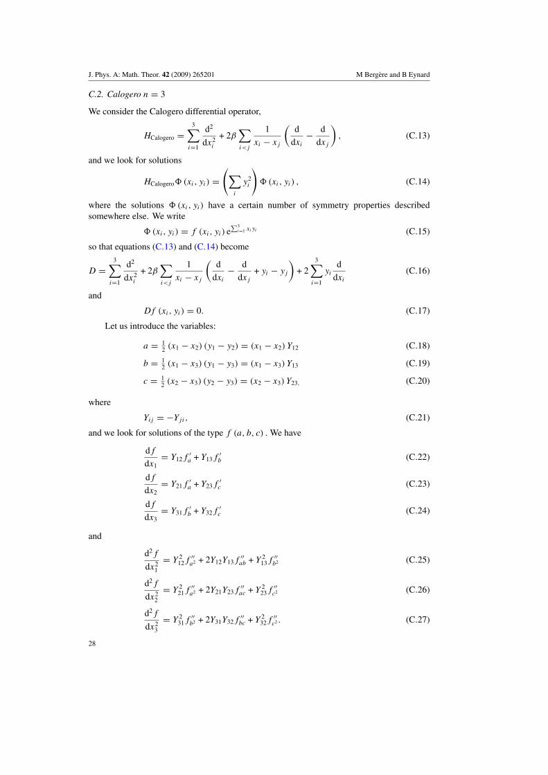
C.2. Calogero n = 3
We consider the Calogero differential operator,
HCalogero =3∑
i=1
d2
dx2i
+ 2β∑i<j
1
xi − xj
(d
dxi
− d
dxj
), (C.13)
and we look for solutions
HCalogero�(xi, yi) =(∑
i
y2i
)�(xi, yi) , (C.14)
where the solutions �(xi, yi) have a certain number of symmetry properties describedsomewhere else. We write
�(xi, yi) = f (xi, yi) e∑3
i=1 xiyi (C.15)
so that equations (C.13) and (C.14) become
D =3∑
i=1
d2
dx2i
+ 2β∑i<j
1
xi − xj
(d
dxi
− d
dxj
+ yi − yj
)+ 2
3∑i=1
yi
d
dxi
(C.16)
and
Df (xi, yi) = 0. (C.17)
Let us introduce the variables:
a = 12 (x1 − x2) (y1 − y2) = (x1 − x2) Y12 (C.18)
b = 12 (x1 − x3) (y1 − y3) = (x1 − x3) Y13 (C.19)
c = 12 (x2 − x3) (y2 − y3) = (x2 − x3) Y23, (C.20)
where
Yij = −Yji, (C.21)
and we look for solutions of the type f (a, b, c) . We have
df
dx1= Y12f
′a + Y13f
′b (C.22)
df
dx2= Y21f
′a + Y23f
′c (C.23)
df
dx3= Y31f
′b + Y32f
′c (C.24)
and
d2f
dx21
= Y 212f
′′a2 + 2Y12Y13f
′′ab + Y 2
13f′′b2 (C.25)
d2f
dx22
= Y 221f
′′a2 + 2Y21Y23f
′′ac + Y 2
23f′′c2 (C.26)
d2f
dx23
= Y 231f
′′b2 + 2Y31Y32f
′′bc + Y 2
32f′′c2 . (C.27)
28
J. Phys. A: Math. Theor. 42 (2009) 265201 M Bergere and B Eynard
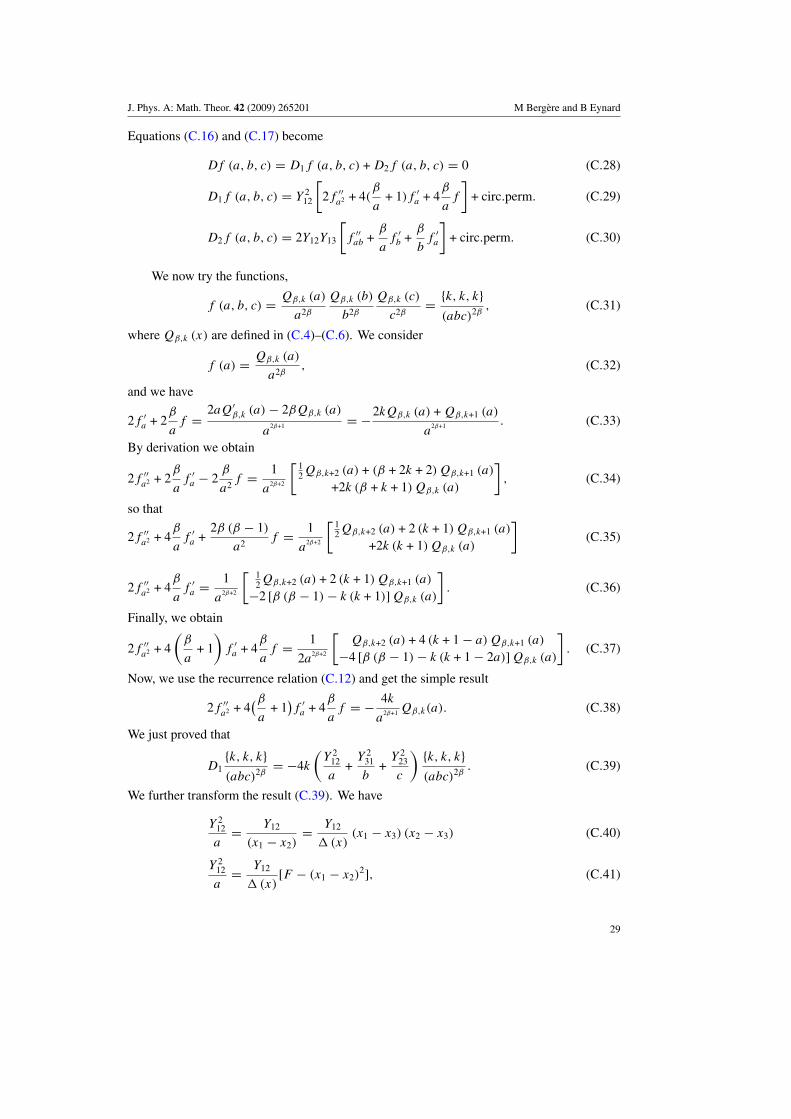
Equations (C.16) and (C.17) become
Df (a, b, c) = D1f (a, b, c) + D2f (a, b, c) = 0 (C.28)
D1f (a, b, c) = Y 212
[2f ′′
a2 + 4(β
a+ 1)f ′
a + 4β
af
]+ circ.perm. (C.29)
D2f (a, b, c) = 2Y12Y13
[f ′′
ab +β
af ′
b +β
bf ′
a
]+ circ.perm. (C.30)
We now try the functions,
f (a, b, c) = Qβ,k (a)
a2β
Qβ,k (b)
b2β
Qβ,k (c)
c2β= {k, k, k}
(abc)2β, (C.31)
where Qβ,k (x) are defined in (C.4)–(C.6). We consider
f (a) = Qβ,k (a)
a2β, (C.32)
and we have
2f ′a + 2
β
af = 2aQ′
β,k (a) − 2βQβ,k (a)
a2β+1 = −2kQβ,k (a) + Qβ,k+1 (a)
a2β+1 . (C.33)
By derivation we obtain
2f ′′a2 + 2
β
af ′
a − 2β
a2f = 1
a2β+2
[ 12Qβ,k+2 (a) + (β + 2k + 2) Qβ,k+1 (a)
+2k (β + k + 1) Qβ,k (a)
], (C.34)
so that
2f ′′a2 + 4
β
af ′
a +2β (β − 1)
a2f = 1
a2β+2
[ 12Qβ,k+2 (a) + 2 (k + 1) Qβ,k+1 (a)
+2k (k + 1) Qβ,k (a)
](C.35)
2f ′′a2 + 4
β
af ′
a = 1
a2β+2
[ 12Qβ,k+2 (a) + 2 (k + 1) Qβ,k+1 (a)
−2 [β (β − 1) − k (k + 1)] Qβ,k (a)
]. (C.36)
Finally, we obtain
2f ′′a2 + 4
(β
a+ 1
)f ′
a + 4β
af = 1
2a2β+2
[Qβ,k+2 (a) + 4 (k + 1 − a) Qβ,k+1 (a)
−4 [β (β − 1) − k (k + 1 − 2a)] Qβ,k (a)
]. (C.37)
Now, we use the recurrence relation (C.12) and get the simple result
2f ′′a2 + 4
(βa
+ 1)f ′
a + 4β
af = − 4k
a2β+1 Qβ,k(a). (C.38)
We just proved that
D1{k, k, k}(abc)2β
= −4k
(Y 2
12
a+
Y 231
b+
Y 223
c
) {k, k, k}(abc)2β
. (C.39)
We further transform the result (C.39). We have
Y 212
a= Y12
(x1 − x2)= Y12
�(x)(x1 − x3) (x2 − x3) (C.40)
Y 212
a= Y12
�(x)[F − (x1 − x2)
2], (C.41)
29
J. Phys. A: Math. Theor. 42 (2009) 265201 M Bergere and B Eynard
where
�(x) = (x1 − x2) (x1 − x3) (x2 − x3), (C.42)
F = x21 + x2
2 + x23 − x1x2 − x1x3 − x2x3. (C.43)
By circular permutation we also have
Y 231
b= Y31
�(x)[F − (x3 − x1)
2] (C.44)
Y 223
c= Y23
�(x)[F − (x2 − x3)
2]. (C.45)
We note that in (C.39) the quantity F disappears since
Y12 + Y23 + Y31 = 0. (C.46)
We may write now
D1{k, k, k}(abc)2β
= 4k
� (x)[(x1 − x2)a + circ.perm.]
{k, k, k}(abc)2β
. (C.47)
We now consider
D2{k, k, k}(abc)2β
. (C.48)
Using
f (a, b, c) = f (a)f (b)f (c), (C.49)
we have
f ′′ab(a, b, c) +
β
af ′
b(a, b, c) +β
bf ′
a(a, b, c) =[(
f ′a(a) + βf (a)
a
)(f ′
b(b) + βf (b)
b
)− β2f (a)f (b)
ab
]f (c) (C.50)
but in (C.30) the term β2
abf (a)f (b)f (c) disappears since
Y12Y13
ab+ circ.perm. = x2 − x3
�(x)+ circ.perm. = 0. (C.51)
Then, from (C.33) we get
=[
2Y12Y13[kQβ,k(a)+ 1
2 Qβ,k+1(a)]a2β+1
[kQβ,k(b)+ 12 Qβ,k+1(b)]
b2β+1Qβ,k(c)
c2β
+circ.perm.
]. (C.52)
Again, the term containing Qβ,k (a) Qβ,k (b) Qβ,k (c) disappears by (C.51). We write
D2{k, k, k}(abc)2β
= 1
�(x)
1
(abc)2β
[(x2 − x3)
[ 12 {k + 1, k + 1, k}
+k {k + 1, k, k} + k {k, k + 1, k}]
+ circ.perm.].
(C.53)
We note that
(x2 − x3) [{k + 1, k, k} + {k, k + 1, k} + {k, k, k + 1}] + circ.perm. = 0, (C.54)
so that
D2{k, k, k}(abc)2β
= 1
�(x)
1
(abc)2β
[(x2 − x3)
[ 12 {k + 1, k + 1, k}−k {k, k, k + 1}
]+ circ.perm.
]. (C.55)
30
J. Phys. A: Math. Theor. 42 (2009) 265201 M Bergere and B Eynard
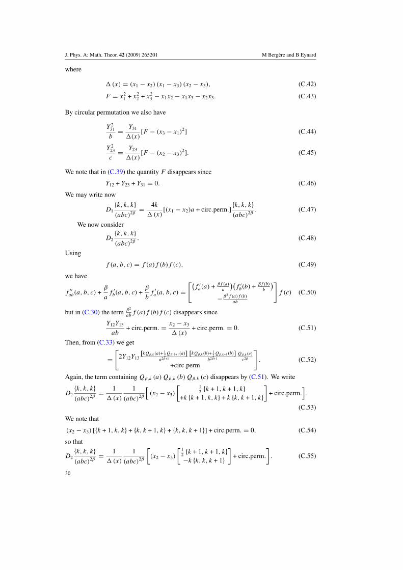
We now collect D1 and D2. From (C.28), (C.31), (C.47) and (C.55), we obtain
D{k, k, k}(abc)2β
= 1
�(x)
1
(abc)2β
⎡⎣(x2 − x3)
[4kc {k, k, k} + 1
2 {k + 1, k + 1, k}−k {k, k, k + 1}
]+circ.perm
⎤⎦ . (C.56)
Again,
(x2 − x3) {k, k, k} + circ.perm = 0 (C.57)
so that
D{k, k, k}(abc)2β
= 1
�(x)
1
(abc)2β
⎡⎣(x2 − x3)
[4k (c − k) {k, k, k}
+ 12 {k + 1, k + 1, k} − k {k, k, k + 1}
]+circ.perm
⎤⎦ .
(C.58)
We now use equation (10) and write
D{k, k, k}(abc)2β
= 1
�(x)
1
(abc)2β
⎡⎣ (x2 − x3)
[12 {k + 1, k + 1, k}
−4k (β − k) (β + k − 1) {k, k, k − 1} ]+circ.perm
⎤⎦ . (C.59)
Consequently, we obtain the remarkable result,
D
[ (β − k)
(β + k)
1
8kk!
{k, k, k}(abc)2β
]
= 1
2�(x)
1
(abc)2β
⎡⎢⎣(x2 − x3)
[ (β−k)
(β+k)1
8kk! {k + 1, k + 1, k}−(β−k+1)
(β+k−1)1
8k−1(k−1)! {k, k, k − 1}
]
+circ.perm
⎤⎥⎦ . (C.60)
Clearly enough, we define for β not the integer
f (abc) =∞∑
k=0
(β − k)
(β + k)
1
8kk!
{k, k, k}(abc)2β
(C.61)
then
Df (abc) = 0 + circ.perm. (C.62)
Now, if β is an integer
Qβ,k�β (x) = 0 (C.63)
and we define
f (abc) =β−1∑k=0
(β − k)
(β + k)
1
8kk!
{k, k, k}(abc)2β
, (C.64)
so that
Df (abc) = 0 + circ.perm. (C.65)
We proved that a solution to (C.14) is
�(xi, yi) =[∞orβ−1∑
k=0
(β − k)
(β + k)
1
8kk!
{k, k, k}(abc)2β
]e∑3
i=1 xiyi (C.66)
HCalogero�(xi, yi) =(∑
i
y2i
)�(xi, yi) , (C.67)
where HCalogero is given in (C.13).
31
J. Phys. A: Math. Theor. 42 (2009) 265201 M Bergere and B Eynard
References
[1] Abramowitz M and Stegun A 1974 Handbook of Mathematical Functions, With Formulas, Graphs, andMathematical Tables (New York: Dover)
[2] Anderson G A 1965 An asymptotic expansion for the distribution of the latent roots of the estimated covariancematrix Ann. Math. Stat. 36 1153–73
[3] Awata H, Matsuo Y, Odake S and Shiraishi J 1995 Phys. Lett. B 347 49[4] Bingham C 1972 An asymptotic expansion for the distribution of the eigenvalues of a 3 by 3 Wishart matrix
Ann. Math. Stat. 43 1498–506[5] Baker T H and Forrester P J 1997 The Calogero–Sutherland model and generalized classical polynomials
Commun. Math. Phys. 188 175–216[6] Brezin E and Hikami S 2002 An extension of the Harish-Chandra–Itzykson–Zuber integral arXiv:
math-ph/0208002[7] Calogero F 1969 Ground state of a one-dimensional N-body system J. Math. Phys. 10 2197–200[8] Carlitz L 1957 A note on the Bessel polynomials Duke Math. J. 24 151–62[9] Chekhov L and Eynard B 2006 Matrix eigenvalue model: Feynman graph technique for all genera J. High
Energy Phys. JHEP12(2006)026 (arXiv:math-ph/0604014)[10] Desrosiers P 2008 Duality in random matrix ensembles for all Beta arXiv:0801.3438[11] Duistermaat J J and Heckman G J 1982 Inv. Math. 69 259[12] Dunkle C F 1989 Transl. Am. Math. Soc. 311 167[13] Dyson F J 1962 Statistical theory of the energy levels of complex systems: I J. Math. Phys. 3 140–56[14] Harish-Chandra 1957 Am. J. Math. 79 87–120[15] Eynard B 2004 A short note about Morozov’s formula arXiv:math-ph/0406063[16] Eynard B 2001 Asymptotics of skew orthogonal polynomials J. Phys. A: Math. Gen. 34 7591
(arXiv:cond-mat/0012046)[17] Eynard B and Prats Ferrer A 2005 Commun. Math. Phys. 264 115–44 (arXiv:hep-th/0502041) (erratum to be
published)[18] Ginibre J 1965 J. Math. Phys. 6 440
Girko V 1985 Theor. Prob. Appl. 29 694[19] Herz C 1955 Ann. Math. 61 474–523[20] Kohler H and Guhr T 2002 J. Math. Phys. 43 2707 (arXiv:math-ph/0011007)[21] Kohler H and Guhr T 2005 Supersymmetric extensions of Calogero–Moser–Sutherland-like models:
construction and some solutions J. Phys. A: Math. Gen. 38 9891–915[22] Itzykson C and Zuber J-B 1980 J. Math. Phys. 21 411–21[23] Jevicki A and Sakita B 1980 Nucl. Phys. B 165 511[24] Jevicki A and Sakita B 1981 Nucl. Phys. B 185 89[25] Jevicki A 1990 Collective field theory and Schwinger–Dyson equations in matrix models Proc. Meeting
‘Symmetries, Quarks and Strings’ (City College, NY, 1–2 Oct.) (Preprint Brown-HET-777)[26] Knapp A W 1986 Representation Theory of Semisimple Groups (Princeton, NJ: Princeton University Press)[27] Krall H L and Fink O 1948 A new class of orthogonal polynomials: the Bessel polynomials Trans. Am. Math.
Soc. 65 100–15[28] Macdonald I G 1995 Symmetric Functions and Hall Polynomials 2nd edn (Oxford: Clarendon)[29] Mehta M L 1991 Random Matrices 3rd edn (New York: Academic)[30] Mehta M L 1981 A method of integration over matrix variables Commun. Math. Phys. 79 3[31] Migdal A A 1983 Phys. Rep. 102 199
David F 1990 Mod. Phys. Lett. A 5 1019[32] Morozov A 1992 Mod. Phys. Lett. A 7 3503–8 (arXiv:hep-th/9209074)[33] Prats Ferrer A, Eynard B, Di Francesco P and Zuber J-B 2009 Correlation functions of Harish-Chandra integrals
over the orthogonal and the symplectic groups J. Stat. Phys. 129 885–935 (arXiv:math-ph/0610049)[34] Shatashvili S 1993 Commun. Math. Phys. 154 421–32 (arXiv:hep-th/9209083)[35] Wiegmann P and Zabrodin A 2006 Large N expansion for the 2D Dyson gas arXiv:hep-th/0601009[36] Zuber J B 2008 On the large N limit of matrix integrals over the orthogonal group arXiv:0805.0315
32


