Northridge, California, earthquake of 1994: density of red-tagged buildings versus peak horizontal velocity and intensity of shaking

E L S E V I E R

Soil Dynamics and Earthquake Engineering 16 (1997) 209-222 © 1997 Elsevier Science Limited

Printed in Great Britain. All rights reserved P I I : S 0 2 6 7 - 7 2 6 1 ( 9 6 ) 0 0 0 4 3 - 7 0267-7261/97/$17.00

Northridge, California, earthquake of 1994: density of red-tagged buildings versus peak horizontal velocity and intensity of shaking

M. D. Trifunac & M. I. Todorovska Department of Civil Engineering, University of Southern California, Los Angeles, CA 90089-2531, USA

(Received 24 September 1996; accepted 25 September 1996)

The 1994 Northridge earthquake occurred underneath a densely populated metropolitan area, and was recorded by over 200 strong motion stations in the metropolitan area and vicinity. This rare coincidence made it an ideal case to study, in statistical sense, the correlation of damage to structures with the level of strong shaking, in particular with respect to (1) instrumental characteristics of shaking and (2) the reported site intensity scale. In this paper, statistics for the incidence of red-tagged building in 1 x 1 km 2 blocks in San Fernando Valley and Los Angeles is presented and analyzed, as function of the observed peak ground velocity or the local intensity of shaking. The 'observed' peak velocity is estimated from contour maps based on the recorded strong motion. The intensity of shaking is estimated from the published intensity map and from our modification of this map to make it more consistent with observed high damage to buildings in some localized areas. Finally, empirical scaling equations are derived which predict the average density of red-tagged buildings (per km 2) as a function of peak ground velocity or site intensity of shaking. These scaling equations are specific to the region studied, and apply to Wooden Frame Construction, typical of post World War II period, which is the prevailing building type in the sample studied. These can be used to predict the density of red-tagged buildings per km ~in San Fernando Valley and in Los Angeles for a scenario earthquake or for an ensemble of earthquakes during specified exposure, within the framework of probabilistic seismic hazard analysis. Such predictions will be useful to government officials for emergency planning, to the insurance industry for realistic assessment of insured losses, and to structural engineers for assessment of the overall performance of this type of buildings. © 1997 Elsevier Science Limited. All rights reserved.

Key words: Northridge earthquake, damage, red-tagged buildings.

I N T R O D U C T I O N

Analysis of earthquake damage to man-made structures is difficult and complex. Neither the structural resistance, nor the local shaking can be represented only by a small number of parameters. Factors which must be considered in describing the response and ultimate strength of structures are, for examples, the differences in the construction materials, the variety of geometrical and architectural characteristics, the presence of and type of members for lateral load resistance and the evolution of the design codes. The strong earthquake shaking also needs to be described by at least several scaling parameters, for example, peak amplitudes, spectral content and duration of strong shaking. These parameters can be

209

related to the total energy or to the power of strong motion, but cannot be related to the damage in a simple and direct way. Much work remains to be carried out to find a set of scaling parameters for strong ground motion which will describe well the observed damage.

Simplified approaches have been proposed and used to describe the observed damage. For example, Benioff 1 proposed to measure the destructiveness of ground motion by computing the area under the response spec- trum, Arias 2 - - by the integral f a2dt, where a is the ground acceleration, and Duvall and Fogelson 3 - - by the peak ground velocity. In such approaches, the effects of the many 'other ' scaling variables are averaged out implicitly or explicitly, and, therefore, the results are at best site or region specific. Results of such simplified

210 M. D. Trifunac, M. I. Todorovska

studies are useful for short term approximate predictions of future overall effects of strong earthquakes in an area.

The inadequate density of strong motion recording instruments further complicates the analysis of earthquake damage. The Los Angeles metropolitan area is probably one of the most densely instrumented areas in the world; yet, the density of the recording instruments is insufficient to describe adequately variations of strong motion over short distances, e.g. hundreds of meters, which is important for structures on multiple supports. 4 Knowledge acquired from specialized dense arrays in other countries (e.g. the SMART-1 array near Lotung in Taiwan) is not directly transferable to specific problems in the United States, due to differences in the nature of the seismogenic zone and in the local geologic and soil site conditions. For example, the differences in the age of surface soils and geology may introduce bias in estimates of amplitudes of strong motion. 5'6 The width, length, and depth of active faults will influence the observed strong motion at long periods 7 and the duration of strong shaking. 8,9

Often earthquake damage has been related to the local intensity of shaking. The intensity scale is a descriptive measure based on the effects of shaking on ground and on structures, and therefore leaves room for subjective interpretation. The field observations and published results on intensities following a damaging earthquake depend not only on the definition of the intensity scale used and on the team that gathers, interprets and presents the results, but also on type and distribution of structures, construction materials, and the geologic setting of the shaken area. Earthquakes of similar magnitudes can be disastrous in one region, but cause minor damage in another. A perusal of damage reports for the western United States during the last 50yr typically indicates only 'little or moderate' damage, so far. One consequence of this is that, for the United States, there is no adequate database on damage for high intensity levels of shaking to construct empirical sets of fragility curves for various structural systems. Comprehensive description of earthquake damage has been attempted by Chinese engineers following the Tangshan earthquake in 1976, l° and by Yugoslav investigators following the Monte Negro earthquake in 1979. ll These results, however, are not directly applicable to urban areas in the United States, due to differences in the intensity scales and in the type of construction. Many metropolitan areas in the United States, do have thousands of old unreinforced brick masonry structures, and would benefit from the avail- ability of fragility functions for these buildings. How- ever, the fragility functions developed for Tangshan and Monte Negro might be used only after careful relative calibration of the intensity scales and of construction methods and materials.

The Northridge earthquake (17 January 1994, ML = 6'4, M w = 6-7, focus at H ~ 18 km) occurred on a blind thrust fault underneath San Fernando Valley, of

the densely populated Los Angeles metropolitan area. In spite of the moderate size of this earthquake, some areas experienced severe shaking (IX on the Modified Mercalli scale), and many buildings, utility lines and freeway structures were damaged. Many buildings were inspected and tagged (as green, yellow or red), and the results were documented and available for analysis. 12-14 The ground shaking was recorded by more than 200 strong motion stations in the metropolitan area and vicinity. Based on the spatial distribution of recorded motion, contour maps were drawn for horizontal and vertical peak ground acceleration and velocity, 4'15 which made it possible to estimate the range of ground motion amplitudes at locations away from the recording stations. A contour map of Modified Mercalli Intensity was also prepared. J6 Using these contour maps, it is possible to estimate the range of peak velocity and the intensity of shaking at all sites of damaged buildings. Although both the information on damage from tagging the buildings and on ground motion from the contour maps of peak velocity or site intensity are simplified, the data are fairly complete for the areas inspected, and covers useful range of the levels of shaking (intensities V-IX).

This paper presents an analysis of the density of red- tagged buildings in San Fernando Valley and in Los Angeles as a function of the horizontal peak ground velocity and the intensity of shaking. The purpose is to derive simple, locally applicable, empirical relations for quick assessment of the density of severely damaged buildings during future earthquakes, based on the simplified characterization of damage in buildings in terms of the peak ground velocity and the local intensity of shaking at the site.

OBSERVATIONS

Strong ground motion

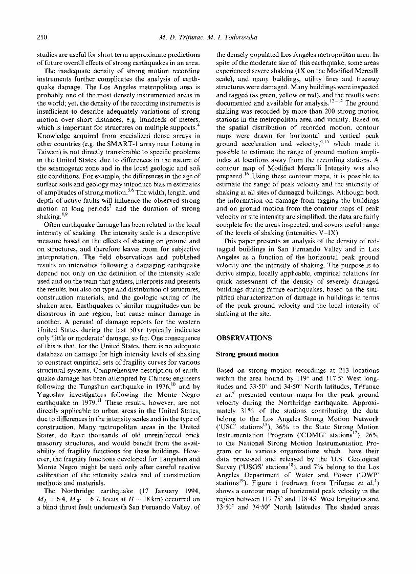
Based on strong motion recordings at 213 locations within the area bound by 119 ° and 117.5 ° West longitudes and 33-50 ° and 34,50 ° North latitudes, Trifunac et al. 4 presented contour maps for the peak ground velocity during the Northridge earthquake. Approxi- mately 31% of the stations contributing the data belong to the Los Angeles Strong Motion Network ( 'USC' stationslS), 36% to the State Strong Motion Instrumentation Program ( 'CDMG' stationsl7), 26% to the National Strong Motion Instrumentation Pro- gram or to various organizations which have their data processed and released by the U.S. Geological Survey ( 'USGS' stationslS), and 7% belong to the Los Angeles Department of Water and Power ( 'DWP' stationsl9). Figure 1 (redrawn from Trifunac et al. 4) shows a contour map of horizontal peak velocity in the region between 117.75 ° and 118.45 ° West longitudes and 33-50 ° and 34-50 ° North latitudes. The shaded areas

Northridge, California, earthquake of 1994: density of red-tagged buildings 211

indicate bedrock, and the white areas sediments. The dashed or full lines, drawn by hand, show smoothed contours of the larger peak velocity value of the two horizontal components recorded in 'free-field'. The circular (USC), triangular (CDMG), square (USGS) and diamond (DWP) symbols show the location of the strong motion instruments.

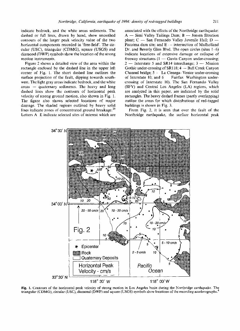
Figure 2 shows a detailed view of the area within the rectangle enclosed by the dashed line in the upper left corner of Fig. 1. The short dashed line outlines the surface projection of the fault, dipping towards south- west. The light gray areas indicate bedrock, and the white areas - - quaternary sediments. The heavy and long dashed lines show the contours of horizontal peak velocity of strong ground motion, also shown in Fig. 1. The figure also shows selected locations of major damage. The shaded regions outlined by heavy solid lines indicate zones of concentrated ground breakage. 2° Letters A - E indicate selected sites of interest which are

associated with the effects of the Northridge earthquake: A - - Simi Valley Tailings Dam; B - - Jensen filtration plant; C - - San Fernando Valley Juvenile Hall; D - - Pacoima dam site; and E - - intersection of Mulholland Dr. and Beverly Glen Blvd. The open circles (sites 1-6) indicate locations of extensive damage or collapse of freeway structures (1 - - Gavin Canyon under-crossing; 2 - - Interstate 5 and SR14 interchange; 3 - - Mission Gothic under-crossing of SR118; 4 - - Bull Creek Canyon Channel bridge; 5 - - La Cienega-Venice under-crossing of Interstate 10; and 6 - - Fairfax-Washington under- crossing of Interstate 10). The San Fernando Valley (SFV) and Central Los Angeles (LA) regions, which are analyzed in this paper, are indicated by the solid rectangles. The heavy dashed frames (partly overlapping) outline the areas for which distributions of red-tagged buildings is shown in Fig. 3.

From Fig. 2, it is seen that over the fault of the Northridge earthquake, the surface horizontal peak

34 ° 30'

34 ° 00' hi

33 ° 30' N

, - - . t i - i i i in i l : ! l i i l ' i i i i , ,~.. ! l l : . i ! i : ' lk i $ - . o 7 l l I i r i i i - : t i ' ~ i ~ i ! l~ i i t i t i t i ' : ! ' i l lm" : : : . ' i t i i . i= i , I , I l D . ! ! f = . t L t i i h , H H I : . I . I = ~ . I ! : ...... oo~ . . . . . . . . . . . . . ! . . . . . ~ 1~i I (~ ' t =~ ' : i I i l t l i i i II tt:t::r:il I l i l i t l t t l l I ......... iniltiiiimLu~ . i ! ! t i : i i t l l h i : l , : ! i ~ l l i - J t Z , J Io f l i i n t,":,:ilililt , ," ",:.It: u:: , : . i i ! ! ! l l l i : i i ! i l ' - ' : ~ i . . ::.l i l ~ ~ • - - i t l I i . ,~ 1~4~ " ---- I \ . " ~ i i , i ~ ~ , , , , ~ , , , , !!~"!!~'LtiU'~!i,ii,l.~llt~t'li'l!ti'~l!'ii"'iliii~!iii.hll~!tttfllll~i

-" U ii:::"~. - ~ - "=i r ' ! ":::, i i" iii"iin"i,'ii o ! t r: I l l ! t l i h'i i l l l l l t E t i l l l t l l l

.............. ~ . i . i ~ " ~ * " - ' - " - ~ ~!~ ........... it.,,,',! .......... mm::m~t:. - : : . • i ~ :" ::.itl U i :: l : l l l l ! !..'.:lli!!l~i pl 0-20"\ di l l i i , : i . ~ i i } i ~ - i ~ ~ : " ' i : i i i~: ' l i t i liii.::iil

.:I • ~ . . : ' i ! q i : l iE:i:,, v ' - - , Httti,, ti~.."i~.." . . . . . . ~ i ~ ' P ° '

'ii.:iiill f i l l iE'i:i:'iiiiiiiitl. :ii~iiiii'iii.:l:il : .......... :i!}: I • • • ,iiiiiiiiiiiiii:,~!iiliiiiiiiii~ ' ~ _" _ t . ~

10 20 ~ +..., _- .,~i'-,,~_~r'~, ,,.' 20"" .' ~']"~i~ 5 ' " ~ r ..riF.:irii:i

. . . . . . 7 : . . . . . . . . . . . . . . . . . . . . . .

o i l • S s S ~ s ~'

Fig. 2

~ i i T i e ~ i : r r y Deposi ts ~ ' ~

Hor zonta Peak Velocity -.cm/s

i I . . . . . . . . . . , ~" i • . l... z";iiiii : ~Ft.:~ilrl .:m, ::: . . : ' i . ti." ,. : :

t • :::..:: :.m.':.li: :..:.::u.:

• • • i n / ~ ": : i!i."::.~.: . . . . E.:|:IE:.-=.4

/ 10-20cm/s. / "105

10 "'} , l ' o ~t T M

• ~ / ~ ~ ii!:'.:i.' I "J :.!i!:

/ "

2-5cm/s 10 ~ • :m ":::::::i: :::i:::::

p a o [ ~ i i t ~ .. l i i i i i ! i lh:it i ! l l

";,'i-:.ii!" Ocean N . . . .

118 ° 30' W 118 ° O0 'W

Fig. 1. Contours of the horizontal peak velocity of strong motion in Los Angeles basin during the Northridge earthquake. The triangular (CDMG), circular (USC), diamond (DWP) and square (USGS) symbols show locations of the recording accelerographs. 4

212

118°45'W

M. D. Trifunac, M. I. Todorovska

1 1 8 ° 3 0 ' W 1 1 8 ° 1 5 ' W

FE

F

. . . . . . . u . . . . . . . ~ . . . . I Fig. 3b i

Fig. 2. The epicentral area of the Northridge earthquake (17 January 1994, ML = 6'4). The short dashed line outlines the surface projection of the fault. The light gray areas indicate bedrock, and the white areas - - quaternary sediments. The circular, triangular, diamond and square, symbols show the locations of the strong motion sites used in the analysis. The shaded regions outlined by heavy

14r9 solid lines indicate zones of concentrated ground breakage. ' A - - Simi Valley Tailings Dam; B - - Jensen filtration plant; C - - San Fernando Valley Juvenile Hall; D - - Pacoima dam site; E - - intersection of Mulholland Dr. and Beverly Glen Blvd. The open circles indicate locations of extensive damage or collapse of freeway structures. 1 - - Gavin Canyon under-crossing; 2 - - Interstate 5 and SR14 interchange; 3 - - Mission Gothic under-crossing of SR118; 4 - - Bull Creek Canyon Channel bridge; 5 - - La Cienega-Venice under-crossing of Interstate 10; and 6 - - Fairfax-Washington under-crossing of Interstate 10. The two regions studied in this paper, San Fernando Valley and Los Angeles, are outlined by heavy frames. The heavy dashed frames outline the areas for which

distribution of red-tagged buildings is shown in Fig. 3.

velocity, 1)max, was about or exceeded 100cm/s. South and central San Fernando Valley experienced horizontal peak ground velocities greater than 50 cm/s. These peak velocity amplitudes depend locally on the soil and on the geologic site conditions. In this paper, however, by the procedure used to correlate peak velocities with the number of red-tagged buildings, those two effects will be implicitly averaged out. Most building sites contributing to these data are located on alluvium and on ' typical ' soil. 4 The magnitude of the Northridge earthquake, the effects of its mechanism and radiation pattern and the changes of wave amplitudes and direction of motion along the propagat ion path are all implicitly considered and are reflected in the geographical variation of the observed peak amplitudes as plotted in Figs 1 and 2. In this study, the amplitudes of maximum horizontal velocity, shown by contours in these figures, will be used as representing 'measured ' peak velocities.

Damage

The data on the location of red-tapped structures, used in this study, were compiled and distributed by the Los Angeles Depar tment of Building Safety. 12 In April 1994, there were more than 1 000 red-tagged buildings and more than 5 500 yellow-tagged buildings. With time, these numbers have changed as additional buildings were inspected and previously tagged buildings re-evaluated. For the purposes of this work, it is assumed that, following April 1994, these changes were minor among the population of red-tagged buildings. Figure 3a (San Fernando Valley region) shows the early distribution of red-tagged buildings, as of March 1994. Figure 3(b) shows this distribution in the Los Angeles region. To show the relationship among several areas of concentrated building damage, the areas in Figs 3(a) and 3(b) partially overlap (Fig. 3b repeats the data shown in the


34°22.~ N -., lg

• , Sylmar

•

.,J . . - ..~ . ,,..,-, ~_ • " • ',- .'" ,.- ~:" / "- 03C

• . . ,ff - ...... ~. "." . [-:.',. :':":='v " ~" '~:" ", *.Sepulved~VA

• " " ~ , Z " " . " . \ = " .

• " v,.. :,. "-':~t" • .~," • ,LArleta 53"

" I " - " " • " . " - - ' k . . . . 5 . _ , . - .

• . •

,". .:, ..,<>" . . " " - , . :: Tarzana:" '" '" "~" ~'~';'g'~" ;i)

34 ° 15' N

34000 ' N

:" 2: .L . . ' ( . i •

. . . .

• 1"3 I1", ~ Y • . -~-Gr i f f i thO.~ \ 5 " • " • 1 E l l "'/ " " • "

••:

o,3o o.59 /

"

e . . . .

118°37.5~ W 118°22.5~ W 118o30, W 118°1,~ W

a) b)

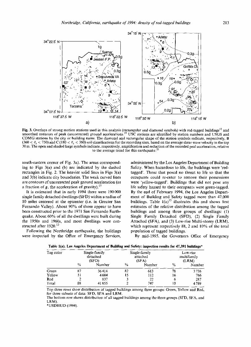
• • 12 Fig. 3. Overlays of strong motion stations used in this analysis (rectangular and diamond symbols) with red-tagged buildings and • 1 5 • smoothed contours of peak (uncorrected) ground acceleraOons. USC stations are identified by station numbers and USGS and

CDMG stations by the city or building name• The diamond and rectangular shape of the station symbols indicate, respectively, B (360 < 9s < 750) and C (180 < ~s < 360) soil classifications for the recording sites, based on the average shear wave velocity in the top 30 m• The open and shaded large symbols indicate, respectively, amplification and reduction of the recorded peal acceleration, relative

to the average trend for this earthquake? t

south-eastern corner of Fig. 3a). The areas cgrrespond- ing to Figs 3(a) and (b) are indicated by the dashed rectangles in Fig. 2. The heavier solid lines in Figs 3(a) and 3(b) indicate city boundaries. The weak curved lines are contours of uncorrected peak ground acceleration (as a fraction of g, the acceleration of gravity)•15

It is estimated that in early 1994 there were 190000 single family detached dwellings (SFD) within a radius of 10 miles centered at the epicenter (i.e. in Greater San Fernando Valley). About 90% of those appear to have been constructed prior to the 1971 San Fernando Earth- quake• About 60% of all the dwellings were built during the 1950s and 1960s, and most dwellings were constructed after 1920.13

Following the Northridge earthquake, the buildings were inspected by the Office of Emergency Services,

administered by the Los Angeles Depar tment of Building Safety. When hazardous to life, the buildings were 'red- tagged'. Those that posed no threat to life so that the occupants could re-enter to remove their possessions were 'yellow-tagged'. Buildings that did not pose any life safety hazard to their occupants were green-tagged. By the end of February 1994, the Los Angeles Depart- ment of Building and Safety tagged more than 47,000 buildings. Table l(a) 13 illustrates this and shows first estimates of the relative distribution among the tagged buildings and among three groups of dwellings: (1) Single Family Detached (SFD), (2) Single Family Attached (SFA), and (3) Low-rise Multi-storey (LRM), which represent respectively 88, 2 and 10% of the total population of tagged buildings.

By mid-1995, the Governors Office of Emergency

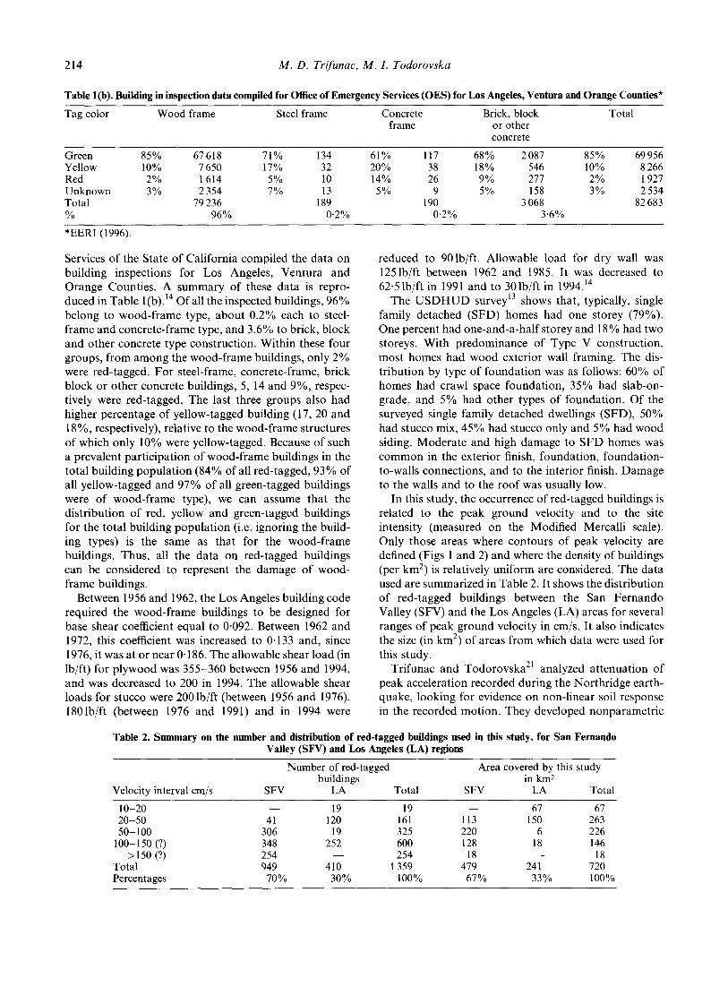
Table l(a). Los Angeles Department of Building and Safety: inspection results for 47,391 buildings*

Tag color Single-family Single-family Low-rise detached attached multifamily

(SFD) (SFA) (LRM) % Number % Number % Number

Green 87 36 414 82 613 78 3 736 Yellow 11 4 604 15 112 16 766 Red 2 837 3 22 6 287 Total 88 41 855 2 747 10 4 789

Top three rows show distribution of tagged buildings among three groups: Green, Yellow and Red, for three subsets of data: SFD, SFA and LRM. The bottom row shows distribution of all tagged buildings among the three groups (SFD, SFA, and LRM). *USDHUD (1994).

214 M . D . Tr~unac, M. I. Todorovska

Table l(b). Building in inspection data compiled for Office of Emergency Services (OES) for Los Angeles, Ventura and Orange Counties*

Tag color Wood frame Steel frame Concrete Brick, block Total frame or other

concrete

Green 85% 67 618 71% 134 61% 117 68% 2087 85% 69 956 Yellow 10% 7 650 17% 32 20% 38 18% 546 10% 8 266 Red 2% 1614 5% 10 14% 26 9% 277 2% 1927 Unknown 3% 2354 7% 13 5% 9 5% 158 3% 2534 Total 79 236 189 190 3068 82 683 % 96% 0-2% 0.2% 3.6%

*EERI (1996).

Services of the State of California compiled the data on building inspections for Los Angeles, Ventura and Orange Counties. A summary of these data is reproduced in Table l(b). 14 Of all the inspected buildings, 96% belong to wood-frame type, about 0.2% each to steel- frame and concrete-frame type, and 3.6% to brick, block and other concrete type construction. Within these four groups, from among the wood-frame buildings, only 2% were red-tagged. For steel-frame, concrete-frame, brick block or other concrete buildings, 5, 14 and 9%, respectively were red-tagged. The last three groups also had higher percentage of yellow-tagged building (17, 20 and 18%, respectively), relative to the wood-frame structures of which only 10% were yellow-tagged. Because of such a prevalent participation of wood-frame buildings in the total building population (84% of all red-tagged, 93 % of all yellow-tagged and 97% of all green-tagged buildings were of wood-frame type), we can assume that the distribution of red, yellow and green-tagged buildings for the total building population (i.e. ignoring the building types) is the same as that for the wood-frame buildings. Thus, all the data on red-tagged buildings can be considered to represent the damage of wood- frame buildings.

Between 1956 and 1962, the Los Angeles building code required the wood-frame buildings to be designed for base shear coefficient equal to 0.092. Between 1962 and 1972, this coefficient was increased to 0.133 and, since 1976, it was at or near 0.186. The allowable shear load (in lb/ft) for plywood was 355-360 between 1956 and 1994, and was decreased to 200 in 1994. The allowable shear loads for stucco were 200 lb/ft (between 1956 and 1976), 1801b/ft (between 1976 and 1991) and in 1994 were

reduced to 901b/ft. Allowable load for dry wall was 1251b/ft between 1962 and 1985. It was decreased to 62-51b/ft in 1991 and to 301b/ft in 1994.14

The U S D H U D survey 13 shows that, typically, single family detached (SFD) homes had one storey (79%). One percent had one-and-a-half storey and 18 % had two storeys. With predominance of Type V construction, most homes had wood exterior wall framing. The distribution by type of foundation was as follows: 60% of homes had crawl space foundation, 35% had slab-on- grade, and 5% had other types of foundation. Of the surveyed single family detached dwellings (SFD), 50% had stucco mix, 45% had stucco only and 5% had wood siding. Moderate and high damage to SFD homes was common in the exterior finish, foundation, foundation- to-walls connections, and to the interior finish. Damage to the walls and to the roof was usually low.

In this study, the occurrence of red-tagged buildings is related to the peak ground velocity and to the site intensity (measured on the Modified Mercalli scale). Only those areas where contours of peak velocity are defined (Figs 1 and 2) and where the density of buildings (per km 2) is relatively uniform are considered. The data used are summarized in Table 2. It shows the distribution of red-tagged buildings between the San Fernando Valley (SFV) and the Los Angeles (LA) areas for several ranges of peak ground velocity in cm/s. It also indicates the size (in km 2) of areas from which data were used for this study.

Trifunac and Todorovska 21 analyzed attenuation of peak acceleration recorded during the Northridge earthquake, looking for evidence on non-linear soil response in the recorded motion. They developed nonparametric

Table 2. Summary on the number and distribution of red-tagged buildings used in this study, for San Fernando Valley (SFV) and Los Angeles (LA) regions

Number of red-tagged Area covered by this study buildings in km 2

Velocity interval cm/s SFV LA Total SFV LA Total

10-20 - - 19 19 - - 67 67 20-50 41 120 161 113 150 263 50-100 306 19 325 220 6 226

100-150 (?) 348 252 600 128 18 146 >150 (?) 254 - - 254 18 - - 18

Total 949 410 1 359 479 241 720 Percentages 70% 30% 100% 67% 33% 100%


attenuation curves for horizontal and vertical peak acceleration for 'hard' and for 'soft' sites. Figure 3 shows overlays of the early reported distribution of red-tagged buildings 12 with contours of horizontal peak acceleration 15 and location of stations used by Trifunac and Todorovska 21 for two regions, enclosed by the dashed rectangular areas in Fig. 2. The enlarged shaded and open station symbols indicate, respectively, reduction and amplification of horizontal peak acceleration, relative to the average trend defined by the attenuation curve for the 'hard' sites. It is seen from Fig. 3 that in central San Fernando Valley, in the regions where there was evidence of non-linear soil response, there were no extended or large areas with concentration of red-tagged buildings; the distribution was 'random', relatively uniform and not very dense. In the blocks surrounding accelerograph stations USC No. 3, 6, 9 and 53 (Fig. 3a), there were not many red- tagged buildings. Moving further south, one encounters four zones of concentrated red-tagged buildings: one along Ventura Blvd, between Laurel Canyon and 405 Freeway (near and north of sites USC No. 13 and 14, Fig. 3a), the second along Sunset Blvd., between Vermont and Highland (near sites USC No. 18 and 21, Fig. 3b), the third along Interstate 10, between Crenshaw Blvd and Fairfax Blvd (near site USC No. 91, Fig. 3b), and the fourth near the intersection of Harbor Freeway and Vernon (near site USC No. 22, Fig. 3b). Figure 3 shows that at least one site with larger than average (amplified, open station symbol) peak acceleration may be associated with the areas of concentration of red-tagged buildings. Thus, it is possible that the overall damage level was

reduced in the San Fernando Valley by nonlinear response of shallow sediments and soft soil layers. 21

In this paper, we analyze the frequency of occurrence of red-tagged buildings only. Many red and yellow- tagged buildings were later downgraded because of overly conservative tagging, or removal of hazard (e.g. leaning or cracked chimneys). The data covering the complete building population have been presented and interpreted by the City of Los Angeles Department of Building and Safety, 12 Office of Emergency Services, 22 LA H D 23 and Comerio. 24 The volume, the nature of these data sets and the methods used in the presentation have varied with time of reporting, and with the agency reporting, and thus it will take some time before all this information is carefully sorted out. We believe that the population of red-tagged buildings is well defined and stable at present, and that the future reviews of data will not result in significant changes in the number or in the geographical distribution of these buildings. After the population of yellow-tagged buildings is studied more, and when the nature and the levels of actual damage are further researched, it will be possible to extend this analysis to yellow-tagged buildings as well.

ANALYSIS

Density of red-tagged buildings versus horizontal peak velocity

San Fernando Valley and Los Angeles regions (Fig. 2)

401 1L <vo< o cm" 2o ~1=0.284

0 o 4 8

N

16o 50 - cm/s

140

120 50 < v ~ < 100 - cm/s

100 100 [r-I iql= 1.44

2O

0 0 ~ ' ~ - ~ - ~ " 0 4 8 0 4 8

N N

cm's :I 150 vo cm,s 20 Iq=3 ,82 ~1=14.11

0 . . . . . O" 0 4 8 12 16 20 0 4 8 12 16 20

N N

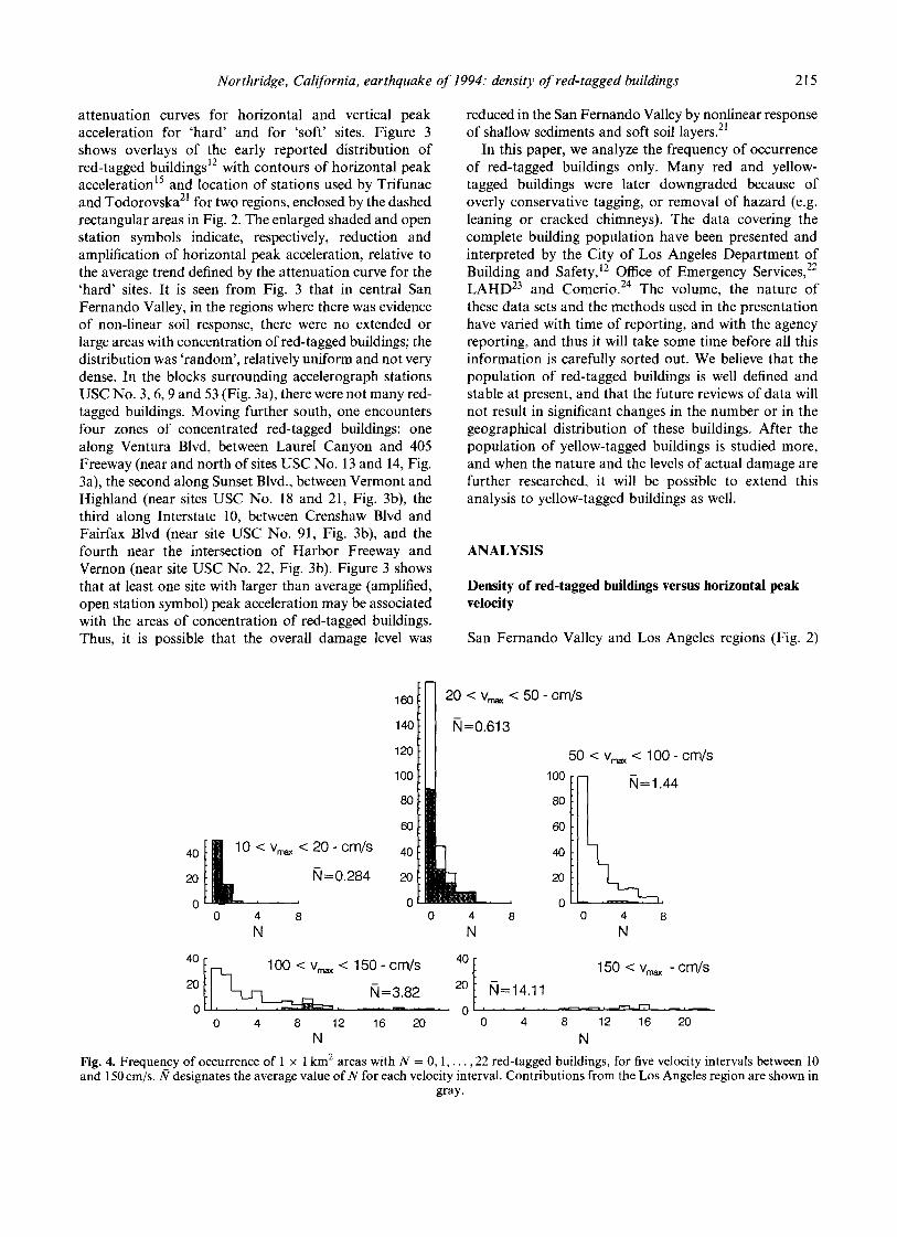
Fig. 4. Frequency of occurrence of l x 1 km 2 areas with N = 0, 1,. . . , 22 red-tagged buildings, for five velocity intervals between l0 and 150 cm/s. N designates the average value of N for each velocity interval. Contributions from the Los Angeles region are shown in

gray.


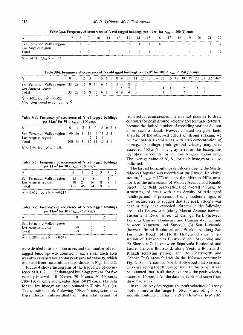
Table 3(a). Frequency of occurrence of N red-tagged buildings per I km z for Vma x > 150 (?) cm/s

N 7 8 9 10 11 12 13 14 15 16 17 18 19 20 21 22

San Fernando Valley region 1 2 1 2 1 3 1 4 1 1 1 Los Angeles region Total 1 2 1 2 1 3 1 4 1 1 1

= 14.11, logl0N = 1"15.

Table 3(b). Frequency of occurrence of N red-tagged buildings per I km 2 for 100 < Vmax < 150 (?) cm/s

N 0 1 2 3 4 5 6 7 8 9 10 11 12 13 14 15 16 17 18 19 20 21 22 46*

San Fernando Valley region 33 28 15 9 15 6 6 5 3 4 2 2 Los Angeles region 2 1 5 2 1 1 1 2 1 1 1 Total 33 28 15 9 15 6 6 7 4 9 4 3 1 1 2 1 1 1

N- -- 3-82, logl0 ~ = 0'582. *Not considered in computing N.

Table 3(c). Frequency of occurrence of N red-tagged buildings per l k m 2 for 50 < Vma x < 100cm/s

N 0 1 2 3 4 5 6 7 8

San Fernando Valley region 99 46 31 14 9 11 5 5 Los Angeles region 1 2 2 1 Total 100 46 31 16 11 12 5 5

= 1.44, log10 S] = 0.158.

Table 3(d). Frequency of occurrence of N red-tagged buildings per I km 2 for 20 < Vma x <~ 50 cm]s

N 0 1 2 3 4 5

San Fernando Valley region 85 18 8 1 1 Los Angeles region 90 27 16 8 8 1 Total 175 45 24 9 9 1

.N = 0.613, lOgl0 N = -0.213.

Table 3(e). Frequency of occurrence of N red-tagged buildings 2 per I km for 10 < Vma x < 20 cm]s

N 0 1 2 3

San Fernando Valley region Los Angeles region 50 15 2 Total 50 15 2

= 0'284, lOgl0 N = -0.547.

were divided into 1 x 1 km areas and the number of red- tagged buildings was counted in each area. Each area was also assigned horizontal peak ground velocity, which was read from the contour maps shown in Figs 1 and 2.

Figure 4 shows histograms of the frequency of occurrence of 0, 1 ,2 , . . . , 22 damaged buildings per km 2 for five velocity intervals: 10-20 cm/s, 20-50 cm/s, 50-100 cm/s, 100 150 (?) cm/s and greater than 150 (?) cm/s. The data for the five histograms are tabulated in Tables 3(a)-(e). The question mark following 150cm/s designates that these interval limits resulted from interpretation and not

from actual measurement. It was not possible to draw contours for peak ground velocity greater than 150 cm/s, because the limited number of recording stations did not allow such a detail. However, based on post facto analysis of the observed effects of strong shaking, we believe that in several areas with high concentration of damaged buildings, peak ground velocity may have exceeded 150cm/s. The gray area in the histograms identifies the counts for the Los Angeles region only. The average value of N, N, for each histogram is also indicated.

The largest horizontal peak velocity during the North- ridge earthquake was recorded at the Rinaldi Receiving station, 19 Vma x = 177cm/s, in the Mission Hills area, north of the intersection of Wooley Avenue and Rinaldi Street. The field observations of overall damage to structures, of areas with high density of red-tagged buildings and of presence of only moderate signs of near surface strains suggest that the peak velocity was near or may have exceeded 150cm/s in the following areas: (1) Chatsworth (along Mason Avenue between Lassen and Devonshire), (2) Canoga Park (between Topanga Canyon Boulevard and Canoga Avenue, and between Vanowen and Saticoy), (3) San Fernando (between Brand Boulevard and Workman, along San Fernando Road), (4) North Hollywood (near intersection of Lankershim Boulevard and Magnolia) and (5) Sherman Oaks (between Sepulveda Boulevard and Laurel Canyon Boulevard, along Ventura Boulevard). Rinaldi receiving station, and the Chatsworth and Canoga Park areas fall within the 100cm/s contour in Fig. 2. San Fernando, North Hollywood and Sherman Oaks are within the 50 cm/s contour. In this paper, it will be assumed that in all these five areas the peak velocity exceeded 150 em/s. All the data in Table 3(a) come from these five areas.

In the Los Angeles region, the peak velocities of strong motion were in the range 10-50cm/s according to the smooth contours in Figs 1 and 2. However, here also,

Northridge, California, earthquake of 1994." density of red-tagged buildings 217

several areas with high concentration of damaged buildings suggest that in those areas the peak velocities were higher. In the following five areas, we believe that Vma x may have approached or exceeded 100cm/s: (1) along Sunset Boulevard in Hollywood (between Wilcox and Vermont), (2) near the intersection of Silver Lake and Sunset Boulevards (south of Silver Lake Reservoir), (3) between Wilshire and Olympic Boulevards, and La Cienega and Roxbury Drive, (4) along Santa Monica Freeway (Interstate 10, between Robertson Boulevard and Crenshaw Boulevard), and (5) along Vernon Avenue (between Western and Normandie) and along Santa Barbara Avenue (between Normandie and Broadway).

In the following four areas, we assume that 50 < Vma x < 100 cm/s: (1) along Sunset Boulevard (between La Brea and Wilcox), (2) along Franklin Avenue (between Ver- mont and Talmadge), (3) along Sunset Boulevard (between Harbor Freeway and Silver Lake), and (4) along Hoover Street, just north of Hollywood Freeway (State 101).

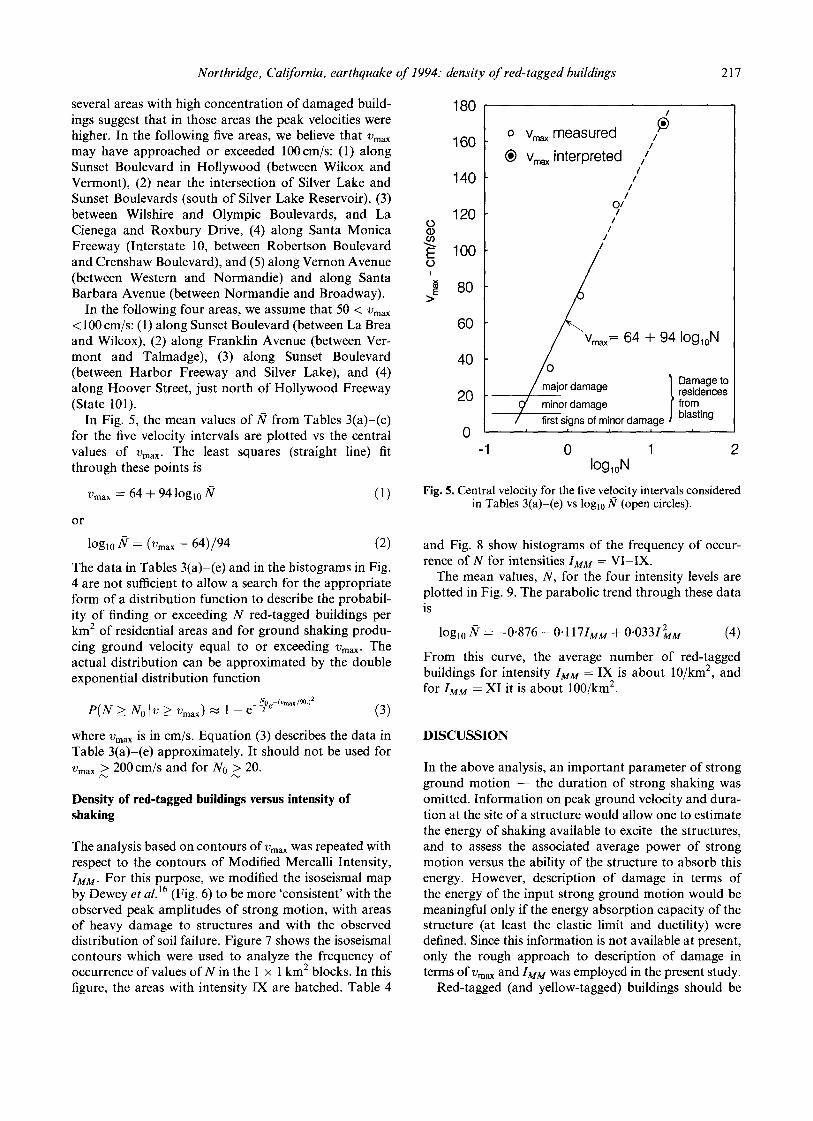
In Fig. 5, the mean values of ,N from Tables 3(a)-(e) for the five velocity intervals are plotted vs the central values of Vmax. The least squares (straight line) fit through these points is

Vmax = 64 + 94 log102V (1)

o r

logl0 N = (/)max - - 64)/94 (2)

The data in Tables 3(a)-(e) and in the histograms in Fig. 4 are not sufficient to allow a search for the appropriate form of a distribution function to describe the probabil- ity of finding or exceeding N red-tagged buildings per km 2 of residential areas and for ground shaking produ- cing ground velocity equal to or exceeding "/3ma x . The actual distribution can be approximated by the double exponential distribution function

P(N > Nolv > /)max) ~ 1 - e -~e-( .... /9o.) 2 (3)

where Vmax is in cm/s. Equation (3) describes the data in Table 3(a)-(e) approximately. It should not be used for Vmax > 200 cm/s and for No > 20.

rxJ

Density of red-tagged buildings versus intensity of shaking

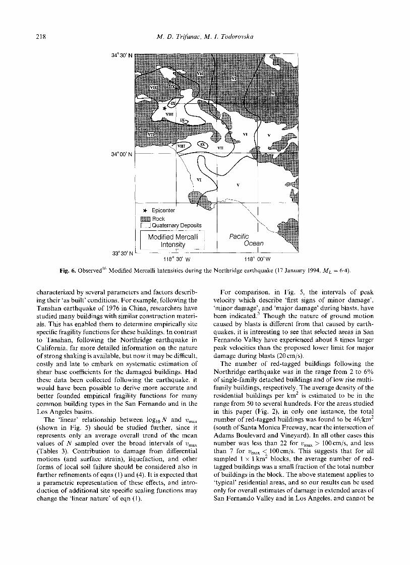
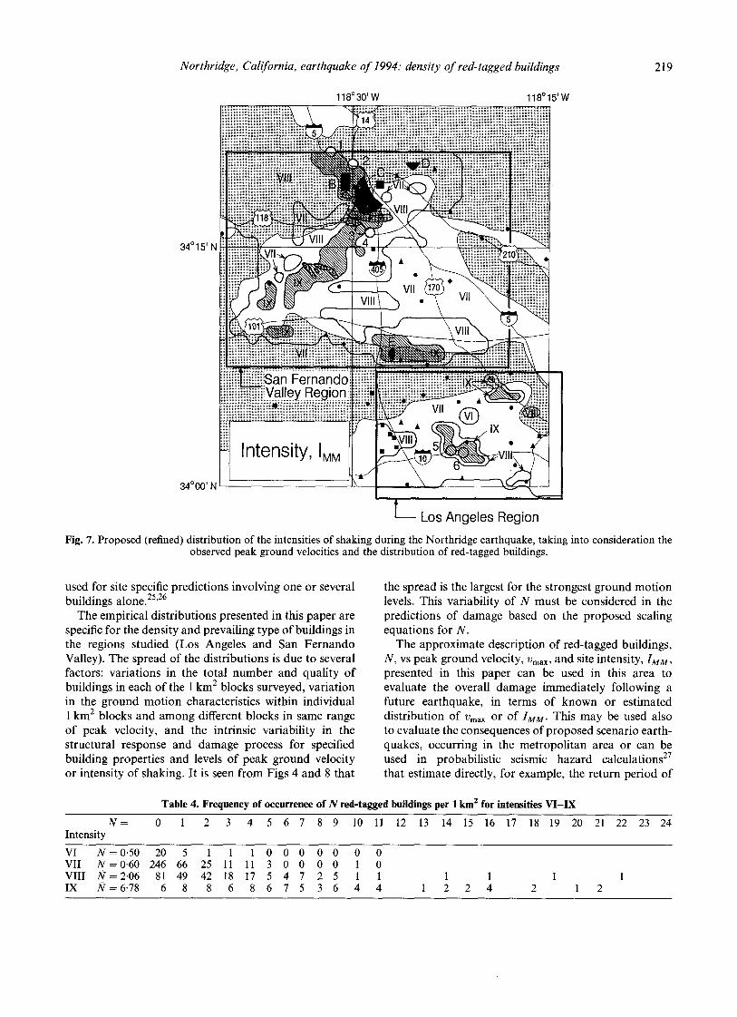
The analysis based on contours of Vma x was repeated with respect to the contours of Modified Mercalli Intensity, IM~t. For this purpose, we modified the isoseismal map by Dewey et al. 16 (Fig. 6) to be more 'consistent' with the observed peak amplitudes of strong motion, with areas of heavy damage to structures and with the observed distribution of soil failure. Figure 7 shows the isoseismal contours which were used to analyze the frequency of occurrence of values of N in the 1 x 1 km 2 blocks. In this figure, the areas with intensity IX are hatched. Table 4

0 (D ¢/}

0 i

>

180

160

140

120

100

80

60

40

20

0

/

o vm~ , measured / /

® vm~ interpreted / /

/ /

/

O/ /

/ /

1 /

= 6 4 + 94 Io010 N

/ major damage } Damage to residences minor damage from first signs of minor damage blasting

i i i L i

-1 0 1 2 log10 N

Fig. 5. Central velocity for the five velocity intervals considered in Tables 3(a)-(e) v s l O g l 0 / ~ - (open circles).

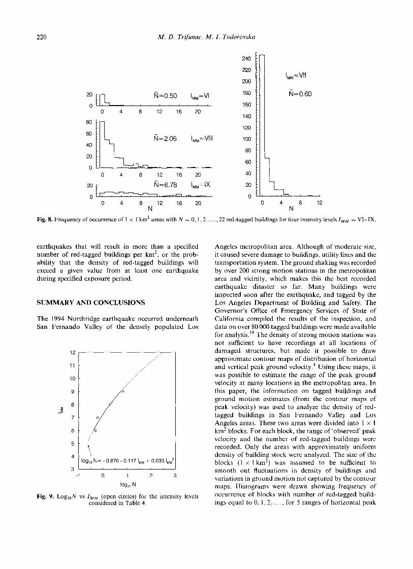
and Fig. 8 show histograms of the frequency of occurrence of N for intensities IM~ = VI-IX.

The mean values, ~7, for the four intensity levels are plotted in Fig. 9. The parabolic trend through these data is

lOgl0 N = -0.876 - 0.117IMM + 0"03312MU (4)

From this curve, the average number of red-tagged buildings for intensity IMM = IX is about 10/km 2, and for IMM = XI it is about 100/km 2.

DISCUSSION

In the above analysis, an important parameter of strong ground motion - - the duration of strong shaking was omitted. Information on peak ground velocity and duration at the site of a structure would allow one to estimate the energy of shaking available to excite the structures, and to assess the associated average power of strong motion versus the ability of the structure to absorb this energy. However, description of damage in terms of the energy of the input strong ground motion would be meaningful only if the energy absorption capacity of the structure (at least the elastic limit and ductility) were defined. Since this information is not available at present, only the rough approach to description of damage in terms OfVma x and IMM was employed in the present study.

Red-tagged (and yellow-tagged) buildings should be

34030' N

34 ° Off N

33 ° 30' N

218 M. D. Trifunac, M. L Todorovska

118 o 30' W 118 ° O0'W

Fig. 6. Observed 16 Modified Mercalli Intensities during the Northridge earthquake (17 January 1994, ML = 6"4).

characterized by several parameters and factors describing their 'as built' conditions. For example, following the Tanshan earthquake of 1976 in China, researchers have studied many buildings with similar construction materials. This has enabled them to determine empirically site specific fragility functions for these buildings. In contrast to Tanshan, following the Northridge earthquake in California, far more detailed information on the nature of strong shaking is available, but now it may be difficult, costly and late to embark on systematic estimation of shear base coefficients for the damaged buildings. Had these data been collected following the earthquake, it would have been possible to derive more accurate and better founded empirical fragility functions for many common building types in the San Fernando and in the Los Angeles basins.

The 'linear' relationship between logl0-N and Vma x (shown in Fig. 5) should be studied further, since it represents only an average overall trend of the mean values of N sampled over the broad intervals of Vma x (Tables 3). Contribution to damage from differential motions (and surface strain), liquefaction, and other forms of local soil failure should be considered also in further refinements ofeqns (1) and (4). It is expected that a parametric representation of these effects, and introduction of additional site specific scaling functions may change the 'linear nature' of eqn (1).

For comparison, in Fig. 5, the intervals of peak velocity which describe 'first signs of minor damage', 'minor damage', and 'major damage' during blasts, have been indicated. 3 Though the nature of ground motion caused by blasts is different from that caused by earthquakes, it is interesting to see that selected areas in San Fernando Valley have experienced about 8 times larger peak velocities than the proposed lower limit for major damage during blasts (20 cm/s).

The number of red-tagged buildings following the Northridge earthquake was in the range from 2 to 6% of single-family detached buildings and of low rise multifamily buildings, respectively. The average density of the residential buildings per km 2 is estimated to be in the range from 50 to several hundreds. For the areas studied in this paper (Fig. 2), in only one instance, the total number of red-tagged buildings was found to be 46/kin 2 (south of Santa Monica Freeway, near the intersection of Adams Boulevard and Vineyard). In all other cases this number was less than 22 for Vma x > 100cm/s, and less than 7 for Vrnax < 100 cm/s. This suggests that for all sampled 1 × 1 km 2 blocks, the average number of red- tagged buildings was a small fraction of the total number of buildings in the block. The above statement applies to 'typical' residential areas, and so our results can be used only for overall estimates of damage in extended areas of San Fernando Valley and in Los Angeles, and cannot be


34o15 ' N

34000 ' N l

118o30 ' W 118° 15' W

l I • . v iiiiiii ! •

ii iiiiii!i ~ , ~ ' ~ ( ~ g - VII ..... ~i~.iii!iill }iiiiiiiiiiii!i!!iiiiiiiiii!i ii ili!!!i!iiiii!!i i iiiiiiii!ii!iiii!ii iiiiii{!iiii{iiiiii!ii!!i ,,

Los Angeles Region Fig. 7. Proposed (refined) distribution of the intensities of shaking during the Northridge earthquake, taking into consideration the

observed peak ground velocities and the distribution of red-tagged buildings.

used for site specific predictions involving one or several buildings alone. 25'26

The empirical distributions presented in this paper are specific for the density and prevailing type of buildings in the regions studied (Los Angeles and San Fernando Valley). The spread of the distributions is due to several factors: variations in the total number and quality of buildings in each of the 1 km 2 blocks surveyed, variation in the ground motion characteristics within individual 1 km 2 blocks and among different blocks in same range of peak velocity, and the intrinsic variability in the structural response and damage process for specified building properties and levels of peak ground velocity or intensity of shaking. It is seen f rom Figs 4 and 8 that

the spread is the largest for the strongest ground motion levels. This variability of N must be considered in the predictions of damage based on the proposed scaling equations for N.

The approximate description of red-tagged buildings, N, vs peak ground velocity, Vma x, and site intensity, IMM, presented in this paper can be used in this area to evaluate the overall damage immediately following a future earthquake, in terms of known or estimated distribution of Vma x or of IMp. This may be used also to evaluate the consequences of proposed scenario earthquakes, occurring in the metropolitan area or can be used in probabilistic seismic hazard calculations 27 that estimate directly, for example, the return period of

Table 4. Frequency of occurrence of N red-tagged buildings per 1 kin z for intensities VI-IX

N = 0 1 2 3 4 5 6 7 8 9 10 11 12 13 14 15 16 17 18 19 20 21 22 23 24 Intensity

VI N-=0-50 20 5 1 1 1 0 0 0 0 0 0 0 VII N'=0.60 246 66 25 11 11 3 0 0 0 0 1 0 VIII ~r=2.06 81 49 42 18 17 5 4 7 2 5 1 1 l 1 I 1 IX N = 6 . 7 8 6 8 8 6 8 6 7 5 3 6 4 4 1 2 2 4 2 1 2


20

o

80

60

40

20

o

20 I F 0

240

220 IMM=VII

2OO

N=O.50 IMM=VI 180 ~1=0.60

. . . . . . . . . . 160 4 8 12 16 20

140

120

N1=2.06 IMM=VIII 100

6O i . . . . i - -

0 4 8 12 16 20 40

~1=6.78 IMM=IX 20 ~

, ~ . . . . . ,-:'1 ~ ~ . 0 " -- 0 4 8 12 16 20 0 4 8 12

N N

Fig. 8. Frequency of occurrence of 1 × 1 km 2 areas with N = 0, 1,2,.. . , 22 red-tagged buildings for four intensity levels IMM = VI-IX.

earthquakes that will result in more than a specified number of red-tagged buildings per km 2, or the prob- ability that the density of red-tagged buildings will exceed a given value from at least one earthquake during specified exposure period.

S U M M A R Y AND CONCLUSIONS

The 1994 Northridge earthquake occurred underneath San Fernando Valley of the densely populated Los

12 . . . . ' "

, , ' "

11 , ' " ...'"

10 .-"

9 ~;

8

7

6 7

5 "

4 \ Ioglo N= - 0.876 - 0.117 IMM 4- 0.033 IMM 2

3 -1 0 1 2

Ioglo N

Fig. 9. Log]0N vs IMM (open circles) for the intensity levels considered in Table 4.

Angeles metropolitan area. Although of moderate size, it caused severe damage to buildings, utility lines and the transportation system. The ground shaking was recorded by over 200 strong motion stations in the metropolitan area and vicinity, which makes this the best recorded earthquake disaster so far. Many buildings were inspected soon after the earthquake, and tagged by the Los Angeles Department of Building and Safety. The Governor 's Office of Emergency Services of State of California compiled the results of the inspection, and data on over 80 000 tagged buildings were made available for analysis.~4 The density of strong motion stations was not sufficient to have recordings at all locations of damaged structures, but made it possible to draw approximate contour maps of distribution of horizontal and vertical peak ground velocity. 4 Using these maps, it was possible to estimate the range of the peak ground velocity at many locations in the metropolitan area. In this paper, the information on tagged buildings and ground motion estimates (from the contour maps of peak velocity) was used to analyze the density of red- tagged buildings in San Fernando Valley and Los Angeles areas. These two areas were divided into 1 x 1 km 2 blocks. For each block, the range of 'observed' peak velocity and the number of red-tagged buildings were recorded. Only the areas with approximately uniform density of building stock were analyzed. The size of the blocks (1 x l km 2) was assumed to be sufficient to smooth out fluctuations in density of buildings and variations in ground motion not captured by the contour maps. Histograms were drawn showing frequency of occurrence of blocks with number of red-tagged buildings equal to 0, 1 ,2 , . . . , for 5 ranges of horizontal peak


velocity (from 10 to over 150cm/s) and for 4 values of site intensity (from VI to IX on the Modified Mercalli scale). The site intensity was estimated from the map drawn by Dewey et al., 16 modified (by the authors of this paper) in the heavily shaken areas to be more consistent with observed damage.

The results can be summarized as follows. The total number of red-tagged buildings and the area covered by the analysis were 949 and 479 km 2 for San Fernando Valley and 410 and 241 km 2 for Los Angeles. The maximum number of red-tagged buildings was 46/km 2 in Los Angeles, and it did not exceed 22/km 2 in the other areas (i.e. it was a small fraction of the total number of buildings in a block). The logarithm of the average density of red-tagged buildings, lOgl0 N, was plotted vs the central value of horizontal peak velocity interval. The linear trend is given by eqn (2). Similarly, log10 N was plotted vs the local intensity of shaking, and the parabolic trend is given by eqn (4).

The analysis in this paper is specific for the regions studied. It is valid for typical residential areas in San Fernando Valley and Los Angeles, i.e. for Wooden Frame Construction, typical of post World War II period, which is the prevailing building type in the sample studied (96% of the total number of tagged buildings in Los Angeles, Ventura and Orange Counties, and 84% of all red-tagged buildings in these areas). The scaling equations and the distribution of N about the mean value are valid for the levels of shaking observed during the Northridge earthquake.

The lack of specific detail in information on the earthquake resistance of the inspected buildings (e.g., shear- base coefficient) and on ground motion characteristics at individual building sites limited the analysis to consider- ing only one parameter of ground shaking (peak velocity or site intensity). In spite of these limitations, the results of this analysis can be useful to predict the density of red- tagged buildings caused by future earthquakes in San Fernando Valley and in Los Angeles, where moderate but near earthquakes are likely to occur. Predictions may be made for scenario earthquake or in probabilistic seismic hazard calculations, for an ensemble of earthquakes with some likelihood to occur during specified exposure. The results of such predictions may be used by government officials for emergency planning, by the insurance industry for assessment of future insured losses, and by structural engineers for assessment of the overall performance of Wooden Frame Construction.

REFERENCES

1. Benioff, H. A physical evaluation of seismic destructiveness. Bulletin of the Seismological Society of America, 1934, 24, 389-403.

2. Arias, A. A measure of earthquake intensity. In Seismic Design of Nuclear Power Plants, ed. R. J. Hansen, The Mass. Inst. of Tech. Press, Cambridge, MA, 1970.

3. Duvall, W. I. & Fogelson, D. E. Review of criteria for estimating damage to residence from blasting vibrations. Report 5968, U.S. Dept. of Interior, 1962.

4. Trifunac, M. D., Todorovska, M. I. & Ivanovic, S. S. Peak velocities and peak surface strains during Northridge, California, earthquake of 17 January 1994. Soil Dynamics and Earthquake Engineering, 1996, 15(5), 301-310.

5. Trifunac, M. D. & Ziv~ir, M. A note on instrumental comparison of the Modified Mercalli Intensity (MMI) in the western United States and the Mercalli-Cancani- Sieberg (MCS) Intensity in Yugoslavia. European Earth- quake Engineering, 1991, V(1), 22-26.

6. Trifunac, M. D., Lee, V. W., Ziv~ir, M. & Manir, M. On the correlation of Mercalli-Cancani-Sieberg Scale in Yugoslavia with the peaks of recorded strong earthquake ground motion. European Earthquake Engineering, 1991, V(1), 27-33.

7. Trifunac, M. D. Long period Fourier amplitude spectra of strong motion acceleration. Soil Dynamics and Earthquake Engineering, 1993, 12(6), 363-382.

8. Trifunac, M. D. & Novikova, E. I. State of the art review on strong motion duration. Proc. lOth European Conf. on Earthquake Engineering, Aug. 28-Sept 2 1994, Vienna, Austria, Vol. I, 131-140.

9. Trifunac, M. D. & Novikova, E. I. Duration of earthquake fault motion in California. Earthquake Engineering and Structural Dynamics, 1995, 24(6), 781-799.

10. Yang, Y. S., Yang, L. & Ko, Y. S. On seismic destruction and seismic design of multi-story masonry buildings. Insti- tute of Engineering Mechanics, Harbin, China, 1981.

11. Petrovski, J., Milutinovir, Z., Ristir, D. & Nocevski, N. Earthquake damage prediction modelling for needs of physical and urban planning. Report IZIIS 84-084, Skopje, Macedonia, 1984.

12. Los Angeles Dept. of Building Safety. Earthquake damage sites, January 17, 1994, in the City of Los Angeles. Map Prepared by Land Development and Mapping Division, City of Los Angeles, CA, 1994.

13. U.S. Department of Housing and Urban Development. Assessment of damage of residential buildings caused by the Northridge Earthquake. Report HUD-1499-PDR, USDHUD, 451 7th Street S.W., Washington DC, 1994.

14. Earthquake Engineering Research Institute. Wood Build- ings, Chapter 6 in Supplement C to Volume 11 of Earth- quake Spectra, Northridge Earthquake Reconnaissance Report, Vol. 2, 1996.

15. Trifunac, M. D., Todorovska, M. I. & Ivanovir, S. S. A note on distribution of uncorrected peak ground accelera- tions during Northridge, California, earthquake of 17 January 1994. Soil Dynamics and Earthquake Engineering, 1994, 13(3), 187-196.

16. Dewey, J. W., Reagor, B. G. & Dengler, L. Isoseismal map of the Northridge, California, earthquake of January 17, 1994. Presented to the Annual Meeting, Seismological Society of America, also reproduced in the introduction to Northridge Earthquake Reconnaissance Report, Vol. 1, Supplement C to Volume 11 of Earthquake Spectra, April 1995.

17. Shakal, A., Huang, M., Darragh, R., Cao, T., Sherburne, R., Malhotra, P., Cramer, C., Sydnor, R., Graizer, V., Maldonado, G., Petersen, C. & Wampole, J. CSMIP strong motion records from the Northridge, California, earthquake of 17 January 1994. Report No. OSMS 94-07, Calif. Dept. of Conservation, Division of Mines and Geology, Sacramento, California, 1994.

18. Porcella, R. L., Etheredge, E. C., Maley, R. P. & Acosta, A. V. Accelerograms recorded at USGS National Strong- Motion Network stations during the Ms = 6.6 Northridge,


California earthquake of January 17, 1994. Open File Report 94-141, Dept. of the Interior, U.S. Geological Survey, 1994.

19. Davis, C. A. &Bardet, J. P. Performance of two reservoirs during Northridge Earthquake. Journal of Geotechnical Engineering ASCE, 122(8), 613-622.

20. Earthquake Engineering Research Institute. Northridge earthquake of January 17, 1994. Preliminary Reconnais- sance Report., EERI 94-01, Oakland, California, 1994.

21. Trifunic, M. D. & Todorovska, M. I. Non-linear soil response - - 1994 Northridge, California, earthquake. Journal of Geo- technical Engineering ASCE, 1996, 122(9), 725-735.

22. Office of Emergency Services. The Northridge earthquake of January 17, 1994: report on data collection and analysis part A: damage and inventory data. Prepared by EQE International Inc. and the Geographic Information Systems Group of the Governor's Office of Emergency Services, State of California, Sacramento, CA, 1995.

23. LAHD. Rebuilding communities; recovering from the

Northridge earthquake, January 17, 1994; the first 365 days. Housing Department, City of Los Angeles, CA, 1995.

24. Comerio, M. C. Northridge housing losses. A study for the California Governor's Office of Emergency Services. Center for Environmental Design Research, Univ. of Cali- fornia, Berkeley, CA, 1995.

25. Jordanovski, L. R., Todorovska, M. I. & Trifunac, M. D. Total loss in a building exposed to earthquake hazard, part I: theory. European Earthquake Engineering, 1993, VI(3), 14 25.

26. Jordanovski, L. R., Todorovska, M. I. & Trifunac, M. D. Total loss in a building exposed to earthquake hazard, part II: a hypothetical example. European Earthquake Engineer- ing, 1993, VI(3), 26-32.

27. Todorovska, M. I. & Trifunac, M. D. Hazard mapping of normalized peak strain in soil during earthquakes - - microzonation of a metropolitan area. Soil Dynamics and Earthquake Engineering, 1996a, 15(5), 321-329.

Documents

Northridge, California, earthquake of 1994: density of red-tagged buildings versus peak horizontal velocity and intensity of shaking