Normalization for Cubical Type TheoryJonathan Sterling

Computer Science DepartmentCarnegie Mellon University

Carlo AngiuliComputer Science Department

Carnegie Mellon University

Abstract—We prove normalization for (univalent, Cartesian)cubical type theory, closing the last major open problem in thesyntactic metatheory of cubical type theory. Our normalizationresult is reduction-free, in the sense of yielding a bijection betweenequivalence classes of terms in context and a tractable languageof β/η-normal forms. As corollaries we obtain both decidabilityof judgmental equality and the injectivity of type constructors.

I. INTRODUCTION

De Morgan [20] and Cartesian [8, 9] cubical type theoryare recent extensions of Martin-Lof type theory which pro-vide constructive formulations of higher inductive types andVoevodsky’s univalence axiom; unlike homotopy type theory[65], both enjoy canonicity, the property that closed terms ofbase type are judgmentally equal to constructors [8, 35].

Several proof assistants already implement cubical typetheory, most notably Cubical Agda [66] (for the De Morganvariant) and redtt [50] (for Cartesian). Like most type-theoretic proof assistants, both typecheck terms using algo-rithms inspired by normalization by evaluation [1], whichinterleave evaluation and decomposition of types. The cor-rectness of these algorithms hinges not on canonicity but onnormalization theorems characterizing judgmental equivalenceclasses of open terms—and consequences thereof, such asdecidability of equality and injectivity of type constructors.But unlike canonicity, normalization and its corollaries haveuntil now remained conjectures for cubical type theory.

We contribute the first normalization proof for Cartesiancubical type theory [9]. By relying on recent advances inthe metatheory of type theory, our proof is significantly moreabstract and concise than existing canonicity proofs for cubicaltype theory; moreover, it can be adapted to De Morgan cubicaltype theory without conceptual changes.

A. Cubical type theory and synthetic semantics

Cubical type theory extends type theory with a number offeatures centered around a primitive interval I with elements0, 1 : I. Propositional equality is captured by a path typepath(A, a0, a1) whose elements are functions f :

∏i:IA(i)

satisfying f(0) = a0 and f(1) = a1 judgmentally. Congruenceof paths follows from substitution; the remaining propertiesof equality are defined at each type by the Kan operations ofcoercion and box filling (or composition).

In Cartesian cubical type theory, coercion is a function

coe :∏A:I→U

∏r,s:IA(r)→ A(s)

satisfying coe(A, r, r, a) = a for all A : I→ U and a : A(r),1

and additional equations for each particular connective, e.g.:

coe(λi.(∏

x:A(i)B(i, x)), r, s, f

)= λx.coe(λi.B(i, coe(A, s, i, x)), r, s, f(coe(A, s, r, x)))

The equations governing coercion and composition arecomplex, especially for the glue type which justifies uni-valence; calculating (and verifying the well-definedness of)these equations was a major obstacle in early work on cubicaltype theory. Orton and Pitts [45, 48] streamlined this processby observing that the model construction for De Morgancubical type theory—the most technical part of which is theseequations—can be carried out synthetically in the internalextensional type theory of any topos satisfying nine axioms(e.g., whose objects are De Morgan cubical sets); Angiuli et al.[9] establish an analogous result for the Cartesian variant.

A subtle aspect of these models is that coercion is definednot on types A : U but on type families A : I → U ;consequently, a semantic universe U of types-with-coercionmust strangely admit a coercion structure for every figureI→ U. Licata et al. [45] obtain U by transposing the coercionmap across the right adjoint to exponentiation by I given bythe tininess of I.

The synthetic approach of Orton and Pitts simplifies andclarifies the model construction of cubical type theory byfactoring out naturality obligations, in much the same waythat homotopy type theory provides a “synthetic homotopytheory” that factors out e.g., continuity obligations.

In this paper, we combine ideas of Orton and Pitts withthe synthetic Tait computability (STC) theory of Sterling andHarper [57], which factors out bureaucratic aspects of syntacticmetatheory. In STC, one considers an extensional type theorywhose types are (proof-relevant) logical relations; the under-lying syntax is exposed via a proof-irrelevant proposition synunder which the syntactic part of a logical relation is projected.

B. Canonicity for cubical type theory

Traditional canonicity proofs fix an evaluation strategy forclosed terms, and associate to each closed type a proof-irrelevant computability predicate or logical relation rangingover closed terms of that type. Then, one ensures that evalua-tion is contained within judgmental equality, that computabil-ity is closed under evaluation, and that computability at base

1In De Morgan cubical type theory, coercion is limited to A(0) → A(1),a restriction counterbalanced by the additional (De Morgan) structure on I.978-1-6654-4895-6/21/$31.00 ©2021 IEEE

arX

iv:2

101.

1147

9v2

[cs

.LO

] 1

9 A

pr 2

021

type implies evaluation to a constructor; canonicity follows byproving that every well-typed closed term is computable.

Whereas evaluation in ordinary type theory need notdescend under binders, evaluating a closed coercioncoe(λi.A, r, s, a) in cubical type theory requires determiningthe head constructor of (i.e., evaluating) the type A in contexti : I. Accordingly, the cubical canonicity proofs of Angiuliet al. [7, 8], Huber [35] define evaluation and computabilityfor terms in context (i1 : I, . . . , in : I). In both proofs, thedifficulty arises that typing and thus computability are closedunder substitutions of the form In Im, but evaluation isnot; both resolve the issue by showing evaluation is closedunder computability up to judgmental equality.

C. Semantic and proof-relevant computability

The past several years have witnessed an explosion insemantic computability techniques for establishing syntacticmetatheorems [4, 21, 23, 27, 40, 53, 57, 58, 63]. What makessemantic computability different from “free-hand” computabil-ity is that it is expressed as a gluing model, parameterized inthe generic model of the type theory; hence one is alwaysworking with typed terms up to judgmental equality.

A new feature of semantic computability, forced in manycases by the absence of raw terms, is that a term maybe computable in more than one way. This proof-relevanceplays an important role in the normalization arguments ofAltenkirch et al. [4], Coquand [21], Fiore [27] as well as thecanonicity arguments of Coquand [21], Sterling et al. [58].The proof-relevant approach is significantly simpler to set upthan the alternative and it provides a compositional accountof computability for universe hierarchies, which had been themain difficulty in conventional free-hand arguments.

Example 1. A semantic canonicity argument for ordinarytype theory associates to each closed type a computabilitystructure which assigns to each equivalence class of closedterms of that type a set of “computability proofs.” We choosethe computability structure at base type to be a collection of“codes” for each constant; then, by exhibiting a choice ofcomputability proof for every well-typed term, we concludethat every equivalence class at base type is a constant.

Crucially, the ability to store data within the computabilityproofs circumvents the need to define a subequational evalu-ation function, allowing us to carry out the entire argumentover equivalence classes of terms; rather than choosing arepresentative of each equivalence class, we encode canonicalforms as a structure indexed over equivalence classes of terms.

1) In what contexts do we compute?: Semantic computabil-ity arguments have already been used to establish ordinarycanonicity, cubical canonicity, and ordinary normalization.The key difference between these arguments lies in what isconsidered an “element” of a type, or more precisely, whatare the contexts (and substitutions) of interest. In ordinarycanonicity proofs, the only context of interest is the closedcontext, in which each type has just a set of elements; thecomputability structures are thus families of sets.

Following Huber and Angiuli, Favonia, and Harper [8, 35],cubical canonicity proofs must consider terms in all contextsIn, with all substitutions In Im between them. These con-texts and substitutions induce a cubical set (i.e., a presheaf) ofelements of each type; the computability structures in questionare thus families of cubical sets indexed in the application of a“cubical nerve” applied to a syntactical object, an arrangementsuggested by Awodey in 2015. Notably, because semanticcomputability arguments are not evaluation-based, cubicalcanonicity proofs in this style (e.g., that of Sterling, Angiuli,and Gratzer [58]) entirely sidestep the evaluation coherencedifficulties of prior work [8, 35].

The passage to presheaves of elements is not a novel featureof cubical canonicity; it appears already in normalizationproofs for ordinary type theory, in the guise of Kripke logicalrelations of varying arities [38]. Because normalization isby definition a characterization of open terms, one mustnecessarily consider the presheaf of elements of a type relativeto all contexts; but in light of the fact that normal formsare not closed under substitutions of terms for variables,one considers only a restricted class of substitutions (e.g.,weakenings, injective renamings, or all variable renamings).

Following Tait [61], the normal forms of type theory aredefined mutually as the neutral forms ne(A) (variables andeliminations thereof) and the normal forms nf(A) (constantsand constructors applied to normals) of each open type A.Proof-irrelevant normalization arguments then establish thatevery neutral term is computable (via reflection ↑A), and thatevery computable term has a normal form (via reification ↓A).Proof-relevant normalization arguments follow the same yogaof reflection and reification, except that we speak not of thesubset of neutral terms but rather the collection of neutrals andnormals encoding each equivalence class of terms [21].

2) Related work on gluing for type theory: The past fortyyears have brought a steady stream of research developingthe gluing perspective on logical relations [4, 24, 27, 28, 60];however, only in the past several years has our understandingof the syntax and semantics of dependent types [3, 12, 29, 46,64] caught up with the mathematical tools required to advancea truly objective metatheory of dependent type theory.

In particular, Coquand’s analysis [21] of proof-relevantcanonicity and normalization arguments for dependent typetheory in terms of categorical gluing was the catalyst for anumber of recent works that obtain non-trivial metatheoremsfor dependent type theory by semantic means, although someyears earlier Shulman [53] had already used gluing to provea homotopy canonicity result for a univalent type theory.

Uemura [63] proved a general gluing theorem for certaindependent type theories in the language of Shulman’s typetheoretic fibration categories; Kaposi et al. [40] proved asimilar result in the language of categories with families.Coquand et al. [23] employed gluing to prove a homotopycanonicity result for a version of cubical type theory thatomits certain computation rules, and Kapulkin and Sattler[41] used gluing to prove homotopy canonicity for homotopytype theory (as famously conjectured by Voevodsky). Sterling

2

et al. [58] adapted Coquand’s gluing argument to prove thefirst non-operational strict canonicity result for a cubical typetheory. Gratzer et al. [30] used gluing to prove canonicityfor a general multi-modal dependent type theory. Sterling andHarper [57] employ a different gluing argument to establisha proof-relevant generalization of the Reynolds AbstractionTheorem for a calculus of ML modules. Gratzer and Sterling[29] used gluing to establish the conservativity of higher-orderjudgments for dependent type theories.

3) What are the neutrals of cubical type theory?: Today’sobstacles to proving cubical normalization are entirely dif-ferent from the obstacles faced in the first proofs of cubicalcanonicity [8, 35]. As we have already discussed, coherenceof evaluation is a non-issue for semantic computability; more-over, as normalization already descends under binders, thisfeature of coercion poses no additional difficulty.

However, cubical type theory includes a number of openjudgmental equalities that challenge the yoga of reflection andreification. Consider the rule that applying any element, evena variable, of type path(A, a0, a1) to 0 : I (resp., 1 : I) equalsa0 (resp., a1). Whereas application of neutrals (e.g., variables)to normal forms (e.g., constants) is typically irreducible, herepath application of a variable to a constant (but not to avariable) is a redex which may uncover further redexes:

x : path(λ .N→ N, fib, fib) ` x(0)(7) = 13 : N

One might imagine defining the normal form of path appli-cation by a case split on the elements of I (sending 0, 1 : I tothe normal form of fib(7), and i : I to a neutral application),but such a case split requires us to model I as a coproduct,which will not be tiny, preventing us from obtaining a universeof Kan types following Licata et al. [45].

Similar issues arise with a number of equations in bothCartesian and De Morgan cubical type theory; in fact, theCartesian variant is a priori more challenging in this regardbecause contraction of interval variables i, j : I may alsoinduce computation (e.g., in coe(A, i, j, a)).

In this paper, we index neutrals neφ(A) by a proposi-tion φ representing their locus of instability, or where theycease to be neutral. For example, path application sends aφ-unstable neutral of type path(A, a0, a1) and an elementr : I to a (φ ∨ (r = 0) ∨ (r = 1))-unstable neutral of typeA(r). Reflection ↑φA operates on stabilized neutrals, pairs ofa neutral neφ(A) with a proof that the term is computableunder φ. In the case of path application x(r), one mustprovide computability proofs for a0, a1 under the assumptionr = 0 ∨ r = 1.

Terms in the ordinary fragment are never unstable (henceφ = ⊥), in which case a stabilized neutral is a neutral inthe ordinary sense; “neutrals” with cubical redexes (such asx(0)) have φ = >, in which case their stabilized neutral isjust a computability proof (and ↑>A is the identity). To ourknowledge, this is the first time that computability data appearsin the domain of the reflection operation.

D. Contributions

We establish the normalization theorem (Theorem 42) forCartesian cubical type theory closed under Π, Σ, path, glue,and a higher inductive circle type, using a cubical extension ofsynthetic Tait computability [57]; the new idea on which ourargument hinges is the concept of stabilized neutrals describedabove. As corollaries to our main result, we obtain the admis-sible injectivity of type constructors (Theorem 43) as well asan algorithm to decide judgmental equality (Corollary 47).

The present paper does not describe universes or the mod-ifications necessary to prove normalization for De Morgancubical type theory; but note that univalence can be statedwithout universes, as we have done here. The novel aspects ofcumulative, univalent universes are already supported becauseof the tininess of the interval and the account of glue types;the difference is that the operator projecting a normal typefrom a normalization structure of size α must be generalizedover β ≥ α. Our argument carries over mutatis mutandis to anormalization proof for De Morgan cubical type theory.

In Section II we discuss the syntax of Cartesian cubical typetheory and its situation within a dependently sorted logicalframework. In Section III, we axiomatize a cubical version ofsynthetic Tait computability (STC) [57], a modal type theoryof synthetic logical relations suitable for proving syntacticmetatheorems; we construct in cubical STC a “normalizationmodel” of cubical type theory displayed over the genericmodel. In Section IV we construct a topos model of cubicalSTC, which takes us the remaining distance to the main resultsof this paper, which are described in Section V.

II. CARTESIAN CUBICAL TYPE THEORY

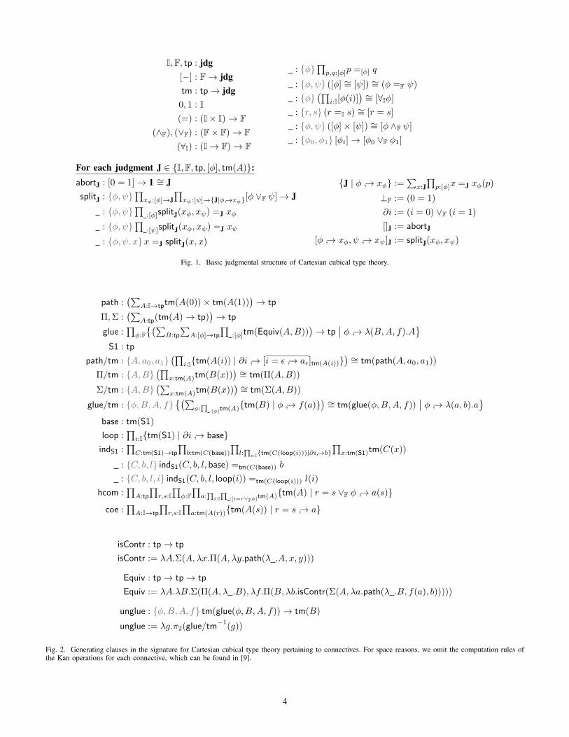
We define the subject of our normalization theorem, inten-sional Cartesian cubical type theory, as a locally Cartesianclosed category of judgments T generated by the signature inFigs. 1 and 2. Readers may consult [9] and [6, Appendix B]for further exposition, including rule-based presentations.

A. LCCCs as a logical framework

The primary aspects of a type theory are its judgmentsA type and a : A and their derivations, many of whichrequire hypothetical judgments (e.g., λx.b : A → B whenx : A ` b : B). One typically restricts which judgments maybe hypothesized, allowing (x : A) but not (X type), judgmen-tal equalities (a = b : A), or hypothetical judgments. Theserestrictions, realized by the notion of context, are crucial tothe syntactic metatheorems on which implementations rely; forexample, decidability of equality requires that intensional typetheory lacks a context former (isomorphic to) 〈Γ, a = b : A〉.

Both the rule-based presentations and the common cate-gorical semantics of type theory—including categories withfamilies [26], natural models [12], and Uemura’s recent gener-alization thereof known as representable map categories [64]—include a notion of context as part of the definition of a typetheory, and require these contexts to be preserved by modelsand their homomorphisms.

3

I,F, tp : jdg[−] : F→ jdgtm : tp→ jdg

0, 1 : I(=) : (I× I)→ F

(∧F), (∨F) : (F× F)→ F(∀I) : (I→ F)→ F

: φ∏p,q:[φ]p =[φ] q

: φ, ψ ([φ] ∼= [ψ]) ∼= (φ =F ψ)

: φ(∏

i:I[φ(i)]) ∼= [∀Iφ]

: r, s (r =I s) ∼= [r = s]

: φ, ψ ([φ]× [ψ]) ∼= [φ ∧F ψ]

: φ0, φ1 [φi]→ [φ0 ∨F φ1]

For each judgment J ∈ I,F, tp, [φ], tm(A):abortJ : [0 = 1]→ 1 ∼= JsplitJ : φ, ψ

∏xφ:[φ]→J

∏xψ:[ψ]→J|φ→xφ[φ ∨F ψ]→ J

: φ, ψ∏

:[φ]splitJ(xφ, xψ) =J xφ

: φ, ψ∏

:[ψ]splitJ(xφ, xψ) =J xψ

: φ, ψ, xx =J splitJ(x, x)

J | φ → xφ :=∑x:J∏p:[φ]x =J xφ(p)

⊥F := (0 = 1)

∂i := (i = 0) ∨F (i = 1)

[]J := abortJ

[φ → xφ, ψ → xψ]J := splitJ(xφ, xψ)

Fig. 1. Basic judgmental structure of Cartesian cubical type theory.

path :(∑

A:I→tptm(A(0))× tm(A(1)))→ tp

Π,Σ :(∑

A:tp(tm(A)→ tp))→ tp

glue :∏φ:F(∑

B:tp

∑A:[φ]→tp

∏:[φ]tm(Equiv(A,B))

)→ tp

∣∣ φ → λ(B,A, f).A

S1 : tp

path/tm : A, a0, a1(∏

i:Itm(A(i)) | ∂i → [i = ε → aε]tm(A(i))) ∼= tm(path(A, a0, a1))

Π/tm : A,B(∏

x:tm(A)tm(B(x))) ∼= tm(Π(A,B))

Σ/tm : A,B(∑

x:tm(A)tm(B(x))) ∼= tm(Σ(A,B))

glue/tm : φ,B,A, f(∑

a:∏

:[φ]tm(A)tm(B) | φ → f(a)) ∼= tm(glue(φ,B,A, f))

∣∣ φ → λ(a, b).a

base : tm(S1)

loop :∏i:Itm(S1) | ∂i → base

indS1 :∏C:tm(S1)→tp

∏b:tm(C(base))

∏l:∏i:Itm(C(loop(i)))|∂i→b

∏x:tm(S1)tm(C(x))

: C, b, l indS1(C, b, l, base) =tm(C(base)) b

: C, b, l, i indS1(C, b, l, loop(i)) =tm(C(loop(i))) l(i)

hcom :∏A:tp

∏r,s:I∏φ:F∏a:∏i:I∏

:[i=r∨Fφ]tm(A)tm(A) | r = s ∨F φ → a(s)

coe :∏A:I→tp

∏r,s:I∏a:tm(A(r))tm(A(s)) | r = s → a

isContr : tp→ tp

isContr := λA.Σ(A, λx.Π(A, λy.path(λ .A, x, y)))

Equiv : tp→ tp→ tp

Equiv := λA.λB.Σ(Π(A, λ .B), λf.Π(B, λb.isContr(Σ(A, λa.path(λ .B, f(a), b)))))

unglue : φ,B,A, f tm(glue(φ,B,A, f))→ tm(B)

unglue := λg.π2(glue/tm−1(g))

Fig. 2. Generating clauses in the signature for Cartesian cubical type theory pertaining to connectives. For space reasons, we omit the computation rules ofthe Kan operations for each connective, which can be found in [9].

4

In contrast, higher-order logical frameworks for definingtype theories, such as Martin-Lof’s logical framework [47] andthe Edinburgh Logical Framework [32], elevate the judgmentalstructure of a type theory; then, as explicated by Harperet al. [32], one may impose after the fact a collection ofLF contexts (or worlds) relative to which adequacy and othermetatheorems hold [31]. These worlds, which can be seen tocorrespond roughly to the arities of Jung and Tiuryn [38], weresubsequently implemented in the Twelf proof assistant [49] as“%worlds declarations.”

In light of that perspective, we regard a notion of contextas a structure placed on a locally Cartesian closed category ofjudgments T of a type theory, whose objects and morphismsare (equivalence classes of) judgments and deductions. Thedependent products of T encode hypothetical judgments, andthe finite limits both encode substitution and judgmentalequality; a notion of context is often a full subcategory C ⊆Tspanned by objects distinguished as contexts.

Example 2. The category of judgments T of Martin-Lof typetheory without any types is the free LCCC generated by asingle map tm tp. The category of contexts C ⊆ T isinductively defined as the full subcategory spanned by theterminal object and any fiber of tm tp over a context.

Equality is undecidable in T (as it has all finite limits),but is decidable for terms and types in context, objectifiedby the restricted Yoneda embedding T Pr( C) taking thejudgment tp : T to its “functor of context-valued points”Hom( C, tp) : Cop Set. Proofs of decidability proceed byfurther restricting to a category of (contexts and) renamingsR along the forgetful map R C [4, 21, 27].

A second distinction between LCCCs and (for instance)Uemura’s framework is that the latter is stratified to ensurethat the use of hypothetical judgment in a theory is strictlypositive, whereas both LCCCs and syntactic logical frame-works place no restriction on hypothetical judgments and evenallow binders of higher-level (e.g., in Martin-Lof’s funsplitoperator [47]). However, using an Artin gluing argument dueto Paul Taylor [62], Gratzer and Sterling [29] have observedthat the extension of a representable map category a la Uemurato a LCCC is conservative (in fact, fully faithful), ensuring theadequacy of LCCC encodings of type theories.

We therefore define the category of judgments of Cartesiancubical type theory as the LCCC T generated by the signaturein Figs. 1 and 2; then, locally Cartesian closed functorsM : T E determine algebras for that signature valuedin E. Unlike homomorphisms of models of type theory, suchfunctors preserve higher-order judgments; note however thatwe are proving a single theorem about the syntactic categoryT , not studying the model theory of cubical type theory.

B. The signature of Cartesian cubical type theory

In Fig. 1 we present the judgmental structure of cubicaltype theory; we inherit from Martin-Lof type theory the basicforms of judgment tp : T and tm : (T )/tp classifyingtypes and terms respectively, and add three additional forms

of judgment for cubical phenomena: I : T for elements of theinterval, F : T for cofibrations (or cofibrant propositions), and[−] : (T )/F for proofs of cofibrations. The standard notion ofcontext is generated by 1 and context extension by (x : A),(i : I), and ( : [φ]).2 In this paper, we will only consider amore restricted notion of atomic context (Section IV-C) thatplays a role analogous to the renamings of Example 2.

Cofibrations are strict propositions; the cofibration classifierF is strictly univalent and closed under ∧F, ∨F, ∀I, and =I.We define ∧F, ∀I, and =I in terms of the same notions in T ,but T has no disjunction or empty type by which to define∨F or stipulate (0 = 1)→ ⊥. Instead, we axiomatize these byeliminators abortJ, splitJ for each generating judgment J.

The following notations in Fig. 1 are used pervasivelythroughout this paper. (At present, “propositions” are elementsof F; later they will be elements of a subobject classifier Ω.)

Notation 3 (Extent types [51]). Given a proposition φ and apartial element aφ : [φ] → A, we write A | φ → aφ forthe collection of elements a : A that restrict to aφ under theassumption of z : [φ]. In other words:

A | φ → aφ := a : A | ∀z : [φ].a = aφ(z)

We will implicitly coerce elements of A | φ → aφ to A.

Notation 4 (Systems [20]). Let φ, ψ be propositions. Under: [φ ∨ ψ], given a pair of partial elements aφ : [φ]→ A and

aψ : [ψ]→ A that agree when : [φ ∧ ψ], we write

[φ → aφ, ψ → aψ] : A

for the “case split” that extends aφ, aψ . Likewise, under theassumption : [⊥], we write [] : A for the unique elementof A. We will leave abstraction and application over z : φimplicit; where it improves clarity, we may write the unarysystem [φ → a] for λz : φ.a.

In Fig. 2 we define the connectives of cubical type theory.We specify the elements of Π, Σ, path, and glue by isomor-phisms whose underlying functions encode introduction andelimination rules, and whose equations encode β and η rules;we will leave the first three of these isomorphisms (and theprojection from equivalences to functions) implicit. The higherinductive circle S1 has constructors base and loop and aneliminator indS1 with computation rules. Finally, we specifythe Kan operations hcom and coe; for space reasons we donot reproduce the computation rules for hcom and coe in eachtype, which can be found in Angiuli et al. [9].

The signature for De Morgan cubical type theory [20, 22]differs only in the structure imposed on I and the types andcomputation rules of hcom and coe.

III. SYNTHETIC TAIT COMPUTABILITY

In this section, we axiomatize a category E whose in-ternal language provides a “type theory of proof-relevantlogical relations” a la Sterling and Harper’s synthetic Taitcomputability [57]. Inside that type theory, we then define

2Syntactic presentations typically write 〈Γ, φ〉 for 〈Γ, : [φ]〉.

5

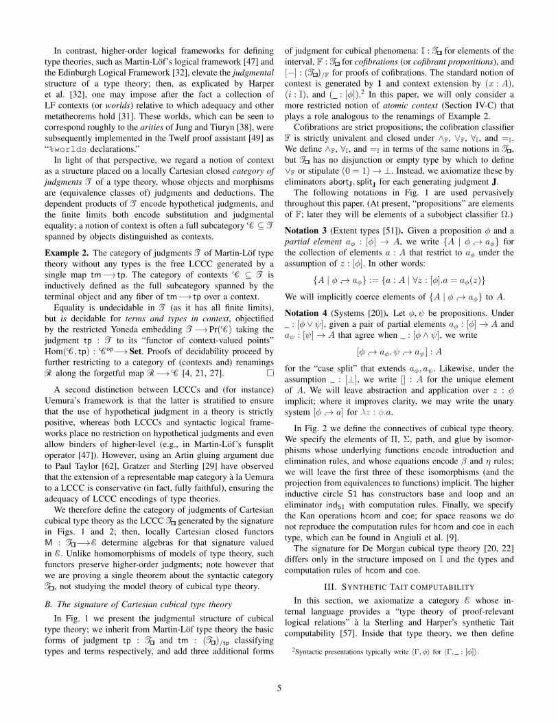
Axiom Substantiation

Axiom STC-1 Lemma 27Axiom STC-2 Construction 31 and Corollary 33Axiom STC-3 Computation 28Axiom STC-4 Remark 29 and Construction 31Axiom STC-5 Lemma 34Axiom STC-6 Construction 25 and Remark 30

Fig. 3. A dictionary between the axioms of Section III and their substantia-tions in the category of computability structures.

a reflection–reification computability model of cubical typetheory from which we will derive normalization. We deferto Section IV an explicit construction of E as a category ofcomputability structures; Fig. 3 provides forward references toour justifications of the axioms.

We begin by assuming that E satisfies Giraud’s axioms[10]; all such categories interpret extensional Martin-Lof typetheory extended by a strictly univalent universe Ω of all proof-irrelevant propositions. Next, we assume that E contains acumulative hierarchy of universes whose elements satisfy astrictification axiom introduced by Birkedal et al. [15], Ortonand Pitts [48].

Definition 5. An strong universe is a type theoretic universeU strictly closed under dependent products, dependent sums,inductive types, quotients, and the subobject classifier, suchthat the following additional strict gluing axiom holds:

Given A : U, write Iso(A) :=∑B:U(A ∼= B) for

the type of U-isomorphs of A. For any propositionφ : Ω, there is a section to the weakening mapIso(A) (φ→ Iso(A)).

Axiom STC-1. There exists a cumulative hierarchy of stronguniverses U0 ⊆ U1 . . . in E such that every map in E isclassified by some Ui.

We schematically write U, V for arbitrary universes in thehierarchy specified by Axiom STC-1.

Axiom STC-2. There exists a tiny [44, 68] interval objectI : U with two endpoints 0, 1 : I.

What it means for the interval to be tiny is that theexponential functor (I→ −) : E E has a right adjoint (−)I.Equivalently, the exponential functor preserves colimits.

A. Modalities for syntax and semantics

The central assumption of synthetic Tait computability isthe existence of an uninterpreted proposition syn from whichwe will generate the modal syntax–semantics duality.

Axiom STC-3. There exists a proposition syn : Ω.

The proposition syn generates complementary open andclosed lex idempotent modalities #, that we interpret asrespectively projecting the syntactic and semantic aspects of agiven computability structure. Because lex modalities descend

to the slices in a fibered way, we can use #, naıvely inthe internal language of E [14, 52]; however, we find it mostconvenient to begin by considering the universes U#, U of“syntactic” and “semantic” types.

1) Universe of syntactic types: Given a universe U : V, wedefine the universe U# : V of syntactic types together withits (dependent) modality; the following definitions are justifiedby strict gluing (Axiom STC-1), setting φ := syn.

U# : V | syn → UU# ∼= syn→ U

# : U→ U# | syn → λA.A# ∼= λA.λ : syn.A

el# : U# → U | syn → λA.Ael# ∼= λA.

∏z:synA(z)

To see how strictification applies, observe that syn→ U isan isomorph of U under the assumption : syn; we may there-fore choose U# to be (totally) isomorphic to (syn→ U) andunder : syn strictly equal to U. The remaining definitionsgo through directly given that U#.

Because it causes no ambiguity, we will leave the decodingel# implicit in our notations; furthermore, we will leave bothabstraction and application over syn implicit.

Our use of strict gluing above can be summed up inthe following syntactic realignment lemma, the workhorse ofsynthetic Tait computability.

Corollary 6 (Syntactic realignment [56, 57, 59]). Given A :U, A : U#, and an isomorphism f : #(A ∼= A), we maydefine a strictly aligned type f∗A : U | syn → A and astrictly aligned isomorphism f† : f∗A ∼= A | syn → f.

Remark 7. The syntactic modality commutes with dependentproducts, dependent sums, equality, etc.

Then we axiomatize the existence of an algebra for thesignature of Cartesian cubical type theory in E. One can inter-nalize as a dependent record the collection T -Mod(V) of T -algebras/models valued in types classified by any universe V,writing M.tp, M.tm, etc. for each component. In Axiom STC-4 below, we require a T -model M valued in U#, such thatM.I is the syntactic part of the interval of Axiom STC-2.

Axiom STC-4. There exists a T -model M : T -Mod(U#)such that #(M.I = I).

2) Universe of semantic types: A type A : U is called se-mantic (or #-connected) when it has no syntactic component,i.e., we have an isomorphism 1 ∼= #A. Using this idea as aprototype, we define a dual universe of semantic types:

U : V | syn → 1U ∼= U | syn → 1

: U→ U

∼= λA.A tA×syn syn

el : U → U

el ∼= λA.A

Above we are writing A tA×syn syn for the pushout of thetwo product projections from A× syn.

The definitions of U , , el are likewise justified bysyntactic realignment (Corollary 6): fixing : syn we notethat each of the types above becomes a singleton, so it can bealigned to restrict to 1 strictly. As with the syntactic modality,we leave the decoding el implicit.

6

Warning 8. The semantic modality commutes with dependentsums and equality, but not much else.

B. Cofibrations and locality

We construct the universe of cofibrations in two steps: firstwe define a universe of propositions E : U | syn → M.F,and then we constrain it to a subclass F ⊆ E generated byequality of the interval, disjunction, conjunction, and universalquantification over the interval. Constraining F in this way willallow us to define an external algorithm to decide equalityunderneath a cofibration (Corollary 47).

E : U | syn → M.FE ∼=

∑φ:M.FΩ | syn → M.[φ]

It is trivial to close E under conjunction, equality of theinterval, and universal quantification over the interval.

Notation 9. The canonical map (− = >E) : E → Ω is asuitable decoding function; we treat it as an implicit coercion.

As in Fig. 1, the difficult part is to close E under disjunctionand to enforce 0 6= 1; because M.splitJ only eliminates intocomponents of M, the “disjunction” M.(∨E) is not even adisjunction relative to types in U#, much less in all of U(and similarly for M.abortJ and M.⊥F).

Construction 10 (Disjunction). We explicitly glue togetherthe syntactic disjunction with the semantic disjunction; to en-sure that the resulting proposition is aligned over the (weaker)syntactic disjunction, we place the semantic disjunction un-derneath the modality to force it to become #-connected.

(∨E) : E× E→ E | syn → M.(∨F)φ ∨E ψ = (φM.∨F ψ,M.[φM.∨F ψ] ∧ ([φ] ∨ [ψ]))

No realignment is required, because Ω is strictly univalent.

We may then define the universe of cofibrations F ⊆ E to bethe smallest subobject of E closed under the following rules:

z : syn φ : Eφ ∈ F

φ ∈ F ψ ∈ Fφ ∧E ψ ∈ F φ ∨E ψ ∈ F

∀i : I.(φ(i) ∈ F)

(∀i.φ(i)) ∈ Fr, s : I

(r = s) ∈ F

To avoid confusion, we will write ∧F,∨F : F× F → F forthe maps induced by the closure of F under ∧E,∨E. Likewisewe define >F = (1 = 1) and ⊥F = (0 = 1) in F. We observethat the universe of cofibrations can be aligned over M.F, i.e.,we have F : U | syn → M.F; this follows from the fact that(φ ∈ F) =Ω > for any φ : E assuming z : syn.

We must define semantic conditions for types that are localwith respect to ∨F and ⊥F, in the sense that they behave asthough the positive cofibrations satisfy universal properties.

Definition 11. A type A : U is called ⊥F-connected when itbehaves as if 0 6= 1, i.e., we have ([⊥F]→ A) ∼= 1.

Definition 12. A type A : U is called F-local when it is ⊥F-connected and, for any two cofibrations φ, ψ : F, the type Ais right-orthogonal to the canonical map [φ] ∨ [ψ] [φ ∨F ψ]in the sense that the dotted map below always exists uniquely:

[φ] ∨ [ψ]

[φ ∨F ψ]

A

1

[φ → aφ, ψ → aψ ]

[φ→aφ, ψ→aψ

]A

A necessary condition for a type A : U being F-local is thatits syntactic part #A is F-local. Axiom STC-5 below impliesthat this condition is sufficient, unfolding Construction 10.

Axiom STC-5. We have ⊥F ≤ syn in the internal logic.

Corollary 13. A type A : U in E is F-local if and only if #Ais F-local.

The interpretation of every syntactic sort of Cartesian cu-bical type theory in M can be seen to be F-local. Therefore,by Axiom STC-5, any type A whose syntactic part #A isisomorphic to one of those sorts is automatically F-local.

C. Kan computability structures

Definition 14. We define Utp to be the object of computabilitystructures, which pair a syntactic type A : M.tp with a totaltype aligned over its elements:

Utp : V | syn → M.tpUtp∼=∑A:M.tpU | syn → M.tm(A)

We leave the projection Utp U implicit in our notation.

Definition 15. A homogeneous composition structure onA : Utp is an element of the type HCom(A) defined inFig. 4; such a structure asserts the existence of an operationhcomA that is aligned over the existing syntactic homogeneouscomposition operation. We define by realignment a weakclassifying object Uhcom

tp for computability structures equippedwith a homogeneous composition structure:

Uhcomtp : V | syn → M.tp

Uhcomtp

∼=∑A:Utp

HCom(A)

We leave the projection Uhcomtp Utp implicit.

Likewise, a coercion structure on a line of computabilitystructures A : I→ Utp is an element of the type Coe(A) alsodefined in Fig. 4; such a structure provides a coeA operationaligned over the existing syntactic coercion operation.

Constructing a weak classifying object for coercion struc-tures is more challenging; we use the method of Licata et al.[45], which relies crucially on the tininess of the interval.

Construction 16. Using the right adjoint (−)I to (I→ −)given by Axiom STC-2, we transpose the map Coe :(I→ Uhcom

tp ) U to obtain Coe] : Uhcomtp (U )I.

7

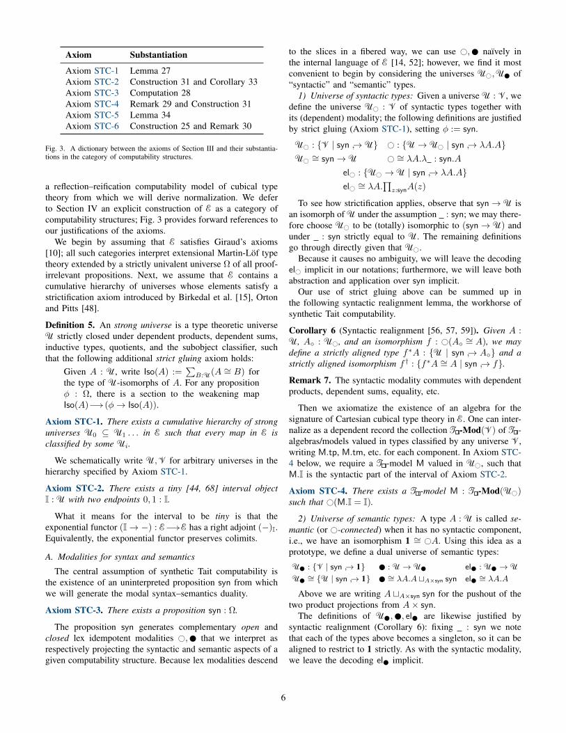
HCom : Utp U

Coe : (I→ Utp) U

HCom(A) ∼=∏

r,s:I∏φ:F∏a:∏i:I∏

:[i=r∨Fφ]AA | r = s ∨F φ → a(s)

∣∣ syn → M.hcomA

Coe(A) ∼=

∏r,s:I∏a:A(r)A(s) | r = s → a

∣∣ syn → M.coeA

Fig. 4. Definitions of homogeneous composition structures for a computability structure and coercion structures for a line of computability structures; theuse of U indicates that these structures are #-connected, i.e., equivalently classified by the subuniverse U | syn → 1.

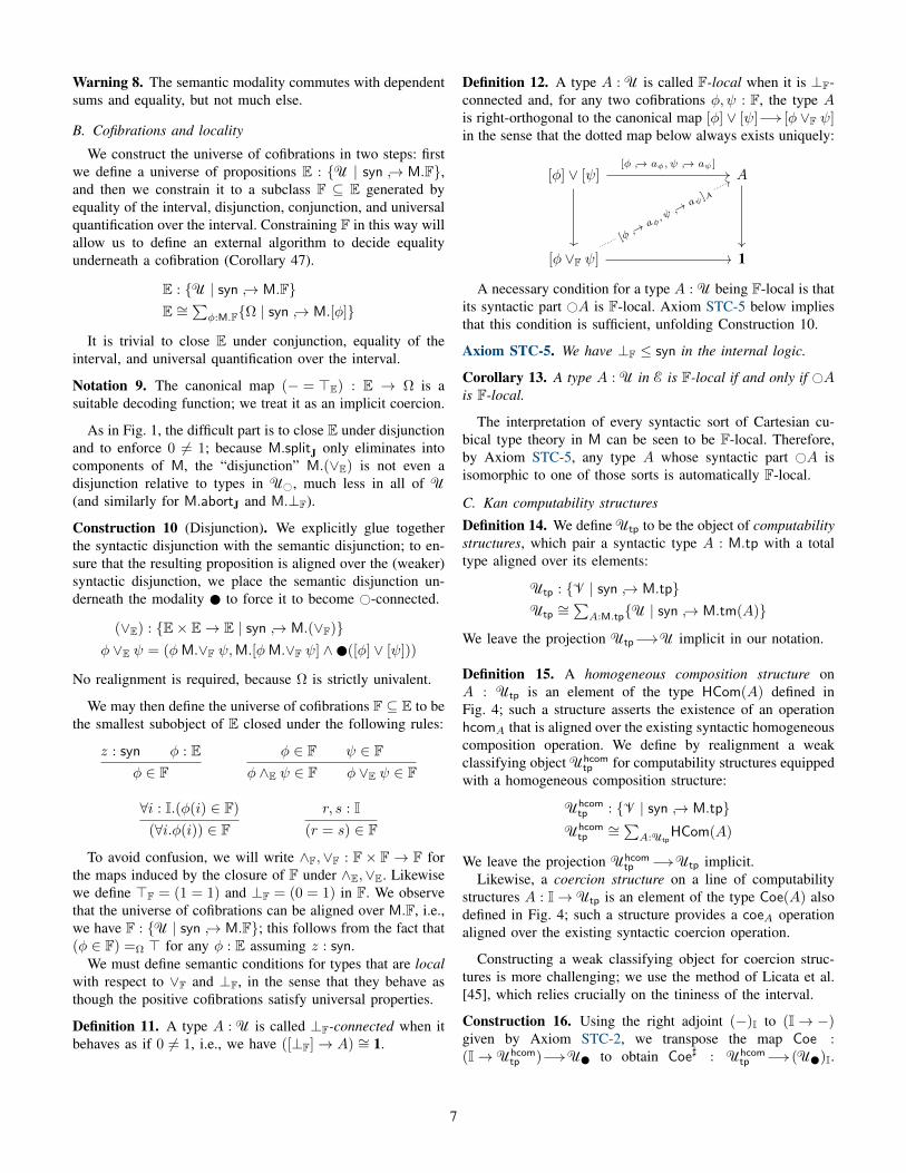
nftp : U | syn → M.tpne(−) :

∏φ:F∏A:M.tpU | φ ∨ syn → M.tm(A)

nf :∏A:M.tpU | syn → M.tm(A)

var : A var(A)→ ne⊥F(A) | syn → λx.x

Fig. 5. Axiomatization of the structure of normal and neutral forms.

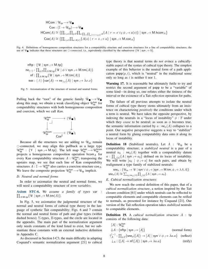
Pulling back the “root” of the generic family U U along this map, we obtain a weak classifying object Ukan

tp forcomputability structures with both homogeneous compositionand coercion, which we call Kan.

Ukantp

Uhcomtp

(U )I

(U )ICoe]

Because all the structures we are adding to Utp remain#-connected, we may align this pullback as a large typeUkan

tp : V | syn → M.tp. The left map Ukantp Uhcom

tp

projects a homogeneous composition operation hcomA forevery Kan computability structure A : Ukan

tp ; transposing theupstairs map, we see that each line of Kan computabilitystructures A : I→ Ukan

tp also carries a coercion structure coeA.We leave the composite projection Ukan

tp Utp implicit.

D. Neutral and normal forms

In order to axiomatize the neutral and normal forms, wewill need a computability structure of term variables.

Axiom STC-6. We assume a family of types var :∏A:M.tpU | syn → M.tm(A).

In Fig. 5, we axiomatize the judgmental structure of thenormal and neutral forms of cubical type theory in the lan-guage of synthetic Tait computability; Figs. 6 and 7 containthe normal and neutral forms of path and glue types (withindashed boxes); Σ-types, Π-types, and the circle are located inthe appendix. The main part of the normalization argumentonly needs constants of the kind listed to exist, but we sub-stantiate these constants with an external inductive definitionin Appendix C.

As discussed in Section I-C3, the main difficulty in adaptingCoquand’s semantic normalization argument [21] to cubical

type theory is that neutral terms do not evince a cubically-stable aspect of the syntax of cubical type theory. The simplestexample of this behavior is the neutral form of a path appli-cation papp(p, i), which is “neutral” in the traditional senseonly so long as i is neither 0 nor 1.

Warning 17. It is reasonable but ultimately futile to try andrestrict the second argument of papp to be a “variable” ofsome kind—in doing so, one refutes either the tininess of theinterval or the existence of a Tait reflection operation for paths.

The failure of all previous attempts to isolate the neutralforms of cubical type theory stems ultimately from an insis-tence on characterizing positively the conditions under whicha term is neutral. We have taken the opposite perspective, byindexing the neutrals in a “locus of instability” φ : F underwhich they cease to be neutral; as soon as φ becomes true,the semantic information carried by a : neφ(A) collapses to apoint. Our negative perspective suggests a way to “stabilize”a neutral form by gluing computability data onto it along itslocus of instability.

Definition 18 (Stabilized neutrals). Let A : Utp be acomputability structure; a stabilized neutral is a pair of aneutral a0 : neφ(A) together with a computability datuma :

∏:[φ]A | syn → a0 defined on its locus of instability.

We will write [a0 | φ → a] for such pairs, and obtain byrealignment a type family of stabilized neutrals:

sneφ : Utp → U | syn ∨ φ → [syn → M.tm, φ → λA.A]sneφ(A) ∼=

∑a0:neφ(A)

∏:[φ]A | syn → a0

E. Cubical normalization structuresWe now reach the central definition of this paper, that of a

cubical normalization structure, a notion inspired by the Taitclosure condition [61] under which neutrals can be reflected tocomputable elements and computable elements can be reifiedto normals, as presented for instance by Coquand [21]. Ourversion of the Tait reflection operation takes stabilized neutralsto computable elements.

Definition 19. A cubical normalization structure A : tpconsists of the following data:

[A] : Ukantp

⇓A : nftp | syn → [A] (normal form)

↑(−)A :

∏φ:Fsneφ([A])→ [A] | syn ∨ φ → λa.a (reflect)

↓A : [A]→ nf([A]) | syn → λa.a (reify)

8

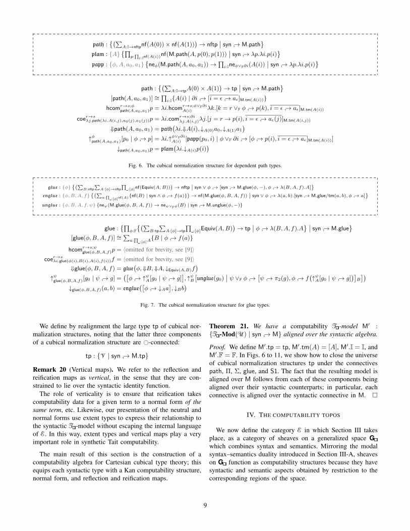
path :(∑

A:I→nftpnf(A(0))× nf(A(1)))→ nftp

∣∣ syn → M.path

plam : A∏

p:∏i:Inf(A(i))nf(M.path(A, p(0), p(1)))

∣∣ syn → λp.λi.p(i)

papp : φ,A, a0, a1neφ(M.path(A, a0, a1))→

∏i:Ineφ∨F∂i(A(i))

∣∣ syn → λp.λi.p(i)

path :(∑

A:I→tpA(0)×A(1))→ tp

∣∣ syn → M.path

[path(A, a0, a1)] ∼=∏i:IA(i) | ∂i → [i = ε → aε]M.tm(A(i))

hcomr→s;φpath(A,a0,a1)p = λi.hcomr→s;φ∨F∂i

A(i) λk.[k = r ∨F φ → p(k), i = ε → aε]M.tm(A(i))

coer→sλj.path(λi.A(i,j),a0(j),a1(j))p = λi.comr→s;∂iλj.A(i,j)λj.[j = r → p(i), i = ε → aε(j)]M.tm(A(i,j))

⇓path(A, a0, a1) = path(λi.⇓A(i), ↓A(0)a0, ↓A(1)a1

)↑φpath(A,a0,a1)[p0 | φ → p] = λi.↑φ∨F∂i

A(i) [papp(p0, i) | φ ∨F ∂i → [φ → p(i), i = ε → aε]M.tm(A(i))]

↓path(A,a0,a1)p = plam(λi.↓A(i)p(i)

)Fig. 6. The cubical normalization structure for dependent path types.

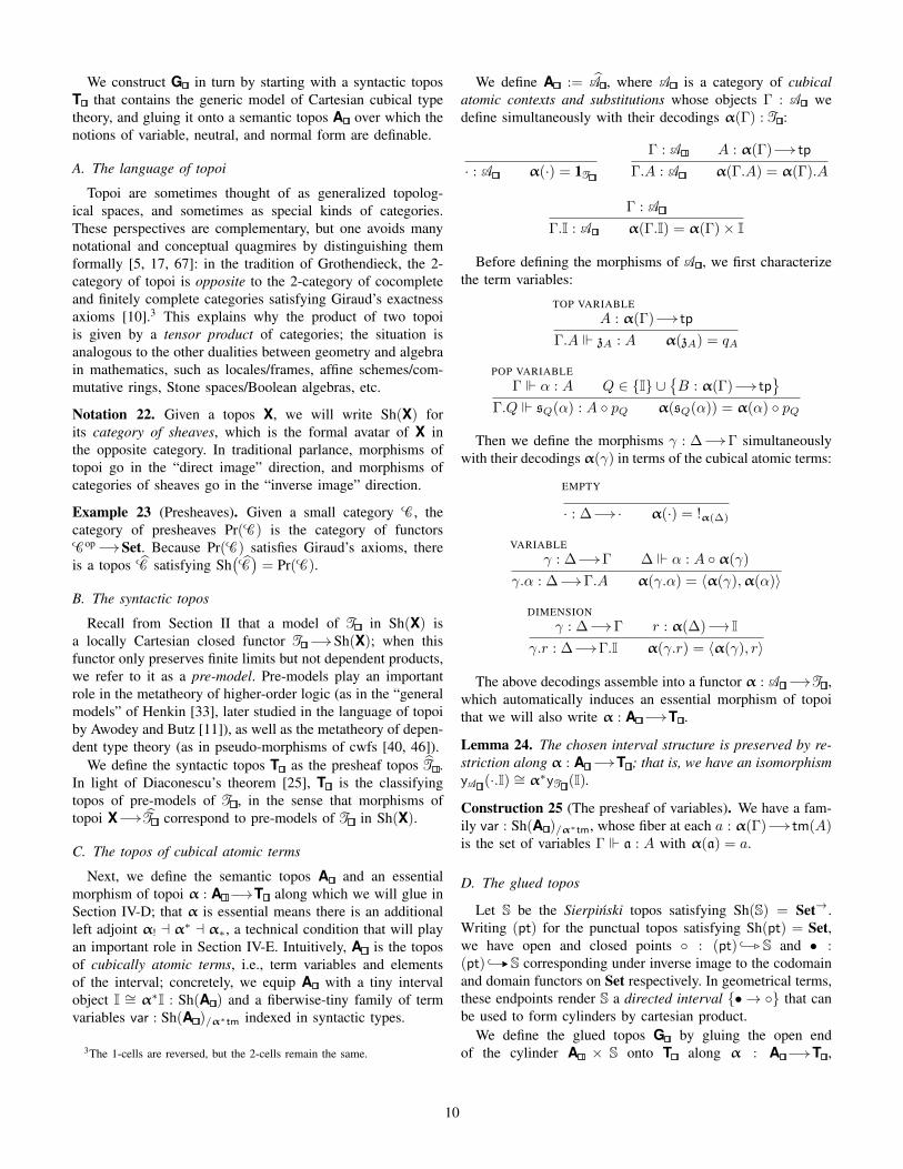
glue : φ(∑

B:nftp

∑A:[φ]→nftp

∏:[φ]nf(Equiv(A,B))

)→ nftp

∣∣ syn ∨ φ → [syn → M.glue(φ,−), φ → λ(B,A, f).A]

englue : φ,B,A, f(∑

a:∏

:[φ]nf(A)nf(B) | syn ∧ φ → f(a))→ nf(M.glue(φ,B,A, f))

∣∣ syn ∨ φ → λ(a, b).[syn → M.glue/tm(a, b), φ → a]

unglue : φ,B,A, f, ψ neψ(M.glue(φ,B,A, f))→ neψ∨Fφ(B) | syn → M.unglue(φ,−)

glue :∏

φ:F(∑

B:tp

∑A:[φ]→tp

∏:[φ]Equiv(A,B)

)→ tp

∣∣ φ → λ(B,A, f).A ∣∣ syn → M.glue

[glue(φ,B,A, f)] ∼=

∑a:∏

:[φ]AB | φ → f(a)

hcomr→s;ψglue(φ,B,A,f)p = 〈omitted for brevity, see [9]〉

coer→sλi.glue(φ(i),B(i),A(i),f(i))f = 〈omitted for brevity, see [9]〉⇓glue(φ,B,A, f) = glue

(φ,⇓B,⇓A, ↓Equiv(A,B)f

)↑ψglue(φ,B,A,f)[g0 | ψ → g] =

([φ → ↑ψA[g0 | ψ → g]

], ↑ψB

[unglue(g0)

∣∣ ψ ∨F φ →[ψ → π2(g), φ → f

(↑ψA[g0 | ψ → g]

)]B

])↓glue(φ,B,A,f)(a, b) = englue

([φ → ↓Aa

], ↓Bb

)Fig. 7. The cubical normalization structure for glue types.

We define by realignment the large type tp of cubical nor-malization structures, noting that the latter three componentsof a cubical normalization structure are #-connected:

tp : V | syn → M.tp

Remark 20 (Vertical maps). We refer to the reflection andreification maps as vertical, in the sense that they are con-strained to lie over the syntactic identity function.

The role of verticality is to ensure that reification takescomputability data for a given term to a normal form of thesame term, etc. Likewise, our presentation of the neutral andnormal forms use extent types to express their relationship tothe syntactic T -model without escaping the internal languageof E. In this way, extent types and vertical maps play a veryimportant role in synthetic Tait computability.

The main result of this section is the construction of acomputability algebra for Cartesian cubical type theory; thisequips each syntactic type with a Kan computability structure,normal form, and reflection and reification maps.

Theorem 21. We have a computability T -model M′ :T -Mod(U) | syn → M aligned over the syntactic algebra.

Proof. We define M′.tp = tp, M′.tm(A) = [A], M′.I = I, andM′.F = F. In Figs. 6 to 11, we show how to close the universeof cubical normalization structures tp under the connectivespath, Π, Σ, glue, and S1. The fact that the resulting model isaligned over M follows from each of these components beingaligned over their syntactic counterparts; in particular, eachconnective is aligned over the syntactic connective in M.

IV. THE COMPUTABILITY TOPOS

We now define the category E in which Section III takesplace, as a category of sheaves on a generalized space Gwhich combines syntax and semantics. Mirroring the modalsyntax–semantics duality introduced in Section III-A, sheaveson G function as computability structures because they havesyntactic and semantic aspects obtained by restriction to thecorresponding regions of the space.

9

We construct G in turn by starting with a syntactic toposT that contains the generic model of Cartesian cubical typetheory, and gluing it onto a semantic topos A over which thenotions of variable, neutral, and normal form are definable.

A. The language of topoi

Topoi are sometimes thought of as generalized topolog-ical spaces, and sometimes as special kinds of categories.These perspectives are complementary, but one avoids manynotational and conceptual quagmires by distinguishing themformally [5, 17, 67]: in the tradition of Grothendieck, the 2-category of topoi is opposite to the 2-category of cocompleteand finitely complete categories satisfying Giraud’s exactnessaxioms [10].3 This explains why the product of two topoiis given by a tensor product of categories; the situation isanalogous to the other dualities between geometry and algebrain mathematics, such as locales/frames, affine schemes/com-mutative rings, Stone spaces/Boolean algebras, etc.

Notation 22. Given a topos X, we will write Sh(X) forits category of sheaves, which is the formal avatar of X inthe opposite category. In traditional parlance, morphisms oftopoi go in the “direct image” direction, and morphisms ofcategories of sheaves go in the “inverse image” direction.

Example 23 (Presheaves). Given a small category C, thecategory of presheaves Pr( C) is the category of functorsCop Set. Because Pr( C) satisfies Giraud’s axioms, thereis a topos C satisfying Sh

(C)

= Pr( C).

B. The syntactic topos

Recall from Section II that a model of T in Sh(X) isa locally Cartesian closed functor T Sh(X); when thisfunctor only preserves finite limits but not dependent products,we refer to it as a pre-model. Pre-models play an importantrole in the metatheory of higher-order logic (as in the “generalmodels” of Henkin [33], later studied in the language of topoiby Awodey and Butz [11]), as well as the metatheory of depen-dent type theory (as in pseudo-morphisms of cwfs [40, 46]).

We define the syntactic topos T as the presheaf topos T .In light of Diaconescu’s theorem [25], T is the classifyingtopos of pre-models of T , in the sense that morphisms oftopoi X T correspond to pre-models of T in Sh(X).

C. The topos of cubical atomic terms

Next, we define the semantic topos A and an essentialmorphism of topoi α : A T along which we will glue inSection IV-D; that α is essential means there is an additionalleft adjoint α! a α∗ a α∗, a technical condition that will playan important role in Section IV-E. Intuitively, A is the toposof cubically atomic terms, i.e., term variables and elementsof the interval; concretely, we equip A with a tiny intervalobject I ∼= α∗I : Sh(A ) and a fiberwise-tiny family of termvariables var : Sh(A )/α∗tm indexed in syntactic types.

3The 1-cells are reversed, but the 2-cells remain the same.

We define A := A , where A is a category of cubicalatomic contexts and substitutions whose objects Γ : A wedefine simultaneously with their decodings α(Γ) : T :

· : A α(·) = 1T

Γ : A A : α(Γ) tp

Γ.A : A α(Γ.A) = α(Γ).A

Γ : A

Γ.I : A α(Γ.I) = α(Γ)× I

Before defining the morphisms of A , we first characterizethe term variables:

TOP VARIABLEA : α(Γ) tp

Γ.A zA : A α(zA) = qA

POP VARIABLEΓ α : A Q ∈ I ∪

B : α(Γ) tp

Γ.Q sQ(α) : A pQ α(sQ(α)) = α(α) pQ

Then we define the morphisms γ : ∆ Γ simultaneouslywith their decodings α(γ) in terms of the cubical atomic terms:

EMPTY

· : ∆ · α(·) = !α(∆)

VARIABLEγ : ∆ Γ ∆ α : A α(γ)

γ.α : ∆ Γ.A α(γ.α) = 〈α(γ),α(α)〉

DIMENSIONγ : ∆ Γ r : α(∆) I

γ.r : ∆ Γ.I α(γ.r) = 〈α(γ), r〉

The above decodings assemble into a functor α : A T ,which automatically induces an essential morphism of topoithat we will also write α : A T .

Lemma 24. The chosen interval structure is preserved by re-striction along α : A T ; that is, we have an isomorphismyA (·.I) ∼= α∗yT (I).

Construction 25 (The presheaf of variables). We have a fam-ily var : Sh(A )/α∗tm, whose fiber at each a : α(Γ) tm(A)is the set of variables Γ a : A with α(a) = a.

D. The glued topos

Let S be the Sierpinski topos satisfying Sh(S) = Set→.Writing (pt) for the punctual topos satisfying Sh(pt) = Set,we have open and closed points : (pt) S and • :(pt) S corresponding under inverse image to the codomainand domain functors on Set respectively. In geometrical terms,these endpoints render S a directed interval • → that canbe used to form cylinders by cartesian product.

We define the glued topos G by gluing the open endof the cylinder A × S onto T along α : A T ,

10

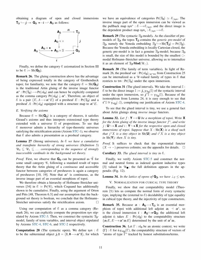
obtaining a diagram of open and closed immersionsT G Aj i as follows:

A

A × S

A ×

T

G

α

j

AA × •

i

Finally, we define the category E axiomatized in Section IIIto be E := Sh(G ).

Remark 26. The gluing construction above has the advantageof being expressed totally in the category of Grothendiecktopoi; for familiarity, we note that the category E = Sh(G )is the traditional Artin gluing of the inverse image functorα∗ : Pr(T ) Pr(A ) and can hence be explicitly computedas the comma category Pr(A ) ↓ α∗. Therefore, an object ofE is a pair

(E,A α∗E

)of a presheaf E : Pr(T ) and a

presheaf A : Pr(A ) equipped with a structure map to α∗E.

E. Verifying the axioms

Because E = Sh(G ) is a category of sheaves, it satisfiesGiraud’s axioms and thus interprets extensional type theoryextended with a universe Ω of propositions. To see thatE moreover admits a hierarchy of type-theoretic universessatisfying the strictification axiom (Axiom STC-1), we observethat E also admits a presentation as a presheaf category.

Lemma 27 (Strong universes). In E we have a cumulativeand transfinite hierarchy of strong universes (Definition 5)U0 ⊆ U1 ⊆ . . . corresponding to the sequence of stronglyinaccessible cardinals in the background set theory.

Proof. First, we observe that G can be presented as G forsome small category G, following a standard result of topostheory that the Artin gluing of a continuous and accessiblefunctor between categories of presheaves is again a categoryof presheaves [10, 19]. Note that α∗ is continuous, as theinverse image part of an essential morphism of topoi.

We therefore obtain a hierarchy of Hofmann–Streicher uni-verses [34] in E ' Pr( G), which Coquand has additionallyshown to be cumulative. Finally, using the argument of Ortonand Pitts [48, Theorem 6.3] and our assumption that the back-ground set theory is boolean, we conclude that the Hofmann–Streicher universes satisfy the strictification axiom.

Using our computation of E as a comma category (Re-mark 26), we can explicitly compute the proposition syn stip-ulated by Axiom STC-3. Then, we construct the syntactic T -model, family of term variables, and interval object stipulatedby Axioms STC-4, STC-6, and STC-2 respectively.

Computation 28 (The syntactic open). We define syn : Eto be the subterminal object j!1 =

(1, 0 α∗1

), for which

we have an equivalence of categories Pr(T ) ' E/syn. Theinverse image part of the open immersion can be viewed asthe pullback map syn∗ : E E/syn, and the direct image isthe dependent product map syn∗ : E/syn E.

Remark 29 (The syntactic T -model). As the classifier of pre-models of T , the topos T contains the generic pre-model ofT , namely the Yoneda embedding T Sh(T ) = Pr(T ).Because the Yoneda embedding is locally Cartesian closed, thegeneric pre-model is in fact a genuine T -model; because Tis small, the size of this model is bounded by the smallest #-modal Hofmann–Streicher universe, allowing us to internalizeit as an element of T -Mod(U#).

Remark 30 (The family of term variables). In light of Re-mark 26, the presheaf var : Pr(A )/α∗tm from Construction 25can be internalized as a U-valued family of types in E thatrestricts to tm : Pr(T ) under the open immersion.

Construction 31 (The glued interval). We take the interval I :E to be the direct image I := j∗yT (I) of the syntactic intervalunder the open immersion, so j∗I = yT (I). Because of theisomorphism from Lemma 24, it is easy enough to see thati∗I ∼= yA (·.I), completing our justification of Axiom STC-4.

To see that the glued interval is tiny, we use a general factabout Artin gluings along inverse image functors.

Lemma 32. Let f : Y U be a morphism of topoi. Write Xfor the Artin gluing of the inverse image functor f∗, and writej : U X and i : Y X for the respective open and closedimmersions of topoi. Suppose that X : Sh(X) is a sheaf suchthat j∗X is a tiny object in Sh(U) and i∗X is a tiny objectin Sh(Y); then X is tiny.

Proof. It suffices to check that the exponential functor(X → −) preserves colimits; see the appendix for details.

Corollary 33. The glued interval is tiny in E.

Finally, we verify Axiom STC-5 and construct the nor-mal and neutral forms as indexed quotient inductive types[3] valued in U ; the full definition appears in the ap-pendix (Fig. 12).

Lemma 34. In the lattice of opens of G , we have ⊥F ≤ syn.

V. NORMALIZATION FOR CUBICAL TYPE THEORY

Finally, we show that our computability model (Theo-rem 21) lets us compute the normal form of every syntactictype, implying the (external to E) decidability of type equalityin cubical type theory, and the injectivity of type constructors.

Remark 35. Because α : A T is an essential mor-phism of topoi with additional left adjoint α! a α∗, sois the closed immersion i : A G ; the additional leftadjoint i! takes E : Pr(A ) to the computability structure(α!E,E α∗α!E

)determined by the unit of α∗α!.

Construction 36. Let Γ : A be an atomic context; we writeLΓM : E for i!yA (Γ), the computability structure of vectors of“atoms of type Γ” tracked by honest substitutions/terms.

11

Construction 37. The computability model evinces a locallyCartesian closed functor M′ : T E; restricting along α :A T , we have an interpretation functor J−K : A Etaking each atomic context to its computability structureM′(α(Γ)). We observe that j∗JΓK = yT (α(Γ)) = α!yA (Γ).

Construction 38. For any X : E there is a canoni-cal natural transformation [J−K, X] α∗j∗X : Pr(A )which restricts M′(α(Γ)) X : E to its syntactic part,noting that Hom(α!yA (Γ), j∗X) ∼= α∗j∗X(Γ). Viewedas a sheaf on G , we write XM′ : E for the pair(j∗X, [J−K, X] α∗j∗X

).

Construction 39. We define a pointwise vertical (Remark 20)natural transformation atom : L−M J−K : Hom(A , E) thatreflects each atomic substitution as a computable substitution.The definition follows by recursion on the index Γ : A , anduses the fact that the locus of instability of a variable is empty:

atom(·)(·) = ·atomΓ.I(γ.r) = (atomΓ(γ), r)

atomΓ.A(γ.x) =(atomΓ(γ), ↑⊥F

M′(A)[var(x) | ⊥F → []M′(A)])

Lemma 40. The pointwise vertical natural transformationatom : L−M J−K induces by precomposition a vertical mapatom∗X : XM′ X for any sheaf X : E.

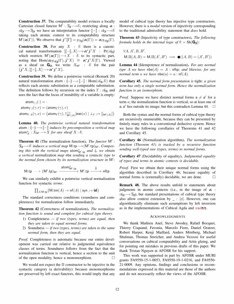
Theorem 41 (The normalization function). The functor M′ :T E induces a vertical map M.tp (M′.tp)M′ . Compos-ing this with the vertical maps atom∗M′.tp and ⇓, we obtaina vertical normalization map nbe sending a syntactic type tothe normal form chosen by its normalization structure in M′:

M.tp (M′.tp)M′ M′.tp nftpatom∗M′.tp ⇓

We can similarly exhibit a pointwise vertical normalizationfunction for syntactic terms:∏

A:M.tpM.tm(A)→ nf(A) | syn → id

The standard correctness conditions (soundness and com-pleteness) for normalization follow immediately.

Theorem 42 (Correctness of normalization). The normaliza-tion function is sound and complete for cubical type theory.

1) Completeness — if two (types, terms) are equal, thenthey are taken to equal normal forms.

2) Soundness — if two (types, terms) are taken to the samenormal form, then they are equal.

Proof. Completeness is automatic because our entire devel-opment was carried out relative to judgmental equivalenceclasses of terms. Soundness follows from the fact that thenormalization function is vertical, hence a section to the unitof the open modality, hence a monomorphism.

We would not expect the Π constructor to be injective in thesyntactic category (a derivability): because monomorphismsare preserved by left exact functors, this would imply that any

model of cubical type theory has injective type constructors.However, there is a modal version of injectivity correspondingto the traditional admissibility statement that does hold.

Theorem 43 (Injectivity of type constructors). The followingformula holds in the internal logic of E = Sh(G ):

∀A,A′, B,B′.M.Π(A,B) = M.Π(A′, B′) =⇒ ((A,B) = (A′, B′))

Lemma 44 (Idempotence of normalization). For any normaltype A we have nbe(A) = A : nftp; and likewise, for anynormal term a we have nbe(a) = a : nf(A).

Corollary 45. The normal form presentation is tight: a giventerm has only a single normal form. Hence the normalizationfunction is an isomorphism.

Proof. Suppose we have distinct normal forms a 6= a′ for aterm a; the normalization function is vertical, so at least one ofa, a′ lies outside its image; but this contradicts Lemma 44.

Both the syntax and the normal forms of cubical type theoryare recursively enumerable, because they can be presented byfinitely many rules in a conventional deductive system. Hencewe have the following corollaries of Theorems 41 and 42and Corollary 45.

Corollary 46 (Normalization algorithm). The normalizationfunction (Theorem 41) is tracked by a recursive functionsending well-typed raw (types, terms) to normal forms.

Corollary 47 (Decidability of equality). Judgmental equalityof types and terms in atomic contexts is decidable.

Proof. First we obtain their unique normal forms using thealgorithm described in Corollary 46; because equality ofnormal forms is (externally) decidable, we are done.

Remark 48. The above results unfold to statements aboutjudgments in atomic contexts (i.e., in the image of α :A T ), but standard presentations of cubical type theoryalso allow context extension by : [φ]. However, one canalgorithmically eliminate such assumptions by left inversionas in the implementations of Cubical Agda and redtt.

ACKNOWLEDGMENTS

We thank Mathieu Anel, Steve Awodey, Rafael Bocquet,Thierry Coquand, Favonia, Marcelo Fiore, Daniel Gratzer,Robert Harper, Kenji Maillard, Anders Mortberg, MichaelShulman, Thomas Streicher, and Andrea Vezzosi for usefulconversations on cubical computability and Artin gluing, andfor pointing out mistakes in previous drafts of this paper. Wethank Tristan Nguyen at AFOSR for his support.

This work was supported in part by AFOSR under MURIgrants FA9550-15-1-0053, FA9550-19-1-0216, and FA9550-21-0009. Any opinions, findings and conclusions or recom-mendations expressed in this material are those of the authorsand do not necessarily reflect the views of the AFOSR.

12

REFERENCES

[1] A. Abel, “Normalization by evaluation: Dependent typesand impredicativity,” Habilitation, Ludwig-Maximilians-Universitat Munchen, 2013.

[2] T. Altenkirch, P. Dybjer, M. Hofmann, and P. Scott, “Nor-malization by evaluation for typed lambda calculus withcoproducts,” in Proceedings of the 16th Annual IEEESymposium on Logic in Computer Science. Washington,DC, USA: IEEE Computer Society, 2001, pp. 303–.

[3] T. Altenkirch and A. Kaposi, “Type theory in type theoryusing quotient inductive types,” in Proceedings of the43rd Annual ACM SIGPLAN-SIGACT Symposium onPrinciples of Programming Languages, ser. POPL ’16.St. Petersburg, FL, USA: ACM, 2016, pp. 18–29.

[4] T. Altenkirch, M. Hofmann, and T. Streicher, “Cate-gorical reconstruction of a reduction free normaliza-tion proof,” in Category Theory and Computer Science,D. Pitt, D. E. Rydeheard, and P. Johnstone, Eds. Berlin,Heidelberg: Springer Berlin Heidelberg, 1995, pp. 182–199.

[5] M. Anel and A. Joyal, “Topo-logie,” in New Spacesin Mathematics: Formal and Conceptual Reflections,M. Anel and G. Catren, Eds. Cambridge UniversityPress, 2021, vol. 1, ch. 4, pp. 155–257.

[6] C. Angiuli, “Computational semantics of Cartesian cu-bical type theory,” Ph.D. dissertation, Carnegie MellonUniversity, 2019.

[7] C. Angiuli, R. Harper, and T. Wilson, “Computationalhigher-dimensional type theory,” in POPL 2017: Pro-ceedings of the 44th ACM SIGPLAN Symposium onPrinciples of Programming Languages. Paris, France:ACM, 2017, pp. 680–693.

[8] C. Angiuli, K.-B. Hou (Favonia), and R. Harper,“Cartesian Cubical Computational Type Theory:Constructive Reasoning with Paths and Equalities,”in 27th EACSL Annual Conference on ComputerScience Logic (CSL 2018), ser. Leibniz InternationalProceedings in Informatics (LIPIcs), D. Ghicaand A. Jung, Eds., vol. 119. Dagstuhl,Germany: Schloss Dagstuhl–Leibniz-Zentrum fuerInformatik, 2018, pp. 6:1–6:17. [Online]. Available:http://drops.dagstuhl.de/opus/volltexte/2018/9673

[9] C. Angiuli, G. Brunerie, T. Coquand, K.-B. Hou(Favonia), R. Harper, and D. R. Licata, “Syntaxand models of Cartesian cubical type theory,” Feb.2019, preprint. [Online]. Available: https://github.com/dlicata335/cart-cube

[10] M. Artin, A. Grothendieck, and J.-L. Verdier, Theoriedes topos et cohomologie etale des schemas. Berlin:Springer-Verlag, 1972, seminaire de GeometrieAlgebrique du Bois-Marie 1963–1964 (SGA 4),Dirige par M. Artin, A. Grothendieck, et J.-L. Verdier.Avec la collaboration de N. Bourbaki, P. Deligne et B.Saint-Donat, Lecture Notes in Mathematics, Vol. 269,270, 305.

[11] S. Awodey and C. Butz, “Topological completeness forhigher-order logic,” The Journal of Symbolic Logic,vol. 65, no. 3, pp. 1168–1182, 2000. [Online]. Available:http://www.jstor.org/stable/2586693

[12] S. Awodey, “Natural models of homotopy type theory,”Mathematical Structures in Computer Science, vol. 28,no. 2, pp. 241–286, 2018.

[13] A. Bauer, “First steps in synthetic computability theory,”Electronic Notes in Theoretical Computer Science, vol.155, pp. 5–31, 2006, proceedings of the 21st AnnualConference on Mathematical Foundations of Program-ming Semantics (MFPS XXI).

[14] L. Birkedal, R. E. Møgelberg, J. Schwinghammer, andK. Stovring, “First steps in synthetic guarded domaintheory: Step-indexing in the topos of trees,” in Proceed-ings of the 2011 IEEE 26th Annual Symposium on Logicin Computer Science. Washington, DC, USA: IEEEComputer Society, 2011, pp. 55–64.

[15] L. Birkedal, A. Bizjak, R. Clouston, H. B. Grathwohl,B. Spitters, and A. Vezzosi, “Guarded Cubical TypeTheory: Path Equality for Guarded Recursion,” in 25thEACSL Annual Conference on Computer Science Logic(CSL 2016), ser. Leibniz International Proceedings inInformatics (LIPIcs), J.-M. Talbot and L. Regnier, Eds.,vol. 62. Dagstuhl, Germany: Schloss Dagstuhl–Leibniz-Zentrum fuer Informatik, 2016, pp. 23:1–23:17.

[16] I. Blechschmidt, “Using the internal language of toposesin algebraic geometry,” Ph.D. dissertation, UniversitatAugsberg, 2017.

[17] M. Bunge and J. Funk, Singular coverings of toposes, ser.Lecture notes in mathematics, 1890. Berlin: Springer,2006.

[18] M. Bunge, F. Gago, and A. M. San Luis, SyntheticDifferential Topology, ser. London Mathematical SocietyLecture Note Series. Cambridge University Press, 2018.

[19] A. Carboni and P. Johnstone, “Connected limits, familialrepresentability and Artin glueing,” Mathematical Struc-tures in Computer Science, vol. 5, no. 4, pp. 441–459,1995.

[20] C. Cohen, T. Coquand, S. Huber, and A. Mortberg,“Cubical Type Theory: a constructive interpretationof the univalence axiom,” IfCoLog Journal of Logicsand their Applications, vol. 4, no. 10, pp. 3127–3169, Nov. 2017. [Online]. Available: http://www.collegepublications.co.uk/journals/ifcolog/?00019

[21] T. Coquand, “Canonicity and normalization for depen-dent type theory,” Theoretical Computer Science, vol.777, pp. 184–191, 2019, in memory of Maurice Nivat, afounding father of Theoretical Computer Science - PartI.

[22] T. Coquand, S. Huber, and A. Mortberg, “On higherinductive types in cubical type theory,” in Proceedingsof the 33rd Annual ACM/IEEE Symposium on Logic inComputer Science. Oxford, United Kingdom: ACM,2018, pp. 255–264.

[23] T. Coquand, S. Huber, and C. Sattler, “Homotopy canon-

13

icity for cubical type theory,” in 4th International Con-ference on Formal Structures for Computation and De-duction (FSCD 2019), ser. Leibniz International Proceed-ings in Informatics (LIPIcs), H. Geuvers, Ed., vol. 131.Dagstuhl, Germany: Schloss Dagstuhl–Leibniz-Zentrumfuer Informatik, 2019.

[24] R. L. Crole, Categories for Types, ser. Cambridge Math-ematical Textbooks. New York: Cambridge UniversityPress, 1993.

[25] R. Diaconescu, “Change of base for toposes with gen-erators,” Journal of Pure and Applied Algebra, vol. 6,no. 3, pp. 191–218, 1975.

[26] P. Dybjer, “Internal type theory,” in Types for Proofs andPrograms: International Workshop, TYPES ’95 Torino,Italy, June 5–8, 1995 Selected Papers, S. Berardi andM. Coppo, Eds. Berlin, Heidelberg: Springer BerlinHeidelberg, 1996, pp. 120–134.

[27] M. Fiore, “Semantic analysis of normalisation by evalua-tion for typed lambda calculus,” in Proceedings of the 4thACM SIGPLAN International Conference on Principlesand Practice of Declarative Programming, ser. PPDP’02. Pittsburgh, PA, USA: ACM, 2002, pp. 26–37.

[28] P. Freyd, “On proving that 1 is an indecomposableprojective in various free categories,” 1978, unpublishedmanuscript.

[29] D. Gratzer and J. Sterling, “Syntactic categories fordependent type theory: sketching and adequacy,” 2020,preprint. [Online]. Available: https://arxiv.org/abs/2012.10783

[30] D. Gratzer, G. A. Kavvos, A. Nuyts, and L. Birkedal,“Multimodal dependent type theory,” in Proceedings ofthe 35th Annual ACM/IEEE Symposium on Logic inComputer Science. Saarbrucken, Germany: Associationfor Computing Machinery, 2020, pp. 492–506.

[31] R. Harper and D. R. Licata, “Mechanizing metatheoryin a logical framework,” Journal of Functional Program-ming, vol. 17, no. 4-5, pp. 613–673, Jul. 2007.

[32] R. Harper, F. Honsell, and G. Plotkin, “A framework fordefining logics,” J. ACM, vol. 40, no. 1, pp. 143–184,Jan. 1993.

[33] L. Henkin, “Completeness in the theory of types,”The Journal of Symbolic Logic, vol. 15, no. 2, pp.81–91, 1950. [Online]. Available: http://www.jstor.org/stable/2266967

[34] M. Hofmann and T. Streicher, “Lifting Grothendieckuniverses,” 1997, unpublished note. [Online].Available: https://www2.mathematik.tu-darmstadt.de/∼streicher/NOTES/lift.pdf

[35] S. Huber, “Canonicity for cubical type theory,” Journalof Automated Reasoning, Jun. 2018.

[36] J. M. E. Hyland, “First steps in synthetic domain theory,”in Category Theory, A. Carboni, M. C. Pedicchio, andG. Rosolini, Eds. Berlin, Heidelberg: Springer BerlinHeidelberg, 1991, pp. 131–156.

[37] P. T. Johnstone, Sketches of an Elephant: A Topos TheoryCompendium: Volumes 1 and 2, ser. Oxford Logical

Guides. Oxford Science Publications, 2002, no. 43.[38] A. Jung and J. Tiuryn, “A new characterization of lambda

definability,” in Typed Lambda Calculi and Applications,M. Bezem and J. F. Groote, Eds. Berlin, Heidelberg:Springer Berlin Heidelberg, 1993, pp. 245–257.

[39] A. Kaposi, “Type theory in a type theory with quotientinductive types,” Ph.D. dissertation, University of Not-tingham, 2017.

[40] A. Kaposi, S. Huber, and C. Sattler, “Gluing for typetheory,” in 4th International Conference on Formal Struc-tures for Computation and Deduction (FSCD 2019),ser. Leibniz International Proceedings in Informatics(LIPIcs), H. Geuvers, Ed., vol. 131. Dagstuhl, Ger-many: Schloss Dagstuhl–Leibniz-Zentrum fuer Infor-matik, 2019.

[41] C. Kapulkin and C. Sattler, “Homotopy canonicity ofhomotopy type theory,” Aug. 2019, slides from a talkgiven at the International Conference on HomotopyType Theory (HoTT 2019). [Online]. Available: https://hott.github.io/HoTT-2019/conf-slides/Sattler.pdf

[42] A. Kock, Synthetic Differential Geometry, 2nd ed.,ser. London Mathematical Society Lecture Note Series.Cambridge University Press, 2006.

[43] ——, Synthetic Geometry of Manifolds, ser. CambridgeTracts in Mathematics. Cambridge University Press,2009.

[44] F. W. Lawvere, “Toward the description in a smoothtopos of the dynamically possible motions and defor-mations of a continuous body,” Cahiers de Topologie etGeometrie Differentielle Categoriques, vol. 21, no. 4, pp.377–392, 1980.

[45] D. R. Licata, I. Orton, A. M. Pitts, and B. Spitters,“Internal universes in models of homotopy type theory,”in 3rd International Conference on Formal Structuresfor Computation and Deduction, FSCD 2018, July 9-12,2018, Oxford, UK, 2018, pp. 22:1–22:17.

[46] C. Newstead, “Algebraic models of dependent type the-ory,” Ph.D. dissertation, Carnegie Mellon University,2018.

[47] B. Nordstrom, K. Peterson, and J. M. Smith, Program-ming in Martin-Lof’s Type Theory, ser. InternationalSeries of Monographs on Computer Science. NY:Oxford University Press, 1990, vol. 7.

[48] I. Orton and A. M. Pitts, “Axioms for modelling cubicaltype theory in a topos,” in 25th EACSL Annual Confer-ence on Computer Science Logic, CSL 2016, August 29- September 1, 2016, Marseille, France, 2016, pp. 24:1–24:19.

[49] F. Pfenning and C. Schurmann, “System description:Twelf — a meta-logical framework for deductive sys-tems,” in Automated Deduction — CADE-16. Berlin,Heidelberg: Springer Berlin Heidelberg, 1999, pp. 202–206.

[50] RedPRL Development Team, “redtt,” 2018. [Online].Available: https://www.github.com/RedPRL/redtt

[51] E. Riehl and M. Shulman, “A type theory for synthetic

14

∞-categories,” Higher Structures, vol. 1, 2017.[52] E. Rijke, M. Shulman, and B. Spitters, “Modalities in

homotopy type theory,” Logical Methods in ComputerScience, vol. Volume 16, Issue 1, Jan. 2020. [Online].Available: https://lmcs.episciences.org/6015

[53] M. Shulman, “Univalence for inverse diagrams and ho-motopy canonicity,” Mathematical Structures in Com-puter Science, vol. 25, no. 5, pp. 1203–1277, 2015.

[54] ——, “Internalizing the external, or thejoys of codiscreteness,” 2011. [Online].Available: https://golem.ph.utexas.edu/category/2011/11/internalizing the external or.html

[55] J. Sterling, “Objective Metatheory of (Cubical) TypeTheories,” 2020, Thesis Proposal. [Online]. Available:http://www.jonmsterling.com/pdfs/proposal-slides.pdf

[56] J. Sterling and D. Gratzer, “Lectures on Synthetic TaitComputability,” 2020, notes on a lecture given by Ster-ling in Summer 2020.

[57] J. Sterling and R. Harper, “Logical Relations As Types:Proof-Relevant Parametricity for Program Modules,”2020, under review. [Online]. Available: https://arxiv.org/abs/2010.08599

[58] J. Sterling, C. Angiuli, and D. Gratzer, “Cubicalsyntax for reflection-free extensional equality,” in4th International Conference on Formal Structuresfor Computation and Deduction (FSCD 2019),ser. Leibniz International Proceedings in Informatics(LIPIcs), H. Geuvers, Ed., vol. 131. Dagstuhl,Germany: Schloss Dagstuhl–Leibniz-Zentrum fuerInformatik, 2019, pp. 31:1–31:25. [Online]. Available:http://drops.dagstuhl.de/opus/volltexte/2019/10538

[59] ——, “A cubical language for Bishop sets,” 2020, underreview. [Online]. Available: https://arxiv.org/abs/2003.01491

[60] T. Streicher, “Categorical intuitions underlying semanticnormalisation proofs,” in Preliminary Proceedings of theAPPSEM Workshop on Normalisation by Evaluation,O. Danvy and P. Dybjer, Eds. Department of ComputerScience, Aarhus University, 1998.

[61] W. W. Tait, “Intensional Interpretations of Functionalsof Finite Type I,” The Journal of Symbolic Logic,vol. 32, no. 2, pp. 198–212, 1967. [Online]. Available:http://www.jstor.org/stable/2271658

[62] P. Taylor, Practical Foundations of Mathematics, ser.Cambridge studies in advanced mathematics. Cam-bridge, New York (N. Y.), Melbourne: Cambridge Uni-versity Press, 1999.

[63] T. Uemura, “Fibred fibration categories,” in Proceedingsof the 32nd Annual ACM/IEEE Symposium on Logicin Computer Science. Reykjavik, Iceland: IEEEPress, 2017, pp. 24:1–24:12. [Online]. Available:http://dl.acm.org/citation.cfm?id=3329995.3330019

[64] ——, “A general framework for the semantics oftype theory,” 2019, preprint. [Online]. Available: https://arxiv.org/abs/1904.04097

[65] Univalent Foundations Program, Homotopy Type Theory:

Univalent Foundations of Mathematics. Institute forAdvanced Study: https://homotopytypetheory.org/book,2013.

[66] A. Vezzosi, A. Mortberg, and A. Abel, “CubicalAgda: A Dependently Typed Programming Languagewith Univalence and Higher Inductive Types,” inProceedings of the 24th ACM SIGPLAN InternationalConference on Functional Programming, ser. ICFP’19. Boston, Massachusetts, USA: ACM, 2019.[Online]. Available: http://www.cs.cmu.edu/∼amoertbe/papers/cubicalagda.pdf

[67] S. Vickers, Locales and Toposes as Spaces. Dordrecht:Springer Netherlands, 2007, pp. 429–496.

[68] D. Yetter, “On right adjoints to exponential functors,”Journal of Pure and Applied Algebra, vol. 45, no. 3,pp. 287–304, 1987. [Online]. Available: http://www.sciencedirect.com/science/article/pii/0022404987900776

APPENDIX

A. Normalization structures

In Figs. 8 to 11, we present the remaining normalizationstructures that could not fit in the main body of Section III.

B. Explicit computations

In Section IV-E we gave a presentation of E as a categoryof presheaves, an apparently necessary step to substantiate thestrict universes of synthetic Tait computability; it is still useful,however, to gain intuitions for the more traditional presentationof E as the comma category Sh(A ) ↓ α∗, and to understandthe explicit computations of the inverse image and direct imageparts of the open and closed immersions respectively.

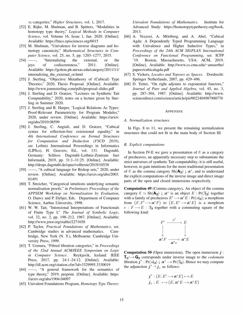
Computation 49 (Comma category). An object of the commacategory E ' Sh(A ) ↓ α∗ is an object E : Pr(T ) togetherwith a family of presheaves E′ α∗E : Pr(A ); a morphismfrom

(F, F ′ α∗F

)to(E,E′ α∗E

)is a morphism

e : F E : T together with a commuting square of thefollowing kind:

F ′

α∗F

E

α∗E

e′

α∗e

Computation 50 (Open immersion). The open immersion j :T G corresponds under inverse image to the codomainfibration j∗ : Pr(A ) ↓ α∗ Pr(T ). Hence we may computethe adjunction j∗ a j∗ as follows:

j∗ :(E,E′ α∗E

)E

j∗ : E(E,α∗E α∗E

)

15

The direct image functor j∗ is fully faithful. In fact, we havetwo additional adjoints j! a j∗ a j∗ a j!, the exceptional rightadjoint by virtue of the adjunction α∗ a α∗.

j! : E(E, 0 α∗E

)j! :

(E,E′ α∗E

)α∗E

′ ×α∗α∗E E

Computation 51 (Closed immersion). The closed immersioni : A G corresponds under inverse image to the domainfunctor i∗ : Sh(A ) ↓ α∗ Pr(A ). We compute the adjunc-tion i∗ a i∗ as follows:

i∗ :(E,E′ α∗E

)E′

i∗ : E′(1, E′ α∗1

)Because α is an essential morphism of topoi, we have an

additional left adjoint i! a i∗ a i∗:

i! : E′(α!E

′, E′ α∗α!E′)

Computation 52 (Open and closed modality). Using thesyntactic open syn (Computation 28), we can compute theopen modality # = j∗j

∗ as the exponential (syn→ −). Like-wise, syn makes another computation of the closed modality = i∗i

∗ available:

A× syn

A

syn

A

Corollary 53. From Computations 28 and 49 to 51 we maymake the following observations:

1) The open modality # := j∗j∗ on E has both a right

adjoint j∗j! and left adjoint j!j

∗; hence the syntacticopen syn : E is a tiny object; the adjunction j!j

∗ a #can be computed as (−× syn) a (syn→ −).

2) The closed modality := i∗i∗ on E has a left adjoint

i!i∗.

3) The gluing functor α∗ : Pr(T ) Pr(A ) can bereconstructed as the composite i∗j∗.

The following fracture theorem is from SGA 4 [10].

Lemma 54 (Fracture [10, 52]). Any sheaf on G can bereconstructed up to isomorphism from its restriction to Tand A ; in particular, the following square is cartesian forany A : E:

A

#A

A

#A

C. Explicit construction of neutral and normal forms

Our construction of the computability model of cubicaltype theory (Theorem 21) requires only that certain constantscorresponding to the neutral and normal forms exist in E.

However, to use this computability model to establish theinjectivity and (external) decidability properties of Section V,it is important to ensure that the corresponding properties holdfor our normal forms.

Concretely, we define them by a family of indexed quotientinductive types (QITs [3]) valued in the modal universe U :

[tp 3nf A] : U (A : M.tp)

[A 3nf a] : U (A : M.tp, a : M.tm(A))

[a ∈φne A] : U (φ : F, A : M.tp, a : M.tm(A))

In fact, we ensure that [a ∈φne A] is not only #-connectedbut actually (φ ∨ syn)-connected, capturing the sense in whichthe data of a neutral form collapses to a point on its locus ofinstability. Then, the collections of normal and neutral formsare obtained by dependent sum and realignment as follows(noting that the fibers of each family are valued in U andare thus #-connected):

nftp ∼=∑A:M.tp[tp 3nf A]

nf(A) ∼=∑a:M.tm(A)[A 3nf a]

neφ(A) ∼=∑a:M.tm(A)[a ∈

φne A]

Our use of quotienting in the definition of normal formsis to impose correct cubical boundaries on constructors: forinstance, we must have ∂i → loop(i) = base. Because thetheory of cofibrations is (externally) decidable, the quotientcan be presented externally by an effective rewriting systemthat reduces size and is therefore obviously noetherian.

Remark 55. An indexed quotient inductive type in U alsohas a universal property in U, obtained by adding an additionalquotient-inductive clause that contracts each fiber to a pointunder z : syn.

In Fig. 12 we present the indexed quotient inductive defini-tion of normal and neutral forms.

Lemma 56 (Decidability of equality of normal forms). Giventwo external normal forms A0, A1 : LΓM nftp, it is recur-sively decidable whether A0 = A1 or A0 6= A1.

Proof. As in the normal form presentation of strict coproducts[2], elements of nftp are not pure data: they include bindersof type I, var(A), and [φ]. Nevertheless, equality is algorith-mically decidable as follows, by recursion on Γ, A0, A1.

At a binder of type I or var(A), we continue at Γ.I orΓ.A respectively. At a binder of type [φ], we note that ourdefinition of F (Section III-B) licenses a case split on the formof φ : F. We eliminate universal quantifications in the style ofCohen et al. [20], proceeding by “left inversion” until reachinga conjunction of equations r =I s. If the conjunction implies0 = 1, we halt; otherwise, we proceed under the equalizingatomic substitution ∆→ Γ.

16

Lemma 57 (Injectivity of normal form constructors). Thefollowing formula holds in the internal logic of E = Sh(G ):

∀A,A′, B,B′.pi(A,B) = pi(A′, B′) =⇒ ((A,B) = (A′, B′))

Proof. We prove this in the same way that one proves injec-tivity of constructors of any inductive type, with one subtlety:we must ensure that our constructions respect the cubicalboundary of glue, which is the only constructor of [tp 3nf −]subject to an equational clause.

By induction on [tp 3nf −], we define a #-connected pred-icate isPi : nftp→ Ω satisfying a universal property:

∀X : nftp.isPi(X) ⇐⇒ (∃A,B.X = pi(A,B))

We define isPi as follows:

isPi( , pi(A,B)) = >isPi( , glueB,A, f(φ,B,A, f)) = ∃z : [φ].isPi(A,A(z))

isPi( , sg(A,B)) = ⊥isPi( , path(A, a0, a1)) = ⊥

isPi( , s1) = ⊥

We must verify that isPi respects the φ-boundary of glue =A(z). But supposing that z : [φ], we can calculate thatisPi( , glue(φ,B,A, f)) = isPi( ,A(z)), which is exactlywhat it means for isPi to respect that equation.

The reverse implication of the universal property of isPiis immediate. We prove the forward implication by inductionon X , where again the only subtlety is in the case of glue:if isPi( , glue(φ,B,A, f)) then we must have isPi(A,A(z)),which by the inductive hypothesis implies A(z) = pi.

Then we define dom : X : nftp | isPi(X) → nftp:

dom( , pi(A,B)) = η (A)

dom( , glue(φ,B,A, f)) = dom(A,A)

Note that these are the only constructors that may satisfy isPi,and in the case of glue, if isPi( , glue(φ,B,A, f)) holds thenφ = > and isPi(A,A). We may define cod similarly.

Finally, suppose that pi(A,B) = pi(A′, B′). Then by apply-ing dom to both sides of this equation, we get (A = A′); theequality of codomains likewise follows by applying cod.

D. Proofs of theorems

Lemma 24. The chosen interval structure is preserved by re-striction along α : A T ; that is, we have an isomorphismyA (·.I) ∼= α∗yT (I).

Proof. First we compute the representable points of α∗yT (I)by transpose and the Yoneda lemma:

HomPr(A )(yA (Γ),α∗yT (I))∼= HomPr(T )(α!yA (Γ), yT (I))∼= HomPr(T )(yT (α(Γ)), yT (I))∼= HomT (α(Γ), I)

We see by induction on the definition of the objects andhom sets of A that this is equivalent to HomA (Γ, ·.I).

Lemma 32. Let f : Y U be a morphism of topoi. Write Xfor the Artin gluing of the inverse image functor f∗, and writej : U X and i : Y X for the respective open and closedimmersions of topoi. Suppose that X : Sh(X) is a sheaf suchthat j∗X is a tiny object in Sh(U) and i∗X is a tiny objectin Sh(Y); then X is tiny.

Proof. We must check that the exponential functor (X → −)preserves colimits. Fixing a diagram E• : I Sh(X), we maycompute the exponential

(X → colimI E•

)in the language of

Sh(Y) as follows; first, the standard computation that glues afunction from the open subtopos onto a function from theclosed subtopos [37]:

i∗(X → colimI E•

)

f∗(j∗X → j∗ colimI E•

)

i∗X → i∗ colimI E•

i∗X → f∗j∗ colimI E•

Commute cocontinuous functors past colimits.

i∗(X → colimI E•

)

f∗(j∗X → colimI j

∗E•)

i∗X → colimI i∗E•

i∗X → colimI f∗j∗E•

Use the tininess of i∗X, j∗X and the cocontinuity of f∗.

i∗(X → colimI E•

)

colimI f∗(j∗X → j∗E•)

colimI (i∗X → i∗E•)

colimI (i∗X → f∗j∗E•)

Hence by the universality of colimits we have:

colimI i∗(X → E•)

colimI f∗(j∗X → j∗E•)

colimI (i∗X → i∗E•)

colimI (i∗X → f∗j∗E•)

Lemma 58. If Γ : A is a formal context, then the hom setHomT (α(Γ), [0 = 1]) is empty.

Proof. Formal contexts do not induce assumptions of falsecofibrations. This can be seen by a model construction inwhich T is interpreted into cubical sets, where the interpre-tation of cofibrations is standard but each type is interpretedas an inhabited type. Such an argument accommodates typesthat are “weakly empty” (e.g. the void type lacking an η-law),because the abort eliminator can simply return the basepointof its motive.

17

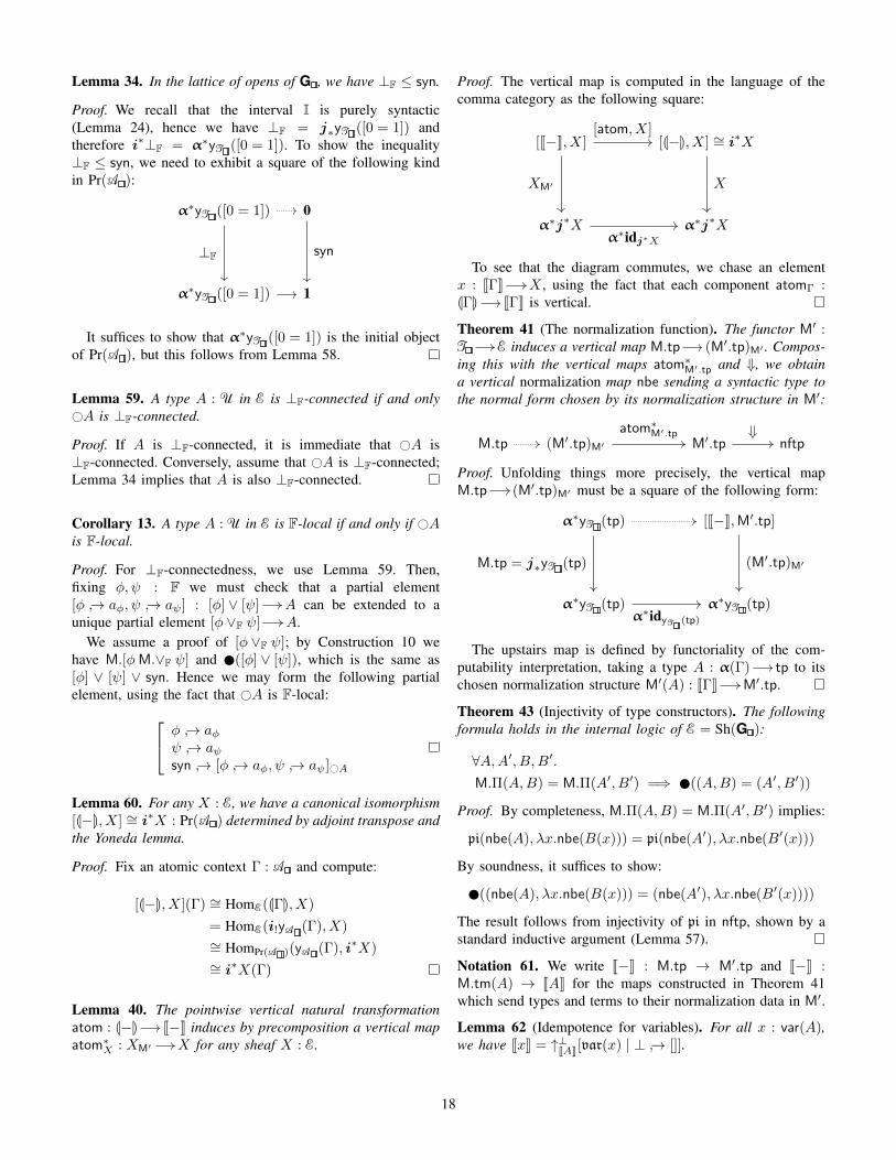
Lemma 34. In the lattice of opens of G , we have ⊥F ≤ syn.

Proof. We recall that the interval I is purely syntactic(Lemma 24), hence we have ⊥F = j∗yT ([0 = 1]) andtherefore i∗⊥F = α∗yT ([0 = 1]). To show the inequality⊥F ≤ syn, we need to exhibit a square of the following kindin Pr(A ):

α∗yT ([0 = 1])

α∗yT ([0 = 1])

⊥F

0

1

syn

It suffices to show that α∗yT ([0 = 1]) is the initial objectof Pr(A ), but this follows from Lemma 58.

Lemma 59. A type A : U in E is ⊥F-connected if and only#A is ⊥F-connected.

Proof. If A is ⊥F-connected, it is immediate that #A is⊥F-connected. Conversely, assume that #A is ⊥F-connected;Lemma 34 implies that A is also ⊥F-connected.

Corollary 13. A type A : U in E is F-local if and only if #Ais F-local.

Proof. For ⊥F-connectedness, we use Lemma 59. Then,fixing φ, ψ : F we must check that a partial element[φ → aφ, ψ → aψ] : [φ] ∨ [ψ] A can be extended to aunique partial element [φ ∨F ψ] A.

We assume a proof of [φ ∨F ψ]; by Construction 10 wehave M.[φM.∨F ψ] and ([φ] ∨ [ψ]), which is the same as[φ] ∨ [ψ] ∨ syn. Hence we may form the following partialelement, using the fact that #A is F-local: φ → aφ

ψ → aψsyn → [φ → aφ, ψ → aψ]#A

Lemma 60. For any X : E, we have a canonical isomorphism[L−M, X] ∼= i∗X : Pr(A ) determined by adjoint transpose andthe Yoneda lemma.

Proof. Fix an atomic context Γ : A and compute:

[L−M, X](Γ) ∼= HomE(LΓM, X)

= HomE(i!yA (Γ), X)∼= HomPr(A )(yA (Γ), i∗X)∼= i∗X(Γ)

Lemma 40. The pointwise vertical natural transformationatom : L−M J−K induces by precomposition a vertical mapatom∗X : XM′ X for any sheaf X : E.

Proof. The vertical map is computed in the language of thecomma category as the following square:

[J−K, X]

α∗j∗X

XM′

[L−M, X] ∼= i∗X

α∗j∗X

[atom, X]

X

α∗idj∗X

To see that the diagram commutes, we chase an elementx : JΓK X , using the fact that each component atomΓ :LΓM JΓK is vertical.

Theorem 41 (The normalization function). The functor M′ :T E induces a vertical map M.tp (M′.tp)M′ . Compos-ing this with the vertical maps atom∗M′.tp and ⇓, we obtaina vertical normalization map nbe sending a syntactic type tothe normal form chosen by its normalization structure in M′:

M.tp (M′.tp)M′ M′.tp nftpatom∗M′.tp ⇓

Proof. Unfolding things more precisely, the vertical mapM.tp (M′.tp)M′ must be a square of the following form:

α∗yT (tp)

α∗yT (tp)

M.tp = j∗yT (tp)

[J−K,M′.tp]

α∗yT (tp)

(M′.tp)M′

α∗idyT (tp)

The upstairs map is defined by functoriality of the com-putability interpretation, taking a type A : α(Γ) tp to itschosen normalization structure M′(A) : JΓK M′.tp.

Theorem 43 (Injectivity of type constructors). The followingformula holds in the internal logic of E = Sh(G ):

∀A,A′, B,B′.M.Π(A,B) = M.Π(A′, B′) =⇒ ((A,B) = (A′, B′))

Proof. By completeness, M.Π(A,B) = M.Π(A′, B′) implies:

pi(nbe(A), λx.nbe(B(x))) = pi(nbe(A′), λx.nbe(B′(x)))

By soundness, it suffices to show:

((nbe(A), λx.nbe(B(x))) = (nbe(A′), λx.nbe(B′(x))))

The result follows from injectivity of pi in nftp, shown by astandard inductive argument (Lemma 57).

Notation 61. We write J−K : M.tp → M′.tp and J−K :M.tm(A) → JAK for the maps constructed in Theorem 41which send types and terms to their normalization data in M′.

Lemma 62 (Idempotence for variables). For all x : var(A),we have JxK = ↑⊥JAK[var(x) | ⊥ → []].

18

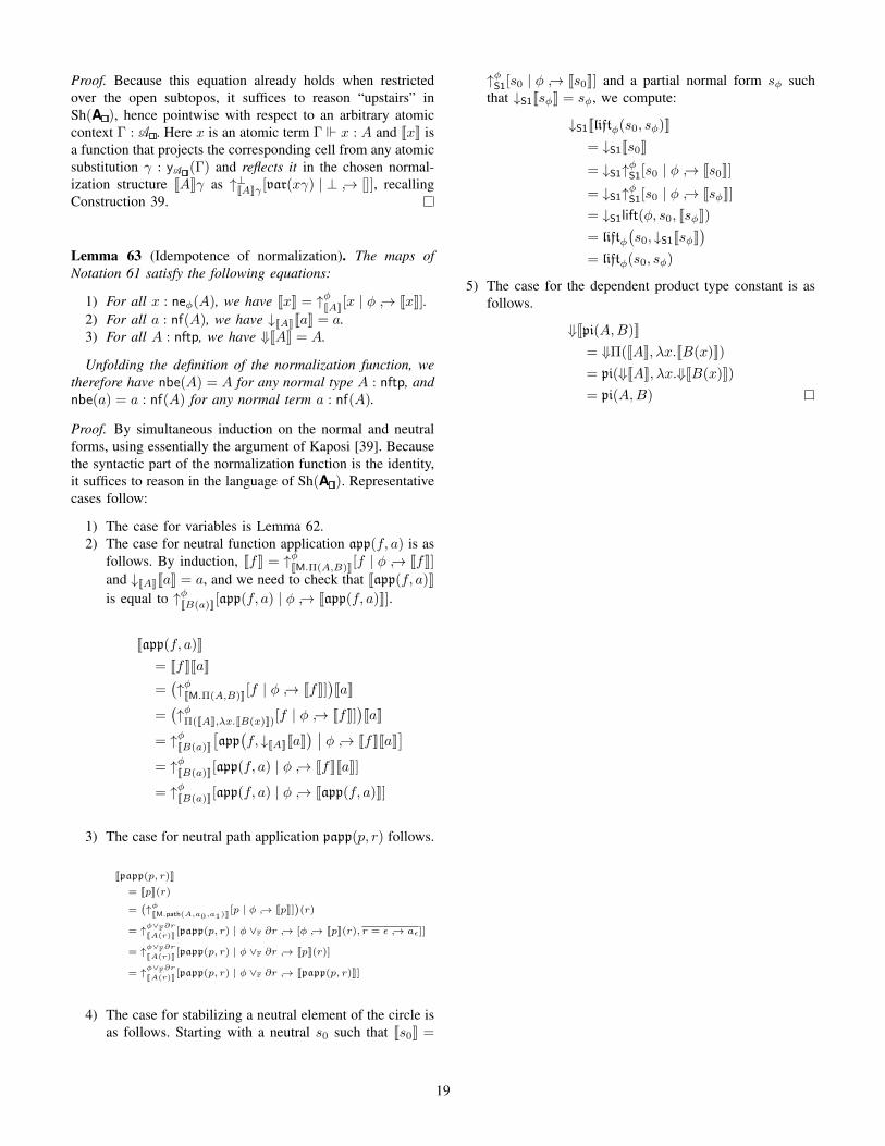
Proof. Because this equation already holds when restrictedover the open subtopos, it suffices to reason “upstairs” inSh(A ), hence pointwise with respect to an arbitrary atomiccontext Γ : A . Here x is an atomic term Γ x : A and JxK isa function that projects the corresponding cell from any atomicsubstitution γ : yA (Γ) and reflects it in the chosen normal-ization structure JAKγ as ↑⊥JAKγ [var(xγ) | ⊥ → []], recallingConstruction 39.

Lemma 63 (Idempotence of normalization). The maps ofNotation 61 satisfy the following equations:

1) For all x : neφ(A), we have JxK = ↑φJAK[x | φ → JxK].2) For all a : nf(A), we have ↓JAKJaK = a.3) For all A : nftp, we have ⇓JAK = A.

Unfolding the definition of the normalization function, wetherefore have nbe(A) = A for any normal type A : nftp, andnbe(a) = a : nf(A) for any normal term a : nf(A).

Proof. By simultaneous induction on the normal and neutralforms, using essentially the argument of Kaposi [39]. Becausethe syntactic part of the normalization function is the identity,it suffices to reason in the language of Sh(A ). Representativecases follow:

1) The case for variables is Lemma 62.2) The case for neutral function application app(f, a) is as

follows. By induction, JfK = ↑φJM.Π(A,B)K[f | φ → JfK]and ↓JAKJaK = a, and we need to check that Japp(f, a)Kis equal to ↑φJB(a)K[app(f, a) | φ → Japp(f, a)K].

Japp(f, a)K= JfKJaK

=(↑φJM.Π(A,B)K[f | φ → JfK]

)JaK

=(↑φΠ(JAK,λx.JB(x)K)[f | φ → JfK]

)JaK

= ↑φJB(a)K

[app(f, ↓JAKJaK

) ∣∣ φ → JfKJaK]

= ↑φJB(a)K[app(f, a) | φ → JfKJaK]

= ↑φJB(a)K[app(f, a) | φ → Japp(f, a)K]

3) The case for neutral path application papp(p, r) follows.

Jpapp(p, r)K

= JpK(r)

=(↑φJM.path(A,a0,a1)K[p | φ → JpK]

)(r)

= ↑φ∨F∂rJA(r)K[papp(p, r) | φ ∨F ∂r → [φ → JpK(r), r = ε → aε]]

= ↑φ∨F∂rJA(r)K[papp(p, r) | φ ∨F ∂r → JpK(r)]

= ↑φ∨F∂rJA(r)K[papp(p, r) | φ ∨F ∂r → Jpapp(p, r)K]

4) The case for stabilizing a neutral element of the circle isas follows. Starting with a neutral s0 such that Js0K =

↑φS1[s0 | φ → Js0K] and a partial normal form sφ suchthat ↓S1JsφK = sφ, we compute:

↓S1Jliftφ(s0, sφ)K= ↓S1Js0K

= ↓S1↑φS1[s0 | φ → Js0K]

= ↓S1↑φS1[s0 | φ → JsφK]= ↓S1lift(φ, s0, JsφK)= liftφ

(s0, ↓S1JsφK

)= liftφ(s0, sφ)

5) The case for the dependent product type constant is asfollows.

⇓Jpi(A,B)K= ⇓Π(JAK, λx.JB(x)K)= pi(⇓JAK, λx.⇓JB(x)K)= pi(A,B)

19

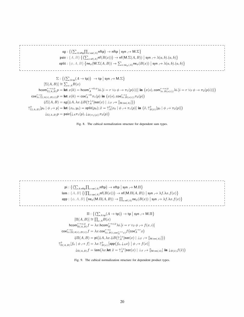
sg :(∑

A:nftp

∏x:var(A)nftp

)→ nftp

∣∣ syn → M.Σ

pair : A,B(∑

x:nf(A)nf(B(x)))→ nf(M.Σ(A,B))

∣∣ syn → λ(a, b).(a, b)

split : φ,A,Bneφ(M.Σ(A,B))→

∑x:neφ(A)neφ(B(x))

∣∣ syn → λ(a, b).(a, b)

Σ :(∑

A:tp(A→ tp))→ tp

∣∣ syn → M.Σ

[Σ(A,B)] ∼=∑x:AB(x)

hcomr→s;φΣ(A,B)p = let x(k) = hcomr→k;φ

A λi.[i = r ∨F φ→ π1(p(i))] in(x(s), comr→s;φ

λi.B(x(i))λi.[i = r ∨F φ→ π2(p(i))])

coer→sλi.Σ(A(i),B(i))p = let x(k) = coer→kA π1(p) in(x(s), coer→sλi.B(x(i))π2(p)

)⇓Σ(A,B) = sg

(⇓A, λx.⇓B

(↑⊥FA [var(x) | ⊥F → []M.tm(A)]

))↑φΣ(A,B)[p0 | φ → p] = let (x0, y0) = split(p0); x = ↑φA[x0 | φ → π1(p)] in

(x, ↑φB(x)[y0 | φ → π2(p)]

)↓Σ(A,B)p = pair

(↓Aπ1(p), ↓B(π1(p))π2(p)

)Fig. 8. The cubical normalization structure for dependent sum types.

pi :(∑

A:nftp

∏x:var(A)nftp

)→ nftp

∣∣ syn → M.Π

lam : A,B(∏

x:var(A)nf(B(x)))→ nf(M.Π(A,B))

∣∣ syn → λf.λx.f(x)

app : φ,A,Bneφ(M.Π(A,B))→

∏x:nf(A)neφ(B(x))

∣∣ syn → λf.λx.f(x)

Π :(∑

A:tp(A→ tp))→ tp

∣∣ syn → M.Π

[Π(A,B)] ∼=∏x:AB(x)

hcomr→s;φΠ(A,B)f = λx.hcomr→s;φ

B λi.[i = r ∨F φ → f(x, i)]

coer→sλi.Π(A(i),B(i))f = λx.coer→sλi.B(i,coes→iA x)

f(coes→rA x

)⇓Π(A,B) = pi

(⇓A, λx.⇓B

(↑⊥FA [var(x) | ⊥F → []M.tm(A)]

))↑φΠ(A,B)[f0 | φ → f ] = λx.↑φB(x)

[app(f0, ↓Ax

) ∣∣ φ → f(x)]

↓Π(A,B)f = lam(λx.let x = ↑⊥F

A [var(x) | ⊥F → []M.tm(A)] in ↓B(x)f(x))

Fig. 9. The cubical normalization structure for dependent product types.

20

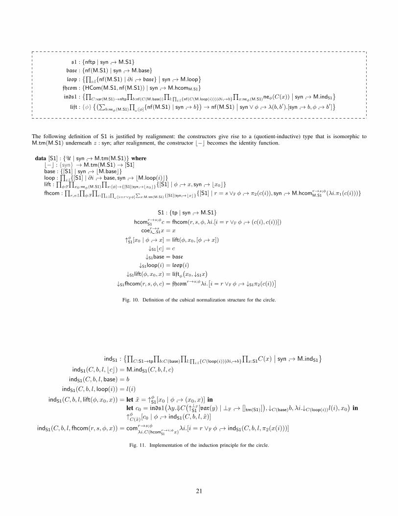
s1 : nftp | syn → M.S1base : nf(M.S1) | syn → M.baseloop :

∏i:Inf(M.S1) | ∂i → base

∣∣ syn → M.loop

fhcom : HCom(M.S1, nf(M.S1)) | syn → M.hcomM.S1inds1 :

∏C:var(M.S1)→nftp

∏b:nf(C(M.base))

∏l:∏i:Inf(C(M.loop(i)))|∂i→b

∏x:neφ(M.S1)neφ(C(x))

∣∣ syn → M.indS1

lift : φ(∑

b:neφ(M.S1)

∏:[φ]nf(M.S1) | syn → b

)→ nf(M.S1)

∣∣ syn ∨ φ → λ(b, b′).[syn → b, φ → b′]

The following definition of S1 is justified by realignment: the constructors give rise to a (quotient-inductive) type that is isomorphic toM.tm(M.S1) underneath z : syn; after realignment, the constructor b−c becomes the identity function.

data [S1] : U | syn → M.tm(M.S1) whereb−c : syn → M.tm(M.S1)→ [S1]base : [S1] | syn → bM.basecloop :

∏i:I[S1] | ∂i → base, syn → bM.loop(i)c

lift :∏φ:F∏x0:neφ(M.S1)

∏x:[φ]→[S1]|syn→bx0c[S1] | φ → x, syn → bx0c

fhcom :∏r,s:I∏φ:F∏c:∏i:I∏

:[i=r∨Fφ]∑x:M.tm(M.S1)[S1]|syn→bxc

[S1] | r = s ∨F φ → π2(c(i)), syn → M.hcomr→s;φM.S1 (λi.π1(c(i)))

S1 : tp | syn → M.S1hcomr→s;φ

S1 c = fhcom(r, s, φ, λi.[i = r ∨F φ → (c(i), c(i))])

coer→sλ .S1x = x

↑φS1[x0 | φ → x] = lift(φ, x0, [φ → x])

↓S1bcc = c

↓S1base = base

↓S1loop(i) = loop(i)

↓S1lift(φ, x0, x) = liftφ(x0, ↓S1x

)↓S1fhcom(r, s, φ, c) = fhcomr→s;φλi.

[i = r ∨F φ → ↓S1π2(c(i))

]Fig. 10. Definition of the cubical normalization structure for the circle.

indS1 :∏

C:S1→tp

∏b:C(base)

∏l:∏i:IC(loop(i))|∂i→b

∏x:S1C(x)

∣∣ syn → M.indS1

indS1(C, b, l, bcc) = M.indS1(C, b, l, c)

indS1(C, b, l, base) = b

indS1(C, b, l, loop(i)) = l(i)

indS1(C, b, l, lift(φ, x0, x)) = let x = ↑φS1[x0 | φ → (x0, x)] inlet c0 = inds1

(λy.⇓C

(↑⊥FS1 [var(y) | ⊥F → []tm(S1)]

), ↓C(base)b, λi.↓C(loop(i))l(i), x0

)in

↑φC(x)[c0 | φ → indS1(C, b, l, x)]

indS1(C, b, l, fhcom(r, s, φ, x)) = comr→s;φλi.C(hcomr→i;φS1 x)

λi.[i = r ∨F φ → indS1(C, b, l, π2(x(i)))]

Fig. 11. Implementation of the induction principle for the circle.

21

CIRCLE TYPE

s1 : [tp 3nf M.S1]

PATH TYPEA :∏i:I[tp 3nf A(i)] a0 : [A(0) 3nf a0] a1 : [A(1) 3nf a1]

pathA, a0, a1(A, a0, a1) : [tp 3nf M.path(A, a0, a1)]

GLUE TYPEφ : F B : [tp 3nf B] A :

∏z:[φ][tp 3nf A(z)] f :

∏z:[φ][M.Equiv(A(z), B) 3nf f(z)]

glueB,A, f(φ,B,A, f) : [tp 3nf M.glue(φ,B,A, f)]

GLUE TYPE BOUNDARYφ : F B : [tp 3nf B] A :

∏z:[φ][tp 3nf A(z)] f :

∏z:[φ][M.Equiv(A(z), B) 3nf f(z)] z : [φ]

glueB,A, f(φ,B,A, f) = A(z) : [tp 3nf A(z)]

PI/SG TYPEA : [tp 3nf A] B :

∏x:var(A)[tp 3nf B(x)]

piA,B(A,B) : [tp 3nf M.Π(A,B)] sgA,B(A,B) : [tp 3nf M.Σ(A,B)]

UNSTABLEz : [φ]

?(z) : [a ∈φne A]

UNSTABLE COLLAPSE

z : [φ] a : [a ∈φne A]

a = ?(z) : [a ∈φne A]

VARIABLEx : var(A)

varA(x) : [x ∈⊥ne A]

FUNCTION APPLICATION

f : [f ∈φne M.Π(A,B)] a : [A 3nf a]

appA,B, f, a(f, a) : [a ∈φne A]

PAIR PROJECTION

p : [p ∈φne M.Σ(A,B)]

fstA,B, p(p) : [π1(p) ∈φne A] sndA,B, p(p) : [π2(p) ∈φne B(π1(p))]

PATH APPLICATION

p : [p ∈φne M.path(A, a0, a1)] r : IpappA, a0, a1(p, r) : [p(r) ∈φ∨F∂r

ne A(r)]

UNGLUE DESTRUCTOR

g : [g ∈ψne M.glue(φ,B,A, f)]

unglueB,A, f, g(φ, g) : [M.unglue(g) ∈ψ∨Fφne B]

CIRCLE INDUCTION

C :∏x:var(M.S1)[tp 3nf C(x)] b : [C(M.base) 3nf b] l :

∏i:I[C(M.loop(i)) 3nf l(i)] s : [s ∈φne M.S1]

indC, b, l, s(C, b, l, s) : [M.indS1(C, b, l, s) ∈φne C(s)]

CIRCLE NEUTRAL LIFT

s0 : [s ∈φne M.S1] sφ :∏

:[φ][M.S1 3nf s]lifts(s0, sφ) : [M.S1 3nf s]

CIRCLE NEUTRAL LIFT BOUNDARY

s0 : [s ∈φne M.S1] sφ :∏

:[φ][M.S1 3nf s] z : [φ]

lifts(s0, sφ) = sφ(z) : [M.S1 3nf s]

CIRCLE BASE

base : [M.S1 3nf M.base]

CIRCLE LOOPr : I

loop(r) : [M.S1 3nf M.loop(r)]

CIRCLE LOOP BOUNDARYr : I : [∂r]

loop(r) = base : [M.S1 3nf M.base]

CIRCLE FORMAL HOMOGENEOUS COMPOSITIONr, s : I φ : F a :

∏i:I∏z:[i=r∨Fφ][M.S1 3nf a(i, z)]

fhcoma(r, s, φ, a) : [M.S1 3nf M.hcom(M.S1, r, s, φ, a)]

FUNCTION ABSTRACTIONf :∏x:var(A)[B(x) 3nf f(x)]

lamA,B, f(f) : [M.Π(A,B) 3nf λx.f(x)]

PAIR CONSTRUCTORa : [A 3nf a] b : [B(a) 3nf b]

pairA,B, a, b(a, b) : [M.Σ 3nf (a, b)]

PATH ABSTRACTIONp :∏i:I[A(i) 3nf p(i)]

plamA, a0, a1, p(p) : [M.path(A, a0, a1) 3nf λi.p(i)]

ENGLUE CONSTRUCTORa :∏z:[φ][A 3nf a] b : [B 3nf b] ∀z : [φ].b = a(z)

englueB,A, f, a, b(φ, a, b) : [M.glue(φ,B,A, f) 3nf M.glue/tm(a, b)]

ENGLUE CONSTRUCTOR BOUNDARYa :∏z:[φ][A 3nf a] b : [B 3nf b] ∀z : [φ].b = a(z) z : [φ]

englueB,A, f, a, b(φ, a, b) = a(z) : [A 3nf a]

Fig. 12. The explicit indexed quotient-inductive definition of normal and neutral forms. The UNSTABLE and UNSTABLE COLLAPSE rules ensure that neφ(A)collapses to M.tm(A) within the locus of instability φ.

22