Embed Size (px)
Citation preview
RETICOLO
Authors: J.P. Hugonin and P. Lalanne
This technical note is composed of three parts:
• Reticolo code 1D for analyzing 1D gratings in classical mountings.
• Reticolo code 1D-conical for analyzing 1D gratings in classical and conical
mountings.
• Reticolo code 2D for analyzing 2D crossed grating.
They are free software that operate under Matlab. To install them, copy the companion
folder “reticolo_allege” and add the folder in the Matlab path. The software can be
downloaded here or there.
The version V9 launched in 01/2021 features a few novelties:
✓ it includes a treatment of stacks of arbitrarily anisotropic multilayered thin-films.1 Be
aware that the substrate and superstrate cannot be anisotropic. This part is documented
in Reticolo codes 1D-conical (or identically 2D).
✓ It features an option to visualize the Bloch modes.
✓ Diagonal anisotropy (𝜀𝑥𝑥 ≠ 𝜀𝑦𝑦 ≠ 𝜀𝑧𝑧) can be incorporated in structured grating layers
and gratings with uniform layers having arbitrary anisotropy (𝜀𝑥𝑦 ≠ 0 …) can also be
handled)
✓ It is fully compatible with earlier versions.
copyright © 2005 Institut d’Optique/CNRS.
Last update: 01/2021
Technical contact : [email protected]
Contact : [email protected]
1 This is simply achieved by retaining a single Fourier harmonics coefficient in the expansion (nn=0). The
extension is not optimal from numerical-efficiency perspectives, but has been provided on demand of several users
who additionally complained of mistakes in available freeware packages on thin films.
RETICOLO 1D – classical diffraction
2
RETICOLO CODE 1D for the diffraction by stacks of lamellar 1D gratings
(classical diffraction)
Authors: J.P. Hugonin and P. Lalanne
Reticolo code 1D is a free software for analyzing 1D gratings in classical mountings. It
operates under Matlab. To install it, copy the companion folder “reticolo_allege” and add
the folder in the Matlab path.
Outline
1. Generality ........................................................................................................................................................... 3
2. The diffraction problem considered................................................................................................................... 4
3. Preliminary input parameters ............................................................................................................................ 5
4. Structure definition (grating parameters) ......................................................................................................... 6
4.1. How to define a texture? ............................................................................................................................ 6
4.2. How to define the layers? .......................................................................................................................... 7
5. Solving the eigenmode problem for every texture ............................................................................................. 8
6. Computing the diffracted waves ........................................................................................................................ 8
6.1. Efficiencies .................................................................................................................................................. 9
6.2. Rayleigh expansion for propagatives modes .......................................................................................... 10
6.3. Amplitude of diffracted propagative waves ........................................................................................... 10 6.3.1 Angle θm ........................................................................................................................................ 10 6.3.2 Otop and Obottom points .................................................................................................................... 10 6.3.3 Jones’ coefficient .......................................................................................................................... 11
7. Using symmetries to accelerate the computational speed ............................................................................... 11
8. Plotting the electromagnetic field and calculating the absorption loss .......................................................... 11
8.1. Computation of the electromagnetic fields............................................................................................. 11
8.2. Computation of the absorption loss ........................................................................................................ 13
9. Bloch-mode effective indices ........................................................................................................................... 14
10. Annex .............................................................................................................................................................. 14
10.1. Checking that the textures are correctly set up ................................................................................... 14
10.2. The “retio” & “retefface” instructions ................................................................................................. 14
10.3. How to save and to reload the “aa” variable ....................................................................................... 15
10.4. Asymmetry of the Fourier harmonics retained in the computation .................................................. 15
11. Summary ......................................................................................................................................................... 15
12. Examples ........................................................................................................................................................ 16
RETICOLO 1D – classical diffraction
3
1. Generality
RETICOLO is a code written in the language MATLAB 9.0. It computes the diffraction efficiencies and the
diffracted amplitudes of gratings composed of stacks of lamellar structures. It incorporates routines for the
calculation and visualisation of the electromagnetic fields inside and outside the grating. With this version, 2D
periodic (crossed) gratings cannot be analysed.
As free alternative to MATLAB, RETICOLO can also be run in GNU Octave with minimal code changes. For
further information, please contact [email protected].
In brief, RETICOLO implements a frequency-domain modal method (known as the Rigorous Coupled wave
Analysis/RCWA). To get an overview of the RCWA, the interested readers may refer to the following articles:
1D-classical and conical diffraction
M.G. Moharam et al., JOSAA 12, 1068 (1995),
M.G. Moharam et al, JOSAA 12, 1077 (1995),
P. Lalanne and G.M. Morris, JOSAA 13, 779 (1996),
G. Granet and B. Guizal, JOSAA 13, 1019 (1996),
L. Li, JOSAA 13, 1870 (1996), see also C. Sauvan et al., Opt. Quantum Electronics 36, 271-284 (2004) which
simply explains the raison of the convergence-rate improvement of the Fourier-Factorization rules without
requiring advanced mathematics on Fourier series and generalizes to other kinds of expansions.
2D-crossed gratings
L. Li, JOSAA 14, 2758-2767 (1997),
E. Popov and M. Nevière, JOSAA 17, 1773 (2000),
which describe the up-to-date formulation of the approach used in RETICOLO. Note that the formulation used in
the last article (which proposes an improvement for analysing metallic gratings with continuous profiles like
sinusoidal gratings) is not available in the RETICOLO version of the web. The RCWA relies on the computation
of the eigenmodes in all the layers of the grating structure in a Fourier basis (plane-wave basis) and on a scattering
matrix approach to recursively relate the mode amplitudes in the different layers.
Eigenmode solver: For conical diffraction analysis of 1D gratings, the Bloch eigenmode solver used in Reticolo
is based on the article "P. Lalanne and G.M. Morris, JOSAA 13, 779 (1996)".
Scattering matrix approach: The code incorporates many refinements that we have not published and that we
do not plan to publish. For instance, although it is generally admitted that the S-matrix is inconditionnally stable,
it is not always the case. We have developed an in-house transfer matrix method which is more stable and accurate.
The new transfer matrix approach is also more general and can handle perfect metals. The essence of the method
has been rapidly published in "J.-P. Hugonin, M. Besbes and P. Lalanne, Op. Lett. 33, 1590 (2008)".
Field calculation: The calculation of the near-field electromagnetic fields everywhere in the grating is performed
according to the method described in "P. Lalanne, M.P. Jurek, JMO 45, 1357 (1998)" and to its generalization to
crossed gratings (unpublished). Basically, no Gibbs phenomenon will be visible in the plots of the discontinuous
electromagnetic quantities, but field singularities at corners will be correctly handled.
Acknowledging the use of RETICOLO: In publications and reports, acknowledgments have to be provided by
referencing to J.P. Hugonin and P. Lalanne, RETICOLO software for grating analysis, Institut d'Optique, Orsay,
France (2005), Version V9, arXiv:????:?????.
In addition, one may fairly quote the following references in journal publications:
-M.G. Moharam, E.B. Grann, D.A. Pommet and T.K. Gaylord, "Formulation for stable and efficient
implementation of the rigorous coupled-wave analysis of binary gratings", J. Opt. Soc. Am. A 12, 1068-1076
(1995), if TE-polarization efficiency calculations are provided
-P. Lalanne and G.M. Morris, "Highly improved convergence of the coupled-wave method for TM polarization",
J. Opt. Soc. Am. A 13, 779-789 (1996) and G. Granet and B. Guizal, "Efficient implementation of the coupled-
wave method for metallic lamellar gratings in TM polarization", J. Opt. Soc. Am. A 13, 1019-1023 (1996), if TM-
polarization efficiency calculations are provided,
-P. Lalanne and M.P. Jurek, "Computation of the near-field pattern with the coupled-wave method for TM
polarization", J. Mod. Opt.45, 1357-1374 (1998), if near-field electromagnetic-field distributions are shown.
RETICOLO 1D – classical diffraction
4
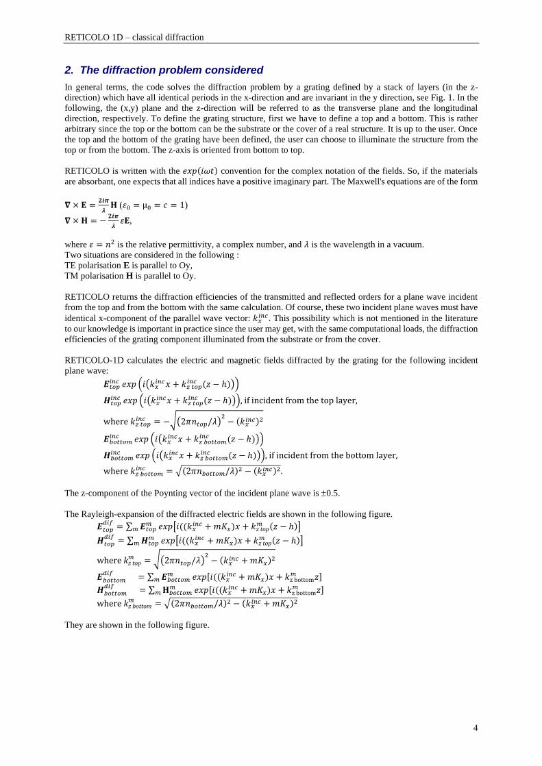
2. The diffraction problem considered
In general terms, the code solves the diffraction problem by a grating defined by a stack of layers (in the z-
direction) which have all identical periods in the x-direction and are invariant in the y direction, see Fig. 1. In the
following, the (x,y) plane and the z-direction will be referred to as the transverse plane and the longitudinal
direction, respectively. To define the grating structure, first we have to define a top and a bottom. This is rather
arbitrary since the top or the bottom can be the substrate or the cover of a real structure. It is up to the user. Once
the top and the bottom of the grating have been defined, the user can choose to illuminate the structure from the
top or from the bottom. The z-axis is oriented from bottom to top.
RETICOLO is written with the 𝑒𝑥𝑝(𝑖𝜔𝑡) convention for the complex notation of the fields. So, if the materials
are absorbant, one expects that all indices have a positive imaginary part. The Maxwell's equations are of the form
𝛁 × 𝐄 =𝟐𝒊𝝅
𝝀𝐇 (𝜀0 = µ0 = 𝑐 = 1)
𝛁 × 𝐇 = −𝟐𝒊𝝅
𝝀𝜀𝐄,
where 𝜀 = 𝑛2 is the relative permittivity, a complex number, and 𝜆 is the wavelength in a vacuum.
Two situations are considered in the following :
TE polarisation E is parallel to Oy,
TM polarisation H is parallel to Oy.
RETICOLO returns the diffraction efficiencies of the transmitted and reflected orders for a plane wave incident
from the top and from the bottom with the same calculation. Of course, these two incident plane waves must have
identical x-component of the parallel wave vector: 𝑘𝑥𝑖𝑛𝑐. This possibility which is not mentioned in the literature
to our knowledge is important in practice since the user may get, with the same computational loads, the diffraction
efficiencies of the grating component illuminated from the substrate or from the cover.
RETICOLO-1D calculates the electric and magnetic fields diffracted by the grating for the following incident
plane wave:
𝑬𝑡𝑜𝑝𝑖𝑛𝑐 𝑒𝑥𝑝 (𝑖(𝑘𝑥
𝑖𝑛𝑐𝑥 + 𝑘𝑧 𝑡𝑜𝑝𝑖𝑛𝑐 (𝑧 − ℎ)))
𝑯𝑡𝑜𝑝𝑖𝑛𝑐 𝑒𝑥𝑝 (𝑖(𝑘𝑥
𝑖𝑛𝑐𝑥 + 𝑘𝑧 𝑡𝑜𝑝𝑖𝑛𝑐 (𝑧 − ℎ))), if incident from the top layer,
where 𝑘𝑧 𝑡𝑜𝑝𝑖𝑛𝑐 = −√(2𝜋𝑛𝑡𝑜𝑝/𝜆)
2− (𝑘𝑥
𝑖𝑛𝑐)2
𝑬𝑏𝑜𝑡𝑡𝑜𝑚𝑖𝑛𝑐 𝑒𝑥𝑝 (𝑖(𝑘𝑥
𝑖𝑛𝑐𝑥 + 𝑘𝑧 𝑏𝑜𝑡𝑡𝑜𝑚𝑖𝑛𝑐 (𝑧 − ℎ)))
𝑯𝑏𝑜𝑡𝑡𝑜𝑚𝑖𝑛𝑐 𝑒𝑥𝑝 (𝑖(𝑘𝑥
𝑖𝑛𝑐𝑥 + 𝑘𝑧 𝑏𝑜𝑡𝑡𝑜𝑚𝑖𝑛𝑐 (𝑧 − ℎ))), if incident from the bottom layer,
where 𝑘𝑧 𝑏𝑜𝑡𝑡𝑜𝑚𝑖𝑛𝑐 = √(2𝜋𝑛𝑏𝑜𝑡𝑡𝑜𝑚/𝜆)2 − (𝑘𝑥
𝑖𝑛𝑐)2.
The z-component of the Poynting vector of the incident plane wave is 0.5.
The Rayleigh-expansion of the diffracted electric fields are shown in the following figure.
𝑬𝑡𝑜𝑝𝑑𝑖𝑓
= ∑ 𝑬𝑡𝑜𝑝𝑚
𝑚 𝑒𝑥𝑝[𝑖((𝑘𝑥𝑖𝑛𝑐 + 𝑚𝐾𝑥)𝑥 + 𝑘z top
𝑚 (𝑧 − ℎ)]
𝑯𝑡𝑜𝑝𝑑𝑖𝑓
= ∑ 𝑯𝑡𝑜𝑝𝑚
𝑚 𝑒𝑥𝑝[𝑖((𝑘𝑥𝑖𝑛𝑐 + 𝑚𝐾𝑥)𝑥 + 𝑘z top
𝑚 (𝑧 − ℎ)]
where kz top𝑚 = √(2𝜋𝑛𝑡𝑜𝑝/𝜆)
2− (𝑘𝑥
𝑖𝑛𝑐 + 𝑚𝐾𝑥)2
𝑬𝑏𝑜𝑡𝑡𝑜𝑚𝑑𝑖𝑓
= ∑ 𝑬𝑏𝑜𝑡𝑡𝑜𝑚𝑚
𝑚 𝑒𝑥𝑝[𝑖((𝑘𝑥𝑖𝑛𝑐 + 𝑚𝐾𝑥)𝑥 + 𝑘z bottom
𝑚 𝑧]
𝑯𝑏𝑜𝑡𝑡𝑜𝑚𝑑𝑖𝑓
= ∑ 𝐇𝑏𝑜𝑡𝑡𝑜𝑚𝑚
𝑚 𝑒𝑥𝑝[𝑖((𝑘𝑥𝑖𝑛𝑐 + 𝑚𝐾𝑥)𝑥 + 𝑘z bottom
𝑚 𝑧]
where kz bottom𝑚 = √(2𝜋𝑛𝑏𝑜𝑡𝑡𝑜𝑚/𝜆)2 − (𝑘𝑥
𝑖𝑛𝑐 + 𝑚𝐾𝑥)2
They are shown in the following figure.
RETICOLO 1D – classical diffraction
5
z
z=0
z=h
Top layer
Bottom layer
grating
O_top
O_bottom
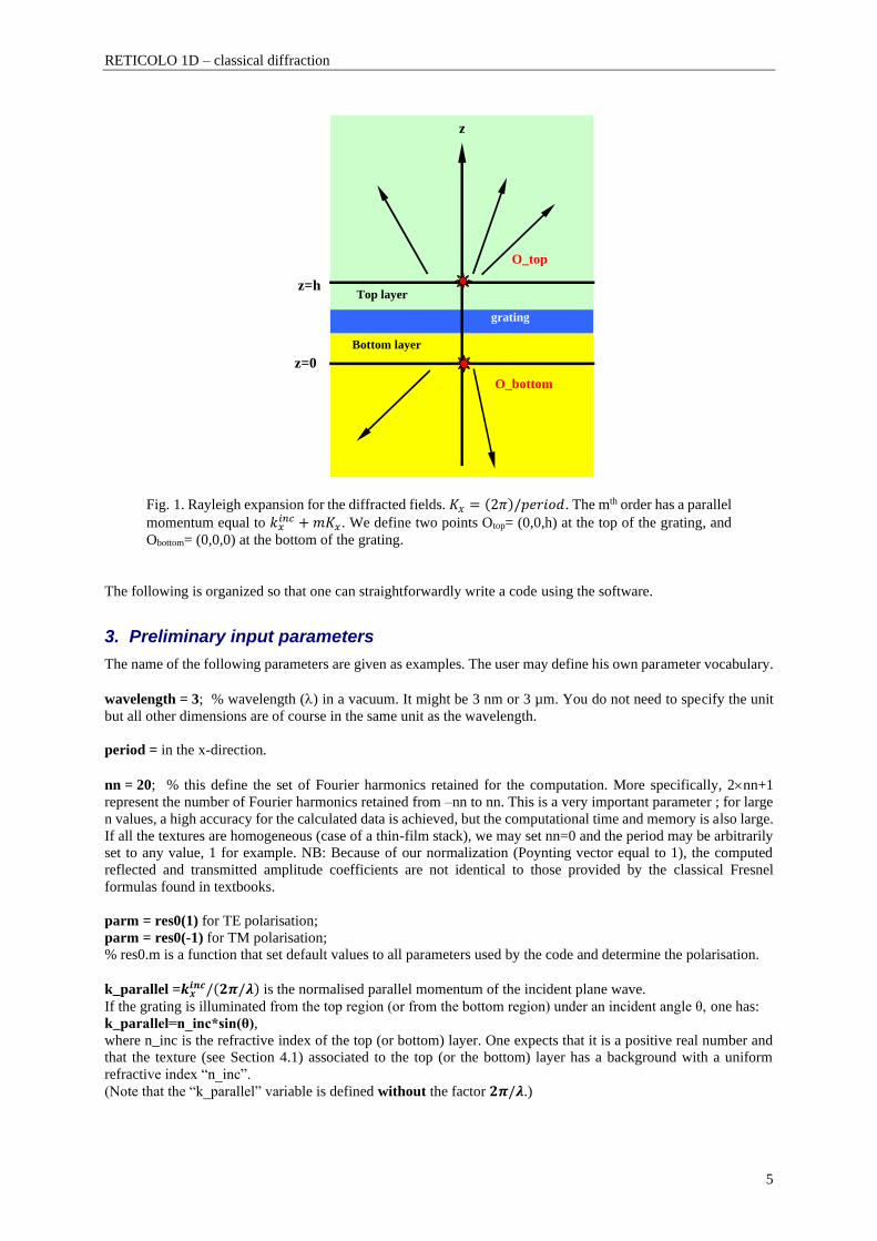
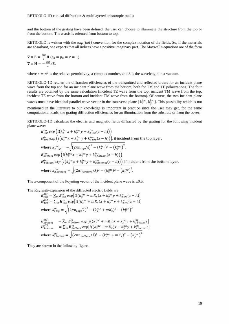
Fig. 1. Rayleigh expansion for the diffracted fields. 𝐾𝑥 = (2𝜋)/𝑝𝑒𝑟𝑖𝑜𝑑. The mth order has a parallel
momentum equal to 𝑘𝑥𝑖𝑛𝑐 + 𝑚𝐾𝑥 . We define two points Otop= (0,0,h) at the top of the grating, and
Obottom= (0,0,0) at the bottom of the grating.
The following is organized so that one can straightforwardly write a code using the software.
3. Preliminary input parameters
The name of the following parameters are given as examples. The user may define his own parameter vocabulary.
wavelength = 3; % wavelength () in a vacuum. It might be 3 nm or 3 µm. You do not need to specify the unit
but all other dimensions are of course in the same unit as the wavelength.
period = in the x-direction.
nn = 20; % this define the set of Fourier harmonics retained for the computation. More specifically, 2nn+1
represent the number of Fourier harmonics retained from –nn to nn. This is a very important parameter ; for large
n values, a high accuracy for the calculated data is achieved, but the computational time and memory is also large.
If all the textures are homogeneous (case of a thin-film stack), we may set nn=0 and the period may be arbitrarily
set to any value, 1 for example. NB: Because of our normalization (Poynting vector equal to 1), the computed
reflected and transmitted amplitude coefficients are not identical to those provided by the classical Fresnel
formulas found in textbooks.
parm = res0(1) for TE polarisation;
parm = res0(-1) for TM polarisation;
% res0.m is a function that set default values to all parameters used by the code and determine the polarisation.
k_parallel =𝒌𝒙𝒊𝒏𝒄/(𝟐𝝅/𝝀) is the normalised parallel momentum of the incident plane wave.
If the grating is illuminated from the top region (or from the bottom region) under an incident angle θ, one has:
k_parallel=n_inc*sin(θ),
where n_inc is the refractive index of the top (or bottom) layer. One expects that it is a positive real number and
that the texture (see Section 4.1) associated to the top (or the bottom) layer has a background with a uniform
refractive index “n_inc”.
(Note that the “k_parallel” variable is defined without the factor 𝟐𝝅/𝝀.)
RETICOLO 1D – classical diffraction
6
It is very important to keep in mind that wether one defines the incident plane wave in the top layer or in the bottom
layer, the calculation will be done for both an incident wave from the top and an incident wave from the bottom,
with an identical parallel momentum k_parallel.
These 5 parameters (“wavelength, nn, parm and k_parallel) are required by the code. Some other parameters can
additionally be defined. For example, the default parameters do not take the symmetry of the problem into account.
So if one wants to use symmetries, a new parameter has to be defined: “parm.sym.x”, (see section 7). If one wants
to calculate accurately the electromagnetics fields, one has to define: ” parm.res1.champ=1”, but this increases
the calculation time and memory loads (see section 8).
4. Structure definition (grating parameters)
The grating encompasses a uniform upperstrate, called the top in the following, a uniform substrate, called the
bottom in the following, and many layers which define the grating, which is defined by a stack of layers. Every
layer is defined by a “texture” and by its thickness. Two different layers may be identical (identical texture and
thickness), may have different thicknesses with identical texture, may have different thicknesses and textures. To
define the diffraction geometry, we need to define the different textures and then the different layers.
4.1. How to define a texture?
Every texture is defined by a cell-array composed of two line-vectors of identical length. The first vector, let us
say [x1 x2 ... xp ...xN], contains all the x-values of the discontinuities. One must have :
N>1,
xp<xp+1 for any p,
and xN - x1<period.
The second line-vector [n1 n2 ... np ... nN] contains the refractive indices of the material between the discontinuities.
More explicitly, we have a refractive index np for xp-1<x<xp. Because of periodicity, note that the refractive index
for xN<x<x1+period is equal to n1.
The specific case of a uniform texture with a refractive index n is easily defined by texture{1}={n}. In that specific
case, no need of a second vector since there is no discontinuity.
The textures have all to be to be packed together in a cell array textures={textures{1}, textures{2}, textures{3}}
prior calling subroutine res1.m.
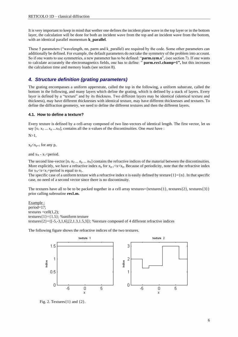
Example :
period=17;
textures =cell(1,2);
textures{1}={1.5}; %uniform texture
textures{2}={[-5,-3,1,6],[2,1.3,1.5,3]}; %texture composed of 4 different refractive indices
The following figure shows the refractive indices of the two textures.
Fig. 2. Textures{1} and {2}.
RETICOLO 1D – classical diffraction
7
Slits in perfectly-conducting metallic textures:
Mixing perfectly-conducting metallic textures and dielectric textures in the same grating structure is possible. We
have first to define a background by its refractive index “inf” (for infinity). In this uniform background, we can
incorporate strip inclusions with a complex or real refractive index “ninclusion” defined by the position c of its
center and its x-width L. The inclusions cannot overlap.
For example:
textures {3}= {inf, [c1,L1,ninclusion1],[c2,L2, ninclusion2]}
Anisotropic layers:
Grating layers (not the substrate nor the superstrate) can be anisotropic with diagonal tensors (𝜀𝑥𝑦 = 𝜀𝑥𝑧 … = 0).
To implement diagonal anisotropy
parm.res1.change_index={[nprov1, nx
1, ny1, nz
1] , [nprov2, nx
2, ny2, nz
2]}; % nprov1 nprov
2
The refractive index nprov1 is then replaced in all textures by epsilon=diag([(nx
1)2, (ny1 )2, (nz
1 )2]). Beware if the
superstate (or substrate) has a refractive index nprov1, it will also be replaced and this is not allowed. Thus we
recommend using an unusual value for nprov1 (e.g. 89.99999 or rand(1)).
The user may also diagonal permeability tensors
parm.res1.change_index={ [nprov1, nx
1, ny1, nz
1 , mx1, my
1, mz1 ] , [nprov
2, nx2, ny
2, nz2] };
The refractive index nprov1 is then replaced in all textures by
epsilon=diag( [(nx1)2, (ny
1 )2, (nz1 )2] ), mu=diag( [(mx
1)2, (my1 )2, (mz
1 )2] ).
For slits in perfectly-conducting metallic textures, anisotropy cannot be implemented.
In order to check if the set of textures is correctly set up, the user can set the variable parm.res1.trace equal to 1:
“parm.res1.trace = 1;”. Then a Matlab figure will show up the refractive-index distribution of all textures. Each
texture is represented with the coordinate x varying from –period/2 to period/2.
4.2. How to define the layers? This is performed by defining the “profile” variable which contains, starting from the top layer and finishing by
the bottom layer, the successive information (thickness and texture-label) relative to every layer. Here is an
example that illustrates how to set up the “profile” variable:
profile = {[0,1,0.5,0.5,1,0.5,0.5,2,0],[1,3,2,4,3,2,4,6,2]}; (1)
It means that from the top to the bottom we have: the top layer is formed by a thickness 0 of texture 1, then we
have twice textures 3, 2 and 4 with depth 1, 0.5 and 0.5 respectively, texture 6 with depth 2, and finally the bottom
layer (formed by texture 2) with null thickness. Since textures 1 and 2 correspond to the top and bottom layers,
they must be uniform. In this example, the top and bottom layers have a null thickness. However, one may set an
arbitrary thickness. Especially, if one needs to plot the electromagnetic fields in the bottom and top layers, the
thicknesses hb and hh (see Fig. 4) over which the fields have to be visualized has to be specified. For hb=hh=0, the
Rayleigh expansions of the fields in the top and bottom layers are not plotted.
In this particular profile, the structure formed by texture 3 with thickness 1, texture 2 with thickness 0.5 and texture
4 with thickness 0.5 is repeated twice. It is possible to simplify the instruction defining the “profile” variable in
order to take into account the repetitions:
profile = {{0,1},{[1,0.5,0.5], [3,2,4], 2},{[2,0],[6,2]}}; (2)
If a structure is repeated many times, the above “factorized” instruction of Eq. 2 is better than the “expanded” one
of Eq. 1, in terms off computational speed, because the calculation will take into account the repetitions.
The profile is shown below.
RETICOLO 1D – classical diffraction
8
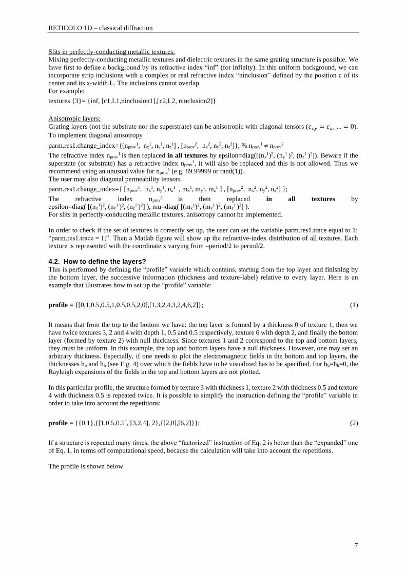
Fig. 3. Texture stacks. The example corresponds to a profile defined by
profile = {[hh,1,0.5,0.5,1,0.5,0.5,2, hb],[1,3,2,4,3,2,4,6,2]}; . The top and bottom layers have
uniform textures.
5. Solving the eigenmode problem for every texture
The first computation with the RCWA consists in calculating the eigenmodes associated to all textures. This is
done by the subroutine “res1.m”, following the instruction:
aa = res1(wavelength,period,textures,nn,k_parallel,parm);
This subroutine has 6 input arguments: the wavelength “wavelength”, the period of the grating “period”, the
“textures” variable, the number of Fourier harmonics “nn”, the normalized parallel incident wave vector
“k_parallel, and the “parm” variable containing the values of all parameters used by the code and the selected
the polarisation. If one has to study the diffraction by different gratings composed of the same textures, one needs
to compute only once the eigenmodes. It is possible to save the “aa” variable in a “.mat” file and to reload it for
the computation of the diffracted waves, see an example in Annex 10.3.
6. Computing the diffracted waves
This is the second step of the computation. This is done by the subroutine “res2.m”, following the instruction:
result = res2(aa, profile);
This subroutine has 2 input arguments: the output “aa” of the subroutine “res1.m” and the “profile” variable. The
output argument “result” contains all the information on the diffracted fields. “result” is an object of class
‘reticolo’ that can be indexed as an usual structure with parentheses, or with the labels of the considered orders
between curly braces. Examples will be given in the following.
This information is divided into the following sub-structures fields :
- “result. inc_top”
- “result. inc_top_reflected”
- “result. inc_top_transmitted”
- “result. inc_bottom”
- “result.inc_bottom_reflected”
- “result. inc_bottom_transmitted”
texture 2
texture 1
texture 6
texture 3texture 2texture 4
texture 2
texture 1
texture 6
texture 3texture 2texture 4
texture 2
texture 1
texture 6
texture 3texture 2texture 4
z
0
h
Bottom layer
Top layerh-hh
hb
RETICOLO 1D – classical diffraction
9
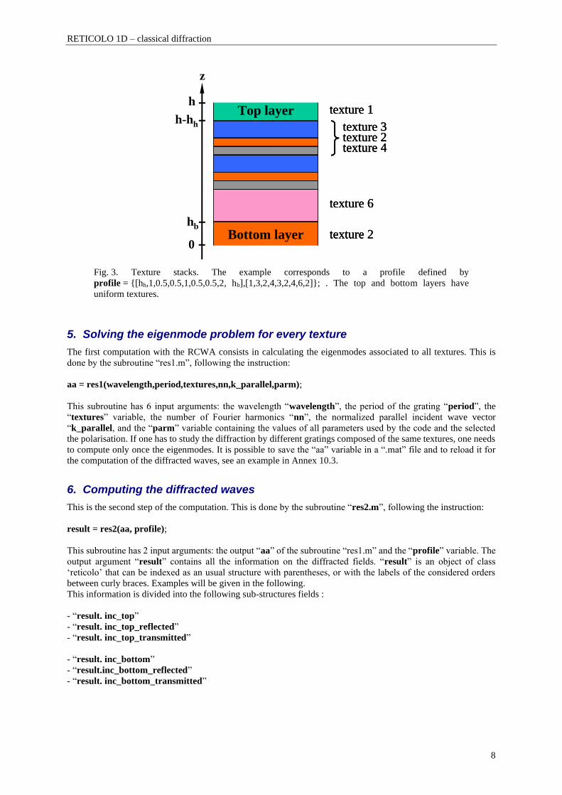
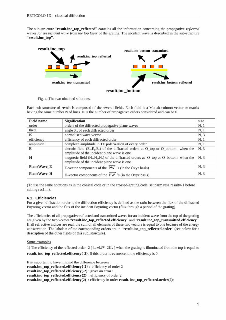
The sub-structure “result.inc_top_reflected” contains all the information concerning the propagative reflected
waves for an incident wave from the top layer of the grating. The incident wave is described in the sub-structure
“result.inc_top”.
result.inc_top result.inc_top_reflected
result.inc_top_transmitted
result.inc_bottom
result.inc_bottom_transmitted
result.inc_bottom_reflected
Fig. 4. The two obtained solutions.
Each sub-structure of result is composed of the several fields. Each field is a Matlab column vector or matrix
having the same number N of lines. N is the number of propagative orders considered and can be 0.
Field name Signification size
order orders of the diffracted propagative plane waves N, 1
theta angle m of each diffracted order N, 1
K normalised wave vector N, 3
efficiency efficiency of each diffracted order N, 1
amplitude complexe amplitude in TE polarization of every order N, 1
E electric field (Ex,Ey,Ez) of the diffracted orders at O_top or O_bottom when the
amplitude of the incident plane wave is one.
N, 3
H magnetic field (Hx,Hy,Hz) of the diffracted orders at O_top or O_bottom when the
amplitude of the incident plane wave is one.
N, 3
PlaneWave_E E-vector components of the PW ’s (in the Oxyz basis) N, 3
PlaneWave_H H-vector components of the PW ’s (in the Oxyz basis) N, 3
(To use the same notations as in the conical code or in the crossed-grating code, set parm.res1.result=-1 before
calling res1.m).
6.1. Efficiencies For a given diffraction order n, the diffraction efficiency is defined as the ratio between the flux of the diffracted
Poynting vector and the flux of the incident Poynting vector (flux through a period of the grating).
The efficiencies of all propagative reflected and transmitted waves for an incident wave from the top of the grating
are given by the two vectors “result.inc_top_reflected.efficiency” and “result.inc_top_transmitted.efficiency”.
If all refractive indices are real, the sum of all elements of these two vectors is equal to one because of the energy
conservation. The labels n of the corresponding orders are in “result.inc_top_reflected.order” (see below for a
description of the other fields of this sub_structure).
Some examples
1) The efficiency of the reflected order -2 ( xincx// K2kk −= ) when the grating is illuminated from the top is equal to
result. inc_top_reflected.efficency{-2}. If this order is evanescent, the efficiency is 0.
It is important to have in mind the difference between :
result.inc_top_reflected.efficiency{-2} : efficiency of order 2
result.inc_top_reflected.efficiency(-2) : gives an error !
result.inc_top_reflected.efficiency{2} : efficiency of order 2
result.inc_top_reflected.efficiency(2) : efficiency in order result. inc_top_reflected.order(2);
RETICOLO 1D – classical diffraction
10
2) The orders of all the transmitted-propagative plane waves for an incident wave from the top of the grating are
given by the vector “result.inc_top_transmitted.order”.
3) The efficiencies of all propagative reflected waves for an incident wave from the bottom in TM polarization are
given by the vector “result.inc_bottom_reflected.efficiency”.
6.2. Rayleigh expansion for propagatives modes The coefficients of the Rayleigh expansion of Fig. 1 can be obtained from the structure result. For instance, when
the grating is illuminated from the bottom with a TE polarised mode, we have : mbottomE =result.inc_bottom_reflected.E{m} (3 components in Oxyz)
mbottomH =result inc_bottom_reflected.H{m} (3 components in Oxyz)
mtopE =result.inc_bottom_transmitted.E{m} (3 components in Oxyz)
mtopH =result.inc_bottom_ transmitted.H{m} (3 components in Oxyz)
and the incident plane wave defined in page 4 is given by : incbottomE =result inc_bottom.E (3 components in Oxyz)
incbottomH =result.inc_bottom.H (3 components in Oxyz).
6.3. Amplitude of diffracted propagative waves
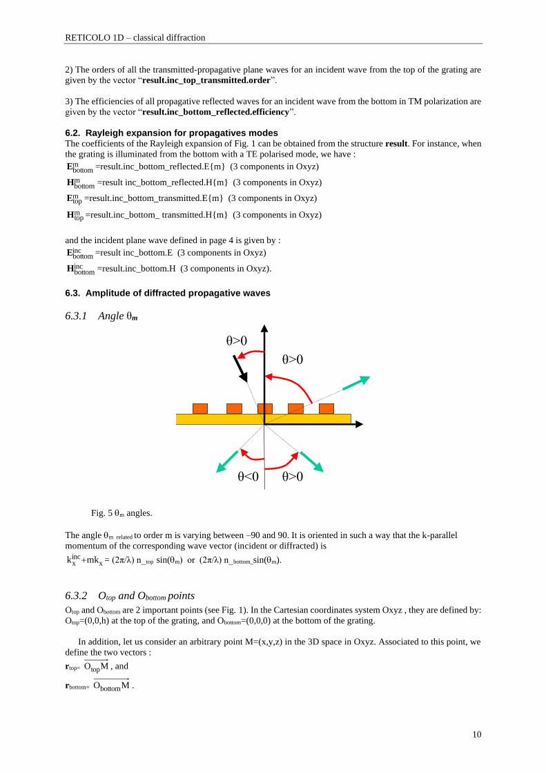
6.3.1 Angle θm
θ>0
θ<0 θ>0
θ>0
Fig. 5 m angles.
The angle m related to order m is varying between –90 and 90. It is oriented in such a way that the k-parallel
momentum of the corresponding wave vector (incident or diffracted) is
xincx mkk + = (2π/λ) n_top sin(m) or (2π/λ) n_bottom_sin(m).
6.3.2 Otop and Obottom points
Otop and Obottom are 2 important points (see Fig. 1). In the Cartesian coordinates system Oxyz , they are defined by:
Otop=(0,0,h) at the top of the grating, and Obottom=(0,0,0) at the bottom of the grating.
In addition, let us consider an arbitrary point M=(x,y,z) in the 3D space in Oxyz. Associated to this point, we
define the two vectors :
rtop= MOtop , and
rbottom= MObottom .
RETICOLO 1D – classical diffraction
11
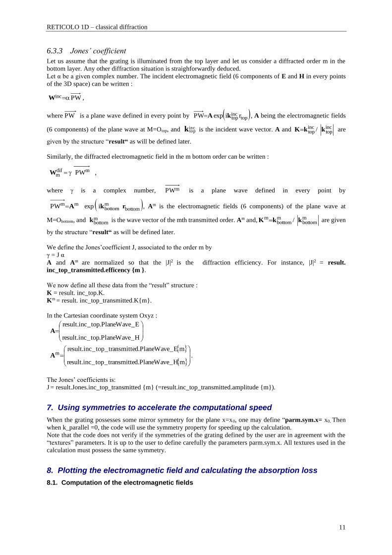
6.3.3 Jones’ coefficient
Let us assume that the grating is illuminated from the top layer and let us consider a diffracted order m in the
bottom layer. Any other diffraction situation is straighforwardly deduced.
Let α be a given complex number. The incident electromagnetic field (6 components of E and H in every points
of the 3D space) can be written :
PWinc =W ,
where PW is a plane wave defined in every point by ( )topinctop riexpPW kA= , A being the electromagnetic fields
(6 components) of the plane wave at M=Otop, and inctopk is the incident wave vector. A and inc
topinctop / kkK= are
given by the structure “result“ as will be defined later.
Similarly, the diffracted electromagnetic field in the m bottom order can be written :
mdifm PW=W ,
where is a complex number, mPW is a plane wave defined in every point by
( )bottommbottom
mm iexpPW rkA= , Am is the electromagnetic fields (6 components) of the plane wave at
M=Obottom, and mbottomk is the wave vector of the mth transmitted order. Am and, m
bottommbottom
m / kkK = are given
by the structure “result“ as will be defined later.
We define the Jones’coefficient J, associated to the order m by
γ = J α
A and Am are normalized so that the |J|2 is the diffraction efficiency. For instance, |J|2 = result.
inc_top_transmitted.efficency {m }.
We now define all these data from the “result” structure :
K = result. inc_top.K.
Km = result. inc_top_transmitted.K{m}.
In the Cartesian coordinate system Oxyz :
=
H_PlaneWave.top_inc.result
E_PlaneWave.top_inc.resultA
=
mH_PlaneWave.dtransmitte_top_inc.result
mE_PlaneWave.dtransmitte_top_inc.resultmA .
The Jones’ coefficients is:
J = result.Jones.inc_top_transmitted {m} (=result.inc_top_transmitted.amplitude {m}).
7. Using symmetries to accelerate the computational speed
When the grating possesses some mirror symmetry for the plane x=x0, one may define “parm.sym.x= x0. Then
when k_parallel =0, the code will use the symmetry property for speeding up the calculation.
Note that the code does not verify if the symmetries of the grating defined by the user are in agreement with the
“textures” parameters. It is up to the user to define carefully the parameters parm.sym.x. All textures used in the
calculation must possess the same symmetry.
8. Plotting the electromagnetic field and calculating the absorption loss
8.1. Computation of the electromagnetic fields
RETICOLO 1D – classical diffraction
12
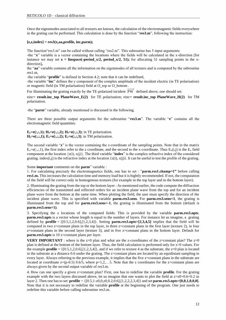
Once the eigenmodes associated to all textures are known, the calculation of the electromagnetic fields everywhere
in the grating can be performed. This calculation is done by the function “res3.m”, following the instruction:
[e,z,index] = res3(x,aa,profile, inc,parm);
The function“res3.m” can be called without calling “res2.m”. This subroutine has 5 input arguments:
-the “x” variable is a vector containing the locations where the fields will be calculated in the x-direction [for
instance we may set x = linspace(-period_x/2, period_x/2, 51); for allocating 51 sampling points in the x-
direction],
the “aa” variable contains all the information on the eigenmodes of all textures and is computed by the subroutine
res1.m,
-the variable “profile” is defined in Section 4.2; note that it can be redefined,
-the variable “inc” defines the y component of the complex amplitude of the incident electric (in TE polarisation)
or magnetic field (in TM polarisation) field at O_top or O_bottom .
For illuminating the grating exactly by the TE-polarized incident PW defined above, one should set:
einc= result.inc_top PlaneWave_E(2) for TE polarisation; einc= result.inc_top PlaneWave_H(2) for TM
polarisation.
-the “parm” variable, already mentioned is discussed in the following.
There are three possible output arguments for the subroutine “res3.m”. The variable “e” contains all the
electromagnetic field quantities:
Ey=e(:,:,1); Hx=e(:,:,2); Hz=e(:,:,3); in TE polarization.
Hy=e(:,:,1); Ex=e(:,:,2); Ez=e(:,:,3); in TM polarization.
The second variable “z” is the vector containing the z-coordinate of the sampling points. Note that in the matrix
Ex=e(:,:,1), the first index refer to the z coordinate, and the second to the x-coordinate. Thus Ex(i,j) is the Ex field
component at the location {z(i), x(j)}. The third variable “index” is the complex refractive index of the considered
grating. index(i,j) is the refractive index at the location {z(i), x(j)}. It can be useful to test the profile of the grating.
Some important comments on the parm” variable :
1. For calculating precisely the electromagnetics fields, one has to set : ”parm.res1.champ=1” before calling
res1.m. This increases the calculation time and memory load but it is hightly recommended. If not, the computation
of the field will be correct only in homogenous textures (for example in the top layer and in the bottom layer).
2. Illuminating the grating from the top or the bottom layer : As mentioned earlier, the code compute the diffraction
efficiencies of the transmitted and reflected orders for an incident plane wave from the top and for an incident
plane wave from the bottom at the same time. When plotting the field, the user must specify the direction of the
incident plane wave. This is specified with variable parm.res3.sens. For parm.res3.sens=1, the grating is
illuminated from the top and for parm.res3.sens=-1, the grating is illuminated from the bottom (default is
parm.res3.sens=1).
3. Specifying the z locations of the computed fields: This is provided by the variable parm.res3.npts.
parm.res3.npts is a vector whose length is equal to the number of layers. For instance let us imagine, a grating
defined by profile = {[0.5,1,2,0.6],[1,2,3,4]}. Setting parm.res3.npts=[2,3,4,5] implies that the field will be
computed in two z=constant plans in the top layer, in three z=constant plans in the first layer (texture 2), in four
z=constant plans in the second layer (texture 3), and in five z=constant plans in the bottom layer. Default for
parm.res3.npts is 10 z=constant plans per layer.
VERY IMPORTANT : where is the z=0 plan and what are the z-coordinates of the z=constant plan? The z=0
plan is defined at the bottom of the bottom layer. Thus, the field calculation is performed only for z>0 values. For
the example profile = {[0.5,1,2,0.6],[1,2,3,4]}, and if we refer to texture 4 as the substrate, the z=0 plan is located
in the substrate at a distance 0.6 under the grating. The z=constant plans are located by an equidistant sampling in
every layer. Always referring to the previous example, it implies that the five z=constant plans in the substrate are
located at coordinate z=(p-0.5) 0.6/5, where p=1,2,…5. Note that the z coordinates for the z=constant plans are
always given by the second output variable of res3.m.
4. How can one specify a given z=constant plan? First, one has to redefine the variable profile. For the grating
example with the two layers discussed above, let us imagine that one wants to plot the field at z=z0+0.6+0.2 in
layer 2. Then one has to set: profile = {[0.5,1-z0,0,z0,0.2,0.6],[1,2,2,2,3,4]} and set parm.res3.npts=[0,0,1,0,0,0].
Note that it is not necessary to redefine the variable profile at the beginning of the program. One just needs to
redefine this variable before calling subroutine res3.m.
RETICOLO 1D – classical diffraction
13
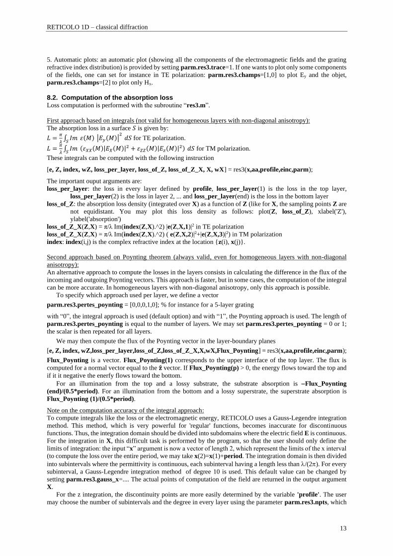
5. Automatic plots: an automatic plot (showing all the components of the electromagnetic fields and the grating
refractive index distribution) is provided by setting parm.res3.trace=1. If one wants to plot only some components
of the fields, one can set for instance in TE polarization: parm.res3.champs=[1,0] to plot Ey and the objet,
parm.res3.champs=[2] to plot only Hx.
8.2. Computation of the absorption loss Loss computation is performed with the subroutine “res3.m”.
First approach based on integrals (not valid for homogeneous layers with non-diagonal anisotropy):
The absorption loss in a surface 𝑆 is given by:
𝐿 =𝜋
𝜆∫ 𝐼𝑚 𝜀(𝑀) |𝐸𝑦(𝑀)|
2 𝑑𝑆
𝑆 for TE polarization.
𝐿 =𝜋
𝜆∫ 𝐼𝑚 (𝜀𝑋𝑋(𝑀)|𝐸𝑋(𝑀)|2 + 𝜀𝑍𝑍(𝑀)|𝐸𝑧(𝑀)|2) 𝑑𝑆
𝑆 for TM polarization.
These integrals can be computed with the following instruction
[e, Z, index, wZ, loss_per_layer, loss_of_Z, loss_of_Z_X, X, wX] = res3(x,aa,profile,einc,parm);
The important ouput arguments are:
loss_per_layer: the loss in every layer defined by profile, loss_per_layer(1) is the loss in the top layer,
loss_per_layer(2) is the loss in layer 2, ... and loss_per_layer(end) is the loss in the bottom layer
loss_of_Z: the absorption loss density (integrated over X) as a function of Z (like for X, the sampling points Z are
not equidistant. You may plot this loss density as follows: plot(Z, loss_of_Z), xlabel('Z'),
ylabel('absorption')
loss_of_Z_X(Z,X) = π/λ Im(index(Z,X).^2) |e(Z,X,1)|2 in TE polarization
loss_of_Z_X(Z,X) = π/λ Im(index(Z,X).^2) ( e(Z,X,2)|2+|e(Z,X,3)|2) in TM polarization
index: index(i,j) is the complex refractive index at the location {z(i), x(j)}.
Second approach based on Poynting theorem (always valid, even for homogeneous layers with non-diagonal
anisotropy):
An alternative approach to compute the losses in the layers consists in calculating the difference in the flux of the
incoming and outgoing Poynting vectors. This approach is faster, but in some cases, the computation of the integral
can be more accurate. In homogeneous layers with non-diagonal anisotropy, only this approach is possible.
To specify which approach used per layer, we define a vector
parm.res3.pertes_poynting = [0,0,0,1,0]; % for instance for a 5-layer grating
with “0”, the integral approach is used (default option) and with “1”, the Poynting approach is used. The length of
parm.res3.pertes_poynting is equal to the number of layers. We may set parm.res3.pertes_poynting = 0 or 1;
the scalar is then repeated for all layers.
We may then compute the flux of the Poynting vector in the layer-boundary planes
[e, Z, index, wZ,loss_per_layer,loss_of_Z,loss_of_Z_X,X,wX,Flux_Poynting] = res3(x,aa,profile,einc,parm);
Flux_Poynting is a vector. Flux_Poynting(1) corresponds to the upper interface of the top layer. The flux is
computed for a normal vector equal to the �̂� vector. If Flux_Poynting(p) > 0, the energy flows toward the top and
if it it negative the enerfy flows toward the bottom.
For an illumination from the top and a lossy substrate, the substrate absorption is −Flux_Poynting
(end)/(0.5*period). For an illumination from the bottom and a lossy superstrate, the superstrate absorption is
Flux_Poynting (1)/(0.5*period).
Note on the computation accuracy of the integral approach:
To compute integrals like the loss or the electromagnetic energy, RETICOLO uses a Gauss-Legendre integration
method. This method, which is very powerful for 'regular' functions, becomes inaccurate for discontinuous
functions. Thus, the integration domain should be divided into subdomains where the electric field E is continuous.
For the integration in X, this difficult task is performed by the program, so that the user should only define the
limits of integration: the input “x” argument is now a vector of length 2, which represent the limits of the x interval
(to compute the loss over the entire period, we may take x(2)=x(1)+period. The integration domain is then divided
into subintervals where the permittivity is continuous, each subinterval having a length less than /(2). For every
subinterval, a Gauss-Legendre integration method of degree 10 is used. This default value can be changed by
setting parm.res3.gauss_x=.... The actual points of computation of the field are returned in the output argument
X.
For the z integration, the discontinuity points are more easily determined by the variable 'profile'. The user
may choose the number of subintervals and the degree in every layer using the parameter parm.res3.npts, which
RETICOLO 1D – classical diffraction
14
is now an array with two lines (in subsection 8.1 this variable is a line vector): the first line defines the degree and
the second line the numbers of subintervals of every layer. For example: parm.res3.npts = [ [10,0,12] ; [3,1,5] ];
means that 3 subintervals with 10-degree points are used in the first layer, 1 subintervals with 0 point in the second
layer, 5 subintervals with 12degree points in the third layer.
The actual z-points of computation of the field are returned in the output variable Z, and the vector wZ
represents the weights and we have sum(loss_of_Z.*wZ)=sum(loss_per_layer). Although the maximum degree
that can be handled by reticolo is 468, it is recommended to limit the degree values to modest numbers (10-30
maximum) and to increase the number of subintervals (the larger the degree, the denser the sampling points in the
vicinity of the subinterval boundaries).
Note that if einc= result. inc_top PlaneWave_E(2), in TE ploarization, or einc= result. inc_top
PlaneWave_H(2), in TE ploarization , the energie conservation test for an incident plane wave from the top is
sum(result. inc_top_reflected.efficiency)+
sum(result. inc_top_transmitted.efficiency)+
sum(loss_per_layer) / (.5*period) = 1.
Usually, this equality is achieved with an absolute error of <10−5.
For specialists:
-loss_of_Z_X =pi/ wavelength*imag(index.^2).* abs(e(:,:,1)).^2; in TE polarization
-loss_of_Z_X =pi/ wavelength*imag(index.^2).*sum(abs(e(:,:,2:3)).^2,3); in TM polarization
-loss_of_Z =(loss_of_Z_X*wX(:)).';
-by setting index(index ~= index_chosen)=0 in the previous formulas, one may calculate the absorption loss in
the medium of refractive index index_chosen.
9. Bloch-mode effective indices
RETICOLO gives access to another output: the Bloch mode associated to all textures. The Bloch mode k of the
texture l can be written
|𝛷𝑘𝑙⟩ = ∑ 𝑎𝑚
k,l exp [𝑖(𝑘𝑥inc + 𝑚K𝑥)𝑥] 𝑒𝑥𝑝 (𝑖
2π
𝜆𝑛eff
k,l 𝑧)𝑚 ,
where 𝑛effk,l
is the effective index of the Bloch mode k of the texture l.
Instruction:
[aa, n_eff] = res1(wavelength,period,textures,nn,kparallel, parm);
Note that the “n_eff” variable is a Matlab cell array: “n_eff{ii}” is a column vector containing all the Bloch-mode
effective indices associated to the texture “textures{ii}”. The element number 5 of this vector, for example, is
called by the instruction “n_eff{ii}(5);”. An attenuated Bloch-mode has a complex effective index.
Bloch mode profile visualization:
To plot the profile of Bloch mode Num_mode of the texture Num_texture:
res1(aa, neff, Num_texture, Num_mode);
To obtain the profile datas in the format given by res3:
[e,o,x] = res1(aa, neff, Num_texture, Num_mode); % by default, |x| < period/2
[e,o] = res1(aa, neff, Num_texture, Num_mode, x); % by specifying the x vector, x=linspace(0, 3*period(1),100)
for example.
10. Annex
10.1. Checking that the textures are correctly set up Setting “parm.res1.trace = 1;” generates a Matlab figure which represents the refractive-index distribution of all
the textures.
10.2. The “retio” & “retefface” instructions RETICOLO automatically creates temporary files in order to save memory. These temporary files are of the form
“abcd0.mat”, “abcd1.mat” … with abcd are randomly chosen) .They are created in the current directory. In general
RETICOLO automatically erases these files when they are no longer needed, but it is recommended to finish all
programs by the instruction “retio;”, which erases all temporary files. Also, if a program anormally stopsone may
execute the instruction “retio” before restarting the program.
RETICOLO 1D – classical diffraction
15
The “retefface” instruction allows to know all the “abcd0.mat” files and to erase them if wanted.
If we are not limited by memory (this is often the case with modern computers), we can prevent the writing of
intermediate files on the hard disk by the setting
parm.not_io = 1;
before the call to res1. Then it is no longer necessary to use the retio instruction at the end of the programs to erase
the files.
IMPORTANT: to use parfor loops, it is imperative to take the option parm.not_io = 1.
10.3. How to save and to reload the “aa” variable To save the “aa” variable in a “.mat” file, the user has to define a new parameter containing the name of the file
he or she wants to create : “parm.res1.fperm = 'file_name';”. field_name is a char string with at least one letter.
The program will automatically save “aa” in the file “file_name.mat”. In a new utilisation it is sufficient to write
aa== 'file_name';.
Example of a program which calculates and saves the “aa” variable
[...] % Definition of the input parameters, see Section 3
parm.res1.fperm = 'toto';
[...] % Definition of the textures, see Section 4.1
aa = res1(wavelength,period,textures,nn,k_parallel,parm);
Example of a program which uses the “aa” variable and then calculates the diffracted waves
[...] % Definition of the profile, see Section 4.2. Note that the textures used to define the profile argument have
to correspond to the textures defined in the program which has previously calculated the “aa” variable.
aa=’toto’;
result = res2(aa,profile);
retio;
10.4. Asymmetry of the Fourier harmonics retained in the computation nn = [-15;20]; % this defines the set of non-symmetric Fourier harmonics retained for the computation. In this
case, the Fourier harmonics from –15 to +20 are retained.
The instructions “nn = 10;” and “nn = [-10;10];” are equivalent.
Take care that the use of symmetry imposes symmetric Fourier harmonics if not the computation will be done
without any symmetry consideration.
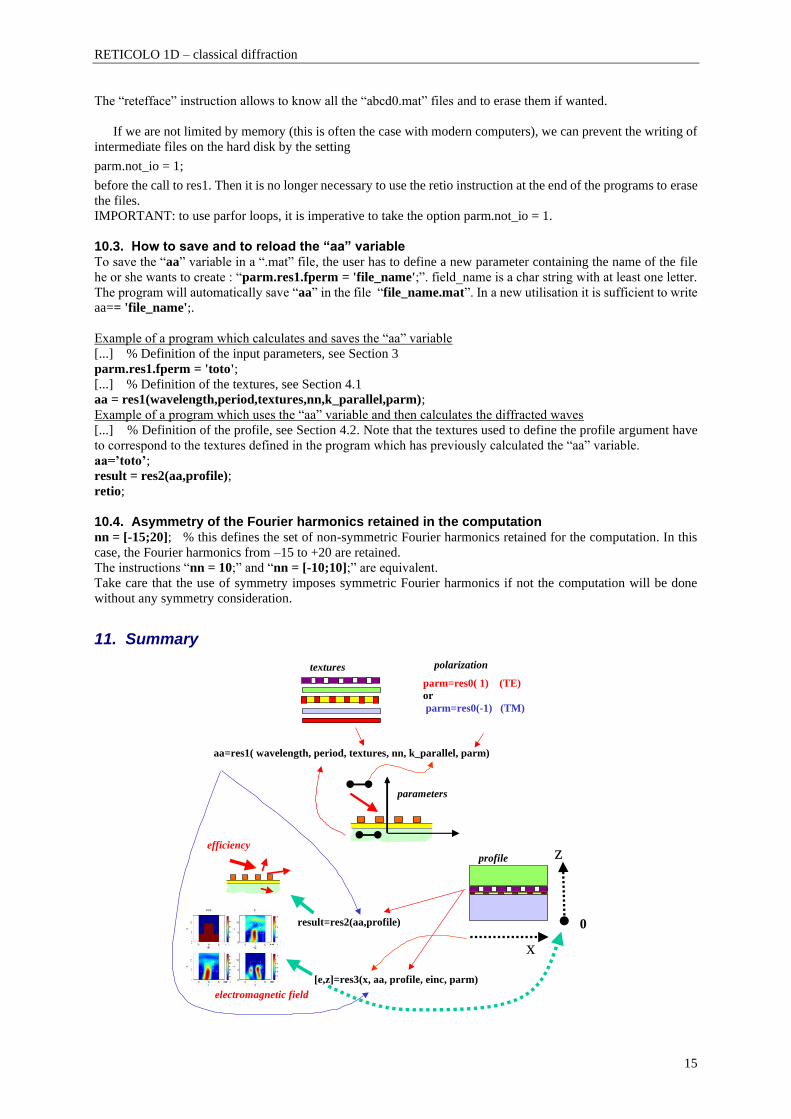
11. Summary
aa=res1( wavelength, period, textures, nn, k_parallel, parm)
result=res2(aa,profile)
[e,z]=res3(x, aa, profile, einc, parm)
profile
textures
efficiency
electromagnetic field
parameters
z
x
0
parm=res0( 1) (TE)
or
parm=res0(-1) (TM)
polarization
RETICOLO 1D – classical diffraction
16
Fig. 6 Summary.
parm = res0( 1) for TE polarisation;
parm = res0(-1) for TM polarisation;
aa = res1(wavelength,period,textures,nn,k_parallel,parm);
result = res2(aa,profile);
J = result.Jones.inc_top_transmitted {m}
[e,z,o] = res3(x,aa,profile, inc,parm);
12. Examples
The following example can be copied and executed in Matlab.
%%%%%%%%%%%%%%%%%%%%%%%%%
% EXAMPLE 1D (TE or TM) %
%%%%%%%%%%%%%%%%%%%%%%%%%
wavelength=8;
period=10;% same unit as wavelength
n_incident_medium=1;% refractive index of the top layer
n_transmitted_medium=1.5;% refractive index of the bottom layer
angle_theta0=-10;k_parallel=n_incident_medium*sin(angle_theta0*pi/180);
parm=res0(1);% TE polarization. For TM : parm=res0(-1)
parm.res1.champ=1;% the electromagnetic field is calculated accurately
nn=40;% Fourier harmonics run from [-40,40]
% textures for all layers including the top and bottom layers
texture=cell(1,3);
textures{1}= n_incident_medium; % uniform texture
textures{2}= n_transmitted_medium; % uniform texture
textures{3}={[-2.5,2.5],[n_incident_medium,n_transmitted_medium] };
aa=res1(wavelength,period,textures,nn,k_parallel,parm);
profile={[4.1,5.2,4.1],[1,3,2]};
one_D_TE=res2(aa,profile)
eff=one_D_TE.inc_top_reflected.efficiency{-1}
J=one_D_TE.Jones.inc_top_reflected{-1};% Jones’coefficients
abs(J)^2 % first order efficiency for an illumination from the top layer
% field calculation
x=linspace(-period/2,period/2,51);% x coordinates(z-coordinates are determined by
res3.m)
einc=1;
parm.res3.trace=1; % plotting automatically
parm.res3.npts=[50,50,50];
[e,z,index]=res3(x,aa,profile,einc,parm);
figure;pcolor(x,z,real(squeeze(e(:,:,1)))); % user plotting
shading flat;xlabel('x');ylabel('y');axis equal;title('Real(Ey)');
% Loss calculation
textures{3}={[-2.5,2.5],[n_incident_medium,.1+5i] };
aa_loss=res1(wavelength,period,textures,nn,k_parallel,parm);
one_D_loss=res2(aa_loss,profile)
parm.res3.npts=[[0,10,0];[1,3,1]];
einc=one_D_loss.inc_top.PlaneWave_E(2);
[e,z,index,wZ,loss_per_layer,loss_of_Z,loss_of_Z_X,X,wX]=res3([-
period/2,period/2],aa_loss,profile,einc,parm);
Energie_conservation=sum(one_D_loss.inc_top_reflected.efficiency)+sum(one_D_loss.in
c_top_transmitted.efficiency)+sum(loss_per_layer)/(.5* period)-1
retio % erase temporary files
RETICOLO 1D conical diffraction & multilayered anisotropic media
17
RETICOLO CODE 1D for the analysis of the diffraction by stacks of lamellar 1D
gratings (conical diffraction)
Authors: J.P. Hugonin and P. Lalanne
Reticolo code 1D-conical is a free software for analyzing 1D gratings in classical and
conical mountings. It operates under Matlab. To install it, copy the companion folder
“reticolo_allege” and add the folder in the Matlab path. The code may also be used to
analyze thin-film stacks with homogeneous and anisotropic materials, see the end of
Section 3.1.
Outline
Generality ............................................................................................................................................................. 18
1. The diffraction problem considered................................................................................................................. 18
2. Preliminary input parameters .......................................................................................................................... 20
3. Structure definition (grating parameters) ....................................................................................................... 21
3.1. How to define a texture? .......................................................................................................................... 21
3.2. How to define the layers? ........................................................................................................................ 23
4. Solving the eigenmode problem for every texture ........................................................................................... 23
5. Computing the diffracted waves ...................................................................................................................... 24
5.1. Efficiency................................................................................................................................................... 26
5.2. Rayleigh expansion for propagatives modes .......................................................................................... 26
5.3. Diffracted amplitudes of propagative waves .......................................................................................... 26 5.3.1 UTE, UTM, θ, δ and K ..................................................................................................................... 26 5.3.2 Otop and Obottom points .................................................................................................................... 27 5.3.3 Jones’ matrix ................................................................................................................................. 27
6. Using symmetries to accelerate the computational speed ............................................................................... 29
7. Plotting the electromagnetic field and calculating the absorption loss .......................................................... 29
7.1. Computation of the electromagnetic fields............................................................................................. 29
7.2. Computation of the absorption loss ........................................................................................................ 30
8. Bloch-mode effective indices ........................................................................................................................... 32
9. Annex ................................................................................................................................................................ 32
9.1. Checking that the textures are correctly set up ..................................................................................... 32
9.2. The “retio” instruction ............................................................................................................................ 32
9.3. How to save and to reload the “aa” variable ......................................................................................... 32
9.4. Asymmetry of the Fourier harmonics retained in the computation .................................................... 33
10. Summary ......................................................................................................................................................... 33
11. Examples ........................................................................................................................................................ 33
RETICOLO 1D conical diffraction & multilayered anisotropic media
18
Generality
RETICOLO is a code written in the language MATLAB 9.0. It computes the diffraction efficiencies and the
diffracted amplitudes of gratings composed of stacks of lamellar structures. It incorporates routines for the
calculation and visualisation of the electromagnetic fields inside and outside the grating. With this version, 2D
periodic (crossed) gratings cannot be analysed.
As free alternative to MATLAB, RETICOLO can also be run in GNU Octave with minimal code changes. For
further information, please contact [email protected].
In brief, RETICOLO implements a frequency-domain modal method (known as the Rigorous Coupled wave
Analysis/RCWA). To get an overview of the RCWA, the interested readers may refer to the following articles:
1D-classical and conical diffraction
M.G. Moharam et al., JOSAA 12, 1068 (1995),
M.G. Moharam et al, JOSAA 12, 1077 (1995),
P. Lalanne and G.M. Morris, JOSAA 13, 779 (1996),
G. Granet and B. Guizal, JOSAA 13, 1019 (1996),
L. Li, JOSAA 13, 1870 (1996), see also C. Sauvan et al., Opt. Quantum Electronics 36, 271-284 (2004) which
simply explains the raison of the convergence-rate improvement of the Fourier-Factorization rules without
requiring advanced mathematics on Fourier series and generalizes to other kinds of expansions.
2D-crossed gratings
L. Li, JOSAA 14, 2758-2767 (1997),
E. Popov and M. Nevière, JOSAA 17, 1773 (2000),
which describe the up-to-date formulation of the approach used in RETICOLO. Note that the formulation used in
the last article (which proposes an improvement for analysing metallic gratings with continuous profiles like
sinusoidal gratings) is not available in the RETICOLO version of the web. The RCWA relies on the computation
of the eigenmodes in all the layers of the grating structure in a Fourier basis (plane-wave basis) and on a scattering
matrix approach to recursively relate the mode amplitudes in the different layers.
Eigenmode solver: For conical diffraction analysis of 1D gratings, the Bloch eigenmode solver used in Reticolo
is based on the article "P. Lalanne and G.M. Morris, JOSAA 13, 779 (1996)".
Scattering matrix approach: The code incorporates many refinements that we have not published and that we
do not plan to publish. For instance, although it is generally admitted that the S-matrix is inconditionnally stable,
it is not always the case. We have developed an in-house transfer matrix method which is more stable and accurate.
The new transfer matrix approach is also more general and can handle perfect metals. The essence of the method
has been rapidly published in "J.-P. Hugonin, M. Besbes and P. Lalanne, Op. Lett. 33, 1590 (2008)".
Field calculation: The calculation of the near-field electromagnetic fields everywhere in the grating is performed
according to the method described in "P. Lalanne, M.P. Jurek, JMO 45, 1357 (1998)" and to its generalization to
crossed gratings (unpublished). Basically, no Gibbs phenomenon will be visible in the plots of the discontinuous
electromagnetic quantities, but field singularities at corners will be correctly handled.
Acknowledging the use of RETICOLO: In publications and reports, acknowledgments have to be provided by
referencing to J.P. Hugonin and P. Lalanne, RETICOLO software for grating analysis, Institut d'Optique, Orsay,
France (2005).
In journal publications and in addition, one may fairly quote the following references:
-P. Lalanne and G.M. Morris, "Highly improved convergence of the coupled-wave method for TM polarization",
J. Opt. Soc. Am. A 13, 779-789 (1996).
-P. Lalanne and M.P. Jurek, "Computation of the near-field pattern with the coupled-wave method for TM
polarization", J. Mod. Opt.45, 1357-1374 (1998), if near-field electromagnetic-field distributions are shown.
1. The diffraction problem considered
In general terms, the code solves the diffraction problem by a grating defined by a stack of layers which have all
identical periods in the x- directions and are invariant in the y direction see the following figure. In the following,
the (x,y) plane and the z-direction will be referred to as the transverse plane and the longitudinal direction,
respectively. To define the grating structure, first we have to define a top and a bottom. This is rather arbitrary
since the top or the bottom can be the substrate or the cover of a real structure. It is up to the user. Once the top
RETICOLO 1D conical diffraction & multilayered anisotropic media
19
and the bottom of the grating have been defined, the user can choose to illuminate the structure from the top or
from the bottom. The z-axis is oriented from bottom to top.
RETICOLO is written with the 𝑒𝑥𝑝(𝑖𝜔𝑡) convention for the complex notation of the fields. So, if the materials
are absorbant, one expects that all indices have a positive imaginary part. The Maxwell's equations are of the form
𝛁 × 𝐄 =2𝑖𝜋
𝜆𝐇 (𝜀0 = µ0 = 𝑐 = 1)
𝛁 × 𝐇 = −2𝑖𝜋
𝜆𝜀𝐄,
where 𝜀 = 𝑛2 is the relative permittivity, a complex number, and 𝜆 is the wavelength in a vacuum.
RETICOLO-1D returns the diffraction efficiencies of the transmitted and reflected orders for an incident plane
wave from the top and for an incident plane wave from the bottom, both for TM and TE polarizations. The four
results are obtained by the same calculation (incident TE wave from the top, incident TM wave from the top,
incident TE wave from the bottom and incident TM wave from the bottom). Of course, the two incident plane
waves must have identical parallel wave vector in the transverse plane [ incxk , inc
yk ]. This possibility which is not
mentioned in the literature to our knowledge is important in practice since the user may get, for the same
computational loads, the grating diffraction efficiencies for an illumination from the substrate or from the cover.
RETICOLO-1D calculates the electric and magnetic fields diffracted by the grating for the following incident
plane wave:
𝑬𝑡𝑜𝑝𝑖𝑛𝑐 𝑒𝑥𝑝 (𝑖(𝑘𝑥
𝑖𝑛𝑐𝑥 + 𝑘𝑦𝑖𝑛𝑐𝑦 + 𝑘𝑧 𝑡𝑜𝑝
𝑖𝑛𝑐 (𝑧 − ℎ)))
𝑯𝑡𝑜𝑝𝑖𝑛𝑐 𝑒𝑥𝑝 (𝑖(𝑘𝑥
𝑖𝑛𝑐𝑥 + 𝑘𝑦𝑖𝑛𝑐𝑦 + 𝑘𝑧 𝑡𝑜𝑝
𝑖𝑛𝑐 (𝑧 − ℎ))), if incident from the top layer,
where 𝑘𝑧 𝑡𝑜𝑝𝑖𝑛𝑐 = −√(2𝜋𝑛𝑡𝑜𝑝/𝜆)
2− (𝑘𝑥
𝑖𝑛𝑐)2 − (𝑘𝑦𝑖𝑛𝑐)
2.
𝑬𝑏𝑜𝑡𝑡𝑜𝑚𝑖𝑛𝑐 𝑒𝑥𝑝 (𝑖(𝑘𝑥
𝑖𝑛𝑐𝑥 + 𝑘𝑦𝑖𝑛𝑐𝑦 + 𝑘𝑧 𝑏𝑜𝑡𝑡𝑜𝑚
𝑖𝑛𝑐 (𝑧 − ℎ)))
𝑯𝑏𝑜𝑡𝑡𝑜𝑚𝑖𝑛𝑐 𝑒𝑥𝑝 (𝑖(𝑘𝑥
𝑖𝑛𝑐𝑥 + 𝑘𝑦𝑖𝑛𝑐𝑦 + 𝑘𝑧 𝑏𝑜𝑡𝑡𝑜𝑚
𝑖𝑛𝑐 (𝑧 − ℎ))), if incident from the bottom layer,
where 𝑘𝑧 𝑏𝑜𝑡𝑡𝑜𝑚𝑖𝑛𝑐 = √(2𝜋𝑛𝑏𝑜𝑡𝑡𝑜𝑚/𝜆)2 − (𝑘𝑥
𝑖𝑛𝑐)2 − (𝑘𝑦𝑖𝑛𝑐)
2.
The z-component of the Poynting vector of the incident plane wave is 0.5.
The Rayleigh-expansion of the diffracted electric fields are
𝑬𝑡𝑜𝑝𝑑𝑖𝑓
= ∑ 𝑬𝑡𝑜𝑝𝑚
𝑚 𝑒𝑥𝑝[𝑖((𝑘𝑥𝑖𝑛𝑐 + 𝑚𝐾𝑥)𝑥 + 𝑘𝑦
𝑖𝑛𝑐𝑦 + 𝑘z top𝑚 (𝑧 − ℎ)]
𝑯𝑡𝑜𝑝𝑑𝑖𝑓
= ∑ 𝑯𝑡𝑜𝑝𝑚
𝑚 𝑒𝑥𝑝[𝑖((𝑘𝑥𝑖𝑛𝑐 + 𝑚𝐾𝑥)𝑥 + 𝑘𝑦
𝑖𝑛𝑐𝑦 + 𝑘z top𝑚 (𝑧 − ℎ)]
where kz top𝑚 = √(2𝜋𝑛𝑡𝑜𝑝/𝜆)
2− (𝑘𝑥
𝑖𝑛𝑐 + 𝑚𝐾𝑥)2 − (𝑘𝑦𝑖𝑛𝑐)
2
𝑬𝑏𝑜𝑡𝑡𝑜𝑚𝑑𝑖𝑓
= ∑ 𝑬𝑏𝑜𝑡𝑡𝑜𝑚𝑚
𝑚 𝑒𝑥𝑝[𝑖((𝑘𝑥𝑖𝑛𝑐 + 𝑚𝐾𝑥)𝑥 + 𝑘𝑦
inc𝑦 + 𝑘z bottom𝑚 𝑧]
𝑯𝑏𝑜𝑡𝑡𝑜𝑚𝑑𝑖𝑓
= ∑ 𝐇𝑏𝑜𝑡𝑡𝑜𝑚𝑚
𝑚 𝑒𝑥𝑝[𝑖((𝑘𝑥𝑖𝑛𝑐 + 𝑚𝐾𝑥)𝑥 + 𝑘𝑦
inc𝑦 + 𝑘z bottom𝑚 𝑧]
where kz bottom𝑚 = √(2𝜋𝑛𝑏𝑜𝑡𝑡𝑜𝑚/𝜆)2 − (𝑘𝑥
𝑖𝑛𝑐 + 𝑚𝐾𝑥)2 − (𝑘𝑦𝑖𝑛𝑐)
2
They are shown in the following figure.
RETICOLO 1D conical diffraction & multilayered anisotropic media
20
z
z=0
z=h
Top layer
Bottom layer
grating
O_top
O_bottom
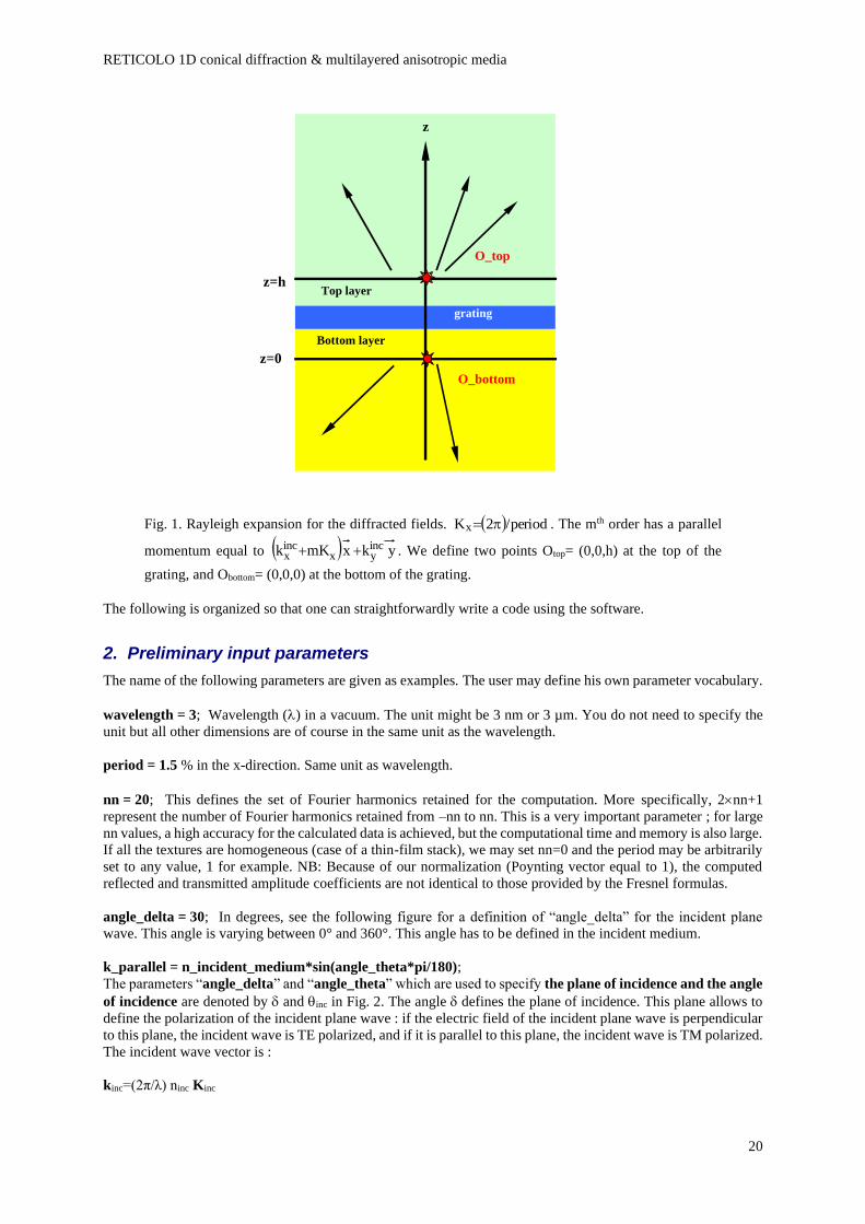
Fig. 1. Rayleigh expansion for the diffracted fields. ( ) period/2Kx = . The mth order has a parallel
momentum equal to ( ) ykxmKk incyx
incx ++ . We define two points Otop= (0,0,h) at the top of the
grating, and Obottom= (0,0,0) at the bottom of the grating.
The following is organized so that one can straightforwardly write a code using the software.
2. Preliminary input parameters
The name of the following parameters are given as examples. The user may define his own parameter vocabulary.
wavelength = 3; Wavelength () in a vacuum. The unit might be 3 nm or 3 µm. You do not need to specify the
unit but all other dimensions are of course in the same unit as the wavelength.
period = 1.5 % in the x-direction. Same unit as wavelength.
nn = 20; This defines the set of Fourier harmonics retained for the computation. More specifically, 2nn+1
represent the number of Fourier harmonics retained from –nn to nn. This is a very important parameter ; for large
nn values, a high accuracy for the calculated data is achieved, but the computational time and memory is also large.
If all the textures are homogeneous (case of a thin-film stack), we may set nn=0 and the period may be arbitrarily
set to any value, 1 for example. NB: Because of our normalization (Poynting vector equal to 1), the computed
reflected and transmitted amplitude coefficients are not identical to those provided by the Fresnel formulas.
angle_delta = 30; In degrees, see the following figure for a definition of “angle_delta” for the incident plane
wave. This angle is varying between 0° and 360°. This angle has to be defined in the incident medium.
k_parallel = n_incident_medium*sin(angle_theta*pi/180);
The parameters “angle_delta” and “angle_theta” which are used to specify the plane of incidence and the angle
of incidence are denoted by and inc in Fig. 2. The angle defines the plane of incidence. This plane allows to
define the polarization of the incident plane wave : if the electric field of the incident plane wave is perpendicular
to this plane, the incident wave is TE polarized, and if it is parallel to this plane, the incident wave is TM polarized.
The incident wave vector is :
kinc=(2π/λ) ninc Kinc
RETICOLO 1D conical diffraction & multilayered anisotropic media
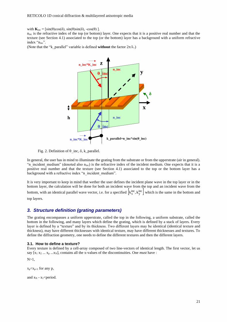
21
with Kinc = [sin(θ)cos(δ), sin(θ)sin(δ), -cos(θ) ].
ninc is the refractive index of the top (or bottom) layer. One expects that it is a positive real number and that the
texture (see Section 4.1) associated to the top (or the bottom) layer has a background with a uniform refractive
index “ninc”.
(Note that the “k_parallel” variable is defined without the factor 2/.)
z
x
δ
h
n_inc
k_parallel=n_inc*sin(θ_inc)
θ_inc
n
n_inc y
θ_inc
n_inc*K_inc
n_inc*K_inc
Fig. 2. Definition of inc, , k_parallel.
In general, the user has in mind to illuminate the grating from the substrate or from the upperstrate (air in general).
“n_incident_medium” (denoted also ninc) is the refractive index of the incident medium. One expects that it is a
positive real number and that the texture (see Section 4.1) associated to the top or the bottom layer has a
background with a refractive index “n_incident_medium”.
It is very important to keep in mind that wether the user defines the incident plane wave in the top layer or in the
bottom layer, the calculation will be done for both an incident wave from the top and an incident wave from the
bottom, with an identical parallel wave vector, i.e. for a specified incy
incx k,k which is the same in the bottom and
top layers.
3. Structure definition (grating parameters)
The grating encompasses a uniform upperstrate, called the top in the following, a uniform substrate, called the
bottom in the following, and many layers which define the grating, which is defined by a stack of layers. Every
layer is defined by a “texture” and by its thickness. Two different layers may be identical (identical texture and
thickness), may have different thicknesses with identical texture, may have different thicknesses and textures. To
define the diffraction geometry, one needs to define the different textures and then the different layers.
3.1. How to define a texture? Every texture is defined by a cell-array composed of two line-vectors of identical length. The first vector, let us
say [x1 x2 ... xp ...xN], contains all the x-values of the discontinuities. One must have :
N>1,
xp<xp+1 for any p,
and xN - x1<period.
RETICOLO 1D conical diffraction & multilayered anisotropic media
22
The second line-vector [n1 n2 ... np ... nN] contains the refractive indices of the material between the discontinuities.
More explicitly, we have a refractive index np for xp-1<x<xp. Because of periodicity, note that the refractive index
for xN<x<x1+period is equal to n1.
The specific case of a uniform texture with a refractive index n is easily defined by texture{1}={n}. In that specific
case, no need of a second vector since there is no discontinuity.
The textures have all to be to be packed together in a cell array textures={textures{1}, textures{2}, textures{3}}
prior calling subroutine res1.m.
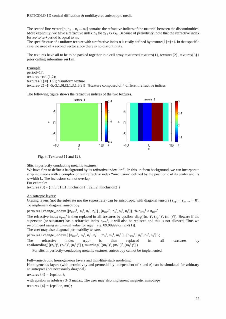
Example
period=17;
textures =cell(1,2);
textures{1}={ 1.5}; %uniform texture
textures{2}={[-5,-3,1,6],[2,1.3,1.5,3]}; %texture composed of 4 different refractive indices
The following figure shows the refractive indices of the two textures.
Fig. 3. Textures{1} and {2}.
Slits in perfectly-conducting metallic textures:
We have first to define a background by its refractive index “inf”. In this uniform background, we can incorporate
strip inclusions with a complex or real refractive index “ninclusion” defined by the position c of its center and its
x-width L. The inclusions cannot overlap.
For example:
textures {3}= {inf, [c1,L1,ninclusion1],[c2,L2, ninclusion2]}
Anisotropic layers:
Grating layers (not the substrate nor the superstrate) can be anisotropic with diagonal tensors (𝜀𝑥𝑦 = 𝜀𝑥𝑧 … = 0).
To implement diagonal anisotropy
parm.res1.change_index={[nprov1, nx
1, ny1, nz
1] , [nprov2, nx
2, ny2, nz
2]}; % nprov1 nprov
2
The refractive index nprov1 is then replaced in all textures by epsilon=diag([(nx
1)2, (ny1 )2, (nz
1 )2]). Beware if the
superstate (or substrate) has a refractive index nprov1, it will also be replaced and this is not allowed. Thus we
recommend using an unusual value for nprov1 (e.g. 89.99999 or rand(1)).
The user may also diagonal permeability tensors
parm.res1.change_index={ [nprov1, nx
1, ny1, nz
1 , mx1, my
1, mz1 ] , [nprov
2, nx2, ny
2, nz2] };
The refractive index nprov1 is then replaced in all textures by
epsilon=diag( [(nx1)2, (ny
1 )2, (nz1 )2] ), mu=diag( [(mx
1)2, (my1 )2, (mz
1 )2] ).
For slits in perfectly-conducting metallic textures, anisotropy cannot be implemented.
Fully-anisotropic homogeneous layers and thin-film-stack modeling:
Homogeneous layers (with permittivity and permeability independent of x and z) can be simulated for arbitrary
anisotropies (not necessarily diagonal)
textures {4} = {epsilon};
with epsilon an arbitrary 33 matrix. The user may also implement magnetic anisotropy
textures {4} = {epsilon, mu};
RETICOLO 1D conical diffraction & multilayered anisotropic media
23
with epsilon and mu arbitrary 33 matrices.
Note that the substrate and superstrates should be uniform and isotropic materials. If all layers are uniform, a
thin-film stack can be computed for arbitrary epsilon and mu 33 matrices by retaining a single Fourier component,
nn = 0.
In order to check if the set of textures is correctly set up, the user can set the variable parm.res1.trace equal
to 1: “parm.res1.trace = 1;”. Then a Matlab figure will show up the refractive-index distribution of all textures.
Each texture is represented with the coordinate x varying from –period/2 to period/2.
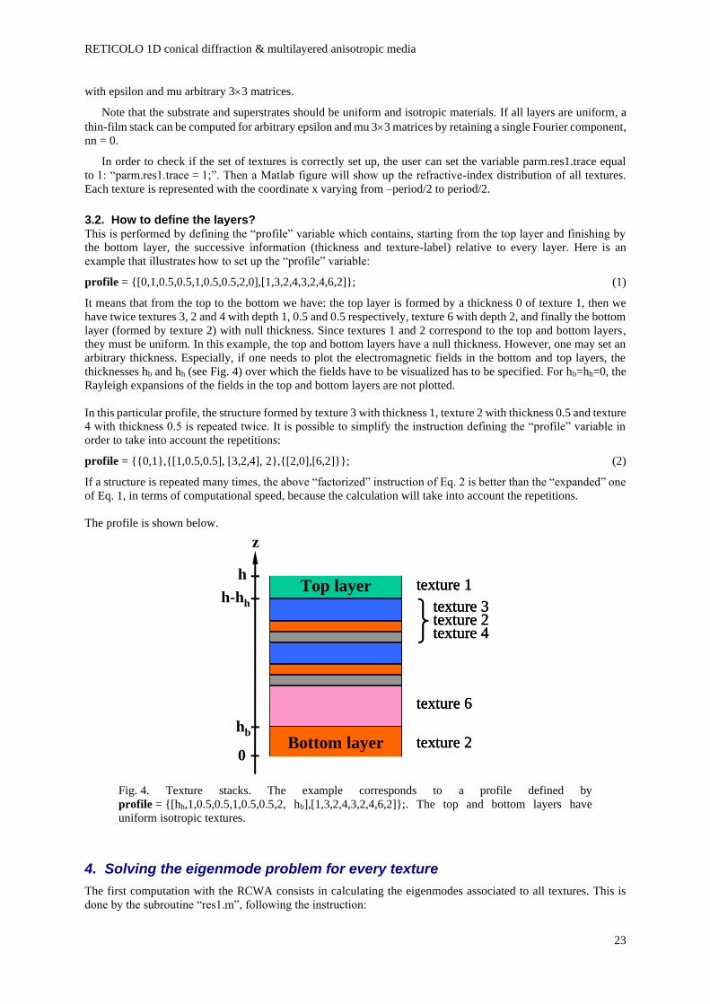
3.2. How to define the layers? This is performed by defining the “profile” variable which contains, starting from the top layer and finishing by
the bottom layer, the successive information (thickness and texture-label) relative to every layer. Here is an
example that illustrates how to set up the “profile” variable:
profile = {[0,1,0.5,0.5,1,0.5,0.5,2,0],[1,3,2,4,3,2,4,6,2]}; (1)
It means that from the top to the bottom we have: the top layer is formed by a thickness 0 of texture 1, then we
have twice textures 3, 2 and 4 with depth 1, 0.5 and 0.5 respectively, texture 6 with depth 2, and finally the bottom
layer (formed by texture 2) with null thickness. Since textures 1 and 2 correspond to the top and bottom layers,
they must be uniform. In this example, the top and bottom layers have a null thickness. However, one may set an
arbitrary thickness. Especially, if one needs to plot the electromagnetic fields in the bottom and top layers, the
thicknesses hb and hh (see Fig. 4) over which the fields have to be visualized has to be specified. For hb=hh=0, the
Rayleigh expansions of the fields in the top and bottom layers are not plotted.
In this particular profile, the structure formed by texture 3 with thickness 1, texture 2 with thickness 0.5 and texture
4 with thickness 0.5 is repeated twice. It is possible to simplify the instruction defining the “profile” variable in
order to take into account the repetitions:
profile = {{0,1},{[1,0.5,0.5], [3,2,4], 2},{[2,0],[6,2]}}; (2)
If a structure is repeated many times, the above “factorized” instruction of Eq. 2 is better than the “expanded” one
of Eq. 1, in terms of computational speed, because the calculation will take into account the repetitions.
The profile is shown below.
Fig. 4. Texture stacks. The example corresponds to a profile defined by
profile = {[hh,1,0.5,0.5,1,0.5,0.5,2, hb],[1,3,2,4,3,2,4,6,2]};. The top and bottom layers have
uniform isotropic textures.
4. Solving the eigenmode problem for every texture
The first computation with the RCWA consists in calculating the eigenmodes associated to all textures. This is
done by the subroutine “res1.m”, following the instruction:
texture 2
texture 1
texture 6
texture 3texture 2texture 4
texture 2
texture 1
texture 6
texture 3texture 2texture 4
texture 2
texture 1
texture 6
texture 3texture 2texture 4
z
0
h
Bottom layer
Top layerh-hh
hb

RETICOLO 1D conical diffraction & multilayered anisotropic media
24
aa = res1(wavelength,period,textures,nn,k_parallel,angle_delta,parm);
The first-six input parameters are absolutely required by the code : the wavelength “wavelength”, the period of
the grating “period”, the “textures” variable, the number of Fourier harmonics “nn”, the norm of the parallel
incident wave vector “k_parallel”, the angle that defines the plane of incidence “angle_delta.
Some other additional parameters can be defined. For example, the default parameters do not take the symmetry
of the problem into account. So if the user wants to use symmetries, new parameters have to be defined :
“parm.sym.x”, “parm.sym.y”, and “parm.sym.pol”. These parameters are defined in Section 7.
parm = res0;
res0.m is a function that changes the default values. This instruction has to be executed before res1.m, if one wants
to modify the default values (for instance to use symmetry).
It is very important to note that if one has to study the diffraction by many different gratings composed of the same
textures, one needs to compute only once the eigenmodes. It is possible to save the “aa” variable in a “.mat” file
and to reload it for the computation of the diffracted waves, see an example in Annex 9.3.
5. Computing the diffracted waves
This is the second step of the computation. This is done by the subroutine “res2.m”, following the instruction:
result = res2(aa,profile);
This subroutine has 2 input arguments: the output “aa” of the subroutine “res1.m” and the “profile” variable. The
output argument “result” contains all the information on the diffracted fields. “result” is an object of class
‘reticolo’ that can be indexed as an usual structure with parentheses, or with the labels of the considered orders
between curly braces. Examples will be given in the following.
This information is divided into the following sub-structures fields :
- “result.TEinc_top”
- “result.TEinc_top_reflected”
- “result.TEinc_top_transmitted”
- “result.TEinc_bottom”
- “result.TEinc_bottom_reflected”
- “result.TEinc_bottom_transmitted”
- “result.TMinc_top”
- “result.TMinc_top_reflected”
- “result.TMinc_top_transmitted”
- “result.TMinc_bottom”
- “result.TMinc_bottom_reflected”
- “result.TMinc_bottom_transmitted”
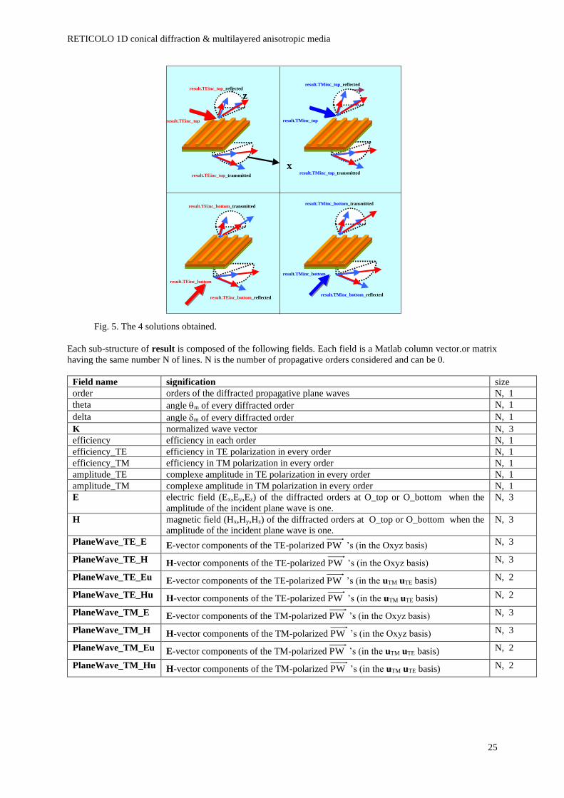
The sub-structure “result.TEinc_top_reflected” contains all the information concerning the propagative reflected
waves for the incident wave from the top of the grating in TE polarization which is described in the sub-structure
“result.TEinc_top”
The sub-structure “result.TMinc_bottom_transmitted” contains all the information concerning the propagative
transmitted waves for the incident wave from the bottom of the grating in TM polarization which is described in
the sub-structure “result.TMinc_ bottom”. And so on.
RETICOLO 1D conical diffraction & multilayered anisotropic media
25
z
x
K
UTM
result.TEinc_top_reflected
result.TEinc_top_transmitted
result.TMinc_top
result.TMinc_top_reflected
result.TMinc_top_transmitted
result.TEinc_bottom
result.TEinc_bottom_transmitted
result.TEinc_bottom_reflected
result.TMinc_bottom
result.TMinc_bottom_transmitted
result.TMinc_bottom_reflected
result.TEinc_top
Fig. 5. The 4 solutions obtained.
Each sub-structure of result is composed of the following fields. Each field is a Matlab column vector.or matrix
having the same number N of lines. N is the number of propagative orders considered and can be 0.
Field name signification size
order orders of the diffracted propagative plane waves N, 1
theta angle m of every diffracted order N, 1
delta angle m of every diffracted order N, 1
K normalized wave vector N, 3
efficiency efficiency in each order N, 1
efficiency_TE efficiency in TE polarization in every order N, 1
efficiency_TM efficiency in TM polarization in every order N, 1
amplitude_TE complexe amplitude in TE polarization in every order N, 1
amplitude_TM complexe amplitude in TM polarization in every order N, 1
E electric field (Ex,Ey,Ez) of the diffracted orders at O_top or O_bottom when the
amplitude of the incident plane wave is one.
N, 3
H magnetic field (Hx,Hy,Hz) of the diffracted orders at O_top or O_bottom when the
amplitude of the incident plane wave is one.
N, 3
PlaneWave_TE_E E-vector components of the TE-polarized PW ’s (in the Oxyz basis) N, 3
PlaneWave_TE_H H-vector components of the TE-polarized PW ’s (in the Oxyz basis) N, 3
PlaneWave_TE_Eu E-vector components of the TE-polarized PW ’s (in the uTM uTE basis) N, 2
PlaneWave_TE_Hu H-vector components of the TE-polarized PW ’s (in the uTM uTE basis) N, 2
PlaneWave_TM_E E-vector components of the TM-polarized PW ’s (in the Oxyz basis) N, 3
PlaneWave_TM_H H-vector components of the TM-polarized PW ’s (in the Oxyz basis) N, 3
PlaneWave_TM_Eu E-vector components of the TM-polarized PW ’s (in the uTM uTE basis) N, 2
PlaneWave_TM_Hu H-vector components of the TM-polarized PW ’s (in the uTM uTE basis) N, 2
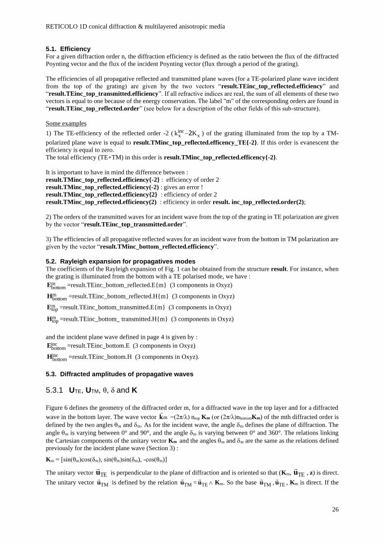
RETICOLO 1D conical diffraction & multilayered anisotropic media
26
5.1. Efficiency For a given diffraction order n, the diffraction efficiency is defined as the ratio between the flux of the diffracted
Poynting vector and the flux of the incident Poynting vector (flux through a period of the grating).
The efficiencies of all propagative reflected and transmitted plane waves (for a TE-polarized plane wave incident
from the top of the grating) are given by the two vectors “result.TEinc_top_reflected.efficiency” and
“result.TEinc_top_transmitted.efficiency”. If all refractive indices are real, the sum of all elements of these two
vectors is equal to one because of the energy conservation. The label "m" of the corresponding orders are found in
“result.TEinc_top_reflected.order” (see below for a description of the other fields of this sub-structure).
Some examples
1) The TE-efficiency of the reflected order -2 ( xincx Kk 2− ) of the grating illuminated from the top by a TM-
polarized plane wave is equal to result.TMinc_top_reflected.efficency_TE{-2}. If this order is evanescent the
efficiency is equal to zero.
The total efficiency (TE+TM) in this order is result.TMinc_top_reflected.efficency{-2}.
It is important to have in mind the difference between :
result.TMinc_top_reflected.efficiency{-2} : efficiency of order 2
result.TMinc_top_reflected.efficiency(-2) : gives an error !
result.TMinc_top_reflected.efficiency{2} : efficiency of order 2
result.TMinc_top_reflected.efficiency(2) : efficiency in order result. inc_top_reflected.order(2);
2) The orders of the transmitted waves for an incident wave from the top of the grating in TE polarization are given
by the vector “result.TEinc_top_transmitted.order”.
3) The efficiencies of all propagative reflected waves for an incident wave from the bottom in TM polarization are
given by the vector “result.TMinc_bottom_reflected.efficiency”.
5.2. Rayleigh expansion for propagatives modes The coefficients of the Rayleigh expansion of Fig. 1 can be obtained from the structure result. For instance, when
the grating is illuminated from the bottom with a TE polarised mode, we have : mbottomE =result.TEinc_bottom_reflected.E{m} (3 components in Oxyz)
mbottomH =result.TEinc_bottom_reflected.H{m} (3 components in Oxyz)
mtopE =result.TEinc_bottom_transmitted.E{m} (3 components in Oxyz)
mtopH =result.TEinc_bottom_ transmitted.H{m} (3 components in Oxyz)
and the incident plane wave defined in page 4 is given by : incbottomE =result.TEinc_bottom.E (3 components in Oxyz)
incbottomH =result.TEinc_bottom.H (3 components in Oxyz).
5.3. Diffracted amplitudes of propagative waves
5.3.1 UTE, UTM, θ, δ and K
Figure 6 defines the geometry of the diffracted order m, for a diffracted wave in the top layer and for a diffracted
wave in the bottom layer. The wave vector mk
=(2π/λ) ntop Km (or (2π/λ)nbottomKm) of the mth diffracted order is
defined by the two angles m and m. As for the incident wave, the angle m defines the plane of diffraction. The
angle m is varying between 0° and 90°, and the angle m is varying between 0° and 360°. The relations linking
the Cartesian components of the unitary vector Km and the angles m and m are the same as the relations defined
previously for the incident plane wave (Section 3) :
Km = [sin(θm)cos(δm), sin(θm)sin(δm), -cos(θm)]
The unitary vector TEu
is perpendicular to the plane of diffraction and is oriented so that (Km, TEu
, z) is direct.
The unitary vector TMu
is defined by the relation TMu
= TEu
Km. So the base TMu
, TEu
, Km is direct. If the
RETICOLO 1D conical diffraction & multilayered anisotropic media
27
diffracted electric field is parallel to TEu
, then the order m is TE polarized, and if the diffracted electric field is
parallel to TMu
, then the order m is TM polarized. In general, the diffracted electric field of the order m has a
non-zero component along both directions.
U TM
z
x
y K m
U TE
δ m
θ m
K m
h
θ m
U TE
U TM
Fig. 6. Definition of the m and m for a specific diffracted order m.
5.3.2 Otop and Obottom points
Otop and Otop are 2 important points (see Fig. 1). In the Cartesian coordinates system Oxyz , they are defined by :
Otop=(0,0,h) at the top of the grating, and Obottom=(0,0,0) at the bottom of the grating.
In addition, let us consider an arbitrary point M=(x,y,z) in the 3D space in Oxyz. Associated to this point, we
define the two vectors :
rtop= MOtop , and
rbottom= MObottom .
5.3.3 Jones’ matrix
Let us assume that the grating is illuminated from the top layer and let us consider a diffracted order m in the
bottom layer. Any other diffraction situation is straightforwardly deduced.
α and β being two given complex numbers, the incident electromagnetic field (6 components of E and H in every
points of the 3D space) can be written :
TMTEinc PWPW +=W ,
where TEPW is a TE-polarized plane wave defined in every point by ( )topinctopTETE riexpPW kA= , and TMPW
a TM polarized plane wave defined in the same way by ( )topinctopTMTM riexpPW kA= , TEA and TMA being the
electromagnetic fields (6 components) of the plane wave at M=Otop. inctopk is the incident wave vector. TEA and
TMA and inctop
inctop/kkK= are given by the structure “result“ as will be defined later.
Similarly, the diffracted electromagnetic field in the mth bottom order can be written :
RETICOLO 1D conical diffraction & multilayered anisotropic media
28
mTM
mTE
difm PWµPW +=W ,
where and µ are complex numbers, mTEPW is a TE-polarized plane wave defined in every point by
( )bottommbottom
mTE
mTE iexpPW rkA= , and m
TMPW a TM-polarized plane wave defined in the same way by
( )bottommbottom
mTM
mTM iexpPW rkA= . m
TEA and mTMA are the electromagnetic fields (6 components) of the
plane wave at M=Obottom, and mbottomk is the wave vector of the m transmitted order. m
TEA and mTMA and
mbottom
mbottom
m / kkK = are given by the structure “result“ as will be defined later.
We define the (4x4) Jones‘ matrix J, associated to the order m by :
=
MMEM
MEEE
JJ
JJ
µ.
JEE, JEM,JME, JMM and J are all given by the structure “result”.
The TEA mTEA TMA m
TMA vectors are normalized so that the |JEE|2, |JEM|2,|JME|2 and |JMM|2 represent diffraction
efficiencies. For instance, |JME|2 =result.TMinc_top_transmitted.efficency_TE{m}.
We now define all these data from the “result” structure :
K = result.TEinc_top.K or K=result.TMinc_top.K.
Km = result.TEinc_top_transmitted.K{m} = result.TMinc_top_transmitted.K{m}. Note that if some symmetries
are used for the calculation, “result.TEinc_top_transmitted.K{m}” or “result.TMinc_top_transmitted.K{m}” can
be an empty vector.
The mTEA ’s coefficients can be obtained either in the Cartesian coordinate system or in the ( TMu
, TEu
) basis.
In the Cartesian coordinate system Oxyz :
=
H_TE_PlaneWave.top_TEinc.result
E_TE_PlaneWave.top_TEinc.result
TEA
=
H_TM_PlaneWave.top_TMinc.result
E_TM_PlaneWave.top_TMinc.result
TMA
=
mH_TE_PlaneWave.dtransmitte_top_TEinc.result
mE_TE_PlaneWave.dtransmitte_top_TEinc.resultmTEA
=
mH_TE_PlaneWave.dtransmitte_top_TMinc.result
mE_TE_PlaneWave.dtransmitte_top_TMinc.result. (same remark as for Km)
=
mH_TE_PlaneWave.dtransmitte_top_TEinc.result
mE_TE_PlaneWave.dtransmitte_top_TEinc.resultmTMA
=
mH_TE_PlaneWave.dtransmitte_top_TMinc.result
mE_TE_PlaneWave.dtransmitte_top_TMinc.result. (same remark as for Km)
In the ( TMu
, TEu
) basis (with only 2 components for each fields E and H) :
=
Hu_TE_PlaneWave.top_TEinc.result
Eu_TE_PlaneWave.top_TEinc.result
TEA
=
Hu_TM_PlaneWave.top_TMinc.result
Eu_TM_PlaneWave.top_TMinc.result
TMA
RETICOLO 1D conical diffraction & multilayered anisotropic media
29
=
mHu_TE_PlaneWave.dtransmitte_top_TEinc.result
mEu_TE_PlaneWave.dtransmitte_top_TEinc.resultmTEA
=
mHu_TE_PlaneWave.dtransmitte_top_TMinc.result
mEu_TE_PlaneWave.dtransmitte_top_TMinc.result. (same remark as for Km)
=mHu_TE_PlaneWave.dtransmitte_top_TEinc.resultmEu_TE_PlaneWave.dtransmitte_top_TEinc.resultm
TMA
=
mHu_TE_PlaneWave.dtransmitte_top_TMinc.result
mEu_TE_PlaneWave.dtransmitte_top_TMinc.result. (same remark as for Km)
The Jones’ coefficients are :
JEE =result.TEinc_top_transmitted.amplitude_TE{m}
JEM =result.TEinc_top_transmitted.amplitude_TM{m}
JME =result.TMinc_top_transmitted.amplitude_TE{m}
JMM =result.TMinc_top_transmitted.amplitude_TM{m}
And the Jones’ matrix is :
mdtransmitte_top_inc.Jones.resultJJ
JJ
MMEM
MEEE=
=J .
6. Using symmetries to accelerate the computational speed
When the grating possesses some mirror symmetry for the plane x=x0, the user may define “parm.sym.x= x0” For
delta=90 or 270, the x-symmetry will be used.
When angle_delta and parameter k_parallel are compatible with the symmetry, the structure "result" contains only
information upon the polarisation selected by parameter parm.sym.pol.
Note that the code does not check if the grating symmetry defined by the user is in agreement with the “textures”.
It is up to the user to define carefully the parameters parm.sym.x.
7. Plotting the electromagnetic field and calculating the absorption loss
7.1. Computation of the electromagnetic fields Once the eigenmodes associated to all textures are known, the calculation of the electromagnetic fields everywhere
in the grating can be performed. This calculation is done by the subroutine “res3.m”, following the instruction
[e,z,index] = res3(x,aa,profile,einc,parm);
The function“res3.m” can be called without calling “res2.m”. This subroutine has 5 input arguments:
-the “x” variable is a vector containing the locations where the fields will be calculated in the x-direction. For
instance, we may set x = linspace(-period/2, period/2, 51); for allocating 51 sampling points in the x-direction,
-the “aa” variable contains all the information on the eigenmodes of all textures and is computed by the subroutine
res1.m,
-the variable “profile” is defined in Section 4.2. Note that it can be redefined,
-the variable “einc” defines the complex amplitude of the incident electric field at O_top or O_bottom in the basis
{uTM, uTE}. For instance, setting einc=[1,0] means that one is looking for TM polarization, and setting
einc=[1,1]/sqrt(2) means that one is looking for a 45° polarization.
If one wants to illumine the grating exactly by the TE-polarized incident TEPW defined above, one
should set: einc= result.TEinc_top PlaneWave_TE_Eu.
If symmetry arguments have been used previously, note that the calculation with res1.m is provided only
for some specific polarization; it would be a nonsense to specify another polarization for the field plots (in this
case the corresponding component of einc is taken as 0).
-the “parm” variable, already mentioned is discussed in the following.
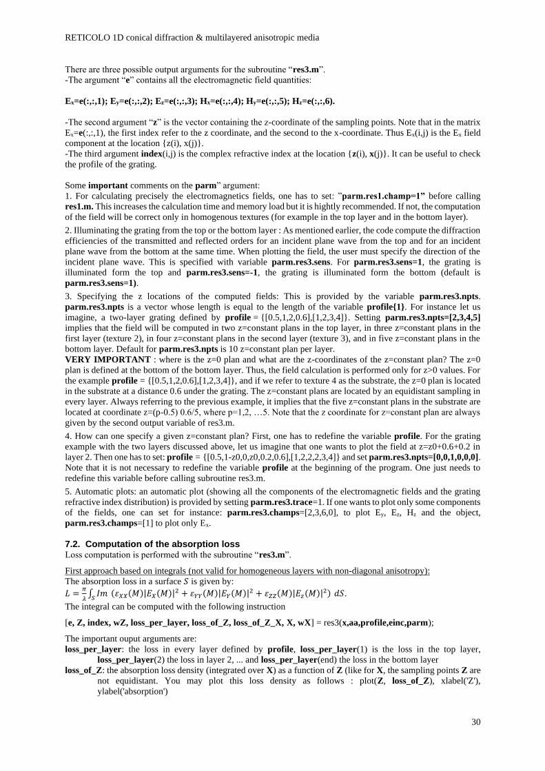
RETICOLO 1D conical diffraction & multilayered anisotropic media
30
There are three possible output arguments for the subroutine “res3.m”.
-The argument “e” contains all the electromagnetic field quantities:
Ex=e(:,:,1); Ey=e(:,:,2); Ez=e(:,:,3); Hx=e(:,:,4); Hy=e(:,:,5); Hz=e(:,:,6).
-The second argument “z” is the vector containing the z-coordinate of the sampling points. Note that in the matrix
Ex=e(:,:,1), the first index refer to the z coordinate, and the second to the x-coordinate. Thus Ex(i,j) is the Ex field
component at the location {z(i), x(j)}.
-The third argument index(i,j) is the complex refractive index at the location {z(i), x(j)}. It can be useful to check
the profile of the grating.
Some important comments on the parm” argument:
1. For calculating precisely the electromagnetics fields, one has to set: ”parm.res1.champ=1” before calling
res1.m. This increases the calculation time and memory load but it is hightly recommended. If not, the computation
of the field will be correct only in homogenous textures (for example in the top layer and in the bottom layer).
2. Illuminating the grating from the top or the bottom layer : As mentioned earlier, the code compute the diffraction
efficiencies of the transmitted and reflected orders for an incident plane wave from the top and for an incident
plane wave from the bottom at the same time. When plotting the field, the user must specify the direction of the
incident plane wave. This is specified with variable parm.res3.sens. For parm.res3.sens=1, the grating is
illuminated form the top and parm.res3.sens=-1, the grating is illuminated form the bottom (default is
parm.res3.sens=1).
3. Specifying the z locations of the computed fields: This is provided by the variable parm.res3.npts.
parm.res3.npts is a vector whose length is equal to the length of the variable profile{1}. For instance let us
imagine, a two-layer grating defined by profile = {[0.5,1,2,0.6],[1,2,3,4]}. Setting parm.res3.npts=[2,3,4,5]
implies that the field will be computed in two z=constant plans in the top layer, in three z=constant plans in the
first layer (texture 2), in four z=constant plans in the second layer (texture 3), and in five z=constant plans in the
bottom layer. Default for parm.res3.npts is 10 z=constant plan per layer.
VERY IMPORTANT : where is the z=0 plan and what are the z-coordinates of the z=constant plan? The z=0
plan is defined at the bottom of the bottom layer. Thus, the field calculation is performed only for z>0 values. For
the example profile = {[0.5,1,2,0.6],[1,2,3,4]}, and if we refer to texture 4 as the substrate, the z=0 plan is located
in the substrate at a distance 0.6 under the grating. The z=constant plans are located by an equidistant sampling in
every layer. Always referring to the previous example, it implies that the five z=constant plans in the substrate are
located at coordinate z=(p-0.5) 0.6/5, where p=1,2, …5. Note that the z coordinate for z=constant plan are always
given by the second output variable of res3.m.
4. How can one specify a given z=constant plan? First, one has to redefine the variable profile. For the grating
example with the two layers discussed above, let us imagine that one wants to plot the field at z=z0+0.6+0.2 in
layer 2. Then one has to set: profile = {[0.5,1-z0,0,z0,0.2,0.6],[1,2,2,2,3,4]} and set parm.res3.npts=[0,0,1,0,0,0].
Note that it is not necessary to redefine the variable profile at the beginning of the program. One just needs to
redefine this variable before calling subroutine res3.m.
5. Automatic plots: an automatic plot (showing all the components of the electromagnetic fields and the grating
refractive index distribution) is provided by setting parm.res3.trace=1. If one wants to plot only some components
of the fields, one can set for instance: parm.res3.champs=[2,3,6,0], to plot Ey, Ez, Hz and the object,
parm.res3.champs=[1] to plot only Ex.
7.2. Computation of the absorption loss Loss computation is performed with the subroutine “res3.m”.
First approach based on integrals (not valid for homogeneous layers with non-diagonal anisotropy):
The absorption loss in a surface 𝑆 is given by:
𝐿 =𝜋
𝜆∫ 𝐼𝑚 (𝜀𝑋𝑋(𝑀)|𝐸𝑋(𝑀)|2 + 𝜀𝑌𝑌(𝑀)|𝐸𝑌(𝑀)|2 + 𝜀𝑍𝑍(𝑀)|𝐸𝑧(𝑀)|2) 𝑑𝑆
𝑆.
The integral can be computed with the following instruction
[e, Z, index, wZ, loss_per_layer, loss_of_Z, loss_of_Z_X, X, wX] = res3(x,aa,profile,einc,parm);
The important ouput arguments are:
loss_per_layer: the loss in every layer defined by profile, loss_per_layer(1) is the loss in the top layer,
loss_per_layer(2) the loss in layer 2, ... and loss_per_layer(end) the loss in the bottom layer
loss_of_Z: the absorption loss density (integrated over X) as a function of Z (like for X, the sampling points Z are
not equidistant. You may plot this loss density as follows : plot(Z, loss_of_Z), xlabel('Z'),
ylabel('absorption')
RETICOLO 1D conical diffraction & multilayered anisotropic media
31
loss_of_Z_X(Z,X) = π/λ Im(index(Z,X).^2) (|e(Z,X,1)|2+|e(Z,X,2)|2+|e(Z,X,3)|2)
index: index(i,j) is the complex refractive index at the location {z(i), x(j)}.
Second approach based on Poynting theorem (always valid even for homogeneous layers with non-diagonal
anisotropy):
An alternative approach to compute the losses in the layers consists in calculating the difference in the flux of the
incoming and outgoing Poynting vectors. This approach is faster, but in some cases, the computation of the integral
can be more accurate. In homogeneous layers with non-diagonal anisotropy, only this approach is possible.
To specify which approach used per layer, we define a vector
parm.res3.pertes_poynting = [0,0,0,1,0]; % for instance for a 5-layer grating
with “0”, the integral approach is used (default option) and with “1”, the Poynting approach is used. The length of
parm.res3.pertes_poynting is equal to the number of layers. We may set parm.res3.pertes_poynting = 0 or 1;
the scalar is then repeated for all layers.
We may then compute the flux of the Poynting vector in the layer-boundary planes
[e, Z, index, wZ,loss_per_layer,loss_of_Z,loss_of_Z_X,X,wX,Flux_Poynting] = res3(x,aa,profile,einc,parm);
Flux_Poynting is a vector. Flux_Poynting(1) corresponds to the upper interface of the top layer. The flux is
computed for a normal vector equal to the �̂� vector. If Flux_Poynting(p) > 0, the energy flows toward the top and
if it it negative the enerfy flows toward the bottom.
For an illumination from the top and a lossy substrate, the substrate absorption is −Flux_Poynting
(end)/(0.5*period). For an illumination from the bottom and a lossy superstrate, the superstrate absorption is
Flux_Poynting (1)/(0.5*period).
Note on the computation accuracy of the integral approach:
To compute integrals like the loss or the electromagnetic energy, we use a Gauss-Legendre integration method.
This method, which is very powerful for 'regular' functions, becomes inaccurate for discontinuous functions. Thus,
the integration domain should be divided into subdomains where the electric field E is continuous. For the
integration in X, this difficult task is performed by the program, so that the user should only define the limits of
integration: the input “x” argument is now a vector of length 2, which represent the limits of the x interval (to
compute the loss over the entire period, we may take x(2)=x(1)+period. The integration domain is then divided
into subintervals where the permittivity is continuous, each subinterval having a length less than /(2). For every
subinterval, a Gauss-Legendre integration method of degree 10 is used. This default value can be changed by
setting parm.res3.gauss_x=.... The actual points of computation of the field are returned in the output argument
X.
For the z integration, the discontinuity points are more easily determined by the variable 'profile'. The user
may choose the number of subintervals and the degree in every layer using the parameter parm.res3.npts, which
is now an array with two lines (in subsection 8.1 this variable is a line vector): the first line defines the degree and
the second line the numbers of subintervals of every layer. For example: parm.res3.npts = [ [10 , 0 , 12 ] ; [3 , 1
, 5 ] ]; means that 3 subintervals with 10-degree points are used in the first layer, 1 subintervals with 0 point in
the second layer, 5 subintervals with 12degree points in the third layer.
The actual z-points of computation of the field are returned in the output variable Z, and the vector wZ
represents the weights and we have sum(loss_of_Z.*wZ)=sum(loss_per_layer). Although the maximum degree
that can be handled by reticolo is 468, it is recommended to limit the degree values to modest numbers (10-30
maximum) and to increase the number of subintervals (the larger the degree, the denser the sampling points in the
vicinity of the subinterval boundaries).
Note that if einc= result.TEinc_top PlaneWave_TE_Eu, the energie conservation test for a TE incident plane
wave from the top is
sum(result.TEinc_top_reflected.efficiency)+
sum(result.TEinc_top_transmitted.efficiency)+
sum(loss_per_layer) / (.5*period) = 1.
Usually, this equality is achieved with an absolute error <10−5.
For specialists:
-loss_of_Z_X =pi/ wavelength*imag(index.^2).*sum(abs(e(:,:,1:3)).^2,3);
RETICOLO 1D conical diffraction & multilayered anisotropic media
32
-loss_of_Z =(loss_of_Z_X*wX(:)).';
-by setting index(index ~= index_chosen)=0 in the previous formulas, one may calculate the absorption loss in
the medium of refractive index index_chosen.
8. Bloch-mode effective indices
RETICOLO gives access to another output: the Bloch mode associated to all textures. The Bloch mode k of the
texture l can be written
|𝛷𝑘𝑙⟩ = ∑ 𝑎𝑚
k,l 𝑒𝑥𝑝[𝑖(𝑘𝑥inc + mK𝑥)𝑥] 𝑒𝑥𝑝(𝑖𝑘𝑦
inc𝑦) 𝑒𝑥𝑝 (𝑖2π
𝜆𝑛eff
k,l 𝑧)𝑚 ,
where 𝑛effk,l
is the effective index of the Bloch mode k of the texture l.
Instruction:
[aa,n_eff] = res1(wavelength,period,textures,nn,kparallel,delta0,parm);
Note that the “n_eff” variable is a Matlab cell array: “n_eff{ii}” is a column vector containing all the Bloch-mode
effective indices associated to the texture “textures{ii}”. The element number 5 of this vector, for example, is
called by the instruction “n_eff{ii}(5);”. An attenuated Bloch-mode has a complex effective index.
Bloch mode profile visualization:
To plot the profile of Bloch mode Num_mode of the texture Num_texture:
res1(aa, neff, Num_texture, Num_mode);
To obtain the profile datas in the format given by res3:
[e,o,x,y] = res1(aa, neff, Num_texture, Num_mode); % by default, for |x| < period/2 and |y| < period/2
[e,o] = res1(aa, neff, Num_texture, Num_mode, x, y); % by specifying the x and y vectors,
x=linspace(0,3*period(1),100) and y=0 for example, but y can be a vector too. The y-dependence is simply a phase
factor 𝑒𝑥𝑝(𝑖𝑘𝑦inc𝑦).
9. Annex
9.1. Checking that the textures are correctly set up Setting “parm.res1.trace = 1;” generates a Matlab figure which represents the refractive-index distribution of all
the textures.
9.2. The “retio” instruction RETICOLO automatically creates temporary files in order to save memory. These temporary files are of the form
“abcd0.mat”, “abcd1.mat” … with abcd randomly chosen) .They are created in the current directory. In general
RETICOLO automatically erases these files when they are no longer needed, but it is recommended to finish all
programs by the instruction “retio;”, which erases all temporary files. Also, if a program anormally stopsone may
execute the instruction “retio” before restarting the program.
The “retefface” instruction allows to know all the “abcd0.mat” files and to erase them if wanted.
If we are not limited by memory (this is often the case with modern computers), we can prevent the writing of
intermediate files on the hard disk by the setting
parm.not_io = 1;
before the call to res1. Then it is no longer necessary to use the retio instruction at the end of the programs to erase
the files.
IMPORTANT: to use parfor loops, it is imperative to take the option parm.not_io = 1.
9.3. How to save and to reload the “aa” variable To save the “aa” variable in a “.mat” file, the user has to define a new parameter containing the name of the file
he or she wants to create : “parm.res1.fperm = 'file_name';”. field_name is a char string with at least one letter.
The program will automatically save “aa” in the file “file_name.mat”. In a new utilisation it is sufficient to write
aa = 'file_name';.
Example of a program which calculates and saves the “aa” variable
[...] % Definition of the input parameters, see Section 3
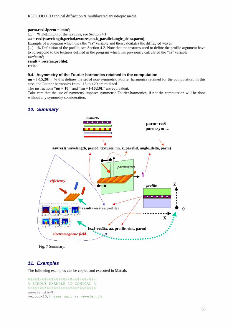
RETICOLO 1D conical diffraction & multilayered anisotropic media
33
parm.res1.fperm = 'toto';
[...] % Definition of the textures, see Section 4.1
aa = res1(wavelength,period,textures,nn,k_parallel,angle_delta,parm);
Example of a program which uses the “aa” variable and then calculates the diffracted waves
[...] % Definition of the profile, see Section 4.2. Note that the textures used to define the profile argument have
to correspond to the textures defined in the program which has previously calculated the “aa” variable.
aa=’toto’;
result = res2(aa,profile);
retio;
9.4. Asymmetry of the Fourier harmonics retained in the computation nn = [-15;20]; % this defines the set of non-symmetric Fourier harmonics retained for the computation. In this
case, the Fourier harmonics from –15 to +20 are retained.
The instructions “nn = 10;” and “nn = [-10;10];” are equivalent.
Take care that the use of symmetry imposes symmetric Fourier harmonics, if not the computation will be done
without any symmetry consideration.
10. Summary
aa=res1( wavelength, period, textures, nn, k_parallel, angle_delta, parm)
result=res2(aa,profile)
[e,z]=res3(x, aa, profile, einc, parm)
profile
textures
efficiency
electromagnetic field
parameters
z
x
0
parm=res0
parm.sym …
Fig. 7 Summary.
11. Examples
The following examples can be copied and executed in Matlab.
%%%%%%%%%%%%%%%%%%%%%%%%%%%%%
% SIMPLE EXAMPLE 1D CONICAL %
%%%%%%%%%%%%%%%%%%%%%%%%%%%%%
wavelength=8;
period=10;% same unit as wavelength
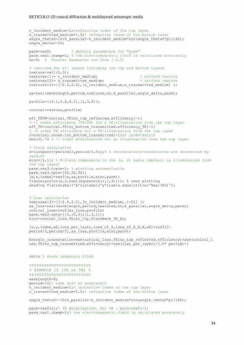
RETICOLO 1D conical diffraction & multilayered anisotropic media
34
n_incident_medium=1;%refractive index of the top layer
n_transmitted_medium=1.5;% refractive index of the bottom layer
angle_theta0=10;k_parallel=n_incident_medium*sin(angle_theta0*pi/180);
angle_delta=-20;
parm=res0; % default parameters for "parm"
parm.res1.champ=1; % the electromagnetic field is calculated accurately
nn=5; % Fourier harmonics run from [-5,5]
% textures for all layers including the top and bottom layers
texture=cell(1,3);
textures{1}= n_incident_medium; % uniform texture
textures{2}= n_transmitted_medium; % uniform texture
textures{3}={[-2.5,2.5],[n_incident_medium,n_transmitted_medium] };
aa=res1(wavelength,period,textures,nn,k_parallel,angle_delta,parm);
profile={[4.1,5.2,4.1],[1,3,2]};
conical=res2(aa,profile)
eff_TETM=conical.TEinc_top_reflected.efficiency{-1}
% -1 order efficiency (TE+TM) for a TE-illumination from the top layer
eff_TE=conical.TEinc_bottom_transmitted.efficiency_TE{-1}
% -1 order TE efficiency for a TE-illumination from the top layer
J=conical.Jones.inc_bottom_transmitted{-1};% Jones’matrix
abs(J).^2 % -1 order efficiencies for an illumination from the top layer
% field calculation
x=linspace(-period/2,period/2,51);% x coordinates(z-coordinates are determined by
res3.m)
einc=[0,1]; % E-field components in the (u, v) basis (default is illumination from
the top layer)
parm.res3.trace=1; % plotting automatically
parm.res3.npts=[50,50,50];
[e,z,index]=res3(x,aa,profile,einc,parm);
figure;pcolor(x,z,real(squeeze(e(:,:,3)))); % user plotting
shading flat;xlabel('x');ylabel('y');axis equal;title('Real(Ez)');
% Loss calculation
textures{3}={[-2.5,2.5],[n_incident_medium,.1+5i] };
aa_loss=res1(wavelength,period,textures,nn,k_parallel,angle_delta,parm);
conical_loss=res2(aa_loss,profile)
parm.res3.npts=[[0,10,0];[1,3,1]];
einc=conical_loss.TEinc_top.PlaneWave_TE_Eu;
[e,z,index,wZ,loss_per_layer,loss_of_Z,loss_of_Z_X,X,wX]=res3([-
period/2,period/2],aa_loss,profile,einc,parm);
Energie_conservation=sum(conical_loss.TEinc_top_reflected.efficiency)+sum(conical_l
oss.TEinc_top_transmitted.efficiency)+sum(loss_per_layer)/(.5* period)-1
retio % erase temporary files
%%%%%%%%%%%%%%%%%%%%%%%%%
% EXAMPLE 1D (TE or TM) %
%%%%%%%%%%%%%%%%%%%%%%%%%
wavelength=8;
period=10;% same unit as wavelength
n_incident_medium=1;% refractive index of the top layer
n_transmitted_medium=1.5;% refractive index of the bottom layer
angle_theta0=-10;k_parallel=n_incident_medium*sin(angle_theta0*pi/180);
parm=res0(1);% TE polarization. For TM : parm=res0(-1)
parm.res1.champ=1;% the electromagnetic field is calculated accurately
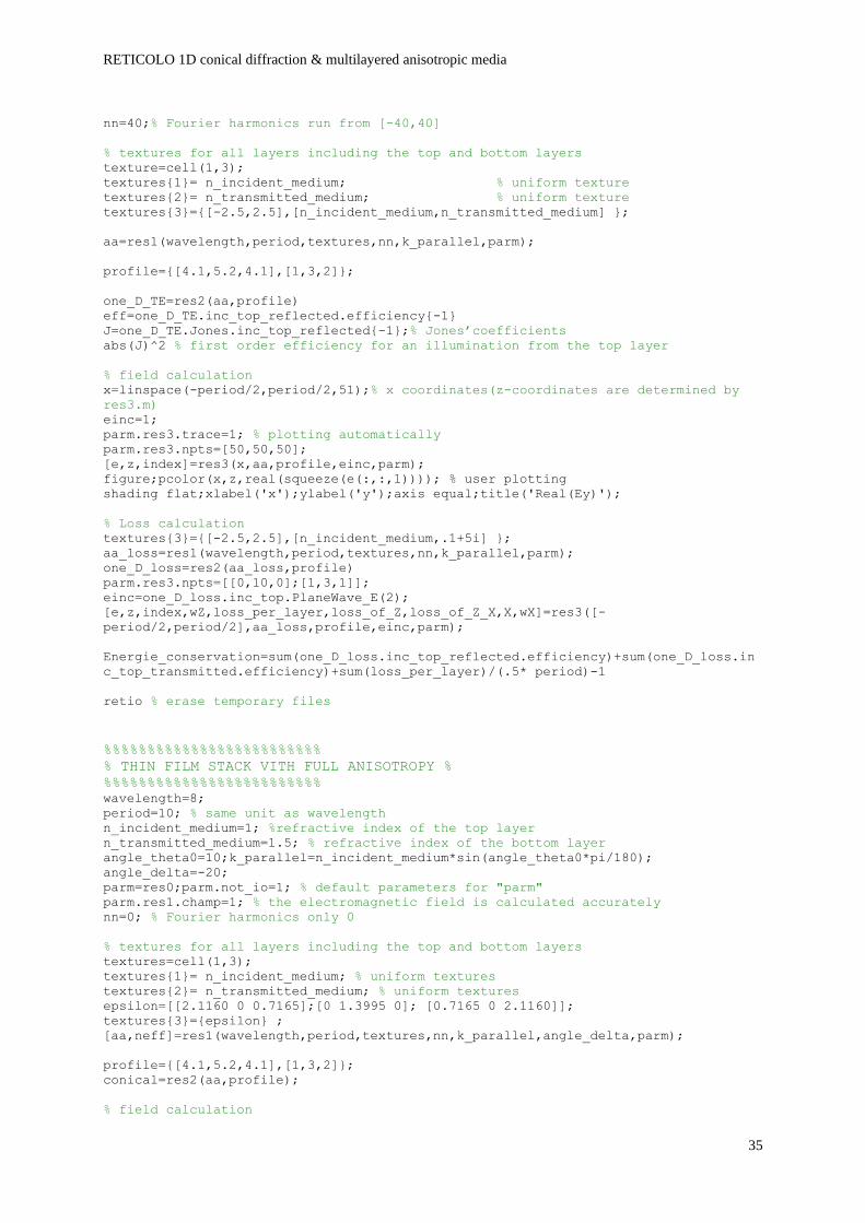
RETICOLO 1D conical diffraction & multilayered anisotropic media
35
nn=40;% Fourier harmonics run from [-40,40]
% textures for all layers including the top and bottom layers
texture=cell(1,3);
textures{1}= n_incident_medium; % uniform texture
textures{2}= n_transmitted_medium; % uniform texture
textures{3}={[-2.5,2.5],[n_incident_medium,n_transmitted_medium] };
aa=res1(wavelength,period,textures,nn,k_parallel,parm);
profile={[4.1,5.2,4.1],[1,3,2]};
one_D_TE=res2(aa,profile)
eff=one_D_TE.inc_top_reflected.efficiency{-1}
J=one_D_TE.Jones.inc_top_reflected{-1};% Jones’coefficients
abs(J)^2 % first order efficiency for an illumination from the top layer
% field calculation
x=linspace(-period/2,period/2,51);% x coordinates(z-coordinates are determined by
res3.m)
einc=1;
parm.res3.trace=1; % plotting automatically
parm.res3.npts=[50,50,50];
[e,z,index]=res3(x,aa,profile,einc,parm);
figure;pcolor(x,z,real(squeeze(e(:,:,1)))); % user plotting
shading flat;xlabel('x');ylabel('y');axis equal;title('Real(Ey)');
% Loss calculation
textures{3}={[-2.5,2.5],[n_incident_medium,.1+5i] };
aa_loss=res1(wavelength,period,textures,nn,k_parallel,parm);
one_D_loss=res2(aa_loss,profile)
parm.res3.npts=[[0,10,0];[1,3,1]];
einc=one_D_loss.inc_top.PlaneWave_E(2);
[e,z,index,wZ,loss_per_layer,loss_of_Z,loss_of_Z_X,X,wX]=res3([-
period/2,period/2],aa_loss,profile,einc,parm);
Energie_conservation=sum(one_D_loss.inc_top_reflected.efficiency)+sum(one_D_loss.in
c_top_transmitted.efficiency)+sum(loss_per_layer)/(.5* period)-1
retio % erase temporary files
%%%%%%%%%%%%%%%%%%%%%%%%%
% THIN FILM STACK VITH FULL ANISOTROPY %
%%%%%%%%%%%%%%%%%%%%%%%%%
wavelength=8;
period=10; % same unit as wavelength
n_incident_medium=1; %refractive index of the top layer
n_transmitted_medium=1.5; % refractive index of the bottom layer
angle_theta0=10;k_parallel=n_incident_medium*sin(angle_theta0*pi/180);
angle_delta=-20;
parm=res0;parm.not_io=1; % default parameters for "parm"
parm.res1.champ=1; % the electromagnetic field is calculated accurately
nn=0; % Fourier harmonics only 0
% textures for all layers including the top and bottom layers
textures=cell(1,3);
textures{1}= n_incident_medium; % uniform textures
textures{2}= n_transmitted_medium; % uniform textures
epsilon=[[2.1160 0 0.7165];[0 1.3995 0]; [0.7165 0 2.1160]];
textures{3}={epsilon} ;
[aa,neff]=res1(wavelength,period,textures,nn,k_parallel,angle_delta,parm);
profile={[4.1,5.2,4.1],[1,3,2]};
conical=res2(aa,profile);
% field calculation

RETICOLO 1D conical diffraction & multilayered anisotropic media
36
x=linspace(-period/2,period/2,51); % x coordinates(z-coordinates are determined by
res3.m)
einc=[0,1]; % E-field components in the (u, v) basis (default is illumination from
the top layer)
parm.res3.trace=1; % plotting automatically
parm.res3.npts=[50,50,50];
[e,z,index]=res3(x,aa,profile,einc,parm);
figure;pcolor(x,z,real(squeeze(e(:,:,3)))); % user plotting
shading flat;xlabel('x');ylabel('y');axis equal;title('Real(Ez)');
% Loss calculation
epsilon=randn(3)+1i*randn(3);epsilon=epsilon+epsilon';H=randn(3,1)+1i*randn(3,1);ep
silon=1i*H*H'+epsilon';
% integral method: general non-diagonal anisotropy without amplification
textures{3}={epsilon};
aa_loss=res1(wavelength,period,textures,nn,k_parallel,angle_delta,parm);
conical_loss=res2(aa_loss,profile);
einc=conical_loss.TEinc_top.PlaneWave_TE_Eu;
parm.res3.npts=[[5,10,5];[4,10,4]];
% Poynting method: diagonal anisotropy only
parm.res3.trace=0;
parm.res3.pertes_poynting=1;
[e,z,index,wZ,loss_per_layer]=res3([-period/2,period/2],aa_loss,profile,einc,parm);
Energie_conservation_Poynting=sum(conical_loss.TEinc_top_reflected.efficiency)+sum(
conical_loss.TEinc_top_transmitted.efficiency)+sum(loss_per_layer)/(.5* period)-1
%%%%%%%%%%%%%%%%%%%%%%%%%
RETICOLO 2D (crossed grating) & multilayered anisotropic media
37
RETICOLO CODE 2D for the analysis of the diffraction by stacks of lamellar 2D
crossed gratings
Authors: J.P. Hugonin and P. Lalanne
Reticolo code 2D is a free software for analyzing 2D crossed grating. It operates under
Matlab. To install it, copy the companion folder “reticolo_allege” and add the folder in
the Matlab path. The code may also be used to analyze thin-film stacks with homogeneous
and anisotropic materials, see the end of Section 4.1.
Outline
Generality ............................................................................................................................................................. 38
1. The diffraction problem considered................................................................................................................. 38
2. Preliminary input parameters .......................................................................................................................... 40
3. Structure definition (grating parameters) ....................................................................................................... 41
3.1. How to define a texture? .......................................................................................................................... 41
3.2. How to define the layers? ........................................................................................................................ 44
4. Solving the eigenmode problem for every texture ........................................................................................... 44
5. Computing the diffracted waves ...................................................................................................................... 45
5.1. Efficiency................................................................................................................................................... 47
5.2. Rayleigh expansion for propagatives modes .......................................................................................... 47
5.3. Diffracted amplitudes of propagative waves .......................................................................................... 47 5.3.1 UTE, UTM, θ, δ and K ..................................................................................................................... 47 5.3.2 Otop and Obottom points .................................................................................................................... 48 5.3.3 Jones’ matrix ................................................................................................................................. 48
6. Using symmetries to accelerate the computational speed ............................................................................... 50
7. Plotting the electromagnetic field and calculating the absorption loss .......................................................... 51
7.1. Computation of the electromagnetic fields............................................................................................. 51
7.2. Computation of the absorption loss ........................................................................................................ 52
8. Bloch-mode effective indices ........................................................................................................................... 54
9. Annex ................................................................................................................................................................ 54
9.1. Checking that the textures are correctly set up ..................................................................................... 54
9.2. The “retio” instruction ............................................................................................................................ 54
9.3. How to save and to reload the “aa” variable ......................................................................................... 54
9.4. Asymmetry of the Fourier harmonics retained in the computation .................................................... 55
10. Summary ......................................................................................................................................................... 55
11. Examples ........................................................................................................................................................ 56
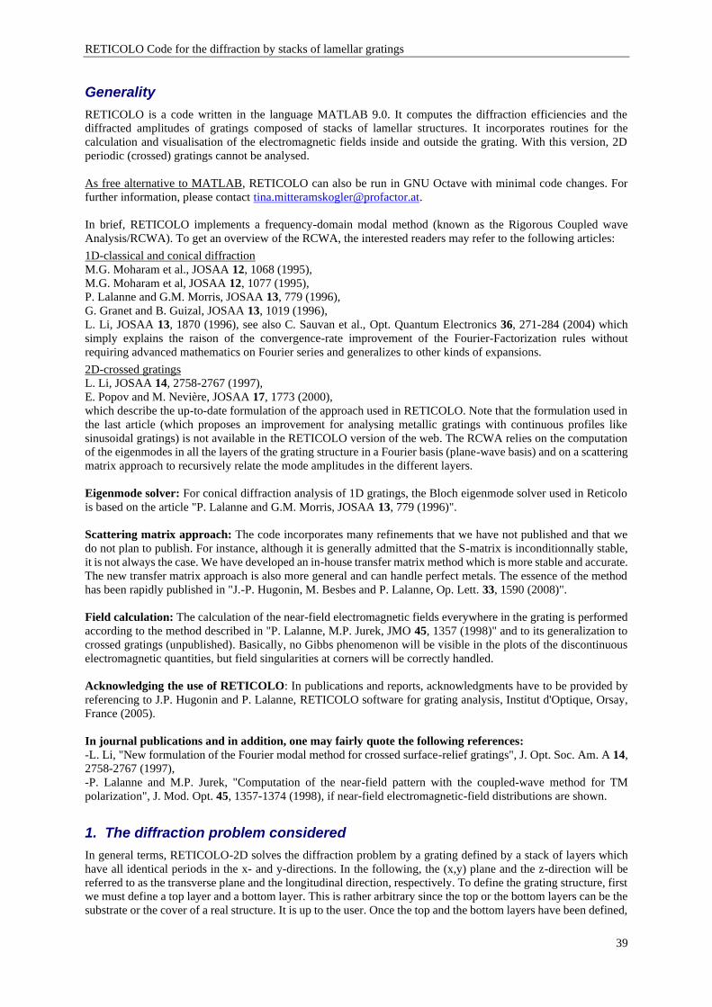
RETICOLO Code for the diffraction by stacks of lamellar gratings
39
Generality
RETICOLO is a code written in the language MATLAB 9.0. It computes the diffraction efficiencies and the
diffracted amplitudes of gratings composed of stacks of lamellar structures. It incorporates routines for the
calculation and visualisation of the electromagnetic fields inside and outside the grating. With this version, 2D
periodic (crossed) gratings cannot be analysed.
As free alternative to MATLAB, RETICOLO can also be run in GNU Octave with minimal code changes. For
further information, please contact [email protected].
In brief, RETICOLO implements a frequency-domain modal method (known as the Rigorous Coupled wave
Analysis/RCWA). To get an overview of the RCWA, the interested readers may refer to the following articles:
1D-classical and conical diffraction
M.G. Moharam et al., JOSAA 12, 1068 (1995),
M.G. Moharam et al, JOSAA 12, 1077 (1995),
P. Lalanne and G.M. Morris, JOSAA 13, 779 (1996),
G. Granet and B. Guizal, JOSAA 13, 1019 (1996),
L. Li, JOSAA 13, 1870 (1996), see also C. Sauvan et al., Opt. Quantum Electronics 36, 271-284 (2004) which
simply explains the raison of the convergence-rate improvement of the Fourier-Factorization rules without
requiring advanced mathematics on Fourier series and generalizes to other kinds of expansions.
2D-crossed gratings
L. Li, JOSAA 14, 2758-2767 (1997),
E. Popov and M. Nevière, JOSAA 17, 1773 (2000),
which describe the up-to-date formulation of the approach used in RETICOLO. Note that the formulation used in
the last article (which proposes an improvement for analysing metallic gratings with continuous profiles like
sinusoidal gratings) is not available in the RETICOLO version of the web. The RCWA relies on the computation
of the eigenmodes in all the layers of the grating structure in a Fourier basis (plane-wave basis) and on a scattering
matrix approach to recursively relate the mode amplitudes in the different layers.
Eigenmode solver: For conical diffraction analysis of 1D gratings, the Bloch eigenmode solver used in Reticolo
is based on the article "P. Lalanne and G.M. Morris, JOSAA 13, 779 (1996)".
Scattering matrix approach: The code incorporates many refinements that we have not published and that we
do not plan to publish. For instance, although it is generally admitted that the S-matrix is inconditionnally stable,
it is not always the case. We have developed an in-house transfer matrix method which is more stable and accurate.
The new transfer matrix approach is also more general and can handle perfect metals. The essence of the method
has been rapidly published in "J.-P. Hugonin, M. Besbes and P. Lalanne, Op. Lett. 33, 1590 (2008)".
Field calculation: The calculation of the near-field electromagnetic fields everywhere in the grating is performed
according to the method described in "P. Lalanne, M.P. Jurek, JMO 45, 1357 (1998)" and to its generalization to
crossed gratings (unpublished). Basically, no Gibbs phenomenon will be visible in the plots of the discontinuous
electromagnetic quantities, but field singularities at corners will be correctly handled.
Acknowledging the use of RETICOLO: In publications and reports, acknowledgments have to be provided by
referencing to J.P. Hugonin and P. Lalanne, RETICOLO software for grating analysis, Institut d'Optique, Orsay,
France (2005).
In journal publications and in addition, one may fairly quote the following references:
-L. Li, "New formulation of the Fourier modal method for crossed surface-relief gratings", J. Opt. Soc. Am. A 14,
2758-2767 (1997),
-P. Lalanne and M.P. Jurek, "Computation of the near-field pattern with the coupled-wave method for TM
polarization", J. Mod. Opt. 45, 1357-1374 (1998), if near-field electromagnetic-field distributions are shown.
1. The diffraction problem considered
In general terms, RETICOLO-2D solves the diffraction problem by a grating defined by a stack of layers which
have all identical periods in the x- and y-directions. In the following, the (x,y) plane and the z-direction will be
referred to as the transverse plane and the longitudinal direction, respectively. To define the grating structure, first
we must define a top layer and a bottom layer. This is rather arbitrary since the top or the bottom layers can be the
substrate or the cover of a real structure. It is up to the user. Once the top and the bottom layers have been defined,
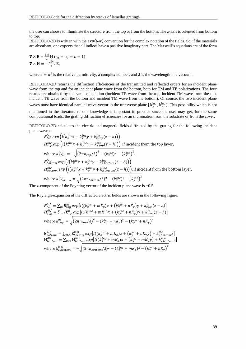
RETICOLO Code for the diffraction by stacks of lamellar gratings
39
the user can choose to illuminate the structure from the top or from the bottom. The z-axis is oriented from bottom
to top.
RETICOLO-2D is written with the 𝑒𝑥𝑝(𝑖𝜔𝑡) convention for the complex notation of the fields. So, if the materials
are absorbant, one expects that all indices have a positive imaginary part. The Maxwell‘s equations are of the form
𝛁 × 𝐄 =2𝑖𝜋
𝜆𝐇 (𝜀0 = µ0 = 𝑐 = 1)
𝛁 × 𝐇 = −2𝑖𝜋
𝜆𝜀𝐄,
where 𝜀 = 𝑛2 is the relative permittivity, a complex number, and 𝜆 is the wavelength in a vacuum.
RETICOLO-2D returns the diffraction efficiencies of the transmitted and reflected orders for an incident plane
wave from the top and for an incident plane wave from the bottom, both for TM and TE polarizations. The four
results are obtained by the same calculation (incident TE wave from the top, incident TM wave from the top,
incident TE wave from the bottom and incident TM wave from the bottom). Of course, the two incident plane
waves must have identical parallel wave-vector in the transverse plane [ incxk , inc
yk ]. This possibility which is not
mentioned in the literature to our knowledge is important in practice since the user may get, for the same
computational loads, the grating diffraction efficiencies for an illumination from the substrate or from the cover.
RETICOLO-2D calculates the electric and magnetic fields diffracted by the grating for the following incident
plane wave :
𝑬𝑡𝑜𝑝𝑖𝑛𝑐 𝑒𝑥𝑝 (𝑖(𝑘𝑥
𝑖𝑛𝑐𝑥 + 𝑘𝑦𝑖𝑛𝑐𝑦 + 𝑘𝑧 𝑡𝑜𝑝
𝑖𝑛𝑐 (𝑧 − ℎ)))
𝑯𝑡𝑜𝑝𝑖𝑛𝑐 𝑒𝑥𝑝 (𝑖(𝑘𝑥
𝑖𝑛𝑐𝑥 + 𝑘𝑦𝑖𝑛𝑐𝑦 + 𝑘𝑧 𝑡𝑜𝑝
𝑖𝑛𝑐 (𝑧 − ℎ))), if incident from the top layer,
where 𝑘𝑧 𝑡𝑜𝑝𝑖𝑛𝑐 = −√(2𝜋𝑛𝑡𝑜𝑝/𝜆)
2− (𝑘𝑥
𝑖𝑛𝑐)2 − (𝑘𝑦𝑖𝑛𝑐)
2.
𝑬𝑏𝑜𝑡𝑡𝑜𝑚𝑖𝑛𝑐 𝑒𝑥𝑝 (𝑖(𝑘𝑥
𝑖𝑛𝑐𝑥 + 𝑘𝑦𝑖𝑛𝑐𝑦 + 𝑘𝑧 𝑏𝑜𝑡𝑡𝑜𝑚
𝑖𝑛𝑐 (𝑧 − ℎ)))
𝑯𝑏𝑜𝑡𝑡𝑜𝑚𝑖𝑛𝑐 𝑒𝑥𝑝 (𝑖(𝑘𝑥
𝑖𝑛𝑐𝑥 + 𝑘𝑦𝑖𝑛𝑐𝑦 + 𝑘𝑧 𝑏𝑜𝑡𝑡𝑜𝑚
𝑖𝑛𝑐 (𝑧 − ℎ))), if incident from the bottom layer,
where 𝑘𝑧 𝑏𝑜𝑡𝑡𝑜𝑚𝑖𝑛𝑐 = √(2𝜋𝑛𝑏𝑜𝑡𝑡𝑜𝑚/𝜆)2 − (𝑘𝑥
𝑖𝑛𝑐)2 − (𝑘𝑦𝑖𝑛𝑐)
2.
The z-component of the Poynting vector of the incident plane wave is 0.5.
The Rayleigh-expansion of the diffracted electric fields are shown in the following figure.
𝑬𝑡𝑜𝑝𝑑𝑖𝑓
= ∑ 𝑬𝑡𝑜𝑝𝑚
𝑚 𝑒𝑥𝑝[𝑖((𝑘𝑥𝑖𝑛𝑐 + 𝑚𝐾𝑥)𝑥 + (𝑘𝑦
𝑖𝑛𝑐 + 𝑛𝐾𝑦)𝑦 + 𝑘z top𝑚 (𝑧 − ℎ)]
𝑯𝑡𝑜𝑝𝑑𝑖𝑓
= ∑ 𝑯𝑡𝑜𝑝𝑚
𝑚 𝑒𝑥𝑝[𝑖((𝑘𝑥𝑖𝑛𝑐 + 𝑚𝐾𝑥)𝑥 + (𝑘𝑦
𝑖𝑛𝑐 + 𝑛𝐾𝑦)𝑦 + 𝑘z top𝑚 (𝑧 − ℎ)]
where kz top𝑚 = √(2𝜋𝑛𝑡𝑜𝑝/𝜆)
2− (𝑘𝑥
𝑖𝑛𝑐 + 𝑛𝐾𝑥)2 − (𝑘𝑦𝑖𝑛𝑐 + 𝑛𝐾𝑦)
2.
𝐄𝑏𝑜𝑡𝑡𝑜𝑚𝑑𝑖𝑓
= ∑ 𝐄𝑏𝑜𝑡𝑡𝑜𝑚𝑚,𝑛
𝑚,𝑛 𝑒𝑥𝑝[𝑖((𝑘𝑥𝑖𝑛𝑐 + 𝑚𝐾𝑥)𝑥 + (𝑘𝑦
inc + 𝑛𝐾𝑦𝑦) + 𝑘z 𝑏𝑜𝑡𝑡𝑜𝑚m,n 𝑧]
𝐇𝑏𝑜𝑡𝑡𝑜𝑚𝑑𝑖𝑓
= ∑ 𝐇𝑏𝑜𝑡𝑡𝑜𝑚𝑚,𝑛
𝑚,𝑛 𝑒𝑥𝑝[𝑖((𝑘𝑥𝑖𝑛𝑐 + 𝑚𝐾𝑥)𝑥 + (𝑘𝑦
inc + 𝑚𝐾𝑦𝑦) + 𝑘z 𝑏𝑜𝑡𝑡𝑜𝑚m,n 𝑧]
where kz 𝑏𝑜𝑡𝑡𝑜𝑚m,n = −√(2𝜋𝑛𝑏𝑜𝑡𝑡𝑜𝑚/𝜆)2 − (𝑘𝑥
𝑖𝑛𝑐 + 𝑚𝐾𝑥)2 − (𝑘𝑦inc + 𝑛𝐾𝑦)
2
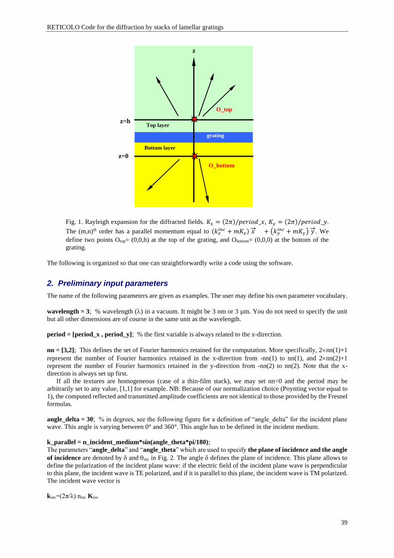
RETICOLO Code for the diffraction by stacks of lamellar gratings
39
z
z=0
z=h
Top layer
Bottom layer
grating
O_top
O_bottom
Fig. 1. Rayleigh expansion for the diffracted fields. 𝐾𝑥 = (2𝜋)/𝑝𝑒𝑟𝑖𝑜𝑑_𝑥, 𝐾𝑦 = (2𝜋)/𝑝𝑒𝑟𝑖𝑜𝑑_𝑦.
The (m,n)th order has a parallel momentum equal to (𝑘𝑥𝑖𝑛𝑐 + 𝑚𝐾𝑥) 𝑥→ + (𝑘𝑦
𝑖𝑛𝑐 + 𝑚𝐾𝑦) 𝑦→. We
define two points Otop= (0,0,h) at the top of the grating, and Obottom= (0,0,0) at the bottom of the
grating.
The following is organized so that one can straightforwardly write a code using the software.
2. Preliminary input parameters
The name of the following parameters are given as examples. The user may define his own parameter vocabulary.
wavelength = 3; % wavelength () in a vacuum. It might be 3 nm or 3 µm. You do not need to specify the unit
but all other dimensions are of course in the same unit as the wavelength.
period = [period_x , period_y]; % the first variable is always related to the x-direction.
nn = [3,2]; This defines the set of Fourier harmonics retained for the computation. More specifically, 2nn(1)+1
represent the number of Fourier harmonics retained in the x-direction from -nn(1) to nn(1), and 2nn(2)+1
represent the number of Fourier harmonics retained in the y-direction from -nn(2) to nn(2). Note that the x-
direction is always set up first.
If all the textures are homogeneous (case of a thin-film stack), we may set nn=0 and the period may be
arbitrarily set to any value, [1,1] for example. NB: Because of our normalization choice (Poynting vector equal to
1), the computed reflected and transmitted amplitude coefficients are not identical to those provided by the Fresnel
formulas.
angle_delta = 30; % in degrees, see the following figure for a definition of “angle_delta” for the incident plane
wave. This angle is varying between 0° and 360°. This angle has to be defined in the incident medium.
k_parallel = n_incident_medium*sin(angle_theta*pi/180);
The parameters “angle_delta” and “angle_theta” which are used to specify the plane of incidence and the angle
of incidence are denoted by and inc in Fig. 2. The angle defines the plane of incidence. This plane allows to
define the polarization of the incident plane wave: if the electric field of the incident plane wave is perpendicular
to this plane, the incident wave is TE polarized, and if it is parallel to this plane, the incident wave is TM polarized.
The incident wave vector is
kinc=(2π/λ) ninc Kinc
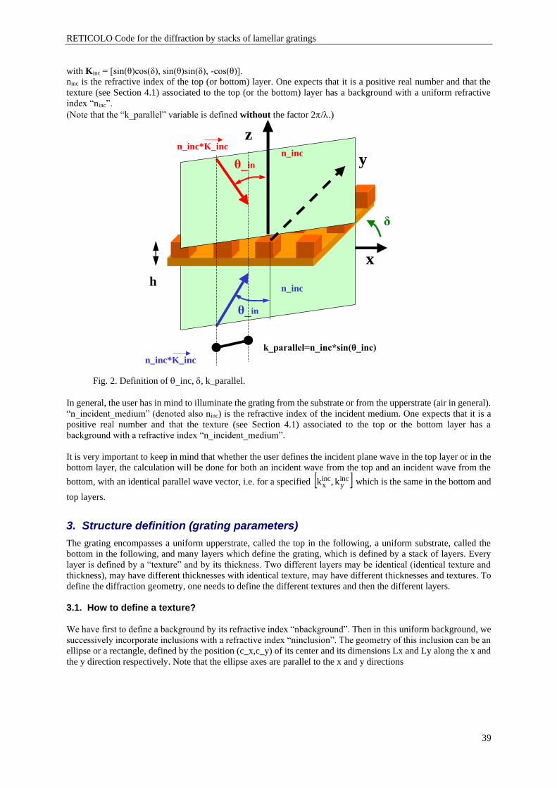
RETICOLO Code for the diffraction by stacks of lamellar gratings
39
with Kinc = [sin(θ)cos(δ), sin(θ)sin(δ), -cos(θ)].
ninc is the refractive index of the top (or bottom) layer. One expects that it is a positive real number and that the
texture (see Section 4.1) associated to the top (or the bottom) layer has a background with a uniform refractive
index “ninc”.
(Note that the “k_parallel” variable is defined without the factor 2/.)
z
x
δ
h
θ_ inc
n_inc
k_parallel=n_inc*sin(θ_inc)
θ_ inc
n_inc y
n_inc*K_inc
n_inc*K_inc
Fig. 2. Definition of inc, , k_parallel.
In general, the user has in mind to illuminate the grating from the substrate or from the upperstrate (air in general).
“n_incident_medium” (denoted also ninc) is the refractive index of the incident medium. One expects that it is a
positive real number and that the texture (see Section 4.1) associated to the top or the bottom layer has a
background with a refractive index “n_incident_medium”.
It is very important to keep in mind that whether the user defines the incident plane wave in the top layer or in the
bottom layer, the calculation will be done for both an incident wave from the top and an incident wave from the
bottom, with an identical parallel wave vector, i.e. for a specified incy
incx k,k which is the same in the bottom and
top layers.
3. Structure definition (grating parameters)
The grating encompasses a uniform upperstrate, called the top in the following, a uniform substrate, called the
bottom in the following, and many layers which define the grating, which is defined by a stack of layers. Every
layer is defined by a “texture” and by its thickness. Two different layers may be identical (identical texture and
thickness), may have different thicknesses with identical texture, may have different thicknesses and textures. To
define the diffraction geometry, one needs to define the different textures and then the different layers.
3.1. How to define a texture?
We have first to define a background by its refractive index “nbackground”. Then in this uniform background, we
successively incorporate inclusions with a refractive index “ninclusion”. The geometry of this inclusion can be an
ellipse or a rectangle, defined by the position (c_x,c_y) of its center and its dimensions Lx and Ly along the x and
the y direction respectively. Note that the ellipse axes are parallel to the x and y directions
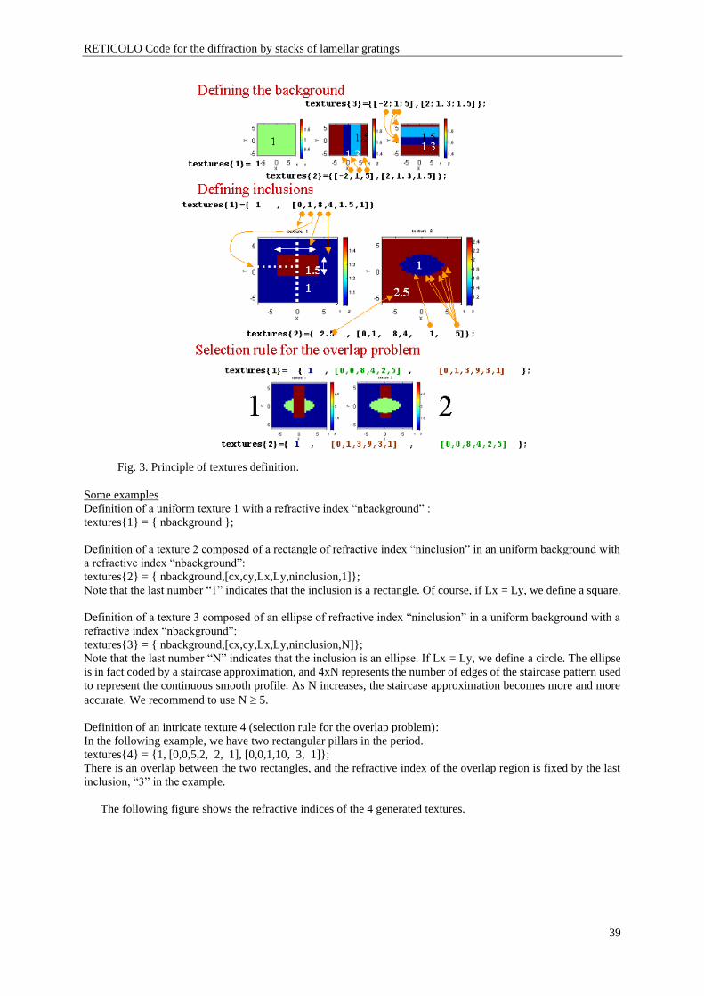
RETICOLO Code for the diffraction by stacks of lamellar gratings
39
Fig. 3. Principle of textures definition.
Some examples
Definition of a uniform texture 1 with a refractive index “nbackground” :
textures{1} = { nbackground };
Definition of a texture 2 composed of a rectangle of refractive index “ninclusion” in an uniform background with
a refractive index “nbackground”:
textures{2} = { nbackground,[cx,cy,Lx,Ly,ninclusion,1]};
Note that the last number “1” indicates that the inclusion is a rectangle. Of course, if Lx = Ly, we define a square.
Definition of a texture 3 composed of an ellipse of refractive index “ninclusion” in a uniform background with a
refractive index “nbackground”:
textures{3} = { nbackground,[cx,cy,Lx,Ly,ninclusion,N]};
Note that the last number “N” indicates that the inclusion is an ellipse. If Lx = Ly, we define a circle. The ellipse
is in fact coded by a staircase approximation, and 4xN represents the number of edges of the staircase pattern used
to represent the continuous smooth profile. As N increases, the staircase approximation becomes more and more
accurate. We recommend to use N 5.
Definition of an intricate texture 4 (selection rule for the overlap problem):
In the following example, we have two rectangular pillars in the period.
textures{4} = {1, [0,0,5,2, 2, 1], [0,0,1,10, 3, 1]};
There is an overlap between the two rectangles, and the refractive index of the overlap region is fixed by the last
inclusion, “3” in the example.
The following figure shows the refractive indices of the 4 generated textures.
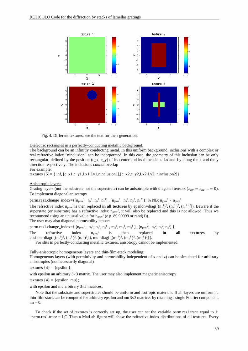
RETICOLO Code for the diffraction by stacks of lamellar gratings
39
Fig. 4. Different textures, see the text for their generation.
Dielectric rectangles in a perfectly-conducting metallic background:
The background can be an infinitly conducting metal. In this uniform background, inclusions with a complex or
real refractive index “ninclusion” can be incorporated. In this case, the geometry of this inclusion can be only
rectangular, defined by the position (c_x, c_y) of its center and its dimensions Lx and Ly along the x and the y
direction respectively. The inclusions cannot overlap
For example:
textures {5}= { inf, [c_x1,c_y1,Lx1,Ly1,ninclusion1],[c_x2,c_y2,Lx2,Ly2, ninclusion2]}
Anisotropic layers:
Grating layers (not the substrate nor the superstrate) can be anisotropic with diagonal tensors (𝜀𝑥𝑦 = 𝜀𝑥𝑧 … = 0).
To implement diagonal anisotropy
parm.res1.change_index={[nprov1, nx
1, ny1, nz
1] , [nprov2, nx
2, ny2, nz
2]}; % NB: nprov1 nprov
2
The refractive index nprov1 is then replaced in all textures by epsilon=diag([(nx
1)2, (ny1 )2, (nz
1 )2]). Beware if the
superstate (or substrate) has a refractive index nprov1, it will also be replaced and this is not allowed. Thus we
recommend using an unusual value for nprov1 (e.g. 89.99999 or rand(1)).
The user may also diagonal permeability tensors
parm.res1.change_index={ [nprov1, nx
1, ny1, nz
1 , mx1, my
1, mz1 ] , [nprov
2, nx2, ny
2, nz2] };
The refractive index nprov1 is then replaced in all textures by
epsilon=diag( [(nx1)2, (ny
1 )2, (nz1 )2] ), mu=diag( [(mx
1)2, (my1 )2, (mz
1 )2] ).
For slits in perfectly-conducting metallic textures, anisotropy cannot be implemented.
Fully-anisotropic homogeneous layers and thin-film-stack modeling:
Homogeneous layers (with permittivity and permeability independent of x and z) can be simulated for arbitrary
anisotropies (not necessarily diagonal)
textures {4} = {epsilon};
with epsilon an arbitrary 33 matrix. The user may also implement magnetic anisotropy
textures {4} = {epsilon, mu};
with epsilon and mu arbitrary 33 matrices.
Note that the substrate and superstrates should be uniform and isotropic materials. If all layers are uniform, a
thin-film stack can be computed for arbitrary epsilon and mu 33 matrices by retaining a single Fourier component,
nn = 0.
To check if the set of textures is correctly set up, the user can set the variable parm.res1.trace equal to 1:
“parm.res1.trace = 1;”. Then a MatLab figure will show the refractive-index distributions of all textures. Every
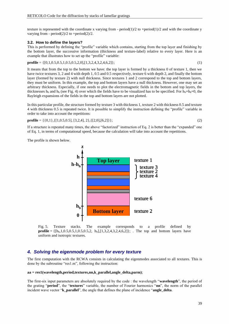
RETICOLO Code for the diffraction by stacks of lamellar gratings
39
texture is represented with the coordinate x varying from - period(1)/2 to +period(1)/2 and with the coordinate y
varying from - period(2)/2 to +period(2)/2.
3.2. How to define the layers? This is performed by defining the “profile” variable which contains, starting from the top layer and finishing by
the bottom layer, the successive information (thickness and texture-label) relative to every layer. Here is an
example that illustrates how to set up the “profile” variable:
profile = {[0,1,0.5,0.5,1,0.5,0.5,2,0],[1,3,2,4,3,2,4,6,2]}; (1)
It means that from the top to the bottom we have: the top layer is formed by a thickness 0 of texture 1, then we
have twice textures 3, 2 and 4 with depth 1, 0.5 and 0.5 respectively, texture 6 with depth 2, and finally the bottom
layer (formed by texture 2) with null thickness. Since textures 1 and 2 correspond to the top and bottom layers,
they must be uniform. In this example, the top and bottom layers have a null thickness. However, one may set an
arbitrary thickness. Especially, if one needs to plot the electromagnetic fields in the bottom and top layers, the
thicknesses hb and hh (see Fig. 4) over which the fields have to be visualized has to be specified. For hb=hh=0, the
Rayleigh expansions of the fields in the top and bottom layers are not plotted.
In this particular profile, the structure formed by texture 3 with thickness 1, texture 2 with thickness 0.5 and texture
4 with thickness 0.5 is repeated twice. It is possible to simplify the instruction defining the “profile” variable in
order to take into account the repetitions:
profile = {{0,1},{[1,0.5,0.5], [3,2,4], 2},{[2,0],[6,2]}}; (2)
If a structure is repeated many times, the above “factorized” instruction of Eq. 2 is better than the “expanded” one
of Eq. 1, in terms of computational speed, because the calculation will take into account the repetitions.
The profile is shown below.
Fig. 5. Texture stacks. The example corresponds to a profile defined by
profile = {[hh,1,0.5,0.5,1,0.5,0.5,2, hb],[1,3,2,4,3,2,4,6,2]}; . The top and bottom layers have
uniform and isotropic textures.
4. Solving the eigenmode problem for every texture
The first computation with the RCWA consists in calculating the eigenmodes associated to all textures. This is
done by the subroutine “res1.m”, following the instruction:
aa = res1(wavelength,period,textures,nn,k_parallel,angle_delta,parm);
The first-six input parameters are absolutely required by the code : the wavelength “wavelength”, the period of
the grating “period”, the “textures” variable, the number of Fourier harmonics “nn”, the norm of the parallel
incident wave vector “k_parallel”, the angle that defines the plane of incidence “angle_delta.
texture 2
texture 1
texture 6
texture 3texture 2texture 4
texture 2
texture 1
texture 6
texture 3texture 2texture 4
texture 2
texture 1
texture 6
texture 3texture 2texture 4
z
0
h
Bottom layer
Top layerh-hh
hb

RETICOLO Code for the diffraction by stacks of lamellar gratings
39
Some other additional parameters can be defined. For example, the default parameters do not take the symmetry
of the problem into account. So if the user wants to use symmetries, new parameters have to be defined :
“parm.sym.x”, “parm.sym.y”, and “parm.sym.pol”. These parameters are defined in Section 7.
parm = res0;
res0.m is a function that changes the default values. This instruction has to be executed before res1.m, if one wants
to modify the default values (for instance to use symmetry).
It is very important to note that if one has to study the diffraction by many different gratings composed of the same
textures, one needs to compute only once the eigenmodes. It is possible to save the “aa” variable in a “.mat” file
and to reload it for the computation of the diffracted waves, see an example in Annex 9.3.
5. Computing the diffracted waves
This is the second step of the computation. This is done by the subroutine “res2.m”, following the instruction:
result = res2(aa,profile);
This subroutine has 2 input arguments: the output “aa” of the subroutine “res1.m” and the “profile” variable. The
output argument “result” contains all the information on the diffracted fields. “result” is an object of class
‘reticolo’ that can be indexed as an usual structure with parentheses, or with the labels of the considered orders
between curly braces. Examples will be given in the following.
This information is divided into the following sub-structures fields :
- “result.TEinc_top”
- “result.TEinc_top_reflected”
- “result.TEinc_top_transmitted”
- “result.TEinc_bottom”
- “result.TEinc_bottom_reflected”
- “result.TEinc_bottom_transmitted”
- “result.TMinc_top”
- “result.TMinc_top_reflected”
- “result.TMinc_top_transmitted”
- “result.TMinc_bottom”
- “result.TMinc_bottom_reflected”
- “result.TMinc_bottom_transmitted”
The sub-structure “result.TEinc_top_reflected” contains all the information concerning the propagative reflected
waves for the incident wave from the top of the grating in TE polarization which is described in the sub-structure
“result.TEinc_top”
The sub-structure “result.TMinc_bottom_transmitted” contains all the information concerning the propagative
transmitted waves for the incident wave from the bottom of the grating in TM polarization, which is described in
the sub-structure “result.TMinc_bottom”. And so on.
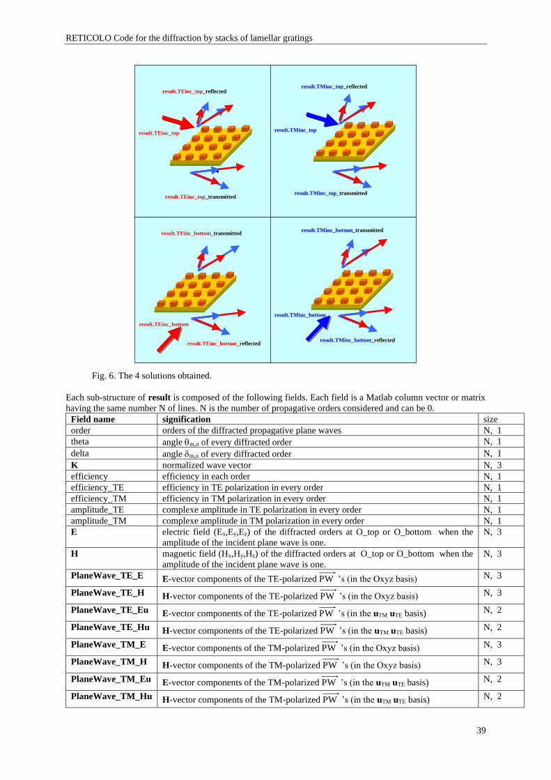
RETICOLO Code for the diffraction by stacks of lamellar gratings
39
result.TEinc_top
result.TEinc_top_reflected
result.TEinc_top_transmitted
result.TMinc_top
result.TMinc_top_reflected
result.TMinc_top_transmitted
result.TEinc_bottom
result.TEinc_bottom_transmitted
result.TEinc_bottom_reflected
result.TMinc_bottom
result.TMinc_bottom_transmitted
result.TMinc_bottom_reflected
Fig. 6. The 4 solutions obtained.
Each sub-structure of result is composed of the following fields. Each field is a Matlab column vector or matrix
having the same number N of lines. N is the number of propagative orders considered and can be 0.
Field name signification size
order orders of the diffracted propagative plane waves N, 1
theta angle m,n of every diffracted order N, 1
delta angle m,n of every diffracted order N, 1
K normalized wave vector N, 3
efficiency efficiency in each order N, 1
efficiency_TE efficiency in TE polarization in every order N, 1
efficiency_TM efficiency in TM polarization in every order N, 1
amplitude_TE complexe amplitude in TE polarization in every order N, 1
amplitude_TM complexe amplitude in TM polarization in every order N, 1
E electric field (Ex,Ey,Ez) of the diffracted orders at O_top or O_bottom when the
amplitude of the incident plane wave is one.
N, 3
H magnetic field (Hx,Hy,Hz) of the diffracted orders at O_top or O_bottom when the
amplitude of the incident plane wave is one.
N, 3
PlaneWave_TE_E E-vector components of the TE-polarized PW ’s (in the Oxyz basis) N, 3
PlaneWave_TE_H H-vector components of the TE-polarized PW ’s (in the Oxyz basis) N, 3
PlaneWave_TE_Eu E-vector components of the TE-polarized PW ’s (in the uTM uTE basis) N, 2
PlaneWave_TE_Hu H-vector components of the TE-polarized PW ’s (in the uTM uTE basis) N, 2
PlaneWave_TM_E E-vector components of the TM-polarized PW ’s (in the Oxyz basis) N, 3
PlaneWave_TM_H H-vector components of the TM-polarized PW ’s (in the Oxyz basis) N, 3
PlaneWave_TM_Eu E-vector components of the TM-polarized PW ’s (in the uTM uTE basis) N, 2
PlaneWave_TM_Hu H-vector components of the TM-polarized PW ’s (in the uTM uTE basis) N, 2
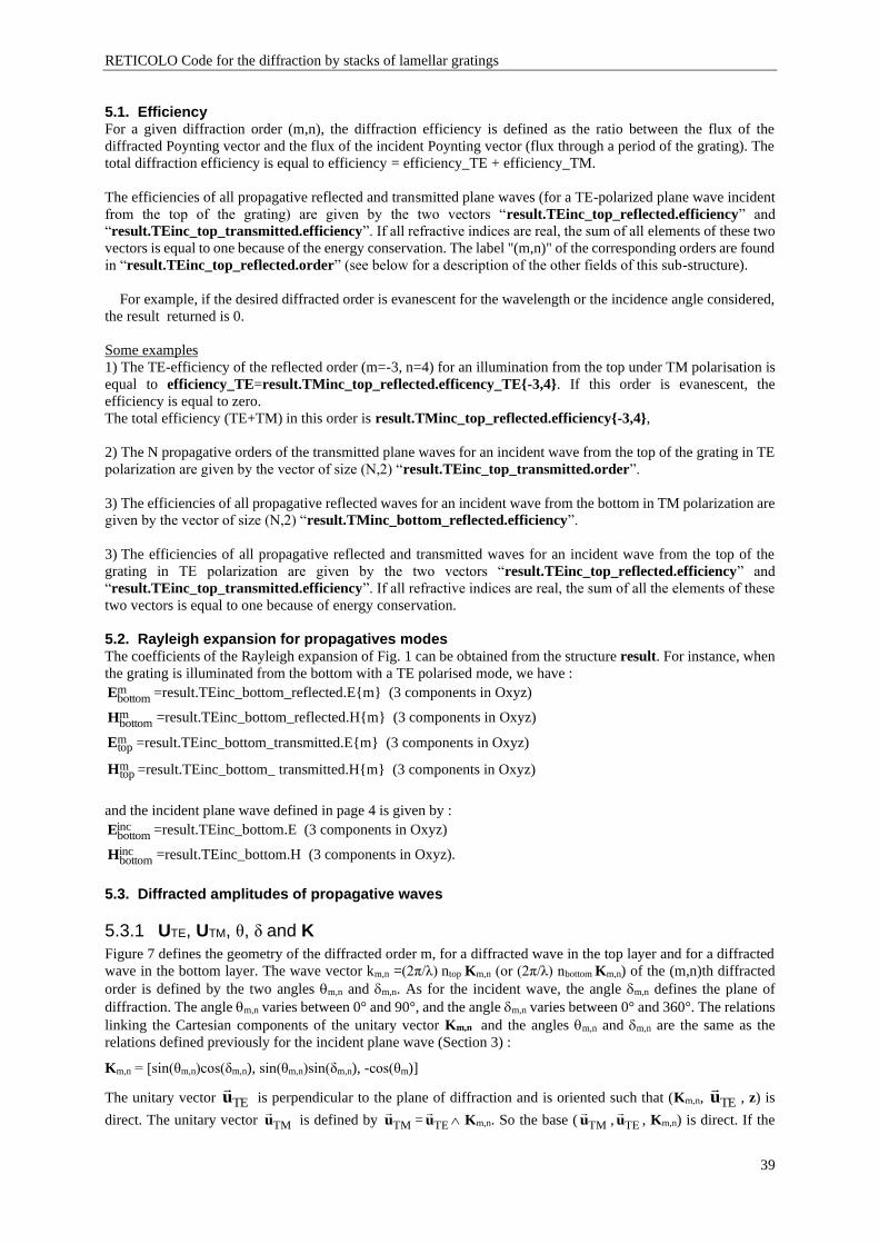
RETICOLO Code for the diffraction by stacks of lamellar gratings
39
5.1. Efficiency For a given diffraction order (m,n), the diffraction efficiency is defined as the ratio between the flux of the
diffracted Poynting vector and the flux of the incident Poynting vector (flux through a period of the grating). The
total diffraction efficiency is equal to efficiency = efficiency_TE + efficiency_TM.
The efficiencies of all propagative reflected and transmitted plane waves (for a TE-polarized plane wave incident
from the top of the grating) are given by the two vectors “result.TEinc_top_reflected.efficiency” and
“result.TEinc_top_transmitted.efficiency”. If all refractive indices are real, the sum of all elements of these two
vectors is equal to one because of the energy conservation. The label "(m,n)" of the corresponding orders are found
in “result.TEinc_top_reflected.order” (see below for a description of the other fields of this sub-structure).
For example, if the desired diffracted order is evanescent for the wavelength or the incidence angle considered,
the result returned is 0.
Some examples
1) The TE-efficiency of the reflected order (m=-3, n=4) for an illumination from the top under TM polarisation is
equal to efficiency_TE=result.TMinc_top_reflected.efficency_TE{-3,4}. If this order is evanescent, the
efficiency is equal to zero.
The total efficiency (TE+TM) in this order is result.TMinc_top_reflected.efficiency{-3,4},
2) The N propagative orders of the transmitted plane waves for an incident wave from the top of the grating in TE
polarization are given by the vector of size (N,2) “result.TEinc_top_transmitted.order”.
3) The efficiencies of all propagative reflected waves for an incident wave from the bottom in TM polarization are
given by the vector of size (N,2) “result.TMinc_bottom_reflected.efficiency”.
3) The efficiencies of all propagative reflected and transmitted waves for an incident wave from the top of the
grating in TE polarization are given by the two vectors “result.TEinc_top_reflected.efficiency” and
“result.TEinc_top_transmitted.efficiency”. If all refractive indices are real, the sum of all the elements of these
two vectors is equal to one because of energy conservation.
5.2. Rayleigh expansion for propagatives modes The coefficients of the Rayleigh expansion of Fig. 1 can be obtained from the structure result. For instance, when
the grating is illuminated from the bottom with a TE polarised mode, we have : mbottomE =result.TEinc_bottom_reflected.E{m} (3 components in Oxyz)
mbottomH =result.TEinc_bottom_reflected.H{m} (3 components in Oxyz)
mtopE =result.TEinc_bottom_transmitted.E{m} (3 components in Oxyz)
mtopH =result.TEinc_bottom_ transmitted.H{m} (3 components in Oxyz)
and the incident plane wave defined in page 4 is given by : incbottomE =result.TEinc_bottom.E (3 components in Oxyz)
incbottomH =result.TEinc_bottom.H (3 components in Oxyz).
5.3. Diffracted amplitudes of propagative waves
5.3.1 UTE, UTM, θ, δ and K
Figure 7 defines the geometry of the diffracted order m, for a diffracted wave in the top layer and for a diffracted
wave in the bottom layer. The wave vector km,n =(2π/λ) ntop Km,n (or (2π/λ) nbottom Km,n) of the (m,n)th diffracted
order is defined by the two angles m,n and m,n. As for the incident wave, the angle m,n defines the plane of
diffraction. The angle m,n varies between 0° and 90°, and the angle m,n varies between 0° and 360°. The relations
linking the Cartesian components of the unitary vector Km,n and the angles m,n and m,n are the same as the
relations defined previously for the incident plane wave (Section 3) :
Km,n = [sin(θm,n)cos(δm,n), sin(θm,n)sin(δm,n), -cos(θm)]
The unitary vector TEu
is perpendicular to the plane of diffraction and is oriented such that (Km,n, TEu
, z) is
direct. The unitary vector TMu
is defined by TMu
= TEu
Km,n. So the base ( TMu
, TEu
, Km,n) is direct. If the
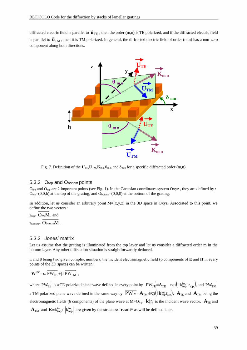
RETICOLO Code for the diffraction by stacks of lamellar gratings
39
diffracted electric field is parallel to TEu
, then the order (m,n) is TE polarized, and if the diffracted electric field
is parallel to TMu
, then it is TM polarized. In general, the diffracted electric field of order (m,n) has a non-zero
component along both directions.
z
x
y K m n
m
U TE
U TE
δ mn
m
n
n
θ m n
K m n
θ m n
h
U TM
U TM
Fig. 7. Definition of the UTE,UTM,Km,n,m,n and m,n for a specific diffracted order (m,n).
5.3.2 Otop and Obottom points
Otop and Otop are 2 important points (see Fig. 1). In the Cartesian coordinates system Oxyz , they are defined by :
Otop=(0,0,h) at the top of the grating, and Obottom=(0,0,0) at the bottom of the grating.
In addition, let us consider an arbitrary point M=(x,y,z) in the 3D space in Oxyz. Associated to this point, we
define the two vectors :
rtop= MOtop , and
rbottom= MObottom .
5.3.3 Jones’ matrix
Let us assume that the grating is illuminated from the top layer and let us consider a diffracted order m in the
bottom layer. Any other diffraction situation is straightforwardly deduced.
α and β being two given complex numbers, the incident electromagnetic field (6 components of E and H in every
points of the 3D space) can be written :
TMTEinc PWPW +=W ,
where TEPW is a TE-polarized plane wave defined in every point by ( )topinctopTETE riexpPW kA= , and TMPW
a TM polarized plane wave defined in the same way by ( )topinctopTMTM riexpPW kA= , TEA and TMA being the
electromagnetic fields (6 components) of the plane wave at M=Otop. inctopk is the incident wave vector. TEA and
TMA and inctop
inctop / kkK= are given by the structure “result“ as will be defined later.
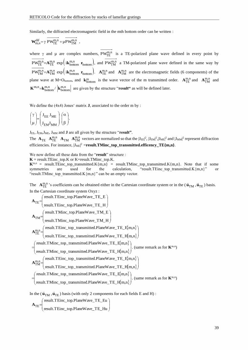
RETICOLO Code for the diffraction by stacks of lamellar gratings
39
Similarly, the diffracted electromagnetic field in the mth bottom order can be written :
n,mTM
n,mTE
difn,m PWµPW +=W ,
where and µ are complex numbers, n,mTEPW is a TE-polarized plane wave defined in every point by
( )bottomn,m
bottomn,m
TEn,m
TE iexpPW rkA= , and n,mTMPW a TM-polarized plane wave defined in the same way by
( )bottomn,m
bottomn,m
TMn,m
TM iexpPW rkA= . n,mTEA and n,m
TMA are the electromagnetic fields (6 components) of the
plane wave at M=Obottom, and mbottomk is the wave vector of the m transmitted order. n,m
TEA and n,mTMA and
n,mbottom
n,mbottom
n,m / kkK = are given by the structure “result“ as will be defined later.
We define the (4x4) Jones‘ matrix J, associated to the order m by :
=
MMEM
MEEE
JJ
JJ
µ.
JEE, JEM,JME, JMM and J are all given by the structure “result”.
The TEA n,mTEA TMA n,m
TMA vectors are normalized so that the |JEE|2, |JEM|2,|JME|2 and |JMM|2 represent diffraction
efficiencies. For instance, |JME|2 =result.TMinc_top_transmitted.efficency_TE{m,n}.
We now define all these data from the “result” structure :
K = result.TEinc_top.K or K=result.TMinc_top.K.
Km,n = result.TEinc_top_transmitted.K{m,n} = result.TMinc_top_transmitted.K{m,n}. Note that if some
symmetries are used for the calculation, “result.TEinc_top_transmitted.K{m,n}” or
“result.TMinc_top_transmitted.K{m,n}” can be an empty vector.
The n,mTEA ’s coefficients can be obtained either in the Cartesian coordinate system or in the ( TMu
, TEu
) basis.
In the Cartesian coordinate system Oxyz :
=
H_TE_PlaneWave.top_TEinc.result
E_TE_PlaneWave.top_TEinc.result
TEA
=
H_TM_PlaneWave.top_TMinc.result
E_TM_PlaneWave.top_TMinc.result
TMA
=
n,mH_TE_PlaneWave.dtransmitte_top_TEinc.result
n,mE_TE_PlaneWave.dtransmitte_top_TEinc.resultn,m
TEA
=
n,mH_TE_PlaneWave.dtransmitte_top_TMinc.result
n,mE_TE_PlaneWave.dtransmitte_top_TMinc.result. (same remark as for Km,n)
=
n,mH_TE_PlaneWave.dtransmitte_top_TEinc.result
n,mE_TE_PlaneWave.dtransmitte_top_TEinc.resultn,m
TMA
=
n,mH_TE_PlaneWave.dtransmitte_top_TMinc.result
n,mE_TE_PlaneWave.dtransmitte_top_TMinc.result. (same remark as for Km,n)
In the ( TMu
, TEu
) basis (with only 2 components for each fields E and H) :
=
Hu_TE_PlaneWave.top_TEinc.result
Eu_TE_PlaneWave.top_TEinc.result
TEA
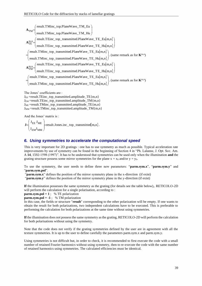
RETICOLO Code for the diffraction by stacks of lamellar gratings
39
=
Hu_TM_PlaneWave.top_TMinc.result
Eu_TM_PlaneWave.top_TMinc.result
TMA
=
n,mHu_TE_PlaneWave.dtransmitte_top_TEinc.result
n,mEu_TE_PlaneWave.dtransmitte_top_TEinc.resultn,m
TEA
=
n,mHu_TE_PlaneWave.dtransmitte_top_TMinc.result
n,mEu_TE_PlaneWave.dtransmitte_top_TMinc.result. (same remark as for Km,n)
=
n,mHu_TE_PlaneWave.dtransmitte_top_TEinc.result
n,mEu_TE_PlaneWave.dtransmitte_top_TEinc.resultn,m
TMA
=
n,mHu_TE_PlaneWave.dtransmitte_top_TMinc.result
n,mEu_TE_PlaneWave.dtransmitte_top_TMinc.result. (same remark as for Km,n)
The Jones’ coefficients are :
JEE =result.TEinc_top_transmitted.amplitude_TE{m,n}
JEM =result.TEinc_top_transmitted.amplitude_TM{m,n}
JME =result.TMinc_top_transmitted.amplitude_TE{m,n}
JMM =result.TMinc_top_transmitted.amplitude_TM{m,n}
And the Jones’ matrix is :
n,mdtransmitte_top_inc.Jones.resultJJ
JJ
MMEM
MEEE=
=J .
6. Using symmetries to accelerate the computational speed
This is very important for 2D gratings : one has to use symmetry as much as possible. Typical acceleration rate
improvements by use of symmetry can be found in the beginning of Section 4 in “Ph. Lalanne, J. Opt. Soc. Am.
A 14, 1592-1598 (1997)”. It has to be understood that symmetries can be used only when the illumination and the
grating structure possess some mirror symmetries for the plane x = x0 and/or y = y0.
To use the symmetry, the user needs to define three new parameters: “parm.sym.x”, “parm.sym.y” and
“parm.sym.pol”.
“parm.sym.x” defines the position of the mirror symmetry plane in the x-direction (if exist)
“parm.sym.y” defines the position of the mirror symmetry plane in the y-direction (if exist)
If the illumination possesses the same symmetry as the grating (for details see the table below),. RETICOLO-2D
will perform the calculation for a single polarisation, according to :
parm.sym.pol = 1 ; % TE polarization
parm.sym.pol = -1 ; % TM polarization
In this case, the fields or structure "result" corresponding to the other polarization will be empty. If one wants to
obtain the result for both polarizations, two independent calculations have to be executed. This is preferable to
performing the calculation for both polarizations at the same time without using symmetries.
If the illumination does not possess the same symmetry as the grating, RETICOLO-2D will perform the calculation
for both polarisations without using the symmetry.
Note that the code does not verify if the grating symmetries defined by the user are in agreement with all the
texture symmetries. It is up to the user to define carefully the parameters parm.sym.x and parm.sym.y.
Using symmetries is not difficult but, in order to check, it is recommended to first execute the code with a small
number of retained Fourier harmonics without using symmetry, then to re-execute the code with the same number
of retained harmonics using symmetries. The calculated efficiencies must be identical.
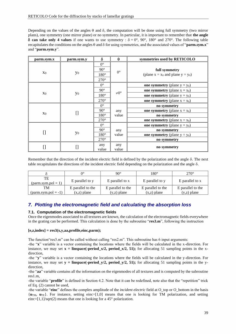
RETICOLO Code for the diffraction by stacks of lamellar gratings
39
Depending on the values of the angles and , the computation will be done using full symmetry (two mirror
plans), one symmetry (one mirror plane) or no symmetry. In particular, it is important to remember that the angle
can take only 4 values if one wants to use symmetry : = 0°, 90°, 180° and 270°. The following table
recapitulates the conditions on the angles and for using symmetries, and the associated values of “parm.sym.x”
and “parm.sym.y”.
parm.sym.x parm.sym.y symmetries used by RETICOLO
x0 y0
0°
0° full symmetry
(plane x = x0 and plane y = y0)
90°
180°
270°
x0 y0
0°
0°
one symmetry (plane y = y0)
90° one symmetry (plane x = x0)
180° one symmetry (plane y = y0)
270° one symmetry (plane x = x0)
x0 []
0°
any
value
no symmetry
90° one symmetry (plane x = x0)
180° no symmetry
270° one symmetry (plane x = x0)
[] y0
0°
any
value
one symmetry (plane y = y0)
90° no symmetry
180° one symmetry (plane y = y0)
270° no symmetry
[] [] any
value
any
value no symmetry
Remember that the direction of the incident electric field is defined by the polarization and the angle . The next
table recapitulates the directions of the incident electric field depending on the polarization and the angle .
0° 90° 180° 270°
TE
(parm.sym.pol = 1) E parallel to y E parallel to x E parallel to y E parallel to x
TM
(parm.sym.pol = -1)
E parallel to the
(x,z) plane
E parallel to the
(y,z) plane
E parallel to the
(x,z) plane
E parallel to the
(y,z) plane
7. Plotting the electromagnetic field and calculating the absorption loss
7.1. Computation of the electromagnetic fields Once the eigenmodes associated to all textures are known, the calculation of the electromagnetic fields everywhere
in the grating can be performed. This calculation is done by the subroutine “res3.m”, following the instruction
[e,z,index] = res3(x,y,aa,profile,einc,parm);
The function“res3.m” can be called without calling “res2.m”. This subroutine has 6 input arguments:
-the “x” variable is a vector containing the locations where the fields will be calculated in the x-direction. For
instance, we may set x = linspace(-period_x/2, period_x/2, 51); for allocating 51 sampling points in the x-
direction,
-the “y” variable is a vector containing the locations where the fields will be calculated in the y-direction. For
instance, we may set y = linspace(-period_y/2, period_y/2, 51); for allocating 51 sampling points in the y-
direction,
-the “aa” variable contains all the information on the eigenmodes of all textures and is computed by the subroutine
res1.m,
-the variable “profile” is defined in Section 4.2. Note that it can be redefined, note also that the “repetition” trick
of Eq. (2) cannot be used,
-the variable “einc” defines the complex amplitude of the incident electric field at O_top or O_bottom in the basis
{uTM, uTE}. For instance, setting einc=[1,0] means that one is looking for TM polarization, and setting
einc=[1,1]/sqrt(2) means that one is looking for a 45° polarization.
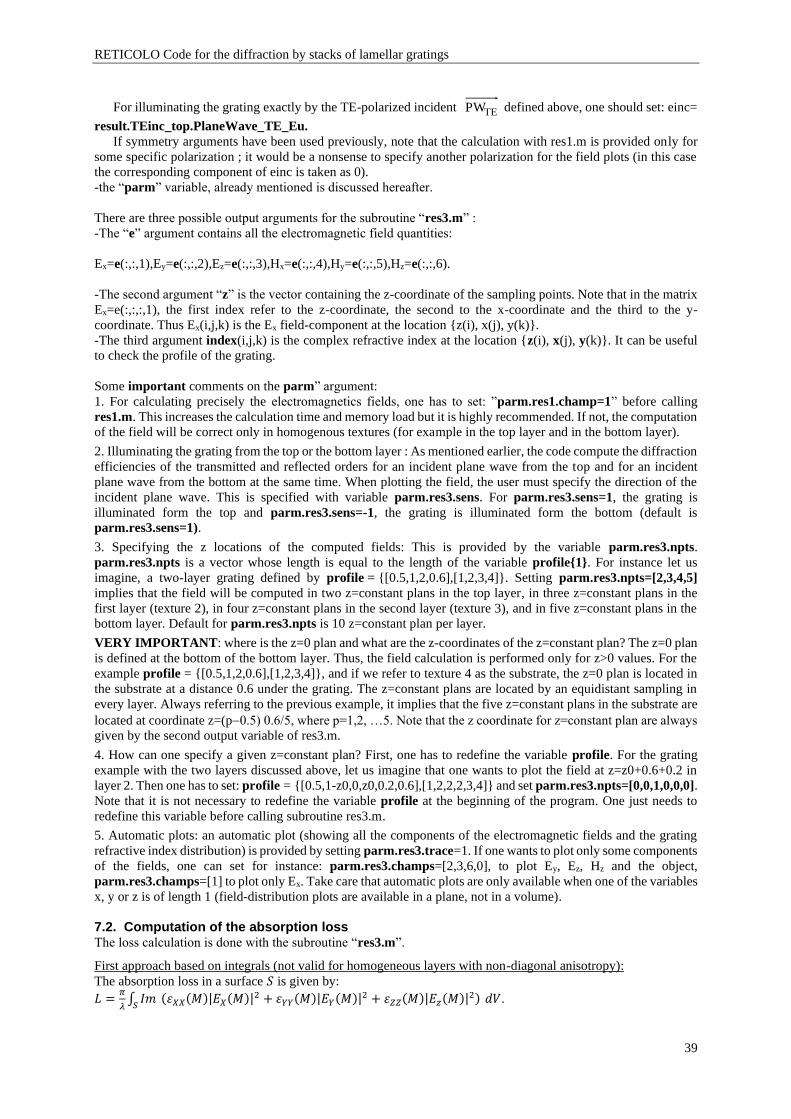
RETICOLO Code for the diffraction by stacks of lamellar gratings
39
For illuminating the grating exactly by the TE-polarized incident TEPW defined above, one should set: einc=
result.TEinc_top.PlaneWave_TE_Eu.
If symmetry arguments have been used previously, note that the calculation with res1.m is provided only for
some specific polarization ; it would be a nonsense to specify another polarization for the field plots (in this case
the corresponding component of einc is taken as 0).
-the “parm” variable, already mentioned is discussed hereafter.
There are three possible output arguments for the subroutine “res3.m” :
-The “e” argument contains all the electromagnetic field quantities:
Ex=e(:,:,1),Ey=e(:,:,2),Ez=e(:,:,3),Hx=e(:,:,4),Hy=e(:,:,5),Hz=e(:,:,6).
-The second argument “z” is the vector containing the z-coordinate of the sampling points. Note that in the matrix
Ex=e(:,:,:,1), the first index refer to the z-coordinate, the second to the x-coordinate and the third to the y-
coordinate. Thus Ex(i,j,k) is the Ex field-component at the location {z(i), x(j), y(k)}.
-The third argument index(i,j,k) is the complex refractive index at the location {z(i), x(j), y(k)}. It can be useful
to check the profile of the grating.
Some important comments on the parm” argument:
1. For calculating precisely the electromagnetics fields, one has to set: ”parm.res1.champ=1” before calling
res1.m. This increases the calculation time and memory load but it is highly recommended. If not, the computation
of the field will be correct only in homogenous textures (for example in the top layer and in the bottom layer).
2. Illuminating the grating from the top or the bottom layer : As mentioned earlier, the code compute the diffraction
efficiencies of the transmitted and reflected orders for an incident plane wave from the top and for an incident
plane wave from the bottom at the same time. When plotting the field, the user must specify the direction of the
incident plane wave. This is specified with variable parm.res3.sens. For parm.res3.sens=1, the grating is
illuminated form the top and parm.res3.sens=-1, the grating is illuminated form the bottom (default is
parm.res3.sens=1).
3. Specifying the z locations of the computed fields: This is provided by the variable parm.res3.npts.
parm.res3.npts is a vector whose length is equal to the length of the variable profile{1}. For instance let us
imagine, a two-layer grating defined by profile = {[0.5,1,2,0.6],[1,2,3,4]}. Setting parm.res3.npts=[2,3,4,5]
implies that the field will be computed in two z=constant plans in the top layer, in three z=constant plans in the
first layer (texture 2), in four z=constant plans in the second layer (texture 3), and in five z=constant plans in the
bottom layer. Default for parm.res3.npts is 10 z=constant plan per layer.
VERY IMPORTANT: where is the z=0 plan and what are the z-coordinates of the z=constant plan? The z=0 plan
is defined at the bottom of the bottom layer. Thus, the field calculation is performed only for z>0 values. For the
example profile = {[0.5,1,2,0.6],[1,2,3,4]}, and if we refer to texture 4 as the substrate, the z=0 plan is located in
the substrate at a distance 0.6 under the grating. The z=constant plans are located by an equidistant sampling in
every layer. Always referring to the previous example, it implies that the five z=constant plans in the substrate are
located at coordinate z=(p−0.5) 0.6/5, where p=1,2, …5. Note that the z coordinate for z=constant plan are always
given by the second output variable of res3.m.
4. How can one specify a given z=constant plan? First, one has to redefine the variable profile. For the grating
example with the two layers discussed above, let us imagine that one wants to plot the field at z=z0+0.6+0.2 in
layer 2. Then one has to set: profile = {[0.5,1-z0,0,z0,0.2,0.6],[1,2,2,2,3,4]} and set parm.res3.npts=[0,0,1,0,0,0].
Note that it is not necessary to redefine the variable profile at the beginning of the program. One just needs to
redefine this variable before calling subroutine res3.m.
5. Automatic plots: an automatic plot (showing all the components of the electromagnetic fields and the grating
refractive index distribution) is provided by setting parm.res3.trace=1. If one wants to plot only some components
of the fields, one can set for instance: parm.res3.champs=[2,3,6,0], to plot Ey, Ez, Hz and the object,
parm.res3.champs=[1] to plot only Ex. Take care that automatic plots are only available when one of the variables
x, y or z is of length 1 (field-distribution plots are available in a plane, not in a volume).
7.2. Computation of the absorption loss The loss calculation is done with the subroutine “res3.m”.
First approach based on integrals (not valid for homogeneous layers with non-diagonal anisotropy):
The absorption loss in a surface 𝑆 is given by:
𝐿 =𝜋
𝜆∫ 𝐼𝑚 (𝜀𝑋𝑋(𝑀)|𝐸𝑋(𝑀)|2 + 𝜀𝑌𝑌(𝑀)|𝐸𝑌(𝑀)|2 + 𝜀𝑍𝑍(𝑀)|𝐸𝑧(𝑀)|2) 𝑑𝑉
𝑆.
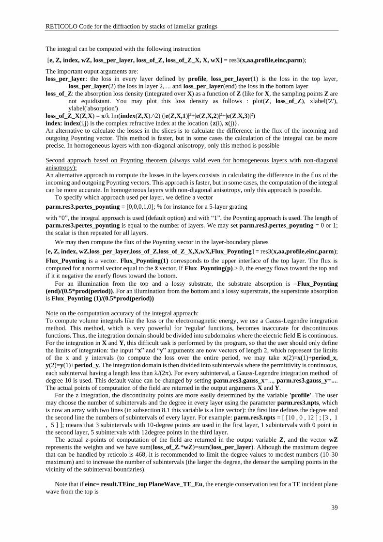
RETICOLO Code for the diffraction by stacks of lamellar gratings
39
The integral can be computed with the following instruction
[e, Z, index, wZ, loss_per_layer, loss_of_Z, loss_of_Z_X, X, wX] = res3(x,aa,profile,einc,parm);
The important ouput arguments are:
loss_per_layer: the loss in every layer defined by profile, loss_per_layer(1) is the loss in the top layer,
loss_per_layer(2) the loss in layer 2, ... and loss_per_layer(end) the loss in the bottom layer
loss_of_Z: the absorption loss density (integrated over X) as a function of Z (like for X, the sampling points Z are
not equidistant. You may plot this loss density as follows : plot(Z, loss_of_Z), xlabel('Z'),
ylabel('absorption')
loss_of_Z_X(Z,X) = π/λ Im(index(Z,X).^2) (|e(Z,X,1)|2+|e(Z,X,2)|2+|e(Z,X,3)|2)
index: index(i,j) is the complex refractive index at the location {z(i), x(j)}.
An alternative to calculate the losses in the slices is to calculate the difference in the flux of the incoming and
outgoing Poynting vector. This method is faster, but in some cases the calculation of the integral can be more
precise. In homogeneous layers with non-diagonal anisotropy, only this method is possible
Second approach based on Poynting theorem (always valid even for homogeneous layers with non-diagonal
anisotropy):
An alternative approach to compute the losses in the layers consists in calculating the difference in the flux of the
incoming and outgoing Poynting vectors. This approach is faster, but in some cases, the computation of the integral
can be more accurate. In homogeneous layers with non-diagonal anisotropy, only this approach is possible.
To specify which approach used per layer, we define a vector
parm.res3.pertes_poynting = [0,0,0,1,0]; % for instance for a 5-layer grating
with “0”, the integral approach is used (default option) and with “1”, the Poynting approach is used. The length of
parm.res3.pertes_poynting is equal to the number of layers. We may set parm.res3.pertes_poynting = 0 or 1;
the scalar is then repeated for all layers.
We may then compute the flux of the Poynting vector in the layer-boundary planes
[e, Z, index, wZ,loss_per_layer,loss_of_Z,loss_of_Z_X,X,wX,Flux_Poynting] = res3(x,aa,profile,einc,parm);
Flux_Poynting is a vector. Flux_Poynting(1) corresponds to the upper interface of the top layer. The flux is
computed for a normal vector equal to the �̂� vector. If Flux_Poynting(p) > 0, the energy flows toward the top and
if it it negative the enerfy flows toward the bottom.
For an illumination from the top and a lossy substrate, the substrate absorption is −Flux_Poynting
(end)/(0.5*prod(period)). For an illumination from the bottom and a lossy superstrate, the superstrate absorption
is Flux_Poynting (1)/(0.5*prod(period))
Note on the computation accuracy of the integral approach:
To compute volume integrals like the loss or the electromagnetic energy, we use a Gauss-Legendre integration
method. This method, which is very powerful for 'regular' functions, becomes inaccurate for discontinuous
functions. Thus, the integration domain should be divided into subdomains where the electric field E is continuous.
For the integration in X and Y, this difficult task is performed by the program, so that the user should only define
the limits of integration: the input “x” and “y” arguments are now vectors of length 2, which represent the limits
of the x and y intervals (to compute the loss over the entire period, we may take x(2)=x(1)+period_x,
y(2)=y(1)+period_y. The integration domain is then divided into subintervals where the permittivity is continuous,
each subinterval having a length less than /(2). For every subinterval, a Gauss-Legendre integration method of
degree 10 is used. This default value can be changed by setting parm.res3.gauss_x=..., parm.res3.gauss_y=....
The actual points of computation of the field are returned in the output arguments X and Y.
For the z integration, the discontinuity points are more easily determined by the variable 'profile'. The user
may choose the number of subintervals and the degree in every layer using the parameter parm.res3.npts, which
is now an array with two lines (in subsection 8.1 this variable is a line vector): the first line defines the degree and
the second line the numbers of subintervals of every layer. For example: parm.res3.npts = [ [10 , 0 , 12 ] ; [3 , 1
, 5 ] ]; means that 3 subintervals with 10-degree points are used in the first layer, 1 subintervals with 0 point in
the second layer, 5 subintervals with 12degree points in the third layer.
The actual z-points of computation of the field are returned in the output variable Z, and the vector wZ
represents the weights and we have sum(loss_of_Z.*wZ)=sum(loss_per_layer). Although the maximum degree
that can be handled by reticolo is 468, it is recommended to limit the degree values to modest numbers (10-30
maximum) and to increase the number of subintervals (the larger the degree, the denser the sampling points in the
vicinity of the subinterval boundaries).
Note that if einc= result.TEinc_top PlaneWave_TE_Eu, the energie conservation test for a TE incident plane
wave from the top is
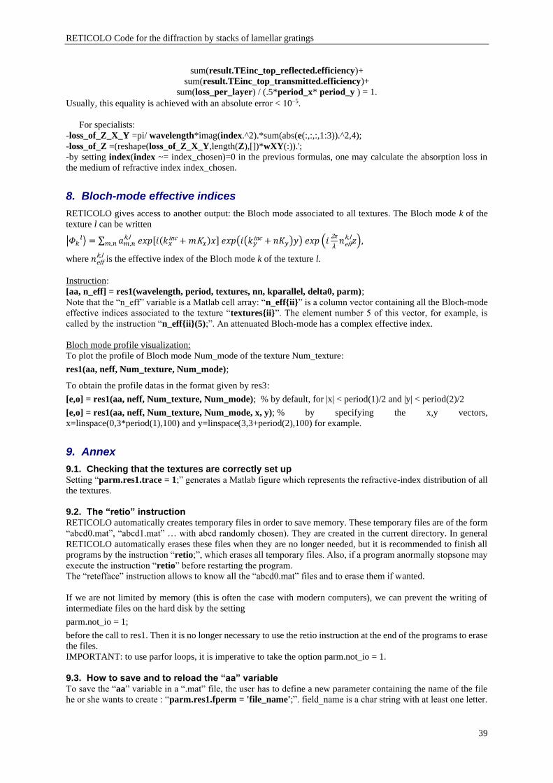
RETICOLO Code for the diffraction by stacks of lamellar gratings
39
sum(result.TEinc_top_reflected.efficiency)+
sum(result.TEinc_top_transmitted.efficiency)+
sum(loss_per_layer) / (.5*period_x* period_y ) = 1.
Usually, this equality is achieved with an absolute error < 10−5.
For specialists:
-loss_of_Z_X_Y =pi/ wavelength*imag(index.^2).*sum(abs(e(:,:,:,1:3)).^2,4);
-loss_of_Z =(reshape(loss_of_Z_X_Y,length(Z),[])*wXY(:)).';
-by setting index(index ~= index_chosen)=0 in the previous formulas, one may calculate the absorption loss in
the medium of refractive index index_chosen.
8. Bloch-mode effective indices
RETICOLO gives access to another output: the Bloch mode associated to all textures. The Bloch mode k of the
texture l can be written
|𝛷𝑘𝑙⟩ = ∑ 𝑎𝑚,𝑛
k,l 𝑒𝑥𝑝[𝑖(𝑘𝑥inc + 𝑚K𝑥)𝑥] 𝑒𝑥𝑝(𝑖(𝑘𝑦
inc + 𝑛𝐾𝑦)𝑦) 𝑒𝑥𝑝 (𝑖2π
𝜆𝑛eff
k,l 𝑧)𝑚,𝑛 ,
where 𝑛effk,l
is the effective index of the Bloch mode k of the texture l.
Instruction:
[aa, n_eff] = res1(wavelength, period, textures, nn, kparallel, delta0, parm);
Note that the “n_eff” variable is a Matlab cell array: “n_eff{ii}” is a column vector containing all the Bloch-mode
effective indices associated to the texture “textures{ii}”. The element number 5 of this vector, for example, is
called by the instruction “n_eff{ii}(5);”. An attenuated Bloch-mode has a complex effective index.
Bloch mode profile visualization:
To plot the profile of Bloch mode Num_mode of the texture Num_texture:
res1(aa, neff, Num_texture, Num_mode);
To obtain the profile datas in the format given by res3:
[e,o] = res1(aa, neff, Num_texture, Num_mode); % by default, for |x| < period(1)/2 and |y| < period(2)/2
[e,o] = res1(aa, neff, Num_texture, Num_mode, x, y); % by specifying the x,y vectors,
x=linspace(0,3*period(1),100) and y=linspace(3,3+period(2),100) for example.
9. Annex
9.1. Checking that the textures are correctly set up Setting “parm.res1.trace = 1;” generates a Matlab figure which represents the refractive-index distribution of all
the textures.
9.2. The “retio” instruction RETICOLO automatically creates temporary files in order to save memory. These temporary files are of the form
“abcd0.mat”, “abcd1.mat” … with abcd randomly chosen). They are created in the current directory. In general
RETICOLO automatically erases these files when they are no longer needed, but it is recommended to finish all
programs by the instruction “retio;”, which erases all temporary files. Also, if a program anormally stopsone may
execute the instruction “retio” before restarting the program.
The “retefface” instruction allows to know all the “abcd0.mat” files and to erase them if wanted.
If we are not limited by memory (this is often the case with modern computers), we can prevent the writing of
intermediate files on the hard disk by the setting
parm.not_io = 1;
before the call to res1. Then it is no longer necessary to use the retio instruction at the end of the programs to erase
the files.
IMPORTANT: to use parfor loops, it is imperative to take the option parm.not_io = 1.
9.3. How to save and to reload the “aa” variable To save the “aa” variable in a “.mat” file, the user has to define a new parameter containing the name of the file
he or she wants to create : “parm.res1.fperm = 'file_name';”. field_name is a char string with at least one letter.
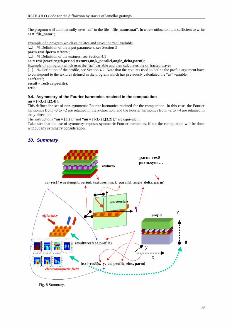
RETICOLO Code for the diffraction by stacks of lamellar gratings
39
The program will automatically save “aa” in the file “file_name.mat”. In a new utilisation it is sufficient to write
aa = 'file_name';.
Example of a program which calculates and saves the “aa” variable
[...] % Definition of the input parameters, see Section 3
parm.res1.fperm = 'toto';
[...] % Definition of the textures, see Section 4.1
aa = res1(wavelength,period,textures,nn,k_parallel,angle_delta,parm);
Example of a program which uses the “aa” variable and then calculates the diffracted waves
[...] % Definition of the profile, see Section 4.2. Note that the textures used to define the profile argument have
to correspond to the textures defined in the program which has previously calculated the “aa” variable.
aa=’toto’;
result = res2(aa,profile);
retio;
9.4. Asymmetry of the Fourier harmonics retained in the computation nn = [[-3,-2];[2,4]];
This defines the set of non-symmetric Fourier harmonics retained for the computation. In this case, the Fourier
harmonics from –3 to +2 are retained in the x-direction, and the Fourier harmonics from –2 to +4 are retained in
the y-direction.
The instructions “nn = [3,2];” and “nn = [[-3,-2];[3,2]];” are equivalent.
Take care that the use of symmetry imposes symmetric Fourier harmonics, if not the computation will be done
without any symmetry consideration.
10. Summary
aa=res1( wavelength, period, textures, nn, k_parallel, angle_delta, parm)
result=res2(aa,profile)
[e,z]=res3(x, y, aa, profile, einc, parm)
profile
textures
efficiency
electromagnetic field
parameters
0
z
x
y
parm=res0
parm.sym …
Fig. 8 Summary.
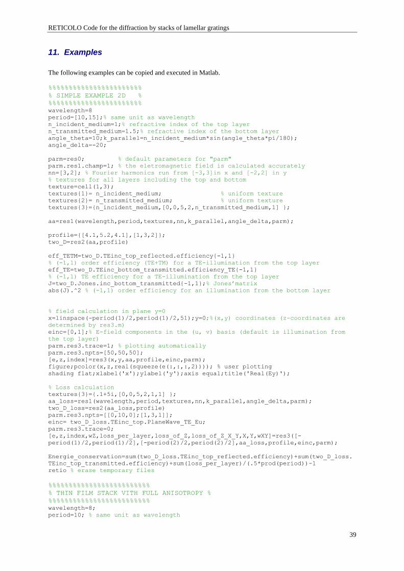
RETICOLO Code for the diffraction by stacks of lamellar gratings
39
11. Examples
The following examples can be copied and executed in Matlab.
%%%%%%%%%%%%%%%%%%%%%%%
% SIMPLE EXAMPLE 2D %
%%%%%%%%%%%%%%%%%%%%%%%
wavelength=8
period=[10,15];% same unit as wavelength
n_incident_medium=1;% refractive index of the top layer
n_transmitted_medium=1.5;% refractive index of the bottom layer
angle_theta=10;k_parallel=n_incident_medium*sin(angle_theta*pi/180);
angle_delta=-20;
parm=res0; % default parameters for "parm"
parm.res1.champ=1; % the eletromagnetic field is calculated accurately
nn=[3,2]; % Fourier harmonics run from [-3,3]in x and [-2,2] in y
% textures for all layers including the top and bottom
texture=cell(1,3);
textures{1}= n_incident_medium; % uniform texture
textures{2}= n_transmitted_medium; % uniform texture
textures{3}={n_incident_medium,[0,0,5,2,n_transmitted_medium,1] };
aa=res1(wavelength,period,textures,nn,k_parallel,angle_delta,parm);
profile={[4.1,5.2,4.1],[1,3,2]};
two_D=res2(aa,profile)
eff_TETM=two_D.TEinc_top_reflected.efficiency{-1,1}
% (-1,1) order efficiency (TE+TM) for a TE-illumination from the top layer
eff_TE=two_D.TEinc_bottom_transmitted.efficiency_TE{-1,1}
% (-1,1) TE efficiency for a TE-illumination from the top layer
J=two_D.Jones.inc_bottom_transmitted{-1,1};% Jones’matrix
abs(J).^2 % (-1,1) order efficiency for an illumination from the bottom layer
% field calculation in plane y=0
x=linspace(-period(1)/2,period(1)/2,51);y=0;%(x,y) coordinates (z-coordinates are
determined by res3.m)
einc=[0,1];% E-field components in the (u, v) basis (default is illumination from
the top layer)
parm.res3.trace=1; % plotting automatically
parm.res3.npts=[50,50,50];
[e,z,index]=res3(x,y,aa,profile,einc,parm);
figure;pcolor(x,z,real(squeeze(e(:,:,:,2)))); % user plotting
shading flat;xlabel('x');ylabel('y');axis equal;title('Real(Ey)');
% Loss calculation
textures{3}={.1+5i,[0,0,5,2,1,1] };
aa_loss=res1(wavelength,period,textures,nn,k_parallel,angle_delta,parm);
two_D_loss=res2(aa_loss,profile)
parm.res3.npts=[[0,10,0];[1,3,1]];
einc= two_D_loss.TEinc_top.PlaneWave_TE_Eu;
parm.res3.trace=0;
[e,z,index,wZ,loss_per_layer,loss_of_Z,loss_of_Z_X_Y,X,Y,wXY]=res3([-
period(1)/2,period(1)/2],[-period(2)/2,period(2)/2],aa_loss,profile,einc,parm);
Energie_conservation=sum(two_D_loss.TEinc_top_reflected.efficiency)+sum(two_D_loss.
TEinc_top_transmitted.efficiency)+sum(loss_per_layer)/(.5*prod(period))-1
retio % erase temporary files
%%%%%%%%%%%%%%%%%%%%%%%%%
% THIN FILM STACK VITH FULL ANISOTROPY %
%%%%%%%%%%%%%%%%%%%%%%%%%
wavelength=8;
period=10; % same unit as wavelength
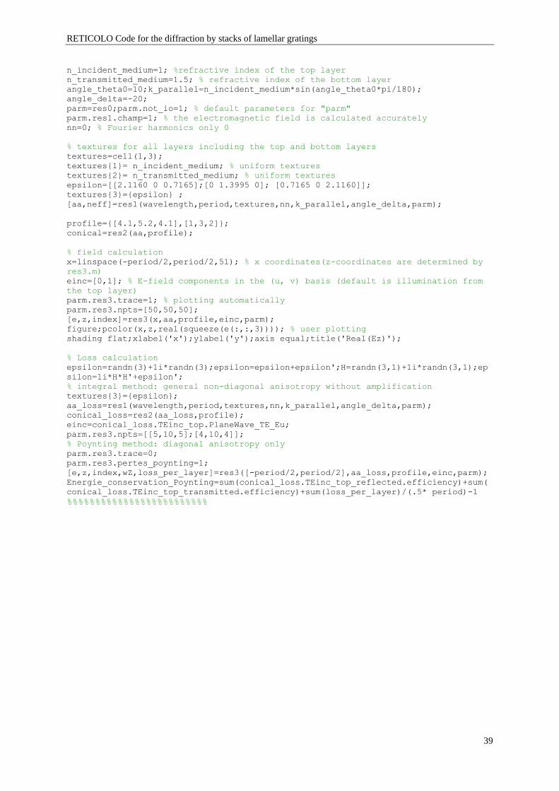
RETICOLO Code for the diffraction by stacks of lamellar gratings
39
n_incident_medium=1; %refractive index of the top layer
n_transmitted_medium=1.5; % refractive index of the bottom layer
angle_theta0=10;k_parallel=n_incident_medium*sin(angle_theta0*pi/180);
angle_delta=-20;
parm=res0;parm.not_io=1; % default parameters for "parm"
parm.res1.champ=1; % the electromagnetic field is calculated accurately
nn=0; % Fourier harmonics only 0
% textures for all layers including the top and bottom layers
textures=cell(1,3);
textures{1}= n_incident_medium; % uniform textures
textures{2}= n_transmitted_medium; % uniform textures
epsilon=[[2.1160 0 0.7165];[0 1.3995 0]; [0.7165 0 2.1160]];
textures{3}={epsilon} ;
[aa,neff]=res1(wavelength,period,textures,nn,k_parallel,angle_delta,parm);
profile={[4.1,5.2,4.1],[1,3,2]};
conical=res2(aa,profile);
% field calculation
x=linspace(-period/2,period/2,51); % x coordinates(z-coordinates are determined by
res3.m)
einc=[0,1]; % E-field components in the (u, v) basis (default is illumination from
the top layer)
parm.res3.trace=1; % plotting automatically
parm.res3.npts=[50,50,50];
[e,z,index]=res3(x,aa,profile,einc,parm);
figure;pcolor(x,z,real(squeeze(e(:,:,3)))); % user plotting
shading flat;xlabel('x');ylabel('y');axis equal;title('Real(Ez)');
% Loss calculation
epsilon=randn(3)+1i*randn(3);epsilon=epsilon+epsilon';H=randn(3,1)+1i*randn(3,1);ep
silon=1i*H*H'+epsilon';
% integral method: general non-diagonal anisotropy without amplification
textures{3}={epsilon};
aa_loss=res1(wavelength,period,textures,nn,k_parallel,angle_delta,parm);
conical_loss=res2(aa_loss,profile);
einc=conical_loss.TEinc_top.PlaneWave_TE_Eu;
parm.res3.npts=[[5,10,5];[4,10,4]];
% Poynting method: diagonal anisotropy only
parm.res3.trace=0;
parm.res3.pertes_poynting=1;
[e,z,index,wZ,loss_per_layer]=res3([-period/2,period/2],aa_loss,profile,einc,parm);
Energie_conservation_Poynting=sum(conical_loss.TEinc_top_reflected.efficiency)+sum(
conical_loss.TEinc_top_transmitted.efficiency)+sum(loss_per_layer)/(.5* period)-1
%%%%%%%%%%%%%%%%%%%%%%%%%


