The Effect of the Normalization Method Used in Different

International Journal of Assessment Tools in Education2019, Vol. 6, No. 2, 170–192https://dx.doi.org/10.21449/ijate.479404Published at http://www.ijate.net http://dergipark.gov.tr/ijate Research Article

170

The Effect of the Normalization Method Used in Different Sample Sizes onthe Success of Artificial Neural Network Model

Gökhan Aksu 1*, Cem Oktay Güzeller 2, Mehmet Taha Eser 3

1 Adnan Menderes University, Vocational High School, Aydın, Turkey2 Akdeniz University, Faculty of Tourism, Antalya, Turkey3 Akdeniz University, Statistical Consultation Center, Antalya, Turkey

ARTICLE HISTORY

Received: 07 November 2018

Revised: 19 February 2019

Accepted: 20 March 2019

KEYWORDS

Artificial Neural Networks,Prediction,MATLAB,Normalization

Abstract: In this study, it was aimed to compare different normalizationmethods employed in model developing process via artificial neuralnetworks with different sample sizes. As part of comparison ofnormalization methods, input variables were set as: work discipline,environmental awareness, instrumental motivation, science self-efficacy,and weekly science learning time that have been covered in PISA 2015,whereas students' Science Literacy level was defined as the output variable.The amount of explained variance and the statistics about the correctclassification ratios were used in the comparison of the normalizationmethods discussed in the study. The dataset was analyzed in Matlab2017bsoftware and both prediction and classification algorithms were used in thestudy. According to the findings of the study, adjusted min-maxnormalization method yielded better results in terms of the amount ofexplained variance in different sample sizes compared to othernormalization methods; no significant difference was found in correctclassification rates according to the normalization method of the data, whichlacked normal distribution and the possibility of overfitting should be takeninto consideration when working with small samples in the modellingprocess of artificial neural network. In addition, it was also found thatsample size had a significant effect on both classification and predictionanalyzes performed with artificial neural network methods. As a result ofthe study, it was concluded that with a sample size over 1000, moreconsistent results can be obtained in the studies performed with artificialneural networks in the field of education.

1. INTRODUCTION

The data collected from different applications require proper method of extracting knowledgefrom large repositories for better decision making. Knowledge discovery in databases (KDD),often called data mining, aims at the discovery of useful information from large collections ofdata (Mannila, 1996). Decision tree, nearest neighborhood, support vector machine, NaiveBayes classifier and artificial neural networks are among the main classification methods andthey are supervised learning approaches (Neelamegam & Ramaraj, 2013). Educational data

CONTACT: Gökhan Aksu [email protected] Menderes University, Vocational HighSchool, Aydın, Turkey

ISSN-e: 2148-7456 /© IJATE 2019

Int. J. Asst. Tools in Educ., Vol. 6, No. 2, (2019) pp. 170–192

171

mining is concerned developing methods for predict student’s academic performance and theirbehaviour towards education by the data that come from educational database (Upadhyay,2016). It aims at devising and using algorithms to improve educational results and explaineducational strategies for further decision making (Silva & Fonseca, 2017). Artificial NeuralNetworks (ANN) is one of the essential mechanisms used in machine learning. Due to theirexcellent capability of self-learning and self-adapting, they have been extensively studied andhave been successfully utilized to tackle difficult real-world problems (Bishop 1995; Haykin1999). Compared to the other approaches, Artificial Neural Networks (ANN), which is one ofthe most effective computation methods applied in data mining and machine learning, seems tobe one of the best and most popular approaches (Gschwind, 2007; Hayashi, Hsieh, & Setiono,2009). The word “Neural” (called as neuron or node, as part of this study the term “node” wasused) included in the name Artificial Neural Network, indicates that the learning structure ofhuman brain was taken as the basis of learning within the system. For a programmer, ANN isthe perfect tool to discover the patterns that are very complex and numerous. The main strengthof ANN lies on predicting multi-directional and non-linear relationships between input andoutput data (Azadeh, Sheikhalishahi, Tabesh, & Negahban, 2011). ANN, which can be used aspart of many disciplines, is frequently used in classification, prediction and finding solutions tolearning problems that involve the minimization of the disadvantages of traditional methods.Non-linear problems can also be solved through ANN, besides linear problems (Uslu, 2013).

Fundamentally, there are three different layers in an artificial neural network; namely inputlayer, hidden layers and output layer. Input layer communicate with the outer environment thatcontributes neural network to have a pattern. Input layer deals only with the inputs. Input layershould represent the condition where the neural network would be trained. Each input nodeshould represent some independent variables that have an effect on the output of the neuralnetwork. Hidden layer is the layers on which the nodes executing activation function aregathered, they are located between input layer and output layer. Hidden layer is formed by manylayers. The task of the hidden layer is processing the input obtained from the previous layer.Therefore, hidden layer is the layer that is responsible for deriving requested outcomes usinginput data (Kriesel, 2007). Numerous studies have been conducted to determine the number ofthe nodes included in the hidden layer but none of these researches were successful in findingthe correct result. Moreover, an ANN may contain more than one hidden layer. There are nosingle formulas for computing the number of the hidden layers and the number of nodes in eachhidden layer, various methods are used for this purpose. The output layer of an ANN collectsand transmits the data considering the design to which the data will be transferred. The designrepresented by the output layer can be directly tracked up to the input layer. The number ofnodes in an output layer should be directly associates to the performance of the neural network.The objective of the relevant neural network should be considered while determining thenumber of nodes in the output layer.

Artificial Neural Networks, is made of artificial neural network cells. An artificial neuralnetwork cell is built on two essential structures, namely neurons and synapses. A node (neuron)is a mathematical function that models the operation of a biologic node. In theory, an artificialnode is formed by a transformation function and an activation function along with a group ofweighted input. A typical node computes the weighted average of its input and this sum isusually processed by a non-linear function (i.e. sigmoid) called as activation function. Theoutput of a node may be sent as input to the nodes of another layer that repeats the samecomputation. The nodes constitute the layers. Each node is connected to another node througha connection. Each connection is associated with a weight, including information about theinput signal. Being associated with a weight is one of the most useful information for the nodeswhile solving a problem because the weight usually triggers or blocks the transmitted signal.Each node has an implicit status called as activation signal. The produced output signals are

Aksu, Güzeller & Eser

172

allowed to be sent to the other units after combining input signal with the activation rule (Hagan,Demuth, Beale, & Jesus, 2014).

Main operating principle of an artificial neural network is s below:

1) Input nodes should represent an input based on the information that we attempt toclassify.

2) A weight is given to each number in the input nodes for each connection.3) In each node located at the next layer, the outputs of the connections coming to this

layer are triggered and added and an activation function is applied to the weighted sum.4) The output of the function is taken as the input of the next connection layer and this

process continues until the output layer is reached (O’Shea & Nash, 2015).

Artificial Neural Networks was built inspiring from biological neural system, in other wordshuman brain’s working pattern. Since the most important characteristic of human brain islearning, the same characteristic was adopted in ANN as well. Artificial Neural Networks is acomplex and adaptive system that can change its inner structure based on the information thatit possesses. Being a complex, adaptive system, the learning of ANN is based on the fact thatinput/output behavior may vary according to the change occurring in the surrounding of a node.Another important feature of neural networks is they have an iterative learning process in whichdata status (lines) are represented to the network one by one and the weights associated withinput values are modified at every turn. Usually the process restarts when all cases arerepresented. A network of learning stage learns by modifying the weights so that the correctclass definitions of input samples are predicted. Neural network learning is also called as“Learning to make a connection” because of the connections among the nodes (Davydov,Osipov, Kilin, & Kulchitsky, 2018).

The most important point in the application of artificial neural networks to real-world problemsis to be able to understand the solution that will be determined without being complicated, easyto interpret and in a practical way to the real world. The common point of these three featuresis very closely related to how the data is managed and processed. Normalization plays a verycritical role, especially in the context of intelligibility and easy interpretation in the most criticalpoint of data management (Weigend & Gershenfeld, 1994; Yu, Wang, & Lai, 2006). Thenormalization process, in which the data is sensible and reassembled in a much smaller interval,arises as a need in the case of a method usually used on very large data sets, such as artificialneural networks. In the case of artificial neural networks, the number of nodes in the input, thenumber of nodes in the hidden layer, and the number of nodes in the output are very importantelements, and the connection for any two layers is called positive or negative weight (Hagan,Demuth, Beale, & Jesus, 2014). The algorithm used in the artificial neural network-based modelestablished when different ranges are used for the variables in the data set will most likely notbe able to discover the possible correlation between the variables. At the same time, the factthat there are different intervals for the variables in the data set causes these weights to beaffected in different meanings. And at the same time, the use of variables with very differentintervals is eliminated in the geometric sense, and the results obtained from the experiments oranalyzes and the results obtained from the experiments in the artificial neural network areeliminated in a smaller and specific range. normalization is needed to make interpretationsmuch easier for the total of variables (Lou, 1993; Weigend & Gershenfeld, 1994; Yu, Wang, &Lai, 2006). And in normal neural network based studies, which are used on normalizationprocess, especially on the methodological data, the number of variables can be high and thepractical benefits of real life are desired, it is more needed in artificial neural network basedstudies.

A network gets ready to learn after being configured for a certain application. The configurationprocess of a network for a certain application is called as “Preliminary preparation process”.


173

Following the completion of the preparation belonging to the preliminary process, eithertraining or learning starts. The network processes the records of the training data at a time usingthe weights and functions in the hidden layers, then compare the outputs with desired outputs.Afterwards, the errors are distributed backwards in the system, which allows the system tomodify application weights for the subsequent records to be processed. This process takes placecontinuously as the weights are modified. The same data sample may be processed many timessince the connection weighs are continuously refined during the training of a network (Wang,Devabhaktuni, Xi, & Zhang, 1998).

The preliminary data processing of an artificial neural network modelling is a process havingbroad applications, rather than a limited definition. Almost all theoretical and practical researchinvolving neural networks focus on the data preparation for neural networks, normalizing datafor conversion and dividing the data for training (Gardner & Dorling, 1998; Rafiq, Bugmann,& Easterbrook, 2001; Krycha & Wagner, 1999; Hunt, Sbarbaro, Bikowski, & Gawthrop, 1992;Rumelhart, 1994; Azimi Sadjadi & Stricker, 1994). In some studies, neural networks were usedfor modelling purposes without any data preparation procedure. For these studies, there is animplicit assumption indicating that all data were prepared in advance so that they can be directlyused in modelling. Regarding the practice, it cannot be said that the data is always ready foranalysis. Usually there are limitations about the integrity and quality of the data. As a result,complex data analysis process cannot be successful without performing a preliminarypreparation process to the data. Researches revealed that data quality has significant impact onartificial neural network models (Famili, Shen, Weber, & Simoudis, 1997; Zhang, Zhang, &Yang, 2003). Smaller and better-quality data sets, which may significantly improve theefficiency of the data analysis, can be produced through preliminary data processing process.Regarding ANN learning, data preparation process allows the users to take decisions about howto represent the data, which concepts to be learned and how to present the outcomes of the dataanalysis, which makes explaining the data in the real world much easier (Redman, 1992; Klein& Rossin, 1999; Zang et al., 2003).

Applying a preliminary preparation process to the data is an important and critical step in neuralnetwork modelling for complex data analysis and it has considerable impact on the success ofthe data analysis performed as part of data mining. Input data affects the quality of neuralnetwork models and the results of the data analysis. Lou (2003) emphasized that the deficienciesin the input data may cause huge differences on the performance of the neural networks. Datathat was subject to preliminary processing play a major role in obtaining reliable analysisoutcomes. In theory, data lacking preliminary process makes data analysis difficult. In addition,data obtained from different data sources and produced by modern data collection techniquesmade data consumption a time-consuming task. 50-70% the time and effort spend on dataanalysis projects is claimed to be for data preparation. Therefore, preliminary data preparationprocess includes getting the data ready to analysis for improving complex data analysis (Sattler,2001; Hu, 2003; Lou, 2003).

There are few parameters affecting the learning process of an artificial neural network.Regarding the learning of the nodes as part of learning process, if a node fails, the remainingnodes may continue to operate without any problem. The weights of the connections located inan artificial neural cell vary, which plays a role in the success of the neural network and in theformation of the differences on the values involving the learning of the neural network. Inaddition to the weights, the settings about the number of nodes in the hidden layers and learningrate parameters affect neural network learning process as well. There is not a constant value forthe mentioned parameters. Usually expert knowledge plays a major role in determining theseparameters (Anderson, 1990; Lawrance, 1991; Öztemel, 2003). Sample size is also one of theparameters that affect learning process. According to “Central Limit Theorem”, each unbiased


174

samples coming from a universe with normal distribution, formed by independent observations,shows normal distribution provided that sample size is over 30. In addition, regardless of theuniverse, the shape of the distribution approaches to normal distribution as the sample sizeincreases and therefore the validity and reliability of the inferences to be made for theparameters increase (Dekking, Kraaikamp, Lopuhaä & Meester, 2005; Roussas, 2007; Ravid,2011). There is no rule indicating that at the end of the learning process the nodes will definitelylearn; some networks never learn.

Number of nodes and learning rate are not the only factors playing a role in making theexecution of certain preliminary data processing more effective as part of the neural networklearning. The normalization process of the raw input is as important as the other preliminarydata processes (reducing the size of the input field, noise reduction and feature extraction). Inmany artificial neural network applications, raw data (not processed or normalized prior to use)is used. As a result of using raw data, multi-dimensional data sets are employed and manyproblems are experienced, including longer analysis duration. The normalization of the data,which scales the data to the same range, minimizes the bias in the artificial neural network. Atthe same time the normalization of the data speeds up the process involving the learning of thefeatures covered in the same scale. In theory, the purpose of the normalization is rescaling theinput vector and modify the weight and bias corresponding to the relevant vector for obtainingthe same output features that have been obtained before (Bishop, 1995; Elmas, 2003;Ayalakshmi & Santhakumaran, 2011). In general, machine learning classifiers cannot computeEuclidian distance between features. Euclidian distance is the linear distance between twopoints (vectors of the nodes) located in Euclidian space, which is simply two or threedimensional. Therefore, the features should be normalized in order to prevent the bias that mayoccur in the model built with artificial neural network (Lou, 1993; Weigend & Gershenfeld,1994; Yu, Wang, & Lai, 2006).

In many cases normalization improves the performance but considering the normalization asmandatory for the operation of the algorithm is wrong. In case of a trained data set, whosemodel is unseen, using raw data may be more useful. There are many data normalizationmethods. Among them the most important ones are Z-score, min-max (feature scaling), median,adjusted min-max and sigmoid normalization methods. As part of the research, differentnormalization methods used in the process of modelling with Artificial Neural Networks (Z-score, min-max, median, adjusted min-max) were applied the learning, test, validation andoverall data sets and the results were compared. Below, the normalization methods used in theresearch are summarized:

1) Z-score Method: Mean and standard deviation of each feature are used across a seriesof learning data to normalize the vector of each feature included in the input data. Meanand standard deviation are calculated for each feature. The equality used in the methodis as below where indicates normalized data, xi input variable, μi arithmetic mean ofthe input variable and σi standard deviation of the input variable.= (1)

This procedure sets the mean of each feature in the data set equal to zero and standarddeviation to one. As a part of the procedure, first the normalization is applied to thefeature vectors in the data set. The mean and standard deviation are calculated for eachfeature over the training data and it is kept for using as weight in the final system design.In short, this procedure is a preliminary processing within the artificial neural networkstructure.


175

2) Min-Max Method: The method is used as an alternative to Z-score Method. This methodrescales the features or the outputs in any range into a new range. Usually the featuresare scaled between 0-1 or (-1)-1. The equality used in the method is as below where

indicates minimum value, maximum value, xi input value andnormalized data: = (2)

When min-max method is applied, each feature remains the same while taking place inthe new range. This method keeps all relational properties in the data.

3) Median Method: As part of median method, the median of each input is calculated andit is used for each sample. The method is not affected by extreme variations and it isquite useful in case of computing the ratio of two samples in hybrid form or to getinformation about the distribution. The equality used in the method is as below where

indicated normalized data, xi input variable:= ( ) (3)

4) Adjusted Min-Max Method: The forth normalization method is adjusted min-maxmethod. For the implementation of the method, all the data are normalized between 0.1and 0.9, with the equality used as part of the method. With the normalization, the dataset gets a dimensionless form. The equality used in the method is as below whereindicated normalized data, xi input variable, maximum value of the input variableand minimum value of the input variable:= 0.8 ∗ + 0.1 (4)

In adjusted min-max method, the results obtained in the previously given formula aremultiplied by a constant value of 0.8 and a constant value of 0.1 is added.

The variables used by the researchers working in the field of educational sciences can besummarized as situations related to the student in terms of the starting point, the situationsrelated to the personnel, the situations related to the administration and the situations related tothe school. All these cases reveal large data sets that need to be analyzed. These large data setsare data sets that consist of too many variables and too many students (participants). In recentyears, the concepts of machine learning, which are related to algorithms working in thebackground of data mining and data mining methods, are frequently mentioned in EducationalSciences. The analysis of the data sets formed by many variables and too many participantsfrom the databases related to Educational Sciences brought with it the concept of EducationalData Mining (Gonzalez & DesJardins, 2002; Scumacher, Olinsky, Quinn, & Smith, 2010;Romero & Ventura, 2011). Nowadays, in the context of educational data mining, studies onmodeling of education and training programs, predictive and classification based models onstudent and teacher are carried out. By using these purposes, artificial neural networks, decisiontrees, clustering and Bayesian based algorithms are used in the background (Gerasimovic,Stajenovic, Bugaric, Miljkovic, & Veljovic, 2011; Wook, Yahaya, Wahab, Isa, Awang, &Seong, 2009).

Artificial neural network is a non-linear model that is easy to use and understand compared toother methods. Most other statistical methods are evaluated within the scope of parametric


176

methods which require a statistical history. Artificial neural networks are often used to solveproblems related to estimation and classification. Artificial neural networks alone areinsufficient to interpret the relationship between input and output and to cope with uncertainsituations. However, these disadvantages can easily be overcome by the structure of artificialneural networks designed to be integrated with many different features (Schmidhuber, 2015;Goodfellow, Bengio, & Courville, 2016). Regarding all of these, the purpose of the researchwill be to determine the differentiation that different normalization methods employed in modeldeveloping process exhibit at different sample sizes. In the study, the changes on the predictionresults obtained from data sets of 250, 500, 1000, 1500 and 2000 cases, through differentnormalization methods were analyzed and the classification level of the normalization methodthat had best prediction results was evaluated. Determining the number of sample sizes thestudy conducted by Finch, West and Mackinnon (1997) in determining the number of samples,it was determined that there were differences in the estimations in different sample sizes. Inaddition, Fan, Wang and Thompson (1996) in their study showed that the calculation methodsin different sample sizes differed and this difference was significant especially in small samples.For this reason, within the framework of the specified objectives, the problem statement of theresearch was set as “Does the sample size affects the normalization method used in predictingscience literacy level of the students using work discipline, environmental awareness,instrumental motivation, science self-efficacy, and weekly science learning time variables inPISA 2015 Turkey sample”. The following research questions were addressed within theframework of the general purpose specified according to the main problem of the study:

1. Does sample size affect Z-score normalization method in the process of modellingwith ANN?

2. Does sample size affect min-max normalization method in the process of modellingwith ANN?

3. Does sample size affect median normalization method in the process of modellingwith ANN?

4. Does sample size affect adjusted min-max normalization method in the process ofmodelling with ANN?

5. Does sample size affect the best normalization method in the process of modellingwith ANN, in case of a two-category output variable?

Allowing input values and output values to be at the same range through the normalization ofthe research data has vital importance for the determination of very high or very low values inthe data (Güzeller & Aksu, 2018). Moreover, very high or very low values in the data, whichmay be originated from various reasons such as wrong data entry, may cause the network toproduce seriously wrong outputs; thus, the normalization of input and output data hassignificant importance for the consistency of the results.

2. METHOD2.1. Research Model

This study is accepted as a basic research because it is aiming to determine the normalizationmethod giving the best result by testing various methods used in modelling process whereArtificial Neural Networks were applied in different sample sizes (Frankel & Wallen, 2006;Karasar, 2009). Basic researches aim to add new knowledge to the existing one, in other wordsimproving the theory or testing existing theories (OECD, 2015).

2.2. Data Collection

The data used within the scope of the study were obtained from PISA 2015 test (MEB, 2016),which has been organized by OECD. The data obtained from 5895 students who haveparticipated in the test from Turkey universe were divided into groups of 250, 500, 1000, 1500


177

and 2000 through systematic sampling method. Students’ work discipline, environmentalawareness, instrumental motivation, science self-efficacy, and weekly science learning timevariables were used as the input variables, whereas students’ science literacy score was used asthe output variable. The names and codes of the input and output variables covered in the studyare illustrated in Table 1.

Table 1. Variables Used in the Analysis

Variable Type Variables Data Set

Output Variables PISA 2015 Science Literacy (PV1SCIE) Output

Input Variables

Work Discipline (DISCLISCI)Environmental Awareness (ENVAWARE)Instrumental Motivation (INSTSCIE)Science Self-Efficacy (SCIEEFF)Weekly Science Learning Time (SMINS)

Input

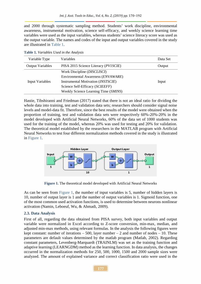
Hastie, Tibshiranni and Friedman (2017) stated that there is not an ideal ratio for dividing thewhole data into training, test and validation data sets; researchers should consider signal noiselevels and model-data fit. Therefore, since the best results of the model were obtained when theproportion of training, test and validation data sets were respectively 60%-20%-20% in themodel developed with Artificial Neural Networks, 60% of the data set of 1000 students wasused for the training of the model, whereas 20% was used for testing and 20% for validation.The theoretical model established by the researchers in the MATLAB program with ArtificialNeural Networks to test four different normalization methods covered in the study is illustratedin Figure 1.

Figure 1. The theoretical model developed with Artificial Neural Networks

As can be seen from Figure 1, the number of input variables is 5, number of hidden layers is10, number of output layer is 1 and the number of output variables is 1. Sigmoid function, oneof the most common used activation functions, is used to determine between neurons nonlinearactivation (Namin, Leboeuf, Wu, & Ahmadi, 2009).

2.3. Data Analysis

First of all, regarding the data obtained from PISA survey, both input variables and outputvariable were normalized in Excel according to Z-score conversion, min-max, median, andadjusted min-max methods, using relevant formulas. In the analysis the following figures werekept constant: number of iterations – 500, layer number – 2 and number of nodes – 10. Theseparameters are default values determined by the matlab program (Matlab, 2002). Regardingconstant parameters, Levenberg-Marquardt (TRAINLM) was set as the training function andadaptive learning (LEARNGDM) method as the learning function. In data analysis, the changesoccurred in the normalization methods for 250, 500, 1000, 1500 and 2000 sample sizes wereanalyzed. The amount of explained variance and correct classification ratio were used in the


178

comparison of the normalization methods discussed in the study, for different sample sizes.Data analysis were performed in Matlab2017b software and both prediction and classificationalgorithms were used in the study. Students who have achieved a score under 425,00, whichwas Turkey average, were coded as unsuccessful (0), whereas those who have achieved a higherscore were coded as successful (1). The success rates of the methods were determined by meansof confusion matrix for the two-category output variable.

3. RESULTS

In the study, the performance of the outcomes obtained from four different normalizationmethods on training, test and validation data sets were determined first, then their overallsuccess rates were compared. But, normality tests were performed before the analysis, to checkthe normality of the data and the results of the analysis are illustrated in Table 2.

Table 2. Test for the Suitability of the Data to Normal Distribution

Method Kolmogorov-Smirnov Shapiro-Wilk

Variables Statistics SD p Statistics SD p

Work discipline .096 1000 .000 .970 1000 .000

Environmental awareness .096 1000 .000 .952 1000 .000

Instrumental motivation .142 1000 .000 .938 1000 .000

Science self-efficacy .120 1000 .000 .934 1000 .000

Weekly science learning time .162 1000 .000 .936 1000 .000

Science literacy .035 1000 .005 .994 1000 .000

Table 2 revealed that both input variables and science literacy scores, which was taken as theoutput variable, were not distributed normally (p<.01). Based on this result, it was concludedthat normalization methods can be applied to the data used as part of the study.

3.1. Findings about Z-Score Normalization

nntool command was used for the introduction of the data set obtained by normalizing fiveinput data and one output data, which have been covered in the study, to Matlab software andfor the regression analysis that would be carried out by means of Artificial Neural Networks.,Analysis results from different sample sizes are illustrated in Table 3; they were obtained afterthe introduction of the input and output data sets to the program, and the execution of tansigconversion function in the network that was defined as 2-layer and 10-neuron.


179

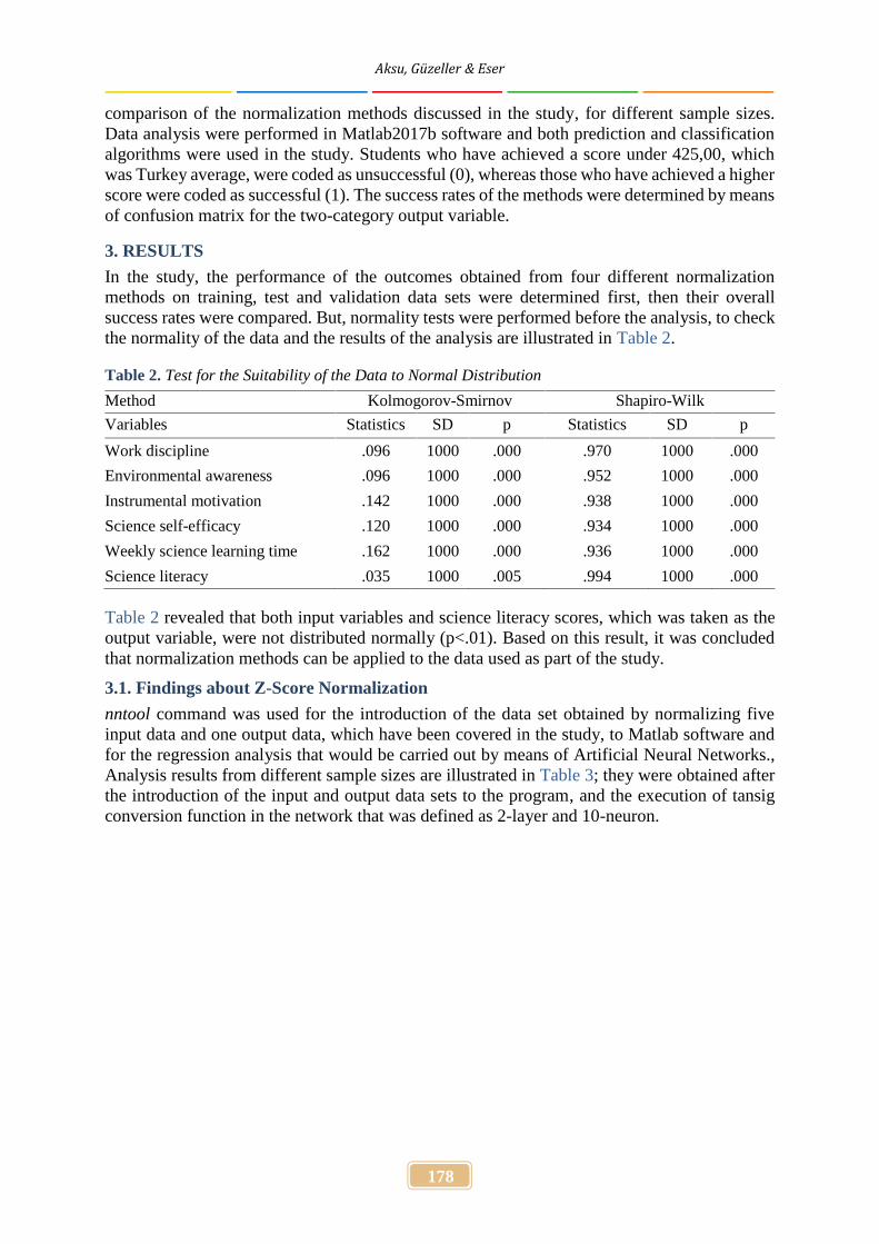
Table 3. Equations Obtained as a Result of Z -Score Normalization

Sample SizeTraining Test Validation Overall

Regressionequation

R2 Regressionequation



R2

N=250Gradient†=5.56 iterations=11 y=0.27x-0.17 55.13 y=0.03x-0.17 8.14 y=0.18x-0.20 33.08 y=0.23x-0.18 45.34

N=500Gradient=2.67 iterations=9 y=0.16x-0.19 38.58 y=0.04x-0.28 10.77 y=0.20x-0.16 44.62 y=0.15x-0.20 36.21

N=1000Gradient=6.33 iterations=9 y=0.17x-0.01 44.91 y=0.15x+0.04 40.57 y=0.16x-0.02 44.37 y=0.17x-0.01 44.24

N=1500Gradient=8.67 iterations=13 y=0.24x-0.00 49.29 y=0.22x+0.04 42.87 y=0.26x-0.04 51.79 y=0.24x-0.01 48.84

N=2000Gradient=10.30 iterations=27 y=0.23x-0.01 48.33 y=0.26x-0.03 51.23 y=0.25x-0.07 46.92 y=0.24x-0.02 48.49

† It is the square of the slope of the error function whose weight and bias are unknown. It is used as the measure of error in Matlab.


180

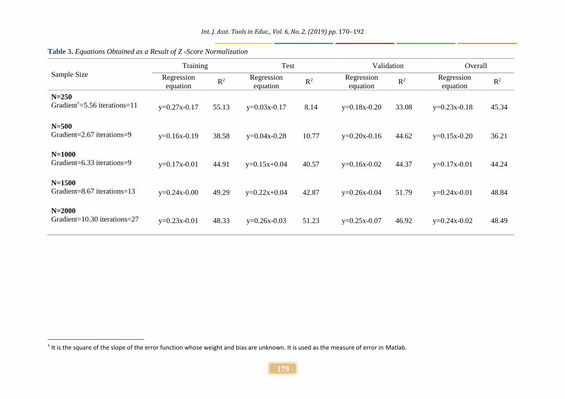
The review of Table 3 revealed that regarding the results of Z-score normalization method, thesample size resulting with: the highest explained variance for the training data set was 250(R2=55.13); the highest explained variance for the test data set was 2000 (R2=51.23); the highestexplained variance for the validation data set was 1500 (R2=51.79); and the highest explainedvariance for the whole data set was 1500 (R2=48.84). When examined in a holistic manner, itis seen that the sample sizes of 250 and 500 have the lowest explained variance. For the samplesize of 2000, the scattering of the output variable predicted from the input variables in two-dimensional space is illustrated in Figure 2 as an example.

Figure 2. The outcomes of Z-Score Normalization in different data sets.

3.2. Findings about Min-max Normalization

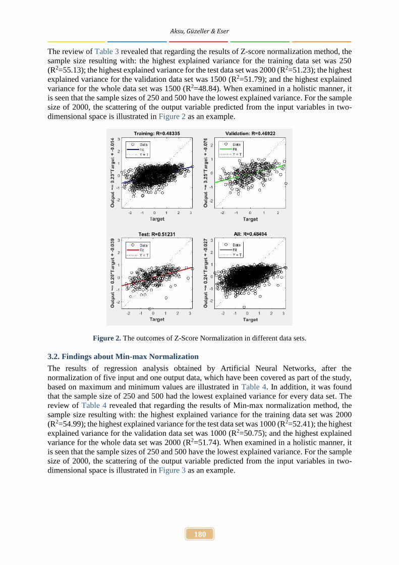
The results of regression analysis obtained by Artificial Neural Networks, after thenormalization of five input and one output data, which have been covered as part of the study,based on maximum and minimum values are illustrated in Table 4. In addition, it was foundthat the sample size of 250 and 500 had the lowest explained variance for every data set. Thereview of Table 4 revealed that regarding the results of Min-max normalization method, thesample size resulting with: the highest explained variance for the training data set was 2000(R2=54.99); the highest explained variance for the test data set was 1000 (R2=52.41); the highestexplained variance for the validation data set was 1000 (R2=50.75); and the highest explainedvariance for the whole data set was 2000 (R2=51.74). When examined in a holistic manner, itis seen that the sample sizes of 250 and 500 have the lowest explained variance. For the samplesize of 2000, the scattering of the output variable predicted from the input variables in two-dimensional space is illustrated in Figure 3 as an example.


181

Figure 3. The outcomes of Min-max Normalization in different data sets

3.3. Findings about Median Normalization

The results of regression analysis obtained by Artificial Neural Networks, after thenormalization of five input and one output data, which have been covered as part of the study,based on median values are illustrated in Table 5.


182

Table 4. Equations Obtained as a Result of Min-max Normalization


Regression equation R2 Regression equation R2 Regression equation R2 Regression equation R2

N=250Gradient=0.09 iteration=10 y=0.13x+0.38 33.05 y=0.03x+0.41 9.01 y=0.12x+0.41 38.21 y=0.12x+0.39 29.98





Table 5. Equations Obtained as a Result of Median Normalization









183

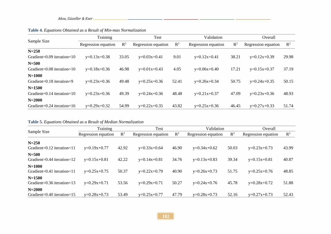
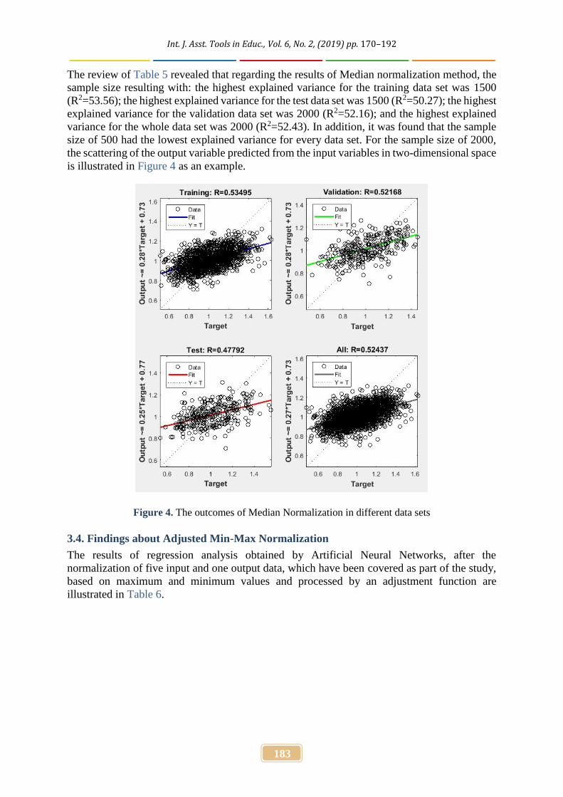
The review of Table 5 revealed that regarding the results of Median normalization method, thesample size resulting with: the highest explained variance for the training data set was 1500(R2=53.56); the highest explained variance for the test data set was 1500 (R2=50.27); the highestexplained variance for the validation data set was 2000 (R2=52.16); and the highest explainedvariance for the whole data set was 2000 (R2=52.43). In addition, it was found that the samplesize of 500 had the lowest explained variance for every data set. For the sample size of 2000,the scattering of the output variable predicted from the input variables in two-dimensional spaceis illustrated in Figure 4 as an example.

Figure 4. The outcomes of Median Normalization in different data sets

3.4. Findings about Adjusted Min-Max Normalization

The results of regression analysis obtained by Artificial Neural Networks, after thenormalization of five input and one output data, which have been covered as part of the study,based on maximum and minimum values and processed by an adjustment function areillustrated in Table 6.


184

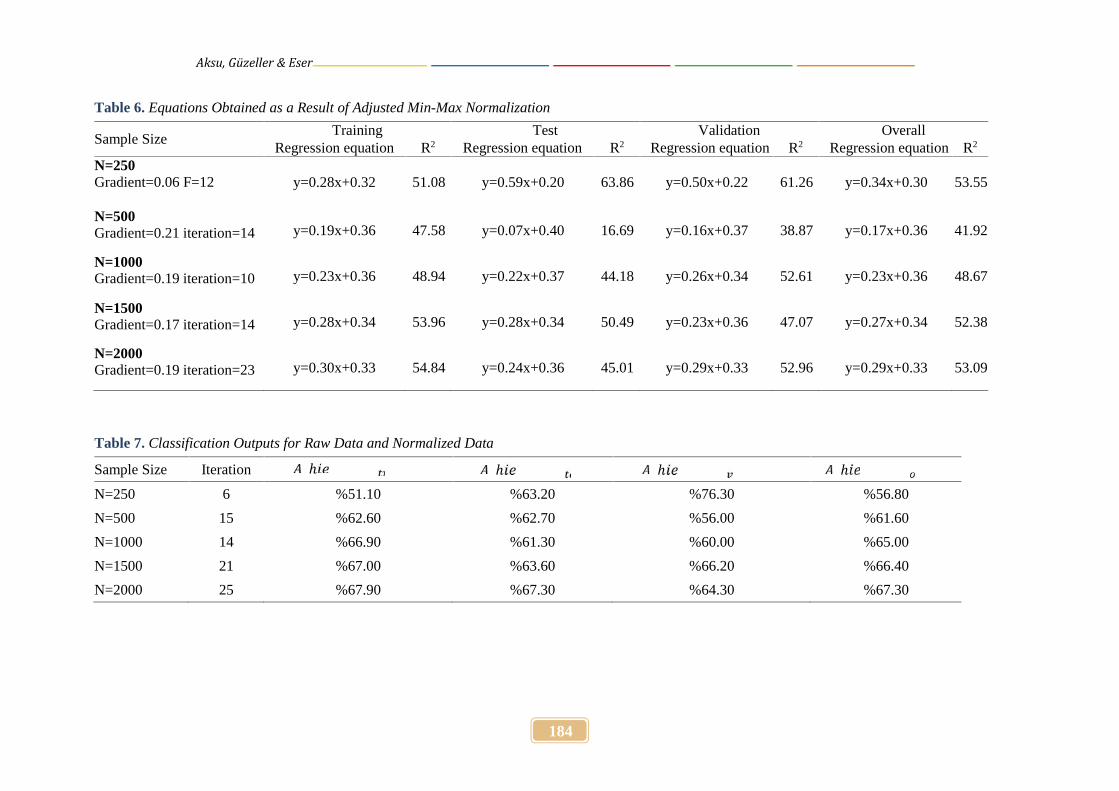
Table 6. Equations Obtained as a Result of Adjusted Min-Max Normalization



N=250Gradient=0.06 F=12 y=0.28x+0.32 51.08 y=0.59x+0.20 63.86 y=0.50x+0.22 61.26 y=0.34x+0.30 53.55





Table 7. Classification Outputs for Raw Data and Normalized Data

Sample Size Iteration ℎ ℎ ℎ ℎN=250 6 %51.10 %63.20 %76.30 %56.80

N=500 15 %62.60 %62.70 %56.00 %61.60

N=1000 14 %66.90 %61.30 %60.00 %65.00

N=1500 21 %67.00 %63.60 %66.20 %66.40

N=2000 25 %67.90 %67.30 %64.30 %67.30


185

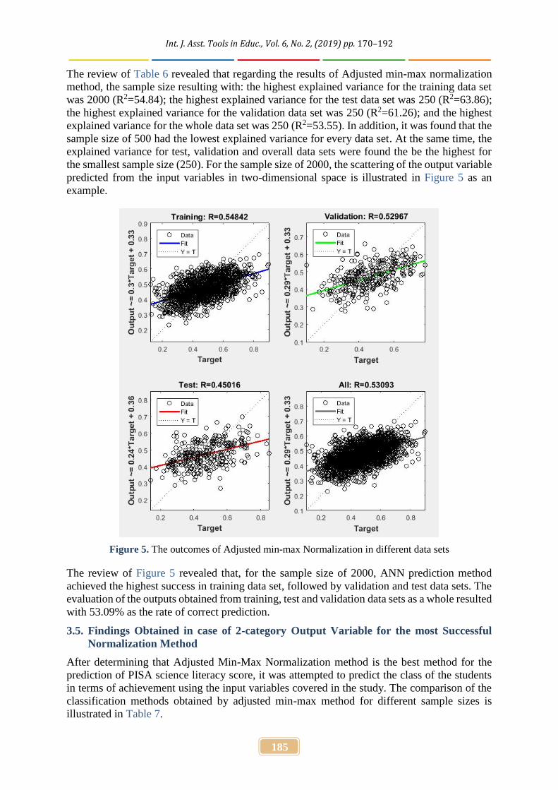
The review of Table 6 revealed that regarding the results of Adjusted min-max normalizationmethod, the sample size resulting with: the highest explained variance for the training data setwas 2000 (R2=54.84); the highest explained variance for the test data set was 250 (R2=63.86);the highest explained variance for the validation data set was 250 (R2=61.26); and the highestexplained variance for the whole data set was 250 (R2=53.55). In addition, it was found that thesample size of 500 had the lowest explained variance for every data set. At the same time, theexplained variance for test, validation and overall data sets were found the be the highest forthe smallest sample size (250). For the sample size of 2000, the scattering of the output variablepredicted from the input variables in two-dimensional space is illustrated in Figure 5 as anexample.

Figure 5. The outcomes of Adjusted min-max Normalization in different data sets

The review of Figure 5 revealed that, for the sample size of 2000, ANN prediction methodachieved the highest success in training data set, followed by validation and test data sets. Theevaluation of the outputs obtained from training, test and validation data sets as a whole resultedwith 53.09% as the rate of correct prediction.

3.5. Findings Obtained in case of 2-category Output Variable for the most SuccessfulNormalization Method

After determining that Adjusted Min-Max Normalization method is the best method for theprediction of PISA science literacy score, it was attempted to predict the class of the studentsin terms of achievement using the input variables covered in the study. The comparison of theclassification methods obtained by adjusted min-max method for different sample sizes isillustrated in Table 7.


186

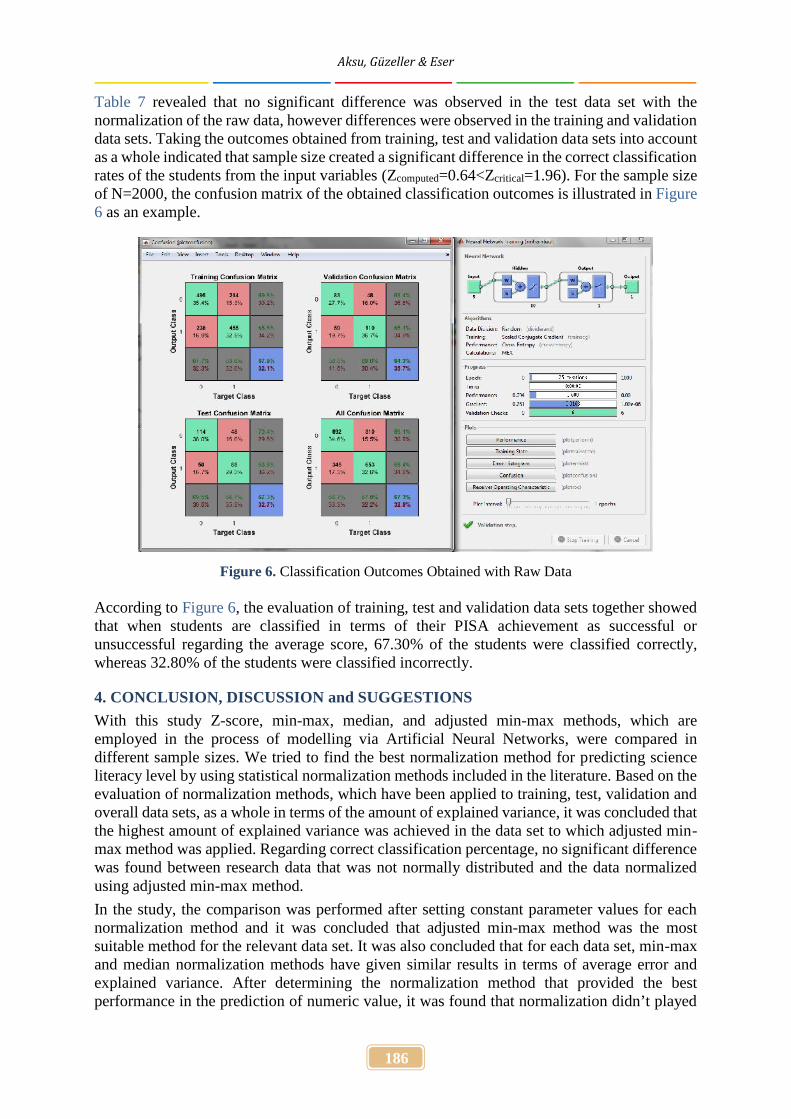
Table 7 revealed that no significant difference was observed in the test data set with thenormalization of the raw data, however differences were observed in the training and validationdata sets. Taking the outcomes obtained from training, test and validation data sets into accountas a whole indicated that sample size created a significant difference in the correct classificationrates of the students from the input variables (Zcomputed=0.64<Zcritical=1.96). For the sample sizeof N=2000, the confusion matrix of the obtained classification outcomes is illustrated in Figure6 as an example.

Figure 6. Classification Outcomes Obtained with Raw Data

According to Figure 6, the evaluation of training, test and validation data sets together showedthat when students are classified in terms of their PISA achievement as successful orunsuccessful regarding the average score, 67.30% of the students were classified correctly,whereas 32.80% of the students were classified incorrectly.

4. CONCLUSION, DISCUSSION and SUGGESTIONS

With this study Z-score, min-max, median, and adjusted min-max methods, which areemployed in the process of modelling via Artificial Neural Networks, were compared indifferent sample sizes. We tried to find the best normalization method for predicting scienceliteracy level by using statistical normalization methods included in the literature. Based on theevaluation of normalization methods, which have been applied to training, test, validation andoverall data sets, as a whole in terms of the amount of explained variance, it was concluded thatthe highest amount of explained variance was achieved in the data set to which adjusted min-max method was applied. Regarding correct classification percentage, no significant differencewas found between research data that was not normally distributed and the data normalizedusing adjusted min-max method.

In the study, the comparison was performed after setting constant parameter values for eachnormalization method and it was concluded that adjusted min-max method was the mostsuitable method for the relevant data set. It was also concluded that for each data set, min-maxand median normalization methods have given similar results in terms of average error andexplained variance. After determining the normalization method that provided the bestperformance in the prediction of numeric value, it was found that normalization didn’t played


187

a role in the classification of the students as successful or unsuccessful. For this purpose,artificial neural network’s classification results were obtained using raw data, then they werecompared with the results obtained with normalized data and it was found that there was nosignificant difference among them. Accordingly, the normalization method used had animportant effect on the prediction of the numeric values, but it had not a significant effect onthe classification outcomes. In other words, the normalization method had a significant effectif the output variable obtained through artificial neural networks was numeric, whereas it hadnot a significant effect if the output variable was categoric (classification).

Regarding the provision of the best results by adjusted min-max normalization method, theresults of the research are parallel to the results of the similar researches in the literature. Yavuzand Deveci (2012), have analyzed the impact of five different normalization methods on theaccuracy of the predictions. They have tested adjusted min-max, Z-score, min-max, median,and sigmoid normalization methods. According to the results of the research, it was found thatconsidering the average error and average absolute percent error values, the highest predictionaccuracy has been obtained from the data set to which adjusted min-max method was applied,whereas the lowest prediction accuracy has been obtained from sigmoid normalization method.Ali and Senan (2017), have analyzed the effect of normalization on achieving best classificationaccuracy. For this purpose, they have observed the effect of three different normalizationmethods on the classification rate of multi-layer sensor for three different numbers of hiddenlayers. In the study, adjusted min-max normalization method, min-max normalization methodin [-1, +1] range, and Z-Score normalization method has been tested for three differentsituations where backpropagation algorithm has been used as the learning algorithm. Accordingto the results of the research, adjusted min-max normalization method has given the bestoutcomes (97%, 98%, 97%) in terms of correct classification ratio for the three cases where thenumber of hidden layers has been 5, 10 and 20. It has been observed that min-max normalizationmethod in [-1, +1] range has been the second best normalization method in terms of correctclassification ratio (57%, 55%, 59%), whereas Z-score method is the third best normalizationmethod (49%, 53%, 50%). Vijayabhanu and Radha (2013), have analyzed the effect of sixdifferent normalization methods on prediction accuracy. For this purpose, they have tested Z-Score normalization method, min-max normalization method, biweight normalization method,tanh normalization method, double sigmoidal normalization method and dynamic scorenormalization with mahalanobis distance. According to the results of the research, thenormalization methods have been ranked as follows with the relevant prediction accuracies:dynamic score normalization with mahalanobis distance (86.2%) has been first followed by Z-score normalization (84.1%), min-max normalization (82.6%), tanh normalization (82.3%),beweight normalization (81.2%), and double sigmoidal normalization (80.5%).

The review of the literature revealed the presence of other researches that are not parallel to thisresearch. Özkan (2017), has analyzed the effects of three different normalization methods onthe accuracy of classification. For this purpose, he has tested Z-Score normalization method,min-max normalization method and decimal scaling normalization method. Considering theaccuracy of classification, sensitivity and selectivity values, it has been observed that Z-Scorenormalization method has provided the best outcomes in general, followed by decimal scalingnormalization and min-max normalization methods. Panigrahi and Behera (2013), haveanalyzed the effect of five different normalization methods on forecast accuracy. For thispurpose, they have tested min-max normalization method, decimal scaling normalizationmethod, median normalization method, vector normalization method, and Z-Scorenormalization method. It has been observed that decimal scaling and vector normalizationmethods have provided better forecast accuracy compared to median, min-max and Z-Scorenormalization methods. Cihan, Kalıpsız and Gökçe (2017), have analyzed the effect of fourdifferent normalization methods on classification accuracy. For this purpose, they have tested


188

min-max normalization method, decimal scaling method, Z-Score method and sigmoid method.According to the results of the research the best classification has been obtained with 0.24sensitivity, 0.99 selectivity and 0.36 f-measurement, by applying sigmoid normalizationmethod, whereas the worst classification has been obtained with 0.21 sensitivity, 0.99selectivity and 0.32 f-measurement, by applying Z-Score Normalization method. Mustaffa andYusof (2011), have analyzed the effect of three different normalization methods on predictionaccuracy. For this purpose, they have tested min-max normalization method, Z-Scorenormalization method and decimal point normalization method. In the study, least squaressupport vector machine model and neural network model have been used as the predictionmodel of the research. According to the results, considering the effect of normalization methodson prediction accuracy and error percentages, it has been found that the outcomes of leastsquares support vector machine model had better outcomes than neural network model. At thesame time, it has been observed that for both least squares support vector machine model andneural network model, the best outcomes have been obtained as a result of the preliminary dataprocessing processes performed with decimal point, min-max and Z-Score normalizationmethods respectively. Nawi, Atomi and Rehman (2013), have analyzed the effect of threedifferent normalization methods on classification accuracy. For this purpose, they have testedmin-max normalization method, Z-Score Normalization method and decimal scaling method.According to the results of the research, it has been found that different normalization methodshave provided better outcomes under different conditions and in general the process ofnormalization has improved the accuracy of artificial neural network classifier at least 95%.Suma, Renjith, Ashok and Judy (2016), have compared the classification accuracy outcomes ofdiscriminant analysis, support vector machine, artificial neural network, naive Bayes anddecision tree models by applying different normalization methods. For this purpose, Z-ScoreNormalization method and min-max normalization method have been used. According to theresults of the research, it has been observed that Z-Score Normalization method have providedbetter outcomes in terms of classification accuracy for all models compared to min-maxnormalization method.

While determining the normalization method to be used as part of any research, taking thegeneral structure of the data set, sample size and the features of the activation function to beused into account may be considered as the best approach. The fourth factor that should beconsidered while determining the normalization method to be used is the algorithm that will beused in training stage. In this regard, the selected training function, number of layers, numberof iterations ad number of nodes have also some importance. For comparing normalizationmethods, the features belonging to the analysis should be kept constant and the methods shouldbe compared accordingly. After setting the constant parameters, as much as possiblenormalization method should be tested on the relevant data set and the method providing thebest outcome should be selected.

Regarding the wholistic analysis of the contribution of different normalization methods, whichwere applied on different sample sizes as part of ANN model, on the variance and classificationaccuracy, it was concluded that the best results were obtained after normalizing via adjustedmin-max method. Getting good results at lowest sample size indicates the problem ofoverfitting. It can be said that the risk of overfitting occurrence is quite high if the developedmodel works too much on the training set and starts to act by rote or if the training set is toomonotonous. Overfitting occurs when the model perceives the noise and random fluctuationsof the training data as a concept and learns them. The problem is the noise and fluctuationsperceived as concepts will not be valid for a new data, which will affect the generalizationability of the models negatively (Haykin, 1999; Holmstrom & Koistinen, 1992). It is possibleto overcome overfitting problem by cross validation method, where data set is divided intopieces to form different training-test pairs and running the model on various data. Overfitting


189

problem may also be prevented by developing a simpler model and allowing the model topredict. Reducing the number of iterations and removing the nodes that makes least contributionto the prediction power are the other methods that can be used in solving overfitting problem(Haykin, 1999; Holmstrom & Koistinen, 1992; Hua, Lowey, Xiong, & Dougherty, 2006; Zur,Jiang, Pesce, & Drukker, 2009).

Related to the subject, a comparison study, including sigmoid normalization method and othernormalization methods that are frequently used in the literature, may be conducted in the futureusing a data set related to educational sciences. Due to the nature of artificial neural networksoutcomes obtained from Matlab software differentiate when the model is rerun. This is due tothe fact that the weight values are randomly determined at random, or at a certain interval,according to a given distribution (i.e. Gaussian). As a matter of fact, in case of reconducting theanalysis with the same data set, without changing any parameter, some differences may beobserved in the outcomes because training, test and validation data sets are randomlydetermined by the program. This is seen as the other important limitation of the research.

4.1. Limitation of the Research

Sigmoid normalization method could not be tested in the researches since only zero and onetype outputs can be generated as a result of sigmoid normalization method. Failure to coversigmoid normalization method constitutes a limitation of the research.

4.2. Superiority of the Research

In addition to analyze the effect of normalization methods for numeric outputs, the performanceof normalization method used in case of categoric output variable was also analyzed as part ofthe study, which is seen as a superiority of the research. In addition, implementing artificialneural network methods into the education area and performing the analysis by taking differentsample sizes into account are considered as the other superiorities of the study.

ORCIDGökhan AKSU https://orcid.org/0000-0003-2563-6112Cem Oktay GÜZELLER https://orcid.org/0000-0002-2700-3565Mehmet Taha ESER https://orcid.org/0000-0001-7031-1953

5. REFERENCES

Aksu, G., & Doğan, N. (2018). Veri Madenciliğinde Kullanılan Öğrenme Yöntemlerinin FarklıKoşullar Altında Karşılaştırılması, Ankara Üniversitesi Eğitim Bilimleri FakültesiDergisi, 51(3), 71-100.

Ali, A. & Senan, N. (2017). The Effect of Normalization in VIOLENCE Video ClassificationPerformance. IOP Conf. Ser.: Mater. Sci. Eng. 226 012082.

Anderson, J. A. (1990). Data Representation in Neural Networks, AI Expert.Ayalakshmi, T., & Santhakumaran, A. (2011). Statistical Normalization and Back Propagation

for Classification. International Journal of Computer Theory and Engineering, 3(1),1793-8201.

Azadeh, M., Sheikhalishahi, M., Tabesh, A., & Negahban (2011). The Effects of Pre-Processing Methods on Forecasting Improvement of Artificial Neural Networks,Australian Journal of Basic and Applied Sciences, 5(6), 570-580.

Azimi-Sadjadi, M.R. & Stricker, S.A. (1994). “Detection and Classification of BuriedDielectric Anomalies Using Neural Networks Further Results,” IEEE Trans.Instrumentations and Measurement, 43, pp. 34-39.

Bishop, C. M. (1995), Neural Networks for Pattern Recognition, Oxford: Oxford UniversityPress.


190

Cihan, P., Kalıpsız, O., & Gökçe, E. (2017). Hayvan Hastalığını Teşhisinde NormalizasyonTekniklerinin Yapay Sinir Ağı Performansına Etkisi [Effect of Normalization Techniqueson Artificial Neural Network and Feature Selection Performance in Animal DiseaseDiagnosis]. e-Turkish Studies (elektronik), 12(11), 59-70, 2017.

Davydov, M.V., Osipov, A.N., Kilin, S.Y. & Kulchitsky, V.A. (2018). Neural NetworkStructures: Current and Future States. Open semantic technologies for intelligent systems,259-264.

Dekking, F.M., Kraaikamp, C., Lopuhaä, H.P., & Meester, L.E. (2005). A modern introductionto probability and statistics: Understanding why and how. United States: Springer-VerlagLondon Limited.

Deveci, M. (2012). Yapay Sinir Ağları ve Bekleme Süresinin Tahmininde Kullanılması[Artificial Neural Networks and Used of Waiting Time Estimation]. Unpublished MasterDissertation, Gazi Üniversitesi Sosyal Bilimleri Enstitüsü, Ankara.

Elmas, Ç. (2003). Yapay Sinir Ağları, Birinci Baskı, Ankara: Seçkin Yayıncılık.Famili, A., Shen, W., Weber, R., & Simoudis, E. (1997). Data Preprocessing and Intelligent

Data Analysis. Intelligent Data Analysis, 1, 3-23.Finch, J. F., West, S. G., & MacKinnon, D. P. (1997). Effects of sample size and nonnormality

on the estimation of mediated effects in latent variable models. Structural EquationModeling: A Multidisciplinary Journal, 4(2), 87-107.

Fraenkel, J.R., & Wallen, N.E. (2006). How to design and evaluate research in education (6thed.). New York, NY: McGraw-Hill.

Gardner, M. W., & Dorling, S. R. (1998). Artificial Neural Networks (The MultilayerPerceptron) - A Review of Applications in the Atmospheric Sciences. AtmosphericEnvironment, 32, 2627-2636.

Gerasimovic, M., Stanojevic, L., Bugaric, U., Miljkovic, Z., & Veljovic, A. (2011). UsingArtificial Neural Networks for Predictive Modeling of Graduates’ Professional Choice.The New Educational Review, 23, 175- 188.

Goodfellow, I., Bengio, Y., & Courville, A. (2016). Deep Learning. MIT Press.Gonzalez, J.M., & DesJardins, S.L. (2002). Artificial neural networks: A new approach to

predicting application behaviour, Research in Higher Education, 43(2), 235–258Gschwind, M. (2007). Predicting Late Payments: A Study in Tenant Behavior Using Data

Mining Techniques. The Journal of Real Estate Portfolio Management, 13(3), 269-288.Hagan, M.T., Demuth, H.B., Beale, M.H., & Jesus, O. (2014). Neural Network Design, Boston:

PWS Publishing Co.Hastie, T., Tibshirani, R., & Friedman, J. H. (2009). The elements of statistical learning: Data

mining, inference, and prediction. New York, NY: Springer.Hayashi, Y., Hsieh, M-H., & Setiono, R. (2009). Predicting Consumer Preference for Fast-Food

Franchises: A Data Mining Approach. The Journal of the Operational Research Society,60(9), 1221-1229.

Haykin, S. (1999). Neural Networks: A Comprehensive Foundation. 2nd Edition, Prentice-Hall, Englewood Cliffs, NJ.

Holmstrom, L., & Koistinen, P. (1992). Using additive noise in back-propagation training.IEEE Trans. Neural Networks, 3, 24–38

Hua, J.P., Lowey, J., Xiong, Z., & Dougherty, E.R. (2006). Noise-injected neural networksshow promise for use on small-sample expression data. BMS Bioinform. 7 (Art. no. 274).

Hu, X. (2003). DB-H Reduction: A Data Preprocessing Algorithm for Data MiningApplications. Applied Math. Letters, 16, 889- 895.

Hunt, K.J., Sbarbaro, D., Bikowski, R., & Gawthrop, P.J. (1992) “Neural Networks for ControlSystems - A Survey. Automatica, 28, pp. 1083-1112.


191

Karasar, N. (2009). Bilimsel Araştırma Yöntemi [Scientific Research Method]. Ankara: NobelYayıncılık.

Klein, B.D., & Rossin, D.F. (1999). Data Quality in Neural Network Models: Effect of ErrorRate and Magnitude of Error on Predictive Accuracy. OMEGA, The Int. J. ManagementScience, 27, pp. 569-582.

Kriesel, D. (2007). A Brief Introduction to Neural Networks. Available athttp://www.dkriesel.com/_media/science/neuronalenetze-en-zeta2-2col-dkrieselcom.pdf

Krycha, K. A., & Wagner, U. (1999). Applications of Artificial Neural Networks inManagement Science: A Survey. J. Retailing and Consumer Services, 6, pp. 185-203,

Lawrance, J. (1991). Data Preparation for a Neural Network, AI Expert. 6 (11), 34-41.Lou, M. (1993). Preprocessing Data for Neural Networks. Technical Analysis of Stocks &

Commodities Magazine, Oct.Mannila, H. (1996). Data mining: machine learning, statistics, and databases, Proceedings of

8th International Conference on Scientific and Statistical Data Base Management,Stockholm, Sweden, June 18–20, 1996.

Matlab (2002). Matlab, Version 6·5. Natick, MA: The Mathworks Inc.,Mustaffa, Z., & Yusof, Y. (2011). A Comparison of Normalization Techniques in Predicting

Dengue Outbreak. International Conference on Business and Economics Research, Vol.1IACSIT Press, Kuala Lumpur, Malaysia

Namin, A. H., Leboeuf, K., Wu, H., & Ahmadi, M. (2009). Artificial Neural NetworksActivation Function HDL Coder, Proceedings of IEEE International Conference onElectro/Information Technology, Ontario, Canada, 7-9 June, 2009.

Narendra, K. S., & Parthasarathy, K. (1990). Identification and Control of Dynamic SystemsUsing Neural Networks. IEEE Trans. Neural Networks, 1, pp. 4-27.

Nawi, N. M., Atomi, W. H., Rehman, M. Z. (2013). The Effect of Data Pre-Processing onOptimized Training of Artificial Neural Networks. Procedia Technology, 11, 32-39.

Neelamegam, S., & Ramaraj, E. (2013). Classification algorithm in Data mining: An Overview.International Journal of P2P Network Trends and Technology (IJPTT), 4(8), 369-374.

OECD, (2015). Frascati Manual 2015: Guidelines for Collecting and Reporting Data onResearch and Experimental Development, The Measurement of Scientific and TechnicalActivities, OECD Publishing, Paris.

O’Shea, K., & Nash, R. (2015). An Introduction to Convolutional Neural Networks,arXiv:1511.08458 [cs. NE], November.

Özkan, A.O. (2017). Effect of Normalization Techniques on Multilayer Perceptron NeuralNetwork Classification Performance for Rheumatoid Arthritis Disease Diagnosis.International Journal of Trend Scientific Research and Development. Volume 1, Issue 6.

Öztemel, E. (2003), Yapay Sinir Ağları [Artificial Neural Networks], İstanbul: PapatyaYayıncılık.

Rafiq, M.Y., Bugmann, G., & Easterbrook, D.J. (2001). Neural Network Design forEngineering Applications. Computers & Structures, 79, pp. 1541-1552.

Ravid, R. (2011). Practical statistics for educators (fourth edition). United States: Rowman &Littlefield Publishers.

Redman, T. C. (1992). Data Quality: Management and Technology. New York: Bantam Books.Ripley, B.D. (1996), Pattern Recognition and Neural Networks, Cambridge: Cambridge

University Press.Romero, C., Ventura, S. (2011). Educational data mining: a review of the state-of-the-art”,

IEEE Trans. Syst. Man Cybernet. C Appl. Rev., 40(6), 601–618.Roussas, G. (2007). Introduction to probability (first edition). United States: Elsevier Academic

Press.Rumelhart, D.E. (1994). The Basic Ideas in Neural Networks. Comm. ACM, 37, pp. 87-92.


192

Panigrahi, S., & Behera, H. S. (2013). Effect of Normalization Techniques on Univariate TimeSeries Forecasting using Evolutionary Higher Order Neural Network. InternationalJournal of Engineering and Advanced Technology, 3(2), 280-285.

Sattler, K.U., & Schallehn, E. (2001). A Data Preparation Framework Based on a MultidatabaseLanguage. Proc. Int’l Symp. Database Eng. & Applications, pp. 219-228.

Schmidhuber, J. (2015). Deep Learning in Neural Networks: An Overview. Neural Networks,61, 85-117.

Schumacher, P., Olinsky, A., Quinn, J., & Smith, R. (2010). A Comparison of LogisticRegression, Neural Networks, and Classification Trees Predicting Success of ActuarialStudents. Journal of Education for Business, 85(5), 258-263.

Silva, C.S. and Fonseca, J.M. (2017). Educational Data Mining: a literature review. Advancesin Intelligent Systems and Computing, 2-9.

Stein, R. (1993). Selecting data for neural networks, AI Expert.Suma, V. R., Renjith, S., Ashok, S., & Judy, M. V. (2016). Analytical Study of Selected

Classification Algorithms for Clinical Dataset. Indian Journal of Science and Technology,9(11), 1-9, DOI: 10.17485/ijst/2016/v9i11/67151.

Upadhyay, N. (2016). Educational Data Mining by Using Neural Network. InternationalJournal of Computer Applications Technology and Research, 5(2), 104-109.

Uslu, M. (2013). Yapay Sinir Ağları ile Sınıflandırma[Classification with Artificial NeuralNetworks], İleri İstatistik Projeleri I [Advanced Statistics Projects I]. HacettepeÜniversitesi Fen Fakültesi İstatistik Bölümü, Ankara.

Vijayabhanu, R. & Radha, V. (2013). Dynamic Score Normalization Technique usingMahalonobis Distance to Predict the Level of COD for an Anaerobic WastewaterTreatment System. The International Journal of Computer Science & Applications. 2(3),May 2013, ISSN – 2278-1080.

Yavuz, S., & Deveci, M. (2012). İstatiksel Normalizasyon Tekniklerinin Yapay Sinir AğınPerformansına Etkisi. [The Effect of Statistical Normalization Techniques on ThePerformance of Artificial Neural Network], Erciyes University Journal of Faculty ofEconomics and Administrative Sciences, 40, 167-187.

Yu, L., Wang, S., & Lai, K.K. (2006). An integrated data preparation scheme for neural networkdata analysis. IEEE Trans. Knowl. Data Eng., 18, 217–230.

Wang, F., Devabhaktuni, V.K.Xi, C., & Zhang, Q. (1998). Neural Network Structures andTraining Algorithms for RF and Microwave Applications. John Wiley & Sons, Inc. Int JRF and Microwave CAE, 9, 216-240.

Wook, M., Yahaya, Y. H., Wahab, N., Isa, M. R. M., Awang, N. F., Seong, H. Y. (2009).Predicting NDUM Student's Academic Performance Using Data Mining Techniques, TheSecond International Conference on Computer and Electrical Engineering, Dubai, UnitedArab Emirates, 28-30 December, 2009.

Zhang, S., Zhang, C., & Yang, Q. (2003). Data Preparation for Data Mining. Applied ArtificialIntelligence, 17, 375-381.

Zur, R.M., Jiang, Y.L., Pesce, L.L., &bDrukker, K. (2009). Noise injection for training artificialneural networks: a comparison with weight decay and early stopping. Med. Phys., 36(10),4810–4818.

Documents

The Effect of the Normalization Method Used in Different