Embed Size (px)
Citation preview

Nonlinear variational method for predicting fast collisionless magnetic reconnection
This article has been downloaded from IOPscience. Please scroll down to see the full text article.
2013 Nucl. Fusion 53 063024
(http://iopscience.iop.org/0029-5515/53/6/063024)
Download details:
IP Address: 139.124.7.178
The article was downloaded on 21/05/2013 at 08:49
Please note that terms and conditions apply.
View the table of contents for this issue, or go to the journal homepage for more
Home Search Collections Journals About Contact us My IOPscience
IOP PUBLISHING and INTERNATIONAL ATOMIC ENERGY AGENCY NUCLEAR FUSION
Nucl. Fusion 53 (2013) 063024 (11pp) doi:10.1088/0029-5515/53/6/063024
Nonlinear variational method forpredicting fast collisionless magneticreconnectionM. Hirota1, P.J. Morrison2, Y. Ishii1, M. Yagi1 and N. Aiba1
1 Japan Atomic Energy Agency, Rokkasho, Aomori 039-3212, Japan2 University of Texas at Austin, Austin, TX 78712, USA
E-mail: [email protected]
Received 29 December 2012, accepted for publication 26 April 2013Published 20 May 2013Online at stacks.iop.org/NF/53/063024
AbstractA mechanism for fast magnetic reconnection in collisionless plasma is studied for understanding sawtooth collapse intokamak discharges using a two-fluid model for cold ions and electrons. Explosive growth of the tearing mode enabledby electron inertia is analytically estimated using an energy principle with a nonlinear displacement map. Decreasein the potential energy in the nonlinear regime (where the island width exceeds the electron skin depth) is found tobe steeper than in the linear regime, resulting in accelerated reconnection. Release of potential energy by such afluid displacement leads to unsteady and strong convective flow, which is not damped by the small dissipation effectsin high-temperature tokamak plasmas. Direct numerical simulation in slab geometry substantiates the theoreticalprediction of the nonlinear growth.
(Some figures may appear in colour only in the online journal)
1. Introduction
Sawtooth collapse in tokamak plasmas has been a puzzlingphenomenon for decades. Although the m = 1 kink-tearing mode is essential for the onset of this dynamics,Kadomtsev’s full reconnection model [1] and the nonlineargrowth of the resistive m = 1 mode [2] (both based on resistivemagnetohydrodynamic (MHD) theory) fail to explain the shortcollapse times (∼100 µs) as well as the partial reconnectionsobserved in experiments [3–5]. Since resistivity is smallin high-temperature tokamaks, two-fluid effects are expectedto play an important role for triggering fast (or explosive)magnetic reconnection as in solar flares and magnetosphericsubstorms.
In earlier works [6–8], the linear growth rate of the kink-tearing mode in the collisionless regime has been analysedextensively using asymptotic matching, which shows anenhancement of the growth rate due to two-fluid effects, evenin the absence of resistivity. Furthermore, direct numericalsimulations [9, 10] of two-fluid models show acceleration ofreconnection in the nonlinear phase, even though realistictwo-fluid simulation of high-temperature tokamaks is still acomputationally demanding task (especially when the resistivelayer width is smaller than the electron skin depth de ∼1 mm). These simulation studies, as a rule, indicate explosivetendencies of collisionless reconnection.
However, theoretical understanding of such explosivephenomena is not yet established due to the lack of analyticaldevelopment. In the neighbourhood of the boundary (orreconnecting) layer, a perturbative approach breaks down at anearly nonlinear phase and, consequently, asymptotic matchingrequires a fully nonlinear inner solution [12]. Moreover,in contrast to the quasi-equilibrium analysis developedfor resistive reconnection [2, 13], the explosive processof collisionless reconnection should be a nonequilibriumproblem, in which inertia is not negligible in the force balanceand hence leads to acceleration of flow. Thus, the convenientassumption of steady reconnection is no longer appropriate.Recent theories [14–16] emphasize the Hamiltonian natureof two-fluid models and try to gain deeper understanding ofcollisionless reconnection in the ideal limit.
The purpose of this work is to predict the explosivegrowth of the kink-tearing mode analytically by developinga new nonlinear variational technique that is based on ageneralization of the MHD energy principle [17, 18] (forgeneralization see [19]). For simplicity, we concentrate onthe effect of electron inertia, which is an attractive mechanismfor triggering fast reconnection in tokamaks; estimates of thereconnection rate are favourable [20], nonlinear accelerationis possible [10, 11], and even the more mysterious partialreconnection may be explained by an inertia-driven collapsemodel [21, 22]. While we address the same problem as that
0029-5515/13/063024+11$33.00 1 © 2013 IAEA, Vienna Printed in the UK & the USA

Nucl. Fusion 53 (2013) 063024 M. Hirota et al
of [10] (see also [11]), our estimated nonlinear growth isquantitatively different from that of this reference, and ourresult is confirmed by direct numerical simulation. Thisadvance in nonlinear theory is indispensable for clarifying theacceleration mechanism of collisionless reconnection.
This paper is organized as follows. In section 2, weinvoke a conventional 2D slab model for electron inertia-drivenreconnection and then construct its Lagrangian in terms ofthe fluid flow map (as in the ideal MHD theory [23–25]).In section 3, we obtain the linear growth rate of the inertialtearing mode in the large-�′ regime (corresponding to them = 1 kink-tearing mode in tokamaks) by applying ourenergy principle to this two-fluid model. We show thata rather simple displacement field is enough to make thepotential energy decrease (δW < 0) and to obtain a tearinginstability whose growth rate agrees with the asymptoticmatching result [6]. Given these observations, we extend theenergy principle to a nonlinear regime in section 4, wherethe displacement (or the magnetic island width) is larger thande. Without relying on perturbation expansion, we directlysubstitute a form of the displacement map into the Lagrangianand attempt to minimize the potential energy W . We showthat a continuous deformation of magnetic field lines into aY -shape [26] asymptotically leads to a steeper decrease of W
than that of the linear regime, which is indeed found to beresponsible for the acceleration phase. In section 5, the effectof small dissipation on this fast reconnection is considered andimplications of our results for sawtooth collapse are finallydiscussed.
2. Model equations and their Lagrangiandescription
We analyse the following vorticity equation and (collisionless)Ohm’s law for φ(x, y, t) and ψ(x, y, t):
∂∇2φ
∂t+ [φ, ∇2φ] + [∇2ψ, ψ] = 0, (1)
∂(ψ − d2e ∇2ψ)
∂t+ [φ, ψ − d2
e ∇2ψ] = 0, (2)
where [f, g] = (∇f × ∇g) · ez [27, 28]. The velocity andmagnetic fields are, respectively, given by v = ez × ∇φ andB = √
µ0min0 ∇ψ × ez + B0ez, where B0 and the massdensity min0 are assumed to be constant (µ0 is the magneticpermeability). Thus, ψ has the same dimension as φ (the so-called Alfven units). As noted in section 1, the parameter de
denotes the electron skin depth, which is much smaller thanthe system size (de � L). The equation (2) can be seen as theconservation law of the electron canonical momentum definedby ψe = ψ − d2
e ∇2ψ . Since the magnetic flux ψ is no longerconserved for de �= 0, the effect of electron inertia permitsmagnetic reconnection within a thin layer (∼de) despite a lackof resistivity in this model.
It should be remarked that, in comparison with the moregeneral two-fluid model [28], the above model assumes coldions and electrons; namely, it is too simplified to directlyapply to tokamaks. In particular, the effects of the ion-soundgyroradius and the diamagnetic drift are known to modify thelinear stability criteria substantially, and resistivity is not so
Figure 1. Contours of ψ when ε = 4.2de (de/Lx = 0.01 andLy/Lx = 4π ). The heavy line highlights the contour ψ = 0, whichis in fact almost equal to the contour ψe = 0.
negligible as will be discussed later in section 5. Moreover,the assumption of isothermal electrons (used in [28]) mayalso lose its validity in a nonlinear phase according to afully gyrokinetic description [29]. Nevertheless, except forresistivity, magnetic field lines can only be broken by electroninertia in the collisionless limit [29], and we will study this keymechanism by analysing the simplest model, (1) and (2).
In the same manner as in [10], we consider a staticequilibrium state,
φ(0) = 0 and ψ(0)(x) = ψ0 cos αx, (3)
on a doubly periodic domain D = [−Lx/2, Lx/2] ×[−Ly/2, Ly/2] (where α = 2π/Lx), and analyse the nonlinearevolution of the tearing mode with wavenumber in they-direction k = 2π/Ly at its early linear stage. For sufficientlysmall k such that
πk2/4α3 = L3x/8L2
y � de � Lx, (4)
this instability is similar to the m = 1 kink-tearing modein tokamaks (which belongs to the large-�′ regime; seeappendix A). Figure 1 shows contours of ψ calculated bydirect numerical simulation, where ε denotes the maximumdisplacement of the fluid in the x-direction. Since ψe isfrozen into the displacement, we numerically measure ε fromthe displacement of the contour ψe = 0 relative to itsinitial position x = ±Lx/4. Our numerical code employsa spectral method in the y-direction with up to 200 modesand a finite difference scheme in the x-direction with uniformgrid points ∼10 000. The growth of ε accelerates whenε = ε/de > 1, as shown in figure 2 (which is faster thanexponential). In accordance with [10], a strong spike ofelectric current J = −∇2ψ develops inside the reconnectinglayer and the width of this current spike continues to shrinkas time progresses, unless a dissipative term is added to (2).Therefore, direct numerical simulation of (1) and (2) inevitablyterminates when this coherent energy cascade reaches the limitof resolution.
In order to clarify the free energy source of thisexplosive instability, we solve the conservation law (2) for
2

Nucl. Fusion 53 (2013) 063024 M. Hirota et al
0.1
1
10
6 7 8 9 10
noitalumiS
Figure 2. Growth of ε = ε/de with respect to time t = t/τ0
(de/Lx = 0.01 and Ly/Lx = 4π ).
ψe = ψ − d2e ∇2ψ by introducing an incompressible flow map
Gt : D → D, which depends on time and correspondsto the identity map when t = −∞ (G−∞ = Id). Let(x, y)(t) = Gt (x0, y0) be orbits of fluid elements labelledby their position (x0, y0) at t = −∞. Then, the velocity field(or φ) is related to Gt as
∂Gt
∂t(x0, y0) = ez × ∇φ(x, y, t). (5)
Regarding Gt as an unstable fluid motion emanating from theequilibrium state (3), we can solve Ohm’s law (2) by
ψe(x, y, t) = ψe(Gt (x0, y0), t) = ψ(0)e (x0), (6)
where ψ(0)e (x) = (1 +d2
e α2)ψ0 cos(αx). Both φ and ψe (or ψ)are thus expressed in terms of Gt . By adapting Newcomb’sLagrangian theory [23], we define the Lagrangian for the fluidmotion Gt as
L[Gt ] = K[Gt ] − W [Gt ], (7)
where
K[Gt ] = 1
2
∫D
d2x |∇φ|2, (8)
W [Gt ] = 1
2
∫D
d2x(|∇ψ |2 + d2
e |∇2ψ |2) . (9)
Then, the variational principle δ∫
L[Gt ] dt = 0 with respectto δGt yields the vorticity equation (1).
Since the Hamiltonian corresponds to H = K + W
(= const.), we note that W plays the role of potential energyand the equilibrium state (3) initially stores it as free energy. Inthe same spirit as the energy principle [17, 18], if the potentialenergy decreases (δW < 0) for some displacement map Gt ,then such a perturbation will grow with the release of freeenergy. In comparison with the ideal MHD case [23], theelectron’s kinetic energy (1/2)
∫D
d2e J 2d2x appears as a part of
the potential energy, because we have treated the conservationlaw of electron’s momentum ψe as a kinematic constraint. Toavoid confusion, we will refer to this (1/2)
∫D
d2e J 2d2x as
current energy in this work.
3. Energy principle for linear stability analysis
In our linear stability analysis, the equilibrium state isperturbed by an infinitesimal displacement, Gt (x0, y0) =(x0, y0)+ξ(x0, y0, t), where ξ is a divergence-free vector fieldon D. For a given wavenumber k = 2π/Ly , we seek a linearlyunstable tearing mode in the form
ξ(x, y, t) = ∇[ε(t)ξ (x)
sin ky
k
]× ez, (10)
with a growth rate ε(t) ∝ eγ t . We normalize the eigenfunctionξ (x) by max |ξ (x)| = 1 so that ε(t) is equal to the maximumdisplacement in the x-direction and, hence, measures the halfwidth of the magnetic island. The linear perturbations, sayφ(1) and ψ
(1)e , are given by
φ(1) = −γ εξsin ky
kand ψ(1)
e = −εξ∂xψ(0)e cos ky, (11)
which follow from the relations v(1) = ∂tξ and ψ(1)e =
−ξ · ∇ψ(0)e .
Upon omitting ‘(0)’ from equilibrium quantities, ψ(0),ψ
(0)e , J (0), etc, to simplify the notation, the eigenvalue problem
can be written in the form
−[(
γ 2/k2 + ψ ′2e
)ξ ′
]′+ k2
(γ 2/k2 + ψ ′2
e
)ξ
= d2e ψ ′
eJ′′′ξ + d2
e ψ ′e∇2 1
1 − d2e ∇2
∇2(ψ ′eξ ), (12)
where ∇2 should be interpreted as ∇2 = ∂2x −k2 and the prime
(′) denotes the x derivative. Note, (12) ranks as a fourth orderordinary differential equation (unless de = 0) because of theintegral operator (1 − d2
e ∇2)−1 on the right-hand side. Bymultiplying the both sides of (12) by ξ and integrating over thedomain, we obtain −γ 2I (2) = W(2), where
I (2) =∫ Lx/2
−Lx/2dx
1
k2
(|ξ ′|2 + k2|ξ |2
), (13)
W(2) =∫ Lx/2
−Lx/2dx
[− (ψ ′
eξ )∇2
1 − d2e ∇2
(ψ ′eξ ) + ψ ′
eψ′′′|ξ |2
].
(14)
Under the periodic boundary condition on ξ , the two operators∇2 and (1−d2
e ∇2)−1 commute in (14). The functionals γ 2I (2)
and W(2) are, respectively, related to the kinetic and potentialenergies for the linear perturbation. Hence, by invoking theenergy principle [17] (or the Rayleigh–Ritz method), we cansearch for the most unstable eigenvalue (γ > 0) by minimizingW(2)/I (2) with respect to ξ .
Because we assume the ordering (4) that corresponds tothe kink-tearing mode, the eigenfunction ξ is approximatelyconstant except for thin boundary layers at x = 0, ±Lx/2and has discontinuities around them because of the singularproperty of (12) in the limit of (γ /k), k, de → 0. The electroninertia effect would smooth out these discontinuities. For thisreason, we choose a piecewise-linear test function shown infigure 3. In a region containing the boundary layer at x = 0,it is given explicitly by
ξ (x) =
1 for x < −de
−x/de for − de < x < de
−1 for de < x.
(15)
3

Nucl. Fusion 53 (2013) 063024 M. Hirota et al
1
0.5
0
-0.5
-1
0
Figure 3. Test function that mimics the unstable tearing mode.
The outer layers at x = ±Lx/2 are equivalent owing to theperiodicity and symmetry of the problem. We recall that theasymptotic matching analysis of [11, 30] has already producedthe inner solution ξ −erf(x/
√2de) for this problem and the
test function (15) is simpler than but analogous to this result.By substituting this test function into (13) and (14), we canmake W(2) negative and keep I (2) finite; i.e. we obtain
I (2) 4
dek2and W(2) −2
(1
3+ 9e−2
)deτ
−2H , (16)
where τ−1H = α2ψ0 and we have extracted only the leading-
order term (see appendix A for details). The linear growth rateis therefore estimated as follows:
γ =√
−W(2)/I (2) =√
0.776τ−20 = 0.881τ−1
0 , (17)
where τ−10 = dekτ−1
H . This result agrees with the generaldispersion relation derived by asymptotic matching [6]. Ofcourse, our analytical estimate of the growth rate dependson how good the chosen test function mimics the genuineeigenfunction. Nevertheless, the result predicted by thesimple function (15) shows satisfactory agreement with thenumerically calculated growth rate (see figure 4) in the smallk region corresponding to the ordering (4). In the followingsimulations, we always put kLx = 0.5.
4. Variational estimate of explosive nonlinear growth
Next, we consider the nonlinear phase of the linear instabilitydiscussed above. We remark in advance that a higher-orderperturbation analysis of the Lagrangian (i.e. weakly nonlinearanalysis) will not be successful, as was already pointed outby Rosenbluth et al for the case of the ideal internal kinkmode [12]. For example, if we identify the flow map as aLie transform Gt = eξ·∇ , the Lie-series expansion [31] of (6)leads to
ψe = e−ξ·∇ψ(0)e = ψ(0)
e − ξ · ∇ψ(0)e
+ 12ξ · ∇(ξ · ∇ψ(0)
e ) − O(ε3/d3e ), (18)
where ξ should agree with the eigenmode (10) in the lowestorder. Thus, such a perturbation expansion easily fails toconverge when the displacement ε (or the island width) reachesthe boundary layer width ∼ de, due to a steep gradient ∂xξ ∼ξ /de of the eigenfunction inside the layers (see figure 3). Naiveperturbation analysis is, therefore, only valid for 0 � ε � de,while ε actually exceeds de without saturation as in figure 2.
Figure 4. Dependence of linear growth rate γ on k (forde/Lx = 0.01). The solid line is calculated by our numerical code.
To avoid difficulties of a rigorous fully nonlinear analysis,we again take advantage of a variational approach. Namely, wedevise a trial fluid motion (parametrized by the amplitude ε)that tends to decrease the potential energy W as muchas possible. When such a motion is substituted into theLagrangian (7), it is expected to be nonlinearly unstable.
Owing to the symmetry of the mode pattern, it is enoughto discuss the boundary layer at x = 0 and, moreover, focuson only the first quadrant, 0 < x and 0 < y < Ly/2. Ina heuristic manner, based on the above linear analysis andsimulation results, we consider a displacement map Gε :(x0, y0) �→ (x, y), where the displacement in the x-directionis prescribed by
x =
gε(x0) for (i)0 < y0 <Ly
4− l
2x0 +
2
lfor (ii)
Ly
4− l
2< y0 <
Ly
4+
l
2
×(
y0 − Ly
4
)×
(x0 − gε(x0)
)2x0 − gε(x0) for (iii)
Ly
4+
l
2< y0 <
Ly
2.
(19)
The regions (i)–(iii) are indicated in figure 5 (left) and wefurthermore define gε as
gε(x0) =
e−εx0 for 0 < x0 < de
deex0−ε
de−1 for de < x0 < de + ε
x0 − ε for de + ε < x0.
(20)
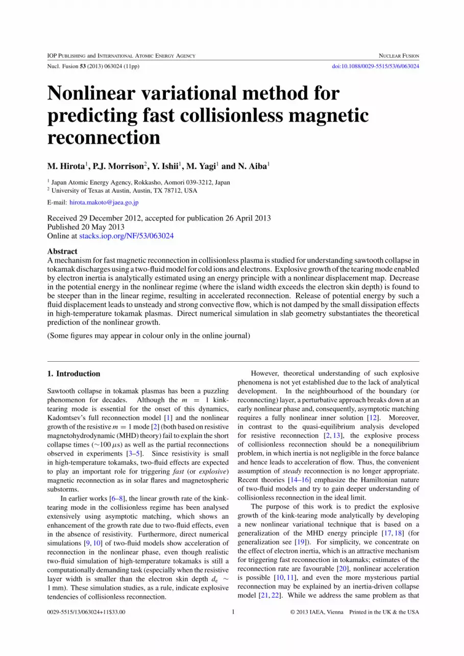
As illustrated in figure 5, this displacement map deforms thecontours of ψe into a pattern with Y -shaped ends [26]. Ina nonlinear regime with de � ε � Lx , we find that such adeformation decreases the potential energy (9) in a manner thatis close to the steepest descent. Leaving the detailed estimateof δW to appendix B, our reasoning process can be detailed asfollows.
First, in the region (i), the flux ψe of the red area of figure 5(left) is squeezed into a thin boundary layer whose width is 2de
in figure 5 (right). On the other hand, the flux is expanded inthe region (iii) and the blue area of figure 5 (left) is almostdoubled in figure 5 (right). The resultant forms of ψe and ψ
4
Nucl. Fusion 53 (2013) 063024 M. Hirota et al
Figure 5. Deformation of contours of ψe by the displacement map (19).
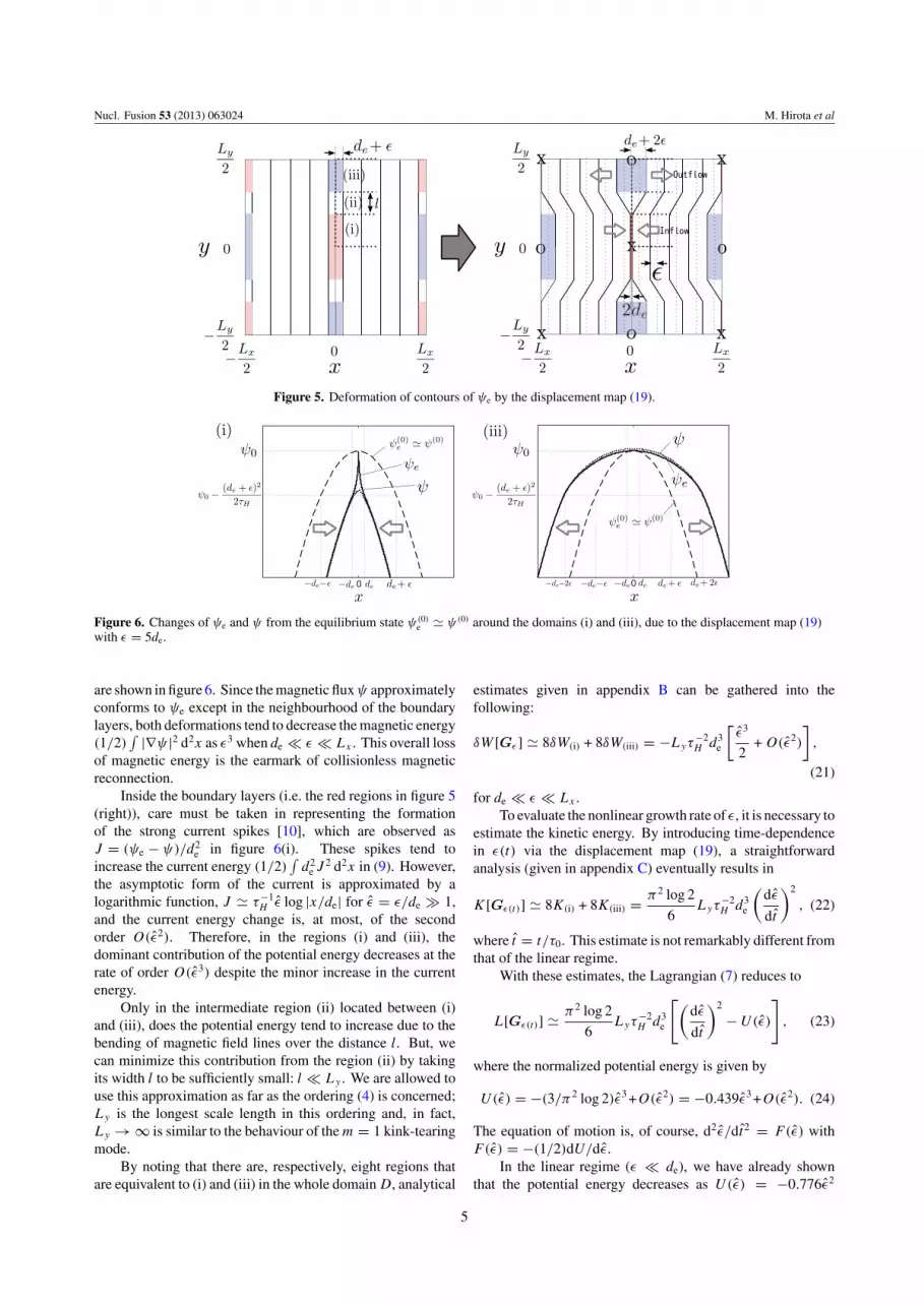
0 0
Figure 6. Changes of ψe and ψ from the equilibrium state ψ(0)e ψ(0) around the domains (i) and (iii), due to the displacement map (19)
with ε = 5de.
are shown in figure 6. Since the magnetic flux ψ approximatelyconforms to ψe except in the neighbourhood of the boundarylayers, both deformations tend to decrease the magnetic energy(1/2)
∫ |∇ψ |2 d2x as ε3 when de � ε � Lx . This overall lossof magnetic energy is the earmark of collisionless magneticreconnection.
Inside the boundary layers (i.e. the red regions in figure 5(right)), care must be taken in representing the formationof the strong current spikes [10], which are observed asJ = (ψe − ψ)/d2
e in figure 6(i). These spikes tend toincrease the current energy (1/2)
∫d2
e J 2 d2x in (9). However,the asymptotic form of the current is approximated by alogarithmic function, J τ−1
H ε log |x/de| for ε = ε/de � 1,and the current energy change is, at most, of the secondorder O(ε2). Therefore, in the regions (i) and (iii), thedominant contribution of the potential energy decreases at therate of order O(ε3) despite the minor increase in the currentenergy.
Only in the intermediate region (ii) located between (i)and (iii), does the potential energy tend to increase due to thebending of magnetic field lines over the distance l. But, wecan minimize this contribution from the region (ii) by takingits width l to be sufficiently small: l � Ly . We are allowed touse this approximation as far as the ordering (4) is concerned;Ly is the longest scale length in this ordering and, in fact,Ly → ∞ is similar to the behaviour of the m = 1 kink-tearingmode.
By noting that there are, respectively, eight regions thatare equivalent to (i) and (iii) in the whole domain D, analytical
estimates given in appendix B can be gathered into thefollowing:
δW [Gε] 8δW(i) + 8δW(iii) = −Lyτ−2H d3
e
[ε3
2+ O(ε2)
],
(21)
for de � ε � Lx .To evaluate the nonlinear growth rate of ε, it is necessary to
estimate the kinetic energy. By introducing time-dependencein ε(t) via the displacement map (19), a straightforwardanalysis (given in appendix C) eventually results in
K[Gε(t)] 8K(i) + 8K(iii) = π2 log 2
6Lyτ
−2H d3
e
(dε
dt
)2
, (22)
where t = t/τ0. This estimate is not remarkably different fromthat of the linear regime.
With these estimates, the Lagrangian (7) reduces to
L[Gε(t)] π2 log 2
6Lyτ
−2H d3
e
[(dε
dt
)2
− U(ε)
], (23)
where the normalized potential energy is given by
U(ε) = −(3/π2 log 2)ε3 +O(ε2) = −0.439ε3 +O(ε2). (24)
The equation of motion is, of course, d2ε/dt2 = F(ε) withF(ε) = −(1/2)dU/dε.
In the linear regime (ε � de), we have already shownthat the potential energy decreases as U(ε) = −0.776ε2
5

Nucl. Fusion 53 (2013) 063024 M. Hirota et al
Figure 7. Contours of ψe convected by the fixed flow (25) (whenε = 5de).
and ε(t) grows exponentially. The steeper descent whereU(ε) = −0.439ε3 in the nonlinear regime (de � ε � Lx)indicates an explosive growth of ε, namely, it reaches the orderof the system size Lx during a finite time ∼ τ0.
We remark that the nonlinear force F(ε) ∼ O(ε2)
obtained here is different from F(ε) ∼ O(ε4) in the earliertheory by Ottaviani and Porcelli [10]. While similar fluidmotion around the X and O points is considered in [10], theydirectly integrate the vorticity equation (1) over the quadrant[0, Lx/2] × [0, Ly/2] and arrive at an equation of motiond2ε/dt2 = F(ε) ∼ O(ε4). However, unless the assumedtrial motion happens to be an exact solution, their treatmentmay lead to a wrong equation of motion that does not satisfyenergy conservation (see appendix D for details). Moreover,their ansatz of the ‘fixed flow-pattern’ is also found to beinappropriate in our trial-and-error process. If we try fixingthe stream function φ throughout the linear and nonlinearregimes as
φ(x, y, t) = −dε
dt(t)ξ (x)
sin ky
k, (25)
with the same ξ (x) as (15), the contours of ψe are deformedinto a mushroom-like shape as shown in figure 7. With thischoice, the potential W does not continue to decrease—sucha fixed flow-pattern merely circulates the flux ψe from the X
point side to the O point side via the boundary layer.In direct numerical simulation, we have calculated the
potential energy U(ε) (or, equivalently, the kinetic energy(dε/dt )2) as a function of ε. As shown in figure 8, the decreasein U(ε) agrees with our scaling and does not support the scalingU ∼ −ε5 of [10].
5. Small dissipation
In this section, we consider the effect of small dissipation byintroducing resistivity (η) and electron perpendicular viscosity(µe) into Ohm’s law (2); i.e.
∂ψe
∂t+ v · ∇ψe = −ηJ + µed
2e ∇2J. (26)
Both terms on the right-hand side only dissipate the potentialenergy W . For sufficiently small η and µe, we can still employthe energy principle in the manner used to describe the resistivewall mode in [32]. Thus, the energy principle is extended as
− γ 2I (2) = W(2) + W(2)
dis + O(η2, µ2e), (27)
Figure 8. Potential energy U(ε) (where de/Lx = 0.01 andLy/Lx = 4π in simulation).
where
W(2)
dis = − 1
γ
∫ Lx/2
−Lx/2dx
(η|J |2 + µed
2e |∇J |2
)< 0, (28)
and
J = ∇2
1 − d2e ∇2
(ψ ′eξ ). (29)
By substituting the same test function ξ of (15) into W(2)
dis , thelinear growth rate (17) is modified to
γ = 0.881τ−10 + 0.367τ−1
e + 0.347τ−1d + τ−1
0 O
(τ 2
0
τ 2e
,τ 2
0
τ 2d
),
(30)
where τe = d2e /η is the electron collision time and τd = d2
e /µe
is the electron diffusion time over a distance de. Small η andµe, therefore, enhance the linear growth rate. This result alsoimplies that the extended energy principle is only valid forτ0/τe � 1 and τ0/τd � 1. When either τ0/τe or τ0/τd islarge, collisional reconnection dominates in the boundary layerand the diffusion process of the inner solution is no longerlegitimately described by Lagrangian mechanics.
Now, let us interpret our result for tokamak parameters.The time scale τ0 in a typical tokamak was already estimatedby Wesson [20], where he compared it with Kadomtsev’sreconnection time. Here, we will repeat a similar argument,but compare τ0 with τe and τd.
Since τe/τd ∼ (ρe/de)2, where ρe is the electron
gyroradius, the effect of electron viscosity is typically muchsmaller than that of resistivity, τe/τd � 1, in stronglymagnetized plasmas in tokamaks.
However, the time scales τ0 and τe can sometimesbe similar in tokamak plasmas. For the m = 1 kink-tearing mode in tokamaks, τ−1
0 = dekτ−1H corresponds to
τ−10 = deq
′1ωA0, where q ′
1 is the derivative of the safety factorq at the q = 1 surface and ωA0 is the toroidal Alfvenfrequency at the magnetic axis. For sample parameters,ωA0 = 6.4 × 10⁶ s−1, Te = 6 keV, n = 3.5 × 10¹⁹ m−3 andq ′
1 = 2.0 m−1, corresponding to TFTR experiments that havesawtooth crashes [4, 5], we obtain τ0 = 90 µs and τe = 270 µs,although the ratio τ0/τe = 0.33 can drastically change inproportion to T
−3/2e n2.
6

Nucl. Fusion 53 (2013) 063024 M. Hirota et al
Figure 9. Instantaneous growth rates (τ0/ε)dε/dt versus resistivityτ0/τe, numerically evaluated at several levels of amplitude ε/de
(de/Lx = 0.01 and Ly/Lx = 4π ).
By recalling that the resistive layer width δη for thecase of �′ = ∞ is given by δη ∼ (η/q ′
1ωA0)1/3, namely,
δη/de ∼ (τ0/τe)1/3, we expect the reconnection to be relatively
collisionless when τ0 is shorter than τe. In fact, the nonlinearacceleration phase is observed numerically for τ0/τe < 1.Figure 9 shows instantaneous growth rates of ε(t) for differentvalues of resistivity τ0/τe(∝ η). The linear growth rate γ ,which emerges at the small amplitude ε/de = 0.1(� 1),obeys the dispersion relation γ τ0 = (τ0/τe + γ τ0)
1/3 obtainedby asymptotic matching [11, 30]. As the amplitude ε entersinto the nonlinear phase ε/de > 1, acceleration occurs forτ0/τe < 1. Since the electron skin depth de is wider thanthe resistive layer width δη for τ0/τe < 1, collisionlessreconnection governs macroscopic fluid motion. In contrast,for τ0/τe > 1, the resistive layer initiates the reconnectionprocess and hence deceleration occurs in figure 9, whichis more like the quasi-equilibrium evolution caused by theresistive kink mode [2].
To obtain a description that is more relevant to actualsawtooth crashes, we would need to improve our developmentby including both ion and electron thermal effects. Invarious high-temperature regimes, the linear stability ofthe m = 1 kink-tearing mode has been treated by manyauthors. For instance, the ion-sound gyroradiusρs (i.e. electronparallel compressibility) enhances the growth rate (17) upto γ ∼ τ−1
0 (ρs/de)2/3 for ρs > de [8]. On the other hand,
diamagnetic effects (stemming from density gradient) rotatethe mode and reduce the growth rate in both collisional andcollisionless regimes [30, 33]. Since the reconnection layeris often narrower than the ion gyroradius, a fully kinetictreatment of ions is appropriate for retaining finite gyroradiuseffects to all orders [34]. The assumption of isothermalelectrons along magnetic fields (which is often used as aclosure of two-fluid models) cannot be also justified by akinetic description of the electrons [29]. By allowing forparallel thermal conductivity derived from electron kinetics,the electron temperature gradient is shown to have a strongstabilizing effect [34–36]. These linear stability theoriesserve to predict the onset of sawteeth, especially, in thesemi-collisional regime [36, 37]. However, the nonlinearrelaxation model remains somewhat heuristic [37], and furtherapplication of this work might provide a pathway for progresson this issue.
6. Summary
In this work, we have analytically elucidated the accelerationmechanism for collisionless reconnection enabled by electroninertia. A variational method based on the Lagrangiandescription of collisionless plasma is shown to be usefulespecially for predicting nonlinear evolution; conventionalasymptotic matching does not apply to this problem unlessan exact nonlinear and unsteady solution is available aroundthe boundary layers.
We have demonstrated the existence of a nonlineardisplacement map that decreases the potential energy of theLagrangian system into the nonlinear regime. No matter howsmall the electron skin depth de, electron inertia enables idealfluid motion to release free energy ( magnetic energy) of theequilibrium state because the frozen-in flux is switched from ψ
to ψe = ψ − d2e ∇2ψ , producing a reconnecting layer of width
de. In the large-�′ limit, the formation of Y -shaped structuresconnected by a current layer in the magnetic configuration isfavourable for the steepest descent of the potential energy. Thisdescent scales as O(ε3) for ε = ε/de � 1 with respect to thedisplacement ε (or the island width). The associated explosivegrowth of ε would continue until ε reaches the system size andleads to an equilibrium collapse during a finite time ∼ τ0.
Although our analytical model is too simple to explainall sawtooth physics in tokamaks, the time scale of explosion(τ0 ∼ 90 µs) that is predicted in this work is comparableto experimentally observed sawtooth collapse times [4, 5].However, resistivity is not negligible in tokamaks and tends todecelerate the reconnection. Our simulations exhibit nonlinearacceleration only for the case of τ0/τe = η/d3
e q ′1ωA0 < 1,
which can be fulfilled by the experiments. In more realisticplasmas, the strong current spike generated by electron inertiawould cause rapid heating of the plasma, which would reducethe local resistivity η, and, what is more, would producerunaway electrons. Since these effects also act as positivefeedback, we expect that sawtooth collapse occurs once theacceleration condition τ0/τe < 1 is satisfied at the q = 1surface.
We infer that the state of lowest potential energy issimilar to Kadomtsev’s fully reconnected state (where q atthe magnetic axis is q0 = 1) [1]. But, if dissipation weresufficiently small, it would also corresponds to the state ofmaximum kinetic energy, where a strong convective flowremains. As shown in numerical simulations [21, 22], sucha residual flow causes a secondary reconnection and restoresa magnetic field similar to the original equilibrium (q0 < 1).If our analytical result is adapted to cylindrical geometry, thispartial reconnection model will be corroborated theoretically.
We expect further application of our variationalapproach to be fruitful for describing strongly nonlinear andnonequilibrium dynamics of sawtooth collapses. As is wellknown, finite-Larmor-radius effects and diamagnetic effectswould modify the island structure and dynamics significantlyon the ion scale which is larger than de. Our approachis feasible even for multiscale problems that require nestedboundary layers, as long as dissipation is not the dominantfactor. Extensions of the present analysis to more general two-fluid equations are in progress and will be reported elsewhere.
7

Nucl. Fusion 53 (2013) 063024 M. Hirota et al
Acknowledgments
The authors would like to thank A. Isayama, M. Furukawa andZ. Yoshida for fruitful discussions. This work was supportedby a grant-in-aid for scientific research from the Japan Societyfor the Promotion of Science (No 22740369). P.J.M. wassupported by the US Department of Energy Contract # DE-FG05-80ET-53088.
Appendix A. Linear stability analysis
In the ideal MHD limit (de = 0), it is well known that theequilibrium (3) has a marginally stable eigenmode (γ = 0)which is expressed by ψ = ψ0 cos κ(α|x| − π/2) (whereκ =
√1 − k2/α2) in terms of ψ = −ψ ′ξ . When k2 < α2,
this eigenmode formally makes W(2) negative;
W(2) = −2 ψψ ′∣∣∣x=+0
x=−0= −2ψ2
0 ακ sin (κπ) < 0, (A.1)
which also implies that the tearing index is positive,�′ = ψ ′/ψ |x=+0
x=−0 = 2ακ tan κ π2 > 0. The corresponding
ξ = −ψ/ψ ′ is, however, discontinuous at x = 0, ±Lx/2 andhence I (2) = ∞. It is therefore reasonable to infer that thismarginal mode would be destabilized by adding electron inertiade � Lx .
Note that the integrand of the potential energy (14) iscomposed of two quadratic terms, which are, respectively,positive and negative definite. Since ψ ′
e ψ ′ for smallde, the main role of the electron inertia is to weaken themagnetic tension (equal to the former positive term) throughthe smoothing operator (1 − d2
e ∇2)−1.By assuming the ordering (4) (in which �′ 8α3/πk2
is large) and employing the test function ξ in figure 3, let usestimate only the leading-order term in (13) and (14). For thatpurpose, we can always use an approximation ∇2 ∂2
x . Then,(13) easily yields the estimate of I (2) in (16).
To calculate the potential energy (14), we introduce aneighbourhood [−d0, d0] of the boundary layer [−de, de],where d0 is supposed to be a few times larger than de. Thepotential energy in the outer region [−Lx/2 + d0, −d0] ∪[d0, Lx/2 − d0] is estimated by
W(2)[−Lx/2+d0,−d0]∪[d0,Lx/2−d0] = −2 ψψ ′
∣∣∣x=d0
x=−d0
−4d0
τ 2H
,
(A.2)
where τ−1H = ψ0α
2, because ψ ψ0 cos(α|x| − π/2) in thisregion.
Next, we focus on the inner region [−d0, d0] using alocal coordinate x = x/de and approximating the equilibriumprofile by ψ ′
e ψ ′ −(de/τH )x. For given
ψe = −ψ ′eξ = de
τH
{−x2 for |x| < 1−|x| for 1 < |x|, (A.3)
the corresponding ψ is obtained by solving ψe = ψ − ∂2xψ
under the boundary condition, ψ → ψe as |x| → ∞. Thisanalysis results in
ψ = de
τH
−(x2 + 2) +3
2e−1(ex + e−x ) |x| < 1
−|x| +3e−1 − e
2e−|x| 1 < |x|,
(A.4)
where ψ(0) �= 0 indicates that this perturbation causesmagnetic reconnection. The potential energy inside the layer[−d0, d0] is calculated as
W(2)[−d0,d0] 1
de
∫ d0/de
−d0/de
dx[|∂xψ |2 + |∂2
x ψ |2]
de
τ 2H
(−1
3− 9e−2 + 2
d0
de
), (A.5)
where we have neglected e−d0/de by making d0 larger than de tosome extent. Since other boundary layers at x = ±Lx/2 canbe treated equivalently, the total potential energy on the wholedomain [−Lx/2, Lx/2] is estimated as (16).
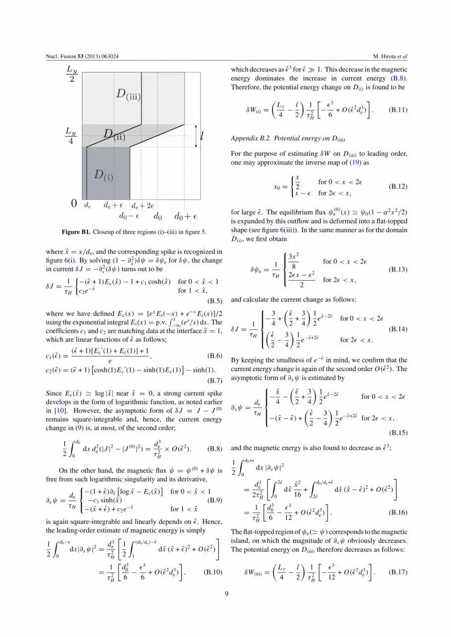
Appendix B. Estimate of potential energy change
Here we estimate change in the potential energy W [Gε] thatis caused by the nonlinear displacement map Gε given in (19).In a way similar to that of the linear analysis (see appendix A),we introduce a domain [0, d0] × [0, Ly/2] where d0 is nowtaken to be somewhat larger than 2de + 2ε. This domain isdeformed by the map Gε as shown in figure B1, where werefer to shrinking and expanding domains as
D(i) = [0, d0 − ε] ×[
0,Ly
4− l
2
], (B.1)
D(iii) = [0, d0 + ε] ×[Ly
4+
l
2,Ly
2
], (B.2)
respectively, and their intermediate domain as D(ii). Thepotential energy will not change significantly outside ofthese domains, because the fluid is simply subject to paralleltranslation along the x-direction. Moreover, we are onlyinterested in the domains D(i) and D(iii), on which efficientdecrease in the potential energy is observed as follows.
Appendix B.1. Potential energy on D(i)
The equilibrium (3) is approximated by ψ(0)e (x) ψ(0)(x)
ψ0(1 − α2x2/2) and it is deformed into ψe(x, y, ε) =ψ
(0)e (g−1
ε (x)) on D(i). Therefore, δψe = ψe −ψ(0)e is given by
δψe = 1
τH
1
2(1 − e2ε )x2 for 0 < x < dee
−ε
−1
2
[de
(log
x
de+ 1
)+ ε
]2
for dee−ε < x < de
+x2
2
−εx − ε2
2 for de < x.
(B.3)
For large ε = ε/de � 1, we can neglect the innermost region0 < x < dee
−ε and the asymptotic form of δψe contains alogarithmic function as follows.
δψe = d2e
τH
−(1 + ε) log x − 12 (1 + ε)2 +
x2
2for 0 < x < 1
−εx − ε2
2for 1 < x,
(B.4)
8
Nucl. Fusion 53 (2013) 063024 M. Hirota et al
Figure B1. Closeup of three regions (i)–(iii) in figure 5.
where x = x/de, and the corresponding spike is recognized infigure 6(i). By solving (1 − ∂2
x)δψ = δψe for δψ , the change
in current δJ = −∂2x (δψ) turns out to be
δJ = 1
τH
{−(ε + 1)Ec(x) − 1 + c1 cosh(x) for 0 < x < 1c2e
−x for 1 < x,
(B.5)
where we have defined Ec(x) = [exEi(−x) + e−xEi(x)]/2using the exponential integral Ei(x) = p.v.
∫ x
−∞(es/s) ds. Thecoefficients c1 and c2 are matching data at the interface x = 1,which are linear functions of ε as follows;
c1(ε) = (ε + 1)[Ec′(1) + Ec(1)] + 1
e, (B.6)
c2(ε) = (ε + 1)[cosh(1)Ec
′(1) − sinh(1)Ec(1)] − sinh(1).
(B.7)
Since Ec(x) log |x| near x = 0, a strong current spikedevelops in the form of logarithmic function, as noted earlierin [10]. However, the asymptotic form of δJ = J − J (0)
remains square-integrable and, hence, the current energychange in (9) is, at most, of the second order;
1
2
∫ d0
0dx d2
e (|J |2 − |J (0)|2) = d3e
τ 2H
× O(ε2). (B.8)
On the other hand, the magnetic flux ψ = ψ(0) + δψ isfree from such logarithmic singularity and its derivative,
∂xψ = de
τH
−(1 + ε)∂x
[log x − Ec(x)
]for 0 < x < 1
−c1 sinh(x)
−(x + ε) + c2e−x for 1 < x
(B.9)
is again square-integrable and linearly depends on ε. Hence,the leading-order estimate of magnetic energy is simply
1
2
∫ d0−ε
0dx|∂xψ |2 = d3
e
τ 2H
[1
2
∫ (d0/de)−ε
1dx (x + ε)2 + O(ε2)
]
= 1
τ 2H
[d3
0
6− ε3
6+ O(ε2d3
e )
], (B.10)
which decreases as ε3 for ε � 1. This decrease in the magneticenergy dominates the increase in current energy (B.8).Therefore, the potential energy change on D(i) is found to be
δW(i) =(
Ly
4− l
2
)1
τ 2H
[−ε3
6+ O(ε2d3
e )
]. (B.11)
Appendix B.2. Potential energy on D(iii)
For the purpose of estimating δW on D(iii) to leading order,one may approximate the inverse map of (19) as
x0 ={x
2for 0 < x < 2ε
x − ε for 2ε < x,(B.12)
for large ε. The equilibrium flux ψ(0)e (x) ψ0(1 − α2x2/2)
is expanded by this outflow and is deformed into a flat-toppedshape (see figure 6(iii)). In the same manner as for the domainD(i), we first obtain
δψe = 1
τH
3x2
8for 0 < x < 2ε
2εx − ε2
2for 2ε < x,
(B.13)
and calculate the current change as follows:
δJ = 1
τH
−3
4+
(ε
2+
3
4
)1
2ex−2ε for 0 < x < 2ε
(ε
2− 3
4
)1
2e−x+2ε for 2ε < x.
(B.14)
By keeping the smallness of e−ε in mind, we confirm that thecurrent energy change is again of the second order O(ε2). Theasymptotic form of ∂xψ is estimated by
∂xψ = de
τH
− x
4−
(ε
2+
3
4
)1
2ex−2ε for 0 < x < 2ε
−(x − ε) +
(ε
2− 3
4
)1
2e−x+2ε for 2ε < x,
(B.15)
and the magnetic energy is also found to decrease as ε3;
1
2
∫ d0+ε
0dx |∂xψ |2
= d3e
2τ 2H
[∫ 2ε
0dx
x2
16+
∫ d0/de+ε
2ε
dx (x − ε)2 + O(ε2)
]
= 1
τ 2H
[d3
0
6− ε3
12+ O(ε2d3
e )
]. (B.16)
The flat-topped region of ψe( ψ) corresponds to the magneticisland, on which the magnitude of ∂xψ obviously decreases.The potential energy on D(iii) therefore decreases as follows:
δW(iii) =(
Ly
4− l
2
)1
τ 2H
[− ε3
12+ O(ε2d3
e )
]. (B.17)
9

Nucl. Fusion 53 (2013) 063024 M. Hirota et al
Appendix C. Estimate of kinetic energy
Here we estimate the kinetic energy K[Gε(t)] of thedisplacement map Gε(t) given in (19), where only ε(t) isassumed to be time-dependent. By invoking figure B1 again,the dominant part of kinetic energy turns out to exist in thedomains D(i), D(ii) and D(iii). Since D(ii) is ignored in thiswork (by assuming l � Ly), we exhibit only the results forD(i) and D(iii) as follows.
Appendix C.1. Kinetic energy on D(i)
Owing to our special choice of gε , the x-component of thevelocity field on D(i) is simply given by
vx(x, y, ε) = dε
dt
dgε
dε(g−1
ε (x)) = dε
dt
− x
defor 0 < x < de
−1 for de < x.
(C.1)
By solving the incompressibility condition ∂xvx + ∂yvy = 0under appropriate boundary conditions, the y-component ofthe velocity field is found to be
vy(x, y, ε) = dε
dt
y
defor 0 < x < de
0 for de < x.
(C.2)
This vy dominantly contributes to the kinetic energy on D(i),which is readily estimated by
K(i) =∫ Ly
4 − l2
0dy
×∫ d0−ε
0dx
1
2(v2
x + v2y) 1
6de
(Ly
4− l
2
)3 (dε
dt
)2
. (C.3)
Appendix C.2. Kinetic energy on D(iii)
We can go through the same procedures as for D(i), but theanalysis is somewhat complicated by the fact that the inversemap x �→ x0 should be dealt with as an implicit function.In terms of the unperturbed position x0, the velocity field isexpressed by
vx(x, y, ε) = dε
dt
∂x
∂ε(x0)
= dε
dt
x0e−ε for 0 < x0 < de
ex0−ε−1 for de < x0 < de + ε
1 for de + ε < x0,
(C.4)
vy(x, y, ε) =(
Ly
2− y
)dε
dt
1
de
×
e−ε
2 − e−εfor 0 < x0 < de
ex0−ε−1
2 − ex0−ε−1for de < x0 < de + ε
0 for de + ε < x0.
(C.5)
Using the change of variables from x to x0, the kinetic energyon D(iii) is therefore estimated as
K(iii) =∫ Ly
2
Ly
4 + l2
dy
∫ d0
0dx0
1
2(v2
x + v2y)
∂x
∂x0
2 log 2 − 1
6de
(Ly
4− l
2
)3 (dε
dt
)2
, (C.6)
where we have neglected e−ε for large ε � 1.
Appendix D. Comparison with the Ottaviani andPorcelli approach
In [10], Ottaviani and Porcelli (hereafter, OP) integrated thevorticity equation (1) over a convection cell, S = [0, Lx/2] ×[0, Ly/2], and obtainedd
dt
∫S
d2x ∇2φ = 2
τH
(δψX − δψO) − 1
d2e
(δψ2X − δψ2
O),
(D.1)
where δψX and δψO denote the values of δψ = ψ − ψ(0)
at the X and O points, respectively. By assuming the fixedflow-pattern (25) with ξ given by (15), one can estimate
δψX − ε2
2τH
and δψO ∼ O
(d2
e
τH
), (D.2)
for ε > de and, using Stokes’ theorem,∫S
d2x ∇2φ =∮
∂S
v · dl 4
k2
dε
dtξ ′(0) = − 4
k2de
dε
dt. (D.3)
Thus, OP derived the nonlinear equation, d2ε/dt2 ε4/16(see also chapter 6.4.1 of [38] and further application in [39]).Even if we employ our displacement map (19) in this OPapproach, the estimates (D.2) and (D.3) are almost invariable(in view of vx of (C.1) and δψ of figure 6) and a similarnonlinear equation is reproduced.
However, we note that the OP approach does not yield avalid result. To demonstrate this fact, let us modify the testfunction ξ slightly as follows:
ξ (x) =
− x
deσ for 0 < x < dee
−ε
−1 − σe−ε
1 − e−ε
x
de+
1 − σ
1 − e−εe−ε for dee
−ε < x < de
−1 for de < x,
(D.4)
and ξ (−x) = −ξ (x), in which a sublayer [0, dee−ε] and
another free parameter σ are newly introduced; thus, the caseσ = 1 reduces to (15). For σ � eε , this modification appearsto be very minor, but the estimate (D.3) drastically changes to∫
S
d2x ∇2φ − 4σ
k2de
dε
dt. (D.5)
Therefore, the result becomes d2ε/dt2 ε4/16σ and thenonlinear growth rate is indeterminate since we can chooseσ = εn with arbitrary n ∈ R. Thus, there is no way toreasonably determine the correct value of σ with this approach.Moreover, only the fluid motion along the boundary (∂S) of S
is actually used for evaluating the equation (D.1) and, hence,the result derived from (D.1) is generally inconsistent with theenergy conservation law on S.
In the variational approach we have used, introduction ofsuch a thin sublayer [0, dee
−ε] into (19) does not affect theoverall estimates of kinetic and potential energies. Therefore,our displacement map (19) is enough to predict the nonlineargrowth, even though it does not perfectly coincide with theexact nonlinear solution.
10

Nucl. Fusion 53 (2013) 063024 M. Hirota et al
References
[1] Kadomtsev B.B. 1975 Sov. J. Plasma Phys. 1 389[2] Waelbroeck F.L. 1989 Phys. Fluids B 1 2372[3] Soltwisch H. 1988 Rev. Sci. Instrum 59 1599[4] Levinton F.M., Batha S.H., Yamada M. and Zarnstorff M.C.
1993 Phys. Fluids B 5 2554[5] Yamada M., Levinton F.M., Pomphrey N., Budny R.,
Manickam J. and Nagayama Y. 1994 Phys. Plasmas 1 3269[6] Drake J.F. 1978 Phys. Fluids 21 1777[7] Basu B. and Coppi B. 1981 Phys. Fluids 24 465[8] Porcelli F. 1991 Phys. Rev. Lett. 66 425[9] Aydemir A.Y. 1992 Phys. Fluids B 4 2469
[10] Ottaviani M. and Porcelli F. 1993 Phys. Rev. Lett. 71 3802[11] Ottaviani M. and Porcelli F. 1995 Phys. Plasmas 2 4104[12] Rosenbluth M.N., Dagazian R.Y. and Rutherford P.H. 1973
Phys. Fluids 16 1894[13] Rutherford P.H. 1973 Phys. Fluids 16 1903[14] Cafaro E., Grasso D., Pegoraro F., Porcelli F. and Saluzzi A.
1998 Phys. Rev. Lett. 80 4430[15] Grasso D., Califano F., Pegoraro F. and Porcelli F. 1999
Plasma Phys. Control. Fusion 41 1497[16] Tassi E., Morrison P.J., Grasso D. and Pegoraro F. 2010 Nucl.
Fusion 50 034007[17] Bernstein I.B., Frieman E.A., Kruskal M.D. and Kulsrud R.M.
1958 Proc. R. Soc. Lond. A 244 17[18] Hain K., Lust R. and Schluter A. 1957 Z. Naturforsch. 12a 833[19] Morrison P.J. 2009 AIP Conf. Proc. 1188 329[20] Wesson J.A. 1990 Nucl. Fusion 30 2545[21] Biskamp D. and Drake J.F. 1994 Phys. Rev. Lett. 73 971
[22] Naitou H., Tsuda K., Lee W.W. and Sydora R.D. 1995 Phys.Plasmas 2 4257
[23] Newcomb W.A. 1962 Nucl. Fusion (Suppl. pt 2) 451[24] Morrison P.J. 1998 Rev. Mod. Phys. 70 467[25] Padhye N. and Morrison P.J. 1996 Plasma Phys. Rep. 22 869[26] Syrovatskii S.I. 1971 Sov. Phys.—JETP 33 933
http://jetp.ac.ru/cgi-bin/e/index/e/33/5/p933?a=list[27] Kuvshinov B.N., Pegoraro F., Schep T.J. 1994 Phys. Lett. A
191 296[28] Schep T.J., Pegoraro F. and Kuvshinov B.N. 1994 Phys.
Plasmas 1 2843[29] Zocco A. and Schekochihin A.A 2011 Phys. Plasmas
18 102309[30] Ara G., Basu B., Coppi B., Laval G., Rosenbluth M.N. and
Waddell B.V. 1978 Ann. Phys. 112 443[31] Hirota M. 2011 J. Plasma Phys. 77 589[32] Haney S.W. and Freidberg J.P. 1989 Phys. Fluids B 1 1637[33] Pegoraro F., Porcelli F. and Schep T.J. 1989 Phys. Fluid B
1 364[34] Antonsen T.M. and Coppi B. 1981 Phys. Lett. A 81 335[35] Cowley S.C., Kulsrud R.M. and Hahm T.S. 1986 Phys. Fluids
29 3230[36] Connor J. W., Hastie R.J. and Zocco A. 2012 Plasma Phys.
Control. Fusion 54 035003[37] Porcelli F., Boucher D. and Rosenbluth M.N. 1996 Plasma
Phys. Control. Fusion 38 2163[38] Biskamp D. 2000 Magnetic Reconnection in Plasmas
(Cambridge: Cambridge University Press) p 227[39] Bhattacharjee A., Germaschewski K. and Ng C.S. 2005 Phys.
Plasmas 12 042305
11


