MHD Reconnection Theory

Eric R Priest and Clare E ParnellMathematics Institute, St Andrews University, ST ANDREWS, KY16 8QR, UK

email: eric@mcs.st-and.ac.uk\ clare@mcs.st-and.ac.uk

http://www-solar.mcs.st-and.ac.uk/ erichttp://www-solar.mcs.st-and.ac.uk/ clare

May 27, 2009

Abstract

In this review we focus on the fundamental theory of magnetohydrodynamic reconnection,mentioning only in passing the related topics of collisionless reconnection and of the applica-tions of reconnection in a wide range of solar processes, such as dynamo theory, magnetocon-vection, coronal heating, solar flares and coronal mass ejections.

The introduction (§1) gives a brief historical survey and an overview of reconnection con-cepts. There follows a treatment of several preliminary topics that are necessary before thesubtleties of reconnection can be fully grasped: these include null points (§§2–3.1), other topo-logical and geometrical features such as separatrices, separators and quasi-separatrix layers(§3), magnetic helicity (§4), and the conservation of magnetic flux and field lines (§5). Theseset the scene for a section (§6) on the nature of reconnection in three dimensions that coversthe conditions for reconnection, the failure of the concept of a flux velocity, the nature ofdiffusion, the differences between two-dimensional and three-dimensional reconnection, andthe definition and classification of reconnection.

Next, the way in which reconnection operates in two dimensions is described in detail,including current sheet formation (§7), magnetic annihilation (§8), slow and fast regimes ofsteady reconnection (§9), and nonsteady reconnection such as the tearing mode (§10). Finally,our current understanding of the different regimes of reconnection that are possible in threedimensions is summarised (§11), together with numerical experiments that are shedding furtherlight on the nature and diversity of three-dimensional reconnection (§12).

1

(a)

A A C

B

(b)

ve 2L 2Le

(c)

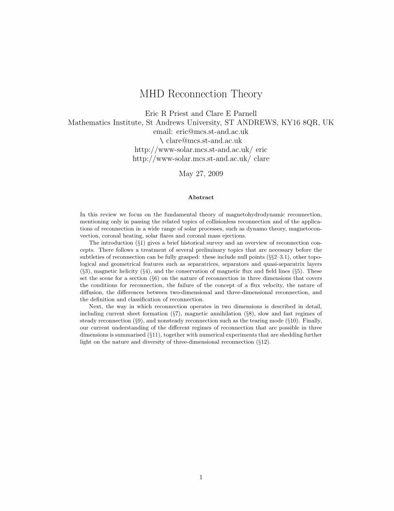
Figure 1: A change of magnetic connectivity is produced by reconnection in a localised diffusionregion (shaded), such that a plasma element A is initially connected to a plasma element B andafter reconnection it is connected to C.

1 Introduction

Magnetic reconnection is responsible for many dynamic processes in laboratory, solar-system andastrophysical plasmas. It is a fundamental process in an almost-ideal plasma whose magneticReynolds number based on global scales (Le) is much larger than unity. In this article we givean overview of the magnetohydrodynamic aspects of reconnection theory and refer the reader forfurther details to Priest and Forbes (2000) or Birn and Priest (2007), including collisionless theoryand observational effects of reconnection.

The magnetic connections of all plasma elements are preserved in an ideal medium, but the keypoint about reconnection is that the presence of a localised region of length L (≪ Le), say, wherenonideal effects are important in the induction equation, can lead to a change of connectivity ofplasma elements – in other words, to magnetic reconnection (Fig.1,2). The reconnection may befast or slow (in a sense defined in §1.1), although in many dynamic phenomena such as solar flaresit is fast. Note also that we refer to a change of connectivity rather than a change of topology,since (as we shall see later) the topology (§1.2) does not always change during reconnection.

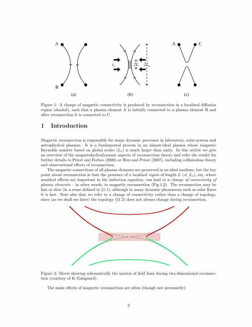
Figure 2: Movie showing schematically the motion of field lines during two-dimensional reconnec-tion (courtesy of K Galsgaard).

The main effects of magnetic reconnection are often (though not necessarily):

2

(i) to convert some of the magnetic energy into heat by ohmic dissipation;(ii) to accelerate plasma by converting magnetic energy into bulk kinetic energy;(iii) to generate strong electric currents and electric fields, as well as shock waves and current

filamentation, all of which, in a low-density plasma such as the solar corona, may acceleratefast particles;

(iv) to change the global connections of the field lines and so affect the paths of fast particlesand heat, which are directed mainly along the magnetic field.

In the solar interior and low solar atmosphere, where the plasma is highly collisional, recon-nection may be well modelled by resistive MHD with classical ohmic dissipation. However, in theouter corona, where collisionless effects dominate, Hall MHD with a two-fluid approach or a kineticmodel are more appropriate for a full treatment (see Birn and Priest, 2007). Nevertheless, even inthe latter case, an MHD approach can capture much of the essence of the process and provide anoverall macroscopic picture or mould within which the detailed micro-plasma physics operates.

In this review, we develop the background and fundamental concepts that are necessary forunderstanding the nature of reconnection in general (§§1–5). To start with, we discuss the struc-ture of null points where the magnetic field vanishes, both in 2D (§2) and 3D (§3.1), as well as theways in which such nulls collapse. Then we describe other geometrical features such as separatricesand quasi-separatrices which map out the skeleton and quasi-skeleton of a complex magnetic con-figuration (§3). Other useful and subtle concepts are magnetic helicity (§4) and the conservationof magnetic flux and field lines (§5). These enable us to describe the nature of three-dimensionalreconnection (§6).

There follow several sections on aspects of two-dimensional reconnection (§§7–10). First of all,we show in §7 how current sheets may be formed by different types of motion, namely, planar,shearing and braiding. Once a current sheet has formed it tends to diffuse away, but, if magneticfield and plasma are brought in at the same rate as the outwards diffusion, then a steady statemay be set up. For the case of straight field lines and a stagnation-point flow, there exists anexact solution of the steady nonlinear MHD equations, known as the Stagnation-Point Flow Model(Sonnerup and Priest, 1975) (§8.3), for both a 2D and a 3D stagnation flow. A generalisation ofthis solution was later discovered, which has an X-point field in place of a 1D field and is referredto as reconnective annihilation (§8.5). Steady 2D reconnection solutions are described in §§9.1–9.3,including the Sweet-Parker model, Petschek’s mechanism and the Almost-Uniform family of fastsolutions. Also, unsteady solutions due to tearing-mode instability are presented in §10.

Finally, the different regimes of three-dimensional reconnection so far discovered are presented(§11), although this is very much a matter of current research. These include quasi-separatrix layer(QSL) reconnection in the absence of a null point at a quasi-separator and separator reconnectionat a separator. Also, three kinds of reconnection may occur at a null point, namely, torsional spinereconnection, torsional fan reconnection and spine-fan reconnection.

Parts of this review have been adapted from sections of the book on reconnection by Priest andForbes (2000), and a concise version of it appears as a chapter in the revised version of the book onSolar MHD (Priest, 2011). A combination of numerical experiment, physical understanding andtheoretical models stimulated by observations will be needed to develop the field further.

1.1 HISTORICAL OVERVIEW

The field of reconnection theory originated with Giovanelli (1947)’s idea that electric fields near amagnetic neutral point could accelerate particles and generate heat in solar flares. Cowling (1953)pointed out that a current sheet only a few metres thick would be needed to do so, while Dungey(1953) showed that such a current sheet can form by the collapse of the magnetic field near an

3

X-type neutral point (§2.2) and was the first to suggest that “lines of force can be broken andrejoined”.

Then Sweet (1958a) presented a model at an IAU Symposium in Stockholm for the way themagnetic field flattens to form a current sheet at an X-type neutral point when two bipolar regionscome together. The magnetic field squeezes out the plasma from between them in a process ofsteady-state reconnection. Parker (1957) was at the meeting and, on the plane home, he cameup with his formulation of scaling laws for the model and coined the phrase “reconnection of fieldlines”.

The Sweet-Parker model, which gives order of magnitude relations between the dimensions of acurrent sheet and the input and output flow and field strength, has a reconnection rate (or inflow

plasma speed) of vi = vAi/R1/2m , where vAi is the inflow Alfven speed and Rm = LvAi/η is the

magnetic Reynolds number based on the length L of the sheet. This rate is a small fraction of theAlfven speed (if Rm ≫ 1) and is much too slow for solar flares, so that it is referred to as slowreconnection.

The next development was a non-ideal stability analysis of a one-dimensional current sheet byFurth et al. (1963), who discovered several resistive instabilities that involve magnetic reconnection,notably the tearing-mode instability (§10).

Furthermore, Petschek (1964) realised that slow-mode shock waves also convert magnetic energyinto heat and kinetic energy and are naturally generated by a tiny diffusion region. His (steady)mechanism (at typically 0.01−0.1vA) is indeed rapid enough for a flare. It possesses four standingslow-mode shock waves extending from a tiny central Sweet-Parker current sheet and is the firstof many regimes of fast reconnection.

For the next few years Petschek’s mechanism was widely accepted as the answer to fast flareenergy release. But then other models were proposed and Sonnerup (1970) came along with analternative reconnection model that could operate at any rate up to the Alfven speed, while Yehand Axford (1970) sought self-similar solutions of the steady MHD equations. Later, Vasyliunas(1975) clarified matters in a major review that highlighted various mathematical and physicaldifficulties with these alternative solutions. In particular, Sonnerup’s model possesses an extrastanding discontinuity in each quadrant in addition to the Petschek shock wave, and, whereas thePetschek shocks are generated by the diffusion region, the Sonnerup discontinuities need to begenerated externally.

The result was that only Petschek’s mechanism was accepted, especially when self-similar solu-tions for the external region were discovered (Soward and Priest, 1977), when the central diffusionregion is regarded as a region of small dimensions as far as the external region is concerned.

A state of calm ensued – until the watershed year of 1986 when new resistive MHD compu-tational and theoretical models led to a new state of ferment. Numerical experiments (Biskamp,1986) revealed solutions that are very different from Petschek’s and so, at first, they seemed tocast doubt on the validity of the Petschek mechanism. However, Priest and Forbes (1986) realisedthat the reason for the difference was the different boundary conditions being imposed by Biskamp.They discovered a whole family of Almost-Uniform solutions for fast reconnection, including thesolutions of both Petschek and Biskamp as special cases.

It is now well established that, when the magnetic diffusivity is enhanced at the X-point,Petschek’s mechanism and the other Almost-Uniform reconnection regimes can indeed occur, andthat an enhancement of diffusivity is a common effect in practice. However, what happens whenthe magnetic diffusivity is spatially uniform is not yet clear. The suspicion from high-resolutionnumerical experiments (Baty et al., 2009a,b) is that the case of uniform diffusivity is neutrallystable such that fast reconnection is stable when the diffusion region diffusivity is enhanced and isunstable (to some, as yet unidentified, instability) when it is reduced.

Fast collisionless reconnection may be assisted by the Hall effect (Shay and Drake, 1998; Huba,2003), in which the resistive diffusion region is replaced by an ion diffusion region of length equal

4

to an ion inertial length and a smaller electron diffusion region. Indeed, the GEM Challengehas shown that full-particle, hybrid and Hall MHD codes all tend to give the same fast rate ofreconnection (Birn et al., 2001).

Most of the attention is now focussed on 3D reconnnection, which is completely different from2D reconnection in ways identified by Priest et al. (2003). A landmark paper by Schindler et al.(1988) proposed a concept of General Magnetic Reconnection, in which reconnection can occureither at null points or in the absence of null points whenever a parallel electric field (E‖) isproduced by any region of local nonidealness. The condition for reconnection to occur is simplythat ∫

E‖ ds 6= 0,

evaluated along a magnetic field line that passes through the region of local nonidealness: indeed,the maximum value of this integral gives the rate of reconnection. So far, the theory of three-dimensional reconnection is not sufficiently well developed to say what is the maximum allowedreconnection rate.

Later, Priest and Pontin (2009) updated an earlier classification (Priest and Titov, 1996) byproposing models for several types of 3D reconnection, known as: torsional spine or torsional fanreconnection when rotational motions concentrate the current along the spine or fan of a null point(§11.2); spine-fan reconnection when shearing motions concentrate it along both; and separatorreconnection when it focusses along the separator field line (§11.3) that joins two null points andrepresents the intersection of two separatrix surfaces. Furthermore, Priest and Demoulin (1995)proposed a concept of reconnection in a quasi-separatrix layer (QSL) (§11.4) in the absence ofnull points, while Demoulin et al. (1996a) applied it to solar flares. QSL reconnection is calledslip-running reconnection by some authors (Aulanier et al., 2006), which refers to the magneticflipping process (Priest and Forbes, 1992b) that is a common feature of much reconnection in threedimensions. In a QSL the mapping of magnetic field lines changes continuously but extremelyrapidly, whereas across a true separatrix surface it changes discontinuously.

1.2 SUMMARY of RECONNECTION CONCEPTS

Several new concepts are involved in moving from two to three dimensions (§6). When non-ideal plasma effects are important in a localised region, there are several classes of evolution of amagnetic field that satisfy Faraday’s law and ∇ · B = 0 (Fig.3 and §5.3). The largest subclassconserves electromagnetic flux

∫

S(t)

B·dS +

∫

S(t)

E·dl dt = const.

One subclass of solutions conserves magnetic flux by itself (∫

S(t) B · dS = const), while another

represents 3D reconnection. Also, the subclass of 3D reconnection that preserves magnetic fluxrepresents 2D reconnection. Furthermore, magnetic flux conservation implies field line conserva-tion, but the reverse is not true since there are solutions that conserve field lines but not flux.

When E+v×B = 0, the magnetic flux and field line connections are both conserved and thereis no reconnection. A consequence of this is that the magnetic topology is conserved. The termmagnetic topology refers here to any property that is preserved by an ideal displacement, such asthe linkage and knottedness of the field.

When the plasma is instead non-ideal with E + v × B = N, where N represents any nonidealterm such as N = ηj, then the condition B× (∇×N) = 0 implies field-line conservation, whereas

5

All

E.m.

3D rec.2D rec.

Magnetic

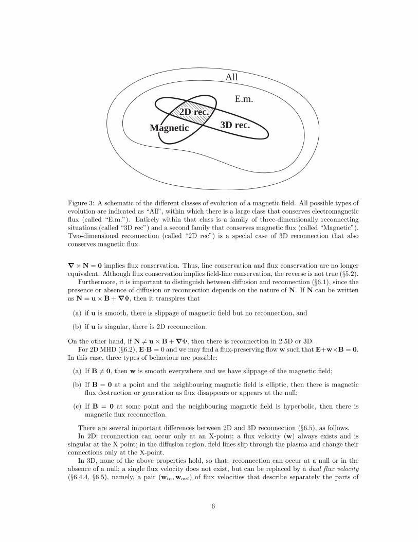
Figure 3: A schematic of the different classes of evolution of a magnetic field. All possible types ofevolution are indicated as “All”, within which there is a large class that conserves electromagneticflux (called “E.m.”). Entirely within that class is a family of three-dimensionally reconnectingsituations (called “3D rec”) and a second family that conserves magnetic flux (called “Magnetic”).Two-dimensional reconnection (called “2D rec”) is a special case of 3D reconnection that alsoconserves magnetic flux.

∇ ×N = 0 implies flux conservation. Thus, line conservation and flux conservation are no longerequivalent. Although flux conservation implies field-line conservation, the reverse is not true (§5.2).

Furthermore, it is important to distinguish between diffusion and reconnection (§6.1), since thepresence or absence of diffusion or reconnection depends on the nature of N. If N can be writtenas N = u × B + ∇Φ, then it transpires that

(a) if u is smooth, there is slippage of magnetic field but no reconnection, and

(b) if u is singular, there is 2D reconnection.

On the other hand, if N 6= u × B + ∇Φ, then there is reconnection in 2.5D or 3D.For 2D MHD (§6.2), E·B = 0 and we may find a flux-preserving flow w such that E+w×B = 0.

In this case, three types of behaviour are possible:

(a) If B 6= 0, then w is smooth everywhere and we have slippage of the magnetic field;

(b) If B = 0 at a point and the neighbouring magnetic field is elliptic, then there is magneticflux destruction or generation as flux disappears or appears at the null;

(c) If B = 0 at some point and the neighbouring magnetic field is hyperbolic, then there ismagnetic flux reconnection.

There are several important differences between 2D and 3D reconnection (§6.5), as follows.In 2D: reconnection can occur only at an X-point; a flux velocity (w) always exists and is

singular at the X-point; in the diffusion region, field lines slip through the plasma and change theirconnections only at the X-point.

In 3D, none of the above properties hold, so that: reconnection can occur at a null or in theabsence of a null; a single flux velocity does not exist, but can be replaced by a dual flux velocity(§6.4.4, §6.5), namely, a pair (win,wout) of flux velocities that describe separately the parts of

6

a field line that enter and leave a diffusion region; in the diffusion region, field lines continuallychange their connections. This leads to a general classification of the different types of nonidealprocess (§6.6), including Schindler et al. (1988)’s concept of “General Magnetic Reconnection”, forwhich

∫E|| ds 6= 0.

7

(a)0.75

-0.75

0.0

0.0

x/L

y/L

1.0-1.0 0.0

x/L

1.0-1.0

(b)

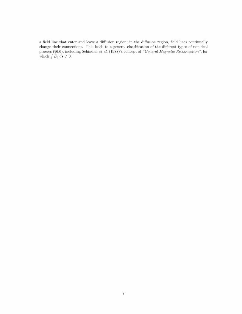
Figure 4: Null points in two dimensions of (a) O-type with α2 = −0.5 and (b) X-type with α2 = 0.5.

2 Neutral Points in Two Dimensions

Neutral (or null) points are locations in a magnetic configuration where the magnetic field van-ishes. X-type null points are important as potential weak spots in a magnetic field, in the sensethat current sheets tend to be created at them in response to external motions. Here we describetheir structure and the way they tend to collapse.

2.1 STRUCTURE of 2D NEUTRAL POINTS

A general linear null point has field components BX = bX + 2cY, BY = −2aX + dY, whichcan be transformed to

Bx = B0y

r0, By = B0α

2 x

r0, (1)

whereB0

r0= (a+ c) −

√

b2 + (a− c)2, α2 =

√

b2 + (a− c)2 + (a+ c)√

b2 + (a− c)2 − (a+ c).

When α2 < 0, the field lines are elliptical (Fig.4a) and the origin is an O-type neutral point.The particular case when α2 = −1 produces circular field lines.

When α2 > 0, the field lines are hyperbolic (Fig.4b) and we have an X-type neutral point orX-point. The limiting field lines y = ± α x through the origin are known as separatrices and areinclined at the angles ± tan−1 α to the x-axis. The separatrices form an “X”, from which the term“X-type” null point is derived.

The value of α (and therefore the angle between the separatrices) is related to the currentdensity. Taking the curl of B we find jz = B0/(µr0)(α

2 − 1), where the z-direction is out of theplane. Thus, when α = 1, jz = 0 and the separatrix angle is 90◦, whereas, when α is imaginary,we have an O-point and jz 6= 0.

2.2 COLLAPSE of 2D NEUTRAL POINTS

An X-type neutral point tends to be locally unstable if the sources of the magnetic field are free

8

(b)

yy

x x

(a)

TP R R

R

R

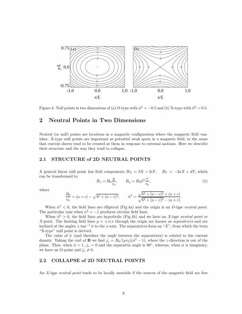
Figure 5: (a) The magnetic field lines near an X-type neutral point that is in equilibrium with nocurrent. A plasma element (shaded) is acted on by a magnetic pressure force (P ) and a magnetictension force (T ). (b) A uniform-current perturbation away from equilibrium with a resultant forceR.

to move (Dungey, 1953). This may be demonstrated in different ways, namely, by a qualitativephysical analysis, by a nonlinear self-similar solution and by a linear analysis as follows.

2.2.1 QUALITATIVE PHYSICAL ANALYSIS

Consider an equilibrium current-free field

Bx = B0y

r0, By = B0

x

r0, (2)

where B0 and r0 are constant. The field lines are the rectangular hyperbolae y2−x2 = constant, asshown in Fig.5a. Any element of plasma, such as the one shown on the negative x-axis, experiencesa magnetic tension force (T ) that acts outwards from the origin due to the outwardly curving fieldlines. It is exactly balanced by a magnetic pressure force (P ), which acts inwards because themagnetic field strength weakens as one approaches the origin.

Now suppose the magnetic field (2) is distorted to the form

Bx =B0

r0y, By =

B0

r0α2x,

where α2 (> 1) is constant. The field lines are given by y2 − α2x2 = constant and are sketchedin Fig.5b. The limiting field lines (y = ± αx) through the origin are no longer inclined at 1

2π, buthave closed up a little, like a pair of scissors.

On the x-axis, the field lines are more closely spaced than in Fig.5a, so the magnetic pressureforce has increased. They also have smaller curvature, so the magnetic tension force has increasedless than the pressure. The dominance of the magnetic pressure produces a resultant force (R)acting inward. On the y-axis, the field lines have the same spacing as in Fig.5a, but they are moresharply curved, so the magnetic pressure force remains the same, while the tension force increases;the resultant force (R) therefore acts outwards as shown. These comments may be borne out by

9

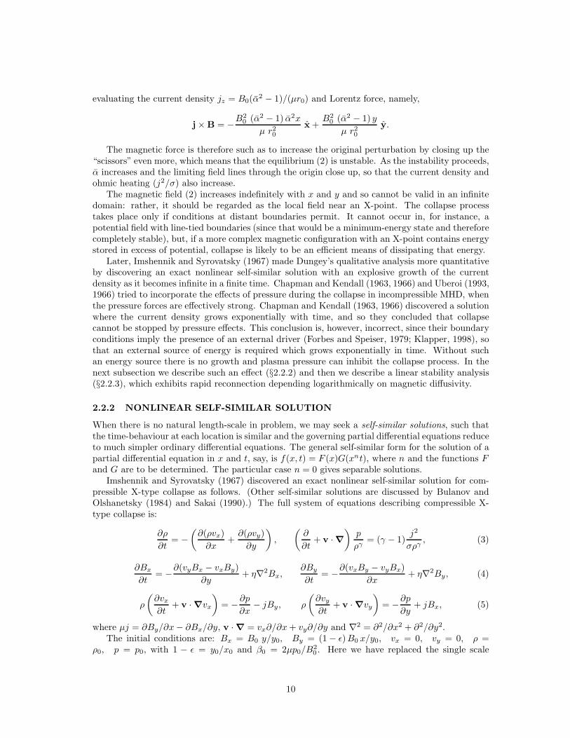
evaluating the current density jz = B0(α2 − 1)/(µr0) and Lorentz force, namely,

j × B = −B20 (α2 − 1) α2x

µ r20x +

B20 (α2 − 1) y

µ r20y.

The magnetic force is therefore such as to increase the original perturbation by closing up the“scissors” even more, which means that the equilibrium (2) is unstable. As the instability proceeds,α increases and the limiting field lines through the origin close up, so that the current density andohmic heating (j2/σ) also increase.

The magnetic field (2) increases indefinitely with x and y and so cannot be valid in an infinitedomain: rather, it should be regarded as the local field near an X-point. The collapse processtakes place only if conditions at distant boundaries permit. It cannot occur in, for instance, apotential field with line-tied boundaries (since that would be a minimum-energy state and thereforecompletely stable), but, if a more complex magnetic configuration with an X-point contains energystored in excess of potential, collapse is likely to be an efficient means of dissipating that energy.

Later, Imshennik and Syrovatsky (1967) made Dungey’s qualitative analysis more quantitativeby discovering an exact nonlinear self-similar solution with an explosive growth of the currentdensity as it becomes infinite in a finite time. Chapman and Kendall (1963, 1966) and Uberoi (1993,1966) tried to incorporate the effects of pressure during the collapse in incompressible MHD, whenthe pressure forces are effectively strong. Chapman and Kendall (1963, 1966) discovered a solutionwhere the current density grows exponentially with time, and so they concluded that collapsecannot be stopped by pressure effects. This conclusion is, however, incorrect, since their boundaryconditions imply the presence of an external driver (Forbes and Speiser, 1979; Klapper, 1998), sothat an external source of energy is required which grows exponentially in time. Without suchan energy source there is no growth and plasma pressure can inhibit the collapse process. In thenext subsection we describe such an effect (§2.2.2) and then we describe a linear stability analysis(§2.2.3), which exhibits rapid reconnection depending logarithmically on magnetic diffusivity.

2.2.2 NONLINEAR SELF-SIMILAR SOLUTION

When there is no natural length-scale in problem, we may seek a self-similar solutions, such thatthe time-behaviour at each location is similar and the governing partial differential equations reduceto much simpler ordinary differential equations. The general self-similar form for the solution of apartial differential equation in x and t, say, is f(x, t) = F (x)G(xnt), where n and the functions Fand G are to be determined. The particular case n = 0 gives separable solutions.

Imshennik and Syrovatsky (1967) discovered an exact nonlinear self-similar solution for com-pressible X-type collapse as follows. (Other self-similar solutions are discussed by Bulanov andOlshanetsky (1984) and Sakai (1990).) The full system of equations describing compressible X-type collapse is:

∂ρ

∂t= −

(∂(ρvx)

∂x+∂(ρvy)

∂y

)

,

(∂

∂t+ v · ∇

)p

ργ= (γ − 1)

j2

σργ, (3)

∂Bx

∂t= −∂(vyBx − vxBy)

∂y+ η∇2Bx,

∂By

∂t= −∂(vxBy − vyBx)

∂x+ η∇2By, (4)

ρ

(∂vx

∂t+ v · ∇vx

)

= − ∂p

∂x− jBy, ρ

(∂vy

∂t+ v · ∇vy

)

= −∂p∂y

+ jBx, (5)

where µj = ∂By/∂x− ∂Bx/∂y, v · ∇ = vx∂/∂x+ vy∂/∂y and ∇2 = ∂2/∂x2 + ∂2/∂y2.The initial conditions are: Bx = B0 y/y0, By = (1 − ǫ)B0 x/y0, vx = 0, vy = 0, ρ =

ρ0, p = p0, with 1 − ǫ = y0/x0 and β0 = 2µp0/B20 . Here we have replaced the single scale

10

00

2

4

6

8

10

1 2 3 4 5 6 7

t (vA0/y0)

=

10

-5ε

(

0,0

,t)

/ (v

A0 B

0)

x 1

0-6

Ε

=

0.9

ε

00

1.6

1.4

1.2

1.0

0.8

0.6

0.4

0.2

1 2 3 4 5 6 7

t (vA0/y0)

= 10-5

aa

bb ε dim

ensi

onle

ss u

nit

s

=

0.9

ε

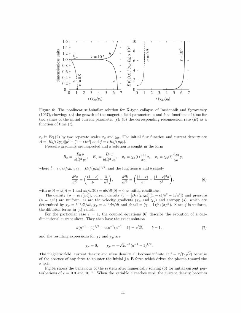
Figure 6: The nonlinear self-similar solution for X-type collapse of Imshennik and Syrovatsky(1967), showing: (a) the growth of the magnetic field parameters a and b as functions of time fortwo values of the initial current parameter (ǫ); (b) the corresponding reconnection rate (E) as afunction of time (t).

r0 in Eq.(2) by two separate scales x0 and y0. The initial flux function and current density areA = [B0/(2y0)][y

2 − (1 − ǫ)x2] and j = ǫB0/(µy0).Pressure gradients are neglected and a solution is sought in the form

Bx =B0 y

a(t)2 y0, By =

B0 x

b(t)2 x0, vx = χx(t)

vA0

x0x, vy = χy(t)

vA0

y0y,

where t = t vA0/y0, vA0 = B0/(µρ0)1/2, and the functions a and b satisfy

d2a

dt2=

((1 − ǫ)

b− b

a2

)

,d2b

dt2=

((1 − ǫ)

a− (1 − ǫ)2a

b2

)

, (6)

with a(0) = b(0) = 1 and da/dt(0) = db/dt(0) = 0 as initial conditions.The density (ρ = ρ0/[a b]), current density (j = [B0/(µ y0)][(1 − ǫ)/b2 − 1/a2]) and pressure

(p = sργ) are uniform, as are the velocity gradients (χx and χy) and entropy (s), which aredetermined by χx = b−1db/dt, χy = a−1da/dt and ds/dt = (γ − 1)j2/(σργ). Since j is uniform,the diffusion terms in (4) vanish.

For the particular case ǫ = 1, the coupled equations (6) describe the evolution of a one-dimensional current sheet. They then have the exact solution

a(a−1 − 1)1/2 + tan−1(a−1 − 1) =√

2t, b = 1, (7)

and the resulting expressions for χx and χy are

χx = 0, χy = −√

2a−1(a−1 − 1)1/2.

The magnetic field, current density and mass density all become infinite at t = π/(2√

2) becauseof the absence of any force to counter the initial j× B force which drives the plasma toward thex-axis.

Fig.6a shows the behaviour of the system after numerically solving (6) for initial current per-turbations of ǫ = 0.9 and 10−5. When the variable a reaches zero, the current density becomes

11

infinite. As ǫ is reduced in value, the time for the singularity to appear takes longer. The asymp-totic behaviour near the singularity time (t = ts) is given by

a ∝ (ts − t)2/3, χy ∝ (ts − t)−1, ρ ∝ (ts − t)−2/3, j ∝ (ts − t)−4/3.

As for any two-dimensional system, the reconnection rate is just the value of the electric field(E) at the X-point, namely,

E =j

σ=

1

σ

[(1 − ǫ

b2

)

b2 − 1

a2

]

,

which is plotted in Fig.6b as a function of time. Reconnection occurs even though the diffusionterms vanish in the induction equation since the current density (j) is uniform. Another indicationthat reconnection is occurring is the presence of Ohmic heating in the energy equation (3).

By considering a system that is bounded in the two-dimensional plane, the physical significanceof the singularity becomes clearer. Suppose the plasma is surrounded by a rigid, circular cylinderof radius r0 located at x2 + y2 = r20 . As long as the fluid is ideal and compressible, the boundaryconditions imposed at the cylinder’s surface cannot effect a particular location within the interioruntil there has been time for a fast-mode wave to travel from the boundary to that particularlocation. Along the y-axis the dimensionless location (yw) of the wave carrying the boundaryinformation is determined by

yw = yw ξ −(y2

w a−3b+ 1

2β0 (a b)γ−1)1/2

, (8)

where the two terms on the right-hand side are the flow speed and fast-mode wave speed at yw.Eq.(8) may then be solved for the wave position as (Forbes, 1982)

yw = a[a−1/2 + (a−1 − 1)1/2]−√

2, (9)

where a is determined by (7). From this result, we see that the wave reaches the origin (yw = 0)at precisely the moment when the singularity occurs (a = 0). If the initial pressure or diffusivityis greater than zero, the wave will travel faster than predicted by (8) and reach the origin first, sothat the self-similar solution breaks down before the singularity occurs.

Suppose first that the pressure gradient force dominates, which is true when β0 & [η/(vA0 y0)]0.565.

Then it should stop the collapse when the sound speed becomes of the same order as the wavespeed (8), i.e., when

(γ

2β0 a

1−γf

)1/2

≈ ywf (ξf − a−3/2f ),

where the f subscripts indicate the final values at the time when the wave reaches the origin. Aftersubstituting for ywf from (9) this leads to

af ∝ β1/(γ+

√2−2)

0 .

If the collapse is pressure-limited and γ = 5/3, the maximum reconnection rate is therefore

Ef =jfσ

=1

σa2f

∝ 1

σβ1.850

,

which increases as the initial pressure decreases.Next, consider the effect of magnetic diffusion, which becomes important when the wave speed

(yw) is of the same order as the diffusion speed (η/yw). Setting β0 = 0 and using (9) and (8) forthe wave position and speed leads to

η

vA0 y0=[

a−1/2f + (a−1

f − 1)1/2]−2

√2 [√

2af (a−1f − 1)1/2 + a

1/2f

]

.

12

Assuming η small and solving for af in terms of η gives af ∝ η−0.522. Thus, if the collapse isdiffusion-limited, the maximum reconnection rate becomes

Ef =η

vA0 y0 a2f

∝ η−0.045.

This remarkable result implies that, as the magnetic diffusivity (η) tends to zero, the reconnectionrate becomes infinite and not zero as we might expect for an ideal-MHD system. The Ohmicheating rate also tends to infinity as η tends to zero, and both of these inverse scaling results havebeen confirmed numerically by McClymont and Craig (1996).

If β0 > [η/(vA0 y0)]0.565, pressure dominates and halts the collapse at a radius af ∝ β

1/(γ+√

2−2)0

and the maximum reconnection rate is Ef = B0/(µy0σa2f ) ∝ 1/(σβ1.85

0 ). If, on the other hand,

β0 < [η/(vA0 y0)]0.565, diffusion dominates with af ∝ η−0.522 and Ef = B0η/(y0 a

2f ) ∝ η−0.045, so

reconnection is fast.

2.2.3 LINEAR SOLUTION

It was only in the 1990’s that the first thorough linear analyses of the collapse process were carriedout (e.g., Bulanov et al., 1990; Craig and McClymont, 1991, 1993; Craig and Watson, 1992; Hassam,1992; Titov and Priest, 1993). They demonstrate that collapse occurs for a wide variety of initialand boundary conditions, provided the perturbation rate is fast, comparable to the fast-modetime-scale, so that dynamic effects are important. A surprising result is that reconnection in thelinear regime is fast, scaling as 1/(ln η).

First, we linearise the MHD equations (3, 4, 5) by expressing the flux function as A = A0 +A1,where A1 is the linear perturbation and A0 is the current-free state 1

2B0r0(y2 − x2), with y = y/r0

and x = x/r0. Neglecting the pressure then leads to

∂2A1

∂t2= (x2 + y2)∇2A1 + η∇2 ∂A1

∂t,

where t = tvA0/r0 and η = η/(vA0r0). We seek separable solutions of the form

A1 = 12B0 r0 ǫRe

[f(r)eimθ+ωt

], (10)

where ω = ωR + iωI , r = r/r0, ω = ωr0/vA0, ǫ is the dimensionless magnitude of the perturbation,and f(r) is a complex function satisfying

rd

dr

(

rdf

dr

)

=

(r2 ω2

r2 + η ω+m2

)

f. (11)

Frozen-flux conditions are imposed at the surface r = 1 by setting f = 0 there. Only the m = 0mode changes A at the origin and so corresponds to reconnection.

The solution of (11) for m = 0 represents an eigenfunction problem, which determines the realand imaginary parts of the eigenvalue (ω = ωR + iωI) as

ωR =−(2n+ 1)2π2

2(n+ 1)ln2η, ωI = − (2n+ 1)π

ln η,

where n is the number of radial nodes. It describes radial oscillations propagating between theboundary and the origin, as shown in Fig.7. The travel-time depends on diffusivity (η) because thewave speed vanishes as the origin is approached, and so diffusion allows a perturbation to reachthe origin and reflect.

13

0 π/ωI 2π/ωI

π/(2ωI) 3π/(2ωI) 8

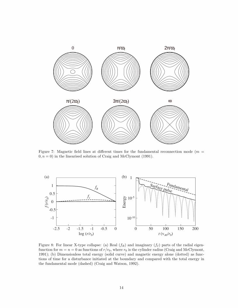
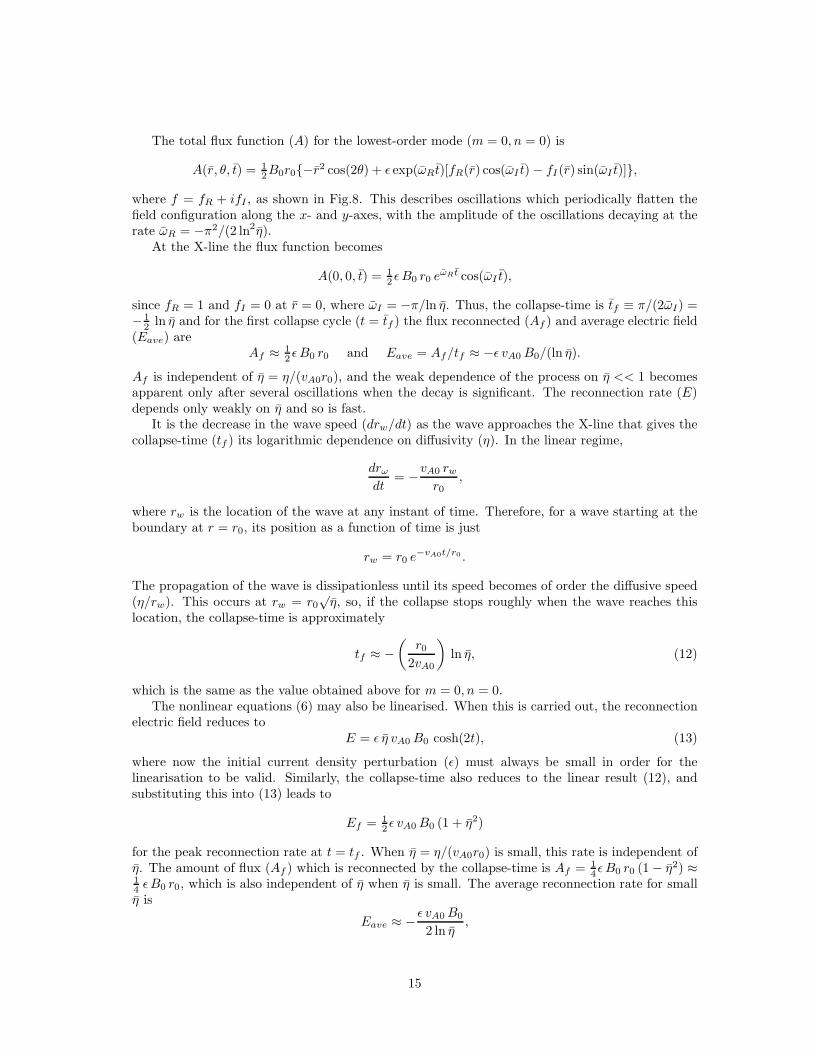
Figure 7: Magnetic field lines at different times for the fundamental reconnection mode (m =0, n = 0) in the linearised solution of Craig and McClymont (1991).

-2.5 -2 -1.5 -1 -0.5 0

-1

-0.5

0

0.5

1

log (r/r0)

fR

f1

f (r

/r0)

10-10

10-5

1(a) (b)

Ener

gy

Fundamental

Surface pulse

0 50 100 150 200

t (vA0/r0)

Figure 8: For linear X-type collapse: (a) Real (fR) and imaginary (fI) parts of the radial eigen-function for m = n = 0 as functions of r/r0, where r0 is the cylinder radius (Craig and McClymont,1991); (b) Dimensionless total energy (solid curve) and magnetic energy alone (dotted) as func-tions of time for a disturbance initiated at the boundary and compared with the total energy inthe fundamental mode (dashed) (Craig and Watson, 1992).

14

The total flux function (A) for the lowest-order mode (m = 0, n = 0) is

A(r, θ, t) = 12B0r0{−r2 cos(2θ) + ǫ exp(ωRt)[fR(r) cos(ωI t) − fI(r) sin(ωI t)]},

where f = fR + ifI , as shown in Fig.8. This describes oscillations which periodically flatten thefield configuration along the x- and y-axes, with the amplitude of the oscillations decaying at therate ωR = −π2/(2 ln2η).

At the X-line the flux function becomes

A(0, 0, t) = 12 ǫB0 r0 e

ωRt cos(ωI t),

since fR = 1 and fI = 0 at r = 0, where ωI = −π/ln η. Thus, the collapse-time is tf ≡ π/(2ωI) =− 1

2 ln η and for the first collapse cycle (t = tf ) the flux reconnected (Af ) and average electric field(Eave) are

Af ≈ 12 ǫB0 r0 and Eave = Af/tf ≈ −ǫ vA0B0/(ln η).

Af is independent of η = η/(vA0r0), and the weak dependence of the process on η << 1 becomesapparent only after several oscillations when the decay is significant. The reconnection rate (E)depends only weakly on η and so is fast.

It is the decrease in the wave speed (drw/dt) as the wave approaches the X-line that gives thecollapse-time (tf ) its logarithmic dependence on diffusivity (η). In the linear regime,

drωdt

= −vA0 rwr0

,

where rw is the location of the wave at any instant of time. Therefore, for a wave starting at theboundary at r = r0, its position as a function of time is just

rw = r0 e−vA0t/r0 .

The propagation of the wave is dissipationless until its speed becomes of order the diffusive speed(η/rw). This occurs at rw = r0

√η, so, if the collapse stops roughly when the wave reaches this

location, the collapse-time is approximately

tf ≈ −(

r02vA0

)

ln η, (12)

which is the same as the value obtained above for m = 0, n = 0.The nonlinear equations (6) may also be linearised. When this is carried out, the reconnection

electric field reduces toE = ǫ η vA0B0 cosh(2t), (13)

where now the initial current density perturbation (ǫ) must always be small in order for thelinearisation to be valid. Similarly, the collapse-time also reduces to the linear result (12), andsubstituting this into (13) leads to

Ef = 12 ǫ vA0B0 (1 + η2)

for the peak reconnection rate at t = tf . When η = η/(vA0r0) is small, this rate is independent ofη. The amount of flux (Af ) which is reconnected by the collapse-time is Af = 1

4ǫB0 r0 (1 − η2) ≈14 ǫB0 r0, which is also independent of η when η is small. The average reconnection rate for smallη is

Eave ≈ − ǫ vA0B0

2 ln η,

15

10–10 10–8 10–6 10–4 10–2 10

1.0

2.0

2.5

1.5

0.5

η / (vA0 r0)

ε =

0.9ε =

10–

5

A(t

f) /

(B0

r 0)

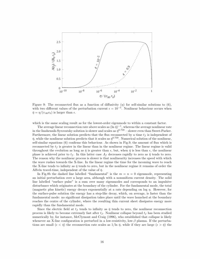
Figure 9: The reconnected flux as a function of diffusivity (η) for self-similar solutions to (6),with two different values of the perturbation current ǫ = 10−5. Nonlinear behaviour occurs whenη = η/(vA0r0) is larger than ǫ.

which is the same scaling result as for the lowest-order eigenmode to within a constant factor.The average linear reconnection rate above scales as (ln η)−1, whereas the average nonlinear rate

in the Imshennik-Syrovatsky solution is slower and scales as η0.739 – slower even than Sweet-Parker.Furthermore, the linear solution predicts that the flux reconnected by a time tf is independent ofη, while the nonlinear solution predicts that it scales as η0.739. Numerical solution of the nonlinear,self-similar equations (6) confirms this behaviour. As shown in Fig.9, the amount of flux which isreconnected by tf is greater in the linear than in the nonlinear regime. The linear regime is validthroughout the evolution as long as η is greater than ǫ, but, when η is less than ǫ, the nonlinearphase is achieved prior to tf . In this latter case Af decreases rapidly to zero as η tends to zero.The reason why the nonlinear process is slower is that nonlinearity increases the speed with whichthe wave rushes towards the X-line. In the linear regime the time for the incoming wave to reachthe X-line tends to infinity as η tends to zero, but in the nonlinear regime it remains of order theAlfven travel-time, independent of the value of η.

In Fig.8b the dashed line labelled “fundamental” is the m = n = 0 eigenmode, representingan initial perturbation over a large area, although with a nonuniform current density. The solidline labelled “surface pulse” is a sum over many eigenmodes and corresponds to an impulsivedisturbance which originates at the boundary of the cylinder. For the fundamental mode, the total(magnetic plus kinetic) energy decays exponentially at a rate depending on log η. However, forthe surface-pulse solution the energy has a step-like decay, which, on average, is faster than thefundamental mode: no significant dissipation takes place until the wave launched at the boundaryreaches the centre of the cylinder, where the resulting thin current sheet dissipates energy morerapidly than the fundamental mode.

Since the electric field at tf tends to infinity as η tends to zero, the nonlinear reconnectionprocess is likely to become extremely fast after tf . Nonlinear collapse beyond tf has been studiednumerically by, for instance, McClymont and Craig (1996), who established that collapse is likelywhenever an X-line configuration is perturbed in a low-resistivity, low-β plasma. If the perturba-tions are small (ǫ < η) the reconnection rate scales as 1/ln η, while if they are large (ǫ > η) the

16

average reconnection rate appears to be nearly independent of η (see also Brushlinskii et al., 1980;Ofman et al., 1992; Roumeliotis and Moore, 1993).

It is only if the plasma β0 is less than η0.56 that rapid reconnection associated with the formationof a thin current sheet occurs; otherwise, the collapse is choked off by the pressure. In solar andastrophysical applications the classical values of η are typically of order 10−10, so this impliesβ0

<∼ 10−6. This is smaller than solar coronal values, so it seems likely that the collapse in such anastrophysical system would be limited by pressure rather than resistivity. However, if we considerlaboratory plasmas or the possibility of anomalous resistivity, then a resistivity-limited collapsecould still be important. For example, if η = 10−2, then β0 < 0.1 is sufficient. In any case,the two-dimensional evolution after an initial collapse has not yet been fully explored, althoughthere is some indication (McClymont and Craig, 1996) that nonlinear, two-dimensional affects mayproduce a secondary phase of reconnection that is not limited by pressure.

17

quasi-separator

current sheet

fan

spine

separator

separatrix null point separatrix

chaotic region

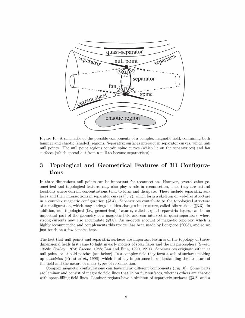
Figure 10: A schematic of the possible components of a complex magnetic field, containing bothlaminar and chaotic (shaded) regions. Separatrix surfaces intersect in separator curves, which linknull points. The null point regions contain spine curves (which lie on the separatrices) and fansurfaces (which spread out from a null to become separatrices).

3 Topological and Geometrical Features of 3D Configura-tions

In three dimensions null points can be important for reconnection. However, several other ge-ometrical and topological features may also play a role in reconnection, since they are naturallocations where current concentrations tend to form and dissipate. These include separatrix sur-faces and their intersections in separator curves (§3.2), which form a skeleton or web-like structurein a complex magnetic configuration (§3.4). Separatrices contribute to the topological structureof a configuration, which may undergo sudden changes in structure, called bifurcations (§3.3). Inaddition, non-topological (i.e., geometrical) features, called a quasi-separatrix layers, can be animportant part of the geometry of a magnetic field and can intersect in quasi-separators, wherestrong currents may also accumulate (§3.5). An in-depth account of magnetic topology, which ishighly recommended and complements this review, has been made by Longcope (2005), and so wejust touch on a few aspects here.

The fact that null points and separatrix surfaces are important features of the topology of three-dimensional fields first came to light in early models of solar flares and the magnetosphere (Sweet,1958b; Cowley, 1973; Greene, 1988; Lau and Finn, 1990, 1991). Separatrices originate either atnull points or at bald patches (see below). In a complex field they form a web of surfaces makingup a skeleton (Priest et al., 1996), which is of key importance in understanding the structure ofthe field and the nature of many types of reconnection.

Complex magnetic configurations can have many different components (Fig.10). Some partsare laminar and consist of magnetic field lines that lie on flux surfaces, whereas others are chaoticwith space-filling field lines. Laminar regions have a skeleton of separatrix surfaces (§3.2) and a

18

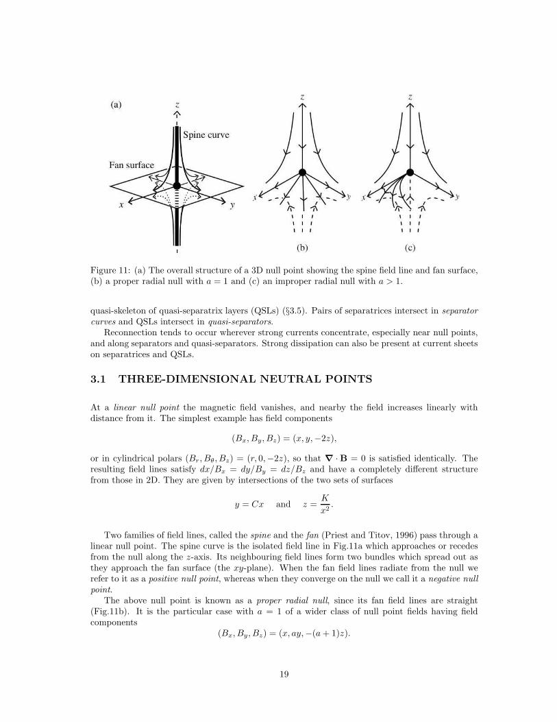
Figure 11: (a) The overall structure of a 3D null point showing the spine field line and fan surface,(b) a proper radial null with a = 1 and (c) an improper radial null with a > 1.

quasi-skeleton of quasi-separatrix layers (QSLs) (§3.5). Pairs of separatrices intersect in separatorcurves and QSLs intersect in quasi-separators.

Reconnection tends to occur wherever strong currents concentrate, especially near null points,and along separators and quasi-separators. Strong dissipation can also be present at current sheetson separatrices and QSLs.

3.1 THREE-DIMENSIONAL NEUTRAL POINTS

At a linear null point the magnetic field vanishes, and nearby the field increases linearly withdistance from it. The simplest example has field components

(Bx, By, Bz) = (x, y,−2z),

or in cylindrical polars (Br, Bθ, Bz) = (r, 0,−2z), so that ∇ ·B = 0 is satisfied identically. Theresulting field lines satisfy dx/Bx = dy/By = dz/Bz and have a completely different structurefrom those in 2D. They are given by intersections of the two sets of surfaces

y = Cx and z =K

x2.

Two families of field lines, called the spine and the fan (Priest and Titov, 1996) pass through alinear null point. The spine curve is the isolated field line in Fig.11a which approaches or recedesfrom the null along the z-axis. Its neighbouring field lines form two bundles which spread out asthey approach the fan surface (the xy-plane). When the fan field lines radiate from the null werefer to it as a positive null point, whereas when they converge on the null we call it a negative nullpoint.

The above null point is known as a proper radial null, since its fan field lines are straight(Fig.11b). It is the particular case with a = 1 of a wider class of null point fields having fieldcomponents

(Bx, By, Bz) = (x, ay,−(a+ 1)z).

19

(a) (b)

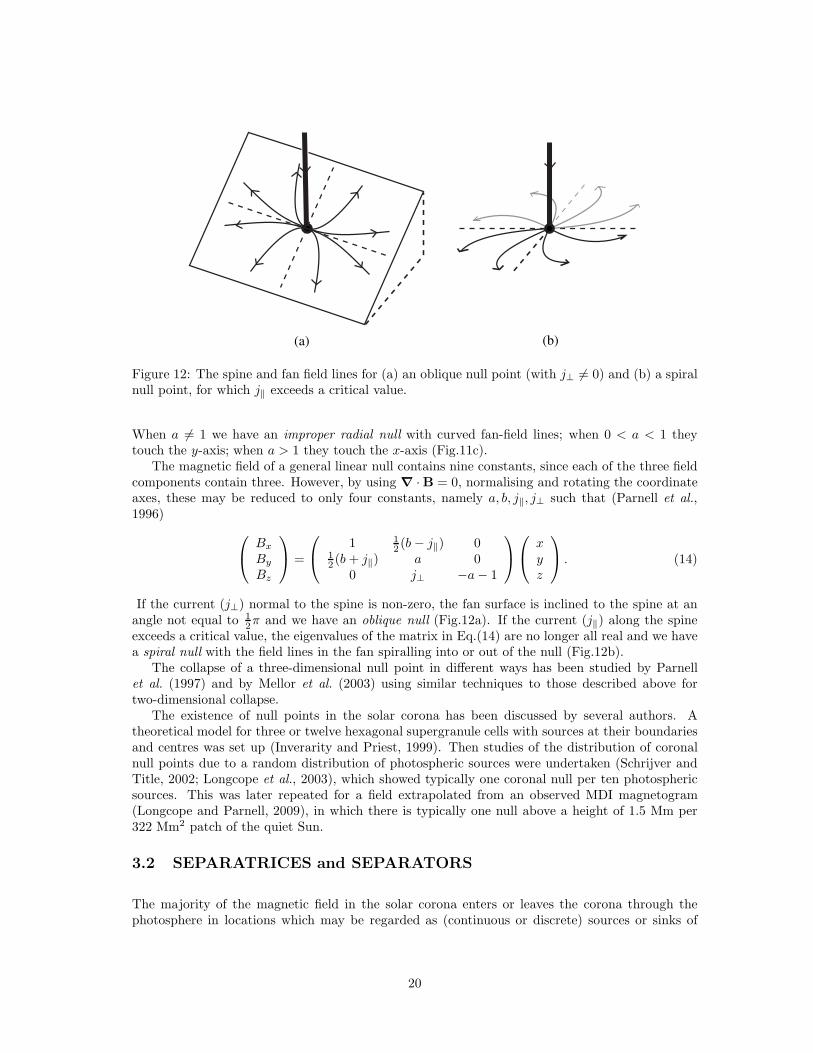
Figure 12: The spine and fan field lines for (a) an oblique null point (with j⊥ 6= 0) and (b) a spiralnull point, for which j‖ exceeds a critical value.

When a 6= 1 we have an improper radial null with curved fan-field lines; when 0 < a < 1 theytouch the y-axis; when a > 1 they touch the x-axis (Fig.11c).

The magnetic field of a general linear null contains nine constants, since each of the three fieldcomponents contain three. However, by using ∇ ·B = 0, normalising and rotating the coordinateaxes, these may be reduced to only four constants, namely a, b, j‖, j⊥ such that (Parnell et al.,1996)

Bx

By

Bz

=

1 12 (b − j‖) 0

12 (b + j‖) a 0

0 j⊥ −a− 1

xyz

. (14)

If the current (j⊥) normal to the spine is non-zero, the fan surface is inclined to the spine at anangle not equal to 1

2π and we have an oblique null (Fig.12a). If the current (j‖) along the spineexceeds a critical value, the eigenvalues of the matrix in Eq.(14) are no longer all real and we havea spiral null with the field lines in the fan spiralling into or out of the null (Fig.12b).

The collapse of a three-dimensional null point in different ways has been studied by Parnellet al. (1997) and by Mellor et al. (2003) using similar techniques to those described above fortwo-dimensional collapse.

The existence of null points in the solar corona has been discussed by several authors. Atheoretical model for three or twelve hexagonal supergranule cells with sources at their boundariesand centres was set up (Inverarity and Priest, 1999). Then studies of the distribution of coronalnull points due to a random distribution of photospheric sources were undertaken (Schrijver andTitle, 2002; Longcope et al., 2003), which showed typically one coronal null per ten photosphericsources. This was later repeated for a field extrapolated from an observed MDI magnetogram(Longcope and Parnell, 2009), in which there is typically one null above a height of 1.5 Mm per322 Mm2 patch of the quiet Sun.

3.2 SEPARATRICES and SEPARATORS

The majority of the magnetic field in the solar corona enters or leaves the corona through thephotosphere in locations which may be regarded as (continuous or discrete) sources or sinks of

20

magnetic flux for the corona. When the corona is modelled as a two-dimensional region, in generalit contains separatrix curves, which are field lines that separate the plane into topologically distinctregions, in the sense that all the field lines in one region start at a particular source and end at aparticular sink (Fig.14a,b,13).

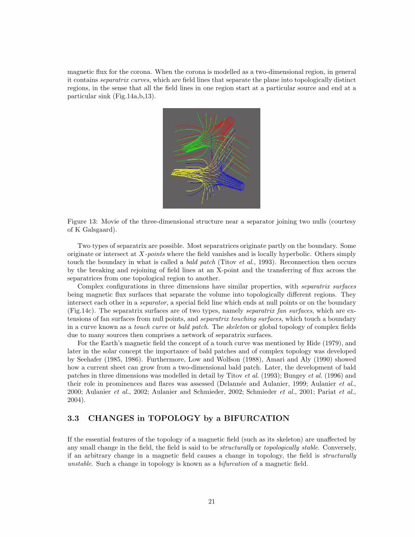
Figure 13: Movie of the three-dimensional structure near a separator joining two nulls (courtesyof K Galsgaard).

Two types of separatrix are possible. Most separatrices originate partly on the boundary. Someoriginate or intersect at X-points where the field vanishes and is locally hyperbolic. Others simplytouch the boundary in what is called a bald patch (Titov et al., 1993). Reconnection then occursby the breaking and rejoining of field lines at an X-point and the transferring of flux across theseparatrices from one topological region to another.

Complex configurations in three dimensions have similar properties, with separatrix surfacesbeing magnetic flux surfaces that separate the volume into topologically different regions. Theyintersect each other in a separator, a special field line which ends at null points or on the boundary(Fig.14c). The separatrix surfaces are of two types, namely separatrix fan surfaces, which are ex-tensions of fan surfaces from null points, and separatrix touching surfaces, which touch a boundaryin a curve known as a touch curve or bald patch. The skeleton or global topology of complex fieldsdue to many sources then comprises a network of separatrix surfaces.

For the Earth’s magnetic field the concept of a touch curve was mentioned by Hide (1979), andlater in the solar concept the importance of bald patches and of complex topology was developedby Seehafer (1985, 1986). Furthermore, Low and Wolfson (1988), Amari and Aly (1990) showedhow a current sheet can grow from a two-dimensional bald patch. Later, the development of baldpatches in three dimensions was modelled in detail by Titov et al. (1993); Bungey et al. (1996) andtheir role in prominences and flares was assessed (Delannee and Aulanier, 1999; Aulanier et al.,2000; Aulanier et al., 2002; Aulanier and Schmieder, 2002; Schmieder et al., 2001; Pariat et al.,2004).

3.3 CHANGES in TOPOLOGY by a BIFURCATION

If the essential features of the topology of a magnetic field (such as its skeleton) are unaffected byany small change in the field, the field is said to be structurally or topologically stable. Conversely,if an arbitrary change in a magnetic field causes a change in topology, the field is structurallyunstable. Such a change in topology is known as a bifurcation of a magnetic field.

21

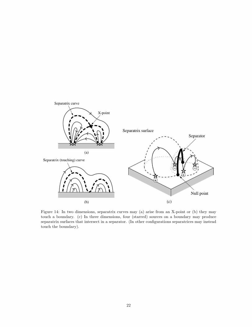
Figure 14: In two dimensions, separatrix curves may (a) arise from an X-point or (b) they maytouch a boundary. (c) In three dimensions, four (starred) sources on a boundary may produceseparatrix surfaces that intersect in a separator. (In other configurations separatrices may insteadtouch the boundary).

22

A local bifurcation involves a change in the number or nature of null points. Thus, in two orthree dimensions isolated linear nulls are structurally stable but null lines or null sheets (consistingof curves or surfaces where the field vanishes) are structurally unstable, since a small perturbationmay break them up into a series of nulls. More general null points are themselves structurallyunstable if they are degenerate (i.e., when the Jacobian matrix (DB) in Eq.(14) is singular at thenull) or if the null points are of second or higher order (i.e., when DB vanishes at the null).

A global bifurcation in two dimensions is one that involves a change in connectivity of theseparatrix field lines. At the moment of bifurcation there exists either a homoclinic separatrix(starting and ending at the same null) or a heteroclinic separatrix (linking one null to another).However, homoclinic and heteroclinic field lines are structurally unstable in two dimensions and sodo not survive the bifurcation, since a general perturbation stops the field line from one null eithercoming back to the null or going to the other null.

In three dimensions, on the other hand, a global bifurcation can involve the creation and contin-ued existence of a separator; or it may involve the destruction of such a separator. Separators thatare (heteroclinic) field lines linking two nulls and representing the intersection of two fan surfacesare structurally stable, whereas those that represent the intersection of the spine of one null withthe spine or fan of another are structurally unstable, since a perturbation of the field in generaldestroys such a separator connection between two nulls.

Linear null points may coalesce at a second-order null (for which the field increases quadraticallyfrom zero) or a second-order null may split and give birth to linear nulls. Such local bifurcationsmay produce global changes of magnetic topology and perhaps stimulate release of magnetic energy.

In two dimensions the field components may be written as dx/ds = Bx = ∂A/∂y, dy/ds =By = −∂A/∂x. The flux function (A) is a Hamiltonian and so the nature of the bifurcations is wellunderstood (e.g., Priest et al., 1996). Isolated linear nulls in 2D are either X-points or O-pointswith flux functions of the form A = b2y2 ± a2x2. Thus, in order to find what kinds of bifurcationare possible, we may consider a general cubic function and suppose there are nulls at (±√

K, 0),say. The simplest generic non-degenerate type is a saddle-centre bifurcation, exemplified by theflux function

A = x3 − 3Kx+ y2,

which represents a set of curved field lines when K < 0; they develop a null at the origin whenK = 0, which then splits into an X and an O when K > 0. Pitchfork bifurcations are also possiblewhen an X- or an O- point changes to one of opposite type and spawns two more of the same type.Examples of resonant and degenerate bifurcations may also be produced (Priest et al., 1996).

The system in three dimensions

dx

ds= Bx,

dy

ds= By,

dz

ds= Bz

is no longer Hamiltonian (but it is conservative since ∇ ·B = 0). The null points and theirbifurcations are therefore much more complex. The first step has been to consider fields withcylindrical symmetry, for which a general categorisation has been completed (Priest et al., 1996),by building on a particular example studied by Lau and Finn (1992).

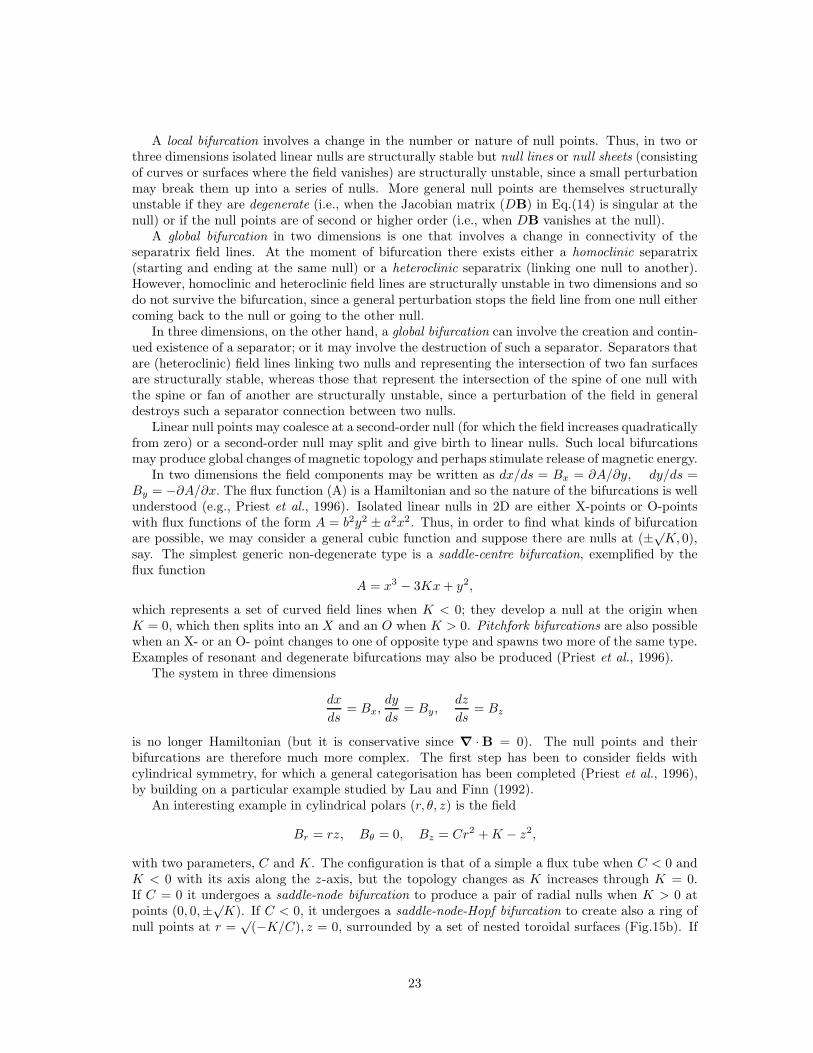
An interesting example in cylindrical polars (r, θ, z) is the field

Br = rz, Bθ = 0, Bz = Cr2 +K − z2,

with two parameters, C and K. The configuration is that of a simple a flux tube when C < 0 andK < 0 with its axis along the z-axis, but the topology changes as K increases through K = 0.If C = 0 it undergoes a saddle-node bifurcation to produce a pair of radial nulls when K > 0 atpoints (0, 0,±√

K). If C < 0, it undergoes a saddle-node-Hopf bifurcation to create also a ring ofnull points at r =

√(−K/C), z = 0, surrounded by a set of nested toroidal surfaces (Fig.15b). If

23

K < 0

(a) (C = 0)

K > 0

K < 0

(b) (C < 0)

K > 0

K < 0

(c) (C > 0)

K > 0

heteroclinic connection

ring of nulls

ring of nulls

Figure 15: Axisymmetric configurations when (a) C = 0, (b) C < 0, (c) C > 0 showing saddle-node(top) or saddle-node-Hopf (middle and bottom) bifurcations as K increases through zero.

24

1.0

0.5

0.0

-0.5

-1.0

-1.5 -1.0 -0.5 0.0 0.5 1 1.5

r

z

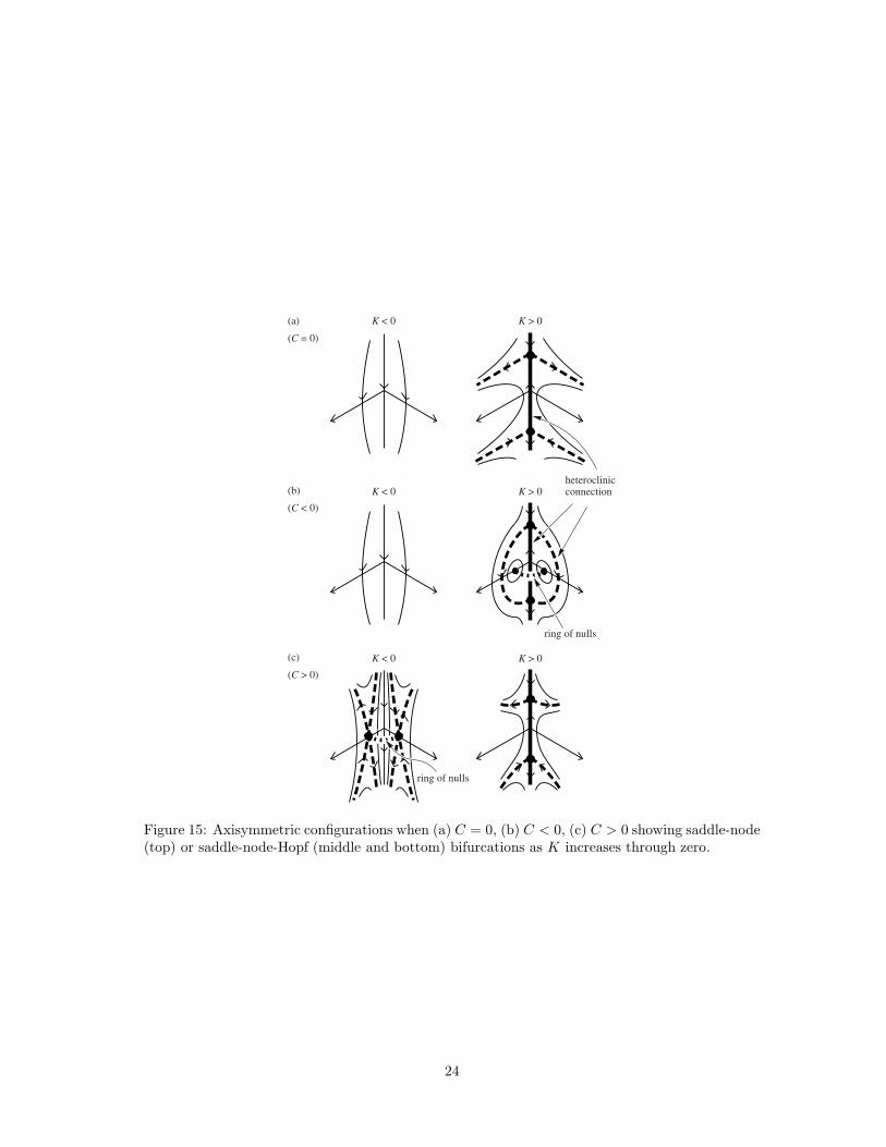
Figure 16: The appearance of chaotic field lines when axial symmetry of Fig.15b with K > 0 isbroken, as shown by a Poincare plot of the intersections of field lines with the zr-plane.

a component Bθ = r is added, the radial nulls on the z-axis become spiral nulls and the ring ofnulls becomes a closed field line encircling the z-axis. If C = 0, a flux tube exists when K < 0and it undergoes a saddle-node bifurcation when K = 0 to produce a pair of radial nulls whenK > 0 at points (0, 0,±√

K) on the z-axis (Fig.15a). If C < 0, a ring of null points is alsoproduced at r =

√(−K/C), z = 0, surrounded by a set of nested toroidal surfaces, and so we have

a saddle-node-Hopf bifurcation (Fig.15b). If C > 0, we start with a ring of nulls when K < 0 whichdisappears and becomes a pair of nulls on the z-axis when K > 0 (Fig.15c). If a component Bθ = ris added, the radial nulls on the z-axis become spiral nulls and the ring of nulls becomes a closedfield line encircling the z-axis and surrounded by a set of nested flux surfaces.

Suppose, however, that also the symmetry is broken by adding periodic terms to Br and Bθ

when K = 1, C = −1 such that

(Br, Bθ, Bz) = (rz + λr2 cos2 θ sin θ, r + λr2 cos3 θ, 1 − r2 − z2).

When λ is non-zero some of the flux surfaces break down as the field lines that pass close to thenulls become chaotic; this is shown in Fig.16 for the case λ = 0.01 by a Poincare plot of theintersections of field lines with a plane θ = constant.

3.4 SKELETONS of COMPLEX MAGNETIC CONFIGURATIONS

A key question is how to describe the nature of complicated magnetic configurations. For ex-ample, the solar corona is incredibly complex, with myriads of magnetic flux sources where fluxpokes through the photosphere from the interior into the overlying atmosphere. The photosphericmagnetic field is concentrated by convection in many intense flux tubes, and each such photosphericsource is itself joined through the corona to many other sources. In a similar way, whenever a nu-merical MHD experiment gives rise to many null points, the fans of the nulls spread out to form

25

Spine

Null

Fan Separatrix

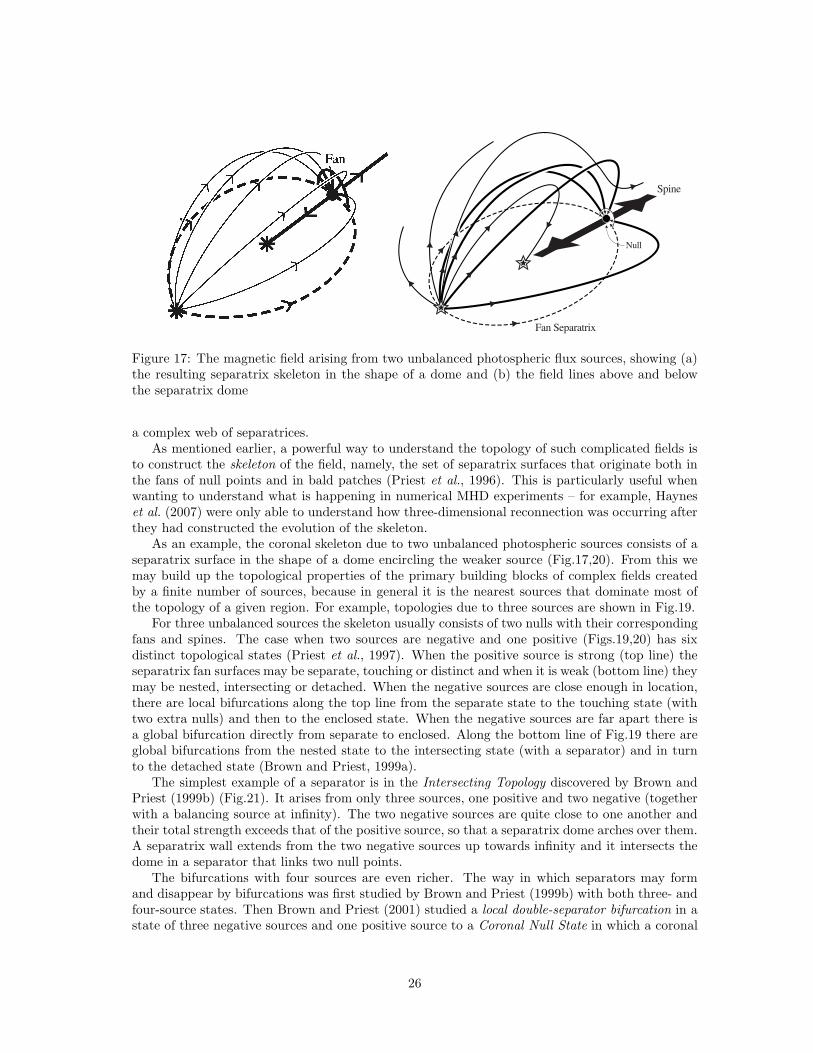
Figure 17: The magnetic field arising from two unbalanced photospheric flux sources, showing (a)the resulting separatrix skeleton in the shape of a dome and (b) the field lines above and belowthe separatrix dome

a complex web of separatrices.As mentioned earlier, a powerful way to understand the topology of such complicated fields is

to construct the skeleton of the field, namely, the set of separatrix surfaces that originate both inthe fans of null points and in bald patches (Priest et al., 1996). This is particularly useful whenwanting to understand what is happening in numerical MHD experiments – for example, Hayneset al. (2007) were only able to understand how three-dimensional reconnection was occurring afterthey had constructed the evolution of the skeleton.

As an example, the coronal skeleton due to two unbalanced photospheric sources consists of aseparatrix surface in the shape of a dome encircling the weaker source (Fig.17,20). From this wemay build up the topological properties of the primary building blocks of complex fields createdby a finite number of sources, because in general it is the nearest sources that dominate most ofthe topology of a given region. For example, topologies due to three sources are shown in Fig.19.

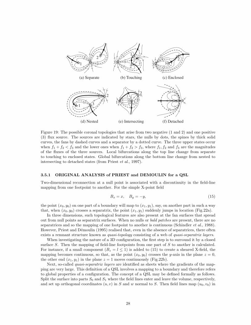
For three unbalanced sources the skeleton usually consists of two nulls with their correspondingfans and spines. The case when two sources are negative and one positive (Figs.19,20) has sixdistinct topological states (Priest et al., 1997). When the positive source is strong (top line) theseparatrix fan surfaces may be separate, touching or distinct and when it is weak (bottom line) theymay be nested, intersecting or detached. When the negative sources are close enough in location,there are local bifurcations along the top line from the separate state to the touching state (withtwo extra nulls) and then to the enclosed state. When the negative sources are far apart there isa global bifurcation directly from separate to enclosed. Along the bottom line of Fig.19 there areglobal bifurcations from the nested state to the intersecting state (with a separator) and in turnto the detached state (Brown and Priest, 1999a).

The simplest example of a separator is in the Intersecting Topology discovered by Brown andPriest (1999b) (Fig.21). It arises from only three sources, one positive and two negative (togetherwith a balancing source at infinity). The two negative sources are quite close to one another andtheir total strength exceeds that of the positive source, so that a separatrix dome arches over them.A separatrix wall extends from the two negative sources up towards infinity and it intersects thedome in a separator that links two null points.

The bifurcations with four sources are even richer. The way in which separators may formand disappear by bifurcations was first studied by Brown and Priest (1999b) with both three- andfour-source states. Then Brown and Priest (2001) studied a local double-separator bifurcation in astate of three negative sources and one positive source to a Coronal Null State in which a coronal

26

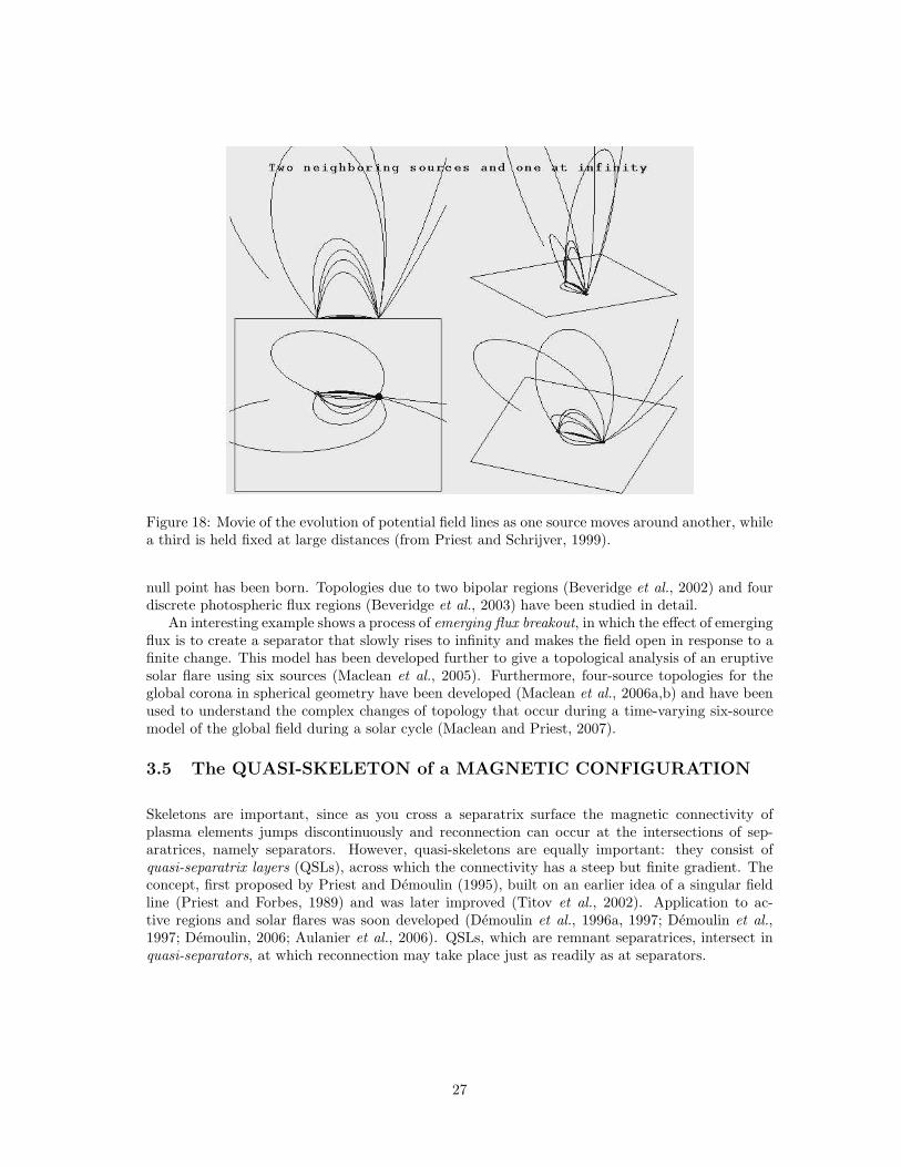
Figure 18: Movie of the evolution of potential field lines as one source moves around another, whilea third is held fixed at large distances (from Priest and Schrijver, 1999).

null point has been born. Topologies due to two bipolar regions (Beveridge et al., 2002) and fourdiscrete photospheric flux regions (Beveridge et al., 2003) have been studied in detail.

An interesting example shows a process of emerging flux breakout, in which the effect of emergingflux is to create a separator that slowly rises to infinity and makes the field open in response to afinite change. This model has been developed further to give a topological analysis of an eruptivesolar flare using six sources (Maclean et al., 2005). Furthermore, four-source topologies for theglobal corona in spherical geometry have been developed (Maclean et al., 2006a,b) and have beenused to understand the complex changes of topology that occur during a time-varying six-sourcemodel of the global field during a solar cycle (Maclean and Priest, 2007).

3.5 The QUASI-SKELETON of a MAGNETIC CONFIGURATION

Skeletons are important, since as you cross a separatrix surface the magnetic connectivity ofplasma elements jumps discontinuously and reconnection can occur at the intersections of sep-aratrices, namely separators. However, quasi-skeletons are equally important: they consist ofquasi-separatrix layers (QSLs), across which the connectivity has a steep but finite gradient. Theconcept, first proposed by Priest and Demoulin (1995), built on an earlier idea of a singular fieldline (Priest and Forbes, 1989) and was later improved (Titov et al., 2002). Application to ac-tive regions and solar flares was soon developed (Demoulin et al., 1996a, 1997; Demoulin et al.,1997; Demoulin, 2006; Aulanier et al., 2006). QSLs, which are remnant separatrices, intersect inquasi-separators, at which reconnection may take place just as readily as at separators.

27

1

2

(a) Separate (b) Touching (c) Enclosed

(d) Nested (e) Intersecting (f) Detached

12

3

1

2

31

2

3

1

23

3

Figure 19: The possible coronal topologies that arise from two negative (1 and 2) and one positive(3) flux source. The sources are indicated by stars, the nulls by dots, the spines by thick solidcurves, the fans by dashed curves and a separator by a dotted curve. The three upper states occurwhen f1 + f2 < f3 and the lower ones when f1 + f2 > f3, where f1, f2 and f3 are the magnitudesof the fluxes of the three sources. Local bifurcations along the top line change from separateto touching to enclosed states. Global bifurcations along the bottom line change from nested tointersecting to detached states (from Priest et al., 1997).

3.5.1 ORIGINAL ANALYSIS of PRIEST and DEMOULIN for a QSL

Two-dimensional reconnection at a null point is associated with a discontinuity in the field-linemapping from one footpoint to another. For the simple X-point field

Bx = x, By = −y, (15)

the point (x0, y0) on one part of a boundary will map to (x1, y1), say, on another part in such a waythat, when (x0, y0) crosses a separatrix, the point (x1, y1) suddenly jumps in location (Fig.22a).

In three dimensions, such topological features are also present at the fan surfaces that spreadout from null points as separatrix surfaces. When no nulls or bald patches are present, there are noseparatrices and so the mapping of one footpoint to another is continuous (Schindler et al., 1988).However, Priest and Demoulin (1995) realised that, even in the absence of separatrices, there oftenexists a remnant structure known as quasi-topology consisting of a web of quasi-separatrix layers.

When investigating the nature of a 3D configuration, the first step is to surround it by a closedsurface S. Then the mapping of field-line footpoints from one part of S to another is calculated.For instance, if a small component (Bz = l ≤ 1) is added to (15) to create a sheared X-field, themapping becomes continuous, so that, as the point (x0, y0) crosses the y-axis in the plane z = 0,the other end (x1, y1) in the plane z = 1 moves continuously (Fig.22b).

Next, so-called quasi-separatrix layers are identified as sheets where the gradients of the map-ping are very large. This definition of a QSL involves a mapping to a boundary and therefore refersto global properties of a configuration. The concept of a QSL may be defined formally as follows.Split the surface into parts S0 and S1 where the field lines enter and leave the volume, respectively,and set up orthogonal coordinates (u, v) in S and w normal to S. Then field lines map (u0, v0) in

28

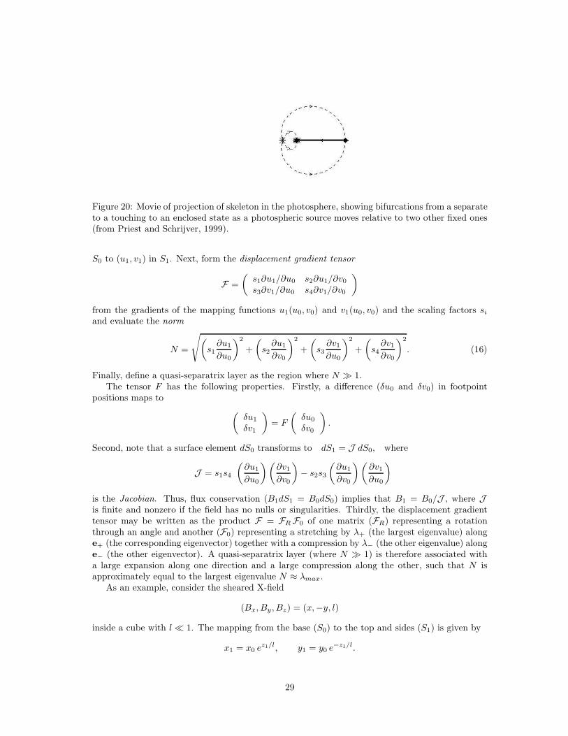
Figure 20: Movie of projection of skeleton in the photosphere, showing bifurcations from a separateto a touching to an enclosed state as a photospheric source moves relative to two other fixed ones(from Priest and Schrijver, 1999).

S0 to (u1, v1) in S1. Next, form the displacement gradient tensor

F =

(s1∂u1/∂u0 s2∂u1/∂v0s3∂v1/∂u0 s4∂v1/∂v0

)

from the gradients of the mapping functions u1(u0, v0) and v1(u0, v0) and the scaling factors si

and evaluate the norm

N =

√(

s1∂u1

∂u0

)2

+

(

s2∂u1

∂v0

)2

+

(

s3∂v1∂u0

)2

+

(

s4∂v1∂v0

)2

. (16)

Finally, define a quasi-separatrix layer as the region where N ≫ 1.The tensor F has the following properties. Firstly, a difference (δu0 and δv0) in footpoint

positions maps to

(δu1

δv1

)

= F

(δu0

δv0

)

.

Second, note that a surface element dS0 transforms to dS1 = J dS0, where

J = s1s4

(∂u1

∂u0

)(∂v1∂v0

)

− s2s3

(∂u1

∂v0

)(∂v1∂u0

)

is the Jacobian. Thus, flux conservation (B1dS1 = B0dS0) implies that B1 = B0/J , where Jis finite and nonzero if the field has no nulls or singularities. Thirdly, the displacement gradienttensor may be written as the product F = FR F0 of one matrix (FR) representing a rotationthrough an angle and another (F0) representing a stretching by λ+ (the largest eigenvalue) alonge+ (the corresponding eigenvector) together with a compression by λ− (the other eigenvalue) alonge− (the other eigenvector). A quasi-separatrix layer (where N ≫ 1) is therefore associated witha large expansion along one direction and a large compression along the other, such that N isapproximately equal to the largest eigenvalue N ≈ λmax.

As an example, consider the sheared X-field

(Bx, By, Bz) = (x,−y, l)

inside a cube with l ≪ 1. The mapping from the base (S0) to the top and sides (S1) is given by

x1 = x0 ez1/l, y1 = y0 e

−z1/l.

29

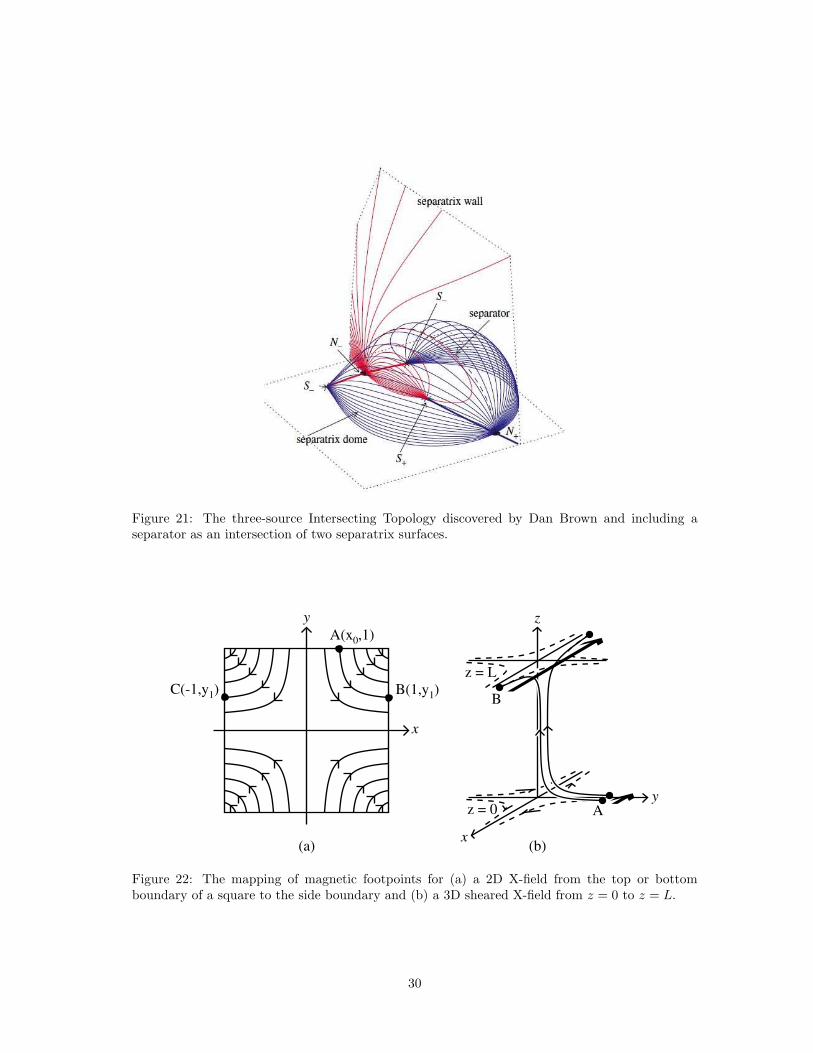
Figure 21: The three-source Intersecting Topology discovered by Dan Brown and including aseparator as an intersection of two separatrix surfaces.

y

(a) (b)

A(x0,1)

B(1,y1)

x

C(-1,y1)

z

y

x

z = 0

z = L

B

A

Figure 22: The mapping of magnetic footpoints for (a) a 2D X-field from the top or bottomboundary of a square to the side boundary and (b) a 3D sheared X-field from z = 0 to z = L.

30

x

z

y

B(x1,y1,1)

2x0

2x1

1

0.8

0.6

0.4

0.2

0 0.2 0.4 0.6 0.8 1

00

C(1/2,y1,z1)C(1/2,y1,z1)

ε

2x0

z1

1

0.8

0.6

0.4

0.2

0 0.2 0.4 0.6 0.8 1ε

2x0

2y1

1

0.8

0.6

0.4

0.2

0 0.2 0.4 0.6 0.8 1ε

2εy0 0

0.3

0.4

0.6

0.8y0 = 0.9

2x0

N

1/ε

30

20

10

0 0.2 0.4 0.6 0.8 1ε

1/ε

A(x0,y0,0)A(x0,y0,0)

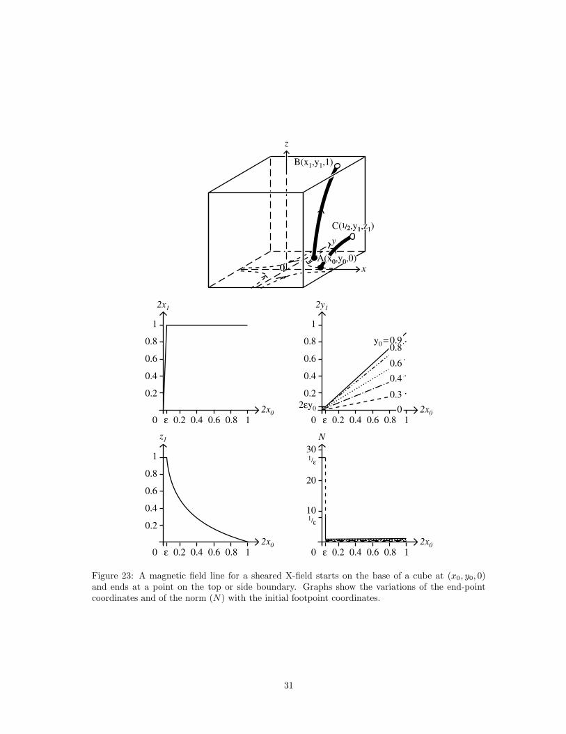
Figure 23: A magnetic field line for a sheared X-field starts on the base of a cube at (x0, y0, 0)and ends at a point on the top or side boundary. Graphs show the variations of the end-pointcoordinates and of the norm (N) with the initial footpoint coordinates.

31

Thus, when the point A(x0, y0, 0) on S0 is so close to the y-axis that 2x0 < ǫ, A maps to a pointB on the top (z1 = 1) and

F =

(ǫ−1 00 ǫ

)

,

while

N ≈ 1

ǫ,

where

ǫ = e−1/l ≪ 1.

On the other hand, when ǫ < 2x0 < 1, A maps to C on the side (x1 = 12 ), while the elements of F

and the value of N are of order unity. The resulting variations of x1, y1, z1, N with x0 are shown inFig.23, which reveals the quasi-separatrix layer as a very narrow region of width ǫ where N ≫ 1.When l = 0.1 the value of N in the quasi-separatrix layer is 104, and even when l is as large as0.3, N is about 28 in the quasi-separatrix layer. If the cube is replaced by a hemisphere or sphere,similar forms are produced but the functions become continuous and differentiable.

3.5.2 TITOV’S IMPROVED DIAGNOSIS for a QSL

Titov et al. (2002) and Titov (2007) have discovered a better way of diagnosing the presence of aQSL by normalising N in a different way to give a so-called squashing factor (Q): it is found bymapping a circle along field lines to give an ellipse, whose aspect ratio gives the value of Q. Thebasic properties of Q are as follows:

(i) Q is independent of the direction of the mapping;

(ii) Q→ ∞ at a separatrix surface;

(iii) Q≫ 1 at a quasi-separatrix layer;

(iv) Maps ofQ identify the locations where large current densities may accumulate under favourablecircumstances and therefore where reconnection has the potential to occur (i.e., separatricesand QSLs).

Titov stresses that a QSL is a geometric rather than a topological feature and also emphasizesits importance for current sheet formation due to stagnation-point flows (Cowley et al., 1997; vanBallegooijen, 1985; Mikic et al., 1989; Longcope and Strauss, 1994a; Galsgaard and Nordlund,1996a).

Titov considers a typical solar active region with field lines joining photospheric domains ofpositive and negative polarity (Fig.24). He sets up Cartesian coordinates with z = 0 representingthe photosphere and supposes that the opposite footpoints in the z = 0 plane of a given field linehave coordinates (x+, y+) and (x−, y−). The mappings of one footpoint to another describe theglobal field line connectivity. They are represented by vector functions (X−(x+, y+), Y−(x+, y+))for the mapping in one direction and (X+(x−, y−), Y+(x−, y−)) for the mapping in the oppositedirection.

Priest and Demoulin (1995) had suggested that the location of QSLs can be found from thecondition N± ≫ 1, where N± are the norms of the footpoint mapping matrices, defined by

N± ≡ N(x±, y±) =

[(∂X∓∂x±

)2

+

(∂X∓∂y±

)2

+

(∂Y∓∂x±

)2

+

(∂Y∓∂y±

)2]1/2

.

32

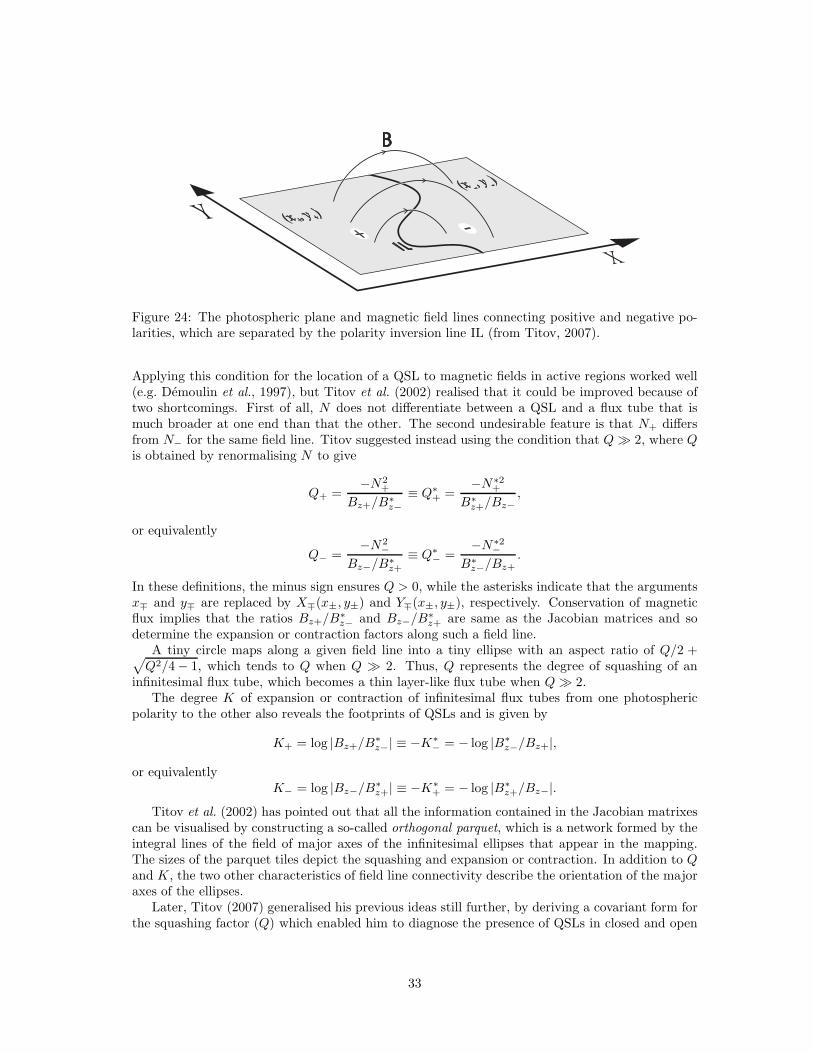
Figure 24: The photospheric plane and magnetic field lines connecting positive and negative po-larities, which are separated by the polarity inversion line IL (from Titov, 2007).

Applying this condition for the location of a QSL to magnetic fields in active regions worked well(e.g. Demoulin et al., 1997), but Titov et al. (2002) realised that it could be improved because oftwo shortcomings. First of all, N does not differentiate between a QSL and a flux tube that ismuch broader at one end than that the other. The second undesirable feature is that N+ differsfrom N− for the same field line. Titov suggested instead using the condition that Q≫ 2, where Qis obtained by renormalising N to give

Q+ =−N2

+

Bz+/B∗z−

≡ Q∗+ =

−N∗2+

B∗z+/Bz−

,

or equivalently

Q− =−N2

−Bz−/B∗

z+

≡ Q∗− =

−N∗2−

B∗z−/Bz+

.

In these definitions, the minus sign ensures Q > 0, while the asterisks indicate that the argumentsx∓ and y∓ are replaced by X∓(x±, y±) and Y∓(x±, y±), respectively. Conservation of magneticflux implies that the ratios Bz+/B

∗z− and Bz−/B∗

z+ are same as the Jacobian matrices and sodetermine the expansion or contraction factors along such a field line.

A tiny circle maps along a given field line into a tiny ellipse with an aspect ratio of Q/2 +√

Q2/4 − 1, which tends to Q when Q ≫ 2. Thus, Q represents the degree of squashing of aninfinitesimal flux tube, which becomes a thin layer-like flux tube when Q≫ 2.

The degree K of expansion or contraction of infinitesimal flux tubes from one photosphericpolarity to the other also reveals the footprints of QSLs and is given by

K+ = log |Bz+/B∗z−| ≡ −K∗

− = − log |B∗z−/Bz+|,

or equivalentlyK− = log |Bz−/B

∗z+| ≡ −K∗

+ = − log |B∗z+/Bz−|.

Titov et al. (2002) has pointed out that all the information contained in the Jacobian matrixescan be visualised by constructing a so-called orthogonal parquet, which is a network formed by theintegral lines of the field of major axes of the infinitesimal ellipses that appear in the mapping.The sizes of the parquet tiles depict the squashing and expansion or contraction. In addition to Qand K, the two other characteristics of field line connectivity describe the orientation of the majoraxes of the ellipses.

Later, Titov (2007) generalised his previous ideas still further, by deriving a covariant form forthe squashing factor (Q) which enabled him to diagnose the presence of QSLs in closed and open

33

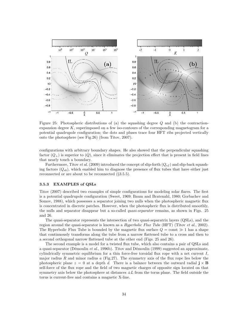
Figure 25: Photospheric distributions of (a) the squashing degree Q and (b) the contraction-expansion degree K, superimposed on a few iso-contours of the corresponding magnetogram for apotential quadrupole configuration; the dots and pluses trace four HFT ribs projected verticallyonto the photosphere (see Fig.26) (from Titov, 2007).

configurations with arbitrary boundary shapes. He also showed that the perpendicular squashingfactor (Q⊥) is superior to (Q), since it eliminates the projection effect that is present in field linesthat nearly touch a boundary.

Furthermore, Titov et al. (2009) introduced the concept of slip-forth (Qsf ) and slip-back squash-ing factors (Qsb), which enabled him to diagnose the presence of flux tubes that have either justreconnected or are about to be reconnected (§3.5.5).

3.5.3 EXAMPLES of QSLs

Titov (2007) described two examples of simple configurations for modeling solar flares. The firstis a potential quadrupole configuration (Sweet, 1969; Baum and Bratenahl, 1980; Gorbachev andSomov, 1988), which possesses a separator joining two nulls when the photospheric magnetic fluxis concentrated in discrete patches. However, when the photospheric flux is distributed smoothly,the nulls and separator disappear but a so-called quasi-separator remains, as shown in Figs. 25and 26.

The quasi-separator represents the intersection of two quasi-separatrix layers (QSLs), and theregion around the quasi-separator is known as a Hyperbolic Flux Tube (HFT) (Titov et al., 2002).The Hyperbolic Flux Tube is bounded by the magnetic flux surface Q = const ≫ 1 has a shapethat continuously transforms along the tube from a narrow flattened tube to a cross and then toa second orthogonal narrow flattened tube at the other end (Figs. 25 and 26).

The second example is a model for a twisted flux tube, which also contains a pair of QSLs anda quasi-separator (Demoulin et al., 1996b). Titov and Demoulin (1999) suggested an approximate,cylindrically symmetric equilibrium for a thin force-free toroidal flux rope with a net current I,major radius R and minor radius a (Fig.27). The symmetry axis of the flux rope lies below thephotospheric plane z = 0 at a depth d. There is a balance between the outward radial j × Bself-force of the flux rope and the field of two magnetic charges of opposite sign located on thatsymmetry axis below the photosphere at distances ±L from the torus plane. The field outside thetorus is current-free and contains a magnetic X-line.

34

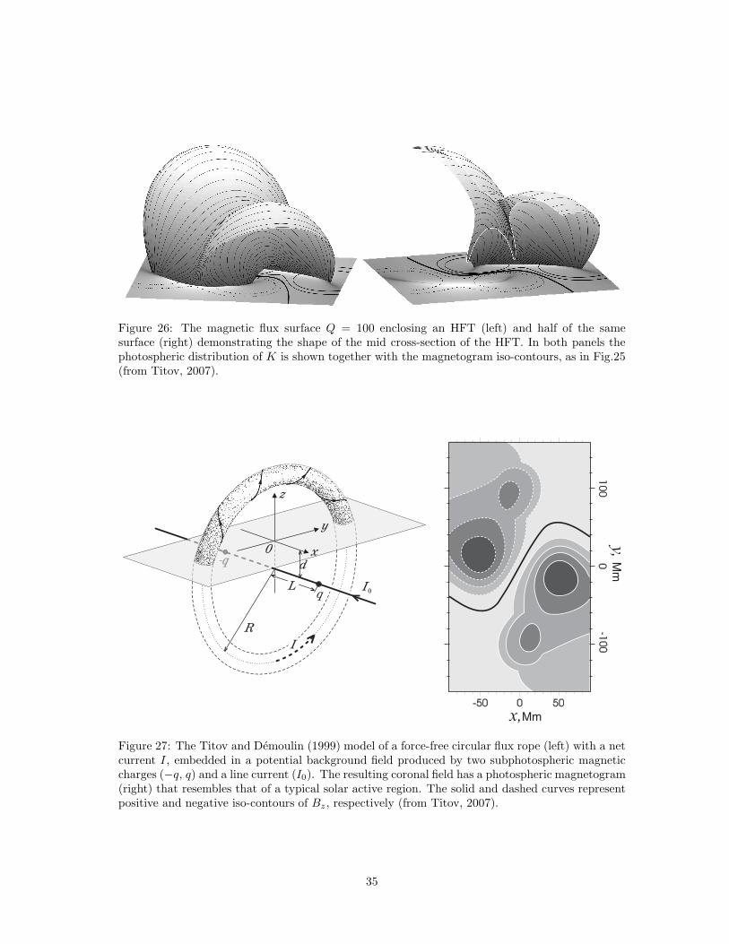
Figure 26: The magnetic flux surface Q = 100 enclosing an HFT (left) and half of the samesurface (right) demonstrating the shape of the mid cross-section of the HFT. In both panels thephotospheric distribution of K is shown together with the magnetogram iso-contours, as in Fig.25(from Titov, 2007).

Figure 27: The Titov and Demoulin (1999) model of a force-free circular flux rope (left) with a netcurrent I, embedded in a potential background field produced by two subphotospheric magneticcharges (−q, q) and a line current (I0). The resulting coronal field has a photospheric magnetogram(right) that resembles that of a typical solar active region. The solid and dashed curves representpositive and negative iso-contours of Bz , respectively (from Titov, 2007).

35

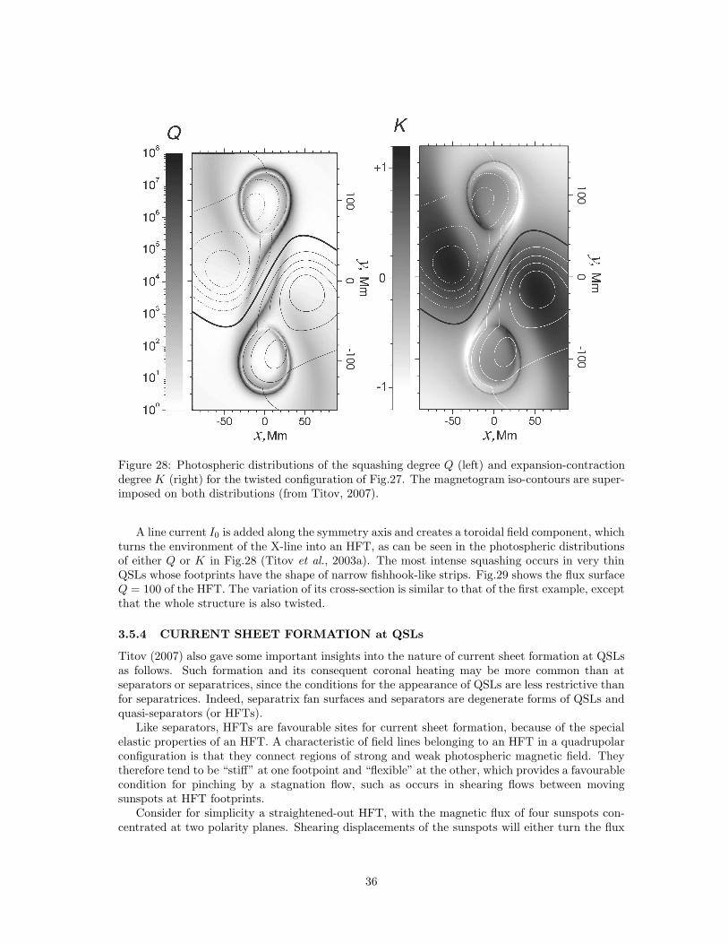
Figure 28: Photospheric distributions of the squashing degree Q (left) and expansion-contractiondegree K (right) for the twisted configuration of Fig.27. The magnetogram iso-contours are super-imposed on both distributions (from Titov, 2007).

A line current I0 is added along the symmetry axis and creates a toroidal field component, whichturns the environment of the X-line into an HFT, as can be seen in the photospheric distributionsof either Q or K in Fig.28 (Titov et al., 2003a). The most intense squashing occurs in very thinQSLs whose footprints have the shape of narrow fishhook-like strips. Fig.29 shows the flux surfaceQ = 100 of the HFT. The variation of its cross-section is similar to that of the first example, exceptthat the whole structure is also twisted.

3.5.4 CURRENT SHEET FORMATION at QSLs

Titov (2007) also gave some important insights into the nature of current sheet formation at QSLsas follows. Such formation and its consequent coronal heating may be more common than atseparators or separatrices, since the conditions for the appearance of QSLs are less restrictive thanfor separatrices. Indeed, separatrix fan surfaces and separators are degenerate forms of QSLs andquasi-separators (or HFTs).

Like separators, HFTs are favourable sites for current sheet formation, because of the specialelastic properties of an HFT. A characteristic of field lines belonging to an HFT in a quadrupolarconfiguration is that they connect regions of strong and weak photospheric magnetic field. Theytherefore tend to be “stiff” at one footpoint and “flexible” at the other, which provides a favourablecondition for pinching by a stagnation flow, such as occurs in shearing flows between movingsunspots at HFT footprints.

Consider for simplicity a straightened-out HFT, with the magnetic flux of four sunspots con-centrated at two polarity planes. Shearing displacements of the sunspots will either turn the flux

36

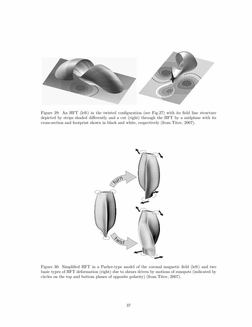
Figure 29: An HFT (left) in the twisted configuration (see Fig.27) with its field line structuredepicted by strips shaded differently and a cut (right) through the HFT by a midplane with itscross-section and footprint shown in black and white, respectively (from Titov, 2007).

Figure 30: Simplified HFT in a Parker-type model of the coronal magnetic field (left) and twobasic types of HFT deformation (right) due to shears driven by motions of sunspots (indicated bycircles on the top and bottom planes of opposite polarity) (from Titov, 2007).

37

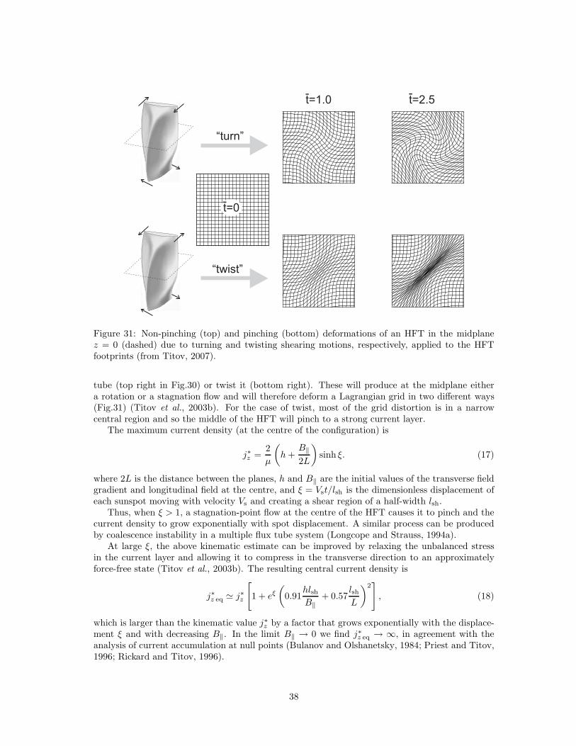
Figure 31: Non-pinching (top) and pinching (bottom) deformations of an HFT in the midplanez = 0 (dashed) due to turning and twisting shearing motions, respectively, applied to the HFTfootprints (from Titov, 2007).

tube (top right in Fig.30) or twist it (bottom right). These will produce at the midplane eithera rotation or a stagnation flow and will therefore deform a Lagrangian grid in two different ways(Fig.31) (Titov et al., 2003b). For the case of twist, most of the grid distortion is in a narrowcentral region and so the middle of the HFT will pinch to a strong current layer.

The maximum current density (at the centre of the configuration) is

j∗z =2

µ

(

h+B‖2L

)

sinh ξ. (17)

where 2L is the distance between the planes, h and B‖ are the initial values of the transverse fieldgradient and longitudinal field at the centre, and ξ = Vst/lsh is the dimensionless displacement ofeach sunspot moving with velocity Vs and creating a shear region of a half-width lsh.

Thus, when ξ > 1, a stagnation-point flow at the centre of the HFT causes it to pinch and thecurrent density to grow exponentially with spot displacement. A similar process can be producedby coalescence instability in a multiple flux tube system (Longcope and Strauss, 1994a).

At large ξ, the above kinematic estimate can be improved by relaxing the unbalanced stressin the current layer and allowing it to compress in the transverse direction to an approximatelyforce-free state (Titov et al., 2003b). The resulting central current density is

j∗z eq ≃ j∗z

[

1 + eξ

(

0.91hlshB‖

+ 0.57lshL

)2]

, (18)

which is larger than the kinematic value j∗z by a factor that grows exponentially with the displace-ment ξ and with decreasing B‖. In the limit B‖ → 0 we find j∗z eq → ∞, in agreement with theanalysis of current accumulation at null points (Bulanov and Olshanetsky, 1984; Priest and Titov,1996; Rickard and Titov, 1996).

38

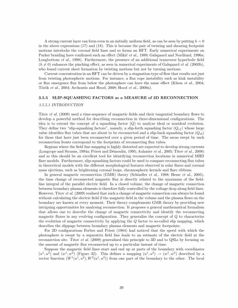
A strong current layer can form even in an initially uniform field, as can be seen by putting h = 0in the above expressions (17) and (18). This is because the pair of twisting and shearing footpointmotions interlocks the coronal field lines and so forms an HFT. Early numerical experiments onParker braiding have confirmed such an effect (Mikic et al., 1989; Galsgaard and Nordlund, 1996a;Longbottom et al., 1998). Furthermore, the presence of an additional transverse hyperbolic field(h 6= 0) enhances the pinching effect, as seen in numerical experiments of Galsgaard et al. (2003b),who found current sheet formation by twisting motions but not by turning motions.

Current concentration in an HFT can be driven by a stagnation-type of flow that results not justfrom twisting photospheric motions. For instance, a flux rope instability such as kink instabilityor flux emergence flux from below the photosphere can have the same effect (Kliem et al., 2004;Torok et al., 2004; Archontis and Hood, 2008; Hood et al., 2009a).

3.5.5 SLIP-SQUASHING FACTORS as a MEASURE of 3D RECONNECTION

3.5.5.1 INTRODUCTION

Titov et al. (2009) used a time-sequence of magnetic fields and their tangential boundary flows todevelop a powerful method for describing reconnection in three-dimensional configurations. Theidea is to extend the concept of a squashing factor (Q) to analyze ideal or nonideal evolution.They define two “slip-squashing factors”, namely, a slip-forth squashing factor (Qsf ) whose largevalue identifies flux tubes that are about to be reconnected and a slip-back squashing factor (Qsb)for those that have just been reconnected over a given period of time. The areas swept by suchreconnection fronts correspond to the footprints of reconnecting flux tubes.

Regions where the field line mapping is highly distorted are expected to develop strong currents(Longcope and Strauss, 1994a; Priest and Demoulin, 1995; Aulanier et al., 2005; Titov et al., 2008)and so this should be an excellent tool for identifying reconnection locations in numerical MHDflare models. Furthermore, slip-squashing factors could be used to compare reconnecting flux tubesin theoretical models with the different morphological features observed in solar flares and coronalmass ejections, such as brightening coronal loops, chromospheric kernels and flare ribbons.

In general magnetic reconnection (GMR) theory (Schindler et al., 1988; Hesse et al., 2005),the time change of reconnected magnetic flux is directly related to the maximum of the field-line integral of the parallel electric field. In a closed volume, the change of magnetic connectionbetween boundary plasma elements is therefore fully controlled by the voltage drop along field lines.However, Titov et al. (2009) realised that such a change of magnetic connection can always be foundwithout calculating the electric field if the magnetic field in the volume and the plasma flows on theboundary are known at every moment. Their theory complements GMR theory by providing newintriguing opportunities for analysing reconnection. It proposes a general mathematical formalismthat allows one to describe the change of magnetic connectivity and identify the reconnectingmagnetic fluxes in any evolving configuration. They generalize the concept of Q to characterizethe evolution of magnetic connectivity by applying the Q factor to so-called slip mapping, whichdescribes the slippage between boundary plasma elements and magnetic footpoints.

For 2D configurations Forbes and Priest (1984) had noticed that the speed with which thephotosphere is swept by a separatrix field line leads to an estimate of the electric field at thereconnection site. Titov et al. (2009) generalised this principle to 3D and to QSLs by focusing onthe amount of magnetic flux reconnected up to a particular instant of time.

Suppose the magnetic field lines start and end up at parts of the boundary with coordinates(u1, u2) and (w1, w2) (Figure 32). This defines a mapping (u1, u2) → (w1, w2) described by avector function (W 1(u1, u2),W 2(u1, u2)) from one part of the boundary to the other. The local

39

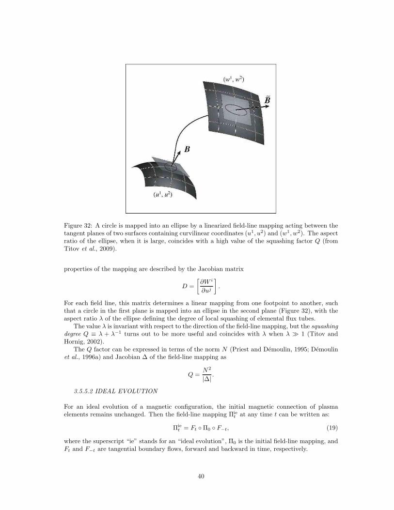
Figure 32: A circle is mapped into an ellipse by a linearized field-line mapping acting between thetangent planes of two surfaces containing curvilinear coordinates (u1, u2) and (w1, w2). The aspectratio of the ellipse, when it is large, coincides with a high value of the squashing factor Q (fromTitov et al., 2009).

properties of the mapping are described by the Jacobian matrix

D =

[∂W i

∂uj

]

.

For each field line, this matrix determines a linear mapping from one footpoint to another, suchthat a circle in the first plane is mapped into an ellipse in the second plane (Figure 32), with theaspect ratio λ of the ellipse defining the degree of local squashing of elemental flux tubes.

The value λ is invariant with respect to the direction of the field-line mapping, but the squashingdegree Q ≡ λ + λ−1 turns out to be more useful and coincides with λ when λ ≫ 1 (Titov andHornig, 2002).

The Q factor can be expressed in terms of the norm N (Priest and Demoulin, 1995; Demoulinet al., 1996a) and Jacobian ∆ of the field-line mapping as

Q =N2

|∆| .

3.5.5.2 IDEAL EVOLUTION

For an ideal evolution of a magnetic configuration, the initial magnetic connection of plasmaelements remains unchanged. Then the field-line mapping Πie

t at any time t can be written as:

Πiet = Ft ◦ Π0 ◦ F−t, (19)

where the superscript “ie” stands for an “ideal evolution”, Π0 is the initial field-line mapping, andFt and F−t are tangential boundary flows, forward and backward in time, respectively.

40

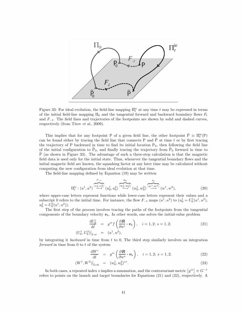
Figure 33: For ideal evolution, the field-line mapping Πiet at any time t may be expressed in terms

of the initial field-line mapping Π0 and the tangential forward and backward boundary flows Ft

and F−t. The field lines and trajectories of the footpoints are shown by solid and dashed curves,respectively (from Titov et al., 2009).

This implies that for any footpoint P of a given field line, the other footpoint P ≡ Πiet (P)

can be found either by tracing the field line that connects P and P at time t or by first tracingthe trajectory of P backward in time to find its initial location P0, then following the field lineof the initial configuration to P0, and finally tracing the trajectory from P0 forward in time toP (as shown in Figure 33). The advantage of such a three-step calculation is that the magneticfield data is used only for the initial state. Thus, whenever the tangential boundary flows and theinitial magnetic field are known, the squashing factor at any later time may be calculated withoutcomputing the new configuration from ideal evolution at that time.

The field-line mapping defined by Equation (19) may be written

Πiet : (u1, u2)

F−t

︷ ︸︸ ︷(U1

0 ,U20 )−→ (u1

0, u20)

Π0︷ ︸︸ ︷(W1

0 ,W20 )−→ (w1

0 , w20)

Ft︷ ︸︸ ︷(W1,W2)−→ (w1, w2), (20)

where upper-case letters represent functions while lower-case letters represent their values and asubscript 0 refers to the initial time. For instance, the flow F−t maps (u1, u2) to (u1

0 = U10 (u1, u2),

u20 = U2

0 (u1, u2)).The first step of the process involves tracing the paths of the footpoints from the tangential

components of the boundary velocity vb. In other words, one solves the initial-value problem

dU i0

dt= gisf

(∂R

∂us· vb

)

, i = 1, 2; s = 1, 2; (21)

(U10 , U

20 )∣∣t=t

= (u1, u2),

by integrating it backward in time from t to 0, The third step similarly involves an integrationforward in time from 0 to t of the system

dW i

dt= gis

(∂R

∂ws· vb

)

, i = 1, 2; s = 1, 2; (22)

(W 1,W 2)∣∣t=0

= (w10 , w

20)

∗∗. (23)

In both cases, a repeated index s implies a summation, and the contravariant metric[gis]≡ G−1

refers to points on the launch and target boundaries for Equations (21) and (22), respectively. A

41

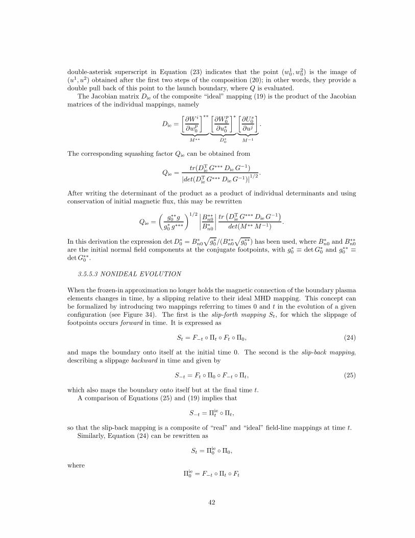
double-asterisk superscript in Equation (23) indicates that the point (w10 , w

20) is the image of

(u1, u2) obtained after the first two steps of the composition (20); in other words, they provide adouble pull back of this point to the launch boundary, where Q is evaluated.

The Jacobian matrix Die of the composite “ideal” mapping (19) is the product of the Jacobianmatrices of the individual mappings, namely

Die =

[∂W i

∂wp0

]∗∗

︸ ︷︷ ︸

M∗∗

[∂W p

0

∂us0

]∗

︸ ︷︷ ︸

D∗

0

[∂Us

0

∂uj

]

︸ ︷︷ ︸

M−1

.

The corresponding squashing factor Qie can be obtained from

Qie =tr(DT

ie G∗∗∗DieG

−1)

|det(DTie G

∗∗∗DieG−1)|1/2.

After writing the determinant of the product as a product of individual determinants and usingconservation of initial magnetic flux, this may be rewritten

Qie =

(g∗∗0 g

g∗0 g∗∗∗

)1/2 ∣∣∣∣

B∗∗n0

B∗n0

∣∣∣∣

tr(DT

ieG∗∗∗DieG

−1)

det(M∗∗M−1).

In this derivation the expression detD∗0 = B∗

n0

√g∗0/(B

∗∗n0

√g∗∗0 ) has been used, where B∗

n0 and B∗∗n0

are the initial normal field components at the conjugate footpoints, with g∗0 ≡ detG∗0 and g∗∗0 ≡

detG∗∗0 .

3.5.5.3 NONIDEAL EVOLUTION

When the frozen-in approximation no longer holds the magnetic connection of the boundary plasmaelements changes in time, by a slipping relative to their ideal MHD mapping. This concept canbe formalized by introducing two mappings referring to times 0 and t in the evolution of a givenconfiguration (see Figure 34). The first is the slip-forth mapping St, for which the slippage offootpoints occurs forward in time. It is expressed as

St = F−t ◦ Πt ◦ Ft ◦ Π0, (24)

and maps the boundary onto itself at the initial time 0. The second is the slip-back mapping,describing a slippage backward in time and given by

S−t = Ft ◦ Π0 ◦ F−t ◦ Πt, (25)

which also maps the boundary onto itself but at the final time t.A comparison of Equations (25) and (19) implies that

S−t = Πiet ◦ Πt,

so that the slip-back mapping is a composite of “real” and “ideal” field-line mappings at time t.Similarly, Equation (24) can be rewritten as

St = Πie0 ◦ Π0,

whereΠie

0 = F−t ◦ Πt ◦ Ft

42

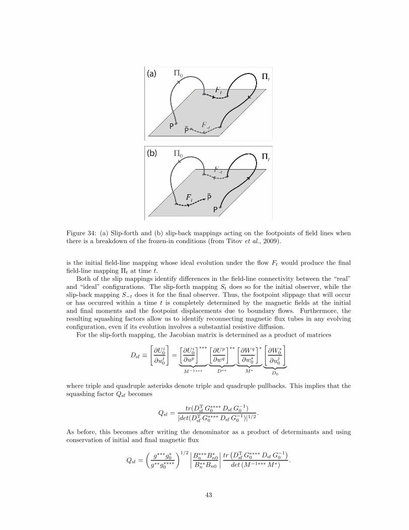
Figure 34: (a) Slip-forth and (b) slip-back mappings acting on the footpoints of field lines whenthere is a breakdown of the frozen-in conditions (from Titov et al., 2009).

is the initial field-line mapping whose ideal evolution under the flow Ft would produce the finalfield-line mapping Πt at time t.

Both of the slip mappings identify differences in the field-line connectivity between the “real”and “ideal” configurations. The slip-forth mapping St does so for the initial observer, while theslip-back mapping S−t does it for the final observer. Thus, the footpoint slippage that will occuror has occurred within a time t is completely determined by the magnetic fields at the initialand final moments and the footpoint displacements due to boundary flows. Furthermore, theresulting squashing factors allow us to identify reconnecting magnetic flux tubes in any evolvingconfiguration, even if its evolution involves a substantial resistive diffusion.

For the slip-forth mapping, the Jacobian matrix is determined as a product of matrices

Dsf ≡[

∂U i0

∂uj0

]

=

[∂U i

0

∂up

]∗∗∗

︸ ︷︷ ︸

M−1∗∗∗

[∂Up

∂wq

]∗∗

︸ ︷︷ ︸

D∗∗

[∂W q

∂ws0

]∗

︸ ︷︷ ︸

M∗

[

∂W s0

∂uj0

]

︸ ︷︷ ︸

D0

where triple and quadruple asterisks denote triple and quadruple pullbacks. This implies that thesquashing factor Qsf becomes

Qsf =tr(DT

sf G∗∗∗∗0 Dsf G

−10 )

|det(DTsf G

∗∗∗∗0 Dsf G

−10 )|1/2

.

As before, this becomes after writing the denominator as a product of determinants and usingconservation of initial and final magnetic flux

Qsf =

(g∗∗∗g∗0g∗∗g∗∗∗∗0

)1/2 ∣∣∣∣

B∗∗∗n B∗

n0

B∗∗n Bn0

∣∣∣∣

tr(DT

sf G∗∗∗∗0 Dsf G

−10

)

det (M−1∗∗∗M∗).

43

Following a similar argument, the slip-back mapping has Jacobian matrix

Dsb ≡[∂U i

∂uj

]

=

[∂U i

∂up0

]∗∗∗

︸ ︷︷ ︸

M∗∗∗∗

[∂Up

0

∂wq0

]∗∗

︸ ︷︷ ︸

D∗∗

0

[∂W q

0

∂ws

]∗

︸ ︷︷ ︸

M−1∗

[∂W s

∂uj

]

︸ ︷︷ ︸

D

and squashing factor

Qsb =

(g∗∗∗0 g∗

g∗∗0 g∗∗∗∗

)1/2 ∣∣∣∣

B∗∗∗n0 B

∗n

B∗∗n0Bn

∣∣∣∣

tr(DT

sbG∗∗∗∗DsbG

−1)

det (M∗∗∗M−1∗).

The flux tubes assembled from such Q-factors have a layer-like structure and are called re-connection fronts (RFs). Each slip mapping has two RFs, one of which, called the instantaneousRF, corresponds to the present moment and approximately coincides with the set of QSLs existingthen. The second RF is called the future RF or past RF, respectively, for the slip-forth or slip-backmapping. The future RF consists of those initial flux tubes whose footprints will become afterreconnection the footprints of the final QSLs, whereas the past RF consists of those final fluxtubes whose footprints are formed by reconnection from the footprints of the initial QSLs.

Titov et al. (2009) presented two examples of the application of their ideas. The first was the onepreviously studied by Hesse et al. (2005) of the formation and rise of a flux rope without null pointsin the framework of general magnetic reconnection (GMR) theory. The second was reconnection ina thin current-layer patch of a sheared force-free field. It shows how the localization of a nonidealprocess may indeed cause structural changes that are characteristic of reconnection rather thanmagnetic diffusion. Such changes include the formation of flux tubes with narrow, ribbon-likefootprints.

Comparing with GMR theory, their analysis treats regions with small or large amounts ofreconnected flux on an equal footing, since slip-squashing factors are dimensionless geometricalquantities measuring only a relative spatial rate of magnetic slippage at the boundary. Slip-squashing factors also discriminate between reconnection and simple diffusion much better thanthe voltage drop method of GMR theory.

44

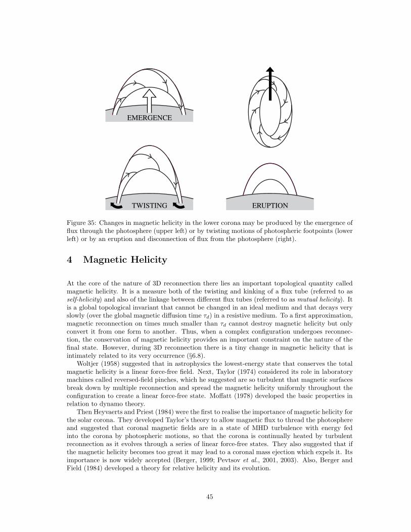
EMERGENCE

TWISTING ERUPTION

Figure 35: Changes in magnetic helicity in the lower corona may be produced by the emergence offlux through the photosphere (upper left) or by twisting motions of photospheric footpoints (lowerleft) or by an eruption and disconnection of flux from the photosphere (right).

4 Magnetic Helicity

At the core of the nature of 3D reconnection there lies an important topological quantity calledmagnetic helicity. It is a measure both of the twisting and kinking of a flux tube (referred to asself-helicity) and also of the linkage between different flux tubes (referred to as mutual helicity). Itis a global topological invariant that cannot be changed in an ideal medium and that decays veryslowly (over the global magnetic diffusion time τd) in a resistive medium. To a first approximation,magnetic reconnection on times much smaller than τd cannot destroy magnetic helicity but onlyconvert it from one form to another. Thus, when a complex configuration undergoes reconnec-tion, the conservation of magnetic helicity provides an important constraint on the nature of thefinal state. However, during 3D reconnection there is a tiny change in magnetic helicity that isintimately related to its very occurrence (§6.8).

Woltjer (1958) suggested that in astrophysics the lowest-energy state that conserves the totalmagnetic helicity is a linear force-free field. Next, Taylor (1974) considered its role in laboratorymachines called reversed-field pinches, which he suggested are so turbulent that magnetic surfacesbreak down by multiple reconnection and spread the magnetic helicity uniformly throughout theconfiguration to create a linear force-free state. Moffatt (1978) developed the basic properties inrelation to dynamo theory.

Then Heyvaerts and Priest (1984) were the first to realise the importance of magnetic helicity forthe solar corona. They developed Taylor’s theory to allow magnetic flux to thread the photosphereand suggested that coronal magnetic fields are in a state of MHD turbulence with energy fedinto the corona by photospheric motions, so that the corona is continually heated by turbulentreconnection as it evolves through a series of linear force-free states. They also suggested that ifthe magnetic helicity becomes too great it may lead to a coronal mass ejection which expels it. Itsimportance is now widely accepted (Berger, 1999; Pevtsov et al., 2001, 2003). Also, Berger andField (1984) developed a theory for relative helicity and its evolution.

45

In the solar atmosphere the continual motion of photospheric magnetic footpoints tends to buildup the magnetic helicity until it is ejected by magnetic eruptions. Thus, the magnetic helicity inthe atmosphere can change either by the emergence of twisted or linked structures from the solarinterior or by the twisting (or untwisting) of the footpoint motions of coronal loops. Magnetichelicity of a coronal loop can be decreased by the detachment and ejection of magnetic structuresfrom the solar surface (as in prominence eruptions) (Fig.35). Here we give definitions of magnetichelicity (§4.1), its evolution (§4.2) and simple examples (§4.3).

4.1 DEFINITION of MAGNETIC HELICITY

Magnetic helicity in a closed volume (V ) bounded by a surface S is defined as

H0 =

∫

V

A · B dV, (26)

where A is the vector potential so that B = ∇ × A. H0 is gauge invariant if the volume is closedbut not if magnetic fields enter or leave it. This is related to the fact that if the volume is open,the field lines that close outside V will have linkage with those inside V , and such a linkage is ill-defined if only the field inside V is prescribed, since there are many ways of continuing it outsideV . The proof is as follows. Suppose A is replaced by A + ∇ΦA (which does not change B), thenH0 changes by

∆H0 =

∫

V

∇ΦA ·B dV =

∫

V

∇ · (ΦAB) dV,

using ∇ · B = 0. Then invoking the divergence theorem for a simply connected volume implies

∆H0 =

∫

S

ΦAB · n dS,

where n is the unit normal to S and pointing out of V0. We therefore have gauge invariance(∆H0 = 0) if B · n = 0 on the surface S, as required.

A gauge-invariant relative magnetic helicity

H =

∫

V∞

A · B− A0 ·B0 dV, (27)

was proposed by Berger and Field (1984) as an alternative to H0, where B0 = ∇ × A0 is a fieldthat is potential inside V with the same B outside V and has A× n = A0×n on S. They realisedthat the difference in helicity integrated over all space (V∞) of any two fields that differ only insideV is independent of the field outside V , and that a particularly useful reference field inside V is apotential field, since it is completely determined by B · n on S.

In other words, a generalization of the definition of helicity requires a ground state that setsthe zero value. The potential field is the best one for this purpose, since it minimises the magneticenergy when the normal field at the boundary is imposed. Furthermore, with the helicity of thepotential field set to zero in this way, the helicity is now uniquely specified.

An alternative form of relative helicity that is sometimes useful and does not require the bound-ary constraint on A is (Finn and Antonsen, 1985)

H =

∫

V

(A + A0) · (B− B0) dV,

where again B0 = ∇ × A0 is potential inside V and has the same normal component as B on S.

46

An added complication arises in a multiply connected domain, namely that you can impose themagnetic fluxes through each of the holes. For example, in a torus you can impose the toroidalflux. However, the above definitions (26) or (27) of magnetic helicity are still valid provided thepotential field (B0) also possesses those fluxes through the holes. One convenient way to ensure thefluxes are correct is to replace the condition (B0 · n = B · n) on the normal fields at the boundaryin (27) with A × n = A0 × n, so that the tangential components of the vector potentials are thesame at the boundary. This implies B ·n = B0 ·n on S and also implies that

∫A · ds =

∫A0 ·ds

along any closed curve drawn on the boundary.

4.2 RATE of CHANGE of MAGNETIC HELICITY

The time variation of magnetic helicity is

dH

dt= −2

∫

V

E ·B dV + 2

∫

S

Ap × E · n dS,

where we have chosen for convenience a gauge (Ap) such that ∇ ·Ap = 0 and Ap · n = 0 on S.If there is no slippage on the boundary and the resistive Ohm’s Law (E = −v × B + j/σ) holds,this becomes

dH

dt= −2

∫

V

j ·B/σ dV + 2

∫

S

(B ·Ap)(v · n) − (v ·Ap)(B · n) dS. (28)

Here the first term represents internal helicity dissipation and the surface integral gives the flowof helicity across the boundary.

Several useful deductions follow. First, if the magnetic field varies on a length-scale (L), equat-ing dH/dt to the first term with j ∼ A/(µL2) implies that the time-scale for magnetic helicitydissipation is the global diffusion time (τd = L2/η). Secondly, on time-scales much shorter than τd,changes of helicity are given by the surface term. Thus, for example, if the volume is closed, withB · n = v · n = 0, the helicity is conserved. But, if instead footpoint motions along the surface areprescribed, we may deduce the resulting injection or extraction of helicity as follows.

For a plane surface (z = 0) Equation (28) gives the magnetic helicity evolution as

dH

dt= 2

∫ ∫

(B · Ap)vz − (v ·Ap)Bz dxdy, (29)

in the ideal limit, where the integration is over the xy-plane. The first term (F⊥, say) involves onlymotions in the z-direction and thus represents the effect of the emergence of structures carryinghelicity through the surface. The second term (F‖, say) involves only motions in the xy-plane andrepresents the way the shuffling of footpoints can inject helicity into fields already present in thevolume (Fig.35).

Suppose the surface S is planar and threaded by the footpoints of N thin flux tubes of magneticflux Fi. If the motion of each footpoint consists of a translation plus a uniform rotation at a rateωi, then the rate of helicity change is

dH

dt= − 1

2π

N∑

i=1

ωiF2i +

N∑

i=1

N∑

j=1

θijFiFj

, (30)

where θij is the time derivative of the relative angle (θij) between footpoints i and j (Berger, 1984).The first term arises because footpoint rotation injects twist into a flux tube at a rate of one unit

47

of twist every 2π/ω seconds. The second term measures the rate at which footpoints circle eachother and braid the flux tubes.

The result (30) may be proved from the surface term of (28) as follows. Using Cartesiancoordinates with the z-axis directed into V and the xy-plane as the surface S, the conditionAp · n = 0 becomes Apz = 0, which implies that ∂Apz/∂x = ∂Apz/∂y = 0. Thus, on the xy-planethe x- and y- coordinates of Ap satisfy

∂Apx

∂x+∂Apy

∂y+∂Apz

∂z= 0,

∂Apy

∂x− ∂Apx

∂y= b,

where b(x, y) = Bz(x, y, 0), which imply that

∂2Apx

∂x2+∂2Apx

∂y2= − ∂b

∂y.

The usual Poisson solution is

Apx = −∫

b(x′, y′)(y − y′)

2π[(x− x′)2 + (y − y′)2]dx′dy′,

(31)

Apy =

∫b(x′, y′)(x− x′)

2π[(x− x′)2 + (y − y′)2]dx′dy′.

For the particular case when vz = 0 on the surface, Eq.(29) becomes after using (31)

dH

dt= −2

∫ ∫

b(x, y)b(x′, y′)r × v(x, y) · z

2πr2dSdS′, (32)

where r = (x− x′)x + (y − y′)y.As an example, suppose we have two thin flux tubes of flux F1 and F2 with a translational

motion plus uniform rotations at angular speeds ω1 and ω2 about points (x1, y1) and (x2, y2),respectively, such that near (xi, yi)

v(x, y) = v(xi, yi) + ωi(x − xi)y − ωi(y − yi)x. (33)

Now write b = b1 + b2, where b1 and b2 are the fields of the flux tube at r1 = (x1, y1) andr2 = (x2, y2), respectively. Then the integrals in (32) have three parts: integrating the first overb1b1

′ gives a contribution of −F 21ω1/(2π), the second over b2b2

′ gives −F 22 ω2/2π, and the third

over (b1b2′ + b2b1

′) gives the cross-term (−F1F2θ12/π), as required in (30), where

θ12 =|(r2 − r1) × (v2 − v1)|

|r2 − r1|2.

4.3 MAGNETIC HELICITY of FLUX TUBES

The magnetic helicity of a variety of different magnetic configurations may be deduced from Eq.(30)when twisting and linking is built up from an initially potential field that has separate untwistedtubes at large distances from one another. The resulting total magnetic helicity consists of theself-helicity (Hs) of each tube due to its own internal twist and mutual helicity (Hm) due to thelinking of one tube with another. Thus, from (30)

H =

N∑

i=1

Hsi +

N∑

i,j=1

i<j

Hmij ,

48

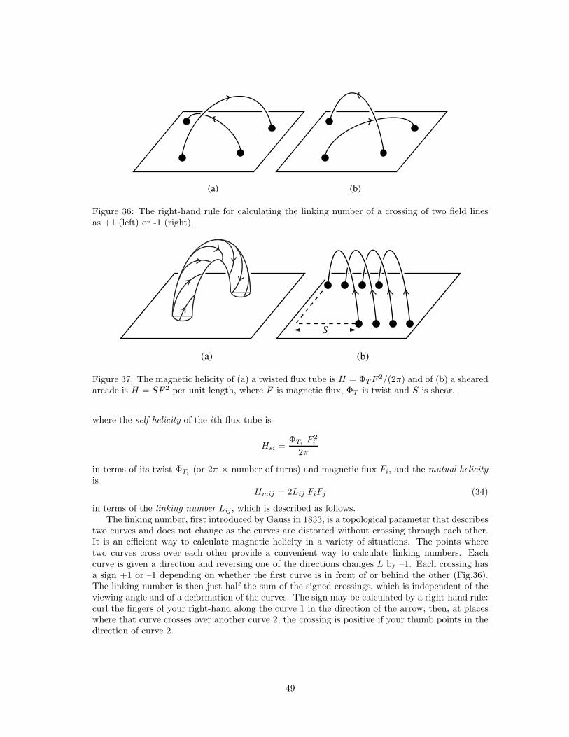
(a) (b)

Figure 36: The right-hand rule for calculating the linking number of a crossing of two field linesas +1 (left) or -1 (right).

(a) (b)

S

Figure 37: The magnetic helicity of (a) a twisted flux tube is H = ΦTF2/(2π) and of (b) a sheared

arcade is H = SF 2 per unit length, where F is magnetic flux, ΦT is twist and S is shear.

where the self-helicity of the ith flux tube is

Hsi =ΦTi

F 2i

2π

in terms of its twist ΦTi(or 2π × number of turns) and magnetic flux Fi, and the mutual helicity

isHmij = 2Lij FiFj (34)

in terms of the linking number Lij , which is described as follows.The linking number, first introduced by Gauss in 1833, is a topological parameter that describes

two curves and does not change as the curves are distorted without crossing through each other.It is an efficient way to calculate magnetic helicity in a variety of situations. The points wheretwo curves cross over each other provide a convenient way to calculate linking numbers. Eachcurve is given a direction and reversing one of the directions changes L by –1. Each crossing hasa sign +1 or –1 depending on whether the first curve is in front of or behind the other (Fig.36).The linking number is then just half the sum of the signed crossings, which is independent of theviewing angle and of a deformation of the curves. The sign may be calculated by a right-hand rule:curl the fingers of your right-hand along the curve 1 in the direction of the arrow; then, at placeswhere that curve crosses over another curve 2, the crossing is positive if your thumb points in thedirection of curve 2.

49

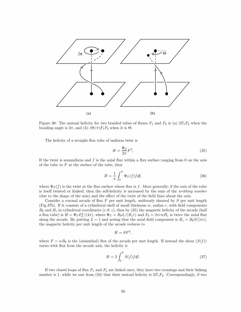
(a)

2π Θ

(b)

Figure 38: The mutual helicity for two braided tubes of fluxes F1 and F2 is (a) 2F1F2 when thebraiding angle is 2π, and (b) (Θ/π)F1F2 when it is Θ.

The helicity of a straight flux tube of uniform twist is

H =ΦT

2πF 2, (35)

If the twist is nonuniform and f is the axial flux within a flux surface ranging from 0 on the axisof the tube to F at the surface of the tube, then

H =1

π

∫ F

0

ΦT (f)fdf, (36)

where ΦT (f) is the twist at the flux surface whose flux is f . More generally, if the axis of the tubeis itself twisted or kinked, then the self-helicity is increased by the sum of the writhing number(due to the shape of the axis) and the effect of the twist of the field lines about the axis.

Consider a coronal arcade of flux F per unit length, uniformly sheared by S per unit length(Fig.37b). If it consists of a cylindrical shell of small thickness w, radius r, with field componentsBθ and Bz in cylindrical coordinates (r, θ, z), then by (35) the magnetic helicity of the arcade (halfa flux tube) is H = ΦTF

20 /(4π), where ΦT = BθL/(Bzr) and F0 = 2πrwBz is twice the axial flux

along the arcade. By putting L = 1 and noting that the axial field component is Bz = BθS/(πr),the magnetic helicity per unit length of the arcade reduces to

H = SF 2,

where F = wBθ is the (azimuthal) flux of the arcade per unit length. If instead the shear (S(f))varies with flux from the arcade axis, the helicity is

H = 2

∫ F

0

S(f)fdf. (37)

If two closed loops of flux F1 and F2 are linked once, they have two crossings and their linkingnumber is 1, while we saw from (34) that their mutual helicity is 2F1F2. Correspondingly, if two

50

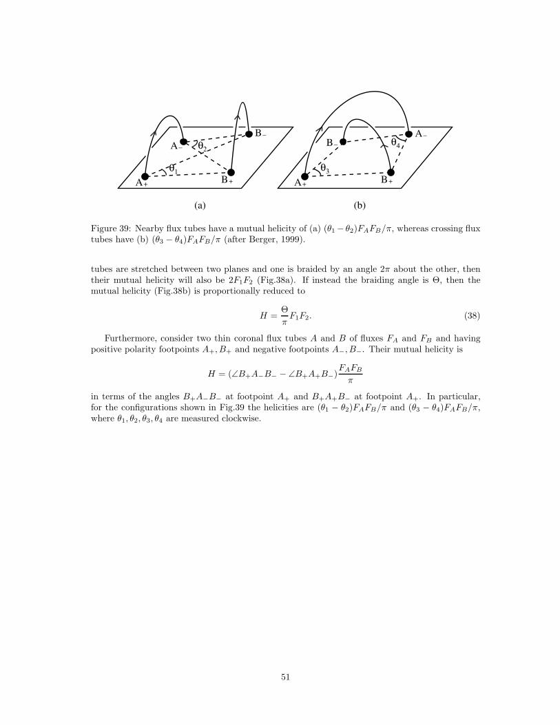
θ2

θ1

(a)

A –

A +B +

B –

(b)

θ4

θ3

B –

A +B +

A –

Figure 39: Nearby flux tubes have a mutual helicity of (a) (θ1 − θ2)FAFB/π, whereas crossing fluxtubes have (b) (θ3 − θ4)FAFB/π (after Berger, 1999).

tubes are stretched between two planes and one is braided by an angle 2π about the other, thentheir mutual helicity will also be 2F1F2 (Fig.38a). If instead the braiding angle is Θ, then themutual helicity (Fig.38b) is proportionally reduced to

H =Θ

πF1F2. (38)

Furthermore, consider two thin coronal flux tubes A and B of fluxes FA and FB and havingpositive polarity footpoints A+, B+ and negative footpoints A−, B−. Their mutual helicity is

H = (∠B+A−B− − ∠B+A+B−)FAFB

π

in terms of the angles B+A−B− at footpoint A+ and B+A+B− at footpoint A+. In particular,for the configurations shown in Fig.39 the helicities are (θ1 − θ2)FAFB/π and (θ3 − θ4)FAFB/π,where θ1, θ2, θ3, θ4 are measured clockwise.

51

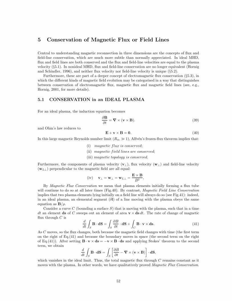
5 Conservation of Magnetic Flux or Field Lines

Central to understanding magnetic reconnection in three dimensions are the concepts of flux andfield-line conservation, which are much more subtle than normally appreciated. In ideal MHD,flux and field lines are both conserved and the flux and field-line velocities are equal to the plasmavelocity (§5.1). In nonideal MHD, flux and field-line conservation are no longer equivalent (Hornigand Schindler, 1996), and neither flux velocity nor field-line velocity is unique (§5.2).

Furthermore, these are part of a deeper concept of electromagnetic flux conservation (§5.3), inwhich the different kinds of magnetic field evolution may be categorised in a way that distinguishesbetween conservation of electromagnetic flux, magnetic flux and magnetic field lines (see, e.g.,Hornig, 2001, for more details).

5.1 CONSERVATION in an IDEAL PLASMA

For an ideal plasma, the induction equation becomes

∂B

∂t= ∇ × (v × B). (39)

and Ohm’s law reduces toE + v × B = 0. (40)

In this large magnetic Reynolds number limit (Rm ≫ 1), Alfven’s frozen-flux theorem implies that:

(i) magnetic f lux is conserved;

(ii) magnetic field lines are conserved;

(iii) magnetic topology is conserved.

Furthermore, the components of plasma velocity (v⊥), flux velocity (w⊥) and field-line velocity(wL⊥) perpendicular to the magnetic field are all equal:

(iv) v⊥ = w⊥ = wL⊥ =E× B

B2,

By Magnetic Flux Conservation we mean that plasma elements initially forming a flux tubewill continue to do so at all later times (Fig.40). By contrast, Magnetic Field Line Conservationimplies that two plasma elements lying initially on a field line will always do so (see Fig.41): indeed,in an ideal plasma, an elemental segment (δl) of a line moving with the plasma obeys the sameequation as B/ρ.

Consider a curve C (bounding a surface S) that is moving with the plasma, such that in a timedt an element ds of C sweeps out an element of area v × ds dt. The rate of change of magneticflux through C is

d

dt

∫

S

B · dS =

∫

S

∂B

∂t· dS +

∫

C

B · v × ds. (41)

As C moves, so the flux changes, both because the magnetic field changes with time (the first termon the right of Eq.(41) and because the boundary moves in space (the second term on the rightof Eq.(41)). After setting B · v × ds = −v × B · ds and applying Stokes’ theorem to the secondterm, we obtain

d

dt

∫

S

B · dS =

∫

S

[∂B

∂t− ∇ × (v × B)

]

· dS,

which vanishes in the ideal limit. Thus, the total magnetic flux through C remains constant as itmoves with the plasma. In other words, we have qualitatively proved Magnetic Flux Conservation.

52

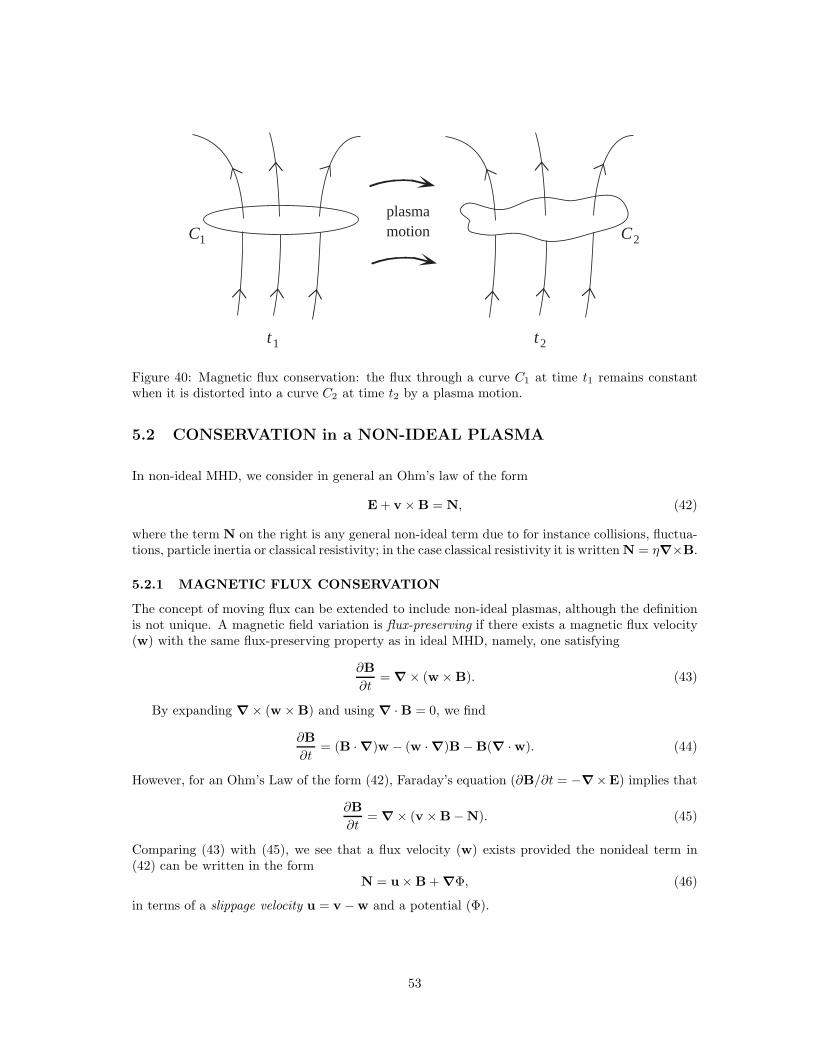
plasmamotion

t1 t2

C1 C2

Figure 40: Magnetic flux conservation: the flux through a curve C1 at time t1 remains constantwhen it is distorted into a curve C2 at time t2 by a plasma motion.

5.2 CONSERVATION in a NON-IDEAL PLASMA

In non-ideal MHD, we consider in general an Ohm’s law of the form

E + v × B = N, (42)

where the term N on the right is any general non-ideal term due to for instance collisions, fluctua-tions, particle inertia or classical resistivity; in the case classical resistivity it is written N = η∇×B.

5.2.1 MAGNETIC FLUX CONSERVATION

The concept of moving flux can be extended to include non-ideal plasmas, although the definitionis not unique. A magnetic field variation is flux-preserving if there exists a magnetic flux velocity(w) with the same flux-preserving property as in ideal MHD, namely, one satisfying

∂B

∂t= ∇ × (w × B). (43)

By expanding ∇ × (w × B) and using ∇ · B = 0, we find

∂B

∂t= (B · ∇)w − (w · ∇)B− B(∇ · w). (44)

However, for an Ohm’s Law of the form (42), Faraday’s equation (∂B/∂t = −∇×E) implies that

∂B

∂t= ∇ × (v × B− N). (45)

Comparing (43) with (45), we see that a flux velocity (w) exists provided the nonideal term in(42) can be written in the form

N = u× B + ∇Φ, (46)

in terms of a slippage velocity u = v − w and a potential (Φ).

53

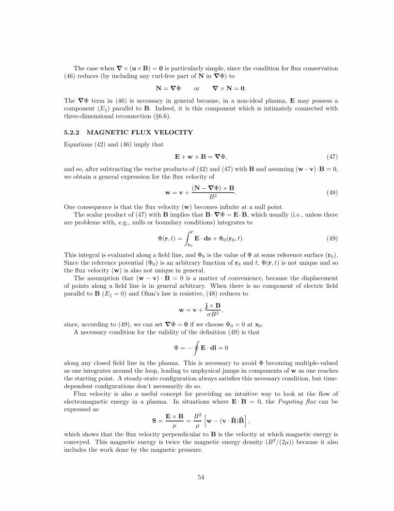
The case when ∇× (u×B) = 0 is particularly simple, since the condition for flux conservation(46) reduces (by including any curl-free part of N in ∇Φ) to

N = ∇Φ or ∇ × N = 0.

The ∇Φ term in (46) is necessary in general because, in a non-ideal plasma, E may possess acomponent (E‖) parallel to B. Indeed, it is this component which is intimately connected withthree-dimensional reconnection (§6.6).

5.2.2 MAGNETIC FLUX VELOCITY

Equations (42) and (46) imply that

E + w × B = ∇Φ, (47)

and so, after subtracting the vector products of (42) and (47) with B and assuming (w−v) ·B = 0,we obtain a general expression for the flux velocity of

w = v +(N − ∇Φ) × B

B2. (48)

One consequence is that the flux velocity (w) becomes infinite at a null point.The scalar product of (47) with B implies that B ·∇Φ = E ·B, which usually (i.e., unless there

are problems with, e.g., nulls or boundary conditions) integrates to

Φ(r, t) =

∫r

r0

E · ds + Φ0(r0, t). (49)

This integral is evaluated along a field line, and Φ0 is the value of Φ at some reference surface (r0).Since the reference potential (Φ0) is an arbitrary function of r0 and t, Φ(r, t) is not unique and sothe flux velocity (w) is also not unique in general.

The assumption that (w − v) · B = 0 is a matter of convenience, because the displacementof points along a field line is in general arbitrary. When there is no component of electric fieldparallel to B (E‖ = 0) and Ohm’s law is resistive, (48) reduces to

w = v +j× B

σB2,

since, according to (49), we can set ∇Φ = 0 if we choose Φ0 = 0 at x0.A necessary condition for the validity of the definition (49) is that

Φ = −∮

E · dl = 0

along any closed field line in the plasma. This is necessary to avoid Φ becoming multiple-valuedas one integrates around the loop, leading to unphysical jumps in components of w as one reachesthe starting point. A steady-state configuration always satisfies this necessary condition, but time-dependent configurations don’t necessarily do so.

Flux velocity is also a useful concept for providing an intuitive way to look at the flow ofelectromagnetic energy in a plasma. In situations where E ·B = 0, the Poynting flux can beexpressed as

S =E× B

µ=B2

µ

[

w − (v · B)B]

,

which shows that the flux velocity perpendicular to B is the velocity at which magnetic energy isconveyed. This magnetic energy is twice the magnetic energy density (B2/(2µ)) because it alsoincludes the work done by the magnetic pressure.

54

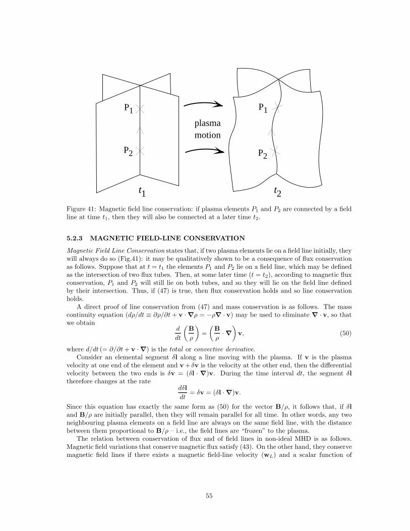
P1

P2

plasmamotion

P1

P2

t1 t2

Figure 41: Magnetic field line conservation: if plasma elements P1 and P2 are connected by a fieldline at time t1, then they will also be connected at a later time t2.

5.2.3 MAGNETIC FIELD-LINE CONSERVATION

Magnetic Field Line Conservation states that, if two plasma elements lie on a field line initially, theywill always do so (Fig.41): it may be qualitatively shown to be a consequence of flux conservationas follows. Suppose that at t = t1 the elements P1 and P2 lie on a field line, which may be definedas the intersection of two flux tubes. Then, at some later time (t = t2), according to magnetic fluxconservation, P1 and P2 will still lie on both tubes, and so they will lie on the field line definedby their intersection. Thus, if (47) is true, then flux conservation holds and so line conservationholds.

A direct proof of line conservation from (47) and mass conservation is as follows. The masscontinuity equation (dρ/dt ≡ ∂ρ/∂t+ v · ∇ρ = −ρ∇ · v) may be used to eliminate ∇ · v, so thatwe obtain

d

dt

(B

ρ

)

=

(B

ρ· ∇)

v, (50)

where d/dt (= ∂/∂t+ v · ∇) is the total or convective derivative.Consider an elemental segment δl along a line moving with the plasma. If v is the plasma

velocity at one end of the element and v + δv is the velocity at the other end, then the differentialvelocity between the two ends is δv = (δl · ∇)v. During the time interval dt, the segment δltherefore changes at the rate

dδl

dt= δv = (δl · ∇)v.

Since this equation has exactly the same form as (50) for the vector B/ρ, it follows that, if δland B/ρ are initially parallel, then they will remain parallel for all time. In other words, any twoneighbouring plasma elements on a field line are always on the same field line, with the distancebetween them proportional to B/ρ – i.e., the field lines are “frozen” to the plasma.

The relation between conservation of flux and of field lines in non-ideal MHD is as follows.Magnetic field variations that conserve magnetic flux satisfy (43). On the other hand, they conservemagnetic field lines if there exists a magnetic field-line velocity (wL) and a scalar function of

55

position λ that satisfy∂B

∂t= ∇ × (wL×B) + λLB, (51)

or, by expanding ∇ × (wL × B), putting λ = λL + ∇ · wL and using ∇ ·B = 0,

∂B

∂t+ (wL ·∇)B− (B·∇)wL = λB.

Now, if we simply pick the particular case where λL = 0 and wL = w, the equation for fieldline conservation (51) becomes the same as that for flux conservation (43). In other words, we haveproved that, whenever flux is conserved (such as in ideal MHD), field lines are also conserved.

It is important to note, however, that the reverse is not true (i.e., field line conservation doesnot necessarily imply flux conservation), since there are many solutions for a non-ideal plasma thatconserve field lines but don’t conserve flux (i.e., all those for which λL 6= 0).

5.2.4 MAGNETIC FIELD-LINE VELOCITY

In an ideal plasma we may define the perpendicular component of magnetic field line or flux velocity(wL⊥ = w⊥ = v⊥) satisfying (40) as E×B/B2. However, in a non-ideal plasma there is no uniquedefinition of field-line velocity. This result is particularly simple in 2D but it also holds in 3D.

The component (wL⊥) of a field-line velocity may be defined if and only if Ohm’s Law can betransformed into the form

E + wL×B = a, (52)

where ∇ × a = −λLB and λL is some scalar function, since the curl of (52) and Faraday’s lawthen imply (51). This definition is field-line preserving but is only flux preserving when λL = 0 sothat ∇ × a = 0 and a = ∇Φ.

The case when ∇ × (wL × B) = ∇ × (v × B) is particularly simple, since a comparison ofthe curls of (52) and (42) then implies that ∇ × a = ∇ × N and so the condition for field-lineconservation becomes

∇ × N = −λLB or B× (∇ × N) = 0.

From Eq.(52) we can deduce the expression

wL⊥ =(E− a) × B

B2

for the field-line velocity. However, this is not unique, since, if we replace a by a′ = a + ∇Ψ∗,where (B · ∇)Ψ∗ = 0, then the magnetic field is unaltered and B·(52) is unchanged, whereas B×(52) gives another flow

w′L⊥ =

(E − a′) × B

B2

in which the magnetic field lines are frozen. The form (52) is always possible for ideal flow (whenwL⊥ = E× B/B2), but it is also always possible when E · B = 0.

5.3 MORE GENERAL CONSERVATION LAWS

When the magnetic Reynolds number is infinite (i.e., in an ideal medium) Eq. (39) holds andAlfven’s theorem implies the constancy of magnetic flux through a surface (S) moving with theplasma (

∫

S(t)B · dS = constant), as well as conservation of field lines, null points, knots and

linkages of field lines.

56

However, magnetic flux conservation is part of a much deeper theory of topological integralconservation laws (Hornig, 2001). Thus, for a fluid with a velocity field v(x, t), the transport of afield (ωk) by the flow of v is given by

∂ωk

∂t+ Lvω

k = 0,

where Lv is the Lie-derivative. Then the Lie-derivative theorem implies conservation of an integralover a k-dimensional comoving volume Ck, namely,

∫

F (Ck)

ωk = const.

This powerful result may be used to clarify at a basic level the relation between field-line and fluxconservation and to show that magnetic flux conservation is part of a more general concept ofelectromagnetic flux conservation, as follows.

The notions of magnetic field lines and flux tubes and their transport with a plasma anddiffusion through it are fundamental. Most of the Sun can be regarded for many purposes as amagnetically ideal medium, so that the magnetic field is frozen to the plasma. It moves with theplasma and, in a magnetically dominated region such as the solar corona, energy changes directlyonly between magnetic and kinetic forms (although the kinetic energy may in turn be dissipatedby, for example, viscous effects). However, localised regions of nonideal behaviour exist, wheremagnetic fields may diffuse through the plasma and often reconnect. In such diffusion regions, thenotions of conservation and transport of magnetic flux tubes invariably break down, but can bereplaced by a more general concept of Electromagnetic Flux Conservation.

When the plasma is nonideal, there are several classes of evolution of a magnetic field B(r, t)and electric field E(r, t), as illustrated schematically in Fig.3. All types of evolution are assumedto satisfy ∇ · B and to obey Faraday’s law

∂B

∂t= −∇ × E.

The largest subclass within all such solutions is the family that also conserves electromagnetic flux

∫

S

B·dS +

∫

S

E·dl dt = const. (53)

A smaller family of solutions lying within this consists of those that conserve magnetic flux byitself ∫

S

B · dS = const. (54)

As far as magnetic reconnection is concerned, the solutions that represent 3D reconnection area particular class of electromagnetic-flux preserving solutions. Furthermore, as can be seen fromFig.3, 2D reconnection represents the particular class of 3D solutions that is also magnetic-fluxpreserving.

57

6 The Nature of Reconnection in Three Dimensions

Before understanding magnetic reconnection in three dimensions, we need to appreciate someof the subtleties about the differences between diffusion and reconnection. In so doing, we shallappreciate that in many respects three-dimensional reconnection is very different indeed from theconcept of two-dimensional reconnection that has dominated the thinking of many of us for decades.

We first determine how the nature of the nonideal term in Ohm’s law determines whether therewill be simple slippage of field lines or 2D reconnection or 3D reconnection. In 2D reconnection theconcept of a flux velocity is useful. In 3D reconnection it fails but can be replaced by a so-calleddual flux velocity (§6.4.4, §6.5). Aso we summarise the differences between 2D and 3D reconnectionand comment on the way reconnection can be defined and classified as a prelude to describing thedifferent 3D regimes (§11).

6.1 FORM of the NON-IDEAL TERM for RECONNECTION

Consider a non-ideal plasma with a general Ohm’s Law of the form

E + v × B = N. (55)

Whether or not reconnection occurs depends on the nature of the non-ideal term N.First of all, from (46) if N can be written in the form

N = u× B + ∇Φ,

then the curl of (55) becomes ∂B/∂t = ∇ × (w ×B), where w = v − u is a flux velocity and u isthe slippage velocity. Thus, by analogy with (39), the magnetic field behaves as if it moves with avelocity w and we can deduce that:

(a) if u is smooth, then there is slippage of magnetic field but no reconnection;

(b) if u is singular, then there is 2D reconnection;

(c) if N 6= u× B + ∇Φ, then there is reconnection in 2.5D or 3D.

Furthermore, an implication of Eq.(55) is that E ·B = N ·B, so that the components of E and Nparallel to the magnetic field are the same.

6.2 TWO-DIMENSIONAL RECONNECTION (E . B =0)

Suppose that E · B = 0, for which Eq. (55) implies that N · B = 0, so that both E and N areperpendicular to B. Then, provided E and B are not both zero, they are locally two-dimensional.For example, if v and B are confined to a plane and depend only on coordinates in that plane,then E and N are normal to that plane.

Since N · B = 0, we may set ∇Φ ≡ 0 in (46), so that (47) becomes

E + w × B = 0.

Thus, the diffusion velocity is u = (B×N)/B2 and a flux-preserving flow w⊥ = E×B/B2 exists,which is smooth except where B = 0 (assuming N 6= 0).

Furthermore, there are three possible types of behaviour:

58

(a) If B 6= 0, then w is smooth everywhere and we have slippage of the magnetic field, which isflux-conserving in a strong sense;

(b) If B = 0 at some point and the neighbouring magnetic field is elliptic, then w has a divergentsingularity and is magnetic flux is destroyed or generated at the null point;

(b) If B = 0 at some point and the neighbouring magnetic field is hyperbolic, then w has ahyperbolic singularity and there is magnetic flux reconnection, with the flux conserved in theweak sense that w is regular except at one point.

6.3 NON-EXISTENCE of FLUX VELOCITY in 3D

The concept of a flux velocity, which has been central to ideas of 2D reconnection, fails in threedimensions (when E · B 6= 0), as expressed by the Flux Velocity Theorem: for an isolated 3Dnonideal region, a flux conservation velocity (w) does not in general exist (Priest et al., 2003).

Proof: If a flux velocity does exist, then Eq.(43) holds and a function Φ exists such that

E + w × B = ∇Φ,

which implies that E · B = ∇Φ · B. If this is integrated along a magnetic field line from a point(r1) on one side of the diffusion region to a point (r2) on the other side, then

∫r2

r1

E‖ds = Φ(r2) − Φ(r1).

If we assume that E‖ is, say, positive in the diffusion region, then Φ(r2) > Φ(r1). However, sincethe diffusion region is isolated and everywhere outside it w = v and ∇Φ = 0, we conclude thatF is uniform outside the diffusion region and so Φ(r2) = Φ(r1). This contradiction implies that aflux velocity does not exist and the theorem is proved.

6.4 MAGNETIC DIFFUSION and FIELD-LINE MOTION

A series of examples of diffusion of a magnetic field through a plasma in one-, two- and three-dimension have been studied by Wilmot-Smith et al. (2005). Diffusion can often be described interms of a magnetic flux velocity, but this is in general non-unique, so that the field evolution canbe described as if the field lines are moving in one of several physically useful ways. For instance,one possibility is to define the flux velocity in terms of the energy flow and another is in such away that it vanishes in a steady state.

Straight magnetic field lines (or plane magnetic flux surfaces) diffuse in current sheets and themagnetic field behaves as if the flux is disappearing at a neutral sheet and/or infinity. For a finiteregion of nonzero diffusivity, the magnetic field diffuses away to a uniform field in the region insuch a way that the flux there remains constant while current sheets of steep magnetic gradientare formed at the ends of the region.

Circular magnetic field lines (or cylindrical flux surfaces) diffuse in a very similar way. Thefield behaves as if the magnetic flux is moving either towards the O-type neutral line or towardsinfinity or both and vanishing there. In particular, an isolated tube of radius a is found to have aflux that decays exponentially over a time-scale a2/(4η).

59

In three dimensions magnetic field lines can always be defined at any instant of time, but thedecay of a field cannot always be described in terms of the motion of field lines from one time toanother, since it is not always possible to define a flux velocity: for example, when the magneticflux through a closed field line is changing in time. Nevertheless, in at least some such cases, it ispossible to describe the magnetic field behaviour in terms of a dual flux velocity (§6.4.4, §6.5). Asummary of the details is as follows (Wilmot-Smith et al., 2005).

6.4.1 INTRODUCTION

Understanding the fundamental processes of advection and diffusion of magnetic field is a key partof describing the behaviour of magnetic fields in magnetohydrodynamics. Wilmot-Smith et al.(2005) focussed on the nature of pure resistive diffusion of magnetic field in the absence of aplasma flow, which is a more primitive problem than the nature of reconnection, but it is notyet fully understood. Their aim was partly to understand how diffusion occurs and magnetic fluxdisappears in a variety of situations, and partly to see whether the concept of the motion of fieldlines, which has proved so useful in an ideal medium, may also be employed in a diffusive medium.

In this case the induction equation reduces to

∂B

∂t= ∇ × (η∇ × B), (56)

or, when the magnetic diffusivity (η) is uniform in space,

∂B

∂t= η∇2B.

In such a diffusive medium, if a magnetic flux velocity (or flux transporting velocity) (w) existsfor a given magnetic field variation, it satisfies

∂B

∂t= ∇ × (w × B),

which impliesE + w × B = ∇F, (57)

where F is an arbitrary function of integration.By comparison, an arbitrary Ohm’s law

E + v × B = N, (58)

contains an arbitrary non-ideal term (N) that is not necessarily just the gradient of a scalar, sothat ideal flux transport does not necessarily hold. For a flux transporting velocity to exist, wehave to be able to write Eq.(58) in the form (57) so that N has the structure

N = (v − w)︸ ︷︷ ︸

:=u

×B + ∇F.

Provided B 6= 0, a sufficient condition for this to hold and thus for the existence of a diffusionvelocity (u) or flux velocity (w) is that

B · ∇F = B ·N ≡ B · E.

This equation can always be solved if E · B = 0 or if N represents a Hall term ((ne)−1 j × B) or,for our purposes here, in the case of two-dimensional diffusion (N = ηj).

60

When F does exist, we can solve Eq.(57) for the normal component of w to give

w⊥ =(E − ∇F ) × B

B2. (59)

Thus, w⊥ is a flux transporting velocity, with respect to which the flux and field line topologyare conserved, with u being a slippage velocity of plasma relative to magnetic field lines. At nullpoints of B the flux transport velocity might become singular, indicating either reconnection or aloss or generation of magnetic flux.

However, even the perpendicular component of w is in general not unique due to the non-uniqueness of F (Hornig and Schindler, 1996; Hornig, 2001), which is determined only up to anarbitrary function (an initial condition for F on a transversal surface which field lines cross once).Uniqueness can be achieved by specifying corresponding boundary or initial conditions for w.

For the pure resistive diffusion considered by Wilmot-Smith et al. (2005), E = η∇ × B, andso, provided w exists, (57) becomes

η∇ × B + w × B = ∇F , (60)

while (59) reduces to

w⊥ =(η∇ × B− ∇F ) × B

B2.

6.4.2 DIFFUSION of MAGNETIC FIELD with STRAIGHT FIELD LINES

Let us consider first the diffusion of a one-dimensional magnetic field (B = B(x, t)y) in a finiteregion, for which we shall find that magnetic field lines can disappear either at a neutral sheet orat the boundary. The diffusion equation (56) reduces to

∂B

∂t=

∂

∂x

(

η∂B

∂x

)

,

or, when the diffusivity is uniform (η = η0)

∂B

∂t= η0

∂2B

∂x2.

(For the case of nonuniform diffusivity or an infinite region, see Wilmot-Smith et al. (2005).)Consider a magnetic field that is held fixed at two points (±ℓ) with B(ℓ, t) = −B(−ℓ, t) = B0,

and that initially has a step profile

B(x, 0) =

{+B0 , x > 0,−B0 , x < 0,

representing an infinitesimally thin current sheet. The solution to the diffusion equation is

B(x, t) = B0x

ℓ+

2B0

π

∞∑

n=1

1

nexp

(−n2π2η0t/ℓ

2)sin(nπx

ℓ

)

.

Figure 42 shows that the magnetic field diffuses away very rapidly towards the steady-statesolution, namely, B(x) = B0x/ℓ. Indeed, after a time of only t = ℓ2/η0, the field is within a factor10−4 of its final profile.

In terms of energy, what is happening is that a decrease in magnetic energy is accounted forby Ohmic heating (j2/σ) and an outwards Poynting flux E × B/µ = −(η/µ)∂B/∂x x into the

61

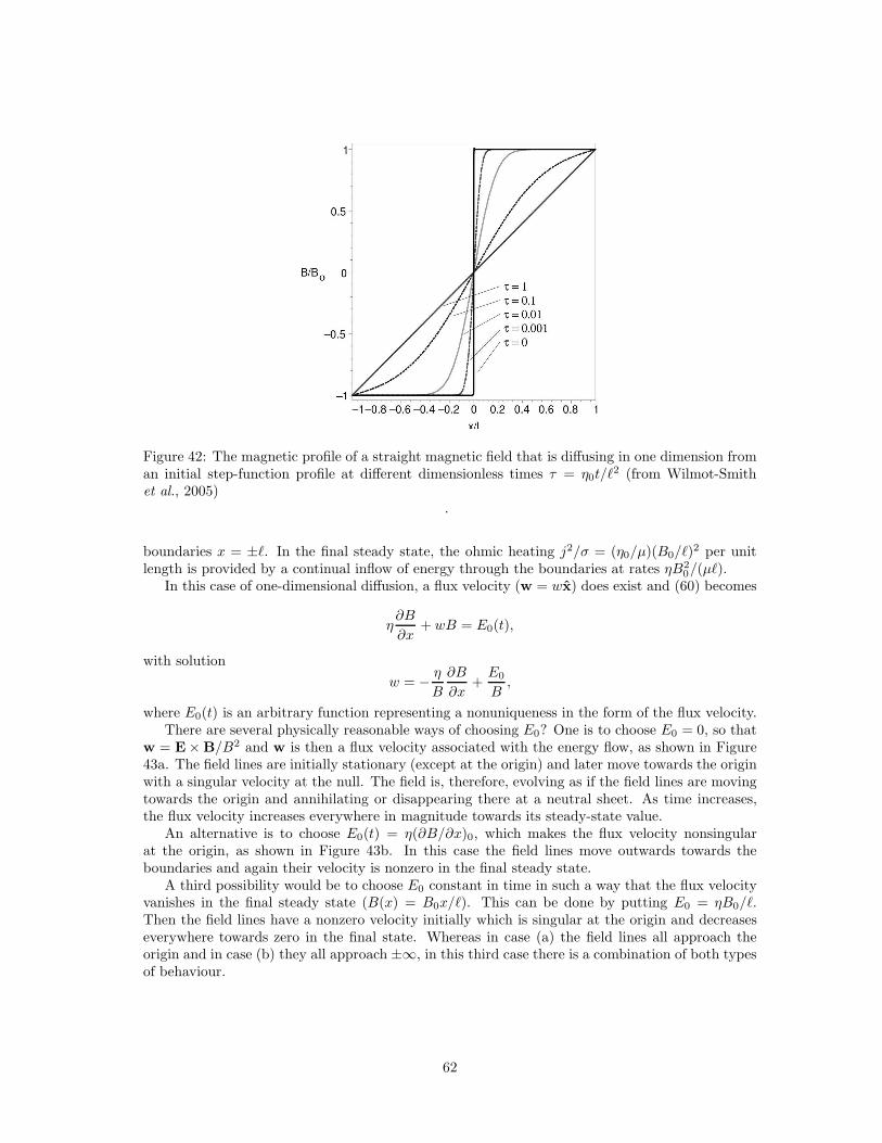
Figure 42: The magnetic profile of a straight magnetic field that is diffusing in one dimension froman initial step-function profile at different dimensionless times τ = η0t/ℓ

2 (from Wilmot-Smithet al., 2005)

.

boundaries x = ±ℓ. In the final steady state, the ohmic heating j2/σ = (η0/µ)(B0/ℓ)2 per unit

length is provided by a continual inflow of energy through the boundaries at rates ηB20/(µℓ).

In this case of one-dimensional diffusion, a flux velocity (w = wx) does exist and (60) becomes

η∂B

∂x+ wB = E0(t),

with solution

w = − η

B

∂B

∂x+E0

B,

where E0(t) is an arbitrary function representing a nonuniqueness in the form of the flux velocity.There are several physically reasonable ways of choosing E0? One is to choose E0 = 0, so that

w = E× B/B2 and w is then a flux velocity associated with the energy flow, as shown in Figure43a. The field lines are initially stationary (except at the origin) and later move towards the originwith a singular velocity at the null. The field is, therefore, evolving as if the field lines are movingtowards the origin and annihilating or disappearing there at a neutral sheet. As time increases,the flux velocity increases everywhere in magnitude towards its steady-state value.

An alternative is to choose E0(t) = η(∂B/∂x)0, which makes the flux velocity nonsingularat the origin, as shown in Figure 43b. In this case the field lines move outwards towards theboundaries and again their velocity is nonzero in the final steady state.

A third possibility would be to choose E0 constant in time in such a way that the flux velocityvanishes in the final steady state (B(x) = B0x/ℓ). This can be done by putting E0 = ηB0/ℓ.Then the field lines have a nonzero velocity initially which is singular at the origin and decreaseseverywhere towards zero in the final state. Whereas in case (a) the field lines all approach theorigin and in case (b) they all approach ±∞, in this third case there is a combination of both typesof behaviour.

62

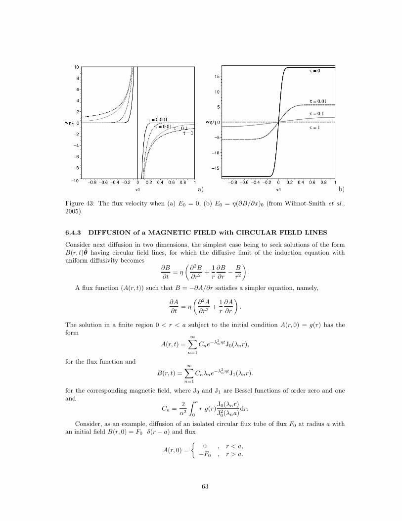
a) b)

Figure 43: The flux velocity when (a) E0 = 0, (b) E0 = η(∂B/∂x)0 (from Wilmot-Smith et al.,2005).

6.4.3 DIFFUSION of a MAGNETIC FIELD with CIRCULAR FIELD LINES

Consider next diffusion in two dimensions, the simplest case being to seek solutions of the formB(r, t)θ having circular field lines, for which the diffusive limit of the induction equation withuniform diffusivity becomes

∂B

∂t= η

(∂2B

∂r2+

1

r

∂B

∂r− B

r2

)

.

A flux function (A(r, t)) such that B = −∂A/∂r satisfies a simpler equation, namely,

∂A

∂t= η

(∂2A

∂r2+

1

r

∂A

∂r

)

.

The solution in a finite region 0 < r < a subject to the initial condition A(r, 0) = g(r) has theform

A(r, t) =

∞∑

n=1

Cne−λ2

nηtJ0(λnr),

for the flux function and

B(r, t) =∞∑

n=1

Cnλne−λ2

nηtJ1(λnr).

for the corresponding magnetic field, where J0 and J1 are Bessel functions of order zero and oneand

Cn =2

α2

∫ a

0

r g(r)J0(λnr)

J20(λna)

dr.

Consider, as an example, diffusion of an isolated circular flux tube of flux F0 at radius a withan initial field B(r, 0) = F0 δ(r − a) and flux

A(r, 0) =

{0 , r < a,

−F0 , r > a.

63

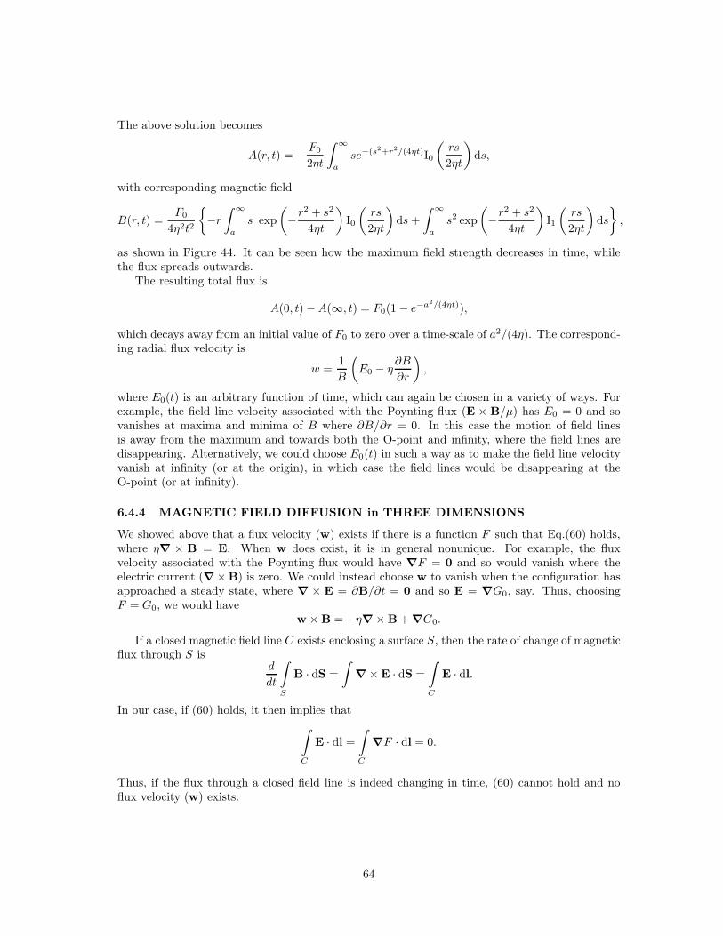
The above solution becomes

A(r, t) = − F0

2ηt

∫ ∞

a

se−(s2+r2/(4ηt)I0

(rs

2ηt

)

ds,

with corresponding magnetic field

B(r, t) =F0

4η2t2

{

−r∫ ∞

a

s exp

(

−r2 + s2

4ηt

)

I0

(rs

2ηt

)

ds+

∫ ∞

a

s2 exp

(

−r2 + s2

4ηt

)

I1

(rs

2ηt

)

ds

}

,

as shown in Figure 44. It can be seen how the maximum field strength decreases in time, whilethe flux spreads outwards.

The resulting total flux is

A(0, t) −A(∞, t) = F0(1 − e−a2/(4ηt)),

which decays away from an initial value of F0 to zero over a time-scale of a2/(4η). The correspond-ing radial flux velocity is

w =1

B

(

E0 − η∂B

∂r

)

,

where E0(t) is an arbitrary function of time, which can again be chosen in a variety of ways. Forexample, the field line velocity associated with the Poynting flux (E × B/µ) has E0 = 0 and sovanishes at maxima and minima of B where ∂B/∂r = 0. In this case the motion of field linesis away from the maximum and towards both the O-point and infinity, where the field lines aredisappearing. Alternatively, we could choose E0(t) in such a way as to make the field line velocityvanish at infinity (or at the origin), in which case the field lines would be disappearing at theO-point (or at infinity).

6.4.4 MAGNETIC FIELD DIFFUSION in THREE DIMENSIONS

We showed above that a flux velocity (w) exists if there is a function F such that Eq.(60) holds,where η∇ × B = E. When w does exist, it is in general nonunique. For example, the fluxvelocity associated with the Poynting flux would have ∇F = 0 and so would vanish where theelectric current (∇×B) is zero. We could instead choose w to vanish when the configuration hasapproached a steady state, where ∇ × E = ∂B/∂t = 0 and so E = ∇G0, say. Thus, choosingF = G0, we would have

w × B = −η∇ × B + ∇G0.

If a closed magnetic field line C exists enclosing a surface S, then the rate of change of magneticflux through S is

d

dt

∫

S

B · dS =

∫

∇ × E · dS =

∫

C

E · dl.

In our case, if (60) holds, it then implies that

∫

C

E · dl =

∫

C

∇F · dl = 0.

Thus, if the flux through a closed field line is indeed changing in time, (60) cannot hold and noflux velocity (w) exists.

64

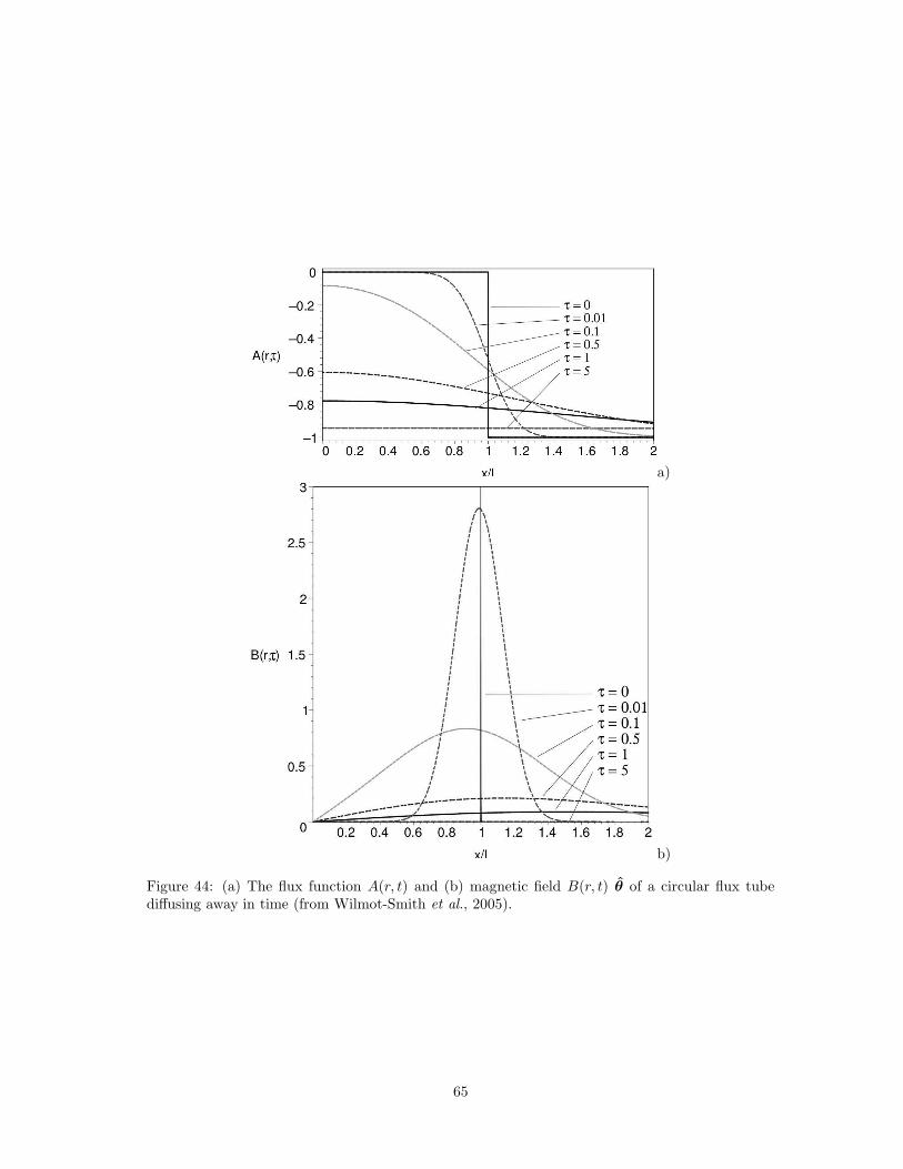
a)

b)

Figure 44: (a) The flux function A(r, t) and (b) magnetic field B(r, t) θ of a circular flux tubediffusing away in time (from Wilmot-Smith et al., 2005).

65

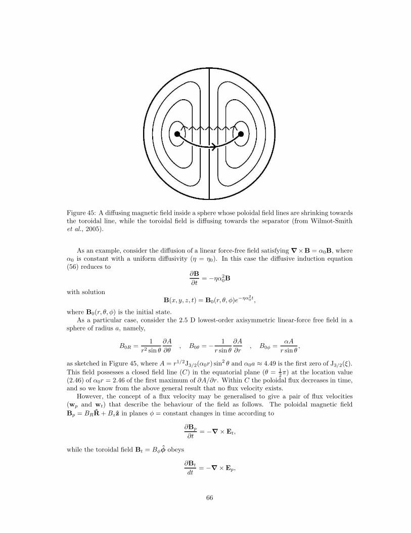
Figure 45: A diffusing magnetic field inside a sphere whose poloidal field lines are shrinking towardsthe toroidal line, while the toroidal field is diffusing towards the separator (from Wilmot-Smithet al., 2005).

As an example, consider the diffusion of a linear force-free field satisfying ∇×B = α0B, whereα0 is constant with a uniform diffusivity (η = η0). In this case the diffusive induction equation(56) reduces to

∂B

∂t= −ηα2

0B

with solutionB(x, y, z, t) = B0(r, θ, φ)e−ηα2

0t,

where B0(r, θ, φ) is the initial state.As a particular case, consider the 2.5 D lowest-order axisymmetric linear-force free field in a

sphere of radius a, namely,

B0R =1

r2 sin θ

∂A

∂θ, B0θ = − 1

r sin θ

∂A

∂r, B0φ =

αA

r sin θ,

as sketched in Figure 45, where A = r1/2J3/2(α0r) sin2 θ and α0a ≈ 4.49 is the first zero of J3/2(ξ).

This field possesses a closed field line (C) in the equatorial plane (θ = 12π) at the location value

(2.46) of α0r = 2.46 of the first maximum of ∂A/∂r. Within C the poloidal flux decreases in time,and so we know from the above general result that no flux velocity exists.

However, the concept of a flux velocity may be generalised to give a pair of flux velocities(wp and wt) that describe the behaviour of the field as follows. The poloidal magnetic field

Bp = BRR +Bzz in planes φ = constant changes in time according to

∂Bp

∂t= −∇ × Et,

while the toroidal field Bt = Bφφ obeys

∂Bt

dt= −∇ × Ep,

66

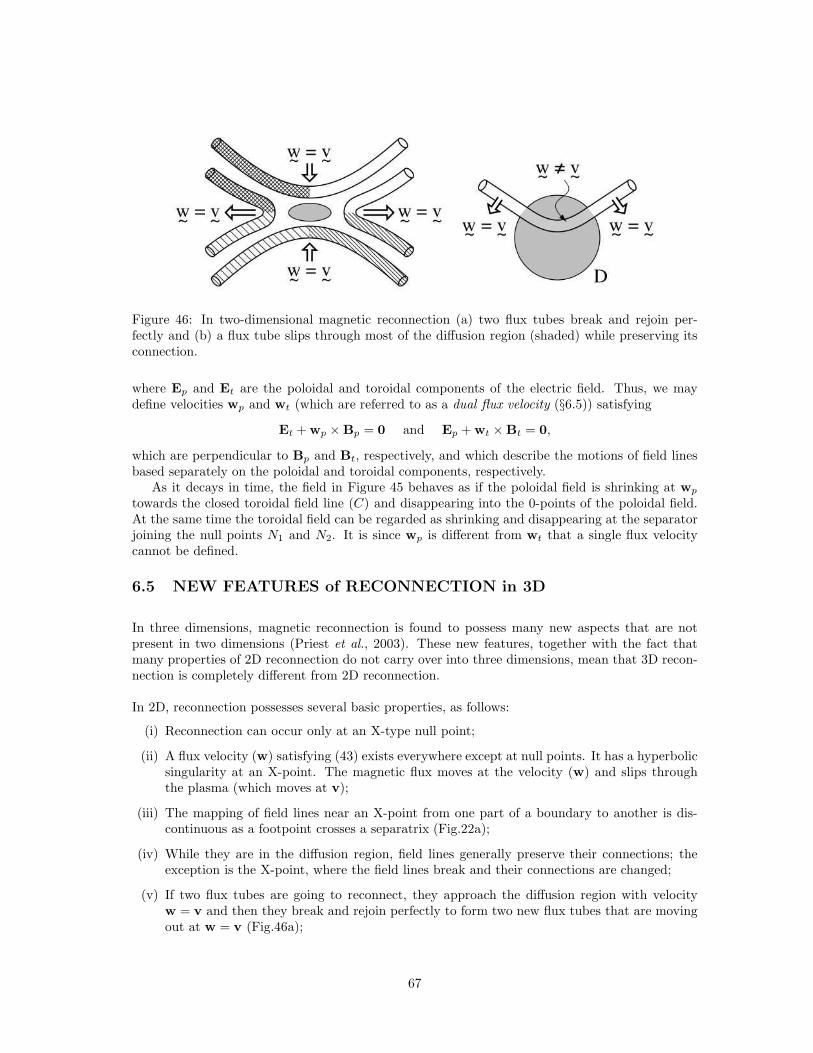
Figure 46: In two-dimensional magnetic reconnection (a) two flux tubes break and rejoin per-fectly and (b) a flux tube slips through most of the diffusion region (shaded) while preserving itsconnection.

where Ep and Et are the poloidal and toroidal components of the electric field. Thus, we maydefine velocities wp and wt (which are referred to as a dual flux velocity (§6.5)) satisfying

Et + wp × Bp = 0 and Ep + wt × Bt = 0,

which are perpendicular to Bp and Bt, respectively, and which describe the motions of field linesbased separately on the poloidal and toroidal components, respectively.

As it decays in time, the field in Figure 45 behaves as if the poloidal field is shrinking at wp

towards the closed toroidal field line (C) and disappearing into the 0-points of the poloidal field.At the same time the toroidal field can be regarded as shrinking and disappearing at the separatorjoining the null points N1 and N2. It is since wp is different from wt that a single flux velocitycannot be defined.

6.5 NEW FEATURES of RECONNECTION in 3D

In three dimensions, magnetic reconnection is found to possess many new aspects that are notpresent in two dimensions (Priest et al., 2003). These new features, together with the fact thatmany properties of 2D reconnection do not carry over into three dimensions, mean that 3D recon-nection is completely different from 2D reconnection.

In 2D, reconnection possesses several basic properties, as follows:

(i) Reconnection can occur only at an X-type null point;

(ii) A flux velocity (w) satisfying (43) exists everywhere except at null points. It has a hyperbolicsingularity at an X-point. The magnetic flux moves at the velocity (w) and slips throughthe plasma (which moves at v);

(iii) The mapping of field lines near an X-point from one part of a boundary to another is dis-continuous as a footpoint crosses a separatrix (Fig.22a);

(iv) While they are in the diffusion region, field lines generally preserve their connections; theexception is the X-point, where the field lines break and their connections are changed;

(v) If two flux tubes are going to reconnect, they approach the diffusion region with velocityw = v and then they break and rejoin perfectly to form two new flux tubes that are movingout at w = v (Fig.46a);

67

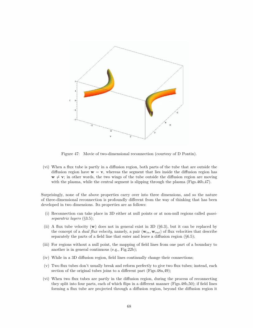
Figure 47: Movie of two-dimensional reconnection (courtesy of D Pontin).

(vi) When a flux tube is partly in a diffusion region, both parts of the tube that are outside thediffusion region have w = v, whereas the segment that lies inside the diffusion region hasw 6= v; in other words, the two wings of the tube outside the diffusion region are movingwith the plasma, while the central segment is slipping through the plasma (Figs.46b,47).

Surprisingly, none of the above properties carry over into three dimensions, and so the natureof three-dimensional reconnection is profoundly different from the way of thinking that has beendeveloped in two dimensions. Its properties are as follows:

(i) Reconnection can take place in 3D either at null points or at non-null regions called quasi-separatrix layers (§3.5);

(ii) A flux tube velocity (w) does not in general exist in 3D (§6.3), but it can be replaced bythe concept of a dual flux velocity, namely, a pair (win,wout) of flux velocities that describeseparately the parts of a field line that enter and leave a diffusion region (§6.5);

(iii) For regions without a null point, the mapping of field lines from one part of a boundary toanother is in general continuous (e.g., Fig.22b);

(iv) While in a 3D diffusion region, field lines continually change their connections;

(v) Two flux tubes don’t usually break and reform perfectly to give two flux tubes; instead, eachsection of the original tubes joins to a different part (Figs.48a,49);

(vi) When two flux tubes are partly in the diffusion region, during the process of reconnectingthey split into four parts, each of which flips in a different manner (Figs.48b,50); if field linesforming a flux tube are projected through a diffusion region, beyond the diffusion region it

68

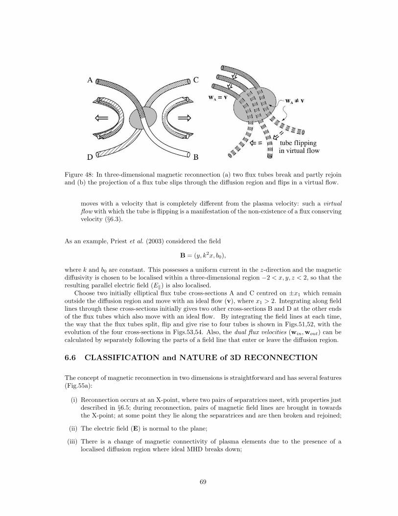
Figure 48: In three-dimensional magnetic reconnection (a) two flux tubes break and partly rejoinand (b) the projection of a flux tube slips through the diffusion region and flips in a virtual flow.

moves with a velocity that is completely different from the plasma velocity: such a virtualflow with which the tube is flipping is a manifestation of the non-existence of a flux conservingvelocity (§6.3).

As an example, Priest et al. (2003) considered the field

B = (y, k2x, b0),

where k and b0 are constant. This possesses a uniform current in the z-direction and the magneticdiffusivity is chosen to be localised within a three-dimensional region −2 < x, y, z < 2, so that theresulting parallel electric field (E‖) is also localised.

Choose two initially elliptical flux tube cross-sections A and C centred on ±x1 which remainoutside the diffusion region and move with an ideal flow (v), where x1 > 2. Integrating along fieldlines through these cross-sections initially gives two other cross-sections B and D at the other endsof the flux tubes which also move with an ideal flow. By integrating the field lines at each time,the way that the flux tubes split, flip and give rise to four tubes is shown in Figs.51,52, with theevolution of the four cross-sections in Figs.53,54. Also, the dual flux velocities (win,wout) can becalculated by separately following the parts of a field line that enter or leave the diffusion region.

6.6 CLASSIFICATION and NATURE of 3D RECONNECTION

The concept of magnetic reconnection in two dimensions is straightforward and has several features(Fig.55a):

(i) Reconnection occurs at an X-point, where two pairs of separatrices meet, with properties justdescribed in §6.5; during reconnection, pairs of magnetic field lines are brought in towardsthe X-point; at some point they lie along the separatrices and are then broken and rejoined;

(ii) The electric field (E) is normal to the plane;

(iii) There is a change of magnetic connectivity of plasma elements due to the presence of alocalised diffusion region where ideal MHD breaks down;

69

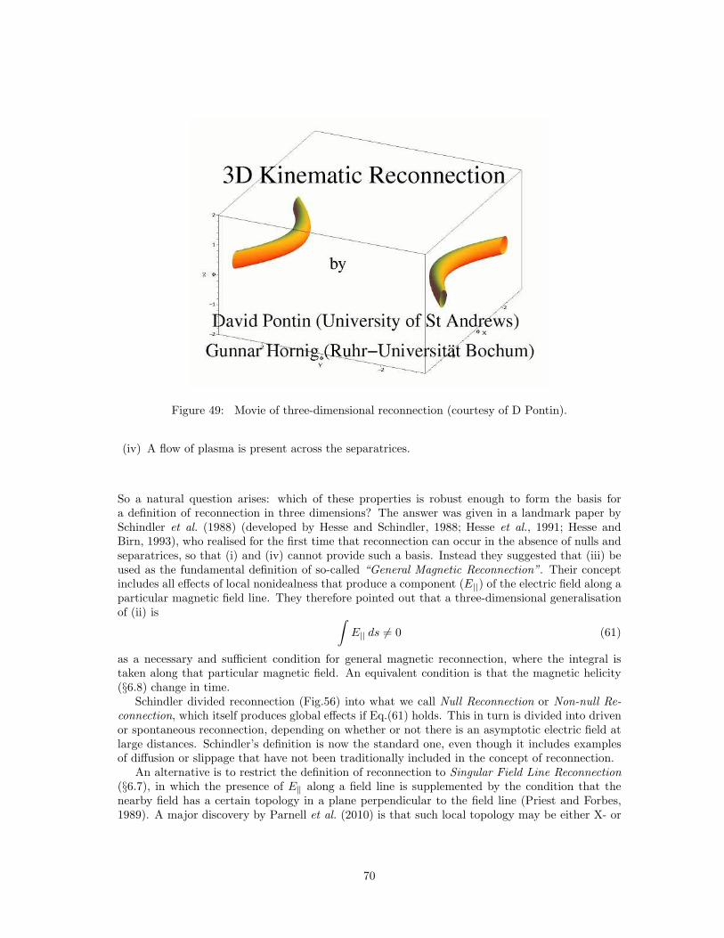
Figure 49: Movie of three-dimensional reconnection (courtesy of D Pontin).

(iv) A flow of plasma is present across the separatrices.

So a natural question arises: which of these properties is robust enough to form the basis fora definition of reconnection in three dimensions? The answer was given in a landmark paper bySchindler et al. (1988) (developed by Hesse and Schindler, 1988; Hesse et al., 1991; Hesse andBirn, 1993), who realised for the first time that reconnection can occur in the absence of nulls andseparatrices, so that (i) and (iv) cannot provide such a basis. Instead they suggested that (iii) beused as the fundamental definition of so-called “General Magnetic Reconnection”. Their conceptincludes all effects of local nonidealness that produce a component (E||) of the electric field along aparticular magnetic field line. They therefore pointed out that a three-dimensional generalisationof (ii) is

∫

E|| ds 6= 0 (61)

as a necessary and sufficient condition for general magnetic reconnection, where the integral istaken along that particular magnetic field. An equivalent condition is that the magnetic helicity(§6.8) change in time.

Schindler divided reconnection (Fig.56) into what we call Null Reconnection or Non-null Re-connection, which itself produces global effects if Eq.(61) holds. This in turn is divided into drivenor spontaneous reconnection, depending on whether or not there is an asymptotic electric field atlarge distances. Schindler’s definition is now the standard one, even though it includes examplesof diffusion or slippage that have not been traditionally included in the concept of reconnection.

An alternative is to restrict the definition of reconnection to Singular Field Line Reconnection(§6.7), in which the presence of E‖ along a field line is supplemented by the condition that thenearby field has a certain topology in a plane perpendicular to the field line (Priest and Forbes,1989). A major discovery by Parnell et al. (2010) is that such local topology may be either X- or

70

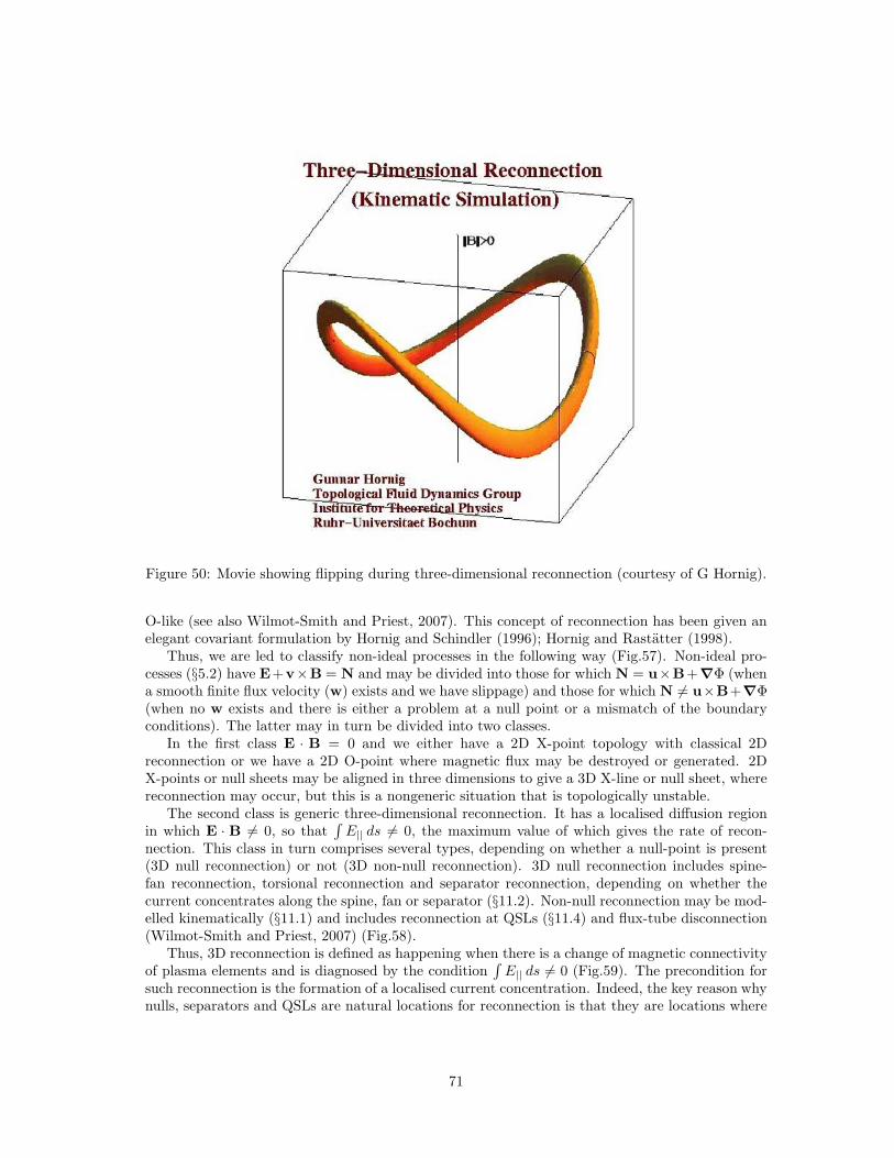
Figure 50: Movie showing flipping during three-dimensional reconnection (courtesy of G Hornig).

O-like (see also Wilmot-Smith and Priest, 2007). This concept of reconnection has been given anelegant covariant formulation by Hornig and Schindler (1996); Hornig and Rastatter (1998).

Thus, we are led to classify non-ideal processes in the following way (Fig.57). Non-ideal pro-cesses (§5.2) have E+v×B = N and may be divided into those for which N = u×B+∇Φ (whena smooth finite flux velocity (w) exists and we have slippage) and those for which N 6= u×B+∇Φ(when no w exists and there is either a problem at a null point or a mismatch of the boundaryconditions). The latter may in turn be divided into two classes.

In the first class E · B = 0 and we either have a 2D X-point topology with classical 2Dreconnection or we have a 2D O-point where magnetic flux may be destroyed or generated. 2DX-points or null sheets may be aligned in three dimensions to give a 3D X-line or null sheet, wherereconnection may occur, but this is a nongeneric situation that is topologically unstable.

The second class is generic three-dimensional reconnection. It has a localised diffusion regionin which E · B 6= 0, so that

∫E|| ds 6= 0, the maximum value of which gives the rate of recon-

nection. This class in turn comprises several types, depending on whether a null-point is present(3D null reconnection) or not (3D non-null reconnection). 3D null reconnection includes spine-fan reconnection, torsional reconnection and separator reconnection, depending on whether thecurrent concentrates along the spine, fan or separator (§11.2). Non-null reconnection may be mod-elled kinematically (§11.1) and includes reconnection at QSLs (§11.4) and flux-tube disconnection(Wilmot-Smith and Priest, 2007) (Fig.58).

Thus, 3D reconnection is defined as happening when there is a change of magnetic connectivityof plasma elements and is diagnosed by the condition

∫E|| ds 6= 0 (Fig.59). The precondition for

such reconnection is the formation of a localised current concentration. Indeed, the key reason whynulls, separators and QSLs are natural locations for reconnection is that they are locations where

71

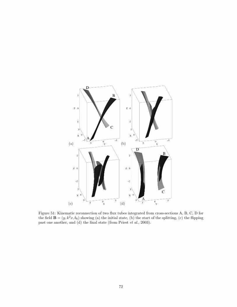
Figure 51: Kinematic reconnection of two flux tubes integrated from cross-sections A, B, C, D forthe field B = (y, k2x, b0) showing (a) the initial state, (b) the start of the splitting, (c) the flippingpast one another, and (d) the final state (from Priest et al., 2003).

72

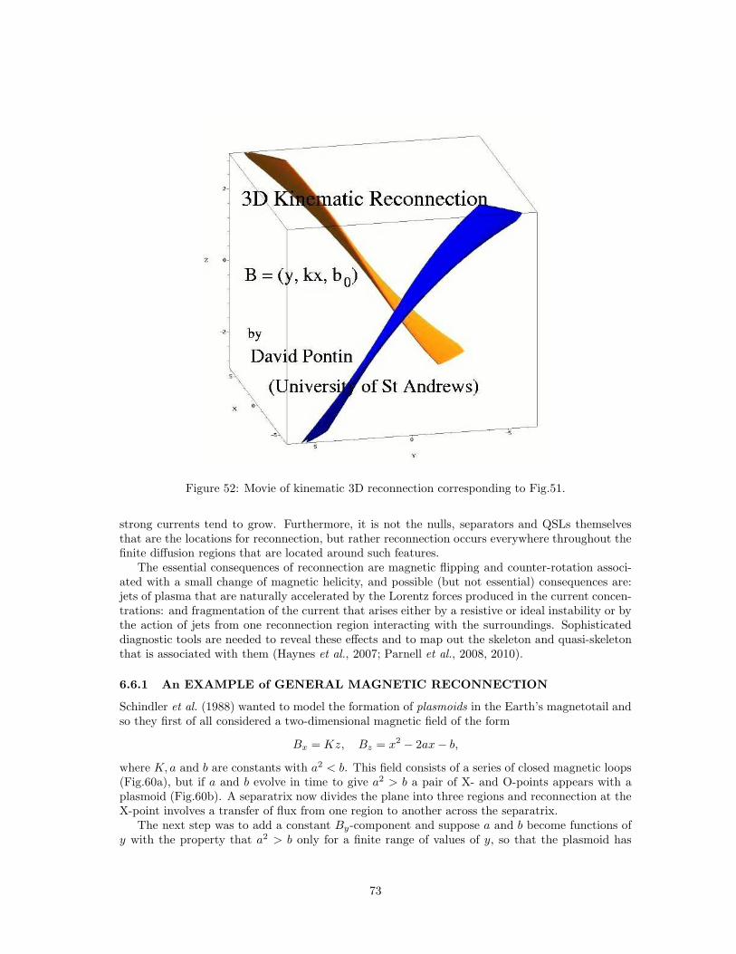
Figure 52: Movie of kinematic 3D reconnection corresponding to Fig.51.

strong currents tend to grow. Furthermore, it is not the nulls, separators and QSLs themselvesthat are the locations for reconnection, but rather reconnection occurs everywhere throughout thefinite diffusion regions that are located around such features.

The essential consequences of reconnection are magnetic flipping and counter-rotation associ-ated with a small change of magnetic helicity, and possible (but not essential) consequences are:jets of plasma that are naturally accelerated by the Lorentz forces produced in the current concen-trations: and fragmentation of the current that arises either by a resistive or ideal instability or bythe action of jets from one reconnection region interacting with the surroundings. Sophisticateddiagnostic tools are needed to reveal these effects and to map out the skeleton and quasi-skeletonthat is associated with them (Haynes et al., 2007; Parnell et al., 2008, 2010).

6.6.1 An EXAMPLE of GENERAL MAGNETIC RECONNECTION

Schindler et al. (1988) wanted to model the formation of plasmoids in the Earth’s magnetotail andso they first of all considered a two-dimensional magnetic field of the form

Bx = Kz, Bz = x2 − 2ax− b,

where K, a and b are constants with a2 < b. This field consists of a series of closed magnetic loops(Fig.60a), but if a and b evolve in time to give a2 > b a pair of X- and O-points appears with aplasmoid (Fig.60b). A separatrix now divides the plane into three regions and reconnection at theX-point involves a transfer of flux from one region to another across the separatrix.

The next step was to add a constant By-component and suppose a and b become functions ofy with the property that a2 > b only for a finite range of values of y, so that the plasmoid has

73

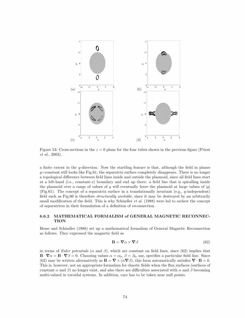
Figure 53: Cross-sections in the z = 0 plane for the four tubes shown in the previous figure (Priestet al., 2003).

a finite extent in the y-direction. Now the startling feature is that, although the field in planesy=constant still looks like Fig.61, the separatrix surface completely disappears. There is no longera topological difference between field lines inside and outside the plasmoid, since all field lines startat a left-hand (i.e., constant-x) boundary and end up there: a field line that is spiralling insidethe plasmoid over a range of values of y will eventually leave the plasmoid at large values of |y|(Fig.61). The concept of a separatrix surface in a translationally invariant (e.g., y-independent)field such as Fig.60 is therefore structurally unstable, since it may be destroyed by an arbitrarilysmall modification of the field. This is why Schindler et al. (1988) were led to eschew the conceptof separatrices in their formulation of a definition of reconnection.

6.6.2 MATHEMATICAL FORMALISM of GENERAL MAGNETIC RECONNEC-TION

Hesse and Schindler (1988) set up a mathematical formalism of General Magnetic Reconnectionas follows. They expressed the magnetic field as

B = ∇α× ∇β (62)

in terms of Euler potentials (α and β), which are constant on field lines, since (62) implies thatB · ∇α = B · ∇β = 0. Choosing values α = α0, β = β0, say, specifies a particular field line. Since(62) may be written alternatively as B = ∇× (α∇β), this form automatically satisfies ∇ · B = 0.This is, however, not an appropriate formalism for chaotic fields when the flux surfaces (surfaces ofconstant α and β) no longer exist, and also there are difficulties associated with α and β becomingmulti-valued in toroidal systems. In addition, care has to be taken near null points.

74

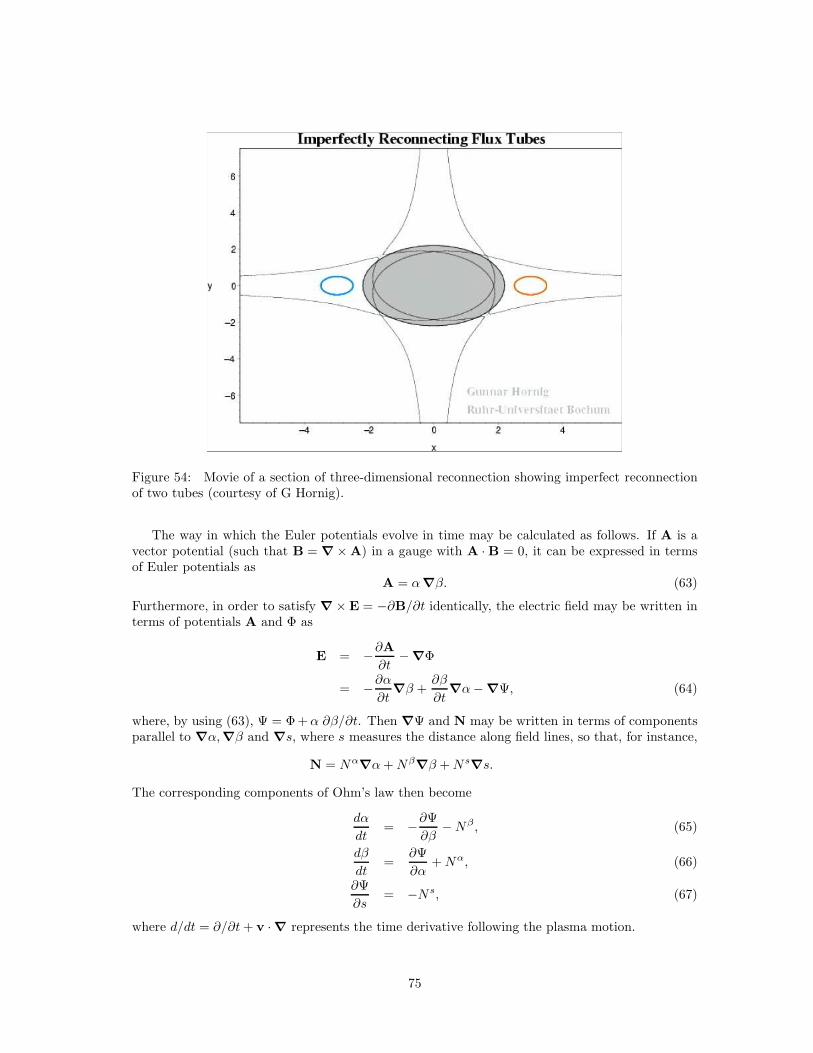
Figure 54: Movie of a section of three-dimensional reconnection showing imperfect reconnectionof two tubes (courtesy of G Hornig).

The way in which the Euler potentials evolve in time may be calculated as follows. If A is avector potential (such that B = ∇ × A) in a gauge with A · B = 0, it can be expressed in termsof Euler potentials as

A = α∇β. (63)

Furthermore, in order to satisfy ∇ × E = −∂B/∂t identically, the electric field may be written interms of potentials A and Φ as

E = −∂A∂t

− ∇Φ

= −∂α∂t

∇β +∂β

∂t∇α− ∇Ψ, (64)

where, by using (63), Ψ = Φ +α ∂β/∂t. Then ∇Ψ and N may be written in terms of componentsparallel to ∇α,∇β and ∇s, where s measures the distance along field lines, so that, for instance,

N = Nα∇α+Nβ

∇β +Ns∇s.

The corresponding components of Ohm’s law then become

dα

dt= −∂Ψ

∂β−Nβ , (65)

dβ

dt=

∂Ψ

∂α+Nα, (66)

∂Ψ

∂s= −Ns, (67)

where d/dt = ∂/∂t+ v · ∇ represents the time derivative following the plasma motion.

75

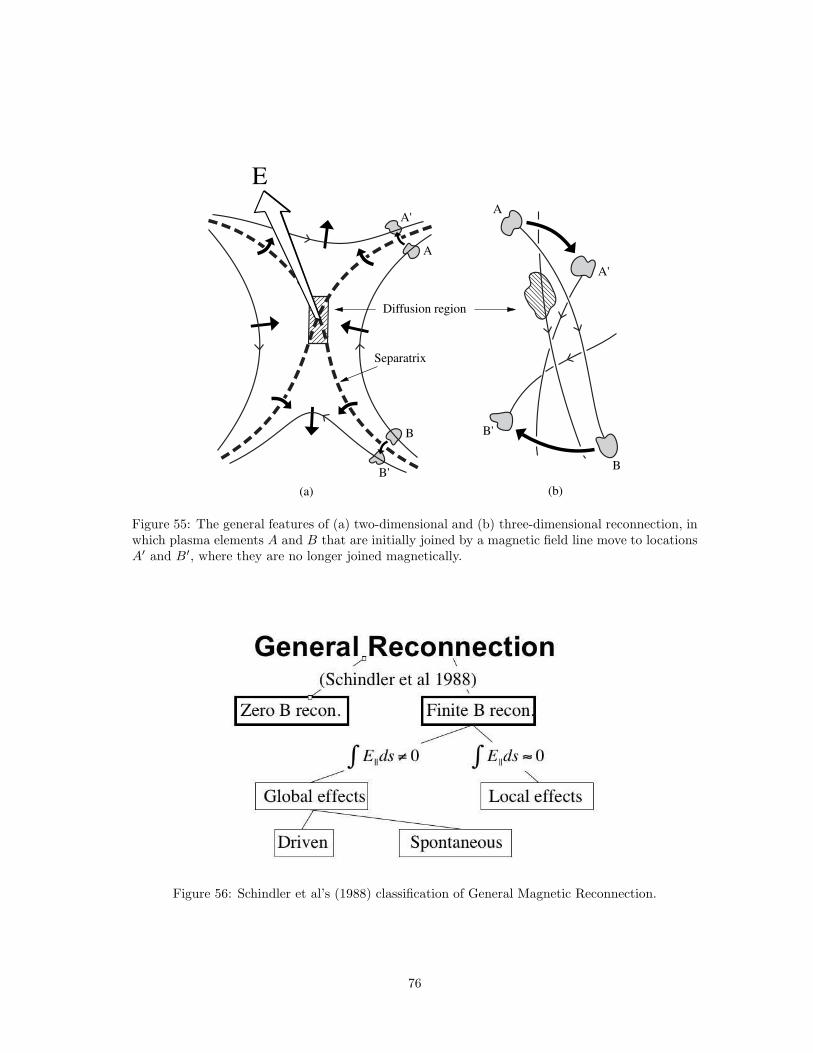
(a) (b)

A'

A'

B'

B'

A

A

E

B

B

Separatrix

Diffusion region

Figure 55: The general features of (a) two-dimensional and (b) three-dimensional reconnection, inwhich plasma elements A and B that are initially joined by a magnetic field line move to locationsA′ and B′, where they are no longer joined magnetically.

Figure 56: Schindler et al’s (1988) classification of General Magnetic Reconnection.

76

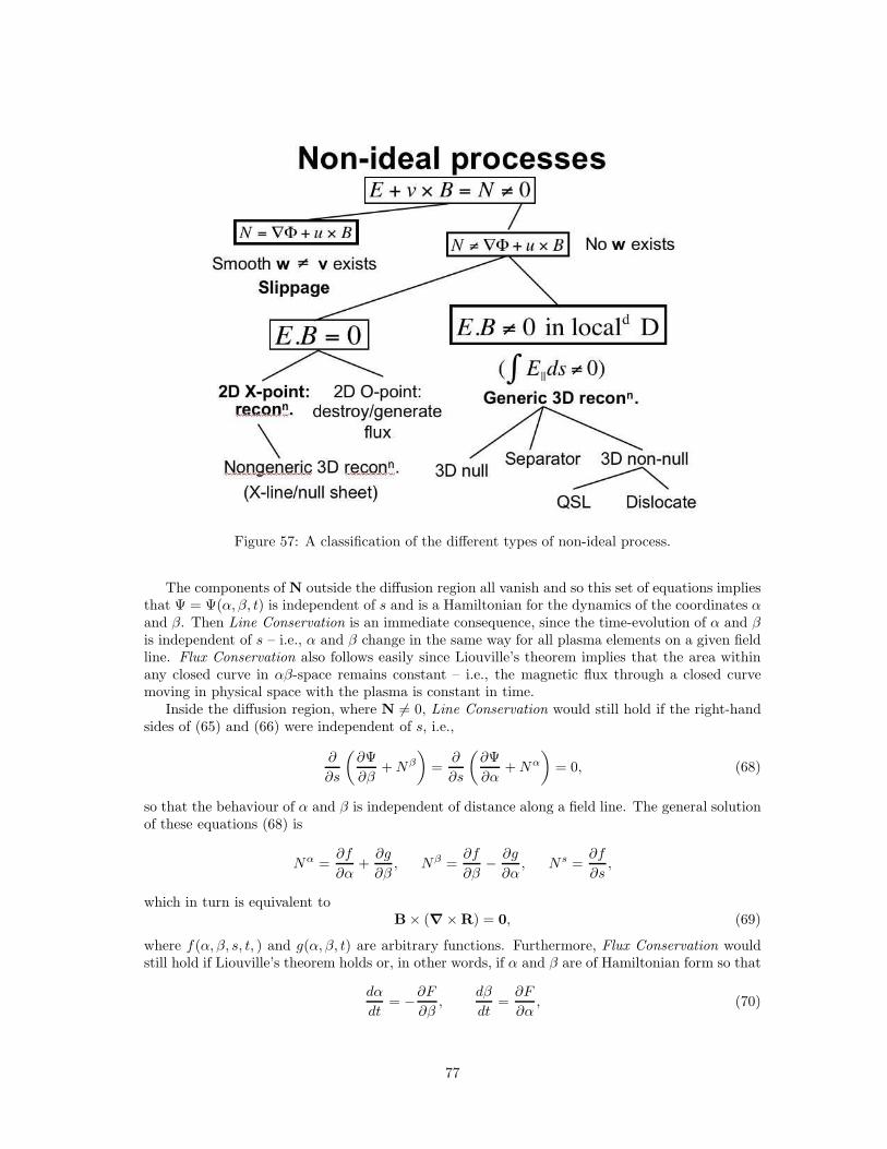
Figure 57: A classification of the different types of non-ideal process.

The components of N outside the diffusion region all vanish and so this set of equations impliesthat Ψ = Ψ(α, β, t) is independent of s and is a Hamiltonian for the dynamics of the coordinates αand β. Then Line Conservation is an immediate consequence, since the time-evolution of α and βis independent of s – i.e., α and β change in the same way for all plasma elements on a given fieldline. Flux Conservation also follows easily since Liouville’s theorem implies that the area withinany closed curve in αβ-space remains constant – i.e., the magnetic flux through a closed curvemoving in physical space with the plasma is constant in time.

Inside the diffusion region, where N 6= 0, Line Conservation would still hold if the right-handsides of (65) and (66) were independent of s, i.e.,

∂

∂s

(∂Ψ

∂β+Nβ

)

=∂

∂s

(∂Ψ

∂α+Nα

)

= 0, (68)

so that the behaviour of α and β is independent of distance along a field line. The general solutionof these equations (68) is

Nα =∂f

∂α+∂g

∂β, Nβ =

∂f

∂β− ∂g

∂α, Ns =

∂f

∂s,

which in turn is equivalent toB × (∇ × R) = 0, (69)

where f(α, β, s, t, ) and g(α, β, t) are arbitrary functions. Furthermore, Flux Conservation wouldstill hold if Liouville’s theorem holds or, in other words, if α and β are of Hamiltonian form so that

dα

dt= −∂F

∂β,

dβ

dt=∂F

∂α, (70)

77

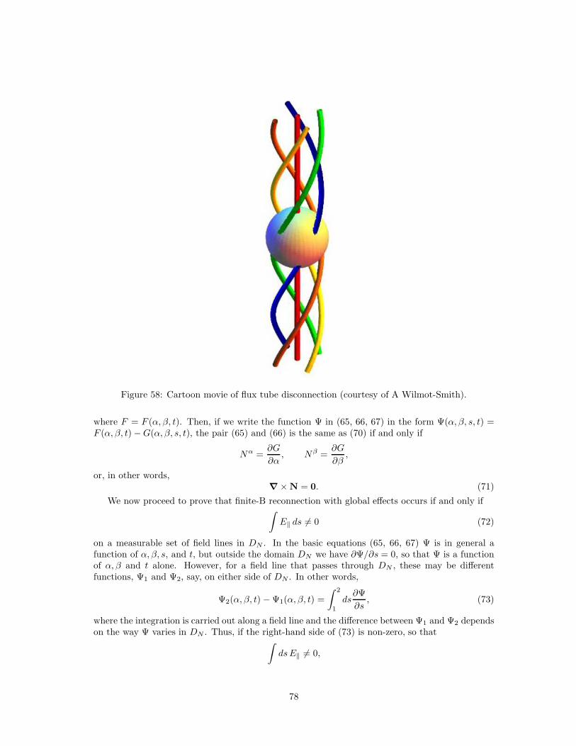
Figure 58: Cartoon movie of flux tube disconnection (courtesy of A Wilmot-Smith).

where F = F (α, β, t). Then, if we write the function Ψ in (65, 66, 67) in the form Ψ(α, β, s, t) =F (α, β, t) −G(α, β, s, t), the pair (65) and (66) is the same as (70) if and only if

Nα =∂G

∂α, Nβ =

∂G

∂β,

or, in other words,∇ × N = 0. (71)

We now proceed to prove that finite-B reconnection with global effects occurs if and only if∫

E‖ ds 6= 0 (72)

on a measurable set of field lines in DN . In the basic equations (65, 66, 67) Ψ is in general afunction of α, β, s, and t, but outside the domain DN we have ∂Ψ/∂s = 0, so that Ψ is a functionof α, β and t alone. However, for a field line that passes through DN , these may be differentfunctions, Ψ1 and Ψ2, say, on either side of DN . In other words,

Ψ2(α, β, t) − Ψ1(α, β, t) =

∫ 2

1

ds∂Ψ

∂s, (73)

where the integration is carried out along a field line and the difference between Ψ1 and Ψ2 dependson the way Ψ varies in DN . Thus, if the right-hand side of (73) is non-zero, so that

∫

dsE‖ 6= 0,

78

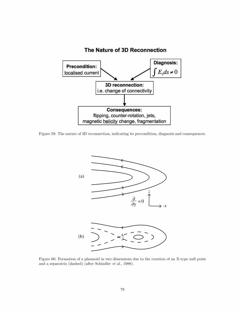
Figure 59: The nature of 3D reconnection, indicating its precondition, diagnosis and consequences.

z

-x

(a)

(b)

∂ ∂y

= 0

Figure 60: Formation of a plasmoid in two dimensions due to the creation of an X-type null pointand a separatrix (dashed) (after Schindler et al., 1988).

79

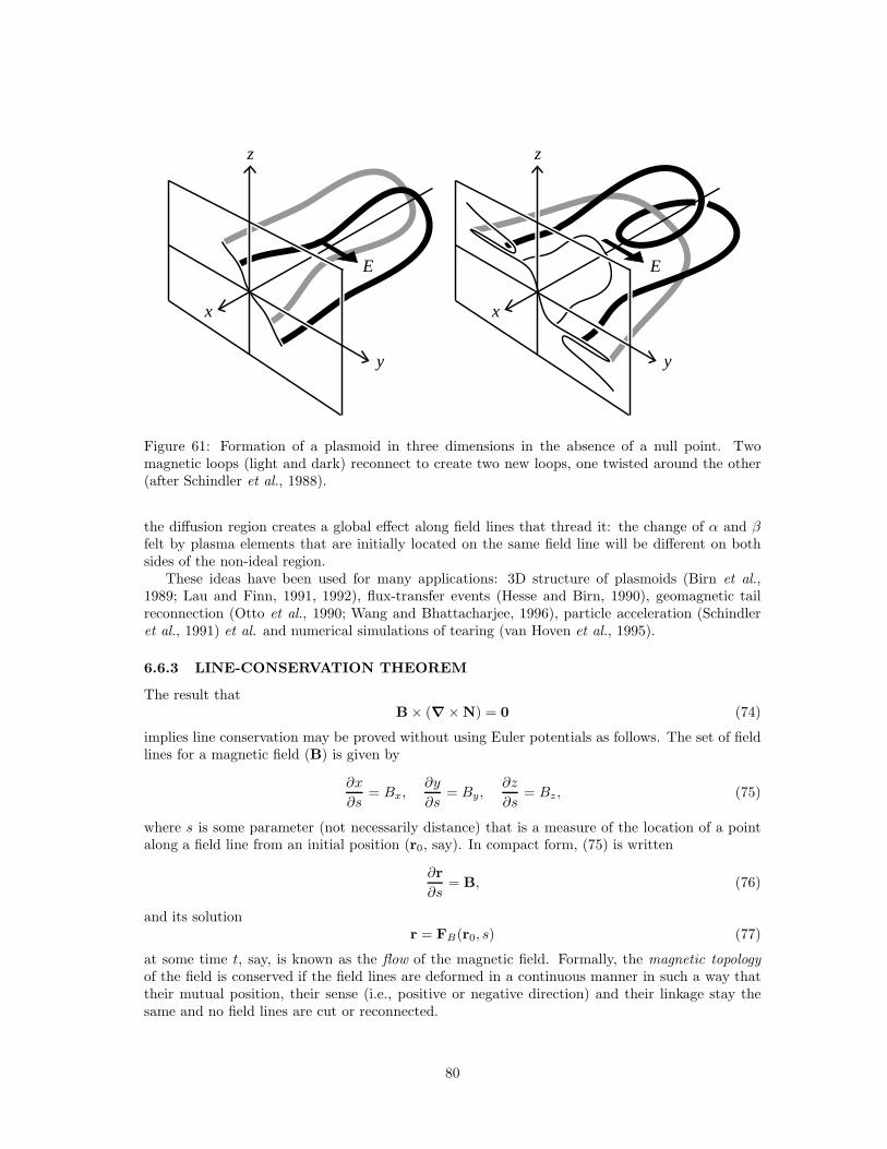
z

E

y

x

z

E

y

x

Figure 61: Formation of a plasmoid in three dimensions in the absence of a null point. Twomagnetic loops (light and dark) reconnect to create two new loops, one twisted around the other(after Schindler et al., 1988).

the diffusion region creates a global effect along field lines that thread it: the change of α and βfelt by plasma elements that are initially located on the same field line will be different on bothsides of the non-ideal region.

These ideas have been used for many applications: 3D structure of plasmoids (Birn et al.,1989; Lau and Finn, 1991, 1992), flux-transfer events (Hesse and Birn, 1990), geomagnetic tailreconnection (Otto et al., 1990; Wang and Bhattacharjee, 1996), particle acceleration (Schindleret al., 1991) et al. and numerical simulations of tearing (van Hoven et al., 1995).

6.6.3 LINE-CONSERVATION THEOREM

The result thatB × (∇ × N) = 0 (74)

implies line conservation may be proved without using Euler potentials as follows. The set of fieldlines for a magnetic field (B) is given by

∂x

∂s= Bx,

∂y

∂s= By,

∂z

∂s= Bz, (75)

where s is some parameter (not necessarily distance) that is a measure of the location of a pointalong a field line from an initial position (r0, say). In compact form, (75) is written

∂r

∂s= B, (76)

and its solutionr = FB(r0, s) (77)

at some time t, say, is known as the flow of the magnetic field. Formally, the magnetic topologyof the field is conserved if the field lines are deformed in a continuous manner in such a way thattheir mutual position, their sense (i.e., positive or negative direction) and their linkage stay thesame and no field lines are cut or reconnected.

80

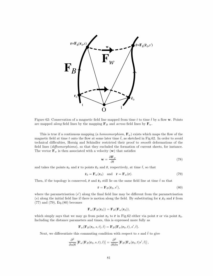
r=FB(r0,s)

r0

FB

Fw

Ot

t

r0

r=FB(r0,s')w

Figure 62: Conservation of a magnetic field line mapped from time t to time t by a flow w. Pointsare mapped along field lines by the mapping FB and across field lines by Fw.

This is true if a continuous mapping (a homeomorphism, Fw) exists which maps the flow of themagnetic field at time t onto the flow at some later time t, as sketched in Fig.62. In order to avoidtechnical difficulties, Hornig and Schindler restricted their proof to smooth deformations of thefield lines (diffeomorphisms), so that they excluded the formation of current sheets, for instance.The vector Fw is then associated with a velocity (w) that satisfies

w =∂Fw

∂t(78)

and takes the points r0 and r to points r0 and r, respectively, at time t, so that

r0 = Fw(r0) and r = Fw(r). (79)

Then, if the topology is conserved, r and r0 still lie on the same field line at time t so that

r = FB(r0, s′), (80)

where the parametrisation (s′) along the final field line may be different from the parametrisation(s) along the initial field line if there is motion along the field. By substituting for r, r0 and r from(77) and (79), Eq.(80) becomes

Fw(FB(r0)) = FB(Fw(r0)),

which simply says that we may go from point r0 to r in Fig.62 either via point r or via point r0.Including the distance parameters and times, this is expressed more fully as

Fw(FB(r0, s, t), t) = FB(Fw(r0, t), s′, t).

Next, we differentiate this commuting condition with respect to s and t to give

∂2

∂s∂t[Fw(FB(r0, s, t), t)] =

∂2

∂t∂s[FB(Fw(r0, t)s

′, t)] ,

81

and use the definitions (78) of Fw and (76) of FB, so that

∂

∂s[w(FB(r0, s, t))] =

∂

∂t

[

B(Fw(r0, t), t)∂s′

∂s

]

or at s = 0 and t = t

(B · ∇)w =∂B

∂t+ (w · ∇)B− λ∗B,

where we have rewritten −∂2s′/∂s∂t as a scalar function λ∗. In other words, we have shown that,if λ∗ and w exist such that

∂B

∂t+ (w · ∇)B− (B · ∇)w = λ∗B,

then the evolution of B(r, t) conserves the magnetic topology. This equation is, finally, the sameas the curl of (E + v × B = N) if w = v and ∇ × R = λR, where λ = −λ∗ − ∇ · v, and so wehave proved (74).

6.7 SINGULAR RECONNECTION

The above definition of general magnetic reconnection is a highly attractive one, although it couldbe regarded as too general, since it includes examples of magnetic diffusion or slippage (such asin double layers or shock waves) that have not been traditionally included in the concept of re-connection. An alternative is therefore to restrict the definition of reconnection to Singular FieldLine Reconnection, in which the presence of E‖ along a field line is supplemented by the conditionthat the nearby field has certain topology in a plane perpendicular to the field line (Priest andForbes, 1989). If the transverse topology is X-type, then we would refer to it as X-type SingularReconnection, which has the advantage of being close in spirit to traditional 2D reconnection. Ifthe transverse topology is O-type, then we would refer to it as O-type Singular Reconnection, whichincludes Flux Tube Disconnection (Wilmot-Smith and Priest, 2007) and some kinds of separatorreconnection discovered in numerical experiments (Parnell et al., 2010). The concept of X-typeSingular Reconnection has been given an elegant covariant formulation by Hornig and Rastatter(1998).

The idea here is to define reconnection in a less general way than Schindler et al. (1988) andthereby exclude many diffusive phenomena that are not normally associated with reconnection(Priest and Forbes, 1989). The aim is to remain close in spirit to the normal two-dimensionalapproach. In two dimensions (x, y) the procedure has two parts:

(i) First of all, we seek X-points, where Bx and By both vanish and there is an X-type typology;

(ii) Then reconnection occurs when there is an electric field Ez, or equivalently a hyperbolic flow(vx, vy), that carries flux in towards the X-point from two opposite quadrants and carries itout in the other two quadrants.

In three dimensions, by analogy, we may proceed as follows:

(i) Seek a set of potential singular lines, which are magnetic field lines near which the magneticfield has an O-type or X-type topology in a plane normal to that field line;

(ii) Then reconnection takes place when there is an electric field E‖ along a potential singularline; in the case of X-type Singular Reconnection this is associated with a hyperbolic flow thatbrings magnetic flux in from two directions towards the potential singular line and carries itoutwards in two other directions.

82

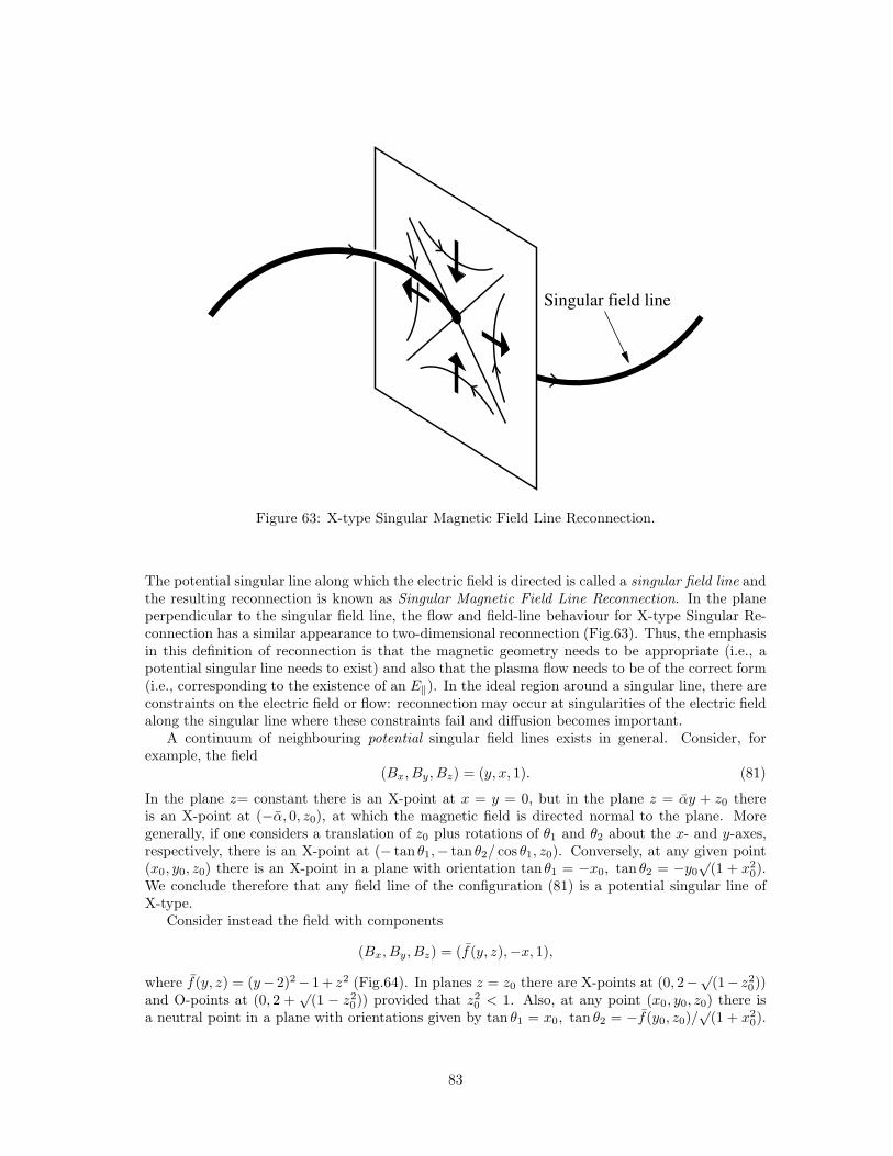
Singular field line

Figure 63: X-type Singular Magnetic Field Line Reconnection.

The potential singular line along which the electric field is directed is called a singular field line andthe resulting reconnection is known as Singular Magnetic Field Line Reconnection. In the planeperpendicular to the singular field line, the flow and field-line behaviour for X-type Singular Re-connection has a similar appearance to two-dimensional reconnection (Fig.63). Thus, the emphasisin this definition of reconnection is that the magnetic geometry needs to be appropriate (i.e., apotential singular line needs to exist) and also that the plasma flow needs to be of the correct form(i.e., corresponding to the existence of an E‖). In the ideal region around a singular line, there areconstraints on the electric field or flow: reconnection may occur at singularities of the electric fieldalong the singular line where these constraints fail and diffusion becomes important.

A continuum of neighbouring potential singular field lines exists in general. Consider, forexample, the field

(Bx, By, Bz) = (y, x, 1). (81)

In the plane z= constant there is an X-point at x = y = 0, but in the plane z = αy + z0 thereis an X-point at (−α, 0, z0), at which the magnetic field is directed normal to the plane. Moregenerally, if one considers a translation of z0 plus rotations of θ1 and θ2 about the x- and y-axes,respectively, there is an X-point at (− tan θ1,− tan θ2/ cos θ1, z0). Conversely, at any given point(x0, y0, z0) there is an X-point in a plane with orientation tan θ1 = −x0, tan θ2 = −y0

√(1 + x2

0).We conclude therefore that any field line of the configuration (81) is a potential singular line ofX-type.

Consider instead the field with components

(Bx, By, Bz) = (f(y, z),−x, 1),

where f(y, z) = (y− 2)2− 1+ z2 (Fig.64). In planes z = z0 there are X-points at (0, 2−√(1− z2

0))and O-points at (0, 2 +

√(1 − z2

0)) provided that z20 < 1. Also, at any point (x0, y0, z0) there is

a neutral point in a plane with orientations given by tan θ1 = x0, tan θ2 = −f(y0, z0)/√

(1 + x20).

83

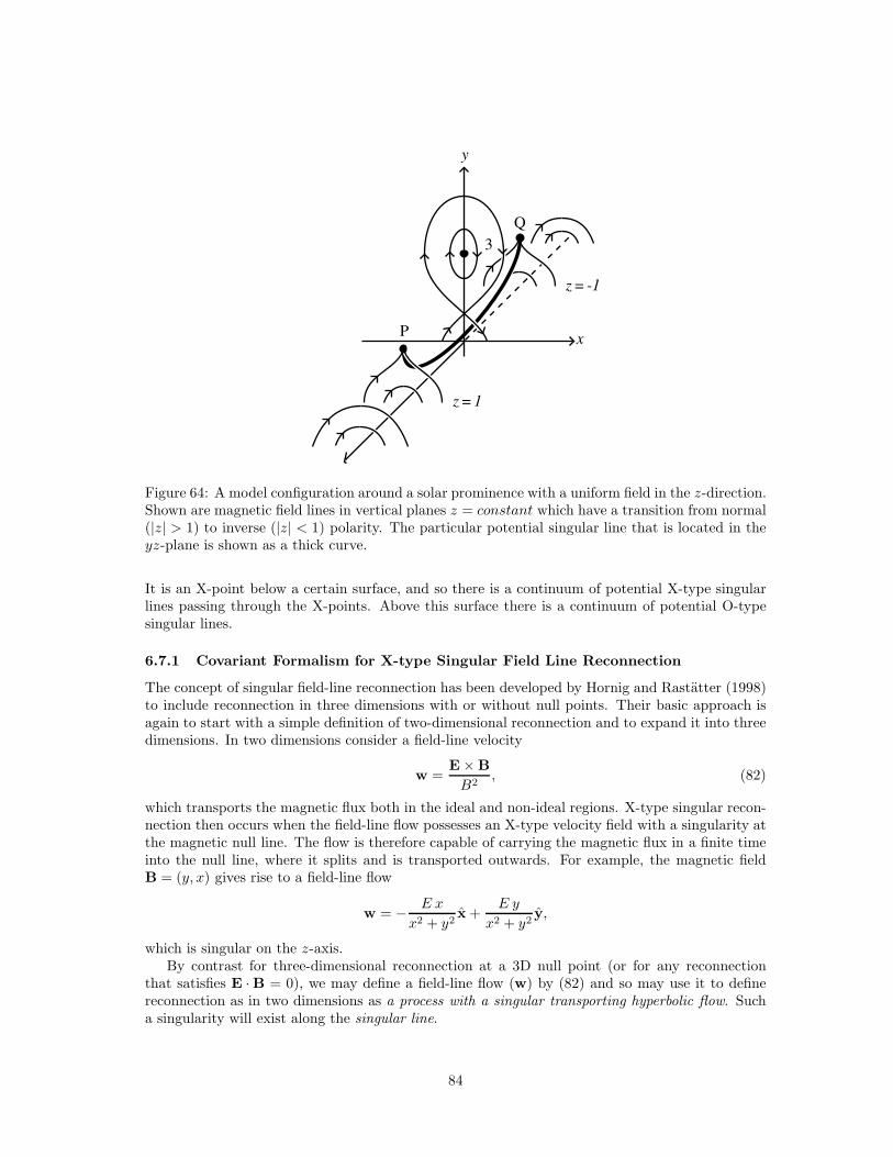
P

Q

3

z = 1

z = -1

x

y

Figure 64: A model configuration around a solar prominence with a uniform field in the z-direction.Shown are magnetic field lines in vertical planes z = constant which have a transition from normal(|z| > 1) to inverse (|z| < 1) polarity. The particular potential singular line that is located in theyz-plane is shown as a thick curve.

It is an X-point below a certain surface, and so there is a continuum of potential X-type singularlines passing through the X-points. Above this surface there is a continuum of potential O-typesingular lines.

6.7.1 Covariant Formalism for X-type Singular Field Line Reconnection

The concept of singular field-line reconnection has been developed by Hornig and Rastatter (1998)to include reconnection in three dimensions with or without null points. Their basic approach isagain to start with a simple definition of two-dimensional reconnection and to expand it into threedimensions. In two dimensions consider a field-line velocity

w =E × B

B2, (82)

which transports the magnetic flux both in the ideal and non-ideal regions. X-type singular recon-nection then occurs when the field-line flow possesses an X-type velocity field with a singularity atthe magnetic null line. The flow is therefore capable of carrying the magnetic flux in a finite timeinto the null line, where it splits and is transported outwards. For example, the magnetic fieldB = (y, x) gives rise to a field-line flow

w = − E x

x2 + y2x +

E y

x2 + y2y,

which is singular on the z-axis.By contrast for three-dimensional reconnection at a 3D null point (or for any reconnection

that satisfies E ·B = 0), we may define a field-line flow (w) by (82) and so may use it to definereconnection as in two dimensions as a process with a singular transporting hyperbolic flow. Sucha singularity will exist along the singular line.

84

However, for finite-B reconnection in the absence of a null point, E ·B does not vanish and nosingularity in w occurs. The above definition then fails not because reconnection is fundamentallydifferent but because the concept of magnetic flux conservation on which the above definition ofw is based is too narrow a framework. Hornig and Rastatter (1998) realised that magnetic fluxconservation is only a special case of a more general conservation of electromagnetic flux and thatthis provides an appropriate framework for both null-point and non-null (B 6= 0) reconnection.The equations for flux conservation from

∂B

∂t= ∇ × (v × B), E + v × B = ∇G,

may be rewritten in covariant form as

−E ·W =∂G

∂x0, W 0E + W × B = ∇G, (83)

where the index 0 denotes the time coordinate x0 = ct. These equations imply conservation ofelectromagnetic flux ∫

C

B · dA +

∫

C

E · drdx0 = constant (84)

for a surface comoving in four-dimensional Minkowski space with the four-velocity W(4) = (W 0,W).The first term of (84) represents the usual magnetic flux threading a curve C, but it is sup-

plemented by the second term representing an extension of the curve along the time-axis. Thefour-velocity W(4) is a transporting velocity for electromagnetic flux. When W 0 ≡ 1 we recovermagnetic flux conservation, but when W 0 is a function of r and t we have a non-flux-conserving(and therefore non-ideal) evolution.

A structurally stable definition of magnetic reconnection occurring is then when:

(a) there is no solution of the ideal covariant equations (83) with W 0 > 0 everywhere and

(b) there is a solution with W 0 > 0 with the exception of a line where W(4) vanishes and ∇W(4)

has a positive and negative eigenvalue.

This definition applies to both null-point and non-null reconnection, and it is covariant sincethe location W(4) = 0 is independent of the frame of reference. It may be noted that, althoughW(4) is not unique, the location where W(4) vanishes is unique. In general, reconnection occursalong a finite singular length of a moving line, and so, if it exists along such a line for a finitetime, it shows up in space-time as a two-dimensional surface. The site of such a singular line isdetermined by a global criterion. Also, the reconnection rate is measured by the quantity

∫E · dr

along the singular line.The Hesse-Schindler definition of general reconnection is essentially equivalent to the violation

of magnetic field-line conservation, but the advantage of the above definition of singular field linereconnection is that it includes only those types of violation of field-line conservation that aretraditionally regarded as being reconnection.

6.8 MAGNETIC HELICITY CHANGES in 3D RECONNECTION

During reconnection the total magnetic helicity is conserved to a high degree of approximation,although magnetic helicity can be changed from mutual helicity to self helicity or vice versa. Recon-nection can redistribute the magnetic helicity within a configuration and often tends to make the

85

distribution more uniform so that it approaches a minimum-energy state having approximately thesame total magnetic helicity but having it uniformly distributed in a linear force-free field. However,the small change in magnetic helicity that does occur is intimately related to three-dimensionalreconnection (Schindler et al., 1988).

Consider undriven non-null (or finite-B) reconnection that is global and spontaneous (§6.12.5),for which there is no energy supply from outside (i.e., the asymptotic electric field at large distancesvanishes). The relative magnetic helicity (§6.10.1) may be written

H =

∫

V

(A + A0)(B − B0) dV,

where B0 is the magnetic field at time (t0) and A0 is the corresponding vector potential. Then,after using E = −∇Φ − ∂A/∂t, we find

dH

dt= −2

∫

V

E ·B dV −∫

S

n · [(B− B0)Φ + E× (A − A0)] dS.

Assuming that E = 0 and B = B0 on S and remembering that E · B = 0 outside the diffusionregion DR, this reduces to

dH

dt= −2

∫

DR

E ·B dV = −2

∫

DR

E‖B dV.

Thus, if the magnetic helicity H changes with time, E‖ 6= 0 and so by (61) three-dimensionalreconnection is occurring.

The rate of change of helicity (dH/dt) may also be written in terms of Euler potentials (α, β),distance (s) along the magnetic field and E‖ = −∂Ψ/ds as

dH

dt= 2

∫

∇Ψ · ∇α× ∇β dV = 2

∫

E‖ ds dα dβ.

Also, this implies the parallel electric field is roughly E‖ ≃ δH/(2VRB0 δt), in terms of the diffusionregion volume (VR) and magnetic helicity time change (δH/δt).

86

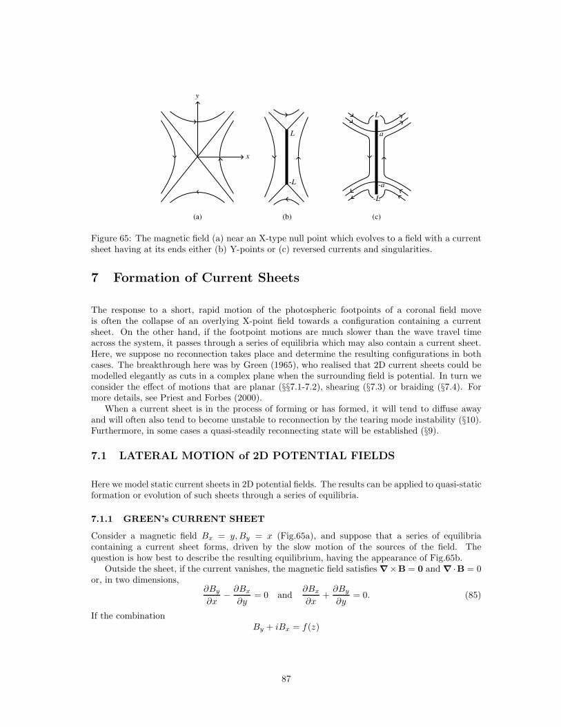
y

x

L

-L

L

-L

(c)(b)(a)

-a

a

Figure 65: The magnetic field (a) near an X-type null point which evolves to a field with a currentsheet having at its ends either (b) Y-points or (c) reversed currents and singularities.

7 Formation of Current Sheets

The response to a short, rapid motion of the photospheric footpoints of a coronal field moveis often the collapse of an overlying X-point field towards a configuration containing a currentsheet. On the other hand, if the footpoint motions are much slower than the wave travel timeacross the system, it passes through a series of equilibria which may also contain a current sheet.Here, we suppose no reconnection takes place and determine the resulting configurations in bothcases. The breakthrough here was by Green (1965), who realised that 2D current sheets could bemodelled elegantly as cuts in a complex plane when the surrounding field is potential. In turn weconsider the effect of motions that are planar (§§7.1-7.2), shearing (§7.3) or braiding (§7.4). Formore details, see Priest and Forbes (2000).

When a current sheet is in the process of forming or has formed, it will tend to diffuse awayand will often also tend to become unstable to reconnection by the tearing mode instability (§10).Furthermore, in some cases a quasi-steadily reconnecting state will be established (§9).

7.1 LATERAL MOTION of 2D POTENTIAL FIELDS

Here we model static current sheets in 2D potential fields. The results can be applied to quasi-staticformation or evolution of such sheets through a series of equilibria.

7.1.1 GREEN’s CURRENT SHEET

Consider a magnetic field Bx = y,By = x (Fig.65a), and suppose that a series of equilibriacontaining a current sheet forms, driven by the slow motion of the sources of the field. Thequestion is how best to describe the resulting equilibrium, having the appearance of Fig.65b.

Outside the sheet, if the current vanishes, the magnetic field satisfies ∇×B = 0 and ∇ ·B = 0or, in two dimensions,

∂By

∂x− ∂Bx

∂y= 0 and

∂Bx

∂x+∂By

∂y= 0. (85)

If the combinationBy + iBx = f(z)

87

is any analytic (i.e., differentiable) function of the complex variable z = x+ iy, then Eqs. (85) areautomatically satisfied. This may be proved as follows. In 1D, if the derivative f ′(x) of a functionof x exists, then the gradient at x has the same value whether x is approached from the left orthe right. In a similar way in 2D, if f ′(z) is analytic, then the gradient has the same value whenz is approached from any direction, in particular keeping y constant (so that z = x) or keeping xconstant (so that z = iy). In other words (∂/∂x)(By + iBx) = (∂/i∂y)(By + iBx), or, by equatingreal and imaginary parts, we obtain (85), as required. Therefore, we can treat the current sheetas a cut in the complex plane and seek a function f(z) with such a cut.

Initially, we haveBy + iBx = x+ iy ≡ z, (86)

but Green (1965) suggested that the field sheet outside a current sheet stretching from z = −iLto z = iL may be written simply as

By + iBx = (z2 + L2)1/2, (87)

with a cut in the complex plane from −iL to iL. This behaves like z when z ≫ L and reducesto z (as required) when L = 0, and so, letting L increase in value in (87) enables us to modelthe evolution through a series of equilibria with a slowly growing sheet. The limiting field lines(separatrices) through the ends of the sheet are inclined to one another by 2π/3, which may beshown by noting that near the upper end of the sheet at z = iL, (87) becomes approximately

By + iBx =√

(2iL)Z1/2,

where Z = z − iL. The corresponding flux function in terms of local polar coordinates (R, θ) is

A =√

(2L)2R3/2

3cos

(3θ

2+π

4

)

,

and so the field lines A = 0 are inclined at 2π/3, as required.

7.1.2 SOMOV-SYROVATSKY CURRENT SHEET

The initial field (86) may perhaps evolve not into the field (87) but instead into the more generalfield (Somov and Syrovatsky, 1976)

By + iBx =z2 + a2

(z2 + L2)1/2, (88)

where a2 < L2 (Fig.65c). The neutral points at the ends (z = ± iL) of the sheet have now ingeneral been replaced by singularities where the field behaves like (z ∓ iL)−1 as z tends to ± iL.The special case when a = L reduces to (87).

The magnitude of the field at the right of the current sheet (x = 0+, y2 < L2) is Bx(0+, y) =(a2 − y2)/(L2 − y2)1/2, which vanishes at y = ±a. The current per unit length in the sheet is thensimply

J ≡∫

jdy =

∫1

µ

∂Bx

∂ydy =

1

µ[Bx(0+, y) −Bx(0−, y)] =

2(a2 − y2)

µ(L2 − y2)1/2,

giving reversed currents between the neutral points and the ends of the sheet. This family ofsolutions was, however, largely ignored until numerical experiments on reconnection sometimesrevealed reversed-current spikes at the ends of a current sheet (Biskamp, 1986; Lee and Fu, 1986b;Forbes and Priest, 1987).

88

Bungey and Priest (1995) realised that they could generalise the Somov-Syrovatsky solution(88) to give (Figs. 66, 67)

By + iBx = −B0

[bd2 + 2dcZ − Z2 + 1

2d2

√Z2 − d2

]

, (89)

where b, c, d, B0 are constants. The solution (88) is the special case given by c = 0, d = 0, B0 =1, d2 = −L2.

Varying the value of the constant b simply moves the position of the null points (Fig.66). As bincreases, the two null points in the configuration given by b = –1.0 converge, meeting at Z = 0 forb = −0.5 (Fig.66b). As b is increased further the null points move apart along the sheet, reachingthe ends for b = 0.5, which gives Green’s solution. When b is greater than this, neutral pointsappear in the surrounding field on the x-axis (Fig.66f).

The effect of increasing the constant c from zero is to produce an asymmetry of the null pointsabout the centre of the sheet. In Eq.(89) the null points of the field occur at the roots of the

numerator on the right-hand side, which lie at the points Z = cd± d√

c2 + b+ 12 . Thus, there are

two null points which converge to the one point Z = cd when c2 = −(b+ 12 ), so that the centre of

convergence of the null points depends on the value of c. An asymmetry of the null points aboutthe centre of the sheet can lead to sheets as in Fig.67b with one singular end and one neutral end.In Figs. 67c and 67d the centre of convergence is at one end of the sheet, with the values b = −1.5and b = −1.2, respectively.

Near an end (Z = d) of such a current sheet the field behaves like B ∼ K/(Z − d)1/2, say, butthe solution (88) fails at these singularities, where diffusive effects become important and slow-mode shocks may be generated. Note that the net magnetic force on the end of the sheet is givenby

Fy + iFx =1

2µ

∮

B2dZ =πK2i

µ,

which is non-zero (essentially due to the inwards magnetic tension force). Thus, the end of thesheet is not in equilibrium, which suggests that an extra feature such as a high-speed outflow atthe tip of the current sheet needs to be added.

7.1.3 MORE GENERAL PLANAR CURRENT SHEETS

Suppose two bipolar regions of moment (2πD/µ) are initially situated at (a0, 0) and (−a0, 0)(Fig.68) and approach one another. The resulting formation of a current sheet in the solar coronacan be modelled in terms of complex variables (Priest and Raadu, 1975). Consider an initialpotential field (B0x, B0y) in y > 0 given by

B0y + iB0x =iD

(z + a0)2+

iD

(z − a0)2.

Assume that there is no significant reconnection and that the field passes through a series ofequilibria with a vertical current sheet stretching from P (0, p) to Q(0, q) along the y-axis whenthe dipole separation is 2a. Outside the current sheet where j = 0, the magnetic field (By + iBx)forms an analytic function of z, namely

By + iBx =D(z2 + p2)1/2(z2 + q2)1/2

(z2 − a2)2,

where D = 4iDa2(a2+p2)−1/2(a2+q2)−1/2 is chosen to give the correct behaviour near the sources.The values of p and q are found as functions of a by assuming frozen-in flux and equating the fluxes

89

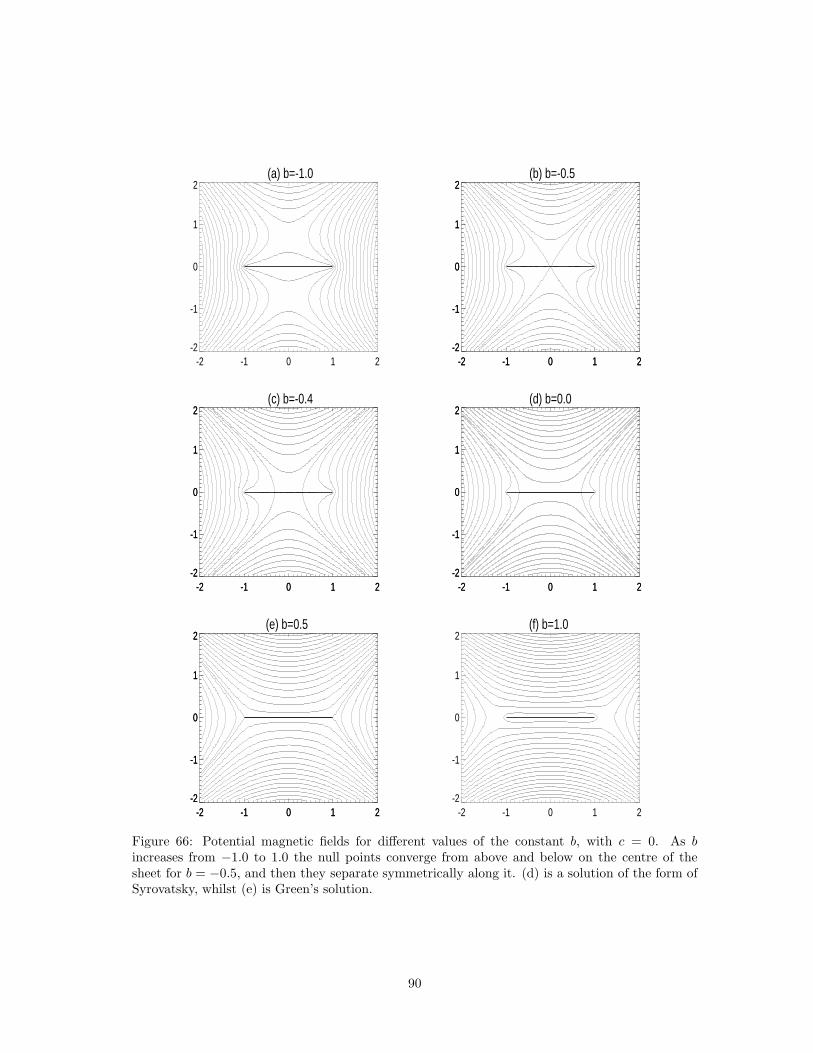
(a) b=-1.0

-2 -1 0 1 2-2

-1

0

1

2(b) b=-0.5

-2 -1 0 1 2-2

-1

0

1

2

-2 -1 0 1 2-2

-1

0

1

2

(c) b=-0.4

-2 -1 0 1 2-2

-1

0

1

2

-2 -1 0 1 2-2

-1

0

1

2(d) b=0.0

-2 -1 0 1 2-2

-1

0

1

2

-2 -1 0 1 2-2

-1

0

1

2

(e) b=0.5

-2 -1 0 1 2-2

-1

0

1

2

-2 -1 0 1 2-2

-1

0

1

2(f) b=1.0

-2 -1 0 1 2-2

-1

0

1

2

Figure 66: Potential magnetic fields for different values of the constant b, with c = 0. As bincreases from −1.0 to 1.0 the null points converge from above and below on the centre of thesheet for b = −0.5, and then they separate symmetrically along it. (d) is a solution of the form ofSyrovatsky, whilst (e) is Green’s solution.

90

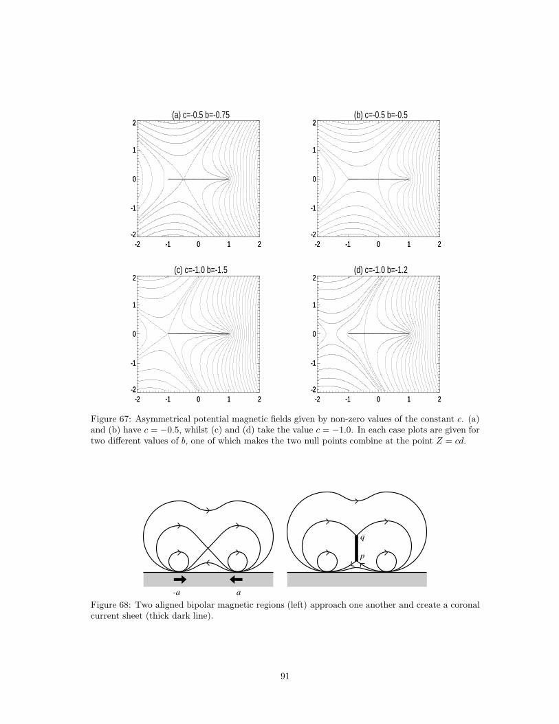
(a) c=-0.5 b=-0.75

-2 -1 0 1 2-2

-1

0

1

2

-2 -1 0 1 2-2

-1

0

1

2(b) c=-0.5 b=-0.5

-2 -1 0 1 2-2

-1

0

1

2

-2 -1 0 1 2-2

-1

0

1

2

(c) c=-1.0 b=-1.5

-2 -1 0 1 2-2

-1

0

1

2

-2 -1 0 1 2-2

-1

0

1

2(d) c=-1.0 b=-1.2

-2 -1 0 1 2-2

-1

0

1

2

-2 -1 0 1 2-2

-1

0

1

2

Figure 67: Asymmetrical potential magnetic fields given by non-zero values of the constant c. (a)and (b) have c = −0.5, whilst (c) and (d) take the value c = −1.0. In each case plots are given fortwo different values of b, one of which makes the two null points combine at the point Z = cd.

a

q

p

-a

Figure 68: Two aligned bipolar magnetic regions (left) approach one another and create a coronalcurrent sheet (thick dark line).

91

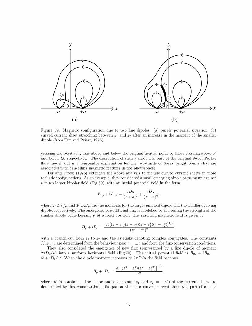
y

x

y

x-a +a

(b)(a)

-a

zN

z2

+a

z1

Figure 69: Magnetic configuration due to two line dipoles: (a) purely potential situation; (b)curved current sheet stretching between z1 and z2 after an increase in the moment of the smallerdipole (from Tur and Priest, 1976).

crossing the positive y-axis above and below the original neutral point to those crossing above Pand below Q, respectively. The dissipation of such a sheet was part of the original Sweet-Parkerflare model and is a reasonable explanation for the two-thirds of X-ray bright points that areassociated with cancelling magnetic features in the photosphere.

Tur and Priest (1976) extended the above analysis to include curved current sheets in morerealistic configurations. As an example, they considered a small emerging bipole pressing up againsta much larger bipolar field (Fig.69), with an initial potential field in the form

B0y + iB0x =iD0

(z + a)2+

iDA

(z − a)2,

where 2πDA/µ and 2πD0/µ are the moments for the larger ambient dipole and the smaller evolvingdipole, respectively. The emergence of additional flux is modelled by increasing the strength of thesmaller dipole while keeping it at a fixed position. The resulting magnetic field is given by

By + iBx =iK[(z − z1)(z − z2)(z − z∗1)(z − z∗2)]1/2

(z2 − a2)2,

with a branch cut from z1 to z2 and the asterisks denoting complex conjugates. The constantsK, z1, z2 are determined from the behaviour near z = ±a and from the flux-conservation conditions.

They also considered the emergence of new flux (represented by a line dipole of moment2πD0/µ) into a uniform horizontal field (Fig.70). The initial potential field is B0y + iB0x =ib+ iD0/z

2. When the dipole moment increases to 2πD/µ the field becomes

By + iBx =K[(z2 − z2

1)(z2 − z∗21 )]1/2

z2,

where K is constant. The shape and end-points (z1 and z2 = −z∗1) of the current sheet aredetermined by flux conservation. Dissipation of such a curved current sheet was part of a solar

92

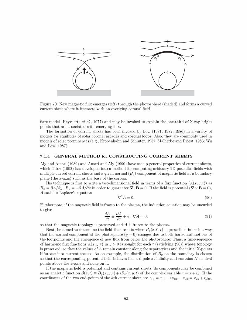
z1 z1*

Figure 70: New magnetic flux emerges (left) through the photosphere (shaded) and forms a curvedcurrent sheet where it interacts with an overlying coronal field.

flare model (Heyvaerts et al., 1977) and may be invoked to explain the one-third of X-ray brightpoints that are associated with emerging flux.

The formation of current sheets has been invoked by Low (1981, 1982, 1986) in a variety ofmodels for equilibria of solar coronal arcades and coronal loops. Also, they are commonly used inmodels of solar prominences (e.g., Kippenhahn and Schluter, 1957; Malherbe and Priest, 1983; Wuand Low, 1987).

7.1.4 GENERAL METHOD for CONSTRUCTING CURRENT SHEETS

Aly and Amari (1989) and Amari and Aly (1990) have set up general properties of current sheets,which Titov (1992) has developed into a method for computing arbitrary 2D potential fields withmultiple curved current sheets and a given normal (By) component of magnetic field at a boundaryplane (the x-axis) such as the base of the corona.

His technique is first to write a two-dimensional field in terms of a flux function (A(x, y, t)) asBx = ∂A/∂y, By = −∂A/∂x in order to guarantee ∇ ·B = 0. If the field is potential (∇×B = 0),A satisfies Laplace’s equation

∇2A = 0. (90)

Furthermore, if the magnetic field is frozen to the plasma, the induction equation may be uncurledto give

dA

dt≡ ∂A

∂t+ v · ∇A = 0, (91)

so that the magnetic topology is preserved and A is frozen to the plasma.Next, he aimed to determine the field that results when By(x, 0, t) is prescribed in such a way

that the normal component at the photosphere (y = 0) changes due to both horizontal motions ofthe footpoints and the emergence of new flux from below the photosphere. Thus, a time-sequenceof harmonic flux functions A(x, y, t) in y > 0 is sought for each t (satisfying (90)) whose topologyis preserved, so that the values of A remain constant along the separatrices and the initial X-pointsbifurcate into current sheets. As an example, the distribution of By on the boundary is chosenso that the corresponding potential field behaves like a dipole at infinity and contains N neutralpoints above the x-axis and none on it.

If the magnetic field is potential and contains current sheets, its components may be combinedas an analytic function B(z, t) ≡ By(x, y, t)+ iBx(x, y, t) of the complex variable z = x+ iy. If thecoordinates of the two end-points of the kth current sheet are z1k = x1k + iy1k, z2k = x2k + iy2k,

93

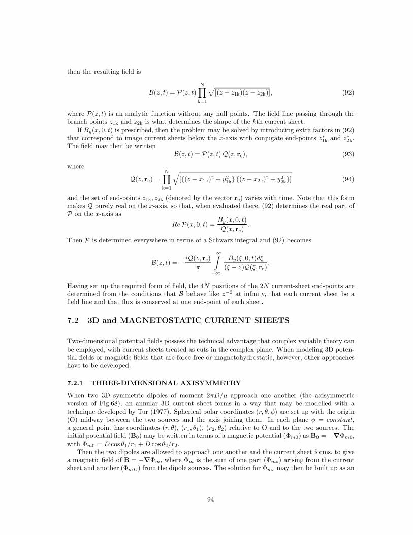
then the resulting field is

B(z, t) = P(z, t)

N∏

k=1

√

[(z − z1k)(z − z2k)], (92)

where P(z, t) is an analytic function without any null points. The field line passing through thebranch points z1k and z2k is what determines the shape of the kth current sheet.

If By(x, 0, t) is prescribed, then the problem may be solved by introducing extra factors in (92)that correspond to image current sheets below the x-axis with conjugate end-points z∗1k and z∗2k.The field may then be written

B(z, t) = P(z, t)Q(z, re), (93)

where

Q(z, re) =N∏

k=1

√

[{(z − x1k)2 + y21k} {(z − x2k)2 + y2

2k}] (94)

and the set of end-points z1k, z2k (denoted by the vector re) varies with time. Note that this formmakes Q purely real on the x-axis, so that, when evaluated there, (92) determines the real part ofP on the x-axis as

Re P(x, 0, t) =By(x, 0, t)

Q(x, re).

Then P is determined everywhere in terms of a Schwarz integral and (92) becomes

B(z, t) = − iQ(z, re)

π

∞∫

−∞

By(ξ, 0, t)dξ

(ξ − z)Q(ξ, re).

Having set up the required form of field, the 4N positions of the 2N current-sheet end-points aredetermined from the conditions that B behave like z−2 at infinity, that each current sheet be afield line and that flux is conserved at one end-point of each sheet.

7.2 3D and MAGNETOSTATIC CURRENT SHEETS

Two-dimensional potential fields possess the technical advantage that complex variable theory canbe employed, with current sheets treated as cuts in the complex plane. When modeling 3D poten-tial fields or magnetic fields that are force-free or magnetohydrostatic, however, other approacheshave to be developed.

7.2.1 THREE-DIMENSIONAL AXISYMMETRY

When two 3D symmetric dipoles of moment 2πD/µ approach one another (the axisymmetricversion of Fig.68), an annular 3D current sheet forms in a way that may be modelled with atechnique developed by Tur (1977). Spherical polar coordinates (r, θ, φ) are set up with the origin(O) midway between the two sources and the axis joining them. In each plane φ = constant,a general point has coordinates (r, θ), (r1, θ1), (r2, θ2) relative to O and to the two sources. Theinitial potential field (B0) may be written in terms of a magnetic potential (Φm0) as B0 = −∇Φm0,with Φm0 = D cos θ1/r1 +D cos θ2/r2.

Then the two dipoles are allowed to approach one another and the current sheet forms, to givea magnetic field of B = −∇Φm, where Φm is the sum of one part (Φms) arising from the currentsheet and another (ΦmD) from the dipole sources. The solution for Φms may then be built up as an

94

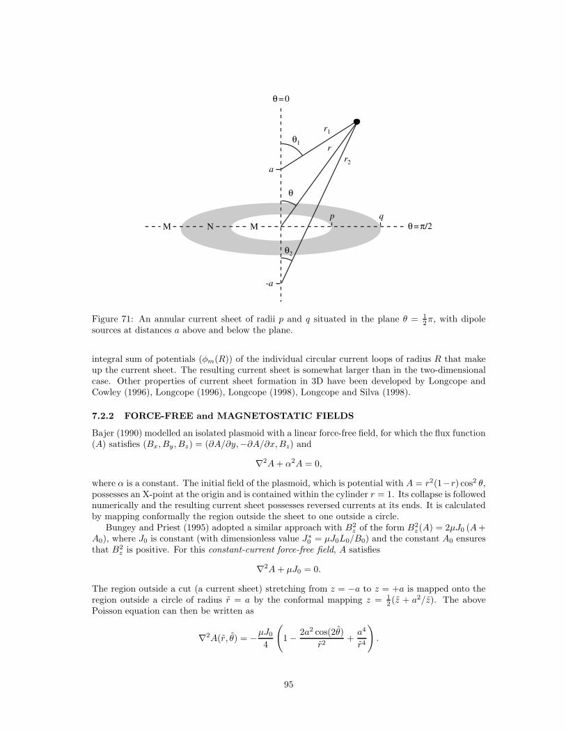
θ = 0

θ = π/2N M

a

-a

M

p

r1

r

r2

q

θ2

θ

θ1

Figure 71: An annular current sheet of radii p and q situated in the plane θ = 12π, with dipole

sources at distances a above and below the plane.

integral sum of potentials (φm(R)) of the individual circular current loops of radius R that makeup the current sheet. The resulting current sheet is somewhat larger than in the two-dimensionalcase. Other properties of current sheet formation in 3D have been developed by Longcope andCowley (1996), Longcope (1996), Longcope (1998), Longcope and Silva (1998).

7.2.2 FORCE-FREE and MAGNETOSTATIC FIELDS

Bajer (1990) modelled an isolated plasmoid with a linear force-free field, for which the flux function(A) satisfies (Bx, By, Bz) = (∂A/∂y,−∂A/∂x,Bz) and

∇2A+ α2A = 0,

where α is a constant. The initial field of the plasmoid, which is potential with A = r2(1−r) cos2 θ,possesses an X-point at the origin and is contained within the cylinder r = 1. Its collapse is followednumerically and the resulting current sheet possesses reversed currents at its ends. It is calculatedby mapping conformally the region outside the sheet to one outside a circle.

Bungey and Priest (1995) adopted a similar approach with B2z of the form B2

z (A) = 2µJ0 (A+A0), where J0 is constant (with dimensionless value J∗

0 = µJ0L0/B0) and the constant A0 ensuresthat B2

z is positive. For this constant-current force-free field, A satisfies

∇2A+ µJ0 = 0.

The region outside a cut (a current sheet) stretching from z = −a to z = +a is mapped onto theregion outside a circle of radius r = a by the conformal mapping z = 1

2 (z + a2/z). The abovePoisson equation can then be written as

∇2A(r, θ) = −µJ0

4

(

1 − 2a2 cos(2θ)

r2+a4

r4

)

.

95

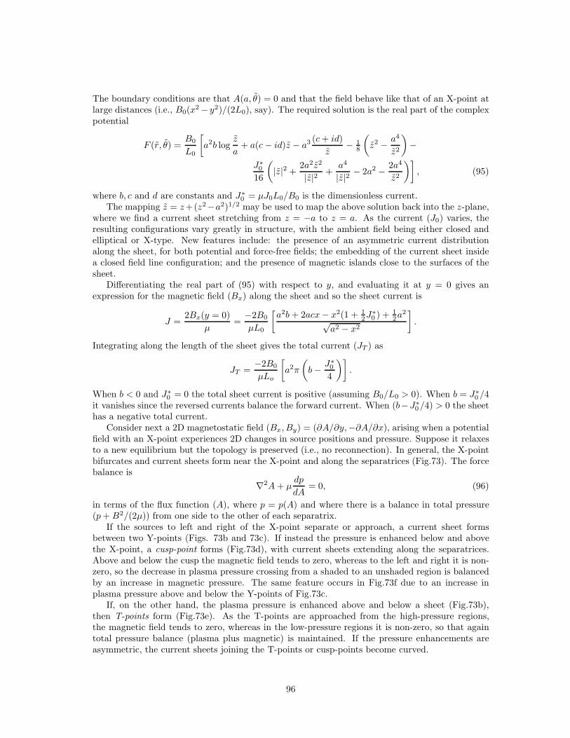
The boundary conditions are that A(a, θ) = 0 and that the field behave like that of an X-point atlarge distances (i.e., B0(x

2 − y2)/(2L0), say). The required solution is the real part of the complexpotential

F (r, θ) =B0

L0

[

a2b logz

a+ a(c− id)z − a3 (c+ id)

z− 1

8

(

z2 − a4

z2

)

−

J∗0

16

(

|z|2 +2a2z2

|z|2 +a4

|z|2 − 2a2 − 2a4

z2

)]

, (95)

where b, c and d are constants and J∗0 = µJ0L0/B0 is the dimensionless current.

The mapping z = z+(z2−a2)1/2 may be used to map the above solution back into the z-plane,where we find a current sheet stretching from z = −a to z = a. As the current (J0) varies, theresulting configurations vary greatly in structure, with the ambient field being either closed andelliptical or X-type. New features include: the presence of an asymmetric current distributionalong the sheet, for both potential and force-free fields; the embedding of the current sheet insidea closed field line configuration; and the presence of magnetic islands close to the surfaces of thesheet.

Differentiating the real part of (95) with respect to y, and evaluating it at y = 0 gives anexpression for the magnetic field (Bx) along the sheet and so the sheet current is

J =2Bx(y = 0)

µ=

−2B0

µL0

[a2b+ 2acx− x2(1 + 1

2J∗0 ) + 1

2a2

√a2 − x2

]

.

Integrating along the length of the sheet gives the total current (JT ) as

JT =−2B0

µLo

[

a2π

(

b− J∗0

4

)]

.

When b < 0 and J∗0 = 0 the total sheet current is positive (assuming B0/L0 > 0). When b = J∗

0 /4it vanishes since the reversed currents balance the forward current. When (b−J∗

0/4) > 0 the sheethas a negative total current.

Consider next a 2D magnetostatic field (Bx, By) = (∂A/∂y,−∂A/∂x), arising when a potentialfield with an X-point experiences 2D changes in source positions and pressure. Suppose it relaxesto a new equilibrium but the topology is preserved (i.e., no reconnection). In general, the X-pointbifurcates and current sheets form near the X-point and along the separatrices (Fig.73). The forcebalance is

∇2A+ µdp

dA= 0, (96)

in terms of the flux function (A), where p = p(A) and where there is a balance in total pressure(p+B2/(2µ)) from one side to the other of each separatrix.

If the sources to left and right of the X-point separate or approach, a current sheet formsbetween two Y-points (Figs. 73b and 73c). If instead the pressure is enhanced below and abovethe X-point, a cusp-point forms (Fig.73d), with current sheets extending along the separatrices.Above and below the cusp the magnetic field tends to zero, whereas to the left and right it is non-zero, so the decrease in plasma pressure crossing from a shaded to an unshaded region is balancedby an increase in magnetic pressure. The same feature occurs in Fig.73f due to an increase inplasma pressure above and below the Y-points of Fig.73c.

If, on the other hand, the plasma pressure is enhanced above and below a sheet (Fig.73b),then T-points form (Fig.73e). As the T-points are approached from the high-pressure regions,the magnetic field tends to zero, whereas in the low-pressure regions it is non-zero, so that againtotal pressure balance (plasma plus magnetic) is maintained. If the pressure enhancements areasymmetric, the current sheets joining the T-points or cusp-points become curved.

96

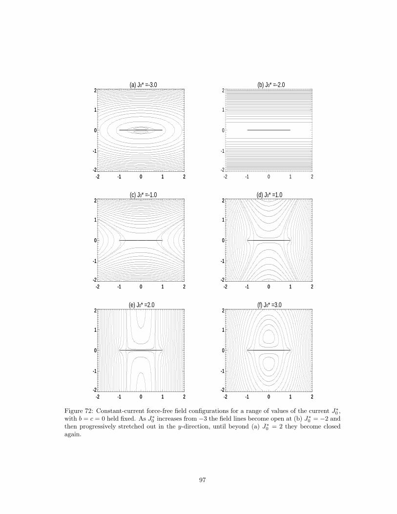
(a) J0* =-3.0

-2 -1 0 1 2-2

-1

0

1

2

-2 -1 0 1 2-2

-1

0

1

2(b) J0* =-2.0

-2 -1 0 1 2-2

-1

0

1

2

(c) J0* =-1.0

-2 -1 0 1 2-2

-1

0

1

2

-2 -1 0 1 2-2

-1

0

1

2(d) J0* =1.0

-2 -1 0 1 2-2

-1

0

1

2

-2 -1 0 1 2-2

-1

0

1

2

(e) J0* =2.0

-2 -1 0 1 2-2

-1

0

1

2

-2 -1 0 1 2-2

-1

0

1

2(f) J0* =3.0

-2 -1 0 1 2-2

-1

0

1

2

-2 -1 0 1 2-2

-1

0

1

2

Figure 72: Constant-current force-free field configurations for a range of values of the current J∗0 ,

with b = c = 0 held fixed. As J∗0 increases from −3 the field lines become open at (b) J∗

0 = −2 andthen progressively stretched out in the y-direction, until beyond (a) J∗

0 = 2 they become closedagain.

97

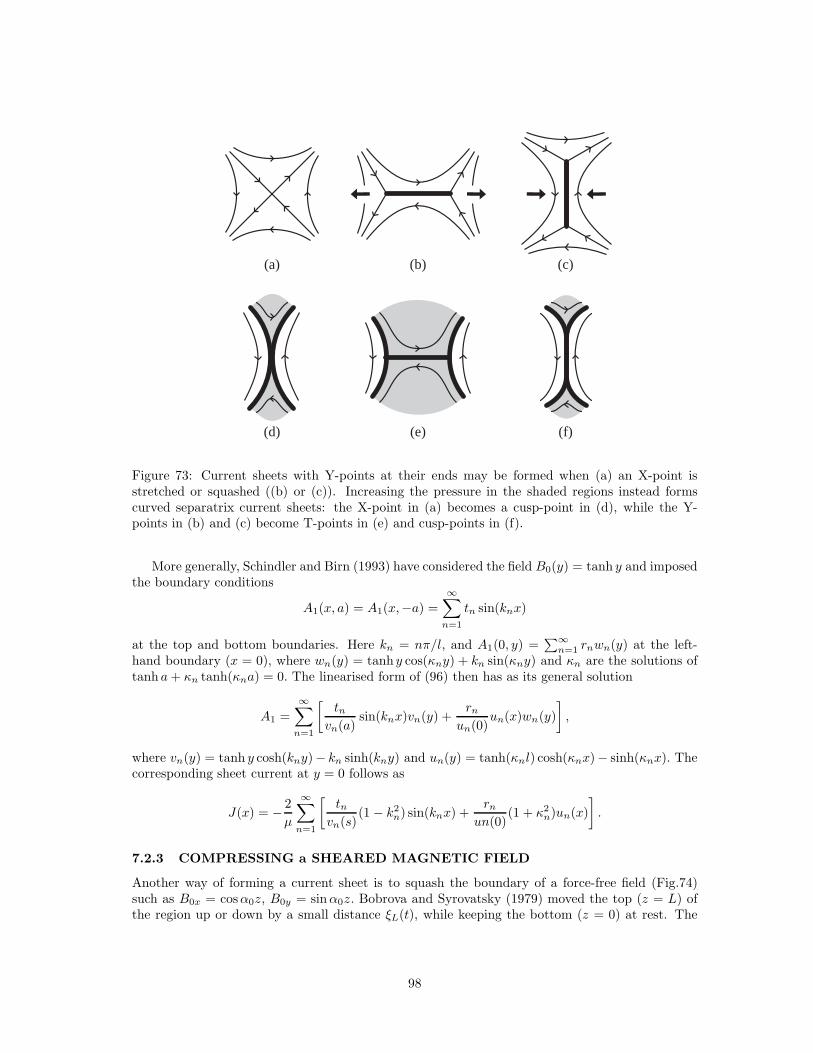
(a) (b) (c)

(d) (e) (f)

Figure 73: Current sheets with Y-points at their ends may be formed when (a) an X-point isstretched or squashed ((b) or (c)). Increasing the pressure in the shaded regions instead formscurved separatrix current sheets: the X-point in (a) becomes a cusp-point in (d), while the Y-points in (b) and (c) become T-points in (e) and cusp-points in (f).

More generally, Schindler and Birn (1993) have considered the field B0(y) = tanh y and imposedthe boundary conditions

A1(x, a) = A1(x,−a) =∞∑

n=1

tn sin(knx)

at the top and bottom boundaries. Here kn = nπ/l, and A1(0, y) =∑∞

n=1 rnwn(y) at the left-hand boundary (x = 0), where wn(y) = tanh y cos(κny) + kn sin(κny) and κn are the solutions oftanh a+ κn tanh(κna) = 0. The linearised form of (96) then has as its general solution

A1 =

∞∑

n=1

[tn

vn(a)sin(knx)vn(y) +

rnun(0)

un(x)wn(y)

]

,

where vn(y) = tanh y cosh(kny)− kn sinh(kny) and un(y) = tanh(κnl) cosh(κnx)− sinh(κnx). Thecorresponding sheet current at y = 0 follows as

J(x) = − 2

µ

∞∑

n=1

[tn

vn(s)(1 − k2

n) sin(knx) +rn

un(0)(1 + κ2

n)un(x)

]

.

7.2.3 COMPRESSING a SHEARED MAGNETIC FIELD

Another way of forming a current sheet is to squash the boundary of a force-free field (Fig.74)such as B0x = cosα0z, B0y = sinα0z. Bobrova and Syrovatsky (1979) moved the top (z = L) ofthe region up or down by a small distance ξL(t), while keeping the bottom (z = 0) at rest. The

98

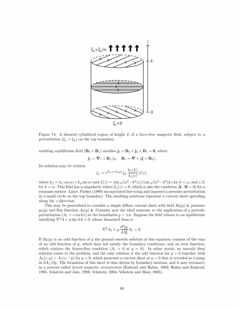
z

ξz = 0

ξz = ξL(t)

L

0

Figure 74: A sheared cylindrical region of height L of a force-free magnetic field, subject to aperturbation (ξz = ξL) on the top boundary.

resulting equilibrium field (B0 + B1) satisfies j1 × B0 + j0 × B1 = 0, where

j1 = ∇1 × B1/µ, B1 = ∇ × (ξ × B0).

Its solution may be written

ξz = e(kxx+kyy) ξLk||(L)

k||(z)f(z),

where k|| = kx cosαz+ky sinαz and f(z) = (sin√

(α2−k2)z)/(sin√

(α2−k2)L) for k < α, and z/Lfor k = α. This field has a singularity where k||(z) = 0, which is also the condition (k ·B = 0) for aresonant surface. Later, Parker (1990) incorporated line-tying and imposed a pressure perturbationin a small circle on the top boundary. The resulting solutions represent a current sheet spirallingalong the z-direction.

This may be generalised to consider a simple diffuse current sheet with field B0(y) x, pressurep0(y) and flux function A0(y) z. Consider now the ideal response to the application of a periodicperturbation (A1 = ǫ cos kx) at the boundaries y = ±a. Suppose the field relaxes to an equilibriumsatisfying ∇2A+ µdp/dA = 0, whose linearized form is

∇2A1 + µd2p0

dA20

A1 = 0.

If B0(y) is an odd function of y the general smooth solution of this equation consists of the sumof an odd function of y, which does not satisfy the boundary conditions, and an even function,which violates the frozen-flux condition (A1 = 0 at y = 0). In other words, no smooth idealsolution exists to the problem, and the only solution is the odd function for y > 0 together withA1(x, y) = A1(x,−y) for y < 0, which possesses a current sheet at y = 0 that is revealed as a jumpin ∂A1/∂y. The formation of this sheet is thus driven by boundary motions, and it may reconnectin a process called forced magnetic reconnection (Kulsrud and Hahm, 1982; Hahm and Kulsrud,1985; Vekstein and Jain, 1998; Vekstein, 2004; Vekstein and Bian, 2005).

99

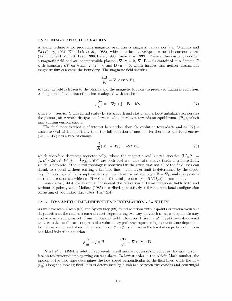
7.2.4 MAGNETIC RELAXATION

A useful technique for producing magnetic equilibria is magnetic relaxation (e.g., Sturrock andWoodbury, 1967; Klimchuk et al., 1988), which has been developed to include current sheets(Arnol’d, 1974; Moffatt, 1985, 1990; Bajer, 1990; Linardatos, 1993). These authors usually considera magnetic field and an incompressible plasma (∇ · v = 0, ∇ · B = 0) contained in a domain Dwith boundary ∂D on which v · n = 0 and B · n = 0, which implies that neither plasma normagnetic flux can cross the boundary. The magnetic field satisfies

∂B

∂t= ∇ × (v × B),

so that the field is frozen to the plasma and the magnetic topology is preserved during is evolution.A simple model equation of motion is adopted with the form

ρ∂v

∂t= −∇p+ j × B−Kv, (97)

where ρ = constant. The initial state (B0) is smooth and static, and a force imbalance acceleratesthe plasma, after which dissipation slows it, while it relaxes towards an equilibrium. (BE), whichmay contain current sheets.

The final state is what is of interest here rather than the evolution towards it, and so (97) iseasier to deal with numerically than the full equation of motion. Furthermore, the total energy(Wm +Wk) has a rate of change

d

dt(Wm +Wk) = −2KWk, (98)

which therefore decreases monotonically, where the magnetic and kinetic energies (Wm(t) =∫

D B2/(2µ)dV , Wk(t) = 1

2ρ∫

D v2dV ) are both positive. The total energy tends to a finite limit,

which is non-zero if the initial topology is nontrivial in the sense that not all of the field lines canshrink to a point without cutting other field lines. This lower limit is determined by the topol-ogy. The corresponding asymptotic state is magnetostatic satisfying j × B = ∇p, and may possesscurrent sheets, across which n ·B = 0 and the total pressure (p+B2/(2µ)) is continuous.

Linardatos (1993), for example, considered the relaxation of two-dimensional fields with andwithout X-points, while Moffatt (1985) described qualitatively a three-dimensional configurationconsisting of two linked flux tubes (Fig.7.2.4).

7.2.5 DYNAMIC TIME-DEPENDENT FORMATION of a SHEET

As we have seen, Green (87) and Syrovatsky (88) found solutions with Y-points or reversed-currentsingularities at the ends of a current sheet, representing two ways in which a series of equilibria mayevolve slowly and passively from an X-point field. However, Priest et al. (1994) have discoveredan alternative nonlinear, compressible evolutionary pathway, representing dynamic time-dependentformation of a current sheet. They assume cs ≪ v ≪ vA and solve the low-beta equation of motionand ideal induction equation

ρdv

dt= j × B,

∂B

∂t= ∇ × (v × B).

Priest et al. (1994)’s solution represents a self-similar, quasi-static collapse through current-free states surrounding a growing current sheet. To lowest order in the Alfven Mach number, themotion of the field lines determines the flow speed perpendicular to the field lines, while the flow(v||) along the moving field lines is determined by a balance between the coriolis and centrifugal

100

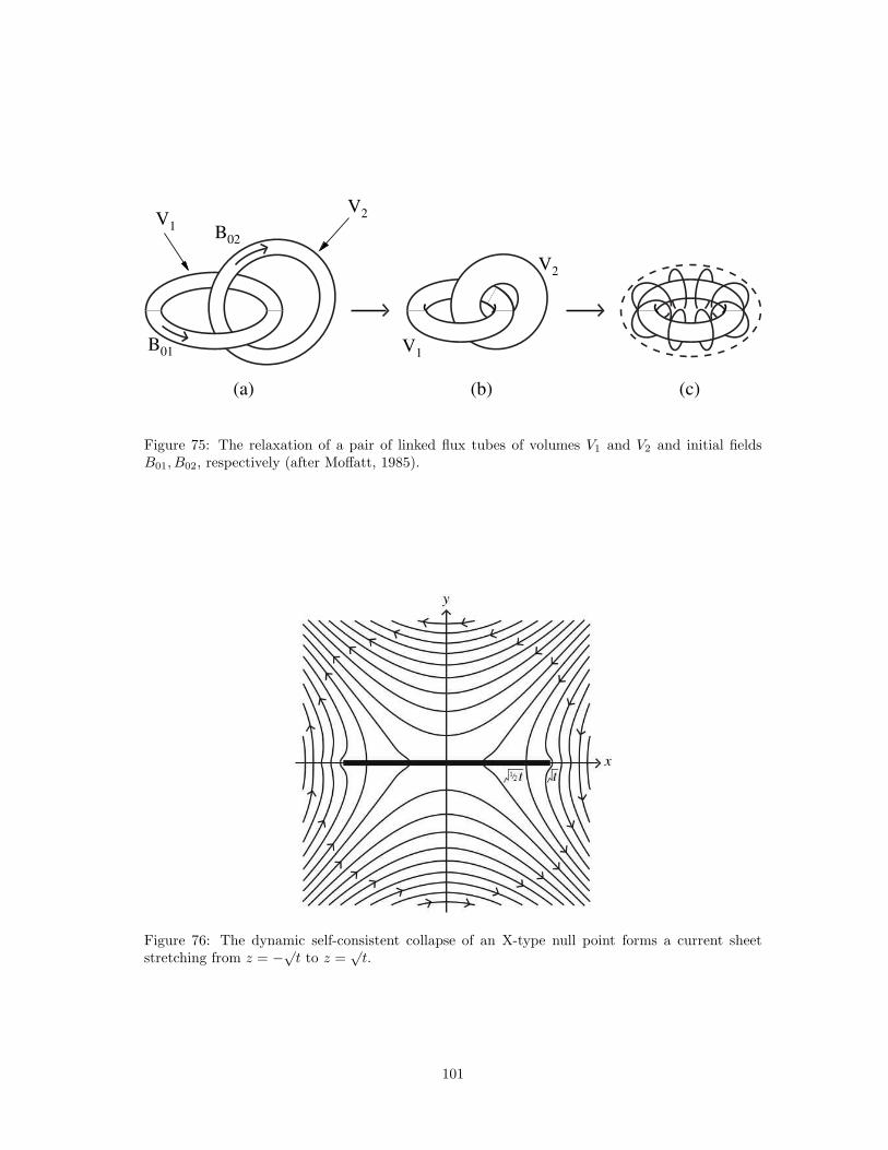
(a)

V2V1 B02

B01

(b) (c)

V2

V1

Figure 75: The relaxation of a pair of linked flux tubes of volumes V1 and V2 and initial fieldsB01, B02, respectively (after Moffatt, 1985).

Figure 76: The dynamic self-consistent collapse of an X-type null point forms a current sheetstretching from z = −√

t to z =√t.

101

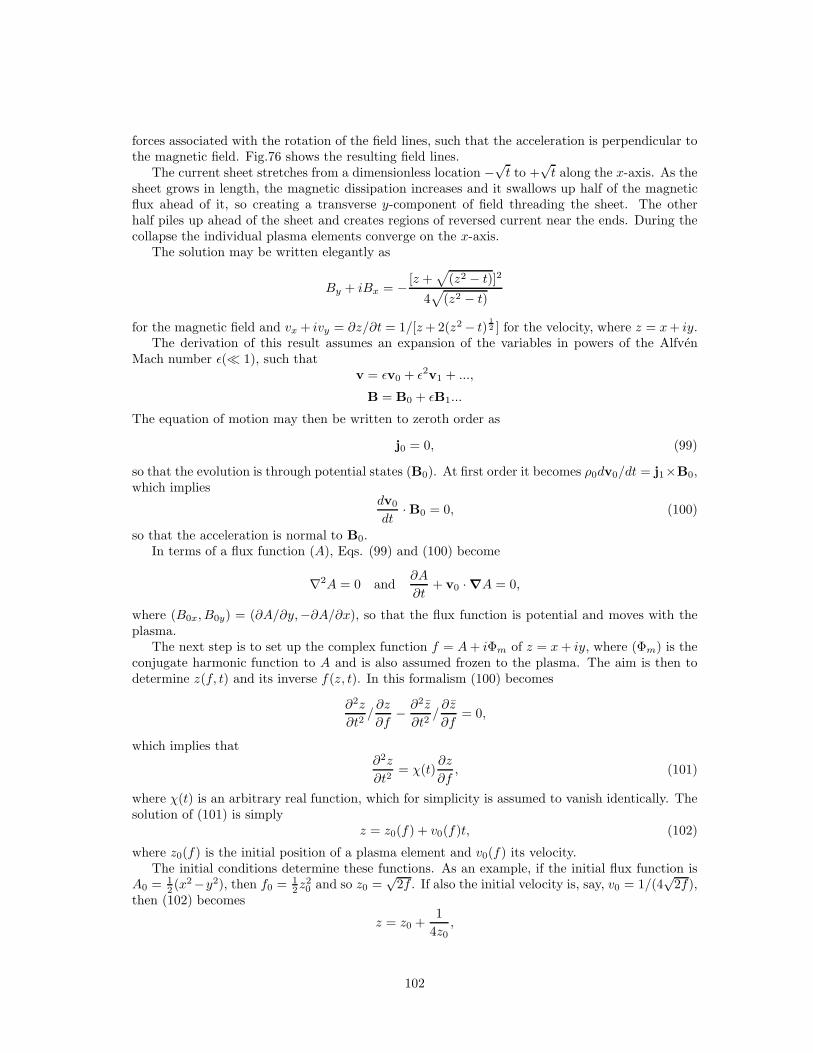
forces associated with the rotation of the field lines, such that the acceleration is perpendicular tothe magnetic field. Fig.76 shows the resulting field lines.

The current sheet stretches from a dimensionless location −√t to +

√t along the x-axis. As the

sheet grows in length, the magnetic dissipation increases and it swallows up half of the magneticflux ahead of it, so creating a transverse y-component of field threading the sheet. The otherhalf piles up ahead of the sheet and creates regions of reversed current near the ends. During thecollapse the individual plasma elements converge on the x-axis.

The solution may be written elegantly as

By + iBx = − [z +√

(z2 − t)]2

4√

(z2 − t)

for the magnetic field and vx + ivy = ∂z/∂t = 1/[z+ 2(z2 − t)12 ] for the velocity, where z = x+ iy.

The derivation of this result assumes an expansion of the variables in powers of the AlfvenMach number ǫ(≪ 1), such that

v = ǫv0 + ǫ2v1 + ...,

B = B0 + ǫB1...

The equation of motion may then be written to zeroth order as

j0 = 0, (99)

so that the evolution is through potential states (B0). At first order it becomes ρ0dv0/dt = j1×B0,which implies

dv0

dt· B0 = 0, (100)

so that the acceleration is normal to B0.In terms of a flux function (A), Eqs. (99) and (100) become

∇2A = 0 and∂A

∂t+ v0 · ∇A = 0,

where (B0x, B0y) = (∂A/∂y,−∂A/∂x), so that the flux function is potential and moves with theplasma.

The next step is to set up the complex function f = A+ iΦm of z = x+ iy, where (Φm) is theconjugate harmonic function to A and is also assumed frozen to the plasma. The aim is then todetermine z(f, t) and its inverse f(z, t). In this formalism (100) becomes

∂2z

∂t2/∂z

∂f− ∂2z

∂t2/∂z

∂f= 0,

which implies that∂2z

∂t2= χ(t)

∂z

∂f, (101)

where χ(t) is an arbitrary real function, which for simplicity is assumed to vanish identically. Thesolution of (101) is simply

z = z0(f) + v0(f)t, (102)

where z0(f) is the initial position of a plasma element and v0(f) its velocity.The initial conditions determine these functions. As an example, if the initial flux function is

A0 = 12 (x2−y2), then f0 = 1

2z20 and so z0 =

√2f . If also the initial velocity is, say, v0 = 1/(4

√2f),

then (102) becomes

z = z0 +1

4z0,

102

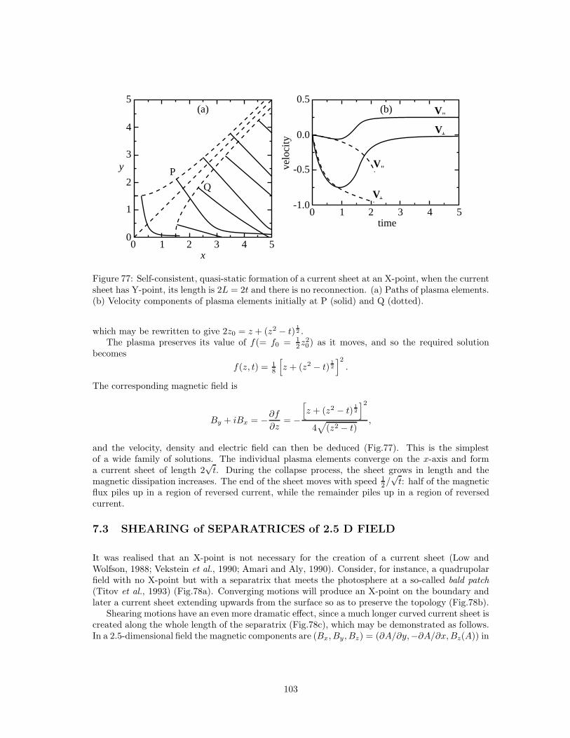
5

4

3

2

1

0.5

0.0

-0.5

-1.0

00 1 2 3

P

Q

(a)

x

(b)

4 5

0 1 2 3time

velo

city

y

4 5

V"

V"

V

V

Figure 77: Self-consistent, quasi-static formation of a current sheet at an X-point, when the currentsheet has Y-point, its length is 2L = 2t and there is no reconnection. (a) Paths of plasma elements.(b) Velocity components of plasma elements initially at P (solid) and Q (dotted).

which may be rewritten to give 2z0 = z + (z2 − t)12 .

The plasma preserves its value of f(= f0 = 12z

20) as it moves, and so the required solution

becomes

f(z, t) = 18

[

z + (z2 − t)12

]2

.

The corresponding magnetic field is

By + iBx = −∂f∂z

= −

[

z + (z2 − t)12

]2

4√

(z2 − t),

and the velocity, density and electric field can then be deduced (Fig.77). This is the simplestof a wide family of solutions. The individual plasma elements converge on the x-axis and forma current sheet of length 2

√t. During the collapse process, the sheet grows in length and the

magnetic dissipation increases. The end of the sheet moves with speed 12/

√t: half of the magnetic

flux piles up in a region of reversed current, while the remainder piles up in a region of reversedcurrent.

7.3 SHEARING of SEPARATRICES of 2.5 D FIELD

It was realised that an X-point is not necessary for the creation of a current sheet (Low andWolfson, 1988; Vekstein et al., 1990; Amari and Aly, 1990). Consider, for instance, a quadrupolarfield with no X-point but with a separatrix that meets the photosphere at a so-called bald patch(Titov et al., 1993) (Fig.78a). Converging motions will produce an X-point on the boundary andlater a current sheet extending upwards from the surface so as to preserve the topology (Fig.78b).

Shearing motions have an even more dramatic effect, since a much longer curved current sheet iscreated along the whole length of the separatrix (Fig.78c), which may be demonstrated as follows.In a 2.5-dimensional field the magnetic components are (Bx, By, Bz) = (∂A/∂y,−∂A/∂x,Bz(A)) in

103

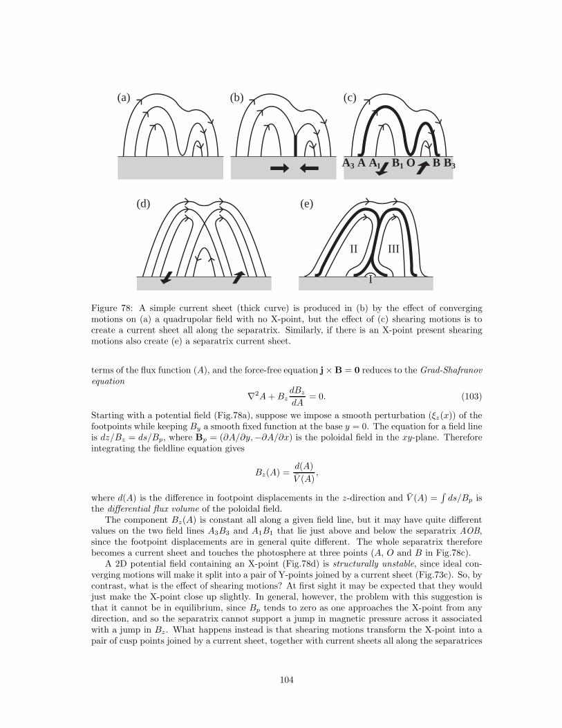
A3 A

(c)(b)(a)

(e)(d)

A1 B1 O B B3

I

IIIII

Figure 78: A simple current sheet (thick curve) is produced in (b) by the effect of convergingmotions on (a) a quadrupolar field with no X-point, but the effect of (c) shearing motions is tocreate a current sheet all along the separatrix. Similarly, if there is an X-point present shearingmotions also create (e) a separatrix current sheet.

terms of the flux function (A), and the force-free equation j × B = 0 reduces to the Grad-Shafranovequation

∇2A+BzdBz

dA= 0. (103)

Starting with a potential field (Fig.78a), suppose we impose a smooth perturbation (ξz(x)) of thefootpoints while keeping By a smooth fixed function at the base y = 0. The equation for a field lineis dz/Bz = ds/Bp, where Bp = (∂A/∂y,−∂A/∂x) is the poloidal field in the xy-plane. Thereforeintegrating the fieldline equation gives

Bz(A) =d(A)

V (A),

where d(A) is the difference in footpoint displacements in the z-direction and V (A) =∫ds/Bp is

the differential flux volume of the poloidal field.The component Bz(A) is constant all along a given field line, but it may have quite different

values on the two field lines A3B3 and A1B1 that lie just above and below the separatrix AOB,since the footpoint displacements are in general quite different. The whole separatrix thereforebecomes a current sheet and touches the photosphere at three points (A, O and B in Fig.78c).

A 2D potential field containing an X-point (Fig.78d) is structurally unstable, since ideal con-verging motions will make it split into a pair of Y-points joined by a current sheet (Fig.73c). So, bycontrast, what is the effect of shearing motions? At first sight it may be expected that they wouldjust make the X-point close up slightly. In general, however, the problem with this suggestion isthat it cannot be in equilibrium, since Bp tends to zero as one approaches the X-point from anydirection, and so the separatrix cannot support a jump in magnetic pressure across it associatedwith a jump in Bz. What happens instead is that shearing motions transform the X-point into apair of cusp points joined by a current sheet, together with current sheets all along the separatrices

104

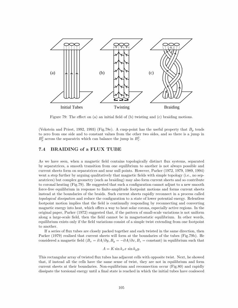
Initial Tubes

(a) (b) (c)

Twisting Braiding

Figure 79: The effect on (a) an initial field of (b) twisting and (c) braiding motions.

(Vekstein and Priest, 1992, 1993) (Fig.78e). A cusp-point has the useful property that Bp tendsto zero from one side and to constant values from the other two sides, and so there is a jump inB2

p across the separatrix which can balance the jump in B2z .

7.4 BRAIDING of a FLUX TUBE

As we have seen, when a magnetic field contains topologically distinct flux systems, separatedby separatrices, a smooth transition from one equilibrium to another is not always possible andcurrent sheets form on separatrices and near null points. However, Parker (1972, 1979, 1989, 1994)went a step further by arguing qualitatively that magnetic fields with simple topology (i.e., no sep-aratrices) but complex geometry (such as braiding) may also form current sheets and so contributeto coronal heating (Fig.79). He suggested that such a configuration cannot adjust to a new smoothforce-free equilibrium in response to finite-amplitude footpoint motions and forms current sheetsinstead at the boundaries of the braids. Such current sheets rapidly reconnect in a process calledtopological dissipation and reduce the configuration to a state of lower potential energy. Relentlessfootpoint motion implies that the field is continually responding by reconnecting and convertingmagnetic energy into heat, which offers a way to heat solar corona, especially active regions. In theoriginal paper, Parker (1972) suggested that, if the pattern of small-scale variations is not uniformalong a large-scale field, then the field cannot be in magnetostatic equilibrium. In other words,equilibrium exists only if the field variations consist of a simple twist extending from one footpointto another.

If a series of flux tubes are closely packed together and each twisted in the same direction, thenParker (1979) realised that current sheets will form at the boundaries of the tubes (Fig.79b). Heconsidered a magnetic field (Bx = ∂A/∂y,By = −∂A/∂x,Bz = constant) in equilibrium such that

A = K sin kxx sin kyy.

This rectangular array of twisted flux tubes has adjacent cells with opposite twist. Next, he showedthat, if instead all the cells have the same sense of twist, they are not in equilibrium and formcurrent sheets at their boundaries. Non-equilibrium and reconnection occur (Fig.80) and rapidlydissipate the torsional energy until a final state is reached in which the initial tubes have coalesced

105

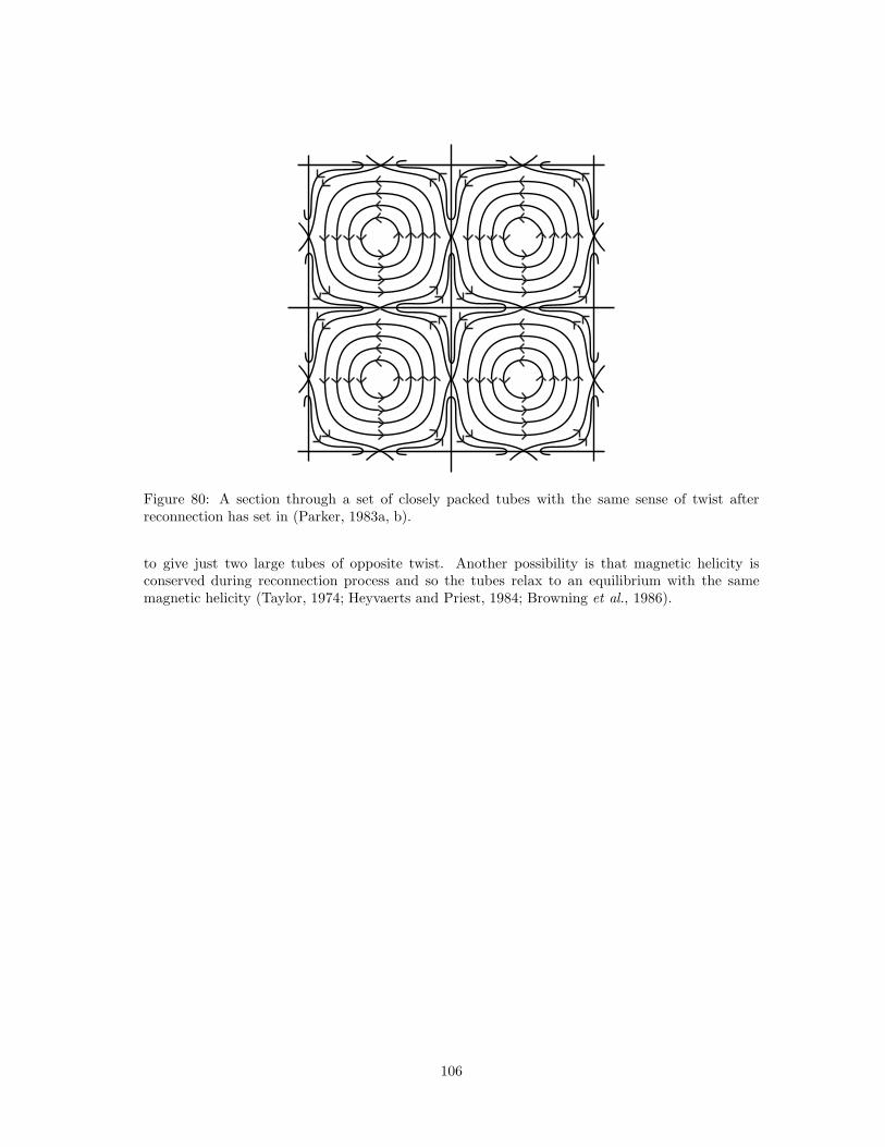
Figure 80: A section through a set of closely packed tubes with the same sense of twist afterreconnection has set in (Parker, 1983a, b).

to give just two large tubes of opposite twist. Another possibility is that magnetic helicity isconserved during reconnection process and so the tubes relax to an equilibrium with the samemagnetic helicity (Taylor, 1974; Heyvaerts and Priest, 1984; Browning et al., 1986).

106

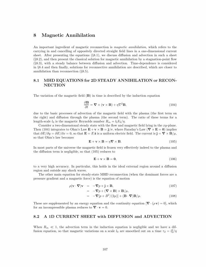
8 Magnetic Annihilation

An important ingredient of magnetic reconnection is magnetic annihilation, which refers to thecarrying in and cancelling of oppositely directed straight field lines in a one-dimensional currentsheet. After presenting the equations (§8.1), we discuss diffusion and advection in such a sheet(§8.2), and then present the classical solution for magnetic annihilation by a stagnation-point flow(§8.3), with a steady balance between diffusion and advection. Time-dependence is consideredin §8.4 and then finally, solutions for reconnective annihilation are described, which are closer toannihilation than reconnection (§8.5).

8.1 MHD EQUATIONS for 2D STEADY ANNIHILATION or RECON-NECTION

The variation of the magnetic field (B) in time is described by the induction equation

∂B

∂t= ∇ × (v × B) + η∇2B, (104)

due to the basic processes of advection of the magnetic field with the plasma (the first term onthe right) and diffusion through the plasma (the second term). The ratio of these terms for alength-scale l0 is the magnetic Reynolds number Rm = l0V0/η.

Consider a two-dimensional steady state with the flow and magnetic field lying in the xy-plane.Then (104) integrates to Ohm’s Law E +v × B = j/σ, where Faraday’s Law (∇ × E = 0) impliesthat ∂E/∂y = ∂E/∂x = 0, so that E = E z is a uniform electric field. The current is j = ∇ × B/µ,so that Ohm’s law becomes

E + v × B = η∇ × B. (105)

In most parts of the universe the magnetic field is frozen very effectively indeed to the plasma andthe diffusion term is negligible, so that (105) reduces to

E + v × B = 0, (106)

to a very high accuracy. In particular, this holds in the ideal external region around a diffusionregion and outside any shock waves.

The other main equation for steady-state MHD reconnection (when the dominant forces are apressure gradient and a magnetic force) is the equation of motion

ρ(v · ∇)v = −∇p+ j× B, (107)

= −∇p+ (∇ × B) × B/µ,

= −∇[p+B2/(2µ)] + (B · ∇)B/µ. (108)

These are supplemented by an energy equation and the continuity equation [∇ · (ρv) = 0], whichfor an incompressible plasma reduces to ∇ · v = 0.

8.2 A 1D CURRENT SHEET with DIFFUSION and ADVECTION

When Rm ≪ 1, the advection term in the induction equation is negligible and we have a dif-fusion equation, so that magnetic variations on a scale l0 are smoothed out on a time τd = l20/η

107

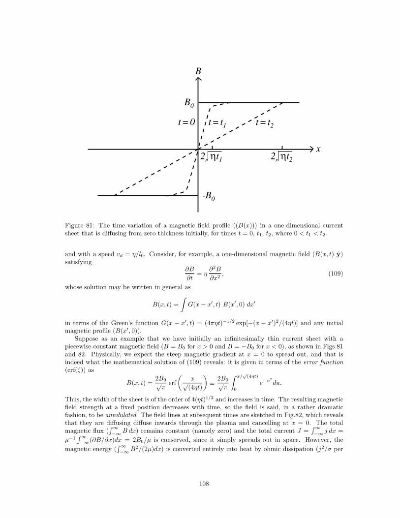
2 ηt2

x

B

B0

-B0

t = t1t = 0 t = t2

2 ηt1

Figure 81: The time-variation of a magnetic field profile ((B(x))) in a one-dimensional currentsheet that is diffusing from zero thickness initially, for times t = 0, t1, t2, where 0 < t1 < t2.

and with a speed vd = η/l0. Consider, for example, a one-dimensional magnetic field (B(x, t) y)satisfying

∂B

∂t= η

∂2B

∂x2, (109)

whose solution may be written in general as

B(x, t) =

∫

G(x − x′, t) B(x′, 0) dx′

in terms of the Green’s function G(x − x′, t) = (4πηt)−1/2 exp[−(x − x′)2/(4ηt)] and any initialmagnetic profile (B(x′, 0)).

Suppose as an example that we have initially an infinitesimally thin current sheet with apiecewise-constant magnetic field (B = B0 for x > 0 and B = −B0 for x < 0), as shown in Figs.81and 82. Physically, we expect the steep magnetic gradient at x = 0 to spread out, and that isindeed what the mathematical solution of (109) reveals: it is given in terms of the error function(erf(ζ)) as

B(x, t) =2B0√π

erf

(x√

(4ηt)

)

≡ 2B0√π

∫ x/√

(4ηt)

0

e−u2

du.

Thus, the width of the sheet is of the order of 4(ηt)1/2 and increases in time. The resulting magneticfield strength at a fixed position decreases with time, so the field is said, in a rather dramaticfashion, to be annihilated. The field lines at subsequent times are sketched in Fig.82, which revealsthat they are diffusing diffuse inwards through the plasma and cancelling at x = 0. The totalmagnetic flux (

∫∞−∞B dx) remains constant (namely zero) and the total current J =

∫∞−∞ j dx =

µ−1∫∞−∞(∂B/∂x)dx = 2B0/µ is conserved, since it simply spreads out in space. However, the

magnetic energy (∫∞−∞B2/(2µ)dx) is converted entirely into heat by ohmic dissipation (j2/σ per

108

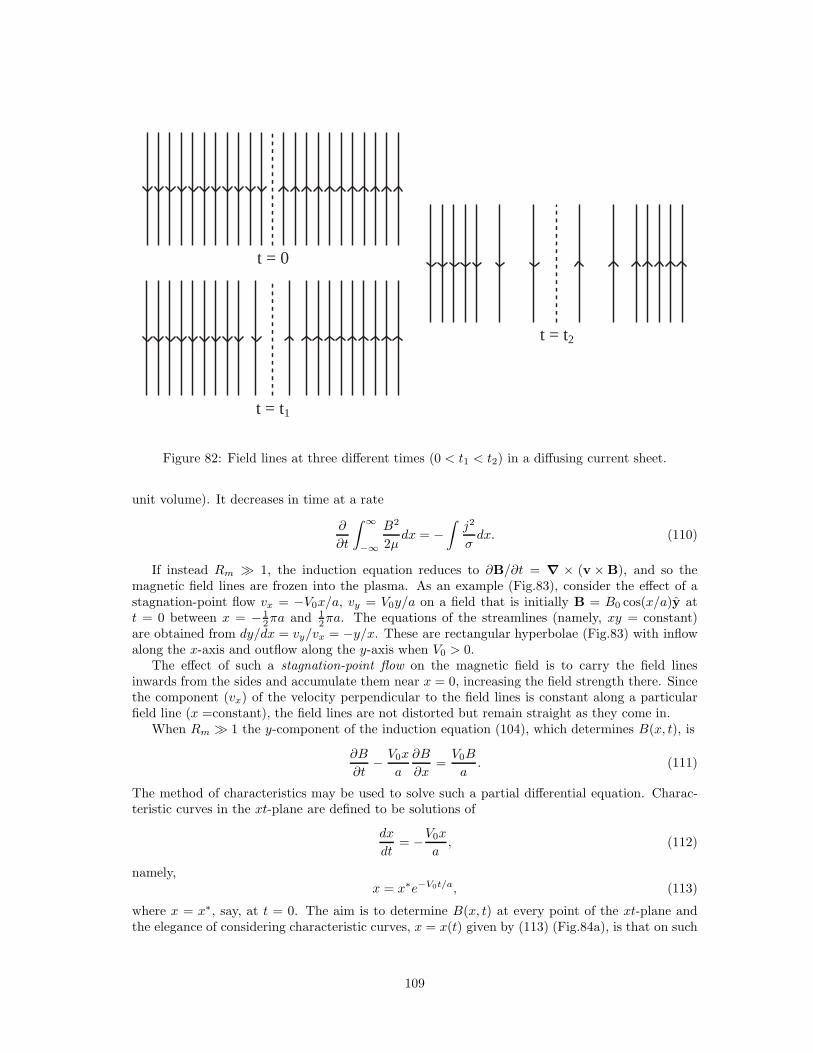
t = t1

t = t2

t = 0

Figure 82: Field lines at three different times (0 < t1 < t2) in a diffusing current sheet.

unit volume). It decreases in time at a rate

∂

∂t

∫ ∞

−∞

B2

2µdx = −

∫j2

σdx. (110)

If instead Rm ≫ 1, the induction equation reduces to ∂B/∂t = ∇ × (v × B), and so themagnetic field lines are frozen into the plasma. As an example (Fig.83), consider the effect of astagnation-point flow vx = −V0x/a, vy = V0y/a on a field that is initially B = B0 cos(x/a)y att = 0 between x = − 1

2πa and 12πa. The equations of the streamlines (namely, xy = constant)

are obtained from dy/dx = vy/vx = −y/x. These are rectangular hyperbolae (Fig.83) with inflowalong the x-axis and outflow along the y-axis when V0 > 0.

The effect of such a stagnation-point flow on the magnetic field is to carry the field linesinwards from the sides and accumulate them near x = 0, increasing the field strength there. Sincethe component (vx) of the velocity perpendicular to the field lines is constant along a particularfield line (x =constant), the field lines are not distorted but remain straight as they come in.

When Rm ≫ 1 the y-component of the induction equation (104), which determines B(x, t), is

∂B

∂t− V0x

a

∂B

∂x=V0B

a. (111)

The method of characteristics may be used to solve such a partial differential equation. Charac-teristic curves in the xt-plane are defined to be solutions of

dx

dt= −V0x

a, (112)

namely,x = x∗e−V0t/a, (113)

where x = x∗, say, at t = 0. The aim is to determine B(x, t) at every point of the xt-plane andthe elegance of considering characteristic curves, x = x(t) given by (113) (Fig.84a), is that on such

109

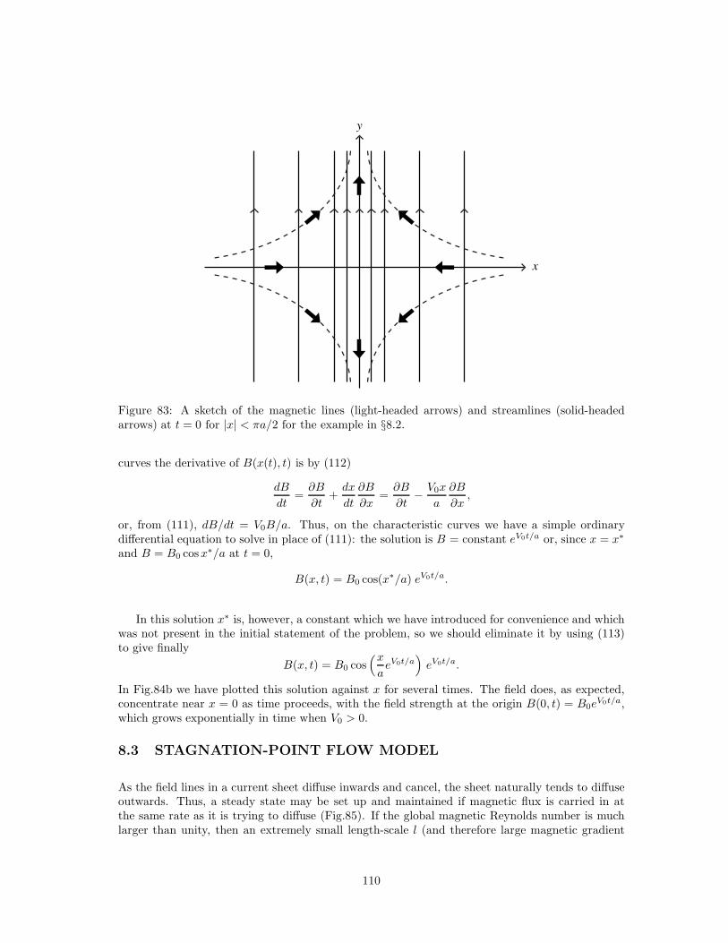
x

y

Figure 83: A sketch of the magnetic lines (light-headed arrows) and streamlines (solid-headedarrows) at t = 0 for |x| < πa/2 for the example in §8.2.

curves the derivative of B(x(t), t) is by (112)

dB

dt=∂B

∂t+dx

dt

∂B

∂x=∂B

∂t− V0x

a

∂B

∂x,

or, from (111), dB/dt = V0B/a. Thus, on the characteristic curves we have a simple ordinarydifferential equation to solve in place of (111): the solution is B = constant eV0t/a or, since x = x∗

and B = B0 cosx∗/a at t = 0,

B(x, t) = B0 cos(x∗/a) eV0t/a.

In this solution x∗ is, however, a constant which we have introduced for convenience and whichwas not present in the initial statement of the problem, so we should eliminate it by using (113)to give finally

B(x, t) = B0 cos(x

aeV0t/a

)

eV0t/a.

In Fig.84b we have plotted this solution against x for several times. The field does, as expected,concentrate near x = 0 as time proceeds, with the field strength at the origin B(0, t) = B0e

V0t/a,which grows exponentially in time when V0 > 0.

8.3 STAGNATION-POINT FLOW MODEL

As the field lines in a current sheet diffuse inwards and cancel, the sheet naturally tends to diffuseoutwards. Thus, a steady state may be set up and maintained if magnetic flux is carried in atthe same rate as it is trying to diffuse (Fig.85). If the global magnetic Reynolds number is muchlarger than unity, then an extremely small length-scale l (and therefore large magnetic gradient

110

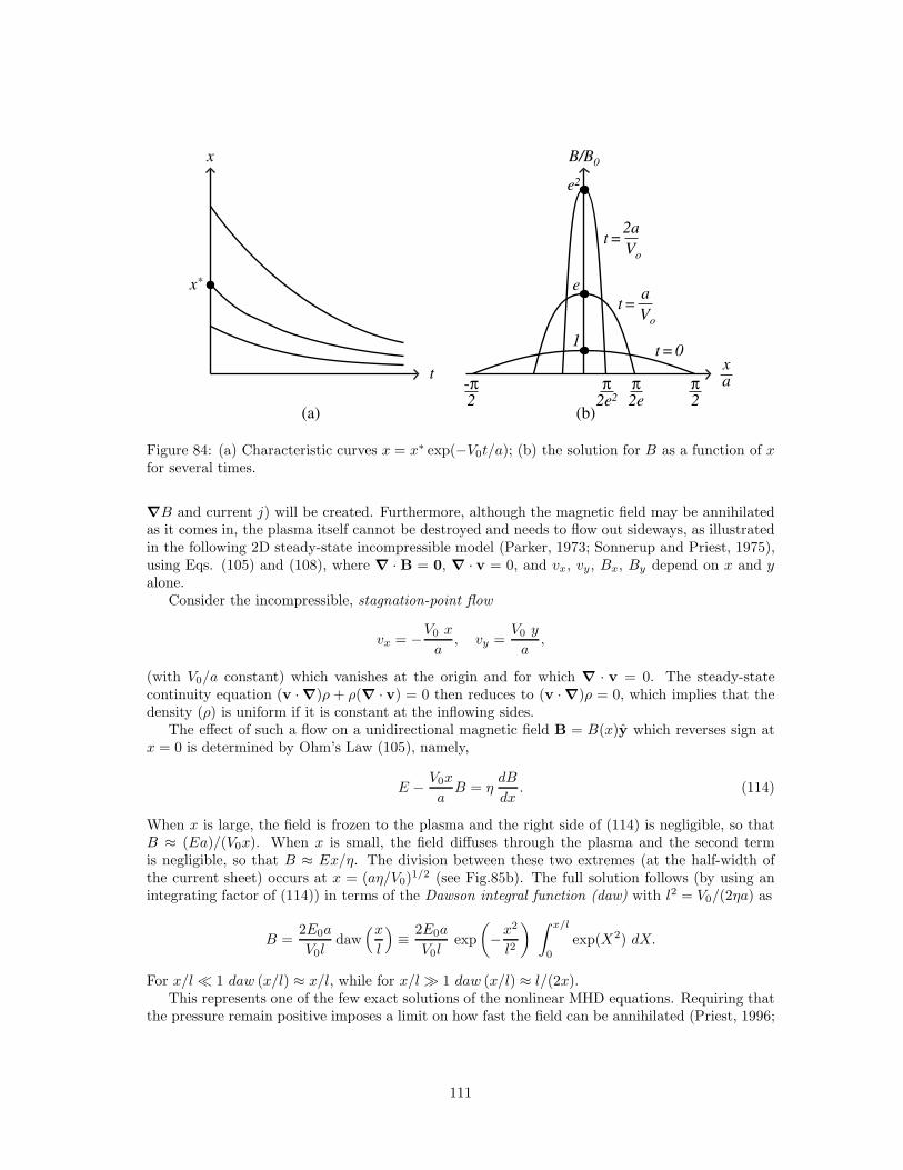
t

t = 0

2a t =

Vo

x*

x

(a)

x a

(b)

B/B0

e2

e

1

π 2

π 2e

π 2e2

-π 2

a t =

Vo

Figure 84: (a) Characteristic curves x = x∗ exp(−V0t/a); (b) the solution for B as a function of xfor several times.

∇B and current j) will be created. Furthermore, although the magnetic field may be annihilatedas it comes in, the plasma itself cannot be destroyed and needs to flow out sideways, as illustratedin the following 2D steady-state incompressible model (Parker, 1973; Sonnerup and Priest, 1975),using Eqs. (105) and (108), where ∇ · B = 0, ∇ · v = 0, and vx, vy, Bx, By depend on x and yalone.

Consider the incompressible, stagnation-point flow

vx = −V0 x

a, vy =

V0 y

a,

(with V0/a constant) which vanishes at the origin and for which ∇ · v = 0. The steady-statecontinuity equation (v · ∇)ρ + ρ(∇ · v) = 0 then reduces to (v · ∇)ρ = 0, which implies that thedensity (ρ) is uniform if it is constant at the inflowing sides.

The effect of such a flow on a unidirectional magnetic field B = B(x)y which reverses sign atx = 0 is determined by Ohm’s Law (105), namely,

E − V0x

aB = η

dB

dx. (114)

When x is large, the field is frozen to the plasma and the right side of (114) is negligible, so thatB ≈ (Ea)/(V0x). When x is small, the field diffuses through the plasma and the second termis negligible, so that B ≈ Ex/η. The division between these two extremes (at the half-width ofthe current sheet) occurs at x = (aη/V0)

1/2 (see Fig.85b). The full solution follows (by using anintegrating factor of (114)) in terms of the Dawson integral function (daw) with l2 = V0/(2ηa) as

B =2E0a

V0ldaw

(x

l

)

≡ 2E0a

V0lexp

(

−x2

l2

) ∫ x/l

0

exp(X2) dX.

For x/l ≪ 1 daw (x/l) ≈ x/l, while for x/l ≫ 1 daw (x/l) ≈ l/(2x).This represents one of the few exact solutions of the nonlinear MHD equations. Requiring that

the pressure remain positive imposes a limit on how fast the field can be annihilated (Priest, 1996;

111

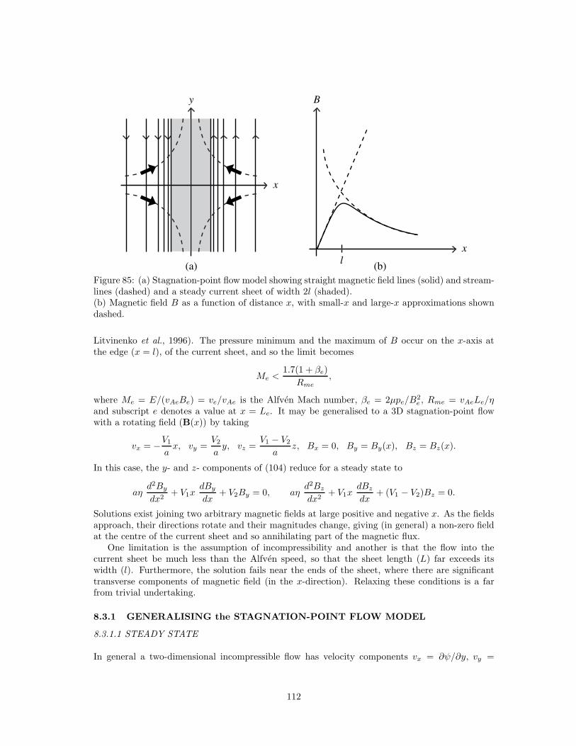
x

y

(a)

x

B

l(b)

Figure 85: (a) Stagnation-point flow model showing straight magnetic field lines (solid) and stream-lines (dashed) and a steady current sheet of width 2l (shaded).(b) Magnetic field B as a function of distance x, with small-x and large-x approximations showndashed.

Litvinenko et al., 1996). The pressure minimum and the maximum of B occur on the x-axis atthe edge (x = l), of the current sheet, and so the limit becomes

Me <1.7(1 + βe)

Rme,

where Me = E/(vAeBe) = ve/vAe is the Alfven Mach number, βe = 2µpe/B2e , Rme = vAeLe/η

and subscript e denotes a value at x = Le. It may be generalised to a 3D stagnation-point flowwith a rotating field (B(x)) by taking

vx = −V1

ax, vy =

V2

ay, vz =

V1 − V2

az, Bx = 0, By = By(x), Bz = Bz(x).

In this case, the y- and z- components of (104) reduce for a steady state to

aηd2By

dx2+ V1x

dBy

dx+ V2By = 0, aη

d2Bz

dx2+ V1x

dBz

dx+ (V1 − V2)Bz = 0.

Solutions exist joining two arbitrary magnetic fields at large positive and negative x. As the fieldsapproach, their directions rotate and their magnitudes change, giving (in general) a non-zero fieldat the centre of the current sheet and so annihilating part of the magnetic flux.

One limitation is the assumption of incompressibility and another is that the flow into thecurrent sheet be much less than the Alfven speed, so that the sheet length (L) far exceeds itswidth (l). Furthermore, the solution fails near the ends of the sheet, where there are significanttransverse components of magnetic field (in the x-direction). Relaxing these conditions is a farfrom trivial undertaking.

8.3.1 GENERALISING the STAGNATION-POINT FLOW MODEL

8.3.1.1 STEADY STATE

In general a two-dimensional incompressible flow has velocity components vx = ∂ψ/∂y, vy =

112

−∂ψ/∂x, written in terms of a stream function (ψ) so that ∇ · v = 0 automatically. The effect ofthis flow on a unidirectional field B(x)y is determined by Ohm’s Law (110), namely,

E +∂ψ

∂yB = η

dB

dx. (115)

Here B and dB/dx are functions of x alone and (E z) is uniform, so that ∂ψ/∂y is also a functionof x alone and therefore ψ = yf(x) + g(x). Eq.(115) becomes

E + fB = ηdB

dx, (116)

which determines the magnetic field (B(x)) if f(x) is known.Inclusion of a viscous force (ρν∇2v) (Besser et al., 1990; Phan and Sonnerup, 1990) in the

equation of motion turns its curl into

(v · ∇)ω = ν ∇2ω,

where the vorticity is ω z = ∇ × v. Substituting for ψ leads to

y(νf (4) + ff ′′′ − f ′f ′′) + (νg(4) + fg′′′ − g′f ′′) = 0. (117)

The expressions in brackets are functions of x alone, and so we need both

νf (4) + ff ′′′ − f ′f ′′ = 0 (118)

andνg(4) + fg′′′ − g′f ′′ = 0. (119)

f(x) is determined by (118) and four boundary conditions, while g(x) follows from (119): it isassociated with an inflow that is skewed about the x-axis.

§6.4.2 studied the simplest solution, namely, f(x) = x. More general solutions have been con-sidered by Gratton et al. (1988); Jardine et al. (1992) allowing for vorticity in an inflow carryingstraight, oppositely directed field lines towards a long thin vortex-current sheet with both viscousand magnetic boundary layers. The widths of the boundary layers adjust themselves to accom-modate different types and magnitudes of inflow. The effects of three-dimensional flows have beenincorporated (Jardine et al., 1993; Craig and Henton, 1995).

8.3.1.2 TIME-DEPENDENT FLOW

A time-dependent flow with stream function

ψ = yf(x, t) + g(x, t)

acting on a field B(x, t)y will satisfy the time-dependent equations of induction and motion. Then(116), (118), (119) generalise to the following system that determine B, f, g (Anderson and Priest,1993):

∂B

∂t=∂f

∂xB + f

∂B

∂x+ η

∂2B

∂x2,

∂3f

∂t∂x2= f

∂3f

∂x3− ∂f

∂x

∂2f

∂x2+ ν

∂4f

∂x4,

∂3g

∂t∂x2= f

∂3g

∂x3− ∂2f

∂x2∂g∂x+ ν

∂4g

∂x4.

113

Suppose that g ≡ 0 and f = U(t)x/L0, so that the last two equations are satisfied trivially andthe induction equation

∂B

∂t=UB

L0+Ux

L0

∂B

∂x+ η

∂2B

∂x2(120)

determines B(x, t) for the given flow

(vx, vy) = −U(t)

L0(x,−y). (121)

The equations ∇ · v = ∇ ·B = 0 are satisfied trivially and the equation of motion determines theplasma pressure as

p = constant − B2

2µ− ρU2

2L20

(x2 − y2) − ρ

2

U2

L20

(x2 + y2).

The solution of (120) on an infinite interval may be obtained by scaling away the constantsL0, η and the magnitude (V0) of U . Also the second term on the right may be transformed away bya change of independent variables from x and t to X = xg(t) and τ , where g and τ are determinedfor a given function U(t) by dg/dt = Ug, dτ/dt = g2. The result is that (120) simplifies to

∂B

∂τ= f(τ)B +

∂2B

∂X2, (122)

where f = U/g2. This may be solved by separation of variables to give

B(X, τ) =g

2√

(πτ)

∫ ∞

−∞B0(ξ)e

−(ξ−X)2/(4τ)dξ, (123)

which determines the time-evolution of an initial magnetic field B(X, 0) = B0(X). The solutiondescribes the effect on a unidirectional field (B y) of any time-modulated stagnation-point flow ofthe form (121). Anderson and Priest (1993) studied the solutions (121) with a variety of initialprofiles, values of the magnetic diffusivity (η) and flow amplitudes U(t).

8.4 TIME-DEPENDENT CURRENT SHEET

Consider now in more detail the behaviour of a purely one-dimensional current sheet with magneticfield B(x, t)y and plasma velocity v(x, t)x, satisfying an induction equation

∂B

∂t= − ∂

∂x(vB) + η

∂2B

∂x2. (124)

The flow couples this to the continuity equation

∂ρ

∂t+

∂

∂x(ρv) = 0 (125)

and to the equation of motion, which, for highly subsonic and sub-Alfvenic flow speeds, reduces tothe force balance

p+B2

2µ=Be(t)

2

2µ. (126)

Assume that the edge of the neutral sheet (x = ±l(t), say) is at zero plasma pressure and at amagnetic pressure of Be(t)

2/(2µ). This is completed by an energy equation, but for simplicity weadopt the polytropic law p = Kρa, with constant K and a.

114

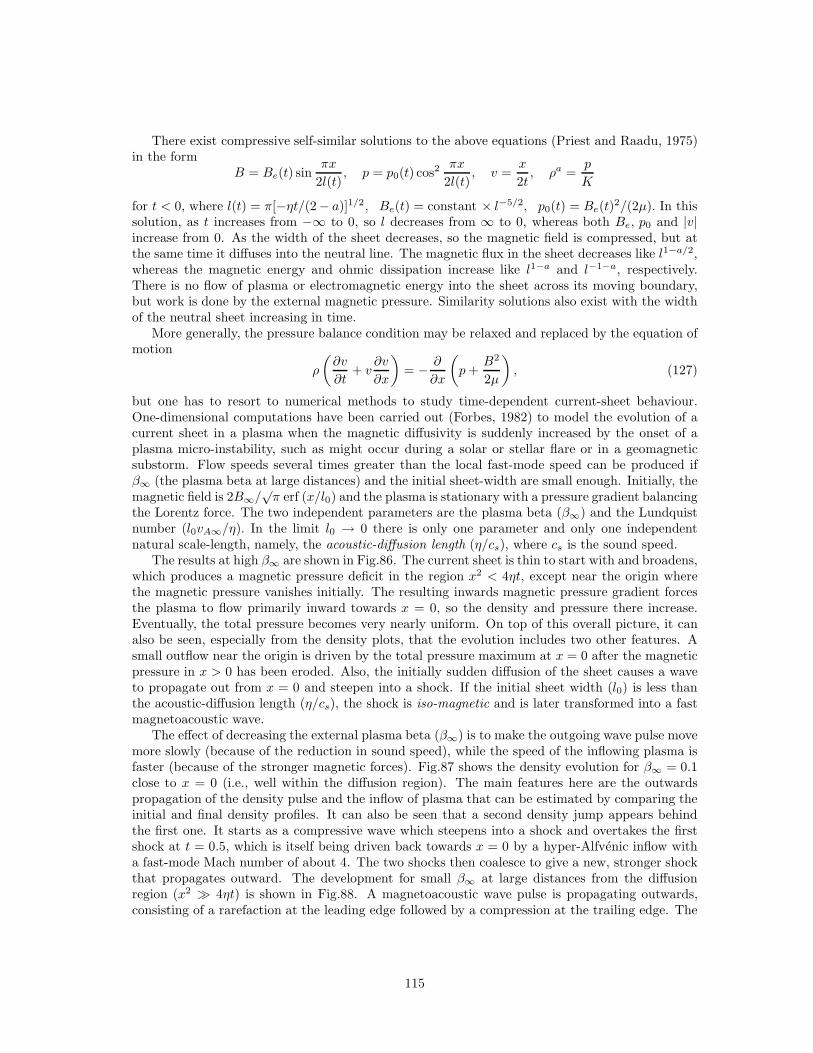
There exist compressive self-similar solutions to the above equations (Priest and Raadu, 1975)in the form

B = Be(t) sinπx

2l(t), p = p0(t) cos2

πx

2l(t), v =

x

2t, ρa =

p

K

for t < 0, where l(t) = π[−ηt/(2− a)]1/2, Be(t) = constant × l−5/2, p0(t) = Be(t)2/(2µ). In this

solution, as t increases from −∞ to 0, so l decreases from ∞ to 0, whereas both Be, p0 and |v|increase from 0. As the width of the sheet decreases, so the magnetic field is compressed, but atthe same time it diffuses into the neutral line. The magnetic flux in the sheet decreases like l1−a/2,whereas the magnetic energy and ohmic dissipation increase like l1−a and l−1−a, respectively.There is no flow of plasma or electromagnetic energy into the sheet across its moving boundary,but work is done by the external magnetic pressure. Similarity solutions also exist with the widthof the neutral sheet increasing in time.

More generally, the pressure balance condition may be relaxed and replaced by the equation ofmotion

ρ

(∂v

∂t+ v

∂v

∂x

)

= − ∂

∂x

(

p+B2

2µ

)

, (127)

but one has to resort to numerical methods to study time-dependent current-sheet behaviour.One-dimensional computations have been carried out (Forbes, 1982) to model the evolution of acurrent sheet in a plasma when the magnetic diffusivity is suddenly increased by the onset of aplasma micro-instability, such as might occur during a solar or stellar flare or in a geomagneticsubstorm. Flow speeds several times greater than the local fast-mode speed can be produced ifβ∞ (the plasma beta at large distances) and the initial sheet-width are small enough. Initially, themagnetic field is 2B∞/

√π erf (x/l0) and the plasma is stationary with a pressure gradient balancing

the Lorentz force. The two independent parameters are the plasma beta (β∞) and the Lundquistnumber (l0vA∞/η). In the limit l0 → 0 there is only one parameter and only one independentnatural scale-length, namely, the acoustic-diffusion length (η/cs), where cs is the sound speed.

The results at high β∞ are shown in Fig.86. The current sheet is thin to start with and broadens,which produces a magnetic pressure deficit in the region x2 < 4ηt, except near the origin wherethe magnetic pressure vanishes initially. The resulting inwards magnetic pressure gradient forcesthe plasma to flow primarily inward towards x = 0, so the density and pressure there increase.Eventually, the total pressure becomes very nearly uniform. On top of this overall picture, it canalso be seen, especially from the density plots, that the evolution includes two other features. Asmall outflow near the origin is driven by the total pressure maximum at x = 0 after the magneticpressure in x > 0 has been eroded. Also, the initially sudden diffusion of the sheet causes a waveto propagate out from x = 0 and steepen into a shock. If the initial sheet width (l0) is less thanthe acoustic-diffusion length (η/cs), the shock is iso-magnetic and is later transformed into a fastmagnetoacoustic wave.

The effect of decreasing the external plasma beta (β∞) is to make the outgoing wave pulse movemore slowly (because of the reduction in sound speed), while the speed of the inflowing plasma isfaster (because of the stronger magnetic forces). Fig.87 shows the density evolution for β∞ = 0.1close to x = 0 (i.e., well within the diffusion region). The main features here are the outwardspropagation of the density pulse and the inflow of plasma that can be estimated by comparing theinitial and final density profiles. It can also be seen that a second density jump appears behindthe first one. It starts as a compressive wave which steepens into a shock and overtakes the firstshock at t = 0.5, which is itself being driven back towards x = 0 by a hyper-Alfvenic inflow witha fast-mode Mach number of about 4. The two shocks then coalesce to give a new, stronger shockthat propagates outward. The development for small β∞ at large distances from the diffusionregion (x2 ≫ 4ηt) is shown in Fig.88. A magnetoacoustic wave pulse is propagating outwards,consisting of a rarefaction at the leading edge followed by a compression at the trailing edge. The

115

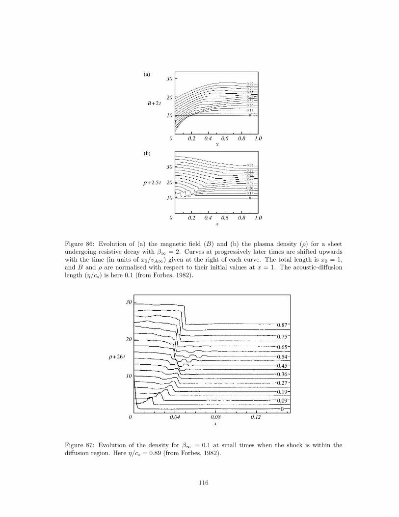
Figure 86: Evolution of (a) the magnetic field (B) and (b) the plasma density (ρ) for a sheetundergoing resistive decay with β∞ = 2. Curves at progressively later times are shifted upwardswith the time (in units of x0/vA∞) given at the right of each curve. The total length is x0 = 1,and B and ρ are normalised with respect to their initial values at x = 1. The acoustic-diffusionlength (η/cs) is here 0.1 (from Forbes, 1982).

Figure 87: Evolution of the density for β∞ = 0.1 at small times when the shock is within thediffusion region. Here η/cs = 0.89 (from Forbes, 1982).

116

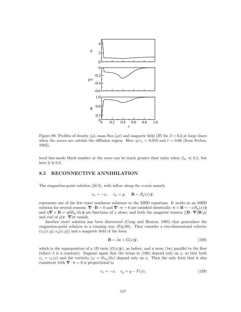
4

2

0

0

B

ρv

ρ

00 0.2 0.4 x

0.6 0.8 1.0

0.2

0.6

1.0

-0.2

-0.4

-0.6

Figure 88: Profiles of density (ρ), mass flux (ρv) and magnetic field (B) for β = 0.2 at large timeswhen the waves are outside the diffusion region. Here η/cs = 0.016 and t = 0.66 (from Forbes,1982).

local fast-mode Mach number at the wave can be much greater than unity when β∞ ≪ 0.1, buthere it is 0.3.

8.5 RECONNECTIVE ANNIHILATION

The stagnation-point solution (§8.3), with inflow along the x-axis namely

vx = −x, vy = y, B = By(x) y,

represents one of the few exact nonlinear solutions to the MHD equations. It works as an MHDsolution for several reasons: ∇ ·B = 0 and ∇ · v = 0 are satisfied identically; v × B = −xBy(x) zand η∇ × B = ηdBy/dx z are functions of x alone; and both the magnetic tension [(B · ∇)B/µ]and curl of ρ(v · ∇)v vanish.

Another exact solution has been discovered (Craig and Henton, 1995) that generalises thestagnation-point solution in a cunning way (Fig.89). They consider a two-dimensional velocity(vx(x, y), vy(x, y)) and a magnetic field of the form

B = λv +G(x)y, (128)

which is the superposition of a 1D term (G(x)y), as before, and a term (λv) parallel to the flow(where λ is a constant). Suppose again that the terms in (108) depend only on x, so that bothvx = vx(x) and the vorticity (ω = ∂vy/∂x) depend only on x. Then the only form that is alsoconsistent with ∇ · v = 0 is proportional to

vx = −x, vy = y − F (x), (129)

117

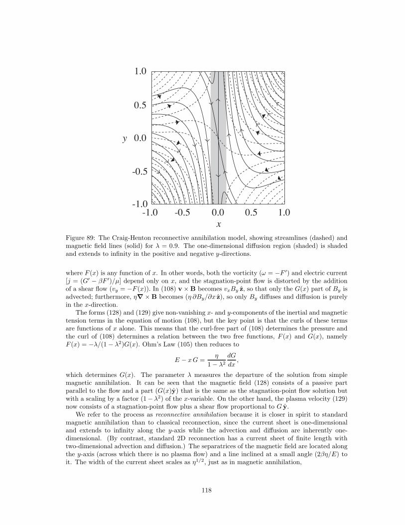
y 0.0

0.0-1.0 -0.5 0.5 1.0

1.0

0.5

-0.5

-1.0

x

Figure 89: The Craig-Henton reconnective annihilation model, showing streamlines (dashed) andmagnetic field lines (solid) for λ = 0.9. The one-dimensional diffusion region (shaded) is shadedand extends to infinity in the positive and negative y-directions.

where F (x) is any function of x. In other words, both the vorticity (ω = −F ′) and electric current[j = (G′ − βF ′)/µ] depend only on x, and the stagnation-point flow is distorted by the additionof a shear flow (vy = −F (x)). In (108) v × B becomes vxBy z, so that only the G(x) part of By isadvected; furthermore, η∇ × B becomes (η ∂By/∂x z), so only By diffuses and diffusion is purelyin the x-direction.

The forms (128) and (129) give non-vanishing x- and y-components of the inertial and magnetictension terms in the equation of motion (108), but the key point is that the curls of these termsare functions of x alone. This means that the curl-free part of (108) determines the pressure andthe curl of (108) determines a relation between the two free functions, F (x) and G(x), namelyF (x) = −λ/(1 − λ2)G(x). Ohm’s Law (105) then reduces to

E − xG =η

1 − λ2

dG

dx,

which determines G(x). The parameter λ measures the departure of the solution from simplemagnetic annihilation. It can be seen that the magnetic field (128) consists of a passive partparallel to the flow and a part (G(x)y) that is the same as the stagnation-point flow solution butwith a scaling by a factor (1−λ2) of the x-variable. On the other hand, the plasma velocity (129)now consists of a stagnation-point flow plus a shear flow proportional to G y.

We refer to the process as reconnective annihilation because it is closer in spirit to standardmagnetic annihilation than to classical reconnection, since the current sheet is one-dimensionaland extends to infinity along the y-axis while the advection and diffusion are inherently one-dimensional. (By contrast, standard 2D reconnection has a current sheet of finite length withtwo-dimensional advection and diffusion.) The separatrices of the magnetic field are located alongthe y-axis (across which there is no plasma flow) and a line inclined at a small angle (2βη/E) toit. The width of the current sheet scales as η1/2, just as in magnetic annihilation,

118

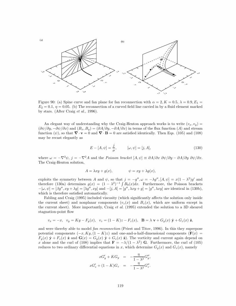
Figure 90: (a) Spine curve and fan plane for fan reconnection with α = 2,K = 0.5, λ = 0.9, E1 =E2 = 0.1, η = 0.05. (b) The reconnection of a curved field line carried in by a fluid element markedby stars. (After Craig et al., 1996).

An elegant way of understanding why the Craig-Henton approach works is to write (vx, vy) =(∂ψ/∂y,−∂ψ/∂x) and (Bx, By) = (∂A/∂y,−∂A/∂x) in terms of the flux function (A) and streamfunction (ψ), so that ∇ · v = 0 and ∇ ·B = 0 are satisfied identically. Then Eqs. (105) and (108)may be recast elegantly as

E − [A,ψ] =j

σ, [ω, ψ] = [j, A], (130)

where ω = −∇2ψ, j = −∇2A and the Poisson bracket [A,ψ] ≡ ∂A/∂x ∂ψ/∂y − ∂A/∂y ∂ψ/∂x.The Craig-Henton solution,

A = λxy + g(x), ψ = xy + λg(x),

exploits the symmetry between A and ψ, so that j = −g′′, ω = −λg′′, [A,ψ] = x(1 − λ2)g′ andtherefore (130a) determines g(x) = (1 − λ2)−1

∫B0(x)dx. Furthermore, the Poisson brackets

−[ω, ψ] = [βg′′, xy+ λg] = [λg′′, xy] and −[j, A] = [g′′, λxy+ g] = [g′′, λxy] are identical in (130b),which is therefore satisfied automatically.

Fabling and Craig (1995) included viscosity (which significantly affects the solution only insidethe current sheet) and nonplanar components (vz(x) and Bz(x), which are uniform except inthe current sheet). More importantly, Craig et al. (1995) extended the solution to a 3D shearedstagnation-point flow

vx = −x, vy = Ky − Fy(x), vz = (1 −K)z − Fz(x), B = λ v +Gy(x) y +Gz(x) z,

and were thereby able to model fan reconnection (Priest and Titov, 1996). In this they superposepotential components (−x,Ky, (1 − K)z) and one-and-a-half-dimensional components (F(x) =Fy(x) y + Fz(x) z and G(x) = Gy(x) y + Gz(x) z). The vorticity and current again depend onx alone and the curl of (108) implies that F = −λ/(1 − λ2) G. Furthermore, the curl of (105)reduces to two ordinary differential equations in x, which determine Gy(x) and Gz(x), namely

xG′y +KGy = − η

1 − λ2G′′

y ,

xG′z + (1 −K)Gz = − η

1 − λ2G′′

z .

119

In Fig.90b we see that curved field lines are advected by the flow during fan reconnection acrossthe spine into the current sheet at x = 0.

Craig and Fabling (1996) have also discovered solutions for spine reconnection in cylindricalpolars (R, φ, z). in the form

vz = −2z + λf(R) cosmφ, vR = R,

Bz = −2λz + f(R) cosmφ, BR = R,

where f(R) satisfies

f +1

2Rf ′ =

η

1 − λ2

(

f ′′ +f ′

R− f

r2

)

.

Flow across the fan produces a cylindrical diffusion region of radius√η with a linearly increasing

field surrounding the spine, outside which the field falls off as R−2.

120

9 Steady 2D Reconnection Models

In many applications reconnection is quasi-steady in the sense that it changes its structure slowlyover many Alfven travel times. Furthermore, nonlinear steady reconnection is technically easierto study than nonlinear time-dependent reconnection, so the emphasis in the early theoreticaldevelopments was on understanding the nature of steady 2D reconnection. In particular, slowSweet-Parker reconnection (§9.1) was followed by fast Petschek reconnection (§9.2) and by otherfamilies of fast reconnection that depend on the initial and boundary conditions (§9.3).

9.1 SWEET-PARKER MECHANISM

Many of the the early researchers tried to understand the nature of magnetic field line break-ing and to determine the rate at which reconnection occurs – i.e., the speed with which field linesare carried into the reconnection site. Much of the focus was on the steady-state process, sinceit is simpler to analyse than time-varying reconnection and also the earliest motivation, namely,that the main phase of a large solar flare is a quasi-steady-state or slowly-varying energy releaseprocess for many hundreds of Alfven travel-times (with a superimposed time-modulation).

In the original model, Sweet (1958a,b) and Parker (1957, 1963) considered a steady diffusionlayer occupying the whole boundary between two opposing magnetic fields. Its length (L) istherefore the global external length-scale (Le), and the reconnection rate (ve) is just the speedwith which field lines are entering the diffusion region. The basic equations are Ohm’s law (105)and the equation of motion (108) with mass continuity (∇ · (ρv) = 0).

By equating the first and third terms in (105), we may obtain the time-scale for magneticdissipation as

τd = L2/η = 10−9L2 T 3/2,

which is vast in most applications (e.g., 1014 s for a typical global solar coronal length-scale (L =107m) and temperature (T = 106K)). Thus, in order to release magnetic energy (in a solar flareor a coronal heating event), one needs to create extremely small length-scales in sheets or filamentsand therefore very large magnetic gradients and electric currents. Ways of accomplishing this are:creating thin shock waves; developing instabilities such as the tearing mode (§10.1); developingstrong turbulence; and forming current sheets at X-points in the way we describe below.

9.1.1 The BASIC SWEET-PARKER MODEL (1958)

The idea of Sweet and Parker was to consider a simple diffusion region of length 2L and width 2l,say, lying between oppositely directed magnetic fields (Fig.91), for which an order-of-magnitudeanalysis may be conducted as follows. First of all, for a steady state, magnetic field of strength Bi

is carried into the diffusion layer at the same speed (vi) as it is trying to diffuse outward, so that

vi =η

l. (131)

This relation may be derived directly from Ohm’s Law (105) in the following way. The value of theelectric field, which is uniform for a steady two-dimensional state, may be found by evaluating (105)at the inflow to the diffusion region where the current vanishes, namely, E = viBi. However, atthe centre (N) of the diffusion region, where the magnetic field vanishes, (105) becomes E = jN/σ,while Ampere’s Law (j = ∇ × B/µ) implies that the current at N is roughly jN = Bi/(µ l).Eliminating E and jN then gives the result (105) that we are seeking.

121

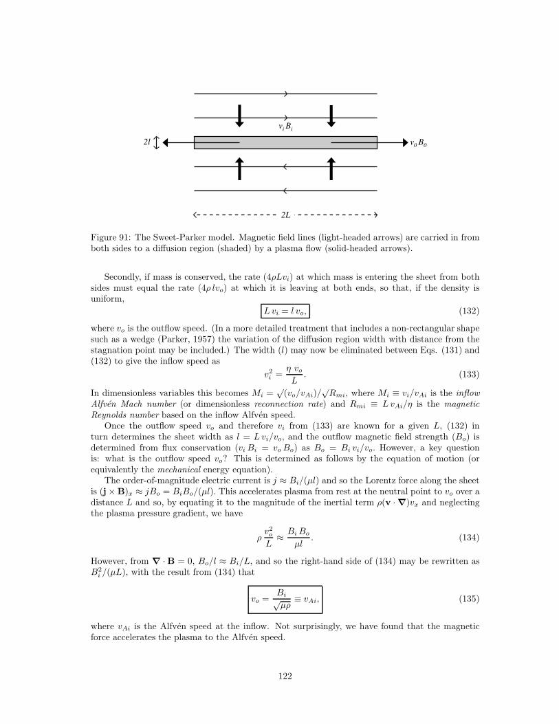
v0 B0

vi Bi

2l

2L

Figure 91: The Sweet-Parker model. Magnetic field lines (light-headed arrows) are carried in fromboth sides to a diffusion region (shaded) by a plasma flow (solid-headed arrows).

Secondly, if mass is conserved, the rate (4ρLvi) at which mass is entering the sheet from bothsides must equal the rate (4ρ lvo) at which it is leaving at both ends, so that, if the density isuniform,

Lvi = l vo, (132)

where vo is the outflow speed. (In a more detailed treatment that includes a non-rectangular shapesuch as a wedge (Parker, 1957) the variation of the diffusion region width with distance from thestagnation point may be included.) The width (l) may now be eliminated between Eqs. (131) and(132) to give the inflow speed as

v2i =

η vo

L. (133)

In dimensionless variables this becomes Mi =√

(vo/vAi)/√Rmi, where Mi ≡ vi/vAi is the inflow

Alfven Mach number (or dimensionless reconnection rate) and Rmi ≡ LvAi/η is the magneticReynolds number based on the inflow Alfven speed.

Once the outflow speed vo and therefore vi from (133) are known for a given L, (132) inturn determines the sheet width as l = Lvi/vo, and the outflow magnetic field strength (Bo) isdetermined from flux conservation (vi Bi = voBo) as Bo = Bi vi/vo. However, a key questionis: what is the outflow speed vo? This is determined as follows by the equation of motion (orequivalently the mechanical energy equation).

The order-of-magnitude electric current is j ≈ Bi/(µl) and so the Lorentz force along the sheetis (j × B)x ≈ jBo = BiBo/(µl). This accelerates plasma from rest at the neutral point to vo over adistance L and so, by equating it to the magnitude of the inertial term ρ(v · ∇)vx and neglectingthe plasma pressure gradient, we have

ρv2

o

L≈ BiBo

µl. (134)

However, from ∇ · B = 0, Bo/l ≈ Bi/L, and so the right-hand side of (134) may be rewritten asB2

i /(µL), with the result from (134) that

vo =Bi√µρ

≡ vAi, (135)

where vAi is the Alfven speed at the inflow. Not surprisingly, we have found that the magneticforce accelerates the plasma to the Alfven speed.

122

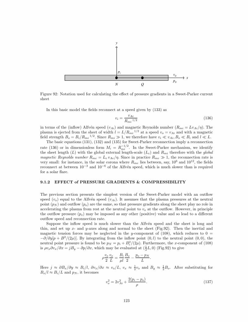
y

xv0

p0QN

pi

Figure 92: Notation used for calculating the effect of pressure gradients in a Sweet-Parker currentsheet

In this basic model the fields reconnect at a speed given by (133) as

vi =vAi

Rmi1/2

(136)

in terms of the (inflow) Alfven speed (vAi) and magnetic Reynolds number (Rmi = LvAi/η). Theplasma is ejected from the sheet of width l = L/Rmi

1/2 at a speed vo = vAi and with a magneticfield strength Bo = Bi/Rmi

1/2. Since Rmi ≫ 1, we therefore have vi ≪ vAi, Bo ≪ Bi and l ≪ L.The basic equations (131), (132) and (135) for Sweet-Parker reconnection imply a reconnection

rate (136) or in dimensionless form Mi = R−1/2mi . In the Sweet-Parker mechanism, we identify

the sheet length (L) with the global external length-scale (Le) and Rmi therefore with the globalmagnetic Reynolds number Rme = Le vAe/η. Since in practice Rme ≫ 1, the reconnection rate isvery small: for instance, in the solar corona where Rme lies between, say, 106 and 1012, the fieldsreconnect at between 10−3 and 10−6 of the Alfven speed, which is much slower than is requiredfor a solar flare.

9.1.2 EFFECT of PRESSURE GRADIENTS & COMPRESSIBILITY

The previous section presents the simplest version of the Sweet-Parker model with an outflowspeed (vo) equal to the Alfven speed (vAi). It assumes that the plasma pressures at the neutralpoint (pN ) and outflow (po) are the same, so that pressure gradients along the sheet play no role inaccelerating the plasma from rest at the neutral point to vo at the outflow. However, in principlethe outflow pressure (po) may be imposed as any other (positive) value and so lead to a differentoutflow speed and reconnection rate.

Suppose the inflow speed is much slower than the Alfven speed and the sheet is long andthin, and set up x- and y-axes along and normal to the sheet (Fig.92). Then the inertial andmagnetic tension forces may be neglected in the y-component of (108), which reduces to 0 =−∂/∂y[p + B2/(2µ)]. By integrating from the inflow point (0, l) to the neutral point (0, 0), theneutral point pressure is found to be pN = pi + B2

i /(2µ). Furthermore, the x-component of (108)is ρvx∂vx/∂x = jBy − ∂p/∂x, which may be evaluated at (1

2L, 0) (Fig.92) to give

ρvo

2

vo

L=Bi

µl

Bo

2− po − pN

L.

Here j ≈ ∂Bx/∂y ≈ Bi/l, ∂vx/∂x ≈ vo/L, vx ≈ 12vo and By ≈ 1

2Bo. After substituting forBo/l ≈ Bi/L and pN , it becomes

v2o = 2v2

Ai +2(pi − po)

ρ. (137)

123

This is the required generalisation of the usual Sweet-Parker result (135). The outflow speednow depends on the imposed values of pi and po, and so the reconnection rate (133) may be written,after substituting for vo/vAi from (137), as

Mi =21/4

(1 + 1

2βi(1 − po/pi))1/4

√Rmi

.

Thus, it is the values of beta (βi = 2µpi/B2i ) and the pressure ratio (po/pi) which determine the

departure from the Sweet-Parker rate (Mi = 1/√Rmi). If po = pN , we recover the Sweet-Parker

result (vo = vAi), whereas if po = pi, then vo =√

2 vAi.When the outflow pressure is small enough (po < pN), then vo > vAi and the reconnection

rate is enhanced (Mi > 1/√Rmi). When the outflow pressure is large enough (po > pN ), the

outflow is slowed (vo < vi) and the reconnection rate is lowered (Mi < 1/√Rmi). If the outflow

pressure is smaller than the inflow pressure (po < pi), then vo >√

2vAi, whereas if it is larger thenvo <

√2vAi. (Another possibility considered by Parker is that the outflow is spread out into a fan;

for example, if it spreads out into a 90◦ wedge (±45◦), when p0 = pi the velocity component inthe x-direction along the sheet is v0x = vAi.)

The above equations are only order of magnitude estimates. Surprisingly, a more accuratetreatment has not yet been accomplished properly. It would need a solution throughout thediffusion layer, a determination of the shape of its boundary and an integration along the boundaryof the conservation equations, taking full account of the variation of the magnitude and inclinationsof the velocity and magnetic field.

The original Sweet-Parker model did not include compressibility and so the density was regardedas uniform. Suppose for example we have a simple current sheet with input and output densitiesρi and ρo, respectively, and acceleration by the magnetic force. The equation of mass continuity(132) is then modified to

ρi Lvi = ρo l vo,

while the momentum balance (134) is altered to ρov2o/L = BiBo/(µl), so that the inflow (133) and

ouflow (135) speeds become

vi =

(ρo

ρi

) 12 (η vo

L

) 12

and vo =Bi√µρo

= vAi

(ρi

ρo

) 12

.

Thus, the outflow speed is a hybrid Alfven speed based on the inflow magnetic field and outflowdensity. We have therefore deduced that, when ρo > ρi, compressibility slows down the outflow bya factor (ρi/ρo)

12 .

The resulting reconnection rate (vi = (ρo/ρi)14 (ηvAi/L)

12 ) is enhanced by a factor (ρo/ρi)

14

when ρo > ρi, since (for a given set of inflow conditions) the width of the sheet is decreased by thecompression. The density ratio ρo/ρi = (po/pi)(Ti/To) is given in terms of the pressure ratio andthe temperature ratio, which is in turn determined by the heat energy equation.

9.1.3 ENERGETICS

Consider a long and thin Sweet-Parker diffusion layer (l ≪ L) with vi ≪ vAi. The rate of inflow ofelectromagnetic energy is the Poynting flux (E× H per unit area), which, after writing E = viBi,becomes E Bi L/µ = vi B

2i L/µ. Therefore, the ratio of the inflows of kinetic to electromagnetic

energy isinflowK.E.

inflowE.M.=

12ρv

2i

B2i /µ

=v2

i

2v2Ai

.

124

By (136) this is much smaller than unity, so most of the inflowing energy is magnetic.Conservation of flux gives voBo = viBi, and so Bo ≪ Bi. Also, the outflow of electromagnetic

energy is EBol/µ, which is much less than the inflow of electromagnetic energy (EBiL/µ) sinceBo ≪ Bi and l ≪ L. However, the ratio of outflowing kinetic to inflowing magnetic energy is

outflowK.E.

inflowE.M.=

12ρv

2o (vol)

viB2i L/µ

=12v

2o

v2Ai

= 12 .

Thus, half of the inflowing magnetic energy is converted to kinetic energy and the rest to thermalenergy. In other words, the effect of the reconnection is to create hot fast streams of plasma witha rough equipartition between flow and thermal energy.

The equations of electromagnetic energy and mechanical energy are secondary, since they maybe derived from the equations of MHD and Maxwell. They provide no extra information aboutthe primary variables, but they do determine the energy partition. Thus, for example, the electro-magnetic energy equation is

−∇ · (E× H) = j2/σ + v · j × B,

which implies that the inflow of electromagnetic energy into a volume produces ohmic heat andwork done by the Lorentz force. By integrating over the diffusion region it can be shown that halfof the inflowing electromagnetic energy goes into ohmic heating and half into the work done bythe magnetic force (which in turn goes into kinetic energy when the pressure gradient along thesheet is negligible).

The way to derive the equation of mechanical energy in the incompressible limit is to take thescalar product of the equation of motion with v and use ∇ · v = 0, so that

∇ ·(

12ρv

2v)

= v · j × B− v · ∇p,

which implies that a change of kinetic energy is produced by the work done by j × B and −∇p.Next, rewriting v · ∇p as ∇ · (pv) since ∇ · v = 0 in the present model and integrating over thediffusion region, we find

∫

S

(12ρv

2v + pv)· dS =

∫

V

(v · j × B) dV,

and so the work done by the magnetic force term on the right of this equation is a combination ofthe change in kinetic energy and the net work done by pressure on the surface.

9.2 PETSCHEK MECHANISM

Petschek made the ground-breaking suggestion that the Sweet-Parker diffusion region be limited toa small segment (of length L ≪ Le) of the boundary between opposing fields. Since the diffusionregion is shorter, it is also thinner and so the diffusion and reconnection can take place faster.Petschek also considered the nature of the external flow outside the diffusion region. He suggestedthat slow-mode MHD shock waves propagate from the diffusion region, which acts as a kind ofobstacle in the flow, which is supersonic relative to the slow-mode wave speed across the magneticfield, since the latter vanishes. Petschek found that the maximum rate of reconnection dependsonly weakly on the magnetic Reynolds number and is typically a tenth or a hundredth of the Alfvenspeed.

To distinguish the outer region from the Sweet-Parker region, we shall denote the flow speed andmagnetic field at large distances (Le) upstream of the X-point by ve and Be. The properties of fastreconnection models depend on two dimensionless parameters, namely the external reconnectionrate (Me = ve/vAe) and the external, or global, magnetic Reynolds number (Rme = LevAe/η).

125

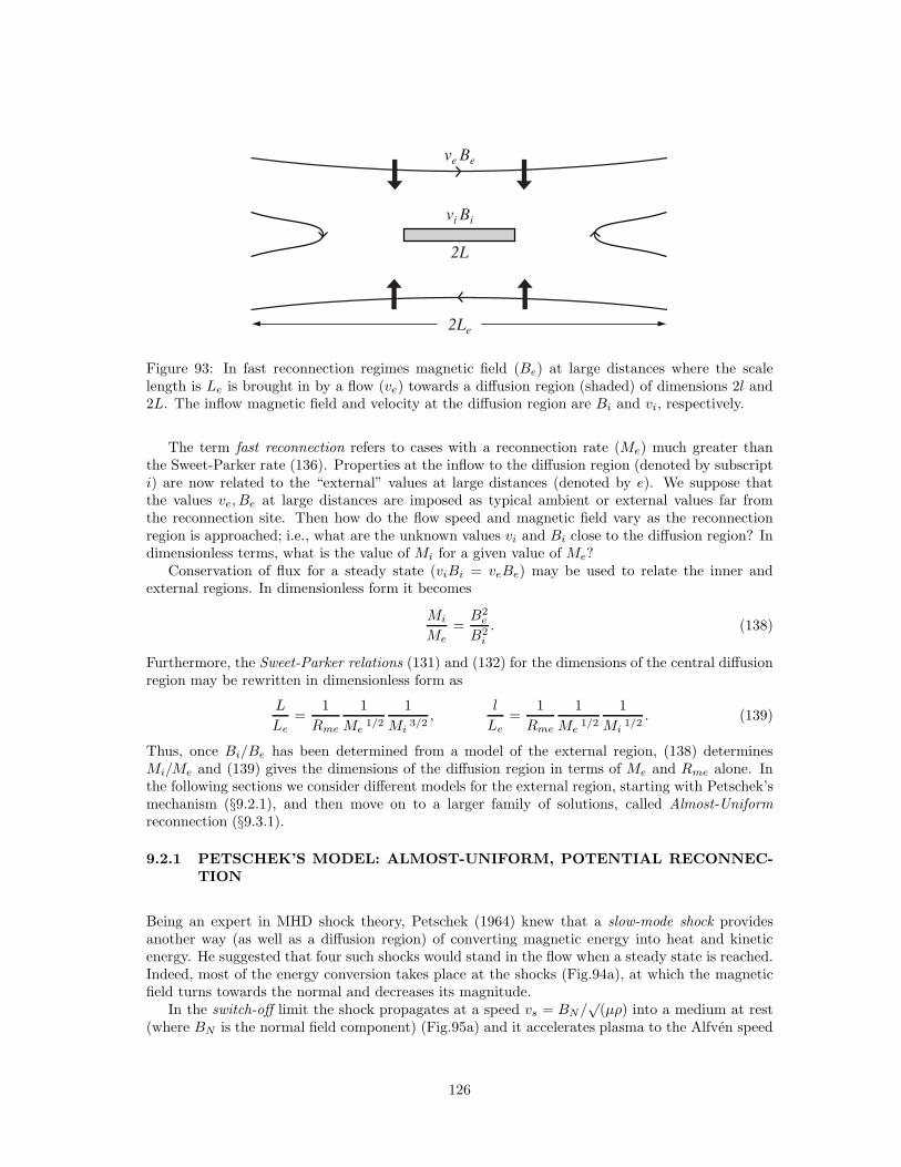
ve Be

vi Bi

2Le

2L

Figure 93: In fast reconnection regimes magnetic field (Be) at large distances where the scalelength is Le is brought in by a flow (ve) towards a diffusion region (shaded) of dimensions 2l and2L. The inflow magnetic field and velocity at the diffusion region are Bi and vi, respectively.

The term fast reconnection refers to cases with a reconnection rate (Me) much greater thanthe Sweet-Parker rate (136). Properties at the inflow to the diffusion region (denoted by subscripti) are now related to the “external” values at large distances (denoted by e). We suppose thatthe values ve, Be at large distances are imposed as typical ambient or external values far fromthe reconnection site. Then how do the flow speed and magnetic field vary as the reconnectionregion is approached; i.e., what are the unknown values vi and Bi close to the diffusion region? Indimensionless terms, what is the value of Mi for a given value of Me?

Conservation of flux for a steady state (viBi = veBe) may be used to relate the inner andexternal regions. In dimensionless form it becomes

Mi

Me=B2

e

B2i

. (138)

Furthermore, the Sweet-Parker relations (131) and (132) for the dimensions of the central diffusionregion may be rewritten in dimensionless form as

L

Le=

1

Rme

1

Me1/2

1

Mi3/2

,l

Le=

1

Rme

1

Me1/2

1

Mi1/2

. (139)

Thus, once Bi/Be has been determined from a model of the external region, (138) determinesMi/Me and (139) gives the dimensions of the diffusion region in terms of Me and Rme alone. Inthe following sections we consider different models for the external region, starting with Petschek’smechanism (§9.2.1), and then move on to a larger family of solutions, called Almost-Uniformreconnection (§9.3.1).

9.2.1 PETSCHEK’S MODEL: ALMOST-UNIFORM, POTENTIAL RECONNEC-TION

Being an expert in MHD shock theory, Petschek (1964) knew that a slow-mode shock providesanother way (as well as a diffusion region) of converting magnetic energy into heat and kineticenergy. He suggested that four such shocks would stand in the flow when a steady state is reached.Indeed, most of the energy conversion takes place at the shocks (Fig.94a), at which the magneticfield turns towards the normal and decreases its magnitude.

In the switch-off limit the shock propagates at a speed vs = BN/√

(µρ) into a medium at rest(where BN is the normal field component) (Fig.95a) and it accelerates plasma to the Alfven speed

126

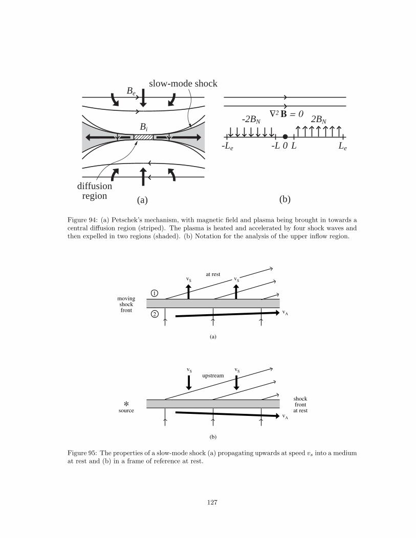
Bi

0

2BN-2BN

L-L Le-Le

(a) (b)

slow-mode shock

diffusionregion

Be

Figure 94: (a) Petschek’s mechanism, with magnetic field and plasma being brought in towards acentral diffusion region (striped). The plasma is heated and accelerated by four shock waves andthen expelled in two regions (shaded). (b) Notation for the analysis of the upper inflow region.

vA

vS vS

(b)

upstream

shock front at rest

* source

vA

vS vS

(a)

at rest

moving shock front

1

2

Figure 95: The properties of a slow-mode shock (a) propagating upwards at speed vs into a mediumat rest and (b) in a frame of reference at rest.

127

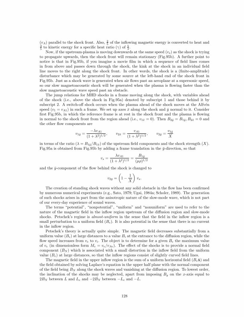
(vA) parallel to the shock front. Also, 25 of the inflowing magnetic energy is converted to heat and

35 to kinetic energy for a specific heat ratio (γ) of 5

3 .Now, if the upstream-plasma is moving downwards at the same speed (vs) as the shock is trying

to propagate upwards, then the shock front will remain stationary (Fig.95b). A further point tonotice is that in Fig.95b, if you imagine a movie film in which a sequence of field lines comesin from above and passes down through the shock, the kink at the shock in an individual fieldline moves to the right along the shock front. In other words, the shock is a (finite-amplitude)disturbance which may be generated by some source at the left-hand end of the shock front inFig.95b. Just as a shock wave is generated when air flows past an aeroplane at a supersonic speed,so our slow magnetoacoustic shock will be generated when the plasma is flowing faster than theslow magnetoacoustic wave speed past an obstacle.

The jump relations for MHD shocks in a frame moving along the shock, with variables aheadof the shock (i.e., above the shock in Fig.95a) denoted by subscript 1 and those behind it bysubscript 2. A switch-off shock occurs when the plasma ahead of the shock moves at the Alfvenspeed (v1 = vA1) in such a frame. We set up axes x along the shock and y normal to it. Considerfirst Fig.95b, in which the reference frame is at rest in the shock front and the plasma is flowingin normal to the shock front from the region ahead (i.e., v1x = 0). Then B2y = B1y, B2x = 0 andthe other flow components are

v1y =−λvA1

(1 + λ2)1/2, v2x =

vA1

(1 + λ2)1/2, v2y =

v1y

X

in terms of the ratio (λ = B1y/B1x) of the upstream field components and the shock strength (X).Fig.95a is obtained from Fig.95b by adding a frame translation in the y-direction, so that

vs =λvA1

(1 + λ2)1/2=

B1y

(µρ)1/2

and the y-component of the flow behind the shock is changed to

v2y =

(

1 − 1

X

)

vs.

The creation of standing shock waves without any solid obstacle in the flow has been confirmedby numerous numerical experiments (e.g., Sato, 1979; Ugai, 1984a; Scholer, 1989). The generationof such shocks arises in part from the anisotropic nature of the slow-mode wave, which is not partof our every-day experience of sound waves.

The terms “potential”, “nonpotential”, “uniform” and “nonuniform” are used to refer to thenature of the magnetic field in the inflow region upstream of the diffusion region and slow-modeshocks. Petschek’s regime is almost-uniform in the sense that the field in the inflow region is asmall perturbation to a uniform field (Be). It is also potential in the sense that there is no currentin the inflow region.

Petschek’s theory is actually quite simple. The magnetic field decreases substantially from auniform value (Be) at large distances to a value Bi at the entrance to the diffusion region, while theflow speed increases from ve to vi. The object is to determine for a given Be the maximum valueof ve (in dimensionless form Me = ve/vAe). The effect of the shocks is to provide a normal fieldcomponent (BN ) which is associated with a small distortion in the inflow field from the uniformvalue (Be) at large distances, so that the inflow regions consist of slightly curved field lines.

The magnetic field in the upper inflow region is the sum of a uniform horizontal field (Bex) andthe field obtained by solving Laplace’s equation in the upper half plane with the normal componentof the field being BN along the shock waves and vanishing at the diffusion region. To lowest order,the inclination of the shocks may be neglected, apart from imposing By on the x-axis equal to2BN between L and Le and −2BN between −Le and −L.

128

The normal component on the x-axis may be regarded as being due to a continuous seriesof poles. If each pole produces a field m/r at distance r, then the flux produced in the upperhalf-plane by that pole will be πm; but, if the pole occupies a length dx of the x-axis, the fluxis also 2BNdx, so that m = 2BNdx/π. Then, integrating along the x-axis gives the field at thediffusion-region inflow as the sum of (Be) and

1

π

∫ −L

−Le

2BN

xdx− 1

π

∫ Le

L

2BN

xdx or Bi = Be −

4BN

πlog

Le

L. (140)

Remembering that, in the switch-off limit, slow shocks travel at the Alfven speed based on thenormal field, BN/

√(µρ) = ve, we can rewrite (140b) as

Bi = Be

(

1 − 4Me

πlog

Le

L

)

, (141)

which is the expression for Bi that we have been seeking.Using Me ≪ 1 and Bi ≈ Be, the scalings (139) reduce to L/Le ≈ 1/(RmeM

2e ) and l/Le ≈

1/(RmeMe), implying that the dimensions of the central region decrease as the magnetic Reynoldsnumber (Rme) or reconnection rate (Me) increase. Petschek suggested that the mechanism chokesitself off when Bi becomes too small, and so, by putting Bi = 1

2Be in (141), he estimated amaximum reconnection rate (M∗

e ) of

M∗e ≈ π

8 logRme. (142)

This lies in practice between 0.1 and 0.01, and so is much faster than Sweet-Parker.Although in 1D annihilation (§8) it is possible to have a formal linking of the external (ideal) and

internal (diffusive) regions, this is not feasible for Petschek’s much more complex 2D magnetic field.Instead, the matching is done in an integral or approximate sense, using the order-of-magnitudeSweet-Parker relations. This is entirely reasonable and is shown by numerical experiments to workwell when the resistivity is enhanced in the diffusion region, as is expected in many applications.

For twenty years, it was thought that Petschek had completely solved the problem of fastreconnection, until in the 1980’s a new generation of reconnection solutions was discovered (§9.3),with Petschek’s mechanism as a special case, and high-resolution numerical experiments wereundertaken.

9.2.2 IMPLICATIONS and EARLY EXTENSIONS

Whereas in the Sweet-Parker model L = Le and so Eq.(132) determines vi, a key to Petschek’smechanism is that Eq.(132) merely determines L once vi has been deduced from external condi-tions. Thus, the diffusion region responds to the driving, and the Sweet-Parker relations (134)and (132) simply determine the dimensions (l and L) of the diffusion region, which shrinks as η

becomes smaller. These relations imply that, as vi varies between vA/R1/2me and vA, so the length

of the diffusion region decreases from a maximum value of Le to a minimum of l. Moreover, thereconnection rate can vary over a wide range, depending on the boundary conditions rather thanthe magnetic diffusivity (η): if the plasma is free to escape, reconnection can be rapid (at themaximum rate); whereas, if there is a pressure build-up downstream, the reconnection may bethrottled to an intermediate rate (Jardine and Priest, 1988a; Priest and Lee, 1990).

Petschek’s mechanism may be modified by allowing the external field to decrease along theshocks away from the diffusion region. This makes the field lines between pairs of shocks curve in

129

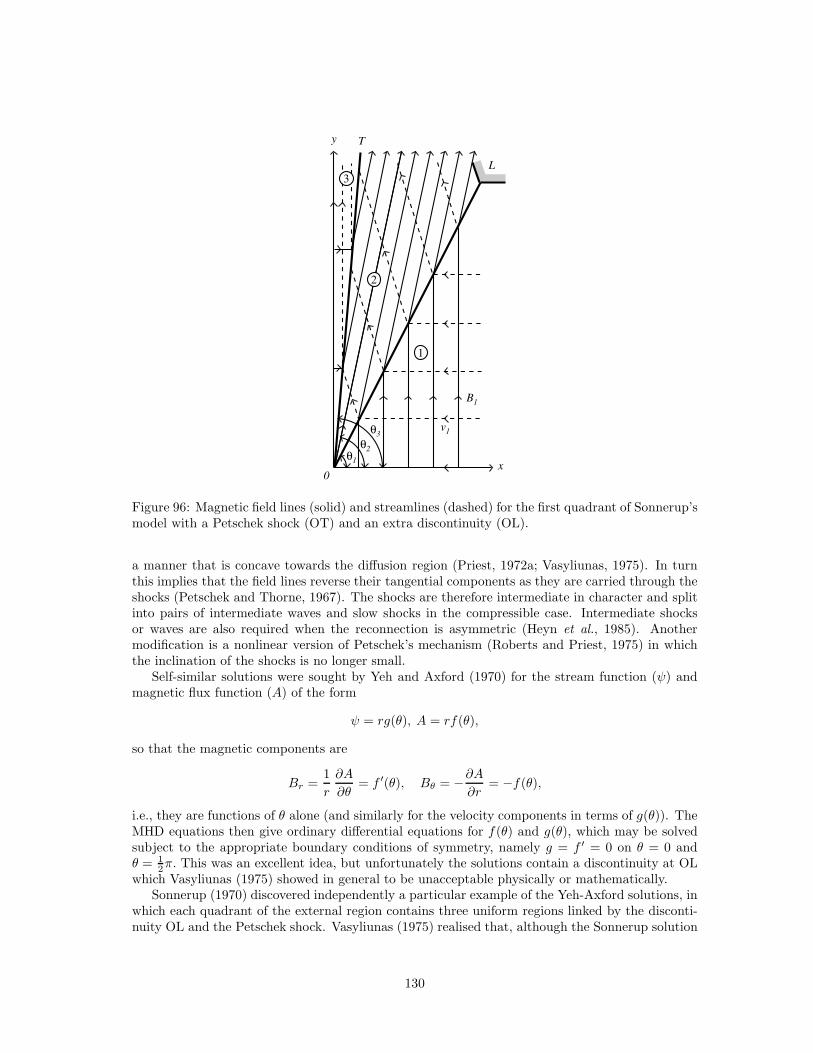
1

0

y T

L

B1

v1θ3

θ2θ1

x

3

2

Figure 96: Magnetic field lines (solid) and streamlines (dashed) for the first quadrant of Sonnerup’smodel with a Petschek shock (OT) and an extra discontinuity (OL).

a manner that is concave towards the diffusion region (Priest, 1972a; Vasyliunas, 1975). In turnthis implies that the field lines reverse their tangential components as they are carried through theshocks (Petschek and Thorne, 1967). The shocks are therefore intermediate in character and splitinto pairs of intermediate waves and slow shocks in the compressible case. Intermediate shocksor waves are also required when the reconnection is asymmetric (Heyn et al., 1985). Anothermodification is a nonlinear version of Petschek’s mechanism (Roberts and Priest, 1975) in whichthe inclination of the shocks is no longer small.

Self-similar solutions were sought by Yeh and Axford (1970) for the stream function (ψ) andmagnetic flux function (A) of the form

ψ = rg(θ), A = rf(θ),

so that the magnetic components are

Br =1

r

∂A

∂θ= f ′(θ), Bθ = −∂A

∂r= −f(θ),

i.e., they are functions of θ alone (and similarly for the velocity components in terms of g(θ)). TheMHD equations then give ordinary differential equations for f(θ) and g(θ), which may be solvedsubject to the appropriate boundary conditions of symmetry, namely g = f ′ = 0 on θ = 0 andθ = 1

2π. This was an excellent idea, but unfortunately the solutions contain a discontinuity at OLwhich Vasyliunas (1975) showed in general to be unacceptable physically or mathematically.

Sonnerup (1970) discovered independently a particular example of the Yeh-Axford solutions, inwhich each quadrant of the external region contains three uniform regions linked by the disconti-nuity OL and the Petschek shock. Vasyliunas (1975) realised that, although the Sonnerup solution

130

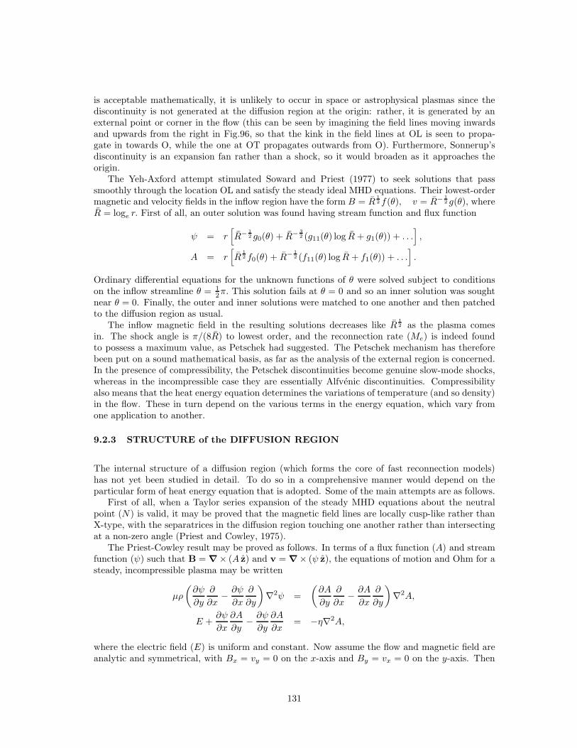
is acceptable mathematically, it is unlikely to occur in space or astrophysical plasmas since thediscontinuity is not generated at the diffusion region at the origin: rather, it is generated by anexternal point or corner in the flow (this can be seen by imagining the field lines moving inwardsand upwards from the right in Fig.96, so that the kink in the field lines at OL is seen to propa-gate in towards O, while the one at OT propagates outwards from O). Furthermore, Sonnerup’sdiscontinuity is an expansion fan rather than a shock, so it would broaden as it approaches theorigin.

The Yeh-Axford attempt stimulated Soward and Priest (1977) to seek solutions that passsmoothly through the location OL and satisfy the steady ideal MHD equations. Their lowest-ordermagnetic and velocity fields in the inflow region have the form B = R

12 f(θ), v = R− 1

2 g(θ), whereR = loge r. First of all, an outer solution was found having stream function and flux function

ψ = r[

R− 12 g0(θ) + R− 3

2 (g11(θ) log R+ g1(θ)) + . . .]

,

A = r[

R12 f0(θ) + R− 1

2 (f11(θ) log R + f1(θ)) + . . .]

.

Ordinary differential equations for the unknown functions of θ were solved subject to conditionson the inflow streamline θ = 1

2π. This solution fails at θ = 0 and so an inner solution was soughtnear θ = 0. Finally, the outer and inner solutions were matched to one another and then patchedto the diffusion region as usual.

The inflow magnetic field in the resulting solutions decreases like R12 as the plasma comes

in. The shock angle is π/(8R) to lowest order, and the reconnection rate (Me) is indeed foundto possess a maximum value, as Petschek had suggested. The Petschek mechanism has thereforebeen put on a sound mathematical basis, as far as the analysis of the external region is concerned.In the presence of compressibility, the Petschek discontinuities become genuine slow-mode shocks,whereas in the incompressible case they are essentially Alfvenic discontinuities. Compressibilityalso means that the heat energy equation determines the variations of temperature (and so density)in the flow. These in turn depend on the various terms in the energy equation, which vary fromone application to another.

9.2.3 STRUCTURE of the DIFFUSION REGION

The internal structure of a diffusion region (which forms the core of fast reconnection models)has not yet been studied in detail. To do so in a comprehensive manner would depend on theparticular form of heat energy equation that is adopted. Some of the main attempts are as follows.

First of all, when a Taylor series expansion of the steady MHD equations about the neutralpoint (N) is valid, it may be proved that the magnetic field lines are locally cusp-like rather thanX-type, with the separatrices in the diffusion region touching one another rather than intersectingat a non-zero angle (Priest and Cowley, 1975).

The Priest-Cowley result may be proved as follows. In terms of a flux function (A) and streamfunction (ψ) such that B = ∇× (A z) and v = ∇× (ψ z), the equations of motion and Ohm for asteady, incompressible plasma may be written

µρ

(∂ψ

∂y

∂

∂x− ∂ψ

∂x

∂

∂y

)

∇2ψ =

(∂A

∂y

∂

∂x− ∂A

∂x

∂

∂y

)

∇2A,

E +∂ψ

∂x

∂A

∂y− ∂ψ

∂y

∂A

∂x= −η∇2A,

where the electric field (E) is uniform and constant. Now assume the flow and magnetic field areanalytic and symmetrical, with Bx = vy = 0 on the x-axis and By = vx = 0 on the y-axis. Then

131

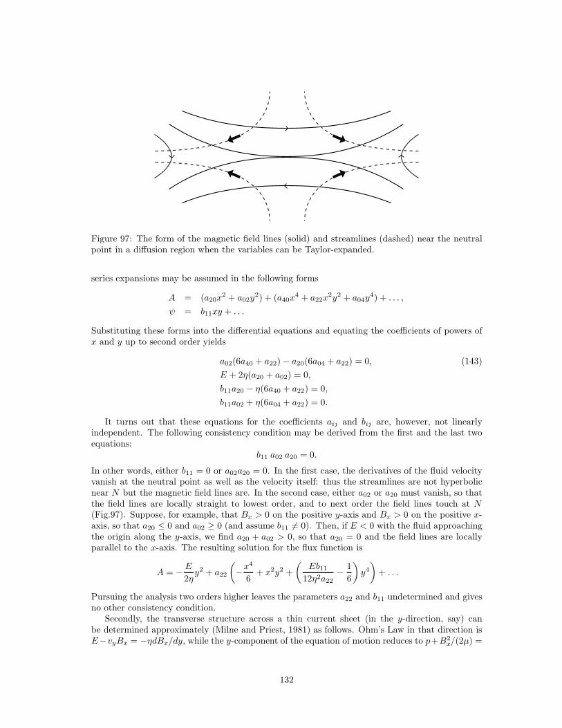
Figure 97: The form of the magnetic field lines (solid) and streamlines (dashed) near the neutralpoint in a diffusion region when the variables can be Taylor-expanded.

series expansions may be assumed in the following forms

A = (a20x2 + a02y

2) + (a40x4 + a22x

2y2 + a04y4) + . . . ,

ψ = b11xy + . . .

Substituting these forms into the differential equations and equating the coefficients of powers ofx and y up to second order yields

a02(6a40 + a22) − a20(6a04 + a22) = 0, (143)

E + 2η(a20 + a02) = 0,

b11a20 − η(6a40 + a22) = 0,

b11a02 + η(6a04 + a22) = 0.

It turns out that these equations for the coefficients aij and bij are, however, not linearlyindependent. The following consistency condition may be derived from the first and the last twoequations:

b11 a02 a20 = 0.

In other words, either b11 = 0 or a02a20 = 0. In the first case, the derivatives of the fluid velocityvanish at the neutral point as well as the velocity itself: thus the streamlines are not hyperbolicnear N but the magnetic field lines are. In the second case, either a02 or a20 must vanish, so thatthe field lines are locally straight to lowest order, and to next order the field lines touch at N(Fig.97). Suppose, for example, that Bx > 0 on the positive y-axis and Bx > 0 on the positive x-axis, so that a20 ≤ 0 and a02 ≥ 0 (and assume b11 6= 0). Then, if E < 0 with the fluid approachingthe origin along the y-axis, we find a20 + a02 > 0, so that a20 = 0 and the field lines are locallyparallel to the x-axis. The resulting solution for the flux function is

A = − E

2ηy2 + a22

(

−x4

6+ x2y2 +

(Eb11

12η2a22− 1

6

)

y4

)

+ . . .

Pursuing the analysis two orders higher leaves the parameters a22 and b11 undetermined and givesno other consistency condition.

Secondly, the transverse structure across a thin current sheet (in the y-direction, say) canbe determined approximately (Milne and Priest, 1981) as follows. Ohm’s Law in that direction isE−vyBx = −ηdBx/dy, while the y-component of the equation of motion reduces to p+B2

x/(2µ) =

132

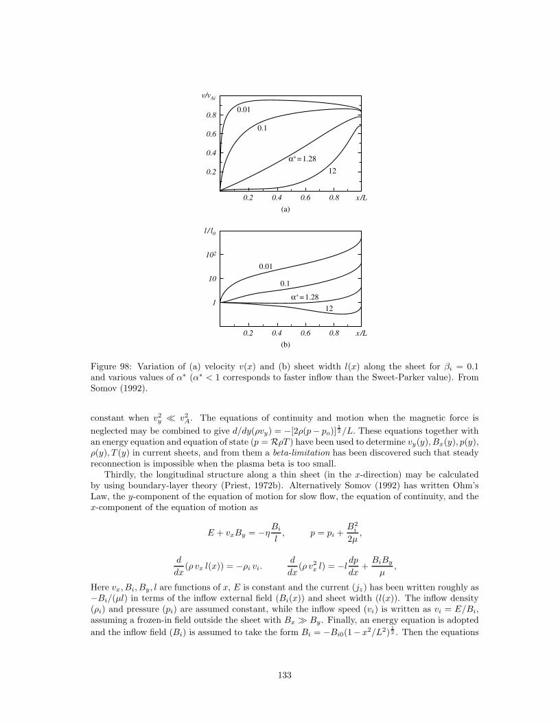
0.2 0.4 0.6

(b)

0.8 x /L

1

10

102

l / l0

0.2

0.01

0.01

0.1

0.1

α∗ = 1.28

α∗ = 1.28

12

12

0.4 0.6

(a)

0.8 x /L

0.2

0.4

0.6

0.8

v/vAi

Figure 98: Variation of (a) velocity v(x) and (b) sheet width l(x) along the sheet for βi = 0.1and various values of α∗ (α∗ < 1 corresponds to faster inflow than the Sweet-Parker value). FromSomov (1992).

constant when v2y ≪ v2

A. The equations of continuity and motion when the magnetic force is

neglected may be combined to give d/dy(ρvy) = −[2ρ(p− po)]12 /L. These equations together with

an energy equation and equation of state (p = RρT ) have been used to determine vy(y), Bx(y), p(y),ρ(y), T (y) in current sheets, and from them a beta-limitation has been discovered such that steadyreconnection is impossible when the plasma beta is too small.

Thirdly, the longitudinal structure along a thin sheet (in the x-direction) may be calculatedby using boundary-layer theory (Priest, 1972b). Alternatively Somov (1992) has written Ohm’sLaw, the y-component of the equation of motion for slow flow, the equation of continuity, and thex-component of the equation of motion as

E + vxBy = −ηBi

l, p = pi +

B2i

2µ,

d

dx(ρ vx l(x)) = −ρi vi.

d

dx(ρ v2

x l) = −l dpdx

+BiBy

µ,

Here vx, Bi, By, l are functions of x, E is constant and the current (jz) has been written roughly as−Bi/(µl) in terms of the inflow external field (Bi(x)) and sheet width (l(x)). The inflow density(ρi) and pressure (pi) are assumed constant, while the inflow speed (vi) is written as vi = E/Bi,assuming a frozen-in field outside the sheet with Bx ≫ By. Finally, an energy equation is adopted

and the inflow field (Bi) is assumed to take the form Bi = −Bi0(1− x2/L2)12 . Then the equations

133

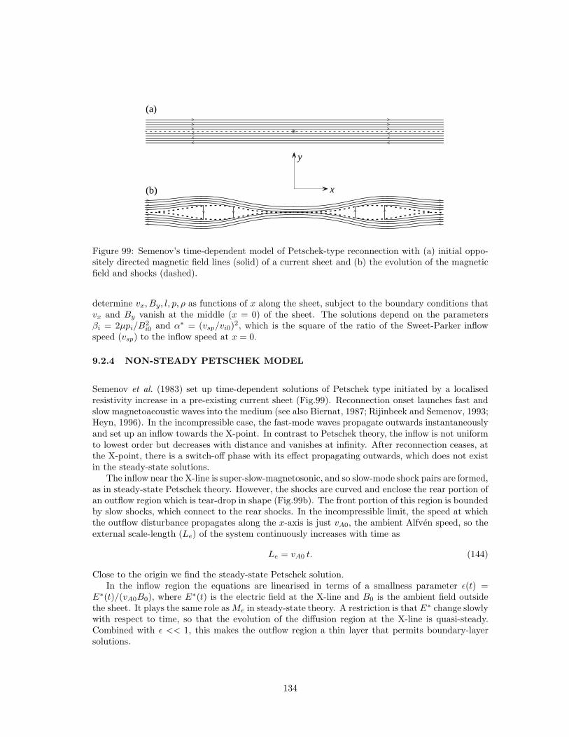
y

x

(a)

(b)

Figure 99: Semenov’s time-dependent model of Petschek-type reconnection with (a) initial oppo-sitely directed magnetic field lines (solid) of a current sheet and (b) the evolution of the magneticfield and shocks (dashed).

determine vx, By, l, p, ρ as functions of x along the sheet, subject to the boundary conditions thatvx and By vanish at the middle (x = 0) of the sheet. The solutions depend on the parametersβi = 2µpi/B

2i0 and α∗ = (vsp/vi0)

2, which is the square of the ratio of the Sweet-Parker inflowspeed (vsp) to the inflow speed at x = 0.

9.2.4 NON-STEADY PETSCHEK MODEL

Semenov et al. (1983) set up time-dependent solutions of Petschek type initiated by a localisedresistivity increase in a pre-existing current sheet (Fig.99). Reconnection onset launches fast andslow magnetoacoustic waves into the medium (see also Biernat, 1987; Rijinbeek and Semenov, 1993;Heyn, 1996). In the incompressible case, the fast-mode waves propagate outwards instantaneouslyand set up an inflow towards the X-point. In contrast to Petschek theory, the inflow is not uniformto lowest order but decreases with distance and vanishes at infinity. After reconnection ceases, atthe X-point, there is a switch-off phase with its effect propagating outwards, which does not existin the steady-state solutions.

The inflow near the X-line is super-slow-magnetosonic, and so slow-mode shock pairs are formed,as in steady-state Petschek theory. However, the shocks are curved and enclose the rear portion ofan outflow region which is tear-drop in shape (Fig.99b). The front portion of this region is boundedby slow shocks, which connect to the rear shocks. In the incompressible limit, the speed at whichthe outflow disturbance propagates along the x-axis is just vA0, the ambient Alfven speed, so theexternal scale-length (Le) of the system continuously increases with time as

Le = vA0 t. (144)

Close to the origin we find the steady-state Petschek solution.In the inflow region the equations are linearised in terms of a smallness parameter ǫ(t) =

E∗(t)/(vA0B0), where E∗(t) is the electric field at the X-line and B0 is the ambient field outsidethe sheet. It plays the same role asMe in steady-state theory. A restriction is that E∗ change slowlywith respect to time, so that the evolution of the diffusion region at the X-line is quasi-steady.Combined with ǫ << 1, this makes the outflow region a thin layer that permits boundary-layersolutions.

134

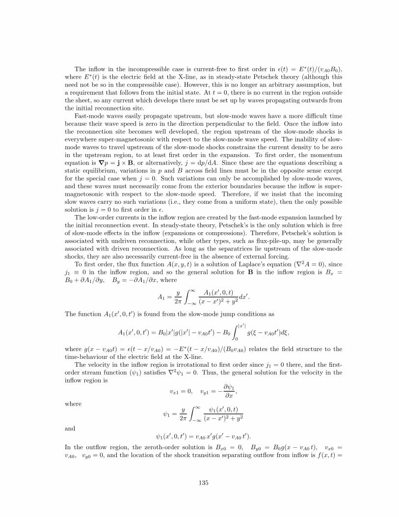
The inflow in the incompressible case is current-free to first order in ǫ(t) = E∗(t)/(vA0B0),where E∗(t) is the electric field at the X-line, as in steady-state Petschek theory (although thisneed not be so in the compressible case). However, this is no longer an arbitrary assumption, buta requirement that follows from the initial state. At t = 0, there is no current in the region outsidethe sheet, so any current which develops there must be set up by waves propagating outwards fromthe initial reconnection site.

Fast-mode waves easily propagate upstream, but slow-mode waves have a more difficult timebecause their wave speed is zero in the direction perpendicular to the field. Once the inflow intothe reconnection site becomes well developed, the region upstream of the slow-mode shocks iseverywhere super-magnetosonic with respect to the slow-mode wave speed. The inability of slow-mode waves to travel upstream of the slow-mode shocks constrains the current density to be zeroin the upstream region, to at least first order in the expansion. To first order, the momentumequation is ∇p = j × B, or alternatively, j = dp/dA. Since these are the equations describing astatic equilibrium, variations in p and B across field lines must be in the opposite sense exceptfor the special case when j = 0. Such variations can only be accomplished by slow-mode waves,and these waves must necessarily come from the exterior boundaries because the inflow is super-magnetosonic with respect to the slow-mode speed. Therefore, if we insist that the incomingslow waves carry no such variations (i.e., they come from a uniform state), then the only possiblesolution is j = 0 to first order in ǫ.

The low-order currents in the inflow region are created by the fast-mode expansion launched bythe initial reconnection event. In steady-state theory, Petschek’s is the only solution which is freeof slow-mode effects in the inflow (expansions or compressions). Therefore, Petschek’s solution isassociated with undriven reconnection, while other types, such as flux-pile-up, may be generallyassociated with driven reconnection. As long as the separatrices lie upstream of the slow-modeshocks, they are also necessarily current-free in the absence of external forcing.

To first order, the flux function A(x, y, t) is a solution of Laplace’s equation (∇2A = 0), sincej1 ≡ 0 in the inflow region, and so the general solution for B in the inflow region is Bx =B0 + ∂A1/∂y, By = −∂A1/∂x, where

A1 =y

2π

∫ ∞

−∞

A1(x′, 0, t)

(x− x′)2 + y2dx′.

The function A1(x′, 0, t′) is found from the slow-mode jump conditions as

A1(x′, 0, t′) = B0|x′|g(|x′| − vA0t

′) −B0

∫ |x′|

0

g(ξ − vA0t′)dξ,

where g(x − vA0t) = ǫ(t − x/vA0) = −E∗(t − x/vA0)/(B0vA0) relates the field structure to thetime-behaviour of the electric field at the X-line.

The velocity in the inflow region is irrotational to first order since j1 = 0 there, and the first-order stream function (ψ1) satisfies ∇2ψ1 = 0. Thus, the general solution for the velocity in theinflow region is

vx1 = 0, vy1 = −∂ψ1

∂x,

where

ψ1 =y

2π

∫ ∞

−∞

ψ1(x′, 0, t)

(x − x′)2 + y2

andψ1(x

′, 0, t′) = vA0 x′g(x′ − vA0 t

′).

In the outflow region, the zeroth-order solution is Bx0 = 0, By0 = B0g(x − vA0 t), vx0 =vA0, vy0 = 0, and the location of the shock transition separating outflow from inflow is f(x, t) =

135

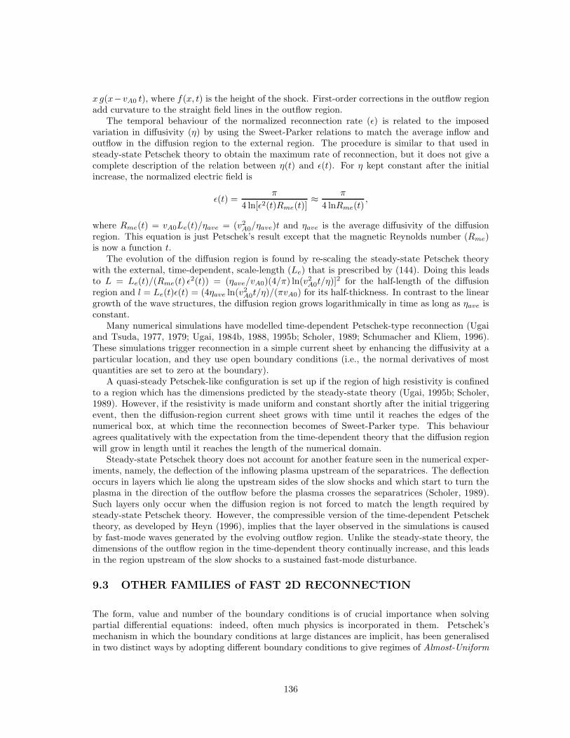
x g(x−vA0 t), where f(x, t) is the height of the shock. First-order corrections in the outflow regionadd curvature to the straight field lines in the outflow region.

The temporal behaviour of the normalized reconnection rate (ǫ) is related to the imposedvariation in diffusivity (η) by using the Sweet-Parker relations to match the average inflow andoutflow in the diffusion region to the external region. The procedure is similar to that used insteady-state Petschek theory to obtain the maximum rate of reconnection, but it does not give acomplete description of the relation between η(t) and ǫ(t). For η kept constant after the initialincrease, the normalized electric field is

ǫ(t) =π

4 ln[ǫ2(t)Rme(t)]≈ π

4 lnRme(t),

where Rme(t) = vA0Le(t)/ηave = (v2A0/ηave)t and ηave is the average diffusivity of the diffusion

region. This equation is just Petschek’s result except that the magnetic Reynolds number (Rme)is now a function t.

The evolution of the diffusion region is found by re-scaling the steady-state Petschek theorywith the external, time-dependent, scale-length (Le) that is prescribed by (144). Doing this leadsto L = Le(t)/(Rme(t) ǫ

2(t)) = (ηave/vA0)(4/π) ln(v2A0t/η)]

2 for the half-length of the diffusionregion and l = Le(t)ǫ(t) = (4ηave ln(v2

A0t/η)/(πvA0) for its half-thickness. In contrast to the lineargrowth of the wave structures, the diffusion region grows logarithmically in time as long as ηave isconstant.

Many numerical simulations have modelled time-dependent Petschek-type reconnection (Ugaiand Tsuda, 1977, 1979; Ugai, 1984b, 1988, 1995b; Scholer, 1989; Schumacher and Kliem, 1996).These simulations trigger reconnection in a simple current sheet by enhancing the diffusivity at aparticular location, and they use open boundary conditions (i.e., the normal derivatives of mostquantities are set to zero at the boundary).

A quasi-steady Petschek-like configuration is set up if the region of high resistivity is confinedto a region which has the dimensions predicted by the steady-state theory (Ugai, 1995b; Scholer,1989). However, if the resistivity is made uniform and constant shortly after the initial triggeringevent, then the diffusion-region current sheet grows with time until it reaches the edges of thenumerical box, at which time the reconnection becomes of Sweet-Parker type. This behaviouragrees qualitatively with the expectation from the time-dependent theory that the diffusion regionwill grow in length until it reaches the length of the numerical domain.

Steady-state Petschek theory does not account for another feature seen in the numerical exper-iments, namely, the deflection of the inflowing plasma upstream of the separatrices. The deflectionoccurs in layers which lie along the upstream sides of the slow shocks and which start to turn theplasma in the direction of the outflow before the plasma crosses the separatrices (Scholer, 1989).Such layers only occur when the diffusion region is not forced to match the length required bysteady-state Petschek theory. However, the compressible version of the time-dependent Petschektheory, as developed by Heyn (1996), implies that the layer observed in the simulations is causedby fast-mode waves generated by the evolving outflow region. Unlike the steady-state theory, thedimensions of the outflow region in the time-dependent theory continually increase, and this leadsin the region upstream of the slow shocks to a sustained fast-mode disturbance.

9.3 OTHER FAMILIES of FAST 2D RECONNECTION

The form, value and number of the boundary conditions is of crucial importance when solvingpartial differential equations: indeed, often much physics is incorporated in them. Petschek’smechanism in which the boundary conditions at large distances are implicit, has been generalisedin two distinct ways by adopting different boundary conditions to give regimes of Almost-Uniform

136

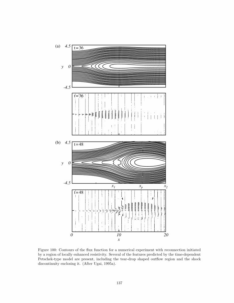
(a) t = 36

t = 36

4.5

0

y

-4.5

(b) t = 48

t = 48

4.5

0

y

-4.5

0 10 x

x1 xp x2

20

Figure 100: Contours of the flux function for a numerical experiment with reconnection initiatedby a region of locally enhanced resistivity. Several of the features predicted by the time-dependentPetschek-type model are present, including the tear-drop shaped outflow region and the shockdiscontinuity enclosing it. (After Ugai, 1995a).

137

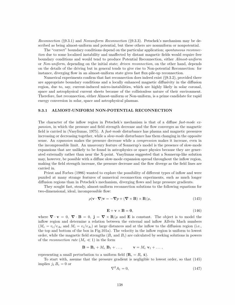
Reconnection (§9.3.1) and Nonuniform Reconnection (§9.3.3). Petschek’s mechanism may be de-scribed as being almost-uniform and potential, but these others are nonuniform or nonpotential.

The “correct” boundary conditions depend on the particular application; spontaneous reconnec-tion due to some localised instability and unaffected by distant magnetic fields would require freeboundary conditions and would tend to produce Potential Reconnection, either Almost-uniformor Non-uniform, depending on the initial state; driven reconnection, on the other hand, dependson the details of the driving but in general tends to give rise to Non-potential Reconnection: forinstance, diverging flow in an almost-uniform state gives fast flux-pile-up reconnection.

Numerical experiments confirm that fast reconnection does indeed exist (§9.3.2), provided thereare appropriate boundary conditions and a locally enhanced magnetic diffusivity in the diffusionregion, due to, say, current-induced micro-instabilities, which are highly likely in solar coronal,space and astrophysical current sheets because of the collisionless nature of their environment.Therefore, fast reconnection, either Almost-uniform or Non-uniform, is a prime candidate for rapidenergy conversion in solar, space and astrophysical plasmas.

9.3.1 ALMOST-UNIFORM NON-POTENTIAL RECONNECTION

The character of the inflow region in Petschek’s mechanism is that of a diffuse fast-mode ex-pansion, in which the pressure and field strength decrease and the flow converges as the magneticfield is carried in (Vasyliunas, 1975). A fast-mode disturbance has plasma and magnetic pressuresincreasing or decreasing together, while a slow-mode disturbance has them changing in the oppositesense. An expansion makes the pressure decrease while a compression makes it increase, even inthe incompressible limit. An unsavoury feature of Sonnerup’s model is the presence of slow-modeexpansions that are unlikely to be found in astrophysics or space physics because they are gener-ated externally rather than near the X-point. Vasyliunas suggested that a Sonnerup-like solutionmay, however, be possible with a diffuse slow-mode expansion spread throughout the inflow region,making the field strength increase, the pressure decrease and the flow diverge as the field lines arecarried in.

Priest and Forbes (1986) wanted to explore the possibility of different types of inflow and werepuzzled at many strange features of numerical reconnection experiments, such as much longerdiffusion regions than in Petschek’s mechanism, diverging flows and large pressure gradients.

They sought fast, steady, almost-uniform reconnection solutions to the following equations fortwo-dimensional, ideal, incompressible flow:

ρ(v · ∇)v = −∇p+ (∇ × B) × B/µ, (145)

E + v × B = 0, (146)

where ∇ · v = 0, ∇ · B = 0, j = ∇ × B/µ and E is constant. The object is to model theinflow region and determine a relation between the external and inflow Alfven Mach numbers(Me = ve/vAe and Mi = vi/vAi) at large distances and at the inflow to the diffusion region (i.e.,the top and bottom of the box in Fig.101a). The velocity in the inflow region is uniform to lowestorder, while the magnetic field strengths (Be and Bi) are calculated by seeking solutions in powersof the reconnection rate (Me ≪ 1) in the form

B = Be +Me B1 + . . . , v = Me v1 + . . . ,

representing a small perturbation to a uniform field (Be = Be x).To start with, assume that the pressure gradient is negligible to lowest order, so that (145)

implies j1Be = 0 or∇2A1 = 0, (147)

138

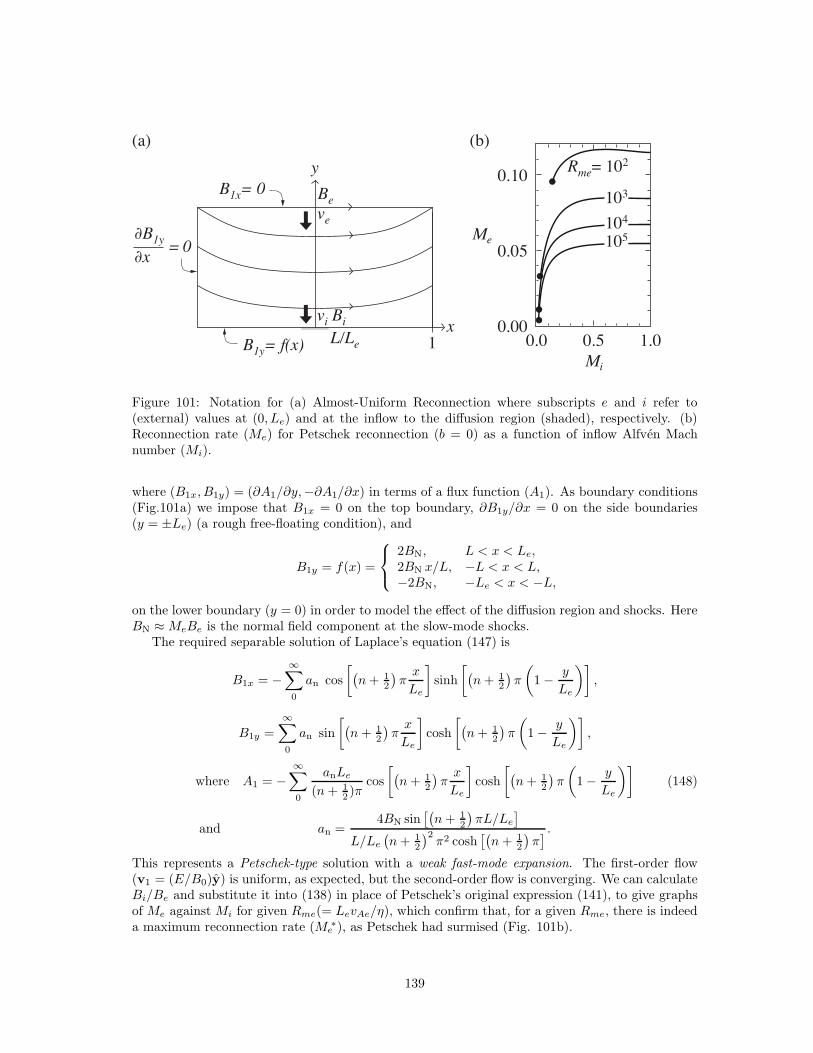
y

x

B1x= 0

Rme= 102

Be

ve

vi Bi

L/Le 1B1y= f(x)

∂B1y = 0∂x

0.0 0.5 1.0

0.10

0.05

0.00

Mi

Me

(a) (b)

103

104

105

Figure 101: Notation for (a) Almost-Uniform Reconnection where subscripts e and i refer to(external) values at (0, Le) and at the inflow to the diffusion region (shaded), respectively. (b)Reconnection rate (Me) for Petschek reconnection (b = 0) as a function of inflow Alfven Machnumber (Mi).

where (B1x, B1y) = (∂A1/∂y,−∂A1/∂x) in terms of a flux function (A1). As boundary conditions(Fig.101a) we impose that B1x = 0 on the top boundary, ∂B1y/∂x = 0 on the side boundaries(y = ±Le) (a rough free-floating condition), and

B1y = f(x) =

2BN, L < x < Le,2BN x/L, −L < x < L,−2BN, −Le < x < −L,

on the lower boundary (y = 0) in order to model the effect of the diffusion region and shocks. HereBN ≈MeBe is the normal field component at the slow-mode shocks.

The required separable solution of Laplace’s equation (147) is

B1x = −∞∑

0

an cos

[(n+ 1

2

)πx

Le

]

sinh

[(n+ 1

2

)π

(

1 − y

Le

)]

,

B1y =

∞∑

0

an sin

[(n+ 1

2

)πx

Le

]

cosh

[(n+ 1

2

)π

(

1 − y

Le

)]

,

where A1 = −∞∑

0

anLe

(n+ 12 )π

cos

[(n+ 1

2

)πx

Le

]

cosh

[(n+ 1

2

)π

(

1 − y

Le

)]

(148)

and an =4BN sin

[(n+ 1

2

)πL/Le

]

L/Le

(n+ 1

2

)2π2 cosh

[(n+ 1

2

)π] .

This represents a Petschek-type solution with a weak fast-mode expansion. The first-order flow(v1 = (E/B0)y) is uniform, as expected, but the second-order flow is converging. We can calculateBi/Be and substitute it into (138) in place of Petschek’s original expression (141), to give graphsof Me against Mi for given Rme(= LevAe/η), which confirm that, for a given Rme, there is indeeda maximum reconnection rate (Me

∗), as Petschek had surmised (Fig. 101b).

139

b

0Petschek

hybrid

M (diffusion region)

Me

(exte

rior)

fluxpile-up

Sonnerup

-like

1

flu

x-p

ile-

up

b

= 1

.1

b = 0.9

Petschek b = 0

Sonne

rup

b =

1

stag

nat

ion

flo

w

b =

1.5

b = -1.5

fast exp

an

sion

slow expansion

(a) (b)

slowcompression compression

Figure 102: (a) The value of the parameter b determines the different regimes of fast Almost-Uniform reconnection. (b) The dimensionless inflow Alfven Mach number ((Me = ve/vAe)) arelarge distances or reconnection rate as a function of Alfven Mach number Mi = vi/vAi at theinflow to the diffusion region for different values of b.

Deriving other people’s results in your own way is often a good exercise, in order to understandtheir motivation and assumptions. While carrying out the above analysis, we realised how togeneralise it by adding a pressure gradient to the right-hand side of (147), which changes to aPoisson equation, namely,

∇2A1 = − µ

Be

dp1

dy.

The effect on (148) is just to add a constant (b) to the x-dependent part of each term, so that

A1 = −∞∑

0

an

(n+ 12 )π

{

b− cos[(n+ 1

2

)πx

L

]}

cosh[(n+ 1

2

)π(

1 − y

L

)]

.

and

(Me

Mi

)2

≈ 4Me(1 − b)

π

0.834 − loge tan

(

4RmeM1/2e M

1/2i

π

)−1

.

Introducing the parameter b produces a new family of regimes with a rich diversity of properties:when b = 0, Petschek’s regime (a weak fast-mode expansion) is recovered; when b = 1, the inflowfield on the y-axis is uniform (a so-called Sonnerup-like solution with a weak slow-mode expansion).The solutions for other values of b are determined by the nature of the flow on the inflow boundary,since the horizontal flow speed at the corner (x, y) = (Le, Le) is proportional to (b − 2/π). Theway that the reconnection rate (Me) varies with Mi and b for a given Rme is shown in Fig.102b.When b > 0 the reconnection rate is faster than the Petschek rate for the same Mi (although theanalysis is valid only for M ≪ 1). For b = 1, Me increases linearly with Mi, while for b = 0 thePetschek maximum can be seen. All regimes with b < 1 possess a maximum reconnection rate,although when b < 0 it is slower than Petschek’s. When b > 1, within the limitations of the theory,there is no maximum rate.

When b < 0 the streamlines (Fig.103) near the y-axis converge and so tend to compress theplasma, thereby producing a slow-mode compression. When b > 1 the streamlines diverge and tendto expand the plasma, producing a slow-mode expansion. We refer to this type as the flux pile–up

140

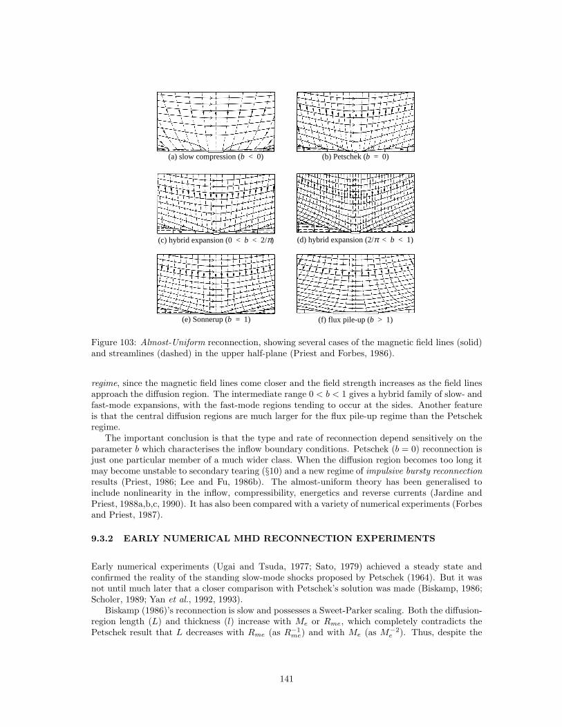
(a) slow compression (b < 0) (b) Petschek (b = 0)

(c) hybrid expansion (0 < b < 2/π) (d) hybrid expansion (2/π < b < 1)

(e) Sonnerup (b = 1) (f) flux pile-up (b > 1)

Figure 103: Almost-Uniform reconnection, showing several cases of the magnetic field lines (solid)and streamlines (dashed) in the upper half-plane (Priest and Forbes, 1986).

regime, since the magnetic field lines come closer and the field strength increases as the field linesapproach the diffusion region. The intermediate range 0 < b < 1 gives a hybrid family of slow- andfast-mode expansions, with the fast-mode regions tending to occur at the sides. Another featureis that the central diffusion regions are much larger for the flux pile-up regime than the Petschekregime.

The important conclusion is that the type and rate of reconnection depend sensitively on theparameter b which characterises the inflow boundary conditions. Petschek (b = 0) reconnection isjust one particular member of a much wider class. When the diffusion region becomes too long itmay become unstable to secondary tearing (§10) and a new regime of impulsive bursty reconnectionresults (Priest, 1986; Lee and Fu, 1986b). The almost-uniform theory has been generalised toinclude nonlinearity in the inflow, compressibility, energetics and reverse currents (Jardine andPriest, 1988a,b,c, 1990). It has also been compared with a variety of numerical experiments (Forbesand Priest, 1987).

9.3.2 EARLY NUMERICAL MHD RECONNECTION EXPERIMENTS

Early numerical experiments (Ugai and Tsuda, 1977; Sato, 1979) achieved a steady state andconfirmed the reality of the standing slow-mode shocks proposed by Petschek (1964). But it wasnot until much later that a closer comparison with Petschek’s solution was made (Biskamp, 1986;Scholer, 1989; Yan et al., 1992, 1993).

Biskamp (1986)’s reconnection is slow and possesses a Sweet-Parker scaling. Both the diffusion-region length (L) and thickness (l) increase with Me or Rme, which completely contradicts thePetschek result that L decreases with Rme (as R−1

me) and with Me (as M−2e ). Thus, despite the

141

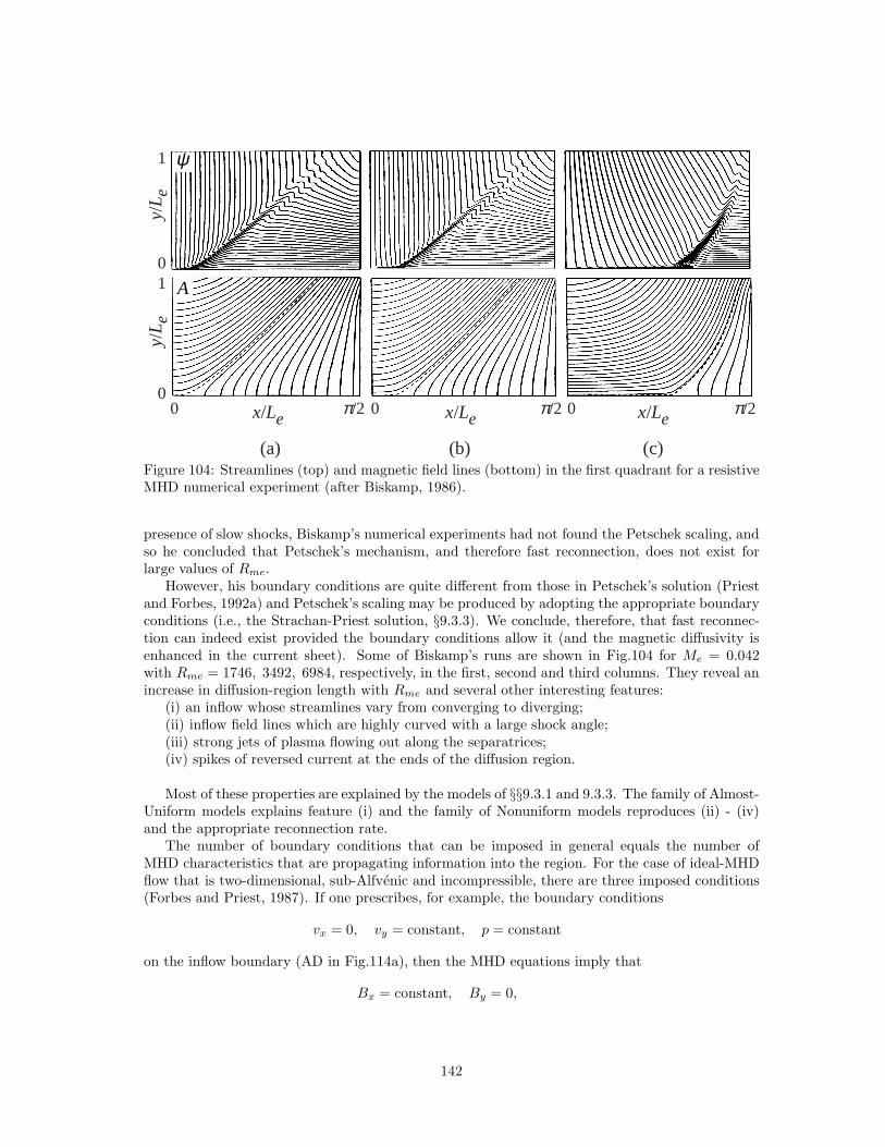
(a) (b) (c)

0 0 0π/2 π/2 π/2

y/L e

y/L e

x/Le x/Le x/Le

0

0

1

1

ψ

A

Figure 104: Streamlines (top) and magnetic field lines (bottom) in the first quadrant for a resistiveMHD numerical experiment (after Biskamp, 1986).

presence of slow shocks, Biskamp’s numerical experiments had not found the Petschek scaling, andso he concluded that Petschek’s mechanism, and therefore fast reconnection, does not exist forlarge values of Rme.

However, his boundary conditions are quite different from those in Petschek’s solution (Priestand Forbes, 1992a) and Petschek’s scaling may be produced by adopting the appropriate boundaryconditions (i.e., the Strachan-Priest solution, §9.3.3). We conclude, therefore, that fast reconnec-tion can indeed exist provided the boundary conditions allow it (and the magnetic diffusivity isenhanced in the current sheet). Some of Biskamp’s runs are shown in Fig.104 for Me = 0.042with Rme = 1746, 3492, 6984, respectively, in the first, second and third columns. They reveal anincrease in diffusion-region length with Rme and several other interesting features:

(i) an inflow whose streamlines vary from converging to diverging;(ii) inflow field lines which are highly curved with a large shock angle;(iii) strong jets of plasma flowing out along the separatrices;(iv) spikes of reversed current at the ends of the diffusion region.

Most of these properties are explained by the models of §§9.3.1 and 9.3.3. The family of Almost-Uniform models explains feature (i) and the family of Nonuniform models reproduces (ii) - (iv)and the appropriate reconnection rate.

The number of boundary conditions that can be imposed in general equals the number ofMHD characteristics that are propagating information into the region. For the case of ideal-MHDflow that is two-dimensional, sub-Alfvenic and incompressible, there are three imposed conditions(Forbes and Priest, 1987). If one prescribes, for example, the boundary conditions

vx = 0, vy = constant, p = constant

on the inflow boundary (AD in Fig.114a), then the MHD equations imply that

Bx = constant, By = 0,

142

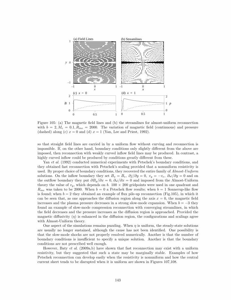
y

x

1

0

–1

x

0 0.5 10

1

2

10.500

1

2(c) x = 0 (d) x = 1

pB

(a) Field Lines (b) Streamlines

–1 0 1 –1 0 1

Figure 105: (a) The magnetic field lines and (b) the streamlines for almost-uniform reconnectionwith b = 2,Me = 0.1, Rme = 2000. The variation of magnetic field (continuous) and pressure(dashed) along (c) x = 0 and (d) x = 1 (Yan, Lee and Priest, 1992).

so that straight field lines are carried in by a uniform flow without curving and reconnection isimpossible. If, on the other hand, boundary conditions only slightly different from the above areimposed, then reconnection with weakly curved inflow field lines may be produced. In contrast, ahighly curved inflow could be produced by conditions greatly different from these.

Yan et al. (1992) conducted numerical experiments with Petschek’s boundary conditions, andthey obtained fast reconnection with Petschek’s scaling provided that a nonuniform resistivity isused. By proper choice of boundary conditions, they recovered the entire family of Almost-Uniformsolutions. On the inflow boundary they set Bx = Be, ∂j/∂y = 0, vy = −ve, ∂ω/∂y = 0 and onthe outflow boundary they put ∂By/∂x = 0, ∂ω/∂x = 0 and imposed from the Almost-Uniformtheory the value of vy, which depends on b. 100 × 200 gridpoints were used in one quadrant andRme was taken to be 2000. When b = 0 a Petschek flow results; when b = 1 Sonnerup-like flowis found; when b = 2 they obtained an example of flux pile-up reconnection (Fig.105), in which itcan be seen that, as one approaches the diffusion region along the axis x = 0, the magnetic fieldincreases and the plasma pressure decreases in a strong slow-mode expansion. When b = −3 theyfound an example of slow-mode compression reconnection with converging streamlines, in whichthe field decreases and the pressure increases as the diffusion region is approached. Provided themagnetic diffusivity (η) is enhanced in the diffusion region, the configurations and scalings agreewith Almost-Uniform theory.

One aspect of the simulations remains puzzling. When η is uniform, the steady-state solutionsare usually no longer sustained, although the cause has not been identified. One possibility isthat the slow-mode shocks are not properly resolved numerically. Another is that the number ofboundary conditions is insufficient to specify a unique solution. Another is that the boundaryconditions are not prescribed well enough.

However, Baty et al. (2009a,b) have shown that fast reconnection may exist with a uniformresistivity, but they suggested that such a state may be marginally stable. Examples of howPetschek reconnection can develop easily when the resistivity is nonuniform and how the centralcurrent sheet tends to be disrupted when it is uniform are shown in Figures 107,108.

143

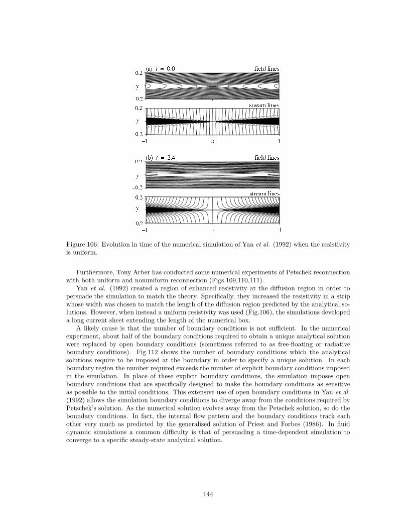
Figure 106: Evolution in time of the numerical simulation of Yan et al. (1992) when the resistivityis uniform.

Furthermore, Tony Arber has conducted some numerical experiments of Petschek reconnectionwith both uniform and nonuniform reconnection (Figs.109,110,111).

Yan et al. (1992) created a region of enhanced resistivity at the diffusion region in order topersuade the simulation to match the theory. Specifically, they increased the resistivity in a stripwhose width was chosen to match the length of the diffusion region predicted by the analytical so-lutions. However, when instead a uniform resistivity was used (Fig.106), the simulations developeda long current sheet extending the length of the numerical box.

A likely cause is that the number of boundary conditions is not sufficient. In the numericalexperiment, about half of the boundary conditions required to obtain a unique analytical solutionwere replaced by open boundary conditions (sometimes referred to as free-floating or radiativeboundary conditions). Fig.112 shows the number of boundary conditions which the analyticalsolutions require to be imposed at the boundary in order to specify a unique solution. In eachboundary region the number required exceeds the number of explicit boundary conditions imposedin the simulation. In place of these explicit boundary conditions, the simulation imposes openboundary conditions that are specifically designed to make the boundary conditions as sensitiveas possible to the initial conditions. This extensive use of open boundary conditions in Yan et al.(1992) allows the simulation boundary conditions to diverge away from the conditions required byPetschek’s solution. As the numerical solution evolves away from the Petschek solution, so do theboundary conditions. In fact, the internal flow pattern and the boundary conditions track eachother very much as predicted by the generalised solution of Priest and Forbes (1986). In fluiddynamic simulations a common difficulty is that of persuading a time-dependent simulation toconverge to a specific steady-state analytical solution.

144

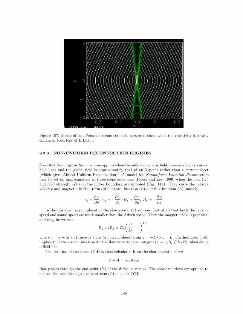
Figure 107: Movie of fast Petschek reconnection in a current sheet when the resistivity is locallyenhanced (courtesy of H Baty).

9.3.3 NON-UNIFORM RECONNECTION REGIMES

So-called Nonuniform Reconnection applies when the inflow magnetic field possesses highly curvedfield lines and the global field is approximately that of an X-point rather than a current sheet(which gives Almost-Uniform Reconnection). A model for Nonuniform Potential Reconnectionmay be set up approximately in three steps as follows (Priest and Lee, 1990) when the flow (ve)and field strength (Be) on the inflow boundary are imposed (Fig. 114). They caste the plasmavelocity and magnetic field in terms of a stream function (ψ) and flux function (A), namely,

vx =∂ψ

∂y, vy = −∂ψ

∂x, Bx =

∂A

∂y, By = −∂A

∂x.

In the upstream region ahead of the slow shock YH suppose first of all that both the plasmaspeed and sound speed are much smaller than the Alfven speed. Then the magnetic field is potentialand may be written

By + iBx = Bi

(z2

L2− 1

)1/2

,

where z = x + iy and there is a cut (a current sheet) from z = −L to z = L. Furthermore, (145)implies that the stream function for the flow velocity is an integral (ψ = veBe

∫ds/B) taken along

a field line.The position of the shock (YH) is then calculated from the characteristic curve

ψ +A = constant

that passes through the end-point (Y) of the diffusion region. The shock relations are applied todeduce the conditions just downstream of the shock (YH).

145

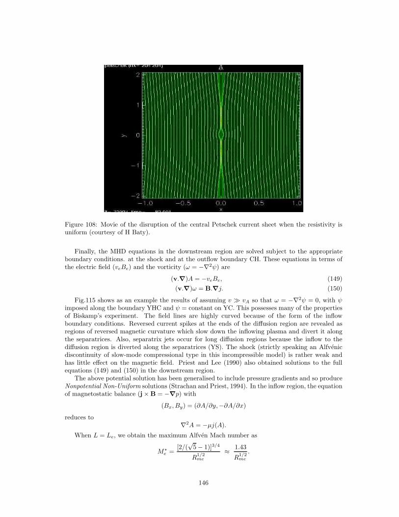
Figure 108: Movie of the disruption of the central Petschek current sheet when the resistivity isuniform (courtesy of H Baty).

Finally, the MHD equations in the downstream region are solved subject to the appropriateboundary conditions. at the shock and at the outflow boundary CH. These equations in terms ofthe electric field (veBe) and the vorticity (ω = −∇2ψ) are

(v.∇)A = −veBe, (149)

(v.∇)ω = B.∇j. (150)

Fig.115 shows as an example the results of assuming v ≫ vA so that ω = −∇2ψ = 0, with ψimposed along the boundary YHC and ψ = constant on YC. This possesses many of the propertiesof Biskamp’s experiment. The field lines are highly curved because of the form of the inflowboundary conditions. Reversed current spikes at the ends of the diffusion region are revealed asregions of reversed magnetic curvature which slow down the inflowing plasma and divert it alongthe separatrices. Also, separatrix jets occur for long diffusion regions because the inflow to thediffusion region is diverted along the separatrices (YS). The shock (strictly speaking an Alfvenicdiscontinuity of slow-mode compressional type in this incompressible model) is rather weak andhas little effect on the magnetic field. Priest and Lee (1990) also obtained solutions to the fullequations (149) and (150) in the downstream region.

The above potential solution has been generalised to include pressure gradients and so produceNonpotential Non-Uniform solutions (Strachan and Priest, 1994). In the inflow region, the equationof magnetostatic balance (j × B = −∇p) with

(Bx, By) = (∂A/∂y,−∂A/∂x)reduces to

∇2A = −µj(A).

When L = Le, we obtain the maximum Alfven Mach number as

M∗e =

[2/(√

5 − 1)]3/4

R1/2me

≈ 1.43

R1/2me

.

146

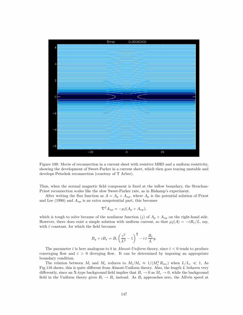
Figure 109: Movie of reconnection in a current sheet with resistive MHD and a uniform resistivity,showing the development of Sweet-Parker in a current sheet, which then goes tearing unstable anddevelops Petschek reconnection (courtesy of T Arber).

Thus, when the normal magnetic field component is fixed at the inflow boundary, the Strachan-Priest reconnection scales like the slow Sweet-Parker rate, as in Biskamp’s experiment.

After writing the flux function as A = Ap + Anp, where Ap is the potential solution of Priestand Lee (1990) and Anp is an extra nonpotential part, this becomes

∇2Anp = −µj(Ap +Anp),

which is tough to solve because of the nonlinear function (j) of Ap + Anp on the right-hand side.However, there does exist a simple solution with uniform current, so that µj(A) = −cBe/L, say,with c constant, for which the field becomes

By + iBx = Bi

(z2

L2− 1

) 12

− i cBe

Ly.

The parameter c is here analogous to b in Almost-Uniform theory, since c < 0 tends to produceconverging flow and c > 0 diverging flow. It can be determined by imposing an appropriateboundary condition.

The relation between Mi and Me reduces to Mi/Me ≈ 1/(M2e Rme) when L/Le ≪ 1, As

Fig.116 shows, this is quite different from Almost-Uniform theory. Also, the length L behaves verydifferently, since an X-type background field implies that Bi → 0 as Me → 0, while the backgroundfield in the Uniform theory gives Bi → Be instead. As Bi approaches zero, the Alfven speed at

147

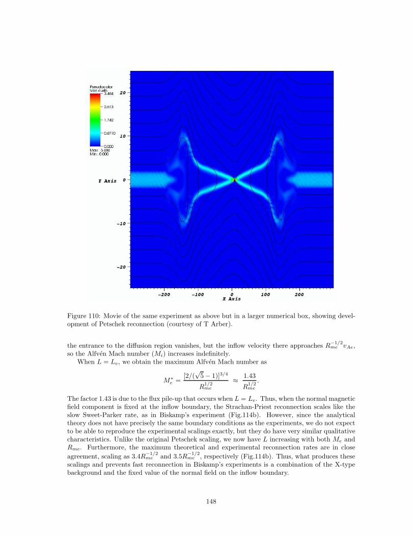
Figure 110: Movie of the same experiment as above but in a larger numerical box, showing devel-opment of Petschek reconnection (courtesy of T Arber).

the entrance to the diffusion region vanishes, but the inflow velocity there approaches R−1/2me vAe,

so the Alfven Mach number (Mi) increases indefinitely.When L = Le, we obtain the maximum Alfven Mach number as

M∗e =

[2/(√

5 − 1)]3/4

R1/2me

≈ 1.43

R1/2me

.

The factor 1.43 is due to the flux pile-up that occurs when L = Le. Thus, when the normal magneticfield component is fixed at the inflow boundary, the Strachan-Priest reconnection scales like theslow Sweet-Parker rate, as in Biskamp’s experiment (Fig.114b). However, since the analyticaltheory does not have precisely the same boundary conditions as the experiments, we do not expectto be able to reproduce the experimental scalings exactly, but they do have very similar qualitativecharacteristics. Unlike the original Petschek scaling, we now have L increasing with both Me andRme. Furthermore, the maximum theoretical and experimental reconnection rates are in close

agreement, scaling as 3.4R−1/2me and 3.5R

−1/2me , respectively (Fig.114b). Thus, what produces these

scalings and prevents fast reconnection in Biskamp’s experiments is a combination of the X-typebackground and the fixed value of the normal field on the inflow boundary.

148

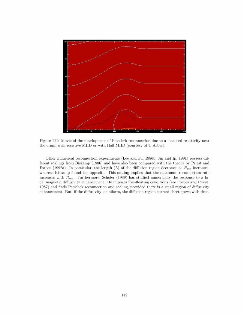
Figure 111: Movie of the development of Petschek reconnection due to a localised resistivity nearthe origin with resistive MHD or with Hall MHD (courtesy of T Arber).

Other numerical reconnection experiments (Lee and Fu, 1986b; Jin and Ip, 1991) possess dif-ferent scalings from Biskamp (1986) and have also been compared with the theory by Priest andForbes (1992a). In particular, the length (L) of the diffusion region decreases as Rme increases,whereas Biskamp found the opposite. This scaling implies that the maximum reconnection rateincreases with Rme. Furthermore, Scholer (1989) has studied numerically the response to a lo-cal magnetic diffusivity enhancement. He imposes free-floating conditions (see Forbes and Priest,1987) and finds Petschek reconnection and scaling, provided there is a small region of diffusivityenhancement. But, if the diffusivity is uniform, the diffusion-region current-sheet grows with time.

149

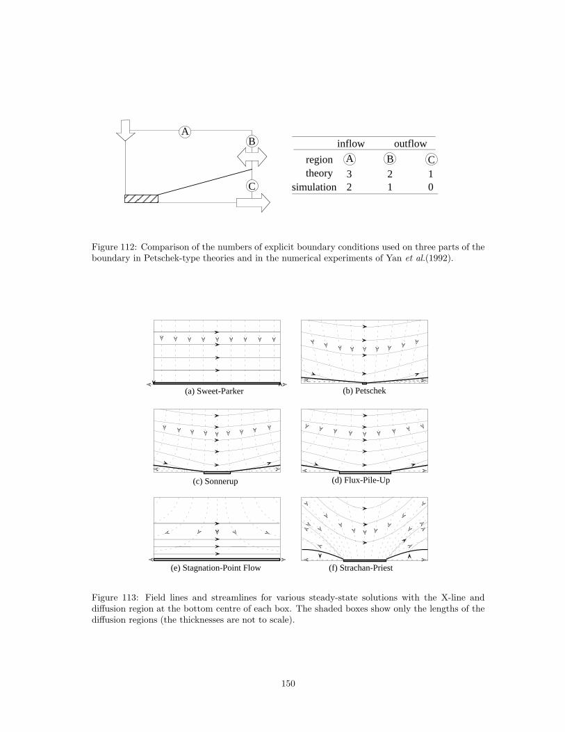
C

AB

simulation 2 01theory 3 12region

inflow outflow

A B C

Figure 112: Comparison of the numbers of explicit boundary conditions used on three parts of theboundary in Petschek-type theories and in the numerical experiments of Yan et al.(1992).

(b) Petschek

(f) Strachan-Priest

(d) Flux-Pile-Up(c) Sonnerup

(a) Sweet-Parker

(e) Stagnation-Point Flow

Figure 113: Field lines and streamlines for various steady-state solutions with the X-line anddiffusion region at the bottom centre of each box. The shaded boxes show only the lengths of thediffusion regions (the thicknesses are not to scale).

150

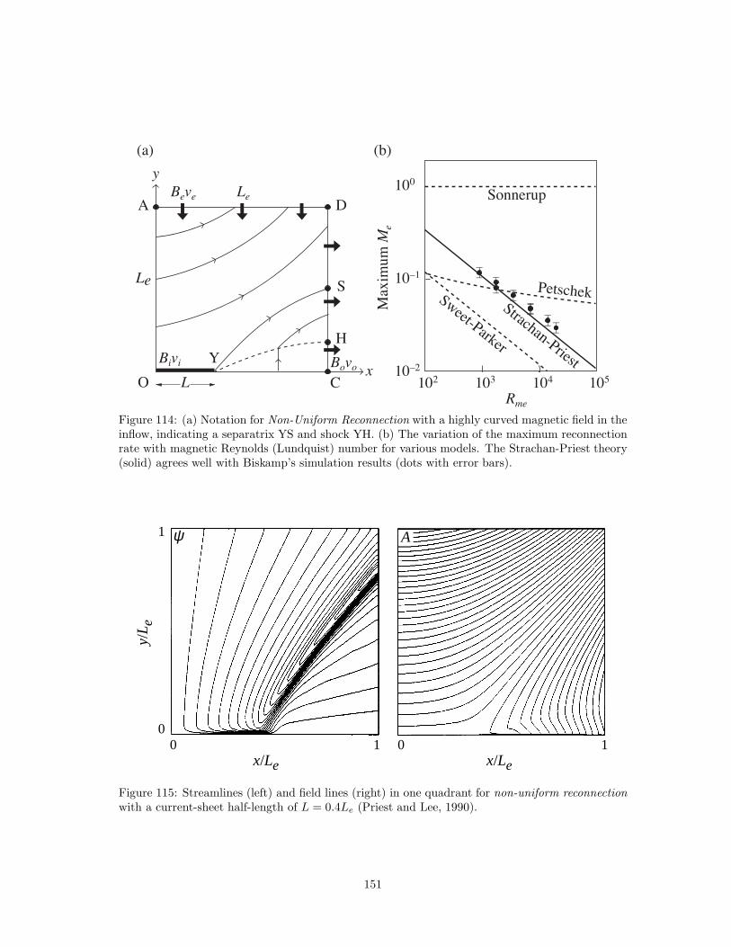
(a) (b)

y

L

A D

S

H

Y

C

Le

LeBeve

BovoBivi

Ox

Sonnerup

Rme

10–1

10–2

102 103 104 105

100

PetschekStrachan-Priest

Sweet-Parker

Max

imum

Me

Figure 114: (a) Notation for Non-Uniform Reconnection with a highly curved magnetic field in theinflow, indicating a separatrix YS and shock YH. (b) The variation of the maximum reconnectionrate with magnetic Reynolds (Lundquist) number for various models. The Strachan-Priest theory(solid) agrees well with Biskamp’s simulation results (dots with error bars).

A

x/Le

100

1

10

y/L e

x/Le

ψ

Figure 115: Streamlines (left) and field lines (right) in one quadrant for non-uniform reconnectionwith a current-sheet half-length of L = 0.4Le (Priest and Lee, 1990).

151

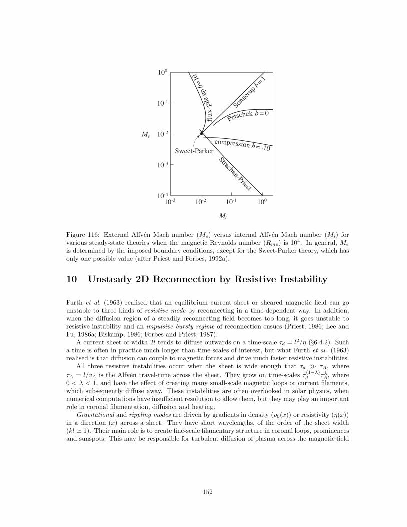
Sweet-Parker

100

10-1

10-2Me

Mi

10-3

10-4

10-3 10-2 10-1 100

Sonne

rup

b = 1

Petschek b = 0

compression b = -10

Strachan-Priest

flu

x-p

ile-

up b

= 10

Figure 116: External Alfven Mach number (Me) versus internal Alfven Mach number (Mi) forvarious steady-state theories when the magnetic Reynolds number (Rme) is 104. In general, Me

is determined by the imposed boundary conditions, except for the Sweet-Parker theory, which hasonly one possible value (after Priest and Forbes, 1992a).

10 Unsteady 2D Reconnection by Resistive Instability

Furth et al. (1963) realised that an equilibrium current sheet or sheared magnetic field can gounstable to three kinds of resistive mode by reconnecting in a time-dependent way. In addition,when the diffusion region of a steadily reconnecting field becomes too long, it goes unstable toresistive instability and an impulsive bursty regime of reconnection ensues (Priest, 1986; Lee andFu, 1986a; Biskamp, 1986; Forbes and Priest, 1987).

A current sheet of width 2l tends to diffuse outwards on a time-scale τd = l2/η (§6.4.2). Sucha time is often in practice much longer than time-scales of interest, but what Furth et al. (1963)realised is that diffusion can couple to magnetic forces and drive much faster resistive instabilities.

All three resistive instabilities occur when the sheet is wide enough that τd ≫ τA, where

τA = l/vA is the Alfven travel-time across the sheet. They grow on time-scales τ(1−λ)d τλ

A, where0 < λ < 1, and have the effect of creating many small-scale magnetic loops or current filaments,which subsequently diffuse away. These instabilities are often overlooked in solar physics, whennumerical computations have insufficient resolution to allow them, but they may play an importantrole in coronal filamentation, diffusion and heating.

Gravitational and rippling modes are driven by gradients in density (ρ0(x)) or resistivity (η(x))in a direction (x) across a sheet. They have short wavelengths, of the order of the sheet width(kl ≃ 1). Their main role is to create fine-scale filamentary structure in coronal loops, prominencesand sunspots. This may be responsible for turbulent diffusion of plasma across the magnetic field

152

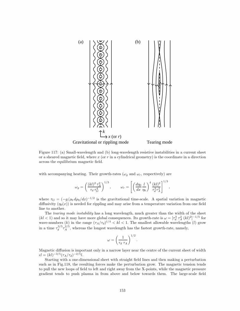
Gravitational or rippling mode Tearing mode

(a) (b)

kx (or r)

Figure 117: (a) Small-wavelength and (b) long-wavelength resistive instabilities in a current sheetor a sheared magnetic field, where x (or r in a cylindrical geometry) is the coordinate in a directionacross the equilibrium magnetic field.

with accompanying heating. Their growth-rates (ωg and ωr, respectively) are

ωg =

((kl)2 τ2

A

τd τ4G

)1/3

, ωr =

[(dη0dx

l

η0

)4(kl)2

τ3d τ

2A

]1/3

,

where τG = (−g/ρ0 dρ0/dx)−1/2 is the gravitational time-scale. A spatial variation in magnetic

diffusivity (η0(x)) is needed for rippling and may arise from a temperature variation from one fieldline to another.

The tearing mode instability has a long wavelength, much greater than the width of the sheet(kl < 1) and so it may have more global consequences. Its growth-rate is ω = [τ3

d τ2A (kl)2]−1/5 for

wave-numbers (k) in the range (τA/τd)1/4 < kl < 1. The smallest allowable wavelengths (l) grow

in a time τ3/5d τ

2/5A , whereas the longest wavelength has the fastest growth-rate, namely,

ω =

(1

τd τA

)1/2

.

Magnetic diffusion is important only in a narrow layer near the centre of the current sheet of widthǫl = (kl)−3/5(τA/τd)

−2/5l.Starting with a one-dimensional sheet with straight field lines and then making a perturbation

such as in Fig.118, the resulting forces make the perturbation grow. The magnetic tension tendsto pull the new loops of field to left and right away from the X-points, while the magnetic pressuregradient tends to push plasma in from above and below towards them. The large-scale field

153

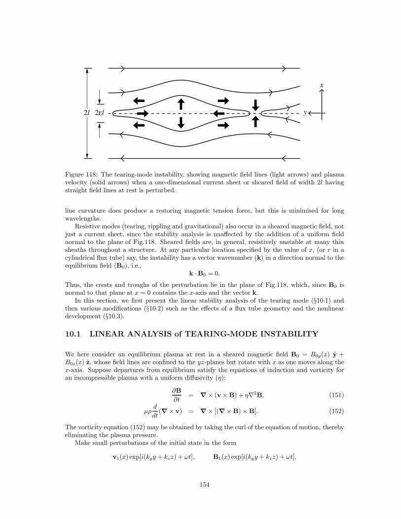
y2εl2l

x

Figure 118: The tearing-mode instability, showing magnetic field lines (light arrows) and plasmavelocity (solid arrows) when a one-dimensional current sheet or sheared field of width 2l havingstraight field lines at rest is perturbed.

line curvature does produce a restoring magnetic tension force, but this is minimised for longwavelengths.

Resistive modes (tearing, rippling and gravitational) also occur in a sheared magnetic field, notjust a current sheet, since the stability analysis is unaffected by the addition of a uniform fieldnormal to the plane of Fig.118. Sheared fields are, in general, resistively unstable at many thinsheaths throughout a structure. At any particular location specified by the value of x, (or r in acylindrical flux tube) say, the instability has a vector wavenumber (k) in a direction normal to theequilibrium field (B0), i.e.,

k ·B0 = 0.

Thus, the crests and troughs of the perturbation lie in the plane of Fig.118, which, since B0 isnormal to that plane at x = 0 contains the x-axis and the vector k.

In this section, we first present the linear stability analysis of the tearing mode (§10.1) andthen various modifications (§10.2) such as the effects of a flux tube geometry and the nonlineardevelopment (§10.3).

10.1 LINEAR ANALYSIS of TEARING-MODE INSTABILITY

We here consider an equilibrium plasma at rest in a sheared magnetic field B0 = B0y(x) y +B0z(x) z, whose field lines are confined to the yz-planes but rotate with x as one moves along thex-axis. Suppose departures from equilibrium satisfy the equations of induction and vorticity foran incompressible plasma with a uniform diffusivity (η):

∂B

∂t= ∇ × (v × B) + η∇2B, (151)

µρd

dt(∇ × v) = ∇ × [(∇ × B) × B]. (152)

The vorticity equation (152) may be obtained by taking the curl of the equation of motion, therebyeliminating the plasma pressure.

Make small perturbations of the initial state in the form

v1(x) exp[i(kyy + kzz) + ωt], B1(x) exp[i(kyy + kzz) + ωt],

154

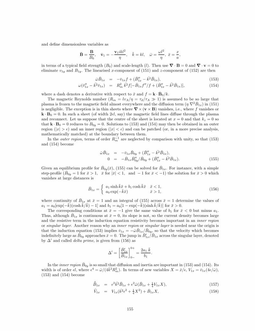
and define dimensionless variables as

B =B

B0, v1 = −v1ikl

2

η, k = kl, ω =

ωl2

η, x =

x

a,

in terms of a typical field strength (B0) and scale-length (l). Then use ∇ · B = 0 and ∇ · v = 0 toeliminate v1y and B1y. The linearised x-component of (151) and z-component of (152) are then

ωB1x = −v1xf + (B′′1x − k2B1x), (153)

ω(v′′1x − k2v1x) = R2m k2f [−B1xf

′′/f + (B′′1x − k2B1x)], (154)

where a dash denotes a derivative with respect to x and f = k · B0/k.The magnetic Reynolds number (Rm = lvA/η = τd/τA ≫ 1) is assumed to be so large that

plasma is frozen to the magnetic field almost everywhere and the diffusion term (η ∇2B1x) in (151)is negligible. The exception is in thin sheets where ∇× (v × B) vanishes, i.e., where f vanishes ork ·B0 = 0. In such a sheet (of width 2ǫl, say) the magnetic field lines diffuse through the plasmaand reconnect. Let us suppose that the centre of the sheet is located at x = 0 and that kz = 0 sothat k ·B0 = 0 reduces to B0y = 0. Solutions to (153) and (154) may then be obtained in an outerregion (|x| > ǫ) and an inner region (|x| < ǫ) and can be patched (or, in a more precise analysis,mathematically matched) at the boundary between them.

In the outer region, terms of order R−1m are neglected by comparison with unity, so that (153)

and (154) become

ωB1x = −v1xB0y + (B′′1x − k2B1x),

0 = −B1xB′′0y/B0y + (B′′

1x − k2B1x). (155)

Given an equilibrium profile for B0y(x), (155) can be solved for B1x. For instance, with a simplestep-profile (B0y = 1 for x > 1, x for |x| < 1, and − 1 for x < −1) the solution for x > 0 whichvanishes at large distances is

B1x =

{a1 sinh kx+ b1 cosh kx x < 1,a0 exp(−kx) x > 1,

(156)

where continuity of B1x at x = 1 and an integral of (155) across x = 1 determine the values ofa1 = a0[exp(−k)(cosh k/k) − 1] and b1 = a0[1 − exp(−k)(sinh k/k)] for x > 0.

The corresponding conditions at x = −1 give the same value of b1 for x < 0 but minus a1.Thus, although B1x is continuous at x = 0, its slope is not, so the current density becomes largeand the resistive term in the induction equation resistivity becomes important in an inner regionor singular layer. Another reason why an inner region or singular layer is needed near the origin isthat the induction equation (153) implies v1x = −ωB1x/B0y, so that the velocity which becomesindefinitely large as B0y approaches x = 0. The jump in B′

1x/B1x across the singular layer, denotedby ∆′ and called delta prime, is given from (156) as

∆′ =

[B′

1x

B1x

]0+

0−=

2a1 k

b1.

In the inner region B0y is so small that diffusion and inertia are important in (153) and (154). Itswidth is of order ǫl, where ǫ4 = ω/(4k2R2

m). In terms of new variables X = x/ǫ, V1x = v1x(4ǫ/ω),(153) and (154) become

¨B1x = ǫ2k2B1x + ǫ2ω(B1x + 14V1xX), (157)

V1x = V1x(k2ǫ2 + 14X

2) + B1xX, (158)

155

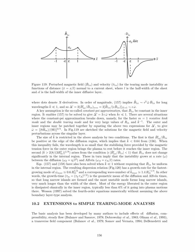
-1 -ε ε 1x

-1 -ε ε 1

B1x

x

-v1x

a0

a0 ω/ε

Figure 119: Perturbed magnetic field (B1x) and velocity (v1x) for the tearing mode instability asfunctions of distance (x = x/l) normal to a current sheet, where l is the half-width of the sheetand ǫl is the half-width of the inner diffusive layer.

where dots denote X-derivatives. In order of magnitude, (157) implies ¨B1x ∼ ǫ2 ω B1x for long

wavelengths k ≪ 1, and so ∆′ = 2(B′1x/B1x)x=ǫ = 2[ ˙B1x/(ǫB1x)]X=1 ∼ ǫ ω.

A key assumption is the so-called constant-psi approximation, that B1x be constant in the innerregion. It enables (157) to be solved to give ∆′ = 3 ǫ ω when kǫ ≪ 1. There are several situationswhere the constant-psi approximation breaks down, namely, for the faster m = 1 resistive kinkmode and the double tearing mode and for very large values of Rm and k−1. The outer andinner regions may be patched together by equating the above two expressions for ∆′, to giveω = [(8Rm)/(9k)]2/5. In Fig.119 are sketched the solutions for the magnetic field and velocityperturbations across the singular layer.

The size of k is restricted in the above analysis by two conditions. The first is that B′1x/B1x

be positive at the edge of the diffusion region, which implies that k < 0.64 from (156). Whenthis inequality fails, the wavelength is so small that the stabilising force provided by the magnetictension force in the outer region brings the plasma to rest before it reaches the inner region. Thesecond (k > 2(8/(3R2

m))1/8) arises from the condition (ǫ |B′1x/B1x| < 1) that B1x does not change

significantly in the internal region. These in turn imply that the instability grows at a rate (ω)between the diffusion (ωd = η/l2) and Alfven (ωA = vA/l) rates.

Eqs. (157) and (158) have also been solved when k ≪ 1 without requiring that B1x be uniformin the internal region. The resulting dispersion relation (Fig.120) has a growth-rate for the fastest-

growing mode of ωmax ≃ 0.6R1/2m and a corresponding wave-number of kmax ≃ 1.4R

−1/4m . In other

words, the growth-time (τm = (τd τA)1/2) is the geometric mean of the diffusion and Alfven times,so that long narrow islands are formed and the most unstable mode forms long narrow islands,very much longer than the width of the sheet. Most of the energy liberated in the outer regionis dissipated ohmically in the inner region, typically less than 6% of it going into plasma motionsthere. Wesson (1997) solved the fourth-order equations numerically without assuming the aboveboundary layer-type analysis.

10.2 EXTENSIONS to SIMPLE TEARING-MODE ANALYSIS

The basic analysis has been developed by many authors to include effects of: diffusion, com-pressibility, steady flow (Bulanov and Sasorov, 1978; Dobrowolny et al., 1983; Ofman et al., 1993),a transverse field component (Bulanov et al., 1979; Somov and Vernata, 1994; DeBenedetti and

156

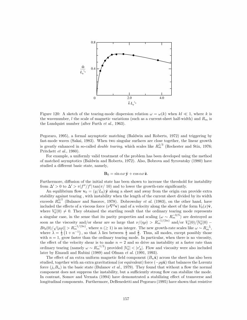
0

0.4

0.8

2.0 4.0

ω

Lu

1/2

k Lu

1/4

Figure 120: A sketch of the tearing-mode dispersion relation ω = ω(k) when kl ≪ 1, where k isthe wavenumber, l the scale of magnetic variations (such as a current-sheet half-width) and Rm isthe Lundquist number (after Furth et al., 1963).

Pegoraro, 1995), a formal asymptotic matching (Baldwin and Roberts, 1972) and triggering byfast-mode waves (Sakai, 1983). When two singular surfaces are close together, the linear growth

is greatly enhanced in so-called double tearing, which scales like R1/3m (Rechester and Stix, 1976;

Pritchett et al., 1980).For example, a uniformly valid treatment of the problem has been developed using the method

of matched asymptotics (Baldwin and Roberts, 1972). Also, Bobrova and Syrovatsky (1980) havestudied a different basic state, namely,

B0 = sinαx y + cosαx z.

Furthermore, diffusion of the initial state has been shown to increase the threshold for instabilityfrom ∆′ > 0 to ∆′ > π|f ′′/f ′| tan(π/ 10) and to lower the growth-rate significantly.

An equilibrium flow v0 = (y/L0) y along a sheet and away from the origin can provide extrastability against tearing , with instability when the length of the current sheet divided by its width

exceeds R3/7m (Bulanov and Sasorov, 1978). Dobrowolny et al. (1983), on the other hand, have

included the effects of a viscous force (ν∇2v) and of a velocity along the sheet of the form V0(x)v,where V ′

0(0) 6= 0. They obtained the startling result that the ordinary tearing mode represents

a singular case, in the sense that its parity properties and scaling (ω ∼ R−3/5m ) are destroyed as

soon as the viscosity and/or shear are so large that ν/(ηρ) > R−1/(3n)m and/or V ′

0(0)/[V ′0(0) −

B′0(0)/√

(µρ)] > R−1/(3n)m , where n (≥ 1) is an integer. The new growth-rate scales like ω ∼ R−λ

m ,where λ = 1

3

(1 + n−1

), so that λ lies between 1

3 and 23 . Thus, all modes, except possibly those

with n = 1, grow faster than the ordinary tearing mode. In particular, when there is no viscosity,the effect of the velocity shear is to make n = 2 and so drive an instability at a faster rate than

ordinary tearing (namely ω ∼ R−1/2m ) provided |V ′

0 | < |v′A|. Flow and viscosity were also includedlater by Einaudi and Rubini (1989) and Ofman et al. (1991, 1993).

The effect of an extra uniform magnetic field component (Bnx) across the sheet has also beenstudied, together with an extra gravitational (or equivalent) force (−ρgx) that balances the Lorentzforce (jzBn) in the basic state (Bulanov et al., 1979). They found that without a flow the normalcomponent does not suppress the instability, but a sufficiently strong flow can stabilize the mode.In contrast, Somov and Vernata (1994) have demonstrated a stabilizing effect of transverse andlongitudinal components. Furthermore, DeBenedetti and Pegoraro (1995) have shown that resistive

157

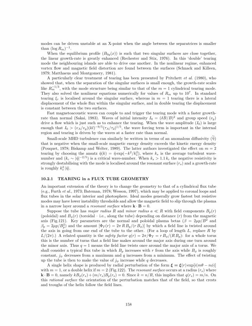
modes can be driven unstable at an X-point when the angle between the separatrices is smallerthan (logRm)−1.

When the equilibrium profile (B0y(x)) is such that two singular surfaces are close together,the linear growth-rate is greatly enhanced (Rechester and Stix, 1976). In this ‘double’ tearingmode the neighbouring islands are able to drive one another. In the nonlinear regime, enhancedvortex flow and magnetic field distortion are found between the surfaces (Schnack and Killeen,1979; Matthaeus and Montgomery, 1981).

A particularly clear treatment of tearing has been presented by Pritchett et al. (1980), whoshowed that, when the separation of the singular surfaces is small enough, the growth-rate scales

like R−1/3m , with the mode structure being similar to that of the m = 1 cylindrical tearing mode.

They also solved the nonlinear equations numerically for values of Rm up to 107. In standardtearing ξr is localised around the singular surface, whereas in m = 1 tearing there is a lateraldisplacement of the whole flux within the singular surface, and in double tearing the displacementis constant between the two surfaces.

Fast magnetoacoustic waves can couple to and trigger the tearing mode with a faster growth-rate than normal (Sakai, 1983). Waves of initial intensity I0 = (δB/B)2 and group speed (vg)drive a flow which is just such as to enhance the tearing. When the wave amplitude (I0) is largeenough that I0 > (vA/vg)(kl)

−9/5(τA/τd)1/5, the wave forcing term is important in the internal

region and tearing is driven by the waves at a faster rate than normal.

Small-scale MHD turbulence can similarly be written in terms of an anomalous diffusivity (∼η)

that is negative when the small-scale magnetic energy density exceeds the kinetic energy density(Pouquet, 1978; Biskamp and Welter, 1989). The latter authors investigated the effect on m = 2tearing by choosing the ansatz η(k) = η exp(−k2/k2

s), where ks is the average turbulent wave-number and (kc ∼ |η|−2/5) is a critical wave-number. When ks > 1.1 kc the negative resistivity isstrongly destabilising with the mode is localised around the resonant surface (rs) and a growth-rateis roughly k2

s |η|.

10.2.1 TEARING in a FLUX TUBE GEOMETRY

An important extension of the theory is to change the geometry to that of a cylindrical flux tube(e.g., Furth et al., 1973; Bateman, 1978; Wesson, 1997), which may be applied to coronal loops andflux tubes in the solar interior and photosphere. Ideal modes generally grow fastest but resistivemodes may have lower instability thresholds and allow the magnetic field to slip through the plasmain a narrow layer around a resonant surface where k · B = 0.

Suppose the tube has major radius R and minor radius a ≪ R with field components Bp(r)(poloidal) and Bφ(r) (toroidal – i.e., along the tube) depending on distance (r) from the magneticaxis (Fig.121). Key parameters are the normal and poloidal plasma betas (β = 2µp/B2 andβp = 2µp/B2

p) and the amount [ΦT (r) = 2πRBp/(r Bφ)] by which a field line is twisted aroundthe axis in going from one end of the tube to the other. (For a loop of length L, replace R byL/(2π).) A related quantity is the safety factor q(r) = 2π/ΦT = r Bφ/(RBp): for a whole torusthis is the number of turns that a field line makes around the major axis during one turn aroundthe minor axis. Thus q = 1 means the field line twists once around the major axis of a torus. Weshall consider a typical flux tube in which Bp increases with r from the axis while Bφ is roughlyconstant, jφ decreases from a maximum and q increases from a minimum. The effect of twistingup the tube is then to make the value of jφ increase while q decreases.

A single helix shape is produced by radial perturbation of the form ξ = ξ(r) exp[i(mθ − nφ)]withm = 1, or a double helix ifm = 2 (Fig.122). The resonant surface occurs at a radius (rs) wherek ·B = 0, namely kBφ(rs)+ (m/rs)Bp(rs) = 0. Since k = n/R, this implies that q(rs) = m/n. Onthis rational surface the orientation of the perturbation matches that of the field, so that crestsand troughs of the helix follow the field lines.

158

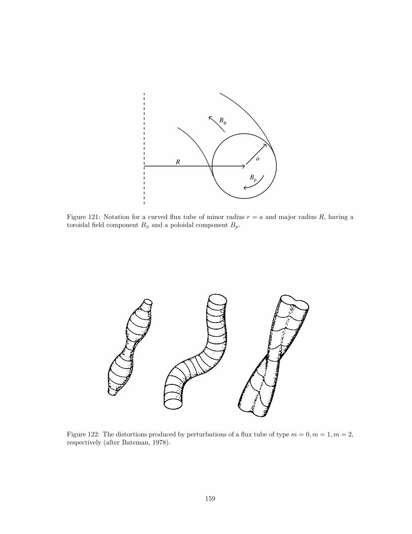
Bϕ

Bp

Ra

Figure 121: Notation for a curved flux tube of minor radius r = a and major radius R, having atoroidal field component Bφ and a poloidal component Bp.

Figure 122: The distortions produced by perturbations of a flux tube of type m = 0,m = 1,m = 2,respectively (after Bateman, 1978).

159

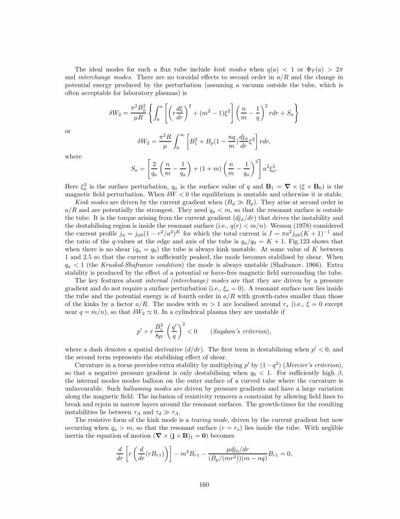
The ideal modes for such a flux tube include kink modes when q(a) < 1 or ΦT (a) > 2πand interchange modes. There are no toroidal effects to second order in a/R and the change inpotential energy produced by the perturbation (assuming a vacuum outside the tube, which isoften acceptable for laboratory plasmas) is

δW2 =π2B2

φ

µR

{∫ a

0

[(

rdξ

dr

)2

+ (m2 − 1)ξ2

](n

m− 1

q

)2

rdr + Sa

}

or

δW2 =π2R

µ

∫ ∞

0

[

B21 +Bp(1 − nq

m)djφdrξ2]

rdr,

where

Sa =

[

2

qa

(n

m− 1

qa

)

+ (1 +m)

(n

m− 1

qa

)2]

a2ξ2a.

Here ξ2a is the surface perturbation, qa is the surface value of q and B1 = ∇ × (ξ × B0) is themagnetic field perturbation. When δW < 0 the equilibrium is unstable and otherwise it is stable.

Kink modes are driven by the current gradient when (Bφ ≫ Bp). They arise at second order ina/R and are potentially the strongest. They need qa < m, so that the resonant surface is outsidethe tube. It is the torque arising from the current gradient (djφ/dr) that drives the instability andthe destabilising region is inside the resonant surface (i.e., q(r) < m/n). Wesson (1978) consideredthe current profile jφ = jφ0(1 − r2/a2)K for which the total current is I = πa2jφ0(K + 1)−1 andthe ratio of the q-values at the edge and axis of the tube is qa/q0 = K + 1. Fig.123 shows thatwhen there is no shear (qa = q0) the tube is always kink unstable. At some value of K between1 and 2.5 so that the current is sufficiently peaked, the mode becomes stabilised by shear. Whenqa < 1 (the Kruskal-Shafranov condition) the mode is always unstable (Shafranov, 1966). Extrastability is produced by the effect of a potential or force-free magnetic field surrounding the tube.

The key features about internal (interchange) modes are that they are driven by a pressuregradient and do not require a surface perturbation (i.e., ξa = 0). A resonant surface now lies insidethe tube and the potential energy is of fourth order in a/R with growth-rates smaller than thoseof the kinks by a factor a/R. The modes with m > 1 are localised around rs (i.e., ξ = 0 exceptnear q = m/n), so that δW2 ≃ 0. In a cylindrical plasma they are unstable if

p′ + rB2

z

8µ

(q′

q

)2

< 0 (Suydam’s criterion),

where a dash denotes a spatial derivative (d/dr). The first term is destabilising when p′ < 0, andthe second term represents the stabilising effect of shear.

Curvature in a torus provides extra stability by multiplying p′ by (1−q2) (Mercier’s criterion),so that a negative pressure gradient is only destabilising when q0 < 1. For sufficiently high β,the internal modes modes balloon on the outer surface of a curved tube where the curvature isunfavourable. Such ballooning modes are driven by pressure gradients and have a large variationalong the magnetic field. The inclusion of resistivity removes a constraint by allowing field lines tobreak and rejoin in narrow layers around the resonant surfaces. The growth-times for the resultinginstabilities lie between τA and τd ≫ τA.

The resistive form of the kink mode is a tearing mode, driven by the current gradient but nowoccurring when qa > m, so that the resonant surface (r = rs) lies inside the tube. With neglibleinertia the equation of motion (∇ × (j × B)1 = 0) becomes

d

dr

[

r

(d

dr(rBr1)

)]

−m2Br1 −µdjφ/dr

(Bp/(mr2))(m − nq)Br1 = 0,

160

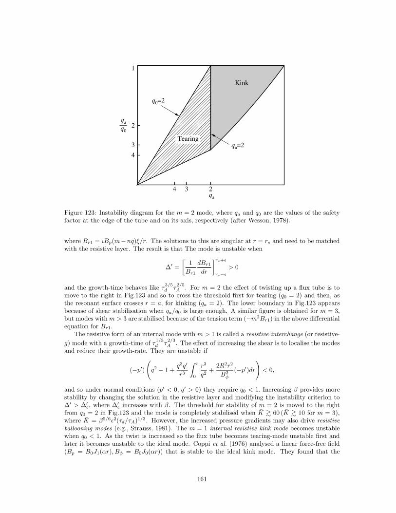
4

3

2

1

4 3 2

qa q0

qa

qa=2

q0=2

Kink

Tearing

Figure 123: Instability diagram for the m = 2 mode, where qa and q0 are the values of the safetyfactor at the edge of the tube and on its axis, respectively (after Wesson, 1978).

where Br1 = iBp(m−nq)ξ/r. The solutions to this are singular at r = rs and need to be matchedwith the resistive layer. The result is that The mode is unstable when

∆′ =

[1

Br1

dBr1

dr

]rs+ǫ

rs−ǫ

> 0

and the growth-time behaves like τ3/5d τ

2/5A . For m = 2 the effect of twisting up a flux tube is to

move to the right in Fig.123 and so to cross the threshold first for tearing (q0 = 2) and then, asthe resonant surface crosses r = a, for kinking (qa = 2). The lower boundary in Fig.123 appearsbecause of shear stabilisation when qa/q0 is large enough. A similar figure is obtained for m = 3,but modes with m > 3 are stabilised because of the tension term (−m2Br1) in the above differentialequation for Br1.

The resistive form of an internal mode with m > 1 is called a resistive interchange (or resistive-

g) mode with a growth-time of τ1/3d τ

2/3A . The effect of increasing the shear is to localise the modes

and reduce their growth-rate. They are unstable if

(−p′)(

q2 − 1 +q3q′

r3

∫ r

0

r3

q2+

2R2r2

B2φ

(−p′)dr)

< 0,

and so under normal conditions (p′ < 0, q′ > 0) they require q0 < 1. Increasing β provides morestability by changing the solution in the resistive layer and modifying the instability criterion to∆′ > ∆′

c, where ∆′c increases with β. The threshold for stability of m = 2 is moved to the right

from q0 = 2 in Fig.123 and the mode is completely stabilised when K & 60 (K & 10 for m = 3),where K = β5/6ǫ2(τd/τA)1/3. However, the increased pressure gradients may also drive resistiveballooning modes (e.g., Strauss, 1981). The m = 1 internal resistive kink mode becomes unstablewhen q0 < 1. As the twist is increased so the flux tube becomes tearing-mode unstable first andlater it becomes unstable to the ideal mode. Coppi et al. (1976) analysed a linear force-free field(Bp = B0J1(αr), Bφ = B0J0(αr)) that is stable to the ideal kink mode. They found that the

161

fastest growing perturbations have long wavelength (krs ≪ 1) and m = 1, with a growth-time

τ ∼ τ1/3d τ

2/3A that is somewhat shorter than the planar value (τ

1/2d τ

1/2A ).

In the case of the solar flare, an important extra effect is line-tying of the ends of coronalmagnetic fields in the dense photosphere. In order of magnitude, an ideal kink mode needs 2π/k ≤L so that a wavelength (2π/k) can fit into a loop of length L. But k satisfies k ·B0 = 0, and sothis condition reduces to ΦT ≥ 2π in terms of the twist (ΦT = LBp/(rBφ)). A precise analysisgives instead a threshold for ideal instability of ΦT = 2.5π for a field of uniform twist or largerfor other equilibria (Hood and Priest, 1981). During its nonlinear development a flux tube maybecome highly kinked, with many reconnecting current sheets (Browning et al., 2008; Hood et al.,2009b).

An important question is the relative thresholds of resistive and ideal modes. In a periodic tubethe resistive kink instability does have a lower threshold than the idea kink, but what happensin a line-tied solar coronal loop is uncertain. A line-tied resistive ballooning mode just diffusesslowly below the ideal threshold and has a fractional power of resistivity when the idea mode ismarginally stable (Velli and Hood, 1986). Possibly, this carries over to the m=1 resistive kink,since there is no mode rational surface in a line-tied cylinder.

10.3 NONLINEAR EVOLUTION of TEARING

In its nonlinear development tearing can follow several pathways, depending on the value of Rm,the equilibrium and the boundary conditions. A full treatment is still needed. Tokamak physicistshave emphasised nonlinear saturation, while solar flare theorists have stressed a rapid nonlinearphase, which may develop from linear tearing (with free boundary conditions) or may be drivenby an ideal instability.

For standard tearing the constant-psi approximation holds, and the instability quickly saturatesnonlinearly (Rutherford, 1973). The unstable perturbation diffuses in from the external region andproduces wider magnetic islands with higher inertia, which greatly slows the rate and magnitudeof energy release. When the island width exceeds the resistive layer width (ǫl) and nonlinear termsare included in the singular layer, the linear exponential growth is replaced by a slower algebraicgrowth of the perturbed magnetic field like t2 and of the island width (w = 4(−A1/B

′0y)1/2) like

t. Eventually, the growth saturates at an island width of order ∆′1(0)l2 (White et al., 1977). In

the linear phase the tearing flow pattern is driven by the linear force j1zB0y, but in the nonlinearphase this force is opposed by a third-order force (j2zB1x).

Rutherford’s theory was extended by White et al. (1977) who set up an analytical model forisland saturation by the quasi-linear development of a single mode. They wrote the magneticfield terms of a flux function A with an equilibrium profile A0(x). A perturbation of the formA1(x) cos ky produces islands of width w = 4(−A1(0)/A′′

0 (0))1/2. They assumed inertia is unim-portant, so that j× B = 0 or ∇2A = −µjz(A). In the external region this becomes, to first order,∇2A1 = −µ(∂j0/∂A)A1, which, for an equilibrium profile B0y = B0 tanhx/l, has solution

A1(x) = A1 exp(∓kx) (1 ± tanh(x/l)

(kl)).

Here A0 → 0 as |x| → ∞ and the upper sign corresponds to the region x > 12w. Inside the island

the flux function and current are approximated by

A = (A0(r) + ǫ(A1(0) +A′1(0)x) cos ky, jz = a+ bA.

Matching to the exterior solution determines the constants a and b. The time-evolution is deter-

162

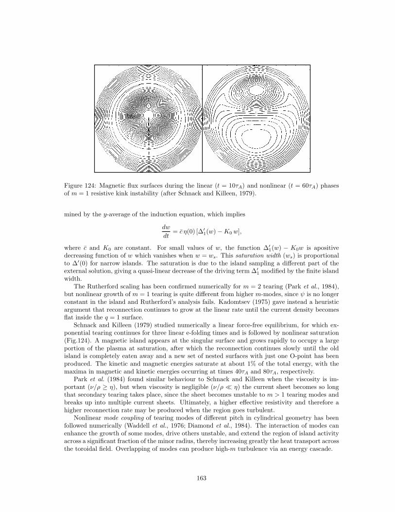
Figure 124: Magnetic flux surfaces during the linear (t = 10τA) and nonlinear (t = 60τA) phasesof m = 1 resistive kink instability (after Schnack and Killeen, 1979).

mined by the y-average of the induction equation, which implies

dw

dt= c η(0) [∆′

1(w) −K0 w],

where c and K0 are constant. For small values of w, the function ∆′1(w) − K0w is apositive

decreasing function of w which vanishes when w = ws. This saturation width (ws) is proportionalto ∆′(0) for narrow islands. The saturation is due to the island sampling a different part of theexternal solution, giving a quasi-linear decrease of the driving term ∆′

1 modified by the finite islandwidth.

The Rutherford scaling has been confirmed numerically for m = 2 tearing (Park et al., 1984),but nonlinear growth of m = 1 tearing is quite different from higher m-modes, since ψ is no longerconstant in the island and Rutherford’s analysis fails. Kadomtsev (1975) gave instead a heuristicargument that reconnection continues to grow at the linear rate until the current density becomesflat inside the q = 1 surface.

Schnack and Killeen (1979) studied numerically a linear force-free equilibrium, for which ex-ponential tearing continues for three linear e-folding times and is followed by nonlinear saturation(Fig.124). A magnetic island appears at the singular surface and grows rapidly to occupy a largeportion of the plasma at saturation, after which the reconnection continues slowly until the oldisland is completely eaten away and a new set of nested surfaces with just one O-point has beenproduced. The kinetic and magnetic energies saturate at about 1% of the total energy, with themaxima in magnetic and kinetic energies occurring at times 40τA and 80τA, respectively.

Park et al. (1984) found similar behaviour to Schnack and Killeen when the viscosity is im-portant (ν/ρ ≥ η), but when viscosity is negligible (ν/ρ ≪ η) the current sheet becomes so longthat secondary tearing takes place, since the sheet becomes unstable to m > 1 tearing modes andbreaks up into multiple current sheets. Ultimately, a higher effective resistivity and therefore ahigher reconnection rate may be produced when the region goes turbulent.

Nonlinear mode coupling of tearing modes of different pitch in cylindrical geometry has beenfollowed numerically (Waddell et al., 1976; Diamond et al., 1984). The interaction of modes canenhance the growth of some modes, drive others unstable, and extend the region of island activityacross a significant fraction of the minor radius, thereby increasing greatly the heat transport acrossthe toroidal field. Overlapping of modes can produce high-m turbulence via an energy cascade.

163

A chain of magnetic islands created by tearing can also be subject to an ideal coalescenceinstability (Finn and Kaw, 1977; Longcope and Strauss, 1993). Such an island chain is similarto an array of current filaments superimposed on the original current sheet, with the O-pointsrepresenting current maxima and the X-points current minima. Neighbouring islands coalescebecause parallel currents at the O-points attract one another. Consider an initial state with a fluxfunction

A0 = loge (cosh kx+ ǫ cos ky),

for which a perturbation (A1) causes an energy change of

δW =

∫

|∇A1|2 +A21 µ

dj0dA0

dV,

The first term is stabilising due to the increase in magnetic pressure as the flux piles up on both sidesof the X-point, whereas the second term is destabilising due to the attraction of current filaments.Here A1 is given by ωA1 = −v1 · ∇A0 in terms of an incompressible velocity v1 = −z × ∇ψ. Atrial stream function is assumed in the form

ψ = ψ0(λ0, x)(sin12y + λ1 sin 3

2y + λ2 sin 52y + . . .),

whereψ0(x) = tanh2(λ0 ǫ

−1/2x) exp(− 12x)(2 + coshx),

which gives the correct behaviour for the single-mode solution to the linear equations at largedistances (|x| ≫ ǫ1/2). The above trial function possesses three parameters, which are determinedby minimising δW to be λ0 ≈ 1, λ1 = −0.32 and λ2 = 0.1. Instability (δW < 0) is foundwith a minimising displacement that peaks around the O-points and vanishes at the X-points.Numerical computations show how nonlinear coalescence depends on the island amplitude (ǫ) andRm (Prichett and Wu, 1979; Biskamp, 1982).

When ǫ = 0.3 neighbouring islands merge completely and oscillate. When ǫ = 0.2 and 104 <

Rm < 5× 104 the sheet width scales as R−1/2m and the diffusion region length L remains constant.

At larger Rm (5×104 - 105), the ideal coalescence instability makes the flux pile up at the diffusionregion, which grows in length until it it undergoes secondary tearing and one enters a regime ofimpulsive bursty reconnection (cf Priest, 1986; Forbes and Priest, 1987).

Coalescence has been investigated numerically by Bhattacharjee et al. (1983), who found thatthe instability proceeded in three stages: the islands first approach and form a current sheet; thereconnection takes place; and the instability saturates after typically 30 τA with the single islandsitting there and oscillating in response to its jarring experience. The amount of reconnected flux

grows linearly with time in the second stage like R−1/2m t for Rm between 500-2000. There is no

evidence of shocks, either because the reconnection is too slow and the current sheet too longor perhaps because of insufficient grid-point resolution. Secondary tearing was observed but thesecondary islands are always swept along the current sheet, since no up-down symmetry conditionsare imposed at the current sheet. The density contours reveal a highly compressed current sheet,which is larger than one expects from Petschek theory (probably because of flux pile-up) but whichbifurcates at its ends to give pairs of structures that are suggestive of slow shocks.

In practice, tearing often favours the longest-wavelength mode that fits a given structure, sincemany structures are shorter than the fastest-growing mode in an infinite medium. Therefore, ifsuch a mode grows and saturates, coalescence is unlikely. However, if an external disturbance orextra physical effects favour a shorter wavelength mode or if the structure is long enough, thencoalescence may follow.

Primary coalescence would be important for solar plasmas or numerical experiments with a largeenough Rm. The coalescence time for islands of initial half-width xi0 = 2lǫ1/2 is τc = τAxi0/2l.

164

Coalescence of such islands will be important if the tearing-mode time (τm = τAR1/2m ) is much

larger than τc, i.e., if R1/2m ≫ 2l/xi0. Coalescence can also be compared with saturation, which

occurs after a time τs ≈ τm log(l/xi0) such that the island half-width (xi = xi0 exp(t/τm)) hasgrown to equal l. Primary coalescence will therefore take place before saturation if τc < τs, or

2(l/xi0) < R1/2m log(l/xi0), so that, for a given (l/xi0), coalescence will occur first if Rm is too

great.The sequence of events expected in a solar current sheet with a large Rm is as follows. If

the sheet is shorter than the fastest-growing mode in an infinite medium, then tearing favoursthe longest-wavelength mode that fits. If it is longer, then, first of all, the sheet tears linearly

at a wavenumber (1.4 R−1/4m /l) of the fastest growing mode. Then primary coalescence combines

neighbouring islands. This may lead to a fast reconnection regime (such as Petschek or flux pile-up), often disrupted by impulsive bursty reconnection due to secondary tearing and coalescence ofthe diffusion region. However, in a current sheet that is line-tied at one end to the photosphere,dominant tearing may develop at the neutral point closest to the surface. This neutral pointdoes not coalesce with its neighbour but develops fast nonlinear reconnection which subsequentlyundergoes secondary tearing and coalescence.

165

11 Magnetic Reconnection Regimes in Three Dimensions

In three dimensions, reconnection may take place in a variety of different regimes and a vari-ety of different geometries, namely, at a null point, at a separator or at non-null regions such as aquasi-separator, as described below. Here we first describe the various complementary techniquesthat can be used to model three-dimensional reconnection (§11.1), and then we discuss the regimesthat have been discovered at a null point (§11.2), a separator (§11.3) and a quasi-separator (§11.4).Finally, we review numerical experiments that are shedding new light on the nature of such regimes(§12).

11.1 TECHNIQUES for MODELLING 3D RECONNECTION

From the kinematics of steady ideal flows in the neighbourhood of a null point or separator(§11.1.1), three distinct types of 3D reconnection were proposed, depending on where the cur-rent concentrates, namely spine, fan and separator reconnection when it focuses along a spine,a fan or a separator, respectively (Priest and Titov, 1996). Later, the nature of the flow in thediffusion region was studied (§11.1.2) and computational experiments were set up (§11.1.3), whichled to a new categorisation of null-point reconnection (§11.2) into spine-fan reconnection, torsionalspine reconnection and torsional fan reconnection (Priest and Pontin, 2009).

11.1.1 KINEMATIC IDEAL MODELS - SPINE and FAN REGIMES

Priest and Titov (1996) extended earlier ideas Lau and Finn (1990) for studying the effects ofsteady reconnection in the ideal region around a 3D null, by solving the kinematic equations for vand E:

E + v × B = 0 and ∇ × E = 0, (159)

when B is given by

(Bx, By, Bz) =B0

L0(x, y,−2z)

and a variety of different boundary conditions is imposed.First of all, Eq. (159b) implies that E = ∇Φ and so the component of Eq. (159a) perpendicular

to B yieldsB · ∇Φ = 0,

which, for given values of Φ on a surface, may be integrated along field lines (characteristics) todetermine the value of Φ (and therefore E) throughout the volume. Then the component of Eq.(159a) perpendicular to B determines the plasma velocity normal to B everywhere as

v⊥ =∇Φ × B

B2. (160)

When a continuous flow is imposed across the fan (Fig.125a,126), singularities in E and voccur at the spine. It was speculated that this would produce a strong current at the spine inwhat was dubbed spine reconnection by Priest and Titov (1996). They considered the effect ofdiffusion in a preliminary manner, but were unable at the time to resolve the singularities at thespine. As an example, they considered flows with no φ-component and an electric field of the formEφ = veB0 sinφ, giving rise to a velocity

v⊥R =2EφL

20z/B0

R(R2 + 4z2), v⊥z =

EφL20z/B0

R2 + 4z2,

166

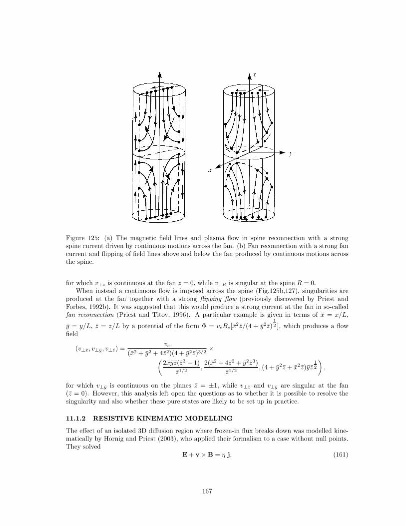
Figure 125: (a) The magnetic field lines and plasma flow in spine reconnection with a strongspine current driven by continuous motions across the fan. (b) Fan reconnection with a strong fancurrent and flipping of field lines above and below the fan produced by continuous motions acrossthe spine.

for which v⊥z is continuous at the fan z = 0, while v⊥R is singular at the spine R = 0.When instead a continuous flow is imposed across the spine (Fig.125b,127), singularities are

produced at the fan together with a strong flipping flow (previously discovered by Priest andForbes, 1992b). It was suggested that this would produce a strong current at the fan in so-calledfan reconnection (Priest and Titov, 1996). A particular example is given in terms of x = x/L,

y = y/L, z = z/L by a potential of the form Φ = veBe[x2z/(4 + y2z)

12 ], which produces a flow

field

(v⊥x, v⊥y, v⊥z) =ve

(x2 + y2 + 4z2)(4 + y2z)3/2×

(2xyz(z3 − 1)

z1/2,2(x2 + 4z2 + y2z3)

z1/2, (4 + y2z + x2z)yz

12

)

,

for which v⊥y is continuous on the planes z = ±1, while v⊥x and v⊥y are singular at the fan(z = 0). However, this analysis left open the questions as to whether it is possible to resolve thesingularity and also whether these pure states are likely to be set up in practice.

11.1.2 RESISTIVE KINEMATIC MODELLING

The effect of an isolated 3D diffusion region where frozen-in flux breaks down was modelled kine-matically by Hornig and Priest (2003), who applied their formalism to a case without null points.They solved

E + v × B = η j, (161)

167

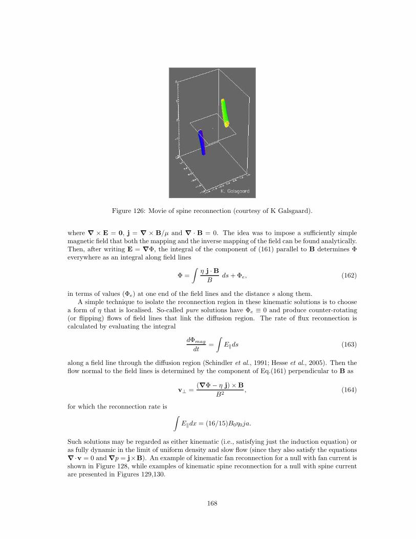
Figure 126: Movie of spine reconnection (courtesy of K Galsgaard).

where ∇ × E = 0, j = ∇ × B/µ and ∇ · B = 0. The idea was to impose a sufficiently simplemagnetic field that both the mapping and the inverse mapping of the field can be found analytically.Then, after writing E = ∇Φ, the integral of the component of (161) parallel to B determines Φeverywhere as an integral along field lines

Φ =

∫η j · BB

ds+ Φe, (162)

in terms of values (Φe) at one end of the field lines and the distance s along them.A simple technique to isolate the reconnection region in these kinematic solutions is to choose

a form of η that is localised. So-called pure solutions have Φe ≡ 0 and produce counter-rotating(or flipping) flows of field lines that link the diffusion region. The rate of flux reconnection iscalculated by evaluating the integral

dΦmag

dt=

∫

E‖ds (163)

along a field line through the diffusion region (Schindler et al., 1991; Hesse et al., 2005). Then theflow normal to the field lines is determined by the component of Eq.(161) perpendicular to B as

v⊥ =(∇Φ − η j) × B

B2, (164)

for which the reconnection rate is∫

E‖dx = (16/15)B0η0ja.

Such solutions may be regarded as either kinematic (i.e., satisfying just the induction equation) oras fully dynamic in the limit of uniform density and slow flow (since they also satisfy the equations∇ ·v = 0 and ∇p = j×B). An example of kinematic fan reconnection for a null with fan current isshown in Figure 128, while examples of kinematic spine reconnection for a null with spine currentare presented in Figures 129,130.

168

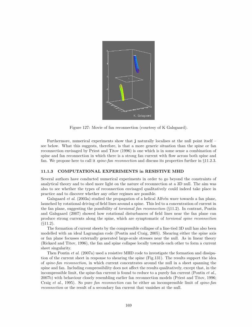
Figure 127: Movie of fan reconnection (courtesy of K Galsgaard).

Furthermore, numerical experiments show that j naturally localises at the null point itself –see below. What this suggests, therefore, is that a more generic situation than the spine or fanreconnection envisaged by Priest and Titov (1996) is one which is in some sense a combination ofspine and fan reconnection in which there is a strong fan current with flow across both spine andfan. We propose here to call it spine-fan reconnection and discuss its properties further in §11.2.3.

11.1.3 COMPUTATIONAL EXPERIMENTS in RESISTIVE MHD

Several authors have conducted numerical experiments in order to go beyond the constraints ofanalytical theory and to shed more light on the nature of reconnection at a 3D null. The aim wasalso to see whether the types of reconnection envisaged qualitatively could indeed take place inpractice and to discover whether any other regimes are possible.

Galsgaard et al. (2003a) studied the propagation of a helical Alfven wave towards a fan plane,launched by rotational driving of field lines around a spine. This led to a concentration of current inthe fan plane, suggesting the possibility of torsional fan reconnection (§11.2). In contrast, Pontinand Galsgaard (2007) showed how rotational disturbances of field lines near the fan plane canproduce strong currents along the spine, which are symptomatic of torsional spine reconnection(§11.2).

The formation of current sheets by the compressible collapse of a line-tied 3D null has also beenmodelled with an ideal Lagrangian code (Pontin and Craig, 2005). Shearing either the spine axisor fan plane focusses externally generated large-scale stresses near the null. As in linear theory(Rickard and Titov, 1996), the fan and spine collapse locally towards each other to form a currentsheet singularity.

Then Pontin et al. (2007a) used a resistive MHD code to investigate the formation and dissipa-tion of the current sheet in response to shearing the spine (Fig.131). The results support the ideaof spine-fan reconnection, in which current concentrates around the null in a sheet spanning thespine and fan. Including compressibility does not affect the results qualitatively, except that, in theincompressible limit, the spine-fan current is found to reduce to a purely fan current (Pontin et al.,2007b) with behaviour closely resembling earlier fan reconnection models (Priest and Titov, 1996;Craig et al., 1995). So pure fan reconnection can be either an incompressible limit of spine-fanreconnection or the result of a secondary fan current that vanishes at the null.

169

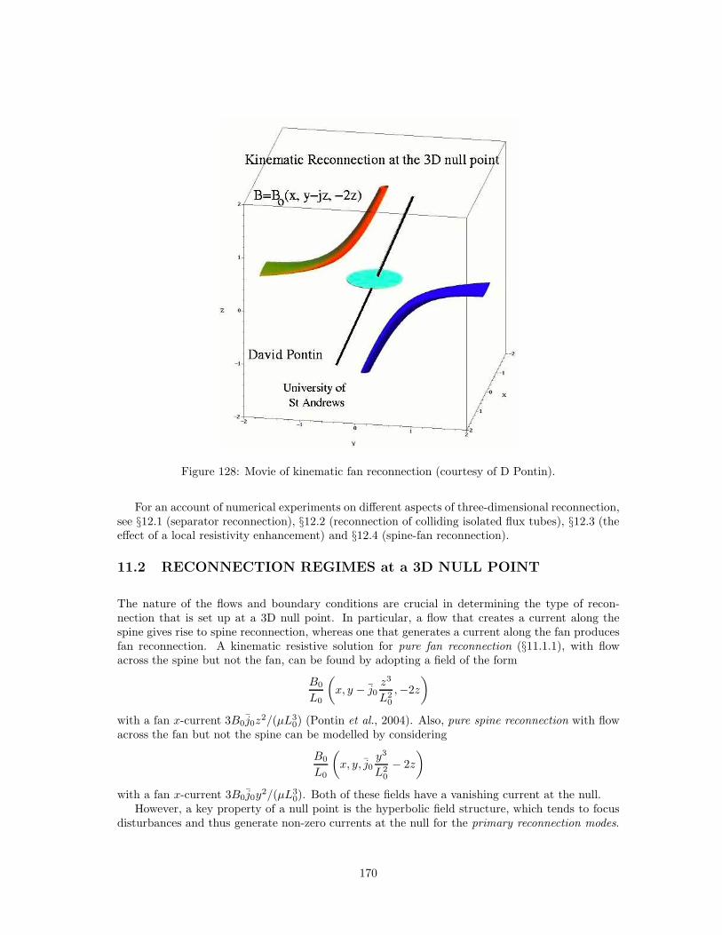
Figure 128: Movie of kinematic fan reconnection (courtesy of D Pontin).

For an account of numerical experiments on different aspects of three-dimensional reconnection,see §12.1 (separator reconnection), §12.2 (reconnection of colliding isolated flux tubes), §12.3 (theeffect of a local resistivity enhancement) and §12.4 (spine-fan reconnection).

11.2 RECONNECTION REGIMES at a 3D NULL POINT

The nature of the flows and boundary conditions are crucial in determining the type of recon-nection that is set up at a 3D null point. In particular, a flow that creates a current along thespine gives rise to spine reconnection, whereas one that generates a current along the fan producesfan reconnection. A kinematic resistive solution for pure fan reconnection (§11.1.1), with flowacross the spine but not the fan, can be found by adopting a field of the form

B0

L0

(

x, y − j0z3

L20

,−2z

)

with a fan x-current 3B0j0z2/(µL3

0) (Pontin et al., 2004). Also, pure spine reconnection with flowacross the fan but not the spine can be modelled by considering

B0

L0

(

x, y, j0y3

L20

− 2z

)

with a fan x-current 3B0j0y2/(µL3

0). Both of these fields have a vanishing current at the null.However, a key property of a null point is the hyperbolic field structure, which tends to focus

disturbances and thus generate non-zero currents at the null for the primary reconnection modes.

170

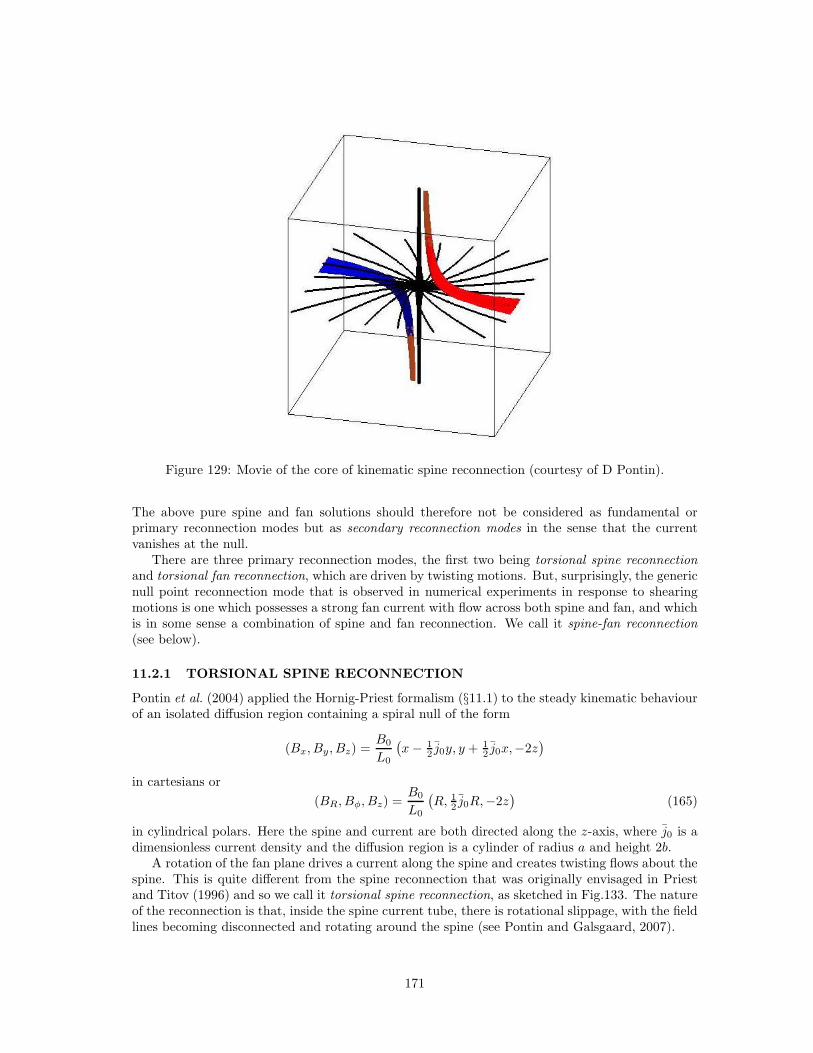
Figure 129: Movie of the core of kinematic spine reconnection (courtesy of D Pontin).

The above pure spine and fan solutions should therefore not be considered as fundamental orprimary reconnection modes but as secondary reconnection modes in the sense that the currentvanishes at the null.

There are three primary reconnection modes, the first two being torsional spine reconnectionand torsional fan reconnection, which are driven by twisting motions. But, surprisingly, the genericnull point reconnection mode that is observed in numerical experiments in response to shearingmotions is one which possesses a strong fan current with flow across both spine and fan, and whichis in some sense a combination of spine and fan reconnection. We call it spine-fan reconnection(see below).

11.2.1 TORSIONAL SPINE RECONNECTION

Pontin et al. (2004) applied the Hornig-Priest formalism (§11.1) to the steady kinematic behaviourof an isolated diffusion region containing a spiral null of the form

(Bx, By, Bz) =B0

L0

(x− 1

2 j0y, y + 12 j0x,−2z

)

in cartesians or

(BR, Bφ, Bz) =B0

L0

(R, 1

2 j0R,−2z)

(165)

in cylindrical polars. Here the spine and current are both directed along the z-axis, where j0 is adimensionless current density and the diffusion region is a cylinder of radius a and height 2b.

A rotation of the fan plane drives a current along the spine and creates twisting flows about thespine. This is quite different from the spine reconnection that was originally envisaged in Priestand Titov (1996) and so we call it torsional spine reconnection, as sketched in Fig.133. The natureof the reconnection is that, inside the spine current tube, there is rotational slippage, with the fieldlines becoming disconnected and rotating around the spine (see Pontin and Galsgaard, 2007).

171

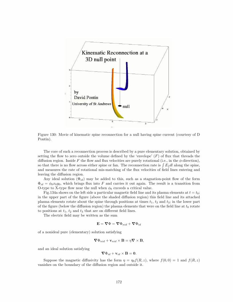
Figure 130: Movie of kinematic spine reconnection for a null having spine current (courtesy of DPontin).

The core of such a reconnection process is described by a pure elementary solution, obtained bysetting the flow to zero outside the volume defined by the ‘envelope’ (F ) of flux that threads thediffusion region. Inside F the flow and flux velocities are purely rotational (i.e., in the φ-direction),so that there is no flow across either spine or fan. The reconnection rate is

∫E‖dl along the spine,

and measures the rate of rotational mis-matching of the flux velocities of field lines entering andleaving the diffusion region.

Any ideal solution (Φid) may be added to this, such as a stagnation-point flow of the formΦid = φ0x0y0, which brings flux into F and carries it out again. The result is a transition fromO-type to X-type flow near the null when φ0 exceeds a critical value.

Fig.134a shows on the left side a particular magnetic field line and its plasma elements at t = t0;in the upper part of the figure (above the shaded diffusion region) this field line and its attachedplasma elements rotate about the spine through positions at times t1, t2 and t3; in the lower partof the figure (below the diffusion region) the plasma elements that were on the field line at t0 rotateto positions at t1, t2 and t3 that are on different field lines.

The electric field may be written as the sum

E = ∇Φ = ∇Φnid + ∇Φid

of a nonideal pure (elementary) solution satisfying

∇Φnid + vnid × B = η∇ × B,

and an ideal solution satisfying∇Φid + vid × B = 0.

Suppose the magnetic diffusivity has the form η = η0f(R, z), where f(0, 0) = 1 and f(R, z)vanishes on the boundary of the diffusion region and outside it.

172

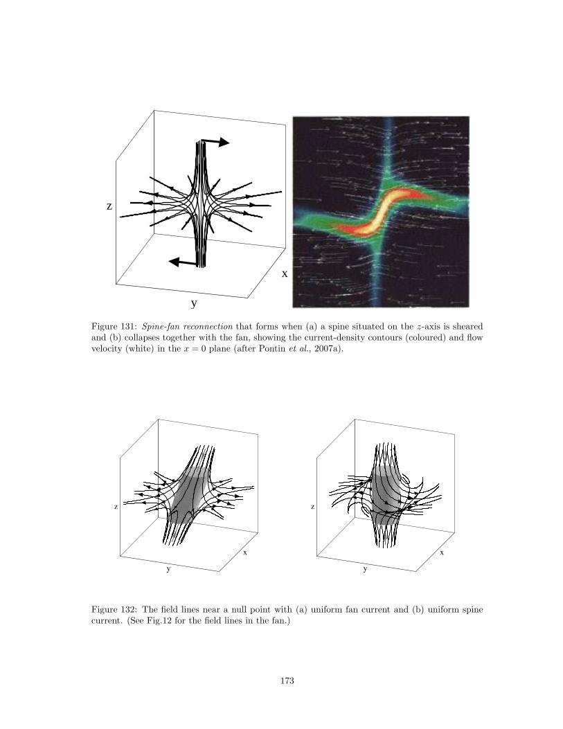
z

y

x

Figure 131: Spine-fan reconnection that forms when (a) a spine situated on the z-axis is shearedand (b) collapses together with the fan, showing the current-density contours (coloured) and flowvelocity (white) in the x = 0 plane (after Pontin et al., 2007a).

Figure 132: The field lines near a null point with (a) uniform fan current and (b) uniform spinecurrent. (See Fig.12 for the field lines in the fan.)

173

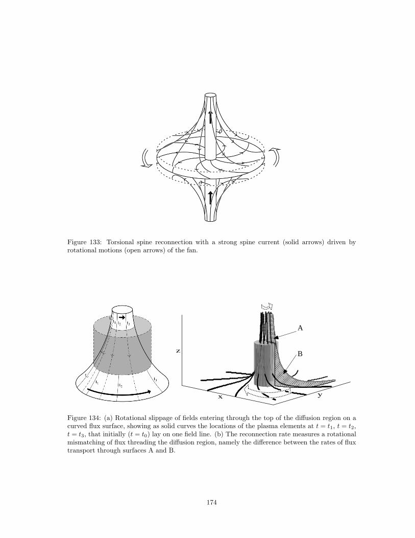
Figure 133: Torsional spine reconnection with a strong spine current (solid arrows) driven byrotational motions (open arrows) of the fan.

B

������������������������������������������

������������������������������������������

������������������������������������������������������������������������������������������������������������������������

������������������������������������������������������������������������������������������������������������������������

������������������������������������������������

������������������������������������������������

������

������

��������

��������

��

������������

����

��������

��������

���

���

��

A

������������������������

������������������������

���������������������

���������������������

Figure 134: (a) Rotational slippage of fields entering through the top of the diffusion region on acurved flux surface, showing as solid curves the locations of the plasma elements at t = t1, t = t2,t = t3, that initially (t = t0) lay on one field line. (b) The reconnection rate measures a rotationalmismatching of flux threading the diffusion region, namely the difference between the rates of fluxtransport through surfaces A and B.

174

The field lines for this spiral null may be obtained by solving

dR

dS=L0BR

B0= R, R

dφ

dS= 1

2 j0R,dz

dS= −2z.

Suppose we start a field line at the point (R, φ, z) = (R0, φ0, b) at S = 0. Then the field lineequations are

R = R0 eS , z = b e−2S , φ = φ0 + 1

2 j0 S. (166)

These give a mapping from an initial point (R0, φ0, b) to any other point (R, φ, z) along a field line.The inverse mapping is

R0 = R e−S , φ0 = φ− 12 j0 S. (167)

where S = − 12 log(z/b).

For the pure elementary solution we have E = ∇Φnid with Φnid given by Eq.(162) and Φe ≡ 0where for the spiral null Φnid becomes

Φnid = −Φnid0

∫

η/η0 e−2SdS,

with Φnid0 = 2B0bj0η0/(µL0). Then, once a form for η is assumed, this may be integrated to giveΦnid(S,R0, φ0). After using the inverse mapping, we can then deduce Φnid(R, φ, z) and thereforeE and v⊥ everywhere.

In this analysis, four regions possess different forms for Φnid, as illustrated in a vertical cutin the first quadrant of the Rz-plane (Fig.135). Region (1) is threaded by field lines that enterthe diffusion region (shaded) from above, and here we assume Φnid(R, z) ≡ 0, so that there is noelectric field or flow. Region (2) lies above the flux surface zR2 = ba2 that touches the upper corner(a, b) of the diffusion region and here we make the same assumption. The forms for Φnid(R, z) arecalculated in the diffusion region (3) and in the region (4) threaded by field lines that leave thediffusion region through its sides. As an example, suppose η vanishes outside the diffusion region(D) and that inside D it has the form

η = η0

(

1 − R4

a4

)(

1 − z2

b2

)

,

which peaks at the origin and vanishes on the boundary of D. First, we use the mapping (166) tosubstitute for R and z, and integrate with respect to S from the point T (R, b) on the top of D tothe point P (R, z) inside D (Fig.135). Then we use the inverse mapping (167) to replace R0 andS, and finally we obtain the potential throughout D (region (3) in Fig.135) as

Φnid(R, z) = − 12Φnid0

[(

1 − z

b

)

− R4

a4

(z

b− z2

b2

)

+ 13

(z3

b3− 1

)

+R4

a4

(z2

b2− z3

b3

)]

.

This then determines the components of the electric field (E = ∇Φnid) everywhere in D.An expression for Φnid(R, z) in region (4) of Fig.135 may be found by starting with the values

of Φnid at the point Q(a, zs) on the side of the diffusion region (Fig.135) and then calculating Φnid

at any point P (R, z) that lies on the same field line in region (4) to the right of Q. Since idealMHD holds in region (4), and Φnid(R, z) is constant along the field line (zR2 = zsa

2) joining Q toP , we find the value of Φnid at P as

Φnid(R, z) = f

(zR2

a2

)

= −Φnid0

[1

3− z

b

R2

a2+z2

b2R4

a4− z3

b3R6

a6

]

.

175

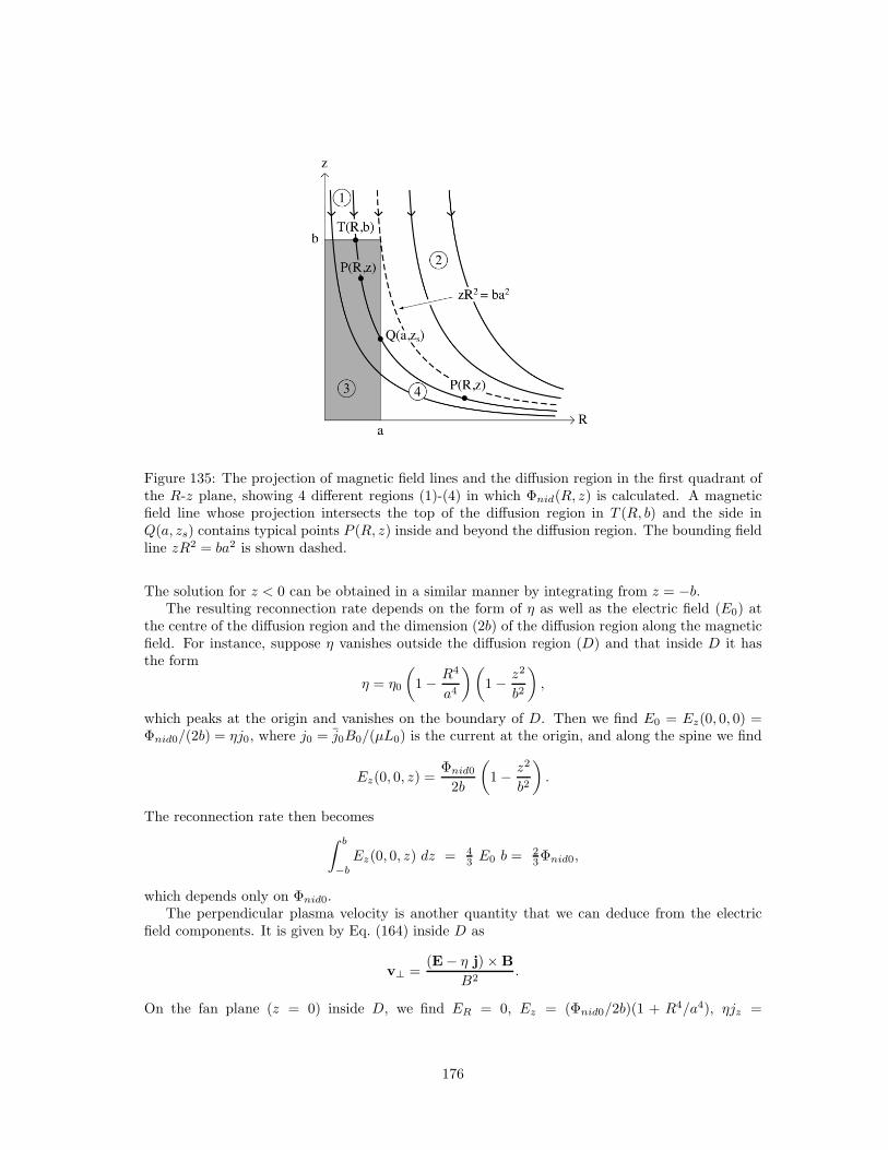
Figure 135: The projection of magnetic field lines and the diffusion region in the first quadrant ofthe R-z plane, showing 4 different regions (1)-(4) in which Φnid(R, z) is calculated. A magneticfield line whose projection intersects the top of the diffusion region in T (R, b) and the side inQ(a, zs) contains typical points P (R, z) inside and beyond the diffusion region. The bounding fieldline zR2 = ba2 is shown dashed.

The solution for z < 0 can be obtained in a similar manner by integrating from z = −b.The resulting reconnection rate depends on the form of η as well as the electric field (E0) at

the centre of the diffusion region and the dimension (2b) of the diffusion region along the magneticfield. For instance, suppose η vanishes outside the diffusion region (D) and that inside D it hasthe form

η = η0

(

1 − R4

a4

)(

1 − z2

b2

)

,

which peaks at the origin and vanishes on the boundary of D. Then we find E0 = Ez(0, 0, 0) =Φnid0/(2b) = ηj0, where j0 = j0B0/(µL0) is the current at the origin, and along the spine we find

Ez(0, 0, z) =Φnid0

2b

(

1 − z2

b2

)

.

The reconnection rate then becomes

∫ b

−b

Ez(0, 0, z) dz = 43 E0 b = 2

3Φnid0,

which depends only on Φnid0.The perpendicular plasma velocity is another quantity that we can deduce from the electric

field components. It is given by Eq. (164) inside D as

v⊥ =(E− η j) × B

B2.

On the fan plane (z = 0) inside D, we find ER = 0, Ez = (Φnid0/2b)(1 + R4/a4), ηjz =

176

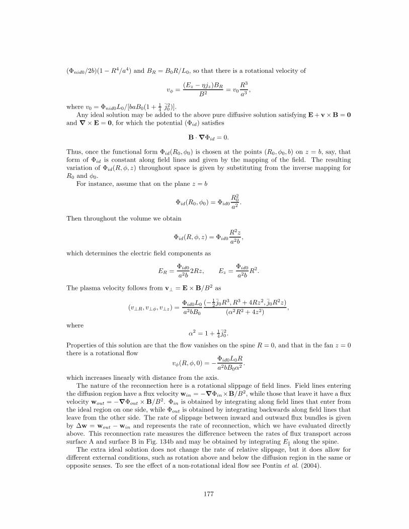
(Φnid0/2b)(1 −R4/a4) and BR = B0R/L0, so that there is a rotational velocity of

vφ =(Ez − ηjz)BR

B2= v0

R3

a3,

where v0 = Φnid0L0/[baB0(1 + 14 j

20 )].

Any ideal solution may be added to the above pure diffusive solution satisfying E + v×B = 0and ∇ × E = 0, for which the potential (Φid) satisfies

B · ∇Φid = 0.

Thus, once the functional form Φid(R0, φ0) is chosen at the points (R0, φ0, b) on z = b, say, thatform of Φid is constant along field lines and given by the mapping of the field. The resultingvariation of Φid(R, φ, z) throughout space is given by substituting from the inverse mapping forR0 and φ0.

For instance, assume that on the plane z = b

Φid(R0, φ0) = Φid0R2

0

a2.

Then throughout the volume we obtain

Φid(R, φ, z) = Φid0R2z

a2b,

which determines the electric field components as

ER =Φid0

a2b2Rz, Ez =

Φid0

a2bR2.

The plasma velocity follows from v⊥ = E× B/B2 as

(v⊥R, v⊥φ, v⊥z) =Φid0L0

a2bB0

(− 12 j0R

3, R3 + 4Rz2, j0R2z)

(α2R2 + 4z2),

whereα2 = 1 + 1

4 j20 .

Properties of this solution are that the flow vanishes on the spine R = 0, and that in the fan z = 0there is a rotational flow

vφ(R, φ, 0) = −Φid0L0R

a2bB0α2.

which increases linearly with distance from the axis.The nature of the reconnection here is a rotational slippage of field lines. Field lines entering

the diffusion region have a flux velocity win = −∇Φin×B/B2, while those that leave it have a fluxvelocity wout = −∇Φout × B/B2. Φin is obtained by integrating along field lines that enter fromthe ideal region on one side, while Φout is obtained by integrating backwards along field lines thatleave from the other side. The rate of slippage between inward and outward flux bundles is givenby ∆w = wout − win and represents the rate of reconnection, which we have evaluated directlyabove. This reconnection rate measures the difference between the rates of flux transport acrosssurface A and surface B in Fig. 134b and may be obtained by integrating E‖ along the spine.

The extra ideal solution does not change the rate of relative slippage, but it does allow fordifferent external conditions, such as rotation above and below the diffusion region in the same oropposite senses. To see the effect of a non-rotational ideal flow see Pontin et al. (2004).

177

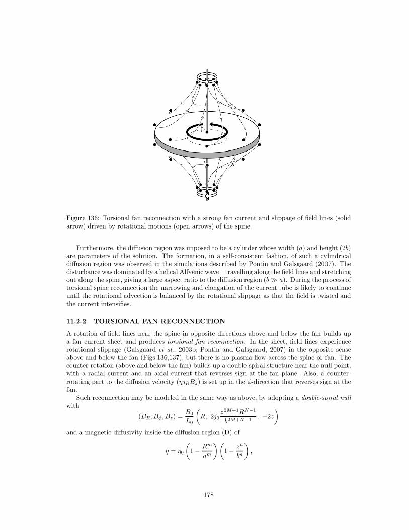
Figure 136: Torsional fan reconnection with a strong fan current and slippage of field lines (solidarrow) driven by rotational motions (open arrows) of the spine.

Furthermore, the diffusion region was imposed to be a cylinder whose width (a) and height (2b)are parameters of the solution. The formation, in a self-consistent fashion, of such a cylindricaldiffusion region was observed in the simulations described by Pontin and Galsgaard (2007). Thedisturbance was dominated by a helical Alfvenic wave – travelling along the field lines and stretchingout along the spine, giving a large aspect ratio to the diffusion region (b≫ a). During the process oftorsional spine reconnection the narrowing and elongation of the current tube is likely to continueuntil the rotational advection is balanced by the rotational slippage as that the field is twisted andthe current intensifies.

11.2.2 TORSIONAL FAN RECONNECTION

A rotation of field lines near the spine in opposite directions above and below the fan builds upa fan current sheet and produces torsional fan reconnection. In the sheet, field lines experiencerotational slippage (Galsgaard et al., 2003b; Pontin and Galsgaard, 2007) in the opposite senseabove and below the fan (Figs.136,137), but there is no plasma flow across the spine or fan. Thecounter-rotation (above and below the fan) builds up a double-spiral structure near the null point,with a radial current and an axial current that reverses sign at the fan plane. Also, a counter-rotating part to the diffusion velocity (ηjRBz) is set up in the φ-direction that reverses sign at thefan.

Such reconnection may be modeled in the same way as above, by adopting a double-spiral nullwith

(BR, Bφ, Bz) =B0

L0

(

R, 2j0z2M+1RN−1

b2M+N−1, −2z

)

and a magnetic diffusivity inside the diffusion region (D) of

η = η0

(

1 − Rm

am

)(

1 − zn

bn

)

,

178

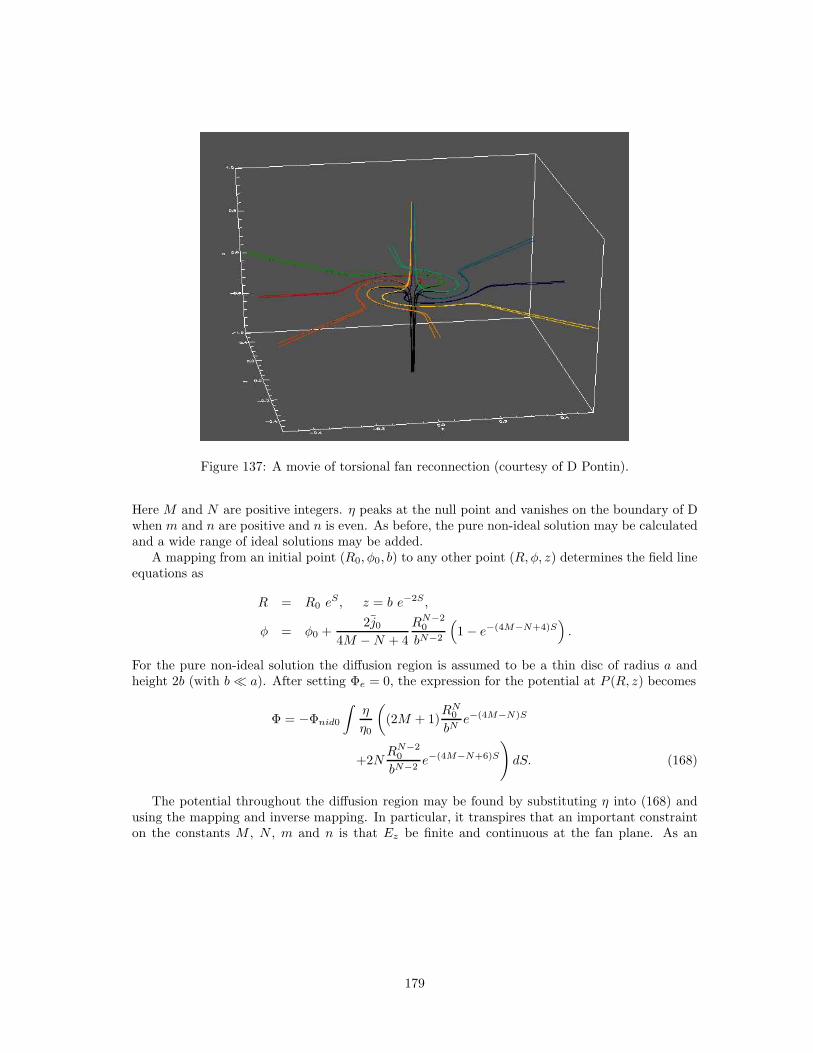
Figure 137: A movie of torsional fan reconnection (courtesy of D Pontin).

Here M and N are positive integers. η peaks at the null point and vanishes on the boundary of Dwhen m and n are positive and n is even. As before, the pure non-ideal solution may be calculatedand a wide range of ideal solutions may be added.

A mapping from an initial point (R0, φ0, b) to any other point (R, φ, z) determines the field lineequations as

R = R0 eS, z = b e−2S ,

φ = φ0 +2j0

4M −N + 4

RN−20

bN−2

(

1 − e−(4M−N+4)S)

.

For the pure non-ideal solution the diffusion region is assumed to be a thin disc of radius a andheight 2b (with b≪ a). After setting Φe = 0, the expression for the potential at P (R, z) becomes

Φ = −Φnid0

∫η

η0

(

(2M + 1)RN

0

bNe−(4M−N)S

+2NRN−2

0

bN−2e−(4M−N+6)S

)

dS. (168)

The potential throughout the diffusion region may be found by substituting η into (168) andusing the mapping and inverse mapping. In particular, it transpires that an important constrainton the constants M , N , m and n is that Ez be finite and continuous at the fan plane. As an

179

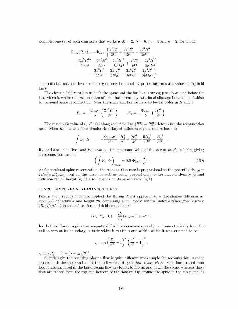
example, one set of such constants that works is M = 2, N = 6, m = 4 and n = 2, for which

Φnid(R, z) = −Φnid0

{z2R4

2b6+

5z3R6

3b9− 5z4R6

2b10

+5z5R10

b11a4+

5z6R6

6b12− 5z6R10

2b12a4+z8R4

b12− 5z4R10

2a4b10

−3z6R4

2b10− 3z4R8

2b8a4− 3z6R8

b10a4− 3z8R8

2b12a4

}

.

The potential outside the diffusion region may be found by projecting constant values along fieldlines.

The electric field vanishes in both the spine and the fan but is strong just above and below thefan, which is where the reconnection of field lines occurs by rotational slippage in a similar fashionto torsional spine reconnection. Near the spine and fan we have to lowest order in R and z

ER = −Φnid0

b

(2z2R3

b5

)

, Ez = −Φnid0

b

(zR4

b5

)

.

The maximum value of (∫E‖ ds) along each field line (R2z = R2

0b) determines the reconnectionrate. When R0 ∼ a≫ b for a slender disc-shaped diffusion region, this reduces to

∫

E‖ ds = −Φnid0a4

2b4

[R4

0

a4+

9R80

a8− 9R12

0

a12− R16

0

a16

]

.

If a and b are held fixed and R0 is varied, the maximum value of this occurs at R0 ≈ 0.90a, givinga reconnection rate of (∫

E‖ ds

)

max

= 0.9 Φnid0a4

b4. (169)

As for torsional spine reconnection, the reconnection rate is proportional to the potential Φnid0 =2B0bj0η0/(µL0), but in this case, as well as being proportional to the current density j0 anddiffusion region height (b), it also depends on its aspect ratio (a/b).

11.2.3 SPINE-FAN RECONNECTION

Pontin et al. (2005) have also applied the Hornig-Priest approach to a disc-shaped diffusion re-gion (D) of radius a and height 2b, containing a null point with a uniform fan-aligned current(B0j0/(µL0)) in the x-direction and field components

(Bx, By, Bz) =B0

L0(x, y − j0z,−2z).

Inside the diffusion region the magnetic diffusivity decreases smoothly and monotonically from thenull to zero at its boundary, outside which it vanishes and within which it was assumed to be

η = η0

(R2

1

a2− 1

)2(z2

b2− 1

)2

,

where R21 = x2 + (y − j0z/3)2.

Surprisingly, the resulting plasma flow is quite different from simple fan reconnection: since itcrosses both the spine and fan of the null we call it spine-fan reconnection. Field lines traced fromfootpoints anchored in the fan-crossing flow are found to flip up and down the spine, whereas thosethat are traced from the top and bottom of the domain flip around the spine in the fan plane, as

180

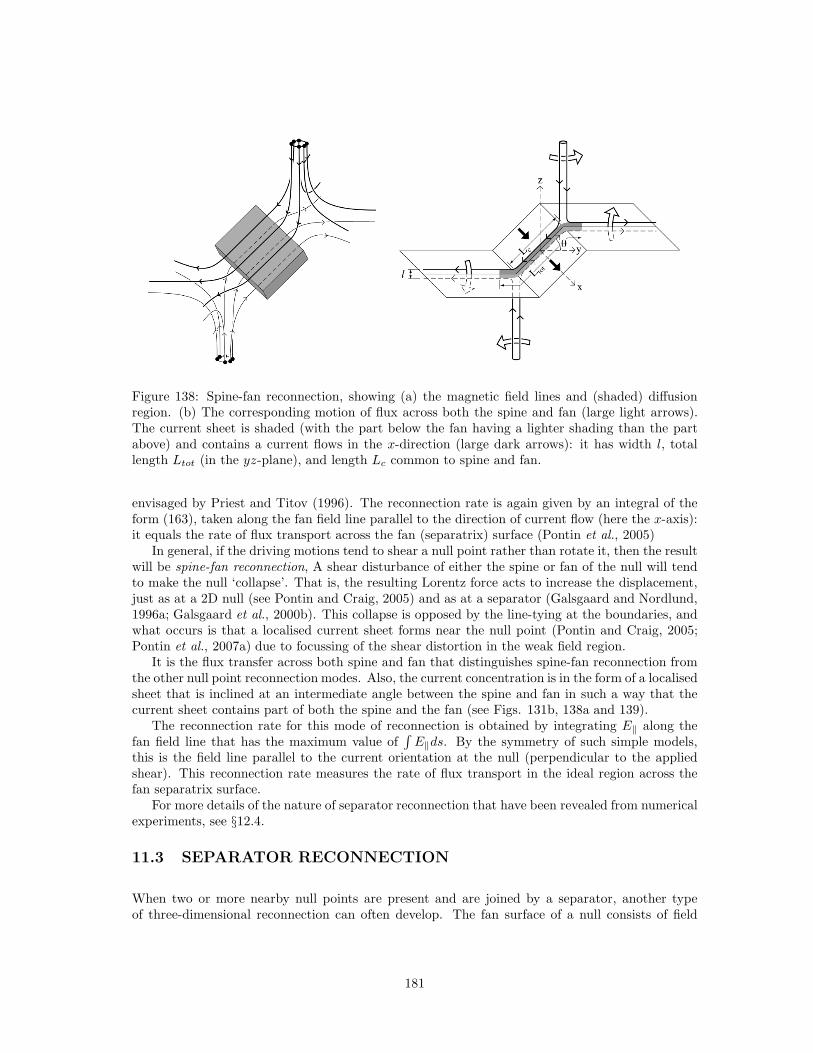
Figure 138: Spine-fan reconnection, showing (a) the magnetic field lines and (shaded) diffusionregion. (b) The corresponding motion of flux across both the spine and fan (large light arrows).The current sheet is shaded (with the part below the fan having a lighter shading than the partabove) and contains a current flows in the x-direction (large dark arrows): it has width l, totallength Ltot (in the yz-plane), and length Lc common to spine and fan.

envisaged by Priest and Titov (1996). The reconnection rate is again given by an integral of theform (163), taken along the fan field line parallel to the direction of current flow (here the x-axis):it equals the rate of flux transport across the fan (separatrix) surface (Pontin et al., 2005)

In general, if the driving motions tend to shear a null point rather than rotate it, then the resultwill be spine-fan reconnection, A shear disturbance of either the spine or fan of the null will tendto make the null ‘collapse’. That is, the resulting Lorentz force acts to increase the displacement,just as at a 2D null (see Pontin and Craig, 2005) and as at a separator (Galsgaard and Nordlund,1996a; Galsgaard et al., 2000b). This collapse is opposed by the line-tying at the boundaries, andwhat occurs is that a localised current sheet forms near the null point (Pontin and Craig, 2005;Pontin et al., 2007a) due to focussing of the shear distortion in the weak field region.

It is the flux transfer across both spine and fan that distinguishes spine-fan reconnection fromthe other null point reconnection modes. Also, the current concentration is in the form of a localisedsheet that is inclined at an intermediate angle between the spine and fan in such a way that thecurrent sheet contains part of both the spine and the fan (see Figs. 131b, 138a and 139).

The reconnection rate for this mode of reconnection is obtained by integrating E‖ along thefan field line that has the maximum value of

∫E‖ds. By the symmetry of such simple models,

this is the field line parallel to the current orientation at the null (perpendicular to the appliedshear). This reconnection rate measures the rate of flux transport in the ideal region across thefan separatrix surface.

For more details of the nature of separator reconnection that have been revealed from numericalexperiments, see §12.4.

11.3 SEPARATOR RECONNECTION

When two or more nearby null points are present and are joined by a separator, another typeof three-dimensional reconnection can often develop. The fan surface of a null consists of field

181

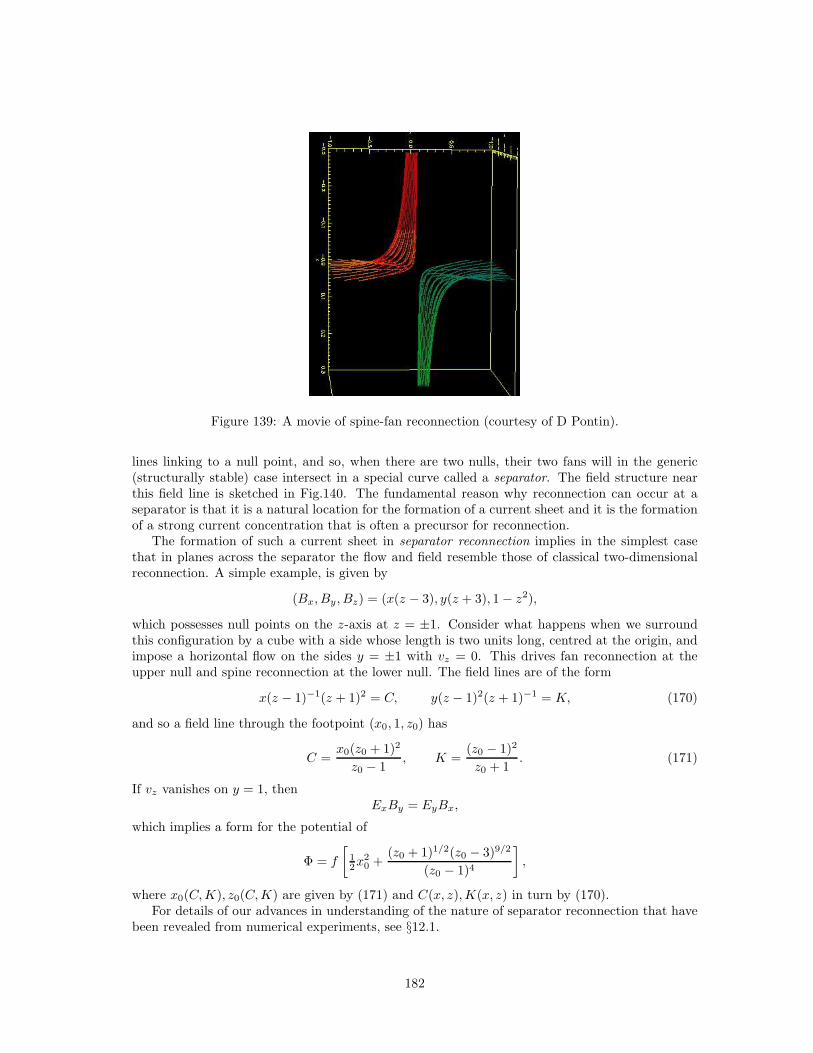
Figure 139: A movie of spine-fan reconnection (courtesy of D Pontin).

lines linking to a null point, and so, when there are two nulls, their two fans will in the generic(structurally stable) case intersect in a special curve called a separator. The field structure nearthis field line is sketched in Fig.140. The fundamental reason why reconnection can occur at aseparator is that it is a natural location for the formation of a current sheet and it is the formationof a strong current concentration that is often a precursor for reconnection.

The formation of such a current sheet in separator reconnection implies in the simplest casethat in planes across the separator the flow and field resemble those of classical two-dimensionalreconnection. A simple example, is given by

(Bx, By, Bz) = (x(z − 3), y(z + 3), 1 − z2),

which possesses null points on the z-axis at z = ±1. Consider what happens when we surroundthis configuration by a cube with a side whose length is two units long, centred at the origin, andimpose a horizontal flow on the sides y = ±1 with vz = 0. This drives fan reconnection at theupper null and spine reconnection at the lower null. The field lines are of the form

x(z − 1)−1(z + 1)2 = C, y(z − 1)2(z + 1)−1 = K, (170)

and so a field line through the footpoint (x0, 1, z0) has

C =x0(z0 + 1)2

z0 − 1, K =

(z0 − 1)2

z0 + 1. (171)

If vz vanishes on y = 1, thenExBy = EyBx,

which implies a form for the potential of

Φ = f

[

12x

20 +

(z0 + 1)1/2(z0 − 3)9/2

(z0 − 1)4

]

,

where x0(C,K), z0(C,K) are given by (171) and C(x, z),K(x, z) in turn by (170).For details of our advances in understanding of the nature of separator reconnection that have

been revealed from numerical experiments, see §12.1.

182

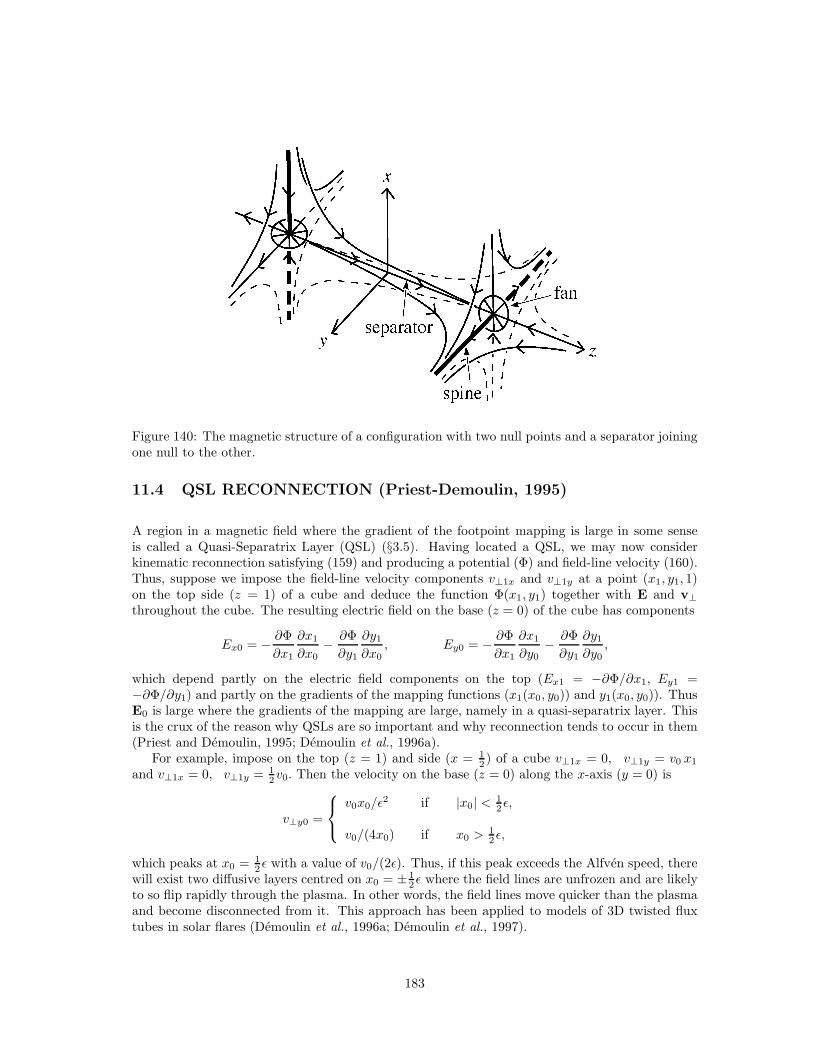
Figure 140: The magnetic structure of a configuration with two null points and a separator joiningone null to the other.

11.4 QSL RECONNECTION (Priest-Demoulin, 1995)

A region in a magnetic field where the gradient of the footpoint mapping is large in some senseis called a Quasi-Separatrix Layer (QSL) (§3.5). Having located a QSL, we may now considerkinematic reconnection satisfying (159) and producing a potential (Φ) and field-line velocity (160).Thus, suppose we impose the field-line velocity components v⊥1x and v⊥1y at a point (x1, y1, 1)on the top side (z = 1) of a cube and deduce the function Φ(x1, y1) together with E and v⊥throughout the cube. The resulting electric field on the base (z = 0) of the cube has components

Ex0 = − ∂Φ

∂x1

∂x1

∂x0− ∂Φ

∂y1

∂y1∂x0

, Ey0 = − ∂Φ

∂x1

∂x1

∂y0− ∂Φ

∂y1

∂y1∂y0

,

which depend partly on the electric field components on the top (Ex1 = −∂Φ/∂x1, Ey1 =−∂Φ/∂y1) and partly on the gradients of the mapping functions (x1(x0, y0)) and y1(x0, y0)). ThusE0 is large where the gradients of the mapping are large, namely in a quasi-separatrix layer. Thisis the crux of the reason why QSLs are so important and why reconnection tends to occur in them(Priest and Demoulin, 1995; Demoulin et al., 1996a).

For example, impose on the top (z = 1) and side (x = 12 ) of a cube v⊥1x = 0, v⊥1y = v0 x1

and v⊥1x = 0, v⊥1y = 12v0. Then the velocity on the base (z = 0) along the x-axis (y = 0) is

v⊥y0 =

v0x0/ǫ2 if |x0| < 1

2ǫ,

v0/(4x0) if x0 >12ǫ,

which peaks at x0 = 12ǫ with a value of v0/(2ǫ). Thus, if this peak exceeds the Alfven speed, there

will exist two diffusive layers centred on x0 = ± 12ǫ where the field lines are unfrozen and are likely

to so flip rapidly through the plasma. In other words, the field lines move quicker than the plasmaand become disconnected from it. This approach has been applied to models of 3D twisted fluxtubes in solar flares (Demoulin et al., 1996a; Demoulin et al., 1997).

183

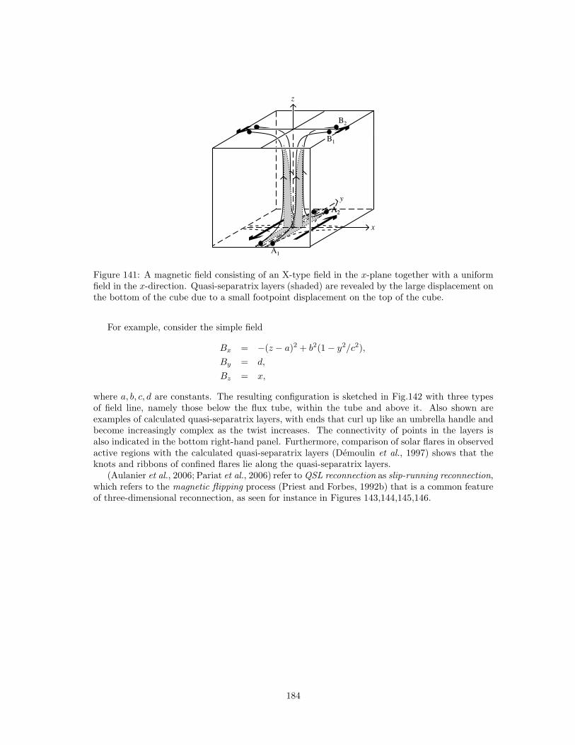
x

z

y

B2

B1

A1

A2A2

Figure 141: A magnetic field consisting of an X-type field in the x-plane together with a uniformfield in the x-direction. Quasi-separatrix layers (shaded) are revealed by the large displacement onthe bottom of the cube due to a small footpoint displacement on the top of the cube.

For example, consider the simple field

Bx = −(z − a)2 + b2(1 − y2/c2),

By = d,

Bz = x,

where a, b, c, d are constants. The resulting configuration is sketched in Fig.142 with three typesof field line, namely those below the flux tube, within the tube and above it. Also shown areexamples of calculated quasi-separatrix layers, with ends that curl up like an umbrella handle andbecome increasingly complex as the twist increases. The connectivity of points in the layers isalso indicated in the bottom right-hand panel. Furthermore, comparison of solar flares in observedactive regions with the calculated quasi-separatrix layers (Demoulin et al., 1997) shows that theknots and ribbons of confined flares lie along the quasi-separatrix layers.

(Aulanier et al., 2006; Pariat et al., 2006) refer to QSL reconnection as slip-running reconnection,which refers to the magnetic flipping process (Priest and Forbes, 1992b) that is a common featureof three-dimensional reconnection, as seen for instance in Figures 143,144,145,146.

184

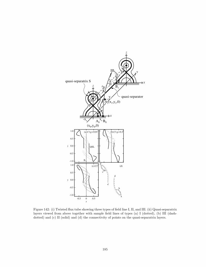
(x0,y0,0)

-xs xsA0

A1(x1,y1,0)P

B0

B1

I

z

quasi-separatrix S

quasi-separator

x

III

z

x

y

y1Q

II

1.0

0.5

0.0y

-0.5

-1.0

-0.5 0

x

0.5

QSL

IL

(c) C2 (d)d'

c'b'

d

a'

b

a

c

1.0

0.5

0.0y

-0.5

-1.0

(a) C1 g = 0.01 (b) C1 g = 0.2(a) C1 g = 0.01 (b) C1 g = 0.2

Figure 142: (i) Twisted flux tube showing three types of field line I, II, and III. (ii) Quasi-separatrixlayers viewed from above together with sample field lines of types (a) I (dotted), (b) III (dash-dotted) and (c) II (solid) and (d) the connectivity of points on the quasi-separatrix layers.

185

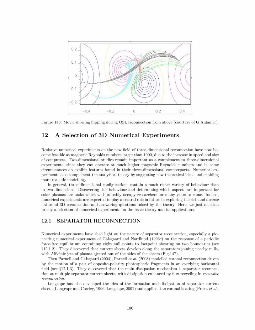
Figure 143: Movie showing flipping during QSL reconnection from above (courtesy of G Aulanier).

12 A Selection of 3D Numerical Experiments

Resistive numerical experiments on the new field of three-dimensional reconnection have now be-come feasible at magnetic Reynolds numbers larger than 1000, due to the increase in speed and sizeof computers. Two-dimensional studies remain important as a complement to three-dimensionalexperiments, since they can operate at much higher magnetic Reynolds numbers and in somecircumstances do exhibit features found in their three-dimensional counterparts. Numerical ex-periments also complement the analytical theory by suggesting new theoretical ideas and enablingmore realistic modelling.

In general, three-dimensional configurations contain a much richer variety of behaviour thanin two dimensions. Discovering this behaviour and determining which aspects are important forsolar plasmas are tasks which will probably occupy researchers for many years to come. Indeed,numerical experiments are expected to play a central role in future in exploring the rich and diversenature of 3D reconnection and answering questions raised by the theory. Here, we just mentionbriefly a selection of numerical experiments on the basic theory and its applications.

12.1 SEPARATOR RECONNECTION

Numerical experiments have shed light on the nature of separator reconnection, especially a pio-neering numerical experiment of Galsgaard and Nordlund (1996c) on the response of a periodicforce-free equilibrium containing eight null points to footpoint shearing on two boundaries (see§12.1.2). They discovered that current sheets develop along the separators joining nearby nulls,with Alfvenic jets of plasma ejected out of the sides of the sheets (Fig.147).

Then Parnell and Galsgaard (2004), Parnell et al. (2008) modelled coronal reconnection drivenby the motion of a pair of opposite-polarity photospheric fragments in an overlying horizontalfield (see §12.1.3). They discovered that the main dissipation mechanism is separator reconnec-tion at multiple separator current sheets, with dissipation enhanced by flux recycling in recursivereconnection.

Longcope has also developed the idea of the formation and dissipation of separator currentsheets (Longcope and Cowley, 1996; Longcope, 2001) and applied it to coronal heating (Priest et al.,

186

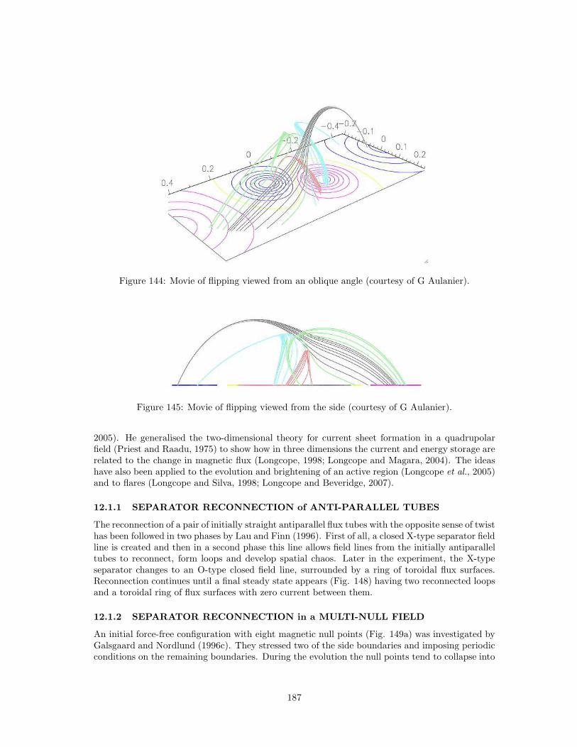
Figure 144: Movie of flipping viewed from an oblique angle (courtesy of G Aulanier).

Figure 145: Movie of flipping viewed from the side (courtesy of G Aulanier).

2005). He generalised the two-dimensional theory for current sheet formation in a quadrupolarfield (Priest and Raadu, 1975) to show how in three dimensions the current and energy storage arerelated to the change in magnetic flux (Longcope, 1998; Longcope and Magara, 2004). The ideashave also been applied to the evolution and brightening of an active region (Longcope et al., 2005)and to flares (Longcope and Silva, 1998; Longcope and Beveridge, 2007).

12.1.1 SEPARATOR RECONNECTION of ANTI-PARALLEL TUBES

The reconnection of a pair of initially straight antiparallel flux tubes with the opposite sense of twisthas been followed in two phases by Lau and Finn (1996). First of all, a closed X-type separator fieldline is created and then in a second phase this line allows field lines from the initially antiparalleltubes to reconnect, form loops and develop spatial chaos. Later in the experiment, the X-typeseparator changes to an O-type closed field line, surrounded by a ring of toroidal flux surfaces.Reconnection continues until a final steady state appears (Fig. 148) having two reconnected loopsand a toroidal ring of flux surfaces with zero current between them.

12.1.2 SEPARATOR RECONNECTION in a MULTI-NULL FIELD

An initial force-free configuration with eight magnetic null points (Fig. 149a) was investigated byGalsgaard and Nordlund (1996c). They stressed two of the side boundaries and imposing periodicconditions on the remaining boundaries. During the evolution the null points tend to collapse into

187

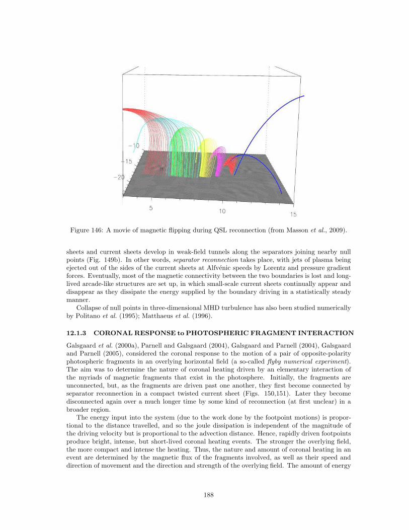
Figure 146: A movie of magnetic flipping during QSL reconnection (from Masson et al., 2009).

sheets and current sheets develop in weak-field tunnels along the separators joining nearby nullpoints (Fig. 149b). In other words, separator reconnection takes place, with jets of plasma beingejected out of the sides of the current sheets at Alfvenic speeds by Lorentz and pressure gradientforces. Eventually, most of the magnetic connectivity between the two boundaries is lost and long-lived arcade-like structures are set up, in which small-scale current sheets continually appear anddisappear as they dissipate the energy supplied by the boundary driving in a statistically steadymanner.

Collapse of null points in three-dimensional MHD turbulence has also been studied numericallyby Politano et al. (1995); Matthaeus et al. (1996).

12.1.3 CORONAL RESPONSE to PHOTOSPHERIC FRAGMENT INTERACTION

Galsgaard et al. (2000a), Parnell and Galsgaard (2004), Galsgaard and Parnell (2004), Galsgaardand Parnell (2005), considered the coronal response to the motion of a pair of opposite-polarityphotospheric fragments in an overlying horizontal field (a so-called flyby numerical experiment).The aim was to determine the nature of coronal heating driven by an elementary interaction ofthe myriads of magnetic fragments that exist in the photosphere. Initially, the fragments areunconnected, but, as the fragments are driven past one another, they first become connected byseparator reconnection in a compact twisted current sheet (Figs. 150,151). Later they becomedisconnected again over a much longer time by some kind of reconnection (at first unclear) in abroader region.

The energy input into the system (due to the work done by the footpoint motions) is propor-tional to the distance travelled, and so the joule dissipation is independent of the magnitude ofthe driving velocity but is proportional to the advection distance. Hence, rapidly driven footpointsproduce bright, intense, but short-lived coronal heating events. The stronger the overlying field,the more compact and intense the heating. Thus, the nature and amount of coronal heating in anevent are determined by the magnetic flux of the fragments involved, as well as their speed anddirection of movement and the direction and strength of the overlying field. The amount of energy

188

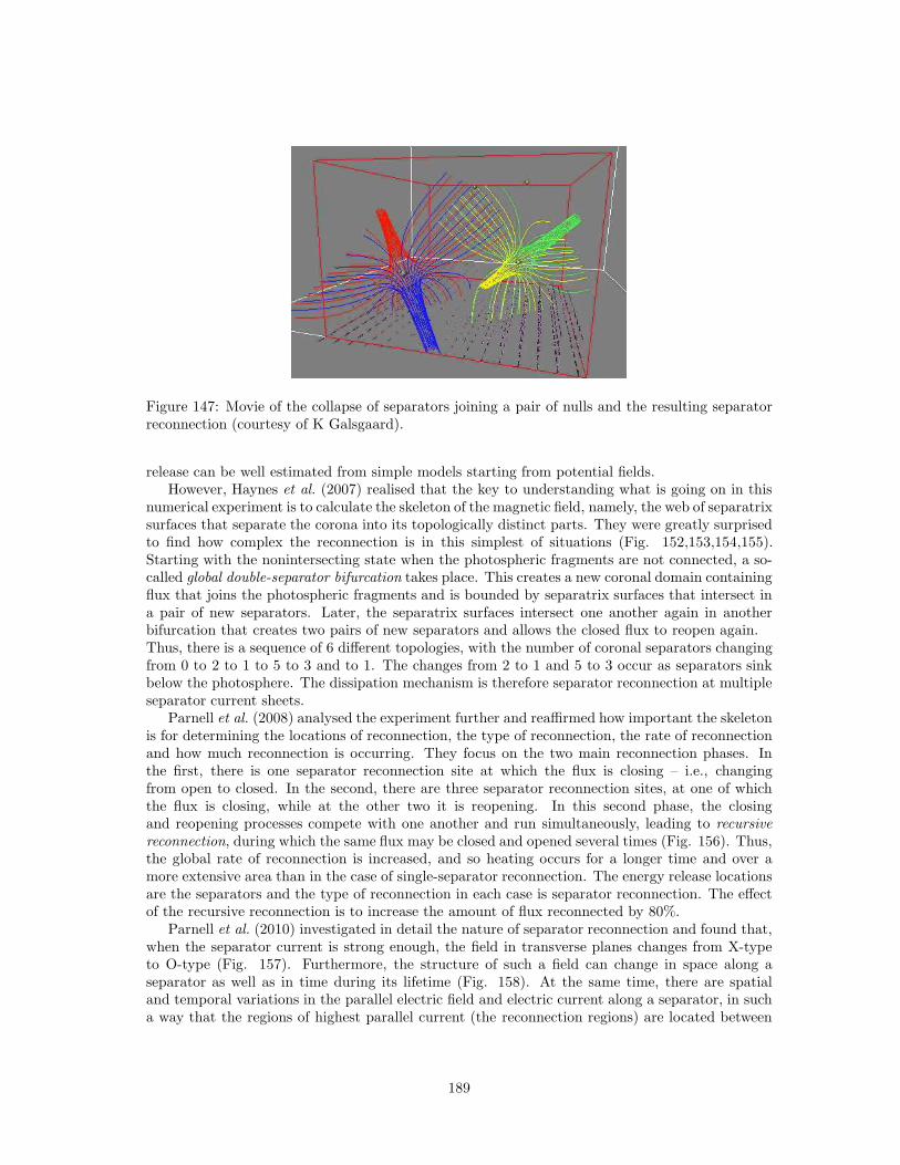
Figure 147: Movie of the collapse of separators joining a pair of nulls and the resulting separatorreconnection (courtesy of K Galsgaard).

release can be well estimated from simple models starting from potential fields.However, Haynes et al. (2007) realised that the key to understanding what is going on in this

numerical experiment is to calculate the skeleton of the magnetic field, namely, the web of separatrixsurfaces that separate the corona into its topologically distinct parts. They were greatly surprisedto find how complex the reconnection is in this simplest of situations (Fig. 152,153,154,155).Starting with the nonintersecting state when the photospheric fragments are not connected, a so-called global double-separator bifurcation takes place. This creates a new coronal domain containingflux that joins the photospheric fragments and is bounded by separatrix surfaces that intersect ina pair of new separators. Later, the separatrix surfaces intersect one another again in anotherbifurcation that creates two pairs of new separators and allows the closed flux to reopen again.Thus, there is a sequence of 6 different topologies, with the number of coronal separators changingfrom 0 to 2 to 1 to 5 to 3 and to 1. The changes from 2 to 1 and 5 to 3 occur as separators sinkbelow the photosphere. The dissipation mechanism is therefore separator reconnection at multipleseparator current sheets.

Parnell et al. (2008) analysed the experiment further and reaffirmed how important the skeletonis for determining the locations of reconnection, the type of reconnection, the rate of reconnectionand how much reconnection is occurring. They focus on the two main reconnection phases. Inthe first, there is one separator reconnection site at which the flux is closing – i.e., changingfrom open to closed. In the second, there are three separator reconnection sites, at one of whichthe flux is closing, while at the other two it is reopening. In this second phase, the closingand reopening processes compete with one another and run simultaneously, leading to recursivereconnection, during which the same flux may be closed and opened several times (Fig. 156). Thus,the global rate of reconnection is increased, and so heating occurs for a longer time and over amore extensive area than in the case of single-separator reconnection. The energy release locationsare the separators and the type of reconnection in each case is separator reconnection. The effectof the recursive reconnection is to increase the amount of flux reconnected by 80%.

Parnell et al. (2010) investigated in detail the nature of separator reconnection and found that,when the separator current is strong enough, the field in transverse planes changes from X-typeto O-type (Fig. 157). Furthermore, the structure of such a field can change in space along aseparator as well as in time during its lifetime (Fig. 158). At the same time, there are spatialand temporal variations in the parallel electric field and electric current along a separator, in sucha way that the regions of highest parallel current (the reconnection regions) are located between

189

.

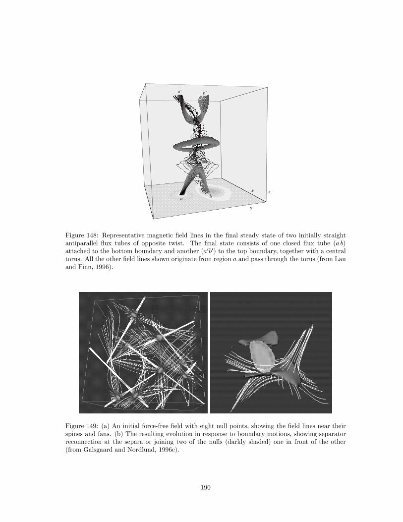
z

y

x

a b

a' b'

Figure 148: Representative magnetic field lines in the final steady state of two initially straightantiparallel flux tubes of opposite twist. The final state consists of one closed flux tube (a b)attached to the bottom boundary and another (a′b′) to the top boundary, together with a centraltorus. All the other field lines shown originate from region a and pass through the torus (from Lauand Finn, 1996).

Figure 149: (a) An initial force-free field with eight null points, showing the field lines near theirspines and fans. (b) The resulting evolution in response to boundary motions, showing separatorreconnection at the separator joining two of the nulls (darkly shaded) one in front of the other(from Galsgaard and Nordlund, 1996c).

190

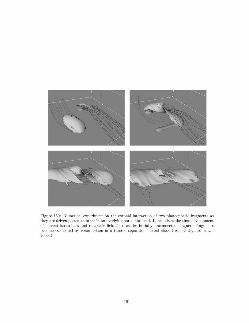
Figure 150: Numerical experiment on the coronal interaction of two photospheric fragments asthey are driven past each other in an overlying horizontal field. Panels show the time-developmentof current isosurfaces and magnetic field lines as the initially unconnected magnetic fragmentsbecome connected by reconnection in a twisted separator current sheet (from Galsgaard et al.,2000a).

191

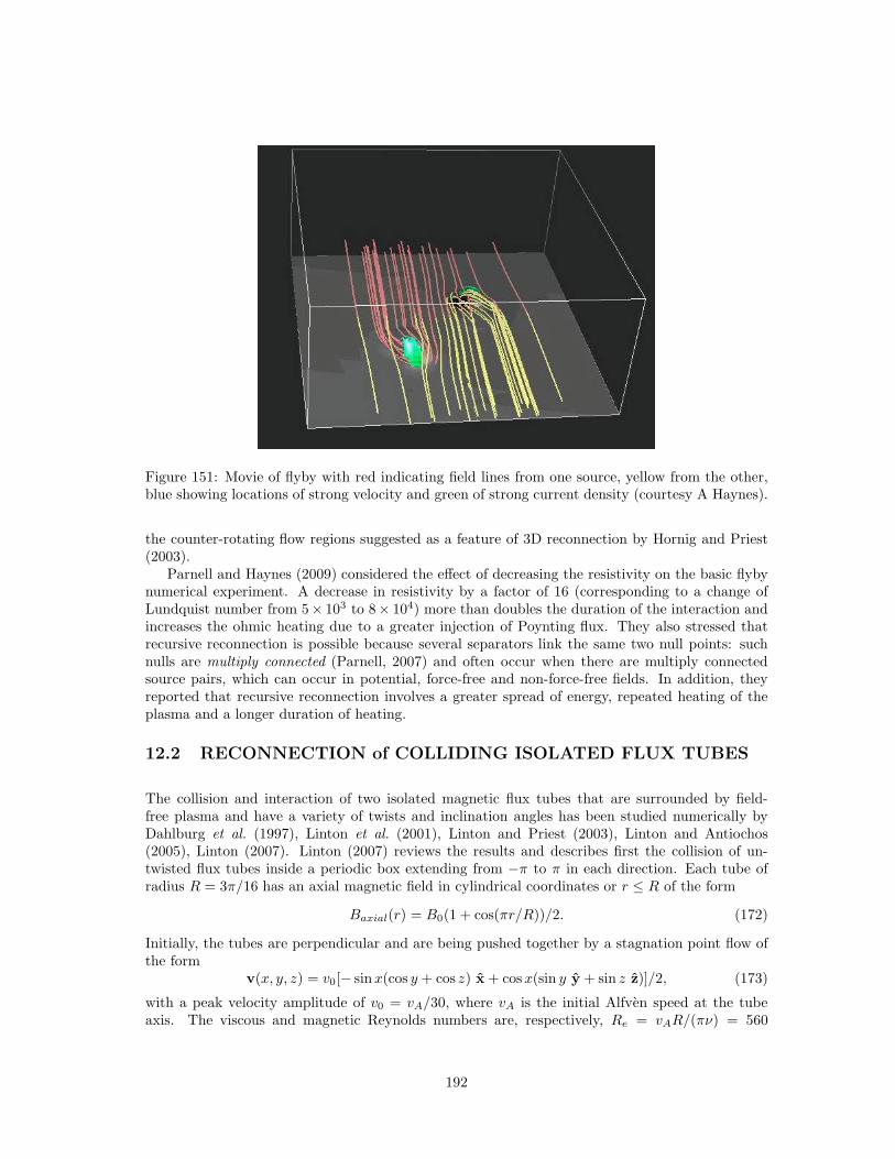
Figure 151: Movie of flyby with red indicating field lines from one source, yellow from the other,blue showing locations of strong velocity and green of strong current density (courtesy A Haynes).

the counter-rotating flow regions suggested as a feature of 3D reconnection by Hornig and Priest(2003).

Parnell and Haynes (2009) considered the effect of decreasing the resistivity on the basic flybynumerical experiment. A decrease in resistivity by a factor of 16 (corresponding to a change ofLundquist number from 5× 103 to 8× 104) more than doubles the duration of the interaction andincreases the ohmic heating due to a greater injection of Poynting flux. They also stressed thatrecursive reconnection is possible because several separators link the same two null points: suchnulls are multiply connected (Parnell, 2007) and often occur when there are multiply connectedsource pairs, which can occur in potential, force-free and non-force-free fields. In addition, theyreported that recursive reconnection involves a greater spread of energy, repeated heating of theplasma and a longer duration of heating.

12.2 RECONNECTION of COLLIDING ISOLATED FLUX TUBES

The collision and interaction of two isolated magnetic flux tubes that are surrounded by field-free plasma and have a variety of twists and inclination angles has been studied numerically byDahlburg et al. (1997), Linton et al. (2001), Linton and Priest (2003), Linton and Antiochos(2005), Linton (2007). Linton (2007) reviews the results and describes first the collision of un-twisted flux tubes inside a periodic box extending from −π to π in each direction. Each tube ofradius R = 3π/16 has an axial magnetic field in cylindrical coordinates or r ≤ R of the form

Baxial(r) = B0(1 + cos(πr/R))/2. (172)

Initially, the tubes are perpendicular and are being pushed together by a stagnation point flow ofthe form

v(x, y, z) = v0[− sinx(cos y + cos z) x + cosx(sin y y + sin z z)]/2, (173)

with a peak velocity amplitude of v0 = vA/30, where vA is the initial Alfven speed at the tubeaxis. The viscous and magnetic Reynolds numbers are, respectively, Re = vAR/(πν) = 560

192

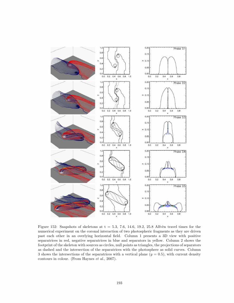
Figure 152: Snapshots of skeletons at t = 5.3, 7.6, 14.6, 19.2, 25.8 Alfven travel times for thenumerical experiment on the coronal interaction of two photospheric fragments as they are drivenpast each other in an overlying horizontal field. Column 1 presents a 3D view with positiveseparatrices in red, negative separatrices in blue and separators in yellow. Column 2 shows thefootprint of the skeleton with sources as circles, null points as triangles, the projections of separatorsas dashed and the intersection of the separatrices with the photosphere as solid curves. Column3 shows the intersections of the separatrices with a vertical plane (y = 0.5), with current densitycontours in colour. (From Haynes et al., 2007).

193

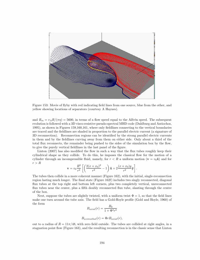
Figure 153: Movie of flyby with red indicating field lines from one source, blue from the other, andyellow showing locations of separators (courtesy A Haynes).

and Rm = vAR/(πη) = 5600, in terms of a flow speed equal to the Alfven speed. The subsequentevolution is followed with a 3D visco-resistive pseudo-spectral MHD code (Dahlburg and Antiochos,1995), as shown in Figures 159,160,161, where only fieldlines connecting to the vertical boundariesare traced and the fieldlines are shaded in proportion to the parallel electric current (a signature of3D reconnection). Reconnection regions can be identified by the strong parallel electric currentsin them and by the fieldlines curving away from them on either side. Only about a third of thetotal flux reconnects, the remainder being pushed to the sides of the simulation box by the flow,to give the purely vertical fieldlines in the last panel of the figure.

Linton (2007) has also modified the flow in such a way that the flux tubes roughly keep theircylindrical shape as they collide. To do this, he imposes the classical flow for the motion of acylinder through an incompressible fluid, namely, for r < R a uniform motion (v = v0x) and forr > R

v = v0R2

r2

[(2(x+ x0)

2

r2− 1

)

x + 2(x+ x0)y

r2y

]

.

The tubes then collide in a more coherent manner (Figure 162), with the initial, single-reconnectionregion lasting much longer. The final state (Figure 162f) includes two singly reconnected, diagonalflux tubes at the top right and bottom left corners, plus two completely vertical, unreconnectedflux tubes near the center, plus a fifth doubly reconnected flux tube, slanting through the centreof the box.

Next, suppose the tubes are slightly twisted, with a uniform twist Φ = 1, so that the field linesmake one turn around the tube axis. The field has a Gold-Hoyle profile (Gold and Hoyle, 1960) ofthe form

Baxial(r) =B0

1 + Φ2r2

Bazimuthal(r) = ΦrBaxial(r),

out to a radius of R = 11π/48, with zero field outside. The tubes are collided at right angles, in astagnation point flow (Figure 163), and the resulting reconnection is in the classic sense that Linton

194

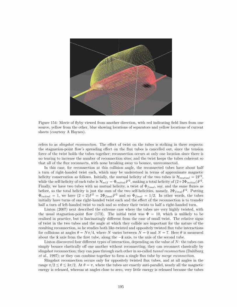
Figure 154: Movie of flyby viewed from another direction, with red indicating field lines from onesource, yellow from the other, blue showing locations of separators and yellow locations of currentsheets (courtesy A Haynes).

refers to as slingshot reconnection. The effect of twist on the tubes is striking in three respects:the stagnation-point flow’s spreading effect on the flux tubes is cancelled out, since the tensionforce of the twist holds the tubes together; reconnection occurs at only one location since there isno tearing to increase the number of reconnection sites; and the twist keeps the tubes coherent sothat all of the flux reconnects, with none breaking away to bounce, unreconnected.

In this case, for reconnection at this collision angle, the reconnected tubes have about halfa turn of right-handed twist each, which may be understood in terms of approximate magnetichelicity conservation as follows. Initially, the mutual helicity of the two tubes is Hmutual = 2F 2,while the self-helicity of each tube is Hself = ΦinitialF

2, making a total helicity of (2+2Φinitial)F2.

Finally, we have two tubes with no mutual helicity, a twist of Φfinal, say, and the same fluxes asbefore, so the total helicity is just the sum of the two self-helicities, namely, 2ΦfinalF

2. PuttingΦinitial = 1, we have (2 + 2)F 2 = 2ΦfinalF

2 and so Φfinal = 1/2. In other words, the tubesinitially have turns of one right-handed twist each and the effect of the reconnection is to transferhalf a turn of left-handed twist to each and so reduce their twists to half a right-handed turn.

Linton (2007) next described the extreme case where the tubes are very highly twisted, withthe usual stagnation-point flow (173). The initial twist was Φ = 10, which is unlikely to berealised in practice, but is fascinatingly different from the case of small twist. The relative signsof twist in the two tubes and the angle at which they collide are important for the nature of theresulting reconnection, so he studies both like-twisted and oppositely twisted flux tube interactionsfor collisions at angles θ = Nπ/4, where N varies between N = 0 and N = 7. Here θ is measuredabout the x axis from the first tube, along the −z axis, to the axis of the second tube.

Linton discovered four different types of interaction, depending on the value of N : the tubes cansimply bounce elastically off one another without reconnecting; they can reconnect classically byslingshot reconnection; they can pass through each other in so-called tunnel reconnection (Dahlburget al., 1997); or they can combine together to form a single flux tube by merge reconnection.

Slingshot reconnection occurs only for oppositely twisted flux tubes, and at all angles in therange π/2 ≤ θ ≤ 3π/2. At θ = π, where the tubes are exactly anti-parallel, nearly all the magneticenergy is released, whereas at angles close to zero, very little energy is released because the tubes

195

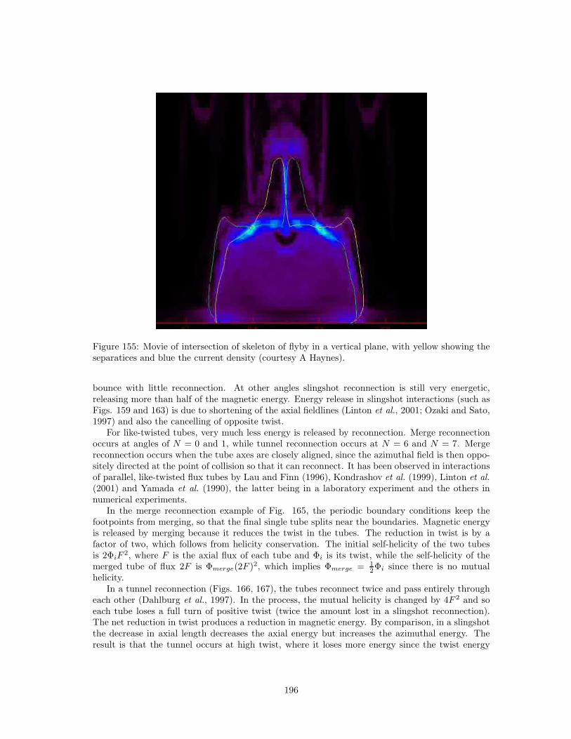
Figure 155: Movie of intersection of skeleton of flyby in a vertical plane, with yellow showing theseparatices and blue the current density (courtesy A Haynes).

bounce with little reconnection. At other angles slingshot reconnection is still very energetic,releasing more than half of the magnetic energy. Energy release in slingshot interactions (such asFigs. 159 and 163) is due to shortening of the axial fieldlines (Linton et al., 2001; Ozaki and Sato,1997) and also the cancelling of opposite twist.

For like-twisted tubes, very much less energy is released by reconnection. Merge reconnectionoccurs at angles of N = 0 and 1, while tunnel reconnection occurs at N = 6 and N = 7. Mergereconnection occurs when the tube axes are closely aligned, since the azimuthal field is then oppo-sitely directed at the point of collision so that it can reconnect. It has been observed in interactionsof parallel, like-twisted flux tubes by Lau and Finn (1996), Kondrashov et al. (1999), Linton et al.(2001) and Yamada et al. (1990), the latter being in a laboratory experiment and the others innumerical experiments.

In the merge reconnection example of Fig. 165, the periodic boundary conditions keep thefootpoints from merging, so that the final single tube splits near the boundaries. Magnetic energyis released by merging because it reduces the twist in the tubes. The reduction in twist is by afactor of two, which follows from helicity conservation. The initial self-helicity of the two tubesis 2ΦiF

2, where F is the axial flux of each tube and Φi is its twist, while the self-helicity of themerged tube of flux 2F is Φmerge(2F )2, which implies Φmerge = 1

2Φi since there is no mutualhelicity.

In a tunnel reconnection (Figs. 166, 167), the tubes reconnect twice and pass entirely througheach other (Dahlburg et al., 1997). In the process, the mutual helicity is changed by 4F 2 and soeach tube loses a full turn of positive twist (twice the amount lost in a slingshot reconnection).The net reduction in twist produces a reduction in magnetic energy. By comparison, in a slingshotthe decrease in axial length decreases the axial energy but increases the azimuthal energy. Theresult is that the tunnel occurs at high twist, where it loses more energy since the twist energy

196

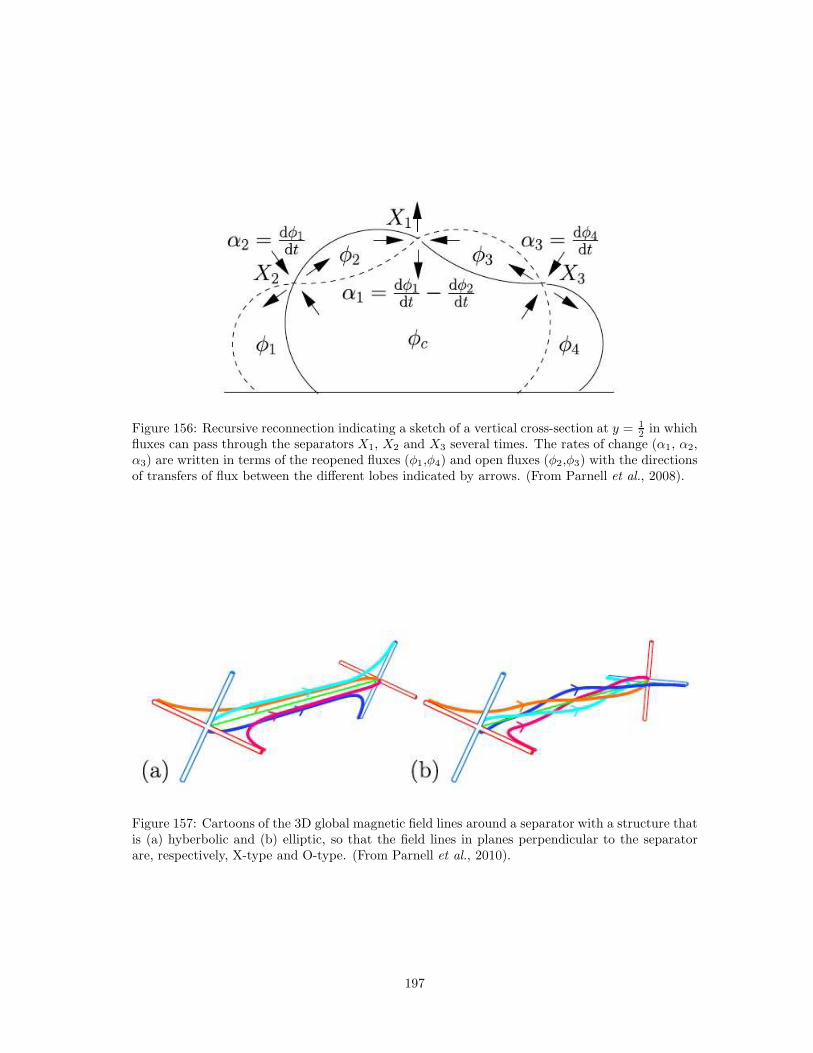
Figure 156: Recursive reconnection indicating a sketch of a vertical cross-section at y = 12 in which

fluxes can pass through the separators X1, X2 and X3 several times. The rates of change (α1, α2,α3) are written in terms of the reopened fluxes (φ1,φ4) and open fluxes (φ2,φ3) with the directionsof transfers of flux between the different lobes indicated by arrows. (From Parnell et al., 2008).

Figure 157: Cartoons of the 3D global magnetic field lines around a separator with a structure thatis (a) hyberbolic and (b) elliptic, so that the field lines in planes perpendicular to the separatorare, respectively, X-type and O-type. (From Parnell et al., 2010).

197

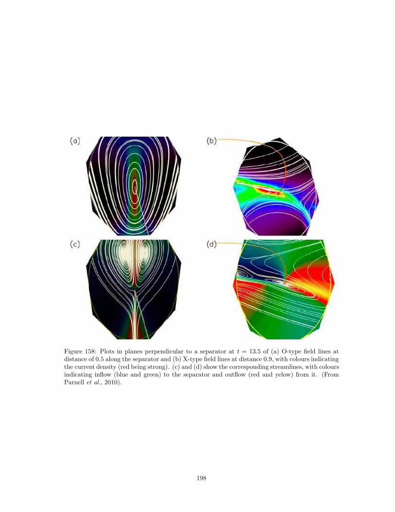
Figure 158: Plots in planes perpendicular to a separator at t = 13.5 of (a) O-type field lines atdistance of 0.5 along the separator and (b) X-type field lines at distance 0.9, with colours indicatingthe current density (red being strong). (c) and (d) show the corresponding streamlines, with coloursindicating inflow (blue and green) to the separator and outflow (red and yelow) from it. (FromParnell et al., 2010).

198

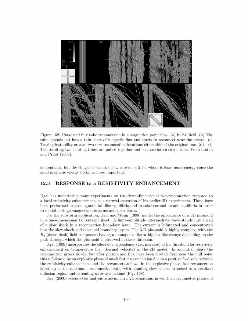
Figure 159: Untwisted flux tube reconnection in a stagnation point flow. (a) Initial field. (b) Thetube spreads out into a thin sheet of magnetic flux and starts to reconnect near the centre. (c)Tearing instability creates two new reconnection locations either side of the original one. (d) - (f)The resulting two slanting tubes are pulled together and coalesce into a single tube. From Lintonand Priest (2003).

is dominant, but the slingshot occurs below a twist of 2.56, where it loses more energy since theaxial magnetic energy becomes more important.

12.3 RESPONSE to a RESISTIVITY ENHANCEMENT

Ugai has undertaken many experiments on the three-dimensional fast-reconnection response toa local resistivity enhancement, as a natural extension of his earlier 2D experiments. These havebeen performed in geomagnetic tail-like equilibria and in solar coronal arcade equilibria in orderto model both geomagnetic substorms and solar flares.

For the substorm application, Ugai and Wang (1998) model the appearance of a 3D plasmoidin a one-dimensional tail current sheet. A finite-amplitude intermediate wave stands just aheadof a slow shock in a reconnection boundary layer. The current is bifurcated and concentratedinto the slow shock and plasmoid boundary layers. The 3-D plasmoid is highly complex, with theBz (dawn-dusk) field component having a monopolar-like or bipolar-like change depending on thepath through which the plasmoid is observed in the x-direction.

Ugai (1999) incorporates the effect of a dependency (i.e., increase) of the threshold for resistivityenhancement on temperature (i.e., thermal velocity) in the 2D model. In an initial phase thereconnection grows slowly, but after plasma and flux have been ejected from near the null pointthis is followed by an explosive phase of much faster reconnection due to a positive feedback betweenthe resisitivity enhancement and the reconnection flow. In the explosive phase, fast reconnectionis set up at the maximum reconnection rate, with standing slow shocks attached to a localizeddiffusion region and extending outwards in time (Fig. 168).

Ugai (2000) extends the analysis to asymmetric 2D situations, in which an asymmetric plasmoid

199

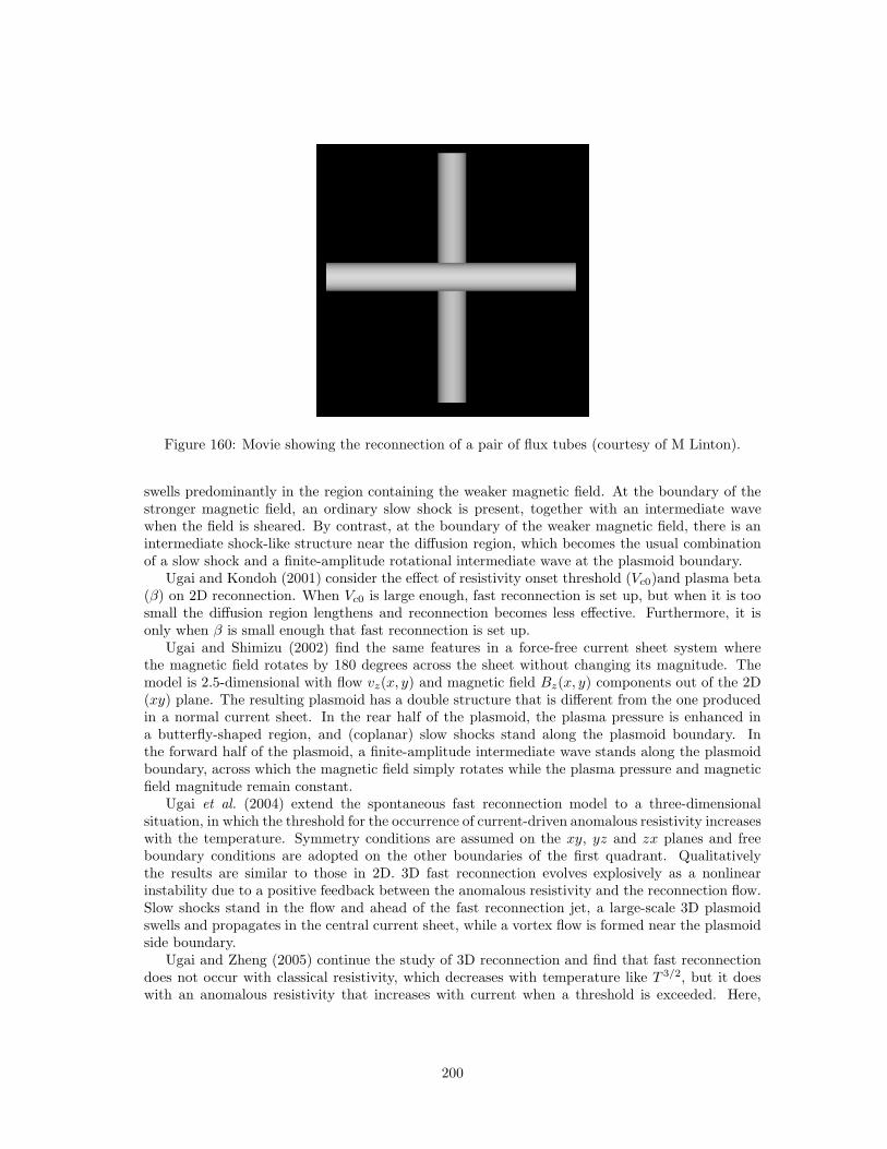
Figure 160: Movie showing the reconnection of a pair of flux tubes (courtesy of M Linton).

swells predominantly in the region containing the weaker magnetic field. At the boundary of thestronger magnetic field, an ordinary slow shock is present, together with an intermediate wavewhen the field is sheared. By contrast, at the boundary of the weaker magnetic field, there is anintermediate shock-like structure near the diffusion region, which becomes the usual combinationof a slow shock and a finite-amplitude rotational intermediate wave at the plasmoid boundary.

Ugai and Kondoh (2001) consider the effect of resistivity onset threshold (Vc0)and plasma beta(β) on 2D reconnection. When Vc0 is large enough, fast reconnection is set up, but when it is toosmall the diffusion region lengthens and reconnection becomes less effective. Furthermore, it isonly when β is small enough that fast reconnection is set up.

Ugai and Shimizu (2002) find the same features in a force-free current sheet system wherethe magnetic field rotates by 180 degrees across the sheet without changing its magnitude. Themodel is 2.5-dimensional with flow vz(x, y) and magnetic field Bz(x, y) components out of the 2D(xy) plane. The resulting plasmoid has a double structure that is different from the one producedin a normal current sheet. In the rear half of the plasmoid, the plasma pressure is enhanced ina butterfly-shaped region, and (coplanar) slow shocks stand along the plasmoid boundary. Inthe forward half of the plasmoid, a finite-amplitude intermediate wave stands along the plasmoidboundary, across which the magnetic field simply rotates while the plasma pressure and magneticfield magnitude remain constant.

Ugai et al. (2004) extend the spontaneous fast reconnection model to a three-dimensionalsituation, in which the threshold for the occurrence of current-driven anomalous resistivity increaseswith the temperature. Symmetry conditions are assumed on the xy, yz and zx planes and freeboundary conditions are adopted on the other boundaries of the first quadrant. Qualitativelythe results are similar to those in 2D. 3D fast reconnection evolves explosively as a nonlinearinstability due to a positive feedback between the anomalous resistivity and the reconnection flow.Slow shocks stand in the flow and ahead of the fast reconnection jet, a large-scale 3D plasmoidswells and propagates in the central current sheet, while a vortex flow is formed near the plasmoidside boundary.

Ugai and Zheng (2005) continue the study of 3D reconnection and find that fast reconnectiondoes not occur with classical resistivity, which decreases with temperature like T 3/2, but it doeswith an anomalous resistivity that increases with current when a threshold is exceeded. Here,

200

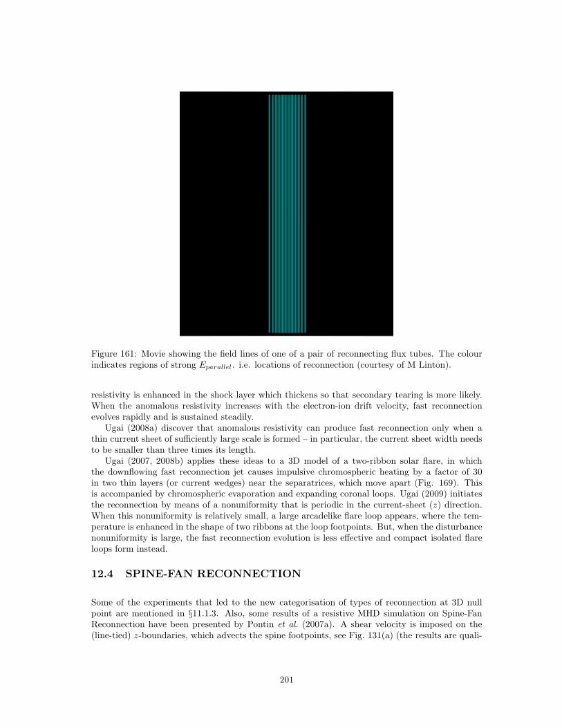
Figure 161: Movie showing the field lines of one of a pair of reconnecting flux tubes. The colourindicates regions of strong Eparallel. i.e. locations of reconnection (courtesy of M Linton).

resistivity is enhanced in the shock layer which thickens so that secondary tearing is more likely.When the anomalous resistivity increases with the electron-ion drift velocity, fast reconnectionevolves rapidly and is sustained steadily.

Ugai (2008a) discover that anomalous resistivity can produce fast reconnection only when athin current sheet of sufficiently large scale is formed – in particular, the current sheet width needsto be smaller than three times its length.

Ugai (2007, 2008b) applies these ideas to a 3D model of a two-ribbon solar flare, in whichthe downflowing fast reconnection jet causes impulsive chromospheric heating by a factor of 30in two thin layers (or current wedges) near the separatrices, which move apart (Fig. 169). Thisis accompanied by chromospheric evaporation and expanding coronal loops. Ugai (2009) initiatesthe reconnection by means of a nonuniformity that is periodic in the current-sheet (z) direction.When this nonuniformity is relatively small, a large arcadelike flare loop appears, where the tem-perature is enhanced in the shape of two ribbons at the loop footpoints. But, when the disturbancenonuniformity is large, the fast reconnection evolution is less effective and compact isolated flareloops form instead.

12.4 SPINE-FAN RECONNECTION

Some of the experiments that led to the new categorisation of types of reconnection at 3D nullpoint are mentioned in §11.1.3. Also, some results of a resistive MHD simulation on Spine-FanReconnection have been presented by Pontin et al. (2007a). A shear velocity is imposed on the(line-tied) z-boundaries, which advects the spine footpoints, see Fig. 131(a) (the results are quali-

201

Figure 162: Untwisted flux tube reconnection in a ‘solid body cylinder’ flow. (a)-(c) show thecreation of half a turn of twist by reconnection at the initial region. (d) Tearing creates one morereconnection region. (e) A reconnected flux tube forms between the two reconnection regions.(f) This flux tube itself reconnects again to form a central tube that is slanted more towards thevertical. From Linton (2007).

Figure 163: Slingshot reconnection of slightly twisted (Φ = 1) flux tubes to form two slanted tubeswith half their initial twist (from Linton, 2007).

202

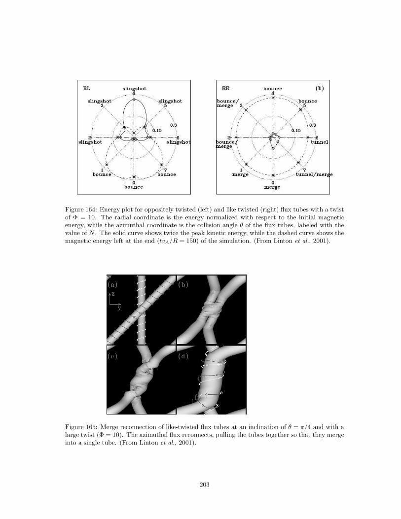
Figure 164: Energy plot for oppositely twisted (left) and like twisted (right) flux tubes with a twistof Φ = 10. The radial coordinate is the energy normalized with respect to the initial magneticenergy, while the azimuthal coordinate is the collision angle θ of the flux tubes, labeled with thevalue of N . The solid curve shows twice the peak kinetic energy, while the dashed curve shows themagnetic energy left at the end (tvA/R = 150) of the simulation. (From Linton et al., 2001).

Figure 165: Merge reconnection of like-twisted flux tubes at an inclination of θ = π/4 and with alarge twist (Φ = 10). The azimuthal flux reconnects, pulling the tubes together so that they mergeinto a single tube. (From Linton et al., 2001).

203

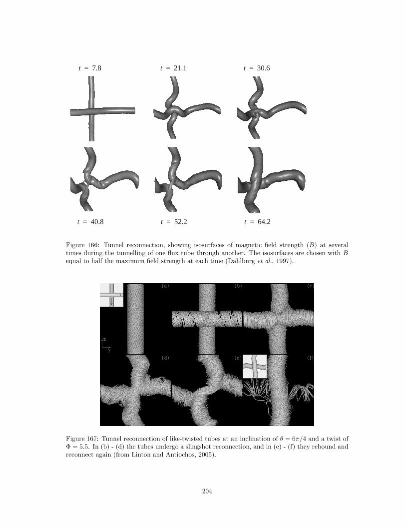
t = 7.8 t = 21.1 t = 30.6

t = 40.8 t = 52.2 t = 64.2

Figure 166: Tunnel reconnection, showing isosurfaces of magnetic field strength (B) at severaltimes during the tunnelling of one flux tube through another. The isosurfaces are chosen with Bequal to half the maximum field strength at each time (Dahlburg et al., 1997).

Figure 167: Tunnel reconnection of like-twisted tubes at an inclination of θ = 6π/4 and a twist ofΦ = 5.5. In (b) - (d) the tubes undergo a slingshot reconnection, and in (e) - (f) they rebound andreconnect again (from Linton and Antiochos, 2005).

204

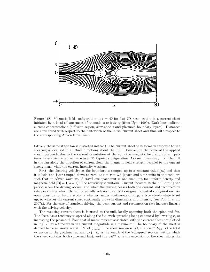
Figure 168: Magnetic field configuration at t = 40 for fast 2D reconnection in a current sheetinitiated by a local enhancement of anomalous resistivity (from Ugai, 1999). Dark lines indicatecurrent concentrations (diffusion region, slow shocks and plasmoid boundary layers). Distancesare normalised with respect to the half-width of the initial current sheet and time with respect tothe corresponding Alfven travel time.

tatively the same if the fan is distorted instead). The current sheet that forms in response to theshearing is localised in all three directions about the null. However, in the plane of the appliedshear (perpendicular to the current orientation at the null) the magnetic field and current pat-terns have a similar appearance to a 2D X-point configuration. As one moves away from the nullin the fan along the direction of current flow, the magnetic field strength parallel to the currentstrengthens, while the current intensity weakens.

First, the shearing velocity at the boundary is ramped up to a constant value (v0) and thenit is held and later ramped down to zero, at t = τ = 3.6 (space and time units in the code aresuch that an Alfven wave would travel one space unit in one time unit for uniform density andmagnetic field |B| = 1, ρ = 1). The resistivity is uniform. Current focusses at the null during theperiod when the driving occurs, and when the driving ceases both the current and reconnectionrate peak, after which the null gradually relaxes towards its original potential configuration. Anopen question for future study is whether, under continuous driving, a true steady state is setup, or whether the current sheet continually grows in dimensions and intensity (see Pontin et al.,2007a). For the case of transient driving, the peak current and reconnection rate increase linearlywith the driving velocity.

The resulting current sheet is focussed at the null, locally spanning both the spine and fan.The sheet has a tendency to spread along the fan, with spreading being enhanced by lowering v0 orincreasing the plasma-β. Four spatial measurements associated with the current sheet are plottedin Fig.170 at a time when the current magnitude is a maximum. The boundary of the sheet isdefined to be an isosurface at 50% of |j|max. The sheet thickness is l, the length Ltot is the totalextension in the yz-plane (normal to j), Lc is the length of the ‘collapsed’ section (within whichthe sheet contains both spine and fan), and the width w is the extension of the sheet along the

205

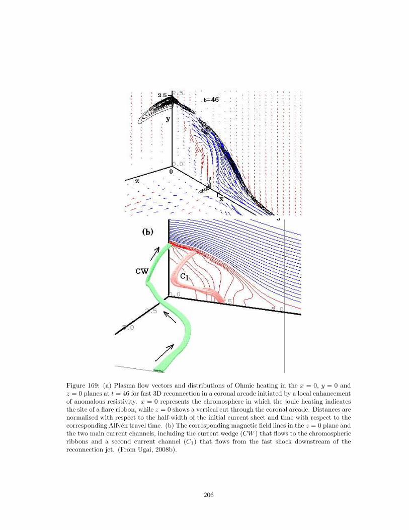
Figure 169: (a) Plasma flow vectors and distributions of Ohmic heating in the x = 0, y = 0 andz = 0 planes at t = 46 for fast 3D reconnection in a coronal arcade initiated by a local enhancementof anomalous resistivity. x = 0 represents the chromosphere in which the joule heating indicatesthe site of a flare ribbon, while z = 0 shows a vertical cut through the coronal arcade. Distances arenormalised with respect to the half-width of the initial current sheet and time with respect to thecorresponding Alfven travel time. (b) The corresponding magnetic field lines in the z = 0 plane andthe two main current channels, including the current wedge (CW ) that flows to the chromosphericribbons and a second current channel (C1) that flows from the fast shock downstream of thereconnection jet. (From Ugai, 2008b).

206

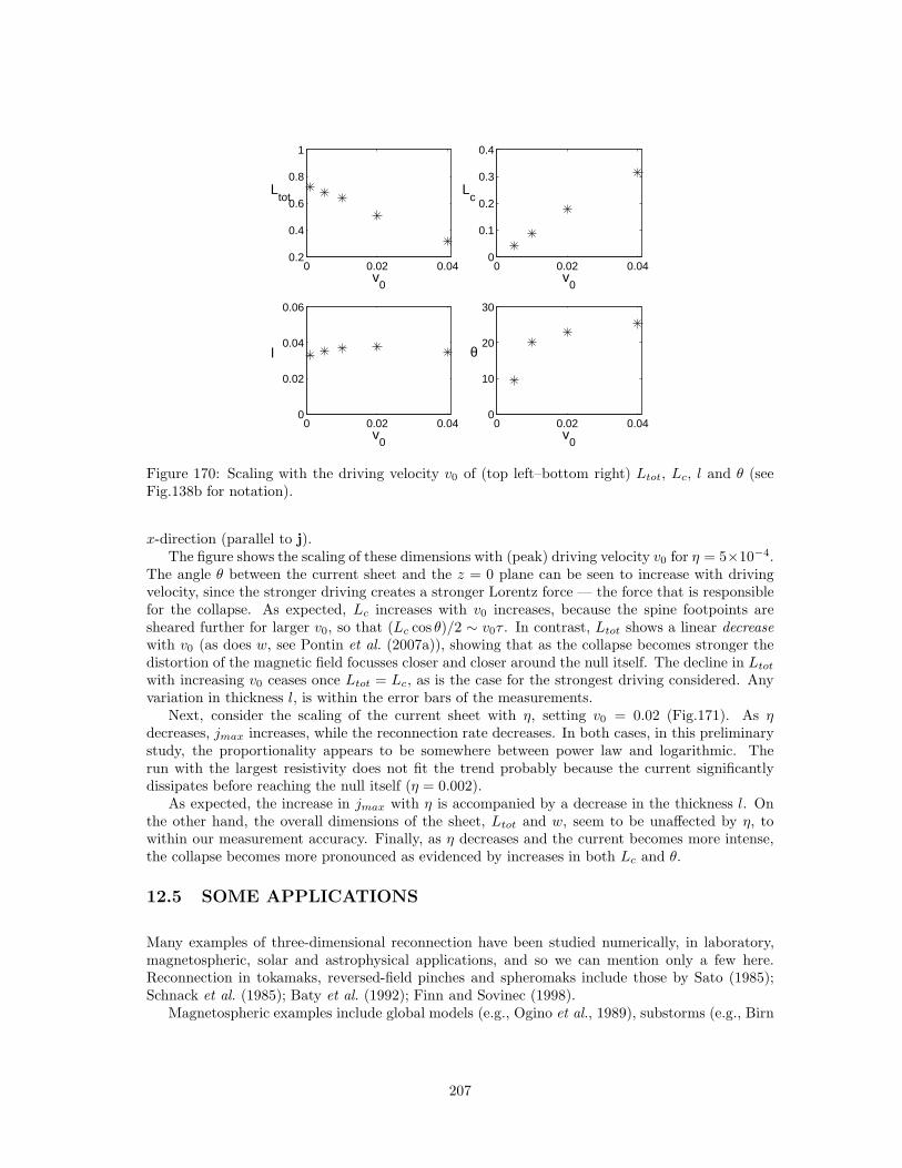
0 0.02 0.040.2

0.4

0.6

0.8

1

v0

Ltot

0 0.02 0.040

0.1

0.2

0.3

0.4

v0

Lc

0 0.02 0.040

0.02

0.04

0.06

v0

l

0 0.02 0.040

10

20

30

v0

θ

Figure 170: Scaling with the driving velocity v0 of (top left–bottom right) Ltot, Lc, l and θ (seeFig.138b for notation).

x-direction (parallel to j).The figure shows the scaling of these dimensions with (peak) driving velocity v0 for η = 5×10−4.

The angle θ between the current sheet and the z = 0 plane can be seen to increase with drivingvelocity, since the stronger driving creates a stronger Lorentz force — the force that is responsiblefor the collapse. As expected, Lc increases with v0 increases, because the spine footpoints aresheared further for larger v0, so that (Lc cos θ)/2 ∼ v0τ . In contrast, Ltot shows a linear decreasewith v0 (as does w, see Pontin et al. (2007a)), showing that as the collapse becomes stronger thedistortion of the magnetic field focusses closer and closer around the null itself. The decline in Ltot

with increasing v0 ceases once Ltot = Lc, as is the case for the strongest driving considered. Anyvariation in thickness l, is within the error bars of the measurements.

Next, consider the scaling of the current sheet with η, setting v0 = 0.02 (Fig.171). As ηdecreases, jmax increases, while the reconnection rate decreases. In both cases, in this preliminarystudy, the proportionality appears to be somewhere between power law and logarithmic. Therun with the largest resistivity does not fit the trend probably because the current significantlydissipates before reaching the null itself (η = 0.002).

As expected, the increase in jmax with η is accompanied by a decrease in the thickness l. Onthe other hand, the overall dimensions of the sheet, Ltot and w, seem to be unaffected by η, towithin our measurement accuracy. Finally, as η decreases and the current becomes more intense,the collapse becomes more pronounced as evidenced by increases in both Lc and θ.

12.5 SOME APPLICATIONS

Many examples of three-dimensional reconnection have been studied numerically, in laboratory,magnetospheric, solar and astrophysical applications, and so we can mention only a few here.Reconnection in tokamaks, reversed-field pinches and spheromaks include those by Sato (1985);Schnack et al. (1985); Baty et al. (1992); Finn and Sovinec (1998).

Magnetospheric examples include global models (e.g., Ogino et al., 1989), substorms (e.g., Birn

207

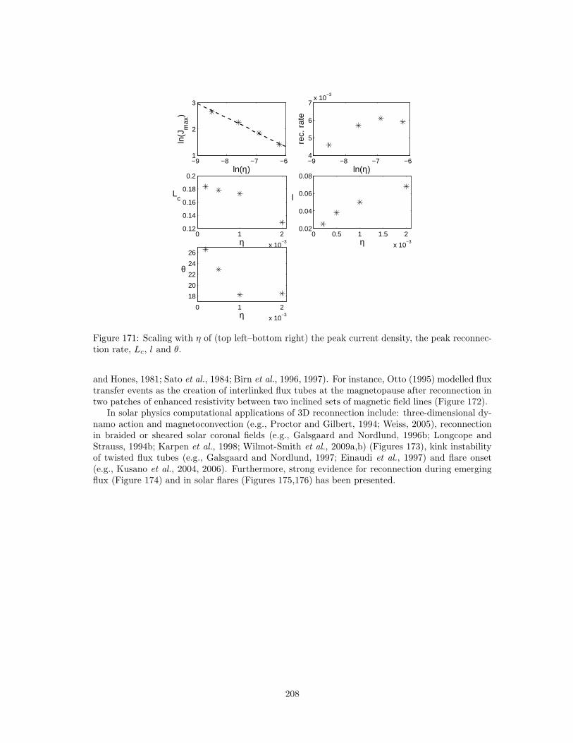
−9 −8 −7 −61

2

3

ln(η)ln

(Jm

ax)

−9 −8 −7 −64

5

6

7x 10

−3

ln(η)

rec.

rat

e

0 1 2

x 10−3

0.12

0.14

0.16

0.18

0.2

η

Lc

0 0.5 1 1.5 2

x 10−3

0.02

0.04

0.06

0.08

η

l

0 1 2

x 10−3

18

20

22

24

26

η

θ

Figure 171: Scaling with η of (top left–bottom right) the peak current density, the peak reconnec-tion rate, Lc, l and θ.

and Hones, 1981; Sato et al., 1984; Birn et al., 1996, 1997). For instance, Otto (1995) modelled fluxtransfer events as the creation of interlinked flux tubes at the magnetopause after reconnection intwo patches of enhanced resistivity between two inclined sets of magnetic field lines (Figure 172).

In solar physics computational applications of 3D reconnection include: three-dimensional dy-namo action and magnetoconvection (e.g., Proctor and Gilbert, 1994; Weiss, 2005), reconnectionin braided or sheared solar coronal fields (e.g., Galsgaard and Nordlund, 1996b; Longcope andStrauss, 1994b; Karpen et al., 1998; Wilmot-Smith et al., 2009a,b) (Figures 173), kink instabilityof twisted flux tubes (e.g., Galsgaard and Nordlund, 1997; Einaudi et al., 1997) and flare onset(e.g., Kusano et al., 2004, 2006). Furthermore, strong evidence for reconnection during emergingflux (Figure 174) and in solar flares (Figures 175,176) has been presented.

208

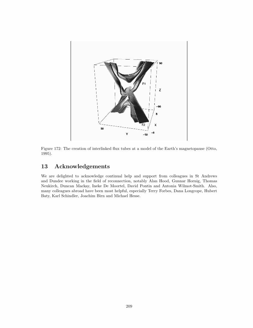
Figure 172: The creation of interlinked flux tubes at a model of the Earth’s magnetopause (Otto,1995).

13 Acknowledgements

We are delighted to acknowledge continual help and support from colleagues in St Andrewsand Dundee working in the field of reconnection, notably Alan Hood, Gunnar Hornig, ThomasNeukirch, Duncan Mackay, Ineke De Moortel, David Pontin and Antonia Wilmot-Smith. Also,many colleagues abroad have been most helpful, especially Terry Forbes, Dana Longcope, HubertBaty, Karl Schindler, Joachim Birn and Michael Hesse.

209

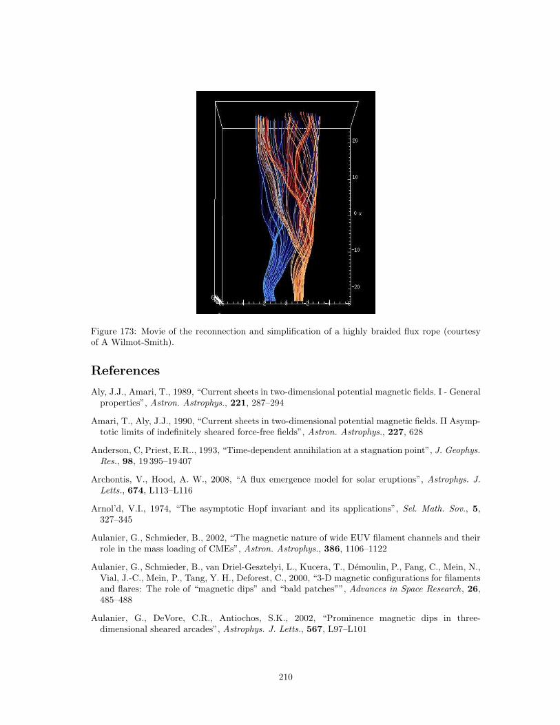
Figure 173: Movie of the reconnection and simplification of a highly braided flux rope (courtesyof A Wilmot-Smith).

References

Aly, J.J., Amari, T., 1989, “Current sheets in two-dimensional potential magnetic fields. I - Generalproperties”, Astron. Astrophys., 221, 287–294

Amari, T., Aly, J.J., 1990, “Current sheets in two-dimensional potential magnetic fields. II Asymp-totic limits of indefinitely sheared force-free fields”, Astron. Astrophys., 227, 628

Anderson, C, Priest, E.R.., 1993, “Time-dependent annihilation at a stagnation point”, J. Geophys.Res., 98, 19 395–19407

Archontis, V., Hood, A. W., 2008, “A flux emergence model for solar eruptions”, Astrophys. J.Letts., 674, L113–L116

Arnol’d, V.I., 1974, “The asymptotic Hopf invariant and its applications”, Sel. Math. Sov., 5,327–345

Aulanier, G., Schmieder, B., 2002, “The magnetic nature of wide EUV filament channels and theirrole in the mass loading of CMEs”, Astron. Astrophys., 386, 1106–1122

Aulanier, G., Schmieder, B., van Driel-Gesztelyi, L., Kucera, T., Demoulin, P., Fang, C., Mein, N.,Vial, J.-C., Mein, P., Tang, Y. H., Deforest, C., 2000, “3-D magnetic configurations for filamentsand flares: The role of “magnetic dips” and “bald patches””, Advances in Space Research, 26,485–488

Aulanier, G., DeVore, C.R., Antiochos, S.K., 2002, “Prominence magnetic dips in three-dimensional sheared arcades”, Astrophys. J. Letts., 567, L97–L101

210

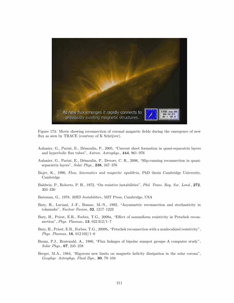
Figure 174: Movie showing reconnection of coronal magnetic fields during the emergence of newflux as seen by TRACE (courtesy of K Schrijver).

Aulanier, G., Pariat, E., Demoulin, P., 2005, “Current sheet formation in quasi-separatrix layersand hyperbolic flux tubes”, Astron. Astrophys., 444, 961–976

Aulanier, G., Pariat, E., Demoulin, P., Devore, C. R., 2006, “Slip-running reconnection in quasi-separatrix layers”, Solar Phys., 238, 347–376

Bajer, K., 1990, Flow, kinematics and magnetic equilibria, PhD thesis Cambridge University,Cambridge

Baldwin, P., Roberts, P. H., 1972, “On resistive instabilities”, Phil. Trans. Roy. Soc. Lond., 272,303–330

Bateman, G., 1978, MHD Instabilities , MIT Press, Cambridge, USA

Baty, H., Luciani, J.-F., Bussac, M.-N., 1992, “Asymmetric reconnection and stochasticity intokamaks”, Nuclear Fusion, 32, 1217–1223

Baty, H., Priest, E.R., Forbes, T.G., 2009a, “Effect of nonuniform resistivity in Petschek recon-nection”, Phys. Plasmas , 13, 022 312/1–7

Baty, H., Priest, E.R., Forbes, T.G., 2009b, “Petschek reconnection with a nonlocalized resistivity”,Phys. Plasmas , 16, 012 102/1–6

Baum, P.J., Bratenahl, A., 1980, “Flux linkages of bipolar sunspot groups–A computer study”,Solar Phys., 67, 245–258

Berger, M.A., 1984, “Rigorous new limits on magnetic helicity dissipation in the solar corona”,Geophys. Astrophys. Fluid Dyn., 30, 79–104

211

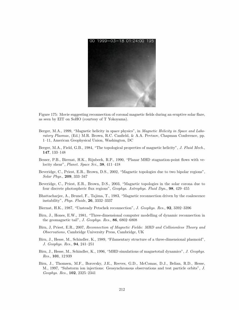
Figure 175: Movie suggesting reconnection of coronal magnetic fields during an eruptive solar flare,as seen by EIT on SoHO (courtesy of T Yokoyama).

Berger, M.A., 1999, “Magnetic helicity in space physics”, in Magnetic Helicity in Space and Labo-ratory Plasmas , (Ed.) M.R. Brown, R.C. Canfield, & A.A. Pevtsov, Chapman Conference, pp.1–11, American Geophysical Union, Washington, DC

Berger, M.A., Field, G.B., 1984, “The topological properties of magnetic helicity”, J. Fluid Mech.,147, 133–148

Besser, P.B., Biernat, H.K., Rijnbeek, R.P., 1990, “Planar MHD stagnation-point flows with ve-locity shear”, Planet. Space Sci., 38, 411–418

Beveridge, C., Priest, E.R., Brown, D.S., 2002, “Magnetic topologies due to two bipolar regions”,Solar Phys., 209, 333–347

Beveridge, C., Priest, E.R., Brown, D.S., 2003, “Magnetic topologies in the solar corona due tofour discrete photospheric flux regions”, Geophys. Astrophys. Fluid Dyn., 98, 429–455

Bhattacharjee, A., Brunel, F., Tajima, T., 1983, “Magnetic reconnection driven by the coalescenceinstability”, Phys. Fluids, 26, 3332–3337

Biernat, H.K., 1987, “Unsteady Petschek reconnection”, J. Geophys. Res., 92, 3392–3396

Birn, J., Hones, E.W., 1981, “Three-dimensional computer modelling of dynamic reconnection inthe geomagnetic tail”, J. Geophys. Res., 86, 6802–6808

Birn, J, Priest, E.R., 2007, Reconnection of Magnetic Fields: MHD and Collisionless Theory andObservations , Cambridge University Press, Cambridge, UK

Birn, J., Hesse, M., Schindler, K., 1989, “Filamentary structure of a three-dimensional plasmoid”,J. Geophys. Res., 94, 241–251

Birn, J., Hesse, M., Schindler, K., 1996, “MHD simulations of magnetotail dynamics”, J. Geophys.Res., 101, 12 939

Birn, J., Thomsen, M.F., Borovsky, J.E., Reeves, G.D., McComas, D.J., Belian, R.D., Hesse,M., 1997, “Substorm ion injections: Geosynchronous observations and test particle orbits”, J.Geophys. Res., 102, 2325–2341

212

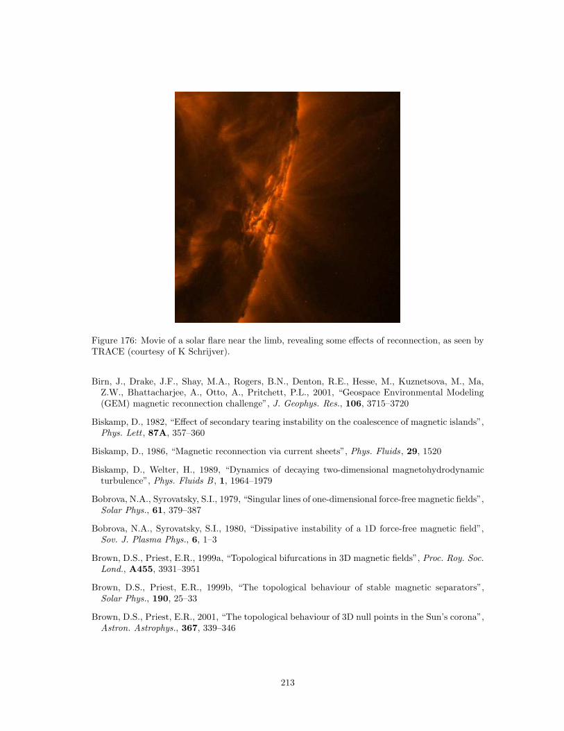
Figure 176: Movie of a solar flare near the limb, revealing some effects of reconnection, as seen byTRACE (courtesy of K Schrijver).

Birn, J., Drake, J.F., Shay, M.A., Rogers, B.N., Denton, R.E., Hesse, M., Kuznetsova, M., Ma,Z.W., Bhattacharjee, A., Otto, A., Pritchett, P.L., 2001, “Geospace Environmental Modeling(GEM) magnetic reconnection challenge”, J. Geophys. Res., 106, 3715–3720

Biskamp, D., 1982, “Effect of secondary tearing instability on the coalescence of magnetic islands”,Phys. Lett , 87A, 357–360

Biskamp, D., 1986, “Magnetic reconnection via current sheets”, Phys. Fluids, 29, 1520

Biskamp, D., Welter, H., 1989, “Dynamics of decaying two-dimensional magnetohydrodynamicturbulence”, Phys. Fluids B , 1, 1964–1979

Bobrova, N.A., Syrovatsky, S.I., 1979, “Singular lines of one-dimensional force-free magnetic fields”,Solar Phys., 61, 379–387

Bobrova, N.A., Syrovatsky, S.I., 1980, “Dissipative instability of a 1D force-free magnetic field”,Sov. J. Plasma Phys., 6, 1–3

Brown, D.S., Priest, E.R., 1999a, “Topological bifurcations in 3D magnetic fields”, Proc. Roy. Soc.Lond., A455, 3931–3951

Brown, D.S., Priest, E.R., 1999b, “The topological behaviour of stable magnetic separators”,Solar Phys., 190, 25–33

Brown, D.S., Priest, E.R., 2001, “The topological behaviour of 3D null points in the Sun’s corona”,Astron. Astrophys., 367, 339–346

213

Browning, P.K., Sakurai, T., Priest, E.R., 1986, “Coronal heating in closely-packed flux tubes - ATaylor-Heyvaerts relaxation theory”, Astron. Astrophys., 158, 217–227

Browning, P.K., Gerrard, C., Hood, A.W., Kevis, R., van der Linden, R.A.M., 2008, “Heatingthe corona by nanoflares: simulations of energy release triggered by a kink instability”, Astron.Astrophys., 485, 837–848

Brushlinskii, K.V., Zaborov, A.M., Syrovatsky, S.I., 1980, “Numerical analysis of the current sheetnear a magnetic null line”, Sov. J. Plasma Phys., 6, 165–173

Bulanov, S.V., Olshanetsky, M.A., 1984, “Magnetic collapse near zero points of the magnetic field”,Phys. Letts., 100A, 35–38

Bulanov, S.V., Sasorov, P.V., 1978, “Tearing of a current sheet and reconnection of magnetic linesof force”, Soviet Journal of Plasma Physics , 4, 746–757

Bulanov, S.V., Sakai, D.-I., Syrovatsky, S.I., 1979, “Tearing instability in quasi-stationary magne-tohydrodynamic configurations”, Soviet Journal of Plasma Physics, 5, 280–290

Bulanov, S.V., Shasharaina, S.G., Pegoraro, F., 1990, “MHD modes near the X-line of a magneticconfiguration”, Plasma Phys. and Control. Fusion, 32, 377–389

Bungey, T.N., Priest, E.R., 1995, “Current sheet configurations in potential and force-free fields”,Astron. Astrophys., 293, 215–224

Bungey, T.N., Titov, V.S., Priest, E.R., 1996, “Basic topological elements of coronal magneticfields”, Astron. Astrophys., 308, 233–247

Chapman, S., Kendall, P.C., 1963, “Liquid instability and energy transformation near a magneticneutral line: A soluble non-linear hydromagnetic problem”, Proc. Roy. Soc., A271, 435–448

Chapman, S., Kendall, P.C., 1966, “Comment on ‘Some exact solutions of magnetohydrodynam-ics”’, Phys. Fluids, 9, 2306–2307

Coppi, B., Pellat, R., Rosenbluth, M., Rutherford, P., Galvao, R., 1976, “Resistive internal kinkmodes”, Soviet Journal of Plasma Physics , 2, 961–966

Cowley, S. C., Longcope, D. W., Sudan, R. N., 1997, “Current sheets in MHD turbulence”, Phys.Rep., 283, 227–251

Cowley, S.W.H., 1973, “A qualitative study of the reconnection between the Earth’s magnetic fieldand an interplanetary field of arbitrary orientation”, Radio Science, 8, 903–913

Cowling, T.G., 1953, “Solar Electrodynamics”, in The Sun, (Ed.) Kuiper, G.P., pp. 532–591, Univ.Chicago Press, Chicago

Craig, I. J. D., Henton, S. M., 1995, “Exact solutions for steady state incompressible magneticreconnection”, ApJ , 450, 280–288

Craig, I.J.D., Fabling, R. B., 1996, “Exact solutions for steady-state spine and fan magneticreconnection”, ApJ , 462, 969–976

Craig, I.J.D., McClymont, A.N., 1991, “Dynamic magnetic reconnection at an X-type neutralpoint”, Astrophys. J., 371, L41–L44

Craig, I.J.D., McClymont, A.N., 1993, “Linear theory of fast reconnection at an X-type neutralpoint”, Astrophys. J., 405, 207–215

214

Craig, I.J.D., Watson, P.G., 1992, “Fast dynamic reconnection at X-type neutral points”, Astro-phys. J., 393, 385–395

Craig, I.J.D., Fabling, R.B., Henton, S.M., Rickard, G.J., 1995, “An exact solution for steady statemagnetic reconnection in three dimensions”, ApJL, 455, L197

Dahlburg, R. B., Antiochos, S. K., 1995, “Reconnection of antiparallel magnetic flux tubes”, J.Geophys. Res., 100, 16 991–16998

Dahlburg, R. B., Antiochos, S. K., Norton, D., 1997, “Magnetic flux tube tunneling”, Phys. Rev.E , 56, 2094–2103

DeBenedetti, M., Pegoraro, F., 1995, “Resistive modes at a magnetic X-point”, Plasma Physicsand Controlled Fusion, 37, 103–116

Delannee, C., Aulanier, G., 1999, “CME associated with transequatorial loops and a bald patchflare”, Solar Phys., 190, 107–129

Demoulin, P., 2006, “Extending the concept of separatrices to QSLs for magnetic reconnection”,Advances in Space Research, 37, 1269–1282

Demoulin, P., Henoux, J.C., Priest, E.R., Mandrini, C.H., 1996a, “Quasi-separatrix layers in solarflares. I. Method”, Astron. Astrophys., 308, 643–655

Demoulin, P., Priest, E. R., Lonie, D.P., 1996b, “3D magnetic reconnection without null points. 2.Application to twisted flux tubes”, J. Geophys. Res., 101, 7631–7646

Demoulin, P., Bagala, L. G., Mandrini, C. H., Henoux, J. C., Rovira, M. G., 1997, “Quasi-separatrix layers in solar flares. II. Observed magnetic configurations”, Astron. Astrophys., 325,305–317

Demoulin, P., Henoux, J.C., Mandrini, C.H., Priest, E.R., 1997, “Can we extrapolate a magneticfield when its topology is complex?”, Solar Phys., 174, 73–89

Diamond, P.H., Hazeltine, R.D., An, Z.G., Carreras, B.A., Hicks, H.R., 1984, “Theory of anoma-lous tearing mode growth and the major tokamak disruption”, Phys. Fluids, 27, 1449–1462

Dobrowolny, M., Veltri, P., Mangeney, A., 1983, “Dissipative instabilities of magnetic neutral layerswith velocity shear”, J. Plasma Phys., 29, 393–407

Dungey, J.W., 1953, “Conditions for the occurrence of electrical discharges in astrophysical sys-tems”, Phil. Mag, 44, 725–738

Einaudi, G., Rubini, F., 1989, “Resistive instability in a flowing plasma. III. Effects of viscosity”,Phys. Fluids B , 1, 2224–2228

Einaudi, G., Lionello, R., Velli, M., 1997, “Magnetic reconnection in solar coronal loops”, Advancesin Space Research, 19, 1875–1878

Fabling, R. B., Craig, I.J.D., 1995, “Exact solutions for steady-state planar magnetic reconnectionin an incompressible viscous plasma”, Phys. Plasmas , 3, 2243–2247

Finn, J.M., Antonsen, Jr., T.M., 1985, “Magnetic helicity: What it is and what is it good for?”,Comments Plasma Phys. Controlled Fusion, 9, 11

Finn, J.M., Kaw, P.K., 1977, “Coalescence instability of magnetic islands”, Phys. Fluids, 20, 72–78

215

Finn, J.M., Sovinec, C.R., 1998, “Nonlinear tearing modes in the presence of resistive wall androtation”, Phys. Plasmas , 5, 461–480

Forbes, T.G., 1982, “Implosion of a uniform current sheet in a low-beta plasma”, J. Plasma Phys.,27, 491–505

Forbes, T.G., Priest, E. R., 1984, “Reconnection in solar flares”, in Solar Terrestrial Phys.: Presentand Future, (Eds.) Butler, D., Papadopoulos, K., pp. 1–35, NASA RP-1120, Washington

Forbes, T.G., Priest, E.R., 1987, “A comparison of analytical and numerical models for steadily-driven magnetic reconnection”, Rev. Geophys., 25, 1583–1607

Forbes, T.G., Speiser, T.W., 1979, “Temporal evolution of magnetic reconnection in the vicinityof a magnetic neutral line”, J. Plasma Phys., 21, 107–126

Furth, H.P., Killeen, J., Rosenbluth, M.N., 1963, “Finite-resistivity instabilities of a sheet pinch”,Phys. Fluids, 6, 459–484

Furth, H.P., Rutherford, P.H., Selberg, H., 1973, “Tearing mode in the cylindrical tokamak”, Phys.Fluids , 16, 1054–1063

Galsgaard, K., Nordlund, A., 1996a, “The heating and activity of the solar corona: I Boundaryshearing of an initially homogeneous magnetic field”, J. Geophys. Res., 101, 13 445–13460

Galsgaard, K., Nordlund, A, 1996b, “Coronal heating by flux braiding”, Astro. Lett. and Commu-nications , 34, 175

Galsgaard, K., Nordlund, A., 1996c, “Heating and activity of the solar corona. III. Dynamics of alow-beta plasma with 3D null points”, J. Geophys. Res., 102, 231–248

Galsgaard, K., Nordlund, A, 1997, “The heating and activity of the solar corona: 2, Kink instabilityin a flux tube”, J. Geophys. Res., 102, 219–230

Galsgaard, K., Parnell, C., 2004, “Fragment-Driven Magnetic Reconnection”, in ESA SP-575:SOHO 15. Proceedings of the Coronal Heating SOHO conference, (Eds.) Walsh, R.W., Ireland,J., Danesy, D., Fleck, B., pp. 351–356, European Space Agency, Paris

Galsgaard, K., Parnell, C., 2005, “Elementary Heating Events - Magnetic Interactions BetweenTwo Flux Sources. III Energy Considerations”, Astron. Astrophys., 439, 335–349

Galsgaard, K., Parnell, C., Blaizot, J., 2000a, “Elementary heating events - Magnetic interactionsbetween two flux sources”, aa, 362, 395–405

Galsgaard, K., Priest, E. R., Nordlund, A., 2000b, “Three-dimensional separator reconnection -How does It occur?”, Solar Phys., 193, 1–16

Galsgaard, K., Priest, E.R., Titov, V.S., 2003a, “Numerical experiments on wave propagationtowards a 3D null point due to rotational motions”, J. Geophys. Res., 108, SSH 10.1–10.9

Galsgaard, K, V.S. Titov, V.S., Neukirch, T., 2003b, “Magnetic pinching of hyperbolic flux tubes.II. Dynamic numerical model”, Astrophys. J., 595, 506–516

Giovanelli, R.G., 1947, “Magnetic and electric phenomena in the Sun’s atmosphere associated withsunspots”, Mon. Not. Roy. Astron. Soc., 107, 338–355

Gold, T., Hoyle, F., 1960, “On the origin of solar flares”, Mon. Not. Roy. Astron. Soc., 120, 89–105

216

Gorbachev, V.S., Somov, B.V., 1988, “Photospheric vortex flows as a cause for two-ribbon flares– A topological model”, Solar Phys., 117, 77–88

Gratton, F.T., Heyn, M.F., Biernat, H.K., Rijnbeek, R.P., Gnavi, G., 1988, “MHD stagnationpoint flows in the presence of resistivity and viscosity”, J. Geophys. Res., 93, 7318–7324

Green, R.M., 1965, “Modes of annihilation and reconnection in magnetic fields”, in Stellar andSolar magnetic fields., (Ed.) Lust, R., IAU Symp. 22, pp. 398–404, North-Holland, Amsterdam

Greene, J.M., 1988, “Geometrical properties of three-dimensional reconnecting magnetic fields withnulls”, J. Geophys. Res., 93, 8583–8590

Hahm, T. S., Kulsrud, R. M., 1985, “Forced magnetic reconnection”, Physics of Fluids, 28, 2412–2418

Hassam, A.B., 1992, “Reconnection of stressed magnetic fields”, Astrophys. J., 399, 159–163

Haynes, A.L., Parnell, C.E., Galsgaard, K., Priest, E.R., 2007, “Magnetohydrodynamic evolutionof magnetic skeletons”, Proc. Roy. Soc. Lond., 463, 1097–1115

Hesse, M., Birn, J., 1990, “Parallel electric fields in a simulation of magnetotail reconnection andplasmoid evolution”, in Phys. of Magnetic Flux Ropes , pp. 679–685, A.G.U., Washington

Hesse, M., Birn, J., 1993, “Parallel electric fields as acceleration mechanisms in three-dimensionalmagnetic reconnnection”, Adv. Space Res., 13, 249

Hesse, M., Schindler, K., 1988, “A theoretical foundation of general magnetic reconnection”, J.Geophys. Res., 93, 5539–5567

Hesse, M., Schindler, K., Birn, J., 1991, “Three-Dimensional Magnetic Reconnection: BasicConcepts”, in Mechanisms of Chromospheric and Coronal Heating, (Ed.) P. Ulmschneider,E. R. Priest, & R. Rosner, pp. 604–608, Springer-Verlag, Berlin

Hesse, M., Forbes, T. G., Birn, J., 2005, “On the relation between connected magnetic flux andparallel electric fields in the solar corona”, Astrophys. J., 631, 1227–1238

Heyn, M.F., 1996, “Rapid reconnection in compressible plasma”, Phys. Plasmas , 3, 2725–2741

Heyn, M.F., Biernat, H.K., Semenov, V.S., Kubyshkin, I.V., 1985, “Dayside magnetopause recon-nection”, J. Geophys. Res., 90, 1781–1785

Heyvaerts, J., Priest, E.R., 1984, “Coronal heating by reconnection in DC current systems - Atheory based on Taylor’s hypothesis”, Astron. Astrophys., 137, 63–78

Heyvaerts, J., Priest, E.R., Rust, D.M., 1977, “An emerging flux model for the solar flare phe-nomenon”, Astrophys. J., 216, 123–137

Hide, R., 1979, “On the magnetic flux linkage of an electrically conducting fluid”, Geophys. Astro-phys. Fluid Dyn., 12, 171–176

Hood, A.W., Priest, E.R., 1981, “Critical conditions for magnetic instabilities in force-free coronalloops”, Geophys. Astrophys. Fluid Dyn., 17, 297–318

Hood, A.W., Archontis, V., Galsgaard, K., Moreno-Insertis, F., 2009a, “The emergence of toroidalflux tubes from beneath the solar photosphere”, Astron. Astrophys., 503, 999–1011

217

Hood, A.W., Browning, P.K., van der Linden, R.A.M., 2009b, “Coronal heating by magneticreconnection in loops with zero net current”, Astron. Astrophys., 506, 913–925

Hornig, G., 2001, “The geometry of reconnection”, in An Introduction to the Geometry and Topol-ogy of Fluid Flows, (Ed.) Ricca, R. L., pp. 295–313, Kluwer, Dordrecht

Hornig, G., Priest, E.R., 2003, “Evolution of magnetic flux in an isolated reconnection process”,Phys. Plasmas , 10, 2712–2721

Hornig, G., Rastatter, L., 1998, “The magnetic structure of B 6=0 reconnection.”, Physica ScriptaVolume T , 74, 34–39

Hornig, G., Schindler, K., 1996, “Magnetic topology and the problem of its invariant definition”,Phys. Plasmas , 3, 781–791

Huba, J. D., 2003, “A tutorial on Hall MHD”, in Space Simulations , (Eds.) Scholer, M., Dum,C.T., Buchner, J., pp. 170–197, Springer, New York

Imshennik, V.S., Syrovatsky, S. I., 1967, “Two-dimensional flow of an ideally conducting gas inthe vicinity of the zero line of a magnetic field”, Sov. Phys. JETP , 25, 656–664

Inverarity, G. W., Priest, E. R., 1999, “Magnetic null points due to multiple sources of solarphotospheric flux”, Solar Phys., 186, 99–121

Jardine, M., Priest, E.R., 1988a, “Weakly nonlinear theory of fast steady-state magnetic reconnec-tion”, J. Plasma Phys., 40, 143–161

Jardine, M., Priest, E.R., 1988b, “Global energetics of fast magnetic reconnection”, J. PlasmaPhys., 40, 505–515

Jardine, M., Priest, E.R., 1988c, “Reverse currents in fast magnetic reconnection”, Geophys. As-trophys. Fluid Dyn., 42, 163–168

Jardine, M., Priest, E.R., 1990, “Energetics of compressible models of fast steady-state magneticreconnection”, J. Plasma Phys., 43, 141–150

Jardine, M., Allen, H.R., Grundy, R.E., Priest, E.R., 1992, “A family of two-dimensional nonlinearsolutions for magnetic field annihilation”, J. Geophys. Res., 97, 4199–4208

Jardine, M., Allen, H.R., Grundy, R.E., 1993, “Three-dimensional magnetic field annihilation”, J.Geophys. Res., 98, 19 409–19417

Jin, S.-P., Ip, W.-H., 1991, “2-D compressible mhd simulation of the drivE.R.connection process”,Phys. Fluids, 3, 1927–1936

Kadomtsev, B. B., 1975, “Disruptive instability in Tokamaks”, Soviet Journal of Plasma Physics,1, 389–391

Karpen, J.T., Antiochos, S.K., Devore, C.R., Golub, L., 1998, “Dynamic Responses to MagneticReconnection in Solar Arcades”, Astrophys. J., 495, 491–501

Kippenhahn, R., Schluter, A., 1957, “Eine Theorie der Solaren Filamente”, Zs. Ap., 43, 36–62

Klapper, I., 1998, “Constraints on finite-time current sheet formation at null points in two-dimensional ideal incompressible magnetohydrodynamics”, Phys. Plasmas , 5, 910–914

218

Kliem, B., Titov, V. S., Torok, T., 2004, “Formation of current sheets and sigmoidal structure bythe kink instability of a magnetic loop”, Astron. Astrophys., 413, L23–L26

Klimchuk, J.A., Sturrock, P.A., Yang, W.-H., 1988, “Coronal magnetic fields produced by photo-spheric shear”, Astrophys. J., 335, 456–467

Kondrashov, D., Feynman, J., Liewer, P.C., Ruzmaikin, A., 1999, “Three-dimensional Magne-tohydrodynamic Simulations of the Interaction of Magnetic Flux Tubes”, Astrophys. J., 519,884–898

Kulsrud, R. M., Hahm, T. S., 1982, “Forced magnetic reconnection”, Physica Scripta Volume T ,2, 525–

Kusano, K., Maeshiro, T., Yokoyama, T., Sakurai, T., 2004, “The Trigger Mechanism of SolarFlares in a Coronal Arcade with Reversed Magnetic Shear”, Astrophys. J., 610, 537–549

Kusano, K., Nishikawa, N., Inoue, S., Maeshiro, T., Sakurai, T., 2006, “Simulation study of theSolar flare onset mechanism and the self-organization in the Solar coronal plasma”, Journal ofPlasma Physics , 72, 979–982

Lau, Y.-T., Finn, J. M., 1990, “Three-dimensional kinematic reconnection in the presence of fieldnulls and closed field lines”, Astrophys. J., 350, 672–691

Lau, Y.-T., Finn, J. M., 1991, “Three-dimensional kinematic reconnection of plasmoids”, Astro-phys. J., 366, 577–591

Lau, Y.-T., Finn, J. M., 1992, “Three-dimensional kinematic reconnection of plasmoids with nulls”,Physica D., 57, 283

Lau, Y.-T., Finn, J. M., 1996, “Magnetic reconnection and the topology of interacting twisted fluxtubes”, Phys. Plasmas , 3, 3983

Lee, L.-C., Fu, Z.F., 1986a, “Multiple X-line reconnection 1. A criterion for the transition from asingle X-line to a multiple X-line reconnection”, J. Geophys. Res., 91, 6807–6815

Lee, L.-C., Fu, Z.F., 1986b, “A simulation study of magnetic reconnection: transition from a fastmode to a slow mode expansion”, J. Geophys. Res., 91, 4551–4556

Linardatos, D., 1993, “Magnetostatic equilibria and analogous Euler flows”, J. Fluid Mech., 246,569–591

Linton, M. G., Antiochos, S. K., 2005, “Magnetic Flux Tube Reconnection: Tunneling VersusSlingshot”, Astrophys. J., 625, 506–521

Linton, M. G., Dahlburg, R. B., Antiochos, S. K., 2001, “Reconnection of Twisted Flux Tubes asa Function of Contact Angle”, Astrophys. J., 553, 905–921

Linton, M.G., 2007, “Three-dimensional flux-tube reconnection”, in Reconnection of MagneticFields: MHD and Collisionless Theory and Observations, (Eds.) Birn, J, Priest, E.R., pp. 74–86, Cambridge University Press, Cambridge, UK

Linton, M.G., Priest, E.R., 2003, “Three-Dimensional Reconnection of Untwisted Magnetic FluxTubes”, Astrophys. J., 595, 1259–1276

Litvinenko, Y.E., Forbes, T.G., Priest, E.R., 1996, “A strong limitation on the rapidity of flux-pile-up reconnection”, Solar Phys., 167, 445–448

219

Longbottom, A.W., Rickard, G. J., Craig, I. J. D., Sneyd, A. D., 1998, “Magnetic flux braiding:force-free equilibria and current sheets”, Astrophys. J., 500, 471–482

Longcope, D. W., 2005, “Topological methods for the analysis of solar magnetic fields”, LivingReviews in Solar Physics , 2, 1–72

Longcope, D. W., Beveridge, C., 2007, “A quantitative, topological model of reconnection and fluxrope formation in a two-ribbon flare”, Astrophys. J., 669, 621–635

Longcope, D. W., Magara, T., 2004, “A comparison of the Minimum Current Corona to a magne-tohydrodynamic simulation of quasi-static coronal evolution”, Astrophys. J., 608, 1106–1123

Longcope, D. W., Parnell, C. E., 2009, “The number of magnetic null points in the quiet-Suncorona”, Solar Phys., 254, 51–75

Longcope, D. W., McKenzie, D., Cirtain, J., Scott, J., 2005, “Observations of separator reconnec-tion to an emerging active region”, Astrophys. J., 630, 596–614

Longcope, D.W., 1996, “Topology and current ribbons: a model for current, reconnection andflaring in a complex, evolving corona”, Solar Phys., 169, 91–121

Longcope, D.W., 1998, “A model for current sheets and reconnection in X-ray bright points”,Astrophys. J., 507, 433–442

Longcope, D.W., 2001, “Separator current sheets: Generic features in minimum-energy magneticfields subject to flux constraints”, Phys. Plasmas , 8, 5277–5289

Longcope, D.W., Cowley, S.C., 1996, “Current sheet formation along three-dimensional magneticseparators”, Phys. Plasmas , 3, 2885–2897

Longcope, D.W., Silva, A.V.R., 1998, “A current ribbon model for energy storage and release withapplication to the flare 1992 Jan. 7”, Solar Phys., 179, 349–377

Longcope, D.W., Strauss, H. R., 1994a, “The form of ideal current layers in line-tied magneticfields”, Astrophys. J., 437, 851–859

Longcope, D.W., Strauss, H.R., 1993, “The coalescence instability and the development of currentsheets in two-dimensional magnetohydrodynamics”, Physics of Fluids B , 5, 2858–2869

Longcope, D.W., Strauss, H.R., 1994b, “Spontaneous reconnection of line-tied flux tubes”, Astro-phys. J., 426, 742–757

Longcope, D.W., Brown, D.S., Priest, E.R., 2003, “On the distribution of magnetic null pointsabove the solar photosphere”, Phys. Plasmas , 10, 3321–3334

Low, B. C., 1981, “Eruptive solar magnetic fields”, Astrophys. J., 251, 352–363

Low, B. C., 1982, “Magnetic field configurations associated with polarity intrusion in a solar activeregion. I - The force-free fields”, Solar Phys., 77, 43–61

Low, B.C., 1986, “Models of partially open magnetospheres with and without magnetodisks”,Astrophys. J., 310, 953–965

Low, B.C., Wolfson, R., 1988, “Spontaneous formation of electric current sheets and the origin ofsolar flares”, Astrophys. J., 324, 574–581

220

Maclean, R.C., Priest, E.R., 2007, “Topological aspects of global magnetic field reversal in thesolar corona”, Solar Phys., 243, 171–191

Maclean, R.C., Beveridge, C., Longcope, D.W., Brown, D.S., Priest, E.R., 2005, “A topologicalanalysis of the magnetic breakout model for an eruptive solar flare”, Proc. Roy. Soc. Lond.,A461, 2099–2120

Maclean, R.C., Beveridge, C., Priest, E.R., 2006a, “Coronal magnetic topologies in a sphericalgeometry - II. Four balanced flux sources”, Solar Phys., 238, 13–27

Maclean, R.C., Hornig, G., Priest, E.R., Beveridge, C., 2006b, “Coronal magnetic topologies in aspherical geometry - I. Two bipolar flux sources”, Solar Phys., 235, 259–280

Malherbe, J.M., Priest, E. R., 1983, “Current sheet models for solar prominences. I Magneto-hydrostatics of support and evolution through quasi-static models”, Astron. Astrophys., 123,80–88

Masson, S., Pariat, E., Aulanier, G., Schrijver, C. J., 2009, “The Nature of Flare Ribbons inCoronal Null-Point Topology”, Astrophys. J., 700, 559–578. [DOI]

Matthaeus, W.H., Montgomery, D.C., 1981, “Nonlinear evolution of the sheet pinch”, J. PlasmaPhys., 25, 11–41

Matthaeus, W.H., Ghosh, S., Oughton, S., Roberts, D.A., 1996, “Anisotropic three-dimensionalMHD turbulence”, J. Geophys. Res., 101, 7619–7630

McClymont, A.N., Craig, I.J.D., 1996, “Dynamical finite-amplitude magnetic reconnection at anX-type neutral point”, Astrophys. J., 466, 487

Mellor, C., Titov, V.S., Priest, E. R., 2003, “Linear collapse of spatially linear 3D potential nullpoints”, Geophys. Astrophys. Fluid Dyn., 97, 489–505

Mikic, Z., Schnack, D. D., Hoven, G. Van, 1989, “Creation of current filaments in the solar corona”,Astrophys. J., 338, 1148–1157

Milne, A.M., Priest, E.R., 1981, “Internal structure of reconnecting current sheets and the emergingflux model for solar flares”, Solar Phys., 73, 157–181

Moffatt, H.K., 1978, Magnetic Field Generation in Electrically Conducting Fluids , CambridgeUniversity Press, Cambridge, England

Moffatt, H.K., 1985, “Magnetostatic equilibria and analogous Euler flows of arbitrarily complextopology. Part 1 Fundamentals”, J. Fluid Mech., 159, 359–378

Moffatt, H.K., 1990, “Structure and stability of solutions of the Euler equations: a Lagrangianapproach”, Phil. Trans. R. Soc. Lond. A., 333, 321–342

Ofman, L., Chen, X. L., Morrison, P. J., Steinolfson, R. S., 1991, “Resistive tearing mode instabilitywith shear flow and viscosity”, Physics of Fluids B , 3, 1364–1373

Ofman, L, Morrison, P.J., Steinolfson, R.S., 1992, “Magnetic reconnection at stressed X-typeneutral points”, Astrophys. J., 417, 748–756

Ofman, L., Morrison, P. J., Steinolfson, R. S., 1993, “Nonlinear evolution of resistive tearing modeinstability with shear flow and viscosity”, Physics of Fluids B , 5, 376–387

221

Ogino, T., Walker, R.J., Ashour-Abdalla, M., 1989, “A magnetohydrodynamic simulation of theformation of magnetic flux tubes at the earth’s dayside magnetopause”, Geophys. Res. Lett., 16,155–158

Otto, A., 1995, “Forced three-dimensional magnetic reconnection due to linkage of magnetic fluxtubes”, J. Geophys. Res., 100, 11 863–11874

Otto, A., Schindler, K., Birn, J., 1990, “Quantitative study of the nonlinear formation and accel-eration of plasmoids in the earth’s magnetotail”, J. Geophys. Res., 95, 15 023–15037

Ozaki, M., Sato, T., 1997, “Interactions of Convecting Magnetic Loops and Arcades”, Astrophys.J., 481, 524–531

Pariat, E., Aulanier, G., Schmieder, B., Georgoulis, M.K., Rust, D.M., Bernasconi, P.N., 2004,“Resistive emergence of undulatory flux tubes”, Astrophys. J., 614, 1099–1112

Pariat, E., Aulanier, G., Demoulin, P., 2006, “A new concept for magnetic reconnection: slip-running reconnection”, in SF2A-2006: Semaine d’Astrophysique Francaise, (Ed.) D. Barret,F. Casoli, G. Lagache, A. Lecavelier, & L. Pagani, pp. 559–562, Societe Francoise d’Astronomieet d’Astrophysique

Park, W., Monticello, D.A., R.B., White, 1984, “Reconnection rates of magnetic fields includingthe effects of viscosity”, Phys. Fluids, 27, 137–149

Parker, E.N., 1957, “Sweet’s mechanism for merging magnetic fields in conducting fluids”, J.Geophys. Res., 62, 509–520

Parker, E.N., 1963, “The solar flare phenomenon and the theory of reconnection and annihilationof magnetic fields”, Astrophys. J., 8, 177–212

Parker, E.N., 1972, “Topological dissipation and the small-scale fields in turbulent gases”, Astro-phys. J., 174, 499–510

Parker, E.N., 1973, “Comments on the reconnection rate of magnetic fields”, J. Plasma Phys., 9,49–63

Parker, E.N., 1979, Cosmical Magnetic Fields, Oxford University Press, Oxford

Parker, E.N., 1989, “Spontaneous tangential discontinuities and the optical analogy for staticmagnetic fields”, Geophys. Astrophys. Fluid Dyn., 45, 159–168

Parker, E.N., 1990, “Tangential discontinuities and the optical analogy for stationary fields. V -Formal integration of the force-free equations”, Geophys. Astrophys. Fluid Dyn., 52, 183–210

Parker, E.N., 1994, Spontaneous Current Sheets in Magnetic Fields , Oxford Univ. Press, NewYork, NY

Parnell, C. E., Haynes, A. L., Galsgaard, K., 2008, “Recursive reconnection and magnetic skele-tons”, Astrophys. J., 675, 1656–1667

Parnell, C.E., 2007, “Multiply connected source and null pairs”, Solar Phys., 242, 21–41

Parnell, C.E., Galsgaard, K., 2004, “Elementary heating events - interaction between two fluxsources. II Rates of flux reconnection”, Astron. Astrophys., 428, 595–612

Parnell, C.E., Haynes, A.L., 2009, “Three-dimensional magnetic reconnection”, in Magnetic Cou-pling Between the Interior and Atmosphere of the Sun, pp. 261–276, Springer-Verlag, Heidelberg

222

Parnell, C.E, Smith, J.M., Neukirch, T, Priest, E.R., 1996, “The structure of 3D magnetic neutralpoints”, Phys. Plasmas , 3, 759–770

Parnell, C.E., Neukirch, T., Smith, J.M., Priest, E.R., 1997, “Structure and collapse of 3D magneticneutral points”, Geophys. Astrophys. Fluid Dyn., 84, 245–271

Parnell, C.E., Haynes, A.L., Galsgaard, K., 2010, “The structure of magnetic separators andseparator reconnection”, J. Geophys. Res., 115, 2102

Petschek, H.E., 1964, “Magnetic field annihilation”, in The Physics of Solar Flares, pp. 425–439,NASA Spec. Publ. SP-50, Washington

Petschek, H.E., Thorne, R.M., 1967, “The existence of intermediate waves in neutral sheets”,Astrophys. J., 147, 1157–1163

Pevtsov, A. A., Maleev, V., Longcope, D. W., 2003, “Helicity evolution in emerging active regions”,Astrophys. J., 593, 1217–1225

Pevtsov, A.A., Canfield, R.C., Latushko, S.M., 2001, “Hemispheric helicity trend for solar cycle 23”,Astrophys. J., 549, L261–L263

Phan, T.D., Sonnerup, B.U.O., 1990, “MHD stagnation-point flows at a current sheet includingviscous and resistive effects: general two-dimensional solutions”, J. Plasma Phys., 44, 525–546

Politano, H., Pouquet, A., Sulem, P.L., 1995, “Current and vorticity dynamics in three-dimensionalmagnetohydrodynamic turbulence”, Phys. Plasmas , 2, 2931–2939

Pontin, D. I., Craig, I. J. D., 2005, “Current singularities at finitely compressible three-dimensionalmagnetic null points”, Phys. Plasmas , 12, 072 112

Pontin, D. I., Galsgaard, K., 2007, “Current amplification and magnetic reconnection at a three-dimensional null point: Physical characteristics”, J. Geophys. Res., 112, A03 103

Pontin, D. I., Hornig, G., Priest, E. R., 2005, “Kinematic reconnection at a magnetic null point:Fan-aligned current”, Geophys. Astrophys. Fluid Dyn., 99, 77–93

Pontin, D. I., Bhattacharjee, A., Galsgaard, K., 2007a, “Current sheet formation and nonidealbehavior at three-dimensional magnetic null points”, Phys. Plasmas , 14, 052 106

Pontin, D. I., Bhattacharjee, A., Galsgaard, K., 2007b, “Current sheets at three-dimensional mag-netic nulls: Effect of compressibility”, Phys. Plasmas , 14, 052 109

Pontin, D.I., Hornig, G., Priest, E.R., 2004, “Kinematic reconnection at a magnetic null point:Spine-aligned current”, Geophys. Astrophys. Fluid Dyn., 98, 407–428

Pouquet, A., 1978, “On two-dimensional MHD turbulence”, J. Fluid Mech., 88, 1–16

Prichett, P.L., Wu, C.C., 1979, “Coalescence of magnetic islands”, Phys. Fluids, 22, 2140–2146

Priest, E. R., Schrijver, C. J., 1999, “Aspects of Three-Dimensional Magnetic Reconnection -(Invited Review)”, Solar Phys., 190, 1–24

Priest, E.R., 1972a, “A modification and criticism of Petschek’s mechanism”, Mon. Not. Roy.Astron. Soc., 159, 389–402

Priest, E.R., 1972b, “Sweet’s mechanism for the destruction of magnetic flux”, Mech. and App.Math., 25, 319–332

223

Priest, E.R., 1986, “Magnetic reconnection on the Sun”, Mit. Astron. Ges., 65, 41–51

Priest, E.R., 1996, “New developments in magnetic reconnection theory”, in Solar and Astrophys-ical MHD Flows , (Ed.) Tsinganos, K, pp. 151–170, Kluwer, Dordrecht

Priest, E.R., 2011, Solar Magnetohydrodynamics , Cambridge University Press, Cambridge, UK

Priest, E.R., Cowley, S.W.H., 1975, “Some comments on magnetic field reconnection”, J. PlasmaPhys., 14, 271–282

Priest, E.R., Demoulin, P., 1995, “3D reconnection without null points”, J. Geophys. Res., 100,23,443–23,463

Priest, E.R., Forbes, T.G., 1986, “New models for fast, steady-state reconnection”, J. Geophys.Res., 91, 5579–5588

Priest, E.R., Forbes, T.G., 1989, “Steady magnetic reconnection in three dimensions”, Solar Phys.,119, 211–214

Priest, E.R., Forbes, T.G., 1992a, “Does fast magnetic reconnection exist?”, J. Geophys. Res., 97,16,757–16772

Priest, E.R., Forbes, T.G., 1992b, “Magnetic flipping – reconnection in three dimensions withoutnull points”, J. Geophys. Res., 97, 1521–1531

Priest, E.R., Forbes, T.G., 2000, Magnetic Reconnection: MHD Theory and Applications , Cam-bridge University Press, Cambridge, UK

Priest, E.R., Lee, L.C., 1990, “Nonlinear magnetic reconnection models with separatrix jets”, J.Plasma Phys., 44, 337–360

Priest, E.R., Pontin, D. I., 2009, “3D null point regimes”, Phys. Plasmas

Priest, E.R., Raadu, M.A., 1975, “Preflare current sheets in the solar atmosphere”, Solar Phys.,43, 177–188

Priest, E.R., Titov, V.S., 1996, “Magnetic reconnection at three-dimensional null points”, Phil.Trans. Roy. Soc. Lond., 355, 2951–2992

Priest, E.R., Titov, V.S., Rickard, G.K., 1994, “The formation of magnetic singularities by nonlin-ear time-dependent collapse of an X-type magnetic field”, Phil. Trans. Roy. Soc. Lond., A351,1–37

Priest, E.R., Lonie, D.P., Titov, V.S., 1996, “Bifurcations of magnetic topology by the creation orannihilation of null points”, J. Plasma Phys., 56, 507–530

Priest, E.R., Bungey, T.N., Titov, V.S., 1997, “The 3D topology and interaction of complexmagnetic flux systems”, Geophys. Astrophys. Fluid Dyn., 84, 127–163

Priest, E.R., Hornig, G., Pontin, D. I., 2003, “On the nature of three-dimensional magnetic recon-nection”, J. Geophys. Res., 108, SSH 6.1–6.8

Priest, E.R., Longcope, D.W., Heyvaerts, J, 2005, “Coronal heating at separators and separatrices”,Astrophys. J., 624, 1057–1071

Pritchett, P.L, , Lee, Y.C., Drake, J.F., 1980, “Linear analysis of the double tearing mode”, Phys.Fluids , 23, 1368–1374

224

Proctor, M. R. E., Gilbert, A. D., 1994, Lectures on Solar and Planetary Dynamos , CambridgeUniversity Press, Cambridge

Rechester, A.B., Stix, T.H., 1976, “Magnetic braiding due to weak asymmetry”, Phys. Rev. Lett.,40, 38–41

Rickard, G.J., Titov, V.S., 1996, “Current accumulation at a three dimensional magnetic null”,Astrophys. J., 472, 840–852

Rijinbeek, R.P., Semenov, V.S., 1993, “Features of a Petschek-type reconnection model”, Trendsin Geophys. Res., 2, 247–268

Roberts, B., Priest, E.R., 1975, “On the maximum rate of reconnection for Petschek’s mechanism”,J. Plasma Phys., 14, 417–431

Roumeliotis, G., Moore, R.L., 1993, “A linear solution for magnetic reconnection driven by con-verging or diverging footpoint motions”, Astrophys. J., 416, 386

Rutherford, P. H., 1973, “Nonlinear growth of the tearing mode”, Phys. Fluids, 16, 1903–1908

Sakai, J.-I., 1983, “Forced reconnexion by fast magnetosonic waves in a current sheet with stagna-tion point flows”, J. Plasma Phys., 30, 109–124

Sakai, J.-I., 1990, “Prompt particle acceleration and plasma jet formation during current loopcoalescence in solar flares”, Astrophys. J., 73, 321–332

Sato, T., 1979, “Strong plasma acceleration by slow shocks resulting from magnetic reconnection”,J. Geophys. Res., 84, 7177–7190

Sato, T., 1985, “Three-dimensional reconnection between two colliding magnetized plasmas”, Phys.Rev. Lett., 54, 1502–1505

Sato, T., Walker, R.J., Ashour-Abdalla, M., 1984, “Driven magnetic reconnection in three dimen-sions - Energy conversion and field-aligned current generation”, J. Geophys. Res., 89, 9761–9769

Schindler, K., Birn, J., 1993, “On the cause of thin current sheets in the near-Earth magnetotailand their possible significance for magnetospheric substorms”, J. Geophys. Res., 98, 15 477–

Schindler, K., Hesse, M., Birn, J., 1988, “General magnetic reconnection, parallel electric fields,and helicity”, J. Geophys. Res., 93, 5547–5557

Schindler, K., Hesse, M., Birn, J., 1991, “Magnetic field-aligned electric potentials in nonidealplasma flows”, Astrophys. J., 380, 293–301

Schmieder, B., Demoulin, P., Fletcher, L., Lopez Fuentes, M.C., Mandrini, C.H., Mason, H.E.,Young, P.R., Nitta, N., 2001, “CDS UV brightenings explained by quasi-separatrices and baldpatches in an S-shaped active region”, in Recent Insights into the Physics of the Sun and Helio-sphere: Highlights from SOHO and Other Space Missions, (Ed.) P. Brekke, B. Fleck, & J. B. Gur-man, IAU Symposium No 203, vol. 203, pp. 314–+, Astronomical Society of the Pacific, SanFrancisco

Schnack, D. D., Killeen, J., 1979, “Nonlinear saturation of the tearing mode in a reversed-fieldpinch”, Nuclear Fusion, 19, 877–887

Schnack, D.D., Caramana, E.J., Nebel, R.A., 1985, “Three-dimensional magnetohydrodynamicstudies of the reversed-field pinch”, Phys. Fluids, 28, 321–333

225

Scholer, M., 1989, “Undriven magnetic reconnection in an isolated current sheet”, J. Geophys.Res., 94, 8805–8812

Schrijver, C. J., Title, A. M., 2002, “The topology of a mixed-polarity potential field, and inferencesfor the heating of the quiet solar corona”, Solar Phys., 207, 223–240

Schumacher, J., Kliem, B., 1996, “Dynamic current sheets with localised anomalous resistivity”,Phys. Plasmas , 3, 4703–4711

Seehafer, N., 1985, “An example of a solar flare caused by magnetic field nonequilibrium”, So-lar Phys., 96, 307–316

Seehafer, N., 1986, “On the magnetic field line topology in solar active regions”, Solar Phys., 105,223–235

Semenov, V.S., Kubyshkin, I.V., Heyn, M.F., 1983, “Asymptotic solution for field-line reconnec-tion. Compressible case of Petschek’s model”, J. Plasma Phys., 30, 303–320

Shafranov, V. D., 1966, “Plasma equilibrium in a magnetic field”, Rev. Plasma Phys., 2, 103–151

Shay, M. A., Drake, J. F., 1998, “The role of electron dissipation on the rate of collisionlessmagnetic reconnection”, Geophys. Res. Lett., 25, 3759–3762

Somov, B., Vernata, A. I., 1994, “Tearing instability of reconnecting current sheets in space plas-mas”, Space Sci. Rev., 65, 253–288

Somov, B.V., 1992, Physical Processes in Solar Flares, Kluwer Academic Publishers, Dordrecht

Somov, B.V., Syrovatsky, S.I., 1976, “Hydrodynamic plasma flow in a strong magnetic field”, inNeutral Current Sheets in Plasmas , pp. 13–72, Lebedev. Phys. Inst., Moscow

Sonnerup, B.U.O., 1970, “Magnetic field reconnection in a highly conducting incompressible fluid”,J. Plasma Phys., 4, 161–174

Sonnerup, B.U.O, Priest, E.R., 1975, “Resistive MHD stagnation-point flows at a current sheet”,J. Plasma Phys., 14, 283–294

Soward, A. M., Priest, E.R., 1977, “Fast magnetic field-line reconnection”, Phil. Trans. Roy. Soc. ,A284, 369–417

Strachan, N.R., Priest, E.R., 1994, “A general family of non-uniform reconnection models withseparatrix jets”, Geophys. Astrophys. Fluid Dyn., 74, 245–274

Strauss, H. R., 1981, “Resistive ballooning modes”, Phys. Fluids, 24, 2004–2009

Sturrock, P.A., Woodbury, E.T., 1967, “Force-free magnetic fields and solar filaments”, in PlasmaAstrophysics , (Ed.) Sturrock, P., pp. 155–167, Academic Press, London

Sweet, P. A., 1969, “Mechanisms of solar flares”, Ann. Rev. Astron. Astrophys., 7, 149–177

Sweet, P.A., 1958a, “The neutral point theory of solar flares”, in Electromagnetic Phenomena inCosmical Physics, (Ed.) Lehnert, B., pp. 124–134, Cambridge University Press, Cambridge, UK

Sweet, P.A., 1958b, “The production of high energy particles in solar flares”, Nuovo CimentoSuppl., 8, 188–196

Taylor, J. B., 1974, “Relaxation of toroidal plasma and generation of reverse magnetic fields”,Phys. Rev. Lett., 33, 1139–1141

226

Titov, V. S., 2007, “Generalized squashing factors for covariant description of magnetic connectivityin the solar corona”, Astrophys. J., 660, 863–873

Titov, V. S., Demoulin, P., 1999, “Basic topology of twisted magnetic configurations in solarflares”, Astron. Astrophys , 351, 707–720

Titov, V. S., Hornig, G., Demoulin, P., 2002, “Theory of magnetic connectivity in the solar corona”,J. Geophys. Res., 7, doi:10.1029/2001JA000278

Titov, V. S., Demoulin, P., Hornig, G., 2003a, “Hyperbolic flux tubes in flaring magnetic configu-rations”, Astron. Nachrichten, 3, 17–18

Titov, V. S., Galsgaard, K., Neukirch, T., 2003b, “Magnetic pinching of hyperbolic flux tubes. I.Basic estimations”, Astrophys. J., 582, 1172–1189

Titov, V. S., Mikic, Z., Linker, J. A., Lionello, R., 2008, “1997 May 12 Coronal Mass EjectionEvent. I. A Simplified Model of the Preeruptive Magnetic Structure”, Astrophys. J., 675, 1614–1628. [DOI], [arXiv:0711.3801]

Titov, V.S., 1992, “On the method of calculating two-dimensional potential magnetic fields withcurrent sheets”, Solar Phys., 139, 401–404

Titov, V.S., 2007, “Pinching of coronal magnetic fields”, in Reconnection of Magnetic Fields: MHDand Collisionless Theory and Observations, (Eds.) Birn, J, Priest, E.R., pp. 250–258, CambridgeUniversity Press, Cambridge, UK

Titov, V.S., Hornig, G., 2002, “Magnetic connectivity of coronal fields: geometrical versus topo-logical description”, Advances in Space Research, 29, 1087–1092

Titov, V.S., Priest, E.R., 1993, “The collapse of an X-type neutral point to form a reconnectingtime-dependent current sheet”, Geophys. Astrophys. Fluid Dyn., 72, 249–276

Titov, V.S., Priest, E.R., Demoulin, P., 1993, “Conditions for the appearance of bald patches atthe solar surface”, Astron. Astrophys., 276, 564–570

Titov, V.S., Forbes, T.G., Priest, E.R., Mikic, Z., Linker, J.A., 2009, “Slip-squashing factors as ameasure of three-dimensional magnetic reconnection”, Astrophys. J., 693, 1029–1044. [0807.2892]

Torok, T., Kliem, B., Titov, V.S., 2004, “Ideal kink instability of a magnetic loop equilibrium”,Astron. Astrophys., 413, L27–L30

Tur, T.J., 1977, Aspects of Current Sheet Theory, PhD thesis St Andrews University, St Andrews

Tur, T.J., Priest, E.R., 1976, “The formation of current sheets during the emergence of newmagnetic flux from below the photosphere”, Solar Phys., 48, 89–100

Uberoi, M.S., 1966, “Reply to comments by S. Chapman and P.C. Kendall”, Phys. Fluids, 9, 2307

Uberoi, M.S., 1993, “Some exact solutions of magnetohydrodynamics”, Phys. Fluids, 6, 1379–1381

Ugai, M., 1984a, “Self-consistent development of fast magnetic reconnection with anamolousplasma resistivity”, Plasma Phys. Contr. Fusion, 26, 1549–1563

Ugai, M., 1984b, “Dependence of fast magnetic reconnection on characteristic plasma quantities”,Phys. Fluids, 27, 1463–1466

227

Ugai, M., 1988, “MHD simulations of fast reconnection spontaneously developing in a currentsheet”, Computer Phys. Communications, 49, 185–192

Ugai, M., 1995a, “Computer studies on plasmoid dynamics associated with the spontaneous fastmagnetic reconnection mechanism”, Phys. Plasmas , 2, 3320–3328

Ugai, M., 1995b, “Computer studies on powerful magnetic energy conversion by the spontaneousfast reconnection mechanism”, Phys. Plasmas , 2, 338–397

Ugai, M., 1999, “Computer studies on the spontaneous fast reconnection model as a nonlinearinstability”, Phys. Plasmas , 6, 1522–1531

Ugai, M., 2000, “Computer simulations of asymmetric spontaneous fast reconnection”, Phys. Plas-mas , 7, 867–874

Ugai, M., 2007, “Modeling of two-ribbon flares by the fast reconnection mechanism”, Phys. Plas-mas , 14, 102 904.1–102904.6

Ugai, M., 2008a, “The evolution of fast reconnection in a three-dimensional current sheet system”,Phys. Plasmas , 15, 082 306.1–082306.10

Ugai, M., 2008b, “Impulsive chromospheric heating of two-ribbon flares by the fast reconnectionmechanism”, Phys. Plasmas , 15, 032 902.1–032902.9

Ugai, M., 2009, “Fast reconnection evolution in an arcadelike magnetic loop structure”, Phys.Plasmas , 16, 062 312.1–062312.9

Ugai, M., Kondoh, K., 2001, “Computer studies on the spontaneous fast reconnection evolution invarious physical situations”, Phys. Plasmas , 8, 1545–1552

Ugai, M., Shimizu, T., 2002, “Computer studies on the spontaneous fast reconnection evolution ina force-free current sheet system”, Phys. Plasmas , 9, 816–823

Ugai, M., Tsuda, T, 1977, “Magnetic field-line reconnection by localised enhancement of resistivity.I: Evolution in a compressible MHD fluid”, J. Plasma Phys., 17, 337–356

Ugai, M., Tsuda, T., 1979, “Magnetic field-line reconnection by localised enhancement of resistivity.3-Controlling factors”, J. Plasma Phys., 21, 459–473

Ugai, M., Wang, W. B., 1998, “Computer simulations on three-dimensional plasmoid dynamics bythe spontaneous fast reconnection model”, J. Geophys. Res., 103, 4573–4586

Ugai, M., Zheng, L., 2005, “Conditions for the fast reconnection mechanism in three dimensions”,Phys. Plasmas , 12, 092 312.1–092312.8

Ugai, M., Kondoh, K., Shimizu, T., 2004, “Computer studies on the three-dimensional spontaneousfast reconnection model as a nonlinear instability”, Phys. Plasmas , 11, 1416–1423

van Ballegooijen, A.A., 1985, “Electric currents in the solar corona and the existence of magneto-static equilibrium”, Astrophys. J., 298, 421–430

van Hoven, G., Hendrix, D. L., Schnack, D. D., 1995, “Diagnosis of general magnetic reconnection”,J. Geophys. Res., 100, 19 819–19828

Vasyliunas, V.M., 1975, “Theoretical models of magnetic line merging”, Rev. Geophys. SpacePhys. , 13, 303–336

228

Vekstein, G., 2004, “Energy release by forced magnetic reconnection in a marginally stable plasma”,Phys. Plasmas , 11, 1723–1725

Vekstein, G., Bian, N., 2005, “Forced magnetic reconnection at a neutral X-point”, Astrophys. J.Letts., 632, L151–L154

Vekstein, G., Priest, E.R., 1993, “Magnetostatic equilibria and current sheets in a sheared magneticfield with an X-point”, Solar Phys., 146, 119–125

Vekstein, G. E., Jain, R., 1998, “Energy release and plasma heating by forced magnetic reconnec-tion”, Phys. Plasmas , 5, 1506–1513

Vekstein, G.E., Priest, E.R., 1992, “Magnetohydrodynamic equilibria and cusp formation at anX-type neutral line by footpoint shearing”, Astrophys. J., 384, 333–340

Vekstein, G.E., Priest, E.R., Amari, T., 1990, “Formation of current sheets in force-free magneticfields”, Astron. Astrophys., 243, 492–500

Velli, M., Hood, A. W., 1986, “Resistive ballooning modes in line-tied coronal fields. I - Arcades”,Solar Phys., 106, 353–364

Waddell, B. V., Rosenbluth, M. N., Monticello, D. A., B., WhitE.R., 1976, “Non-linear growth ofthe m = 1 tearing mode”, Nuclear Fusion, 16, 528–532

Wang, X., Bhattacharjee, A., 1996, “A three-dimensional reconnection model of the magneto-sphere: Geometry and kinematics”, J. Geophys. Res., 101, 2641–2654

Weiss, N. O., 2005, “Linear and nonlinear dynamos”, Astronomische Nachrichten, 326, 157–165

Wesson, J., 1978, “Finite resistivity instabilities of a sheet pinch”, Nuclear Fusion, 6, 130–134

Wesson, J., 1997, Tokamaks , Clarendon Press, Oxford

White, R. B., Monticello, D. A., Rosenbluth, M. N., Waddell, B. V., 1977, “Saturation of thetearing mode”, Phys. Fluids, 20, 800–805

Wilmot-Smith, A. L., Priest, E.R., 2007, “Flux tube disconnection - An example of 3D reconnec-tion”, Phys. Plasmas , 14, 102 903 (1–9)

Wilmot-Smith, A. L., Priest, E.R., Hornig, G., 2005, “Magnetic diffusion and the motion of mag-netic field lines”, Geophys. Astrophys. Fluid Dyn., 99, 177–197

Wilmot-Smith, A. L., Hornig, G., Pontin, D. I., 2009a, “Magnetic Braiding and Quasi-SeparatrixLayers”, Astrophys. J., 704, 1288–1295. [DOI], [ADS], [arXiv:0907.3820]

Wilmot-Smith, A. L., Hornig, G., Pontin, D. I., 2009b, “Magnetic Braiding and Parallel ElectricFields”, Astrophys. J., 696, 1339–1347. [DOI], [ADS], [arXiv:0810.1415]

Woltjer, L., 1958, “A theorem on force-free fields”, Proc. Nat. AcaD.S.i. USA, 44, 489

Wu, F., Low, B.C., 1987, “Static current-sheet models of quiescent prominences”, Astrophys. J.,312, 431–443

Yamada, M., Ono, Y., Hayakawa, A., Katsurai, M., 1990, “Magnetic reconnection of plasma toroidswith cohelicity and counter-helicity”, Phys. Rev. Lett., pp. 721–724

Yan, M., Lee, L.C., Priest, E.R., 1992, “Fast magnetic reconnection with small shock angles”, J.Geophys. Res., 97, 8277–8293

229

Yan, M., Lee, L.C., Priest, E.R., 1993, “Magnetic reconnection with large separatrix angles”, J.Geophys. Res., 98, 7593–7602

Yeh, T., Axford, W.I., 1970, “On the reconnection of magnetic field lines in conducting fluids”, J.Plasma Phys., 4, 207–229

230